Multimedia Signal Processing - CiteSeerX
94
EURASIP Journal on Applied Signal Processing Multimedia Signal Processing Guest Editors: Jean-Luc Dugelay and Kenneth Rose
-
Upload
khangminh22 -
Category
Documents
-
view
1 -
download
0
Transcript of Multimedia Signal Processing - CiteSeerX

EURASIP Journal on Applied Signal Processing
Multimedia Signal Processing
Guest Editors: Jean-Luc Dugelay and Kenneth Rose

Multimedia Signal Processing
EURASIP Journal on Applied Signal Processing

Multimedia Signal Processing
Guest Editors: Jean-Luc Dugelay and Kenneth Rose
EURASIP Journal on Applied Signal Processing

Copyright © 2003 Hindawi Publishing Corporation. All rights reserved.
This is a special issue published in volume 2003 of “EURASIP Journal on Applied Signal Processing.” All articles are open accessarticles distributed under the Creative Commons Attribution License, which permits unrestricted use, distribution, and reproductionin any medium, provided the original work is properly cited.

Editor-in-ChiefMarc Moonen, Belgium
Senior Advisory EditorK. J. Ray Liu, College Park, USA
Associate EditorsKiyoharu Aizawa, Japan Ulrich Heute, Germany Naohisa Ohta, JapanGonzalo Arce, USA Yu Hen Hu, USA Antonio Ortega, USAJaakko Astola, Finland Jiri Jan, Czech Bjorn Ottersten, SwedenKenneth Barner, USA Søren Holdt Jensen, Denmark Mukund Padmanabhan, USAMauro Barni, Italy Ton Kalker, The Netherlands Ioannis Pitas, GreeceSankar Basu, USA Mos Kaveh, USA Phillip Regalia, FranceShih-Fu Chang, USA Bastiaan Kleijn, Sweden Hideaki Sakai, JapanJie Chen, USA Ut-Va Koc, USA Wan-Chi Siu, Hong KongTsuhan Chen, USA Aggelos Katsaggelos, USA Dirk Slock, FranceM. Reha Civanlar, Turkey C. C. Jay Kuo, USA Piet Sommen, The NetherlandsTony Constantinides, UK S. Y. Kung, USA John Sorensen, DenmarkLuciano Costa, Brazil Chin-Hui Lee, USA Michael G. Strintzis, GreeceZhi Ding, USA Kyoung Mu Lee, Korea Tomohiko Taniguchi, JapanPeter M. Djurić, USA Sang Uk Lee, Korea Sergios Theodoridis, GreeceJean-Luc Dugelay, France Y. Geoffrey Li, USA Xiaodong Wang, USAPierre Duhamel, France Heinrich Meyr, Germany An-Yen (Andy) Wu, TaiwanTariq Durrani, UK Ferran Marqués, Spain Xiang-Gen Xia, USATouradj Ebrahimi, Switzerland José M. F. Moura, USA Kung Yao, USASadaoki Furui, Japan King N. Ngan, SingaporeMoncef Gabbouj, Finland Takao Nishitani, Japan

Contents
Editorial, Jean-Luc Dugelay and Kenneth RoseVolume 2003 (2003), Issue 1, Pages 3-4
Musical Instrument Timbres Classification with Spectral Features, Giulio Agostini, Maurizio Longari,and Emanuele PollastriVolume 2003 (2003), Issue 1, Pages 5-14
Sinusoidal Analysis-Synthesis of Audio Using Perceptual Criteria, Ted Painter and Andreas SpaniasVolume 2003 (2003), Issue 1, Pages 15-20
An Acoustic Human-Machine Front-End for Multimedia Applications, Wolfgang Herbordt,Herbert Buchner, and Walter KellermannVolume 2003 (2003), Issue 1, Pages 21-31
Embedding Color Watermarks in Color Images, Chun-Hsien Chou and Tung-Lin WuVolume 2003 (2003), Issue 1, Pages 32-40
Retrieval by Local Motion, Berna Erol and Faouzi KossentiniVolume 2003 (2003), Issue 1, Pages 41-47
Comparison of Multiepisode Video Summarization Algorithms, Itheri Yahiaoui, Bernard Merialdo,and Benoit HuetVolume 2003 (2003), Issue 1, Pages 48-55
3D Scan-Based Wavelet Transform and Quality Control for Video Coding, Christophe Parisot,Marc Antonini, and Michel BarlaudVolume 2003 (2003), Issue 1, Pages 56-65
Combined Wavelet Video Coding and Error Control for Internet Streaming and Multicast, Tianli Chuand Zixiang XiongVolume 2003 (2003), Issue 1, Pages 66-80
Unbalanced Multiple-Description Video Coding with Rate-Distortion Optimization, David Comas,Raghavendra Singh, Antonio Ortega, and Ferran MarquésVolume 2003 (2003), Issue 1, Pages 81-90

EURASIP Journal on Applied Signal Processing 2003:1, 3–4c© 2003 Hindawi Publishing Corporation
Editorial
Jean-Luc DugelayInstitut Eurecom MultiMedia Communications Department, 2229 route des Cretes, BP 193, F-06904Sophia Antipolis Cedex, FranceEmail: [email protected]
Kenneth RoseDepartment of Electrical and Computer Engineering, University of California, Santa Barbara, CA 93106-9560, USAEmail: [email protected]
Recent years have seen the emergence of a variety of newmultimedia (text, speech, music, image, graphics, and video)services, which accompanied an unprecedented explosion inthe capacity and universal availability of networks. This evo-lution raised considerable challenges in the area of signal pro-cessing, where new algorithms are needed for efficient ma-nipulation, analysis, interactive accessing, compression, stor-age, indexing, watermarking, and communication of mul-timedia signals, as well as the associated problems of hard-ware implementation, database management, understandingof human perception, and so on. Not surprisingly, the fieldof multimedia signal processing (MMSP) has been experi-encing progress at a rapid pace. As evident from the abovepartial lists of signals and research problems, MMSP involvesa diverse research community with complementary areas ofexpertise. Hence the continuing need for cross-fertilizationand exchange of ideas, which also motivates the present col-lection of research papers.
This special issue offers a sample of current research inseveral areas of MMSP. It grew out of the October 2001 IEEEWorkshop on Multimedia Signal Processing, and is a collec-tion of invited papers that were selected to provide full treat-ment of work whose preliminary presentation at the work-shop generated considerable interest. In particular, the ar-eas of audio signal recognition and compression; human-machine interaction; image watermarking; video indexing;and video coding and streaming are covered.
The first group of three papers is dedicated to algorithmsfor audio signal compression, classification, and human-machine interaction. In Musical Instrument Timbres Classi-fication with Spectral Features, G. Agostini, M. Longari, andE. Pollastri propose a framework for the classification andrecognition of musical instruments based on monophonicmusic signals. In Sinusoidal Analysis-Synthesis of Audio UsingPerceptual Criteria, T. Painter and A. Spanias present a new
method for the selection of sinusoidal components for usein compact representation of narrowband audio. Finally, inAn Acoustic Human-Machine Front-End for Multimedia Ap-plications, W. Herbordt, H. Buchner, and W. Kellermann ad-dress the problem of stereophonic acoustic echo cancella-tion.
The fourth paper entitled Embedding Color Watermarksin Color Images, by C.-H. Chou and T.-L. Wu, focuses on im-age watermarking with particular emphasis on color infor-mation, which has not been given enough consideration inthe literature.
The next group of two papers is concerned with videoindexing, which is crucial to the management of, navigationin, and retrieval from large databases. The paper Retrievalby Local Motion, by B. Erol and F. Kossentini, focuses on theimportant role of local motion in indexing. It proposes twonew descriptors that capture the local motion of the videoobject within its bounding box. I. Yahiaoui, B. Huet, and B.Merialdo present a comparison of methodologies for auto-matic generation of video summaries in Comparison of Mul-tiepisode Video Summarization Algorithms.
The last group of three papers addresses various aspectsof video coding and transmission and focuses on source-channel coding optimization or compression-complexitytradeoffs. In 3D Scan-Based Wavelet Transform and QualityControl for Video Coding, C. Parisot, M. Antonini, and M.Barlaud propose a new temporal scan-based wavelets thatmaintain the central advantages of wavelet coding withoutrecourse to excessive complexity. The next paper, CombinedWavelet Video Coding and Error Control for Internet Streamingand Multicast, by T. Chu and Z. Xiong, is also concerned withwavelet video coding and proposes an integrated (compres-sion and error control) approach to Internet video stream-ing and multicast. The last paper, by D. Comas R. Singh,A. Ortega, and F. Marques, entitled Unbalanced Multiple

4 EURASIP Journal on Applied Signal Processing
Description Video Coding Based on a Rate-Distortion Opti-mization tackles the problem of robust streaming of videodata over best-effort packet networks, using the multiple de-scription paradigm.
Jean-Luc DugelayKenneth Rose
Jean-Luc Dugelay was born in Rouen(Normandy, France) in 1965. He joinedthe Eurecom Institute (Sophia Antipolis)in 1992, where he is currently a Professorin charge of image and video research andteaching activities inside the MultimediaCommunications Department. Previously,he was a Ph.D. candidate at the Departmentof Advanced Image Coding and Processingat France Telecom Research in Rennes(Brittany, France), where he worked on stereoscopic TV and 3Dmotion estimation. He received his Ph.D. degree from the Univer-sity of Rennes in 1992. His main and current research interestsare in the area of multimedia signal processing; in particular,security imaging (i.e., watermarking and biometrics) and virtualimaging (i.e., realistic face cloning). His group is currently involvedin several national and European projects related to multimediasignal processing. Jean-Luc Dugelay’s recent professional activitiesinclude: Associate Editor of the IEEE Trans. on Image Processing,of the IEEE Trans. on Multimedia, and of the Journal MultimediaTools and Applications; Guest Editor of several special issues innational and international journals. He is a senior member ofthe IEEE Signal Processing Society, Multimedia Signal ProcessingTechnical Committee (IEEE MMSP TC), and Image and Multidi-mensional Signal Processing (IEEE IMDSP TC). Jean-Luc Dugelaywas a tutorial and invited speaker for several conferences includingIEEE PCM 2001 and ACM MM 2002. He serves as a Consultantfor several major companies; in particular, France Telecom R & Dand STMicroelectronics.
Kenneth Rose received his Ph.D. degree inelectrical engineering from Caltech in 1991.He then joined the Department of Electri-cal and Computer Engineering, Universityof California at Santa Barbara, where he iscurrently a Professor. His research activi-ties are in the areas of information theory,signal compression, source-channel coding,image/video coding and processing, patternrecognition, and nonconvex optimization.He is particularly interested in the application of information andestimation theoretic approaches to fundamental problems in sig-nal processing. Recent research contributions of his group includemethods for end-to-end distortion estimation in video transmis-sion and streaming over lossy packet networks, optimal predictionin scalable video and audio coding, as well as information theoreticapproaches to optimization with applications in pattern recogni-tion, signal compression and content-based search and retrievalfrom high-dimensional databases. His optimization algorithmshave been adopted by others in numerous disciplines beside elec-trical engineering and computer science, including physics, chem-istry, biology, medicine, materials, astronomy, geology, psychology,
linguistics, ecology, and economics. Dr. Rose is a Fellow of theIEEE. He currently serves as an Editor of source-channel coding forthe IEEE Transactions on Communications. In 1990, he received(with A. Heiman) the William R. Bennett Prize Paper Award fromthe IEEE Communications Society.

EURASIP Journal on Applied Signal Processing 2003:1, 5–14c© 2003 Hindawi Publishing Corporation
Musical Instrument Timbres Classificationwith Spectral Features
Giulio AgostiniDipartimento di Scienze dell’Informazione, Universita degli Studi di Milano, Via Comelico 39, 20135 Milano, ItalyEmail: [email protected]
Maurizio LongariDipartimento di Scienze dell’Informazione, Universita degli Studi di Milano, Via Comelico 39, 20135 Milano, ItalyEmail: [email protected]
Emanuele PollastriDipartimento di Scienze dell’Informazione, Universita degli Studi di Milano, Via Comelico 39, 20135 Milano, ItalyEmail: [email protected]
Received 10 May 2002 and in revised form 29 August 2002
A set of features is evaluated for recognition of musical instruments out of monophonic musical signals. Aiming to achieve acompact representation, the adopted features regard only spectral characteristics of sound and are limited in number. On topof these descriptors, various classification methods are implemented and tested. Over a dataset of 1007 tones from 27 musicalinstruments, support vector machines and quadratic discriminant analysis show comparable results with success rates close to 70%of successful classifications. Canonical discriminant analysis never had momentous results, while nearest neighbours performedon average among the employed classifiers. Strings have been the most misclassified instrument family, while very satisfactoryresults have been obtained with brass and woodwinds. The most relevant features are demonstrated to be the inharmonicity, thespectral centroid, and the energy contained in the first partial.
Keywords and phrases: timbre classification, content-based audio indexing/searching, pattern recognition, audio featuresextraction.
1. INTRODUCTION
This paper addresses the problem of musical instrumentclassification from audio sources. The need for this appli-cation strongly arises in the context of multimedia con-tent description. A great number of commercial applicationswill be available soon, especially in the field of multime-dia databases, such as automatic indexing tools, intelligentbrowsers, and search engines with querying by content capa-bilities.
The goal of automatic music-content understanding anddescription is not new and it is traditionally divided intotwo subtasks: pitch detection, or the extraction of score-likeattributes from an audio signal (i.e., notes and durations),and sound-source recognition, or the description of soundsinvolved in an excerpt of music [1]. The former has re-ceived a lot of attention and some recent experiments aredescribed in [2, 3]; the latter has not been studied so muchbecause of the lack of knowledge about human perceptionand cognition of sounds. This work belongs to the secondarea and it is devoted to a more modest goal, but important
nevertheless, automatic timbre classification of audio sourcescontaining no more than one instrument at a time (sourcemust be monotimbral and monophonic).
Focusing on this area, the forthcoming MPEG-7 stan-dard should provide a list of metadata for multimedia con-tent [4], nevertheless, two important aspects still need to beexplored further. First, the best features for a particular taskmust be identified. Then, once obtained a set of descriptors,some classification algorithms should be employed to orga-nize metadata in meaningful categories. All these facets willbe considered by the present work with the objective of au-tomatic timbres classification for sound databases.
This paper is organized as follows. First, we give somebackground information on the notion of timbre and previ-ous related works; then, some details about feature propertiesand calculation are presented. A brief description of variousclassification techniques is followed by the experiments. Fi-nally, results are presented and compared to previous stud-ies on the same topic. Discussion and further work close thepaper.

6 EURASIP Journal on Applied Signal Processing
Zero-crossing rateCentroidBandwidthHarm. energy %InharmonicityHarm. skewness
Harmonicestimation
Window3
(variable size)
Pitchtracking
Roughboundaryestimation
Window2 (5 ms)
Silencedetection
Window1 (46 ms)
Bandpass filter
(80 Hz–5 kHz)
Figure 1: Description of the feature extraction process.
2. BACKGROUND
Timbre differs from the other sound attributes; namely,pitch, loudness, and duration, because it is ill-defined; infact, it cannot be directly associated with a particular physicalquantity. The American National Standards Institute (ANSI)defines timbre as “that attribute of auditory sensation interms of which a listener can judge that two sounds similarlypresented and having the same loudness and pitch are dis-similar” [5]. The uncertainty about the notion of timbre isreflected by the huge amount of studies that have tackled thisproblem. Since the first studies by Grey [6], it was clear thatwe are dealing with a multidimensional attribute, which in-cludes spectral and temporal features. Therefore, early workson timbre recognition focused on the exploration of pos-sible relationships between the perceptual and the acousticdomains. The first experiments on sound classification areillustrated in [7, 8, 9] where a limited number of musical in-struments (eight instruments or less) has been recognized,implementing a basic set of features. Other works exploredissues about the relationship between acoustic features andsound properties [10, 11], justifying their choice in terms ofmusical relevance, brightness, spectral synchronicities, har-monicity, and so forth. Recently, the diffusion of multimediadatabases has brought to the forth problem of musical in-strument identification out of a fragment of audio signal. Inthis context, deep investigations on sound classification as apattern recognition problem began to appear in the last fewyears [12, 13, 14, 15, 16, 17]. These works emphasized the im-portance of testing different classifiers and set of features withdatasets of dimension comparable to real world applications.Further works related to timbre classification have dealt withthe more general problem of audio segmentation [18, 19], es-pecially with the purpose of automatic (video) scene segmen-tation [20]. Finally, the introduction of content managementapplications like the ones envisioned by MPEG-7 boosted theinterest in the topic [4, 21].
3. FEATURE EXTRACTION
A considerable number of features is currently available inthe literature, each one describing some aspects of audio con-tent [22, 23]. In the digital domain, features are usually cal-culated from a window of samples, which is normally veryshort compared to the total duration of a tone. Thus, wemust face the problem of summarizing their temporal evo-lution into a small set of values. Mean, standard deviation,skewness, and autocorrelation have been the preferred strate-gies for their simplicity, but more advanced methods like
hidden Markov models could be employed, as illustrated in[21, 22]. By combining these time-spanning statistics withthe known features, an impressive number of variables canbe extracted from each sound. The researcher, though, has tocarefully select them in order to both keep the time requiredfor the extraction to a minimum and, more importantly, toprevent from incurring into the so-called curse of dimen-sionality. This fanciful term refers to a well-known result ofclassification theory [24] which states that, as the number ofvariables grows, in order to maintain the same error rate,the classifier has to be trained with an exponentially grow-ing training set. The process of feature extraction is crucial;it should perform efficient data reduction while preservingthe appropriate amount of information. Thus, sound analy-sis techniques must be tailored to the temporal and spectralevolution of musical signals. As it will be demonstrated inSection 6, a set of features related mainly to the harmonicproperties of sounds allows a simplified representation ofdata. However, lacking features for the discrimination be-tween sustained sounds and percussive sounds, a classifica-tion solely based on spectral properties has some drawbacks(see Section 7 for details).
The extraction of descriptors relies on a number of pre-liminary steps: temporal segmentation of the signal, detec-tion of the fundamental frequency, and the estimation of theharmonic structure (Figure 1).
3.1. Audio segmentation
The aim of the first stage is twofold. First of all, the audio sig-nal must be segmented into a sequence of meaningful events.We do not make any assumptions about the content of eachevent, which corresponds to an isolated tone in the ideal case.Subsequently, a decision based on the pitch estimation istaken for a fine adjustment of event boundaries. The outputof this stage is a list of nonsilent events (starting and endingpoints) and estimated pitch values.
In the experiment reported in this paper, we assumeto deal with audio signals characterized by a low level ofnoise and a good dynamic range. Therefore, a simple pro-cedure based on energy evaluation is expected to satisfacto-rily perform in the segmentation task. The signal is first pro-cessed with a bandpass Chebyshev filter of order five; cut-off frequencies are set to 80 Hz to filter out noise due tounwanted vibrations (for instance, oscillation of the micro-phone stand) and 5000 Hz, corresponding to E8 in a tem-pered musical scale. After windowing the signal (46 ms Ham-ming), an root mean square (RMS)-energy curve is com-puted with the same frame size. By comparing the energy toan absolute threshold empirically set to −50 dB (0 dB being

Musical Instrument Timbres Classification with Spectral Features 7
the full scale reference value), we find out a rough estimateof the boundaries of the events. A finer analysis is then con-ducted with a 5-ms frame to determine actual on/offsets; inparticular, we look for a 6-dB step around every rough esti-mate. Through pitch detection, we achieve a refinement ofsignal segmentation, identifying notes that are not well de-fined by the energy curve or that are possibly played legato.Pitch is also input to the calculation of some spectral features.The pitch-tracking algorithm employed follows the one pre-sented in [25], so it will not be described here. The out-put of the pitch tracker is the average value (in hertz) ofeach note hypothesis, a frame-by-frame value of pitch anda confidence value that measures the uncertainty of the esti-mate.
3.2. Spectral features
We collect a total of 18 descriptors for each tone isolatedthrough the procedure just described. More precisely, wecompute mean and standard deviation of 9 features over thelength of each tone. The zero-crossing rate is measured di-rectly from the waveform as the number of sign inversionswithin a 46 ms window. Then, the harmonic structure of thesignal is evaluated through a short-time Fourier analysis withhalf-overlapping windows. The size of the analysis windowis variable in order to have a frequency resolution of at least1/24 of octave, even for the lowest tones (1024–8192 samples,for tones sampled at 44100 Hz). The signal is first analyzedat a low-frequency resolution; the analysis is repeated withfiner resolutions until a sufficient number of harmonics isestimated. This process is controlled by the pitch-tracking al-gorithm [25]. From the harmonic analysis, we calculate spec-tral centroid and bandwidth according to the following equa-tions:
Centroid =∑ fmax
f= fminf · E( f )∑ fmax
f= fminE( f )
,
Bandwidth =∑ fmax
f= fmin|centroid− f | · E( f )∑ fmax
f= fminE( f )
,
(1)
where fmin = 80 Hz and fmax = 5000 Hz, and E( f ) is theenergy of the spectral component at frequency f .
Since several sounds slightly deviate from the harmonicrule, a feature called inharmonicity is measured as a cumu-lative distance between the first four estimated partials (pi)and their theoretical values (i · f0, where f0 is the fundamen-tal frequency of the sound),
Inharmonicity =4∑i=1
∣∣pi − i · f0∣∣
i · f0 . (2)
The percentage of energy contained in each one of thefirst four partials is calculated for bins 1/12 oct wide, provid-ing four different features.
Finally, we introduce a feature obtained by combin-ing the energy confined in each partial and its respective
inharmoncity
Harmonic energy skewness =4∑i=1
∣∣pi − i · f0∣∣
i · f0 · Epi , (3)
where Epi is the percentage of energy contained in the respec-tive partial.
4. CLASSIFICATION TECHNIQUES
In this section, we provide a brief survey on the most popularclassification techniques, comparing different approaches. Asan abstract task, pattern recognition aims at associating avector y in a p-dimensional space (the feature space) to aclass, given a dataset (or training set) of N vectors di. Sinceeach of these observations belong to a known class, amongthe c available, this is said to be a supervised classification.In our instance of the problem, the features extracted are thedimensions, or variables, and the instrument labels are theclasses. The vector y represents the tone played by an un-known musical instrument.
4.1. Discriminant analysis
The multivariate statistical approach to the question [26] hasa long tradition of research. Considering y and di as realiza-tions of random vectors, the probability of a misclassificationof a classifier g can be expressed as a function of the proba-bility density functions (PDFs) fi(·) of each class
γg = 1−c∑
i=1
(πi
∫Rp
fi(y)dy), (4)
where πi is the a priori probability that an observation be-longs to the ith class. It can also be proven that the optimalclassifier, which is the classifier that minimizes the error rate,is the one that associates to the ith class every vector y forwhich
πi fi(y) > πj f j(y), ∀i �= j. (5)
Unfortunately, PDFs fi(·) are generally unknown. Nonethe-less, we can make assumptions about the distributions ofthe classes and estimate the necessary parameters to obtaina good guess of those functions.
4.1.1 Quadratic discriminant analysis (QDA)
This technique starts from the working hypothesis thatclasses have multivariate normal PDFs. The only parame-ters characterizing those distributions are the mean vectors µiand the covariance matrices Σi. We can easily estimate themby computing the traditional sample statistics
mi = 1Ni
Ni∑j=1
di j ,
Si = 1Ni − 1
Ni∑j=1
(di j −mi
)(di j −mi
)′,
(6)

8 EURASIP Journal on Applied Signal Processing
using the Ni observations di j available for the ith class fromthe training sequence. It can be shown that, in this case,the hypersurfaces delimiting the regions of classification—inwhich the associated class is the same—are quadratic forms,hence the name of the classifier.
Although this is the optimal classifier for normal mix-tures, it could lead to suboptimal error rates in practical casesfor two reasons. First, classes may depart sensibly from theassumption of normality. A more subtle source of errors isthe fact that, with this method, the actual distributions re-main unknown, since we only have the best estimates ofthem, based on a finite training set.
4.1.2 Canonical discriminant analysis
The canonical discriminant analysis (CDA) is a generaliza-tion of the linear discriminant analysis which separates twoclasses (c = 2) in a plane (p = 2) by means of a line. Thisline is found by maximizing the separation of the two one-dimensional distributions that result from the projection ofthe two bivariate distributions on the direction normal to theline of separation sought.
In a p-dimensional space, using a similar criterion, wecan separate c ≥ 2 classes with hyperplanes by maximizing,with respect to a generic vector a, the figure of merit
D(a) = a′SBaa′SWa
, (7)
where
SB = 1N
c∑j=1
Nj(
m j −m)(
m j −m)′
(8)
is the between-class scatter matrix, and
SW = 1N
c∑i=1
Ni∑j=1
(di j −mi
)(di j −mi
)′(9)
is the within-class scatter matrix, m being the sample meanof all the observations, and N the total number of observa-tions. Equivalent to QDA from the point of view of compu-tational complexity, CDA has proven to perform better whenthere are few samples available, because it is less sensitive tooverfitting. CDA and QDA are identical (i.e., optimal) rulesunder homoscedasticity conditions. Thus, if the underlyingcovariance matrices are quite different, QDA has lower errorrates. QDA is also preferred in presence of long tails and pro-nounced kurtosis, whereas a moderate skewness suggests touse CDA.
4.2. k-nearest neighbours (k-NN)
This is one of the most popular nonparametric techniquesin pattern recognition. It does not require any knowledgeabout the distribution of the samples and it is quite easy toimplement. In fact, this method classifies y as belonging tothe class which is most frequent among its k-nearest obser-vations. Thus, only two parameters are needed: a distance
metric and the number of nearest samples considered (k).An important drawback is its poor ability to abstract fromdata since only local information is taken into account.
4.3. Support vector machines
The support vector machines (SVM) are a recently developedapproach to the learning problem [27]. The aim is to findthe hyperplane that best separates observations belonging todifferent classes. This is done by satisfying a generalizationbound which maximizes the geometric margin between thesample data and the hyperplane, as briefly detailed below.
Suppose we have a set of linearly separable training sam-ples d1, . . . ,dN , with di ∈ Rp. We refer to the simplified bi-nary classification problem (two classes, c = 2), in which alabel li ∈ {−1, 1} is assigned to the ith sample, indicating theclass they belong to. The hyperplane f (y) = (w · y) + b thatseparates the data can be found by minimizing the 2-normof the weight vector w,
minw,b〈w ·w〉 (10)
subject to the following class separation constraints:
li(⟨
w · di⟩
+ b) ≥ 1, 1 ≤ i ≤ N. (11)
This approach is called maximal margin classifier. Theoptimal solution can be viewed in a dual form by apply-ing the Lagrange theory and imposing the conditions of sta-tionariness. The objective and decision functions can thus bewritten in terms of the Lagrange multipliers αi as
L(w, b,α) =N∑i=1
αi − 12
N∑i, j=1
lil jαiαj⟨
di · d j⟩,
f (y) =N∑i=1
liαi⟨
di · y⟩
+ b.
(12)
The support vectors are defined as the input samples di forwhich the respective Lagrange multiplier αi is nonzero, sothey contain all the information needed to reconstruct thehyperplane. Geometrically, they are the closest samples to thehyperplane to lie on the border of the geometric margin.
In case the classes are not linearly separable, the sam-ples are projected through a nonlinear function Φ(·) fromthe input space Y in a higher-dimensional space (with possi-bly infinite dimensions), which we will call the transformedspace1 T . The transformation Φ(y) : Y → T has to be anonlinear function so that the transformed samples can belinearly separable. Since the high number of dimensions in-creases the computational effort, it is possible to introducethe kernel functions K(y, z) = 〈Φ(y)·Φ(z)〉, which implicitlydefine the transformation Φ(·) and allow to find the solu-tion in the transformed space T by making simpler calcula-tions in the input space Y . The theory does not grant that the
1For the sake of clarity, we will avoid the traditional name “feature space.”

Musical Instrument Timbres Classification with Spectral Features 9
Table 1: Taxonomy of the instruments employed in the experiments.
Pizzicati Sustained
Piano et al. Rock strings Pizz. strings Strings Woodwinds Brass
Piano Electric bass Violin pizzicato Violin bowed Flute C trumpet
Harpsichord Elect. bass slap Viola pizzicato Viola bowed Organ French horn
Classic guitar Electric guitar Cello pizzicato Cello bowed Accordion Tuba
Harp Dist. elect. guitar Doublebass pizz. Doublebass bowed Bassoon
Oboe
English horn
E� clarinet
Sax
best linear hyperplane can always be found, but, in practice,a solution can be heuristically obtained. Thus, the problemis now to find a kernel function that well separates the ob-servations. Not just any function is a kernel function; it mustbe symmetric, it must satisfy the Cauchy-Schwartz inequal-ity, and must satisfy the condition imposed in Mercer’s the-orem. The simplest example of a kernel function is the dotkernel, which maps the input space directly into the trans-formed space. Radial basis functions (RBF) and polynomialkernels are widely used in image recognition, speech recog-nition, handwritten digit recognition, and protein homologydetection problems.
5. EXPERIMENT
The adopted dataset has been extracted by the MUMS(McGill University Master Samples) CDs [28], which is a li-brary of isolated sample tones from a wide number of musi-cal instruments, played with several articulation styles andcovering the entire pitch range. We considered 30 musicalinstruments ranging from orchestral sounds (strings, wood-winds, brass) to pop/electronic instruments (bass, electric,and distorted guitar). An extended collection of musical in-strument tones is essential for training and testing classifiersfor two distinct reasons. First, methods that require an es-timate of the covariance matrices, namely, QDA and CDA,must compute it with at least p + 1 linearly independentobservations for each class, p being the number of featuresextracted, so that they are definite positive. In addition, weneed to avoid the curse of dimensionality discussed in page 6,therefore a rich collection of samples brings the expectederror rate down. It follows from the first observation thatwe could not include musical instruments with less than 19tones in the training set. This is why we collapsed the fam-ily of saxophones (alto, soprano, tenor, baritone) to a singleinstrument class.2 Having said that, the total number of mu-sical instruments considered was 27, but the classification re-
2We observe that the recognition of the single instrument within the saxclass can be easily accomplished by inspecting the pitch, since the ranges donot overlap.
sults reported in Section 6 can be claimed to hold for a set of30 instruments (Table 1).
The audio files have been analyzed by the feature extrac-tion algorithms. If the accuracy of a pitch estimate is be-low a predefined threshold, the corresponding tone is re-jected from the training set. Following this procedure, thenumber of tones accepted for training/testing is 1007 in to-tal. Various classification techniques have been implementedand tested: CDA, QDA, k-NN, and SVM. k-NN has beentested with k = 1, 3, 5, 7 and with 3 different distance met-rics (1-norm, 2-norm, 3-norm). In one experiment, we mod-ified the input space through a kernel function. For SVM,we adopted a software tool developed at the Royal HollowayUniversity of London [29]. A number of kernel functionshas been considered (dot product, simple polynomial, RBF,linear splines, regularized Fourier). Input values have beennormalized independently and we chose a multiclass clas-sification method that trains c(c − 1)/2 binary classifiers,where c is the number of instruments. Therefore, recogni-tion rates in the classification of instrument families havebeen calculated by grouping results from the recognition ofindividual instruments. All error rates estimates reported inSection 6 have been computed using a leave-one-out proce-dure.
6. RESULTS
The experiments illustrated have been evaluated by means ofoverall success rate and confusion matrices. In the first case,results have been calculated as the ratio of estimated and ac-tual stimuli. Confusion matrices represent a valid methodfor inspecting performances from a qualitative point of view.Although we put the emphasis on the instrument level, wehave also grouped instruments belonging to the same fam-ily (strings, brass, woodwinds and the like), extending Sachstaxonomy [30] with the inclusion of rock strings (deep bass,electric guitar, distorted guitar). Figure 2 provides a graphi-cal representation of the best results both at the instrumentlevel (17, 20, and 27 instruments) and at the family level(pizzicato-sustained, instrument family).
SVM with RBF kernel was the best classifier in therecognition of individual instruments, with a success rate

10 EURASIP Journal on Applied Signal Processing
27 instr. pizz/sust.discrimination
27 instr. familydiscrimination
27 instr.20 instr.17 instr.
90.090.488.7
92.2
72.976.277.6
80.8
60.3
65.7
69.768.568.5
74.5
78.575.0
71.273.5
80.277.2
Succ
ess
rate
(%)
QDA
SVMk-NNCDA
Figure 2: Graphical representation of the success rates for each experiment.
of 69.7%, 78.6%, and 80.2% for, respectively, 27, 20, and17 instruments. In comparison with the work by Marquesand Moreno [15], where 8 instruments were recognized withan error rate of 30%, the SVM implemented in our experi-ments had an error rate of 19.8% in the classification of 17instruments. The second best score was achieved by QDA,with success rates close to SVM’s performances. In the caseof instrument family recognition and sustain/pizzicato clas-sification, QDA overcame all other classifiers with a successrate of 81%. Success rates with SVM at the family and pizzi-cato/sustained levels should be carefully evaluated since wedid not train a new SVM for each family (i.e., grouping in-struments by family or pizzicato/sustained). Thus, we haveto consider results for pizzicato/sustained discrimination forthis classifier as merely indicative although success rates withall classifiers are comparable for this task.
CDA never obtained momentous results, ranging from71.2% with 17 instruments to 60.3% with 27 instruments.In spite of their simplicity, k-NN performed quite close toQDA. Among the k-NN classifiers, 1-NN with 1-norm dis-tance metric obtained the best performance. Since the k-NNwas employed in a number of experiments, we observe thatour results are similar to those previously reported, for ex-ample, in [31]. Using a kernel function to modify the in-put space did not bring any advantage (71% with kernel and74.5% without kernel for 20 instruments).
A deeper analysis of the results achieved with SVM andQDA (see Figures 3, 4, 5, 6) showed that strings have beenthe most misclassified family with 39.52% and 46.75% of in-dividual instruments identified correctly on average, respec-tively, for SVM and QDA. Leaving out strings samples, thesuccess rates for the remaining 19 instruments grow up tosome 80% for the classification of individual instruments.Since this behaviour has been registered for both pizzicatiand sustained strings, we should conclude that our featuresare not suitable for describing such instruments. In par-ticular, SVM classifiers seem to be unable to recognize the
doublebass and the pizzicato strings, for which, results havebeen as low as some 7% and 30%; instead, sustained stringshave been identified correctly in 64% of cases, conform-ing to the overall rate. QDA classifiers did not show a con-siderable difference in performance between pizzicato andsustained strings. Moreover, most of the misclassificationshave been within the same family. This fact explains theslight advantage of QDA in the classifications at the familylevel.
The recognition of woodwinds, brass, and rock stringshas been very successful (94%, 96%, 89% with QDA), with-out noticeable differences between QDA and SVM. Misclassi-fications within these families reveal strong and well-knownsubjective evidence. For example, basoon has been estimatedas tuba (21% with QDA), oboe as flute (11% with QDA), anddeep bass as deep bass slap (24% with QDA). The detectionof stimuli from the family of piano and other instruments isdefinitely more spread around the correct family, with suc-cess rates for the detection of this family close to 70% withSVM and to 64% with QDA.
We have also calculated a list of the most relevant fea-tures through the forward selection procedure detailed in[32]. The values reported are the normalized versions ofthe statistics on which the procedure is based, and can beinterpreted as the amount of the information added by eachfeature. They cannot be strictly decreasing because a featuremight bring more information only jointly with other fea-tures. For 27 instruments, the most informative feature hasbeen the mean of the inharmonicity, followed by the meanand standard deviation of the spectral centroid and the meanof the energy contained in the first partial (see Table 2).
In one of our experiments, we have also introduced amachine-built decisional tree. We used a hierarchical clus-tering algorithm [33] to build the structure. CDA or QDAmethods have been employed at each node of the hierarchy.Even with these techniques, though, we could not improvethe error rates, thus confirming the previous findings [13].

Musical Instrument Timbres Classification with Spectral Features 11
Hamburg steinwayHarpsichord
Classic guitarHarp
Deep electric bassDeep electric bass slap
Electric guitarDistorted electric guitar
Violin pizz.Viola pizz.Cello pizz.
Doublebass pizz.Family success (%)
Pizzicato success (%)
Ham
burg
stei
nway
Har
psic
hor
d
Cla
ssic
guit
ar
Har
p
Dee
pel
ectr
icba
ss
Dee
pel
ectr
icba
sssl
ap
Ele
ctri
cgu
itar
Dis
tort
edel
ectr
icgu
itar
Vio
linpi
zz.
Vio
lapi
zz.
Cel
lopi
zz.
Dou
bleb
ass
pizz
.
Stimulus input
Recognize as
91.2788.6464.00 79.04
7 29 64216412116
7182239 21
68294
63217117
25 24
1665842
7664 8
2532
122
33 9
362
26 10 14
1
15
Figure 3: Confusion matrix for the classification of individual instruments in the family of pizzicati with QDA.
Violin bowedViola bowed
Cello bowedDoublebass bowed
FluteB. Plenum organ
AccordionBassoon
OboeEnglish horn
E� clarinetSax
C trumpetFrench horn
TubaFamily success (%)
Sustained success (%)
Vio
linbo
wed
Vio
labo
wed
Cel
lobo
wed
Dou
bleb
ass
bow
ed
Flu
te
B.P
len
um
orga
n
Acc
ordi
on
Bas
soon
Obo
e
En
glis
hh
orn
Eb
clar
inet
Sax
Ctr
um
pet
Fren
chh
orn
Tuba
Stimulus input
Recognize as
93.07
94.0862.92 95.8295
10092
621
8 4
73 4
4
76
9112
48079
68100
9194
6 5
114
5
512
2
4
44181135
373038 39
2
81
6
8
3
6
4
6
7
Figure 4: Confusion matrix for the classification of individual instruments in the family of sustained with QDA.
7. DISCUSSION AND FURTHER WORK
A thorough evaluation of the resulting performances illus-trated in Section 6 reveals the power of SVM in the task oftimbre classification, thus confirming the successful resultsin other fields (e.g., face detection, text classification). Fur-
thermore, in our experiments, we employed widely used ker-nel functions, so there is a room for improvement adopt-ing dedicated kernels. However, QDA performed similarly inthe recognition of individual instruments with errors closerto the way human classify sounds. It was highlighted thatmuch of the QDA errors are within the correct family, while

12 EURASIP Journal on Applied Signal Processing
Hamburg steinwayHarpsichord
Classic guitarHarp
Deep electric bassDeep electric bass slap
Electric guitarDistorted electric guitar
Violin pizz.Viola pizz.Cello pizz.
Doublebass pizz.Family success (%)
Pizzicato success (%)
Ham
burg
stei
nway
Har
psic
hor
d
Cla
ssic
guit
ar
Har
p
Dee
pel
ectr
icba
ss
Dee
pel
ectr
icba
sssl
ap
Ele
ctri
cgu
itar
Dis
tort
edel
ectr
icgu
itar
Vio
linpi
zz.
Vio
lapi
zz.
Cel
lopi
zz.
Dou
bleb
ass
pizz
.
Stimulus input
Recognize as
86.2985.2469.41 57.09
782241104041034412
33 17 34 3 476
966323506
19 32
131461
6475
69 3 4
2
6
33 3
3
11
772
117103
78
43144
Figure 5: Confusion matrix for the classification of individual instruments in the family of pizzicati with SVM.
Violin bowedViola bowedCello bowed
Doublebass bowedFlute
B. Plenum organAccordion
BassoonOboe
English horn
E� clarinetSax
C trumpetFrench horn
TubaFamily success (%)
Sustained success (%)
Vio
linbo
wed
Vio
labo
wed
Cel
lobo
wed
Dou
bleb
ass
bow
ed
Flu
te
B.P
len
um
orga
n
Acc
ordi
on
Bas
soon
Obo
e
En
glis
hh
orn
Eb
clar
inet
Sax
Ctr
um
pet
Fren
chh
orn
Tuba
Stimulus input
Recognize as
91.0493.7068.60 91.51
9483
94 3
6
69
3 7
3
80981
9293842
81 3855
96100
62
510
2
5
3 3 3
71870
602764 29
2
222
2
Figure 6: Confusion matrix for the classification of individual instruments in the family of sustained with SVM.
SVM show errors scattered throughout the confusion matri-ces. Since QDA is the optimal classifier under multivariatenormality hypotheses, we should conclude that the featureswe extracted from isolated tones follow such distribution. Tovalidate this hypothesis, a series of statistical tests are under-going on the dataset.
As it was anticipated, sounds that exhibit a predomi-nant percussive nature are not well characterized by a set offeatures solely based on spectral properties, while sustainedsounds like brass are perfectly tailored. Our experiments havedemonstrated that classifiers are not able to overcome thisdifficulty. Moreover, the closeness of performances between

Musical Instrument Timbres Classification with Spectral Features 13
Table 2: Most discriminating features for 27 instruments.
Feature Name Score
Inharmonicity mean 1.0
Centroid mean 0.202121
Centroid standard deviation 0.184183
Harmonic energy percentage(partial 0) mean 0.144407
Zero-crossing mean 0.130214
Bandwidth standard deviation 0.141585
Bandwidth mean 0.1388
Harmonic energy skewnessstandard deviation 0.130805
Harmonic energy percentage(partial 2) standard deviation 0.116544
k-NN and SVM indicates that the choice of features is morecritical than the choice of a classification method. However,that may be—beside a set of spectral features, it is importantto introduce temporal descriptors of sounds—like the log at-tack slope or similar.
The method employed in our experiments to extract fea-tures out of a tone (i.e., mean and standard deviation) doesnot consider the time-varying nature of sounds known asarticulation. If the multivariate normality hypotheses wereconfirmed, a suitable model of articulation is the continu-ous hidden Markov model, in which the PDFs of each stateis Gaussian [21].
The experiments described so far has been conducted onreal acoustic instruments with relatively little influence of thereverberant field. A preliminary test with performances oftrumpet and trombone has shown that our features are quiterobust against the effects of room acoustics. The only weak-ness is their dependence from the pitch, which can be reliablyestimated out of monophonic sources only. We are planningto introduce novel harmonic features that are independent ofpitch estimation.
As a final remark, it is interesting to compare our resultswith human performances. In a recent paper [34], 88 con-servatory students were asked to recognize 27 musical instru-ments out of a number of isolated tones randomly played bya CD player. An average of 55.7% of tones has been correctlyclassified. Thus, timbre recognition by computer model isable to exceed human performance under the same condi-tions (isolated tones).
ACKNOWLEDGMENTS
Authors are grateful to Prof. N. Cesa Bianchi, Ryan Rifkin,and Alessandro Conconi for the fruitful discussions aboutSVM and pattern classification. Portions of this work werepresented at the Multimedia Signal Processing 2001 IEEEWorkshop and the Content-Based Multimedia Indexing2001 IEEE Workshop.
REFERENCES
[1] G. Peeters, S. McAdams, and P. Herrera, “Instrument sounddescription in the context of MPEG-7,” in Proc. InternationalComputer Music Conference, pp. 166–169, Berlin, Germany,August-September 2000.
[2] T. Virtanen and A. Klapuri, “Separation of harmonic soundsusing linear models for the overtones series,” in Proc. IEEEInt. Conf. Acoustics, Speech, Signal Processing, Orlando, Fla,USA, May 2002.
[3] P. J. Walmsley, “Polyphonic pitch tracking using joint bayesianestimation of multiple frame parameters,” in Proc. IEEE Work-shop on Applications of Signal Processing to Audio and Acous-tics, New Paltz, NY, USA, October 1999.
[4] Moving Pictures Experts Group, “Overview of the MPEG-7 standard,” Document ISO/IEC JTC1/SC29/WG11 N4509,Pattaya, Thailand, December 2001.
[5] American National Standards Institute, American NationalPsychoacoustical Terminology. S3.20, Acoustical Society ofAmerica (ASA), New York, NY, USA, 1973.
[6] J. M. Grey, “Multidimensional perceptual scaling of musicaltimbres,” Journal of the Acoustical Society of America, vol. 61,no. 5, pp. 1270–1277, 1977.
[7] P. Cosi, G. De Poli, and P. Prandoni, “Timbre characteriza-tion with Mel-Cepstrum and neural nets,” in Proc. Interna-tional Computer Music Conference, pp. 42–45, Aarhus, Den-mark, 1994.
[8] B. Feiten and S. Gunzel, “Automatic indexing of a sounddatabase using self-organizing neural nets,” Computer MusicJournal, vol. 18, no. 3, pp. 53–65, 1994.
[9] I. Kaminskyj and A. Materka, “Automatic source identifica-tion of monophonic musical instrument sounds,” in Proc.IEEE Int. Conf. Neural Networks, vol. 1, pp. 189–194, Perth,Australia, November 1995.
[10] S. Dubnov, N. Tishby, and D. Cohen, “Polyspectra as mea-sures of sound texture and timbre,” Journal of New Music Re-search, vol. 26, no. 4, pp. 277–314, 1997.
[11] S. Rossignol, X. Rodet, J. Soumagne, J. L. Colette, and P. De-palle, “Automatic characterisation of musical signals: Featureextraction and temporal segmentation,” Journal of New MusicResearch, vol. 28, no. 4, pp. 281–295, 1999.
[12] J. C. Brown, “Musical instrument identification using patternrecognition with cepstral coefficients as features,” Journal ofthe Acoustical Society of America, vol. 105, no. 3, pp. 1933–1941, 1999.
[13] A. Eronen, “Comparison of features for musical instrumentrecognition,” in IEEE Workshop on Applications of Signal Pro-cessing to Audio and Acoustics, New Paltz, NY, USA, October2001.
[14] P. Herrera, X. Amatriain, E. Batlle, and X. Serra, “Towards in-strument segmentation for music content description: a criti-cal review of instrument classification techniques,” in Interna-tional Symposium on Music Information Retrieval, pp. 23–25,Plymouth, Mass, USA, October 2000.
[15] J. Marques and P. J. Moreno, “A study of musical instrumentclassification using gaussian mixture models and support vec-tor machines,” Tech. Rep., Cambridge Research Laboratory,Cambridge, Mass, USA, June 1999.
[16] K. D. Martin, Sound-source recognition: a theory and compu-tational model, Ph.D. thesis, Massachusetts Institute of Tech-nology, Cambridge, Mass, USA, 1999.
[17] E. Wold, T. Blum, D. Keislar, and J. Wheaton, “Content-basedclassification, search, and retrieval of audio,” IEEE Multime-dia, vol. 3, no. 3, pp. 27–36, Fall 1996.
[18] J. Foote, “Automatic audio segmentation using a measureof audio novelty,” in Proc. IEEE International Conference on
14 EURASIP Journal on Applied Signal Processing
Multimedia and Expo, vol. I, pp. 452–455, New York, NY, USA,August 2000.
[19] S. Pfeiffer, S. Fischer, and W. E. Effelsberg, “Automatic au-dio content analysis,” in Proc. ACM Multimedia, pp. 21–30,Boston, Mass, USA, November 1996.
[20] T. Zhang and C.-C. Jay Kuo, Eds., Content-Based Au-dio Classification and Retrieval for Audiovisual Data Parsing,Kluwer Academic Publishers, Boston, Mass, USA, February2001.
[21] M. Casey, “General sound classification and similarity inMPEG-7,” Organized Sound, vol. 6, no. 2, pp. 153–164, 2001.
[22] L. Lu, H. Jiang, and H. Zhang, “A robust audio classificationand segmentation method,” in Proc. ACM Multimedia, pp.203–211, Ottawa, Canada, October 2001.
[23] E. Scheirer and M. Slaney, “Construction and evalua-tion of a robust multifeature speech/music discriminator,”in Proc. IEEE Int. Conf. Acoustics, Speech, Signal Processing,vol. II, pp. 1331–1334, Munich, Germany, April 1997.
[24] L. Devroye, L. Gyorfi, and G. Lugosi, A Probabilistic Theoryof Pattern Recognition, Springer-Verlag, New York, NY, USA,1996.
[25] G. Haus and E. Pollastri, “A multimodal framework for musicinputs,” in Proc. ACM Multimedia, pp. 382–384, Los Angeles,Calif, USA, November 2000.
[26] B. Flury, A First Course in Multivariate Statistics, Springer-Verlag, New York, NY, USA, 1997.
[27] N. Cristianini and J. Shawe-Taylor, An Introduction to Sup-port Vector Machines and Other Kernel-based Learning Meth-ods, Cambridge University Press, Cambridge, UK, 2000.
[28] F. Opolko and J. Wapnick, McGill University Master Samples,McGill Univeristy, Montreal, Quebec, Canada, 1987.
[29] C. Saunders, M. O. Stitson, J. Weston, L. Bottou, B. Scholkopf,and A. Smola, “Support vector machine reference manual,”Tech. Rep., Royal Holloway Department of Computer ScienceComputer Learning Research Centre, University of London,Egham, London, UK, 1998, http://svm.dcs.rhbnc.ac.uk/.
[30] E. M. Hornbostel and C. Sachs, “Systematik der Musikinstru-mente. ein Versuch,” Zeitschrift fur Ethnologie, vol. 46, no. 4-5,pp. 553–590, 1914, [English translation by A. Baines and K. P.Wachsmann, “Classification of musical instruments” GalpinSociety Journal, vol. 14, pp. 3–29, 1961].
[31] I. Fujinaga and K. MacMillan, “Realtime recognition of or-chestral instruments,” in Proc. International Computer MusicConference, Berlin, Germany, August–September 2000.
[32] G. J. McLachlan, Discriminant Analysis and Statistical PatternRecognition, John Wiley & Sons, New York, NY, USA, 1992.
[33] H. Spath, Cluster Analysis Algorithms, E. Horwood, Chich-ester, UK, 1980.
[34] A. Srinivasan, D. Sullivan, and I. Fujinaga, “Recognition ofisolated instrument tones by conservatory students,” in Proc.International Conference on Music Perception and Cognition,pp. 17–21, Sidney, Australia, July 2002.
Giulio Agostini received a “Laurea” incomputer science and software engineer-ing from the Politecnico di Milano, Italy,in February 2000. His thesis dissertationcovered the automatic recognition of musi-cal timbres through multivariate statisticalanalysis techniques. During the followingyears, he has continued to study the samesubject and published his contributions totwo IEEE international workshops devotedto multimedia signal processing. His other research interests arecombinatorics and mathematical finance.
Maurizio Longari was born in 1973. In1998, he received his M.S. degree in in-formation technology from Universita degliStudi di Milano, Milan, Italy, LIM (Labora-torio di Informatica Musicale). In January2000, he started his research activity as aPh.D. student at Dipartimento di Scienzedell’Informazione in the same university.His main research interests are symbolicmusical representation, web/music applica-tions, and multimedia database. He is a member of the IEEE SAWorking Group on Music Application of XML.
Emanuele Pollastri received his M.S. de-gree in electrical engineering from Politec-nico di Milano, Milan, Italy, in 1998. He is aPh.D. candidate in computer science at Uni-versita degli Studi di Milano, Milan, Italy,where he is expected to graduate at the be-ginning of 2003 with a thesis entitled “Pro-cessing singing voice for music retrieval.”His research interests include audio analy-sis, understanding and classification, digitalsignal processing, music retrieval, and music classification. He iscofounder of Erazero S.r.l., a leading Italian multimedia company.He worked as a software engineer for speech recognition applica-tions at IBM Italia S.p.A. and he was a consultant for a number ofcompanies in the field of professional audio equipments.

EURASIP Journal on Applied Signal Processing 2003:1, 15–20c© 2003 Hindawi Publishing Corporation
Sinusoidal Analysis-Synthesis of Audio UsingPerceptual Criteria
Ted PainterIntel Corporation HD2-230, Handheld Computing Division, 77 Reed Road, Hudson, MA 01749, USAEmail: [email protected]
Andreas SpaniasDepartment of Electrical Engineering, Arizona State University, Tempe, AZ 85287-7206, USAEmail: [email protected]
Received 23 May 2002 and in revised form 4 November 2002
This paper presents a new method for the selection of sinusoidal components for use in compact representations of narrowbandaudio. The method consists of ranking and selecting the most perceptually relevant sinusoids. The idea behind the method isto maximize the matching between the auditory excitation pattern associated with the original signal and the correspondingauditory excitation pattern associated with the modeled signal that is being represented by a small set of sinusoidal parameters.The proposed component-selection methodology is shown to outperform the maximum signal-to-mask ratio selection strategyin terms of subjective quality.
Keywords and phrases: audio-coding, sinusoidal synthesis, audio coders.
1. INTRODUCTION
Sinusoidal modeling of speech and audio has been success-fully used in several speech-coding applications such as thesinusoidal transform coder [1], the multiband excitationcoder by [2], as well as in some of the recent wideband mul-tiresolution audio applications [3]. One of the most recentenhancements of the sinusoidal model is the introduction ofa new method that handles not only the harmonic aspects ofthe signal but also its broadband and transient components.This new form of adaptive signal representation is called thesines + transients + noise (STN) model [4].
The paper presents a new method for the selection ofsinusoids in hybrid (STN) sinusoidal modeling of audio.This consists of ranking and selecting the most perceptu-ally relevant sinusoids. The method maximizes the match-ing between the excitation pattern associated with the sig-nal and the corresponding pattern associated with the si-nusoidal model. The new method is based on excitationsimilarity weighting (ESW). The reconstruction quality pro-vided by ESW is compared against a quality benchmark es-tablished with the maximum signal-to-mask ratio (maxi-mum SMR) methodology. The ESW component-selectionmethodology is shown to outperform the maximum SMRselection strategy in terms of both objective and subjectivequality.
This method is inherently different than previously pro-posed methods that select components by either peak pick-ing [5] or by harmonic constraints [1, 2]. In fact, the si-nusoids chosen by ESW are generally neither harmonic normaximum amplitude. The paper is organized as follows. InSection 2, the classical sinusoidal model is presented alongwith the STN extensions. Section 3 describes the ESW selec-tion process and gives sample results. Section 4 gives our con-cluding remarks.
2. SINUSOIDAL ANALYSIS-SYNTHESIS
The classical sinusoidal model comprises an analysis-synthesis framework [5] that represents a signal s(n) as thesum of a collection of K sinusoids (partials) with time-varying frequencies, phases, and amplitudes, that is,
s(n) ≈ s(n) =K∑k=1
Ak(n) cos(ωk(n)n + φk(n)
), (1)
where Ak(n) represents the amplitude, ωk(n) represents theinstantaneous frequency, and φk(n) represents the instan-taneous phase of the kth sinusoid. Estimation of parame-ters is typically accomplished by peak picking the short-timeFourier transform (STFT) [5]. In the synthesis stage, the

16 EURASIP Journal on Applied Signal Processing
Noise
Sines
Bark-bandnoise model
+− ∑
+−
∑Sinusoidalmodeling
Transientdetector
s(n)
Figure 1: STN model.
model parameters are subjected to spectral line tracking andframe-to-frame amplitude and phase interpolation.
Although the basic sinusoidal model achieves efficientrepresentation of harmonically structured signals, extensionsto the basic model have also been proposed for signals con-taining nontonal energy [6]. The spectral modeling and syn-thesis system treats audio as the sum of K sinusoids alongwith a stochastic component (en), that is,
s(n) ≈ s(n) =K∑k=1
Ak(n) cos(ωk(n)n + φk(n)
)+ e(n). (2)
Although the sines + noise signal model gave improved per-formance, the addition of transient components giving riseto a three-part model consisting of STN [4, 7] (Figure 1)provides additional enhancements. In STN, sinusoidal mod-eling is applied to the input. Then, transients are detectedvia an energy threshold combined with a partial loudnessedge detection scheme that operates on the sinusoidal mod-eling residual. The idea behind this system is to identifyunmasked transients, while, at the same time, disregard-ing masked transients. Both masked and unmasked tran-sients have the potential to trip the energy threshold detec-tor, but masked transients will have a significantly lower im-pact on residual noise loudness than will unmasked tran-sients. Standard time resolution is adequate for masked tran-sients, at least in the low-rate coding scenario. Once the tonaland transient components have been analyzed, the resid-ual of the sines + transients modeling procedure is cap-tured by the Bark-band noise model [8, 9]. Although themethods proposed in this paper are concerned with sinu-soidal model estimation, ultimately they can also be ap-plied to optimize the STN model for a scalable audio-codingapplication.
3. COMPACT REPRESENTATION OF STN PARAMETERS
This section is concerned with the ranking and selectionof perceptually relevant sinusoids on a compact set. Wecall this the ESW ranking and selection procedure. Whereassome of the current audio coders tend to choose maxi-mum SMR components and therefore base the selection de-cision on the masked threshold, the ESW methodology seeks
IterativeESW
selection
Excitationpattern
generatorTo tracking,trajectory selection,quantization, andencoding
{ f , A, φ}Sinusoidal
analysis
s(n)
Figure 2: The ESW scheme.
to maximize the matching between the excitation patternsevoked by the coded and original signals on a short-timebasis.
In contrast to ESW, the maximum SMR selection cri-terion does not guarantee maximal matching between themodeled and the original excitation patterns [8]. The ideabehind the ESW technique is to select sinusoids such thateach new sinusoid added will provide a maximum incremen-tal gain in matching between the auditory excitation patternassociated with the original signal and the auditory excita-tion pattern associated with the modeled signal. In orderto accomplish this goal, an iterative process is proposed inwhich each sinusoid extracted during conventional analysisis assigned an excitation similarity weight. During each it-eration, the sinusoid having the largest weight is added tothe modeled representation. New sinusoids are accumulateduntil some constrain is exhausted, for example, a bit bud-get. The algorithm tends to converge as the number of mod-eled sinusoids increases. The ESW sinusoidal component-selection strategy (Figure 2) works as follows. First, a com-plete set of sinusoids is estimated using the STFT. Then, areference excitation pattern is computed for the original sig-nal in a manner similar to the method outlined in the de-scription of PERCEVAL [10]. PERCEVAL is a software thatwas developed to evaluate audio signals corrupted by noise.This is based on a frequency-domain model that computesa basilar energy distribution in terms of Mel from a high-fidelity energy spectrum (0–20 kHz). This pattern may con-tain up to 2500 discrete excitation levels (0–2500 Mel) thatcorrespond to assumed discrete detectors along the basilarmembrane. A logarithmic function is applied to these en-ergy values and a 2500-component basilar sensation vector(reference excitation pattern) is obtained. This reference ex-citation pattern is then used in conjunction with an itera-tive ranking procedure to select the sinusoids. The objectiveof the kth iteration is to extract from the candidate set themost perceptually salient sinusoid, given the previous k − 1selections. The method assumes that maximum perceptualsalience is associated with the component able to affect thegreatest improvement in matching between the excitationpattern associated with the original signal and the excitationpattern that is associated with the modeled signal. To selectfrom the candidates during the kth iteration, a complete set

Sinusoidal Analysis-Synthesis of Audio Using Perceptual Criteria 17
of candidate excitation patterns is computed, one for each ofthe patterns associated with the modeled signal containingthe first k − 1 selected sinusoids, as well as each of the can-didates currently available. The candidate that minimizes thedifference between the reference and the modeled excitationpatterns is selected for the kth iteration. The resulting sinu-soidal parameters of the best candidate are passed to the tra-jectory tracking and model pruning components. The coreESW calculation comprises an average difference calculationthat operates on the reference and test excitation patterns.In particular, the average difference ∆k between the origi-nal (reference) and the test patterns on the kth iteration isgiven by
∆k = 1D
D∑i=1
[E(i)− Xk(i)
], (3)
where E(i) is the reference excitation pattern level (in dB),Xk(i) is the level (in dB) of any of the candidate test excitationpatterns on the kth iteration, and D is the number of detec-tors. Therefore, for each pattern, the improvement in match-ing on the kth iteration for each candidate pattern Xk(i) isgiven by
∆k − ∆k+1 = 1D
D∑i=1
[Xk+1(i)− Xk(i)
]. (4)
The ESW technique computes the matching improvementfor all candidate patterns during the kth iteration and se-lects the component that maximizes (4). Once the best candi-date pattern X∗k (i) has been identified on the kth iteration (inthe sense of maximizing (4)), an excitation similarity weightis assigned to the sinusoidal component that provided themaximum incremental matching improvement. The ESWassigned to the kth component is
ESWk = ∆k−1 − ∆k. (5)
3.1. Comparison of ESW versus maximum SMR
For validation, the ESW component-selection and rankingscheme was compared against a reference maximum-SMRselection scheme over a diverse collection of audio programmaterial. The ESW-based output samples generated fromSTN model parameters consistently outperformed the SMR-based audio samples in terms of both subjective informal lis-tening tests and objective evaluations using the partial loud-ness model described earlier. We give here sample compara-tive results in graphical format for a selection of rock musicthat was judged to be spectrally complex and therefore chal-lenging for a low-rate coding application. Figure 3 providesinsight on how the ESW methodology selects components incontrast to the maximum SMR methodology. These compar-ative results (Figure 3) show a spectral view corresponding to23 milliseconds of audio. The vertical arrows in both figurepanels correspond to the complete set of sinusoids returnedby classical sinusoidal analysis. The dashed line correspondsto a short-time spectral estimate (magnitude FFT) mapped
to SPL, and the solid line corresponds to an estimate of themasked threshold generated by the MPEG-1 Psychoacousticmodel 2.
Sinusoids labeled in panel (a) of Figure 3 were selectedon the basis of maximum SMR. Each of the selected sinu-soids is labeled with its rank, one through ten, and its SMRin dB. It is clear from the figure that the ranking is in termsof descending SMR. This ranking directly corresponds to thecurrently popular method of sinusoid selection. Panel (b) ofFigure 3 shows the selection process for the ESW methodol-ogy. In this figure, each of the ten selected sinusoids is labeledwith its rank and ESW score (5).
A comparison of the figures reveals that the ESW methodtends to choose sinusoids across the spectrum, whereas themaximum SMR method tends to choose sinusoids of higherenergy that are clustered at lower frequencies. This trend wasmanifested across time in the given example and also acrossmany musical selections. The second set of comparative re-sults (Figure 4) shows the convergence trends for each selec-tion methodology. In both panels of Figure 4, the referenceexcitation pattern (same in both) is labeled with an arrow.The reference pattern corresponds to the internal represen-tation that is associated with the original short-time spectralslice shown in Figure 3.
The second solid line labeled in each panel of Figure 4shows the final modeled excitation pattern, that is, the pat-tern generated by the subset of sinusoids selected during theSMR and ESW pruning processes illustrated in Figure 3. Fi-nally, the set of dashed lines in each figure (Figure 4) illus-trate the best excitation patterns generated by the sets of si-nusoids selected during iterations 1 through 10. In addition,each panel is labeled with the average detector difference indB that is present at the conclusion of the selection process.Panel (a) of Figure 4 clearly shows that the SMR methodtends to cluster its estimates of the most important sinusoidsin the low-frequency regions. Inspection of the final max-imum SMR modeled pattern demonstrates how this strat-egy handicaps the excitation pattern matching. Substantialgaps in excitation pattern matching occur at high frequen-cies, where the SMRs tend to be quite small. As a result,after choosing ten sinusoids, the average dB difference be-tween the reference and modeled patterns after 10 iterationsexceeds 30 dB. Given Zwicker’s 1 dB difference detection cri-terion, it is likely that this short-time segment will not re-semble the original sound very closely. In contrast, panel (b)shows that the ESW method tends to push the modeled ex-citation pattern very close to the reference pattern across theentire spectrum (Bark rate shown), such that the final ESWpattern creates an average detector difference of only 7.7 dB.The demonstrated trend of dramatically improved matchingachieved by ESW relative to maximum SMR in this examplefor very few sinusoidal components generalizes across timefor this selection and across musical selections to other sam-ples as well. The significant improvement in pattern match-ing was observed for a diverse set of music samples and, per-haps most importantly, informal subjective quality evalua-tions confirmed the expected improvements in output qual-ity associated with the ESW selection scheme.

18 EURASIP Journal on Applied Signal Processing
2520151050Bark rate (z)
−10
0
10
20
30
40
50
60
70
80
90
100
Sou
nd
pres
sure
leve
l(dB
SPL
)
Signal-to-mask ratio (SMR)
6 (15.7)4 (17.7)10 (12.2)1 (23.7)2 (23.4)8 (15.3)3 (19.2)7 (15.6)5 (16.1)9 (12.8)
(a)
2520151050Bark rate (z)
−10
0
10
20
30
40
50
60
70
80
90
100
Sou
nd
pres
sure
leve
l(dB
SPL
)
Excitation pattern similarity weight (ESW)
7 (0.9)3 (13.7)8 (0.5)10 (0.2)1 (49.0)4 (3.9)9 (0.4)5 (1.7)2 (18.8)6 (1.1)
(b)
Figure 3: (a) Comparison of sinusoidal pruning methodologies for the maximum SMR method. (b) Comparison of sinusoidal pruningmethodologies for the maximum ESW method.
The final set of comparative results (Figure 5) showsthe time-domain residuals associated with each component-selection strategy, and then provides a view of the partialloudness measured in sones for each residual across time.
The results are for a compact set of 10 out of more than200 sinusoids on each frame. A dashed line on each of theloudness plots represents the time-averaged loudness overthe entire record. Although it is difficult to detect significant

Sinusoidal Analysis-Synthesis of Audio Using Perceptual Criteria 19
2520151050Bark rate (z)
−60
−40
−20
0
20
40
60
80
Leve
l(dB
)
SMR excitation pattern convergence
Reference excitation pattern
Final modeledexcitation patternafter component 10
Modeled excitationpatterns, components1 through 9
Average detector delta = 32.0 dB
(a)
2520151050Bark rate (z)
−60
−40
−20
0
20
40
60
80
Leve
l(dB
)
ESW excitation pattern convergence
Reference excitation pattern
Final modeledexcitation patternafter component 10
Modeled excitationpatterns, components1 through 9
Average detector delta = 7.7 dB
(b)
Figure 4: (a) Excitation pattern convergence for the spectral slices shown in Figure 3 for the maximum SMR method. (b) Excitation patternconvergence for the spectral slices shown in Figure 3 for the maximum ESW method.
differences in the time-domain residuals, comparison of thepartial loudness results shows a significant difference. Notethat the SMR method creates a residual with an average par-tial loudness of 5.3 sones, with maxima in the vicinity of 7to 8 sones. In contrast, the ESW method is characterized byan average partial loudness of only 3.5 sones, with worst-casevalues in the vicinity of only 5 sones.
4. CONCLUDING REMARKS
The results presented in Figures 4 and 5 clearly suggest thatthe ESW sinusoidal component-selection strategy tends tooutperform the now popular maximum SMR method on
compact sets of sinusoidal parameters. This implied resultwas verified through extensive informal subjective listeningtests across a diverse set of program material. The resultssuggest that the realized enhancements in sinusoidal selec-tion lead to several methods for achieving compact repre-sentations of ESW-ranked sinusoidal components. Perhapsthe most intuitive is that of thresholding on the basis ofa minimum ESW. All sinusoids below the minimum ESWcan be discarded. We note that the ESW method providedimprovements in cases where the number of sinusoids se-lected was small. For large sets of sinusoids, we anticipatethat a combined ESW/SMR-selection process will have to bedeveloped.

20 EURASIP Journal on Applied Signal Processing
1009080706050403020100Frame number
0
2
4
6
8
10
Son
es
Mean loudness = 5.3 sones
111098765432
Distortion loudness
×104
−1
−0.5
0
0.5
1
Am
plit
ude
SMR method
(a)
1009080706050403020100Frame number
1
2
3
4
5
6
Son
es
Mean loudness = 3.5 sones
111098765432×104
−1
−0.5
0
0.5
1
Am
plit
ude
ESW method
(b)
Figure 5: (a) Time-domain residuals and their partial loudness forthe maximum SMR method. (b) Time-domain residuals and theirpartial loudness for the maximum ESW method.
ACKNOWLEDGMENTS
Part of this work was presented at MMSP-02. Research per-formed at Arizona State University as part of a Ph.D. thesisof Dr. Painter. Paper was invited by J. Dugaley.
REFERENCES
[1] R. McAulay and T. Quateri, “The sinusoidal transform coderat 2400 b/s,” in Military Communications Conference, SanDiego, Calif, USA, October 1992.
[2] D. Griffin and J. Lim, “Multiband excitation vocoder,” IEEETrans. on Acoustics, Speech and Signal Processing, vol. 36, no.8, pp. 1223–1235, 1988.
[3] D. V. Anderson, “Speech analysis and coding using a multi-resolution sinusoidal transform,” in Proc. IEEE Int. Conf.Acoustics, Speech, Signal Processing, pp. 1045–1048, Salt LakeCity, Utah, USA, May 1996.
[4] S. Levine and J. Smith, “A Sines+Transients+Noise Audio rep-resentation for data compression and time/pitch scale modi-fications,” in Proc. Audio Engineering Society 105th Int. Conv,San Francisco, Calif, USA, preprint #4781, September 1998.
[5] R. McAulay and T. Quatieri, “Speech analysis/synthesis basedon a sinusoidal representation,” IEEE Trans. Acoustics, Speech,and Signal Processing, vol. 34, no. 4, pp. 744–754, 1986.
[6] X. Serra, A system for sound analysis/transformation/synthesisbased on a deterministic plus stochastic decomposition, Ph.D.thesis, Stanford University, Stanford, Calif, USA, 1989.
[7] T. Verma, S. Levine, and T. Meng, “Transient modelingsynthesis: a flexible analysis/synthesis tool for transient sig-nals,” in International Computer Music Conference, Thessa-loniki, Greece, September 1997.
[8] T. Painter, Scalable perceptual audio coding with a hybrid adap-tive sinusoidal signal model, Ph.D. thesis, Arizona State Uni-versity, Tempe, Ariz, USA, June 2000.
[9] T. Painter and A. Spanias, “Perceptual coding of digital audio,”Proceedings of the IEEE, vol. 88, no. 4, pp. 451–513, 2000.
[10] B. Paillard, P. Mabilleau, S. Morisette, and J. Soumagne,“PERCEVAL: Perceptual evaluation of the quality of audio sig-nals,” J. Audio Eng. Soc., vol. 40, no. 1/2, pp. 21–31, 1992.
Ted Painter received his Ph.D. in electrical engineering from Ari-zona State University in August 2000. He is currently a software Ar-chitect in the handheld Computing Division of Intel Corporationin Hudson, Mass, USA. He specializes in the development of high-performance multimedia software for next generation portable andwireless computing devices. His primary interests are in speech andaudio signal processing, perceptual coding, and psychoacoustics.Ted Painter is corecipient of the 2002 IEEE Donald G. Fink BestPaper Award along with Andreas Spanias.
Andreas Spanias is a Professor in the De-partment of Electrical Engineering at Ari-zona State University (ASU). His researchinterests are in the areas of adaptive sig-nal processing, speech/audio and multime-dia signal processing. While at ASU, he de-veloped and taught courses in digital sig-nal processing (DSP), adaptive signal pro-cessing, and speech-coding. He is a seniormember of the IEEE and has served as amember in the Technical Committee on Statistical Signal and Ar-ray Processing of the IEEE Signal Processing society. He has alsoserved as an Associate Editor of the IEEE Transactions on SignalProcessing and as a General Cochair of the 1999 International Con-ference on Acoustics Speech and Signal Processing (ICASSP-99) inPhoenix. He is currently the IEEE Signal Processing Vice-Presidentfor Conferences and the Chair of the Conference Board. He is alsoa member of the IEEE Signal Processing Executive Committee andan Associate Editor of the IEEE Signal Processing Letters. AndreasSpanias has served as the Chair (for four years) of the IEEE Com-munications and Signal Processing Chapter in Phoenix, and is amember of Eta Kappa Nu and Sigma Xi. Andreas Spanias is a core-cipient of the 2002 IEEE Donald G. Fink Best Paper Award alongwith Ted Painter.

EURASIP Journal on Applied Signal Processing 2003:1, 21–31c© 2003 Hindawi Publishing Corporation
An Acoustic Human-Machine Front-Endfor Multimedia Applications
Wolfgang HerbordtTelecommunications Laboratory, University Erlangen-Nuremberg, Cauerstraße 7, 91058 Erlangen, GermanyEmail: [email protected]
Herbert BuchnerTelecommunications Laboratory, University Erlangen-Nuremberg, Cauerstraße 7, 91058 Erlangen, GermanyEmail: [email protected]
Walter KellermannTelecommunications Laboratory, University Erlangen-Nuremberg, Cauerstraße 7, 91058 Erlangen, GermanyEmail: [email protected]
Received 31 May 2002 and in revised form 24 September 2002
A concept of robust adaptive beamforming integrating stereophonic acoustic echo cancellation is presented which reconciles theneed for low-computational complexity and efficient adaptive filtering with versatility and robustness in real-world scenarios. Thesynergetic combination of a robust generalized sidelobe canceller and a stereo acoustic echo canceller is designed in the frequencydomain based on a general framework for multichannel adaptive filtering in the frequency domain. Theoretical analysis andreal-time experiments show the superiority of this concept over comparable time-domain approaches in terms of computationalcomplexity and adaptation behaviour. The real-time implementation confirms that the concept is robust and meets well thepractical requirements of real-world scenarios, which makes it a promising candidate for commercial products.
Keywords and phrases: hands-free acoustic human-machine front-end, microphone arrays, robust adaptive beamforming, stereo-phonic acoustic echo cancellation, generalized sidelobe canceller, frequency-domain adaptive filters.
1. INTRODUCTION
With a continuously increasing desire for convenient hu-man-machine interaction, the acoustic interface of any ter-minal for multimedia or telecommunication services is chal-lenged to allow seamless, hands-free, and untethered audiocommunication for the benefit of human users.
Audio capture is usually responsible for extracting de-sired signals for the multimedia device or, in telecommuni-cation applications, for remote listeners. Compared to soundcapture by a microphone next to the source, seamless audiointerfaces as depicted in Figure 1 cause the desired signals tobe impaired by
(a) acoustic echoes from the loudspeaker(s),(b) local interferers, and(c) reverberation due to distant talking.
Techniques for acoustic echo cancellation (AEC) evolvedover the last two decades [1, 2] and lead to the recent pre-sentation of a five-channel AEC for real-time operation ona personal computer (PC) [3, 4]. If no distortion of the
desired signal should be allowed, suppression of local inter-ference is best handled by microphone arrays [5, 6]. Here, ro-bust adaptive beamforming algorithms are necessary to copewith time-varying acoustic environments including movingdesired sources. Removing reverberation from the desiredsignal, ideally, requires blind identification and inversion ofthe channel(s) from the source to the sensor(s). For realis-tic time-varying environments, this problem still awaits the-oretical solutions with robust implementations out of reach.Consequently, practical dereverberation is limited to the spa-tial filtering effected by a beamforming microphone array,which suppresses acoustic reflections from undesired direc-tions.
From the above, for practical multimedia terminals, acombination of a beamforming microphone array with AECis desirable. While the general properties and synergies ofsuch combinations have been studied in [7], we describehere a system which incorporates advanced adaptive filter-ing techniques for both beamforming and multichannel AECleading to a highly efficient and robust real-time imple-mentation. For beamforming, a robust generalized sidelobe

22 EURASIP Journal on Applied Signal Processing
Automaticspeech
recognizerB
A
Far-end
MC-AEC
Adaptivebeamformer
Desired speaker
Interference
Acousticechoes
Near-end
...
...
Figure 1: Seamless human-machine interface.
canceller (RGSC) [8] serves as a starting point which is dis-cussed in Section 2. For stereo sound reproduction as con-sidered here, the system identification problem of stereo AEC(SAEC) is described in Section 3.
In Section 4, a general framework for multichannel adap-tive filtering in the frequency domain (more exactly, discreteFourier transform (DFT) domain) is presented, which is sub-sequently used to systematically derive efficient algorithmsfor both adaptive beamforming and SAEC using the formal-ism.
In Section 5, as the main contribution of this paper, theembedding of SAEC into an RGSC structure in the frequencydomain is described. The algorithms for each of the adaptivebuilding blocks are formulated while including crucial issuesof adaptation control.
The functionality and efficiency of the realized system aredocumented in Section 6. Results for convergence behaviourof the various adaptive components are presented for well-defined real-world simulation scenarios, and main charac-teristics of the real-time implementation are described.
Compared to [9], (a) the frequency-domain system is de-rived starting from a description in the time domain andrigorously applying the concept of multiple-input multiple-output (MIMO) frequency-domain adaptive filtering, and(b) the AEC part is integrated such that the system usingstereophonic AEC runs in real time on low-cost PC plat-forms.
2. GENERALIZED SIDELOBE CANCELLER (GSC)FOR NONSTATIONARY BROADBAND SIGNALS
Essentially, beamforming microphone arrays separate de-sired signals from interference by exploiting spatial informa-tion about the source location. Since acoustic environmentsare strongly time-variant, means of adaptive beamformingare necessary. First approaches only took the time-varianceof the interference into account but assumed fixed positionsfor the desired speaker [10]. Although this yields sufficientinterference suppression, it often leads to cancellation of thedesired signal for even slightly moving desired sources. Thus,adaptive beamformers are necessary, which track (a) tran-sient interference and (b) moving desired sources. Due totheir simplicity, adaptive beamformers realized as GSC struc-tures [11] are especially promising. A RGSC was presentedin [8] that explicitly takes the time-variance of the desired
source position into account, which enhances robustnessagainst desired signal cancellation compared to conventionalGSCs.
In this section, we describe the RGSC algorithm (seeFigure 2). It consists of a fixed-reference path, which isformed by a fixed beamformer (FBF), and an adaptivesidelobe-cancelling path with the adaptive blocking matrix(ABM) and the adaptive interference canceller (AIC). Thesebuilding blocks are described in the discrete time domain inSections 2.1, 2.2, and 2.3. In Section 2.4, we show problemsof the original RGSC structure and propose solutions by wayof a realization in the DFT domain (see Sections 4 and 5).
2.1. Fixed beamformer
Capturing the Lf most recent output samples of M micro-phone signals xm(k), m = 1, 2, . . . ,M, by vectors
xm(k) = (xm(k), xm(k − 1), . . . , xm
(k − Lf + 1
))T,
x(k) = (xT
1 (k), xT2 (k), . . . , xT
M(k))T,
(1)
where T denotes a vector or matrix transposition, and de-scribing the FBF impulse responses by vectors
wm =(w0,m, w1,m, . . . , wLf−1,m
)T,
w = (wT
1 ,wT2 , . . . ,wT
M
)T,
(2)
where Lf is the number of filter taps, we can write the FBFoutput signal as
yf (k) = wTx(k), (3)
w defines the beamformer response with respect to (w.r.t.)the signal impinging from the location of the desired sourced(k). The weight vector w is designed such that desiredspeaker movements within a predefined region are possiblewithout distorting the desired signal (see, e.g., [9]), whereasany interference n(k) arriving from another direction is at-tenuated.
2.2. Adaptive blocking matrix
The ABM suppresses the desired signal components in theadaptive sidelobe-cancelling path. The M-channel ABM out-put, ideally, only contains interference components which areused in the AIC to form an estimate of the interference con-tained in yf (k).
The ABM is realized by M adaptive filters with impulserespons vectors bm(k) of length Lb,
bm(k) = (b0,m(k), b1,m(k), . . . , bLb−1,m(k)
)T, (4)
using the FBF output
xb(k) = (yf (k), yf (k − 1), . . . , yf
(k − Lb + 1
))T(5)
as reference signals and the sensor signals
yb(k) = (x1(k), x2(k), . . . , xM(k)
)T(6)

An Acoustic Human-Machine Front-End for Multimedia Applications 23
ea(k)
−
+
a1(k)
a2(k)
aM(k)
AIC
eb,1(k)
eb,2(k)
eb,M(k)−+
−+
−+
...
ABM
b1(k
)
b2(k
)
bM
(k)
· · ·yf (k)
FBF
w1
w2
wM
x1(k)
x2(k)
xM(k)
...
d(k)
n(k)
Figure 2: The structure of the RGSC after [8].
as desired signals (see Figure 2). Defining a matrix B(k)which captures all adaptive filters bm(k),
B(k) = (b1(k),b2(k), . . . ,bM(k)
), (7)
we obtain for the ABM output signals in vector notation
eb(k) = yb(k)− BT(k)xb(k). (8)
In order to cancel the desired signal d(k) by the ABM,B(k) must be determined such that the ABM output signalseb(k) are minimized w.r.t. desired signal components. Thiscan be expressed as an exponentially weighted least-squaresproblem [12] by
k∑i=0
λk−ib
∣∣eb(i)∣∣2 −→ min
B(k), (9)
where λb (0 < λb < 1) is an exponential forgetting factor.In contrast to fixed blocking matrices, which ensure
distortion-free desired signals only for very few predeter-mined source positions [10], the adaptivity of the ABM al-lows to track arbitrarily moving desired speakers. Leakageof desired signal components is efficiently prevented by theABM so that the RGSC is more robust against desired signalcancellation than GSCs using fixed blocking matrices.
2.3. Adaptive interference canceller
The AIC is realized by M adaptive filters with impulse re-sponse vectors am(k) of length La,
am(k) = (a0,m(k), a1,m(k), . . . , aLa−1,m(k)
)T,
a(k) = (aT1 (k), aT2 (k), . . . , aTM(k)
)T,
(10)
using the ABM outputs eb,m(k),
eb,m(k) = (eb,m(k), eb,m(k − 1), . . . , eb,m
(k − La + 1
))T,
xa(k) = (eTb,1, eTb,2, . . . , eTb,M
)T (11)
as reference signals and the FBF output yf (k) as desired sig-nal.
The AIC structure minimizes the interference at theRGSC output ea(k) by subtracting the produced estimate ofthe interference from the fixed beamforming path
ea(k) = yf (k)− aT(k)xa(k). (12)
Nonstationary interference is efficiently suppressed by deter-mining the optimum AIC filters using again an exponen-tially weighted least-squares optimization criterion with λa
(0 < λa < 1) as an exponential forgetting factor
k∑i=0
λk−ia
∣∣ea(i)∣∣2 −→ min
a(k). (13)
2.4. Adaptation strategy
The above description reveals the fundamental problem ofthe RGSC of adapting the adaptive sidelobe-cancelling path.In this section, we first describe this problem, and, second,we show how it can be relieved by transforming the systeminto the frequency domain.
The adaptive sidelobe-cancelling path consists of twocascaded adaptive modules, ABM and AIC. Although theyneed to be adapted simultaneously for optimum-tracking ofnonstationarities of the desired signal and the interference,they can only be adapted separately, which impairs trackingperformance and output signal quality.
The ABM ideally suppresses only desired signal com-ponents. Interference must be excluded from the (uncon-strained) adaptation of the ABM (see (9)). Therefore, theABM cannot be adapted during double-talk, tracking per-formance is impaired, and desired signal may leak to the AICinput.
Ideally, the ABM output only contains interference com-ponents, which are used as reference for the AIC for mini-mizing interference in the GSC output signal (see (13)). Sincethe ABM output may contain desired signal during double-talk, the AIC cannot be adapted during double-talk for pre-venting cancellation of the desired signal by the AIC.

24 EURASIP Journal on Applied Signal Processing
Automatic
speechrecognizerB
A
g1(k)...g2(k)
Far-endxls,1(k)
xls,2(k)
e(k)
h2(k)h1(k)
y2(k)y1(k)
y(k)
−+
−+
h1(k) h2(k)
+ +
Near-end
Figure 3: Stereophonic AEC.
As a result, the ABM/AIC should only be adapted if thesignal-to-noise ratio (SNR) is high/low. Otherwise the adap-tation should be stopped for optimum output signal qual-ity. When applying this adaptation strategy for nonstation-ary signals in the full frequency band, then the adaptive in-terference cancelling path is nearly inefficient. Interferencesuppression is reduced to that of the FBF [9].
Application of this adaptation strategy not in the full-band but in narrow subbands allows more flexibility for non-stationary signals. For each of the subbands, the SNR can beestimated independently and, based on this SNR-estimate,adaptation of ABM and AIC can be performed. In Section 6,we illustrate that tracking performance, interference sup-pression, and output signal quality are improved by our real-ization in the DFT domain.
3. STEREOPHONIC AEC
The fundamental idea of any two-channel AEC structure(Figure 3) is to use adaptive FIR filters with length-L impulseresponse vectors
hp(k) = (h0,p(k), . . . , hL−1,p(k)
)T, p = 1, 2, (14)
which identify the truncated (generally time-varying) echopath impulse responses hp(k). The filters hp(k) are stimu-lated by the loudspeaker signals xls,p(k) and then the result-ing echo estimates yp(k) are subtracted from the microphonesignal y(k) to cancel the echoes. The generalization to themultimicrophone case is straightforward, but is disregardedin this section. The residual echo signal reads
e(k) = y(k)−2∑
p=1
xTls,p(k)hp(k), (15)
where
xls,p(k) = (xls,0,p(k), . . . , xls,L−1,p(k)
)T. (16)
Adaptation of the filters minimizing the power of e(k) is car-ried out only if there is no activity of the speaker in the re-ceiving room.
3.1. Specific problems of SAEC comparedto single-channel AEC
The specific problems of SAEC include all those known forsingle-channel AEC such as colored and nonstationary ex-citation of very long adaptive filters (e.g., [1]), but in ad-dition to that, SAEC usually has to cope with high cross-correlation between the loudspeaker signals, which in turncause correlated echoes that cannot easily be distinguishedin the microphone signal [13]. The correlation results fromthe fact that the signals are usually derived from a commonsound source at the far-end, for example, a speaker as shownin Figure 3. Straightforward extension of known mono AECschemes thus often leads to very slow convergence of theadaptive filter towards the physically true echo paths [13].If the relation between the signals xls,p(k) is strictly linear,then there is a fundamental problem of nonuniqueness inthe two-channel case as was shown in [13]. In general, con-vergence to the true echo paths is necessary since otherwisethe AEC would have to track not only changes of the echopaths at the near-end but also any changes of the crosscor-relation between the channels of the incoming audio signal,leading to sudden degradation of the echo cancellation per-formance [13]. To some extent, the problem can be relievedby some nearly inaudible preprocessing of the loudspeakersignals (e.g., [14, 15]) for partial decorrelation of the chan-nels, but in addition, sophisticated adaptation algorithmstaking the crosscorrelations into account are still necessaryfor SAEC. This is discussed next.
3.2. Two-channel and multichannel adaptive filteringfor highly cross-correlated excitation signals
Multichannel versions of known adaptation algorithms suchas the (normalized) least-mean squares ((N)LMS) or the re-cursive least-squares (RLS) algorithms can be straightfor-wardly derived by rewriting (15) using concatenated vectorsin the same way as shown in (12). However, due to the highcrosscorrelation between the loudspeaker signals, the per-formance of SAEC is more severely affected by the choiceof algorithm than the monophonic counterpart. This is eas-ily recognized since the convergence speed of most adaptivealgorithms depends on the condition number of the inputsignal’s covariance matrix. In the stereo case, this condition
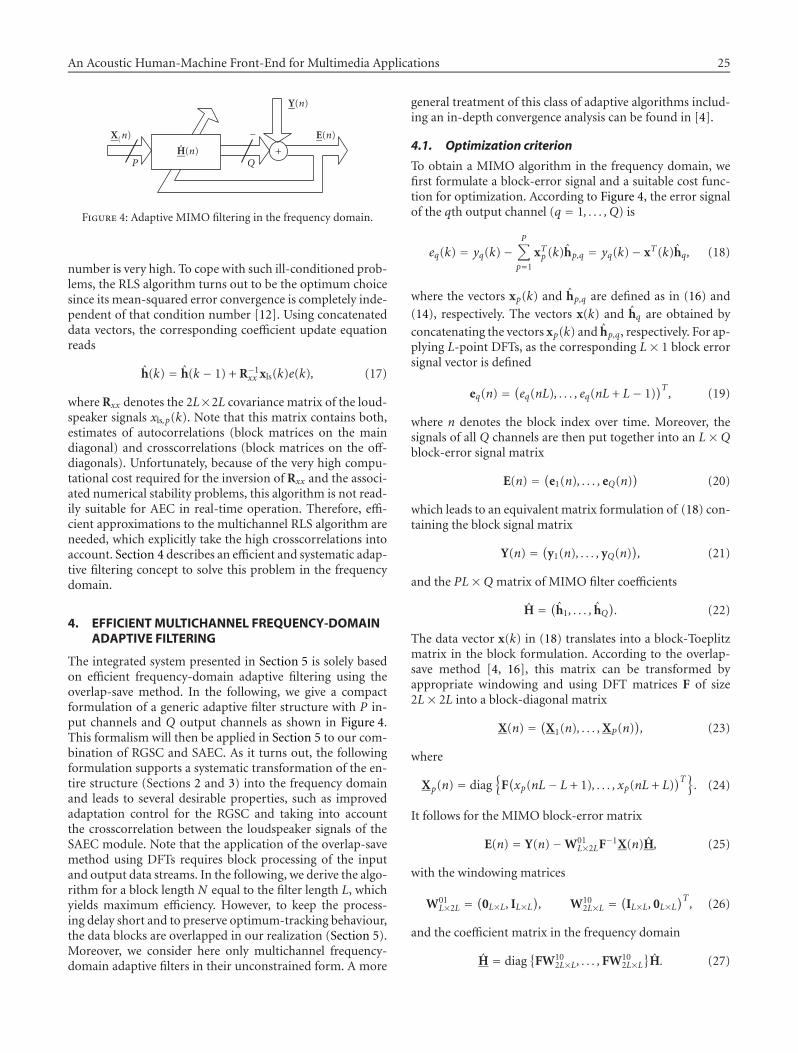
An Acoustic Human-Machine Front-End for Multimedia Applications 25
E(n)
Y(n)
+Q
−H(n)
P
X(n)
Figure 4: Adaptive MIMO filtering in the frequency domain.
number is very high. To cope with such ill-conditioned prob-lems, the RLS algorithm turns out to be the optimum choicesince its mean-squared error convergence is completely inde-pendent of that condition number [12]. Using concatenateddata vectors, the corresponding coefficient update equationreads
h(k) = h(k − 1) + R−1xx xls(k)e(k), (17)
where Rxx denotes the 2L×2L covariance matrix of the loud-speaker signals xls,p(k). Note that this matrix contains both,estimates of autocorrelations (block matrices on the maindiagonal) and crosscorrelations (block matrices on the off-diagonals). Unfortunately, because of the very high compu-tational cost required for the inversion of Rxx and the associ-ated numerical stability problems, this algorithm is not read-ily suitable for AEC in real-time operation. Therefore, effi-cient approximations to the multichannel RLS algorithm areneeded, which explicitly take the high crosscorrelations intoaccount. Section 4 describes an efficient and systematic adap-tive filtering concept to solve this problem in the frequencydomain.
4. EFFICIENT MULTICHANNEL FREQUENCY-DOMAINADAPTIVE FILTERING
The integrated system presented in Section 5 is solely basedon efficient frequency-domain adaptive filtering using theoverlap-save method. In the following, we give a compactformulation of a generic adaptive filter structure with P in-put channels and Q output channels as shown in Figure 4.This formalism will then be applied in Section 5 to our com-bination of RGSC and SAEC. As it turns out, the followingformulation supports a systematic transformation of the en-tire structure (Sections 2 and 3) into the frequency domainand leads to several desirable properties, such as improvedadaptation control for the RGSC and taking into accountthe crosscorrelation between the loudspeaker signals of theSAEC module. Note that the application of the overlap-savemethod using DFTs requires block processing of the inputand output data streams. In the following, we derive the algo-rithm for a block length N equal to the filter length L, whichyields maximum efficiency. However, to keep the process-ing delay short and to preserve optimum-tracking behaviour,the data blocks are overlapped in our realization (Section 5).Moreover, we consider here only multichannel frequency-domain adaptive filters in their unconstrained form. A more
general treatment of this class of adaptive algorithms includ-ing an in-depth convergence analysis can be found in [4].
4.1. Optimization criterion
To obtain a MIMO algorithm in the frequency domain, wefirst formulate a block-error signal and a suitable cost func-tion for optimization. According to Figure 4, the error signalof the qth output channel (q = 1, . . . , Q) is
eq(k) = yq(k)−P∑
p=1
xTp (k)hp,q = yq(k)− xT(k)hq, (18)
where the vectors xp(k) and hp,q are defined as in (16) and
(14), respectively. The vectors x(k) and hq are obtained by
concatenating the vectors xp(k) and hp,q, respectively. For ap-plying L-point DFTs, as the corresponding L× 1 block errorsignal vector is defined
eq(n) = (eq(nL), . . . , eq(nL + L− 1)
)T, (19)
where n denotes the block index over time. Moreover, thesignals of all Q channels are then put together into an L× Qblock-error signal matrix
E(n) = (e1(n), . . . , eQ(n)
)(20)
which leads to an equivalent matrix formulation of (18) con-taining the block signal matrix
Y(n) = (y1(n), . . . , yQ(n)
), (21)
and the PL×Q matrix of MIMO filter coefficients
H = (h1, . . . , hQ
). (22)
The data vector x(k) in (18) translates into a block-Toeplitzmatrix in the block formulation. According to the overlap-save method [4, 16], this matrix can be transformed byappropriate windowing and using DFT matrices F of size2L× 2L into a block-diagonal matrix
X(n) = (X1(n), . . . ,XP(n)
), (23)
where
Xp(n) = diag{
F(xp(nL− L + 1), . . . , xp(nL + L)
)T}. (24)
It follows for the MIMO block-error matrix
E(n) = Y(n)−W01L×2LF−1X(n)H, (25)
with the windowing matrices
W01L×2L =
(0L×L, IL×L
), W10
2L×L =(
IL×L, 0L×L)T, (26)
and the coefficient matrix in the frequency domain
H = diag{
FW102L×L, . . . ,FW10
2L×L}
H. (27)
26 EURASIP Journal on Applied Signal Processing
Multiplying (25) by FW012L×L, we get the block-error signal
matrix in the frequency domain
E(n) = Y(n)−GX(n)H, (28)
where
E(n) = FW012L×LE(n) = F
(0L×1 · · · 0L×1
e1(n) · · · eQ(n)
), (29)
Y(n) = FW012L×LY(n) = F
(0L×1 · · · 0L×1
y1(n) · · · yQ(n)
), (30)
G = FW012L×2LF−1, (31)
W012L×2L = W01
2L×LW01L×2L =
(0L×L 0L×L0L×L IL×L
). (32)
Having derived a frequency-domain error matrix, thefollowing frequency-domain criterion [4] is applied for opti-mizing the coefficient matrix H = H(n):
Jf (n) = (1− λ)n∑i=0
λn−i tr{
EH(i)E(i)}, (33)
where H denotes conjugate transpose and λ (0 < λ < 1) isan exponential forgetting factor. The criterion (33) is verysimilar to the one leading to the well-known RLS algorithm.The main advantage of using (33) is to take advantage of thefast Fourier transform (FFT) in order to have low-complexityadaptive filters.
4.2. Adaptive algorithm
An RLS-like algorithm can be straightforwardly derived fromthe so-called normal equation that is obtained by setting thegradient of (33) w.r.t H equal to zero. According to [12] andby noting that GHG = G and GHY(i) = Y(i), we have for thegradient
∇HJf (n) = 2∂Jf (n)
∂H∗
(n)
= 2(1− λ)n∑i=0
λn−i[−XH(i)Y(i) + XH(i)GX(i)H
].
(34)
Setting this gradient equal to zero, we obtain the normalequation
Sxx(n)H(n) = Sxy(n), (35)
where
Sxx(n) = (1− λ)n∑i=0
λn−iXH(i)GX(i)
= λSxx(n− 1) + (1− λ)XH(n)GX(n),
(36)
Sxy(n) = (1− λ)n∑i=0
λn−iXH(i)Y(i)
= λSxy(n− 1) + (1− λ)XH(n)Y(n).
(37)
The iterative algorithm, that is, the recursive update ofthe coefficient matrix H, is directly derived from (35), (36),and (37). In the recursive equation (37), we replace Sxy(n)and Sxy(n − 1) by formulating (35) in terms of block-timeindices n and n − 1, respectively. We then eliminate Sxx(n −1) from the resulting equation using (36). Reintroducing theerror signal vector (28), we obtain the adaptive algorithm
E(n) = Y(n)−GX(n)H(n− 1), (38)
H(n) = H(n− 1) + (1− λ)S−1xx (n)XH(n)E(n). (39)
Additionally, matrix Sxx(n) is estimated by (36).The above algorithm is equivalent to the RLS algorithm
in the sense that its mean-squared error convergence is alsoindependent of the condition number of the input covari-ance matrix. To reduce the computational complexity of theadaptation drastically, it is shown in [4] that matrix G in (36)can be well approximated by a diagonal matrix G ≈ I/2. Us-ing this approximation and introducing a diagonal 2L × 2Lmatrix µ containing frequency-dependent stepsizes, we mayrewrite (36) and (39) as
S′xx(n) = λS′xx(n− 1) + (1− λ)XH(n)X(n),
H(n) = H(n− 1) + (1− λ)µS′−1xx (n)XH(n)E(n),
(40)
where µ is a diagonal matrix of stepsizes, with elements 0 ≤µi ≤ 2, i = 0, 1, . . . , L−1, and optimum stepsize µ = 2I. Notethat prior to inversion of S′xx(n), a proper regularization byadding a suitable diagonal matrix [4] is important to ensurerobust convergence behaviour.
5. REALIZATION OF RGSC WITH EMBEDDEDSTEREOPHONIC AEC IN THE DFT DOMAIN
Fundamentally, adaptive beamforming and AEC need to becombined such that advantages are explored and insufficien-cies are relieved. Optimum positive synergies between SAECand GSC are obtained when the SAEC is placed in the sen-sor channels of the GSC (AEGSC) [7]. Maximum computa-tional efficiency is given if the SAEC is located in the fixed-reference path after the FBF (GSAEC), since the number ofSAEC output channelsQ is minimized (see Figure 5). In [17],it is shown that most of the synergies are preserved for thelatter structure.
In Section 6, we present a frequency-domain GSAEC re-alization (FGSAEC). Systematic application of multichannelfrequency-domain adaptive filters (see Section 4) yields a sys-tem that exploits the advantages of multichannel frequency-domain adaptive filtering while preserving positive synergiesbetween GSC and SAEC. Especially, (a) crosscorrelation be-tween the loudspeaker signals is taken into account for fastconvergence of the SAEC, (b) adaptation problems of theadaptive sidelobe-cancelling path of the GSC are efficientlyresolved (see Section 5.6), and (c) computational complexityis minimized for efficient implementation of the integratedsystem on low-cost PC platforms for real-time application(see Section 6 and [9]).

An Acoustic Human-Machine Front-End for Multimedia Applications 27
GSAEC
a(n)B(n)
w
h(n)
−+ −
+
Figure 5: System overview.
AEC
xb(n)
xls,1(k)
xls,2(k)
FFTFFT
eh(r)
eh(r)
FFT
+−
W01Lh×2Lh
IFFT
Updateh2(r)h1(r)
Xls,1(r) Xls,2(r)
y f (k)w1
...
wMFBF
x1(k)
xM(k)
Figure 6: SAEC in the fixed-reference path of the GSC.
5.1. Notations
For optimum performance, we use different DFT lengths 2Lg
and 2Lh for GSC and SAEC, respectively, which yields theDFT matrices F2Lg×2Lg and F2Lh×2Lh . The parameters Lg =Lb = La and Lh are identical to the number of filter taps ofGSC and AEC adaptive filters, respectively. For better track-ing behavior of the adaptive filters, block overlaps by factorsαg and αh are introduced in the GSC and AEC input signalblocks, respectively [18]. This leads to the block-time indexn = kαg/Lg. It reflects the discrete time in numbers of blocksof length Lg/αg. In the sequel, we assume that Lh/αh is aninteger multiple of Lg/αg which maximizes efficiency. For abetter reading, we define R = Lhαg/Lgαh and the time in-dex r = kαh/Lh. GSC and AEC adaptive filters are updated attimes n and r, respectively.
5.2. FBF
The mainlobe of simple delay&sum beamformer with broad-side steered microphone arrays is too narrow at high frequen-cies. This often leads to cancellation of the desired signal athigh frequencies if the desired speaker position and the steer-ing direction do not match.
Dolph-Chebyshev beamformer design [19] allows to ar-bitrarily choose the first null of the array pattern relativeto the steering direction while minimizing the level of the
sidelobes. It allows to design filter&sum beamformers withpredefined mainlobe widths that are constant over a widerange of frequencies. This makes this design method espe-cially appropriate for our application since it allows to arbi-trarily specify a region where desired signals are not attenu-ated [9].
5.3. Stereophonic AEC integrated in fixed-referencepath of RGSC
Using the notations of Section 4, the basic signal-processingof the SAEC in the fixed-reference path of the GSC can besummarized as follows (see Figure 6). The number of inputchannels is P = 2 and the number of output channels is Q =1. According to (24), we capture the last 2Lh samples of theloudspeaker signals xls,p(k), p = 1, 2, in vectors, and we findfor the frequency-domain loudspeaker signals,
X ls,p(r) = diag
F2Lh×2Lh
xls,p
(rLh
αh− 2Lh + 1
)xls,p
(rLh
αh− 2Lh + 2
)...
xls,p
(rLh
αh
)
. (41)
The loudspeaker signals xls,p(k) are assumed to be prepro-cessed by inaudible nonlinearities [14]. Capturing the 2Lh×1vectors of adaptive filter transfer functions hp(r) according to(27) in a vector
h(r) = (hT
1 (r),hT2 (r)
)T, (42)
and defining a matrix of loudspeaker signals
X ls(r) = (X ls,1(r),X ls,2(r)
), (43)
as in (23), we obtain for the Lh × 1 time-domain block errorsignal vector (see (25))
eh(r) = yf (r)−W01Lh×2Lh
F−12Lh×2Lh
X ls(r)h(r − 1), (44)
where the Lh × 1 vector of FBF output signal samples is de-fined as
yf (r) =
yf
(rLh
αh− Lh + 1
)yf
(rLh
αh− Lh + 2
)...
yf
(rLh
αh
)
. (45)
We define a frequency-domain error signal eh(r) accordingto (29) as
eh(r) = F2Lh×2Lh W012Lh×Lh
eh(r). (46)

28 EURASIP Journal on Applied Signal Processing
AIC
Xa(n)
Xa(n)
FFT
a(n)
ea(n)
FFT
ea(n)+−
ya(n)z−κaαg/Lg
xb(n)
W01Lg×2Lg
IFFTFFT
Xb(n)
B(n)
Eb(n)IFFT
FFTW01Lg×2Lg
+−
Eb(n)
ABM
Yb(n)
Figure 7: FGSAEC: ABM and AIC.
This allows us to write the SAEC filter update equation as
h(r) = h(r − 1) + µh(1− λh
)S−1XlsXls
(r)XHls (r)eh(r), (47)
where µh (0 ≤ µh ≤ 2) is a stepsize parameter, λh (0 < λh < 1)is an exponential forgetting factor, and SXlsXls
(r) is a recur-sive estimate of the cross-power spectral density matrix ofthe loudspeaker signals
SXlsXls(r) = (
1− λh)
SXlsXls(r − 1) + λhXH
ls (r)X ls(r). (48)
With the inverse of the cross-power spectral density matrixSXlsXls
(r) in the update equation, crosscorrelation of the loud-speaker signals is explicitly taken into account, leading to fastconvergence of the adaptive filters.
One block of length Lh/αh of the AEC output signal is fi-nally given by the last Lh/αh samples of the error signal eh(r),which is by a factor R larger than the signal blocks which arerequired for the GSC. We split eh(r) into R blocks xb(n − i),i = 0, 1, . . . , R − 1 of length Lh/R. Therefore, R − 1 blocks ofxb(n− i) are buffered until they are used by the GSC.
5.4. Adaptive blocking matrix
In Figure 7, reference path and adaptive sidelobe-cancellingpath are depicted. For the ABM, P = 1, Q =M. For applyingthe overlap-save method to the ABM adaptive filter inputs inthe frequency domain, we have to transform 2αg subsequentblocks of the AEC output signal xb(n) into the frequency do-main. That is,
Xb(n) = diag
F2Lg×2Lg
xb(n− 2αg + 1
)xb(n− 2αg + 2
)...
xb(n)
. (49)
With the ABM adaptive filters B(n), written in the frequencydomain according to (27) as a 2Lg × M matrix B(n), the
Lg ×M block error matrix Eb(n) is obtained from (25) as
Eb(n) = Yb(n)−W01Lg×2Lg
F−12Lg×2Lg
Xb(n)B(n− 1), (50)
where the Lg ×M block sensor signal matrix is defined as
Yb(n) = (yb,1(n), yb,2(n), . . . , yb,M(n)
),
yb,m(n) =
xm(nLg
αg− κb − Lg + 1
)xm
(nLg
αg− κb − Lg + 2
)...
xm(nLg
αg− κb
)
.
(51)
The time delay κb ensures causality of the ABM adaptive fil-ters. Defining Eb(n) as
Eb(n) = F2Lg×2Lg W012Lg×Lg
Eb(n), (52)
the update equation for B(n) reads1
B(n) = B(n−1)+(1−λb
)Gµb(n)S−1
XbXb(n)XH
b (k)Eb(n). (53)
The matrix G is defined according to (31) with L replaced byLg. In contrast to the SAEC (see Section 5.3), circular convo-lution constraints [4] are required for the ABM since the im-pulse responses of the ideal ABM filters are generally muchlonger than the length of the adaptive filters. Thus, circularconvolution effects cannot be disregarded.
The 2Lg × 2Lg diagonal matrix µb(n) is a matrix withfrequency-dependent stepsizes on the main diagonal, whichcontrol the adaptation of the ABM (see Section 5.6).
The diagonal power spectral density matrix is given by
SXbXb(n) = (
1− λb)
SXbXb(n− 1) + λbXH
b (n)Xb(n). (54)
One block of length Lg/αg of the time-domain AIC inputsignals xa,s(n) is obtained by saving the last Lg/αg samples ofthe mth column of the block error signal matrix Eb(n).
5.5. Adaptive interference canceller
With P = M, Q = 1, the frequency-domain adaptive filterinput matrix Xa(n) of size 2Lg × 2LgM is given by
Xa(n) = (Xa,1(n),Xa,2(n), . . . ,Xa,M(n)
), (55)
where Xa,m(n) is obtained in the same way as in (49) withXb(n) and xb(n) replaced by Xa,m(n) and xa,m(n), respec-tively.
Writing the AIC adaptive filters a(n) after (27) in the fre-quency domain as a 2LgM × 1 vector a(n), then the time-domain block error vector reads
ea(n) = ya(n)−W01Lg×2Lg
F−12Lg×2Lg
Xa(n)a(n− 1), (56)
1Coefficient constraints for improved robustness against cancellation ofdesired signal components may be introduced according to [8, 9].

An Acoustic Human-Machine Front-End for Multimedia Applications 29
where ya(n) is defined as
ya(n) =
xb
(n− κaαg
Lg− αg + 1
)xb
(n− κaαg
Lg− αg + 2
)...
xb
(n− κaαg
Lg
)
. (57)
The time delay κa ensures causality. Defining the frequency-domain error signal
ea(n) = F2Lg×2Lg W012Lg×Lg
ea(n), (58)
we obtain the multichannel filter update equation as2
a(n) = a(n− 1) +(1− λa
)Gµa(n)S−1
XaXa(n)XH
a (n)ea(n), (59)
where we introduced the 2Lg × 2Lg diagonal matrix µa(n)with frequency-dependent stepsizes on the main diagonalfor controlling the adaptation of the AIC (see Section 5.6).Note that circular convolution is prevented by the matrixG (see (31)). As for the ABM, ideal impulse responses AICare much longer than the length of the adaptive filters.The diagonal power spectral density matrix is computedfrom
SXaXa(n) = (
1−λa)
SXaXa(n−1)+λa diag
{XH
a (n)Xa(n)}, (60)
where diag{·} extracts the main diagonal of the given argu-ment.
Finally, one block of length Lg/αg of the GSC output sig-nal is obtained by saving the last Lg/αg samples of ea(n).
5.6. Adaptation control
In this system, we modified the GSC adaptation control pre-sented in [8] to a DFT-binwise operation, which increasesconvergence speed and robustness significantly. It is based ona spatial SNR estimate: the FBF output yields an estimate ofthe desired signal PSD. A fixed beamformer, which is com-plementary to the FBF, yields an estimate of the interferencePSD. A frequency-dependent SNR estimate is then obtainedby the ratio of desired signal PSD and interference PSD. Thisis used for a bin-wise decision whether the ABM or the AICis adapted.
We do not consider the stepsize control of the AEC here.Various stepsize-control methods can be found in the liter-ature (see, e.g., [2, 20]). The adaptation control of GSC andSAEC does not need to rely on synergies between both adap-tation mechanisms, so that GSC and SAEC can be adaptedindependently of each other.
2 A norm constraint for improved robustness against desired signal can-cellation may be introduced according to [9, 10].
6. REAL-TIME IMPLEMENTATION ANDEXPERIMENTAL EVALUATION
For demonstrating the performance of our acoustic human-machine interface in real time, we implemented the FGSAECalgorithm on a PC platform. The multichannel audio captureunit is realized as separate hardware integrating the micro-phones, the preamplifiers, the A/D conversion, and the mi-crophone calibration. The digitized sensor data is fed intothe PC via a standard USB port with specific drivers for themicrophone array.
Our experiments were conducted on an Intel Pentium IV1.8 GHz processor at a sampling rate of 12 kHz. Optimumperformance of the frequency-domain RGSC (FGSC) andFGSAEC was obtained with 30% and 52% CPU load, respec-tively.
For all experiments, we use a linear microphone arraywith 8 equally spaced, broadside-steered sensors with 4 cmspacing in an office environment with 300 ms reverberationtime. The male desired speaker and the male interferer withan average signal power ratio of 0 dB are located in the arraylook-direction and 30 degrees off the array axis, respectively.The stereophonic loudspeakers emitting music are placed tothe left and to the right of the microphone array. All distancesto the array center are 60 cm. The frequency band is 300 Hz–5.9 kHz. The FBF is realized by a Dolph-Chebyshev designdescribed in [9]. Typical numerical values for filter lengthsand block overlapping factors are Lg = 128, Lh = 2048 andαg = 2, αh = 8, respectively. In Section 6.1, we study steady-state performance of FGSAEC. In Section 6.2, tracking capa-bility of RGSC with moving desired speaker is illustrated.
6.1. Performance after convergenceof the adaptive filters
For evaluating the proposed system after convergence ofthe adaptive filters, we compare the average interferencerejection (IR) and the average echo-return-loss enhance-ment (ERLE) of FGSAEC, FGSC, frequency-domain AEGSC(FAEGSC), and TGSAEC, (the time-domain equivalent ofFGSAEC) for only interference and for double-talk of inter-ference and desired speaker.
Since it is difficult to study IR and ERLE separately forreal-time scenarios, we illustrate the results that we obtainedwith recorded signals in simulations. Audio examples whichillustrate the performance of the real-time system can befound in [21].
The results are depicted in Table 1. For only interference,IR and ERLE are higher than for the double-talk case sincethe ABM is fixed and since the AIC can be adapted perma-nently over the entire frequency range, yielding optimum-tracking capability of nonstationary interference. The perfor-mance of TGSAEC and FGSAEC is identical. During double-talk, IR and ERLE are considerably improved for FGSAECrelative to TGSAEC as controlling the adaptation in individ-ual frequency bins still allows tracking the transient ABMand of nonstationary interference at frequencies with lowSNR [9]. FGSAEC clearly improves the suppression of acous-tic echoes relative to FGSC; however, optimum performance

30 EURASIP Journal on Applied Signal Processing
Table 1: Performance evaluation.
Interference only Double-talk
(in dB) IR ERLE IR ERLE
TGSAEC 22.4 26.0 5.6 12.3
FGSAEC 21.1 25.6 14.7 21.0
FGSC 20.7 21.9 14.5 14.7
FAEGSC 22.0 30.5 14.9 28.1
32.521.510.5Time (in s)
ABM
Fixed BM
0
10
20
30
IR(k
)in
dB
32.521.510.5
ABMFixed BM−10
0
10
DR
(k)
indB
32.521.510.5−1
0
1
n(k)
d(k)
Figure 8: Tracking performance of the ABM in comparison withthe BM after [11], position change of the desired speaker at 1.66 s.
of FAEGSC cannot be obtained due to leakage effects acrossthe GSC sidelobe-cancelling path [17].
6.2. Tracking of the ABM
For illustrating the tracking capability of the ABM, desiredsignal rejection (DR) and interference rejection of the FGSCover time are measured for changing desired speaker posi-tion. Both rejections are estimated by the ratio of recursivelyaveraged squared sensor signals and beamformer output sig-nals w.r.t. the desired signal components and interferencecomponents.
Figure 8 depicts the results for the ABM in comparisonwith a fixed blocking matrix (BM) after [11]. Parameters arechosen to have the same IR(k) for ABM and fixed BM. Forcontrolling the adaptation of both GSC realizations, knowl-edge about the true sensor SIR is assumed. For controllingthe adaptation of ABM and AIC, knowledge of the true sen-sor SNR is assumed.
At 1.66 s, the desired speaker switches from broadside (0degrees) to 10 degrees; neither interference suppression nordesired signal quality are impaired due to fast-tracking ca-pability of FGSC. The fixed blocking matrix is designed tosuppress signals from a single-propagation path. Due to re-verberation, it leads to considerable desired signal distortionbefore and after changing the desired speaker position.
7. CONCLUSIONS
The presented signal-processing algorithms describe an ex-ample of efficient integration of adaptive beamforming andmultichannel AEC which meets well the practical require-ments regarding the suppression of interference and acous-tic echoes for seamless acoustic human-machine interfaces.Without structural changes, it can be extended to more re-production channels and even multichannel recording. Mov-ing the implementation from the PC platform to a more spe-cialized hardware will be smooth as long as efficient and nu-merically sound implementations of basic signal-processingalgorithms such as fast Fourier transforms are assured andas long as block processing and control loops pose no obsta-cles.
ACKNOWLEDGMENTS
This work was supported by a grant from Intel Corp., Hills-boro, OR. The authors would like to acknowledge the fruit-ful discussions with Jacob Benesty of Bell Labs, Lucent Tech-nologies, that led to the development of the efficient mul-tichannel adaptive filtering framework in the frequency do-main. The authors would also like to thank the speech com-munication group of Intel China Research Center, Beijing,for providing the microphone array USB hardware.
REFERENCES
[1] C. Breining, P. Dreiseitel, E. Hansler, et al., “Acoustic echocontrol—an application of very-high-order adaptive filters,”IEEE Signal Processing Magazine, vol. 16, no. 4, pp. 42–69,1999.
[2] S. L. Gay and J. Benesty, Eds., Acoustic Signal Processing forTelecommunications, Kluwer Academic Publishers, Boston,Mass, USA, 2000.
[3] H. Buchner and W. Kellermann, “Improved Kalman gaincomputation for multichannel frequency-domain adaptivefiltering and application to acoustic echo cancellation,” inProc. IEEE Int. Conf. Acoustics, Speech, Signal Processing, pp.1909–1912, Orlando, Fla, USA, May 2002.
[4] H. Buchner, J. Benesty, and W. Kellermann, “Multichan-nel frequency-domain adaptive filtering with application toacoustic echo cancellation,” in Adaptive Signal Processing: Ap-plication to Real-World Problems, J. Benesty and Y. Huang,Eds., Springer-Verlag, Berlin, Germany, January 2003, to ap-pear.
[5] M. S. Brandstein and D. B. Ward, Eds., Microphone Ar-rays: Signal Processing Techniques and Applications, Springer,Berlin, Germany, 2001.
[6] W. Herbordt and W. Kellermann, “Adaptive beamforming foraudio signal acquisition,” in Adaptive Signal Processing: Appli-cation to Real-World Problems, J. Benesty and Y. Huang, Eds.,Springer-Verlag, Berlin, Germany, January 2003, to appear.
[7] W. Kellermann, “Acoustic echo cancellation for beamformingmicrophone arrays,” in Microphone Arrays: Signal ProcessingTechniques and Applications, M. S. Brandstein and D. B. Ward,Eds., pp. 281–306, Springer-Verlag, Berlin, Germany, 2001.
[8] O. Hoshuyama, A. Sugiyama, and A. Hirano, “A robust adap-tive beamformer for microphone arrays with a blocking ma-trix using constrained adaptive filters,” IEEE Trans. Signal Pro-cessing, vol. 47, no. 10, pp. 2677–2684, 1999.
An Acoustic Human-Machine Front-End for Multimedia Applications 31
[9] W. Herbordt and W. Kellermann, “Frequency-domain inte-gration of acoustic echo cancellation and a generalized side-lobe canceller with improved robustness,” European Trans. onTelecommunications, vol. 13, no. 2, pp. 123–132, 2002.
[10] D. H. Johnson and D. E. Dudgeon, Array Signal Processing,Prentice-Hall, Englewood Cliffs, NJ, USA, 1993.
[11] L. J. Griffiths and C. W. Jim, “An alternative approach to lin-early constrained adaptive beamforming,” IEEE Trans. on An-tennas and Propagation, vol. 30, no. 1, pp. 27–34, 1982.
[12] S. Haykin, Adaptive Filter Theory, Prentice-Hall, EnglewoodCliffs, NJ, USA, 3rd edition, 1996.
[13] M. M. Sondhi, D. R. Morgan, and J. L. Hall, “Stereophonicecho cancellation—An overview of the fundamental prob-lem,” IEEE Signal Processing Letters, vol. 2, no. 8, pp. 148–151,1995.
[14] J. Benesty, D. R. Morgan, and M. M. Sondhi, “A better under-standing and an improved solution to the specific problems ofstereophonic acoustic echo cancellation,” IEEE Trans. Speech,and Audio Processing, vol. 6, no. 2, pp. 156–165, 1998.
[15] A. Sugiyama, Y. Joncour, and A. Hirano, “A stereo echo can-celer with correct echo-path identification based on an input-sliding technique,” IEEE Trans. Signal Processing, vol. 49, no.11, pp. 2577–2587, 2001.
[16] J. G. Proakis and D. G. Manolakis, Digital Signal Processing:Principles, Algorithms, and Applications, Prentice-Hall, UpperSaddle River, NJ, USA, 1996.
[17] W. Herbordt and W. Kellermann, “Limits for generalized side-lobe cancellers with embedded acoustic echo cancellation,” inProc. IEEE Int. Conf. Acoustics, Speech, Signal Processing, vol. 5,Salt Lake City, Utah, USA, May 2001.
[18] E. Moulines, O. A. Amrane, and Y. Grenier, “The generalizedmultidelay adaptive filter: structure and convergence analy-sis,” IEEE Trans. Signal Processing, vol. 43, no. 1, pp. 14–28,1995.
[19] C. L. Dolph, “A current distribution for broadside arrayswhich optimize the relationship between beam width andside-lobe level,” Proceedings of the I.R.E. and Waves and Elec-trons, vol. 34, no. 6, pp. 335–348, 1946.
[20] A. Mader, H. Puder, and G. U. Schmidt, “Step-size controlsfor acoustic echo cancellation filters—an overview,” SignalProcessing, vol. 80, no. 9, pp. 1697–1719, 2000.
[21] W. Herbordt, http://www.LNT.de/∼herbordt.
Wolfgang Herbordt received the Dipl.-Ing.degree in electrical engineering from theUniversity of Erlangen-Nuremberg in 1999after studying at INSA Rennes, France,and at the University Erlangen-Nuremberg,Germany. Since 1999, he is a Researcher atthe Chair of Multimedia Communicationsand Signal Processing at the University ofErlangen-Nuremberg. He has been involvedin signal processing for hands-free acoustichuman-machine interfaces, that is, array signal-processing, blindsource separation, multichannel AEC, noise-robust speech recog-nition, and acoustic source localization. He received the Best Stu-dent Paper Award at the International Conference on Acoustics,Speech, and Signal Processing (ICASSP), Istanbul 2000. In 2000,he was a visiting Scientist at Intel Corp., Hillsboro, OR, and in 2001and 2002 at Intel Corp., Beijing, China.
Herbert Buchner is a member of the re-search staff at the Chair of MultimediaCommunications and Signal Processing,University of Erlangen-Nuremberg, Ger-many. He received the Dipl.-Ing. (FH) andthe Dipl.-Ing. Univ. degrees in electrical en-gineering from the University of AppliedSciences, Regensburg in 1997, and the Uni-versity of Erlangen-Nuremberg in 2000, re-spectively. In 1995, he was a visiting Re-searcher at the Colorado Optoelectronic Computing Systems Cen-ter (OCS), Boulder/Ft. Collins, Colorado, where he worked in thefield of microwave technology. From 1996 to 1997, he did researchat the Cyber Space Labs (former Human Interface Labs) of theR&D division of Nippon Telegraph and Telephone Corp. (NTT),Tokyo, Japan, working on adaptive filtering for teleconferencing. In1997/1998, he was with the Driver Information Systems Depart-ment of Siemens Automotive in Regensburg, Germany. His currentareas of interest include efficient multichannel algorithms for adap-tive digital filtering, and their applications for acoustic human-machine interfaces such as multichannel AEC, beamforming, blindsource separation, and dereverberation. He received the VDI Awardin 1998 for his Dipl.-Ing. (FH) thesis from the Verein Deutscher In-genieure and an IEEE Best Student Paper Award in 2001.
Walter Kellermann is a Professor of com-munications at the Chair of Multime-dia Communications and Signal Processingof the University of Erlangen-Nuremberg,Germany. He received the Dipl.-Ing. (univ.)degree in electrical engineering from theUniversity of Erlangen-Nuremberg in 1983,and the Dr.-Ing. degree from the TechnicalUniversity Darmstadt, Germany, in 1988.From 1989 to 1990, he was a PostdoctoralMember of technical staff at AT&T Bell Laboratories, Murray Hill,NJ. From 1990 to 1993, he was with Philips Kommunikations In-dustrie, Nuremberg, Germany. From 1993 to 1999, he was a Pro-fessor at the Fachhochschule Regensburg, and in 1997, he be-came a Director of the Institute of Applied Research of the Fach-hochschule Regensburg. In 1999, he cofounded DSP Solutions, aconsulting firm in digital signal-processing, and he joined the Uni-versity Erlangen-Nuremberg as a professor and head of the audioresearch laboratory. Dr. Kellermann authored and coauthored fivebook chapters and more than 35 papers in journals and confer-ence proceedings. He served as a Guest Editor for various journalsand presently serves as an Associate Editor of IEEE Transactions onSpeech and Audio Processing. His current research interests includespeech signal-processing, array signal-processing, and adaptive fil-tering and its applications to acoustic human/machine interfaces.
EURASIP Journal on Applied Signal Processing 2003:1, 32–40c© 2003 Hindawi Publishing Corporation
Embedding Color Watermarks in Color Images
Chun-Hsien ChouDepartment of Electrical Engineering, Tatung University, 40 Chungshan North Road, 3rd Section, Taipei 104, Taiwan
Email: [email protected]
Tung-Lin WuOpto-Electronics & System Laboratories, Industrial Technology Research Institute, Hsinchu, Taiwan
Email: [email protected]
Received 17 May 2002 and in revised form 4 October 2002
Robust watermarking with oblivious detection is essential to practical copyright protection of digital images. Effective exploitationof the characteristics of human visual perception to color stimuli helps to develop the watermarking scheme that fills the require-ment. In this paper, an oblivious watermarking scheme that embeds color watermarks in color images is proposed. Through colorgamut analysis and quantizer design, color watermarks are embedded by modifying quantization indices of color pixels withoutresulting in perceivable distortion. Only a small amount of information including the specification of color gamut, quantizer step-size, and color tables is required to extract the watermark. Experimental results show that the proposed watermarking schemeis computationally simple and quite robust in face of various attacks such as cropping, low-pass filtering, white-noise addition,scaling, and JPEG compression with high compression ratios.
Keywords and phrases: robust and transparent watermarking, oblivious watermark detection, uniform color space, color quanti-zation, just noticeable color difference.
1. INTRODUCTION
Digital watermarking is a technique that hides a piece ofinformation in an original media for the purpose of copy-right protection, integrity checking, or captioning [1, 2, 3,4, 5, 6, 7, 8, 9]. The hidden information, or the so-calleddigital watermark, as usually represented by a sequence ofrandom numbers or a recognizable binary pattern, shouldsupply enough information for establishing rightful owner-ship or provide additional information about the originalcontent. An effective watermarking scheme should meet cer-tain requirements including transparency, robustness, secu-rity, unambiguity, and low-computational complexity. De-pending on the application to be developed, the originaldata may or may not be used in the detection of water-marks. As considering the portability and availability ofthe original data, the oblivious (or blind) watermarkingscheme without resorting to the original data is preferred.That is, a feasible image watermarking scheme should al-low users to extract watermarks without referring to originalimages.
In the past few years, most researches focused on devel-oping watermarking schemes for grayscale images. Only acomparatively small number of researches on color image
watermarking can be found [10, 11, 12, 13, 14, 15, 16, 17].Some extend the algorithm used for grayscale images to thecolor case by marking the image luminance [10, 11]. Fleetand Heeger [12] suggested to embed the watermark in theyellow-blue channel of the opponent-color representation ofcolor images. Kutter et al. [13] embedded the watermark bymodifying a selected set of pixels in the blue channel sincethe human eye is less sensitive to changes in this color chan-nel. In [15], a repeated LSB-insertion watermarking tech-nique for palette-based color images was proposed. In themethod of quantization index modulation [16], each of thehost signal is quantized by one of a number of quantiz-ers, of which indices are used to carry the watermark in-formation. A watermarking scheme based on ordered colorquantization is proposed in [17]. It is found that the colorquantization and processing in most of these proposed tech-niques are not optimized by taking properties of humanvisual perception into account. To gain high robustnessand transparency in color image watermarking, the knowl-edge of human visual perception of color stimuli must bewell utilized in designing watermark embedding/extractionalgorithms.
In this paper, a spatial-domain color image watermark-ing scheme is proposed. Without resorting to the original

Embedding Color Watermarks in Color Images 33
image and with very little information as private key, the vi-sually recognizable color watermarks can be detected by de-coding each color pixel’s quantization index which is modi-fied to carry the watermark signal in the embedding process.The quantization index is modified in a way that results ina minimum color deviation. The color quantizer is so de-signed such that the quantization error and the distortioncaused by the modification in quantization index will not beperceptible.
2. COLOR QUANTIZATION
Color is a visual perception of the light in the visible regionof the electromagnetic wave spectrum incident on the retina.Since the retina has three types of photoreceptors that re-spond to different parts of the visible spectrum, three com-ponents are necessary and sufficient to specify a color. It haslong been found that mean square error is a very poor mea-sure of color difference in many tristimulus color spaces, suchas RGB, CIEXYZ, YUV, and so forth. Color distributionsin these tristimulus spaces are nonuniform in that the Eu-clidean distance between any two colors is usually not closelycorrelated with the associated perceptual difference. In casea nonuniform color space is uniformly quantized, the fixedcolor distance between any two colors of the quantized colorspace will result in large variation in perceptual difference,and perceptible distortion if the quantizer stepsize is large. Inthe proposed watermarking scheme, embedding and extrac-tion of color watermarks are accomplished by color quantiza-tion. The image with the watermark embedded is actually thedequantization of a quantized image, of which quantizationindices are disturbed by watermark information. To guaran-tee the transparency of the embedded watermark, the colordifference between a pixel and its watermarked counterpartshould be uniform and must not be perceptible throughoutthe whole image. To attain this goal, uniform quantizationmust be carried out in a uniform color space with the quan-tizer stepsize tuned to result in imperceptible color differ-ence between any two adjacent colors in the quantized colorspace.
3. PERCEPTUALLY LOSSLESS COLOR QUANTIZATION
In this paper, color quantization is performed in the CIE-Labcolor space where the color difference is more closely corre-lated with the perceptual difference. Any two colors with thesame Euclidean distance in this space have approximately thesame perceptual difference. A useful rule of thumb in thiscolor space is that any two colors can be distinguished in asense if their color distance
∆ELap =[(∆L)2 + (∆a)2 + (∆b)2]1/2
(1)
is greater than 3, the so-called just noticeable color differ-ence (JNCD). The stepsize of the proposed uniform quan-tizer is thus determined in a way that the color difference be-tween any two neighboring colors centroids should not be
L
b
C
JNCD
a
(a)
L
a
b
(b)
Figure 1: (a) The spherical subspace defined by color C and theJNCD in the CIE-Lab space, within which all colors are perceptu-ally indistinguishable from the color C; (b) the 27 uniform cubicsubspaces that accommodate the spherical subspace.
(000)
(001)
(010)
(011)
(100)
(101)
(110)
(111)
White
Yellow
Blue
Cyan
Red
Green
Purple
Brown
(a)
(001)
(010)
(011)
(100)
(101)
(110)
(111)
(000)
Black
White
(b)
Figure 2: (a) The watermark represented by 8 different colors; (b)the watermark represented by two colors where the code (000) isassigned to represent color white and the rest of the codes colorblack.

34 EURASIP Journal on Applied Signal Processing
Host image
Color spacetransformation
Color Gamutanalysis
Quantizerdesign
Private key
Colorquantization
Color watermark
Colorencoding
Repetition &permutation
Private key
Watermarkembedding
Colordequantization
Inverse color spacetransformation
The watermarked image
Figure 3: Watermark embedding process.
perceivable, or not to exceed the JNCD. By considering themasking effect mainly due to local variations in luminancemagnitude, the quantizer stepsize can be set to be larger thanJNCD.
Colors that are perceptually indistinguishable from a par-ticular color in the uniform color space form a sphere with aradius equal to the JNCD (Figure 1a). As shown in Figure 1b,the spherical space can be approximated by a cubic spacewhich can be further partitioned into 3×3×3 uniform cubicsubspaces. Colors within the centered cubic subspace are per-ceptually indistinguishable from colors within each of 26 pe-ripheral cubic subspaces. Hence, as the uniform color spaceis partitioned into uniform cubic bins and the centroid ofeach bin is computed as a representative color, any color canbe quantized and represented as a three-dimensional quanti-zation index. A color pixel Pi in the RGB space can be trans-formed into a quantization index vector qi in the CIE-Labspace
qi =(qLi , qai , qbi
) = Q(Li, ai, bi
),
(Li, ai, bi
) = T(Ri, Gi, Bi
),
(2)
where (Li, ai, bi) and (Ri, Gi, Bi) are tristimulus values ofthe pixel Pi in the CIE-Lab space and RGB space, respec-tively, while T denotes color transformation and Q uniformquantization. The transformation between the RGB spaceand the CIE-Lab space is through the XYZ space. The RGBspace is first converted to the XYZ space through a lineartransformation
XYZ
=0.490 0.310 0.200
0.177 0.813 0.0110.000 0.010 0.990
RGB
. (3)
Then, the XYZ space is converted to the CIE-Lab spacethrough a nonlinear transformation
L = 116 f(Y/Y0
)− 16,
a = 500[f(X/X0
)− f(Y/Y0
)],
b = 200[f(Y/Y0
)− f(Z/Z0
)],
(4)
where
f (x) =
1
3x, x > 0.008856,
7.787x +16
116, otherwise
(5)
and (X0, Y0, Z0) represents the reference white. If the dimen-sion of the cubic bin is appropriately set, the quantizationerror between a color and its counterpart after quantizationand dequantization will not be perceivable, and so is thecolor difference between two adjacent colors in the quantizedcolor space.
4. SIGNAL SPACE FOR HIDING COLOR WATERMARKS
By applying modulo-2 operation to each component of thethree-dimensional quantization index, the quantization in-dex qi is mapped to a binary vector
qi =(qiL, qia, qib
) = (qiL mod 2, qia mod 2, qib mod 2
)(6)

Embedding Color Watermarks in Color Images 35
L
Qs
Qs
Qs
b
a
Qs: Quantizer stepsize
Figure 4: The quantizer design based on uniformly partitioning thesubspace that best accommodates the color gamut of the host image.
in a three-dimensional binary space Φ = {(φ1, φ2, φ3) : φk =1, or 0, k = 1, 2, 3}. The space consists of eight binary vec-tors to which each centroid color of the uniform quantizerand its 26 adjacent centroid colors can be mapped. The map-ping implies that any two vectors in Φ are associated withtwo adjacent centroid colors of the uniform quantizer, whichwill be perceptually indistinguishable from each other if thequantization stepsize is small enough.
The eight binary vectors actually provide the space forcarrying watermark information and can be used as codesfor representing colors of the multilevel watermark. Withmultiple ways of color coding, the same watermark can havemore than one representations at the same time. As shown inFigure 2, the watermark can be rendered by eight distinct col-ors, or as a binary image with the vector (000) being assignedto represent color white and the rest assigned to representcolor black. With multiple codes being assigned to representthe same color, the watermark is expected to be more robustin that the color is enabled to tolerate a number of erroneousbits.
5. WATERMARK EMBEDDING
The process of embedding color watermarks in color im-ages is described by the functional block diagram shown inFigure 3. The host image is first transformed into the CIE-Lab color space where the color gamut of the host imageis analyzed. With a quantizer stepsize, the rectangular sub-space that best accommodates the color gamut is uniformlypartitioned into cubic bins of identical dimension (Figure 4).The centroid of each cubic bin is then calculated as an outputcolor of the quantization. One of eight corners of the rectan-gular subspace can be chosen as the reference origin which,together with the information of the subspace’s dimension,is then taken as a part of the private key for specifying thecolor gamut. As the reference origin of the color gamut is de-termined, the centroid of each cubic bin can be addressed bya three-dimensional quantization index as described above.Before watermark embedding, one or more sets of color
The watermarked image
Color spacetransformation
Quantizerdesign
Colorquantization
Private key
Watermarkextraction
Inverse permutation andmajority-vote decoding
Colordecoding
The extracted watermark
Figure 5: Watermark extraction process.
L0 a0 b0 DL Da Db Qs FP Pk N C00, · · · Cn0,
7 × 8(bits)
1 8 4 8 × 15 8 × 15
L0, a0, b0: reference origin of the color gamutDL,Da,Db : dimension of the color gamutQs: quantizer stepsizeFP : flag for optional permutationPk : permutation keyN : number of color tablesCi0, Ci1, . . . , Ci7 : 8 colors in the ith color table
Figure 6: Information contained in the private key.
tables are adopted as a part of the private key to render thewatermark to multiple presentations, and the watermark isrepeated to form a watermark image having the same dimen-sion as the host image. In cooperating with the majority votedecision in the watermark extraction process, repeated em-bedding also functions to enhance the robustness of the wa-termark as subjected to various attacks that change tristim-ulus values of color pixels. Permutation is optionally appliedto the watermark image for dispersing its spatial relationship,such that the watermark will not be easily removed by attacksthat crop some parts of the image. A pseudorandom num-ber traversing method is applied to both the row-number se-quence {0, 1, . . . , H − 1} and the column-number sequence{0, 1, . . . ,W − 1} with different seeds for random numbergeneration to obtain a 2 D sequence of coordinates, where Wand H denote the width and height of the watermark image,respectively. The permutation is then accomplished by relo-cating the original pixels according to the new randomized

36 EURASIP Journal on Applied Signal Processing
(a) (b) (c)
Figure 7: The color images (a) “PEPPER” and (b) “TTU,” into which (c) the 8-color watermark to be inserted.
coordinates. The watermark signal wi = (wi1, wi2, wi3) is em-bedded into the color pixel Pi by modifying its quantizationindex qi in the following way:
qwi =
qi, if d
(qi,wi
)=0,
qi +(νi1·
(qiL⊕wi1
), νi2·
(qia⊕wi2
),
νi3 ·(qib ⊕wi3
)), if d
(qi,wi
) �=0,(7)
where d(qi,wi) is the Hamming distance between vectors qi
and wi, and νi = (νi1, νi2, νi3) is a random vector with νik = 1,or −1 for k = 1, 2, 3. The modification, if required, is madesuch that quantization index is mapped to a binary vectoridentical to wi. That is,
qwi =
(qwiL mod 2, qwia mod 2, qwib mod 2
) = wi. (8)
The watermarked image, Iw = {Pwi }, is then obtained by
color dequantization and inverse color transformation
Pwi = T−1(Q−1(qw
i
)). (9)
6. WATERMARK EXTRACTION
The process of watermark extraction is described by thefunctional block diagram shown in Figure 5, where the tar-get image is first transformed to the CIE-Lab color space. Theuniform quantizer used for watermark embedding is rebuiltby the private key information. As shown in Figure 6, theinformation organized in the private key contains the colorgamut of the host image, quantizer stepsize, permutation key,and tables of colors for multiple representations. The num-ber of bits required for representing these watermarking pa-rameters can be as minimal as 189 bits. Each color pixel Pw
i
of the watermarked image is then quantized by the uniformquantizer
q∗i = Q(
T(Pwi
)). (10)
The watermark signal, w∗i , carried by the quantization index
is decoded by applying modulo-2 operation to each compo-nent of the quantization index
w∗i =
(q∗iL mod 2, q∗ia mod 2, q∗ib mod 2
). (11)
The image of the extracted watermark {w∗i } is then option-
ally arranged by the inverse permutation R and decoded bymajority-vote decision M for obtaining the final watermark
W = M(
R({
w∗i
})). (12)
Then, according to color tables found in the private key, thewatermark is rendered to different representations. The in-telligibility of the extracted watermark can be enhanced ifsome appropriate sets of colors are chosen for representingthe multilevel watermark.
7. EXPERIMENTAL RESULTS
The performance of the proposed watermarking scheme inrobustness and transparency is evaluated by attacking thewatermarked image with various attacks listed in the Check-mark package [18] such as Gaussian noise addition, low-passfiltering, lossy JPEG compression, and geometric attacks in-cluding cropping, scaling, and rotation. Color images of size512 × 512 are used as host images where each pixel is rep-resented by 24 bits in the RGB space, while the watermarkimage of size 128 × 128 contains visually recognizable pat-terns having at most 8 different colors. By taking the mask-ing effect into account, the stepsize of the uniform quan-tizer designed in the CIE-Lab space is set to two times ofthe JNCD. In the simulation, attacks on the watermarkedimage are performed in the RGB space. In Figure 7, an 8-color watermark is embedded into two color images. Fromthe watermarked images shown in Figure 8, the embeddedwatermark is visually transparent, and low values of PSNRindicate that the modification due to watermark embeddingdoes not result in obvious and perceptible distortion. The ex-tracted watermarks remain intact if no attack is performedon the watermarked images. Figure 9 shows the watermarksextracted from watermarked images which are attacked by
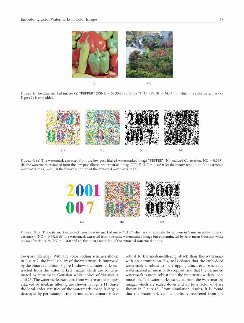
Embedding Color Watermarks in Color Images 37
(a) (b)
Figure 8: The watermarked images (a) “PEPPER” (PSNR = 33.35 dB) and (b) “TTU” (PSNR = 34.47), in which the color watermark ofFigure 7c is embedded.
(a) (b) (c) (d)
Figure 9: (a) The watermark extracted from the low-pass filtered watermarked image “PEPPER” (Normalized Correlation, NC = 0.539);(b) the watermark extracted from the low-pass filtered watermarked image “TTU” (NC = 0.423); (c) the binary rendition of the extractedwatermark in (a); and (d) the binary rendition of the extracted watermark in (b).
(a) (b) (c)
Figure 10: (a) The watermark extracted from the watermarked image “TTU” which is contaminated by zero-mean Gaussian white noises ofvariance 4 (NC = 0.982); (b) the watermark extracted from the same watermarked image but contaminated by zero-mean Gaussian whitenoises of variance 25 (NC = 0.36); and (c) the binary rendition of the extracted watermark in (b).
low-pass filterings. With the color coding schemes shownin Figure 2, the intelligibility of the watermark is improvedby the binary rendition. Figure 10 shows the watermarks ex-tracted from the watermarked images which are contam-inated by zero-mean Gaussian white noises of variance 4and 25. The watermarks extracted from watermarked imagesattacked by median filtering are shown in Figure 11. Sincethe local order statistics of the watermark image is largelydestroyed by permutation, the permuted watermark is less
robust to the median-filtering attack than the watermarkwith no permutation. Figure 12 shows that the embeddedwatermark is robust to the cropping attack even when thewatermarked image is 50% cropped, and that the permutedwatermark is more robust than the watermark with no per-mutation. The watermarks extracted from the watermarkedimages which are scaled down and up by a factor of 4 areshown in Figure 13. From simulation results, it is foundthat the watermark can be perfectly recovered from the

38 EURASIP Journal on Applied Signal Processing
(a) (b) (c)
Figure 11: (a) The watermark extracted from the median-filtered watermarked image “TTU” with the watermark being permuted in theembedding process (NC = 0.17); (b) the binary rendition of the extracted watermark in (a) (NC = 0.253); and (c) the watermark extractedfrom the median-filtered watermarked image “TTU” with the watermark not being permuted in the embedding process (NC = 0.993).
(a)
(b) (c)
Figure 12: (a) The watermarked image which is 50% cropped; (b)the extracted watermark (NC = 0.553) which is permuted in em-bedding process; and (c) the extracted watermark (NC = 0.413)which is not permuted in embedding process.
watermarked images which are rotated by multiples of 90◦,but it is not the case by other rotation angles. If the wa-termark image is not permuted in the embedding process,the watermark may survive the attack. The watermark im-age extracted from the watermarked image which is rotatedby 30◦ is shown in Figure 14. It demonstrates that the mostpart of the lwatermark image is destroyed by rotation, butthe content of the watermark can still be identifiable by piec-ing up the parts that are readable. Figure 15 shows the water-marks extracted from watermarked images which are JPEG-compressed at different compression ratios. With multiple-color tables, the extracted watermark can be rendered inmultiple ways to give intelligible contents even if the com-
(a) (b)
Figure 13: (a) The watermark extracted from the watermarked im-age “PEPPER” which is scaled down to a quarter of its original di-mension (NC = 0.536); (b) the watermark extracted from the wa-termarked image “PEPPER” which is scaled up to 4 times of its orig-inal dimension (NC = 0.851).
Figure 14: The watermark image extracted from the watermarkedimage “PEPPER” which is rotated by 30◦.
pression ratio is as high as 27.5. As for the attack of colormodification, the watermark may or may not be removed,depending on whether the amount of color pixels beingmodified dominates over the other, also both the originalcolor and the modified color are mapped to the same binaryvector as described in (6). From simulation results, the wa-termark can always survive the attack if half of all pixels ischanged in colors in a random way.

Embedding Color Watermarks in Color Images 39
(a) (b) (c) (d)
Figure 15: (a) The watermark extracted from the watermarked image “PEPPER” which is JPEG-compressed at a compression ratio of12 (NC = 0.439); (b) the binary rendition of the extracted watermark in (a) according to the color coding scheme of Figure 2a; (c) Thewatermark extracted from the watermarked image “PEPPER” which is JPEG-compressed at a compression ratio of 27.5 (NC = 0.343); and(d) the binary rendition of the extracted watermark in (c) according to the color coding scheme of Figure 2a.
8. CONCLUSION
In this paper, a color-image watermarking scheme that satis-fies the requirements of transparency, robustness, and oblivi-ous detection is proposed. Through color quantization, colorwatermarks are carried by the quantization indices of thehost image in the uniform color space. Watermark trans-parency is achieved by perceptually lossless color quantiza-tion and modification in quantization indices. Watermarkrobustness is attained by repeated embedding, majority-votedecision, and multiple renditions of the watermark. Colorwatermarks are extracted without resorting to original im-ages, but with a small amount of private-key informationwhich can be as minimum as 189 bits. The proposed water-marking scheme also features its simplicity in computationand implementation. To further enhance the robustness ofthe color watermark in the color image, the same idea can beapplied to images in the frequency domain. Embedding colorwatermarks in perceptually significant wavelet coefficients ofthe color image has already been under investigation.
REFERENCES
[1] R. G. van Schyndel, A. Z. Tirkel, and C. F. Osborne, “A digitalwatermark,” in Proc. IEEE International Conference on Im-age Processing, vol. 2, pp. 86–90, Austin, Tex, USA, November1994.
[2] I. Pitas, “A method for watermark casting on digital images,”IEEE Trans. Circuits and Systems for Video Technology, vol. 8,no. 6, pp. 775–780, 1998.
[3] M. D. Swanson, M. Kobayashi, and A. H. Tewfik, “Multimediadata embedding and watermarking technologies,” Proceedingsof the IEEE, vol. 86, no. 6, pp. 1064–1087, 1998.
[4] M. Barni, F. Bartolini, V. Cappellini, and A. Piva, “Copy-right protection of digital images by embedded unperceivablemarks,” Image and Vision Computing, vol. 16, no. 12-13, pp.897–906, 1998.
[5] I. J. Cox, M. L. Miller, and J. A. Bloom, Digital Watermark-ing, Morgan Kaufmann Publishers, San Francisco, Calif, USA,2001.
[6] F. Hartung and B. Girod, “Watermarking of uncompressedand compressed video,” Signal Processing, vol. 66, no. 3, pp.283–302, 1998.
[7] C. I. Podilchuk and W. Zeng, “Image-adaptive watermarkingusing visual models,” IEEE Journal on Selected Areas in Com-munications, vol. 16, no. 4, pp. 525–539, 1998.
[8] C.-T. Hsu and J.-L. Wu, “Multiresolution watermarking fordigital images,” IEEE Trans. Circuits and Systems for VideoTechnology, vol. 45, no. 8, pp. 1097–1101, 1998.
[9] C.-S. Lu, S.-K. Huang, C.-J. Sze, and H.-Y. M. Liao, “Cocktailwatermarking for digital image protection,” IEEE Trans. Mul-timedia, vol. 2, no. 4, pp. 209–224, 2000.
[10] R. B. Wolfgang and E. J. Delp, “A watermarking techniquefor digital image: further studies,” in Proc. IEEE InternationalConference on Imaging Science,System, and Technology, vol. 1,pp. 279–287, las Vegas, Nev, USA, 30 June–3 July 1997.
[11] I. J. Cox, J. Kilian, F. T. Leighton, and T. Shamoon, “Se-cure spread spectrum watermarking for multimedia,” IEEETrans. Image Processing, vol. 6, no. 12, pp. 1673–1687, 1997.
[12] D. J. Fleet and D. J. Heeger, “Embedding invisible informa-tion in color images,” in Proc. IEEE International Conferenceon Image Processing, vol. 1, pp. 532–535, Santa Barbara, Calif,USA, October 1997.
[13] M. Kutter, F. Jordan, and F. Bossen, “Digital signature of colorimages using amplitude modulation,” Journal of ElectronicImaging, vol. 7, no. 2, pp. 326–332, 1998.
[14] J. J. Chae, D. Mukherjee, and B. S. Manjunath, “Color im-age embedding using multidimensional lattice structure,” inProc. IEEE International Conference of Image Processing, pp.460–464, Chicago, Ill, USA, October 1998.
[15] S. C. Pei and C. M. Cheng, “Pallete-based color image wa-termarking using neural network training and repeated LSBinsertion,” in Proc. the 13th IPPR Conference on Computer Vi-sion, Graphics and Image Processing, vol. 1, pp. 1–8, August2000.
[16] B. Chen and G. W. Wornell, “Quantization index modulation:A class of provably good methods for digital watermarkingand information embedding,” IEEE Transactions on Informa-tion Theory, vol. 47, no. 4, pp. 1423–1443, 2001.
[17] C. C. Tseng, C. J. Juan, and S. L. Lee, “Color image water-marking based on ordered color quantization,” in Proc. the13th IPPR Conference on Computer Vision, Graphics and Im-age Processing, vol. 1, pp. 458–466, August 2000.
[18] S. Pereira, S. Voloshynovskiy, M. Madueno, S. Marchand-Maillet, and T. Pun, “Second generation benchmarking andapplication oriented evaluation,” in Information Hiding Work-shop III, pp. 340–353, Pittsburgh, Pa, USA, April 2001.

40 EURASIP Journal on Applied Signal Processing
Chun-Hsien Chou graduated from Na-tional Taipei Institute of Technology, TaipeiTaiwan in 1979, and received the M.S. andPh.D. degrees in electrical engineering fromNational Tsing Hua University, Hsinchu,Taiwan, in 1986 and 1990, respectively. In1990, he joined the Department of Electri-cal Engineering at Tatung Institute of Tech-nology, Taipei, Taiwan, as an Associate Pro-fessor. During the academic year from 1991to 1992, he was a Postdoctoral Research member at AT&T Bell Lab-oratories, Murray Hill, NJ. In 1996, he became a Professor at theDepartment of Electrical Engineering, Tatung University, Taipei,Taiwan. His current research areas include color models of the hu-man visual system, perceptual coding of color images, streamingvideo coding, virtual reality, and digital watermarking techniques.
Tung-Lin Wu received the B.S. degree inelectrical engineering from Tamkang Uni-versity, Tamshui, Taiwan in 1999, and theM.S. degree in communication engineer-ing from Tatung University, Taipei, Tai-wan in 2001. He is currently working inOpto-Electronics & Systems Laboratoriesof Industrial Technology Research Institute,Hsinchcu, Taiwan, as an Associate Engineer.His current research areas include color sig-nal processing and image coding.

EURASIP Journal on Applied Signal Processing 2003:1, 41–47c© 2003 Hindawi Publishing Corporation
Retrieval by Local Motion
Berna ErolRicoh California Research Center, 2882 Sand Hill Road, Suite 115, Menlo Park, CA 94025-7022, USAEmail: berna [email protected]
Faouzi KossentiniDepartment of Electrical and Computer Engineering, University of British Columbia,2356 Main Mall, Vancouver, British Columbia, Canada V6T 1Z4Email: [email protected]
Received 15 May 2002 and in revised form 30 September 2002
Motion feature plays an important role in video retrieval. The current literature mostly addresses motion retrieval only by cameramotion and global motion of individual video objects in a video scene. In this paper, we propose two new motion descriptors thatcapture the local motion of the video object within its bounding box. The proposed descriptors are rotation and scale invariant andbased on the angular and circular area variances of the video object and the variances of the angular radial transform coefficients.Experiments show that ranking obtained by querying with our proposed descriptors closely match with the human ranking.
Keywords and phrases: video databases, video indexing and retrieval, object-based video, motion descriptor, MPEG-4, MPEG-7.
1. INTRODUCTION
As the advancements in digital video compression resultedin the availability of large video databases, indexing and re-trieval of video became a very active research area. Unlikestill images, video has a temporal dimension that we can as-sociate with motion features. We use this information as oneof the key components to describe video sequences; for ex-ample, “this is the part where we were salsa dancing” or “thisvideo shows my daughter skating for the first time.” Conse-quently, motion features play an important role in content-based video retrieval.
It is possible to classify the types of video motion featuresinto three groups.
(i) Global motion of the video or camera motion (e.g.,camera zoom, pan, tilt, roll).
(ii) Global motion of the video objects within a frame(e.g., an object is moving from the left to the right ofthe scene).
(iii) Local motion of the video object (e.g., a person is rais-ing his/her arms).
Camera operation analysis is generally performed by an-alyzing the directions of motion vectors that are present incompressed video bit stream [1, 2, 3] or optical flow analysisin the spatial domain [4]. For example, panning and tiltingmotions are likely to be present if most of the motion vec-tors inside a frame are in the same direction. Similarly, zoom-ing motion can be identified by determining whether or not
the motion vectors at the top/left of the frame have oppositedirections than the motion vectors at the bottom/right of theframe [5, 6].
Global motion of video objects is represented with theirmotion trajectories, which are formed by tracking the loca-tion of video objects (object’s mass center or some selectedpoints on the object) over a sequence of frames. Formingmotion trajectories generally requires segmentation of videoobjects in a video scene. In MPEG-4, the location informa-tion of the video object bounding box (the upper-left cor-ner) is already available in the bit stream making the for-mation of the trajectory a simple task [7]. The classificationand matching of object motion trajectories is a challengingissue as the trajectories contain both the path and the veloc-ity information of the objects. In [8], Little and Gu proposedto extract separate curves for the object path and speed andmatch these two components separately. Rangarajan et al. [9]demonstrated a two-dimensional motion trajectory match-ing through scale-space and Chen and Chang [10] proposedto match the motion trajectories via a wavelet decomposi-tion.
Most available content-based video retrieval systems inthe literature employ camera motion features and/or globalobject motion for retrieval by motion. For example, the Jacobsystem [11] supports queries using common camera motionchanges such as pan, zoom, and tilt. Another retrieval sys-tem, VideoQ, employs a spatio-temporal segmentation algo-rithm in order to retrieve individual objects with their globalmotion inside a scene [12]. It allows the user to specify an

42 EURASIP Journal on Applied Signal Processing
arbitrary polygonal trajectory for the query object and re-trieves the video sequences that contain video objects withsimilar trajectories. Similar to VideoQ, NeTra-V supportsspatio-temporal queries and utilizes motion histograms forglobal camera and video object motion retrieval [13]. More-over, the content-based description standard MPEG-7 [14,15] supports motion descriptors, in particular, camera mo-tion which characterizes the 3D camera operations, mo-tion trajectory which captures 2D transitional motion of ob-jects, parametric motion which describes the global defor-mations, and motion activity which specifies the intensity ofaction.
On the other hand, local motion, the motion video ob-jects within their bounding box, could give valuable in-formation about its articulated parts, elasticity, occlusion,and so forth. Classifying and identifying video objects us-ing their local motion is potentially useful in many applica-tions. For example, it could be useful to identify some sus-picious human actions in surveillance video sequences. Itcould also be useful for efficient video compression, wherethe encoder can allocate more coding bits or a better com-munication channel for the video objects that demonstratesimportant actions, for example, a person running out of astore (there is a chance that the person might be a crim-inal) or a player scoring. Moreover, processing databasequeries such as “find a video sequence where people aredancing” would be possible only by enabling the retrievalof video objects with their local motion. The current re-search in detecting the local motion of video objects hasbeen restricted mostly to specific domains. Stalidis et al.employed a wavelet-based model using boundary pointsof magnetic resonance images (MRI) to describe the car-diac motion in [16]. Miyamori and Iisaku [17] proposed toclassify the actions of tennis players using 2D appearance-based matching. Hoey and Little suggested a method forthe classification of motion, which is based on the repre-sentation of flow fields with Zernike polynomials in [18].Their method is applied to the classification of facial ex-pressions. In [19], Fujiyoshi and Lipton presented a pro-cess to analyze human motion by first obtaining the skele-ton of the objects and then determining the body pos-ture and motion of skeleton segments to determine hu-man activities. Human motion classification was also stud-ied by other researchers including Little and Boyd in [20],where they proposed to recognize individuals by periodicvariation in the shape of their motion, and Heisele andWoehler in [21], where they suggested discriminating pedes-trians by characterizing the motion of the legs. Moreover,Cutler and Davis [22] proposed to characterize the localmotion by detecting periodicity of the motion by Fourieranalysis on the gray scale video. Most of the work in thisarea focuses on “recognizing” the motion of specific ob-jects and they assume prior knowledge about the videocontent.
As the video object content becomes more widely avail-able, mostly due to the emergence of 3D video capture de-vices [23, 24], object-based MPEG-4 [25] video encoding
standard, and the availability of the state of the art segmen-tation algorithms [26, 27], there is a need for more genericmotion features that describe the local motion of video ob-jects. In this paper, we propose two content-independent lo-cal motion descriptors. Motivated by the fact that any sig-nificant motion of video objects within their bounding boxwould very likely result in changes in their shape, our mo-tion descriptors are based on the shape deformations of videoobjects. The first descriptor, angular circular local motion(ACLM), is computed by dividing the video object area into anumber of angular and circular segments and computing thevariance of each segment over a period of time. The otherproposed descriptor is based on the variances of the angularradial transform (ART) coefficients. We assume that the seg-mented objects are obtained prior. The proposed descriptorsare extracted using video objects’ binary shape masks. Therest of the paper is organized as follows. Sections 2 and 3 de-scribe the proposed local motion descriptors as well as theirextraction and matching. Experimental results that illustratethe retrieval performance of our methods and the associatedtrade-offs are presented in Section 4. Conclusions are givenin Section 5.
2. ANGULAR CIRCULAR LOCAL MOTION (ACLM)DESCRIPTOR
Unlike the shape of visual objects in still images, the shapeof a video object is not fixed and is very likely to changewith time. Given that the camera effects, such as zooming,are compensated for, the shape deformations in an object’slifespan could offer some valuable information about the ob-ject’s local motion, occlusion, articulated parts, and elasticity.The variance of the object area is a good measure for suchshape deformations. Nevertheless, it may not be sufficient tocapture the motion of the video objects in some cases, es-pecially if the object motion does not have an effect on thearea of the object. For example, if an object has an articu-lated part that is rigid in shape, then the object’s area maynot change even if there is local motion. Here, we propose todivide the binary shape mask of a video object into M angu-lar and N circular segments and use the variance of the pixelsthat fall into each segment to describe the local motion. Vari-ances are computed for each angular circular segment in thetemporal direction using the temporal instances of the videoobjects. Then, the local motion feature matrix is formed foreach video object as follows:
R =
σ20,0 · · · σ2
0,m · · · σ20,M−1
......
...
σ2n,0 · · · σ2
n,m · · · σ2n,M−1
......
...
σ2N−1,0 · · · σ2
N−1,m · · · σ2N−1,M−1
, (1)
where M and N are the number of angular and circular sec-tions, respectively, and σ2
n,m is the variance of the pixels that

Retrieval by Local Motion 43
fall into the segment (n,m) and computed as follows:
σ2n,m =
1A(n,m)K
K−1∑k=0
θm+1∑θ=θm
ρn+1∑ρ=ρn
(VOPk(ρ, θ)− µn,m
)2,
µn,m = 1A(n,m)K
K−1∑k=0
θm+1∑θ=θm
ρn+1∑ρ=ρn
VOPk(ρ, θ),
(2)
where K is the number of the temporal instances of the videoobject, VOPk is the binary shape mask of the video objectplane (VOP) at kth instant, VOPk(ρ, θ) is the value of thebinary shape mask in VOPk at the (θ, ρ) position in the po-lar coordinate system centered at the mass center of VOPk,A(n,m) is the area, θm is the start angle, and ρm is the startradius of the angular circular segment (n,m), and they aredefined as
A(n,m) = π(ρ2n+1 − ρ2
n
)M
,
θm = m× 2πM
, ρn = n× ρmax
N,
(3)
where M and N are the number of angular and circular sec-tions, respectively and ρmax is found by
ρmax = maxVOPk∈VO
{ρVOPk
}, (4)
where VOPk is the kth instant of the video object and ρVOPk
is the radius of the tightest circle around the VOPk that iscentered at the mass center of VOPk.
The proposed descriptor is scale invariant since the num-ber of angular and circular segments is the same for all videoobjects, and the size of each segment is scaled with ρmax.We attain an approximate rotation invariance of the descrip-tor by employing an appropriate query matching methodsimilar to the one used for matching the contour-basedshape descriptor in MPEG-7 [14]. That is, we provide therotation invariance by reordering the feature matrix R sothat the angular segment with the largest variance is in thefirst column of R. This is achieved by first summing thecolumns of the feature matrix R to obtain the 1 × M pro-
jection vector �A and then finding the maximum element of�A, which corresponds to the angular segment mL that hasthe largest variance. Finally, we circularly shift to the left thecolumns of R by mL to obtain a rotation invariant featurevector.
The trade-offs associated with using different numbersof angular and circular segments for this descriptor are pre-sented in Section 4.
3. ART-BASED LOCAL MOTION DESCRIPTOR
Employing angular radial transform (ART)-based shape de-scriptors is an efficient way to retrieve shape informationas they are easy to extract and match. Consequently, anART-based descriptor was recently adopted by MPEG-7 [14].Here, we propose to use the variance of the ART coefficients,
computed for each object plane of a video object, as a localmotion descriptor. As the ART descriptors describe the re-gion of a shape, different than their contour-based counter-parts such as curvature scale-space and Fourier descriptors,they are capable of representing holes and unconnected re-gions in the shape. Therefore, our proposed ART-based de-scriptor captures a large variety of shape region deformationscaused by the local motion. The ART transform is definedas [14]
Fnm =∫ 2π
0
∫ 1
0Vnm(ρ, θ) f (ρ, θ)ρ dρ dθ, (5)
where Fnm is an ART coefficient of order n and m, f (ρ, θ) isthe binary shape map in polar coordinates, and Vnm(ρ, θ) isthe ART basis function, which is separable along the angularand radial directions as follows:
Vnm(ρ, θ) = Am(θ)Rn(ρ). (6)
The angular and radial basis functions are given by
Am(θ) = 12π
e jmθ, Rn(ρ) =1, n = 0,
2 cos(πnρ), n �= 0.(7)
The discrete ART coefficients of a binary shape map arefound as follows. First, the size of the binary shape data isnormalized by a linear interpolation to a predefined width Wand height H , to obtain the size invariant shape map I(x, y).The mass center of the binary shape map is aligned with thecenter of I(x, y), that is, I(W/2, H/2). Then, the discrete ARTcoefficients of the shape map of the object plane k (VOPk)are computed by
Fnm(VOPk
) = W/2∑x=−W/2
H/2∑y=−H/2
Vnm
(√x2 + y2, arctan
y
x
)
× IVOPk
(x +
W
2, y +
H
2
).
(8)
The ART coefficients of the individual object planes arerotation variant. When ART coefficients are employed forstill shape retrieval, the magnitude of the ART coefficients areemployed for rotation invariance. Since we would like to cap-ture any rotational changes that may be present in the shapeof the video object when computing the variances in the ARTcoefficients, we employ the complex ART coefficients. The fi-nal ART-based local motion descriptor is defined as the mag-nitude of the complex variance computed over time, which isrotation invariant.
Because the area of the object shape is normalized forsize prior to computing the ART coefficients, the local mo-tion descriptor captures the real deformations of the shape,and it is robust to changes in the area of the video objectsdue to the events such as camera zooming, partial occlu-sion, and so on. If it is desired by the application that themotion descriptor capture such events, the size normaliza-tion of the descriptor should be done with respect to the

44 EURASIP Journal on Applied Signal Processing
largest object plane of the video object. The retrieval per-formance results of this descriptor, obtained by using a vari-ous number of angular and radial functions, are presented inSection 4.
4. EXPERIMENTAL RESULTS
4.1. Performance evaluation
We present our retrieval results by utilizing the normal-ized modified retrieval rank (NMRR) measure used in theMPEG-7 standardization activity [28]. NMRR not only in-dicates how much of the correct items are retrieved, butalso how highly they are ranked among the retrieved items.NMRR is given by
NMRR(n) =(∑NG(n)
k=1 Rank(k)/ NG(n))− 0.5−NG(n)/2
K + 0.5− 0.5∗ NG(n),
(9)
where NG is the number of ground truth items marked assimilar to the query item and Rank(k) is the ranking of theground truth items by the retrieval algorithm, where K isequal to min(4∗ NG(q), 2∗GTM) where GTM is the maxi-mum of NG(q) for all the queries. The NMRR is in the rangeof [0 1] and the smaller values represent a better retrievalperformance. ANMRR is defined as the average NMRR overa range of queries.
4.2. Retrieval performance
Here, we demonstrate the performance of each of our pro-posed local motion descriptors. Our database contains over20 arbitrarily shaped video objects, coded in 2 to 3 differ-ent spatial resolutions, each resulting in an MPEG-4 ob-ject database of over 50 bit streams. The ANMRR valuespresented in this section are obtained by averaging the re-trieval results of 12 query video objects that have a largevariety of local motions. The ground truth objects are de-cided by having three human subjects rank the video ob-jects for their local motion similarity to the query video ob-jects. The similarity distance between two shapes is measuredby computing the Euclidean distance on their local motiondescriptors.
Retrieval performance results using the ACLM descrip-tor with various numbers of angular and circular segmentsis presented in Figure 1. Note that smaller ANMRR valuesrepresent a better retrieval performance. Employing a largenumber of angular and circular bins generally results in abetter retrieval performance but with the cost of more bits re-quired to represent the descriptor. The highest retrieval rates(i.e., lowest ANMRR) here are obtained by using 6 angularand 3 circular segments (ANMRR = 0.090) and 8 angular and2 circular segments (ANMRR = 0.089).
Some query examples using 6 angular and 3 circular seg-ments are presented in Tables 1 and 2. Note that the di-mensions given in the parentheses are not the dimensionsof the video objects, but the resolutions of the video se-quences from which they are extracted. The dimensions of
8642Number of angular segments
0
0.05
0.1
0.15
0.2
0.25
0.3
0.35
0.4
0.45
AN
MR
R
CIR = 1CIR = 2CIR = 3
Figure 1: Retrieval results of the ACLM descriptor obtained by us-ing various numbers of angular and circular (CIR) segments.
Coastguard 2 VO
News 1 VO News 2 VO Akiyo VO
Figure 2: The video objects classified as being similar in terms oftheir local motion to the query video object News 1.
the video objects are different for each plane of the videoobject. One important point to note is that, because of thesimple upsampling/downsampling methods used to obtainvarious resolutions of the same video objects, the differentresolutions of the same objects are not likely to have ex-actly the same shapes. Thus, even though our descriptoris scale invariant, the query distances corresponding to thedifferent resolutions of the same object may not be identi-cal.
The first query, shown in Figure 2,1 is a very low-motionanchorperson video object, News 1, which is coded in twodifferent resolutions in our database. As presented in Table 1,
1The query and database items presented in this section are video ob-jects, and the illustration given in the figures are some representative VOPsof these objects.

Retrieval by Local Motion 45
Table 1: Local motion retrieval results for the News 1 video objectquery.
Rank Video object Query distance
1 News 1 (360× 240) 0.00
2 News 1 (180× 120) 6.68
3 Akiyo (360× 240) 11.07
4 News 2 (360× 240) 12.55
5 Akiyo (180× 120) 14.06
6 News 2 (180× 120) 19.52
7 Coastguard 2 (352× 288) 27.12
8 Coastguard 2 (176× 144) 27.63
9 Coastguard 2 (528× 432) 27.68
Hall Monitor 1 VO
Hall Monitor 2 VO
Stefan VO
Fish VO
Figure 3: The video objects classified as being similar in terms oftheir local motion to the query video object Hall Monitor 1.
using the ACLM descriptor, the two different resolutionsof the News 1 video object are retrieved as the first twoitems. The other highly ranked two anchorperson video ob-jects, illustrated in Figure 2, are also very low in motion. TheCoastguard video object, ranked 7th, 8th, and 9th, is also anobject without any articulated parts (a boat object and itswaves) and with moderate local motion. Our second query,Hall Monitor 1, is the video object of a walking man capturedby a surveillance camera as shown in Figure 3. The query re-sults for this object are presented in Table 2. The three differ-ent resolutions of the video object are ranked the highest, andanother walking man video object from the same sequence,
Table 2: Local motion retrieval results for the Hall Monitor 1 videoobject query.
Rank Video object Query distance
1 Hall Monitor 1 (360× 240) 0.00
2 Hall Monitor 1 (540× 360) 2.89
3 Hall Monitor 1 (180× 120) 10.23
4 Hall Monitor 2 (180× 120) 46.85
5 Hall Monitor 2 (360× 240) 50.25
6 Hall Monitor 2 (540× 360) 50.31
7 Fish 1 (352× 240) 84.59
8 Stefan (176× 144) 90.31
9 Stefan (352× 244) 90.80
14121086420Number of angular basis functions
0
0.05
0.1
0.15
0.2
0.25
0.3
0.35
0.4
AN
MR
R
ART based descriptor
RAD = 3RAD = 2
Figure 4: Retrieval results of the ART-based local motion descrip-tor obtained by employing different number of angular and radial(RAD) basis functions.
Hall Monitor 2, is ranked immediately after. The fish object,which has large moving fins and a tail as depicted in Figure 3,is ranked 6th. The different resolutions of a video objectthat contain a person playing tennis are ranked 8th and 9th.As can be seen from these query examples, the ACLM de-scriptor successfully classifies the local motion of the videoobjects.
The number of angular and radial functions of the ARTdescriptor determines how accurately the shape is repre-sented. Considering that the video object shapes, differentthan trademark shapes for example, generally do not con-tain much detail, using a small number of basis functionsto represent the shape maps would be sufficient and resultin a more compact descriptor. Representation with a smallnumber of basis functions also makes the descriptor morerobust to the potential segmentation errors. The retrievalperformance achieved by using different number of angularand radial functions is presented in Figure 4. As can be ob-served from the table, employing 4 angular and 2 radial basis

46 EURASIP Journal on Applied Signal Processing
functions offers a good trade-off between the retrieval per-formance (ANMRR = 0.181141) and the compactness of thedescriptor.
5. CONCLUSIONS
In this paper, we proposed two local motion descriptorsfor the retrieval of video objects. As presented in Section 4,the ranking obtained by employing our descriptors closelymatches with the human ranking. According to the AN-MRR scores obtained, the ACLM descriptor offers a betterretrieval rate than the ART-based descriptor. Given that eachdescriptor value is quantized to [0 255] range, ACLM de-scriptor requires 16 bytes and the ART-based descriptor re-quires 8 bytes to represent. ACLM descriptor is less compu-tationally complex to extract. Nevertheless, if the ART coef-ficients of the video object is already computed and attachedto the video objects as metadata for shape retrieval, thenthe extra computations required to extract the local motiondescriptors based on the ART coefficients are minimal. De-pending on the application, either of the proposed descrip-tors could be used for efficient video object retrieval by localmotion.
REFERENCES
[1] A. Smolic, M. Hoeynck, and J.-R. Ohm, “Low-complexityglobal motion estimation from P-frame motion vectors forMPEG-7 applications,” in Proc. IEEE International Confer-ence on Image Processing, vol. 2, pp. 271–274, Vancouver, BC,Canada, September 2000.
[2] H. J. Zhang, Y. L. Chien, and S. W. Smoliar, “Video parsingand browsing using compressed data,” Multimedia Tools andApplications, vol. 1, no. 1, pp. 89–111, 1995.
[3] R. R. Wang and T. Huang, “Fast camera analysis in MPEG do-main,” in Proc. IEEE International Conference on Image Pro-cessing, pp. 24–28, Kobe, Japan, October 1999.
[4] M. Shah, K. Rangarajan, and P. S. Tsai, “Motion trajectories,”IEEE Trans. Systems, Man, and Cybernetics, vol. 23, no. 4, pp.1138–1150, 1993.
[5] R. Brunelli, O. Mich, and C. Modena, “A survey on videoindexing,” IRST Technical Report 9612-06, Istituto per laRicerca Scientifica e Tecnologica, Trento, Italy, 1996.
[6] H. Sawhney, S. Ayer, and M. Gorkani, “Model-based 2D&3Ddominant motion estimation for mosaicing and video repre-sentation,” in Proc. International Conf. on Computer Vision,pp. 583–590, Boston, Mass, USA, June 1995.
[7] A. M. Ferman, B. Gunsel, and A. M. Tekalp, “Motion andshape signatures for object-based indexing of MPEG-4 com-pressed video,” in Proc. IEEE Int. Conf. Acoustics, Speech, Sig-nal Processing, vol. 4, pp. 2601–2604, Munich, Germany, April1997.
[8] J. Little and Z. Gu, “Video retrieval by spatial and temporalstructure of trajectories,” in SPIE Storage and Retrieval for Me-dia Databases, vol. 4315, San Jose, Calif, USA, January 2001.
[9] K. Rangarajan, W. Allen, and M. Shah, “Matching motiontrajectories using scale-space,” Pattern Recognition, vol. 26,no. 4, pp. 595–610, 1993.
[10] W. Chen and S. F. Chang, “Motion trajectory matchingof video objects,” in SPIE Storage and Retrieval for Media
Databases, vol. 3972, pp. 544–553, San Jose, Calif, USA, Jan-uary 2000.
[11] E. Ardizzone and M. La Cascia, “Automatic video databaseindexing and retrieval,” Multimedia Tools and Applications,vol. 4, no. 1, pp. 29–56, 1997.
[12] S. F. Chang, W. Chen, H. J. Meng, H. Sundaram, andD. Zhong, “A fully automated content-based video search en-gine supporting spatiotemporal queries,” IEEE Trans. Circuitsand Systems for Video Technology, vol. 8, no. 5, pp. 602–615,1998.
[13] Y. Deng and B. S. Manjunath, “NeTra-V: Toward an objectbased video representation,” IEEE Trans. Circuits and Systemsfor Video Technology, vol. 8, no. 5, pp. 616–627, 1998.
[14] ISO/IEC JTC1/SC29/WG11, ISO/IEC 15938-3:2002, “In-formation technology—Multimedia content descriptioninterface—Part 3: Visual,” 2002.
[15] M. Abdel-Mottaleb, N. Dimitrova, L. Agnihotri, et al.,“MPEG-7: A content description standard beyond compres-sion,” in IEEE 42nd Midwest Symposium on Circuits and Sys-tem, vol. 2, pp. 770–777, Las Cruces, NM, USA, August 1999.
[16] G. Stalidis, N. Maglaveras, A. Dimitriadis, and C. Pappas,“Modeling of cardiac motion using wavelets: comparison withFourier-based models,” in Proc. IEEE Computers in Cardiol-ogy, pp. 733–736, 1998.
[17] H. Miyamori and S. Iisaku, “Video annotation for content-based retrieval using human behavior analysis and domainknowledge,” in Proc. IEEE International Conference on Au-tomatic Face and Gesture Recognition, pp. 320–325, Grenoble,France, March 2000.
[18] J. Hoey and J. Little, “Representation and recognition of com-plex human motion,” in Proc. IEEE Computer Vision and Pat-tern Recognition, vol. 1, pp. 752–759, Hilton Head, SC, USA,June 2000.
[19] H. Fujiyoshi and A. J. Lipton, “Real-time human motion anal-ysis by image skeletonization,” in Proc. IEEE Workshop on Ap-plications of Computer Vision, pp. 15–21, Princeton, NJ, USA,October 1998.
[20] J. Little and J. E. Boyd, “Recognizing people by their gait: Theshape of motion,” Videre: Journal of Computer Vision Research,vol. 1, no. 2, pp. 2–32, 1998.
[21] B. Heisele and C. Woehler, “Motion-based recognition ofpedestrians,” in Proc. IEEE International Conference on Pat-tern Recognition, vol. 2, pp. 1325–1330, Brisbane, Australia,August 1998.
[22] R. Cutler and L. S. Davis, “Robust real-time periodic motiondetection, analysis, and applications,” IEEE Trans. on PatternAnalysis and Machine Intelligence, vol. 22, pp. 781–796, 2000.
[23] “Z-Cam from 3DV Systems,” 2002, http://www.3dvSystems.com.
[24] “Electronic perception technology from Canesta,” 2002,http://www.canesta.com.
[25] ISO/IEC JTC1/SC29/WG11, “Coding of audio-visual objects:Video,” 1999.
[26] D. Zhong and S. F. Chang, “AMOS: An active system forMPEG-4 video object segmentation,” in Proc. IEEE Interna-tional Conference on Image Processing, pp. 4–7, Chicago, Ill,USA, October 1998.
[27] H. T. Nguyen, M. Worring, and A. Dev, “Detection of movingobjects in video using a robust motion similarity measure,”IEEE Trans. Image Processing, vol. 9, no. 1, pp. 137–141, 2000.
[28] ISO/IEC JTC1/SC29/WG11, “Description of core experi-ments for MPEG-7 color/texture descriptors,” doc no. N3090,December 1999.

Retrieval by Local Motion 47
Berna Erol received the B.S. degree fromthe Istanbul Technical University, Istanbul,Turkey, in 1994, and the M.A.S. and Ph.D.degrees from the Department of Electricaland Computer Engineering, the Universityof British Columbia, Vancouver, Canada, in1998 and 2002, respectively. Since Septem-ber 2001, she has been with the Multime-dia Document Analysis Group at Ricoh Cal-ifornia Research Center as a Research Sci-entist. Her research interests include multimedia signal processingand communications, image and video compression, object-basedvideo representations, and content-based retrieval and analysis. Shehas coauthored more than twenty journal papers, conference pa-pers, and book chapters.
Faouzi Kossentini received the B.S., M.S., and Ph.D. degrees fromthe Georgia Institute of Technology, Atlanta, USA, in 1989, 1990,and 1994, respectively. He is presently an Associate Professor in theDepartment of Electrical and Computer Engineering at the Uni-versity of British Columbia, where he is involved in research in theareas of signal processing, communications, and multimedia, andmore specifically in subband/wavelet image transformation, quan-tization, audiovisual signal compression and coding, channel errorresilience, joint source and channel coding, image and video com-munication, and image analysis. He has coauthored more than onehundred and thirty journal papers, conference papers, and bookchapters. Dr. Kossentini is a senior member of the IEEE. He hasserved as a Vice General Chair of the ICIP-2000, and he has alsoserved as an Associate Editor of the IEEE Transactions on ImageProcessing and the IEEE Transactions on Multimedia.

EURASIP Journal on Applied Signal Processing 2003:1, 48–55c© 2003 Hindawi Publishing Corporation
Comparison of Multiepisode VideoSummarization Algorithms
Itheri YahiaouiDepartment of Multimedia Communications, Institut Eurecom, BP 193, 06904 Sophia Antipolis, FranceEmail: [email protected]
Bernard MerialdoDepartment of Multimedia Communications, Institut Eurecom, BP 193, 06904 Sophia Antipolis, FranceEmail: [email protected]
Benoit HuetDepartment of Multimedia Communications, Institut Eurecom, BP 193, 06904 Sophia Antipolis, FranceEmail: [email protected]
Received 26 April 2002 and in revised form 30 September 2002
This paper presents a comparison of some methodologies for the automatic construction of video summaries. The work is basedon the simulated user principle to evaluate the quality of a video summary in a way that is automatic, yet related to the user’sperception. The method is studied for the case of multiepisode video, where we do not describe only what is important in a videobut rather what distinguishes this video from the others. Experimental results are presented to support the proposed ideas.
Keywords and phrases: multimedia content analysis, video summaries, image similarity, automated evaluation.
1. INTRODUCTION
The ever-growing availability of multimedia data creates astrong requirement for efficient tools to manipulate andpresent data in an effective manner. Automatic video sum-marization tools aim at creating, with little or no human in-teraction, short versions which contains the salient informa-tion of original video. The key issue here is to identify whatshould be kept in the summary and how relevant informa-tion can be automatically extracted. To perform this task, weconsider several algorithms and compare their performanceto define the most appropriate one for our application.
2. RELATED WORK
A number of approaches have been proposed to define andidentify what is the most important content in a video. How-ever, most have two major limitations. First, evaluation isdifficult in the sense that it is hard to judge the quality ofa summary or, when a performance measure is available, itis hard to understand its interpretation. Secondly, while thesummarization of a single video has received increasing at-tention [1, 2, 3, 4, 5, 6], little work has been devoted to theproblem of multiepisode video summarization [7, 8] whichraises other interesting difficulties.
Existing video summarization approaches can be classi-fied in two categories. The rule-based approaches combineevidences from several types of processing (audio, video,text) to detect certain configuration of events to includein the summary. Examples of this approach are the “videoskims” of the Informedia Project [3] and the movie trailersof the MoCA project [5]. The mathematically oriented ap-proaches, on the other hand, use similarities within the videoto compute a relevance value of video segments or frames.Possible relevance criteria include segments duration, inter-segment similarities, and combination of temporal and posi-tional measures. Examples of this approach include the use ofsingular value decomposition [9] and shot importance mea-sure [6]. Among the most recent and noticeable work, thework of the Sundaram and Chang [10, 11] based on bothaudio and video content, developed a measure of complex-ity and comprehension time of the shot based on user eval-uation. The summary presented as a skim of the original isconstructed, thanks to a function which describes the utilityof each shot. The methods we propose in this paper fall inthe same category. However, our approach does not involveusers but, instead, is fully automated.
A key issue in automated summary construction is theevaluation of the quality of the summary with respect to the

Comparison of Multiepisode Video Summarization Algorithms 49
original data. Since there is no ideal solution, a number ofalternative approaches are available. With user-based evalua-tion methods, a group of users is asked to provide an evalu-ation of the summaries. Another method is to ask a groupof users to accomplish certain tasks (i.e., answering ques-tions) with or without the knowledge of the summary andto measure the effect of the summary on their performance.Alternatively, for summaries created using a mathematicalcriterion, the corresponding value can be used directly as ameasure of quality. However, all these evaluation techniquespresent drawbacks; user-based ones are difficult and expen-sive to set up and their bias is nontrivial to control, whereasmathematically based ones are difficult to interpret and com-pare to human judgment.
In this paper, we propose a new approach for the auto-matic creation and evaluation of summaries based on thesimulated user principle. This method addresses the problemrelated to the evaluation of the summary and is applicable toboth cases of single video and multiepisode videos. This pa-per is organized as follows. Section 2 describes some basicsabout the simulated user principle approach. In Section 3,we describe the different algorithms used to construct mul-tiepisode summaries. Experimental results and a study ofsummary robustness are presented in Sections 4 and 5. Con-clusions and future extensions of the work are presented inSection 6.
3. SIMULATED USER PRINCIPLE
In the simulated user principle, we define a real experimen-tation, a task that some user has to accomplish, on whicha performance measure is defined. Then, we use reasonableassumptions to predict the simulated user behavior on thistask. The performance of the simulated user on the experi-ment is defined mathematically.
Applying the simulated user principle to the problemof multiepisode video summarization leads to the followingscenario for the simulated user experiment:
(i) show all the summaries to the user,(ii) show a randomly chosen excerpt of a randomly chosen
video,(iii) ask the user to guess which video this excerpt was ex-
tracted from.
The simulated behavior of the user is the following:
(i) if the excerpt contains images which are similar to oneor several images in a single summary, he will providethe corresponding video as an answer,
(ii) if the excerpt contains images which are similar to im-ages in several summaries, the situation is ambiguousand the user cannot provide a definite answer,
(iii) if the excerpt contains no image similar to any imagein any summary, the user has no indication and cannotprovide a definite answer.
The performance of the user in this experiment is the per-centage of correct answers that he is able to provide when he
is shown all possible excerpts of all videos. Note that onlyin the first case described above is the user able to identifya particular video. But this answer might not be necessarilycorrect, because an image in an excerpt of one video can besimilar to an image in the summary of another video.
4. COMPARISON OF ALGORITHMS
In this paper, we present several algorithms employed to au-tomatically construct multiepisode video summaries. We in-tend to compare the quality of the summaries created withour new method (and its possible variations) and other well-known techniques for video or text summarization. The sim-ulated user principle is then used to evaluate the “quality”of the different summaries. Finally, we compare and discussevaluation results to define the most appropriate algorithmfor the task in hand.
Each multiepisode summary building process is dividedinto five phases: video streams preprocessing, feature vectorsconstruction, classification, selection, and summary presen-tation. The first three and the last one are the same for the sixalgorithms, nevertheless the fourth phase, which performsthe selection of the elements to include in the summaries,is specific to each method.
Video streams preprocessingThe opening and ending scenes, common to all episodes, areremoved from further processing since they are not of in-terest to a viewer attempting to understand the content of aparticular episode.
Feature vectors constructionThe next phase consists of analyzing the content of the videoto create characteristic vectors to represent visual informa-tion included in the video frames. Frames are divided intonine equal regions on which the color histograms are com-puted to capture both locality information and color distri-bution. The nine histograms are then concatenated to makeup the characteristic vector of the corresponding frame. Inorder to reduce computation and memory cost, we sub-sample the video such that only one frame per second is pro-cessed.
ClassificationFrames are clustered with an initial step where we create anew cluster when the distance of a frame to existing clustersis greater than a threshold, followed by several k-Means typesteps to refine the clusters. This clustering operation pro-duces classes of video frames with similar visual content.
Video segment selectionFor each episode, we select the most pertinent classes basedon six alternative methods. More details are reported inSection 4.1.
Summary presentationFinally, the global summary can be constructed and pre-sented to the user as a hypermedia document composed of

50 EURASIP Journal on Applied Signal Processing
representative images or as an audio-video sequence of re-duced duration. In this paper, summaries are presented in theform of a table of images (frames extracted from the video),where each row represents a particular episode. The numberof images describing each episode (column) is, however, en-tirely user definable.
4.1. Alternative selection methods
Once video frames have been clustered, the videos might bedescribed as sets of frame classes. The most pertinent classeswill be kept. We now see a number of methodologies devisedto compute this pertinence value.
First, we describe the principle of the first four methodswhich are based on our newly proposed ideas. Secondly, thefifth algorithm based on closely related published work is ex-posed. Finally, we describe method six inspired from the TF-IDF which is commonly employed for the construction oftext summaries.
The basic method
Having described the principle of the simulated user, we maynow formally describe the summary creation methodology.We need a process to automatically construct a summarywith good (and, if possible, optimal) performance for thisexperiment. In the case of single video summarization, thisturns out to be relatively simple.
Assume that the excerpts we consider have duration d. Ifthe video contains N frames, there are the following N−d+1different excerpts:
(i) E1 contains frames f1, f2, . . . , fd,(ii) E2 contains frames f2, f3, . . . , fd+1,
(iii) and so on up to EN−d+1, which contains frames fN−d+1,fN−d+2, . . . , fN .
We assume that the frames have been clustered into “sim-ilarity classes,” so that two frames are considered to be similarif and only if they belong to the same class
fi and f j similar ⇐⇒ C(fi) = C
(f j). (1)
This is a very strong assumption and the similarity classes arebuilt as described in Section 4.
Figure 1 illustrates the relations between excerpts,frames, and classes.
We define the coverage Cov(C) of a class C as the numberof excerpts which contain at least one frame from class C,
Cov(C) = Card{i : ∃ j, f j ∈ Ei and C
(f j) = C
}. (2)
The coverage of a set of classes C1, C2, . . . , Ck is the numberof excerpts which contain at least one frame from one of theclasses
Cov(C1, C2, . . . , Ck
)= Card
{i : ∃ j, r f j ∈ Ei and C
(f j) = C1
}and 1 ≤ r ≤ k.
(3)
C( fN )Classes C( f1)C( f2)C( f3)
fNf4f3f2f1Frames
EN−d+1
E4E3
E2E1
Excerpts
Figure 1: View of excerpts, frames, and classes.
If a video summary is composed of frames f1, f2, . . . , fk, it in-duces a performance in the simulated user experiment whichequals
Cov(C(f1), C
(f2), . . . , C
(fk))/(N − d + 1). (4)
Therefore, the optimal summary is simply one which maxi-mizes
S = arg maxf1 , f2 ,..., fk
Cov(C(f1), C
(f2),
. . . , C(fk))/(N − d + 1).
(5)
This can be achieved in two steps as follows:
(i) first, find a set of classes with maximal coverage,(ii) second, select a representative frame in each class.
Summary construction
The optimal summary can be found by enumerating all thesets of k classes {C1, C2, . . . , Ck} and keeping the best one. Be-cause the enumeration can be computer intensive, it is prof-itable to carefully select the order in which classes are selectedso that the best solutions are found early.
If a class Cm is added to an existing set {C1, C2,. . . , Cm−1}, we can define the “conditional coverage” as itscontribution to the coverage of the final set
Cov(Cm
∣∣C1C2 · · ·Cm−1)
= Cov(C1C2 · · ·Cm
)− Cov(C1C2 · · ·Cm−1
)= Card
{i : ∃ j, f j ∈ Ei and C
(f j) = Cm and∀ f ∈ Ei,
∀r = 1, 2, . . . ,m− 1, C( f ) �= Cr}.
(6)
Then, the coverage of a set of classes {C1, C2, . . . , Ck} can becomputed as
Cov(C1 · · ·Ck
) = Cov(C1
)+ Cov
(C2
∣∣C1)
+ · · · + Cov(Ck
∣∣C1 · · ·Ck−1).
(7)
In order to enable multiple video to be considered at oncefor summarization, we denote by Ev
i an excerpt of a video v,and Sv a summary for video v; the various cases that havebeen described in the simulated user behavior can be for-mally characterized by the following properties:
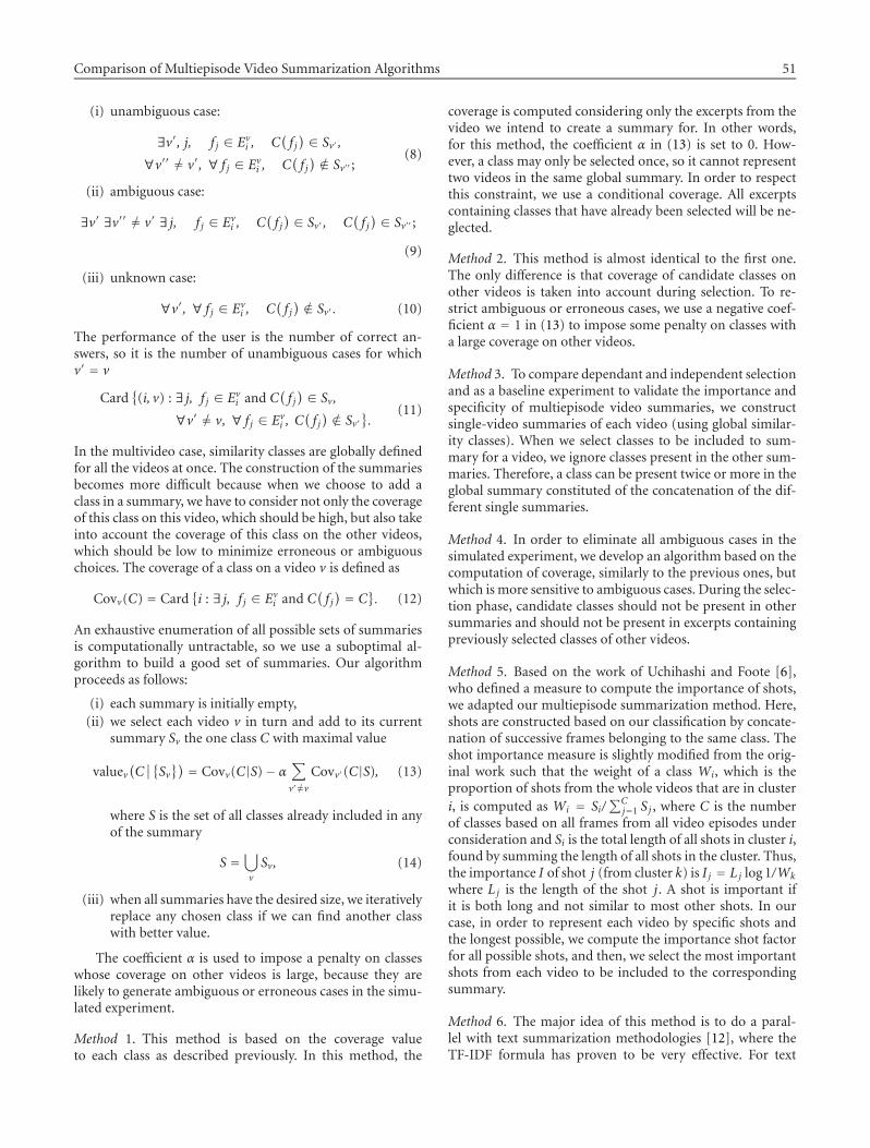
Comparison of Multiepisode Video Summarization Algorithms 51
(i) unambiguous case:
∃v′, j, f j ∈ Evi , C
(f j) ∈ Sv′ ,
∀v′′ �= v′, ∀ f j ∈ Evi , C
(f j) �∈ Sv′′ ;
(8)
(ii) ambiguous case:
∃v′ ∃v′′ �= v′ ∃ j, f j ∈ Evi , C
(f j) ∈ Sv′ , C
(f j) ∈ Sv′′ ;
(9)
(iii) unknown case:
∀v′, ∀ f j ∈ Evi , C
(f j) �∈ Sv′ . (10)
The performance of the user is the number of correct an-swers, so it is the number of unambiguous cases for whichv′ = v
Card{
(i, v) : ∃ j, f j ∈ Evi and C
(f j) ∈ Sv,
∀v′ �= v, ∀ f j ∈ Evi , C
(f j) �∈ Sv′
}.
(11)
In the multivideo case, similarity classes are globally definedfor all the videos at once. The construction of the summariesbecomes more difficult because when we choose to add aclass in a summary, we have to consider not only the coverageof this class on this video, which should be high, but also takeinto account the coverage of this class on the other videos,which should be low to minimize erroneous or ambiguouschoices. The coverage of a class on a video v is defined as
Covv(C) = Card{i : ∃ j, f j ∈ Ev
i and C(f j) = C
}. (12)
An exhaustive enumeration of all possible sets of summariesis computationally untractable, so we use a suboptimal al-gorithm to build a good set of summaries. Our algorithmproceeds as follows:
(i) each summary is initially empty,(ii) we select each video v in turn and add to its current
summary Sv the one class C with maximal value
valuev(C∣∣{Sv}) = Covv(C|S)− α
∑v′ �=v
Covv′(C|S), (13)
where S is the set of all classes already included in anyof the summary
S =⋃v
Sv, (14)
(iii) when all summaries have the desired size, we iterativelyreplace any chosen class if we can find another classwith better value.
The coefficient α is used to impose a penalty on classeswhose coverage on other videos is large, because they arelikely to generate ambiguous or erroneous cases in the simu-lated experiment.
Method 1. This method is based on the coverage valueto each class as described previously. In this method, the
coverage is computed considering only the excerpts from thevideo we intend to create a summary for. In other words,for this method, the coefficient α in (13) is set to 0. How-ever, a class may only be selected once, so it cannot representtwo videos in the same global summary. In order to respectthis constraint, we use a conditional coverage. All excerptscontaining classes that have already been selected will be ne-glected.
Method 2. This method is almost identical to the first one.The only difference is that coverage of candidate classes onother videos is taken into account during selection. To re-strict ambiguous or erroneous cases, we use a negative coef-ficient α = 1 in (13) to impose some penalty on classes witha large coverage on other videos.
Method 3. To compare dependant and independent selectionand as a baseline experiment to validate the importance andspecificity of multiepisode video summaries, we constructsingle-video summaries of each video (using global similar-ity classes). When we select classes to be included to sum-mary for a video, we ignore classes present in the other sum-maries. Therefore, a class can be present twice or more in theglobal summary constituted of the concatenation of the dif-ferent single summaries.
Method 4. In order to eliminate all ambiguous cases in thesimulated experiment, we develop an algorithm based on thecomputation of coverage, similarly to the previous ones, butwhich is more sensitive to ambiguous cases. During the selec-tion phase, candidate classes should not be present in othersummaries and should not be present in excerpts containingpreviously selected classes of other videos.
Method 5. Based on the work of Uchihashi and Foote [6],who defined a measure to compute the importance of shots,we adapted our multiepisode summarization method. Here,shots are constructed based on our classification by concate-nation of successive frames belonging to the same class. Theshot importance measure is slightly modified from the orig-inal work such that the weight of a class Wi, which is theproportion of shots from the whole videos that are in clusteri, is computed as Wi = Si/
∑Cj=1 Sj , where C is the number
of classes based on all frames from all video episodes underconsideration and Si is the total length of all shots in cluster i,found by summing the length of all shots in the cluster. Thus,the importance I of shot j (from cluster k) is I j = Lj log 1/Wk
where Lj is the length of the shot j. A shot is important ifit is both long and not similar to most other shots. In ourcase, in order to represent each video by specific shots andthe longest possible, we compute the importance shot factorfor all possible shots, and then, we select the most importantshots from each video to be included to the correspondingsummary.
Method 6. The major idea of this method is to do a paral-lel with text summarization methodologies [12], where theTF-IDF formula has proven to be very effective. For text

52 EURASIP Journal on Applied Signal Processing
4035302520151050
Excerpt duration
10
15
20
25
30
35
40
45
50
55
Cov
erag
e
Method 1Method 2Method 3
Method 4Method 5Method 6
Figure 2: Multisummaries coverage as function of excerpt dura-tion.
summarization, this approach is based on terms which repre-sent the items, whereas for multivideo summaries, items areclasses. Therefore, the importance I of class c is computed asIc = Lc logn/nc, where Lc is the length (total duration) of theclass c, n the number of videos, and nc the number of videoscontaining at least one frame from the class c.
Having computed the importance of each class, we selectthe most important ones to be included in the global sum-mary. In the case where the class is present in more than onevideo, we have to determine to which summary it should beaffected. We do this by computing for each video the propor-tion of frames belonging to this class that are present in thisvideo, and we take the most probable one.
5. COVERAGE EXPERIMENTS
In this section, we present the evaluation results usingthe simulated user principal on multiepisodes video sum-maries created with six different algorithms. As test data,we recorded six episodes of the TV series “Friends.” Theserecordings were compressed Mpeg1 with a digitization rateof 14 frames per second. We fixed the size of the summariesto six segments (which provides a convenient display on aconventional TV 4/3 or 16/9 screen).
The graph in Figure 2 shows the respective performanceof the six methods presented in Section 4 when the dura-tion of the excerpt used for both construction and evalua-tion varies. For additional information the exact data valuesobtained are presented in Table 1. We note that the first twomethods that build summaries, based on a mathematical cri-terion inspired for the evaluation criterion itself, give the bestperformance. We note also that the multiepisode summaries(Methods 1 and 2) are more efficient than the single videosummaries (Method 3).
Method 5 consists in selecting the rarest and longestshots. Despite the fact that our performance criterion isbased on the rate of correct simulated user responses (ex-cerpts for which the simulated user has correctly guessed thecorresponding video) and the fact that the rarest shots areby definition highly specific of the video they originate from,the results based on this method are quite poor. The reasonis that the rarest shots are likely to be nonredundant (theyoccur only once) within the video and therefore unlikely tobe widely spread across the video. This greatly reduces thenumber of possible excerpts covering the selected shots and,consequently, low performance results, based on coverage in-formation, are obtained.
Method 6, inspired from TF-IDF, provides rather averageresults when compared with others. It should also be notedthat the results obtained using Method 4 can be compared tothose of Method 2 and that both give the best coverage forlarge excerpts duration.
As a general comment, we can observe on Figure 2 that,for excerpt duration of approximately over 27 seconds, theresults of Method 2 (with α = 1) and Method 4 (with no am-biguity requirement) perform better than the basic method(Method 1), whereas it was the opposite for shorter excerpts.A possible explanation consist in considering that, for thelongest excerpt, the probability of finding similar images inother videos increases. In this approach, the simulated useris more likely to make an incorrect guess, leading to a perfor-mance reduction which does not occur with the other twomethods.
Similarly, the third method offers reasonable perfor-mance results for short excerpt. As the duration of the ex-cerpt used for construction increases, the number of ambigu-ous cases increases. This is due to the fact that key framesfrom the same similarity class may be employed in manysummaries.
6. ROBUSTNESS OF THE SUMMARIES
Having constructed multiepisode video summaries using sixalternative methods, it is of interest to evaluate the per-formance of the summaries for unrestricted excerpt dura-tion. The first four methods are dependent on the excerptduration whereas the last two are not. To study robust-ness, summaries were built for various excerpts durationand then evaluated, using various excerpts duration. Figure 3presents the results of this experiment for summaries basedon Method 1. The choice was made to perform this study us-ing the first method as it is the one which provided the bestoverall results in the performance experiments.
Note that the construction method itself suggests that thecoverage of the summary over the video should be maxi-mum when the same excerpt duration is employed for bothconstruction and evaluation. However, the results shown inTable 2 do not follow the same trend. Indeed, for each of thesummaries, the best coverage results are obtained for largeevaluation excerpt size. Except in the case of summaries cre-ated with excerpt duration of 1 second, all the remaining
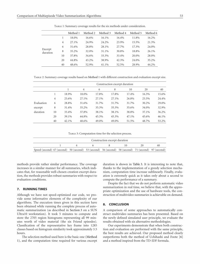
Comparison of Multiepisode Video Summarization Algorithms 53
Table 1: Summary coverage results for the six methods under consideration.
Method 1 Method 2 Method 3 Method 4 Method 5 Method 6
Excerptduration
1 18.0% 16.6% 16.1% 16.4% 11.8% 16.2%
4 27.1% 24.9% 24.2% 23.9% 15.5% 21.3%
6 31.6% 28.8% 28.1% 27.7% 17.3% 24.0%
8 35.2% 32.0% 31.1% 30.8% 18.8% 26.1%
10 37.8% 34.6% 33.3% 33.4% 20.0% 28.0%
20 44.8% 43.2% 38.9% 42.3% 24.0% 35.2%
40 48.6% 52.9% 41.1% 52.5% 28.9% 44.2%
Table 2: Summary coverage results based on Method 1 with different construction and evaluation excerpt size.
Construction excerpt duration
1 4 6 8 10 20 40
1 18.9% 18.0% 17.8% 17.8% 17.4% 16.3% 15.6%
4 25.6% 27.1% 27.1% 27.1% 26.8% 25.5% 24.4%
Evaluation 6 28.8% 31.6% 31.7% 31.7% 31.7% 30.2% 29.0%
excerpt 8 31.4% 35.2% 35.3% 35.3% 35.6% 34.0% 32.9%
duration 10 33.4% 37.8% 38.1% 38.1% 38.8% 37.1% 36.2%
20 39.1% 44.8% 45.3% 45.3% 47.1% 45.6% 46.1%
40 42.1% 48.6% 49.0% 49.0% 51.5% 48.7% 53.2%
Table 3: Computation time for the selection process.
Construction excerpt duration
1 4 6 8 10 20 40
Speed (second) 47 (second) 50 (second) 53 (second) 56 (second) 58 (second) 71 (second) 97 (second)
methods provide rather similar performance. The coverageincreases in a similar manner for all summaries, which indi-cates that, for reasonable well-chosen creation excerpt dura-tion, the methods provides robust summaries with respect toevaluation conditions.
7. RUNNING TIMES
Although we have not speed-optimized our code, we pro-vide some informative elements of the complexity of ouralgorithms. The execution times given in this section havebeen obtained while running the complete process of auto-matic summarization (as described in Section 3 on a SUNUltra10 workstation). It took 5 minutes to compute andstore the 2705 region histograms representing all 99 min-utes worth of video material (the six Friend episodes).Classification of the representative key frame into 1285classes based on histogram similarity took approximately 3.5hours.
The selection method used here is the basic one (Method1), and the computation time required for various excerpt
duration is shown in Table 3. It is interesting to note that,thanks to the implementation of a greedy selection mecha-nism, computation time increase sublinearly. Finally, evalu-ation is extremely quick as it takes only about a second tocompute the performance of a summary.
Despite the fact that we do not perform automatic videosummarization in real time, we believe that, with the appro-priate optimization and the use of hardware tools, the con-struction of multivideo summaries is achievable on demand.
8. CONCLUSION
A comparison of some approaches to automatically con-struct multivideo summaries has been presented. Based onthe newly defined simulated user principle, we evaluate theresults obtained with six alternative methodologies.
Our experiments demonstrate that when both construc-tion and evaluation are performed with the same principle,the best results are achieved. Our proposed method clearlyoutperforms both the method of Uchihashi and Foote [6]and a method inspired from the TD-IDF formula.

54 EURASIP Journal on Applied Signal Processing
4035302520151050Excerpt duration
15
20
25
30
35
40
45
50
55
Cov
erag
e
S1S4S8
S10S20S40
Figure 3: Summary coverage as function of excerpt duration usingMethod 1.
An evaluation of the robustness of the summaries showsthat it is possible to obtain reasonable results with summariescreated for specific excerpt duration. We envisage the cre-ation of optimal summaries independently of the excerpt du-ration in order to achieve high coverage performance for anyselected excerpt.
ACKNOWLEDGMENT
This research was supported by Eurecom’s industrial mem-bers: Ascom, Bouygue, Cegetel, France Telecom, Hitachi,ST Microelectronics, Motorola, Swisscom, Texas Instrumentsand Thales.
REFERENCES
[1] A. D. Doulamis, N. D. Doulamis, and S. D. Kollias, “Effi-cient video summarization based on a fuzzy video contentrepresentation,” in Proc. IEEE Int. Symp. Circuits and Systems,vol. 4, pp. 301–304, Geneva, Switzerland, May 2000.
[2] G. Iyengar and A. B. Lippman, “Videobook: An experimentin characterization of video,” in Proc. IEEE International Con-ference on Image Processing, vol. 3, pp. 855–858, Lausanne,Switzerland, September 1996.
[3] M. A. Smith and T. Kanade, “Video skimming and charac-terization through the combination of image and languageunderstanding,” in Proc. IEEE International Workshop onContent-Based Access of Image and Video Databases, pp. 61–70, Bombay, India, January 1998.
[4] N. Vasconcelos and A. Lippman, “Bayesian modeling of videoediting and structure: Semantic features for video summariza-tion and browsing,” in Proc. IEEE International Conference onImage Processing, vol. 3, pp. 153–157, Chicago, Ill, USA, 1998.
[5] R. Lienhart, S. Pfeiffer, and W. Effelsberg, “Video abstracting,”Communications of the ACM, vol. 40, no. 12, pp. 54–62, 1997.
[6] S. Uchihashi and J. Foote, “Summarizing video using a shotimportance measure and a frame-packing algorithm,” in
Proc. IEEE Int. Conf. Acoustics, Speech, Signal Processing, vol. 6,pp. 3041–3044, Phoenix, Ariz, USA, 1999.
[7] B. Merialdo, “Automatic indexing of tv news,” in Workshop onImage Analysis for Multimedia Integrated Services, pp. 99–104,Louvain-la-neuve, Belgium, June 1997.
[8] M. T. Maybury and A. E. Merlino, “Multimedia summariesof broadcast news,” in Proc. IEEE International Conference onIntelligent Information Systems, pp. 442–449, Grand BahamaIsland, Bahamas, December 1997.
[9] Y. Gong and X. Liu, “Generating optimal video summaries,”in Proc. IEEE International Conference on Multimedia andExpo, vol. 3, pp. 1559–1562, New York, NY, USA, 2000.
[10] H. Sundaram and S.-F. Chang, “Constrained utility maxi-mization for generating visual skims,” in Proc. IEEE Inter-national Conference on Multimedia and Expo, Tokyo, Japan,August 2001.
[11] S.-F. Chang, “Optimal video adaptation and skimming usinga utility-based framework,” in Tyrrhenian International Work-shop on Digital Communications, Capri Island, Italy, Septem-ber 2002.
[12] I. Mani and M. T. Maybury, Eds., Advances in Automatic TextSummarization, M. I. T. Press, Cambridge, Mass, USA, 1999.
Itheri Yahiaoui graduated in the Depart-ment of Computer Science and Engineeringin 1997 from the University of Batna, Alge-ria. She received the Diplome d’Etudes Ap-profondies in Robotics in June 1999 fromthe University of Pierre et Marie Curie, ParisVI, France. In September 1999, she joinedthe Multimedia Communications Depart-ment at Institut Eurecom to study towardthe Ph.D. degree under the supervision ofProfessor Bernard Merialdo. Her work focuses on the automaticconstruction of video summaries. Her research interests includemultimedia indexing (video analysis, segmentation and classifica-tion), content-based retrieval, and image processing.
Bernard Merialdo graduated from theEcole Normale Superieure (Mathema-tiques) in 1975. He received the Ph.D. de-gree in computer science from Paris 6University in 1979 and an “Habilitationa Diriger des Recherches” from Paris 7University in 1992. He first taught at theFaculty of Sciences in Rabat, Morocco. In1981, he joined the IBM France Scien-tific Center in Paris, where he led severalresearch projects on natural language processing and speechrecognition using probabilistic models. From 1988 to 1990, hewas a Visiting Scientist in the IBM TJ Watson Research Center inYorktown Heights, NY, USA. In 1992, he joined the MultimediaCommunications Department of the Institut Eurecom. He is nowa full Professor and head of this department. His current researchtopics are multimedia indexing (video segmentation, analysis andclassification, information filtering) and multimedia collaborativeapplications. His group is involved in several research projects inpartnership with other universities and industrial companies. Heis an Associate Editor of the IEEE Transactions on Multimedia. Heparticipates in numerous scientific organizations, program com-mittees, expert boards; for example, he is the General Chairman ofthe ACM Multimedia 2002 conference.

Comparison of Multiepisode Video Summarization Algorithms 55
Benoit Huet received his B.S. degree incomputer science and engineering from theEcole Superieure de Technologie Electrique(Groupe ESIEE, France) in 1992. In 1993, hewas awarded the M.S. degree in artificial in-telligence from the University of Westmin-ster, UK, with distinction, where he thenspent two years working as a Research andTeaching Assistant. He received his Ph.D.degree in computer science from the Uni-versity of York, UK, in 1999 for his research on the topic of ob-ject recognition from large databases. He is currently an AssistantProfessor in the Multimedia Information Processing Group of theInstitut Eurecom, France. He has published some 35 papers in jour-nals, edited books, and refereed conferences. His research interestsinclude computer vision, content-based retrieval, multimedia dataindexing (still and/or moving images), and pattern recognition. Heis involved in major scientific organizations, reviewing panels, andprogram committees.

EURASIP Journal on Applied Signal Processing 2003:1, 56–65c© 2003 Hindawi Publishing Corporation
3D Scan-Based Wavelet Transform and QualityControl for Video Coding
Christophe ParisotLaboratoire I3S, UMR 6070 (CNRS, Universite de Nice-Sophia Antipolis) Bat. Algorithmes/Euclide 2000,route des Lucioles, BP 121 F-06903 Sophia Antipolis Cedex, FranceEmail: [email protected]
Marc AntoniniLaboratoire I3S, UMR 6070 (CNRS, Universite de Nice-Sophia Antipolis) Bat. Algorithmes/Euclide 2000,route des Lucioles, BP 121 F-06903 Sophia Antipolis Cedex, FranceEmail: [email protected]
Michel BarlaudLaboratoire I3S, UMR 6070 (CNRS, Universite de Nice-Sophia Antipolis) Bat. Algorithmes/Euclide 2000,route des Lucioles, BP 121 F-06903 Sophia Antipolis Cedex, FranceEmail: [email protected]
Received 4 March 2002 and in revised form 17 October 2002
Wavelet coding has been shown to achieve better compression than DCT coding and moreover allows scalability. 2D DWT canbe easily extended to 3D and thus applied to video coding. However, 3D subband coding of video suffers from two drawbacks.The first is the amount of memory required for coding large 3D blocks; the second is the lack of temporal quality due to thesequence temporal splitting. In fact, 3D block-based video coders produce jerks. They appear at blocks temporal borders duringvideo playback. In this paper, we propose a new temporal scan-based wavelet transform method for video coding combiningthe advantages of wavelet coding (performance, scalability) with acceptable reduced memory requirements, no additional CPUcomplexity, and avoiding jerks. We also propose an efficient quality allocation procedure to ensure a constant quality over time.
Keywords and phrases: scan-based DWT, 3D subband coding, quality control, video coding.
1. INTRODUCTION
Although 3D subband coding of video [1, 2, 3, 4, 5] providesencouraging results compared to MPEG [6, 7, 8, 9], its gener-alization suffers from significant memory requirements. Oneway to reduce memory requirements is to apply the tempo-ral discrete wavelet transform (DWT) on 3D blocks comingfrom a temporal splitting of the sequence. But this block-based DWT method introduces temporal blocking artifactswhich result in undesirable jerks during video playback. Inthis paper, we propose new tools for 3D subband codecs toguarantee the output frames a constant quality over time.
Scan-based 2D wavelet transforms were first suggestedfor on-board satellite compression in [10, 11] and byChrysafis and Ortega in [12].
In Section 2, we propose a 3D scan-based DWT methodand a 3D scan-based motion-compensated lifting DWT forvideo coding. The method allows the computation of thetemporal wavelet decomposition of a sequence with infinitelength using little memory and no extra CPU. Furthermore,
the proposed wavelet transform provides higher quality con-trol than 3D block-based video compression schemes (avoid-ing jerks).
In Section 3, we propose an efficient model-based qualitycontrol procedure. This bit-allocation procedure controls theoutput frames quality over time. This new quality-controlprocedure takes advantage of the model-based rate allocationmethods described in [13].
Finally, Section 4 presents experimental results obtainedby our method.
2. 3D VIDEO WAVELET TRANSFORM
2.1. Principle
The method generally used to reduce memory requirementsfor large image coding is to split the image and then performthe transform on tiles such as JPEG with 8 × 8 DCT blocksor JPEG2000 [14]. Unfortunately, the coefficients are com-puted from periodic or symmetrical extensions of the signal.

3D Scan-Based Wavelet Transform and Quality Control for Video Coding 57
This results in undesirable blocking artifacts. For video cod-ing, the same blocking artifacts in the temporal direction (in-troduced by temporal splitting) result in jerks.
In this section, we propose a 3D wavelet transformframework for video coding that requires storing a minimumamount of data without any additional CPU complexity [15].The frames of the sequence are acquired and processed on thefly.
Definitions of the temporal coherence and the buffer names
We consider a temporal interval (set of input frames). We de-fine the set of its temporally coherent wavelet coefficients as theset of all coefficients, in all subbands, obtained by a filter (orconvolution of filters) centered on any one of the frames ofthis temporal interval. In this paper, we assume that encod-ing is allowed only when we have a temporally coherent setof wavelet coefficients. Temporal coherence improves the en-coder performance since it allows optimal bit allocation forwavelet coefficients of the same temporal interval.
The set of buffers used to perform the temporal wavelettransform will be called filtering buffers. These buffers pro-duce low- and high-frequency temporal wavelet coefficients.In the same way, we call synchronization buffers, the set ofbuffers used to store output coefficients before their encod-ing.
2.2. Temporal scan-based video DWT and delay
Consider the case of a 3D wavelet transform which can besplit into a 2D DWT on each frame and an additional 1DDWT in the time direction [16]. In this paper, we focus on anefficient implementation of the temporal wavelet transformand we propose a method independent of the choice of thespatial wavelet transform.
Each time a frame is received, we perform its 2D wavelettransform and send it into our scan-based temporal wavelettransform system. We consider symmetrical filters with oddlength since they are the most widely used in image com-pression algorithms [14, 17]. To simplify, we also supposethat the low-pass filter is longer than the high-pass one. LetL = 2S + 1 be the length of the low-pass filter with S ≥ 2.We want to design components that can be easily reused forany wavelet decomposition tree. Therefore, the memory usedfor the filtering buffers is supposed to be internal and cannotbe shared with other filtering buffers nor with the synchro-nization buffers for wavelet coefficients storage. We proposea method that minimizes the total memory requirements forFIR filtering.
2.2.1 Single-stage DWT
We first consider a single stage of the temporal wavelet trans-form.
The length of the low-pass filter is L. Therefore, we needL frames of 2D wavelet coefficients in memory to computeone frame of low-frequency temporal wavelet coefficients.The high-pass filter is shorter. Thus, our filtering buffer mustcontain exactly L frames of 2D wavelet coefficients. Conse-quently, filtering buffers are FIFO with length L. Figure 1
Temporal synchronization buffers
Temporal filtering bufferInput frame
HF
LF
Central point of the low-pass filter
Central point of the high-pass filter
Figure 1: One-level temporal scan-based wavelet decompositionfor the 5/3 filter bank.
shows the scheme for a single stage of a 5/3 temporal waveletdecomposition. The filtering buffer contains five frames of2D wavelet coefficients. The synchronization buffers are usedto store output 3D wavelet coefficients until we get a tempo-rally coherent set of 3D wavelet coefficients.
When the (S+ 1)st 2D transformed frame is received, thefiltering buffer is symmetrically filled up in order to avoidside effects. The central frame is the 2D wavelet transformof the first image of the sequence. We can compute the firstlow-frequency temporal coefficients applying the low-passfilter to the central frame of the filtering buffer (gray framein Figure 1). The first high-frequency temporal coefficientsmust be computed on the second 2D transformed frame.This frame (hatched frame in Figure 1) and all its necessaryneighbours are already present in the filtering buffer since thehigh-pass filter is shorter than the low-pass one. Therefore,the high-frequency temporal wavelet coefficients can also becomputed without additional input frame.
Finally, we have to wait for only S + 1 input frames to getone low-frequency and one high-frequency temporal framesof wavelet coefficients. Then, for each pair of input frames,we can compute both low-frequency and high-frequency co-efficients. Each pair of low- and high-frequency frames is aset of temporally coherent wavelet coefficients. Therefore, weneed S+1 input frames to get the first set of temporally coher-ent wavelet coefficients and S+1+2(n−1) = S+2n−1 inputframes to get a set of n low-frequency and n high-frequencyoutput frames.
When the input sequence is finished, input frames are re-placed by a symmetrical extension using the frames presentin the filtering buffer in order to flush it.

58 EURASIP Journal on Applied Signal Processing
1
2
6
HF3
HF2
HF1
LF3
LF2
LF1
1
5
5
5
Input frame
Central point of the low-pass filterCentral point of the high-pass filterTemporally coherent 3D wavelet coefficients
Figure 2: Three-level temporal scan-based wavelet decomposition for the 5/3 filter bank.
2.2.2 Multistage DWT
We now consider the general scheme of an N-level temporalwavelet decomposition. We focus only on the usual dyadicdecomposition without additional high-frequency subbanddecomposition. We assume that decomposition levels are in-dexed from 1 to N , where level j corresponds to the coeffi-cients produced by the jth wavelet decomposition (level 0 isthe sequence of all 2D wavelet transformed frames).
We compute the encoding delay for a two-level waveletdecomposition. The first stage has to compute S + 1 low-frequency temporal frames to get coefficients in both low-frequency and high-frequency subbands of the second level.In the same time, the first stage has also computed S+1 high-frequency temporal frames. But, from Section 2.2.1, we knowthat these S+ 1 low-frequency and S+ 1 high-frequency out-put frames of 3D wavelet coefficients can only be computedafter the delay of S + 2(S + 1) − 1 frames. Thus, we have towait for 3S+1 frames to get one frame of 3D coefficients in allsubbands of the second decomposition level and S+ 1 framesof 3D coefficients in the first level. Notice that for temporalcoherence, we need only the first two frames among the S+ 1of the first level.
To compute the delay for an N-level temporal wavelet de-composition, we define dj as the number of frames requiredat the input of the jth filtering buffer to get temporally coher-ent coefficients in all subbands. The processing of the first setof 3D subbands of temporally coherent wavelet coefficientswill be possible after D = d1 frames have been received.From Section 2.2.1, we know that dj = S + 2dj+1 − 1 forj ∈ {1, . . . , N−1} and dN = S+1. Solving these equations, wefind that the number of input frames required at level j be-fore the first wavelet coefficients are available for processing
Table 1: Number of input frames necessary to get the first set oftemporally coherent wavelet coefficients (1).
Number of levels (N) 9/7 DWT 5/3 DWT
1 5 3
2 13 7
3 29 15
is dj = (2N+1− j − 1)S+ 1. Therefore, for an N-level temporalwavelet decomposition, the number of input frames neededto get the first set of temporally coherent wavelet coefficientsis
D = (2N − 1
)S + 1. (1)
Thus, the number of frames needed for the synchroniza-tion of the multistage decomposition increases exponentiallywith the number of decomposition levels. Figure 2 shows thescheme of a three-level wavelet decomposition for S = 2.Dark frames in the synchronization buffers are the set of co-efficients which will be processeded together (quantized andencoded) as soon as we have coefficients in all temporal fre-quency bands. This set of coefficients is temporally coherent.At the beginning of the sequence, we have to wait for D inputframes. Then, sets of temporally coherent coefficients will beavailable each 2N input frames. Table 1 shows the numberof input frames needed to get the first set of temporally co-herent wavelet coefficients for two widely used filter banks.This table shows that a three-level decomposition introducesan encoding delay of less than one second with the 9/7 filter

3D Scan-Based Wavelet Transform and Quality Control for Video Coding 59
bank and only half a second with the 5/3 filter bank. In 3Dblock-based video coders, the delay is equal to the size of thetemporal block. As blocks are larger in order to minimize thenumber of jerks, the delay is more important for 3D block-based wavelet transform video coders.
2.3. Memory requirements
Memory requirements are given by the sum of the numberof frames in the N filtering buffers and the number of framesin the synchronization buffers.
The memory requirements for the filtering buffers areequal to (2S + 1)N frames.
The synchronization buffers of the last decompositionlevel must contain one frame of 3D wavelet coefficients forboth the low-frequency and high-frequency subbands. Forthe jth decomposition level ( j < N), dj+1, low-frequencyoutputs need to be computed and, in the same time, dj+1
high-frequency outputs can be computed. As we know thattemporal coherence requires less than dj+1 3D frames ofwavelet coefficients at level j, we can decide to delay thecomputation of the last computable high-frequency coeffi-cients until the new set of temporally coherent 3D waveletcoefficients has been encoded. Once the set of temporallycoherent coefficients has been encoded, we compute all thehigh-frequency coefficients for levels 1 to N − 1 and sendthem into the synchronization buffers. Then, the on-the-flywavelet transform can resume normally. This trick allows tospare one frame in the memory requirements of each syn-chronization buffer for levels 1 to N − 1. Thus, the memoryrequirements for the synchronization buffers are limited to2 +
∑N−1j=1 (dj+1 − 1).
We need to store MS = (2N −N−1)S+2 frames of coeffi-cients for all the synchronization buffers. Therefore, the totalmemory requirements of this method are
M = (2N + N − 1
)S + N + 2 (2)
frames, for an N-level temporal wavelet transform with filterlength L = 2S + 1. When memory can be shared between fil-tering buffers and synchronization buffers, the total memoryrequirements are limited to
M = (2N + N − 1
)S + 1 (3)
frames. See [18] for complete memory requirements formu-lae.
Tables 2 and 3 show the total memory requirements forthe 9/7 and 5/3 filter banks, respectively, for independent andshared buffers.
Memory requirements increase as an exponential func-tion of the resolution N and as a linear function of the filterlength.
Note that, for the same memory requirements (e.g., 48frames) and three levels of the 9/7 DWT decomposition witha frame rate of 30 fps, the encoding delay for temporal block-based video coders is equal to 1.6 second while it is 0.97 sec-ond in our case (from Table 1). Furthermore, block-basedvideo coders have jerks for each group of 48 frames whileour method avoids these annoying artifacts.
Table 2: Memory requirements (2), in terms of frames, of the scan-based DWT system including both filtering and synchronizationbuffers.
Number of levels (N) 9/7 DWT 5/3 DWT
1 11 7
2 24 14
3 45 25
Table 3: Memory requirements (3), in terms of frames, of the scan-based DWT system including both filtering and synchronizationbuffers when memory can be shared between filtering and synchro-nization buffers.
Number of levels (N) 9/7 DWT 5/3 DWT
1 9 5
2 21 11
3 41 21
The CPU complexity of our temporal scan-based DWTis exactly the same as to perform the regular 1D DWT in thetemporal direction on the entire sequence.
2.4. Scan-based motion compensated lifting
The main drawback of the 3D scan-based DWT is that itdoes not take motion compensation into account. 3D mo-tion compensated lifting is an efficient tool to take accountof motion in video [4, 6, 9, 19, 20, 21].
Thus, we propose a new 3D scan-based motion compen-sated lifting scheme [18, 22]. This method combines the ben-efits of scan-based filtering, block-based coding, and qualitycontrol [22].
When filtering and synchronization buffers are indepen-dent, the total memory requirements become
M = (2N −N − 1
)S + βN + 2, (4)
where β is a parameter depending on the filter, β = 6 for the9/7 Daubechies DWT [23], and β = 4 for the 5/3 DWT. Whenmemory can be shared between filtering and synchronizationbuffers, the total memory requirements are limited to
M = (2N −N − 1
)S + (β − 1)N + 1. (5)
Complete memory requirements computation can befound in [18]. The scan-based motion compensated lift-ing scheme saves memory compared to the regular filterbanks implementation. Furthermore, our method does notincrease the CPU complexity compared to the usual liftingimplementation.
Tables 4 and 5 show the memory requirements for scan-based motion compensated lifting video coders, respectively,for independant and shared buffers.
Thus, the scan-based motion compensated lifting schemesaves 12 to 33% memory (Tables 2 and 4 or Tables 3 and 5)and takes account motion compensation.
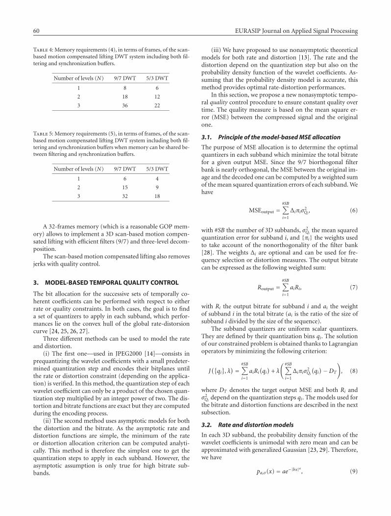
60 EURASIP Journal on Applied Signal Processing
Table 4: Memory requirements (4), in terms of frames, of the scan-based motion compensated lifting DWT system including both fil-tering and synchronization buffers.
Number of levels (N) 9/7 DWT 5/3 DWT
1 8 6
2 18 12
3 36 22
Table 5: Memory requirements (5), in terms of frames, of the scan-based motion compensated lifting DWT system including both fil-tering and synchronization buffers when memory can be shared be-tween filtering and synchronization buffers.
Number of levels (N) 9/7 DWT 5/3 DWT
1 6 4
2 15 9
3 32 18
A 32-frames memory (which is a reasonable GOP mem-ory) allows to implement a 3D scan-based motion compen-sated lifting with efficient filters (9/7) and three-level decom-position.
The scan-based motion compensated lifting also removesjerks with quality control.
3. MODEL-BASED TEMPORAL QUALITY CONTROL
The bit allocation for the successive sets of temporally co-herent coefficients can be performed with respect to eitherrate or quality constraints. In both cases, the goal is to finda set of quantizers to apply in each subband, which perfor-mances lie on the convex hull of the global rate-distorsioncurve [24, 25, 26, 27].
Three different methods can be used to model the rateand distortion.
(i) The first one—used in JPEG2000 [14]—consists inprequantizing the wavelet coefficients with a small predeter-mined quantization step and encodes their bitplanes untilthe rate or distortion constraint (depending on the applica-tion) is verified. In this method, the quantization step of eachwavelet coefficient can only be a product of the chosen quan-tization step multiplied by an integer power of two. The dis-tortion and bitrate functions are exact but they are computedduring the encoding process.
(ii) The second method uses asymptotic models for boththe distortion and the bitrate. As the asymptotic rate anddistortion functions are simple, the minimum of the rateor distortion allocation criterion can be computed analyti-cally. This method is therefore the simplest one to get thequantization steps to apply in each subband. However, theasymptotic assumption is only true for high bitrate sub-bands.
(iii) We have proposed to use nonasymptotic theoreticalmodels for both rate and distortion [13]. The rate and thedistortion depend on the quantization step but also on theprobability density function of the wavelet coefficients. As-suming that the probability density model is accurate, thismethod provides optimal rate-distortion performances.
In this section, we propose a new nonasymptotic tempo-ral quality control procedure to ensure constant quality overtime. The quality measure is based on the mean square er-ror (MSE) between the compressed signal and the originalone.
3.1. Principle of the model-based MSE allocation
The purpose of MSE allocation is to determine the optimalquantizers in each subband which minimize the total bitratefor a given output MSE. Since the 9/7 biorthogonal filterbank is nearly orthogonal, the MSE between the original im-age and the decoded one can be computed by a weighted sumof the mean squared quantization errors of each subband. Wehave
MSEoutput =#SB∑i=1
∆iπiσ2Qi, (6)
with #SB the number of 3D subbands, σ2Qi
the mean squaredquantization error for subband i, and {πi} the weights usedto take account of the nonorthogonality of the filter bank[28]. The weights ∆i are optional and can be used for fre-quency selection or distortion measures. The output bitratecan be expressed as the following weighted sum:
Routput =#SB∑i=1
aiRi, (7)
with Ri the output bitrate for subband i and ai the weightof subband i in the total bitrate (ai is the ratio of the size ofsubband i divided by the size of the sequence).
The subband quantizers are uniform scalar quantizers.They are defined by their quantization bins qi. The solutionof our constrained problem is obtained thanks to Lagrangianoperators by minimizing the following criterion:
J({qi}, λ) = #SB∑
i=1
aiRi(qi)
+ λ
( #SB∑i=1
∆iπiσ2Qi
(qi)−DT
), (8)
where DT denotes the target output MSE and both Ri andσ2Qi
depend on the quantization steps qi. The models used forthe bitrate and distortion functions are described in the nextsubsection.
3.2. Rate and distortion models
In each 3D subband, the probability density function of thewavelet coefficients is unimodal with zero mean and can beapproximated with generalized Gaussian [23, 29]. Therefore,we have
pα,σ(x) = ae−|bx|α, (9)

3D Scan-Based Wavelet Transform and Quality Control for Video Coding 61
with b = (1/σ)√Γ(3/α)/Γ(1/α) and a = bα/2Γ(1/α). We also
assume that wavelet coefficients are independent and identi-cally distributed (i.i.d.) [13] in each subband.
Let Pr(m) be the probability of the quantization level mso that
Pr(m) =∫ (|m|+1/2)q
(|m|−1/2)qpα,σ(x)dx, (10)
for m �= 0 and
Pr(0) =∫ +q/2
−q/2pα,σ(x)dx. (11)
From (10) and (11), we can approximate the bitrate R bythe entropy of the output quantization levels
R = −+∞∑
m=−∞Pr(m) log2 Pr(m). (12)
The best coding value for the quantization level m [30] isthe centroid of its quantization bin
xm = sign(m)×∫ (|m|+1/2)q
(|m|−1/2)q xpα,σ(x)dx
Pr(m), (13)
for m �= 0 and x0 = 0.The mean squared quantization error is given by
σ2Q =
∫ +q/2
−q/2x2pα,σ(x)dx + 2
+∞∑m=1
∫ (m+1/2)q
(m−1/2)q
(x − xm
)2pα,σ(x)dx.
(14)
Inserting the value of xm into (14), we get
σ2Q = σ2 − 2
+∞∑m=1
( ∫ (m+1/2)q(m−1/2)q xpα,σ(x)dx
)2
∫ (m+1/2)q(m−1/2)q pα,σ(x)dx
. (15)
Proposition 1. When pα,σ is a generalized Gaussian distribu-tion with standard deviation σ and shape parameter α, there isa family of functions fn,m which verifies∫ +q/2
−q/2xnpα,σ(x)dx = σn fn,0
(α,
q
σ
),
∫ (m+1/2)q
(m−1/2)qxnpα,σ(x)dx = σn fn,m
(α,
q
σ
)∀m > 0
(16)
with
fn,0
(α,
q
σ
)=∫ +(1/2)(q/σ)
−(1/2)(q/σ)xnpα,1(x)dx,
fn,m
(α,
q
σ
)=∫ (m+1/2)(q/σ)
(m−1/2)(q/σ)xnpα,1(x)dx.
(17)
Proof of Proposition 1 is given in [18].
Therefore, the bitrate R and the quantization distortionσ2Q depend only on the shape parameter α and the ratio q/σ ,
R = R(α,
q
σ
), σ2
Q = σ2D(α,
q
σ
)(18)
with
R(α,
q
σ
)= − f0,0
(α,
q
σ
)log2 f0,0
(α,
q
σ
)
− 2+∞∑m=1
f0,m
(α,
q
σ
)log2 f0,m
(α,
q
σ
),
(19)
D(α,
q
σ
)= 1− 2
+∞∑m=1
f1,m(α, q/σ)2
f0,m(α, q/σ). (20)
3.3. Optimal model-based quantizationfor MSE control
Therefore, the goal is to find the quantization steps {qi} andλ which minimize
J({qi}, λ)=#SB∑
i=1
aiR(αi,
qiσi
)+ λ
( #SB∑i=1
∆iπiσ2i D
(αi,
qiσi
)−DT
).
(21)
We differentiate the criterion with respect to qi and λ.This provides the following equations:
ai∂R
∂qi
(αi, qi
)+ λ∆iπiσ
2i∂D
∂qi
(αi, qi
) = 0, ∀i,#SB∑i=1
∆iπiσ2i D
(αi, qi
)−DT = 0,
(22)
where qi = qi/σi.Thus, the quantizers parameters {qi}must verify the fol-
lowing system of #SB + 1 equations and #SB + 1 unknowns:
(∂D/∂qi)(αi, qi
)(∂R/∂qi)
(αi, qi
) = − aiλ∆iπiσ
2i
, ∀i,
#SB∑i=1
∆iπiσ2i D
(αi, qi
) = DT.
(23)
In order to simplify the notation, write
hαi(qi) = (∂D/∂qi)
(αi, qi
)(∂R/∂qi)
(αi, qi
) , (24)
where
hα(q) = A
Bln 2, (25)
where A = ∑+∞m=1(2(∂ f1,m/∂q)(α, q) f1,m(α, q) f0,m(α, q) −
f1,m(α, q)2(∂ f0,m/∂q)(α, q))/ f0,m(α, q)2, B = (pα,1(q/2)/2)× [ln f0,0(α, q) + 1] +
∑+∞m=1(∂ f0,m/∂q)(α, q)[ln f0,m(α, q) + 1]

62 EURASIP Journal on Applied Signal Processing
−10
−8
−6
−4
−2
0
2
4
6
8
10
ln(q/σ)
−4 0 4ln(−h
)
α = 1/4α = 1/3α = 1/2
α = 1Asymptotic
Figure 3: Tables of ln(−h(q/σ)) for different shape parameters α ofthe generalized Gaussian distribution.
with
∂ fn,m∂q
(α, q
) = [(m +
12
)n+1
pα,1
(mq +
q
2
)
−(m− 1
2
)n+1
pα,1
(mq − q
2
)]q n.
(26)
Equations (23) become
hαi(qi) = − ai
λ∆iπiσ2i
, ∀i,#SB∑i=1
∆iπiσ2i D
(αi, qi
) = DT.(27)
The solution of the MSE allocation problem can be ob-tained with the following equations:
#SB∑i=1
∆iπiσ2i D
(αi, h
−1αi
(− ai
λ∆iπiσ2i
))= DT, (28)
qi = h−1αi
(− ai
λπiσ2i
), ∀i, (29)
where h−1 is the inverse function of h. The parameter λ can befound from (28), and then (29) provides the optimal quan-tization steps qi. Unfortunately, as there is no analytical for-mula for h−1, the MSE allocation problem will be solved us-ing a parametric approach described below.
3.4. Parametric approach
Equation (29) gives the values of the quantization steps us-ing tables of the function h for different shape parameters α.Figure 3 shows the tables of ln(−hα(q)) for α = 1, 1/2, 1/3,and 1/4 and the asymptotic curve of equation
ln(−h) = 2 lnq
σ+ ln
ln 26
. (30)
−8
−6
−4
−2
0
2
4
6
8
ln(D)
−7 −6 −5 −4 −3 −2 −1 0ln(−h
)
α = 1/4α = 1/3α = 1/2
α = 1Asymptotic
Figure 4: Tables of ln(−h) = ln(ai/λπiσ2i ) versus lnD for different
shape parameters α of the generalized Gaussian distribution.
To solve (28), we need tables linking D and λ. Using (20)and (25), we plot the parametric curve (with parameter q)
[lnD
(α, q
); ln
(− hα(q))]
, (31)
for a given α. Using (29), this parametric curve is equivalentin each subband to the following parametric curve:
[lnD; ln
(ai
λπiσ2i
)]. (32)
Figure 4 shows these tables for α = 1, 1/2, 1/3, and 1/4 andthe asymptotic curve of equation
ln(−h) = lnD + ln(2 ln 2). (33)
Thus, we have a relation between D and λ in each sub-band. The optimal λ is found using the constraint (28). Then,we have a relation between λ and the quantization step qi ineach subband.
3.5. Algorithm of the model-based MSE allocation
The proposed MSE allocation procedure is the following.
(1) Set the initial value of λ to its asymptotic optimumvalue λ = 1/2DT ln 2.
(2) For each 3D subband i, compute ln(ai/λ∆iπiσ2i ) =
ln(−h) and read the corresponding normalized MSEDi using the tables shown in Figure 4.
(3) Compute |∑#SBi=1 ∆iπiσ
2i Di − DT |. If it is lower than a
given threshold, the constraint (28) is verified and thecurrent λ is optimal. Otherwise, compute1 a new valueof λ and go back to step (1).
1Several methods (such as dichotomy, bisection, secant method, goldensection search) can be used.

3D Scan-Based Wavelet Transform and Quality Control for Video Coding 63
−1.2
−1
−0.8
−0.6
−0.4
−0.2
0
0.2
0.4
0.6
0.8
PSN
Rva
riat
ion
s(d
B)
80644832160
Frame
Figure 5: PSNR variations for the 3D scan-based temporal DWT(continuous) and the 3D temporal tiling approach (dashed) onthe 89 first luminance frames of the sequence Akiyo at 80 kbps(25 fps). 9/7 DWT with two levels of decomposition; bitrate controlfor groups of 16 frames.
(4) For each 3D subband i, compute ln(ai/λ∆iπiσ2i ) =
ln(−h) with the optimal λ and read qi/σi using the ta-bles shown in Figure 3. This qi is the optimal quanti-zation step for subband i.
The tables shown in Figures 3 and 4 are stored for severalshape parameters α. They are valid for any video sequence.
4. EXPERIMENTAL RESULTS
To show the efficiency of our 3D scan-based wavelet trans-form method in removing the temporal blocking artifacts(jerks), we first extended EBWIC [13] to 3D data. Thequantized wavelet coefficients have been encoded usingJPEG2000’s bit-plane context-based arithmetic coder [14].We first encoded a sequence with the proposed 3D scan-based temporal wavelet transform and a bitrate regulationfor the temporally coherent coefficients of each group of 16frames. Then, we encoded the same sequence with the block-based approach, where the temporal wavelet coefficients andtheir encoding were performed on independent temporalblocks of 16 frames. Figure 5 shows a global PSNR improve-ment of mean 0.11 dB with our approach. Furthermore, wehave reduced the PSNR variance from 0.13 to 0.06. The peaksof the block-based approach fit with the artifacts produced attemporal tiles borders (jerks). Regarding the visual quality,the proposed method is also better since the annoying jerksare cancelled out.
Then, we replaced the bitrate regulation by our newMSE allocation procedure. Figure 6 shows that the quality ofsuccessive groups of 8 frames is well controlled. The PSNRvariations are less than 1 dB with our method while they wereup to 9 dB with a bitrate control procedure. The global se-quence PSNR is 32.7 dB in both cases. Therefore, our methodprovides the same global rate-distortion performance but en-sures constant quality output frames. This results in a bettervisual quality.
3020100GOF
25
27
29
31
33
35
37
39
PSN
R(d
B)
Figure 6: PSNR of each group of height frames (GOF) for the pro-posed quality control procedure (continuous) and a bitrate controlprocedure (dashed). The sequence is Foreman at 890 kbps (30 fps)in both cases.
5. CONCLUSION
In this paper, we have proposed methods for efficient qualitycontrol in video-coding applications.
In Section 2, we have proposed a 3D scan-based DWTmethod which allows the computation of the temporalwavelet decomposition of a sequence with infinite length us-ing few memory and no extra CPU. Compared to tempo-ral tiling approaches often used to reduce memory require-ments, our method avoids temporal tiles artefacts. We havealso shown in Section 2.3 that, for the same memory require-ments, our method reduces the encoding delay. We have pro-posed the scan-based motion compensated lifting which re-sults in both saving memory and temporal quality control.
In Section 3, we have proposed a new efficient model-based quality control procedure. This bit allocation proce-dure controls the output frames quality over time. The ex-tension to scalar quantizers with a deadzone [31, 32, 33] isstraightforward.
These methods combine the advantages of wavelet cod-ing (performance, scalability) with minimum memory re-quirements and low CPU complexity.
REFERENCES
[1] G. Karlsson and M. Vetterli, “Three-dimensional subbandcoding of video,” in Proc. IEEE Int. Conf. Acoustics, Speech,Signal Processing, pp. 1100–1103, New York, NY, USA, April1988.
[2] C. I. Podilchuk, N. S. Jayant, and N. Farvardin, “Three-dimensional subband coding of video,” IEEE Trans. ImageProcessing, vol. 4, no. 2, pp. 125–139, 1995.
[3] B. Felts and B. Pesquet-Popescu, “Efficient context model-ing in scalable 3D wavelet-based video compression,” in Proc.IEEE International Conference on Image Processing, Vancouver,BC, Canada, September 2000.
[4] A. Wang, Z. Xiong, P. A. Chou, and S. Mehrotra, “Three-dimensional wavelet coding of video with global motion com-pensation,” in Proc. IEEE Data Compression Conference, pp.404–414, Snowbird, Utah, USA, March 1999.
[5] J. Xu, S. Li, Y.-Q. Zhang, and Z. Xiong, “A wavelet video coder

64 EURASIP Journal on Applied Signal Processing
using three-dimensional embedded subband coding with op-timized truncation (3-D ESCOT),” in Proc. IEEE Pacific-RimConf. on Multimedia, Sydney, Australia, December 2000.
[6] S. J. Choi and J. W. Woods, “Motion-compensated 3-D sub-band coding of video,” IEEE Trans. Image Processing, vol. 8,no. 2, pp. 155–167, 1999.
[7] D. Taubman and A. Zakhor, “Multirate 3-D subband codingof video,” IEEE Trans. Image Processing, vol. 3, no. 5, pp. 572–588, 1994.
[8] B.-J. Kim and W. A. Pearlman, “An embedded wavelet videocoder using three-dimensional set partitioning in hierarchicaltrees (SPIHT),” in Proc. IEEE Data Compression Conference,pp. 251–260, Snowbird, Utah, USA, March 1997.
[9] J.-R. Ohm, “Three-dimensional subband coding with motioncompensation,” IEEE Trans. Image Processing, vol. 3, no. 5, pp.559–571, 1994.
[10] P. Charbonnier, M. Antonini, and M. Barlaud, “Implantationd’une transformee en ondelettes 2D dyadique au fil de l’eau,”CNES contract report 896/95/CNES/1379/00, CNES, October1995.
[11] C. Parisot, M. Antonini, M. Barlaud, C. Lambert-Nebout,C. Latry, and G. Moury, “On board stripe-based wavelet im-age coding for future space remote sensing missions,” in Proc.IEEE International Geoscience and Remote Sensing Symposium,pp. 2651–2653, Honolulu, Hawaii, July 2000.
[12] C. Chrysafis and A. Ortega, “Line based, reduced memory,wavelet image compression,” IEEE Trans. Image Processing,vol. 9, no. 3, pp. 378–389, 2000.
[13] C. Parisot, M. Antonini, and M. Barlaud, “EBWIC: Alow complexity and efficient rate constrained wavelet imagecoder,” in Proc. IEEE International Conference on Image Pro-cessing, Vancouver, BC, Canada, September 2000.
[14] ISO/IEC 15444-1:2000, “Information technology—JPEG2000 image coding system,” 2000.
[15] C. Parisot, M. Antonini, and M. Barlaud, “3D scan-basedwavelet transform for video coding,” in Proc. IEEE Workshopon Multimedia Signal Processing, pp. 403–408, Cannes, France,October 2001.
[16] M. Vetterli and J. Kovacevic, Wavelets and Subband Coding,Prentice-Hall, Englewood Cliffs, NJ, USA, 1995.
[17] J. D. Villasenor, B. Belzer, and J. Liao, “Wavelet filter evalu-ation for image compression,” IEEE Trans. Image Processing,vol. 4, no. 8, pp. 1053–1060, 1995.
[18] C. Parisot, Allocations basees modeles et transformee enondelettes au fil de l’eau pour le codage des images et desvideos, Ph.D. thesis, University of Nice-Sophia Antipolis, Nice,France, January 2003.
[19] J.-R. Ohm, “Motion-compensated wavelet lifting filters withflexible adaptation,” in Proc. Tyrrhenian International Work-shop on Digital Communications, Palazzo dei Congressi, Capri,Italy, September 2002.
[20] J. Vieron, C. Guillemot, and S. Pateux, “Motion compensated2D+t wavelet analysis for low rate FGS video compression,” inProc. Tyrrhenian International Workshop on Digital Communi-cations, Palazzo dei Congressi, Capri, Italy, September 2002.
[21] T. Wiegand and B. Girod, Multi-frame Motion-CompensatedPrediction for Video Transmission, Kluwer Academic, Boston,Mass, USA, 2001.
[22] C. Parisot, M. Antonini, and M. Barlaud, “Motion-compensated scan based wavelet transform for video coding,”in Proc. Tyrrhenian International Workshop on Digital Com-munications, Palazzo dei Congressi, Capri, Italy, September2002.
[23] M. Antonini, M. Barlaud, P. Mathieu, and I. Daubechies, “Im-age coding using wavelet transform,” IEEE Trans. Image Pro-cessing, vol. 1, no. 2, pp. 205–220, 1992.
[24] Y. Shoham and A. Gersho, “Efficient bit allocation for an ar-bitrary set of quantizers,” IEEE Trans. Acoustics, Speech, andSignal Processing, vol. 36, no. 9, pp. 1445–1453, 1988.
[25] K. Ramchandran and M. Vetterli, “Best wavelet packet basesin a rate-distorsion sense,” IEEE Trans. Image Processing, vol.1, no. 2, pp. 160–176, 1993.
[26] A. Gersho and R. M. Gray, Vector Quantization and SignalCompression, Kluwer Academic, Boston, Mass, USA, 1992.
[27] A. Ortega, “Variable bit-rate video coding,” in CompressedVideo Over Networks, M.-T. Sun and A. R. Reibman, Eds., pp.343–382, Marcel Dekker, New York, NY, USA, 2000.
[28] B. Usevitch, “Optimal bit allocation for biorthogonal waveletcoding,” in Proc. IEEE Data Compression Conference, pp. 387–395, Snowbird, Utah, USA, April 1996.
[29] M. Barlaud, Wavelets in Image Communication, Elsevier, Am-sterdam, Netherlands, 1994.
[30] S. P. Lloyd, “Least squares quantization in PCM,” IEEE Trans-actions on Information Theory, vol. 28, no. 2, pp. 129–137,1982.
[31] C. Parisot, M. Antonini, and M. Barlaud, “Optimal nearlyuniform scalar quantizer design for wavelet coding,” in Vi-sual Communications and Image Processing, vol. 4671 of SPIEProceedings, San Jose, Calif, USA, January 2002.
[32] C. Parisot, M. Antonini, and M. Barlaud, “Stripe-based MSEcontrol in image coding,” in Proc. IEEE International Con-ference on Image Processing, Rochester, NY, USA, September2002.
[33] P. Raffy, M. Antonini, and M. Barlaud, “Non-asymptoticaldistortion-rate models for entropy coded lattice vector quan-tization,” IEEE Trans. Image Processing, vol. 9, no. 12, pp.2006–2017, 2000.
Christophe Parisot graduated and receivedthe M.S. degree in computer vision fromthe Ecole Superieure en Sciences Informa-tiques (ESSI), Sophia Antipolis, France, in1998. He will receive the Ph.D. degree in im-age processing from the University of Nice-Sophia Antipolis, France, in 2003. His re-search interests include image and videocompression, quantization, and bit alloca-tion problems.
Marc Antonini received the Ph.D. degree inelectrical engineering from the University ofNice-Sophia Antipolis, France, in 1991. Hewas a Postdoctoral Fellow at the Centre Na-tional d’Etudes Spatiales, Toulouse, France,in 1991 and 1992. Since 1993, he has beenworking with the CNRS at the I3S labora-tory both from the CNRS and the Univer-sity of Nice-Sophia Antipolis. He is a regularreviewer for several journals (IEEE Transac-tions on Image Processing, Information Theory and Signal Process-ing, IEE Electronics Letters) and participated in the organizationof the IEEE Workshop Multimedia and Signal Processing 2001 inCannes, France. He also participates in several national researchand development projects with French industries, and in several in-ternational academic collaborations. His research interests includemultidimensional image processing, wavelet analysis, lattice vec-tor quantization, information theory, still image and video coding,joint source/channel coding, inverse problem for decoding, multi-spectral image coding, and multiresolution 3D mesh coding.

3D Scan-Based Wavelet Transform and Quality Control for Video Coding 65
Michel Barlaud received his These d’Etatfrom the University of Paris XII. He is cur-rently a Professor of image processing at theUniversity of Nice-Sophia Antipolis, andthe leader of the Image Processing Group ofI3S. His research topics are image and videocoding using scan-based wavelet transform,inverse problem using half-quadratic regu-larization, and image and video segmenta-tion using region-based active contours andPDEs. He is a regular reviewer for several journals, a member ofthe technical committees of several scientific conferences. He leadsseveral national research and development projects with Frenchindustries and participates in several international academic col-laborations (Universities of Maryland, Stanford, Boston, LouvainLa Neuve). He is the author of a large number of publications inthe area of image and video processing and the editor of the bookWavelets and Image Communication Elsevier, 1994.

EURASIP Journal on Applied Signal Processing 2003:1, 66–80c© 2003 Hindawi Publishing Corporation
Combined Wavelet Video Coding and Error Controlfor Internet Streaming and Multicast
Tianli ChuDepartment of Electrical Engineering, Texas A&M University, College Station, TX 77843, USAEmail: [email protected]
Zixiang XiongDepartment of Electrical Engineering, Texas A&M University, College Station, TX 77843, USAEmail: [email protected]
Received 23 December 2001 and in revised form 9 September 2002
This paper proposes an integrated approach to Internet video streaming and multicast (e.g., receiver-driven layered multicast(RLM) by McCanne) based on combined wavelet video coding and error control. We design a packetized wavelet video (PWV)coder to facilitate its integration with error control. The PWV coder produces packetized layered bitstreams that are independentamong layers while being embedded within each layer. Thus, a lost packet only renders the following packets in the same layeruseless. Based on the PWV coder, we search for a multilayered error-control strategy that optimally trades off source and channelcoding for each layer under a given transmission rate to mitigate the effects of packet loss. While both the PWV coder and theerror-control strategy are new—the former incorporates embedded wavelet video coding and packetization and the latter extendsthe single-layered approach for RLM by Chou et al.—the main distinction of this paper lies in the seamless integration of thetwo parts. Theoretical analysis shows a gain of up to 1 dB on a channel with 20% packet loss using our combined approach overseparate designs of the source coder and the error-control mechanism. This is also substantiated by our simulations with a gain ofup to 0.6 dB. In addition, our simulations show a gain of up to 2.2 dB over previous results reported by Chou et al.
Keywords and phrases: wavelet video coding, error control, internet streaming, multicast, PWV.
1. INTRODUCTION
In recent years, we have witnessed explosive growth of the In-ternet. Driven by the rapid increase of bandwidth and com-puting power and, more importantly, the consumer’s insa-tiable demand for multimedia content, media streaming overthe Internet has quickly evolved from novelty to mainstreamin multimedia communications. As the flagship applica-tion that underscores the ongoing Internet revolution, videostreaming has become an important way for informationdistribution. For example, distance learning, telemedicine,and live webcast of music concerts and sports events are allbenefiting from video streaming technology. People are al-ready more and more dependent on this new technology intheir daily lives and business. As such, Internet video stream-ing has attracted attention from both the industry (e.g., Mi-crosoft and RealNetworks) and academia [1, 2, 3].
From a schematic point of view, Internet video stream-ing involves video compression, Quality-of-Service (QoS)control (error control and congestion control), streamingservers, streaming protocols, and media synchronization, ofwhich the first two components are the most important.
Compression is a must in video streaming, because fullmotion video requires at least 8 Mbps bandwidth. A com-pression ratio of over 200 : 1 is needed for the transmis-sion of video over a 56 kbps modem connection! Inter-national standards like MPEG-4 [4] and H.263+ [5] forvideo compression have been developed during the pastfive years for the applications related to streaming me-dia. Nowadays, commercial client players (e.g., QuickTime,Windows Media Player and RealOnePlayer) employ mostlyMPEG-4 or H.263+ related technologies. In the mean-while, corporate companies are developing new scalablevideo-coding technology over and beyond the MPEG-4and H.263+ standards. For example, Microsoft chose the3D SPIHT coder [6] as a core technology in its next-generation video streaming product. A key feature of the3D SPIHT coder is that it is 100% scalable—there is noperformance penalty due to scalability. This is differentfrom MPEG-4 fine-granularity scalable (FGS) coding [7],which suffers a loss of 1–1.5 dB compared to single-layerMPEG-4 coding. Details on source coding—3D embeddedwavelet video coding in particular—are provided in Section2.1.

Combined Wavelet Video Coding and Error Control for Internet Streaming and Multicast 67
Another reason for our emphasis on 3D embeddedwavelet video coding is that today’s streaming video appli-cations mostly use unicast. There is an increasing momen-tum to move towards multicast applications [8] and bringthe broadcasting flavor [9] to the streaming world. Becauselayered source coding can be conveniently used to deal withbandwidth heterogeneity in the Internet, it is the foundationof receiver-driven layered multicast (RLM) [10], in which thesender broadcasts source and parity packets to different mul-ticast groups after layered source coding and channel coding.Each receiver estimates its available bandwidth and accord-ingly subscribes to the right combination of multicast groupsto optimize its video quality.
Since the Internet is the best-effort network that offersno QoS guarantee, ambient packet loss is inevitable in theInternet and the use of error-control techniques is thus nec-essary. The purpose of error control is to use the avail-able transmission rate, as determined by the congestion-control mechanism [11, 12], to mitigate the effects of packetloss. Error control is generally accomplished by transmit-ting some amount of redundant information to compensatefor the loss of some important packet. This is achieved viajoint source-channel coding (JSCC) [13, 14, 15] by findingthe optimal source-redundancy mix or source-channel cod-ing trade-off. Internet video streaming requires that pack-ets be received within a bounded delay. Therefore, error-control techniques, such as forward error correction (FEC),are often used. Unequal error protection (UEP) using rate-compatible codes was popularized by Hagenauer [16]. It canbe achieved by fixing the source block length K and vary-ing the channel block length N across the different sourcelayers.
Chou et al. [17] addressed error control for RLM basedon the 3D SPIHT coder [6] that encodes each group offrames (GOF) of a video sequence into an embedded bit-stream. Each 3D SPIHT bitstream is uniformly divided intoa series of 1000-byte source packets; parity packets are gen-erated with Reed-Solomon (RS) style erasure codes; an iter-ative descent algorithm is used to compute the JSCC solu-tion in the form of UEP for the given bandwidth and packetloss probability. Each receiver first estimates the channel con-dition and then follows this solution to join the multicastgroups for optimal collection of source and parity packets.
While the error-control mechanism in [17] can be ap-plied to any layered source bitstream, no interaction existsbetween source coding and error control. This separate de-sign philosophy has some drawbacks. To see this, we notethat 3D SPIHT packets are sequentially dependent, and los-ing any packet will render all the following packets in the en-tire bitstream useless, even though these packets are correctlyreceived.
In this paper, we take an integrated approach [18, 19] to-ward joint source coding and error control by incorporat-ing packetization and layered coding in the source coder andfinding a new error-control strategy. Our approach appliesequally to unicast and multicast. In the sequel, we base ourexposition on multicast in general and RLM in particular asunicast is a special case of multicast.
We design a packetized wavelet video (PWV) coder basedon the work in [20] that generates layered bitstreams thatare independent among layers while being embedded withineach layer. Packetization is simply done by rounding eachlayer of the bitstream to its nearest packet boundary. This wasshown to suffer little source-coding performance loss in [21].The PWV coder achieves better rate-distortion (R-D) per-formance than 3D SPIHT. In addition, and because differentlayers in the PWV bitstream are independent, a lost packet inthe PWV bitstream only renders the following packets in thesame layer useless. It will not affect packets in other layers,making it more error-robust than 3D SPIHT.
Layered channel coding is accomplished in our systemusing a systematic rate-compatible RS style erasure code [22].The server multicasts all PWV bitstream layers and all par-ity layers to separate multicast groups. With error control,each receiver can decide to subscribe to or unsubscribe fromthe multicast groups based on the packet loss ratio and theavailable channel bandwidth, as determined by the conges-tion control mechanism [11, 12].
The layered structure of PWV calls for error-controlstrategies in video streaming that offer UEP not only amongbitstream layers, but also within packets in each layer. It isthis interplay between source coding and error control thatdistinguishes our integrated paradigm from past “plug-and-use” approaches. We formulate a rate-allocation problemand give a multi-layered error control solution in the formof optimal collection of multicast groups (or collection ofsource and channel layers) for the receiver to subscribe. ThisFEC-based error-control mechanism can be constructed asan extension of the approach in [17], which is single-layeredin nature.
Using ideas of the “digital fountain” approach [23], wealso consider pseudo-ARQ [17, 24] in the above FEC sys-tem for reliable multicast by sending delayed parity packetsto some additional multicast groups at the server. Within atolerable delay bound, the receiver is allowed to join and sub-sequently leave these groups to retrieve packets that are lostin previous transmissions. Error control in this FEC/pseudo-ARQ system in terms of a receiver joining and leaving mul-ticast groups is given by the subscription policy in a finite-horizon Markov decision process [15].
While both the PWV coder and the multilayered error-control strategy are new—the former incorporates embed-ded wavelet video coding and packetization and the latterextends the single-layered approach in [17]—the main con-tribution of this paper lies in the synergistic integration ofthe two. Theoretical analysis shows a gain of up to one dBon a channel with 20% packet loss using our combined ap-proach over separate designs of the source coder and theerror-control mechanism. This is also substantiated by oursimulations with a gain of up to 0.6 dB.
Recent work [24, 25, 26] on multimedia streaming hasshown the benefit of the joint design of the source codersand the streaming protocols. While our integrated approachechoes this interlayer interaction philosophy, we focus oncombining the two most important components of In-ternet streaming video: source coding and error control

68 EURASIP Journal on Applied Signal Processing
Receiver
Controlprocess
RSdecoder
PWVdecoder
PWVpackets
PWVpackets
Paritypackets
Subscribedpackets
Subscriptionmessages
Network
Receiver
Receiver
Playback
Recoveredvideo
Video storage
Raw sequences
Video cam.
Raw sequences
PWVencoder
RSencoder
PWVpackets
PWVpackets
Paritypackets Server
Multicast
Figure 1: Block diagram of our integrated video multicast system.
(see Figure 1 for the block diagram of our system). We donot address congestion control [11, 12] in this work, al-though our system allows easy incorporation of TCP-friendlycongestion-control protocols to form a true end-to-end ar-chitecture for video streaming. This opens doors for moreexciting research and we leave this aspect of our work to fu-ture publications.
The rest of this paper is organized as follows. Section 2focuses on our source-coding and packetization schemesthat lead to the PWV coder. Section 3 describes our FEC-based error-control model, while Section 4 presents com-bined PWV coding and FEC-based error control. Section 5considers pseudo-ARQ and outlines the pseudo-ARQ-basederror-control model. Section 6 presents combined PWV cod-ing and FEC/pseudo-ARQ. Section 7 includes both analyticaland simulation results. Section 8 concludes the paper.
2. SOURCE CODING AND PACKETIZATION
In this section, we describe our schemes for source codingand packetization, leading to the development of a PWVcoder that facilitates easy integration with error control forInternet streaming.
2.1. Source coding
Although international standards like MPEG-2 [27] forvideo compression have been developed during the pastdecade for a number of important commercial applications
(e.g., satellite TV and DVD), these algorithms cannot meetthe general needs of Internet video because they are not de-signed or optimized for handling packet loss and heterogene-ity in the emerging world of packet networks. Scalable cod-ing, also known as layered, embedded, or progressive coding,is very desirable in Internet streaming because it encodes avideo source in layers, like an onion, that facilitate easy band-width adaptation. But it is extremely difficult to write a com-pression algorithm that can layer the data properly, withouta performance penalty. That is, a scalable compression al-gorithm inherently delivers lower quality than an algorithmthat can optimally encode the source monolithically, like asolid ball. So, the difficulty lies in minimizing the effect ofthis structural constraint on the efficiency of the compres-sion algorithm, both in terms of computational complexityand quality delivered at a given bandwidth.
Standard algorithms do not do well in this regard. Exper-iments with H.263+ in scalable mode show that, comparedwith monolithic (nonlayered) coding [28], the average PSNRloses roughly 1 dB with each layer. The main focus of theMPEG-4 standard [4] is object-based coding and the scala-bility in it is very limited. MPEG-4’s streaming video pro-file on FGS coding [7] only provides flexible rate scalabilityand the coding performance is still about 1–1.5 dB lower thanthat of a monolithic coding scheme [29]. In addition, errorpropagation [30] due to packet loss is particularly severe ifthe video-coding scheme exploits temporal redundancy ofthe video sequence as H.263+ and MPEG-4.

Combined Wavelet Video Coding and Error Control for Internet Streaming and Multicast 69
3D wavelet video coding [31, 32, 33, 34] deviates fromthe standard motion compensated DCT approach in H.263+or MPEG-4. Instead, it seeks after alternative means ofvideo coding by exploiting spatiotemporal redundancies via3D wavelet transformation. Promising results have been re-ported. For example, Choi and Woods [34] presented betterresults than MPEG-1 using a 3D subband approach, togetherwith hierarchical variable-size block-based motion compen-sation. In particular, the 3D SPIHT [6] video coder, whichis a 3D extension of the celebrated SPIHT image coder [35],was chosen by Microsoft as the basis of its next-generationstreaming video technology [17]. The latest 3D embeddedwavelet video (3D EWV) coder [20], which borrows ideasfrom the 2D EBCOT algorithm [36], showed for the first timethat 3D wavelet video coding outperforms MPEG-4 codingby as much as 2 dB for most low-motion and average-motionsequences. 3D EWV also has comparable performance toMPEG-4 for most high-motion sequences. In this work, wechoose to use the 3D EWV coder because of its good per-formance and its embeddedness. In the following, we brieflyreview the 3D EWV coding algorithm.
The Daubechies 9/7 biorthogonal filters of [37] are usedin all three dimensions to perform a separable wavelet de-composition in the 3D EWV coder. The temporal trans-form and 2D spatial transform are done separately by firstperforming a dyadic wavelet decomposition in the tempo-ral direction, and then within each of the resulting temporalbands, performing three levels of a 2D spatial dyadic decom-position.
After 3D wavelet transformation, the wavelet coefficientscan be coded with a bit-plane coding scheme like 3D SPIHT[6]. The 3D EWV algorithm is more powerful yet flexiblethan 3D SPIHT. It is powerful because the context forma-tion in arithmetic coding does not have to be restricted tothe rigid cubic structure imposed by zerotrees in 3D SPIHT.It is flexible due to the fact that samples on each bit-plane arecoded one at a time, making the extension to object-basedcoding very easy. The core of the algorithm consists of thefollowing three parts.
(1) 3D context modeling. Adaptive context formation in3D EWV primarily relies on a binary-valued statevariable σ[i, j, k] that characterizes the significance1 ofcoefficient x[i, j, k] at position [i, j, k] after subbandtransposition. It is initialized to 0 and toggled to 1when x[i, j, k]’s first nonzero bit-plane value is en-coded. Depending on the state of σ[i, j, k], the binaryinformation bit of x[i, j, k] is coded at each bit-planeusing one of the following three primitives: zero cod-ing (ZC), sign coding (SC), and magnitude refinement(MR). If σ[i, j, k] = 0 in the current bit-plane, ZC andSC are used to code new information about x[i, j, k];otherwise, MR is used instead. Each of the above threecoding primitives has its own context formation andassignment rules.
1A coefficient is called significant if it is nonzero at the current bit-planelevel.
Diagonal neighbor
Temporal neighbor
Vertical neighbor
Horizontal neighbor
Current sample
h
v
t
d
d
d
t
d
d
d
v
h d
h
dv
d
d
t
d
d
d
Figure 2: Immediate neighbors are considered in context formationand assignments for ZC in 3D EWV.
(i) ZC. When a coefficient x[i, j, k] is not yet signifi-cant in previous bit-planes, this primitive is usedto code new information about whether it be-comes significant or not in the current bit-plane.ZC uses significance information about x[i, j, k]’simmediate neighbors as contexts to code its ownsignificance information (see Figure 2).
(ii) SC. Once x[i, j, k] becomes significant in the cur-rent bit-plane, the SC primitive is called to codeits sign. SC also utilizes high-order context-basedarithmetic coding with fourteen contexts.
(iii) MR. This primitive is used to code new infor-mation about x[i, j, k] if it becomes significant ina previous bit-plane. MR uses three contexts forarithmetic coding.
(2) Fractional bit-plane coding. With the above three cod-ing primitives in bit-plane coding, an embedded bit-stream can be generated for each subband with excel-lent coding performance. The practical coding gain of3D EWV over 3D SPIHT [6] (and EBCOT [36] overSPIHT [35]) stems from two aspects: one lies in high-order context modeling for SC and MR; the other oneis the use of fractional bit-plane coding, which providesa practical means of scanning the wavelet coefficientswithin each bit-plane for R-D optimization at differentrates. Specifically, the coding procedure in 3D EWVconsists of three consecutive passes in each bit-plane.
(i) Significance propagation pass. This pass pro-cesses coefficients that are not yet significant buthave a preferred neighborhood. A coefficient isdesignated as having a preferred neighborhoodif and only if it has at least one significant im-mediate diagonal neighbor for diagonal bands,or at least one significant horizontal, vertical, ortemporal neighbor for other bands. For these co-efficients, the ZC primitive is used to code theirsignificance information in the current bit-planeand, if any of them becomes significant in thecurrent bit-plane, the SC primitive is used tocompress their sign bits.
(ii) Magnitude refinement pass. Coefficients that be-came significant in previous bit-planes are coded

70 EURASIP Journal on Applied Signal Processing
in this pass. The binary bits corresponding tothese coefficients in the current bit-plane arecoded by the MR primitive.
(iii) Normalization pass. Processed in this pass are co-efficients that were not coded in the previous twopasses. These coefficients are not yet significant,so only ZC and SC are applied in this pass.
Each of the above passes processes one fractional bit-plane in the natural raster scan order. Note that pro-cessing ZC and MR in different fractional bit-planescomes naturally from their separate treatments in con-text modeling. In addition, the processing order of thethree fractional bit-planes follows the order of theirperceived R-D significance levels. The first fractionalbit-plane typically achieves a higher R-D ratio than thesecond one, which in turn is easier to code than thethird one. Using fractional bit-plane coding thus en-sures that each subband gives an R-D optimized em-bedded bitstream.
(3) Bitstream construction and scalability. In the previouscoding stage of 3D EWV, an embedded bitstream isgenerated for each subband. In this stage, bitstreamscorresponding to different subbands are truncated andmultiplexed to construct a final bitstream. The ques-tion now is how to determine where to truncate a bit-stream and how to multiplex different bitstreams inorder to provide functionalities such as rate and res-olution scalability. The bitstream truncation and mul-tiplexing procedure is described as follows.
(i) Bitstream truncation with R-D optimization.Given a target bit rate R0, our objective is to con-struct a final bitstream that satisfies the bit rateconstraint and meanwhile minimizes the overalldistortion. The end of each fractional bit-planeis a candidate truncation point. The R-D pair ateach candidate truncation point can be obtainedby calculating the bitstream length and distor-tion at that point. An operational R-D curve canbe constructed for each subband. All valid trun-cation points must lie on the convex hull of theR-D curve to guarantee R-D optimality at eachtruncation point. Optimal rate allocation over allsubbands is achieved when operation points onall operational R-D curves have an equal slope λ.The slope λ0, corresponding to R0, is found via afast bisectional algorithm [38].
(ii) Multilayer bitstream construction. To make an L-layer bitstream, L R-D slopes λ1, λ2, . . . , λL with|λ1| > |λ2| > · · · > |λL| are first chosen. Acorresponding truncation point (hence a layer ofbitstream) is found from each subband for everyR-D slope λi. The corresponding layers from allthe subbands constitute the ith layer of the finalbitstream. Depending on its available bandwidthand computational capability, the receiver can se-lectively decode the first few layers.
(iii) Bitstream scalability. Fractional bit-plane cod-ing in 3D EWV ensures that the final bitstream
is scalable with fine granularity. Furthermore,the final bitstream can be rearranged to achieveother functionalities easily because the offset andlength of each layer of bitstream for each sub-band are coded in the header of the bitstream.This makes the final bitstream very flexible foruse in applications like video browsing and mul-ticasting over the Internet.
2.2. Packetization
In the above original EWV coder, bitstream truncation at theend of each fractional bit-plane (i.e., treating each fractionalbit-plane as a basic unit in bitstream formation) makes sensebecause each bit spent in coding a fractional bit-plane re-duces the distortion by roughly the same amount. In addi-tion, multiplexing different layers according to the decreas-ing magnitudes of their R-D slopes gives the best progressivecoding performance. These strategies work great in terms ofimproving source-coding performance. But they might notbe suitable for designing source coders for video streamingapplications that involve JSCC, in which it often pays to leavesome redundancy in the source bitstream. Thus, our phi-losophy in packetization is to achieve bitstream resynchro-nization and easy integration with error control via judiciousmodification of the original EWV coder so that the sacrificein source-coding performance is small.
Note that packetizing the original EWV bitstream intofixed-length packets, in general, is not allowed, because thetruncation points in the EWV bitstream typically are not seton packet boundaries. This is due to the fact that the EWVbitstream is not as fine-grained as the 3D SPIHT bitstream,which can be truncated at the byte level, making fixed-lengthpacketization trivial as in [17].
To rectify this shortcoming in the original EWV bit-stream, we mark any multiple of packet size in the bitstream(instead of the end of each fractional bit-plane) as a candi-date truncation point in EWV coding. In addition, we skipthe bitstream multiplexing step and output multiple layeredbitstreams in the new video coder for the purpose of in-creasing error resilience. In forming each bitstream layer,we note that the original 3D EWV coder already provideslots of flexibilities—it allows a multilayered structure witheach layer corresponding to one or several subbands and alsoachieves spatial/temporal scalability by coding each group ofsubbands independently into an embedded bitstream. In thiswork, we form layers by resolution, that is, we choose to en-code all the subbands in each resolution into an embeddedbitstream for each layer. See Figure 3 for a 2D example.
The bitstream layers allow R-D truncation at each layerfor a given target bit rate (typically given in terms of the num-ber of packets per GOF). Because of the constraint that can-didate truncation points for each bitstream layer must lie onpacket boundaries, optimal rate allocation over all layers isachieved when the slopes at operation points on all opera-tional R-D curves are approximately equal.
We now have a new coder that generates packetized lay-ered bitstreams with each layer having an integer number of

Combined Wavelet Video Coding and Error Control for Internet Streaming and Multicast 71
Layer 4
Layer 3
Layer 2
Layer 1
Figure 3: A 2D example where all the subbands in each resolutionare coded into an embedded bitstream for each layer.
Layer 4
Layer 3
Layer 2
Layer 1
GOF 1 GOF 2 GOF K
· · ·
Figure 4: The PWV coder generates packetized layered bitstreamsfor each GOF that are independent among layers while being em-bedded within each layer.
packets and being embedded (see Figure 4). We call it a 3DPWV coder. For example, when a color QCIF sequence iscoded at 50 packets (1000 bytes per packet) per GOF of 32frames using a three-level wavelet transform, the lengths ofthe four bitstream layers are typically 2, 6, 17, and 25 pack-ets. Each layer of the PWV bitstream can be independentlydecoded, thus error resilience is improved during transmis-sion when compared with transmitting the original EWV bit-stream.
It was shown in [21] that the source coding performanceof the PWV coder is very close to that of the original EWVcoder. That is, the performance loss due to packetization isvery small when there is no packet loss. To see this, the PWV
Layer 4
Layer 3
Layer 2
Layer 1
GOF 1 GOF 2 GOF K 1 2 3 Nmax − K
· · · · · ·
Parity packetsSource packets
Figure 5: The (Nmax, K) rate-compatible RS erasure code is used togenerate Nmax − K parity packets for each K-packet coding block.A typical receiver subscribes to source/parity packets highlighted inshaded areas.
bitstream can be thought of as a slightly modified version ofthe original EWV bitstream after rounding each EWV bit-stream layer to its nearest packet boundary by either pruningthe extra fractional packet or growing it out to fill the re-maining fractional packet. Of course, the EWV bitstream for-mation involves multiplexing or interleaving of different bit-stream layers whereas there is no such a step in PWV coding.In summary, the PWV coder achieves a performance close toEWV with very low complexity using a simple packetizationscheme.
3. FEC-BASED ERROR-CONTROL MODEL
We now discuss our FEC-based error-control model. As wecan see from Figure 4, the PWV bitstream in each layer isdivided and packetized into a certain number of packets;packets from different GOFs along the horizontal (or time)axis form a sublayer. We partition each sublayer into codingblocks, each having K source packets. The blocksize K is con-stant across all sublayers. For each coding block, we apply asystematic (Nmax, K) RS style erasure correction code [22] toproduce Nmax−K parity packets (see Figure 5). And Nmax−Kis the maximum amount of redundancy that will be neededby the transmitter to protect the source layer. It is determinedby the worst channel condition. The Nmax − K parity pack-ets p1, . . . ,pNmax−K are generated byte-wise from the K sourcepackets s1, . . . , sK in the coding block by[
s1 · · · sK | p1 · · ·pNmax−K] = [
s1 · · · sK]G, (1)
where
G = [IK | PK,Nmax−K
](2)
is the generator matrix over the finite Galois field GF(28) thatis composed of a K×K identity matrix and a K × (Nmax − K)
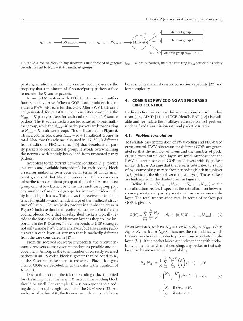
72 EURASIP Journal on Applied Signal Processing
Multicast group Nmax − K + 1
Multicast group 2
Multicast group 1
PNmax−K
P1
s1, . . . , sK
Multicasts1, . . . , sK , P1, . . . , PNmax−KRS encoders1, . . . , sK
Figure 6: A coding block in any sublayer is first encoded to generate Nmax − K parity packets, then the resulting Nmax source plus paritypackets are sent to Nmax − K + 1 multicast groups.
parity generation matrix. The erasure code possesses theproperty that a minimum of K source/parity packets sufficeto recover the K source packets.
In our RLM system with FEC, the transmitter buffersframes as they arrive. When a GOF is accumulated, it gen-erates a PWV bitstream for this GOF. After PWV bitstreamsare generated for K GOFs, the transmitter computes theNmax − K parity packets for each coding block of K sourcepackets. The K source packets are broadcasted to one multi-cast group, while theNmax−K parity packets are broadcastingto Nmax − K multicast groups. This is illustrated in Figure 6.Thus, a coding block uses Nmax − K + 1 multicast groups intotal. Note that this scheme, also used in [17, 39], is differentfrom traditional FEC schemes [40] that broadcast all par-ity packets to one multicast group. It avoids overwhelmingthe network with unduly heavy load from unwanted paritypackets.
According to the current network condition (e.g., packetloss ratio and available bandwidth), for each coding blocka receiver makes its own decision in terms of which mul-ticast groups of that block to subscribe. The receiver cansubscribe to no multicast group at all, to the first multicastgroup only at low latency, or to the first multicast group plusany number of multicast groups for improved video qual-ity but at high latency. This allows the receiver to trade la-tency for quality—another advantage of the multicast struc-ture of Figure 6. Source/parity packets in the shaded areas inFigure 5 indicate those the receiver subscribes to in differentcoding blocks. Note that unsubscribed packets typically re-side at the bottom of each bitstream layer as they are less im-portant in the R-D sense. This corresponds to UEP strategiesnot only among PWV bitstream layers, but also among pack-ets within each layer—a scenario that is markedly differentfrom the case considered in [17].
From the received source/parity packets, the receiver in-stantly recovers as many source packets as possible and de-code them. As long as the total number of correctly receivedpackets in an RS coded block is greater than or equal to K ,all the K source packets can be recovered. Playback beginsafter K GOFs are decoded. Thus the delay is the duration ofK GOFs.
Due to the fact that the tolerable coding delay is limitedfor streaming video, the length K in a channel-coding blockshould be small. For example, K = 8 corresponds to a cod-ing delay of roughly eight seconds if the GOF size is 32. Forsuch a small value of K , the RS erasure code is a good choice
because of its maximal erasure correction capability [22] andlow complexity.
4. COMBINED PWV CODING AND FEC-BASEDERROR CONTROL
In this Section, we assume that a congestion-control mecha-nism (e.g., AIMD [11] and TCP-friendly RAP [12]) is avail-able and formulate the multilayered error-control problemunder a fixed transmission rate and packet loss ratio.
4.1. Problem formulation
To facilitate easy intergration of PWV coding and FEC-basederror control, PWV bitstreams for different GOFs are gener-ated so that the number of layers and the number of pack-ets/sublayers within each layer are fixed. Suppose that thePWV bitstream for each GOF has L layers with Pl packetsin the lth layer. Assume that the receiver subscribes to a totalof Nl,i source plus parity packets per coding block in sublayer{l, i} (which is the ith sublayer of the lth layer). These packetsare highlighted in the shaded areas in Figure 5.
Define N = (N1,1, . . . , N1,P1 , . . . , NL,1, . . . , NL,PL) as therate allocation vector. It specifies the rate allocation betweensource packets and parity packets within each source sub-layer. The total transmission rate, in terms of packets perGOF, is given by
R(N) =L∑l=1
Pl∑i=1
Nl,i
K, Nl,i ∈
{0, K, K + 1, . . . , Nmax
}. (3)
From Section 3, we have Nl,i = 0 or K ≤ Nl,i ≤ Nmax. WhenNl,i > K , the factor Nl,i/K measures the redundancy whichthe receiver chooses in order to protect source packets in sub-layer {l, i}. If the packet losses are independent with proba-bility ε, then, after channel decoding, any packet in that sub-layer can be recovered with probability
Pl,i(Nl,i
) = 1K
K∑s=0
Nl,i−K∑c=0
(Ks
)εK−s(1− ε)s
×(Nl,i − K
c
)εNl,i−K−c(1− ε)c
×K, if s + c ≥ K,
s, if s + c < K.
(4)

Combined Wavelet Video Coding and Error Control for Internet Streaming and Multicast 73
The double sum computes the expected number of correctlyrecovered source packets within one coding block in sublayer{l, i}. Note that when s + c ≥ K , all the K source packets canbe recovered. While if s+c < K , this number can only be s, nomatter how many parity packets are received. The expectedreconstruction distortion per GOF is given by
D(N) = D0 −L∑l=1
Pl∑i=1
Pl,�i∆Dl,i, (5)
where
Pl,�i = P(the first i sublayers in the lth layer
are decoded correctly)
=i∏
i′=1
Pl,i′(Nl,i′
),
(6)
D0 is the expected reconstruction distortion when the trans-mission rate is zero, and ∆Dl,i represents the expected reduc-tion of distortion if the packet in sublayer {l, i} can be de-coded. Let Dl,0 be the expected reconstruction distortion ofthe lth layer when the transmission rate is zero, then we haveD0 =
∑Ll=1 Dl,0.
In our analysis, we use an operational distortion-ratefunction D(R) = σ22−2R/A to model the R-D performanceof the PWV coder, where A is a scaling factor. Based onthis model, ∆Dl,i can be computed from Dl,0 as ∆Dl,i =Dl,0(2−2i/Al − 2−2(i−1)/Al ). Because each layer of the PWV bit-stream is embedded, a packet is dependent on those ahead ofit within the same layer. That the ith packet can be decodedimplies that the i− 1 packets ahead of it can also be correctlydecoded; this dependency is reflected in (6).
Equations (3) and (5) give the total transmission rate andthe expected distortion as a function of the rate allocationvector N. Now we want to find the optimal rate allocationvector to minimize the expected distortion subject to a trans-mission rate constraint. That is, we consider the followingconstraint optimization problem:
minN
D(N) subject to R(N) ≤ R0, (7)
where R0 is the given rate constraint.
4.2. The optimization algorithm
One way to solve the above problem is by finding the rateallocation vector N that minimizes the Lagrangian
J(N) = D(N) + λR(N)
= D0 −L∑l=1
Pl∑i=1
( i∏i′=1
Pl,i′(Nl,i′
))∆Dl,i
+ λL∑l=1
Pl∑i=1
Nl,i
K.
(8)
The solution to this problem is completely character-ized by the set of distortion increments ∆Dl,i, which are de-termined by the source coding and packetization, and the
probability Pl,i′ (Nl,i′ ) with which a packet in sublayer {l, i}can be correctly recovered, which is in turn determined bythe channel coding. There are many methods to solve thisoptimization problem with a rate constraint [13, 14, 15].
We solve this problem by using an iterative approach thatis based on the method of alternating variables for multivari-able minimization [41]. The objective function
J(N) = J(N1,1, . . . , N1,P1 , . . . , NL,1, . . . , NL,PL
)(9)
in (8) is minimized over one variable at a time, while keepingthe other variables constant, until convergence. To be spe-cific, let N(0) be the initial rate allocation vector. Let N(t) =(N (t)
1,1, . . . , N(t)L,PL) be determined for t = 1, 2, . . . , as follows.
Select one component Nlt,it ∈ {N1,1, . . . , NL,PL} to optimizeat step t. This can be done in a round-robin style. Then for
Nl,i (l �= lt or i �= it), let N (t)l,i = N (t−1)
l,i . For Nlt,it , we performthe following rate optimization:
N (t)lt ,it=arg min
Nlt ,it
J(N1,1, . . . , N1,P1 , . . . , NL,1, . . . , NL,PL
)(10)
=arg minNlt ,it
Plt∑i=it
(−
i∏i′=1
Plt ,i′(Nlt,i
′))∆Dlt,i + λ
Nlt ,it
K. (11)
Equation (11) contains only those items in (8) that are re-lated to Nlt,it . For fixed λ, the 1-dimensional minimizationproblem (11) can be solved using standard nonlinear op-timization procedures, such as gradient-descent-type algo-rithm [41]. Now, in order to minimize the Lagrangian J(N)given by (8), we proceed as follows: first, for fixed λ, we min-imize J(N, λ) and get a total transmission rate R(N, λ). Com-pare this rate with the target transmission rate and accord-ingly adjust λ. This procedure is repeated until convergence.Generally, the resulting R(N) will not be exactly equal to thetarget rate constraint, because it only picks limited discretevalues.
In our experiments, we always start with the initial rateallocation vector N = (1, 1, . . . , 1). We cycle through all thecomponents, beginning with the component associated withthe first sublayer and ending with the component associatedwith the last sublayer. The resulting rate allocation
N∗ = (N∗
1,1, . . . , N∗1,P1
, . . . , N∗L,1, . . . , N
∗L,PL
)(12)
gives the optimal error-control solution, generally in theform of unequal error protection, for the different sourcesublayers.
5. PSEUDO-ARQ-BASED ERROR-CONTROL MODEL
In this Section, we augment the FEC-based error-controlmodel by considering (ARQ), which is extensively used inpacket networks because it makes the most use of the net-work capacity. In conventional ARQ, only those packets lostduring previous transmissions are retransmitted. Obviously,it is adaptive because the number of retransmission requestsreflects exactly the current packet loss probability. However,ARQ is regarded as impractical in multicast because of the

74 EURASIP Journal on Applied Signal Processing
feedback implosion problem. As a common approach, feed-back suppression partially solves this problem at the expenseof increased latency, more complexity at receivers, or addi-tional requirements of the network.
Nonnenmacher et al. [40] demonstrate that hybridFEC/ARQ is very powerful in reducing the number of re-transmissions at low packet loss rate. But it cannot com-pletely eliminate the need of retransmissions, especially whenthe number of receivers grows large or the packet loss ratebecomes high. Byers et al. [23] further develop this idea byusing pure FEC to form a digital fountain for reliable multi-cast of bulk data. It can be viewed as a form of pseudo-ARQ.Application of hybrid FEC/Pseudo-ARQ to video multicastis studied in [17, 24]. ARQ is simulated by sending delayedparity packets to some additional multicast groups. The re-ceiver can join and subsequently leave these groups to re-trieve packets that are lost in previous transmissions. Thisscheme can satisfy the retransmission needs of a large num-ber of receivers with a small number of retransmitted paritypackets.
In our work, we also applied this hybrid method onthe PWV encoded video for multicast. Specifically, insteadof being transmitted at the same time of the source pack-ets, some of the parity packets are multicast in subsequenttime slots with different delays. According to the currentnumber of received packets, the network condition, and theavailable transmission rate, each receiver can choose to jointhese multicast groups to retrieve the delayed parity pack-ets. Figure 7 depicts the flowgraph of our pseudo-ARQ-basederror-control scheme. Obviously, this pseudo-ARQ schemeis more efficient than pure FEC because the delayed paritypackets are subscribed to only when necessary. However, thisefficiency is at the expense of larger latency. In real applica-tions, the tolerable latency is limited and the number of deci-sion time slots should also be fixed. Thus we have a problemof making optimal subscription decisions at different timeslots in order to minimize the expected reconstruction dis-tortion under a transmission rate constraint.
6. COMBINED PWV CODING AND FEC/PSEUDO-ARQ
Just as in pure FEC, the goal of error control in hybridFEC/pseudo-ARQ is to minimize the expected distortionin the reconstruction given a transmission rate constraint.However, with ARQ the receiver can take a series of actionsbased on the state of each step. This control process at eachreceiver can be modeled as a finite horizon Markov decisionprocess [15]. A Markov decision process with finite horizonW is a W-step stochastic process through a state space. Anaction is associated with each trellis state to maximize orminimize an expected quantity. The assignment of actionsto trellis states is called a policy.
In this problem, each state s in the trellis space is uniquelydetermined by the number of received source packets x, thenumber of total received packets k, and the step number (ortime index) w. We want the policy π to minimize J(π) =D(π) + λR(π). This can be solved by a dynamic program-ming algorithm, which regressively minimizes the partial
End
No
Subscribemore?
Yes
No
T = T max?Yes
No
Enoughpackets?
Yes
Receivesubscribed
packets
Send subscribtionmessages
T = T + 1
Subscribe tothis layer?
No
Begin T = 1
Figure 7: The decision process at each receiver for any sublayer.T max is the number of decision time slots.
Lagrangian J(π, s) of each state s as a function of the tran-sition probability to the next state s′
J(π, s) =∑s′P(s′ | s, π(s)
)× [∆J
(s′ | s, π(s)
)+ J(π, s′)
].
(13)
Here, the partial Lagrangian J(π, s) represents the cost D+λRbeginning from state s with policy π; P(s′ | s, π(s)) is thetransition probability from the current state s to the next states′ given the policy component π(s) at state s; ∆J(s′ | s, π(s))represents the cost reduction in this transition and it is notrelated to states other than s and s′. At state s, the algorithmupdates J(π, s) and π(s), respectively, by
J(π∗, s
) = minπ∗(s)
∑s′P(s′ | s, π∗(s)
)× [
∆J(s′ | s, π∗(s)
)+ J
(π∗, s′
)],
(14)
π∗(s) = arg minπ∗(s)
∑s′P(s′ | s, π∗(s)
)× [
∆J(s′ | s, π∗(s)
)+ J
(π∗, s′
)].
(15)

Combined Wavelet Video Coding and Error Control for Internet Streaming and Multicast 75
Let Ltotal =∑
l Pl represent the total number of sublayers;let W be the number of decision steps and K the size of anRS coding block. The algorithm runs as follows.
Algorithm 1. (1) Initialize the policy components π(l, s) ofall the layers 0 ≤ l < Ltotal and all the states s(0 ≤ w <W, 0 ≤ k ≤ K, 0 ≤ x ≤ k) throughout the trellis space;set λ to an initial value.
(2) Set πold(l, s) = π(l, s) for all l and s.(3) Start from the first layer l = 0.(4) Start from the last step w =W − 1; set Jnext(l, s) = 0 for
all l and s.(5) For each state s, compute J(l, s) which represents the cost
D + λR of the current layer l starting from the currentstep w, given the current policy π and Jnext(l, s) whichrepresents the cost starting from the next step w + 1.
(6) Find the optimal policy component π∗(l, s) (15) for allthe states s at the current step w which minimize J(l, s).Set J(l, s) to the new minimum and π(l, s) = π∗(l, s).
(7) Let w = w − 1; if w ≥ 0, set Jnext(l, s) = J(l, s) for all land s and go to step (5).
(8) Let l = l + 1; if l < Ltotal, go to step (4).(9) If π(l, s) = πold(l, s) for all l and s, convergence is met for
the current λ; else go to step (2).(10) Compute the expected transmission rate R with the cur-
rent policy π.(11) Check if the computed R has most closely approached the
rate constraint Rtarget. If not, adjust λ and go to step (2).(12) End.
7. RESULTS
7.1. Analysis
The optimization algorithm described in Section 4.2 extendsthe single-layered optimization algorithm in [17]. To com-pare the performance difference between the two error-control mechanisms, we assume that bitstreams generated by3D SPIHT and PWV coding have the same R-D curve, that is,D(R) = σ22−2R/A. Note that the 3D SPIHT bitstream has a se-quential dependency among all the source packets of a GOF,whereas in the PWV coder only packets within the same layerare sequentially dependent.
Applying the algorithm described in Sections 4 and 6, wecompute the signal-to-reconstruction noise ratio as a func-tion of the transmission rate as shown in Figure 8 for ε =20% and in Figure 9 for ε = 5%. We assume that the PWVbitstream consists of four layers, with the numbers of packetsin different layers being 2, 6, 17, and 25.
When only pure FEC is used, we see that integrat-ing PWV coding and error control outperforms the single-layered approach in [17] by up to one dB when ε = 20%and up to 0.6 dB when ε = 5%. In the hybrid FEC/pseudo-ARQ case, however, the difference of performance betweenthe two coders becomes very small. Note that when ARQ isintroduced, any subscribed packet can almost always reachthe receiver with little increase in the expected transmission
4035302520151050Packet transmission rate (packets per GOF)
0
5
10
15
20
25
30
35
Sign
alto
reco
nst
ruct
ion
noi
sera
tio
(dB
)
Reconstruction of 2 idealized sources with 20% packet loss rate
12
34
5
6
1. (W,K) = (8, 1), multi- and single-layer
2. (W,K) = (4, 2), multi- and single-layer
3. (W,K) = (2, 4), multi-layer
4. (W,K) = (2, 4), single-layer
5. (W,K) = (1, 8), multi-layer
6. (W,K) = (1, 8), single-layer
Figure 8: Analytical results using optimal error control for trans-mitting a single-layered video bitstream and a multilayered videobitstream over a network with 20% packet loss.
rate. Thus, the dependency among layers does not play a sig-nificant role any more. Take (W,K) = (8, 1), for example, ifwe fix the policy component π(s = 0, c = 0, w = 0) = 1 andincrease the policy components π(s = 0, c = 0, 0 < w < 8)from 0 to 1, the expected transmission rate is increased byonly 0.25 (from 1 to 1.25) packets per GOF. However, nowthe probability that any packet in the corresponding layercannot be recovered is reduced from 20% to 3 × 10⁻⁶. Alsonote that in Figure 9 for ε = 5%, because the packet loss rateis small enough, both (W,K) = (8, 1) and (W,K) = (4, 2)can achieve near-perfect transmission. Therefore, they actu-ally share the same performance curve.
7.2. Simulations
Simulations are also carried out, in which two 288-frame25 fps QCIF color sequences Foreman and Akiyo, encodedusing the PWV coder and protected with a systematic RSerasure code with a block size K = 8, are transmitted overa simulated network with 20% and 5% packet loss, respec-tively. Each video sequence is blocked into 9 GOFs contain-ing 32 frames per GOF and encoded at 50 packets per GOFwith 1000 bytes per packet. The duration of each GOF is 1.28seconds. Thus, the number of packets N allowed for eachGOF in term of the transmission rate R in bps is given byN = 1.28R/8000 packets per GOF.
The quantities ∆Dl,i needed for the solution in Section 4are given by the encoded source packets and revealed to thereceiver. In real applications, they can be either sent by the

76 EURASIP Journal on Applied Signal Processing
4035302520151050Packet transmission rate (packets per GOF)
0
5
10
15
20
25
30
35
40
Sign
alto
reco
nst
ruct
ion
noi
sera
tio
(dB
)
Reconstruction of 2 idealized sources with 5% packet loss rate
1
23 4
5
1. (W,K) = (8, 1) & (W,K) = (4, 2)
2. (W,K) = (2, 4), multi-layer
3. (W,K) = (2, 4), single-layer
4. (W,K) = (1, 8), multi-layer
5. (W,K) = (1, 8), single-layer
Figure 9: Analytical results using optimal error control for trans-mitting a single-layered video bitstream and a multilayered videobitstream over a network with 5% packet loss.
server as a side information or estimated adaptively by thereceiver using previously recovered packets. For each trans-mission rate, the selected combination of source and paritypackets is transmitted and each simulation runs 100 times.
In order to compare our multilayered scheme with thesingle-layered scheme in [17] on a fair basis, we modify thePWV coder to make it produce single-layered bitstreams.That is, the packets of each GOF have a sequential depen-dency as in 3D SPIHT. Loss of any packet will render thefollowing packets of the same GOF useless. Thus we havea single-layered version of the PWV coder with comparablecoding efficiency to the original PWV coder. The same pro-cedure as in [17] is applied to provide error protection for thebitstreams generated by this new coder. In Figures 10, 11, 12,and 13, we refer to the single-layered PWV coder as sPWVand the multilayered PWV coder as mPWV.
Figure 10 presents the average PSNRs of two sets of sim-ulations using Foreman based on the two versions of PWV,respectively. The packet loss rate is 20%. Note that when pureFEC is used, the multilayered approach gains up to 0.64 dB.This gap widens as the number of subscribed source pack-ets goes larger. When W = 2, the maximum gain reducesto 0.3 dB. When W = 4, 8, there is virtually no differencebetween the two because the error-control strategy is strongenough to ensure every subscribed packet to be correctly re-covered.
Figure 11 shows the same results as in Figure 10, but witha different packet loss rate of 5%. The maximum perfor-mance difference is about 0.5 dB, which happens in pure
20015010050Transmission rate (kbps)
27
28
29
30
31
32
33
PSN
R(d
B)
Transmission of Foreman over a simulated networkwith 20% packet loss
(W,K) = (8, 1) mPWV(W,K) = (8, 1) sPWV(W,K) = (4, 2) mPWV(W,K) = (4, 2) sPWV
(W,K) = (2, 4) mPWV(W,K) = (2, 4) sPWV(W,K) = (1, 8) mPWV(W,K) = (1, 8) sPWV
Figure 10: Simulation results using error control for transmittingmPWV and sPWV coded Foreman over a network with 20% packetloss.
20015010050Transmission rate (kbps)
27
28
29
30
31
32
33
34
PSN
R(d
B)
Transmission of Foreman over a simulated networkwith 5% packet loss
(W,K) = (8, 1) mPWV(W,K) = (8, 1) sPWV(W,K) = (4, 2) mPWV(W,K) = (4, 2) sPWV
(W,K) = (2, 4) mPWV(W,K) = (2, 4) sPWV(W,K) = (1, 8) mPWV(W,K) = (1, 8) sPWV
Figure 11: Simulation results using error control for transmittingmPWV and sPWV coded Foreman over a network with 5% packetloss.
FEC case at the highest rate. With a small packet loss rate of5%, hybrid FEC/pseudo-ARQ method with W = 2 already

Combined Wavelet Video Coding and Error Control for Internet Streaming and Multicast 77
20015010050Transmission rate (kbps)
32
34
36
38
40
42
44
46
48
PSN
R(d
B)
Transmission of Akiyo over a simulated network
with 20% packet loss
(W,K) = (8, 1) mPWV(W,K) = (8, 1) sPWV(W,K) = (4, 2) mPWV(W,K) = (4, 2) sPWV
(W,K) = (2, 4) mPWV(W,K) = (2, 4) sPWV(W,K) = (1, 8) mPWV(W,K) = (1, 8) sPWV
Figure 12: Simulation results using error control for transmittingmPWV and sPWV coded Akiyo over a network with 20% packetloss.
20015010050Transmission rate (kbps)
34
36
38
40
42
44
46
48
PSN
R(d
B)
Transmission of Akiyo over a simulated network
with 5% packet loss
(W,K) = (8, 1) mPWV(W,K) = (8, 1) sPWV(W,K) = (4, 2) mPWV(W,K) = (4, 2) sPWV
(W,K) = (2, 4) mPWV(W,K) = (2, 4) sPWV(W,K) = (1, 8) mPWV(W,K) = (1, 8) sPWV
Figure 13: Simulation results using error control for transmittingmPWV and sPWV coded Akiyo over a network with 5% packet loss.
achieves performance very close to higher W = 4 and W =8 cases. This substantiates our analysis result as shown inFigure 9.
Table 1: Numbers of subscribed source packets of all four layersin the transmission of PWV coded Foreman using pure FEC with apacket loss rate of 20% at four different transmission rates.
Rtotal(kbps) 50 100 150 200
Ptotal(packets) 8 16 24 32
S1(packets) 1 1 1 2
S2(packets) 2 3 3 4
S3(packets) 1 4 7 9
S4(packets) 1 2 4 5
Stotal(packets) 5 10 15 20
Table 2: Numbers of subscribed source packets of all four layers inthe transmission of PWV coded Foreman using hybrid FEC/pseudo-ARQ ((W,K) = (2, 4)) with a packet loss rate of 20% at four differ-ent transmission rates.
Rtotal(kbps) 50 100 150 200
Ptotal(packets) 8 16 24 32
S1(packets) 1 1 1 2
S2(packets) 2 3 3 4
S3(packets) 2 5 8 9
S4(packets) 1 2 5 6
Stotal(packets) 6 11 17 21
The simulation results using Akiyo are presented inFigure 12 for 20% packet loss rate and in Figure 13 for 5%packet loss rate, respectively. Average PSNRs of two sets ofsimulations based on single-layered PWV coding and mul-tilayered PWV coding are presented. The maximal gain inpure FEC is 0.53 dB for 20% packet loss rate and 0.48 for 5%packet loss rate. Because the Akiyo sequence contains muchless high-frequency components than Foreman, packets inhigher-frequency layers have a smaller contribution to the re-duction of distortion. As a result when pseudo-ARQ is used(W = 2, 4, 8), the subscription policy tends to spend moreon channel coding part instead of increasing the source rate.Thus, there is very little packet loss in pseudo-ARQ cases, andthe performance of the two error-control schemes are almostthe same.
Table 1 lists the number of subscribed source packets ofall four layers in the transmission of PWV coded Foremanusing pure FEC with a packet loss rate of 20%. Note thatRtotal is the total transmission rate in kbps. And Ptotal is thecorresponding number of 1000-byte packets at rate Rtotal.The number of subscribed source packets of the ith layeris denoted by Si (i = 1, 2, 3, 4). These numbers are deter-mined by the UEP algorithm described in Section 4. FromTable 1, we see that the source bitstreams at lower trans-mission rates (e.g., 50, 100, and 150 kbps) are truncatedversions of one preencoded embedded bitstream at a higherrate (e.g., 200 kbps). Reencoding is thus avoided, and pro-gressive transmission in video streaming or receiver adapta-tion in video multicast is made possible.
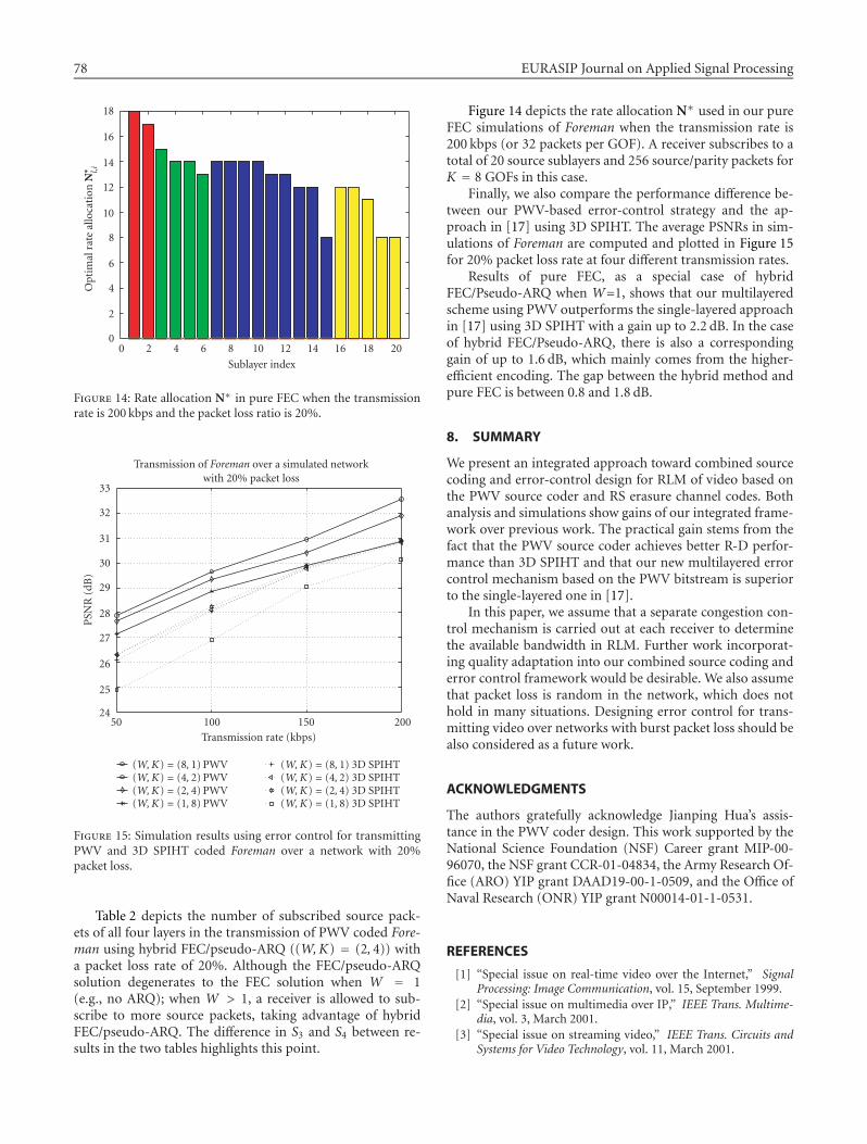
78 EURASIP Journal on Applied Signal Processing
20181614121086420
Sublayer index
0
2
4
6
8
10
12
14
16
18
Opt
imal
rate
allo
cati
onN
∗ l,i
Figure 14: Rate allocation N∗ in pure FEC when the transmissionrate is 200 kbps and the packet loss ratio is 20%.
20015010050Transmission rate (kbps)
24
25
26
27
28
29
30
31
32
33
PSN
R(d
B)
Transmission of Foreman over a simulated networkwith 20% packet loss
(W,K) = (8, 1) PWV(W,K) = (4, 2) PWV(W,K) = (2, 4) PWV(W,K) = (1, 8) PWV
(W,K) = (8, 1) 3D SPIHT(W,K) = (4, 2) 3D SPIHT(W,K) = (2, 4) 3D SPIHT(W,K) = (1, 8) 3D SPIHT
Figure 15: Simulation results using error control for transmittingPWV and 3D SPIHT coded Foreman over a network with 20%packet loss.
Table 2 depicts the number of subscribed source pack-ets of all four layers in the transmission of PWV coded Fore-man using hybrid FEC/pseudo-ARQ ((W,K) = (2, 4)) witha packet loss rate of 20%. Although the FEC/pseudo-ARQsolution degenerates to the FEC solution when W = 1(e.g., no ARQ); when W > 1, a receiver is allowed to sub-scribe to more source packets, taking advantage of hybridFEC/pseudo-ARQ. The difference in S3 and S4 between re-sults in the two tables highlights this point.
Figure 14 depicts the rate allocation N∗ used in our pureFEC simulations of Foreman when the transmission rate is200 kbps (or 32 packets per GOF). A receiver subscribes to atotal of 20 source sublayers and 256 source/parity packets forK = 8 GOFs in this case.
Finally, we also compare the performance difference be-tween our PWV-based error-control strategy and the ap-proach in [17] using 3D SPIHT. The average PSNRs in sim-ulations of Foreman are computed and plotted in Figure 15for 20% packet loss rate at four different transmission rates.
Results of pure FEC, as a special case of hybridFEC/Pseudo-ARQ when W=1, shows that our multilayeredscheme using PWV outperforms the single-layered approachin [17] using 3D SPIHT with a gain up to 2.2 dB. In the caseof hybrid FEC/Pseudo-ARQ, there is also a correspondinggain of up to 1.6 dB, which mainly comes from the higher-efficient encoding. The gap between the hybrid method andpure FEC is between 0.8 and 1.8 dB.
8. SUMMARY
We present an integrated approach toward combined sourcecoding and error-control design for RLM of video based onthe PWV source coder and RS erasure channel codes. Bothanalysis and simulations show gains of our integrated frame-work over previous work. The practical gain stems from thefact that the PWV source coder achieves better R-D perfor-mance than 3D SPIHT and that our new multilayered errorcontrol mechanism based on the PWV bitstream is superiorto the single-layered one in [17].
In this paper, we assume that a separate congestion con-trol mechanism is carried out at each receiver to determinethe available bandwidth in RLM. Further work incorporat-ing quality adaptation into our combined source coding anderror control framework would be desirable. We also assumethat packet loss is random in the network, which does nothold in many situations. Designing error control for trans-mitting video over networks with burst packet loss should bealso considered as a future work.
ACKNOWLEDGMENTS
The authors gratefully acknowledge Jianping Hua’s assis-tance in the PWV coder design. This work supported by theNational Science Foundation (NSF) Career grant MIP-00-96070, the NSF grant CCR-01-04834, the Army Research Of-fice (ARO) YIP grant DAAD19-00-1-0509, and the Office ofNaval Research (ONR) YIP grant N00014-01-1-0531.
REFERENCES
[1] “Special issue on real-time video over the Internet,” SignalProcessing: Image Communication, vol. 15, September 1999.
[2] “Special issue on multimedia over IP,” IEEE Trans. Multime-dia, vol. 3, March 2001.
[3] “Special issue on streaming video,” IEEE Trans. Circuits andSystems for Video Technology, vol. 11, March 2001.

Combined Wavelet Video Coding and Error Control for Internet Streaming and Multicast 79
[4] ISO/IEC JTC 1/SC29/WG11 N2687, “MPEG-4 Video Verifi-cation Model Version 13.0,” March 1999.
[5] ITU-T Recommendation H.263, version 2, “Video coding forlow bitrate communication,” January 1998.
[6] B.-J. Kim, Z. Xiong, and W. A. Pearlman, “Low bit-rate scal-able video coding with 3D set partitioning in hierarchical trees(3D SPIHT),” IEEE Trans. Circuits and Systems for Video Tech-nology, vol. 10, no. 8, pp. 1365–1374, 2000.
[7] H. Radha, M. van der Schaar, and Y. Chen, “The MPEG-4 fine-grained scalable video coding method for multimediastreaming over IP,” IEEE Trans. Multimedia, vol. 3, no. 1, pp.53–68, 2001.
[8] S. Paul, Multicasting on the Internet and Its Applications,Kluwer Academic, Boston, Mass, USA, 1998.
[9] S. Servetto and K. Nahrstedt, “Broadcast quality video overIP,” IEEE Trans. Multimedia, vol. 3, no. 1, pp. 162–173, 2001.
[10] S. R. McCanne, Scalable compression and transmission of In-ternet multicast video, Ph.D. thesis, University of California,Berkeley, Calif, USA, December 1996.
[11] D. Chiu and R. Jain, “Analysis of the increase and decreasealgorithms for congestion avoidance in computer networks,”Journal of Computer Networks and ISDN, vol. 17, no. 1, pp.1–14, 1989.
[12] R. Rejaie, M. Handley, and D. Estrin, “Layered quality adap-tation for Internet video streaming,” IEEE Journal on Se-lected Areas in Communications, vol. 18, no. 12, pp. 2530–2544, 2000.
[13] J. Lu, A. Nosratinia, and B. Aazhang, “Progressive source-channel coding of images over bursty error channels,” inProc. International Conference on Image Processing, Chicago,Ill, USA, October 1998.
[14] M. Ruf and J. Modestino, “Operational rate-distortion perfor-mance for joint source and channel coding of images,” IEEETrans. Image Processing, vol. 8, no. 3, pp. 305–320, 1999.
[15] V. Chande, H. Jafarkhani, and N. Farvardin, “Joint source-channel coding of images for channels with feedback,” in Proc.IEEE Information Theory Workshop, San Diego, Calif, USA,February 1998.
[16] J. Hagenauer, “Rate-compatible punctured convolutionalcodes (RCPC codes) and their applications,” IEEETrans. Communications, vol. 36, no. 4, pp. 389–400, 1988.
[17] P. A. Chou, A. E. Mohr, A. Wang, and S. Mehrotra, “Er-ror control for receiver-driven layered multicast of audio andvideo,” IEEE Trans. Multimedia, vol. 3, no. 1, pp. 108–122,2001.
[18] T. Chu and Z. Xiong, “Combined wavelet video cod-ing and error control for Internet streaming and multicast,”in Proc. GlobeCom ’01, San Antonio, Tex, USA, November2001.
[19] T. Chu, J. Hua, and Z. Xiong, “Packetized wavelet video cod-ing and error control for receiver-driven layered multicast: anintegrated approach,” in Proc. Multimedia Signal ProcessingWorkshop, Cannes, France, October 2001.
[20] J. Hua, Z. Xiong, and X. Wu, “High-performance 3-D embed-ded wavelet video (EWV) coding,” in Proc. Multimedia SignalProcessing Workshop, Cannes, France, October 2001.
[21] X. Wu, S. Cheng, and Z. Xiong, “On packetization of embed-ded multimedia bitstreams,” IEEE Trans. Multimedia, vol. 3,no. 1, pp. 132–140, 2001.
[22] L. Rizzo, “Effective erasure codes for reliable computer com-munication protocols,” ACM Computer Communication Re-view, vol. 27, no. 2, pp. 24–36, 1997.
[23] J. Byers, M. Luby, M. Mitzenmacher, and A. Rege, “A dig-ital fountain approach to reliable distribution of bulk data,”
in Proc. ACM SIGCOMM ’98, pp. 56–67, Vancouver, BC,Canada, September 1998.
[24] W.-T. Tan and A. Zakhor, “Real-time Internet video using er-ror resilient scalable compression and TCP-friendly transportprotocol,” IEEE Trans. Multimedia, vol. 1, no. 2, pp. 172–186,1999.
[25] S. Servetto and K. Nahrstedt, “Video streaming over the pub-lic Internet: Multiple description codes and adaptive trans-port protocols,” in Proc. IEEE International Conference on Im-age Processing, vol. 3, Kobe, Japan, October 1999.
[26] R. Puri, K. Lee, K. Ramchandran, and V. Bharghavan, “An in-tegrated source transcoding and congestion control paradigmfor video streaming in the Internet,” IEEE Trans. Multimedia,vol. 3, no. 1, pp. 18–32, 2001.
[27] B. G. Haskell, A. Puri, and A. N. Netravali, Digital Video: AnIntroduction to MPEG-2, Chapman & Hall, New York, NY,USA, 1997.
[28] L. Yang, F. C. M. Martins, and T. R. Gardos, “ImprovingH.263+ scalability performance for very low bit rate applica-tions,” in Proc. Visual Communications and Image Processing,San Jose, Calif, USA, January 1999.
[29] S. Li, F. Wu, and Y.-Q. Zhang, “Study of a new approach toimprove FGS video coding efficiency,” in ISO/IEC MPEG 50thmeeting, M5583, Maui, Hawaii, USA, December 1999.
[30] E. Steinbach, N. Farber, and B. Girod, “Standard compati-ble extension of H.263 for robust video transmission in mo-bile environments,” IEEE Trans. Circuits and Systems for VideoTechnology, vol. 7, no. 6, pp. 872–881, 1997.
[31] G. Karlsson and M. Vetterli, “Three dimensional subbandcoding of video,” in Proc. IEEE Int. Conf. Acoustics, Speech,Signal Processing, pp. 1100–1103, New York, NY, USA, April1988.
[32] D. Taubman and A. Zakhor, “Multirate 3-D subband codingof video,” IEEE Trans. Image Processing, vol. 3, no. 5, pp. 572–588, 1994.
[33] J. R. Ohm, “Three-dimensional subband coding with motioncompensation,” IEEE Trans. Image Processing, vol. 3, no. 5, pp.559–571, 1994.
[34] S. J. Choi and J. W. Woods, “Motion compensated 3-D sub-band coding of video,” IEEE Trans. Image Processing, vol. 8,no. 2, pp. 155–167, 1999.
[35] A. Said and W. A. Pearlman, “A new, fast, and efficient imagecodec based on set partitioning in hierarchical trees,” IEEETrans. Circuits and Systems for Video Technology, vol. 6, no. 3,pp. 243–250, 1996.
[36] D. Taubman, “High performance scalable image compressionwith EBCOT,” IEEE Trans. Image Processing, vol. 9, no. 7, pp.1158–1170, 2000.
[37] M. Antonini, M. Barlaud, P. Mathieu, and I. Daubechies, “Im-age coding using wavelet transform,” IEEE Trans. Image Pro-cessing, vol. 1, no. 2, pp. 205–220, 1992.
[38] Y. Shoham and A. Gersho, “Efficient bit allocation for an ar-bitrary set of quantizers,” IEEE Trans. Acoustics, Speech, andSignal Processing, vol. 36, no. 9, pp. 1445–1453, 1988.
[39] W.-T. Tan and A. Zakhor, “Video multicast using layered FECand scalable compression,” IEEE Trans. Circuits and Systemsfor Video Technology, vol. 11, no. 3, pp. 373–386, 2001.
[40] J. Nonnenmacher, E. Biersack, and D. Towsley, “Parity-basedloss recovery for reliable multicast transmission,” IEEE Trans.Networking, vol. 6, no. 4, pp. 349–361, 1998.
[41] R. Fletcher, Practical Methods of Optimization, John Wiley &Sons, New York, NY, USA, 2nd edition, 1987.

80 EURASIP Journal on Applied Signal Processing
Tianli Chu received the B.Eng. degree intelecommunication and information sys-tems from Tsinghua University, China, in1999, and the M.S. degree in electrical en-gineering in 2002 from Texas A&M Univer-sity, College Station, where he is currentlyworking toward the Ph.D. degree in the De-partment of Electrical and Computer En-gineering. His research interests are imageand video coding, multimedia communica-tion, and information theory.
Zixiang Xiong received the Ph.D. degree inelectrical engineering in 1996 from the Uni-versity of Illinois at Urbana-Champaign.From 1997 to 1999, he was with the Univer-sity of Hawaii. Since 1999, he has been withthe Department of Electrical Engineering atTexas A&M University, where he is an As-sociate Professor. He spent the summers of1998 and 1999 at Microsoft Research, Red-mond, WA, and the summers of 2000 and2001 at Microsoft Research in Beijing. His current research inter-ests are Internet/wireless multimedia, distributed signal processing,and genomic image processing. Dr. Xiong received an NSF CareerAward in 1999, an ARO Young Investigator Award in 2000, and anONR Young Investigator Award in 2001. He also received an EugeneWebb Faculty Fellow Award in 2001 and a Select Young FacultyAward in 2002, both from Texas A&M University. He is currentlyan Associate Editor for the IEEE Trans. on Circuits and Systems forVideo Technology, the IEEE Trans. on Signal Processing, and theIEEE Trans. on Image Processing.

EURASIP Journal on Applied Signal Processing 2003:1, 81–90c© 2003 Hindawi Publishing Corporation
Unbalanced Multiple-Description Video Codingwith Rate-Distortion Optimization
David ComasImage Processing Group, Department of Signal Theory and Communications,Technical University of Catalonia (UPC), 08034 Barcelona, SpainEmail: [email protected]
Raghavendra SinghIBM India Research Lab., Indian Institute of Technology (IIT) Delhi, New Delhi, IndiaEmail: [email protected]
Antonio OrtegaSignal and Image Processing Institute and Integrated Media Systems Center, Department of Electrical Engineering,University of Southern California, Los Angeles, CA 90089-2564, USAEmail: [email protected]
Ferran MarquesImage Processing Group, Department of Signal Theory and Communications,Technical University of Catalonia (UPC), 08034 Barcelona, SpainEmail: [email protected]
Received 7 May 2002 and in revised form 11 November 2002
We propose to use multiple-description coding (MDC) to protect video information against packet losses and delay, while alsoensuring that it can be decoded using a standard decoder. Video data are encoded into a high-resolution stream using a standardcompliant encoder. In addition, a low-resolution stream is generated by duplicating the relevant information (motion vectors,headers and some of the DCT coefficient) from the high-resolution stream while the remaining coefficients are set to zero. Bothstreams are independently decodable by a standard decoder. However, only in case of losses in the high resolution description, thecorresponding information from the low resolution stream is decoded, else the received high resolution description is decoded.The main contribution of this paper is an optimization algorithm which, given the loss ratio, allocates bits to both descriptionsand selects the right number of coefficients to duplicate in the low-resolution stream so as to minimize the expected distortion atthe decoder end.
Keywords and phrases: multiple-description coding, robust video transmission, rate-distortion optimization, packet networks.
1. INTRODUCTION
In recent years, the volume of multimedia data transmittedover best-effort networks such as the Internet has continuedto increase while packet losses and delays, due to conges-tion, routing delay, and network heterogeneity, continue tobe commonplace. In this paper, we address the issue of robuststreaming of video data. Video data is usually encoded us-ing predictive encoders, for example, motion compensationin the standard H.263 [1] and MPEG [2] encoders. Theseencoders take advantage of the temporal redundancy in thedata to achieve high compression performance. However, themain drawback of a predictive coding scheme is that even
a single packet loss (or erasure) in the transmitted streamcauses decoding errors to propagate through all the samplesfollowing the erasure. This severely affects the video qualityavailable at the receiver and motivates the need for robusttransmission of video data.
A common approach to limit the length of error prop-agation in video coders is to restart the prediction loop byperiodically inserting intracoded (nonpredicted) frames (ormacroblocks). A disadvantage of this approach is that there isa loss in coding efficiency due to the frequent restarting of theloop. Moreover, the emphasis of this approach is on limitingthe error propagation rather than on recovering the lost data.Automatic repeat request (ARQ) can be used to retransmit

82 EURASIP Journal on Applied Signal Processing
Signal sourceMDC encoder
S1
S2
Channel 1
Channel 2
Side decoder1
Centraldecoder
Side decoder2
Side distortionDS1
Central distortionDc
Side distortionDS2
Figure 1: Generic MDC system. The source is encoded in two descriptions: S1 and S2. They are transmitted through the network overdifferent channels. At the decoder, if only one description is received, the signal can be reconstructed with acceptable side distortion whereasif both descriptions are received, the distortion obtained is less than or equal to the lowest side distortion.
the erased data; however, for streaming multimedia applica-tions, especially real-time applications, there is a strict timeconstraint on the transmission of the data, which will limitthe number of retransmissions that are possible and, conse-quently, the overall applicability of ARQ in certain scenarios.Further, in a broadcast network scenario that is often usedfor multimedia data transmission, ARQ can cause a nega-tive acknowledgement (NACK) implosion at the transmitter[3]. Thus, for streaming video applications, local recovery oferasures is often preferable to retransmission. Local recoveryat the decoder could be provided with the use of forward-error-correction (FEC) techniques. In an FEC scheme, re-dundancy is added to the encoded data so that in case of era-sures, the redundancy can be used to reconstruct the lost dataat the receiver. One drawback of FEC schemes is that they arenot as bandwidth efficient as the ARQ schemes; in case ofwidely changing network conditions, FEC schemes are oftendesigned for the worst case scenario, which usually leads toa waste of precious network resources. Moreover, the perfor-mance of popular FEC schemes like the FEC channel codes[4] suffers from the cliff effect [5]: for an (n, k)-channel code,if the number of errors exceed n − k, then the channel codecannot recover from the channel errors. Hence, the perfor-mance is constant for up to e = n−k erasures but then dropsvery sharply when the actual number of erasures is greaterthan e.
An alternative approach for reliable transmission of mul-timedia data that provides graceful degradation of perfor-mance in presence of channel noise is multiple-descriptioncoding (MDC) [6, 7]. In MDC, two or more independentlydecodable descriptions of the source are sent to the re-ceiver (Figure 1). If only description S1 (or S2) is received,the signal can be reconstructed with acceptable side distor-tion DS1 (or DS2 ). If both descriptions are received, the dis-tortion obtained at the central decoder DC is less than orequal to the lowest side distortion; that is, if DS1 is the low-est side distortion, then DC ≤ DS1 . Thus, in an MDC sys-tem, there are three different decoders, each corresponding to
one of the possible loss scenarios. In an ideal MDC channelenvironment, the channels are independent and data on eachchannel is either completely lost or received intact. This en-vironment has been studied extensively both theoretically[6, 7] and practically [8, 9, 10, 11, 12]. The paper by Goyal[5] provides a good overview of MDC systems.
In a packet network environment, these ideal conditionsmay not hold true; packet losses can be correlated and onlypartial data (of either description) may be received at the de-coder. Sufficient interleaving of packets of the two descrip-tions could provide a degree of independence between thepacket losses of the descriptions. However, there still remainsthe issue of partially received data, which is especially im-portant for video streaming because of the associated er-ror propagation. There has been limited work on MD videocoders for packet networks. Vaishampayan [8] used MDCscalar quantizers to develop robust image and video codersfor packet loss environments. Recently, Reibman [13] has,independently, proposed an MD video coder for packet net-works based on a rate-allocation principle similar to the onethat we propose. One of the novelties of this coder is thatin minimizing the expected distortion for a given bitrate, ittakes the error propagation into account.
In this paper, we propose an unbalanced MDC (UMDC)system for transmission of video data over best-effort packetnetworks. The system is unbalanced because the rate distri-bution among the various descriptions is not even; hence,one description has high rate (high resolution/quality) andthe other low rate (low resolution); that is, if S1 is the high-resolution (HR) description, then DS1 ≤ DS2 and DC = DS1 .In the proposed system, the low-resolution (LR) descrip-tion is primarily used as redundancy, to be decoded onlywhen there are losses in the HR description. Most work inMDC has been on balanced systems where each descrip-tion is equally important, but we propose that for the lowpacket-loss rate conditions considered in this paper (below10%), a UMDC system would be more useful. This is be-cause the overhead in making descriptions balanced, which

Unbalanced Multiple-Description Video Coding with Rate-Distortion Optimization 83
is particularly significant if the descriptions are to be coded ina standard syntax, would adversely affect the performance ofbalanced systems for low packet-loss rates. Moreover, thoughthe UMDC encoder produces unbalanced descriptions, weuse a smart packetization (similar to the one in [14]) to cre-ate packets that are equally important; thus, from the net-work viewpoint, all packets have equal priority.
In the proposed MDC system, the input video sequenceis encoded into a high rate and quality video stream (HR de-scription) using an encoder that produces an H.263 compli-ant stream. The important parts of this HR description areduplicated in a low rate and quality video stream (LR de-scription). The important information includes the headers,motion vectors, and a subset of the DCT coefficients in theHR video stream. The remaining DCT coefficients are set tozero in the LR video stream. At the receiver, if informationfrom the HR description is lost, the corresponding informa-tion from the LR description is decoded, else the HR descrip-tion decoded. The main advantages of our MD video coderare stated as follows:
(1) optimal descriptions that minimize the expected dis-tortion for a given probability of packet loss and ratebudget are generated;
(2) the MD representation is constructed in such a waythat both the descriptions are independently decod-able by a standard H.263 decoder, that is, the MDvideo coder maintains compatibility with the H.263syntax [1].
The main disadvantage of our work is that, currently, weare not considering error propagation in our expected distor-tion formulation. We propose this as part of future work.
The rest of the paper is organized as follows. In Section 2,we discuss other MDC-based video transmission systems. InSection 3, we present our encoding algorithm. In Section 4,we compare our system with other MDC systems. We con-clude the paper with some thoughts for future work inSection 5.
2. RELATED WORK
There has been substantial work in the area of MDC for videotransmission over the ideal MD channel environment, for ex-ample, [15, 16, 17, 18]. A key challenge in designing MDCtechniques that incorporate predictive coding is to avoid theprediction loop mismatch problem. When prediction is used,the decoder can only operate properly if it has received thedata that the encoder used to generate the predictor, elsethere is a prediction loop mismatch that leads to poor per-formance. In an MDC system, if both descriptions were re-ceived at the decoder, the best predictor to be used by thecentral decoder would be the one formed from past infor-mation produced by the central decoder; that is, formed bycombining information received in both descriptions. How-ever, if only a single-description was received, the best pre-dictor to use in encoding should be based only on data pro-duced by the side decoder corresponding to the descrip-tion that has been received. Thus, ideally, for an MDC-based
prediction system, there should be three prediction loops,one for each decoder (Figure 1). Many MD video coders, forexample, [16, 17, 18], are designed to send redundancy toavoid this mismatch problem.
Reibman et al. [15] proposed an MDC video coder thatis similar in principle to our video coder. Descriptions arecreated by splitting the output of a standard codec; impor-tant information (DCT coefficients above a certain thresh-old, motion vectors, and headers) is duplicated in the de-scriptions while the remaining DCT coefficients are alter-nated between the descriptions, thus generating balanced de-scriptions. The threshold is found in a rate-distortion (R-D)optimal manner. At the decoder, if both descriptions are re-ceived, then the duplicate information is discarded, else thereceived description is decoded. This is in principle very sim-ilar to our MD video coder, with the main difference be-ing that we duplicate the first K coefficients of the blockand we do not alternate coefficients. The number K is alsofound in a rate-distortion optimal framework. The advan-tage of our method is that its coding efficiency is better thanthat of [15]. This is because in our system, in compliancewith the standard syntax of H.263, an efficient end-of-block(EOB) symbol can be sent after the Kth symbol. Moreover,in [15], inefficient runs of zeros are created by alternatingDCT coefficients between the descriptions. The disadvantageof our system is that it is unbalanced in nature; hence, incase of losses in the HR description, there is a sharper dropin performance than in case of losses in either of the bal-anced descriptions of [15]. However, for low packet (< 10%)loss scenarios, which are commonplace over the Internet,our system performs better than [13] (a version of [15] ex-tended to packet networks). This is shown in Section 4 of thispaper.
In [15], the prediction loop mismatch problem, thatwould arise if a description was lost, was not considered.In a later work, Reibman [13] extended this rate-distortionoptimal-splitting method to design an MD video coder fora packet network. For a packet-loss environment, predic-tion loop mismatch could be due to loss of current and/orprevious data. In [14], the Recursive Optimal per-Pixel Es-timate (ROPE) formulation was developed to calculate theoverall distortion of the decoder reconstruction due to quan-tization, error propagation, and error concealment for a one-layer video coder subject to packet losses. Using this distor-tion, the best location for intrablocks was found using rate-distortion optimization. In [13], this optimal mode selectionalgorithm (i.e., coding a macroblock as inter/intra) was ex-tended to the MD framework to limit the error propagationdue to the prediction mismatch. Thus, for each macroblockof a frame, given the bitrate and probability of packet loss, theoptimal threshold and mode was selected; that is, the redun-dancy bits were optimally distributed between informationneeded for local recovery and information needed to limitthe error propagation.
In this paper, we are proposing a UMD video coder forpacket networks. In our system, the LR description is usedas redundancy to be decoded only in case of losses in theHR description. Thus, the central decoder is the same as the

84 EURASIP Journal on Applied Signal Processing
HR side decoder, which implies that there is no predictionloop mismatch if there are no losses in the HR description.In case of a loss in the HR description, there is a predic-tion loop mismatch. This is because at the encoder, the in-formation in the HR description is used to predict the nextframe, while at the decoder at the point of erasure, we will de-code the LR description. Thus, the prediction for the frameafter the erasure will not be from the full HR informationbut only from the partial information that is available inthe LR description. However, in this work, we have not con-sidered error propagation due to prediction loop mismatch.The formulation in ROPE, though exact, is computation-ally intensive and may not be suitable for real-time applica-tions. We are currently exploring alternative mode selectionmethods.
Both our MD video coder and Reibman’s [13, 15] aresyntax compatible with existing standard codecs. Preservingcompatibility with existing standard decoders can affect theperformance of an MDC system. For example, it will not bepossible to use several techniques, such as MDC scalar quan-tization or MDC transform coding, while still preservingcompatibility with the standard. However, preserving com-patibility may still be useful because these standard decodersare very commonly used. In particular, if syntax compatibil-ity with standard decoders is preserved, we can think of anMDC system as a wrapper that can use off the shelf encodersand decoders to generate loss-robust transmitted data. Notethat by standard compliance we imply that an H.263 compli-ant decoder can decode either of the descriptions. However,in our system, decoding the LR video stream by itself willnot give very high quality, as the LR description has been de-signed only to add robustness to the HR stream. Hence, weneed a parser, which in case of losses in the HR stream, canextract information from the LR stream and pass it to stan-dard decoder.
In this paper, we compare against the MD video coder,presented in [15], extended to the packet network envi-ronments. We also compare against the video redundancycoding (VRC) mode in H.263+ [19]. In VRC, the encodedframes are split into multiple-descriptions in a round-robinway and the prediction of a frame in one description is basedon the past frames in the same description. In the case oftwo descriptions, an even frame is predicted from the nearesteven frame and an odd frame from the nearest odd frame.Compared to a conventional single-description coder, thereis a significantly lower prediction gain and hence higher re-dundancy to achieve the same distortion when both descrip-tions are received. A sync frame is also added periodicallyto prevent error propagation. The periodicity of the syncframe can be varied to increase robustness but at the ex-pense of additional redundancy. The advantage of VRC isthat it is part of a standard and also that it avoids the pre-diction loop mismatch problem. However, in avoiding thisproblem, it adds implicit redundancy that adversely affects itsperformance.
Note that our UMDC system is not equivalent to the con-ventional scalable system. In a conventional scalable scheme,for example, [20], the signal is coded into a low rate base
layer and a hierarchy of high rate enhancement layers. Anenhancement layer is useful, that is, it decreases the distor-tion if and only if all the layers below it, in the hierarchy,have been decoded. Scalable coding schemes are rate distor-tion efficient; however, due to the dependency of layers, theirperformance decreases sharply in presence of packet losses.On the other hand, in the proposed UMDC scheme, thetwo descriptions are not complementary; the lowest distor-tion is achieved when the HR description is received. Thus,UMDC as opposed to scalable coding has been designed tominimize the expected distortion at the receiver. Moreover,in the proposed UMDC system, the important layer is codedat HR description while the additional layer is coded at lowrate.
3. PROPOSED MDC SYSTEM
The block diagram of the proposed system is shown inFigure 2. Two descriptions are generated, an HR (quality andbitrate) description and an LR description. The HR descrip-tion is obtained by coding the input video sequence by astandard compliant H.263 encoder [21]. The important partsof the HR description are duplicated in the LR description.Since the motion vectors and the header information are im-portant, they are transmitted in both descriptions. More-over, for each frame of the video sequence, a select num-ber of high energy discrete cosine transform (DCT) coeffi-cients in an HR block, that is, a block of the frame in the HRdescription, are duplicated in the corresponding LR block.The remaining DCT coefficients in the LR block are set tozero.
For each frame of the video sequence, two packets aregenerated. Each packet contains the headers and the mo-tion vectors, in addition, one packet contains the odd groupof blocks (GOB) of the HR frame (i.e., the frame in theHR description) and the even GOB of the LR frame. Theother packet contains the even GOB of the HR frame andthe odd GOB of the LR frame. Thus, contents of eachpacket are independently decodable by a standard H.263decoder. If both packets are received, then HR GOBs aredecoded and LR GOBs are discarded, else the receivedpacket’s GOBs are decoded. These equal-importance pack-ets are transmitted over the packet network; virtual indepen-dent channels are created by sufficiently interleaving the twopackets.
The main contribution of this work is that the descrip-tions are generated in a rate-distortion optimal framework;that is, given the probability of packet loss and the total avail-able rate RTOT, the MD video coder generates HR and LRdescriptions that minimize the expected distortion. This in-volves finding the rate allocation, RHR, for the HR descrip-tion, coding the HR description, and parsing the resultingHR video stream to select the right number of coefficientsto duplicate in the LR description. In order to formulate thisoptimization problem, we assume that there are N frames inthe video sequence, with M macroblocks per frame, and let
di, jHR and d
i, jLR represent the distortion in the jth macroblock
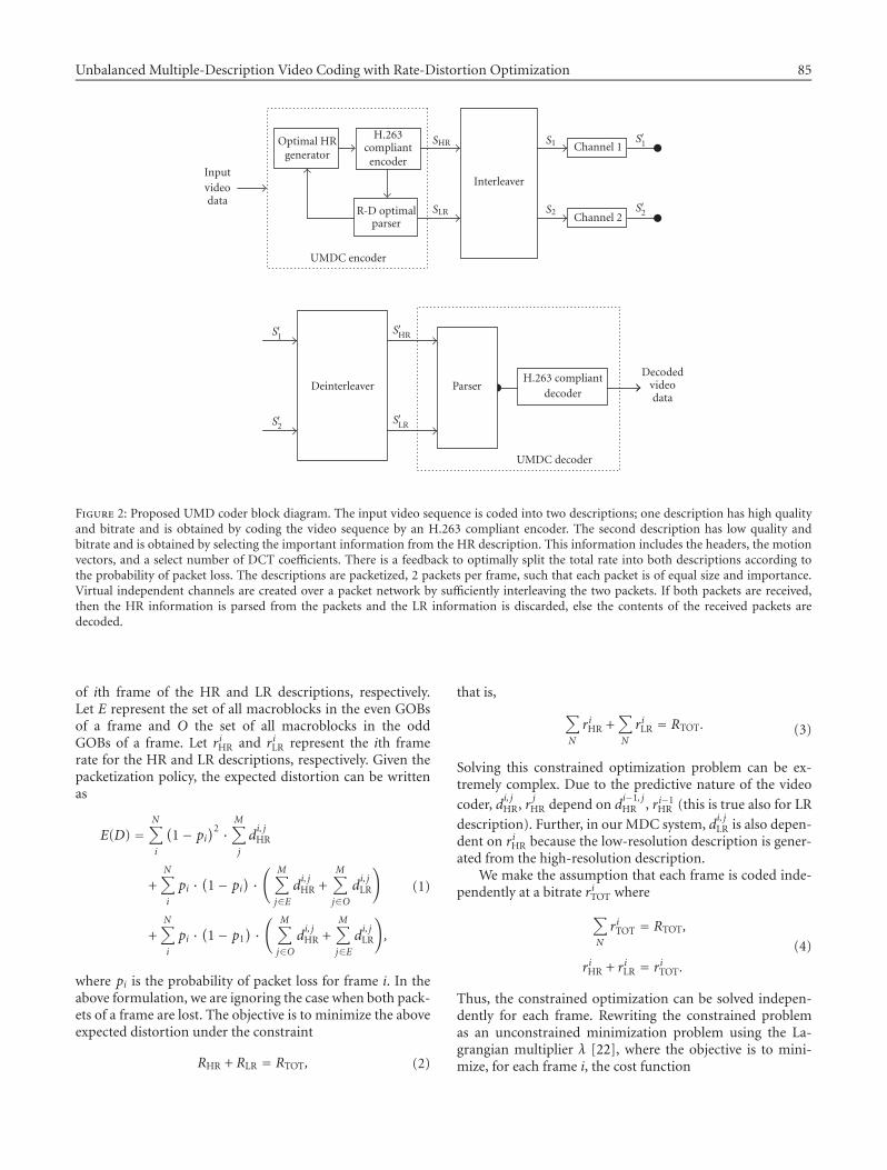
Unbalanced Multiple-Description Video Coding with Rate-Distortion Optimization 85
Inputvideodata
Optimal HRgenerator
H.263compliantencoder
R-D optimalparser
UMDC encoder
SHR
SLR
Interleaver
S1
S2
Channel 1
Channel 2
S′1
S′2
S′1
S′2
Deinterleaver
S′HR
S′LR
ParserH.263 compliant
decoder
Decodedvideodata
UMDC decoder
Figure 2: Proposed UMD coder block diagram. The input video sequence is coded into two descriptions; one description has high qualityand bitrate and is obtained by coding the video sequence by an H.263 compliant encoder. The second description has low quality andbitrate and is obtained by selecting the important information from the HR description. This information includes the headers, the motionvectors, and a select number of DCT coefficients. There is a feedback to optimally split the total rate into both descriptions according tothe probability of packet loss. The descriptions are packetized, 2 packets per frame, such that each packet is of equal size and importance.Virtual independent channels are created over a packet network by sufficiently interleaving the two packets. If both packets are received,then the HR information is parsed from the packets and the LR information is discarded, else the contents of the received packets aredecoded.
of ith frame of the HR and LR descriptions, respectively.Let E represent the set of all macroblocks in the even GOBsof a frame and O the set of all macroblocks in the oddGOBs of a frame. Let riHR and riLR represent the ith framerate for the HR and LR descriptions, respectively. Given thepacketization policy, the expected distortion can be writtenas
E(D) =N∑i
(1− pi
)2 ·M∑j
di, jHR
+N∑i
pi ·(1− pi
) · ( M∑j∈E
di, jHR +
M∑j∈O
di, jLR
)
+N∑i
pi ·(1− p1
) · ( M∑j∈O
di, jHR +
M∑j∈E
di, jLR
),
(1)
where pi is the probability of packet loss for frame i. In theabove formulation, we are ignoring the case when both pack-ets of a frame are lost. The objective is to minimize the aboveexpected distortion under the constraint
RHR + RLR = RTOT, (2)
that is, ∑N
riHR +∑N
riLR = RTOT. (3)
Solving this constrained optimization problem can be ex-tremely complex. Due to the predictive nature of the video
coder, di, jHR, r
jHR depend on d
i−1, jHR , ri−1
HR (this is true also for LR
description). Further, in our MDC system, di, jLR is also depen-
dent on riHR because the low-resolution description is gener-ated from the high-resolution description.
We make the assumption that each frame is coded inde-pendently at a bitrate riTOT where∑
N
riTOT = RTOT,
riHR + riLR = riTOT.
(4)
Thus, the constrained optimization can be solved indepen-dently for each frame. Rewriting the constrained problemas an unconstrained minimization problem using the La-grangian multiplier λ [22], where the objective is to mini-mize, for each frame i, the cost function

86 EURASIP Journal on Applied Signal Processing
24
26
28
30
32
34
36
38
40
42
44
Dis
tort
ion
atde
code
r(d
B)
10−3 10−2 10−1
Probability of packet loss
UMDCMD-RDSSD
(a) Akiyo. 256 kbps. 30 fps.
20
25
30
35
40
45
Dis
tort
ion
atde
code
r(d
B)
10−3 10−2 10−1
Probability of packet loss
UMDCMD-RDSSD
(b) Akiyo. 384 kbps. 30 fps.
Figure 3: UMDC versus MD-RDS and SD. Akiyo. 256 (a) and 384 (b) kbps.
J(D) = (1− pi
)2 ·M∑j
di, jHR
+ pi ·(1− pi
) · ( M∑j∈E
di, jHR +
M∑j∈O
di, jLR
)
+ pi ·(1− pi
) · ( M∑j∈O
di, jHR +
M∑j∈E
di, jLR
)
+ λ · (riHR + riLR − riTOT
).
(5)
With this formulation, allocation is done independently foreach frame based on the budget obtained from TMN8 [23].Therefore, in what follows we can ignore the frame index iwhen stating the objective function.
In the present work, we do not take error propagationinto account; we are currently exploring ways of incorporat-ing the error propagation in this formulation while keepingthe computational cost reasonably low for real-time appli-
cations. Thus, the distortion djHR of the jth macroblock in
the HR description is a function of the quantization param-
eter Qj , while djLR is a function of Qj and k j , the number of
DCT coefficients duplicated, that is, not set to zero in all 8×8blocks in the macroblock j. We assume that all the blocks in a
macroblock employ the same value of k j . This is reasonablesince most of the processes done in the encoder treat mac-roblocks as single entities (e.g., motion estimation, headergeneration, etc). The optimization can be then written as
minQ,k
[(1− p)2 ·
M∑j
djHR
(Qj
)
+ p · (1− p) ·( M∑
j∈EdjHR
(Qj
)+
M∑j∈O
djLR
(Qj, k j
))
+ p · (1− p) ·( M∑
j∈OdjHR
(Qj
)+
M∑j∈E
djLR
(Qj, k j
))
+ λ · (rHR(Qj
)+ rLR
(Qj, k j
)− rTOT)]
,
(6)
where Q and k are the sets of quantization steps and theDCT coefficients duplicated in LR for each block j in thecurrent frame, respectively. In our previous work, [24], wedeveloped an algorithm for finding the optimal k, given Qand p. We assume that only the first k j DCT coefficients,along the zig-zag scan, are duplicated. To reduce the searchcomplexity, the admissible values of k j are restricted to be0, 1, 2, 4, 8, 10, 12, 16, 32, or 64.

Unbalanced Multiple-Description Video Coding with Rate-Distortion Optimization 87
27
28
29
30
31
32
33
34
35
36
Dis
tort
ion
atde
code
r(d
B)
10−3 10−2 10−1
Probability of packet loss
UMDCMD-RDS
Figure 4: UMDC versus MD-RDS. Akiyo. 800 kbps. 30 fps.
We use mean square error (MSE) as our distortion met-ric. Since DCT is an orthogonal transform, the distortion in ablock of a frame can also be written as a function of the corre-sponding transform coefficients. Let l denote the index of theluminance block in the current macroblock j (l ∈ (1, . . . , 4)).Thus, Cn
l, j is the nth coefficient in block l from the current
macroblock j, and Cnl, j its quantized value, dependant on the
quantization step (Qj) used. We then can define the distor-tion in the HR and LR macroblocks as follows:
djHR
(Qj
) = 4∑l=1
64∑n=1
(Cnl, j − Cn
l, j
(Qj
))2, (7)
djLR
(Qj, k j
) = 4∑l=1
( k j∑n=1
(Cnl, j − Cn
l, j
(Qj
))2+
64∑n=k j+1
(Cnl, j
)2).
(8)
The rate and distortion of a macroblock for each possible k j
is calculated directly in the H.263 codec. We ignore headers,motion vectors, and other side information since they will bepresent in both descriptions.
The proposed rate-distortion optimal algorithm for gen-erating the descriptions can be summarized into the follow-ing steps.
Using the TMN8 rate control algorithm find the requiredframe rate, rTOT, for each frame. Then, for each frame of theinput sequence,
(a) find all the dHR(Qj) and dLR(Qj, k j) for all possible Qand k;
(b) minimize the expected frame distortion (1) under therate-budget rTOT constraint for the frame in consider-ation (6);
(c) generate HR frame and LR frame according to the op-timal Q and k found.
4. SIMULATIONS AND RESULTS
The reported results are expressed in terms of the signal-to-noise ratio (SNR) of the luminance components of thefirst 100 frames of the two QCIF (176 × 144 pixels) test se-quences, namely, Akiyo and Coastguard. We compare theperformance of our UMDC with the MD-RDS coder pro-posed by Reibman et al. [15]. The work in [15] has beenextended to a packet network environment, similar to thework in [13] except that optimal mode selection is not con-sidered in the present work. Both systems are coded at thesame total bitrate, RTOT, and each frame is packetized intotwo packets. In the UMDC case, the packetization is as ex-plained in Section 3, whereas in the MD-RDS case, eachpacket contains a description. Thus, while our system cre-ates packets of equal size and importance by combining por-tions of the HR and LR descriptions, in MD-RDS, each de-scription can be packetized separately due to the balancednature of the descriptions. In both cases, if both descrip-tions are completely lost, we replace the lost informationwith the spatially corresponding information from the pre-vious frame. If this situation happens in the first frame,where no information is available, the lost macroblocks areset to their statistical mean value. We consider randomlosses with identical loss sequences being injected in bothsystems.
Figures 3 and 4 show the results for the sequence Akiyocoded at different bitrates. The frame rate is 30 fps and onlythe initial frame of the stream is intracoded. The results showthat for lossy conditions, MD coding method easily outper-forms the single-description (with no redundancy) methodSD. Among the MD methods, UMDC performs better thanMD-RDS for low packet-loss conditions; this improvementin performance increases with increasing bitrate. This can beexplained by the fact that because MD-RDS alternates coef-ficients in order to make the descriptions balanced its codingefficiency decreases. Alternate nonzero coefficients adverselyaffect the entropy coder of standards like H.263. This im-plicit redundancy increases with the increase in the numberof nonzero coefficients.
Plots in Figure 5 shows the results for the sequence Coast-guard.
Figure 6 shows the comparison of both systems whenonly the first frame is coded in intraframe mode (Figure 6a)and when an intraframe is transmitted every 10 frames(Figure 6b). In this last case, a larger number of DCT co-efficients are different from zero since intraframes containa larger number of nonzero transform coefficients than in-terframes. Hence, the coding efficiency of the UMDC ismuch better than that of MD-RDS. The maximum gain overMD-RDS when an intraframe is inserted every 10 frames isaround 1.3 dB, whereas in the case where only the first frameis coded without prediction, the gain is about 0.8 dB. The re-sults also show that MD methods perform better than sin-gle description. The test sequence used is Akiyo, coded at512 kbps.
In Table 1, we compare UMDC with VRC. For VRC,we sent two packets per frame, where one packet contained

88 EURASIP Journal on Applied Signal Processing
23
23.5
24
24.5
25
25.5
26
26.5
27
27.5
Dis
tort
ion
atde
code
r
10−3 10−2 10−1
Probability of packet loss
UMDCMD-RDS
(a) Coastguard. 256 kbps. 30 fps.
23
23.5
24
24.5
25
25.5
26
26.5
27
27.5
28
Dis
tort
ion
atde
code
r10−3 10−2 10−1
Probability of packet loss
UMDCMD-RDS
(b) Coastguard. 384 kbps. 30 fps.
Figure 5: UMDC versus MD-RDS. Coastguard. 256 (a) and 384 (b) kbps.
Table 1: UMDC versus MD-RDS and versus VRC. Akiyo. 30 kbps.10 fps.
Probability of packet loss 3% 5% 10%
UMDC 34.05 dB 34.01 dB 33.89 dB
MD-RDS 33.91 dB 33.87 dB 33.8 dB
VRC 33.7 dB 33.4 dB 32.5 dB
only the even GOBs and the other packet odd GOBs. Akiyosequence is coded at 30 kbps with frame rate 10 fps. AgainUMDC does very well for low packet-loss scenarios.
5. CONCLUSIONS AND FUTURE WORK
We have shown that the proposed UMDC system enhancesthe robustness of video coders to packet losses using a verysmall amount of extracomputational resources and beingcompliant with the existing video decoder standard syntax.The algorithm takes advantage of the processes done in the
encoder and then, by just pruning coefficients in a rate-distortion framework, generates a low-resolution stream tobe used in case the main stream (HR) is lost.
One of the main emphases in our work was to design anMDC video system being compatible with existing codecs.As previously commented, better results could be obtainedby removing this constraint.
Comparing our proposed system to MD-RDS, we haveseen that the main benefits of UMDC are due to the un-balanced nature of the proposed scheme: by coding runs ofzeroed DCT coefficients, the coding efficiency obtained islarger than the one obtained by alternating the transformcoefficients. As part of our future work, we would like to keepon studying different options of UMDC schemes and com-pare them against balanced ones.
In future work, we would also like to take error propaga-tion into account as in [14], but since the generation of thelow-resolution stream is done frame by frame, an appropri-ate model of the rate distribution among frames prior to anyencoding should be found.
In another future work we would like to use the LR se-quence, not just as plain redundancy but also as a refiner ofthe HR description.

Unbalanced Multiple-Description Video Coding with Rate-Distortion Optimization 89
15
20
25
30
35
40
45
Dis
tort
ion
atde
code
r(d
B)
10−3 10−2 10−1
Probability of packet loss
UMDCMD-RDSSD
(a) Akiyo. 512 kbps. 1 Intra, 99 Inter.
20
22
24
26
28
30
32
34
36
38
40
Dis
tort
ion
atde
code
r(d
B)
10−3 10−2 10−1
Probability of packet loss
UMDCMD-RDSSD
(b) Akiyo. 512 kbps. 1 Intra every 10 frames.
Figure 6: UMDC versus MD-RDS and SD. Akiyo. 512 kbps. 30 fps.
ACKNOWLEDGMENTS
The authors would like to thank the reviewers for their help-ful suggestions. This work was done while the first and thesecond authors were affiliated with USC. The research hasbeen funded in part by the Integrated Media Systems Center,a National Science Foundation Engineering Research Center,Cooperative Agreement no. EEC-9529152, by the NationalScience Foundation under grant MIP-9804959 and by theCICYT TIC2001-0996 project of the Spanish government.
REFERENCES
[1] ITU-T Recommendation H.263, “Video Coding for lowbit rate communication,” International TelecommunicationsUnion-Telecommunications, Geneva. 1, 1995; 2 (H.263+),1998; 3 (H.263++), 2000.
[2] Motion Pictures Expert Group (ISO/IEC JTC 1/SC 2/WG 11),“Information Technology-Coding of Moving Pictures andAssociated Audio for Digital Storage Media at up to About1.5 Mbits/s - Part 2: Video,” Int. Std, 11172, November 1992.
[3] R. Rejaie, M. Handley, and D. Estrin, “Quality adaptation forcongestion controlled video playback over the internet,” inProc. ACM SIGCOMM ’99, pp. 189–200, Cambridge, Mass,USA, September 1999.
[4] S. Lin and D. J. Costello, Error Control Coding: Fundamentalsand Applications, Prentice-Hall, Englewood Cliffs, NJ, USA,1983.
[5] V. K. Goyal, “Multiple description coding: Compressionmeets the network,” IEEE Signal Processing Magazine, vol. 18,no. 5, pp. 74–93, 2001.
[6] L. Ozarow, “On a source coding problem with two channelsand three receivers,” Bell System Technical Journal, vol. 59, no.10, pp. 1909–1921, 1980.
[7] A. A. El Gamal and T. M. Cover, “Achievable rates for multipledescriptions,” IEEE Transactions on Information Theory, vol.28, no. 6, pp. 851–857, 1982.
[8] V. A. Vaishampayan, “Design of multiple description scalarquantizers,” IEEE Transactions on Information Theory, vol. 39,no. 3, pp. 821–834, 1993.
[9] V. K. Goyal, J. Kovacevic, R. Arean, and M. Vetterli, “Multipledescription transform coding of images,” in Proc. IEEE Inter-national Conference on Image Processing, vol. 1, pp. 674–678,Chicago, Ill, USA, October 1998.
[10] Y. Wang, M. T. Orchard, and A. R. Reibman, “Optimal pair-wise correlating transforms for multiple description coding,”in Proc. IEEE International Conference on Image Processing,Chicago, Ill, USA, October 1998.
[11] R. Puri and K. Ramchandran, “Multiple description sourcecoding through forward error correction codes,” in Proc.33rd Asilomar Conference on Signals, Systems, and Computers,vol. 1, pp. 342–346, October 1999.

90 EURASIP Journal on Applied Signal Processing
[12] W. Jiang and A. Ortega, “Multiple description coding viapolyphase transform and selective quantization,” in Proc. Vi-sual Communications and Image Processing, San Jose, Calif,USA, January 1999.
[13] A. R. Reibman, “Optimizing multiple description videocoders in a packet loss environment,” in Proc. Packet VideoWorkshop, Pittsburgh, Pa, USA, March 2002.
[14] R. Zhang, S. L. Regunathan, and K. Rose, “Video coding withoptimal inter/intra mode switching for packet loss resilience,”IEEE Journal on Selected Areas in Communications, vol. 18, no.6, pp. 966–976, 2000.
[15] A. R. Reibman, H. Jafarkhani, Y. Wang, and M. T. Orchard,“Multiple description video using rate-distortion splitting,” inProc. IEEE International Conference on Image Processing, Tes-saloniki, Greece, October 2001.
[16] V. A. Vaishampayan and S. John, “Interframe balanced mul-tiple description video compression,” in Proc. Packet VideoWorkshop, New York, NY, USA, April 1999.
[17] A. R. Reibman, H. Jafarkhani, Y. Wang, M. T. Orchard, andR. Puri, “Multiple description coding for video using motioncompensated prediction,” in Proc. IEEE International Confer-ence on Image Processing, Kobe, Japan, October 1999.
[18] Y. Wang and S. Lin, “Error resilient video coding using mul-tiple description motion compensation,” in Proc. IEEE Mul-timedia Signal Processing Workshop, Cannes, France, October2001.
[19] S. Wenger, “Video redundancy coding in H.263+,” in Proc.Workshop on Audio-Visual Services for Packet Networks, Ab-erdeen, UK, 1997.
[20] M. van der Schaar and H. Radha, “A hybrid temporal-SNRfine-granular scalability for internet video,” IEEE Trans. Cir-cuits and Systems for Video Technology, vol. 11, no. 3, pp. 318–331, 2001.
[21] M. Gallant, G. Cote, B. Erol, and F. Kossentini, “UBC’sH.263+ Public Domain Software, Version 3.2.0,” Official ITU-T Study Group 16 Video Experts Group Reference C Codec,July 1998.
[22] A. Ortega and K. Ramchandran, “Rate-distortion methodsfor image and video compression,” IEEE Signal ProcessingMagazine, vol. 15, no. 6, pp. 23–50, 1998.
[23] J. Ribas-Corbera and S. Lei, “Rate control in DCT video cod-ing for low-delay communications,” IEEE Trans. Circuits andSystems for Video Technology, vol. 9, no. 1, pp. 172–185, 1999.
[24] D. Comas, R. Singh, and A. Ortega, “Rate-distortion op-timization in a robust video transmission based on unbal-anced multiple description coding,” in Proc. IEEE Workshopon Multimedia Signal Processing, Cannes, France, October2001.
David Comas was born in Barcelona(Spain) in 1976. In 2001, he receivedhis M.S. degree in electrical engineeringfrom the Technical University of Catalo-nia (UPC), Barcelona, Spain. From May2000 to April 2001, he was with the Signaland Image Processing Institute (SIPI) at theUniversity of Southern California (USC),Los Angeles, USA, doing his Master the-sis. In 2001, he joined the Image ProcessingGroup, in the Department of Signal Theory and Communications(TSC) and he is currently pursuing a Ph.D. degree in electrical engi-neering. His current research interests include multiple-descriptioncoding for video, image and sequence analysis, and image and se-quence coding.
Raghavendra Singh was born in New Delhi, India, in 1971. Hereceived the B.E. in electrical and electronics from the Birla In-stitute of Technology and Science, Pilani, India in 1993 and thePh.D. in electrical engineering from University of Southern Cali-fornia in 2001. His research interests are in the area of digital imageand video processing, and reliable transmission of real-time multi-media data.
Antonio Ortega received the Telecommunications Engineering de-gree from the Universidad Politecnica de Madrid (UPM), Madrid,Spain in 1989 and the Ph.D. in electrical engineering fromColumbia University, New York, NY in 1994. At Columbia, he wassupported by a Fulbright scholarship. In 1994, he joined the Elec-trical Engineering-System department at the University of South-ern California, where he is currently an Associate Professor. AtUSC, he is also a member of the Integrated Media Systems Center(IMSC) and the Signal and Image Processing Institute. He is a se-nior member of the IEEE, and a member of SPIE and ACM. He wasa Technical Program Cochair of ICME 2002. He has been an Asso-ciate Editor for the IEEE Transactions on Image Processing and forthe IEEE Signal Processing Letters. He has been a member of theBoard of Governors of the IEEE SPS. He has received the NSF CA-REER Award, the 1997 IEEE Communications Society Leonard G.Abraham Prize Paper Award and the IEEE Signal Processing Soci-ety 1999 Magazine Award. His research interests are in the areas ofmultimedia compression and communications. They include top-ics such as rate control and video transmission over packet networkand compression for recognition and classification applications.
Ferran Marques received the M.S. degreein electrical engineering from the TechnicalUniversity of Catalonia (UPC), Barcelona,Spain, in 1988. From 1989 to June 1990,he worked in the Swiss Federal Instituteof Technology in Lausanne (EPFL) and inJune 1990, he joined the Department ofSignal Theory and Communications of theTechnical University of Catalonia (UPC). In1991, he was with the Signal and Image Pro-cessing Institute at USC in Los Angeles (California). He received thePh.D. degree from the UPC in December 1992 and the Spanish BestPh.D. thesis in electrical engineering award in 1992. Since 1995, heis an Associate Professor at UPC. He has served for the EURASIPAdCom as responsible of the member services (1998–2000), as Sec-retary and Treasurer (2000–2002), and currently as President. Hewas an Associate Editor of the Journal of Electronic Imaging (SPIE)in the area of image communications (1996–2000) and currently,he serves in the Editorial Board of the EURASIP Journal on Ap-plied Signal Processing. He is an author or a coauthor of more than70 publications that have appeared as journal papers and proceed-ing articles, 4 book chapters, and 4 international patents.