Multiblock copolymers at selective liquid–liquid interfaces: Toward a block size chromatography

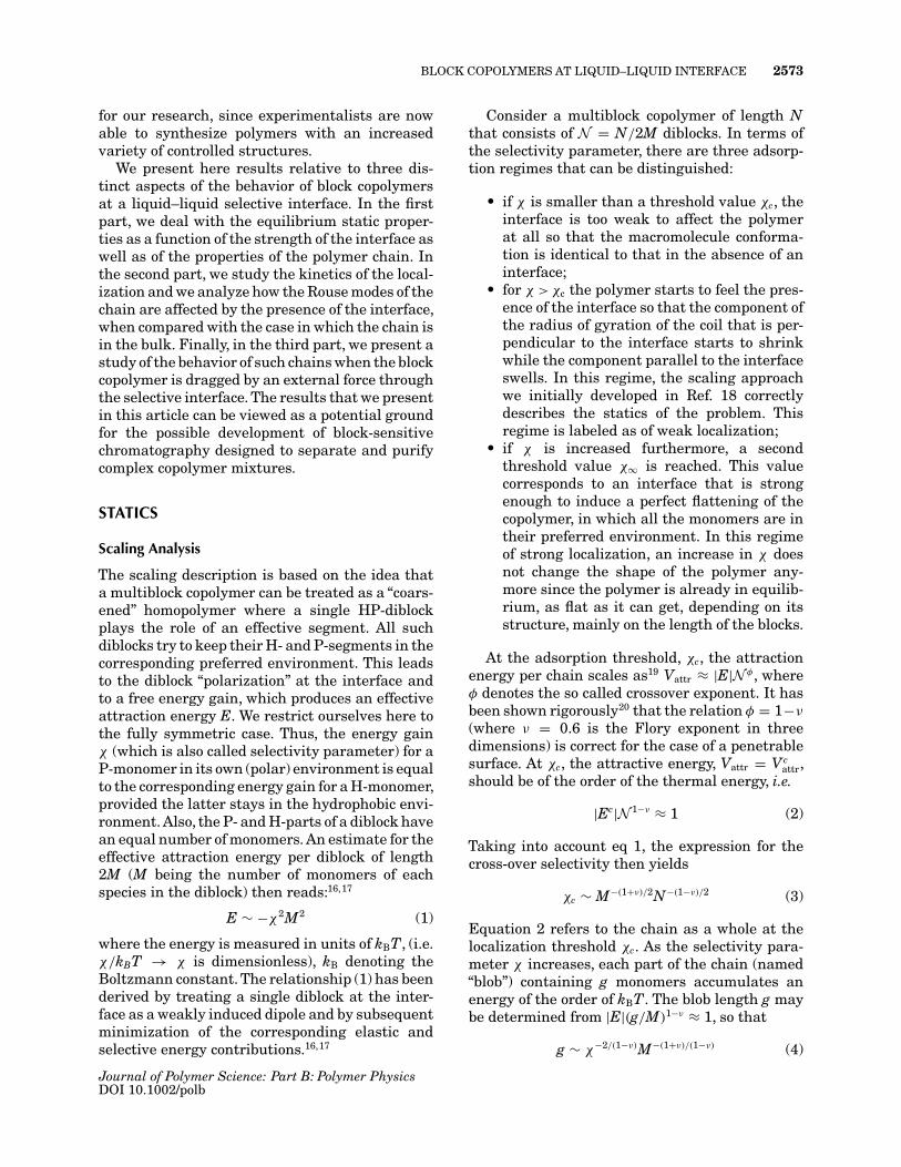
Multiblock Copolymers at Selective Liquid–LiquidInterfaces: Toward a Block Size Chromatography

ANDREA CORSI,1,* ANDREY MILCHEV,1,2 VAKHTANG G. ROSTIASHVILI,1 THOMAS A. VILGIS1

1Max Planck Institute for Polymer Research, 55128 Mainz, Germany

2Institute for Physical Chemistry, Bulgarian Academy of Science, 1113 Sofia, Bulgaria

Received 11 January 2006; revised 21 March 2006; accepted 21 March 2006DOI: 10.1002/polb.20909Published online in Wiley InterScience (www.interscience.wiley.com).

ABSTRACT: We report some very recent studies on the localization of hydrophobic-polarregular copolymers at a selective solvent–solvent interface with emphasis on the impactof block length M on their static properties and dynamics. A simple scaling theory isdeveloped and its predictions are compared with extensive Monte Carlo simulationsto provide an adequate description of copolymers behavior at such penetrable phaseboundary. We have derived and verified the scaling of various quantities such as thecomponents of the radius of gyration parallel and perpendicular to the interface, the lat-eral diffusion constant, as well as the characteristic relaxation times for the localizationof the polymer coil in terms of chain length N and block size M for various strength ofthe interface. The copolymer dynamics is elucidated by a Rouse-mode analysis, whichreveals a specific coupling of the modes once a copolymer is adsorbed at the selectiveinterface. For the case of copolymer chains being dragged by an external field throughthe selective interface, we provide results, which suggest a possible application as a newtype of chromatography designed to separate and purify complex mixtures with respectto the chain length and the block size of the individual macromolecules. © 2006 WileyPeriodicals, Inc. J Polym Sci Part B: Polym Phys 44: 2572–2588, 2006Keywords: block copolymers; interfaces; Monte Carlo simulation; theory

INTRODUCTION

The behavior of hydrophobic-polar (HP) copoly-mers at a selective penetrable interface (the inter-face which divides two immiscible liquids, likewater and oil, each of them being favored by oneof the two types of monomers) is of great impor-tance in the chemical physics of polymers. Forstrongly selective interfaces, when the energy gainfor a monomer in the favored solvent is large,the hydrophobic and polar blocks of a copolymer

*Present address: Dipartimento di Fisica, Università degliStudi di Milano, Milano, Italy

Correspondence to: T. A. Vilgis (E-mail: [email protected])Journal of Polymer Science: Part B: Polymer Physics, Vol. 44, 2572–2588 (2006)© 2006 Wiley Periodicals, Inc.

chain try to stay on different sides of the interfacethus leading to a major reduction of the interfacialtension between the immiscible liquids or melts,which has important technological applications,e.g. for compatibilizers, thickeners, or emulsifiers.Not surprisingly, during the last two decadesthe problem has gained a lot of attention fromexperiment,1–5 theory6–10 as well as from computerexperiment.11–15 While in earlier studies attentionhas been mostly focused on diblock copolymers2,4

because of their relatively simple structure, thescientific interest shifted later to random HP-copolymers at penetrable interfaces.7–10,15 Untilrecently, the properties of regular multiblockcopolymers, especially with emphasis on theirdependence on block length M, have remainedlargely unexplored. This has been a driving force

2572

BLOCK COPOLYMERS AT LIQUID–LIQUID INTERFACE 2573

for our research, since experimentalists are nowable to synthesize polymers with an increasedvariety of controlled structures.

We present here results relative to three dis-tinct aspects of the behavior of block copolymersat a liquid–liquid selective interface. In the firstpart, we deal with the equilibrium static proper-ties as a function of the strength of the interface aswell as of the properties of the polymer chain. Inthe second part, we study the kinetics of the local-ization and we analyze how the Rouse modes of thechain are affected by the presence of the interface,when compared with the case in which the chain isin the bulk. Finally, in the third part, we present astudy of the behavior of such chains when the blockcopolymer is dragged by an external force throughthe selective interface. The results that we presentin this article can be viewed as a potential groundfor the possible development of block-sensitivechromatography designed to separate and purifycomplex copolymer mixtures.

STATICS

Scaling Analysis

The scaling description is based on the idea thata multiblock copolymer can be treated as a “coars-ened” homopolymer where a single HP-diblockplays the role of an effective segment. All suchdiblocks try to keep their H- and P-segments in thecorresponding preferred environment. This leadsto the diblock “polarization” at the interface andto a free energy gain, which produces an effectiveattraction energy E. We restrict ourselves here tothe fully symmetric case. Thus, the energy gainχ (which is also called selectivity parameter) for aP-monomer in its own (polar) environment is equalto the corresponding energy gain for a H-monomer,provided the latter stays in the hydrophobic envi-ronment. Also, the P- and H-parts of a diblock havean equal number of monomers. An estimate for theeffective attraction energy per diblock of length2M (M being the number of monomers of eachspecies in the diblock) then reads:16,17

E ∼ −χ2M2 (1)

where the energy is measured in units of kBT, (i.e.χ/kBT → χ is dimensionless), kB denoting theBoltzmann constant. The relationship (1) has beenderived by treating a single diblock at the inter-face as a weakly induced dipole and by subsequentminimization of the corresponding elastic andselective energy contributions.16,17

Consider a multiblock copolymer of length Nthat consists of N = N/2M diblocks. In terms ofthe selectivity parameter, there are three adsorp-tion regimes that can be distinguished:

• if χ is smaller than a threshold value χc, theinterface is too weak to affect the polymerat all so that the macromolecule conforma-tion is identical to that in the absence of aninterface;

• for χ > χc the polymer starts to feel the pres-ence of the interface so that the component ofthe radius of gyration of the coil that is per-pendicular to the interface starts to shrinkwhile the component parallel to the interfaceswells. In this regime, the scaling approachwe initially developed in Ref. 18 correctlydescribes the statics of the problem. Thisregime is labeled as of weak localization;

• if χ is increased furthermore, a secondthreshold value χ∞ is reached. This valuecorresponds to an interface that is strongenough to induce a perfect flattening of thecopolymer, in which all the monomers are intheir preferred environment. In this regimeof strong localization, an increase in χ doesnot change the shape of the polymer any-more since the polymer is already in equilib-rium, as flat as it can get, depending on itsstructure, mainly on the length of the blocks.

At the adsorption threshold, χc, the attractionenergy per chain scales as19 Vattr ≈ |E|N φ, whereφ denotes the so called crossover exponent. It hasbeen shown rigorously20 that the relation φ = 1−ν

(where ν = 0.6 is the Flory exponent in threedimensions) is correct for the case of a penetrablesurface. At χc, the attractive energy, Vattr = Vc

attr,should be of the order of the thermal energy, i.e.

|Ec|N 1−ν ≈ 1 (2)

Taking into account eq 1, the expression for thecross-over selectivity then yields

χc ∼ M−(1+ν)/2N−(1−ν)/2 (3)

Equation 2 refers to the chain as a whole at thelocalization threshold χc. As the selectivity para-meter χ increases, each part of the chain (named“blob”) containing g monomers accumulates anenergy of the order of kBT. The blob length g maybe determined from |E|(g/M)1−ν ≈ 1, so that

g ∼ χ−2/(1−ν)M−(1+ν)/(1−ν) (4)

Journal of Polymer Science: Part B: Polymer PhysicsDOI 10.1002/polb

2574 CORSI ET AL.

The localized chain as a whole can be consideredas a string of such blobs.

It is customary21 to take the number of blobs,N/g ∼ χ2/(1−ν)M(1+ν)/(1−ν)N as a natural scalingvariable in the various scaling relations. For thesake of convenience, we take this variable in thefollowing form

η ≡ χ M(1+ν)/2 N (1−ν)/2 (5)

Then the chain size perpendicular to the interfacedirection scales as

Rg⊥ = lNνG(η) (6)

where l is the Kuhn segment and G(η) is somescaling function.

As explained above, one should discriminatebetween the cases of weak and strong localiza-tion.22 Around the onset of the weak localizationregime, the scaling argument η is of the order ofone (cf. eq 3), and the scaling function G(η) has apower law behavior, i.e.

G(η) ={

1, at η < 1ηα, at η ≥ 1

(7)

where α = −2ν/(1 − ν). This value of the expo-nent α has been found from the condition that atη ≥ 1 the value of Rg⊥ is determined by the blobsize alone, i.e. it does not depend on N.

Similar reasoning can be used for the chain sizein the direction parallel to the interface R||, namelyit is possible to write

Rg‖ = lNνH(η) (8)

where H(η) is some scaling function. Again, theform of H(η) can be determined by the condi-tion that at η ≥ 1 the localized multiblock chainbehaves as a two-dimensional self-avoiding stringof blobs, i.e. R|| ∼ Nν2 , where ν2 = 0.75 is the Floryexponent in two dimensions. As a result one finds

H(η) ={

1, at η < 1ηβ , at η ≥ 1

(9)

where β = 2(ν2 − ν)/(1 − ν).As the selectivity parameter χ grows even fur-

ther, a characteristic point χ = χ∞ can be reachedwhere Rg⊥ and Rg‖ approach a plateau and do notchange any further. This is the strong localiza-tion limit where the number of monomers in theblob becomes of the order of the block length. By

making use of this condition in eq 4, we can writefor the characteristic selectivity χ∞ the followingsimple relation22

χ∞ ∼ M−1 (10)

This corresponds to the well known Flory-Hugginslimit of phase separation. Note that χ∞ dependsonly on the block size M and does not depend onthe chain length N. Given this value one can goback to eqs 6–9 and check the scaling in the stronglocalization limit. The resulting relations are

Rg⊥ = lMν (11)

Rg‖ = lMν

(NM

)ν2

∼ M−(ν2−ν)Nν2 (12)

This reflects the pancake geometry of a polymerlocalized at the surface. The relations (11) and (12)can be expected because in this regime all P- andH-segments are predominantly in their preferredsolvents. In addition, the scaling estimate of thepolymer size perpendicular to the interface showsthat the perpendicular extension of the chain isentirely determined by the size of the blob.

The free energy gain in the localized state isproportional to the number of blobs,21 i.e.

Floc ∼ Ng

∼ χ2/(1−ν)NM(1+ν)/(1−ν) (13)

where eq 4 has been used. In terms of η eq 13 reads

Floc = η2/(1−ν) at 1 ≤ η ≤ η∞ (14)

where η∞ = χ∞M(1+ν)/2N (1−ν)/2 ∼ (N/M)(1−ν)/2. Forχ > χ∞, the free energy gain follows the stronglocalization law

Floc ∼ χN (15)

This is mainly triggered by the energy gain.After the localization at the selective interface,

the multiblock copolymer can only diffuse in theplane of the surface. Here, we give the scalingestimate for the characteristic time τ , which is nec-essary for a chain to displace along the surface adistance equal to its own gyration radius in thestrong localization limit.

The diffusion coefficient of the whole chainalong the surface can be estimated as

D‖ ≈(

1ζ

)1N = Dblock

N (16)

where Dblock is the diffusion coefficient of one block,ζ = ζ0M the corresponding friction coefficient, and



the number of diblocks N = N/2M. The character-istic time of the two-dimensional chain displace-ment obeys

τ ≈ R2blockN 2ν2(

1ζ

)1N

(17)

where the characteristic size of the block (whichspreads in the three-dimensional space) Rblock

≈ lMν (ν = 0.6) whereas the two-dimensionalFlory exponent is ν2 = 0.75.

Now, one can express all quantities in eq 17 interms of N and M. As a result one obtains

τ ≈ ζ0 l2M2(ν−ν2)N2ν2+1

≈ ζ0 l2M−0.3 N2.5 (18)

It is clear that this result should hold for suffi-ciently long chains and blocks.

Simulation Model

The off-lattice bead-spring model employed duringour study has been previously used for simula-tions of polymers both in the bulk23,24 and nearconfining surfaces;25–30 thus, we describe here thesalient features only. Each polymer chain con-tains N effective monomers connected by anhar-monic springs described by the finitely extendiblenonlinear elastic (FENE) potential:

UFENE = −K2

R2 ln[1 − ( − 0)

2

R2

](19)

Here is the length of an effective bond, which canvary in between min < < max, with min = 0.4,max = 1 being the unit of length, and has the equi-librium value 0 = 0.7, while R = max − 0 = 0

−min = 0.3, and the spring constant K is taken asK/kBT = 40. The nonbonded interactions betweenthe effective monomers are described by the Morsepotential

UM = εM{exp[−2α(r − rmin)] − 2 exp[−α(r − rmin)]}(20)

where r is the distance between the beads, and theparameters are chosen as rmin = 0.8, εM = 1, andα = 24. Owing to the large value of the latter con-stant, UM(r) decays to zero very rapidly for r > rmin,and is completely negligible for distances largerthan unity. This choice of parameters is usefulfrom a computational point of view, since it allowsthe use of a very efficient link-cell algorithm.31

From a physical point of view, these potentials

eqs 19 and 20 make sense when one interpretsthe effective bonds as kind of Kuhn segments,comprising a number of chemical monomers alongthe chain, and thus the length unit max = 1 corre-sponds physically rather to 1 nm than to the lengthof a covalent C C bond (which would only be about1.5Å). Since in the present study we are concernedwith the localization of a copolymer in good solventconditions, in eq 20 we retain the repulsive branchof the Morse potential only by setting UM(r) = 0for r > rmin and shifting UM(r) up by εM .

The interface potential is taken simply as a stepfunction with amplitude χ ,

Uint(n, z)

{−σ(n)χ/2, z > 0σ(n)χ/2, z ≤ 0

(21)

where the interface plane is fixed at z = 0, andσ(n) = ±1 denotes a “spin” variable, which distin-guishes between P- and H-monomers. The energygain of each chain segment is thus −χ , provided itstays in its preferred solvent.

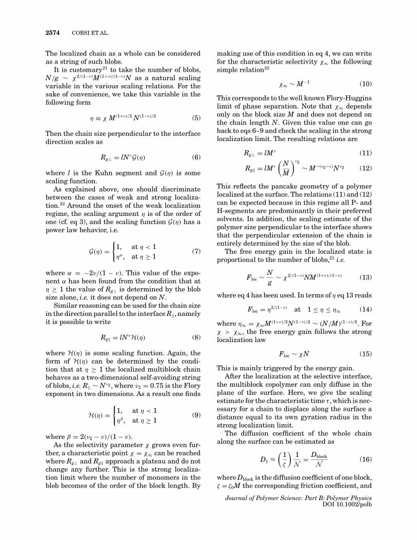
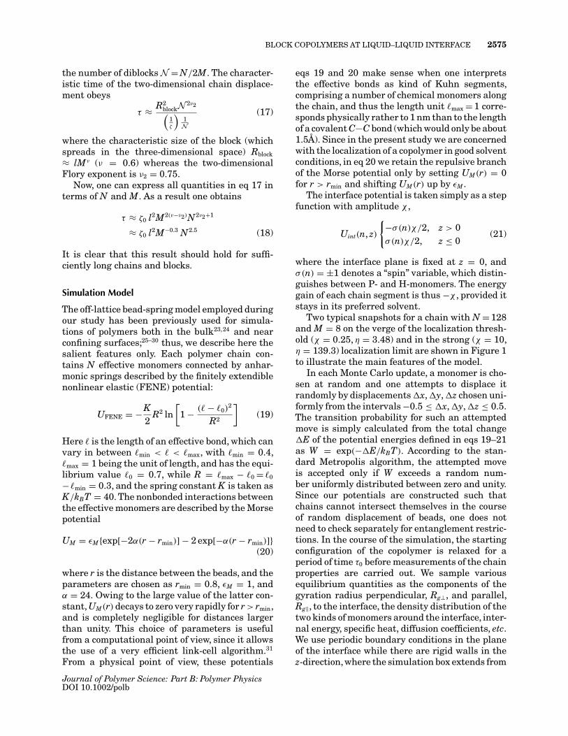
Two typical snapshots for a chain with N = 128and M = 8 on the verge of the localization thresh-old (χ = 0.25, η = 3.48) and in the strong (χ = 10,η = 139.3) localization limit are shown in Figure 1to illustrate the main features of the model.

In each Monte Carlo update, a monomer is cho-sen at random and one attempts to displace itrandomly by displacements �x, �y, �z chosen uni-formly from the intervals −0.5 ≤ �x, �y, �z ≤ 0.5.The transition probability for such an attemptedmove is simply calculated from the total change�E of the potential energies defined in eqs 19–21as W = exp(−�E/kBT). According to the stan-dard Metropolis algorithm, the attempted moveis accepted only if W exceeds a random num-ber uniformly distributed between zero and unity.Since our potentials are constructed such thatchains cannot intersect themselves in the courseof random displacement of beads, one does notneed to check separately for entanglement restric-tions. In the course of the simulation, the startingconfiguration of the copolymer is relaxed for aperiod of time τ0 before measurements of the chainproperties are carried out. We sample variousequilibrium quantities as the components of thegyration radius perpendicular, Rg⊥, and parallel,Rg‖, to the interface, the density distribution of thetwo kinds of monomers around the interface, inter-nal energy, specific heat, diffusion coefficients, etc.We use periodic boundary conditions in the planeof the interface while there are rigid walls in thez-direction,where the simulation box extends from


2576 CORSI ET AL.

Figure 1. Snapshots of typical configurations of acopolymer with N = 128, M = 8 on the verge of theadsorption threshold at χ = 0.25 (a) and in the stronglocalization limit χ = 10 (b). The value of the crossoverselectivity for this chain is χc = 0.67.

z = −32 to z = 32. The algorithm is reasonably fast,i.e. one performs ≈ 0.5×106 updates per CPU sec-ond on a 2.8 GHz PC. Typically, we studied chainswith length 32 ≤ N ≤ 512 and all measurementshave been averaged over 217 samples.

Results and Discussion

The localization at the selective interface canbe considered as a phase transition at leastin the limits: N → ∞, M → ∞, and χ → 0 withηc ≡ χcN (1−ν)/2M(1+ν)/2 = 1. At finite N, M, and χ ,the transition looks like a smooth crossover andone can define an order parameter (OP) in termsof the fractions of P- and H-monomers in the polar

(at z > 0) and hydrophobic (at z < 0) semi-space,respectively, i.e.

OP =√

f >P f <

H (22)

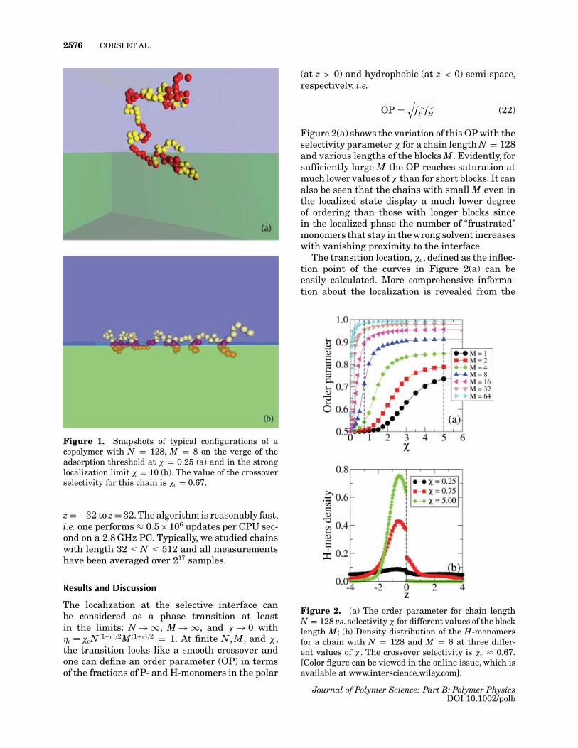
Figure 2(a) shows the variation of this OP with theselectivity parameter χ for a chain length N = 128and various lengths of the blocks M. Evidently, forsufficiently large M the OP reaches saturation atmuch lower values of χ than for short blocks. It canalso be seen that the chains with small M even inthe localized state display a much lower degreeof ordering than those with longer blocks sincein the localized phase the number of “frustrated”monomers that stay in the wrong solvent increaseswith vanishing proximity to the interface.

The transition location, χc, defined as the inflec-tion point of the curves in Figure 2(a) can beeasily calculated. More comprehensive informa-tion about the localization is revealed from the

Figure 2. (a) The order parameter for chain lengthN = 128 vs. selectivity χ for different values of the blocklength M; (b) Density distribution of the H-monomersfor a chain with N = 128 and M = 8 at three differ-ent values of χ . The crossover selectivity is χc ≈ 0.67.[Color figure can be viewed in the online issue, which isavailable at www.interscience.wiley.com].



Figure 3. Variation of the chain size for chains equi-librated at the interface as a function of the scalingvariable η for block length M = 4: (a) perpendicularand (b) parallel components. In both cases the dashedline indicates the scaling prediction. [Color figure canbe viewed in the online issue, which is available atwww.interscience.wiley.com].

monomer density distribution histogram, which isgiven in Fig. 2(b). While for χ = 0.25 the copolymeris still not localized, even at χ = 0.75 > χc thereis still a considerable amount of segments thatstay in the wrong solvent and one needs a ratherstrong segregation χ = 5.0 in order to keep thesegments entirely in their preferred environment.The three vertical lines in Figure 2(a) correspondto the three χ values chosen for the histogramsshown in Figure 2(b).

Weak Localization

We turn now to the comparison of our data withthe scaling prediction given in Scaling AnalysisSection. Figure 3(a) displays the variation of the

chain size perpendicular to the interface Rg⊥ withscaling parameter η for M = 4 and different val-ues of N. One can easily distinguish between thecases of weak and strong localization. In the firstcase, the curves collapse nicely on a master curvein a range of η (which gets narrower with increas-ing M). This complies with the scaling law givenby eq 7. The scaling function, eq 7, is character-ized by the exponent α = −3, which is indicatedby the dashed line in Fig. 3(a) and appears in goodagreement with the simulation data.

A similar scaling representation has been pre-pared also for the parallel component of the chainsize Rg‖ [see Fig. 3(b)]. In the weak localizationregime, all data collapse again into a master curve.The scaling exponent β = 3/4 (noted by the dashedline, see eq 9) is fairly close to the simulationalresults.

Strong Localization

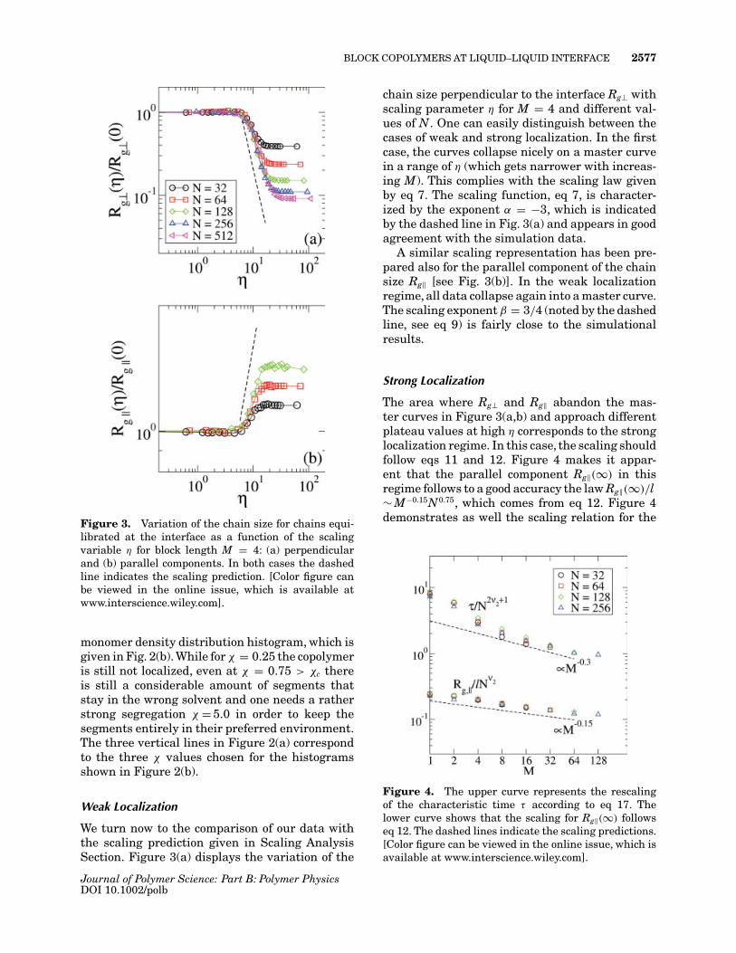
The area where Rg⊥ and Rg‖ abandon the mas-ter curves in Figure 3(a,b) and approach differentplateau values at high η corresponds to the stronglocalization regime. In this case, the scaling shouldfollow eqs 11 and 12. Figure 4 makes it appar-ent that the parallel component Rg‖(∞) in thisregime follows to a good accuracy the law Rg‖(∞)/l∼ M−0.15N0.75, which comes from eq 12. Figure 4demonstrates as well the scaling relation for the

Figure 4. The upper curve represents the rescalingof the characteristic time τ according to eq 17. Thelower curve shows that the scaling for Rg‖(∞) followseq 12. The dashed lines indicate the scaling predictions.[Color figure can be viewed in the online issue, which isavailable at www.interscience.wiley.com].


2578 CORSI ET AL.

relaxation time τ given by eq 17. The fit of ourMC-results with the theoretical scaling predictionτ ∼ M−0.3N2.5 is very good especially taking intoaccount the relatively small values of the blocklength.

To conclude this section devoted to the staticproperties of block copolymers at selective inter-faces, we observe how within the framework ofour simple scaling approach we arrive at severalimportant conclusions characterizing the impactof block length M on the behavior of regularmultiblock copolymers at a fluid–fluid interface:the cross-over selectivity decreases with growingblock length as χc ∼ M−(1+ν)/2 while the charac-teristic selectivity marking the cross-over to thestrong localization regime vanishes as χ∞ ∼ M−1.Also, the typical relaxation time in the case ofstrong localization varies as τ ∼ M2(ν−ν2) with blocklength.

Our computer experiments appear to confirmthese predictions quite nicely.

KINETICS

Scaling Analysis

In our dynamical scaling analysis,32,33 we considera coarse-grained model of a multiblock copolymerconsisting of N repeat units, which is built up froma sequence of H- and P-blocks each of length M. Forsimplicity, one may take the interface with negli-gible thickness as a flat plane, which separates thetwo selective immiscible solvents. The energy gainof each repeat unit is thus −χ , provided it staysin its preferred solvent, and the system is con-sidered in the strong localization limit where18,22

χ > χ∞ ∝ M−1. In our consideration, we skip thetime needed by the polymer to move by diffusionthrough the bulk into the vicinity of the interface,and place the center of mass of an unperturbedcoil at time t = 0 at the interface whereby thelocalization field is switched on. The initial coilwill then start relaxing with time into a flat (“pan-cake”) equilibrium configuration in-plane with theinterface and the kinetics of relaxation will bedetermined by the sum of the various forces actingon the copolymer.

It might be argued that a more physical initialconfiguration could be represented by a polymerthat, after diffusing in the bulk of one of the sol-vents, gets to the interface and touches it withone single monomer. We have indeed tried thisinitial configuration as well, and concluded that,once the adsorption process starts, it proceeds

exhibiting the same physics (e.g. the same scal-ing behavior, see below). The choice of our initialcondition just eliminates the spread in the initialtime at which adsorption sets on. This spread iscaused by polymers that occasionally drift awayfrom the interface, provided the coil touches theinterface initially with the “wrong” kind of P- orH-monomers.

Rouse Dynamics

To estimate the driving force of the flatten-ing process, one may recall18,22 that the effec-tive attractive energy ε (per diblock, e.g. a pair ofconsecutive blocks of H- and P-monomers) in thestrong localization limit is ε ≈ χM. In this case,the diblock plays the role of a blob and the over-all attractive free energy Fattr ∝ εN ∝ χN, seeeq 15, where N � N/M is the total number ofblobs. Thus, the effective driving force perpendic-ular to the interface is f ⊥

attr ≈ −χ∞N/R⊥, whereR⊥ denotes the perpendicular component of theradius of gyration. This force is opposed by a forceof confinement because of the deformation of theself-avoiding chain into a layer of thickness R⊥.34

The corresponding free energy of deformation issimply estimated as Fconf � N(b/R⊥)1/ν , where b isthe Kuhn segment size.21 For the respective forcethen one gets f ⊥

conf � Nb1/ν/R1/ν+1⊥ .

The equation of motion for R⊥ follows from thecondition that the friction force that the chainexperiences during the motion in the directionperpendicular to the interface is balanced by thesum of f ⊥

attr and f ⊥conf . In the case of Rouse dynam-

ics, each chain segment experiences independentStokes friction so that the resulting equation ofmotion has the form

ζ0NdR⊥dt

= −χ∞NR⊥

+ Nb1/ν

R1/ν+1⊥

(23)

where ζ0 is the friction coefficient per segment.During the flattening process, the chain spreads

parallel to the interface because of the excludedvolume interaction. Within Flory mean-field argu-ments, the corresponding free energy Fev � vN2/

(R2‖R⊥), where v is the second virial coefficient and

R‖ is the gyration radius component parallel tothe interface. The corresponding driving force isf ‖ev � vN2/(R3

‖R⊥). This term is counterbalancedby the elastic force of chain deformation, i.e. byf ‖def � −R‖/(b2N).

Taking into account the balance of forces in theparallel direction, the equation of motion for R‖



takes then the following form

ζ0NdR‖dt

= vN2

R3‖R⊥

− R‖b2N

(24)

Evidently, the excluded volume interactions pro-vide a coupling between the relaxation perpendic-ular and parallel to the interface. Thus, eqs 23and 24 describe the relaxation kinetics of amultiblock copolymer conformation at a selectiveliquid–liquid interface. One may readily verifythat the equilibrium solutions that follow fromthese equations are

Req⊥ � bMν (25)

andReq

‖ � (vb)1/4M−ν/4Nν2 (26)

These coincide with the equilibrium expres-sions for R⊥ and R‖ derived in Scaling Analy-sis section from purely scaling-based considera-tions. The only difference is in the power of theM-dependence in eq 26, which looks like M−ν/4

instead of M−(ν2−ν) in eq 12, albeit numerically thevalues of both exponents coincide: ν/4 � (ν2 − ν)

� 0.15. To get the full solution of the equations ofmotion, it is convenient to rescale the variables asx ≡ R⊥/(bMν), y ≡ R4

‖Mν/(vbN3) so that eqs 23and 24 can be written in the dimensionless form

τ⊥dxdt

= 1x1/ν+1

− 1x

(27)

τ‖dydt

= 1x

− y (28)

The characteristic times for relaxation perpen-dicular and parallel to the interface in eqs 27and 28 should then scale as τ⊥ � ζ0b2M1+2ν andτ‖ � ζ0b2N2.

Equation 27 is independent of y so that it canbe solved exactly:

x2(t)2

[1 − F(2ν, 1; 1 + 2ν; x1/ν(t))

]− x2(0)

2[1 − F(2ν, 1; 1 + 2ν; x1/ν(0))

] = − tτ⊥

(29)

where F(α, β; γ ; z) is the hypergeometric functionand x(0) = R⊥(0)/bMν is the initial value. In theearly stages of relaxation (i.e. at t � τ⊥) one hasx 1 and the solution, eq 29, with R⊥(0) � bNν

reduces to

R2⊥(t) � R2

⊥(0) − tζ0M

(30)

so that the characteristic time of the perpendicu-lar collapse of the chain should be proportional tothe block length M.

In the opposite limit of late stages kinetics,t � τ⊥ and x ≥ 1, that is, close to equilibrium, therelaxation of Rg(t) is essentially exponential withτ⊥ ∝ M2.2:

R⊥(t)Req

⊥� 1 + exp

(− t

τ⊥

)(31)

Moreover, as typically N M, one expects thatτ‖ τ⊥, i.e. the chain coil collapses first in the per-pendicular direction to its equilibrium value andafter that slowly extends in the parallel direction.In this case, one can use x(t) � xeq = 1 in eq 28and derive the resulting solution for the parallelcomponent of Rg as

y(t) − 1 = [y(0) − 1] exp(−t/τ‖) (32)

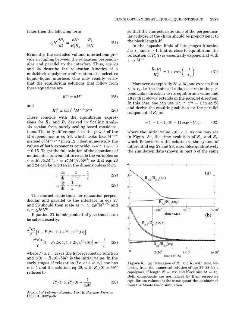
where the initial value y(0) < 1. As one may seein Figure 5a, the time evolution of R⊥ and R‖,which follows from the solution of the system ofdifferential eqs 27 and 28, resembles qualitativelythe simulation data (shown in part b of the same

Figure 5. (a) Relaxation of R⊥ and R‖ with time, fol-lowing from the numerical solution of eqs 27–28 for acopolymer of length N = 128 and block size M = 16.Both components are normalized by their respectiveequilibrium values; (b) the same quantities as obtainedfrom the Monte Carlo simulation.


2580 CORSI ET AL.

figure) even though one should bear in mind thatthe time axis for the former is in arbitrary units(scaling always holds up to a prefactor) whereasin the simulation, time is measured in MC steps(MCS) per monomer (i.e., a MCS has passed afterall monomers have been allowed to perform a moveat random). The relaxation of R‖ looks somewhatslower and, as our data for longer chains show,this effect becomes much more pronounced withgrowing number of blocks. Concerning Figure 5,note that there are several approximations onwhich our analytical derivations rely. First of all,our expressions for the attractive free energy,Fattr, and the confinement free energy, Fconf , areonly appropriate in the limit of strong flatten-ing, which occurs during the late stages of thelocalization process. Moreover, the free energy Fev,due to excluded volume interactions, is somewhatunderestimated if one uses the second virial termapproximation only. This explains why both ana-lytic curves in Figure 5 are in a better qualitativeagreement with the simulation data at the latestages of the relaxation process whereas, not sur-prisingly, this agreement is missing during itsinitial stages.

Zimm Dynamics

In the case of Zimm dynamics, the hydrodynamiclong-ranged interactions couple the motion of thesolvent to that of the coil within the framework ofthe nondraining coil model.34 When the coil flat-tens, the solvent velocity u(r) follows the velocityof the coil segments (the solvent entrainment).One can then calculate the friction forces, whichact during the coil flattening,33 making use ofa standard expression for the energy dissipationin an incompressible fluid in terms of a solventvelocity field and viscosity.35

The resulting equation of motion, however, incontrast to the case of Rouse dynamics, providesno clear-cut scaling relationship for the typicalrelaxation time τZimm with respect to N and M.

We will not present the complete mathemati-cal description of the Zimm model (that can befound in33) since the predictions of the Zimm modelcannot be tested by Monte Carlo simulationswhere the hydrodynamic effects are neglected. Butthere are some conclusions that are worth men-tioning. In particular, two major conclusions aresuggested by a close inspection of the results ofthe Zimm analysis. The presence of hydrodynamicinteractions tends to erase the asymmetry in thelocalization rates perpendicular and parallel to

the interface. This is due to the strong couplingbetween perpendicular and horizontal degrees offreedom induced by the solvent. In addition, com-pared with the case of Rouse dynamics, the local-ization in the presence of hydrodynamic effectstakes considerably longer, at least one order ofmagnitude in time, under otherwise identical con-ditions. The physical reason for this slowing downis the presence of high velocity gradients, whichdevelop in the incompressible solvent during thecoil flattening.

Results and Discussion

The results of the Monte Carlo simulations havebeen compared with the predictions of the Rousemodel introduced above. It is not possible to com-pare the simulation results to the predictions ofthe Zimm model since Monte Carlo simulationsdo not take into account the hydrodynamic con-tributions that are so important in the Zimmtreatment.

To determine the early stages dynamics, the ini-tial slope of the R2

⊥(t) curves has been obtained andcompared with the theoretical prediction of eq 30.The results are presented in Figure 6(a).

From Figure 6(a), one may readily verify thatthe initial collapse of R⊥(t � τ⊥) with time closelyfollows the predicted rate ∝ M−1, according toeq 30 in the limit of N, M 1. For sufficientlylarge block size M the N-dependence of this ini-tial rate disappears so that asymptotically thisinitial perpendicular collapse is governed by thelength M only, as predicted by the theory. Thedisagreement between the prediction of the scal-ing theory and the results of the simulations forsmall values of polymer length and block lengthis not surprising since the predictions of the scal-ing theory are valid only in the limit of N → ∞and M → ∞, with N/M large. So, we can expectthe results of the simulations to have a betteragreement with the predictions of the theory inthe case of very long polymers with many longblocks.

From the behavior of the perpendicular compo-nent of Rg as a function of time, it is also possible toobtain the characteristic time corresponding to thelate stages of adsorption. To this end, the fits of τ⊥are taken only after the initially unperturbed coilhas sufficiently relaxed, R⊥(t)/R⊥(0) ≤ 1/e. Thetwo vertical lines shown in Figure 5(b), for exam-ple, indicate the time interval used to fit the latestages behavior for the polymer with total lengthof N = 128 and block length M = 8.



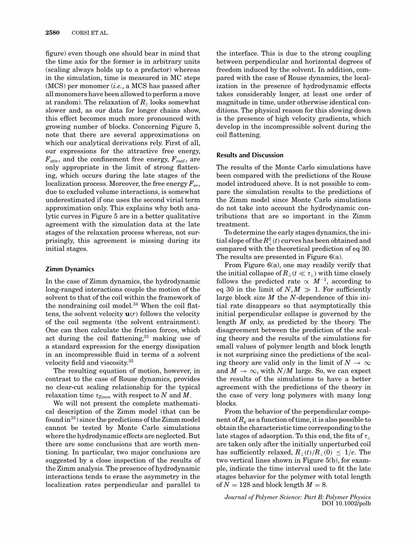
Figure 6. (a) Variation of the characteristic time forthe initial relaxation of R⊥ with block length M forchains of length 32 ≤ N ≤ 512. The prediction of the scal-ing theory is shown by a dashed line; (b) variation ofτ⊥ in the late stages of localization as a function ofblock length M for chains of length 32 ≤ N ≤ 512. Theslope of the dashed line is ≈2.2, according to eq 31. Themeaning of symbols is the same as in (a); (c) variationof τ‖ with chain length N for blocks of size M = 2, 4,8, and 16. The slope of the dashed line is 2, as pre-dicted by the theory. [Color figure can be viewed inthe online issue, which is available at www.interscience.wiley.com].

As shown in Figure 6(b), during the latestages of localization at the interface one observesthe expected, cf. eq 31, characteristic scaling ofτ⊥ ∝ M1+2ν , which progressively improves as theasymptotic limit is approached. As expected, theinitial dependence of τ⊥ on N is seen to vanish asM and N become sufficiently large, in agreementwith eq 31.

Eventually, in Figure 6(c), we display the mea-sured scaling of the late stage characteristic timefor the spreading of the chain in the plane of theinterface, τ‖, with chain length N for differentblock sizes M = 2, 4, 8, 16. Apart from some scatterof data for too small N = N/M, one nicely recov-ers the relationship τ‖ ∝ N2 whereby, once again,the initial M-dependence gradually diminishes asN 1.

An interesting question about the relationshipbetween localization rate and copolymer compo-sition concerns the mechanism that drives theinitially unperturbed coil into a localized state andmakes it “feel” the presence of a selective interface.A useful insight in this respect may be derivedby the detailed Rouse mode analysis of the moderelaxation times.

The Rouse modes are defined as the Fouriercosine transforms of the position vectors, rn, of therepeat unit n of a polymer chain. For the modelof a discrete polymer chain considered here theycan be written in terms of collective coordinatesXp as:36

Xp(t) = 1N

N∑n=1

rn(t) cos[(n − 1/2)pπ

N

],

p = 0, 1, 2, . . . , N − 1 (33)

The factor 1/2 is related to the nature of the chainthat has free ends. The time-correlation functionof the Rouse modes is given by

�pq(t) = 〈Xp(t)Xq(0)〉 (34)

where the angular brackets denote taking an aver-age over different moments of time t′ separated byan interval t. For phantom Gaussian chains withno excluded volume interactions one gets

�gausspq (t)

= 〈Xp(0)Xq(0)〉 exp(

− tτp

), p = 1, 2, . . . , N − 1

(35)

with (p, q �= 0) coefficients 〈Xp(0)Xq(0)〉gauss = δpqb2/

[8N sin2(pπ/2N)] and relaxation times

τ gaussp = ζb2

12kBT sin2(pπ/2N)

(36)

so that the typical decay times for the first modesscale as τ gauss

p ∝ N2. The mode corresponding top = 0 describes the self diffusion of the chain.For polymers with excluded volume interactions


2582 CORSI ET AL.

no such analytic results exist but one can show37

that τp ∝ N1+2ν .It is interesting to examine how the presence

of an interface between the two solvents affectsthe leading modes dynamics. In the absence ofan interface, we find that in equilibrium the firstRouse modes (1 ≤ p ≤ 10) of a homopolymer chainin a good solvent decay according to expecta-tions, τp ∝ (1/p)1+2ν ∝ N1+2ν and 〈Xp(0)Xq(0)〉 ∝(1/p)1+2ν . In contrast to what is observed in thebulk, for copolymers localized at the liquid–liquidinterface one finds a clear asymmetry in theirbehavior, strongly dependent on the direction thatis considered.

Consider first the modes components that arein plane with the interface, x and y. The val-ues of 〈Xp(0)Xp(0)〉 and 〈Zp(0)Zp(0)〉 are shownin Figure 7(a) for a copolymer adsorbed at theinterface. Again one can see that the decay of theamplitude of the Rouse modes with mode numberp still obeys a power-law. However, the polymersare not anymore 3D but rather 2D self-avoidingrandom walks. Evidently, the relevant Flory expo-nent in two dimensions ν2 = 3/4 describes well the

Figure 7. Rouse modes for a chain at the interface: (a)〈Xp(0)Xp(0)〉 and 〈Zp(0)Zp(0)〉 as a function of the modenumber p for a chain with N = 128 and M = 16 stronglyadsorbed at a selective interface. The dashed lines in(a) show the predicted scaling laws; (b) 〈Xp(0)X1(0)〉and 〈Zp(0)Z1(0)〉 as a function of the mode number p.[Color figure can be viewed in the online issue, which isavailable at www.interscience.wiley.com].

dependence of the mode amplitudes on the modenumbers as demonstrated by the dashed line withslope −(1 + 2ν2) = −2.5. It is very interesting tonotice how the modes corresponding to large val-ues of p follow the power-law decay observed inthe three-dimensional case. The modes with p < 8describe monomer motions, which involve morethan M particles. Thus, the modes correspond-ing to long wavelengths that span more than oneblock length feel the presence of the interface incontrast to those corresponding to shorter wave-lengths [and show a dependence like ∝ p−(1+2ν),see Fig. 7(a)].

If we look at the component of the Rouse modescorresponding to the direction perpendicular tothe interface, the results are quite different. Onefinds no power-law dependence of 〈Zp(0)Zp(0)〉on the mode number p. The amplitudes of theperpendicular components of the modes decreaseweakly with p and are several orders of magni-tude smaller than those of the parallel componentsof the modes. Evidently, the strong interface sup-presses all fluctuations of the chain perpendicularto the interface, which is manifested by the strongdecrease in the amplitude of the perpendicularcomponents of the modes.

In part (b) of the same figure, we show that theRouse modes components parallel to the interfaceare still orthogonal to each other. The only nonzero〈Xp(0)X1(0)〉 is the one corresponding to p = 1.This holds for both the x and y components of themodes.

Another striking difference in comparison to theresults observed for the parallel components, canbe seen just looking at the behavior of 〈Zp(0)Z1(0)〉.The modes are not orthogonal to each otheranymore since the quantities 〈Zp(0)Z1(0)〉, corre-sponding to p = 3, 5, 7 up to p = 15, are nonzero andof the same order of magnitude as 〈Z1(0)Z1(0)〉.Thus, one can conclude that the odd-numberedmodes are coupled to one another. The ampli-tude of these couplings is so small, although thesystem does not lose its ergodicity. The samecan be observed for the even-numbered modestoo but the amplitude of these terms is evensmaller than the amplitude observed for the odd-numbered modes.

Another observation concerns the average val-ues of the perpendicular components of theRouse modes. If one calculates 〈Xp〉 or 〈Yp〉, thenbecause of the isotropy of the system in the planeof the interface, these values vanish for all p’sbecause there is no preferential orientation in theplane. If one calculates 〈Zp〉, instead, the results



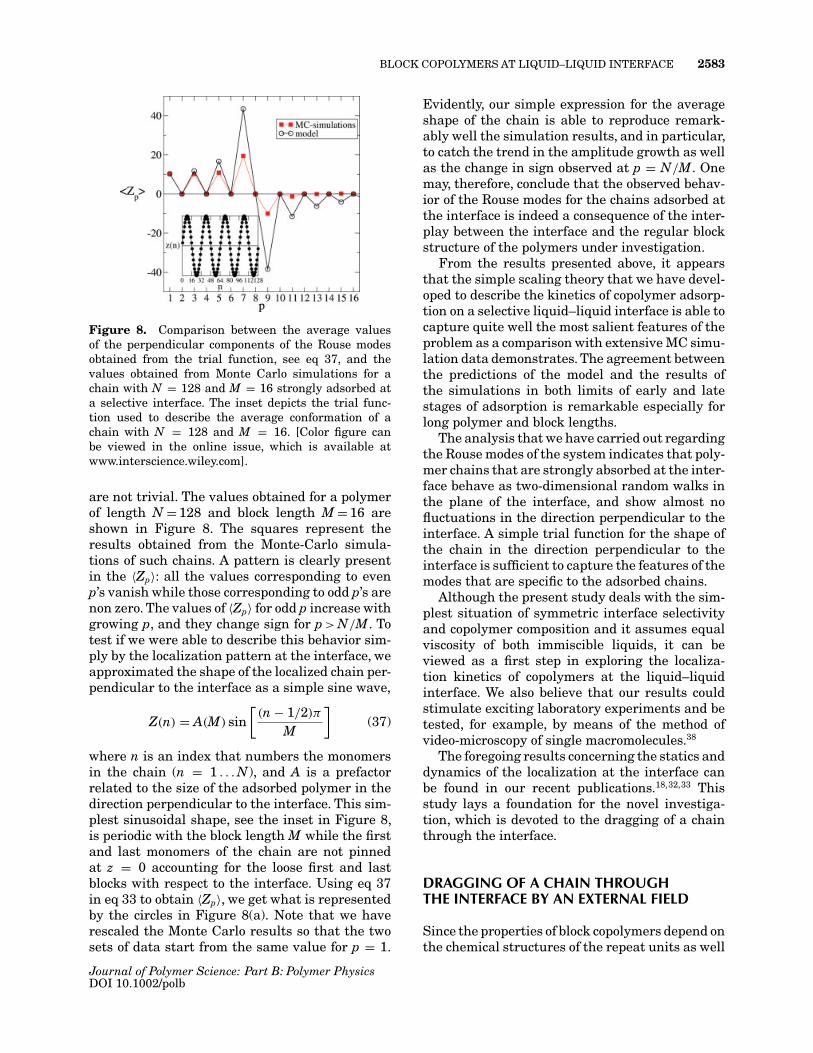
Figure 8. Comparison between the average valuesof the perpendicular components of the Rouse modesobtained from the trial function, see eq 37, and thevalues obtained from Monte Carlo simulations for achain with N = 128 and M = 16 strongly adsorbed ata selective interface. The inset depicts the trial func-tion used to describe the average conformation of achain with N = 128 and M = 16. [Color figure canbe viewed in the online issue, which is available atwww.interscience.wiley.com].

are not trivial. The values obtained for a polymerof length N = 128 and block length M = 16 areshown in Figure 8. The squares represent theresults obtained from the Monte-Carlo simula-tions of such chains. A pattern is clearly presentin the 〈Zp〉: all the values corresponding to evenp’s vanish while those corresponding to odd p’s arenon zero. The values of 〈Zp〉 for odd p increase withgrowing p, and they change sign for p > N/M. Totest if we were able to describe this behavior sim-ply by the localization pattern at the interface, weapproximated the shape of the localized chain per-pendicular to the interface as a simple sine wave,

Z(n) = A(M) sin[(n − 1/2)π

M

](37)

where n is an index that numbers the monomersin the chain (n = 1 . . . N), and A is a prefactorrelated to the size of the adsorbed polymer in thedirection perpendicular to the interface. This sim-plest sinusoidal shape, see the inset in Figure 8,is periodic with the block length M while the firstand last monomers of the chain are not pinnedat z = 0 accounting for the loose first and lastblocks with respect to the interface. Using eq 37in eq 33 to obtain 〈Zp〉, we get what is representedby the circles in Figure 8(a). Note that we haverescaled the Monte Carlo results so that the twosets of data start from the same value for p = 1.

Evidently, our simple expression for the averageshape of the chain is able to reproduce remark-ably well the simulation results, and in particular,to catch the trend in the amplitude growth as wellas the change in sign observed at p = N/M. Onemay, therefore, conclude that the observed behav-ior of the Rouse modes for the chains adsorbed atthe interface is indeed a consequence of the inter-play between the interface and the regular blockstructure of the polymers under investigation.

From the results presented above, it appearsthat the simple scaling theory that we have devel-oped to describe the kinetics of copolymer adsorp-tion on a selective liquid–liquid interface is able tocapture quite well the most salient features of theproblem as a comparison with extensive MC simu-lation data demonstrates. The agreement betweenthe predictions of the model and the results ofthe simulations in both limits of early and latestages of adsorption is remarkable especially forlong polymer and block lengths.

The analysis that we have carried out regardingthe Rouse modes of the system indicates that poly-mer chains that are strongly absorbed at the inter-face behave as two-dimensional random walks inthe plane of the interface, and show almost nofluctuations in the direction perpendicular to theinterface. A simple trial function for the shape ofthe chain in the direction perpendicular to theinterface is sufficient to capture the features of themodes that are specific to the adsorbed chains.

Although the present study deals with the sim-plest situation of symmetric interface selectivityand copolymer composition and it assumes equalviscosity of both immiscible liquids, it can beviewed as a first step in exploring the localiza-tion kinetics of copolymers at the liquid–liquidinterface. We also believe that our results couldstimulate exciting laboratory experiments and betested, for example, by means of the method ofvideo-microscopy of single macromolecules.38

The foregoing results concerning the statics anddynamics of the localization at the interface canbe found in our recent publications.18,32,33 Thisstudy lays a foundation for the novel investiga-tion, which is devoted to the dragging of a chainthrough the interface.

DRAGGING OF A CHAIN THROUGHTHE INTERFACE BY AN EXTERNAL FIELD

Since the properties of block copolymers depend onthe chemical structures of the repeat units as well


2584 CORSI ET AL.

as on the architectural arrangement of these units,it is important to develop methods, which canextract copolymers with desired architecture outof a complex mixture of block copolymers. Recently,a novel method to characterize individual blocksby means of liquid chromatography at the criti-cal condition (LCCC)39 has been proposed. In thefollowing of this section, we discuss another possi-bility of a new type chromatography, based on theaforementioned results.

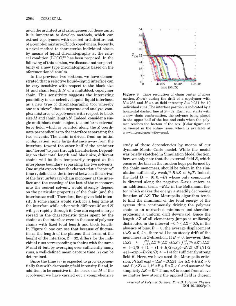
In the previous two sections, we have demon-strated that a selective liquid–liquid interface canbe very sensitive with respect to the block sizeM and chain length N of a multiblock copolymerchain. This sensitivity suggests the interestingpossibility to use selective liquid–liquid interfacesas a new type of chromatographic tool wherebyone can “sieve”, that is, separate and analyze, com-plex mixtures of copolymers with respect to blocksize M and chain length N. Indeed, consider a sin-gle multiblock chain subject to a uniform externalforce field, which is oriented along the Z coordi-nate perpendicular to the interface separating thetwo solvents. The chain is driven from an initialconfiguration, some large distance away from theinterface, toward the other half of the containerand“forced” to pass through the interface. Depend-ing on their total length and block size, differentchains will be then temporarily trapped at theinterphase boundary separating the two solvents.One might expect that the characteristic “capture”time τ , defined as the interval between the arrivalof the first (arbitrary) chain monomer at the inter-face and the crossing of the last of the monomersinto the second solvent, would strongly dependon the particular properties of the chain (and theinterface as well).Therefore, for a given field inten-sity B some chains would stick for a long time atthe interface while other with different M and Nwill get rapidly through it. One can expect a largespread in the characteristic times spent by thechains at the interface even in the case of polymerchains with fixed total length and block length.In Figure 9, one can see that because of fluctua-tions, the length of the plateau that forms at theheight of the interface, Z = 32, differs for the indi-vidual runs corresponding to chains with the sameN and M but, by averaging over sufficiently manyruns, a well-defined mean capture time 〈τ 〉 can bedetermined.

Since the time 〈τ 〉 is expected to grow exponen-tially fast with decreasing field intensity B and, inaddition, to be sensitive to the block size M of thecopolymer, we have carried out a comprehensive

Figure 9. Time resolution of chain center of massmotion, ZCM(t) during the drift of a copolymer withN = 256 and M = 4 at field intensity B = 0.031 for 10individual runs. The interface position is indicated by ahorizontal dashed line at Z = 32. Each run starts witha new chain conformation, the polymer being placedin the upper half of the box and ends when the poly-mer reaches the bottom of the box. [Color figure canbe viewed in the online issue, which is available atwww.interscience.wiley.com].

study of these dependencies by means of ourdynamic Monte Carlo model. While the modelwas briefly sketched in Simulation Model Section,here we only note that the external field B, whichensures the bias in the random hops performed bythe chain monomers, should be taken in the sim-ulation sufficiently weak,40 B�Z � kBT. Indeed,the field B = (0, 0, −B) whose only componentis directed along the negative Z-axis enters asan additional term, −B�z in the Boltzmann fac-tor, which makes the energy a steadily decreasingfunction of �Z. The Metropolis algorithm tendsto find the minimum of the total energy of thesystem thus continuously driving the polymerchain to an unreached minimum and thereforeproducing a uniform drift downward. Since thelength �Z of all elementary jumps is uniformlydistributed in the interval −0.5 ≤ �Z ≤ 0.5, in theabsence of bias, B = 0, the average displacement〈�Z〉 = 0, i.e., there will be no steady drift of themonomers in Z-direction. If B �= 0, however, then〈�Z〉 ≈ ∫ 0.5

−0.5 �Z′P(�Z′)d�Z′/∫ 0.5

−0.5 P(�Z′)d�Z′

= (−1/8 + [1 − (1 + B/2) exp(−B/2)]/B2)/(1/2+[1−exp(−B/2)]/B) ≈ −1/4 for sufficiently strongfield B. Here, we have used the Metropolis crite-rion, P(�Z) exp[−(�E − B�Z)] for �E + B�Z > 0and P(�Z) = 1, if �E + B�Z < 0 and assumed forsimplicity �E ≈ 0.40 Thus,�Z is bound from aboveno matter how strong the applied field is chosen,



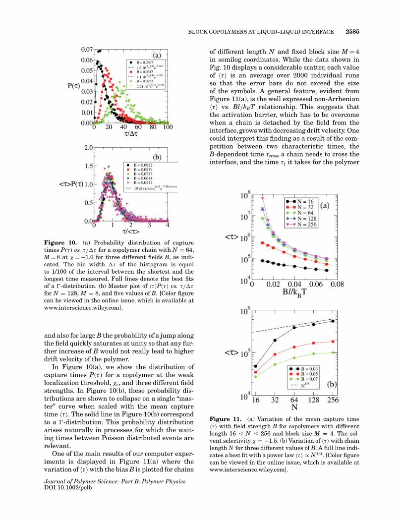
Figure 10. (a) Probability distribution of capturetimes P(τ ) vs. τ/�τ for a copolymer chain with N = 64,M = 8 at χ = −1.0 for three different fields B, as indi-cated. The bin width �τ of the histogram is equalto 1/100 of the interval between the shortest and thelongest time measured. Full lines denote the best fitsof a �-distribution. (b) Master plot of 〈τ 〉P(τ ) vs. τ/�τ

for N = 128, M = 8, and five values of B. [Color figurecan be viewed in the online issue, which is available atwww.interscience.wiley.com].

and also for large B the probability of a jump alongthe field quickly saturates at unity so that any fur-ther increase of B would not really lead to higherdrift velocity of the polymer.

In Figure 10(a), we show the distribution ofcapture times P(τ ) for a copolymer at the weaklocalization threshold, χc, and three different fieldstrengths. In Figure 10(b), these probability dis-tributions are shown to collapse on a single “mas-ter” curve when scaled with the mean capturetime 〈τ 〉. The solid line in Figure 10(b) correspondto a �-distribution. This probability distributionarises naturally in processes for which the wait-ing times between Poisson distributed events arerelevant.

One of the main results of our computer exper-iments is displayed in Figure 11(a) where thevariation of 〈τ 〉 with the bias B is plotted for chains

of different length N and fixed block size M = 4in semilog coordinates. While the data shown inFig. 10 displays a considerable scatter, each valueof 〈τ 〉 is an average over 2000 individual runsso that the error bars do not exceed the sizeof the symbols. A general feature, evident fromFigure 11(a), is the well expressed non-Arrhenian〈τ 〉 vs. Bl/kBT relationship. This suggests thatthe activation barrier, which has to be overcomewhen a chain is detached by the field from theinterface, grows with decreasing drift velocity. Onecould interpret this finding as a result of the com-petition between two characteristic times, theB-dependent time τcross a chain needs to cross theinterface, and the time τ‖ it takes for the polymer

Figure 11. (a) Variation of the mean capture time〈τ 〉 with field strength B for copolymers with differentlength 16 ≤ N ≤ 256 and block size M = 4. The sol-vent selectivity χ = −1.5. (b) Variation of 〈τ 〉 with chainlength N for three different values of B. A full line indi-cates a best fit with a power law 〈τ 〉 ∝ N1/4. [Color figurecan be viewed in the online issue, which is available atwww.interscience.wiley.com].


2586 CORSI ET AL.

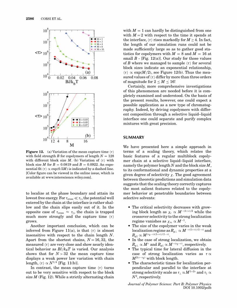
Figure 12. (a) Variation of the mean capture time 〈τ 〉with field strength B for copolymers of length N = 128with different block size M. (b) Variation of 〈τ 〉 withblock size M for B = 0.0819 and B = 0.0922. An expo-nential fit 〈τ 〉 ∝ exp(0.5M) is indicated by a dashed line.[Color figure can be viewed in the online issue, which isavailable at www.interscience.wiley.com].

to localize at the phase boundary and attain itslowest free energy. For τcross � τ‖, the potential wellentered by the chain at the interface is rather shal-low and the chain slips easily out of it. In theopposite case of τcross ≈ τ‖, the chain is trappedmuch more strongly and the capture time 〈τ 〉grows.

Another important conclusion, which can beinferred from Figure 11(a), is that 〈τ 〉 is almostinsensitive with respect to the chain length N.Apart from the shortest chains, N = 16, 32, themeasured 〈τ 〉 are very close and show nearly iden-tical behavior as Bl/kBT is varied. Our analysisshows that for N > 32 the mean capture timedisplays a weak power law variation with chainlength, 〈τ 〉 ∝ N1/4 [Fig. 11(b)].

In contrast, the mean capture time 〈τ 〉 turnsout to be very sensitive with respect to the blocksize M (Fig. 12). While a strictly alternating chain

with M = 1 can hardly be distinguished from onewith M = 2 with respect to the time it spends atthe interface, 〈τ 〉 rises markedly for M ≥ 4. In fact,the length of our simulation runs could not bemade sufficiently large so as to gather good sta-tistics for copolymers with M = 8 and M = 16 atsmall B - [Fig. 12(a)]. Our study for those valuesof B where we managed to sample 〈τ 〉 for severalblock sizes indicate an exponential relationship,〈τ 〉 ∝ exp(M/2), see Figure 12(b). Thus the mea-sured values of 〈τ 〉 differ by more than three ordersof magnitude for 2 ≤ M ≤ 16!

Certainly, more comprehensive investigationsof this phenomenon are needed before it is com-pletely examined and understood. On the basis ofthe present results, however, one could expect apossible application as a new type of chromatog-raphy. Indeed, by driving copolymers with differ-ent composition through a selective liquid–liquidinterface one could separate and purify complexmixtures with great precision.

SUMMARY

We have presented here a simple approach interms of a scaling theory, which relates thebasic features of a regular multiblock copoly-mer chain at a selective liquid–liquid interface,namely the polymer length N and the block size M,to its conformational and dynamic properties at agiven degree of selectivity χ . The good agreementbetween theoretic predictions and simulation datasuggests that the scaling theory correctly capturesthe most salient features related to the copoly-mer behavior at penetrable boundaries betweenselective solvents:

• The critical selectivity decreases with grow-ing block length as χc ∝ M−(1+ν)/2 while thecrossover selectivity to the strong localizationregime vanishes as χ∞ ∝ M−1.

• The size of the copolymer varies in the weaklocalization regime as Rg⊥ ∝ M−ν(1+ν)/(1−ν) andRg‖ ∝ M(ν2−ν)(1+ν)/(1−ν).

• In the case of strong localization, we obtainRg⊥ ∝ Mν and Rg‖ ∝ M−(ν2−ν), respectively.

• The typical time for lateral diffusion in thecase of strong localization varies as τ ∝M2(ν−ν2) with block length.

• The characteristic times for localization per-pendicular and parallel to the interface atstrong selectivity scale as τ⊥ ∝ M1+2ν and τ‖ ∝N2, respectively.



• The averaged Zp-components of the Rousemodes of a copolymer, adsorbed at a liquid–liquid interface, are not orthogonal as in thebulk but rather coupled for small p with thecoupling gradually vanishing as the modenumber p grows.

• For chains driven by an external fieldthrough a selective interface, one finds thatthe mean capture time 〈τ 〉 displays a non-Arrhenian dependence on the field intensityB, and increases almost exponentially withthe block size M.

We think it is worth observing that in the richbehavior listed above, we have not included resultspertaining to random copolymers at penetrableselective interfaces where the range of sequencecorrelations plays a role similar to that of the blocksize M. Moreover, here we have totally ignoredthe possible effects of hydrodynamic interactionson the localization kinetics albeit we have consid-ered the case of Zimm dynamics in our scalingapproach. Clearly, the verification of these predic-tions requires considerable computational effortsand therefore is on the agenda in our futurework.

One should also keep in mind that all resultshave been derived and checked against MonteCarlo simulations within the simplest model ofan interface of zero thickness. It is conceivablethat by allowing for the presence of an intrinsicwidth of the interface as well as for a more realisticdescription involving capillary waves, etc., manyadditional facets of the general picture shouldbecome clearer. While these and other aspectsimply the need of further investigations, i.e., bymeans of single-chain laboratory experiments,we still believe that the present study consti-tutes a first step into a fascinating world, whichmight offer broad perspectives for applicationsand development.

A. Milchev acknowledges the support and hospital-ity of the Max-Planck Institute for Polymer Researchin Mainz during this study. This research has beensupported by the Sonderforschungsbereich (SFB 625).

REFERENCES AND NOTES

1. Clifton, B. J.; Cosgrove, T.; Richardson, R. M.;Zarbakhsh,A.;Webster, J. R. P. Physica B 1998, 248,289.

2. Rother, G.; Findenegg, G. F. Colloid Polym Sci 1998,276, 496.

3. Wang, R.; Schlenoff, J. B. Macromolecules 1998, 31,494.

4. Cornec, M.; Cho, D.; Narsimhan, G. J Colloid Inter-face Sci 1999, 214, 129.

5. (a) Nardin, C.; Meier, W. Chimia 2001, 55, 142;(b) Taubert, A.; Napoli, A.; Meier, W. Current OpinChem Biol 2004, 8, 598; (c) Taubert, A.; Napoli, A.;Meier, W. Eur Phys J E 2001, 4, 45.

6. Sommer, J.-U.; Daoud, M. Europhys Lett 1995, 32,407.

7. Sommer, J.-U.; Peng, G.; Blumen, A. J Phys II(France) 1996, 6, 1061.

8. Garel, T.; Huse, D. A.; Leibler, S.; Orland, H. Euro-phys Lett 1998, 8, 9.

9. Chatellier, X.; Joanny, J.-F. Eur Phys J E 2000,1, 9.

10. Denesyuk, N. A.; Erukhimovich, I. Ya. J Chem Phys2000, 113, 3894.

11. Balasz, A. C.; Semasko, C. P. J Chem Phys 1990, 94,1653.

12. Israels, R.; Jasnow, D.; Balazs, A. C.; Guo, L.;Krausch, G.; Sokolov, J.; Rafailovich, M. J ChemPhys 1995, 102, 8149.

13. Sommer, J.-U.; Peng, G.; Blumen, A. J Chem Phys1996, 105, 8376.

14. Lyatskaya, Y.; Gersappe, D.; Gross, N. A.; Balazs,A. C. J Chem Phys 1996, 100, 1449.

15. Chen, Z. Y. J Chem Phys 1999, 111, 5603; 112, 8665(2000).

16. Sommer, J.-U.; Halperin, A.; Daoud, M. Macromole-cules 1994, 27, 6991.

17. Sommer, J.-U.; Daoud, M. Phys Rev E 1996, 53,905.

18. Corsi, A.; Milchev, A.; Rostiashvili, V. G.; Vilgis, T. A.J Chem Phys 2005, 122, 094907.

19. Eisenriegler, E.; Binder, E.; Kremer, K. J Chem Phys1982, 77, 6296.

20. Bray, A. J.; Moore, M. A. J Phys A 1977, 10, 1927.21. de Gennes, P.-G. Scaling Concepts in Polymer

Physics; Cornell University Press: New York, 1979.22. Leclerc, E.; Daoud, M. Macromolecules 1997, 30,

293.23. Milchev, A.; Paul, W.; Binder, K. J Chem Phys 1993,

99, 4786.24. Milchev, A.; Binder, K. Macromol Theory Simul

1994, 3, 915.25. Milchev,A.; Binder, K. J Chem Phys 2001, 114, 8610.26. Milchev,A.; Milchev,A. Europhys Lett 2001, 56, 695.27. Milchev, A.; Binder, K. Macromolecules 1996, 29,

343.28. (a) Milchev, A.; Binder, K. J Phys (Paris) II 1996, 6,

21; (b) Milchev, A.; Binder, K. Eur Phys J B 1998, 9,477.

29. Pandey, R. B.; Milchev, A.; Binder, K. Macromole-cules 1997, 30, 1194.

30. Milchev, A.; Binder, K. J Chem Phys 1997, 106,1978.

31. Gerroff, I.; Milchev, A.; Paul, W.; Binder, K. J ChemPhys 1993, 98, 6526.


2588 CORSI ET AL.

32. Corsi, A.; Milchev, A.; Rostiashvili, V. G.; Vilgis, T. A.Europhys Lett 2006, 73, 204.

33. Corsi, A.; Milchev, A.; Rostiashvili, V. G.; Vilgis, T. A.Macromolecules 2006, 39, 1234.

34. Grosberg, A. Yu.; Khokhlov, A. R. Statistical Physicsof Macromolecules; AIP Press: New York, 1994.

35. Landau, L. D.; Lifshitz, E. M. In Course of The-oretical Physics, Vol. 6, Fluid Mechanics, 3rd ed.;Butterworth-Heinemann: Oxford, 1987.

36. Verdier, P. H. J Chem Phys 1966, 45, 2118.37. Doi, M.; Edwards, S. F. The Theory of Polymer

Dynamics; Clarendon: Oxford, 1986.38. Gurrieri, S.; Smit, B.; Wells, S.; Johnson, D.; Busta-

mante, C. Nucleic Acids Res 1996, 24, 4759.39. Jiang, W.; Khan, S.; Wang, Y. Macromolecules 2005,

38, 7514.40. Milchev, A.; Wittmer, J.; Landau, D. P. Eur Phys J B

1999, 12, 241.


Multiblock copolymers at selective liquid–liquid interfaces: Toward a block size chromatography

Documents

Transcript of Multiblock copolymers at selective liquid–liquid interfaces: Toward a block size chromatography