Multiaxial Interaction Domains of R.C. sections derived through a parametric subdomains discretization

Deborah Briccola1) Elisa Conti2)

Pier Giorgio Malerba3) and *Manuel Quagliaroli4)

1), 2), 3), 4)Department of Civil & Environmental Engineering, Politecnico di Milano, Milan, Italy

4) manuel.quagliaroli@polimi.it

ABSTRACT

The paper concerns the analysis of reinforced concrete sections of arbitrary shape under axial load and biaxial bending moments. Equilibrium and compatibility equations are recalled and put in an effective and general matrix form. The kernel of the problem is the integration of the terms of the stiffness matrix of the section. The integration is carried out by subdividing the section into parametric subdomains and by using Gauss integration rules. In particular it is shown how, through a double transformation, a more refined discretization of circular and hollow circular sections is possible. Many comparative examples are presented and, in particular, it is also shown how the widely used fiber method is a particular case of the present more general approach. In the end, a rational way to determine the frontier of the interaction domain and characteristic applications are shown. 1. INTRODUCTION The treatment of complex reinforced concrete sections with arbitrary shape, with any arbitrary arrangement of reinforcement and subjected to axial load and biaxial bending has been object of a large number of studies and proposals for suitable mathematical solutions (Furlong 2004). Before the use of computers became widespread, and according to the working stress design criteria adopted in the past, graphical or cumbersome hand computation methods were proposed in order to find the neutral axis position and then the maximum stresses in the concrete and in the reinforcing bars. With the coming of the first mainframes and the introduction of the limit state design, many numerical approaches were presented, mainly with the aim to draft, but only for certain types of sections, interaction charts or load contour charts. Interaction charts gave the variations of the ultimate axial load with respect to uniaxial moment capacity of the section, while load contour charts represented the variation of ultimate moment capacities about the two orthogonal axes of the column, for a specific axial load value. Nowadays, new proposals periodically appear and many software tools, easy to use and effective also in the graphical outputs, are available. Even though the problem is 1), 2) Master Student 3) Professor 4) PhD Candidate

923

considered completely and effectively solved, the conceptual variety and complexities adopted in dealing with the topical difficulties associated to its solution seems, in many cases, involved. This paper concerns the analysis of reinforced concrete sections with arbitrary shape, with any arbitrary arrangement of reinforcement and subjected to axial load and biaxial bending. Apart from the solution here proposed, aim of the work is to remark few theoretical concepts which are at the basis of the problem and, with reference to these concepts, set up a clear and effective numerical approach, which uses well known standard finite elements algorithms. The present approach is based on the following statements: - the state of the section is completely defined by its equilibrium and compatibility

equations. Such equations allow to set a relationship between the deformations (elongation of a reference point and two curvatures) and the forces acting on the section, which may be written in an effective and general matrix form.

- to the design purposes, this matrix equation may be used to solve two types of basic problems: (i) given a deformation state, determine the corresponding stress state (direct problem); (ii) given the stress state, determine the sectional deformation state. The first problem consists in integrating the stress acting on the section. It is, in fact, a simple quadrature problem. For this reason we can call it the direct problem. The second problem involves the search of a deformation state and, to this purpose, it requires the solution of a nonlinear system of equations.

- a crucial step in both these problems requires the integration of the terms of the section stiffness matrix. The presence of non linearities, the section partialization and the aim to deal with sections having arbitrary geometry, the solving equation is put in a suitable algebraic form. In order to deal with the geometrical complexities, the section is subdivided into subdomains, related to parents domains through parametric transformations. Then the integration is carried out through standard Gauss rules. Different Gauss rules may be used and the paper compare several of them, in order to find the most effective ones. In particular it is shown how, through a double transformation, a more refined discretization of circular and hollow circular sections is possible. It is also shown how the widely used fiber method is a simple particular case of the of the present more general approach.

In the end, we would outline that an efficient solution of this problem, already important in itself, is also of great relevance as an intermediate tool for integrating the element stiffness matrix in a general finite element code for the analysis of R.C. framed structures. 2. SECTION KINEMATICS We consider a reinforced concrete section of arbitrary shape, referred to a right handed reference system (0, x, y, z), with the origin placed in the centroid of the concrete domain. The x-axis is normal to the sectional plane and oriented along the element (Fig. 1). The following hypotheses are assumed:

(a) plane sections remain plane after deformations (Navier-Bernoulli hypothesis); (b) perfect bond holds between steel and concrete.

924

Fig. 1 A generic section and its relative reference system According to these hypotheses, in a deformed configuration, the normal displacement at a generic point m (Fig. 1) of the section is given by:

( ) ( ) ( ) ( )0, ,m z yw x y z w x y x z xφ φ= − ⋅ + ⋅ (1)

where 0w is the displacement at the origin and zφ , yφ are, respectively, the rotations

around the z and y-axes. The corresponding normal strain at point m (Fig. 1) is given by:

( ) ( ) ( ) ( )0, , mm z y

dwx y z x y x z x

dxε ε χ χ= = − ⋅ + ⋅ (2)

where 0ε is the normal strain at the origin and zχ , yχ are, respectively, the curvatures

around the z and y axes. The kinematic variables can be grouped by introducing the sectional displacement and deformation vectors ( )xs and ( )xe :

( ) ( ) ( ) ( )0

T

z yx w x x xφ φ = s ( ) ( ) ( ) ( )0

T

z yx x x xε χ χ = e (3)

Through the operator ( )z, ysa :

( ) [ ]z,y 1s y z= −a (4)

Equations (1) and (2) can be put in the matrix form:

( ) ( ) ( ), , z,ym sw x y z x= a s ( ) ( ) ( ), ,z z,ym sx y xε = a e (5)

925

If we consider the section belonging to a beam element, Eq. (5) decomposes the kinematic field into the product of a function ( )z,ysa , depending on the coordinates on

the section, by a function of the coordinate ( )x of the section along the beam axis.

3. SECTION EQUILIBRIUM The sectional equilibrium equations are derived through the Principle of Virtual Displacement, by equating the work done by the static quantities of the actual equilibrated field and the kinematic quantities of a virtual kinematic field:

e iW Wδ δ= (6)

The external and internal works are, respectively:

( ) ( )T

external eW W x xδ δ δ= = ⋅e f (7)

( ) ( )z, y , ,= = ⋅∫internal i m m

A

W W x y z dAδ δ δε σ (8)

By substituting in eq. (6) the expression of mε given by eq. (5) we obtain:

e iW Wδ δ= → ( ) ( ) ( ) ( ) ( )z, y , ,

T TTs m

A

x x x x y z dAδ δ σ δ⋅ = ⋅ ∀∫e f e a e (9)

Doing such an equation be valid for any virtual ( )xδe , the following relationship must

hold:

( ) ( ) ( ) ( )1

z, y , , , ,T

s m m

A A

x x y z dA x y z dAy

z

σ σ = ⋅ = ⋅−

∫ ∫f a (10)

This equation defines the generalized section stresses N , zM , yM which equilibrate

the distribution of the internal uniaxial stresses xσ :

( ) ( )( )( )( )

1

, , with m z

Ay

N x

x x y z dA M xy

M xz

σ = ⋅ =−

∫f

( ) m

A

N x dAσ= ∫ ( )z m

A

M x y dAσ= − ⋅∫ ( )y m

A

M x z dAσ= ⋅∫

(11)

Clearly, the integrals are meant extended to all the materials composing the section. These integrals will be continuous over the concrete domain and discrete sums on the reinforcing bars. In the following the focus will be put mainly on the concrete contribution.

926

4. THE TWO TYPES OF SECTION PROBLEMS The stress ( ), ,m x y zσ in eq. (11) is given as function of the strain ( ), ,m x y zε by an

assumed uniaxial constitutive law. The most known stress-strain relationships are those proposed by (Sargin 1971), (Kent and Park 1971) and (Mander 1988).

( )( )= m m mσ σ ε e ( ) ( ) Ts m

A

x dAσ= ⋅∫f a e (12)

Eq. 12, strictly speaking, is an equilibrium equation. Its use in the design practice can be associated to the following two types of problems: 1. given a strain state (the sectional strains) ( )xe , determine the stress state (the

resultant section forces) ( )xf ;

2. given a stress state ( )xf , determine the sectional strain state ( )xe .

4.1 Type 1 problem The first problem is formulated in a direct way. In fact, given the section deformations ( )xe , the section stresses in any point are directly given by the assumed

constitutive law. The integral of the stresses over the section domain gives the section forces ( )xf . Hence Problem 1 requires a suitable integration strategy only.

4.2 Type 2 problem The second problem can’t have a direct solution. It involves the solution of a system of nonlinear equations and can be stated as: for an assigned vector of section forces ff ,

reckon the section deformations ( )xe giving corresponding internal forces (resisting or

restoring forces) equilibrating ff .

The internal forces are computed through the integration of the stress distribution over the section domain:

( ) ( ) Ts m

A

dAσ= ⋅∫f e a e

The equilibrium condition states that

( )f =f f e

Such a condition is written in homogeneous form as follows:

( ) ( )f= − =g e f f e 0 (13)

927

and solved by Newton-Raphson (NR) method. The main steps of the NR solution are:

1. choice of an initial solution 0e ; 2. linearization of the problem as follows:

( ) ( ) ( ) ( )0 0 0+ ⋅ − =g e g e J e e e 0≃ (14)

where in (14) ( )0J e is the Jacobian matrix evaluated in 0e .

3. search for a new solution, by solving eq. (14). We obtain:

( ) ( )1

1 0 0 0

− = − e e J e g e (15)

4. iteration until convergence.

In a more explicit form, the Jacobian matrix is given by the Equation:

( ) ( ) ( )( ) ( )( )f

∂ ∂ ∂= = − = −∂ ∂ ∂g e

J e f f e f ee e e

(16)

which shows how ( )J e equals the derivatives of the resisting forces with respect to e .

By expanding eq. (16) we have:

( )( ) ( ) ( )( ) ( )( )

( )

T T Ts m s m s m

A A A

T T Tm m m ms s s s s

m m mA A A

Ts m s t

A

dA dA dA

dA dA dA

E dA

σ σ σ

σ ε σ σε ε ε

∂ ∂ ∂ ∂= ⋅ = ⋅ = = ∂ ∂ ∂ ∂

∂ ∂ ∂ ∂∂= = ⋅ = =∂ ∂ ∂ ∂ ∂

= ≅

∫ ∫ ∫

∫ ∫ ∫

∫

f e a e a e a ee e e e

a a a e a ae e

a a K

(17)

where mE is the tangent modulus and tK is the tangent sectional stiffness matrix. The following relationship between Jacobian matrix and tangent stiffness matrix holds:

( ) t= −J e K (18)

The recursive equation of the NR solution results:

( ) ( )1

1i i t i i i i

−+ = + = + ∆ e e K e g e e e (19)

and will be iterated until convergence.

928

5. REMARKS ON THE SECTION STIFFNESS MATRIX

For a linear elastic material, the expanded form of the sectional stiffness matrix tK is:

2

2

1T

t s m s m

A A

y z

E dA E y y yz dA

z yz z

− = = − − −

∫ ∫K a a (20)

The stress-strain relationship is simply Eσ ε= and m

m

Eσε

∂ =∂

, where E is the Young’s

modulus. For the special case of homogeneous sections, Eq. (20) can be rewritten as:

2

2

1T

t s s

A A

y z

E dA E y y yz dA

z yz z

− = ⋅ = ⋅ − − −

∫ ∫K a a (21)

If the system y-z coincides with that of the principal axis of the section, the static moments equal zero and the two flexural components uncouple, so that eq. (21) becomes:

0 0

0 0

0 0t y

z

A

E I

I

= ⋅

K (22)

For a non linear stress strain relationship and non homogeneous sections, the tangent modulus varies with the sampling point m on the section. Further complications arise if the section is non homogeneous (made of concrete and reinforcing bars). In this case there isn’t a reference system more effective than another. The simplest way is to assume the origin in the centroid of the concrete section. As a consequence, the tangent stiffness matrix is always full (Ciampi 1977). In conclusion, two types of problems arise dealing with the section state. The first one is written in an explicit way, the second one requires a numerical strategy for solving systems of nonlinear equations. In both of them, however, several integrals over the section must be evaluated. This aspect is specifically examined in the following section where a particular type of numerical integration strategy is proposed an compared with the know fibers model.

929

6. NUMERICAL INTEGRATION THROUGH PARAMETRIC TRANSFORMATION In order to deal with sections of arbitrary shape, the numerical integration is based on parametric transformations. The section is divided into subdomains and the actual geometry of each subdomain is transformed into a parent geometry by using parametric equations (Malerba 1984). In this way, sampling points refer to the parent domain and the relation with the reference to the actual geometry is ruled by Jacobian of the transformation. We set the integral form as follows:

( )z, yA

I f dA= ∫ (23)

and we consider the section subdivided with these two types of subdomains:

1. trapezoidal subdomains; 2. circle or semicircle or circular ring subdomains.

Obviously, sections composed by both can be dealt with. The application fields of such discretization choices are shown in Fig. 2. In case 1, only one parametric transformation is needed. In case 2 two different transformations are required.

Fig. 2 Integration strategies. The section is divided into subdomains and the integration works sampling in a parent domain by using parametric transformations. The so called fibers approach is a particular case of these integration procedures

930

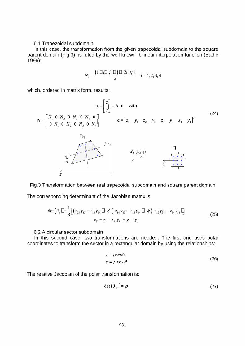
6.1 Trapezoidal subdomain In this case, the transformation from the given trapezoidal subdomain to the square parent domain (Fig.3) is ruled by the well-known bilinear interpolation function (Bathe 1996):

( ) ( )1 11, 2, 3, 4

4i i

iN iζ ζ η η+ ⋅ ⋅ + ⋅

= =

which, ordered in matrix form, results:

z

y

= = ⋅

x N c with

1 2 3 4

31 2 4

00 0 0

0 0 0 0

N N N N

NN N N

=

N [ ]1 1 2 2 3 3 4 4

Tz y z y z y z y=c

(24)

Fig.3 Transformation between real trapezoidal subdomain and square parent domain The corresponding determinant of the Jacobian matrix is:

( ) ( ) ( ) ( )24 13 13 24 14 23 23 14 12 34 34 12

1det

8t z y z y z y z y z y z yζ η = − + ⋅ − + ⋅ − J

ij i jz z z= − ij i jy y y= − (25)

6.2 A circular sector subdomain In this second case, two transformations are needed. The first one uses polar coordinates to transform the sector in a rectangular domain by using the relationships:

cos

z sen

y

ρ ϑρ ϑ

==

(26)

The relative Jacobian of the polar transformation is:

( )det p ρ=J (27)

931

Then, a second step transforms the rectangular subdomain in the usual square parent domain, Fig.4.

Fig. 4 From a quadratic shape to a circular sector: a double transformation

6.3 Integration Rules Through the transformations previously exposed, the generic integral is written with reference to the basic square parent domain. The differential must contain the corresponding Jacobian matrix.

( ) ( ) ( )( )1 1

1 1

z, y , det ,A

I f dA f d dζ η ζ η ζ η+ +

− −

= =∫ ∫ ∫ J (28)

The problem is reduced to algebraic form through sums, which for the trapezoidal subdomain, are:

( ) ( )( )1 1

, det ,n n

j i t j i i ji j

I f w wζ η ζ η= =

⋅ ⋅∑∑ J≃ (29)

And for the circular sector subdomain are:

( ) ( )( ) ( )( )1 1

, det , det ,n n

j i t j i p j i i ji j

I f w wζ η ζ η ϑ ρ= =

⋅ ⋅∑∑ J J≃ (30)

As shown, in this second case two Jacobian matrices are involved. The sampling points location and the relative weights depend on the quadrature rule adopted (Abramowitz 1964). For the sake of comparison, in this work, three type of quadratures rules and different numbers of sampling points n have been considered. • Newton-Cotes rule, that integrates exactly polynomials of grade n-1; • Gauss-Legendre rule, that integrates exactly polynomials of grade 2n-1; • Gauss-Lobatto rule, that integrates exactly polynomials of grade 2n-3. We remember that we are dealing with problems concerning reinforced concrete sections. In this field the most used integration strategy discretizes the section into

932

fibers (“slices”) (CEB 1996), that in fact are subdomains with only one sampling point. Such an integration rule (midpoint integration rule) is the simplest possible and corresponds to what proposed in this work just putting n=1. On the other side, working with R.C. sectional problems, we know that the maximum strains lie on the boundaries, so it seems more effective adopt Gauss-Lobatto rule, which choses sampling points on the frontier of the domain. 7. DETERMINATION OF THE INTERACTION DOMAIN We refer to a generic reinforced concrete section. The interaction domain is a volume which contains all the states ( , , )y zN M M acceptable within certain limits, stated

according to given hypotheses. Its frontier is the locus of the points corresponding to an ultimate sectional state. In such a surface frontier lie the points having as coordinates the triplets of values ( , , )y zN M M which lead a fiber of concrete or a bar of steel to reach

its ultimate strain. In this paragraph we deal with the problem to define such a surface. The problem may be solved both in the space of the deformations e as well as in the space of the forces f . In the first case we have to solve an ordinate succession of problems Type 1 (direct problems). The succession will explore all the deformative states corresponding to an ultimate value of the material strains. In the second case, working in the space of forces, we have to solve problems Type 2, involving repeated solutions of nonlinear equations. This second way is time consuming, but more effective from a practical point of view, because it works defining the 3D domain ( , , )y zN M M as a succession of 2D domains

( , , )y zN M M , reckoned for a constant value N of the axial force.

Fig.5 Generic interaction domain

According to (Bontempi 1992), we work through the following steps, Fig. 5: 1. we chose a value N N N N+ − = ∈ ;

2. in the plane ( , , )y zN M M we have to find the points associated to an ultimate limit

state. To this purpose:

933

− we chose at first an angle 0 : 2ϕ π= .This angle gives a line on which we define a local variable λ so that:

cos

siny

z

M

M

λ ϕλ ϕ

⋅ = ⋅

− with the bisection method we find the value of λ to which correspond the forces producing an ultimate state.

By repeating this search for a discrete set of angles ϕ and axial forces N we the surface frontier is built point wise. The same approach is applicable to the definition of 2D domains ( ( , )N M moment-axial force). 8. VALIDATION AND APPLICATIONS The three reinforced concrete sections shown in Fig. 6 are considered: the first one is a square section reinforced with symmetrical bars, the second is a L shaped section, with distributed bars and the third is an hollow circular section with distributed bars. As already explained the first and the second sections need only one transformation while the third involves two parametric transformations.

(a) Square section (b) L shaped section (c) Hollow circular section

Fig.6 R.C. sections considered for benchmarking

For concrete the stress-strain parabola-rectangle relationship has been used. The steel is assumed having an elastic perfectly plastic behaviour. The strength and ultimate strains parameters are listed in Table 1. Concrete

- fc = -15 Mpa - εc0 = -0.0020 - εcu = -0.0035

Steel - fys= 375 Mpa - εys = -0.0020 - εsu = -0.0100

Table 1 Material characteristics

934

Benchmark organization. Goals of the benchmarks are: • Square RC Section: reckoning of moment-curvature diagrams, with comparisons

among different discretizations and different grids of sampling points. The fiber discretization method is also used. The results are compared in term of moment-curvature diagrams and assigned and approximate stress distributions.

• Square, L-shaped and hollow circular sections: construction of the multiaxial interaction domains.

8.1 Square section. Moment-curvature diagrams and comparisons among different discretizations The square reinforced concrete section of Fig. 6(a), loaded by three different axial forces N = 240-1200-1680 kN, is considered. The section is subdived into 30 subdomains and in each subdomain a Gauss-Lobatto integration scheme with n=3 sampling points is used. The corresponding moment-curvature diaghrams are shown in Fig. 7. The results obtained with this fine discretization agree with those reported in the (C.E.B. 1978) and will be considered in the following as the reference solution.

Fig.7 Moment-curvature diagrams for different axial forces Figure 8 shows the stress distributions for different states of the moment-curvature diagram for the case with N=-240 kN. One can observe how the neutral axis is moving upward and how at the final stage the points on the upper border catch the maximum compressive stress equal to 15 MPa.

Fig.8 Stresses in the concrete at different states (N = -240 kN)

0 2.5 5 7.5 10 12.5 15 17.5 20

χz [1/m.103]

0

20

40

60

80

100

120

140

160

180

200

Mz [

kNm

]

C.E.B. 123 (1978)Reference Solution

N = -240 kN

Sta

te 1

Sta

te 2

Sta

te 3

Sta

te 4

ν = 0.1

0 2.5 5 7.5 10 12.5 15 17.5 20

χz [1/m.103]

0

20

40

60

80

100

120

140

160

180

200

Mz [

kNm

]

C.E.B. 123 (1978)Reference Solution

N = -1200 kNν = 0.5

0 2.5 5 7.5 10 12.5 15 17.5 20

χz [1/m.103]

0

20

40

60

80

100

120

140

160

180

200

Mz [

kNm

]

C.E.B. 123 (1978)Reference Solution

N = -1680 kNν = 0.7

935

Tensile stresses are null below the neutral axis, so we have to deal with the integration of a function that presents discontinuities whose position is state-dependent. On the other hand the interpolation functions associated to the integration rules are continuous. In order to deal with the local discontinuity, three possible ways are explored and compared:

1. by fixing the dimension of the subdomains and improving the integration by changing or the quadrature rule or the number of the sampling points;

2. by fixing the quadrature rule and increasing the number of subdomains in order to increase the possibility to catch the stress discontinuity;

3. a combination of the two previous cases. Figure 9 shows the moment-curvature diagram for the square R.C. section with N=-240kN. One can observe that by increasing the number of the sampling points the accuracy increases. From 5n ≥ , no practical differences are observed in the results. Considering now the case with n=8 sampling points. By working with strategy 2 we use different subdomain discretizations, taking always n=8. The results are reported in Fig. 9(c). No practical differences are observed in the results.

(a) Single subdomain (n=1:4) (b) Single subdomain (n=5:8) (c) Different subdomains (n=8)

Fig.9 Moment-curvature diagrams for different integration orders

Fig. 10 and Fig.11 report the results for different discretizations and different numbers of sampling points. With reference to the ultimate states, these figures compare the stress distribution, associated to the assumed constitutive law, and the stress distributions as interpolated according to the integration rule. Even though the final results globally agree with the equilibrium condition, we observe that the interpolated stresses may have shapes quite different with respect the given one and that, in particular, they have non-null values below the neutral axis. Numerical convergence is reached through the balance of positive and negative areas, which tends to sum zero. As a consequence of these first results, it appears more convenient deal with to a so marked discontinuity, by adopting more small subdomains. In fact, the well known fiber approach works with many fibers and uses a single sampling point.

0 2.5 5 7.5 10 12.5 15 17.5 20

χz [1/m.103]

0

20

40

60

80

100

120

140

160

180

200

Mz

[kN

m]

Reference Solutionn = 1n = 2n = 3n = 4

N = -240 kNν = 0.1

0 2.5 5 7.5 10 12.5 15 17.5 20

χz [1/m.103]

0

20

40

60

80

100

120

140

160

180

200

Mz [

kNm

]

Reference Solutionn = 5n = 6n = 7n = 8

N = -240 kNν = 0.1

0 2.5 5 7.5 10 12.5 15 17.5 20

χz [1/m.103]

0

20

40

60

80

100

120

140

160

180

200

Mz [

kNm

]

Reference Solution1 subdomain - n = 82 subdomain - n = 44 subdomain - n = 28 subdomain - n = 1

N = -240 kNν = 0.1

936

(a) n=1 (e) n=5

(b) n=2 (f) n=6

(c) n=3 (g) n=7

(d) n=4 (h) n=8

Fig.10 First discretization strategy. Real (black) and approximated (blue) distributions of stresses at the final state of moment-curvature curve. Comparison between the exact resultant of stresses (grey area) and approximate distribution (cyan area)

937

(a) 1 subdomain, n=8 (c) 4 subdomains, n=2

(b) 2 subdomains, n=4 (d) 8 subdomains, n=1

Fig.11 Second discretization strategy. Real (black) and approximated (blue) distributions of stresses at the final state of moment-curvature curve. Comparison between the exact resultant of stresses (grey area) and approximate distribution (cyan area)

(a) 30 subdomains, n=1 (c) 30 subdomains, n=3

Fig.12 Huge discretization. Real (black) and approximated (blue) distributions of stresses at the final state of moment-curvature curve. Comparison between the exact resultant of stresses (grey area) and approximate distribution (cyan area)

938

8.2 Multiaxial interaction domains For the three R.C. sections shown in Fig. 6, the multiaxial interaction domain are exposed in the next. A square r.c section The first example concerns the square R.C. section reported in Fig. 6(a). The section has been subdivided in 4 subdomains and the Gauss-Lobatto rule with 5 sampling points has been used in each of them. The geometry of the section and the relative discretization used is reported in Fig. 13(a). Fig. 13(b) shows the 3D interaction domain. The relative bottom, top and lateral view are reported in Fig. 13(c-d-e).

(a) Points and subdomains (b) 3D view

(c) Bottom view (d) Top view (e) Lateral view

Fig.13 Interaction domain for the square section of Fig. 6(a)

939

An L shaped r.c section The second example concerns the L-shaped R.C. section reported in Fig. 6(b). The section has been subdivided in 4 subdomains and the Gauss-Lobatto rule with 7 sampling points has been used in each of them. The geometry of the section and the relative discretization used is reported in Fig. 14(a). Fig. 14(b) shows the 3D interaction domain. The relative bottom, top and lateral view are reported in Fig. 14(c-d-e).

(a) Points and subdomains (b) 3D view

(c) Bottom view (d) Top view (e) Lateral view

Fig.14 Interaction domain for the L shaped section of Fig. 6(b)

A circular cave r.c section The third example concerns the circular cave R.C. section reported in Fig. 6(b). The section has been subdivided in 10 subdomains and the Gauss-Lobatto rule with 5 sampling points has been used in each of them.

940

The geometry of the section and the relative discretization used is reported in Fig. 15(a). Fig. 15(b) shows the 3D interaction domain. The relative bottom, top and lateral view are reported in Fig. 15(c-d-e).

(a) Points and subdomains (b) 3D view

(c) Bottom view (d) Top view (e) Lateral view

Fig.15 Interaction domain for the circular section of Fig. 6(c)

9. CONCLUSIONS The paper concerns the analysis of reinforced concrete sections of arbitrary shape under normal stresses. The proposed approach deals with the most general section state, subjected to axial load and biaxial flexure. The equilibrium and compatibility equations are recalled and put in an effective and general matrix form. Their use in the design practice can be associated to the following two types of basic problems: •••• given the strain state, determine the stress state (direct problem); •••• given the stress state, determine the sectional strain state (non linear search of the

equilibrium state).

941

Through the solution of these problems, the interaction failure surface of the section may be derived in different ways. The presence of non linearities, the section partialization and the aim to deal with sections having arbitrary geometry, require that the solving equation is put in a suitable algebraic form. The kernel of the problem is the integration of the terms of the stiffness matrix of the section. Such a problem is solved by subdividing the section into subdomains and by using parametric transformations to a parent domain geometry, to which Gauss integration rules refer. In particular it is shown how, through a double transformation, a more refined discretization of circular and hollow circular sections is possible. Different types of quadrature rules have been experienced and many sensitivity tests have been carried out and compared. It is also shown how the widely used fiber method is a simple particular case of the present more general approach. On these basis, a way to determine the frontier of the interaction domain (surface failure domain) and characteristic applications are shown. In the end, such an approach has to be considered as an intermediate tool for integrating the element stiffness matrix in a general finite element code for the analysis of R.C. framed structures. REFERENCES Abramowitz, M. and Stegun, I. (1964), “Handbook of mathematical functions with

formulas, graphs, and mathematical tables”, Dover publications. Bathe, K.-J. (1996), “Finite element procedures”, Prentice hall Englewood Cliffs

publications. Bontempi, F. (1992), “Sulla costruzione dei domini di rottura di sezioni in C.A. e C.A.P.

soggette a pressoflessione deviata”, STUDI E RICERCHE, Scuola di Specializzazione in Costruzioni in C.A. - Fratelli Pesenti., 13(1), 261-277.

CEB - FIP Bullettin (1978). “Manual of Buckling and Instability”, Bull Inf 123. CEB Bullettin (1996). “Reinforced concrete elements under cyclic loading state-of-the-

art report”, Bull Inf 230. Ciampi, V. and Di Carlo, A. (1977), “Sulla pressoflessione dei cosiddetti solidi non

reagenti a trazione”, Università degli Studi de l’Aquila, Facoltà di Ingegneria, Istituto di Scienza delle Costruzioni.

Furlong, R.W., Hsu, C.T.T. and Mirza, S.A. (2004), “Analysis and Design of Concrete Columns for Biaxial Bending—Overview”, ACI Structural Journal, 101(3), May-June, 413-422.

Kent, D., Park, R. (1971), “Flexural members with confined concrete”, Journal of the Structural Division, 97(7), ASCE, 1969-1990.

Malerba, P. (1984), “Aspetti numerici dell’analisi di sezioni in C.A. soggette a sforzo normale”, Atti del IV Congresso C.T.E. (Collegio dei Tecnici dell’Industrializzazione Edilizia) Firenze, 165–171.

Mander, J., Priestley, M., Park, R. (1988), “Theoretical stress-strain model for confined concrete”, Journal of structural engineering, 114(8), 1804-1826, American Society of Civil Engineers.

Sargin, M. (1971), “Stress-strain relationships for concrete and the analysis of structural concrete sections”, Solid Mechanics Division, University of Waterloo, 4.

942