Multi-scale sampling and statistical linear estimators to assess land use

status and change

Rocchini, D.1,2�

; Marignani, M.2,3; Bacaro, G.

1,2; Chiarucci, A.

1,2; Ferretti, M.

1,2;

De Dominicis, V.1& Maccherini, S.

1,2

1Dipartimento di Scienze Ambientali ‘G. Sarfatti’, Universita di Siena, via P.A. Mattioli 4, IT 53100 Siena, Italy;2TerraData srl environmetrics, via P.A. Mattioli 4, IT 53100 Siena, Italy;

3Dipartimento di Biologia Vegetale, Universita di Roma ‘‘La Sapienza’’, Piazzale Aldo Moro 5, IT 00185, Rome, Italy;

E-mails: michela.marignani@uniroma1.it; bacaro@terradata.it; chiarucci@unisi.it; ferretti@terradata.it;

dedominicis@unisi.it; maccherini@unisi.it;�Corresponding author; Fax 139 057 723 2896; E-mail rocchini@unisi.it

Abstract

Question: Multi-temporal analysis of remotely sensedimagery has proven to be a powerful tool for assessmentand monitoring of landscape diversity. Here the feasibilityof assessing land-use diversity and land-use change wastested at multiple scales and over time by means ofstatistical linear estimators based on a probabilistic sam-pling design.

Location: The study area (the district of Asciano, Tuscany,Italy) is characterized by erosional forms typical of Plio-cene claystone (i.e. calanchi and biancane) that have beensubject to the phenomenon of biancane reworking overthe past 50 years, mainly owing to the expansion ofintensive agriculture.

Methods: Cells at two different scales (50m�50m and10m�10m) were classified by two operators according toa multilevel legend, using 1954 and 2000 aerial photo-graphs. Inter-operator agreement and accuracy weretested by Cohen’s K coefficient. Total land cover estima-tion for each class was carried out using a multistageestimator, while the variance was estimated by means ofthe Wolter estimator. Field-based information on plantspecies composition was recorded in order to test for arelationship between land use and plant community com-position by ANOVA and indicator species analysis.

Results: Agreement between photointerpreters and accu-racy were significantly higher than those expected bychance, proving that the approach proposed is reproduci-ble, as long as proper quality assurance methods are used.Our data show that, at the two scales considered (50m�50m and 10m�10m), crops have increased against wood-lands and semi-natural areas, the latter showing thehighest and significantly different mean species richness.Meanwhile, an increase in the coverage of trees and shrubswas found within the semi-natural areas, probably as aresult of secondary succession occurring on typical land-scape elements such as biancane.

Conclusions: Inferential statistics made it possible toacquire quantitative information on the abundance ofland cover classes, allowing formal multi-temporal andmulti-scale analysis. Sampling design-based statistical lin-ear estimators were found to be a powerful tool forassessing landscape trends considering both time expendi-ture and other costs. They make it possible to maintain thesame scale of analysis over time series data and to detectboth coarse- and fine-grained changes in spatial patterns.

Keywords: Indicator species analysis; Inferential statistics;Multi-temporal analysis; Remote sensing; Statistical line-ar estimators.

Nomenclature: Pignatti (1982)

Introduction

Owing to concern about the loss of diversity inlandscapes, estimates of land cover status andchanges are crucial environmental information forscience-oriented resource management, for policypurposes, and for a range of human activities (Cih-lar 2000). In this perspective, multi-temporalanalysis of remotely sensed imagery has great po-tential for the assessment and monitoring oflandscape diversity (Stoms & Estes 1993; Butaye etal. 1999; Defries & Townshend 1999; Rocchini et al.2006). However, several problems may arise in in-terpretation of aerial photographs, involving issuessuch as scale, observer bias, spatial resolution andcosts.

Scale is a key issue in ecological monitoringprograms. In practice, thematic classification isstructurally, functionally and operationally depen-dent on the scale at which the interpretation iscarried out (Stohlgren et al. 1997; Saura 2002; see

Applied Vegetation Science 12: 225–236, 2009& 2009 International Association for Vegetation Science

225

also review by Fassnacht et al. 2006). In addition,classification attributes should fit into a given re-ference framework, such as the CORINE system(i.e. a standardized land use legend used by all theEuropean countries; see, Acosta et al. 2005; Bar-tholome & Belward 2005).

Moreover, thematic classification requires greataccuracy when defining the boundaries of the ele-ments being studied. This has led to criticism aboutthe definition of the spatial resolution of input data(Burnett & Blaschke 2003) in manual digitization ofpolygons. ‘‘Manual vegetation mapping is not onlytime/labour intensive, but also subjective’’ (Muller-ova et al. 2005), which limits its reproducibility andintroduces a serious source of bias in the resultingcover estimates. Pioneering studies on automatedpixel-based classification (Carmel & Kadmon 1998)– now principally used with satellite imagery (seealso Townshend et al. 2004) – have not resulted inincreased classification accuracy, mainly because ofthe low spectral resolution of aerial photographs.However, object-based approaches appear promis-ing: in the near future they will likely provide robustalgorithms to produce a reproducible classification,also based on robust topological rules (Devereux etal. 2004).

Nevertheless, classification of aerial photo-graphs over vast study areas can be extremely timeconsuming and costly, particularly considering theneed to extract information at high resolutions.

Despite these problems, the classification ofairborne imagery has the potential to assess land usestatus and change, coupling rigorous quality assur-ance with assessment. In this paper the aim is to: (1)propose a design-based cover estimation from air-borne imagery by investigating advantages anddisadvantages of this approach for assessing bothdiversity of land-cover types and their changes overtime, by means of statistical linear estimators; and(2) analyse the relationships between the classifica-tion of land-cover types and plant species richnessand composition. If proven feasible, this approachcan be of use to investigate comprehensively land-use status and changes over large areas, at multiplespatial scales.

Methods

Study area

The study area is the district of Asciano (cen-troid coordinates: longitude 1113100300E, latitude4311500300N, datum ED50), a 215 km2 area situated

in the landscape of the Crete Senesi, near Siena,Italy. The typical morphology of the landscape,which is dominated by arable land, derives from theerosion of Pliocene claystone resulting in particularforms of erosion (e.g. calanchi, peculiar erodedclaystone hill sides, and biancane, peculiar claystonedomes; see Phillips 1998). This particular culturallandscape has been subject to geomorphologicalsimplification over the past 50 years (Guasparri1993), following the advent of intensive agriculture.The abandonment of traditional activities and theintensification of agriculture are quickly reducingtraditional cultural landscapes, leading to a loss ofhabitats and species diversity in many parts of pe-ninsular Italy (Vos & Stortelder 1992; Phillips 1998).

Sampling design

Sampling units of predefined sizes (50m�50mand 10m�10m, depending on scale) were selectedaccording to a stratified random sampling over the215 square kilometres of the area frame (Fig. 1).First, 977 non-overlapping spatial strata, defined asL spatial units (500m�500m cells, derived from theUTM (ED50) kilometric grid), were distributed overthe study area. Each 500m�500m unit l (l5 1, . . . ,L) was then divided into Nl 50m�50m units, theboundary of the study area being approximated tothese units, thus resulting in 1 � Nl � 100 (Fig. 1).One 50m�50m unit j was then randomly selectedfor each l 500m�500m unit. Subsequently, each ofthese 50m�50m units j (j5 1, . . . , L) was dividedinto 25 10m�10m units. All the 10m�10m unitsbelonging to the selected 50m�50m units j wereconsidered for the aerial survey at that scale. A ran-dom selection of 98 ( � 10%) of the 977 50m�50msampling units was selected for the field survey (seesection entitled Field sampling and analysis of plantspecies data). To this end, one 10m�10m unit(hereafter referred to as a plot) was randomly se-lected for each of the 98 50m�50m sampling unitsidentified.

Aerial survey and field sampling were combinedin order to obtain information on land use and spe-cies richness and diversity at several spatial scales.The integrated analysis was performed as follows:aerial photos from different years were photo-interpreted at two different scales (50m�50m and10m�10m), while field sampling was performed ata scale of 10m�10m with four inner subplots (re-plicates) of 1m�1m. The most recent photos wereinterpreted by two operators to test for agreementbetween photointerpreters and accuracy with re-spect to the field survey. Thus, further analysis was

226 ROCCHINI, D. ET AL.

performed considering both aerial and field surveys(Fig. 2).

Aerial survey

Photograph interpretation and classification schemeAerial panchromatic photographs (grey scale, 8

bit) from 1954 (flight height 6000m) were acquiredand scanned at high resolution (1000 dpi). Orthor-ectification was performed by using 20 groundcontrol points (GCPs) for each photograph and aDigital Terrain Model (DTM, 10m pixel dimen-sion). In order to avoid spatial displacement effects

(Rocchini 2004; Rocchini & Di Rita 2005) the50m�50m sample (and subsequently the 10m�10m sample) was reselected for the 1954 photographs,thus different samples were used to carry out thetotal (i.e. population) estimate. Photointerpretationof the 977 50m�50m units was based on a standar-dized classification scheme, derived from the INFClegend (National Inventory of Forests & CarbonSinks, see Table 1 for description of the classes; forfurther information see De Natale & Gasparini2003). Heterogeneity within the 977 50m�50munits was investigated by photointerpreting the 25inner 10m�10m units (see Fig. 1) using a more de-tailed classification scheme. The classes used for the

Fig. 1. Stratified random procedure applied for remote and field sampling design. We refer to the main text for major ex-planations.

- MULTI-SCALE SAMPLING AND STATISTICAL LINEAR ESTIMATORS - 227

10m�10m classification, defined on the basis ofsurface predominance, were: artificial use, crops,trees and shrubs, pastures, bare soil or sparse vege-tation, natural and artificial lakes.

Quality assurance: classification agreement andaccuracy

The 1954 photographs were photointerpretedby a single operator while the 2000 photographswere photointerpreted by two different operators, inorder to ensure the quality of the approach used bytesting the classification agreement between opera-tors (Fig. 2). Two operators were used only for themost recent photographs (2000) since the aim was tocheck for both classification agreement and accu-racy using the same photograph classified bydifferent photointerpreters. Similar comparisons forthe 1954 photographs would not add significant in-formation regarding the extent to which the propo-sed approach is replicable.

Classification agreement (i.e. the agreement be-tween operators when classifying the same50m�50m or 10m�10m unit) was measured by thetwo most commonly used tests: overall agreement(Equation (1)) and Cohen’s K coefficient, which alsotakes into account the probability of agreement oc-curring by chance (Equation (2)) (for further details

Fig. 2. Collection and analysis of remote and field data. The integration of results is achievable on the strength of the spatialstratification adopted for the sampling design.

Table 1. Classification scheme adopted for the photoin-terpretation of 50m�50m units, derived from the INFClegend (National Inventory of Forests and Forest CarbonSinks, De Natale & Gasparini (2003) for further informa-tion).

50�50 classes Description

Artificial use Urban settlements and isolated housing,commercial and industrial buildings, roads

Crops Arable land, vineyards, olive groves,artificial wood plantations

Woodlands andsemi-natural areas

Natural and semi-natural woodland areas,areas with herbaceous vegetation andshrublands, pastures, grasslands, bare soilareas such as calanchi and biancane

Water Lakes, natural or artificial basins, streams,pipes

228 ROCCHINI, D. ET AL.

see Cohen 1960; for a comprehensive review seeCongalton 1991).

a% ¼P

a� 100

Nð1Þ

where a5 raw agreement; N5 total number ofcases.

K ¼P

a�P

ef

N �P

efð2Þ

where K5Cohen’s coefficient and ef5 expectedfrequency of agreement by chance.

The agreement between the classification basedon the aerial survey and the classification based onthe field survey (i.e. classification accuracy; see sec-tion entitled Field sampling and analysis of plantspecies data) was also based on the overall agree-ment, hereafter named ‘‘overall accuracy’’, and theCohen’s K coefficient.

Statistical inference via linear estimatorsTotal land cover estimation for each class was

carried out using a multistage estimator, while thevariance was estimated by means of the Wolter esti-mator (Wolter 1985; Equations (3) and (4), forestimates at the 50m�50m scale).

T ¼XLl¼1

Xj2Sl

ylj

plj¼XLl¼1

Nlylj� ð3Þ

~V T� �¼ 1

n� 1nXLl¼1

Xj2Sl

y2lj

p2lj� T2

!

¼ 1

n� 1nXLl¼1

N2l ylj� � T2

! ð4Þ

where Nl 5 number of 50m�50m units within the500m�500m unit l; plj ¼ 1

Nl5 inclusion prob-

ability of 50m�50m units j within the 500m�500munit l; j�5 index identifying the 50m�50m unitselected within the 500m�500m unit;

ylj ¼1 if j 2 c

0 if j =2 c

�for a class c; n5#(S)5 977

where S denotes the set of indices that identify the50m�50m units selected within the area.

Based on the calculation of variance, the 95%confidence interval was calculated as:

CI95% ¼ T � 1:96ffiffiffiffiffiffiffiffiffiffiffiffi~V T� �q

ð5Þ

where CI95% 5 95% confidence interval; T 5 totalestimate (as in Equation (3)); ~VðTÞ5 variance (as inEquation (4)).

Total and variance estimates were carried out atboth spatial scales (50m�50m and 10m�10m)considering both survey years (1954 and 2000).

Field sampling and analysis of plant species data

Vascular plant species composition (presence/absence) was recorded within each of the 98 selected10m�10m plots by using four randomly selected1m�1m subplots per 10m�10m plot (total 392subplots; Figs. 1 and 2), located following a restric-ted random procedure. For a complete discussion ofthe statistical properties of this sort of nested sam-pling procedure, which represents one of the mostcost effective approaches for gathering plant spe-cies-composition data, and is based on an objectivesampling design, see Kumar et al. (2006) and Baf-fetta et al. (2007).

The data on species richness per subplot werenormalized by an iterative Box-Cox transformation.Amaximum likelihood approach gave the best valueof g5 0.066 where g is the Box-Cox power (Le-gendre & Legendre 1998).

To investigate the relationship between plantspecies richness and remotely sensed classes, thetransformed data on plant species richness per sub-plot were analysed using a mixed-model nestedANOVA. By this model we tested for the effect of fixedfactors such as land cover classes (level 1 classifica-tion) and random factors such as plots within classeson species richness. Summarizing, the model in-corporated the following factors: (1) land cover class(fixed factor with three levels: artificial, crops,woodlands and semi-natural areas. No subplots fellwithin the ‘‘water’’ class); and (2) 10m�10m plots(random factors nested within classes). WheneverANOVA detected significant differences for the fac-tors, independent comparisons were performed(Underwood 1997) using Tukey’s test.

The contribution of particular species as in-dicators of the dominating physiognomycharacterizing the different land cover classes wasalso assessed by performing an indicator speciesanalysis (Dufrene & Legendre 1997; McCune &Mefford 1999). The method combines informationon the concentration of species, defined as speciesfrequency in the subplots, in two or more groupsdefined a priori, considering the constancy of oc-currence of a species in a particular group. Thiscomparison produces an indicator value (IV) foreach species in each group, ranging from zero (noindication) to 100 (perfect indication). The resultswere tested for statistical significance using a Monte

- MULTI-SCALE SAMPLING AND STATISTICAL LINEAR ESTIMATORS - 229

Carlo technique: the null hypothesis is that the in-dicator value observed is no higher than thatexpected by chance (i.e. that the species has no in-dicator value, since its presence is the same as thatexpected by chance).

Results

Aerial survey

Quality Assurance: classification agreement andaccuracy

Agreement between photointerpreters, based onthe most recent photographs (2000, see the corre-sponding Methods section entitled Qualityassurance: classification agreement and accuracy)was 91.09% and 91.12% at 50m�50m and10m�10m, respectively. Cohen’s K coefficientswere 0.81 and 0.84 at 50m�50m and 10m�10m,respectively, and they were significantly differentfrom zero (Po0.01), indicating that agreement wassignificantly higher than expected by chance. Accu-racy (i.e. the agreement between aerial classificationand field-based classification) at the 10m�10mscale was 74% and 77%, for operators 1 and 2, re-spectively, and therefore lower than the agreementbetween photointerpreters. However, Cohen’s Kcoefficient was significantly different from zero inboth cases (0.52 and 0.60, for operators 1 and 2, re-spectively, with Po0.01 in both cases).

Land-cover estimates: status and changeSince agreement between observers was high,

the results presented here were based on the classifi-cation of only one of them. The 2000 data were inline with the CORINE Land Cover level 2 data(standardized to the classification scheme used) forthe same study area (Table 2).

Multi-temporal analysis at the 50m�50m scaleshowed a substantial increase in crops compared

with woodlands and semi-natural areas (Fig. 3).Artificial areas remained almost unchanged. Nowater bodies were detected on the basis of the 1954photos, while 300 50m�50m units were assigned tothis class in the year 2000.

The proportions of 10m�10m units assigned todifferent categories within each 50m�50m classi-fied unit are reported in Fig. 4. Within the artificialuse class (estimated total: 1.1�103 cells; 1.3% of thetotal), 67% was constituted by urban settlements,isolated houses, industrial buildings and roads (Fig.4), which were interspersed with crops, trees andshrubs and pastures. This composition remained al-most unchanged over the period 1954-2000 andfitted the characteristics of a poorly industrialized orbuilt-up landscape matrix.

Crops were by far the most frequent land-usecategory, amounting to 57.8�103 cells (66.1% of thetotal), with an increase between 1954 and 2000 (Fig.3). Intra-class heterogeneity (Fig. 4) was unchangedbetween 1954 and 2000: crops maintained a high le-vel of homogeneity, with trees and shrubs andpastures occupying less than 10% of the class onboth survey dates. This pattern reveals a homo-geneous landscape matrix dominated by intensiveagriculture and characterized by a scarcity of ecolo-gical corridors such as remnant hedges and woods.

Woodlands and semi-natural areas were thesecond most frequent land use category (Fig. 3),covering 28.2�103 cells, amounting to 32.3% of thetotal. A higher intra-class fragmentation was evi-dent in 1954 (Fig. 4), when trees and shrubs werelimited to 49.7% of ‘‘woodlands and semi-naturalvegetation’’ class, the remaining land being dividedinto pastures, bare soil (42.3%) and crops (6.2%).

Table 2. Comparison between photointerpreted data(scale 50m�50m, 2000) and CORINE land-cover data(standardized to the classification scheme used).

Class % CORINE land cover % 50m�50m units

Artificial use 0.9 1.3 � 0.7Crops 66.5 66.1 � 3.3Woodlands and semi-natural areas

32.5 32.3 � 3.1

Water 0 0.3 � 0.4

0

10 000

20 000

30 000

40 000

50 000

60 000

70 000

Artificial Crops Woodlands andseminatural areas

Water

1954

2000

Est

imat

ednu

mbe

rof

cells

Fig. 3. Temporal variation between 1954 and 2000 in thefrequencies of the land cover classes recorded in the50m�50m cells. Error bars represent the 95% confidenceinterval.

230 ROCCHINI, D. ET AL.

Artificial areas occupied a small area in both surveyyears. A general increase in trees and shrubswas found, indicating encroachment on open areassuch as pastures and bare soil (i.e. typical badlandsformations such as calanchi and biancane; seeFig. 4).

Water bodies (Fig. 4), detected only in 2000,were represented by artificial lakes for irrigation(84% of the water class). Fragments of crops andtrees occasionally occurred within the class.

Species richness and indicator species analysis

A total of 244 species was recorded in the 392(i.e. 98�4) subplots. Species richness per subplotranged from 0 to 25 (mean 6.1). Mean species rich-ness differed among the classes (Table 3):woodlands and semi-natural areas showed thehighest species richness, while the species richness ofartificial use and crops classes was similar (P40.05,Tukey’s test, Table 4).

Species classified as indicator species for thephotointerpreted land cover classes (Table 5)showed a high and statistically significant IndicatorValue (Po0.001). Five indicator species were in-dicated for the artificial use class (Papaver rhoeas,Brachypodium rupestre, Quercus ilex, Plantago lan-ceolata and Bromus erectus) but, because of thesmall sample size (four subplots, compared to 268for crops and 120 for woodlands and semi-naturalareas), this class was excluded from further indicatorspecies analysis (Table 5).

0

10

20

30

40

50

60

70

80

90

100

0

10

20

30

40

50

60

70

80

90

100

0

10

20

30

40

50

60

70

80

90

100

0

10

20

30

40

50

60

70

80

90

100

A C TS P BSV L

A C TS P BSV LA C TS P BSV L

A C TS P BSV L

1954

2000

10x1

0m c

ellc

over

(%

)

10x1

0m c

ellc

over

(%

)

10x1

0m c

ellc

over

(%

)

10x1

0m c

ellc

over

(%

)

1954

2000

1954

2000

1954

2000

CropsArtificial

Woodlands and seminatural areas Water

Fig. 4. Temporal variation between 1954 and 2000 in the frequencies of the land cover classes recorded in the 10m�10mcells, as percentages within the 50�50m cells. Classes used for the 10m�10m classification (x axis) were based on innerdominance: A, artificial; C, crops; TS, trees and shrubs; P, pastures; BSV, bare soil or sparse vegetation; L, natural or arti-ficial lakes.

Table 3. Nested analysis of variance on the number ofspecies per subplot. Summary of the results of a mixedmodel nested ANOVA for species richness. ���Po0.001.

Source of variation df SS MS F

Intercept 1 312.0927 312.0927 279.0213���

Class 2 25.4806 12.7403 13.3113���

Plot (Class) 95 106.26 1.1185 12.1005���

Residual 294 23.1666 0.0788

- MULTI-SCALE SAMPLING AND STATISTICAL LINEAR ESTIMATORS - 231

Discussion

Advantages and disadvantages of design-based coverestimation from airborne imagery

Inferential statistics permitted the acquisition ofquantitative information on the abundance of land-cover classes, allowing multi-temporal and multi-scale analyses on a formal basis. This is of help indetecting processes that are typical of particularspatial scales (e.g. fine-scale shrub and wood en-croachment). Moreover, as noted by Cihlar et al.(2000), who implemented an image subsamplingapproach for land cover classification, when dealingwith the extraction of quantitative landscape in-formation, measures of statistical confidence need tobe obtained. This can be done only if the probability

of each sample is known, as shown in this paper.Such a procedure is much more cost-effective thantraditional land-cover estimates derived from digi-tized maps, which do not guarantee an a prioridefinition of the MMU (Minimum Mapping Unit –see Mullerova et al. 2005).

Unlike a map-based approach, the proposedsampling approach makes it possible to acquire in-formation on landscape composition rather thanlandscape structure. Thus, no information aboutlandscape structure, as obtained by commonly usedpatch-based metrics (e.g. shape metrics, isolationmetrics; for a comprehensive review see Wu et al.2002) can be calculated. Meanwhile, a semi-vario-gram-based theory, considering not only pixelcomposition but also the pixel structuring (Cressie1993), could help to solve this issue in a straightfor-ward manner. It is worth noting that, generallyspeaking, a map would be highly beneficial to illus-trate the spatial extent of changes. The lack of a mapwould probably represent a defect in most spatialapproaches to landscape change (Rocchini & Ri-cotta 2007). However, the improper use of colouredmaps without considering MMU problems wouldlead to quantitatively incorrect results (Rocchini etal. 2006). Moreover, while automatic boundary de-lineation techniques such as segmentation (Burnett& Blaschke 2003) could be used to address the pro-blem of MMU definition, it should be stressed thatpanchromatic imagery would require manual post-classification due to the poor spectral resolution ofthe 8-bit single band (panchromatic) support (Mar-ignani et al. 2008). This would imply an increase intime and effort, thus limiting the powerfulness ofsegmentation for large study areas such as that ana-lysed here. Even if the proposed method does notallow us to build ‘‘maps’’, it represents a robust andabove all reproducible approach. It is worth re-membering that this paper focuses on thequantitative problems that arise when approachinglandscape status and changes at a specific spatialscale, even if the method is restricted to coverage orabundance of classes and changes between them,mainly based on pixel counting.

Nevertheless, pixel counting (like that used inthis paper) could be misleading because it does nottake into account the probability of obtaining mixedpixels (i.e. pixels with a high inner heterogeneity; seealso Congalton 1991; Fisher 1997; Cracknell 1998;Foody 2000). Conversely, because of the depen-dence of information contained in landscape metrics(in this case, area covered by classes) on the spatialresolution associated with their calculation (the wellknownMMU Problem: see, for example, Openshaw

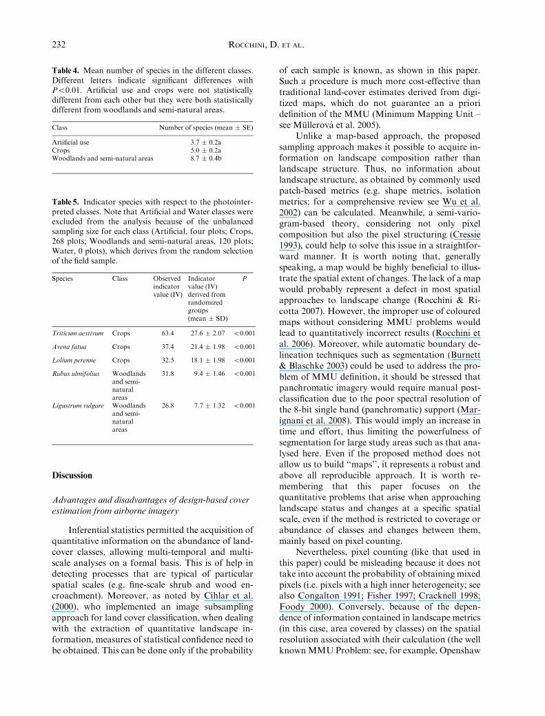
Table 4. Mean number of species in the different classes.Different letters indicate significant differences withPo0.01. Artificial use and crops were not statisticallydifferent from each other but they were both statisticallydifferent from woodlands and semi-natural areas.

Class Number of species (mean � SE)

Artificial use 3.7 � 0.2aCrops 5.0 � 0.2aWoodlands and semi-natural areas 8.7 � 0.4b

Table 5. Indicator species with respect to the photointer-preted classes. Note that Artificial and Water classes wereexcluded from the analysis because of the unbalancedsampling size for each class (Artificial, four plots; Crops,268 plots; Woodlands and semi-natural areas, 120 plots;Water, 0 plots), which derives from the random selectionof the field sample.

Species Class Observedindicatorvalue (IV)

Indicatorvalue (IV)derived fromrandomizedgroups(mean � SD)

P

Triticum aestivum Crops 63.4 27.6 � 2.07 o0.001

Avena fatua Crops 37.4 21.4 � 1.98 o0.001

Lolium perenne Crops 32.5 18.1 � 1.98 o0.001

Rubus ulmifolius Woodlandsand semi-naturalareas

31.8 9.4 � 1.46 o0.001

Ligustrum vulgare Woodlandsand semi-naturalareas

26.8 7.7 � 1.32 o0.001

232 ROCCHINI, D. ET AL.

1984; Jelinski & Wu 1996), cells with a predefineddimension at different resolutions guarantee arobust definition of the MMU during classificationprocedures. This permits (1) the association of thelandscape pattern to the ecological processes thatgenerate them (acting at a given scale) in a quanti-tative way, and (2) the translation of informationfrom one scale to another (Wu & Qi 2000; Wu et al.2002). It is worth recalling that results of analysesfor the same area can vary because of the spatial re-solution (Johnson & Howarth 1987) and that somepatterns or processes can only be recognized at spe-cific resolutions (Jelinski & Wu 1996). A pheno-menon could remain undetected because of im-proper matching with the scale of analysis(Stohlgren et al. 1997).

As stressed by Cihlar (2000), reproducibility is acrucial criterion in land cover classification (i.e. thesame result should be obtained by various analystsgiven the same input data). In this paper we focusedon the scale properties of land cover classification(i.e. maintenance of the same MMU) rather than onissues of thematic attribution. However, it should benoted that classification is in its very nature a humanconstruct (Palmer et al. 2002), with the analystplaying a key role in the entire classification process.At present, even considering thematic attribution,the proposed methodology represents a re-producible approach on the strength of the highclassification agreement achieved between differentphotointerpreters.

Contribution of land use and species information toexplaining ongoing ecological dynamics

Remote sensing has long been used to relatefield data directly to the spectral properties of map-ped habitats and vegetation communities(Nagendra 2001; Palmer et al. 2002; Acosta et al.2005; Thessler et al. 2005; Fassnacht et al. 2006;Marignani et al. 2007; Rocchini et al. 2007). In ourstudy the remote approach, performed at multiplescales of analysis, allowed us to separate vegetationphysiognomy. Moreover, the results obtained fromremotely sensed data were closely related to the in-formation gathered for plant species richness andcomposition. In the crops class, the homogeneouslandscape matrix dominated by intensive agriculturewas confirmed by the low values of species richness(comparable to the species richness of the artificialareas), reinforced by the high values of the indicatorspecies Avena fatua and Lolium perenne (see Table 5),which are typical cereal weeds; this means that a fewvery abundant species characterize these environ-

ments. Species indications confirm that the crops classis principally occupied by agriculture and lacks areasof natural vegetation, with a scarcity of natural ele-ments, such as hedgerows and remnant woodlands.

In contrast, the woodlands and semi-naturalareas class was characterized by a higher speciesrichness and by indicator species that suggested thepresence of transitional woodland shrubs ratherthan real forests. Rubus ulmifolius and Ligustrumvulgare are typical shrubland species that character-ize secondary succession as well as marginalvegetation found in impluvia and edges (De Do-minicis 1980; Chiarucci et al. 1995; Maccherini et al.1998, 2000).

The trend observed from remote sensing andconfirmed by field data is coherent with the Eur-opean situation in which the recent abandonment oftraditional management techniques in favour of theintensification of agriculture has drastically reducednatural and semi-natural areas, producing a generalhomogenization of the landscape (Vos & Stortelder1992; Bakker & Berendse 1999; Stoate et al. 2001;van Eetvelde & Antrop 2004).

This tendency, together with the loss of the tra-ditional state of dynamic equilibrium betweenanthropogenic management and natural dynamics,is allowing woody species to progressively encroachon open habitats and directly influences biodiversityat species, community and landscape scales (Maz-zoleni et al. 2004; Tatoni et al. 2004; Rocchini et al.2006). An increase in surfaces used for crop cultiva-tion in relation to those covered by woodlands andsemi-natural areas in the study area was clearly visi-ble from 1954 to 2000. Meanwhile, an increase in thecoverage of trees and shrubs was noticeable withinthe woodlands and semi-natural areas, probably asa result of secondary succession occurring on typicallandscape elements such as biancane. A decrease inpastures and bare soil or sparse vegetation was ob-served in the ‘‘woodlands and semi-natural vegeta-tion’’ class, accompanied by an increase in trees andshrubs. This suggests a secondary succession patternin these areas, as also demonstrated by the presenceof R. ulmifolius and L. vulgare as indicator species ofwoodlands and semi-natural areas.

The general trend from 1954 to 2000 showed anecological dynamic that is leading to a more coarselygrained pattern even at a detailed scale, by losing theremnants of ecological corridors (i.e. hedges andmarginal woods) and typical geomorphologicallandforms (such as calanchi and biancane) of 1954,with a homogenization of the landscape matrix to-wards an extensive agriculture framework. Further-more, the abandonment of pastures and reduced

- MULTI-SCALE SAMPLING AND STATISTICAL LINEAR ESTIMATORS - 233

grazing pressure on biancane fields are the mainfactors behind the priorities on conservation of thesegeomorphological landforms. In fact, when dis-turbance induced by humans decreases and even-tually stops, shrubs promptly encroach on aban-doned lands, leading to an overall homogenizationof the landscape (Noy-Meir et al. 1989).

Thus, both the increase in the crop area and theencroachment on semi-natural formations, such asgrasslands, by dense shrubs and woods are expectedto convert a complex landscape matrix into a highlyhomogeneous system, adversely affecting the overalldiversity of the areas examined (Baessler & Klotz2006).

Conclusions

The feasibility of land-use diversity assessmentat multiple scales by means of statistical linear esti-mators was tested in this paper. In particular, wepresented an integrative approach combining re-motely sensed and field-based data. The proposedsampling design was useful for studying ecologicaldynamics at several spatial scales, in that it allowedanalyses starting from the community level (e.g. AN-

OVA and indicator species analysis) up to thelandscape level. Moreover, the comparison betweenobservers proved that the proposed approach is re-producible, as long as proper quality assurancemethods are used.

Multiscale sampling and statistical linear esti-mators seem to be essential in different respects:first, they make it possible to extract quantitativedata for the attribute of interest; second, they im-prove cost efficiency; third, they allow one tomaintain the same scale of analysis over time seriesdata; and fourth, they permit the detection of bothcoarse- and fine-grained spatial pattern changes.The proposed approach therefore seems to be bothfeasible and reliable for land-cover estimation overlarge areas.

Acknowledgements. We thank the Coordinating Editor

Kerry Woods and two anonymous referees for improve-

ments and insights made on a previous version of the

paper. Federica Baffetta had a crucial role in the statistical

analysis of remotely sensed data. Ilaria Cirillo andArianna

Vannini orthorectified and photointerpreted some of the

aerial photos while Manuela Boddi and Bernardo Pellizzi

worked on the field sampling task. This research was fun-

ded by the Fondazione Monte dei Paschi di Siena as part

of a research project promoted by the University of Siena.

References

Acosta, A., Carranza, M.L. & Izzi, C.F. 2005. Combining

land cover mapping of coastal dunes with vegetation.

Applied Vegetation Science 8: 133–138.

Baessler, C. & Klotz, S. 2006. Effects of changes in

agricultural land-use on landscape structure and

arable weed vegetation over the last 50 years.

Agriculture Ecosystems & Environment 115: 43–50.

Baffetta, F., Bacaro, G., Fattorini, L., Rocchini, D. &

Chiarucci, A. 2007. Multi-stage cluster sampling for

estimating average species richness at different spatial

grains. Community Ecology 8: 119–127.

Bakker, J.P. & Berendse, F. 1999. Constraints in the

restoration of ecological diversity in grassland and

heathland communities. Trends in Ecology &

Evolution 14: 63–68.

Bartholome, E. & Belward, A.S. 2005. GLC2000: a new

approach to global land cover mapping from Earth

observation data. International Journal of Remote

Sensing 26: 1959–1977.

Burnett, C. & Blaschke, T. 2003. A multi-scale

segmentation/object relationship modelling

methodology for landscape analysis. Ecological

Modelling 168: 233–249.

Butaye, J., Honnay, O. & Hermy, M. 1999. Vegetation

mapping as an aid in detecting temporal vegetation

changes in the Demer valley (Belgium). Belgian

Journal of Botany 132: 119–140.

Carmel, Y. & Kadmon, R. 1998. Computerized classi-

fication of Mediterranean vegetation using panchro-

matic aerial photographs. Journal of Vegetation

Science 9: 445–454.

Chiarucci, A., De Dominicis, V., Ristori, J. & Calzolari,

C. 1995. Biancana badland vegetation in relation to

morphology and soil in Orcia Valley, central Italy.

Phytocoenologia 25: 69–87.

Cihlar, J. 2000. Land cover mapping of large areas from

satellites: status and research priorities. International

Journal of Remote Sensing 21: 1093–1114.

Cihlar, J., Latifovic, R., Chen, J., Beaubien, J. & Li, Z.

2000. Selecting representative high resolution sample

images for land cover studies. Part 1: methodology.

Remote Sensing of Environment 71: 26–42.

Cohen, J. 1960. A coefficient of agreement for nominal

scales. Educational and Psychological Measurement 20:

37–46.

Congalton, R.G. 1991. A review of assessing the accuracy

of classifications of remotely sensed data. Remote

Sensing of Environment 37: 35–46.

Cracknell, A.P. 1998. Synergy in remote sensing: what’s in

a pixel? International Journal of Remote Sensing 19:

2025–2047.

Cressie, N.A.C. 1993. Statistics for spatial data. John

Wiley & Sons, New York.

De Dominicis, V. 1980. L’evoluzione della vegetazione sui

terreni argillosi pliocenici della Toscana. Giornale

Botanico Italiano 114: 104–105.

234 ROCCHINI, D. ET AL.

Defries, R.S. & Townshend, J.R.G. 1999. Global land

cover characterization from satellite data: from

research to operational implementation? Global

Ecology and Biogeography 8: 367–379.

De Natale, F. & Gasparini, P. 2003. Manuale di

fotointerpretazione per la classificazione delle unita di

campionamento di prima fase. Inventario Nazionale

delle Foreste e dei Serbatoi Forestali di Carbonio.

MiPAF – Direzione Generale per le Risorse Forestali

Montane e Idriche, Corpo Forestale dello Stato,

CRA-ISAFA, Trento, IT.

Devereux, B.J., Amable, G.S. & Posada, C.C. 2004. An

efficient image segmentation algorithm for landscape

analysis. International Journal of Applied Earth

Observation and Geoinformation 6: 47–61.

Dufrene, M. & Legendre, P. 1997. Species assemblages

and indicator species: the need for a flexible

asymmetrical approach. Ecological Monographs 67:

345–366.

Fassnacht, K.S., Cohen, W.B. & Spies, T.A. 2006. Key

issues in making and using satellite-based maps in

ecology: a primer. Forest Ecology and Management

222: 167–181.

Fisher, P. 1997. The pixel: a snare and a delusion.

International Journal of Remote Sensing 18: 679–685.

Foody, G.M. 2000. Estimation of sub-pixel land cover

composition in the presence of untrained classes.

Computational Geoscience 26: 469–478.

Guasparri, G. 1993. I lineamenti geomorfologici dei

terreni argillosi pliocenici. In: Giusti, F. (ed.) La

storia naturale della Toscana Meridionale. pp. 89–106.

Pizzi, Milano, IT.

Jelinski, D.E. & Wu, J. 1996. The modifiable areal unit

problem and implications for landscape ecology.

Landscape Ecology 11: 129–140.

Johnson, D.D. & Howarth, P.J. 1987. The effects of

spatial resolution on land cover/land use theme

extraction from airborne digital data. Canadian

Journal of Remote Sensing 13: 68–75.

Kumar, S., Stohlgren, T.J. & Chong, G.W. 2006. Spatial

heterogeneity influences native and nonnative plant

species richness. Ecology 87: 3186–3199.

Legendre, P. & Legendre, L. 1998. Numerical ecology.

2nd English edn. Elsevier Science BV, Amsterdam,

NL.

Maccherini, S., Chiarucci, A. & De Dominicis, V. 1998.

Relationships between vegetation and morphology in

the Radicofani calanchi (southern Tuscany). Atti del

Museo di Storia Naturale della Maremma 17: 91–108.

Maccherini, S., Chiarucci, A. & De Dominicis, V. 2000.

Structure and species diversity of Bromus erectus

grasslands of biancana badlands. Belgian Journal of

Botany 133: 3–14.

Marignani, M., Del Vico, E. & Maccherini, S. 2007.

Spatial scale and sampling size affect the concordance

between remotely sensed information and plant

community discrimination in restoration monitoring.

Biodiversity and Conservation 16: 3851–3861.

Marignani, M., Rocchini, D., Torri, D., Chiarucci, A. &

Maccherini, S. 2008. Planning restoration in a cultural

landscape in Italy using an object-based approach and

historical analysis. Landscape and Urban Planning 84:

28–37.

Mazzoleni, S., Di Pasquale, G., Mulligan, M., Di

Martino, P. & Rego, F. 2004. Recent dynamics of

mediterranean vegetation and landscape. John Wiley

and Sons, Chichester, UK.

McCune, B. & Mefford, M.J. 1999. Multivariate analysis

of ecological data version 4.25. MjM Software,

Gleneden Beach, OR, USA.

Mullerova, J., Pysek, P., Jarosık, V. & Pergi, J. 2005.

Aerial photographs as a tool for assessing the regional

dynamics of the invasive plant species Heracleum

mantegazzianum. Journal of Applied Ecology 42:

1042–1053.

Nagendra, H. 2001. Using remote sensing to assess

biodiversity. International Journal of Remote Sensing

22: 2377–2400.

Noy-Meir, I., Gutman, M. & Kaplan, Y. 1989. Responses

of Mediterranean grassland plants to grazing and

protection. Journal of Ecology 77: 290–310.

Openshaw, S. 1984. The modifiable areal unit problem:

concepts and techniques in modern geography. Geo

Books, Norwich, UK.

Palmer, M.W., Earls, P., Hoagland, B.W., White, P.S. &

Wohlgemuth, T. 2002. Quantitative tools for

perfecting species lists. Environmetrics 13: 121–137.

Phillips, C.P. 1998. The badlands of Italy: a vanishing

landscape? Applied Geography 18: 243–257.

Pignatti, S. 1982. Flora d’Italia. Edagricole, Bologna, IT.

Rocchini, D. 2004. Misleading information from direct

interpretation of geometrically incorrect aerial

photographs. Photogrammetric Record 19: 138–148.

Rocchini, D. & Di Rita, A. 2005. Relief effects on aerial

photos geometric correction. Applied Geography 25:

159–168.

Rocchini, D. & Ricotta, C. 2007. Are landscapes as crisp

as we may think? Ecological Modelling 204: 535–539.

Rocchini, D., Perry, G.L.W., Salerno, M., Maccherini, S.

& Chiarucci, A. 2006. Landscape change and the

dynamics of open formations in a natural reserve.

Landscape Urban Planning 77: 167–177.

Rocchini, D., Ricotta, C. & Chiarucci, A. 2007. Using

remote sensing to assess plant species richness: the role

of multispectral systems. Applied Vegetation Science

10: 325–332.

Saura, S. 2002. Effects of minimum mapping unit on land

cover data spatial configuration and composition.

International Journal of Remote Sensing 23: 4853–

4880.

Stoate, C., Boatman, N.D., Borralho, R.J., Rio Carvalho,

C., de Snoo, G.R. & Eden, P. 2001. Ecological impacts

of arable intensification in Europe. Journal of

Environmental Management 63: 337–365.

Stohlgren, T.J., Coughenour, M.B., Chong, G.W.,

Binkley, D., Kalkhan, M.A., Schell, L.D., Buckley,

- MULTI-SCALE SAMPLING AND STATISTICAL LINEAR ESTIMATORS - 235

D.J. & Berry, J.K. 1997. Landscape analysis of plant

diversity. Landscape Ecology 12: 155–170.

Stoms, D.M. & Estes, J.E. 1993. A remote sensing

research agenda for mapping and monitoring

biodiversity. International Journal of Remote Sensing

14: 1839–1860.

Tatoni, T., Medail, F., Roche, P. & Barbero,M. 2004. The

impact of changes in land use on ecological patterns in

Provence Mediterranean France. In: Mazzoleni, S., Di

Pasquale, G., Mulligan, M., Di Martino, P. & Rego,

F. (eds.) Recent dynamics of mediterranean vegetation

and landscape. pp. 107–120. John Wiley and Sons,

Chichester, UK.

Thessler, S., Ruokolainen, K., Tuomisto, H. & Tomppo,

E. 2005. Mapping gradual landscape-scale floristic

changes in Amazonian primary rain forests by

combining ordination and remote sensing. Global

Ecology and Biogeography 14: 315–325.

Townshend, J.R.G., Huang, C., Kalluri, S.N.V., Defries,

R.S., Liang, S. & Yang, K. 2004. Beware of per-pixel

characterization of land cover. International Journal of

Remote Sensing 21: 839–843.

Underwood, A.J. 1997. Experiments in ecology: their logi-

cal design and interpretation using analysis of variance.

Cambridge University Press, Cambridge, UK.

van Eetvelde, V. & Antrop, M. 2004. Analyzing structural

and functional changes of traditional landscape – two

examples from Southern France. Landscape Urban

Planning 67: 79–95.

Vos, W. & Stortelder, A. 1992. Vanishing Tuscan

landscape. Pudoc, Wageningen, NL.

Wolter, K.M. 1985. Introduction to variance estimation.

Springer, New York, NY, USA.

Wu, J. & Qi, Y. 2000. Dealing with scale in landscape

analysis: an overview. Geographical Information

Science 6: 1–5.

Wu, J., Shen, W., Sun, W. & Tueller, P.T. 2002. Empirical

patterns of the effects of changing scale on landscape

metrics. Landscape Ecology 17: 761–782.

Received 20 December 2007;

Accepted 20 October 2008.

Co-ordinating Editor: K.D. Woods

236 ROCCHINI, D. ET AL.