New difference-cum-ratio and exponential type estimators in median ranked set sampling

New difference-cum-ratio and exponential typeestimators in median ranked set sampling

Nursel Koyuncu∗†

Abstract

This paper suggests difference-cum-ratio and exponential type estima-tors of population mean using first or third quartiles and mean of aux-iliary variable under median ranked set sampling scheme and we haveextended our study in double sampling scheme when the population pa-rameters are unknown. The bias and mean square error of estimatorsare derived by theoretically both of sampling designs. Empirical stud-ies have been done to demonstrate the efficiency of proposed estimatorsover the existing estimators. We have found that difference-cum-ratioestimator is always more efficient than regression estimator and bothof the estimators are considerable efficient than existing estimators.

Keywords: Median ranked set sampling, Exponential estimator, Ratio estima-tor, Efficiency.

2000 AMS Classification: 62D05

1. Introduction

The ranked set sampling (RSS) is conducted by selecting n random samplesfrom the population of size n units each, and ranking each unit within each setwith respect to variable of interest. Then an actual measurement is taken of theunit with the smallest rank from the first sample. From the second sample anactual measurement is taken from the second smallest rank, and the procedureis continued until the unit with the largest rank is chosen for actual measure-ment from the n-th sample. Median ranked set sampling (MRSS) as proposed byMuttlak [10] can be formed by selecting n random samples of size n units fromthe population and rank the units within each sample with respect to variableof interest. Many authors developed and modified this sampling scheme such asAl-Saleh and Al-Omari[2], Jemain and Al-Omari[4] and Jemain et al.[5], Ozturkand Jafari Jozani[11] etc. Recently Al-Omari[1] has introduced modified ratio es-timators in median ranked set sampling. In sampling theory some authors suchas Singh and Solanki[12, 13], Singh et al.[14, 15] and Solanki et al.[16] etc. pro-posed estimators for population parameters using auxiliary information. Bahl andTuteja [3], Yadav et al. [18], Koyuncu and Kadilar[7], Koyuncu[8], Koyuncu etal.[9] studied the exponential estimators to get more efficient estimators than ratioand regression estimators. In this paper following Koyuncu [8], we have suggested

∗Hacettepe University,Department of Statistics, Beytepe, 06800, Ankara, Turkey Email:

[email protected]†Corresponding Author.

2

two new estimators of population mean under Al-Omari[1] median ranked set sam-pling scheme, extended our results to double sampling and we have found that thesuggested estimators are considerable efficient than classical ratio estimator andAl-Omari[1] estimator.

Simple Random Sampling Design

Let (X1, Y1), (X2, Y2), . . . , (Xn, Yn) be a bivariate random sample with pdf f(x, y),means µx, µy, variances σ2

x, σ2y and correlation coefficient ρxy. Assume that the

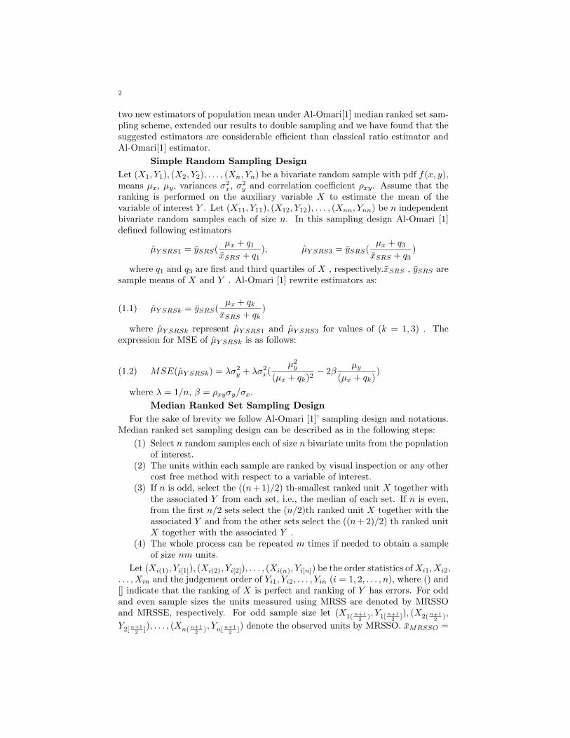
ranking is performed on the auxiliary variable X to estimate the mean of thevariable of interest Y . Let (X11, Y11), (X12, Y12), . . . , (Xnn, Ynn) be n independentbivariate random samples each of size n. In this sampling design Al-Omari [1]defined following estimators

µY SRS1 = ySRS(µx + q1xSRS + q1

), µY SRS3 = ySRS(µx + q3xSRS + q3

)

where q1 and q3 are first and third quartiles of X , respectively.xSRS , ySRS aresample means of X and Y . Al-Omari [1] rewrite estimators as:

(1.1) µY SRSk = ySRS(µx + qkxSRS + qk

)

where µY SRSk represent µY SRS1 and µY SRS3 for values of (k = 1, 3) . Theexpression for MSE of µY SRSk is as follows:

(1.2) MSE(µY SRSk) = λσ2y + λσ2

x(µ2y

(µx + qk)2− 2β

µy(µx + qk)

)

where λ = 1/n, β = ρxyσy/σx.

Median Ranked Set Sampling Design

For the sake of brevity we follow Al-Omari [1]’ sampling design and notations.Median ranked set sampling design can be described as in the following steps:

(1) Select n random samples each of size n bivariate units from the populationof interest.

(2) The units within each sample are ranked by visual inspection or any othercost free method with respect to a variable of interest.

(3) If n is odd, select the ((n+ 1)/2) th-smallest ranked unit X together withthe associated Y from each set, i.e., the median of each set. If n is even,from the first n/2 sets select the (n/2)th ranked unit X together with theassociated Y and from the other sets select the ((n+ 2)/2) th ranked unitX together with the associated Y .

(4) The whole process can be repeated m times if needed to obtain a sampleof size nm units.

Let (Xi(1), Yi[1]), (Xi(2), Yi[2]), . . . , (Xi(n), Yi[n]) be the order statistics ofXi1, Xi2,. . . , Xin and the judgement order of Yi1, Yi2, . . . , Yin (i = 1, 2, . . . , n), where () and[] indicate that the ranking of X is perfect and ranking of Y has errors. For oddand even sample sizes the units measured using MRSS are denoted by MRSSOand MRSSE, respectively. For odd sample size let (X1(n+1

2 ), Y1[n+12 ]), (X2(n+1

2 ),

Y2[n+12 ]), . . . , (Xn(n+1

2 ), Yn[n+12 ]) denote the observed units by MRSSO. xMRSSO =

3

1n

n∑i=1

Xi(n+12 ) and yMRSSO = 1

n

n∑i=1

Xi[n+12 ] be the sample mean of X and Y re-

spectively.For even sample size let (X1(n2 ), Y1[n2 ]), (X2(n2 ), Y2[n2 ]), . . . , (Xn

2 (n2 ), Yn2 [n2 ]),

(Xn+22 (n+2

2 ), Yn+22 [n+2

2 ]), (Xn+42 (n+2

2 ), Yn+42 [n+2

2 ]), . . . , (Xn(n2 ), Yn[n2 ]) denote the ob-

served units by MRSSE. xMRSSE = 1n (

n2∑i=1

Xi(n2 ) +n∑

i=n+22

Xi(n+22 )) and yMRSSE =

1n (

n2∑i=1

Yi[n2 ] +n∑

i=n+22

Yi[n+22 ]) be the sample mean of X and Y respectively.

To obtain the bias and the mean square error (MSE), let us define

ε0(j) =yMRSS(j) − µy

µy, ε1(j) =

xMRSS(j) − µxµx

, ε2(j) =syx(j) − σyx(j)

σyx(j),

ε3(j) =s2x(j) − σ

2x(j)

σ2x(j)

where j = (E,O) denote the sample size even or odd. If sample size n is oddwe can write

E(ε20(O)) =1

nµ2y

σ2y(n+1

2 ), E(ε21(O)) =

1

nµ2x

σ2x(n+1

2 ),

E(ε0(O)ε1(O)) =1

nµxµyσxy(n+1

2 )

If sample size n is even we can write

E(ε20(E)) =1

2nµ2y

(σ2y[n2 ] + σ2

y[n+22 ]

), E(ε21(E)) =1

2nµ2x

(σ2x(n2 ) + σ2

x(n+22 )

),

E(ε0(E)ε1(E)) =1

2nµxµy(σyx[n2 ] + σyx[n+2

2 ])

(i) Al-Omari(2012) estimator The estimator of population mean proposedby Al-Omari[1] as

µYMRRS1 = yMRSS(µx + q1

xMRSS + q1), µYMRRS3 = yMRSS(

µx + q3xMRSS + q3

)

For odd and even sample sizes the estimator can be rewritten as

(1.3) µYMRSSk = yMRSS(j)(µx + qk

xMRSS(j) + qk)

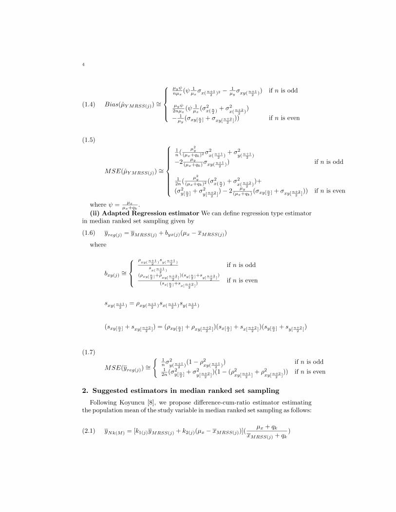
To the first degree of approximation the Bias and MSE of µYMRRSk are respec-tively given by

4

(1.4) Bias(µYMRSS(j)) ∼=

µyψnµx

(ψ 1µxσx(n+1

2 )2 −1µyσxy(n+1

2 )) if n is odd

µyψ2nµx

(ψ 1µx

(σ2x(n2 ) + σ2

x(n+22 )

)

− 1µy

(σxy[n2 ] + σxy[n+22 ])) if n is even

(1.5)

MSE(µYMRSS(j)) ∼=

1n (

µ2y

(µx+qk)2σ2x(n+1

2 )+ σ2

y(n+12 )

−2µy

(µx+qk)σxy(n+1

2 )) if n is odd

12n (

µ2y

(µx+qk)2(σ2x(n2 ) + σ2

x(n+22 )

)+

(σ2y[n2 ] + σ2

y[n+22 ]

)− 2µy

(µx+qk)(σxy[n2 ] + σxy[n+2

2 ])) if n is even

where ψ = µxµx+qk

.

(ii) Adapted Regression estimator We can define regression type estimatorin median ranked set sampling given by

(1.6) yreg(j) = yMRSS(j) + byx(j)(µx − xMRSS(j))

where

bxy(j) ∼=

ρxy(n+1

2)sy(n+1

2)

sx(n+1

2)

if n is odd

(ρxy[n2

]+ρxy[n+22

])(sy[n

2]+sy[n+2

2])

(sx[n2

]+sx[n+22

]) if n is even

sxy(n+12 ) = ρxy(n+1

2 )sx(n+12 )sy(n+1

2 )

(sxy[n2 ] + sxy[n+22 ]) = (ρxy[n2 ] + ρxy[n+2

2 ])(sx[n2 ] + sx[n+22 ])(sy[n2 ] + sy[n+2

2 ])

(1.7)

MSE(yreg(j))∼=

{1nσ

2y(n+1

2 )(1− ρ2

xy(n+12 )

) if n is odd12n (σ2

y[n2 ] + σ2y[n+2

2 ])(1− (ρ2

xy[n+12 ]

+ ρ2xy[n+2

2 ])) if n is even

2. Suggested estimators in median ranked set sampling

Following Koyuncu [8], we propose difference-cum-ratio estimator estimatingthe population mean of the study variable in median ranked set sampling as follows:

(2.1) yNk(M) = [k1(j)yMRSS(j) + k2(j)(µx − xMRSS(j))](µx + qk

xMRSS(j) + qk)

5

where k1(j) and k2(j) are determined so as to minimize the MSE of yNk(M) .Expressing yNk(M) in terms of ε(j)’s up to the second degree and extracting µyboth sides we have

(2.2)yNk(M) − µy =(k1(j) − 1)µy + k1(j)µyε0(j) − k2(j)µxε1(j) − k1(j)µyψε1(j)

+ k1(j)µyψε0(j)ε1(j) + k2(j)µxψε21(j) + k1(j)µyψ

2ε21(j)

Taking expectation in equation in (2.2), we obtain

(2.3)

Bias(yNk(M))∼=

(k1(O) − 1)µy − k1(O)µyψ1

nµyµxσxy(n+1

2 ) + (k2(O)µxψ

+k1(O)µyψ2) 1nµ2

xσ2x(n+1

2 )if n is odd

(k1(E) − 1)µy − k1(E)µyψ1

2nµyµx(σxy[n2 ] + σxy[n+2

2 ])

+(k2(E)µxψ + k1(E)µyψ2) 1

2nµ2x

(σ2x(n2 ) + σ2

x(n+22 )

) if n is even

Squaring both sides in (2.2), then taking expectation, we obtain the MSE ofthe estimator yNk(M), as given by

(2.4)

MSEmin(yNk(M))∼=

(1− ψ2

nµ2xσ2x(n+1

2 ))

× MSE(yreg(O))

1− ψ2

nµ2xσ2

x(n+12

)+ 1µ2yMSE(yreg(O))

if n is odd

(1− ψ2

nµ2x

(σ2x(n2 ) + σ2

x(n+22 )

)

× MSE(yreg(E))

1− ψ2

2nµ2x(σ2x(n

2)+σ2

x(n+22

))+ 1

µ2yMSE(yreg(E))

if n is even

The optimum values of k1(j) and k2(j) for odd and even sample sizes are givenrespectively

k∗1(O) =1− ψ2

nµ2xσ2x(n+1

2 )

1− ψ2

nµ2xσ2x(n+1

2 )) + 1

µ2yMSE(yreg(O))

k∗1(E) =1− ψ2

2nµ2x

(σ2x(n2 ) + σ2

x(n+22 )

)

1− ψ2

2nµ2x

(σ2x(n2 ) + σ2

x(n+22 )

) + 1µ2yMSE(yreg(E))

k∗2(O) =µyµx

(ψ +( 1µyµx

σxy(n+12 ) − 2ψ 1

µ2xσ2x(n+1

2 ))(1− ψ2

nµ2xσ2x(n+1

2 ))

1µ2xσ2x(n+1

2 )((1− ψ2

nµ2xσ2x(n+1

2 )) + 1

µ2yMSE(yreg(O))

)

k∗2(E) =µyµx

(ψ+( 1µyµx

(σxy[n2 ] + σxy[n+22 ])− 2ψ 1

µ2x

(σ2x(n2 ) + σ2

x(n+22 )

))(1− ψ2

2nµ2x

(σ2x(n2 ) + σ2

x(n+22 )

))

1µ2x

(σ2x(n2 ) + σ2

x(n+22 )

)((1− ψ2

2nµ2x

(σ2x(n2 ) + σ2

x(n+22 )

)) + 1µ2yMSE(yreg(E))

)

6

Note that the optimum choice of the constants involve unknown parameters.These quantities can be guessed quite accurately through pilot sample surveyor sample data or experience gathered in due course of time as mentioned inUpadhyaya and Singh[17], and Koyuncu and Kadilar[6].

Secondly following exponential estimator is proposed:

(2.5) yKk(M) = [w1(j)yMRSS(j) + w2(j)(xMRSS(j)

µx)γ ]exp(

µx − xMRSS(j)

µx − xMRSS(j) + 2qk)

where w1(j) and w2(j) are determined so as to minimize the MSE of yKk(M).ExpressingyKk(M) in terms of εj ’s up to the second degree and extracting µy both sides, wehave

(2.6)

yKk(M) − µy ={w1(j)µy − µy + w1(j)µyε0(j) + w2(j) + w2(j)γε1(j) + w2(j)γ(γ − 1)

2ε21(j)

− 1

2w1(j)ψµyε1(j) −

1

2w1(j)ψµyε0(j)ε1(j) −

1

2w2(j)ψε1(j)

− 1

2w2(j)ψγε

21(j) +

3

8w1(j)ψ

2µyε21(j) +

3

8w2(j)ψ

2ε21(j)}

Taking expectation in equation in (2.6), we obtain

(2.7)

Bias(yKk(M))∼=

w1(O)µy − µy + w2(O) −w1(O)ψ

2nµxσxy(n+1

2 )

+(w2(O)

2 (−ψγ + 34ψ

2 + γ(γ − 1))+ 3

8w1(O)ψ2µy) 1

nµ2xσ2x(n+1

2 )if n is odd

w1(E)µy − µy + w2(E) −w1(E)ψ

4nµx(σxy[n2 ] + σxy[n+2

2 ])

+(w2(E)

2 (−ψγ + 34ψ

2 + γ(γ − 1))+ 3

8w1(E)ψ2µy) 1

2nµ2x

(σ2x(n2 ) + σ2

x(n+22 )

) if n is even

Squaring both sides in (2.6), then taking expectation, we obtain the MSE ofthe estimator yKk(M) , as given by

(2.8)

MSE(yKk(M)) = µ2y+w2

1(j)µ2y+Aj+w

22(j)Bj+w1(j)µ

2y+Dj+w2(j)µy+Gj+w1(j)w2(j)µyFj

where

A(j) = 1 + E(ε20(j)) + ψ2E(ε21(j))− 2ψE(ε0(j)ε1(j))

B(j) = 1 + (γ2 + ψ2 + γ(γ − 1)− 2γψ)E(ε21(j))

7

D(j) = −2 + ψE(ε0(j)ε1(j))−3

4ψ2E(ε21(j))

G(j) = −2 + (ψγ − γ(γ − 1)− 3

4ψ2)E(ε21(j))

F(j) = 2 + (γ(γ − 1)− 2γψ + 2ψ2)E(ε21(j)) + 2(γ − ψ)E(ε0(j)ε1(j))

Minimization of (2.8) with respect to w1(j) and w2(j) yields its optimum valuewhen

(2.9) w1(j) =F(j)G(j) − 2B(j)D(j)

4B(j)A(j) − F 2(j)

, w2(j) = µyD(j)F(j) − 2A(j)G(j)

4B(j)A(j) − F 2(j)

Substituting optimum values of w1(j) and w2(j) in (2.9), we get minimum MSEof yKk(M) as

(2.10) MSEmin(yKk(M)) = µ2y[1−

B(j)D2(j) +A(j)G

2(j) −D(j)F(j)G(j)

4B(j)A(j) − F 2(j)

]

3. Theoretical comparison

Firstly, we compare the MSE of proposed difference-cum-ratio estimator yKk(M)

with the MSE of regression estimator yReg(O) when sample size is odd.

MSEmin(yNk(M)) < MSE(yReg(O))

(1− ψ2

nµ2x

σ2x(n+1

2 ))

MSE(yreg(O))

1− ψ2

nµ2xσ2x(n+1

2 )+ 1

µ2yMSE(yreg(O))

< MSE(yReg(O))

(3.1) 0 <1

µ2y

MSE(yReg(O))

From (3.1), we can conclude that yNk(M) is always more efficient that yReg(O).Secondly, we compare the suggested exponential estimator yNk(M) with the re-gression estimator yReg(E) when sample size n is even.

MSEmin(yNk(M)) < MSE(yReg(E))

(1− ψ2

nµ2x

(σ2x(n2 )+σ

2x(n+2

2 ))

MSE(yreg(E))

1− ψ2

2nµ2x

(σ2x(n2 ) + σ2

x(n+22 )

) + 1µ2yMSE(yreg(E))

< MSE(yReg(E))

(3.2) 0 <1

µ2y

MSE(yReg(E))

8

From (3.2), we can conclude that yNk(M) is always more efficient than regressionestimator.

4. Estimation of population mean when µx is unknown

In practice, when the population mean of auxiliary variable is unknown, doublesampling method can be used to estimate µx. In this section we assume thatmean of auxiliary variable is unavailable. Thus following the procedure outlinedin Al-Omari[1], in SRS, a large sample of size n

′is selected to estimate µx. Then

a sub sample of size n′′

is selected from the target population in order to studythe characteristic variable Y . In MRSS, simple random sampling is used at firstphase and median ranked set sampling is used at second phase where n

′= n2 and

n′′

= n. Let x′

SRS(j) and x′

MRSS(j) be the unbiased sample means of µx obtained

using SRS and MRSS, respectively. Al-Omari [1] defined following estimator indouble sampling

(4.1) µ′

Y SRSk = ySRS(x′

SRS + qkxSRS + qk

)

In order to obtain the bias and mean square of the estimator in (4.1), let usdefine

e0 =ySRS − µy

µy, e1 =

xSRS − µxµx

, e′

1 =x′

SRS − µxµx

.

Using these notations, the expectations are defined as E(e0) = E(e1) = E(e1)′

E(e20) =1

n′′σ2y

µ2y

, E(e21) =1

n′′σ2x

µ2x

, E(e′21 ) =

1

n′σ2x

µ2x

, E(e0e1) =1

n′′σyxµxµy

,

E(e1e′

1) =1

n′σ2x

µ2x

, E(e0e′

1) =1

n′σyxµxµy

.

Applying the same procedure for double sampling the bias and MSE of µ′

Y SRSk

are obtained respectively as,

(4.2) Bias(µ′

Y SRSk) = (1

n′′− 1

n′)(

µy(µx + qk)2

σ2x −

1

µx + qkσyx)

(4.3) MSE(µ′

Y SRSk) =1

n′′σ2y + (

1

n′′− 1

n′)σ2x(

µ2y

(µx + qk)2− 2β

µyµx + qk

)

Secondly Al-Omari [1] defined following estimator in double sampling

(4.4) µ′

YMRSSk = yMRSS(j)(x′

MRSS(j) + qk

xMRSS(j) + qk)

To obtain the bias and the MSE, let us define

9

δ0(j) =yMRSS(j) − µy

µy, δ1(j) =

xMRSS(j) − µxµx

, δ1(j)′ =x′

MRSS(j) − µxµx

.

such that E(δ0(j)) = E(δ1(j)) = E(δ′

1(j)) where (j) = O,E represents the sample

size is odd or even. If sample size n′′

is odd we can write

E(δ20(O)) =1

n′′

σ2y(n+1

2 )

µ2y

, E(δ21(O)) =1

n′′

σ2x(n+1

2 )

µ2x

, E(δ0(O)δ1(O)) =1

n′′

σ2xy(n+1

2 )

µxµy,

E(δ′21(O)) =

1

n′

σ2x(n+1

2 )

µ2x

, E(δ0(O)δ′

1(O)) =1

n′σxy(n+1

2 )

µxµy, E(δ1(O)δ

′

1(O)) =1

n′

σ2x(n+1

2 )

µ2x

.

If sample size n′′

is even we can write

E(δ20(E)) =1

2n′′

σ2y[n2 ] + σ2

y[n+22 ]

µ2y

, E(δ21(E)) =1

2n′′

σ2x(n2 ) + σ2

x(n+22 )

µ2x

,

E(δ0(E)δ1(E)) =1

2n′′σyx[n2 ] + σyx[n+2

2 ]

µxµy, E(δ21(E)) =

1

2n′′

σ2x(n2 ) + σ2

x(n+22 )

µ2x

,

E(δ0(E)δ′

1(E)) =1

2n′σyx[n2 ] + σyx[n+2

2 ]

µxµy, E(δ1(E)δ

′

1(E)) =1

2n′

σ2x(n2 ) + σ2

x(n+22 )

µ2x

.

Using the defined expectations the bias and MSE of µ′

YMRSS(j) are obtained

respectively as,

(4.5)

Bias(µ′

YMRSS(j))∼=

µyψµx

( 1n′′− 1

n′)(ψ 1

µxσx(n+1

2 )2 −1µyσxy(n+1

2 )) if n is odd

µyψ2µx

( 1n′′− 1

n′)(ψ 1

µx(σ2x(n2 ) + σ2

x(n+22 )

)

− 1µy

(σxy[n2 ] + σxy[n+22 ])) if n is even

(4.6)

MSE(µ′

YMRSS(j))∼=

1n′′σ2y(n+1

2 )+ ( 1

n′′− 1

n′)

µ2y

(µx+qk)2σ2x(n+1

2 )

−2( 1n′′− 1

n′)

µy(µx+qk)

σxy(n+12 ) if n is odd

12 [ 1n′′

(σ2y[n2 ] + σ2

y[n+22 ]

) + ( 1n′′− 1

n′)

µ2y

(µx+qk)2(σ2x(n2 ) + σ2

x(n+22 )

)

−2( 1n′′− 1

n′)

µy(µx+qk)

(σxy[n2 ] + σxy[n+22 ])] if n is even

We have suggested new double sampling estimators as follows:

(4.7) y′

reg(j) = yMRSS(j) + byx(j)(x′

MRSS(j) − xMRSS(j))

10

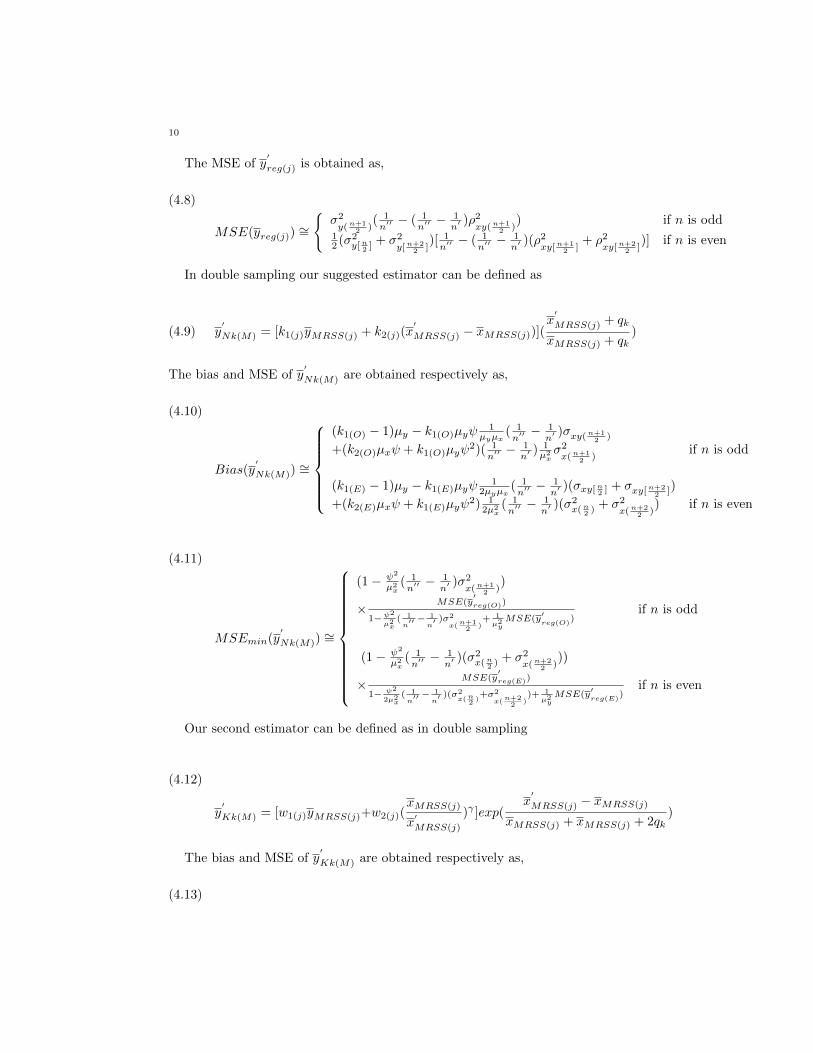
The MSE of y′

reg(j) is obtained as,

(4.8)

MSE(yreg(j))∼=

{σ2y(n+1

2 )( 1n′′− ( 1

n′′− 1

n′)ρ2xy(n+1

2 )) if n is odd

12 (σ2

y[n2 ] + σ2y[n+2

2 ])[ 1n′′− ( 1

n′′− 1

n′)(ρ2

xy[n+12 ]

+ ρ2xy[n+2

2 ])] if n is even

In double sampling our suggested estimator can be defined as

(4.9) y′

Nk(M) = [k1(j)yMRSS(j) + k2(j)(x′

MRSS(j) − xMRSS(j))](x′

MRSS(j) + qk

xMRSS(j) + qk)

The bias and MSE of y′

Nk(M) are obtained respectively as,

(4.10)

Bias(y′

Nk(M))∼=

(k1(O) − 1)µy − k1(O)µyψ1

µyµx( 1n′′− 1

n′)σxy(n+1

2 )

+(k2(O)µxψ + k1(O)µyψ2)( 1

n′′− 1

n′) 1µ2xσ2x(n+1

2 )if n is odd

(k1(E) − 1)µy − k1(E)µyψ1

2µyµx( 1n′′− 1

n′)(σxy[n2 ] + σxy[n+2

2 ])

+(k2(E)µxψ + k1(E)µyψ2) 1

2µ2x

( 1n′′− 1

n′)(σ2

x(n2 ) + σ2x(n+2

2 )) if n is even

(4.11)

MSEmin(y′

Nk(M))∼=

(1− ψ2

µ2x

( 1n′′− 1

n′)σ2x(n+1

2 ))

× MSE(y′reg(O))

1−ψ2

µ2x( 1

n′′ − 1

n′ )σ

2

x(n+12

)+ 1µ2yMSE(y

′reg(O)

)if n is odd

(1− ψ2

µ2x

( 1n′′− 1

n′)(σ2

x(n2 ) + σ2x(n+2

2 )))

× MSE(y′reg(E))

1− ψ2

2µ2x( 1

n′′ − 1

n′ )(σ

2x(n

2)+σ2

x(n+22

))+ 1

µ2yMSE(y

′reg(E)

)if n is even

Our second estimator can be defined as in double sampling

(4.12)

y′

Kk(M) = [w1(j)yMRSS(j)+w2(j)(xMRSS(j)

x′

MRSS(j)

)γ ]exp(x′

MRSS(j) − xMRSS(j)

xMRSS(j) + xMRSS(j) + 2qk)

The bias and MSE of y′

Kk(M) are obtained respectively as,

(4.13)

11

Bias(y′

Kk(M))∼=

w1(O)µy − µy + w2(O) −w1(O)ψ

2µx( 1n′′− 1

n′)σxy(n+1

2 )

+(w2(O)

2 (−ψγ + 34ψ

2 + γ(γ − 1))+ 3

8w1(O)ψ2µy) 1

µ2x

( 1n′′− 1

n′)σ2x(n+1

2 )if n is odd

w1(E)µy − µy + w2(E) −w1(E)ψ

4µx( 1n′′− 1

n′)(σxy[n2 ] + σxy[n+2

2 ])

+(w2(E)

2 (−ψγ + 34ψ

2 + γ(γ − 1))+ 3

8w1(E)ψ2µy) 1

2µ2x

( 1n′′− 1

n′)(σ2

x(n2 ) + σ2x(n+2

2 )) if n is even

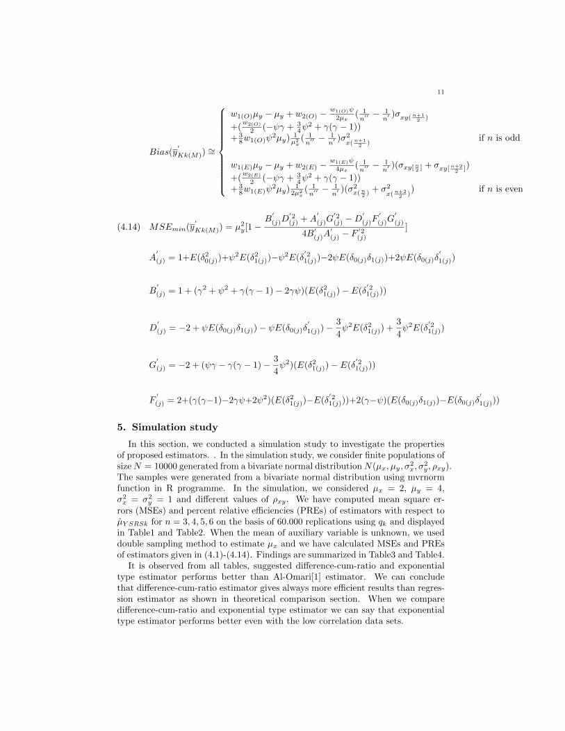
(4.14) MSEmin(y′

Kk(M)) = µ2y[1−

B′

(j)D′2(j) +A

′

(j)G′2(j) −D

′

(j)F′

(j)G′

(j)

4B′

(j)A′

(j) − F′2(j)

]

A′

(j) = 1+E(δ20(j))+ψ2E(δ21(j))−ψ

2E(δ′21(j))−2ψE(δ0(j)δ1(j))+2ψE(δ0(j)δ

′

1(j))

B′

(j) = 1 + (γ2 + ψ2 + γ(γ − 1)− 2γψ)(E(δ21(j))− E(δ′21(j)))

D′

(j) = −2 + ψE(δ0(j)δ1(j))− ψE(δ0(j)δ′

1(j))−3

4ψ2E(δ21(j)) +

3

4ψ2E(δ

′21(j))

G′

(j) = −2 + (ψγ − γ(γ − 1)− 3

4ψ2)(E(δ21(j))− E(δ

′21(j)))

F′

(j) = 2+(γ(γ−1)−2γψ+2ψ2)(E(δ21(j))−E(δ′21(j)))+2(γ−ψ)(E(δ0(j)δ1(j))−E(δ0(j)δ

′

1(j)))

5. Simulation study

In this section, we conducted a simulation study to investigate the propertiesof proposed estimators. . In the simulation study, we consider finite populations ofsizeN = 10000 generated from a bivariate normal distributionN(µx, µy, σ

2x, σ

2y, ρxy).

The samples were generated from a bivariate normal distribution using mvrnormfunction in R programme. In the simulation, we considered µx = 2, µy = 4,σ2x = σ2

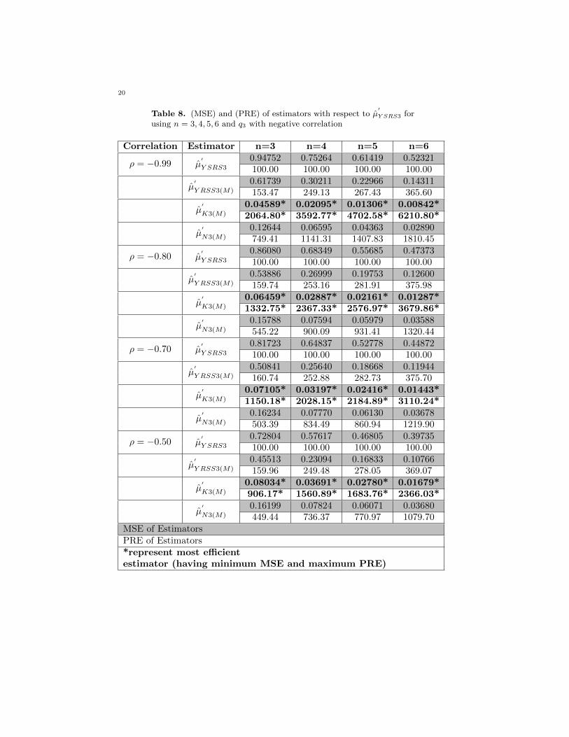
y = 1 and different values of ρxy. We have computed mean square er-rors (MSEs) and percent relative efficiencies (PREs) of estimators with respect toµY SRSk for n = 3, 4, 5, 6 on the basis of 60.000 replications using qk and displayedin Table1 and Table2. When the mean of auxiliary variable is unknown, we useddouble sampling method to estimate µx and we have calculated MSEs and PREsof estimators given in (4.1)-(4.14). Findings are summarized in Table3 and Table4.

It is observed from all tables, suggested difference-cum-ratio and exponentialtype estimator performs better than Al-Omari[1] estimator. We can concludethat difference-cum-ratio estimator gives always more efficient results than regres-sion estimator as shown in theoretical comparison section. When we comparedifference-cum-ratio and exponential type estimator we can say that exponentialtype estimator performs better even with the low correlation data sets.

12

6. Conclusion

In this paper we have suggested difference-cum-ratio and exponential type esti-mator in median ranked set sampling and extended our result to double sampling.We have found that difference-cum-ratio estimator is always more efficient thanregression estimator and exponential type is better than difference-cum-ratio esti-mator. Both of the estimators are considerable efficient than Al-Omari[1] estima-tor.

Acknowledgement I’m thankful to learned referees for their constructive com-ments.

References

[1] Al-Omari, A. I. Ratio estimation of the population mean using auxiliary information in

simple random sampling and median ranked set sampling, Statistics and Probability Letters82, 1883-1890, 2012.

[2] Al-Saleh, M.F. and Al-Omari, A.I. Multistage ranked set sampling, Journal of Statistical

Planning and Inference 102, 273-286, 2002.[3] Bahl, S. and Tuteja, R.K. Ratio and product exponential estimators, Journal of Information

and Optimization Sciences 12 (1), 159-164, 1991.

[4] Jemain, A.A. and Al-Omari, A.I. Multistage median ranked set samples for estimating thepopulation mean, Pakistan Journal of Statistics 22, 195-207, 2006.

[5] Jemain, A.A., Al-Omari, A.I. and Ibrahim, K. Multistage extreme ranked set sampling for

estimating the population mean, Journal of Statistical Theory and Application 6 (4), 456-471, 2007.

[6] Koyuncu, N. and Kadilar, C. Family of estimators of population mean using two auxiliaryvariables in stratified random sampling, Communications in Statistics: Theory and Methods

38 (14), 2398-2417, 2009.

[7] Koyuncu, N. and Kadilar, C. (2010). On improvement in estimating population mean instratified random sampling, Journal of Applied Statistics 37 (6), 999-1013, 2010.

[8] Koyuncu, N. Effcient estimators of population mean using auxiliary attributes. Applied

Mathematics Computation 218, 10900-10905, 2012.[9] Koyuncu, N., Gupta, S. and Sousa, R. Exponential type estimators of the mean of a sen-

sitive variable in the presence of non-sensitive auxiliary information, Communications in

Statistics: Simulation and Computation 43, 1583-1594, 2014.[10] Muttlak, H.A. Median ranked set sampling, Journal of Applied Statistical Science 6, 245-

255, 1997.

[11] Ozturk, O. and Jafari Jozani, M. Inclusion probabilities in partially rank ordered set sam-pling, Computational Statistics and Data Analysis 69, 122-132, 2014.

[12] Singh, H.P. and Solanki, R.S. An alternative procedure for estimating the population meanin simple random sampling, Pak. Jour. Statist. Oper. Res. 8 (2), 213-232, 2012.

[13] Singh, H.P. and Solanki, R.S. Improved estimation of population mean in simple randomsampling using information on auxiliary attribute, Appl. Math. Com. 218 (15), 7798-7812,2012.

[14] Singh, H.P., Tailor, R. and Tailor, R. On ratio and product methods with certain known

population parameters of auxiliary variable in sample surveys, SORT 34 (2), 157-180, 2010.[15] Singh, S., Singh, H.P. and Upadhyaya, L.N. Chain ratio and regression type estimators for

median estimation in survey sampling, Statist. Papers 48, 23-46, 2006.[16] Solanki R. S., Singh H.P. and Pal S. K. Improved estimation of finite population mean

sample surveys, J. Adv. Com. 1 (2), 70-78, 2013.

[17] Upadhyaya, L.N., Singh, H.P. Almost unbiased ratio and product-type estimators of finite

population variance in sample surveys, Statistics in Transition 7 (5), 1087-1096, 2006.[18] Yadav, R., Upadhyaya, L.N., Singh, H.P. and Chatterjee, S. Improved separate ratio ex-

ponential estimator for population mean using auxiliary information, Statist. Trans.-newseries 12 (2), 401-411, 2011.

13

Table 1. Mean Square Error (MSE) and the Percent Relative Ef-ficiency (PRE) of estimators with respect to µY SRS1 for using n =3, 4, 5, 6 and q1 with positive correlation

Correlation Estimator n=3 n=4 n=5 n=60.02716 0.01918 0.01473 0.01200

ρ = 0.99 µY SRS1 100.00 100.00 100.00 100.000.01467 0.00602 0.00657 0.00331

µY RSS1(M) 185.20 318.43 224.29 362.870.01134 0.00441 0.00611 0.00276

µK1(M) 239.49 435.31 241.05 435.660.00628* 0.00236* 0.00334* 0.00148*

µN1(M) 432.73* 812.15* 440.79* 811.72*0.20222 0.14713 0.11344 0.09326

ρ = 0.80 µY SRS1 100.00 100.00 100.00 100.000.12239 0.05059 0.05039 0.02702

µY RSS1(M) 165.23 290.84 225.11 345.120.07085* 0.03298* 0.02971* 0.01706*

µK1(M) 285.43* 446.14* 381.86* 546.66*0.07993 0.0344 0.03402 0.01845

µN1(M) 253.00 427.70 333.44 505.590.29675 0.21575 0.16607 0.13646

ρ = 0.70 µY SRS1 100.00 100.00 100.00 100.000.16636 0.07052 0.06580 0.03650

µY RSS1(M) 178.39 305.96 252.36 373.840.07411* 0.03588* 0.02998* 0.01799*

µK1(M) 400.41* 601.30* 553.97* 758.65*0.10245 0.04585 0.04203 0.0238

µN1(M) 289.67 470.60 395.13 573.360.47919 0.34640 0.26697 0.22066

ρ = 0.50 µY SRS1 100.00 100.00 100.00 100.000.23938 0.10748 0.09296 0.05362

µY RSS1(M) 200.18 322.29 287.17 411.510.07394* 0.03637* 0.02849* 0.01778*

µK1(M) 648.06* 952.42* 936.95* 1240.76*0.13382 0.06211 0.05219 0.03109

µN1(M) 358.10 557.71 511.54 709.69MSE of EstimatorsPRE of Estimators*represent most efficientestimator (having minimum MSE and maximum PRE)

14

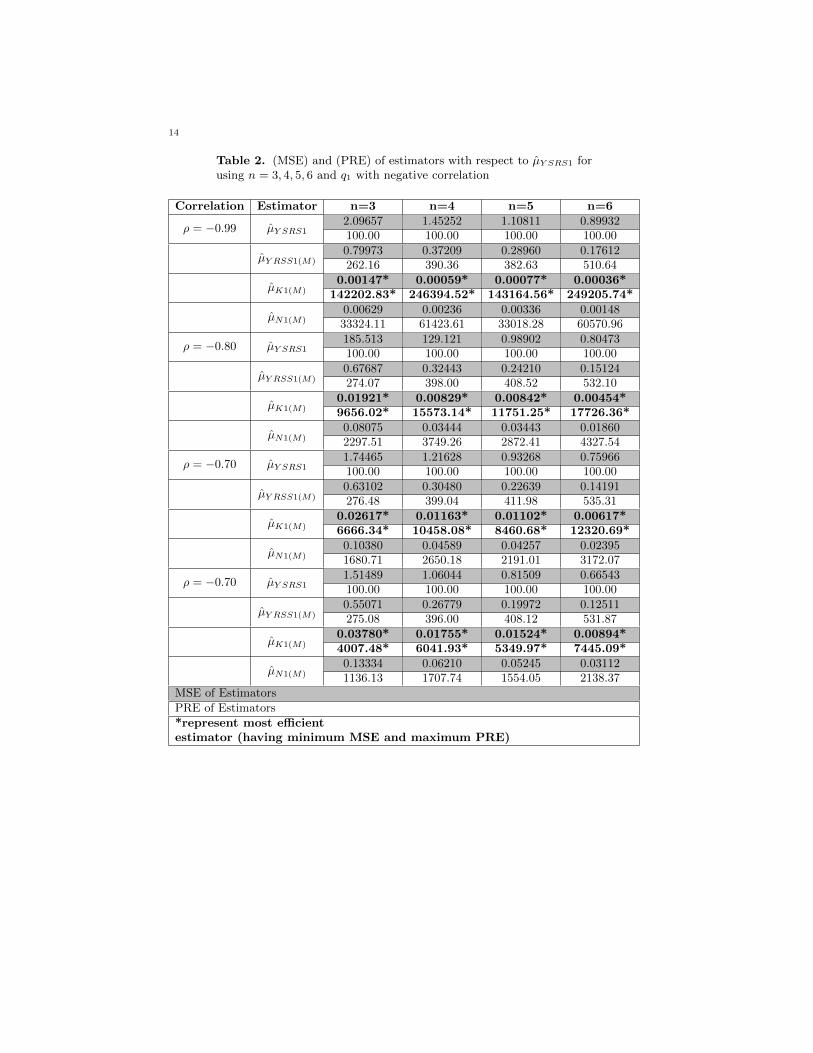
Table 2. (MSE) and (PRE) of estimators with respect to µY SRS1 forusing n = 3, 4, 5, 6 and q1 with negative correlation


ρ = −0.99 µY SRS1 100.00 100.00 100.00 100.000.79973 0.37209 0.28960 0.17612

µY RSS1(M) 262.16 390.36 382.63 510.640.00147* 0.00059* 0.00077* 0.00036*

µK1(M) 142202.83* 246394.52* 143164.56* 249205.74*0.00629 0.00236 0.00336 0.00148

µN1(M) 33324.11 61423.61 33018.28 60570.96185.513 129.121 0.98902 0.80473

ρ = −0.80 µY SRS1 100.00 100.00 100.00 100.000.67687 0.32443 0.24210 0.15124

µY RSS1(M) 274.07 398.00 408.52 532.100.01921* 0.00829* 0.00842* 0.00454*

µK1(M) 9656.02* 15573.14* 11751.25* 17726.36*0.08075 0.03444 0.03443 0.01860

µN1(M) 2297.51 3749.26 2872.41 4327.541.74465 1.21628 0.93268 0.75966

ρ = −0.70 µY SRS1 100.00 100.00 100.00 100.000.63102 0.30480 0.22639 0.14191

µY RSS1(M) 276.48 399.04 411.98 535.310.02617* 0.01163* 0.01102* 0.00617*

µK1(M) 6666.34* 10458.08* 8460.68* 12320.69*0.10380 0.04589 0.04257 0.02395

µN1(M) 1680.71 2650.18 2191.01 3172.071.51489 1.06044 0.81509 0.66543

ρ = −0.70 µY SRS1 100.00 100.00 100.00 100.000.55071 0.26779 0.19972 0.12511

µY RSS1(M) 275.08 396.00 408.12 531.870.03780* 0.01755* 0.01524* 0.00894*

µK1(M) 4007.48* 6041.93* 5349.97* 7445.09*0.13334 0.06210 0.05245 0.03112


15

Table 3. (MSE) and (PRE) of estimators with respect to µY SRS3 forusing n = 3, 4, 5, 6 and q3 with positive correlation


ρ = 0.99 µY SRS3 100.00 100.00 100.00 100.000.00833 0.00351 0.00402 0.00198

µY RSS3(M) 156.24 274.21 186.70 315.510.01403 0.00545 0.00761 0.00342

µK3(M) 92.82 176.83 98.71 182.940.00613* 0.00233* 0.00331* 0.00147*

µN3(M) 212.37* 412.55* 227.00* 425.46*0.12348 0.09280 0.07286 0.06073

ρ = 0.80 µY SRS3 100.00 100.00 100.00 100.000.08088 0.03462 0.03474 0.01869

µY RSS3(M) 152.68 268.03 209.72 324.980.08867 0.04142 0.03733 0.02146

µK3(M) 139.26 224.05 195.20 283.030.07802* 0.03400* 0.03371* 0.01834*

µN3(M) 158.27* 272.91* 216.14* 331.24*0.18311 0.13745 0.10786 0.08983

ρ = 0.70 µY SRS3 100.00 100.00 100.00 100.000.11056 0.04855 0.04559 0.02540

µY RSS3(M) 165.62 283.15 236.59 353.620.09278* 0.04508* 0.03768* 0.02264*

µK3(M) 197.35* 304.93* 286.25* 396.84*0.10004 0.04533 0.04166 0.02366

µN3(M) 183.04 303.22 258.89 379.640.30341 0.22668 0.17871 0.14877

ρ = 0.50 µY SRS3 100.00 100.00 100.00 100.000.16198 0.07396 0.06427 0.03738

µY RSS3(M) 187.32 306.48 278.08 398.020.09301* 0.04591* 0.03596* 0.02248*

µK3(M) 326.21* 493.78* 496.96* 661.91*0.13094 0.06145 0.05165 0.03088


16

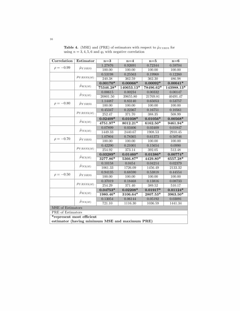
Table 4. (MSE) and (PRE) of estimators with respect to µY SRS3 forusing n = 3, 4, 5, 6 and q3 with negative correlation


ρ = −0.99 µY SRS3 100.00 100.00 100.00 100.000.53198 0.25563 0.19968 0.12260

µY RSS3(M) 240.38 362.59 362.30 486.980.00170* 0.00066* 0.00092* 0.00041*

µK3(M) 75346.28* 140653.13* 78496.62* 143988.13*0.00615 0.00234 0.00332 0.00147

µN3(M) 20801.50 39655.80 21769.81 40491.471.14487 0.83140 0.65053 0.53757

ρ = −0.80 µY SRS3 100.00 100.00 100.00 100.000.45347 0.22367 0.16751 0.10561

µY RSS3(M) 252.47 371.70 388.35 508.990.02409* 0.01038* 0.01056* 0.00568*

µK3(M) 4751.97* 8012.21* 6162.50* 9461.94*0.07899 0.03406 0.03409 0.01847

µN3(M) 1449.33 2440.67 1908.53 2910.451.07804 0.78365 0.61373 0.50746

ρ = −0.70 µY SRS3 100.00 100.00 100.00 100.000.42290 0.21001 0.15654 0.0990

µY RSS3(M) 254.92 373.14 392.05 512.480.03289* 0.01460* 0.01386* 0.00774*

µK3(M) 3277.86* 5366.87* 4429.80* 6557.28*0.10158 0.0454 0.04214 0.02379

µN3(M) 1061.33 1726.09 1456.49 2133.320.94135 0.68590 0.53818 0.44554

ρ = −0.50 µY SRS3 100.00 100.00 100.00 100.000.37019 0.18468 0.13816 0.08733

µY RSS3(M) 254.29 371.40 389.52 510.170.04753* 0.02208* 0.01917* 0.01124*

µK3(M) 1980.46* 3106.64* 2807.53* 3963.50*0.13054 0.06144 0.05192 0.03091


17

Table 5. (MSE) and (PRE) of estimators with respect to µ′Y SRS1 for

using n = 3, 4, 5, 6 and q1 with positive correlation


ρ = 0.99 µ′

Y SRS1 100.00 100.00 100.00 100.000.23023 0.11654 0.08777 0.05530

µ′

Y RSS1(M) 77.80 100.87 98.78 122.270.13146* 0.06466* 0.05121* 0.03149*

µ′

K1(M) 136.26* 181.81* 169.30* 214.73*0.13819 0.06916 0.05378 0.03343

µ′

N1(M) 129.62 169.98 161.21 202.280.23888 0.16633 0.12742 0.10244

ρ = 0.80 µ′

Y SRS1 100.00 100.00 100.00 100.000.28069 0.13827 0.10670 0.06626

µ′

Y RSS1(M) 85.10 120.30 119.42 154.600.09576* 0.04582* 0.03806* 0.02298*

µ′

K1(M) 249.45* 363.05* 334.76* 445.74*0.15289 0.07387 0.05938 0.03623

µ′

N1(M) 156.25 225.17 214.58 282.760.30028 0.21632 0.16904 0.13807

ρ = 0.70 µ′

Y SRS1 100.00 100.00 100.00 100.000.32584 0.15892 0.12276 0.07609

µ′

Y RSS1(M) 92.16 136.12 137.70 181.460.08211* 0.03926* 0.03228* 0.01962*

µ′

K1(M) 365.69* 551.02* 523.62* 703.64*0.16068 0.07666 0.06180 0.03760

µ′

N1(M) 186.87 282.19 273.51 367.230.42384 0.31654 0.25222 0.20933

ρ = 0.50 µ′

Y SRS1 100.00 100.00 100.00 100.000.40172 0.19537 0.14864 0.09282

µ′

Y RSS1(M) 105.51 162.02 169.69 225.520.07532* 0.03651* 0.02847* 0.01773*

µ′

K1(M) 562.73* 867.00* 885.88* 1180.43*0.16669 0.07933 0.06271 0.03849

µ′

N1(M) 254.27 399.03 402.20 543.81MSE of EstimatorsPRE of Estimators*represent most efficientestimator (having minimum MSE and maximum PRE)

18


using n = 3, 4, 5, 6 and q1 with negative correlation


ρ = −0.99 µ′

Y SRS1 100.00 100.00 100.00 100.000.97002 0.46323 0.34803 0.21602

µ′

Y RSS1(M) 148.77 243.48 261.29 355.380.03720* 0.01674* 0.01039* 0.00668*

µ′

K1(M) 3879.01* 6736.19* 8751.86* 11490.33*0.14743 0.07198 0.04646 0.03019

µ′

N1(M) 978.84 1566.82 1957.45 2542.771.30377 1.02123 0.82264 0.69395

ρ = −0.80 µ′

Y SRS1 100.00 100.00 100.00 100.000.85105 0.41594 0.30128 0.19141

µ′

Y RSS1(M) 153.20 245.52 273.05 362.540.05221* 0.02310* 0.01720* 0.01023*

µ′

K1(M) 2497.40* 4421.60* 4783.49* 6785.34*0.17864 0.08184 0.06264 0.03715

µ′

N1(M) 729.85 1247.78 1313.19 1868.151.23136 0.96516 0.77731 0.65554

ρ = −0.70 µ′

Y SRS1 100.00 100.00 100.00 100.000.80362 0.39541 0.28511 0.18167

µ′

Y RSS1(M) 153.23 244.09 272.64 360.850.05748* 0.02561* 0.01925* 0.01148*

µ′

K1(M) 2142.34* 3769.17* 4037.59* 5711.08*0.18225 0.08339 0.06404 0.03800

µ′

N1(M) 675.63 1157.41 1213.80 1725.341.09266 0.85687 0.68971 0.58123

ρ = −0.50 µ′

Y SRS1 100.00 100.00 100.00 100.000.72687 0.36005 0.25968 0.16548

µ′

Y RSS1(M) 150.32 237.99 265.60 351.230.06490* 0.02952* 0.02212* 0.01334*

µ′

K1(M) 1683.64* 2902.88* 3117.84* 4357.02*0.18003 0.08347 0.06318 0.03790

µ′


19


using n = 3, 4, 5, 6 and q3 with positive correlation


ρ = 0.99 µ′

Y SRS3 100.00 100.00 100.00 100.000.12748 0.06367 0.04988 0.03089

µ′

Y RSS3(M) 121.88 154.74 142.64 176.060.17019 0.08280 0.06496 0.03992

µ′

K3(M) 91.30 118.97 109.54 136.230.13735* 0.06895* 0.05361* 0.03335*

µ′

N3(M) 113.12* 142.89* 132.73* 163.03*0.19485 0.13146 0.09912 0.07844

ρ = 0.80 µ′

Y SRS3 100.00 100.00 100.00 100.000.1619 0.07880 0.06320 0.03863

µ′

Y RSS3(M) 120.35 166.82 156.85 203.060.12187* 0.05821* 0.04810* 0.02907*

µ′

K3(M) 159.88* 225.85* 206.12* 269.90*0.15044 0.07315 0.05893 0.03602

µ′

N3(M) 129.49 179.72 168.20 217.790.23451 0.16460 0.12719 0.10263

ρ = 0.70 µ′

Y SRS3 100.00 100.00 100.00 100.000.19195 0.09286 0.07424 0.04542

µ′

Y RSS3(M) 122.17 177.25 171.33 225.960.10334* 0.04963* 0.04074* 0.02481*

µ′

K3(M) 226.93* 331.64* 312.17* 413.65*0.15691 0.07548 0.06112 0.03727

µ′

N3(M) 149.45 218.09 208.10 275.390.31428 0.23118 0.18340 0.15113

ρ = 0.50 µ′

Y SRS3 100.00 100.00 100.00 100.000.24300 0.11807 0.09222 0.05714

µ′

Y RSS3(M) 129.33 195.81 198.88 264.490.09368* 0.04586* 0.03586* 0.02239*

µ′

K3(M) 335.49* 504.12* 511.49* 675.08*0.16062 0.07734 0.06163 0.03795

µ′


20


using n = 3, 4, 5, 6 and q3 with negative correlation


ρ = −0.99 µ′

Y SRS3 100.00 100.00 100.00 100.000.61739 0.30211 0.22966 0.14311

µ′

Y RSS3(M) 153.47 249.13 267.43 365.600.04589* 0.02095* 0.01306* 0.00842*

µ′

K3(M) 2064.80* 3592.77* 4702.58* 6210.80*0.12644 0.06595 0.04363 0.02890

µ′

N3(M) 749.41 1141.31 1407.83 1810.450.86080 0.68349 0.55685 0.47373

ρ = −0.80 µ′

Y SRS3 100.00 100.00 100.00 100.000.53886 0.26999 0.19753 0.12600

µ′

Y RSS3(M) 159.74 253.16 281.91 375.980.06459* 0.02887* 0.02161* 0.01287*

µ′

K3(M) 1332.75* 2367.33* 2576.97* 3679.86*0.15788 0.07594 0.05979 0.03588

µ′

N3(M) 545.22 900.09 931.41 1320.440.81723 0.64837 0.52778 0.44872

ρ = −0.70 µ′

Y SRS3 100.00 100.00 100.00 100.000.50841 0.25640 0.18668 0.11944

µ′

Y RSS3(M) 160.74 252.88 282.73 375.700.07105* 0.03197* 0.02416* 0.01443*

µ′

K3(M) 1150.18* 2028.15* 2184.89* 3110.24*0.16234 0.07770 0.06130 0.03678

µ′

N3(M) 503.39 834.49 860.94 1219.900.72804 0.57617 0.46805 0.39735

ρ = −0.50 µ′

Y SRS3 100.00 100.00 100.00 100.000.45513 0.23094 0.16833 0.10766

µ′

Y RSS3(M) 159.96 249.48 278.05 369.070.08034* 0.03691* 0.02780* 0.01679*

µ′

K3(M) 906.17* 1560.89* 1683.76* 2366.03*0.16199 0.07824 0.06071 0.03680

µ′


New difference-cum-ratio and exponential type estimators in median ranked set sampling

Documents

Transcript of New difference-cum-ratio and exponential type estimators in median ranked set sampling