Geoderma 155 (2010) 175–185

Contents lists available at ScienceDirect

Geoderma

j ourna l homepage: www.e lsev ie r.com/ locate /geoderma

Multi-scale digital terrain analysis and feature selection for digital soil mapping

Thorsten Behrens a, A-Xing Zhu b,c, Karsten Schmidt a,⁎, Thomas Scholten a

a Institute of Geography, Physical Geography, University of Tübingen, Rümelinstraße 19-23, D-72074, Tübingen, Germanyb State Key Laboratory of Environment and Resources Information System, Institute of Geographical Science and Resources Research, Chinese Academy of Sciences, Beijing 100101, Chinac Department of Geography, University of Wisconsin-Madison, Madison, Wisconsin 53706, USA

⁎ Corresponding author. Tel.: +49 7071 29 78943.E-mail address: karsten.schmidt@uni-tuebingen.de (

0016-7061/$ – see front matter © 2009 Published by Edoi:10.1016/j.geoderma.2009.07.010

a b s t r a c t

a r t i c l e i n f o

Article history:Received 21 May 2008Received in revised form 10 June 2009Accepted 18 July 2009Available online 28 August 2009

Keywords:Multi-scale digital terrain analysisFeature selectionSpatial data miningDigital soil mappingANOVAPrincipal components analysisRandom subsetsDecision trees

Terrain attributes are the most widely used predictors in digital soil mapping. Nevertheless, discussion oftechniques for addressing scale issues and feature selection has been limited. Therefore, we provide aframework for incorporating multi-scale concepts into digital soil mapping and for evaluating these scaleeffects. Furthermore, soil formation and soil-forming factors vary and respond at different scales. The spatialdata mining approach presented here helps to identify both the scale which is important for mapping soilclasses and the predictive power of different terrain attributes at different scales. The multi-scale digitalterrain analysis approach is based on multiple local average filters with filter sizes ranging from 3×3 up to31×31 pixels. We used a 20-m DEM and a 1:50 000 soil map for this study. The feature space is extended toinclude the terrain conditions measured at different scales, which results in highly correlated features(terrain attributes). Techniques to condense the feature space are therefore used in order to extract therelevant soil forming features and scales. The prediction results, which are based on a robust classificationtree (CRUISE) show that the spatial pattern of particular soil classes varies at characteristic scales in responseto particular terrain attributes. It is shown that some soil classes are more prevalent at one scale than at otherscales and more related to some terrain attributes than to others. Furthermore, the most computationallyefficient ANOVA-based feature selection approach is competitive in terms of prediction accuracy and theinterpretation of the condensed datasets. Finally, we conclude that multi-scale as well as feature selectionapproaches deserve more research so that digital soil mapping techniques are applied in a proper spatialcontext and better prediction accuracy can be achieved.

© 2009 Published by Elsevier B.V.

1. Introduction

Terrain attributes are themost widely used predictors in digital soilmapping (McBratney et al., 2003). This is because relief is one of themost important soil-forming factors (Jenny, 1941) and digital eleva-tion models (DEM) are widely available at different resolutions.These range from b1 m for LIDAR data up to 1 km for datasets withglobal coverage. Scale is an important consideration when mapsof soil classes are produced. The map-user requires information at aparticular scale and available covariates have a particular spatialresolution.

The impact of scale and resolution on soil property and soil classmapping is analyzed and described in various publications. Theinfluence of the resolution (grid size) of digital elevation models onsoil landscape modelling as well as applications has been widelydiscussed (e.g. Thompson et al., 1999; Schoorl et al., 2000; Valeo andMoin, 2000; Vázquez et al., 2002; Claessens et al. 2005; Smith et al.,2006; Zhu, 2008).

K. Schmidt).

lsevier B.V.

Concerning the influence of scale on the spatial distribution ofsoils, most authors focus on soil properties (Burrough, 1983;Goovaerts and Webster, 1994; German, 1999; Lark and Webster,2001; Nemes et al., 2003; Lark, 2005; Zhu et al., 2004; Bartoli et al.,1991, 2005; Zhao et al., 2006). Methods for incorporating analyses ofdifferent scales of variation into techniques for mapping thedistribution of soil classes have not been widely reported in theliterature (Hupy et al., 2004).

Classical machine learning approaches like classification trees,artificial neural networks, support vector machines etc. have nomechanisms to detect spatial relationships (Moran and Bui, 2002).However, the need to develop straightforward approaches to dealwith multi-scale variations in digital soil mapping is of greatimportance (McBratney et al., 2003; Lagacherie, 2008). To analyzethe effect of scales and to incorporate the spatial domain in datamining or prediction processes Moran and Bui (2002), Behrens(2003), Behrens et al. (2005), Smith et al. (2006), and Grinand et al.(2008) use contextual spatial information, whereas Lark (2006) andMendonca-Santos et al. (2006) demonstrate the use of wavelets.

This paper demonstrates how contextual information from pre-dictor variables can be incorporated into statistical digital soilmapping. It helps to analyze both the scale of soil classes and the

176 T. Behrens et al. / Geoderma 155 (2010) 175–185

predictive power of different terrain attributes at different scales. Alarger number of terrain attributes than is commonly used in suchstudies are analyzed. A multi-scale digital terrain analysis approachbased on multiple local average filters (Behrens et al., 2005; Grinandet al., 2008) is proposed, which produces separate hierarchical spatialcomponents (McBratney et al., 2003). This can be applied to variouskinds of spatial predictor variables. The core of this approach is tocompute terrain variables over a range of filter sizes, which not onlyincreases the feature space, that is, the number of variables used aspredictors, but also produces a set of highly correlated features (ter-rain attributes). Dimension reduction and feature selection techniques(cf. Liu and Motoda, 1998) are then used to reduce the feature spaceand select proper features in order to extract the relevant soil-formingfeatures and scales for each soil class in a map.

The methodological framework introduced in this study offers thepossibility to answer the following questions:

– Is prediction accuracy effected by incorporating predictors withexplicit information on scale dependence?

– Which terrain attributes are most important to predict certain soilclasses?

– Do optimal scales in terms of filter size exist to best predict specificsoil classes?

– Are there differences in prediction accuracies based on differentfeature selection approaches?

– How does prediction accuracy change with respect to the numberof features?

– Can the selected features be interpreted in terms of soil formation?– Which approach for selecting the relevant features would best

answer these questions?

The approach is introduced and applied to datasets typicallyavailable for DSM approaches in Germany: a 20-m DEM and a1:50 000 soil map.

2. Material and methods

2.1. Study area and datasets

The study area, Palatinate Forest, is located in southern Rhineland-Palatinate, Germany. It is a low mountain range area within thesouthwest German–Lorraine Triassic escarpment. The soils in thePalatinate Forest were formed from substrates of the Upper Red BedSandstone, Bunter, and Lower Limestone. According to the currentGerman mapping standard (Ad-hoc-AG Boden, 2005) the soil mapswithin the Palatinate Forest were produced at a scale of 1:50 000relating soil classes to geology and terrain conditions.

The entire study area covers about 300 km². All modelling ap-proaches are based on a DEM with a resolution of 20 m. For trainingand validation, two spatial subsets were selected from the soil map,each consisting of the same six soil classes (Table 1, Fig. 1) and eachcovering an area of about 40 km². This dataset is similar to the oneused by Behrens and Scholten (2006a,b), a comparative study ofdifferent data mining approaches. The two soil datasets are locatedabout 50 km apart.

Table 1Analyzed soil classes and their distribution in the training and the validation area; Tr: coverage

Soil class Parent material

S1 Cumulic anthrosols, gleyic anthrosols, gleysols and fluvisols Fluvic soil materialS2 Haplic cambisols Loess-containing sa

weathered sandstonS3 Dystric cambisols Loess-containing sa

weathered sandstonS4 Haplic podzols Sandy slope depositS5 Dystric cambisols Blocky, sandy slopeS6 Dystric cambisols and Cambi-haplic podzols Blocky, sandy slope

2.2. Digital terrain analysis and terrain attributes

We used 19 terrain attributes in this study. As some of them werecalculated on the basis of different thresholds, a total of 38 terraindatasets were created (Table 2). The attributes are classified into 9different groups based on how they are computed and their postu-lated effects on soil formation.

All attributes are explained briefly below, starting with local terrainattributes calculated on the basis of moving window techniques overthe same spatial extent for each pixel (e.g. Zevenbergen and Thorne,1987), followed by regional terrain attributes based on contributingarea concepts (e.g. Quinn et al., 1991), and combined terrain attributesbased on local and regional attributes such as the compound topo-graphic index (e.g. Beven and Kirkby, 1979).

2.2.1. Local terrain attributes

2.2.1.1. Non-curvature attributes.Elevation (EL)Elevation is the original values of the DEM.Mean slope (SLD)Mean slope is the average slope over a neighbourhood. Following

the approach of Dietrich and Montgomery (1998), mean slope iscalculated based on the geometricmean of the slopes between the twocardinal and the two diagonal slopes in a 3×3 pixel neighbourhood.

Steepest slope (SLT)Steepest slope is the steepest decent within a neighbourhood. It is

the slope gradient between two adjacent cells forming the steepestline orientated in a down slope direction over a 3×3 pixel neighbour-hood (Tarboton, 1997).

Aspect (D)Aspect is the average orientation of the neighbourhood centred

around a given pixel. The calculation is based on the finite differencesapproach introduced by Horn (1981). There are two concepts totransform the circular character of aspect into the linear space: oneis the sine and cosine transformation, which result in parameterspresenting eastness and northness; the other is deviation from bear-ings. We prefer the deviations from bearings because more directionalderivates can be calculated and thus the influence of aspect on soil canbe easily interpreted. We use the deviations from 0°, 45°, 90° and 135°in this study.

2.2.1.2. Curvatures. Curvature is a measure of convexity or concavityof terrain surface. It is often used to indicate areas of material removaland areas of material accumulation. Curvature can be defined and socomputed in various ways. We used twomajor categories of curvaturemeasure.

a) Based on finite differences

The curvatures in this group are based on finite differenceequations given by Evans (1980). The curvature attributes used inthis study were selected from a system of curvatures introduced byShary et al. (2002): Mean curvature (MEC), Profile curvature (PRC),Horizontal curvature (HOC), Minimal curvature (MIC), and Maximum

in the training area; VA: coverage in the validation area; (Behrens and Scholten, 2006a).

TR [%] VA [%]

in valleys and adjacent to water courses 5 4ndy Pleistocene periglacial slope deposits coveringe (Middle Bunter)

32 34

ndy Pleistocene periglacial slope deposits covering elevatione (Middle Bunter)

5 2

s rich in debris covering weathered sandstone (Middle Bunter) 32 32deposits covering deep-weathered sandstone (Lower Bunter) 11 20deposits covering weathered blocky sandstone (Middle Bunter) 12 5

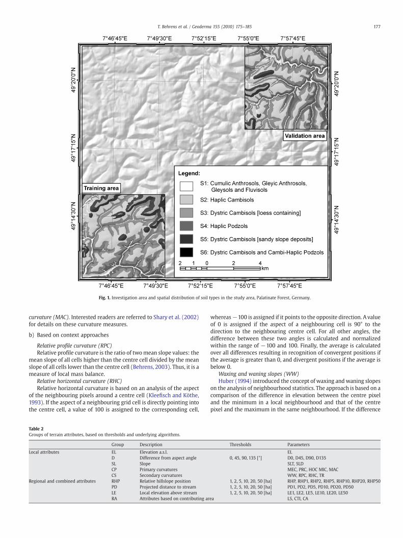
Fig. 1. Investigation area and spatial distribution of soil types in the study area, Palatinate Forest, Germany.

177T. Behrens et al. / Geoderma 155 (2010) 175–185

curvature (MAC). Interested readers are referred to Shary et al. (2002)for details on these curvature measures.

b) Based on context approaches

Relative profile curvature (RPC)Relative profile curvature is the ratio of twomean slope values: the

mean slope of all cells higher than the centre cell divided by the meanslope of all cells lower than the centre cell (Behrens, 2003). Thus, it is ameasure of local mass balance.

Relative horizontal curvature (RHC)Relative horizontal curvature is based on an analysis of the aspect

of the neighbouring pixels around a centre cell (Kleefisch and Köthe,1993). If the aspect of a neighbouring grid cell is directly pointing intothe centre cell, a value of 100 is assigned to the corresponding cell,

Table 2Groups of terrain attributes, based on thresholds and underlying algorithms.

Group Description

Local attributes EL Elevation a.s.l.D Difference from aspect angleSL SlopeCP Primary curvaturesCS Secondary curvatures

Regional and combined attributes RHP Relative hillslope positionPD Projected distance to streamLE Local elevation above streamRA Attributes based on contributing ar

whereas−100 is assigned if it points to the opposite direction. A valueof 0 is assigned if the aspect of a neighbouring cell is 90° to thedirection to the neighbouring centre cell. For all other angles, thedifference between these two angles is calculated and normalizedwithin the range of −100 and 100. Finally, the average is calculatedover all differences resulting in recognition of convergent positions ifthe average is greater than 0, and divergent positions if the average isbelow 0.

Waxing and waning slopes (WW)Huber (1994) introduced the concept of waxing andwaning slopes

on the analysis of neighbourhood statistics. The approach is based on acomparison of the difference in elevation between the centre pixeland the minimum in a local neighbourhood and that of the centrepixel and the maximum in the same neighbourhood. If the difference

Thresholds Parameters

EL0, 45, 90, 135 [°] D0, D45, D90, D135

SLT, SLDMEC, PRC, HOC MIC, MACWW, RPC, RHC, TR

1, 2, 5, 10, 20, 50 [ha] RHP, RHP1, RHP2, RHP5, RHP10, RHP20, RHP501, 2, 5, 10, 20, 50 [ha] PD1, PD2, PD5, PD10, PD20, PD501, 2, 5, 10, 20, 50 [ha] LE1, LE2, LE5, LE10, LE20, LE50

ea LS, CTI, CA

178 T. Behrens et al. / Geoderma 155 (2010) 175–185

from the maximum is smaller than that from the minimum, it is anupper or waxing slope; otherwise, it is a toe or awaning slope. Waxingand waning slopes (WW) are generally calculated on neighbourhoodslarger than 3×3 pixels (Huber, 1994). In this study, WW was calcu-lated on the basis of a 7×7 pixel neighbourhood.

Topographic roughness (TR)The approach to calculate topographic roughness is based on the

variation of slope and aspect within a local neighbourhood (Behrens,2003). As generally all neighbouring pixel values are slightly differentfrom the values of the slope and the aspect grid are rounded to thenearest integer. The variety (number of different values) is calculatedwithin a 7×7 pixel neighbourhood for both slope and aspect. Topo-graphic roughness value for a given pixel is the product of the numberof different slope gradient values and the number of different aspectvalues within the window.

2.2.2. Regional terrain attributes

2.2.2.1. Contributing area (CA). In this study, CA is computed basedon the multi-flow algorithm introduced by Quinn et al. (1991). Thisvariable is used both as a stand-alone attribute and as the basis tocalculate relative hillslope position, compound topographic index andUSLE LS-factor (see below). The algorithm uses the neighbouringslopes in a 3×3 pixel neighbourhood to weigh the outflow of each cellto its neighbours (Dietrich and Montgomery, 1998).

2.2.2.2. Projected distance to stream (PD). Projected distance tostream is the Euclidian distance between the local pixel and theclosest pixel on the streamline network. The streamline network isderived from the DEM using a so-called single-flow algorithm (Jensonand Domingue, 1988). The level of detail of the stream networkdepends on the threshold of flow accumulation used to define thestream network (Behrens, 2003). We used 6 different thresholds,namely 1, 2, 5, 10, 20, and 50 ha, to derive the streamlines for com-parison and for scale analysis, based on the assumption that differentcatchment sizes and hydrological processes have different impacts onsoil formation.

2.2.2.3. Local elevation (LE). Local elevation is the elevation dif-ference between the elevation of a local pixel and the elevation of itsclosest stream pixel. After delineating the streamline from the DEM,the pixel values of the stream are replaced by the original elevationvalues of the DEM. Afterwards, a nearest neighbour approach is usedto assign the elevation on the streamline to other non-stream pixels.This elevation data layer is referred to as streamline elevation datalayer (sEL). Finally, the streamline DEM is subtracted from the originalDEM, resulting in a grid containing local elevation (e.g., MacMillanet al., 2000; Behrens, 2003).

2.2.2.4. Relative hillslope position (RHP). Relative hillslope positionis a measure of relative distance between valley bottoms and ridges.Two approaches for determining RHPwere used in this study. The firstapproach, as introduced by Hatfield (1999), is related to local eleva-tion. The calculation is based on the original elevation data layer (EL),the streamline elevation data layer (sEL) and the crest elevation datalayer (cEL), which is created similarly to sEL, but using the elevation ofridge lines (crest). The final equation is:

RHP = fðEL−sELÞ= ðcEL−sELÞg × 100 ð1Þ

The other approach (RHPCA), is to subtract the CA of the original DEMand the CA calculated over an inverted DEM (Behrens, 2003). Thus, inmid slope positions the values are close to zero. In upper slopes thevalues are negative, whereas in toe slopes the resulting values arepositive.

2.2.3. Combined terrain attributes

2.2.3.1. Compound topographic index (CTI). The compound topographicindex, as originally introduced by Beven and Kirkby (1979), is definedas:

CTI = lnðCA= tanðSLTÞÞ ð2Þ

Where SLT (Tarboton,1997) is the steepest (maximum) slope gradientover a neighbourhood centred around a local pixel and CA is thecontributing area (Dietrich and Montgomery, 1998) of that pixel. Thisindex measures the balance of water accumulation and drainage overa local neighbourhood around a given pixel.

2.2.3.2. USLE LS-factor (LS). The USLE LS-factor (Wischmeier andSmith, 1978) is a well-known and important parameter. In this studywe use an approach modified for German mid-latitude landscapes(Feldwisch, 1995).

For slopes b9% the S-factor is:

S = 0:063 + 10:461 × sinðSLDÞ ð3Þ

whereas for slopes N=9 % the RUSLE equation (McCool et al., 1987) isused:

S = 16:8 × sinðSLDÞ−0:5 ð4Þ

The L-factor is then based on:

b = 11:16 × sinðSLDÞ= ð0:765 + 2:625 × sinðSLDÞÞ ð5Þ

m = b= ðb + 1Þ ð6Þ

L = ðCA= 22:13Þm ð7Þ

Finally the LS-factor is calculated bymultiplying the L- and the S-factorgrids.

2.3. The multi-scale approach

In terms of specific geomorphometry (Evans, 1972) and the nu-merical description of continuous surface forms (Pike, 1993), mosttechniques to derive terrain attributes are constrained by the reso-lution of the DEM (Wood, 1996). Wood (1996) argues that the scaleimplied by the resolution of DEM is not always appropriate in thecontext of landscape characterization. We assume that this holds truefor digital soil mapping, as has been shown in other works (Behrens,2003; Behrens et al., 2005, 2008; Smith et al., 2006; Zhu, 2008).

We applied square local neighbourhood averaging filters with sizesof n×n pixels, where n is an odd number ranging from 3 to 31, to allterrain attributes to investigate the influence of scale in digital soilmapping systematically. This local averaging extends the feature spaceby a factor of 14. Filtering is also applied to terrain attributes based ondifferent thresholds of contributing area (Section 2.2.2). Examples offiltered terrain attributes are given in Fig. 2.

Other options to analyze and incorporate scale exist but were notused in this study. One alternative method is to calculate terrainattributes based on DEMs with different resolutions. This approachcan result in errors of the surface models (Wood, 1996) as well asresampling problems within the prediction approach. Another alter-native approach is to fit multi-scale quadratic approximations toelevation values withinwindows of varying dimensions (e.g. Haralick,1983; Wood, 1996; Smith et al. 2006). Compared to these two alter-natives, the main technical advantage of the approach of local averagefiltering used in the present study is that it can easily be applied to anyterrain attribute, regardless of the underlying algorithm.

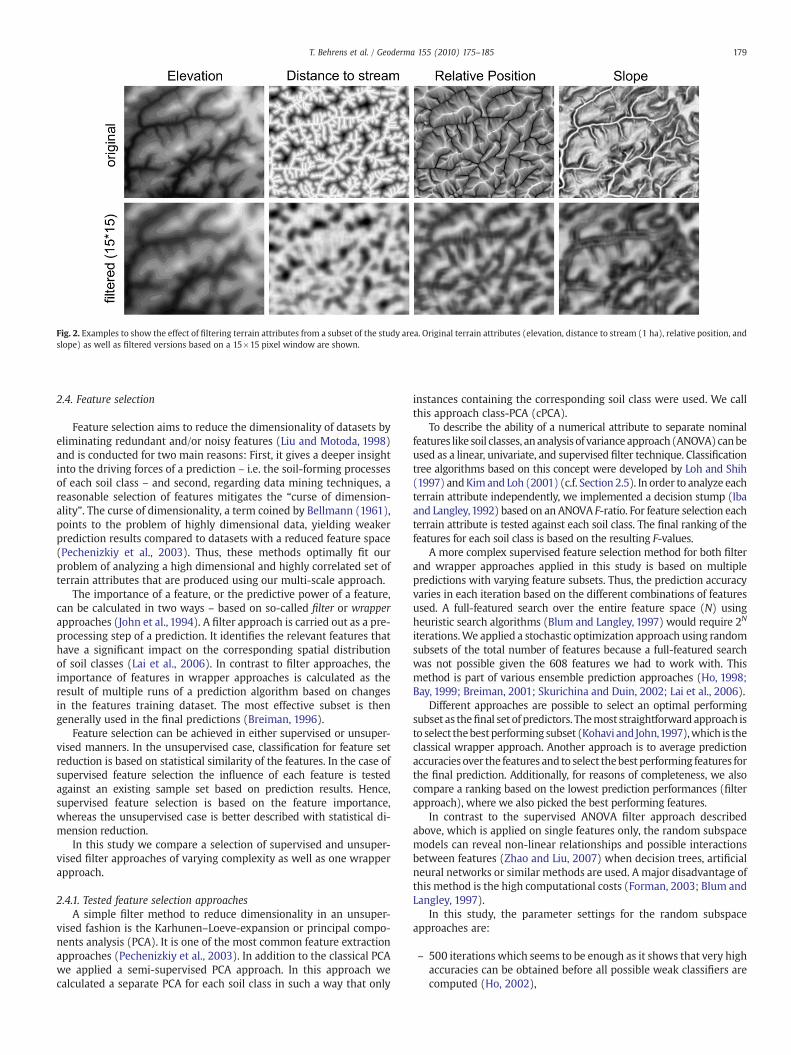
Fig. 2. Examples to show the effect of filtering terrain attributes from a subset of the study area. Original terrain attributes (elevation, distance to stream (1 ha), relative position, andslope) as well as filtered versions based on a 15×15 pixel window are shown.

179T. Behrens et al. / Geoderma 155 (2010) 175–185

2.4. Feature selection

Feature selection aims to reduce the dimensionality of datasets byeliminating redundant and/or noisy features (Liu and Motoda, 1998)and is conducted for two main reasons: First, it gives a deeper insightinto the driving forces of a prediction – i.e. the soil-forming processesof each soil class – and second, regarding data mining techniques, areasonable selection of features mitigates the “curse of dimension-ality”. The curse of dimensionality, a term coined by Bellmann (1961),points to the problem of highly dimensional data, yielding weakerprediction results compared to datasets with a reduced feature space(Pechenizkiy et al., 2003). Thus, these methods optimally fit ourproblem of analyzing a high dimensional and highly correlated set ofterrain attributes that are produced using our multi-scale approach.

The importance of a feature, or the predictive power of a feature,can be calculated in two ways – based on so-called filter or wrapperapproaches (John et al., 1994). A filter approach is carried out as a pre-processing step of a prediction. It identifies the relevant features thathave a significant impact on the corresponding spatial distributionof soil classes (Lai et al., 2006). In contrast to filter approaches, theimportance of features in wrapper approaches is calculated as theresult of multiple runs of a prediction algorithm based on changesin the features training dataset. The most effective subset is thengenerally used in the final predictions (Breiman, 1996).

Feature selection can be achieved in either supervised or unsuper-vised manners. In the unsupervised case, classification for feature setreduction is based on statistical similarity of the features. In the case ofsupervised feature selection the influence of each feature is testedagainst an existing sample set based on prediction results. Hence,supervised feature selection is based on the feature importance,whereas the unsupervised case is better described with statistical di-mension reduction.

In this study we compare a selection of supervised and unsuper-vised filter approaches of varying complexity as well as one wrapperapproach.

2.4.1. Tested feature selection approachesA simple filter method to reduce dimensionality in an unsuper-

vised fashion is the Karhunen–Loeve-expansion or principal compo-nents analysis (PCA). It is one of the most common feature extractionapproaches (Pechenizkiy et al., 2003). In addition to the classical PCAwe applied a semi-supervised PCA approach. In this approach wecalculated a separate PCA for each soil class in such a way that only

instances containing the corresponding soil class were used. We callthis approach class-PCA (cPCA).

To describe the ability of a numerical attribute to separate nominalfeatures like soil classes, ananalysis of variance approach (ANOVA) canbeused as a linear, univariate, and supervised filter technique. Classificationtree algorithms based on this concept were developed by Loh and Shih(1997) andKim and Loh (2001) (c.f. Section 2.5). In order to analyze eachterrain attribute independently, we implemented a decision stump (Ibaand Langley,1992) based on an ANOVA F-ratio. For feature selection eachterrain attribute is tested against each soil class. The final ranking of thefeatures for each soil class is based on the resulting F-values.

A more complex supervised feature selection method for both filterand wrapper approaches applied in this study is based on multiplepredictions with varying feature subsets. Thus, the prediction accuracyvaries in each iteration based on the different combinations of featuresused. A full-featured search over the entire feature space (N) usingheuristic search algorithms (Blum and Langley, 1997) would require 2N

iterations.We applied a stochastic optimization approach using randomsubsets of the total number of features because a full-featured searchwas not possible given the 608 features we had to work with. Thismethod is part of various ensemble prediction approaches (Ho, 1998;Bay, 1999; Breiman, 2001; Skurichina and Duin, 2002; Lai et al., 2006).

Different approaches are possible to select an optimal performingsubset as thefinal set of predictors. Themost straightforward approach isto select thebestperforming subset (Kohavi and John,1997),which is theclassical wrapper approach. Another approach is to average predictionaccuracies over the features and to select thebest performing features forthe final prediction. Additionally, for reasons of completeness, we alsocompare a ranking based on the lowest prediction performances (filterapproach), where we also picked the best performing features.

In contrast to the supervised ANOVA filter approach describedabove, which is applied on single features only, the random subspacemodels can reveal non-linear relationships and possible interactionsbetween features (Zhao and Liu, 2007) when decision trees, artificialneural networks or similar methods are used. A major disadvantage ofthis method is the high computational costs (Forman, 2003; Blum andLangley, 1997).

In this study, the parameter settings for the random subspaceapproaches are:

– 500 iterations which seems to be enough as it shows that very highaccuracies can be obtained before all possible weak classifiers arecomputed (Ho, 2002),

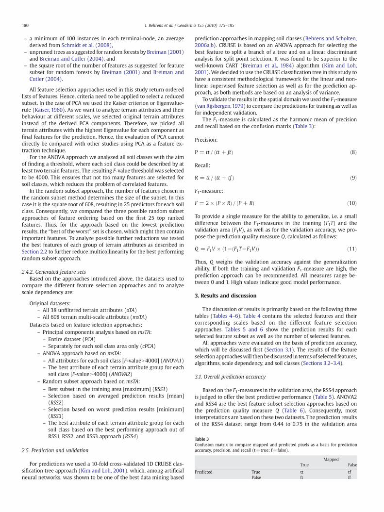
Table 3Confusion matrix to compare mapped and predicted pixels as a basis for predictionaccuracy, precision, and recall (t=true; f=false).

MappedTrue False

Predicted True tt tfFalse ft ff

180 T. Behrens et al. / Geoderma 155 (2010) 175–185

– a minimum of 100 instances in each terminal-node, an averagederived from Schmidt et al. (2008),

– unpruned trees as suggested for random forests by Breiman (2001)and Breiman and Cutler (2004), and

– the square root of the number of features as suggested for featuresubset for random forests by Breiman (2001) and Breiman andCutler (2004).

All feature selection approaches used in this study return orderedlists of features. Hence, criteria need to be applied to select a reducedsubset. In the case of PCA we used the Kaiser criterion or Eigenvalue-rule (Kaiser, 1960). As we want to analyze terrain attributes and theirbehaviour at different scales, we selected original terrain attributesinstead of the derived PCA components. Therefore, we picked allterrain attributes with the highest Eigenvalue for each component asfinal features for the prediction. Hence, the evaluation of PCA cannotdirectly be compared with other studies using PCA as a feature ex-traction technique.

For the ANOVA approach we analyzed all soil classes with the aimof finding a threshold, where each soil class could be described by atleast two terrain features. The resulting F-value thresholdwas selectedto be 4000. This ensures that not too many features are selected forsoil classes, which reduces the problem of correlated features.

In the random subset approach, the number of features chosen inthe random subset method determines the size of the subset. In thiscase it is the square root of 608, resulting in 25 predictors for each soilclass. Consequently, we compared the three possible random subsetapproaches of feature ordering based on the first 25 top rankedfeatures. Thus, for the approach based on the lowest predictionresults, the “best of theworst” set is chosen, whichmight then containimportant features. To analyze possible further reductions we testedthe best features of each group of terrain attributes as described inSection 2.2 to further reduce multicollinearity for the best performingrandom subset approach.

2.4.2. Generated feature setsBased on the approaches introduced above, the datasets used to

compare the different feature selection approaches and to analyzescale dependency are:

Original datasets:– All 38 unfiltered terrain attributes (oTA)– All 608 terrain multi-scale attributes (msTA)

Datasets based on feature selection approaches:– Principal components analysis based on msTA:

– Entire dataset (PCA)– Separately for each soil class area only (cPCA)

– ANOVA approach based on msTA:– All attributes for each soil class [F-valueN4000] (ANOVA1)– The best attribute of each terrain attribute group for each

soil class [F-valueN4000] (ANOVA2)– Random subset approach based on msTA:

– Best subset in the training area [maximum] (RSS1)– Selection based on averaged prediction results [mean]

(RSS2)– Selection based on worst prediction results [minimum]

(RSS3)– The best attribute of each terrain attribute group for each

soil class based on the best performing approach out ofRSS1, RSS2, and RSS3 approach (RSS4)

2.5. Prediction and validation

For predictions we used a 10-fold cross-validated 1D CRUISE clas-sification tree approach (Kim and Loh, 2001), which, among artificialneural networks, was shown to be one of the best data mining based

prediction approaches in mapping soil classes (Behrens and Scholten,2006a,b). CRUISE is based on an ANOVA approach for selecting thebest feature to split a branch of a tree and on a linear discriminantanalysis for split point selection. It was found to be superior to thewell-known CART (Breiman et al., 1984) algorithm (Kim and Loh,2001). We decided to use the CRUISE classification tree in this study tohave a consistent methodological framework for the linear and non-linear supervised feature selection as well as for the prediction ap-proach, as both methods are based on an analysis of variance.

To validate the results in the spatial domainwe used the F1-measure(van Rijsbergen,1979) to compare the predictions for training aswell asfor independent validation.

The F1-measure is calculated as the harmonic mean of precisionand recall based on the confusion matrix (Table 3):

Precision:

P = tt = ðtt + ftÞ ð8Þ

Recall:

R = tt = ðtt + tf Þ ð9Þ

F1-measure:

F = 2 × ðP × RÞ= ðP + RÞ ð10Þ

To provide a single measure for the ability to generalize, i.e. a smalldifference between the F1-measures in the training (F1T) and thevalidation area (F1V), as well as for the validation accuracy, we pro-pose the prediction quality measure Q, calculated as follows:

Q = F1V × ð1−ðF1T−F1VÞÞ ð11Þ

Thus, Q weighs the validation accuracy against the generalizationability. If both the training and validation F1-measure are high, theprediction approach can be recommended. All measures range be-tween 0 and 1. High values indicate good model performance.

3. Results and discussion

The discussion of results is primarily based on the following threetables (Tables 4–6). Table 4 contains the selected features and theircorresponding scales based on the different feature selectionapproaches. Tables 5 and 6 show the prediction results for eachselected feature subset as well as the number of selected features.

All approaches were evaluated on the basis of prediction accuracy,which will be discussed first (Section 3.1). The results of the featureselection approacheswill thenbediscussed in termsof selected features,algorithms, scale dependency, and soil classes (Sections 3.2–3.4).

3.1. Overall prediction accuracy

Based on the F1-measures in the validation area, the RSS4 approachis judged to offer the best predictive performance (Table 5). ANOVA2and RSS4 are the best feature subset selection approaches based onthe prediction quality measure Q (Table 6). Consequently, mostinterpretations are based on these two datasets. The prediction resultsof the RSS4 dataset range from 0.44 to 0.75 in the validation area

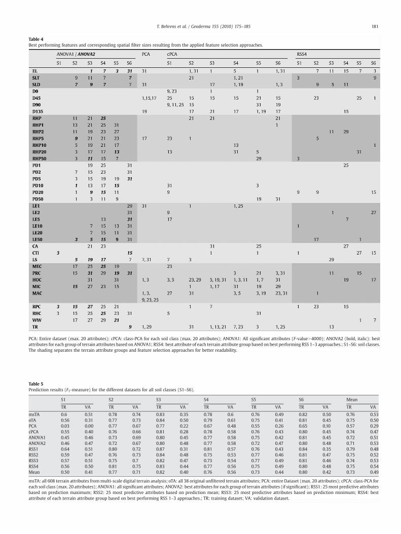
Table 4Best performing features and corresponding spatial filter sizes resulting from the applied feature selection approaches.

PCA: Entire dataset (max. 20 attributes); cPCA: class-PCA for each soil class (max. 20 attributes); ANOVA1: All significant attributes (F-valueN4000); ANOVA2 (bold, italic): bestattributes for each group of terrain attributes based on ANOVA1; RSS4: best attribute of each terrain attribute group based on best performing RSS 1–3 approaches.; S1–S6: soil classes.The shading separates the terrain attribute groups and feature selection approaches for better readability.

Table 5Prediction results (F1-measure) for the different datasets for all soil classes (S1–S6).

S1 S2 S3 S4 S5 S6 Mean

TR VA TR VA TR VA TR VA TR VA TR VA TR VA

msTA 0.6 0.51 0.78 0.74 0.83 0.35 0.78 0.6 0.76 0.49 0.82 0.50 0.76 0.53oTA 0.56 0.31 0.77 0.73 0.84 0.50 0.79 0.61 0.75 0.41 0.81 0.45 0.75 0.50PCA 0.03 0.00 0.77 0.67 0.77 0.22 0.67 0.48 0.55 0.26 0.65 0.10 0.57 0.29cPCA 0.55 0.40 0.76 0.66 0.81 0.28 0.78 0.58 0.76 0.43 0.80 0.45 0.74 0.47ANOVA1 0.45 0.46 0.73 0.69 0.80 0.45 0.77 0.58 0.75 0.42 0.81 0.45 0.72 0.51ANOVA2 0.46 0.47 0.72 0.67 0.80 0.48 0.77 0.58 0.72 0.47 0.80 0.48 0.71 0.53RSS1 0.64 0.51 0.80 0.72 0.87 0.31 0.81 0.57 0.76 0.43 0.84 0.35 0.79 0.48RSS2 0.59 0.47 0.76 0.73 0.84 0.48 0.75 0.53 0.77 0.46 0.81 0.47 0.75 0.52RSS3 0.57 0.51 0.75 0.7 0.82 0.47 0.73 0.54 0.77 0.49 0.81 0.46 0.74 0.53RSS4 0.56 0.50 0.81 0.75 0.83 0.44 0.77 0.56 0.75 0.49 0.80 0.48 0.75 0.54Mean 0.50 0.41 0.77 0.71 0.82 0.40 0.76 0.56 0.73 0.44 0.80 0.42 0.73 0.49

msTA: all 608 terrain attributes frommulti-scale digital terrain analysis; oTA: all 38 original unfiltered terrain attributes; PCA: entire Dataset (max. 20 attributes); cPCA: class-PCA foreach soil class (max. 20 attributes); ANOVA1: all significant attributes; ANOVA2: best attributes for each group of terrain attributes (if significant); RSS1: 25most predictive attributesbased on prediction maximum; RSS2: 25 most predictive attributes based on prediction mean; RSS3: 25 most predictive attributes based on prediction minimum; RSS4: bestattribute of each terrain attribute group based on best performing RSS 1–3 approaches.; TR: training dataset; VA: validation dataset.

181T. Behrens et al. / Geoderma 155 (2010) 175–185

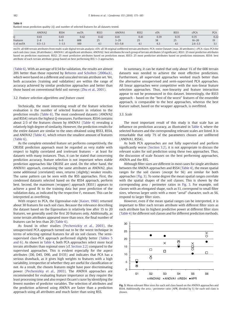
Table 6Ranked mean prediction quality (Q) and number of selected features for all datasets tested.

ANOVA2 RSS4 msTA RSS3 ANOVA1 RSS2 oTA RSS1 cPCA PCA

Q 0.43 0.43 0.42 0.42 0.41 0.41 0.39 0.35 0.35 0.22Features 2–8 6–9 608 25 3–29 25 38 25 16–20 19% of msTA 0.3–1.3 1–1.5 100 4.1 0.5–5.8 4.1 6.3 4.1 2.6–3.3 3.1

msTA: all 608 terrain attributes frommulti-scale digital terrain analysis; oTA: all 38 original unfiltered terrain attributes; PCA: entire Dataset (max. 20 attributes); cPCA: class-PCA foreach soil class (max. 20 attributes); ANOVA1: all significant attributes; ANOVA2: best attributes for each group of terrain attributes (if significant); RSS1: 25most predictive attributesbased on prediction maximum; RSS2: 25 most predictive attributes based on prediction mean; RSS3: 25 most predictive attributes based on prediction minimum; RSS4: bestattribute of each terrain attribute group based on best performing RSS 1–3 approaches.

Fig. 3.Mean relevant filter sizes for each soil class based on the ANOVA approaches andRSS4. Additionally the area / perimeter ratio (APR, divided by 5) for each soil class isshown.

182 T. Behrens et al. / Geoderma 155 (2010) 175–185

(Table 6). With an average of 0.54 for validation, the results are almost20% better than those reported by Behrens and Scholten (2006a,b),whichwere based on a different and unscaled terrain attribute set. Yet,both accuracies (training and validation) are within the range ofaccuracy achieved by similar prediction approaches and better thanthose based on conventional field soil surveys (Zhu et al., 2001).

3.2. Feature selection algorithms and feature count

Technically, the most interesting result of the feature selectionevaluation is the number of selected features in relation to theprediction results (Table 6). The most condensed datasets (ANOVA2and RSS4) return the highest Q-measures. Furthermore, RSS4 containsabout 2/3 of the features chosen by ANOVA1 (Table 4) revealing arelatively high degree of similarity. However, the prediction results forthe entire dataset are similar to the ones obtained using RSS3, RSS4,and ANOVA2 (Table 4), which return the smallest amount of features(Table 6).

As the complete extended feature set performs competitively, theCRUISE prediction approach must be regarded as very stable withrespect to highly correlated and irrelevant features – at least fordatasets with many instances. Thus, it can be stated that concerningprediction accuracy, feature selection is not important when stableprediction approaches like CRUISE are used. On the other hand, theANOVA1 approach, containing the same attributes as ANOVA2, plussome additional (correlated) ones, returns (slightly) weaker results.The same pattern can be seen with the RSS approaches. First, thecondensed datasets selected based on the RSS4 approach, performbest. Second, the maximum (wrapper) approach (RSS1) appears toachieve a good fit to the training data but poor prediction of thevalidation data, as indicated by the respective F1 measure. This can beinterpreted as overfitting.

With respect to PCA, the Eigenvalue-rule (Kaiser, 1960) returnedabout 30 features for each soil class. Because the relevance describingthe dataset based on the Eigenvalues is relatively low after 15 to 20features, we generally used the first 20 features only. Additionally, assome terrain attributes appeared more than once, the final number offeatures can be less than 20 (Table 6).

As found in other studies (Pechenizkiy et al., 2003), theunsupervised PCA approach turned out to be the worst technique interms of selecting optimal features for all six soil classes. The semi-supervised class-PCA approach performed slightly better (Tables 5and 6). As shown in Table 4, both PCA approaches select more localterrain attributes than regional ones (cf. Section 2.2) compared to thesupervised approaches. This is evident especially for the aspectattributes (D0, D45, D90, and D135) and indicates that PCA has aserious drawback, as it gives high weights to features with a highvariability, irrespective of whether they are useful for classification ornot. As a result, the chosen features might have poor discriminatingpower (Pechenizkiy et al., 2003). The ANOVA approaches arerecommended for evaluating feature importance as they require theleast processing time and also respect Occam's razor by identifying thefewest number of predictor variables. The selection of attributes andthe prediction achieved using ANOVA are faster than a predictionapproach using all attributes and much faster than using RSS.

In summary, it can be stated that only about 1% of the 608 terraindatasets was needed to achieve the most effective predictions.Furthermore, all supervised approaches worked much better thanthe alternative unsupervised and semi-supervised PCA approaches.All linear approaches were competitive with the non-linear featureselection approaches. Thus, non-linearity and feature interactionappear to not be pronounced in this dataset. Interestingly, the RSS3approach – based on the “best of the worst” features of the ensembleapproach, is comparable to the best approaches, whereas the bestfeature subset, based on the wrapper approach, is overfitted.

3.3. Scale

The most important result of this study is that scale has aninfluence on prediction accuracy, as illustrated in Table 4, where theselected features and the corresponding relevant scales are listed. It isremarkable that only 7% of the parameters chosen are unfiltered(ANOVA1, RSS4).

As both PCA approaches are not fully supervised and performsignificantly worse (Section 3.2), it is not appropriate to discuss therelevant scales for soil prediction using these two approaches. Thus,the discussion of scale focuses on the best performing approaches,ANOVA and the RSS.

Although filter sizes are different in most cases for single attributesbetween the ANOVA approaches and RSS4 (Table 4), the mean spatialranges for the soil classes (except for S6) are similar for bothapproaches (Fig. 3). To some degree the mean spatial ranges correlatewith the spatial shapes of the soil classes. This is shown by thecorresponding area / perimeter ratios in Fig. 3. For example, soilclasses with an elongated shape, such as S1, correspond to small filtersizes, whereas larger units with a more “areal” character, such as S6,respond to larger filter sizes.

However, even if the mean spatial ranges can be interpreted, it isimportant to filter each terrain attribute with different filter sizes aseach attribute has its highest predictive power at different filter sizes(Table 4) for different soil classes and for different predictionmethods.

183T. Behrens et al. / Geoderma 155 (2010) 175–185

This is one of themost important results. It shows that evenwithin onesoil class different filter sizes are needed for different terrain attributesto achieve optimized predictions. Thus, it is important to test allfiltered attributes on all soil classes of a map separately.

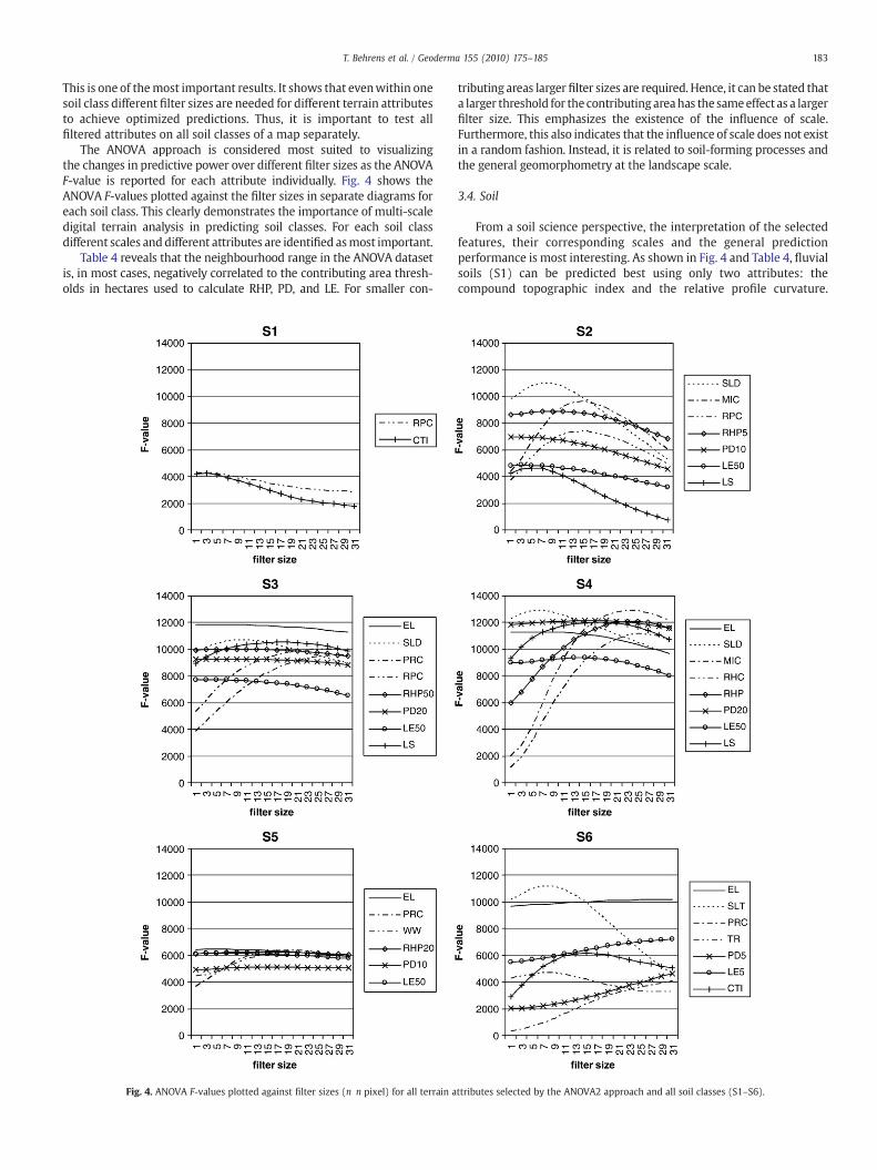
The ANOVA approach is considered most suited to visualizingthe changes in predictive power over different filter sizes as the ANOVAF-value is reported for each attribute individually. Fig. 4 shows theANOVA F-values plotted against the filter sizes in separate diagrams foreach soil class. This clearly demonstrates the importance of multi-scaledigital terrain analysis in predicting soil classes. For each soil classdifferent scales anddifferent attributes are identified asmost important.

Table 4 reveals that the neighbourhood range in the ANOVA datasetis, in most cases, negatively correlated to the contributing area thresh-olds in hectares used to calculate RHP, PD, and LE. For smaller con-

Fig. 4. ANOVA F-values plotted against filter sizes (n n pixel) for all terrain a

tributing areas larger filter sizes are required. Hence, it can be stated thata larger threshold for the contributingareahas the sameeffect as a largerfilter size. This emphasizes the existence of the influence of scale.Furthermore, this also indicates that the influence of scale does not existin a random fashion. Instead, it is related to soil-forming processes andthe general geomorphometry at the landscape scale.

3.4. Soil

From a soil science perspective, the interpretation of the selectedfeatures, their corresponding scales and the general predictionperformance is most interesting. As shown in Fig. 4 and Table 4, fluvialsoils (S1) can be predicted best using only two attributes: thecompound topographic index and the relative profile curvature.

ttributes selected by the ANOVA2 approach and all soil classes (S1–S6).

184 T. Behrens et al. / Geoderma 155 (2010) 175–185

Interestingly, the accuracy in the validation area only increases slightlywhen all 608 predictor data sets are used. This demonstrates the highpredictive power of these two attributes alone. The importance ofthese two variables can easily be interpreted in terms of their role insoil formation, as both were developed to describe soil–water andmass-movement relationships (Beven and Kirkby, 1979; Behrens,2003). Most of the other soil classes can be described by a mixture ofregional, local, and combined terrain attributes (Fig. 4). As the studyarea is a cuesta landscape, terrain position attributes (LE, RHP, and PD)become most important as they discern the vertical structure of thelandscape. The vertical structure of the area is highly influenced bygeology, whichwas not used as a predictor in this study (Schmidt et al.,2008). Slope plays an important role for 3 soil classesmainly occurringon steeper slopes.

The PCA approaches for feature selection returned comparativelyweak prediction accuracies for four soil classes. Only for soil classes S2and S4 PCA shows reasonable results. Two reasons might explain thisfact: First, both soil classes are generally easy to predict as they showthe highest F1-measures in the validation area for all feature selectionapproaches. S2 are Haplic Cambisols occurring on steep slopes, whileS4 are Haplic Podzols, which are located on the flat hilltops and thuscontain a higher Loess component due to lower erosion rates. Second,both soil classes comprise about 30% of the training and the validationarea each (Table 1). Thus, due to this large spatial extent, the selectionof features, which describe the structure of the dataset (as derived byPCA) seems to be relevant for prediction, or at least does not seem tohave a negative influence.

Concerning soil classes S3, S4, S5, and S6, all of which occur onsteeper slopes, terrain attribute EL returns the highest ANOVA F-values(Table 4, Fig. 4) indicating their relation to geological settings in thisarea.

Another interesting aspect concerning filter sizes is, that for somesoil classes (i.e. S2 and S4), nearly all relevant attributes varysubstantially in optimal scale in terms of the ANOVA F-value, whereas,for some other soil classes (i.e. S1 and S3), this effect is comparativelymoderate. This again seems to be related to the shape of areas occupiedby these soil classes. S1 andS5have the lowest area/perimeter ratio of allsoil classes (Fig. 3); the smallest soil classes S1 and S3 (Table 1) returntheweakest prediction results (Table 5). Hence, thefilter effect increasesin cases where the area of the soil class is large compared to theresolution of the DEM. In cases where the shape of the soil class iselongated and/or the soil class is comparatively small, the beneficialeffect of the multi-scale approach is limited.

Based on the highest prediction accuracies obtained for soil classes2 and 4, it can be hypothesized that these soil classes can be predictedwell on the basis of terrain attributes only, whereas soil classes S1 andS3 might need other additional predictors to achieve best predictionresults.

4. Conclusions

Several conclusions can be drawn based on the spatial data miningframework introduced in this study:

• multi-scale digital terrain analysis is an important tool for datamining based digital soil mapping approaches as it helps increaseprediction accuracy compared to standard digital terrain analysis,

• each soil class is best predicted by different combinations of featuresfiltered at different scales,

• only a small number of features are typically required to achievegood predictions,

• the selection of features in this way appears to aid the interpretationof the data with respect to soil formation,

• supervised feature selection approaches are superior to unsuper-vised ones,

• simple linear feature selection approaches are superior to muchmore complex approaches, and

• for straightforward predictions, multi co-linearity does not decreaseprediction results substantially if robust algorithms, such as CRUISE,are used.

With respect to future digital soil mapping studies, it is importantto validate these results in different soil landscapes. In the context ofscale, wavelet analysis (Lark and Webster, 2001; Lark, 2006) shouldalso be considered as an analytical tool. Furthermore, the proposedframework needs to be tested on soil attributes where similar resultsare expected (Behrens, 2003). Additional data mining and featureselection approaches need to be tested and compared. The interestingpoint in this respect is that the feature selection approaches appliedcan be combined with “black box” approaches like artificial neuralnetworks. Feature selection, in combination with instance selectionapproaches (Schmidt et al., 2008), might help to further reducemodel complexity while decreasing computation time and improvingprediction accuracy.

Finally, we conclude that multi-scale and feature selectionapproaches have not yet received the attention they deserve in soilscience literature. Both offer the possibility to learn more about soilformation in a spatial context and to increase the accuracy of digitalsoil mapping.

Acknowledgements

We are grateful to the Federal Geological Survey of Rhineland-Palatinate for providing the data.

A-Xing Zhu appreciates funding from the National Basic ResearchProgram of China 2007CB407207, the Chinese Academy of SciencesInternational Partnership Project “Human Activities and EcosystemChanges” CXTD-Z2005-1, the National Key Technology R&D Programof China (2007BAC15B01), and the support by the Vilas Trustees via itsVilas Associate Program to the University of Wisconsin-Madison.

References

Bartoli, F., Philippy, R., Doirisse, M., Niquet, S., Dubuit, M., 1991. The mass and porosityfractal dimensions (Dm and Dp) of silty and sandy soils were determined on in situsoils using a variety of soil sections (thin, very-thin and ultra-thin), by imageanalysis on a continuous scale from m to 10–9 to 10–1 m. European Journal of SoilScience 42, 167–185.

Bartoli, F., Genevois-Gomendy, V., Royer, J.J., Niquet, S., Vivier, H., Grayson, R., 2005. Amultiscale study of silty soil structure. European Journal of Soil Science 56,207–224.

Bay, D., 1999. Nearest neighbor classification from multiple feature subsets. IntelligentData Analysis 3, 191–209.

Behrens, T., 2003. Digitale Reliefanalyse als Basis von Boden-Landschafts-Modellen –am Beispiel der Modellierung periglaziärer Lagen im Ostharz. Boden undLandschaft 42 42, 189 pp. Giessen.

Behrens, T., Scholten, T., 2006a. A comparison of data mining approaches in predictive soilmapping. In: Lagacherie, P., McBratney, A., Voltz, M. (Eds.), Digital Soil Mapping –

An Introductory Perspective. In: Developments in Soil Science, vol. 31. Elsevier,Amsterdam.

Behrens, T., Scholten, T., 2006b. Digital Soil Mapping in Germany – a review. J. PlantNutr. Soil Sci. 169, 434–443 invited paper.

Behrens, T., Förster, H., Scholten, T., Steinrücken, U., Spies, E.-D., Goldschmidt, M., 2005.Digital soil mapping using artificial neural networks. Journal of Plant Nutrition andSoil Science 168, 21–33.

Behrens, T., Schmidt, K., Scholten, T., 2008. An approach to removing uncertainties innominal environmental covariates and soil class maps. In: Hartemink, A.,McBratney, A., Mendoca-Santos, M.L. (Eds.), Digital Soil Mapping with LimitedData. Springer.

Bellmann, R., 1961. Adaptive Control Processes: A Guided Tour. Princeton Univ, Press.Beven, K., Kirkby, M.J., 1979. A physically based, variable contributing area model of

basin hydrology. Bulletin of Hydrologic Sciences 24, 4369.Blum, A., Langley, P., 1997. Selection of relevant features and examples in machine

learning. Artificial Intelligence 97, 12.Boden, Ad-Hoc-AG, 2005. Bodenkundliche Kartieranleitung. Schweitzerbart'sche

Verlagsbuchhandlung, Hannover.Breiman, L., 1996. Bagging predictors. Machine Learning 24, 123–140.Breiman, L., 2001. Random forests. Machine Learning 45, 5–32.Breiman L. and Cutler, A., 2004. Random Forests – Manual. http://oz.berkeley.edu/

users/breiman/RandomForests/cc_manual.htm.

185T. Behrens et al. / Geoderma 155 (2010) 175–185

Breiman, L., Friedman, J.H., Olshen, R.A., Stone, C.J., 1984. Classification and regressiontrees. Wadsworth, California.

Burrough, P.A., 1983. Multiscale sources of spatial variation in soil. I. The application offractal concepts to nested levels of soil variation. Journal of Soil Science 34, 577–597.

Claessens, L., Heuvelink, G.B.M., Schoorl, J.M., Veldkamp, A., 2005. DEM resolutioneffects on shallow landslide hazard and soil redistribution modelling. Earth SurfaceProcesses and Landforms 30, 461–477.

Dietrich, W.E., Montgomery, D.R., 1998. A digital terrain model for mapping shallowlandslide potential. http://socrates.berkeley.edu/~geomorph/shalstab.

Evans, I.S., 1972. General geomorphometry, derivatives of altitude, and descriptivestatistics. In: Chorley, R.J. (Ed.), Spatial Analysis in Geomorphology. Methuen,London, pp. 17–90.

Evans, I.S., 1980. An integrated system of terrain analysis and slope mapping. Zeitschriftfür Geomorphologie 36, 274–295.

Feldwisch, N., 1995. Hangneigung und Bodenerosion. Boden und Landschaft 3, Giessen.Forman, G., 2003. An extensive empirical study of feature selection metrics for text

classification. Journal of Machine Learning Research 3, 1289–1305.German, P., 1999. Scale dependence and scale invariance in hydrology. Soil Science 164,

694–695.Goovaerts, P., Webster, R., 1994. Scale-dependent correlation between topsoil copper

and cobalt concentrations in Scotland. European Journal of Soil Science 45, 79–95.Grinand, C., Arrouays, D., Laroche, B., Martin, M.P., 2008. Extrapolating regional soil

landscapes from an existing soil map: sampling intensity, validation procedures,and integration of spatial context. Geoderma 143, 180–190.

Haralick, R.M., 1983. Ridge and valley detection on digital images. Computer Vision,Graphics and Image Processing 22, 28–38.

Hatfield, D.C., 1999. TopoTools – A Collection of Topographic Modeling Tools forArcINFO. http://www.giscafe.com/GISVision/TechPaper/TopoTools.html.

Ho, K.L., 1998. The random subspace method for constructing decision forests.IEEE Transactions on Pattern Analysis and Machine Intelligence, vol. 20. NewYork, pp. 832–844.

Ho, K.L., 2002. A data complexity analysis of comparative advantages of decision forestconstructors. In: Pattern Analysis & Applications, vol. 5. London, pp. 102–112.

Horn, B.K.P., 1981. Hillshading and the reflectance map. Proceedings of the IEEE 69,14–47.

Huber, M., 1994. The digital geo-ecological map – concepts, GIS-methods and casestudies: Physiogeographica. Basel, 144 p.

Hupy, C.M., Schaetzl, R.J., Messina, J.P., Hupy, J.P., Delamater, P., Enander, H., Hughey, B.D.,Boehm, R., Mitrok, M.J., Fashoway, M.T., 2004. Modeling the complexity of different,recently deglaciated soil landscapes as a function of map scale. Geoderma 123,115–130.

Iba, W., Langley, P., 1992. Induction of one-level decision trees. Proc. of the 9thInternational Workshop on Machine Learning.

Jenny, H., 1941. Factors of Soil Formation. New York, McGraw-Hill. 281.Jenson, S.K., Domingue, J.O., 1988. Extracting topographic structure from digital

elevation data for geographic information systems analysis. PhotogrammetricEngineering and Remote Sensing 54, 1593–1600.

John, G.H., Kohavi, R., Pfleger, K., 1994. Irrelevant features and the subset selectionproblem. Proceedings of the Eleventh International Machine Learning Conference.Morgan Kaufmann, New Brunswick, pp. 121–129.

Kaiser, H.F., 1960. The application of electronic computers to factor analysis. Educationaland psychological measurement 20, 141–151.

Kim, H., Loh, W.-Y., 2001. Classification trees with unbiased multiway splits. Journal ofthe American Statistical Association 96, 598–604.

Kleefisch, B., Köthe, R., 1993. Wege zur rechnergestützten bodenkundlichen Interpreta-tion digitaler Reliefdaten. Geologisches Jahrbuch F, pp. 59–122.

Kohavi, R., John, G.H., 1997. Wrappers for features subset selection. Artificial Intelligence97, 1–2.

Lagacherie, P., 2008. Digital soil mapping: a state of the art. In: Hartemink, A.,McBratney, A. and Mendoca-Santos, M.L.: Digital Soil Mapping with Limited Data.Springer.

Lai, C., Reinders, M.J.T., Wessels, L., 2006. Random subspace method for multivariatefeature selection. In: Patter Recognition Letters, vol. 27. New York, pp. 1067–1076.

Lark, R.M., 2005. Exploring scale‐dependent correlation of soil properties by nestedsampling. European Journal of Soil Science 56, 307–317.

Lark, R.M., 2006. Decomposing digital soil information by spatial scale. In: Lagacherie, P.,McBratney, A., Voltz, M. (Eds.), Digital Soil Mapping – An Introductory Perspective.Developments in Soil Science, vol. 31. Elsevier, Amsterdam.

Lark, R.M., Webster, R., 2001. Changes in variance and correlation of soil properties withscale and location: analysis using an adapted maximal overlap discrete wavelettransform. European Journal of Soil Science 52, 547–562.

Liu, H., Motoda, H., 1998. Feature Selection for Knowledge Discovery And Data Mining.Kluver.

Loh, W.-Y., Shih, Y.-S., 1997. Split selection methods for classification trees. StatisticaSinica 7, 815–840.

MacMillan, R.A., Pettapiece, W.W., Nolan, S.C., Goddard, T.W., 2000. A generic procedurefor automatically segmenting landforms into landform elements using DEMs,heuristic rules and fuzzy logic. Fuzzy Sets and Systems 113, 81–109.

McBratney, A.B., Mendonca Santos, M.L., Minasny, B., 2003. On digital soil mapping.Geoderma 117, 3–52.

McCool, D.K., Brown, L.C., Foster, G.R., Mutchler, C.K., Meyer, D., 1987. Revised slopesteepness factor for the universal soil loss equation. Transactions of the ASAE 30,1387–1396.

Mendonca-Santos, M.L., McBratney, A.B., Minasny, B., 2006. Soil prediction withspatially decomposed environmental factors. In: Lagacherie, P., McBratney, A.,Voltz, M. (Eds.), Digital Soil Mapping – An Introductory Perspective. Developmentsin Soil Science, vol. 31. Elsevier, Amsterdam.

Moran, C., Bui, E., 2002. Spatial data mining for enhanced soil map modelling.International Journal of Geographical Information Science 16, 533–549.

Nemes, A., Schaap, M.G., Wösten, J.H.M., 2003. Functional evaluation of pedotransferfunctions derived from different scales of data collection. Soil Science Society ofAmerica Journal 67, 1093–1102.

Pechenizkiy, M., Puuronen, S., Tsymbal, A., 2003. Feature extraction for classification inknowledge discovery systems. Proc. 7th Int. Conf. on Knowledge-based IntelligentInformation & Engineering Systems, Berlin, pp. 526–532.

Pike, R.J., 1993. A bibliography of geomorphometry. United States Geological SurveyOpen-File Report 93-262-A, p. 132. Menlo Park, CA.

Quinn, P., Beven, K., Chevallier, P., Planchon, O., 1991. The prediction of hillslope flowpaths for distributed hydrological modelling using digital terrain models. Hydro-logical Processes 5, 59–79.

Schmidt, K., Behrens, T., Scholten, T., 2008. Instance selection and classification treeanalysis for large spatial datasets in digital soil mapping. Geoderma 146, 138–146.

Schoorl, J.M., Sonneveld, M.P.W., Veldkamp, A., 2000. Three-dimensional landscapeprocess modelling: the effect of DEM resolution. Earth Surface Processes andLandforms 25, 1025–1034.

Shary, P.A., Sharaya, L.S., Mitusov, A.V., 2002. Fundamental quantitative methods of landsurface analysis. Geoderma 107, 1–35.

Skurichina, M., Duin, R.P.W., 2002. Bagging, boosting and the random subspace methodfor linear classifiers. Pattern Analysis & Applications 5, 121–135.

Smith, M.P., Zhu, A.-X., Burt, J.E., Stiles, C., 2006. The effects of DEM resolution andneighborhood size on digital soil survey. Geoderma 137, 58–69.

Tarboton, D.G., 1997. A new method for the determination of flow directions and upslopeareas in grid digital elevation models. Water Resources Research 33, 309–319.

Thompson, J.A., Bell, J.C., Butler, C.A., 1999. Digital elevation model resolution: effects onterrain attribute calculation and quantitative soil-landscape modelling. Geoderma100, 67–89.

Valeo, C., Moin, S.M.A., 2000. Grid-resolution effects on a model for integrating urbanand rural areas. Hydrological Processes 14, 2505–2525.

Van Rijsbergen, C.J., 1979. Information Retrieval. Butterworth, London.Vázquez, R.F., Feyen, L., Feyen, J., Refsgaard, J.C., 2002. Effect of grid size on effective

parameters and model performance of the MIKE-SHE code. Hydrological Processes16, 355–372.

Wischmeier, W.H., Smith, D.D., 1978. Predicting Rainfall Erosion Losses – A Guide toConservation Planning. USDA Handbook 537. InUS Government Printing Office,Washington, DC.

Wood, J., 1996. The geomorphological characterization of digital elevation models. PhDThesis. University of Leichester, UK.

Zevenbergen, L.W., Thorne, C.R., 1987. Quantitative analysis of land surface topography.Earth Surface Processes Landforms 12, 47–56.

Zhao, Z., Liu, H., 2007. Searching for interacting features. Proc. of International JointConference on Artificial Intelligence (IJCAI). Hyderabad, India.

Zhao, Y., Shi, X., Weindorf, D.C., Yu, D., Sun, W., Wang, H., 2006. Map scale effects on soilorganic carbon stock estimation in North China. Soil Science Society of AmericaJournal 70, 1377–1386.

Zhu, A.X., 2008. Spatial scale and neighborhood size in spatial data processing formodeling the natural environment. In: Mount, N.J., Harvey, G.L., Aplin, P., Priestnall, G.(Eds.), Representing, Modeling and Visualizing the Natural Environment: Innovationsin GIS 13. InCRC Press, Florida.

Zhu, A.X., Hudson, B., Burt, J., Lubich, K., Simonson, D., 2001. Soil mapping using GIS,expert knowledge, and fuzzy logic. Soil Science Society of America Journal 65,1463–1472.

Zhu, J., Morgan, C.L.S., Norman, J.M., Yue, W., Lowery, B., 2004. Combined mapping ofsoil properties using a multi-scale tree-structured spatial model. Geoderma 118,321–334.