A new digital terrain model of the Huygenslanding site on Saturn's largest moon, Titan

The MIT Faculty has made this article openly available. Please share how this access benefits you. Your story matters.

As Published 10.1029/2020EA001127

Publisher American Geophysical Union (AGU)

Version Final published version

Citable link https://hdl.handle.net/1721.1/133648

Terms of Use Creative Commons Attribution 4.0 International license

Detailed Terms https://creativecommons.org/licenses/by/4.0/

A New Digital Terrain Model of the Huygens Landing Siteon Saturn's Largest Moon, Titan

C. Daudon1 , A. Lucas1 , S. Rodriguez1 , S. Jacquemoud1, A. Escalante López2 ,B. Grieger2, E. Howington-Kraus3, E. Karkoschka4, R. L. Kirk3 , J. T. Perron5 ,J. M. Soderblom5 , and M. Costa2

1Université de Paris, Institut de Physique du Globe de Paris, CNRS, Paris, France, 2RHEA System for ESA, EuropeanSpace Astronomy Centre, Madrid, Spain, 3Astrogeology Science Center, U.S. Geological Survey, Flagstaff, AZ, USA,4Lunar and Planetary Laboratory, Tucson, AZ, USA, 5Department of Earth, Atmospheric and Planetary Sciences,Massachusetts Institute of Technology, Cambridge, MA, USA

Abstract River valleys have been observed on Titan at all latitudes by the Cassini-Huygens mission.Just like water on Earth, liquid methane carves into the substrate to form a complex network of rivers,particularly stunning in the images acquired near the equator by the Huygens probe. To better understandthe processes at work that form these landscapes, one needs an accurate digital terrain model (DTM) ofthis region. The first and to date the only existing DTM of the Huygens landing site was produced by theU.S. Geological Survey (USGS) from high-resolution images acquired by the DISR (DescentImager/Spectral Radiometer) cameras on board the Huygens probe and using the SOCET SETphotogrammetric software. However, this DTM displays inconsistencies, primarily due to nonoptimalviewing geometries and to the poor quality of the original data, unsuitable for photogrammetricreconstruction. We investigate a new approach, benefiting from a recent reprocessing of the DISR imagescorrecting both the radiometric and geometric distortions. For the DTM reconstruction, we use MicMac,a photogrammetry software based on automatic open-source shape-from-motion algorithms. To overcomechallenges such as data quality and image complexity (unusual geometric configuration), we developeda specific pipeline that we detailed and documented in this article. In particular, we take advantage ofgeomorphic considerations to assess ambiguity on the internal calibration and the global orientation of thestereo model. Besides the novelty in this approach, the resulting DTM obtained offers the best spatialsampling of Titan's surface available and a significant improvement over the previous results.

1. IntroductionAfter 13 years of observations by the Cassini-Huygens mission (Cassini orbiter and Huygens lander),Titan, Saturn's largest moon, turned out to be a unique body in the solar system. Singularly similarto the Earth, its surface displays morphologies that look familiar to us: drainage basins and river sys-tems (Burr et al., 2006, 2013; Collins, 2005; Lorenz & Lunine, 1996; Lorenz et al., 2008), lakes and seas(Cornet et al., 2012; Hayes et al., 2008; Lopes et al., 2007; Porco et al., 2005; Stofan et al., 2007), dune fields(Barnes et al., 2008; Lorenz et al., 2006; Radebaugh et al., 2008; Rodriguez et al., 2014), and incised moun-tains (Aharonson et al., 2014; Barnes et al., 2007; Lorenz et al., 2007; Radebaugh et al., 2007; J. M. Soderblomet al., 2010).

Titan has a thick atmosphere mainly composed of nitrogen and methane that are ionized and dissociatedin the upper atmosphere by ultraviolet photons and the associated photoelectrons (Galand et al., 2010;Yung et al., 1984). These complex reactions produce aerosols, which end up as solid sediments on the icysurface. They have a strong impact on surface energy budget and on the climate of Titan, consequentlyplaying an active role on landscape formation. The pressure (1.5 bar) and temperature (94 K) prevailingon the surface of Titan induce a methane cycle similar to Earth's water cycle. It allows evaporation, con-densation into clouds, and rainfalls (Atreya et al., 2006; Hayes et al., 2018; Lunine & Atreya, 2008). Thiscycle also induces a range of processes, such as fluvial erosion, that shape landscapes (Jaumann et al., 2008;Lorenz & Lunine, 1996). Similar to erosion by water on Earth, liquid methane carves into the surface toform river valleys clearly visible at all latitudes in the images acquired by the Cassini-Huygens mission

RESEARCH ARTICLE10.1029/2020EA001127

Key Points:• We create a new digital terrain

model (DTM) of the Huygens land-ing site that offers the best availableresolution of river valleys on Titan

• The complexity of the dataset requires a tailor-madereconstruction procedure that isdetailed

• The workflow uses reprocessedHuygens/DISR images and anautomated shape-from-motionalgorithm to improve an earlierDTM

Supporting Information:• Supporting Information S1

Correspondence to:C. Daudon,daudon@ipgp.fr

Citation:Daudon, C., Lucas, A., Rodriguez, S.,Jacquemoud, S., Escalante López, A.,Grieger, B., et al. (2020). A new digitalterrain model of the Huygens landingsite on Saturn's largest moon,Titan. Earth and Space Science, 7,e2020EA001127. https://doi.org/10.1029/2020EA001127

Received 3 FEB 2020Accepted 9 AUG 2020Accepted article online 12 AUG 2020

©2020 The Authors.This is an open access article under theterms of the Creative CommonsAttribution License, which permitsuse, distribution and reproduction inany medium, provided the originalwork is properly cited.

DAUDON ET AL. 1 of 19

Earth and Space Science 10.1029/2020EA001127

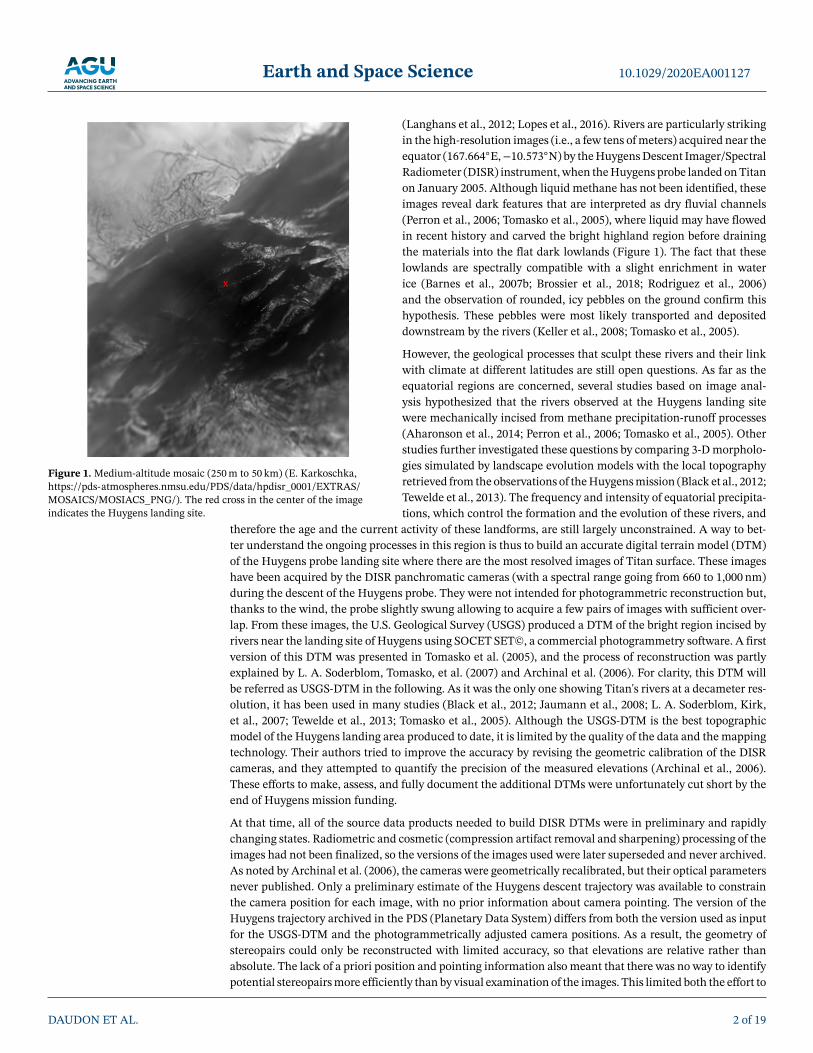
Figure 1. Medium-altitude mosaic (250 m to 50 km) (E. Karkoschka,https://pds-atmospheres.nmsu.edu/PDS/data/hpdisr_0001/EXTRAS/MOSAICS/MOSIACS_PNG/). The red cross in the center of the imageindicates the Huygens landing site.

(Langhans et al., 2012; Lopes et al., 2016). Rivers are particularly strikingin the high-resolution images (i.e., a few tens of meters) acquired near theequator (167.664◦E,−10.573◦N) by the Huygens Descent Imager/SpectralRadiometer (DISR) instrument, when the Huygens probe landed on Titanon January 2005. Although liquid methane has not been identified, theseimages reveal dark features that are interpreted as dry fluvial channels(Perron et al., 2006; Tomasko et al., 2005), where liquid may have flowedin recent history and carved the bright highland region before drainingthe materials into the flat dark lowlands (Figure 1). The fact that theselowlands are spectrally compatible with a slight enrichment in waterice (Barnes et al., 2007b; Brossier et al., 2018; Rodriguez et al., 2006)and the observation of rounded, icy pebbles on the ground confirm thishypothesis. These pebbles were most likely transported and depositeddownstream by the rivers (Keller et al., 2008; Tomasko et al., 2005).

However, the geological processes that sculpt these rivers and their linkwith climate at different latitudes are still open questions. As far as theequatorial regions are concerned, several studies based on image anal-ysis hypothesized that the rivers observed at the Huygens landing sitewere mechanically incised from methane precipitation-runoff processes(Aharonson et al., 2014; Perron et al., 2006; Tomasko et al., 2005). Otherstudies further investigated these questions by comparing 3-D morpholo-gies simulated by landscape evolution models with the local topographyretrieved from the observations of the Huygens mission (Black et al., 2012;Tewelde et al., 2013). The frequency and intensity of equatorial precipita-tions, which control the formation and the evolution of these rivers, and

therefore the age and the current activity of these landforms, are still largely unconstrained. A way to bet-ter understand the ongoing processes in this region is thus to build an accurate digital terrain model (DTM)of the Huygens probe landing site where there are the most resolved images of Titan surface. These imageshave been acquired by the DISR panchromatic cameras (with a spectral range going from 660 to 1,000 nm)during the descent of the Huygens probe. They were not intended for photogrammetric reconstruction but,thanks to the wind, the probe slightly swung allowing to acquire a few pairs of images with sufficient over-lap. From these images, the U.S. Geological Survey (USGS) produced a DTM of the bright region incised byrivers near the landing site of Huygens using SOCET SET©, a commercial photogrammetry software. A firstversion of this DTM was presented in Tomasko et al. (2005), and the process of reconstruction was partlyexplained by L. A. Soderblom, Tomasko, et al. (2007) and Archinal et al. (2006). For clarity, this DTM willbe referred as USGS-DTM in the following. As it was the only one showing Titan's rivers at a decameter res-olution, it has been used in many studies (Black et al., 2012; Jaumann et al., 2008; L. A. Soderblom, Kirk,et al., 2007; Tewelde et al., 2013; Tomasko et al., 2005). Although the USGS-DTM is the best topographicmodel of the Huygens landing area produced to date, it is limited by the quality of the data and the mappingtechnology. Their authors tried to improve the accuracy by revising the geometric calibration of the DISRcameras, and they attempted to quantify the precision of the measured elevations (Archinal et al., 2006).These efforts to make, assess, and fully document the additional DTMs were unfortunately cut short by theend of Huygens mission funding.

At that time, all of the source data products needed to build DISR DTMs were in preliminary and rapidlychanging states. Radiometric and cosmetic (compression artifact removal and sharpening) processing of theimages had not been finalized, so the versions of the images used were later superseded and never archived.As noted by Archinal et al. (2006), the cameras were geometrically recalibrated, but their optical parametersnever published. Only a preliminary estimate of the Huygens descent trajectory was available to constrainthe camera position for each image, with no prior information about camera pointing. The version of theHuygens trajectory archived in the PDS (Planetary Data System) differs from both the version used as inputfor the USGS-DTM and the photogrammetrically adjusted camera positions. As a result, the geometry ofstereopairs could only be reconstructed with limited accuracy, so that elevations are relative rather thanabsolute. The lack of a priori position and pointing information also meant that there was no way to identifypotential stereopairs more efficiently than by visual examination of the images. This limited both the effort to

DAUDON ET AL. 2 of 19

Earth and Space Science 10.1029/2020EA001127

Table 1Characteristics of the Images Selected to Reconstruct the IPGP-DTM

Image ID 414 420 450 462 471 541 553 601Camera HRI HRI HRI HRI HRI MRI MRI MRIAltitude (km) 16.7 16.7 14.5 14.1 12.8 10.1 9.9 7.4Average ground sampling (m/px) 17.8 17.8 15.5 15.1 13.7 21.4 21.0 15.0

map additional areas and the ability to improve the quality of a DTM by using multiple overlapping images.Finally, attempts to use the automatic image matching module of SOCET SET were unsuccessful because ofthe relatively low signal-to-noise level and the extremely small size of the DISR images. The USGS-DTM wasthus generated by visually identifying remarkable features. This process restricts the resolution of the DTMbecause areas that do not contain mappable features have been filled by interpolation. Unfortunately, theavailable output from SOCET SET includes only the resulting gridded DTM, not the record of the featuresactually measured. For all these reasons, it is difficult, or even impossible, to reproduce the USGS-DTM as isand to assess the impact of changing individual steps of the processing, because most of the input parametersare unavailable in their original form.

There are other reasons for concern that impact the use of the USGS-DTM to interpret the morphology andthe geology of the landing site. The dome shape of the bright highlands is particularly inconsistent with thedrainage patterns observed in the images. Such a topography should lead to a radial shape of the river net-work, while a dendritic one is observed. Moreover, because of this dome shape, some rivers flow in the wrongdirection (upstream), whereas most studies suggest a runoff from the bright highlands to the dark lowlands,which are considered as a dry riverbed or lakebed (Burr et al., 2013; Perron et al., 2006). These discrepanciesmay result from the difficulty of controlling the images (i.e., improving the knowledge of camera positionsand pointing given the limited starting data that were available) described above. As a result, it is likely thatthe overall USGS-DTM is not properly leveled, and because it was produced from overlapping stereopairs,the apparent dome could be the result of different leveling errors on the two sides. The limited resolution ofthe manually produced DTM also confounds efforts to assess the complete geometry of the stream courses.

All theses reasons led us to revisit the topographic mapping of the Huygens site. In addition to investigatethe apparent errors in the USGS-DTM, we will take advantage of recent advances in the processing of theHuygens data and the stereoanalysis softwares to generate a significantly improved DTM and, ultimately,to map a larger area of the landing site with additional stereopairs. We will also fully document our datasources, methodology, and final products so that others can reproduce or extend our work.

Since the USGS-DTM realization, recent postprocessing of the DISR images were performed (Figure 3) tocorrect both for the radiometric and geometric distortions (Karkoschka & Schröder, 2016; Karkoschka et al.,2007). A reestimate of the navigation data (SPICE kernels) is also available (Charles, 1996; ESA SPICE Ser-vice, 2019). The new DTM, hereafter called the IPGP-DTM, was built using MicMac, a free and open-sourcephotogrammetry software (Bretar et al., 2013; Pierrot-Deseilligny & Clery, 2011; Pierrot-Deseilligny &Paparoditis, 2006). MicMac applies a shape-from-motion (SfM) algorithm to generate large point clouds. Tomanipulate the Huygens images, which were originally not intended for photogrammetric reconstruction,a tailor-made reconstruction procedure was required. The strategy detailed in this article can be applied toany target with unusual photogrammetric conditions, for instance, when the parallax between images isvery small. In section 2, we present the DISR instrument and the new image processing. Section 3 detailsthe method used to build the IPGP-DTM, and in section 4 we compare the (new) IPGP-DTM to the (old)USGS-DTM and validate it against morphometric arguments.

2. New Processing of the DISR/Huygens Images2.1. The DISR Instrument and Images: Nominal Processing

The region of interest has been imaged by the DISR instrument, which observed the surface of Titan withunprecedented resolution near the equator (Table 1). The DISR downward-looking instruments includethree panchromatic cameras (Table 2): the Side-Looking Imager (SLI), the Medium-Resolution Imager(MRI), and the High-Resolution Imager (HRI). The light is transmitted from the lens system of each camera

DAUDON ET AL. 3 of 19

Earth and Space Science 10.1029/2020EA001127

Table 2Characteristics of the DISR Downward-Looking Instruments: High-Resolution Imager (HRI),Medium-Resolution Imager (MRI), and Side-Looking Imager (SLI) (Lebreton et al., 2005; Tomasko etal., 2002, 2003)

Camera Focal length (mm) Sensor size (mm) Zenith range (◦) Size (pixel)SLI 6.262 2.94 × 5.88 45.2–96 128 × 256MRI 10.841 4.05 × 5.88 15.8–46.3 176 × 256HRI 21.463 3.68 × 5.88 6.5–21.5 160 × 256

Note. The focal length is provided by Archinal et al. (2006), and the sensor size can be deducedfrom the size of the individual pixels/photosites found on the ESA PSA website (https://sci.esa.int/cassini-huygens/31193-instruments/?fbodylongid=734).

to a shared charge-coupled device (CCD) through optical fiber bundles. The optical fiber ribbons are con-tained in independent conduits; therefore, each camera can be treated as a separate sensor throughout theDTM reconstruction pipeline (Figure 2).

Half of the DISR images are missing due to the loss of one of the two radio transmission channels in the probereceiver on board the orbiter (Karkoschka & Schröder, 2016; Lebreton et al., 2005; Tomasko et al., 2005).Nevertheless, about 300 images of the surface of Titan are available at a resolution ranging from ∼3 mm to∼1 km. The aerosol haze was too thick to discern the surface in the first 25 min of the descent of Huygens,but the landscape started to be visible at an altitude of about 50 km.

Before their transmission to Earth, onboard processing operations including flat-field correction, darksubtraction, and replacement of bad pixels were carried out. Unfortunately, image artifacts have beenintroduced on this occasion. The most significant comes from the use of prelaunch, embedded algo-rithms dedicated to the flat-field correction. The displacement of the fiber optic bundle during launch,entry, and descent greatly changed the response of the flat fields (Figure 2). The application of prelaunchreduction algorithms consequently ended in a significant degradation of the overall quality of the images(DISR Data User's Guide, https://pds-atmospheres.nmsu.edu/PDS/data/hpdisr_0001/DOCUMENT/DISR_SUPPORTING_DOCUMENTS/DISR_DATA_USERS_GUIDE/DISR_DATA_USERS_GUIDE_3.PDF).

Another issue concerns the irreversible image compression before transmission to Earth. The images werefirst converted from 12 bits to 8 bits using a look-up table similar to a square root transformation. Then theywere compressed on board with a discrete cosine transform (DCT) algorithm. This transform is equivalentto a JPEG compression, a lossy operation that discards small valued coefficients. Although the loss waslower than the noise in most images, it was significant in some images with a high information content(Karkoschka & Schröder, 2016).

Figure 2. Flat field of (a) the HRI camera and (b) the MRI camera, showing the response of the instrument to uniform illumination. The “chicken wire”pattern is due to the seams between individual fiber optic strands (DISR Data User's Guide). (c) The DISR instrument looking out of the Huygens probe. Thethree viewing directions of the imagers (HRI, MRI, and SLI) are shown (University of Arizona).

DAUDON ET AL. 4 of 19

Earth and Space Science 10.1029/2020EA001127

Figure 3. Comparison of five generations of images (Image #414): (a) Raw image photometrically stretched. (b) Imagecorrected for flat-field, dark, bad pixels, and electronic shutter effect. (c) Image further processed to removecompression-induced artifacts and to adjust for geometric distortions. (d) Image with undocumented postprocessingused to produce the USGS-DTM. (e) Enhanced image obtained with the new processing and used to produce theIPGP-DTM (Karkoschka & Schröder, 2016).

2.2. Decompression and Postprocessing

The DISR images are decompressed and postprocessed after transmission to Earth: (1) Their photomet-ric stretch is square root expanded to restore the 12-bit depth, (2) they are flat-field corrected to eliminatethe photometric distortions of the cameras, (3) the dark current is removed using the camera model at theexposure temperature, (4) the electronic shutter effect caused by data clocking is compensated for, (5) theimages are further flat fielded to remove artifacts seen at the highest altitudes (flat, homogeneous upperatmosphere), (6) the stretch is enhanced to increase the dynamics, and (7) the bad pixels are replaced bytheir neighbors. The images have also been processed so as to remove compression artifacts and adjusted forgeometric distortions of the camera optics and refraction from the atmosphere (see supporting informationFigure S1).

In an early version of the DISR data set, the decompressed pixel values were rounded to the nearest inte-ger before applying an inverse square root, which led to a significant information loss. The new imageprocessing has corrected these errors and removed the residual radiometric artifacts (e.g., Karkoschka, 2016;

DAUDON ET AL. 5 of 19

Earth and Space Science 10.1029/2020EA001127

Figure 4. Position and orientation of the HRI and MRI cameras at theshooting time of the eight selected images, extracted from the SPICEkernels (ESA SPICE Service, 2019), and images footprint. The focal lengthsare enlarged by a factor of 300, and the coordinates are expressed in metersin a local tangent frame (Appendix A).

Karkoschka & Schröder, 2016; Karkoschka et al., 2007). Indeed, the stan-dard decompression scheme produced images that consist of certainspatial frequencies in each 16 × 16 pixel block with noticeable bound-aries between adjacent blocks. In many images, artifacts generated bythe compression were more apparent than real features on the surfaceof Titan. That problem was fixed by smoothing high spatial frequen-cies (Karkoschka et al., 2007). The method was recently improved byKarkoschka and Schröder (2016) who use a lower degree of smoothingso the new images display significant radiometric and geometric differ-ences compared to those used to build the USGS-DTM (L. A. Soderblom,Tomasko, et al., 2007; Tomasko et al., 2005). Note that the latter havebeen also postprocessed, but the method used is not documented. Theimages with the most up-to-date corrections are used to reconstruct theIPGP-DTM (Figure 3e).

3. Building the IPGP-DTM3.1. Image Selection and Navigation Data

Eight stereoscopic images (#414, #420, #450, #462, #471, #541, #553,and #601) were selected for the photogrammetric reconstruction (seesupporting information Figure S2) of the IPGP-DTM owing to their opti-mal areas of overlap and resolutions (Table 1). Half of them were usedto generate the USGS-DTM (#414, #450, #553, and #601). We only pro-cessed those acquired by the HRI and MRI cameras because the coarsersurface resolution and the higher emission angles of the SLI camera werenot suitable for DTM reconstruction. The HRI camera acquired imageswith the largest focal length and from the highest altitude compared tothe MRI camera (Figure 4). Such a configuration enabled us to use thetwo cameras because the average ground sampling is similar for both ofthem (Table 1).

Due to the presence of a thick haze layer in Titan's atmosphere, theimages acquired between 50- and 30-km altitudes were too blurry for pho-togrammetric reconstruction. Below, the wind was weak (4 m/s) and thedescent almost straight with a slight lateral drift (Karkoschka et al., 2007;

Tomasko et al., 2005). Such a geometry is definitely not optimal for photogrammetric reconstruction becauseof low image overlap, variable pixel size, and very small B/H ratio (the distance B between two camera pointof views compared to the altitude H) (Figure 4).

The position and orientation of the Huygens probe during the descent were first computed by the HuygensDescent Trajectory Working Group (DTWG). The positions are given with an uncertainty of the order of0.24◦ in longitude, 0.17◦ in latitude, and ranging from 0.05 to 8.3 km in altitude. They have been reestimatedby the ESA SPICE Service. The Spacecraft Ephemeris Kernel (SPK) containing the position and velocity ofthe probe during the descent were generated using data from the DTWG (Kazeminejad & Atkinson, 2004;Kazeminejad et al., 2011). They were computed by numerical integration of the equations of motion, provid-ing the position of the probe in spherical coordinates with respect to the Titan centered fixed frame, togetherwith the altitude derivative with time. The finite difference method provided good results for the velocityvectors thanks to the high time resolution of the data. Finally, a polynomial interpolation was performedbetween datapoints for the creation of the kernel.

For the generation of the Camera Kernel (CK) that contains the attitude of the probe, thus the pointingdirection of the cameras, the body angles of the probe were reconstructed with the geometry derived from theDISR images provided by Karkoschka et al. (2007). Lastly, in order to smooth the evolution of the data points,the spin rate from housekeeping data was introduced in the calculations and used to write another CK,which implements the actual angular rate with the exact attitude of the probe at each moment of shooting.The Frame Kernel (FK) and Instrument Kernel (IK) that complement the CK have been defined accordingto the standard fixed frames and parameters of the probe provided by the Huygens User manual.

DAUDON ET AL. 6 of 19

Earth and Space Science 10.1029/2020EA001127

Figure 5. Diagrams of a typical reconstruction workflow for (a) an “architectural” scenario and (b) a “drone” scenario. (c) Summary diagram of the specificIPGP-DTM extraction workflow. GCP refers to ground control points. The MicMac commands are noted in quotation marks along with the corresponding stepsin the workflows.

3.2. IPGP-DTM Construction Using MicMac

The construction of the IPGP-DTM was carried out with MicMac, a free and open-source photogram-metry suite developed by IGN (Institut National de l'Information Géographique et Forestière) and ENSG(Ecole Nationale des Sciences Géographiques) (Bretar et al., 2013; Pierrot-Deseilligny & Clery, 2011;Pierrot-Deseilligny & Paparoditis, 2006). We selected MicMac because it allows a large degree of freedomin the sensor models and in the 3-D reconstruction strategies, which makes it a relevant tool for our appli-cation. Since the images and the geometries of acquisition are not optimal, it is important to control theparameters at each stage of the reconstruction. MicMac also incorporates a correlator that proved to be morereliable and robust than in other photogrammetry softwares (Rosu et al., 2015). Another important issue isthat any user can reproduce the IPGP-DTM.

Regarding our particular data set, we developed a specific workflow. Indeed, we are in a particular case at acrossroads between two typical scenarios:

• the “architectural” scenario, which tries to reconstruct a complex structure and usually deals withdifferent focal lengths of the same camera in order to capture all the details of the studied structure.

• the “drone” scenario, where images are acquired by a short focal length camera on board a drone withinaccurate GPS data.

These two scenarios can be easily handled by MicMac following a classical pipeline (Figure 5). Yet our dataset is a mix of the two scenarios with different focal lengths and imprecise navigation data. Moreover, the

DAUDON ET AL. 7 of 19

Earth and Space Science 10.1029/2020EA001127

Figure 6. Example of homologous points found between two image pairs by the SIFT correlator of MicMac: in yellow,between #MRI601 and #MRI541 (79 points) and in red, between #MRI601 and #HRI414 (29 points).

parallax of our images is small, and we are working with two different cameras. We therefore could not applyan existing workflow and had to develop an entirely new procedure for this particular data set (Figure 5).This workflow can be extended to any case where the camera configuration is complex (low parallax andoverlap, imprecise navigation data, no ground control points [GCP], etc.).

Batch commands can be run from a command line, and the three main steps of the photogrammetric recon-struction (homologous points search, absolute orientation, and depth map construction) are divided intosix substeps corresponding to different commands (Figure 5). The entire reconstruction process is fast (i.e.,about 5 min on a dual socket Xeon workstation) on small images (five images 256 × 160 pixels and threeimages 256 × 176 pixels).3.2.1. Homologous Points SearchThe first step consists in applying the SIFT correlation algorithm to find homologous points between eachimage pairs (Lowe, 2004). MicMac applies SfM techniques (Bretar et al., 2013); that is, it works with multi-view stereo images. To maximize the number of points, we look for the homologous points of each pixel ofthe images without degrading the resolution of the images. Depending on the image pair (Figure 6), between10 and 80 points are detected. Their high density and their homogeneous distribution are a prerequisite foran optimal DTM reconstruction. Considering the low contrast and low texture of the images, especially inthe dark area, the number and distribution of homologous points are satisfying. In comparison, we also triedto search homologous point with SOCET SET and found only three points with these new images.3.2.2. Orientation and Position of the CamerasThe second step aims to find the orientation and the position of the cameras as the images were acquired.It is the most delicate stage. Indeed, although the SPICE kernels predicting the Huygens probe position andorientation during the descent have been recently recomputed, the altitude and the attitude are determinedwith an accuracy larger than 0.24◦ in longitude and 0.17◦ in latitude, which is inadequate for photogram-metry reconstruction. Thus, given the poor quality of the images and the low constraints on the cameraposition and orientation, this stage must be performed carefully.

The absolute orientation of the sensor is generally found by MicMac in two stages. The first is the internalcalibration that computes a relative orientation using only the images; it provides an initial estimate ofthe position and the orientation of the optical center in any reference frame, allowing a reestimation ofthe sensor parameters such as the focal length, the boresight position and orientation, and the distortionparameters. Then, one can provide the absolute orientation that consists in replacing the nongeoreferenceddata computed by the relative orientation by the georeferenced data. In our case, four substeps are requiredto achieve the final orientation: one for the relative orientation, two for the absolute orientation, and one forthe orientation refinement. At the end, the absolute positions and orientations of the cameras at the time ofshooting are provided for the eight selected DISR images in a local tangent frame (Appendix A).

DAUDON ET AL. 8 of 19

Earth and Space Science 10.1029/2020EA001127

Figure 7. (a) Orthorectified mosaic of the selected DISR image (i.e., projected mosaic accounting for the relief) buildby MicMac. (b) Orthorectified image masked according to the correlation score and the EP value (see section 3.2.4).The shoreline is depicted by a yellow dotted line, the ground control points are represented by cyan triangles, and themajor rivers are drawn as red lines. The coordinates (in m) are in a local tangent frame (Appendix A).

After several tests, we decided to discard the internal calibration during the relative orientation becausereestimating these parameters using poor-quality images is unreliable. We consequently trusted the preex-isting calibration of the sensors using the focal lengths and the sensor size found in the DISR User Guide.If not, this step does not converge. However, a first estimation of the position of the optical center and theorientation of the optical axis is carried out during this stage using the images. This step is not essential tocompute the final orientation but necessary for MicMac to calculate the absolute orientation.

Then, the absolute orientation is determined in two steps. The first one aims to compensate between therelative orientation and the positions provided by the SPICE kernels, which means that it applies a 3-Dhomothety (rotation, translation, and scaling) to the preexisting relative orientation. This first step is nec-essary in order to switch to field coordinates because no preexisting cartography is at our disposal. Thesecond one consists of fixing GCP, the field coordinates of which are known, in order to externally constrainthe global orientation. Even if the absolute field coordinates of the site are unknown, some GCPs can bedefined with a priori knowledge of the landscape. For instance, several studies asserted that the boundarybetween the dark and bright areas observed in the Huygens landing site (Figure 7) was a remnant shoreline(e.g., Perron et al., 2006; L. A. Soderblom, Tomasko, et al., 2007; Tomasko et al., 2005). We therefore choseto set GCP on the shoreline by imposing on them the same relative elevation (i.e., the shoreline being anequipotential). This second step allows to constrain and improve the orientation, as shown by the projectedorthoimages taking into account this new orientation and position of the cameras (Figure 8).

Finally, we performed a bundle adjustment to refine the position and the orientation of the cameras byunlocking the distortion parameters. This technique allows to simultaneously reestimate the coordinates ofthe 3-D points (i.e., the GCP) and the camera positions. To do so, it minimizes the root-mean-square error

Figure 8. (a) Orthorectified mosaic obtained by projecting DISR images using the positions and orientations from theSPICE kernels only, (b) orthorectified mosaic obtained from the position and orientation of the cameras computedthrough the pipeline presented in this work but without using GCP (see Figure 5), and (c) orthorectified mosaicobtained with the final position and orientation computed through the entire pipeline (and thus, using GCP).

DAUDON ET AL. 9 of 19

Earth and Space Science 10.1029/2020EA001127

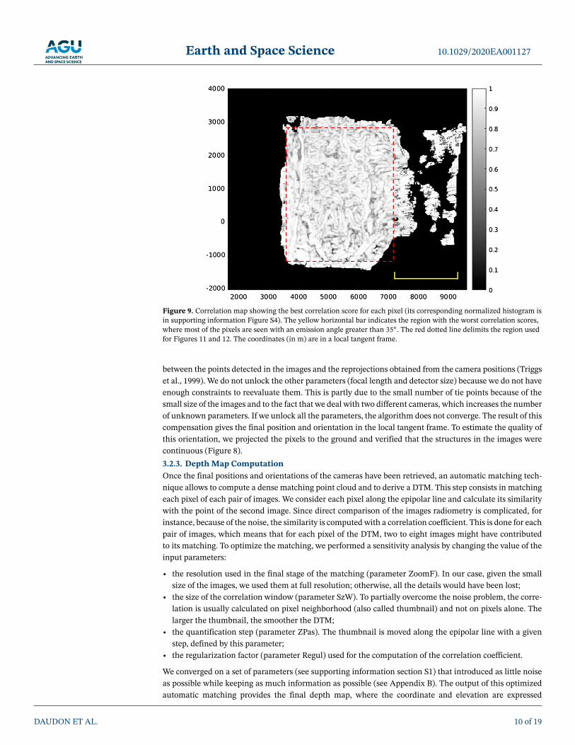
Figure 9. Correlation map showing the best correlation score for each pixel (its corresponding normalized histogram isin supporting information Figure S4). The yellow horizontal bar indicates the region with the worst correlation scores,where most of the pixels are seen with an emission angle greater than 35◦. The red dotted line delimits the region usedfor Figures 11 and 12. The coordinates (in m) are in a local tangent frame.

between the points detected in the images and the reprojections obtained from the camera positions (Triggset al., 1999). We do not unlock the other parameters (focal length and detector size) because we do not haveenough constraints to reevaluate them. This is partly due to the small number of tie points because of thesmall size of the images and to the fact that we deal with two different cameras, which increases the numberof unknown parameters. If we unlock all the parameters, the algorithm does not converge. The result of thiscompensation gives the final position and orientation in the local tangent frame. To estimate the quality ofthis orientation, we projected the pixels to the ground and verified that the structures in the images werecontinuous (Figure 8).3.2.3. Depth Map ComputationOnce the final positions and orientations of the cameras have been retrieved, an automatic matching tech-nique allows to compute a dense matching point cloud and to derive a DTM. This step consists in matchingeach pixel of each pair of images. We consider each pixel along the epipolar line and calculate its similaritywith the point of the second image. Since direct comparison of the images radiometry is complicated, forinstance, because of the noise, the similarity is computed with a correlation coefficient. This is done for eachpair of images, which means that for each pixel of the DTM, two to eight images might have contributedto its matching. To optimize the matching, we performed a sensitivity analysis by changing the value of theinput parameters:

• the resolution used in the final stage of the matching (parameter ZoomF). In our case, given the smallsize of the images, we used them at full resolution; otherwise, all the details would have been lost;

• the size of the correlation window (parameter SzW). To partially overcome the noise problem, the corre-lation is usually calculated on pixel neighborhood (also called thumbnail) and not on pixels alone. Thelarger the thumbnail, the smoother the DTM;

• the quantification step (parameter ZPas). The thumbnail is moved along the epipolar line with a givenstep, defined by this parameter;

• the regularization factor (parameter Regul) used for the computation of the correlation coefficient.

We converged on a set of parameters (see supporting information section S1) that introduced as little noiseas possible while keeping as much information as possible (see Appendix B). The output of this optimizedautomatic matching provides the final depth map, where the coordinate and elevation are expressed

DAUDON ET AL. 10 of 19

Earth and Space Science 10.1029/2020EA001127

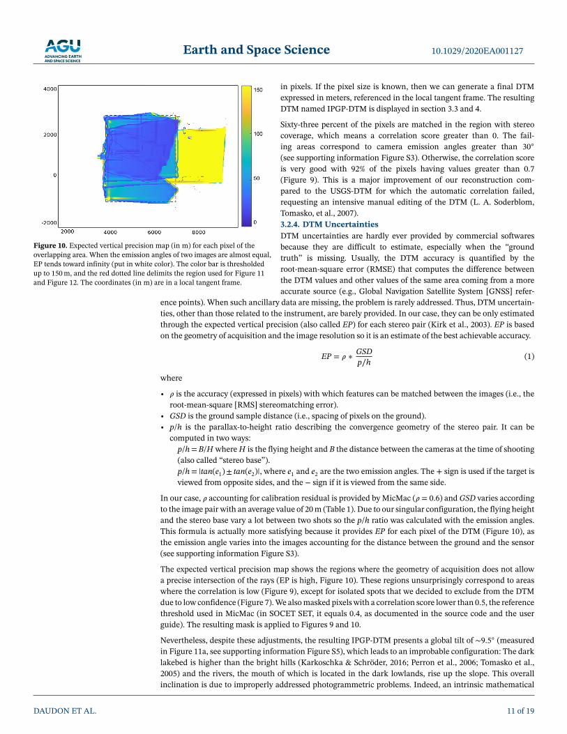
Figure 10. Expected vertical precision map (in m) for each pixel of theoverlapping area. When the emission angles of two images are almost equal,EP tends toward infinity (put in white color). The color bar is thresholdedup to 150 m, and the red dotted line delimits the region used for Figure 11and Figure 12. The coordinates (in m) are in a local tangent frame.

in pixels. If the pixel size is known, then we can generate a final DTMexpressed in meters, referenced in the local tangent frame. The resultingDTM named IPGP-DTM is displayed in section 3.3 and 4.

Sixty-three percent of the pixels are matched in the region with stereocoverage, which means a correlation score greater than 0. The fail-ing areas correspond to camera emission angles greater than 30◦

(see supporting information Figure S3). Otherwise, the correlation scoreis very good with 92% of the pixels having values greater than 0.7(Figure 9). This is a major improvement of our reconstruction com-pared to the USGS-DTM for which the automatic correlation failed,requesting an intensive manual editing of the DTM (L. A. Soderblom,Tomasko, et al., 2007).3.2.4. DTM UncertaintiesDTM uncertainties are hardly ever provided by commercial softwaresbecause they are difficult to estimate, especially when the “groundtruth” is missing. Usually, the DTM accuracy is quantified by theroot-mean-square error (RMSE) that computes the difference betweenthe DTM values and other values of the same area coming from a moreaccurate source (e.g., Global Navigation Satellite System [GNSS] refer-

ence points). When such ancillary data are missing, the problem is rarely addressed. Thus, DTM uncertain-ties, other than those related to the instrument, are barely provided. In our case, they can be only estimatedthrough the expected vertical precision (also called EP) for each stereo pair (Kirk et al., 2003). EP is basedon the geometry of acquisition and the image resolution so it is an estimate of the best achievable accuracy.

EP = 𝜌 ∗ GSDp∕h

(1)

where

• 𝜌 is the accuracy (expressed in pixels) with which features can be matched between the images (i.e., theroot-mean-square [RMS] stereomatching error).

• GSD is the ground sample distance (i.e., spacing of pixels on the ground).• p/h is the parallax-to-height ratio describing the convergence geometry of the stereo pair. It can be

computed in two ways:p/h = B/H where H is the flying height and B the distance between the cameras at the time of shooting(also called “stereo base”).p/h = |tan(e1)± tan(e2)|, where e1 and e2 are the two emission angles. The + sign is used if the target isviewed from opposite sides, and the − sign if it is viewed from the same side.

In our case, 𝜌 accounting for calibration residual is provided by MicMac (𝜌 = 0.6) and GSD varies accordingto the image pair with an average value of 20 m (Table 1). Due to our singular configuration, the flying heightand the stereo base vary a lot between two shots so the p/h ratio was calculated with the emission angles.This formula is actually more satisfying because it provides EP for each pixel of the DTM (Figure 10), asthe emission angle varies into the images accounting for the distance between the ground and the sensor(see supporting information Figure S3).

The expected vertical precision map shows the regions where the geometry of acquisition does not allowa precise intersection of the rays (EP is high, Figure 10). These regions unsurprisingly correspond to areaswhere the correlation is low (Figure 9), except for isolated spots that we decided to exclude from the DTMdue to low confidence (Figure 7). We also masked pixels with a correlation score lower than 0.5, the referencethreshold used in MicMac (in SOCET SET, it equals 0.4, as documented in the source code and the userguide). The resulting mask is applied to Figures 9 and 10.

Nevertheless, despite these adjustments, the resulting IPGP-DTM presents a global tilt of ∼9.5◦ (measuredin Figure 11a, see supporting information Figure S5), which leads to an improbable configuration: The darklakebed is higher than the bright hills (Karkoschka & Schröder, 2016; Perron et al., 2006; Tomasko et al.,2005) and the rivers, the mouth of which is located in the dark lowlands, rise up the slope. This overallinclination is due to improperly addressed photogrammetric problems. Indeed, an intrinsic mathematical

DAUDON ET AL. 11 of 19

Earth and Space Science 10.1029/2020EA001127

Figure 11. (a) DTM resulting from MicMac reconstruction (global tilt of about 9.5◦). (b) Same DTM after a rotation of−10◦ along the y axis and 3◦ along the x axis. Both DTM are superimposed on their corresponding orthorectifiedmosaics (with transparency). White and neutral gray patches on (a) are due to NoData values in the DTM (due tomasking process) that take the color of the superimposed orthoimage (they do not appear in panel b because thesevalues have been reinterpolated during the rotation process). Color bars show the DTM elevations (in meters) and thecoordinates (in meters) are in a local tangent frame.

indeterminacy affects the global orientation of the IPGP-DTM plane. A reason is the nonoptimal positionsand orientations of the DISR cameras at the acquisition time and by the alignment of the GCP (Figure 7).Note that the global tilt of the IPGP-DTM does not affect the high-frequency topography (i.e., the relativelocal slopes). Thus, it is necessary to find an alternative method to solve for the global inclination of thescene, independent of the photogrammetric reconstruction software.

3.3. Determination of the IPGP-DTM Tilt

The last step of the workflow consists in finding the overall inclination of the IPGP-DTM. As no other topo-graphic data derived from the Cassini mission can help constrain the global tilt of the IPGP-DTM, a newstrategy should be adopted. The USGS scientists fixed this problem by setting the elevation of lakebed in theUSGS-DTM to 0, assuming that there is no global slope. To avoid making any prior assumption concerningthe global inclination, we determined the tilt using morphological information and river routing. Routing iscommonly used in hydrology to determine the natural route taken by a liquid over a given topography. Ide-ally, a liquid flowing on the IPGP-DTM should choose the same path as the one followed by the rivers seenin the images. Thus, the idea is to compare this routing with the actual location of the rivers (Burr et al.,2013; Perron et al., 2006; L. A. Soderblom, Tomasko, et al., 2007; Tomasko et al., 2005). The tilt correspond-ing to the best match will be considered as the optimal one. This original method is completely new and hasbeen developed for this particular study. Nevertheless, it could be apply to any case where there is a lack ofGCP as long as the DTM includes rivers (or other morphological features bringing external constraints).

We considered that the flow path remained unchanged and that the rivers should flow downhill. Note thatwe can reasonably consider that the formation of the landscape in this region is due to recent erosion withlittle to no contribution from uplift. Indeed, during the 13 years of the mission, the Cassini spacecraft hasobserved two superstorms at the equator (Turtle et al., 2011). Their large extent (more than 500,000 km2)and the proximity of one of them to the Huygens landing site (about nearly 50◦ to the west) sign that recentrains may occur in this region.

The strategy therefore consists in (i) rotating the IPGP-DTM produced with MicMac along the x axisand y axis, from −20◦ to +20◦ with a 1◦ step, (ii) calculating the routing using the Matlab TopoToolBox(Schwanghart & Scherler, 2014; Tarboton, 1997), and (iii) comparing it to a river mask produced using theorthorectified mosaic (Figure 7). To minimize misinterpretation, three masks were manually drawn by dif-ferent operators, and we kept their intersection as the final one. For this comparison, we only focused onthe major rivers to the right of the scene (outlined in red in Figure 7), leaving aside the shorter and stubbierrivers to the left that are not discernible enough.

DAUDON ET AL. 12 of 19

Earth and Space Science 10.1029/2020EA001127

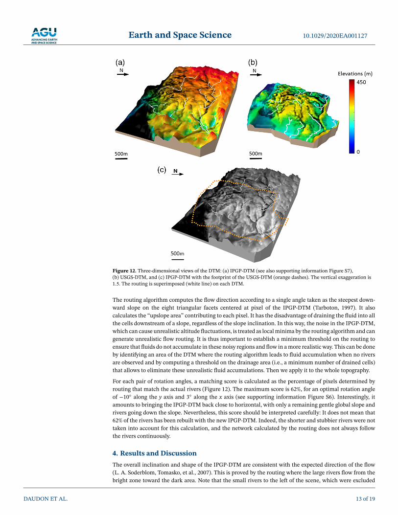
Figure 12. Three-dimensional views of the DTM: (a) IPGP-DTM (see also supporting information Figure S7),(b) USGS-DTM, and (c) IPGP-DTM with the footprint of the USGS-DTM (orange dashes). The vertical exaggeration is1.5. The routing is superimposed (white line) on each DTM.

The routing algorithm computes the flow direction according to a single angle taken as the steepest down-ward slope on the eight triangular facets centered at pixel of the IPGP-DTM (Tarboton, 1997). It alsocalculates the “upslope area” contributing to each pixel. It has the disadvantage of draining the fluid into allthe cells downstream of a slope, regardless of the slope inclination. In this way, the noise in the IPGP-DTM,which can cause unrealistic altitude fluctuations, is treated as local minima by the routing algorithm and cangenerate unrealistic flow routing. It is thus important to establish a minimum threshold on the routing toensure that fluids do not accumulate in these noisy regions and flow in a more realistic way. This can be doneby identifying an area of the DTM where the routing algorithm leads to fluid accumulation when no riversare observed and by computing a threshold on the drainage area (i.e., a minimum number of drained cells)that allows to eliminate these unrealistic fluid accumulations. Then we apply it to the whole topography.

For each pair of rotation angles, a matching score is calculated as the percentage of pixels determined byrouting that match the actual rivers (Figure 12). The maximum score is 62%, for an optimal rotation angleof −10◦ along the y axis and 3◦ along the x axis (see supporting information Figure S6). Interestingly, itamounts to bringing the IPGP-DTM back close to horizontal, with only a remaining gentle global slope andrivers going down the slope. Nevertheless, this score should be interpreted carefully: It does not mean that62% of the rivers has been rebuilt with the new IPGP-DTM. Indeed, the shorter and stubbier rivers were nottaken into account for this calculation, and the network calculated by the routing does not always followthe rivers continuously.

4. Results and DiscussionThe overall inclination and shape of the IPGP-DTM are consistent with the expected direction of the flow(L. A. Soderblom, Tomasko, et al., 2007). This is proved by the routing where the large rivers flow from thebright zone toward the dark area. Note that the small rivers to the left of the scene, which were excluded

DAUDON ET AL. 13 of 19

Earth and Space Science 10.1029/2020EA001127

from the score calculation, also flow in the right direction from the highlands to the riverbed (see Figure 12and supporting information Figure S7).

However, some areas display a suspicious morphology. For instance the edges of the IPGP-DTM, which wedid not mask because of high correlation scores, are very steep. Since such slopes (up to 80◦) are not observedon Earth at such small scales, the accuracy of the IPGP-DTM in these regions is questionable. Moreover, therouting does not well match the rivers in these regions that display the highest EP values, in particular theregion for y< 0, which is 2 to 3 times higher than in the center of the DTM (Figure 10). As a consequence,we advise users to always refer to the EP map when using the IPGP-DTM.

The first improvement of the IPGP-DTM concerns the size of the reconstructed region, which is largerthan the USGS-DTM (10.3 km2 vs. 7.5 km2) because we used more images. The horizontal sampling of theIPGP-DTM is also better (18 m/px vs. 50 m/px).

The flow direction on the topography of both DTM was calculated in the same way using the TopoTool-Box routine. Since they do not have the same size and resolution, we cannot apply the same threshold forrouting, nevertheless we applied the same method to determine it. The resulting matching score is 35% ifwe compute it on the original USGS-DTM (L. A. Soderblom, Tomasko, et al., 2007). It is worth noting that,since the orientation of the USGS-DTM was manually clipped to 0, we tried to find out if we could findan optimal orientation as we did for the IPGP-DTM. Therefore, we rotated the USGS-DTM in order to findthe best matching score, as done with the IPGP-DTM, and found a score of 56%. This score correspond to arotation angle of 4◦ along the y axis and 3◦ along the x axis, which means that the global slope was under-estimated, and by slightly tilting the USGS-DTM, we find a more coherent configuration with regard tothe shape and location of the routing (see supporting information Figure S8). However, with this rotation,the land at the bottom right of Figure S4 is at the same elevation as the lakebed at the bottom left, whichis questionable.

If we consider the original USGS-DTM (no inclination) used in previous studies (Jaumann et al., 2008;Tewelde et al., 2013; Tomasko et al., 2005), the routing shapes calculated from the two DTM are very dif-ferent. The USGS-DTM provides a radial shape routing, while the IPGP-DTM provides a rather dendriticor rectangular shape. According to the literature (Burr et al., 2013; Perron et al., 2006) and even by simplevisual inspection, the networks observed in our region of interest have dendritic or rectangular shapes. Asa consequence the IPGP-DTM seems to provide a better representation of the local topography.

The last comparison consists in analyzing several river profiles and transects/cross sections in order to checkif the inclination of the rivers is consistent with the theoretical direction of flow and if the rivers, carvedby liquid hydrocarbons, form depressions. As far as the cross sections are concerned, the river bottoms aregenerally located on flat areas or in depressions for both DTM, except in a few cases where the rivers arelocated on slopes (Figure 13). However, it is worth to note that, due to a coarser resolution, the USGS-DTMhas only one manual measurement point per river transect compared to an average of three points for theIPGP-DTM. As for the river profiles, the flow of the main river (Profile C-C' in green in Figure 13) followsthe expected flow direction in the case of the IPGP-DTM as opposed to the USGS-DTM, where the channelflows in the wrong direction.

5. ConclusionNew investigation of the topography around the Huygens landing site has been successfully carried out.We developed a new strategy that could overcome the high complexity of the data set, unusual even forplanetary data, and provided a fully documented and reproducible workflow. This procedure could beapply in situations with such a complex data set. For instance, it could be applied both to poorly knownand hard-to-reach terrestrial areas (i.e., Antarctica) and to archive data from former planetary missions(i.e., Voyager and Galileo). Besides a new strategy, the article provides a new DTM with a higher spatial sam-pling and a more reliable topography since it is much less interpolated than the previous product. This DTMoffers new opportunities for investigating the topography of fluvial landscape at Titan's equatorial regionwith an unprecedented resolution. It could bring new insights on Titan's landscape formation mechanismsby quantitatively characterizing the morphometry of these rivers and the topography of their associateddrainage basins.

DAUDON ET AL. 14 of 19

Earth and Space Science 10.1029/2020EA001127

Figure 13. Orthorectified mosaics calculated from (a) the IPGP-DTM and (b) the USGS-DTM. We display twocross-sectional profiles (c and d) and a profile along a river (e). The horizontal axis of the graphs represents the lengthof the transect and the vertical axis represents the altitude (in meters). The darker colors in each graph represent thecross sections and follow-ups of the USGS-DTM, while the lighter colors correspond to those of the IPGP-DTM. Thedark red arrows refer to the valley bottoms visible on the orthorectified mosaics of USGS-DTM, and the light redarrows correspond to those of our orthorectified mosaics. The two orthorectified images (and therefore the arrows) areoffset because the topography of the two DTMs are not identical.

Appendix A: Local Tangent Plane definitionThe local tangent plane (LTP) is an orthogonal, rectangular, reference system, the origin of which is definedat an arbitrary point on the planet surface (here we took the nadir of the Image #450 located at (167.64370◦E,−10.577749◦N)). Among the three coordinates one represents the position along the northern axis, one alongthe local eastern axis, and the last one is the vertical position. If (𝜆, 𝜙, h) are the coordinates of a given point

DAUDON ET AL. 15 of 19

Earth and Space Science 10.1029/2020EA001127

Figure B1. (a) Orthorectified mosaic calculated from the IPGP-DTM. We display the cross-sectional profile of the river(in orange on the orthoimage) and change the value of each parameters for each panel. On every plot, the orange linerepresent the profile of the final DTM, and the other line is the profile of the DTM with a different parameter (the unitfor both axes is the meter). (b) The dark blue line is the profile of the DTM for a smaller final resolution value, (c) thedark green plot for a smaller size correlation window, (d) the dark line correspond to a higher quantification step, and(e) the blue plot is for a larger regularization factor. The dashed red line refers to the valley bottoms visible on theorthorectified mosaics of DTM.

DAUDON ET AL. 16 of 19

Earth and Space Science 10.1029/2020EA001127

in the geographical frame, the coordinates (xt,yt,zt) of the LTP are defined as follows:

⎛⎜⎜⎝

xt𝑦tzt

⎞⎟⎟⎠=⎛⎜⎜⎝

−sin(𝜙) cos(𝜙) 0−cos(𝜙)sin(𝜆) −sin(𝜆)sin(𝜙) cos(𝜆)cos(𝜆)cos(𝜙) cos(𝜆)sin(𝜙) sin(𝜆)

⎞⎟⎟⎠·⎛⎜⎜⎝

x − x0𝑦 − 𝑦0z − z0

⎞⎟⎟⎠

with:

• (x,y,z) the Cartesian coordinates of the given point• (x0,y0,z0) the Cartesian coordinates of our reference point

Appendix B: Dense Pixel Matching ParametersA sensitivity analysis has been performed on all the parameters of the dense pixel matching step. The param-eters selection was done manually, by changing their value in order to keep most of the details while reducingthe noise level. As observed on the Figure B1, a smaller final resolution and a bigger quantification step andregularization factor tend to smooth the DTM and cannot detect the bottom of the rivers. On the contrary,a smaller size of correlation window tends to noise the DTM.

Data Availability StatementMicMac software can be downloaded for free (https://micmac.ensg.eu/index.php/Accueil), and the SPICEkernels are publicly available (https://doi.org/10.5270/esa-ssem3np). The DTM and other products resultingfrom this work are available online (https://doi.org/10.5270/esa-3uja374).

ReferencesAharonson, O., Hayes, A. G., Lopes, R., Lucas, A., Hayne, P., & Perron, J. T. (2014). Titan: Surface, atmosphere and magnetosphere

(pp. 43–75). Cambridge: Cambridge University Press.Archinal, B. A., Tomasko, M. G., Rizk, B., Soderblom, L. A., Kirk, R. L., Howington-Kraus, E., et al. (2006). Photogrammetric analysis of

Huygens DISR images of Titan. ISPRS.Atreya, S. K., Adams, E. Y., Niemann, H. B., Demick-Montelara, J. E., Owen, T. C., Fulchignoni, M., et al. (2006). Titan's methane cycle.

Planetary and Space Science, 54(12), 1177–1187.Barnes, J. W., Brown, R. H., Soderblom, L. A., Buratti, B. J., Sotin, C., Rodriguez, S., et al. (2007b). Global-scale surface spectral variations

on Titan seen from Cassini/VIMS. Icarus, 186(1), 242–258.Barnes, J. W., Brown, R. H., Soderblom, L. A., Sotin, C., Le Mouèlic, S., Rodriguez, S., et al. (2008). Spectroscopy, morphometry, and

photoclinometry of Titan's dunefields from Cassini/VIMS. Icarus, 195(1), 400–414.Barnes, J. W., Radebaugh, J., Brown, R. H., Wall, S., Soderblom, L. A., Lunine, J., et al. (2007). Near-infrared spectral mapping of Titan's

mountains and channels. Journal of Geophysical Research, 112, E11006. https://doi.org/10.1029/2007JE002932Black, B. A., Perron, J. T., Burr, D. M., & Drummond, S. A. (2012). Estimating erosional exhumation on Titan from drainage network

morphology. Journal of Geophysical Research, 117, E08006. https://doi.org/10.1029/2012JE004085Bretar, F., Arab-Sedze, M., Champion, J., Pierrot-Deseilligny, M., Heggy, E., & Jacquemoud, S. (2013). An advanced photogrammetric

method to measure surface roughness: Application to volcanic terrains in the Piton de la Fournaise, Reunion Island. Remote Sensing ofEnvironment, 135, 1–11.

Brossier, J. F., Rodriguez, S., Cornet, T., Lucas, A., Radebaugh, J., Maltagliati, L., et al. (2018). Geological evolution of Titan's equatorialregions: Possible nature and origin of the dune material. Journal of Geophysical Research: Planets, 123, 1089–1112. https://doi.org/10.1029/2017JE005399

Burr, D. M., Emery, J. P., Lorenz, R. D., Collins, G. C., & Carling, P. A. (2006). Sediment transport by liquid surficial flow: Application toTitan. Icarus, 181(1), 235–242.

Burr, D. M., Perron, J. T., Lamb, M. P., Irwin III, R. P., Collins, G. C., Howard, A. D., & Drummond, S. A. (2013). Fluvial features on Titan:Insights from morphology and modeling. GSA Bulletin, 125(3-4), 299–321.

Charles, H. A. (1996). Ancillary data services of NASA's navigation and ancillary information facility. Planetary and Space Science, 44(1),65–70. https://doi.org/10.1016/0032-0633(95)00107-7

Collins, G. C. (2005). Relative rates of fluvial bedrock incision on Titan and Earth. Geophysical Research Letters, 32, L22202. https://doi.org/10.1029/2005GL024551

Cornet, T., Bourgeois, O., Le Moulic, S., Rodriguez, S., Lopez Gonzalez, T., Sotin, C., et al. (2012). Geomorphological significance ofontario lacus on Titan: Integrated interpretation of Cassini VIMS, ISS and RADAR data and comparison with the Etosha Pan(Namibia). Icarus, 218(2), 788–806.

ESA SPICE Service (2019). Huygens Operational SPICE kernel dataset.Galand, M., Yelle, R., Cui, J., Wahlund, J.-E., Vuitton, V., Wellbrock, A., & Coates, A. (2010). Ionization sources in Titan's deep

ionosphere. Journal of Geophysical Research, 115, A07312. https://doi.org/10.1029/2009JA015100Hayes, A. G., Aharonson, O., Callahan, P., Elachi, C., Gim, Y., Kirk, R., et al. (2008). Hydrocarbon lakes on Titan: Distribution and

interaction with a porous regolith. Geophysical Research Letters, 35, L09204. https://doi.org/10.1029/2008GL033409Hayes, A. G., Lorenz, R. D., & Lunine, J. I. (2018). A post-Cassini view of Titan's methane-based hydrologic cycle. Nature Geoscience,

11(5), 306–313.Jaumann, R., Brown, R. H., Stephan, K., Barnes, J. W., Soderblom, L. A., Sotin, C., et al. (2008). Fluvial erosion and post-erosional

processes on Titan. Icarus, 197(2), 526–538.

AcknowledgmentsThe authors thank Chuck See forproviding the reprocessed DISRimages. They also thank the reviewersfor their valuable commentsand advice.

DAUDON ET AL. 17 of 19

Earth and Space Science 10.1029/2020EA001127

Karkoschka, E. (2016). Titan's meridional wind profile and Huygens orientation and swing inferred from the geometry of DISR imaging.Icarus, 270, 326–338. Titan's Surface and Atmosphere.

Karkoschka, E., & Schröder, S. E. (2016). The DISR imaging mosaic of Titan's surface and its dependence on emission angle. Icarus, 270,307–325. Titan's Surface and Atmosphere.

Karkoschka, E., Tomasko, M. G., Doose, L. R., See, C., McFarlane, E. A., Schrder, S. E., & Rizk, B. (2007). Disr imaging and the geometryof the descent of the huygens probe within Titan's atmosphere. Planetary and Space Science, 55(13), 1896–1935. Titan as seen fromHuygens.

Kazeminejad, B., & Atkinson, D. H. (2004). The ESA huygens probe entry and descent trajectory reconstruction. In Planetary probeatmospheric entry and descent trajectory analysis and science, 544, pp. 137–149.

Kazeminejad, B., Atkinson, D. H., & Lebreton, J.-P. (2011). Titan's new pole: Implications for the Huygens entry and descent trajectoryand landing coordinates. Advances in Space Research, 47(9), 1622–1632.

Keller, H. U., Grieger, B., Kppers, M., Schrder, S. E., Skorov, Y. V., & Tomasko, M. G. (2008). The properties of Titan's surface at thehuygens landing site from DISR observations. Planetary and Space Science, 56(5), 728–752. Titan as seen from Huygens - Part 2.

Kirk, R. L., Howington Kraus, E., Redding, B., Galuszka, D., Hare, T. M., Archinal, B. A., et al. (2003). High-resolution topomapping ofcandidate MER landing sites with Mars Orbiter Camera narrow-angle images. Journal of Geophysical Research, 108(E12), 8088.

Langhans, M. H., Jaumann, R., Stephan, K., Brown, R. H., Buratti, B. J., Clark, R. N., et al. (2012). Titan's fluvial valleys: Morphology,distribution, and spectral properties. Planetary and Space Science, 60(1), 34–51. Titan Through Time: A Workshop on Titan'sFormation, Evolution and Fate.

Lebreton, J.-P., Witasse, O., Sollazzo, C., Blancquaert, T., Couzin, P., Schipper, A.-M., et al. (2005). An overview of the descent andlanding of the Huygens probe on Titan. Nature, 438(7069), 1476–4687.

Lopes, R. M. C., Malaska, M. J., Solomonidou, A., Le Gall, A., Janssen, M. A., Neish, C. D., et al. (2016). Nature, distribution, and origin ofTitan's undifferentiated plains. Icarus, 270, 162–182.

Lopes, R. M. C., Mitchell, K. L., Wall, S. D., Mitri, G., Janssen, M., Ostro, S., et al. (2007). The lakes and seas of Titan. Eos, TransactionsAmerican Geophysical Union, 88(51), 569–570.

Lorenz, R. D., Lopes, R. M., Paganelli, F., Lunine, J. I., Kirk, R. L., Mitchell, K. L., et al. (2008). Fluvial channels on Titan: Initial Cassiniradar observations. Planetary and Space Science, 56(8), 1132–1144.

Lorenz, R. D., & Lunine, J. I. (1996). Erosion on Titan: Past and present. Icarus, 122(1), 79–91.Lorenz, R. D., Wall, S., Radebaugh, J., Boubin, G., Reffet, E., Janssen, M., et al. (2006). The sand seas of Titan: Cassini radar observations

of longitudinal dunes. Science, 312(5774), 724–727.Lorenz, R. D., Wood, C. A., Lunine, J. I., Wall, S. D., Lopes, R. M., Mitchell, K. L., et al. (2007). Titan's young surface: Initial impact crater

survey by cassini radar and model comparison. Geophysical Research Letters, 34, L07204. https://doi.org/10.1029/2006GL028971Lowe, D. G. (2004). Distinctive image features from scale-invariant keypoints. International Journal of Computer Vision, 60(2), 91–110.Lunine, J. I., & Atreya, S. K. (2008). The methane cycle on Titan. Nature, 1(159).Perron, J. T., Lamb, M. P., Koven, C. D., Fung, I. Y., Yager, E., & Ádámkovics, M. (2006). Valley formation and methane precipitation rates

on Titan. Journal of Geophysical Research, 111, E11001. https://doi.org/10.1029/2005JE002602Pierrot-Deseilligny, M., & Clery, I. (2011). APERO, an open source bundle adjusment software for automatic calibration and orientation

of set of images. International Archives of the Photogrammetry, Remote Sensing and Spatial Information Sciences, XXXVIII-5, 269–276.Pierrot-Deseilligny, M., & Paparoditis, N. (2006). A multiresolution and optimization-based image matching approach: An application to

surface reconstruction from SPOT5-HRS stereo imagery. ISPRS Workshop on Topographic Mapping from Space (With SpecialEmphasis on Small Satellites, 15.

Porco, C. C., Baker, E., Barbara, J., Beurle, K., Brahic, A., Burns, J. A., et al. (2005). Imaging of Titan from the Cassini spacecraft. Nature,434(7030), 159. https://10.1038/nature03436

Radebaugh, J., Lorenz, R. D., Kirk, R. L., Lunine, J. I., Stofan, E., Lopes, R., Wall, S., & The Cassini Radar Team (2007). Mountains onTitan from Cassini radar. Icarus, 192, 77–91.

Radebaugh, J., Lorenz, R. D., Lunine, J. I., Wall, S. D., Boubin, G., Reffet, E., et al. The Cassini Radar Team (2008). Dunes on Titanobserved by Cassini radar. Icarus, 194(2), 690–703.

Rodriguez, S., Garcia, A., Lucas, A., Appr, T., Le Gall, A., Reffet, E., et al. (2014). Global mapping and characterization of Titan's dunefields with Cassini: Correlation between radar and VIMS observations. Icarus, 230, 168–179.

Rodriguez, S., Le Moulic, S., Sotin, C., Clnet, H., Clark, R. N., Buratti, B., et al. (2006). Cassini/VIMS hyperspectral observations of thehuygens landing site on Titan. Planetary and Space Science, 54(15), 1510–1523.

Rosu, A.-M., Pierrot-Deseilligny, M., Delorme, A., Binet, R., & Klinger, Y. (2015). Measurement of ground displacement from opticalsatellite image correlation using the free open-source software MicMac. ISPRS Journal of Photogrammetry and Remote Sensing, 100,48–59.

Schwanghart, W., & Scherler, D. (2014). TopoToolbox 2 MATLAB-based software for topographic analysis and modeling in Earth surfacesciences. Earth Surface Dynamics, 2, 1–7.

Soderblom, J. M., Brown, R. H., Soderblom, L. A., Barnes, J. W., Jaumann, R., Le Mouélic, S., et al. (2010). Geology of the selk craterregion on Titan from Cassini VIMS observations. Icarus, 208(2), 905–912.

Soderblom, L. A., Kirk, R. L., Lunine, J. I., Anderson, J. A., Baines, K. H., Barnes, J., et al. Cassini Vims Team, Cassini Radar Team, &Huygens Disr Team (2007). Correlations between Cassini VIMS spectra and RADAR SAR images: Implications for Titan's surfacecomposition and the caractere of the Huygens probe landing Site. Planetary and Space Science, 55, 2025–2036.

Soderblom, L. A., Tomasko, M. G., Archinal, B. A., Becker, T. L., Bushroe, M. W., Cook, D. A., et al. (2007). Topography andgeomorphology of the Huygens landing site on Titan. Planetary and Space Science, 55(13), 2015–2024.

Stofan, E. R., Elachi, C., Lunine, J. I., Lorenz, R. D., Stiles, B., Mitchell, K. L., et al. (2007). The lakes of Titan. Nature, 445(7123), 61–64.https://doi.org/10.1038/nature05438

Tarboton, D. G. (1997). A new method for the determination of flow directions and upslope areas in grid digital elevation models. WaterResources Research, 33(2), 309–319.

Tewelde, Y., Perron, J. T., Ford, P., Miller, S., & Black, B. (2013). Estimates of fluvial erosion on Titan from sinuosity of lake shorelines.Journal of Geophysical Research: Planets, 118, 2198–2212. https://doi.org/10.1002/jgre.20153

Tomasko, M. G., Archinal, B., Becker, T., Bézard, B., Bushroe, M., Combes, M., et al. (2005). Rain, winds and haze during the Huygensprobe's descent to Titan's surface. Nature, 438(7069), 765–778.

Tomasko, M. G., Buchhauser, D., Bushroe, M., Dafoe, L. E., Doose, L. R., Eibl, A., et al. (2002). The Descent Imager/Spectral Radiometer(DISR) experiment on the huygens entry probe of Titan. Space Science Reviews, 104, 469–551.

DAUDON ET AL. 18 of 19

Earth and Space Science 10.1029/2020EA001127

Tomasko, M. G., Buchhauser, D., Bushroe, M., Dafoe, L. E., Doose, L. R., Eibl, A., et al. (2003). The Descent Imager/Spectral Radiometer(DISR) experiment on the huygens entry probe of Titan. In Russell C. T. (Ed.), The Cassini-Huygens mission pp. 469–551). Dordrecht:Springer.

Triggs, B., McLauchlan, P. F., Hartley, R. I., & Fitzgibbon, A. W. (1999). Bundle adjustment a modern synthesis. In Internationalworkshop on vision algorithms, Springer, pp. 298–372.

Turtle, E. P., Perry, J. E., Hayes, A. G., Lorenz, R. D., Barnes, J. W., McEwen, A. S., et al. (2011). Rapid and extensive surface changes nearTitan's equator: Evidence of April showers. Science, 331(6023), 1414–1417. https://science.sciencemag.org/content/331/6023/1414

Yung, Y. L., Allen, M., & Pinto, J. P. (1984). Photochemistry of the atmosphere of Titan—Comparison between model and observations.Astrophysical Journal Supplement Series, 55, 465–506.

DAUDON ET AL. 19 of 19