
3. Digital Terrain Modeling - K-State Canvas
93
This chapter we give an introduction to Digital Terrain Modeling and focus on modeling or representing such data. 3.1 Introduction 3.1.1 What is Digital Terrain Modeling 3.1.2 Why use Digital Terrain Models 3.2 Delineating Terrain 3.2.1 Communication of Terrain 3.2.2 Communication of Terrain through Rasters 3.2.3 Communication of Terrain through Vectors 3.2.4 Understanding Contours 3.2.5 Visualizing Landforms and Interpolating Surfaces 3.2.6 Exercise A and B 3.2.7 Calculating Slope 3.2.8 Calculating Slope using Contours 3.2.9 Calculating Slope with Rasters 3.2.10 Exercises C, D, and E 3.2.11 Interpolating Surfaces with Slopes 3.2.12 Slope Considerations 3.2.13 Exercise F, G 3.3 Surfaces 3.3.1 Introductory Overview 3.3.2 Types of Surfaces 3.3.3 Delauney’s Triangulation 3.4 Work Flow Overview 3.4.1 Introductory Overview 3.4.2 Types of Surfaces 3.5 Building Surfaces from Mesh 3.5.1 Overview 3.5.2 Workflow 3.6 Surface Approximation Method 3.6.1 What is the Surface Approximation Method 3.6.2 Workflow 3.7 Survey Points 3.7.1 What are Survey Points 3.7.2 Workflow 3.8 Grading with Contours 3.8.1 Overview 3.8.2 Workflow 3.9 Contours Labels 3.9.1 Adding Labels 3.9.2 Accessing Label Styles 3.9.3 Removing Additional Zeros 3.10 Grading with COGO Points 3.10.1 Overview 3.10.2 Workflow 3.11 Surface Analysis Tools 3. Digital Terrain Modeling
-
Upload
khangminh22 -
Category
Documents
-
view
0 -
download
0
Transcript of 3. Digital Terrain Modeling - K-State Canvas

This chapter we give an introduction to Digital Terrain Modeling and focus on modeling or representing such data.
3.1 Introduction3.1.1 What is Digital Terrain Modeling3.1.2 Why use Digital Terrain Models
3.2 Delineating Terrain 3.2.1 Communication of Terrain3.2.2 Communication of Terrain through Rasters3.2.3 Communication of Terrain through Vectors3.2.4 Understanding Contours3.2.5 Visualizing Landforms and Interpolating Surfaces3.2.6 Exercise A and B3.2.7 Calculating Slope3.2.8 Calculating Slope using Contours3.2.9 Calculating Slope with Rasters3.2.10 Exercises C, D, and E3.2.11 Interpolating Surfaces with Slopes3.2.12 Slope Considerations3.2.13 Exercise F, G
3.3 Surfaces3.3.1 Introductory Overview3.3.2 Types of Surfaces3.3.3 Delauney’s Triangulation
3.4 Work Flow Overview3.4.1 Introductory Overview3.4.2 Types of Surfaces
3.5 Building Surfaces from Mesh3.5.1 Overview3.5.2 Workfl ow
3.6 Surface Approximation Method3.6.1 What is the Surface Approximation Method3.6.2 Workfl ow
3.7 Survey Points3.7.1 What are Survey Points3.7.2 Workfl ow
3.8 Grading with Contours3.8.1 Overview3.8.2 Workfl ow
3.9 Contours Labels3.9.1 Adding Labels3.9.2 Accessing Label Styles3.9.3 Removing Additional Zeros
3.10 Grading with COGO Points3.10.1 Overview3.10.2 Workfl ow
3.11 Surface Analysis Tools
3. Digital Terrain Modeling

3.1 INTR
OD
UC
TION
104 ● Digital Terrain Modeling \\ Introduction copyright Dereatha Cross
What is Digital Terrain Modeling?
The fi rst step involves the acquisition of terrain data, processing of that raw data into useful information, and then representation.
Acquisition of Terrain dataThis is where surface information is collected. There are a number of ways to collect this information and each year that number grows as the technology for gathering such data advances. The most important factors in collecting this type of data often involves resolution and accuracy. There are other factors involved such as the cost and time to collect and process such data. Resolution is important because this drives accuracy. Points that are far apart means the computer will “approximate” what the surface is doing in between. What if there happens to be a dip or a peak between the two points? The DTM will likely not model that dip if a point has not collected that elevation information. What if the dip has near vertical walls on each side? Again, unless there is point information showing that topographic behavior it will not be modeled in the DTM.
Processing of Raw DataProfessionals who process raw point data collected using laser ranging and scanning, for example, are familiar with the equipment used, look for certain horizontal and vertical errors in points, and are often skilled at automating the process of removing such errors. Processing the raw point clouds often takes time and money. As technology advances this process takes less time. The end product is useful information other applications and professions can utilize. Refer to Figure 3.1a.
RepresentationThis is where the landscape architect takes the information processed from the previous step and visually represents the output. How this is represented often depends on the target audience, what problem the landscape architect is trying to solve, and the applications available capable of handing the quantity of the terrain data.
Digital Terrain modeling (DTM) is a term used to describe a mathematical representation of a continuous surface of the ground using X, Y, Z coordinates. Imagine building a model of the ground using chipboard. Each sheet represents an elevation. If we glue enough of those together we have a terrain representing our site. Now let us imagine instead of building this ground surface with chipboard we do it with the computer, digitally. Instead of sheets of chipboard if have points and each point represents and elevation. We use the points as our basic building block and connect three points together and we have a series of triangles representing the ground or surface.
Other terms have been used to describe digital terrain models and are often used synonymously but they are actually used to refer to certain end products.
DSMThis is short for Digital Surface Model. This term is used in reference to a product received directly after acquiring terrain data. It may be unprocessed information containing both vegetation and man-made structure heights.
DEMThis is short for Digital Elevation Model. The word elevation emphasizes the measurement of height above a datum and the absolute altitude or elevation of the point in the model. The datum is often elevation zero. The points are those residing on the surface of the ground.
DHMThis abbreviates Digital Height Model. It has the same meaning as DEM as height and elevation mean the same thing here. DHM term originated in Germany.
DGMThis stands for Digital Ground Model. Somewhat the same meaning as DEM and DHM.
DTEDThis term is used by US Defense Mapping Agency (DMA) and it describes essentially data produced by the same process as above but it specifi cally uses grid-based data.
Why use Digital Terrain Models?
Modeling allows us to represent real world phenomena. Mathematics is often used to describe such models. Once a terrain is modeled it becomes easier to develop “what if scenarios” and run simulations, analyze, and make better informed decisions.
How is it relevant to Landscape Architecture? The nature of the profession places landscape architects in an infl uential position at the table. --Not really an expert at any one fi eld of study, but possessing awareness level knowledge of everything gives you a better understanding of how systems come together. Landscape Architects often work closely with Civil Engineers who both work towards providing solutions for road design, grading and site planning, and stormwater management to name a few. Landscape Architects can be found working with earth science disciplines such as geography using applications such as GIS to analyze drainage, develop hazard maps such as FEMA fl ood maps, and other types of maps describing the earth’s surface. Planning and Resource Management is an important part of the landscape architect’s job. It can include but is not limited to remote sensing, soil management, climatology, and suitability modeling to name a small handful. There are many more disciplines a landscape architect will likely fi nd themselves working with. All of the above require some kind of working base or digital terrain model in order to develop the kind of solutions needed.
How are Digital Terrain Models built?

Introduction to Digital Terrain Modeling for Landscape Architects ● 105copyright Dereatha Cross
3.1 INTR
OD
UC
TION
The focus of this chapter will largely be on representation using the Autodesk Civil 3D software. However, we will cover basic principles about data acquisition and processing such that the reader has a basic awareness of the journey and transformation the data took to arrive at the desktop of the landscape architect.
Figure 3.1a The above image illustrates a LiDAR point cloud. The greens and yellows represent vegetation where a laser likely hit a leaf or branch. Where the blues represent ground points. We will learn about LiDAR in later sections. This example image was taken from a video located at http://www.oregongeology.org/sub/projects/olc accessed Spring 2013.
3.2 DELIN
EATING
TERR
AIN
106 ● Digital Terrain Modeling \\ Delineating Terrain copyright Dereatha Cross
There are different ways to represent terrain. The method chosen really depends on the application or situation. One critical factor determining the representation method is accuracy. For the most part, digital terrain models are approximations so they will never be accurate. Another critical factor determining representation method is how you will communicate design. Will it be an illustrative 3D model or animation the public will view? Or will it be a 2D black and white construction document a contractor will replicate in the fi eld? 3D models and visualizations are more concerned with visual representation than accuracy. Where construction documents are very concerned with accuracy and precision.
The focus of the following chapters will assume you will likely need to use the terrain information for creating construction documents. However, many of the methods can also be used for 3D modeling and visualization.
We can represent terrain in a variety of forms. The way in which we communicate this information is dependent upon the purpose of our communication. When looking at examples of how others communicate elevation information it is clear there are two main ways.
1. Communication of terrain through pixels or rasters
2. Communication of terrain through vectors (points, lines, and polygons)
Communication of Terrain
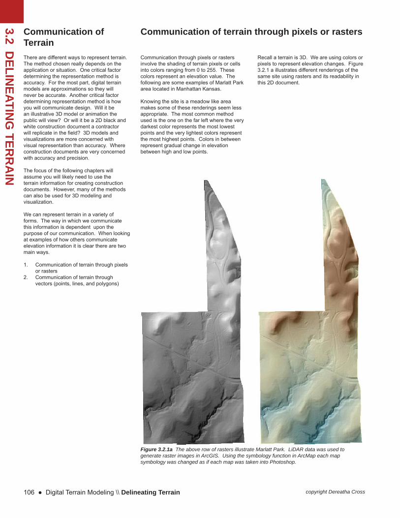
Figure 3.2.1a The above row of rasters illustrate Marlatt Park. LiDAR data was used to generate raster images in ArcGIS. Using the symbology function in ArcMap each map symbology was changed as if each map was taken into Photoshop.
Communication through pixels or rasters involve the shading of terrain pixels or cells into colors ranging from 0 to 255. These colors represent an elevation value. The following are some examples of Marlatt Park area located in Manhattan Kansas.
Knowing the site is a meadow like area makes some of these renderings seem less appropriate. The most common method used is the one on the far left where the very darkest color represents the most lowest points and the very lightest colors represent the most highest points. Colors in between represent gradual change in elevation between high and low points.
Communication of terrain through pixels or rasters
Recall a terrain is 3D. We are using colors or pixels to represent elevation changes. Figure 3.2.1 a illustrates different renderings of the same site using rasters and its readability in this 2D document.

Introduction to Digital Terrain Modeling for Landscape Architects ● 107copyright Dereatha Cross
3.2 DELIN
EATING
TERR
AIN

3.2 DELIN
EATING
TERR
AIN
108 ● Digital Terrain Modeling \\ Delineating Terrain copyright Dereatha Cross
Recall vectors are points, lines, and polygons. Civil 3D is a vector based program meaning it will use points, lines, and polygons to represent objects. The same is true for Terrain. In fact, the basic building block of terrain are points. These points are connected to form polylines or contours. Together they create a surface.
Each type has strengths and weaknesses. Recall a DTM is really an approximation. Points give you better resolution of elevation information. Because of this, most terrains are built from points or points are “made-up” so a surface can be built. The weakness of this type is in visualization. When one looks at a series of points it can be diffi cult to tell what the surface is trying to represent. On the other hand, the second, contours, is easier to visualize than points. We can follow the lines which connect the points and understand the surface as a topographic map. It’s weakness is in its resolution. Contours often come in integer whole numbers. For example, 100, 101, 102. 103, etc. Rarely would you see a contour at 100.5. This is where points come in. Finally we have surfaces. This is the product of points connected by lines to form polygons.
Unlike rasters, it may not be readily noticeable the surface is actually 3D until it is rotated in 3-space. The following are some examples of terrain represented by points, lines, and polygons. Refer to Figure 3.3.2a.
Contours and point representations are commonly used in construction documents where surfaces are used for volumetric type calculations such as earthwork estimations. Surfaces can also be used for 3D modeling work where a scene needs a base and this surface can be used as such.
Communication of Terrain through Vectors
Points Contours
Figure 3.3.2a The above row of rasters illustrate Marlatt Park. LiDAR data was used to generate raster images in ArcGIS. Using the symbology function in ArcMap each map symbology was changed as if each map was taken into Photoshop.

Introduction to Digital Terrain Modeling for Landscape Architects ● 109copyright Dereatha Cross
3.2 DELIN
EATING
TERR
AIN
Polygon Surface
3.2 DELIN
EATING
TERR
AIN
110 ● Digital Terrain Modeling \\ Delineating Terrain copyright Dereatha Cross
Understanding Contours
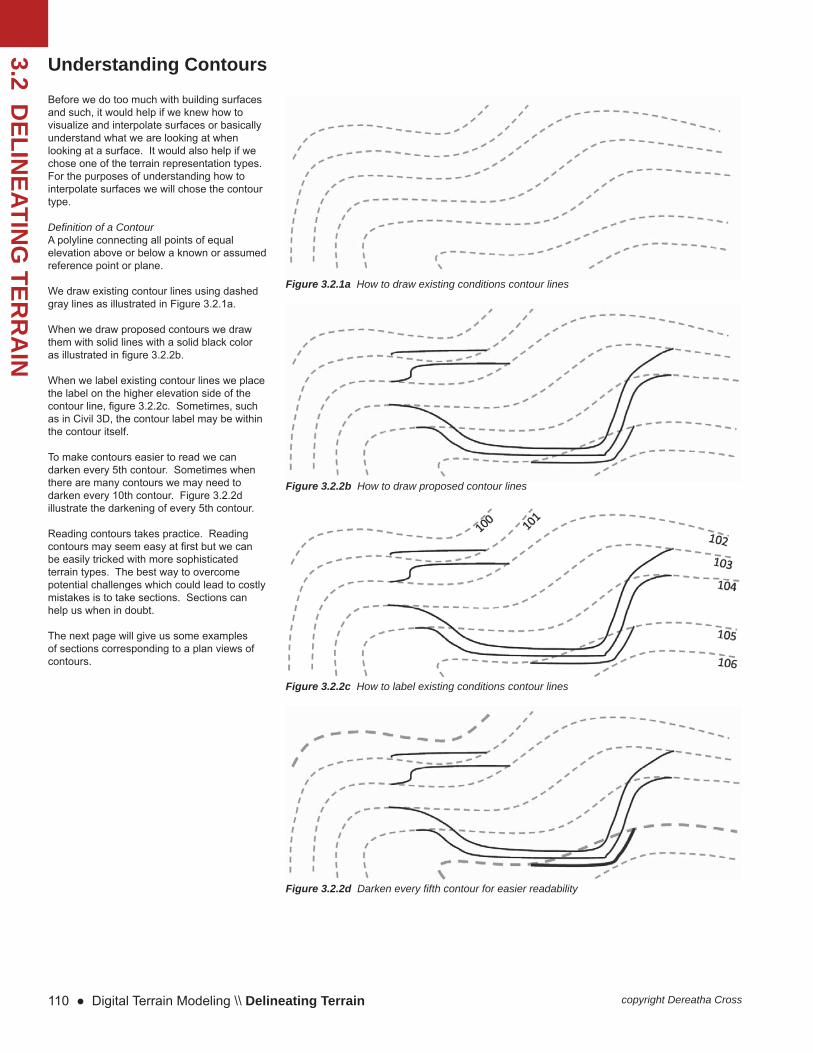
Before we do too much with building surfaces and such, it would help if we knew how to visualize and interpolate surfaces or basically understand what we are looking at when looking at a surface. It would also help if we chose one of the terrain representation types. For the purposes of understanding how to interpolate surfaces we will chose the contour type.
Defi nition of a ContourA polyline connecting all points of equal elevation above or below a known or assumed reference point or plane.
We draw existing contour lines using dashed gray lines as illustrated in Figure 3.2.1a.
When we draw proposed contours we draw them with solid lines with a solid black color as illustrated in fi gure 3.2.2b.
When we label existing contour lines we place the label on the higher elevation side of the contour line, fi gure 3.2.2c. Sometimes, such as in Civil 3D, the contour label may be within the contour itself.
To make contours easier to read we can darken every 5th contour. Sometimes when there are many contours we may need to darken every 10th contour. Figure 3.2.2d illustrate the darkening of every 5th contour.
Reading contours takes practice. Reading contours may seem easy at fi rst but we can be easily tricked with more sophisticated terrain types. The best way to overcome potential challenges which could lead to costly mistakes is to take sections. Sections can help us when in doubt.
The next page will give us some examples of sections corresponding to a plan views of contours.
Figure 3.2.1a How to draw existing conditions contour lines
Figure 3.2.2b How to draw proposed contour lines
Figure 3.2.2c How to label existing conditions contour lines
Figure 3.2.2d Darken every fi fth contour for easier readability

Introduction to Digital Terrain Modeling for Landscape Architects ● 111copyright Dereatha Cross
3.2 DELIN
EATING
TERR
AIN

3.2 DELIN
EATING
TERR
AIN
112 ● Digital Terrain Modeling \\ Delineating Terrain copyright Dereatha Cross
Visualizing Landform and Interpolating Surfaces
Let us get out our engineering paper and fi rst study a gradually slopped terrain in plan view:
Notice we are at a one foot contour interval. We don’t know much about the horizontal distance. Lets say these contours are about 20’ apart. That means each grid cell in our engineering paper would be 10’ x 10’.
If we take a section from A-A this is what it would look like:
So on the left side we have your elevation values. 1245 is the low point and 1250 is the high point of this section. We can see this is a steady straight line slope moving from left to right downwards.
So what if the contours are not regularly spaced. How do we read those?
Using the same section line at A-A we mark on our section graph points that touch that line. We connect those dots to produce a line that curves downwards.
This is what it looks like:
What if instead of curving downwards, what if it was upwards instead?
If we mirror the previous plan this is what we will get:
Using the same section line along A-A we mark our graph with points that touch the section line and connect those points. We get a curve that is upwards.
Before we jump into the computer let us make sure we can really read contours. We looked at a simple example in the previous section. Let us study more patterns we can expect to come across or have the need to create.
Let us look at more examples.

Introduction to Digital Terrain Modeling for Landscape Architects ● 113copyright Dereatha Cross
3.2 DELIN
EATING
TERR
AIN
Let us now examine how we might grade into our fi rst example, the gradual steady sloped terrain. As landscape architects there are three main reasons to grade:1. Control the follow of water across the terrain2. Make the terrain usable for a particular type of function (for humans or nature)3. Aesthetic reasons
In this example let us assume we need to grade in a fl ag area such that a building or parking lot can be placed onto the terrain.
Recall the bold line is what we wish to propose. Notice we have created a “fl at” area at elevation 1247.
Notice some of the proposed grade line in the section goes under the terrain while some of it is above the terrain. When it goes under the terrain it creates a “cut” situation. This is where earth is cut out of the terrain. When the line is above the terrain it creates a “fi ll” situation. This is where earth must be added.
When moving earth around one should strive to balance the amount of cut and fi ll. If there is excess cut or fi ll this can be costly to haul away or bring onto the site. There are other environmental impacts associated with hauling away or bringing in earth. For example if developing in an area that normally fl oods and one brings in excess earth than what was there normally it can raise the fl ood line in that area or neighboring areas. This principle is very similar to fi lling a bathtub up to the rim with water and then stepping into the bath. As your body or the earth displaces the water it will rise up overfl owing the bathtub or raising the fl ood line in that area. In some cases this maybe be unavoidable and a desired affect.
Speaking of water, what if we need to channel it to a desired location. How might we grade that into our example surface?
Starting at elevation 1250 we begin to redirect surface sheet fl ow such that it converges into a channel fl ow. At section line B-B we create a dip.
Let us now examine the inverse. We may need to create these to elevate something or simply hide something.
We can see in this example the protrusion has potential usefulness if you need to hide a hideous needed landscape feature such as a parking lot.
Water will drain outward to create divergent fl ow pattern.
In this example we can see why water might become more channelized. When water is accumulated in this way the fl ow becomes concentrated, has less opportunity to infi ltrate, and depending on the slope of the “ditch” water will have more mass and velocity having the potential to erode soil.
There are techniques which can be used to slow the water and sediment. Sometimes you may see ditches lined with rock or allowed to become populated with dense grass vegetation. Rocks can slow down channeled fl ow. Vegetation can also slow it down but the root systems can hold onto the soil. At the same time the plant material itself will absorb some of the water while letting some of it to percolate into the soil through its root structures allowing for deeper infi ltration.
Contour Rules:When working with contours there are some general rules we follow:• All points on a contour line have the
same elevation• Contours closing on itself within the
limits of a map is either a summit or depression
• Contour lines do not cross• Contours close together indicate a
steep slope• Contours spaced far apart indicate a
fl at area with slight grade• The steepest area will be
perpendicular to contours• Water fl ows perpendicular to contours

3.2 DELIN
EATING
TERR
AIN
114 ● Digital Terrain Modeling \\ Delineating Terrain copyright Dereatha Cross
3.2.6 Exercise A
In this exercise draw a section of the following land form. Is this a cut or fi ll situation? Draw in using arrows where the water might fl ow.
Introduction to Digital Terrain Modeling for Landscape Architects ● 115copyright Dereatha Cross
3.2 DELIN
EATING
TERR
AIN
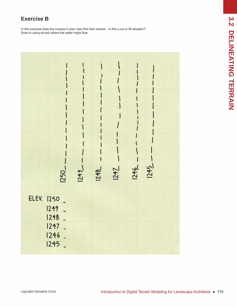
Exercise B
In this exercise draw the inverse in plan view fi rst then section. Is this a cut or fi ll situation? Draw in using arrows where the water might fl ow.

3.2 DELIN
EATING
TERR
AIN
116 ● Digital Terrain Modeling \\ Delineating Terrain copyright Dereatha Cross
Calculating Slope
Slope in the context of terrain surfaces is used to described the rate of change of a surface within a given area. Slopes can also be used to describe a surface.
For example landscape architects often express slope as a percentage such as 25%. If you work with a contractor in the fi eld, they will describe the same surface as having a ratio of 4:1. And fi nally, we may encounter a description in reference to an angle.
The rest of this section will explain these three concepts in more detail using the two most common terrain representation types: Vector and Raster.
Let us fi rst understand how to calculate slope in a more generic sense. There are several equations used to calculate slope that all yield the same result. The following is just a few:
Rise/Run = Slope
Difference / Length = Grade
Vertical / Horizontal = Slope, where means change.
If we want to apply this concept over different terrain representations it is important to make sure we know what this means.
Let us first define a coordinate system. Recall a coordinate system is just a means to help us make reference to something in space, in this case 3D-space. We will use a rectangular coordinate system with X, Y, and Z. Let X and Y be the coordinates in plan view. Refer to Figure 3.2.7a.
X
Y
Figure 3.2.7a illustrates a terrain lying in the X and Y plane of this coordinate system.
Figure 3.2.7a shows a fl at terrain. But what if it wasn’t fl at. How do we change our coordinate system so we may measure and communicate 3D information. --We add a 3rd axis called Z. The Z axis will correspond to our elevation. Consider Figure 3.2.7b.
X
YZ
Figure 3.2.7b illustrates the same terrain with a “bend” on one end.
If we needed to calculate the slope on that bend how would we conceptually accomplish this task?
Let us take a section at that bend and only at the bend and examine the section. Consider Figure 3.2.7c.
X
Z
Figure 3.2.7c illustrates a section cut slope line parallel to the X axis through the terrain.
Notice our coordinate system. Our view is coplanar with the XZ plane. We don’t need Y because it is a section which is 2D.
How do we describe the slope of this “bend” from this view? We can turn this section of the surface into a right triangle, Figure 3.2.7d.
X
Z
Figure 3.2.7d illustrates the same section which now has a horizontal and vertical line added to create a right triangle.
X
Z
We can now call the horizontal line the change in X and the vertical line the change in Z or elevation. --Recall we made Z represent elevation. Refer to Figure 3.2.7e.
X
Z
Figure 3.2.7e Assigning variables
So this means to fi nd the slope of the ramp we can use the equation rise/run or change in z divided by change in x or do the following:
Z / X = Slope
This will come out to be some number like 0.25. We multiply this value by 100 to give us 25%.
( Z / X ) x 100 = Slope
Let us examine different ways we can apply this concept.
Z

Introduction to Digital Terrain Modeling for Landscape Architects ● 117copyright Dereatha Cross
3.2 DELIN
EATING
TERR
AIN
Let us consider the followings snippet of terrain, Figure 3.2.8a.
300
301
302
303
304
305
Figure 3.2.8a A snippet of terrain
To calculate its slope we need to recognize the following (Figure 3.2.8b):
300
301
302
303
304
305
Z
X
Slope
Figure 3.2.8b Assigning the variables
Once we assign the variables we can then fi nd knowns and unknowns to calculate the slope.
Let us work some examples.
Example 1
Using the snippet of terrain, we have a 4% slope. What is the change in X?
Step #0: Study Given informationMake sure there isn’t any hidden information.
Step #1: Draw a DiagramAssign variables and fi gure out the knowns and unknowns. See Figure 3.2.8b.
We know Slope = 4%Z = High Point - Low Point = 305-300 = 5X = Unknown
Step #2: Setup EquationWe know we will use the Slope equation. So we will state that:
( Z / X ) x 100 = Slope
Step #3: Plug in and solveIt is important to first plug in so the reader knows what values you used.( 6 / X ) x 100 = 4%
Now we can solve. If you think it may not be obvious how you solved a particular problem you can label each step.
Isolate X.
Divide both sides by 100 to get:( 6 / X ) = 0.04
Multiply both sides by X to get:6 = 0.04 X
Divide both sides by 0.04 to get our answer:X = 6 / 0.04 = 150
We will assume the units are in feet. So the horizontal change or the change in X is 150 feet. It is important to declare what the answer is. If writing it out by hand sometimes it is boxed in.
Calculating Slope with Contours
Example 2
Using the same snippet of terrain, we have a 4% slope and we know the horizontal length is 150 feet. What if we didn’t know the elevation change. How would we re-arrange the equation to solve for the elevation change?
Step #0: Study given information
Step #1: Draw a Diagram.Assign variables and fi gure out knowns and unknowns. We will use same diagram from Figure 3.2.8b.
We know Slope = 4%Z = UnknownX = 150’
Step #2: Setup EquationUsing Slope Equation:( Z / X ) x 100 = Slope
Step #3: Plug in and solvePlug in variables( Z / 150 ) x 100 = 4%
Isolate Z.
Divide both sides by 100 to get:( Z / 150 ) = 0.04
Multiply both sides by 150 to get:Z = 0.04 *150
Solution:Z = 6
We will assume the units are in feet. So the elevation change or the change in Z is 6 feet.
The two examples use “clean math”. Each step is clearly outlines such that if someone needed to check your work they can quickly understand your logic. When working on high dollar projects it is common for your work to be checked by others to avoid costly mistakes. By having each step outlines to begin with many of these costly mistakes can be avoided by you.

3.2 DELIN
EATING
TERR
AIN
118 ● Digital Terrain Modeling \\ Delineating Terrain copyright Dereatha Cross
Calculating Slope with Rasters
Let us consider the followings snippet of terrain. Refer to Figure 3.2.9a
344 337
355 343
2 meters
2 meters
Figure 3.2.9a A raster containing elevation information
Recall rasters are essentially pixels or cells with information contained within. In our example we have numbers and the numbers correspond to an elevation value. Using this information and the raster cell size we can calculate the slope between two points.
Let us look at an example.
Example 1
Suppose we wanted to know the slope of the slope line connecting points A and B. Points A and B reside at the center if each grid cell. Refer to Figure 3.2.9b.
344 337
355 343
2 meters
2 meters
A
B
Figure 3.2.9b Point A’s spot elevation is 344 and point B’s spot elevation is 343.
Step #0: Study givenTwo variables are not directly given. We will need to solve for those.
Step #1: Draw a DiagramSlope = UnknownZ = Must be solved for = High Point - Low Point = 344-343 = 1
Figure 3.2.9c Section line taken from point A to B.
Finding the change in Z is simply knowing the elevation difference.
A = Elevation 344
B = Elev. 343
Z = 344 - 343= 1
A
B
C
Figure 3.2.9d illustrates yet another right triangle. Unlike fi gure 3.2.9c, the angle at A and B are 45 degrees (even if the diagram may not illustrate that clearly).
Step 2: Setup EquationRise / Run = Slope( Z / X ) x 100 = Slope
Step #3: Plug in and Solve( 1 / SQRT(8) ) * 100 = SlopeSlope = 35 %
X = Must be solved for as wellRecall Pythagorean Theorem:2+ 2= 2
We can manipulate the equation to get:= ( 2+ 2 )
Or more specifi cally (plug in numeric values):= ( 22 + 22 ) = (8) = 2(2)
This means the length of AB in the XY plane is 2(2). We want to leave it in this exact form and not convert it to a decimal such as 2.xxxxx. By doing this we are asking the computer to round it off which introduces error. Always save rounding for the very last step.

Introduction to Digital Terrain Modeling for Landscape Architects ● 119copyright Dereatha Cross
3.2 DELIN
EATING
TERR
AIN
1234 1233
1233 1232
1 meters
1 meters
A
B
The following is a raster. Calculate the slope between point A and B. Show the workfl ow process to include equation used and how unknowns were found. Indicate where water is moving by drawing an arrow.
Exercise C: Computing Slope
Student Name:________________________________
3.2 DELIN
EATING
TERR
AIN
120 ● Digital Terrain Modeling \\ Delineating Terrain copyright Dereatha Cross
1300
1301
1302
1303
1304
1305
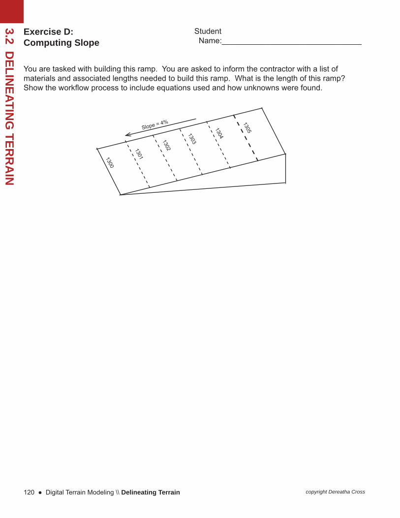
You are tasked with building this ramp. You are asked to inform the contractor with a list of materials and associated lengths needed to build this ramp. What is the length of this ramp? Show the workfl ow process to include equations used and how unknowns were found.
Slope = 4%
Student Name:________________________________
Exercise D: Computing Slope

Introduction to Digital Terrain Modeling for Landscape Architects ● 121copyright Dereatha Cross
3.2 DELIN
EATING
TERR
AIN
Exercise E: Grading with Slope Constraint
Student Name:________________________________
The client has discussed with you the following sketched on on engineering paper. Each grid cell is 5’ by 5’. The client wishes to build a gazebo with a concrete base and walk in their backyard. The client does not know what the elevation of the gazebo should be but she does know the ramp leading to the gazebo must be a 5% slope and start at existing elevation 1212’. She also would like to know other information such as will there be a need for a retaining wall. If there is a 3 foot drop in any location there will also need to be a rail. Where should the rail go? She is also interested in fi nish grade slope percentages with arrows.
3.2 DELIN
EATING
TERR
AIN
122 ● Digital Terrain Modeling \\ Delineating Terrain copyright Dereatha Cross
Interpolating Surfaces with Slope
Overview
We have spent some time fi guring out grading with a slope constraint by hand with paper and pencil. So now we must think about how we might apply what we have learned in Civil 3D.
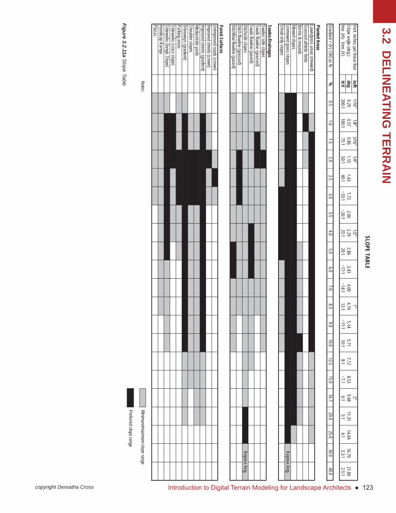
Recall the most common reasons for the need to grade is to conform with some slope requirement. The following table illustrates what some of these slope constraints might be in a typical project, refer to Figure 3.2.11a on the next page.
Grading to a Slope ConstraintIf we think about the previous exercise and the need to move the contours to conform with a 5% slope constraint we needed to do the following steps:
1.Determine existing slopeThis involved fi gure out what exactly is the existing slope. In the previous exercise it was 10%.
2.Determine proposed slopeWe would use the slope table in Figure 3.2.11a. In the previous exercise this was given to us to be 5%.
3. Determine contour spacingThis would be the horizontal contour spacing. This means fi guring out existing and proposed contour space.
Existing:Rise/Run = slope1/10’ = .10 or 10%
Proposed:1/? = .05 or 5%, what should ? be?Using information from the previous section we know ? = 20
So this means our proposed contours must be 20’ apart.
In the previous exercise we simply counted the number of squares in the engineering paper which was 5’ each until we counted up 20’ and moved contours accordingly.
Grading to a Slope Constraint in Civil 3DGiven the same problem now in CAD, how do we accomplish the same task?
1. Determining existing slopeWhat if we didn’t know it was 10%. We can use the measure tool located in the Drafting and Annotations workspace, Home tab, Utilities, measure.
If we do this we need to be careful. Recall contours are actually 3D. We want the horizontal distance and not the hypotenuse. So to ensure this it might be useful if we drew a polyline fi rst. Recall those must be 2D or coplanar. We can draw a pline connecting to contours perpendicularly. Once the line is drawn we can measure it or use the “list” command to view its properties. The list command will tel us see the length of the pline which would essentially be the spacing between two contours in the horizontal. Now that we know the length we can divide 1 by the length to give us the slope.
2.Determining proposed slopeWe would use the slope table here as well. But we know it should be 5% because it was given to us in the previous exercise.
3.Determine contour spacingWe know what the existing contour space is from step 1 above. We just need proposed. We would use the same equation that would yield 20’ in our example from Exercise E.
So now how do we draw this in CAD?
Recall there are several tools available to us in CAD allowing us to either copy or offset items a certain fi xed distance.
This means we can draw one contours and either copy or offset it a certain distance. We could also instead of drawing entire contours use “tick” marks like a “make-shift” ruler to guide us as to where contours need to go.
For example, you may fi nd it useful to fi rst draw a short pline and offset it 20’. Then begin sketching contours using these series of polylines as a guide. Refer to Figure 3.2.11a.
If one prefers this method it may be useful to create a series of such tick marks for different slope ranges and create blocks of them to be used later.
Figure 3.2.11a A series of seemingly random “tick” marks used to correctly space contours.
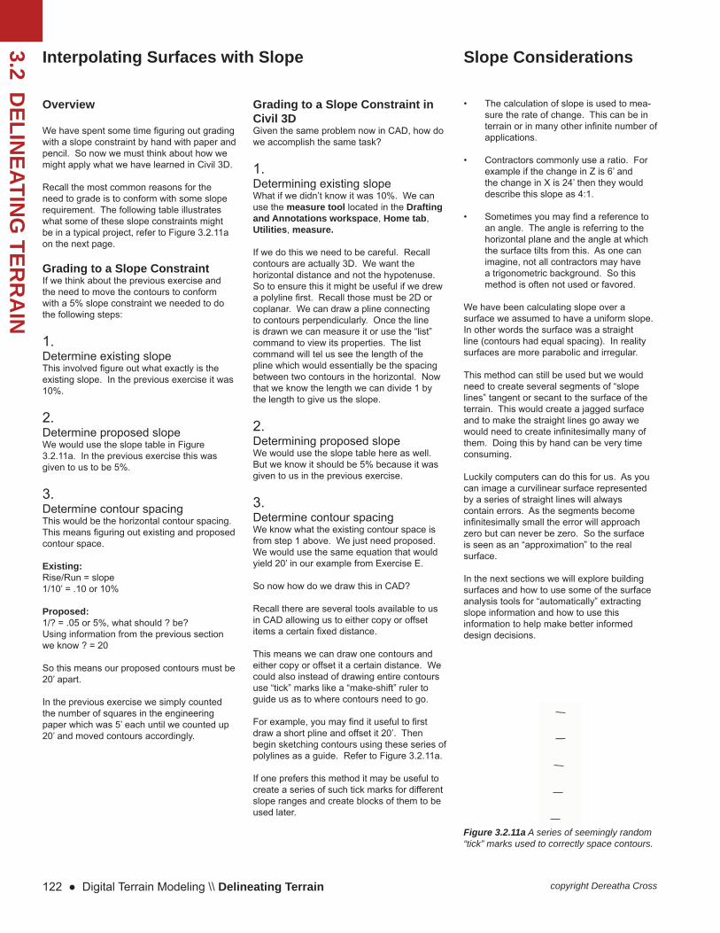
• The calculation of slope is used to mea-sure the rate of change. This can be in terrain or in many other infi nite number of applications.
• Contractors commonly use a ratio. For example if the change in Z is 6’ and the change in X is 24’ then they would describe this slope as 4:1.
• Sometimes you may fi nd a reference to an angle. The angle is referring to the horizontal plane and the angle at which the surface tilts from this. As one can imagine, not all contractors may have a trigonometric background. So this method is often not used or favored.
We have been calculating slope over a surface we assumed to have a uniform slope. In other words the surface was a straight line (contours had equal spacing). In reality surfaces are more parabolic and irregular.
This method can still be used but we would need to create several segments of “slope lines” tangent or secant to the surface of the terrain. This would create a jagged surface and to make the straight lines go away we would need to create infi nitesimally many of them. Doing this by hand can be very time consuming.
Luckily computers can do this for us. As you can image a curvilinear surface represented by a series of straight lines will always contain errors. As the segments become infi nitesimally small the error will approach zero but can never be zero. So the surface is seen as an “approximation” to the real surface.
In the next sections we will explore building surfaces and how to use some of the surface analysis tools for “automatically” extracting slope information and how to use this information to help make better informed design decisions.
Slope Considerations
Introduction to Digital Terrain Modeling for Landscape Architects ● 123copyright Dereatha Cross
3.2 DELIN
EATING
TERR
AIN
Vert. inches per linear footin/ft
1/16"1/8"
3/16"1/4"
1/2"1"
2"Slope angle (deg.)
deg0.29
0.570.86
1.151.43
1.722.00
2.292.86
3.434.00
4.745.14
5.717.12
8.539.48
11.3114.04
16.7021.80
Hor. (H): Vert. (V)H:V
200:1 100:1
75:150:1
40:1~33:1
~26:125:1
20:1~17:1
~14:1 12:1
~11:110:1
8:1~7.1
6:15:1
4:1 3.3:1
2.5:1
Gradient = (V) / (H) as %%
0.51.0
1.52.0
2.53.0
3.54.0
5.06.0
7.08.3
9.010.0
12.515.0
16.720.0
25.030.0
40.0
Planted AreasLawn/grass areas (mowed)Grassed athletic fieldsBerms & moundsMowed slopesUnmowed grass slopesShrub only slopes
Swales/DrainagesSwales side slopesSwale flowline (grassed)Swale flowline (paved)Ditchside slopesDitch flowline (grassed)Ditchflow flowline (paved)
Paved SurfacesUnimproved roads (crown)Improved streets (crown)Improved streets (gradient)Median/side yardsShoulder slopesDriveways (gradient)Parking areasSidewalks (cross slope)Sidewalks (longit. Slope)Handicap RampsPlazas
Notes: Minimum/maximum slope range
Preferred slope range
Repose Ang.
Repose Ang.
SLOPE TABLE
Figure 3.2.11a Slope Table
3.2 DELIN
EATING
TERR
AIN
124 ● Digital Terrain Modeling \\ Delineating Terrain copyright Dereatha Cross
Exercise F: Grading with Slope Constraint in Civil 3D
In this exercise we will use Exercise E’s scenario. We will assume the client has OK’d your sketch and would like to have it in CAD now. You have requested for the area of interest to be surveyed. A base map has been provided. In this exercise please locate the InterpolatingSlope.7z fi le and follow the following steps:
1.Extract the fi le into your projects directoryEnsure it unpacks into X:\Projects where X is your drive letter.
2.Open the drawing.a. Ensure you have NCS pen tables installed on your computer before starting.b. Open Civil 3D fi rst and ensure you open Imperial.c. Within Civil 3D locate the basemap. It is likely saved in 01_Sourced. Save as the drawing under a different name by versioning the fi le.
3.Explore the fi leNotice the following:• Layer setup• Paper space setup• Scale• Existing vs proposed
4.Create New LayersCreate layers for the landscape elements:• Gazebo• Walk• Drain• Rail if needed• Retaining wall if used
5.Sketch in the line work.Do the best you can to replicate the hand sketch from Exercise E. Use the Engineer-ing paper grid in the background as a guide. Ensure all line work is:• On the correct layers• Continuous• Have proper line weights assigned• Have proper line types assigned
6.Sketch Proposed ContoursUsing Exercise E and the pline command begin sketching proposed contours. • Ensure majors and minors are on the
correct layer. • Ensure all contours have elevation• All proposed contours must tie back to
existing• All proposed grading must be within the
extents of the property line
7.Label contoursLabel contours with elevation information. You may want to copy and paste existing labels and use those to label your proposed contours. Ensure proposed contour labels are on their own layer and have proper line weight.
8.Plot to PDFOnce you are done go to paper space and ensure line weights and line types have been properly assigned. Confi gure Title Block Template. Plot to PDF. Ensure you are using Arch D size.

Introduction to Digital Terrain Modeling for Landscape Architects ● 125copyright Dereatha Cross
3.2 DELIN
EATING
TERR
AIN
Exercise G: Exploring contours on a base map
Download the base map and study the contours on the 1in-40ft 24x36 r296.67 sheet. Plot the sheet to 11 x 17. Using color pencils and a sheet of trace paper answer the following questions:
1. Orange PencilWhere are the high points? Indicate with an X and based on nearby contour pattern indicate what the spot elevation might be. Use a darker color pencil or marker to write the numerical values. Recall spot elevations do not need to be whole numbers.
2. Red Where is the low point? Indicate with an X and based on nearby contour patterns indicate what the spot elevation might be. Use a darker color pencil or marker to write the numerical values. Recall spot elevations do not need to be whole numbers.
3. Purple PencilWhere is the property boundary?
4. Blue PencilIndicate the surface drainage pattern. We are interested in sheet fl ow, channeled fl ow, convergent fl ow, and divergent fl ow. You can use arrows and other types of symbology to indicate drainage patterns.
5. Green PencilUsing slope arrows indicate slopes throughout the site. Indicate percentages using dark green pencil or marker. You will need to fi gure out the contour spacing from the Civil 3D fi le.
3.2 DELIN
EATING
TERR
AIN
126 ● Digital Terrain Modeling \\ Delineating Terrain copyright Dereatha Cross
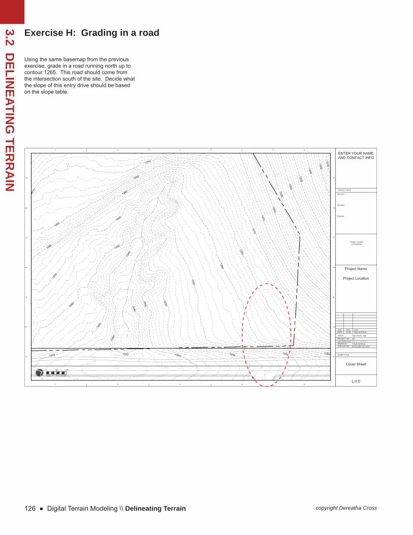
Exercise H: Grading in a road
Using the same basemap from the previous exercise, grade in a road running north up to contour 1265. This road should come from the intersection south of the site. Decide what the slope of this entry drive should be based on the slope table.

Introduction to Digital Terrain Modeling for Landscape Architects ● 127copyright Dereatha Cross
3.2 DELIN
EATING
TERR
AIN

3.2 DELIN
EATING
TERR
AIN
128 ● Digital Terrain Modeling \\ Delineating Terrain copyright Dereatha Cross

Introduction to Digital Terrain Modeling for Landscape Architects ● 129copyright Dereatha Cross
3.2 DELIN
EATING
TERR
AIN

3.3 SUR
FAC
ES
130 ● Digital Terrain Modeling \\ Surfaces copyright Dereatha Cross
Introductory Overview
In the last section we spent some time creating abstract terrain and visualizing different land forms. It is important for us to understand no matter the representation the object we are manipulating is a 3 dimensional object.
In order to create a design we need a base. That base is our terrain sometimes called a surface. This is where we can begin placing objects.
When we design we will need to sculpt this terrain object to accommodate different functions such as building pads, parking, and handicapped accessibility. There are many other reasons to grade such as controlling what you want to do with water. The act of sculpting is called “grading”.
There are several ways we can grade. We can do this by hand meaning we manually draw in contours and later manually perform earthwork calculations. Earthwork calculations involve calculating the volume of earth your proposed design will require moved to help determine the cost of the project. This can be time consuming.
Historically, before the use of computers, this was done by hand. For example if our area is a building pad where we have both cut (taking soil away) and fi ll (adding soil) we would draw section lines perpendicular to the contours in the graded area. These section lines would occur so many feet apart. --Let us say 50’.
We then delineated these sections by drawing it by hand. Then we use a planimeter device to measure the area of cut and fi ll in this section.
Taking sections every 50’ and using a planimeter to measure the area within the each section would give us the area. To get the volume, we know the sections are every 50’ feet apart which means we can multiply the area of the section times 50’ to give us the volume. We do this repetitiously for each section. We then add up all the volumes. This would give us volume of earth moved in this area.
This method works great if your area is a perfect cube or rectangular shaped volume. Your volume calculation would be very close to actual.
50'
What if the volume you need is more organic shaped like a sphere or maybe a fl attened egg shape? And to further complicate things, what if it is not a symmetrical form? Also, this method likes the section lines to be perpendicular to the contours and what if this is not possible?
What if we could simply create two surfaces-- one with existing conditions and the other proposed (your designed grading plan). Instead of creating many time consuming sections what if we could simply compare the two surfaces and fi nd the volume of earth moved?
There are several mathematical models in existence allowing us to do this. One concept is called Riemann’s sum. A single Riemann’s sum would fi nd the area but a double Riemann’s sum would fi nd the volume between two surfaces. N MΣ Σ f(Pij) Δxi Δyji=1 j=1
where:
f(Pij) is the function describing the height between two points vertically connecting two surfaces
Δxi is the change in the width in the x direction of each grid cell covering the area of interest in plan view
Δyj is the change in the width in the y direction of each grid cell covering the area of interest in plan view
This would give us a more precision but still it is an estimate as this is still an approximation. As the area between sample points become smaller and smaller the precision approaches the actual value but never really gets there.
Let us consider this example surface in plan view:
[ f(1.50, 1.25) + f(1.50, 1.75) + f(1.75, 1.25) + f(1.75, 1.75) + f(2.25, 1.25) + f(2.25, 1.75) ] * (1/2) * (1.2)
But again, this has the potential to be time consuming especially if we want our calculations to approach zero error.
Today we have computers. And computers are great at doing repetitious tasks automatically for us. More specifi cally Autodesk Civil 3D can do this work for us. However, in order for Civil3D to do this for us, we would need to make our terrain of contour lines or points a surface in Civil 3D. This means if you have contour lines Civil 3D sees these contour lines as simply polylines with elevation and nothing else. What we need is for these polylines to be come an object and a particular type of object such that Civil 3D will see it as a surface. This surface object will become a dynamic intelligent object allowing us to use Civil 3D’s built in automated functions such as calculating earthwork for us.
Area

Introduction to Digital Terrain Modeling for Landscape Architects ● 131copyright Dereatha Cross
3.3 SUR
FAC
ES
Before we can analyze a surface we will need to make one. The surface is a terrain base where we can begin placing objects.
There are three main categories of surfaces:
• Standard surfaces • Volume surfaces • Corridor surfaces
Standard surfaces are based on a single set of points.
Volume surfaces builds a surface by measuring vertical distances between two standard surfaces. Both standard and volumetric surfaces can be a grid or TIN surface.
The corridor surface is created from a corridor such as a road/street corridor alignment.
We will explore the fi rst two in this chapter.
Delaunay’s TriangulationTypes of Surfaces
In planar geometry, two points defi ne a line and three points defi ne a plane. Using these basic concepts the computer is able to create a triangular plane using groups of three points. The computer algorithm is called Delaunay triangulation. The end product from this algorithm is called a triangulated irregular network (TIN).
Standard surfaces will have two major limitations. It is important to understand Delaunay’s triangulation means that for any given (x, y) point, there can only be one unique z value within the surface (since slope is equal to rise over run, when the run is equal to 0 the result is undefi ned.
Surfaces will have no thickness. Modeled surfaces are thin sheets of polygons. Surfaces also have no vertical faces. Vertical faces cannot exist in a TIN because two elevation points on the surface cannot have the same (x, y) coordinate pair.
Surfaces on the other hand can model very detailed terrain at any size depending on your computer’s hardware ability.

3.4 WO
RK
FLOW
S
132 ● Digital Terrain Modeling \\ Workfl ows copyright Dereatha Cross
Overview
As a landscape architect you will receive surface data in a variety of formats ranging from something that came from a 3D application to a notepad fi le full of numbers. Regardless of the format it will be your responsibility to setup your basemap and be ready to grade in your design.
This section is designed to give you a general idea of what you will need to do depending on what you are starting with. We will assume you are starting with existing conditions and will eventually need to grade a proposed surface. The following descriptions are just that, a short overview. More details will follow in this chapter about each step.
As applications are updated and newer versions are released you may fi nd certain steps to be slightly different from what is written here. Before starting on these procedures it is always recommended to perform these procedures on a copy of the original dataset.
Recognizing the Starting Data
Survey PointsThis typically comes in a text fi le with x,y,z values and some other data such as point number and a raw description.
Messy CAD FileThis is one of those fi les full of data that might be on the wrong layer has contours crossing each other or missing contours.
Object from a 3D ProgramThese come from a 3D application such as Revit, Rhino, Vue, Max, Sketchup or possibly other programs
GIS DataThis is data from GIS. Usually a raster or TIN surface created from LiDAR.
Formatting and Conditioning the Starting Data
Create Survey PointsThis point fi le will need to be imported into Civil 3D as Survey Points. You will want to use Survey Points and not COGO points because this is existing data.
Drawing CleanupYou will need to clean this up. A word of caution though. If you are creating construction documents where hundreds of thousands of dollars are involved then you could be liable for mistakes. It might be safer to ask for a clean drawing from the surveyor.
File ConversionYou may need to export objects from the 3D program to make it CAD ready. Civil 3D is not the only application that uses dynamic intelligent objects. When bringing another applications dynamic intelligent objects into Civil 3D you may experience “undocumented features” --or crashes. Once you can get it into a format Civil 3D will see (dwg or dxf) you are good to go.
Raster to ContoursMost GIS terrain data is in the form of a raster. This will need to be converted to contours then imported into Civil 3D.
As one can imagine this part can be somewhat laborious depending on what you are starting with. It is good practice to try each of these simply to gain experience and recognize errors when they occur and how to fi x them. Some may require simply converting 3D line work that came from Bentley to 2D line work so Civil 3D will recognize them as contours while others require you to go through an elaborate database setup.
There are many types of data you may start with. This section hopes to cover the major forms of data types but not all. However, enough information is given here to give you an idea of where you might want to look if you run into something exotic.
PhotogrammetryThis is data collected from photographs using drone technology. The images are converted to point cloud data.
Point Cloud to ContoursOnce in point cloud format, GIS can convert the data to any form needed rather it be a raster or contours for Civil 3D.

Introduction to Digital Terrain Modeling for Landscape Architects ● 133copyright Dereatha Cross
3.4 WO
RK
FLOW
S
Build EG Surface
Step 1. Create Existing Grade surface containerStep 2. Defi ne surfaceStep 3. Add breaklinesStep 4. Add boundary
Build Existing Surfacein Civil 3D
Create Design Grade
Build DG Surface
Step 1. Create Design Grade Surface Container (for contours and/or points)Step 2. Defi ne surfaceStep 3. Add breaklinesStep 4. Add boundary
Create Proposed Grade
Build PG Surface
Step 1. Create Proposed Grade Surface ContainerStep 2. Paste Existing GradeStep 3. Paste Design ContoursStep 4. Paste Design Points
Once Civil 3D can recognize the drawing objects you can now build an existing grade surface. The general outline for doing this below. This is a simple 4 step process and will be the same regardless of where your data came from.
This is done in a variety of ways. The most common ways are from contours and points. This can be done by taking the existing sur-face and extracting the needed information so you can edit a copy of the object as a simple drawing object. COGO points are used for spot elevations to control the surface at a more refi ned level. After you are done grading you will want to create a design surfaces. The steps are outlined below.
There are a variety of ways to create a proposed surface. The use of the Paste command is recommended to retain the original surface data in the event you need to edit it later which is pretty common. Always paste existing always fi rst. Then the least resolution proposed data you have which would be your proposed contours followed b points.. This will grade in your proposed contours into the existing grade and then the points on to of the contours.

3.5 BU
ILDIN
G SU
RFA
CES FR
OM
MESH
ES
134 ● Digital Terrain Modeling \\ Building Surfaces from Meshes copyright Dereatha Cross
Surfaces From Mesh Terrains Workfl ow
Step 1: Starting data
It is helpful to know where the terrain came from. We know it is a Mesh terrain because it came from Vue.
A mesh terrain typically comes from a 3D program like E-On Software Vue or Autodesk 3ds Max. Civil 3D sees such objects as “Drawing Objects”. This will become relevant to us later in the surface creation process. Figure 3.4a, is an example of a mesh terrain from a 3D application called Vue Infi nite from E-On Software.
Step 2a: Condition Data - Export
In Vue we will need to export this terrain as a dxf object if we want to bring it into Civil 3D, fi gure 3.4b. As the fi le is exported Vue will strip the fi le down to basic geometry such that Civl 3D so that can read the geometry. Most applications that have exporters will do this and they do this so you can import it into another application. Often times you may fi nd the fi le size shrinks after export
a. In the World Browser select the terrain to be exported.
b. Click the Edit Object button in the Aspect tab.
c. In the Terrain Editor click the Export button.
Figure 3.5b: Process of exporting Terrain for Civil 3D in Vue
Overview
We may receive terrain data from another 3D application. For example, if you are working at an architecture based fi rm you may receive terrain data from 3ds Max or other applications. In this example we will work through how to take terrain from Vue into Civil 3D. The example terrain is illustrated on the next page, refer to Figure 3.5a.
a
b
c
d
d. In the Terrain Export Options dialog box set the following options:• File Name: Click the Browse button and
choose dxf from the drop down menu. Save the fi le in the correct fi le manage-ment location. For example:
X:\Projects\<Project Site Name>\C3D\Imports\Terrain.dxf
• Set the mesh resolution such that the number of polygons is close to but is not equal to or exceeds 65,000 polygons.
• Uncheck “Generate Material Maps.
• Click OK
Depending upon the version of Vue you are running you may get an error message indicating the terrain was unable to export. Check to see if this is in deed true. In most cases it is not. If it is, repeat procedure but reduce the number of polygons exported until you have a successful terrain export.
If you are unable to successfully export your terrain make sure the mesh count is 256 x256.
Refer to Figure 3.5b.

Introduction to Digital Terrain Modeling for Landscape Architects ● 135copyright Dereatha Cross
3.5 BU
ILDIN
G SU
RFA
CES FR
OM
MESH
ES
Figure 3.5a: Example terrain created in Vue

3.5 BU
ILDIN
G SU
RFA
CES FR
OM
MESH
ES
136 ● Digital Terrain Modeling \\ Building Surfaces from Meshes copyright Dereatha Cross
Surfaces From Mesh Terrains Workfl ow
Figure 3.5d: Import results
Step 2b: Condition Data - Import
In Civil 3D we need to insert the terrain into a native Civil 3D fi le. This means opening the dxf fi le directly and working straight from that fi le will not work for us. We need all of the Civil 3D layers and other template information that comes in a new fi le. This dxf fi le will also not contain any dynamic intelligent objects. Upon export from Vue this information is stripped out. Figure 3.5c illustrates this workfl ow.
1.Use the Insert command to insert the DXFIn a native Civil 3D fi le, type insert.
2.Confi gure Insert optionsThe Insert dialog box opens. • Click Browse and locate the dxf fi le we
exported from Vue. Click OK.
• Ensure the units are set correctly. If Unit is set to inches and you want feet you will need to type 12 next to X in the Scale group and check in uniform scale. The number 12 refers to 12 inches in 1 foot and will convert your model from inches to feet by multiplying what you input in the XYZ by one drawing unit.
• Click OK.
3.Inspect ImportYou may not see anything on your screen. This is because you may need to zoom extents (ze is the keyboard command).
It may not be readily apparent there is a 3D terrain until we rotate the view. Recall Shift + middle mouse button will rotate the model into a 3D view.
To get back to plan view type plan view and press enter twice.
Rotate the view to ensure your import is truly 3D. If it is not you may need to repeat procedures. Refer to Figure 3.5d.
Figure 3.5c: Inserting the exported fi le from Vue as a block

Introduction to Digital Terrain Modeling for Landscape Architects ● 137copyright Dereatha Cross
3.5 BU
ILDIN
G SU
RFA
CES FR
OM
MESH
ES
Step 2c: Condition Data - Examine and Explode
4.Turn off auto-selectNext we will need to explode this object because it is in a block form. Before we do this we may want to turn off a few settings that can slow us down.
Recall by default as you roll your mouse over objects in the drawing space Civil 3D wants to highlight objects. In a Mesh terrain it can really slow down our workfl ow as it will want to highlight each and every single triangle our mouse hits. To turn this off do the following:
• Right click on the drawing space and select Options.
• The Options window opens. • In the Selection tab, in the Preview
group, uncheck When a command is active and When no command is active.
• Click OK.
This can be rechecked in when needed. Refer to fi gure 3.5e.
5.ExplodeExplode the mesh terrain by selecting it and typing explode followed by enter.
6.Object Type Identifi cationTo examine the type of objects we now have we can select one of the triangles and type list followed by the enter.
Figure 3.5f shows 3D FACE is listed next to Layer: “object”. This is the object type.
Figure 3.5e: Turning off cursor auto-selecting to speed up production.
Figure 3.5f: List command reveals object is a 3D face and is on the “object” layer.
3.5 BU
ILDIN
G SU
RFA
CES FR
OM
MESH
ES
138 ● Digital Terrain Modeling \\ Building Surfaces from Meshes copyright Dereatha Cross
Surfaces From Mesh Terrains Workfl ow
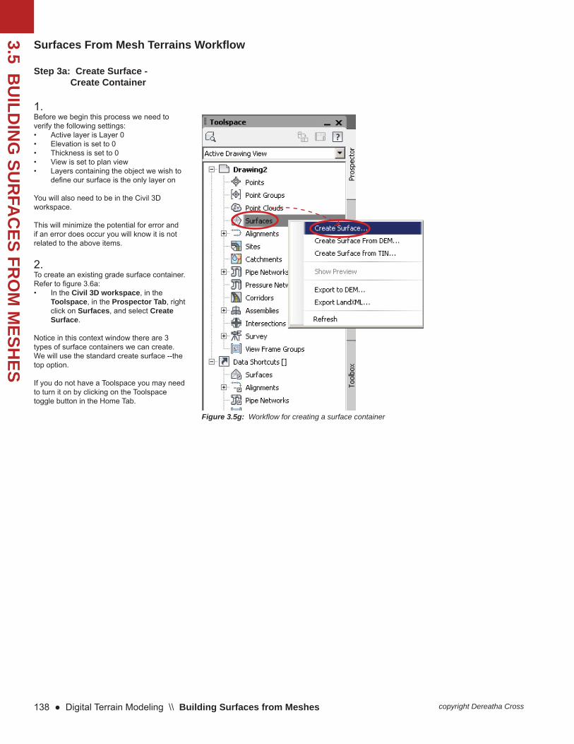
Step 3a: Create Surface - Create Container
1.Before we begin this process we need to verify the following settings:• Active layer is Layer 0• Elevation is set to 0 • Thickness is set to 0 • View is set to plan view• Layers containing the object we wish to
defi ne our surface is the only layer on
You will also need to be in the Civil 3D workspace.
This will minimize the potential for error and if an error does occur you will know it is not related to the above items.
2.To create an existing grade surface container. Refer to fi gure 3.6a:• In the Civil 3D workspace, in the
Toolspace, in the Prospector Tab, right click on Surfaces, and select Create Surface.
Notice in this context window there are 3 types of surface containers we can create. We will use the standard create surface --the top option.
If you do not have a Toolspace you may need to turn it on by clicking on the Toolspace toggle button in the Home Tab.
Figure 3.5g: Workfl ow for creating a surface container

Introduction to Digital Terrain Modeling for Landscape Architects ● 139copyright Dereatha Cross
3.5 BU
ILDIN
G SU
RFA
CES FR
OM
MESH
ES
2.Once you click on Create Surface the Create Surface window opens.• Click the Layer button next to Surface
Layer C-TOPO
3.The Object Layer Dialog opens.• In the Object Layer dialog, select the
Suffi x dropdown.• Type -* in the Modifi er value. This will
cause what ever you choose to name your surface to be added to the end of C-TOPO-. Basically, the * will be replaced with what you type here.
• Click OK to the Object Layer dialog
Notice most of the layers in Civil 3D start with C. C is what Civil Engineers start their layers with where L is what Landscape Architects use to start their layers. We will use C in these examples.
4.In the Create Surface dialogue:• Next to Name type EG for existing grade• Description: Existing Ground Surface• Style: Contours 1’ and 5’ (Background)
Notice in the select Surface Style drop down there are several options to pick from. If no options appear here it is because the fi le is not a native Civil 3D fi le.
• Click OK
Figure 3.5h illustrates this process.
A surface container is created in the Prospector Tab.
Figure 3.5h: The process of assigning layers, names, and style to the surface container.

3.5 BU
ILDIN
G SU
RFA
CES FR
OM
MESH
ES
140 ● Digital Terrain Modeling \\ Building Surfaces from Meshes copyright Dereatha Cross
Surfaces From Mesh Terrains Workfl ow
Step 3b: Create Surface - Defi nition
It would seem nothing had happened. But upon examining the Prospector tab we notice Surfaces is now expandable and contains several objects. One of which is named EG, existing grade. This is an empty container where our surface will go. --Right now it has nothing in it.
Notice there is a Defi nition group with several items listed underneath. This area is used for defi ning our surface and there are several ways we can defi ne our surface.
The following is a selection of surface defi nitions and their descriptions. Refer to fi gure 3.5i.
Boundaries
Boundaries are closed 2D or 3D polylines and can be feature lines. Only X, Y information is used.
There are two types of boundaries:
1. Outer Boundaries - used to eliminate stray triangulation2. Hide boundaries - used to indicate areas that could not be surveyed such as a building pad.
Boundaries should not be confused with borders. Boundaries are added to a surface where a border is the limit of a surface. A surface will always have a border but it may not always have a defi ned boundary.
Breaklines
Breaklines are used to create hard-coded triangulation paths, even when those paths violate Delaunay algorithms for normal TIN creation. Breaklines can describe anything from the top of a ridge to the fl owline of a curb section. TINS may not cross the path of a breakline. Breaklines can be 2D or 3D polylines or feature lines.
Contours
Contours can be inserted into a surface our built as a surface. These are typically 2D polylines with an elevation. Points will be created along the contour to be used in the triangulation process.
DEM Files
Digital Elevation Model (DEM) fi les are the standard format fi les from governmental agencies and GIS systems. These fi les tend to be very large and useful for planning purposes. GIS fi les are free and can be used to defi ne a surface. USGS may distribute elevation data in the form of an Spatial Data Transfer Standard (SDTS) fi le. A program called sdts2dem can convert SDTS fi les to DEM format allowing Civil 3D to read the fi le as a DEM.
Drawing Objects
AutoCAD objects having an insertion point at an elevation can be used to populate a surface with points. It’s important to remember that no relationship to the drawing object is maintained; only the point data associated with the drawing object is added to the surface, not the actual drawing object.
Edits
This area keeps track of any edits made and functions as an edit history. Edits can be toggled on and off individually and are listed in the order they were added.
Figure3.5i: Surface defi nitions

Introduction to Digital Terrain Modeling for Landscape Architects ● 141copyright Dereatha Cross
3.5 BU
ILDIN
G SU
RFA
CES FR
OM
MESH
ES
Point Files
This is useful when working with large datasets. A drawing will stay referenced to a point fi le. If the point fi le is moved or deleted, the reference in the drawing will be broken.
Point Groups
Point groups or survey point groups can be used to build a surface from their respective members and maintain the link between the membership point group and membership of the surface. In other words, points edited in either the group or the surface will update in the other.
Point Survey and Figure Survey
This area is used for Survey data covered in a previous section.
LandXML Files
These come from an outside source or are exported from another project. LandXML has become a common means of communicating data in the land development industry. These fi les include information about points and triangulation, making replication of the original surface as easy as a few mouse clicks.
TIN Files
These fi les come from a land development project which you or a peer has worked on and contain the baseline TIN information from the original surface and can be used to replicate easily.

3.5 BU
ILDIN
G SU
RFA
CES FR
OM
MESH
ES
142 ● Digital Terrain Modeling \\ Building Surfaces from Meshes copyright Dereatha Cross
Surfaces From Mesh Terrains Workfl ow
Step 3c: Create Surface - Add Data to Container
Recall from our list command, our surface was a 3D face. Civil 3D classifi es 3D faces as Drawing Objects.
Make sure you are in plan view before starting the step. You will need to type “plan” then enter twice. It is not recommended to use the view cube as you may not be perfectly in plan view.
Refer to fi gure 3.6d for adding a defi nition.
1.Right click on Drawing Objects and select Add.
A dialog window opens.
2. Object type should be set to 3D Face. Recall from our list command we found this terrain to be a 3D Face type Drawing Object.
3.In the description we can type “From Vue”. Click OK.
4.Select the Objects. There are several ways we can do this. The most effi cient would be to type w which will activate the Window command. Click in the upper left corner then click the lower right corner, fi gure 3.6e. Anything contained with in this window will be selected. Press Enter to end the select objects command.
Figure 3.5j: Add a defi nition
Figure 3.5k: Window command to select drawing objects

Introduction to Digital Terrain Modeling for Landscape Architects ● 143copyright Dereatha Cross
3.5 BU
ILDIN
G SU
RFA
CES FR
OM
MESH
ES
Step 3d: Create Surface - Error Inspection
5.Turn off the mesh terrain.Our Civil 3D dynamic intelligent terrain object is sitting within our Mesh terrain. In the layers list, we can turn off the mesh terrain. Recall it came in on a layer named Object.
6.Once the mesh object is turned off we can better see our contours. The pink lines are minor contours, the dark green lines are major contours, and the light green outer line is the border.
7.Sometimes it may be hard to fi nd errors in the surface in contour representation form. It may be better to look at it as a more “solid” or “continuous” surface. We can do this by changing the view.
In the View ribbon tab, in the Visual style, change the view from 2D Wireframe to Shaded.
Recall you can press the shift key + the middle mouse button and drag to rotate in 3D. You can also use the view cube.
Once you are done inspecting you will need to change the view back to 2D wireframe and move back to plan view.
From here objects can be extracted from the surface. Once extracted they can be edited to build yet another surface. This process will be explained in later sections of this chapter.
Figure 3.5l: Civil 3D terrain object on top of the Mesh terrain import
Figure 3.5n: Civil 3D terrain view style changed and object rotated in 3D
Figure 3.5m: Mesh terrain import layer turned off.

3.6 SUR
FAC
E APPR
OXIM
ATION
METH
OD
144 ● Digital Terrain Modeling \\ Surface Approximation Method copyright Dereatha Cross
What is the Surface Approximation Method Method?Using this method to create a surface means you have a drawing with polylines that have elevation. These polylines we see as contours representing elevation. Unfortunately to Civil 3D they are simply a series of polylines with x, y, z information. In order for them to have more meaning to Civil 3D we will need to create a surface using these polylines. Once a surface, it then becomes a dynamic intelligent object from which we can link information and other intelligent objects to and perform tasks.
One of the challenges of choosing this method to defi ne a surface is the fact Civil 3D will have to approximate surface information. In other words it will create points along the contour lines and approximate points in between contour lines. As can be expected, there can be some error due to some guess work needing to be done on Civil 3D’s part.
Civil 3D does have several surface algorithms designed to provide additional derived data points to minimize error. Surface editing tools can also be used to further edit the surface.
There are two ways you can receive contour data. One way is from GIS and the other is from another application. Both of these ways will have the same fundamental challenges --that is the fi le is not a native Civil 3D fi le.
We will fi rst look at a fi le from GIS and then a fi le from another application.
Step #1: Starting Data Working with LiDAR
The use of GIS data is becoming more and more common these days because LiDAR is becoming more accessible and affordable. Now that we are on the topic of LiDAR it would be good to defi ne some of these terms and where some of this data comes from.
What is LiDAR?LiDAR stands for Light Detection and Ranging. This is one of the most common forms of data you can expect to fi nd for a large scale area with relatively decent resolution. Resolution has to do with the spacing between the points and how well it actually represents landform.
Why is LiDAR signifi cant to Landscape Architects? LiDAR’s higher resolution allows us to create digital terrain models, fi nd and measure stream channels, generate 3D models of buildings and bridges, locate and measure vegetation, locate and estimate surface types, model fl ood and fi re events, defi ne watersheds and viewsheds, map road centerlines and edge of pavement lines. These are just a small handful of uses as many more uses are being discovered every day the use of LiDAR becomes preferred in the profession.
How is LiDAR Data Collected?This is actually important to somewhat understand because as you go out and download LiDAR you will be confronted with data collection terms such as BR and FR.
With advances of technology there are several ways elevation or terrain information is collected. This section will cover some of the most common ones in a generic sense.
LiDAR is basically a series of points spaced about 1 to 2 meters, not strategically placed. With advances in technology the spacing becomes smaller.
These points are collected using an air craft, GPS devices, and lasers. As the technology advances other types of technology are utilized such as drones.
Workfl ow

Introduction to Digital Terrain Modeling for Landscape Architects ● 145copyright Dereatha Cross
3.6 SUR
FAC
E APPR
OXIM
ATION
METH
OD
An aircraft or drone will have a laser mounted underneath. A laser can emits 1000 pulses/sec of laser light onto the surface. Each unique x,y shot is called a point. The elevation is measured by how long it takes for the energy to refl ect back to the laser collector. Distances from the laser to the surface, surface type, and other information can be determined from the intensity and time of the pulse return.
An Inertia Measurement Unit is attached to the laser scanner unit and is used to record the orientation of the laser platform during pulse fi rings.
GPS broadcasts corrections to the airborne GPS unit locating the aircraft within an accuracy of a few inches. Meantime the Rangefi nder scans across the surface at 100,000 to 200,000 pulses per second, collecting millions or billions of precise distance measurements, which are converted to 3-D coordinates. The data is collected in a grid pattern often called Tiles.
The data collected comes in the form of a point cloud. Each point contains X, Y, Z information and a return number:
First return (FR)Second Return (SR)Third Return (TR)
The LiDAR is often delivered from aerial surveying companies in a LAS format. LAS is a small binary fi le format easy to share.
How is LiDAR Processed?LAS is not end user friendly. The large point clouds pose unique and complex challenges in problem solving and computation requiring specialized software and keenly trained professionals to analyze. The point clouds require someone to fi nd and eliminate errors, and classify points into different kinds of landscape features, and generate both accurate and precise digital terrain and digital surface models.
The term Bare Earth or BE often refers to processed LiDAR only showing points of the bare earth and not obstructions such as buildings.
Vertical ErrorsErrors will consistently occur over water surfaces because of how the laser pulse works. Over water the intensity is returned slightly different confusing the sensor causing incorrect distance measurements. Random errors of extreme high or low points can be caused by a bird or other unknown objects the laser pulse might have hit.
Vertical Error CorrectionPython scripts are often written to automate the process of eliminating errors. For water bodies boundary shapefi les are used to “cut” out the errors. The good points around the boundary shapefi le can then be used to create the water body forcing triangulation around these known good points.
To get rid of extreme high and low points, maximums and minimums can be set essentially clipping off extreme errors.
Horizontal ErrorsThrough qualitative analysis horizontal error can be found. Data is collected in tiles or grids with each grid having a number designation corresponding to a row and column. Data can be fl own at different times and by different companies and resolutions creating horizontal error. However, together a whole terrain can be constructed once errors are resolved.
When processing LAS fi les, fi le management is critical. Let us consider the following example. If vendor A delivers tile number 12345678 with only the southern portion populated with points and vendor B delivers tile number 12345678 with only the northern portion populated with points, which fi le do you use? Common mistake is to let one overwrite the other. However, both will create a gap because of overwrite issues.
Horizontal Error CorrectingAgain, python can be used to merge the two fi les together creating a whole tile.
Triangulation errors involving triangulating across concave corners can be corrected by adding a boundary.
Signifi cance
It is important to know about LiDAR for many reasons. Below are three main ones.
When you go out to gather data you may see the terms FR and BE. First return indicates teh fi rst laster return. This will give you vegetation information. BE will only give you bare earth.
When you fi nd errors in your LiDAR it can be easy to determine the cause. Most of the time it is because the person who processed it missed the error. Being able to recognize the error and not dismiss it as part of the terrain is important.
The term Tile is used to indicate a grid in which the data was fl own. When looking for LiDAR data you will need to download the tiles and locate which tile your site resides in. Then look for the LiDAR data corresponding to that grid reference.

3.6 SUR
FAC
E APPR
OXIM
ATION
METH
OD
146 ● Digital Terrain Modeling \\ Surface Approximation Method copyright Dereatha Cross
Step #2a: Condition DataCreating Contours from a Raster
Before we export this from GIS we need to make sure our terrain in GIS is in the correct x, y, z spatial projection. LiDAR typically by default is always in meters. In other words, if we want to work in feet then everything must be in feet. A common mistake people often make is when they reproject one and not the other.
The terrain must also reside in a geodatabase. If it is not in a geodatabase what we are about to do may not work.
1.Create ContoursIn the ArcToolbox, navigate to Spatial Analyst Tools, Surfaces, Contours.
• Input raster: The DEM you wish to create contours from
• Output polyline features: Save your results into a geodatabase
• Contour interval: 1• Base Contour: Leave at default
or 0• Z Factor (optional): You can
convert the vertical from meters to feet. If it is already converted leave this set to 1. It will multiply your raster by what ever value you put in this fi eld.
• Click OK.
Figure 3.6a: Contour tool in GIS

Introduction to Digital Terrain Modeling for Landscape Architects ● 147copyright Dereatha Cross
3.6 SUR
FAC
E APPR
OXIM
ATION
METH
OD
Figure 3.6c: Process of setting Elevation = Contours
2.Add Elevation Field. Civil 3D will be looking for a fi eld called Elevation. Even though we have one called Contours Civil 3D will not recognize it.
• Right click on the layer and open the attribute table
• Click the Table Options drop down and select Add Field.
• Type Elevation in the name• Click OK
An elevation Column has been created. Refer to fi gure 3.6b
3.Elevation equal contours
• Right click on the elevation column and select Field Calculator.
• Click Yes to the dialog warning you cannot undo changes
• In the fi eld calculator set Elevation = contour
• Click OK.The elevation fi eld should now contain the same data as the contour fi eld. Refer to fi gure 3.6c.
Figure 3.6b: Adding Elevation Field

3.6 SUR
FAC
E APPR
OXIM
ATION
METH
OD
148 ● Digital Terrain Modeling \\ Surface Approximation Method copyright Dereatha Cross
4. Export DataThis step is needed to make sure our edits from the previous step will “stick”.
• Right click on the DEM and navigate to Data, Export Data...
• Ensure the export will match the correct coordinate system
• Save the data to a geodatabase.• Click OK.
Right click on the exported data and ensure the Elevation fi eld has “stuck”.
Figure 3.6d: Process of exporting data
Step #2b: Condition DataExport Contours from GIS
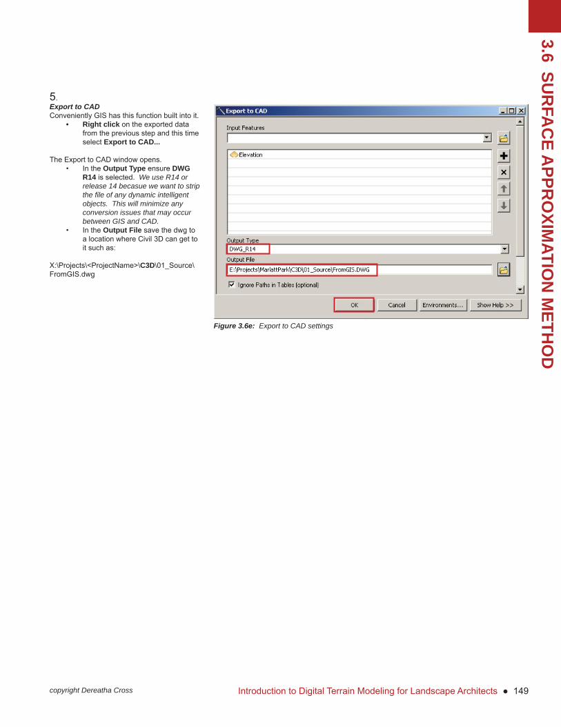
Introduction to Digital Terrain Modeling for Landscape Architects ● 149copyright Dereatha Cross
3.6 SUR
FAC
E APPR
OXIM
ATION
METH
OD
5.Export to CADConveniently GIS has this function built into it.
• Right click on the exported data from the previous step and this time select Export to CAD...
The Export to CAD window opens.• In the Output Type ensure DWG
R14 is selected. We use R14 or release 14 becasue we want to strip the fi le of any dynamic intelligent objects. This will minimize any conversion issues that may occur between GIS and CAD.
• In the Output File save the dwg to a location where Civil 3D can get to it such as:
X:\Projects\<ProjectName>\C3D\01_Source\FromGIS.dwg
Figure 3.6e: Export to CAD settings

3.6 SUR
FAC
E APPR
OXIM
ATION
METH
OD
150 ● Digital Terrain Modeling \\ Surface Approximation Method copyright Dereatha Cross
6.Insert to CAD.
• In a native Civil 3D fi le type insert.
The Insert window opens.• In the Block Unit group ensure
the Unit is set correctly. If it is in inches and it should be feet make the necessary conversion under the Scale group. The example is in inches and a conversion to feet is needed. Ensure all dimensions (x, y, and z) will be converted or your import will be distorted.
• Click OK• Civil 3D will ask for insertion point.
Type 0,0,0 and press enter.
This will bring the contours from GIS in the correct spatial location.
You may need to zoom extents (ZE) to locate the inserted contours from GIS.
7.Ensure the contours have elevation.
• Explode the block• Select one contour• Type properties• Look for the elevation value
Sometimes for what ever reason the contours may not have elevation. So it is always good practice to check.
If they do not have an elevation it does not always mean you did something wrong. Sometimes it is a software glitch. Try re-importing the block. If that still fails the repeat the GIS steps. Often times the problem is with the export from GIS. Sometimes one may forget to make sure it is being exported at R14 version. Try saving it as a new fi le instead of over-writing. Be patient as it will eventual work.
Figure 3.6f: Export to CAD settings
Figure 3.6g: Properties tab of one polyline
Step #2c: Condition DataImport Contours into Civil 3D

Introduction to Digital Terrain Modeling for Landscape Architects ● 151copyright Dereatha Cross
3.6 SUR
FAC
E APPR
OXIM
ATION
METH
OD

3.6 SUR
FAC
E APPR
OXIM
ATION
METH
OD
152 ● Digital Terrain Modeling \\ Surface Approximation Method copyright Dereatha Cross
Step #3a: Creating Surface Create Container
Before we begin this process we need to verify the following settings:• Active layer is Layer 0• Elevation is set to 0 • Thickness is set to 0 • View is set to plan view and in 2D
wireframe• Layers containing the object we wish to
defi ne our surface is the only layer on
You will also need to be in the Civil 3D workspace.
1.To create an existing grade surface container. • In the Civil 3D workspace, in the
Toolspace, in the Prospector Tab, right click on Surfaces, and select Create Surface.
Notice in this context window there are 3 types of surface containers we can create. We will use the standard create surface --the top option.
If you do not have a Toolspace you may need to turn it on by clicking on the Toolspace toggle button in the Home Tab.
2.Once you click on Create Surface the Create Surface window opens.• Click the Layer button next to Surface
Layer C-TOPO
3.The Object Layer Dialog opens.• In the Object Layer dialog, select the
Suffi x dropdown.• Type -* in the Modifi er value. This will
cause what ever you choose to name your surface to be added to the end of C-TOPO-. Basically, the * will be replaced with what you type here.
• Click OK to the Object Layer dialog
Notice most of the layers in Civil 3D start with C. C is what Civil Engineers start their layers with where L is what Landscape Architects use to start their layers. We will use C in these examples.
4.In the Create Surface dialogue:• Next to Name type EG for existing grade• Description: Existing Ground Surface• Style: Contours 1’ and 5’ (Background)
Notice in the select Surface Style drop down there are several options to pick from. If no options appear here it is because the fi le is not a native Civil 3D fi le.
• Click OK
A surface container is created in the Prospector Tab.

Introduction to Digital Terrain Modeling for Landscape Architects ● 153copyright Dereatha Cross
3.6 SUR
FAC
E APPR
OXIM
ATION
METH
OD
1.Right click on Contours and select Add... Figure 3.6h illustrates where to fi nd the Contours defi nition
2.The Add Contour Data window opens. Figure 3.6i.• Next to description type in where the
data came fromIn the weeding factors area leave at default:• Distance: 15’• Angle: 4 (d)• Distance: 100’• Mid-ordinate distance: 1’• Check all of the boxes• Click OKWeeding factors reduces the number of points generated along contours. You can search the help in Civil 3D for “weeding factors” to learn more.
3.Civil 3D now asks to Select objects • Window select (w) the contours and
press enter on the keyboard• Press enter to fi nish the select objects
process
The new surface appears on top of the inserted contours. We can turn off the imported contours so that we only see our newly created surface.
We may want to inspect our surface by exploring it in 3D and turning on a shading mode.
Step 2: Surface Defi nition Selection
Figure 3.6h: Surface defi nition selection by contours
Figure 3.6i: Add Contour settings
Step #3b: Create Surface - Defi nition

3.6 SUR
FAC
E APPR
OXIM
ATION
METH
OD
154 ● Digital Terrain Modeling \\ Surface Approximation Method copyright Dereatha Cross
No breaklines were made for this particular surface. But since we are on this step let us explore different types of breaklines.
There are fi ve types of breaklines. 1. Standard BreaklinesThese are 3D lines, feature lines, or polylines. Standard breaklines typically connect points already included in the surface defi nition but can contain their own elevation data. This type of breaklines is often used to defi ne the edges of a building pad or parking lot --anything proposed to be graded in.
2. Proximity BreaklinesThese breaklines allow you to force triangulation without picking precise points. They will not add vertical information to the surface. The X, Y, Z coordinates will be based on the surface points in close proximity to the breakline.
Figure 3.6k: Standard Breakline Figure 3.6l: Proximity Breakline
Step #3c: Create Surface Breaklines Selection

Introduction to Digital Terrain Modeling for Landscape Architects ● 155copyright Dereatha Cross
3.6 SUR
FAC
E APPR
OXIM
ATION
METH
OD
3. Wall BreaklinesThese breaklines defi ne walls in surfaces. Because of the limitation of true vertical surfaces, a wall breakline will let you approximate a wall without having to create two separate breaklines. They are defi ned on the basis of an elevation at a vertex, and then an elevation difference at each vertex or for the full length of the breakline on a selected side. So a single wall breakline set with elevations will have the same result as creating a breakline with those same elevations and a second breakline that is vertically offset from the fi rst.
4. From File BreaklinesThese are breaklines contained in a text fi le. This fi le can be the output of another program and can be used to modify the surfaced without creating additional drawing objects.
5. Non-destructive BreaklinesThis type of breakline is used to maintain the original integrity of the surface while updating triangulation.
Figure 3.6m: Wall Breakline Figure 3.6n: From File Figure 3.6o: Non Destructive

3.6 SUR
FAC
E APPR
OXIM
ATION
METH
OD
156 ● Digital Terrain Modeling \\ Surface Approximation Method copyright Dereatha Cross
Finally we are on boundaries. The last step of our building existing condition surfaces workfl ow.
Boundaries prevent stray triangulation around the edges. A border is different from a boundary. A border is the extent of the surface. Not all surfaces may have boundaries but all surfaces do have borders.
We can extract the border of an existing surface and modify it to our needs into a boundary.
• Select the tin surface in the drawing space.
• In the ribbon interface under Tin Surface: EG select Extract Objects.
• Un-check everything except the border.• Click OK
A boundary can be a 2D polyline.
If using one from another program ensure it is a 2D polyline. You may need to explode or convert to a 2D polyline.
Figure 3.6p: Extract Objects, this ribbon only appears if you have your surface selected in the drawing space.
Step #3d: Create Surface Boundary Selection

Introduction to Digital Terrain Modeling for Landscape Architects ● 157copyright Dereatha Cross
3.6 SUR
FAC
E APPR
OXIM
ATION
METH
OD
There are four types of boundaries in Civil 3D (Figure 3.6q):
1. Outer BoundariesThis type is used to defi ne the outer edge of the boundary.
2. Show BoundariesThis type is used to show the surface inside a hide boundary.
3. Hide BoundariesThis type is used to create a hole in the surface removing points. This is used for building footprints or wetland areas such as ponds. Volumes will not appear here.
4. Data Clip BoundariesData clip boundaries place limits on data that will be considered as part of the surface from that point going forward. This is mostly used for processing LiDAR data.
Sometimes you may need to experiment in order to get the affect you need. Surface edits can be undone using the Prospector tab, see fi gure 3.6r.
Figure 3.6q: Boundary dialog box.
Figure 3.6r: Edits area

3.6 SUR
FAC
E APPR
OXIM
ATION
METH
OD
158 ● Digital Terrain Modeling \\ Surface Approximation Method copyright Dereatha Cross
Step #3e: Create Surface Error Inspection
After the surface is created it can be inspect-ed in 3D. Press the shift key and the middle mouse button and drag. You may also want to shade your terrain. This can be done by going to the View ribbon, in the Visual Styles, click the drop down and choose Shaded.

Introduction to Digital Terrain Modeling for Landscape Architects ● 159copyright Dereatha Cross
3.6 SUR
FAC
E APPR
OXIM
ATION
METH
OD

3.7 SUR
VEY POIN
TS
160 ● Digital Terrain Modeling \\ Survey Points copyright Dereatha Cross
What are Points?Points are basically spot elevations.
Why use Points?When working at the smaller lot scale LiDAR data may not be at a suffi cient enough resolution. Also recall LiDAR will have a regular point spacing and it may not pick up a critical spot elevation anomaly such as top of curb and bottom of curb. If we want higher resolution and points collected at strategic locations, we tend to send a surveyor out to collect more detailed information. This information is often times collected on what is called a Total Station. A Total Station is an electronic device capable of collecting geospatially located elevation data in digital format. Because a surveyor is collecting the elevation information, points can be strategically collected at elevation anomalies where LiDAR would potentially miss. The output fi le from a Total Station is a text fi le Civil 3D can use to build terrain. Figure 3.6a illustrates a typical point text fi le one would expect from a total station.
Another set of points we can expect to work with are those modeling proposed conditions. These may come on a sheet of trace paper or a scanned in sheet of trace paper. Often times we start on trace and want to move our grading plan to Civil 3D. Figure 3.6b illustrates a sketch of a rough grading plan ready to be transferred into Civil 3D.
Also recall the basic terrain building block in Civil 3D are points. This means regardless if you import terrain meshes or contours, Civil 3D will translate this surface information into points before it builds a surface.
The following section will cover how to take in existing conditions survey fi le into Civil 3D much like the fi le in fi gure 3.7.1a.
The section after this section will look at COGO points and working with a fi le similar to what is shown in fi gure 3.7.1b.
What are Survey Points?
1,315561.62600,1715790.80200,1032.64770,light pole2,315718.42800,1715780.31700,1035.66000,pavement cov3,315538.93800,1715767.03700,0.00000,culvert corner4,315722.15600,1715767.29100,0.00000,5,315655.51620,1715815.33480,1035.66660,mhbm6,315655.37090,1715815.24210,1035.19780,mhbm7,315634.49650,1715813.31720,1035.38750,mh1908,315574.80460,1715818.18460,1035.19110,mh1929,315546.69750,1715814.87960,1034.64450,MH19510,315562.00310,1715828.74380,1035.61630,MH19311,315562.54460,1715841.17620,1036.12060,MH19112,315726.59620,1715832.71840,1037.23880,ST1ELE13,315717.27580,1715836.20520,1037.11840,ST1GD14,315708.04220,1715839.73140,1036.50560,ST1GD15,315698.69820,1715843.31330,1036.00900,ST1GD16,315689.16190,1715847.02150,1035.54440,ST1GD17,315679.96740,1715850.19280,1035.27070,ST1GD18,315670.62370,1715853.89770,1035.18770,ST1GD19,315661.30250,1715857.44630,1035.11870,ST1GD20,315658.68850,1715858.51410,1035.14910,ST1GDFigure 3.7.1a A snippet of a total station point text fi le
Figure 3.7.1b A scanned in preliminary grading plan

Introduction to Digital Terrain Modeling for Landscape Architects ● 161copyright Dereatha Cross
3.7 SUR
VEY POIN
TS
COGO Points vs. Survey Points
When working in Civil 3D we often hear the terms COGO points and Survey points. The outcome is generally the same but the difference is in where the point data is stored. Points brought in using survey data are referred to as survey points. Points brought in using a delimited text fi le and/or placing them in CAD using point creation tools are called COGO points. This means COGO points are unlocked by default making them editable. A Survey points must be unlocked if a user wishes to edit them. Survey points are also tied to an external database or the fi le that help create the points. Where as a COGO point maintains no tie to the originating text fi le.
We will fi rst look at an example Survey point fi le and then explore COGO points. Both COGO points and Survey Points will follow the same major concepts outlined in this section.
In Civil 3D points are dynamic intelligent objects. Information is linked to a point allowing for other information to be linked to that point and vice versa. Points are the foundation of a Civil 3D terrain. Even if we brought in contours, Civil 3D in the background will convert those contours to points before it creates a surface. Each point will contain X, Y, Z information along with a unique point number and optionally a point name.
There are two major components of a point:1) the maker and 2) its label. The marker is its spatial location. The Label is the data linked with that point. Refer to Figure 3.7.3a.
Anatomy of a Point
Point Number (Label)
Elevation (Label)
Description (Label)
Figure 3.7.3a Anatomy of a point.
Marker ComponentLabel Component
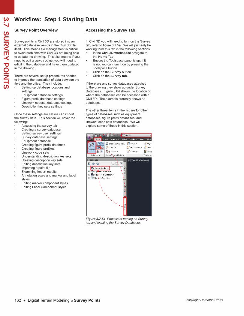
3.7 SUR
VEY POIN
TS
162 ● Digital Terrain Modeling \\ Survey Points copyright Dereatha Cross
Survey points in Civil 3D are stored into an external database versus in the Civil 3D fi le itself. This means fi le management is critical to avoid problems with Civil 3D not being able to update the drawing. This also means If you need to edit a survey object you will need to edit it in the database and have them updated in the drawing.
There are several setup procedures needed to improve the translation of data between the fi eld and the offi ce. They include:• Setting up database locations and
settings• Equipment database settings• Figure prefi x database settings• Linework codeset database settings• Description key sets settings
Once these settings are set we can import the survey data. This section will cover the following:• Accessing the survey tab• Creating a survey database• Setting survey user settings• Survey database settings• Equipment database• Creating fi gure prefi x database• Creating fi gure prefi xes• Linework code sets• Understanding description key sets• Creating description key sets• Editing description key sets• Importing a point fi le• Examining import results• Annotation scale and marker and label
styles• Editing marker component styles• Editing Label Component styles
Survey Point Overview
In Civil 3D you will need to turn on the Survey tab, refer to fi gure 3.7.5a. We will primarily be working form this tab in the following sections.• In the Civil 3D workspace navigate to
the Home Tab.• Ensure the Toolspace panel is up, if it
is not you can turn it on by pressing the Toolspace button.
• Click on the Survey button.• Click on the Survey tab.
If there are any survey databases attached to the drawing they show up under Survey Databases. Figure 3.6d shows the location of where the databases can be accessed within Civil 3D. The example currently shows no databases.
The other three items in the list are for other types of databases such as equipment databases, fi gure prefi x databases, and linework code sets databases. We will explore some of these in this section.
Accessing the Survey Tab
Figure 3.7.5a Process of turning on Survey tab and locating the Survey Databases
Workfl ow: Step 1 Starting Data
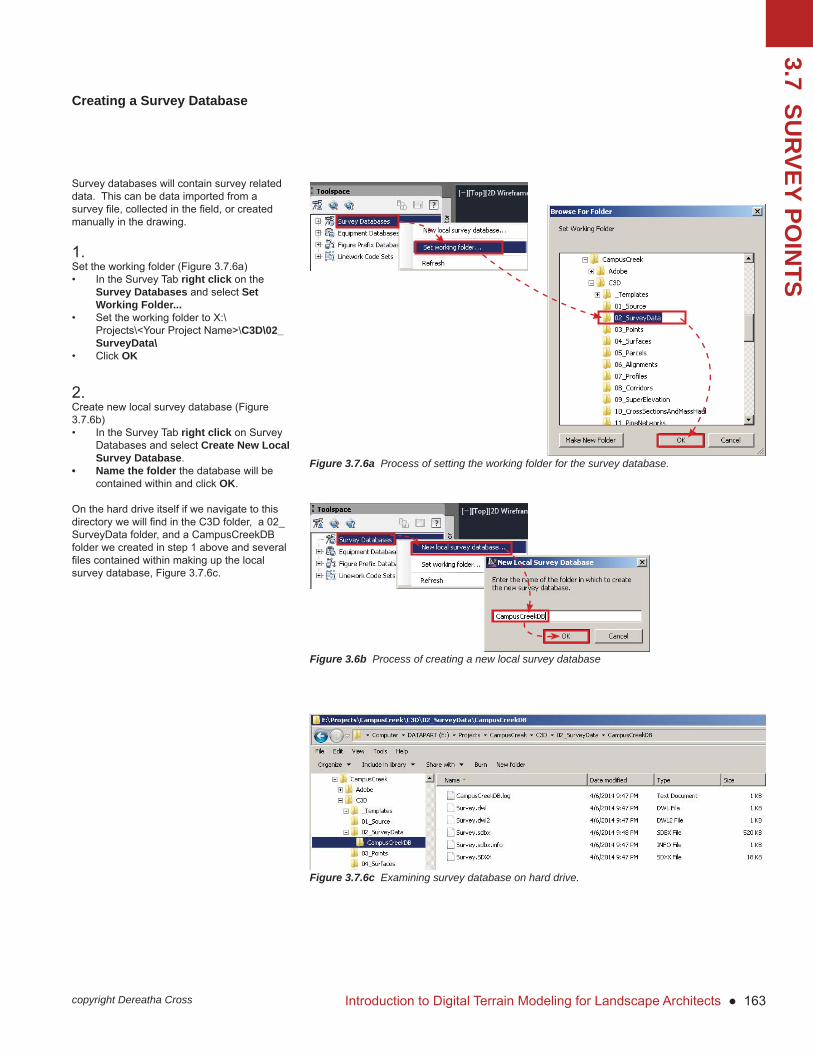
Introduction to Digital Terrain Modeling for Landscape Architects ● 163copyright Dereatha Cross
3.7 SUR
VEY POIN
TS
Survey databases will contain survey related data. This can be data imported from a survey fi le, collected in the fi eld, or created manually in the drawing.
1.Set the working folder (Figure 3.7.6a)• In the Survey Tab right click on the
Survey Databases and select Set Working Folder...
• Set the working folder to X:\Projects\<Your Project Name>\C3D\02_SurveyData\
• Click OK
2. Create new local survey database (Figure 3.7.6b)• In the Survey Tab right click on Survey
Databases and select Create New Local Survey Database.
• Name the folder the database will be contained within and click OK.
On the hard drive itself if we navigate to this directory we will fi nd in the C3D folder, a 02_SurveyData folder, and a CampusCreekDB folder we created in step 1 above and several fi les contained within making up the local survey database, Figure 3.7.6c.
Figure 3.7.6a Process of setting the working folder for the survey database.
Figure 3.6b Process of creating a new local survey database
Figure 3.7.6c Examining survey database on hard drive.
Creating a Survey Database

3.7 SUR
VEY POIN
TS
164 ● Digital Terrain Modeling \\ Survey Points copyright Dereatha Cross
The database defaults, equipment database, linework code sets, and fi gure prefi x database should be in place before you import any survey data. Some companies would like you to keep the data on their server so it is easy to share and backup. You can confi gure where these fi les are located.• In the Survey tab, on the Toolspace
panel, click on the Survey User Settings button. (It is located on the upper left corner of this toolspace panel.)
These settings will stick with every drawing you open. Refer to fi gure 3.7.7a.
Survey User Settings
Figure 3.7.7a Process of locating the Survey User Settings

Introduction to Digital Terrain Modeling for Landscape Architects ● 165copyright Dereatha Cross
3.7 SUR
VEY POIN
TS
Right clicking on the survey database will give you access to a context menu. This menu gives us access to properties, changes that were made, the ability to translate survey database options, edit survey database settings, manage extended properties, import, export survey landxml, and the ability to refresh the content list under the database.
Under CampusCreekDB we also see several items. These items are confi gurable and will allow us to populate our survey database container we have created in previous steps.
• Right click on CampusCreekDB and select Edit database settings...
There are several settings we can change here.
There can be multiple survey databases and these settings can be confi gured uniquely for each one. Refer to fi gure 3.7.8a.
Survey Database Settings
Figure 3.7.8a Process of locating the survey database settings.

3.7 SUR
VEY POIN
TS
166 ● Digital Terrain Modeling \\ Survey Points copyright Dereatha Cross
This database allows you to setup various types of survey equipment you are using in the fi eld. This allows you to apply the proper correction factors to traverse analyses when you need to balance your traverse. Civil 3D comes with example equipment so you can fi gure out which pieces of information you need.
To access the equipment database manager do the following:
• In the Toolspace, in Survey tab, expand Survey Databases, Equipment Databases, and select the equipment. Figure 3.7.9a shows “Sample” as the equipment. This is the Civil 3D default.
• Right click on the equipment and select Manage Equipment Database.
• The Equipment Database Manager - Equipment Name window will open.
There are several settings here that can be changed to your particular device.
Figure 3..7.9a Settings location for confi guring equipment database.
Equipment Database Settings
Introduction to Digital Terrain Modeling for Landscape Architects ● 167copyright Dereatha Cross
3.7 SUR
VEY POIN
TS
Next, we will need to create a Figure Prefi x database. The fi gure prefi x database is used to translate descriptions in the fi eld to lines in CAD. In the context of Figure Prefi x Databases, fi gures are the line objects. This database will sort through created fi gures allowing you to place them on different layers, assign styles, determine object type based on the fi gure name.
Create a new fi gure prefi x database (fi gure 3.7.10a).• In the Toolspace, Survey Tab, right click
the Figure Prefi x Databases and select New.
A New Figure Prefi x Database dialog window opens. • Give the Figure Prefi x Database a
name. In the example we named in CampusCreekFDB
• Right click on the newly created Figure Prefi x database and select Manage Figure Prefi x Database.
A Figure Prefi x Database Manager window opens. Refer to fi gure 3.7.10b.
Figure 3.7.10a Process of creating a new fi gure prefi x database.
Figure 3.7.10b Process of accessing the Figure Prefi x Database Manager
Creating Figure Prefi x Database

3.7 SUR
VEY POIN
TS
168 ● Digital Terrain Modeling \\ Survey Points copyright Dereatha Cross
Figure 3.7.11a Figure Prefi x Database Manager.
Figure prefi xes will allow us to create linework from survey data. We will need to tell Civil 3D what the fi gure prefi xes correspond to. For example we may have surveyed a curb. We may have surveyed several x,y,z coordinates for the top of a curb and named it TC1, TC2, etc for Top of Curb point 1, point 2, etc. We want Civil 3D to connect these points to create a curb. How can we tell Civil 3D to do this?
1.Click the plus sign to add a row to the database.
2.Name the fi gure prefi x after how it is named in the txt fi le. In the example we created a scenario stating we collected curb data along a curb and named it TC1, TC2, TC3, etc. Figure 3.6m illustrates under the Name column “TC”. Because we do not specify 1, 2, or 3 it will grab everything with TC in the name meaning it will include the 1, 2, and 3. We call this a wildcard. A wildcard means it could be anything. So anything after TC could be anything. If we want it to be TC1 then we have to include TC1. If we have a TC12 and a TC13 it will include those two points as well. So if you want unique points you must create unique names.
3.Breaklines indicate how you want Civil 3D to create the surface around this line. Because the example is a curb we want Delaunay’s triangulation to respect this “edge”.
4.Lot Line - this is not a lot line
5. Layer - you can indicate which layer you want this line to occur on.
6.Style - There is a premade curb style. You can change the way curbs appear by going to the Settings tab and navigating to Survey, Figures, and Figure Styles.
7.Site - you can specify the site.
1.
2. 3. 4. 5. 6. 7.
Creating Figure Prefi xes
Introduction to Digital Terrain Modeling for Landscape Architects ● 169copyright Dereatha Cross
3.7 SUR
VEY POIN
TS
The linework code set lists what designators are used to start, stop, continue, or add additional geometry to lines.
Create a new Linework Code Set• In the Toolspace, in the Survey tab,
expand Linework Code Sets.• Right click on Linework Code Sets and
select New.• Name the new Linework Code Sets. • Click OK
The Edit Linework Code Set window opens.
If the survey plans to use the same code sets for each survey fi le you can set these code sets to match what the surveyor will use and re-use these code sets.
Coding MethodsYou can indicate the specifi cs of how the survey fi le was created.
Special CodesBegin helps indicate the beginning of a fi gure. Recall a fi gure is an object and in this case a line. Continue, End, Close, and the other special codes have similar functions to that of Begin as their names indicate.
Line Segment Codes These are similar to the other codes we looked at.
Curve Segment CodesBegin curve and End curve often need to be changes. Everything else is left at default.
This linework code set can be recycled to other projects as long as the survey is consistent with their codes.
Figure 3.7.12a Process of creating new Linework Code Sets.
Linework Code Set

3.7 SUR
VEY POIN
TS
170 ● Digital Terrain Modeling \\ Survey Points copyright Dereatha Cross
Description keys bridge the gap between the fi eld and the offi ce. Description key sets are a listing of fi eld descriptions and how they should look and behave once they are imported into Civil 3D. They are used to automate the process of organizing your points, assigning them to layers, assigning point and label styles, converting raw descriptions to full descriptions, and optionally scaling points. Description key sets are different from fi gure prefi x databases and linework code sets. The later two are external fi les where description key sets are part of your Civil 3D template fi le.
Examining the Survey FileThe fi rst step in creating description key sets is to examine the survey point fi le. Figure 3.7.13a illustrates 20 points copied from a survey point fi le. The fi rst row has been highlighted to illustrate what each number corresponds to.
The purple number 1 corresponds to the Point number.
The red number 315561.62600 corresponds to a value in the X-axis. This is also called the “easting” value. We know this number is easting and not northing because the surveyor either told us or we found out using Google Earth or ArcGIS.
The green number 1715790.80200 corresponds to a value in the Y-axis. This is also called the “northing” value.
The blue number 1032.64770 corresponds to a value in the Z-axis. This is also called the “elevation” value.
The orange value is the point description. When working with Description Key Sets it is this value we are trying to use when making the connection between fi eld and offi ce work.
Figure 3.7.13b illustrates how these points exist in Euclidean space.
Figure 3.7.13a Survey point fi le.
1,315561.62600,1715790.80200,1032.64770,light pole2,315718.42800,1715780.31700,1035.66000,pavement cov3,315538.93800,1715767.03700,0.00000,culvert corner4,315722.15600,1715767.29100,0.00000,5,315655.51620,1715815.33480,1035.66660,mhbm6,315655.37090,1715815.24210,1035.19780,mhbm7,315634.49650,1715813.31720,1035.38750,mh1908,315574.80460,1715818.18460,1035.19110,mh1929,315546.69750,1715814.87960,1034.64450,MH19510,315562.00310,1715828.74380,1035.61630,MH19311,315562.54460,1715841.17620,1036.12060,MH19112,315726.59620,1715832.71840,1037.23880,ST1ELE13,315717.27580,1715836.20520,1037.11840,ST1GD14,315708.04220,1715839.73140,1036.50560,ST1GD15,315698.69820,1715843.31330,1036.00900,ST1GD16,315689.16190,1715847.02150,1035.54440,ST1GD17,315679.96740,1715850.19280,1035.27070,ST1GD18,315670.62370,1715853.89770,1035.18770,ST1GD19,315661.30250,1715857.44630,1035.11870,ST1GD20,315658.68850,1715858.51410,1035.14910,ST1GD
Easting or X axis
Northin
g or Y
axis
Z ax
is o
r ele
vatio
n
X: (315561.6260, 0, 0)Y: (0, 1715790.80200, 0)
Z: (0, 0, 1032.64770)
Point 1: (315561.6260, 1715790.80200, 1032.64770)
Figure 3.7.13b Survey point in Euclidean space.
Understanding Description Key Sets

Introduction to Digital Terrain Modeling for Landscape Architects ● 171copyright Dereatha Cross
3.7 SUR
VEY POIN
TS
When working in the fi eld surveyors may use cryptic numbers instead of text. When moving this information to a CAD drawing it may be more useful to us to convert these raw descriptions into a full description.
We can set this up by doing the following:
• In the Toolspace, in the Settings Tab, expand Point, expand Description Key Sets. The default description key set that comes with Civil 3D is the Civil 3D keyset.
• Right click on the Description Key Sets and select New.
• Input the name of the description key set. In the example we have named it CampusCreekDKS.
• Click OK.
A new description key set is created under Description Key Sets.
Figure 3.7.14a Process of creating a new Description Key Set.
Creating Description Key Sets
3.7 SUR
VEY POIN
TS
172 ● Digital Terrain Modeling \\ Survey Points copyright Dereatha Cross
After creating a new description key set we can edit it.• In the Toolspace, in the settings tab,
expand points, expand description key sets, and right click on the description key set you wish to edit and select Edit Keys.
The Description Key Set panorama window opens. This is called the Description Key editor.
1.CodeThis column must match the description in the Survey fi le. This column is also case sensitive. Wildcards can be used to group together coding such as TC* to include TC1, TC2, TC3, etc.
2.StyleWe can assign a style or leave it as the default style. This can be changed later. This style refers to the marker component.
3.Point Label StyleWe can assign a style or leave it as the default style. This can be changed later. This style refers to the label component.
4.FormatThis is were we can decrypt the code. We can put in this box instead of TC we can write Top of Curb. If we want it to use the same value as the code column then we can indicate $*. These symbols mean use the same value as that in the Code column.
5.LayerWe can assign points to different layers
Right click an existing row and select Copy or New to create a new row. Refer to fi gure 3.6r.
1. 5.4.3.2.
Figure 3.7.15a Process of editing a Description Key Set.
Editing Description Key Sets

Introduction to Digital Terrain Modeling for Landscape Architects ● 173copyright Dereatha Cross
3.7 SUR
VEY POIN
TS

3.7 SUR
VEY POIN
TS
174 ● Digital Terrain Modeling \\ Survey Points copyright Dereatha Cross
Now that we have a Survey Database, Equipment Database, Figure Prefi x Database, Linework Code Sets, and Description Key Sets we can begin importing survey data.
• In the Home tab, in the Create Ground Data group, click on Import Survey Data.
A wizard opens, refer to fi gure 3.7.16a.
Specify Database• Select the database and click Next.
Specify Data Source• Next to Database type click the drop
down and select Point fi le. • Click the “+” button and navigate to
where the saved database fi le is located.• As soon as it is added we need to specify
point fi le format. Recall from an earlier step we had examined the point fi le to be organized using commas. It started with the Point number, easting, northing, z-elevation, and some description. If we take the fi rst letters of each we get PENZD. If we scrolled own the list we can fi nd a PENZD (comma delimited)
• Below it shows a preview of how it will interpret the text fi le.
• Click Next.
Importing a Point File
Workfl ow: Step 2 Condition Data

Introduction to Digital Terrain Modeling for Landscape Architects ● 175copyright Dereatha Cross
3.7 SUR
VEY POIN
TS
Specify NetworkWe can optionally create a network. The example created a CampusCreekNetwork.• Click Next.
Import OptionsWe can specify the import settings for the selected data source.• Current fi gure prefi x database should
be set to the one we created• Process linework during import should
be set to yes. (This fi le doesn’t have any line work)
• Current linework code set should be set to the one we created
• Insert network object is set to No because we don’t have any in this fi le.
• Insert fi gure objects is set to yes• Insert survey points is set to yes.• Click Finish.
Figure 3.7.16a Process of editing a Description Key Set.

3.7 SUR
VEY POIN
TS
176 ● Digital Terrain Modeling \\ Survey Points copyright Dereatha Cross
The results may not be what you expected. Figure 3.7.17a illustrates our results. The red X’s are the point markers. We see a tree symbol. This symbol occurs because the description “tree” happens to match up with a Civil 3D graphic symbol “tree” and so we see a tree. --Recall we are dealing with intelligent objects.
The overlapping text is our point labels. We need to confi gure the styles to prevent our point labels from overlapping each other. We may also only be concerned about elevation and description and we don’t really care about the point number.
We can see from the results in fi gure 3.6t we will need to confi gure the point styles. The size of the marker component and label component are controlled by the annotation scale of the drawing. Let us consider fi gure 3.7.18a. Recall we can change the annotation scale using the status bar.
There are other controls we can also set to control the marker and label components. These styles can be accessed using the Settings tab.
In the Toolspace panel, in the Settings tab, expand Point, and expand Point Styles. Under Point Styles you can fi nd Label Styles. Refer to Figure 3.7.18b.
Figure 3.7.17a Results of point import.
So what we see below is actually correct all things considered. We just need to adjust the annotation scale and marker and label styles.
Import Results Annotation Scale and Marker and Label Styles
Introduction to Digital Terrain Modeling for Landscape Architects ● 177copyright Dereatha Cross
3.7 SUR
VEY POIN
TS
Scale: 1” = 10’
Scale: 1” = 20’
Scale: 1” = 40’
Figure 3.7.18a Different annotation scales changes the size of the point label component.
Figure 3.7.18b Where to fi nd the Point Styles.
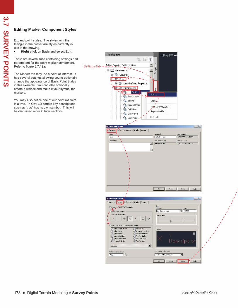
3.7 SUR
VEY POIN
TS
178 ● Digital Terrain Modeling \\ Survey Points copyright Dereatha Cross
Expand point styles. The styles with the triangle in the corner are styles currently in use in the drawing.• Right click on Basic and select Edit.
There are several tabs containing settings and parameters for the point marker component. Refer to fi gure 3.7.19a.
The Marker tab may be a point of interest. It has several settings allowing you to optionally change the appearance of Basic Point Styles in this example. You can also optionally create a wblock and make it your symbol for markers.
You may also notice one of our point markers is a tree. In Civil 3D certain key descriptions such as “tree” has its own symbol. This will be discussed more in later sections.
Settings Tab
Editing Marker Component Styles

Introduction to Digital Terrain Modeling for Landscape Architects ● 179copyright Dereatha Cross
3.7 SUR
VEY POIN
TS
Figure 3.7.19a Point marker component settings.
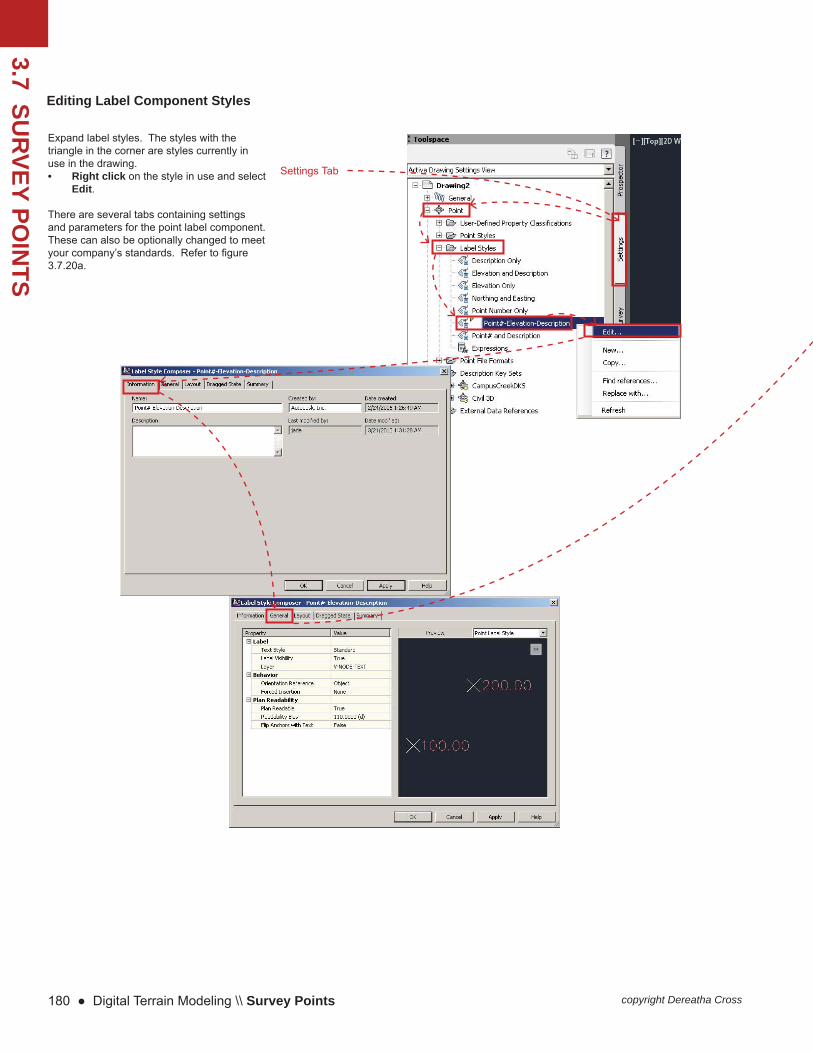
3.7 SUR
VEY POIN
TS
180 ● Digital Terrain Modeling \\ Survey Points copyright Dereatha Cross
Editing Label Component Styles
Expand label styles. The styles with the triangle in the corner are styles currently in use in the drawing.• Right click on the style in use and select
Edit.
There are several tabs containing settings and parameters for the point label component. These can also be optionally changed to meet your company’s standards. Refer to fi gure 3.7.20a.
Settings Tab

Introduction to Digital Terrain Modeling for Landscape Architects ● 181copyright Dereatha Cross
3.7 SUR
VEY POIN
TS
Figure 3.7.20a Point label component settings.
Figure 3.6w After setting changes results.
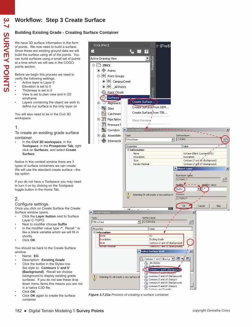
3.7 SUR
VEY POIN
TS
182 ● Digital Terrain Modeling \\ Survey Points copyright Dereatha Cross
Building Existing Grade - Creating Surface Container
We have 3D surface information in the form of points. We now need to build a surface. Since these are existing ground data we will build the surface using all of the points. You can build surfaces using a small set of points at a time which we will see in the COGO points section.
Before we begin this process we need to verify the following settings:• Active layer is Layer 0• Elevation is set to 0 • Thickness is set to 0 • View is set to plan view and in 2D
wireframe• Layers containing the object we wish to
defi ne our surface is the only layer on
You will also need to be in the Civil 3D workspace.
1.To create an existing grade surface container. • In the Civil 3D workspace, in the
Toolspace, in the Prospector Tab, right click on Surfaces, and select Create Surface.
Notice in this context window there are 3 types of surface containers we can create. We will use the standard create surface --the top option.
If you do not have a Toolspace you may need to turn it on by clicking on the Toolspace toggle button in the Home Tab.
2.Confi gure settings.Once you click on Create Surface the Create Surface window opens.• Click the Layer button next to Surface
Layer C-TOPO• Next to modifi er choose Suffi x • In the modifi er value type -*. Recall * is
like a blank variable which we will fi ll in shortly.
• Click OK
You should be back to the Create Surface window. • Name: EG• Description: Existing Grade• Click the button in the Styles row.
Set style to: Contours 1’ and 5’ (Background). Recall we choose background to display existing grade surfaces. If you do not see these drop down menu items this means you are not in a native C3D fi le.
• Click OK.• Click OK again to create the surface
containerFigure 3.7.21a Process of creating a surface container.
Workfl ow: Step 3 Create Surface

Introduction to Digital Terrain Modeling for Landscape Architects ● 183copyright Dereatha Cross
3.7 SUR
VEY POIN
TS
Figure 3.7.22a Process of adding points to the surface container.
Building Existing Grade - Surface Defi nition
3.Add the point data• In the Civil 3D workspace, in the
Toolspace, in the Prospector Tab, in Surfaces, in Defi nition, right click Point Groups, and select Add.
The Point Groups window opens.• Select CampusCreek. Notice there
is also All Points which will allow you to add all points. There are also up and down arrows to the right which will allow you to move groups up and down. This becomes relevant when you have multiple groups.
• Click OK
The surface should build. It currently does not have a boundary so you may see stray triangulation.
From here you can add breaklines which we do not have any for this particular example.
After adding breaklines the next step of the process is to add the boundary to control stray triangulation.

3.8 GR
AD
ING
WITH
CO
NTO
UR
S
184 ● Digital Terrain Modeling \\ Grading with Contours copyright Dereatha Cross
Overview
Thus far we have been building existing grade surfaces using existing data. We have took a look at 3 possible scenarios you might expect to see in practice. Once you have your existing surface built it is time to create a design grade or design surface. This is where we take the existing surface and manipulate it so we can begin to sculpt the surface.
We will now take a look at how to create a proposed surface using the “paste” technique. When using this technique. In order to do this we need to create three surfaces (1) Existing Grade, (2) Design Grade, and (3) Proposed Grade.
Creating Proposed Contours
To manipulate contours, we will fi rst need contours to manipulate. We can obtain this data either through scanning in an image where we have sketched some contours and tracing the contours using the polyline tool or by extracting them from the surface.
If you choose to scan in your plan from trace or other medium you will need to ensure it is “georeferenced”. This means matched the scanned in image with the CAD drawing. You will need to lock it into at least two points to control the scale and rotation of the scanned in image. The “alignment” tool can accomplish this task in Civil 3D.
To use contours from the surface they will need to be extracted from the surface. One might have noticed upon selecting the surface it is one solid object as if it was a block. Yes, it is a solid object and it is actually a dynamic intelligent object. We will need to extract the contours from the object in order to manipulate them. We will then use the extracted contours to create a grading plan. The following illustrates how to extract objects from a surface.
Figure 3.8.1a Existing Grade
Figure 3.8.1b Design Grade
Figure 3.8.1c Proposed Grade

Introduction to Digital Terrain Modeling for Landscape Architects ● 185copyright Dereatha Cross
3.8 GR
AD
ING
WITH
CO
NTO
UR
S
Workfl ow
Figure 3.8.2a The process of accessing the surface styles
Understanding Surface Styles
The surface style we choose during the surface creation process is nothing more than just a style. This means we can make our surface appear as triangles, contours, and even points.
We are preparing to extract objects from our surface. What is extractable is dependent upon what surface style you have turned on at that given moment. So this means if we want polygons we need to make sure the triangle style is selected.
To change the style of a surface, do the following:
1.In Civil 3D workspace, in the Toolspace panel, in the Prospector Tab, expand the Surfaces container.
2.Right click on EG, select Surface Properties.
The Surface Properties window opens for that surface.
3.In the information tab, in the Default styles group, next to the Surface Style, select the drop down to access default surface styles.
Notice the drop menu has several options for different scenarios. Thus far we have only been working with existing conditions. In terms of contours, we would choose (Back-ground) for existing grade. For proposed we would choose (Design).
Contours and Triangles are used for 3D modeling.
Elevation and slope bandings are used for surface analysis.
Refer to Figure 3.8.2a.
If you do not see anything in the drop down menu it means you are not working in a native Civil 3D fi le. One way to fi x this is to wblock out your drawing and insert your linework into a new native Civil 3D drawing.

3.8 GR
AD
ING
WITH
CO
NTO
UR
S
186 ● Digital Terrain Modeling \\ Grading with Contours copyright Dereatha Cross
Workfl ow
Editing Surface Styles
There may be the need to edit an existing surface style to accomplish certain tasks. One such task may involve editing surface points in a proposed grade surface. Another may be to simply solve a problem with an existing style that may not be working. One way to solve this is to create a new surface style with the desired style settings.
Notice in the drop down list, points are not an option. However, we can create a style for points.
To create a surface style we choose one that comes close and edit:
1.Create New StyleFrom the previous page, choose the button next to Surface style as indicated in fi gure 3.8.2b and choose Copy Current Selection or Create New.
The Surface Style - New Surface Style window opens.
2. Name the StyleIn the Information Tab, give the surface style a name.
3.Change the settingsIn the display tab, turn on and off components you wish to appear or not appear under visible. Also, you can change the color of each component under the color column.Click Apply and OK to all windows to close them out to view your results.
Figure 3.8.2b Creating a custom surface from an existing surface.
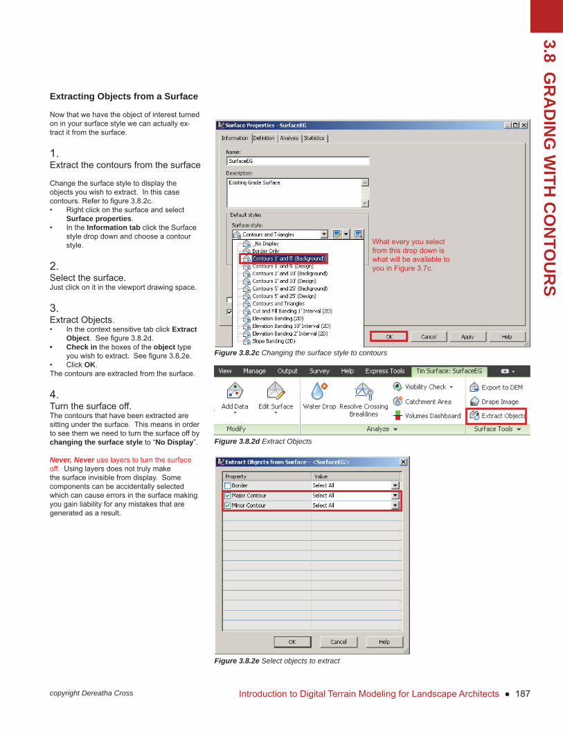
Introduction to Digital Terrain Modeling for Landscape Architects ● 187copyright Dereatha Cross
3.8 GR
AD
ING
WITH
CO
NTO
UR
S
Extracting Objects from a Surface
Now that we have the object of interest turned on in your surface style we can actually ex-tract it from the surface.
1.Extract the contours from the surface
Change the surface style to display the objects you wish to extract. In this case contours. Refer to fi gure 3.8.2c.• Right click on the surface and select
Surface properties.• In the Information tab click the Surface
style drop down and choose a contour style.
2.Select the surface.Just click on it in the viewport drawing space.
3.Extract Objects.• In the context sensitive tab click Extract
Object. See fi gure 3.8.2d.• Check in the boxes of the object type
you wish to extract. See fi gure 3.8.2e.• Click OK.The contours are extracted from the surface.
4.Turn the surface off.The contours that have been extracted are sitting under the surface. This means in order to see them we need to turn the surface off by changing the surface style to “No Display”.
Never, Never use layers to turn the surface off. Using layers does not truly make the surface invisible from display. Some components can be accidentally selected which can cause errors in the surface making you gain liability for any mistakes that are generated as a result.
Figure 3.8.2c Changing the surface style to contours
Figure 3.8.2d Extract Objects
Figure 3.8.2e Select objects to extract
What every you select from this drop down is what will be available to you in Figure 3.7c.

3.8 GR
AD
ING
WITH
CO
NTO
UR
S
188 ● Digital Terrain Modeling \\ Grading with Contours copyright Dereatha Cross
Layer Management
You will need to move the contours from the default layer Civil 3D has extracted them to because Civil 3D will re-use these layers in future extractions.
5.Move the contours to a layer starting with L.• Create two layers named L-TOPO-Minr
and L-TOPO-Majr• Select minor contours and move to
L-TOPO-Minr• Select major contours and move to
L-TOPO-Majr
Anything we design should go on layers starting with an L. This helps others to know the content of that layer was designed by a Landscape Architect.
Recall you can create layer group fi lters and copy layers you need into them so you do not have to scroll through the 200+ layers.
Once you have the contours moved to their own layer you can begin manipulating them to create your design.
6.Manipulate the extracted objectThis part involves grading. When grading a site with many contours, grade the major ones fi rst. Then turn on the minor ones to conform with the majors. Recall some of the main reasons why we grade:
1. To make the terrain suitable for some time of use such as parking, building pad, handicap accessibility, etc.2. Control the follow of water. Will water be a liability or asset on your site?3. Aesthetics. This is what sets us apart from Engineers.
Workfl ow
Figure 3.8.2f Ensure contours are on their own layer.

Introduction to Digital Terrain Modeling for Landscape Architects ● 189copyright Dereatha Cross
3.8 GR
AD
ING
WITH
CO
NTO
UR
S
Build Design Grade Surface
The following methodology will be very similar to the surface approximation method. Please refer to that section if you still need more detailed step-by-step instruction.
Step1Create Design Grade Surface ContainerLayer should be set to C-TOPO-DGDescription should be set to “Design Grade”Styles should be set to 1 and 5 Design.
Step 2Surface Defi nitionUsing the surface approximation method defi ne the surface using contours.
Step 3Add breaklinesIf there are any, add breaklines.
Step 4Add BoundaryIf needed add a boundary.
Step 5Examine the surfaceExamine the surface for errors.
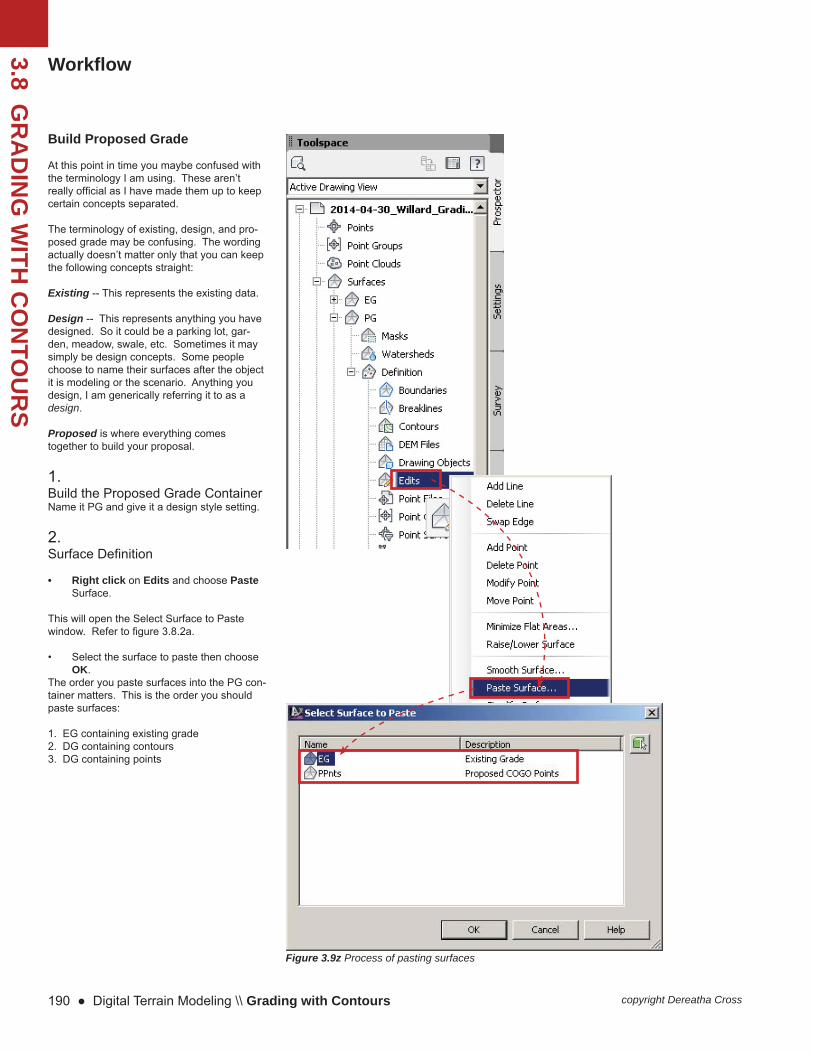
3.8 GR
AD
ING
WITH
CO
NTO
UR
S
190 ● Digital Terrain Modeling \\ Grading with Contours copyright Dereatha Cross
Build Proposed Grade
At this point in time you maybe confused with the terminology I am using. These aren’t really offi cial as I have made them up to keep certain concepts separated.
The terminology of existing, design, and pro-posed grade may be confusing. The wording actually doesn’t matter only that you can keep the following concepts straight:
Existing -- This represents the existing data.
Design -- This represents anything you have designed. So it could be a parking lot, gar-den, meadow, swale, etc. Sometimes it may simply be design concepts. Some people choose to name their surfaces after the object it is modeling or the scenario. Anything you design, I am generically referring it to as a design.
Proposed is where everything comes together to build your proposal.
1.Build the Proposed Grade ContainerName it PG and give it a design style setting.
2.Surface Defi nition
• Right click on Edits and choose Paste Surface.
This will open the Select Surface to Paste window. Refer to fi gure 3.8.2a.
• Select the surface to paste then choose OK.
The order you paste surfaces into the PG con-tainer matters. This is the order you should paste surfaces:
1. EG containing existing grade2. DG containing contours3. DG containing points
Figure 3.9z Process of pasting surfaces
Workfl ow

Introduction to Digital Terrain Modeling for Landscape Architects ● 191copyright Dereatha Cross
3.8 GR
AD
ING
WITH
CO
NTO
UR
S
Why use this Technique?
Often times you will see new users of Civil 3D create a surface for their existing and then a proposed grade. In other words, there are no design grades. There are many reasons why I use this technique:
1.Delegation of tasksPasting surfaces using Edit Surface allows the Landscape Architect to break surfaces down by areas and delegate those areas to different team members. The surfaces can then be brought together to create one large proposed grade.
2.Keeping Surface Data IntactWhen pasting surfaces into PG you are pasting a “copy” of the original surface. This means you are keeping the original data intact. In practice you surface will undergo many design iterations. Being able to modify small areas at a time versus the entire surrface can save you time.
3.Design Scenario FreedomIt also gives you the freedom to create several design scenarios and grade it into the existing terrain rather quickly. If a DG scenario is undesirable it can be removed from the PG container without deleting the actual DG data. Another version of that DG can be added to the proposed container in seconds. This is perhaps one of the most powerful features of using this technique.
To delete a surfaces select Edit in the surface container under defi nition and then in the box at the lower half of the prospector panel, you can select that surface and delete it. From there you simply rebuild all affected surfaces. Again, this does not delete the original DG surface but simply removes a copy of it from the PG container.
ORDER MATTERS!
Order matters when pasting surfaces. We always choose existing grade fi rst. Then we work from the bottom up in regards to how we want to grade features into the existing terrain.
For example, if we created a lake like situation with a ramp going into the lake for boaters then we should add our lake grading fi rst followed by the ramp. If we added the ramp fi rst, Civil 3D will grade in the ramp into the existing surface. When we add the lake, it will grade on top of the ramp because the lake elevation would be lower than the ramp. The result would be the ramp disappearing.
Grade carefully!

3.9 CO
NTO
UR
LAB
ELS
192 ● Digital Terrain Modeling \\ Contour Labels copyright Dereatha Cross
Adding Labels
Adding contour labels is very simple now that we have a surface. We can do this by doing the following:
In the Civil 3D workspace, in the Annotate tab, in the Add Labels drop down, in surface, choose one of the 3 ways you can add labels:
• Contour - Single• Contour - Multiple• Contour - Multiple at Interval
Refer to Figure 3.9.1a.
Adding and Manipulating Contour Labels
Figure 3.9.1a Accessing contour label feature in C3D.
Accessing Label Styles
To access styles in general we go into the Settings tab. Every possible object having styles or the ability to change its behavior will be listed here.
To access contour label styles specifi cally we click on the Surface. Under Surface are several style groups. Like Points, there is the marker component and the label component for surfaces. You can tell what styles are being used in the drawing by the little triangle appearing in the left corner. Refer to Figure 3.9.2b.
Figure 3.9.2b Accessing the label style settings.

Introduction to Digital Terrain Modeling for Landscape Architects ● 193copyright Dereatha Cross
3.9 CO
NTO
UR
LAB
ELS

3.9 CO
NTO
UR
LAB
ELS
194 ● Digital Terrain Modeling \\ Contour Labels copyright Dereatha Cross
Removing Additional Zero’s
Locating where to remove the additional zeros should be easy but in actuallity can be somewhat challenging in Civil 3D as it may not be obvious in the styles settings. Recall contours are whole number integers and not decimal value doubles. To remove unneeded cluter from the drawing refer to the following.
1.Access the Label StyleIn the Settings tab navigate to Surface, Label Styles, Contour, and select the label you wish to change.
2.Edit the label styleRight click on the label and choose Edit.
The Label Style Composer - Exiting Minor Labels dialog window opens.• Click on the Layout tab• In the Component name: select Surface
Elevation• In the Content row click inside the box
starting with <[Surface Elev... so the 3 dot button appear.
• Click on the button with the three dots.Refer to Figure 3.9.3c
Figure 3.9.3c Accessing the label style settings for contour labels.
Adding and Manipulating Contour Labels
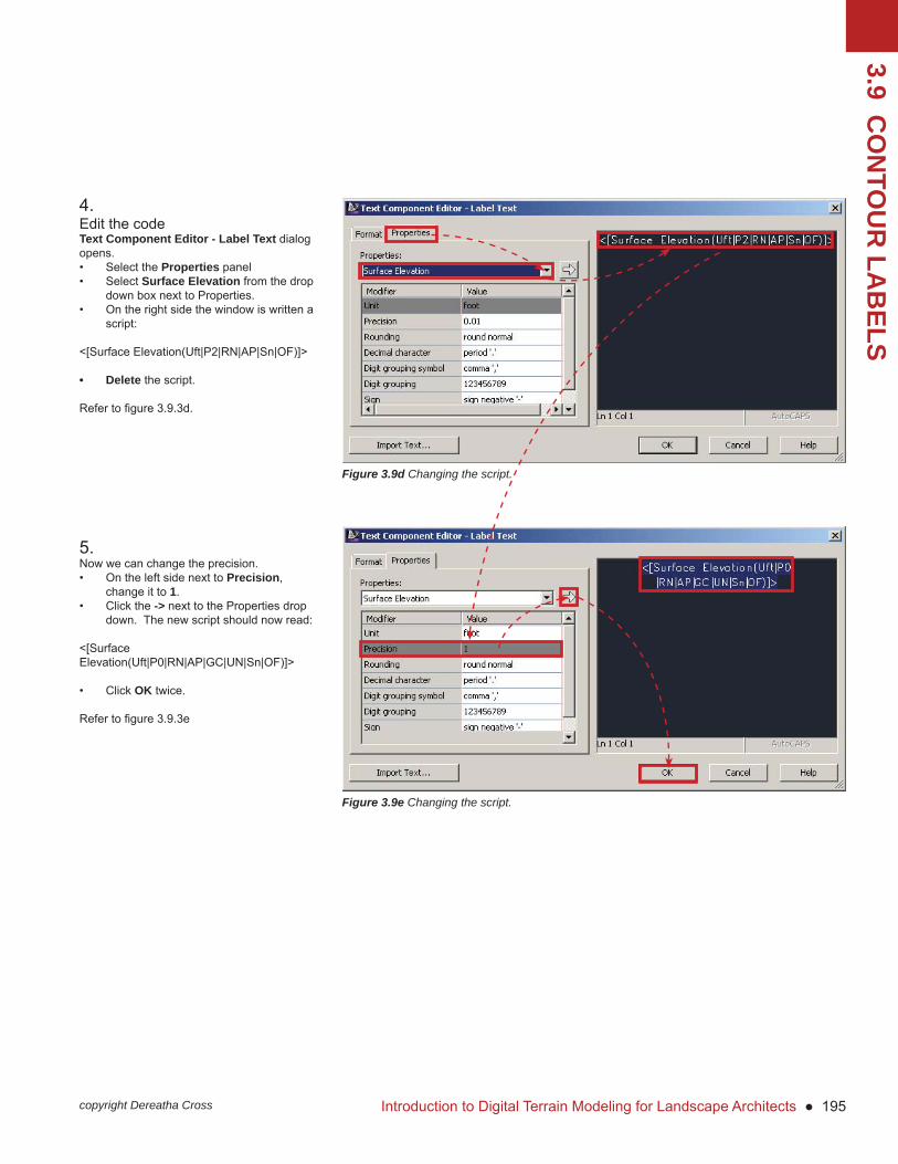
Introduction to Digital Terrain Modeling for Landscape Architects ● 195copyright Dereatha Cross
3.9 CO
NTO
UR
LAB
ELS
4.Edit the codeText Component Editor - Label Text dialog opens. • Select the Properties panel• Select Surface Elevation from the drop
down box next to Properties.• On the right side the window is written a
script:
<[Surface Elevation(Uft|P2|RN|AP|Sn|OF)]>
• Delete the script.
Refer to fi gure 3.9.3d.
5.Now we can change the precision.• On the left side next to Precision,
change it to 1.• Click the -> next to the Properties drop
down. The new script should now read:
<[Surface Elevation(Uft|P0|RN|AP|GC|UN|Sn|OF)]>
• Click OK twice.
Refer to fi gure 3.9.3e
Figure 3.9e Changing the script.
Figure 3.9d Changing the script.