Advanced Analytics with Spark - K-State Canvas

Sandy Ryza, Uri Laserson, Sean Owen, & Josh Wills

Advanced Analytics with

SparkPATTERNS FOR LEARNING FROM DATA AT SCALE

2nd Edition

https://sci101web.wordpress.com/

Sandy Ryza, Uri Laserson, Sean Owen, and Josh Wills

Advanced Analytics with SparkPatterns for Learning from Data at Scale

SECOND EDITION

Boston Farnham Sebastopol TokyoBeijing Boston Farnham Sebastopol TokyoBeijing


978-1-491-97295-3

[LSI]

Advanced Analytics with Sparkby Sandy Ryza, Uri Laserson, Sean Owen, and Josh Wills

Copyright © 2017 Sanford Ryza, Uri Laserson, Sean Owen, Joshua Wills. All rights reserved.

Printed in the United States of America.

Published by O’Reilly Media, Inc., 1005 Gravenstein Highway North, Sebastopol, CA 95472.

O’Reilly books may be purchased for educational, business, or sales promotional use. Online editions arealso available for most titles (http://oreilly.com/safari). For more information, contact our corporate/insti‐tutional sales department: 800-998-9938 or [email protected].

Editor: Marie BeaugureauProduction Editor: Melanie YarbroughCopyeditor: Gillian McGarveyProofreader: Christina Edwards

Indexer: WordCo Indexing ServicesInterior Designer: David FutatoCover Designer: Karen MontgomeryIllustrator: Rebecca Demarest

June 2017: Second Edition

Revision History for the Second Edition2017-06-09: First Release

The O’Reilly logo is a registered trademark of O’Reilly Media, Inc. Advanced Analytics with Spark, thecover image, and related trade dress are trademarks of O’Reilly Media, Inc.

While the publisher and the authors have used good faith efforts to ensure that the information andinstructions contained in this work are accurate, the publisher and the authors disclaim all responsibilityfor errors or omissions, including without limitation responsibility for damages resulting from the use ofor reliance on this work. Use of the information and instructions contained in this work is at your ownrisk. If any code samples or other technology this work contains or describes is subject to open sourcelicenses or the intellectual property rights of others, it is your responsibility to ensure that your usethereof complies with such licenses and/or rights.


http://oreilly.com/safari

Table of Contents

Foreword. . . . . . . . . . . . . . . . . . . . . . . . . . . . . . . . . . . . . . . . . . . . . . . . . . . . . . . . . . . . . . . . . . . . . vii

Preface. . . . . . . . . . . . . . . . . . . . . . . . . . . . . . . . . . . . . . . . . . . . . . . . . . . . . . . . . . . . . . . . . . . . . . . ix

1. Analyzing Big Data. . . . . . . . . . . . . . . . . . . . . . . . . . . . . . . . . . . . . . . . . . . . . . . . . . . . . . . . . . 1The Challenges of Data Science 3Introducing Apache Spark 4About This Book 6The Second Edition 7

2. Introduction to Data Analysis with Scala and Spark. . . . . . . . . . . . . . . . . . . . . . . . . . . . . . . 9Scala for Data Scientists 10The Spark Programming Model 11Record Linkage 12Getting Started: The Spark Shell and SparkContext 13Bringing Data from the Cluster to the Client 19Shipping Code from the Client to the Cluster 22From RDDs to Data Frames 23Analyzing Data with the DataFrame API 26Fast Summary Statistics for DataFrames 32Pivoting and Reshaping DataFrames 33Joining DataFrames and Selecting Features 37Preparing Models for Production Environments 38Model Evaluation 40Where to Go from Here 41

3. Recommending Music and the Audioscrobbler Data Set. . . . . . . . . . . . . . . . . . . . . . . . . . 43Data Set 44

iii


The Alternating Least Squares Recommender Algorithm 45Preparing the Data 48Building a First Model 51Spot Checking Recommendations 54Evaluating Recommendation Quality 56Computing AUC 58Hyperparameter Selection 60Making Recommendations 62Where to Go from Here 64

4. Predicting Forest Cover with Decision Trees. . . . . . . . . . . . . . . . . . . . . . . . . . . . . . . . . . . . 65Fast Forward to Regression 65Vectors and Features 66Training Examples 67Decision Trees and Forests 68Covtype Data Set 71Preparing the Data 71A First Decision Tree 74Decision Tree Hyperparameters 80Tuning Decision Trees 82Categorical Features Revisited 86Random Decision Forests 88Making Predictions 91Where to Go from Here 91

5. Anomaly Detection in Network Traffic with K-means Clustering. . . . . . . . . . . . . . . . . . . 93Anomaly Detection 94K-means Clustering 94Network Intrusion 95KDD Cup 1999 Data Set 96A First Take on Clustering 97Choosing k 99Visualization with SparkR 102Feature Normalization 106Categorical Variables 108Using Labels with Entropy 109Clustering in Action 111Where to Go from Here 112

6. Understanding Wikipedia with Latent Semantic Analysis. . . . . . . . . . . . . . . . . . . . . . . . 115The Document-Term Matrix 116Getting the Data 118

iv | Table of Contents


Parsing and Preparing the Data 118Lemmatization 120Computing the TF-IDFs 121Singular Value Decomposition 123Finding Important Concepts 125Querying and Scoring with a Low-Dimensional Representation 129Term-Term Relevance 130Document-Document Relevance 132Document-Term Relevance 133Multiple-Term Queries 134Where to Go from Here 136

7. Analyzing Co-Occurrence Networks with GraphX. . . . . . . . . . . . . . . . . . . . . . . . . . . . . . . 137The MEDLINE Citation Index: A Network Analysis 139Getting the Data 140Parsing XML Documents with Scala’s XML Library 142Analyzing the MeSH Major Topics and Their Co-Occurrences 143Constructing a Co-Occurrence Network with GraphX 146Understanding the Structure of Networks 150

Connected Components 150Degree Distribution 153

Filtering Out Noisy Edges 155Processing EdgeTriplets 156Analyzing the Filtered Graph 158

Small-World Networks 159Cliques and Clustering Coefficients 160Computing Average Path Length with Pregel 161

Where to Go from Here 166

8. Geospatial and Temporal Data Analysis on New York City Taxi Trip Data. . . . . . . . . . . 169Getting the Data 170Working with Third-Party Libraries in Spark 171Geospatial Data with the Esri Geometry API and Spray 172

Exploring the Esri Geometry API 172Intro to GeoJSON 174

Preparing the New York City Taxi Trip Data 176Handling Invalid Records at Scale 178Geospatial Analysis 182

Sessionization in Spark 185Building Sessions: Secondary Sorts in Spark 186

Where to Go from Here 189

Table of Contents | v


9. Estimating Financial Risk Through Monte Carlo Simulation. . . . . . . . . . . . . . . . . . . . . . 191Terminology 192Methods for Calculating VaR 193

Variance-Covariance 193Historical Simulation 193Monte Carlo Simulation 193

Our Model 194Getting the Data 195Preprocessing 195Determining the Factor Weights 198Sampling 201

The Multivariate Normal Distribution 204Running the Trials 205Visualizing the Distribution of Returns 208Evaluating Our Results 209Where to Go from Here 211

10. Analyzing Genomics Data and the BDG Project. . . . . . . . . . . . . . . . . . . . . . . . . . . . . . . . . 213Decoupling Storage from Modeling 214Ingesting Genomics Data with the ADAM CLI 217

Parquet Format and Columnar Storage 223Predicting Transcription Factor Binding Sites from ENCODE Data 225Querying Genotypes from the 1000 Genomes Project 232Where to Go from Here 235

11. Analyzing Neuroimaging Data with PySpark and Thunder. . . . . . . . . . . . . . . . . . . . . . . 237Overview of PySpark 238

PySpark Internals 239Overview and Installation of the Thunder Library 241Loading Data with Thunder 241

Thunder Core Data Types 248Categorizing Neuron Types with Thunder 249Where to Go from Here 254

Index. . . . . . . . . . . . . . . . . . . . . . . . . . . . . . . . . . . . . . . . . . . . . . . . . . . . . . . . . . . . . . . . . . . . . . . 255

vi | Table of Contents


Foreword

Ever since we started the Spark project at Berkeley, I’ve been excited about not justbuilding fast parallel systems, but helping more and more people make use of large-scale computing. This is why I’m very happy to see this book, written by four expertsin data science, on advanced analytics with Spark. Sandy, Uri, Sean, and Josh havebeen working with Spark for a while, and have put together a great collection of con‐tent with equal parts explanations and examples.

The thing I like most about this book is its focus on examples, which are all drawnfrom real applications on real-world data sets. It’s hard to find one, let alone 10,examples that cover big data and that you can run on your laptop, but the authorshave managed to create such a collection and set everything up so you can run themin Spark. Moreover, the authors cover not just the core algorithms, but the intricaciesof data preparation and model tuning that are needed to really get good results. Youshould be able to take the concepts in these examples and directly apply them to yourown problems.

Big data processing is undoubtedly one of the most exciting areas in computingtoday, and remains an area of fast evolution and introduction of new ideas. I hopethat this book helps you get started in this exciting new field.

— Matei Zaharia, CTO at Databricksand Vice President, Apache Spark

vii


Preface

Sandy Ryza

I don’t like to think I have many regrets, but it’s hard to believe anything good cameout of a particular lazy moment in 2011 when I was looking into how to best distrib‐ute tough discrete optimization problems over clusters of computers. My advisorexplained this newfangled Apache Spark thing he had heard of, and I basically wroteoff the concept as too good to be true and promptly got back to writing my undergradthesis in MapReduce. Since then, Spark and I have both matured a bit, but only oneof us has seen a meteoric rise that’s nearly impossible to avoid making “ignite” punsabout. Cut to a few years later, and it has become crystal clear that Spark is somethingworth paying attention to.

Spark’s long lineage of predecessors, from MPI to MapReduce, makes it possible towrite programs that take advantage of massive resources while abstracting away thenitty-gritty details of distributed systems. As much as data processing needs havemotivated the development of these frameworks, in a way the field of big data hasbecome so related to these frameworks that its scope is defined by what these frame‐works can handle. Spark’s promise is to take this a little further—to make writing dis‐tributed programs feel like writing regular programs.

Spark is great at giving ETL pipelines huge boosts in performance and easing some ofthe pain that feeds the MapReduce programmer’s daily chant of despair (“why?whyyyyy?”) to the Apache Hadoop gods. But the exciting thing for me about it hasalways been what it opens up for complex analytics. With a paradigm that supportsiterative algorithms and interactive exploration, Spark is finally an open sourceframework that allows a data scientist to be productive with large data sets.

I think the best way to teach data science is by example. To that end, my colleaguesand I have put together a book of applications, trying to touch on the interactionsbetween the most common algorithms, data sets, and design patterns in large-scaleanalytics. This book isn’t meant to be read cover to cover. Page to a chapter that lookslike something you’re trying to accomplish, or that simply ignites your interest.

ix


What’s in This BookThe first chapter will place Spark within the wider context of data science and bigdata analytics. After that, each chapter will comprise a self-contained analysis usingSpark. The second chapter will introduce the basics of data processing in Spark andScala through a use case in data cleansing. The next few chapters will delve into themeat and potatoes of machine learning with Spark, applying some of the most com‐mon algorithms in canonical applications. The remaining chapters are a bit more of agrab bag and apply Spark in slightly more exotic applications—for example, queryingWikipedia through latent semantic relationships in the text or analyzing genomicsdata.

The Second EditionSince the first edition, Spark has experienced a major version upgrade that instated anentirely new core API and sweeping changes in subcomponents like MLlib and SparkSQL. In the second edition, we’ve made major renovations to the example code andbrought the materials up to date with Spark’s new best practices.

Using Code ExamplesSupplemental material (code examples, exercises, etc.) is available for download athttps://github.com/sryza/aas.

This book is here to help you get your job done. In general, if example code is offeredwith this book, you may use it in your programs and documentation. You do notneed to contact us for permission unless you’re reproducing a significant portion ofthe code. For example, writing a program that uses several chunks of code from thisbook does not require permission. Selling or distributing a CD-ROM of examplesfrom O’Reilly books does require permission. Answering a question by citing thisbook and quoting example code does not require permission. Incorporating a signifi‐cant amount of example code from this book into your product’s documentation doesrequire permission.

We appreciate, but do not require, attribution. An attribution usually includes thetitle, author, publisher, and ISBN. For example: "Advanced Analytics with Spark bySandy Ryza, Uri Laserson, Sean Owen, and Josh Wills (O’Reilly). Copyright 2015Sandy Ryza, Uri Laserson, Sean Owen, and Josh Wills, 978-1-491-91276-8.”

If you feel your use of code examples falls outside fair use or the permission givenabove, feel free to contact us at [email protected].

x | Preface


https://github.com/sryza/aas

mailto:[email protected]

O’Reilly SafariSafari (formerly Safari Books Online) is a membership-basedtraining and reference platform for enterprise, government,educators, and individuals.

Members have access to thousands of books, training videos, Learning Paths, interac‐tive tutorials, and curated playlists from over 250 publishers, including O’ReillyMedia, Harvard Business Review, Prentice Hall Professional, Addison-Wesley Profes‐sional, Microsoft Press, Sams, Que, Peachpit Press, Adobe, Focal Press, Cisco Press,John Wiley & Sons, Syngress, Morgan Kaufmann, IBM Redbooks, Packt, AdobePress, FT Press, Apress, Manning, New Riders, McGraw-Hill, Jones & Bartlett, andCourse Technology, among others.

For more information, please visit http://oreilly.com/safari.

How to Contact UsPlease address comments and questions concerning this book to the publisher:

O’Reilly Media, Inc.1005 Gravenstein Highway NorthSebastopol, CA 95472800-998-9938 (in the United States or Canada)707-829-0515 (international or local)707-829-0104 (fax)

To comment or ask technical questions about this book, send email to bookques‐[email protected].

For more information about our books, courses, conferences, and news, see our web‐site at http://www.oreilly.com.

Find us on Facebook: https://facebook.com/oreilly

Follow us on Twitter: https://twitter.com/oreillymedia

Watch us on YouTube: https://www.youtube.com/oreillymedia

AcknowledgmentsIt goes without saying that you wouldn’t be reading this book if it were not for theexistence of Apache Spark and MLlib. We all owe thanks to the team that has builtand open sourced it, and the hundreds of contributors who have added to it.

Preface | xi






http://www.oreilly.com

https://facebook.com/oreilly

https://twitter.com/oreillymedia

https://www.youtube.com/oreillymedia

We would like to thank everyone who spent a great deal of time reviewing the contentof the book with expert eyes: Michael Bernico, Adam Breindel, Ian Buss, Parviz Dey‐him, Jeremy Freeman, Chris Fregly, Debashish Ghosh, Juliet Hougland, JonathanKeebler, Nisha Muktewar, Frank Nothaft, Nick Pentreath, Kostas Sakellis, Tom White,Marcelo Vanzin, and Juliet Hougland again. Thanks all! We owe you one. This hasgreatly improved the structure and quality of the result.

I (Sandy) also would like to thank Jordan Pinkus and Richard Wang for helping mewith some of the theory behind the risk chapter.

Thanks to Marie Beaugureau and O’Reilly for the experience and great support ingetting this book published and into your hands.

xii | Preface


CHAPTER 1

Analyzing Big Data

Sandy Ryza

[Data applications] are like sausages. It is better not to see them being made.—Otto von Bismarck

• Build a model to detect credit card fraud using thousands of features and billionsof transactions

• Intelligently recommend millions of products to millions of users• Estimate financial risk through simulations of portfolios that include millions of

instruments• Easily manipulate data from thousands of human genomes to detect genetic asso‐

ciations with disease

These are tasks that simply could not have been accomplished 5 or 10 years ago.When people say that we live in an age of big data they mean that we have tools forcollecting, storing, and processing information at a scale previously unheard of. Sit‐ting behind these capabilities is an ecosystem of open source software that can lever‐age clusters of commodity computers to chug through massive amounts of data.Distributed systems like Apache Hadoop have found their way into the mainstreamand have seen widespread deployment at organizations in nearly every field.

But just as a chisel and a block of stone do not make a statue, there is a gap betweenhaving access to these tools and all this data and doing something useful with it. Thisis where data science comes in. Just as sculpture is the practice of turning tools andraw material into something relevant to nonsculptors, data science is the practice ofturning tools and raw data into something that non–data scientists might care about.

Often, “doing something useful” means placing a schema over it and using SQL toanswer questions like “Of the gazillion users who made it to the third page in our

1


registration process, how many are over 25?” The field of how to structure a datawarehouse and organize information to make answering these kinds of questionseasy is a rich one, but we will mostly avoid its intricacies in this book.

Sometimes, “doing something useful” takes a little extra. SQL still may be core to theapproach, but in order to work around idiosyncrasies in the data or perform complexanalysis, we need a programming paradigm that’s a little bit more flexible and closerto the ground, and with richer functionality in areas like machine learning and statis‐tics. These are the kinds of analyses we are going to talk about in this book.

For a long time, open source frameworks like R, the PyData stack, and Octave havemade rapid analysis and model building viable over small data sets. With fewer than10 lines of code, we can throw together a machine learning model on half a data setand use it to predict labels on the other half. With a little more effort, we can imputemissing data, experiment with a few models to find the best one, or use the results ofa model as inputs to fit another. What should an equivalent process look like that canleverage clusters of computers to achieve the same outcomes on huge data sets?

The right approach might be to simply extend these frameworks to run on multiplemachines to retain their programming models and rewrite their guts to play well indistributed settings. However, the challenges of distributed computing require us torethink many of the basic assumptions that we rely on in single-node systems. Forexample, because data must be partitioned across many nodes on a cluster, algorithmsthat have wide data dependencies will suffer from the fact that network transfer ratesare orders of magnitude slower than memory accesses. As the number of machinesworking on a problem increases, the probability of a failure increases. These factsrequire a programming paradigm that is sensitive to the characteristics of the under‐lying system: one that discourages poor choices and makes it easy to write code thatwill execute in a highly parallel manner.

Of course, single-machine tools like PyData and R that have come to recent promi‐nence in the software community are not the only tools used for data analysis. Scien‐tific fields like genomics that deal with large data sets have been leveraging parallelcomputing frameworks for decades. Most people processing data in these fields todayare familiar with a cluster-computing environment called HPC (high-performancecomputing). Where the difficulties with PyData and R lie in their inability to scale,the difficulties with HPC lie in its relatively low level of abstraction and difficulty ofuse. For example, to process a large file full of DNA-sequencing reads in parallel, wemust manually split it up into smaller files and submit a job for each of those files tothe cluster scheduler. If some of these fail, the user must detect the failure and takecare of manually resubmitting them. If the analysis requires all-to-all operations likesorting the entire data set, the large data set must be streamed through a single node,or the scientist must resort to lower-level distributed frameworks like MPI, which are

2 | Chapter 1: Analyzing Big Data


difficult to program without extensive knowledge of C and distributed/networkedsystems.

Tools written for HPC environments often fail to decouple the in-memory data mod‐els from the lower-level storage models. For example, many tools only know how toread data from a POSIX filesystem in a single stream, making it difficult to maketools naturally parallelize, or to use other storage backends, like databases. Recentsystems in the Hadoop ecosystem provide abstractions that allow users to treat a clus‐ter of computers more like a single computer—to automatically split up files and dis‐tribute storage over many machines, divide work into smaller tasks and execute themin a distributed manner, and recover from failures. The Hadoop ecosystem can auto‐mate a lot of the hassle of working with large data sets, and is far cheaper than HPC.

The Challenges of Data ScienceA few hard truths come up so often in the practice of data science that evangelizingthese truths has become a large role of the data science team at Cloudera. For a sys‐tem that seeks to enable complex analytics on huge data to be successful, it needs tobe informed by—or at least not conflict with—these truths.

First, the vast majority of work that goes into conducting successful analyses lies in preprocessing data. Data is messy, and cleansing, munging, fusing, mushing, andmany other verbs are prerequisites to doing anything useful with it. Large data sets inparticular, because they are not amenable to direct examination by humans, canrequire computational methods to even discover what preprocessing steps arerequired. Even when it comes time to optimize model performance, a typical datapipeline requires spending far more time in feature engineering and selection than inchoosing and writing algorithms.

For example, when building a model that attempts to detect fraudulent purchases ona website, the data scientist must choose from a wide variety of potential features:fields that users are required to fill out, IP location info, login times, and click logs asusers navigate the site. Each of these comes with its own challenges when convertingto vectors fit for machine learning algorithms. A system needs to support more flexi‐ble transformations than turning a 2D array of doubles into a mathematical model.

Second, iteration is a fundamental part of data science. Modeling and analysis typi‐cally require multiple passes over the same data. One aspect of this lies withinmachine learning algorithms and statistical procedures. Popular optimization proce‐dures like stochastic gradient descent and expectation maximization involve repeatedscans over their inputs to reach convergence. Iteration also matters within the datascientist’s own workflow. When data scientists are initially investigating and trying toget a feel for a data set, usually the results of a query inform the next query thatshould run. When building models, data scientists do not try to get it right in one try.

The Challenges of Data Science | 3


Choosing the right features, picking the right algorithms, running the right signifi‐cance tests, and finding the right hyperparameters all require experimentation. Aframework that requires reading the same data set from disk each time it is accessedadds delay that can slow down the process of exploration and limit the number ofthings we get to try.

Third, the task isn’t over when a well-performing model has been built. If the point ofdata science is to make data useful to non–data scientists, then a model stored as a listof regression weights in a text file on the data scientist’s computer has not reallyaccomplished this goal. Uses of data recommendation engines and real-time frauddetection systems culminate in data applications. In these, models become part of aproduction service and may need to be rebuilt periodically or even in real time.

For these situations, it is helpful to make a distinction between analytics in the laband analytics in the factory. In the lab, data scientists engage in exploratory analytics.They try to understand the nature of the data they are working with. They visualize itand test wild theories. They experiment with different classes of features and auxiliarysources they can use to augment it. They cast a wide net of algorithms in the hopesthat one or two will work. In the factory, in building a data application, data scientistsengage in operational analytics. They package their models into services that caninform real-world decisions. They track their models’ performance over time andobsess about how they can make small tweaks to squeeze out another percentagepoint of accuracy. They care about SLAs and uptime. Historically, exploratory analyt‐ics typically occurs in languages like R, and when it comes time to build productionapplications, the data pipelines are rewritten entirely in Java or C++.

Of course, everybody could save time if the original modeling code could be actuallyused in the app for which it is written, but languages like R are slow and lack integra‐tion with most planes of the production infrastructure stack, and languages like Javaand C++ are just poor tools for exploratory analytics. They lack read-evaluate-printloop (REPL) environments to play with data interactively and require large amountsof code to express simple transformations. A framework that makes modeling easybut is also a good fit for production systems is a huge win.

Introducing Apache SparkEnter Apache Spark, an open source framework that combines an engine for distrib‐uting programs across clusters of machines with an elegant model for writing pro‐grams atop it. Spark, which originated at the UC Berkeley AMPLab and has sincebeen contributed to the Apache Software Foundation, is arguably the first opensource software that makes distributed programming truly accessible to datascientists.



One illuminating way to understand Spark is in terms of its advances over its prede‐cessor, Apache Hadoop’s MapReduce. MapReduce revolutionized computation overhuge data sets by offering a simple model for writing programs that could execute inparallel across hundreds to thousands of machines. The MapReduce engine achievesnear linear scalability—as the data size increases, we can throw more computers at itand see jobs complete in the same amount of time—and is resilient to the fact thatfailures that occur rarely on a single machine occur all the time on clusters of thou‐sands of machines. It breaks up work into small tasks and can gracefully accommo‐date task failures without compromising the job to which they belong.

Spark maintains MapReduce’s linear scalability and fault tolerance, but extends it inthree important ways. First, rather than relying on a rigid map-then-reduce format,its engine can execute a more general directed acyclic graph (DAG) of operators. Thismeans that in situations where MapReduce must write out intermediate results to thedistributed filesystem, Spark can pass them directly to the next step in the pipeline. Inthis way, it is similar to Dryad, a descendant of MapReduce that originated at Micro‐soft Research. Second, it complements this capability with a rich set of transforma‐tions that enable users to express computation more naturally. It has a strongdeveloper focus and streamlined API that can represent complex pipelines in a fewlines of code.

Third, Spark extends its predecessors with in-memory processing. Its Dataset andDataFrame abstractions enable developers to materialize any point in a processingpipeline into memory across the cluster, meaning that future steps that want to dealwith the same data set need not recompute it or reload it from disk. This capabilityopens up use cases that distributed processing engines could not previouslyapproach. Spark is well suited for highly iterative algorithms that require multiplepasses over a data set, as well as reactive applications that quickly respond to userqueries by scanning large in-memory data sets.

Perhaps most importantly, Spark fits well with the aforementioned hard truths of datascience, acknowledging that the biggest bottleneck in building data applications is notCPU, disk, or network, but analyst productivity. It perhaps cannot be overstated howmuch collapsing the full pipeline, from preprocessing to model evaluation, into a sin‐gle programming environment can speed up development. By packaging an expres‐sive programming model with a set of analytic libraries under a REPL, Spark avoidsthe roundtrips to IDEs required by frameworks like MapReduce and the challenges ofsubsampling and moving data back and forth from the Hadoop distributed file sys‐tem (HDFS) required by frameworks like R. The more quickly analysts can experi‐ment with their data, the higher likelihood they have of doing something useful withit.

With respect to the pertinence of munging and ETL, Spark strives to be somethingcloser to the Python of big data than the MATLAB of big data. As a general-purpose

Introducing Apache Spark | 5


http://bit.ly/2r3TRpE

computation engine, its core APIs provide a strong foundation for data transforma‐tion independent of any functionality in statistics, machine learning, or matrix alge‐bra. Its Scala and Python APIs allow programming in expressive general-purposelanguages, as well as access to existing libraries.

Spark’s in-memory caching makes it ideal for iteration both at the micro- and macro‐level. Machine learning algorithms that make multiple passes over their training setcan cache it in memory. When exploring and getting a feel for a data set, data scien‐tists can keep it in memory while they run queries, and easily cache transformed ver‐sions of it as well without suffering a trip to disk.

Last, Spark spans the gap between systems designed for exploratory analytics and sys‐tems designed for operational analytics. It is often quoted that a data scientist issomeone who is better at engineering than most statisticians, and better at statisticsthan most engineers. At the very least, Spark is better at being an operational systemthan most exploratory systems and better for data exploration than the technologiescommonly used in operational systems. It is built for performance and reliabilityfrom the ground up. Sitting atop the JVM, it can take advantage of many of theoperational and debugging tools built for the Java stack.

Spark boasts strong integration with the variety of tools in the Hadoop ecosystem. Itcan read and write data in all of the data formats supported by MapReduce, allowingit to interact with formats commonly used to store data on Hadoop, like Apache Avroand Apache Parquet (and good old CSV). It can read from and write to NoSQL data‐bases like Apache HBase and Apache Cassandra. Its stream-processing library, SparkStreaming, can ingest data continuously from systems like Apache Flume and ApacheKafka. Its SQL library, SparkSQL, can interact with the Apache Hive Metastore, andthe Hive on Spark initiative enabled Spark to be used as an underlying executionengine for Hive, as an alternative to MapReduce. It can run inside YARN, Hadoop’sscheduler and resource manager, allowing it to share cluster resources dynamicallyand to be managed with the same policies as other processing engines, like Map‐Reduce and Apache Impala.

About This BookThe rest of this book is not going to be about Spark’s merits and disadvantages. Thereare a few other things that it will not be about either. It will introduce the Spark pro‐gramming model and Scala basics, but it will not attempt to be a Spark reference orprovide a comprehensive guide to all its nooks and crannies. It will not try to be amachine learning, statistics, or linear algebra reference, although many of the chap‐ters will provide some background on these before using them.

Instead, it will try to help the reader get a feel for what it’s like to use Spark for com‐plex analytics on large data sets. It will cover the entire pipeline: not just building and



evaluating models, but also cleansing, preprocessing, and exploring data, with atten‐tion paid to turning results into production applications. We believe that the best wayto teach this is by example, so after a quick chapter describing Spark and its ecosys‐tem, the rest of the chapters will be self-contained illustrations of what it looks like touse Spark for analyzing data from different domains.

When possible, we will attempt not to just provide a “solution,” but to demonstratethe full data science workflow, with all of its iterations, dead ends, and restarts. Thisbook will be useful for getting more comfortable with Scala, Spark, and machinelearning and data analysis. However, these are in service of a larger goal, and we hopethat most of all, this book will teach you how to approach tasks like those described atthe beginning of this chapter. Each chapter, in about 20 measly pages, will try to get asclose as possible to demonstrating how to build one of these pieces of data applica‐tions.

The Second EditionThe years 2015 and 2016 saw seismic changes in Spark, culminating in the release ofSpark 2.0 in July of 2016. The most salient of these changes are the modifications toSpark’s core API. In versions prior to Spark 2.0, Spark’s API centered around ResilientDistributed Datasets (RDDs), which are lazily instantiated collections of objects, par‐titioned across a cluster of computers.

Although RDDs enabled a powerful and expressive API, they suffered two mainproblems. First, they didn’t lend themselves well to performant, stable execution. Byrelying on Java and Python objects, RDDs used memory inefficiently and exposedSpark programs to long garbage-collection pauses. They also tied the execution planinto the API, which put a heavy burden on the user to optimize the execution of theirprogram. For example, where a traditional RDBMS might be able to pick the best joinstrategy based on the size of the tables being joined, Spark required users to make thischoice on their own. Second, Spark’s API ignored the fact that data often fits into astructured relational form, and when it does, an API can supply primitives thatmakes the data much easier to manipulate, such as by allowing users to refer to col‐umn names instead of ordinal positions in a tuple.

Spark 2.0 addressed these problems by replacing RDDs with Datasets and Data‐Frames. Datasets are similar to RDDs but map the objects they represent to encoders,which enable a much more efficient in-memory representation. This means thatSpark programs execute faster, use less memory, and run more predictably. Spark alsoplaces an optimizer between data sets and their execution plan, which means that itcan make more intelligent decisions about how to execute them. DataFrame is a sub‐class of Dataset that is specialized to model relational data (i.e., data with rows andfixed sets of columns). By understanding the notion of a column, Spark can offer acleaner, expressive API, as well as enable a number of performance optimizations. For

The Second Edition | 7


example, if Spark knows that only a subset of the columns are needed to produce aresult, it can avoid materializing those columns into memory. And many transforma‐tions that previously needed to be expressed as user-defined functions (UDFs) arenow expressible directly in the API. This is especially advantageous when usingPython, because Spark’s internal machinery can execute transformations much fasterthan functions defined in Python. DataFrames also offer interoperability with SparkSQL, meaning that users can write a SQL query that returns a data frame and thenuse that DataFrame programmatically in the Spark-supported language of theirchoice. Although the new API looks very similar to the old API, enough details havechanged that nearly all Spark programs need to be updated.

In addition to the code API changes, Spark 2.0 saw big changes to the APIs used formachine learning and statistical analysis. In prior versions, each machine learningalgorithm had its own API. Users who wanted to prepare data for input into algo‐rithms or to feed the output of one algorithm into another needed to write their owncustom orchestration code. Spark 2.0 contains the Spark ML API, which introduces aframework for composing pipelines of machine learning algorithms and featuretransformation steps. The API, inspired by Python’s popular Scikit-Learn API,revolves around estimators and transformers, objects that learn parameters from thedata and then use those parameters to transform data. The Spark ML API is heavilyintegrated with the DataFrames API, which makes it easy to train machine learningmodels on relational data. For example, users can refer to features by name instead ofby ordinal position in a feature vector.

Taken together, all these changes to Spark have rendered much of the first editionobsolete. This second edition updates all of the chapters to use the new Spark APIswhen possible. Additionally, we’ve cut some bits that are no longer relevant. Forexample, we’ve removed a full appendix that dealt with some of the intricacies of theAPI, in part because Spark now handles these situations intelligently without userintervention. With Spark in a new era of maturity and stability, we hope that thesechanges will preserve the book as an useful resource on analytics with Spark for yearsto come.



CHAPTER 2

Introduction to Data Analysis withScala and Spark

Josh Wills

If you are immune to boredom, there is literally nothing you cannot accomplish.—David Foster Wallace

Data cleansing is the first step in any data science project, and often the most impor‐tant. Many clever analyses have been undone because the data analyzed had funda‐mental quality problems or underlying artifacts that biased the analysis or led thedata scientist to see things that weren’t really there.

Despite its importance, most textbooks and classes on data science either don’t coverdata cleansing or only give it a passing mention. The explanation for this is simple:cleansing data is really boring. It is the tedious, dull work that you have to do beforeyou can get to the really cool machine learning algorithm that you’ve been dying toapply to a new problem. Many new data scientists tend to rush past it to get their datainto a minimally acceptable state, only to discover that the data has major qualityissues after they apply their (potentially computationally intensive) algorithm andend up with a nonsense answer as output.

Everyone has heard the saying “garbage in, garbage out.” But there is something evenmore pernicious: getting reasonable-looking answers from a reasonable-looking dataset that has major (but not obvious at first glance) quality issues. Drawing significantconclusions based on this kind of mistake is the sort of thing that gets data scientistsfired.

One of the most important talents that you can develop as a data scientist is the abil‐ity to discover interesting and worthwhile problems in every phase of the data analyt‐ics lifecycle. The more skill and brainpower that you can apply early on in an analysisproject, the stronger your confidence will be in your final product.

9


Of course, it’s easy to say all that—it’s the data science equivalent of telling children toeat their vegetables—but it’s much more fun to play with a new tool like Spark thatlets us build fancy machine learning algorithms, develop streaming data processingengines, and analyze web-scale graphs. And what better way to introduce you toworking with data using Spark and Scala than a data cleansing exercise?

Scala for Data ScientistsMost data scientists have a favorite tool, like R or Python, for interactive data mung‐ing and analysis. Although they’re willing to work in other environments when theyhave to, data scientists tend to get very attached to their favorite tool, and are alwayslooking to find a way to use it. Introducing a data scientist to a new tool that has anew syntax and set of patterns to learn can be challenging under the best of circum‐stances.

There are libraries and wrappers for Spark that allow you to use it from R or Python.The Python wrapper, which is called PySpark, is actually quite good; we’ll cover someexamples that involve using it in Chapter 11. But the vast majority of our exampleswill be written in Scala, because we think that learning how to work with Spark in thesame language in which the underlying framework is written has a number of advan‐tages, such as the following:

It reduces performance overhead.Whenever we’re running an algorithm in R or Python on top of a JVM-basedlanguage like Scala, we have to do some work to pass code and data across thedifferent environments, and oftentimes, things can get lost in translation. Whenyou’re writing data analysis algorithms in Spark with the Scala API, you can befar more confident that your program will run as intended.

It gives you access to the latest and greatest.All of Spark’s machine learning, stream processing, and graph analytics librariesare written in Scala, and the Python and R bindings tend to get support this newfunctionality much later. If you want to take advantage of all the features thatSpark has to offer (without waiting for a port to other language bindings), youwill need to learn at least a little bit of Scala; and if you want to be able to extendthose functions to solve new problems you encounter, you’ll need to learn a littlebit more.

It will help you understand the Spark philosophy.Even when you’re using Spark from Python or R, the APIs reflect the underlyingcomputation philosophy that Spark inherited from the language in which it wasdeveloped—Scala. If you know how to use Spark in Scala—even if you primarilyuse it from other languages—you’ll have a better understanding of the systemand will be in a better position to “think in Spark.”

10 | Chapter 2: Introduction to Data Analysis with Scala and Spark


There is another advantage of learning how to use Spark from Scala, but it’s a bitmore difficult to explain because of how different Spark is from any other data analy‐sis tool. If you’ve ever analyzed data pulled from a database in R or Python, you’reused to working with languages like SQL to retrieve the information you want, andthen switching into R or Python to manipulate and visualize that data. You’re used tousing one language (SQL) for retrieving and manipulating lots of data stored in aremote cluster, and another language (Python/R) for manipulating and visualizinginformation stored on your own machine. And if you wanted to move some of yourcomputation into the database engine via a SQL UDF, you needed to move to yetanother programming environment like C++ or Java and learn a bit about the inter‐nals of the database. If you’ve been doing this for long enough, you probably don’teven think about it anymore.

With Spark and Scala, the experience is different, because you have the option ofusing the same language for everything. You’re writing Scala to retrieve data from thecluster via Spark. You’re writing Scala to manipulate that data locally on yourmachine. And then—and this is the really neat part—you can send Scala code into thecluster so that you can perform the exact same transformations that you performedlocally on data that is still stored in the cluster. Even when you’re working in a higher-level language like Spark SQL, you can write your UDFs inline, register them with theSpark SQL engine, and use them right away—no context switching required.

It’s difficult to express how transformative it is to do all of your data munging andanalysis in a single environment, regardless of where the data itself is stored and pro‐cessed. It’s the sort of thing that you have to experience to understand, and we wantedto be sure that our examples captured some of that magic feeling we experiencedwhen we first started using Spark.

The Spark Programming ModelSpark programming starts with a data set, usually residing in some form of dis‐tributed, persistent storage like HDFS. Writing a Spark program typically consists of afew related steps:

1. Define a set of transformations on the input data set.2. Invoke actions that output the transformed data sets to persistent storage or

return results to the driver’s local memory.3. Run local computations that operate on the results computed in a distributed

fashion. These can help you decide what transformations and actions to under‐take next.

As Spark has matured from version 1.2 to version 2.1, the number and quality oftools available for performing these steps have increased. You can mix and match

The Spark Programming Model | 11


complex SQL queries, machine learning libraries, and custom code as you carry outyour analysis, and you can leverage all of the higher-level abstractions that the Sparkcommunity has developed over the past few years in order to answer more questionsin less time. At the same time, it’s important to remember that all of these higher-levelabstractions still rely on the same philosophy that has been present in Spark since thevery beginning: the interplay between storage and execution. Spark pairs theseabstractions in an elegant way that essentially allows any intermediate step in a dataprocessing pipeline to be cached in memory for later use. Understanding these prin‐ciples will help you make better use of Spark for data analysis.

Record LinkageThe problem that we’re going to study in this chapter goes by a lot of different namesin the literature and in practice: entity resolution, record deduplication, merge-and-purge, and list washing. Ironically, this makes it difficult to find all of the researchpapers on this topic in order to get a good overview of solution techniques; we need adata scientist to deduplicate the references to this data cleansing problem! For ourpurposes in the rest of this chapter, we’re going to refer to this problem as record link‐age.

The general structure of the problem is something like this: we have a large collectionof records from one or more source systems, and it is likely that multiple recordsrefer to the same underlying entity, such as a customer, a patient, or the location of abusiness or an event. Each entity has a number of attributes, such as a name, anaddress, or a birthday, and we will need to use these attributes to find the records thatrefer to the same entity. Unfortunately, the values of these attributes aren’t perfect:values might have different formatting, typos, or missing information that means thata simple equality test on the values of the attributes will cause us to miss a significantnumber of duplicate records. For example, let’s compare the business listings shownin Table 2-1.

Table 2-1. The challenge of record linkage

Name Address City State PhoneJosh’s Coffee Shop 1234 Sunset Boulevard West Hollywood CA (213)-555-1212

Josh Coffee 1234 Sunset Blvd West Hollywood CA 555-1212

Coffee Chain #1234 1400 Sunset Blvd #2 Hollywood CA 206-555-1212

Coffee Chain Regional Office 1400 Sunset Blvd Suite 2 Hollywood California 206-555-1212

The first two entries in this table refer to the same small coffee shop, even though adata entry error makes it look as if they are in two different cities (West Hollywoodand Hollywood). The second two entries, on the other hand, are actually referring todifferent business locations of the same chain of coffee shops that happen to share a



common address: one of the entries refers to an actual coffee shop, and the other onerefers to a local corporate office location. Both of the entries give the official phonenumber of corporate headquarters in Seattle.

This example illustrates everything that makes record linkage so difficult: eventhough both pairs of entries look similar to each other, the criteria that we use tomake the duplicate/not-duplicate decision is different for each pair. This is the kindof distinction that is easy for a human to understand and identify at a glance, but isdifficult for a computer to learn.

Getting Started: The Spark Shell and SparkContextWe’re going to use a sample data set from the UC Irvine Machine Learning Reposi‐tory, which is a fantastic source for interesting (and free) data sets for research andeducation. The data set we’ll analyze was curated from a record linkage study per‐formed at a German hospital in 2010, and it contains several million pairs of patientrecords that were matched according to several different criteria, such as the patient’sname (first and last), address, and birthday. Each matching field was assigned anumerical score from 0.0 to 1.0 based on how similar the strings were, and the datawas then hand-labeled to identify which pairs represented the same person andwhich did not. The underlying values of the fields that were used to create the data setwere removed to protect the privacy of the patients. Numerical identifiers, the matchscores for the fields, and the label for each pair (match versus nonmatch) were pub‐lished for use in record linkage research.

From the shell, let’s pull the data from the repository:

$ mkdir linkage$ cd linkage/$ curl -L -o donation.zip https://bit.ly/1Aoywaq$ unzip donation.zip$ unzip 'block_*.zip'

If you have a Hadoop cluster handy, you can create a directory for the block data inHDFS and copy the files from the data set there:

$ hadoop fs -mkdir linkage$ hadoop fs -put block_*.csv linkage

The examples and code in this book assume you have Spark 2.1.0 available. Releasescan be obtained from the Spark project site. Refer to the Spark documentation forinstructions on setting up a Spark environment, whether on a cluster or simply onyour local machine.

Now we’re ready to launch the spark-shell, which is a REPL for the Scala languagethat also has some Spark-specific extensions. If you’ve never seen the term REPLbefore, you can think of it as something similar to the R environment: it’s a console

Getting Started: The Spark Shell and SparkContext | 13


https://spark.apache.org/downloads.html

https://spark.apache.org/docs/latest/

where you can define functions and manipulate data in the Scala programming lan‐guage.

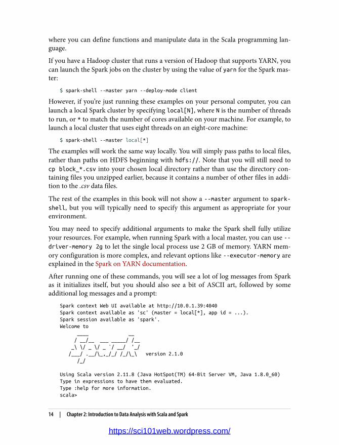
If you have a Hadoop cluster that runs a version of Hadoop that supports YARN, youcan launch the Spark jobs on the cluster by using the value of yarn for the Spark mas‐ter:

$ spark-shell --master yarn --deploy-mode client

However, if you’re just running these examples on your personal computer, you canlaunch a local Spark cluster by specifying local[N], where N is the number of threadsto run, or * to match the number of cores available on your machine. For example, tolaunch a local cluster that uses eight threads on an eight-core machine:

$ spark-shell --master local[*]

The examples will work the same way locally. You will simply pass paths to local files,rather than paths on HDFS beginning with hdfs://. Note that you will still need tocp block_*.csv into your chosen local directory rather than use the directory con‐taining files you unzipped earlier, because it contains a number of other files in addi‐tion to the .csv data files.

The rest of the examples in this book will not show a --master argument to spark-shell, but you will typically need to specify this argument as appropriate for yourenvironment.

You may need to specify additional arguments to make the Spark shell fully utilizeyour resources. For example, when running Spark with a local master, you can use --driver-memory 2g to let the single local process use 2 GB of memory. YARN mem‐ory configuration is more complex, and relevant options like --executor-memory areexplained in the Spark on YARN documentation.

After running one of these commands, you will see a lot of log messages from Sparkas it initializes itself, but you should also see a bit of ASCII art, followed by someadditional log messages and a prompt:

Spark context Web UI available at http://10.0.1.39:4040Spark context available as 'sc' (master = local[*], app id = ...).Spark session available as 'spark'.Welcome to ____ __ / __/__ ___ _____/ /__ _\ \/ _ \/ _ `/ __/ '_/ /___/ .__/\_,_/_/ /_/\_\ version 2.1.0 /_/

Using Scala version 2.11.8 (Java HotSpot(TM) 64-Bit Server VM, Java 1.8.0_60)Type in expressions to have them evaluated.Type :help for more information.scala>



https://bit.ly/1BVpP9J

If this is your first time using the Spark shell (or any Scala REPL, for that matter), youshould run the :help command to list available commands in the shell. :historyand :h? can be helpful for finding the names of variables or functions that you wroteduring a session but can’t seem to find at the moment. :paste can help you correctlyinsert code from the clipboard—something you might want to do while followingalong with the book and its accompanying source code.

In addition to the note about :help, the Spark log messages indicated “Spark contextavailable as sc.” This is a reference to the SparkContext, which coordinates the execu‐tion of Spark jobs on the cluster. Go ahead and type sc at the command line:

sc...res: org.apache.spark.SparkContext = org.apache.spark.SparkContext@DEADBEEF

The REPL will print the string form of the object. For the SparkContext object, this issimply its name plus the hexadecimal address of the object in memory. (DEADBEEF is aplaceholder; the exact value you see here will vary from run to run.)

It’s good that the sc variable exists, but what exactly do we do with it? SparkContextis an object, so it has methods associated with it. We can see what those methods arein the Scala REPL by typing the name of a variable, followed by a period, followed bytab:

sc.[\t]...!= hashCode## isInstanceOf+ isLocal-> isStopped== jarsaccumulable killExecutoraccumulableCollection killExecutorsaccumulator listFilesaddFile listJarsaddJar longAccumulator... (lots of other methods)getClass stopgetConf submitJobgetExecutorMemoryStatus synchronizedgetExecutorStorageStatus textFilegetLocalProperty toStringgetPersistentRDDs uiWebUrlgetPoolForName uniongetRDDStorageInfo versiongetSchedulingMode waithadoopConfiguration wholeTextFileshadoopFile →



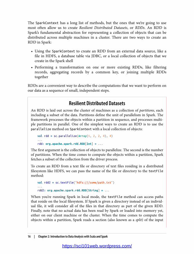
The SparkContext has a long list of methods, but the ones that we’re going to usemost often allow us to create Resilient Distributed Datasets, or RDDs. An RDD isSpark’s fundamental abstraction for representing a collection of objects that can bedistributed across multiple machines in a cluster. There are two ways to create anRDD in Spark:

• Using the SparkContext to create an RDD from an external data source, like afile in HDFS, a database table via JDBC, or a local collection of objects that wecreate in the Spark shell

• Performing a transformation on one or more existing RDDs, like filteringrecords, aggregating records by a common key, or joining multiple RDDstogether

RDDs are a convenient way to describe the computations that we want to perform onour data as a sequence of small, independent steps.

Resilient Distributed DatasetsAn RDD is laid out across the cluster of machines as a collection of partitions, eachincluding a subset of the data. Partitions define the unit of parallelism in Spark. Theframework processes the objects within a partition in sequence, and processes multi‐ple partitions in parallel. One of the simplest ways to create an RDD is to use theparallelize method on SparkContext with a local collection of objects:

val rdd = sc.parallelize(Array(1, 2, 2, 4), 4)...rdd: org.apache.spark.rdd.RDD[Int] = ...

The first argument is the collection of objects to parallelize. The second is the numberof partitions. When the time comes to compute the objects within a partition, Sparkfetches a subset of the collection from the driver process.

To create an RDD from a text file or directory of text files residing in a distributedfilesystem like HDFS, we can pass the name of the file or directory to the textFilemethod:

val rdd2 = sc.textFile("hdfs:///some/path.txt")...rdd2: org.apache.spark.rdd.RDD[String] = ...

When you’re running Spark in local mode, the textFile method can access pathsthat reside on the local filesystem. If Spark is given a directory instead of an individ‐ual file, it will consider all of the files in that directory as part of the given RDD.Finally, note that no actual data has been read by Spark or loaded into memory yet,either on our client machine or the cluster. When the time comes to compute theobjects within a partition, Spark reads a section (also known as a split) of the input



file, and then applies any subsequent transformations (filtering, aggregation, etc.) thatwe defined via other RDDs.

Our record linkage data is stored in a text file, with one observation on each line. Wewill use the textFile method on SparkContext to get a reference to this data as anRDD:

val rawblocks = sc.textFile("linkage")...rawblocks: org.apache.spark.rdd.RDD[String] = ...

There are a few things happening on this line that are worth going over. First, we’redeclaring a new variable called rawblocks. As we can see from the shell, the rawblocks variable has a type of RDD[String], even though we never specified that typeinformation in our variable declaration. This is a feature of the Scala programminglanguage called type inference, and it saves us a lot of typing when we’re working withthe language. Whenever possible, Scala figures out what type a variable has based onits context. In this case, Scala looks up the return type from the textFile function onthe SparkContext object, sees that it returns an RDD[String], and assigns that type tothe rawblocks variable.

Whenever we create a new variable in Scala, we must preface the name of the variablewith either val or var. Variables that are prefaced with val are immutable, and can‐not be changed to refer to another value once they are assigned, whereas variablesthat are prefaced with var can be changed to refer to different objects of the sametype. Watch what happens when we execute the following code:

rawblocks = sc.textFile("linkage")...<console>: error: reassignment to val

var varblocks = sc.textFile("linkage")varblocks = sc.textFile("linkage")

Attempting to reassign the linkage data to the rawblocks val threw an error, butreassigning the varblocks var is fine. Within the Scala REPL, there is an exception tothe reassignment of vals, because we are allowed to redeclare the same immutablevariable, like the following:

val rawblocks = sc.textFile("linakge")val rawblocks = sc.textFile("linkage")



In this case, no error is thrown on the second declaration of rawblocks. This isn’t typ‐ically allowed in normal Scala code, but it’s fine to do in the shell, and we will makeextensive use of this feature throughout the examples in the book.

The REPL and CompilationIn addition to its interactive shell, Spark also supports compiled applications. We typ‐ically recommend using Apache Maven for compiling and managing dependencies.The GitHub repository included with this book holds a self-contained Maven projectin the simplesparkproject/ directory to help you get started.

With both the shell and compilation as options, which should you use when testingand building a data pipeline? It is often useful to start working entirely in the REPL.This enables quick prototyping, faster iteration, and less lag time between ideas andresults. However, as the program builds in size, maintaining a monolithic file of codecan become more onerous, and Scala’s interpretation eats up more time. This can beexacerbated by the fact that, when you’re dealing with massive data, it is not uncom‐mon for an attempted operation to cause a Spark application to crash or otherwiserender a SparkContext unusable. This means that any work and code typed in so farbecomes lost. At this point, it is often useful to take a hybrid approach. Keep the fron‐tier of development in the REPL and as pieces of code harden, move them over into acompiled library. You can make the compiled JAR available to spark-shell by pass‐ing it to the --jars command-line flag. When done right, the compiled JAR onlyneeds to be rebuilt infrequently, and the REPL allows for fast iteration on code andapproaches that still need ironing out.

What about referencing external Java and Scala libraries? To compile code that refer‐ences external libraries, you need to specify the libraries inside the project’s Mavenconfiguration (pom.xml). To run code that accesses external libraries, you need toinclude the JARs for these libraries on the classpath of Spark’s processes. A good wayto make this happen is to use Maven to package a JAR that includes all of your appli‐cation’s dependencies. You can then reference this JAR when starting the shell byusing the --jars property. The advantage of this approach is that the dependenciesonly need to be specified once: in the Maven pom.xml. Again, the simplesparkproject/directory in the GitHub repository shows you how to accomplish this.

If you know of a third-party JAR that is published to a Maven repository, you can tellthe spark-shell to load the JAR by passing its Maven coordinates via the --packagescommand-line argument. For example, to load the Wisp Visualization Library forScala 2.11, you would pass --packages "com.quantifind:wisp_2.11:0.0.4" to thespark-shell. If the JAR is stored in a repository besides Maven Central, you can tellSpark where to look for the JAR by passing the repository URL to the --repositories argument. Both the --packages and --repositories arguments can



https://maven.apache.org

http://bit.ly/2rnWGlI

take comma-separated arguments if you need to load from multiple packages or repo‐sitories.

Bringing Data from the Cluster to the ClientRDDs have a number of methods that allow us to read data from the cluster into theScala REPL on our client machine. Perhaps the simplest of these is first, whichreturns the first element of the RDD into the client:

rawblocks.first...res: String = "id_1","id_2","cmp_fname_c1","cmp_fname_c2",...

The first method can be useful for sanity checking a data set, but we’re generallyinterested in bringing back larger samples of an RDD into the client for analysis.When we know that an RDD only contains a small number of records, we can use thecollect method to return all the contents of an RDD to the client as an array.Because we don’t know how big the linkage data set is just yet, we’ll hold off on doingthis right now.

We can strike a balance between first and collect with the take method, whichallows us to read a given number of records into an array on the client. Let’s use taketo get the first 10 lines from the linkage data set:

val head = rawblocks.take(10)...head: Array[String] = Array("id_1","id_2","cmp_fname_c1",...

head.length...res: Int = 10

ActionsThe act of creating an RDD does not cause any distributed computation to take placeon the cluster. Rather, RDDs define logical data sets that are intermediate steps in acomputation. Distributed computation occurs upon invoking an action on an RDD.For example, the count action returns the number of objects in an RDD:

rdd.count()14/09/10 17:36:09 INFO SparkContext: Starting job: count ...14/09/10 17:36:09 INFO SparkContext: Job finished: count ...res0: Long = 4

The collect action returns an Array with all the objects from the RDD. This Arrayresides in local memory, not on the cluster:

Bringing Data from the Cluster to the Client | 19


rdd.collect()14/09/29 00:58:09 INFO SparkContext: Starting job: collect ...14/09/29 00:58:09 INFO SparkContext: Job finished: collect ...res2: Array[(Int, Int)] = Array((4,1), (1,1), (2,2))

Actions need not only return results to the local process. The saveAsTextFile actionsaves the contents of an RDD to persistent storage, such as HDFS:

rdd.saveAsTextFile("hdfs:///user/ds/mynumbers")14/09/29 00:38:47 INFO SparkContext: Starting job:saveAsTextFile ...14/09/29 00:38:49 INFO SparkContext: Job finished:saveAsTextFile ...

The action creates a directory and writes out each partition as a file within it. Fromthe command line outside of the Spark shell:

hadoop fs -ls /user/ds/mynumbers

-rw-r--r-- 3 ds supergroup 0 2014-09-29 00:38 myfile.txt/_SUCCESS-rw-r--r-- 3 ds supergroup 4 2014-09-29 00:38 myfile.txt/part-00000-rw-r--r-- 3 ds supergroup 4 2014-09-29 00:38 myfile.txt/part-00001

Remember that textFile can accept a directory of text files as input, meaning that afuture Spark job could refer to mynumbers as an input directory.

The raw form of data returned by the Scala REPL can be somewhat hard to read,especially for arrays that contain more than a handful of elements. To make it easierto read the contents of an array, we can use the foreach method in conjunction withprintln to print out each value in the array on its own line:

head.foreach(println)..."id_1","id_2","cmp_fname_c1","cmp_fname_c2","cmp_lname_c1","cmp_lname_c2", "cmp_sex","cmp_bd","cmp_bm","cmp_by","cmp_plz","is_match"37291,53113,0.833333333333333,?,1,?,1,1,1,1,0,TRUE39086,47614,1,?,1,?,1,1,1,1,1,TRUE70031,70237,1,?,1,?,1,1,1,1,1,TRUE84795,97439,1,?,1,?,1,1,1,1,1,TRUE36950,42116,1,?,1,1,1,1,1,1,1,TRUE42413,48491,1,?,1,?,1,1,1,1,1,TRUE25965,64753,1,?,1,?,1,1,1,1,1,TRUE49451,90407,1,?,1,?,1,1,1,1,0,TRUE39932,40902,1,?,1,?,1,1,1,1,1,TRUE

The foreach(println) pattern is one that we will frequently use in this book. It’s anexample of a common functional programming pattern, where we pass one function(println) as an argument to another function (foreach) in order to perform someaction. This kind of programming style will be familiar to data scientists who haveworked with R and are used to processing vectors and lists by avoiding for loops and



instead using higher-order functions like apply and lapply. Collections in Scala aresimilar to lists and vectors in R in that we generally want to avoid for loops andinstead process the elements of the collection using higher-order functions.

Immediately, we see a couple of issues with the data that we need to address before webegin our analysis. First, the CSV files contain a header row that we’ll want to filterout from our subsequent analysis. We can use the presence of the "id_1" string in therow as our filter condition, and write a small Scala function that tests for the presenceof that string inside the line:

def isHeader(line: String) = line.contains("id_1")isHeader: (line: String)Boolean

Like Python, we declare functions in Scala using the keyword def. Unlike Python, wehave to specify the types of the arguments to our function; in this case, we have toindicate that the line argument is a String. The body of the function, which uses thecontains method for the String class to test whether or not the characters "id_1"appear anywhere in the string, comes after the equals sign. Even though we had tospecify a type for the line argument, note that we did not have to specify a returntype for the function, because the Scala compiler was able to infer the type based onits knowledge of the String class and the fact that the contains method returns trueor false.

Sometimes we will want to specify the return type of a function ourselves, especiallyfor long, complex functions with multiple return statements, where the Scala com‐piler can’t necessarily infer the return type itself. We might also want to specify areturn type for our function in order to make it easier for someone else reading ourcode later to be able to understand what the function does without having to rereadthe entire method. We can declare the return type for the function right after theargument list, like this:

def isHeader(line: String): Boolean = { line.contains("id_1")}isHeader: (line: String)Boolean

We can test our new Scala function against the data in the head array by using thefilter method on Scala’s Array class and then printing the results:

head.filter(isHeader).foreach(println)..."id_1","id_2","cmp_fname_c1","cmp_fname_c2","cmp_lname_c1",...

It looks like our isHeader method works correctly; the only result that was returnedfrom applying it to the head array via the filter method was the header line itself.But of course, what we really want to do is get all of the rows in the data except the

Bringing Data from the Cluster to the Client | 21


header rows. There are a few ways that we can do this in Scala. Our first option is totake advantage of the filterNot method on the Array class:

head.filterNot(isHeader).length...res: Int = 9

We could also use Scala’s support for anonymous functions to negate the isHeaderfunction from inside filter:

head.filter(x => !isHeader(x)).length...res: Int = 9

Anonymous functions in Scala are somewhat like Python’s lambda functions. In thiscase, we defined an anonymous function that takes a single argument called x, passesx to the isHeader function, and returns the negation of the result. Note that we didnot have to specify any type information for the x variable in this instance; the Scalacompiler was able to infer that x is a String from the fact that head is anArray[String].

There is nothing that Scala programmers hate more than typing, so Scala has lots oflittle features designed to reduce the amount of typing necessary. For example, in ouranonymous function definition, we had to type the characters x => to declare ouranonymous function and give its argument a name. For simple anonymous functionslike this one, we don’t even have to do that—Scala allows us to use an underscore (_)to represent the argument to the function so that we can save four characters:

head.filter(!isHeader(_)).length...res: Int = 9

Sometimes, this abbreviated syntax makes the code easier to read because it avoidsduplicating obvious identifiers. But other times, this shortcut just makes the codecryptic. The code listings throughout this book use one or the other according to ourbest judgment.

Shipping Code from the Client to the ClusterWe just saw a wide variety of ways to write and apply functions to data in Scala. Allthe code that we executed was done against the data inside the head array, which wascontained on our client machine. Now we’re going to take the code that we just wroteand apply it to the millions of linkage records contained in our cluster and repre‐sented by the rawblocks RDD in Spark.

Here’s what the code for this looks like; it should feel eerily familiar to you:

val noheader = rawblocks.filter(x => !isHeader(x))



The syntax we used to express the filtering computation against the entire data set onthe cluster is exactly the same as the syntax we used to express the filtering computa‐tion against the array in head on our local machine. We can use the first method onthe noheader RDD to verify that the filtering rule worked correctly:

noheader.first...res: String = 37291,53113,0.833333333333333,?,1,?,1,1,1,1,0,TRUE

This is incredibly powerful. It means that we can interactively develop and debug ourdata-munging code against a small amount of data that we sample from the cluster,and then ship that code to the cluster to apply it to the entire data set when we’reready to transform the entire data set. Best of all, we never have to leave the shell.There really isn’t another tool that gives you this kind of experience.

In the next several sections, we’ll use this mix of local development and testing andcluster computation to perform more munging and analysis of the record linkagedata, but if you need to take a moment to drink in the new world of awesome thatyou have just entered, we certainly understand.

From RDDs to Data FramesIn the first edition of this book, we spent the next several pages in this chapter usingour newfound ability to mix local development and testing with cluster computationsfrom inside the REPL to write code that parsed the CSV file of record linkage data,including splitting the line up by commas, converting each column to an appropriatedata type (like Int or Double), and handling invalid values that we encountered. Hav‐ing the option to work with data in this way is one of the most compelling aspects ofworking with Spark, especially when we’re dealing with data sets that have an espe‐cially unusual or nonstandard structure that make them difficult to work with anyother way.

At the same time, most data sets we encounter have a reasonable structure in place,either because they were born that way (like a database table) or because someoneelse has done the work of cleaning and structuring the data for us. For these data sets,it doesn’t really make sense for us to have to write our own code to parse the data; weshould simply use an existing library that can leverage the structure of the existingdata set to parse the data into a form that we can use for immediate analysis. Spark1.3 introduced just such a structure: the DataFrame.

In Spark, the DataFrame is an abstraction built on top of RDDs for data sets that havea regular structure in which each record is a row made up of a set of columns, andeach column has a well-defined data type. You can think of a data frame as the Sparkanalogue of a table in a relational database. Even though the naming conventionmight make you think of a data.frame object in R or a pandas.DataFrame object in

From RDDs to Data Frames | 23


Python, Spark’s DataFrames are a different beast. This is because they represent dis‐tributed data sets on a cluster, not local data where every row in the data is stored onthe same machine. Although there are similarities in how you use DataFrames andthe role they play inside the Spark ecosystem, there are some things you may be usedto doing when working with data frames in R and Python that do not apply to Spark,so it’s best to think of them as their own distinct entity and try to approach them withan open mind.

To create a data frame for our record linkage data set, we’re going to use the otherobject that was created for us when we started the Spark REPL, the SparkSessionobject named spark:

spark...res: org.apache.spark.sql.SparkSession = ...

SparkSession is a replacement for the now deprecated SQLContext object that wasoriginally introduced in Spark 1.3. Like SQLContext, SparkSession is a wrapperaround the SparkContext object, which you can access directly from the SparkSession:

spark.sparkContext...res: org.apache.spark.SparkContext = ...

You should see that the value of spark.sparkContext is identical to the value of thesc variable that we have been using to create RDDs thus far. To create a data framefrom the SparkSession, we will use the csv method on its Reader API:

val prev = spark.read.csv("linkage")...prev: org.apache.spark.sql.DataFrame = [_c0: string, _c1: string, ...

By default, every column in a CSV file is treated as a string type, and the columnnames default to _c0, _c1, _c2, …. We can look at the head of a data frame in theshell by calling its show method:

prev.show()

We can see that the first row of the DataFrame is the name of the header columns, aswe expected, and that the CSV file has been cleanly split up into its individual col‐umns. We can also see the presence of the ? strings in some of the columns; we willneed to handle these as missing values. In addition to naming each column correctly,it would be ideal if Spark could properly infer the data type of each of the columns forus.

Fortunately, Spark’s CSV reader provides all of this functionality for us via optionsthat we can set on the reader API. You can see the full list of options that the APItakes at the spark-csv project’s GitHub page, which was developed separately for



http://bit.ly/2i8zW6y

Spark 1.x but is included in Spark 2.x. For now, we’ll read and parse the linkage datalike this:

val parsed = spark.read. option("header", "true"). option("nullValue", "?"). option("inferSchema", "true"). csv("linkage")

When we call show on the parsed data, we see that the column names are set correctlyand the ? strings have been replaced by null values. To see the inferred type for eachcolumn, we can print the schema of the parsed DataFrame like this:

parsed.printSchema()...root |-- id_1: integer (nullable = true) |-- id_2: integer (nullable = true) |-- cmp_fname_c1: double (nullable = true) |-- cmp_fname_c2: double (nullable = true)...

Each StructField instance contains the name of the column, the most specific datatype that could handle the type of data contained in each record, and a boolean fieldthat indicates whether or not the column may contain null values, which is true bydefault. In order to perform the schema inference, Spark must do two passes over thedata set: one pass to figure out the type of each column, and a second pass to do theactual parsing. If you know the schema that you want to use for a file ahead of time,you can create an instance of the org.apache.spark.sql.types.StructType classand pass it to the Reader API via the schema function, which can have a significantperformance benefit when the data set is very large, since Spark will not need to per‐form an extra pass over the data to figure out the data type of each column.

Data Formats and Data FramesSpark 2.0 ships with built-in support for reading and writing data frames in a varietyof formats via the DataFrameReader and DataFrameWriter APIs. In addition to theCSV format discussed here, you can also read and write structured data from the fol‐lowing sources:

json

Supports many of the same schema-inference functionality that the CSV formatdoes

parquet and orcCompeting columnar-oriented binary file formats

From RDDs to Data Frames | 25


jdbc

Connects to a relational database via the JDBC data connection standard

libsvm

Popular text file format for representing labeled observations with sparse features

text

Maps each line of a file to a data frame with a single column of type string

You access the methods of the DataFrameReader API by calling the read method on aSparkSession instance, and you can load data from a file using either the format andload methods, or one of the shortcut methods for built-in formats:

val d1 = spark.read.format("json").load("file.json")val d2 = spark.read.json("file.json")

In this example, d1 and d2 reference the same underlying JSON data and will have thesame contents. Each of the different file formats has its own set of options that can beset via the same option method that we used for CSV files.

To write data out again, you access the DataFrameWriter API via the write methodon any DataFrame instance. The DataFrameWriter API supports the same built-informats as the DataFrameReader API, so the following two methods are equivalentways of writing the contents of the d1 DataFrame as a Parquet file:

d1.write.format("parquet").save("file.parquet")d1.write.parquet("file.parquet")

By default, Spark will throw an error if you try to save a data frame to a file thatalready exists. You can control Spark’s behavior in this situation via the SaveModeenum on the DataFrameWriter API to either Overwrite the existing file, Append thedata in the DataFrame to the file (if it exists), or Ignore the write operation if the filealready exists and leave it in place:

d2.write.mode(SaveMode.Ignore).parquet("file.parquet")

You can also specify the SaveMode as a string literal ("overwrite", "append","ignore") in Scala, just as you can when working with the DataFrame API in R andPython.

Analyzing Data with the DataFrame APIAlthough the RDD API in Spark provides a small number of handy methods for ana‐lyzing data—like the count method to count the number of records an RDD con‐tained, countByValue to get a histogram of the distinct values, or the stats methodto get summary statistics like min, max, mean, and standard deviation for an RDD[Double]—the DataFrame API comes with a more powerful set of tools that will likely be



familiar to data scientists who are used to R, Python, and SQL. In this section, we willbegin to explore these tools and how to apply them to the record linkage data.

If we look at the schema of the parsed DataFrame and the first few rows of data, wesee this:

• The first two fields are integer IDs that represent the patients that were matchedin the record.

• The next nine values are (possibly missing) numeric values (either doubles orints) that represent match scores on different fields of the patient records, such astheir names, birthdays, and locations. The fields are stored as integers when theonly possible values are match (1) or no-match (0), and doubles whenever partialmatches are possible.

• The last field is a boolean value (true or false) indicating whether or not thepair of patient records represented by the line was a match.

Our goal is to come up with a simple classifier that allows us to predict whether arecord will be a match based on the values of the match scores for the patient records.Let’s start by getting an idea of the number of records we’re dealing with via the countmethod, which works in exactly the same way for DataFrames and RDDs:

parsed.count()...res: Long = 5749132

This is a relatively small data set—certainly small enough to fit in memory on one ofthe nodes in a cluster or even on your local machine if you don’t have a cluster avail‐able. Thus far, every time we’ve processed the data in the data set, Spark has re-opened the file, reparsed the rows, and then performed the action requested, likeshowing the first few rows of the data or counting the number of records. When weask another question, Spark will do these same operations, again and again, even if wehave filtered the data down to a small number of records or are working with anaggregated version of the original data set.

This isn’t an optimal use of our compute resources. After the data has been parsedonce, we’d like to save the data in its parsed form on the cluster so that we don’t haveto reparse it every time we want to ask a new question of the data. Spark supports thisuse case by allowing us to signal that a given RDD or DataFrame should be cached inmemory after it is generated by calling the cache method on the instance. Let’s dothat now for the parsed DataFrame:

parsed.cache()

Analyzing Data with the DataFrame API | 27


CachingAlthough the contents of DataFrames and RDDs are transient by default, Spark pro‐vides a mechanism for persisting the underlying data:

cached.cache()cached.count()cached.take(10)

The call to cache indicates that the contents of the DataFrame should be stored inmemory the next time it’s computed. In this example, the call to count computes thecontents initially, and the take action returns the first 10 elements of the DataFrameas a local Array[Row]. When take is called, it accesses the cached elements of cachedinstead of recomputing them from their dependencies.

Spark defines a few different mechanisms, or StorageLevel values, for persistingdata. cache() is shorthand for persist(StorageLevel.MEMORY), which stores therows as unserialized Java objects. When Spark estimates that a partition will not fit inmemory, it simply will not store it, and it will be recomputed the next time it’sneeded. This level makes the most sense when the objects will be referenced fre‐quently and/or require low-latency access, because it avoids any serialization over‐head. Its drawback is that it takes up larger amounts of memory than its alternatives.Also, holding on to many small objects puts pressure on Java’s garbage collection,which can result in stalls and general slowness.

Spark also exposes a MEMORY_SER storage level, which allocates large byte buffers inmemory and serializes the records into them. When we use the right format (more onthis in a bit), serialized data usually takes up two to five times less space than its rawequivalent.

Spark can use disk for caching data as well. The MEMORY_AND_DISK and MEMORY_AND_DISK_SER are similar to the MEMORY and MEMORY_SER storage levels, respec‐tively. For the latter two, if a partition will not fit in memory, it is simply not stored,meaning that it must be recomputed from its dependencies the next time an actionuses it. For the former, Spark spills partitions that will not fit in memory to disk.

Although both DataFrames and RDDs can be cached, Spark can use the detailedknowledge of the data stored with a data frame available via the DataFrame’s schemato persist the data far more efficiently than it can with Java objects stored inside ofRDDs.

Deciding when to cache data can be an art. The decision typically involves trade-offsbetween space and speed, with the specter of garbage-collecting looming overhead tooccasionally confound things further. In general, data should be cached when it islikely to be referenced by multiple actions, is relatively small compared to the amountof memory/disk available on the cluster, and is expensive to regenerate.



Once our data has been cached, the next thing we want to know is the relative frac‐tion of records that were matches versus those that were nonmatches. With the RDDAPI, we would need to write an inlined Scala function to extract the value of theis_match column from each record and then call countByValue on the resultingRDD[Boolean] to sum up the frequency of each record and return it to the client as aMap[Boolean, Long]. In fact, we can still do this calculation against the RDD thatunderlies the parsed DataFrame:

parsed.rdd. map(_.getAs[Boolean]("is_match")). countByValue()...Map(true -> 20931, false -> 5728201)

The RDD that a data frame wraps is made up of instances of theorg.apache.spark.sql.Row class, which has accessor methods for getting the valuesinside each record by index position (counting from zero) as well as the getAs[T]method, which allows us to look up fields of a given type by their name.

Although the RDD-based analysis gets us the result we want, it still leaves a lot to bedesired as a general-purpose way of analyzing data in Spark. First, using the countByValue function to do the counts is only the right thing to do when we know that thereare just a few distinct values in the data set. If there are lots of distinct values, it’s moreefficient to use an RDD function that won’t return the results to the client, like reduceByKey. Second, if we require the results of the countByValue aggregation in a subse‐quent computation, we need to use the parallelize method of the SparkContext toship the data back from the client to the cluster. In general, we prefer to have a singleway of aggregating structured data that would work for any size data set, and this isexactly what the DataFrame API provides:

parsed. groupBy("is_match"). count(). orderBy($"count".desc) show()...+--------+-------+|is_match| count|+--------+-------+| false|5728201|| true| 20931|+--------+-------+

Instead of writing a function to extract the is_match column, we simply pass itsname to the groupBy method on the DataFrame, call the count method to, well, countthe number of records inside each grouping, sort the resulting data in descendingorder based on the count column, and then cleanly render the result of the computa‐



tion in the REPL with show. Under the covers, the Spark engine determines the mostefficient way to perform the aggregation and return the results, without us having toworry about the details of which RDD APIs to use. The result is a cleaner, faster, andmore expressive way to do data analysis in Spark.

Note that there are two ways we can reference the names of the columns in the Data‐Frame: either as literal strings, like in groupBy("is_match"), or as Column objects byusing the special $"<col>" syntax that we used on the count column. Either approachis valid in most cases, but we needed to use the $ syntax to call the desc method onthe count column. If we had omitted the $ in front of the string, Scala would havethrown an error because the String class does not have a method named desc.

DataFrame Aggregation FunctionsIn addition to count, we can also compute more complex aggregations like sums,mins, maxes, means, and standard deviation using the agg method of the DataFrameAPI in conjunction with the aggregation functions defined in theorg.apache.spark.sql.functions package. For example, to find the mean and stan‐dard deviation of the cmp_sex field in the overall parsed DataFrame, we could type:

parsed.agg(avg($"cmp_sex"), stddev($"cmp_sex")).show()+-----------------+--------------------+| avg(cmp_sex)|stddev_samp(cmp_sex)|+-----------------+--------------------+|0.955001381078048| 0.2073011111689795|+-----------------+--------------------+

Note that by default, Spark computes the sample standard deviation; there is also astddev_pop function for computing the population standard deviation.

You may have noticed that the functions on the DataFrame API are similar to thecomponents of a SQL query. This isn’t a coincidence, and in fact we have the optionof treating any DataFrame we create as if it were a database table and expressing ourquestions using familiar and powerful SQL syntax. First, we need to tell the SparkSQL execution engine the name it should associate with the parsed DataFrame, sincethe name of the variable itself (“parsed”) isn’t available to Spark:

parsed.createOrReplaceTempView("linkage")

Because the parsed DataFrame is only available during the length of this Spark REPLsession, it is a temporary table. Spark SQL may also be used to query persistent tablesin HDFS if we configure Spark to connect to an Apache Hive metastore that tracksthe schemas and locations of structured data sets.

Once our temporary table is registered with the Spark SQL engine, we can query itlike this:



spark.sql(""" SELECT is_match, COUNT(*) cnt FROM linkage GROUP BY is_match ORDER BY cnt DESC""").show()...+--------+-------+|is_match| cnt|+--------+-------+| false|5728201|| true| 20931|+--------+-------+

Like Python, Scala allows us to write multiline strings via the convention of threedouble quotes in a row. In Spark 1.x, the Spark SQL compiler was primarily aimed atreplicating the nonstandard syntax of HiveQL in order to support users who weremigrating to Spark from Apache Hive. In Spark 2.0, you have the option of runningSpark using either an ANSI 2003-compliant version of Spark SQL (the default) or inHiveQL mode by calling the enableHiveSupport method when you create a SparkSession instance via its Builder API.

Should you use Spark SQL or the DataFrame API to do your analysis in Spark? Thereare pros and cons to each: SQL has the benefit of being broadly familiar and expres‐sive for simple queries. It is also the best way to quickly read and filter data stored incommonly used columnar file formats like ORC and Parquet. The downside of SQLis that it can be difficult to express complex, multistage analyses in a dynamic, reada‐ble, and testable way—all areas where the DataFrame API shines. Throughout therest of the book, we use both Spark SQL and the DataFrame API, and leave it as anexercise for the reader to examine the choices we made and translate our computa‐tions from one interface to the other.

Connecting Spark SQL to HiveSpark 1.x shipped with a HiveContext class that was a subclass of SQLContext andsupported Hive’s unique SQL dialect (HiveQL). This class could be used to talk to aHive metastore by copying a hive-site.xml file into the conf directory of the Sparkinstallation. In Spark 2.x, the HiveContext is deprecated, but you can still connect to aHive metastore via a hive-site.xml file, and you can also use HiveQL in queries by call‐ing the enableHiveSupport method on the SparkSession Builder API:

val sparkSession = SparkSession.builder. master("local[4]") .enableHiveSupport() .getOrCreate()

In Spark 2.x, you can treat any table in the Hive metastore as a data frame, executeSpark SQL queries against tables defined in the metastore, and persist the output of



those queries to the metastore so that they can be queried by other tools, includingHive itself, Apache Impala, or Presto.

Fast Summary Statistics for DataFramesAlthough there are many kinds of analyses that may be expressed equally well in SQLor with the DataFrame API, there are certain common things that we want to be ableto do with data frames that can be tedious to express in SQL. One such analysis that isespecially helpful is computing the min, max, mean, and standard deviation of all thenon-null values in the numerical columns of a data frame. In R, this function isnamed summary; and in Spark, this function has the same name that it does in Pandas,describe:

val summary = parsed.describe()...summary.show()

The summary DataFrame has one column for each variable in the parsed DataFrame,along with another column (also named summary) that indicates which metric—count, mean, stddev, min, or max—is present in the rest of the columns in the row. Wecan use the select method to choose a subset of the columns in order to make thesummary statistics easier to read and compare:

summary.select("summary", "cmp_fname_c1", "cmp_fname_c2").show()+-------+------------------+------------------+|summary| cmp_fname_c1| cmp_fname_c2|+-------+------------------+------------------+| count| 5748125| 103698|| mean|0.7129024704436274|0.9000176718903216|| stddev|0.3887583596162788|0.2713176105782331|| min| 0.0| 0.0|| max| 1.0| 1.0|+-------+------------------+------------------+

Note the difference in the value of the count variable between cmp_fname_c1 andcmp_fname_c2. While almost every record has a non-null value for cmp_fname_c1,less than 2% of the records have a non-null value for cmp_fname_c2. To create a usefulclassifier, we need to rely on variables that are almost always present in the data—unless their missingness indicates something meaningful about whether the recordmatches.

Once we have an overall feel for the distribution of the variables in our data, we wantto understand how the values of those variables are correlated with the value of theis_match column. Therefore, our next step is to compute those same summary statis‐tics for just the subsets of the parsed DataFrame that correspond to matches andnonmatches. We can filter DataFrames using either SQL-style where syntax or with



Column objects using the DataFrame API and then use describe on the resultingDataFrames:

val matches = parsed.where("is_match = true")val matchSummary = matches.describe()

val misses = parsed.filter($"is_match" === false)val missSummary = misses.describe()

The logic inside the string we pass to the where function can include statements thatwould be valid inside a WHERE clause in Spark SQL. The filtering condition that usesthe DataFrame API is a bit more complex: we need to use the === operator on the$"is_match" column, and we need to wrap the boolean literal false with the litfunction in order to turn it into another column object that is_match can be com‐pared with. Note that the where function is an alias for the filter function; we couldhave reversed the where and filter calls in the above snippet and everything wouldhave worked the same way.

We can now start to compare our matchSummary and missSummary DataFrames to seehow the distribution of the variables changes depending on whether the record is amatch or a miss. Although this is a relatively small data set, doing this comparison isstill somewhat tedious—what we really want is to transpose the matchSummary andmissSummary DataFrames so that the rows and columns are swapped, which wouldallow us to join the transposed DataFrames together by variable and analyze the sum‐mary statistics, a practice that most data scientists know as “pivoting” or “reshaping”a data set. In the next section, we’ll show you how to perform these transforms inSpark.

Pivoting and Reshaping DataFramesThe first thing we need to do in order to transpose our summary statistics is to con‐vert the matchSummary and missSummary from “wide” form, in which we have rows ofmetrics and columns of variables, into “long” form, where each row has one metric,one variable, and the value of that metric/variable pair. Once that is done, we willcomplete our transpose operation by transforming the long-form DataFrame intoanother wide-form DataFrame, only this time the variables will correspond to therows and the metrics will be in the columns.

To convert from a wide form to a long form, we’ll take advantage of the DataFrame’sflatMap function, which is a wrapper around RDD.flatMap. A flatMap is one of themost useful transforms in Spark: it takes a function argument that processes eachinput record and returns a sequence of zero or more output records. You can think offlatMap as a generalization of the map and filter transforms that we have used sofar: a map is a specialization of flatMap for the case where each input record hasexactly one output record, and a filter is a specialization of flatMap where the

Pivoting and Reshaping DataFrames | 33


input and output types are the same and either zero or one records are returnedbased on a boolean condition function.

For our flatMap function to work for general data frames, we need to use the schemaobject of the DataFrame returned by a call to describe to get the names of the col‐umns:

summary.printSchema()...root |-- summary: string (nullable = true) |-- id_1: string (nullable = true) |-- id_2: string (nullable = true) |-- cmp_fname_c1: string (nullable = true)...

In the summary schema, every field is treated as a string. Since we want to analyze thesummary statistics as numbers, we’ll need to convert the values from strings to dou‐bles as we process them. Our output should be a data frame that has three columns:the name of the metric (count, mean, etc.), the name of the column (id1, cmp_by,etc.), and the Double value of the summary statistic for that column:

val schema = summary.schemaval longForm = summary.flatMap(row => { val metric = row.getString(0) (1 until row.size).map(i => { (metric, schema(i).name, row.getString(i).toDouble) })})

There is a lot going on in this snippet, so let’s take each line one by one. For each rowin the summary DataFrame, we are getting the name of the metric for that row posi‐tionally, by calling row.getString(0). For the other columns in the row, from posi‐tion 1 until the end, we are generating a sequence of tuples as the result of theflatMap operation, where the first entry in the tuple is the name of the metric, thesecond entry is the name of the column (which we access via the schema(i).nameobject), and the third entry is the value of the statistic, which we have coerced to aDouble value from its original string by calling the toDouble method on row.getString(i).

The toDouble method is an example of one of Scala’s most powerful (and arguablydangerous) features: implicit types. In Scala, an instance of the String class is just ajava.lang.String, and the java.lang.String class does not have a method namedtoDouble. Instead, the methods are defined in a Scala class called StringOps. Implic‐its work like this: if you call a method on a Scala object, and the Scala compiler doesnot see a definition for that method in the class definition for that object, the com‐piler will try to convert your object to an instance of a class that does have thatmethod defined. In this case, the compiler will see that Java’s String class does not



have a toDouble method defined but that the StringOps class does, and that theStringOps class has a method that can convert an instance of the String class into aninstance of the StringOps class. The compiler silently performs the conversion of ourString object into a StringOps object, and then calls the toDouble method on thenew object.

Developers who write libraries in Scala (including the core Spark developers) reallylike implicit type conversion; it allows them to enhance the functionality of coreclasses like String that are otherwise closed to modification. For a user of these tools,implicit type conversions are more of a mixed bag, because they can make it difficultto figure out exactly where a particular class method is defined. Nonetheless, we’regoing to encounter implicit conversions throughout our examples, so it’s best that weget used to them now.

The last thing to note about this snippet is the type of the longForm variable:

longForm: org.apache.spark.sql.Dataset[(String, String, Double)]

This is our first direct encounter with the Dataset[T] interface, although we havebeen using it all along—a data frame is simply an alias for the Dataset[Row] type!Dataset[T] is a new addition to the Spark 2.0 APIs and generalizes the DataFrametype that was introduced in Spark 1.3 to be able to handle a richer set of data typesthan just instances of the Row class. We’ll look at the Dataset interface a bit moreclosely later in the chapter, but for now, all you need to know is that we can alwaysconvert a Dataset back to a data frame thanks to some implicit conversion magic inthe Spark API:

val longDF = longForm.toDF("metric", "field", "value")longDF.show()+------+------------+-------------------+|metric| field| value|+------+------------+-------------------+| count| id_1| 5749132.0|| count| id_2| 5749132.0|| count|cmp_fname_c1| 5748125.0|...| count| cmp_by| 5748337.0|| count| cmp_plz| 5736289.0|| mean| id_1| 33324.48559643438|| mean| id_2| 66587.43558331935|| mean|cmp_fname_c1| 0.7129024704436274|...| mean| cmp_bd|0.22446526708507172|| mean| cmp_bm|0.48885529849763504|+------+------------+-------------------+

Given a data frame in long form, we can transform it to a wide form by using thegroupBy operator on the column that we want to use as the pivot table’s row followed

Pivoting and Reshaping DataFrames | 35


by the pivot operator on the column that we want to use as the pivot table’s column.The pivot operator needs to know the distinct set of values of the pivot column thatwe want to use for the columns, and we can specify the value in each cell of the widetable by using an agg(first) operation on the values column, which works cor‐rectly because there is only a single value for each combination of field and metric:

val wideDF = longDF. groupBy("field"). pivot("metric", Seq("count", "mean", "stddev", "min", "max")). agg(first("value"))wideDF.select("field", "count", "mean").show()...+------------+---------+-------------------+| field| count| mean|+------------+---------+-------------------+| cmp_plz|5736289.0|0.00552866147434343||cmp_lname_c1|5749132.0| 0.3156278193084133||cmp_lname_c2| 2464.0|0.31841283153174377|| cmp_sex|5749132.0| 0.955001381078048|| cmp_bm|5748337.0|0.48885529849763504|...| cmp_bd|5748337.0|0.22446526708507172|| cmp_by|5748337.0| 0.2227485966810923|+------------+---------+-------------------+

Now that we have figured out how to transpose a summary DataFrame, let’s imple‐ment our logic into a function that we can reuse on the matchSummary and missSummary DataFrames. Using a text editor in another shell window, copy and paste thefollowing code and save it in a file called Pivot.scala:

import org.apache.spark.sql.DataFrameimport org.apache.spark.sql.functions.first

def pivotSummary(desc: DataFrame): DataFrame = { val schema = desc.schema import desc.sparkSession.implicits._

val lf = desc.flatMap(row => { val metric = row.getString(0) (1 until row.size).map(i => { (metric, schema(i).name, row.getString(i).toDouble) }) }).toDF("metric", "field", "value")

lf.groupBy("field"). pivot("metric", Seq("count", "mean", "stddev", "min", "max")). agg(first("value"))}



Now in your Spark shell, type :load Pivot.scala, and the Scala REPL will compileyour code on the fly and make the pivotSummary function available for use on thematchSummary and missSummary DataFrames:

val matchSummaryT = pivotSummary(matchSummary)val missSummaryT = pivotSummary(missSummary)

Joining DataFrames and Selecting FeaturesSo far, we have only used Spark SQL and the DataFrame API to filter and aggregatethe records from a data set, but we can also use these tools in order to perform joins(inner, left outer, right outer, or full outer) on DataFrames as well. Although the Data‐Frame API includes a join function, it’s often easier to express these joins usingSpark SQL, especially when the tables we are joining have a large number of columnnames in common and we want to be able to clearly indicate which column we arereferring to in our select expressions. Let’s create temporary views for the matchSummaryT and missSummaryT DataFrames, join them on the field column, and computesome simple summary statistics on the resulting rows:

matchSummaryT.createOrReplaceTempView("match_desc")missSummaryT.createOrReplaceTempView("miss_desc")spark.sql(""" SELECT a.field, a.count + b.count total, a.mean - b.mean delta FROM match_desc a INNER JOIN miss_desc b ON a.field = b.field WHERE a.field NOT IN ("id_1", "id_2") ORDER BY delta DESC, total DESC""").show()...+------------+---------+--------------------+| field| total| delta|+------------+---------+--------------------+| cmp_plz|5736289.0| 0.9563812499852176||cmp_lname_c2| 2464.0| 0.8064147192926264|| cmp_by|5748337.0| 0.7762059675300512|| cmp_bd|5748337.0| 0.775442311783404||cmp_lname_c1|5749132.0| 0.6838772482590526|| cmp_bm|5748337.0| 0.5109496938298685||cmp_fname_c1|5748125.0| 0.2854529057460786||cmp_fname_c2| 103698.0| 0.09104268062280008|| cmp_sex|5749132.0|0.032408185250332844|+------------+---------+--------------------+

A good feature has two properties: it tends to have significantly different values formatches and nonmatches (so the difference between the means will be large) and itoccurs often enough in the data that we can rely on it to be regularly available for anypair of records. By this measure, cmp_fname_c2 isn’t very useful because it’s missing alot of the time and the difference in the mean value for matches and nonmatches isrelatively small—0.09, for a score that ranges from 0 to 1. The cmp_sex feature also

Joining DataFrames and Selecting Features | 37


isn’t particularly helpful because even though it’s available for any pair of records, thedifference in means is just 0.03.

Features cmp_plz and cmp_by, on the other hand, are excellent. They almost alwaysoccur for any pair of records, and there is a very large difference in the mean values(more than 0.77 for both features.) Features cmp_bd, cmp_lname_c1, and cmp_bm alsoseem beneficial: they are generally available in the data set and the difference, in meanvalues for matches and nonmatches are substantial.

Features cmp_fname_c1 and cmp_lname_c2 are more of a mixed bag: cmp_fname_c1doesn’t discriminate all that well (the difference in the means is only 0.28) eventhough it’s usually available for a pair of records, whereas cmp_lname_c2 has a largedifference in the means but it’s almost always missing. It’s not quite obvious underwhat circumstances we should include these features in our model based on this data.

For now, we’re going to use a simple scoring model that ranks the similarity of pairsof records based on the sums of the values of the obviously good features: cmp_plz,cmp_by, cmp_bd, cmp_lname_c1, and cmp_bm. For the few records where the values ofthese features are missing, we’ll use 0 in place of the null value in our sum. We canget a rough feel for the performance of our simple model by creating a data frame ofthe computed scores and the value of the is_match column and evaluating how wellthe score discriminates between matches and nonmatches at various thresholds.

Preparing Models for Production EnvironmentsAlthough we could write this scoring function as a Spark SQL query, there are manysituations in which we want to be able to deploy a scoring rule or machine learningmodel into a production environment, and where we may not have enough time torun a Spark SQL to generate an answer to our question. For these situations, we wantto be able to write and test functions that are able to work with Spark but that do notrequire any production code to depend on the Spark JARs or require that a SparkSes‐sion be run in order to excecute the code.

To abstract away the Spark-specific components of our model, we would like to havea way of creating a simple record type that allows us to work with the fields in theDataFrame as statically typed variables instead of as fields that we look up dynami‐cally inside a Row. Fortunately, Scala provides a convenient syntax for creating theserecords, called case classes. A case class is a simple type of immutable class that comeswith implementations of all of the basic Java class methods, like toString, equals,and hashCode, which makes them very easy to use. Let’s declare a case class for ourrecord linkage data, where the names and types of the fields map exactly to the namesand types of the columns in the parsed DataFrame:



case class MatchData( id_1: Int, id_2: Int, cmp_fname_c1: Option[Double], cmp_fname_c2: Option[Double], cmp_lname_c1: Option[Double], cmp_lname_c2: Option[Double], cmp_sex: Option[Int], cmp_bd: Option[Int], cmp_bm: Option[Int], cmp_by: Option[Int], cmp_plz: Option[Int], is_match: Boolean)

Note that we are using Scala’s built-in Option[T] type to represent fields whose valuesmay be null in our input data. The Option class requires that client code check to seewhether a particular field is absent (represented by the None object) before it is used,which significantly reduces the occurrence of NullPointerExceptions in Scala code.For fields that can never be null, like id_1, id_2, and is_match, we can omit theOption wrapper.

Once our class is defined, we can use the as[T] method to convert the parsed Data‐Frame into a Dataset[MatchData]:

val matchData = parsed.as[MatchData]matchData.show()

As you can see, all of the columns and values of the matchData data set are the sameas the data in the parsed DataFrame, and we can still use all of the SQL-style Data‐Frame API methods and Spark SQL code against the matchData data set. The majordifference between the two is that when we call functions like map, flatMap, or filter against matchData, we are processing instances of the MatchData case classinstead of the Row class.

For our scoring function, we are going to sum up the value of one field of typeOption[Double] (cmp_lname_c1) and four fields of type Option[Int] (cmp_plz,cmp_by, cmp_bd, and cmp_bm). Let’s write a small helper case class to cut down onsome of the boilerplate code associated with checking for the presence of the Optionvalues:

case class Score(value: Double) { def +(oi: Option[Int]) = { Score(value + oi.getOrElse(0)) }}

The Score case class starts with a value of type Double (the running sum) and definesa \+ method that allows us to merge an Option[Int] value into the running sum by

Preparing Models for Production Environments | 39


getting the value of the Option or returning 0 if it is missing. Here, we’re takingadvantage of the fact that Scala lets you define functions using a much broader set ofnames than Java to make our scoring function a bit eaiser to read:

def scoreMatchData(md: MatchData): Double = { (Score(md.cmp_lname_c1.getOrElse(0.0)) + md.cmp_plz + md.cmp_by + md.cmp_bd + md.cmp_bm).value}

With our scoring function in hand, we can now compute our scores and the value ofthe is_match field for each MatchData object in the matchData data set and store theresults in a data frame:

val scored = matchData.map { md =>(scoreMatchData(md), md.is_match)}.toDF("score", "is_match")

Model EvaluationThe final step in creating our scoring function is to decide on what threshold thescore must exceed in order for us to predict that the two records represent a match. Ifwe set the threshold too high, then we will incorrectly mark a matching record as amiss (called the false-negative rate), whereas if we set the threshold too low, we willincorrectly label misses as matches (the false-positive rate.) For any nontrivial prob‐lem, we always have to trade some false positives for some false negatives, and thequestion of what the threshold value should be usually comes down to the relativecost of the two kinds of errors in the situation to which the model is being applied.

To help us choose a threshold, it’s helpful to create a 2×2 contingency table (which issometimes called a cross tabulation, or crosstab) that counts the number of recordswhose scores fall above/below the threshold value crossed with the number of recordsin each of those categories that were/were not matches. Since we don’t know whatthreshold value we’re going to use yet, let’s write a function that takes the scoredDataFrame and the choice of threshold as parameters and computes the crosstabsusing the DataFrame API:

def crossTabs(scored: DataFrame, t: Double): DataFrame = { scored. selectExpr(s"score >= $t as above", "is_match"). groupBy("above"). pivot("is_match", Seq("true", "false")). count()}

Note that we are including the selectExpr method of the DataFrame API to dynami‐cally determine the value of the field named above based on the value of the t argu‐ment using Scala’s string interpolation syntax, which allows us to substitute variablesby name if we preface the string literal with the letter s (yet another handy bit of Scala



implicit magic). Once the above field is defined, we create the crosstab with a stan‐dard combination of the groupBy, pivot, and count methods that we used before.

Applying a high threshold value of 4.0, meaning that the average of the five features is0.8, we can filter out almost all of the nonmatches while keeping over 90% of thematches:

crossTabs(scored, 4.0).show()...+-----+-----+-------+|above| true| false|+-----+-----+-------+| true|20871| 637||false| 60|5727564|+-----+-----+-------+

Applying the lower threshold of 2.0, we can ensure that we capture all of the knownmatching records, but at a substantial cost in terms of false positive (top-right cell):

crossTabs(scored, 2.0).show()...+-----+-----+-------+|above| true| false|+-----+-----+-------+| true|20931| 596414||false| null|5131787|+-----+-----+-------+

Even though the number of false positives is higher than we want, this more generousfilter still removes 90% of the nonmatching records from our consideration whileincluding every positive match. Even though this is pretty good, it’s possible to doeven better; see if you can find a way to use some of the other values from MatchData(both missing and not) to come up with a scoring function that successfully identifiesevery true match at the cost of less than 100 false positives.

Where to Go from HereIf this chapter was your first time carrying out data preparation and analysis withScala and Spark, or if you’re familiar with the Spark 1.0 APIs and are getting up tospeed with the new techniques in Spark 2.0, we hope that you got a feel for what apowerful foundation these tools provide. If you have been using Scala and Spark for awhile, we hope that you will pass this chapter along to your friends and colleagues asa way of introducing them to that power as well.

Our goal for this chapter was to provide you with enough Scala knowledge to be ableto understand and complete the rest of the examples in this book. If you are the kindof person who learns best through practical examples, your next step is to continue

Where to Go from Here | 41


on to the next set of chapters, where we will introduce you to MLlib, the machinelearning library designed for Spark.

As you become a seasoned user of Spark and Scala for data analysis, it’s likely that youwill reach a point where you begin to build tools and libraries designed to help otheranalysts and data scientists apply Spark to solve their own problems. At that point inyour development, it would be helpful to pick up additional books on Scala, like Pro‐gramming Scala by Dean Wampler and Alex Payne, and The Scala Cookbook by AlvinAlexander (both from O’Reilly).



http://shop.oreilly.com/product/0636920033073.do



CHAPTER 3

Recommending Music and theAudioscrobbler Data Set

Sean Owen

De gustibus non est disputandum.(There’s no accounting for taste.)

—Anonymous

When somebody asks what it is I do for a living, the direct answer of “data science” or“machine learning” sounds impressive but usually draws a blank stare. Fair enough;even actual data scientists seem to struggle to define what these mean—storing lots ofdata, computing, predicting something? Inevitably, I jump straight to a relatableexample: “OK, you know how Amazon will tell you about books like the ones youbought? Yes? Yes! It’s like that.”

Empirically, the recommender engine seems to be an example of large-scale machinelearning that everyone understands, and most people have seen Amazon’s. It is acommon denominator because recommender engines are everywhere, from socialnetworks to video sites to online retailers. We can also directly observe them inaction. We’re aware that a computer is picking tracks to play on Spotify, in much thesame way we don’t necessarily notice that Gmail is deciding whether inbound email isspam.

The output of a recommender is more intuitively understandable than other machinelearning algorithms. It’s exciting, even. For as much as we think that musical taste ispersonal and inexplicable, recommenders do a surprisingly good job of identifyingtracks we didn’t know we would like.

Finally, for domains like music or movies where recommenders are usually deployed,it’s comparatively easy to reason about why a recommended piece of music fits with

43


someone’s listening history. Not all clustering or classification algorithms match thatdescription. For example, a support vector machine classifier is a set of coefficients,and it’s hard even for practitioners to articulate what the numbers mean when theymake predictions.

So, it seems fitting to kick off the next three chapters, which will explore key machinelearning algorithms on Spark, with a chapter built around recommender engines, andrecommending music in particular. It’s an accessible way to introduce real-world useof Spark and MLlib, and some basic machine learning ideas that will be developed insubsequent chapters.

Data SetThis example will use a data set published by Audioscrobbler. Audioscrobbler was thefirst music recommendation system for last.fm, one of the first internet streamingradio sites, founded in 2002. Audioscrobbler provided an open API for “scrobbling,”or recording listeners’ song plays. last.fm used this information to build a powerfulmusic recommender engine. The system reached millions of users because third-party apps and sites could provide listening data back to the recommender engine.

At that time, research on recommender engines was mostly confined to learningfrom rating-like data. That is, recommenders were usually viewed as tools that oper‐ated on input like “Bob rates Prince 3.5 stars.”

The Audioscrobbler data set is interesting because it merely records plays: “Bobplayed a Prince track.” A play carries less information than a rating. Just because Bobplayed the track doesn’t mean he actually liked it. You or I may occasionally play asong by an artist we don’t care for, or even play an album and walk out of the room.

However, listeners rate music far less frequently than they play music. A data set likethis is therefore much larger, covers more users and artists, and contains more totalinformation than a rating data set, even if each individual data point carries lessinformation. This type of data is often called implicit feedback data because the user-artist connections are implied as a side effect of other actions, and not given asexplicit ratings or thumbs-up.

A snapshot of a data set distributed by last.fm in 2005 can be found online as a com‐pressed archive. Download the archive, and find within it several files. The main dataset is in the user_artist_data.txt file. It contains about 141,000 unique users, and 1.6million unique artists. About 24.2 million users’ plays of artists are recorded, alongwith their counts.

The data set also gives the names of each artist by ID in the artist_data.txt file. Notethat when plays are scrobbled, the client application submits the name of the artistbeing played. This name could be misspelled or nonstandard, and this may only be

44 | Chapter 3: Recommending Music and the Audioscrobbler Data Set


http://www.last.fm

https://bit.ly/1KiJdOR

https://bit.ly/1KiJdOR

detected later. For example, “The Smiths,” “Smiths, The,” and “the smiths” may appearas distinct artist IDs in the data set even though they are plainly the same. So, the dataset also includes artist_alias.txt, which maps artist IDs that are known misspellings orvariants to the canonical ID of that artist.

The Alternating Least Squares Recommender AlgorithmWe need to choose a recommender algorithm that is suitable for this implicit feed‐back data. The data set consists entirely of interactions between users and artists’songs. It contains no information about the users, or about the artists other than theirnames. We need an algorithm that learns without access to user or artist attributes. These are typically called collaborative filtering algorithms. For example, decidingthat two users might share similar tastes because they are the same age is not anexample of collaborative filtering. Deciding that two users might both like the samesong because they play many other same songs is an example.

This data set looks large because it contains tens of millions of play counts. But in adifferent sense, it is small and skimpy, because it is sparse. On average, each user hasplayed songs from about 171 artists—out of 1.6 million. Some users have listened toonly one artist. We need an algorithm that can provide decent recommendations toeven these users. After all, every single listener must have started with just one play atsome point!

Finally, we need an algorithm that scales, both in its ability to build large models andto create recommendations quickly. Recommendations are typically required in nearreal time—within a second, not tomorrow.

This example will employ a member of a broad class of algorithms called latent-factormodels. They try to explain observed interactions between large numbers of users anditems through a relatively small number of unobserved, underlying reasons. It is analo‐gous to explaining why millions of people buy a particular few of thousands of possi‐ble albums by describing users and albums in terms of tastes for perhaps tens ofgenres—tastes that are not directly observable or given as data.

For example, consider a customer who has bought albums by metal bands Megadethand Pantera, but also classical composer Mozart. It may be difficult to explain whyexactly these albums were bought and nothing else. However, it’s probably a smallwindow on a much larger set of tastes. Maybe the customer likes a coherent spectrumof music from metal to progressive rock to classical. That explanation is simpler, andas a bonus, suggests many other albums that would be of interest. In this example,“liking metal, progressive rock, and classical” are three latent factors that couldexplain tens of thousands of individual album preferences.

More specifically, this example will use a type of matrix factorization model. Mathe‐matically, these algorithms treat the user and product data as if it were a large matrix

The Alternating Least Squares Recommender Algorithm | 45


https://en.wikipedia.org/wiki/Collaborative_filtering

https://en.wikipedia.org/wiki/Factor_analysis

https://en.wikipedia.org/wiki/Non-negative_matrix_factorization

A, where the entry at row i and column j exists if user i has played artist j. A is sparse:most entries of A are 0, because only a few of all possible user-artist combinationsactually appear in the data. They factor A as the matrix product of two smaller matri‐ces, X and Y. They are very skinny—both have many rows because A has many rowsand columns, but both have just a few columns (k). The k columns correspond to thelatent factors that are being used to explain the interaction data.

The factorization can only be approximate because k is small, as shown in Figure 3-1.

Figure 3-1. Matrix factorization

These algorithms are sometimes called matrix completion algorithms, because theoriginal matrix A may be quite sparse, but the product XYT is dense. Very few, if any,entries are 0, and therefore the model is only an approximation to A. It is a model inthe sense that it produces (“completes”) a value for even the many entries that aremissing (that is, 0) in the original A.

This is a case where, happily, the linear algebra maps directly and elegantly to intu‐ition. These two matrices contain a row for each user and each artist, respectively.The rows have few values—k. Each value corresponds to a latent feature in the model.So the rows express how much users and artists associate with these k latent features,which might correspond to tastes or genres. And it is simply the product of a user-feature and feature-artist matrix that yields a complete estimation of the entire, denseuser-artist interaction matrix. This product might be thought of as mapping items totheir attributes, and then weighting those by user attributes.

The bad news is that A = XYT generally has no exact solution at all, because X and Yaren’t large enough (technically speaking, too low rank) to perfectly represent A. Thisis actually a good thing. A is just a tiny sample of all interactions that could happen. Ina way, we believe A is a terribly spotty and therefore hard-to-explain view of a simplerunderlying reality that is well explained by just some small number of factors, k, ofthem. Think of a jigsaw puzzle depicting a cat. The final puzzle is simple to describe: a



https://bit.ly/1ALoQFK

cat. When you’re holding just a few pieces, however, the picture you see is quite diffi‐cult to describe.

XYT should still be as close to A as possible. After all, it’s all we’ve got to go on. It willnot and should not reproduce it exactly. The bad news again is that this can’t besolved directly for both the best X and best Y at the same time. The good news is thatit’s trivial to solve for the best X if Y is known, and vice versa. But neither is knownbeforehand!

Fortunately, there are algorithms that can escape this catch-22 and find a decent solu‐tion. More specifically still, the example in this chapter will use the Alternating LeastSquares (ALS) algorithm to compute X and Y. This type of approach was popularizedaround the time of the Netflix Prize by papers like “Collaborative Filtering forImplicit Feedback Datasets” and “Large-Scale Parallel Collaborative Filtering for theNetflix Prize”. In fact, Spark MLlib’s ALS implementation draws on ideas from both ofthese papers.

Y isn’t known, but it can be initialized to a matrix full of randomly chosen row vec‐tors. Then simple linear algebra gives the best solution for X, given A and Y. In fact,it’s trivial to compute each row i of X separately as a function of Y and of one row ofA. Because it can be done separately, it can be done in parallel, and that is an excellentproperty for large-scale computation:

AiY(YTY)–1 = Xi

Equality can’t be achieved exactly, so in fact the goal is to minimize |AiY(YTY)–1 – Xi|,or the sum of squared differences between the two matrices’ entries. This is where the“least squares” in the name comes from. In practice, this is never solved by actuallycomputing inverses but faster and more directly via methods like the QR decomposi‐tion. This equation simply elaborates on the theory of how the row vector is compu‐ted.

The same thing can be done to compute each Yj from X. And again, to compute Xfrom Y, and so on. This is where the “alternating” part comes from. There’s just onesmall problem: Y was made up, and random! X was computed optimally, yes, butgiven a bogus solution for Y. Fortunately, if this process is repeated, X and Y do even‐tually converge to decent solutions.

When used to factor a matrix representing implicit data, there is a little more com‐plexity to the ALS factorization. It is not factoring the input matrix A directly, but amatrix P of 0s and 1s, containing 1 where A contains a positive value and 0 elsewhere.The values in A are incorporated later as weights. This detail is beyond the scope ofthis book, but is not necessary to understand how to use the algorithm.

Finally, the ALS algorithm can take advantage of the sparsity of the input data as well.This, and its reliance on simple, optimized linear algebra and its data-parallel nature,

The Alternating Least Squares Recommender Algorithm | 47


https://bit.ly/16ilZZV

https://bit.ly/16ilZZV

https://en.wikipedia.org/wiki/Netflix_Prize

http://yifanhu.net/PUB/cf.pdf

http://yifanhu.net/PUB/cf.pdf

http://bit.ly/2rtogOx

http://bit.ly/2rtogOx

https://en.wikipedia.org/wiki/QR_decomposition

https://en.wikipedia.org/wiki/QR_decomposition

make it very fast at large scale. This is much of the reason it is the topic of this chapter—that, and the fact that ALS is the only recommender algorithm currently imple‐mented in Spark MLlib!

Preparing the DataFirst, the data set’s files need to be made available. Copy all three data files into HDFS.This chapter will assume that the files are available at /user/ds/. Start spark-shell.Note that this computation will take up more memory than simple applications. Ifyou are running locally rather than on a cluster, for example, you will likely need tospecify something like --driver-memory 4g to have enough memory to completethese computations.

The first step in building a model is to understand the data that is available, and parseor transform it into forms that are useful for analysis in Spark.

Spark MLlib’s ALS implementation does not strictly require numeric IDs for usersand items, but is more efficient when the IDs are in fact representable as 32-bit inte‐gers. It’s advantageous to use Int to represent IDs, but this would mean that the IDscan’t exceed Int.MaxValue, or 2147483647. Does this data set conform to thisrequirement already? Access the file as a data set of Strings in Spark with SparkSession’s textFile method:

val rawUserArtistData = spark.read.textFile("hdfs:///user/ds/user_artist_data.txt")

rawUserArtistData.take(5).foreach(println)

...1000002 1 551000002 1000006 331000002 1000007 81000002 1000009 1441000002 1000010 314

By default, the data set will contain one partition for each HDFS block. Because thisfile consumes about 400 MB on HDFS, it will split into about three to six partitionsgiven typical HDFS block sizes. This is normally fine, but machine learning tasks likeALS are likely to be more compute-intensive than simple text processing. It may bebetter to break the data into smaller pieces—more partitions—for processing. Thiscan let Spark put more processor cores to work on the problem at once, because eachcan run a task that processes one partition independently. You can chain a callto .repartition(n) after reading the text file to specify a different and larger numberof partitions. You might set this higher to match the number of cores in your cluster,for example.



Each line of the file contains a user ID, an artist ID, and a play count, separated byspaces. To compute statistics on the user ID, we split the line by a space character, andparse the first two values as integers. The result is conceptually two “columns”: a userID and artist ID as Ints. It makes sense to transform this to a data frame with col‐umns named “user” and “artist,” because it then becomes simple to compute simplestatistics like the maximum and minimum of both columns:

val userArtistDF = rawUserArtistData.map { line => val Array(user, artist, _*) = line.split(' ') (user.toInt, artist.toInt)}.toDF("user", "artist")

userArtistDF.agg( min("user"), max("user"), min("artist"), max("artist")).show()

...+---------+---------+-----------+-----------+|min(user)|max(user)|min(artist)|max(artist)|+---------+---------+-----------+-----------+| 90| 2443548| 1| 10794401|+---------+---------+-----------+-----------+

Match and discard remaining tokens.

The maximum user and artist IDs are 2443548 and 10794401, respectively (and theirminimums are 90 and 1; no negative values). These are comfortably smaller than2147483647. No additional transformation will be necessary to use these IDs.

It will be useful later in this example to know the artist names corresponding to theopaque numeric IDs. This information is contained in artist_data.txt. This time, itcontains the artist ID and name separated by a tab. However, a straightforward pars‐ing of the file into (Int,String) tuples will fail:

val rawArtistData = spark.read.textFile("hdfs:///user/ds/artist_data.txt")

rawArtistData.map { line => val (id, name) = line.span(_ != '\t') (id.toInt, name.trim)}.count()

...java.lang.NumberFormatException: For input string: "Aya Hisakawa"

Split line at first tab.

Trigger parsing with .count; this will fail!

Here, span() splits the line by its first tab by consuming characters that aren’t tabs. Itthen parses the first portion as the numeric artist ID, and retains the rest as the artist

Preparing the Data | 49


name (with whitespace—the tab—removed). A small number of the lines appear tobe corrupted. They don’t contain a tab or they inadvertently include a newline char‐acter. These lines cause a NumberFormatException, and ideally, they would not mapto anything at all.

However, the map() function must return exactly one value for every input, so it can’tbe used. It’s possible to remove the lines that don’t parse with filter(), but thiswould duplicate the parsing logic. The flatMap() function is appropriate when eachelement maps to zero, one, or more results because it simply “flattens” these collec‐tions of zero or more results from each input into one big data set. It works with ScalaCollections, but also with Scala’s Option class. Option represents a value that mightonly optionally exist. It is like a simple collection of 1 or 0 values, corresponding to itsSome and None subclasses. So, while the function in flatMap in the following codecould just as easily return an empty List or a List of one element, this is a reasonableplace to instead use the simpler and clearer Some and None:

val artistByID = rawArtistData.flatMap { line => val (id, name) = line.span(_ != '\t') if (name.isEmpty) { None } else { try { Some((id.toInt, name.trim)) } catch { case _: NumberFormatException => None } }}.toDF("id", "name")

This gives a data frame with the artist ID and name as columns “id” and “name”.

The artist_alias.txt file maps artist IDs that may be misspelled or nonstandard to theID of the artist’s canonical name. It contains two IDs per line, separated by a tab. Thisfile is relatively small, containing about 200,000 entries. It will be useful to collect it asa Map, mapping “bad” artist IDs to “good” ones, instead of just using it as a data set ofpairs of artist IDs. Again, some lines are missing the first artist ID for some reason,and are skipped:

val rawArtistAlias = spark.read.textFile("hdfs:///user/ds/artist_alias.txt")val artistAlias = rawArtistAlias.flatMap { line => val Array(artist, alias) = line.split('\t') if (artist.isEmpty) { None } else { Some((artist.toInt, alias.toInt)) }}.collect().toMap

artistAlias.head



...(1208690,1003926)

The first entry, for instance, maps ID 1208690 to 1003926. We can look these up fromthe DataFrame containing artist names:

artistByID.filter($"id" isin (1208690, 1003926)).show()

...+-------+----------------+| id| name|+-------+----------------+|1208690|Collective Souls||1003926| Collective Soul|+-------+----------------+

This entry evidently maps “Collective Souls” to “Collective Soul,” which is in fact thecorrect name for the band.

Building a First ModelAlthough the data set is in nearly the right form for use with Spark MLlib’s ALSimplementation, it requires a small extra transformation. The aliases data set shouldbe applied to convert all artist IDs to a canonical ID, if a different canonical ID exists.Aside from that, all that’s required is to parse the lines of input into suitable columns.A helper function is defined to do this, for later reuse.

import org.apache.spark.sql._import org.apache.spark.broadcast._

def buildCounts( rawUserArtistData: Dataset[String], bArtistAlias: Broadcast[Map[Int,Int]]): DataFrame = { rawUserArtistData.map { line => val Array(userID, artistID, count) = line.split(' ').map(_.toInt) val finalArtistID = bArtistAlias.value.getOrElse(artistID, artistID) (userID, finalArtistID, count) }.toDF("user", "artist", "count")}

val bArtistAlias = spark.sparkContext.broadcast(artistAlias)

val trainData = buildCounts(rawUserArtistData, bArtistAlias)trainData.cache()

Get artist’s alias if it exists, otherwise get original artist.

The artistAlias mapping created earlier could be referenced directly in a map()function even though it is a local Map on the driver. This works, because it would be

Building a First Model | 51


copied automatically with every task. However, it is not tiny, consuming about 15megabytes in memory and at least several megabytes in serialized form. Becausemany tasks execute in one JVM, it is wasteful to send and store so many copies of thedata.

Instead, we create a broadcast variable called bArtistAlias for artistAlias. Thismakes Spark send and hold in memory just one copy for each executor in the cluster.When there are thousands of tasks and many execute in parallel on each executor,this can save significant network traffic and memory.

Broadcast VariablesWhen Spark runs a stage, it creates a binary representation of all the informationneeded to run tasks in that stage; this is called the closure of the function that needs tobe executed. This closure includes all the data structures on the driver referenced inthe function. Spark distributes it with every task that is sent to an executor on thecluster.

Broadcast variables are useful when many tasks need access to the same (immutable)data structure. They extend normal handling of task closures to enable:

• Caching data as raw Java objects on each executor, so they need not be deserial‐ized for each task

• Caching data across multiple jobs, stages, and tasks

For example, consider a natural language processing application that requires a largedictionary of English words, and has a score function that accepts a line of input anddictionary of words. Broadcasting the dictionary means it is transferred to each exec‐utor only once:

val dict: Seq[String] = ...val bDict = spark.sparkContext.broadcast(dict)

def query(path: String) = { spark.read.textFile(path).map(score(_, bDict.value)) ...}

Although it’s beyond the scope of this book, DataFrame operations can at times alsoautomatically take advantage of broadcasts when performing joins between a largeand small table. Just broadcasting the small table is advantageous sometimes. This iscalled a broadcast hash join.

The call to cache() suggests to Spark that this DataFrame should be temporarilystored after being computed, and furthermore, kept in memory in the cluster. This ishelpful because the ALS algorithm is iterative, and will typically need to access this



https://bit.ly/1ALqojd

data 10 times or more. Without this, the DataFrame could be repeatedly recomputedfrom the original data each time it is accessed! The Storage tab in the Spark UI willshow how much of the DataFrame is cached and how much memory it uses, asshown in Figure 3-2. This one consumes about 120 MB across the cluster.

Figure 3-2. Storage tab in the Spark UI, showing cached DataFrame memory usage

Note that the label “Deserialized” in the UI above is actually only relevant for RDDs,where “Serialized” means data are stored in memory not as objects, but as serializedbytes. However, Dataset and DataFrame instances like this one perform their own“encoding” of common data types in memory separately.

Actually, 120 MB is surprisingly small. Given that there are about 24 million playsstored here, a quick back-of-the-envelope calculation suggests that this would meanthat each user-artist-count entry consumes only 5 bytes on average. However, thethree 32-bit integers alone ought to consume 12 bytes. This is one of the advantagesof a DataFrame. Because the types of data stored are primitive 32-bit integers, theirrepresentation can be optimized in memory internally. In the original RDD-basedAPI for ALS, which would have required storing a collection of 24 million Ratingobjects in memory, the RDD would have consumed over 900 MB.

Finally, we can build a model:

import org.apache.spark.ml.recommendation._import scala.util.Random

val model = new ALS(). setSeed(Random.nextLong()). setImplicitPrefs(true). setRank(10). setRegParam(0.01). setAlpha(1.0). setMaxIter(5). setUserCol("user"). setItemCol("artist"). setRatingCol("count"). setPredictionCol("prediction"). fit(trainData)

Use random seed

Building a First Model | 53


This constructs model as an ALSModel with some default configuration. The operationwill likely take minutes or more depending on your cluster. Compared to somemachine learning models, whose final form may consist of just a few parameters orcoefficients, this type of model is huge. It contains a feature vector of 10 values foreach user and product in the model, and in this case there are more than 1.7 millionof them. The model contains these large user-feature and product-feature matrices asDataFrames of their own.

The values in your results may be somewhat different. The final model depends on arandomly chosen initial set of feature vectors. The default behavior of this and othercomponents in MLlib, however, is to use the same set of random choices every timeby defaulting to a fixed seed. This is unlike other libraries, where behavior of randomelements is typically not fixed by default. So, here and elsewhere, a random seed is setwith setSeed(Random.nextLong()).

To see some feature vectors, try the following, which displays just one row and doesnot truncate the wide display of the feature vector:

model.userFactors.show(1, truncate = false)

...+---+----------------------------------------------- ...|id |features ...+---+----------------------------------------------- ...|90 |[-0.2738046, 0.03154172, 1.046261, -0.52314466, ...+---+----------------------------------------------- ...

The other methods invoked on ALS, like setAlpha, set hyperparameters whose valuecan affect the quality of the recommendations that the model makes. These will beexplained later. The more important first question is, is the model any good? Does itproduce good recommendations?

Spot Checking RecommendationsWe should first see if the artist recommendations make any intuitive sense, by exam‐ining a user, plays, and recommendations for that user. Take, for example, user2093760. First, let’s look at his or her plays to get a sense of the person’s tastes. Extractthe IDs of artists that this user has listened to and print their names. This meanssearching the input for artist IDs played by this user, and then filtering the set ofartists by these IDs in order to print the names in order:

val userID = 2093760

val existingArtistIDs = trainData. filter($"user" === userID). select("artist").as[Int].collect()

artistByID.filter($"id" isin (existingArtistIDs:_*)).show()



...+-------+---------------+| id| name|+-------+---------------+| 1180| David Gray|| 378| Blackalicious|| 813| Jurassic 5||1255340|The Saw Doctors|| 942| Xzibit|+-------+---------------+

Find lines whose user is 2093760.

Collect data set of Int artist ID.

Filter in those artists; note :_* varargs syntax.

The artists look like a mix of mainstream pop and hip-hop. A Jurassic 5 fan? Remem‐ber, it’s 2005. In case you’re wondering, the Saw Doctors are a very Irish rock bandpopular in Ireland.

The bad news is that, surprisingly, ALSModel does not have a method that directlycomputes top recommendations for a user. Its purpose is to estimate a user’s prefer‐ence for any given artist. Spark 2.2 will add a recommendAll method to address this,but this has not been released at the time fo this writing. This can be used to score allartists for a user and then return the few with the highest predicted score:

def makeRecommendations( model: ALSModel, userID: Int, howMany: Int): DataFrame = {

val toRecommend = model.itemFactors. select($"id".as("artist")). withColumn("user", lit(userID))

model.transform(toRecommend). select("artist", "prediction"). orderBy($"prediction".desc). limit(howMany) }

Select all artist IDs and pair with target user ID.

Score all artists, return top by score.

Note that this method does not bother to filter out the IDs of artists the user hasalready listened to. Although this is common, it’s not always desirable, and won’t mat‐ter for our purposes anyway.

Spot Checking Recommendations | 55


Now, it’s simple to make recommendations, though computing them this way willtake a few moments. It’s suitable for batch scoring but not real-time use cases:

val topRecommendations = makeRecommendations(model, userID, 5)topRecommendations.show()

...+-------+-----------+| artist| prediction|+-------+-----------+| 2814|0.030201003||1300642|0.029290354||1001819|0.029130368||1007614|0.028773561||1037970|0.028646756|+-------+-----------+

The results contain an artist ID of course, and also a “prediction.” For this type of ALSalgorithm, the prediction is an opaque value normally between 0 and 1, where highervalues mean a better recommendation. It is not a probability, but can be thought of asan estimate of a 0/1 value indicating whether the user won’t or will interact with theartist, respectively.

After extracting the artist IDs for the recommendations, we can look up artist namesin a similar way:

val recommendedArtistIDs = topRecommendations.select("artist").as[Int].collect()

artistByID.filter($"id" isin (recommendedArtistIDs:_*)).show()

...+-------+----------+| id| name|+-------+----------+| 2814| 50 Cent||1007614| Jay-Z||1037970|Kanye West||1001819| 2Pac||1300642| The Game|+-------+----------+

The result is all hip-hop. This doesn’t look like a great set of recommendations, at firstglance. While these are generally popular artists, they don’t appear to be personalizedto this user’s listening habits.

Evaluating Recommendation QualityOf course, that’s just one subjective judgment about one user’s results. It’s hard foranyone but that user to quantify how good the recommendations are. Moreover, it’s



infeasible to have any human manually score even a small sample of the output toevaluate the results.

It’s reasonable to assume that users tend to play songs from artists who are appealing,and not play songs from artists who aren’t appealing. So, the plays for a user give apartial picture of “good” and “bad” artist recommendations. This is a problematicassumption but about the best that can be done without any other data. For example,presumably user 2093760 likes many more artists than the 5 listed previously, andamong the 1.7 million other artists not played, a few are of interest and not all are“bad” recommendations.

What if a recommender were evaluated on its ability to rank good artists high in a listof recommendations? This is one of several generic metrics that can be applied to asystem that ranks things, like a recommender. The problem is that “good” is definedas “artists the user has listened to,” and the recommender system has already receivedall of this information as input. It could trivially return the user’s previously listened-to artists as top recommendations and score perfectly. But this is not useful, especiallybecause the recommender’s role is to recommend artists that the user has never lis‐tened to.

To make this meaningful, some of the artist play data can be set aside and hiddenfrom the ALS model-building process. Then, this held-out data can be interpreted asa collection of good recommendations for each user but one that the recommenderhas not already been given. The recommender is asked to rank all items in the model,and the ranks of the held-out artists are examined. Ideally, the recommender placesall of them at or near the top of the list.

We can then compute the recommender’s score by comparing all held-out artists’ranks to the rest. (In practice, we compute this by examining only a sample of all suchpairs, because a potentially huge number of such pairs may exist.) The fraction ofpairs where the held-out artist is ranked higher is its score. A score of 1.0 is perfect,0.0 is the worst possible score, and 0.5 is the expected value achieved from randomlyranking artists.

This metric is directly related to an information retrieval concept called the receiveroperating characteristic (ROC) curve. The metric in the preceding paragraph equalsthe area under this ROC curve, and is indeed known as AUC, or Area Under theCurve. AUC may be viewed as the probability that a randomly chosen good recom‐mendation ranks above a randomly chosen bad recommendation.

The AUC metric is also used in the evaluation of classifiers. It is implemented, alongwith related methods, in the MLlib class BinaryClassificationMetrics. For recom‐menders, we will compute AUC per user and average the result. The resulting metricis slightly different, and might be called “mean AUC.” We will implement this,because it is not (quite) implemented in Spark.

Evaluating Recommendation Quality | 57


https://bit.ly/18sUUQK

https://bit.ly/18sUUQK

Other evaluation metrics that are relevant to systems that rank things are imple‐mented in RankingMetrics. These include metrics like precision, recall, and meanaverage precision (MAP). MAP is also frequently used and focuses more narrowly onthe quality of the top recommendations. However, AUC will be used here as a com‐mon and broad measure of the quality of the entire model output.

In fact, the process of holding out some data to select a model and evaluate its accu‐racy is common practice in all of machine learning. Typically, data is divided intothree subsets: training, cross-validation (CV), and test sets. For simplicity in this ini‐tial example, only two sets will be used: training and CV. This will be sufficient tochoose a model. In Chapter 4, this idea will be extended to include the test set.

Computing AUCAn implementation of mean AUC is provided in the source code accompanying thisbook. It is complex and not reproduced here, but is explained in some detail in com‐ments in the source code. It accepts the CV set as the “positive” or “good” artists foreach user, and a prediction function. This function translates a data frame containingeach user-artist pair into a data frame that also contains its estimated strength ofinteraction as a “prediction,” a number wherein higher values mean higher rank inthe recommendations.

In order to use it, we must split the input data into a training and CV set. The ALSmodel will be trained on the training data set only, and the CV set will be used toevaluate the model. Here, 90% of the data is used for training and the remaining 10%for cross-validation:

def areaUnderCurve( positiveData: DataFrame, bAllArtistIDs: Broadcast[Array[Int]], predictFunction: (DataFrame => DataFrame)): Double = { ...}

val allData = buildCounts(rawUserArtistData, bArtistAlias) val Array(trainData, cvData) = allData.randomSplit(Array(0.9, 0.1))trainData.cache()cvData.cache()

val allArtistIDs = allData.select("artist").as[Int].distinct().collect() val bAllArtistIDs = spark.sparkContext.broadcast(allArtistIDs)

val model = new ALS(). setSeed(Random.nextLong()). setImplicitPrefs(true). setRank(10).setRegParam(0.01).setAlpha(1.0).setMaxIter(5). setUserCol("user").setItemCol("artist"). setRatingCol("count").setPredictionCol("prediction").



https://bit.ly/1ALr1cG

https://bit.ly/1ALr1cG

fit(trainData)areaUnderCurve(cvData, bAllArtistIDs, model.transform)

Note that this function is defined above.

Remove duplicates, and collect to driver.

Note that areaUnderCurve() accepts a function as its third argument. Here, the transform method from ALSModel is passed in, but it will shortly be swapped out for analternative.

The result is about 0.879. Is this good? It is certainly higher than the 0.5 that isexpected from making recommendations randomly, and it’s close to 1.0, which is themaximum possible score. Generally, an AUC over 0.9 would be considered high.

But is it an accurate evaluation? This evaluation could be repeated with a different90% as the training set. The resulting AUC values’ average might be a better estimateof the algorithm’s performance on the data set. In fact, one common practice is todivide the data into k subsets of similar size, use k – 1 subsets together for training,and evaluate on the remaining subset. We can repeat this k times, using a different setof subsets each time. This is called k-fold cross-validation. This won’t be implementedin examples here, for simplicity, but some support for this technique exists in MLlibin its CrossValidator API. The validation API will be revisited in Chapter 4.

It’s helpful to benchmark this against a simpler approach. For example, consider rec‐ommending the globally most-played artists to every user. This is not personalized,but it is simple and may be effective. Define this simple prediction function and eval‐uate its AUC score:

def predictMostListened(train: DataFrame)(allData: DataFrame) = {

val listenCounts = train. groupBy("artist"). agg(sum("count").as("prediction")). select("artist", "prediction")

allData. join(listenCounts, Seq("artist"), "left_outer"). select("user", "artist", "prediction")}

areaUnderCurve(cvData, bAllArtistIDs, predictMostListened(trainData))

This is another interesting demonstration of Scala syntax, where the function appearsto be defined to take two lists of arguments. Calling the function and supplying thefirst argument creates a partially applied function, which itself takes an argument (allData) in order to return predictions. The result of predictMostListened(trainData) is a function.

Computing AUC | 59


https://bit.ly/1BVTEa9

The result is also about 0.880. This suggests that nonpersonalized recommendationsare already fairly effective according to this metric. However, we’d expect the “person‐alized” recommendations to score better in comparison. Clearly, the model needssome tuning. Can it be made better?

Hyperparameter SelectionSo far, the hyperparameter values used to build the ALSModel were simply givenwithout comment. They are not learned by the algorithm and must be chosen by thecaller. The configured hyperparameters were:

setRank(10)

The number of latent factors in the model, or equivalently, the number of col‐umns k in the user-feature and product-feature matrices. In nontrivial cases, thisis also their rank.

setMaxIter(5)

The number of iterations that the factorization runs. More iterations take moretime but may produce a better factorization.

setRegParam(0.01)

A standard overfitting parameter, also usually called lambda. Higher values resistoverfitting, but values that are too high hurt the factorization’s accuracy.

setAlpha(1.0)

Controls the relative weight of observed versus unobserved user-product interac‐tions in the factorization.

rank, regParam, and alpha can be considered hyperparameters to the model. (maxIter is more of a constraint on resources used in the factorization.) These are notvalues that end up in the matrices inside the ALSModel—those are simply its parame‐ters and are chosen by the algorithm. These hyperparameters are instead parametersto the process of building itself.

The values used in the preceding list are not necessarily optimal. Choosing goodhyperparameter values is a common problem in machine learning. The most basicway to choose values is to simply try combinations of values and evaluate a metric foreach of them, and choose the combination that produces the best value of the metric.

In the following example, eight possible combinations are tried: rank = 5 or 30,regParam = 4.0 or 0.0001, and alpha = 1.0 or 40.0. These values are still something ofa guess, but are chosen to cover a broad range of parameter values. The results areprinted in order by top AUC score:

val evaluations = for (rank <- Seq(5, 30);



regParam <- Seq(4.0, 0.0001); alpha <- Seq(1.0, 40.0)) yield { val model = new ALS(). setSeed(Random.nextLong()). setImplicitPrefs(true). setRank(rank).setRegParam(regParam). setAlpha(alpha).setMaxIter(20). setUserCol("user").setItemCol("artist"). setRatingCol("count").setPredictionCol("prediction"). fit(trainData)

val auc = areaUnderCurve(cvData, bAllArtistIDs, model.transform)

model.userFactors.unpersist() model.itemFactors.unpersist()

(auc, (rank, regParam, alpha)) }

evaluations.sorted.reverse.foreach(println)

...(0.8928367485129145,(30,4.0,40.0))(0.891835487024326,(30,1.0E-4,40.0))(0.8912376926662007,(30,4.0,1.0))(0.889240668173946,(5,4.0,40.0))(0.8886268430389741,(5,4.0,1.0))(0.8883278461068959,(5,1.0E-4,40.0))(0.8825350012228627,(5,1.0E-4,1.0))(0.8770527940660278,(30,1.0E-4,1.0))

Read as a triply nested for loop.

Free up model resources immediately.

Sort by first value (AUC), descending, and print.

The for syntax here is a way to write nested loops in Scala. It is likea loop over alpha, inside a loop over regParam, inside a loop overrank.

The differences are small in absolute terms, but are still somewhat significant forAUC values. Interestingly, the parameter alpha seems consistently better at 40 than 1.(For the curious, 40 was a value proposed as a default in one of the original ALSpapers mentioned earlier.) This can be interpreted as indicating that the model is bet‐

Hyperparameter Selection | 61


ter off focusing far more on what the user did listen to than what he or she did notlisten to.

A higher regParam looks better too. This suggests the model is somewhat susceptibleto overfitting, and so needs a higher regParam to resist trying to fit the sparse inputgiven from each user too exactly. Overfitting will be revisited in more detail in Chap‐ter 4.

As expected, 5 features is pretty low for a model of this size, and underperforms themodel that uses 30 features to explain tastes. It’s possible that the best number of fea‐tures is actually higher than 30, and that these values are alike in being too small.

Of course, this process can be repeated for different ranges of values or more values.It is a brute-force means of choosing hyperparameters. However, in a world whereclusters with terabytes of memory and hundreds of cores are not uncommon, andwith frameworks like Spark that can exploit parallelism and memory for speed, itbecomes quite feasible.

It is not strictly required to understand what the hyperparameters mean, although itis helpful to know what normal ranges of values are like in order to start the searchover a parameter space that is neither too large nor too tiny.

This was a fairly manual way to loop over hyperparameters, build models, and evalu‐ate them. In Chapter 4, after learning more about the Spark ML API, we’ll find thatthere is a more automated way to compute this using Pipelines and TrainValidationSplit.

Making RecommendationsProceeding for the moment with the best set of hyperparameters, what does the newmodel recommend for user 2093760?

+-----------+| name|+-----------+| [unknown]||The Beatles|| Eminem|| U2|| Green Day|+-----------+

Anecdotally, this makes a bit more sense for this user, being dominated by pop rockinstead of all hip-hop. [unknown] is plainly not an artist. Querying the original dataset reveals that it occurs 429,447 times, putting it nearly in the top 100! This is somedefault value for plays without an artist, maybe supplied by a certain scrobbling cli‐ent. It is not useful information and we should discard it from the input before start‐



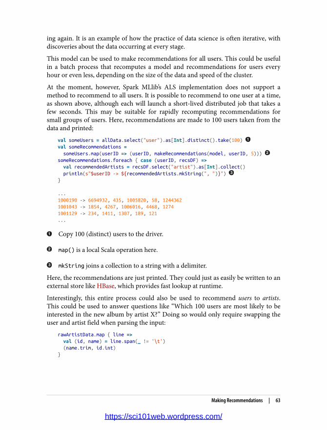
ing again. It is an example of how the practice of data science is often iterative, withdiscoveries about the data occurring at every stage.

This model can be used to make recommendations for all users. This could be usefulin a batch process that recomputes a model and recommendations for users everyhour or even less, depending on the size of the data and speed of the cluster.

At the moment, however, Spark MLlib’s ALS implementation does not support amethod to recommend to all users. It is possible to recommend to one user at a time,as shown above, although each will launch a short-lived distributed job that takes afew seconds. This may be suitable for rapidly recomputing recommendations forsmall groups of users. Here, recommendations are made to 100 users taken from thedata and printed:

val someUsers = allData.select("user").as[Int].distinct().take(100) val someRecommendations = someUsers.map(userID => (userID, makeRecommendations(model, userID, 5))) someRecommendations.foreach { case (userID, recsDF) => val recommendedArtists = recsDF.select("artist").as[Int].collect() println(s"$userID -> ${recommendedArtists.mkString(", ")}") }

...1000190 -> 6694932, 435, 1005820, 58, 12443621001043 -> 1854, 4267, 1006016, 4468, 12741001129 -> 234, 1411, 1307, 189, 121...

Copy 100 (distinct) users to the driver.

map() is a local Scala operation here.

mkString joins a collection to a string with a delimiter.

Here, the recommendations are just printed. They could just as easily be written to anexternal store like HBase, which provides fast lookup at runtime.

Interestingly, this entire process could also be used to recommend users to artists.This could be used to answer questions like “Which 100 users are most likely to beinterested in the new album by artist X?” Doing so would only require swapping theuser and artist field when parsing the input:

rawArtistData.map { line => val (id, name) = line.span(_ != '\t') (name.trim, id.int)}

Making Recommendations | 63


https://hbase.apache.org

Where to Go from HereNaturally, it’s possible to spend more time tuning the model parameters, and findingand fixing anomalies in the input, like the [unknown] artist. For example, a quickanalysis of play counts reveals that user 2064012 played artist 4468 an astonishing439,771 times! Artist 4468 is the implausibly successful alterna-metal band System ofa Down, who turned up earlier in recommendations. Assuming an average songlength of 4 minutes, this is over 33 years of playing hits like “Chop Suey!” and“B.Y.O.B.” Because the band started making records in 1998, this would require play‐ing four or five tracks at once for seven years. It must be spam or a data error, andanother example of the types of real-world data problems that a production systemwould have to address.

ALS is not the only possible recommender algorithm, but at this time, it is the onlyone supported by Spark MLlib. However, MLlib also supports a variant of ALS fornon-implicit data. Its use is identical, except that ALS is configured with setImplicitPrefs(false). This is appropriate when data is rating-like, rather than count-like.For example, it is appropriate when the data set is user ratings of artists on a 1–5scale. The resulting prediction column returned from ALSModel.transform recom‐mendation methods then really is an estimated rating. In this case, the simple RMSE(root mean squared error) metric is appropriate for evaluating the recommender.

Later, other recommender algorithms may be available in Spark MLlib or otherlibraries.

In production, recommender engines often need to make recommendations in realtime, because they are used in contexts like ecommerce sites where recommendationsare requested frequently as customers browse product pages. Precomputing and stor‐ing recommendations in a NoSQL store, as mentioned previously, is a reasonable wayto make recommendations available at scale. One disadvantage of this approach isthat it requires precomputing recommendations for all users who might need recom‐mendations soon, which is potentially any of them. For example, if only 10,000 of 1million users visit a site in a day, precomputing all million users’ recommendationseach day is 99% wasted effort.

It would be nicer to compute recommendations on the fly, as needed. While we cancompute recommendations for one user using the ALSModel, this is necessarily a dis‐tributed operation that takes several seconds, because ALSModel is uniquely large andtherefore actually a distributed data set. This is not true of other models, which affordmuch faster scoring. Projects like Oryx 2 attempt to implement real-time on-demandrecommendations with libraries like MLlib by efficiently accessing the model data inmemory.



https://en.wikipedia.org/wiki/System_of_a_Down

https://en.wikipedia.org/wiki/System_of_a_Down

https://github.com/OryxProject/oryx

CHAPTER 4

Predicting Forest Cover with Decision Trees

Sean Owen

Prediction is very difficult, especially if it’s about the future.—Niels Bohr

In the late nineteenth century, the English scientist Sir Francis Galton was busy meas‐uring things like peas and people. He found that large peas (and people) had larger-than-average offspring. This isn’t surprising. However, the offspring were, on average,smaller than their parents. In terms of people: the child of a seven-foot-tall basketballplayer is likely to be taller than the global average but still more likely than not to beless than seven feet tall.

As almost a side effect of his study, Galton plotted child versus parent size andnoticed there was a roughly linear relationship between the two. Large parent peashad large children, but slightly smaller than themselves; small parents had small chil‐dren, but generally a bit larger than themselves. The line’s slope was therefore positivebut less than 1, and Galton described this phenomenon as we do today, as regressionto the mean.

Although maybe not perceived this way at the time, this line was, to me, an earlyexample of a predictive model. The line links the two values, and implies that thevalue of one suggests a lot about the value of the other. Given the size of a new pea,this relationship could lead to a more accurate estimate of its offspring’s size thansimply assuming the offspring would be like the parent or like every other pea.

Fast Forward to RegressionMore than a century of statistics later, and since the advent of modern machine learn‐ing and data science, we still talk about the idea of predicting a value from other val‐ues as regression, even though it has nothing to do with slipping back toward a mean

65


https://en.wikipedia.org/wiki/Regression_analysis

value, or indeed moving backward at all. Regression techniques also relate to classifi‐cation techniques. Generally, regression refers to predicting a numeric quantity likesize or income or temperature, whereas classification refers to predicting a label orcategory, like “spam” or “picture of a cat.”

The common thread linking regression and classification is that both involve predict‐ing one (or more) values given one (or more) other values. To do so, both require abody of inputs and outputs to learn from. They need to be fed both questions andknown answers. For this reason, they are known as types of supervised learning.

Classification and regression are the oldest and most well-studied types of predictiveanalytics. Most algorithms you will likely encounter in analytics packages and libra‐ries are classification or regression techniques, like support vector machines, logisticregression, naïve Bayes, neural networks, and deep learning. Recommenders, thetopic of Chapter 3, were comparatively more intuitive to introduce, but are also just arelatively recent and separate subtopic within machine learning.

This chapter will focus on a popular and flexible type of algorithm for both classifica‐tion and regression: decision trees, and the algorithm’s extension, random decisionforests. The exciting thing about these algorithms is that, with all due respect to Mr.Bohr, they can help predict the future—or at least, predict the things we don’t yetknow for sure, like the likelihood you will buy a car based on your online behavior,whether an email is spam given its words, or which acres of land are likely to growthe most crops given their location and soil chemistry.

Vectors and FeaturesTo explain the choice of the data set and algorithm featured in this chapter, and tobegin to explain how regression and classification operate, it is necessary to brieflydefine the terms that describe their input and output.

Consider predicting tomorrow’s high temperature given today’s weather. There isnothing wrong with this idea, but “today’s weather” is a casual concept that requiresstructuring before it can be fed into a learning algorithm.

Really, it is certain features of today’s weather that may predict tomorrow’s tempera‐ture, such as:

• Today’s high temperature• Today’s low temperature• Today’s average humidity• Whether it’s cloudy, rainy, or clear today• The number of weather forecasters predicting a cold snap tomorrow

66 | Chapter 4: Predicting Forest Cover with Decision Trees


https://en.wikipedia.org/wiki/Statistical_classification

https://en.wikipedia.org/wiki/Statistical_classification

https://en.wikipedia.org/wiki/Supervised_learning

https://en.wikipedia.org/wiki/Decision_tree

https://en.wikipedia.org/wiki/Random_forest

https://en.wikipedia.org/wiki/Random_forest

These features are also sometimes called dimensions, predictors, or just variables. Eachof these features can be quantified. For example, high and low temperatures are meas‐ured in degrees Celsius, humidity can be measured as a fraction between 0 and 1, andweather type can be labeled cloudy, rainy, or clear. The number of forecasters is, ofcourse, an integer count. Today’s weather might therefore be reduced to a list of val‐ues like 13.1,19.0,0.73,cloudy,1.

These five features together, in order, are known as a feature vector, and can describeany day’s weather. This usage bears some resemblance to use of the term vector in lin‐ear algebra, except that a vector in this sense can conceptually contain nonnumericvalues, and even lack some values.

These features are not all of the same type. The first two features are measured indegrees Celsius, but the third is unitless, a fraction. The fourth is not a number at all,and the fifth is a number that is always a nonnegative integer.

For purposes of discussion, this book will talk about features in two broad groupsonly: categorical features and numeric features. In this context, numeric features arethose that can be quantified by a number and have a meaningful ordering. For exam‐ple, it’s meaningful to say that today’s high was 23ºC, and that this is higher than yes‐terday’s high of 22ºC. All of the features mentioned previously are numeric, exceptthe weather type. Terms like clear are not numbers, and have no ordering. It ismeaningless to say that cloudy is larger than clear. This is a categorical feature,which instead takes on one of several discrete values.

Training ExamplesA learning algorithm needs to train on data in order to make predictions. It requires alarge number of inputs, and known correct outputs, from historical data. For exam‐ple, in this problem, the learning algorithm would be given that, one day, the weatherwas between 12º and 16ºC, with 10% humidity, clear, with no forecast of a cold snap;and the following day, the high temperature was 17.2ºC. With enough of these exam‐ples, a learning algorithm might learn to predict the following day’s high temperaturewith some accuracy.

Feature vectors provide an organized way to describe input to a learning algorithm(here: 12.5,15.5,0.10,clear,0). The output, or target, of the prediction can also bethought of as a feature. Here, it is a numeric feature: 17.2. It’s not uncommon to sim‐ply include the target as another feature in the feature vector. The entire trainingexample might be thought of as 12.5,15.5,0.10,clear,0,17.2. The collection of allof these examples is known as the training set.

Note that regression problems are just those where the target is a numeric feature,and classification problems are those where the target is categorical. Not every

Training Examples | 67


regression or classification algorithm can handle categorical features or categoricaltargets; some are limited to numeric features.

Decision Trees and ForestsIt turns out that the family of algorithms known as decision trees can naturally handleboth categorical and numeric features. Building a single tree can be done in parallel,and many trees can be built in parallel at once. They are robust to outliers in the data,meaning that a few extreme and possibly erroneous data points might not affect pre‐dictions at all. They can consume data of different types and on different scaleswithout the need for preprocessing or normalization, which is an issue that will reap‐pear in Chapter 5.

Decision trees generalize into a more powerful algorithm, called random decision for‐ests. Their flexibility makes these algorithms worthwhile to examine in this chapter,where Spark MLlib’s DecisionTree and RandomForest implementation will beapplied to a data set.

Decision tree–based algorithms have the further advantage of being comparativelyintuitive to understand and reason about. In fact, we all probably use the same rea‐soning embodied in decision trees, implicitly, in everyday life. For example, I sitdown to have morning coffee with milk. Before I commit to that milk and add it tomy brew, I want to predict: is the milk spoiled? I don’t know for sure. I might check ifthe use-by date has passed. If not, I predict no, it’s not spoiled. If the date has passed,but that was three or fewer days ago, I take my chances and predict no, it’s not spoiled.Otherwise, I sniff the milk. If it smells funny, I predict yes, and otherwise no.

This series of yes/no decisions that lead to a prediction are what decision treesembody. Each decision leads to one of two results, which is either a prediction oranother decision, as shown in Figure 4-1. In this sense, it is natural to think of theprocess as a tree of decisions, where each internal node in the tree is a decision, andeach leaf node is a final answer.



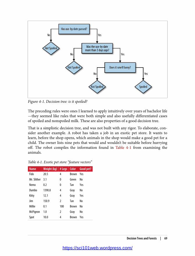
Figure 4-1. Decision tree: is it spoiled?

The preceding rules were ones I learned to apply intuitively over years of bachelor life—they seemed like rules that were both simple and also usefully differentiated casesof spoiled and nonspoiled milk. These are also properties of a good decision tree.

That is a simplistic decision tree, and was not built with any rigor. To elaborate, con‐sider another example. A robot has taken a job in an exotic pet store. It wants tolearn, before the shop opens, which animals in the shop would make a good pet for achild. The owner lists nine pets that would and wouldn’t be suitable before hurryingoff. The robot compiles the information found in Table 4-1 from examining theanimals.

Table 4-1. Exotic pet store “feature vectors”

Name Weight (kg) # Legs Color Good pet?Fido 20.5 4 Brown Yes

Mr. Slither 3.1 0 Green No

Nemo 0.2 0 Tan Yes

Dumbo 1390.8 4 Gray No

Kitty 12.1 4 Gray Yes

Jim 150.9 2 Tan No

Millie 0.1 100 Brown No

McPigeon 1.0 2 Gray No

Spot 10.0 4 Brown Yes

Decision Trees and Forests | 69


Although a name is given, it will not be included as a feature. There is little reason tobelieve the name alone is predictive; “Felix” could name a cat or a poisonous taran‐tula, for all the robot knows. So, there are two numeric features (weight, number oflegs) and one categorical feature (color) predicting a categorical target (is/is not agood pet for a child).

The robot might try to fit a simple decision tree to this training data to start, consist‐ing of a single decision based on weight, as shown in Figure 4-2.

Figure 4-2. Robot’s first decision tree

The logic of the decision tree is easy to read and make some sense of: 500kg animalscertainly sound unsuitable as pets. This rule predicts the correct value in five of ninecases. A quick glance suggests that we could improve the rule by lowering the weightthreshold to 100kg. This gets six of nine examples correct. The heavy animals are nowpredicted correctly; the lighter animals are only partly correct.

So, a second decision can be constructed to further refine the prediction for exampleswith weights less than 100kg. It would be good to pick a feature that changes some ofthe incorrect Yes predictions to No. For example, there is one small green animal,sounding suspiciously like a snake, that the robot could predict correctly by decidingon color, as shown in Figure 4-3.

Figure 4-3. Robot’s next decision tree



Now, seven of nine examples are correct. Of course, decision rules could be addeduntil all nine were correctly predicted. The logic embodied in the resulting decisiontree would probably sound implausible when translated into common speech: “If theanimal’s weight is less than 100kg, and its color is brown instead of green, and it hasfewer than 10 legs, then yes it is a suitable pet.” While perfectly fitting the given exam‐ples, a decision tree like this would fail to predict that a small, brown, four-leggedwolverine is not a suitable pet. Some balance is needed to avoid this phenomenon,known as overfitting.

This is enough of an introduction to decision trees for us to begin using them withSpark. The remainder of the chapter will explore how to pick decision rules, how toknow when to stop, and how to gain accuracy by creating a forest of trees.

Covtype Data SetThe data set used in this chapter is the well-known Covtype data set, available onlineas a compressed CSV-format data file, covtype.data.gz, and accompanying info file,covtype.info.

The data set records the types of forest-covering parcels of land in Colorado, USA. It’sonly a coincidence that the data set concerns real-world forests! Each example con‐tains several features describing each parcel of land—like its elevation, slope, distanceto water, shade, and soil type—along with the known forest type covering the land.The forest cover type is to be predicted from the rest of the features, of which thereare 54 in total.

This data set has been used in research and even a Kaggle competition. It is an inter‐esting data set to explore in this chapter because it contains both categorical andnumeric features. There are 581,012 examples in the data set, which does not exactlyqualify as big data but is large enough to be manageable as an example and still high‐light some issues of scale.

Preparing the DataThankfully, the data is already in a simple CSV format and does not require muchcleansing or other preparation to be used with Spark MLlib. Later, it will be of interestto explore some transformations of the data, but it can be used as is to start.

The covtype.data file should be extracted and copied into HDFS. This chapter willassume that the file is available at /user/ds/. Start spark-shell. You may again find ithelpful to give the shell a healthy amount of memory to work with, as building deci‐sion forests can be resource-intensive. If you have the memory, specify --driver-memory 8g or similar.

Covtype Data Set | 71


https://bit.ly/1KiJRfg

https://www.kaggle.com/c/forest-cover-type-prediction

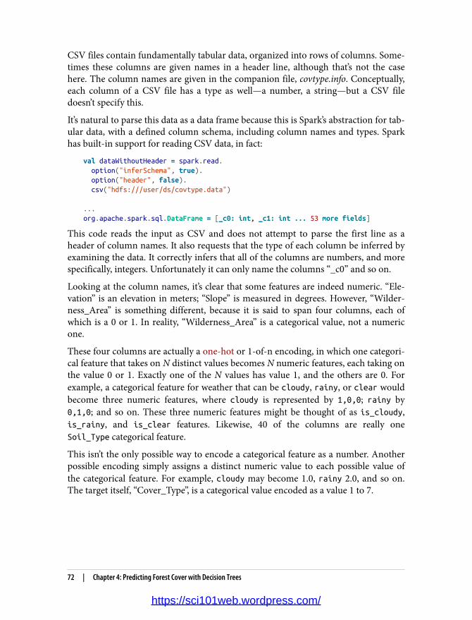
CSV files contain fundamentally tabular data, organized into rows of columns. Some‐times these columns are given names in a header line, although that’s not the casehere. The column names are given in the companion file, covtype.info. Conceptually,each column of a CSV file has a type as well—a number, a string—but a CSV filedoesn’t specify this.

It’s natural to parse this data as a data frame because this is Spark’s abstraction for tab‐ular data, with a defined column schema, including column names and types. Sparkhas built-in support for reading CSV data, in fact:

val dataWithoutHeader = spark.read. option("inferSchema", true). option("header", false). csv("hdfs:///user/ds/covtype.data")

...org.apache.spark.sql.DataFrame = [_c0: int, _c1: int ... 53 more fields]

This code reads the input as CSV and does not attempt to parse the first line as aheader of column names. It also requests that the type of each column be inferred byexamining the data. It correctly infers that all of the columns are numbers, and morespecifically, integers. Unfortunately it can only name the columns “_c0” and so on.

Looking at the column names, it’s clear that some features are indeed numeric. “Ele‐vation” is an elevation in meters; “Slope” is measured in degrees. However, “Wilder‐ness_Area” is something different, because it is said to span four columns, each ofwhich is a 0 or 1. In reality, “Wilderness_Area” is a categorical value, not a numericone.

These four columns are actually a one-hot or 1-of-n encoding, in which one categori‐cal feature that takes on N distinct values becomes N numeric features, each taking onthe value 0 or 1. Exactly one of the N values has value 1, and the others are 0. Forexample, a categorical feature for weather that can be cloudy, rainy, or clear wouldbecome three numeric features, where cloudy is represented by 1,0,0; rainy by0,1,0; and so on. These three numeric features might be thought of as is_cloudy,is_rainy, and is_clear features. Likewise, 40 of the columns are really oneSoil_Type categorical feature.

This isn’t the only possible way to encode a categorical feature as a number. Anotherpossible encoding simply assigns a distinct numeric value to each possible value ofthe categorical feature. For example, cloudy may become 1.0, rainy 2.0, and so on.The target itself, “Cover_Type”, is a categorical value encoded as a value 1 to 7.



https://en.wikipedia.org/wiki/One-hot

Be careful when encoding a categorical feature as a single numericfeature. The original categorical values have no ordering, but whenencoded as a number, they appear to. Treating the encoded featureas numeric leads to meaningless results because the algorithm iseffectively pretending that rainy is somehow greater than, and twotimes larger than, cloudy. It’s OK as long as the encoding’s numericvalue is not used as a number.

So we see both types of encodings of categorical features. It would have, perhaps, beensimpler and more straightforward to not encode such features (and in two ways, noless), and instead simply include their values directly like “Rawah Wilderness Area.”This may be an artifact of history; the data set was released in 1998. For performancereasons or to match the format expected by libraries of the day, which were builtmore for regression problems, data sets often contain data encoded in these ways.

In any event, before proceeding, it is useful to add column names to this DataFramein order to make it easier to work with:

val colNames = Seq( "Elevation", "Aspect", "Slope", "Horizontal_Distance_To_Hydrology", "Vertical_Distance_To_Hydrology", "Horizontal_Distance_To_Roadways", "Hillshade_9am", "Hillshade_Noon", "Hillshade_3pm", "Horizontal_Distance_To_Fire_Points" ) ++ ( (0 until 4).map(i => s"Wilderness_Area_$i") ) ++ ( (0 until 40).map(i => s"Soil_Type_$i") ) ++ Seq("Cover_Type")

val data = dataWithoutHeader.toDF(colNames:_*). withColumn("Cover_Type", $"Cover_Type".cast("double"))

data.head...org.apache.spark.sql.Row = [2596,51,3,258,0,510,221,232,148,6279,1,0,0,0,...

++ concatenates collections

The wilderness- and soil-related columns are named “Wilderness_Area_0”,“Soil_Type_0”, and a bit of Scala can generate these 44 names without having to typethem all out. Finally, the target “Cover_Type” column is cast to a double valueupfront, because it will actually be necessary to consume it as a double rather thanint in all Spark MLlib APIs. This will become apparent later.

You can call data.show() to see some rows of the data set, but the display is so widethat it will be difficult to read at all. data.head displays it as a raw Row object, whichwill be more readable in this case.

Preparing the Data | 73


A First Decision TreeIn Chapter 3, we built a recommender model right away on all of the available data.This created a recommender that could be sense-checked by anyone with someknowledge of music: looking at a user’s listening habits and recommendations, we gotsome sense that it was producing good results. Here, that is not possible. We wouldhave no idea how to make up a new 54-feature description of a new parcel of land inColorado or what kind of forest cover to expect from such a parcel.

Instead, we must jump straight to holding out some data for purposes of evaluatingthe resulting model. Before, the AUC metric was used to assess the agreementbetween held-out listening data and predictions from recommendations. The princi‐ple is the same here, although the evaluation metric will be different: accuracy. Themajority—90%—of the data will again be used for training, and later, we’ll see that asubset of this training set will be held out for cross-validation (the CV set). The other10% held out here is actually a third subset, a proper test set.

val Array(trainData, testData) = data.randomSplit(Array(0.9, 0.1))trainData.cache()testData.cache()

The data needs a little more preparation to be used with a classifier in Spark MLlib.The input DataFrame contains many columns, each holding one feature that could beused to predict the target column. Spark MLlib requires all of the inputs to be collec‐ted into one column, whose value is a vector. This class is an abstraction for vectors inthe linear algebra sense, and contains only numbers. For most intents and purposes,they work like a simple array of double values (floating-point numbers). Of course,some of the input features are conceptually categorical, even if they’re all representedwith numbers in the input. For now, we’ll overlook this point and return to it later.

Fortunately, the VectorAssembler class can do this work:

import org.apache.spark.ml.feature.VectorAssembler

val inputCols = trainData.columns.filter(_ != "Cover_Type")val assembler = new VectorAssembler(). setInputCols(inputCols). setOutputCol("featureVector")

val assembledTrainData = assembler.transform(trainData)assembledTrainData.select("featureVector").show(truncate = false)

...+------------------------------------------------------------------- ...|featureVector ...+------------------------------------------------------------------- ...|(54,[0,1,2,3,4,5,6,7,8,9,13,15],[1863.0,37.0,17.0,120.0,18.0,90.0,2 ...|(54,[0,1,2,5,6,7,8,9,13,18],[1874.0,18.0,14.0,90.0,208.0,209.0,135. ...



|(54,[0,1,2,3,4,5,6,7,8,9,13,18],[1879.0,28.0,19.0,30.0,12.0,95.0,20 ......

Its key parameters are the columns to combine into the feature vector, and the nameof the new column containing the feature vector. Here, all columns—except—the tar‐get, of course—are included as input features. The resulting DataFrame has a new“featureVector” column, as shown.

The output doesn’t look exactly like a sequence of numbers, but that’s because thisshows a raw representation of the vector, represented as a SparseVector instance tosave storage. Because most of the 54 values are 0, it only stores nonzero values andtheir indices. This detail won’t matter in classification.

VectorAssembler is an example of Transformer within the current Spark MLlib“Pipelines” API. It transforms another DataFrame into a DataFrame, and is composa‐ble with other transformations into a pipeline. Later in this chapter, these transforma‐tions will be connected into an actual Pipeline. Here, the transformation is justinvoked directly, which is sufficient to build a first decision tree classifier model.

import org.apache.spark.ml.classification.DecisionTreeClassifierimport scala.util.Random

val classifier = new DecisionTreeClassifier(). setSeed(Random.nextLong()). setLabelCol("Cover_Type"). setFeaturesCol("featureVector"). setPredictionCol("prediction")

val model = classifier.fit(assembledTrainData)println(model.toDebugString)

...DecisionTreeClassificationModel (uid=dtc_29cfe1281b30) of depth 5 with 63 nodes If (feature 0 <= 3039.0) If (feature 0 <= 2555.0) If (feature 10 <= 0.0) If (feature 0 <= 2453.0) If (feature 3 <= 0.0) Predict: 4.0 Else (feature 3 > 0.0) Predict: 3.0 ...

Use random seed

Again, the essential configuration for the classifier consists of column names: the col‐umn containing the input feature vectors and the column containing the target valueto predict. Because the model will later be used to predict new values of the target, itis given the name of a column to store predictions.

A First Decision Tree | 75


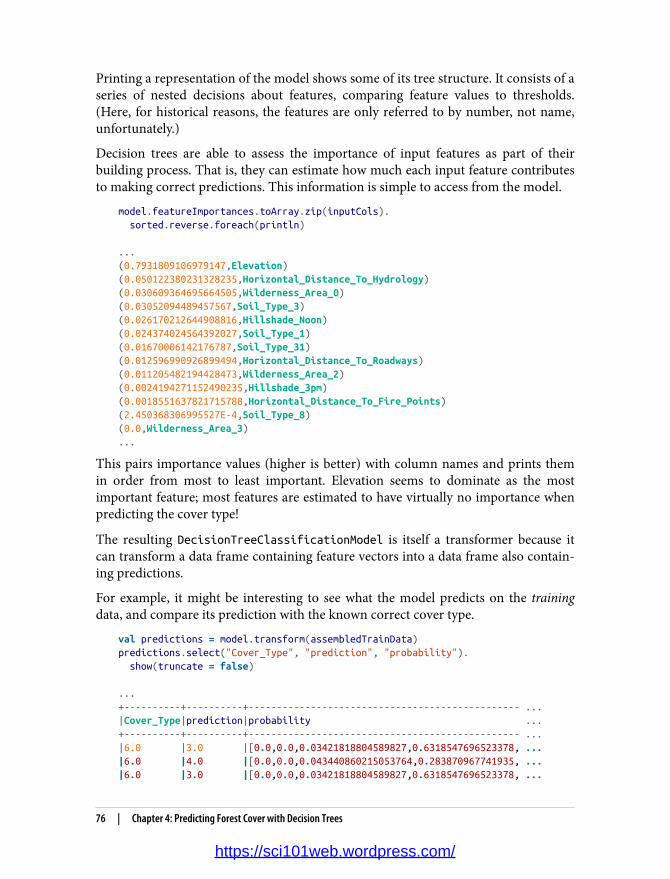
Printing a representation of the model shows some of its tree structure. It consists of aseries of nested decisions about features, comparing feature values to thresholds.(Here, for historical reasons, the features are only referred to by number, not name,unfortunately.)

Decision trees are able to assess the importance of input features as part of theirbuilding process. That is, they can estimate how much each input feature contributesto making correct predictions. This information is simple to access from the model.

model.featureImportances.toArray.zip(inputCols). sorted.reverse.foreach(println)

...(0.7931809106979147,Elevation)(0.050122380231328235,Horizontal_Distance_To_Hydrology)(0.030609364695664505,Wilderness_Area_0)(0.03052094489457567,Soil_Type_3)(0.026170212644908816,Hillshade_Noon)(0.024374024564392027,Soil_Type_1)(0.01670006142176787,Soil_Type_31)(0.012596990926899494,Horizontal_Distance_To_Roadways)(0.011205482194428473,Wilderness_Area_2)(0.0024194271152490235,Hillshade_3pm)(0.0018551637821715788,Horizontal_Distance_To_Fire_Points)(2.450368306995527E-4,Soil_Type_8)(0.0,Wilderness_Area_3)...

This pairs importance values (higher is better) with column names and prints themin order from most to least important. Elevation seems to dominate as the mostimportant feature; most features are estimated to have virtually no importance whenpredicting the cover type!

The resulting DecisionTreeClassificationModel is itself a transformer because itcan transform a data frame containing feature vectors into a data frame also contain‐ing predictions.

For example, it might be interesting to see what the model predicts on the trainingdata, and compare its prediction with the known correct cover type.

val predictions = model.transform(assembledTrainData)predictions.select("Cover_Type", "prediction", "probability"). show(truncate = false)

...+----------+----------+------------------------------------------------ ...|Cover_Type|prediction|probability ...+----------+----------+------------------------------------------------ ...|6.0 |3.0 |[0.0,0.0,0.03421818804589827,0.6318547696523378, ...|6.0 |4.0 |[0.0,0.0,0.043440860215053764,0.283870967741935, ...|6.0 |3.0 |[0.0,0.0,0.03421818804589827,0.6318547696523378, ...



|6.0 |3.0 |[0.0,0.0,0.03421818804589827,0.6318547696523378, ......

Interestingly, the output also contains a “probability” column that gives the model’sestimate of how likely it is that each possible outcome is correct. This shows that inthese instances, it’s fairly sure the answer is 3 in several cases and quite sure theanswer isn’t 1.

Eagle-eyed readers might note that the probability vectors actually have eight valueseven though there are only seven possible outcomes. The vector’s values at indices 1to 7 do contain the probability of outcomes 1 to 7. However, there is also a value atindex 0, which always shows as probability 0.0. This can be ignored, as 0 isn’t even avalid outcome, as this says. It’s a quirk of representing this information as a vectorthat’s worth being aware of.

Based on this snippet, it looks like the model could use some work. Its predictionslook like they are often wrong. As with the ALS implementation, the DecisionTreeClassifier implementation has several hyperparameters for which a value must bechosen, and they’ve all been left to defaults here. Here, the test set can be used to pro‐duce an unbiased evaluation of the expected accuracy of a model built with thesedefault hyperparameters.

MulticlassClassificationEvaluator can compute accuracy and other metrics thatevaluate the quality of the model’s predictions. It’s an example of an evaluator inSpark MLlib, which is responsible for assessing the quality of an output DataFrame insome way.

import org.apache.spark.ml.evaluation.MulticlassClassificationEvaluator

val evaluator = new MulticlassClassificationEvaluator(). setLabelCol("Cover_Type"). setPredictionCol("prediction")

evaluator.setMetricName("accuracy").evaluate(predictions)evaluator.setMetricName("f1").evaluate(predictions)

...0.69763713855029890.6815943874214012

After being given the column containing the “label” (target, or known correct outputvalue) and the name of the column containing the prediction, it finds that the twomatch about 70% of the time. This is the accuracy of this classifier. It can computeother related measures, like the F1 score. For purposes here, accuracy will be used toevaluate classifiers.

This single number gives a good summary of the quality of the classifier’s output.Sometimes, however, it can be useful to look at the confusion matrix. This is a table



https://en.wikipedia.org/wiki/F1_score

with a row and a column for every possible value of the target. Because there areseven target category values, this is a 7×7 matrix, where each row corresponds to anactual correct value, and each column to a predicted value, in order. The entry at rowi and column j counts the number of times an example with true category i was pre‐dicted as category j. So, the correct predictions are the counts along the diagonal andthe predictions are everything else.

Fortunately, Spark provides support code to compute the confusion matrix. Unfortu‐nately, that implementation exists as part of the older MLlib APIs that operate onRDDs. However, that’s no big deal, because data frames and data sets can freely beturned into RDDs and used with these older APIs. Here, MulticlassMetrics isappropriate for a data frame containing predictions.

import org.apache.spark.mllib.evaluation.MulticlassMetrics

val predictionRDD = predictions. select("prediction", "Cover_Type"). as[(Double,Double)]. rdd val multiclassMetrics = new MulticlassMetrics(predictionRDD)multiclassMetrics.confusionMatrix

...143125.0 41769.0 164.0 0.0 0.0 0.0 5396.065865.0 184360.0 3930.0 102.0 39.0 0.0 677.00.0 5680.0 25772.0 674.0 0.0 0.0 0.00.0 21.0 1481.0 973.0 0.0 0.0 0.087.0 7761.0 648.0 0.0 69.0 0.0 0.00.0 6175.0 8902.0 559.0 0.0 0.0 0.08058.0 24.0 50.0 0.0 0.0 0.0 10395.0

Convert to data set.

Convert to RDD.

Your values will be a little different. The process of building a deci‐sion tree includes some random choices that can lead to slightlydifferent classifications.

Counts are high along the diagonal, which is good. However, there are certainly anumber of misclassifications, and, for example, category 5 is never predicted at all.

Of course, it’s also possible to calculate something like a confusion matrix directlywith the DataFrame API, using its more general operators. It is not necessary to relyon a specialized method anymore.



val confusionMatrix = predictions. groupBy("Cover_Type"). pivot("prediction", (1 to 7)). count(). na.fill(0.0). orderBy("Cover_Type")

confusionMatrix.show()

...+----------+------+------+-----+---+---+---+-----+|Cover_Type| 1| 2| 3| 4| 5| 6| 7|+----------+------+------+-----+---+---+---+-----+| 1.0|143125| 41769| 164| 0| 0| 0| 5396|| 2.0| 65865|184360| 3930|102| 39| 0| 677|| 3.0| 0| 5680|25772|674| 0| 0| 0|| 4.0| 0| 21| 1481|973| 0| 0| 0|| 5.0| 87| 7761| 648| 0| 69| 0| 0|| 6.0| 0| 6175| 8902|559| 0| 0| 0|| 7.0| 8058| 24| 50| 0| 0| 0|10395|+----------+------+------+-----+---+---+---+-----+

Replace null with 0

Microsoft Excel users may have recognized the problem as just like that of computing a pivot table. A pivot table groups values by two dimensions whose values becomerows and columns of the output, and compute some aggregation within those group‐ings, like a count here. This is also available as a PIVOT function in several databases,and is supported by Spark SQL. It’s arguably more elegant and powerful to compute itthis way.

Although 70% accuracy sounds decent, it’s not immediately clear whether it is out‐standing or poor. How well would a simplistic approach do to establish a baseline?Just as a broken clock is correct twice a day, randomly guessing a classification foreach example would also occasionally produce the correct answer.

We could construct such a random “classifier” by picking a class at random in pro‐portion to its prevalence in the training set. For example, if 30% of the training setwere cover type 1, then the random classifier would guess “1” 33% of the time. Eachclassification would be correct in proportion to its prevalence in the test set. If 40% ofthe test set were cover type 1, then guessing “1” would be correct 40% of the time.Cover type 1 would then be guessed correctly 30% x 40% = 12% of the time and con‐tribute 12% to overall accuracy. Therefore, we can evaluate the accuracy by summingthese products of probabilities:

import org.apache.spark.sql.DataFrame

def classProbabilities(data: DataFrame): Array[Double] = { val total = data.count()



https://en.wikipedia.org/wiki/Pivot_table

data.groupBy("Cover_Type").count(). orderBy("Cover_Type"). select("count").as[Double]. map(_ / total). collect()}

val trainPriorProbabilities = classProbabilities(trainData)val testPriorProbabilities = classProbabilities(testData)trainPriorProbabilities.zip(testPriorProbabilities).map { case (trainProb, cvProb) => trainProb * cvProb}.sum

...0.3771270477245849

Count by category

Order counts by category

To data set

Sum products of pairs in training, test sets

Random guessing achieves 37% accuracy then, which makes 70% seem like a goodresult after all. But this result was achieved with default hyperparameters. We can doeven better by exploring what these actually mean for the tree-building process.

Decision Tree HyperparametersIn Chapter 3, the ALS algorithm exposed several hyperparameters whose values wehad to choose by building models with various combinations of values and thenassessing the quality of each result using some metric. The process is the same here,although the metric is now multiclass accuracy instead of AUC. The hyperparameterscontrolling how the tree’s decisions are chosen will be quite different as well: maxi‐mum depth, maximum bins, impurity measure, and minimum information gain.

Maximum depth simply limits the number of levels in the decision tree. It is the max‐imum number of chained decisions that the classifier will make to classify an exam‐ple. It is useful to limit this to avoid overfitting the training data, as illustratedpreviously in the pet store example.

The decision tree algorithm is responsible for coming up with potential decision rulesto try at each level, like the weight >= 100 or weight >= 500 decisions in the petstore example. Decisions are always of the same form: for numeric features, decisionsare of the form feature >= value; and for categorical features, they are of the formfeature in (value1, value2, …). So, the set of decision rules to try is really a set of



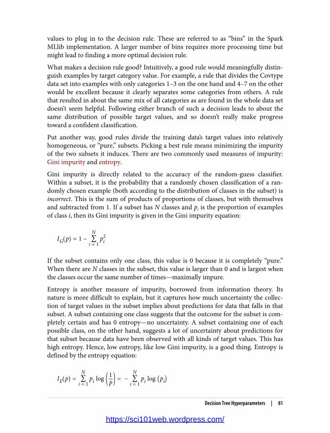
values to plug in to the decision rule. These are referred to as “bins” in the SparkMLlib implementation. A larger number of bins requires more processing time butmight lead to finding a more optimal decision rule.

What makes a decision rule good? Intuitively, a good rule would meaningfully distin‐guish examples by target category value. For example, a rule that divides the Covtypedata set into examples with only categories 1–3 on the one hand and 4–7 on the otherwould be excellent because it clearly separates some categories from others. A rulethat resulted in about the same mix of all categories as are found in the whole data setdoesn’t seem helpful. Following either branch of such a decision leads to about thesame distribution of possible target values, and so doesn’t really make progresstoward a confident classification.

Put another way, good rules divide the training data’s target values into relativelyhomogeneous, or “pure,” subsets. Picking a best rule means minimizing the impurityof the two subsets it induces. There are two commonly used measures of impurity:Gini impurity and entropy.

Gini impurity is directly related to the accuracy of the random-guess classifier.Within a subset, it is the probability that a randomly chosen classification of a ran‐domly chosen example (both according to the distribution of classes in the subset) isincorrect. This is the sum of products of proportions of classes, but with themselvesand subtracted from 1. If a subset has N classes and pi is the proportion of examplesof class i, then its Gini impurity is given in the Gini impurity equation:

IG p = 1 − ∑i = 1

Npi

2

If the subset contains only one class, this value is 0 because it is completely “pure.”When there are N classes in the subset, this value is larger than 0 and is largest whenthe classes occur the same number of times—maximally impure.

Entropy is another measure of impurity, borrowed from information theory. Itsnature is more difficult to explain, but it captures how much uncertainty the collec‐tion of target values in the subset implies about predictions for data that falls in thatsubset. A subset containing one class suggests that the outcome for the subset is com‐pletely certain and has 0 entropy—no uncertainty. A subset containing one of eachpossible class, on the other hand, suggests a lot of uncertainty about predictions forthat subset because data have been observed with all kinds of target values. This hashigh entropy. Hence, low entropy, like low Gini impurity, is a good thing. Entropy isdefined by the entropy equation:

IE p = ∑i = 1

Npi log 1

p = − ∑i = 1

Npi log pi

Decision Tree Hyperparameters | 81


https://en.wikipedia.org/wiki/Decision_tree_learning#Gini_impurity

https://en.wikipedia.org/wiki/Entropy_(information_theory)

Interestingly, uncertainty has units. Because the logarithm is thenatural log (base e), the units are nats, the base-e counterpart tomore familiar bits (which we can obtain by using log base 2instead). It really is measuring information, so it’s also common totalk about the information gain of a decision rule when usingentropy with decision trees.

One or the other measure may be a better metric for picking decision rules in a givendata set. They are, in a way, similar. Both involve a weighted average: a sum over val‐ues weighted by pi. The default in Spark’s implementation is Gini impurity.

Finally, minimum information gain is a hyperparameter that imposes a minimuminformation gain, or decrease in impurity, for candidate decision rules. Rules that donot improve the subsets impurity enough are rejected. Like a lower maximum depth,this can help the model resist overfitting because decisions that barely help divide thetraining input may in fact not helpfully divide future data at all.

Tuning Decision TreesIt’s not obvious from looking at the data which impurity measure leads to better accu‐racy, or what maximum depth or number of bins is enough without being excessive.Fortunately, as in Chapter 3, it’s simple to let Spark try a number of combinations ofthese values and report the results.

First, it’s necessary to set up a pipeline encapsulating the same two steps above. Creat‐ing the VectorAssembler and DecisionTreeClassifier and chaining these twoTransformers together results in a single Pipeline object that represents these twooperations together as one operation:

import org.apache.spark.ml.Pipeline

val inputCols = trainData.columns.filter(_ != "Cover_Type")val assembler = new VectorAssembler(). setInputCols(inputCols). setOutputCol("featureVector")

val classifier = new DecisionTreeClassifier(). setSeed(Random.nextLong()). setLabelCol("Cover_Type"). setFeaturesCol("featureVector"). setPredictionCol("prediction")

val pipeline = new Pipeline().setStages(Array(assembler, classifier))

Naturally, pipelines can be much longer and more complex. This is about as simple asit gets. Now we can also define the combinations of hyperparameters that should betested using the Spark ML API’s built-in support, ParamGridBuilder. It’s also time to



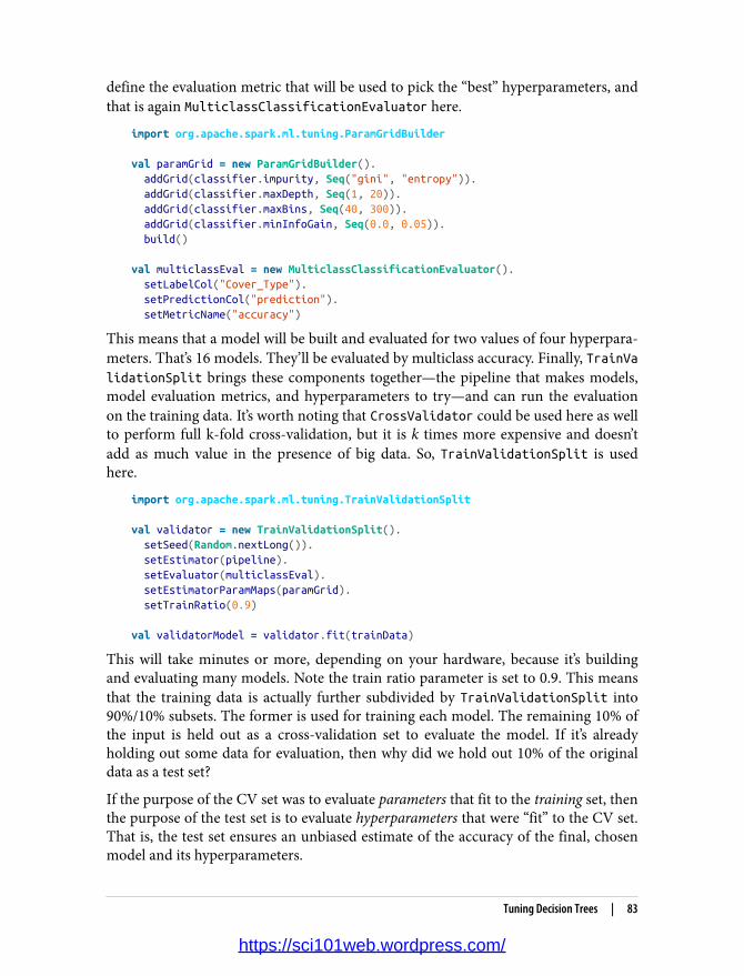
define the evaluation metric that will be used to pick the “best” hyperparameters, andthat is again MulticlassClassificationEvaluator here.

import org.apache.spark.ml.tuning.ParamGridBuilder

val paramGrid = new ParamGridBuilder(). addGrid(classifier.impurity, Seq("gini", "entropy")). addGrid(classifier.maxDepth, Seq(1, 20)). addGrid(classifier.maxBins, Seq(40, 300)). addGrid(classifier.minInfoGain, Seq(0.0, 0.05)). build()

val multiclassEval = new MulticlassClassificationEvaluator(). setLabelCol("Cover_Type"). setPredictionCol("prediction"). setMetricName("accuracy")

This means that a model will be built and evaluated for two values of four hyperpara‐meters. That’s 16 models. They’ll be evaluated by multiclass accuracy. Finally, TrainValidationSplit brings these components together—the pipeline that makes models,model evaluation metrics, and hyperparameters to try—and can run the evaluationon the training data. It’s worth noting that CrossValidator could be used here as wellto perform full k-fold cross-validation, but it is k times more expensive and doesn’tadd as much value in the presence of big data. So, TrainValidationSplit is usedhere.

import org.apache.spark.ml.tuning.TrainValidationSplit

val validator = new TrainValidationSplit(). setSeed(Random.nextLong()). setEstimator(pipeline). setEvaluator(multiclassEval). setEstimatorParamMaps(paramGrid). setTrainRatio(0.9)

val validatorModel = validator.fit(trainData)

This will take minutes or more, depending on your hardware, because it’s buildingand evaluating many models. Note the train ratio parameter is set to 0.9. This meansthat the training data is actually further subdivided by TrainValidationSplit into90%/10% subsets. The former is used for training each model. The remaining 10% ofthe input is held out as a cross-validation set to evaluate the model. If it’s alreadyholding out some data for evaluation, then why did we hold out 10% of the originaldata as a test set?

If the purpose of the CV set was to evaluate parameters that fit to the training set, thenthe purpose of the test set is to evaluate hyperparameters that were “fit” to the CV set.That is, the test set ensures an unbiased estimate of the accuracy of the final, chosenmodel and its hyperparameters.

Tuning Decision Trees | 83


Say that the best model chosen by this process exhibits 90% accuracy on the CV set. Itseems reasonable to expect it will exhibit 90% accuracy on future data. However,there’s an element of randomness in how these models are built. By chance, thismodel and evaluation could have turned out unusually well. The top model and eval‐uation result could have benefited from a bit of luck, so its accuracy estimate is likelyto be slightly optimistic. Put another way, hyperparameters can overfit too.

To really assess how well this best model is likely to perform on future examples, weneed to evaluate it on examples that were not used to train it. But we also need toavoid examples in the CV set that were used to evaluate it. That is why a third subset,the test set, was held out.

The result of the validator contains the best model it found. This itself is a representa‐tion of the best overall pipeline it found, because we provided an instance of a pipelineto run. In order to query the parameters chosen by DecisionTreeClassifier, it’snecessary to manually extract DecisionTreeClassificationModel from the resultingPipelineModel, which is the final stage in the pipeline.

import org.apache.spark.ml.PipelineModel

val bestModel = validatorModel.bestModelbestModel.asInstanceOf[PipelineModel].stages.last.extractParamMap

...{ dtc_9136220619b4-cacheNodeIds: false, dtc_9136220619b4-checkpointInterval: 10, dtc_9136220619b4-featuresCol: featureVector, dtc_9136220619b4-impurity: entropy, dtc_9136220619b4-labelCol: Cover_Type, dtc_9136220619b4-maxBins: 40, dtc_9136220619b4-maxDepth: 20, dtc_9136220619b4-maxMemoryInMB: 256, dtc_9136220619b4-minInfoGain: 0.0, dtc_9136220619b4-minInstancesPerNode: 1, dtc_9136220619b4-predictionCol: prediction, dtc_9136220619b4-probabilityCol: probability, dtc_9136220619b4-rawPredictionCol: rawPrediction, dtc_9136220619b4-seed: 159147643}

This contains a lot of information about the fitted model, but it also tells us that“entropy” apparently worked best as the impurity measure and that a max depth of 20was not surprisingly better than 1. It might be surprising that the best model was fitwith just 40 bins, but this is probably a sign that 40 was “plenty” rather than “better”than 300. Lastly, no minimum information gain was better than a small minimum,which could imply that the model is more prone to underfit than overfit.



You may wonder if it is possible to see the accuracy that each of the models achievedfor each combination of hyperparameters. The hyperparameters as well as the evalua‐tions are exposed by getEstimatorParamMaps and validationMetrics, respectively.They can be combined to display all of the parameter combinations sorted by metricvalue:

val validatorModel = validator.fit(trainData)

val paramsAndMetrics = validatorModel.validationMetrics. zip(validatorModel.getEstimatorParamMaps).sortBy(-_._1)

paramsAndMetrics.foreach { case (metric, params) => println(metric) println(params) println()}

...0.9138483377774368{ dtc_3e3b8bb692d1-impurity: entropy, dtc_3e3b8bb692d1-maxBins: 40, dtc_3e3b8bb692d1-maxDepth: 20, dtc_3e3b8bb692d1-minInfoGain: 0.0}

0.9122369506416774{ dtc_3e3b8bb692d1-impurity: entropy, dtc_3e3b8bb692d1-maxBins: 300, dtc_3e3b8bb692d1-maxDepth: 20, dtc_3e3b8bb692d1-minInfoGain: 0.0}...

What was the accuracy that this model achieved on the CV set? And finally, whataccuracy does the model achieve on the test set?

validatorModel.validationMetrics.maxmulticlassEval.evaluate(bestModel.transform(testData))

...0.91384833777743680.9139978718291971

bestModel is a complete pipeline.

The results are both about 91%. It happens that the estimate from the CV set waspretty fine to begin with. In fact, it is not usual for the test set to show a very differentresult.

Tuning Decision Trees | 85


This is an interesting point at which to revisit the issue of overfitting. As discussedpreviously, it’s possible to build a decision tree so deep and elaborate that it fits thegiven training examples very well or perfectly but fails to generalize to other examplesbecause it has fit the idiosyncrasies and noise of the training data too closely. This is aproblem common to most machine learning algorithms, not just decision trees.

When a decision tree has overfit, it will exhibit high accuracy when run on the sametraining data that it fit the model to, but low accuracy on other examples. Here, thefinal model’s accuracy was about 91% on other, new examples. Accuracy can just aseasily be evaluated over the same data that the model was trained on, trainData. Thisgives an accuracy of about 95%.

The difference is not large but suggests that the decision tree has overfit the trainingdata to some extent. A lower maximum depth might be a better choice.

Categorical Features RevisitedSo far, the code examples have implicitly treated all input features as if they’renumeric (though “Cover_Type”, despite being encoded as numeric, has actually beencorrectly treated as a categorical value.) This isn’t exactly wrong, because the categori‐cal features here are one-hot encoded as several binary 0/1 values. Treating theseindividual features as numeric turns out to be fine, because any decision rule on the“numeric” features will choose thresholds between 0 and 1, and all are equivalentsince all values are 0 or 1.

Of course, this encoding forces the decision tree algorithm to consider the values ofthe underlying categorical features individually. Because features like soil type arebroken down into many features, and because decision trees treat features individu‐ally, it is harder to relate information about related soil types.

For example, nine different soil types are actually part of the Leighcan family, andthey may be related in ways that the decision tree can exploit. If soil type were enco‐ded as a single categorical feature with 40 soil values, then the tree could express ruleslike “if the soil type is one of the nine Leighton family types” directly. However, whenencoded as 40 features, the tree would have to learn a sequence of nine decisions onsoil type to do the same, this expressiveness may lead to better decisions and moreefficient trees.

However, having 40 numeric features represent one 40-valued categorical featureincreases memory usage and slows things down.

What about undoing the one-hot encoding? This would replace, for example, thefour columns encoding wilderness type with one column that encodes the wildernesstype as a number between 0 and 3, like “Cover_Type”.



import org.apache.spark.sql.functions._

def unencodeOneHot(data: DataFrame): DataFrame = { val wildernessCols = (0 until 4).map(i => s"Wilderness_Area_$i").toArray

val wildernessAssembler = new VectorAssembler(). setInputCols(wildernessCols). setOutputCol("wilderness")

val unhotUDF = udf((vec: Vector) => vec.toArray.indexOf(1.0).toDouble)

val withWilderness = wildernessAssembler.transform(data). drop(wildernessCols:_*). withColumn("wilderness", unhotUDF($"wilderness"))

val soilCols = (0 until 40).map(i => s"Soil_Type_$i").toArray

val soilAssembler = new VectorAssembler(). setInputCols(soilCols). setOutputCol("soil")

soilAssembler.transform(withWilderness). drop(soilCols:_*). withColumn("soil", unhotUDF($"soil"))}

Note UDF definition

Drop one-hot columns; no longer needed

Overwrite column with numeric one of same name

Here VectorAssembler is deployed to combine the 4 and 40 wilderness and soil typecolumns into two Vector columns. The values in these Vectors are all 0, except forone location that has a 1. There’s no simple DataFrame function for this, so we haveto define our own UDF that can be used to operate on columns. This turns these twonew columns into numbers of just the type we need.

From here, nearly the same process as above can be used to tune the hyperparametersof a decision tree model built on this data and to choose and evaluate a best model.There’s one important difference, however. The two new numeric columns havenothing about them that indicates they’re actually an encoding of categorical values.To treat them as numbers would be wrong, as their ordering is meaningless. However,it would silently succeed; the information in these features would be all but lostthough.

Internally Spark MLlib can store additional metadata about each column. The detailsof this data are generally hidden from the caller, but includes information such aswhether the column encodes a categorical value and how many distinct values it takes

Categorical Features Revisited | 87


on. In order to add this metadata, it’s necessary to put the data through VectorIndexer. Its job is to turn input into properly labeled categorical feature columns.Although we did much of the work already to turn the categorical features into 0-indexed values, VectorIndexer will take care of the metadata.

We need to add this stage to the Pipeline:

import org.apache.spark.ml.feature.VectorIndexer

val inputCols = unencTrainData.columns.filter(_ != "Cover_Type")val assembler = new VectorAssembler(). setInputCols(inputCols). setOutputCol("featureVector")

val indexer = new VectorIndexer(). setMaxCategories(40). setInputCol("featureVector"). setOutputCol("indexedVector")

val classifier = new DecisionTreeClassifier(). setSeed(Random.nextLong()). setLabelCol("Cover_Type"). setFeaturesCol("indexedVector"). setPredictionCol("prediction")

val pipeline = new Pipeline().setStages(Array(assembler, indexer, classifier))

>= 40 because soil has 40 values

The approach assumes that the training set contains all possible values of each of thecategorical features at least once. That is, it works correctly only if all 4 soil values andall 40 wilderness values appear in the training set so that all possible values get a map‐ping. Here, that happens to be true, but may not be for small training sets of data inwhich some labels appear very infrequently. In those cases, it could be necessary tomanually create and add a VectorIndexerModel with the complete value mappingsupplied manually.

Aside from that, the process is the same as before. You should find that it chose a sim‐ilar best model but that accuracy on the test set is about 93%. By treating categoricalfeatures as actual categorical features, the classifier improved its accuracy by almost2%.

Random Decision ForestsIf you have been following along with the code examples, you may have noticed thatyour results differ slightly from those presented in the code listings in the book. Thatis because there is an element of randomness in building decision trees, and the ran‐



domness comes into play when you’re deciding what data to use and what decisionrules to explore.

The algorithm does not consider every possible decision rule at every level. To do sowould take an incredible amount of time. For a categorical feature over N values,there are 2N–2 possible decision rules (every subset except the empty set and entireset). For even moderately large N, this would create billions of candidate decisionrules.

Instead, decision trees use several heuristics to determine which few rules to actuallyconsider. The process of picking rules also involves some randomness; only a few fea‐tures picked at random are looked at each time, and only values from a random sub‐set of the training data. This trades a bit of accuracy for a lot of speed, but it alsomeans that the decision tree algorithm won’t build the same tree every time. This is agood thing.

It’s good for the same reason that the “wisdom of the crowds” usually beats individualpredictions. To illustrate, take this quick quiz: How many black taxis operate in Lon‐don?

Don’t peek at the answer; guess first.

I guessed 10,000, which is well off the correct answer of about 19,000. Because Iguessed low, you’re a bit more likely to have guessed higher than I did, and so theaverage of our answers will tend to be more accurate. There’s that regression to themean again. The average guess from an informal poll of 13 people in the office wasindeed closer: 11,170.

A key to this effect is that the guesses were independent and didn’t influence oneanother. (You didn’t peek, did you?) The exercise would be useless if we had all agreedon and used the same methodology to make a guess, because the guesses would havebeen the same answer—the same potentially quite wrong answer. It would even havebeen different and worse if I’d merely influenced you by stating my guess upfront.

It would be great to have not one tree, but many trees, each producing reasonable butdifferent and independent estimations of the right target value. Their collective aver‐age prediction should fall close to the true answer, more than any individual tree’sdoes. It’s the randomness in the process of building that helps create this independ‐ence. This is the key to random decision forests.

Randomness is injected by building many trees, each of which sees a different ran‐dom subset of data—and even of features. This makes the forest as a whole less proneto overfitting. If a particular feature contains noisy data or is deceptively predictiveonly in the training set, then most trees will not consider this problem feature most ofthe time. Most trees will not fit the noise and will tend to “outvote” the trees that havefit the noise in the forest.

Random Decision Forests | 89


The prediction of a random decision forest is simply a weighted average of the trees’predictions. For a categorical target, this can be a majority vote or the most probablevalue based on the average of probabilities produced by the trees. Random decisionforests, like decision trees, also support regression, and the forest’s prediction in thiscase is the average of the number predicted by each tree.

While random decision forests are a more powerful and complex classification tech‐nique, the good news is that it’s virtually no different to use it in the pipeline that hasbeen developed in this chapter. Simply drop in a RandomForestClassifier in place ofDecisionTreeClassifier and proceed as before. There’s really no more code or APIto understand in order to use it.

import org.apache.spark.ml.classification.RandomForestClassifier

val classifier = new RandomForestClassifier(). setSeed(Random.nextLong()). setLabelCol("Cover_Type"). setFeaturesCol("indexedVector"). setPredictionCol("prediction")

Note that this classifier has another hyperparameter: the number of trees to build.Like the max bins hyperparameter, higher values should give better results up to apoint. The cost, however, is that building many trees of course takes many timeslonger than building one.

The accuracy of the best random decision forest model produced from a similar tun‐ing process is 95% off the bat—about 2% better already, although viewed another way,that’s a 28% reduction in the error rate over the best decision tree built previously,from 7% down to 5%. You may do better with further tuning.

Incidentally, at this point we have a more reliable picture of feature importance:

import org.apache.spark.ml.classification.RandomForestClassificationModel

val forestModel = bestModel.asInstanceOf[PipelineModel]. stages.last.asInstanceOf[RandomForestClassificationModel]

forestModel.featureImportances.toArray.zip(inputCols). sorted.reverse.foreach(println)

...(0.28877055118903183,Elevation)(0.17288279582959612,soil)(0.12105056811661499,Horizontal_Distance_To_Roadways)(0.1121550648692802,Horizontal_Distance_To_Fire_Points)(0.08805270405239551,wilderness)(0.04467393191338021,Vertical_Distance_To_Hydrology)(0.04293099150373547,Horizontal_Distance_To_Hydrology)(0.03149644050848614,Hillshade_Noon)(0.028408483578137605,Hillshade_9am)



(0.027185325937200706,Aspect)(0.027075578474331806,Hillshade_3pm)(0.015317564027809389,Slope)

Random decision forests are appealing in the context of big data because trees aresupposed to be built independently, and big data technologies like Spark and Map‐Reduce inherently need data-parallel problems, where parts of the overall solutioncan be computed independently on parts of the data. The fact that trees can, andshould, train on only a subset of features or input data makes it trivial to parallelizebuilding the trees.

Making PredictionsBuilding a classifier, while an interesting and nuanced process, is not the end goal.The goal is to make predictions. This is the payoff, and it is comparatively quite easy.

The resulting “best model” is actually a whole pipeline of operations, which encapsu‐late how input is transformed for use with the model and includes the model itself,which can make predictions. It can operate on a data frame of new input. The onlydifference from the data DataFrame we started with is that it lacks the “Cover_Type”column. When we’re making predictions—especially about the future, says Mr. Bohr—the output is of course not known.

To prove it, try dropping the “Cover_Type” from the test data input and obtaining aprediction:

bestModel.transform(unencTestData.drop("Cover_Type")).select("prediction").show()

...+----------+|prediction|+----------+| 6.0|+----------+

The result should be 6.0, which corresponds to class 7 (the original feature was 1-indexed) in the original Covtype data set. The predicted cover type for the landdescribed in this example is Krummholz. Obviously.

Where to Go from HereThis chapter introduced two related and important types of machine learning, classi‐fication and regression, along with some foundational concepts in building and tun‐ing models: features, vectors, training, and cross-validation. It demonstrated how topredict a type of forest cover from things like location and soil type using the Covtypedata set, with decision trees and forests implemented in Spark MLlib.

Making Predictions | 91


As with recommenders in Chapter 3, it could be useful to continue exploring theeffect of hyperparameters on accuracy. Most decision tree hyperparameters tradetime for accuracy: more bins and trees generally produce better accuracy but hit apoint of diminishing returns.

The classifier here turned out to be very accurate. It’s unusual to achieve more than95% accuracy. In general, you will achieve further improvements in accuracy byincluding more features or transforming existing features into a more predictiveform. This is a common, repeated step in iteratively improving a classifier model. Forexample, for this data set, the two features encoding horizontal and vertical distance-to-surface-water features could produce a third feature: straight-line distance-to-surface-water features. This might turn out to be more useful than either originalfeature. Or, if it were possible to collect more data, we might try adding new informa‐tion like soil moisture in order to improve classification.

Of course, not all prediction problems in the real world are exactly like the Covtypedata set. For example, some problems require predicting a continuous numeric value,not a categorical value. Much of the same analysis and code applies to this type ofregression problem; the RandomForestRegressor class will be of use in this case.

Furthermore, decision trees and forests are not the only classification or regressionalgorithms, and not the only ones implemented in Spark MLlib. For classification, itincludes implementations of:

• Naïve Bayes• Gradient boosting• Logistic regression• Multilayer perceptron

Yes, logistic regression is a classification technique. Underneath the hood, it classifiesby predicting a continuous function of a class probability. This detail is not necessaryto understand.

Each of these algorithms operates quite differently from decision trees and forests.However, many elements are the same: they plug into a Pipeline and operate on col‐umns in a data frame, and have hyperparameters that you must select using training,cross-validation, and test subsets of the input data. The same general principles, withthese other algorithms, can also be deployed to model classification and regressionproblems.

These have been examples of supervised learning. What happens when some, or all,of the target values are unknown? The following chapter will explore what can bedone in this situation.



https://en.wikipedia.org/wiki/Naive_Bayes_classifier

https://en.wikipedia.org/wiki/Gradient_boosting

https://en.wikipedia.org/wiki/Logistic_regression

https://en.wikipedia.org/wiki/Multilayer_perceptron

CHAPTER 5

Anomaly Detection in Network Trafficwith K-means Clustering

Sean Owen

There are known knowns; there are things that we know that we know. We also know thereare known unknowns; that is to say, we know there are some things we do not know. Butthere are also unknown unknowns, the ones we don’t know we don’t know.

—Donald Rumsfeld

Classification and regression are powerful, well-studied techniques in machine learn‐ing. Chapter 4 demonstrated using a classifier as a predictor of unknown values. Butthere was a catch: in order to predict unknown values for new data, we had to knowthe target values for many previously seen examples. Classifiers can only help if we,the data scientists, know what we are looking for and can provide plenty of exampleswhere input produced a known output. These were collectively known as supervisedlearning techniques, because their learning process receives the correct output valuefor each example in the input.

However, sometimes the correct output is unknown for some or all examples. Con‐sider the problem of dividing up an ecommerce site’s customers by their shoppinghabits and tastes. The input features are their purchases, clicks, demographic infor‐mation, and more. The output should be groupings of customers: perhaps one groupwill represent fashion-conscious buyers, another will turn out to correspond to price-sensitive bargain hunters, and so on.

If you were asked to determine this target label for each new customer, you wouldquickly run into a problem in applying a supervised learning technique like a classi‐fier: you don’t know a priori who should be considered fashion-conscious, for exam‐ple. In fact, you’re not even sure if “fashion-conscious” is a meaningful grouping ofthe site’s customers to begin with!

93




Fortunately, unsupervised learning techniques can help. These techniques do not learnto predict a target value, because none is available. They can, however, learn structurein data and find groupings of similar inputs, or learn what types of input are likely tooccur and what types are not. This chapter will introduce unsupervised learningusing clustering implementations in MLlib.

Anomaly DetectionThe inherent problem of anomaly detection is, as its name implies, that of findingunusual things. If we already knew what “anomalous” meant for a data set, we couldeasily detect anomalies in the data with supervised learning. An algorithm wouldreceive inputs labeled “normal” and “anomaly”, and learn to distinguish the two.However, the nature of anomalies is that they are unknown unknowns. Put anotherway, an anomaly that has been observed and understood is no longer an anomaly.

Anomaly detection is often used to find fraud, detect network attacks, or discoverproblems in servers or other sensor-equipped machinery. In these cases, it’s impor‐tant to be able to find new types of anomalies that have never been seen before—newforms of fraud, intrusions, and failure modes for servers.

Unsupervised learning techniques are useful in these cases because they can learnwhat input data normally looks like, and therefore detect when new data is unlikepast data. Such new data is not necessarily attacks or fraud; it is simply unusual, andtherefore, worth further investigation.

K-means ClusteringClustering is the best-known type of unsupervised learning. Clustering algorithms tryto find natural groupings in data. Data points that are like one another but unlikeothers are likely to represent a meaningful grouping, so clustering algorithms try toput such data into the same cluster.

K-means clustering may be the most widely used clustering algorithm. It attempts todetect k clusters in a data set, where k is given by the data scientist. k is a hyperpara‐meter of the model, and the right value will depend on the data set. In fact, choosing agood value for k will be a central plot point in this chapter.

What does “like” mean when the data set contains information like customer activity?Or transactions? K-means requires a notion of distance between data points. It iscommon to use simple Euclidean distance to measure distance between data pointswith K-means, and as it happens, this is the only distance function supported bySpark MLlib as of this writing. The Euclidean distance is defined for data pointswhose features are all numeric. “Like” points are those whose intervening distance issmall.

94 | Chapter 5: Anomaly Detection in Network Traffic with K-means Clustering


https://en.wikipedia.org/wiki/Unsupervised_learning

https://en.wikipedia.org/wiki/K-means_clustering

To K-means, a cluster is simply a point: the center of all the points that make up thecluster. These are, in fact, just feature vectors containing all numeric features, and canbe called vectors. However, it may be more intuitive to think of them as points here,because they are treated as points in a Euclidean space.

This center is called the cluster centroid, and is the arithmetic mean of the points—hence the name K-means. To start, the algorithm picks some data points as the initialcluster centroids. Then each data point is assigned to the nearest centroid. Then foreach cluster, a new cluster centroid is computed as the mean of the data points justassigned to that cluster. This process is repeated.

Enough about K-means for now. Some more interesting details will emerge in the usecase to follow.

Network IntrusionSo-called cyberattacks are increasingly visible in the news. Some attacks attempt toflood a computer with network traffic to crowd out legitimate traffic. But in othercases, attacks attempt to exploit flaws in networking software to gain unauthorizedaccess to a computer. While it’s quite obvious when a computer is being bombardedwith traffic, detecting an exploit can be like searching for a needle in an incrediblylarge haystack of network requests.

Some exploit behaviors follow known patterns. For example, accessing every port ona machine in rapid succession is not something any normal software program shouldever need to do. However, it is a typical first step for an attacker looking for servicesrunning on the computer that may be exploitable.

If you were to count the number of distinct ports accessed by a remote host in a shorttime, you would have a feature that probably predicts a port-scanning attack quitewell. A handful is probably normal; hundreds indicates an attack. The same goes fordetecting other types of attacks from other features of network connections—numberof bytes sent and received, TCP errors, and so forth.

But what about those unknown unknowns? The biggest threat may be the one thathas never yet been detected and classified. Part of detecting potential network intru‐sions is detecting anomalies. These are connections that aren’t known to be attacksbut do not resemble connections that have been observed in the past.

Here, unsupervised learning techniques like K-means can be used to detect anoma‐lous network connections. K-means can cluster connections based on statistics abouteach of them. The resulting clusters themselves aren’t interesting per se, but they col‐lectively define types of connections that are like past connections. Anything notclose to a cluster could be anomalous. Clusters are interesting insofar as they define

Network Intrusion | 95


regions of normal connections; everything else outside is unusual and potentiallyanomalous.

KDD Cup 1999 Data SetThe KDD Cup was an annual data mining competition organized by a special interestgroup of the Assocation for Computing Machinery (ACM). Each year, a machinelearning problem was posed, along with a data set, and researchers were invited tosubmit a paper detailing their best solution to the problem. It was like Kaggle beforethere was Kaggle. In 1999, the topic was network intrusion, and the data set is stillavailable. The remainder of this chapter will walk through building a system to detectanomalous network traffic using Spark, by learning from this data.

Don’t use this data set to build a real network intrusion system! Thedata did not necessarily reflect real network traffic at the time—even if it did, it reflects traffic patterns from 17 years ago.

Fortunately, the organizers had already processed raw network packet data into sum‐mary information about individual network connections. The data set is about 708MB in size and contains about 4.9 million connections. This is large, if not massive,and is certainly sufficient for our purposes here. For each connection, the data setcontains information like the number of bytes sent, login attempts, TCP errors, andso on. Each connection is one line of CSV-formatted data set, containing 38 features,like this:

0,tcp,http,SF,215,45076,0,0,0,0,0,1,0,0,0,0,0,0,0,0,0,0,1,1,0.00,0.00,0.00,0.00,1.00,0.00,0.00,0,0,0.00,0.00,0.00,0.00,0.00,0.00,0.00,0.00,normal.

This connection, for example, was a TCP connection to an HTTP service—215 byteswere sent and 45,706 bytes were received. The user was logged in, and so on. Manyfeatures are counts, like num_file_creations in the 17th column.

Many features take on the value 0 or 1, indicating the presence or absence of a behav‐ior, like su_attempted in the 15th column. They look like the one-hot encoded cate‐gorical features from Chapter 4, but are not grouped and related in the same way.Each is like a yes/no feature, and is therefore arguably a categorical feature. It is notalways valid to translate categorical features as numbers and treat them as if they hadan ordering. However, in the special case of a binary categorical feature, in mostmachine learning algorithms, mapping these to a numeric feature taking on values 0and 1 will work well.



http://www.kdd.org/kdd-cup

https://www.kaggle.com

https://bit.ly/1ALCuZN

https://bit.ly/1ALCuZN

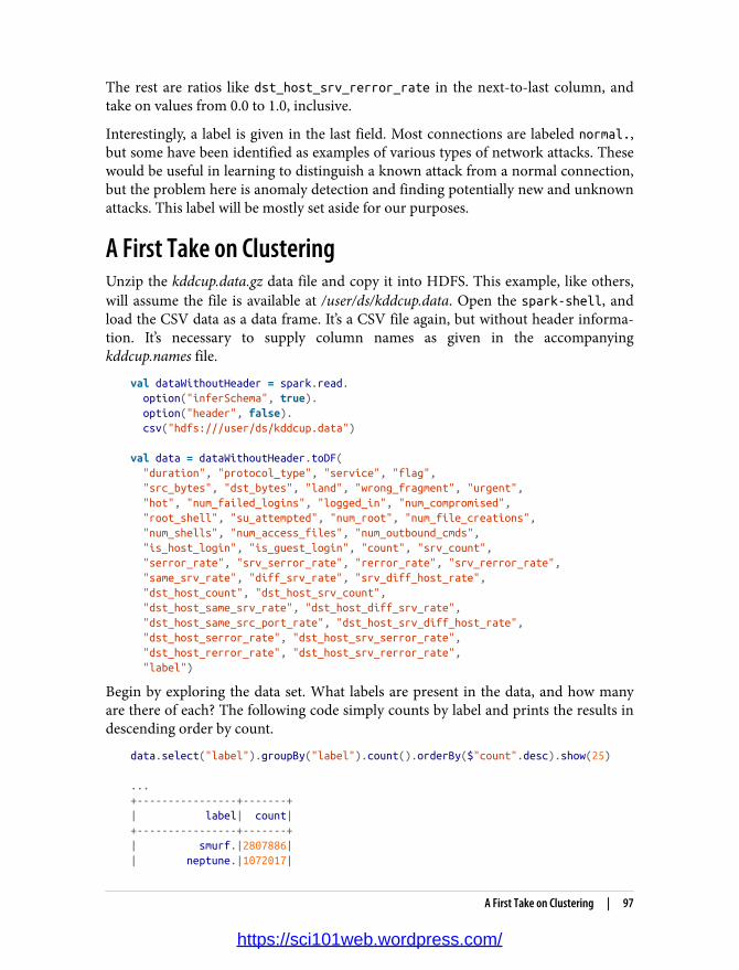
The rest are ratios like dst_host_srv_rerror_rate in the next-to-last column, andtake on values from 0.0 to 1.0, inclusive.

Interestingly, a label is given in the last field. Most connections are labeled normal.,but some have been identified as examples of various types of network attacks. Thesewould be useful in learning to distinguish a known attack from a normal connection,but the problem here is anomaly detection and finding potentially new and unknownattacks. This label will be mostly set aside for our purposes.

A First Take on ClusteringUnzip the kddcup.data.gz data file and copy it into HDFS. This example, like others,will assume the file is available at /user/ds/kddcup.data. Open the spark-shell, andload the CSV data as a data frame. It’s a CSV file again, but without header informa‐tion. It’s necessary to supply column names as given in the accompanyingkddcup.names file.

val dataWithoutHeader = spark.read. option("inferSchema", true). option("header", false). csv("hdfs:///user/ds/kddcup.data")

val data = dataWithoutHeader.toDF( "duration", "protocol_type", "service", "flag", "src_bytes", "dst_bytes", "land", "wrong_fragment", "urgent", "hot", "num_failed_logins", "logged_in", "num_compromised", "root_shell", "su_attempted", "num_root", "num_file_creations", "num_shells", "num_access_files", "num_outbound_cmds", "is_host_login", "is_guest_login", "count", "srv_count", "serror_rate", "srv_serror_rate", "rerror_rate", "srv_rerror_rate", "same_srv_rate", "diff_srv_rate", "srv_diff_host_rate", "dst_host_count", "dst_host_srv_count", "dst_host_same_srv_rate", "dst_host_diff_srv_rate", "dst_host_same_src_port_rate", "dst_host_srv_diff_host_rate", "dst_host_serror_rate", "dst_host_srv_serror_rate", "dst_host_rerror_rate", "dst_host_srv_rerror_rate", "label")

Begin by exploring the data set. What labels are present in the data, and how manyare there of each? The following code simply counts by label and prints the results indescending order by count.

data.select("label").groupBy("label").count().orderBy($"count".desc).show(25)

...+----------------+-------+| label| count|+----------------+-------+| smurf.|2807886|| neptune.|1072017|

A First Take on Clustering | 97


| normal.| 972781|| satan.| 15892|...| phf.| 4|| perl.| 3|| spy.| 2|+----------------+-------+

There are 23 distinct labels, and the most frequent are smurf. and neptune. attacks.

Note that the data contains nonnumeric features. For example, the second columnmay be tcp, udp, or icmp, but K-means clustering requires numeric features. The finallabel column is also nonnumeric. To begin, these will simply be ignored.

Aside from this, creating a K-means clustering of the data follows the same pattern aswas seen in Chapter 4. A VectorAssembler creates a feature vector, a KMeans imple‐mentation creates a model from the feature vectors, and a Pipeline stitches it alltogether. From the resulting model, it’s possible to extract and examine the clustercenters.

import org.apache.spark.ml.Pipelineimport org.apache.spark.ml.clustering.{KMeans, KMeansModel}import org.apache.spark.ml.feature.VectorAssembler

val numericOnly = data.drop("protocol_type", "service", "flag").cache()

val assembler = new VectorAssembler(). setInputCols(numericOnly.columns.filter(_ != "label")). setOutputCol("featureVector")

val kmeans = new KMeans(). setPredictionCol("cluster"). setFeaturesCol("featureVector")

val pipeline = new Pipeline().setStages(Array(assembler, kmeans))val pipelineModel = pipeline.fit(numericOnly)val kmeansModel = pipelineModel.stages.last.asInstanceOf[KMeansModel]

kmeansModel.clusterCenters.foreach(println)

...[48.34019491959669,1834.6215497618625,826.2031900016945,793027561892E-4,...[10999.0,0.0,1.309937401E9,0.0,0.0,0.0,0.0,0.0,0.0,0.0,0.0,0.0,0.0,0.0,...

It’s not easy to interpret the numbers intuitively, but each of these represents the cen‐ter (also known as centroid) of one of the clusters that the model produced. The val‐ues are the coordinates of the centroid in terms of each of the numeric input features.

Two vectors are printed, meaning K-means was fitting k=2 clusters to the data. For acomplex data set that is known to exhibit at least 23 distinct types of connections, this



is almost certainly not enough to accurately model the distinct groupings within thedata.

This is a good opportunity to use the given labels to get an intuitive sense of whatwent into these two clusters by counting the labels within each cluster.

val withCluster = pipelineModel.transform(numericOnly)

withCluster.select("cluster", "label"). groupBy("cluster", "label").count(). orderBy($"cluster", $"count".desc). show(25)

...+-------+----------------+-------+|cluster| label| count|+-------+----------------+-------+| 0| smurf.|2807886|| 0| neptune.|1072017|| 0| normal.| 972781|| 0| satan.| 15892|| 0| ipsweep.| 12481|...| 0| phf.| 4|| 0| perl.| 3|| 0| spy.| 2|| 1| portsweep.| 1|+-------+----------------+-------+

The result shows that the clustering was not at all helpful. Only one data point endedup in cluster 1!

Choosing kTwo clusters are plainly insufficient. How many clusters are appropriate for this dataset? It’s clear that there are 23 distinct patterns in the data, so it seems that k could beat least 23, or likely even more. Typically, many values of k are tried to find the bestone. But what is “best”?

A clustering could be considered good if each data point were near its closest cent‐roid, where “near” is defined by the Euclidean distance. This is a simple, commonway to evaluate the quality of a clustering, by the mean of these distances over allpoints, or sometimes, the mean of the distances squared. In fact, KMeansModel offers acomputeCost method that computes the sum of squared distances and can easily beused to compute the mean squared distance.

Unfortunately, there is no simple Evaluator implementation to compute this meas‐ure, not like those available to compute multiclass classification metrics. It’s simple

Choosing k | 99


enough to manually evaluate the clustering cost for several values of k. Note that thiscode could take 10 minutes or more to run.

import org.apache.spark.sql.DataFrame

def clusteringScore0(data: DataFrame, k: Int): Double = { val assembler = new VectorAssembler(). setInputCols(data.columns.filter(_ != "label")). setOutputCol("featureVector") val kmeans = new KMeans(). setSeed(Random.nextLong()). setK(k). setPredictionCol("cluster"). setFeaturesCol("featureVector") val pipeline = new Pipeline().setStages(Array(assembler, kmeans)) val kmeansModel = pipeline.fit(data).stages.last.asInstanceOf[KMeansModel] kmeansModel.computeCost(assembler.transform(data)) / data.count() }

(20 to 100 by 20).map(k => (k, clusteringScore0(numericOnly, k))). foreach(println)

...(20,6.649218115128446E7)(40,2.5031424366033625E7)(60,1.027261913057096E7)(80,1.2514131711109027E7)(100,7235531.565096531)

Compute mean from total squared distance (“cost”)

The (x to y by z) syntax is a Scala idiom for creating a collection of numbersbetween a start and end (inclusive), with a given difference between successive ele‐ments. This is a compact way to create the values “20, 40, …, 100” for k, and then dosomething with each.

The printed result shows that the score decreases as k increases. Note that scores areshown in scientific notation; the first value is over 107, not just a bit over 6.

Again, your values will be somewhat different. The clusteringdepends on a randomly chosen initial set of centroids.

However, this much is obvious. As more clusters are added, it should always be possi‐ble to put data points closer to the nearest centroid. In fact, if k is chosen to equal thenumber of data points, the average distance will be 0 because every point will be itsown cluster of one!



Worse, in the preceding results, the distance for k=80 is higher than for k=60. Thisshouldn’t happen because higher k always permits at least as good a clustering as alower k. The problem is that K-means is not necessarily able to find the optimal clus‐tering for a given k. Its iterative process can converge from a random starting point toa local minimum, which may be good but is not optimal.

This is still true even when more intelligent methods are used to choose initial cent‐roids. K-means++ and K-means|| are variants of selection algorithms that are morelikely to choose diverse, separated centroids and lead more reliably to a good cluster‐ing. Spark MLlib, in fact, implements K-means||. However, all still have an element ofrandomness in selection and can’t guarantee an optimal clustering.

The random starting set of clusters chosen for k=80 perhaps led to a particularly sub‐optimal clustering, or it may have stopped early before it reached its local optimum.

We can improve it by running the iteration longer. The algorithm has a threshold viasetTol() that controls the minimum amount of cluster centroid movement consid‐ered significant; lower values mean the K-means algorithm will let the centroids con‐tinue to move longer. Increasing the maximum number of iterations withsetMaxIter() also prevents it from potentially stopping too early at the cost of possi‐bly more computation.

def clusteringScore1(data: DataFrame, k: Int): Double = { ... setMaxIter(40). setTol(1.0e-5) ...}


Increase from default 20

Decrease from default 1.0e-4

This time, at least the scores decrease consistently:

(20,1.8041795813813403E8)(40,6.33056876207124E7)(60,9474961.544965891)(80,9388117.93747141)(100,8783628.926311461)

We want to find a point past which increasing k stops reducing the score much—oran “elbow” in a graph of k versus score, which is generally decreasing but eventuallyflattens out. Here, it seems to be decreasing notably past 100. The right value of k maybe past 100.

Choosing k | 101


https://stanford.io/1ALCOaN

Visualization with SparkRAt this point, it could be useful to step back and understand more about the databefore clustering again. In particular, looking at a plot of the data points could behelpful.

Spark itself has no tools for visualization, but the popular open source statistical envi‐ronment R has libraries for both data exploration and data visualization. Further‐more, Spark also provides some basic integration with R via SparkR. This briefsection will demonstrate using R and SparkR to cluster the data and explore the clus‐tering.

SparkR is a variant of the spark-shell used throughout this book, and is invokedwith the command sparkR. It runs a local R interpreter, like spark-shell runs a var‐iant of the Scala shell as a local process. The machine that runs sparkR needs a localinstallation of R, which is not included with Spark. This can be installed, for example,with sudo apt-get install r-base on Linux distributions like Ubuntu, or brewinstall R with Homebrew on macOS.

sparkR is a command-line shell environment, like R. To view visualizations, it’s neces‐sary to run these commands within an IDE-like environment that can display images.RStudio is an IDE for R (and works with SparkR); it runs on a desktop operating sys‐tem so it will only be usable here if you are experimenting with Spark locally ratherthan on a cluster.

If you are running Spark locally, download the free version of RStudio and install it. Ifnot, then most of the rest of this example can still be run with sparkR on a commandline; for example, on a cluster. It won’t be possible to display visualizations this waythough.

If running via RStudio, launch the IDE and configure SPARK_HOME and JAVA_HOME, ifyour local environment does not already set them, to point to the Spark and JDKinstallation directories, respectively.

Sys.setenv(SPARK_HOME = "/path/to/spark") Sys.setenv(JAVA_HOME = "/path/to/java")library(SparkR, lib.loc = c(file.path(Sys.getenv("SPARK_HOME"), "R", "lib")))sparkR.session(master = "local[*]", sparkConfig = list(spark.driver.memory = "4g"))

Replace with actual paths, of course.

Note that these steps aren’t needed if you are running sparkR on the command line.Instead, it accepts command-line configuration parameters like --driver-memory,just like spark-shell.



https://www.r-project.org

https://spark.apache.org/docs/latest/sparkr.html

http://brew.sh/

https://www.rstudio.com

http://bit.ly/2qdhxHy

SparkR is an R-language wrapper around the same DataFrame and MLlib APIs thathave been demonstrated in this chapter. It’s therefore possible to recreate a K-meanssimple clustering of the data:

clusters_data <- read.df("/path/to/kddcup.data", "csv", inferSchema = "true", header = "false")colnames(clusters_data) <- c( "duration", "protocol_type", "service", "flag", "src_bytes", "dst_bytes", "land", "wrong_fragment", "urgent", "hot", "num_failed_logins", "logged_in", "num_compromised", "root_shell", "su_attempted", "num_root", "num_file_creations", "num_shells", "num_access_files", "num_outbound_cmds", "is_host_login", "is_guest_login", "count", "srv_count", "serror_rate", "srv_serror_rate", "rerror_rate", "srv_rerror_rate", "same_srv_rate", "diff_srv_rate", "srv_diff_host_rate", "dst_host_count", "dst_host_srv_count", "dst_host_same_srv_rate", "dst_host_diff_srv_rate", "dst_host_same_src_port_rate", "dst_host_srv_diff_host_rate", "dst_host_serror_rate", "dst_host_srv_serror_rate", "dst_host_rerror_rate", "dst_host_srv_rerror_rate", "label")

numeric_only <- cache(drop(clusters_data, c("protocol_type", "service", "flag", "label")))

kmeans_model <- spark.kmeans(numeric_only, ~ ., k = 100, maxIter = 40, initMode = "k-means||")

Replace with path to kddcup.data.

Name columns.

Drop nonnumeric columns again.

~ . means all columns.

From here, it’s straightforward to assign a cluster to each data point. The operationsabove show usage of the SparkR APIs, which naturally correspond to core Spark APIsbut are expressed as R libraries in R-like syntax. The actual clustering is executedusing the same JVM-based, Scala-language implementation in MLlib. These opera‐tions are effectively a handle or remote control to distributed operations that are notexecuting in R.

R has its own rich set of libraries for analysis, and its own similar concept of a dataframe. It is sometimes useful, therefore, to pull some data down into the R interpreterin order to be able to use these native R libraries, which are unrelated to Spark.

Of course, R and its libraries are not distributed, and so it’s not feasible to pull thewhole data set of 4,898,431 data points into R. However, it’s easy to pull only a sample:

Visualization with SparkR | 103


clustering <- predict(kmeans_model, numeric_only)clustering_sample <- collect(sample(clustering, FALSE, 0.01))

str(clustering_sample)

...'data.frame': 48984 obs. of 39 variables: $ duration : int 0 0 0 0 0 0 0 0 0 0 ... $ src_bytes : int 181 185 162 254 282 310 212 214 181 ... $ dst_bytes : int 5450 9020 4528 849 424 1981 2917 3404 ... $ land : int 0 0 0 0 0 0 0 0 0 0 ...... $ prediction : int 33 33 33 0 0 0 0 0 33 33 ...

1% sample without replacement

clustering_sample is actually a local R data frame, not a Spark DataFrame, so it canbe manipulated like any other data in R. Above, str() shows the structure of the dataframe.

For example, it’s possible to extract the cluster assignment and then show statisticsabout the distribution of assignments:

clusters <- clustering_sample["prediction"] data <- data.matrix(within(clustering_sample, rm("prediction")))

table(clusters)

...clusters 0 11 14 18 23 25 28 30 31 33 36 ...47294 3 1 2 2 308 105 1 27 1219 15 ...

Only the clustering assignment column

Everything but the clustering assignment

For example, this shows that most points fell into cluster 0. Although much morecould be done with this data in R, further coverage of this is beyond the scope of thisbook.

To visualize the data, a library called rgl is required. It will only be functional if run‐ning this example in RStudio. First, install (once) and load the library:

install.packages("rgl")library(rgl)

Note that R may prompt you to download other packages or compiler tools to com‐plete installation, because installing the package means compiling its source code.



This data set is 38-dimensional. It will have to be projected down into at most threedimensions in order to visualize it with a random projection:

random_projection <- matrix(data = rnorm(3*ncol(data)), ncol = 3) random_projection_norm <- random_projection / sqrt(rowSums(random_projection*random_projection))

projected_data <- data.frame(data %*% random_projection_norm)

Make a random 3D projection and normalize

Project and make a new data frame

This creates a 3D data set out of a 38D data set by choosing three random unit vectorsand projecting the data onto them. This is a simplistic, rough-and-ready form ofdimension reduction. Of course, there are more sophisticated dimension reductionalgorithms, like principal component analysis (PCA) or the singular value decompo‐sition (SVD). These are available in R but take much longer to run. For purposes ofvisualization in this example, a random projection achieves much the same result,faster.

Finally, the clustered points can be plotted in an interactive 3D visualization:

num_clusters <- max(clusters)palette <- rainbow(num_clusters)colors = sapply(clusters, function(c) palette[c])plot3d(projected_data, col = colors, size = 10)

Note that this will require running RStudio in an environment that supports the rgllibrary and graphics. For example, on macOS, it requires that X11 from Apple’sDeveloper Tools be installed.

The resulting visualization in Figure 5-1 shows data points in 3D space. Many pointsfall on top of one another, and the result is sparse and hard to interpret. However, thedominant feature of the visualization is its L shape. The points seem to vary along twodistinct dimensions, and little in other dimensions.

This makes sense because the data set has two features that are on a much larger scalethan the others. Whereas most features have values between 0 and 1, the bytes-sentand bytes-received features vary from 0 to tens of thousands. The Euclidean distancebetween points is therefore almost completely determined by these two features. It’salmost as if the other features don’t exist! So it’s important to normalize away thesedifferences in scale to put features on near-equal footing.

Visualization with SparkR | 105


https://en.wikipedia.org/wiki/Principal_component_analysis

https://en.wikipedia.org/wiki/Singular_value_decomposition

https://en.wikipedia.org/wiki/Singular_value_decomposition

Feature NormalizationWe can normalize each feature by converting it to a standard score. This means sub‐tracting the mean of the feature’s values from each value, and dividing by the stan‐dard deviation, as shown in the standard score equation:

normalizedi =f eaturei − μi

σi

Figure 5-1. Random 3D projection

In fact, subtracting means has no effect on the clustering because the subtractioneffectively shifts all the data points by the same amount in the same directions. Thisdoes not affect interpoint Euclidean distances.

MLlib provides StandardScaler, a component that can perform this kind of stand‐ardization and be easily added to the clustering pipeline.



https://en.wikipedia.org/wiki/Standard_score

We can run the same test with normalized data on a higher range of k:

import org.apache.spark.ml.feature.StandardScaler

def clusteringScore2(data: DataFrame, k: Int): Double = { val assembler = new VectorAssembler(). setInputCols(data.columns.filter(_ != "label")). setOutputCol("featureVector") val scaler = new StandardScaler() .setInputCol("featureVector") .setOutputCol("scaledFeatureVector") .setWithStd(true) .setWithMean(false) val kmeans = new KMeans(). setSeed(Random.nextLong()). setK(k). setPredictionCol("cluster"). setFeaturesCol("scaledFeatureVector"). setMaxIter(40). setTol(1.0e-5) val pipeline = new Pipeline().setStages(Array(assembler, scaler, kmeans)) val pipelineModel = pipeline.fit(data) val kmeansModel = pipelineModel.stages.last.asInstanceOf[KMeansModel] kmeansModel.computeCost(pipelineModel.transform(data)) / data.count()}


This has helped put dimensions on more equal footing, and the absolute distancesbetween points (and thus the cost) is much smaller in absolute terms. However, thereisn’t yet an obvious value of k beyond which increasing it does little to improve thecost:

(60,1.2454250178069293)(90,0.7767730051608682)(120,0.5070473497003614)(150,0.4077081720067704)(180,0.3344486714980788)(210,0.276237617334138)(240,0.24571877339169032)(270,0.21818167354866858)

Another 3D visualization of the normalized data points reveals a richer structure, asexpected. Some points are spaced in regular, discrete intervals in a direction; these arelikely projections of discrete dimensions in the data, like counts. With 100 clusters,it’s hard to make out which points come from which clusters. One large cluster seemsto dominate, and many clusters correspond to small compact subregions (some ofwhich are omitted from this zoomed detail of the entire 3D visualization). The result,shown in Figure 5-2, does not necessarily advance the analysis but is an interestingsanity check.

Feature Normalization | 107


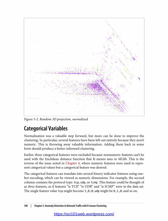
Figure 5-2. Random 3D projection, normalized

Categorical VariablesNormalization was a valuable step forward, but more can be done to improve theclustering. In particular, several features have been left out entirely because they aren’tnumeric. This is throwing away valuable information. Adding them back in someform should produce a better-informed clustering.

Earlier, three categorical features were excluded because nonnumeric features can’t beused with the Euclidean distance function that K-means uses in MLlib. This is thereverse of the issue noted in Chapter 4, where numeric features were used to repre‐sent categorical values but a categorical feature was desired.

The categorical features can translate into several binary indicator features using one-hot encoding, which can be viewed as numeric dimensions. For example, the secondcolumn contains the protocol type: tcp, udp, or icmp. This feature could be thought ofas three features, as if features “is TCP,” “is UDP,” and “is ICMP” were in the data set.The single feature value tcp might become 1,0,0; udp might be 0,1,0; and so on.



Here again, MLlib provides components that implement this transformation. In fact,one-hot-encoding string-valued features like protocol_type is actually a two-stepprocess. First, the string values are converted to integer indices like 0, 1, 2, and so onusing StringIndexer. Then these integer indices are encoded into a vector with OneHotEncoder. These two steps can be thought of as a small Pipeline in themselves.

import org.apache.spark.ml.feature.{OneHotEncoder, StringIndexer}

def oneHotPipeline(inputCol: String): (Pipeline, String) = { val indexer = new StringIndexer(). setInputCol(inputCol). setOutputCol(inputCol + "_indexed") val encoder = new OneHotEncoder(). setInputCol(inputCol + "_indexed"). setOutputCol(inputCol + "_vec") val pipeline = new Pipeline().setStages(Array(indexer, encoder)) (pipeline, inputCol + "_vec") }

Return Pipeline and name of output vector column

This method produces a Pipeline that can be added as a component in the overallclustering pipeline; pipelines can be composed. All that is left is to make sure to addthe new vector output columns into VectorAssembler’s output and proceed as beforewith scaling, clustering, and evaluation. The source code is omitted for brevity here,but can be found in the repository accompanying this chapter.

(60,39.739250062068685)(90,15.814341529964691)(120,3.5008631362395413)(150,2.2151974068685547)(180,1.587330730808905)(210,1.3626704802348888)(240,1.1202477806210747)(270,0.9263659836264369)

These sample results suggest, possibly, k=180 as a value where the score flattens out abit. At least the clustering is now using all input features.

Using Labels with EntropyEarlier, we used the given label for each data point to create a quick sanity check ofthe quality of the clustering. This notion can be formalized further and used as analternative means of evaluating clustering quality, and therefore, of choosing k.

The labels tell us something about the true nature of each data point. A good cluster‐ing, it seems, should agree with these human-applied labels. It should put togetherpoints that share a label frequently and not lump together points of many differentlabels. It should produce clusters with relatively homogeneous labels.

Using Labels with Entropy | 109


You may recall from Chapter 4 that we have metrics for homogeneity: Gini impurityand entropy. These are functions of the proportions of labels in each cluster, and pro‐duce a number that is low when the proportions are skewed toward few, or one, label.Entropy will be used here for illustration.

def entropy(counts: Iterable[Int]): Double = { val values = counts.filter(_ > 0) val n = values.map(_.toDouble).sum values.map { v => val p = v / n -p * math.log(p) }.sum}

A good clustering would have clusters whose collections of labels are homogeneousand so have low entropy. A weighted average of entropy can therefore be used as acluster score:

val clusterLabel = pipelineModel.transform(data). select("cluster", "label").as[(Int, String)]

val weightedClusterEntropy = clusterLabel. groupByKey { case (cluster, _) => cluster }. mapGroups { case (_, clusterLabels) => val labels = clusterLabels.map { case (_, label) => label }.toSeq val labelCounts = labels.groupBy(identity).values.map(_.size) labels.size * entropy(labelCounts) }.collect()

weightedClusterEntropy.sum / data.count()

Predict cluster for each datum

Extract collections of labels, per cluster

Count labels in collections

Average entropy weighted by cluster size

As before, this analysis can be used to obtain some idea of a suitable value of k.Entropy will not necessarily decrease as k increases, so it is possible to look for a localminimum value. Here again, results suggest k=180 is a reasonable choice because itsscore is actually lower than 150 and 210:

(60,0.03475331900669869)(90,0.051512668026335535)(120,0.02020028911919293)(150,0.019962563512905682)(180,0.01110240886325257)(210,0.01259738444250231)



(240,0.01357435960663116)(270,0.010119881917660544)

Clustering in ActionFinally, with confidence, we can cluster the full normalized data set with k=180.Again, we can print the labels for each cluster to get some sense of the resulting clus‐tering. Clusters do seem to be dominated by one type of attack each, and contain onlya few types.

val pipelineModel = fitPipeline4(data, 180) val countByClusterLabel = pipelineModel.transform(data). select("cluster", "label"). groupBy("cluster", "label").count(). orderBy("cluster", "label")countByClusterLabel.show()

...+-------+----------+------+|cluster| label| count|+-------+----------+------+| 0| back.| 324|| 0| normal.| 42921|| 1| neptune.| 1039|| 1|portsweep.| 9|| 1| satan.| 2|| 2| neptune.|365375|| 2|portsweep.| 141|| 3|portsweep.| 2|| 3| satan.| 10627|| 4| neptune.| 1033|| 4|portsweep.| 6|| 4| satan.| 1|...

See accompanying source code for fitPipeline4() definition

Now we can make an actual anomaly detector. Anomaly detection amounts to meas‐uring a new data point’s distance to its nearest centroid. If this distance exceeds somethreshold, it is anomalous. This threshold might be chosen to be the distance of, say,the 100th-farthest data point from among known data:

import org.apache.spark.ml.linalg.{Vector, Vectors}

val kMeansModel = pipelineModel.stages.last.asInstanceOf[KMeansModel]val centroids = kMeansModel.clusterCenters

val clustered = pipelineModel.transform(data)val threshold = clustered. select("cluster", "scaledFeatureVector").as[(Int, Vector)].

Clustering in Action | 111


map { case (cluster, vec) => Vectors.sqdist(centroids(cluster), vec) }. orderBy($"value".desc).take(100).last

Single output implicitly named “value”

The final step is to apply this threshold to all new data points as they arrive. Forexample, Spark Streaming can be used to apply this function to small batches of inputdata arriving from sources like Flume, Kafka, or files on HDFS. Data points exceed‐ing the threshold might trigger an alert that sends an email or updates a database.

As an example, we will apply it to the original data set, to see some of the data pointsthat are, we might believe, most anomalous within the input.

val originalCols = data.columnsval anomalies = clustered.filter { row => val cluster = row.getAs[Int]("cluster") val vec = row.getAs[Vector]("scaledFeatureVector") Vectors.sqdist(centroids(cluster), vec) >= threshold}.select(originalCols.head, originalCols.tail:_*)

anomalies.first()

...[9,tcp,telnet,SF,307,2374,0,0,1,0,0,1,0,1,0,1,3,1,0,0,0,0,1,1, 0.0,0.0,0.0,0.0,1.0,0.0,0.0,69,4,0.03,0.04,0.01,0.75,0.0,0.0, 0.0,0.0,normal.]

Note odd (String, String*) signature for selecting columns

show() works; hard to read

This example shows a slightly different way of operating on data frames. Pure SQLcan’t express the computation of squared distance. A UDF could be used, as before, todefine a function of two columns that returns a squared distance. However, it’s alsopossible to interact with rows of data programmatically as a Row object, much like inJDBC.

A network security expert would be more able to interpret why this is or is notactually a strange connection. It appears unusual at least because it is labeled normal,but involves connections to 69 different hosts.

Where to Go from HereThe KMeansModel is, by itself, the essence of an anomaly detection system. The pre‐ceding code demonstrated how to apply it to data to detect anomalies. This samecode could be used within Spark Streaming to score new data as it arrives in near realtime, and perhaps trigger an alert or review.



https://spark.apache.org/streaming/

MLlib also includes a variation called StreamingKMeans, which can update a cluster‐ing incrementally as new data arrives in a StreamingKMeansModel. We could use thisto continue to learn, approximately, how new data affects the clustering, and not justto assess new data against existing clusters. It can be integrated with Spark Streamingas well. However, it has not been updated for the new DataFrame-based APIs.

This model is only a simplistic one. For example, Euclidean distance is used in thisexample because it is the only distance function supported by Spark MLlib at thistime. In the future, it may be possible to use distance functions that can betteraccount for the distributions of and correlations between features, such as the Maha‐lanobis distance.

There are also more sophisticated cluster-quality evaluation metrics that could beapplied (even without labels) to pick k, such as the Silhouette coefficient. These tendto evaluate not just closeness of points within one cluster, but closeness of points toother clusters. Finally, different models could be applied instead of simple K-meansclustering; for example, a Gaussian mixture model or DBSCAN could capture moresubtle relationships between data points and the cluster centers. Spark MLlib alreadyimplements Gaussian mixture models; implementations of others may become avail‐able in Spark MLlib or other Spark-based libraries in the future.

Of course, clustering isn’t just for anomaly detection. In fact, it’s more often associ‐ated with use cases where the actual clusters matter! For example, clustering can alsobe used to group customers according to their behaviors, preferences, and attributes.Each cluster, by itself, might represent a usefully distinguishable type of customer.This is a more data-driven way to segment customers rather than leaning on arbi‐trary, generic divisions like “age 20–34” and “female.”



http://bit.ly/2qYLZbx

http://bit.ly/2qYLZbx

http://bit.ly/2qYQlzf

http://bit.ly/2qYQkLH

https://bit.ly/1GzKhLJ

https://bit.ly/1GzKCOG

http://bit.ly/2qYwxMu

CHAPTER 6

Understanding Wikipedia with LatentSemantic Analysis

Sandy Ryza

Where are the Snowdens of yesteryear?—Capt. Yossarian

Most of the work in data engineering consists of assembling data into some sort ofqueryable format. We can query structured data with formal languages. For example,when this structured data is tabular, we can use SQL. While it is by no means an easytask in practice, at a high level, the work of making tabular data accessible is oftenstraightforward—pull data from a variety of data sources into a single table, perhapscleansing or fusing intelligently along the way. Unstructured text data presents awhole different set of challenges. The process of preparing data into a format thathumans can interact with is not so much “assembly,” but rather “indexing” in the nicecase or “coercion” when things get ugly. A standard search index permits fast queriesfor the set of documents that contains a given set of terms. Sometimes, however, wewant to find documents that relate to the concepts surrounding a particular word evenif the documents do not contain that exact string. Standard search indexes often failto capture the latent structure in the text’s subject matter.

Latent semantic analysis (LSA) is a technique in natural language processing andinformation retrieval that seeks to better understand a corpus of documents and therelationships between the words in those documents. It attempts to distill the corpusinto a set of relevant concepts. Each concept captures a thread of variation in the dataand often corresponds to a topic that the corpus discusses. Without yet delving intothe mathematics, each concept consists of three attributes: a level of affinity for eachdocument in the corpus, a level of affinity for each term in the corpus, and an impor‐tance score reflecting how useful the concept is in describing variance in the data set.For example, LSA might discover a concept with high affinity for the terms “Asimov”

115


and “robot,” and high affinity for the documents “foundation series” and “science fic‐tion.” By selecting only the most important concepts, LSA can throw away some irrel‐evant noise and merge co-occurring strands to come up with a simpler representationof the data.

We can employ this concise representation in a variety of tasks. It can provide scoresof similarity between terms and other terms, between documents and other docu‐ments, and between terms and documents. By encapsulating the patterns of variancein the corpus, it can base scores on a deeper understanding than simply on countingoccurrences and co-occurrences of words. These similarity measures are ideal fortasks such as finding the set of documents relevant to query terms, grouping docu‐ments into topics, and finding related words.

LSA discovers this lower-dimensional representation using a linear algebra techniquecalled SVD. SVD can be thought of as a more powerful version of the ALS factoriza‐tion described in Chapter 3. It starts with a document-term matrix generated throughcounting word frequencies for each document. In this matrix, each document corre‐sponds to a column, each term corresponds to a row, and each element represents theimportance of a word to a document. SVD then factorizes this matrix into threematrices, one of which expresses concepts in regard to documents, one of whichexpresses concepts in regard to terms, and one of which contains the importance foreach concept. The structure of these matrices can achieve a low-rank approximationof the original matrix by removing a set of rows and columns corresponding to theleast important concepts. That is, the matrices in this low-rank approximation can bemultiplied to produce a matrix close to the original, with increasing loss of fidelity aseach concept is removed.

In this chapter, we’ll embark upon the modest task of enabling queries against the fullextent of human knowledge based on its latent semantic relationships. More specifi‐cally, we’ll apply LSA to a corpus consisting of the full set of articles contained inWikipedia, which is about 46 GB of raw text. We’ll cover how to use Spark for prepro‐cessing the data: reading it, cleansing it, and coercing it into a numerical form. We’llshow how to compute the SVD and explain how to interpret and make use of it.

SVD has wide applications outside LSA. It appears in such diverse places as detectingclimatological trends (Michael Mann’s famous “hockey-stick” graph), face recogni‐tion, and image compression. Spark’s implementation can perform the matrix factori‐zation on enormous data sets, which opens up the technique to a whole new set ofapplications.

The Document-Term MatrixBefore performing any analysis, LSA requires transforming the raw text of the corpusinto a document-term matrix. In this matrix, each column represents a term that

116 | Chapter 6: Understanding Wikipedia with Latent Semantic Analysis


http://bit.ly/2qcHozy

occurs in the corpus, and each row represents a document. Loosely, the value at eachposition should correspond to the importance of the column’s term to the row’s docu‐ment. A few weighting schemes have been proposed, but by far the most common isterm frequency times inverse document frequency, or TF-IDF. Here’s a representationin Scala code of the formula. We won’t actually end up using this code because Sparkprovides its own implementation.

def termDocWeight(termFrequencyInDoc: Int, totalTermsInDoc: Int, termFreqInCorpus: Int, totalDocs: Int): Double = { val tf = termFrequencyInDoc.toDouble / totalTermsInDoc val docFreq = totalDocs.toDouble / termFreqInCorpus val idf = math.log(docFreq) tf * idf}

TF-IDF captures two intuitions about the relevance of a term to a document. First, wewould expect that the more often a term occurs in a document, the more important itis to that document. Second, not all terms are equal in a global sense. It is moremeaningful to encounter a word that occurs rarely in the entire corpus than a wordthat appears in most of the documents, thus the metric uses the inverse of the word’sappearance in documents in the full corpus.

The frequency of words in a corpus tends to be distributed exponentially. A commonword will often appear ten times as often as a mildly common word, which in turnmight appear ten or a hundred times as often as a rare word. Basing a metric on theraw inverse document frequency would give rare words enormous weight and practi‐cally ignore the impact of all other words. To capture this distribution, the schemeuses the log of the inverse document frequency. This mellows the differences in docu‐ment frequencies by transforming the multiplicative gaps between them into additivegaps.

The model relies on a few assumptions. It treats each document as a “bag of words,”meaning that it pays no attention to the ordering of words, sentence structure, ornegations. By representing each term once, the model has difficulty dealing with polysemy, the use of the same word for multiple meanings. For example, the modelcan’t distinguish between the use of “band” in “Radiohead is the best band ever” and“I broke a rubber band.” If both sentences appear often in the corpus, it may come toassociate “Radiohead” with “rubber.”

The corpus has 10 million documents. Counting obscure technical jargon, theEnglish language contains about a million terms, some subset in the tens of thou‐sands of which is likely useful for understanding the corpus. Because the corpus con‐tains far more documents than terms, it makes the most sense to generate thedocument-term matrix as a row matrix—a collection of sparse vectors—each corre‐sponding to a document.

The Document-Term Matrix | 117


Getting from the raw Wikipedia dump into this form requires a set of preprocessingsteps. First, the input consists of a single enormous XML file with documents delimi‐ted by <page> tags. This needs to be broken up to feed to the next step, turningWiki-formatting into plain text. The plain text is then split into tokens, which arereduced from their different inflectional forms to a root term through a processcalled lemmatization. These tokens can then be used to compute term and documentfrequencies. A final step ties these frequencies together and builds the actual vectorobjects. In the book repo, all the code for performing these steps is encapsulated inthe AssembleDocumentTermMatrix class.

The first steps can be performed for each document fully in parallel (which, in Spark,means as a set of map functions), but computing the inverse document frequenciesrequires aggregation across all the documents. A number of useful general NLP andWikipedia-specific extraction tools exist that can aid in these tasks.

Getting the DataWikipedia makes dumps of all its articles available. The full dump comes in a singlelarge XML file. These can be downloaded and then placed on HDFS. For example:

$ curl -s -L https://dumps.wikimedia.org/enwiki/latest/\$ enwiki-latest-pages-articles-multistream.xml.bz2 \$ | bzip2 -cd \$ | hadoop fs -put - wikidump.xml

This will take a little while.

Chugging through this volume of data makes the most sense with a cluster of a fewnodes to work with. To run this chapter’s code on a local machine, a better option isto generate a smaller dump using Wikipedia’s exports page. Try getting all the pagesfrom a category that has many pages and few subcategories, such as Megafauna orGeometry. For the following code to work, download the dump into the ch06-lsa/directory and rename it to wikidump.xml.

Parsing and Preparing the DataHere’s a snippet at the beginning of the dump:

<page> <title>Anarchism</title> <ns>0</ns> <id>12</id> <revision> <id>584215651</id> <parentid>584213644</parentid> <timestamp>2013-12-02T15:14:01Z</timestamp> <contributor> <username>AnomieBOT</username>



https://dumps.wikimedia.org/enwiki

https://en.wikipedia.org/wiki/Special:Export

<id>7611264</id> </contributor> <comment>Rescuing orphaned refs ("autogenerated1" from rev 584155010; "bbc" from rev 584155010)</comment> <text xml:space="preserve">{{Redirect|Anarchist|the fictional character| Anarchist (comics)}}{{Redirect|Anarchists}}{{pp-move-indef}}{{Anarchism sidebar}}

'''Anarchism''' is a [[political philosophy]] that advocates [[stateless society|stateless societies]] often defined as [[self-governance|self-governed]]voluntary institutions,<ref>"ANARCHISM, a social philosophy thatrejects authoritarian government and maintains that voluntary institutions arebest suited to express man's natural social tendencies." George Woodcock."Anarchism" at The Encyclopedia of Philosophy</ref><ref>"In a society developed on these lines, the voluntary associations whichalready now begin to cover all the fields of human activity would take a stillgreater extension so as to substitute...

Let’s fire up the Spark shell. In this chapter, we rely on several libraries to make ourlives easier. The GitHub repo contains a Maven project that can be used to build aJAR file that packages all these dependencies together:

$ cd ch06-lsa/$ mvn package$ spark-shell --jars target/ch06-lsa-2.0.0-jar-with-dependencies.jar

To start operating on this dump, we’ll need to strip out the formatting and get to thecontent. A good start would be to produce a data set of (title, document content)tuples that we can then run further processing on. The Cloud9 project provides a setof APIs that are really helpful for this.

Cloud9 provides a class, XMLInputFormat, derived from the Apache Mahout project,that can split up the enormous Wikipedia dump into documents. To create a data setwith it:

import edu.umd.cloud9.collection.XMLInputFormatimport org.apache.hadoop.conf.Configurationimport org.apache.hadoop.io._

val path = "wikidump.xml"@transient val conf = new Configuration()conf.set(XMLInputFormat.START_TAG_KEY, "<page>")conf.set(XMLInputFormat.END_TAG_KEY, "</page>")val kvs = spark.sparkContext.newAPIHadoopFile(path, classOf[XMLInputFormat], classOf[LongWritable], classOf[Text], conf)val rawXmls = kvs.map(_._2.toString).toDS()

Turning the Wiki XML into the plain text of article contents could require a chapterof its own, but luckily the Cloud9 project provides APIs that handle this entirely:

Parsing and Preparing the Data | 119


import edu.umd.cloud9.collection.wikipedia.language._import edu.umd.cloud9.collection.wikipedia._

def wikiXmlToPlainText(pageXml: String): Option[(String, String)] = { // Wikipedia has updated their dumps slightly since Cloud9 was written, // so this hacky replacement is sometimes required to get parsing to work. val hackedPageXml = pageXml.replaceFirst( "<text xml:space=\"preserve\" bytes=\"\\d+\">", "<text xml:space=\"preserve\">")

val page = new EnglishWikipediaPage() WikipediaPage.readPage(page, hackedPageXml) if (page.isEmpty) None else Some((page.getTitle, page.getContent))}

val docTexts = rawXmls.filter(_ != null).flatMap(wikiXmlToPlainText)

LemmatizationWith the plain text in hand, next we need to turn it into a bag of terms. This steprequires care for a couple of reasons. First, common words like “the” and “is” take upspace but at best offer no useful information to the model. Filtering out a list of stopwords can both save space and improve fidelity. Second, terms with the same meaningcan often take slightly different forms. For example, “monkey” and “monkeys” do notdeserve to be separate terms. Nor do “nationalize” and “nationalization.” Combiningthese different inflectional forms into single terms is called stemming or lemmatiza‐tion. Stemming refers to heuristics-based techniques for chopping off characters atthe ends of words, while lemmatization refers to more principled approaches. Forexample, the former might truncate “drew” to “dr,” while the latter might more cor‐rectly output “draw.” The Stanford Core NLP project provides an excellent lemma‐tizer with a Java API that Scala can take advantage of.

The following snippet takes the data set of plain-text documents and both lemmatizesit and filters out stop words. Note that this code relies on a file of stopwords calledstopwords.txt, which is available in the accompanying source code repo and should bedownloaded into the current working directory first:

import scala.collection.JavaConverters._import scala.collection.mutable.ArrayBufferimport edu.stanford.nlp.pipeline._import edu.stanford.nlp.ling.CoreAnnotations._import java.util.Propertiesimport org.apache.spark.sql.Dataset

def createNLPPipeline(): StanfordCoreNLP = { val props = new Properties() props.put("annotators", "tokenize, ssplit, pos, lemma") new StanfordCoreNLP(props)



http://bit.ly/2psi9Ms

}

def isOnlyLetters(str: String): Boolean = { str.forall(c => Character.isLetter(c))}

def plainTextToLemmas(text: String, stopWords: Set[String], pipeline: StanfordCoreNLP): Seq[String] = { val doc = new Annotation(text) pipeline.annotate(doc)

val lemmas = new ArrayBuffer[String]() val sentences = doc.get(classOf[SentencesAnnotation]) for (sentence <- sentences.asScala; token <- sentence.get(classOf[TokensAnnotation]).asScala) { val lemma = token.get(classOf[LemmaAnnotation]) if (lemma.length > 2 && !stopWords.contains(lemma) && isOnlyLetters(lemma)) { lemmas += lemma.toLowerCase } } lemmas}

val stopWords = scala.io.Source.fromFile("stopwords.txt").getLines().toSetval bStopWords = spark.sparkContext.broadcast(stopWords)

val terms: Dataset[(String, Seq[String])] = docTexts.mapPartitions { iter => val pipeline = createNLPPipeline() iter.map { case(title, contents) => (title, plainTextToLemmas(contents, bStopWords.value, pipeline)) } }

Specify some minimal requirements on lemmas to weed out garbage.

Broadcast the stop words to save on memory in the executors.

Use mapPartitions so that we only initialize the NLP pipeline object once perpartition instead of once per document.

Computing the TF-IDFsAt this point, terms refers to a data set of sequences of terms, each corresponding to adocument. The next step is to compute the frequencies for each term within eachdocument and for each term within the entire corpus. The spark.ml package containsEstimator and Transformer implementations for doing exactly this.

Computing the TF-IDFs | 121


To take advantage of them, first we’ll need to convert our data set into a data frame:

val termsDF = terms.toDF("title", "terms")

Let’s filter out all documents that have zero or one term:

val filtered = termsDF.where(size($"terms") > 1)

The CountVectorizer is an Estimator that can help compute the term frequenciesfor us. The CountVectorizer scans the data to build up a vocabulary, a mapping ofintegers to terms, encapsulated in the CountVectorizerModel, a Transformer. TheCountVectorizerModel can then be used to generate a term frequency Vector foreach document. The vector has a component for each term in the vocabulary, and thevalue for each component is the number of times the term appears in the document.Spark uses sparse vectors here, because documents typically only contain a small sub‐set of the full vocabulary.

import org.apache.spark.ml.feature.CountVectorizer

val numTerms = 20000val countVectorizer = new CountVectorizer(). setInputCol("terms").setOutputCol("termFreqs"). setVocabSize(numTerms)val vocabModel = countVectorizer.fit(filtered)val docTermFreqs = vocabModel.transform(filtered)

Notice the use of setVocabSize. The corpus contains millions of terms, but many arehighly specialized words that only appear in one or two documents. Filtering out lessfrequent terms can both improve performance and remove noise. When we set avocabulary size on the estimator, it leaves out all but the most frequent words.

The resulting DataFrame will be used at least twice after this point: to calculate theinverse document frequencies and the final document-term matrix. So caching it inmemory is a good idea:

docTermFreqs.cache()

With the document frequencies in hand, we can compute the inverse document fre‐quencies. For this, we use IDF, another Estimator, which counts the number of docu‐ments in which each term in the corpus appears and then uses these counts tocompute the IDF scaling factor for each term. The IDFModel that it yields can thenapply these scaling factors to each term in each vector in the data set.

import org.apache.spark.ml.feature.IDF

val idf = new IDF().setInputCol("termFreqs").setOutputCol("tfidfVec")val idfModel = idf.fit(docTermFreqs)val docTermMatrix = idfModel.transform(docTermFreqs).select("title", "tfidfVec")

As we descend from data frames into the world of vectors and matrices, we lose theability to key by strings. Thus, if we want to trace what we learn back to recognizable



entities, it’s important for us to save a mapping of positions in the matrix to the termsand document titles in our original corpus. Positions in the term vectors are equiva‐lent to columns in our document-term matrix. The mapping of these positions toterm strings is already saved in our CountVectorizerModel. We can access it with:

val termIds: Array[String] = vocabModel.vocabulary

Creating a mapping of row IDs to document titles is a little more difficult. To achieveit, we can use the zipWithUniqueId function, which associates a unique deterministicID with every row in the DataFrame. We rely on the fact that, if we call this functionon a transformed version of the DataFrame, it will assign the same unique IDs to thetransformed rows as long as the transformations don’t change the number of rows ortheir partitioning. Thus, we can trace the rows back to their IDs in the DataFrameand, consequently, the document titles that they correspond to:

val docIds = docTermFreqs.rdd.map(_.getString(0)). zipWithUniqueId(). map(_.swap). collect().toMap

Singular Value DecompositionWith the document-term matrix M in hand, the analysis can proceed to the factoriza‐tion and dimensionality reduction. MLlib contains an implementation of the SVDthat can handle enormous matrices. The singular value decomposition takes an m × nmatrix and returns three matrices that approximately equal it when multipliedtogether:

M ≈ U S VT

The matrices are:

• U is an m × k matrix whose columns form an orthonormal basis for the docu‐ment space.

• S is a k × k diagonal matrix, each of whose entries correspond to the strength ofone of the concepts.

• VT is a k × n matrix whose columns form an orthonormal basis for the termspace.

In the LSA case, m is the number of documents and n is the number of terms. Thedecomposition is parameterized with a number k, less than or equal to n, which indi‐cates how many concepts to keep around. When k=n, the product of the factor matri‐ces reconstitutes the original matrix exactly. When k<n, the multiplication results in alow-rank approximation of the original matrix. k is typically chosen to be muchsmaller than n. SVD ensures that the approximation will be the closest possible to the

Singular Value Decomposition | 123


original matrix (as defined by the L2 Norm—that is, the sum of squares—of the dif‐ference), given the constraint that it needs to be expressible in only k concepts.

At the time of this writing, the spark.ml package, which operates on DataFrames,does not include an implementation of SVD. However, the older spark.mllib, whichoperates on RDDs, does. This means that to compute the SVD of our document-termmatrix, we need to represent it as an RDD of vectors. On top of this, the spark.ml andspark.mllib packages each have their own Vector class. The spark.ml Transformerswe used earlier yield spark.ml vectors but the SVD implementation only acceptsspark.mllib vectors, so we need to perform a conversion. This is not the most elegantpiece of code, but it gets the job done:

import org.apache.spark.mllib.linalg.{Vectors, Vector => MLLibVector}import org.apache.spark.ml.linalg.{Vector => MLVector}

val vecRdd = docTermMatrix.select("tfidfVec").rdd.map { row => Vectors.fromML(row.getAs[MLVector]("tfidfVec"))}

To find the singular value decomposition, we simply wrap an RDD of row vectors in aRowMatrix and call computeSVD:

import org.apache.spark.mllib.linalg.distributed.RowMatrix

vecRdd.cache()val mat = new RowMatrix(vecRdd)val k = 1000val svd = mat.computeSVD(k, computeU=true)

The RDD should be cached in memory beforehand because the computation requiresmultiple passes over the data. The computation requires O(nk) storage on the driver,O(n) storage for each task, and O(k) passes over the data.

As a reminder, a vector in term space means a vector with a weight on every term, avector in document space means a vector with a weight on every document, and a vec‐tor in concept space means a vector with a weight on every concept. Each term, docu‐ment, or concept defines an axis in its respective space, and the weight ascribed to theterm, document, or concept means a length along that axis. Every term or documentvector can be mapped to a corresponding vector in concept space. Every concept vec‐tor has possibly many term and document vectors that map to it, including a canoni‐cal term and document vector that it maps to when transformed in the reversedirection.

V is an n × k matrix in which each row corresponds to a term and each column corre‐sponds to a concept. It defines a mapping between term space (the space where eachpoint is an n-dimensional vector holding a weight for each term) and concept space



(the space where each point is a k-dimensional vector holding a weight for eachconcept).

Similarly, U is an m × k matrix where each row corresponds to a document and eachcolumn corresponds to a concept. It defines a mapping between document space andconcept space.

S is a k × k diagonal matrix that holds the singular values. Each diagonal element in Scorresponds to a single concept (and thus a column in V and a column in U). Themagnitude of each of these singular values corresponds to the importance of thatconcept: its power in explaining the variance in the data. An (inefficient) implemen‐tation of SVD could find the rank-k decomposition by starting with the rank-ndecomposition and throwing away the n–k smallest singular values until there are kleft (along with their corresponding columns in U and V). A key insight of LSA is thatonly a small number of concepts is important to represent that data. The entries inthe S matrix directly indicate the importance of each concept. They also happen to bethe square roots of the eigenvalues of MMT.

Finding Important ConceptsSo SVD outputs a bunch of numbers. How can we inspect these to verify they actuallyrelate to anything useful? The V matrix represents concepts through the terms thatare important to them. As discussed earlier, V contains a column for every conceptand a row for every term. The value at each position can be interpreted as the rele‐vance of that term to that concept. This means that the most relevant terms to each ofthe top concepts can be found with something like this:

import org.apache.spark.mllib.linalg.{Matrix, SingularValueDecomposition}import org.apache.spark.mllib.linalg.distributed.RowMatrix

def topTermsInTopConcepts( svd: SingularValueDecomposition[RowMatrix, Matrix], numConcepts: Int, numTerms: Int, termIds: Array[String]) : Seq[Seq[(String, Double)]] = { val v = svd.V val topTerms = new ArrayBuffer[Seq[(String, Double)]]() val arr = v.toArray for (i <- 0 until numConcepts) { val offs = i * v.numRows val termWeights = arr.slice(offs, offs + v.numRows).zipWithIndex val sorted = termWeights.sortBy(-_._1) topTerms += sorted.take(numTerms).map { case (score, id) => (termIds(id), score) } }

Finding Important Concepts | 125


http://bit.ly/2qcP6d3

topTerms}

This last step finds the actual terms that correspond to the positions in the termvectors. Recall that termIds is the integer->term mapping we got from the CountVectorizer.

Note that V is a matrix in local memory in the driver process, and the computationoccurs in a nondistributed manner. We can find the documents relevant to each ofthe top concepts in a similar manner using U, but the code looks a little bit differentbecause U is stored as a distributed matrix:

def topDocsInTopConcepts( svd: SingularValueDecomposition[RowMatrix, Matrix], numConcepts: Int, numDocs: Int, docIds: Map[Long, String]) : Seq[Seq[(String, Double)]] = { val u = svd.U val topDocs = new ArrayBuffer[Seq[(String, Double)]]() for (i <- 0 until numConcepts) { val docWeights = u.rows.map(_.toArray(i)).zipWithUniqueId() topDocs += docWeights.top(numDocs).map { case (score, id) => (docIds(id), score) } } topDocs}

monotonically_increasing_id/zipWithUniqueId trick discussed in the previ‐ous section of the chapter. This allows us to maintain continuity between rows inthe matrix and rows in the DataFrame it is derived from, which also has the titles.

Let’s inspect the first few concepts:

val topConceptTerms = topTermsInTopConcepts(svd, 4, 10, termIds)val topConceptDocs = topDocsInTopConcepts(svd, 4, 10, docIds)for ((terms, docs) <- topConceptTerms.zip(topConceptDocs)) { println("Concept terms: " + terms.map(_._1).mkString(", ")) println("Concept docs: " + docs.map(_._1).mkString(", ")) println()}

Concept terms: summary, licensing, fur, logo, album, cover, rationale, gif, use, fairConcept docs: File:Gladys-in-grammarland-cover-1897.png, File:Gladys-in-grammarland-cover-2010.png, File:1942ukrpoljudeakt4.jpg, File:Σακελλαρίδης.jpg, File:Baghdad-texas.jpg, File:Realistic.jpeg, File:DuplicateBoy.jpg, File:Garbo-the-spy.jpg, File:Joysagar.jpg, File:RizalHighSchoollogo.jpg

Concept terms: disambiguation, william, james, john, iran, australis, township, charles, robert, river



Concept docs: G. australis (disambiguation), F. australis (disambiguation), U. australis (disambiguation), L. maritima (disambiguation), G. maritima (disambiguation), F. japonica (disambiguation), P. japonica (disambiguation), Velo (disambiguation), Silencio (disambiguation), TVT (disambiguation)

Concept terms: licensing, disambiguation, australis, maritima, rawal, upington, tallulah, chf, satyanarayana, valérieConcept docs: File:Rethymno.jpg, File:Ladycarolinelamb.jpg, File:KeyAirlines.jpg, File:NavyCivValor.gif, File:Vitushka.gif, File:DavidViscott.jpg, File:Bigbrother13cast.jpg, File:Rawal Lake1.JPG, File:Upington location.jpg, File:CHF SG Viewofaltar01.JPG

Concept terms: licensing, summarysource, summaryauthor, wikipedia, summarypicture, summaryfrom, summaryself, rawal, chf, upingtonConcept docs: File:Rethymno.jpg, File:Wristlock4.jpg, File:Meseanlol.jpg, File:Sarles.gif, File:SuzlonWinMills.JPG, File:Rawal Lake1.JPG, File:CHF SG Viewofaltar01.JPG, File:Upington location.jpg, File:Driftwood-cover.jpg, File:Tallulah gorge2.jpg

Concept terms: establishment, norway, country, england, spain, florida, chile, colorado, australia, russiaConcept docs: Category:1794 establishments in Norway, Category:1838 establishments in Norway, Category:1849 establishments in Norway, Category:1908 establishments in Norway, Category:1966 establishments in Norway, Category:1926 establishments in Norway, Category:1957 establishments in Norway, Template:EstcatCountry1stMillennium, Category:2012 establishments in Chile, Category:1893 establishments in Chile

The documents in the first concept appear to all be image files, and the terms appearto be related to image attributes and licensing. The second concept appears to be dis‐ambiguation pages. It seems that perhaps this dump is not restricted to the raw Wiki‐pedia articles and is cluttered by administrative pages as well as discussion pages.Inspecting the output of intermediate stages is useful for catching this kind of issueearly. Luckily, it appears that Cloud9 provides some functionality for filtering theseout. An updated version of the wikiXmlToPlainText method looks like the following:

def wikiXmlToPlainText(xml: String): Option[(String, String)] = { ... if (page.isEmpty || !page.isArticle || page.isRedirect || page.getTitle.contains("(disambiguation)")) { None } else { Some((page.getTitle, page.getContent)) }}

Finding Important Concepts | 127


Rerunning the pipeline on the filtered set of documents yields a much more reason‐able result:

Concept terms: disambiguation, highway, school, airport, high, refer, number, squadron, list, may, division, regiment, wisconsin, channel, countyConcept docs: Tri-State Highway (disambiguation), Ocean-to-Ocean Highway (disambiguation), Highway 61 (disambiguation), Tri-County Airport (disambiguation), Tri-Cities Airport (disambiguation), Mid-Continent Airport (disambiguation), 99 Squadron (disambiguation), 95th Squadron (disambiguation), 94 Squadron (disambiguation), 92 Squadron (disambiguation)

Concept terms: disambiguation, nihilistic, recklessness, sullen, annealing, negativity, initialization, recapitulation, streetwise, pde, pounce, revisionism, hyperspace, sidestep, bandwagonConcept docs: Nihilistic (disambiguation), Recklessness (disambiguation), Manjack (disambiguation), Wajid (disambiguation), Kopitar (disambiguation), Rocourt (disambiguation), QRG (disambiguation), Maimaicheng (disambiguation), Varen (disambiguation), Gvr (disambiguation)

Concept terms: department, commune, communes, insee, france, see, also, southwestern, oise, marne, moselle, manche, eure, aisne, isèreConcept docs: Communes in France, Saint-Mard, Meurthe-et-Moselle, Saint-Firmin, Meurthe-et-Moselle, Saint-Clément, Meurthe-et-Moselle, Saint-Sardos, Lot-et-Garonne, Saint-Urcisse, Lot-et-Garonne, Saint-Sernin, Lot-et-Garonne, Saint-Robert, Lot-et-Garonne, Saint-Léon, Lot-et-Garonne, Saint-Astier, Lot-et-Garonne

Concept terms: genus, species, moth, family, lepidoptera, beetle, bulbophyllum, snail, database, natural, find, geometridae, reference, museum, noctuidaeConcept docs: Chelonia (genus), Palea (genus), Argiope (genus), Sphingini, Cribrilinidae, Tahla (genus), Gigartinales, Parapodia (genus), Alpina (moth), Arycanda (moth)

Concept terms: province, district, municipality, census, rural, iran, romanize, population, infobox, azerbaijan, village, town, central, settlement, kermanConcept docs: New York State Senate elections, 2012, New York State Senate elections, 2008, New York State Senate elections, 2010, Alabama State House of Representatives elections, 2010, Albergaria-a-Velha, Municipalities of Italy, Municipality of Malmö, Delhi Municipality, Shanghai Municipality, Göteborg Municipality

Concept terms: genus, species, district, moth, family, province, iran, rural, romanize, census, village, population, lepidoptera, beetle, bulbophyllumConcept docs: Chelonia (genus), Palea (genus), Argiope (genus), Sphingini, Tahla (genus), Cribrilinidae, Gigartinales, Alpina (moth), Arycanda (moth), Arauco (moth)

Concept terms: protein, football, league, encode, gene, play, team, bear,



season, player, club, reading, human, footballer, cupConcept docs: Protein FAM186B, ARL6IP1, HIP1R, SGIP1, MTMR3, Gem-associated protein 6, Gem-associated protein 7, C2orf30, OS9 (gene), RP2 (gene)

The first two concepts remain ambiguous, but the rest appear to correspond to mean‐ingful categories. The third appears to be composed of locales in France, the fourthand sixth of animal and bug taxonomies. The fifth concerns elections, municipalities,and government. The articles in the seventh concern proteins, while some of theterms also reference football, perhaps with a crossover of fitness of performance-enhancing drugs? Even though unexpected words appear in each, all the conceptsexhibit some thematic coherence.

Querying and Scoring with a Low-DimensionalRepresentationHow relevant is a term to a document? How relevant are two terms to each other?Which documents most closely match a set of query terms? The original document-term matrix provides a shallow way to answer these questions. We can achieve a rele‐vance score between two terms by computing the cosine similarity between their twocolumn vectors in the matrix. Cosine similarity measures the angle between two vec‐tors. Vectors that point in the same direction in the high-dimensional documentspace are thought to be relevant to each other. This is computed as the dot product ofthe vectors divided by the product of their lengths.

Cosine similarity sees wide use as a similarity metric between vectors of term anddocument weights in natural language and information retrieval applications. Like‐wise, for two documents, a relevance score can be computed as the cosine similaritybetween their two row vectors. A relevance score between a term and document cansimply be the element in the matrix at the intersection of both.

However, these scores come from shallow knowledge about the relationships betweenthese entities, relying on simple frequency counts. LSA provides the ability to basethese scores on a deeper understanding of the corpus. For example, if the term “artil‐lery” appears nowhere in a document on the “Normandy landings” article but it men‐tions “howitzer” frequently, the LSA representation may be able to recover therelation between “artillery” and the article based on the co-occurrence of “artillery”and “howitzer” in other documents.

The LSA representation also offers benefits from an efficiency standpoint. It packs theimportant information into a lower-dimensional representation that can be operatedon instead of the original document-term matrix. Consider the task of finding the setof terms most relevant to a particular term. The naive approach requires computingthe dot product between that term’s column vector and every other column vector inthe document-term matrix. This involves a number of multiplications proportional to

Querying and Scoring with a Low-Dimensional Representation | 129


the number of terms times the number of documents. LSA can achieve the same bylooking up its concept-space representation and mapping it back into term space,requiring a number of multiplications only proportional to the number of termstimes k. The low-rank approximation encodes the relevant patterns in the data, so thefull corpus need not be queried.

In this final section, we’ll build a primitive query engine using the LSA representationof our data. In the book repo, the code for this section is encapsulated in the LSAQueryEngine class.

Term-Term RelevanceLSA understands the relation between two terms as the cosine similarity betweentheir two columns in the reconstructed low-rank matrix; that is, the matrix thatwould be produced if the three approximate factors were multiplied back together.One of the ideas behind LSA is that this matrix offers a more useful representation ofthe data. It offers this in a few ways:

• Accounting for synonymy by condensing related terms• Accounting for polysemy by placing less weight on terms that have multiple

meanings• Throwing out noise

However, we need not actually calculate the contents of this matrix to discover thecosine similarity. Some linear algebra manipulation reveals that the cosine similaritybetween two columns in the reconstructed matrix is exactly equal to the cosine simi‐larity between the corresponding columns in SVT. Consider the task of finding the setof terms most relevant to a particular term. Finding the cosine similarity between aterm and all other terms is equivalent to normalizing each row in VS to length 1 andthen multiplying the row corresponding to that term by it. Each element in the result‐ing vector will contain a similarity between a term and the query term.

For the sake of brevity, the implementations of the methods that compute VS andnormalize its rows are omitted, but they can be found in the repository. We carrythem out in the LSAQueryEngine class’s initialization so that they can be reused:

import breeze.linalg.{DenseMatrix => BDenseMatrix}

class LSAQueryEngine( val svd: SingularValueDecomposition[RowMatrix, Matrix], ... ) {

val VS: BDenseMatrix[Double] = multiplyByDiagonalMatrix(svd.V, svd.s)



val normalizedVS: BDenseMatrix[Double] = rowsNormalized(VS) ...

In the initializer, we also compute invert our id-to-document and id-to-term map‐pings so that we can map query strings back into positions in our matrices:

val idTerms: Map[String, Int] = termIds.zipWithIndex.toMapval idDocs: Map[String, Long] = docIds.map(_.swap)

Now, to find terms relevant to a term:

def topTermsForTerm(termId: Int): Seq[(Double, Int)] = { val rowVec = normalizedVS(termId, ::).t

val termScores = (normalizedVS * termRowVec).toArray.zipWithIndex

termScores.sortBy(-_._1).take(10) }

def printTopTermsForTerm(term: String): Unit = { val idWeights = topTermsForTerm(idTerms(term)) println(idWeights.map { case (score, id) => (termIds(id), score) }.mkString(", "))}

Look up the row in VS corresponding to the given term ID

Compute scores against every term

Find the terms with the highest scores

Compute a mapping of terms to term IDs

If you are following along in spark-shell, this functionality can be loaded using:

import com.cloudera.datascience.lsa.LSAQueryEngine

val termIdfs = idfModel.idf.toArrayval queryEngine = new LSAQueryEngine(svd, termIds, docIds, termIdfs)

Here are the highest-scored terms for a few example terms:

queryEngine.printTopTermsForTerm("algorithm")

(algorithm,1.000000000000002), (heuristic,0.8773199836391916),(compute,0.8561015487853708), (constraint,0.8370707630657652),(optimization,0.8331940333186296), (complexity,0.823738607119692),(algorithmic,0.8227315888559854), (iterative,0.822364922633442),(recursive,0.8176921180556759), (minimization,0.8160188481409465)

queryEngine.printTopTermsForTerm("radiohead")

Term-Term Relevance | 131


(radiohead,0.9999999999999993), (lyrically,0.8837403315233519),(catchy,0.8780717902060333), (riff,0.861326571452104),(lyricsthe,0.8460798060853993), (lyric,0.8434937575368959),(upbeat,0.8410212279939793), (song,0.8280655506697948),(musically,0.8239497926624353), (anthemic,0.8207874883055177)

queryEngine.printTopTermsForTerm("tarantino")

(tarantino,1.0), (soderbergh,0.780999345687437),(buscemi,0.7386998898933894), (screenplay,0.7347041267543623),(spielberg,0.7342534745182226), (dicaprio,0.7279146798149239),(filmmaking,0.7261103750076819), (lumet,0.7259812377657624),(directorial,0.7195131565316943), (biopic,0.7164037755577743)

Document-Document RelevanceThe same goes for computing relevance scores between documents. To find the simi‐larity between two documents, compute the cosine similarity between u1

T S and u2T S,

where ui is the row in U corresponding to document i. To find the similarity betweena document and all other documents, compute normalized(US) ut.

Similar to normalized(VS), we compute normalized(US) in the initialization of theLSAQueryEngine class so the results can be reused. In this case, the implementation isslightly different because U is backed by an RDD, not a local matrix.

val US: RowMatrix = multiplyByDiagonalRowMatrix(svd.U, svd.s)val normalizedUS: RowMatrix = distributedRowsNormalized(US)

Then, to find documents relevant to a document:

import org.apache.spark.mllib.linalg.Matrices

def topDocsForDoc(docId: Long): Seq[(Double, Long)] = { val docRowArr = normalizedUS.rows.zipWithUniqueId.map(_.swap) .lookup(docId).head.toArray val docRowVec = Matrices.dense(docRowArr.length, 1, docRowArr)

val docScores = normalizedUS.multiply(docRowVec)

val allDocWeights = docScores.rows.map(_.toArray(0)). zipWithUniqueId()

allDocWeights.filter(!_._1.isNaN).top(10) }

def printTopDocsForDoc(doc: String): Unit = { val idWeights = topDocsForDoc(idDocs(doc)) println(idWeights.map { case (score, id) => (docIds(id), score) }.mkString(", "))}



Look up the row in US corresponding to the given doc ID.

Compute scores against every doc.

Find the docs with the highest scores.

Docs can end up with NaN score if their row in U is all zeros. Filter these out.

Here are the most similar documents for a few example documents:

queryEngine.printTopDocsForDoc("Romania")

(Romania,0.9999999999999994), (Roma in Romania,0.9229332158078395),(Kingdom of Romania,0.9176138537751187),(Anti-Romanian discrimination,0.9131983116426412),(Timeline of Romanian history,0.9124093989500675),(Romania and the euro,0.9123191881625798),(History of Romania,0.9095848558045102),(Romania–United States relations,0.9016913779787574),(Wiesel Commission,0.9016106300096606),(List of Romania-related topics,0.8981305676612493)

queryEngine.printTopDocsForDoc("Brad Pitt")

(Brad Pitt,0.9999999999999984), (Aaron Eckhart,0.8935447577397551),(Leonardo DiCaprio,0.8930359829082504), (Winona Ryder,0.8903497762653693),(Ryan Phillippe,0.8847178312465214), (Claudette Colbert,0.8812403821804665),(Clint Eastwood,0.8785765085978459), (Reese Witherspoon,0.876540742663427),(Meryl Streep in the 2000s,0.8751593996242115),(Kate Winslet,0.873124888198288)

queryEngine.printTopDocsForDoc("Radiohead")

(Radiohead,1.0000000000000016), (Fightstar,0.9461712602479349),(R.E.M.,0.9456251852095919), (Incubus (band),0.9434650141836163),(Audioslave,0.9411291455765148), (Tonic (band),0.9374518874425788),(Depeche Mode,0.9370085419199352), (Megadeth,0.9355302294384438),(Alice in Chains,0.9347862053793862), (Blur (band),0.9347436350811016)

Document-Term RelevanceWhat about computing a relevance score between a term and a document? This isequivalent to finding the element corresponding to that term and document in thereduced-rank approximation of the document-term matrix. This is equal to ud

T S vt,where ud is the row in U corresponding to the document, and vt is the row in V corre‐sponding to the term. Some simple linear algebra manipulation reveals that comput‐ing a similarity between a term and every document is equivalent to US vt. Eachelement in the resulting vector will contain a similarity between a document and thequery term. In the other direction, the similarity between a document and every termcomes from ud

T SV:

Document-Term Relevance | 133


def topDocsForTerm(termId: Int): Seq[(Double, Long)] = { val rowArr = (0 until svd.V.numCols). map(i => svd.V(termId, i)).toArray val rowVec = Matrices.dense(termRowArr.length, 1, termRowArr)

val docScores = US.multiply(rowVec)

val allDocWeights = docScores.rows.map(_.toArray(0)). zipWithUniqueId() allDocWeights.top(10)}

def printTopDocsForTerm(term: String): Unit = { val idWeights = topDocsForTerm(US, svd.V, idTerms(term)) println(idWeights.map { case (score, id) => (docIds(id), score) }.mkString(", "))}

Compute scores against every doc.

Find the docs with the highest scores.

queryEngine.printTopDocsForTerm("fir")

(Silver tree,0.006292909647173194),(See the forest for the trees,0.004785047583508223),(Eucalyptus tree,0.004592837783089319),(Sequoia tree,0.004497446632469554),(Willow tree,0.004442871594515006),(Coniferous tree,0.004429936059594164),(Tulip Tree,0.004420469113273123),(National tree,0.004381572286629475),(Cottonwood tree,0.004374705020233878),(Juniper Tree,0.004370895085141889)

queryEngine.printTopDocsForTerm("graph")

(K-factor (graph theory),0.07074443599385992),(Mesh Graph,0.05843133228896666), (Mesh graph,0.05843133228896666),(Grid Graph,0.05762071784234877), (Grid graph,0.05762071784234877),(Graph factor,0.056799669054782564), (Graph (economics),0.05603848473056094),(Skin graph,0.05512936759365371), (Edgeless graph,0.05507918292342141),(Traversable graph,0.05507918292342141)

Multiple-Term QueriesLastly, what about servicing queries with multiple terms? That is, finding documentsrelevant to a single term involved by selecting the row corresponding to that termfrom V. This is equivalent to multiplying V by a term vector with a single nonzeroentry. To move to multiple terms, instead compute the concept-space vector by sim‐



ply multiplying V by a term vector with nonzero entries for multiply terms. To main‐tain the weighting scheme used for the original document-term matrix, set the valuefor each term in the query to its inverse document frequency:

termIdfs = idfModel.idf.toArray

In one sense, querying in this way is like adding a new document to the corpus withjust a few terms, finding its representation as a new row of the low-rank document-term matrix approximation, and then discovering the cosine similarity between it andthe other entries in this matrix:

import breeze.linalg.{SparseVector => BSparseVector}

def termsToQueryVector(terms: Seq[String]) : BSparseVector[Double] = { val indices = terms.map(idTerms(_)).toArray val values = terms.map(idfs(_)).toArray new BSparseVector[Double](indices, values, idTerms.size)}

def topDocsForTermQuery(query: BSparseVector[Double]) : Seq[(Double, Long)] = { val breezeV = new BDenseMatrix[Double](V.numRows, V.numCols, V.toArray) val termRowArr = (breezeV.t * query).toArray

val termRowVec = Matrices.dense(termRowArr.length, 1, termRowArr)

val docScores = US.multiply(termRowVec)

val allDocWeights = docScores.rows.map(_.toArray(0)). zipWithUniqueId() allDocWeights.top(10)}

def printTopDocsForTermQuery(terms: Seq[String]): Unit = { val queryVec = termsToQueryVector(terms) val idWeights = topDocsForTermQuery(queryVec) println(idWeights.map { case (score, id) => (docIds(id), score) }.mkString(", "))}

Compute scores against every doc

Find the docs with the highest scores

queryEngine.printTopDocsForTermQuery(Seq("factorization", "decomposition"))

(K-factor (graph theory),0.04335677416674133),(Matrix Algebra,0.038074479507460755),(Matrix algebra,0.038074479507460755),

Multiple-Term Queries | 135


(Zero Theorem,0.03758005783639301),(Birkhoff-von Neumann Theorem,0.03594539874814679),(Enumeration theorem,0.03498444607374629),(Pythagoras' theorem,0.03489110483887526),(Thales theorem,0.03481592682203685),(Cpt theorem,0.03478175099368145),(Fuss' theorem,0.034739350150484904)

Where to Go from HereSVD and its sister technique, PCA, have a wide variety of applications outside of textanalysis. A common method of recognizing human faces known as eigenfaces relieson it to understand the patterns of variation in human appearance. In climateresearch, it is used to find global temperature trends from disparate noisy data sour‐ces like tree rings. Michael Mann’s famous “hockey stick” graph, depicting the rise oftemperatures throughout the 20th century, in fact depicts a concept. SVD and PCAare also useful in the visualization of high-dimensional data sets. When a data set isreduced down to its first two or three concepts, it can be plotted on a graph thathumans can view.

A variety of other methods exist for understanding large corpora of text. For exam‐ple, a technique known as latent dirichlet allocation is useful in many similar applica‐tions. As a topic model, it infers a set of topics from a corpus and assigns eachdocument a level of participation in each topic.



http://bit.ly/2qcHozy

http://bit.ly/2jxBq8h

CHAPTER 7

Analyzing Co-OccurrenceNetworks with GraphX

Josh Wills

It’s a small world. It keeps recrossing itself.—David Mitchell

Data scientists come in all shapes and sizes from a remarkably diverse set of academicbackgrounds. Although many have some training in disciplines like computer sci‐ence, mathematics, and physics, others have studied neuroscience, sociology, andpolitical science. Although these fields study different things (e.g., brains, people,political institutions) and have not traditionally required students to learn how toprogram, they all share two important characteristics that have made them fertiletraining ground for data scientists.

First, all of these fields are interested in understanding relationships between entities,whether between neurons, individuals, or countries, and how these relationshipsaffect the observed behavior of the entities. Second, the explosion of digital data overthe past decade has given researchers access to vast quantities of information aboutthese relationships and required that they develop new skills in order to acquire andmanage these data sets.

As these researchers began to collaborate with each other and with computer scien‐tists, they also discovered that many of the techniques they were using to analyze rela‐tionships could be applied to problems across domains, and the field of networkscience was born. Network science applies tools from graph theory, the mathematicaldiscipline that studies the properties of pairwise relationships (called edges) between aset of entities (called vertices). Graph theory is also widely used in computer scienceto study everything from data structures to computer architecture to the design ofnetworks like the internet.

137


Graph theory and network science have had a significant impact in the businessworld as well. Almost every major internet company derives a significant fraction ofits value from its ability to build and analyze an important network of relationshipsbetter than any of its competitors: the recommendation algorithms used at Amazonand Netflix rely on the networks of consumer-item purchases (Amazon) and user-movie ratings (Netflix) that each company creates and controls. Facebook andLinkedIn have built graphs of relationships between people that they analyze in orderto organize content feeds, promote advertisements, and broker new connections. Andperhaps most famously of all, Google used the PageRank algorithm that the foundersdeveloped to create a fundamentally better way to search the web.

The computational and analytical needs of these network-centric companies helpeddrive the creation of distributed processing frameworks like MapReduce as well as thehiring of data scientists who were capable of using these new tools to analyze and cre‐ate value from the ever-expanding volume of data. One of the earliest use cases forMapReduce was to create a scalable and reliable way to solve the equation at the heartof PageRank. Over time, as the graphs became larger and data scientists needed toanalyze them faster, new graph-parallel processing frameworks—like Pregel at Goo‐gle, Giraph at Yahoo!, and GraphLab at Carnegie Mellon—were developed. Theseframeworks supported fault-tolerant, in-memory, iterative, and graph-centric pro‐cessing, and were capable of performing certain types of graph computations ordersof magnitude faster than the equivalent data-parallel MapReduce jobs.

In this chapter, we’re going to introduce a Spark library called GraphX, which extendsSpark to support many of the graph-parallel processing tasks that Pregel, Giraph, andGraphLab support. Although it cannot handle every graph computation as quickly asthe custom graph frameworks do, the fact that it is a Spark library means that it isrelatively easy to bring GraphX into your normal data analysis workflow wheneveryou want to analyze a network-centric data set. With it, you can combine graph-parallel programming with the familiar Spark abstractions you are used to workingwith.

GraphX and GraphFramesGraphX was created prior to the introduction of DataFrames in Spark 1.3, and itsAPIs are all designed to work with RDDs. More recently, effort is being made to portGraphX to the new APIs developed around DataFrames; it is called (appropriatelyenough) GraphFrames. GraphFrames promises a number of benefits over the legacyGraphX API, including richer support for reading and writing graphs to serializeddata formats via the DataFrame API and expressive graph queries.

At the time we were writing the second edition of the book, not all of the analyses thatwe conduct in this chapter were possible against the GraphFrames API on Spark 2.1,so we decided to continue using the fully functional GraphX API for this chapter. The

138 | Chapter 7: Analyzing Co-Occurrence Networks with GraphX


good news is that the GraphFrames API takes a lot of inspiration from GraphX, so allthe methods and concepts we introduce in this chapter have a one-to-one mapping toGraphFrames. We’re looking forward to migrating to GraphFrames for the (currentlypurely hypothetical) next edition of this book; you can follow the status of the project.

The MEDLINE Citation Index: A Network AnalysisMEDLINE (Medical Literature Analysis and Retrieval System Online) is a database ofacademic papers that have been published in journals covering the life sciences andmedicine. It is managed and released by the US National Library of Medicine (NLM),a division of the National Institutes of Health (NIH). Its citation index, which tracksthe publication of articles across thousands of journals, can trace its history back to1879, and it has been available online to medical schools since 1971 and to the gen‐eral public via the web since 1996. The main database contains more than 20 millionarticles going back to the early 1950s and is updated 5 days a week.

Due to the volume of citations and the frequency of updates, the research communitydeveloped an extensive set of semantic tags, called MeSH (Medical Subject Headings),that are applied to all of the citations in the index. These tags provide a meaningfulframework that can be used to explore relationships between documents to facilitateliterature reviews, and they have also been used as the basis for building data prod‐ucts: in 2001, PubGene demonstrated one of the first production applications of bio‐medical text mining by launching a search engine that allowed users to explore thegraph of MeSH terms that connect related documents together.

In this chapter, we’re going to use Scala, Spark, and GraphX to acquire, transform,and then analyze the network of MeSH terms on a recently published subset of cita‐tion data from MEDLINE. The network analysis we’ll be performing was inspired bythe paper “Large-Scale Structure of a Network of Co-Occurring MeSH Terms: Statis‐tical Analysis of Macroscopic Properties”, by Kastrin et al. (2014), although we’ll beusing a different subset of the citation data and performing the analysis with GraphXinstead of the R packages and C++ code used in that paper.

Our goal will be to get a feel for the shape and properties of the citation graph. We’llattack this from a few different angles to get a full view of the data set. First, we’ll getour feet wet by looking at the major topics and their co-occurrences—a simpler anal‐ysis that doesn’t require using GraphX. Then we’ll look for connected components—can one follow a path of citations from any topic to any other topic, or is the dataactually a set of separate smaller graphs? We’ll move on to look at the degree distribu‐tion of the graph, which gives a sense of how the relevance of topics can vary, andfind the topics that are connected to the most other topics. Last, we’ll compute a cou‐ple of slightly more advanced graph statistics: the clustering coefficient and the averagepath length. Among other uses, these allow us to understand how similar the citation

The MEDLINE Citation Index: A Network Analysis | 139


http://graphframes.github.io

https://www.ncbi.nlm.nih.gov/pmc/articles/PMC4090190/

https://www.ncbi.nlm.nih.gov/pmc/articles/PMC4090190/

graph is to other common real-world graphs like the web and Facebook’s social net‐work.

Getting the DataWe can retrieve a sample of the citation index data from the NIH’s FTP server:

$ mkdir medline_data$ cd medline_data$ wget ftp://ftp.nlm.nih.gov/nlmdata/sample/medline/*.gz

Let’s uncompress the citation data and examine it before we load it into HDFS:

$ gunzip *.gz$ ls -ltr...total 1814128-rw-r--r-- 1 jwills staff 145188012 Dec 3 2015 medsamp2016h.xml-rw-r--r-- 1 jwills staff 133663105 Dec 3 2015 medsamp2016g.xml-rw-r--r-- 1 jwills staff 131298588 Dec 3 2015 medsamp2016f.xml-rw-r--r-- 1 jwills staff 156910066 Dec 3 2015 medsamp2016e.xml-rw-r--r-- 1 jwills staff 112711106 Dec 3 2015 medsamp2016d.xml-rw-r--r-- 1 jwills staff 105189622 Dec 3 2015 medsamp2016c.xml-rw-r--r-- 1 jwills staff 72705330 Dec 3 2015 medsamp2016b.xml-rw-r--r-- 1 jwills staff 71147066 Dec 3 2015 medsamp2016a.xml

The sample files contain about 600 MB of XML-formatted data, uncompressed. Eachentry in the sample files is a MedlineCitation record, which contains informationabout the publication of an article in a biomedical journal, including the journalname, issue, publication date, the names of the authors, the abstract, and the set ofMeSH keywords that are associated with the article. In addition, each of the MeSHkeywords has an attribute to indicate whether or not the concept the keyword refersto was a major topic of the article. Let’s take a look at the first citation record in med‐samp2016a.xml:

<MedlineCitation Owner="PIP" Status="MEDLINE"><PMID Version="1">12255379</PMID><DateCreated> <Year>1980</Year> <Month>01</Month> <Day>03</Day></DateCreated>...<MeshHeadingList>... <MeshHeading> <DescriptorName MajorTopicYN="N">Humans</DescriptorName> </MeshHeading> <MeshHeading> <DescriptorName MajorTopicYN="Y">Intelligence</DescriptorName> </MeshHeading>



<MeshHeading> <DescriptorName MajorTopicYN="Y">Rorschach Test</DescriptorName> </MeshHeading>...</MeshHeadingList>...</MedlineCitation>

In our latent semantic analysis of Wikipedia articles, we were primarily interested inthe unstructured article text contained in each of the XML records. But for our co-occurrence analysis, we’re going to want to extract the values contained within theDescriptorName tags by parsing the structure of the XML directly. Fortunately, Scalacomes with an excellent library called scala-xml for parsing and querying XML docu‐ments directly, which we can use to help us out.

Let’s get started by loading the citation data into HDFS:

$ hadoop fs -mkdir medline$ hadoop fs -put *.xml medline

Now we can start up an instance of the Spark shell. The chapter relies on the codedescribed in Chapter 6 for parsing XML-formatted data. To compile this code into aJAR so that we can make use of it, go into the ch07-graph/ directory in the Git repoand build it with Maven:

$ cd ch07-graph/$ mvn package$ cd target$ spark-shell --jars ch07-graph-2.0.0-jar-with-dependencies.jar

Let’s write a function to read the XML-formatted MEDLINE data into the shell:

import edu.umd.cloud9.collection.XMLInputFormatimport org.apache.spark.sql.{Dataset, SparkSession}import org.apache.hadoop.io.{Text, LongWritable}import org.apache.hadoop.conf.Configuration

def loadMedline(spark: SparkSession, path: String) = { import spark.implicits._ @transient val conf = new Configuration() conf.set(XMLInputFormat.START_TAG_KEY, "<MedlineCitation ") conf.set(XMLInputFormat.END_TAG_KEY, "</MedlineCitation>") val sc = spark.sparkContext val in = sc.newAPIHadoopFile(path, classOf[XMLInputFormat], classOf[LongWritable], classOf[Text], conf) in.map(line => line._2.toString).toDS()}val medlineRaw = loadMedline(spark, "medline")

We are setting the value of the START_TAG_KEY configuration parameter to be the pre‐fix of the MedlineCitation start tag, because the values of the tag’s attributes may

Getting the Data | 141


change from record to record. The XmlInputFormat will include these varyingattributes in the record values that are returned.

Parsing XML Documents with Scala’s XML LibraryScala has an interesting history with XML. Since version 1.2, Scala has treated XMLas a first-class data type. This means that the following code is syntactically valid:

import scala.xml._

val cit = <MedlineCitation>data</MedlineCitation>

This support for XML literals has always been somewhat unusual among major pro‐gramming languages, especially as other serialization formats such as JSON havecome into widespread use. In 2012, Martin Odersky published the following note tothe Scala language mailing list:

[XML literals] Seemed a great idea at the time, now it sticks out like a sore thumb. Ibelieve with the new string interpolation scheme we will be able to put all of XML pro‐cessing in the libraries, which should be a big win.

As of Scala 2.11, the scala.xml package is no longer a part of the core Scala libraries.After you upgrade, you will need to explicitly include the scala-xml dependency touse the Scala XML libraries in your projects.

With that caveat in mind, Scala’s support for parsing and querying XML documents istruly excellent, and we will be availing ourselves of it to help extract the informationwe want from the MEDLINE citations. Let’s get started by pulling the unparsed firstcitation record into our Spark shell:

val rawXml = medlineRaw.take(1)(0)val elem = XML.loadString(rawXml)

The elem variable is an instance of the scala.xml.Elem class, which is how Scala rep‐resents an individual node in an XML document. The class contains a number ofbuilt-in functions for retrieving information about the node and its contents, such as:

elem.labelelem.attributes

It also contains a small set of operators for finding the children of a given XML node;the first one, for retrieving a node’s direct children by name, is called \:

elem \ "MeshHeadingList"...NodeSeq(<MeshHeadingList><MeshHeading><DescriptorName MajorTopicYN="N">Behavior</DescriptorName></MeshHeading>...



The \ operator only works on direct children of the node; if we execute elem \ "MeshHeading", the result is an empty NodeSeq. To extract nondirect children of a givennode, we need to use the \\ operator:

elem \\ "MeshHeading"...NodeSeq(<MeshHeading><DescriptorName MajorTopicYN="N">Behavior</DescriptorName></MeshHeading>,...

We can also use the \\ operator to get at the DescriptorName entries directly, andthen retrieve the MeSH tags within each node by calling the text function on eachelement of the NodeSeq:

(elem \\ "DescriptorName").map(_.text)...List(Behavior, Congenital Abnormalities, ...

Finally, note that each of the DescriptorName entries has an attribute called MajorTopicYN that indicates whether or not this MeSH tag was a major topic of the cited arti‐cle. We can look up the value of attributes of XML tags using the \ and \\ operators ifwe preface the attribute name with an @ symbol. We can use this to create a filter thatonly returns the names of the major MeSH tags for each article:

def majorTopics(record: String): Seq[String] = { val elem = XML.loadString(record) val dn = elem \\ "DescriptorName" val mt = dn.filter(n => (n \ "@MajorTopicYN").text == "Y") mt.map(n => n.text)}majorTopics(elem)

Now that we have our XML parsing code working locally, let’s apply it to parse theMeSH codes for each citation record in our RDD and cache the result:

val medline = medlineRaw.map(majorTopics)medline.cache()medline.take(1)(0)

Analyzing the MeSH Major Topics and TheirCo-OccurrencesNow that we’ve extracted the MeSH tags we want from the MEDLINE citationrecords, let’s get a feel for the overall distribution of tags in our data set by calculatingsome basic summary statistics using Spark SQL, such as the number of records and ahistogram of the frequencies of various major MeSH topics:

medline.count()val topics = medline.flatMap(mesh => mesh).toDF("topic")

Analyzing the MeSH Major Topics and Their Co-Occurrences | 143


topics.createOrReplaceTempView("topics")val topicDist = spark.sql(""" SELECT topic, COUNT(*) cnt FROM topics GROUP BY topic ORDER BY cnt DESC""")topicDist.count()...res: Long = 14548topicDist.show()...+--------------------+----+| topic| cnt|+--------------------+----+| Research|1649|| Disease|1349|| Neoplasms|1123|| Tuberculosis|1066|| Public Policy| 816|| Jurisprudence| 796|| Demography| 763|| Population Dynamics| 753|| Economics| 690|| Medicine| 682|...

The most frequently occurring major topics are, unsurprisingly, some of the mostgeneral ones, like the uber-generic Research and Disease, or the slightly less genericNeoplasms and Tuberculosis. Fortunately, there are more than 13,000 different majortopics in our data set, and given that the most frequently occurring major topic onlyoccurs in a tiny fraction of all the documents (1,649/240,000 ~ 0.7%), we wouldexpect that the overall distribution of the number of documents containing a topichas a relatively long tail. We can verify this by creating a frequency count of the valuesof the topicDist DataFrame:

topicDist.createOrReplaceTempView("topic_dist")spark.sql(""" SELECT cnt, COUNT(*) dist FROM topic_dist GROUP BY cnt ORDER BY dist DESC LIMIT 10""").show()...+---+----+|cnt|dist|+---+----+| 1|3106|| 2|1699|| 3|1207|| 4| 902|| 5| 680|



| 6| 571|| 7| 490|| 8| 380|| 9| 356|| 10| 296|+---+----+

Of course, our primary interest is in co-occurring MeSH topics. Each entry in themedline data set is a list of strings that are the names of topics that are mentioned ineach citation record. To get the co-occurrences, we need to generate all of the two-element subsets of this list of strings. Fortunately, Scala’s Collections library has abuilt-in method called combinations to make generating these sublists extremelyeasy. combinations returns an Iterator, meaning that the combinations need not allbe held in memory at the same time:

val list = List(1, 2, 3)val combs = list.combinations(2)combs.foreach(println)

When using this function to generate sublists that we are going to aggregate withSpark, we need to be careful that all of the lists are sorted in the same way. This isbecause the lists returned from the combinations function depend on the order ofthe input elements, and lists with the same elements in a different order are not equalto one another:

val combs = list.reverse.combinations(2)combs.foreach(println)List(3, 2) == List(2, 3)

Therefore, when we generate the two-element sublists for each citation record, we’llensure that the list of topics is sorted before we call combinations:

val topicPairs = medline.flatMap(t => { t.sorted.combinations(2)}).toDF("pairs")topicPairs.createOrReplaceTempView("topic_pairs")val cooccurs = spark.sql(""" SELECT pairs, COUNT(*) cnt FROM topic_pairs GROUP BY pairs""")cooccurs.cache()cooccurs.count()

Because there are 14,548 topics in our data, there are potentially 14,548*14,547/2 =105,814,878 unordered co-occurrence pairs. However, the count of co-occurrencesreveals that only 213,745 pairs actually appear in the data set, a tiny fraction of thepossible pairs. If we look at the most frequently appearing co-occurrence pairs in thedata, we see this:

cooccurs.createOrReplaceTempView("cooccurs")spark.sql("""

Analyzing the MeSH Major Topics and Their Co-Occurrences | 145


SELECT pairs, cnt FROM cooccurs ORDER BY cnt DESC LIMIT 10""").collect().foreach(println)...[WrappedArray(Demography, Population Dynamics),288][WrappedArray(Government Regulation, Social Control, Formal),254][WrappedArray(Emigration and Immigration, Population Dynamics),230][WrappedArray(Acquired Immunodeficiency Syndrome, HIV Infections),220][WrappedArray(Antibiotics, Antitubercular, Dermatologic Agents),205][WrappedArray(Analgesia, Anesthesia),183][WrappedArray(Economics, Population Dynamics),181][WrappedArray(Analgesia, Anesthesia and Analgesia),179][WrappedArray(Anesthesia, Anesthesia and Analgesia),177][WrappedArray(Population Dynamics, Population Growth),174]

As we might have suspected from the counts of the most frequently occurring majortopics, the most frequently occurring co-occurrence pairs are also relatively uninter‐esting. Most of the top pairs, such as (Demography, Population Dynamics), are eitherthe product of two of the most frequently occurring individual topics, or terms thatoccur together so frequently that they are nearly synonyms, like (Analgesia, Anesthe‐sia). There’s nothing surprising or informative about the fact that these topic pairsexist in the data.

Constructing a Co-Occurrence Network with GraphXAs we saw in the preceding section, when we’re studying co-occurrence networks, ourstandard tools for summarizing data don’t provide us much insight. The overall sum‐mary statistics we can calculate, like raw counts, don’t give us a feel for the overallstructure of the relationships in the network, and the co-occurrence pairs that we cansee at the extremes of the distribution are usually the ones that we care about least.

What we really want to do is analyze the co-occurrence network: by thinking of thetopics as vertices in a graph, and the existence of a citation record that features bothtopics as an edge between those two vertices. Then, we could compute network-centric statistics that would help us understand the overall structure of the networkand identify interesting local outlier vertices that are worthy of further investigation.

We can also use co-occurrence networks to identify meaningful interactions betweenentities that are worthy of further investigation. Figure 7-1 shows part of a co-occurrence graph for combinations of cancer drugs that were associated with adverseevents in the patients who were taking them. We can use the information in thesegraphs to help us design clinical trials to study these interactions.



Figure 7-1. Partial co-occurrence graph for combinations of cancer drugs associated withadverse events in patients

In the same way that MLlib provides a set of patterns and algorithms for creatingmachine learning models in Spark, GraphX is a Spark library that is designed to helpus analyze various kinds of networks using the language and tools of graph theory.Because GraphX builds on top of Spark, it inherits all of Spark’s scalability properties,which means that it is capable of carrying out analyses on extremely large graphs thatare distributed across multiple machines. GraphX also integrates well with the rest ofthe Spark platform and, as we will see, makes it easy for data scientists to move fromwriting data-parallel ETL routines against RDDs to executing graph-parallel algo‐rithms against a graph, to analyzing and summarizing the output of the graph com‐putation in a data-parallel fashion again. It is the seamless way that GraphX allows usto introduce graph-style processing into our analytic workflow, which makes it sopowerful.

Like the Dataset API, GraphX is built on top of Spark’s fundamental data primitive,the RDD. Specifically, GraphX is based on two custom RDD implementations that areoptimized for working with graphs. The VertexRDD[VD] is a specialized implementa‐tion of RDD[(VertexId, VD)], in which the VertexID type is an instance of Long and

Constructing a Co-Occurrence Network with GraphX | 147


is required for every vertex, while the VD can be any other type of data associated withthe vertex, and is called the vertex attribute. The EdgeRDD[ED] is a specialized imple‐mentation of RDD[Edge[ED]], where Edge is a case class that contains two VertexIdvalues and an edge attribute of type ED. Both the VertexRDD and the EdgeRDD haveinternal indices within each partition of the data that are designed to facilitate fastjoins and attribute updates. Given both a VertexRDD and an associated EdgeRDD, wecan create an instance of the Graph class, which contains a number of methods forefficiently performing graph computations.

The first requirement in creating a graph is to have a Long value that can be used asan identifier for each vertex in the graph. This is a bit of a problem for us in con‐structing our co-occurrence network, because all of our topics are identified asstrings. We need a way to come up with a unique 64-bit value that can be associatedwith each topic string, and ideally, we’d like to do it in a distributed fashion so that itcan be done quickly across all of our data.

One option would be to use the built-in hashCode method, which will generate a 32-bit integer for any given Scala object. For our problem, which only has 13,000 verticesin the graph, the hash code trick will probably work. But for graphs that have millionsor tens of millions of vertices, the probability of a hash code collision might be unac‐ceptably high. For this reason, we’re going to copy a hashing implementation fromGoogle’s Guava Library to create a unique 64-bit identifier for each topic using theMD5 hashing algorithm:

import java.nio.charset.StandardCharsetsimport java.security.MessageDigest

def hashId(str: String): Long = { val bytes = MessageDigest.getInstance("MD5"). digest(str.getBytes(StandardCharsets.UTF_8)) (bytes(0) & 0xFFL) | ((bytes(1) & 0xFFL) << 8) | ((bytes(2) & 0xFFL) << 16) | ((bytes(3) & 0xFFL) << 24) | ((bytes(4) & 0xFFL) << 32) | ((bytes(5) & 0xFFL) << 40) | ((bytes(6) & 0xFFL) << 48) | ((bytes(7) & 0xFFL) << 56)}

We can apply this hashing function to our MEDLINE data to generate a data framethat will be the basis for the set of vertices in our co-occurrence graph. We can also doa simple verification check to ensure that the hash value was unique for each topic:

import org.apache.spark.sql.Rowval vertices = topics.map{ case Row(topic: String) =>(hashId(topic), topic) }.toDF("hash", "topic")val uniqueHashes = vertices.agg(countDistinct("hash")).take(1)



...res: Array[Row] = Array([14548])

We will generate the edges for the graph from the co-occurrence counts that we cre‐ated in the previous section, using the hashing function to map each topic name to itscorresponding vertex ID. A good habit to get into when generating edges is to ensurethat the left side VertexId (which GraphX refers to as the src) is less than the rightside VertexId (which GraphX refers to as the dst). Although most of the algorithmsin the GraphX library do not assume anything about the relationship between srcand dst, there are a few that do, so it’s a good idea to implement this pattern early sothat you don’t have to think about it later on:

import org.apache.spark.graphx._

val edges = cooccurs.map{ case Row(topics: Seq[_], cnt: Long) => val ids = topics.map(_.toString).map(hashId).sorted Edge(ids(0), ids(1), cnt)}

Now that we have both the vertices and the edges, we can create our Graph instanceand mark it as cached so we can keep it around for subsequent processing:

val vertexRDD = vertices.rdd.map{ case Row(hash: Long, topic: String) => (hash, topic)}val topicGraph = Graph(vertexRDD, edges.rdd)topicGraph.cache()

The vertexRDD and edges arguments that we used to construct the Graph instancewere regular RDDs—we didn’t even deduplicate the entries in the vertices so thatthere was only a single instance of each topic. Fortunately, the Graph API does thisfor us, converting the RDDs we passed in to a VertexRDD and an EdgeRDD, so that thevertex counts are now unique:

vertexRDD.count()...280464

topicGraph.vertices.count()...14548

Note that if there are duplicate entries in the EdgeRDD for a given pair of vertices, theGraph API will not deduplicate them: GraphX allows us to create multigraphs, whichcan have multiple edges with different values between the same pair of vertices. Thiscan be useful in applications where the vertices in the graph represent rich objects,like people or businesses, that may have many different kinds of relationships amongthem (e.g., friends, family members, customers, partners, etc.). It also allows us totreat the edges as either directed or undirected, depending on the context.

Constructing a Co-Occurrence Network with GraphX | 149


Understanding the Structure of NetworksWhen we explore the contents of a table, there are a number of summary statisticsabout the columns that we want to calculate right away so that we can get a feel forthe structure of the data and explore any problem areas. The same principle applieswhen we are investigating a new graph, although the summary statistics we are inter‐ested in are slightly different. The Graph class provides built-in methods for calculat‐ing a number of these statistics and, in combination with the regular Spark RDDAPIs, makes it easy for us to quickly get a feel for the structure of a graph to guide ourexploration.

Connected ComponentsOne of the most basic things we want to know about a graph is whether or not it isconnected. In a connected graph, it is possible for any vertex to reach any other vertexby following a path, which is simply a sequence of edges that lead from one vertex toanother. If the graph isn’t connected, it may be divided into a smaller set of connectedsubgraphs that we can investigate individually.

Connectedness is a fundamental graph property, so it shouldn’t be surprising thatGraphX includes a built-in method for identifying the connected components in agraph. You’ll note that as soon as you call the connectedComponents method on thegraph, a number of Spark jobs will be launched, and then you’ll finally see the resultof the computation:

val connectedComponentGraph = topicGraph.connectedComponents()

Look at the type of the object returned by the connectedComponents method: it’sanother instance of the Graph class, but the type of the vertex attribute is a VertexIdthat is used as a unique identifier for the component that each vertex belongs to. Toget a count of the number of connected components and their size, we can convertthe VertexRDD back into a data frame and then use our standard toolkit:

val componentDF = connectedComponentGraph.vertices.toDF("vid", "cid")val componentCounts = componentDF.groupBy("cid").count()componentCounts.count()...878

Let’s look a bit closer at some of the largest connected components:

componentCounts.orderBy(desc("count")).show()...+--------------------+-----+| cid|count|+--------------------+-----+|-9218306090261648869|13610||-8193948242717911820| 5|



|-2062883918534425492| 4||-8679136035911620397| 3|| 1765411469112156596| 3||-7016546051037489808| 3||-7685954109876710390| 3|| -784187332742198415| 3|| 2742772755763603550| 3|...

The largest component includes more than 90% of the vertices, while the second larg‐est contains only 4 vertices—a vanishingly small fraction of the graph. It’s worthwhileto take a look at the topics for some of these smaller components, if only to under‐stand why they were not connected to the largest component. To see the names of thetopics associated with these smaller components, we’ll need to join the VertexRDD forthe connected components graph with the vertices from our original concept graph.VertexRDD provides an innerJoin transformation that can take advantage of the wayGraphX lays out data for much better performance than Spark’s regular join trans‐formation. The innerJoin method requires that we provide a function on the VertexID and the data contained inside each of the two VertexRDDs that returns a valuethat will be used as the new data type for the resulting VertexRDD. In this case, wewant to understand the names of the concepts for each connected component, sowe’ll return a data frame that contains both the topic name and the component ID:

val topicComponentDF = topicGraph.vertices.innerJoin( connectedComponentGraph.vertices) { (topicId, name, componentId) => (name, componentId.toLong)}.toDF("topic", "cid")

Let’s take a look at the topic names for the largest connected component that wasn’t apart of the giant component:

topicComponentDF.where("cid = -2062883918534425492").show()...+--------------------+--------------------+| topic| cid|+--------------------+--------------------+| Serotyping|-2062883918534425492||Campylobacter jejuni|-2062883918534425492||Campylobacter Inf...|-2062883918534425492|| Campylobacter coli|-2062883918534425492|+--------------------+--------------------+

A bit of Google searching reveals that “Campylobacter” is a genus of bacteria that isone of the most common causes of food poisoning, and “serotyping” is a techniqueused for classifying bacteria based on their cell surface “antigens,” which is a toxinthat induces an immune response in the body. (It’s this kind of research work thatleads your average data scientist to spend at least two hours a day wandering aroundWikipedia.)

Understanding the Structure of Networks | 151


Let’s take a look at the original topic distribution to see if there are any similarlynamed topics in the data set that did not end up in this cluster:

val campy = spark.sql(""" SELECT * FROM topic_dist WHERE topic LIKE '%ampylobacter%'""")campy.show()...+--------------------+---+| topic|cnt|+--------------------+---+|Campylobacter jejuni| 3||Campylobacter Inf...| 2|| Campylobacter coli| 1|| Campylobacter| 1|| Campylobacter fetus| 1|+--------------------+---+

The “Campylobacter fetus” topic sounds similar to the topic of our Campylobactercluster, but was not connected to it via a paper in the MEDLINE citation data. A bitof additional internet searching reveals that this subspecies of Campylobacter primar‐ily occurs in cattle and sheep, not humans, hence the disconnection in the researchliterature in spite of its similar name.

The broader pattern we see in this data is that the topic co-occurrence network istending toward being fully connected as we add more citations to it over time, andthere do not appear to be structural reasons that we would expect it to become dis‐connected into distinct subgraphs.

Under the covers, the connectedComponents method is performing a series of itera‐tive computations on our graph in order to identify the component that each vertexbelongs to, taking advantage of the fact that the VertexId is a unique numeric identi‐fier for each vertex. During each phase of the computation, each vertex broadcasts thesmallest VertexID value that it has seen to each of its neighbors. During the first iter‐ation, this will simply be the vertex’s own ID, but this will generally be updated insubsequent iterations. Each vertex keeps track of the smallest VertexID it has seen,and when none of these smallest IDs changes during an iteration, the connected com‐ponent computation is complete, with each vertex assigned to the component that isrepresented by the smallest VertexID value for a vertex that was a part of that compo‐nent. These kinds of iterative computations on graphs are common, and later in thischapter, we will see how we can use this iterative pattern to compute other graph met‐rics that illuminate the structure of the graph.



Degree DistributionA connected graph can be structured in many different ways. For example, theremight be a single vertex that is connected to all of the other vertices, but none ofthose other vertices connect to each other. If we eliminated that single central vertex,the graph would shatter into individual vertices. We might also have a situation inwhich every vertex in the graph was connected to exactly two other vertices, so thatthe entire connected component formed a giant loop.

Figure 7-2 illustrates how connected graphs may have radically different degreedistributions.

Figure 7-2. Degree distributions in connected graphs

To gain additional insight into how the graph is structured, it’s helpful to look at thedegree of each vertex, which is simply the number of edges that a particular vertexbelongs to. In a graph without loops (i.e., an edge that connects a vertex to itself), thesum of the degrees of the vertices will be equal to twice the number of edges, becauseeach edge will contain two distinct vertices.

In GraphX, we can get the degree of each vertex by calling the degrees method onthe Graph object. This method returns a VertexRDD of integers that is the degree ateach vertex. Let’s get the degree distribution and some basic summary statistics on itfor our concept network:

val degrees: VertexRDD[Int] = topicGraph.degrees.cache()degrees.map(_._2).stats()...(count: 13721, mean: 31.155892, stdev: 65.497591, max: 2596.000000, min: 1.000000)

There are a few interesting bits of information in the degree distribution. First, notethat the number of entries in the degrees RDD is less than the number of vertices inthe graph: while the graph contains 13,034 vertices, the degrees RDD only has 12,065entries. Some vertices have no edges that touch them. This is probably caused by cita‐

Understanding the Structure of Networks | 153


tions in the MEDLINE data that only had a single major topic, which means that theywould not have had any other topics to co-occur within our data. We can confirmthat this is the case by revisiting the original medline data set:

val sing = medline.filter(x => x.size == 1)sing.count()...44509

val singTopic = sing.flatMap(topic => topic).distinct()singTopic.count()...8243

There are 8,243 distinct topics that occur as singletons inside of 44,509 MEDLINEdocuments. Let’s remove the instances of those topics that already occur in the topicPairs data set:

val topic2 = topicPairs.flatMap(_.getAs[Seq[String]](0))singTopic.except(topic2).count()...827

This leaves 827 topics that only occur as singletons inside MEDLINE documents, and14,548–827 is 13,721, the number of entries in the degrees RDD.

Next, note that although the mean is relatively small, indicating that the average ver‐tex in the graph is only connected to a small fraction of the other nodes, the maxi‐mum value indicates that there is at least one highly connected node in the graph thatis connected to almost a third of the other nodes in the graph.

Let’s take a closer look at the concepts for these high-degree vertices by joining thedegrees VertexRDD to the vertices in the concept graph using GraphX’s innerJoinmethod and an associated function for combining the name of a concept and thedegree of the vertex into a tuple. Remember, the innerJoin method only returns ver‐tices that are present in both of the VertexRDDs, so the concepts that do not have anyco-occurring concepts will be filtered out.

val namesAndDegrees = degrees.innerJoin(topicGraph.vertices) { (topicId, degree, name) => (name, degree.toInt)}.values.toDF("topic", "degree")

When we print the top 20 elements of the namesAndDegrees DataFrame ordered bythe value of the degree, we get this:

namesAndDegrees.orderBy(desc("degree")).show()...+-------------------+------+| topic|degree|+-------------------+------+| Research| 2596|



| Disease| 1746|| Neoplasms| 1202|| Blood| 914|| Pharmacology| 882|| Tuberculosis| 815|| Toxicology| 694|| Drug Therapy| 678|| Jurisprudence| 661||Biomedical Research| 633|

Unsurprisingly, most of the high-degree vertices refer to the same generic conceptsthat we’ve been seeing throughout this analysis. In the next section, we’ll use somenew functionality of the GraphX API and a bit of old-fashioned statistics to filter outsome of the less interesting co-occurrence pairs from the graph.

Filtering Out Noisy EdgesIn the current co-occurrence graph, the edges are weighted based on the count ofhow often a pair of concepts appears in the same paper. The problem with this simpleweighting scheme is that it doesn’t distinguish concept pairs that occur togetherbecause they have a meaningful semantic relationship from concept pairs that occurtogether because they happen to both occur frequently for any type of document. Weneed to use a new edge-weighting scheme that takes into account how “interesting” or“surprising” a particular pair of concepts is for a document given the overall preva‐lence of those concepts in the data. We will use Pearson’s chi-squared test to calculatethis “interestingness” in a principled way—that is, to test whether the occurrence of aparticular concept is independent from the occurrence of another concept.

For any pair of concepts A and B, we can create a 2×2 contingency table that containsthe counts of how those concepts co-occur in MEDLINE documents:

Yes B No B A Total

Yes A YY YN YA

No A NY NN NA

B Total YB NB T

In this table, the entries YY, YN, NY, and NN represent the raw counts of presence/absence for concepts A and B. The entries YA and NA are the row sums for conceptA, YB and NB are the column sums for concept B, and the value T is the total numberof documents.

For the chi-squared test, we think of YY, YN, NY, and NN as sampled from anunknown distribution. We can compute a chi-squared statistic from these values with:

Filtering Out Noisy Edges | 155


χ2 = T YY * NN − YN * NY − T /2 2

YA * NA * YB * NB

Note that this formulation of the chi-squared statistic includes a term “- T / 2”. This isYates’s continuity correction and it is not included in some formulations.

If our samples are in fact independent, we would expect the value of this statistic to bedrawn from a chi-squared distribution with the appropriate degrees of freedom.Where r and c are the cardinalities of the two random variables being compared, thedegrees of freedom are calculated as (r–1)(c–1)=1. A large chi-squared statistic indi‐cates that the variables are less likely to be independent, and thus we find the pair ofconcepts more interesting. More specifically, the CDF of the one-degree chi-squareddistribution yields a p-value that is the level of confidence with which we can rejectthe null hypothesis that the variables are independent.

In this section, we’ll compute the value of the chi-squared statistic for each pair ofconcepts in our co-occurrence graph using GraphX.

Processing EdgeTripletsThe easiest part of the chi-squared statistic to count is T, which is the total number ofdocuments under consideration. We can get this easily by simply counting the num‐ber of entries in the medline RDD:

val T = medline.count()

It’s also relatively easy for us to get the counts of how many documents feature eachconcept. We already did this analysis to create the topicDist DataFrame earlier inthis chapter, but now we’ll get the hashed versions of the topic and their counts as anRDD:

val topicDistRdd = topicDist.map{ case Row(topic: String, cnt: Long) => (hashId(topic), cnt)}.rdd

Once we have this VertexRDD of counts, we can create a new graph using it as thevertex set, along with the existing edges RDD:

val topicDistGraph = Graph(topicDistRdd, topicGraph.edges)

Now we have all of the information we need to compute the chi-squared statistic foreach edge in the topicDistGraph. To do the calculation, we need to combine datathat is stored at both the vertices (i.e., the count of how often each concept appears ina document) as well as the edges (i.e., the count of how often each pair of conceptsoccurs in the same document). GraphX supports this kind of computation via a datastructure called an EdgeTriplet[VD,ED], which has information about the attributesof both the vertices and the edges contained within a single object, as well as the IDs



http://bit.ly/2qKl0RM

of both of the vertices. Given an EdgeTriplet over our topicDistGraph, we can cal‐culate the chi-squared statistic as follows:

def chiSq(YY: Long, YB: Long, YA: Long, T: Long): Double = { val NB = T - YB val NA = T - YA val YN = YA - YY val NY = YB - YY val NN = T - NY - YN - YY val inner = math.abs(YY * NN - YN * NY) - T / 2.0 T * math.pow(inner, 2) / (YA * NA * YB * NB)}

We can then apply this method to transform the value of the graph edges via the mapTriplets operator, which returns a new graph whose edge attributes will be the valueof the chi-squared statistic for each co-occurrence pair, and then get an idea of thedistribution of the values for this statistic across the edges:

val chiSquaredGraph = topicDistGraph.mapTriplets(triplet => { chiSq(triplet.attr, triplet.srcAttr, triplet.dstAttr, T)})chiSquaredGraph.edges.map(x => x.attr).stats()...(count: 213745, mean: 877.96, stdev: 5094.94, max: 198668.41, min: 0.0)

Having calculated the chi-squared statistic value, we want to use it to filter out edgesthat don’t appear to have any meaningful relationship between the co-occurring con‐cepts. As we can see from the distribution of the edge values, there is an enormousrange of values for the chi-squared statistic across the data, which should make us feelcomfortable experimenting with an aggressive filtering criterion to eliminate noisyedges. For a 2×2 contingency table in which there is no relationship between the vari‐ables, we expect that the value of the chi-squared metric will follow the chi-squareddistribution with one degree of freedom. The 99.999th percentile of the chi-squareddistribution with one degree of freedom is approximately 19.5, so let’s try this value asa cutoff to eliminate edges from the graph, leaving us with only those edges where weare extremely confident that they represent an interesting co-occurrence relationship.We’ll perform this filtering on the graph with the subgraph method, which takes aboolean function of an EdgeTriplet to determine which edges to include in thesubgraph:

val interesting = chiSquaredGraph.subgraph( triplet => triplet.attr > 19.5)interesting.edges.count...140575

Filtering Out Noisy Edges | 157


Our extremely strict filtering rule removed about one third of the edges in the origi‐nal co-occurrence graph. It isn’t a bad thing that the rule didn’t remove more of theedges because we expect that most of the co-occurring concepts in the graph areactually semantically related to one another, so they would co-occur more often thanthey would simply by chance. In the next section, we’ll analyze the connectedness andoverall degree distribution of the subgraph, to see if there was any major impact tothe structure of the graph when we removed the noisy edges.

Analyzing the Filtered GraphWe’ll start by rerunning the connected component algorithm on the subgraph andchecking the component counts and sizes, using the function we wrote earlier for theoriginal graph:

val interestingComponentGraph = interesting.connectedComponents()val icDF = interestingComponentGraph.vertices.toDF("vid", "cid")val icCountDF = icDF.groupBy("cid").count()icCountDF.count()...878

icCountDF.orderBy(desc("count")).show()...+--------------------+-----+| cid|count|+--------------------+-----+|-9218306090261648869|13610||-8193948242717911820| 5||-2062883918534425492| 4||-7016546051037489808| 3||-7685954109876710390| 3|| -784187332742198415| 3|| 1765411469112156596| 3|| 2742772755763603550| 3||-8679136035911620397| 3|

Filtering out a third of the edges in the graph had no impact on the connectedness ofthe overall graph, nor did it change the size of the largest connected component;removing the “uninteresting” edges in the graph left the overall connectedness of thetopic graph intact. When we look at the degree distribution for the filtered graph, wesee a similar story:

val interestingDegrees = interesting.degrees.cache()interestingDegrees.map(_._2).stats()...(count: 13721, mean: 20.49, stdev: 29.86, max: 863.0, min: 1.0)

The mean degree for the original graph was about 43, and the mean degree for thefiltered graph has fallen a bit, to about 28. More interesting, however, is the precipi‐



tous drop in the size of the largest degree vertex, which has fallen from 3,753 in theoriginal graph to 1,603 in the filtered graph. If we look at the association betweenconcept and degree in the filtered graph, we see this:

interestingDegrees.innerJoin(topicGraph.vertices) { (topicId, degree, name) => (name, degree)}.values.toDF("topic", "degree").orderBy(desc("degree")).show()...+--------------------+------+| topic|degree|+--------------------+------+| Research| 863|| Disease| 637|| Pharmacology| 509|| Neoplasms| 453|| Toxicology| 381|| Metabolism| 321|| Drug Therapy| 304|| Blood| 302|| Public Policy| 279|| Social Change| 277|...

Our chi-squared filtering criterion appears to have the desired effect: it’s eliminatingedges in our graph related to generic concepts, while preserving the edges in the restof the graph that represent meaningful and interesting semantic relationshipsbetween concepts. We can continue to experiment with different chi-squared filteringcriteria to see how it impacts the connectedness and degree distribution in the graph;it would be interesting to find out what value of the chi-squared distribution wouldcause the large connected component in the graph to break up into smaller pieces, orif the largest component would simply continue to “melt,” like a giant iceberg slowlylosing tiny pieces over time.

Small-World NetworksThe connectedness and degree distribution of a graph can give us a basic idea of itsoverall structure, and GraphX makes it easy to calculate and analyze these properties.In this section, we’ll go a bit deeper into the GraphX APIs and show how we can usethem to calculate some more advanced properties of a graph that do not have built-insupport in GraphX.

With the rise of computer networks like the web and social networks like Facebookand Twitter, data scientists now have rich data sets that describe the structure and for‐mation of real-world networks versus the idealized networks that mathematiciansand graph theorists have traditionally studied. One of the first papers to describe theproperties of these real-world networks and how they differed from the idealizedmodels was published in 1998 by Duncan Watts and Steven Strogatz and was titled

Small-World Networks | 159


“Collective Dynamics of ‘Small-World’ Networks”. It was a seminal paper that out‐lined the first mathematical model for how to generate graphs that exhibited the two“small-world” properties that we see in real-world graphs:

• Most of the nodes in the network have a small degree and belong to a relativelydense cluster of other nodes; that is, a high fraction of a node’s neighbors are alsoconnected to each other.

• Despite the small degree and dense clustering of most nodes in the graph, it ispossible to reach any node in the network from any other network relativelyquickly by traversing a small number of edges.

For each of these properties, Watts and Strogatz defined a metric that could be usedto rank graphs based on how strongly they expressed these properties. In this section,we will use GraphX to compute these metrics for our concept network, and comparethe values we get to the values we would get for an idealized random graph in orderto test whether our concept network exhibits the small-world property.

Cliques and Clustering CoefficientsA graph is complete if every vertex is connected to every other vertex by an edge. In agiven graph, there may be many subsets of vertices that are complete, and we callthese complete subgraphs cliques. The presence of many large cliques in a graph indi‐cates that the graph has the kind of locally dense structure that we see in real small-world networks.

Unfortunately, finding cliques in a given graph turns out to be very difficult to do.The problem of detecting whether or not a given graph has a clique of a given size isNP-complete, which means that finding cliques in even small graphs can be computa‐tionally intensive.

Computer scientists have developed a number of simple metrics that give us a goodfeel for the local density of a graph without the computational costs of finding all ofthe cliques of a given size. One of these metrics is the triangle count at a vertex. Atriangle is a complete graph on three vertices, and the triangle count at a vertex V issimply the number of triangles that contain V. The triangle count is a measure of howmany neighbors of V are also connected to each other. Watts and Strogatz defined anew metric, called the local clustering coefficient, that is the ratio of the actual trianglecount at a vertex to the number of possible triangles at that vertex based on howmany neighbors it has. For an undirected graph, the local clustering coefficient C fora vertex that has k neighbors and t triangles is:

C = 2tk k − 1



http://bit.ly/2pshNFH

Let’s use GraphX to compute the local clustering coefficients for each node in the fil‐tered concept network. GraphX has a built-in method called triangleCount thatreturns a Graph whose VertexRDD contains the number of triangles at each vertex:

val triCountGraph = interesting.triangleCount()triCountGraph.vertices.map(x => x._2).stats()...(count: 14548, mean: 74.66, stdev: 295.33, max: 11023.0, min: 0.0)

To compute the local clustering coefficient, we’ll need to normalize these trianglecounts by the total number of possible triangles at each vertex, which we can computefrom the interestingDegrees RDD:

val maxTrisGraph = interestingDegrees.mapValues(d => d * (d - 1) / 2.0)

Now we’ll join the VertexRDD of triangle counts from triCountGraph to the VertexRDD of normalization terms we calculated and compute the ratio of the two, beingcareful to avoid dividing by zero for any vertices that only have a single edge:

val clusterCoef = triCountGraph.vertices. innerJoin(maxTrisGraph) { (vertexId, triCount, maxTris) => { if (maxTris == 0) 0 else triCount / maxTris }}

Computing the average value of the local clustering coefficient for all of the verticesin the graph gives us the network average clustering coefficient:

clusterCoef.map(_._2).sum() / interesting.vertices.count()...0.30624625605188605

Computing Average Path Length with PregelThe second property of small-world networks is that the length of the shortest pathbetween any two randomly chosen nodes tends to be small. In this section, we’ll com‐pute the average path length for nodes contained in the large connected componentof our filtered graph.

Computing the path length between vertices in a graph is an iterative process that issimilar to the iterative process we use to find the connected components. At eachphase of the process, each vertex will maintain a collection of the vertices that itknows about and how far away each vertex is. Each vertex will then query its neigh‐bors about the contents of their lists, and it will update its own list with any new verti‐ces that are contained in its neighbors’ lists that were not contained in its own list.This process of querying neighbors and updating lists will continue across the entiregraph until none of the vertices are able to add any new information to their lists.

This iterative, vertex-centric method of parallel programming on large, distributedgraphs is based on a paper that Google published in 2009 called “Pregel: a system for



http://bit.ly/2qKTfbL

large-scale graph processing”. Pregel is based on a model of distributed computationthat predates MapReduce called bulk-synchronous parallel (BSP). BSP programsdivide parallel processing stages into two phases: computation and communication.During the computation phase, each vertex in the graph examines its own internalstate and decides to send zero or more messages to other vertices in the graph. Duringthe communication phase, the Pregel framework handles routing the messages thatresulted from the previous communication phase to the appropriate vertices, whichthen process those messages, updates their internal state, and potentially generatesnew messages during the next computation phase. The sequence of computation andcommunication steps continues until all of the vertices in the graph vote to halt, atwhich point the computation is finished.

BSP was one of the first parallel programming frameworks that was both fairly gen‐eral purpose as well as fault tolerant: it was possible to design BSP systems in such away that the state of the system at any computation phase could be captured andstored so that if a particular machine failed, the state of that machine could be repli‐cated on another machine, the overall computation could be rolled back to the earlierstate before the failure occurred, and then the computation could continue.

Since Google published its paper on Pregel, a number of open source projects havebeen developed that replicate aspects of the BSP programming model on top ofHDFS, such as Apache Giraph and Apache Hama. These systems have proven veryuseful for specialized problems that fit nicely into the BSP computational model, suchas large-scale PageRank computations, but they are not widely deployed as part of theanalysis toolkit for regular data scientists because it is relatively difficult to integratethem into a standard data-parallel workflow. GraphX solves this problem by allowingdata scientists to easily bring graphs into a data-parallel workflow when it is conve‐nient for representing data and implementing algorithms, and it provides a built-inpregel operator for expressing BSP computations on top of graphs.

In this section, we’ll demonstrate how to use this operator to implement the iterative,graph-parallel computations we need to compute the average path length for a graph:

1. Figure out what state we need to keep track of at each vertex.2. Write a function that takes the current state into account and evaluates each pair

of linked vertices to determine which messages to send at the next phase.3. Write a function that merges the messages from all of the different vertices before

we pass the output of the function to the vertex for updating.

There are three major decisions we need to make in order to implement a distributedalgorithm using Pregel. First, we need to decide what data structure we’re going to useto represent the state of each vertex, and what data structure we’re going to use to rep‐resent the messages passed between vertices. For the average path length problem, wewant each vertex to have a lookup table that contains the IDs of the vertices it cur‐



http://bit.ly/2qKTfbL

rently knows about and how far away from those vertices it is. We’ll store this infor‐mation inside of a Map[VertexId, Int] that we maintain for each vertex. Similarly,the messages that are passed to each vertex should be a lookup table of vertex IDs anddistances that are based on information that the vertex receives from its neighbors,and we can use a Map[VertexId, Int] to represent this information as well.

Once we know the data structures that we’ll use for representing the state of the verti‐ces and the content of the messages, we need to write two functions. The first one,which we’ll call mergeMaps, is used to merge the information from the new messagesinto the state of the vertex. In this case, both the state and the message are of typeMap[VertexId, Int], so we need to merge the contents of these two maps whileretaining the smallest value associated with any VertexId entries that occur in bothmaps:

def mergeMaps(m1: Map[VertexId, Int], m2: Map[VertexId, Int]) : Map[VertexId, Int] = { def minThatExists(k: VertexId): Int = { math.min( m1.getOrElse(k, Int.MaxValue), m2.getOrElse(k, Int.MaxValue)) }

(m1.keySet ++ m2.keySet).map { k => (k, minThatExists(k)) }.toMap}

The vertex update function also includes the VertexId value as an argument, so we’lldefine a trivial update function that takes the VertexId along with the Map[VertexId, Int] arguments, but delegates all of the actual work to mergeMaps:

def update( id: VertexId, state: Map[VertexId, Int], msg: Map[VertexId, Int]) = { mergeMaps(state, msg)}

Because the messages we will pass during the algorithm are also of type Map[VertexId, Int], and we want to merge them and keep the minimal value of each keythey possess, we will be able to use the mergeMaps function for the reduce phase of thePregel run as well.

The final step is usually the most involved: we need to write the code that constructsthe message that will be sent to each vertex based on the information it receives fromits neighbors at each iteration. The basic idea here is that each vertex should incre‐ment the value of each key in its current Map[VertexId, Int] by one, combine theincremented map values with the values from its neighbor using the mergeMaps



method, and send the result of the mergeMaps function to the neighboring vertex if itdiffers from the neighbor’s internal Map[VertexId, Int]. The code for performingthis sequence of operations looks like this:

def checkIncrement( a: Map[VertexId, Int], b: Map[VertexId, Int], bid: VertexId) = { val aplus = a.map { case (v, d) => v -> (d + 1) } if (b != mergeMaps(aplus, b)) { Iterator((bid, aplus)) } else { Iterator.empty }}

With the checkIncrement function in hand, we can define the iterate function thatwe will use for performing the message updates at each Pregel iteration for both thesrc and dst vertices inside of an EdgeTriplet:

def iterate(e: EdgeTriplet[Map[VertexId, Int], _]) = { checkIncrement(e.srcAttr, e.dstAttr, e.dstId) ++ checkIncrement(e.dstAttr, e.srcAttr, e.srcId)}

During each iteration, we need to determine the path lengths that need to be commu‐nicated to each of the vertices based on the path lengths that they already knowabout, and then we need to return an Iterator that contains a tuple of (VertexId,Map[VertexId, Int]), where the first VertexId indicates where the message shouldbe routed and the Map[VertexId, Int] is the message itself.

If a vertex does not receive any messages during an iteration, the pregel operatorassumes that this vertex is finished computing, and it will be excluded from subse‐quent processing. As soon as no more messages are sent to any vertex from the iterate method, the algorithm is complete.

The implementation of the pregel operator in GraphX has a limi‐tation compared to BSP systems like Giraph: GraphX can only sendmessages between vertices that are connected by an edge, whereasGiraph can send messages between any two vertices in a graph.

Now that our functions are complete, let’s prepare the data for the BSP run. Given alarge enough cluster and plenty of memory, we could compute the path lengthsbetween every pair of vertices using a Pregel-style algorithm with GraphX. However,this isn’t necessary for us to get an idea of the general distribution of path lengths inthe graph; instead, we can randomly sample a small subset of the vertices and thencompute the path lengths for each vertex to just that subset. Using the RDD sample



method, let’s select 2% of the VertexId values for our sample without replacement,using the value 1729L as the seed for the random number generator:

val fraction = 0.02val replacement = falseval sample = interesting.vertices.map(v => v._1). sample(replacement, fraction, 1729L)val ids = sample.collect().toSet

Now we’ll create a new Graph object whose vertex Map[VertexId, Int] values areonly nonempty if the vertex is a member of the sampled IDs:

val mapGraph = interesting.mapVertices((id, _) => { if (ids.contains(id)) { Map(id -> 0) } else { Map[VertexId, Int]() }})

Finally, to kick off the run, we need an initial message to send to the vertices. For thisalgorithm, that initial message is an empty Map[VertexId, Int]. We can then call thepregel method, followed by the update, iterate, and mergeMaps functions to exe‐cute during each iteration:

val start = Map[VertexId, Int]()val res = mapGraph.pregel(start)(update, iterate, mergeMaps)

This should run for a few minutes; the number of iterations of the algorithm will beone plus the length of the longest path in our sample. Once it completes, we can flatMap the vertices to extract the tuples of (VertexId, VertexId, Int) values that rep‐resent the unique path lengths that were computed:

val paths = res.vertices.flatMap { case (id, m) => m.map { case (k, v) => if (id < k) { (id, k, v) } else { (k, id, v) } }}.distinct()paths.cache()

We can now compute summary statistics for the nonzero path lengths and computethe histogram of path lengths in our sample:

paths.map(_._3).filter(_ > 0).stats()...(count: 3197372, mean: 3.63, stdev: 0.78, max: 8.0, min: 1.0)

val hist = paths.map(_._3).countByValue()



hist.toSeq.sorted.foreach(println)...(0,255)(1,4336)(2,159813)(3,1238373)(4,1433353)(5,335461)(6,24961)(7,1052)(8,23)

The average path length of our sample was 3.63, while the clustering coefficient thatwe calculated in the last section was 0.306. Table 7-1 shows the values of these statis‐tics for three different small-world networks as well as for random graphs that weregenerated on the same number of vertices and edges as each of the real-world net‐works, and is taken from a paper titled “Multiscale Visualization of Small World Net‐works” by Auber et al. (2003).

Table 7-1. Example small-world networks

Graph Avg path length (APL) Clustering coefficient (CC) Random APL Random CCIMDB 3.20 0.967 2.67 0.024

macOS 9 3.28 0.388 3.32 0.018

.edu sites 4.06 0.156 4.048 0.001

The IMDB graph was built from actors who had appeared in the same movies—themacOS 9 network referred to header files that were likely coincluded in the samesource files in the OS 9 source code, and .edu sites refer to sites in the .edu top-leveldomain that linked to one another and are drawn from a paper by Adamic (1999).Our analysis shows that the network of MeSH tags in the MEDLINE citation indexfits naturally into the same range of average path length and clustering coefficient val‐ues that we see in other well-known small-world networks, with a much higher clus‐tering coefficient value than we would expect given the relatively low average pathlength.

Where to Go from HereAt first, small-world networks were a curiosity; it was interesting that so many differ‐ent types of real-world networks, from sociology and political science to neuroscienceand cell biology, had such similar and peculiar structural properties. More recently,however, it seems that deviances from small-world structure in these networks can beindicative of the potential for functional problems. Dr. Jeffrey Petrella at Duke Uni‐versity gathered research that indicates that the network of neurons in the brainexhibits a small-world structure, and that deviance from this structure occurs in



https://dl.acm.org/citation.cfm?id=1947385

https://dl.acm.org/citation.cfm?id=1947385

https://bit.ly/1wuHgfB

https://bit.ly/1wuHi7f

patients who have been diagnosed with Alzheimer’s disease, schizophrenia, depres‐sion, and attention-deficit disorders. In general, real-world graphs should exhibit thesmall-world property; if they do not, that may be evidence of a problem, such as frau‐dulent activity in a small-world graph of transactions or trust relationships betweenbusinesses.



CHAPTER 8

Geospatial and Temporal Data Analysis onNew York City Taxi Trip Data

Josh Wills

Nothing puzzles me more than time and space;and yet nothing troubles me less, as I never think about them.

—Charles Lamb

New York City is widely known for its yellow taxis, and hailing one is just as much apart of the experience of visiting the city as eating a hot dog from a street vendor orriding the elevator to the top of the Empire State Building.

Residents of New York City have all kinds of tips based on their anecdotal experiencesabout the best times and places to catch a cab, especially during rush hour and whenit’s raining. But there is one time of day when everyone will recommend that you sim‐ply take the subway instead: during the shift change that happens between 4 and 5PMevery day. During this time, yellow taxis have to return to their dispatch centers(often in Queens) so that one driver can quit for the day and the next one can start,and drivers who are late to return have to pay fines.

In March of 2014, the New York City Taxi and Limousine Commission shared aninfographic on its Twitter account, @nyctaxi, that showed the number of taxis on theroad and the fraction of those taxis that was occupied at any given time. Sure enough,there was a noticeable dip of taxis on the road from 4 to 6PM, and two-thirds of thetaxis that were driving were occupied.

This tweet caught the eye of self-described urbanist, mapmaker, and data junkie ChrisWhong, who sent a tweet to the @nyctaxi account to find out if the data it used in itsinfographic was publicly available. The taxi commission replied that he could havethe data if he filed a Freedom of Information Law (FOIL) request and provided thecommission with hard drives that they could copy the data on to. After filling out one

169


https://twitter.com/nyctaxi

PDF form, buying two new 500 GB hard drives, and waiting two business days, Chrishad access to all of the data on taxi rides from January 1 through December 31, 2013.Even better, he posted all of the fare data online, where it has been used as the basisfor a number of beautiful visualizations of transportation in New York City.

One statistic that is important to understanding the economics of taxis is utilization:the fraction of time that a cab is on the road and is occupied by one or more passen‐gers. One factor that impacts utilization is the passenger’s destination: a cab thatdrops off passengers near Union Square at midday is much more likely to find itsnext fare in just a minute or two, whereas a cab that drops someone off at 2AM onStaten Island may have to drive all the way back to Manhattan before it finds its nextfare. We’d like to quantify these effects and find out the average time it takes for a cabto find its next fare as a function of the borough in which it dropped its passengersoff—Manhattan, Brooklyn, Queens, the Bronx, Staten Island, or none of the above(e.g., if it dropped the passenger off somewhere outside of the city, like Newark Inter‐national Airport).

To carry out this analysis, we need to deal with two types of data that come up all thetime: temporal data, such as dates and times, and geospatial information, like points oflongitude and latitude and spatial boundaries. Since the first edition of this book wasreleased, there have been a number of improvements in the ways that we can workwith temporal data in Spark, such as the new java.time package that was released inJava 8 and the incorporation of UDFs from the Apache Hive project in SparkSQL;these include many functions that deal with time, like date_add and from_timestamp,which make it much easier to work with time in Spark 2 than it was in Spark 1. Geo‐spatial data, on the other hand, is still a fairly specialized kind of analysis, and we willneed to work with third-party libraries and write our own custom UDFs in order tobe able to effectively work with this data inside Spark.

Getting the DataFor this analysis, we’re only going to consider the fare data from January 2013, whichwill be about 2.5 GB of data after we uncompress it. You can access the data for eachmonth of 2013, and if you have a sufficiently large Spark cluster at your disposal, youcan re-create the following analysis against all of the data for the year. For now, let’screate a working directory on our client machine and take a look at the structure ofthe fare data:

$ mkdir taxidata$ cd taxidata$ curl -O https://nyctaxitrips.blob.core.windows.net/data/trip_data_1.csv.zip$ unzip trip_data_1.csv.zip$ head -n 10 trip_data_1.csv

170 | Chapter 8: Geospatial and Temporal Data Analysis on New York City Taxi Trip Data


http://www.andresmh.com/nyctaxitrips/

http://www.andresmh.com/nyctaxitrips/

Each row of the file after the header represents a single taxi ride in CSV format. Foreach ride, we have some attributes of the cab (a hashed version of the medallion num‐ber) as well as the driver (a hashed version of the hack license, which is what licensesto drive taxis are called), some temporal information about when the trip started andended, and the longitude/latitude coordinates for where the passenger(s) were pickedup and dropped off.

Working with Third-Party Libraries in SparkOne of the great features of the Java platform is the sheer volume of code that hasbeen developed for it over the years: for any kind of data type or algorithm you mightneed to use, it’s likely that someone else has written a Java library that you can use tosolve your problem, and there’s also a good chance that an open source version of thatlibrary exists that you can download and use without having to purchase a license.

Of course, just because a library exists and is freely available doesn’t mean you neces‐sarily want to rely on it to solve your problem. Open source projects have a lot of var‐iation in terms of their quality, state of development in terms of bug fixes and newfeatures, and ease-of-use in terms of API design and the presence of useful documen‐tation and tutorials.

Our decision-making process is a bit different than that of a developer choosing alibrary for an application; we want something that will be pleasant to use for interac‐tive data analysis and that is easy to use in a distributed application. In particular, wewant to be sure that the main data types we will be working with in our RDDs imple‐ment the Serializable interface and/or can be easily serialized using libraries likeKryo.

Additionally, we would like the libraries we use for interactive data analysis to have asfew external dependencies as possible. Tools like Maven and SBT can help applicationdevelopers deal with complex dependencies when building applications, but for inter‐active data analysis, we would much rather simply grab a JAR file with all of the codewe need, load it into the Spark shell, and start our analysis. Additionally, bringing inlibraries with lots of dependencies can cause version conflicts with other libraries thatSpark depends on, which can cause difficult-to-diagnose error conditions that devel‐opers refer to as JAR hell.

Finally, we would like our libraries to have relatively simple and rich APIs that do notmake extensive use of Java-oriented design patterns like abstract factories and visi‐tors. Although these patterns can be very useful for application developers, they tendto add a lot of complexity to our code that is unrelated to our analysis. Even better,many Java libraries have Scala wrappers that take advantage of Scala’s power to reducethe amount of boilerplate code required to use them.

Working with Third-Party Libraries in Spark | 171


Geospatial Data with the Esri Geometry API and SprayWorking with temporal data on the JVM has become significantly easier in Java 8thanks to the java.time package, whose design is based on the highly successfulJodaTime library. For geospatial data, the answer isn’t nearly so simple; there aremany different libraries and tools that have different functions, states of development,and maturity levels, so there is not a dominant Java library for all geospatial use cases.

The first thing you must consider when choosing a library is determine what kind ofgeospatial data you will need to work with. There are two major kinds—vector andraster—and there are different tools for working with each type. In our case, we havelatitude and longitude for our taxi trip records, and vector data stored in the Geo‐JSON format that represents the boundaries of the different boroughs of New York.So we need a library that can parse GeoJSON data and can handle spatial relation‐ships, like detecting whether a given longitude/latitude pair is contained inside a pol‐ygon that represents the boundaries of a particular borough.

Unfortunately, there isn’t an open source library that fits our needs exactly. There is aGeoJSON parser library that can convert GeoJSON records into Java objects, butthere isn’t an associated geospatial library that can analyze spatial relationships on thegenerated objects. There is the GeoTools project, but it has a long list of componentsand dependencies—exactly the kind of thing we try to avoid when choosing a libraryto work with from the Spark shell. Finally, there is the Esri Geometry API for Java,which has few dependencies and can analyze spatial relationships but can only parsea subset of the GeoJSON standard, so it won’t be able to parse the GeoJSON data wedownloaded without us doing some preliminary data munging.

For a data analyst, this lack of tooling might be an insurmountable problem. But weare data scientists: if our tools don’t allow us to solve a problem, we build new tools.In this case, we will add Scala functionality for parsing all of the GeoJSON data,including the bits that aren’t handled by the Esri Geometry API, by leveraging one ofthe many Scala projects that support parsing JSON data. The code that we will be dis‐cussing in the next few sections is available in the book’s Git repo, but has also beenmade available as a standalone library on GitHub, where it can be used for any kindof geospatial analysis project in Scala.

Exploring the Esri Geometry APIThe core data type of the Esri library is the Geometry object. A Geometry describes ashape, accompanied by a geolocation where that shape resides. The library contains aset of spatial operations that allows analyzing geometries and their relationships.These operations can do things like tell us the area of a geometry and whether twogeometries overlap, or compute the geometry formed by the union of two geometries.



https://github.com/jwills/geojson

In our case, we’ll have Geometry objects representing dropoff points for cab rides(longitude and latitude), and Geometry objects that represent the boundaries of a bor‐ough in NYC. The spatial relationship we’re interested in is containment: is a givenpoint in space located inside one of the polygons associated with a borough ofManhattan?

The Esri API provides a convenience class called GeometryEngine that contains staticmethods for performing all of the spatial relationship operations, including a contains operation. The contains method takes three arguments: two Geometry objects,and one instance of the SpatialReference class, which represents the coordinate sys‐tem used to perform the geospatial calculations. For maximum precision, we need toanalyze spatial relationships relative to a coordinate plane that maps each point onthe misshapen spheroid that is planet Earth into a 2D coordinate system. Geospatialengineers have a standard set of well-known identifiers (referred to as WKIDs) thatcan be used to reference the most commonly used coordinate systems. For our pur‐poses, we will be using WKID 4326, which is the standard coordinate system used byGPS.

As Scala developers, we’re always on the lookout for ways to reduce the amount oftyping we need to do as part of our interactive data analysis in the Spark shell, wherewe don’t have access to development environments like Eclipse and IntelliJ that canautomatically complete long method names for us and provide some syntactic sugarto make it easier to read certain kinds of operations. Following the naming conven‐tion we saw in the NScalaTime library, which defined wrapper classes like RichDateTime and RichDuration, we’ll define our own RichGeometry class that extends theEsri Geometry object with some useful helper methods:

import com.esri.core.geometry.Geometryimport com.esri.core.geometry.GeometryEngineimport com.esri.core.geometry.SpatialReference

class RichGeometry(val geometry: Geometry, val spatialReference: SpatialReference = SpatialReference.create(4326)) { def area2D() = geometry.calculateArea2D()

def contains(other: Geometry): Boolean = { GeometryEngine.contains(geometry, other, spatialReference) }

def distance(other: Geometry): Double = { GeometryEngine.distance(geometry, other, spatialReference) }}

We’ll also declare a companion object for RichGeometry that provides support forimplicitly converting instances of the Geometry class into RichGeometry instances:

Geospatial Data with the Esri Geometry API and Spray | 173


object RichGeometry { implicit def wrapRichGeo(g: Geometry) = { new RichGeometry(g) }}

Remember, to be able to take advantage of this conversion, we need to import theimplicit function definition into the Scala environment, like this:

import RichGeometry._

Intro to GeoJSONThe data we’ll use for the boundaries of boroughs in New York City comes written ina format called GeoJSON. The core object in GeoJSON is called a feature, which ismade up of a geometry instance and a set of key-value pairs called properties. A geom‐etry is a shape like a point, line, or polygon. A set of features is called a FeatureCollection. Let’s pull down the GeoJSON data for the NYC borough maps and take alook at its structure.

In the taxidata directory on your client machine, download the data and rename thefile to something a bit shorter:

$ curl -O https://nycdatastables.s3.amazonaws.com/2013-08-19T18:15:35.172Z/ nyc-borough-boundaries-polygon.geojson$ mv nyc-borough-boundaries-polygon.geojson nyc-boroughs.geojson

Open the file and look at a feature record. Note the properties and the geometryobjects—in this case, a polygon representing the boundaries of the borough, and theproperties containing the name of the borough and other related information.

The Esri Geometry API will help us parse the Geometry JSON inside each feature butwon’t help us parse the id or the properties fields, which can be arbitrary JSONobjects. To parse these objects, we need to use a Scala JSON library, of which there aremany to choose from.

Spray, an open source toolkit for building web services with Scala, provides a JSONlibrary that is up to the task. spray-json allows us to convert any Scala object to a cor‐responding JsValue by calling an implicit toJson method. It also allows us to convertany String that contains JSON to a parsed intermediate form by calling parseJson,and then converting it to a Scala type T by calling convertTo[T] on the intermediatetype. Spray comes with built-in conversion implementations for the common Scalaprimitive types as well as tuples and collection types, and it also has a formattinglibrary that allows us to declare the rules for converting custom types like our RichGeometry class to and from JSON.

First, we’ll need to create a case class for representing GeoJSON features. Accordingto the specification, a feature is a JSON object that is required to have one field



named “geometry” that corresponds to a GeoJSON Geometry type, and one fieldnamed “properties” that is a JSON object with any number of key-value pairs of anytype. A feature may also have an optional “id” field that may be any JSON identifier.Our Feature case class will define corresponding Scala fields for each of the JSONfields, and will add some convenience methods for looking up values from the map ofproperties:

import spray.json.JsValue

case class Feature( val id: Option[JsValue], val properties: Map[String, JsValue], val geometry: RichGeometry) { def apply(property: String) = properties(property) def get(property: String) = properties.get(property)}

We’re representing the Geometry field in Feature using an instance of our RichGeometry class, which we’ll create with the help of the GeoJSON geometry parsing func‐tions from the Esri Geometry API.

We’ll also need a case class that corresponds to the GeoJson FeatureCollection. Tomake the FeatureCollection class a bit easier to use, we will have it extend the IndexedSeq[Feature] trait by implementing the appropriate apply and length methods sothat we can call the standard Scala Collections API methods like map, filter, andsortBy directly on the FeatureCollection instance itself, without having to accessthe underlying Array[Feature] value that it wraps:

case class FeatureCollection(features: Array[Feature]) extends IndexedSeq[Feature] { def apply(index: Int) = features(index) def length = features.length}

After we have defined the case classes for representing the GeoJSON data, we need todefine the formats that tell Spray how to convert between our domain objects (RichGeometry, Feature, and FeatureCollection) and a corresponding JsValue instance.To do this, we need to create Scala singleton objects that extend the RootJsonFormat[T] trait, which defines abstract read(jsv: JsValue): T and write(t: T):JsValue methods. For the RichGeometry class, we can delegate most of the parsingand formatting logic to the Esri Geometry API, particularly the geometryToGeoJsonand geometryFromGeoJson methods on the GeometryEngine class. But for our caseclasses, we need to write the formatting code ourselves. Here’s the formatting code forthe Feature case class, including some special logic to handle the optional id field:

implicit object FeatureJsonFormat extends RootJsonFormat[Feature] { def write(f: Feature) = {

Geospatial Data with the Esri Geometry API and Spray | 175


val buf = scala.collection.mutable.ArrayBuffer( "type" -> JsString("Feature"), "properties" -> JsObject(f.properties), "geometry" -> f.geometry.toJson) f.id.foreach(v => { buf += "id" -> v}) JsObject(buf.toMap) }

def read(value: JsValue) = { val jso = value.asJsObject val id = jso.fields.get("id") val properties = jso.fields("properties").asJsObject.fields val geometry = jso.fields("geometry").convertTo[RichGeometry] Feature(id, properties, geometry) }}

The FeatureJsonFormat object uses the implicit keyword so that the Spray librarycan look it up when the convertTo[Feature] method is called on an instance ofJsValue. You can see the rest of the RootJsonFormat implementations in the sourcecode for the GeoJSON library on GitHub.

Preparing the New York City Taxi Trip DataWith the GeoJSON and JodaTime libraries in hand, it’s time to begin analyzing theNYC taxi trip data interactively using Spark. Let’s create a taxidata directory in HDFSand copy the trip data into the cluster:

$ hadoop fs -mkdir taxidata$ hadoop fs -put trip_data_1.csv taxidata/

Now start the Spark shell, using the --jars argument to make the libraries we needavailable in the REPL:

$ mvn package$ spark-shell --jars ch08-geotime-2.0.0-jar-with-dependencies.jar

Once the Spark shell has loaded, we can create a data set from the taxi data and exam‐ine the first few lines, just as we have in other chapters:

val taxiRaw = spark.read.option("header", "true").csv("taxidata")taxiRaw.show()

The taxi data appears to be a well-formatted CSV file with clearly defined data types.In Chapter 2, we used the built-in type inference library included in spark-csv toautomatically convert our CSV data from strings to column-specific types. The costof this automatic conversion is two-fold. First, we need to do an extra pass over thedata so that the converter can infer the type of each column. Second, if we only wantto use a subset of the columns in the data set for our analysis, we will need to spendextra resources to do type inference on columns that we will end up dropping imme‐



diately when we begin our analysis. For smaller data sets, like the record linkage datawe analyzed in Chapter 2, these costs are relatively inconsequential. But for very largedata sets that we’re planning on analyzing again and again, it may be a better use ofour time to create code for performing custom type conversions on just the subset ofcolumns we know we’re going to need. In this chapter, we’re going to opt to do theconversion ourselves via custom code.

Let’s begin by defining a case class that contains just the information about each taxitrip that we want to use in our analysis. Since we’re going to use this case class as thebasis for a data set, we need to be mindful of the fact that a data set can only be opti‐mized for a relatively small set of data types, including Strings, primitives (like Int,Double, etc.), and certain special Scala types like Option. If we want to take advantageof the performance enhancements and analysis utilities that the Dataset class pro‐vides, our case class can only contain fields that belong to this small set of supportedtypes. (Note that the code listings below are only illustrative extracts from the com‐plete code that you will need to execute to follow along with this chapter. Please referto the accompanying Chapter 8 source code repository, in particular GeoJson.scala.)

case class Trip( license: String, pickupTime: Long, dropoffTime: Long, pickupX: Double, pickupY: Double, dropoffX: Double, dropoffY: Double)

We are representing the pickupTime and dropoffTime fields as Longs that are thenumber of milliseconds since the Unix epoch, and storing the individual xy coordi‐nates of the pickup and dropoff locations in their own fields, even though we will typ‐ically work with them by converting these values to instances of the Point class in theEsri API.

To parse the Rows from the taxiRaw data set into instances of our case class, we willneed to create some helper objects and functions. First, we need to be mindful of thefact that it’s likely that some of the fields in a row may be missing from the data, so it’spossible that when we go to retrieve them from the Row, we’ll first need to check to seeif they are null before we retrieve them or else we’ll get an error. We can write a smallhelper class to handle this problem for any kind of Row we need to parse:

class RichRow(row: org.apache.spark.sql.Row) { def getAs[T](field: String): Option[T] = { if (row.isNullAt(row.fieldIndex(field))) { None } else { Some(row.getAs[T](field)) }

Preparing the New York City Taxi Trip Data | 177


http://bit.ly/2qj8oRr

}}

In the RichRow class, the getAs[T] method always returns an Option[T] instead ofthe raw value directly so that we can explicitly handle a situation in which a field ismissing when we parse a Row. In this case, all of the fields in our data set are Strings,so we’ll be working with values of type Option[String].

Next, we’ll need to process the pickup and dropoff times using an instance of Java’sSimpleDateFormat class with an appropriate formatting string to get the time inmilliseconds:

def parseTaxiTime(rr: RichRow, timeField: String): Long = { val formatter = new SimpleDateFormat( "yyyy-MM-dd HH:mm:ss", Locale.ENGLISH) val optDt = rr.getAs[String](timeField) optDt.map(dt => formatter.parse(dt).getTime).getOrElse(0L)}

Then we will parse the longitude and latitude of the pickup and dropoff locationsfrom Strings to Doubles using Scala’s implicit toDouble method, defaulting to avalue of 0.0 if the coordinate is missing:

def parseTaxiLoc(rr: RichRow, locField: String): Double = { rr.getAs[String](locField).map(_.toDouble).getOrElse(0.0)}

Putting these functions together, our resulting parse method looks like this:

def parse(row: org.apache.spark.sql.Row): Trip = { val rr = new RichRow(row) Trip( license = rr.getAs[String]("hack_license").orNull, pickupTime = parseTaxiTime(rr, "pickup_datetime"), dropoffTime = parseTaxiTime(rr, "dropoff_datetime"), pickupX = parseTaxiLoc(rr, "pickup_longitude"), pickupY = parseTaxiLoc(rr, "pickup_latitude"), dropoffX = parseTaxiLoc(rr, "dropoff_longitude"), dropoffY = parseTaxiLoc(rr, "dropoff_latitude") )}

We can test the parse function on several records from the head of the taxiRaw datato verify that it can correctly handle a sample of the data.

Handling Invalid Records at ScaleAnyone who has been working with large-scale, real-world data sets knows that theyinvariably contain at least a few records that do not conform to the expectations ofthe person who wrote the code to handle them. Many MapReduce jobs and Spark



pipelines have failed because of invalid records that caused the parsing logic to throwan exception.

Typically, we handle these exceptions one at a time by checking the logs for the indi‐vidual tasks, figuring out which line of code threw the exception, and then figuringout how to tweak the code to ignore or correct the invalid records. This is a tediousprocess, and it often feels like we’re playing whack-a-mole: just as we get one excep‐tion fixed, we discover another one on a record that came later within the partition.

One strategy that experienced data scientists deploy when working with a new dataset is to add a try-catch block to their parsing code so that any invalid records canbe written out to the logs without causing the entire job to fail. If there are only ahandful of invalid records in the entire data set, we might be okay with ignoring themand continuing with our analysis. With Spark, we can do even better: we can adaptour parsing code so that we can interactively analyze the invalid records in our datajust as easily as we would perform any other kind of analysis.

For any individual record in an RDD or data set, there are two possible outcomes forour parsing code: it will either parse the record successfully and return meaningfuloutput, or it will fail and throw an exception, in which case we want to capture boththe value of the invalid record and the exception that was thrown. Whenever an oper‐ation has two mutually exclusive outcomes, we can use Scala’s Either[L, R] type torepresent the return type of the operation. For us, the “left” outcome is the success‐fully parsed record and the “right” outcome is a tuple of the exception we hit and theinput record that caused it.

The safe function takes an argument named f of type S => T and returns a new S =>Either[T, (S, Exception)] that will return either the result of calling f or, if anexception is thrown, a tuple containing the invalid input value and the exceptionitself:

def safe[S, T](f: S => T): S => Either[T, (S, Exception)] = { new Function[S, Either[T, (S, Exception)]] with Serializable { def apply(s: S): Either[T, (S, Exception)] = { try { Left(f(s)) } catch { case e: Exception => Right((s, e)) } } }}

We can now create a safe wrapper function called safeParse by passing our parsefunction (of type String => Trip) to the safe function, and then applying safeParseto the backing RDD of the taxiRaw data set:



val safeParse = safe(parse)val taxiParsed = taxiRaw.rdd.map(safeParse)

(Note that we cannot apply safeParse to the taxiRaw data set directly because theEither[L, R] type isn’t supported by the Dataset API.)

If we want to determine how many of the input lines were parsed successfully, we canuse the isLeft method on Either[L, R] in combination with the countByValueaction:

taxiParsed.map(_.isLeft).countByValue().foreach(println)...(true,14776615)

What luck—none of the records threw exceptions during parsing! We can now con‐vert the taxiParsed RDD into a Dataset[Trip] instance by getting the left elementof the Either value:

val taxiGood = taxiParsed.map(_.left.get).toDStaxiGood.cache()

Even though the records in the taxiGood data set parsed correctly, they may still havedata quality problems that we want to uncover and handle. To find the remainingdata quality problems, we can start to think of conditions that we expect to be true forany correctly recorded trip.

Given the temporal nature of our trip data, one reasonable invariant that we canexpect is that the dropoff time for any trip will be sometime after the pickup time. Wemight also expect that trips will not take more than a few hours to complete, althoughit’s certainly possible that long trips, trips that take place during rush hour, or tripsthat are delayed by accidents could go on for several hours. We’re not exactly surewhat the cutoff should be for a trip that takes a “reasonable” amount of time.

Let’s define a helper function named hours that uses Java’s TimeUnit helper method toconvert the difference of the pickup and dropoff times in milliseconds to hours:

val hours = (pickup: Long, dropoff: Long) => { TimeUnit.HOURS.convert(dropoff - pickup, TimeUnit.MILLISECONDS)}

We would like to be able to use our hours function to compute a histogram of thenumber of trips that lasted at least a given number of hours. This sort of calculation isexactly what the Dataset API and Spark SQL are designed to do, but by default, wecan only use these methods on the columns of a Dataset instance, whereas the hourUDF is computed from two of these columns—the pickupTime and the dropoffTime.We need a mechanism that allows us to apply the hours functions to the columns of a



data set and then perform the normal filtering and grouping operations that we arefamiliar with to the results.

This is exactly the use case that Spark SQL UDFs are designed to address. By wrap‐ping a Scala function in an instance of Spark’s UserDefinedFunction class, we canapply the function to the columns of a data set and analyze the results. Let’s start bywrapping hours in a UDF and computing our histogram:

import org.apache.spark.sql.functions.udfval hoursUDF = udf(hours)taxiGood. groupBy(hoursUDF($"pickupTime", $"dropoffTime").as("h")). count(). sort("h"). show()...+---+--------+| h| count|+---+--------+| -8| 1|| 0|22355710|| 1| 22934|| 2| 843|| 3| 197|| 4| 86|| 5| 55|...

Everything looks fine here, except for one trip that took a -8 hours to complete! Per‐haps the DeLorean from Back to the Future is moonlighting as an NYC taxi? Let’sexamine this record:

taxiGood. where(hoursUDF($"pickupTime", $"dropoffTime") < 0). collect(). foreach(println)

This reveals the one odd record—a trip that began around 6PM on January 25 andfinished just before 10AM the same day. It isn’t obvious what went wrong with therecording of this trip but because it only seemed to happen for a single record, itshould be okay to exclude it from our analysis for now.

Looking at the remainder of the trips that went on for a nonnegative number ofhours, it appears that the vast majority of taxi rides last for no longer than threehours. We’ll apply a filter to the taxiGood RDD so that we can focus on the distribu‐tion of these “typical” rides and ignore the outliers for now. Because it’s a bit easier toexpress this filtering condition in Spark SQL, let’s register our hours function withSpark SQL under the name “hours”, so that we can use it inside SQL expressions:



spark.udf.register("hours", hours)val taxiClean = taxiGood.where( "hours(pickupTime, dropoffTime) BETWEEN 0 AND 3")

To UDF or Not to UDF?Spark SQL makes it very easy to inline business logic into functions that can be usedfrom standard SQL, as we did here with the hours function. Given this, you mightthink that it would be a good idea to move all of your business logic into UDFs inorder to make it easy to reuse, test, and maintain. However, there are a few caveats forusing UDFs that you should be mindful of before you start sprinkling them through‐out your code.

First, UDFs are opaque to Spark’s SQL query planner and execution engine in a waythat standard SQL query syntax is not, so moving logic into a UDF instead of using aliteral SQL expression could hurt query performance.

Second, handling null values in Spark SQL can get complicated quickly, especially forUDFs that take multiple arguments. To properly handle nulls, you need to use Scala’sOption[T] type or write your UDFs using the Java wrapper types, likejava.lang.Integer and java.lang.Double, instead of the primitive types Int andDouble in Scala.

Geospatial AnalysisLet’s start examining the geospatial aspects of the taxi data. For each trip, we have lon‐gitude/latitude pairs representing where the passenger was picked up and droppedoff. We would like to be able to determine which borough each of these longitude/latitude pairs belongs to, and identify any trips that did not start or end in any of thefive boroughs. For example, if a taxi took passengers from Manhattan to NewarkInternational Airport, that would be a valid ride that would be interesting to analyze,even though it would not end within one of the five boroughs. However, if it looks asif a taxi took a passenger to the South Pole, we can be reasonably confident that therecord is invalid and should be excluded from our analysis.

To perform our borough analysis, we need to load the GeoJSON data we downloadedearlier and stored in the nyc-boroughs.geojson file. The Source class in the scala.iopackage makes it easy to read the contents of a text file or URL into the client as asingle String:

val geojson = scala.io.Source. fromFile("nyc-boroughs.geojson"). mkString



Now we need to import the GeoJSON parsing tools we reviewed earlier in the chapterusing Spray and Esri into the Spark shell so that we can parse the geojson string intoan instance of our FeatureCollection case class:

import com.cloudera.datascience.geotime._import GeoJsonProtocol._import spray.json._

val features = geojson.parseJson.convertTo[FeatureCollection]

We can create a sample point to test the functionality of the Esri Geometry API andverify that it can correctly identify which borough a particular xy coordinate belongsto:

import com.esri.core.geometry.Pointval p = new Point(-73.994499, 40.75066)val borough = features.find(f => f.geometry.contains(p))

Before we use the features on the taxi trip data, we should take a moment to thinkabout how to organize this geospatial data for maximum efficiency. One optionwould be to research data structures that are optimized for geospatial lookups, suchas quad trees, and then find or write our own implementation. But let’s see if we cancome up with a quick heuristic that will allow us to bypass that bit of work.

The find method will iterate through the FeatureCollection until it finds a featurewhose geometry contains the given Point of longitude/latitude. Most taxi rides inNYC begin and end in Manhattan, so if the geospatial features that represent Manhat‐tan are earlier in the sequence, most of the find calls will return relatively quickly. Wecan use the fact that the boroughCode property of each feature can be used as a sort‐ing key, with the code for Manhattan equal to 1 and the code for Staten Island equalto 5. Within the features for each borough, we want the features associated with thelargest polygons to come before the smaller polygons, because most trips will be toand from the “major” region of each borough. Sorting the features by the combina‐tion of the borough code and the area2D() of each feature’s geometry should do thetrick:

val areaSortedFeatures = features.sortBy(f => { val borough = f("boroughCode").convertTo[Int] (borough, -f.geometry.area2D())})

Note that we’re sorting based on the negation of the area2D() value because we wantthe largest polygons to come first, and Scala sorts in ascending order by default.

Now we can broadcast the sorted features in the areaSortedFeatures sequence tothe cluster and write a function that uses these features to find out in which of the fiveboroughs (if any) a particular trip ended:



val bFeatures = sc.broadcast(areaSortedFeatures)

val bLookup = (x: Double, y: Double) => { val feature: Option[Feature] = bFeatures.value.find(f => { f.geometry.contains(new Point(x, y)) }) feature.map(f => { f("borough").convertTo[String] }).getOrElse("NA")}val boroughUDF = udf(bLookup)

We can apply boroughUDF to the trips in the taxiClean RDD to create a histogram oftrips by borough:

taxiClean. groupBy(boroughUDF($"dropoffX", $"dropoffY")). count(). show()...+-----------------------+--------+|UDF(dropoffX, dropoffY)| count|+-----------------------+--------+| Queens| 672192|| NA| 7942421|| Brooklyn| 715252|| Staten Island| 3338|| Manhattan|12979047|| Bronx| 67434|+-----------------------+--------+

As we expected, the vast majority of trips end in the borough of Manhattan, whilerelatively few trips end in Staten Island. One surprising observation is the number oftrips that end outside of any borough; the number of NA records is substantially largerthan the number of taxi rides that end in the Bronx. Let’s grab some examples of thiskind of trip from the data:

taxiClean. where(boroughUDF($"dropoffX", $"dropoffY") === "NA"). show()

When we print out these records, we see that a substantial fraction of them start andend at the point (0.0, 0.0), indicating that the trip location is missing for theserecords. We should filter these events out of our data set because they won’t help uswith our analysis:

val taxiDone = taxiClean.where( "dropoffX != 0 and dropoffY != 0 and pickupX != 0 and pickupY != 0").cache()

When we rerun our borough analysis on the taxiDone RDD, we see this:



taxiDone. groupBy(boroughUDF($"dropoffX", $"dropoffY")). count(). show()...+-----------------------+--------+|UDF(dropoffX, dropoffY)| count|+-----------------------+--------+| Queens| 670912|| NA| 62778|| Brooklyn| 714659|| Staten Island| 3333|| Manhattan|12971314|| Bronx| 67333|+-----------------------+--------+

Our zero-point filter removed a small number of observations from the output bor‐oughs, but it removed a large fraction of the NA entries, leaving a much more reason‐able number of observations that had dropoffs outside the city.

Sessionization in SparkOur goal, from many pages ago, was to investigate the relationship between the bor‐ough in which a driver drops his passenger off and the amount of time it takes toacquire another fare. At this point, the taxiDone data set contains all of the individualtrips for each taxi driver in individual records distributed across different partitionsof the data. To compute the length of time between the end of one ride and the startof the next one, we need to aggregate all of the trips from a shift by a single driverinto a single record, and then sort the trips within that shift by time. The sort stepallows us to compare the dropoff time of one trip to the pickup time of the next trip. This kind of analysis, in which we want to analyze a single entity as it executes a seriesof events over time, is called sessionization, and is commonly performed over weblogs to analyze the behavior of the users of a website.

Sessionization can be a very powerful technique for uncovering insights in data andbuilding new data products that can be used to help people make better decisions. Forexample, Google’s spell-correction engine is built on top of the sessions of user activ‐ity that Google builds each day from the logged records of every event (searches,clicks, maps visits, etc.) occurring on its web properties. To identify likely spell-correction candidates, Google processes those sessions looking for situations where auser typed a query, didn’t click anything, typed a slightly different query a few sec‐onds later, and then clicked a result and didn’t come back to Google. Then it countshow often this pattern occurs for any pair of queries. If it occurs frequently enough(e.g., if every time we see the query “untied stats,” it’s followed a few seconds later bythe query “united states”), then we assume that the second query is a spell correctionof the first.

Sessionization in Spark | 185


This analysis takes advantage of the patterns of human behavior that are representedin the event logs to build a spell-correction engine from data that is more powerfulthan any engine that could be created from a dictionary. The engine can be used toperform spell correction in any language, and can correct words that might not beincluded in any dictionary (e.g., the name of a new startup), and can even correctqueries like “untied stats” where none of the words are misspelled! Google uses simi‐lar techniques to show recommended and related searches, as well as to decide whichqueries should return a OneBox result that gives the answer to a query on the searchpage itself, without requiring that the user click through to a different page. There areOneBoxes for weather, scores from sports games, addresses, and lots of other kinds ofqueries.

So far, information about the set of events that occurs to each entity is spread outacross the RDD’s partitions, so, for analysis, we need to place these relevant eventsnext to each other and in chronological order. In the next section, we’ll show how toefficiently construct and analyze sessions using advanced functionality that was intro‐duced in Spark 2.0.

Building Sessions: Secondary Sorts in SparkThe naive way to create sessions in Spark is to perform a groupBy on the identifier wewant to create sessions for and then sort the events postshuffle by a timestamp identi‐fier. If we only have a small number of events for each entity, this approach will workreasonably well. However, because this approach requires all the events for any partic‐ular entity to be in memory at the same time, it will not scale as the number of eventsfor each entity gets larger and larger. We need a way of building sessions that does notrequire all of the events for a particular entity to be held in memory at the same timefor sorting.

In MapReduce, we can build sessions by performing a secondary sort, where we createa composite key made up of an identifier and a timestamp value, sort all of therecords on the composite key, and then use a custom partitioner and grouping func‐tion to ensure that all of the records for the same identifier appear in the same outputpartition. Fortunately, Spark can also support this same secondary sort pattern bycombining its repartition and a sortWithinPartitions transformation; in Spark2.0, sessionizing a data set can be done in three lines of code:

val sessions = taxiDone. repartition($"license"). sortWithinPartitions($"license", $"pickupTime")

First, we use the repartition method to ensure that all of the Trip records that havethe same value for the license column end up in the same partition. Then, withineach of these partitions, we sort the records by their license value (so all trips by thesame driver appear together) and then by their pickupTime, so that the sequence of



trips appear in sorted order within the partition. Now when we process the triprecords using a method like mapPartitions, we can be sure that the trips are orderedin a way that is optimal for sessions analysis. Because this operation triggers a shuffleand a fair bit of computation, and we’ll need to use the results more than once, wecache them:

sessions.cache()

Executing a sessionization pipeline is an expensive operation, and the sessionizeddata is often useful for many different analysis tasks that we might want to perform.In settings where one might want to pick up on the analysis later or collaborate withother data scientists, it’s a good idea to amortize the cost of sessionizing a large dataset by only performing the sessionization once, and then writing the sessionized datato HDFS so that it can be used to answer lots of different questions. Performing ses‐sionization once is also a good way to enforce standard rules for session definitionsacross the entire data science team, which has the same benefits for ensuring apples-to-apples comparisons of results.

At this point, we are ready to analyze our sessions data to see how long it takes for adriver to find his next fare after a dropoff in a particular borough. We will create aboroughDuration method that takes two instances of the Trip class and computesboth the borough of the first trip and the duration in seconds between the dropofftime of the first trip and the pickup time of the second:

def boroughDuration(t1: Trip, t2: Trip): (String, Long) = { val b = bLookup(t1.dropoffX, t1.dropoffY) val d = (t2.pickupTime - t1.dropoffTime) / 1000 (b, d)}

We want to apply our new function to all sequential pairs of trips inside our sessionsdata set. Although we could write a for loop to do this, we can also use the slidingmethod of the Scala Collections API to get the sequential pairs in a more functionalway:

val boroughDurations: DataFrame = sessions.mapPartitions(trips => { val iter: Iterator[Seq[Trip]] = trips.sliding(2) val viter = iter. filter(_.size == 2). filter(p => p(0).license == p(1).license) viter.map(p => boroughDuration(p(0), p(1))) }).toDF("borough", "seconds")

The filter call on the result of the sliding method ensures that we ignore any ses‐sions that contain only a single trip, or any trip pairs that have different values of thelicense field. The result of our mapPartitions over the sessions is a data frame of

Sessionization in Spark | 187


borough/duration pairs that we can now examine. First, we should do a validationcheck to ensure that most of the durations are nonnegative:

boroughDurations. selectExpr("floor(seconds / 3600) as hours"). groupBy("hours"). count(). sort("hours"). show()...+-----+--------+|hours| count|+-----+--------+| -3| 2|| -2| 16|| -1| 4253|| 0|13359033|| 1| 347634|| 2| 76286|| 3| 24812|| 4| 10026|| 5| 4789|

Only a few of the records have a negative duration, and when we examine them moreclosely, there don’t seem to be any common patterns to them that we could use tounderstand the source of the erroneous data. If we exclude these negative durationrecords from our input data set and look at the average and standard deviation of thepickup times by borough, we see this:

boroughDurations. where("seconds > 0 AND seconds < 60*60*4"). groupBy("borough"). agg(avg("seconds"), stddev("seconds")). show()...+-------------+------------------+--------------------+| borough| avg(seconds)|stddev_samp(seconds)|+-------------+------------------+--------------------+| Queens|2380.6603554494727| 2206.6572799118035|| NA| 2006.53571169866| 1997.0891370324784|| Brooklyn| 1365.394576250576| 1612.9921698951398||Staten Island| 2723.5625| 2395.7745475546385|| Manhattan| 631.8473780726746| 1042.919915477234|| Bronx|1975.9209786770646| 1704.006452085683|+-------------+------------------+--------------------+

As we would expect, the data shows that dropoffs in Manhattan have the shortestamount of downtime for drivers, at around 10 minutes. Taxi rides that end in Brook‐lyn have a downtime of more than twice that, and the relatively few rides that end inStaten Island take a driver an average of almost 45 minutes to get to his next fare.



As the data demonstrates, taxi drivers have a major financial incentive to discriminateamong passengers based on their final destination; dropoffs in Staten Island, in par‐ticular, involve an extensive amount of downtime for a driver. The NYC Taxi andLimousine Commission has made a major effort over the years to identify this dis‐crimination and has fined drivers who have been caught rejecting passengers becauseof where they wanted to go. It would be interesting to attempt to examine the data forunusually short taxi rides that could be indicative of a dispute between the driver andthe passenger about where the passenger wanted to be dropped off.

Where to Go from HereImagine using this same technique on the taxi data to build an application that couldrecommend the best place for a cab to go after a dropoff based on current traffic pat‐terns and the historical record of next-best locations contained within this data. Youcould also look at the information from the perspective of someone trying to catch acab: given the current time, place, and weather data, what is the probability that I willbe able to hail a cab from the street within the next five minutes? This sort of infor‐mation could be incorporated into applications like Google Maps to help travelersdecide when to leave and which travel option they should take.

The Esri API is one of a few different tools that can help us interact with geospatialdata from JVM-based languages. Another is GeoTrellis, a geospatial library written inScala, that seeks to be easily accessible from Spark. A third is GeoTools, a Java-basedGIS toolkit.



CHAPTER 9

Estimating Financial RiskThrough Monte Carlo Simulation

Sandy Ryza

If you want to understand geology, study earthquakes.If you want to understand the economy, study the Depression.

—Ben Bernanke

Under reasonable circumstances, how much can you expect to lose? This is the quan‐tity that the financial statistic Value at Risk (VaR) seeks to measure. Since its develop‐ment soon after the stock market crash of 1987, VaR has seen widespread use acrossfinancial services organizations. The statistic plays a vital role in the management ofthese institutions by helping to determine how much cash they must hold to meet thecredit ratings they seek. In addition, some use it to more broadly understand the riskcharacteristics of large portfolios, and others compute it before executing trades tohelp inform immediate decisions.

Many of the most sophisticated approaches to estimating this statistic rely on compu‐tationally intensive simulation of markets under random conditions. The techniquebehind these approaches, called Monte Carlo simulation, involves posing thousands ormillions of random market scenarios and observing how they tend to affect a portfo‐lio. Spark is an ideal tool for Monte Carlo simulation, because the technique is natu‐rally massively parallelizable. Spark can leverage thousands of cores to run randomtrials and aggregate their results. As a general-purpose data transformation engine, itis also adept at performing the pre- and postprocessing steps that surround the simu‐lations. It can transform raw financial data into the model parameters needed to carryout the simulations, as well as support ad hoc analysis of the results. Its simple pro‐gramming model can drastically reduce development time compared to more tradi‐tional approaches that use HPC environments.

191


Let’s define “how much can you expect to lose” a little more rigorously. VaR is a sim‐ple measure of investment risk that tries to provide a reasonable estimate of the maxi‐mum probable loss in value of an investment portfolio over a particular time period.A VaR statistic depends on three parameters: a portfolio, a time period, and a proba‐bility. A VaR of $1 million with a 5% probability and two weeks indicates the beliefthat the portfolio stands only a 5% chance of losing more than $1 million over twoweeks.

We’ll also discuss how to compute a related statistic called Conditional Value at Risk(CVaR), sometimes known as expected shortfall, which the Basel Committee onBanking Supervision has recently proposed as a better risk measure than VaR. ACVaR statistic has the same three parameters as a VaR statistic, but considers theexpected loss instead of the cutoff value. A CVaR of $5 million with a 5% q-value andtwo weeks indicates the belief that the average loss in the worst 5% of outcomes is $5million.

In service of modeling VaR, we’ll introduce a few different concepts, approaches, andpackages. We’ll cover kernel density estimation and plotting using the breeze-vizpackage, sampling using the multivariate normal distribution, and statistics functionsusing the Apache Commons Math package.

TerminologyThis chapter makes use of a set of terms specific to the finance domain. We’ll brieflydefine them here:

InstrumentA tradable asset, such as a bond, loan, option, or stock investment. At any partic‐ular time, an instrument is considered to have a value, which is the price forwhich it could be sold.

PortfolioA collection of instruments owned by a financial institution.

ReturnThe change in an instrument or portfolio’s value over a time period.

LossA negative return.

IndexAn imaginary portfolio of instruments. For example, the NASDAQ CompositeIndex includes about 3,000 stocks and similar instruments for major US andinternational companies.

192 | Chapter 9: Estimating Financial Risk Through Monte Carlo Simulation


Market factorA value that can be used as an indicator of macroaspects of the financial climateat a particular time—for example, the value of an index, the gross domestic prod‐uct of the United States, or the exchange rate between the dollar and the euro. Wewill often refer to market factors as just factors.

Methods for Calculating VaRSo far, our definition of VaR has been fairly open-ended. Estimating this statisticrequires proposing a model for how a portfolio functions and choosing the probabil‐ity distribution its returns are likely to take. Institutions employ a variety ofapproaches for calculating VaR, all of which tend to fall under a few general methods.

Variance-CovarianceVariance-covariance is by far the simplest and least computationally intensivemethod. Its model assumes that the return of each instrument is normally dis‐tributed, which allows deriving a estimate analytically.

Historical SimulationHistorical simulation extrapolates risk from historical data by using its distributiondirectly instead of relying on summary statistics. For example, to determine a 95%VaR for a portfolio, we might look at that portfolio’s performance for the last 100 daysand estimate the statistic as its value on the fifth-worst day. A drawback of thismethod is that historical data can be limited and fails to include what-ifs. For exam‐ple, what if the history we have for the instruments in our portfolio lacks market col‐lapses, and we want to model what happens to our portfolio in these situations.Techniques exist for making historical simulation robust to these issues, such asintroducing “shocks” into the data, but we won’t cover them here.

Monte Carlo SimulationMonte Carlo simulation, which the rest of this chapter will focus on, tries to weakenthe assumptions in the previous methods by simulating the portfolio under randomconditions. When we can’t derive a closed form for a probability distribution analyti‐cally, we can often estimate its probability density function (PDF) by repeatedly sam‐pling simpler random variables that it depends on and seeing how it plays out inaggregate. In its most general form, this method:

• Defines a relationship between market conditions and each instrument’s returns.This relationship takes the form of a model fitted to historical data.

Methods for Calculating VaR | 193


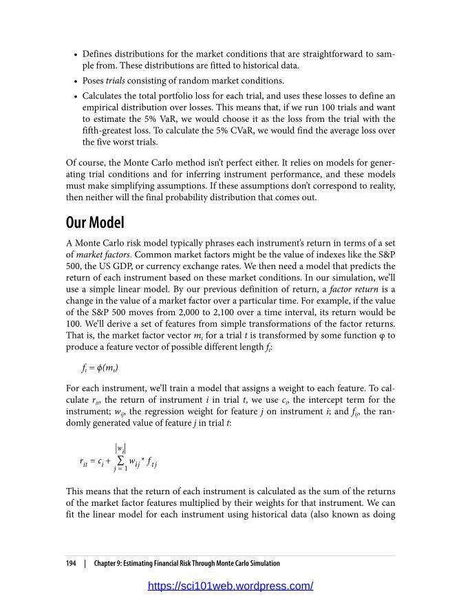
• Defines distributions for the market conditions that are straightforward to sam‐ple from. These distributions are fitted to historical data.

• Poses trials consisting of random market conditions.• Calculates the total portfolio loss for each trial, and uses these losses to define an

empirical distribution over losses. This means that, if we run 100 trials and wantto estimate the 5% VaR, we would choose it as the loss from the trial with thefifth-greatest loss. To calculate the 5% CVaR, we would find the average loss overthe five worst trials.

Of course, the Monte Carlo method isn’t perfect either. It relies on models for gener‐ating trial conditions and for inferring instrument performance, and these modelsmust make simplifying assumptions. If these assumptions don’t correspond to reality,then neither will the final probability distribution that comes out.

Our ModelA Monte Carlo risk model typically phrases each instrument’s return in terms of a setof market factors. Common market factors might be the value of indexes like the S&P500, the US GDP, or currency exchange rates. We then need a model that predicts thereturn of each instrument based on these market conditions. In our simulation, we’lluse a simple linear model. By our previous definition of return, a factor return is achange in the value of a market factor over a particular time. For example, if the valueof the S&P 500 moves from 2,000 to 2,100 over a time interval, its return would be100. We’ll derive a set of features from simple transformations of the factor returns.That is, the market factor vector mt for a trial t is transformed by some function φ toproduce a feature vector of possible different length ft:

ft = ϕ(mt)

For each instrument, we’ll train a model that assigns a weight to each feature. To cal‐culate rit, the return of instrument i in trial t, we use ci, the intercept term for theinstrument; wij, the regression weight for feature j on instrument i; and ftj, the ran‐domly generated value of feature j in trial t:

rit = ci + ∑j = 1

wiwi j * f t j

This means that the return of each instrument is calculated as the sum of the returnsof the market factor features multiplied by their weights for that instrument. We canfit the linear model for each instrument using historical data (also known as doing



linear regression). If the horizon of the VaR calculation is two weeks, the regressiontreats every (overlapping) two-week interval in history as a labeled point.

It’s also worth mentioning that we could have chosen a more complicated model. Forexample, the model need not be linear: it could be a regression tree or explicitlyincorporate domain-specific knowledge.

Now that we have our model for calculating instrument losses from market factors,we need a process for simulating the behavior of market factors. A simple assumptionis that each market factor return follows a normal distribution. To capture the factthat market factors are often correlated—when NASDAQ is down, the Dow is likelyto be suffering as well—we can use a multivariate normal distribution with a non-diagonal covariance matrix:

mt ∼ � μ, Σ

where μ is a vector of the empirical means of the returns of the factors and Σ is theempirical covariance matrix of the returns of the factors.

As before, we could have chosen a more complicated method of simulating the mar‐ket or assumed a different type of distribution for each market factor, perhaps usingdistributions with fatter tails.

Getting the DataIt can be difficult to find large volumes of nicely formatted historical price data, butYahoo! has a variety of stock data available for download in CSV format. The follow‐ing script, located in the risk/data directory of the repo, will make a series of RESTcalls to download histories for all the stocks included in the NASDAQ index andplace them in a stocks/ directory:

$ ./download-all-symbols.sh

We also need historical data for risk factors. For our factors, we’ll use the values of theS&P 500 and NASDAQ indexes, as well as the prices of 5-year and 30-year US Treas‐ury bonds. These can all be downloaded from Yahoo! as well:

$ mkdir factors/$ ./download-symbol.sh ^GSPC factors$ ./download-symbol.sh ^IXIC factors$ ./download-symbol.sh ^TYX factors$ ./download-symbol.sh ^FVX factors

PreprocessingThe first few rows of the Yahoo!-formatted data for GOOGL looks like:

Getting the Data | 195


Date,Open,High,Low,Close,Volume,Adj Close2014-10-24,554.98,555.00,545.16,548.90,2175400,548.902014-10-23,548.28,557.40,545.50,553.65,2151300,553.652014-10-22,541.05,550.76,540.23,542.69,2973700,542.692014-10-21,537.27,538.77,530.20,538.03,2459500,538.032014-10-20,520.45,533.16,519.14,532.38,2748200,532.38

Let’s fire up the Spark shell. In this chapter, we rely on several libraries to make ourlives easier. The GitHub repo contains a Maven project that can be used to build aJAR file that packages all these dependencies together:

$ cd ch09-risk/$ mvn package$ cd data/$ spark-shell --jars ../target/ch09-risk-2.0.0-jar-with-dependencies.jar

For each instrument and factor, we want to derive a list of (date, closing price) tuples.The java.time library contains useful functionality for representing and manipulat‐ing dates. We can represent our dates as LocalDate objects. We can use the DateTimeFormatter to parse dates in the Yahoo date format:

import java.time.LocalDateimport java.time.format.DateTimeFormatter

val format = DateTimeFormatter.ofPattern("yyyy-MM-dd")LocalDate.parse("2014-10-24")res0: java.time.LocalDate = 2014-10-24

The 3,000-instrument histories and 4-factor histories are small enough to read andprocess locally. This remains the case even for larger simulations with hundreds ofthousands of instruments and thousands of factors. The need arises for a distributedsystem like Spark when we’re actually running the simulations, which can requiremassive amounts of computation on each instrument.

To read a full Yahoo history from local disk:

import java.io.File

def readYahooHistory(file: File): Array[(LocalDate, Double)] = { val formatter = DateTimeFormatter.ofPattern("yyyy-MM-dd") val lines = scala.io.Source.fromFile(file).getLines().toSeq lines.tail.map { line => val cols = line.split(',') val date = LocalDate.parse(cols(0), formatter) val value = cols(1).toDouble (date, value) }.reverse.toArray}

Notice that lines.tail is useful for excluding the header row. We load all the dataand filter out instruments with less than five years of history:



val start = LocalDate.of(2009, 10, 23)val end = LocalDate.of(2014, 10, 23)

val stocksDir = new File("stocks/")val files = stocksDir.listFiles()val allStocks = files.iterator.flatMap { file =>> try { Some(readYahooHistory(file)) } catch { case e: Exception => None }}val rawStocks = allStocks.filter(_.size >= 260 * 5 + 10)

val factorsPrefix = "factors/"val rawFactors = Array( "^GSPC.csv", "^IXIC.csv", "^TYX.csv", "^FVX.csv"). map(x => new File(factorsPrefix + x)). map(readYahooHistory)

Using iterator here allows us to stream over the files instead of loading theirfull contents in memory all at once.

Different types of instruments may trade on different days, or the data may havemissing values for other reasons, so it is important to make sure that our differenthistories align. First, we need to trim all of our time series to the same region in time.Then we need to fill in missing values. To deal with time series that are missing valuesat the start and end dates in the time region, we simply fill in those dates with nearbyvalues in the time region:

def trimToRegion(history: Array[(LocalDate, Double)], start: LocalDate, end: LocalDate) : Array[(LocalDate, Double)] = { var trimmed = history.dropWhile(_._1.isBefore(start)). takeWhile(x => x._1.isBefore(end) || x._1.isEqual(end)) if (trimmed.head._1 != start) { trimmed = Array((start, trimmed.head._2)) ++ trimmed } if (trimmed.last._1 != end) { trimmed = trimmed ++ Array((end, trimmed.last._2)) } trimmed}

To deal with missing values within a time series, we use a simple imputation strategythat fills in an instrument’s price as its most recent closing price before that day.Because there is no pretty Scala Collections method that can do this for us, we write iton our own. The spark-ts and flint libraries are alternatives that contain an array ofuseful time series manipulations functions.

Preprocessing | 197


https://github.com/sryza/spark-timeseries

https://github.com/twosigma/flint

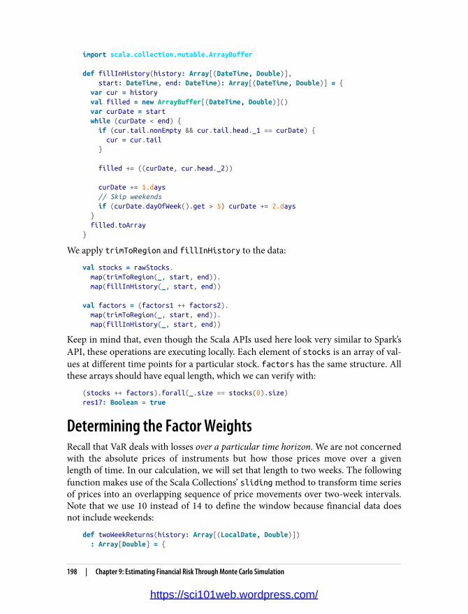
import scala.collection.mutable.ArrayBuffer

def fillInHistory(history: Array[(DateTime, Double)], start: DateTime, end: DateTime): Array[(DateTime, Double)] = { var cur = history val filled = new ArrayBuffer[(DateTime, Double)]() var curDate = start while (curDate < end) { if (cur.tail.nonEmpty && cur.tail.head._1 == curDate) { cur = cur.tail }

filled += ((curDate, cur.head._2))

curDate += 1.days // Skip weekends if (curDate.dayOfWeek().get > 5) curDate += 2.days } filled.toArray}

We apply trimToRegion and fillInHistory to the data:

val stocks = rawStocks. map(trimToRegion(_, start, end)). map(fillInHistory(_, start, end))

val factors = (factors1 ++ factors2). map(trimToRegion(_, start, end)). map(fillInHistory(_, start, end))

Keep in mind that, even though the Scala APIs used here look very similar to Spark’sAPI, these operations are executing locally. Each element of stocks is an array of val‐ues at different time points for a particular stock. factors has the same structure. Allthese arrays should have equal length, which we can verify with:

(stocks ++ factors).forall(_.size == stocks(0).size)res17: Boolean = true

Determining the Factor WeightsRecall that VaR deals with losses over a particular time horizon. We are not concernedwith the absolute prices of instruments but how those prices move over a givenlength of time. In our calculation, we will set that length to two weeks. The followingfunction makes use of the Scala Collections’ sliding method to transform time seriesof prices into an overlapping sequence of price movements over two-week intervals.Note that we use 10 instead of 14 to define the window because financial data doesnot include weekends:

def twoWeekReturns(history: Array[(LocalDate, Double)]) : Array[Double] = {



history.sliding(10). map { window => val next = window.last._2 val prev = window.head._2 (next - prev) / prev }.toArray}

val stocksReturns = stocks.map(twoWeekReturns).toArray.toSeq val factorsReturns = factors.map(twoWeekReturns)

Because of our earlier use of iterator, stocks is an iterator. .toArray.toSeqruns through it and collects the elements in memory into a sequence.

With these return histories in hand, we can turn to our goal of training predictivemodels for the instrument returns. For each instrument, we want a model that pre‐dicts its two-week return based on the returns of the factors over the same timeperiod. For simplicity, we will use a linear regression model.

To model the fact that instrument returns may be nonlinear functions of the factorreturns, we can include some additional features in our model that we derive fromnonlinear transformations of the factor returns. We will try adding two additionalfeatures for each factor return: square and square root. Our model is still a linearmodel in the sense that the response variable is a linear function of the features. Someof the features just happen to be determined by nonlinear functions of the factorreturns. Keep in mind that this particular feature transformation is meant to demon‐strate some of the options available—it shouldn’t be perceived as a state-of-the-artpractice in predictive financial modeling.

Even though we will be carrying out many regressions—one for each instrument—the number of features and data points in each regression is small, meaning that wedon’t need to make use of Spark’s distributed linear modeling capabilities. Instead,we’ll use the ordinary least squares regression offered by the Apache Commons Mathpackage. While our factor data is currently a Seq of histories (each an array of (DateTime, Double) tuples), OLSMultipleLinearRegression expects data as an array ofsample points (in our case a two-week interval), so we need to transpose our factormatrix:

def factorMatrix(histories: Seq[Array[Double]]) : Array[Array[Double]] = { val mat = new Array[Array[Double]](histories.head.length) for (i <- histories.head.indices) { mat(i) = histories.map(_(i)).toArray } mat}

val factorMat = factorMatrix(factorsReturns)

Determining the Factor Weights | 199


Then we can tack on our additional features:

def featurize(factorReturns: Array[Double]): Array[Double] = { val squaredReturns = factorReturns. map(x => math.signum(x) * x * x) val squareRootedReturns = factorReturns. map(x => math.signum(x) * math.sqrt(math.abs(x))) squaredReturns ++ squareRootedReturns ++ factorReturns}

val factorFeatures = factorMat.map(featurize)

And then we can fit the linear models. In addition, to find the model parameters foreach instrument, we can use the OLSMultipleLinearRegression’s estimateRegressionParameters method:

import org.apache.commons.math3.stat.regression.OLSMultipleLinearRegression

def linearModel(instrument: Array[Double], factorMatrix: Array[Array[Double]]) : OLSMultipleLinearRegression = { val regression = new OLSMultipleLinearRegression() regression.newSampleData(instrument, factorMatrix) regression}

val factorWeights = stocksReturns. map(linearModel(_, factorFeatures)). map(_.estimateRegressionParameters()). toArray

We now have a 1,867×8 matrix where each row is the set of model parameters (coeffi‐cients, weights, covariants, regressors, or whatever you wish to call them) for aninstrument.

We will elide this analysis for brevity, but at this point in any real-world pipeline itwould be useful to understand how well these models fit the data. Because the datapoints are drawn from time series, and especially because the time intervals are over‐lapping, it is very likely that the samples are autocorrelated. This means that commonmeasures like R2 are likely to overestimate how well the models fit the data. TheBreusch-Godfrey test is a standard test for assessing these effects. One quick way toevaluate a model is to separate a time series into two sets, leaving out enough datapoints in the middle so that the last points in the earlier set are not autocorrelatedwith the first points in the later set. Then train the model on one set and look at itserror on the other.



http://bit.ly/2psAwB7

SamplingWith our models that map factor returns to instrument returns in hand, we now needa procedure for simulating market conditions by generating random factor returns.That is, we need to decide on a probability distribution over factor return vectors andsample from it. What distribution does the data actually take? It can often be useful tostart answering this kind of question visually. A nice way to visualize a probabilitydistribution over continuous data is a density plot that plots the distribution’s domainversus its PDF. Because we don’t know the distribution that governs the data, we don’thave an equation that can give us its density at an arbitrary point, but we can approxi‐mate it through a technique called kernel density estimation. In a loose way, kerneldensity estimation is a way of smoothing out a histogram. It centers a probability dis‐tribution (usually a normal distribution) at each data point. So a set of two-week-return samples would result in 200 normal distributions, each with a different mean.To estimate the probability density at a given point, it evaluates the PDFs of all thenormal distributions at that point and takes their average. The smoothness of a kerneldensity plot depends on its bandwidth, the standard deviation of each of the normaldistributions. The GitHub repository comes with a kernel density implementationthat works both over RDDs and local collections. For brevity, it is elided here.

breeze-viz is a Scala library that makes it easy to draw simple plots. The followingsnippet creates a density plot from a set of samples:

import org.apache.spark.mllib.stat.KernelDensityimport org.apache.spark.util.StatCounterimport breeze.plot._

def plotDistribution(samples: Array[Double]): Figure = { val min = samples.min val max = samples.max val stddev = new StatCounter(samples).stdev val bandwidth = 1.06 * stddev * math.pow(samples.size, -0.2)

val domain = Range.Double(min, max, (max - min) / 100). toList.toArray val kd = new KernelDensity(). setSample(samples.toSeq.toDS.rdd). setBandwidth(bandwidth) val densities = kd.estimate(domain) val f = Figure() val p = f.subplot(0) p += plot(domain, densities) p.xlabel = "Two Week Return ($)" p.ylabel = "Density" f}

Sampling | 201


plotDistribution(factorsReturns(0))plotDistribution(factorsReturns(2))

We use what is known as “Silverman’s rule of thumb,” named after the British sta‐tistician Bernard Silverman, to pick a reasonable bandwidth.

Figure 9-1 shows the distribution (probability density function) of two-week returnsfor the S&P 500 in our history.

Figure 9-1. Two-week S&P 500 returns distribution

Figure 9-2 shows the same for two-week returns of 30-year Treasury bonds.



Figure 9-2. Two-week 30-year Treasury bond returns distribution

We will fit a normal distribution to the returns of each factor. Looking for a moreexotic distribution, perhaps with fatter tails, that more closely fits the data is oftenworthwhile. However, for the sake of simplicity, we will avoid tuning our simulationin this way.

The simplest way to sample factors’ returns would be to fit a normal distribution toeach of the factors and sample from these distributions independently. However, thisignores the fact that market factors are often correlated. If the S&P is down, the Dowis likely to be down as well. Failing to take these correlations into account can give usa much rosier picture of our risk profile than its reality. Are the returns of our factorscorrelated? The Pearson’s correlation implementation from Commons Math can helpus find out:

import org.apache.commons.math3.stat.correlation.PearsonsCorrelation

val factorCor = new PearsonsCorrelation(factorMat).getCorrelationMatrix().getData()println(factorCor.map(_.mkString("\t")).mkString("\n"))1.0 -0.3472 0.4424 0.4633 -0.3472 1.0 -0.4777 -0.50960.4424 -0.4777 1.0 0.91990.4633 -0.5096 0.9199 1.0

Digits truncated to fit within the margins

Because we have nonzero elements off the diagonals, it doesn’t look like it.

Sampling | 203


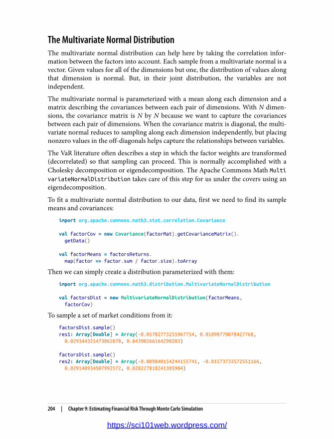
The Multivariate Normal DistributionThe multivariate normal distribution can help here by taking the correlation infor‐mation between the factors into account. Each sample from a multivariate normal is avector. Given values for all of the dimensions but one, the distribution of values alongthat dimension is normal. But, in their joint distribution, the variables are notindependent.

The multivariate normal is parameterized with a mean along each dimension and amatrix describing the covariances between each pair of dimensions. With N dimen‐sions, the covariance matrix is N by N because we want to capture the covariancesbetween each pair of dimensions. When the covariance matrix is diagonal, the multi‐variate normal reduces to sampling along each dimension independently, but placingnonzero values in the off-diagonals helps capture the relationships between variables.

The VaR literature often describes a step in which the factor weights are transformed(decorrelated) so that sampling can proceed. This is normally accomplished with aCholesky decomposition or eigendecomposition. The Apache Commons Math MultivariateNormalDistribution takes care of this step for us under the covers using aneigendecomposition.

To fit a multivariate normal distribution to our data, first we need to find its samplemeans and covariances:

import org.apache.commons.math3.stat.correlation.Covariance

val factorCov = new Covariance(factorMat).getCovarianceMatrix(). getData()

val factorMeans = factorsReturns. map(factor => factor.sum / factor.size).toArray

Then we can simply create a distribution parameterized with them:

import org.apache.commons.math3.distribution.MultivariateNormalDistribution

val factorsDist = new MultivariateNormalDistribution(factorMeans, factorCov)

To sample a set of market conditions from it:

factorsDist.sample()res1: Array[Double] = Array(-0.05782773255967754, 0.01890770078427768, 0.029344325473062878, 0.04398266164298203)

factorsDist.sample()res2: Array[Double] = Array(-0.009840154244155741, -0.01573733572551166, 0.029140934507992572, 0.028227818241305904)



Running the TrialsWith the per-instrument models and a procedure for sampling factor returns, wenow have the pieces we need to run the actual trials. Because running the trials is verycomputationally intensive, we will finally turn to Spark to help us parallelize them. Ineach trial, we want to sample a set of risk factors, use them to predict the return ofeach instrument, and sum all those returns to find the full trial loss. To achieve a rep‐resentative distribution, we want to run thousands or millions of these trials.

We have a few choices for how to parallelize the simulation. We can parallelize alongtrials, instruments, or both. To parallelize along both, we would create a data set ofinstruments and a data set of trial parameters, and then use the crossJoin transfor‐mation to generate a data set of all the pairs. This is the most general approach, but ithas a couple of disadvantages. First, it requires explicitly creating an RDD of trialparameters, which we can avoid by using some tricks with random seeds. Second, itrequires a shuffle operation.

Partitioning along instruments would look something like this:

val randomSeed = 1496val instrumentsDS = ...def trialLossesForInstrument(seed: Long, instrument: Array[Double]) : Array[(Int, Double)] = { ...}instrumentsDS.flatMap(trialLossesForInstrument(randomSeed, _)). reduceByKey(_ + _)

With this approach, the data is partitioned across an RDD of instruments, and foreach instrument a flatMap transformation computes and yields the loss against everytrial. Using the same random seed across all tasks means that we will generate thesame sequence of trials. A reduceByKey sums together all the losses corresponding tothe same trials. A disadvantage of this approach is that it still requires shuffling O(|instruments| * |trials|) data.

Our model data for our few thousand instruments data is small enough to fit in mem‐ory on every executor, and some back-of-the-envelope calculations reveal that this isprobably still the case even with a million or so instruments and hundreds of factors.A million instruments times 500 factors times the 8 bytes needed for the double thatstores each factor weight equals roughly 4 GB, small enough to fit in each executor onmost modern-day cluster machines. This means that a good option is to distributethe instrument data in a broadcast variable. The advantage of each executor having afull copy of the instrument data is that total loss for each trial can be computed on asingle machine. No aggregation is necessary.

Running the Trials | 205


With the partition-by-trials approach (which we will use), we start out with an RDDof seeds. We want a different seed in each partition so that each partition generatesdifferent trials:

val parallelism = 1000val baseSeed = 1496

val seeds = (baseSeed until baseSeed + parallelism)val seedDS = seeds.toDS().repartition(parallelism)

Random number generation is a time-consuming and CPU-intensive process. Whilewe don’t employ this trick here, it can often be useful to generate a set of randomnumbers in advance and use it across multiple jobs. The same random numbersshould not be used within a single job, because this would violate the Monte Carloassumption that the random values are independently distributed. If we were to gothis route, we would replace toDS with textFile and load randomNumbersDS.

For each seed, we want to generate a set of trial parameters and observe the effects ofthese parameters on all the instruments. Let’s start from the ground up by writing afunction that calculates the return of a single instrument underneath a single trial. Wesimply apply the linear model that we trained earlier for that instrument. The lengthof the instrument array of regression parameters is one greater than the length of thetrial array, because the first element of the instrument array contains the interceptterm:

def instrumentTrialReturn(instrument: Array[Double], trial: Array[Double]): Double = { var instrumentTrialReturn = instrument(0) var i = 0 while (i < trial.length) { instrumentTrialReturn += trial(i) * instrument(i+1) i += 1 } instrumentTrialReturn}

We use a while loop here instead of a more functional Scala construct becausethis is a performance-critical region.

Then, to calculate the full return for a single trial, we simply average over the returnsof all the instruments. This assumes that we’re holding an equal value of each instru‐ment in the portfolio. A weighted average would be used if we held different amountsof each stock.

def trialReturn(trial: Array[Double], instruments: Seq[Array[Double]]): Double = { var totalReturn = 0.0 for (instrument <- instruments) { totalReturn += instrumentTrialReturn(instrument, trial)



} totalReturn / instruments.size}

Lastly, we need to generate a bunch of trials in each task. Because choosing randomnumbers is a big part of the process, it is important to use a strong random numbergenerator that will take a very long time to repeat itself. Commons Math includes aMersenne Twister implementation that is good for this. We use it to sample from amultivariate normal distribution as described previously. Note that we are applyingthe featurize method that we defined before on the generated factor returns inorder to transform them into the feature representation used in our models:

import org.apache.commons.math3.random.MersenneTwister

def trialReturns(seed: Long, numTrials: Int, instruments: Seq[Array[Double]], factorMeans: Array[Double], factorCovariances: Array[Array[Double]]): Seq[Double] = { val rand = new MersenneTwister(seed) val multivariateNormal = new MultivariateNormalDistribution( rand, factorMeans, factorCovariances)

val trialReturns = new Array[Double](numTrials) for (i <- 0 until numTrials) { val trialFactorReturns = multivariateNormal.sample() val trialFeatures = featurize(trialFactorReturns) trialReturns(i) = trialReturn(trialFeatures, instruments) } trialReturns}

With our scaffolding complete, we can use it to compute an RDD where each elementis the total return from a single trial. Because the instrument data (matrix including aweight on each factor feature for each instrument) is large, we use a broadcast vari‐able for it. This ensures that it only needs to be deserialized once per executor:

val numTrials = 10000000

val trials = seedDS.flatMap( trialReturns(_, numTrials / parallelism, factorWeights, factorMeans, factorCov))

trials.cache()

If you recall, the whole reason we’ve been messing around with all these numbers is tocalculate VaR. trials now forms an empirical distribution over portfolio returns. Tocalculate 5% VaR, we need to find a return that we expect to underperform 5% of thetime, and a return that we expect to outperform 5% of the time. With our empiricaldistribution, this is as simple as finding the value that 5% of trials are worse than and95% of trials are better than. We can accomplish this using the takeOrdered action to

Running the Trials | 207


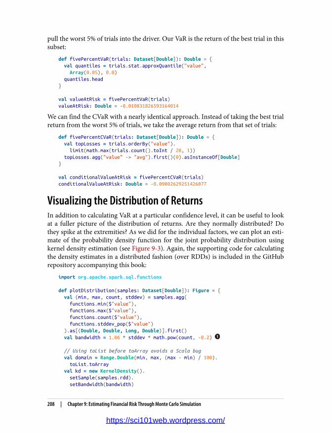
pull the worst 5% of trials into the driver. Our VaR is the return of the best trial in thissubset:

def fivePercentVaR(trials: Dataset[Double]): Double = { val quantiles = trials.stat.approxQuantile("value", Array(0.05), 0.0) quantiles.head}

val valueAtRisk = fivePercentVaR(trials)valueAtRisk: Double = -0.010831826593164014

We can find the CVaR with a nearly identical approach. Instead of taking the best trialreturn from the worst 5% of trials, we take the average return from that set of trials:

def fivePercentCVaR(trials: Dataset[Double]): Double = { val topLosses = trials.orderBy("value"). limit(math.max(trials.count().toInt / 20, 1)) topLosses.agg("value" -> "avg").first()(0).asInstanceOf[Double]}

val conditionalValueAtRisk = fivePercentCVaR(trials)conditionalValueAtRisk: Double = -0.09002629251426077

Visualizing the Distribution of ReturnsIn addition to calculating VaR at a particular confidence level, it can be useful to lookat a fuller picture of the distribution of returns. Are they normally distributed? Dothey spike at the extremities? As we did for the individual factors, we can plot an esti‐mate of the probability density function for the joint probability distribution usingkernel density estimation (see Figure 9-3). Again, the supporting code for calculatingthe density estimates in a distributed fashion (over RDDs) is included in the GitHubrepository accompanying this book:

import org.apache.spark.sql.functions

def plotDistribution(samples: Dataset[Double]): Figure = { val (min, max, count, stddev) = samples.agg( functions.min($"value"), functions.max($"value"), functions.count($"value"), functions.stddev_pop($"value") ).as[(Double, Double, Long, Double)].first() val bandwidth = 1.06 * stddev * math.pow(count, -0.2)

// Using toList before toArray avoids a Scala bug val domain = Range.Double(min, max, (max - min) / 100). toList.toArray val kd = new KernelDensity(). setSample(samples.rdd). setBandwidth(bandwidth)



val densities = kd.estimate(domain) val f = Figure() val p = f.subplot(0) p += plot(domain, densities) p.xlabel = "Two Week Return ($)" p.ylabel = "Density" f}

plotDistribution(trials)

Again, Silverman’s rule of thumb.

Figure 9-3. Two-week returns distribution

Evaluating Our ResultsHow do we know whether our estimate is a good estimate? How do we know whetherwe should simulate with a larger number of trials? In general, the error in a MonteCarlo simulation should be proportional to 1/ n. This means that, in general, quad‐rupling the number of trials should approximately cut the error in half.

A nice way to get a confidence interval on our VaR statistic is through bootstrapping.We achieve a bootstrap distribution over the VaR by repeatedly sampling withreplacement from the set of portfolio return results of our trials. Each time, we take anumber of samples equal to the full size of the trials set and compute a VaR fromthose samples. The set of VaRs computed from all the times form an empirical distri‐bution, and we can get our confidence interval by simply looking at its quantiles.

Evaluating Our Results | 209


The following is a function that will compute a bootstrapped confidence interval forany statistic (given by the computeStatistic argument) of an RDD. Notice its use ofSpark’s sample where we pass true for its first argument withReplacement, and 1.0for its second argument to collect a number of samples equal to the full size of thedata set:

def bootstrappedConfidenceInterval( trials: Dataset[Double], computeStatistic: Dataset[Double] => Double, numResamples: Int, probability: Double): (Double, Double) = { val stats = (0 until numResamples).map { i => val resample = trials.sample(true, 1.0) computeStatistic(resample) }.sorted val lowerIndex = (numResamples * probability / 2 - 1).toInt val upperIndex = math.ceil(numResamples * (1 - probability / 2)) .toInt (stats(lowerIndex), stats(upperIndex))}

Then we call this function, passing in the fivePercentVaR function we defined earlierthat computes the VaR from an RDD of trials:

bootstrappedConfidenceInterval(trials, fivePercentVaR, 100, .05)...(-0.019480970253736192,-1.4971191125093586E-4)

We can bootstrap the CVaR as well:

bootstrappedConfidenceInterval(trials, fivePercentCVaR, 100, .05)...(-0.10051267317397554,-0.08058996149775266)

The confidence interval helps us understand how confident our model is in its result,but it does little to help us understand how well our model matches reality. Backtest‐ing on historical data is a good way to check the quality of a result. One common testfor VaR is Kupiec’s proportion-of-failures (POF) test. It considers how the portfolioperformed at many historical time intervals and counts the number of times the los‐ses exceeded the VaR. The null hypothesis is that the VaR is reasonable, and a suffi‐ciently extreme test statistic means that the VaR estimate does not accurately describethe data. The test statistic—which relies on p, the confidence level parameter of theVaR calculation; x, the number of historical intervals over which the losses exceededthe VaR; and T, the total number of historical intervals considered—is computed as:

−2 ln 1 − p T − xpx

1 − xT

T − x xT

x



The following computes the test statistic on our historical data. We expand out thelogs for better numerical stability:

−2 T − x ln 1 − p + x ln p − T − x ln 1 − xT − x ln x

T

var failures = 0for (i <- stocksReturns.head.indices) { val loss = stocksReturns.map(_(i)).sum / stocksReturns.size if (loss < valueAtRisk) { failures += 1 }}failures...257

val total = stocksReturns.sizeval confidenceLevel = 0.05val failureRatio = failures.toDouble / totalval logNumer = ((total - failures) * math.log1p(-confidenceLevel) + failures * math.log(confidenceLevel))val logDenom = ((total - failures) * math.log1p(-failureRatio) + failures * math.log(failureRatio))val testStatistic = -2 * (logNumer - logDenom)...180.3543986286574

If we assume the null hypothesis that the VaR is reasonable, then this test statistic isdrawn from a chi-squared distribution with a single degree of freedom. We can usethe Commons Math ChiSquaredDistribution to find the p-value accompanying ourtest statistic value:

import org.apache.commons.math3.distribution.ChiSquaredDistribution

1 - new ChiSquaredDistribution(1.0).cumulativeProbability(testStatistic)

This gives us a tiny p-value, meaning we do have sufficient evidence to reject the nullhypothesis that the model is reasonable. While the fairly tight confidence intervals wecomputed earlier indicate that our model is internally consistent, the test result indi‐cates that it doesn’t correspond well to observed reality. Looks like we need toimprove it a little.

Where to Go from HereThe model laid out in this exercise is a very rough first cut of what would be used inan actual financial institution. In building an accurate VaR model, we glossed over afew very important steps. Curating the set of market factors can make or break a



model, and it is not uncommon for financial institutions to incorporate hundreds offactors in their simulations. Picking these factors requires both running numerousexperiments on historical data and a heavy dose of creativity. Choosing the predictivemodel that maps market factors to instrument returns is also important. Although weused a simple linear model, many calculations use nonlinear functions or simulate thepath over time with Brownian motion.

Lastly, it is worth putting care into the distribution used to simulate the factorreturns. Kolmogorov-Smirnoff tests and chi-squared tests are useful for testing anempirical distribution’s normality. Q-Q plots are useful for comparing distributionsvisually. Usually, financial risk is better mirrored by a distribution with fatter tailsthan the normal distribution that we used. Mixtures of normal distributions are onegood way to achieve these fatter tails. “Financial Economics, Fat-tailed Distributions”,an article by Markus Haas and Christian Pigorsch, provides a nice reference on someof the other fat-tailed distributions out there.

Banks use Spark and large-scale data processing frameworks for calculating VaR withhistorical methods as well. “Evaluation of Value-at-Risk Models Using HistoricalData”, by Darryll Hendricks, provides a good overview and performance comparisonof historical VaR methods.

Monte Carlo risk simulations can be used for more than calculating a single statistic.The results can be used to proactively reduce the risk of a portfolio by shaping invest‐ment decisions. For example, if, in the trials with the poorest returns, a particular setof instruments tends to come up losing money repeatedly, we might consider drop‐ping those instruments from the portfolio or adding instruments that tend to move inthe opposite direction from them.



https://bit.ly/1ACazwy

https://nyfed.org/1ACaI2O

https://nyfed.org/1ACaI2O

CHAPTER 10

Analyzing Genomics Dataand the BDG Project

Uri Laserson

So we need to shoot our SCHPON [Sulfur Carbon Hydrogen Phosphorous Oxygen Nitro‐gen] ... into the void.

—George M. Church

The advent of next-generation DNA sequencing (NGS) technology is rapidly trans‐forming the life sciences into a data-driven field. However, making the best use of thisdata is butting up against a traditional computational ecosystem that builds ondifficult-to-use, low-level primitives for distributed computing (e.g., DRMAA orMPI) and a jungle of semistructured text-based file formats.

This chapter will serve three primary purposes. First, we introduce the general Sparkuser to a set of Hadoop-friendly serialization and file formats (Avro and Parquet) thatsimplify many problems in data management. We broadly promote the use of theseserialization technologies to achieve compact binary representations, service-orientedarchitectures, and language cross-compatibility. Second, we show the experiencedbioinformatician how to perform typical genomics tasks in the context of Spark.

Specifically, we will use Spark to manipulate large quantities of genomics data to pro‐cess and filter data, build a model that predicts transcription factor (TF) binding sites,and join ENCODE genome annotations against the 1000 Genome Project variants.Finally, this chapter will serve as a tutorial to the ADAM project, which comprises aset of genomics-specific Avro schemas, Spark-based APIs, and command-line toolsfor large-scale genomics analysis. Among other applications, ADAM provides anatively distributed implementation of the Genome Analysis Toolkit (GATK) bestpractices using Hadoop and Spark.

213


https://www.encodeproject.org

http://www.internationalgenome.org

https://software.broadinstitute.org/gatk/best-practices/

The genomics portions of this chapter are targeted at experienced bioinformaticiansfamiliar with typical problems. However, the data serialization portions should beuseful to anyone who is processing large amounts of data. For the interested novice, agreat introduction to biology is Eric Lander’s EdX course. For an introduction to bio‐informatics, see Arthur Lesk’s Introduction to Bioinformatics (Oxford UniversityPress).

Finally, because the genome implies a 1D coordinate system, many genomics opera‐tions are spatial in nature. The ADAM project provides a genomics-targeted APIalong with implementations for performing distributed spatial joins using the olderRDD interface. Therefore, this chapter continues to use the original interface ratherthan the newer Dataset and DataFrame interfaces.

A Note on the Use of RDDsIn contrast to the rest of this book, this chapter and the next make use of Spark’s olderresilient distributed data sets (RDD) API. The primary reason is that the ADAMproject has implemented a number of join operators specific for 1D geometric com‐putations that are common in genomics processing. These operators have not yetbeen ported to the newer Dataset API, though this is on the roadmap. Furthermore,the DataFrame API abstracts away more details about the distributed computation;porting the ADAM join operators will require interfacing with Spark’s query planner.On the other hand, this chapter can be referred to when the reader encounters uses ofthe RDD API, either through other Spark-based libraries or in legacy code.

Decoupling Storage from ModelingBioinformaticians spend a disproportionate amount of time worrying about file for‐mats—.fasta, .fastq, .sam, .bam, .vcf, .gvcf, .bcf, .bed, .gff, .gtf, .narrowPeak, .wig, .big‐Wig, .bigBed, .ped, and .tped, to name a few—not to mention the scientists who feel itis necessary to specify their own custom format for their custom tool. On top of that,many of the format specifications are incomplete or ambiguous (which makes it hardto ensure implementations are consistent or compliant) and specify ASCII-encodeddata. ASCII data is very common in bioinformatics, but it is inefficient and com‐presses relatively poorly—this is starting to be addressed by community efforts toimprove the specs. In addition, the data must always be parsed, necessitating addi‐tional compute cycles. This is particularly troubling because all of these file formatsessentially store just a few common object types: an aligned sequence read, a calledgenotype, a sequence feature, and a phenotype. (The term sequence feature is slightlyoverloaded in genomics, but in this chapter we mean it in the sense of an elementfrom a track of the UCSC Genome Browser.) Libraries like biopython are popularbecause they are chock-full-o’ parsers (e.g., Bio.SeqIO) that attempt to read all the file

214 | Chapter 10: Analyzing Genomics Data and the BDG Project


http://bit.ly/2qKJCcQ

https://github.com/samtools/hts-specs

http://biopython.org

formats into a small number of common in-memory models (e.g., Bio.Seq, Bio.SeqRecord, Bio.SeqFeature).

We can solve all of these problems in one shot using a serialization framework likeApache Avro. The key lies in Avro’s separation of the data model (i.e., an explicitschema) from the underlying storage file format and also the language’s in-memoryrepresentation. Avro specifies how data of a certain type should be communicatedbetween processes, whether that’s between running processes over the Internet, or aprocess trying to write the data into a particular file format. For example, a Java pro‐gram that uses Avro can write the data into multiple underlying file formats that areall compatible with Avro’s data model. This allows each process to stop worryingabout compatibility with multiple file formats: the process only needs to know how toread Avro, and the filesystem needs to know how to supply Avro.

Let’s take the sequence feature as an example. We begin by specifying the desiredschema for the object using the Avro interface definition language (IDL):

enum Strand { Forward, Reverse, Independent}

record SequenceFeature { string featureId; string featureType; string chromosome; long startCoord; long endCoord; Strand strand; double value; map<string> attributes;}

For example, “conservation,” “centipede,” “gene”

This data type could be used to encode, for example, conservation level, the presenceof a promoter or ribosome binding site, a TF binding site, and so on at a particularlocation in the genome. One way to think about it is a binary version of JSON butmore restricted and with higher performance. Given a particular data schema, theAvro spec then determines the precise binary encoding for the object so that it can beeasily communicated between processes (even if written in different programing lan‐guages), over the network, or onto disk for storage. The Avro project includes mod‐ules for processing Avro-encoded data from many languages, including Java, C/C++,Python, and Perl; after that, the language is free to store the object in memory inwhichever way is deemed most advantageous. The separation of data modeling fromthe storage format provides another level of flexibility/abstraction; Avro data can be

Decoupling Storage from Modeling | 215


stored as Avro-serialized binary objects (Avro container file), in a columnar file for‐mat for fast queries (Parquet file), or as text JSON data for maximum flexibility (min‐imum efficiency). Finally, Avro supports schema evolution, allowing the user to addnew fields as they become necessary, while the software gracefully deals with new/oldversions of the schema.

Overall, Avro is an efficient binary encoding that allows you to easily specify evolva‐ble data schemas, process the same data from many programming languages, andstore the data using many formats. Deciding to store your data using Avro schemasfrees you from perpetually working with more and more custom data formats, whilesimultaneously increasing the performance of your computations.

Serialization/RPC FrameworksThere exist a large number of serialization frameworks in the wild. The most com‐monly used frameworks in the big data community are Apache Avro, Apache Thrift,and Google’s Protocol Buffers (protobuf). At the core, they all provide an interfacedefinition language for specifying the schemas of object/message types, and they allcompile into a variety of programming languages. On top of IDL, Thrift also adds away to specify RPCs. (Google’s RPC framework for protobuf has been open-sourcedas gRPC.) Finally, on top of IDL and RPC, Avro adds a file format specification forstoring the data on-disk. Google more recently released a “serialization” frameworkthat uses the same byte representation on-the-wire and in-memory, effectively elimi‐nating the expensive serialization step.

It’s difficult to make generalizations about which framework is appropriate in whatcircumstances because they all support different languages and have different perfor‐mance characteristics for the various languages.

The particular SequenceFeature model used in the preceding example is a bit sim‐plistic for real data, but the Big Data Genomics (BDG) project has already definedAvro schemas to represent the following objects, as well as many others:

• AlignmentRecord for reads• Variant for known genome variants and metadata• Genotype for a called genotype at a particular locus• Feature for a sequence feature (annotation on a genome segment)

The actual schemas can be found in the bdg-formats GitHub repo. The BDG formatscan function as a replacement of the ubiquitous “legacy” formats (like BAM andVCF), but more commonly function as high-performance “intermediate” formats.(The original goal of these BDG formats was to replace the use of BAM and VCF, but



http://bdgenomics.org/

https://github.com/bigdatagenomics/bdg-formats

their stubborn ubiquity has proved this goal to be difficult.) The Global Alliance forGenomics and Health has also developed its own set of schemas using Protocol Buf‐fers. Hopefully, this will not turn into its own situation, where there is a proliferationof competing schemas. Even so, Avro provides many performance and data modelingbenefits over the custom ASCII status quo. In the remainder of the chapter, we’ll usesome of the BDG schemas to accomplish some typical genomics tasks.

Ingesting Genomics Data with the ADAM CLIThis chapter makes heavy use of the ADAM project for genomicson Spark. The project is under heavy development, including thedocumentation. If you run into problems, make sure to check thelatest README files on GitHub, the GitHub issue tracker, or theadam-developers mailing list.

BDG’s core set of genomics tools is called ADAM. Starting from a set of mappedreads, this core includes tools that can perform mark-duplicates, base quality scorerecalibration, indel realignment, and variant calling, among other tasks. ADAM alsocontains a command-line interface that wraps the core for ease of use. In contrast toHPC, these command-line tools know about Hadoop and HDFS, and many of themcan automatically parallelize across a cluster without having to split files or schedulejobs manually.

We’ll start by building ADAM like the README tells us to:

git clone https://github.com/bigdatagenomics/adam.git && cd adamexport "MAVEN_OPTS=-Xmx512m -XX:MaxPermSize=128m"mvn clean package -DskipTests

Alternatively, download one of the ADAM releases from the GitHub release page.

ADAM comes with a submission script that facilitates interfacing with Spark’s spark-submit script; the easiest way to use it is probably to alias it:

export ADAM_HOME=path/to/adamalias adam-submit="$ADAM_HOME/bin/adam-submit"

At this point, you should be able to run ADAM from the command line and get theusage message. As noted in the usage message below, Spark arguments are givenbefore ADAM-specific arguments.

Ingesting Genomics Data with the ADAM CLI | 217


https://github.com/ga4gh/schemas

https://github.com/ga4gh/schemas

https://xkcd.com/927/

$ adam-submitUsing ADAM_MAIN=org.bdgenomics.adam.cli.ADAMMain[...]

e 888~-_ e e e d8b 888 \ d8b d8b d8b /Y88b 888 | /Y88b d888bdY88b / Y88b 888 | / Y88b / Y88Y Y888b /____Y88b 888 / /____Y88b / YY Y888b / Y88b 888_-~ / Y88b / Y888b

Usage: adam-submit [<spark-args> --] <adam-args>

Choose one of the following commands:

ADAM ACTIONS countKmers : Counts the k-mers/q-mers from a read dataset. countContigKmers : Counts the k-mers/q-mers from a read dataset. transform : Convert SAM/BAM to ADAM format and optionally perform... transformFeatures : Convert a file with sequence features into correspondin... mergeShards : Merges the shards of a file reads2coverage : Calculate the coverage from a given ADAM file[...]

You may have to set some environment variables for this to succeed, such asSPARK_HOME and HADOOP_CONF_DIR.

We’ll start by taking a .bam file containing some mapped NGS reads, converting themto the corresponding BDG format (AlignedRecord in this case), and saving them toHDFS. First, we get our hands on a suitable .bam file and put it in HDFS:

# Note: this file is 16 GBcurl -O ftp://ftp.ncbi.nih.gov/1000genomes/ftp/phase3/data\/HG00103/alignment/HG00103.mapped.ILLUMINA.bwa.GBR\.low_coverage.20120522.bam

# or using Aspera instead (which is *much* faster)ascp -i path/to/asperaweb_id_dsa.openssh -QTr -l 10G \[email protected]:/1000genomes/ftp/phase3/data\/HG00103/alignment/HG00103.mapped.ILLUMINA.bwa.GBR\.low_coverage.20120522.bam .

hadoop fs -put HG00103.mapped.ILLUMINA.bwa.GBR\.low_coverage.20120522.bam /user/ds/genomics

We can then use the ADAM transform command to convert the .bam file to Parquetformat (described in “Parquet Format and Columnar Storage” on page 223). Thiswould work both on a cluster and in local mode:



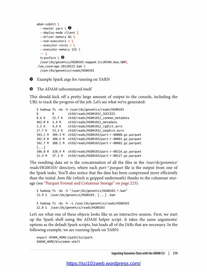
adam-submit \ --master yarn \ --deploy-mode client \ --driver-memory 8G \ --num-executors 6 \ --executor-cores 4 \ --executor-memory 12G \ -- \ transform \ /user/ds/genomics/HG00103.mapped.ILLUMINA.bwa.GBR\.low_coverage.20120522.bam \ /user/ds/genomics/reads/HG00103

Example Spark args for running on YARN

The ADAM subcommand itself

This should kick off a pretty large amount of output to the console, including theURL to track the progress of the job. Let’s see what we’ve generated:

$ hadoop fs -du -h /user/ds/genomics/reads/HG001030 0 ch10/reads/HG00103/_SUCCESS8.6 K 25.7 K ch10/reads/HG00103/_common_metadata462.0 K 1.4 M ch10/reads/HG00103/_metadata1.5 K 4.4 K ch10/reads/HG00103/_rgdict.avro17.7 K 53.2 K ch10/reads/HG00103/_seqdict.avro103.1 M 309.3 M ch10/reads/HG00103/part-r-00000.gz.parquet102.9 M 308.6 M ch10/reads/HG00103/part-r-00001.gz.parquet102.7 M 308.2 M ch10/reads/HG00103/part-r-00002.gz.parquet[...]106.8 M 320.4 M ch10/reads/HG00103/part-r-00126.gz.parquet12.4 M 37.3 M ch10/reads/HG00103/part-r-00127.gz.parquet

The resulting data set is the concatenation of all the files in the /user/ds/genomics/reads/HG00103/ directory, where each part-*.parquet file is the output from one ofthe Spark tasks. You’ll also notice that the data has been compressed more efficientlythan the initial .bam file (which is gzipped underneath) thanks to the columnar stor‐age (see “Parquet Format and Columnar Storage” on page 223).

$ hadoop fs -du -h "/user/ds/genomics/HG00103.*.bam"15.9 G /user/ds/genomics/HG00103. [...] .bam

$ hadoop fs -du -h -s /user/ds/genomics/reads/HG0010312.8 G /user/ds/genomics/reads/HG00103

Let’s see what one of these objects looks like in an interactive session. First, we startup the Spark shell using the ADAM helper script. It takes the same arguments/options as the default Spark scripts, but loads all of the JARs that are necessary. In thefollowing example, we are running Spark on YARN:

export SPARK_HOME=/path/to/spark$ADAM_HOME/bin/adam-shell



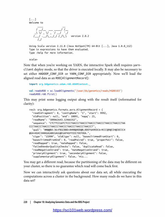
[...]Welcome to ____ __ / __/__ ___ _____/ /__ _\ \/ _ \/ _ `/ __/ '_/ /___/ .__/\_,_/_/ /_/\_\ version 2.0.2 /_/

Using Scala version 2.11.8 (Java HotSpot(TM) 64-Bit [...], Java 1.8.0_112)Type in expressions to have them evaluated.Type :help for more information.

scala>

Note that when you’re working on YARN, the interactive Spark shell requires yarn-client deploy mode, so that the driver is executed locally. It may also be necessary toset either HADOOP_CONF_DIR or YARN_CONF_DIR appropriately. Now we’ll load thealigned read data as an RDD[AlignmentRecord]:

import org.bdgenomics.adam.rdd.ADAMContext._

val readsRDD = sc.loadAlignments("/user/ds/genomics/reads/HG00103")readsRDD.rdd.first()

This may print some logging output along with the result itself (reformatted forclarity):

res3: org.bdgenomics.formats.avro.AlignmentRecord = { "readInFragment": 0, "contigName": "1", "start": 9992, "oldPosition": null, "end": 10091, "mapq": 25, "readName": "SRR062643.12466352", "sequence": "CTCTTCCGATCTCCCTAACCCTAACCCTAACCCTAACCCTAACCCTAACCCTAACCCTAACCCTAACCCTAACCCTAACCCTAACCCTAACCCTAACCCT", "qual": "##@@BA:36<FBGCBBD>AHHB@4DD@B;0DEF6A9EDC6>9CCC@9@IIH@I8IIC4@GH=HGHCIHHHGAGABEGAGG@EGAFHGFFEEE?DEFDDA.", "cigar": "1S99M", "oldCigar": null, "basesTrimmedFromStart": 0, "basesTrimmedFromEnd": 0, "readPaired": true, "properPair": false, "readMapped": true, "mateMapped": false, "failedVendorQualityChecks": false, "duplicateRead": false, "readNegativeStrand": true, "mateNegativeStrand": true, "primaryAlignment": true, "secondaryAlignment": false, "supplementaryAlignment": false, "mis...

You may get a different read, because the partitioning of the data may be different onyour cluster, so there is no guarantee which read will come back first.

Now we can interactively ask questions about our data set, all while executing thecomputations across a cluster in the background. How many reads do we have in thisdata set?



readsRDD.rdd.count()...res16: Long = 160397565

Do the reads in this data set derive from all human chromosomes?

val uniq_chr = (readsRDD.rdd .map(_.getContigName) .distinct() .collect())uniq_chr.sorted.foreach(println)...1101112[...]GL000249.1MTNC_007605XYhs37d5

Yep, we observe reads from chromosomes 1 through 22, X and Y, along with someother chromosomal chunks that are not part of the “main” chromosomes or whoselocations are unknown. Let’s analyze the statement a little more closely:

val uniq_chr = (readsRDD .rdd .map(_.getContigName) .distinct() .collect())

AlignedReadRDD: an ADAM type that contains the RDD that contains all our data.

RDD[AlignmentRecord]: the underlying Spark RDD.

RDD[String]: from each AlignmentRecord object, we extract the contig name. (A“contig” is basically equivalent to a “chromosome.”)

RDD[String]: this will cause a reduce/shuffle to aggregate all the distinct contignames; should be small, but still an RDD.

Array[String]: this triggers the computation and brings the data in the RDDback to the client app (the shell).

For a more clinical example, say we are testing an individual’s genome to checkwhether they carry any gene variants that put them at risk for having a child withcystic fibrosis (CF). Our genetic test uses next-generation DNA sequencing to gener‐



ate reads from multiple relevant genes, such as the CFTR gene (whose mutations cancause CF). After running our data through our genotyping pipeline, we determinethat the CFTR gene appears to have a premature stop codon that destroys its func‐tion. However, this mutation has never been reported before in HGMD, nor is it inthe Sickkids CFTR database, which aggregates CF gene variants. We want to go backto the raw sequencing data to see if the potentially deleterious genotype call is a falsepositive. To do so, we need to manually analyze all the reads that map to that variantlocus, say, chromosome 7 at 117149189 (see Figure 10-1):

val cftr_reads = (readsRDD.rdd .filter(_.getContigName == "7") .filter(_.getStart <= 117149189) .filter(_.getEnd > 117149189) .collect())cftr_reads.length // cftr_reads is a local Array[AlignmentRecord]...res2: Int = 9

Figure 10-1. IGV visualization of the HG00103 at chr7:117149189 in the CFTR gene

It is now possible to manually inspect these nine reads, or process them through acustom aligner, for example, and check whether the reported pathogenic variant is afalse positive. Exercise for the reader: what is the average coverage on chromosome 7?(It’s definitely too low for reliably making a genotype call at a given position.)

Say we’re running a clinical lab that is performing such carrier screening as a serviceto clinicians. Archiving the raw data using Hadoop ensures that the data stays rela‐tively warm (compared with, say, tape archive). In addition to having a reliable sys‐tem for actually performing the data processing, we can easily access all of the pastdata for quality control (QC) or for cases where there need to be manual interven‐tions, like the CFTR example presented earlier. In addition to the rapid access to the



http://www.hgmd.cf.ac.uk

http://www.genet.sickkids.on.ca

totality of the data, the centrality also makes it easy to perform large analytical stud‐ies, like population genetics, large-scale QC analyses, and so on.

Parquet Format and Columnar StorageIn the previous section, we saw how we can manipulate a potentially large amount ofsequencing data without worrying about the specifics of the underlying storage or theparallelization of the execution. However, it’s worth noting that the ADAM projectmakes use of the Parquet file format, which confers some considerable performanceadvantages that we introduce here.

Parquet is an open source file format specification and a set of reader/writer imple‐mentations that we recommend for general use for data that will be used in analyticalqueries (write once, read many times). It is largely based on the underlying data stor‐age format used in Google’s Dremel system (see “Dremel: Interactive Analysis ofWeb-scale Datasets” Proc. VLDB, 2010, by Melnik et al.), and has a data model that iscompatible with Avro, Thrift, and Protocol Buffers. Specifically, it supports most ofthe common database types (int, double, string, etc.), along with arrays andrecords, including nested types. Significantly, it is a columnar file format, meaningthat values for a particular column from many records are stored contiguously ondisk (see Figure 10-2). This physical data layout allows for far more efficient dataencoding/compression, and significantly reduces query times by minimizing theamount of data that must be read/deserialized. Parquet supports specifying differentcompression schemes for each column, as well as column-specific encoding schemessuch as run-length encoding, dictionary encoding, and delta encoding.

Another useful feature of Parquet for increasing performance is predicate pushdown.A predicate is some expression or function that evaluates to true or false based onthe data record (or equivalently, the expressions in a SQL WHERE clause). In our earlierCFTR query, Spark had to deserialize/materialize the each AlignmentRecord beforedeciding whether or not it passes the predicate. This leads to a significant amount ofwasted I/O and CPU time. The Parquet reader implementations allow us to provide apredicate class that only deserializes the necessary columns for making the decision,before materializing the full record.



http://bit.ly/2qKpnw4

http://bit.ly/2qKpnw4

http://bit.ly/2qKKkqG

http://bit.ly/2qKKkqG

Figure 10-2. Differences between a row-major and column-major data layout

For example, to implement our CFTR query using predicate pushdown, we must firstdefine a suitable predicate class that tests whether the AlignmentRecord is in the tar‐get locus:

import org.apache.parquet.filter2.dsl.Dsl._

val chr = BinaryColumn("contigName")val start = LongColumn("start")val end = LongColumn("end")

val cftrLocusPredicate = ( chr === "7" && start <= 117149189 && end >= 117149189)

See the documentation for more info on the DSL. Note we use === instead of ==.

Because we use Parquet-specific features, we must load the data explicitly with theParquet reader:

val readsRDD = sc.loadParquetAlignments( "/user/ds/genomics/reads/HG00103", Some(cftrLocusPredicate))

This should execute faster because it no longer must materialize all of theAlignmentRecord objects.



Predicting Transcription Factor Binding Sites fromENCODE DataIn this example, we will use publicly available sequence feature data to build a simplemodel for transcription factor binding. TFs are proteins that bind to specific DNAsequences in the genome and help control the expression of different genes. As aresult, they are critical in determining the phenotype of a particular cell, and areinvolved in many physiological and disease processes. ChIP-seq is an NGS-basedassay that allows the genome-wide characterization of binding sites for a particularTF in a particular cell/tissue type. However, in addition to ChIP-seq’s cost and techni‐cal difficulty, it requires a separate experiment for each tissue/TF pair. In contrast,DNase-seq is an assay that finds regions of open-chromatin genome-wide, and onlyneeds to be performed once per tissue type. Instead of assaying TF binding sites byperforming a ChIP-seq experiment for each tissue/TF combination, we’d like to pre‐dict TF binding sites in a new tissue type assuming only the availability of DNase-seqdata.

In particular, we will predict the binding sites for the CTCF TF using DNase-seq dataalong with known sequence motif data (from HT-SELEX) and other data from thepublicly available ENCODE data set. We have chosen six different cell types that haveavailable DNase-seq and CTCF ChIP-seq data for training. A training example will bea DNase hypersensitivity (HS) peak (a segment of the genome), and the binary labelfor whether the TF is bound/unbound will be derived from the ChIP-seq data.

To summarize the overall data flow: the main training/test examples will be derivedfrom the DNase-seq data. Each region of open-chromatin (an interval on thegenome) will be used to generate a prediction of whether a particular TF in a particu‐lar tissue type will be bound there. To do so, we spatially join the ChIP-seq data to theDNase-seq data; every overlap is a positive label for the DNase seq objects. Finally, toimprove the prediction accuracy, we generate some additional features at each inter‐val in the DNase-seq data, such as conservation scores (from the phylop data set), dis‐tance to a transcription start site (using the Gencode data set), and how well thesequence of the DNase-seq interval matches the known binding motif of the TF(using an empirically determined position weight matrix). In almost all cases, the fea‐tures are added into the training examples by performing a spatial join (with a possi‐ble aggregation).

We will use data from the following cell lines:

GM12878Commonly studied lymphoblastoid cell line

K562Female chronic myelogenous leukemia

Predicting Transcription Factor Binding Sites from ENCODE Data | 225


http://bit.ly/2qjsTNL



BJSkin fibroblast

HEK293Embryonic kidney

H54Glioblastoma

HepG2Hepatocellular carcinoma

First, we download the DNase data for each cell line in .narrowPeak format:

hadoop fs -mkdir /user/ds/genomics/dnasecurl -s -L <...DNase URL...> \ | gunzip \ | hadoop fs -put - /user/ds/genomics/dnase/sample.DNase.narrowPeak[...]

See accompanying code repo for actual curl commands.

Streaming decompression.

Next, we download the ChIP-seq data for the CTCF TF, also in .narrowPeak format,and the GENCODE data, in GTF format:

hadoop fs -mkdir /user/ds/genomics/chip-seqcurl -s -L <...ChIP-seq URL...> \ | gunzip \ | hadoop fs -put - /user/ds/genomics/chip-seq/samp.CTCF.narrowPeak[...]

See accompanying code repo for actual curl commands

Note how we unzip the stream of data with gunzip on the way to depositing it inHDFS. Now we download the actual human genome sequence, which is used to eval‐uate a position weight matrix to generate one of the features:

# the hg19 human genome reference sequencecurl -s -L -O \ "http://hgdownload.cse.ucsc.edu/goldenPath/hg19/bigZips/hg19.2bit"

Finally, the conservation data is available in fixed wiggle format, which is difficult toread as a splittable file. Specifically, it is not “splittable” because it is very difficult toenter the file at an arbitrary location and start reading records. This is because thewiggle format intersperses data records with some metadata that describes the currentgenome location. It is not possible to predict how far back in a file a particular taskmust read in order to obtain the metadata about the contig coordinates. Therefore,



we convert the .wigFix data to BED format using the BEDOPS tool on the way intoHDFS as well:

hadoop fs -mkdir /user/ds/genomics/phylopfor i in $(seq 1 22); do curl -s -L <...phyloP.chr$i URL...> \ | gunzip \ | wig2bed -d \ | hadoop fs -put - "/user/ds/genomics/phylop/chr$i.phyloP.bed"done[...]

See accompanying code repo for actual curl commands

This command is from the BEDOPS CLI. It’s easy to write your own Pythonscript as well

Finally, we perform a one-time conversion of the phyloP data from the text-based .bed format to Parquet in a Spark shell:

import org.bdgenomics.adam.rdd.ADAMContext._(sc .loadBed("/user/ds/genomics/phylop_text") .saveAsParquet("/user/ds/genomics/phylop"))

From all of this raw data, we want to generate a training set with a schema like thefollowing:

1. Chromosome2. Start3. End4. Highest TF motif position weight matrix (PWM) score5. Average phyloP conservation score6. Minimum phyloP conservation score7. Maximum phyloP conservation score8. Distance to closest transcription start site (TSS)9. TF identity (always “CTCF” in this case)

10. Cell line11. TF binding status (boolean; the target variable)

This data set can easily be converted into an RDD[LabeledPoint] to carry into amachine learning library. Since we need to generate the data for multiple cell lines, wewill define an RDD for each cell line individually and concatenate them at the end:



val cellLines = Vector( "GM12878", "K562", "BJ", "HEK293", "H54", "HepG2")val dataByCellLine = cellLines.map(cellLine => { // For each cell line… // …generate an RDD suitable for conversion // to RDD[LabeledPoint]})// Concatenate the RDDs and carry through into MLlib, for example

Before we start, we load some data that will be used throughout the computation,including conservation, transcription start sites, the human genome referencesequence, and the CTCF PWM as derived from HT-SELEX. We also define a coupleof utility functions that will be used to generate the PWM and TSS features:

val hdfsPrefix = "/user/ds/genomics"val localPrefix = "/user/ds/genomics"

// Set up broadcast variables for computing features along with some// utility functions

// Load the human genome reference sequenceval bHg19Data = sc.broadcast( new TwoBitFile( new LocalFileByteAccess( new File(Paths.get(localPrefix, "hg19.2bit").toString))))

// fn for finding closest transcription start site// naive; exercise for reader: make this fasterdef distanceToClosest(loci: Vector[Long], query: Long): Long = { loci.map(x => math.abs(x - query)).min}

// CTCF PWM from https://dx.doi.org/10.1016/j.cell.2012.12.009// generated with genomics/src/main/python/pwm.pyval bPwmData = sc.broadcast(Vector( Map('A'->0.4553,'C'->0.0459,'G'->0.1455,'T'->0.3533), Map('A'->0.1737,'C'->0.0248,'G'->0.7592,'T'->0.0423), Map('A'->0.0001,'C'->0.9407,'G'->0.0001,'T'->0.0591), Map('A'->0.0051,'C'->0.0001,'G'->0.9879,'T'->0.0069), Map('A'->0.0624,'C'->0.9322,'G'->0.0009,'T'->0.0046), Map('A'->0.0046,'C'->0.9952,'G'->0.0001,'T'->0.0001), Map('A'->0.5075,'C'->0.4533,'G'->0.0181,'T'->0.0211), Map('A'->0.0079,'C'->0.6407,'G'->0.0001,'T'->0.3513), Map('A'->0.0001,'C'->0.9995,'G'->0.0002,'T'->0.0001), Map('A'->0.0027,'C'->0.0035,'G'->0.0017,'T'->0.9921), Map('A'->0.7635,'C'->0.0210,'G'->0.1175,'T'->0.0980), Map('A'->0.0074,'C'->0.1314,'G'->0.7990,'T'->0.0622), Map('A'->0.0138,'C'->0.3879,'G'->0.0001,'T'->0.5981), Map('A'->0.0003,'C'->0.0001,'G'->0.9853,'T'->0.0142), Map('A'->0.0399,'C'->0.0113,'G'->0.7312,'T'->0.2177), Map('A'->0.1520,'C'->0.2820,'G'->0.0082,'T'->0.5578), Map('A'->0.3644,'C'->0.3105,'G'->0.2125,'T'->0.1127)))



http://bit.ly/2qjsTNL

// compute a motif score based on the TF PWMdef scorePWM(ref: String): Double = { val score1 = (ref.sliding(bPwmData.value.length) .map(s => { s.zipWithIndex.map(p => bPwmData.value(p._2)(p._1)).product}) .max) val rc = Alphabet.dna.reverseComplementExact(ref) val score2 = (rc.sliding(bPwmData.value.length) .map(s => { s.zipWithIndex.map(p => bPwmData.value(p._2)(p._1)).product}) .max) math.max(score1, score2)}

// build in-memory structure for computing distance to TSS// we are essentially manually implementing a broadcast join hereval tssRDD = ( sc.loadFeatures( Paths.get(hdfsPrefix, "gencode.v18.annotation.gtf").toString).rdd .filter(_.getFeatureType == "transcript") .map(f => (f.getContigName, f.getStart))).rdd .filter(_.getFeatureType == "transcript") .map(f => (f.getContigName, f.getStart)))// this broadcast variable will hold the broadcast side of the "join"val bTssData = sc.broadcast(tssRDD // group by contig name .groupBy(_._1) // create Vector of TSS sites for each chromosome .map(p => (p._1, p._2.map(_._2.toLong).toVector)) // collect into local in-memory structure for broadcasting .collect().toMap)

// load conservation data; independent of cell lineval phylopRDD = ( sc.loadParquetFeatures(Paths.get(hdfsPrefix, "phylop").toString).rdd // clean up a few irregularities in the phylop data .filter(f => f.getStart <= f.getEnd) .map(f => (ReferenceRegion.unstranded(f), f))).rdd // clean up a few irregularities in the phylop data .filter(f => f.getStart <= f.getEnd) .map(f => (ReferenceRegion.unstranded(f), f)))

Now that we’ve loaded the data necessary for defining our training examples, wedefine the body of the “loop” for computing the data on each cell line. Note how weread the text representations of the ChIP-seq and DNase data, because the data setsare not so large that they will hurt performance.

To do so, we load the DNase and ChIP-seq data as RDDs:

val dnasePath = ( Paths.get(hdfsPrefix, s"dnase/$cellLine.DNase.narrowPeak") .toString)



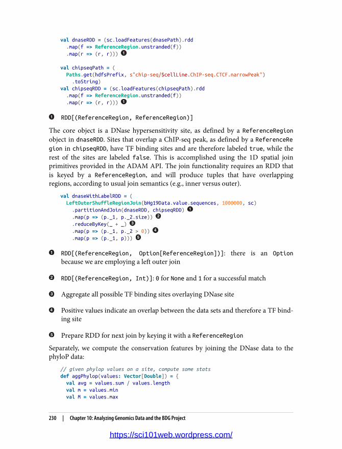
val dnaseRDD = (sc.loadFeatures(dnasePath).rdd .map(f => ReferenceRegion.unstranded(f)) .map(r => (r, r)))

val chipseqPath = ( Paths.get(hdfsPrefix, s"chip-seq/$cellLine.ChIP-seq.CTCF.narrowPeak") .toString)val chipseqRDD = (sc.loadFeatures(chipseqPath).rdd .map(f => ReferenceRegion.unstranded(f)) .map(r => (r, r)))

RDD[(ReferenceRegion, ReferenceRegion)]

The core object is a DNase hypersensitivity site, as defined by a ReferenceRegionobject in dnaseRDD. Sites that overlap a ChIP-seq peak, as defined by a ReferenceRegion in chipseqRDD, have TF binding sites and are therefore labeled true, while therest of the sites are labeled false. This is accomplished using the 1D spatial joinprimitives provided in the ADAM API. The join functionality requires an RDD thatis keyed by a ReferenceRegion, and will produce tuples that have overlappingregions, according to usual join semantics (e.g., inner versus outer).

val dnaseWithLabelRDD = ( LeftOuterShuffleRegionJoin(bHg19Data.value.sequences, 1000000, sc) .partitionAndJoin(dnaseRDD, chipseqRDD) .map(p => (p._1, p._2.size)) .reduceByKey(_ + _) .map(p => (p._1, p._2 > 0)) .map(p => (p._1, p)))

RDD[(ReferenceRegion, Option[ReferenceRegion])]: there is an Option

because we are employing a left outer join

RDD[(ReferenceRegion, Int)]: 0 for None and 1 for a successful match

Aggregate all possible TF binding sites overlaying DNase site

Positive values indicate an overlap between the data sets and therefore a TF bind‐ing site

Prepare RDD for next join by keying it with a ReferenceRegion

Separately, we compute the conservation features by joining the DNase data to thephyloP data:

// given phylop values on a site, compute some statsdef aggPhylop(values: Vector[Double]) = { val avg = values.sum / values.length val m = values.min val M = values.max



(avg, m, M)}val dnaseWithPhylopRDD = ( LeftOuterShuffleRegionJoin(bHg19Data.value.sequences, 1000000, sc) .partitionAndJoin(dnaseRDD, phylopRDD) .filter(!_._2.isEmpty) .map(p => (p._1, p._2.get.getScore.doubleValue)) .groupByKey() .map(p => (p._1, aggPhylop(p._2.toVector))))

RDD[(ReferenceRegion, Option[Feature])]

Filter out sites for which there is missing phylop data

Aggregate together all phylop values for each site

RDD[(ReferenceRegion, (Double, Double, Double))]

Now we compute the final set of features on each DNase peak by joining together thetwo RDDs from above and adding a few additional features by mapping over thesites:

// build final training example RDDval examplesRDD = ( InnerShuffleRegionJoin(bHg19Data.value.sequences, 1000000, sc) .partitionAndJoin(dnaseWithLabelRDD, dnaseWithPhylopRDD) .map(tup => { val seq = bHg19Data.value.extract(tup._1._1) (tup._1, tup._2, seq)}) .filter(!_._3.contains("N")) .map(tup => { val region = tup._1._1 val label = tup._1._2 val contig = region.referenceName val start = region.start val end = region.end val phylopAvg = tup._2._1 val phylopMin = tup._2._2 val phylopMax = tup._2._3 val seq = tup._3 val pwmScore = scorePWM(seq) val closestTss = math.min( distanceToClosest(bTssData.value(contig), start), distanceToClosest(bTssData.value(contig), end)) val tf = "CTCF" (contig, start, end, pwmScore, phylopAvg, phylopMin, phylopMax, closestTss, tf, cellLine, label)}))

Inner join to ensure we get well-defined feature vectors



Extract the genome sequence corresponding to this site in the genome and attachit to the tuple

Drop any site where the genome sequence is ambiguous

Here we build the final feature vector

This final RDD is computed in each pass of the loop over the cell lines. Finally, weunion each RDD from each cell line, and cache this data in memory in preparationfor training models off of it:

val preTrainingData = dataByCellLine.reduce(_ ++ _)preTrainingData.cache()

preTrainingData.count() // 802059preTrainingData.filter(_._12 == true).count() // 220344

At this point, the data in preTrainingData can be normalized and converted into anRDD[LabeledPoint] for training a classifier, as described in Chapter 4. Note that youshould perform cross-validation, where in each fold, you hold out the data from oneof the cell lines.

Querying Genotypes from the 1000 Genomes ProjectIn this example, we will be ingesting the full 1000 Genomes genotype data set. First,we will download the raw data directly into HDFS, unzipping in-flight, and then runan ADAM job to convert the data to Parquet. The following example commandshould be executed for all chromosomes, and can be parallelized across the cluster:

curl -s -L ftp://.../1000genomes/.../chr1.vcf.gz \ | gunzip \ | hadoop fs -put - /user/ds/genomics/1kg/vcf/chr1.vcf

adam/bin/adam-submit --master yarn --deploy-mode client \ --driver-memory 8G --num-executors 192 --executor-cores 4 \ --executor-memory 16G \ -- \ vcf2adam /user/ds/genomics/1kg/vcf /user/ds/genomics/1kg/parquet

See the accompanying repo for the actual curl commands

Copy the text VCF file into Hadoop

From an ADAM shell, we load and inspect an object like so:

import org.bdgenomics.adam.rdd.ADAMContext._

val genotypesRDD = sc.loadGenotypes("/user/ds/genomics/1kg/parquet")



val gt = genotypesRDD.rdd.first()...

Say we want to compute the minor allele frequency across all our samples for eachvariant genome-wide that overlaps a CTCF binding site. We essentially must join ourCTCF data from the previous section with the genotype data from the 1000 Genomesproject. In the previous TF binding site example, we showed how to use the ADAMjoin machinery directly. However, when we load data through ADAM, in many caseswe obtain an object that implements the GenomicRDD trait, which has some built-inmethods for filtering and joining, as we show below:

import org.bdgenomics.adam.models.ReferenceRegionimport org.bdgenomics.adam.rdd.InnerTreeRegionJoinval ctcfRDD = (sc.loadFeatures( "/user/ds/genomics/chip-seq/GM12878.ChIP-seq.CTCF.narrowPeak").rdd .map(f => { f.setContigName(f.getContigName.stripPrefix("chr")) f }) .map(f => (ReferenceRegion.unstranded(f), f)))val keyedGenotypesRDD = genotypesRDD.rdd.map(f => (ReferenceRegion(f), f))val filteredGenotypesRDD = ( InnerTreeRegionJoin().partitionAndJoin(ctcfRDD, keyedGenotypesRDD) .map(_._2))filteredGenotypesRDD.cache() filteredGenotypesRDD.count() // 408107700

We must perform this mapping because the CTCF data uses “chr1” whereas thegenotype data uses “1” to refer to the same chromosome.

The inner join performs the filtering. We broadcast the CTCF data because it isrelatively small.

Because the computation is large, we cache the resulting filtered data to avoidrecomputing it.

We also need a function that will take a Genotype and compute the counts of the ref‐erence/alternate alleles:

import scala.collection.JavaConverters._import org.bdgenomics.formats.avro.{Genotype, Variant, GenotypeAllele}def genotypeToAlleleCounts(gt: Genotype): (Variant, (Int, Int)) = { val counts = gt.getAlleles.asScala.map(allele => { allele match { case GenotypeAllele.REF => (1, 0) case GenotypeAllele.ALT => (0, 1) case _ => (0, 0) }}).reduce((x, y) => (x._1 + y._1, x._2 + y._2)) (gt.getVariant, (counts._1, counts._2))}

Querying Genotypes from the 1000 Genomes Project | 233


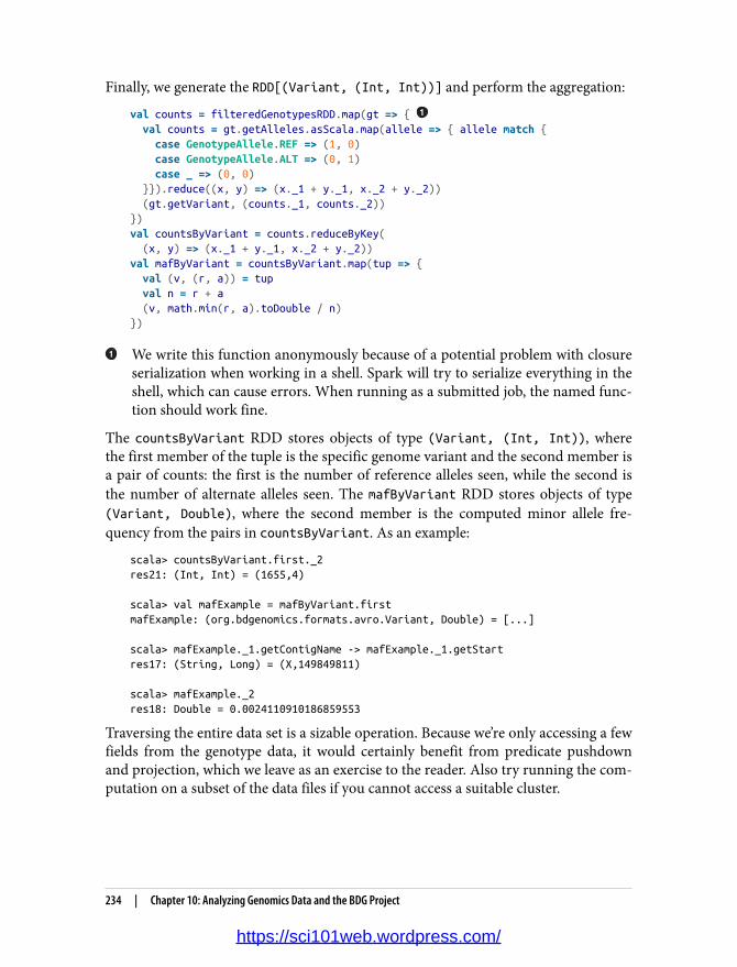
Finally, we generate the RDD[(Variant, (Int, Int))] and perform the aggregation:

val counts = filteredGenotypesRDD.map(gt => { val counts = gt.getAlleles.asScala.map(allele => { allele match { case GenotypeAllele.REF => (1, 0) case GenotypeAllele.ALT => (0, 1) case _ => (0, 0) }}).reduce((x, y) => (x._1 + y._1, x._2 + y._2)) (gt.getVariant, (counts._1, counts._2))})val countsByVariant = counts.reduceByKey( (x, y) => (x._1 + y._1, x._2 + y._2))val mafByVariant = countsByVariant.map(tup => { val (v, (r, a)) = tup val n = r + a (v, math.min(r, a).toDouble / n)})

We write this function anonymously because of a potential problem with closureserialization when working in a shell. Spark will try to serialize everything in theshell, which can cause errors. When running as a submitted job, the named func‐tion should work fine.

The countsByVariant RDD stores objects of type (Variant, (Int, Int)), wherethe first member of the tuple is the specific genome variant and the second member isa pair of counts: the first is the number of reference alleles seen, while the second isthe number of alternate alleles seen. The mafByVariant RDD stores objects of type(Variant, Double), where the second member is the computed minor allele fre‐quency from the pairs in countsByVariant. As an example:

scala> countsByVariant.first._2res21: (Int, Int) = (1655,4)

scala> val mafExample = mafByVariant.firstmafExample: (org.bdgenomics.formats.avro.Variant, Double) = [...]

scala> mafExample._1.getContigName -> mafExample._1.getStartres17: (String, Long) = (X,149849811)

scala> mafExample._2res18: Double = 0.0024110910186859553

Traversing the entire data set is a sizable operation. Because we’re only accessing a fewfields from the genotype data, it would certainly benefit from predicate pushdownand projection, which we leave as an exercise to the reader. Also try running the com‐putation on a subset of the data files if you cannot access a suitable cluster.



Where to Go from HereMany computations in genomics fit nicely into the Spark computational paradigm.When you’re performing ad hoc analysis, the most valuable contribution that projectslike ADAM provide is the set of Avro schemas that represents the underlying analyti‐cal objects (along with the conversion tools). We saw how once data is converted intothe corresponding Avro schemas, many large-scale computations become relativelyeasy to express and distribute.

While there may still be a relative dearth of tools for performing scientific research onHadoop/Spark, there do exist a few projects that could help avoid reinventing thewheel. We explored the core functionality implemented in ADAM, but the projectalready has implementations for the entire GATK best-practices pipeline, includingBQSR, indel realignment, and deduplication. In addition to ADAM, many institu‐tions have signed on to the Global Alliance for Genomics and Health, which hasstarted to generate schemas of its own for genomics analysis. The Broad Institute isnow developing major software projects using Spark, including the newest version ofthe GATK4 and a new project called Hail for large-scale population genetics compu‐tations. The Hammerbacher lab at Mount Sinai School of Medicine has also devel‐oped Guacamole, a suite of tools mainly aimed at somatic variant calling for cancergenomics. All of these tools are open source, so if you start using them in your ownwork, please consider contributing improvements!



https://github.com/broadinstitute/gatk

https://github.com/hail-is/hail

https://github.com/hammerlab/guacamole

CHAPTER 11

Analyzing Neuroimaging Data withPySpark and Thunder

Uri Laserson

We are not interested in the fact that the brain has the consistency of cold porridge.—Alan Turing

Advances in imaging equipment and automation have led to a glut of data on thefunction of the brain. While past experiments might have generated time series datafrom only a handful of electrodes in the brain or a small number of static images ofbrain slices, technologies today can sample brain activity from a large number of neu‐rons in a large region while organisms are actively behaving. Indeed, the BRAIN Ini‐tiative is a government-funded initiative with the lofty technology development goalsof enabling, for example, simultaneous recording of the electrical activity of everyneuron of the mouse brain over an extended period of time. While breakthroughs inmeasurement technology are certainly necessary, the amount of data generated willcreate completely new paradigms for biology.

In this chapter, we will introduce the PySpark API for interacting with Spark throughPython, as well as the Thunder project, which is developed on top of PySpark for pro‐cessing large amounts of time series data in general and neuroimaging data in partic‐ular. PySpark is a particularly flexible tool for exploratory big data analysis because itintegrates well with the rest of the PyData ecosystem, including matplotlib for visuali‐zation, and even IPython Notebook (Jupyter) for “executable documents.”

We will marshal these tools for the task of understanding some of the structure ofzebrafish brains. Using Thunder, we will cluster different regions of the brain (repre‐senting groups of neurons) to discover patterns of activity as the zebrafish behavesover time. Like the chapter, Thunder was built on the PySpark RDD API, and contin‐ues to use it.

237


https://www.braininitiative.nih.gov

https://www.braininitiative.nih.gov

https://spark.apache.org/docs/latest/api/python/

http://thunder-project.org

Overview of PySparkPython is a favorite tool for many data scientists, due to its high-level syntax andextensive library of packages, among other things. The Spark ecosystem has recog‐nized Python’s importance in the data analytics milieu and has invested in a PythonAPI for using Spark, despite Python’s historical difficulties integrating with the JVM.

Python for Scientific Computing and Data SciencePython has become a favorite tool for scientific computing and data science. It is nowbeing used for many applications that would have traditionally used MATLAB, R, orMathematica. The reasons include the following:

• Python is a high-level language that is easy to use and learn.• It has an extensive library system ranging from niche numerical calculations to

web-scraping utilities to data visualization tools.• It interfaces easily with C/C++ code, allowing access to high-performance libra‐

ries, including BLAS/LAPACK/ATLAS.

Some libraries to keep in mind in particular include:

numpy/scipy/matplotlibThese libraries recapitulate typical MATLAB functionality, including fast arrayoperations, scientific functions, and a widely used MATLAB-inspired plottinglibrary.

pandas

This library provides functionality similar to R’s data.frame, and oftentimes withmuch higher performance to boot.

scikit-learn/statsmodelsThese libraries provide high-quality implementations of machine learning algo‐rithms (e.g., classification/regression, clustering, matrix factorization) and statis‐tical models.

nltk

A popular library for natural language processing.

You can find a large list of many other available libraries curated at the awesome-python repository on GitHub.

Start PySpark just like Spark:

export PYSPARK_DRIVER_PYTHON=ipython # PySpark can use the IPython shellexport PYSPARK_PYTHON=path/to/desired/python # For the worker nodespyspark --master ... --num-executors ...

238 | Chapter 11: Analyzing Neuroimaging Data with PySpark and Thunder


https://bit.ly/186ShId

https://github.com/vinta/awesome-python

https://github.com/vinta/awesome-python

pyspark takes the same Spark arguments as spark-submit and spark-shell

We can submit Python scripts using spark-submit, which will detect the .py exten‐sion on our scripts. You can specify which version of Python to use for the driver(e.g., IPython) and for the worker nodes; their versions must match. When thePython shell starts, it creates a Python SparkContext object (named sc) throughwhich we interact with the cluster. Once the SparkContext is available, the PySparkAPI is very similar to the Scala API. For example, to load some CSV data:

raw_data = sc.textFile('path/to/csv/data') # RDD[string]# filter, split on comma, parse floats to get a RDD[list[float]]data = (raw_data .filter(lambda x: x.startswith("#")) .map(lambda x: map(float, x.split(','))))data.take(5)

Just like in the Scala RDD API, we load a text file, filter out rows that start with #, andparse the CSV data into a list of float values. The Python functions passed to, forexample, filter and map, are very flexible. They must take a Python object andreturn a Python object (in the case of filter, the return value is interpreted as aboolean). The only restrictions are that the Python function objects must be serializa‐ble with cloudpickle (which includes anonymous lambda functions), and any neces‐sary modules referenced in the closures must be available on the PYTHONPATH of theexecutor Python processes. To ensure the availability of referenced modules, eitherthe modules must be installed cluster-wide and available on the PYTHONPATH of theexecutor Python processes, or the corresponding module ZIP/EGG files must beexplicitly distributed around by Spark, which will then add them to the PYTHONPATH.This latter functionality can be accomplished by a call to sc.addPyFile().

The PySpark RDDs are just RDDs of Python objects: like Python lists, they can storeobjects with mixed types (because underneath, all the objects are instances of PyObject).

PySpark InternalsIt is useful to understand a bit about how PySpark is implemented in order to sim‐plify debugging and also to be conscious of possible performance pitfalls (seeFigure 11-1).

Overview of PySpark | 239


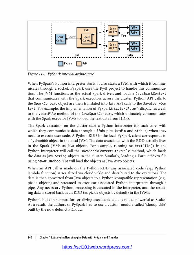
Figure 11-1. PySpark internal architecture

When PySpark’s Python interpreter starts, it also starts a JVM with which it commu‐nicates through a socket. PySpark uses the Py4J project to handle this communica‐tion. The JVM functions as the actual Spark driver, and loads a JavaSparkContextthat communicates with the Spark executors across the cluster. Python API calls tothe SparkContext object are then translated into Java API calls to the JavaSparkContext. For example, the implementation of PySpark’s sc.textFile() dispatches a callto the .textFile method of the JavaSparkContext, which ultimately communicateswith the Spark executor JVMs to load the text data from HDFS.

The Spark executors on the cluster start a Python interpreter for each core, withwhich they communicate data through a Unix pipe (stdin and stdout) when theyneed to execute user code. A Python RDD in the local PySpark client corresponds toa PythonRDD object in the local JVM. The data associated with the RDD actually livesin the Spark JVMs as Java objects. For example, running sc.textFile() in thePython interpreter will call the JavaSparkContexts textFile method, which loadsthe data as Java String objects in the cluster. Similarly, loading a Parquet/Avro fileusing newAPIHadoopFile will load the objects as Java Avro objects.

When an API call is made on the Python RDD, any associated code (e.g., Pythonlambda function) is serialized via cloudpickle and distributed to the executors. Thedata is then converted from Java objects to a Python-compatible representation (e.g.,pickle objects) and streamed to executor-associated Python interpreters through apipe. Any necessary Python processing is executed in the interpreter, and the result‐ing data is stored back as an RDD (as pickle objects by default) in the JVMs.

Python’s built-in support for serializing executable code is not as powerful as Scala’s.As a result, the authors of PySpark had to use a custom module called “cloudpickle”built by the now defunct PiCloud.



Overview and Installation of the Thunder LibraryThunder Examples and Documentation

The Thunder package has excellent documentation and tutorials.The following examples draw from the documentation’s data setsand tutorials.

Thunder is a Python tool set for processing large amounts of spatial/temporal datasets (i.e., large multidimensional matrices) on Spark. It makes heavy use of NumPyfor matrix computations and also the MLlib library for distributed implementationsof some statistical techniques. Python also makes it very flexible and accessible to abroad audience. In the following section, we introduce the Thunder API and attemptto classify some neural traces into a set of patterns using MLlib’s K-means implemen‐tation as wrapped by Thunder and PySpark. Installing Thunder simply requires call‐ing pip install thunder-python, though it must be installed on all worker nodes.

After installation, and setting the SPARK_HOME environment variable, we can createPySpark shell like so:

$ export PYSPARK_DRIVER_PYTHON=ipython # recommended as usual$ pyspark --master ... --num-executors ...

[...some logging output...]Welcome to ____ __ / __/__ ___ _____/ /__ _\ \/ _ \/ _ `/ __/ '_/ /__ / .__/\_,_/_/ /_/\_\ version 2.0.2 /_/

Using Python version 2.7.6 (default, Apr 9 2014 11:54:50)SparkContext available as sc.

Running thunder version 0.5.0_devA thunder context is available as tsc

In [1]:

Loading Data with ThunderThunder was designed especially with neuroimaging data sets in mind. Therefore, itis geared toward analyzing data from large sets of images that are often captured overtime.

Let’s start by loading some images of zebrafish brains from an example data set pro‐vided by the Thunder repository in S3: s3://thunder-sample-data/images/fish/. For

Overview and Installation of the Thunder Library | 241


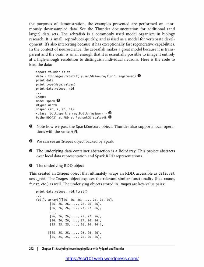
the purposes of demonstration, the examples presented are performed on enor‐mously downsampled data. See the Thunder documentation for additional (andlarger) data sets. The zebrafish is a commonly used model organism in biologyresearch. It is small, reproduces quickly, and is used as a model for vertebrate devel‐opment. It’s also interesting because it has exceptionally fast regenerative capabilities.In the context of neuroscience, the zebrafish makes a great model because it is trans‐parent and the brain is small enough that it is essentially possible to image it entirelyat a high-enough resolution to distinguish individual neurons. Here is the code toload the data:

import thunder as tddata = td.images.fromtif('/user/ds/neuro/fish', engine=sc) print dataprint type(data.values)print data.values._rdd...Imagesmode: spark dtype: uint8shape: (20, 2, 76, 87)<class 'bolt.spark.array.BoltArraySpark'> PythonRDD[2] at RDD at PythonRDD.scala:48

Note how we pass the SparkContext object. Thunder also supports local opera‐tions with the same API.

We can see an Images object backed by Spark.

The underlying data container abstraction is a BoltArray. This project abstractsover local data representation and Spark RDD representations.

The underlying RDD object

This created an Images object that ultimately wraps an RDD, accessible as data.values._rdd. The Images object exposes the relevant similar functionality (like count,first, etc.) as well. The underlying objects stored in Images are key-value pairs:

print data.values._rdd.first()...((0,), array([[[26, 26, 26, ..., 26, 26, 26], [26, 26, 26, ..., 26, 26, 26], [26, 26, 26, ..., 27, 27, 26], ..., [26, 26, 26, ..., 27, 27, 26], [26, 26, 26, ..., 27, 26, 26], [25, 25, 25, ..., 26, 26, 26]],

[[25, 25, 25, ..., 26, 26, 26], [25, 25, 25, ..., 26, 26, 26],



[26, 26, 26, ..., 26, 26, 26], ..., [26, 26, 26, ..., 26, 26, 26], [26, 26, 26, ..., 26, 26, 26], [25, 25, 25, ..., 26, 26, 26]]], dtype=uint8))

The key (0,) corresponds to the zeroth image in the set (they are ordered lexico‐graphically from the data directory), and the value is a NumPy array correspondingto the image. All of the core data types in Thunder are ultimately backed by PythonRDDs of key-value pairs, where the keys are typically some kind of tuple and the val‐ues are NumPy arrays. The keys and values always have a homogeneous type acrossthe RDD, even though PySpark generally allows RDDs of heterogeneous collections.Because of the homogeneity, the Images object exposes a .shape property describingthe underlying dimensions:

print data.shape...(20, 2, 76, 87)

This describes 20 “images” where each image is a 2×76×87 stack.

Pixels, Voxels, and Stacks“Pixel” is a portmanteau of “picture element.” Digital images can be modeled as sim‐ple 2D matrices of intensity values, and each element in the matrix is a pixel. (A colorimage would require three of these matrices, one each for a red, green, and blue chan‐nel.) However, because the brain is a 3D object, a single 2D slice is not nearly enoughto capture its activity. To address this, multiple techniques will either acquire multiple2D images in different planes on top of each other (a z-stack), and some will evengenerate 3D information directly (e.g., light field microscopy). This ultimately pro‐duces a 3D matrix of intensity values, where each value represents a “volume ele‐ment,” or “voxel.” Consistent with this, Thunder models all images as 2D or 3Dmatrices, depending on the specific data type, and can read file formats like .tiff thatcan natively represent 3D stacks.

One of the features of working in Python is that we can easily visualize our data whileworking with the RDDs, in this case using the venerable matplotlib library (seeFigure 11-2):

import matplotlib.pyplot as pltimg = data.first()plt.imshow(img[:, :, 0], interpolation='nearest', aspect='equal', cmap='gray')

Loading Data with Thunder | 243


Figure 11-2. A single slice from the raw zebrafish data

The Images API offers useful methods for working with the image data in a dis‐tributed fashion—for example, to subsample each image down (see Figure 11-3):

subsampled = data.subsample((1, 5, 5)) plt.imshow(subsampled.first()[:, :, 0], interpolation='nearest', aspect='equal', cmap='gray')print subsampled.shape...(20, 2, 16, 18)

The stride to subsample each dimension: the first dimension is not subsampledwhile the second and third dimensions take every fifth value. Note that this is anRDD operation, so it returns immediately, waiting for an RDD action to triggercomputation.



Figure 11-3. A single slice from the subsampled zebrafish data

While analyzing the collection of images may be useful for certain operations (e.g.,normalizing images in certain ways), it’s difficult to take the temporal relationship ofthe images into account. To do so, we’d rather work with the image data as a collec‐tion of pixel/voxel time series. This is exactly what the Thunder Series object is for,and there is an easy way to convert:

series = data.toseries()

This operation executes a large-scale reorganization of the data into a Series object,which is an RDD of key-value pairs where the key is a tuple of the coordinates of eachimage (i.e., the voxel identifier) and the value is a 1D NumPy array corresponding tothe time series of values:

print series.shapeprint series.indexprint series.count()...(2, 76, 87, 20)[ 0 1 2 3 4 5 6 7 8 9 10 11 12 13 14 15 16 17 18 19]13224

Whereas data was a collection of 20 images with dimensions 76×87×2, series is acollection of 13,224 (76×87×2) time series of length 20. The series.index property



is a Pandas-style index that can be used to reference each of the arrays. Because ouroriginal images were 3D, the keys are 3-tuples:

print series.values._rdd.takeSample(False, 1)[0]...((0, 50, 6), array([29, 29, 29, 29, 29, 29, 29, 29, 29, 29, 29, 29, 29, 29, 29, 29, 29, 29, 29, 29], dtype=uint8))

The Series API offers many methods for performing computations across the timeseries, either at the per-series level or across all series. For example:

print series.max().values...[[[[158 152 145 143 142 141 140 140 139 139 140 140 142 144 153 168 179 185 185 182]]]]

computes the maximum value across all voxels at each time point, while:

stddev = series.map(lambda s: s.std())print stddev.values._rdd.take(3)print stddev.shape...[((0, 0, 0), array([ 0.4])), ((0, 0, 1), array([ 0.35707142]))](2, 76, 87, 20)

computes the standard deviation of each time series and returns the result as an RDD,preserving all the keys.

We can also locally repack the Series into a NumPy array with the specified shape(2×76×87 in this case):

repacked = stddev.toarray()plt.imshow(repacked[:,:,0], interpolation='nearest', cmap='gray', aspect='equal')print type(repacked)print repacked.shape...<type 'numpy.ndarray'>(2, 76, 87)

This allows us to plot the standard deviation of each voxel using the same spatial rela‐tionships (see Figure 11-4). We should take care to make sure that we’re not trying toreturn too much data to the client, because it will consume significant network andmemory resources.



Figure 11-4. Standard deviation of each voxel in the raw zebrafish data

Alternatively, we can look at the centered time series directly, by plotting a subset ofthem (see Figure 11-5):

plt.plot(series.center().sample(50).toarray().T)



Figure 11-5. A random subset of 50 of the centered time series

It’s also very easy to apply any UDFs to each series (including lambda functions),using the map method, which calls the underlying RDD’s .map() method on the val‐ues in the underlying key-value pairs.

series.map(lambda x: x.argmin())

Thunder Core Data TypesMore generally, the two core data types in Thunder, Series and Images, both inheritfrom the Data class, which ultimately contains a BoltArray that is backed by either alocal NumPy array or a Spark RDD. The Data class models RDDs of key-value pairs,where the key represents some type of semantic identifier (e.g., a tuple of coordinatesin space), and the value is a NumPy array of actual data. For the Images object, thekey could be a time point, for example, and the value is the image at that time pointformatted as a NumPy array. For the Series object, the key might be an n-dimensional tuple with the coordinates of the corresponding voxel, while the value isa 1D NumPy array representing the time series of measurements at that voxel. All thearrays in Series must have the same dimensions.



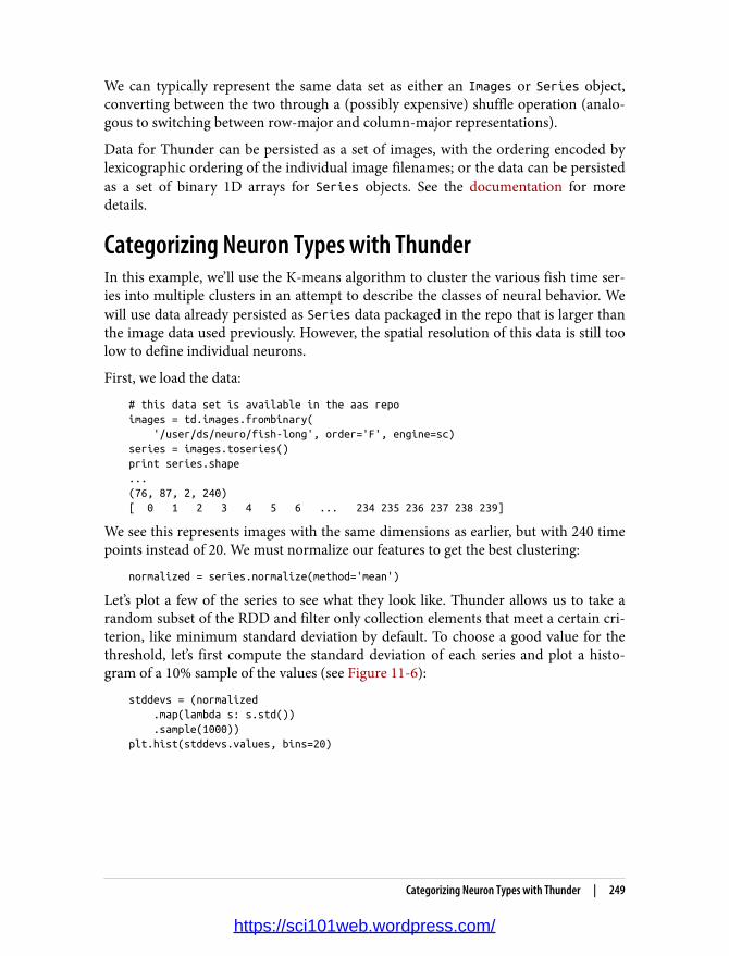
We can typically represent the same data set as either an Images or Series object,converting between the two through a (possibly expensive) shuffle operation (analo‐gous to switching between row-major and column-major representations).

Data for Thunder can be persisted as a set of images, with the ordering encoded bylexicographic ordering of the individual image filenames; or the data can be persistedas a set of binary 1D arrays for Series objects. See the documentation for moredetails.

Categorizing Neuron Types with ThunderIn this example, we’ll use the K-means algorithm to cluster the various fish time ser‐ies into multiple clusters in an attempt to describe the classes of neural behavior. Wewill use data already persisted as Series data packaged in the repo that is larger thanthe image data used previously. However, the spatial resolution of this data is still toolow to define individual neurons.

First, we load the data:

# this data set is available in the aas repoimages = td.images.frombinary( '/user/ds/neuro/fish-long', order='F', engine=sc)series = images.toseries()print series.shape...(76, 87, 2, 240)[ 0 1 2 3 4 5 6 ... 234 235 236 237 238 239]

We see this represents images with the same dimensions as earlier, but with 240 timepoints instead of 20. We must normalize our features to get the best clustering:

normalized = series.normalize(method='mean')

Let’s plot a few of the series to see what they look like. Thunder allows us to take arandom subset of the RDD and filter only collection elements that meet a certain cri‐terion, like minimum standard deviation by default. To choose a good value for thethreshold, let’s first compute the standard deviation of each series and plot a histo‐gram of a 10% sample of the values (see Figure 11-6):

stddevs = (normalized .map(lambda s: s.std()) .sample(1000))plt.hist(stddevs.values, bins=20)

Categorizing Neuron Types with Thunder | 249


http://docs.thunder-project.org

Figure 11-6. Distribution of the standard deviations of the voxels

With this in mind, we’ll choose a threshold of 0.1 to look at the most “active” series(see Figure 11-7):

plt.plot( normalized .filter(lambda s: s.std() >= 0.1) .sample(50) .values.T)



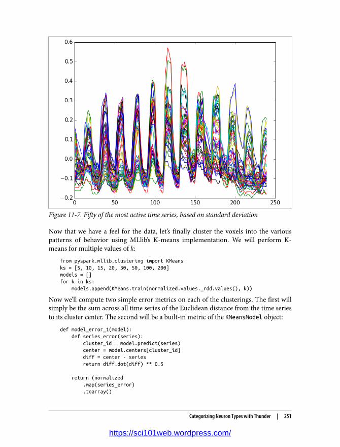
Figure 11-7. Fifty of the most active time series, based on standard deviation

Now that we have a feel for the data, let’s finally cluster the voxels into the variouspatterns of behavior using MLlib’s K-means implementation. We will perform K-means for multiple values of k:

from pyspark.mllib.clustering import KMeansks = [5, 10, 15, 20, 30, 50, 100, 200]models = []for k in ks: models.append(KMeans.train(normalized.values._rdd.values(), k))

Now we’ll compute two simple error metrics on each of the clusterings. The first willsimply be the sum across all time series of the Euclidean distance from the time seriesto its cluster center. The second will be a built-in metric of the KMeansModel object:

def model_error_1(model): def series_error(series): cluster_id = model.predict(series) center = model.centers[cluster_id] diff = center - series return diff.dot(diff) ** 0.5

return (normalized .map(series_error) .toarray()



.sum())

def model_error_2(model): return model.computeCost(normalized.values._rdd.values())

We will compute both error metrics for each value of k and plot them (seeFigure 11-8):

import numpy as nperrors_1 = np.asarray(map(model_error_1, models))errors_2 = np.asarray(map(model_error_2, models))plt.plot( ks, errors_1 / errors_1.sum(), 'k-o', ks, errors_2 / errors_2.sum(), 'b:v')

Figure 11-8. K-means error metrics as a function of k (black circles are model_error_1and blue triangles are model_error_2)

We’d expect these metrics to generally be monotonically decreasing with k; it seemslike k=20 might be a sharper elbow in the curve. Let’s visualize the cluster centers thatwe’ve learned from the data (see Figure 11-9):

model20 = models[3]plt.plot(np.asarray(model20.centers).T)



Figure 11-9. Model centers for k=20

It’s also easy to plot the images themselves with the voxels colored according to theirassigned cluster (see Figure 11-10):

import seaborn as snsfrom matplotlib.colors import ListedColormapcmap_cat = ListedColormap(sns.color_palette("hls", 10), name='from_list')by_cluster = normalized.map(lambda s: model20.predict(s)).toarray()plt.imshow(by_cluster[:, :, 0], interpolation='nearest', aspect='equal', cmap='gray')



Figure 11-10. Voxels colored by cluster membership

It’s clear that the learned clusters recapitulate certain elements of zebrafish brain anat‐omy. If the original data were high resolution enough to resolve subcellular struc‐tures, we could first perform clustering of the voxels with k equal to an estimate ofthe number of neurons in the imaged volume. This would allow us to effectively mapout the entire neuron cell bodies. We would then define time series for each neuron,which could be used for clustering again to determine different functional categories.

Where to Go from HereThunder is a relatively new project, but includes a rich set of functionality. In addi‐tion to statistics on time series and clustering, it has modules for matrix factoriza‐tions, regression/classification, and tools for visualization. It has fantasticdocumentation and tutorials covering a large array of its functionality. To see Thun‐der in action, see the “Mapping brain activity at scale with cluster computing” byThunder authors in Nature Methods (July 2014).



https://bit.ly/186YPqi

Index

Aactions, 19ADAM (genomics tool set)

ingesting data with ADAM CLI, 217-224Parquet format and columnar storage,

223-224aggregations, computing with DataFrame, 30alternating least squares (ALS) algorithm, 45-48anomaly detection

about, 94categorical variables, 108choosing K, 99-101clustering of full normalized data set, 111data visualization with SparkR, 102-105defined for K-means clustering, 111feature normalization, 106initial clustering attempt, 97-99K-means clustering for, 95-113KDD Cup 1999 data set, 96network intrusion, 95using labels with entropy, 109

Apache Maven, 18area under the curve (AUC)

computing for recommendation engine, 58defined, 57

Audioscrobbler data set, 44average path length, 161-166Avro, 215-217

Bbandwidth, 201big data

analyzing, 1-8and challenges of data science, 3

Big Data Genomics (BDG) Project, 216(see also genomics data analysis)

bioinformatics (see genomics data analysis)bootstrapping, 209breeze-viz library, 201broadcast variables, 52bulk-synchronous parallel (BSP) programs, 162

Ccaching, 6, 28case classes, 38categorical features, 86-88

defined, 67encoding as number, 72translating into binary indicator features,

108categorical variables, 108chi-squared test, 155classification, defined, 66client

bringing data from cluster to, 19-22shipping code to cluster from, 22

cliques, 160cluster

bringing data to client from, 19-22shipping code from client to, 22

clusteringK-means (see K-means clustering)

clustering coefficient, 160clustering, defined, 94co-occurrence network analysis

analyzing MeSH major topics and co-occurrences, 143-146

analyzing the filtered graph, 158

255


connected components, 150-152constructing a co-occurrence network with

GraphX, 146-149degree distribution, 153-155filtering out noisy edges, 155-159getting data for, 140-142parsing XML documents with Scala XML

library, 142processing EdgeTriplets, 156-158small-world networks, 159-166understanding the structure of networks,

150-155co-occurrence networks

analyzing with GraphX, 137-167MEDLINE citation index analysis, 139-166

code, shipping from client to cluster, 22collaborative filtering algorithms, 45columnar storage, 223-224compilation, 18concept space, 123Conditional Value at Risk (CVaR), 192, 208confusion matrix, 77connected components(), 150-152connected graph, 150, 153contingency table, 40cosine similarity, 129CountVectorizer, 122Covtype data set, 71cross tabulation (crosstab), 40cross-validation (CV) set, 58, 74, 83cross-validation, k-fold, 59, 83CVaR (see Conditional Value at Risk)cyber attacks (see network traffic, anomaly

detection in)

DDAG (directed acyclic graph), 5data analytics (generally)

exploratory vs. operational, 6lab vs. factory settings, 4

data cleansing, 9bringing data from cluster to client, 19-22DataFrame and, 23-26fast summary statistics for DataFrame, 32for recommendation engine, 48-51record linkage, 12Scala, 10Scala and Spark, 9-42shipping code from client to cluster, 22

Spark programming model, 11Spark shell, 13-18SparkContext, 15-18with DataFrame API, 26-32

data sciencechallenges of, 3defined, 1

DataFrame, 23-26about, 5, 7aggregation functions, 30caching, 28data formats supported by, 25fast summary statistics for, 32feature selection, 37joins, 37pivoting/reshaping, 33-37

DataFrame APIanalyzing data with, 26-32Spark SQL vs., 31, 37

Dataset, 5, 7decision rules, 81decision trees, 68-71

categorical features and, 86-88for forest cover prediction, 74-80hyperparameters, 80-82tuning, 82-86

degree distributions, 153-155directed acyclic graph (DAG), 5document space, 123document-term matrix, 116-118

Eedge weighting

analyzing the filtered graph, 158filtering out noisy edges, 155-159processing EdgeTriplets, 156-158

EdgeTriplets, 156-158ENCODE data set, 225-232entropy

and labeling, 109defined, 81

Esri Geometry API, 172-174Estimators, 8, 122Euclidean distance, 94exceptions (see invalid records)expected shortfall, 192

(see also conditional value at risk)experimentation, 3exploratory analytics, 6

256 | Index


Ffactor weights, 198-200false negatives, 40false positives, 40feature vectors, 67features

categorical, 86-88in prediction, 66normalization, 106selecting, 37

financial risk, estimating with Monte Carlosimulation (see Monte Carlo simulation)

forest cover prediction, 71-92categorical features, 86-88data preparation, 71-73decision tree hyperparameters, 80-82decision tree tuning, 82-86first decision tree, 74-80making predictions, 91random decision forests in, 88-91

functions, Scala, 21

GGalton, Sir Francis, 65genomics data analysis, 213-235

decoupling storage from modeling, 214-217ingesting data with ADAM CLI, 217-224predicting transcription factor binding sites

from ENCODE data, 225-232querying genotypes from the 1000 Genomes

Project data set, 232-234GeoJSON, 174-176geospatial data

Esri Geometry API, 172-174GeoJSON, 174-176

Gini impurity, 81graph theory, 137GraphFrames, 138GraphX

analyzing co-occurrence networks with,137-167

constructing a co-occurrence network with,146-149

GraphFrames and, 138MEDLINE citation index network analysis,

139-166

HHadoop ecosystem, 3, 6Hive, connecting Spark SQL to, 31HPC (high-performance computing), 2hyperparameters

decision tree, 80-82for recommendation engine, 60-62

Iimplicit feedback, 44implicit types, 34in-memory caching, 6invalid records, 178-182iteration, 3

Jjoins, DataFrames, 37

Kk, choosing, 99-101k-fold cross-validation, 59, 83K-means clustering, 93-113

categorical variables, 108choosing K, 99-101clustering of full normalized data set, 111feature normalization, 106for anomaly detection, 95-113for neuroimaging data, 251initial clustering attempt, 97-99KDD Cup 1999 data set, 96using labels with entropy, 109visualization with SparkR, 102-105

KDD Cup 1999 data set, 96kernel density estimation, 201

Llabels, 109latent semantic analysis (LSA), 115-136

about, 115computing TF-IDFs for, 121-123document-document relevance, 132document-term matrix, 116-118document-term relevance, 133finding important concepts with, 125-129getting data for, 118lemmatization, 120multiple-term queries, 134parsing/preparing data for, 118

Index | 257


querying/scoring with low-dimensionalrepresentation, 129

SVD and, 123-125term-term relevance, 130

latent-factor models, 45learning algorithms, 67lemmatization, 120libraries

compiling code referencing external libra‐ries, 18

external, 18working with third-party libraries in Spark,

171local clustering coefficient, 160low-dimensional representation, 129LSA (see latent semantic analysis)

MMapReduce, Spark vs., 5matrix, 123-125matrix completion algorithms, 46matrix factorization model, 45MEDLINE citation index, 139-166MeSH (Medical Subject Headings), 139,

143-146MLlib

ALS implementation, 48, 63inputs for recommendation engine, 74K-means clustering, 94, 101, 251metadata storage, 87random element behavior, 54StandardScaler, 106StreamingKMeans, 113SVD implementation, 123translating categorical features into binary

indicator features, 109modeling, decoupling storage from, 214-217Monte Carlo simulation, 191-212

about, 193data preprocessing, 195-198defined, 191determining factor weights, 198-200evaluating results, 209-211financial terminology, 192getting data for, 195multivariate normal distribution, 204risk model, 194running trials, 205-208sampling, 201-204

visualizing distribution of returns, 208multigraphs, 149multivariate normal distribution, 204music recommendations (see recommendation

engine)

Nnetwork intrusion, 95network science

analyzing co-occurrence networks withGraphX, 137-167

origins, 137network traffic, anomaly detection in, 95-113

categorical variables, 108choosing K, 99-101clustering of full normalized data set, 111data visualization with SparkR, 102-105feature normalization, 106initial clustering attempt, 97-99KDD Cup 1999 data set, 96network intrusion, 95using labels with entropy, 109

neuroimaging data analysis, 237-254categorizing neuron types with Thunder,

249-254loading data with Thunder, 241-249PySpark and, 238-240Thunder, 241-254Thunder core data types, 248Thunder installation and overview, 241

New York City taxi trips, geospatial/temporaldata analysis of, 169-189geospatial analysis, 182-185geospatial data, 172-176getting data, 170handling invalid records at scale, 178-182preparing data, 176-185sessionization in Spark, 185-189temporal data, 172, 180working with third-party libraries in Spark,

171normalization of features, 106numeric features, 67

O1000 Genomes Project data set, 232open-source libraries, 171operational analytics, 4, 6overfitting, 71, 86

258 | Index


PParquet, 223-224partially applied function, 59partitions, RDDs and, 16pivot table, 79pixels, 243POF (proportion-of-failures) test, 210polysemy, 117predicate pushdown, 223prediction, 65-92

categorical features, 86-88data preparation, 71-73decision tree hyperparameters, 80-82decision tree tuning, 82-86decision trees, 68-71feature vectors, 67features in, 66first decision tree for, 74-80making, 91of forest cover in Colorado, 71-92random decision forests in, 88-91regression and, 65training examples, 67

Pregel, 161-166preprocessing, importance of, 3production environments, preparing models

for, 38-40proportion-of-failures (POF) test, 210PySpark

internal architecture, 239overview, 238-240

Python, 238

Rrandom decision forests, 68, 88-91RDDs (see Resilient Distributed Datasets)Receiver Operating Characteristic (ROC)

curve, 57recommendation engine, 43-64

alternating least squares algorithm, 45-48Audioscrobbler data set, 44building first model for, 51-54computing AUC, 58data preparation for, 48-51data set for, 44evaluating recommendation quality, 56-58hyperparameter selection, 60-62making recommendations, 62spot checking recommendations, 54-56

record linkage, 12records, invalid, 178-182regression

defined, 66prediction and, 65

regression to the mean, 65REPL, 18Resilient Distributed Datasets (RDDs)

about, 16actions on, 19DataFrame and, 23-26GraphX and, 147problems with, 7

risk, estimating with Monte Carlo simulation(see Monte Carlo simulation)

ROC (Receiver Operating Characteristic)curve, 57

RPC frameworks, 216

SScala

basics, 10bringing data from cluster to client, 19-22declaring functions in, 21model evaluation, 40parsing XML documents with Scala XML

library, 142preparing models for production environ‐

ments, 38-40scoring models, 38-41

evaluation, 40preparing for production environments,

38-40secondary sorts, 186-189serialization frameworks, 216sessionization

defined, 185in Spark, 185-189secondary sorts in Spark, 186-189

singular value decomposition (SVD), 116,123-125

small-world networks, 159-166cliques, 160computing average path length with Pregel,

161-166local clustering coefficients, 160

sorts, secondary, 186-189Spark 2.0, 7, 25Spark ML API, 8

Index | 259


Spark shell, 13-18Spark, origins of, 4-6Spark SQL

connecting to Hive, 31DataFrame API vs., 31, 37UDFs and, 182

SparkContext, 15-18SparkR, 102-105Spray, 174-176stemming, 120stop words, 120storage, decoupling from modeling, 214-217summary statistics

for DataFrame, 32pivoting/reshaping, 33-37

supervised learning, 66SVD (see singular value decomposition)

Ttarget, of prediction, 67temporal data, 172, 180

(see also New York City taxi trip data)term space, 123test set, 74, 83text data (see latent semantic analysis)TF-IDF

computing for LSA, 121-123defined, 117

third-party libraries, 171Thunder, 241-254

categorizing neuron types with, 249-254core data types, 248installation and overview, 241loading data with, 241-249

tokens, 118training set, 67training, of learning algorithm, 67Transformers, 8, 75, 82type inference, 17

Uunstructured text data (see latent semantic

analysis)unsupervised learning, 94

(see also K-means clustering)user-defined functions (UDFs), 8, 181

VValue at Risk (VaR)

conditional, 192, 208estimating with Monte Carlo simulation

(see Monte Carlo simulation)historical simulation, 193methods for calculating, 193variance-covariance calculation, 193

variablescategorical, 108in Scala, 17

vectors, 67, 122, 129voxels, 243

WWikipedia, understanding with LSA, 116-136

(see also latent semantic analysis)

XXML documents, parsing, 142

260 | Index


About the AuthorsSandy Ryza develops algorithms for public transit at Remix. Before that, he was asenior data scientist at Cloudera and Clover Health. He is an Apache Spark commit‐ter, Apache Hadoop PMC member, and founder of the Time Series for Spark project. He holds the Brown University computer science department’s 2012 Twining awardfor “Most Chill.”

Uri Laserson is an Assistant Professor of Genetics at the Icahn School of Medicine atMount Sinai, where he develops scalable technology for genomics and immunologyusing the Hadoop ecosystem.

Sean Owen is Director of Data Science at Cloudera. He is an ApacheSpark committer and PMC member, and was an Apache Mahout committer.

Josh Wills is the Head of Data Engineering at Slack, the founder of the ApacheCrunch project, and wrote a tweet about data scientists once.

ColophonThe animal on the cover of Advanced Analytics with Spark is a peregrine falcon (Falcoperegrinus); these falcons are among the world’s most common birds of prey and liveon all continents except Antarctica. They can survive in a wide variety of habitatsincluding urban cities, the tropics, deserts, and the tundra. Some migrate long distan‐ces from their wintering areas to their summer nesting areas.

Peregrine falcons are the fastest-flying birds in the world—they are able to dive at 200miles per hour. They eat other birds such as songbirds and ducks, as well as bats, andthey catch their prey in mid-air.

Adults have blue-gray wings, dark brown backs, a buff-colored underside with brownspots, and white faces with a black tear stripe on their cheeks. They have a hookedbeak and strong talons. Their name comes from the Latin word peregrinus, whichmeans “to wander.” Peregrines are favored by falconers, and have been used in thatsport for many centuries.

Many of the animals on O’Reilly covers are endangered; all of them are important tothe world. To learn more about how you can help, go to animals.oreilly.com.

The cover image is from Lydekker’s Royal Natural History. The cover fonts are URWTypewriter and Guardian Sans. The text font is Adobe Minion Pro; the heading fontis Adobe Myriad Condensed; and the code font is Dalton Maag’s Ubuntu Mono.


http://animals.oreilly.com

Advanced Analytics with Spark - K-State Canvas

Documents

Transcript of Advanced Analytics with Spark - K-State Canvas