arX

iv:h

ep-t

h/04

0624

3v2

1 O

ct 2

004

ROM2F/2004/06

Multi instanton calculus on ALE spaces

Francesco Fucito

Dipartimento di Fisica, Universita di Roma “Tor Vergata”, I.N.F.N. Sezione di Roma II

Via della Ricerca Scientifica, 00133 Roma, Italy

Jose F. Morales

Dipartimento di Fisica, Universita di Torino

Laboratori Nazionali di Frascati,

P.O. Box, 00044 Frascati, Rome, Italy

and

Rubik Poghossian

Yerevan Physics Institute

Alikhanian Br. st. 2, 375036 Yerevan, Armenia

Abstract

We study SYM gauge theories living on ALE spaces. Using localization formulae we

compute the prepotential (and its gravitational corrections) for SU(N) supersymmetric

N = 2, 2∗ gauge theories on ALE spaces of the An type. Furthermore we derive the

Poincare polynomial describing the homologies of the corresponding moduli spaces of

self-dual gauge connections. From these results we extract the N = 4 partition function

which is a modular form in agreement with the expectations of SL(2, Z) duality.

Contents

1 Introduction 1

2 Preliminaries 3

2.1 Localization on the ADHM manifold . . . . . . . . . . . . . . . . . . . . . 3

2.2 The construction of Kronheimer and Nakajima . . . . . . . . . . . . . . . . 8

3 Cohomology of moduli spaces 11

3.1 U(n) gauge theory on R4 . . . . . . . . . . . . . . . . . . . . . . . . . . . . 11

3.2 Instantons on R4/Zp . . . . . . . . . . . . . . . . . . . . . . . . . . . . . . 13

3.3 The N = 4 partition function on the Eguchi-Hanson manifold for gauge group SU(2) 18

4 The prepotential 19

A Theta functions 22

B Cohomology of the ALE space 22

1 Introduction

In the past two years localization techniques have proved to be very useful for the computa-

tion of non perturbative effects in gauge theories [1]-[8]. Besides being very powerful, these

techniques are also very flexible and can be applied in a variety of different contexts. This

work, in which we compute non perturbative effect (i.e. the prepotential) for ALE mani-

folds of the Ap type is an explicit demonstration of this. The viewpoint that allows for such

unifying treatment is that of D-branes. In fact the bound state of k D(-1) and n D3 branes

describes, in the α′ → 0 limit, the moduli space, M, of gauge connections for the super-

symmetric Yang-Mills gauge theory (SYM) with sixteen supercharges [9, 10, 11]. This

prototype example is the starting point for further generalizations. The presence of the

1

D3 branes naturally suggests to consider the original ten dimensional space R10 as R4⊗R6

and the original symmetry group SO(10) as SO(4)×SO(6) ∼ SU(2)L×SU(2)R×SU(4).

These spaces can then be modded by some discrete Zp group [12]. Modding the first R4

by embedding the Zp into one of the two U(1)’s of SU(2)L ×SU(2)R, we get ALE spaces,

while if we embed Zp into one of the two SU(2)’s in the maximal subalgebra of SU(4)

we find certain quiver gauge theories. The latter case will be the subject of a separate

publication [13].

For some of the present authors, the interest in such models was sparked by their

relation with the AdS/CFT correspondence. It is in fact well known that in the N = 4

SYM the space-time geometry AdS5 × S5 is replicated in the moduli space of gauge

connections [11]. The same holds true for the cases with lower supersymmetries in which

large N geometries of the type AdS5 × S5/Z2, AdS5 × S3, AdS5 × S1 and AdS5 × S5/Zp

[14, 15, 16] were recovered. At last these examples were reconsidered in [17] from the D

brane viewpoint: according to the type of probe used to test the space-time geometry, the

AdS5×S1 (pure N = 2 SYM), AdS5×S5/Zp (quiver case) and AdS5/Zp×S5 (ALE case)

cases were recovered at finite n. The present paper draws largely from this last reference

and from [18] in which SYM theories on ALE instantons were studied as exact solutions

of the four dimensional heterotic string equations of motion with constant dilaton and

zero torsion. The techniques of the two last mentioned reference can be very profitably

incorporated into the scheme of the localization described in [2, 3].

For localization to happen the gauge theories of our interest need to be deformed in

a suitable. For these four dimensional theories such deformation is provided by a rigid

rotation under the torus Tǫ = U(1) × U(1) acting as (z1, z2) → zǫ = (eiǫ1z1, eiǫ2z2) where

z1, z2 ∈ C2 are complex coordinates on the Euclidean space time. Moreover the moduli

space of gauge connections must be made compact by introducing a regularization, ζ . The

blow down ALE is defined via an orbifold projection with Γ inside Tǫ [17, 18]. This implies

in particular that fixed points under Tǫ are automatically invariant under Γ and therefore

the analysis on R4 adapts easily to the ALE case. In addition localization provides us

with a powerful tool to compute the homologies of M as we will explain later following

2

[19].

All of the results in the present paper are obtained for blown down ALE spaces and in

the limit of vanishing ζ . Still our results are valid for the full ALE due to the topological

nature of the quantities we compute [19, 1, 2].

This is the plan of the paper: in section 2 we recall some details of the solution

of N = 2, 2∗ SYM theories on R4 that will be important for the following. In this very

section we also briefly recall the construction of gauge connections on ALE manifold which

appeared in [20]. In section 3 we study the cohomologies of the moduli spaces of self dual

gauge connections on ALE manifolds and compute the N = 4 partition function which

turns out to be a modular form. This is a strong check for the conjectured invariance

(in the “weak” sense described in [21]) of N = 4 under electro-magnetic duality. Finally

in section 4 we compute, for arbitrary values of the winding number, the prepotential

for a N = 2, 2∗ SYM theory living on an ALE manifold. To make these results more

transparent we write down the lowest terms in the expansion of the prepotential giving

also the gravitational corrections.

2 Preliminaries

2.1 Localization on the ADHM manifold

The ADHM construction can be seen as a way to construct non flat hyperkhaler manifolds

of a given dimension starting from completely flat manifolds of dimension greater than

the given one. The coordinates of the flat manifolds are organized in the ADHM matrix

∆ = a + bx. Due to the symmetries of the ADHM construction (we will later come back

to this point at greater length) we may choose the matrix b so that it does not contain

any moduli. Then for the gauge group SU(n), the matrix ∆ can be written as

∆ = a + bz =

J I†

B1 −B†2

B2 B†1

+

0 0

z1 −z2

z2 z1

. (2.1)

Here z1,2 (which in (2.1) are meant to be multiplied by a unit [k]×[k] matrix) parameterize

the position in the base space R4 while m = {J, I†, B1, B2} are coordinates on the flat

3

4k2 +4kn-dimensional hyperkhaler manifold M = R4k2+4kn. More precisely B1,2 and J, I†

are [2k] × [2k] and [n] × [2k] dimensional matrices respectively. They can be thought

of as homomorphisms B1,2 : V × Q → V and J : V → W × Λ2Q, I : W → V . V, W

are [k] and [n] dimensional spaces respectively. Q is the 2 dimensional chiral spin space.

1 ⊕ Λ2Q ≡ 1 ⊕ Q ∧ Q is the antichiral spin space. A self-dual field strength is built out

of the ADHM connection

Aµ = U(x)∂µU(x). (2.2)

with U a [2k +n]× [n] matrix satisfying ∆U = 0. Given the three complex structures J iab

where i = 1, 2, 3 and a, b = 1, . . . , dim M , we can build the 2-forms ωi = J iabdma ∧ dmb.

The real forms ωi allow one to define a (2, 0) and a (1, 1) form

ωC = Tr dB1 ∧ dB2 + Tr dI ∧ dJ ,

ωR = Tr dB1 ∧ B†1 + Tr dB2 ∧ dB†

2 + Tr dI ∧ dI† − Tr dJ† ∧ dJ . (2.3)

The ADHM data is invariant under

B1 → Tǫ1TφB1T−1φ ,

B2 → Tǫ2TφB2T−1φ ,

I → TφIT−1a ,

J → TǫTaJT−1φ (2.4)

with Tφ = eiφ ∈ U(k), Ta = diag(eia1 , . . . , eian) ∈ SU(n) ,Tǫ1,2= eiǫ1,2 ∈ U(1)2. The

transformations U(n) × U(1)2 describe the gauge and Lorentz symmetries of the theory

while U(k) parameterizes the redundancy of the ADHM construction. Having fixed a

basis {ea} of g = U(k), the condition that the Lie derivative annihilates the two forms

ωi, Leaωi = 0, leads to conserved quantities. Using a complex notation for the momenta

f iξ = f i

aea, we get

fC = [B1, B2] + IJ

fR = [B1, B†1] + [B2, B

†2] + II† − J†J. (2.5)

The hypersurface fC = fR = 0, modded out by the U(k) symmetries, is the ADHM moduli

space M.

4

In the non commutative case in which we allow [z1, z1] = −ζ/2, [z2, z2] = −ζ/2 [22],

the above condition becomes fC = 0, fR = ζ . For ζ 6= 0 the resulting space is compact.

The localization formula described below is valid only for compact spaces and therefore

ζ 6= 0 will be always understood.

In the D-brane picture where instantons are thought of as D(-1)-branes superposed

over D3-branes, the homomorphisms are realized by open strings connecting the k D(-1)-

branes and n D3-branes and the ADHM constraints arise as D and F flatness condition

(with ζ the Fayet-Iliopoulos term) on the effective U(k) gauge theory living in the D-

instanton.

Multi instanton corrections to correlators in four-dimensional gauge theories can be

cast in the form of an integral over the ADHM manifold just described. Integrals over

the ADHM manifold are in general hard to handle, but for particular deformations of the

ADHM manifold they greatly simplify due to localizations. The physical quantities can

be extracted from the final result after turning off the deformations in an suitable way.

Here we briefly describe the localization formula.

Localization in the ADHM moduli space is based on the vector field ξ∗, the fundamental

vector field associated with the group element ξ ∈ U(1)n−1 × U(1)2, that generates the

one-parameter group etξ of transformations on M. The vector field is parameterized

by the elements Ta, Tǫ1,2in the Cartan of the ADHM symmetry group representing vevs

and gravitational deformations. In the presence of such deformation it is possible to see

that the action of N = 2 SYM is invariant under a deformed BRST charge operator Q∗,

ξ∗ = 1/2{Q∗, Q∗} , and it can interpreted as a closed equivariant form [3]. This BRST

charge implements the action of supersymmetry and of the symmetries (2.4) on M and

it can be identified with the equivariant derivative dξ = d + iξ∗ with iξ∗ the contraction

using the vector field ξ∗. The localization formula is now

∫

M

α(ξ) = (−2π)n/2∑

x0

α0(ξ)(x0)

det12 Lx0

(2.6)

where α(ξ) is an equivariant form (e−S in our case where S is the SYM action in M)

, α0(ξ) its zero degree part and Lx0: Tx0

M → Tx0M the map generated by the vector

5

field ξ∗ evaluated at the critical points x0. See [3] for a more detailed explanation of the

notations employed here. The critical points are defined to be the fixed points ξ∗(x0) = 0

of the vector field ξ∗ up to a diagonalizable U(k) gauge transformation given by Tφ =

diag(eiφ1 , . . . , eiφk),

¿From the infinitesimal version of (2.4) we find

(φIJ + ǫℓ) BℓIJ = 0

(φI − aα) IIα = 0

(−φI + aα + ǫ) JαI = 0 (2.7)

with ǫ = ǫ1 + ǫ2 and φIJ = φI − φJ .

The solutions of (2.7) can be put in one to one correspondence with a set of n Young

tableaux (Y1, . . . Yn) with k =∑

α kα boxes distributed between the Yα’s. The boxes

in a Yα diagram are labelled either by the instanton index Iα = 1, . . . , kα or by a pair

of integers jα, iα denoting the vertical and horizontal position respectively in the Young

diagram. The explicit solutions to (2.7) can then be written as

φIα= φiαjα

= aα + (jα − 1)ǫ1 + (iα − 1)ǫ2 (2.8)

and J = Bℓ = I = 0 except for the components B1(iαjα),(iα−1jα), B2(iαjα),(iαjα−1), I1,1, Ikα+1,α+1

α = 1, . . . , n. At the critical points the spaces V, W become Tǫ and Ta modules allowing

the decomposition

V =∑

(iα,jα)∈Yα

TaαT−jα+1

1 T−iα+12

W =n∑

α=1

Taα(2.9)

It is then possible to compute the character as [2, 3]

χ = V ∗ × V × [T1 + T2 − T1T2 − 1] + W ∗ × V + V ∗ × W × T1T2

=n∑

α,β

∑

s∈Yj

(

TaαβT

−hβ(s)1 T

vα(s)+12 + Taβα

Thβ(s)+11 T

−vα(s)2

)

(2.10)

with aαβ = aα − aβ . hβ(s) (vα(s)) is the horizontal(vertical) distance from s till the right

(top) end of the α(β) diagram, i.e. the number of black (white) circles in Fig.1. See

6

Appendix C of [3] for a more detailed explanation of the computation and meaning of

(2.10). The exponents in (2.10) are the eigenvalues of the operator Lx0which enters in

our localization formula (2.6). Using these eigenvalues and (2.6), the partition function

of N = 2 SYM for winding number k is [2, 3]

Zk =∑

x0

1

detLx0

=∑

{Yα;∑

α |Yα|=k}

n∏

α,β=1

∏

s∈Yα

1

Eαβ(s)(ǫ − Eαβ(s))(2.11)

and

Eαβ(s) = aαβ − ǫ1hβ(s) + ǫ2(vα(s) + 1) (2.12)

N = 2∗ SYM is obtained from pure N = 4 SYM giving mass to the adjoint N = 2

hypermultiplet. In this latter case the character is [3]

χm = (1 − T−1m )χ (2.13)

where χ is the character of pure N = 2 SYM which was defined in (2.10). Tm = eim

parameterizes the mass deformation. In fact, a mass deformation can be introduced

in a way similar to the equivariant deformation Tǫ1,2. While Tǫ1,2

is embedded in the

SU(2) × SU(2) acting on Euclidean space time, Tm = eim is a SO(2) subgroup of the

SO(6) R-symmetry group which acts on the R6 space transverse to the D3 branes we

introduced before. In this case the partition function for winding number k is given by

[3]

Zk =∑

{Yλ}

N∏

λ,λ=1

∏

s∈Yλ

(Eαβ(s) − m)(Eαβ(s) − ǫ + m)

Eαβ(s)(Eαβ(s) − ǫ). (2.14)

The results for pure N = 2 SYM are easily obtained from (2.14) in the limit in which the

mass of the hypermultiplet decouples, i.e. m → ∞, m4q = Λ.

For simplicity we take ǫ2 = −ǫ1 = ~. It is convenient to introduce

the notation

f(x) =(x − m)(x + m)

x2

Tα(x) =∏

β 6=α

(aαβ + x + m)(aαβ + x − m)

(aαβ + x)2(2.15)

7

The contributions coming from the first few tableaux can then be written as [3]

Z =∑

α

f(~)Tα

Z , = 12

∑

α6=β

TαTβ f(aαβ + ~)f(aαβ − ~)f(~)2

f(aαβ)2

Z =∑

α

f(~)f(2~)TαTα(~) (2.16)

with Tα = Tα(0) and Z given by Z with ~ → −~. The multi instanton partition

function Z(q) =∑

k Zkqk determines the prepotential F(q) via the relation

F(q) ≡ lim~→0

F(q, ~) = lim~→0

~2ln Z(q) (2.17)

The general function F(q, ~) encodes the gravitational corrections to the N = 2 superpo-

tential.

2.2 The construction of Kronheimer and Nakajima

In this section we review the construction of gauge instantons on ALE spaces [20]. ALE

spaces can be obtained from the minimal resolution of orbifolds of the type R4/Γ. In

terms of the D-brane construction we discussed in the introduction, the orbifold quotient

is taken along the directions longitudinal to the D3-brane system. These directions form

a R4 space acted upon by the Lorentz group SO(4) ∼= SU(2)L × SU(2)R. Γ is a discrete

Kleinian subgroup of SU(2), i.e. Γ = Zp, D∗N , O∗, T ∗, I∗. The explicit computations in the

next section will be carried out for the Zp case only. The recipe to get an ALE space is

simple: take a pair of |Γ| × |Γ| complex matrices α, β satisfying the Γ invariance property

γv

(

α

β

)

γ−1v = γQ

(

α

β

)

γ ∈ Γ (2.18)

where γv ∈ U(|Γ|) and γQ ∈ SU(2) are matrices realizing the element γ ∈ Γ and (α, β)

transforming in the adjoint of U(|Γ|) and in the fundamental of SU(2). We then introduce

a manifold Ξ with coordinates Ξ = (α, β) of real dimension

dimΞ = 2

|Γ|∑

i,j=1

Aijmimj = 4

|Γ|∑

i=1

(mi)2 = 4|Γ| (2.19)

8

where mi are the dimensions of the irreducible representations, Ri in the decomposition

Γ =∑|Γ|

i=1 miRi, Aij = 2δij − Cij with Cij the extended Cartan matrix connected to Γ.

See [18] for an exhaustive description of these points. Starting from the datum Ξ, it is

possible to build a two form analogous to (2.3), invariant under U(|Γ|) transformations.

This invariance leads to two conserved quantities and to the constraints

[α, β] = ζC

[α, α†] + [β, β†] = ζR (2.20)

where ζ ∈ R3 ⊗Z∗, with Z∗ the dual to the center of the Lie algebra of G = ⊗p−1i=1 U(mi),

1

with∑p−1

i=1 ζi = 0. Taking the quotient by G we finally get a manifold of dimension

dim Xζ = dim Ξ − 4 dim G = 4|Γ| − 4(|Γ| − 1) = 4.

On these spaces it is then possible to extend the ADHM construction of the previous

subsection. With respect to what we already said, there are two further requests which

need to be satisfied

• The matrix ∆ in (2.1) needs to be invariant under the action of Γ. The projection is

acting on the Lorentz indices as γQ ∈ Tǫ and on Chan-Paton indices V, W as γv, γw.

• The instanton solution is classified by both the first and second Chern classes. To

properly define them we introduce a tautological bundle T with fiber the regular

representation of Γ and base the ALE space itself. T keeps in account the fact that

parallel transporting a section of the bundle at infinity gives a holonomy due to the

non trivial topology of the base space.

Under the action of Γ this tautological bundle admits a decomposition T =∑

q Tq ⊗ Rq

with Rq (q = 0, 1, ....p − 1) the irreducible representations of Γ. The first Chern Class

c1(Tq) of the Tq bundles, q 6= 0 ( c1(T0) = 0 ), forms a basis of the second cohomology

group. Under Γ we get the decompositions

V =∑

q

Vq ⊗ Rq, W =∑

q

Wq ⊗ Rq Q = Q1 + Q2

1G is obtained from U(|Γ|) keeping in account the previous decomposition of Γ. In its decomposition

we have omitted U(m0) whose action is trivial.

9

γv,wRq = e2πiq

p Rq γQ Q1 = e2πip Q1 γQ Q2 = e−

2πip Q2 (2.21)

The winding number k =∑

q kq and the rank of the bundle n =∑

q nq are given in terms

of the integers kq = dimVq, nq = dimWq.2

The decompositions (2.21) determines that of the ADHM variables I, J, Bl. In partic-

ular the Γ-invariant components are

mΓ = {IIqαq, JαqIq

, B1(Iq+1Jq), B2(Iq−1Jq)} (2.22)

A similar result can be obtained for the fermions in the theory [17]. Notice that super-

symmetry is preserved by this projection since Γ acts in the same way on the different

components of a given supermultiplet.

The moduli space of multi instanton solutions and ADHM constraints can be described

as before through (2.1), (2.5) written in terms of the invariant components (2.22). In

particular the dimension of the moduli space is given by the total number of components

in (2.22), minus the number of ADHM constraints (given by 3k2q for each q), minus the

dimension of∏

q U(kq)

dimM = 4∑

q

(kqnq +1

2kq+1kq +

1

2kq−1kq − k2

q) (2.23)

The decomposition properties can be used to relate the Chern character of the instanton

bundle to the Chern characters of the individual bundles Tq. The instanton bundle is

specified then by giving the first and second Chern class

c1 =∑

q

(nq − 2kq + kq+1 + kq−1) c1(Tq)

c2 =∑

q

(nq − 2kq + kq+1 + kq−1) c2(Tq) +k

|Γ|(2.24)

The restriction to the interesting case of instanton solutions with vanishing first Chern

class imposes, as we will see, strong constraints on the allowed instanton configurations

{kq} for a given partition {nq}. In particular an instanton solution with vanishing first

2The reader should not confuse this decomposition with the partitions leading to the Young tableaux

we introduce in the previous subsection. The different notation emphasizes this fact.

10

Chern class is given by

nq − 2kq + kq+1 + kq−1 = 0 for q > 0. (2.25)

This is a highly non trivial constraint on the allowed values of (kq, nq). Notice that only

in this case the instanton number defined as k/|Γ| = k/p coincides with the second Chern

class.

In [18] the reader will be able to find detailed discussions of various cases. Here we

simply recall the results in the simplest context: the SU(2) gauge bundle on the Eguchi-

Hanson blown down space R4/Z2. Solutions to (2.25) in this case are given by either

~n = (2, 0), ~k = (k, k) or ~n = (0, 2), ~k = (k − 1, k). They lead to instanton solutions with

integer and half-integer second Chern class respectively, as can be easily seen from (2.24).

The dimension of the multi instanton moduli space can be read from (2.23) and turns

out to be respectively equal to 8k and 8k − 4, in agreement with [18]. In the next section

we derive again these results in a more general perspective and derive the corresponding

N = 2 prepotential describing the low energy physics in the ALE.

3 Cohomology of moduli spaces

Localization is a powerful tool in the study of cohomology. Here we apply this techniques

to various instanton moduli spaces. The basic idea is to associate a perfect Morse function,

i.e. a function f(M) such that the part of the manifold M satisfying f ≤ c for arbitrary

positive c is compact, to a given momentum map defined by the action of a group G on

M . Non-trivial p-cycles in M are then in one-to-one correspondence to the number of

critical points ∂if(x0) = 0 with p-negative eigenvalues for the Hessian ∂i∂jf(x0)[23].

3.1 U(n) gauge theory on R4

Let us start by considering the Poincare polynomial for the moduli space of U(n) gauge

connections of winding number k, Mnk : Pt(Mn

k) =∑

n≥0 tndimHn(Mnk)

3. First we ob-

3The case of SU(n) is given by choosing∑n

α=1aα = 0. This corresponds to factorize the center of

mass of the brane system. For the computations we carry on in this paper this difference is immaterial.

11

serve that the momentum map obtained by acting on (2.3) with the Lie derivative with

respect to the action of T 2ǫ and Ta

M(Bl, I, J) =

n∑

α=1

{

2∑

l=1

kα∑

i,j=1

ǫl|(Bl)ij|2 +

kα∑

i=1

(aα|Iiα|2 + (ǫ1 + ǫ2 − aα)|Jαi|

2)}

(3.1)

is a perfect Morse function [19]. In fact choosing ǫ1 ≫ an ≫ . . . ≫ a1 ≫ ǫ2 > 0 one

fulfills the condition that the part of M satisfying M ≤ c for arbitrary positive c is

compact. From the point of view of the brane system, the above choice means that the

D(-1) instantons (whose position in the transverse space is given by (2.8)) are far enough

(ǫ1 ≫ aα) to feel the whole U(n) stack of D3 branes. This choice also insures that the

D(-1) instantons never sit on top of each other to avoid a singularity of the moduli space.

The Betti’s numbers b2q = dimH2q(M) (remember we are discussing a complex case)

are given by the sum of all those Young tableaux Yα with q negative eigenvalues. Ex-

amining the character χ of (2.10) we find the negative eigenvalues of the Hessian. They

satisfy the conditions [19]

• hβ(s) > 0

• hβ(s) = 0 but α < β

The case hβ(s) = 0, α = β, 1 + vα(s) < 0, never happens.

At each row there is a single box with h(s) = 0 and therefore the number of boxes in

Yα with h(s) = 0 is the number of rows lα. The total number of negative eigenvalues in

the Young tableaux pair (Yα, Yβ) is then given by

∑

α,β

(kα − lα) +∑

α<β

lα = nk +n∑

α=1

(α − 1 − n)lα. (3.2)

kα is the number of boxes in the α-th diagram. The generating function for the Poincare

polynomials is then

∞∑

k=0

qk Pt(Mnk) =

∞∑

k=0

∑

{Yα;|Yα|=k}

qkt2(nk+∑

α(α−1−n)lα)

=

n∏

α=1

∑

n1,n2,...

∞∏

m=1

(

qmt2(n(m−1)+α−1))nm

12

=n∏

α=1

∞∏

m=1

1

1 − qmt2(n(m−1)+α−1). (3.3)

In writing this we use the standard trick to rewrite k =∑

α

∑lαm=1 mnα

m, lα =∑lα

m=1 1

and exchange the constrained sums with unconstrained ones over the nα1 , nα

2 , . . .. nαi is

the number of times the integer i appears in the partition of kα.

A different choice of the relation between the parameters ǫ1,2 and the v.e.v.’s aα leads

to a different physical situation. Choosing an ≫ . . . ≫ a1 ≫ ǫ1 ≫ ǫ2 > 0 corresponds to

D(-1) instantons living in well separated D3 branes and the Poincare polynomial reduces

to the one of the case U(1)n.

3.2 Instantons on R4/Zp

Next we consider instanton on R4/Γ with Γ = Zp. The homologies of this space are the

same of those for the manifold in which the conical singularity is simply resolved. The

orbifold action is chosen to be

aα → aα +2πqα

p, ǫ1 → ǫ1 +

2π

p, ǫ2 → ǫ2 −

2π

p. (3.4)

where qα, α = 1, . . . , n can take integer values between 0 and p − 1, specifying the

representations under which the subspace Wα ∈ W transform. In particular the integers

nq characterizing the unbroken gauge group∏

q U(nq) are given by the number of times

that the qth-representation appears in W , i.e. nq =∑

α δq,qα. Similarly the ADHM

auxiliary group U(k) breaks into∏

q U(kq) with kq the number of instantons transforming

in the representation Rq, i.e. kq = dimVq. According to (3.4) the instanton associated

to the box (iα, jα) in the tableaux Yα transforms in the representation Rqα+i−j. Take for

example the following tableaux for a U(4) gauge theory on R4/Z3

2

0 1 2

1 2 0 1

2 0 1 2

0 1 2 0

1

2 01•

2• (3.5)

The number in the box in the bottom left position in the Young tableaux in (3.5) gives

the representation, Rq, in which each D3 brane transforms. The bullet stands for an

13

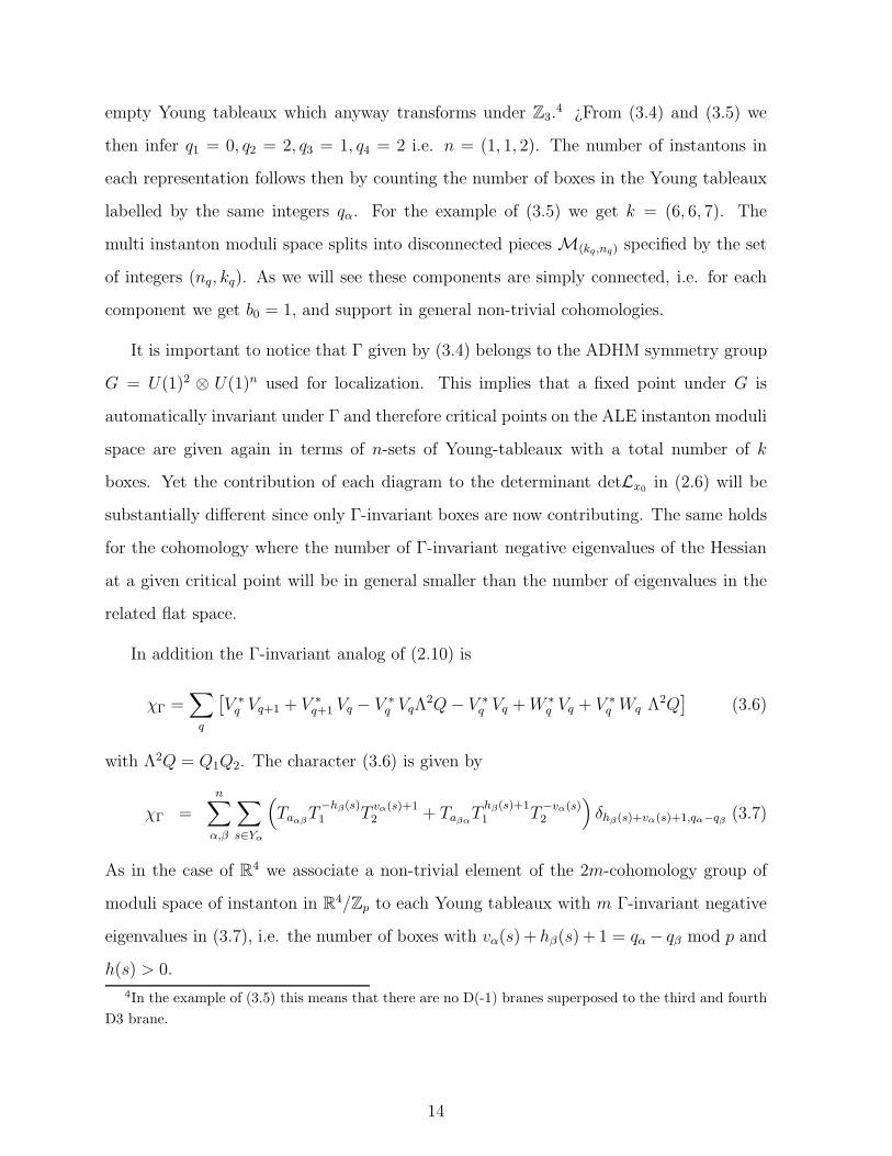
empty Young tableaux which anyway transforms under Z3.4 ¿From (3.4) and (3.5) we

then infer q1 = 0, q2 = 2, q3 = 1, q4 = 2 i.e. n = (1, 1, 2). The number of instantons in

each representation follows then by counting the number of boxes in the Young tableaux

labelled by the same integers qα. For the example of (3.5) we get k = (6, 6, 7). The

multi instanton moduli space splits into disconnected pieces M(kq,nq) specified by the set

of integers (nq, kq). As we will see these components are simply connected, i.e. for each

component we get b0 = 1, and support in general non-trivial cohomologies.

It is important to notice that Γ given by (3.4) belongs to the ADHM symmetry group

G = U(1)2 ⊗ U(1)n used for localization. This implies that a fixed point under G is

automatically invariant under Γ and therefore critical points on the ALE instanton moduli

space are given again in terms of n-sets of Young-tableaux with a total number of k

boxes. Yet the contribution of each diagram to the determinant detLx0in (2.6) will be

substantially different since only Γ-invariant boxes are now contributing. The same holds

for the cohomology where the number of Γ-invariant negative eigenvalues of the Hessian

at a given critical point will be in general smaller than the number of eigenvalues in the

related flat space.

In addition the Γ-invariant analog of (2.10) is

χΓ =∑

q

[

V ∗q Vq+1 + V ∗

q+1 Vq − V ∗q VqΛ

2Q − V ∗q Vq + W ∗

q Vq + V ∗q Wq Λ2Q

]

(3.6)

with Λ2Q = Q1Q2. The character (3.6) is given by

χΓ =

n∑

α,β

∑

s∈Yα

(

TaαβT

−hβ(s)1 T

vα(s)+12 + Taβα

Thβ(s)+11 T

−vα(s)2

)

δhβ(s)+vα(s)+1,qα−qβ(3.7)

As in the case of R4 we associate a non-trivial element of the 2m-cohomology group of

moduli space of instanton in R4/Zp to each Young tableaux with m Γ-invariant negative

eigenvalues in (3.7), i.e. the number of boxes with vα(s) + hβ(s) + 1 = qα − qβ mod p and

h(s) > 0.

4In the example of (3.5) this means that there are no D(-1) branes superposed to the third and fourth

D3 brane.

14

As an illustration consider U(1) instantons on R4/Z3 with n = (1, 0, 0)

k = (2, 2, 2) : • • + • • + • • +•

• +•

• +×

• +•

× +

×

• +

×

×

k = (3, 1, 2) :

k = (3, 1, 2) : (3.8)

Bullets and crosses stand for Γ-invariant boxes with h(s) > 0 and h(s) = 0 respectively.

Counting the number of tableaux with a fixed number of bullets in (3.8) we find that the

k = 6 U(1) instanton moduli space with n = (1, 0, 0) on R4/Z3 splits into three simply

connected (b0 = 1) pieces which contribute to the Poincare polynomial as

q6 r2R0+2R1+2R2(1 + 3t2 + 5t4) : b0 = 1 b2 = 3 b4 = 5

q6 r3R0+R1+2R2 : b0 = 1

q6 r3R0+2R1+R2 : b0 = 1 (3.9)

with q = e2πiτ . The factor rkqRq describes the Γ-content.

U(1) instantons

Here we consider arbitrary instanton configurations for the U(1) case. For con-

creteness we take n = (1, 0, . . . , 0) and compute the Poincare polynomial as a series∑

m,kqbm(Mkq

) q∑

q kq tm rkqRq . Let us start by considering R4/Z2. The Poincare polyno-

mial of multi instanton moduli space on R4/Z2 follows from that on R4 after decomposition

in classes k0R0 + k1R1

Y = • + +(

• + ×

)

+

(

• + +×

)

+

• • + • • +•

× +×

• +

×

×

+ . . .

= 1 + q rR0 + (1 + t2)q2 rR0+R1 + q3(r2R0+R1(1 + t2) + rR0+2R1) +

+q4r2R0+2R1(1 + 2t2 + 2t4) + . . . (3.10)

There are two particularly interesting classes of diagrams entering in (3.10). The first one

will be associated to the contribution of regular instantons and can be found by restricting

15

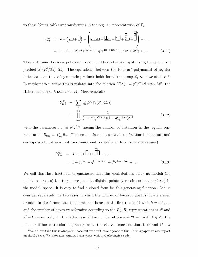
to those Young tableaux transforming in the regular representation of Z2

Y Z2

reg = • +(

• + ×

)

+

• • + • • +•

× +×

• +

×

×

+ . . .

= 1 + (1 + t2)q2 rR0+R1 + q4r2R0+2R1(1 + 2t2 + 2t4) + . . . (3.11)

This is the same Poincare polynomial one would have obtained by studying the symmetric

product Sk(R4/Z2) [25]. The equivalence between the Poincare polynomial of regular

instantons and that of symmetric products holds for all the group Zp we have studied 5.

In mathematical terms this translates into the relation (C[k])Γ = (C/Γ)[k] with M [k] the

Hilbert scheme of k points on M . More generally

Y Zp

reg =∑

k

qkregY (Sk(R

4/Zp))

=

∞∏

m=1

1

(1 − qmreg t2m−2)(1 − qm

reg t2m)p−1(3.12)

with the parameter qreg ≡ qp rReg tracing the number of instanton in the regular rep-

resentation Rreg ≡∑

q Rq. The second class is associated to fractional instantons and

corresponds to tableaux with no Γ-invariant boxes (i.e with no bullets or crosses)

Y Z2

frac = • + + + + . . .

= 1 + q rR0 + q3rR0+2R1 + q6r4R0+2R1 + . . . (3.13)

We call this class fractional to emphasize that this contributions carry no moduli (no

bullets or crosses) i.e. they correspond to disjoint points (zero dimensional surfaces) in

the moduli space. It is easy to find a closed form for this generating function. Let us

consider separately the two cases in which the number of boxes in the first row are even

or odd. In the former case the number of boxes in the first row is 2k with k = 0, 1, . . .

and the number of boxes transforming according to the R0, R1 representations is k2 and

k2 + k respectively. In the latter case, if the number of boxes is 2k − 1 with k ∈ Z+ the

number of boxes transforming according to the R0, R1 representations is k2 and k2 − k

5We believe that this is always the case but we don’t have a proof of this. In this paper we also report

on the Z3 case. We have also studied other cases with a Mathematica code.

16

respectively. Then

Y Z2

frac = 1 +∞∑

k=1

(

qk(2k−1)rk2R0+(k2−k)R1 + qk(2k+1)rk2R0+(k2+k)R1

)

=

∞∑

k=−∞

(

qrR1)k (

q2rR0+R1)k2

= θ3(z1|q2reg) (3.14)

with e2πiz1 ≡ qrR1 and qreg ≡ qprRreg with Rreg =∑

q Rq. Conventions for theta functions

are explained in Appendix A. Each power of e2πiz1 correspond to an unpaired fractional

instanton in the R1-representation of Z2. Remarkably the full instanton character Y can

be written as the product of the regular Yreg and fractional Yfrac contributions

Y = Y Z2

regYZ2

frac (3.15)

as can be explicitly checked by taking the product of (3.12) and (3.14) and comparing

against (3.10). The Poincare polynomial can then be written as

Pt =∑

m,k,R

bm(Mk,R) qk tm rR =∞∏

n=1

(1 − q2nreg)(1 + q rR1q2n−1

reg )(1 + (qrR1)−1q2n−1reg )

(1 − qnregt

2n−2)(1 − qnregt

2n)(3.16)

Similar relations hold for Z3. Now

Y = • + +(

+)

+

(

• + • + ×

)

+

• + + • + +×

+ . . .

= 1 + q rR0 + q2 (rR0+R1 + rR0+R2) + q3rR0+R1+R2(1 + 2t2)

+ q4(rR0+2R1+R2 + rR0+R1+2R2 + (1 + 2t2)r2R0+R1+R2) . . . (3.17)

and

Y Z3

reg = • +

(

• + • + ×

)

+ . . .

= 1 + q3 rR0+R1+R2(1 + 2t2) + . . .

Y Z3

frac = • + +(

+)

+ +

(

+

)

+ + . . . (3.18)

= 1 + q rR0 + q2 (rR0+R1 + rR0+R2) + q4 (rR0+R1+2R2 + rR0+2R1+R2) + . . .

Again the relation (3.15) is verified. The extension of this algorithm to the case of U(n)

is a straightforward matter.

17

3.3 The N = 4 partition function on the Eguchi-Hanson mani-

fold for gauge group SU(2)

In this last section of this chapter, we compute the Euler characteristic for the moduli

space of gauge connections with half integer winding number on the Eguchi-Hanson man-

ifold which is the simplest ALE variety. The Euler characteristic of the multi-instanton

moduli space is the N = 4 partition function of the theory. Taking the limit of zero mass

in the partition function (2.14) we in fact find that the N = 4 partition function is given

by the sum over all critical points i.e. the Euler characteristic. With respect to the R4

case [3] the novelty is that for the SU(2) Eguchi-Hanson case we have to consider only

those critical points obeying to the conditions

q1 = q2 = 1 : k = (k0, k0 + 1) n = (0, 2)

q1 = q2 = 0 : k = (k0, k0) n = (2, 0)

These conditions force us to count all the pairs of Young tableaux with an odd(even)

number of boxes belonging to the classes k0Rreg + R1(k0Rreg) with the first box trans-

forming according to the R1(R0) representation of Zp. The starting point is the U(2)

Euler polynomial YU(2) = (Y Z2regY

Z2

frac)2|t=1 given by (3.12,3.14) i.e. before imposing the

c1 = 0 condition. Singling out the classes k0Rreg and k0Rreg +R1 in this formula it is now

easy. Unpaired instantons come only from

Y Z2

frac =

∞∑

k=−∞

(

qrR1+q1

)kqk2

reg (3.19)

where we have modified the subscript of the term R1 to generalize (3.14) which was found

in the case q1 = 06. Then

YU(2) = (Y Z2

reg)2

∞∑

k1,k2=−∞

(

qrR1+q1

)k1(

qrR1+q2

)k2(qreg)

k21+k2

2 . (3.20)

The factors (qrR1+q1 )k1 and (qrR1+q2 )k2 in (3.19) are the only potential sources of asym-

metry between the R0 and R1 representations. The classes k0Rreg (with q1 = q2 = 0) and

6We remind the reader that the subscripts of the representations are always understood modulo p.

18

k0Rreg + R1 (with q1 = q2 = 1) are extracted from (3.20) by picking up the terms with

k1 = −k2 and k1 = −k2 − 1 and specializing to r = 1

Y SU(2)even = q

− 16

reg (Y Z2

reg)2

∞∑

k=−∞

q2k2

reg =θ3(0|q

4reg)

η(qreg)4

YSU(2)odd = q

− 16

reg (Y Z2

reg)2

∞∑

k=−∞

q42(k− 1

2)2

reg =θ2(0|q4

reg)

η(qreg)4(3.21)

The factor q− 1

6reg (Casimir energy) has been included as in [21] in order to reconstruct the

modular functions. See the Appendix and (A.9) for our notation. The partition function

of N = 4 is then

ZN=4 = q16 Y SU(2) =

1

η4(qreg)

[

θ3(0|q4reg) + θ2(0|q

4reg)]

=θ3(0|τ)

η4(τ)(3.22)

Notice that the number of boxes in the diagrams is one half the Chern class (2.24).

Therefore the correct expansion parameter for the R4/Z2 case is qreg = q2. (3.22) is a

modular form as expected from the SL(2, Z) duality of N = 4 [21].

4 The prepotential

Finally we derive the multi instanton partition functions and prepotentials describing the

N = 2 low energy physics on the ALE manifold 7. For simplicity we take ǫ2 = −ǫ1 = ~.

The ALE projection is defined by omitting the eigenvalues in (2.14) that are not

invariant under the Zp projections

Zp : ~ → ~ +2π

paα → aα +

2πqα

p(4.1)

SU(2) gauge theory on R4/Z2

For concreteness we consider SU(2) gauge theory on R4/Z2. The condition of vanishing

of the first Chern class (2.25), c1 = 0, is only satisfied by the instanton configurations

7In this chapter we will give the lowest terms in the expansion of the prepotential using an analytical

method for pedagogical purposes. To check highest order terms, this way is not practical and we have

written a Mathematica code.

19

[18] k = (k0, k0), n = (2, 0)(q1 = q2 = 0) and k = (k0, k0 + 1), n = (0, 2)(q1 = q2 = 1).

According to (2.24) they correspond to bundles with second Chern classes c2 = k0 and

c′2 = 12(2k0 + 1) respectively.

The instanton partition function on the orbifold, follows from that in flat space after

imposing invariance under (4.1). Thus only the eigenvalues (appearing as factors in (2.15))

invariant under (4.1) must be taken into account. In addition the ALE partition function

is defined by

Z(q) =∑

k

Zkqk2

since c2 = 12k.

Furthermore let us remark that (2.16) only depend on aαβ . Since for instanton config-

urations with c1 = 0 one has qα = qβ, under (4.1) we get δaαβ = π(qα − qβ) = 0. We now

have to examine the behavior under ~ → ~ +π. Only functions of the type f(n~), Tα(n~)

with n even survive this projection. Collecting these type of terms in (2.16) and setting

a1 = −a2 = a one finds

Z = 2

(

1 −m2

4a2

)

(4.2)

Z = Z = 2

(

1 −m2

(2~)2

)(

1 −m2

4a2

)

(4.3)

The configuration Z , does not contribute, since it has c1 6= 0. Computing also terms

which come from Young tableaux with three and four boxes we finally get

Z(q) = 1 +(4a2 − m2)

2a2q

12 +

(4a2 − m2)(4~2 − m2)

4a2~2q

+m2a2(4a2 − m2) + ~2(128a6 − 64m2a4 + 8m4a2 − 3m6)

16a6~2q

32

+[4m4a4(−4a2 + m2) + ~2a2(−704a6m2 + 352a4m4 − 120a2m6 + 5m8)

128a8~4

+~4(2048a8 − 1152m2a6 + 640m4a4 − 152a2m6 + 9m8)

128a8~4

]

q2 + . . . (4.4)

¿From (4.4) we can extract the partition function for the pure N = 2 case by taking the

limit m → ∞, m4q = Λ

Z(Λ) = 1 −Λ

12

2 a2+

Λ

4 a2 ~2− Λ

32(a2 + 3~2)

8~2a6+ Λ2 (4 a4 + 5 a2 ~2 + 9 ~4)

128 a8 ~4+ . . . (4.5)

20

The presence of half-integer powers of q makes Z(q) double-valued in the complex

plane, i.e. Z(q) is not invariant under q12 → −q

12 or τ → τ + 1. Out of Z(q) we can build

two objects with definite transformation properties under τ → τ + 1:

Feven(q, m, ~) = 12~

2[

ln Z(q12 ) + ln Z(−q

12 )]

Fodd(q, m, ~) = −12

[

ln Z(q12 ) − ln Z(−q

12 )]

(4.6)

The two terms correspond to contributions with integer and half-integer Chern class re-

spectively. Notice the different normalization of the two pieces. The 1~2 volume factor in

front of the odd term has been projected out by the Z2 orbifold group action. Notwith-

standing the odd term is now regular in the limit ~ → 0. The quadratic divergence is in

fact connected to the breaking of translational invariance8 in the lagrangian of the theory

due to the rotations Tǫ1,2. The lagrangian invariant under the infinitesimal action of Tǫ1,2

explicitly contains the modulus which gives the position of the center of the instanton.

The integration over this modulus is responsible for the above mentioned quadratic di-

vergence. The Z2 invariant instanton is clearly centered in zero and there is no modulus

for its center. For N = 2∗ one finds

Feven(q) =

(

m4 − 4m2a2

4a2

)

q +m2

128a6(5m6 − 48m4a2 + 96m2a4 − 192a6)q2

+~2

[(

16a4 − m4

8a4

)

q +

(

−17m8 + 72m6a2 − 128m2a6 + 512a8

128a8

)

q2

]

+ . . .

Fodd(q) =

(

m2 − 4a2

2a2

)

q12 −

(

32a6 − 24m2a4 + 24m4a2 − 5m6

12a6

)

q32

+

(

48m2a4 − 32m4a2 + 5m6

8a8

)

q32 + . . . (4.7)

Once again the pure N = 2 limit is recovered in the limit m → ∞, m4q = Λ

Feven(Λ) =

(

1

4

Λ

a2+

5

128

Λ2

a6+

3

128

Λ3

a10

)

− ~2

(

1

8

Λ

a4+

17

128

Λ2

a8+

13

64

Λ3

a12

)

+ . . .

Fodd(Λ) =

(

1

2

Λ12

a2+

5

12

Λ32

a6+

207

320

Λ52

a10

)

+ ~2

(

5

8

Λ32

a8+

269

64

Λ52

a12

)

+ . . . (4.8)

8This translational symmetry of the lagrangian in the moduli space follows from the translational

invariance of the instanton solution in Euclidean space time. In [1] it was suggested to deform the

original lagrangian under Tǫ1,2to allow for a localization with isolated critical points.

21

The k = 1/2, ~ = 0 term matches (4.14) in [26]9. For completeness we have also given the

first gravitational correction to the prepotential.

Acknowledgements

The authors want to thank A. Maffei for very enlightening discussions on the properties

of moduli spaces of gauge connections on ALE manifolds and R.Flume for collaboration

in the early stage of this work. R.P. have been partially supported by the Volkswa-

gen foundation of Germany and he also would like to thank I.N.F.N. for supporting a

visit to the University of Tor Vergata. This work was supported in part by the EC

contract HPRN-CT-2000-00122, the EC contract HPRN-CT-2000-00148, the EC con-

tract HPRN-CT-2000-00131, the MIUR-COFIN contract 2003-023852, the NATO con-

tract PST.CLG.978785 and the INTAS contracts 03-51-6346 and 00-561.

A Theta functions

The conventions for theta functions in the text are:

θ[ab ](z|q) =∑

n∈Z

q12(n−a)2e2πi(z−b)(n−a)

η(q) = q124

∞∏

n=1

(1 − qn) (A.9)

where θ1 = θ[1212

], θ2 = θ[12

0 ], θ3 = θ[00], θ4 = θ[012

].

B Cohomology of the ALE space

As an illustration here we compute the homologies of the ALE space itself. This is a

well known result (see [24] for a review). Here we will derive it using the methods of

subsection 2.1: the ALE space can be described in terms of the non commutative ADHM

9In that reference the correlator Trφ2 is computed. For the lowest winding number this is the same

as the prepotential.

22

formalism for the U(1) case. In fact we have seen in subsection 2.2 that the matrices

which describe the ALE space are subject to the constraint (2.20) and to the Γ invariant

condition (2.18). If in the ADHM construction we described in subsection 2.1 we take

the U(1) case (i.e. the space W becomes a k dimensional vector), we can set J = 0 and

the constraints fC = 0, fR = ζ coincide with (2.20)10 Moreover choosing k = p in the

regular representation the projection on ADHM moduli space matches that in (2.18). We

can then compute the homologies of an ALE space using the character χ in (3.7). The

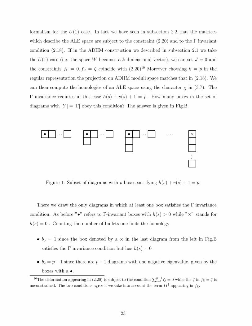
Γ invariance requires in this case h(s) + v(s) + 1 = p. How many boxes in the set of

diagrams with |Y | = |Γ| obey this condition? The answer is given in Fig.B.

• · · · • · · · • · · · · · · ×

...

Figure 1: Subset of diagrams with p boxes satisfying h(s) + v(s) + 1 = p.

There we draw the only diagrams in which at least one box satisfies the Γ invariance

condition. As before ”•” refers to Γ-invariant boxes with h(s) > 0 while ”×” stands for

h(s) = 0 . Counting the number of bullets one finds the homology

• b0 = 1 since the box denoted by a × in the last diagram from the left in Fig.B

satisfies the Γ invariance condition but has h(s) = 0

• b2 = p− 1 since there are p− 1 diagrams with one negative eigenvalue, given by the

boxes with a •.

10The deformation appearing in (2.20) is subject to the condition∑p−1

i=1ζi = 0 while the ζ in fR = ζ is

unconstrained. The two conditions agree if we take into account the term II† appearing in fR.

23

References

[1] N. A. Nekrasov, “Seiberg-Witten prepotential from instanton counting”,

arXiv:hep-th/0206161.

[2] R. Flume and R. Poghossian, Int. J. Mod. Phys. A 18 (2003) 2541,

arXiv:hep-th/0208176.

[3] U. Bruzzo, F. Fucito, J. F. Morales and A. Tanzini, JHEP 0305 (2003) 054,

arXiv:hep-th/0211108.

[4] A. S. Losev, A. Marshakov and N. A. Nekrasov, arXiv:hep-th/0302191.

[5] N. Nekrasov and A. Okounkov, arXiv:hep-th/0306238.

[6] R. Flume, F. Fucito, J. F. Morales and R. Poghossian, JHEP 0404 (2004) 008

[arXiv:hep-th/0403057].

[7] M. Marino and N. Wyllard, “A note on instanton counting for N = 2 gauge theories

with classical gauge groups,” JHEP 0405 (2004) 021, arXiv:hep-th/0404125.

[8] N. Nekrasov and S. Shadchin, “ABCD of instantons,” arXiv:hep-th/0404225.

[9] E. Witten, Nucl. Phys. B460 (1996) 541, hep-th/9511030.

[10] M. R. Douglas, “Branes within branes”, hep-th/9512077; J. Geom. Phys. 28, 255

(1998), hep-th/9604198.

[11] N Dorey, T.J. Hollowood, V.V. Khoze, M.P. Mattis and S. Vandoren, Nucl. Phys.

B552 (1999) 88, hep-th/9901128

[12] M. R. Douglas and G. Moore, “D-branes, Quivers, and ALE Instantons”,

hep-th/9603167; C. V. Johnson and R. C. Myers, Phys. Rev. D 55 (1997) 6382,

hep-th/9610140.

[13] F. Fucito, J. F. Morales and R. Poghossian, arXiv:hep-th/0408090.

24

[14] E. Gava, K. S. Narain and M. H. Sarmadi, Nucl. Phys. B 569 (2000) 183,

hep-th/9908125.

[15] T.J. Hollowood, V.V. Khoze and M.P. Mattis, HEP 9910 (1999) 019,

hep-th/9905209.

[16] T. J. Hollowood and V.V. Khoze, Nucl.Phys. B575 (2000) 78, hep-th/9908035.

[17] F. Fucito, J. F. Morales and A. Tanzini, JHEP 0107 (2001) 012,

arXiv:hep-th/0106061.

[18] M. Bianchi, F. Fucito, G. Rossi and M. Martellini, Nucl. Phys. B 473 (1996) 367,

hep-th/9601162.

[19] H. Nakajima, “Lectures on Hilbert Schemes of Points on Surfaces”, American Math-

ematical Society,University Lectures Series v.18 (1999)

[20] P. Kronheimer and H. Nakajima, Math. Ann. 288 (1990) 263.

[21] C. Vafa and E. Witten, Nucl. Phys. B 431 (1994) 3, arXiv:hep-th/9408074.

[22] N. Nekrasov and A. Schwarz, Commun. Math. Phys. 198 (1998) 689,

arXiv:hep-th/9802068.

[23] R. Bott, L. W. Tu, “Differential Forms in Algebraic Topology”, Berlin, Germany:

Springer (1982)

[24] T. Eguchi, P. B. Gilkey and A. J. Hanson, Phys. Rept. 66 (1980) 213.

[25] R. Dijkgraaf, G. W. Moore, E. Verlinde and H. Verlinde, Commun. Math. Phys. 185

(1997) 197, arXiv:hep-th/9608096.

[26] D. Bellisai and G. Travaglini, Phys. Rev. D 58 (1998) 025008, arXiv:hep-th/9712218.

25