Portland State University Portland State University

PDXScholar PDXScholar

Dissertations and Theses Dissertations and Theses

Fall 11-30-2017

Multi-Dimensional Drought Risk Assessment Based Multi-Dimensional Drought Risk Assessment Based

on Socio-Economic Vulnerabilities and Hydro-on Socio-Economic Vulnerabilities and Hydro-

Climatological Factors Climatological Factors

Ali Ahmadalipour Portland State University

Follow this and additional works at: https://pdxscholar.library.pdx.edu/open_access_etds

Part of the Civil and Environmental Engineering Commons, Climate Commons, and the Hydrology

Commons

Let us know how access to this document benefits you.

Recommended Citation Recommended Citation Ahmadalipour, Ali, "Multi-Dimensional Drought Risk Assessment Based on Socio-Economic Vulnerabilities and Hydro-Climatological Factors" (2017). Dissertations and Theses. Paper 4038. https://doi.org/10.15760/etd.5922

This Dissertation is brought to you for free and open access. It has been accepted for inclusion in Dissertations and Theses by an authorized administrator of PDXScholar. Please contact us if we can make this document more accessible: pdxscholar@pdx.edu.

Multi-dimensional Drought Risk Assessment based on Socio-economic Vulnerabilities

and Hydro-Climatological Factors

by

Ali Ahmadalipour

A dissertation submitted in partial fulfillment of the

requirements for the degree of

Doctor of Philosophy

in

Civil and Environmental Engineering

Dissertation Committee:

Hamid Moradkhani, Chair

Gwynn Johnson

Max Nielsen-Pincus

Paul Loikith

Portland State University

2017

Abstract

Drought is among the costliest natural hazards developing slowly and affecting

large areas, which imposes severe consequences on society and economy. Anthropogenic

climate change is expected to exacerbate drought in various regions of the globe, making

its associated socioeconomic impacts more severe. Such impacts are of higher concern in

Africa, which is mainly characterized by arid climate and lacking infrastructure as well as

social development. Furthermore, the continent is expected to experience vast population

growth, which will make it more vulnerable to the adverse effects of drought. This study

provides the first comprehensive multi-dimensional assessment of drought risk across the

African continent as a function of hazard, vulnerability, and exposure. A multi-model and

multi-scenario approach is employed to quantify drought hazard using the most recent

ensemble of regional climate models and a multi-scalar drought index. Moreover, a

rigorous framework is proposed and applied to assess drought vulnerability based on

various sectors of economy, energy and infrastructure, health, land use, society, and water

resources. Drought risk is then projected for different population scenarios and the changes

of drought risk and the role of each component are investigated. In addition, the impacts of

climate change on heat-stress mortality risk is assessed across the Middle East and North

Africa. The results indicate vast increase for the projected drought risk with varied

spatiotemporal patterns. Population growth and climate change will significantly escalate

drought risk, especially in distant future. Therefore, climate change mitigation and

adaptation planning as well as social development strategies should be carried out

immediately in order to reduce the projected adverse risks on human life and society.

i

ii

Acknowledgements

In the past few years, many people have supported me throughout my PhD, and I

am truly indebted to them for their time, help, and concern. First, I would like to

acknowledge and thank my advisor, Dr. Hamid Moradkhani, who supervised me in my

PhD studies, and I highly benefitted from his knowledge, guidance, and experience. I

would like to also thank my dissertation committee members, Dr. Gwynn Johnson, Dr.

Max Nielsen-Pincus, and Dr. Paul Loikith for their willingness to serve on my committee

and for their valuable comments and feedbacks on my research. Their comments and

suggestions helped me significantly improve the quality and clarity of my research.

I should also thank all the post-doctoral associates and graduate students that I had

the pleasure to work with in the Water Resources and Remote Sensing Lab, including Arun

Rana, Mehmet Demirel, Hongxiang Yan, Sepideh Khajehei, Mahkameh Zarekarizi, and

Maysoun Hameed. Our collaborations expanded my knowledge and abilities, and provided

me strong leadership and communication skills.

I am also thankful of the kind staff of the Department of Civil and Environmental

Engineering, including Megan Falcone and Ariel Lewis, who were always great resources

and helped me navigate my work in the department. Moreover, I must express my gratitude

to the lovely staff of the International Student Life team at PSU, especially Jill Townley

and Yoko Honda, who helped me adapt my life and overcome any cultural shocks.

Finally, I must express my deepest gratitude and appreciation to my family for their

continuous and unconditional love, care, and support. Their encouragement motivated me

iii

to strive to achieve my dreams, and I could have not completed this work without their

support and patience.

iv

Table of Contents

Abstract ................................................................................................................................ i

Acknowledgements ............................................................................................................. ii

List of Tables ..................................................................................................................... vi

List of Figures ................................................................................................................... vii

List of Abbreviations ........................................................................................................ xii

1 Introduction ............................................................................................................... 1

1.1 Drought................................................................................................................. 1

1.2 Climate Change .................................................................................................... 4

1.3 Vulnerability, Hazard, and Risk ........................................................................... 5

1.4 Objectives of Dissertation .................................................................................... 8

2 Climate Change Impact Assessment ...................................................................... 10

2.1 Background ........................................................................................................ 10

2.2 Global Climate Models (GCMs) ........................................................................ 10

2.3 Regional Impacts of Climate Change................................................................. 12

2.4 Climate Change and Drought ............................................................................. 20

3 Drought Vulnerability in Africa ............................................................................. 26

3.1 Background ........................................................................................................ 26

3.2 Data .................................................................................................................... 27

3.3 Methodology ...................................................................................................... 30

3.3.1 Normalizing Factors.................................................................................... 32

3.3.2 Multi-collinearity (Independence) Test ...................................................... 33

3.3.3 Weighting and Averaging ........................................................................... 34

3.3.4 Cluster Analysis .......................................................................................... 35

3.3.5 Change-Point Analysis................................................................................ 36

3.3.6 Future Drought Vulnerability Projection .................................................... 38

3.4 Results and Discussion ....................................................................................... 39

3.4.1 Historical Assessment of DVI .................................................................... 39

3.4.2 Change-Point Analysis and Future Projection of DVI ............................... 51

v

3.4.3 Evaluating DVI estimates ........................................................................... 58

3.5 Summary and Conclusion .................................................................................. 61

4 Drought Hazard and Risk in Africa ...................................................................... 63

4.1 Background ........................................................................................................ 63

4.2 Data .................................................................................................................... 65

4.3 Methodology ...................................................................................................... 66

4.4 Results and Discussion ....................................................................................... 71

4.4.1 Drought Hazard ........................................................................................... 71

4.4.2 Exposure ..................................................................................................... 76

4.4.3 Drought Risk ............................................................................................... 78

4.5 Summary and Conclusion .................................................................................. 88

5 Climate Change and Heat-Related Mortality Risk .............................................. 91

5.1 Background ........................................................................................................ 91

5.2 Data .................................................................................................................... 93

5.3 Methodology ...................................................................................................... 95

5.3.1 Calculating Wet-bulb Temperature (TW) ................................................... 95

5.3.2 Quantifying Mortality Risk ......................................................................... 96

5.4 Results and Discussion ....................................................................................... 99

5.5 Summary and Conclusion ................................................................................ 113

6 Conclusions and Future Studies ........................................................................... 115

References ....................................................................................................................... 118

vi

List of Tables

Table 3-1. The functions used for projecting future DVI, the starting years (representing

no change afterwards), and the coefficient of determination for each case. ............... 54

Table 4-1. The 10 RCMs used in this study and their characteristics. All the RCMs are

developed by the Swedish Meteorological and Hydrological Institute (SMHI) and have

a spatial resolution of 0.44°. ....................................................................................... 66

Table 5-1. The 17 RCMs used in this study and their characteristics. All the RCMs have a

spatial resolution of 0.44°. .......................................................................................... 94

vii

List of Figures

Figure 2-1. Global decadal mean air temperature increase calculated from 9 GCMs and

the ensemble mean for RCP4.5 (top) and RCP8.5 (bottom)....................................... 12

Figure 2-2. Future changes of seasonal precipitation compared to the historical period of

1951-2000 across the CONUS calculated from 21 downscaled CMIP5 GCMs. ....... 13

Figure 2-3. Same as Figure 2-2, but for mean air temperature. ....................................... 14

Figure 2-4. Projection of annual precipitation for each sub-basin using BCSD dataset. The

figure is generated using spatially averaged annual precipitation over each sub-basin

for GCMs and BMA. .................................................................................................. 15

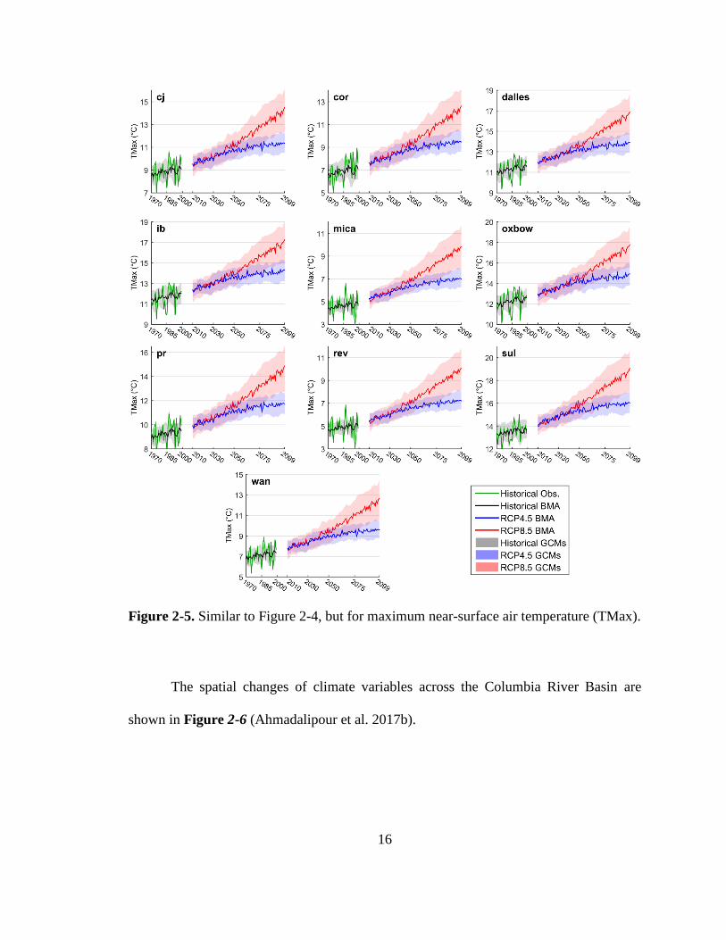
Figure 2-5. Similar to Figure 2-4, but for maximum near-surface air temperature (TMax).

..................................................................................................................................... 16

Figure 2-6. Long-term seasonal changes of precipitation (top) and temperature (bottom)

for summer (JJA) and winter (DJF) from BMA projections. ..................................... 17

Figure 2-7. Fraction of the total variance of future projections of precipitation (top) and

temperature (bottom) for each season. ........................................................................ 18

Figure 2-8. Changes of annual maximum air temperature across the Middle East and North

Africa (MENA) calculated from 17 CORDEX RCMs. .............................................. 19

Figure 2-9. Regional changes of maximum air temperature (ΔTx) compared to the global

warming rate (𝛥𝑇𝑔𝑙𝑜𝑏𝑎𝑙). .......................................................................................... 20

Figure 2-10. Spatial extent of drought according to SPEI-3 for the historical of 1950-2005

and two future scenarios during 2006-2099. ............................................................... 22

Figure 2-11. Same as Figure 2-10, but calculated for SPI-3. ........................................... 22

Figure 2-12. Long-term trend of drought indices for the future period of 2005-2099

according to the SPEI-3. ............................................................................................. 23

Figure 2-13. Same as Figure 2-12, but for the SPI-3. ...................................................... 24

Figure 3-1. The 6 components and 28 factors considered in the analysis, and the

availability of each factor during the historical period. The signs in the brackets indicate

the correlation of the factor to the overall vulnerability. In each particular year, a factor

is eliminated if it does not provide data for at least half of the countries. .................. 29

viii

Figure 3-2. The methodology employed to assess data, calculate Drought Vulnerability

Index (DVI), and project it for the future period. ....................................................... 31

Figure 3-3. Spatial changes of Drought Vulnerability Index (DVI) calculated using simple

averaging (arithmetic mean) of the corresponding factors in each year during the

historical period. ......................................................................................................... 40

Figure 3-4. Polar dendrogram representing the results of clustering DVI using the

hierarchical cluster analysis based on the average Euclidean linkage distance and

optimal leaf ordering. In general, the green, yellow, and red colors indicate countries

with low, medium, and high drought vulnerability, respectively. .............................. 42

Figure 3-5. Drought Vulnerability Index (DVI) of each country calculated using the

random-weighted averaging method........................................................................... 44

Figure 3-6. Comparison of the DVI calculated using the simple averaging method (green

asterisks) and the DVI calculated by the random weighted averaging (boxplots) for

1995 and 2015. In both plots, the countries are ordered according to their DVIs. ..... 46

Figure 3-7. Radar plots representing drought vulnerability index (DVI) of each component

for the top-3 least vulnerable countries in Africa (i.e. Algeria, Egypt, and Tunisia). 48

Figure 3-8. Radar plots representing drought vulnerability index (DVI) of each component

for the top-3 most vulnerable countries in Africa (i.e. Chad, Malawi, and Niger). .... 49

Figure 3-9. Historical changes of DVI in each component for the most progressive

countries with a decreasing trend of DVI (top) and the most aggravating countries with

an increasing trend of DVI (bottom). .......................................................................... 51

Figure 3-10. Change-point analysis for Lesotho (top) indicating a significant change in the

DVI time-series, and Nigeria (bottom) without any change point. Plots (a) and (d) show

the DVI time-series. Plots (b) and (e) represent the CUSUM results for original DVI

(line) and bootstrapped DVI (boxplots), and the distribution of 𝑆𝑑𝑖𝑓𝑓0, and 𝑆𝑑𝑖𝑓𝑓 are

shown in plots (c) and (f). ........................................................................................... 53

Figure 3-11. Temporal variations of Drought Vulnerability Index (DVI) for each country

during the historical period of 1960-2015 and future projections of 2020-2100. ....... 56

ix

Figure 3-12. Violin plots representing the DVI distribution of the 46 African countries for

historical simulations (green) and future projections (blue). The red plus (+) signs

indicate the median of DVI in each year. ................................................................... 58

Figure 4-1. Schematic diagram of the risk analysis methodology employed in this study

and its different components in historical and future periods. .................................... 70

Figure 4-2. Spatial extent of historical and future droughts across Africa based on the

SPEI-12 results. The shaded area represents the results from 10 RCMs and the lines

indicate the ensemble mean dry area for each corresponding concentration pathway.

..................................................................................................................................... 72

Figure 4-3. Long-term trend of SPEI-12 for the future period of 2005-2100 for each RCM

in RCP4.5 (top) and RCP8.5 (bottom). The Mann-Kendall trend test is used at 0.05

significance level and only the significantly negative trends are plotted. .................. 74

Figure 4-4. Temporal variations of the annual Hazard Index for each country in Africa

during the historical period as well as two future scenarios of RCP4.5 and RCP8.5. The

shaded areas represent the results of 10 RCMs and the lines indicate the ensemble

mean. ........................................................................................................................... 75

Figure 4-5. Violin plots showing the distribution of the Hazard Index among the African

countries for historical and future periods. The plus signs (+) indicate the median

Hazard Index in each case. .......................................................................................... 76

Figure 4-6. Historical record and projected population of each country in the African

continent. The last subplot shows the total population of the African continent. The y-

axis in all subplots is in million people, except for the last subplot (Total Africa) which

shows the population in billions. ................................................................................ 78

Figure 4-7. Boxplots showing the drought risk ratio of each country in the African

continent for 10 RCMs, two climate pathways (RCP4.5 and RCP8.5) and two

population scenarios (Low and High Variant). The red dash in the middle of each plot

indicates the median of the 10 RCMs. ........................................................................ 80

Figure 4-8. Projections of the ensemble mean drought risk ratio of each African country

in all the future scenarios (two climate pathways of RCP4.5 and RCP8.5 as well as

x

three population scenarios of Low, Medium, and High Variant) for near, intermediate,

and distant future......................................................................................................... 82

Figure 4-9. Spatial distribution of the projected drought risk ratios in the African countries

for all scenarios in near and distant future. ................................................................. 83

Figure 4-10. Violin plots representing the distribution of the drought risk ratio among the

African countries for the future periods/scenarios. The plus signs (+) indicate the

median risk ratio in each case. .................................................................................... 84

Figure 4-11. Decomposition of the drought risk components and their changes compared

to the historical period. The figure shows the mean change rates among various

scenarios and the countries are arranged in descending order from the highest to lowest

risk ratios. .................................................................................................................... 86

Figure 5-1. Optimum wet-bulb temperature calculated for each of the RCMs using the

historical data of 1951-2005. ...................................................................................... 97

Figure 5-2. a) The function used for quantifying the relative mortality risk based on

temperature offset (Equation 5-2). b) Annual excessive mortality risk as a function of

temperature offset and frequency (Equation 5-3). ...................................................... 98

Figure 5-3. Historical mean summer (JJA) maximum near-surface air temperature (Tx) for

the common period of 1979-2005. ............................................................................ 100

Figure 5-4. Spatial mean annual Tx for five regions across the MENA for historical and

future projections. The shaded area indicates the results of 17 RCMs. .................... 101

Figure 5-5. Decadal mortality risk ratio compared to the historical period. The figure

represents the ensemble mean of 17 RCMs and shows the exacerbation rate of mortality

compared to the historical period. ............................................................................. 103

Figure 5-6. Latitudinal mean of future mortality risk ratio over land from 17 RCMs (shaded

area) and the ensemble mean (bold line) for each 30-year future period. The boxplots

at the bottom of each plot indicate the results across the entire MENA region........ 104

Figure 5-7. The change of maximum air temperature (ΔTx) and wet-bulb temperature

(ΔTW) across MENA over land (top) and water (bottom). The histogram plots (the first

and third rows) show the distribution of the ensemble mean of 17 RCMs. The density-

xi

type scatterplots (the second and fourth rows) compare ΔTx and ΔTW of all RCMs,

with the colorbar indicating the density. ................................................................... 106

Figure 5-8. Decadal mean changes of maximum near-surface air temperature (ΔTx) and

wet-bulb temperature (ΔTW) for 30-year future periods. The figure is generated using

the results of ensemble mean of 17 RCMs. .............................................................. 107

Figure 5-9. The percentage of the days with TW>Topt during each 30-year future period.

The frequency is extracted for each RCM in each period, and the figure represents the

ensemble mean of 17 RCMs. .................................................................................... 109

Figure 5-10. (Top) standard deviation of TW during the historical period, indicating the

inter-annual variations of TW. (Bottom) the changes of inter-annual standard deviation

of TW in each 30-year period compared to the historical period. Standard deviation is

calculated for each RCM in each period, and the figure shows the results from ensemble

mean of 17 RCMs. .................................................................................................... 111

xii

List of Abbreviations

CMIP5: Coupled Model Inter-comparison Project Phase 5

CORDEX: Coordinated Regional Climate Downscaling Experiment

DVI: Drought Vulnerability Index

FAO: Food and Agricultural Organization of the United Nations

GCM: Global Climate Model

IPCC: Intergovernmental Panel on Climate Change

MENA: Middle East and North Africa

PDSI: Palmer Drought Severity Index

PET: Potential Evapotranspiration

RCM: Regional Climate Model

RCP: Representative Concentration Pathway

RDI: Reconnaissance Drought Index

SDDI: Supply–Demand Drought Index

SPEI: Standardized Precipitation Evapotranspiration Index

SPI: Standardized Precipitation Index

TW: Wet-bulb Temperature

Tx: Maximum Air Temperature

UNISDR: United Nations International Strategy for Disaster Reduction

VIF: Variance Inflation Factors

WHO: World Health Organization

1

1 Introduction

Climate change and population growth have exacerbated water insecurity in many

regions of the globe, and it is expected that they become grand challenges of the society in

the twenty first century (Risley et al. 2011; DeChant and Moradkhani 2015; Zhao and Dai

2015). The issue is more concerning in Africa with exceptional population growth and

extreme changes in climate which is expected to intensify droughts in many regions of

Africa (Dai 2012; Touma et al. 2015). Despite the critical challenges facing the continent,

few studies have comprehensively investigated the socioeconomic risks of concurrent

changes in climate and population growth in Africa. The current study aims to bridge such

scientific gap and assess drought vulnerability and risk in Africa based on a comprehensive

multi-dimensional framework to help with future planning and management of resources

in order to mitigate drought hazard impacts at regional scales.

1.1 Drought

Drought is a prolonged period of water deficiency (Madadgar and Moradkhani

2013a; Yan et al. 2017). It is among the costliest natural disasters affecting large extents of

area and lasting up to several years (Madadgar and Moradkhani 2014a; Ahmadalipour et

al. 2017c). Drought can be classified into four different types of meteorological (deficit in

precipitation), hydrological (surface and subsurface water deficiency), agricultural (root

zone soil moisture deficiency), and socio-economic (failure of water resources systems and

market prices) (Mishra and Singh 2010). Drought is a complex phenomenon and among

2

the most severe natural hazards which is often developed slowly and affecting large areas

for a long period of time compared to the eye-catching flash flood events (Van Loon 2015;

Ahmadalipour et al. 2017a). It can affect water supply, agriculture, hydropower, river

navigation , and it may escalate wildfire risk (Madadgar and Moradkhani 2014a; Turner et

al. 2015; Abatzoglou and Williams 2016).

Several drought indices have been developed for quantifying the severity of

different types of drought. The Palmer Drought Severity Index (PDSI) is among the first

indices proposed for assessing meteorological droughts (Palmer 1965). PDSI considers

several water balance variables such as precipitation, soil moisture, and runoff to quantify

drought severity (Liu et al. 2016; Yan et al. 2016). Decades later, the Standardized

Precipitation Index (SPI) was developed as a simple meteorological drought index focusing

solely on precipitation variation (Mckee et al. 1993). SPI then became one of the most

popular drought indices and researchers investigated its applicability for other types of

drought (Bloomfield and Marchant 2013; Musuuza et al. 2016). Similar drought indices

were developed using the same formulation while considering different variables such as

runoff or streamflow (Shukla and Wood 2008; Vicente-Serrano et al. 2012b). Later on, the

Standardized Precipitation Evapotranspiration Index (SPEI) was introduced by Vicente-

Serrano et al. (2010) as a multi-scalar index based on a climatic water balance between

precipitation and potential evapotranspiration, which allows for considering the effects of

temperature on drought.

3

Despite the extreme social, economic, and ecological impacts, drought is not yet

thoroughly understood mainly due to the complexity and variety of drought origins,

uncertain mechanisms for drought advancement and recovery, and the multiscale

spatiotemporal characteristics of it (Sohrabi et al. 2004; Hobbins et al. 2016; Wang et al.

2016; Ahmadalipour and Moradkhani 2017).

Recent studies have discussed that the agricultural failing and water shortages, both

caused or affected by drought, have exacerbated the social structure and spurred the

ongoing violence that began in Syria in March 2011 (Gleick 2014; Kelley et al. 2015).

Researchers have reported that drought and war will soon increase the possibility of

extensive famine in four countries (i.e. Somalia, South Sudan, Nigeria, and Yemen)

endangering more than 20 million lives (Gettleman 2017).

Drought is particularly more critical in Africa as it imposes the most negative

consequences and causes famine and land degradation (Scrimshaw 1987; Lyon 2014).

There were a total of 382 reported drought events in Africa between 1960-2006 which

affected 326 million people (Gautam 2006; Shiferaw et al. 2014). Prolonged droughts

impose the most considerable climatic impact on gross domestic product (GDP) per capita

growth in Africa (Brown et al. 2011). The Ethiopia/Sudan drought of 1974 and the Sahel

drought of 2007 were the worst natural disasters of the world in the past decades causing

450,000 and 325,000 deaths, respectively (Vicente-Serrano et al. 2012a). The 2010-2011

drought in the Greater Horn of Africa was the worst drought in the past 60 years in the

region and affected over 12 million people (Zaitchik et al. 2012; Checchi and Robinson

4

2013; Dutra et al. 2013), causing massive migration, extreme famine, and death of over

260,000 people (Loewenberg 2011; Nicholson 2014).

1.2 Climate Change

Multitude of studies have demonstrated that the global climate has changed in the

past decades primarily due to the increase in concentration of greenhouse gases (IPCC

2014; Rana and Moradkhani 2016). Numerous studies have pointed out the impacts of

climate change on precipitation and temperature (Halmstad et al. 2013; Rana and

Moradkhani 2016; Rana et al. 2016), extreme events (Halmstad et al. 2013; Najafi and

Moradkhani 2014; Zarekarizi et al. 2016), drought (Madadgar and Moradkhani 2013b;

Ahmadalipour et al. 2016), and flood (Moradkhani et al. 2010; Jung et al. 2011; Najafi and

Moradkhani 2015a). It has been concluded that climate change will exacerbate the impacts

of hydrologic and weather extremes in many parts of the globe (Jung et al. 2012). Such

impacts are not uniform in different regions and it has been shown that the majority of

Africa will be vigorously affected by climate change (Sheffield and Wood 2008; Asadi

Zarch et al. 2014; Zhao and Dai 2016; Carrão et al. 2017).

The hydrological impacts of climate change on different geographical domains,

along with information regarding climate modeling are elaborated in more details in

Chapter 2.

5

1.3 Vulnerability, Hazard, and Risk

Vulnerability is defined as the level of susceptibility of a system to harm from

exposure to stresses and hazards (Adger 2006). It identifies the degree that a system is

unable to adapt to the adverse impacts of a shock. Vulnerability is often characterized by

components of exposure and sensitivity to external stresses (Parry et al. 2007). Therefore,

the same natural disaster poses different consequences in various regions due to their

distinct vulnerabilities (Vicente-Serrano et al. 2012a).

The concept of vulnerability has been used in different subjects including

economics, sociology, urban studies, environment, and natural hazards. Although there is

a semantic debate on the terminology among different contexts, the concept of vulnerability

used in the United Nations and the Intergovernmental Panel on Climate Change (IPCC)

attributes the components of risk through exposure and sensitivity (Adger 2006; Füssel

2007; O’BRIEN et al. 2007; IPCC 2014).

Comprehending drought vulnerability improves preparedness of a region and limits

the devastating impacts of drought hazard at national and regional levels (Naumann et al.

2014). However, quantifying vulnerability is a great challenge as it depends on biophysical

and socioeconomic sectors, and requires expert knowledge (Adger 2006; Shiferaw et al.

2014). Assessing drought vulnerability is particularly more complex because of the

diversity of the natural and social systems impacted by drought. Furthermore, there is no

common approach for quantitative assessment of drought vulnerability (Vicente-Serrano

et al. 2012a). Thus, it is crucial to investigate different components that will be affected by

6

drought including social, economic, health, and environmental, for vulnerability

assessments (Smit et al. 1999).

Studies have discussed that the vulnerability of communities and ecosystems to

drought has increased in Africa over the past decades mainly due to population growth and

over-exploitation of natural resources (Antwi-Agyei et al. 2012). Therefore, there is a need

to assess drought vulnerability in a quantitative and objective manner to understand the

vulnerability and its historical variations, especially over Africa.

A few studies have assessed drought vulnerability in Africa. Eriksen et al. (2005)

assessed drought vulnerability of Kenya and Tanzania based on few socio-economic

factors and food insecurity. Eriksen and O’Brien (2007) investigated how climate change

adaptation can reduce poverty and vulnerability in Kenya. Schilling et al. (2012)

investigated the impacts of climate change on drought hazard in the Sahel region. They

quantified drought vulnerability according to agricultural and economic sectors. Antwi-

Agyei et al. (2012) carried out a regional drought vulnerability analysis based on the

impacts of drought on crop yield in Ghana. Shiferaw et al. (2014) investigated drought

vulnerability and impacts in Africa based on agricultural yield and economic losses for the

period of 2006-2012. More recently, Naumann et al. (2014) presented a comprehensive

assessment of drought vulnerability at national level in Africa. They studied 17 indicators

for quantifying drought vulnerability from four components of renewable natural capital,

economic capacity, human and civic resources, and infrastructure and technology.

Drought hazard is commonly quantified by a set of drought indicators (Blauhut et

al. 2015a). Standardized drought indices are among the most common tools employed for

7

investigating drought hazard. The drought indices are reviewed in multitude of studies to

point out their differences and applications (Mishra and Singh 2010; Dai 2011; Schyns et

al. 2015).

Drought risk is characterized as a function of hazard, vulnerability, and exposure

(Blauhut et al. 2015b; Gudmundsson and Seneviratne 2016). Therefore, aggravation of

drought hazard (e.g. exacerbation of drought severity) eventuates in drought risk

escalation, if other variables are kept constant. Meanwhile, it also implies that despite a

magnifying hazard, drought risk can be mitigated by reducing vulnerability. The dynamic

nature of both vulnerability and hazard leads to dynamic and time-varying nature of

drought risk, which should be considered in risk assessments (Birkmann et al. 2013).

While many studies have used the term “risk” in their drought assessment, most of

them have actually investigated drought hazard, as the components of vulnerability or

exposure were ignored (Kam et al. 2014; Cook et al. 2015). Meanwhile, few studies have

practically investigated drought risk and vulnerability using socio-economic factors

(Antwi-Agyei et al. 2012; Schilling et al. 2012; Blauhut et al. 2015b; Naumann et al. 2015).

The majority of studies focus solely on hazards, due to the difficulties in characterizing

social indicators of vulnerability (Naumann et al. 2014).

In general, the frameworks for understanding vulnerability and risk can be

classified into four different approaches, each having a distinct viewpoint. The four

vulnerability assessment approaches are distinguished based on their root in (1) political

economy; (2) social-ecology; (3) climate change system science; and (4) a holistic view

(Birkmann et al. 2013).

8

1.4 Objectives of Dissertation

The objective of this dissertation is to assess and project drought risk in Africa, as

a function of vulnerability, hazard, and exposure. Therefore, the three main components

should be studied separately. The primary objectives of the study can be categorized as

follows:

i. Performing a comprehensive assessment of hydrologic and socio-economic

variables to analyze drought vulnerability in Africa (Chapter 3)

ii. Investigating decadal changes of drought vulnerability for each country during the

past decades, and addressing the countries that indicate low progress and

identifying sectors that require more attention (Section 3.4.1)

iii. Analyzing the historical variations and trends of drought vulnerability for each

country and projecting it for future period (Section 3.4.2)

iv. Utilizing climate data and multi-scalar drought indices to investigate historical and

future changes of drought hazard over Africa (Section 4.4.1)

v. Assessing the population changes of each African country in the historical period

and future projections (Section 4.4.2)

vi. Utilizing vulnerability, hazard, and exposure at national-scale to assess drought risk

of each country (Section 4.4.3)

vii. Providing decadal risk maps for different future scenarios, and investigating the

role of each component of risk (Section 4.4.3)

9

viii. Apart from the drought risk, the impacts of climate change on heat-related mortality

risk will also be assessed, and its spatiotemporal patterns will be characterized

(Chapter 5).

10

2 Climate Change Impact Assessment

2.1 Background

It is generally accepted that global climate has changed and it is affecting

environmental systems at both global and regional scales (Ahmadalipour et al. 2017b).

Climate change is expected to have severe effects on global hydrological cycle along with

several natural and social parameters such as water availability, crop yield, health, and

ecology (Mote and Salathé 2010; Fan et al. 2014). Global climate models (GCMs) are

large-scale coarse-resolution models developed based on atmospheric, oceanic, and

chemical processes in the Earth system. GCMs provide simulations of climate variables

during the historical period as well as future projections for different scenarios. The most

recent ensemble of climate models were provided by the Coupled Model Intercomparison

Project Phase 5 (CMIP5) (Taylor et al. 2012). The future projections of CMIP5 GCMs are

generated for four different scenarios (i.e. representative concentration pathway; RCP)

depending on the concentration of greenhouse gases.

This chapter provides a brief overview of the climate modeling and climate change

impact analyses I performed across various geospatial domains.

2.2 Global Climate Models (GCMs)

Global climate models (GCMs) are the primary tools utilized for assessing the

impacts of climate change. Different institutions have developed GCMs with various

11

assumptions and diverse initial conditions at distinct spatial resolutions. Uncertainty is an

inevitable characteristic for future climate projections (Najafi et al. 2011; Ahmadalipour et

al. 2015; Hawkins et al. 2015). Furthermore, the varying nature of climate and the unknown

concentration of greenhouse gases aggravate the uncertainty at annual to decadal

timescales, respectively (Mote and Salathé 2010; Ahmadalipour et al. 2017b). Bayesian

frameworks have been developed and utilized in various model averaging assessments to

reduce the uncertainty of climate model simulations and provide a likely prediction

scenario (Madadgar and Moradkhani 2014b; Sun et al. 2014a, 2016; Najafi and

Moradkhani 2015b).

Regional climate models (RCMs) are the models developed using GCMs for the

lateral boundary conditions of a specific region. Several studies have evaluated the

performance of GCMs and RCMs for various regions of the globe, and it has been shown

that RCMs are generally more accurate and less biased than their driving GCMs (Saini et

al. 2015; Diasso and Abiodun 2017; Ring et al. 2017). Advanced bias-correction methods

have been proposed in recent years to generate more reliable simulations at short- and long-

range predictions (DeChant and Moradkhani 2014; Madadgar et al. 2014; Khajehei and

Moradkhani 2017; Khajehei et al. 2017).

Figure 2-1 shows the global mean air temperature increase calculated at decadal

timescale for 9 CMIP5 GCMs and their ensemble mean for two representative

concentration pathways of RCP4.5 (moderate increase in greenhouse gases) and RCP8.5

(business as usual scenario). RCP4.5 leads to about 2°C global temperature rise compared

to the pre-industrial era, whereas the same for RCP8.5 is above 5°C. The difference

12

between the two scenarios is merely noticeable in near future, whereas they indicate vast

differences after 2060s.

Figure 2-1. Global decadal mean air temperature increase calculated from 9 GCMs and

the ensemble mean for RCP4.5 (top) and RCP8.5 (bottom).

2.3 Regional Impacts of Climate Change

Contiguous US: The regional impacts of climate change are not necessarily the

same as the global impacts. Furthermore, the seasonal patterns are not necessarily similar

either. For instance, Ahmadalipour et al. (2016) assessed the impacts of climate change

across the contiguous U.S. (CONUS). They used 21 downscaled CMIP5 GCMs provided

by NASA (NEX-GDDP) at 0.25 degree spatial resolution for the period of 1951-2099 using

two future scenarios of RCP4.5 and RCP8.5. Figure 2-2 presents the seasonal changes of

13

precipitation in 50-year future periods compared to the historical period of 1951-2000. The

figure shows the differences in seasonal and regional changing patterns of precipitation.

Similarly, Figure 2-3 shows the seasonal changes of mean air temperature over the

CONUS.

Figure 2-2. Future changes of seasonal precipitation compared to the historical period of

1951-2000 across the CONUS calculated from 21 downscaled CMIP5 GCMs.

14

Figure 2-3. Same as Figure 2-2, but for mean air temperature.

Pacific Northwest US (PNW): The uncertainties in GCMparameterization and the

existence of large biases in raw GCM outputs given the model development assumptions

have resulted in overestimation of precipitation (Rupp et al. 2013; Ahmadalipour et al.

2015). Ahmadalipour et al. (2017b) utilized 10 downscaled CMIP5 GCMs at 1/16° spatial

resolution to understand the impacts of climate change on seasonal climate variables across

sub-basins of Columbia River Basin. Bayesian Model Averaging was implemented to

generate likely future climate projections. Employing data from 10 climate models, two

future scenarios (RCP4.5 and RCP8.5), and two downscaling techniques, the model,

scenario, and downscaling uncertainty were characterized for various variables,

respectively. Figure 2-4 shows the annual precipitation projections for 10 sub-basins of

15

Columbia River Basin. Similarly, the annual projections of maximum near surface air

temperature (TMax) are presented in Figure 2-5.

Figure 2-4. Projection of annual precipitation for each sub-basin using BCSD dataset. The

figure is generated using spatially averaged annual precipitation over each sub-basin for

GCMs and BMA.

16

Figure 2-5. Similar to Figure 2-4, but for maximum near-surface air temperature (TMax).

The spatial changes of climate variables across the Columbia River Basin are

shown in Figure 2-6 (Ahmadalipour et al. 2017b).

17

Figure 2-6. Long-term seasonal changes of precipitation (top) and temperature (bottom)

for summer (JJA) and winter (DJF) from BMA projections.

The ensemble of climate projections were then utilized to characterize the

uncertainties of climate projections from various sources, and the results are shown in

Figure 2-7. The results indicated that model uncertainty is the primary source of

uncertainty in climate projections across the PNW. However, downscaling uncertainty

demonstrates to be a considerable source of uncertainty, especially in summer

(Ahmadalipour et al. 2017b).

18

Figure 2-7. Fraction of the total variance of future projections of precipitation (top) and

temperature (bottom) for each season.

Middle East and North Africa (MENA): The changes of annual maximum air

temperature across the Middle East and North Africa (MENA) are calculated from 17

RCMs at 0.44 degree spatial resolution for near future (2010-2039), intermediate future

(2040-2069), and distant future (2070-2099) compared to the historical period simulations.

Results are shown in Figure 2-8. The figure indicates that although the global mean

temperature change (as shown in Figure 2-1) is about 2°C in intermediate future, the

maximum air temperature is expected to increase over 4°C in many regions.

19

Figure 2-8. Changes of annual maximum air temperature across the Middle East and North

Africa (MENA) calculated from 17 CORDEX RCMs.

To better emphasize the regional impacts of climate change, the changes of

maximum air temperature (ΔTx) are plotted against the global mean air temperature

changes (ΔTglobal) for various regions across the MENA, and the results are presented in

Figure 2-9. The figure shows that the regional changes of maximum air temperature is

expected to be much higher than the global warming rate, especially for Mediterranean

regions.

20

Figure 2-9. Regional changes of maximum air temperature (ΔTx) compared to the global

warming rate (𝛥𝑇𝑔𝑙𝑜𝑏𝑎𝑙).

2.4 Climate Change and Drought

Numerous studies have investigated the impacts of climate change and

anthropogenic warming on hydrological patterns and drought (Swain and Hayhoe 2014;

Ahmadalipour et al. 2016). The rise in global temperature will influence various

hydrological processes such as evapotranspiration and snowmelt (Diffenbaugh et al. 2013;

Sima et al. 2013). It has been shown that climate change will affect the hydrologic cycle

and its seasonal patterns, which will consequently alter drought characteristics (Dai 2012;

Diffenbaugh et al. 2015; Duffy et al. 2015). For instance, several studies investigated the

2011-2014 California drought to diagnose the attribution of anthropogenic warming on it

21

(Shukla et al. 2015; Williams et al. 2015; Mao et al. 2015), and concluded that climate

change exacerbated the severity of California drought (Diffenbaugh et al. 2015; Williams

et al. 2015).

Ahmadalipour et al. (2016) employed 21 downscaled CMIP5 GCMs and assessed

the impacts of climate change on seasonal drought characteristics across the CONUS. They

utilized the SPEI and SPI, and studied the changes of drought extent, intensity, and

frequency. Figure 2-10 and Figure 2-11 show the changes of drought extent according to

the SPEI and SPI, respectively. Both of the indices were calculated at 3-months

accumulation period to better capture the seasonal patterns of drought. The figures indicate

increasing drought extent for most regions during summer, and illustrate the role of

temperature on drought exacerbation, where the SPEI drought extent is much higher than

that of SPI, especially in summers. Moreover, linear trend of drought indices are calculated

for the 21 GCMs during the future period of 2005-2099, and the ensemble mean trend of

the SPEI and SPI are plotted in Figure 2-12 and Figure 2-13, respectively. It should be

noted that a trend of −0.02 in SPEI means that in 25 years, the mean value of SPEI will

decrease by 0.5 (−0.02×25), which is significant given that the SPEI thresholds of −1, −

1.5, and −2 represent moderate, severe, and extreme drought conditions, respectively.

22

Figure 2-10. Spatial extent of drought according to SPEI-3 for the historical of 1950-2005

and two future scenarios during 2006-2099.

Figure 2-11. Same as Figure 2-10, but calculated for SPI-3.

23

Figure 2-12. Long-term trend of drought indices for the future period of 2005-2099

according to the SPEI-3.

24

Figure 2-13. Same as Figure 2-12, but for the SPI-3.

Faramarzi et al. (2013) employed SWAT hydrologic model and used five CMIP3

Global Climate Models (GCMs) with four future scenarios to investigate the impacts of

climate change on water availability in Africa. They found that in general, the mean

25

quantity of water would slightly increase in Africa as a whole, while diverse spatial patterns

exist. Overall, the changes in seasonal patterns of precipitation and the population growth

are expected to exacerbate drought risk and per capita water availability in Africa (Shiferaw

et al. 2014).

26

3 Drought Vulnerability in Africa

3.1 Background

Regional drought vulnerability assessments are of high importance for local water

resource management and drought preparedness. Studies have investigated drought

vulnerability in Bangladesh (Shahid and Behrawan 2008), China (Simelton et al. 2009),

Morocco (Schilling et al. 2012), South Korea (Kim et al. 2015), and India (Singh and

Kumar 2015) for such purposes. However, the regional assessments are unable to reliably

address the resilience and adaptive capacity from a comparative viewpoint. On the other

hand, some other studies have assessed vulnerability at global scale (Fraser et al. 2013;

Carrao et al. 2016). However, comparing developed countries having abundant water

resources (e.g. Sweden) and poorly developed countries with low access to freshwater (e.g.

Chad) does not accurately capture the regional characteristics of vulnerability. In other

words, country-level vulnerability assessments should be implemented for the countries

with an overall climatological or geopolitical similarity.

One of the primary shortcomings of most drought vulnerability assessments is their

static formulation and investigation, which does not allow for diagnosing the effectiveness

of adaptation plans nor capable of comprehending the influence of different factors through

time. Furthermore, many studies solely focused on economical or agricultural factors of

vulnerability and ignored other aspects such as health and social development. Considering

the devastating impacts of drought in the least developed countries of Africa, it is crucial

to account for as many factors as possible.

27

The present study provides a comprehensive assessment of drought vulnerability

across the African continent based on a multi-dimensional analysis of several different

socio-economic components. Drought Vulnerability Index (DVI) is quantified and

analyzed for each country during the historical period. It is then projected for future period

in order to provide a probable DVI for each country based on its long-term historical

variations and trends. The study builds up on the previous drought vulnerability

assessments through the following research tasks:

Identifying the dominant independent factors of drought vulnerability in Africa

Providing a reliable weighting method for probabilistic calculation of DVI from

different factors

Assessing the historical changes of DVI for each country in Africa during 1960-

2015 and projecting DVI for 2020-2100

Detecting the most and least vulnerable countries in Africa, and analyzing their

changes over time

3.2 Data

The first step for quantifying drought vulnerability is to identify the relevant factors

that address different dimensions of drought impacts including environment, health,

society, and economy. Since the impacts of drought on natural and human resources are

distinct for different regions, it is not possible to define a single measurement of drought

vulnerability suitable for all regions. Therefore, selecting relevant factors requires expert

knowledge about the study region.

28

Here, vulnerability factors are divided into six main categories (components)

including economy, energy and infrastructure, health, land use, social, and water resources.

Different data sources such as Food and Agricultural Organization (FAO) of the United

Nations and the World Bank are explored to investigate data for each component.

A total of 61 factors were initially investigated mainly from two data sources; the

AQUASTAT as FAO’s global water information system and the World Bank. Some of

these factors were eliminated due to their discontinued or limited availability. After

preliminary investigations and rational reasoning, 36 factors were remained. Each factor

should at least meet the following requirements in order to be considered for further

analysis:

a. The factor should be continuously available for at least a decade in the historical

period.

b. The factor should provide data for at least half of the African countries.

Analyzing the factors for the above requirements eliminated 6 more of them, and

30 factors were remained. Then, the factors were normalized and a multi-collinearity

analysis was performed to assess the independence of each pair of factors, which

eliminated two more factors. The test is described in details in the Methodology section.

Eventually, an ensemble of 28 factors were selected as the indicators of drought

vulnerability. The 28 factors and their corresponding components are presented in Figure

3-1. The correlation of each factor to the overall vulnerability is indicated in the brackets.

The figure also shows the number of countries that have data for each factor in each year.

29

Figure 3-1. The 6 components and 28 factors considered in the analysis, and the

availability of each factor during the historical period. The signs in the brackets indicate

the correlation of the factor to the overall vulnerability. In each particular year, a factor is

eliminated if it does not provide data for at least half of the countries.

The data for each factor is averaged in 5-year periods for each country during 1960-

2015 since many of the factors have missing data in some years and averaging will

eliminate the issue of missing data. It will also improve the overall accuracy of the

calculated vulnerability index. Moreover, the assessment is not applied to the extremely

small countries and islands, as the traditional definition of drought and its impacts are not

practically applicable in such places. Finally, for the case of the countries that were

30

established in recent decades (e.g. South Sudan gained independence from Sudan in 2011),

both countries were considered and assessed as a whole to utilize long-term data.

It should be noted that population is not considered as a separate factor. In fact,

population is incorporated in 20 of the chosen factors, and 6 other factors are independent

of population (i.e. percentage of agricultural land, percentage of forest land, inflation rate,

life expectancy at birth, agricultural machinery, and the human development index). Only

two of the chosen factors were originally dependent of population (i.e. total reserves and

net migration), both of which were divided by the corresponding population of the

countries in each year, acquired from the population estimates of the United Nation (2015).

Therefore, instead of using population as a single factor, it is implicitly considered in the

majority of the chosen factors.

3.3 Methodology

The drought vulnerability assessment of this study is performed in seven steps as

follows:

1. Data selection, download, and reformatting

2. Normalizing factors and calculating vulnerability for each factor

3. Multi-collinearity test and eliminating redundant factors

4. Weighting and averaging to compute Drought Vulnerability Index (DVI)

5. Cluster analysis and categorizing countries based on their vulnerability to

drought

6. Change-point analysis to diagnose for any substantial changes in historical DVI

31

7. Future DVI projection

The flowchart for calculating drought vulnerability and the main analyses applied

in this study are presented in Figure 3-2. Each step of the assessment is described in more

details in the following.

Figure 3-2. The methodology employed to assess data, calculate Drought Vulnerability

Index (DVI), and project it for the future period.

32

3.3.1 Normalizing Factors

Each of the 28 chosen factors (shown in Figure 3-1) are normalized among all

countries and through time to enable comparing different variables and to comprehend the

temporal changes. This is carried out considering the minimum and maximum value of

each factor during the historical period for all countries according to Equation 3-1 as

follows:

{

𝑍𝑖,𝑡 =𝑋𝑖,𝑡 − 𝑋𝑚𝑖𝑛𝑋𝑚𝑎𝑥 − 𝑋𝑚𝑖𝑛

For the factors with a positive correlation to the

overall vulnerability

3-1

𝑍𝑖,𝑡 = 1 −𝑋𝑖,𝑡 − 𝑋𝑚𝑖𝑛𝑋𝑚𝑎𝑥 − 𝑋𝑚𝑖𝑛

For the factors with a negative correlation to the

overall vulnerability

where 𝑋𝑖,𝑡 is the value of a particular factor for the ith country and time t, and 𝑋𝑚𝑖𝑛

and 𝑋𝑚𝑎𝑥 represent the minimum and maximum values of the factor among all countries

throughout the time, respectively. In both cases, Z=0 and Z=1 indicate the lowest and

highest vulnerability, respectively.

It should be noted that in each case, the outliers are identified if they are larger than

the upper limit (𝑈𝐿 = 𝑞3 + 1.5 × 𝐼𝑄𝑅) or less than the lower limit (𝐿𝐿 = 𝑞1 − 1.5 × 𝐼𝑄𝑅),

where 𝑞1 and 𝑞3 are the first and third quartiles of data indicating 25th and 75th percentiles,

respectively, and IQR is the interquartile range (𝐼𝑄𝑅 = 𝑞3 − 𝑞1). Therefore, 𝑍 > 𝑈𝐿 and

𝑍 < 𝐿𝐿 are eliminated in each factor for accurate normalization of the factors. For instance,

considering the GDP per capita, a high GDP associates with lower vulnerability. Therefore,

it has a negative correlation with the overall vulnerability and the bottom equation should

be used for normalization. Some of the countries indicate much higher GDPs than other

33

African countries. For instance, Egypt is a positive outlier of GDP per capita in almost all

years (thus, indicating the lowest vulnerability, i.e. Z=0). Hence, the outlier values of GDP

were identified and removed, and Z=0 was assigned to the GDP per capita of Egypt in the

corresponding years. Similar procedure is applied to each of the 28 factors separately.

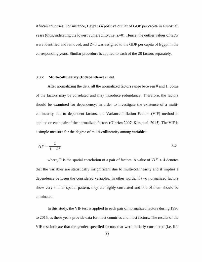
3.3.2 Multi-collinearity (Independence) Test

After normalizing the data, all the normalized factors range between 0 and 1. Some

of the factors may be correlated and may introduce redundancy. Therefore, the factors

should be examined for dependency. In order to investigate the existence of a multi-

collinearity due to dependent factors, the Variance Inflation Factors (VIF) method is

applied on each pair of the normalized factors (O’brien 2007; Kim et al. 2015). The VIF is

a simple measure for the degree of multi-collinearity among variables:

𝑉𝐼𝐹 =1

1 − 𝑅2 3-2

where, R is the spatial correlation of a pair of factors. A value of 𝑉𝐼𝐹 > 4 denotes

that the variables are statistically insignificant due to multi-collinearity and it implies a

dependence between the considered variables. In other words, if two normalized factors

show very similar spatial pattern, they are highly correlated and one of them should be

eliminated.

In this study, the VIF test is applied to each pair of normalized factors during 1990

to 2015, as these years provide data for most countries and most factors. The results of the

VIF test indicate that the gender-specified factors that were initially considered (i.e. life

34

expectancy at birth for male/female and unemployment rate for male/female) are highly

correlated between the genders and indicate 𝑉𝐼𝐹 > 4 for all the chosen years. Therefore,

for both cases, the data is averaged between the genders and the gender-neutralized factors

are utilized for quantifying drought vulnerability. The rest of the factors did not indicate

any dependence and resulted in 𝑉𝐼𝐹 < 2. Therefore, the results of the VIF test lead to

selection of a total of 28 independent factors for quantifying drought vulnerability.

3.3.3 Weighting and Averaging

Drought Vulnerability Index (DVI) in each year is calculated by weighted

averaging of the ensemble of 28 normalized vulnerability factors. In other words, DVI can

be viewed as a multi-dimensional metric that can be decomposed to measure the effect of

an individual factor and analyze the adaptation plans of a country.

Three different weighting methods are implemented in this study to calculate DVI:

a. Simple averaging (equal weights)

b. Random weighted averaging

c. Component averaging

The first method (i.e. simple averaging) treats all factors with equal importance and

assigns a weight of 1

𝑛 to each of the factors, where n is the total number of available factors

in a particular year for a specific country (shown in Figure 3-1).

35

The assigned weights may affect the final value of DVI. Therefore, random

weighted averaging is proposed and applied in order to provide a probabilistic measure of

DVI and to investigate and minimize the sensitivity of the calculated DVI to the chosen

weighting method. An ensemble of 1000 set of uniform random weights were generated

for each year and each country, and they were applied to the factors in order to obtain 1000

set of DVI values for each country in each year. The distribution of the 1000 DVIs will

reveal the effect of the assigned weights on the calculated vulnerability.

Lastly, the component averaging method is utilized to calculate the DVI for each

component by applying equal weights to the factors of each component in each year.

Component averaging will be beneficial for understanding the historical changes of

vulnerability and determines the resilience of each country in each component, and will

also provide valuable information for establishing long-term adaptation plans for

improving drought vulnerability of African countries.

3.3.4 Cluster Analysis

Cluster analysis is a common method for classifying data into sub-groups (clusters)

based on their similarities (Wilks 2011; Ahmadalipour et al. 2015). The dendrogram plots

of the cluster analysis provide apprehensible graphical illustration of the (dis)similarities

among various observations. In this study, we have employed the linkage function in order

to create an agglomerative hierarchical cluster tree (a bottom up approach where each

observation starts in its own cluster and pairs of clusters are merged) from the DVI of all

countries using the unweighted average distance algorithm (known as group average). The

36

linkage function is calculated based on the average distance between all pairs of objects in

any two clusters. Then, the pairwise Euclidean distance between DVIs is used to obtain the

optimal leaf ordering for the hierarchical clustering, and the results are plotted here using

a polar dendrogram. For more information about the details of cluster analysis and its

different options, readers are referred to Wilks (2011).

3.3.5 Change-Point Analysis

DVI is calculated for the historical period of 1960-2015 for each country as

described. The factors used for calculating DVI varies through time, and this may result in

sudden changes in the time-series of DVI. Since the historical variations of DVI in each

country is supposed to be utilized for projecting future DVI, it is necessary to determine if

any substantial change has happened in the time-series of DVI for each country. The

change-point analysis is a useful tool for diagnosing whether a change has taken place

according to confidence intervals (Taylor 2000).

The procedure for conducting a change-point analysis is based on a combination of

cumulative sum charts (CUSUM) for the original time-series as well as the bootstrapped

data from a large ensemble of randomly resampled time-series of the original data. Let

𝐷1, 𝐷2, … , 𝐷12 represent the DVI time-series for a particular country in 1960, 1965, …,

2015, respectively. The average DVI is calculated as:

�̅� =𝐷1 + 𝐷2 +⋯+𝐷12

12

3-3

37

Then, the initial cumulative sum is assigned zero (𝑆0 = 0), and the subsequent

cumulative sums are calculated as follows:

𝑆𝑖 = 𝑆𝑖−1 + (𝐷𝑖 − �̅�) 3-4

𝑆𝑖 is the cumulative sum and always ends at zero (in this case, 𝑆12 = 0). An upward

slope in the CUSUM chart indicates a period that the values are higher than the overall

average, and vice versa. Therefore, a sudden change in the direction (slope) of the CUSUM

implies a sudden change in the data. An estimator of the magnitude of change is the range

of CUSUM (𝑆𝑑𝑖𝑓𝑓), which is a practical choice regardless of the distribution and even if

multiple changes have occurred. It is defined as:

𝑆𝑑𝑖𝑓𝑓 = 𝑆𝑚𝑎𝑥 − 𝑆𝑚𝑖𝑛 3-5

where 𝑆𝑚𝑎𝑥 and 𝑆𝑚𝑖𝑛 represent the maximum and minimum values of 𝑆𝑖,

respectively.

In order to determine if a change has occurred at a certain confidence level, a

bootstrap analysis is performed. For such purpose, a large ensemble of randomly reordered

samples of data with the same length and without replacement is generated

(𝐷10, 𝐷2

0, … , 𝐷120 ). Then, the bootstrapped CUSUM is calculated (𝑆0

0, 𝑆10, … , 𝑆12

0 ), and the

magnitude of change (𝑆𝑑𝑖𝑓𝑓0 ) will be determined. The procedure is applied to each of the

resampled time-series. A confidence level is then calculated as:

𝐶𝑜𝑛𝑓𝑖𝑑𝑒𝑛𝑐𝑒 𝐿𝑒𝑣𝑒𝑙 = 𝑛

𝑁× 100% 3-6

38

Here n is the number of bootstraps where 𝑆𝑑𝑖𝑓𝑓0 < 𝑆𝑑𝑖𝑓𝑓, and N is the total number

of bootstraps. In this study, N=10,000 bootstraps are generated to reliably investigate the

change-point in each country. The 95% confidence level has been proposed as a minimum

threshold for concluding that a significant change has occurred (Taylor 2000). After

detecting the existence of a change, the farthest point of the CUSUM from zero (max |𝑆𝑖|)

indicates the last point before the change happened.

3.3.6 Future Drought Vulnerability Projection

After applying the change-point analysis and determining whether a change has

occurred or not, the change in the trend of DVI is also considered and the longest reliable

continuous historical period of DVI is determined for each country. Then, a regression

model is fitted to the time-series of DVI for each country and it is extrapolated into the

future period of 2020-2100. Different regression models are evaluated including

exponential, logarithmic, linear, polynomial, and power, and the appropriate function is

chosen based on the highest coefficient of determination (R2), the lowest root mean square

error (RMSE), and considering the theoretical thresholds of DVI (which should be between

0 to 1, according to the definition). Therefore, although polynomial functions might yield

to high R2 in some cases, they did not satisfy the threshold requirement in most cases. The

results of DVI projection and the regression functions used for each country are discussed

in more details in the results section.

39

3.4 Results and Discussion

The results of vulnerability assessment are divided into three sections. At first, the

characteristics of DVI are investigated during the historical period. Then, the future

projections of DVI are presented and discussed. Finally, the calculated drought

vulnerability indices are evaluated according to the historical observed droughts and their

impacts.

3.4.1 Historical Assessment of DVI

The 28 independent normalized factors are averaged for each country in each 5-

year period to calculate DVI using the simple averaging method. Figure 3-3 shows the

DVI of each country calculated using the simple averaging (arithmetic mean) of the

corresponding factors in each year. From the figure, the overall drought vulnerability has

decreased in some regions over the past decades. This is especially perceived for the

western Saharan countries (i.e. Mali, Niger, and Chad) where DVI values range up to 0.8

in the 1970s and 1980s, and decrease to about 0.6 in recent years. In general, the northern

countries of the African continent (i.e. Egypt, Libya, Tunisia, and Algeria) indicate the

lowest DVI in most years, followed by South Africa and Morocco. It is worth mentioning

that all of these countries receive low annual precipitation (less than 400mm per year).

However, their economy and infrastructure are more developed than the majority of

African countries. Furthermore, the total water resources of a country is not solely

dependent on its rainfall. In fact, many countries depend on transboundary sources for a

large portion of their water resources. For instance, Egypt receives about 97% of its total

40

water resources from the Nile River which originates in other countries (FAO 2016).

Therefore, albeit receiving limited precipitation, Egypt is among the least vulnerable

countries in Africa based on the water resources components.

Figure 3-3. Spatial changes of Drought Vulnerability Index (DVI) calculated using simple

averaging (arithmetic mean) of the corresponding factors in each year during the historical

period.

The time-series of DVI for the period of 1960-2015 is utilized to apply cluster

analysis. Figure 3-4 shows the polar dendrogram of the cluster analysis results. The linkage

function determines the similarities among countries (the connections and the linkage

41

distance) and the optimal leaf order indicates the order of countries (from top to bottom).

In general, the connected countries are more similar to each other, and it continues with

the hierarchy of the dendrogram. For instance, Egypt and Algeria are very similar (in terms

of vulnerability) since they are connected. Then, these two countries are similar to Tunisia,

connected at the next level. Furthermore, the order of countries in the dendrogram indicate

their overall DVI value. In other words, the first countries of the plot (Equatorial Guinea,

Gabon, and so on) generally have lower DVI than the last countries of plot (Mali, Rwanda,

and so on). A dendrogram may be crossed (cut) at any linkage distance and the generated

branches will indicate an individual cluster of similar countries. In this case, considering

𝐿𝑖𝑛𝑘𝑎𝑔𝑒 𝐷𝑖𝑠𝑡𝑎𝑛𝑐𝑒 = 0.65, three separate clusters are created representing low, medium,

and high drought vulnerability, which are plotted in green, yellow, and red, respectively.

The number of clusters will change according to the chosen linkage distance, whereas the

order of countries and their connections are fixed.

42

Figure 3-4. Polar dendrogram representing the results of clustering DVI using the

hierarchical cluster analysis based on the average Euclidean linkage distance and optimal

leaf ordering. In general, the green, yellow, and red colors indicate countries with low,

medium, and high drought vulnerability, respectively.

Figure 3-5 represents the DVI of each country calculated using the random

weighted averaging. Considering a particular country and a particular year, the boxplots

show the distribution of the 1000 DVIs for each year. In general, the number of factors for

quantifying DVI is higher in recent years than the earlier decades, and the range of DVI

(boxplot quartiles) is generally smaller as well. This implies that the calculated DVI is less

43

sensitive to the chosen weights in recent years. Figure 3-5 also identifies the temporal

variations of DVI during the past decades. Some of the countries show minor variations of

DVI in the historical period (e.g. Kenya). In some cases, there is an obvious abrupt change

in DVI. For instance, Algeria indicates DVI values of higher than 0.4 with a decreasing

trend until 1985, whereas DVI values of about 0.25 are found after 1990 with a slightly

increasing trend. The contrast is found for Mali, where slightly increasing DVI values of

above 0.8 are followed by decreasing DVIs ranging about 0.6, prior and after 1990,

respectively. These changes are identified and discussed in more details for future DVI

projections.

44

Figure 3-5. Drought Vulnerability Index (DVI) of each country calculated using the

random-weighted averaging method.

The median of boxplots of Figure 3-5 can be used as a likely prediction of DVI in

each year. In order to understand the differences between the DVI calculated from simple

averaging method and the DVI from the random weighted averaging, the results for 1995

and 2015 are plotted against each other in Figure 3-6. Both these years have the highest

45

number of available factors and thus, the DVIs have high reliability. In the figure, the

countries are ordered according to their DVI value acquired from the simple averaging

method. Therefore, the figure also indicates the changes of countries’ drought vulnerability

in 20 years. In Figure 3-6, the set of 1000 DVIs from random weighted averaging method

are plotted using boxplots and the simple averaged DVIs are shown in green asterisks. In

general, the DVI from simple averaging method is almost the same as the median of

random weighted averaging. In both years, Egypt has the lowest DVI of about 0.2, followed

by Algeria, Tunisia, and Libya (with different order). Somalia is the second most

vulnerable country, and Malawi and Ethiopia are also among the high vulnerable countries.

Comparing the ranks of countries in the 20 year timeframe, Central African Republic has

the most exacerbation, falling from rank 17 in 1995 (with a DVI of 0.55) to the third most

vulnerable country in 2015 (with a DVI of 0.7). On the other hand, Rwanda denotes the

most progress in drought vulnerability between these two years, with 16 ranks

improvement (from 38th to 22nd).

46

Figure 3-6. Comparison of the DVI calculated using the simple averaging method (green

asterisks) and the DVI calculated by the random weighted averaging (boxplots) for 1995

and 2015. In both plots, the countries are ordered according to their DVIs.

Least Drought Vulnerable Countries

The top-three countries with the least DVIs are identified as Egypt, Tunisia, and

Algeria, all of which are located at the northern part of the African continent. Figure 3-7

47

shows the component averaged drought vulnerability for the top-3 least drought vulnerable

countries during 1990-2015. This period is chosen as it provides data for the majority of

factors, which allows reliable quantification of vulnerability for each component. Drought

vulnerability of each component is quantified using the component averaging method. It

should be noted that the land use component is not considered here as it has only two factors

and may not conform to the other components. Radar plots are used to show the results of

component averaged drought vulnerability in Figure 3-7. In the radar plots, each

component is located on one of the angles, and the area of the generated pentagon

corresponds to the overall drought vulnerability (i.e. a higher plot area implies higher

vulnerability). From Figure 3-7, focusing on Egypt (shown in green), the social component

has decreased from about 0.7 in 1990s to about 0.4 in 2010s (mainly due to the increase of

the human development index), while the Water resources component has stayed about 0.4

in all years. All three countries are among the most improved countries in terms of Health

and Infrastructure components. Egypt has lower Water resources vulnerability to drought

than the two other countries, mainly due to the abundant streamflow received from the Nile

River.

48

Figure 3-7. Radar plots representing drought vulnerability index (DVI) of each component

for the top-3 least vulnerable countries in Africa (i.e. Algeria, Egypt, and Tunisia).

Most Drought Vulnerable Countries

Chad, Niger, and Malawi are found to be the most drought vulnerable countries.

The first two countries are neighbors and located primarily in central parts of Sahara, and

Malawi is a fairly smaller country in southeastern Africa. Again, the radar plots are

employed to quantify drought vulnerability of these countries, and the results are shown in

Figure 3-8. From the figure, Malawi and Niger (plotted in green and red, respectively)

indicate improvements for the Health component, especially Niger with a continuous

decrease of vulnerability from about 0.7 in 1990 to about 0.35 in 2015. On the contrary,

Chad (plotted in blue) shows almost no change for the Health component, and indicates a

vulnerability of 0.7 for it in all years. Furthermore, Chad demonstrates aggravation for the

49

Social component too. The Social component for Chad has raised from 0.55 to about 0.8

during 1995 to 2015. Both Niger and Chad have the highest vulnerability for Energy and

Infrastructure component among other African countries. For instance, only 8% of Chad’s

population had access to electricity in 2014. The rate for Niger and Malawi is 14% and

11%, respectively. In general, Malawi has lower drought vulnerability for the Water

resources component, mainly because it receives above 1000mm/year precipitation, which

is much higher than the average precipitation of the other two countries. Having arid

climate with low precipitation, Niger and Chad are highly dependent on transboundary

water resources with dependency ratios (i.e. the ratio of freshwater received from the

sources outside the country borders) of 90% and 67%, respectively (FAO 2016).

Figure 3-8. Radar plots representing drought vulnerability index (DVI) of each component

for the top-3 most vulnerable countries in Africa (i.e. Chad, Malawi, and Niger).

50

Although the water resources component cannot be improved easily and it is

primarily dependent on the regional climatic characteristics, the other four components are

inter-connected and improving either of them will have positive feedbacks on the rest of

the components to some extent. For instance, in order to improve the Health component,

hospitals and medical centers should be advanced or even established, which in turn

improves Infrastructure and Economy, and will have positive impact on society by

decreasing the unemployment rate and advancing the human development index (another

point of view is that improving any factor requires investment in other factors as well). In

fact, many under-developed countries invest in their infrastructure (e.g. power plants and

energy sectors, water storage facilities, or railroads) to advance their economy as well as

the corresponding invested component.

Progressive and Retrogressive Countries

Figure 3-9 shows three progressive countries (Burkina Faso, Mali and Rwanda)

with a decreasing trend of drought vulnerability and three retrogressive countries (Djibouti,

Kenya, and Zimbabwe) with an increasing drought vulnerability over time. For each year,

drought vulnerability of each component is calculated separately in order to attribute the

overall changes of each component. In some cases, the data is limited before 1980s. For

instance, the data for Economy component (shown in purple) for Mali is not available in

1960. In general, the progressive countries show a decrease in the vulnerability of Health

component (shown in green). On the contrary, Zimbabwe indicates large increase for

vulnerability from the Health component in the past decades. It also shows aggravation of

51

vulnerability to Social component, and the accumulation of these two components are the

primary reason for its increasing vulnerability, albeit the improvements on the Water

Resources component (shown in blue). It should be noted that both Zimbabwe and Kenya

indicate decreasing drought vulnerability since 2010 mainly for Economy and

Infrastructure components, respectively. Furthermore, Djibouti and Rwanda show

considerable decreasing vulnerability to Water Resources component.

Figure 3-9. Historical changes of DVI in each component for the most progressive

countries with a decreasing trend of DVI (top) and the most aggravating countries with an

increasing trend of DVI (bottom).

3.4.2 Change-Point Analysis and Future Projection of DVI

The median DVI from random weighted averaging is chosen as the representative

of drought vulnerability, and it is gathered for each country during the historical period to

52

be utilized for change-point analysis and projecting future DVI. Figure 3-10 shows the

results of the change-point analysis for Lesotho (top) and Nigeria (bottom). A visual

inspection of DVI time-series for Lesotho (plot a.) implies that a change-point exists in

1990, whereas for Nigeria (plot d.), no obvious change can be detected. Change-point

analysis is employed to statistically inspect for any significant changes in the DVI time-

series. The middle boxplots (plots b. and e.) show the CUSUM for the 10,000 bootstrapped

resamples, and the line plot indicate the CUSUM for the original DVI time-series. The Sdiff

is calculated for each case, and the histogram of 𝑆𝑑𝑖𝑓𝑓 and 𝑆𝑑𝑖𝑓𝑓0 (corresponding to the

original and resampled DVI time-series, respectively) are shown in the right plots. From

plot c, a confidence level of 99.23% is found for Lesotho, which is greater than the 95%

threshold and indicates that a change has occurred in the DVI timeseries of Lesotho. The

peak of the CUSUM for Lesotho (plot b.) has happened in 1985, and thus, 1985 is the last

point before the change occurred. Therefore, DVI values of 1990 onward should be used

for future projection of DVI in Lesotho. On the other hand, for Nigeria, 88.69% of the

bootstrapped DVIs have 𝑆𝑑𝑖𝑓𝑓0 < 𝑆𝑑𝑖𝑓𝑓, and therefore, the test is unable to detect any

significant changes in the DVI time-series at 95% confidence level. In general, most of the

time-series that indicate a change-point, have one peak in their CUSUM plot (as in plot b.),

whereas for the cases without a change-point, there is usually more than one peak (as in

plot e.).

53

Figure 3-10. Change-point analysis for Lesotho (top) indicating a significant change in the

DVI time-series, and Nigeria (bottom) without any change point. Plots (a) and (d) show

the DVI time-series. Plots (b) and (e) represent the CUSUM results for original DVI (line)

and bootstrapped DVI (boxplots), and the distribution of 𝑆𝑑𝑖𝑓𝑓0 , and 𝑆𝑑𝑖𝑓𝑓 are shown in

plots (c) and (f).

The change-point is investigated for each country, and a regression function is fitted

to each case considering the start year. The functions, start years, and the coefficient of

determination (R2) for each country are presented in Table 3-1. In all cases, the power

functions resulted in the highest R2 among others, while meeting the DVI thresholds. In

some cases, the DVI shows several variations in the historical period and does not follow

a constant direction. For instance, Mozambique shows a decreasing trend during 1990-

2000 and an increasing trend after 2000, which makes it difficult to fit a regression model

to it. Therefore, it has one of the least R2 among other countries. Although if the DVI after

2000 is considered for Mozambique, R2 of 0.95 is achieved. However, such decision will

54

be an overestimation of vulnerability with a considerable positive slope, ignoring the long-

term changes of DVI. In other words, it is not practical to extrapolate for 80 years in future

while relying on only 15 years of data. Therefore, at least 30 years of data is employed to

project DVI for the future period, and in almost all cases, the projected DVI has accurately

captured the long-term trend and direction of drought vulnerability.

Table 3-1. The functions used for projecting future DVI, the starting years (representing

no change afterwards), and the coefficient of determination for each case.

No. Country Start Year Function R2

1 Algeria 1990 DVI(t)=0.2153t0.0896 0.68

2 Angola 1960 DVI(t)=0.7895t-0.123 0.68

3 Benin 1980 DVI(t)=0.7825t-0.141 0.86

4 Botswana 1980 DVI(t)=0.4743t-0.168 0.81

5 Burkina Faso 1970 DVI(t)=0.8946t-0.156 0.92

6 Burundi 1985 DVI(t)=0.7379t-0.06 0.34

7 Cameroon 1985 DVI(t)=0.5033t0.0241 0.97

8 Cent. African Rep. 1990 DVI(t)=0.5292t0.1378 0.79

9 Chad 1985 DVI(t)=0.6825t0.0104 0.03

10 Rep. Congo 1985 DVI(t)=0.3996t0.1383 0.76

11 Côte dIvoire 1975 DVI(t)=0.4955t0.042 0.46

12 Dem. Rep. Congo 1990 DVI(t)=0.6449t0.043 0.42

13 Djibouti 1990 DVI(t)=0.4701t0.0638 0.82

14 Egypt 1990 DVI(t)=0.2409t-0.066 0.17

15 Equatorial Guinea 1980 DVI(t)=0.5405t-0.155 0.68

16 Eritrea 1980 DVI(t)=0.6045t0.0537 0.42

17 Ethiopia 1960 DVI(t)=0.5504t0.1097 0.78

18 Gabon 1975 DVI(t)=0.2983t-0.028 0.11

19 Ghana 1970 DVI(t)=0.6944t-0.122 0.75

20 Guinea 1980 DVI(t)=0.5667t0.0539 0.74

21 Guinea-Bissau 1965 DVI(t)=0.6599t0.0169 0.05

22 Kenya 1975 DVI(t)=0.6232t-0.025 0.28

23 Lesotho 1990 DVI(t)=0.4471t0.1752 0.91

24 Liberia 1975 DVI(t)=0.5339t0.0797 0.64

25 Libya 1975 DVI(t)=0.3333t-0.154 0.48

26 Madagascar 1960 DVI(t)=0.5766t0.0462 0.45

27 Malawi 1965 DVI(t)=0.8699t-0.083 0.88

55

28 Mali 1990 DVI(t)=0.6624t-0.077 0.69

29 Mauritania 1985 DVI(t)=0.6488t-0.113 0.88

30 Morocco 1990 DVI(t)=0.3793t-0.13 0.87

31 Mozambique 1990 DVI(t)=0.6647t0.0089 0.07

32 Namibia 1980 DVI(t)=0.3756t0.0579 0.55

33 Niger 1970 DVI(t)=0.8397t-0.092 0.72

34 Nigeria 1960 DVI(t)=0.7798t-0.081 0.72

35 Rwanda 1980 DVI(t)=0.8027t-0.137 0.88

36 Senegal 1990 DVI(t)=0.5969t-0.091 0.72

37 Sierra Leone 1965 DVI(t)=0.626t0.0513 0.41

38 Somalia 1980 DVI(t)=0.88t-0.109 0.67

39 South Africa 1990 DVI(t)=0.2566t0.167 0.68

40 Sudan 1965 DVI(t)=0.5912t0.0181 0.35

41 Togo 1985 DVI(t)=0.6674t-0.049 0.62

42 Tunisia 1990 DVI(t)=0.2448t-0.088 0.47

43 Uganda 1970 DVI(t)=0.7209t-0.059 0.47

44 Rep. Tanzania 1980 DVI(t)=0.6405t0.0185 0.86

45 Zambia 1980 DVI(t)=0.559t0.0702 0.43

46 Zimbabwe 1980 DVI(t)=0.371t0.2716 0.85

The functions of Table 3-1 are applied to extrapolate the DVI for the future period

of 2020-2100, and the results are plotted along with the historical DVIs. Figure 3-11 shows

the timeseries of DVI for each country during the historical period (1960-2015) and future

projections (2020-2100). Focusing on the late 21st century, Egypt, Libya, and Tunisia

indicate the least DVIs, and Central African Republic, Ethiopia, and Zimbabwe show the

highest drought vulnerability.

56

Figure 3-11. Temporal variations of Drought Vulnerability Index (DVI) for each country

during the historical period of 1960-2015 and future projections of 2020-2100.

Results of Table 3-1 and Figure 3-11 demonstrate that the number of countries

showing decreasing, increasing, and no considerable change in DVI are 19, 13, and 14,

respectively. In order to better understand the overall pattern of DVI through time, violin

57

plots (Hintze and Nelson 1998) are used and the distribution of DVI in each year is

investigated. Figure 3-12 shows the distribution of DVIs for the 46 African countries in

each year for the historical period (plotted in green) and future projections (plotted in blue).

The red plus signs in the figure indicate the median of DVI in each year. As it can be

inferred, in the 2000s (when the number of factors used are considerably higher than

before) the distribution is highly skewed having one peak above 0.6 and a smaller peak

around 0.5. There is also a small group of countries that have DVI values less than 0.4.

However, the distribution is considerably changed by 2080s, with both parts growing and

two peaks found; one peak for the DVIs less than 0.4, and one peak around the median for

the DVIs ranging between 0.4-0.8. In other words, during 1995-2015, the countries can be

classified to two groups of low vulnerable (𝐷𝑉𝐼 < 0.4) and moderate-to-high vulnerable

(0.5 < 𝐷𝑉𝐼 < 0.8). Whereas in 2090s, three groups of countries are identified as low

vulnerable (𝐷𝑉𝐼 < 0.35), moderate vulnerable (0.35 < 𝐷𝑉𝐼 < 0.6), and high vulnerable

(𝐷𝑉𝐼 > 0.6). Furthermore, almost no country had DVIs less than 0.2 or above 0.8 during

1995-2015. Whereas, the distribution of DVI is much wider after 2070s, and several

countries indicate extremely high and extremely low drought vulnerability. In general, the

median DVI shows a slightly increasing trend during the historical period and it seems to

be slightly decreasing over time for the future projections.

58

Figure 3-12. Violin plots representing the DVI distribution of the 46 African countries for

historical simulations (green) and future projections (blue). The red plus (+) signs indicate

the median of DVI in each year.

The projected DVIs should be considered for long-term assessments and not for

short-term changes. In other words, DVI projections provide probable simulations of future

drought vulnerability in each 5-year period, whereas they should be implemented for multi-

decadal analysis. This is somehow similar to the application of Global Climate Models

(GCMs) for climate change studies, in which the models provide daily simulations, while

their primary purpose is mainly for long-term assessments (Ahmadalipour et al. 2017b).

3.4.3 Evaluating DVI estimates

The calculated drought vulnerability index should be evaluated in order to reveal

its reliability for further applications in drought risk management and adaptation planning.

Two main sources are utilized for the evaluation purposes: 1) the previous assessments of

59

drought vulnerability, and 2) the historical observed drought impacts. A large-scale

national-level assessment of drought vulnerability in Africa was employed by Naumann et

al. (2014), which is a static investigation and it did not investigate the temporal variations

of vulnerability. The results of this study have been used as the former source of evaluation.

For the latter, the International Disaster Database (EM-DAT) and the review of droughts

in Africa carried out by Masih et al. (2014) were utilized to perform a descriptive and

qualitative evaluation of the estimated DVI.

Naumann et al. (2014) found Somalia, Burundi, Niger, Mali, Ethiopia, and Chad as

the top-6 most vulnerable countries to drought with DVIs higher than 0.6. The current study

confirms it for most years, and the top-3 most drought vulnerable countries of this study

are among those identified before. Furthermore, Naumann et al. (2014) identifies Egypt as

the least vulnerable country, which is similar to our assessment, followed by Tunisia and

Gabon, both of which are among the low drought vulnerable countries in our findings. The

spatial pattern of DVI in both studies seem to be similar, with few differences. For instance,

this study characterizes Libya among the least vulnerable countries, whereas Naumann et

al. (2014) classifies it as a moderate country, mainly due to its deficiencies in renewable

natural resources component.

Considering the drought impacts and damages, the 2010-2011 drought of the Horn

of Africa affected over 12 million people (Zaitchik et al. 2012; Dutra et al. 2013). During

1960-2012, droughts in Ethiopia and Somalia affected more than 66 million and 13 million

people, and resulted in mortality of over 400,000 and 100,000 people, respectively (Masih

et al. 2014). Therefore, it can be concluded that Somalia and Ethiopia are highly vulnerable

60

to drought. The number of affected people and the total mortality caused by drought is over

30 million and 150,000 for Sudan, and over 5.5 million and 3000 for Chad, respectively.

The numbers are extremely high considering the total populations of 27 million and 8

million (in 2005) for Sudan and Chad, respectively. The values are similar for Niger (23

million and 85,000) indicating high drought vulnerability. On the other hand, over 17

million people have been affected by droughts in South Africa during 1960-2015, none of

whom were killed (Vogel et al. 2010). In general, droughts in northern and southern parts

of Africa have higher economic damages, whereas in central parts, many people have been

affected and killed by droughts in the past.

This section provided a comprehensive assessment of drought vulnerability at a

national level across the African continent. The future drought vulnerability projections

was calculated based on a statistical analysis of the historical relative changes of the

African countries’ drought vulnerabilities. Therefore, although it provides probable

estimates of future vulnerability, it is not a numerical simulation forecast, and it should be

applied for long-term assessments. Forecasting the future drought vulnerability is an

extremely complicated challenge, which is dependent on numerous sectors having dynamic

feedbacks on each other. For instance, growing population is a serious issue in the

undeveloped African countries, which is expected to impose severe impacts on food

security and social development (Godfray et al. 2010; Hanjra and Qureshi 2010; Tomlinson

2013; Khan et al. 2014). Moreover, climate change will alter the seasonal cycle of the

hydrologic system, which will in turn significantly affect the water resources component

of vulnerability (Leichenko and O’brien 2002; Sowers et al. 2011; IPCC 2014). It will also

61

impact the agricultural productivity and food security (Fischer et al. 2002; Mougou et al.

2011; Wheeler and Von Braun 2013). Apart from the impacts on the natural resources,

societal instability, conflicts, wars, and diseases may considerably impacts the socio-

economic components of a region, causing abrupt changes in the drought vulnerability

(Scheffran et al. 2012).

3.5 Summary and Conclusion

This section presented a comprehensive assessment of drought vulnerability across

Africa using a composite Drought Vulnerability Index (DVI) for the historical period of

1960-2015. Vulnerability was quantified at a national level using 28 factors from six

components of economy, energy and infrastructure, health, land use, society, and water

resources. All the factors were diagnosed for dependency using multi-collinearity tests, and

various weighting methodologies were implemented to calculate DVI. A change-point

analysis was conducted for the DVI of each country, and the calculated DVIs were then

projected into the future period of 2020-2100. The main findings of the study are as

follows:

The least vulnerable countries to drought are Egypt, Libya, Tunisia, and Algeria

(all located in northern parts of Africa) and South Africa.

The most vulnerable countries to drought are Chad, Malawi, Niger, and Somalia,

all of which are highly vulnerable to energy and infrastructure component.

62

Burkina Faso, Mali, and Rwanda indicate improvements for drought vulnerability

with a decreasing DVI and progressive health components. On the other hand,

Djibouti, Kenya, and Zimbabwe show increasing DVI over time.

In general, the median DVI of African countries shows slightly decreasing trend in

future projections. Meanwhile, a considerable number of countries are expected to

become extremely vulnerable to drought, with DVI>0.8.

Central African Republic, Ethiopia, Lesotho, and Zimbabwe will be among the

most vulnerable countries in the late 21st century. The least vulnerable countries in

future are expected to be the same as in historical period.

63

4 Drought Hazard and Risk in Africa

4.1 Background

Drought risk is generally characterized as a function of three primary components:

(i) hazard that is the possible future occurrence of drought , (ii) vulnerability that is the

susceptibility of exposed elements to the adverse effects of drought, and (iii) exposure that

is the population and assets affected by drought (Blauhut et al. 2015b; Han et al. 2016).

Drought risk refers to the potential losses from a particular hazard imposed by a drought

event (Brooks et al. 2005; Cardona et al. 2012). In other words, drought risk is determined

not only by the intensity of the event and the amount of exposure, but also by the

vulnerability of the society at a given time (Birkmann 2007; Carrao et al. 2016).

Reactive approaches are still used for drought management in most parts of the

world, which is commonly referred to as crisis management, responding to the impacts that

have already occurred (Wilhite et al. 2014; Svoboda et al. 2015). Nevertheless, these

approaches are known to be untimely and disintegrated, and thus, previous drought

management attempts have usually been ineffective with a rise in the socioeconomic

impacts of drought (Peterson et al. 2013; Sivakumar et al. 2014). The scientific consensus

has pointed out the necessity to move from reactive to proactive risk management strategies

(Birkmann et al. 2013; Rossi and Cancelliere 2013).

Climate change and the anthropogenic global temperature rise will have significant

impacts on natural hazards, extreme events, economy, and health (Honda et al. 2014;

Ahmadalipour et al. 2017b; Gergel et al. 2017). Multitude of studies have investigated the

64

impacts of climate change on drought for various regions of the globe (Zhao and Dai 2016;

Ahmadalipour et al. 2016). It has been concluded that climate change will intensify drought

in many regions across the world (Ahmadalipour et al. 2017a). This is especially more

considerable in arid regions (e.g. Northern Africa) as global warming will increase the

potential evapotranspiration (Asadi Zarch et al. 2014; Touma et al. 2015).

Besides the severe impacts of climate change on the African continent, population

growth is also expected to augment the natural resources scarcity and food insecurity

(Godfray et al. 2010; Seto et al. 2012; Khan et al. 2014). Population growth affects drought

risk both directly, i.e. through increasing the exposure component of the risk, and

indirectly, i.e. by altering the vulnerability components. It is a grand challenge in Africa,

especially for the least developed countries, and it will be a huge burden for the social and

human development (Hanjra and Qureshi 2010; Antwi-Agyei et al. 2012).

Despite the increasing concerns regarding the escalating impacts of droughts on

food, energy, and water resources in the 21st century, it has been argued that more attention

has been given to studying drought hazard rather than providing consistent drought risk

assessment frameworks (Shiau and Hsiao 2012; Kim et al. 2015; Tánago et al. 2016). In

fact, many of the recent studies that claim to assess “drought risk” have actually studied

the probability of drought hazard, ignoring the vulnerability and exposure components of

risk (e.g. Kam et al. 2014; Cook et al. 2015; Diffenbaugh et al. 2015).

The combination of climate change, population growth, and the aggravation of

socioeconomic vulnerabilities will intensify drought hazard, exposure, and vulnerability in

many regions of Africa. It will in turn substantially increase drought risk across the

65

continent. Therefore, it is important to investigate the changes of each component of risk

separately and understand their cumulative impacts on drought risk. The current study is

the first comprehensive and multi-dimensional assessment of the compounding effects of

climate change, population growth, and vulnerability changes on drought risk over Africa.

Drought risk is assessed at a national scale for the historical as well as future periods, and

its decadal changes are investigated for each country. The results will provide long-term

projections of drought risk and will reveal the role of each component (hazard,

vulnerability, and exposure) in each country, which will be beneficial for strategic planning

and adaptation policy making over the continent.

4.2 Data

Three different types of data are used to address the three components of risk (i.e.

hazard, vulnerability, and exposure). Vulnerability assessment has been thoroughly

explained in the previous chapter. For quantifying the hazard, Regional Climate Models

(RCMs) developed by the Coordinated Regional Climate Downscaling Experiment

(CORDEX) are utilized over the African domain, i.e. AFR-44 (Jones et al. 2011).

Precipitation (Prec) and potential evapotranspiration (PET) are acquired from 10 RCMs at

a daily timescale and 0.44° spatial resolution for the entire African continent during the

historical period of 1951-2005 as well as two future scenarios of RCP4.5 (representing

moderate emission increase in future) and RCP8.5 (representing business as usual scenario)

for the period of 2006-2100. The data are then accumulated to monthly timescale to be

66

employed for drought analysis. More information about the RCMs used in this study are

presented in Table 4-1.

Table 4-1. The 10 RCMs used in this study and their characteristics. All the RCMs are

developed by the Swedish Meteorological and Hydrological Institute (SMHI) and have a

spatial resolution of 0.44°.

No Deriving GCM Original Modeling Institute

Original

Resolution

(lat × lon)

Ens.

Member

1 CanESM2 Canadian Centre for Climate Modeling and Analysis 2.8° × 2.8° r1i1p1

2 CNRM-CM5 National Centre of Meteorological Research, France 1.4° × 1.4° r1i1p1

3 CSIRO-Mk3-6-0 Commonwealth Scientific and Industrial Research

Organization, Australia 1.8° × 1.8° r1i1p1

4 EC-EARTH EC-EARTH consortium 1.0° × 1.0° r12i1p1

5 GFDL-ESM2M Geophysical Fluid Dynamics Laboratory 2.5° × 2.0° r1i1p1

6 HadGEM2-ES Met. Office Hadley Centre 1.88° × 1.25° r1i1p1

7 IPSL-CM5A-MR Institut Pierre-Simon Laplace 2.5° × 1.25° r1i1p1

8 MIROC5

Atmosphere and Ocean Research Institute (The

University of Tokyo), National Institute for

Environmental Studies, and Japan Agency for

Marine-Earth Science and Technology

1.4° × 1.4° r1i1p1

9 MPI-ESM-LR Max Planck Institute for Meteorology (MPI-M) 1.9° × 1.9° r1i1p1

10 NorESM1-M Norwegian Climate Centre 2.5° × 1.9° r1i1p1

Lastly, exposure is investigated using human population data for each African

country. The population data are acquired from United Nations (2015) and utilized for the

historical period of 1950-2015 as well as three future population projection scenarios of

low, medium, and high variant over the period of 2015-2100.

4.3 Methodology

The risk formulation employed in this study is the same as that implemented by the

United Nations International Strategy for Disaster Reduction (UNISDR 2015) and the

67

Intergovernmental Panel on Climate Change (IPCC 2012), and it has been utilized in

multitude of earlier assessments (Peduzzi et al. 2002, 2009; Cardona et al. 2012; Carrao et

al. 2016). It is defined as:

𝑅𝑖𝑠𝑘 = 𝐻𝑎𝑧𝑎𝑟𝑑 × 𝐸𝑥𝑝𝑜𝑠𝑢𝑟𝑒 × 𝑉𝑢𝑙𝑛𝑒𝑟𝑎𝑏𝑖𝑙𝑖𝑡𝑦 4-1

As mentioned in the data section, the population of each county is used as exposure,

and a comprehensive multi-dimensional framework was carried out to quantify

vulnerability at a national level. Drought hazard is quantified using the Standardized

Precipitation Evapotranspiration Index (SPEI) (Vicente-Serrano et al. 2010). SPEI is a

multi-scalar drought index that accounts for temperature effects on drought and it has been

employed in numerous studies (Li et al. 2015; Touma et al. 2015; Ahmadalipour et al.

2016, 2017a). It is based on a climatic water balance and considers the water deficit as the

difference between precipitation and potential evapotranspiration (D = P − PET). The

water deficit (D) can be calculated at different accumulation periods to reflect the variations

at different timescales. In this study, D is calculated for each grid (at 0.44-degree spatial

resolution) and each month, and then accumulated to 12-month timescale in order to

capture the long-term impacts of climate change as suggested by previous studies

(Ahmadalipour et al. 2017a). The nonparametric Weibull plotting position is utilized to

calculate the SPEI as follows:

𝑃(𝑋𝑖) =𝑖

𝑛 + 1 4-2

where i is the rank of D from smallest to largest, n is the sample size, and 𝑃(𝑋𝑖)

denotes the empirical probability. 𝑃(𝑋𝑖) is then transformed to the standard normal

68

distribution (with zero mean and unit standard deviation) which will be the corresponding

value of the SPEI:

𝑆𝑃𝐸𝐼 = ∅−1(𝑃) 4-3

The SPEI is calculated separately for each month, and the monthly values are

arranged to obtain the time-series of drought index. A zero value for SPEI indicates no

drought condition and negative values represent an imbalance in the available water,

indicating dry conditions. The lower the value of SPEI, the higher is the intensity of

drought.

The SPEI-12 is calculated for each grid of each RCM for the historical period of

1951-2005 and two future scenarios of RCP4.5 and RCP8.5 during 2006-2099. The

calculated SPEI is at 0.44-degree spatial resolution. A Hazard Index is proposed and

utilized to quantify drought hazard at national scales. After calculating the intensity of

drought for each month using the SPEI, drought hazard of a particular month in a country

will be calculated by averaging the negative SPEI values across the country divided by the

total number of grids of that country. Then, the annual drought hazard will be the mean of

monthly drought hazards as follows:

𝐻𝑎𝑧𝑎𝑟𝑑 𝐼𝑛𝑑𝑒𝑥 = |∑∑𝑆𝑃𝐸𝐼(< 0)

𝑁

𝑛=1

12

𝑖=1

12. 𝐺⁄ | 4-4

where i indicates the month, N denotes the number of grids in the country that

experience drought in a particular month, and G is the total number of grids that cover the

country. The drought hazard calculated by the above function will have the same absolute

69

range as the SPEI (i.e. 0 < Hazard Index < ~2.2). It reflects the overall severity of

drought in a particular region. For instance, if half of a country experiences moderate

drought (SPEI = −1) for 6 months in a year and no drought for the rest of the year, the

calculated Hazard Index will be 0.25 (1 × 0.5 ×6

12= 0.25). The maximum Hazard Index

is observed when the entire region experiences extreme drought (SPEI < −2) for the entire

year. Therefore, the proposed Hazard Index is a compound indicator of the intensity,

duration, and extent of drought.

After quantifying hazard, vulnerability, and exposure of each country, drought risk

is also quantified at national scale. For each country, drought risk is quantified for the

historical period for each RCM, and a historical mean drought risk value is calculated for

each RCM by averaging the corresponding drought risk values during the period of 1975-

2005. This 30-year period is chosen since it provides more accurate data than the

antecedent years (especially the socio-economic data for quantifying vulnerability).

Similar procedure is implemented to calculate drought risk projections in near future

(2010-2040), intermediate future (2040-2070), and distant future (2070-2100).

After calculating drought risks for historical and future periods, the changes in

drought risk are assessed by comparing the projected risk scenarios with the simulated

historical drought risk. Risk ratio is calculated for each country as follows:

𝑅𝑖𝑠𝑘 𝑅𝑎𝑡𝑖𝑜𝑚,𝑟,𝑝 =𝑅𝑖𝑠𝑘𝑓𝑢𝑡;𝑚,𝑟,𝑝

𝑅𝑖𝑠𝑘ℎ𝑖𝑠𝑡;𝑚

=𝐻𝑎𝑧𝑎𝑟𝑑𝑓𝑢𝑡;𝑚,𝑟

𝐻𝑎𝑧𝑎𝑟𝑑ℎ𝑖𝑠𝑡;𝑚×𝐸𝑥𝑝𝑜𝑠𝑢𝑟𝑒𝑓𝑢𝑡;𝑝

𝐸𝑥𝑝𝑜𝑠𝑢𝑟𝑒ℎ𝑖𝑠𝑡×𝑉𝑢𝑙𝑛𝑒𝑟𝑎𝑏𝑖𝑙𝑖𝑡𝑦𝑓𝑢𝑡

𝑉𝑢𝑙𝑛𝑒𝑟𝑎𝑏𝑖𝑙𝑖𝑡𝑦ℎ𝑖𝑠𝑡

4-5

70

where hist and fut indicate the values for historical and future periods, respectively.

m, r, and p denote different permutations of climate model (RCMs), climate scenarios

(RCPs), and population scenarios, respectively. This has been performed for each country

for the three future periods. Figure 4-1 shows a schematic diagram of the risk components

utilized in this study during historical and future periods.

Figure 4-1. Schematic diagram of the risk analysis methodology employed in this study

and its different components in historical and future periods.

The changes of each component of risk are also studied along with the overall

changes of drought risk ratio. Future drought risk ratio is quantified for each African

country (46 countries) using 10 RCMs, 2 climate scenarios (RCP4.5 and RCP8.5), 3

population scenarios (low, medium, and high variability), and three 30-year future periods

(near, intermediate, and distant future), totaling 8280 drought risk scenarios across the

continent (46×10×2×3×3=8280). This makes it possible to probabilistically assess future

drought risk conditions and characterize the uncertainties associated with different sources.

71

Besides the national-scale Hazard Index and drought risk, two important

characteristics of drought hazard are investigated at grid-scale (0.44° spatial resolution):

the spatial extent of drought and drought intensity. Drought extent is calculated by

detecting the area of Africa affected by drought (i.e. SPEI < −0.8; Chen et al., 2012)

divided by the total area of the African continent. Moreover, the long-term linear trends of

drought intensity are assessed for each grid during the future period of 2005-2100. The

Mann-Kendall trend test, as a rank-based non-parametric test and independent of the

statistical distribution, is utilized to investigate the significance of trends (Kendall 1948).

4.4 Results and Discussion

The results for drought vulnerability assessment and projection were exclusively

explained in previous chapter. Here, the results of the other components of risk (i.e. drought

hazard and exposure) are thoroughly investigated, followed by the results and discussion

for drought risk. Drought hazard is investigated at both grid- and national-scale, whereas

the other components (vulnerability and exposure) and hence the drought risk are

quantified at a national-scale.

4.4.1 Drought Hazard

Figure 4-2 shows the spatial extent of drought across Africa calculated from the

SPEI-12 results for the historical period (shown in grey) as well as two future scenarios of

RCP4.5 and RCP8.5 (shown in blue and red, respectively). The shaded area indicates the

results of 10 RCMs, and the lines represent the ensemble mean drought extent of the

72

corresponding scenario. The figure shows that the historical mean dry area over Africa is

about 7%, and it increases to about 25% in the late 21st century. Slightly increasing dry

extent is detected during the historical period, especially after 1990s. The drought extent

projections of RCP4.5 and RCP8.5 are similar until the 2030s, with the latter showing

higher dry area afterwards.

Figure 4-2. Spatial extent of historical and future droughts across Africa based on the

SPEI-12 results. The shaded area represents the results from 10 RCMs and the lines

indicate the ensemble mean dry area for each corresponding concentration pathway.

The long-term future trends of SPEI-12 is calculated for each RCM over the period

of 2005-2100, and the results are shown in Figure 4-3. The figure shows the mean decadal

change of SPEI for RCP4.5 (top) and RCP8.5 (bottom). A negative trend value indicates

decreasing SPEI and thus increasing intensity of drought. The Mann-Kendall trend test is

utilized to investigate the significance of trends at 0.05 significance level, and the negative

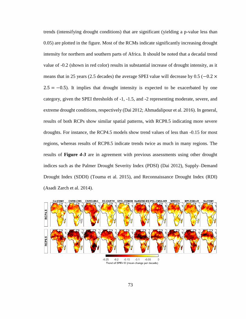
73

trends (intensifying drought conditions) that are significant (yielding a p-value less than

0.05) are plotted in the figure. Most of the RCMs indicate significantly increasing drought

intensity for northern and southern parts of Africa. It should be noted that a decadal trend

value of -0.2 (shown in red color) results in substantial increase of drought intensity, as it

means that in 25 years (2.5 decades) the average SPEI value will decrease by 0.5 (−0.2 ×

2.5 = −0.5). It implies that drought intensity is expected to be exacerbated by one

category, given the SPEI thresholds of -1, -1.5, and -2 representing moderate, severe, and

extreme drought conditions, respectively (Dai 2012; Ahmadalipour et al. 2016). In general,

results of both RCPs show similar spatial patterns, with RCP8.5 indicating more severe

droughts. For instance, the RCP4.5 models show trend values of less than -0.15 for most

regions, whereas results of RCP8.5 indicate trends twice as much in many regions. The

results of Figure 4-3 are in agreement with previous assessments using other drought

indices such as the Palmer Drought Severity Index (PDSI) (Dai 2012), Supply–Demand

Drought Index (SDDI) (Touma et al. 2015), and Reconnaissance Drought Index (RDI)

(Asadi Zarch et al. 2014).

74

Figure 4-3. Long-term trend of SPEI-12 for the future period of 2005-2100 for each RCM

in RCP4.5 (top) and RCP8.5 (bottom). The Mann-Kendall trend test is used at 0.05

significance level and only the significantly negative trends are plotted.

The Hazard Index (Equation 4-4) is calculated for the 10 RCMs for each country

during the historical as well as future periods, and the results are shown in Figure 4-4. The

figure shows the temporal changes of Hazard Index and the associated model and scenario

uncertainties. The historical, RCP4.5, and RCP8.5 results are plotted in grey, blue, and red,

respectively, with the shaded area showing the results of 10 RCMs and the lines

representing the ensemble mean results. The projections of Hazard Index show different

patterns and diverse uncertainties in different countries. In general, the northern African

countries (i.e. Algeria, Egypt, Libya, Morocco, and Tunisia) indicate an increasing Hazard

Index during the historical period, all of which demonstrate aggravating future Hazard

Index as well. The countries located at the southern parts of Africa (i.e. Botswana, Namibia,

South Africa, and Mozambique) follow similar yet moderate increasing patterns. On the

other hand, the western African countries below the Sahel region (i.e. Côte d'Ivoire,

Guinea, Liberia, and Sierra Leone) do not indicate any significant changes in the Hazard

Index of neither the historical period nor the future projections, and the Hazard Index of

the two future scenarios are similar for these countries. For other countries, RCP8.5

indicates higher Hazard Index than RCP4.5. The worst drought hazard conditions are

expected to happen in Egypt and Libya, both indicating substantial increase of Hazard

Index. Egypt is also the country with -the lowest model uncertainty (the narrowest shaded

area), especially for the RCP8.5 scenario.

75

Figure 4-4. Temporal variations of the annual Hazard Index for each country in Africa

during the historical period as well as two future scenarios of RCP4.5 and RCP8.5. The

shaded areas represent the results of 10 RCMs and the lines indicate the ensemble mean.

In order to better understand the overall changes of drought hazard over Africa, the

Hazard Index of each RCM is averaged in 5-year periods for each country, and the

distribution of the Hazard Index among the African countries is plotted using violin plots

76

(Hintze and Nelson 1998). This is done for the historical and future periods, and the results

are shown in Figure 4-5. The colors used are consistent with the previous figures. The plus

signs (+) indicate the median of distribution in each case. The figure shows that the Hazard

Index has generally increased during the historical period, and it is expected to substantially

increase in future. The median of Hazard Index is below 0.5 in the historical period, and it

is projected to become twice as much in the distant future. The two future RCPs have

similar distributions in near future (until 2040s), whereas RCP8.5 generally projects higher

values afterwards.

Figure 4-5. Violin plots showing the distribution of the Hazard Index among the African

countries for historical and future periods. The plus signs (+) indicate the median Hazard

Index in each case.

4.4.2 Exposure

Figure 4-6 shows the annual population projection of each country as well as the

total population of the African continent during the historical period (shown in grey) and

three future scenarios of low, medium, and high variant (shown in green, yellow, and red,

77

respectively). In general, the majority of African countries are expected to experience vast

expansion in their population in the upcoming decades. This can be realized by considering

the results for Total Africa (the last subplot in Figure 4-6) where the population of Africa

at the end of 20th century was about 1 billion people, whereas it will increase to 3, 4.5, and

6 billion people by the end of the 21st century for low, medium, and high variant scenarios,

respectively. This unprecedented population will impose serious challenges for Africa

regarding social development, food security, health, and many other sectors (Vörösmarty

et al. 2000; Gerland et al. 2014; Schlosser et al. 2014). The most population increase rate

is found in Niger and Chad (neighboring countries located at the sub-Saharan region), both

among the highly vulnerable countries in terms of the social and human development

components (Neumayer 2001). For instance, Niger’s population was about 10 million

people in the 2000s, and it is expected to increase to 150-250 million people by 2100s; a

1500-2500% increase rate. Considering the limited economic and natural resources of the

country due to its geopolitical location and the arid climate of the region, the vast

population increase will have substantial effects on drought risk with devastating

socioeconomic impacts on the country. On the contrary, Libya, Morocco, and Tunisia (all

of which are located at the northern parts of the African continent) show the least

population change rate, indicating decreasing population for the low variant scenario.

These three countries are also among the least drought vulnerable countries in Africa.

78

Figure 4-6. Historical record and projected population of each country in the African

continent. The last subplot shows the total population of the African continent. The y-axis

in all subplots is in million people, except for the last subplot (Total Africa) which shows

the population in billions.

4.4.3 Drought Risk

Drought risk ratio (Equation 4-5) is calculated in each country for 10 RCMs, 3

population scenarios, and 2 representative concentration pathways during the future

79

periods of 2010-2040, 2040-2070, and 2070-2100. Figure 4-7 shows the risk ratio

projections of each country for low and high variant population scenarios (the medium

variant scenario is not shown in the figure to have a clearer representation). The three

periods are shown in distinct colors, and the order of all subplots are consistent as identified

in the bottom row plots. In each plot, boxplots are used to show the risk ratio of 10 RCMs

and the red dash in the middle of each box represents the median of 10 RCMs. The figure

shows that the lowest risk ratio is found in Tunisia, Morocco, and Libya, respectively, all

of which are located at the northern parts of Africa. Despite the substantial increase of

drought hazard in these three countries, all of them indicate decreasing vulnerability and

low changes in exposure. For instance, for the case of low variant population scenario, the

exposure is expected to decrease in these countries, thus keeping the risk ratio at almost

constant rates in the future periods, despite the significant increase of drought hazard.

Nonetheless, even in most moderate cases, the drought risk is expected to become 2-3 times

higher than that in the historical period. On the contrary, Niger and Chad demonstrate the

highest risk ratios.

80

Figure 4-7. Boxplots showing the drought risk ratio of each country in the African

continent for 10 RCMs, two climate pathways (RCP4.5 and RCP8.5) and two population

scenarios (Low and High Variant). The red dash in the middle of each plot indicates the

median of the 10 RCMs.

Considering the drought risk ratios of near future (plotted in cyan in Figure 4-7),

all scenarios show similar ranges in each countries. Whereas in distant future (brown plots

81

in Figure 4-7), the exposure proves to have significant effects on the risk ratio, even more

influential than the climate pathway in many cases. For instance, the distant future drought

risk ratio (brown boxplots) of High Var.-RCP4.5 is higher than that for Low Var.-RCP8.5

in most countries. In order to better understand the risk ratios and their differences in

various scenarios, the ensemble mean drought risk ratio of each African country is shown

in Figure 4-8 for all the future scenarios. The figure shows that in several cases, the High

Var.-RCP4.5 drought risks are even greater than the Med. Var.-RCP8.5 risks in distant

future. Moreover, the combination of higher concentration pathway (RCP8.5) and high

variant population scenario in intermediate future (2040-2070) leads to risk ratios as large

as a moderate condition (Low Var.-RCP4.5) in distant future (2070-2100). In other words,

if no adaptation/mitigation planning is followed for climate emissions and population, it

will accelerate the devastating risks to happen decades sooner.

82

Figure 4-8. Projections of the ensemble mean drought risk ratio of each African country

in all the future scenarios (two climate pathways of RCP4.5 and RCP8.5 as well as three

population scenarios of Low, Medium, and High Variant) for near, intermediate, and

distant future.

83

The spatial patterns of the projected drought risk ratios can be understood from

Figure 4-9 which shows the risk ratios in near and distant future periods. The figure shows

that the central African countries should expect higher risk ratios than the southern and

northern African countries. The spatial patterns are somehow similar to those for drought

vulnerability in Africa (Naumann et al. 2014). In general, the southern and northern African

countries are more industrialized, having access to more resources and thus indicating

lower socioeconomic vulnerabilities and higher social development. This will in turn be

effective for their future population projections, keeping the exposure at mediocre levels

for the majority of those countries (Gerland et al. 2014).

Figure 4-9. Spatial distribution of the projected drought risk ratios in the African countries

for all scenarios in near and distant future.

84

In order to understand the overall changes of drought risk ratio across the African

continent, the distribution of the risk ratio among 46 African countries is plotted for each

future period/scenario using the violin plots, and the results are shown in Figure 4-10. The

plus signs (+) indicate the median of each plot. The figure clearly shows the overall changes

of drought risk in different scenarios. The median of drought risk ratio is about 4 in near

future, whereas it increases to about 10 in intermediate future, and reaches to 9-19 in distant

future. The difference between the different scenarios is negligible in near future, whereas

disparities are found among them in distant future. In fact, the highest risk ratio of the

optimum (most favorable) scenario (Low Var.-RCP4.5) is about the same as the median of

the worst-case scenario (High Var.-RCP8.5), which reflects the importance of climate and

population planning and management.

Figure 4-10. Violin plots representing the distribution of the drought risk ratio among the

African countries for the future periods/scenarios. The plus signs (+) indicate the median

risk ratio in each case.

85

The results implicate that the controlling component of drought risk is different for

each country. In some countries (e.g. Niger) the population increase seems to be the main

challenge for drought risk, which is accompanied by intensifying hazard conditions. Since

drought risk formulation is an integration of hazard, exposure, and vulnerability, it is

necessary to decompose it and assess the role of each component on drought risk. Figure

4-11 shows the change rates of each component in each country for near and distant future.

For instance, the change rate of vulnerability is calculated as 𝑉𝑢𝑙𝑛𝑒𝑟𝑎𝑏𝑖𝑙𝑖𝑡𝑦𝑓𝑢𝑡

𝑉𝑢𝑙𝑛𝑒𝑟𝑎𝑏𝑖𝑙𝑖𝑡𝑦ℎ𝑖𝑠𝑡. The figure

shows the mean change rate from the multiple available scenarios of hazard and exposure.

In Figure 4-11, the countries are arranged in descending order of drought risk ratio from

the highest to lowest (it should be noted that multiplication of the component yields the

risk, and not the summation of them). In each component, a change rate lower than 1

indicates a decreasing trend, which is in favor of decreasing drought risk. This is found to

be true in several countries, e.g. Egypt, Morocco, and Tunisia indicate vulnerability rates

of about half the historical period. Focusing on the hazard change rates, Liberia shows the

lowest rate with a slightly decreasing hazard for both near and distant future, whereas all

other countries show increasing hazard trends with varied ranges.

86

Figure 4-11. Decomposition of the drought risk components and their changes compared

to the historical period. The figure shows the mean change rates among various scenarios

and the countries are arranged in descending order from the highest to lowest risk ratios.

Figure 4-11 clearly identifies the difference between hazard and exposure change

rates. For instance, in near future, most of the countries indicate similar change rates for

87

hazard and exposure, except for the northern African countries (i.e. Algeria, Egypt, and

Morocco) having hazard change rates higher than that of exposure, and the central African

countries (i.e. Burundi, Equatorial Guinea, and Rwanda) where exposure change rate is

greater than hazard rates. For distant future however, the majority of countries indicate

significantly higher exposure change rates than hazard rates, which reflects the impacts of

population growth on drought risk. Comparing the countries’ overall rank between near

and distant future, the few top and low countries are the same in both periods. Djibouti

shows the highest relative improvement of drought risk ratio from the near future (ranked

36th among African countries) to distant future (ranked 13th among African countries). On

the other hand, Burundi is ranked 26th among all African countries in near future, and it is

dropped to rank 38th in distant future. In both of these countries, the changes in exposure

has an important role for mitigating or aggravating the relative order of a country’s drought

risk ratio.

The present study provided a comprehensive assessment of the projected drought

risk across Africa by means of an integrated drought risk framework based on hazard,

exposure, and vulnerability. The spatial patterns of drought risk results of this study are

consistent with the earlier assessments (Kiguchi et al. 2015; Veldkamp et al. 2016). Brooks

et al. (2005) classified the sub-Saharan African countries among the most vulnerable to

climate hazards in the world. Carrao et al. (2016) assessed the current state of global

drought risk and found the vulnerability and risks of the southern African countries lower

than the central African nations. Several other studies indicate similar spatial patterns for

the impacts of climate change on drought hazard and water scarcity projections (Sheffield

88

and Wood 2008; Hanasaki et al. 2013; Schewe et al. 2014; Gosling and Arnell 2016; Liu

et al. 2017).

Drought and water scarcity are among the severe challenges affecting the world,

and climate change and population growth will exacerbate them (Hirabayashi et al. 2008;

Jaeger et al. 2013; Mekonnen and Hoekstra 2016). The issue is of higher concern for Africa,

where the majority of countries experience deficiency in natural and economical resources

(Neumayer 2001). Results of this study identified increasing drought risk for the entire

African continent, with the central African countries indicating the most severe

aggravation. The results indicate that controlling the population growth can improve the

vulnerability and decrease potential exposure, which will in turn significantly mitigate

drought risk. Meanwhile, reducing net emissions to limit the global warming and climate

change will substantially decrease drought risk, especially in distant future (Gudmundsson

and Seneviratne 2016; Chen and Sun 2017). According to recent assessments, it is still

feasible to limit the global warming to less than 2°C compared to the pre-industrialized era

(Millar et al. 2017), albeit it is unlike to achieve it (Raftery et al. 2017). Therefore, the

sooner climate change mitigation planning is started, the higher is the chance to reduce its

associated risks.

4.5 Summary and Conclusion

This chapter provided the first comprehensive centennial assessment of drought

risk over Africa considering the components of hazard, exposure, and vulnerability. An

ensemble of 10 spatially fine-resolution CORDEX regional climate models (RCMs) were

89

utilized for two future concentration pathways of RCP4.5 and RCP8.5 to quantify drought

hazard. Furthermore, three different population projection scenarios were employed to

characterize the exposure. Therefore, drought risk is quantified using a multi-model and

multi-scenario approach capable of characterizing the uncertainties at different levels. The

spatiotemporal trends and changing patterns of the drought risk and its components were

investigated, and the main findings of the study are as follows:

Drought risk will increase in future for the entire African continent. The change

rates are higher for the central African countries compared to the southern and

northern African countries.

Although different future scenarios indicate similar results in near future, vast

differences are found between the moderate and extreme scenarios in distant future.

Niger and Chad indicate the highest risk ratios among other African countries

compared to the historical period. Their tremendous drought risk ratios are

attributed mainly to their considerable population growth as well as the augmented

drought hazard due to global warming.

Tunisia and Morocco indicate the lowest risk ratio, albeit their drought hazard

increase. This is mainly due to their advanced socioeconomic sectors, which

stabilizes the population and decreases drought vulnerability.

Population growth is a serious concern in Africa, as the majority of African

countries are already dealing with lack of natural and financial resources, and it will

90

further aggravate their social development and exacerbate drought risk in the

continent.

The results demonstrated the significant impacts of climate change and population

growth on drought risk across Africa, and corroborated the urgency for climate adaptation

planning and social development in the continent.

91

5 Climate Change and Heat-Related Mortality Risk

5.1 Background

Studies have reported that even if the global mean temperature increase is limited

to 2°C, warming over land will be far beyond 2°C in many regions. Global climate change

will increase the frequency of heatwaves and extreme high temperatures in various regions

(Fischer and Knutti 2015). The social impacts of climate change and extreme temperatures

received higher attention after the 2003 European heatwave caused high mortality

(Christidis et al. 2015; Li et al. 2016). For instance, several studies assessed the impacts of

climate change on labor capacity (Dunne et al. 2013; Zhao et al. 2016). It has been shown

that anthropogenic warming has already prolonged the heatwaves and increased their

frequency in various locations of the world (Sun et al. 2014b). The severe heatwaves of

Texas in 2011 (Luo and Zhang 2012), Australia in 2012 (Lewis and Karoly 2013), and

Egypt in 2015 (Mitchell 2016) were all associated with large spatial extent and prolonged

duration.

In the Middle East and North Africa (MENA), the anthropogenic warming is

strongest in summer; whereas elsewhere it is usually stronger in winter (Lelieveld et al.

2016; Waha et al. 2017). Considering the hot arid climate of the region, the morbidity and

mortality risk of extreme high temperatures is one of the grand challenges facing human

health and society (Russo et al. 2016). Pal and Eltahir (2016) showed that climate change

will increase the air temperature across the Middle East to thresholds not tolerable for

human body, especially around the Persian Gulf. Schär (2016) discussed that the

92

temperature has already exceeded the safe threshold in some humid locations of the Persian

Gulf (e.g. Bandar Mahshahr, Iran).

When exposed to hot temperatures, human body dissipates heat by sweating and

increasing heart rate in order to increase blood flow to the body surface, which in turn

reduces the oxygen supply to muscles and brain. In addition, dehydration increases blood

viscosity and makes it harder for the heart to circulate it. The physiological processes

caused by increased core body temperature result in mental and physical fatigue, and

augments the likelihood of exhaustion, heart attack, and mortality (Loughnan et al. 2010;

Kjellstrom et al. 2016).

Dry-bulb temperature (simply referred to as temperature) is different from the

temperature that the body feels. Humidity, radiation, and wind speed are among the factors

influencing the real-feel temperature that human body experiences. Therefore, wet-bulb

temperature (TW) has been proposed as a proxy of the real-feel temperature, and it has

been utilized as a measure for human discomfort (Dunne et al. 2013). TW is more confined

compared to the dry-bulb temperature and thus, it is more reliable and more accurate for

assessing human health-related issues (Zhao et al. 2016).

Few studies have investigated the mortality caused by extreme temperatures. Some

of them solely focused on the relationship (mostly linear correlation) between global

warming and the changes in mortality (Huber et al. 2017; Mazdiyasni et al. 2017). It has

been discussed that climate change is not the only cause for mortality. In fact, heat-related

excessive mortality may occur at any time and any location (Loughnan et al. 2010; WHO

2014). Therefore, health risk models have been developed in recent years to quantify the

93

heat-related mortality risk, and a robust scientific research question is to assess how climate

change aggravates mortality risk (Honda et al. 2014).

This chapter investigates the impacts of climate change and global warming on the

mortality risk caused by extreme high temperatures. An ensemble of regional climate

models (RCMs) are implemented to calculate TW across the MENA. The mortality risk is

then quantified using a recently developed health risk model, and the impacts of climate

change on the mortality risk caused by excessive heat stress is investigated.

5.2 Data

MENA is located between the latitudes 6.6°S–42°N and longitudes 20°W–60°E

covering parts of 70 countries and accommodating over 600 million inhabitants. The

climate of the region is mostly characterized by hot arid areas with very low precipitation.

Daily maximum near surface temperature (Tx) and relative humidity (hurs) are

acquired during summer (June, July, and August) for 17 RCMs, observation, and reanalysis

datasets. For climate data, we utilized RCMs developed by Coordinated Regional Climate

Downscaling Experiment (CORDEX) (Jones et al. 2011). The CORDEX RCMs are

developed at 14 different domains across the world, two of which cover the MENA region

and their spatial overlap is used in this study. Tx and hurs are acquired from 17 RCMs at a

daily temporal resolution and 0.44° spatial resolution for summers during the historical

period of 1951-2005 and two future scenarios of RCP4.5 (corresponding to 2°C global

warming by the end of 21st century) and RCP8.5 (business as usual scenario) for the period

94

of 2006-2100. More information about the RCMs used in this study are provided in Table

5-1.

Table 5-1. The 17 RCMs used in this study and their characteristics. All the RCMs have a

spatial resolution of 0.44°.

For observation, CRU (Climate Research Unit) dataset is utilized for the period of

1951-2016 at a monthly timescale and 0.5° spatial resolution (Harris et al. 2014).

Moreover, daily data from ERA-interim reanalysis are also acquired for the period of 1979-

2015 at 0.4° spatial resolution (Dee et al. 2011). To ensure spatial consistency, the observed

No. Deriving GCM Original Modeling Institute

Original

Resolution

(lat x lon)

DomainEns.

Member

Downscaling

Institute*tasmax hurs

1 CanESM2Canadian Centre for Climate Modeling and

Analysis2.8° × 2.8° AFR-44 r1i1p1 SMHI ✓ ✓

2 AFR-44 r1i1p1 CLM ✓ ×

3 AFR-44 r1i1p1 SMHI ✓ ✓

4 MNA-44 r1i1p1 SMHI ✓ ✓

5 CSIRO-Mk3-6-0Commonwealth Scientific and Industrial

Research Organization, Australia1.8° × 1.8° AFR-44 r1i1p1 SMHI ✓ ✓

6 AFR-44 r12i1p1 CLM ✓ ×

7 AFR-44 r12i1p1 MPI ✓ ×

8 AFR-44 r12i1p1 SMHI ✓ ✓

9 MNA-44 r12i1p1 SMHI ✓ ✓

10 AFR-44 r1i1p1 SMHI ✓ ✓

11 MNA-44 r1i1p1 SMHI ✓ ✓

12 IPSL-CM5A-MR   Institut Pierre-Simon Laplace 2.5° × 1.25° AFR-44 r1i1p1 SMHI ✓ ✓

13 MIROC5

Atmosphere and Ocean Research Institute (The

University of Tokyo), National Institute for

Environmental Studies, and Japan Agency for

Marine-Earth Science and Technology

1.4° × 1.4° AFR-44 r1i1p1 SMHI ✓ ✓

14 AFR-44 r1i1p1 CLM ✓ ×

15 AFR-44 r1i1p1 MPI ✓ ×

16 AFR-44 r1i1p1 SMHI ✓ ✓

17 NorESM1-M   Norwegian Climate Centre 2.5° × 1.9° AFR-44 r1i1p1 SMHI ✓ ✓

CNRM-CM5National Centre of Meteorological Research,

France1.4° × 1.4°

EC-EARTH   EC-EARTH consortium 1.0° × 1.0°

*SMHI: Swedish Meteorological and Hydrological Institute; CLM: Climate Limited-area Modelling Community;

GFDL-ESM2M   Geophysical Fluid Dynamics Laboratory 2.5° × 2.0°

MPI-ESM-LR  Max Planck Institute for Meteorology (MPI-M) 1.9° × 1.9°

95

and reanalysis data are interpolated to 0.44° spatial resolution using a bilinear interpolation

technique.

5.3 Methodology

5.3.1 Calculating Wet-bulb Temperature (TW)

The first step of the analysis is to calculate daily TW. To do so, an empirical

equation developed by Stull (2011) is used, which is based on air temperature and relative

humidity, as follows:

𝑇𝑤 = 𝑇 atan [0.151977(𝑅𝐻%+ 8.313659)1

2] + atan(𝑇 + 𝑅𝐻%) −

atan(𝑅𝐻%− 1.676331) + 0.00391838(𝑅𝐻%)3

2 atan(0.023101𝑅𝐻%) −

4.686035

5-1

where T is the dry-bulb air temperature in Celsius, RH% indicates the relative

humidity, and 𝑇𝑤 is the TW in Celsius.

Daily TW is calculated using Equation 5-1 for each RCM over the period of 1951-

2100. Although more simplified equations have been used for calculating TW in other

studies (e.g. Mitchell 2016), the equation used here has proved to be accurate for high

temperatures of up to 50°C and a wide range of relative humidity (5%-99%).

96

5.3.2 Quantifying Mortality Risk

Some of the previous studies considered a constant threshold (e.g. TW>35°C) to

investigate the health-related risks of climate change (Pal and Eltahir 2015). However, the

physiological attributes of human body and its tolerance to heat is different in different

regions of the world. For instance, people living in sub-Saharan Africa have been exposed

to (and are adapted to) higher temperatures than those living in Northern Canada, for

example. Therefore, considering spatially variable temperature threshold is necessary for

reliable assessment of mortality risk.

The methodology for quantifying the impacts of excessive heat on mortality is

developed by Honda et al. (2014) and it has been employed by various agencies including

the World Health Organization (WHO 2014). It is based on a comprehensive global

analysis of the relationship between mortality and temperature. Honda et al. (2014) showed

that heat-related excessive mortality has the lowest value in an optimum temperature (Topt)

and it increases afterwards. They found the 84th percentile of daily maximum temperature

as the closest proxy of Topt in over 90% of the cities they assessed. Thus in this study, Topt

is calculated for each grid of each RCM as the 84th percentile of the historical daily TW.

The calculated Topt from each RCM is shown in Figure 5-1.

97

Figure 5-1. Optimum wet-bulb temperature calculated for each of the RCMs using the

historical data of 1951-2005.

After calculating Topt, relative mortality risk (RMR) is quantified based on the

temperature offset (𝛥𝑇 = 𝑇 − 𝑇𝑜𝑝𝑡) using Equation 5-2 as follows:

𝑅𝑀𝑅 = −2.91 · 10−5𝛥𝑇3 + 0.00153𝛥𝑇2 + 0.0054𝛥𝑇 + 1 5-2

where RMR is the daily relative mortality risk, and it is calculated for each day

during the summer. For temperatures below Topt, RMR=1. Therefore, for the days warmer

98

than Topt (days with RMR>1), the excessive mortality risk (RMR-1) is calculated. It is then

aggregated for each year to obtain the annual excessive mortality risk of the year, as

follows:

𝐴𝑛𝑛𝑢𝑎𝑙 𝐸𝑥𝑐𝑒𝑠𝑠𝑖𝑣𝑒 𝑀𝑜𝑟𝑡𝑎𝑙𝑖𝑡𝑦 𝑅𝑖𝑠𝑘 = ∑(𝑅𝑀𝑅𝑛 − 1)

𝑁

𝑛=1

5-3

where N denotes the number of days (in a particular year) that RMR>1. Figure 5-2

presents the methodology for quantifying mortality risk. The plots 1a. and 1b. indicate the

results for Equations 5-2 and 5-3, respectively. The figure shows that the annual excessive

mortality risk of a year is a function of temperature offset (ΔT) and frequency (number of

days warmer than Topt). For instance, in a particular year, if 40 days are ~5°C warmer than

the optimum temperature, the annual excessive mortality risk will be about 2.5.

Figure 5-2. a) The function used for quantifying the relative mortality risk based on

temperature offset (Equation 5-2). b) Annual excessive mortality risk as a function of

temperature offset and frequency (Equation 5-3).

99

After calculating the annual excessive mortality risk, it will be compared to the

historical mean excessive mortality risk to provide the rate of change for the mortality risk.

(𝑀𝑜𝑟𝑡𝑎𝑙𝑖𝑡𝑦 𝑅𝑖𝑠𝑘 𝑅𝑎𝑡𝑖𝑜)𝑖|𝑖=2006:2100 =(𝐴𝑛𝑛𝑢𝑎𝑙 𝐸𝑥𝑐𝑒𝑠𝑠𝑖𝑣𝑒 𝑀𝑜𝑟𝑡𝑎𝑙𝑖𝑡𝑦 𝑅𝑖𝑠𝑘)𝑖𝐻𝑖𝑠𝑡𝑜𝑟𝑖𝑐𝑎𝑙 𝑀𝑒𝑎𝑛 𝑀𝑜𝑟𝑡𝑎𝑙𝑖𝑡𝑦 𝑅𝑖𝑠𝑘

5-4

The mortality risk ratio indicates the ratio that mortality risk will change compared

to the historical period. Mortality risk ratio will be assessed at decadal timescales in order

to investigate the long-term impacts of climate change. The methodology is implemented

separately for each RCM and each future scenario to characterize the uncertainties.

5.4 Results and Discussion

The analysis starts with assessing RCMs’ ability in simulating the historical Tx

compared to observation and reanalysis. Historical mean summer Tx is calculated for the

common period of 1979-2005, and the results are shown in Figure 5-3. RCMs show

acceptable performance compared to the observation for most regions. The fine-scale

spatial resolution of RCMs allows them to capture the regional climate characteristics

associated with the land cover and elevation patterns fairly well. Comparing CRU and

ERA-interim, disparities are found, especially across the central Africa. This is reflected

more clearly in Figure 5-4 when assessing the regional Tx simulations in historical and

future periods. Although CRU and ERA-interim are highly correlated, they show about

2°C difference, with CRU being warmer in most regions except for the Middle East where

ERA-interim indicates higher Tx than CRU.

100

Figure 5-3. Historical mean summer (JJA) maximum near-surface air temperature (Tx) for

the common period of 1979-2005.

101

Figure 5-4. Spatial mean annual Tx for five regions across the MENA for historical and

future projections. The shaded area indicates the results of 17 RCMs.

The lack of accurate and reliable long-term observational data is a critical issue

across most regions of Africa, which makes the evaluation of climate models a challenge.

Due to the unavailability of accurate observations, the RCMs are not bias-corrected in this

study. Instead, the methodology is designed such that it compares the future projections of

each model with its own historical simulations to reliably assess the impacts of climate

change.

102

The mortality risk ratio (Equation 5-4) is quantified for each RCM and each year,

and the ensemble mean of 17 RCMs is calculated for 30-year periods of near future (2010-

2039), intermediate future (2040-2069), and distant future (2070-2099). The results of

mortality risk ratio are plotted in Figure 5-5. In the figure, the results for RCP4.5 are

plotted on the left column, and the right column represents RCP8.5 results. Figure 5-5

captures the regional intensification of heat-related mortality compared to the historical

period. For instance, considering the results of near future (top row), the risk of heat-related

mortality over the middle east is expected to be 2-3 times higher than that of the historical

period. The difference between the RCP4.5 and RCP8.5 is negligible in near future and it

increases through time with large differences in distant future.

103

Figure 5-5. Decadal mortality risk ratio compared to the historical period. The figure

represents the ensemble mean of 17 RCMs and shows the exacerbation rate of mortality

compared to the historical period.

Figure 5-5 shows that even if the future global temperature increase is limited to

2°C (RCP4.5), the heat-related mortality risk in western Africa will be about 10 times

higher than the historical period. However, following a business as usual scenario

104

(RCP8.5), the mortality risk for the same region will be about 30 times higher than the

historical period.

From Figure 5-5, the highest mortality risk is found in the areas of western Africa

below the Sahara. In general, the southern regions of MENA indicate higher mortality ratio

compared to northern parts, and there seems to be a latitudinal pattern associated with the

risk ratio. In order to investigate for latitudinal patterns, the mortality risk ratio of each

RCM is averaged over land for each latitude, and the results are plotted in Figure 5-6. In

the figure, the results of RCMs are plotted using the shaded area, and the line in the middle

represents the ensemble mean of 17 RCMs. The boxplots at the bottom of each plot show

the distribution of mortality risk ratio from all models across all latitudes, as a proxy of the

mortality risk over MENA in each period. Results for RCP4.5 and RCP8.5 are plotted in

blue and red, respectively.

Figure 5-6. Latitudinal mean of future mortality risk ratio over land from 17 RCMs (shaded

area) and the ensemble mean (bold line) for each 30-year future period. The boxplots at the

bottom of each plot indicate the results across the entire MENA region.

105

Figure 5-6 shows that the highest mortality risk ratio across MENA is found at

12°N (also associated with the highest uncertainty), and both future scenarios indicate

similar latitudinal pattern for all the periods. Considering the boxplots, the mortality risk

of MENA in near future is expected to become 2-3 times higher than the historical period,

with both scenarios indicating similar results. However, in distant future, it will be 3-7 and

8-20 times higher for RCP4.5 and RCP8.5, respectively. In distant future, some of the

models indicate risk ratios of up to 40 times the historical mortality risk. Furthermore,

Figure 5-6 shows that although in future the moderate scenario (RCP4.5) is not much

different from the business as usual scenario (RCP8.5), the latter leads to devastating

mortality risk in distant future. In fact, the highest (least probable) mortality risk ratio from

RCP4.5 is lower than the median (most probable) mortality risk of the RCP8.5 scenario.

Focusing again on Figure 5-5, the mortality risk over water is much higher than

that over land, which will be a critical issue for the regions located in the Persian Gulf (e.g.

Dubai) or the Mediterranean Sea (e.g. southern Italy), both among the destinations that

millions of people visit each year for leisure.

In order to better understand the spatial patterns of mortality risk ratio and to figure

out why it is higher over water than land, we first investigate the future temperature

changes. Figure 5-7 represents the decadal changes of maximum air temperature (ΔTx)

and wet-bulb temperature (ΔTW) over land (the two top rows) and water (the two bottom

rows). In the figure, the brown and green histograms (the first and third rows) indicate the

probability density function (PDF) of the ensemble mean of ΔTx and ΔTW, respectively.

106

Furthermore, the density-type scatterplots (the second and fourth rows) are employed to

compare ΔTx and ΔTW of all the 17 RCMs.

Figure 5-7. The change of maximum air temperature (ΔTx) and wet-bulb temperature

(ΔTW) across MENA over land (top) and water (bottom). The histogram plots (the first

and third rows) show the distribution of the ensemble mean of 17 RCMs. The density-type

scatterplots (the second and fourth rows) compare ΔTx and ΔTW of all RCMs, with the

colorbar indicating the density.

107

Figure 5-7 demonstrates the difference between changing patterns over land and

water. From the figure, ΔTx and ΔTW have a linear relationship with similar values over

water (the bottom rows). However, ΔTx is always higher than ΔTW over land (the top two

rows). In simple words, the changes of dry- and wet-bulb temperature are similar over

water, whereas the former is higher than the latter over land (ΔTx over land is higher than

that over water). The decadal spatial changes of Tx and TW are shown in Figure 5-8 to

better elaborate on the regional differences. For ΔTx, the highest increase over land is

found over the Mediterranean region; whereas for ΔTW, central African regions below the

Sahel show the highest values.

Figure 5-8. Decadal mean changes of maximum near-surface air temperature (ΔTx) and

wet-bulb temperature (ΔTW) for 30-year future periods. The figure is generated using the

results of ensemble mean of 17 RCMs.

108

Focusing on the ΔTW in Figure 5-7 (the green histograms) and comparing the

changes over land and water (the first and third rows), ΔTW is higher over land than water.

Hence, the question still remains; why is the future mortality risk ratio higher over water

than land, while ΔTW shows the opposite pattern? The answer can be explored in the

second factor that affects mortality: the frequency. The percentage of days with TW>Topt

is extracted for each RCM, and the ensemble mean of the results are plotted in Figure 5-9.

The figure shows that during the historical period, 14-18% of summer days had TW>Topt

over land. The same for near and distant future is about 20-50% and 30-100%, respectively.

However, the percentage of days with TW>Topt over water in near and distant future are

about 40-70% and 85-100%, respectively. The combination of ΔTW (Figure 5-8) and

frequency (Figure 5-9) explain the higher mortality risk ratio of water than land (Figure

5-5).

109

Figure 5-9. The percentage of the days with TW>Topt during each 30-year future period.

The frequency is extracted for each RCM in each period, and the figure represents the

ensemble mean of 17 RCMs.

Results indicate that in distant future, almost the entire summer will have a TW

higher than Topt over water. The reason for such high frequency is perceived by

investigating the variation (standard deviation) of air temperature, as shown in Figure

5-10. The figure shows that the TW has low inter-annual variation over water. Therefore,

110

a slight increase in mean temperature translates to a shift in the frequency of occurrences.

Comparing Topt, ΔTW, and the changes in the frequency (plotted in Figure 5-1, Figure

5-7, and Figure 5-10, respectively), it is found that in general, the southwestern parts of

MENA have the highest Topt and indicate the highest ΔTW, eventually resulting in the

highest mortality risk ratio.

111

Figure 5-10. (Top) standard deviation of TW during the historical period, indicating the

inter-annual variations of TW. (Bottom) the changes of inter-annual standard deviation of

TW in each 30-year period compared to the historical period. Standard deviation is

calculated for each RCM in each period, and the figure shows the results from ensemble

mean of 17 RCMs.

112

This study quantified the heat-related mortality risk and investigated the impacts of

climate change on human mortality. It should be noted that although spatially variable Topt

was used, no adaptation scenario (i.e. temporally variable Topt) were considered here. This

is due to two main reasons: a) some studies have argued that although human body may

adapt to dry-bulb temperature to some extent, its adaptation capacity is less for TW (Pal

and Eltahir 2016), b) an accurate and realistic adaptation scenario should be defined based

on physiological characteristics of human body as well as biological factors. It (at least)

requires investigating the likely adaptation scenarios of human body during the past

decades, which is beyond the scope of the current study. Albeit some studies have proposed

theoretical adaptation scenarios (e.g. WHO 2014), they fail to provide a realistic and

physically-based assessment. Therefore, researchers are encouraged to assess the regional

characteristics of air temperature as well as social and physiological attributes of human

body to develop adaptation scenarios for further heat-related assessments.

In the present study, daily maximum air temperature (i.e. the finest temporal

resolution available from the CORDEX RCMs over Africa) were analyzed. Hence, it does

not reflect the peak heat stress amplified by diurnal temperature cycles. Furthermore, the

analysis applies to fully shaded conditions, and the effects of solar insolation and wind are

neglected. Thus, for instance, the mortality risk for construction workers who work during

the peak sunshine hours in a humid region is expected to be higher than that calculated

here.

Numerous studies have assessed the hydrological, environmental, or economic

impacts of climate change (Dai 2012; Ahmadalipour et al. 2016, 2017b). However, climate

113

change impacts on human and livestock have not been investigated thoroughly. This study

is the first attempt of using fine-resolution CORDEX RCMs to project the health impacts

of a warming world. It was shown that climate change will intensify extreme temperatures

and heatwaves, which will in turn exacerbate the mortality risk across MENA. The findings

of the current study are in consensus with previous studies and corroborate the need for

urgent restriction and mitigation of climate change in order to attenuate future social and

human-related impacts (WHO 2014; Lelieveld et al. 2016; Pal and Eltahir 2016).

5.5 Summary and Conclusion

In this section, the daily maximum near-surface air temperature and humidity from

17 RCMs are utilized to quantify the impacts of climate change on mortality risk caused

by excessive heat stress. The analysis is applied to the historical period of 1951-2005 and

two future scenarios of RCP4.5 and RCP8.5 for the period of 2006-2100. The main findings

are summarized as follows:

The fine-resolution CORDEX RCMs accurately capture regional land cover and

elevation effects on mortality risk.

ΔTx and ΔTW (changes of dry- and wet-bulb temperature) show linear relationship

over water. Whereas over land, ΔTx is always higher than ΔTW.

Although ΔTW over land is higher than that of water, the mortality risk ratio over

water is expected to be higher than land, due to the following reasons:

114

o Frequency: Surface air temperature has low variations over water, and a

slight increase in mean temperature substantially increases the frequency of

heatwaves over water.

o Intensity: Due to abundant humidity over water (no humidity constraint), a

slight increase in surface temperature translates to wet bulb temperature

increase.

The coastal regions of the Red sea, Persian Gulf, and the Mediterranean Sea

indicate the highest increase of mortality risk, respectively.

The mortality risk ratio shows a similar latitudinal pattern over time, and the 12°N

latitude indicates the highest increase of mortality among others, with the highest

uncertainty.

115

6 Conclusions and Future Studies

In this dissertation, rigorous frameworks were developed and implemented to

quantify drought risk and mortality risk. The study provided a multi-disciplinary

assessment of the hydro-climatology and socio-economy of the African continent for the

period of 1950-2100. The results identified substantial impacts of climate change and

population growth on drought risk, and highlighted the necessity for urgent

mitigation/adaptation planning and management. In general, drought hazard will be

aggravated across Africa due to anthropogenic climate change, tripling the drought extent

across the continent in distant future. The intensity of drought hazard is expected to

increase in southern and northern parts of the continent. The total African continent

population is also expected to increase from about one billion people in the early 21st

century to 3-6 billion people at the end of the century.

The compounding effects of climate change, population growth, and socio-

economic vulnerability changes will significantly increase drought risk. In near future,

drought risk is expected to become 2-6 times higher than that of the historical period, with

different scenarios indicating similar ranges. However, the risk ratio in distant future is

expected to become 3-40 times higher than the historical period, and large uncertainty is

found among the results of different scenarios. In general, the central African countries

have limited access to natural and financial resources and they are not socially developed

in many countries. Thus, the central African countries show higher drought risk ratios than

other regions.

116

In addition, climate change will escalate the mortality risk caused by extreme

temperatures over the North Africa. The results showed that in near future, mortality risk

caused by heat stress will become 2-4 times higher than that in the historical period. The

mortality risk in distant future is expected to become 3-7 times higher, if net emissions are

limited, and 8-20 times higher, if no climate change mitigation policy is adopted.

Therefore, climate change mitigation is necessary to reduce the risks of drought and heat-

related mortality.

While comprehensive analyses were carried out to provide accurate and reliable

assessments, this study can be further improved from various perspectives considering

vulnerability, hazard, and mortality risk. Suggestions regarding improvements on each

sector are introduced in the following:

a. Vulnerability

Assessing drought vulnerability depends on the chosen factors and the quality of

data. Since there is no unified framework for quantifying vulnerability, this part is more

subjective than the other topics. Although this study provided the most comprehensive

number of factors compared to other assessments, it can still be further improved by

collecting or reconstructing more socio-economic data from diverse sources at longer

periods, which is a challenge, especially for Africa. A solution for the recent decades is to

develop socio-economic data from remote sensing observations (Jensen and Cowen 1999;

Herold et al. 2003).

117

b. Hazard

In this dissertation, 10 CORDEX regional climate models were utilized to assess

drought hazard using the Standardized Precipitation Evapotranspiration Index (SPEI). The

drought index was calculated at 12-month timescale to better reflect the long-term impacts

caused by climate change (Ahmadalipour et al. 2017a). The drought hazard analyses can

be further expanded using larger ensemble of climate models. Furthermore, different

drought indices can be employed for characterizing drought hazard at various timescales.

In general, the impacts of climate change on drought projections of the African continent

has received less attention compared to other regions of the globe. The next generation of

climate models, i.e. CMIP6 (Eyring et al. 2016), are expected to become available soon

and that provides the opportunity to perform investigations in that regard.

c. Mortality Risk

As it has been mentioned in chapter 4, the formulation of mortality risk in this study

is based on the wet-bulb temperature which has been calculated using air temperature and

humidity. It can be further improved by employing more advanced formulations which

consider other variables, e.g. wind speed, sunshine duration. Moreover, the assessment was

implemented at daily timescale, which does not necessarily reflect peak heat-stress, and it

can be further investigated by utilizing sub-daily datasets.

The drought and mortality risk assessments of this study can be implemented for

other regions (e.g. sub-national levels at the United States) and explore the associated risks

for different parts of the world too.

118

References

Abatzoglou JT, Williams AP (2016) Impact of anthropogenic climate change on wildfire

across western US forests. Proc Natl Acad Sci 113:11770–11775

Adger WN (2006) Vulnerability. Glob Environ Chang 16:268–281

Ahmadalipour A, Moradkhani H (2017) Analyzing the uncertainty of ensemble-based

gridded observations in land surface simulations and drought assessment. J Hydrol

Ahmadalipour A, Moradkhani H, Demirel MC (2017a) A comparative assessment of

projected meteorological and hydrological droughts: Elucidating the role of

temperature. J Hydrol 553:785–797 . doi: 10.1016/j.jhydrol.2017.08.047

Ahmadalipour A, Moradkhani H, Rana A (2017b) Accounting for downscaling and model

uncertainty in fine-resolution seasonal climate projections over the Columbia River

Basin. Clim Dyn 1–17 . doi: 10.1007/s00382-017-3639-4

Ahmadalipour A, Moradkhani H, Svoboda M (2016) Centennial drought outlook over the

CONUS using NASA-NEX downscaled climate ensemble. Int J Climatol 37:2477–

2491 . doi: 10.1002/joc.4859

Ahmadalipour A, Moradkhani H, Yan H, Zarekarizi M (2017c) Remote Sensing of

Drought: Vegetation, Soil Moisture and Data Assimilation. In: Remote Sensing of

Hydrological Extremes. Springer International Publishing Switzerland, pp 121–149,

DOI 10.1007/978-3-319-43744-6_7

Ahmadalipour A, Rana A, Moradkhani H, Sharma A (2015) Multi-criteria evaluation of

CMIP5 GCMs for climate change impact analysis. Theor Appl Climatol. doi:

10.1007/s00704-015-1695-4

Antwi-Agyei P, Fraser EDG, Dougill AJ, et al (2012) Mapping the vulnerability of crop

production to drought in Ghana using rainfall, yield and socioeconomic data. Appl

Geogr 32:324–334

Asadi Zarch MA, Sivakumar B, Sharma A (2014) Droughts in a warming climate: A global

119

assessment of Standardized precipitation index (SPI) and Reconnaissance drought

index (RDI). J Hydrol. doi: 10.1016/j.jhydrol.2014.09.071

Birkmann J (2007) Risk and vulnerability indicators at different scales: Applicability,

usefulness and policy implications. Environ hazards 7:20–31

Birkmann J, Cardona OD, Carreño ML, et al (2013) Framing vulnerability, risk and societal

responses: the MOVE framework. Nat hazards 67:193–211

Blauhut V, Gudmundsson L, Stahl K (2015a) Towards pan-European drought risk maps:

quantifying the link between drought indices and reported drought impacts. Environ

Res Lett 10:14008

Blauhut V, Stahl K, Stagge JH, et al (2015b) Estimating drought risk across Europe from

reported drought impacts, hazard indicators and vulnerability factors. Hydrol Earth

Syst Sci Discuss 12:

Bloomfield JP, Marchant BP (2013) Analysis of groundwater drought building on the

standardised precipitation index approach. Hydrol Earth Syst Sci 17:4769–4787

Brooks N, Adger WN, Kelly PM (2005) The determinants of vulnerability and adaptive

capacity at the national level and the implications for adaptation. Glob Environ Chang

15:151–163

Brown C, Meeks R, Hunu K, Yu W (2011) Hydroclimate risk to economic growth in sub-

Saharan Africa. Clim Change 106:621–647

Cardona O-D, van Aalst MK, Birkmann J, et al (2012) Determinants of risk: exposure and

vulnerability. In: Managing the Risks of Extreme Events and Disasters to Advance

Climate Change Adaptation. Cambridge University Press

Carrao H, Naumann G, Barbosa P (2016) Mapping global patterns of drought risk: An

empirical framework based on sub-national estimates of hazard, exposure and

vulnerability. Glob Environ Chang 39:108–124

Carrão H, Naumann G, Barbosa P (2017) Global projections of drought hazard in a

120

warming climate: a prime for disaster risk management. Clim Dyn 1–19

Checchi F, Robinson WC (2013) Mortality among populations of southern and central

Somalia affected by severe food insecurity and famine during 2010-2012. Food and

Agriculture Organization of the United Nations

Chen G, Tian H, Zhang C, et al (2012) Drought in the Southern United States over the 20th

century: Variability and its impacts on terrestrial ecosystem productivity and carbon

storage. Clim Change 114:379–397 . doi: 10.1007/s10584-012-0410-z

Chen H, Sun J (2017) Anthropogenic warming has caused hot droughts more frequently in

China. J Hydrol 544:306–318

Christidis N, Jones GS, Stott PA (2015) Dramatically increasing chance of extremely hot

summers since the 2003 European heatwave. Nat Clim Chang 5:46–50

Cook BI, Ault TR, Smerdon JE (2015) Unprecedented 21st century drought risk in the

American Southwest and Central Plains. Sci Adv 1:1–7 . doi: 10.1126/sciadv.1400082

Dai A (2012) Increasing drought under global warming in observations and models. Nat

Clim Chang 3:52–58

Dai A (2011) Drought under global warming: a review. Wiley Interdiscip Rev Clim Chang

2:45–65

DeChant CM, Moradkhani H (2015) Analyzing the sensitivity of drought recovery

forecasts to land surface initial conditions. J Hydrol 526:89–100

DeChant CM, Moradkhani H (2014) Toward a reliable prediction of seasonal forecast

uncertainty: addressing model and initial condition uncertainty with ensemble data

assimilation and sequential bayesian combination. J Hydrol 519:2967–2977

Dee DP, Uppala SM, Simmons AJ, et al (2011) The ERA‐Interim reanalysis: Configuration

and performance of the data assimilation system. Q J R Meteorol Soc 137:553–597

Diasso U, Abiodun BJ (2017) Drought modes in West Africa and how well CORDEX

RCMs simulate them. Theor Appl Climatol 128:223–240

121

Diffenbaugh NS, Scherer M, Ashfaq M (2013) Response of snow-dependent hydrologic

extremes to continued global warming. Nat Clim Chang 3:379–384

Diffenbaugh NS, Swain DL, Touma D (2015) Anthropogenic warming has increased

drought risk in California. Proc Natl Acad Sci 112:201422385 . doi:

10.1073/pnas.1422385112

Duffy PB, Brando P, Asner GP, Field CB (2015) Projections of future meteorological

drought and wet periods in the Amazon. Proc Natl Acad Sci 112:201421010 . doi:

10.1073/pnas.1421010112

Dunne JP, Stouffer RJ, John JG (2013) Reductions in labour capacity from heat stress

under climate warming. Nat Clim Chang 3:563–566

Dutra E, Magnusson L, Wetterhall F, et al (2013) The 2010-2011 drought in the Horn of

Africa in ECMWF reanalysis and seasonal forecast products. Int J Climatol 33:1720–

1729 . doi: 10.1002/joc.3545

Eriksen SH, Brown K, Kelly PM (2005) The dynamics of vulnerability: locating coping

strategies in Kenya and Tanzania. Geogr J 171:287–305

Eriksen SH, O’Brien K (2007) Vulnerability, poverty and the need for sustainable

adaptation measures. Clim policy 7:337–352

Eyring V, Bony S, Meehl GA, et al (2016) Overview of the Coupled Model

Intercomparison Project Phase 6 (CMIP6) experimental design and organization.

Geosci Model Dev 9:1937–1958

Fan F, Bradley RS, Rawlins M a. (2014) Climate change in the northeastern US: regional

climate model validation and climate change projections. Clim Dyn 43:145–161 . doi:

10.1007/s00382-014-2198-1

FAO (2016) AQUASTAT Main Database, Food and Agriculture Organization of the

United Nations (FAO)

Faramarzi M, Abbaspour KC, Vaghefi SA, et al (2013) Modeling impacts of climate

122

change on freshwater availability in Africa. J Hydrol 480:85–101

Fischer EM, Knutti R (2015) Anthropogenic contribution to global occurrence of heavy-

precipitation and high-temperature extremes. Nat Clim Chang 5:560–564

Fischer G, Shah MM, Van Velthuizen HT (2002) Climate change and agricultural

vulnerability

Fraser EDG, Simelton E, Termansen M, et al (2013) “Vulnerability hotspots”: Integrating

socio-economic and hydrological models to identify where cereal production may

decline in the future due to climate change induced drought. Agric For Meteorol

170:195–205

Füssel H-M (2007) Vulnerability: a generally applicable conceptual framework for climate

change research. Glob Environ Chang 17:155–167

Gautam M (2006) Managing drought in sub-Saharan Africa: Policy perspectives. Invit Pap

Prep Present Int Assoc Agric Econ Gold Coast, Aust

Gergel DR, Nijssen B, Abatzoglou JT, et al (2017) Effects of climate change on snowpack

and fire potential in the western USA. Clim Change 141:287–299

Gerland P, Raftery AE, Ševčíková H, et al (2014) World population stabilization unlikely

this century. Science (80- ) 346:234–237

Gettleman J (2017) Drought and War Heighten Threat of Not Just 1 Famine, but 4. In: New

York Times

Gleick PH (2014) Water, Drought, Climate Change, and Conflict in Syria. Weather Clim

Soc 6:331–340 . doi: 10.1175/WCAS-D-13-00059.1

Godfray HCJ, Beddington JR, Crute IR, et al (2010) Food security: the challenge of feeding

9 billion people. Science (80- ) 327:812–818

Gosling SN, Arnell NW (2016) A global assessment of the impact of climate change on

water scarcity. Clim Change 134:371–385

Gudmundsson L, Seneviratne SI (2016) Anthropogenic climate change affects

123

meteorological drought risk in Europe. Environ Res Lett 11:44005

Halmstad A, Najafi MR, Moradkhani H (2013) Analysis of precipitation extremes with the

assessment of regional climate models over the Willamette River Basin, USA. Hydrol

Process 27:2579–2590

Han L, Zhang Q, Ma P, et al (2016) The spatial distribution characteristics of a

comprehensive drought risk index in southwestern China and underlying causes.

Theor Appl Climatol 124:517–528

Hanasaki N, Fujimori S, Yamamoto T, et al (2013) A global water scarcity assessment

under shared socio-economic pathways. Hydrol Earth Syst Sci 17:2393

Hanjra MA, Qureshi ME (2010) Global water crisis and future food security in an era of

climate change. Food Policy 35:365–377

Harris I, Jones PD, Osborn TJ, Lister DH (2014) Updated high‐resolution grids of monthly

climatic observations–the CRU TS3. 10 Dataset. Int J Climatol 34:623–642

Hawkins E, Smith RS, Gregory JM, Stainforth D a. (2015) Irreducible uncertainty in near-

term climate projections. Clim Dyn. doi: 10.1007/s00382-015-2806-8

Herold M, Goldstein NC, Clarke KC (2003) The spatiotemporal form of urban growth:

measurement, analysis and modeling. Remote Sens Environ 86:286–302

Hintze JL, Nelson RD (1998) Violin plots: a box plot-density trace synergism. Am Stat

52:181–184

Hirabayashi Y, Kanae S, Emori S, et al (2008) Global projections of changing risks of

floods and droughts in a changing climate. Hydrol Sci J 53:754–772

Hobbins M, Wood A, McEvoy D, et al (2016) The Evaporative Demand Drought Index:

Part I-Linking Drought Evolution to Variations in Evaporative Demand. J

Hydrometeorol

Honda Y, Kondo M, McGregor G, et al (2014) Heat-related mortality risk model for

climate change impact projection. Environ Health Prev Med 19:56–63

124

Huber V, Ibarreta D, Frieler K (2017) Cold-and heat-related mortality: a cautionary note

on current damage functions with net benefits from climate change. Clim Change 1–

12

IPCC (2014) Climate Change 2014–Impacts, Adaptation and Vulnerability: Regional

Aspects. Cambridge University Press

IPCC (2012) Managing the risks of extreme events and disasters to advance climate change

adaptation: special report of the intergovernmental panel on climate change.

Cambridge University Press

Jaeger WK, Plantinga AJ, Chang H, et al (2013) Toward a formal definition of water

scarcity in natural‐human systems. Water Resour Res 49:4506–4517

Jensen JR, Cowen DC (1999) Remote sensing of urban/suburban infrastructure and socio-

economic attributes. Photogramm Eng Remote Sensing 65:611–622

Jones C, Giorgi F, Asrar G (2011) The Coordinated Regional Downscaling Experiment:

CORDEX–an international downscaling link to CMIP5. CLIVAR Exch 56:34–40

Jung I-W, Chang H, Moradkhani H (2011) Quantifying uncertainty in urban flooding

analysis considering hydro-climatic projection and urban development effects. Hydrol

Earth Syst Sci 15:617–633 . doi: 10.5194/hess-15-617-2011

Jung I-W, Moradkhani H, Chang H (2012) Uncertainty assessment of climate change

impacts for hydrologically distinct river basins. J Hydrol 466:73–87

Kam J, Sheffield J, Wood EF (2014) Changes in drought risk over the contiguous United

States (1901–2012): The influence of the Pacific and Atlantic Oceans. Geophys Res

Lett 41:5897–5903

Kelley CP, Mohtadi S, Cane MA, et al (2015) Climate change in the Fertile Crescent and

implications of the recent Syrian drought. Proc Natl Acad Sci 112:3241–3246

Kendall MG (1948) Rank correlation methods.

Khajehei S, Ahmadalipour A, Moradkhani H (2017) An effective post-processing of the

125

North American multi-model ensemble (NMME) precipitation forecasts over the

continental US. Clim Dyn 1–16

Khajehei S, Moradkhani H (2017) Towards an improved ensemble precipitation forecast:

A probabilistic post-processing approach. J Hydrol 546:476–489

Khan ZR, Midega CAO, Pittchar JO, et al (2014) Achieving food security for one million

sub-Saharan African poor through push–pull innovation by 2020. Philos Trans R Soc

London B Biol Sci 369:20120284

Kiguchi M, Shen Y, Kanae S, Oki T (2015) Re-evaluation of future water stress due to

socio-economic and climate factors under a warming climate. Hydrol Sci J 60:14–29

Kim H, Park J, Yoo J, Kim T-W (2015) Assessment of drought hazard, vulnerability, and

risk: a case study for administrative districts in South Korea. J Hydro-environment

Res 9:28–35

Kjellstrom T, Briggs D, Freyberg C, et al (2016) Heat, human performance, and

occupational health: a key issue for the assessment of global climate change impacts.

Annu Rev Public Health 37:97–112

Leichenko RM, O’brien KL (2002) The dynamics of rural vulnerability to global change:

the case of southern Africa. Mitig Adapt Strateg Glob Chang 7:1–18

Lelieveld J, Proestos Y, Hadjinicolaou P, et al (2016) Strongly increasing heat extremes in

the Middle East and North Africa (MENA) in the 21st century. Clim Change 137:245–

260

Lewis SC, Karoly DJ (2013) Anthropogenic contributions to Australia’s record summer

temperatures of 2013. Geophys Res Lett 40:3705–3709

Li T, Horton RM, Bader DA, et al (2016) Aging will amplify the heat-related mortality risk

under a changing climate: projection for the elderly in Beijing, China. Sci Rep

6:28161

Li X, He B, Quan X, et al (2015) Use of the Standardized Precipitation Evapotranspiration

126

Index (SPEI) to Characterize the Drying Trend in Southwest China from 1982–2012.

Remote Sens 7:10917–10937 . doi: 10.3390/rs70810917

Liu J, Yang H, Gosling SN, et al (2017) Water scarcity assessments in the past, present and

future. Earth’s Futur

Liu Y, Ren L, Hong Y, et al (2016) Sensitivity analysis of standardization procedures in

drought indices to varied input data selections. J Hydrol 538:817–830

Loewenberg S (2011) Humanitarian response inadequate in Horn of Africa crisis. Lancet

378:555–558

Loughnan M, Nicholls N, Tapper N (2010) Mortality–temperature thresholds for ten major

population centres in rural Victoria, Australia. Health Place 16:1287–1290

Luo L, Zhang Y (2012) Did we see the 2011 summer heat wave coming? Geophys Res

Lett 39:L09708

Lyon B (2014) Seasonal drought in the Greater Horn of Africa and its recent increase

during the March–May long rains. J Clim 27:7953–7975

Madadgar S, Moradkhani H (2013a) A Bayesian Framework for Probabilistic Seasonal

Drought Forecasting. J Hydrometeorol 14:1685–1705 . doi: 10.1175/JHM-D-13-

010.1

Madadgar S, Moradkhani H (2014a) Spatio-temporal drought forecasting within Bayesian

networks. J Hydrol 512:134–146 . doi: 10.1016/j.jhydrol.2014.02.039

Madadgar S, Moradkhani H (2013b) Drought Analysis under Climate Change Using

Copula. J Hydrol Eng 18:746–759 . doi: 10.1061/(ASCE)HE.1943-5584.0000532

Madadgar S, Moradkhani H (2014b) Improved Bayesian Multimodeling; Integration of

Copulas and BMA. Water Resour Res 1–18 . doi: 10.1002/2014WR015965.Received

Madadgar S, Moradkhani H, Garen D (2014) Towards improved post-processing of

hydrologic forecast ensembles. Hydrol Process 28:104–122 . doi: 10.1002/hyp.9562

Mao Y, Nijssen B, Lettenmaier DP (2015) Is climate change implicated in the 2013-2014

127

California drought? A hydrologic perspective. Geophys Res Lett n/a-n/a . doi:

10.1002/2015GL063456

Masih I, Maskey S, Mussá FEF, Trambauer P (2014) A review of droughts on the African

continent: a geospatial and long-term perspective. Hydrol Earth Syst Sci 18:3635

Mazdiyasni O, AghaKouchak A, Davis SJ, et al (2017) Increasing probability of mortality

during Indian heat waves. Sci Adv 3:e1700066

Mckee TB, Doesken NJ, Kleist J (1993) The relationship of drought frequency and duration

to time scales. AMS 8th Conf Appl Climatol 179–184 . doi: citeulike-article-

id:10490403

Mekonnen MM, Hoekstra AY (2016) Four billion people facing severe water scarcity. Sci

Adv 2:e1500323

Millar RJ, Fuglestvedt JS, Friedlingstein P, et al (2017) Emission budgets and pathways

consistent with limiting warming to 1.5 °C. Nat Geosci 10:741–747 . doi:

10.1038/ngeo3031

Mishra AK, Singh VP (2010) A review of drought concepts. J Hydrol 391:202–216 . doi:

10.1016/j.jhydrol.2010.07.012

Mitchell D (2016) Human Influences on Heat-Related Health Indicators During the 2015

Egyptian Heat Wave. Bull Am Meteorol Soc 97:S70–S74

Moradkhani H, Baird RG, Wherry S a. (2010) Assessment of climate change impact on

floodplain and hydrologic ecotones. J Hydrol 395:264–278 . doi:

10.1016/j.jhydrol.2010.10.038

Mote PW, Salathé EP (2010) Future climate in the Pacific Northwest. Clim Change

102:29–50 . doi: 10.1007/s10584-010-9848-z

Mougou R, Mansour M, Iglesias A, et al (2011) Climate change and agricultural

vulnerability: a case study of rain-fed wheat in Kairouan, Central Tunisia. Reg

Environ Chang 11:137–142

128

Musuuza JL, Van Loon AF, Teuling AJ (2016) Multiscale evaluation of the Standardized

Precipitation Index as a groundwater drought indicator. Hydrol Earth Syst Sci 20:1117

Najafi MR, Moradkhani H (2014) A hierarchical Bayesian approach for the analysis of

climate change impact on runoff extremes. Hydrol Process 28:6292–6308 . doi:

10.1002/hyp.10113

Najafi MR, Moradkhani H (2015a) Multi-model ensemble analysis of runoff extremes for

climate change impact assessments. J Hydrol 525:352–361 . doi:

10.1016/j.jhydrol.2015.03.045

Najafi MR, Moradkhani H (2015b) Ensemble combination of seasonal streamflow

forecasts. J Hydrol Eng 21:4015043

Najafi MR, Moradkhani H, Jung IW (2011) Assessing the uncertainties of hydrologic

model selection in climate change impact studies. Hydrol Process 25:2814–2826 . doi:

10.1002/hyp.8043

Naumann G, Barbosa P, Garrote L, et al (2014) Exploring drought vulnerability in Africa:

an indicator based analysis to be used in early warning systems. Hydrol Earth Syst Sci

18:1591–1604

Naumann G, Spinoni J, Vogt J V, Barbosa P (2015) Assessment of drought damages and

their uncertainties in Europe. Environ Res Lett 10:124013

Neumayer E (2001) The human development index and sustainability—a constructive

proposal. Ecol Econ 39:101–114

Nicholson SE (2014) A detailed look at the recent drought situation in the Greater Horn of

Africa. J Arid Environ 103:71–79 . doi: 10.1016/j.jaridenv.2013.12.003

O’BRIEN K, Eriksen S, Nygaard LP, Schjolden A (2007) Why different interpretations of

vulnerability matter in climate change discourses. Clim policy 7:73–88

O’brien RM (2007) A caution regarding rules of thumb for variance inflation factors. Qual

Quant 41:673–690

129

Pal JS, Eltahir EAB (2016) Future temperature in southwest Asia projected to exceed a

threshold for human adaptability. Nat Clim Chang 6:197–200

Palmer WC (1965) Meteorological drought. US Department of Commerce, Weather

Bureau Washington, DC, USA

Parry M, Canziani OF, Palutikof JP, et al (2007) Climate change 2007: impacts, adaptation

and vulnerability. Cambridge University Press Cambridge

Peduzzi P, Dao H, Herold C, Mouton F (2009) Assessing global exposure and vulnerability

towards natural hazards: the Disaster Risk Index. Nat Hazards Earth Syst Sci 9:1149–

1159

Peduzzi P, Dao Q-H, Herold C, et al (2002) Global Risk And Vulnerability Index Trends

per Year (GRAVITY) Phase II: Development, analysis and results

Peterson TC, Hoerling MP, Stott PA, Herring SC (2013) Explaining extreme events of

2012 from a climate perspective. Bull Am Meteorol Soc 94:S1–S74

Raftery AE, Zimmer A, Frierson DMW, et al (2017) Less than 2 °C warming by 2100

unlikely. Nat Clim Chang 7:637–641 . doi: 10.1038/nclimate3352

Rana A, Moradkhani H (2016) Spatial, temporal and frequency based climate change

assessment in Columbia River Basin using multi downscaled-Scenarios. Clim Dyn

47:579–600

Rana A, Moradkhani H, Qin Y (2016) Understanding the joint behavior of temperature and

precipitation for climate change impact studies. Theor Appl Climatol 1–19

Ring C, Pollinger F, Kaspar-Ott I, et al (2017) A comparison of metrics for assessing state-

of-the-art climate models and implications for probabilistic projections of climate

change. Clim Dyn 1–20

Risley J, Moradkhani H, Hay L, Markstrom S (2011) Statistical Comparisons of

Watershed-Scale Response to Climate Change in Selected Basins across the United

States. Earth Interact 15:1–26 . doi: 10.1175/2010EI364.1

130

Rossi G, Cancelliere A (2013) Managing drought risk in water supply systems in Europe:

a review. Int J water Resour Dev 29:272–289

Rupp DE, Abatzoglou JT, Hegewisch KC, Mote PW (2013) Evaluation of CMIP5 20 th

century climate simulations for the Pacific Northwest USA. J Geophys Res Atmos

118:10,884-10,906 . doi: 10.1002/jgrd.50843

Russo S, Marchese AF, Sillmann J, Immé G (2016) When will unusual heat waves become

normal in a warming Africa? Environ Res Lett 11:54016

Saini R, Wang G, Yu M, Kim J (2015) Comparison of RCM and GCM projections of

boreal summer precipitation over Africa. J Geophys Res Atmos 120:3679–3699

Schär C (2016) Climate extremes: the worst heat waves to come. Nat Clim Chang 6:128–

129

Scheffran J, Brzoska M, Brauch HG, et al (2012) Climate change, human security and

violent conflict: challenges for societal stability. Springer Science & Business Media

Schewe J, Heinke J, Gerten D, et al (2014) Multimodel assessment of water scarcity under

climate change. Proc Natl Acad Sci 111:3245–3250

Schilling J, Freier KP, Hertig E, Scheffran J (2012) Climate change, vulnerability and

adaptation in North Africa with focus on Morocco. Agric Ecosyst Environ 156:12–26

Schlosser CA, Strzepek K, Gao X, et al (2014) The future of global water stress: An

integrated assessment. Earth’s Futur 2:341–361

Schyns JF, Hoekstra AY, Booij MJ (2015) Review and classification of indicators of green

water availability and scarcity. Hydrol Earth Syst Sci Discuss 12:5519–5564 . doi:

10.5194/hessd-12-5519-2015

Scrimshaw NS (1987) The phenomenon of famine. Annu Rev Nutr 7:1–22

Seto KC, Güneralp B, Hutyra LR (2012) Global forecasts of urban expansion to 2030 and

direct impacts on biodiversity and carbon pools. Proc Natl Acad Sci 109:16083–

16088

131

Shahid S, Behrawan H (2008) Drought risk assessment in the western part of Bangladesh.

Nat Hazards 46:391–413

Sheffield J, Wood E (2008) Projected changes in drought occurrence under future global

warming from multi-model, multi-scenario, IPCC AR4 simulations. Clim Dyn 31:79–

105

Shiau J-T, Hsiao Y-Y (2012) Water-deficit-based drought risk assessments in Taiwan. Nat

hazards 64:237–257

Shiferaw B, Tesfaye K, Kassie M, et al (2014) Managing vulnerability to drought and

enhancing livelihood resilience in sub-Saharan Africa: Technological, institutional

and policy options. Weather Clim Extrem 3:67–79

Shukla S, Safeeq M, Aghakouchak A, et al (2015) Temperature impacts on the water year

2014 drought in California. 1–10 . doi: 10.1002/2015GL063666.Received

Shukla S, Wood AW (2008) Use of a standardized runoff index for characterizing

hydrologic drought. Geophys Res Lett 35:

Sima S, Ahmadalipour A, Tajrishy M (2013) Mapping surface temperature in a hyper-

saline lake and investigating the effect of temperature distribution on the lake

evaporation. Remote Sens Environ 136:374–385

Simelton E, Fraser EDG, Termansen M, et al (2009) Typologies of crop-drought

vulnerability: an empirical analysis of the socio-economic factors that influence the

sensitivity and resilience to drought of three major food crops in China (1961–2001).

Environ Sci Policy 12:438–452

Singh R, Kumar R (2015) Vulnerability of water availability in India due to climate change:

A bottom‐up probabilistic Budyko analysis. Geophys Res Lett 42:9799–9807

Sivakumar MVK, Stefanski R, Bazza M, et al (2014) High level meeting on national

drought policy: summary and major outcomes. Weather Clim Extrem 3:126–132

Smit B, Burton I, Klein RJT, Street R (1999) The science of adaptation: a framework for

132

assessment. Mitig Adapt Strateg Glob Chang 4:199–213

Sohrabi MM, Ryu JH, Asce M, et al (2004) Development of Soil Moisture Drought Index

to Characterize Droughts. 1–15 . doi: 10.1061/(ASCE)HE.1943-5584.0001213.

Sowers J, Vengosh A, Weinthal E (2011) Climate change, water resources, and the politics

of adaptation in the Middle East and North Africa. Clim Change 104:599–627

Stull R (2011) Wet-bulb temperature from relative humidity and air temperature. J Appl

Meteorol Climatol 50:2267–2269

Sun Q, Miao C, Duan Q (2014a) Projected changes in temperature and precipitation in ten

river basins over China in 21st century. Int J Climatol n/a-n/a . doi: 10.1002/joc.4043

Sun Q, Miao C, Duan Q (2016) Extreme climate events and agricultural climate indices in

China: CMIP5 model evaluation and projections. Int J Climatol 36:43–61

Sun Y, Zhang X, Zwiers FW, et al (2014b) Rapid increase in the risk of extreme summer

heat in Eastern China. Nat Clim Chang 4:1082–1085

Svoboda MD, Fuchs BA, Poulsen CC, Nothwehr JR (2015) The drought risk atlas:

enhancing decision support for drought risk management in the United States. J

Hydrol 526:274–286

Swain S, Hayhoe K (2014) CMIP5 projected changes in spring and summer drought and

wet conditions over North America. Clim Dyn 2737–2750 . doi: 10.1007/s00382-014-

2255-9

Tánago IG, Urquijo J, Blauhut V, et al (2016) Learning from experience: a systematic

review of assessments of vulnerability to drought. Nat Hazards 80:951–973

Taylor KE, Stouffer RJ, Meehl G a. (2012) An Overview of CMIP5 and the Experiment

Design. Bull Am Meteorol Soc 93:485–498 . doi: 10.1175/BAMS-D-11-00094.1

Taylor WA (2000) Change-point analysis: a powerful new tool for detecting changes.

http://www.variation.com/cpa/tech/changepoint.html

Tomlinson I (2013) Doubling food production to feed the 9 billion: a critical perspective

133

on a key discourse of food security in the UK. J Rural Stud 29:81–90

Touma D, Ashfaq M, Nayak M a., et al (2015) A multi-model and multi-index evaluation

of drought characteristics in the 21st century. J Hydrol 526:196–207 . doi:

10.1016/j.jhydrol.2014.12.011

Turner DP, Conklin DR, Bolte JP (2015) Projected climate change impacts on forest land

cover and land use over the Willamette River Basin, Oregon, USA. Clim Change

133:335–348

UNISDR (2015) Sendai framework for disaster risk reduction 2015–2030 Geneva,

Switzerland

United Nations, Department of Economic and Social Affairs PD (2015) World Population

Prospects: The 2015 Revision, DVD Edition.

Van Loon AF (2015) Hydrological drought explained. Wiley Interdiscip Rev Water n/a-

n/a . doi: 10.1002/wat2.1085

Veldkamp TIE, Wada Y, Aerts J, Ward PJ (2016) Towards a global water scarcity risk

assessment framework: incorporation of probability distributions and hydro-climatic

variability. Environ Res Lett 11:24006

Vicente-Serrano SM, Beguería S, Gimeno L, et al (2012a) Challenges for drought

mitigation in Africa: The potential use of geospatial data and drought information

systems. Appl Geogr 34:471–486

Vicente-Serrano SM, Beguería S, López-Moreno JI (2010) A multiscalar drought index

sensitive to global warming: The standardized precipitation evapotranspiration index.

J Clim 23:1696–1718 . doi: 10.1175/2009JCLI2909.1

Vicente-Serrano SM, López-Moreno JI, Beguería S, et al (2012b) Accurate Computation

of a Streamflow Drought Index. J. Hydrol. Eng. 17:318–332

Vogel C, Koch I, Van Zyl K (2010) “A Persistent Truth”—Reflections on Drought Risk

Management in Southern Africa. Weather Clim Soc 2:9–22

134

Vörösmarty CJ, Green P, Salisbury J, Lammers RB (2000) Global water resources:

vulnerability from climate change and population growth. Science (80- ) 289:284–

288

Waha K, Krummenauer L, Adams S, et al (2017) Climate change impacts in the Middle

East and Northern Africa (MENA) region and their implications for vulnerable

population groups. Reg Environ Chang 17:1623–1638

Wang L, Yuan X, Xie Z, et al (2016) Increasing flash droughts over China during the recent

global warming hiatus. Sci Rep 6:

Wheeler T, Von Braun J (2013) Climate change impacts on global food security. Science

(80- ) 341:508–513

WHO (2014) Quantitative risk assessment of the effects of climate change on selected

causes of death, 2030s and 2050s. World Health Organization

Wilhite DA, Sivakumar MVK, Pulwarty R (2014) Managing drought risk in a changing

climate: The role of national drought policy. Weather Clim Extrem 3:4–13

Wilks DS (2011) Statistical methods in the atmospheric sciences. Academic press

Williams a. P, Seager R, Abatzoglou JT, et al (2015) Contribution of anthropogenic

warming to California drought during 2012-2014. Geophys Res Lett in press:1–10 .

doi: 10.1002/2015GL064924

Yan H, Moradkhani H, Zarekarizi M (2017) A probabilistic drought forecasting

framework: A combined dynamical and statistical approach. J Hydrol 548:291–304

Yan H, Wang S, Wang J, et al (2016) Assessing spatiotemporal variation of drought in

China and its impact on agriculture during 1982‐2011 by using PDSI indices and

agriculture drought survey data. J Geophys Res Atmos

Zaitchik BF, Hain CR, Yilmaz MT, et al (2012) Towards an integrated soil moisture

drought monitor for East Africa. Hydrol Earth Syst Sci 16:2893

Zarekarizi M, Rana A, Moradkhani H (2016) Precipitation extremes and their relation to

135

climatic indices in the Pacific Northwest USA. Clim Dyn 1–19

Zhao T, Dai A (2015) The magnitude and causes of global drought changes in the twenty-

first century under a low–moderate emissions scenario. J Clim 28:4490–4512

Zhao T, Dai A (2016) Uncertainties in historical changes and future projections of drought.

Part II: model-simulated historical and future drought changes. Clim Change 1–14

Zhao Y, Sultan B, Vautard R, et al (2016) Potential escalation of heat-related working costs

with climate and socioeconomic changes in China. Proc Natl Acad Sci 113:4640–

4645