www.ietdl.org

IE

d

Published in IET Generation, Transmission & DistributionReceived on 19th June 2013Revised on 4th February 2014Accepted on 13th February 2014doi: 10.1049/iet-gtd.2013.0830

T Gener. Transm. Distrib., pp. 1–12oi: 10.1049/iet-gtd.2013.0830

ISSN 1751-8687

Multi-agent receding horizon control withneighbour-to-neighbour communication for preventionof voltage collapse in a multi-area power systemSk. Razibul Islam, Kashem M. Muttaqi, Danny Sutanto

Australian Power Quality and Reliability Centre, School of Electrical, Computer and Telecommunications Engineering,

University of Wollongong, Wollongong, NSW 2522, Australia

E-mail: kashem@uow.edu.au

Abstract: In this study, a multi-agent receding horizon control is proposed for emergency control of long-term voltage instabilityin a multi-area power system. The proposed approach is based on a distributed control of intelligent agents in a multi-agentenvironment where each agent preserves its local information and communicates with its neighbours to find an optimalsolution. In this study, optimality condition decomposition is used to decompose the overall problem into several sub-problems, each to be solved by an individual agent. The main advantage of the proposed approach is that the agents can findan optimal solution without the interaction of any central controller and by communicating with only its immediateneighbours through neighbour-to-neighbour communication. The proposed control approach is tested using the Nordic-32 testsystem and simulation results show its effectiveness, particularly in terms of its ability to provide solution in distributedcontrol environment and reduce the control complexity of the problem that may be experienced in a centralised environment.The proposed approach has been compared with the traditional Lagrangian decomposition method and is found to be better interms of fast convergence and real-time application.

1 Introduction

Emergency voltage control has become an important task to beimplemented by the power system control centre and has gainedmuch attention among the research community, especially afterseveral wide-spread blackout events throughout the world in thelast few decades [1, 2]. An added concern is the complicatedsituation to fulfil this task by the transmission system operator(TSO) arising from the large-scale interconnection of electricpower system. Furthermore, the reported incidents of voltagecollapse have shown that the timespan between an initiatingdisturbance and system breakdown is too limited and toocomplex for the TSO to take manual control action to preventthe system from undergoing voltage instability [3]. Accordingto the stability definition of IEEE/CIGRE task force [3],voltage stability refers to the ability of a power system tomaintain steady voltages at all buses in the system after beingsubjected to a disturbance from a given initial operatingcondition. Instability that may result occurs in the form of aprogressive fall or rise of voltages of some buses. Voltagecollapse refers to the process by which the sequence ofevents accompanying voltage instability leads to a blackout orabnormally low voltages in a significant part of the powersystem. As a result, many automatic voltage control schemeshave been proposed in the literature that deal with thereal-time assessment of the control system to avoid voltagecollapse during emergency condition involving severalcoincident disturbances [4–6].

Recently, many emergency voltage control strategies havebeen developed using the concept of receding horizon control(RHC) [also known as model predictive control (MPC)] [7–15]. RHC is a special class of online control strategies inwhich the control actions and closed-loop feedback of thesystem are computed at each moving window of time ratherthan at a single time instance. In the context of voltagecontrol, this strategy helps to take advantage of the dynamicsystem evolution and to provide a feasible transition tostable system equilibrium. A pioneering work using RHCtechnique is the coordinated secondary voltage controladdressed in [6]. In this study, the original predictivecontrol scheme is separated into two sub-problems, namelythe ‘static’ and ‘dynamic’ sub-problems taking into accountthe transmission delays and asynchronous measurement. Atree search method has been employed in [8] to coordinatethe generator voltages, tap changers and load shedding inthe RHC approach and an Euler state predictor (ESP) hasbeen used to predict the output state trajectories. Wen et al.[9] also used ESP based on non-linear system equations andthe optimisation problem was solved using pseudo-gradientevolutionary programming. A RHC based real-time systemprotection scheme against voltage instability by means ofcapacitor switching is proposed in [10]. A receding horizonmulti-step optimisation has been used in [11] based on thesteady-state power-flow equations to alleviate unacceptablevoltage profile. The evolution of the load power restorationbecause of on load tap changing transformers (OLTCs) and

1& The Institution of Engineering and Technology 2014

Fig. 1 Conceptual diagram of RHC

www.ietdl.org

the activation of the over-excitation limiter (OEL) wereformulated explicitly to capture the dynamic behaviour ofthe system. In [12], a sensitivity approach based onlinearised power-flow equations was presented using MPC(or RHC) to control transmission voltages. Amraee et al.[13] also used the sensitivity-based approach and a variablereference trajectory to adaptively determine the amount ofload shedding for voltage control.All the aforementioned methods are of the centralised

architecture in which the control actions are implementedby a central controller. However, because of large-scaleinterconnections among transmission networks spanningover a wide geographical regions, the centralisedformulation of the RHC strategy may have some difficultiesbecause of the huge computational cost and communicationfacility, requirement of the global knowledge of the systemand a single point of failure. Moreover, with theintroduction of deregulation and market liberalisation in thepower utilities, many of them are reluctant to disclose theirlocal information. These facts have led to the distributedapproach of RHC technique by many researchers [14, 15].A non-cooperative distributed RHC withneighbour-to-neighbour communication has been putforward in [14] to coordinate the LTC actions to preventvoltage collapse. The approach is based on the Nashequilibrium of different coordination areas; however, thiswill not provide a globally optimal solution. A Lagrangiandecomposition-based optimal control scheme has beenproposed in [15] in an iterative fashion to find the globaloptimal solution. The key idea behind this approach is tosolve a local problem, which is a sub-problem of theoriginal global problem, and update some parameters by acentral controller until a convergence is achieved. Thisapproach still needs a central controller to coordinate thesub-problems to find the optimal solution. In [16–18],evolutionary algorithms are used to determine or improvevoltage collapse margin for system planning purposes;however, these are not generally suitable for dynamic typeof optimisation in the RHC, as the system conditions andoperating points change continuously during an emergency.This paper proposes a novel emergency voltage and

reactive power control approach based on the multi-agentstructure of RHC scheme using optimality conditiondecomposition (OCD) to decompose the overall probleminto several sub-problems, each to be solved by anindividual agent. An online distributed optimisationtechnique is employed based on the linearised steady-statemodel of the system. The optimisation problem isformulated as a quadratic programming problem and analgorithm for global coordination is presented to get theoptimum operating point. The agents only requirecommunication with the neighbours, and no centralcoordinator is necessary for the convergence of the algorithm.

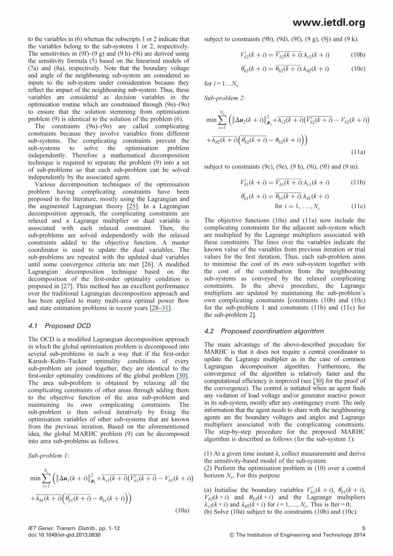
Fig. 2 Multi-agent RHC

2 Multi-agent RHC

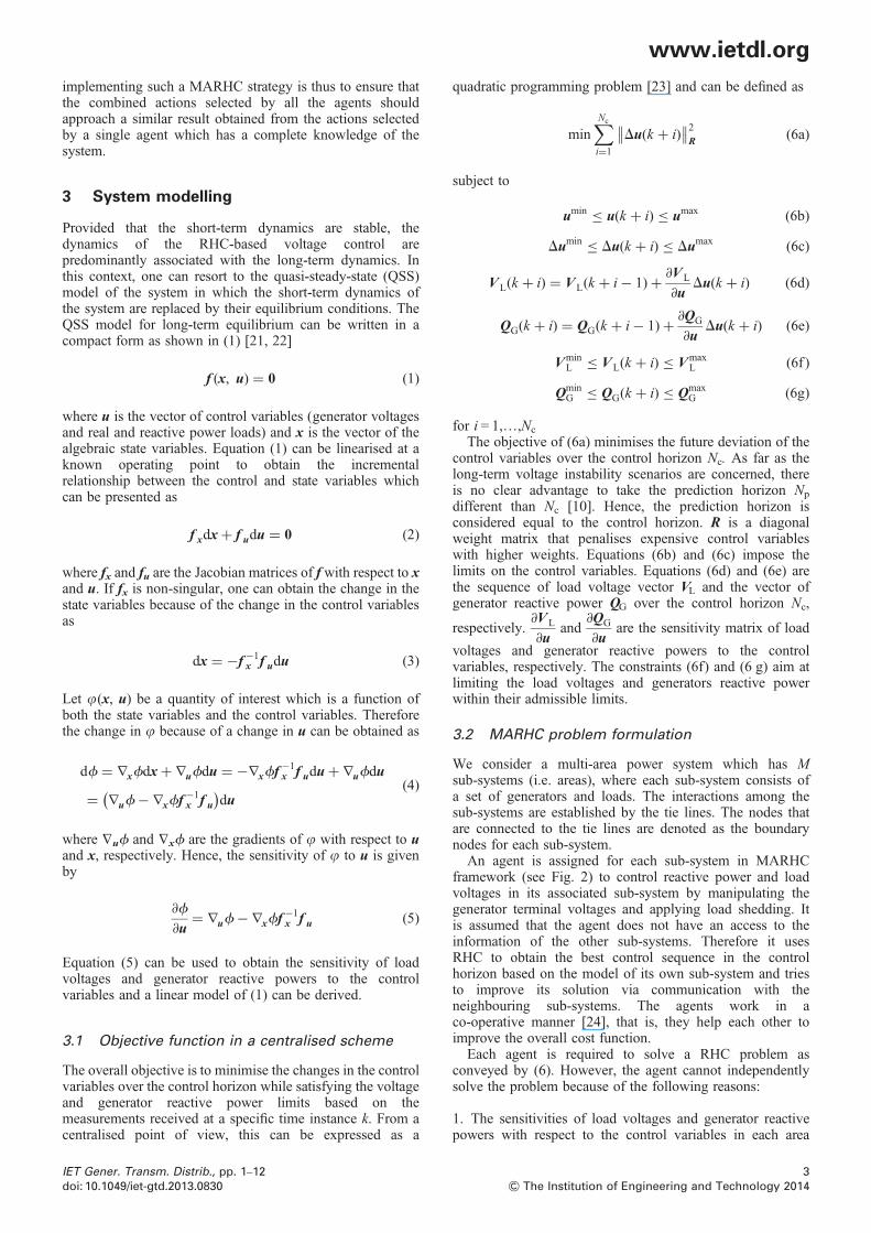
RHC is one of the most widely used advanced controlstrategies which has been successfully applied in theprocess industries [19]. One of the most useful features ofthis framework is the ability to handle the input and outputconstraints efficiently by formulating a discrete-time controlmodel of the system. The conceptual structure of the RHCapproach is shown in Fig. 1. The main idea is to formulatean online optimisation problem subject to the input andoutput constraints which results in a sequence of future

2& The Institution of Engineering and Technology 2014

control actions over a control horizon (NC) given a systemmodel in hand. The output is predicted over a predictionhorizon (NP) which is usually different from NC. The firstsequence of the so-computed actions is actuallyimplemented and the process is repeated at the nextsampling time when new measurements are available.According to Fig. 1, a set of admissible control sequence

u = {uk, uk+1,…, uk + Nc−1} is computed at a givendiscrete-time instance k to minimise the output trajectorydeviation from the desired reference set-point over theprediction horizon with minimum control efforts. In thesingle agent architecture, this optimisation is performed bya central controller. The central agent thus requires theknowledge of the complete model of the system and thesystem-wide measurement should be available to the agent.In a multi-agent RHC (MARHC), multiple control agents

use RHC where each agent is assigned to control asub-system which is a part of overall system [20]. Theagents first evaluate the sub-system states, compute the bestcontrol actions for the predicted sub-system state and inputevolution and then implement actions. The actions that anagent takes in a MARHC structure influence both theevolution of its own sub-system and the evolution of thesub-system connected to it. Since the agents usually haveno global overview and can access only a limited portion ofthe overall network, the future sub-system state predictionbecomes uncertain without any interactions among theagents. Therefore a communication network must beestablished among the agents (see Fig. 2). The challenge in

IET Gener. Transm. Distrib., pp. 1–12doi: 10.1049/iet-gtd.2013.0830

www.ietdl.org

implementing such a MARHC strategy is thus to ensure thatthe combined actions selected by all the agents shouldapproach a similar result obtained from the actions selectedby a single agent which has a complete knowledge of thesystem.

3 System modelling

Provided that the short-term dynamics are stable, thedynamics of the RHC-based voltage control arepredominantly associated with the long-term dynamics. Inthis context, one can resort to the quasi-steady-state (QSS)model of the system in which the short-term dynamics ofthe system are replaced by their equilibrium conditions. TheQSS model for long-term equilibrium can be written in acompact form as shown in (1) [21, 22]

f (x, u) = 0 (1)

where u is the vector of control variables (generator voltagesand real and reactive power loads) and x is the vector of thealgebraic state variables. Equation (1) can be linearised at aknown operating point to obtain the incrementalrelationship between the control and state variables whichcan be presented as

f xdx+ f udu = 0 (2)

where fx and fu are the Jacobian matrices of f with respect to xand u. If fx is non-singular, one can obtain the change in thestate variables because of the change in the control variablesas

dx = −f −1x f udu (3)

Let j(x, u) be a quantity of interest which is a function ofboth the state variables and the control variables. Thereforethe change in j because of a change in u can be obtained as

df = ∇xfdx+ ∇ufdu = −∇xff−1x f udu+ ∇ufdu

= ∇uf− ∇xff−1x f u

( )du

(4)

where ∇uf and ∇xf are the gradients of j with respect to uand x, respectively. Hence, the sensitivity of j to u is givenby

∂f

∂u= ∇uf− ∇xff

−1x f u (5)

Equation (5) can be used to obtain the sensitivity of loadvoltages and generator reactive powers to the controlvariables and a linear model of (1) can be derived.

3.1 Objective function in a centralised scheme

The overall objective is to minimise the changes in the controlvariables over the control horizon while satisfying the voltageand generator reactive power limits based on themeasurements received at a specific time instance k. From acentralised point of view, this can be expressed as a

IET Gener. Transm. Distrib., pp. 1–12doi: 10.1049/iet-gtd.2013.0830

quadratic programming problem [23] and can be defined as

min∑Nc

i=1

Du(k + i)∥∥ ∥∥2

R (6a)

subject to

umin ≤ u(k + i) ≤ umax (6b)

Dumin ≤ Du(k + i) ≤ Dumax (6c)

VL(k + i) = VL(k + i− 1)+ ∂VL

∂uDu(k + i) (6d)

QG(k + i) = QG(k + i− 1)+ ∂QG

∂uDu(k + i) (6e)

VminL ≤ VL(k + i) ≤ Vmax

L (6f )

QminG ≤ QG(k + i) ≤ Qmax

G (6g)

for i = 1,…,Nc

The objective of (6a) minimises the future deviation of thecontrol variables over the control horizon Nc. As far as thelong-term voltage instability scenarios are concerned, thereis no clear advantage to take the prediction horizon Np

different than Nc [10]. Hence, the prediction horizon isconsidered equal to the control horizon. R is a diagonalweight matrix that penalises expensive control variableswith higher weights. Equations (6b) and (6c) impose thelimits on the control variables. Equations (6d) and (6e) arethe sequence of load voltage vector VL and the vector ofgenerator reactive power QG over the control horizon Nc,

respectively.∂VL

∂uand

∂QG

∂uare the sensitivity matrix of load

voltages and generator reactive powers to the controlvariables, respectively. The constraints (6f) and (6 g) aim atlimiting the load voltages and generators reactive powerwithin their admissible limits.

3.2 MARHC problem formulation

We consider a multi-area power system which has Msub-systems (i.e. areas), where each sub-system consists ofa set of generators and loads. The interactions among thesub-systems are established by the tie lines. The nodes thatare connected to the tie lines are denoted as the boundarynodes for each sub-system.An agent is assigned for each sub-system in MARHC

framework (see Fig. 2) to control reactive power and loadvoltages in its associated sub-system by manipulating thegenerator terminal voltages and applying load shedding. Itis assumed that the agent does not have an access to theinformation of the other sub-systems. Therefore it usesRHC to obtain the best control sequence in the controlhorizon based on the model of its own sub-system and triesto improve its solution via communication with theneighbouring sub-systems. The agents work in aco-operative manner [24], that is, they help each other toimprove the overall cost function.Each agent is required to solve a RHC problem as

conveyed by (6). However, the agent cannot independentlysolve the problem because of the following reasons:

1. The sensitivities of load voltages and generator reactivepowers with respect to the control variables in each area

3& The Institution of Engineering and Technology 2014

www.ietdl.org

will depend on the state variables of the whole system, that is,these sensitivities are global quantities.2. Each agent will try to optimise its local decision variables.The control action in one sub-system may affect anothersub-system’s state because of the relative coupling betweenthem. Therefore the optimal decision for one agent may notbe the optimal decision for the overall problem.

Owing to the fact mentioned above, a decompositionscheme to decompose the overall problem intosub-problems is proposed in this paper which can be solvedin a coordinated way to find the global optimal solution.This also complies with the proposed MARHC scheme thatthe task of the emergency voltage control problem is sharedby multiple agents; each is in charge of its associatedsub-system.

4 Multi-area system modelling

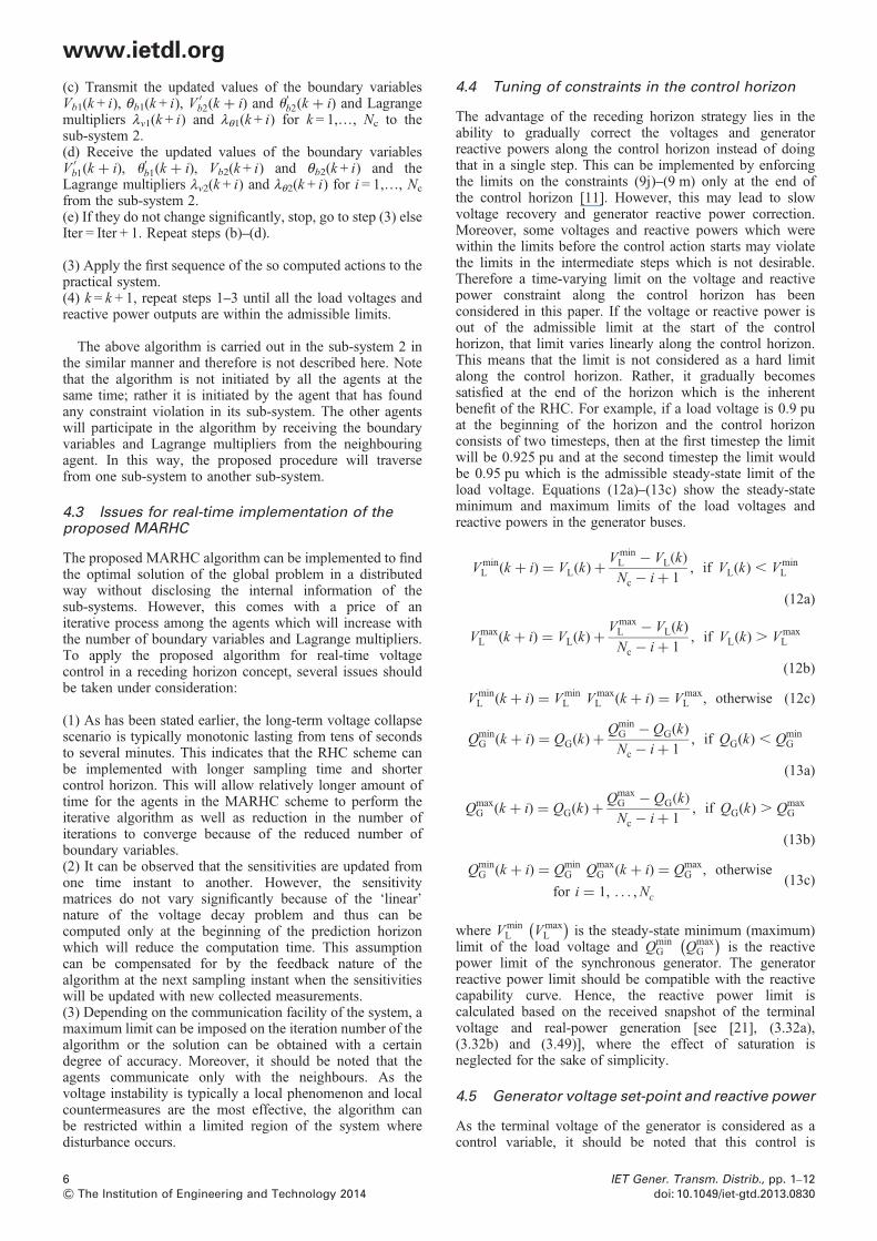
Fig. 3 illustrates the equivalent systems for a two-area powersystem. The sub-systems/areas are connected by tie lines. Inthe equivalent model, each area preserves the actual modelof its sub-system and replaces the neighbouring sub-systemsby the voltage and angle of the neighbouring boundarynode(s). For the sake of simplicity, only one boundary nodeper area is shown but the concept can be extended withoutany loss of generality to any number of boundary nodesand any number of neighbouring areas.The decomposed equivalent steady-state model of the

above system can be expressed as

f 1 x1, u1, V′b2, u

′b2

( ) = 0 (7a)

V ′b2 = Vb2 (7b)

u′b2 = ub2 (7c)

f 2 x2, u2, V′b1, u

′b1

( ) = 0 (8a)

V ′b1 = Vb1 (8b)

u′b1 = ub1 (8c)

Equation (7a) indicates the steady-state model for sub-system1. x1 refers to the state variables and u1 refers to the control

Fig. 3 Decomposed model of a two-area system

4& The Institution of Engineering and Technology 2014

variables of sub-system 1. Note that the boundary voltageV ′b2 and angle u′b2 are appended in (7a) because the

power-flow equations of the boundary buses of sub-system1 depend on these variables. These two variables areconstrained through (7b)–(7c) which are the couplingequations for the model of sub-system 1. These equationsimply that the variables V ′

b2 and u′b2 must be equal to theactual variables Vb2 and θb2, respectively. This ensures thatfor a given system state and input set, the same solutionwill be obtained using the models (7) and (8) as wouldhave been obtained from the model (1) [15].The equivalent MARHC problem of the problem in (6) for

the decomposed model of (7)–(8) can be stated as

min∑Nc

i=1

Du1(k + i)∥∥ ∥∥2

R1

+ Du2(k + i)∥∥ ∥∥2

R2

( )(9a)

subject to

umin1 ≤ u1(k + i) ≤ umax

1 (9b)

umin2 ≤ u2(k + i) ≤ umax

2 (9c)

Dumin1 ≤ Du1(k + i) ≤ Dumax

1 (9d)

Dumin2 ≤ Du2(k + i) ≤ Dumax

2 (9e)

VL1(k + i) = VL1(k + i− 1)+ ∂VL1

∂u1Du1(k + i)

+ ∂VL1

∂Vb2DVb2(k + i)+ ∂VL1

∂ub2Dub2(k + i)

(9f )

QG1(k + i) = QG1(k + i− 1)+ ∂QG1

∂u1Du1(k + i)

+ ∂QG1

∂Vb2DVb2(k + i)+ ∂QG1

∂ub2Dub2(k + i)

(9g)

VL2(k + i) = VL2(k + i− 1)+ ∂VL2

∂u2Du1(k + i)

+ ∂VL2

∂Vb1DVb1(k + i)+ ∂VL2

∂ub1Dub1(k + i)

(9h)

QG2(k + i) = QG2(k + i− 1)+ ∂QG2

∂u2Du2(k + i)

+ ∂QG2

∂Vb1DVb1(k + i)+ ∂QG2

∂ub1Dub1(k + i)

(9i)

VminL1 ≤ VL1(k + i) ≤ Vmax

L1 (9j)

QminG1 ≤ QG1(k + i) ≤ Qmax

G1 (9k)

VminL2 ≤ VL2(k + i) ≤ Vmax

L2 (9l)

QminG2 ≤ QG2(k + i) ≤ Qmax

G2 (9m)

V ′b2(k + i) = Vb2(k + i) u′b2(k + i) = ub2(k + i) (9n)

V ′b1(k + i) = Vb1(k + i) u′b1(k + i) = ub1(k + i)

for i = 1, . . . ,Nc (9o)

In (9a), the centralised objective function is split into two parts,where the first part belongs to the sub-system 1 and the secondpart belongs to the sub-system 2. All the variables in (9) relate

IET Gener. Transm. Distrib., pp. 1–12doi: 10.1049/iet-gtd.2013.0830

)

www.ietdl.org

to the variables in (6) whereas the subscripts 1 or 2 indicate thatthe variables belong to the sub-systems 1 or 2, respectively.The sensitivities in (9f)–(9 g) and (9 h)–(9i) are derived usingthe sensitivity formula (5) based on the linearised models of(7a) and (8a), respectively. Note that the boundary voltageand angle of the neighbouring sub-system are considered asinputs to the sub-system under consideration because theyreflect the impact of the neighbouring sub-system. Thus, thesevariables are considered as decision variables in theoptimisation routine which are constrained through (9n)–(9o)to ensure that the solution stemming from optimisationproblem (9) is identical to the solution of the problem (6).The constraints (9n)–(9o) are called complicating

constraints because they involve variables from differentsub-systems. The complicating constraints prevent thesub-systems to solve the optimisation problemindependently. Therefore a mathematical decompositiontechnique is required to separate the problem (9) into a setof sub-problems so that each sub-problem can be solvedindependently by the associated agent.Various decomposition techniques of the optimisation

problem having complicating constraints have beenproposed in the literature, mostly using the Lagrangian andthe augmented Lagrangian theory [25]. In a Lagrangiandecomposition approach, the complicating constraints arerelaxed and a Lagrange multiplier or dual variable isassociated with each relaxed constraint. Then, thesub-problems are solved independently with the relaxedconstraints added to the objective function. A mastercoordinator is used to update the dual variables. Thesub-problems are repeated with the updated dual variablesuntil some convergence criteria are met [26]. A modifiedLagrangian decomposition technique based on thedecomposition of the first-order optimality condition isproposed in [27]. This method has an excellent performanceover the traditional Lagrangian decomposition approach andhas been applied to many multi-area optimal power flowand state estimation problems in recent years [28–31].

4.1 Proposed OCD

The OCD is a modified Lagrangian decomposition approachin which the global optimisation problem is decomposed intoseveral sub-problems in such a way that if the first-orderKarush–Kuhn–Tucker optimality conditions of everysub-problem are joined together, they are identical to thefirst-order optimality conditions of the global problem [30].The area sub-problem is obtained by relaxing all thecomplicating constraints of other areas through adding themto the objective function of the area sub-problem andmaintaining its own complicating constraints. Thesub-problem is then solved iteratively by fixing theoptimisation variables of other sub-systems that are knownfrom the previous iteration. Based on the aforementionedidea, the global MARHC problem (9) can be decomposedinto area sub-problems as follows.

Sub-problem 1:

min∑Nc

i=1

Du1(k + i)∥∥ ∥∥2

R1+lv1(k + i) V ′

b1(k + i)− Vb1(k + i)((

+lu1(k + i) u′b1(k + i)− ub1(k + i)( ))

(10a)

IET Gener. Transm. Distrib., pp. 1–12doi: 10.1049/iet-gtd.2013.0830

subject to constraints (9b), (9d), (9f), (9 g), (9j) and (9 k).

V ′b2(k + i) = Vb2(k + i):lv2(k + i) (10b)

u′b2(k + i) = ub2(k + i):lu2(k + i) (10c)

for i = 1…Nc.

Sub-problem 2:

min∑Nc

i=1

Du2(k + i)∥∥ ∥∥2

R2+lv2(k + i) V ′

b2(k + i)− Vb2(k + i)( )(

+lu2(k + i) u′b2(k + i)− ub2(k + i)( ))

(11a)

subject to constraints (9c), (9e), (9 h), (9i), (9l) and (9 m).

V ′b1(k + i) = Vb1(k + i):lv1(k + i) (11b)

u′b1(k + i) = ub1(k + i):lu1(k + i)

for i = 1, . . . ,Nc (11c)

The objective functions (10a) and (11a) now include thecomplicating constraints for the adjacent sub-system whichare multiplied by the Lagrange multipliers associated withthese constraints. The lines over the variables indicate theknown value of the variables from previous iteration or trialvalues for the first iteration. Thus, each sub-problem aimsto minimise the cost of its own sub-system together withthe cost of the contribution from the neighbouringsub-systems as conveyed by the relaxed complicatingconstraints. In the above procedure, the Lagrangemultipliers are updated by maintaining the sub-problem’sown complicating constraints [constraints (10b) and (10c)for the sub-problem 1 and constraints (11b) and (11c) forthe sub-problem 2].

4.2 Proposed coordination algorithm

The main advantage of the above-described procedure forMARHC is that it does not require a central coordinator toupdate the Lagrange multiplier as in the case of commonLagrangian decomposition algorithm. Furthermore, theconvergence of the algorithm is relatively faster and thecomputational efficiency is improved (see [30] for the proof ofthe convergence). The control is initiated when an agent findsany violation of load voltage and/or generator reactive powerin its sub-system, mostly after any contingency event. The onlyinformation that the agent needs to share with the neighbouringagents are the boundary voltages and angles and Lagrangemultipliers associated with the complicating constraints.The step-by-step procedure for the proposed MARHCalgorithm is described as follows (for the sub-system 1):

(1) At a given time instant k, collect measurement and derivethe sensitivity-based model of the sub-system.(2) Perform the optimisation problem in (10) over a controlhorizon Nc. For this purpose

(a) Initialise the boundary variables V ′b1(k + i), u′b1(k + i),

Vb2(k + i) and θb2(k + i) and the Lagrange multipliersλv2(k + i) and λθ2(k + i) for i = 1,…, Nc. This is Iter = 0;(b) Solve (10a) subject to the constraints (10b) and (10c).

5& The Institution of Engineering and Technology 2014

www.ietdl.org

(c) Transmit the updated values of the boundary variablesVb1(k + i), θb1(k + i), V ′

b2(k + i) and u′b2(k + i) and Lagrangemultipliers λv1(k + i) and λθ1(k + i) for k = 1,…, Nc to thesub-system 2.(d) Receive the updated values of the boundary variablesV ′b1(k + i), u′b1(k + i), Vb2(k + i) and θb2(k + i) and the

Lagrange multipliers λv2(k + i) and λθ2(k + i) for i = 1,…, Nc

from the sub-system 2.(e) If they do not change significantly, stop, go to step (3) elseIter = Iter + 1. Repeat steps (b)–(d).

(3) Apply the first sequence of the so computed actions to thepractical system.(4) k = k + 1, repeat steps 1–3 until all the load voltages andreactive power outputs are within the admissible limits.

The above algorithm is carried out in the sub-system 2 inthe similar manner and therefore is not described here. Notethat the algorithm is not initiated by all the agents at thesame time; rather it is initiated by the agent that has foundany constraint violation in its sub-system. The other agentswill participate in the algorithm by receiving the boundaryvariables and Lagrange multipliers from the neighbouringagent. In this way, the proposed procedure will traversefrom one sub-system to another sub-system.

4.3 Issues for real-time implementation of theproposed MARHC

The proposed MARHC algorithm can be implemented to findthe optimal solution of the global problem in a distributedway without disclosing the internal information of thesub-systems. However, this comes with a price of aniterative process among the agents which will increase withthe number of boundary variables and Lagrange multipliers.To apply the proposed algorithm for real-time voltagecontrol in a receding horizon concept, several issues shouldbe taken under consideration:

(1) As has been stated earlier, the long-term voltage collapsescenario is typically monotonic lasting from tens of secondsto several minutes. This indicates that the RHC scheme canbe implemented with longer sampling time and shortercontrol horizon. This will allow relatively longer amount oftime for the agents in the MARHC scheme to perform theiterative algorithm as well as reduction in the number ofiterations to converge because of the reduced number ofboundary variables.(2) It can be observed that the sensitivities are updated fromone time instant to another. However, the sensitivitymatrices do not vary significantly because of the ‘linear’nature of the voltage decay problem and thus can becomputed only at the beginning of the prediction horizonwhich will reduce the computation time. This assumptioncan be compensated for by the feedback nature of thealgorithm at the next sampling instant when the sensitivitieswill be updated with new collected measurements.(3) Depending on the communication facility of the system, amaximum limit can be imposed on the iteration number of thealgorithm or the solution can be obtained with a certaindegree of accuracy. Moreover, it should be noted that theagents communicate only with the neighbours. As thevoltage instability is typically a local phenomenon and localcountermeasures are the most effective, the algorithm canbe restricted within a limited region of the system wheredisturbance occurs.

6& The Institution of Engineering and Technology 2014

4.4 Tuning of constraints in the control horizon

The advantage of the receding horizon strategy lies in theability to gradually correct the voltages and generatorreactive powers along the control horizon instead of doingthat in a single step. This can be implemented by enforcingthe limits on the constraints (9j)–(9 m) only at the end ofthe control horizon [11]. However, this may lead to slowvoltage recovery and generator reactive power correction.Moreover, some voltages and reactive powers which werewithin the limits before the control action starts may violatethe limits in the intermediate steps which is not desirable.Therefore a time-varying limit on the voltage and reactivepower constraint along the control horizon has beenconsidered in this paper. If the voltage or reactive power isout of the admissible limit at the start of the controlhorizon, that limit varies linearly along the control horizon.This means that the limit is not considered as a hard limitalong the control horizon. Rather, it gradually becomessatisfied at the end of the horizon which is the inherentbenefit of the RHC. For example, if a load voltage is 0.9 puat the beginning of the horizon and the control horizonconsists of two timesteps, then at the first timestep the limitwill be 0.925 pu and at the second timestep the limit wouldbe 0.95 pu which is the admissible steady-state limit of theload voltage. Equations (12a)–(13c) show the steady-stateminimum and maximum limits of the load voltages andreactive powers in the generator buses.

VminL (k + i) = VL(k)+

VminL − VL k( )Nc − i+ 1

, if VL(k) , VminL

(12a)

VmaxL (k + i) = VL(k)+

VmaxL − VL(k)

Nc − i+ 1, if VL(k) . Vmax

L

(12b)

VminL (k + i) = Vmin

L VmaxL (k + i) = Vmax

L , otherwise (12c)

QminG (k + i) = QG(k)+

QminG − QG(k)

Nc − i+ 1, if QG(k) , Qmin

G

(13a)

QmaxG (k + i) = QG(k)+

QmaxG − QG k( )Nc − i+ 1

, if QG(k) . QmaxG

(13b)

QminG (k + i) = Qmin

G QmaxG (k + i) = Qmax

G , otherwise

for i = 1, . . . ,Nc

(13c)

where VminL Vmax

L

( )is the steady-state minimum (maximum)

limit of the load voltage and QminG Qmax

G

( )is the reactive

power limit of the synchronous generator. The generatorreactive power limit should be compatible with the reactivecapability curve. Hence, the reactive power limit iscalculated based on the received snapshot of the terminalvoltage and real-power generation [see [21], (3.32a),(3.32b) and (3.49)], where the effect of saturation isneglected for the sake of simplicity.

4.5 Generator voltage set-point and reactive power

As the terminal voltage of the generator is considered as acontrol variable, it should be noted that this control is

IET Gener. Transm. Distrib., pp. 1–12doi: 10.1049/iet-gtd.2013.0830

www.ietdl.org

implemented by changing the automatic voltage regulator(AVR) reference voltage which is usually different from theactual terminal voltage. Based on the fact that a change inAVR reference voltage results in almost equal change in theterminal voltage [11], the controller changes the AVRreference voltage by the amount equal to the desiredterminal voltage correction.The generator reactive power under over-excitation (OXL)

control of the excitation system (i.e. constant field current) isgiven by

Qg =VImax

FD

Xdcos (d− u)

− V 2 sin2 (d− u)

Xq+ cos2 (d− u)

Xd

( )(14)

This clearly shows that the reactive power is dependent on thegenerator terminal voltage. As the OXL tends to lowerthe AVR reference voltage to control the excitation current,the terminal voltage of the generator also gradually falls.As a result, the reactive power also gradually falls underOXL control.

Fig. 4 Single-line diagram of Nordic32 test system

IET Gener. Transm. Distrib., pp. 1–12doi: 10.1049/iet-gtd.2013.0830

Generator bus voltage is used as control variable because ofthe fact that the generator excitation control is able to controlthe voltage directly and can adjust the bus voltage. Loadshedding is the another control variable that is used in theproposed method, when the countermeasures are notsufficient. In the proposed method, the on-load tap changers(LTC) are also allowed to vary automatically within thetimeframe before load shedding is activated.

5 Validation of the proposed method usingcase studies

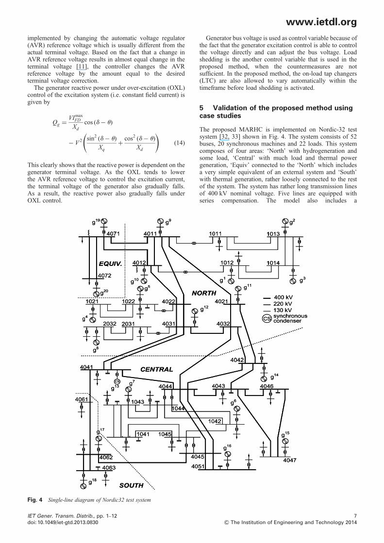
The proposed MARHC is implemented on Nordic-32 testsystem [32, 33] shown in Fig. 4. The system consists of 52buses, 20 synchronous machines and 22 loads. This systemcomposes of four areas: ‘North’ with hydrogeneration andsome load, ‘Central’ with much load and thermal powergeneration, ‘Equiv’ connected to the ‘North’ which includesa very simple equivalent of an external system and ‘South’with thermal generation, rather loosely connected to the restof the system. The system has rather long transmission linesof 400 kV nominal voltage. Five lines are equipped withseries compensation. The model also includes a

7& The Institution of Engineering and Technology 2014

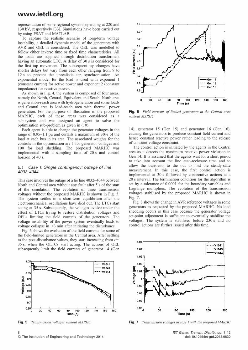
Fig. 6 Field currents of limited generators in the Central areawithout MARHC

www.ietdl.org

representation of some regional systems operating at 220 and130 kV, respectively [33]. Simulations have been carried outby using PSAT and MATLAB.To capture the realistic scenario of long-term voltage

instability, a detailed dynamic model of the generators withAVR and OEL is considered. The OEL was modelled tofollow either inverse time or fixed time characteristics. Allthe loads are supplied through distribution transformershaving an automatic LTC. A delay of 30 s is considered forthe first tap movement. The subsequent tap changes haveshorter delays but vary from each other ranging from 9 to12 s to prevent the unrealistic tap synchronisation. Anexponential model for the load is used with exponent 1(constant current) for active power and exponent 2 (constantimpedance) for reactive power.As shown in Fig. 4, the system is composed of four areas,

namely the North, Central, Equivalent and South. North areais generation-reach area with hydrogeneration and some loadsand Central area is load-reach area with thermal powergeneration. For the purpose of illustration of the proposedMARHC, each of these areas was considered as asub-system and was assigned an agent to solve theoptimisation sub-problem as given in (10).Each agent is able to change the generator voltages in the

range of 0.95–1.1 pu and curtails a maximum of 30% of theload at each bus in its area. The associated weights for thecontrols in the optimisation are 1 for generator voltages and100 for load shedding. The proposed MARHC wasimplemented with a sampling time of 20 s and controlhorizon of 40 s.

5.1 Case 1: Single contingency: outage of line4032–4044

This case involves the outage of a tie line 4032–4044 betweenNorth and Central area without any fault after 5 s of the startof the simulation. The evolution of three transmissionvoltages without the proposed MARHC is shown in Fig. 5.The system settles to a short-term equilibrium after theelectromechanical oscillations have died out. The LTCs startacting at 35 s. Subsequently, the voltages evolve under theeffect of LTCs trying to restore distribution voltages andOELs limiting the field currents of the generators. Thevoltage instability of the power system eventually leads tovoltage collapse in <3 min after initiating the disturbance.Fig. 6 shows the evolution of the field currents for some of

the field-limited generators in the Central area. After settlingto the post-disturbance values, they start increasing from t =35 s, when the OLTCs start acting. The actions of OELsubsequently limit the field currents of generator 14 (Gen

Fig. 5 Transmission voltages without MARHC

8& The Institution of Engineering and Technology 2014

14), generator 15 (Gen 15) and generator 16 (Gen 16),causing the generators to produce constant field current andhence constant reactive power rather leading to the releaseof constant voltage constraint.The control action is initiated by the agents in the Central

area as it detects the maximum reactive power violation inGen 14. It is assumed that the agents wait for a short periodto take into account the line auto-reclosure time and toallow the transients to die out to find the steady-statemeasurement. In this case, the first control action isimplemented at 30 s followed by consecutive actions at a20 s interval. The termination condition for the algorithm isset by a tolerance of 0.0001 for the boundary variables andLagrange multipliers. The evolution of the transmissionvoltages stabilised by the proposed MARHC is shown inFig. 7.Fig. 8 shows the change in AVR reference voltages in some

generators as requested by the proposed MARHC. No loadshedding occurs in this case because the generator voltageset-point adjustment is sufficient to eventually stabilise thevoltages. The system is stabilised before 230 s and nocontrol actions are further issued after this time.

Fig. 7 Transmission voltages in case 1 with the proposed MARHC

IET Gener. Transm. Distrib., pp. 1–12doi: 10.1049/iet-gtd.2013.0830

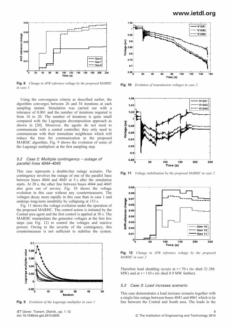
Fig. 8 Change in AVR reference voltage by the proposed MARHCin case 1

Fig. 10 Evolution of transmission voltages in case 2

www.ietdl.org

Using the convergence criteria as described earlier, thealgorithm converges between 26 and 34 iterations at eachsampling instant. Simulation was carried out with atolerance of 0.001 and the number of iterations required isfrom 16 to 20. The number of iterations is quite smallcompared with the Lagrangian decomposition approach asshown in [20]. Moreover, the agents do not need tocommunicate with a central controller; they only need tocommunicate with their immediate neighbours which willreduce the time for communication in the proposedMARHC algorithm. Fig. 9 shows the evolution of some ofthe Lagrange multipliers at the first sampling step.

Fig. 11 Voltage stabilisation by the proposed MARHC in case 2

5.2 Case 2: Multiple contingency – outage ofparallel lines 4044–4045

This case represents a double-line outage scenario. Thecontingency involves the outage of one of the parallel linesbetween buses 4044 and 4045 at 5 s after the simulationstarts. At 20 s, the other line between buses 4044 and 4045also goes out of service. Fig. 10 shows the voltageevolution in this case without any countermeasures. Thevoltages decay more rapidly in this case than in case 1 andundergo long-term instability by collapsing at 153 s.Fig. 11 shows the voltage evolution under the operation of

the proposed MARHC. The control action is initiated by theCentral area agent and the first control is applied at 30 s. TheMARHC manipulates the generator voltages at the first fewsteps (see Fig. 12) to control the voltages and reactivepowers. Owing to the severity of the contingency, thiscountermeasure is not sufficient to stabilise the system.

Fig. 9 Evolution of the Lagrange multiplier in case 1

Fig. 12 Change in AVR reference voltage by the proposedMARHC in case 2

IET Gener. Transm. Distrib., pp. 1–12doi: 10.1049/iet-gtd.2013.0830

Therefore load shedding occurs at t = 70 s (to shed 21.386MW) and at t = 110 s (to shed 8.9 MW further).

5.3 Case 3: Load increase scenario

This case demonstrates a load increase scenario together witha single-line outage between buses 4041 and 4061 which is tieline between the Central and South area. The loads in the

9& The Institution of Engineering and Technology 2014

Fig. 13 Evolution of transmission voltages in case 3

Table 1 Optimal values of the generator bus voltage in perunit

Bus number Case 1 Case 2 Case 3

1 1.1000 1.0975 1.09602 1.0375 1.0416 1.07093 1.0610 1.0931 1.07204 1.1000 1.0564 1.05485 1.0876 1.0844 1.05056 1.0421 0.9838 1.01747 1.0306 0.9530 1.00088 1.0855 1.0732 1.06469 1.0682 1.0602 1.051710 1.0625 1.0558 1.044811 1.0484 1.0832 1.024112 1.0326 1.0484 1.011013 1.0904 1.1000 1.049014 1.0158 1.0654 1.019515 1.0766 1.0951 1.057216 1.0940 1.0960 1.071417 1.0356 1.0947 1.033118 0.9879 1.0697 1.056519 1.0807 1.0338 1.055620 1.0414 0.9545 1.0319

www.ietdl.org

Central area are linearly increased from 20 s to 120 s by a totalamount of 100 MW. The voltage collapse occurs at t = 213.3s in this case (see Fig. 13).Fig. 14 shows the system response with the MARHC

controller in action. The proposed MARHC smoothlystabilises the system mainly with the control of thegenerator terminal voltages (see Fig. 15) and the systemsettles to a post-disturbance equilibrium at t = 250 s. A verylittle amount of load shedding (5.6 MW) occurred at t =210 s.

Fig. 14 Voltage stabilisation by the proposed MARHC in case 3

Fig. 15 Change in AVR reference voltage by the proposedMARHC in case 3

10& The Institution of Engineering and Technology 2014

The optimisation routine directly gives the amount of load(active and reactive power) that needs to be shed. A constantpower factor is preserved from the original load in the loadshedding algorithm, such that if 10 MW is shed at any bus,a proportional amount of reactive power is also shed toensure that the power factor remains constant. This practiceis also adopted in [11, 12]. We also follow the practicedescribed in [11], where a load < 0.1 MW is assumed to beso small that no shedding will be carried out on this type ofload. Table 1 shows the final optimal values of generatorvoltages after the system is stabilised in per unit. Table 2shows the bus number and the amount of load shedding inMW. A constant power factor has been preserved for theload shedding as adopted in [11, 12].

5.4 Case 4: Testing the effectiveness of theproposed approach

To demonstrate the effectiveness of the proposed approach, acomparative study is carried out in this section. The proposedapproach is compared with a traditional approach. Also, the

Table 2 Optimal values of load shedding in MW in thesub-systems under control – the Central and South areas

Bus number Case 1 Case 2 Case 3No load shed

1041 0 9.989 0.71042 0 0.919 0.331043 0 4.652 0.591044 0 0.84 0.491045 0 6.552 0.54041 0 0 0.184042 0 0 0.294043 0 0.202 0.474046 0 0.136 0.614047 0 0 0.334051 0 5.384 0.44061 0 0.561 0.264062 0 0.646 0.254063 0 0.405 0.21

The power factor of the original load is preserved.

IET Gener. Transm. Distrib., pp. 1–12doi: 10.1049/iet-gtd.2013.0830

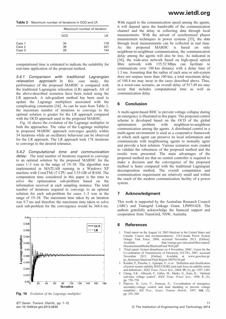
Table 3 Maximum number of iterations in OCD and LR

Maximum number of iteration

OCD LR

Case 1 34 178Case 2 39 201Case 3 28 144

www.ietdl.org

computational time is estimated to indicate the suitability forreal-time application of the proposed method.

5.4.1 Comparison with traditional Lagrangianrelaxation approach: In this case study, theperformance of the proposed MARHC is compared withthe traditional Lagrangian relaxation (LR) approach. All ofthe above-described scenarios have been tested using theLR approach. A sub-gradient method has been used toupdate the Lagrange multipliers associated with thecomplicating constraints [34]. As can be seen from Table 3,the maximum number of iterations to converge to theoptimal solution is greater for the LR approach comparedwith the OCD approach used in the proposed MARHC.Fig. 16 shows the evolution of the Lagrange multiplier in

both the approaches. The value of the Lagrange multiplierin proposed MARHC approach converges quickly within34 iterations while an oscillatory behaviour can be observedfor the LR approach. The LR approach took 178 iterationsto converge to the desired tolerance.

5.4.2 Computational time and communicationdelay: The total number of iterations required to convergeto an optimal solution by the proposed MARHC for thecases 1–3 was in the range of 19–38. The algorithm wasimplemented in MATLAB running in a Windows XPmachine with Core(TM) i7 CPU and 3.55 GB of RAM. Thecomputation time considered in this paper is the time tosolve the optimisation sub-problem based on theinformation received at each sampling instance. The totalnumber of iterations required to converge to an optimalsolution for each sub-problem for cases 1–3 was in therange of 19–38. The maximum time taken by an iterationwas 9.7 ms and therefore the maximum time taken to solveeach sub-problem for the convergence would be 368.6 ms.

Fig. 16 Evolution of the Lagrange multiplier

IET Gener. Transm. Distrib., pp. 1–12doi: 10.1049/iet-gtd.2013.0830

With regard to the communication speed among the agents,it will depend upon the bandwidth of the communicationchannel and the delay in collecting data through localmeasurements. With the advent of synchronised phasormeasurement techniques in power systems [35], the datathrough local measurements can be collected in real time.As the proposed MARHC is based on onlyneighbour-to-neighbour communication, the communicationdelay among the agents will also be less. As indicated in[36], the wide-area network based on high-speed opticalfibre network with 155.52 Mbps can facilitate tocommunicate over 180 km distance with a delay time of1.3 ms. Assuming that the radius of each area or sub-systemdoes not surpass more than 100 km, a total maximum delayof 548.8 ms may incur in the cases described above. Thus,in a worst-case scenario, an overall delay of 917.49 ms mayoccur that includes computational time as well ascommunication delay.

6 Conclusion

A multi-agent-based RHC to prevent voltage collapse duringan emergency is illustrated in this paper. The proposed controlscheme is developed based on the OCD of the globaloptimisation problem with neighbour-to-neighbourcommunication among the agents. A distributed control in amulti-agent environment is used as a cooperative frameworkin which each agent can preserve its local information andcommunicate with neighbouring agents to mutually agreeand provide a best solution. Various scenarios were createdto validate the robustness of the proposed method and theresults were presented. The main advantages of theproposed method are that no central controller is required tomake a decision and the convergence of the proposedmethod is faster compared with the traditional Lagrangiandecomposition method. The overall computation andcommunication requirement are relatively small and withinthe reach of the modern communication facility of a powersystem.

7 Acknowledgment

This work is supported by the Australian Research Council(ARC) and Transgrid Linkage Grant, LP0991428. Theauthors gratefully acknowledge the financial support andcooperation from TransGrid, NSW, Australia.

8 References

1 ‘Final report on the August 14, 2003 blackout in the United States andCanada: Causes and recommendations’, US-Canada Power SystemOutage Task Force, 2004, accessed November 2013. [Online].Available at http://energy.gov/sites/prod/files/oeprod/DocumentsandMedia/BlackoutFinal-Web.pdf

2 ‘Final report: System disturbance on 4 November, 2006’, Union for theCo-ordination of Transmission of Electricity (UCTE), 2007, accessedNovember 2013. [Online]. Available at www.geocities.jp/ps_dictionary/blackout/Final-Report-20070130.pdf

3 Kundur, P., Paserba, J., Ajjarapu, V., et al.: ‘Definition and classificationof power system stability IEEE/CIGRE joint task force on stability termsand definitions’, IEEE Trans. Power Syst., 2004, 19, (3), pp. 1387–1401

4 Chang, S.K., Albuyeh, F., Gilles, M., Marks, G., Kato, K.: ‘Optimalreal-time voltage control’, IEEE Trans. Power Syst., 1990, 5, (3),pp. 750–758

5 Popovic, D., Levi, V., Gorecan, Z.: ‘Co-ordination of emergencysecondary-voltage control and load shedding to prevent voltageinstability’, IEE Proc., Gener. Transm. Distrib., 1997, 144, (3),pp. 293–300

11& The Institution of Engineering and Technology 2014

www.ietdl.org

6 Vu, H., Pruvot, P., Launay, C., Harmand, Y.: ‘An improved voltage

control on large-scale power system’, IEEE Trans. Power Syst., 1996,11, (3), pp. 1295–303

7 Marinescu, B., Bourles, H.: ‘Robust predictive control for the flexiblecoordinated secondary voltage control of large-scale power systems’,IEEE Trans. Power Syst., 1999, 14, (4), pp. 1262–8

8 Larsson, M., Hill, D.J., Olsson, G.: ‘Emergency voltage control usingsearch and predictive control’, Int. J. Electr. Power Energy Syst.,2002, 24, pp. 121–130

9 Wen, J., Wu, Q., Turner, D., Cheng, S., Fitch, J.: ‘Optimal coordinatedvoltage control for power system voltage stability’, IEEE Trans. PowerSyst., 2004, 19, (2), pp. 1115–22

10 Jin, L., Kumar, R., Elia, N.: ‘Model predictive control-based real-timepower system protection schemes’, IEEE Trans. Power Syst., 2010,25, (2), pp. 988–998

11 Glavic, M., Hajian, M., Rosehart, W., Van Cutsem, T.: ‘Receding horizonmulti-step optimization to correct nonviable or unstable transmissionvoltages’, IEEE Trans. Power Syst., 2011, 26, (3), pp. 1641–1650

12 Hajian, M., Rosehart, W., Glavic, M., Zareipour, H., Van Cutsem, T.:‘Linearized power flow equations based predictive control oftransmission voltages’. Forty-Sixth Hawaii Int. Conf. System Sciences(HICSS), 2013, 7–10 January 2013, pp. 2298–2304, 2013

13 Amraee, T., Ranjbar, A.M., Feuillet, R.: ‘Adaptive under-voltage loadshedding scheme using model predictive control’, Electr. Power Syst.Res., 2011, 81, (7), pp. 1507–1513

14 Moradzadeh, M., Boel, R., Vandevelde, L.: ‘Voltage coordination inmulti-area power systems via distributed model predictive control’,IEEE Trans. Power Syst., 2013, 28, (1), pp. 513–521

15 Beccuti, A., Demiray, T., Andersson, G., Morari, M.: ‘A Lagrangiandecomposition algorithm for optimal emergency voltage control’,IEEE Trans. Power Syst., 2010, 25, (4), pp. 1769–1779

16 Goh, S.H., Saha, T.P., Dong, Z.Y.: ‘Solving multi-objective voltagestability constrained power transfer capability problem usingevolutionary computation’, Int. J. Emerg. Electr. Power Syst., 2011,12, (1), pp. 5.1–5.22

17 Šosic, D., Škokljev, I.: ‘Evolutionary algorithm for calculating availabletransfer capability’, J. Electr. Eng., 2013, 64, (5), pp. 291–297

18 Liu, Y., Zhang, L., Zhao, Y.: ‘Calculation of static voltage stabilitymargin based on continuous power flow and improved differentialevolution algorithm’, Int. J. Digit. Content Technol. Appl., 2012, 6,(17), pp. 86–95

19 Camacho, E.F., Bordons, C.: ‘Model predictive control’(Springer-Verlag, London, 2004)

20 Negenborn, R.R.: ‘Multi-agent model predictive control withapplications to power networks’. PhD thesis, University of Delft, 2007

12& The Institution of Engineering and Technology 2014

21 Van Cutsem, T., Vournas, C.: ‘Voltage stability of electric powersystems’ (Kluwer, Boston, MA, 1998)

22 Glavic, M., Van Cutsem, T.: ‘Some reflections on model predictivecontrol of transmission voltages’. Thirty-Eighth North AmericanPower Symp. (NAPS), Carbondale, IL, September 2006

23 Valverde, G., Van Cutsem, T.: ‘Model predictive control of voltages inactive distribution networks’, IEEE Trans. Smart Grid, 2013, PP, (99),pp. 1–10

24 Maestre, J.M., Munoz de la Pena, D., Camacho, E.F.: ‘Distributed modelpredictive control based on a cooperative game’, Optim. Control Appl.Methods, 2011, 32, (2), pp. 153–176

25 Conejo, A.J., Minguez, R., Castillo, E., Garcia-Bertrand, R.:‘Decomposition techniques in mathematical programming’ (Springer,New York, 2006)

26 Bertsekas, D.: ‘Nonlinear programming’ (Athena Scientific, Nashua,NH, 1995)

27 Conejo A.J., Nogales, F.J., Prieto, F.J.F.J.: ‘A decomposition procedurebased on approximate Newton directions’, Math. Program., 2002, 93,(3), pp. 495–515

28 Nogales, F.J., Prieto, F.J., Conejo, A.J.: ‘A decomposition methodologyapplied to the multi-area optimal power flow problem’, Ann. Oper. Res.,2003, 120, pp. 99–116

29 Granada, M., Marcos, J., Rider, M.J., Mantovani, J.R.S., Shahidehpour,M.: ‘A decentralized approach for optimal reactive power dispatch usingLagrangian decomposition method’, Electr. Power Syst. Res., 2012, 89,pp. 148–156

30 Conejo, A.J., de la Torre, S., Canas, M.: ‘An optimization approach tomultiarea state estimation’, IEEE Trans. Power Syst., 2007, 22, (1),pp. 213–221

31 Milano, F.: ‘An open source power system analysis toolbox’, IEEETrans. Power Syst., 2005, 20, (3), pp. 1199–1206

32 Stubbe, M. ‘Long-term dynamics phase II’. Report of CIGRE TaskForce 32.02.08, 1995

33 Cutsem, T.V.: ‘Description, modeling and simulation results of a testsystem for voltage stability analysis version 4’ (University of Liège,Belgium, 2013)

34 Bertsekas, D.: ‘Constrained optimization and lagrange multipliermethods’ (Academic Press, New York, 1982)

35 Phadke, A.G., Thorp, J.S.: ‘Synchronized phasor measurements andtheir applications’ (Springer, New York, 2008)

36 Tong, X., Wang, X., Wang, R., et al.: ‘The study of a regionaldecentralized peer-to-peer negotiation-based wide-area backupprotection multi-agent system’, IEEE Trans. Smart Grid, 2013, 4, (2),pp.1197–1206

IET Gener. Transm. Distrib., pp. 1–12doi: 10.1049/iet-gtd.2013.0830