Mulder S. (1)
77
Delft Center for Systems and Control Energy Management Strategy for a Hybrid Container Crane Steven Mulder Master of Science Thesis
Transcript of Mulder S. (1)
Delft Center for Systems and Control
Energy Management Strategy fora Hybrid Container Crane
Steven Mulder
Maste
rof
Scie
nce
Thesis

Energy Management Strategy for aHybrid Container Crane
Master of Science Thesis
For the degree of Master of Science in Systems and Control at Delft
University of Technology
Steven Mulder
July 16, 2009
Faculty of Mechanical, Maritime and Materials Engineering · Delft University of Technology
The work in this thesis was generously supported by Siemens Nederland. Their cooperationis hereby gratefully acknowledged.
Copyright © Delft Center for Systems and Control (DCSC)All rights reserved.
Abstract
Siemens has developed a hybrid drive system for rubber-tired gantry (RTG) cranes that dras-tically reduces their fuel consumption. The hybrid crane uses ultracapacitors to store energythat is regenerated when a container is lowered or during braking, and reuses this energyto assist the engine later on. The main goal of this thesis is improving the crane’s energymanagement strategy. This is the system that optimizes the fuel cost by controlling in realtime how and when the two available power sources of the hybrid crane are used.
Currently, the crane uses a rule-based heuristic strategy. This is reliable and predictable, butdoes not achieve optimal results and is difficult to tune. As an alternative, this thesis proposesto use an Equivalent Consumption Minimization Strategy (ECMS). This is an optimization-based strategy of limited complexity that revolves around assigning a weight to the usage ofthe ultracapacitors that represents the equivalent “future fuel cost”. The idea is that usingthe ultracapacitors at one moment means that they cannot be used anymore in the next,which will then cost extra fuel.
The main issue for ECMS is selecting a proper way to assign the future fuel cost. In the end,two new strategies are presented that each have their own approach to this issue. The firstuses feedback from the state of the ultracapacitors to assign a weight to the ultracapacitorpower, the second uses predictions about the upcoming power demand.
The new strategies were compared to the current one using a custom-built RTG crane sim-ulator. The simulation results show that new strategies consistently outperform the currentsystem, significantly improving the fuel savings and therefore increasing the operational prof-its. Encouraged by these results, Siemens plans to test the new approach on hybrid cranes inthe Port of Felixstowe (UK).
Master of Science Thesis Steven Mulder

vi Abstract
Steven Mulder Master of Science Thesis
Table of Contents
Abstract v
Preface xi
1 General Introduction 1
1.1 Background . . . . . . . . . . . . . . . . . . . . . . . . . . . . . . . . . . . . . 1
1.1.1 Container shipping . . . . . . . . . . . . . . . . . . . . . . . . . . . . . 1
1.1.2 Siemens hybrid ECO-RTG . . . . . . . . . . . . . . . . . . . . . . . . . . 3
1.2 Problem statement . . . . . . . . . . . . . . . . . . . . . . . . . . . . . . . . . 4
1.2.1 Main thesis goal . . . . . . . . . . . . . . . . . . . . . . . . . . . . . . . 4
1.2.2 Subproblems . . . . . . . . . . . . . . . . . . . . . . . . . . . . . . . . . 4
1.3 Outline . . . . . . . . . . . . . . . . . . . . . . . . . . . . . . . . . . . . . . . . 5
2 Power Demand Model 7
2.1 Power consuming subsystems . . . . . . . . . . . . . . . . . . . . . . . . . . . . 7
2.2 Typical operation . . . . . . . . . . . . . . . . . . . . . . . . . . . . . . . . . . 8
2.2.1 Crane movements during operation . . . . . . . . . . . . . . . . . . . . . 9
2.2.2 Power demand for one move . . . . . . . . . . . . . . . . . . . . . . . . 9
2.2.3 Varying level of busyness . . . . . . . . . . . . . . . . . . . . . . . . . . 11
3 Power Supply Model 13
3.1 Introduction . . . . . . . . . . . . . . . . . . . . . . . . . . . . . . . . . . . . . 13
3.1.1 Power system overview . . . . . . . . . . . . . . . . . . . . . . . . . . . 13
3.1.2 Model goals and approach . . . . . . . . . . . . . . . . . . . . . . . . . 14
3.2 Diesel generator set . . . . . . . . . . . . . . . . . . . . . . . . . . . . . . . . . 14
3.2.1 Introduction . . . . . . . . . . . . . . . . . . . . . . . . . . . . . . . . . 14
3.2.2 Diesel generator set model . . . . . . . . . . . . . . . . . . . . . . . . . 15
Master of Science Thesis Steven Mulder
viii Table of Contents
3.3 Ultracapacitor bank model . . . . . . . . . . . . . . . . . . . . . . . . . . . . . 17
3.3.1 Ultracapacitor data . . . . . . . . . . . . . . . . . . . . . . . . . . . . . 17
3.3.2 Ultracapacitor bank model . . . . . . . . . . . . . . . . . . . . . . . . . 18
3.4 The complete simulator . . . . . . . . . . . . . . . . . . . . . . . . . . . . . . . 20
4 Energy Management Strategy 23
4.1 Introduction . . . . . . . . . . . . . . . . . . . . . . . . . . . . . . . . . . . . . 23
4.2 Current approach: rule-based strategy . . . . . . . . . . . . . . . . . . . . . . . 24
4.2.1 The decision making process . . . . . . . . . . . . . . . . . . . . . . . . 25
4.2.2 Advantages and drawbacks . . . . . . . . . . . . . . . . . . . . . . . . . 26
4.3 Alternative approach: optimization-based strategies . . . . . . . . . . . . . . . . 26
4.3.1 Optimization framework . . . . . . . . . . . . . . . . . . . . . . . . . . . 26
4.3.2 Objective function for energy management strategies . . . . . . . . . . . 27
4.3.3 Constraints for energy management strategies . . . . . . . . . . . . . . . 29
4.3.4 Feasibility of the optimization-based approach . . . . . . . . . . . . . . . 31
4.3.5 Off-line solution: dynamic programming . . . . . . . . . . . . . . . . . . 32
4.4 Equivalent consumption minimization strategy . . . . . . . . . . . . . . . . . . . 34
4.4.1 Change of the objective function . . . . . . . . . . . . . . . . . . . . . . 34
4.4.2 Approximating λuc with feedback . . . . . . . . . . . . . . . . . . . . . . 39
4.4.3 Approximating λuc with prediction . . . . . . . . . . . . . . . . . . . . . 40
4.4.4 Idle mode . . . . . . . . . . . . . . . . . . . . . . . . . . . . . . . . . . 43
4.5 Summary . . . . . . . . . . . . . . . . . . . . . . . . . . . . . . . . . . . . . . . 44
5 Simulation Results 45
5.1 Introduction . . . . . . . . . . . . . . . . . . . . . . . . . . . . . . . . . . . . . 45
5.1.1 Simulation setup . . . . . . . . . . . . . . . . . . . . . . . . . . . . . . . 45
5.1.2 Limitations . . . . . . . . . . . . . . . . . . . . . . . . . . . . . . . . . . 46
5.2 Case studies . . . . . . . . . . . . . . . . . . . . . . . . . . . . . . . . . . . . . 47
5.2.1 Test descriptions . . . . . . . . . . . . . . . . . . . . . . . . . . . . . . 47
5.2.2 Test results . . . . . . . . . . . . . . . . . . . . . . . . . . . . . . . . . 48
5.3 Simulation of real operation . . . . . . . . . . . . . . . . . . . . . . . . . . . . . 50
5.4 Financial benefits . . . . . . . . . . . . . . . . . . . . . . . . . . . . . . . . . . 51
5.5 Conclusions . . . . . . . . . . . . . . . . . . . . . . . . . . . . . . . . . . . . . 51
6 Conclusions and Recommendations 53
6.1 Conclusions . . . . . . . . . . . . . . . . . . . . . . . . . . . . . . . . . . . . . 53
6.1.1 Simulator . . . . . . . . . . . . . . . . . . . . . . . . . . . . . . . . . . 54
6.1.2 Energy management strategy . . . . . . . . . . . . . . . . . . . . . . . . 54
6.1.3 Simulation results . . . . . . . . . . . . . . . . . . . . . . . . . . . . . . 55
6.2 Recommendations . . . . . . . . . . . . . . . . . . . . . . . . . . . . . . . . . . 55
Bibliography 57
Steven Mulder Master of Science Thesis
List of Figures
1.1 Top view of a container terminal in the Port of Los Angeles . . . . . . . . . . . . 2
1.2 Container handling vehicles . . . . . . . . . . . . . . . . . . . . . . . . . . . . . 2
1.3 Front and side view of an RTG crane . . . . . . . . . . . . . . . . . . . . . . . . 3
2.1 Power architecture of the ECO-RTG . . . . . . . . . . . . . . . . . . . . . . . . . 8
2.2 Movements of an RTG crane unloading a truck . . . . . . . . . . . . . . . . . . . 9
2.3 Typical power demand during loading and unloading of a 40 t container . . . . . 10
2.4 Power demand during quiet, normal, and busy operational activity . . . . . . . . 12
3.1 Overview of the power system in the hybrid ECO-RTG . . . . . . . . . . . . . . . 14
3.2 Schematic of the GenSet model . . . . . . . . . . . . . . . . . . . . . . . . . . . 15
3.3 GenSet fuel consumption measurements and model . . . . . . . . . . . . . . . . 16
3.4 Specific fuel consumption of the GenSet . . . . . . . . . . . . . . . . . . . . . . 17
3.5 Schematic of ultracapacitor bank model . . . . . . . . . . . . . . . . . . . . . . 19
3.6 Ultracapacitor efficiency model . . . . . . . . . . . . . . . . . . . . . . . . . . . 20
3.7 Example of the GenSet and ultracapacitors working together . . . . . . . . . . . 21
4.1 Flowchart of suboptimal rule-based strategy currently in use in the hybrid ECO-RTG 25
4.2 The fuel cost for a single time step, for Pd(k) = 241 kW . . . . . . . . . . . . . 28
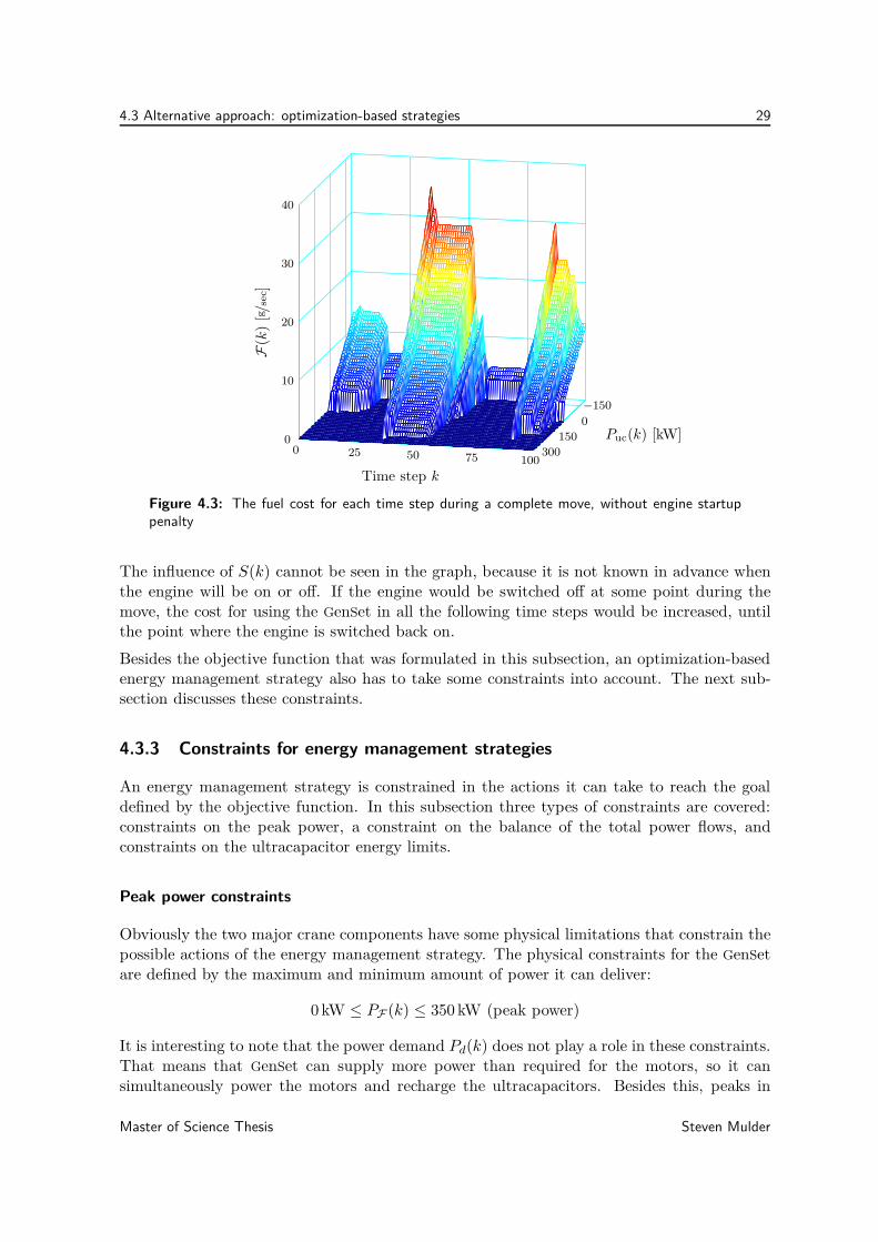
4.3 The fuel cost for each time step during a complete move . . . . . . . . . . . . . 29
4.4 The grid on the energy levels for the DP algorithm . . . . . . . . . . . . . . . . . 33
4.5 ECMS objective function, showing the influence of λuc on the optimal solutions . 37
4.6 Block scheme of first new strategy, using SOC feedback to approximate λuc for ECMS 39
4.7 Variation of λuc during operation . . . . . . . . . . . . . . . . . . . . . . . . . . 40
4.8 Block scheme of second new strategy, using prediction to approximate λuc for ECMS 42
4.9 Typical shape of the objective function for the λuc optimization . . . . . . . . . 43
Master of Science Thesis Steven Mulder

x List of Figures
5.1 Simulation results of the four case studies . . . . . . . . . . . . . . . . . . . . . 49
5.2 Cumulative fuel consumption over 21 hour day with varying activity . . . . . . . 50
Steven Mulder Master of Science Thesis
Preface
Somehow, container cranes have managed to work their way into every major project I haveperformed during my studies. My final bachelor’s project at Electrical Engineering—“IPP”for intimi—involved creating the electrical instrumentation for the simulator crane of theTU Delft department of Transport and Logistics. After this project, I made the jump fromElectrical Engineering to Systems and Control. At the end of the first year, I was confrontedwith another container crane during the Integration Project. It seems inevitable that thesubject of my final thesis also has to do with container cranes.
When I stepped into prof. Hans Hellendoorn’s office in the end of 2007, the purpose of thevisit was discussing the study tour to Israel that we were planning to organize in the followingyear. Over the course of a few more visits, this resulted in a number of valuable contacts forour study tour, including Thomas Cohn, ex-CEO of Siemens Nederland and the uncrownedking of Israeli startup companies. On top of this, professor Hans also went along with us toIsrael, where we had a great time discovering the Israeli culture and technology.
During the preparation of the study tour, we also started talking about the possibility ofgraduating at Siemens. The initial plan was to work on model-based fault detection (appliedto container cranes of course), but soon the choice was made to continue Joe George’s workfor the hybrid ECO-RTG. After a meeting with Rob Kuilboer at Siemens in The Hague, aformal assignment was drafted and I started my internship in august 2008.
During my internship, I learned a lot more than just designing energy management strate-gies. Actually, I think I learned far more about business politics and economics than I didabout engineering. The crane department was just going through a reorganization and themanagement was partially moved to Germany. It seemed to me that no one in The Haguewas completely happy with the way things were going.
At the same time, the global financial crisis broke out. For me, the crisis had two directrepercussions. First and foremost, the dropping oil prices meant that my fancy graph of ex-ploding fuel costs became obsolete overnight. On the other hand, the topics for the lunchtimediscussions did take a welcome diversion from the policy for flying business class and theconfusion about everybody’s job description to falling stocks and companies going bankrupt.Especially Rob turned out to have a wealth of macro-economic knowledge and little-known
Master of Science Thesis Steven Mulder

xii Preface
statistics about world trade. I never would have guessed that the Baltic Dry Index hadnothing to do with the Baltic countries.
Overall, I can look back at a very nice time at Siemens and I am quite proud of the endresults. Before continuing to the rest of this thesis, I want to thank a number of people thathave helped me along the way. First of all my supervisor, Hans Hellendoorn. You were agreat support for me, especially during the final writing weeks where I was struggling to getanything on paper. The encouraging discussions about my progress really pulled me through,not to mention the weekly deadlines. I will be recommending you to anyone looking for agraduation supervisor.
Another important role was played by my supervisor at Siemens, Rob Kuilboer. I know youhad a lot of other things on your mind (the ECO-RTG gearbox springs to mind), but you stillwere able to keep track of my progress and help me out wherever you could. I appreciate howyou involved me in some projects besides my own thesis work, and also left me free to spendtime on the organization of the study tour. Besides this, I also really enjoyed hearing aboutyour experience as an expat in China.
Back in Delft, there are a number of fellow students that perhaps did not contribute directlyto this thesis, but did make life a lot more fun while I was working on it. I have to thankmy MTB241 flatmates Siebe and Tamar for always finding creative ways of dragging me awayfrom the computer screen to (briefly) get my mind away from optimization algorithms. EvenHJ Thijs contributed to this sometimes, although, really, you should have spent less time inyour other “homes”. Tamar deserves a special mention for his part in the black gold alliance,keeping me supplied with coffee when I needed it most.
I also want to thank ex-MTBewoner Kenneth for keeping me active in sports throughoutthe project. Although the recent long distance running hype is a bridge too far for me, ourtraditional squash games were a great way to let off steam. I just wish you would let me wina little more often.
Finally, there is my eternal project partner Vincent. I have lost count of how many projectswe did together during our six years together in Delft, but it seems like I completed at least50 percent of my courses by working together with you in some way. It was quite a changeto have to find all my own bugs in this project. I wish you a lot of success with completingyour thesis on the Moving Base, I am sure you will manage without me.
A final, special word of thanks is meant for my family. To my parents, thank you for support-ing me all these years of my studies. Mom, I always knew there was at least one person whowas interested in what I was doing, even though sometimes I still struggle to properly explainit to you. Dad, thanks for your advice on many things, even proofreading my thesis. Iris, mybig little sister, thanks for the long Vogelpark Walsrode Verhalen that kept me entertainedwhen I didn’t feel like writing. I wish you a lot of luck with the completion of your new Mas-ter. To Opa en Oma, I am really lucky to have you as grandparents. Thank you for alwaysbeing there, from the bottom of my heart (and also from my wife’s bottom). Finally, I wantto thank Mieke for always supporting me and being so incredibly understanding whenever Idecided I would go kluizenaar for the weekend. I love you, you mean the world to me.
Steven MulderDelft, June 30, 2009
Steven Mulder Master of Science Thesis

xiii
“An algorithm must be seen to be believed.”
— Donald E. Knuth, The Art of Computer Programming
“Meer control is meer gaver.”
— Siebe Krijgsman, MSc (2008)
Master of Science Thesis Steven Mulder

xiv
Steven Mulder Master of Science Thesis
Chapter 1
General Introduction
This chapter serves as a general introduction for the rest of the thesis. Section 1.1 starts withsome background information on the subject of container cranes and on the developmentof Siemens’ hybrid ECO-RTG crane. This is followed in Section 1.2 by the definition of theproblem that is going to be addressed in this thesis, along with the way this problem is splitup into smaller subproblems. Finally, Section 1.3 outlines the way the rest of the thesis isstructured.
1.1 Background
1.1.1 Container shipping
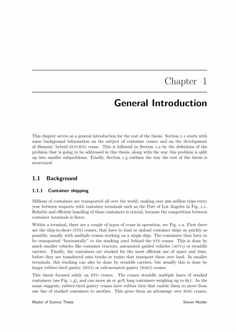
Millions of containers are transported all over the world, making over 200 million trips everyyear between seaports with container terminals such as the Port of Los Angeles in Fig. 1.1.Reliable and efficient handling of these containers is crucial, because the competition betweencontainer terminals is fierce.
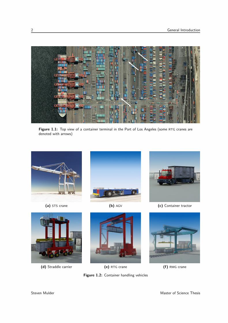
Within a terminal, there are a couple of types of crane in operation, see Fig. 1.2. First thereare the ship-to-shore (STS) cranes, that have to load or unload container ships as quickly aspossible, usually with multiple cranes working on a single ship. The containers then have tobe transported “horizontally” to the stacking yard behind the STS cranes. This is done bymuch smaller vehicles like container tractors, automated guided vehicles (AGVs) or straddlecarriers. Finally, the containers are stacked for the most efficient use of space and time,before they are transferred onto trucks or trains that transport them over land. In smallerterminals, this stacking can also be done by straddle carriers, but usually this is done bylarger rubber-tired gantry (RTG) or rail-mounted gantry (RMG) cranes.
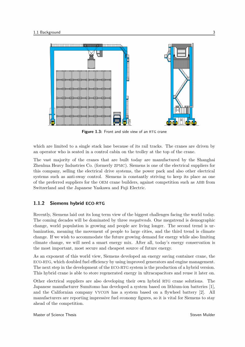
This thesis focused solely on RTG cranes. The cranes straddle multiple lanes of stackedcontainers (see Fig. 1.3), and can move 20 or 40 ft long containers weighing up to 65 t. As thename suggests, rubber-tired gantry cranes have rubber tires that enable them to move fromone line of stacked containers to another. This gives them an advantage over RMG cranes,
Master of Science Thesis Steven Mulder
2 General Introduction
Figure 1.1: Top view of a container terminal in the Port of Los Angeles (some RTG cranes aredenoted with arrows)
(a) STS crane (b) AGV (c) Container tractor
(d) Straddle carrier (e) RTG crane (f) RMG crane
Figure 1.2: Container handling vehicles
Steven Mulder Master of Science Thesis
1.1 Background 3
Figure 1.3: Front and side view of an RTG crane
which are limited to a single stack lane because of its rail tracks. The cranes are driven byan operator who is seated in a control cabin on the trolley at the top of the crane.
The vast majority of the cranes that are built today are manufactured by the ShanghaiZhenhua Heavy Industries Co. (formerly ZPMC). Siemens is one of the electrical suppliers forthis company, selling the electrical drive systems, the power pack and also other electricalsystems such as anti-sway control. Siemens is constantly striving to keep its place as oneof the preferred suppliers for the OEM crane builders, against competition such as ABB fromSwitzerland and the Japanese Yaskawa and Fuji Electric.
1.1.2 Siemens hybrid ECO-RTG
Recently, Siemens laid out its long term view of the biggest challenges facing the world today.The coming decades will be dominated by three megatrends. One megatrend is demographicchange, world population is growing and people are living longer. The second trend is ur-banization, meaning the movement of people to large cities, and the third trend is climatechange. If we wish to accommodate the future growing demand for energy while also limitingclimate change, we will need a smart energy mix. After all, today’s energy conservation isthe most important, most secure and cheapest source of future energy.
As an exponent of this world view, Siemens developed an energy saving container crane, theECO-RTG, which doubled fuel efficiency by using improved generators and engine management.The next step in the development of the ECO-RTG system is the production of a hybrid version.This hybrid crane is able to store regenerated energy in ultracapacitors and reuse it later on.
Other electrical suppliers are also developing their own hybrid RTG crane solutions. TheJapanese manufacturer Sumitomo has developed a system based on lithium-ion batteries [1],and the Californian company VYCON has a system based on a flywheel battery [2]. Allmanufacturers are reporting impressive fuel economy figures, so it is vital for Siemens to stayahead of the competition.
Master of Science Thesis Steven Mulder
4 General Introduction
An important aspect of the hybrid system is the control policy that optimizes the use of theregenerated energy. By using a strategy that makes smart decisions about when and howto use the secondary ultracapacitor power source, the overall efficiency of the crane can beoptimized. In the literature this is known as energy management. Due to the advent ofhybrid cars, this has been a popular research subject in recent years. The challenge in energymanagement is making the best use of the limited storage capacity of the secondary source,so that the primary combustion engine runs as efficiently as possible. What makes improvingthe energy management strategy so interesting is that it only changes the software of thesystem, so no additional hardware costs are necessary.
This study focuses on the design of an optimal energy management strategy for Siemens’hybrid ECO-RTG crane. It is a continuation of the Master’s Thesis work by Joe George [3]. Inhis project, Joe George developed a system that can calculate an optimal strategy for a givenpower demand, where the existing research into hybrid cars was used as a starting point.Although this particular system could not be directly applied in practice for various reasons,it did prove that improving the strategy can lead to significant fuel consumption gains.
1.2 Problem statement
1.2.1 Main thesis goal
With the tough competition in the “green” RTG business, Siemens wants to stay in the leadby achieving the best fuel economy at a relatively low cost. This leads to the following formaldefinition of the problem that is addressed in this thesis:
How can the energy management strategy of the Siemens hybrid ECO-RTG cranebe improved in order to enhance its fuel economy?
An important constraint on the possible solutions is that the performance of the crane cannotbe compromised. A fuel efficient crane that is much slower than a normal crane is notinteresting for terminal operators, whose main concern is still container throughput.
1.2.2 Subproblems
At the start of the project it was not exactly clear to the people at Siemens what the perfor-mance of the hybrid ECO-RTG is, and whether it could be improved significantly. A prototypecrane is in use at the Port of Algeciras (Spain), and it has shown promising fuel consumptionfigures, but essentially the hybrid crane remains a black box. The only way to see whetheradjustments to the system improve the performance is by putting the crane into operationfor a longer period of time. After this period, data about the total fuel consumption duringthat period can give an indication of the fuel efficiency. For structured improvements to thesystem is is necessary to have some way of analyzing the crane’s fuel consumption, so creatinga simulator for this is the first subproblem to address in the thesis.
The simulator can be split up in two distinct parts. The first part is simulating the crane’spower demand. There are some measurements available of the power flow when the crane isin action, but these are both limited in duration and in variety. A solution is required to make
Steven Mulder Master of Science Thesis

1.3 Outline 5
it possible to simulate the crane’s performance in any possible circumstance. For instance, tosimulate the fuel consumption during a busy period, or while the crane is moving a series ofvery heavy containers.
The second part of the simulator is a model of the crane’s power sources, which can simulatethe fuel consumption of the crane given a certain power demand. This model also includes thebehavior of the ultracapacitors, which function both as energy storage and as power source.
Summarizing, the first subproblem is:
1. Create a simulator to analyze the fuel consumption of the hybrid ECO-RTG crane.
(a) Create a system to mimic the power demand of the crane during specific types ofoperations.
(b) Create a model that simulates the total power system of the hybrid ECO-RTG,including the fuel consumption and the ultracapacitors.
When the simulator is available, the focus can be on the energy management strategies. Thefirst step in improving the strategy is looking at the current situation, and analyzing what isgood and what is not. Based on this information, a choice can be made on how to proceedin order to improve the current situation. The final step is actually implementing theseimprovements in a new strategy, so the second subproblem is formulated as:
2. Design a system that improves the current energy management strategy.
(a) Analyze the current strategy to find its strong points and weaknesses.
(b) Find an approach to improve the weaknesses of the current strategy
(c) Implement the improved strategy so it can be tested in the simulator.
It turns out—perhaps unsurprisingly—that there is no definitive best approach to improvethe current energy management strategy. In the end, the choice was made to implementtwo new strategies and compare them using the simulator. Of course, the original strategyshould also be taken into account in this comparison, so in total there are three alternatives.To make a good comparison of the strategies, well-designed experiments are necessary. Theexperiments have to uncover as much relevant information about the strategies as possible,so a well-founded choice for the best strategy can be made in the end. This task forms thethird and final subproblem of this thesis:
3. Select the best strategy from the three alternatives.
(a) Design experiments that show relevant characteristics of the strategies.
(b) Analyze the simulation results to find the best strategy.
1.3 Outline
The contents of the rest of this thesis are structured much in the same way as the threesubproblems. In the first two chapters, the simulator is discussed. Chapter 2 explains the
Master of Science Thesis Steven Mulder
6 General Introduction
power consumption of RTG cranes, loading to a system that simulates the power demandduring operation. Chapter 3 then deals with the mathematical model that is created of thecrane’s power sources. This model serves both as a simulation model and as the basis for theenergy management strategy.
In Chapter 4 the actual design of the strategy is explained, which corresponds with thesecond subproblem. The chapter starts with a brief discussion of the current strategy. Theperformance of this strategy will function as a benchmark for the new designs. Next, a briefsurvey is given of the various alternative approaches that are available in the literature, andthe choice for an optimization-based strategy is explained. The final two sections of Chapter 4
explain the implementation of the two new strategies.
The third subproblem is next. The comparison of the different strategies is handled in Chap-ter 5. Simulation results of the different strategies under various circumstances are presentedin this chapter, so they can be compared and the best strategy is found.
Finally, Chapter 6 draws conclusions about the success of the project, and gives some recom-mendations about possibilities for further improvement.
Steven Mulder Master of Science Thesis

Chapter 2
Power Demand Model
The first step in the design process of any technical system is understanding the way it is goingto be used. The energy management strategy that we want to design will control the powersupply for a larger system, the rubber-tired gantry (RTG) crane. Therefore it is necessary toresearch the RTG crane’s typical power demand.
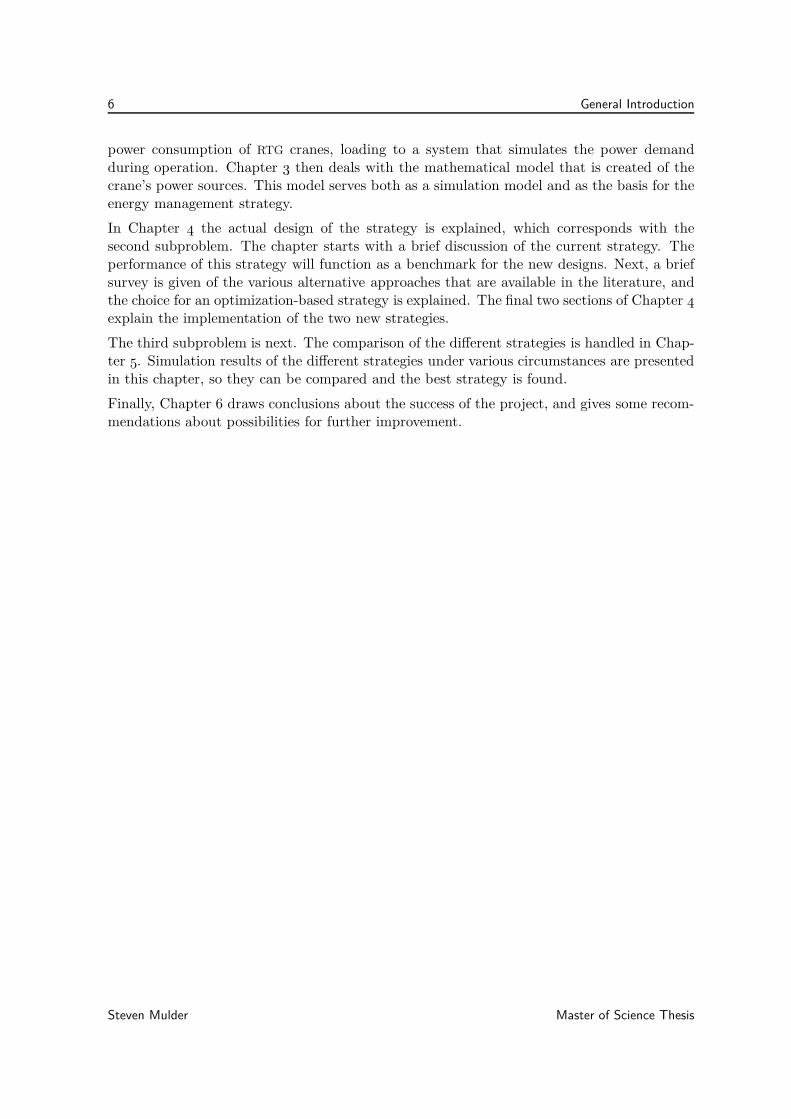
The complete power system of the ECO-RTG is shown in Fig. 2.1. This chapter is onlyconcerned with the bottom half of the system, i.e., the power consumers. The goal is tocreate a model of the typical power consumption of the crane during operation. Section 2.1
explains the different subsystems that consume power on the crane. Next, Section 2.2 explainshow these subsystems are used during typical operation, which leads to a model of the typicalpower demand of an RTG crane. This system will be combined with a model of the crane’spower sources—the top half of Fig. 2.1—to form the simulation framework in which thestrategies are tested.
2.1 Power consuming subsystems
It is often easy to relate an unknown drivetrain to that of a standard personal car. Unlikethe situation on a car, an RTG crane moves using electric motors, its combustion engine isonly used to generate electrical energy for these motors. Another thing that is different froma car’s power system is that the power demand is dominated by only the propulsion system,there are several major power consumers on an RTG crane. The power demand is due to acombination of the following subsystems, which are also depicted in Fig. 2.1.
• The hoist mechanism, powered by a single electric motor capable of peaks of 200–400 kW.
• The wheels for moving the complete crane around the yard, driven by the gantry motors.These motors are typically four heavy-duty motors capable of 40 kW of power each.
• The trolley with the control cabin, and the spreader suspended beneath it. The spreaderis the part of the crane that attaches to the top of a container. The trolley can move
Master of Science Thesis Steven Mulder
8 Power Demand Model
Diesel engine
G∼
G∼
Variable SpeedGenerators
∼=
Rectifier(AC/DC) Ultracaps
=∼
Auxiliaries
=∼
Trolley Motors
=∼
Gantry Motors
=∼
Inverter(DC/AC)
Hoist Motor
Figure 2.1: Power architecture of the ECO-RTG
on rails at the top of the crane and is driven by two trolley motors with 20 kW nominalpower each.
• The auxiliary systems, such as the heating, ventilating, and air conditioning (HVAC)systems, the big lights for night time operation, and the crane’s computer system.These systems have a more or less constant power demand of 10–30 kW, depending onthe circumstances, e.g., temperature or daylight.
During operation of the crane, all subsystems contribute to the total power demand. Thehoist, gantry and trolley motors only need power when they are moving, while the auxil-iary systems are always on. The specific usage of the subsystems during the cranes normaloperation is discussed in the next section.
2.2 Typical operation
The activities of an RTG crane can be separated in four categories:
• Loading a container from the stack downto a truck.
• Unloading a container from a truck onto the stack.
• Gantry movement from one row of stacked containers to another.
• Idling.
The loading or unloading of a container is usually called a “move”. The gantry movementwill not be considered specifically in this thesis, because this operation is not done very oftencompared to the other three activities. In general, the contribution of the gantry movementsto the power demand is very similar to that of the trolley system.
Steven Mulder Master of Science Thesis
2.2 Typical operation 9
A
BC
DEF
Figure 2.2: Movements of an RTG crane unloading a truck
2.2.1 Crane movements during operation
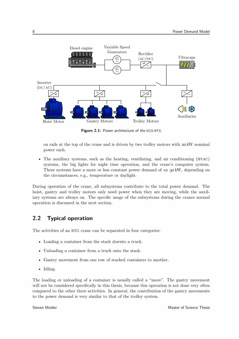
Figure 2.2 shows the crane’s movements during the unloading of a truck:
A. move the trolley over the pick-up point (either above the stack or a truck);
B. lower the empty spreader onto the container;
C. hoist the container up to clear the top of the stack;
D. move the container over the release point;
E. lower the container to the release point;
F. lift the empty spreader from the container.
The basic movements during a container move cycle are identical for both loading and un-loading. The only difference between the two is the height of the pickup and release points,i.e., the length of the “B–C” and “E–F” sections. In general, unloading a truck costs more netenergy because the container is moved up to the stack.
2.2.2 Power demand for one move
The power demand during each section “A” to “F” depends on the required force, the speedof the movement and the efficiency of the motors and inverters. The required force can alsobe negative when the container is lowered or during braking, so the power demand is modeledas:
Pd(k) =
η · F (k) · v(k) if F (k) ≥ 01η· F (k) · v(k) if F (k) < 0
Master of Science Thesis Steven Mulder

10 Power Demand Model
0
150
300
−150
−3000.5 1.0 1.5 2.0 2.5
Time [min]
Pow
erdem
and
[kW
]
AB CD
E F
(a) Loading a container down to a truck
0
150
300
−150
−3000.5 1.0 1.5 2.0 2.5
Time [min]
Pow
erdem
and
[kW
]
A B CD
E F
(b) Unloading a container up from a truck
Figure 2.3: Typical power demand during loading and unloading of a 40 t container from a truckonto the stack (row 6, height 5)
Note that the model is in discrete time. This is the most logical choice, because the simulatorwill be implemented on a computer. The final energy management strategies will also beimplemented in discrete time.
The motor efficiency η is assumed to be a fixed value that depends on whether the crane ishoisting or using the trolley or gantry motors. The required force F (k) depends on the weightof the load that the crane is carrying. This weight determines the gravitational force thatthe hoist motors need to overcome, and also the frictional forces for the trolley and gantrymovements. To limit the required power for very heavy containers, the speed v(k) of themovements is adjusted by the crane software according to the weight of the load. This meansthat moving heavy containers takes more time, but the maximum power demand is not toohigh for the generator to handle.
Besides the continuous power during each move, the motors need to accelerate and overcomethe inertia of the crane’s moving parts such as the big cable reels. This creates a peak of extrapower demand at the start of each movement. On the other hand, there also is a peak ofnegative power each time the crane decelerates at the end of each movement, albeit somewhatsmaller because of the losses in the electric motors and inverters.
Figure 2.3 shows the modeled power demand during both loading and unloading moves. Whenthe power demand is positive, the crane has to supply power to the electric motors. Duringthe sections where the power demand is negative, energy is released to the crane, e.g., duringbraking or lowering of the container. In regular cranes this energy is dissipated by the brakes,but the hybrid ECO-RTG can store it in the ultracapacitors so it can be reused later on. It isclear that the hoist movements dominate the power demand of the crane. The influence ofthe speed of the movements is visible by relatively small difference in the height of the peakswhen the crane is empty and when it is full, e.g., between “B”’ and “E”. The peaks in thedemand during acceleration and deceleration are also visible.
Steven Mulder Master of Science Thesis
2.2 Typical operation 11
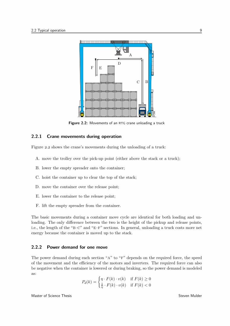
Table 2.1: Key figures for the three general activity profiles
Profile Avg. move duration Avg. idle time per move Avg. moves per hour
Quiet 150 sec 200 sec 10 move/hr
Normal 150 sec 100 sec 14 move/hr
Busy 150 sec < 10 sec 23 move/hr
2.2.3 Varying level of busyness
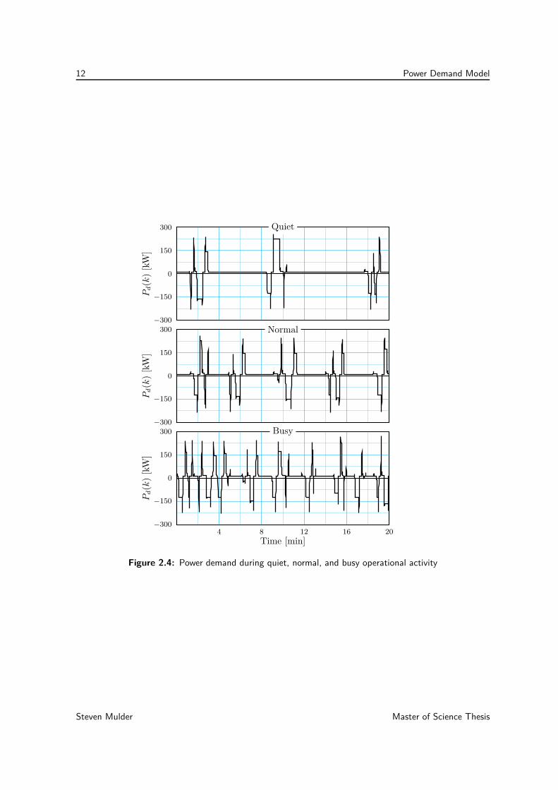
Over the course of a day of activities, the number of container moves per hour will varyaccording to the level of activity in the container terminal. When a ship is docked, containersare loaded or unloaded as quickly as possible, creating a peak of activity in the terminal.Conversely, there can also be relatively quiet periods during which the crane spends a lot oftime idling between moves. Table 2.1 shows the average idle times and number of cranes perhour for three general activity profiles, which will be used in simulations of the crane’s powerdemand. Figure 2.4 shows the power demand for three levels of activity in simulations.
The varying idle times can have an important effect on the choice for the best strategy. Tosave fuel, the engine of the diesel generator set (GenSet) is usually shut off during idle periodsin hybrid cranes. Even though the power demand is only 10–30 kW, during longer idle timesthis can significantly decrease the energy level of the ultracapacitors at the start of a newmove. Sometimes it is even necessary to restart the diesel generator set and briefly rechargethe ultracapacitors.
It has to be noted that the power demand model is not validated in the sense that it isguaranteed to mimic the crane’s power demand for each specific movement 100% accurately.After all, this is not the goal of the model, it will only be used as a simulation of the powerdemand of the crane while it is loading and unloading different containers, so the energymanagement strategy have realisitic input signals to work with. In this sense, the powerdemand model is sufficiently accurate.
Master of Science Thesis Steven Mulder
12 Power Demand Model
0
150
300
−150
−300
Pd(k
)[k
W]
Quiet
0
150
300
−150
−300
Pd(k
)[k
W]
Normal
0
150
300
−150
−3004 8 12 16 20
Time [min]
Pd(k
)[k
W]
Busy
Figure 2.4: Power demand during quiet, normal, and busy operational activity
Steven Mulder Master of Science Thesis
Chapter 3
Power Supply Model
The previous chapter set the first steps toward the creation of a simulator for the hybridECO-RTG. The power system was discussed in general and a model for the power demandwas developed. The next step for the simulator is creating a model for the power generatingsystem of the crane. The model of the power system is also needed for the design of anoptimal energy management strategy. The model should simulate the power behavior of thereal crane, i.e., the electrical power use and fuel consumption.
The hybrid ECO-RTG crane has two power sources on board: the diesel generator set (GenSet)and the ultracapacitor bank. This chapter is split up in a similar way: after the introductionof the model goals and approach in Section 3.1, Section 3.2 discusses the model of the GenSet,and Section 3.3 the ultracapacitors. After this, Section 3.4 concludes with an overview of thecomplete crane simulator model.
3.1 Introduction
3.1.1 Power system overview
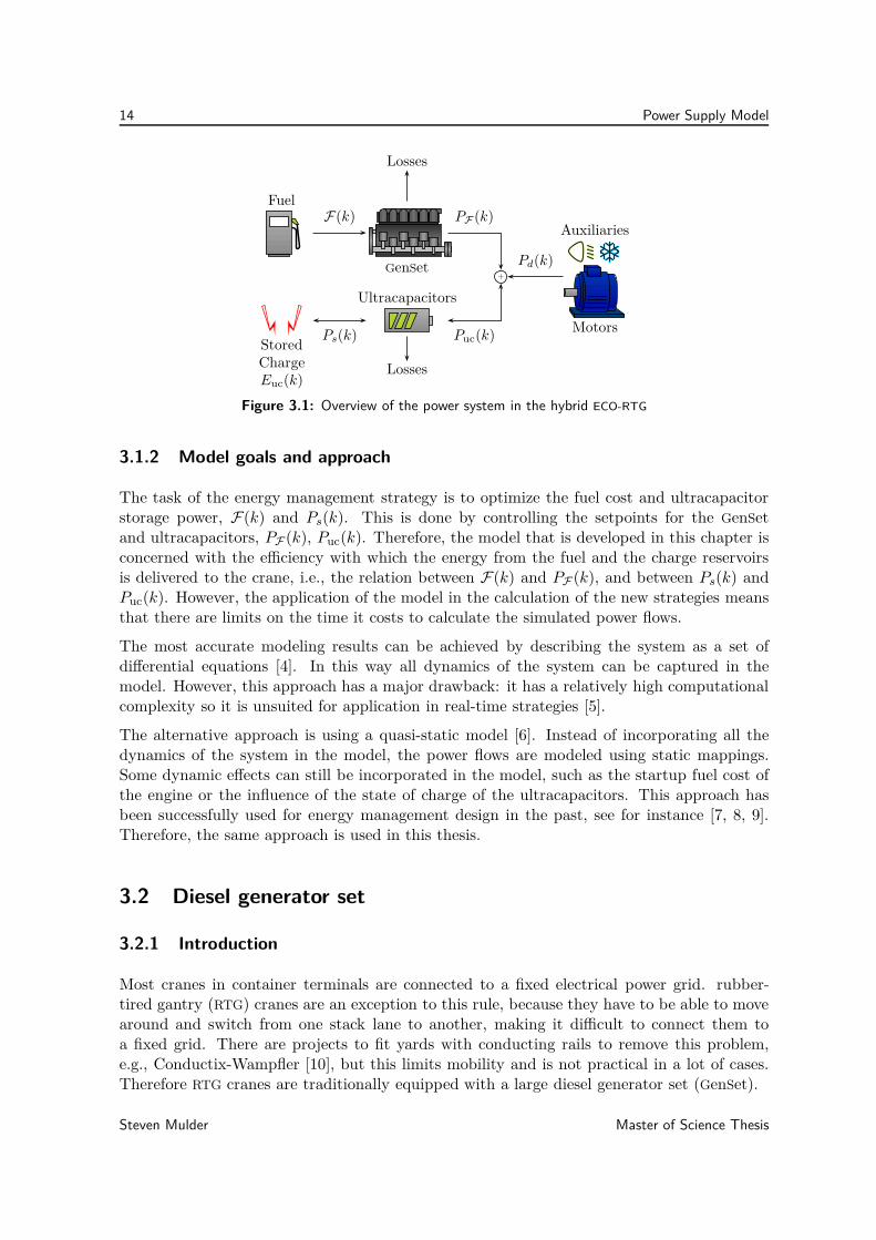
Figure 3.1 shows a schematic overview of the power system in the hybrid ECO-RTG crane. Onthe right side there are the power consumers: the electric motors and the auxiliary systemslike the lighting and the air-conditioning. The power demand of these systems was discussedin the previous chapter. On the left side there are the GenSet and the ultracapacitors, whichhave to fulfill the power demand.
The two power sources of the hybrid ECO-RTG crane each have their own energy “reservoir”,the GenSet has its diesel fuel tank and the ultracapacitors have electrical charge stored in thecapacitors. The ultracapacitors also have the ability to store regenerated energy coming fromthe electric motors, increasing the amount of stored charge. Obviously the GenSet cannotstore regenerated energy and convert it back into fuel.
Master of Science Thesis Steven Mulder
14 Power Supply Model
Ultracapacitors
Fuel
StoredChargeEuc(k)
Motors
Auxiliaries
GenSet+
F(k) PF(k)
Ps(k) Puc(k)
Pd(k)
Losses
Losses
Figure 3.1: Overview of the power system in the hybrid ECO-RTG
3.1.2 Model goals and approach
The task of the energy management strategy is to optimize the fuel cost and ultracapacitorstorage power, F(k) and Ps(k). This is done by controlling the setpoints for the GenSetand ultracapacitors, PF (k), Puc(k). Therefore, the model that is developed in this chapter isconcerned with the efficiency with which the energy from the fuel and the charge reservoirsis delivered to the crane, i.e., the relation between F(k) and PF (k), and between Ps(k) andPuc(k). However, the application of the model in the calculation of the new strategies meansthat there are limits on the time it costs to calculate the simulated power flows.
The most accurate modeling results can be achieved by describing the system as a set ofdifferential equations [4]. In this way all dynamics of the system can be captured in themodel. However, this approach has a major drawback: it has a relatively high computationalcomplexity so it is unsuited for application in real-time strategies [5].
The alternative approach is using a quasi-static model [6]. Instead of incorporating all thedynamics of the system in the model, the power flows are modeled using static mappings.Some dynamic effects can still be incorporated in the model, such as the startup fuel cost ofthe engine or the influence of the state of charge of the ultracapacitors. This approach hasbeen successfully used for energy management design in the past, see for instance [7, 8, 9].Therefore, the same approach is used in this thesis.
3.2 Diesel generator set
3.2.1 Introduction
Most cranes in container terminals are connected to a fixed electrical power grid. rubber-tired gantry (RTG) cranes are an exception to this rule, because they have to be able to movearound and switch from one stack lane to another, making it difficult to connect them toa fixed grid. There are projects to fit yards with conducting rails to remove this problem,e.g., Conductix-Wampfler [10], but this limits mobility and is not practical in a lot of cases.Therefore RTG cranes are traditionally equipped with a large diesel generator set (GenSet).
Steven Mulder Master of Science Thesis
3.2 Diesel generator set 15
Fuel tank
GenSet
Diesel engine
G∼
G∼
Variable SpeedGenerators
∼=
Rectifier(AC/DC)
Auxiliaries
Motors
F(k) PF(k)
Figure 3.2: Schematic of the GenSet model
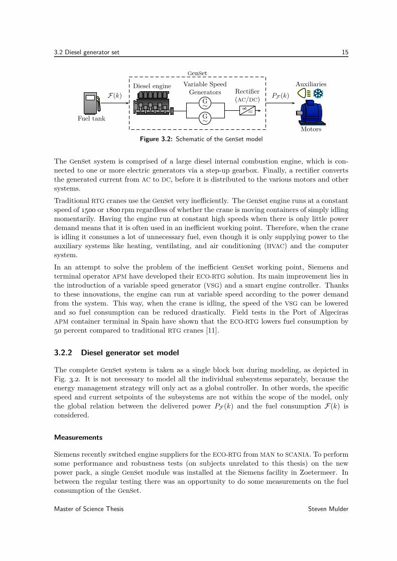
The GenSet system is comprised of a large diesel internal combustion engine, which is con-nected to one or more electric generators via a step-up gearbox. Finally, a rectifier convertsthe generated current from AC to DC, before it is distributed to the various motors and othersystems.
Traditional RTG cranes use the GenSet very inefficiently. The GenSet engine runs at a constantspeed of 1500 or 1800 rpm regardless of whether the crane is moving containers of simply idlingmomentarily. Having the engine run at constant high speeds when there is only little powerdemand means that it is often used in an inefficient working point. Therefore, when the craneis idling it consumes a lot of unnecessary fuel, even though it is only supplying power to theauxiliary systems like heating, ventilating, and air conditioning (HVAC) and the computersystem.
In an attempt to solve the problem of the inefficient GenSet working point, Siemens andterminal operator APM have developed their ECO-RTG solution. Its main improvement lies inthe introduction of a variable speed generator (VSG) and a smart engine controller. Thanksto these innovations, the engine can run at variable speed according to the power demandfrom the system. This way, when the crane is idling, the speed of the VSG can be loweredand so fuel consumption can be reduced drastically. Field tests in the Port of AlgecirasAPM container terminal in Spain have shown that the ECO-RTG lowers fuel consumption by50 percent compared to traditional RTG cranes [11].
3.2.2 Diesel generator set model
The complete GenSet system is taken as a single block box during modeling, as depicted inFig. 3.2. It is not necessary to model all the individual subsystems separately, because theenergy management strategy will only act as a global controller. In other words, the specificspeed and current setpoints of the subsystems are not within the scope of the model, onlythe global relation between the delivered power PF (k) and the fuel consumption F(k) isconsidered.
Measurements
Siemens recently switched engine suppliers for the ECO-RTG from MAN to SCANIA. To performsome performance and robustness tests (on subjects unrelated to this thesis) on the newpower pack, a single GenSet module was installed at the Siemens facility in Zoetermeer. Inbetween the regular testing there was an opportunity to do some measurements on the fuelconsumption of the GenSet.
Master of Science Thesis Steven Mulder
16 Power Supply Model
5
10
15
20
0 100 200 300−100
PF (k) [kW]
F(k
)[g
/sec]
bC
bC bCbCbC
bC
bC
bC
bC
bC
S(k − 1): Engine ON
S(k − 1): Engine OFF
Measurements
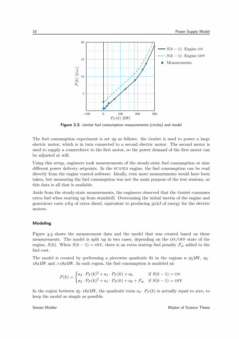
Figure 3.3: GenSet fuel consumption measurements (circles) and model
The fuel consumption experiment is set up as follows: the GenSet is used to power a largeelectric motor, which is in turn connected to a second electric motor. The second motor isused to supply a counterforce to the first motor, so the power demand of the first motor canbe adjusted at will.
Using this setup, engineers took measurements of the steady-state fuel consumption at ninedifferent power delivery setpoints. In the SCANIA engine, the fuel consumption can be readdirectly from the engine control software. Ideally, even more measurements would have beentaken, but measuring the fuel consumption was not the main purpose of the test sessions, sothis data is all that is available.
Aside from the steady-state measurements, the engineers observed that the GenSet consumesextra fuel when starting up from standstill. Overcoming the initial inertia of the engine andgenerators costs 2.6 g of extra diesel, equivalent to producing 50 kJ of energy for the electricmotors.
Modeling
Figure 3.3 shows the measurement data and the model that was created based on thesemeasurements. The model is split up in two cases, depending on the ON/OFF state of theengine, S(k). When S(k − 1) = OFF, there is an extra startup fuel penalty Fst added to thefuel cost.
The model is created by performing a piecewise quadratic fit in the regions 0–25 kW, 25–182 kW and >182 kW. In each region, the fuel consumption is modeled as:
F(k) =
a2 · PF (k)2 + a1 · PF (k) + a0 if S(k − 1) = ON
a2 · PF (k)2 + a1 · PF (k) + a0 + Fst if S(k − 1) = OFF
In the region between 25–182 kW, the quadratic term a2 · PF (k) is actually equal to zero, tokeep the model as simple as possible.
Steven Mulder Master of Science Thesis
3.3 Ultracapacitor bank model 17
150
200
250
300
0 100 200 300−100
PF (k) [kW]
F(k
)[g
/kW
h]
Figure 3.4: Specific fuel consumption of the GenSet
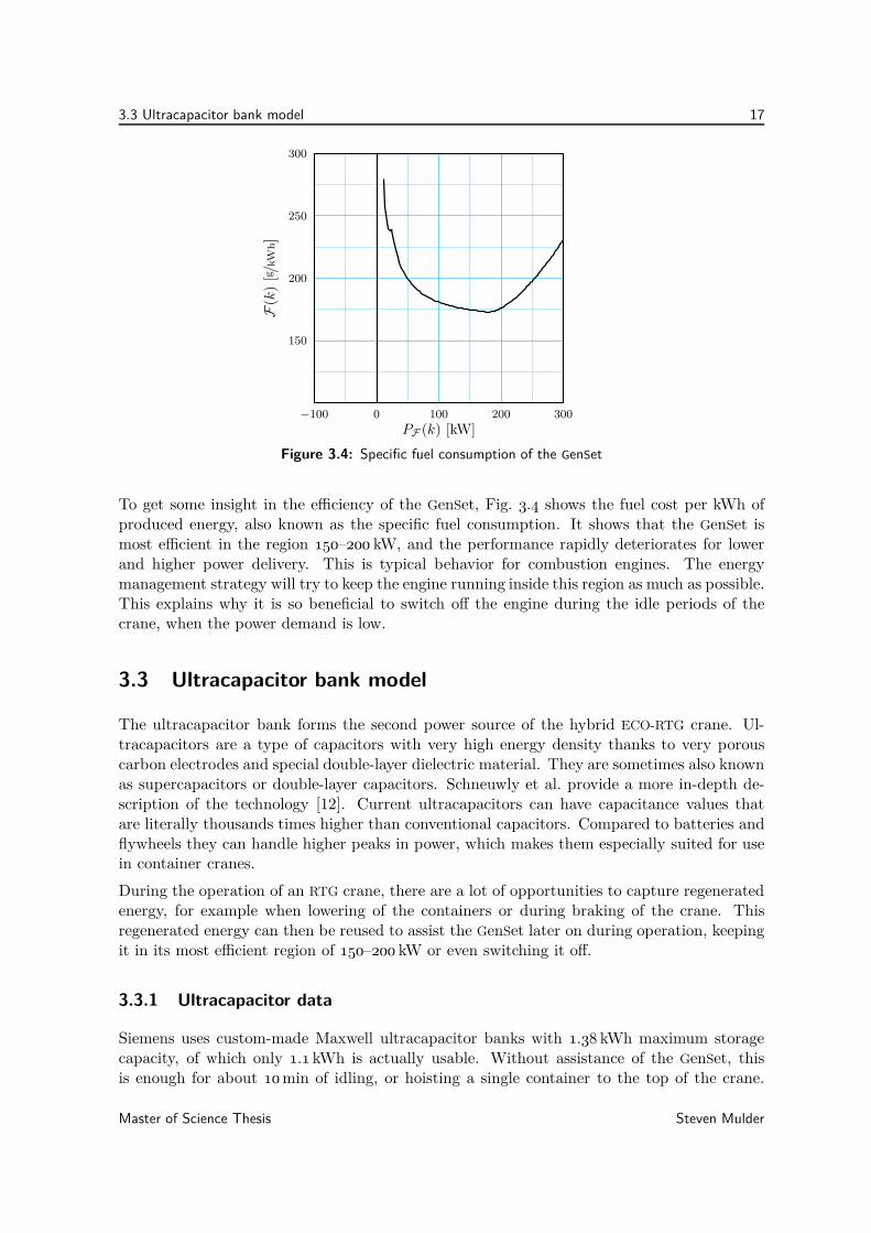
To get some insight in the efficiency of the GenSet, Fig. 3.4 shows the fuel cost per kWh ofproduced energy, also known as the specific fuel consumption. It shows that the GenSet ismost efficient in the region 150–200 kW, and the performance rapidly deteriorates for lowerand higher power delivery. This is typical behavior for combustion engines. The energymanagement strategy will try to keep the engine running inside this region as much as possible.This explains why it is so beneficial to switch off the engine during the idle periods of thecrane, when the power demand is low.
3.3 Ultracapacitor bank model
The ultracapacitor bank forms the second power source of the hybrid ECO-RTG crane. Ul-tracapacitors are a type of capacitors with very high energy density thanks to very porouscarbon electrodes and special double-layer dielectric material. They are sometimes also knownas supercapacitors or double-layer capacitors. Schneuwly et al. provide a more in-depth de-scription of the technology [12]. Current ultracapacitors can have capacitance values thatare literally thousands times higher than conventional capacitors. Compared to batteries andflywheels they can handle higher peaks in power, which makes them especially suited for usein container cranes.
During the operation of an RTG crane, there are a lot of opportunities to capture regeneratedenergy, for example when lowering of the containers or during braking of the crane. Thisregenerated energy can then be reused to assist the GenSet later on during operation, keepingit in its most efficient region of 150–200 kW or even switching it off.
3.3.1 Ultracapacitor data
Siemens uses custom-made Maxwell ultracapacitor banks with 1.38 kWh maximum storagecapacity, of which only 1.1 kWh is actually usable. Without assistance of the GenSet, thisis enough for about 10 min of idling, or hoisting a single container to the top of the crane.
Master of Science Thesis Steven Mulder
18 Power Supply Model
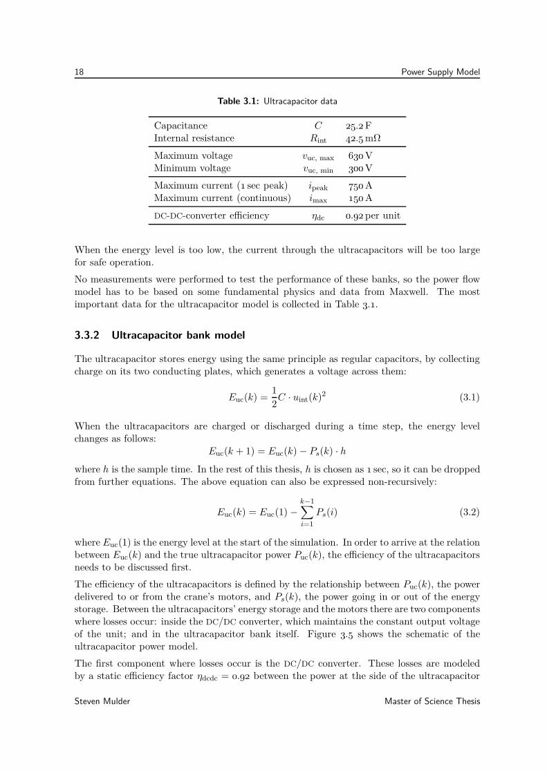
Table 3.1: Ultracapacitor data
Capacitance C 25.2 FInternal resistance Rint 42.5 mΩ
Maximum voltage vuc, max 630 VMinimum voltage vuc, min 300 V
Maximum current (1 sec peak) ipeak 750 AMaximum current (continuous) imax 150 A
DC-DC-converter efficiency ηdc 0.92 per unit
When the energy level is too low, the current through the ultracapacitors will be too largefor safe operation.
No measurements were performed to test the performance of these banks, so the power flowmodel has to be based on some fundamental physics and data from Maxwell. The mostimportant data for the ultracapacitor model is collected in Table 3.1.
3.3.2 Ultracapacitor bank model
The ultracapacitor stores energy using the same principle as regular capacitors, by collectingcharge on its two conducting plates, which generates a voltage across them:
Euc(k) =1
2C · uint(k)
2 (3.1)
When the ultracapacitors are charged or discharged during a time step, the energy levelchanges as follows:
Euc(k + 1) = Euc(k)− Ps(k) · h
where h is the sample time. In the rest of this thesis, h is chosen as 1 sec, so it can be droppedfrom further equations. The above equation can also be expressed non-recursively:
Euc(k) = Euc(1) −k−1∑
i=1
Ps(i) (3.2)
where Euc(1) is the energy level at the start of the simulation. In order to arrive at the relationbetween Euc(k) and the true ultracapacitor power Puc(k), the efficiency of the ultracapacitorsneeds to be discussed first.
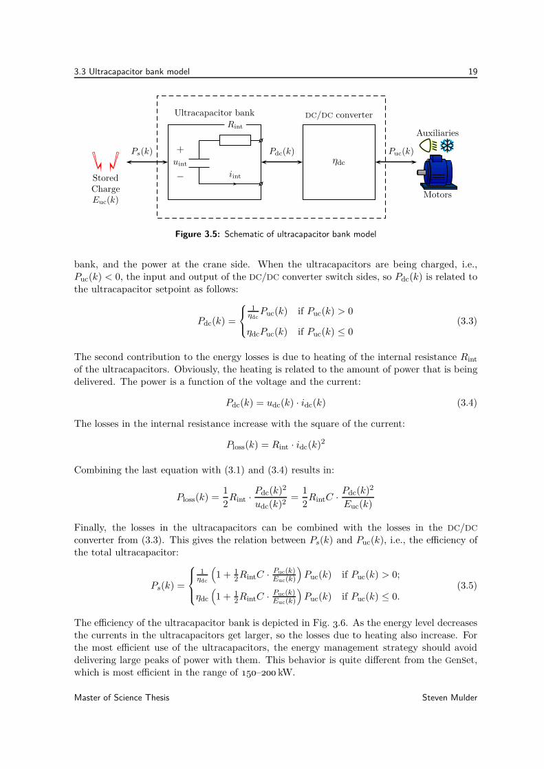
The efficiency of the ultracapacitors is defined by the relationship between Puc(k), the powerdelivered to or from the crane’s motors, and Ps(k), the power going in or out of the energystorage. Between the ultracapacitors’ energy storage and the motors there are two componentswhere losses occur: inside the DC/DC converter, which maintains the constant output voltageof the unit; and in the ultracapacitor bank itself. Figure 3.5 shows the schematic of theultracapacitor power model.
The first component where losses occur is the DC/DC converter. These losses are modeledby a static efficiency factor ηdcdc = 0.92 between the power at the side of the ultracapacitor
Steven Mulder Master of Science Thesis
3.3 Ultracapacitor bank model 19
Puc(k)Pdc(k)Ps(k)
Rint
iint
+uint
−
Ultracapacitor bank
ηdc
DC/DC converter
StoredChargeEuc(k)
Motors
Auxiliaries
Figure 3.5: Schematic of ultracapacitor bank model
bank, and the power at the crane side. When the ultracapacitors are being charged, i.e.,Puc(k) < 0, the input and output of the DC/DC converter switch sides, so Pdc(k) is related tothe ultracapacitor setpoint as follows:
Pdc(k) =
1ηdcPuc(k) if Puc(k) > 0
ηdcPuc(k) if Puc(k) ≤ 0(3.3)
The second contribution to the energy losses is due to heating of the internal resistance Rint
of the ultracapacitors. Obviously, the heating is related to the amount of power that is beingdelivered. The power is a function of the voltage and the current:
Pdc(k) = udc(k) · idc(k) (3.4)
The losses in the internal resistance increase with the square of the current:
Ploss(k) = Rint · idc(k)2
Combining the last equation with (3.1) and (3.4) results in:
Ploss(k) =1
2Rint ·
Pdc(k)2
udc(k)2=
1
2RintC ·
Pdc(k)2
Euc(k)
Finally, the losses in the ultracapacitors can be combined with the losses in the DC/DC
converter from (3.3). This gives the relation between Ps(k) and Puc(k), i.e., the efficiency ofthe total ultracapacitor:
Ps(k) =
1ηdc
(
1 + 12RintC ·
Puc(k)Euc(k)
)
Puc(k) if Puc(k) > 0;
ηdc
(
1 + 12RintC ·
Puc(k)Euc(k)
)
Puc(k) if Puc(k) ≤ 0.(3.5)
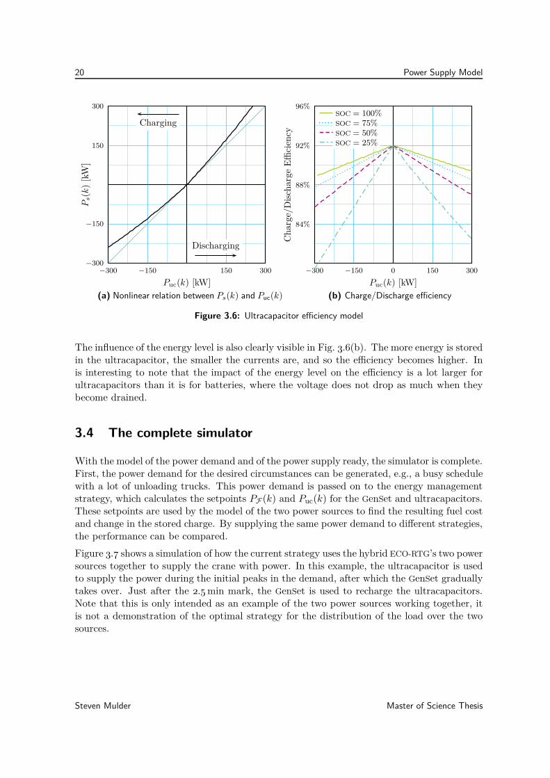
The efficiency of the ultracapacitor bank is depicted in Fig. 3.6. As the energy level decreasesthe currents in the ultracapacitors get larger, so the losses due to heating also increase. Forthe most efficient use of the ultracapacitors, the energy management strategy should avoiddelivering large peaks of power with them. This behavior is quite different from the GenSet,which is most efficient in the range of 150–200 kW.
Master of Science Thesis Steven Mulder
20 Power Supply Model
150
300
−150
−300150 300−150−300
Puc(k) [kW]
Ps(k
)[k
W]
Discharging
Charging
(a) Nonlinear relation between Ps(k) and Puc(k)
84%
88%
92%
96%
0 150 300−150−300
Puc(k) [kW]C
harg
e/D
isch
arg
eE
ffici
ency
SOC = 100%SOC = 75%SOC = 50%SOC = 25%
(b) Charge/Discharge efficiency
Figure 3.6: Ultracapacitor efficiency model
The influence of the energy level is also clearly visible in Fig. 3.6(b). The more energy is storedin the ultracapacitor, the smaller the currents are, and so the efficiency becomes higher. Inis interesting to note that the impact of the energy level on the efficiency is a lot larger forultracapacitors than it is for batteries, where the voltage does not drop as much when theybecome drained.
3.4 The complete simulator
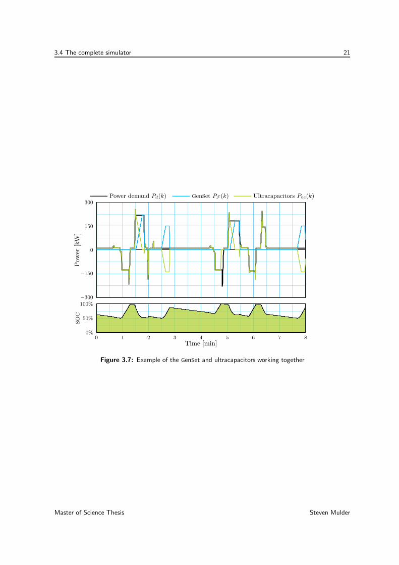
With the model of the power demand and of the power supply ready, the simulator is complete.First, the power demand for the desired circumstances can be generated, e.g., a busy schedulewith a lot of unloading trucks. This power demand is passed on to the energy managementstrategy, which calculates the setpoints PF (k) and Puc(k) for the GenSet and ultracapacitors.These setpoints are used by the model of the two power sources to find the resulting fuel costand change in the stored charge. By supplying the same power demand to different strategies,the performance can be compared.
Figure 3.7 shows a simulation of how the current strategy uses the hybrid ECO-RTG’s two powersources together to supply the crane with power. In this example, the ultracapacitor is usedto supply the power during the initial peaks in the demand, after which the GenSet graduallytakes over. Just after the 2.5 min mark, the GenSet is used to recharge the ultracapacitors.Note that this is only intended as an example of the two power sources working together, itis not a demonstration of the optimal strategy for the distribution of the load over the twosources.
Steven Mulder Master of Science Thesis
3.4 The complete simulator 21
0
150
300
−150
−300
Pow
er[k
W]
Power demand Pd(k) GenSet PF (k) Ultracapacitors Puc(k)
0%
50%
100%
0 1 2 3 4 5 6 7 8Time [min]
SO
C
Figure 3.7: Example of the GenSet and ultracapacitors working together
Master of Science Thesis Steven Mulder

22 Power Supply Model
Steven Mulder Master of Science Thesis
Chapter 4
Energy Management Strategy
The previous chapters laid the groundwork for the design of the energy management strategy.The intended usage of the strategy in the hybrid ECO-RTG crane is clear, and the mathematicalmodel of the crane shows some important characteristics of the crane’s power system. In thischapter the steps taken in the design of the new energy management strategies are explained,which is the second subproblem of this thesis after the simulator.
Because the energy management strategy is the main subject of this thesis, this chapter runsquite a bit longer than the previous ones. First, Section 4.1 gives a short introduction ofenergy management strategies in general. The workings of the current strategy, which willfunction as a benchmark, are outlined in Section 4.2. There are some fundamental problemswith the current strategy, so in Section 4.3 an alternative approach is presented: optimization-based strategies. Unfortunately, this new formulation has some challenges of its own, whichare also explained in this section. As a result of these problems, the optimization needs to beadjusted to be feasible in practice. This leads to the Equivalent Consumption MinimizationStrategy (ECMS) approach, which is presented in Section 4.4. In this section the two newstrategies that were designed for the hybrid ECO-RTG are explained in detail. Finally, thechapter is rounded off by a brief summary in Section 4.5.
4.1 Introduction
The goal of the energy management strategy is to minimize the fuel consumption of thehybrid ECO-RTG crane during operation. This can be achieved by constantly controlling theamount of power supplied by the diesel generator set (GenSet) and by the ultracapacitors,while they work together to meet the power demand. The two power sources should alwayssupply at least as much power as is currently demanded, so PF (k) + Puc(k) ≥ Pd(k). Anyexcess power will be burnt off in braking resistors, so usually it is most efficient to havePF (k) + Puc(k) = Pd(k).
The most straightforward way to save fuel is by turning off the GenSet engine and only usingthe ultracapacitors to power the crane. Unfortunately the energy storage capacity of the
Master of Science Thesis Steven Mulder
24 Energy Management Strategy
ultracapacitors is not big enough for this simple strategy, so it is necessary to use the GenSetat least part of the time when the crane is in operation. The challenge is to use the GenSet asefficiently as possible, by selecting the best time to turn the GenSet on and off, and by usingit in its most efficient operating range.
It is clear from the previous chapter that, when the engine is running, the GenSet is mostefficient when it delivers 150–200 kW (cf. Fig. 3.4 on page 17) of power, while the ultraca-pacitors perform best when they are delivering small amounts of power. The energy level ofthe ultracapacitors is also important, because they are more efficient when the energy levelis high, as was shown in Fig. 3.6 on page 20.
Selecting the best time to shut the GenSet engine off and when to turn it back on again,presents the strategy with a crucial dilemma. This can be compared to the automatic stop/s-tart mechanism in some modern cars: when a car spends two minutes standing in front of anopened bridge, it is best to turn the engine off and save fuel; on the other hand, when thecar is in a traffic jam, it would be disadvantageous for the fuel consumption to switch off theengine every time it came to a stop. The same decision of when to switch the engine on andoff has to be made for the hybrid ECO-RTG crane.
With the use of the model crane’s power supply systems from Chapter 3, it is theoreticallypossible to calculate the optimal solution to the fuel consumption problem. It is even possiblethat multiple optimal solutions exist for a given power demand cycle. The difficulty lies inthe fact that optimal solution has to be found in real time, so there is limited calculationtime available. Furthermore, the exact power demand for each move is not known in advance.The crane software does not know the locations where the containers have to be picked up orreleased, or even the weight of the container is unknown until it is picked up.
Even more importantly, the software also does not know when the crane is going to start amove or when it going to be idle for some time. This is crucial in trying to decide when bestto switch the GenSet engine off. Because of the lack of knowledge about the upcoming powerdemand, the energy management strategy has to react on the real-time power demand andalso has to try to anticipate what will happen in the next two minutes—the average durationof a typical move.
There are a number of different techniques to design an energy management strategy, eachwith their own approach to find the best way to use the available power sources. The currentstrategy—which will act as a benchmark—will be presented in the next section. After this,the rest of this chapter explains the steps taken in the design of the two alternative strategies,which use an approach that is different from the current one.
4.2 Current approach: rule-based strategy
Siemens currently has a prototype hybrid ECO-RTG crane in operation in the Port of Algeciras(Spain). Of course, this prototype already has an energy management strategy on board.The current strategy is based on a set of rules that tries to determine the best strategyheuristically by looking at the current state of the crane. This section describes this strategyand its advantages and weaknesses.
Steven Mulder Master of Science Thesis
4.2 Current approach: rule-based strategy 25
SOC too high?(over 85%?)
SOC too high
PF = 0 kWPuc = PdEngine OFF
YES
SOC too low?(below 50%?)
NO
Pd < 0 kW?
YES
Regenerative
braking
PF = 0 kWPuc = PdEngine ON
YES
Recharge
PF = 150 kWPuc = Pd−PFEngine ON
NO
Containerloaded?
NO
Container
loaded
PF = ramp upPuc = PdEngine ON
YES
Crane idling
PF = 0 kWPuc = PdEngine OFF
NO
Figure 4.1: Flowchart of suboptimal rule-based strategy currently in use in the hybrid ECO-RTG
4.2.1 The decision making process
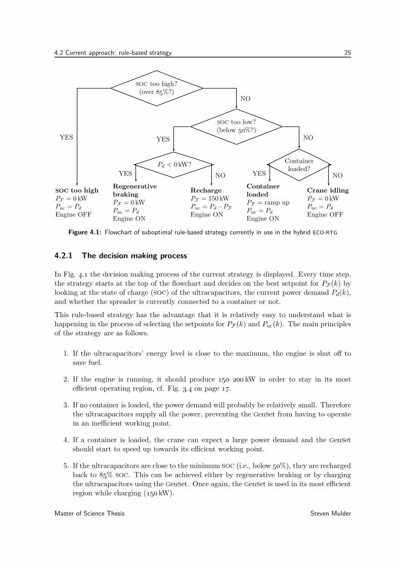
In Fig. 4.1 the decision making process of the current strategy is displayed. Every time step,the strategy starts at the top of the flowchart and decides on the best setpoint for PF (k) bylooking at the state of charge (SOC) of the ultracapacitors, the current power demand Pd(k),and whether the spreader is currently connected to a container or not.
This rule-based strategy has the advantage that it is relatively easy to understand what ishappening in the process of selecting the setpoints for PF (k) and Puc(k). The main principlesof the strategy are as follows.
1. If the ultracapacitors’ energy level is close to the maximum, the engine is shut off tosave fuel.
2. If the engine is running, it should produce 150–200 kW in order to stay in its mostefficient operating region, cf. Fig. 3.4 on page 17.
3. If no container is loaded, the power demand will probably be relatively small. Thereforethe ultracapacitors supply all the power, preventing the GenSet from having to operatein an inefficient working point.
4. If a container is loaded, the crane can expect a large power demand and the GenSetshould start to speed up towards its efficient working point.
5. If the ultracapacitors are close to the minimum SOC (i.e., below 50%), they are rechargedback to 85% SOC. This can be achieved either by regenerative braking or by chargingthe ultracapacitors using the GenSet. Once again, the GenSet is used in its most efficientregion while charging (150 kW).
Master of Science Thesis Steven Mulder
26 Energy Management Strategy
4.2.2 Advantages and drawbacks
A rule-based strategy is a good choice for many applications, and especially for prototypesystems. This is mainly because the reasoning behind the strategy is immediately clear fromthe rule base, which results in reliable and predictable behavior of the crane. Besides this,it is also easy to implement the strategy in the crane software, saving development time andcost.
On the other hand, rule-based systems also have certain drawbacks. The most importantdrawback is the performance. Without expert knowledge of the system to be controlled, it isvery difficult to construct a rule base that achieves optimal performance. Even when expertknowledge of the system is available, it is often still difficult to produce a good controller.All the different rules need to be tuned to fit all possible circumstances, so there are manythreshold values and output parameters that can influence the performance of the system.
4.3 Alternative approach: optimization-based strategies
To improve the current strategy, it might seem appealing to start a thorough analysis of therule base and to tune the threshold values for each rule and the resulting setpoints to see howeach of these affect the performance. There are also a number of other rule-based approachesfound in literature, see for instance [13, 14, 15]. Nonetheless, a completely different approachis needed to overcome the main structural drawback of rule-based strategies, namely the largenumber of parameters that can influence the performance of the system.
The most commonly used alternative is an optimization-based approach, where hand-tuningof the parameters is no longer needed. This section presents the optimization framework andhow it can be applied to energy management strategies. Unfortunately, there are also somedifficulties associated with the initial formulation of the optimization-based approach. Thedetails of these problems are discussed at the end of this section. Afterwards, Section 4.4
will explain a new strategy that is also based on the optimization framework, but uses uses adifferent formulation of the optimization goals.
4.3.1 Optimization framework
According to Van den Boom and De Schutter, a general optimization problem consists of fourseparate characteristics [16].
• J or J(θ), the objective function or criterion that expresses the intention or goal.
• θ, the parameter vector that can be used to optimize the objective function J(θ).
• H(θ) = 0, (optional) equality constraints that bound the solution to a certain subset ofthe parameter space.
• G(θ) ≤ 0, (optional) inequality constraints that bound the solution to a certain allowedregion in the parameter space.
Steven Mulder Master of Science Thesis
4.3 Alternative approach: optimization-based strategies 27
The optimization problem is defined as a search for the combination of parameters thatminimize the objective function J(θ):
J(θ∗) = minθJ(θ) subject to H(θ) = 0 and G(θ) ≤ 0
where
θ∗ = arg minθJ(θ)
Finding θ∗ is done using optimization algorithms. There are many algorithms available,ranging from basic solvers like the Simplex Method to complex nonlinear solvers like Ge-netic Algorithms. The optimization algorithm determines the computational complexity ofthe solution. Simpler solvers generally need less calculation steps, but they are not alwaysapplicable for each optimization problem.
Before an optimization algorithm is selected, the first important step in the design of anoptimization problem is the selection of an appropriate objective function and constraints.The objective function not only determines the desired goal, but its shape in the parameterspace also influences how difficult it will be for an optimization algorithm to find the optimalsolution. In the end, the type of solver depends on the characteristics of the objective functionand the constraints, i.e., on the application for which the optimization is used.
4.3.2 Objective function for energy management strategies
The goal for the energy management strategy is to minimize the fuel consumption of the crane,so this has to be expressed in the objective function. Furthermore, the strategy should notonly minimize the fuel consumption for a single time instant, but it should do a cumulativeoptimization over a longer period of time. The time it takes to do a single load/unloadmove is a good choice for this time period. Selecting a shorter time period would cause partof the typical power demand cycle to be ignored in the optimization, yielding suboptimalresults. On the other hand, selecting the time period too long would result in unnecessarycalculation, because the load demand is quasi-periodic thanks to the repetitive activities ofthe crane. Overall, the objective function should take 750 time samples into account, becausean average move takes up to 150 sec and the sample frequency is 5 Hz.
Now that the optimization goal is determined, the next step are the optimization parameters,i.e., the parameters that are used to achieve the optimization goal. The set of parametersthat is used to minimize the cumulative fuel cost is the amount of ultracapacitor power ateach time step: Puc(k). The ultracapacitor power directly influences the GenSet power PF (k),because of the relation PF (k) = Pd(k)−Puc(k). That means that it is not necessary to includePF (k) as a parameter.
In addition to Puc(k), there is one other parameter that influences the fuel consumption:the state of the engine, or rather the fact whether it is running or not. When the engineis switched off, it obviously does not use any fuel. However, switching on the engine fromstandstill requires extra fuel, so deciding when to turn the engine on or off is an importantissue. The on/off state of the engine is defined by the boolean signal S(k), which is the secondset of optimization parameters.
Master of Science Thesis Steven Mulder
28 Energy Management Strategy
5
10
15
20
0 100 200 300−100Puc(k) [kW]
F(k
)[g
/sec]
Pd(k)
S(k − 1): Engine ON
S(k − 1): Engine OFF
Figure 4.2: The fuel cost for a single time step, for Pd(k) = 241 kW
The resulting optimization goal becomes:
minPuc(k), S(k)
J(Puc(k), S(k)) = minPuc(k), S(k)
N∑
k=1
F (Pd(k)− Puc(k), S(k)) where N = 750 (4.1)
Note that the power demand Pd(k) cannot be influenced by the strategy, because it is deter-mined by the way the driver moves the crane. Therefore Pd(k) cannot act as an optimizationparameter, although it does determine the eventual optimal strategy.
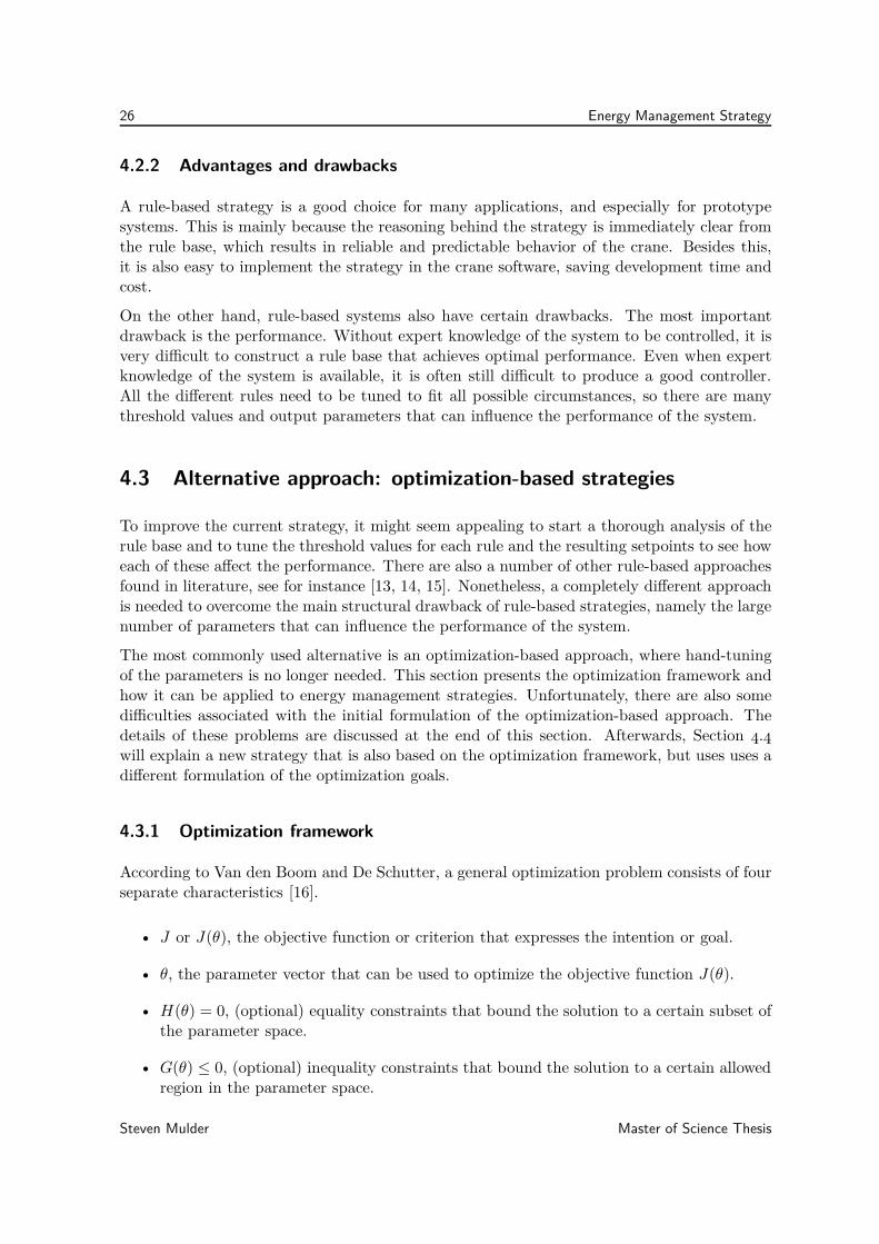
Shape of the objective function
The shape of the objective function in the parameter space has a big influence on the resultsof the optimization problem. The minimum will be more difficult to find in an irregularnonlinear function than in a straightforward linear function. To give a better impression ofthe objective function, Fig. 4.2 shows F (Pd(k)− Puc(k), S(k)), i.e., the fuel cost for a singletime step. The shape is a mirrored image of the GenSet fuel consumption model of Fig. 3.3,shifted right or left according to Pd(k).
There are two notable things about the shape of the fuel cost. First there is the influence ofS(k−1), which makes using the GenSet more costly when the engine was previously switchedoff. It also shows that switching the engine off is beneficial for a single time instance, but itwill hurt performance a the future time step. The second thing to note is the discontinuityat Puc(k) = Pd(k) when the engine is switched off. While the rest of the shape is a nicepiecewise quadratic function, the discontinuity makes the shape non-convex, and thereforethe total objective function will also be non-convex. Non-convex objective functions are moredifficult to optimize than convex functions. They have the drawback that the function canhave multiple local minima, so the result of the optimization is not guaranteed to be theglobal minimum.
Figure 4.3 shows the shape of the fuel cost during a complete container move. Essentially,it is built up using the shape from Fig. 4.2 and shifting it according to the varying Pd(k).
Steven Mulder Master of Science Thesis
4.3 Alternative approach: optimization-based strategies 29
Puc(k) [kW]
−150
0
150
300
Time step k
0 25 50 75 100
F(k
)[g
/sec]
40
30
20
10
0
Figure 4.3: The fuel cost for each time step during a complete move, without engine startuppenalty
The influence of S(k) cannot be seen in the graph, because it is not known in advance whenthe engine will be on or off. If the engine would be switched off at some point during themove, the cost for using the GenSet in all the following time steps would be increased, untilthe point where the engine is switched back on.
Besides the objective function that was formulated in this subsection, an optimization-basedenergy management strategy also has to take some constraints into account. The next sub-section discusses these constraints.
4.3.3 Constraints for energy management strategies
An energy management strategy is constrained in the actions it can take to reach the goaldefined by the objective function. In this subsection three types of constraints are covered:constraints on the peak power, a constraint on the balance of the total power flows, andconstraints on the ultracapacitor energy limits.
Peak power constraints
Obviously the two major crane components have some physical limitations that constrain thepossible actions of the energy management strategy. The physical constraints for the GenSetare defined by the maximum and minimum amount of power it can deliver:
0 kW ≤ PF (k) ≤ 350 kW (peak power)
It is interesting to note that the power demand Pd(k) does not play a role in these constraints.That means that GenSet can supply more power than required for the motors, so it cansimultaneously power the motors and recharge the ultracapacitors. Besides this, peaks in
Master of Science Thesis Steven Mulder
30 Energy Management Strategy
the power demand of more than 300 kW are very rare in normal operation. Therefore, theconstraints on the GenSet do not play an important role in the solution of the optimizationproblem.
In addition to the limitations of the GenSet, the ultracapacitor bank is limited by its maximumallowed current:
iint(k) ≤ 750 A (1 sec peak current)
iint(k) ≤ 150 A (continuous current)
For the optimization framework, these constraints need to be reformulated in terms of theultracapacitor power instead of the current. Of course, the ultracapacitor power and thecurrent are related by the voltage. Furthermore, the voltage can be expressed in terms of thestored energy (cf. (3.1) in the previous chapter), so it can be written as:
Ps(k) ·
√12C
Euc(k)≤ imax (4.2)
where imax is either 750 A or 150 A, depending on whether the peak power or the continuouspower is considered. In practice, these constraints have the effect that the ultracapacitors arelimited to 45 kW of continuous power when they are empty, while they can handle 95 kW ofcontinuous power when they are completely full.
Energy balance constraint
The second set of constraints does not have to do with physical limitations, but instead isdue to the limited number time steps that are considered in the optimization. The formaloptimization objective is to minimize the fuel consumption during a single container load-ing/unloading move, but another container move will begin after the end of the optimizedmove cycle. In order to make sure that the ultracapacitor storage is not completely drained atthe end of the cycle—which would create a difficult situation for the next cycle—the followingconstraint is added on the ultracapacitor energy level:
Euc(1) = Euc(N)
In other words, over the course of the container move, the total amount of energy going outof the ultracapacitors has to be balanced with the energy flowing back. This can be achievedby regenerative braking or by charging the ultracapacitors with the GenSet. This constraintensures that the strategy does not drain the ultracapacitors for short-term gains.
The energy balance constraint also has to be formulated in terms of the ultracapacitor power.The relation between the ultracapacitor power and energy was discussed in the previouschapter. From (3.2) it immediately follows that the constraint can be rewritten as:
N∑
k=1
Ps(k) = 0 (4.3)
Steven Mulder Master of Science Thesis
4.3 Alternative approach: optimization-based strategies 31
Energy storage constraints
The final constraining issue are the bounds on the amount of energy that is stored in theultracapacitors. Because the storage capacity is relatively small—just enough for hoistingone container from the bottom to the top of the crane—this constraint plays an importantrole in the optimization problem. The constraints on the storage are:
Emin ≤ Euc(k) ≤ Emax
where Emin = 0.32 kWh (1 152 kJ), and Emax = 1.38 kWh (4 968 kJ). For the sake of legibility,only the upper bound will be discussed in detail. The lower bound can be handled exactlythe same as the upper bound.
Just like in the discussion of the energy balance constraint, (3.2) is used to reformulate theconstraints in terms of the ultracapacitor power. The constraints for each time step are asfollows.
Euc(1)− Ps(1) ≤ Emax
Euc(1)− Ps(1)− Ps(2) ≤ Emax
Euc(1) − Ps(1)− Ps(2)− Ps(3) ≤ Emax etc.
In general, the constraint means that the upper bound on the ultracapacitor power for eachtime step is given by the maximum energy level, the energy at the start of the simulation andthe change in the energy due to the power flow in the previous time steps:
− Ps(k) ≤ Emax − Euc(1) +k−1∑
i=1
Ps(i) (4.4)
4.3.4 Feasibility of the optimization-based approach
Now that the optimization objective and the constraints are formulated as best as possible,the feasibility of an optimization-based strategy with this formulation can be examined. Theoptimization problem needs to be solvable in reasonable time for it to be useful in practice.For instance, in an optimization-based model-based predictive control (MPC) strategy, theoptimization process needs to start and finish within a single time step. This makes thecomplexity of the optimization problem a critical issue. Unfortunately, the formulation thatwas discussed in the previous sections is too complex for practical applications.
First of all, the influence of S(k) on the objective function of (4.1) has a negative effect on thesolvability of the optimization problem. The possibility to switch the GenSet off complicatesthe objective function by introducing a “dent” in the fuel consumption when the engineis switched off. This gives F (Pd(k)− Puc(k), S(k)) a non-convex shape. The startup fuelpenalty creates further complications in the shape of the objective function. As a result ofthe non-convexity, the objective function will have multiple local minima, complicating thesolving algorithm and increasing the chance of a suboptimal solution.
Another challenge is posed by the constraints. Note that all the constraints (4.2), (4.3)and (4.4) are actually constraints on Ps(k) instead of on the true optimization parameterPuc(k). To use the constraints in the optimization framework, they need to be reformulated
Master of Science Thesis Steven Mulder
32 Energy Management Strategy
in terms of Puc(k). However, in Section 3.3 it was discussed that the relation between Ps(k)and Puc(k), i.e., the efficiency of the ultracapacitors, depends strongly on the energy levelEuc(k).
The problem is that Euc(k) in turn depends on Puc(k) in the previous time steps. That meansthat for each time step, the ultracapacitor efficiency can only be calculated using the valuesof Puc(k) in the earlier time steps. This creates the strange situation that the constraints onPuc(k) are unknown until Puc(k) itself is known. It is needless to say that it is very difficult tosolve an optimization problem when the constraints on the optimization parameter are onlygradually becoming known during the optimization.
In the light of these calculation problems, the conclusion is as follows. To accomplish feasibilityof the optimization-based approach in practice, the formulation of the objective and theconstraints needs to be changed in some way to avoid the problems that were just discussed.Section 4.4 will show how this is done by the new energy management strategy, which featuresa different choice for the objective function. That said, Section 4.3.5 first discusses an off-linesolution of the optimization problem, to discover what performance might be achieved whengiven enough time and computing power.
4.3.5 Off-line solution: dynamic programming
The challenges that were just discussed are important issues for an on-line solution, wherecomputational time is an important factor. Nevertheless, it is also interesting to see whatperformance could theoretically be achieved. This would give some insight on what perfor-mance gain to expect, before making a lot of effort to design a new strategy. By disregardingcalculation time and the fact that we do not know exactly what the future power demand willbe, it should be possible to find the absolute optimal strategy. Unfortunately, unexpectedproblems forced this project to be abandoned without actually producing results.
The Dynamic Programming algorithm
In the literature on energy management strategies for hybrid vehicles, an off-line solution isoften used as a benchmark to show the best possible results with a certain hybrid system.Richard Bellman’s Dynamic Programming (DP) algorithm [17] is well-suited for this task,since it is able to handle the complex constraints, and is guaranteed to find the optimalsolution with a certain accuracy. This subsection applies the DP algorithm to an energymanagement as explained by Koot et al. [7].
As depicted in Fig. 4.4, Dynamic Programming works by putting a grid on the feasiblesolution-space, i.e., all values for Ps(k) and S(k) that result in energy levels within the boundsof the ultracapacitors. Then, starting at the desired finishing point Euc(N) = Euc(1), thealgorithm calculates the minimum cumulative cost of getting from each point to the desiredend point. By working its way “back in time”, the algorithm eventually finds the minimumcumulative cost to get from start to finish. Depending on the density of the grid, the globaloptimum is guaranteed to be be found with a certain accuracy.
Steven Mulder Master of Science Thesis
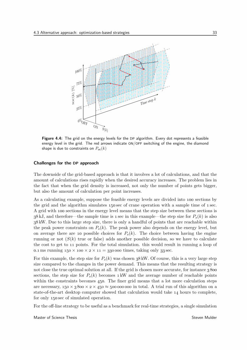
4.3 Alternative approach: optimization-based strategies 33
0%
25%
50%
75%
100%
Time step k
SO
C(k
)[%
]
S(k)
OFFON
Figure 4.4: The grid on the energy levels for the DP algorithm. Every dot represents a feasibleenergy level in the grid. The red arrows indicate ON/OFF switching of the engine, the diamondshape is due to constraints on Puc(k)
Challenges for the DP approach
The downside of the grid-based approach is that it involves a lot of calculations, and that theamount of calculations rises rapidly when the desired accuracy increases. The problem lies inthe fact that when the grid density is increased, not only the number of points gets bigger,but also the amount of calculation per point increases.
As a calculating example, suppose the feasible energy levels are divided into 100 sections bythe grid and the algorithm simulates 150 sec of crane operation with a sample time of 1 sec.A grid with 100 sections in the energy level means that the step size between these sections is38 kJ, and therefore—the sample time is 1 sec in this example—the step size for Ps(k) is also38 kW. Due to this large step size, there is only a handful of points that are reachable withinthe peak power constraints on Ps(k). The peak power also depends on the energy level, buton average there are 10 possible choices for Ps(k). The choice between having the enginerunning or not (S(k) true or false) adds another possible decision, so we have to calculatethe cost to get to 11 points. For the total simulation. this would result in running a loop of0.1 ms running 150× 100 × 2× 11 = 330 000 times, taking only 33 sec.
For this example, the step size for Ps(k) was chosen 38 kW. Of course, this is a very large stepsize compared to the changes in the power demand. This means that the resulting strategy isnot close the true optimal solution at all. If the grid is chosen more accurate, for instance 3 800
sections, the step size for Ps(k) becomes 1 kW and the average number of reachable pointswithin the constraints becomes 450. The finer grid means that a lot more calculation stepsare necessary, 150× 3 800× 2× 450 ≈ 500 000 000 in total. A trial run of this algorithm on astate-of-the-art desktop computer showed that calculation would take 14 hours to complete,for only 150 sec of simulated operation.
For the off-line strategy to be useful as a benchmark for real-time strategies, a single simulation
Master of Science Thesis Steven Mulder
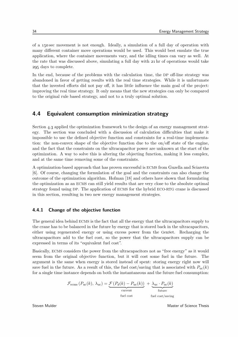
34 Energy Management Strategy
of a 150 sec movement is not enough. Ideally, a simulation of a full day of operation withmany different container move operations would be used. This would best emulate the trueapplication, where the container movements vary, and the idling times can vary as well. Atthe rate that was discussed above, simulating a full day with 21 hr of operations would take295 days to complete.
In the end, because of the problems with the calculation time, the DP off-line strategy wasabandoned in favor of getting results with the real time strategies. While it is unfortunatethat the invested efforts did not pay off, it has little influence the main goal of the project:improving the real time strategy. It only means that the new strategies can only be comparedto the original rule based strategy, and not to a truly optimal solution.
4.4 Equivalent consumption minimization strategy
Section 4.3 applied the optimization framework to the design of an energy management strat-egy. The section was concluded with a discussion of calculation difficulties that make itimpossible to use the defined objective function and constraints for a real-time implementa-tion: the non-convex shape of the objective function due to the on/off state of the engine,and the fact that the constraints on the ultracapacitor power are unknown at the start of theoptimization. A way to solve this is altering the objecting function, making it less complex,and at the same time removing some of the constraints.
A optimization-based approach that has proven successful is ECMS from Guzella and Sciaretta[6]. Of course, changing the formulation of the goal and the constraints can also change theoutcome of the optimization algorithm. Hofman [18] and others have shown that formulatingthe optimization as an ECMS can still yield results that are very close to the absolute optimalstrategy found using DP. The application of ECMS for the hybrid ECO-RTG crane is discussedin this section, resulting in two new energy management strategies.
4.4.1 Change of the objective function
The general idea behind ECMS is the fact that all the energy that the ultracapacitors supply tothe crane has to be balanced in the future by energy that is stored back in the ultracapacitors,either using regenerated energy or using excess power from the GenSet. Recharging theultracapacitors add to the fuel cost, so the power that the ultracapacitors supply can beexpressed in terms of its “equivalent fuel cost”.
Basically, ECMS considers the power from the ultracapacitors not as “free energy” as it wouldseem from the original objective function, but it will cost some fuel in the future. Theargument is the same when energy is stored instead of spent: storing energy right now willsave fuel in the future. As a result of this, the fuel cost/saving that is associated with Puc(k)for a single time instance depends on both the instantaneous and the future fuel consumption:
Fecms (Puc(k), λuc) = F (Pd(k)− Puc(k))︸ ︷︷ ︸
current
fuel cost
+ λuc · Puc(k)︸ ︷︷ ︸
future
fuel cost/saving
Steven Mulder Master of Science Thesis
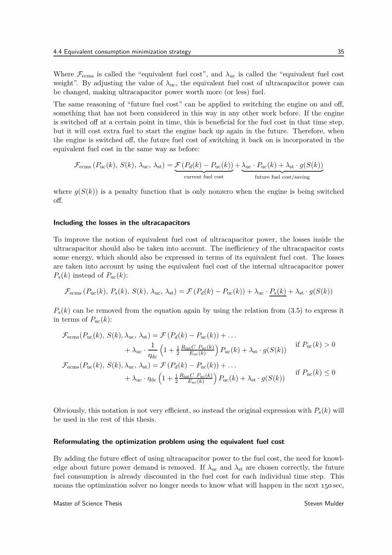
4.4 Equivalent consumption minimization strategy 35
Where Fecms is called the “equivalent fuel cost”, and λuc is called the “equivalent fuel costweight”. By adjusting the value of λuc, the equivalent fuel cost of ultracapacitor power canbe changed, making ultracapacitor power worth more (or less) fuel.
The same reasoning of “future fuel cost” can be applied to switching the engine on and off,something that has not been considered in this way in any other work before. If the engineis switched off at a certain point in time, this is beneficial for the fuel cost in that time step,but it will cost extra fuel to start the engine back up again in the future. Therefore, whenthe engine is switched off, the future fuel cost of switching it back on is incorporated in theequivalent fuel cost in the same way as before:
Fecms (Puc(k), S(k), λuc, λst) = F (Pd(k)− Puc(k))︸ ︷︷ ︸
current fuel cost
+λuc · Puc(k) + λst · g(S(k))︸ ︷︷ ︸
future fuel cost/saving
where g(S(k)) is a penalty function that is only nonzero when the engine is being switchedoff.
Including the losses in the ultracapacitors
To improve the notion of equivalent fuel cost of ultracapacitor power, the losses inside theultracapacitor should also be taken into account. The inefficiency of the ultracapacitor costssome energy, which should also be expressed in terms of its equivalent fuel cost. The lossesare taken into account by using the equivalent fuel cost of the internal ultracapacitor powerPs(k) instead of Puc(k):
Fecms (Puc(k), Ps(k), S(k), λuc, λst) = F (Pd(k)− Puc(k)) + λuc · Ps(k) + λst · g(S(k))
Ps(k) can be removed from the equation again by using the relation from (3.5) to express itin terms of Puc(k):
Fecms(Puc(k), S(k), λuc, λst) = F (Pd(k)− Puc(k)) + . . .
+ λuc ·1
ηdc
(
1 + 12RintC Puc(k)Euc(k)
)
Puc(k) + λst · g(S(k))if Puc(k) > 0
Fecms(Puc(k), S(k), λuc, λst) = F (Pd(k)− Puc(k)) + . . .
+ λuc · ηdc
(
1 + 12RintC Puc(k)Euc(k)
)
Puc(k) + λst · g(S(k))if Puc(k) ≤ 0
Obviously, this notation is not very efficient, so instead the original expression with Ps(k) willbe used in the rest of this thesis.
Reformulating the optimization problem using the equivalent fuel cost
By adding the future effect of using ultracapacitor power to the fuel cost, the need for knowl-edge about future power demand is removed. If λuc and λst are chosen correctly, the futurefuel consumption is already discounted in the fuel cost for each individual time step. Thismeans the optimization solver no longer needs to know what will happen in the next 150 sec,
Master of Science Thesis Steven Mulder
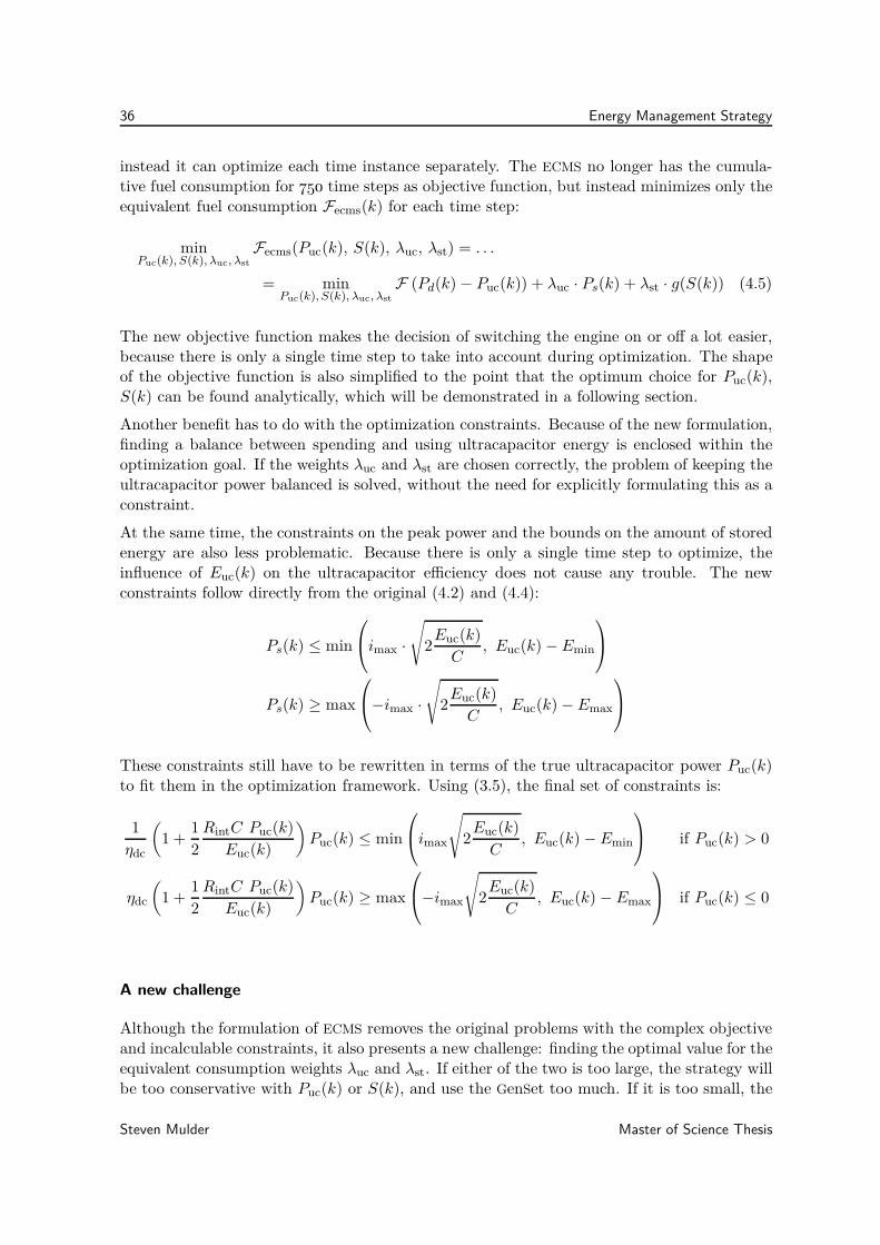
36 Energy Management Strategy
instead it can optimize each time instance separately. The ECMS no longer has the cumula-tive fuel consumption for 750 time steps as objective function, but instead minimizes only theequivalent fuel consumption Fecms(k) for each time step:
minPuc(k), S(k), λuc, λst
Fecms(Puc(k), S(k), λuc, λst) = . . .
= minPuc(k), S(k), λuc, λst
F (Pd(k)− Puc(k)) + λuc · Ps(k) + λst · g(S(k)) (4.5)
The new objective function makes the decision of switching the engine on or off a lot easier,because there is only a single time step to take into account during optimization. The shapeof the objective function is also simplified to the point that the optimum choice for Puc(k),S(k) can be found analytically, which will be demonstrated in a following section.
Another benefit has to do with the optimization constraints. Because of the new formulation,finding a balance between spending and using ultracapacitor energy is enclosed within theoptimization goal. If the weights λuc and λst are chosen correctly, the problem of keeping theultracapacitor power balanced is solved, without the need for explicitly formulating this as aconstraint.
At the same time, the constraints on the peak power and the bounds on the amount of storedenergy are also less problematic. Because there is only a single time step to optimize, theinfluence of Euc(k) on the ultracapacitor efficiency does not cause any trouble. The newconstraints follow directly from the original (4.2) and (4.4):
Ps(k) ≤ min
imax ·
√
2Euc(k)
C, Euc(k)− Emin
Ps(k) ≥ max
−imax ·
√
2Euc(k)
C, Euc(k)− Emax
These constraints still have to be rewritten in terms of the true ultracapacitor power Puc(k)to fit them in the optimization framework. Using (3.5), the final set of constraints is:
1
ηdc
(
1 +1
2
RintC Puc(k)
Euc(k)
)
Puc(k) ≤ min
imax
√
2Euc(k)
C, Euc(k)− Emin
if Puc(k) > 0
ηdc
(
1 +1
2
RintC Puc(k)
Euc(k)
)
Puc(k) ≥ max
−imax
√
2Euc(k)
C, Euc(k) − Emax
if Puc(k) ≤ 0
A new challenge
Although the formulation of ECMS removes the original problems with the complex objectiveand incalculable constraints, it also presents a new challenge: finding the optimal value for theequivalent consumption weights λuc and λst. If either of the two is too large, the strategy willbe too conservative with Puc(k) or S(k), and use the GenSet too much. If it is too small, the
Steven Mulder Master of Science Thesis
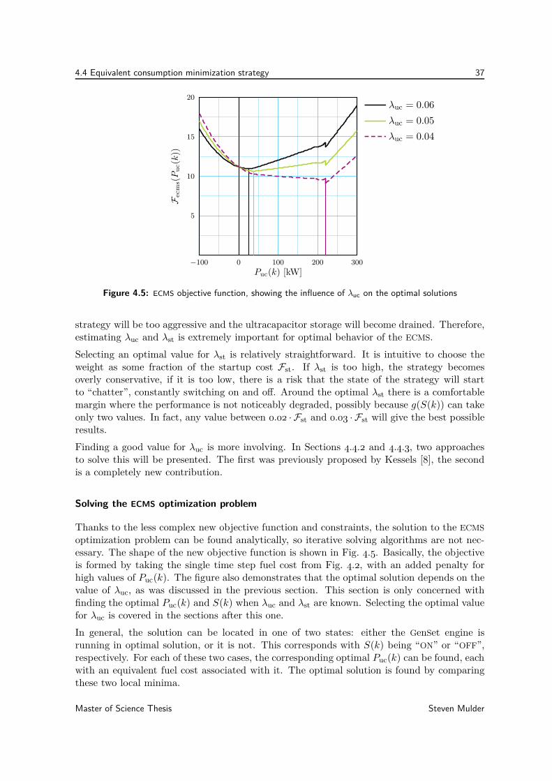
4.4 Equivalent consumption minimization strategy 37
5
10
15
20
0 100 200 300−100
Puc(k) [kW]
Fecm
s(P
uc(k
))
λuc = 0.06
λuc = 0.05
λuc = 0.04
Figure 4.5: ECMS objective function, showing the influence of λuc on the optimal solutions
strategy will be too aggressive and the ultracapacitor storage will become drained. Therefore,estimating λuc and λst is extremely important for optimal behavior of the ECMS.
Selecting an optimal value for λst is relatively straightforward. It is intuitive to choose theweight as some fraction of the startup cost Fst. If λst is too high, the strategy becomesoverly conservative, if it is too low, there is a risk that the state of the strategy will startto “chatter”, constantly switching on and off. Around the optimal λst there is a comfortablemargin where the performance is not noticeably degraded, possibly because g(S(k)) can takeonly two values. In fact, any value between 0.02 · Fst and 0.03 · Fst will give the best possibleresults.
Finding a good value for λuc is more involving. In Sections 4.4.2 and 4.4.3, two approachesto solve this will be presented. The first was previously proposed by Kessels [8], the secondis a completely new contribution.
Solving the ECMS optimization problem
Thanks to the less complex new objective function and constraints, the solution to the ECMS
optimization problem can be found analytically, so iterative solving algorithms are not nec-essary. The shape of the new objective function is shown in Fig. 4.5. Basically, the objectiveis formed by taking the single time step fuel cost from Fig. 4.2, with an added penalty forhigh values of Puc(k). The figure also demonstrates that the optimal solution depends on thevalue of λuc, as was discussed in the previous section. This section is only concerned withfinding the optimal Puc(k) and S(k) when λuc and λst are known. Selecting the optimal valuefor λuc is covered in the sections after this one.
In general, the solution can be located in one of two states: either the GenSet engine isrunning in optimal solution, or it is not. This corresponds with S(k) being “ON” or “OFF”,respectively. For each of these two cases, the corresponding optimal Puc(k) can be found, eachwith an equivalent fuel cost associated with it. The optimal solution is found by comparingthese two local minima.
Master of Science Thesis Steven Mulder
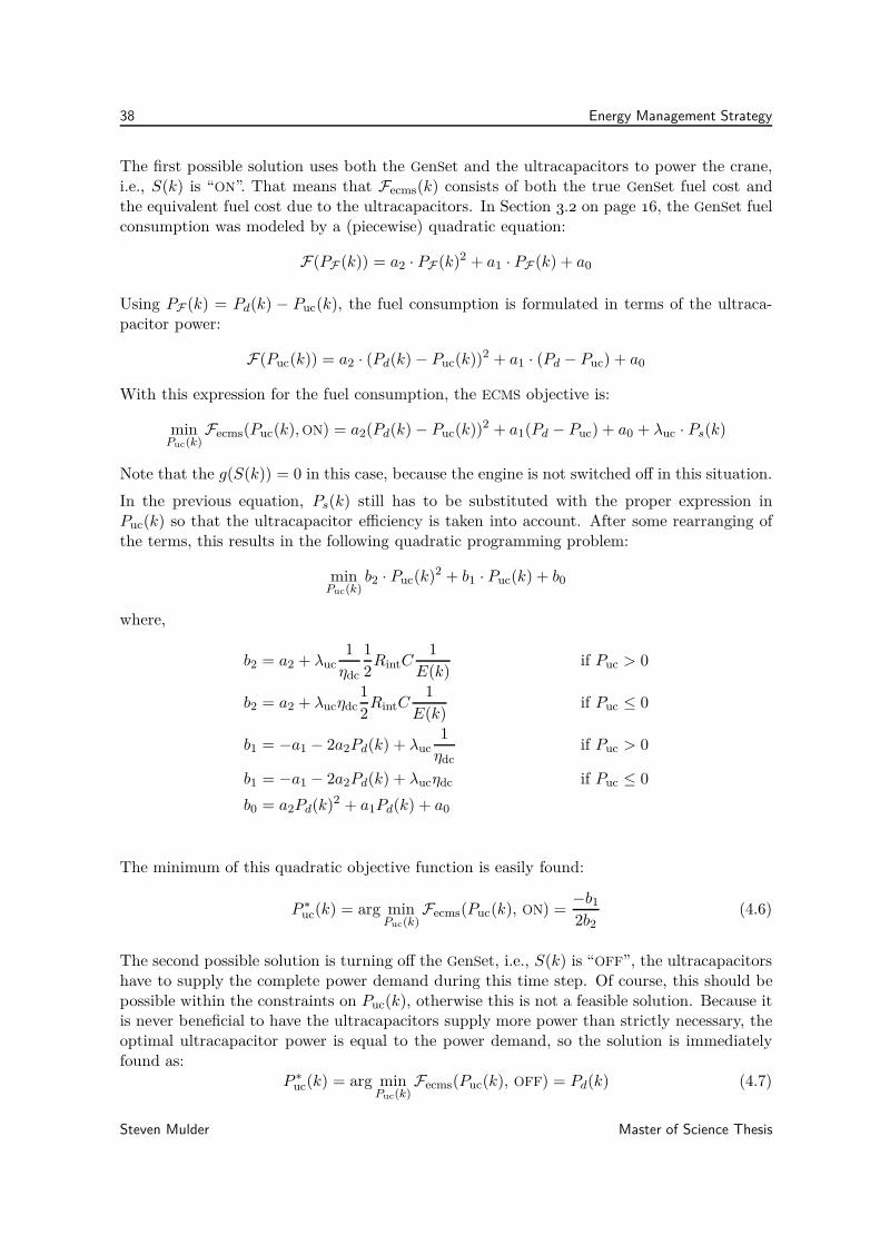
38 Energy Management Strategy
The first possible solution uses both the GenSet and the ultracapacitors to power the crane,i.e., S(k) is “ON”. That means that Fecms(k) consists of both the true GenSet fuel cost andthe equivalent fuel cost due to the ultracapacitors. In Section 3.2 on page 16, the GenSet fuelconsumption was modeled by a (piecewise) quadratic equation:
F(PF (k)) = a2 · PF (k)2 + a1 · PF (k) + a0
Using PF (k) = Pd(k) − Puc(k), the fuel consumption is formulated in terms of the ultraca-pacitor power:
F(Puc(k)) = a2 · (Pd(k)− Puc(k))2 + a1 · (Pd − Puc) + a0
With this expression for the fuel consumption, the ECMS objective is:
minPuc(k)
Fecms(Puc(k),ON) = a2(Pd(k)− Puc(k))2 + a1(Pd − Puc) + a0 + λuc · Ps(k)
Note that the g(S(k)) = 0 in this case, because the engine is not switched off in this situation.
In the previous equation, Ps(k) still has to be substituted with the proper expression inPuc(k) so that the ultracapacitor efficiency is taken into account. After some rearranging ofthe terms, this results in the following quadratic programming problem:
minPuc(k)
b2 · Puc(k)2 + b1 · Puc(k) + b0
where,
b2 = a2 + λuc1
ηdc
1
2RintC
1
E(k)if Puc > 0
b2 = a2 + λucηdc1
2RintC
1
E(k)if Puc ≤ 0
b1 = −a1 − 2a2Pd(k) + λuc1
ηdcif Puc > 0
b1 = −a1 − 2a2Pd(k) + λucηdc if Puc ≤ 0
b0 = a2Pd(k)2 + a1Pd(k) + a0
The minimum of this quadratic objective function is easily found:
P ∗uc(k) = arg minPuc(k)
Fecms(Puc(k), ON) =−b12b2
(4.6)
The second possible solution is turning off the GenSet, i.e., S(k) is “OFF”, the ultracapacitorshave to supply the complete power demand during this time step. Of course, this should bepossible within the constraints on Puc(k), otherwise this is not a feasible solution. Because itis never beneficial to have the ultracapacitors supply more power than strictly necessary, theoptimal ultracapacitor power is equal to the power demand, so the solution is immediatelyfound as:
P ∗uc(k) = arg minPuc(k)
Fecms(Puc(k), OFF) = Pd(k) (4.7)
Steven Mulder Master of Science Thesis
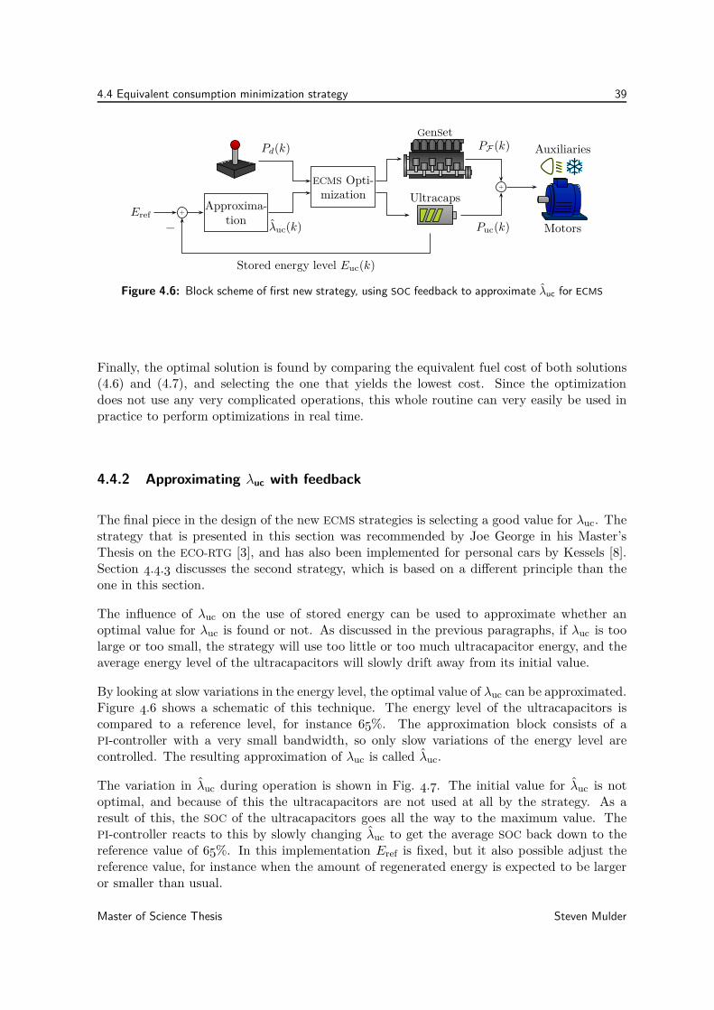
4.4 Equivalent consumption minimization strategy 39
Auxiliaries
Motors
Ultracaps
GenSet
+Approxima-
tion
ECMS Opti-mization
+
λuc(k)
Pd(k)
Stored energy level Euc(k)
−
Eref
PF (k)
Puc(k)
Figure 4.6: Block scheme of first new strategy, using SOC feedback to approximate λuc for ECMS
Finally, the optimal solution is found by comparing the equivalent fuel cost of both solutions(4.6) and (4.7), and selecting the one that yields the lowest cost. Since the optimizationdoes not use any very complicated operations, this whole routine can very easily be used inpractice to perform optimizations in real time.
4.4.2 Approximating λuc with feedback
The final piece in the design of the new ECMS strategies is selecting a good value for λuc. Thestrategy that is presented in this section was recommended by Joe George in his Master’sThesis on the ECO-RTG [3], and has also been implemented for personal cars by Kessels [8].Section 4.4.3 discusses the second strategy, which is based on a different principle than theone in this section.
The influence of λuc on the use of stored energy can be used to approximate whether anoptimal value for λuc is found or not. As discussed in the previous paragraphs, if λuc is toolarge or too small, the strategy will use too little or too much ultracapacitor energy, and theaverage energy level of the ultracapacitors will slowly drift away from its initial value.
By looking at slow variations in the energy level, the optimal value of λuc can be approximated.Figure 4.6 shows a schematic of this technique. The energy level of the ultracapacitors iscompared to a reference level, for instance 65%. The approximation block consists of aPI-controller with a very small bandwidth, so only slow variations of the energy level arecontrolled. The resulting approximation of λuc is called λuc.
The variation in λuc during operation is shown in Fig. 4.7. The initial value for λuc is notoptimal, and because of this the ultracapacitors are not used at all by the strategy. As aresult of this, the SOC of the ultracapacitors goes all the way to the maximum value. ThePI-controller reacts to this by slowly changing λuc to get the average SOC back down to thereference value of 65%. In this implementation Eref is fixed, but it also possible adjust thereference value, for instance when the amount of regenerated energy is expected to be largeror smaller than usual.
Master of Science Thesis Steven Mulder
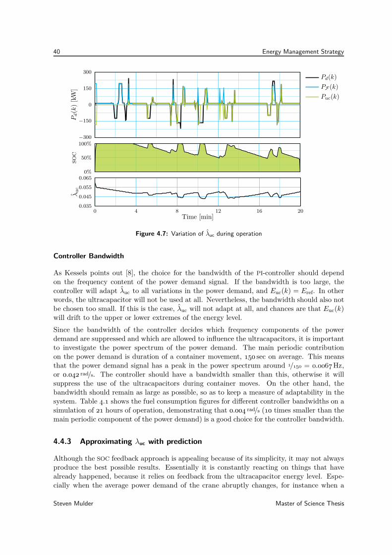
40 Energy Management Strategy
0
150
300
−150
−300
Pd(k
)[k
W]
Pd(k)
PF (k)
Puc(k)
0%
50%
100%
SO
C
0.035
0.045
0.055
0.065
0 4 8 12 16 20Time [min]
λu
c
Figure 4.7: Variation of λuc during operation
Controller Bandwidth
As Kessels points out [8], the choice for the bandwidth of the PI-controller should dependon the frequency content of the power demand signal. If the bandwidth is too large, thecontroller will adapt λuc to all variations in the power demand, and Euc(k) = Eref. In otherwords, the ultracapacitor will not be used at all. Nevertheless, the bandwidth should also notbe chosen too small. If this is the case, λuc will not adapt at all, and chances are that Euc(k)will drift to the upper or lower extremes of the energy level.
Since the bandwidth of the controller decides which frequency components of the powerdemand are suppressed and which are allowed to influence the ultracapacitors, it is importantto investigate the power spectrum of the power demand. The main periodic contributionon the power demand is duration of a container movement, 150 sec on average. This meansthat the power demand signal has a peak in the power spectrum around 1/150 = 0.0067Hz,or 0.042 rad/s. The controller should have a bandwidth smaller than this, otherwise it willsuppress the use of the ultracapacitors during container moves. On the other hand, thebandwidth should remain as large as possible, so as to keep a measure of adaptability in thesystem. Table 4.1 shows the fuel consumption figures for different controller bandwidths on asimulation of 21 hours of operation, demonstrating that 0.004 rad/s (10 times smaller than themain periodic component of the power demand) is a good choice for the controller bandwidth.
4.4.3 Approximating λuc with prediction
Although the SOC feedback approach is appealing because of its simplicity, it may not alwaysproduce the best possible results. Essentially it is constantly reacting on things that havealready happened, because it relies on feedback from the ultracapacitor energy level. Espe-cially when the average power demand of the crane abruptly changes, for instance when a
Steven Mulder Master of Science Thesis
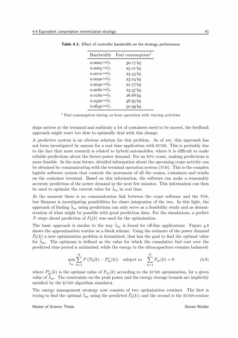
4.4 Equivalent consumption minimization strategy 41
Table 4.1: Effect of controller bandwidth on the strategy performance
Bandwidth Fuel consumption1
0.0002 rad/s 30.17 kg0.0005 rad/s 25.21 kg0.0010 rad/s 23.45 kg0.0020 rad/s 23.24 kg0.0040 rad/s 22.77 kg0.0080 rad/s 23.37 kg0.0160 rad/s 26.68 kg0.0320 rad/s 38.95 kg0.0640 rad/s 50.39 kg
1 Fuel consumption during 10 hour operation with varying activities
ships arrives at the terminal and suddenly a lot of containers need to be moved, the feedbackapproach might react too slow to optimally deal with this change.
A predictive system is an obvious solution for this problem. As of yet, this approach hasnot been investigated by anyone for a real time application with ECMS. This is probably dueto the fact that most research is related to hybrid automobiles, where it is difficult to makereliable predictions about the future power demand. For an RTG crane, making predictions ismore feasible. In the near future, detailed information about the upcoming crane activity canbe obtained by communicating with the terminal operation system (TOS). This is the complexlogistic software system that controls the movement of all the cranes, containers and truckson the container terminal. Based on this information, the software can make a reasonablyaccurate prediction of the power demand in the next few minutes. This information can thenbe used to optimize the current value for λuc in real time.
At the moment there is no communication link between the crane software and the TOS,but Siemens is investigating possibilities for closer integration of the two. In this light, theapproach of finding λuc using predictions can only serve as a feasibility study and as demon-stration of what might be possible with good prediction data. For the simulations, a perfectN steps ahead prediction of Pd(k) was used for the optimization.
The basic approach is similar to the way λuc is found for off-line applications. Figure 4.8
shows the approximation routine as a block scheme. Using the estimate of the power demandPd(k) a new optimization problem is formulated, that has the goal to find the optimal valuefor λuc. The optimum is defined as the value for which the cumulative fuel cost over thepredicted time period is minimized, while the energy in the ultracapacitors remains balanced:
minλuc
N∑
k=1
F (Pd(k)− P∗
uc(k)) subject toN∑
k=1
Puc(k) = 0 (4.8)
where P ∗uc(k) is the optimal value of Puc(k) according to the ECMS optimization, for a givenvalue of λuc. The constraints on the peak power and the energy storage bounds are implicitlysatisfied by the ECMS algorithm simulator.
The energy management strategy now consists of two optimization routines. The first istrying to find the optimal λuc using the predicted Pd(k); and the second is the ECMS-routine
Master of Science Thesis Steven Mulder
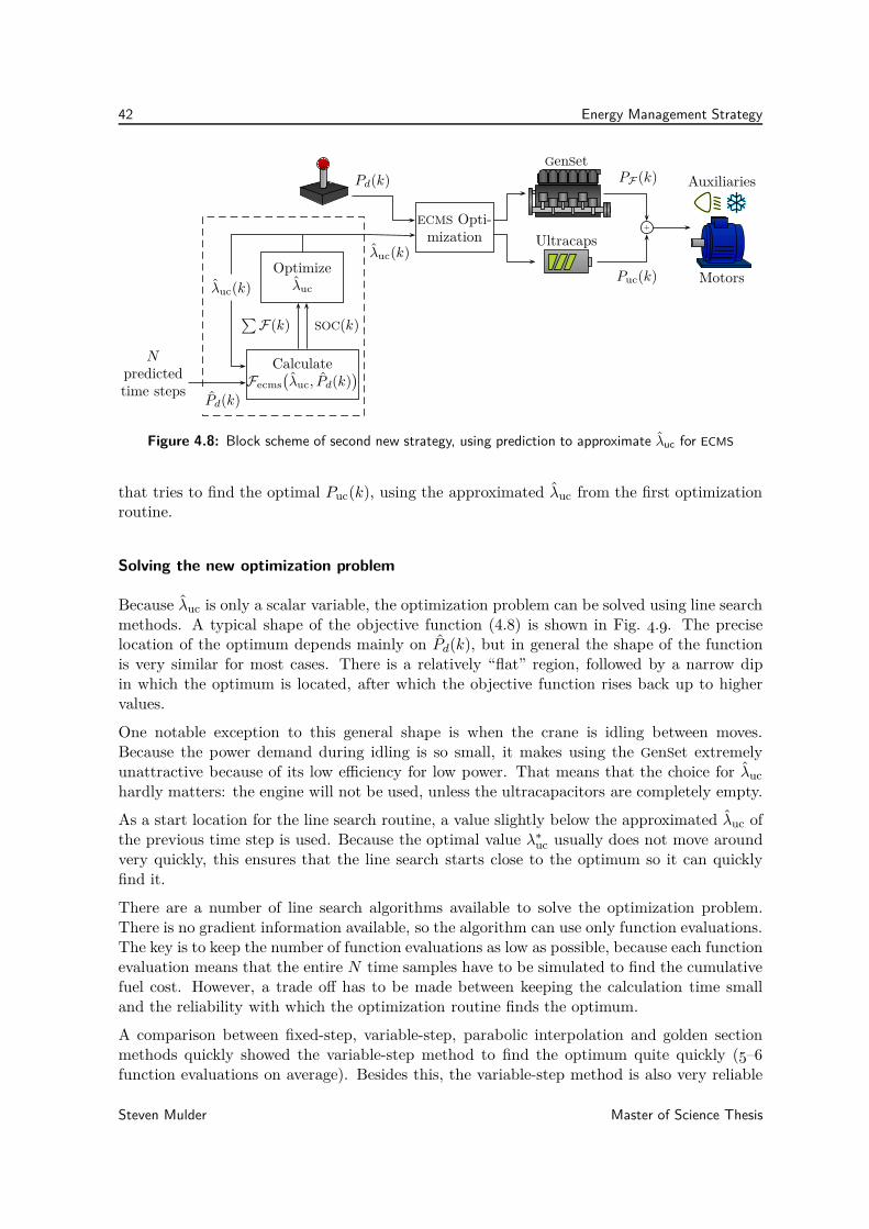
42 Energy Management Strategy
Auxiliaries
Motors
Ultracaps
GenSet
Optimizeλuc
CalculateFecms
(λuc, Pd(k)
)
Npredictedtime steps
Pd(k)
∑F(k) SOC(k)
λuc(k)
ECMS Opti-mization
+
Pd(k)
λuc(k)
PF (k)
Puc(k)
Figure 4.8: Block scheme of second new strategy, using prediction to approximate λuc for ECMS
that tries to find the optimal Puc(k), using the approximated λuc from the first optimizationroutine.
Solving the new optimization problem
Because λuc is only a scalar variable, the optimization problem can be solved using line searchmethods. A typical shape of the objective function (4.8) is shown in Fig. 4.9. The preciselocation of the optimum depends mainly on Pd(k), but in general the shape of the functionis very similar for most cases. There is a relatively “flat” region, followed by a narrow dipin which the optimum is located, after which the objective function rises back up to highervalues.
One notable exception to this general shape is when the crane is idling between moves.Because the power demand during idling is so small, it makes using the GenSet extremelyunattractive because of its low efficiency for low power. That means that the choice for λuc
hardly matters: the engine will not be used, unless the ultracapacitors are completely empty.
As a start location for the line search routine, a value slightly below the approximated λuc ofthe previous time step is used. Because the optimal value λ∗uc usually does not move aroundvery quickly, this ensures that the line search starts close to the optimum so it can quicklyfind it.
There are a number of line search algorithms available to solve the optimization problem.There is no gradient information available, so the algorithm can use only function evaluations.The key is to keep the number of function evaluations as low as possible, because each functionevaluation means that the entire N time samples have to be simulated to find the cumulativefuel cost. However, a trade off has to be made between keeping the calculation time smalland the reliability with which the optimization routine finds the optimum.
A comparison between fixed-step, variable-step, parabolic interpolation and golden sectionmethods quickly showed the variable-step method to find the optimum quite quickly (5–6
function evaluations on average). Besides this, the variable-step method is also very reliable
Steven Mulder Master of Science Thesis
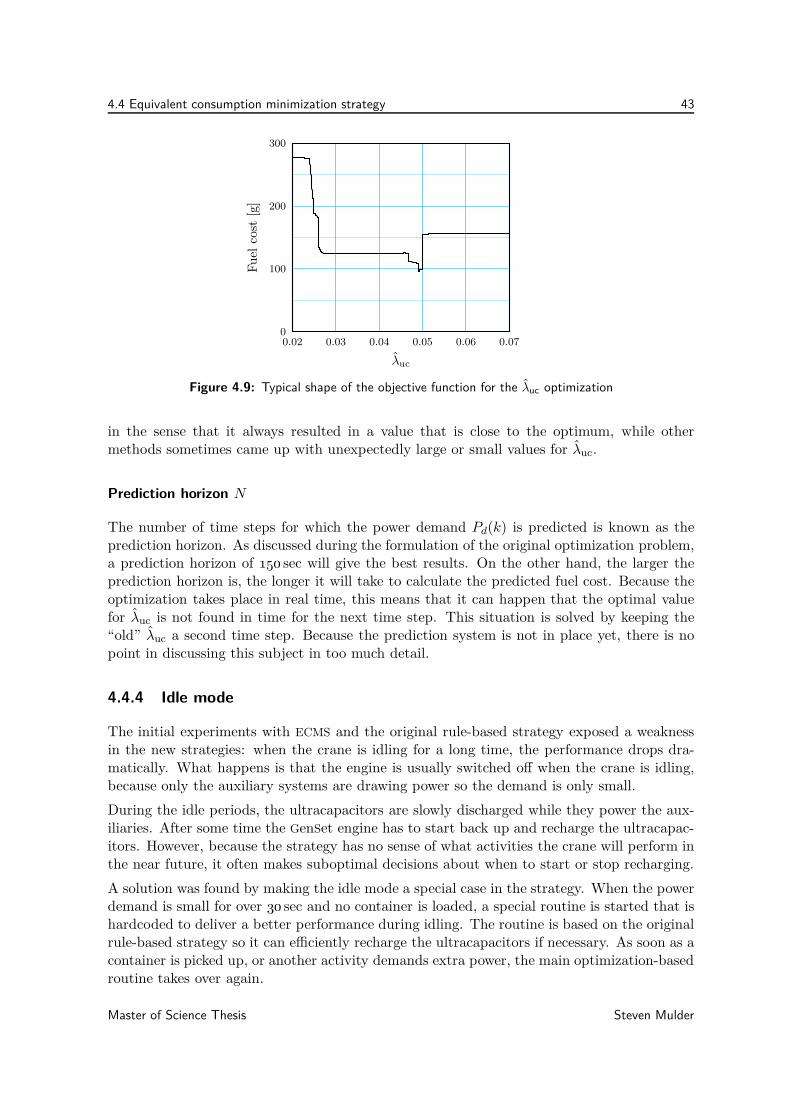
4.4 Equivalent consumption minimization strategy 43
0
100
200
300
0.02 0.03 0.04 0.05 0.06 0.07
λuc
Fuel
cost
[g]
Figure 4.9: Typical shape of the objective function for the λuc optimization
in the sense that it always resulted in a value that is close to the optimum, while othermethods sometimes came up with unexpectedly large or small values for λuc.
Prediction horizon N
The number of time steps for which the power demand Pd(k) is predicted is known as theprediction horizon. As discussed during the formulation of the original optimization problem,a prediction horizon of 150 sec will give the best results. On the other hand, the larger theprediction horizon is, the longer it will take to calculate the predicted fuel cost. Because theoptimization takes place in real time, this means that it can happen that the optimal valuefor λuc is not found in time for the next time step. This situation is solved by keeping the“old” λuc a second time step. Because the prediction system is not in place yet, there is nopoint in discussing this subject in too much detail.
4.4.4 Idle mode
The initial experiments with ECMS and the original rule-based strategy exposed a weaknessin the new strategies: when the crane is idling for a long time, the performance drops dra-matically. What happens is that the engine is usually switched off when the crane is idling,because only the auxiliary systems are drawing power so the demand is only small.
During the idle periods, the ultracapacitors are slowly discharged while they power the aux-iliaries. After some time the GenSet engine has to start back up and recharge the ultracapac-itors. However, because the strategy has no sense of what activities the crane will perform inthe near future, it often makes suboptimal decisions about when to start or stop recharging.
A solution was found by making the idle mode a special case in the strategy. When the powerdemand is small for over 30 sec and no container is loaded, a special routine is started that ishardcoded to deliver a better performance during idling. The routine is based on the originalrule-based strategy so it can efficiently recharge the ultracapacitors if necessary. As soon as acontainer is picked up, or another activity demands extra power, the main optimization-basedroutine takes over again.
Master of Science Thesis Steven Mulder
44 Energy Management Strategy
4.5 Summary
The goal of the energy management strategy is to minimize the fuel consumption of the hybridECO-RTG crane during operation. This is achieved by constantly controlling the amount ofpower supplied by the GenSet and ultracapacitors, while they work together to meet thecrane’s power demand.
Siemens currently uses a rule-based approach for the energy management of its hybrid systems.This approach is attractive because it results in reliable and predictable behavior of the crane.Unfortunately, it is very difficult to achieve optimal fuel efficiency with a rule-based strategybecause of the many parameters that are involved that have to be tuned. To overcome thedisadvantages with the rule-based strategy’s performance, an alternative approach is proposedto achieve optimal fuel economy. The alternative is based on the optimization framework.
An optimization problem can be formulated that minimizes the cumulative fuel consumptionover a container movement. The optimization parameters are the setpoints for the ultraca-pacitor power and the ON/OFF state of the GenSet engine in each time step of the move.Changing the amount of ultracapacitor power influences both the remaining power demandthat the GenSet needs to supply, and the amount of stored energy in the ultracapacitors.Changing the ON/OFF state of the engine is more complex than in may seem. Switchingthe engine off makes it more costly to use the GenSet in the following time steps, due to theadditional startup costs. The result is a non-convex objective function with multiple localminima that is difficult to use in optimization.
Furthermore, the optimization is bound by a couple of constraints that limit the possibleactions of the energy management strategy. There are constraints on the peak power, themaximum and minimum ultracapacitor energy and on the ultracapacitor energy balance. Animportant factor in these constraints is the influence of the ultracapacitors’ efficiency, whichis in turn related to the level of energy in the ultracapacitors. This relation means that theefficiency of the ultracapacitors cannot be calculated until it is known how much power theyhave supplied, and so the constraints on the ultracapacitor power can only be calculated afterthe optimization has already finished.
In order to solve the difficulties with the non-convex objective and problematic constraints,the optimization problem is recast in the ECMS framework. The main idea of this strategyis that the use of ultracapacitor power can be expressed in terms of “equivalent fuel cost”.This removes the need to optimize the strategy for a complete container move, reducing theoptimization problem to a single time step. The traditional ECMS framework was extendedto incorporate the “equivalent fuel cost” of switching the GenSet engine off.
The performance of the ECMS approach relies strongly on selecting a good value for theequivalent fuel cost weight λuc. Two approaches to solve this problem were presented. The firstis based on a low-bandwidth PI controller, that adjusts the approximated λuc by comparingthe ultracapacitor energy to a reference value.
Finally, the second approach attempts to find λuc by using predictions of the power demandin the upcoming time steps. This should improve the quality of the strategy compared tothe feedback approach, because it can anticipate future events instead of only reacting onchanges in the energy level. A line search routine is used to select the optimal value for λuc,by optimizing the total fuel cost over the predicted time steps.
Steven Mulder Master of Science Thesis
Chapter 5
Simulation Results
The previous chapter proposed two new energy management strategies for the hybrid ECO-RTG
crane, both based on the Equivalent Consumption Minimization Strategy (ECMS) approach.In this chapter the fuel economy achievements of these new strategies are presented andcompared to the current rule-based strategy, based on simulations of the crane in operation.Section 5.1 introduces the chapter with a general overview of the simulation goals. Next,the three strategies are subjected to four different case studies in Section 5.2. The testshighlight the performance in specific situations such as peak busyness. After these casestudies, Section 5.3 presents the results of a simulation of a complete day of operation. Next,Section 5.4 discusses the financial benefits that the three different strategies provide, arguablythe most important issue for terminal operators. In Section 5.5 an overview of all simulationresults can be found.
5.1 Introduction
To get an indication of the fuel consumption gain that can be achieved with the new strategies,the performance has to be compared to the performance of the rule-based strategy that iscurrently in place. Eventually this comparison should be made based on tests with a realcrane in real operation, but setting up such a test requires a lot of planning and preliminarywork. Furthermore, the terminal operator would need to be convinced to have one of itsECO-RTG cranes modified with experimental software. Before all of these steps are taken,computer simulations can give an indication whether these new strategies are worth goingthrough all this trouble.
5.1.1 Simulation setup
The first step in performing the simulations is creating a simulator. This simulator is madeup of two parts: a fuel consumption model, and a power demand model. The simulator wasbuilt in MATLAB, because the new strategies were also written in MATLAB. The rule-based
Master of Science Thesis Steven Mulder
46 Simulation Results
strategy was also implemented in MATLAB for this project in order to compare it to the othertwo.
The fuel consumption model consists of the model from Chapter 3, which mimics the powerflows in the crane’s diesel generator set (GenSet) and ultracapacitor banks. The power demandmodel calculates the power demand of the crane for a given container move. Every importantparameter for the move can be varied to simulate real-world conditions, such as the spreader’sstart point, the container pickup and release points, the height of the stack and the weightof the container. By giving the model a sequence of move parameters, the power demand forthat specific situation can be generated.
The simulated power demand is fed to the three energy management strategies, that calculatethe corresponding setpoints for PF (k) and Puc(k). These setpoints are then used by the fuelconsumption model to calculate the fuel cost for each strategy. Finally, the fuel cost for anon-hybrid ECO-RTG is found by calculating the consumption for PF (k) = Pd(k), i.e., withoutusing the ultracapacitors.
The performance studies are all based on simulations of longer time periods, minimally to10 hrs simulated operation. This was done to even out the influence of extreme situations,where one of the strategies makes a decision that turns out extremely bad, such as rechargingthe ultracapacitors right before a container is lowered. All three strategies sometimes make“stupid mistakes” like this, it is impossible to avoid this because the strategies simply cannotplan ahead far enough. Because of this, there deliberately is no discussion of specific behaviorof the strategies in specific situations. The only metric of interest is the cumulative fuelconsumption over a longer period of time.
5.1.2 Limitations
It is important to note that these simulations have certain limitations, even though a lot ofeffort was made to make sure the simulator is as close to reality as possible.
The limitations on the crane’s fuel consumption model the most important issue. For instance,the influence of the temperature and humidity is not included in the simulator, because nodata for these situations was available. Furthermore, the decision was made not to performformal verification of the model, because the focus of this project is demonstrating the useof alternative strategies compared to the current one. Gathering the required data for verifi-cation would simply take too much time away from developing the strategies, so the model’saccuracy has not been tested against fuel consumption data from the crane in operation. Ofcourse, the model is based on real measurements of the GenSet, so it will definitely be able togive a reliable indication of which strategy gives the best performance in practice.
The power demand model is based on internal Siemens calculations for the crane’s powerpack. The model has not been formally verified by comparing it to the power demand of areal crane during specific movements, but it was not the goal of the model to be 100 percentaccurate. The simulated power demand should only give a representation of the average powerdemand and the variations in the demand between different moves, and in this respect themodel performs very well. Nonetheless, the accuracy of the power demand model is somewhatlimited by the lack of gantry movements, although these are arguably not very important forthe total power demand of the crane.
Steven Mulder Master of Science Thesis
5.2 Case studies 47
5.2 Case studies
In total, four case studies were carried out to find out as much as possible about the per-formance of the energy management strategies, in order to make a well-founded comparisonbetween the three. The setup and goals of the tests are described in Section 5.2.1, and thesimulation results can be found in Section 5.2.2.
5.2.1 Test descriptions
Test 1: quiet/busy/normal activity
One of the factors worth studying is whether there is a difference in performance when theamount of moves per hour changes. If one of the strategies excels at quiet or busy ports,this information would be useful for container terminals with more (or less) than averageactivity. The test consist of 10 hours of randomized loading and unloading, with either “quiet”,“normal”, or “busy” operational activity.
Test 2: load/unload activity
Similar to the first test case, this case study does not look at the activity level but thedifference between loading or unloading trucks.The difference between loading and unloadinglies in the net amount of energy required for each move: lowering a container down fromthe stack onto a truck requires less energy than the other way around. By looking at thetwo situations separately, it is possible to see if there is a difference in the way the strategieshandle these situations. A “normal” amount of containers per hour is used for the simulation.
Test 3: sudden busyness changes
This case tries to show the result of the different approximation methods. The amount ofactivity in the simulation switches every half an hour from “quiet” to “busy”, and the strategyhas to adjust each time to the changing power demand. While the predictive approach cananticipate the changes, the feedback approach can only react on things that have alreadyhappened.
Test 4: different ultracapacitor sizes
The final case study highlights an important trade-off in the design of hybrid vehicles: the sizeof the energy storage versus the cost of the system. With the ECO-RTG, Siemens chooses touse a relatively small ultracapacitor bank to keep the initial purchase price as low as possible.The goal of this study is to find out whether the choice for a certain size of ultracapacitorshas an influence on the best choice for the strategy.
Master of Science Thesis Steven Mulder
48 Simulation Results
5.2.2 Test results
Figure 5.1 shows the simulation results for the four case studies. The graphs show the totalfuel cost over the 10 hours of simulated operation, relative to the (simulated) performance ofthe non-hybrid ECO-RTG. That means that the fuel cost of the non-hybrid crane represents100%. As a general remark, the fuel cost for all tests is around 50–60%, which correspondsnicely with the performance figures that were reported for the real prototype crane.
Test 1: quiet/busy/normal activity
The first case study shows that the performance of all the strategies increases as the cranemoves more containers per hour. Furthermore, the two new strategies show a small gain forquiet periods, but a very large gain of almost 10 percentage points when it is busy. Thesmall difference for the quiet case is likely due to the fact that all three strategies have a verysimilar rule-based strategy when the crane is idling.
It is notable that while the fuel savings percentages improve with increasing activity, the totalfuel cost also goes up. This means that the absolute improvements are even higher than thepercentages indicate. During the 10 hours of busy activity, the ECMS strategies save close to50 kg of diesel. That is 6 kg more fuel saved than the total fuel consumption of the non-hybridcrane during the quiet test.
Test 2: load/unload activity
The test on the difference between loading and unloading shows interesting results. The factthat it is more costly to unload containers from the trucks up onto the stack is not surprising,there is less regenerative energy available because the containers are lowered less far in thiscase. What is surprising however, is the large difference between the three strategies duringloading. It seems that the rule-based strategy is too conservative with its energy in thissituation, while predictive approach can adequately anticipate on each peak of regeneratedenergy. This test most clearly shows the advantage of using a predictive strategy.
Test 3: sudden busyness changes
This test was intended to highlight the predictive capabilities of the second new strategy, butinstead it shows one of its limitations. There is virtually no difference between the two newstrategies, even though the expectation was that the predictive strategy should be able tobetter prepare for the change between busy and quiet periods. The cause for this unexpectedresult is the limited prediction horizon of only 150 sec, which means that the prediction doesnot extend far enough to notice much difference between quiet and busy periods.
It is also interesting to see that all three strategies perform a lot better than what can beexpected by looking at the results from the first test. Intuitively, a 50/50 mix of busy andquiet periods should result in a performance that is in the middle between the results of thetwo scenarios, but the simulations show that all three perform much better than that. This isdue to the fact that the busy periods have a much larger influence on the total cost than thequiet periods. All three strategies have the best performance when it is busy, which explainswhy the results are better than expected.
Steven Mulder Master of Science Thesis
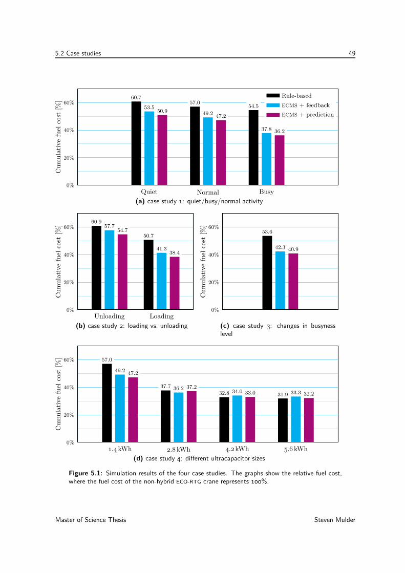
5.2 Case studies 49
0%
20%
40%
60%
Cum
ula
tive
fuel
cost
[%] 60.7
53.550.9
57.0
49.247.2
54.5
37.8 36.2
Quiet Normal Busy
Rule-based
ECMS + feedback
ECMS + prediction
(a) case study 1: quiet/busy/normal activity
0%
20%
40%
60%
Cum
ula
tive
fuel
cost
[%]
60.957.7
54.750.7
41.338.4
Unloading Loading
(b) case study 2: loading vs. unloading
0%
20%
40%
60%
Cum
ula
tive
fuel
cost
[%]
53.6
42.3 40.9
(c) case study 3: changes in busynesslevel
0%
20%
40%
60%
Cum
ula
tive
fuel
cost
[%] 57.0
49.247.2
37.7 36.2 37.232.8 34.0 33.0 31.9 33.3 32.2
1.4 kWh 2.8 kWh 4.2 kWh 5.6 kWh
(d) case study 4: different ultracapacitor sizes
Figure 5.1: Simulation results of the four case studies. The graphs show the relative fuel cost,where the fuel cost of the non-hybrid ECO-RTG crane represents 100%.
Master of Science Thesis Steven Mulder
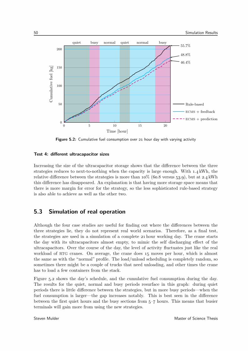
50 Simulation Results
0
50
100
150
200
0 5 10 15 20
Time [hour]
Cum
ula
tive
fuel
[kg]
quiet busy normal quiet normal busy55.7%
48.8%
46.4%
Rule-based
ECMS + feedback
ECMS + prediction
Figure 5.2: Cumulative fuel consumption over 21 hour day with varying activity
Test 4: different ultracapacitor sizes
Increasing the size of the ultracapacitor storage shows that the difference between the threestrategies reduces to next-to-nothing when the capacity is large enough. With 1.4 kWh, therelative difference between the strategies is more than 10% (60.8 versus 53.9), but at 2.4 kWhthis difference has disappeared. An explanation is that having more storage space means thatthere is more margin for error for the strategy, so the less sophisticated rule-based strategyis also able to achieve as well as the other two.
5.3 Simulation of real operation
Although the four case studies are useful for finding out where the differences between thethree strategies lie, they do not represent real world scenarios. Therefore, as a final test,the strategies are used in a simulation of a complete 21 hour working day. The crane startsthe day with its ultracapacitors almost empty, to mimic the self discharging effect of theultracapacitors. Over the course of the day, the level of activity fluctuates just like the realworkload of RTG cranes. On average, the crane does 15 moves per hour, which is almostthe same as with the “normal” profile. The load/unload scheduling is completely random, sosometimes there might be a couple of trucks that need unloading, and other times the cranehas to load a few containers from the stack.
Figure 5.2 shows the day’s schedule, and the cumulative fuel consumption during the day.The results for the quiet, normal and busy periods resurface in this graph: during quietperiods there is little difference between the strategies, but in more busy periods—when thefuel consumption is larger—the gap increases notably. This is best seen in the differencebetween the first quiet hours and the busy sections from 5–7 hours. This means that busierterminals will gain more from using the new strategies.
Steven Mulder Master of Science Thesis
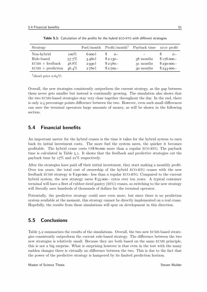
5.4 Financial benefits 51
Table 5.1: Calculation of the profits for the hybrid ECO-RTG with different strategies
Strategy Fuel/month Profit/month1 Payback time 10 yr profit
Non-hybrid 100% 6 000 l $ 0.- - $ 0.-Rule-based 57.7% 3 460 l $ 2 130.- 38 months $ 176 000.-ECMS + feedback 48.8% 2 930 l $ 2 580.- 31 months $ 230 000.-ECMS + prediction 46.4% 2 780 l $ 2 700.- 30 months $ 244 000.-
1diesel price 0.84 $/l
Overall, the new strategies consistently outperform the current strategy, as the gap betweenthem never gets smaller but instead is continually growing. The simulation also shows thatthe two ECMS-based strategies stay very close together throughout the day. In the end, thereis only 2.4 percentage points difference between the two. However, even such small differencescan save the terminal operators large amounts of money, as will be shown in the followingsection.
5.4 Financial benefits
An important metric for the hybrid cranes is the time it takes for the hybrid system to earnback its initial investment costs. The more fuel the system saves, the quicker it becomesprofitable. The hybrid crane costs US$ 80 000 more than a regular ECO-RTG. The paybacktime is calculated in Table 5.1. It shows that the feedback and predictive strategies cut thepayback time by 17% and 21% respectively.
After the strategies have paid off their initial investment, they start making a monthly profit.Over ten years, the total cost of ownership of the hybrid ECO-RTG cranes with the newfeedback ECMS strategy is $ 230 000.- less than a regular ECO-RTG. Compared to the currenthybrid system, the new strategy saves $ 55 000.- extra over ten years. A typical containerterminal will have a fleet of rubber-tired gantry (RTG) cranes, so switching to the new strategywill literally save hundreds of thousands of dollars for the terminal operator.
Potentially, the predictive strategy could save even more, but since there is no predictionsystem available at the moment, this strategy cannot be directly implemented on a real crane.Hopefully, the results from these simulations will spur on development in this direction.
5.5 Conclusions
Table 5.2 summarizes the results of the simulations. Overall, the two new ECMS-based strate-gies consistently outperform the current rule-based strategy. The difference between the twonew strategies is relatively small. Because they are both based on the same ECMS principle,this is not a big surprise. What is surprising however is that even in the test with the manysudden changes there is virtually no difference between the two. This is due to the fact thatthe power of the predictive strategy is hampered by its limited prediction horizon.
Master of Science Thesis Steven Mulder
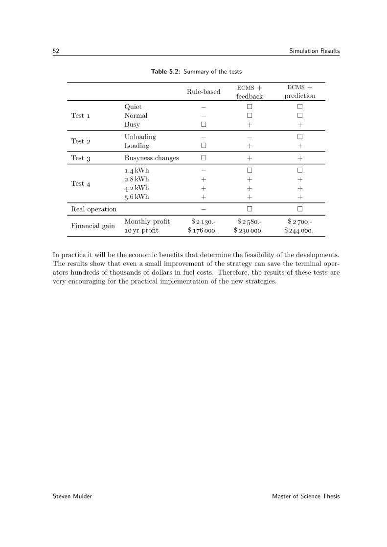
52 Simulation Results
Table 5.2: Summary of the tests
Rule-basedECMS +feedback
ECMS +prediction
Test 1
Quiet −
Normal −
Busy + +
Test 2Unloading − −
Loading + +
Test 3 Busyness changes + +
Test 4
1.4 kWh −
2.8 kWh + + +4.2 kWh + + +5.6 kWh + + +
Real operation −
Financial gainMonthly profit $ 2 130.- $ 2 580.- $ 2 700.-10 yr profit $ 176 000.- $ 230 000.- $ 244 000.-
In practice it will be the economic benefits that determine the feasibility of the developments.The results show that even a small improvement of the strategy can save the terminal oper-ators hundreds of thousands of dollars in fuel costs. Therefore, the results of these tests arevery encouraging for the practical implementation of the new strategies.
Steven Mulder Master of Science Thesis
Chapter 6
Conclusions and Recommendations
This chapter starts by presenting the conclusions of the previous chapters. Section 6.2 pro-poses some recommendations for further research in the subject of energy management forhybrid cranes.
6.1 Conclusions
As a supplier of electrical systems for container cranes, Siemens faces tough competition,forcing it to keep innovating in order to deliver superior products. A major innovation is thehybrid ECO-RTG crane, which uses an ultracapacitor bank that can store regenerated energyto assist the crane’s diesel generator set (GenSet) during operation. This thesis focused onimproving the energy management strategy, which is the system that governs the use of theultracapacitor in combination with the GenSet. The main subject is formulated as follows.
How can the energy management strategy of the Siemens hybrid ECO-RTG cranebe improved in order to enhance its fuel economy?
In order to answer this question, it was split up into three subproblems. These three sub-problems will be discussed in the following three sections.
1. Create a simulator to analyze the fuel consumption of the hybrid ECO-RTG crane.
(a) Create a system to mimic the power demand of the crane during specific types ofoperations.
(b) Create a model that simulates the total power system of the hybrid ECO-RTG,including the fuel consumption and the ultracapacitors.
2. Design a system that improves the current energy management strategy.
(a) Analyze the current strategy to find its strong points and weaknesses.
Master of Science Thesis Steven Mulder
54 Conclusions and Recommendations
(b) Find an approach to improve the weaknesses of the current strategy
(c) Implement the improved strategy so it can be tested in the simulator.
3. Select the best strategy from the three alternatives.
(a) Design experiments that show relevant characteristics of the strategies.
(b) Analyze the simulation results to find the best strategy.
6.1.1 Simulator
Power demand simulator
The power demand of the crane was analyzed in Chapter 2. The motion of the crane ishandled by a set of electric motors, of which the hoist motor is by far the largest. The powerdemand of the crane is also dominated by the hoist action, which creates 150–250 kW peaks inthe power demand and also large amounts of regenerated power. There is a difference in theduration of these peaks for loading and unloading containers from trucks, due to the heightdifference between the truck and the stack. Unloading a truck generally requires more netenergy than loading, where the container is moved “down” from the stack.
In between the moving of containers the crane is idling. During these periods, the auxiliarysystems of the crane still demand 10–30 kW of power. The amount of idle time dependson the busyness of the container terminal: 200 sec during quiet periods, 100 sec for normalactivity, and < 10 sec during busy periods. The long idle times have a large influence on theperformance of the hybrid crane, because the ultracapacitors are gradually drained duringidling.
Power supply model
The power system of the crane was modeled in Chapter 3. The model consists of two parts:the GenSet and the ultracapacitor bank. A quasi-static fuel consumption model of the GenSetwas constructed, based on measurements of the ECO-RTG power pack. Overall, the GenSetis most efficient when it is generating power in the 150–200 kW range, and its efficiencydrastically deteriorates outside this region. Furthermore, the ON/OFF state of the engine isalso important. The engine burns extra diesel when cranking, which adds to the fuel costright after startup.
The ultracapacitors can both store and deliver power. A model was created, based on datafrom the manufacturer. The efficiency of the ultracapacitor bank depends on the currentflowing through it. This means that the ultracapacitors are most efficient when they supplylow power. The energy level of the ultracapacitors is also a factor in the efficiency. A fullycharged ultracapacitor is significantly more efficient than when it is nearly empty.
6.1.2 Energy management strategy
Two new energy management strategies were developed in Chapter 4. The strategy that iscurrently used in the prototype crane is a rule-based heuristic strategy that is reliable and
Steven Mulder Master of Science Thesis
6.2 Recommendations 55
predictable, but is difficult to tune for optimal performance. An optimization-based strategyis better suited to achieve the best possible performance.
Initially, a strategy that optimizes the fuel cost for a complete move cycle was described,but this approach was unsuitable for implementation because of calculation issues. Instead,an Equivalent Consumption Minimization Strategy (ECMS) is proposed, which only takes asingle time step into account for the optimization. The approach revolves around assigningan “equivalent fuel cost” weight λuc to the ultracapacitor power. The strategy was furtherexpanded to also include the equivalent fuel cost of starting and stopping the GenSet engine.
The performance of ECMS depends heavily on the choice of the weight λuc, because it de-termines how much the ultracapacitors will be used. The two new strategies each have adifferent approach to solve this issue. The first approach uses a low-bandwidth PI-controllerthat adjusts λuc to keep the ultracapacitor energy level near a set reference value.
The second approach does not rely on feedback to react on things that have already happened,but instead intends to use predictive information to anticipate upcoming power demand. As ofyet, the required information about upcoming events is not available to the strategy, but thiscan be accomplished by connecting to the terminal operation system (TOS). The predictivestrategy performs a line search optimization to select λuc.
6.1.3 Simulation results
The current strategy and the two new alternatives are compared in Chapter 5. The resultsof the various tests and calculations is shown in Table 6.1. The new strategies consistentlyoutperform the current one. This difference in performance leads to significant long-termgains, and also reduces the time it takes for the hybrid crane to break-even on its initialinvestment cost.
Between the two new strategies, the difference is small. The advantage of the more complexpredictive strategy is small because of the limited prediction horizon. The relatively smallstorage size also makes long-term planning infeasible. However, because these cranes are usedso much, even a small improvement in the strategy can have large effects in the long run, soit might still be interesting to research the prediction system.
6.2 Recommendations
The thesis work focused on researching feasibility of improving the current energy manage-ment strategy. The results are encouraging, but there are still a number of things left forfuture research.
First and foremost, a real life test of the new strategies should be performed to accuratelymeasure the gains the new system during actual operation. The predictive system is still tooimmature for this step, but the combination of ECMS with SOC feedback should be relativelyeasy to implement into the crane software. Siemens is already planning to perform these testsusing hybrid ECO-RTG cranes that are scheduled for delivery to the Port of Felixstowe.
While the ECMS/feedback strategy is ready for implementation on the crane, the predictivestrategy cannot be implemented yet because there are no predictions available. The simula-tions showed that even a few percentage points improved performance can save large amounts
Master of Science Thesis Steven Mulder
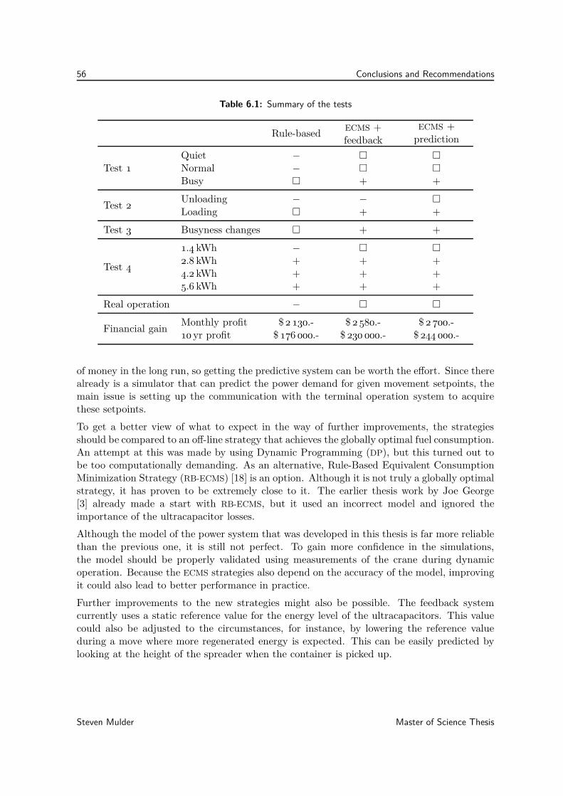
56 Conclusions and Recommendations
Table 6.1: Summary of the tests
Rule-basedECMS +feedback
ECMS +prediction
Test 1
Quiet −
Normal −
Busy + +
Test 2Unloading − −
Loading + +
Test 3 Busyness changes + +
Test 4
1.4 kWh −
2.8 kWh + + +4.2 kWh + + +5.6 kWh + + +
Real operation −
Financial gainMonthly profit $ 2 130.- $ 2 580.- $ 2 700.-10 yr profit $ 176 000.- $ 230 000.- $ 244 000.-
of money in the long run, so getting the predictive system can be worth the effort. Since therealready is a simulator that can predict the power demand for given movement setpoints, themain issue is setting up the communication with the terminal operation system to acquirethese setpoints.
To get a better view of what to expect in the way of further improvements, the strategiesshould be compared to an off-line strategy that achieves the globally optimal fuel consumption.An attempt at this was made by using Dynamic Programming (DP), but this turned out tobe too computationally demanding. As an alternative, Rule-Based Equivalent ConsumptionMinimization Strategy (RB-ECMS) [18] is an option. Although it is not truly a globally optimalstrategy, it has proven to be extremely close to it. The earlier thesis work by Joe George[3] already made a start with RB-ECMS, but it used an incorrect model and ignored theimportance of the ultracapacitor losses.
Although the model of the power system that was developed in this thesis is far more reliablethan the previous one, it is still not perfect. To gain more confidence in the simulations,the model should be properly validated using measurements of the crane during dynamicoperation. Because the ECMS strategies also depend on the accuracy of the model, improvingit could also lead to better performance in practice.
Further improvements to the new strategies might also be possible. The feedback systemcurrently uses a static reference value for the energy level of the ultracapacitors. This valuecould also be adjusted to the circumstances, for instance, by lowering the reference valueduring a move where more regenerated energy is expected. This can be easily predicted bylooking at the height of the spreader when the container is picked up.
Steven Mulder Master of Science Thesis

Bibliography
[1] Sumitomo Heavy Industries, “SYBRID system,” http://www.shi.co.jp, 2008.
[2] VYCON, “REGEN crane system,” http://www.vyconenergy.com, 2008.
[3] J. V. George, “Optimal design and control of a full hybrid RTG crane,” Master’s thesis,Delft University of Technology, 2008.
[4] B. K. Powell, K. E. Bailey, and S. R. Cikanek, “Dynamic modeling and control of hybridelectric vehicle powertrain systems,” IEEE Control Syst. Mag., vol. 18, no. 5, pp. 17–33,1998.
[5] D. W. Gao, C. Mi, and A. Emadi, “Modeling and simulation of electric and hybridvehicles,” in Proc. IEEE, vol. 95, Apr. 2007, pp. 729–745.
[6] L. Guzzella and A. Sciaretta, Vehicle Propulsion Systems. Berlin Heidelberg: Springer,2005.
[7] M. Koot, J. T. B. A. Kessels, B. de Jager, W. P. M. H. Heemels, P. P. J. van den Bosch,and M. Steinbuch, “Energy management strategies for vehicular electric power systems,”IEEE Trans. Veh. Technol., vol. 54, no. 3, pp. 771–782, May 2005.
[8] J. T. B. A. Kessels, “Energy management for automotive power nets,” Ph.D. dissertation,Eindhoven University of Technology, 2007.
[9] A. Sciarretta, M. M. Back, and L. Guzzella, “Optimal control of parallel hybrid electricvehicles,” IEEE Trans. Control Syst. Techn., vol. 12, no. 3, pp. 352–363, May 2004.
[10] Wampfler A.G., “Conductor rails,” http://www.wampfler.com, 2008.
[11] Siemens Cranes, “ECO-RTG, A revolutionary new drive concept,” Brochure.
[12] A. Schneuwly, M. Bärtschi, V. Hermann, R. Sartorelli, R. Gallay, and R. Koetz,“BOOSTCAP double-layer capacitors for peak power automotive applications,” in Proc.Adv. Automot. Batt. Conf. (AABC 02), Spring 2002.
Master of Science Thesis Steven Mulder
58 Bibliography
[13] J. F. Baalbergen and P. Bauer, “Verification by simulation of power management strate-gies for 4Q-load,” 2008, accepted for Publication.
[14] J.-S. Won and R. Langari, “Intelligent energy management agent for a parallel hybridvehicle-part II: torque distribution, charge sustenance strategies, and performance re-sults,” IEEE Trans. Veh. Technol., vol. 54, no. 3, pp. 935–953, May 2005.
[15] P. Pisu and R. Rizzoni, “A comparative study of supervisory control strategies for hybridelectric vehicles,” IEEE Trans. Control Syst. Technol., vol. 15, pp. 506–518, May 2007.
[16] T. J. J. van den Boom and B. H. K. De Schutter, Optimization in Systems and Control.Delft University of Technology, 2007.
[17] R. Bellman, “Dynamic Programming,” Science, vol. 153, pp. 34–37, July 1966.
[18] T. Hofman, “Framework for combined control and design optimization of hybrid vehiclepropulsion systems,” Ph.D. dissertation, Eindhoven University of Technology, 2007.
Steven Mulder Master of Science Thesis
Glossary
Abbreviations
AGV Automated Guided Vehicle
DP Dynamic Programming
ECMS Equivalent Consumption Minimization Strategy
GenSet (Diesel) Generator Set
HVAC Heating, Ventilating, and Air Conditioning
MPC Model-based Predictive Control
RB-ECMS Rule-Based Equivalent Consumption Minimization Strategy
RMG Rail-Mounted Gantry
RTG Rubber-Tired Gantry
SOC State Of Charge
STS Ship-To-Shore
TOS Terminal Operation System
VSG Variable Speed Generator
Greek Symbols
η Efficiency pu
ηdc DC/DC converter efficiency pu
λst Equivalent fuel cost weight for engine shutdown g
λuc Equivalent fuel cost weight for ultracapacitors g/kW
λuc Approximated equivalent fuel cost weight for ultracapacitors g/kW
θ Generalized optimization parameter -
θ∗ Generalized optimization solution -
Master of Science Thesis Steven Mulder
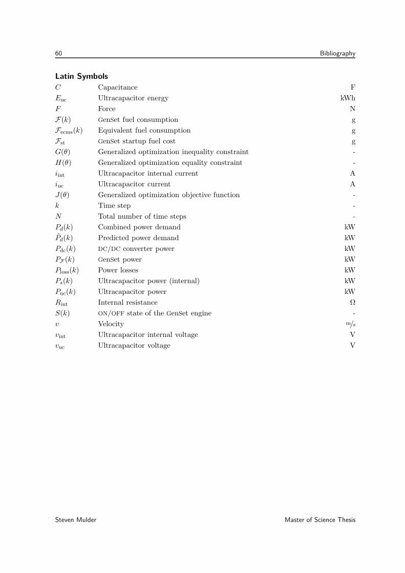
60 Bibliography
Latin Symbols
C Capacitance F
Euc Ultracapacitor energy kWh
F Force N
F(k) GenSet fuel consumption g
Fecms(k) Equivalent fuel consumption g
Fst GenSet startup fuel cost g
G(θ) Generalized optimization inequality constraint -
H(θ) Generalized optimization equality constraint -
iint Ultracapacitor internal current A
iuc Ultracapacitor current A
J(θ) Generalized optimization objective function -
k Time step -
N Total number of time steps -
Pd(k) Combined power demand kW
Pd(k) Predicted power demand kW
Pdc(k) DC/DC converter power kW
PF (k) GenSet power kW
Ploss(k) Power losses kW
Ps(k) Ultracapacitor power (internal) kW
Puc(k) Ultracapacitor power kW
Rint Internal resistance Ω
S(k) ON/OFF state of the GenSet engine -
v Velocity m/s
vint Ultracapacitor internal voltage V
vuc Ultracapacitor voltage V
Steven Mulder Master of Science Thesis
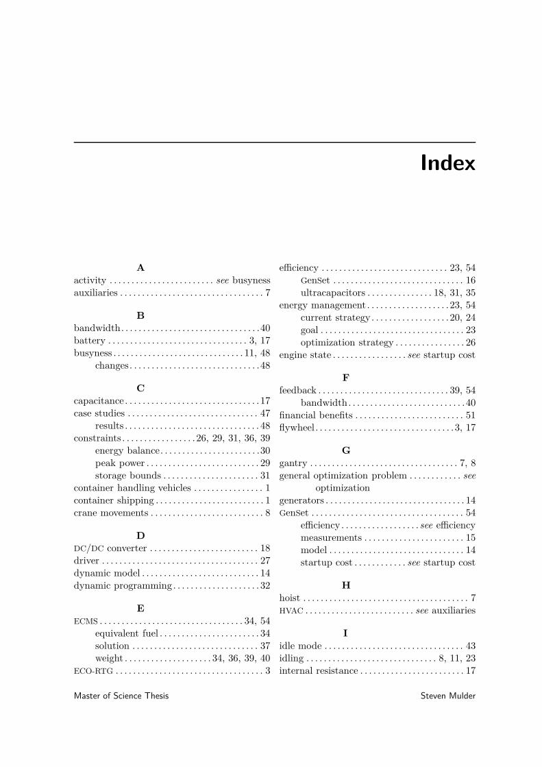
Index
A
activity . . . . . . . . . . . . . . . . . . . . . . . . see busyness
auxiliaries . . . . . . . . . . . . . . . . . . . . . . . . . . . . . . . . . 7
B
bandwidth. . . . . . . . . . . . . . . . . . . . . . . . . . . . . . . .40
battery . . . . . . . . . . . . . . . . . . . . . . . . . . . . . . . . 3, 17
busyness . . . . . . . . . . . . . . . . . . . . . . . . . . . . . . 11, 48
changes. . . . . . . . . . . . . . . . . . . . . . . . . . . . . .48
C
capacitance. . . . . . . . . . . . . . . . . . . . . . . . . . . . . . . 17
case studies . . . . . . . . . . . . . . . . . . . . . . . . . . . . . . 47
results . . . . . . . . . . . . . . . . . . . . . . . . . . . . . . . 48constraints . . . . . . . . . . . . . . . . . 26, 29, 31, 36, 39
energy balance. . . . . . . . . . . . . . . . . . . . . . .30
peak power . . . . . . . . . . . . . . . . . . . . . . . . . . 29
storage bounds . . . . . . . . . . . . . . . . . . . . . . 31container handling vehicles . . . . . . . . . . . . . . . . 1
container shipping . . . . . . . . . . . . . . . . . . . . . . . . . 1
crane movements . . . . . . . . . . . . . . . . . . . . . . . . . . 8
D
DC/DC converter . . . . . . . . . . . . . . . . . . . . . . . . . 18
driver . . . . . . . . . . . . . . . . . . . . . . . . . . . . . . . . . . . . 27
dynamic model . . . . . . . . . . . . . . . . . . . . . . . . . . . 14
dynamic programming. . . . . . . . . . . . . . . . . . . . 32
E
ECMS . . . . . . . . . . . . . . . . . . . . . . . . . . . . . . . . . 34, 54
equivalent fuel . . . . . . . . . . . . . . . . . . . . . . . 34
solution . . . . . . . . . . . . . . . . . . . . . . . . . . . . . 37weight . . . . . . . . . . . . . . . . . . . . 34, 36, 39, 40
ECO-RTG . . . . . . . . . . . . . . . . . . . . . . . . . . . . . . . . . . 3
efficiency . . . . . . . . . . . . . . . . . . . . . . . . . . . . . 23, 54
GenSet . . . . . . . . . . . . . . . . . . . . . . . . . . . . . . 16
ultracapacitors . . . . . . . . . . . . . . . 18, 31, 35energy management. . . . . . . . . . . . . . . . . . . 23, 54
current strategy. . . . . . . . . . . . . . . . . . 20, 24
goal . . . . . . . . . . . . . . . . . . . . . . . . . . . . . . . . . 23
optimization strategy . . . . . . . . . . . . . . . . 26engine state . . . . . . . . . . . . . . . . . see startup cost
F
feedback . . . . . . . . . . . . . . . . . . . . . . . . . . . . . . 39, 54
bandwidth. . . . . . . . . . . . . . . . . . . . . . . . . . .40
financial benefits . . . . . . . . . . . . . . . . . . . . . . . . . 51flywheel. . . . . . . . . . . . . . . . . . . . . . . . . . . . . . . .3, 17
G
gantry . . . . . . . . . . . . . . . . . . . . . . . . . . . . . . . . . . 7, 8
general optimization problem . . . . . . . . . . . . seeoptimization
generators . . . . . . . . . . . . . . . . . . . . . . . . . . . . . . . . 14GenSet . . . . . . . . . . . . . . . . . . . . . . . . . . . . . . . . . . . 54
efficiency . . . . . . . . . . . . . . . . . . see efficiency
measurements . . . . . . . . . . . . . . . . . . . . . . . 15model . . . . . . . . . . . . . . . . . . . . . . . . . . . . . . . 14
startup cost . . . . . . . . . . . . see startup cost
H
hoist . . . . . . . . . . . . . . . . . . . . . . . . . . . . . . . . . . . . . . 7
HVAC . . . . . . . . . . . . . . . . . . . . . . . . . see auxiliaries
I
idle mode . . . . . . . . . . . . . . . . . . . . . . . . . . . . . . . . 43idling . . . . . . . . . . . . . . . . . . . . . . . . . . . . . . 8, 11, 23
internal resistance . . . . . . . . . . . . . . . . . . . . . . . . 17
Master of Science Thesis Steven Mulder

62 Index
L
lighting . . . . . . . . . . . . . . . . . . . . . . . see auxiliariesline search . . . . . . . . . . . . . . . . . . . . . . . . . . . . . . . . 42loading . . . . . . . . . . . . . . . . . . . . . . . . . 8, 10, 29, 48
M
MATLAB . . . . . . . . . . . . . . . . . . . . . . . . . . . . . . . . . . 45megatrends . . . . . . . . . . . . . . . . . . . . . . . . . . . . . . . . 3
model . . . . . . . . . . . . . . . . . . . . . . . . . see simulatormove . . . . . . . . . . . . . . . . . . . . . . . . . . . . see loading
MPC . . . . . . . . . . . . . . . . . . . . . . . . . . see prediction
O
objective function . . . . . . . . . . 26–29, 31, 35, 37
predictive . . . . . . . . . . . . . . . . . . . . . . . . . . . 41off-line solution . . . . . . . . . . . . . . . . . . . . . . . . . . . 32off-line strategy. . . . . . . . . . . . . . . . . . . . . . . . . . .55
optimization . . . . . . . . . . . . . . . . . . . . . . . . . . . . . .26feasibility . . . . . . . . . . . . . . . . . . . . . . . . . . . . 31
optimization parameter . . . . . . . . . . . . . . . . . . . 26
P
PI-controller . . . . . . . . . . . . . . . . . . . . see feedbackpiecewise fit . . . . . . . . . . . . . . . . . . . . . . . . . . . . . . 16
power demand . . . . . . . . . . . . . . . . . . . 7, 9, 20, 54acceleration. . . . . . . . . . . . . . . . . . . . . . . . . . . 9
deceleration . . . . . . . . . . . . . . . . . . . . . . . . . . 9power supply. . . . . . . . . . . . . . . . . . . . . . 13, 20, 54prediction . . . . . . . . . . . . . . . . . . . . . . . . . . . . 40, 54
horizon . . . . . . . . . . . . . . . . . . . . . . . . . . . . . . 43solution . . . . . . . . . . . . . . . . . . . . . . . . . . . . . 42
Q
quadratic programming. . . . . . . . . . . . . . . . . . . 38quasi-static model . . . . . . . . . . . . . . . . . . . . . . . . 14
R
RB-ECMS . . . . . . . . . . . . . . . . . . . . . . . . . . . . . . . . . 55recharging . . . . . . . . . . . . . . . . . . . . . . . . . . . . . . . . 43
recommendations . . . . . . . . . . . . . . . . . . . . . . . . . 55resistance . . . . . . . . . . . . . see internal resistancerule base . . . . . . . . . . . . . . . . . . . . . . . . . . . . . . . . . 25
rule-based . . . . . . . . . . . see energy management
S
sample time . . . . . . . . . . . . . . . . . . . . . . . . . . 18, 27
simulations . . . . . . . . . . . . . . . . . . . . . . . . . . . . . . . 45limitations. . . . . . . . . . . . . . . . . . . . . . . . . . .46
real operation . . . . . . . . . . . . . . . . . . . . . . . 50setup . . . . . . . . . . . . . . . . . . . . . see simulator
simulator . . . . . . . . . . . . . . . . . . . . . . . 7, 13, 45, 54results . . . . . . . . . . . . . . . . . . . . . . . . . . . . . . . 20
specific fuel consumption . . . . . . . see efficiencystacking yard . . . . . . . . . . . . . . . . . . . . . . . . . . . . . . 1startup cost . . . . . . . . . . . . . . . . . . . . . . . 23, 27, 31
T
terminal operation system. . . . . . . . . 40, 54, 55thesis goal . . . . . . . . . . . . . . . . . . . . . . . . . . . . . 4, 53
subproblems . . . . . . . . . . . . . . . . . . . . . . . . . . 4trolley . . . . . . . . . . . . . . . . . . . . . . . . . . . . . . . . . . . . . 7
U
ultracapacitor size . . . . . . . . . . . . . . . . . . . . . . . . 50ultracapacitors . . . . . . . . . . . . . . . . . . . . . . . . . . . 54
data . . . . . . . . . . . . . . . . . . . . . . . . . . . . . . . . . 17efficiency . . . . . . . . . . . . . . . . . . see efficiencymodel. . . . . . . . . . . . . . . . . . . . . . . . . . . .17, 18
unloading . . . . . . . . . . . . . . . . . . . . . . . .see loading
V
variable speed generators . . . . . . . . . . . . . . . . . 14
Steven Mulder Master of Science Thesis

63
MTB241 B’VO
Master of Science Thesis Steven Mulder