NBER WORKING PAPER SERIES

MOTHER’S SCHOOLING AND FERTILITY UNDER LOW FEMALE LABOR FORCE PARTICIPATION:EVIDENCE FROM A NATURAL EXPERIMENT

Victor LavyAlexander Zablotsky

Working Paper 16856http://www.nber.org/papers/w16856

NATIONAL BUREAU OF ECONOMIC RESEARCH1050 Massachusetts Avenue

Cambridge, MA 02138March 2011

We benefited from comments by Josh Angrist, Esther Duflo, Ephraim Kleinman, Melanie Luhrmann,Daniele Paserman, Steve Pischke, Yona Rubinstein, Yannay Spitzer, Natalia Weisshaar, Asaf Zussmanand seminar participants at the Bocconi University, Hebrew University, LSE, NBER Labor Studiesconference in Autumn 2010, Oxford University, RH University of London, Tel Aviv University, andUniversity of Zurich. The views expressed herein are those of the authors and do not necessarily reflectthe views of the National Bureau of Economic Research.

NBER working papers are circulated for discussion and comment purposes. They have not been peer-reviewed or been subject to the review by the NBER Board of Directors that accompanies officialNBER publications.

© 2011 by Victor Lavy and Alexander Zablotsky. All rights reserved. Short sections of text, not toexceed two paragraphs, may be quoted without explicit permission provided that full credit, including© notice, is given to the source.

Mother’s Schooling and Fertility under Low Female Labor Force Participation: Evidencefrom a Natural ExperimentVictor Lavy and Alexander ZablotskyNBER Working Paper No. 16856March 2011, Revised August 2011JEL No. I1,J2

ABSTRACT

This paper studies the effect of mothers‘ education on fertility in a population with very low femalelabor force participation. The results we present are particularly relevant to many countries in the Muslimworld where 70-80 percent of women are still out of the labor force. For identification we exploit theabrupt end of the military rule which greatly restricted the mobility of Arabs in Israel until the mid-1960's.This change improved access to schooling in communities that lacked schools and, as a consequence,significantly increased the education of affected cohorts, mainly of girls. The very large increase inschooling attainment triggered a sharp decline in completed fertility. We show that no other changesexplain these findings and that the results are robust to checks against various threats to identification.We rule out convergence in fertility and schooling, changes in labor-force participation, age uponmarriage, marriage and divorce rates, and spousal labor-force participation and earnings as mechanismsin this fertility decline. Spousal education increased however sharply through assortative matchingand played a role in the fertility decline. We also show that the increase in mother‘s education wassignificantly and positively correlated with several potential mechanisms such as a reduction in thedesired number of children, better knowledge and higher probability of using contraceptives, recognitionthat family size can compromise children quality, larger role for women in family decision making,less religiosity, and positive attitude towards modern health care and modernism in general.

Victor LavyDepartment of EconomicsHebrew UniversityMount ScopusJerusalem 91905ISRAELand Royal Holloway University of Londonand also NBERmsvictor@mscc.huji.ac.il

Alexander ZablotskyThe Hebrew University of JerusalemDepartment of EconomicsMount Scopus Jerusalem Israel 91905alex.zablotsky@mail.huji.ac.il

1

1. Introduction

In the economic model of fertility (Becker, 1960; Mincer, 1963), education increases the

opportunity cost of women‘s time, prompting them to have fewer children but also raising their

permanent income through earnings and tilting their optimal fertility choices toward higher

quality (Becker and Lewis, 1973; Willis, 1973). In these models, the link between education and

fertility crucially depends on labor force participation. However, it appears that some societies

have experienced a fertility transition without this mechanism playing a major role. In the past

half-century, for example, the total fertility rate of Muslim women in Israel fell sharply, from over

9.8 children in the mid-1950s to 3.9 in 2008.1 Concurrently, Israeli-Arab women‘s average years

of schooling increased more than threefold, from three years in 1951 to over ten in 2008. This

change, however, hardly affected their labor-force participation and employment over those years;

the respective rates were only 15 percent in 2000 and 18 percent in 2009.2 Whether education

plays a role in lowering fertility in the absence of the labor market mechanism is of great

importance since in most of the Arab and Muslim world women are practically absent from the

labor force. For example, the most recent World Bank statistics3 show that in 2009 the labor force

participation rate of women over 15 years old was 20-24 percent in Egypt, Jordan, Lebanon, and

Yemen, and it was 14-17 percent in Iraq, Saudi Arabia, and the West Bank and Gaza. In Pakistan

and Turkey, Muslim though not Arab countries, female labor force participation is also very low,

23-24 percent. However, female education has increased to various degrees in all these countries

and this change could have lowered fertility through other channels.4

This paper studies the role of female education in reducing fertility through mechanisms

other than the labor market and its implied female value of time. In particular, we present

evidence that the strong negative relationship between women‘s fertility and education of Arab

women in Israel reflects a causal effect. It shows that women‘s labor-force participation, as well

as other potential mechanisms such as age upon marriage, marriage rates, and divorce rates, did

1 Israel Central Bureau of Statistics (hereinafter: CBS) website, online tables and figures. 2 CBS (2002), State of Israel Prime Minister‘s Office, and Yashiv and Kasir (2009). 3 http://data.worldbank.org/indicator/SL.TLF.CACT.FE.ZS 4 The increase in education may impact women fertility by improving an individual‘s knowledge of, and ability to process information regarding, fertility options and healthy pregnancy behaviors (Grossman, 1972). Second, education may enhance females‘ ability to process information and contraception options (Strauss and Thomas, 1995). Education may also improve a wife‘s bargaining power inside her marriage (Thomas, 1990) and may also tilt the tradeoff from the number of children to their quality (Moav (2005). McCrary and Royer (forthcoming, 2011) present an insightful summary of how education may affect fertility and children outcomes and discuss the related empirical evidence. However, there is little evidence of the importance of these channels in the absence of meaningful increases in women‘s employment and the opportunity cost of their time.

2

not play any role in this fertility decline. The impact of women‘s education remained very large

after we accounted for spouse‘s employment. Furthermore, spouse‘s education increased

immensely through assortative matching and, therefore, probably played a major role in the

decline in demand for children. Other mechanisms that seem to be relevant for the role of

education in reducing fertility of Arab women in Israel are changes in fertility preferences,

knowledge and use of contraceptives, higher bargaining power within the household and role of

women in family decisions, reduced religiosity, and positive attitude towards modern health care

and modernism in general.

We base the evidence presented in this paper on a natural experiment that increased

sharply the education of affected cohorts of children as a result of the de facto revocation in

October 1963 of military rule over Arabs in Israel, which immediately allowed some of the Arab

population to regain access to schooling institutions. Military rule was in effect from 1948 to

1966 in several geographical areas of Israel that had large Arab populations. Since 1948, the Arab

residents of these areas were subject to measures that placed tight controls on all aspects of their

lives, including restrictions on mobility and the requirement of a permit from the Military

Governor to travel to outside of a person‘s registered domicile.5 The travel restrictions were

revoked in October 1963 following unexpected political and government change.6

The Military Government restricted de facto access to schools for children in localities

and villages that had no primary or secondary schools while not affecting access in localities in

the relevant regions that already had such institutions. By so doing, it created two zones in the

Arab-populated areas, one in which school attendance required travel that had become difficult if

not impossible and one in which schooling access was not disrupted at all. In the latter group, we

distinguish between Arab localities that were under military rule and the Arab population that

lived in predominantly Jewish cities. The latter population group was also placed under military

rule at first (1948) but was exempted de facto from some of the restrictions a short time later.

5 A recent historical episode of similar restrictions on perceived ―enemy― populations is the United States Government‘s internment and forced relocation of Japanese Americans and Japanese residing along the Pacific coast of the United States to War Relocation Camps in the wake of Japan‗s attack on Pearl Harbor. President Franklin Roosevelt authorized the internment by Executive Order on February 19, 1942. On January 2, 1945, the exclusion order was totally rescinded. Another example is the arrest in camps of Germans in England during World War II. 6 In June 1963 the Prime Minister, David Ben-Gurion, who together with his ruling Labor Party strongly supported the continuation of the Military Government, resigned unexpectedly. The change was also a response to the mounting pressure from the Israeli public and many political parties, including the right-wing party Herut, to annul military rule over Israeli Arabs. This effort led in 1966 to the complete revocation of military rule and the equalization of Arab citizens‘ rights with those of other citizens.

3

The change which took place in late 1963 reduced the cost of primary or secondary

schooling for children in localities that lacked schools. Therefore, the exposure of an individual to

this ―treatment‖ was determined both by her location and by her year of birth. After controlling

for locality and year of birth fixed effects, we use the interaction between a dummy variable

indicating the age of the individual in 1964 and whether or not her locality was part of the

Military Government zone and had no schools as an exogenous variable and as an instrument for

an individual‘s education. This is a similar identification strategy as that used to estimate the

effect of school quality on returns to education (Card and Krueger, 1992), the effect of college

education on earnings (Card and Lemieux, 1998) and the effect of school construction on

education and earnings (Duflo, 2001). We allowed the affected cohorts to include children aged

4–13 in 1964, leaving older cohorts to be used in controlled experiments. We used data from the

1983 and 1995 censuses. In the 1983 census, the affected cohorts were just over 23–33 years old,

making it possible to study the effect of education on early-age fertility. In 1995, the affected

cohorts were already aged 36–46, allowing estimation of the effect of education on completed

fertility.

The evidence we present below suggests that the decline in the cost of attending primary

and secondary schooling from 1964 onward increased females‘ years of schooling by 1.02 for

women who were aged 4–9 in 1964 and by 0.58 for women aged 9–14 at that time. These

educational gains are associated with a large increase in the probability of a woman‘s completing

primary schooling and also of the completion of at least some years of secondary schooling.

Much smaller effects are estimated for men, suggesting that the travel restrictions did not limit

boys‘ access to schooling as badly.

These very large effects on girls‘ schooling levels induced a sharp decline in fertility,

measured at 0.61 children in the younger affected cohorts and 0.47 children in the older cohorts.

Implied 2SLS estimates show that a one-year increase in maternal schooling caused a 0.6-child

decline in fertility. This fertility decline, however, was not accompanied by discernible changes in

women‘s age upon marriage, divorce rate, labor-force participation, and spouse‘s employment,

earnings, and age upon marriage. Spouse‘s education, however, did increase through assortative

marriage matching, although not directly through the change in access to schooling, and therefore

may have had an effect on fertility. This evidence suggests that the increase in mothers‘ schooling

had a large and negative effect on fertility even though the actual opportunity cost of their time

did not change much. We also find that mother‘s education was highly correlated with other

potential mechanisms, in particular a change in fertility preferences, changes in contraceptive

details, a preferences shift towards quality children and reduced child and infant mortality, higher

4

bargaining power of women as reflected in their larger role in family decisions, less religiosity,

and positive attitude towards modern health care and modernism in general.

The identification assumption in estimating the causal effect of mother‘s schooling on

fertility is that the removal of the travel restrictions had neither a direct nor an indirect effect on

fertility except for its effect on creating access to schooling. We support this assumption with

broad range of evidence demonstrating that the removal of the travel restrictions did not have

differential impacts on cohorts aside from their effects on education. For example, we show that

the travel changes did not affect differentially the labor market opportunities, measured by the

probability of working outside of the locality (after the movement restrictions had been removed),

number of weeks of work, and wages and earnings, of the affected cohorts. We also present

evidence that the changes did not affect differentially measures of family wealth and income.

Regarding other potential confounding effects, we show that the removal of travel restrictions in

late 1963 did not improve differentially access to services that may have affected fertility directly.

For example, we demonstrate that the changes did not lead to differential improved access to

healthcare services, particularly pre- and post-natal services that the state provided at special

public well-baby centers and general clinics. Another identification concern that we rule out is

that the treatment estimates may be biased due to a pre-existing control–treatment differential

time trend in the fertility rate and female education. We use pre-reform data relating to the

localities‘ mean fertility rate and years of schooling for cohorts aged 14–24 in 1964 and show that

the treatment and control localities had similar fertility and female education time trends. We also

show that our results are robust to various sensitivity and falsification tests.

An extensive literature documents associations between education and fertility (Strauss

and Thomas. 1995). However, whether they represent causal relationships has been the subject of

debate. Breirova and Duflo (2002) and Osili and Long (2008) use school expansion as a source of

exogenous decrease in the cost of schooling and find a negative causal effect of education on

early age fertility in Indonesia and Nigeria. Black, Devereux, and Salvanes (2008) find that gains

in education resulting from compulsory-schooling laws decreased teenage pregnancy in the U.S.

and Norway. Also in Norway, Monstad, Propper and Salvanes (2008) find that increases in

education did not lead to decreased fertility but did lead to childbirth at older ages. In contrast,

McCrary and Royer (2011), using exact cutoff dates for school entry, find that education does not

affect fertility. Kirdar, Tayfur, and Koç (2009) use the extension of compulsory schooling in

Turkey in 1997 and find that it increased age of marriage and reduced fertility at young ages.

Duflo, Kremer, and Dupas (2010) provide experimental evidence that access to education for

adolescent girls reduced early fertility among girls who were likely to drop out of school. This

5

evidence obviously suggests a lack of consensus regarding the causal effect of women‘s

education on fertility. As we noted above, maternal education can affect fertility through many

different channels, and as such it is not evident that there should be one universal effect of

maternal education on fertility. Therefore, it is important to identify separately the different

channels through which the effect works, and in particular those channels which do not operate

through the labor market; thus, the main contribution in the evidence we present is in studying a

case in which the level of education had increased without changes in the labor market taking

place. This evidence is not only important in abstracting from the labor market effects; it is also

highly relevant for understanding the fertility transition in the Muslim and the Arab world, where

women's education had increased significantly, yet their labor force participation remained low.

The rest of the paper is organized as follows: Section 2 describes the political and policy

context of the Military Government and the mechanisms that it could have used to affect

education. After describing the data in Section 3, we discuss our identification strategy and

present the results of our estimation of the effect of schooling on fertility in Section 4. In Section

5, we check the robustness of the results and discuss possible threats to our identification strategy.

Section 6 concludes.

2. The 1948–1966 Military Government and Restricted Mobility of Arabs in Israel7

On 14 May 1948, the day that Britain had announced it would end its Mandate in

Palestine, the Jewish community in Palestine published a Declaration of Independence which

announced the creation of the State of Israel. The declaration was based on the United Nations

Partition Plan for Palestine adopted as a resolution on 29 November 1947 by the General

Assembly of the United Nations. The declaration did not define what the borders of the new state

were. On the following day, 15 May, most of the remaining British troops departed and five Arab

armies crossed the borders of what had formerly been Mandate Palestine. This event marked the

beginning of the 1948 Arab–Israeli War. The Palestinian Arabs, against which the Jewish

population fought its war of independence, became subjected to the new Jewish state at the end of

the war. During the war the Jewish Provisional Council of State decided to impose a special

military governmental authority on areas populated by Palestinian Arabs. The Military

Government was extended after the war and disbanded only in 1966. It was legally based on

defense regulations enacted in 1945 by the British Mandate Government that ruled Palestine at

the time. From then until the cessation of the enforcement of these regulations, the Military

Government was the dominant Israeli governmental authority exercising control over the Israeli 7 Much of the material in this section is based on Bauml (2002), Abu-Saad (2006) and Al-Haj (1995).

6

Arab minority. At first, the Military Government worked together with the Ministry of Minorities,

which was responsible for humanitarian aspects of the treatment of the Arab population, but this

ministry was abolished in 1949. Thereafter, the Military Government held sole responsibility for

all affairs of the Arab population. Although all Arab citizens were subject to military rule, those

who lived in mixed Arab-Jewish cities such as Haifa and Jaffa enjoyed greater freedom than the

others from the early 1950s on, largely because the travel restrictions were harder to enforce in

predominantly Jewish cities.

A Separate school system was developed for the Arab population in Israel, even in towns that

had mixed Jewish and Arab populations. The conditions of the school facilities in Arab schools

were extremely bad, and classrooms were over-crowded, even-though in some places students

were taught in two shifts (Abu-Saad, 2006, Kopelevitch, 1973). Essential supplies were lacking,

such as desks and chairs, blackboards and textbooks. However, the most important element of this

regime for the purposes of our study was the special travel permits, issued on a daily or weekly

basis, which the Military Government required Arab citizens to obtain in order to leave their

villages and towns by day or night. Such permits were needed for receiving medical services in

the cities, for travel to port cities for importation of capital goods (such as tractors), access to

work or educational opportunities, and practically every other purpose which required travelling

outside the locality. It has been claimed that obtaining these permits often involved side payments

to Arab collaborators. The Arab-populated ―enclosed areas‖ were divided into three separate army

commands: north (Galilee), south (Negev), and center (the "Triangle"). Each area was isolated

from the other and most Arab citizens were, of course, isolated from the majority Jewish

population as well. Enclosure orders controlled mobility by the required permits.

Apart from the practical hardships, the travel restrictions took a toll on their subjects by

creating a sense of uncertainty and personal risk. The army set up checkpoints and inspected

Arabs regularly for their passes. Those found with an expired pass or no pass at all were fined or

imprisoned. The Military Government also imposed a regular curfew from dark to sunrise or, at

times, before dawn. The public was not always aware of changes in curfew, resulting in several

tragic events. In one notorious case, on October 29, 1956, on the eve of the Suez War, the

Government changed the curfew to an earlier hour. Border Guard forces entered the large village

of Kafr Qasem and imposed this curfew on the village while many of its residents were out

working their fields some distance away, unaware of the revised curfew; some children were still

in school. By the end of the Border Guard operation, 51 villagers had been killed, including

women and young boys and girls, seven aged 8–13, along with others who were wounded

7

(Hadawi, 1991). This event and lesser tragedies created a climate of fear and insecurity, especially

when travel outside the village or town was needed.

There are plenty of stories and anecdotal evidence from personal diaries about the effect of

the increase in the cost of school attendance on school enrollment during the tenure of the

Military Government. El-Asmar (1975) recounts an experience typical of many youngsters at this

time. Since Fouzi‘s home town had no complete eight-grade primary school, "[Families that]

wanted their sons to continue their schooling had to send them to Nazareth or to the Triangle area.

My father had to send me and my big brother away to a residential school in Nazareth, which cost

him a fortune."

To avoid the dangerous and costly daily trip, some boys were sent to residential schools at a

much higher cost than attending the nearest school. Importantly, this solution was available for

boys only; girls had to drop out of school in such cases because there were no boarding schools

for girls. Ziad Mahjena tells much the same story.8 He completed primary school in 1957/58 in

his home town and aspired to continue in nearby schools in Nazareth or the nearby Jewish town

of Hadera but could not due to the state of military rule and the dearth of family resources. He

recounts the story of his three male friends who could afford to enroll in a residential high school.

In Israel‘s first years but mainly after 1957, some criticism and reservations were

expressed among the Israeli public, the Knesset (parliament) and Mapai (the ruling party) about

the need for the Military Government. The critics‘ main argument—that the Military Government

damaged Israeli democracy—led to many initiatives to abolish it. In February 1962 and February

1963, four political parties (including Menachem Begin‘s right-wing Herut Party) presented

parliamentary motions to revoke the entity‘s status. All the motions were voted down by a close

margin. However, the resignation of Prime Minister David Ben-Gurion on June 16, 1963, and the

appointment of Levi Eshkol as his successor led immediately to a dramatic and unexpected

change. In a speech to the Knesset in October 1963, Eshkol announced that the Arab population

would no longer need travel permits and that Arabs could once again move freely around the

country.9 This change removed one of the most burdensome restrictions, one that had profoundly

affected the daily lives of Arabs in Israel since the creation of the state. In 1966, the Military

Government was abolished altogether; all that remained were several specific restrictions, such as

8 Retrieved from a memoire website: http://www.Sochrot.org.index.php?id+164. 9 The populations of five Arab villages adjacent to the frontier were excluded from the new free-mobility policy. Another restriction that prohibited all Arabs from entering certain areas intended for Jewish settlement and defined as military zones was not cancelled.

8

traveling to the nuclear plant in Dimona, and to the vicinities of the Jordanian border in the Arava

Valley and the Egyptian Sinai Peninsula.

The Military Government and Restricted Access to Schooling

As noted above, Arabs who lived under military rule and were confined to specific

geographic areas faced severe restrictions in their ability to travel in pursuit of educational and

training opportunities and compete for better jobs in the labor market (Okun and Friedlander,

2005). This increased the cost of schooling for Arab children who resided in villages and towns

that had no schools. Commuting to the nearest school was complicated due to the need for a

travel permit and costly because of the longer travel time (passing checkpoints, etc.) and the

financial cost of obtaining permits or enrolling in residential schools. Sometimes travel was also

dangerous due, for example, to potential altercations with border police and soldiers at

checkpoints and on the roads, changes in curfew, and so on. Table A1 lists the Arab localities that

were under military rule and travel restrictions as of 1948 and the number of primary and

secondary schools in each locality in 1964/65, the first year for which such information was

available (Central Bureau of Statistics, 1966). Five of the localities (Acre, Haifa, Lod, Ramla, and

Tel Aviv-Jaffa) were mixed cities with a Jewish majority and an Arab minority. All five had Arab

primary schools; three of them also had Arab secondary schools. As noted above, however, the

Arab populations of these cities were exempted from military rule and the travel restrictions from

the mid-1950s on; we exclude them from our analysis. Five other localities—small villages—

were also exempt from military rule because most of their populations were of other minorities

(Druze and Circassians) which were not perceived to be a threat; the analysis excludes them, too.

This leaves us with 49 Arab localities. Twenty-three of them had neither a primary school nor a

secondary school by 1964/65; the other 26 had at least one primary school and eight had one or

more secondary school. Thus, the treatment group includes all localities that were under military

rule and had neither a primary school nor a secondary school. The control group includes all

localities under military rule that had at least one primary school. Column 4 of Table A1 lists the

distance from each such locality to the nearest Arab locality that had a school. This distance

ranges from 3 to 15 kilometers, and it is likely that the cost of attending a school rose

commensurably with the distance to the nearest school. We will exploit this variation in the

empirical work to assess whether the effect of lifting the travel restrictions in late 1963, is

sensitive to the distance to the nearest school.

Another important point to note here is that the control population experienced exactly

the same travel and other restrictions due to military rule as did the treated group. This implies,

9

for example, that the populations in both types of localities experienced the same limitations in

access to labor-market opportunities, social and healthcare services outside the locality. In an

attempt to eliminate further control-treatment differences in pre-program differences, we will also

use two alternative comparison groups, both of which are much more similar to the treatment

group in pre-program outcomes (education and fertility). The first group excludes the seven

largest towns; the second, which we use for a robustness check, comprises the Arab population of

the mixed cities listed in Table A1. The importance of using this comparison group is that it had

much better pre-1964 outcomes, i.e., higher average years of schooling and much lower fertility.

We will show that the results based on these two additional control groups are very similar to

those obtained from our benchmark comparison group.

3. The Data

Our main source of data is the 20% public-use micro-data samples from the 1983 and

1995 Israeli censuses of population and housing, linked with information about the localities and

regions that were under military rule from 1948 to 1966. We also use information from

government records about localities that had primary and secondary schools before 1963. The

Israeli census micro files are 1-in-5 random samples that include information culled from a fairly

detailed long-form questionnaire similar to the one used to create the PUMS files for U.S.

censuses.10 The micro data of the 1983 census are available in one version that includes all

variables from the extended questionnaire and data from the short questionnaire that was

administered to households selected in the sample. These data identify age, occupation,

household income, marriage, and education, as well as residential and household details, and

importantly for our purpose it identifies the locality in which the household dwells (or the

restricted geographic area, for small villages). Both the 1983 and the 1995 census provide the

current locality which could in principle be different from the locality of birth. However, these

censuses also include a question of whether the current locality is also the place of birth and

almost 75 percent of the sample replied positively to this question. We will show below in section

5 that the main results we obtain from the full sample are identical to those we obtain from the

sample that exclude individuals not living at census day at their place of birth. This insensitivity

of the results is probably due to the fact that until the late 1960‘s the Arab population in Israel was

10 For documentation, see the Israel Social Sciences Data Center web site: http://isdc.huji.ac.il/mainpage_e.html (data sets 115 [1995 demographic file] and 301 [1983 files]). The census enumerates residents of dwellings in Israel proper and Jewish settlements in the occupied territories, including residents abroad for less than one year, recent immigrants, and non-citizen tourists and temporary residents living at the indicated address for more than a year.

10

not allowed to relocate and that on average this population tend to remain leaving in their village,

town or city of birth. I will return to discuss this issue in the results‘ section of the paper.

Due to statistical confidentiality requirements, the data file available from the 1995

census, which includes detailed geographic codes down to code of locality, contains other

variables that have been grouped. Thus, age is reported in five-year cohorts and years of

schooling are reported in seven groups (0, 1–4, 5–8, 9–10, 11–12, 13–15, 16 and above).

Education is also reported by the highest certificate earned: never studied, did not get any

certificate, primary or intermediate school, secondary school, matriculation, post-secondary

certificate (non-academic), bachelor‘s degree, and master‘s degree or above. The number of

children born (reported only for mothers) is grouped as follows: 0, 1, 2, 3–4, 5–7, and 8 and

above.

There exists another version of the 1995 census that does not include detailed locality

code but provides all detailed ungrouped values of these demographic and education variables.

However, since we needed the detailed locality code in order to assign individuals to treatment

and control groups, we were constrained to use the grouped demographic data. For years of

schooling and number of children in 1995, we used the midpoints in each range. As noted,

however, the 1983 census data fully report the values of each variable and with the exception of

completed fertility we can assess and compare the results on the basis of the 1983 detailed data

and the 1995 grouped data. We also grouped the 1983 data in the same way the 1995 data is

grouped and used it for estimation. The results from the detailed ungrouped 1983 data and those

obtained based on the 1983 grouped data are almost identical. We therefore conclude that the

grouping of some of the variables in the 1995 data is not an important limitation for our purpose.

Table 1 presents the 1983 and 1995 mean demographic and economic outcomes for two

cohorts, those aged 14–19 and 19–24 in 1964. As we explain below, these cohorts were unlikely

to have been affected by the change in travel policy at the end of 1963. Comparison of the means

of the control and treatment groups shows that the treated population had lower socioeconomic

outcomes. For example, the mean years of schooling in 1983 of the age 14–19 cohorts was 5.79

in the control group and 4.36 in the treated group. Mean fertility in the age 14–19 cohort in 1983

was 4.8 in the control group and 5.5 in the treated group, a difference of 0.7 children. In 1995, the

same difference was 1.0, reflecting the gap in completed fertility. However, the gaps between

treated group and control group based on the age 14–19 cohort strongly resemble the treatment–

control differences based on the age 19–24 cohort. For example, mean years of schooling of the

age 19–24 cohort in 1983 was 4.16 in the control group and 2.71 in the treated group; the

difference, 1.44, is identical to the corresponding difference in the age 14–19 cohort. Also, the

11

treatment–control difference for fertility in 1995 was 1.03 for the age 14–19 cohort and 1.10 for

the 19–23 cohorts. The stability of these disparities suggests that there were no dynamic

differences between treatment and control during the 1948–1963 period. This pattern is important

for our identification strategy; we turn to it in the next section when we discuss the threat of

convergence in fertility and education. Finally, as noted above, we also use a subset of the control

group that excludes the population of the largest seven towns for a robustness check. This

comparison group has the valuable advantage of being almost identical to the treatment group in

its pre-1964 characteristics and mean outcomes which eliminates the concern of convergence.

4. Identification, Estimation, and Basic Results

An individual‘s exposure to the change in access to schooling due to the cancellation of

travel restrictions in late 1963 is determined jointly by two variables: her age in 1964 and her

locality of residence. Until the mid-1970s, Israeli children attended primary school (grades 1–8)

between the ages of 6 and 13 and secondary school (grades 9–12) at age 14–18. We expect

children of primary-school or early secondary school age in 1964 to have benefited from the

regaining of access to schooling institutions. Therefore, all children born in 1950 or later, i.e.,

those who were under 14 years at the end of 1963, when the travel restrictions were removed,

could benefit from the lifting of the restrictions. Older cohorts could not, because they were too

old to enroll in primary school or even in secondary school if they had completed primary

schooling so long ago. Among the affected cohorts, the youngest in 1964 had the highest

exposure to the renewed access to schooling; therefore, we expect the effect to be stronger among

the younger members of this group than among the older affected cohorts. However, as described

in the previous section, access to schooling could be affected by the annulment of the travel

restrictions only in localities that were under military rule and did not have a primary school.

Therefore, the second variable in exposure to the change in access to schooling is locality of

residence in 1964. After controlling for locality and year-of-birth fixed effects, we use the

interactions between a dummy variable for individual‘s age in 1964 and the indicator for the

existence of a school in locality of residence before 1964 as exogenous variables which can be

used as instruments for an individual‘s education. This identification strategy may be presented in

an interaction-terms analysis of the first-stage relationship between education (Silj) of individual i,

who resided in locality j and belonged to cohort l, and her exposure to the program:

(1) 18

2

S a µ A Tilj ij l j il l iljl

12

where Til is a dummy that indicates whether individual i is age l in 1964 (a cohort dummy), α is a

constant, µl is a cohort of birth fixed effect, aij is a locality-of-residence fixed effect, and Aj

denotes a locality that was exposed to treatment (=under military rule and lacking a primary

school). In this equation, we measure the time dimension of exposure to the program with 22

year-of-birth dummies. Individuals aged 22–23 in 1964 constitute the control group; for them this

dummy is omitted from the regression. Each coefficient δl can be interpreted as an estimate of the

treatment of a given cohort. We expect coefficients δl to be 0 for l > 14 and to start increasing for l

values below some threshold (the oldest age at which an individual could have been exposed to

treatment and still could have benefited from it).

Figure 1 plots the δl coefficients when, for considerations of sample size and estimation

precision, we group the cohorts by 2-years cohorts and impose the same δl on each of the

following age groups: 2–3, 4–5, 6–7, 8–9, 10–11, 12-13, 14–15, 16–17, 18-19 and 20–21.

Notably, we use the 1983 census for this estimation because its data provide detailed age

information, unlike the 1995 census data, which groups individuals‘ ages. Results based on a

separate regression for each group of birth cohorts yield a very similar pattern. Each dot on the

solid line represents the coefficient of the interaction between a dummy for being in a given

group of age cohorts in 1964 and the dummy indicator of exposure to treatment. The 90 percent

confidence interval is plotted by dashed lines. In Figure 1, the estimated coefficients are small,

similar in size, and not statistically different from 0 for the 14–15, 16–17, and 18–19 age groups,

and clearly suggest no differential time trend in education for those in the treatment group who

were 14 or older in 1964. The estimated δl then jumps to about 0.75 at age 12–13, reaches 1.0 at

age 8–10, and remains at this level or higher for the youngest age cohorts, 2-6. The six estimates

in the younger than 14 groups are significantly different from zero and more precisely estimated

for cohorts age 9 and younger. In contrast, the average estimated coefficient for cohorts over 14 is

about 0.02 and is not significantly different from zero.

The evidence presented in Figure 1 suggests, as expected, that the treatment had no effect

on the education of cohorts older than 13 years in 1964 and had a positive effect on the education

of younger cohorts. This shows that the identification strategy is reasonable and that the change in

travel policy that led to a change in access to schooling affected girls‘ education. By implication,

we may use the unaffected older cohorts as a comparison group for estimation of the effect of

treatment on the affected cohorts.

13

4a.Simple Difference-in-Differences Estimates of Access to Schooling on Education

Given these results, we move on to the use of data from the 1983 and 1995 censuses to

estimate the effect of the change in travel restrictions in 1963 on schooling and fertility. We focus

our analysis on four 5-years cohorts. Two cohorts, those who were born in the periods 1955-1960

and 1950-1955, were young enough to be affected by the treatment, since their ages at the end of

1963 were 4-9 and 9-14, respectively. The other two, who were born in the years 1945-1950 and

1940-1945, were too old to be affected, as their ages were 14-19 and 19-24. At the time of the

earlier census in June 1983, our youngest treated group was aged just over 23–28 years old, and

the older treated cohort was 28–33. By the later census in November 1995, the youngest treated

group was aged 36–41 and the oldest was aged 41–46. The unaffected cohorts were 33-38 and 38-

43 in mid-1983 and 46-51 and 51-56 by the end of 1995. On the basis of this range of treated

groups, we may estimate the effect of treatment on women in various age groups, including one

that is definitely old enough (over age 40) to have completed its education and, in all likelihood,

its fertility as well.

We first present in Table 2 the means of years of schooling of the four cohorts by

exposure to the regained access to schooling, which we use to analyze an uncontrolled difference

in the differences estimates. In Panel A, we compare the schooling attainments of individuals in

the control group (women aged 14–19 in 1964) with those of the women who were exposed the

longest to treatment (aged 4–9 in 1964) in affected and unaffected areas. In both cohort groups,

mean years of schooling were higher in areas not affected by the travel restrictions than

elsewhere. Note that years of schooling increased in both treated and control areas but increased

much more in localities included in the former group. For example, on the basis of the 1983

census data, average schooling in the treatment group increased from 4.4 years among the older

group to 8.2 years among the younger group, a difference of 3.8 years of schooling. In the control

group, average schooling increased from 5.8 years among the older group to 8.9 years among the

younger group, a difference of 3 years of schooling. The exact difference of these differences

amounts to a relative increase of 0.75 years of schooling in the treatment group, with a 0.279

standard error. Performing the same analysis on the basis of 1995 census data (shown in Columns

4–6 of Panel A), we obtain an increase of 1.078 years of schooling (SE=0.297).

Panel B of Table 2 presents a similar analysis for the older cohorts that were affected by

regained access to schooling. The comparison group again comprises the cohorts closest in age

that were hardly exposed to this change. The mean of years of schooling remains higher in areas

that were not affected by regained access to schooling. As in the comparison presented in Panel

A, years of schooling increased in both groups but more so in treated communities. However, the

14

relative estimated gain on the basis of 1983 census data is only 0.49 year of schooling, about two-

thirds of the corresponding average gain among the younger cohorts. The difference-in-

differences (DID) estimate of the gain in schooling among the older cohort, on the basis of 1995

census data, is 0.605 year of schooling, again about two-thirds of the corresponding estimate for

the younger affected age cohorts.

The two simple DID estimates presented above may be interpreted as the causal effect of

treatment under the assumption that in the absence of the change towards free access to schooling

the increase in years of schooling would not have been systematically different in affected and

unaffected areas. This identification assumption should be checked because the pattern of

increase in education may vary systematically across areas. For example, convergence may

confound the estimated effect of interest. However, an implication of the identification

assumption may be tested because the schooling of individuals aged 14 and above in 1964 cannot

have been affected by the removal of the travel restrictions and the restoration of access to

schooling in the Military Government regions. The increase in education among cohorts older

than 14 in 1964 should not differ systematically across affected and unaffected areas. In Table 2,

Panel C, we present one example of such a control experiment, in which we contrast cohorts aged

19–24 in 1964 with cohorts aged 14–19. The estimated DID is 0.026 (SE=0.344) year of

schooling on the basis of 1983 census data, which is very small (and statistically insignificant),

whereas based on the 1995 data it is even negative, –0.384 (0.374). We also analyzed a control

experiment based on older cohorts and obtained similar results. These outcomes provide some

suggestive evidence that in spite of the lower initial levels of education among the treatment

localities, there was no tendency towards convergence that was responsible for greater

improvements among the treated students, and thus the DID estimates presented in Panels A and

B are not driven by inappropriate identification assumptions. In the next section, we present more

precise results after conditioning the regression on individuals‘ religion and locality fixed effects.

Table 3 presents the elements of the DID estimates for the two treatment groups of the

effect of access to schooling on the average number of children per woman. The treatment–

control difference in number of children among the 4–9 age cohorts based on the 1983 census

data is 0.122 (SE=0.07). The corresponding difference between treatment and control unaffected

cohorts aged 14–19 is 0.677 (SE=0.166), implying a DID estimate of a decline of 0.555

(SE=0.155) child in the affected cohorts. Similarly, based on the 1995 census data, fertility

declined in both treated and control areas but much more in the former. In the treated group,

fertility declined from 6.049 children per women in the 14–19 age group in 1964 to 5.088 in the

9–14 age group and 4.115 for women in the 4–9 age group in 1964. In the control group, the

15

respective fertility rates were 5.023, 4.606, and 3.816 children per women. The implied DID

estimate of the effect of the removal of travel restrictions is –0.727 (SE=0.195) for women aged

4–9 in 1964 and –0.543 (SE=0.227) for women aged 9–14 in 1964. The changes estimated on the

basis of the later census, naturally, are closely related to changes in completed fertility because

the youngest treated cohort was over 36 years old by the census day in 1995.

The causal interpretation of the estimated decline in fertility due to the reopening of

access to schooling is supported by the evidence of no change in fertility based on estimates from

the control experiment presented in Panel C of Table 3. The DID estimate is –0.193 (SE=0.263)

based on the 1983 census data and –0.092 (SE=0.285) on the basis of the 1995 census data; the

two estimates have different signs and both are statistically insignificant, which supports the

assumption that otherwise the decline in fertility would not have been systematically different in

affected and unaffected areas, despite the greater initial levels of fertility in the treated localities.

In the next section we show more evidence that this is indeed the case.

We may use the DID estimates of the change in education and fertility to compute a Wald

estimate of the effect of mother‘s schooling on fertility. This estimate is obtained as computed for

each affected cohort on the basis of the simple DID estimates of the first-stage and reduced-form

relationships. For example, the Wald estimate based on the sample of the young affected cohorts

in 1983 is –0.74 (–0.555 divided by 0.751) and for the old it is –0.57 (–0.279 divided by 0.490).

Testing for convergence

As suggested above, the DID estimates of the effect on fertility may be biased due to pre-

existing differences in fertility rates which led to differential rates of convergence. We use pre-

reform data (from the 1983 census) relating to the localities‘ mean fertility rate for cohorts aged

14–24 in 1964 to estimate different time trends in treatment and control localities. We employ two

methods for this estimation. First, we estimate a model with cohort dummies and include in the

regression an interaction of each of these cohort dummies with the treatment indicator. Second,

we estimate a constant linear time-trend model while allowing for interaction of the constant

linear trend with the treatment indicator. In both models, we also include a main effect for the

treatment group indictor (treatment group dummy). Both models suggest that there is a time trend

in the fertility rate but that this trend is identical in treatment and control localities. This result is

presented in Column 1of Table 4a. Panel A presents the estimates of the model that includes the

cohort dummies and their interaction with the treatment indicator. The interaction terms are all

small and not significantly different from zero; furthermore, some are positive and others are

negative, lacking any consistent pattern. The omitted cohort in this regression is age 14 but

16

regardless of which cohort is omitted the important point is that the interaction terms are not

changing in way which is consistent over time. Panel B presents the estimates of the linear trend

model. The mean trend is an annual decline of 0.241 in the fertility rate. The estimated coefficient

of the interaction of this trend with the treatment indicator is practically zero, –0.014 (SE=0.046).

This evidence is fully consistent with the results presented in Panel a. Therefore, we are confident

that there were no pre-reform differential time trends in treated and control localities that might

confound the estimated treatment effects that we present below.

We also extended the time-trend analysis to show that that there was no pre-reform

treatment-control differential time trend in mean years of schooling. These results are presented

in column 2 of Table 4a and they fully confirm that there was no treatment-control differential

time trend in female education before 1964. For example, the estimated coefficients of the

interaction terms between the treatment status and cohort dummies are sometime positive and

sometime negative and these changes are not consistent over time. These estimates are also not

statistically different from zero. ). The estimates presented in Panel B of columns 2 are consistent

with the estimates presented in panel A. For example, the mean trend among cohorts aged 14–23

in 1964 is an annual increase of 0.290 (SE=0.033) in years of schooling. The estimated

coefficient of the interaction of this trend with the treatment indicator is practically zero, 0.017

(SE=0.061). Overall, the estimates presented in column 2 are fully consistent with the evidence in

Figure 1 for cohorts older than 13 in 1964.

Before moving to the controlled DID estimation, we present in Table 4b time trend

estimates where we pool together data for ages 2-23 in 1964 and allow for trend differences for

affected cohorts (age 2-13) and unaffected cohorts (ages 14-23). Strikingly, the linear trend

estimates for the two age groups in control group are identical, both for the fertility and the years

of schooling trend models. However, the estimates of the interaction between time trend and

treatment indicator are very different for the two age groups. These interactions in the fertility

equations are negative and significantly different from zero and they are positive and significantly

different from zero in the education equation. Extrapolating these trend estimates for say a decade

implies an increase of almost 0.5 year of schooling and a fertility decline of 0.4 children. In the

next section we sharpen the estimation of the sharp trend break in fertility and education in

treatment localities and the implied changes in women‘s education and fertility.

17

4b.Controlled DID Estimates of Access to Schooling on Education

The simple DID estimate may be generalized to a regression framework in order to allow

the addition of controls that will improve estimation efficiency and precision of estimates. This

suggests running the following regression:

(2) Silj = α + aij + µl + (Aj Yi) δ + εilj

where Silj is the education of individual i from cohort l who lives in locality j, Yi is a dummy

indicating whether the individual belongs to the ‗‗young‖ cohort in the subsample, α is a constant,

µl is a year-of-birth (cohort) fixed effect, alj is a locality-of-birth fixed effect, and Aj denotes areas

that were exposed to the treatment.

Columns 1–3 in Table 5 present estimates of Equation (2) for three subsamples. In Panel

A, we compare children aged 4–9 in 1964 with children aged 14–19 on the basis of the 1983

census data (first row) and the 1995 census (second row). In Column 1, we replicate for

convenience of comparison the simple DID estimates presented in Table 2. Recall that this

specification controls only for the cohort-of-birth dummy of the population aged 4–9 in 1964 and

a dummy indicator for localities without schools until 1964. The treatment indicator is the

interaction of these two variables, and its estimates show that treatment increased the education of

female children aged 4–9 in 1964 by 0.751 year by 1983 and by 1.078 years by 1995. This

interpretation relies on the identification assumption that there are no omitted time-varying and

area-specific effects that correlate with the removal of travel restrictions. Column 2 presents

estimates that add individuals‘ religion as control. The resulting conditional DID estimates are

0.694 by 1983 and 0.921 by 1995, only marginally lower than the uncontrolled DID estimate.

Column 3 adds locality fixed effects as controls, eliciting DID estimates of 0.738 and 1.018 for

1983 and 1995, respectively—almost identical to the uncontrolled DID estimates in Column 1.

Since the estimated standard errors hardly change when we add these controls, all three estimates

are equally precise. The similarity of these three alternative estimates, especially the first and the

third, is reassuring because they show that no local or regional effects that might confound the

treatment effect of interest have been omitted.

Panel B of Table 5 shows the results of the cohort aged 9–14 in 1964; again, the control

group is children aged 14–19 in 1964. Here as well, we report results based on 1983 and 1995

census data. The estimated effect of treatment on the older cohorts, as expected, is lower than the

estimated effects obtained from the younger sample cohorts. The 1995 simple DID estimate,

based on the later census, is 0.605, just over half as large as the corresponding estimate for the

young cohorts. The controlled DID estimates presented in Columns 2–3 are 0.533 and 0.575,

18

respectively. Again all three estimates are very similar, giving further evidence that omitted

confounding factors do not affect our simple DID estimates.

Panel C of Table 5 presents the results of the control experiment based on comparing the

14–19 cohorts with those aged 19–24 in 1964. If education had increased faster in affected areas

before the removal of the travel restrictions, Panel C would show positive coefficients (which can

not reflect an actual treatment effect). The impact of this false ―treatment,‖ however, is very small

or even negative and never significant. Each coefficient in Panel C is statistically different from

its corresponding coefficient in Panel A and from two of the corresponding estimates in Panel C.

For example, the control-experiment estimate in Row 1 and Column 3 of panel C is 0.039

(SE=0.291), practically zero and much lower than the respective estimates in Panel A and Panel

B. Although this is not definitive evidence (the education level could have started converging

precisely after 1963), it is reassuring.

As noted in the data section, the age, education and the fertility variable in the 1995

census are grouped and we used the mid points in each range of grouping. To assess how the

grouping affects our results, we also grouped similarly the 1983 data and used it for estimating all

models of Table 5. The results from the 1983 grouped data are identical to the 1983 results

presented in Table 5 and are available from the authors.

Which levels of education were affected by the change in access to schooling?

To interpret the estimates of the effect of education on fertility and children‘s schooling,

we need relevant evidence about the levels of education at which the policy change had this

effect. Table A2 presents estimates of reduced-form Equation (2), in which the dependent variable

is now a dummy indicator of the education level attained. We consider the following educational

thresholds that individuals attained at least: 5–8 years of schooling, primary school (6 years of

schooling), 9–10 years of schooling, secondary-school diploma (12 years of schooling),

matriculation certificate, and post-secondary certificate. The estimated equation includes

individual controls and locality fixed effects and is based on 1995 census data.

The first column of Table A2 presents the estimated reduced-form effect for the 4–9 age

cohort. The effect is positive and significant for attainment of three of these thresholds. The

estimates indicate that the policy change allowing access to schools increased the probability of

completing at least primary school by 8 percent and of attaining at least 9–10 years of schooling

by 6.4 percent. Overall, these estimates suggest that the mean gain in years of schooling included

individuals who reached high school but did not complete it. Conversely, the evidence in Column

2 for the older affected cohort suggests that the gain for the 9–14 age group originated mainly in

19

an increase in post-primary schooling, but these effects are not precisely measured. Column 3

presents estimates based on the control experiment. Although the evidence overall shows mostly

negative estimates for all educational-attainment thresholds, most of the estimates are not

statistically different from zero.

The effect of access to schooling on men’s education

Before presenting the results concerning the effect of mother‘s education on fertility, we

should note that the travel-policy change may also have affected the education of Arab men.

Appendix Table A3 presents results of the estimation of Equation (2) based on a pooled sample of

men and women. The results, calculated for the 4–9 and 9–14 age cohorts, are based on 1995

census data but are not different when 1983 census data are used. Much as in our earlier results,

the estimates for women are positive and significant in all three specifications. However, the

estimated effect of treatment on men is practically zero in both the 4–8 and the 9–13 age cohorts.

For the 9–13 age cohort, for example, the effect on women‘s schooling is 0.620 (SE=0.245) and

that on men‘s schooling is 0.117 (SE=0.256).

The very small and insignificant effect on men‘s schooling as against the strong effect on

women‘s schooling is not surprising for two reasons. First, we expect females‘ schooling

investment to be much more sensitive to cost shocks due to its expected low return.11 The strong

effect on women and the near-absence of an effect on men is related to the expectation that

women will not participate in the labor market and, therefore, will not earn a financial market

return on their schooling. When the cost of schooling went up sharply because of the travel

restrictions, parents might have preferred to keep girls at home and invest all their resources on

the schooling of their sons, all of whom were expected to participate in the labor force and obtain

a return on their education.

Second, in the context of a traditional Arab-Muslim society, travel restrictions are much

more onerous for women than for men because alternative ways of accessing schooling, such as

walking long distances daily or living with relatives or in residential schools, are less likely for

girls than for boys. Of course, the personal danger related to travel under military rule and the risk

of friction with soldiers and other security forces would affect girls more than boys, again

especially in a religious Muslim community that often confines girls and women to home and

does not permit them to travel alone. Interestingly, too, Gould, Lavy, and Paserman (2010) report

that a low-quality childhood environment had a large negative effect only on the education of

11 All it may takes to withdraw girls from schooling is a small increase in cost while for boys there is a large enough margin in the cost-benefit comparison of investment in education to absorb such changes without withdrawing them from schooling.

20

girls from traditional Jewish families in Israel during the 1950s and 1960s and did not affect the

schooling attainments of boys in the same families at all. The gain in years of schooling from

access to a better childhood environment estimated in this study was almost 0.75 year, very

similar to our estimate for Arab women in this study.

4c.Effect of Access to Schooling on Fertility

The same reduced-form identification strategy can be applied to estimate the effect of

access to schooling on fertility. The identification assumption—that the change in fertility and

education across cohorts would not have varied systematically across affected and unaffected

areas in the absence of the removal of the travel restrictions—suffices to estimate the reduced-

form impact of the change in travel policy. Additionally, if we assume that the change in access to

schooling had no effect on fertility other than by increasing educational attainment, we may use

this policy change to construct instrumental-variable estimates of the impact of additional years

of education on fertility. As for education, we can write an unrestricted reduced-form relationship

between exposure to the travel-policy change and women‘s fertility women. Therefore, we

estimate:

(3) Filj = α + aij + µl + (Aj Yi) δ + εilj

where Filj is the number of children in 1995 of individual I of cohort l, who was born in locality j.

Aj is an indicator for the localities without a school and Yi indicates the young affected cohorts.

The results of the estimates of parameter δ based on the three specifications of Equation (3) are

presented in Table 5, Columns 4–6. Panel A compares the fertility of women who were aged 4–9

in 1964 with that of women aged 14–19 in 1964. In Column 4, the specification controls only for

the interaction of a cohort of birth dummy and the population of the young cohort in 1964.

Adding individuals‘ religion as control lowers the estimate to –0.533. When we add the locality

fixed effects to the regression estimated, the estimate is practically unchanged. The estimates

based on the 1995 census data and these three specifications are marginally higher than the

estimates reported above. However, the 1995 reduced-form estimate based on the third

specification (with individual controls and locality fixed effects) is –0.609 (SE=0.188), very

similar to the corresponding 1983 estimate (–0.539). This estimate implies that the removal of the

travel restrictions reduced these women‘s completed fertility by just over half a child.

Panel B of Table 5 presents DID estimates based on age 9–14 cohort as the treatment

group. The estimated effect of the improved access to schooling is, as expected, lower among

older cohorts than among younger ones. Based on the 1983 census data, the simple DID estimate

is –0.279, the controlled DID estimate is –0.346, and the full DID estimate with locality fixed

21

effect is –0.342 (SE=0.181). The latter estimate is about 40 percent lower than the reduced-form

estimated effect obtained for the younger cohorts. Given that the reduced-form effect on the older

group‘s education is also 50 percent lower than that on the younger cohorts, we should expect the

2SLS estimate of the effect of education on fertility obtained from the young and older age

cohorts to be very similar. The estimates obtained while using the 1995 census data are, again as

expected, greater than those based on the 1983 census data (because it captures complete fertility)

but smaller than the corresponding estimates of the younger affected cohorts.

The evidence obtained from the control experiment presented in Panel C supports the

identification assumption that there are no omitted time-varying and area-specific effects

correlated with the removal of travel restrictions. If fertility decreased faster in affected regions

before the removal of the travel restrictions, Panel C would show (spurious) negative coefficients.

The impact of ―treatment,‖ however, is very small and never significant. For example, the DID

estimate in Column 6 of Panel C, based on the 1995 census data is –0.124 (SE=0.271), not

allowing us to reject that it is not statistically different from zero.12

4d.IV Estimates of the Effect of Mother’s Education on Completed Fertility

The estimates of Equations (2) and (3) are first-stage and reduced-form equations that can

be used for instrumental variable (IV) estimation of the impact of female education on fertility.

Consider the following equation, which characterizes the causal effect of education on fertility:

(4) Filj = α + lij + µl + Silj λ + εilj

where lij denotes locality-of-birth fixed effects, and λ is the marginal effect of education on

fertility. Ordinary least-squares (OLS) estimates of the relationship between fertility and

education may lead to biased estimates if there is a correlation between εilj and Silj. However,

under the assumptions that the cross-cohort differences in fertility would not have been

systematically correlated with the removal of barriers to access to schools in the absence of the

removal of travel restrictions in October 1963 and that this policy change had no direct effect on

fertility, the interaction between belonging to young cohorts in 1964 and exposure to regained

access to schooling in the locality of residence may be used as an instrument for Equation (4).

This instrument has been shown to have good explanatory power in the first stage presented in

Table 5.

12 We also estimated another placebo regressions looking at the effects of the removal of the travel restrictions on the Jewish population of towns and small cities in the geographical region of the Arab treated and control localities. We note that no Arab resides in these localities so spillover effects are very unlikely. These estimates show no first stage and reduce form effects.

22

The 2SLS results of estimating λ are shown in Table 5—the OLS estimates in column 7

and the 2SLS results in column 8. The OLS estimate for the youngest affected cohort based on

the 1983 data, presented in Row 1 of Panel A, is negative at –0.240 and very precisely measured

(SE=0.009). The IV estimate is also negative, –0.730, and significantly different from zero and

larger than the OLS estimate. This suggests that the OLS estimate is upward-biased, implying less

sensitivity of fertility to changes in mothers‘ education. Row 2 of Panel A presents the results for

the young cohort based on the 1995 census data. The 2SLS estimate here is –0.598, marginally

lower than the estimates obtained from the 1983 data. The latter 2SLS estimate reflects a

relatively short-term effect, as the affected cohorts were less than 30 years old on the survey date

while the former estimate (based on 1995 census data) reflects the effect of education on

completed fertility, as all affected women were already close to or older than 40 years at survey

date.

We have shown above evidence that the removal of travel restrictions did not affect male

years of schooling. However, in order to further substantiate the evidence that our estimated effect

of mother‘s schooling is not confounded by a direct effect of father‘s education, Table 6 presents

evidence on the basis of two subsamples differentiated by spouse‘s age in 1964. This estimation is

subject to the caveat that the age gap between spouses can be endogenous. The first subsample is

restricted to women who were aged 4–9 in 1964 and their husbands were older than 8 in that

same year; it includes 60% of the full sample of women. In Table A3 we showed that the change

in travel restriction had no effect on the schooling of men aged 9–14 (37% of the full sample).

The second subsample is restricted to women whose husbands were older than 13 in 1964; it

includes 35% of all women in this sample. This group of men could not have benefited from the

change in access to schooling in 1964 because they were simply too old at the time. The IV

estimate based on the first sample and presented in Panel A of Table 6 is 0.683 (SE=0.312), very

similar to the estimate based on the full sample of women in these age cohorts (0.598, SE=0.238).

It is also reassuring to note that the first-stage and reduced form effects reported in Table 6 are

also almost identical to their corresponding estimates in Table 5. Finally, the estimates obtained

from the second restricted subsample (based on spouse‘s age) are also very similar to the

corresponding estimates reported in Table 5. These results support the interpretation of our

estimates of the effect of mother‘s schooling on fertility as causal, net of the direct effect of her

spouse‘s schooling.

23

4e. IV Effects by Distance to Nearest School and Implied 2SLS Estimates

We expect the effect on years of schooling to be smaller in localities near schools because

the post-1963 decline in the cost of attending school is lower in such localities. To test this

prediction, we divided the treated localities into two groups differentiated by distance to the

nearest (control) locality that had a school. The first group included all localities with a distance

of less than 4 kilometers; the second group included all other localities (distance of 4 kilometers

or more). We then estimated first-stage reduced-form OLS and IV models separately for each

sample, leaving the control group the same as before. To assure a meaningful sample size for the

two treatment groups, we combined the two age groups (the 4–9 and 9–14 age cohorts) into one

sample but added an indicator to the regression to distinguish between them.

The results are presented in Panel A of Table 7. The first row in this panel includes the

estimates from the regressions based on the first sample (treatment localities at shorter distances

from schools); the second row shows localities that are farther from schools. The first-stage

estimated effect on schooling is larger in localities farther from the nearest school, 1.023

(SE=0.329 of the effect of the travel-policy change in 1963 on schooling as reflecting a decline in

the cost of attending school.

To check whether the differences in first-stage and reduced-form effects by distance to

nearest school do not reflect some other heterogeneity, Panels B and C of Table 7 presents

evidence based on stratification of the sample by size of locality. In Panel B, the treatment group

is divided into small and large localities while the full control group is used; Panel C also divides

the control group into small and large localities and matches both groups with their respective

treatment groups. The evidence clearly shows no apparent differences in the first-stage and

reduced-form estimates for the small and large treatment localities, irrespective of the control

group used. The estimated 2SLS estimates are also similar for the small and large localities and in

Panel C are even identical, at –0.683 and –0.686, respectively.

We conclude this section by discussing the differences between the 2SLS and the OLS

estimates. First, our IV estimate is greater than the OLS estimate (Leon, 2004, reports a similar

direction of bias), although we cannot reject the hypothesis that the IV estimate is not different

from the OLS estimate based on the confidence interval of the IV estimate and an Hausman test.

One explanation for this direction of bias in the OLS estimate is that we are a estimating a LATE

and that the population affected most by the IV is also more vigorous about its children‘s

education and, in particular, more concerned about that of its daughters. Another explanation of

the high LATE estimate is that primary schooling has a stronger effect on fertility than gains in

secondary or tertiary schooling. As we saw, the increase in years of schooling due to the natural

24

experiment was primarily among students who otherwise wouldn't have completed primary

school. It is reasonably possible that an increase in the lower levels of education (say, 5 to 6

years) is much more effective in reducing fertility than in the higher level of schooling (say, 10 to

11). Since the treated localities initially had lower levels of education, this can explain why the

LATE is different from the OLS estimate. Finally, potential measurement error in the schooling

variable may have biased the OLS estimate downward, a bias corrected by our instrumental

variable estimation. A different explanation for the higher IV estimate may come from the fertility

hypothesis regarding minority-group status and fertility (Goldscheider and Uhlenberg, 1969,

Ritchey, 1976). This hypothesis posits that a deprived minority group that also experiences

discrimination will adopt a higher fertility rate as a strategy to strengthen itself against an external

threat. Keyfitz and Flieger (1990) use this hypothesis to explain the high fertility rates in Northern

Ireland and among the black and white populations of South Africa. Anton and Meir (2002)

suggest that the fertility of Muslims in Israel reflects a survival strategy inspired by radical

nationalism. However, if radicalism and education are correlated but the latter does not cause the

former, it may induce a downward bias in the OLS effect of education on fertility. Having

provided these possible explanations, we reiterate that our IV estimate is not significantly higher

than the OLS. Finally, we note that our estimate represents an effect size only marginally higher

than Leon‘s (2004) estimates, based on 1950–1990 U.S. census data. Leon reports an instrumental

variable estimate of –0.35 using changes in state compulsory-schooling laws as a source of

exogenous variation in women‘s education.13

4f. Mechanisms of Effect of Education on Fertility

As discussed in the Introduction (footnote 4), education may affect fertility in various

ways, including labor-force participation and wages that figure in the shadow cost of children,

age upon marriage, and marriage and divorce rates. Through assortative matching, education can

also affect fertility via spousal outcomes, e.g., spouse‘s education, and labor-market outcomes. To

examine these potential mechanisms, we estimated IV equations similar to Equation (4), in which

the outcome is one of these own demographic and labor outcomes and the labor-market outcomes

of the spouse. These results, presented in Table 8, suggest overall that the increase in women‘s

education had no discernible effect on any of the own economic and demographic outcomes

shown in the table.

13 Leon's (2004) study is about much more educated cohorts. This can support the explanation that the effect is stronger among lower levels of education.

25

The OLS estimated effect on labor-force participation is positive and highly significant

for both affected cohorts, while the IV estimates are all negative but very imprecisely measured

and therefore practically not different from zero with the exception of the estimated effect on the

young age group in the 1983 census which is -0.139 with a standard error of 0.070. The absence

of a positive effect of education on female labor-force participation may trace to the

preponderance of primary schooling in the gain in total schooling in a traditional society, which

may induce little or no change in market participation. Recall also that average female labor-force

participation is very low in this population group ab initio and that the employment of Arab

women, especially Muslims, is largely local, with no out-of-town travel. These constraints narrow

the potential effect of education on female employment.

The OLS relationships between women‘s education and marriage and between women‘s

education and age upon marriage, are positive and highly significant but the IV estimates show no

such relationship in either outcome. The estimated effects of education on these two outcomes is

relatively small,14 inconsistent across samples, and given their estimated standard errors, not

statistically different from zero. Conversely, the effect of education on the probability of divorce

is small and insignificant in both the OLS and the IV estimation.

Summarizing the above evidence we note that the most important finding is that

education had no effect on mothers‘ labor-force participation, a clear indication that the decline in

fertility is not due to an increase in the effective cost of children resulting from an increase in cost

of mother‘s opportunity time. Education must have affected fertility through other channels to

which we turn next. One potential mediating factor is spouse selection. Panel B of Table 8

presents OLS and IV estimates of the effect of women‘s education on spouse‘s education, labor-

force participation, and earnings. The spouses (husbands) in our sample are on average five years

older than their wives and 30 percent of them are seven or more years older. This marital age gap

implies that the spouses of those in our 4–9 age cohorts may have been affected by the annulment

of the travel restrictions whereas the spouses of those in the affected older age cohort (9–14) were

too old to have been affected by the regained access to schooling. However, since the travel-

policy change had little effect on men in general (as shown in Table A3), we may conclude that

the spouses of the women in our samples were not affected directly by the travel-policy change.

These facts help interpret our finding that the increase in female education led to marriage with

better educated men, i.e., one additional year of schooling enabled women to marry men who had

14 Note that columns 6 and 8 on the marriage row show a negative effect of 6%, which may not be small when only 10% of the women are unmarried.

26

an additional half-year of schooling. Note that the OLS and IV estimates of this effect are almost

identical. This large magnitude of assortative mating suggests that some of the reduction in

fertility of women in the young and older affected cohorts also traces to better schooling on the

part of their husbands. Although marrying better educated men may be at the ‗expense‘ of women

from older cohorts, this supply constraint (of educated spouses) was probably less binding in our

context for two different reasons. The first is polygamy, which was prevalent among the Muslim

population at the time; If polygamy prevalence has indeed increased among individuals in our

treatment sample, it could also be a mechanism for the decline in fertility. However, we cannot

assess this possibility due to data limitation about the practice of polygamy in our sample.The

second is the removal of the travel restrictions, which probably expanded the geographic

‖coverage‖ of the marriage market and expanded the range of mating options for both genders.

Finally, we note that while the OLS effects of mother‘s schooling on spouse‘s labor-force

participation and earnings (Table 8) are positive and significant for both affected cohorts in both

census datasets, the respective IV estimates are much smaller, sometimes change signs, and are

always not significantly different from zero. Therefore, it seems that neither outcome is a

mediating channel through which the increase in mothers‘ education reduced their fertility.

For evidence on additional potential mechanisms, we resort to data from a very detailed

fertility survey conducted in 1974/75 among a representative sample of some 3,000 currently

married Arab women under age 55 in Israel.15 The women were asked about their childbirth

histories, use of family planning, socio-economic characteristics and other topics which were

thought to be relevant to reproductive behavior. Regretfully this data source does not include

information on locality of residence and therefore we could not link women in the sample to the

natural experiment we used in this paper. However, the rich information the survey provides

allows relating the potential mechanisms to level of schooling of women in regressions with

different number of controls. We than regress mother schooling on number of children and

examine how the estimate of this coefficient changes as we add as controls measures of potential

mechanisms. This strategy does not amount to a clean identification of mechanisms.

Nevertheless, as will be shown below, mother schooling is highly correlated with almost all of the

potential mechanisms and the estimate of mother education in the fertility equation is eroded

substantially when these potential channels of effect are added.

15 Details about the survey and variables for analysis are presented in the following link: http://geobase.huji.ac.il:8080/catalog/?dataset=0187.

27

We grouped questionnaire items under the following six mechanisms: Fertility

preferences16, Contraceptive details17, Beliefs about the effect of family size on quality of children

and about gender differences in schooling investment18, Child mortality19, Religiosity20, Role of

women in family decision making21, Health knowledge and modernism22.

Table A4 presents the estimated coefficients of mother and father years of schooling on

each of these 23 items by three different regression specifications. The first specification includes

only woman‘s age and a religion dummy as controls. In the second we add the husband‘s age and

age of marriage, wife age of marriage, indicators of whether husband and wife are currently

working and indicators of whether they have ever worked. In the third specification we add a

measure of standard of living, and number rooms, and availability of electricity, running water

and toilet in the woman home. The parameters in Table A4 suggest that mother schooling is

highly correlated with almost all of the 23 potential mechanisms, even in the regressions that

includes all the controls (specification 3). The estimates of mother schooling are much larger than

those of father schooling. The latter are often small and not significantly different from zero.

In Table 9 we report the estimated coefficients of mother schooling in a fertility equation

in four different age samples: 40-55, 30-55 and 20-55. We use four different specifications that

vary by the set of control variables included in the regression. The estimated parameter of mother

schooling from age 40-55 sample and the first specification (only mother‘s age included as a

control) is -0.444. Note that this OLS estimate is much higher than the OLS estimate reported in

Table 5 and it is much closer to the IV estimates reported in that table. Adding to the regression

as controls all the measures of potential mechanisms reduces the coefficient of mother schooling

to -0.285, a decline of 36 percent from -0.444. The R2 is on the other hand goes up from 0.188 to

0.401. This is evidence that more than a third of the correlation between mother‘s education and

16Measured by these items: respondent considered desired number of children; number of children desired;

it is important to have at least one son; it is important to have at least one daughter. 17 Measured by these items: respondent consulted with a doctor about birth control; consulted with anyone else about birth control; ever done anything to prevent pregnancy; used a particular contraceptive method to prevent pregnancy (birth control pills, I.U.D, condom, diaphragm, coitus interruptus, rhythm method), knows how to prevent pregnancy. 18 Measured by these items: limiting the number of children influences chances of their advance in life; should 14 years old boy continue studying; should 14 years old girls continue studying. 19 Measured by these items: ever experienced child mortality; number of children who died; number of miscarriages and abortions. 20 Measured by these items: degree of religiosity in current home; respondents’ observe religious laws and rituals. 21 Measured by these items: who decides on daily expenses, who decided on large expenses; who decided on children’s education; who decided on shopping for children. 22 Measured by these items: what are the causes of sickness? woman wears traditional or religious clothes).

28

fertility operates through these mechanisms.23 A similar pattern is seen based on the estimates

from the other two samples. We view these results as evidence that the increase in education of

Arab women had an impact on women fertility through mechanisms that capture most of the

channels suggested in the economic literature and summarized here in footnote 3. In our context

these mechanisms include fertility preferences, knowledge and use of contraceptives, some

awareness to the effect of family size on quality of children, degree of religiosity, bargaining

power of women in the household as reflected by her role in family decision making, reduced

infant and child mortality and degree of modernism.

5. Robustness Checks and Threats to Identification

Our identification assumption for estimating the causal effect of mother‘s schooling on

fertility may be violated if the removal of travel restrictions caused other changes that could have

affected fertility directly or indirectly. Below we address such potential threats due to improved

access to labor market opportunities, pre- and post-natal health care and general health care

services and show evidence that suggest that they cannot account for our results.

Improved access to labor market opportunities that might have impacted differentially the

younger cohorts in treated localities could have caused the decline in fertility that we documented

above. However, we have shown above that the labor force participation (as measured in 1983

and in 1995 censuses) of the affected cohort was not affected by lifting the travel restrictions and

here we add more related evidence based on data from the 1972 and 1983 censuses.

The affected cohorts who were 4-13 years old in 1963 came to the age of 24-33 in 1983.

Based on these cohorts and those of similar age in 1972, we estimated DID treatment effect on

four labor market outcomes: labor force participation, number of weeks worked in the last 12

months, an indicator of working outside the locality and the natural log of wages. Note that both

in 1983 and in 1972 the travel restrictions have already been removed, and so there was no

differential change in accessibility to the labor market between the two censuses. What we test

here is whether being released from the restrictions while being at school earlier on has had an

effect on the later labor market outcomes. The results are presented in appendix Table A5,

separately for men and women. All estimates presented in the table are very small and none are

significantly different from zero. Of particular importance is the zero effect on the probability of

23 Adding the personal characteristics (husband's age, age of marriage, and current and past labor force participation, woman age of marriage, current and past labor force participation as controls reduced further the estimate of mother‘s schooling to -0.150 but it does not change further when the family wealth variables (number of rooms, electricity, water and toilet at woman's home. and an index of family standard of living.) are added as well.

29

working outside the locality, which is further evidence that the removal of the travel restrictions

did not have differential effect at a later time on the cohorts that were subjected to the treatment

while being at school age, aside from their effects on education. This is evidence that the travel

changes did not affect the labor market opportunities of adults.

We can further check for potential confounders based on the 1972 census data which

includes measures of family wealth and income. We used the following variables as outcome

measures: number of rooms at home, indicators of availability at home of electricity, running

water and toilet, and log of family income.24 The cohorts of age 12-21 in 1972 are our treatment

group (those who were of age 4-13 in 1964) and the cohorts of age 22-26 in 1972 are our control

group (individuals who were of age 14-19 in 1964). We estimated DID regressions based on these

definitions of treatment and control groups and the definition of treatment and control localities.

These estimates are presented appendix Table A6. All estimates are small and none is

significantly different from zero. Another possible important confounder is the access to pre- and post-natal services that

could have improved after 1964 and perhaps more so in the treated localities. These services are

provided in Israel on site at special public well-baby centers, who also provide family-planning

services and contraceptive information as well as checkups and immunizations for children in

kindergarten and schools. If, for example, such centers existed in localities that had schools

before 1964 and not in localities that lacked them until after 1964, then the cancelation of travel

restrictions in 1963 could have facilitated access to such centers. Such access could have reduced

infant mortality, for example, and, in turn, fertility and it could have increased exposure to

contraceptives which could also lower fertility. Such direct effect on fertility would have

coincided with the fertility decline occasioned by the increase in mother‘s schooling and would

make the two difficult to disentangle. The 1965 annual report of the Israel State Comptroller and

Ombudsman, however, provides information indicating that this concern is not relevant in our

case. The report notes that in 1964 there were 46 Arab localities that did not have well-baby

centers and where the population did not receive these services locally in any other way and 40 of

them had schools,. This suggests a low or even zero correlation between access to schools and

access to well-baby centers. Another possibility is that when the government cancelled the travel

restrictions it also expanded its investments in well-baby health services precisely in treatment

24 We focus on access to electricity, running water and indoor toilet because they were shown in Gould, Lavy and Paserman (2011) to be important determinant of long term human capital outcomes and fertility of immigrants from Yemen to in Israel. The 1972 census data includes other measures ownership of appliances such as television, telephone, cooking oven, car and more but very few families owned such appliances at the time, especially among the Arab population of Israel.

30

localities. Our evidence suggests that this did not happen because large public investments and

other types of government initiatives to improve social and economic infrastructure in the Arab

sector were not evidenced until the 1980s, partly due to the severe economic recession in 1966

and partly due to the heavy military burden of the 1967 and the 1973 wars.

Another argument why differential access to pre- and post-natal services wasn't likely to

have been a major issue is that the oldest girls in the control group were 24 when the restrictions

were removed, and so almost all of them had access to these services while giving births. This

evidence are further supported by the fact that in the early 1960‘s there were no significant

differences in infant mortality rates between treatment and control localities in our sample. The

1960 census included a question on infant mortality. The mean infant mortality per women aged

18-30 in 1960 was 0.41and 0.32 in treatment and control localities, respectively and the

difference (0.09) is not statistically different from zero (se=0.08). Controlling for exact age this

difference decline to 0.06 (se=0.07). This pattern is similar when older age groups are considered.

Consequently, the reduction in fertility that we estimate is very unlikely to have been caused by

improved access to well-baby centers.

Another similar potential concern is that localities that had schools had also general

health clinics and that those lacking the former also lacked the latter. If such was the case, the

exposure of the treated population to lower cost of schooling may be correlated with lower cost of

visiting general health clinics, which could have reduced infant mortality and improved adult

health. Both potential effects may have affected fertility directly, although it is not clear to which

direction, confounding our estimates of the effect of mothers‘ schooling on fertility. The State

Comptroller‘s report cited above, however, also provides information about the location of

general health clinics and we used these data to investigate this concern about our identification.

The report shows that while there were 54 clinics in Arab localities in Israel in 1964, the two

regions where most of the Arab population in Israel lived at the time—Acco (north) and Hadera

(center)—had no such clinics at all in any of the Arab localities. Thirteen of our treated localities

and 11 of our control localities were in Acco region. The nearest school for each of the 13 treated

localities was in one of the 11 control localities. By implication, in all 13 cases the nearest locality

with a school did not have a health clinic. A similar pattern emerges in the Hadera region, which

included five of our treated and four of our control localities. However, to further study the

potential confounding effect of access to general health clinics, we obtained data from the main

provider of healthcare in Israel at the time about the exact location of its clinics in the localities in

our sample. Thirteen of the control localities and five of the treated localities had such clinics in

1964. Table 10 presents evidence based on adding to the regression a control for localities that

31

had a general health clinic. In the first specification, we include a main effect for this control and

its interaction with the cohort dummy variable. In the second specification, we include only the

main effect of clinic availability. Although neither specification includes locality fixed effects, our

earlier results showed that these controls did not affect the treatment point estimates in any way.

The results presented in the table are based on data for the 4–8 age cohort and the 1995 census

data. The first-stage, reduced form, the OLS and 2SLS estimates presented in Table 10 are almost

identical to those in Table 5. The corresponding results that we obtained using the 9–13 age

cohort are identical to those in Table 5; we do not present them here due to space considerations.

This evidence permits us to conclude that the reduction in fertility was not caused by improved

access to general health services that were unique to the treated localities in our sample.25 Yet, it

is it important to note again that even if the cancelation of travel restrictions created access to

other services such as healthcare services, these services cannot threaten the identification

strategy in this paper unless they affected young mothers (cohorts aged 13 or younger in 1964)

differently than slightly older mothers (aged 14 and above in 1964). This is very unlikely because

there is a large overlap in the time periods at which women in both cohorts gave birth,

particularly in the 9–13 and 14–18 age groups. For this reason, women in both groups would most

likely have experienced the same improvement in pre-natal and general healthcare as well as in

family planning and contraceptive information.

More on Convergence and Results Based on Alternative Control Groups

We discussed above the issue of convergence as a threat to identification and presented

evidence in Table 4 that alleviate this concern. The evidence presented in this section is a further

check against the threat of convergence. We present estimates based on two alternative control

groups. The first is a subsample of the original control group, excluding the population of the

seven largest localities in the sample. We excluded seven and not more localities due to sample-

size considerations. The results of excluding the largest five or largest eight localities, however,

are very similar to those obtained after the exclusion of seven. In any case, this modification

produced a control group that is more similar to the treatment group in terms of the characteristics

and pre-reform outcomes of unaffected cohorts of both groups. This change may be seen in

Columns 1–4 of Table A7, which present the mean characteristics of this control group. For

example, the control-treatment difference in fertility rate among those in the 19–24 age cohort 25 Additional evidence suggests that the health improvements were not unique to the population in localities that had no schools. The Israel Government Yearbook for 1995, for example, provides details on health improvement programs for the Arab population that were implemented in all localities, such as a campaign to stamp out tuberculosis, scalp ringworm (jointly with UNICEF), and trachoma among schoolchildren.

32

declines from 1.12 based on the full sample of control localities to 0.72 based on the control

group that excludes the seven largest localities.

A second alternative comparison group is the Arab population of mixed cities. Recall that

this population was not subject to the travel restrictions and all these cities had primary schools

and all but two also had secondary schools. The mean characteristics and outcomes of this

comparison group for the older cohorts (14–19 and 19–24) are much better than those of the

treatment group. (See Columns 5–8 in Table A7)

The results based on these two alternative comparison groups, presented in the first two

panels of Table 11 and based on the youngest affected cohorts only (ages 4–8) and on 1995

census data, strongly resemble those reported in Table 5. The first panel reports estimates when

the control group is the original less the observations from the largest seven localities, causing the

sample of the control group to fall by about half. The first-stage effect is 1.171, the reduced-form

effect is –0.705, and the 2SLS estimate is –0.602 (SE=0.251), remarkably similar to the estimate

obtained based on the original control group (–0.598, SE=0.238). Note that the corresponding

OLS estimate is lower than that reported in Table 5. This is expected because the population

eliminated from the control group (that of the largest towns) is better educated and also has fewer

children. Since the latter characteristic may trace to reasons other than education, the OLS

estimate become less negative when this group is excluded from the sample. Panel B in Table 11

reports estimates when the control group is the Arab population of the mixed cities. The 2SLS

estimate is –0.485 (SE=0.140) whereas that in Table 5 is –0.598 (SE=0.238).

The fact that two alternative sets of DID estimates, one based on a comparison group that

has much better characteristics and outcomes than the treated group and another based on a

comparison group that has marginally better characteristics and outcomes, yield the same

qualitative results is reassuring given the possibility that the DID estimates are biased because of

convergence due to differential time trends.

Panel C in Table 11 presents estimates based on a sample that includes only individuals

who were living in their locality of birth at the time of the 1995 census. This sample includes 75

percent of the original sample. The first-stage, reduced-form, and 2SLS estimates are almost

identical to the corresponding estimates reported in Table 5. For example, the 2SLS estimate in

Table 11 is –0.602 (SE=0.258) while that in Table 5 is –0.598. This result is not surprising

because very few who left their locality of birth most likely moved to a nearby village or town

that had the same treatment status as their locality of birth. Another, and perhaps more important,

explanation for the similarity of results is that the pattern of movement from the place of birth is

33

not different between the affected and unaffected older cohorts that we include in the treatment

group and similarly across cohorts in the control group.

We also estimated treatment effects using as a comparison group the Jewish population of

towns and small cities in the geographical region of the Arab treated localities. This alternative

control group includes mainly Jewish immigrants from Arab countries who had arrived to Israel

after 1948. The results based on this sample (not shown here) strongly resemble those reported in

Table 5: based on 1995 census data, the 2SLS estimates were –0.494 (SE=0.052) for the 4–9 age

cohort and –0.585 (SE=0.176) for the 9–14 age cohort.

6. Conclusions

This paper studied the effect of women‘s education on their fertility in an economic

environment with very low levels of female labor force participation. This is an important

question with implications for economic development and growth and for social change,

particularly among Muslim populations where many women are still out of the labor force. The

evidence about the effect of women‘s education on fertility in general is mixed and inconclusive,

and there is even less related evidence for populations where women are practically absent from

the labor market. We extend this literature in a few directions by making several unique

contributions. The policy change/natural experiment that we used pointed to a large change in

women‘s education: a gain of over a year of schooling among affected children who were young

enough to have benefited from the opening of access to primary schools. This is a large enough

change to allow us to determine precisely its effect on fertility, which turns out to be positive and

large; it explains some of the dramatic decline in the fertility of Israel‘s Arab-Muslim population

which was correlated with increasing levels of women's education.

To justify our identification strategy we provide evidence that makes it seem very

unlikely that the effect of education on fertility that we estimated merely reflects other changes

that impacted the fertility of our treatment group differentially. In particular, we show that the

travel changes did not affect the labor market opportunities of adults, did not lead to a change in

the proportion of men and women working outside the locality when the students came to labor

age, which was after the restrictions had been removed, and did not affect differentially measures

of family wealth and income of affected and unaffected cohorts. Similarly, we find very low

correlation between the availability of schools in the community and the availability of pre- and

post-natal services and general health clinics. We also show that our results are robust to various

sensitivity and falsification tests.

34

A central feature of the paper is that the estimated effect of education on fertility does not

operate through the opportunity cost of mother‘s time. Since this result is derived from a

population-based sample of mostly Muslim women with very low levels of labor force

participation, they provide a desired dimension of external validity for many other settings of

Muslim countries in the Middle East and Asia where female labor force participations is still very

low. We also find very little change over this period in other demographic variables such as

marriage, age upon marriage, and divorce, but we do find evidence that the increase in women‘s

education led to an increase in spousal education through assortative mating. We also provide

evidence on other mechanisms and show that education of Arab women in Israel is highly

correlated with changes in fertility preferences, knowledge and ability to process information

about fertility options, healthy pregnancy behaviors, contraception options, less religiosity, more

modern attitudes, and larger role for women in household decision making which might signal an

increase in wife‘s bargaining power inside the marriage.

35

7. References

Abu-Saad, Ismael, Palestinian Education in Israel: The Legacy of the Military Government Holy Land Studies: A Multidisciplinary Journal, Volume 5, Number 1, May 2006, pp. 21-56.

Al-Haj, Majid. 1995. Education, Empowerment and Control: The Case of the Arabs in Israel. New York: State University of New York Press.

Angrist, Josh, Victor Lavy, and Analia Schlosser, ―Multiple Experiments for the Causal Link between the Quantity and Quality of Children,‖ Journal of Labor Economics, Volume 28, October 2010, 773-823.

Anton J. and A. Meir, ―Religion, Nationalism and Fertility in Israel,‖ European Journal of Population, 12 (1996), pp. 1-25.

Bauml Yair (2002), ―The Military Government and the Process of its Revocation, 1958-1968,‖ Hamizrach Hehadash, Volume XLIII, pp:133-156.

Becker, Gary S. (1960). An Economic Analysis of Fertility, in Demographic and Economic Change in Developed Countries, Universities---National Bureau Conference Series 11, Princeton: Princeton University Press, 1960, pp. 209--240.

Becker, G. and H. G. Lewis (1973). On the Interaction Between the Quantity and Quality of Children, Journal of Political Economy, Part 2: New Economic Approaches to Fertility, 81 (2), S279--S288.

Black, Sandra, Paul Devereux and Kjell Silvanes. (2008). ―Staying in the Classroom and Out of the Maternity Ward? The Effect of Compulsory Schooling Laws on Teenage Births.‖. Economic Journal 118 (July), 1025-1034.

Breierova, L. and E. Duflo (2004). The Impact of Education on Fertility and Child Mortality: Do Fathers Really Matter Less Than Mothers?, NBER Working Paper #10513.

Card, David and Krueger, Alan. ―Does School Quality Matter? Returns to Education and the Characteristics of Public Schools in the United States.‖ Journal of Political Economy, February 1992, 100(1), pp. 1-40.

Card, David and Lemieux, Thomas. ―Earnings, Education and the Canadian GI Bill.‖ National Bureau of Economic Research (Cambridge, MA) Working Paper No. 6718, September 1998.

Central Bureau of Statistics (1966), Kindergartens and Schools in Local Authorities, School Year 1964-65. Special Series No. 196, Jerusalem, Israel

Central Bureau of Statistics (2002), The Arab Population In Israel, Center for Statistical Information, State of Israel Prime Minister‘s Office. Statistline Number 27, November.

Duflo, Esther (2001), Schooling and Labor Market Consequences of School Construction in Indonesia: Evidence from an Unusual Policy Experiment, American Economic Review, 91:4, 795---813.

Duflo, Esther, Pascaline Dupas, and Michael Kremer, ―Education and Fertility: Experimental Evidence from Kenya?,‖ Draft, 2010.

El-Asmar Fouzi, 1975, To Be an Arab in Israel, Printed in Israel, Published by Prof. Israel Shahak (in Hebrew).

Goldscheider, C. and P.H. Uhlenberg. 1969 "Minority status and fertility." American Journal of Sociology 74:361-72.

Gould Eric, Victor Lavy and Daniele Paserman, ―Fifty-five Years after the Magic Carpet Ride: The Long-Run Effect of the Early Childhood Environment on Social and Economic Outcomes,‖ Review of Economic Studies, (2011) 78(3): 938-973.

Grossman, Michael, ―On the Concept of Health Capital and the Demand for Health,‖ Journal of Political Economy, March/April 1972, 80 (2), 223–255.

Hadawi, S. 1991 Bitter Harvest: A Modern History of Palestine (4th edition) (New York: Olive Branch Press).

36

Jiryis Sabri, 1966, The Arabs In Israel, Al-Ittihad, Haifa, Israel. Keyfitz, N. and Flieger, W. (1990), World Population Growth and Aging: Demographic Trends in

the Late Twentieth Century, Chicago: Chicago University press. Kopelevitch Emanuel, (1973), ―The Education in the Arab Sector- Facts and Problems,‖ appeared

in edited volume, Education In Israel, Ministry of Education, Jerusalem, 1973. Kirdar, M. G., M. D. Tayfur and İ. Koç, ―The Impact of Schooling on the Timing of Marriage and

Fertility: Evidence from a Change in Compulsory Schooling Law,‖ Department of Economics, Middle East Technical University, Ankara, 2009.

Leon, Alexis, ―The Effect of Education on Fertility: Evidence from Compulsory Schooling Laws,‖ 2004. Unpublished manuscript, University of Pittsburgh.

McCrary, J. and H. Royer, ―The Effect of Female Education on Fertility and Infant Health: Evidence From School Entry Policies Using Exact Date of Birth,‖ Forthcoming (2011) American Economic Review.

Mincer, Jacob, ―Market Prices, Opportunity Costs, and Income Effects,‖ in C. Christ, ed., Measurement in Economics: Studies in Mathematical Economics and Econometrics in Memory of Yehuda Grunfeld, Stanford: Stanford University Press, 1963.

Moav, Omer (2005) ―Cheap Children and the Persistence of Poverty‖ Economic Journal 115, 88-110.

Monstad, Karin, Carol Propper, Kjell G. Salvanes, (2008), ―Education and Fertility: Evidence from a Natural Experiment,‖ Scandinavian Journal of Economics, 827–852, December.

Okun, Barbara S., and Dov Friedlander, (2005), ―Educational Stratification among Arabs and Jews in Israel: Historical Disadvantage, Discrimination, and Opportunity,‖ Population Studies, Vol. 59, No. 2 (Jul., 2005), pp. 163–180.

Osili U. & and B.T. Long (2008). ―Does female schooling reduce fertility? Evidence from Nigeria,‖ Journal of Development Economics 87 (2008), 57–75.

Ritchey, P. N. (1976), ―The Effects of Minority Group Status on Fertility: A Reexamination of Concepts‖, Population Studies, 29: 249-257.

State of Israel, 1955. The Arabs in Israel. Government Printer. State of Israel, 1965. State Comptroller and Ombudsman, Annual Report. Strauss, John and Duncan Thomas. (1995). ―Human Resources: Empirical Modeling of

Household and Family Decisions.‖ in J. Behrman and T.N. Srinivasan, eds., The Handbook of Development Economics, Vol. 3A, Amsterdam: Elsevier.

Thomas Duncan, 1990. "Intra-Household Resource Allocation: An Inferential Approach," Journal of Human Resources, vol. 25(4), pages 635-664.

Yashiv, Eran and Nitsa Kasir, ―Arab Israelis: Patterns of Labor Force Participation,‖ Research Department, Bank of Israel, Working Paper 2009.11, November 2009.

Willis, Robert J., ―A New Approach to the Economic Theory of Fertility Behavior,‖ Journal of Political Economy, Part 2: New Economic Approaches to Fertility 1973, 81 (2), S14–S64.

14-19 19-24 14-19 19-24 14-19 19-24 14-19 19-24

(1) (2) (3) (4) (5) (6) (7) (8)

A: Women

Years of schooling 4.364 2.709 3.935 2.864 5.791 4.162 5.864 4.409(4.186) (3.540) (3.651) (3.468) (4.359) (4.164) (4.388) (4.105)

Fertility 5.486 6.869 6.049 6.763 4.809 5.999 5.023 5.646(2.911) (3.539) (3.016) (3.082) (2.875) (3.437) (3.009) (3.262)

Labor-force participation 0.155 0.108 0.081 0.040 0.152 0.151 0.180 0.151(0.362) (0.311) (0.273) (0.197) (0.359) (0.358) (0.385) (0.358)

Marriage 0.920 0.947 0.927 0.960 0.893 0.919 0.915 0.916(0.271) (0.224) (0.260) (0.197) (0.309) (0.274) (0.278) (0.278)

Age upon marriage 20.45 20.86 21.06 19.53 20.53 20.94 21.48 19.92(3.944) (4.658) (5.922) (8.027) (3.949) (4.587) (6.060) (8.062)

Divorce 0.002 0.005 0.019 0.007 0.008 0.014 0.008 0.015(0.048) (0.071) (0.136) (0.082) (0.088) (0.117) (0.088) (0.123)

Observations 426 398 371 298 1,029 1,007 898 784

B: Spouse

Years of schooling 7.366 6.125 6.279 5.991 8.063 6.745 7.442 6.723(3.778) (3.611) (3.520) (3.961) (3.881) (3.902) (3.897) (3.926)

Labor-force participation 0.924 0.816 0.701 0.579 0.919 0.886 0.743 0.672(0.265) (0.388) (0.458) (0.495) (0.273) (0.318) (0.437) (0.470)

Ln (monthly earnings) 9.783 9.755 8.193 8.163 9.876 9.811 8.186 8.152(0.625) (0.639) (0.535) (0.551) (0.616) (0.616) (0.550) (0.567)

Observations 382 359 308 235 887 870 725 600

Notes: Standard deviations are presented in parentheses. The fertility measure is a woman's totalnumber of live births until the census year. Log monthly earnings is measured in Israel shekels incensus-year prices. Number of observations is presented for all variables except age upon marriageand log monthly earnings of spouse. Because data on these variables are lacking for some women inthe sample, the corresponding number of observations is slightly lower.

1983 census 1995 census

Treatment

Age in 1964 Age in 1964Age in 1964 Age in 1964

Table 1: Pre-Program Mean Outcomes, 1983 and 1995 Census Data

Control

1983 census 1995 census

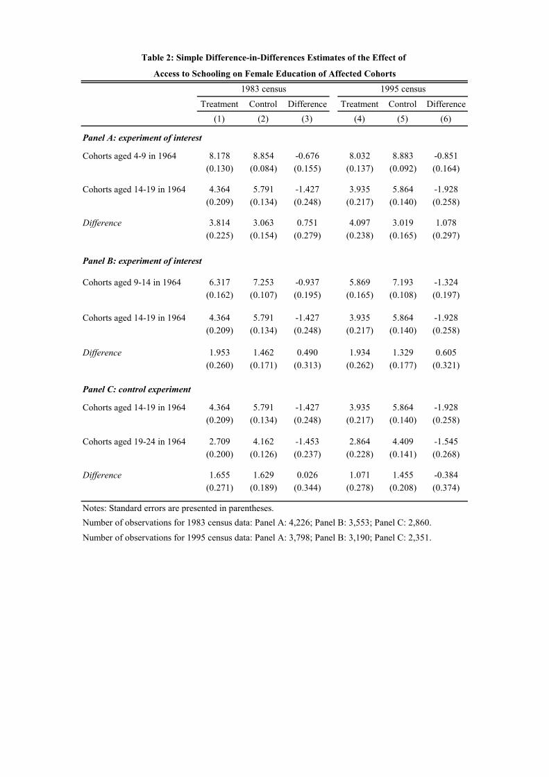
Treatment Control Difference Treatment Control Difference(1) (2) (3) (4) (5) (6)

Panel A: experiment of interest

Cohorts aged 4-9 in 1964 8.178 8.854 -0.676 8.032 8.883 -0.851(0.130) (0.084) (0.155) (0.137) (0.092) (0.164)

Cohorts aged 14-19 in 1964 4.364 5.791 -1.427 3.935 5.864 -1.928(0.209) (0.134) (0.248) (0.217) (0.140) (0.258)

Difference 3.814 3.063 0.751 4.097 3.019 1.078(0.225) (0.154) (0.279) (0.238) (0.165) (0.297)

Panel B: experiment of interest

Cohorts aged 9-14 in 1964 6.317 7.253 -0.937 5.869 7.193 -1.324(0.162) (0.107) (0.195) (0.165) (0.108) (0.197)

Cohorts aged 14-19 in 1964 4.364 5.791 -1.427 3.935 5.864 -1.928(0.209) (0.134) (0.248) (0.217) (0.140) (0.258)

Difference 1.953 1.462 0.490 1.934 1.329 0.605(0.260) (0.171) (0.313) (0.262) (0.177) (0.321)

Panel C: control experiment

Cohorts aged 14-19 in 1964 4.364 5.791 -1.427 3.935 5.864 -1.928(0.209) (0.134) (0.248) (0.217) (0.140) (0.258)

Cohorts aged 19-24 in 1964 2.709 4.162 -1.453 2.864 4.409 -1.545(0.200) (0.126) (0.237) (0.228) (0.141) (0.268)

Difference 1.655 1.629 0.026 1.071 1.455 -0.384(0.271) (0.189) (0.344) (0.278) (0.208) (0.374)

Number of observations for 1995 census data: Panel A: 3,798; Panel B: 3,190; Panel C: 2,351.

Notes: Standard errors are presented in parentheses.

Access to Schooling on Female Education of Affected Cohorts

Table 2: Simple Difference-in-Differences Estimates of the Effect of

1983 census 1995 census

Number of observations for 1983 census data: Panel A: 4,226; Panel B: 3,553; Panel C: 2,860.

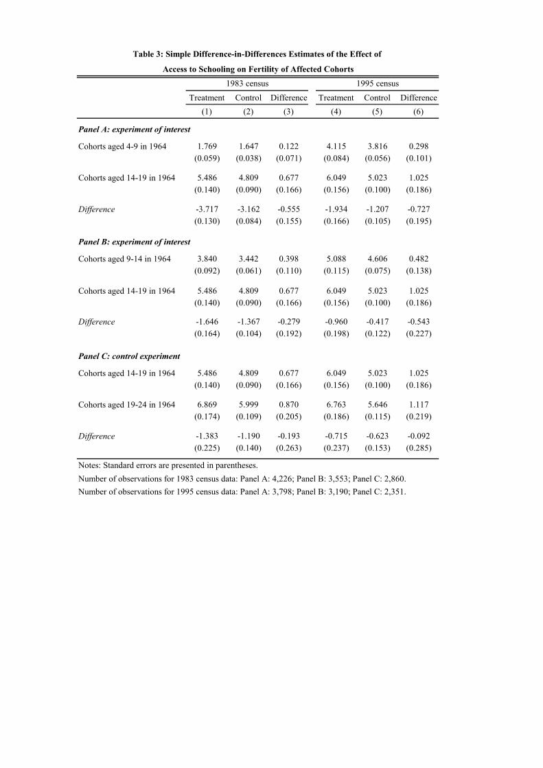
Treatment Control Difference Treatment Control Difference(1) (2) (3) (4) (5) (6)

Panel A: experiment of interest

Cohorts aged 4-9 in 1964 1.769 1.647 0.122 4.115 3.816 0.298(0.059) (0.038) (0.071) (0.084) (0.056) (0.101)

Cohorts aged 14-19 in 1964 5.486 4.809 0.677 6.049 5.023 1.025(0.140) (0.090) (0.166) (0.156) (0.100) (0.186)

Difference -3.717 -3.162 -0.555 -1.934 -1.207 -0.727(0.130) (0.084) (0.155) (0.166) (0.105) (0.195)

Panel B: experiment of interest

Cohorts aged 9-14 in 1964 3.840 3.442 0.398 5.088 4.606 0.482(0.092) (0.061) (0.110) (0.115) (0.075) (0.138)

Cohorts aged 14-19 in 1964 5.486 4.809 0.677 6.049 5.023 1.025(0.140) (0.090) (0.166) (0.156) (0.100) (0.186)

Difference -1.646 -1.367 -0.279 -0.960 -0.417 -0.543(0.164) (0.104) (0.192) (0.198) (0.122) (0.227)

Panel C: control experiment

Cohorts aged 14-19 in 1964 5.486 4.809 0.677 6.049 5.023 1.025(0.140) (0.090) (0.166) (0.156) (0.100) (0.186)

Cohorts aged 19-24 in 1964 6.869 5.999 0.870 6.763 5.646 1.117(0.174) (0.109) (0.205) (0.186) (0.115) (0.219)

Difference -1.383 -1.190 -0.193 -0.715 -0.623 -0.092(0.225) (0.140) (0.263) (0.237) (0.153) (0.285)

Number of observations for 1995 census data: Panel A: 3,798; Panel B: 3,190; Panel C: 2,351.

Table 3: Simple Difference-in-Differences Estimates of the Effect of

1983 census 1995 census

Notes: Standard errors are presented in parentheses.

Access to Schooling on Fertility of Affected Cohorts

Number of observations for 1983 census data: Panel A: 4,226; Panel B: 3,553; Panel C: 2,860.

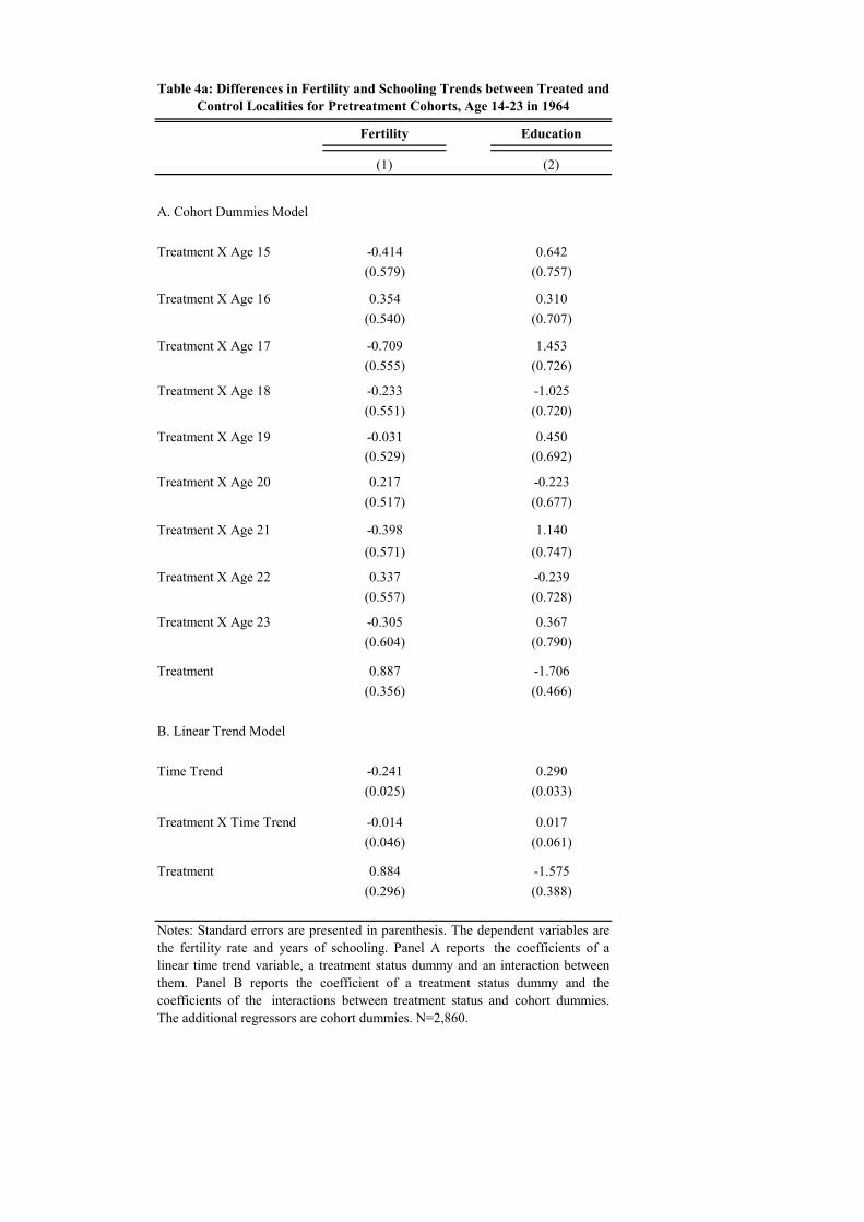
Fertility Education

(1) (2)

A. Cohort Dummies Model

Treatment X Age 15 -0.414 0.642(0.579) (0.757)

Treatment X Age 16 0.354 0.310(0.540) (0.707)

Treatment X Age 17 -0.709 1.453(0.555) (0.726)

Treatment X Age 18 -0.233 -1.025(0.551) (0.720)

Treatment X Age 19 -0.031 0.450(0.529) (0.692)

Treatment X Age 20 0.217 -0.223(0.517) (0.677)

Treatment X Age 21 -0.398 1.140(0.571) (0.747)

Treatment X Age 22 0.337 -0.239(0.557) (0.728)

Treatment X Age 23 -0.305 0.367(0.604) (0.790)

Treatment 0.887 -1.706(0.356) (0.466)

B. Linear Trend Model

Time Trend -0.241 0.290(0.025) (0.033)

Treatment X Time Trend -0.014 0.017(0.046) (0.061)

Treatment 0.884 -1.575(0.296) (0.388)

Table 4a: Differences in Fertility and Schooling Trends between Treated and Control Localities for Pretreatment Cohorts, Age 14-23 in 1964

Notes: Standard errors are presented in parenthesis. The dependent variables arethe fertility rate and years of schooling. Panel A reports the coefficients of alinear time trend variable, a treatment status dummy and an interaction betweenthem. Panel B reports the coefficient of a treatment status dummy and thecoefficients of the interactions between treatment status and cohort dummies.The additional regressors are cohort dummies. N=2,860.

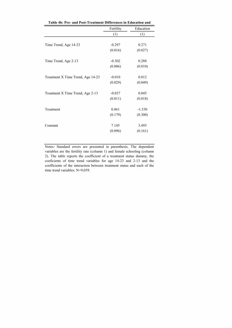
Fertility Education(1) (1)

Time Trend, Age 14-23 -0.297 0.271(0.016) (0.027)

Time Trend, Age 2-13 -0.302 0.288(0.006) (0.010)

Treatment X Time Trend, Age 14-23 -0.010 0.012(0.029) (0.049)

Treatment X Time Trend, Age 2-13 -0.037 0.045(0.011) (0.018)

Treatment 0.861 -1.530(0.179) (0.300)

Constant 7.145 3.493(0.096) (0.161)

Table 4b: Pre- and Post-Treatment Differences in Education and Fertility Trends between Treated and Control Localities, Age 2-23 in

Notes: Standard errors are presented in parenthesis. The dependentvariables are the fertility rate (column 1) and female schooling (column2). The table reports the coefficient of a treatment status dummy, thecoeficients of time trend variables for age 14-23 and 2-13 and thecoefficients of the interaction between treatment status and each of thetime trend variables. N=9,059.

OLS 2SLS

(1) (2) (3) (4) (5) (6) (7) (8)

A. Experiment of interest:Cohorts aged 4-9 and 14-19 in 1964

1983 census 0.751 0.694 0.738 -0.555 -0.533 -0.539 -0.240 -0.730(N=4,226) (0.279) (0.262) (0.257) (0.155) (0.147) (0.147) (0.009) (0.303)

1995 census 1.078 0.921 1.018 -0.727 -0.651 -0.609 -0.119 -0.598(N=3,798) (0.297) (0.283) (0.276) (0.195) (0.190) (0.188) (0.010) (0.238)

B. Experiment of interest:Cohorts aged 9-14 and 14-19 in 1964

1983 census 0.490 0.545 0.514 -0.279 -0.346 -0.342 -0.134 -0.665(N=3,553) (0.313) (0.289) (0.283) (0.192) (0.183) (0.181) (0.011) (0.480)

1995 census 0.605 0.533 0.575 -0.543 -0.507 -0.465 -0.088 -0.808(N=3,190) (0.321) (0.300) (0.293) (0.227) (0.220) (0.218) (0.013) (0.536)

C. Control experiment:Cohorts aged 14-19 and 19-24 in 1964

1983 census 0.026 0.028 0.039 -0.193 -0.189 -0.251 - -(N=2,860) (0.344) (0.305) (0.291) (0.263) (0.250) (0.246)

1995 census -0.384 -0.367 -0.334 -0.092 -0.101 -0.124 - -(N=2,351) (0.374) (0.342) (0.335) (0.285) (0.273) (0.271)

Control variablesIndividual level religion dummy No Yes Yes No Yes Yes Yes Yes

Locality fixed effects No No Yes No No Yes No YesNotes: Standard errors are presented in parentheses. The religion dummy indicates Muslim or Christian. In the 1983 census data, columns (2),(3), (5), (6), (7) and (8) include cohort dummies.

Table 5: Estimated Effect of Female Education on Fertility: First Stage, Reduced Form, OLS and 2SLS Estimates

Years of schooling Fertility Fertility

First stage Reduced form

OLS 2SLS(1) (2) (3) (4) (5) (6) (7) (8)

A. Spouse older than 8 in 1964a. Experiment of interest:Cohorts aged 4-9 and 14-19 in 1964

1995 census 1.006 0.934 0.889 -0.670 -0.631 -0.607 -0.165 -0.683(N=2,239) (0.365) (0.345) (0.340) (0.212) (0.202) (0.201) (0.011) (0.312)

b. Experiment of interest:Cohorts aged 14-19 and 19-24 in 1964

1995 census -0.541 -0.477 -0.439 0.202 0.171 0.142 - -(N=1,856) (0.418) (0.379) (0.375) (0.281) (0.267) (0.267)

B. Spouse older than 13 in 1964a. Experiment of interest:Cohorts aged 4-9 and 14-19 in 1964

1995 census 0.800 0.746 0.793 -0.569 -0.542 -0.594 -0.155 -0.749(N=1,338) (0.544) (0.506) (0.503) (0.339) (0.323) (0.324) (0.016) (0.573)

b. Experiment of interest:Cohorts aged 14-19 and 19-24 in 1964

1995 census -0.650 -0.574 -0.522 0.360 0.323 0.305 - -(N=1,785) (0.425) (0.385) (0.381) (0.286) (0.272) (0.271)

Control variablesIndividual level religion dummy No Yes Yes No Yes Yes Yes Yes

Locality fixed effects No No Yes No No Yes No Yes

Notes: Standard errors are presented in parentheses. The religion dummy indicates Muslim or Christian. In the 1983 census data, columns (2), (3), (5), (6) and (8) include cohort dummies.

Table 6: Estimated Effect of Female Education on Fertility: First Stage,Reduced Form, OLS and 2SLS Estimates, Sample of Women Married to Older Spouses

Years of schooling Fertility FertilityFirst stage Reduced form

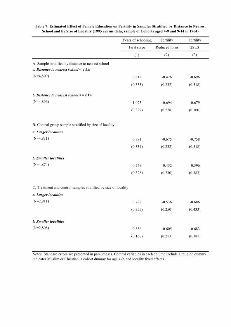
Years of schooling Fertility Fertility

First stage Reduced form 2SLS

(1) (2) (3)

A. Sample stratified by distance to nearest schoola. Distance to nearest school < 4 km

(N=4,809) 0.612 -0.426 -0.696

(0.333) (0.232) (0.518)

b. Distance to nearest school >= 4 km

(N=4,896) 1.023 -0.694 -0.679

(0.329) (0.228) (0.300)

B. Control-group sample stratified by size of locality

a. Larger localities (N=4,831) 0.891 -0.675 -0.758

(0.334) (0.232) (0.518)

b. Smaller localities (N=4,874) 0.759 -0.452 -0.596

(0.328) (0.230) (0.383)

C. Treatment and control samples stratified by size of locality

a. Larger localities (N=2,911) 0.782 -0.536 -0.686

(0.355) (0.250) (0.433)

b. Smaller localities (N=2,808) 0.886 -0.605 -0.683

(0.160) (0.253) (0.387)

Notes: Standard errors are presented in parentheses. Control variables in each column include a religion dummy indicates Muslim or Christian, a cohort dummy for age 4-9, and locality fixed effects.

Table 7: Estimated Effect of Female Education on Fertility in Samples Stratified by Distance to Nearest School and by Size of Locality (1995 census data, sample of Cohorts aged 4-9 and 9-14 in 1964)

OLS 2SLS OLS 2SLS OLS 2SLS OLS 2SLS(1) (2) (3) (4) (5) (6) (7) (8)

Panel A: own outcomes

Labor-force participation 0.032 -0.139 0.039 -0.040 0.030 -0.035 0.036 -0.007(0.001) (0.070) (0.001) (0.034) (0.001) (0.063) (0.002) (0.051)

Marriage -0.007 0.055 0.003 -0.011 0.005 -0.068 0.004 -0.061(0.002) (0.042) (0.001) (0.024) (0.001) (0.063) (0.001) (0.051)

Age upon marriage 0.115 -0.107 0.216 0.506 0.150 -0.091 0.157 -0.490(0.014) (0.230) (0.023) (0.472) (0.016) (0.331) (0.028) (1.084)

Divorce -0.000 0.004 -0.001 -0.009 -0.000 0.002 -0.001 -0.028(0.000) (0.006) (0.000) (0.008) (0.000) (0.011) (0.000) (0.020)

Panel B: spouse outcomes

Years of schooling 0.498 0.579 0.545 0.537 0.502 0.464 0.466 0.538(0.014) (0.223) (0.015) (0.283) (0.015) (0.285) (0.017) (0.449)

Labor-force participation 0.007 0.006 0.019 -0.018 0.007 -0.019 0.017 -0.007(0.001) (0.017) (0.002) (0.033) (0.001) (0.026) (0.002) (0.056)

Ln (monthly earnings) 0.027 0.067 0.034 -0.034 0.033 0.092 0.030 0.001(0.003) (0.042) (0.003) (0.058) (0.003) (0.076) (0.003) (0.102)

Table 8: OLS and 2SLS Estimates of the Effect of Education on Woman's

Labor-Force Participation, Marriage, Age upon Marriage, Divorce, and Spouse's Outcomes

Notes: Standard errors are presented in parentheses.

Cohorts aged 9-14 and 14 -19 in 1964

1983 census 1995 census

Cohorts aged 4-9 and 14 -19 in 1964

1983 census 1995 census

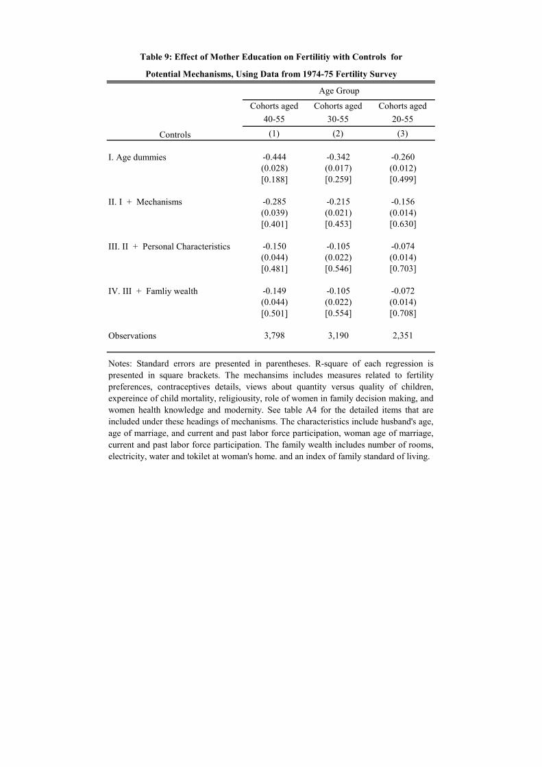
Cohorts aged Cohorts aged Cohorts aged40-55 30-55 20-55

Controls (1) (2) (3)

I. Age dummies -0.444 -0.342 -0.260(0.028) (0.017) (0.012)[0.188] [0.259] [0.499]

II. I + Mechanisms -0.285 -0.215 -0.156(0.039) (0.021) (0.014)[0.401] [0.453] [0.630]

III. II + Personal Characteristics -0.150 -0.105 -0.074(0.044) (0.022) (0.014)[0.481] [0.546] [0.703]

IV. III + Famliy wealth -0.149 -0.105 -0.072(0.044) (0.022) (0.014)[0.501] [0.554] [0.708]

Observations 3,798 3,190 2,351

Table 9: Effect of Mother Education on Fertilitiy with Controls for

Potential Mechanisms, Using Data from 1974-75 Fertility Survey

Age Group

Notes: Standard errors are presented in parentheses. R-square of each regression ispresented in square brackets. The mechansims includes measures related to fertilitypreferences, contraceptives details, views about quantity versus quality of children,expereince of child mortality, religiousity, role of women in family decision making, andwomen health knowledge and modernity. See table A4 for the detailed items that areincluded under these headings of mechanisms. The characteristics include husband's age,age of marriage, and current and past labor force participation, woman age of marriage,current and past labor force participation. The family wealth includes number of rooms,electricity, water and tokilet at woman's home. and an index of family standard of living.

(1) (2) (3) (4) (5) (6) (7) (8)

Experiment of interest:Cohorts aged 4-9 and 14-19 in 1964

1.046 0.992 -0.660 -0.663 -0.088 -0.100 -0.631 -0.669(N=3,798) (0.296) (0.289) (0.199) (0.194) (0.011) (0.010) (0.250) (0.265)

Control variables

Individual level religion dummy Yes Yes Yes Yes Yes Yes Yes Yes

Clinics dummy Yes No Yes No Yes No Yes No

Clinics dummy* cohort dummy Yes Yes Yes Yes Yes Yes Yes Yes

Notes: Standard errors are presented in parentheses. The religion dummy indicates Muslim or Christian..

Table 10: Estimated Effect of Female Education on Fertility with Control for Access to Health Servicesusing 1995 Census Data

Years of schooling Fertility FertilityFirst stage Reduced form OLS 2SLS

OLS 2SLS(1) (2) (3) (4) (5) (6) (7) (8)

A. Original control group excluding seven largest localities

Experiment of interest:Cohorts aged 4-9 and 14-19 1.245 1.011 1.171 -0.856 -0.734 -0.705 -0.100 -0.602(N=2,283) (0.353) (0.338) (0.328) (0.232) (0.226) (0.225) (0.013) (0.251)

Control experiment:Cohorts aged 14-19 and 19-24 -0.608 -0.667 -0.667 0.114 0.149 0.151 - -(N=1,577) (0.399) (0.373) (0.369) (0.318) (0.307) (0.305)

B. Control group includes only Arabs from mixed cities

Experiment of interest:Cohorts aged 4-9 and 14-19 2.424 2.155 2.249 -1.210 -1.094 -1.091 -0.131 -0.485(N=1,751) (0.430) (0.408) (0.399) (0.275) (0.269) (0.266) (0.015) (0.140)

Control experiment:Cohorts aged 14-19 and 19-24 0.124 0.148 0.053 0.041 0.028 0.101 - -(N=1,065) (0.514) (0.471) (0.461) (0.381) (0.365) (0.363)

C. Sample of Table 5 restricted to persons born in current locality

Experiment of interest:Cohorts aged 4-9 and 14-19 1.149 0.966 1.092 -0.822 -0.720 -0.657 -0.140 -0.602(N=2,729) (0.337) (0.324) (0.313) (0.232) (0.226) (0.224) (0.012) (0.258)

Control experiment:Cohorts aged 14-19 and 19-24 -0.770 -0.662 -0.672 0.138 0.074 0.007 - -(N=1,714) (0.414) (0.384) (0.377) (0.326) (0.313) (0.311)

Control variablesIndividual level religion dummy No Yes Yes No Yes Yes Yes Yes

Locality fixed effects No No Yes No No Yes No Yes

Notes: Standard errors are presented in parentheses. Individual characteristics include a religion dummy (Muslim or Christian). In the 1983 census data,

Columns (2), (3), (5), (6) and (8) include cohort dummies. Experiment of interest:Cohorts aged 4-8 and 14-18 in 1964. Control experiment:Cohorts aged

14-18 and 19-23 in 1964.

Table 11: Estimated Effect of Female Education on Fertility Based on Alternative Control Groups and Samples (1995 Census Data)

Years of schooling Fertility Fertility

First stage Reduced form

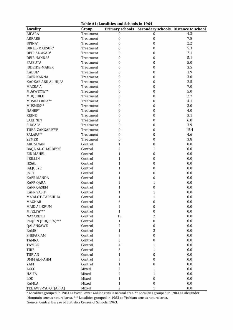
Locality Group Primary schools Secondary schools Distance to schoolAR'ARA Treatment 0 0 4.3ARRABE Treatment 0 0 7.8BI'INA* Treatment 0 0 2.2BIR EL-MAKSUR* Treatment 0 0 5.3DEIR AL-ASAD* Treatment 0 0 2.1DEIR HANNA* Treatment 0 0 5.1FASSUTA Treatment 0 0 5.0JUDEIDE-MAKER Treatment 0 0 3.5KABUL* Treatment 0 0 1.9KAFR KANNA Treatment 0 0 3.0KAOKAB ABU AL-HIJA* Treatment 0 0 2.5MAZRA'A Treatment 0 0 7.0MUAWIYYE** Treatment 0 0 5.0MUQEIBLE Treatment 0 0 2.7MUSHAYRIFA** Treatment 0 0 4.1MUSMUS** Treatment 0 0 3.0NAHEF* Treatment 0 0 4.0REINE Treatment 0 0 3.1SAKHNIN Treatment 0 0 6.8SHA'AB* Treatment 0 0 3.9TUBA-ZANGARIYYE Treatment 0 0 15.4ZALAFA** Treatment 0 0 4.6ZEMER Treatment 0 0 3.8ABU SINAN Control 1 0 0.0BAQA AL-GHARBIYYE Control 2 1 0.0EIN MAHEL Control 1 0 0.0I'BILLIN Control 1 0 0.0IKSAL Control 1 0 0.0JALJULYE Control 1 0 0.0JATT Control 1 0 0.0KAFR MANDA Control 1 0 0.0KAFR QARA Control 2 1 0.0KAFR QASEM Control 1 0 0.0KAFR YASIF Control 1 1 0.0MA'ALOT-TARSHIHA Control 1 1 0.0MAGHAR Control 3 0 0.0MAJD AL-KRUM Control 2 0 0.0MI'ELYA*** Control 1 0 0.0NAZARETH Control 13 2 0.0PEQI'IN (BUQEI'A)*** Control 1 0 0.0QALANSAWE Control 2 0 0.0RAME Control 1 2 0.0SHEFAR'AM Control 3 0 0.0TAMRA Control 3 0 0.0TAYIBE Control 4 1 0.0TIRE Control 3 1 0.0TUR'AN Control 1 0 0.0UMM AL-FAHM Control 5 0 0.0YAFI Control 1 0 0.0ACCO Mixed 2 1 0.0HAIFA Mixed 2 1 0.0LOD Mixed 1 0 0.0RAMLA Mixed 1 0 0.0TEL AVIV-YAFO (JAFFA) Mixed 2 1 0.0* Localities grouped in 1983 as West Lower Galilee census natural area. ** Localities grouped in 1983 as Alexander Mountain census natural area. *** Localities grouped in 1983 as Yechiam census natural area. Source: Central Bureau of Statistics Census of Schools, 1963.

Table A1: Localities and Schools in 1964

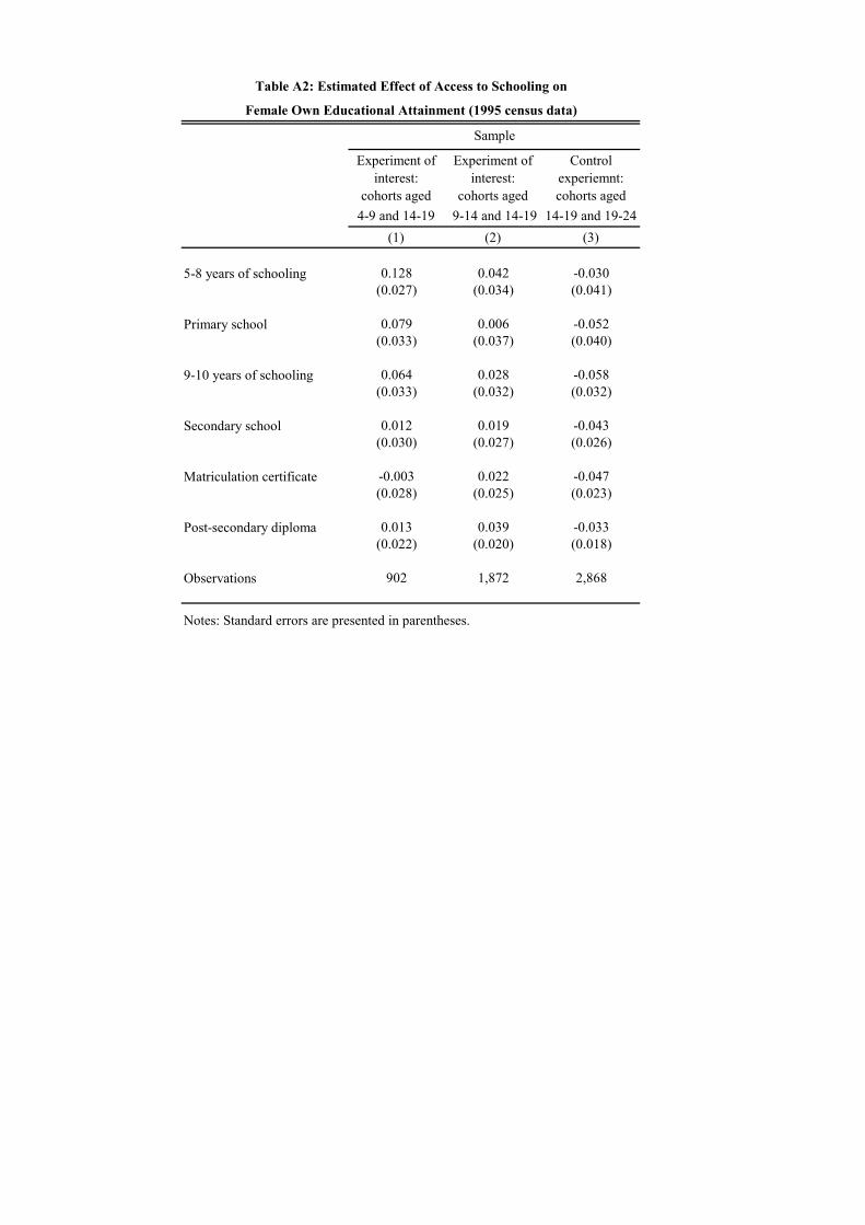
Experiment of interest:

Experiment of interest:

Control experiemnt:

cohorts aged cohorts aged cohorts aged4-9 and 14-19 9-14 and 14-19 14-19 and 19-24

(1) (2) (3)

5-8 years of schooling 0.128 0.042 -0.030(0.027) (0.034) (0.041)

Primary school 0.079 0.006 -0.052(0.033) (0.037) (0.040)

9-10 years of schooling 0.064 0.028 -0.058(0.033) (0.032) (0.032)

Secondary school 0.012 0.019 -0.043(0.030) (0.027) (0.026)

Matriculation certificate -0.003 0.022 -0.047(0.028) (0.025) (0.023)

Post-secondary diploma 0.013 0.039 -0.033(0.022) (0.020) (0.018)

Observations 902 1,872 2,868

Table A2: Estimated Effect of Access to Schooling on

Sample

Notes: Standard errors are presented in parentheses.

Female Own Educational Attainment (1995 census data)

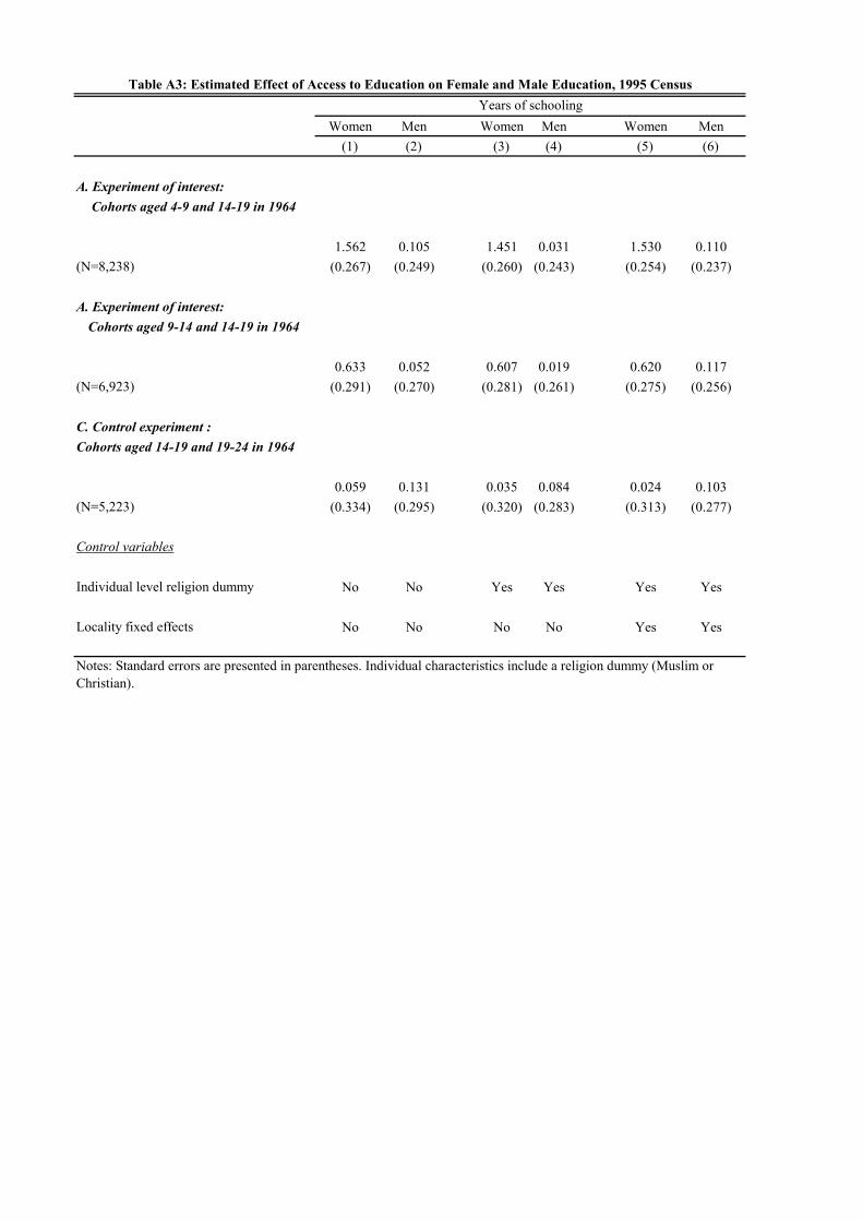
Women Men Women Men Women Men(1) (2) (3) (4) (5) (6)

A. Experiment of interest: Cohorts aged 4-9 and 14-19 in 1964

1.562 0.105 1.451 0.031 1.530 0.110(N=8,238) (0.267) (0.249) (0.260) (0.243) (0.254) (0.237)

A. Experiment of interest: Cohorts aged 9-14 and 14-19 in 1964

0.633 0.052 0.607 0.019 0.620 0.117(N=6,923) (0.291) (0.270) (0.281) (0.261) (0.275) (0.256)

C. Control experiment : Cohorts aged 14-19 and 19-24 in 1964

0.059 0.131 0.035 0.084 0.024 0.103(N=5,223) (0.334) (0.295) (0.320) (0.283) (0.313) (0.277)

Control variables

Individual level religion dummy No No Yes Yes Yes Yes

Locality fixed effects No No No No Yes Yes

Table A3: Estimated Effect of Access to Education on Female and Male Education, 1995 CensusYears of schooling

Notes: Standard errors are presented in parentheses. Individual characteristics include a religion dummy (Muslim or Christian).

Mother's Education

Father's Education

Mother's Education

Father's Education

Mother's Education

Father's Education

(1) (2) (3) (4) (5) (6)

Woman's fertility preferences

Considered desired number of children 0.027 0.022 0.025 0.020 0.021 0.017(0.003) (0.003) (0.004) (0.004) (0.004) (0.004)

Number of children desired -0.063 -0.018 -0.051 -0.011 -0.046 -0.012(0.016) (0.016) (0.017) (0.017) (0.017) (0.017)

Important to have at least one son -0.004 0.003 -0.003 0.003 -0.003 0.002(0.002) (0.002) (0.002) (0.002) (0.002) (0.002)

Important to have at least one daughter -0.003 0.005 -0.002 0.003 -0.002 0.002(0.002) (0.002) (0.002) (0.003) (0.002) (0.003)

Contraceptives details

Consulted wth doctor about birth control 0.027 0.006 0.028 0.005 0.021 -0.001(0.004) (0.004) (0.004) (0.004) (0.004) (0.004)

Consulted with anyone about birth control 0.029 0.006 0.029 0.005 0.024 0.000(0.003) (0.004) (0.004) (0.004) (0.004) (0.004)

Ever done anything to prevent pregnancy 0.030 0.007 0.030 0.007 0.025 0.002(0.004) (0.004) (0.004) (0.004) (0.004) (0.004)

Used any method to prevent pregnancy 0.031 0.006 0.031 0.007 0.026 0.002(0.004) (0.004) (0.004) (0.004) (0.004) (0.004)

Respondent knows how prevent pregnancy 0.025 0.000 0.024 -0.003 0.022 -0.004(0.005) (0.005) (0.005) (0.005) (0.005) (0.005)

Attidude about Quantity versus quality of children

Limiting number of children influences chances 0.010 0.001 0.010 -0.003 0.011 -0.001 of their advance (0.003) (0.003) (0.003) (0.003) (0.003) (0.003)

Should 14 years old boy continue studying -0.001 0.003 -0.000 0.003 -0.000 0.003(0.001) (0.001) (0.001) (0.001) (0.001) (0.001)

Should 14 years old girl continue studying 0.005 0.007 0.004 0.006 0.004 0.005(0.001) (0.002) (0.001) (0.002) (0.001) (0.002)

Notes: on next page.

Table A4 : Education and Fertility Preferences, Contraceptives Details, Quality of children, Child Mortality, Religiousity, Family Decision Making, and Health knowledge, Using Data from 1974-75 Fertility Survey

Conrol 1 Conrol 2 Conrol 3

Mother's Education

Father's Education

Mother's Education

Father's Education

Mother's Education

Father's Education

(1) (2) (3) (4) (5) (6)

Incidence of child mortality

Ever experienced child mortality -0.011 -0.006 -0.010 -0.006 -0.009 -0.005(0.003) (0.003) (0.003) (0.003) (0.003) (0.003)

Number of children deaths -0.013 -0.012 -0.015 -0.009 -0.014 -0.007(0.005) (0.007) (0.005) (0.006) (0.005) (0.006)

Number of miscarriages and abortions 0.007 -0.017 0.008 -0.011 0.009 -0.009(0.009) (0.010) (0.009) (0.010) (0.009) (0.010)

Religiousity

Degree of religiosity in current home -0.009 -0.006 -0.010 -0.003 -0.009 -0.003(0.003) (0.003) (0.003) (0.003) (0.003) (0.003)

Observe religious laws/rituals -0.006 -0.007 -0.008 -0.004 -0.011 -0.006(0.003) (0.004) (0.004) (0.004) (0.004) (0.004)

Woman role in family decision making

Respondent decides on daily expenses 0.004 -0.000 0.005 -0.002 0.005 -0.003(0.002) (0.002) (0.002) (0.002) (0.002) (0.002)

Respondent decides on large expenses 0.017 -0.002 0.016 -0.006 0.014 -0.006(0.003) (0.004) (0.004) (0.004) (0.004) (0.004)

Respondent decides on childen's education 0.011 0.003 0.014 0.002 0.012 0.001(0.003) (0.003) (0.003) (0.003) (0.003) (0.003)

Respondent decides on shopping for children 0.007 0.003 0.010 0.004 0.009 0.003(0.002) (0.003) (0.002) (0.003) (0.002) (0.003)

Health knowledge/ modernity

Sickness is due to physical/medical reasons 0.030 0.005 0.028 0.004 0.023 -0.001(0.004) (0.004) (0.004) (0.004) (0.004) (0.004)

Wears traditional (religious) clothes -0.035 -0.014 -0.037 -0.013 -0.031 -0.011(0.003) (0.003) (0.003) (0.003) (0.003) (0.003)

Control 2: Control 1 + husband's age, age of marriage of husband/wife, husband and wife current working status indicators, husband and wife ever worked indicators.Control 3: Control 2 + number of rooms, electricity, running water and toilet in woman's home, and an index of standard of living.

Table A4: Continued

Conrol 1 Conrol 2 Conrol 3

Notes: Standard errors are presented in parenthesis. The table presents estimates from three different specifcations, each different set of controls, defined as follows:

Control 1: religion and wife's age.

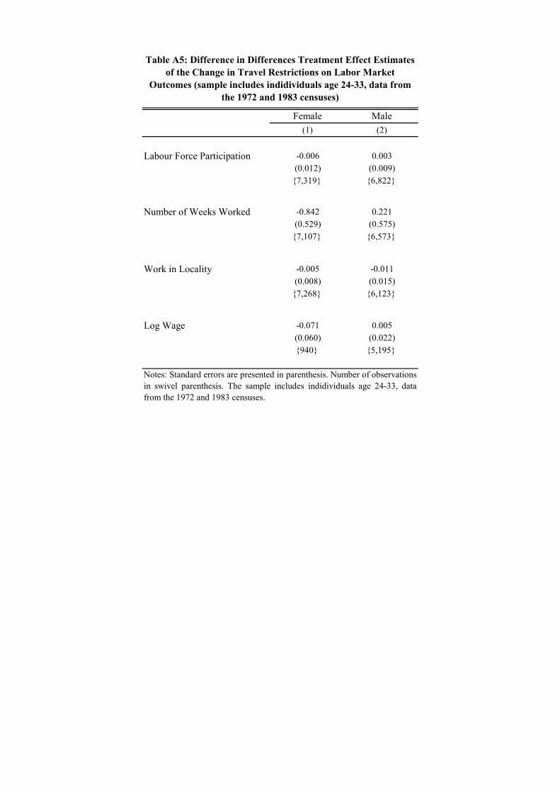
Female Male

(1) (2)

Labour Force Participation -0.006 0.003(0.012) (0.009)

{7,319} {6,822}

Number of Weeks Worked -0.842 0.221(0.529) (0.575)

{7,107} {6,573}

Work in Locality -0.005 -0.011(0.008) (0.015)

{7,268} {6,123}

Log Wage -0.071 0.005(0.060) (0.022){940} {5,195}

Table A5: Difference in Differences Treatment Effect Estimates of the Change in Travel Restrictions on Labor Market

Outcomes (sample includes indidividuals age 24-33, data from the 1972 and 1983 censuses)

Notes: Standard errors are presented in parenthesis. Number of observationsin swivel parenthesis. The sample includes indidividuals age 24-33, datafrom the 1972 and 1983 censuses.

Female Male

(1) (2)

Number of Rooms at Home 0.061 -0.037(0.078) (0.077)

Running Water at Home 0.012 0.037(0.025) (0.024)

Electricity at Home 0.001 -0.001(0.025) (0.023)

Toilet at Home 0.037 0.013(0.022) (0.020)

Log Family Income 0.010 0.017(0.061) (0.055)

Table A6: Difference in Differences Treatment Effect Estimates of the Change in Travel Restrictions on Family Wealth and Assets at Ages 12-21 and 22-26 (data from the 1972 census)

Notes: Standard errors are presented in parenthesis.

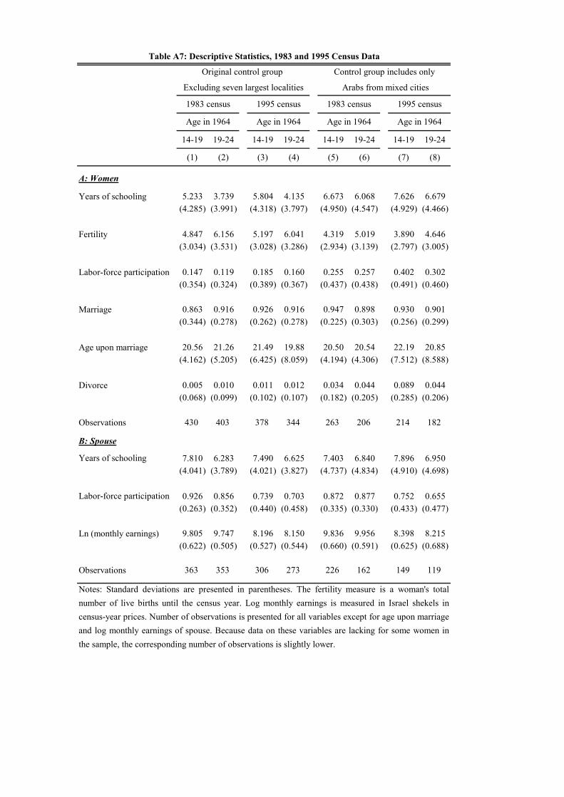
14-19 19-24 14-19 19-24 14-19 19-24 14-19 19-24

(1) (2) (3) (4) (5) (6) (7) (8)

A: Women

Years of schooling 5.233 3.739 5.804 4.135 6.673 6.068 7.626 6.679(4.285) (3.991) (4.318) (3.797) (4.950) (4.547) (4.929) (4.466)

Fertility 4.847 6.156 5.197 6.041 4.319 5.019 3.890 4.646(3.034) (3.531) (3.028) (3.286) (2.934) (3.139) (2.797) (3.005)

Labor-force participation 0.147 0.119 0.185 0.160 0.255 0.257 0.402 0.302(0.354) (0.324) (0.389) (0.367) (0.437) (0.438) (0.491) (0.460)

Marriage 0.863 0.916 0.926 0.916 0.947 0.898 0.930 0.901(0.344) (0.278) (0.262) (0.278) (0.225) (0.303) (0.256) (0.299)

Age upon marriage 20.56 21.26 21.49 19.88 20.50 20.54 22.19 20.85(4.162) (5.205) (6.425) (8.059) (4.194) (4.306) (7.512) (8.588)

Divorce 0.005 0.010 0.011 0.012 0.034 0.044 0.089 0.044(0.068) (0.099) (0.102) (0.107) (0.182) (0.205) (0.285) (0.206)

Observations 430 403 378 344 263 206 214 182

B: Spouse

Years of schooling 7.810 6.283 7.490 6.625 7.403 6.840 7.896 6.950(4.041) (3.789) (4.021) (3.827) (4.737) (4.834) (4.910) (4.698)

Labor-force participation 0.926 0.856 0.739 0.703 0.872 0.877 0.752 0.655(0.263) (0.352) (0.440) (0.458) (0.335) (0.330) (0.433) (0.477)

Ln (monthly earnings) 9.805 9.747 8.196 8.150 9.836 9.956 8.398 8.215(0.622) (0.505) (0.527) (0.544) (0.660) (0.591) (0.625) (0.688)

Observations 363 353 306 273 226 162 149 119

Table A7: Descriptive Statistics, 1983 and 1995 Census Data

Original control group Control group includes only

1983 census 1995 census 1983 census 1995 census

Notes: Standard deviations are presented in parentheses. The fertility measure is a woman's totalnumber of live births until the census year. Log monthly earnings is measured in Israel shekels incensus-year prices. Number of observations is presented for all variables except for age upon marriageand log monthly earnings of spouse. Because data on these variables are lacking for some women inthe sample, the corresponding number of observations is slightly lower.

Excluding seven largest localities Arabs from mixed cities

Age in 1964 Age in 1964 Age in 1964 Age in 1964

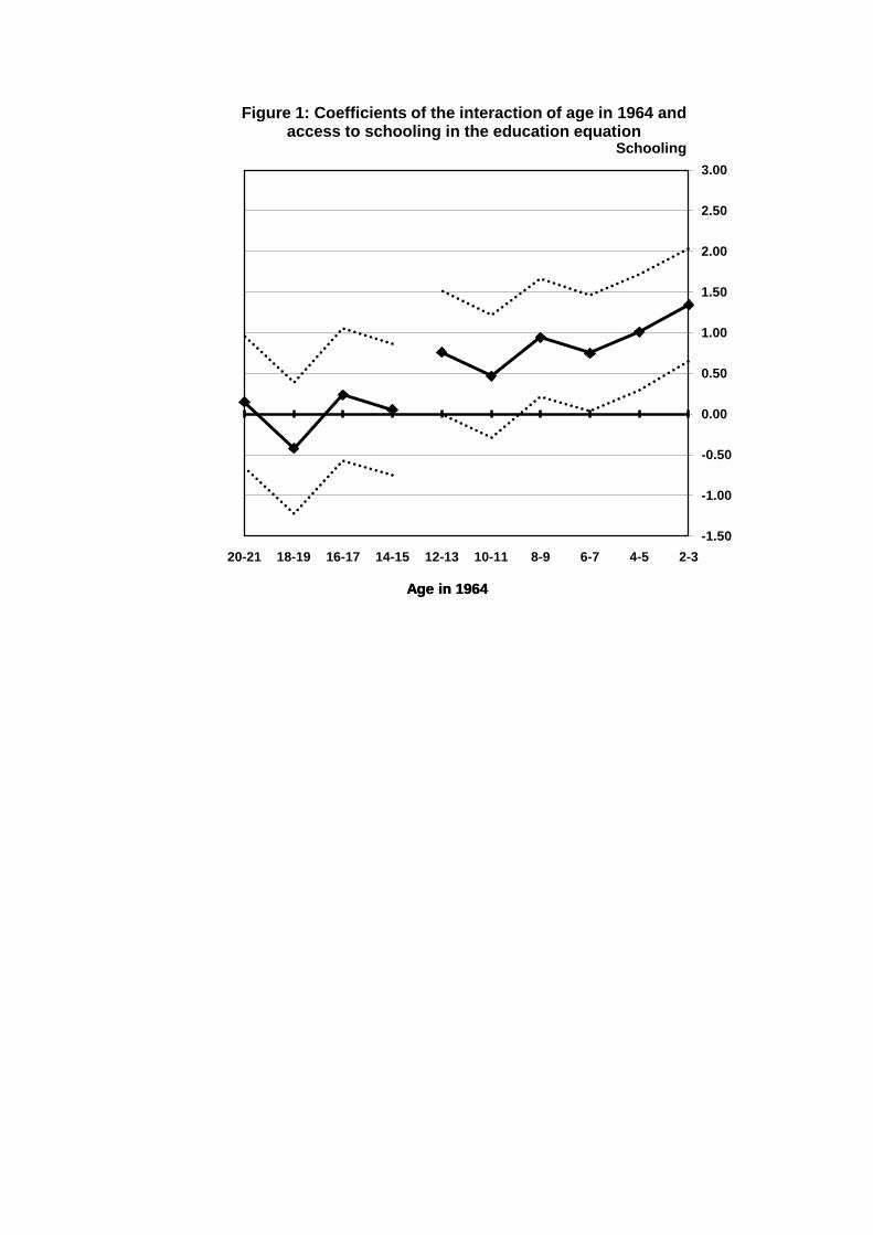
-1.50

-1.00

-0.50

0.00

0.50

1.00

1.50

2.00

2.50

3.00

2-34-56-78-910-1112-1314-1516-1718-1920-21

Figure 1: Coefficients of the interaction of age in 1964 and access to schooling in the education equation

Age in 1964Age in 1964

Schooling