Morphology from imagery: detecting and measuring the density of urban land use
23
CHAPTER 40 MORPHOLOGY FROM IMAGERY: DETECTING AND MEASURING THE DENSITY OF URBAN LAND USE (TV Mesev, P Longley M Batty and Y Xie) Environment and Planning A, 1995, 27, 759-780 726
Transcript of Morphology from imagery: detecting and measuring the density of urban land use

CHAPTER 40
MORPHOLOGY FROM IMAGERY DETECTING AND MEASURING THE DENSITY OF URBAN LAND USE
(TV Mesev P Longley M Batty and Y Xie)
Environment and Planning A 1995 27 759-780
726
Environment and Planning A 1995 volume 27 pages 759 -780
MorPhology from imagery detecting and measuring the density of urban land use
T V Mesev P A Longley Department of Geography University of Bristol University Road Bristol BS8 ISS England
M Batty Y Xie National Center for Geographic Information and Analysis State University of New York Wilkeson Quad Buffalo NY 14261-0023 USA Received 15 January 1994 in revised form 20 April 1994
Abstract Defining urban morphology in terms of the shape and density of urban land use has hitherto depended upon the informed yet subjective recognition of patterns consistent with spatial theory In this paper we exploit the potential of urban image analysis from remotely sensed data to detect then measure various elements of urban form and its land use thus providing a basis for consistent definition and thence comparison First we introduce methods for classifying urban areas and individual land uses from remotely sensed images by using conventional maximum likelihood discriminators which utilize the spectral densities associated with different elements of the image As a benchmark to our classifications we use smoothed UK Population Census data From the analysis we then extract various definitions of the urban area and its distinct land uses which we represent in terms of binary surfaces arrayed on fine grids with resolutions of approxishymately 20 m and 30 m These images form surfaces which reveal both the shape of land use and its density in terms of the amount of urban space filled and these provide the data for subsequent density analysis This analysis is based upon fractal theory in which densities of occupancy at different distances from fixed points are modeled by means of power functions We illustrate this for land use in Bristol England extracted from Landsat TM-5 and SPOT HRV images and dimensioned from population census data for 1981 and 1991 We provide for the first time not only fractal measurements of the density of different land uses but measures of the temporal change in these densities
1 Measuring urban morphology Whatever approach to urban analysis is taken cities are usually visualized at some stage in terms of their geometric form Urban economics transportation and social structure are predicated in spatial terms and thus the effects of such theory are often articulated through geometric notions involving the shape of urban land use and the manner in which it spreads Shape and density measure the way in which urban space is filled and are thus key elements in the definition of morphology Until recently it has been difficult to link the geometric form of real cities to formal theories explaining densities and thus urban economic theory for example has evolved within highly idealized geometries which bear little relation to real spatial patterns
The development of fractal geometry however which is in essence a geometry of the irregular has clear relevance to spatial systems such as cities The rudiments of a fractal theory of cities now exists which has the potential to synthesize many ideas from location theory with spatial form (Batty and Longley 1994 frankhauser 1994) The notion that cities are self-similar in their functions has been writ large in urban theory for over a century and is manifest in terms of relations such as the rank - size rule hierarchical differentiation of service centers as in central place theory transportation hierarchies and modes and in the area and importance of different orders of hinterland (Arlinghaus 1985 1993) All these relations which form the cornerstones of urban geography can be described and modeled by using
727
760 T V Mesev M Batty P A Longley i Xie
power laws which are fractaL What this new geometry is beginning to do is to tie all these notions explicitly together in a geometry of the irregular a geometry of the real world (Mandelbrot 1983)
We take this fractal theory as our starting point and in this paper we use its simplest elements which involve the measurement of shape and density Our purshypose here however is not to extend this theory very far but to concentrate on the equally important problem of detecting the appropriate shape and density of urban areas and the land uses which occupy them Hitheno most characterizations of urban land use have depended upon some visual inspection of spatial patterns and the identification of visual distinctions which serve to reinforce functional differshyences Such classification is often informed by statistical analysis but methods for controlling the consistency of such definitions between different case studies are
Jacking and thus comparative analysis is limited Measurement of course prescribes analysis and it is only as improved data sets
become available and methods of representing urban phenomena become more transparent that morphological analysis becomes more tractable In our own previshyous work (Batty and Longley 1994 Longley and Batty 1989a 1989b) we have been aware that the definitions of urbanity adopted for particular administrative purposes are not usually the most appropriate to more general measurement and analysis Yet issues of confidentiality and aggregation dictated that socioeconomic data are rarely available for disaggregate study at finer resolutions
Where models of socioeconomic data have been devised to interpolate continushyous surfaces about point infonnation (Martin 1991) estimates are not accurate at any scale finer than around a 200 m resolution and there is the concern that measurement of urban fonn in fact represents the assumptions in the modeling procedure rather than the underlying distributions of individuals buildings and land uses which it is intended to detect With the development of remotely sensed data however the prospect exists for both finer resolution and consistent classificashytion of urban areas and land use across universally available data This is the task we will address here showing how the data which are derived can be interpreted by means of fractal theory
In this paper we are thus concerned with the detection then measurement of urban morphologies from remotely sensed imagery We will begin with methods for the generation of distinct land uses from such images outlining the conventional technique of discrimination based on maximum likelihood estimators applied to the spectral bands which define such images We augment this method by using small area census statistics from the UK Population Census to ground the interpretations we make in an independent data source and from the resulting analysis we define discrete categories of land use for each pixel in the image The resulting surfaces show the presence or absence of a particular land use in each cell and it is these that are then measured in terms of their shape and_ density by means of fractal methods
Here we use two broad approaches to measuring density First we consider the absolute amount of space within the total available which is filled by a given land use and second we consider the ra~e at which space is filled with respect to distance from some central point in the city [usually the central business district or (CBD)] Both these methods yield various parameters the most significant of which is the fractal dimension However because these methods yield different estimates we introduce a new method which is based upon elements of each We also test the sensitivity of these methods to reductions in the size of the images over which the analysis takes place 728
Measuring the density of urban land use
The data for which we develop these applications are derived from the Landsat TM-5 image taken in April 1984 and from the SPOT HRV image taken in June 1988 f0r the urban area of Bristol England From these images together with socioeconomic data from the 1981 and 1991 Population Censuses different types of land use are extracted and these form the surfaces which are then subject to fractar analysis Four distinct components of land use can be identified from the 1981 data eight from the 1991 and this enables some comparison through fractal theory of urban form in terms of individual land-use patterns Temporal comparishysons are also made with the emphasis on comparative analysis demonstrating how such analysis can be made routine by use of remotely sensed data We conclude the paper with some comments on the potential for using remotely sensed data for extensive comparative analysis of urban morphologies a potential which has not been realizable hitherto
2 Extracting land-use patterns from remotely sensed data Standard methods for classifying remotely sensed data exist within proprietary software image analysis packages and here we have used the most commonly used commercial per-pixel classifier the maximum likelihood classifier based on Bayesian principles The version we have chosen is implemented in the Imagine Version 802 package from ERDAS Inc Atlanta GA This software computes the likelihood of a pixel belonging to any class with the spectral categories of the image represented by Gaussian probability density functions described by associated mean vector and covariance matrices Readers who are unfamiliar with these methods and the process are referred to any of the standard works such as Strahler (1980) The maximum likelihood discriminant function Fik is given as
~k = (2~) ICkr exp[ -(X -MkCI(Xi -MIc )] (1)
where Fik is the probability of pixel i belonging to class k n is the number of spectral bands X is the 1 x n pixel vector of spectral band values for each pixel i where i = 1 2 N Mk is the 1 x n mean vector for class k over all bands and Ck is the n x n variance - covariance matrix for class k over all bands Mic and C k
are based on those subsets of observations of pixels in the image that represent training samples that the user identifies as being representative of each class k
Given these parameters it is possible to compute the statistical probability of a given pixel value being a member of a particular spectral class assuming equal class prior probabilities Parametric classifiers such as this take into account not only the marginal properties of the data sets but also their internal relationships through the standardization on the inverse of the variance -covariance matrix of each class This is one of the prime reasons for the great robustness of the technique as well as for its relative insensitivity to distributional anomalies If the spectral distribushytions for each class deviate greatly from the normal the procedure identifie-s poor performances and if no information about the actual dimension of the group is available areal estimates tend to be highly inaccurate (Maselli et aI 1992) The problems encountered with the conventional maximum likelihood classifier have been to a certain extent circumvented by non parametric algorithms such as the one developed by Skidmore and Turner (1988) who documented a 14-16 improvement in overall accuracy Their decision rule lies on the extraction of class probabilities from the gray-level frequency histograms In this way all the inforshymation about the class probability distribution is extracted from the analysis of
762 T V Mesev M Batty P A Longley y Xie
training samples with modifications intended to preserve the areal estimates of each land-cover type
In our applications we have avoided the equal probability assumption by incorporating as prior probabilities knowledge from outside the spectral domain (Mesev 1992) Prior probabilities describe how likely a class is to occur in the population of observations They can simply be seen as estimates of the proportion of the pixels which fall into a particular class Formally this is the conditional probability PklXi bull Yf of spectral class k given pixel vector X and some ancillary variable l-j This forms the basis of a modified decision rule assigning the ith observation to that class k which has the highest probability of occurrence given the multispectral dimension vector X (which has been observed) and ancillary variable l-j The probability in equation (1) can thus be modified as Pile with respect to these priors
_ Fk PkIX IfPik - (2)I Fw PWIXi bull If
w
The numerator shows how the joint prior probabilities of the spectral and ancillary variable are incorporated into the maximum likelihood estimator Filo with the denominator ensuring that all conditional probabilities sum to 1
Classification of urban images is common within the remote-sensing literature although the purpose of most such exercises is the differentiation between broad land-use categories rather than the differentiation of land-use types within the urban mosaic The process of classifying an image by means of any of the standard techniques requires the user to identify in advance the number of distinct classes into which the image is to be partitioned in this case land-use categories To this end we adapt established methods based upon equation ( 1) by defining urban areas of the image which show clusters of like spectral values as training samples these are used in an iterative process of classification of the image into relevant classes and in the computation of the appropriate likelihood statistics The process is of course intuitive to a degree but it is aided by the variance-covariance analysis and in this case we have used socioeconomic data from the Population Censuses to inform the process
To this end we have used the surface smoothing technique developed by Bracken and Martin (1989) When applied to socioeconomic data based on irregshyular zonal units this method transforms the data to regular units at finer levels of spatial disaggregation (see also the approaches of Langford et aI 1991 Sadler and Barnsley 1990) In these applications socioeconomic data recorded in Population Census enumeration district (EDs) are spread to a finer grid Data in each ED are associated with their appropriate centroids and are distributed spatially (according to assumptions of distance-decay) by centering in turn a moving window (Kernel) over the cells containing each centroid The distance-decay model is then used to compute the probability of each local (within-window) cell containing a proportion of the count For any cell j the variable l-j is allocated as
11 = I ~ ~n (3) mEC
where v is the estimated value in the jth cell of the output surface ~ is the value of the variable assigned to the mth centroid (where C is the total number of centroids in the model area) and im is a unique weighting of cell j relative to centroid m (based on the distance-decay assumptions) This method enables data on irregular surfaces to be dis aggregated to sp~i911lnits which reduce the dependence of density
731
763 Measuring the density of urban land use
on the geographic tessellation used (Openshaw 1984) In these applications the surfaces are in a raster format with a resolution of 200 m x 200 m
Theprocess of generating land~use classes is informed by the surfaces generated from census data in two ways by directing the training sample process and by determining the areal estimates for each class (Mesev 1993) First samples of classes are needed for all supervised image classifications These are- usually spectrally homogeneous areas of the image that represent a distinct category Urban - rural distinctions are relatively straightforward Artificial structures are physically more solid and smoother than vegetation or soiL As a result urban areas tend to reflect higher proportions of their incident energy than their rural counterparts
The spectral recognition of housing types is primarily based upon the amount of building materials per pixel where for example detached housing represents the lowest ratio of materials to nonbuilding materials (vegetation soil water etc) Additional information is essential to define the most appropriate breaks in the somewhat continuous multispectral data that represent built-up land and this is where the census data are used The surface model can display areas with high probabilities of occurrence of concentrations of particular census variables For example ED cells with large relative counts of say terraced housing can be used to direct the analyst towards that part of the image for the selection of a training sample to be labeled terraced housing For this to be possible both the satellite image and the surface model need to be in very close spatial agreement We illusshytrate this in the empirical work which follows
Second the deterministic probabilities of census variables are in effect the prior probabilities As described they can weight each training sample within the maxishymum likelihood classifier For example if the census indicates that terraced housing represents 39 of the residential land cover of a scene then this should be incorporated into the maximum likelihood algorithm as a prior probability of 039 -The effect is to preserve the areal approximations of the terraced-housing category We will show how these various elements are used in the analysis of the Bristol images when we broach the empirical work introduced below where we indicate how probabilities are transformed to distinct (binary) land-use categories
3 Density and fractal dimension There are a multitude of geometric measures of morphology which could be applied to cities but as we noted in the introduction we concentrate here upon the spread of cities in terms of their density using ideas from fractal geometry which relate the conventional theory of urban density to the irregularity and self-similarity of urban shapes (Batty and Longley 1994) Urban systems particularly in the developed world display clear patterns of density with respect to their historic development despite changes in overall densities and massive shifts in population over the last century Even where development no longer focuses upon this core-edge cities as they are called in North America-density still declines with distance from the original seed of development because of inertia in the built form and the fact that rent per unit of space is always higher in denser areas
The traditional model originates from Clark (1951) and is based on the definishytion of population density p( R) at distance R from the core (or CBD) as a negative exponential function of that distance R Then
p(R) = t exp - tR) (4 )
732
764 T V Mesev M Batty P A Longley Y Xie
where A is a friction-of-distance parameter or elasticity controlling the spread or density In fact we argue elsewhere (Batty and Kim 1992) that this model although originally predicated as a better alternative to the Pareto or inverse power law which appears extensively in social physics is flawed its parameter is scale depenshydent whereas urban systems manifest a degree of scale independence in terms of the extent to which development fills the space available The model adopted here can be stated as
pR) = KR -a (5)
where a is a parameter related to the spread of the function and K is a norshymalizing constant
It is thus possible to show given limits on the range of equation (5) that the cumulative population N(R) associated with the density p(R) can be modeled as
N(R) = GR2-a (6)
where G is some constant From equation (6) it is clear that the area A(R) over which density is defined with respect to distance from the CBD is given by
A(R) = ZR2 (7)
where Z is some constant For an area which is enclosed by a perfect circle Z = n There are very strong connections between urban density and urban allometry based on equations (5)-(7) but the most appealing link between these relations is through ideas from fractal geometry which seek through the concept of fractal dimension to relate density to the extent to which population fills space The rationale for these links has been developed extensively (Batty and Longley 1994 Frankhauser 1994 Longley et aI 1991) and in this paper we will only document results In short the power law defined by equation (6) is consistent with systems whose activities are distributed according to the principle of similitude or self-similarity Such laws thus apply whatever the scale In this context it is easy to show that the density parameter a is related to the fractal dimension D that is
D = 2-a
and that the cumulative population relation can be written as
N(R) = GRD (8)
where D is a measure of both the extent and the rate at which space is filled by population with increasing distance from the CBp
Fractal geometry provides a much deeper insight into density functions than has been available hitherto in that it provides ways in which the form of development can be linked to its spread and extent In this paper we do not discuss form per se but simply concentrate upon the values of the parameters as measures of the way spaced is filled and the rate at which this space-filling changes with respect to distance from the CBD In fact the parameters D and a both measure more than one effect First as these parameters are related to the slopes of their respective functions they can be used to detec-t the attenuation effects of distance At the same time the extent to which space is actually filled is also measured by D and a
This interpretation is both important and problematic It is argued that in urban systems the fractal dimension of any development should lie between 1 and 2 that
733
765 Measuring the density of urban land use
cities (and their land uses) fill more than the linear extent of the two-dimensional space in which they exist (where D = 1) but less than the entire space (D = 2) Notwithstanding the notion that cities may fill some of their third dimension the way we define density as simple occupancy of space means that we constrain the dimension to lie between 1 and 2 However D and a also measure the attenuation effects and it is quite possible for these parameters to take on values outside the range 1-2 if significant changes in the slopes of their respective functions occur over the distances used to detect them Accordingly we have developed several techniques for estimating dimension the first set of which emphasizes space-filling the second set density attenuation
4 Estimating fractal dimensions The simplest method and perhaps the most robust involves approximating the dimension from the models of occupancy based on various forms of idealized lattice Consider a square lattice centrally positioned on the CBD each square of the grid being either occupied (developed) or not Then if every square were occupied (with the implication that D = 2) then the sequence of occupancy would
be as follows first for 1 unit of spacing (or distance) 4 points would be occupied for 2 units 16 points occupied for 3 units 36 points occupied and so on In this case it is clear that the relation is given by N( R) = 4R 2 = (2R)2 and therefore we might approximate this for a grid which is less than entirely occupied as N(R) = 4RD Thus for any value of R we can compute directly the value of D or a As we argue below probably the most appropriate value for R is the mean distance R which for a discrete distribution of populations ni where i indicates the grid location is given as
IniRi R = i=-_
I ni
-Note that R is the distance from the core to i Using R we calculate the dimenshysion as follows
1 [N(R)] (9)D = 10glOR 10glO -4-
This is our first estimate of dimension from which a can be computed as 2 - D Equation (9) depends upon the constant being known and strictly this constant
is not 4 but 2D or in the case of a continuous system re However a simple translashytion of this involving density rather than cumulative population removes this restriction The area A(R) of the grid is proportional to its full occupation that is A(R) = Z R2 Forming the density directly from equations (7) and (8) gives
GR D
p(R) = ZR 2
(10)
where we assume that G Z Rearranging equation (10) gives a second estimate of =I
dimension for any value of R Thus for the mean value R I is given by
D 2 + 10gIOP(~) (11)=I
10glOR
734
766 T V Mesev M Batty P A Longley Y Xie
Cleady the dimensions in equations (9) and (11) can be computed by using values of R other than the mean R but we restrict our usage to the mean here which has been found in previous work to give the best estimates (Batty and Longley 1994) Last from these equations it is clear that D must lie between 1 and 2
The two methods of estimation defined so far do not take account of any variance within the distributions other than through the use of the mean However an obvious and well-used method is to linearize the power laws for density as in equation (5) andor for the cumulative population relation in equation (6) and perform regression to give values for K and a andor for Gmiddot and D respectively These linearized forms are given as follows for the case where discrete densities Pi and cumulative populations M are defined Then
Pi = 10glOK - a 10giORi ( 12)
Ni = 10glO G - D 10glO Rj bull (13)
From these equations we can compute the whole range of performance measures associated with linear regression and we will use the square of the correlation coefficient r2 as a measure of fit This will give us some idea of the strength of the relationships Also because equations (12) and (13) are related to one another the parameter values of a and 2 - D will be identical for consistently defined data (see Batty and Kim 1992)
The regression method of estimation can generate fractal dimensions which are outside the logical limits associated with space-filling in two dimensions Because the slope parameters in equations (12) and (13) measure the rate at which density attenuates and population increases with respect to distance dimensions greater than 2 occur when physical constraints restrict development near the CBD or when density profiles show major departures from the norm of monotonic decline from the core Values less than 1 can also occur if reversals from the norm appear In both of these cases the divergence of dimension outside the range 1 lt D lt 2 is reflected in the value of the intercept constants K and G in equations (12) and (13) However if these constants are constrained to values which reflect idealized spaceshyfilling then estimates of a and D will be within the space-filling limits In this way a measure of the variance in the distribution of densities and populations can be accounted for through constrained regression This is tantamount to replacing the constant K in equation (12) with a value such as 1 and G in equation (13) with a value such as 4 or n We will use these constraints in the empirical work which follows
5 Constructing the land-use surfaces The two images used to create the surfaces reflecting early-1980s and late-1980s distributions of urban land use in Bristol are based upon the Landsat TM-5 three-band (blue red green) image taken on 26 April 1984 and the SPOT HRV three-band false-color 1024 x 1024 pixel satellite images taken on 18 June 1988 These images were judged to be sufficiently different to measure land-use change which we grounded in socioeconomic data taken from the 1981 and 1991 Population Censuses Hereafter we refer to these as 1981 and 1991 distributions although the usual caveats apply where data are being synthesized from sets at different points in time The methods outlined in section 2 and illustrated in figure 1 were applied This procedure involves taking each image and identifying relevant land-use categories which are taken from census variables by using the training samples explained earlier In figure 2 we show the two elements of this process-the 1984 Landsat and 1988 SPOT HRV images (in terms of the urban-rural contrast in the blue
735
767 Measuring the density of urban land use
wavelength) and examples of the 1981 and 1991 numbers of household surfaces (in terms of a threefold gray-scale classification) which are used in the process of creating the residential-housing land-use category Also shown is a schematic map of the study area urban Bristol illustrating the main route network and physical constraints on the development to provide the reader with some sense of the scale of the problem
After each surface was generated with respect to each land-use category each scene was processed by means of the Unix-based ERDAS software geo-referenced
Census data
I SASPAC retrieval system
ERDAS Processing Selected census data at the ED level
Prior probabilities
MINITAB statistical program
Probability distributions
Population surface model
Probability surfaces
Fortran program
ERDAS probability
surfaces
Binary matrix
Fortran program
Fractal measurements
SignatureC programs Regression Count analysis Density
Figure 1 The procedure for generating land-use categories from the remotely sensed data Note ED enumeration district
736
768 T v Mesev M Batty P A Longley Y XIe
by ground control points with a first-order bilinear interpolation and classified by using the specially modified maximum likelihood algorithm sketched above in section 2 Nonurban areas were first excluded with a standard spectral density slice as indicated by figure 2 For the 19811984 data four land-use categories were defined first urban land as defined by the Office of Population Censuses and Surveys (Longley et aI 1992) second built-up land a more restrictive definition than the first but both of these categories being defined by use of spectral values only third residential land and fourth nonresidential land both defined with respect to the population count and household size surfaces These were the only relevant variables in the 1981 Census which were consistent with the 1991 Census
The Bristol urban area
Landsat TM-5 image 26 April 1984 Residential-housing surface 1981
SPOT HRV image 18 June 1988 Residential-housing surface 1991
Figure 2 The basic data the 1984 and 1988 images of Bristol and [he 1981 and 1991 residential surfaces
737
769 Measuring the density of urban land use
For the 19881991 data these first four categories were also defined under identical criteria but four others were added because of the availability of census data These were fifth detached housing sixth semidetached housing seventh terraced housing and eighth residential flats Each of these last four categories is based on the numbers of detached semidetached terraced and flatted properties in each 100 m grid square of the associated surfaces The final land-use categories for each of the two years were then compiled simply by selecting the maximum probability for each pixel in the image Thus for each year in question
1 in land -use category k if Pik = max Piw
Lik = w (14)[ 0 otherwise
The four surfaces for 1981 are shown in figure 3 (see over) the eight for 1991 in figshyure 4 These form the basic data upon which the empirical analysis is accomplished
The density analysis first requires the definition of a central seed site about which the urban area is deemed to have grown and in the Bristol case we have taken the historical center to be the Bristol Bridge The 19881991 SPOT HRV
image was then reduced to a 453 x 453 pixel subsection centered upon the bridge and as the nominal spatial resolution is 20 m the geographic coverage is 9060 m x 9060 m (82084 km2 ) The 19811984 Landsat image has a resolution of 30 m and this was then sectioned and scaled to the same area These requirements are necessary for all subsequent analyses of urban density measurements in this paper To organize the data for this analysis we then counted the numbers of cells of each land use in successive rings of about 13 m width thus giving the variables we refer to subseshyquently as the count values Ni (where i now refers to the individual ring) These counts when normalized by area of each ring form the densities Pi and each of these densities is defined for the land uses in question The cumulative count and density profiles are based on these definitions We are now at last in a position to present the empirical analysis
6 Applications to land-use densities in Bristol The first measures of density and dimension are close to the idea of measuring the occupancy of each land use and give values between 1 and 2 that is fractal dimensions which show that each land use fills more than a line across the space (D = 1) but less than the complete plane (D = 2) Equations (9) and (11) were applied to the surfaces in figures 3 and 4 yielding the dimensions shown in table 1 There is remarkable consistency in these estimates between land uses at each time slice First all the estimates fall in the range 1399 lt D lt 1837 with the mean
Table 1 Space-filling dimensions based on occupancy class
Land-use category Equation (9) of text Equation (11) of text
1981 1991 1981 1991
Urban 1780 1817 1795 1837 Built-up 1776 1808 1790 1826 Residential 1756 17TT 1768 1792 Nonresidential 1598 1568 1598 1556 Detached housing 1556 1542 Semidetached housing 1604 1596 Terraced housing 1663 1630 Apartments or flats 1399 1362
738
770 T V Mesev M Batty P A Longley Y Xie
Urban Built-up
Residential N onresiden tial
Figure 3 The 1981 binary land-use surfaces
value of D over all land uses the two time points and the two equations being 1673 The theory of the fractal city sketched out elsewhere by two of the authors (Batty and Longley 1994) argues that cities are likely to have fractal dimensions between 166 and 171 which are those consistent with randomly constrained diffusion processes such as DLA (diffusion-limited aggregation) (Vicsek 1989) The results bear out these notions
The order given by the fractal dimensions [D(land use)] with respect to all land uses is also consistent between the estimates from the two equations and from the two time slices This order is
D(urban) gt D(built-up) gt D(residential) gt D(terraced) gt D(semidetached)
gt D(nonresidential) gt D(detached) gt D(apartments or flats)
and there are no reversals of rank in any of the four columns of table 1- There is perhaps a logic to the absolute values of these dimensions too Urban built-up and residential land uses clearly occupy more space than any of their dis aggregates and the order within these three land uses also reflects that residential is a proper subset of built-up which in turn is a proper subset of urban In terms of property types terraced and semidetached are likely to be most clustered in the city than detached and apartments or flats and the values generated are similarly consisshytent Nonresidential is a residual category the complement of the residential land-use set and as such there is an obvious relation between each However although it may be possible to derive one fractal dimension from the other it is not clear how this might be done in terms of equations (9) or (11) because of the
739
771 Measuring the density of urban land use
Urban Built-up
Residential Nonresidential
Detached housing Semidetached housing
Terraced housing Apartments or flats
~
Figure 4 The 1991 binary land-use surfaces
740
772 T V Mesev M Batty P A Longley y Xie
definition of the mean distances R This is a matter for further research The last substantive point relates to the change in dimensions between the 19811984 and the 19881991 data There is a small but significant increase in the dimensions of urban built-up and residential land use over this period with a slight decrease in that for nonresidential land use This is consistent with urban growth in this period but to generate stronger conclusions more and better temporal information is required
The two types of estimate just presented do not account for the variance in each land-use pattern and thus it is impossible to speculate upon the shapes of these patterns with respect to density profiles Thus the main body of analysis is based on fitting regression lines to the profiles generated from each surface in terms of the count of land-use cells in each circular band from the core (the Bristol Bridge) given as N i
and their normalization to densities Pi These data are then used to estimate the parameters in equations (8) and (5) respectively from their logarithmic transforms in equations (13) and (12) respectively The profiles based on the count and density for the four land-use categories in 1981 are shown in figures 5 and 6 and the same profiles for the eight categories for 1991 are shown in figures 7 and 8 (see over)
Some comment on these profiles is required There are strong similarities between the 1981 and 1991 graphs for the same land uses as might be expected from data which are in part only four years different in terms of the remotely sensed images and this also provides some check on the confidence we have in our methods for extracting land uses But the most significant features pertain to the density plots which reveal the existence of clear physical constraints on developshyment in our example (see figures 6 and 8) These densities fall in the manner anticipated as distance increases away from the core for all land uses in both of the time periods For the disaggregate housing land uses this decline is steepest but at
Urban Built-up 130
110
~ 90~
z 70-= Oii 9 50
30
10
NonresidentialResidential 130 350
110 184 ~ 90 ~
Z 70-= Oii 9 50
30
10 10 20 30 40 50 60 10 20 30 40 50 60
Figure 5 The 1981 count profiles for four land uses defined Note numbers within the graphs are the zone numbers of the data points indicated
741
773 Measuring the density of urban land use
a distance of about 3 - 4 km from the core the city is cut by river valleys and gorges (see figure 2) Once these and other (for example public open space) constraints are passed land uses increase in density quite rapidly soon peaking then declining again in the manner expected This is bound to lead to poor estimates of perforshymance in terms of fitting these profiles by means of equation (12) For the cumulashytive counts shown in figures 5 and 7 these reversals simply manifest themselves in terms of breaks in slope but the implications of fitting equation (13) to these graphs is that fractal dimensions are likely to exceed 2 in several cases
The results of fitting equations (12) and (13) to all land uses from each of the time slices are shown in table 2 The parameter estimates from each of these equations are identical but the performance measures based on r2 differ substanshytially For the fractal dimensions the order is quite different from that associated with the occupancy values in table 1 There is little point in commenting on the order although it is consistent for both time slices as this order reflects the gradient changes arising from physical constraints In fact only for detached housing and flats is a clear inverse distance decay of densities observed and this is reflected in the fact that the fractal dimensions of these profiles are in the correct range and give high r2 values both for counts and for densities The performance of the count distributions is good as is always the case with cumulative profiles
Examination of the profiles in figures 5 - 8 reveals immediately the problems which are reflected in table 2 There are two ways in which we might generate more acceptable dimensions from these data First we can constrain the regression by fixing the intercept values in advance for as we indicated above this will ensure that the values fall within the range 1 lt D lt 2 (subject to a normal error range) Second we can reduce the range of the plots over which these regressions are made thus cutting off extreme segments and omitting outliers We will develop the
Built-upUrban 00---=-------------
-10 177 209
-20 73
-30
-40
-50
- 60 -i-------r---r--------------
172 207
350
Residential Nonresidential 00----------------
-10
Q -20
c -30- 36 62
i -40
-50
- 60 +----------~_--__----r
178 202 47
228
10 20 30 40 50 60 10 20 30 40 50 60
Figure 6 The 1981 density profiles for the four land uses defined Note see figure 5
7 1 w
774 T V Mesev M Batty P A Longley Y Xie
constrained regression first and the results of fitting equations (12) and (13) in this way are presented in table 3 With this method the fractal dimensions generated for the count and the densities now differ In general the performance of the estimates improves for the density profiles and worsens slightly for the counts but these results are not significant What does happen as expected is that all the values generated fall now within the range 1 lt D lt 2 with the exception of the urban density profile for 1991 which yields a D value of 2012 from equation (13)
Urban Built-up 130 -----------------
110
90
70
50
30
10 -l--------------r---------J
Residential Nonresidential 130 -------------3-1--3
110 254 90c
Z 70
~ 50 13
30
10 -j----y----------------r--T
Detached Semidetached 130 ---------------
110
~ 90 ~
Z 70-
~ 50
30
10 -l-------------------r
Terraced Apartments or flats 130-----------------
300110
90
70 Oil 2 50
30
10 --==----------r--------------r 10 20 30 40 50 60 10 20 30 40 50 60
logloR logloR
Figure 7 The 1991 count profiles for the eight land uses defined Note see figure 5
743
188
775 Measuring the density of urban land use
This is because the fact that the intercept values which have to be fixed in advance are always approximations to an unknown value which will ensure the constraints are met In fact it is likely that the intercept values used should be higher and thus this would lower the dimensions a little in all cases enough to keep all values within the range
The order of values generated in this way now corresponds much more closely to that noted above for dimensions associated with equations (9) and (11)
Urban 00 --------------
162 -10 13
C -20 60 350
-30 eQ
9 -40
-50
-604-~--r_~_r~--r-~~--~~
Residential 00 ---------------------------
168-10
e -20 10 43
0 - 30Q
E -40
-50
-604-~--r_~_r~--~-r-~----~
Detached 00 ----------------------------
- 10 -l--__
C - 20
e -30
i ltgt
-40
-50
- 60 -+------~--_---___r-T-_r___t
Terraced 00 --y---------------
-10
-20
-30
-40
-50
- 60 -+-----r-~__r_---_r----_r_---r
171
10 20 30 40 50 60
Built-up
166
10 42
Nonresidential
2
105
267
13
Semidetached
168
311
27
Apartments or flats
10 20 30 40 50 60
Figure 8 The 1991 density profiles for the eight land uses defined Note see figure 5
776 T V Mesev M Batty P A Longley Y Xie
Table 2 Dimensions D from regression of equations (12) and (13) in text and r2 values for equations (12) and (13) (rb and r(h respectively)
Land-use category 1981 data 1991 data
D r(i2) ri3) D ra2) r(iJ)
Urban 1988 0002 0977 1861 0335 0989 Built-up 2293 0304 0964 2190 0274 0980 Residential 2251 0264 0966 2123 0179 0983 N onresiden tial 1429 0802 0962 2118 0060 0953 Detached housing 1534 0873 0986 Semidetached housing 2375 0529 0978 Terraced housing 2657 0490 0940 Apartments or flats 1407 0824 0964
Table 3 Dimensions D obtained from the constrained regression and r2 values Note subscripts (12) and (13) indicate the data applying to equation (12) and equation (I 3) respectively
- Land-use category 1981 data 1991 data
DOt) rIb D(ll) r(h DOt) r(i) D(U) r(i3)
Urban 1741 0033 1954 0960 1800 0483 2012 0935 Built-up 1709 0302 1921 0808 1759 0347 1973 0883 Residential 1691 0325 1903 0917 1730 0374 1944 0898 Nonresidential 1557 0622 1787 0831 1479 0267 1701 0766 Detached housing 1498 0941 1713 0908 Semidetached housing 1510 0691 1727 0711 Terraced housing 1523 0356 1738 0615 Apartments or flats 1313 0954 1539 0949
The order for the 1991 data for both the count and density land-use categories in terms of D is
D(urban) gt D(built-up) gt D(residential) gt D(terraced) gt D(semidetached)
gt D(detached) gt D(nonresidential) gt D(apartments or flats)
and this is the same as that noted above with the exception of D (nonresidential) which moves down a couple of ranks The 1981 data are consistent with this order too with the values increasing a little for urban built-up and residential land uses for both count and density over the time period with the value for nonresidential land uses falling a little One interesting difference is that the estimates of dimenshysions from the density profiles are higher by around 02 in value than those from the count but this is likely to be a result of the different intercept values used One issue has become very clear from this analysis and this is that space-filling and the attenuation of densities are different aspects of morphology and that in future work some attention should be given to the extent to which different dimensions can be developed to reflect this
The second method of refining the dimensions involves cutting down the set of observations which constitute the population density and count profiles In terms of a theory of the fractal city if such cities are generated according to some diffusion about a seed or core site as historic cities in the industrial and preindustrial ages clearly were then it is likely that the profiles observed show departures from inverse distance relations in the vicinity of the core and the periphery Around the core population has been displaced whereas on the periphery the city is still
745
777 Measuring the density of urban land use
groWing and thus the inverse relation will be distorted It is standard practice to exclude observations in these areas and in previous work (Batty et al 1989) dimensions have been refined by using such exclusions In the case of the Bristol profiles this issue is further complicated by the existence of the physical constraints on development because of the river gorges which cut through the city Accordshyingly we have taken the profiles in figures 5 - 8 and simply fitted the density and count relations to their various linear segments
The count profiles for 1981 and 1991 shown in figures 5 and 7 have charactershyistic profiles for all land use involving a single break in slope most uses accumulate slowly up to the gorge areas of the city and then increase suddenly thus producing fractal dimensions greater than those generated by the simpler occupancy equations (9) and (11) For some land uses particularly nonresidential land use this pattern is reversed in that the break in slope is from steep to less steep when the gorges are encountered In table 4 we have selected three count profiles for 1981 and four for 1991 and have performed the regressions implied by equation (13) for restricted portions of the curves indicated in figures 5 and 7 and noted in terms of zones Most of these regressions emphasize the steepest parts of these curves and yield dimensions greater than 2 thus illustrating the effect of physical constraints on the development of the city Constrained regressions are less meaningful in this context although these can still be considered relevant for the portion of the curves considered However these have been excluded
Table 4 Dimensions D(l3) associated with partial population counts based on equation (13) in text and associated r(13) values
Land-use category 1981 data 1991 data
zone range a D(13) ih zone range a
D(13) r(h
Built-up Residential Nonresidential Terraced housing Apartments or flats
32-309 20- 350 2-184
2774 2536 1518
0978 0977 0973
53-313 13 -254 19- 300 2-188
2093 2310 3034 1545
0968 0955 0942 0985
a This shows the zone numbers which are included in the regressions where there are 350 zones in the complete set The ranges implied by these numbers are shown in figures 5 and 7
Reducing the range of density profiles however is likely to provide more signifishycant results for the profiles are distorted in characteristic manner over all land uses For both 1981 and 1991 as figures 6 and 8 reveal the curves decline in the usual manner but at a faster rate than might be anticipated in the absence of constraints Hence once the gorge areas have been crossed densities increase and then decline again following the more usual pattern The obvious partition is thus into three linear segments each of which can be fitted by equation (12) We have not divided all four land uses in 1981 and all eight in 1991 into these three segments but we have concentrated upon those curves where breaks in slope are most significant
These breaks are indicated on the profiles in figures 6 and 8 and the associated dimensions and r2 values are presented in table 5 (see over) For both 1981 and 1991 the two segments of these profiles which decline inversely with distance yield dimensions much lower than expected that is nearer 1 than 17 whereas the positive segments of these curves give dimensions greater than 2 The model fits however are good with r2 values all greater than 08 and most over 095 Yet all this analysis ~~
746
778 T V Mesev M Batty P A Longley y Xie
on urban development it becomes exceptionally difficult to unravel the effect of distortions at the core and the periphery which still need to be excluded if the equishylibrium fractal dimensions are to be measured This clearly requires further research as we begin to augment our research to embrace more thoroughly than any previous research the role of constraints on fractal dimension and density
Table 5 Dimensions D02j associated with partial population densities based on equation (12) in text and associated rIb values
Land-use category 1981 data 1991 data
zone range D(ll) r(12) zone range D(u) rIb
Urban 20-72 1083 0955 13-60 1309 0960 Urban 73 -177 2816 0964 162 -350 1234 0952 Urban 209-350 1065 0964 Built-up 4-36 1203 0993 10-42 1446 0949 Built-up 62-172 3531 0950 166-327 1076 0959 Built-up 207 -350 1134 0951 Residential 4-36 1203 0993 10 -43 1431 0946 Residential 62-178 3366 0955 168-327 1105 0958 Residential 202-350 1186 0940 Nonresidential 47 -228 0927 0990 2-13 0452 0996 Nonresidential 105-267 0995 0961 Semidetached 6-26 0914 0987 Semidetached 27-167 2826 0880 Semidetached 168-311 1326 0865 Terraced housing 2-36 0898 0999 Terraced housing 37 -170 3617 0802 Terraced housing 171-323 1012 0954 Apartments or flats 38 -221 1113 0950
bull This shows the zone numbers which are included in the regressions where there are 350 zones in the complete set The ranges implied by these numbers are shown in figures 6 and 8
7 Conclusions future research The theory of the fractal city requires extensive empirical testing through the development of typologies based on different urban morphologies Using the concept of fractal dimension and its relation to density we have made a start upon this quest but its successful embodiment depends upon the existence of widely available data to define urban form data which enable consistent comparisons between case studies Remotely sensed data fulfill this role The methods developed here can be applied routinely thus generating consistent land-use classifications for different examples and the existence of a universal data set which is continually being updated enables many different types of city forms to be explored through time There is no other data set which has such properties of generality and although comprehensive digital data exist in the USA (for example from the TIGER files) this is manually collected in the first instance and cannot be used for the kind of temporal analysis essential to questions of urban growth There are problems in classifying such images into land-use categories but there is much research on this frontier at present within remote sensing which bodes well for better classifications There are even possibilities for improving image analysis by means of fractal statistics which are naturally occurring measures for such images (de Cola 1993)
In this paper we have been able to extend our analysis to different land uses and to begin some rudimentary analysis of their change over time in terms of their morphology A widely recognized focus within contemporary urban theory
747
179 Measuring the density of urban land use
concerns the evolution of cities and in this regard we see remotely sensed imagery as the database upon which we can truly develop the dynamics of the city in fractal terms (Dendrinos 1992 Longley and Batty 1993) For changes in fractal dimenshysion through time fractal theory is well worked out in terms of growth dynamics (Vicsek 1989) but there is much more work to be done on how the morphologies of individual land uses coalesce to produce more aggregate morphologies of urban development
Here we have produced fractal dimensions for urban development and then for the land uses which compose it As yet we have no formal theory as to how the fractal dimensions of individual land uses add up to those of the whole For example the four housing types defined from the 1991 data form when aggregated the residential class The question is how do the individual dimensions D(land use) where land use = terraced semidetached detached and apartments or flats comshybine to produce D(residential) There is some formal theory to be developed here which involves an extension of fractal theory per se and thus might be applicable to any problem of a form in which the parts add up to the whole This is a question we intend to address in future work
Finally the example of Bristol we have chosen is one which illustrates how problematic the analysis becomes when several physical constraints distort the development of the city So far in our more general research program concerning the analysis of urban form by use of fractals we have concentrated upon cities which have been developed in relatively unconstrained situations or we have dealt with cities where physical constraints have been well defined because of natural features such as rivers and estuaries which rule out development completely (Batty and Longley 1994) The Bristol example we have dealt with here extends our approach considerably thus raising two issues First new measures are required which distinguish between the space-filling function of the fractal dimension and its reflection of the attenuation of densities This suggests that D might be used purely for space-filling as implied by equations (9) and (11) and that a new measure of the effect of attenuation be composed from D (= 2 - a) and K in equation (12) say Calling D in equation (12) D then we might construct indiCes which measure the combined effect of D and K relative to some idealized space-filling norm or we might take differences between D and D All of these are for the future but work in this area has implications for fractal theory beyond the immediate domain of urban systems The development of constrained regression might be improved too The selection of predetermined constants is problematic the lattice-based example which we have treated here as the ideal type is in itself an approximation and more thought is needed concerning this
Nevertheless what we have shown in this paper is that morphology can be extracted from remotely sensed data and be measured by calling upon new ideas which link fractal theory with urban density The ultimate quest in this work is of course the development of a classification of morphologies based on a deeper understanding of how urban processes lead to cities of different shapes and denshysities There are many policy implications stemming form such work particularly involving accessibility and energy use as well as questions of social and economic segregation It is our view that we are at the beginning of developing useful ideas in this domain The existence of remotely sensed imagery and its classification in terms of urban land use as we have developed here will speed progress towards the goal of understanding how cities fill the space available to them and of how distortions to this process through policy intervention might affect issues of spatial efficiency and equity
748
IOU t~ev 11 bally 1 r Longley I Ale
References Arlinghaus S L 1985 Fractals take a central place Geografiska Annaler i3 67 83 - 88 Arlinghaus S L 1993 Central place fractals theoretical geography in an urban setting in
Fractals in Geography Eds N S-N Lam L de Cola (Prentice-Hall Englewood Cliffs NJ) pp 213 -227
Batty M Kim K S 1992 Form follows function reformulating urban population density functions Urban Studies 29 1043 -1070
Batty M Longley P A 1994 Fractal Cities A Geometry of Form and Function (Academic Press London)
Batty M Longley P A Fotheringham S 1989 Urban growth and form scaling fractal geometry and diffusion-limited aggregation Environment and Planning A 21 1447 -1472
Bracken I Martin D J 1989 The generation of spatial population distributions from census centroid data Environment and Planning A 21 537 - 543
Clark C 1951 Urban population densities Journal of the Royal Statistical Society (Series A) 114 490-496
de Cola L 1993 Multifractals in image processing and process imagining in Fractals in Geography Eds N S-N Lam L de Cola (Prentice-Hall Englewood Cliffs NJ) pp 213-227
Dendrinos D S 1992 The Evolution of Cities (Routledge London) Frankhauser P 1994 La Fractalite des Structures Urbaines (Anthropos Paris) Langford M Maguire D J Unwin D J 1991 The areal interpolation problem in estimating
population using remote sensing in a GIS framework in Handling Geographical Information Eds I Masser M Blakemore (Longman Harlow Essex) pp 55-77
Longley P Batty M 1989a Fractal measurement and cartographic line generalisation Computers and Geosciences 15 167 -183
Longley P Batty M 1989b On the fractal measurement of geographical boundaries Geographical Analysis 21 47 - 67
Longley P A Batty M 1993 Speculation on fractal geometry in spatial dynamics in Nonlinear Evolution of Spatial Economic Systems Eds P Nijkamp A Reggiani (Springer Berlin) pp 203 - 222
Longley P Batty M Shepherd J 1991 The size shape and dimension of urban settlements Transactions of the Institute of British Geographers New Series 16 75 - 94
Longley P A Batty M Shepherd J Sadler G 1992 Do green belts change the shape of urban areas A preliminary analysis of the settlement geography of South East England Regional Studies 26 437 -452
Mandelbrot B B 1983 The Fractal Geometry of Nature (W H Freeman San Francisco CA) Martin D J 1991 Geographic Information Systems and their Socioeconomic Applications
(Routledge London) Maselli F C Conese L Petkov L Resti R 1992 Inclusion of prior probabilities derived
from a non parametric process in the maximum likelihood classifier Photogrammetric Engineering and Remote Sensing 58 201-207
Mesev T V 1992 Integration between remotely sensed images and population surface models paper presented to the Regional Science Association University of Dundee Scotland 15 - 18 September copy available from author
Mesev T V 1993 Population prior probabilities in urban image classification paper presented at the Annual Meeting of the Association of American Geographers Atlanta GA 6 -10 April copy available from author
Openshaw S 1984 Concepts and Techniques in Modern Geography 38 The Modifiable Areal Unit Problem (Ge-o Books Norwich)
Sadler G J Barnsley M F 1990 Use of popUlation density data to improve classification accuracies in remotely-sensed images of urban areas working report 22 South East Regional Research Laboratory Birkbeck College London
Skidmore A K Turner B J 1988 Forest mapping accuracies are improved using a supervised nonparametric classifier with SPOT data Photogrammetric Engineering and Remote Sensing 54 1415-1421
Strahler A H 1980 The use of prior probabilities in maximum likelihood classification of remotely sensed data Remote Sensing of Environment 10 135-163
Vicsek T-1989 Fractal Growth Phenomena (World Scientific Singapore)
p ~ 1995 a Pion publication printed in Great Britain
749
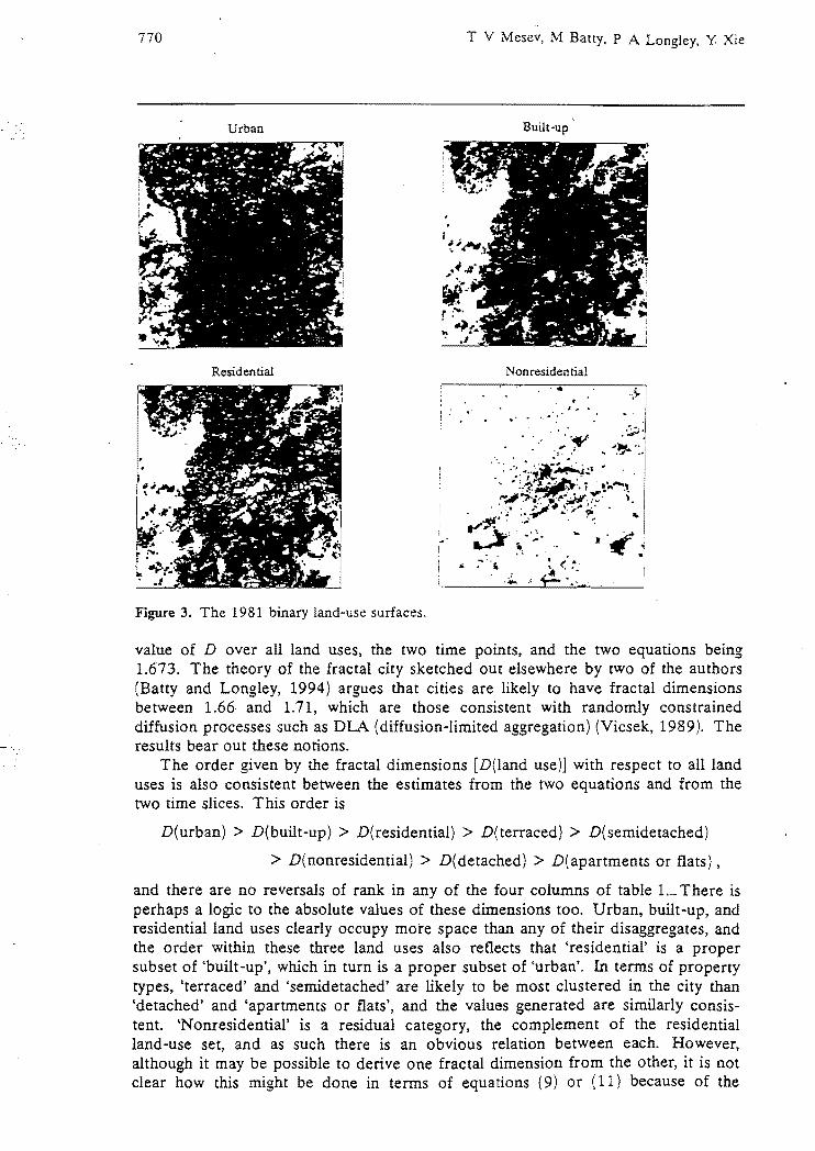