Pivotal Moments in Nursing: Leaders Who Changed the Path ...
Upload
khangminh22Category
view
5download
0
Monetary policy has changed dramatically in the United States over the past decade, with potential implications for inves-tors’ inflation expectations. During the financial crisis and
Great Recession of 2007–09, the Federal Reserve’s conventional policy tool, the nominal short-term interest rate, was constrained by its effec-tive lower bound. At the time, monetary policy makers were concerned the U.S. economy might slip into a deflationary trap similar to Japan’s during the period of 1999–2003. As a result, the Fed responded aggres-sively to stabilize the economy through multiple rounds of large-scale asset purchases (LSAPs) and forward guidance on the future interest rate. In addition, the Federal Open Market Committee (FOMC) ad-opted a formal inflation target at its meeting in January 2012, em-phasizing that “communicating this inflation goal clearly to the public helps keep longer-term inflation expectations firmly anchored.”
Well-anchored inflation expectations are a key measure of suc-cessful monetary policy, because in the long run, inflation is mainly determined by monetary policy. Inflation expectations drifting away from the central bank’s implicit or explicit inflation targets can generate highly inflationary or disinflationary episodes. For example, businesses expecting a higher inflation rate may increase current prices to offset
Has the Anchoring of Inflation Expectations Changed in the United States during the Past Decade?
By Taeyoung Doh and Amy Oksol
Taeyoung Doh is a senior economist at the Federal Reserve Bank of Kansas City. Amy Oksol is a research associate at the bank. This article is on the bank’s website at www.KansasCityFed.org
31
32 FEDERAL RESERVE BANK OF KANSAS CITY
high future costs of production. Similarly, consumers expecting prices to fall may delay their spending, reinforcing disinflationary pressures with the resulting lack of demand.
Prior to the financial crisis, researchers found that the level and vola-tility of inflation expectations decreased dramatically from 1981:Q3 to 2008:Q2, suggesting investors’ inflation expectations were well anchored (Clark and Davig 2011). But did their expectations remain anchored af-ter the crisis, during a period of unconventional monetary policy?
We use a model consistent with previous research to examine whether inflation expectations became unanchored after the crisis. Our analysis of three metrics of inflation expectations—their level, vola-tility, and persistence—suggests that the degree of anchoring deterio-rated somewhat in late 2010, coinciding with the start of the second round of LSAPs, but has improved since then. Other rounds of LSAPs and the adoption of a formal inflation target are associated with bet-ter anchoring of inflation expectations to varying degrees. Finally, we find inflation expectations have remained well anchored more recently (2017:Q3), returning to their pre-crisis behavior.
Section I defines the level, volatility, and persistence metrics as well as the data used to construct inflation expectations. Section II discusses the channels through which monetary policy can affect inflation expec-tations. Section III introduces a model for inflation expectations and analyzes how the Federal Reserve’s monetary policy actions affected the anchoring of inflation expectations over the past decade.
I. Measuring the Degree of Anchoring in Inflation Expectations
To evaluate the degree to which inflation expectations have been anchored over time, we first examine the level, volatility, and persistence that summarize their long-run predictive distribution.1 These metrics allow us to quantify the degree to which inflation expectations are an-chored. If the level of inflation expectations gets closer to the central bank’s longer-run objective, for example, then inflation expectations are better anchored. If the volatility of inflation expectations declines, then inflation expectations are also better anchored. Finally, if unantici-pated shocks to inflation expectations have less persistent effects over the long run, then inflation expectations are better anchored. All three
ECONOMIC REVIEW • FIRST QUARTER 2018 33
metrics are consistent with the FOMC’s interpretation of price stabil-ity in terms of “preventing persistent deviations of inflation from its longer-run objective.”
Both financial market data and survey forecasts can be used to mea-sure inflation expectations. One widely used, market-based measure of inflation expectations is the “breakeven inflation rate,” calculated as the difference between yields on nominal U.S. Treasury bonds and Treasury Inflation-Protected Securities (TIPS) of the same maturity. The break-even inflation rate reveals the additional compensation that bond mar-ket investors demand for putting money in nominal bonds whose value will decline in real terms with inflation. As the risk of higher future inflation increases, investors will demand more compensation, thereby driving down the prices of nominal bonds and driving up their yields relative to TIPS. Therefore, a higher breakeven rate suggests investors perceive a higher risk of future inflation. The advantage of using finan-cial market data is that they provide high-frequency information about inflation expectations and are available at more horizons than survey data. However, they can also be contaminated by market-related factors other than inflation expectations, such as trading liquidity.
One alternative is to use direct observations of investors’ inflation expectations from survey data. Since survey participants provide their actual inflation expectations, the data are not contaminated by other fac-tors.2 Additionally, inflation forecasts using survey data tend to generate more accurate out-of-sample forecasts than those using actual inflation data or financial market data (Ang, Bekaert, and Wei 2007; Faust and Wright 2013; Mertens 2016). However, available forecast horizons in survey data are limited compared with market-based measures.
Aruoba (2016) overcomes this shortcoming by fitting an inflation expectations curve, which plots the average inflation expected between today and any point three to 120 months in the future, with survey data from three different sources: the Survey of Professional Forecast-ers (SPF), Blue Chip Economic Indicators (BCEI), and Blue Chip Fi-nancial Forecasts (BCFF).3 Table 1 summarizes the forecast horizons and frequency of collection and publication for all three surveys. One complication in combining data from these surveys is that the frequen-cies and forecast horizons differ significantly. To account for these dif-ferences, Aruoba (2016) starts out by assuming that the spot inflation expectations for a particular horizon (h), which represent the expected

34 FEDERAL RESERVE BANK OF KANSAS CITY
inflation averaged between the current period, (t), and a specific fu-ture period, (t+h), are spanned by three latent variables that vary at the monthly frequency.4 In the fitted curve, any point in the spot inflation expectations curve is a function of the three latent variables. We esti-mate parameters and latent variables by matching the curve-implied forecasts of inflation with the observed median survey forecasts for con-sumer price index (CPI) inflation.5
Once we obtain the spot inflation expectations curve from Aruoba (2016), we can compute inflation expectations at any horizon, analo-gous to the five-year, five-year forward breakeven inflation measure. Since the spot inflation expectations curve spans multiple horizons, from three to 120 months, it can provide one-month-forward inflation expectations at any horizon from three to 119 months. For example, the value of the forward inflation expectations for the 12-month horizon at time t represents the expected inflation between t+12 and t+13. Chart 1 illustrates the spot inflation expectations curve and the corresponding one-month-forward inflation expectations curve as of October 2017. Each point on the spot inflation expectations curve shows the expected inflation between the current month and some point in the future—for example, the spot curve suggests that expected inflation would aver-age a little over 2.1 percent between today and 60 months from now. The corresponding one-month-forward inflation expectations curve shows what expected inflation would be one-month ahead of that fu-ture point—for example, the expected inflation between month 60 and
Table 1 Survey Data Sources Used in the Inflation Expectations Curve
SourceFrequency of publication
Frequency of forecasts Horizons
Survey of Professional Forecasters Quarterly Quarterly, annual −1 quarter to +4 quarters; current year to +2 years; average over +5 yrs, average over +10 years
Blue Chip Economic Indicators Monthly Quarterly, annual* From current quarter** to +7 quarters; +5 years following next year, 5 year forward
Blue Chip Financial Forecasts Monthly Annual*** +5 years following next year, 5 year forward
* Annual forecasts only available in March and October issues ** May also include previous quarter if currently in first month of a quarter*** Annual forecast only available in June and December issuesSource: Aruoba (2016).

ECONOMIC REVIEW • FIRST QUARTER 2018 35
1.8
1.9
2.0
2.1
2.2
2.3
2.4
2.5
1.8
1.9
2.0
2.1
2.2
2.3
2.4
2.5
20 40 60 80 100 120Horizon (months)
Spot in�ation expectations (as of October 2017)
Forward in�ation expectations (as of October 2017)
Percent Percent
month 61. The flattening of the forward inflation expectations curve after 36 months suggests that inflation expectations beyond that hori-zon would converge to the long-run level in three years.
II. Using Monetary Policy to Anchor Inflation Expectations
Changes in monetary policy can directly or indirectly affect all three metrics of anchored inflation expectations—level, volatility, and persistence. For instance, a central bank can directly affect the level of inflation expectations by announcing an explicit target rate for infla-tion. This action can, in turn, indirectly reduce the volatility of in-flation expectations by reducing uncertainty about the central bank’s intent. In addition, both the volatility and persistence of inflation ex-pectations may decline if the central bank adjusts the nominal interest rate more aggressively to stabilize inflation around its target. If inves-tors anticipate the central bank will respond aggressively to inflation-ary shocks, they may assume the effects of these shocks will dissipate sooner and set prices accordingly. As a result, actual inflation and infla-tion expectations will be less responsive to exogenous shocks (Davig and Doh 2014). Furthermore, the central bank can boost aggregate
Chart 1 Inflation Expectations at Multiple Horizons
Notes: Each point on the spot inflation expectations curve shows what the expected inflation would be between the current month and the future month given by the horizon at the point. The corresponding one-month-forward infla-tion expectations curve shows what the one-month-ahead expected inflation would be from the horizon at the point.Sources: Federal Reserve Bank of Philadelphia and authors’ calculations.

36 FEDERAL RESERVE BANK OF KANSAS CITY
demand and thereby push up inflation expectations by easing financial market conditions. Through these channels, monetary policy can affect both near-term and long-term inflation expectations.
Although monetary policy makers are mostly concerned about movements in long-term inflation expectations, they must also monitor fluctuations in near-term inflation expectations, which may spill over into long-term inflation expectations in the future.6 Chart 2 plots two measures of inflation expectations—the two-year and 10-year inflation rates—along with the actual inflation rate from January 1998 to Oc-tober 2017. Although two-year inflation expectations moved together with the actual inflation rate, 10-year inflation expectations remained relatively stable. Nonetheless, if movements in two-year inflation ex-pectations spilled over into 10-year inflation expectations over time, the distribution of 10-year inflation expectations might shift.
Japan’s experience in the 1990s provides a cautionary tale regard-ing this risk. While long-term (five-to-10 year) inflation expectations were quite stable in Japan during the late 1990s, near-term (one-year) inflation expectations often deviated quite noticeably on the downside. Actual inflation became negative from 1999 to 2003, tracking the plunge in short-run inflation expectations (Fuhrer 2017). Long-term inflation expectations eventually dropped below 1 percent in the early 2000s, concurrent with this prolonged period of deflation.7 Japan’s ex-perience suggests substantial changes in near-term inflation expecta-tions should be watched carefully, as they could augur similar changes in long-term inflation expectations.
Changes in monetary policy actions and inflation expectations in the United States over the past decade highlight how a concern for drift-ing inflation expectations shaped monetary policy. During the financial crisis of 2008, policymakers were concerned about the possibility of deflation and stagnation and took aggressive steps to avoid it. Table 2 summarizes the timing and purpose of the Fed’s policy responses during this period, including multiple rounds of LSAPs intended to facilitate economic recovery by easing financial market conditions. Each of these unprecedented, aggressive policy responses had the potential to better anchor inflation expectations at the FOMC’s implicit (before January 2012) or explicit (after January 2012) long-run target. In each state-ment that announced LSAPs, the FOMC acknowledged the risk that
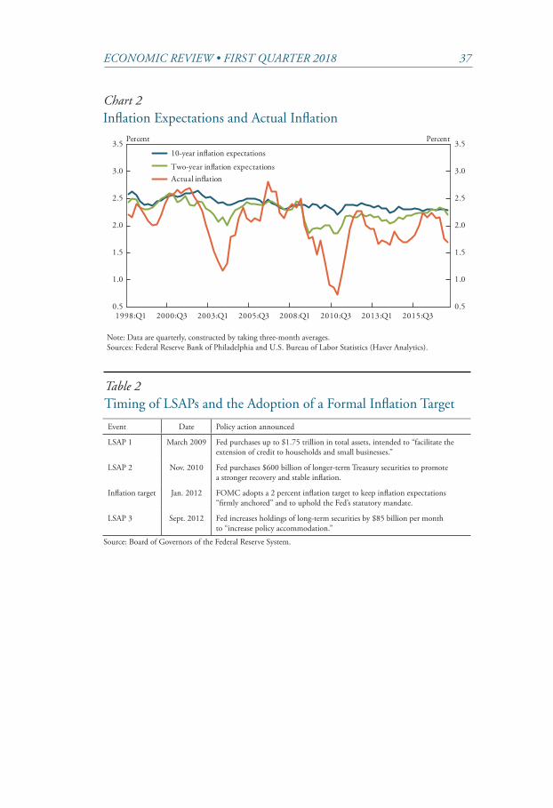
ECONOMIC REVIEW • FIRST QUARTER 2018 37
Chart 2Inflation Expectations and Actual Inflation
Table 2Timing of LSAPs and the Adoption of a Formal Inflation Target
Note: Data are quarterly, constructed by taking three-month averages. Sources: Federal Reserve Bank of Philadelphia and U.S. Bureau of Labor Statistics (Haver Analytics).
Event Date Policy action announced
LSAP 1 March 2009 Fed purchases up to $1.75 trillion in total assets, intended to “facilitate the extension of credit to households and small businesses.”
LSAP 2 Nov. 2010 Fed purchases $600 billion of longer-term Treasury securities to promote a stronger recovery and stable inflation.
Inflation target Jan. 2012 FOMC adopts a 2 percent inflation target to keep inflation expectations “firmly anchored” and to uphold the Fed’s statutory mandate.
LSAP 3 Sept. 2012 Fed increases holdings of long-term securities by $85 billion per month to “increase policy accommodation.”
Source: Board of Governors of the Federal Reserve System.
0.5
1.0
1.5
2.0
2.5
3.0
3.5
0.5
1.0
1.5
2.0
2.5
3.0
3.5
1998:Q1 2000:Q3 2003:Q1 2005:Q3 2008:Q1 2010:Q3 2013:Q1 2015:Q3
Actual in�ation
Percent Percent
Two-year in�ation expectations
10-year in�ation expectations

38 FEDERAL RESERVE BANK OF KANSAS CITY
inflation might run below a rate consistent with stable prices. For in-stance, in the March 18, 2009 statement announcing the first round of LSAPs, the FOMC mentioned that it saw “some risk that inflation could persist for a time below rates that best foster economic growth and price stability in the longer term.” The FOMC raised a similar concern in the statement announcing the second round of LSAPs, stat-ing that “measures of underlying inflation have trended lower in recent quarters” (2010b). And the FOMC also mentioned a subdued out-look for inflation in the statement following the September 13, 2012 meeting that announced the third round of LSAPs: specifically, the Committee anticipated that “inflation over the medium term likely would run at or below its 2 percent objective.”
However, the projected effect of LSAPs on inflation expectations was not without controversy. Although most FOMC participants saw the second round of LSAPs as helpful for lifting inflation expectations, some participants, such as then-Governor Kevin Warsh, expressed con-cern that the second round would increase the risk of future inflation and distortions in currency and capital markets without much effect on economic growth (FOMC 2010a).
In addition to multiple rounds of LSAPs, the adoption of a formal inflation target in January 2012 might also have affected the anchoring of inflation expectations. Although the FOMC announced the adop-tion of a formal inflation target in a consensus statement, academic researchers and policymakers had previously debated its merits. Some researchers argued that it would lower long-run inflation and provide more room for countercyclical stabilization policy by reducing con-cerns about the Federal Reserve’s ability to achieve stable prices (Good-friend 2005). But some policymakers resisted the idea of a formal in-flation target, arguing that adopting a target would constrain policy flexibility in future contingencies with little additional benefit, given that long-run inflation expectations had been as stable in the United States as in other inflation-targeting countries, such as Sweden, since 1990 (Kohn 2005).
The Great Recession of 2007–09 enhanced the case for adopting a formal inflation target. Policymakers at that time wanted to make sure the Federal Reserve’s credibility in achieving price stability had not eroded in a way that would hamper aggressive policy responses to sta-bilize the economy. As then-Chair Ben Bernanke noted during a press
ECONOMIC REVIEW • FIRST QUARTER 2018 39
conference on January 25, 2012, the FOMC adopted a formal inflation target of 2 percent, measured by the price index for personal consump-tion expenditures (PCE), to “foster price stability” and “enhance the FOMC’s ability to promote maximum employment in the face of sig-nificant economic disturbances.” According to this view, LSAPs and the adoption of a formal inflation target were complementary measures to achieve the same goal of well-anchored inflation expectations.
To evaluate whether LSAPs and the adoption of the inflation target were indeed associated with well-anchored inflation expectations, we track the time variation in the degree of anchoring around these major monetary policy events in the subsequent analysis.
III. Analyzing the Effect of Monetary Policy on Anchoring Inflation Expectations: Evidence from Survey Data
To quantitatively measure how well inflation expectations are an-chored, we incorporate survey data information into an empirical mac-roeconomic forecasting model and use this model to predict future val-ues of inflation expectations. While the model’s predictions may differ from the current level of inflation expectations, the predicted future value of inflation expectations is still a relevant measure for monetary policy, as it may help a central bank take preemptive actions to reduce the risk of unanchored inflation expectations.
Anchored inflation expectations require inflation expectations to be stable not only at the current level but also in future projections. Therefore, we look at changes in the probability distribution of future projected values of inflation expectations to observe possible shifts in the degree of anchoring of inflation expectations. In general, character-izing changes in the distribution over time is a very challenging, com-plex task. However, the three metrics of anchored inflation expectations discussed in the previous section provide an effective way to summa-rize changes in the long-run predictive distribution. By associating the timing of shifts in these metrics with the timing of major changes in monetary policy—such as LSAPs and the adoption of a formal infla-tion target—we can examine whether policy changes helped long-term inflation expectations become better anchored.
We use two measures of inflation expectations in our estimat-ed forecasting model to examine possible spillovers from changes in

40 FEDERAL RESERVE BANK OF KANSAS CITY
near-term inflation expectations to long-term expectations. We choose the 10-year and two-year inflation expectations from the spot inflation expectations curve in Aruoba (2016) as proxies for long-term inflation expectations and near-term inflation expectations, respectively. We choose 10-year expectations because 10 years is the longest horizon for which we can obtain survey data on inflation forecasts; we choose two-year expectations because monetary policy typically affects inflation with a one-year lag (Svensson 1996). Our estimated forecasting model links future values of 10-year inflation expectations to the current and past values of two-year inflation expectations. Whether the two mea-sures move together has implications for the degree of anchoring. If the current and past values of two-year inflation expectations influence 10-year inflation expectations, the persistence metrics for both horizons are likely to move together, because forecastable variations in two-year inflation expectations would show up as forecastable variations in 10-year inflation expectations, too. In this way, increased persistence in two-year inflation expectations—an increased probability of inflation deviating from its long-run average level—would likely lead 10-year inflation expectations to become unanchored. However, if two-year in-flation expectations do not influence 10-year inflation expectations, the two persistence metrics should move independently.
A multivariate forecasting model of inflation and inflation expectations
We consider a vector autoregression model (VAR) of five macro-economic variables to estimate the three metrics of anchored inflation expectations. Following Clark and Davig (2011), we use monthly ob-servations for headline CPI inflation (π t ) and the Chicago Fed Na-tional Activity Index (CFNAI, denoted at ) as well as the short-term interest rate (rt ) and two-year (π t ,2yr
e ) and 10-year (π t ,10yre ) inflation
expectations. To measure the stance of monetary policy when the fed-eral funds rate was constrained at its effective lower bound, we use the estimated shadow rate in Doh and Choi (2016). This measure backs out the short-term interest rate implied by government and private bor-rowing conditions, including long-term rates, and is not constrained by the effective lower bound on the short-term interest rate.8 Thus, the shadow rate can capture the additional monetary stimulus the Fed-eral Reserve provided by influencing long-term interest rates through
ECONOMIC REVIEW • FIRST QUARTER 2018 41
LSAPs and forward guidance on the future path of the short-term in-terest rate. When the short-term interest rate is not constrained by the effective lower bound, the shadow rate is highly correlated with the fed-eral funds rate itself, making it a useful metric to capture the monetary policy stance both on and off the effective lower bound. In the VAR, we order inflation expectations before inflation, real activity, and the shadow rate.9 The variables are summarized in the vector yt:
yt = π t ,10yr ,e π t
e,2yr ,π t ,at ,rt⎡⎣ ⎤⎦.
We transform monthly variables into quarterly variables by taking three-month average values of inflation and the activity index. Since our inflation expectations data are only available starting in January 1998, our sample period is 1998:Q1 to 2017:Q3. We estimate VAR(1) to obtain the three metrics of anchored inflation expectations.10 The model can be written as:
yt = A0,t + A1t yt-1+Σt∈t , Var (∈t)
The five VAR residual shocks (∈t ) follow a multivariate normal dis-tribution and are serially and cross-sectionally uncorrelated. The VAR coefficients (A0,t , A1,t ) and covariance matrix (ΣtΣt
′ ) are time varying, because we estimate the VAR(1) for rolling samples of 40 quarters. In this way, we can identify the timing of shifts in the metrics of anchored inflation expectations.
The anchoring of U.S. inflation expectations during the recent decade
From the estimated VAR model, we can derive a long-run pre-dictive distribution of inflation expectations that provides informa-tion on the probabilities of possible future outcomes.11 As the debates on LSAPs considered the future risk of inflation expectations drifting above the Federal Reserve’s long-run objective, we use the long-run predictive distribution to quantify the probability of this risk.
Because the long-run predictive distribution considers the cumula-tive effects of future shocks, the range of possible outcomes is much wider than in the short-run predictive distribution. For this reason, we look at changes in the long-run predictive distribution of inflation expectations in our analysis. Furthermore, the long-run distribution allows us to see through the temporary effects of unanticipated shocks.

42 FEDERAL RESERVE BANK OF KANSAS CITY
Under our assumptions about the distribution of the VAR’s residual shocks, the long-run predictive distribution is completely determined by the long-run mean and the long-run variance, which are closely re-lated to the three metrics of anchored inflation expectations.12
The level metric can be equated with the long-run mean, while the volatility metric can be equated with the long-run variance. The persis-tence metric provides information on the factors driving the long-run variance. The long-run variance of inflation expectations may go up either because persistence goes up or because the range of potential shocks widens. In other words, by looking at the long-run variance metric together with the persistence metric, we can identify which fac-tor drives the long-run variance metric. The distinction is relevant for policy, because monetary policy can reduce the long-run volatility of inflation expectations more effectively by influencing the parameters determining persistence than by influencing the volatility of unantici-pated shocks, which are more likely to change for reasons other than monetary policy.
To assess whether inflation expectations became less anchored after the financial crisis, we first look at the level metric, defined as the mean of inflation expectations in the long-run predictive distribution. This value represents the central point around which future values of infla-tion expectations would fluctuate over a long time. A significant shift in the level metric would change the probability of inflation expectations crossing certain thresholds in the future, influencing the calculation of risks in both directions. The rolling-sample estimates of the VAR model provide time-varying estimates of this level metric, which we use to cal-culate the future risk of inflation expectations becoming unanchored.
Chart 3 shows the evolution of the model-implied, long-run mean values for both two-year and 10-year inflation expectations. The hori-zontal axis represents the timing of the last observation used in each sample. As the 40-quarter window rolls forward, estimates change due to changes in the rolling sample’s first and last observations. For in-stance, the change in the level metric from the rolling sample ending in 2010:Q4 when the second round of LSAPs was adopted to the roll-ing sample ending in 2011:Q1 can be attributed to the deletion of the 2001:Q4 observation and the addition of the 2002:Q1 observation—only these two observations differ from the previous rolling sample.

ECONOMIC REVIEW • FIRST QUARTER 2018 43
For this particular change in rolling samples, we find that estimates of the three metrics barely change even if we use an alternative rolling sample that adds the observation for 2011:Q1 but does not drop the initial observation from the previous rolling sample (2000:Q4). For the other rounds of LSAPs and the adoption of a formal inflation tar-get, retaining the initial observation from the previous rolling sample produces changes in the metrics that are qualitatively similar but have some quantitative differences. Hence, we attribute changes in the met-rics related to anchoring during these quarters to changes in the ending quarter rather than changes in the beginning quarter of rolling samples.
After the global financial crisis of 2008, the two-year and 10-year measures drifted down by 15 and 30 basis points, respectively, until 2010:Q3. However, both estimates recovered two-thirds of their de-clines by the start of the second round of LSAPs in 2010:Q4. After-ward, 10-year inflation expectations gradually declined by 10 basis points and stabilized at 2.33 percent as of 2017:Q3, while two-year inflation expectations experienced small ups and downs before stabiliz-ing at 2.15 percent in the same quarter.
Because we derive our inflation expectations from CPI inflation forecasts, the overall level of inflation expectations is higher than the
Chart 3Long-Run Average and Current Values of Inflation Expectations
Note: “Level” represents the long-run mean from the VAR model, while “spot” describes the current value of the spot inflation expectations. Sources: Federal Reserve Bank of Philadelphia and authors’ calculations.
1.6
1.8
2.0
2.2
2.4
2.6
2.8
3.0
1.6
1.8
2.0
2.2
2.4
2.6
2.8
3.0
2008:Q1 2009:Q2 2010:Q3 2011:Q4 2013:Q1 2014:Q2 2015:Q3 2016:Q4
Percent PercentLSAP 3
10-year level Two-year level10-year spot Two-year spot
LSAP 2LSAP 1 In�ation target
44 FEDERAL RESERVE BANK OF KANSAS CITY
FOMC’s 2 percent target, which is based on the PCE inflation rate. Haubrich and Millington (2014) suggest that the CPI inflation rate is about 0.5 percentage point higher than the PCE inflation rate on aver-age. Therefore, the 2.33 percent CPI-based level of 10-year inflation expectations can be translated to 1.83 percent PCE-based inflation, a level close to but lower than the 2 percent target.
The level metric of inflation expectations suggests that the second round of LSAPs coincided with the reversal of a downward trend in in-flation expectations. Chart 3 shows that our level metric declined more than the corresponding spot value of inflation expectations around this time, suggesting spot values underestimate the extent to which inflation expectations became unanchored. Interestingly, announcing a formal inflation target barely moved the long-run mean value of 10-year infla-tion expectations. One explanation for this subdued response is that the announced 2 percent target of PCE inflation was roughly consistent with a CPI inflation rate of about 2.4 percent, which was the long-run mean of 10-year inflation expectations at the time, suggesting that the average level of long-run inflation expectations was already anchored around 2 percent.
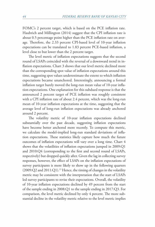
The volatility metric of 10-year inflation expectations declined substantially over the past decade, suggesting inflation expectations have become better anchored more recently. To compute this metric, we calculate the model-implied long-run standard deviations of infla-tion expectations. These statistics likely capture how much the future outcomes of inflation expectations will vary over a long time. Chart 4 shows that the volatilities of inflation expectations jumped in 2009:Q1 and 2010:Q4 (corresponding to the first and second round of LSAPs, respectively) but dropped quickly after. Given the lag in collecting survey responses, however, the effect of LSAPs on the inflation expectations of survey participants is more likely to show up in the following quarters (2009:Q2 and 2011:Q1).13 Hence, the timing of changes in the volatility metric may be consistent with the interpretation that the start of LSAPs led survey participants to revise their expectations. Overall, the volatility of 10-year inflation expectations declined by 49 percent from the start of the sample ending in 2008:Q1 to the sample ending in 2017:Q3. For comparison, the level metric declined by only 4 percent. The more sub-stantial decline in the volatility metric relative to the level metric implies

ECONOMIC REVIEW • FIRST QUARTER 2018 45
Chart 4 Long-Run Volatility of Inflation Expectations
Note: “Volatility” represents the long-run standard deviation from the VAR model. Sources: Federal Reserve Bank of Philadelphia and authors’ calculations.
0.1
0.2
0.3
0.4
0.1
0.2
0.3
0.4
2008:Q1 2009:Q2 2010:Q3 2011:Q4 2013:Q1 2014:Q2 2015:Q3 2016:Q4
LSAP 1 LSAP 3Inflation target
Percent PercentLSAP 2
10-year volatility Two-year volatility
that the risk of inflation expectations surging or plummeting has been significantly reduced.
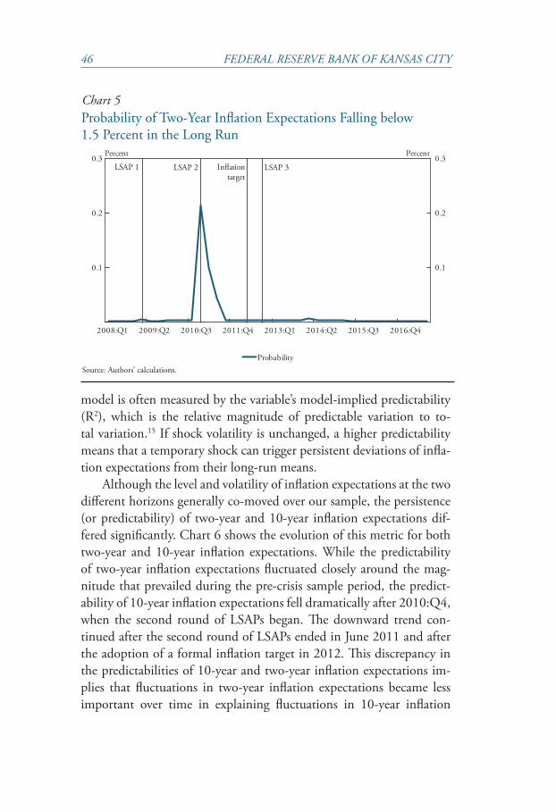
By combining the level and volatility metrics, we can calculate the probability of any future outcome for inflation expectations. In this way, we can use the probability of inflation falling below a certain thresh-old—1 percent for the PCE inflation rate or 1.5 percent for our CPI inflation measure—to measure whether inflation expectations have be-come unanchored.14 Chart 5 shows that the probability of inflation fall-ing below the CPI threshold was negligible (below 1 percent) for 10-year inflation expectations throughout the past decade. The probability was similarly negligible for two-year inflation expectations much of the past decade—for the rolling sample ending in 2010:Q4, however, the prob-ability of two-year expectations falling below 1.5 percent spiked to 21 percent before declining again to a negligible level by 2011:Q3. Taken together, however, our estimates of the levels and volatilities in the long-run predictive distribution of inflation expectations suggest that the sec-ond round of LSAPs was associated with a large reduction in the risk of inflation expectations falling substantially below the FOMC’s target.
Finally, we look at the persistence of inflation expectations as a measure of anchoring. The persistence of a variable in a multivariate
46 FEDERAL RESERVE BANK OF KANSAS CITY
model is often measured by the variable’s model-implied predictability (R2), which is the relative magnitude of predictable variation to to-tal variation.15 If shock volatility is unchanged, a higher predictability means that a temporary shock can trigger persistent deviations of infla-tion expectations from their long-run means.
Although the level and volatility of inflation expectations at the two different horizons generally co-moved over our sample, the persistence (or predictability) of two-year and 10-year inflation expectations dif-fered significantly. Chart 6 shows the evolution of this metric for both two-year and 10-year inflation expectations. While the predictability of two-year inflation expectations fluctuated closely around the mag-nitude that prevailed during the pre-crisis sample period, the predict-ability of 10-year inflation expectations fell dramatically after 2010:Q4, when the second round of LSAPs began. The downward trend con-tinued after the second round of LSAPs ended in June 2011 and after the adoption of a formal inflation target in 2012. This discrepancy in the predictabilities of 10-year and two-year inflation expectations im-plies that fluctuations in two-year inflation expectations became less important over time in explaining fluctuations in 10-year inflation
Chart 5Probability of Two-Year Inflation Expectations Falling below 1.5 Percent in the Long Run
Source: Authors’ calculations.
0.1
0.2
0.3
0.1
0.2
0.3
2008:Q1 2009:Q2 2010:Q3 2011:Q4 2013:Q1 2014:Q2 2015:Q3 2016:Q4
Probability
Percent Percent
LSAP 3Inflationtarget
LSAP 2LSAP 1

ECONOMIC REVIEW • FIRST QUARTER 2018 47
expectations—in other words, the spillovers from short-term to long-term inflation expectations diminished.
The timing of the shifts in the persistence of long-term inflation ex-pectations suggests that the announcement of a formal inflation target as well as multiple rounds of LSAPs contributed to better anchored infla-tion expectations.16 Overall, the timing of shifts in the three metrics (lev-el, volatility, and persistence) of the anchoring of inflation expectations suggests that the second round of LSAPs was consequential in reversing the downward drift in inflation expectations. Other policy actions, such as the first round of LSAPs and the adoption of a formal inflation target, were also largely consistent with the timing of shifts in the volatility and persistence metrics toward better anchoring. While the realized value of long-term inflation expectations might have changed little during the recent decade, our time-varying estimates show that the model-implied distribution of inflation expectations has changed significantly at certain times. Our analysis is consistent with the view that the Federal Reserve’s actions, such as LSAPs and the adoption of a formal inflation target, led to better anchored inflation expectations. Furthermore, we do not find any meaningful evidence that the anchoring of inflation expectations in
Chart 6 Percentage of Forecastable Variations for Inflation Expectations
Note: “Predictability” represents the percentage of variations in inflation expectations that are forecastable by the VAR model.Sources: Federal Reserve Bank of Philadelphia and authors’ calculations.
40
50
60
70
80
90
100
40
50
60
70
80
90
100
2008:Q1 2009:Q2 2010:Q3 2011:Q4 2013:Q1 2014:Q2 2015:Q3 2016:Q4
Percent Percent
LSAP 3In�ationtarget
10-year predictability Two-year predictability
LSAP 1 LSAP 2

48 FEDERAL RESERVE BANK OF KANSAS CITY
2017:Q3, the final quarter for our sample, deteriorated relative to the degree of anchoring in the pre-crisis period.
Our results may seem to conflict with Reis (2016), who finds little change in inflation expectations around the announcement of the sec-ond round of LSAPs. Reis’s analysis uses an event study methodology and inflation swap market data to back out the distribution of infla-tion expectations. We attribute the difference in our results mostly to the fact that financial markets already anticipated the second round of LSAPs before the November 3, 2010 announcement. Indeed, break-even inflation and other market-based inflation measures of inflation expectations jumped after August 27, 2010, when then-Chair Bernanke strongly suggested the possibility of additional asset purchases.17
IV. Conclusion
Inflation expectations have become better anchored in the United States during the past decade. We use three different metrics (level, vol-atility, and persistence) to quantify the degree of anchoring in inflation expectations and find that the timing of shifts in these metrics is as-sociated with the Federal Reserve’s unconventional policy actions. Our findings are consistent with the interpretation that the second round of LSAPs, which the Federal Reserve began in November 2010, was significant in preventing long-term inflation expectations from drifting down. In addition, the timing of shifts in the volatility and persistence metrics of inflation expectations is consistent with the interpretation that other rounds of LSAPs and the adoption of a formal inflation tar-get also helped reduce the volatility and persistence of long-term infla-tion expectations. In general, our results as of 2017:Q3 suggest that inflation expectations have not become less anchored after the financial crisis and Great Recession when compared with their pre-crisis level. In particular, our results suggest the Federal Reserve’s policies during the recent decade may have played a role in keeping them that way.
ECONOMIC REVIEW • FIRST QUARTER 2018 49
Appendix A
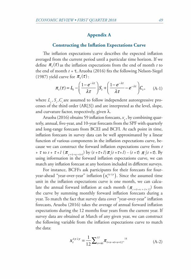
Constructing the Inflation Expectations Curve
The inflation expectations curve describes the expected inflation averaged from the current period until a particular time horizon. If we define π t (τ ) as the inflation expectations from the end of month t to the end of month t + τ, Aruoba (2016) fits the following Nelson-Siegel (1987) yield curve for π t (τ ) :
π t (τ ) = Lt −1−e −λτ
λτ⎛⎝⎜
⎞⎠⎟St +
1−e −λτ
λτ−e −λτ⎛
⎝⎜⎞⎠⎟Ct ,
(A-1)
where Lt , St ,Ct are assumed to follow independent autoregressive pro-cesses of the third order (AR[3]) and are interpreted as the level, slope, and curvature factor, respectively, given λ.
Aruoba (2016) obtains 59 inflation forecasts, xt , by combining quar-terly, annual, five-year, and 10-year forecasts from the SPF with quarterly and long-range forecasts from BCEI and BCFI. At each point in time, inflation forecasts in survey data can be well approximated by a linear function of various components in the inflation expectations curve, be-cause we can construct the forward inflation expectations curve from t + τ to t + τ +1 (π t + τ→t + τ+1) by (t +τ +1)π t(t +τ +1) − (t +τ) π t(t +τ). By using information in the forward inflation expectations curve, we can match any inflation forecast at any horizon included in different surveys.
For instance, BCFFs ask participants for their forecasts for four-year-ahead “year-over-year” inflation xt4y ,1y( ) . Since the assumed time unit in the inflation expectations curve is one month, we can calcu-late the annual forward inflation at each month (π t +τ→ t + τ + 12) from the curve by summing monthly forward inflation forecasts during a year. To match the fact that survey data cover “year-over-year” inflation forecasts, Aruoba (2016) takes the average of annual forward inflation expectations during the 12 months four years from the current year. If survey data are obtained at March of any given year, we can construct the following variable from the inflation expectations curve to match the data:
18xt4y ,1y = 1
12π t +s→t +s+12.s=46
57∑
(A-2)
50 FEDERAL RESERVE BANK OF KANSAS CITY
We can specify similar measurement equations for other survey forecasts, too. For the actual estimation, we add measurement errors that follow mean-zero normal distributions to survey forecasts. The re-sulting equation is:
xt=Zαt + ϵt , ϵt ~N(0,H), (A-3)
where αt=[Lt St Ct Lt−1 St−1Ct−1 Lt−2 St−2 Ct−2 ] and αt evolves according to
(αt−μ)=T (αt−1−μ)+ηt ,ηt ~ N (0,Q). (A-4)
Since (A-3) and (A-4) represent a linear and Gaussian state-space model, all the model parameters can be estimated by the maximum likelihood method using the Kalman filter. Once we obtain parameter estimates, we can back out the estimate for αt and construct the infla-tion expectations curve at time t using that information.

ECONOMIC REVIEW • FIRST QUARTER 2018 51
Appendix B
Alternative Measures of Long-Term Inflation Expectations
One potential caveat to our results is that our measure of long-term inflation expectations considers inflation averaged over 10 years, a window sufficiently short for a temporary but moderately persistent shock to influence inflation expectations. In contrast, a forward infla-tion expectations measure, such as expected inflation eight to 10 years from now, is insulated from a temporary shock, because it is outside a typical business cycle frequency of six to 32 quarters (Burns and Mitch-ell 1946). To check the robustness of our findings against this alterna-tive measure of long-run inflation expectations, we calculate eight-year, two-year forward inflation (π t
e,8yr 2yr ) from the inflation expectations
curve in Aruoba (2016). We recompute the three metrics of anchored inflation expectations with eight-year, two-year forward inflation as a proxy for long-term inflation expectations.
As Charts B-1 through B-3 illustrate, the overall pattern of the time variation in the three metrics is largely consistent with our previous analysis. Specifically, the significant shifts in the three metrics toward better-anchored inflation expectations coincide with the second round of LSAPs. The other rounds of LSAPs and the adoption of a formal in-flation target are also associated with shifts in the volatility and predict-ability metrics toward better-anchored inflation expectations. However, one notable difference is the run-up in the predictability metric of the 10-year inflation expectations near the end of the sample period. Still, the degree of predictability remains lower than its value during the pre-crisis period and does not indicate any material deterioration in the anchoring of inflation expectations.

52 FEDERAL RESERVE BANK OF KANSAS CITY
Chart B-1 Long-Run Average of Forward Inflation Expectations
Chart B-2Long-Run Volatility of Forward Inflation Expectations
Note: “Level” represents the long-run mean from the VAR model, while “forward” describes the current value of the eight-year, two-year forward inflation expectations. Sources: Federal Reserve Bank of Philadelphia and authors’ calculations.
1.6
1.8
2.0
2.2
2.4
2.6
2.8
3.0
1.6
1.8
2.0
2.2
2.4
2.6
2.8
3.0
2008:Q1 2009:Q2 2010:Q3 2011:Q4 2013:Q1 2014:Q2 2015:Q3 2016:Q4
Percent PercentLSAP 1 LSAP 3In�ation
target
Eight-year, two-year level Eight-year, two-year forward Two-year spotTwo-year level
LSAP 2
Note: “Volatility” represents the long-run standard deviation from the VAR model. Sources: Federal Reserve Bank of Philadelphia and authors’ calculations.
0.1
0.2
0.3
0.4
0.1
0.2
0.3
0.4
2008:Q1 2009:Q2 2010:Q3 2011:Q4 2013:Q1 2014:Q2 2015:Q3 2016:Q4
Standard deviation Standard deviation
LSAP 3Inflation target
Eight-year, two-year volatility Two-year volatility
LSAP 1 LSAP 2

ECONOMIC REVIEW • FIRST QUARTER 2018 53
Chart B-3Percentage of Forecastable Variations for Forward Inflation Expectations
Note: “Predictability” represents the percentage of variations in inflation expectations that are forecastable by the VAR model. Sources: Federal Reserve Bank of Philadelphia and authors’ calculations.
40
50
60
70
80
90
100
40
50
60
70
80
90
100
2008:Q1 2009:Q2 2010:Q3 2011:Q4 2013:Q1 2014:Q2 2015:Q3 2016:Q4
Percent PercentLSAP 3Inflation
target
Eight-year, two-year predictability Two-year predictability
LSAP 1 LSAP 2

54 FEDERAL RESERVE BANK OF KANSAS CITY
Endnotes
1Kumar and others (2015) define five statistics to measure the degree of an-choring in inflation expectations based on individual responses to a survey: 1) the average expectation of each individual forecaster, 2) the cross-sectional dispersion in individual forecasts, 3) uncertainty in each individual’s forecast, 4) the magnitude of forecast revision, and 5) the predictability of long-run expectations using short-run expectations. Although we do not consider the cross-sectional dispersion of forecasts because we focus on median forecasts, the four other statistics are strongly connected with our level (1), volatility (3), and persistence measures (4, 5).
2In fact, Andreasen and Christensen (2017) show that breakeven inflation measures are more correlated with survey-based measures of inflation expectations after adjusting for liquidity-related factors.
3Kozicki and Tinsley (2012) and Chernov and Mueller (2012) construct the term structure of inflation expectations using alternative methods. We choose to use Aruoba (2016)’s dataset because Kozicki and Tinsley (2012) rely on only one survey dataset (the Livingston Survey) and while the no-arbitrage term structure model used in Chernov and Mueller (2012) is theoretically appealing, it is not robust to the misspecification of the asset pricing model used in the paper. Aruoba (2016)’s data on inflation expectations are available on the Federal Reserve Bank of Philadelphia’s website (https://www.philadelphiafed.org/research-and-data/real-time-center/atsix).
4The three variables are called “level,” “slope,” and “curvature,” because em-pirical proxies for these factors are closely related to the average across different horizons, the difference between the long end of the curve and the short end of the curve, and the change in the slope of the curve, respectively. Further details on the construction of the inflation expectations curve are provided in Appendix A.
5Since the inflation expectations curve fits only median forecasts, it ignores the cross-sectional dispersion of inflation forecasts among survey participants, which may reduce the uncertainty surrounding inflation expectations. Williams (2003) attributes most of the cross-sectional dispersion in forecasts to the fact that each participant may use a different model that the available data cannot convinc-ingly reject. Although this model uncertainty may be important, it is beyond the scope of our article.
6Policymakers may monitor spillover risk by looking at the evolution of for-ward inflation expectations above certain horizons instead of long-horizon in-flation expectations. Since the forward inflation measure strips away short-term fluctuations, this measure may provide a cleaner proxy for anchored long-term inflation expectations.
7While Japan again experienced persistent deflation from 2009 to 2012 af-ter the global financial crisis, long-term inflation expectations remained stable around 1 percent during this period, perhaps reflecting unconventional policies
ECONOMIC REVIEW • FIRST QUARTER 2018 55
adopted by major central banks around the world. However, the international repercussions of the Federal Reserve’s policies are beyond the scope of this article.
8The construction of this measure relies on the assumption that the historical relationship between the short-term interest rate and long-term rates that pre-vailed before the federal funds rate reached its effective lower bound would be maintained once the effective lower bound became a binding constraint.
9This ordering follows Clark and Davig (2011), who identify a monetary policy shock from its lagged effect on the real economy and inflation. However, in this article, we do not focus on the identification of a structural shock, and the ordering does not matter much in our discussion of changes in metrics related to well-anchored inflation expectations.
10The VAR contains only one lag of the five variables. Longer lags would introduce too many additional parameters, since we use only 40 quarters of data in the rolling-sample estimation. We also estimate a model with two lags and find that the changes in our metrics of anchored expectations are essentially the same.
11Whether the linear and Gaussian VAR(1) model can adequately capture the probabilities of tail events is unclear. One way to address this concern is to introduce nonlinearities explicitly using a time-varying parameter VAR(1) model in which VAR coefficients are assumed to follow random walk processes. Our rolling sample estimation approximates a time-varying parameter VAR(1) model in a simple way by allowing changes in the stationary distribution of the model each period. In fact, our volatility estimate of 10-year inflation expectations at the first rolling sample ending in 2008:Q4 is consistent with the volatility estimate of 10-year inflation expectations in Clark and Davig (2011), who estimate a time-varying parameter VAR model.
12Technically, any normal distribution is fully characterized by the mean and the variance. In our case, the long-run mean of y
t is (I
5−A
1,t )-1 A
0,t , and the long-
run variance is A1,tj A1,
jtt
'∑t∑j=0
∞∑ . 13Our interpretation linking the timing of the change in the volatility metric
with LSAPs is also consistent with the month-to-month shift in the inflation expectations curve around LSAP events in Aruoba (2016).
14The comparable upside risk that inflation expectations would cross 3.5 per-cent was negligible throughout the past decade for both 10-year and two-year inflation expectations. Therefore, we omit a detailed discussion of the upside risk.
15Of course, if inflation expectations were constant without any variation, this metric would not be well defined, because the denominator (total variation) would be zero. However, constant inflation expectations with no future variation would be a very strong assumption. More realistically, we can assume the total predictable variation is zero under well-anchored inflation expectations but with non-zero chances for them to change in the future due to unanticipated shocks. In this case, the predictability is zero, in line with our definition of well-anchored inflation expectations.
′′

56 FEDERAL RESERVE BANK OF KANSAS CITY
16Our finding about the timing of the shift in the predictability metric after the adoption of a formal inflation target is consistent with Bundick and Smith (2018), who find that the sensitivity of long-horizon-forward breakeven inflation to surprise news in realized inflation declined after the adoption of a formal infla-tion target. In both cases, forecastable variations in the long-run inflation expecta-tions declined. Our findings are also robust to the use of long-horizon-forward inflation instead of 10-year inflation expectations, as shown in Appendix B.
17This interpretation is consistent with Chart 6 of Reis (2016, p. 447).18This derivation relies on the approximation using continuous compound-
ing and geometric averaging as discussed in the appendix of Aruoba (2016).
ECONOMIC REVIEW • FIRST QUARTER 2018 57
References
Andreasen, Martin M., and Jens H.E. Christensen. 2017. “The TIPS Liquidity Premium.” Federal Reserve Bank of San Francisco, working paper no. 2017-11, October.
Ang, Andrew, Geert Bekaert, and Min Wei. 2007. “Do Macro Variables, Asset Markets, or Surveys Forecast Inflation Better?” Journal of Monetary Econom-ics, vol. 54, no. 4, pp. 1163–1212. Available at https://doi.org/10.1016/j.jmoneco.2006.04.006
Aruoba, S. Borağan. 2016. “Term Structures of Inflation Expectations and Real Interest Rates.” Federal Reserve Bank of Philadelphia, working paper no. 16-09, December.
Bundick, Brent, and A. Lee Smith. 2018. “Does Communicating a Numerical Inflation Target Anchor Inflation Expectations? Evidence & Bond Market Implications.” Federal Reserve Bank of Kansas City, Research Working Paper no. 18-01, January. Available at https://doi.org/10.18651/RWP2018-01
Burns, Arthur M., and Wesley C. Mitchell. 1946. Measuring Business Cycles. New York: National Bureau of Economic Research.
Chernov, Mikhail, and Phillippe Mueller. 2012. “The Term Structure of Inflation Expectations.” Journal of Financial Economics, vol. 106, pp. 367–394.
Clark, Todd E., and Troy Davig. 2011. “Decomposing the Declining Volatility of Long-term Inflation Expectations.” Journal of Economic Dynamics and Control, vol. 35, no. 7, pp. 981–999. Available at https://doi.org/10.1016/j.jedc.2010.12.008
Cochrane, John H. 2015. “Testimony before the Subcommittee on Monetary Policy and Trade of the Committee on Financial Services of the U.S. House of Representatives.” Available at https://financialservices.house.gov/upload-edfiles/hhrg-114-ba19-wstate-jcochrane-20150722.pdf
Davig, Troy, and Taeyoung Doh. 2014. “Monetary Policy Regime Shifts and In-flation Persistence.” Review of Economics and Statistics, vol. 96, no. 5, pp. 862–875. Available at https://doi.org/10.1162/REST_a_00415
Doh, Taeyoung, and Jason Choi. 2016. “Measuring the Stance of Monetary Policy on and off the Zero Lower Bound.” Federal Reserve Bank of Kansas City, Economic Review, vol. 101, no. 3, pp. 5–24.
Faust, Jon, and Jonathan H. Wright. 2013. “Forecasting Inflation,” in Graham Elliott and Alan Timmermann, eds., Handbook of Economic Forecasting. St. Louis: Elsevier.
Federal Open Market Committee (FOMC). 2012. “FOMC Statement, Septem-ber 13, 2012” Available at https://www.federalreserve.gov/newsevents/press-releases/monetary20120913a.htm
———. 2010a. “Transcript of the Meeting of the Federal Open Market Commit-tee on November 2–3, 2010.” Available at https://www.federalreserve.gov/monetarypolicy/files/FOMC20101103meeting.pdf
———. 2010b. “FOMC Statement, November 03, 2010.” Available at https://www.federalreserve.gov/newsevents/pressreleases/monetary20101103a.htm
———. 2009. “FOMC Statement, March 18, 2009.” Available at https://www.federalreserve.gov/newsevents/pressreleases/monetary20090318a.htm

58 FEDERAL RESERVE BANK OF KANSAS CITY
Fuhrer, Jeff. 2017. “Japanese and U.S. Inflation Dynamics in the 21st Century,” in the Bank of Japan-IMES Conference, June.
Goodfriend, Marvin. 2005. “Inflation Targeting in the United States?” in Ben S. Bernanke and Michael Woodford, eds., The Inflation-Targeting Debate, Chi-cago: The University of Chicago Press.
Haubrich, Joseph, G., and Sara Millington. 2014. “PCE and CPI Inflation: What’s the Difference?” Federal Reserve Bank of Cleveland, Economic Trends, April. Available at https://www.clevelandfed.org/newsroom-and-events/pub-lications/economic-trends/2014-economic-trends/et-20140417-pce-and-cpi-inflation-whats-the-difference.aspx
Kohn, Donald. 2005. “Comment: Inflation Targeting in the United States?” in Ben S. Bernanke and Michael Woodford, eds., The Inflation-Targeting De-bate. Chicago: The University of Chicago Press.
Kozicki, Sharon, and P.A. Tinsley. 2012. “Effective Use of Survey Information in Estimating the Evolution of Expected Inflation.” Journal of Money, Credit, and Banking, vol. 44, no. 1, pp. 145–169.
Kumar, Saten, Hassan Afrouzi, Olivier Coibion, and Yuriy Gorodnichenko. 2015. “Inflation Targeting Does Not Anchor Inflation Expectations: Evidence from Firms in New Zealand.” Brookings Papers on Economic Activity, Fall, pp. 151–225. Available at https://doi.org/10.1353/eca.2015.0007
Mertens, Elmar. 2016. “Measuring the Level and Uncertainty of Trend Inflation.” Review of Economics and Statistics, vol. 98, no. 5, pp. 950–967. Available at https://doi.org/10.1162/REST_a_00549
Nelson, Charles R., and Andrew F. Siegel. 1987. “Parsimonious Modeling of Yield Curves.” Journal of Business, vol. 60, no. 4, pp. 473–489. Available at https://doi.org/10.1086/296409
Reis, Ricardo. 2016. “Funding Quantitative Easing to Target Inflation.” Designing Resilient Monetary Policy Frameworks for the Future. Proceedings of the Federal Reserve Bank of Kansas City Economic Policy Symposium, Jackson Hole, WY, August 25–27.
Svensson, Lars E.O. 1996. “Commentary: How Should Monetary Policy Respond to Shocks While Maintaining Long-Run Price Stability? Conceptual Issues.” Achieving Price Stability. Proceedings of the Federal Reserve Bank of Kansas City Economic Policy Symposium, Jackson Hole, WY, August 29–31.
Copyright © 2022 FDOKUMEN