Developing New Monetary Economics Using the Monetary Theory of Schumpeter, Mises, and Wicksell
Upload
independentCategory
view
0download
0
Journal of Economic Theory 107, 70�94 (2002)
Indivisibilities, Lotteries, and Monetary Exchange1
Aleksander Berentsen
Department of Economics, University of Bern, Bern, Switzerlandaleksander.berentsen�vwi.unibe.ch
Miguel Molico
Department of Economics, University of Western Ontario, London, Canadammolico�julian.uwo.ca
and
Randall Wright
Department of Economics, University of Pennsylvania, Philadelphia, Pennsylvaniarwright�econ.sas.upenn.edu
Received December 29, 1998; final version received May 13, 2000;published online January 25, 2001
We introduce lotteries (randomized trading) into search-theoretic models ofmoney. In a model with indivisible goods and fiat money, we show goods tradewith probability 1 and money trades with probability {, where {<1 iff buyers havesufficient bargaining power. With divisible goods, a nonrandom quantity q tradeswith probability 1 and, again, money trades with probability { where {<1 iffbuyers have sufficient bargaining power. Moreover, q never exceeds the efficientquantity (not true without lotteries). We consider several extensions designed to getcommodities as well as money to trade with probability less than 1, and toilluminate the efficiency role of lotteries. Journal of Economic Literature Classifica-tion Numbers: E40, D83. � 2002 Elsevier Science (USA)
Key Words: indivisibilities; lotteries; search; money.
doi:10.1006�jeth.2000.2689
700022-0531�02 �35.00
� 2002 Elsevier Science (USA)All rights reserved.
1 We have benefitted from the comments of Gabriel Camera, Dean Corbae, John Moore,Martin Schindler, and Neil Wallace, as well as participants in presentations at the Cornell�Penn State Macro Workshop, the Penn State Conference on Exchange in Search Equilibrium,the 1999 Society for Economic Dynamics, European Economic Association and EuropeanEconometric Society meetings, the Universities of Pennsylvania, Vienna and Western Ontario,and the London School of Economics. A referee and an associate editor also made severalimportant suggestions. The National Science Foundation and Schweizerische Nationalfondsprovided financial support. Last, for their hospitable and stimulating environment, we thankCafe Lutecia in Philadelphia, where we did much of the work on this project.

1. INTRODUCTION
In this paper we introduce lotteries��that is, randomized trading��intosearch-theoretic models of monetary exchange. There are several reasonsfor doing so. First, consider the most basic version of the model, withindivisible goods and money and a storage technology that allows agentsto inventory at most one object at a time (Kiyotaki and Wright [9, 10]).Although this model is simplistic, it does have virtues. In particular, sinceevery trade is a one-for-one swap, one can relatively easily study certainaspects of the exchange process and illustrate certain interesting featuresof money without having to determine exchange rates or the distributionof inventories. To the extent that this model is useful, one would like tounderstand its properties. It is well known from the study of variouseconomic environments with indivisibilities or other nonconvexities thatagents can often do better using randomized rather than deterministic trad-ing mechanisms, and so it is interesting to ask if there is a role for lotteriesin this model, too.2
In this simple model with indivisible goods and money, bargaining overlotteries means bargaining over the joint probability distribution of (q, m),where q # [0, 1] is the amount of the good and m # [0, 1] the amount ofmoney to be exchanged. We show that monetary equilibria exist iff buyers(agents with money) have bargaining power % above some threshold. If %is above the threshold but not too large, then when a buyer meets a sellerwith a good he desires he gives the seller money with probability 1 andreceives the good with probability 1. If % is larger, however, the good stillchanges hands with probability 1, but now the buyer gives up the moneywith probability {<1. Hence, there is a role for lotteries. Moreover, lot-teries allow us to discuss a notion of prices, even with indivisible goods andmoney, since { is the average amount of currency that trades for a good.3
71INDIVISIBILITIES, LOTTERIES, AND MONEY
2 Previous analyses of nonconvexities and lotteries include Prescott and Townsend [13,14], Rogerson [15], Diamond [6], Shell and Wright [18], and Chatterjee and Corbae [4].
3 We emphasize here that lotteries are different from mixed strategies. In particular, withindivisible goods and money and no lotteries, suppose that, as is typically the case, there existsboth an equilibrium where money is accepted with probability 1 and an equilibrium where itis accepted with probability 0. Then there is also a mixed strategy equilibrium where moneyis accepted with probability in (0, 1). In a mixed strategy equilibrium sellers are indifferentbetween getting and not getting the money; in the lottery model, by contrast, sellers strictlyprefer getting the money. Once we allow lotteries, mixed strategy equilibria of the abovevariety no longer exist. Thus, another reason to introduce lotteries into the simplest(indivisible goods) model is that this serves to eliminate the somewhat unnatural mixed equi-libria.

Now consider the model with divisible consumption goods, where evenif we continue to assume that money is indivisible and agents have a unitstorage capacity, prices can be determined by letting agents bargain overthe quantity of goods buyers get for a unit of currency (Shi [19]; Trejosand Wright [21]). Agents again bargain over the joint probability distribu-tion of (q, m), but now q # [0, �). In this model, there is a uniquemonetary equilibrium for all parameters, and when a buyer meets a sellerwith a good he desires, he gives him money with probability { where again{ is strictly less than 1 iff % is above some threshold, and gets q units of thegood with probability 1 where q is deterministic and independent ofwhether the money changes hands. Hence, there is again a role for lotteries,even when goods are perfectly divisible.
Furthermore, we show that q may be less than but can never exceedthe efficient quantity q* (defined below). One reason this is interestingis the following. It is natural to expect q will be less than q* in a monetarymodel, as argued in Trejos and Wright [21], for example; but one canonly rule out q>q* for some parameters in the model in that paper. Oncelotteries are introduced, we can show q�q* for all parameters.Moreover, this immediately implies that welfare is higher, and strictlyhigher for some parameters, when lotteries are allowed. This is notnecessarily so in the indivisible goods model, where allowing lotteriescan actually reduce welfare for some values of the bargaining powerparameter; however, if we solve the social planner's problem of maximizingex ante utility, as opposed to looking for equilibria for arbitrary bargainingparameters, we show that lotteries also increase welfare in the indivisiblegoods model.
One perhaps surprising feature of both models described above is theasymmetry between goods and money: goods always change hands withprobability 1 while money may change hands with probability {<1. Toinvestigate what is behind this result, we discuss some alternative models,including ones where agents barter consumption goods directly, wherethere is commodity rather than fiat money, and where the bargainingpowers of agents varies across meetings. In each of these cases goods maytrade with probability less than 1, and we discuss the reasons. Also on thesubject of commodity money, we find that if a commodity money is suf-ficiently intrinsically valuable then equilibria are necessarily efficient.Moreover, the introduction of lotteries allows us to derive a new version ofGresham's Law, which says that a sufficiently valuable commodity moneywill be withdrawn from circulation in a probabilistic sense, but this will notharm the efficiency of exchange.
The rest of the paper is organized as follows. In Section 2 we present thebasic assumptions underlying all of the models. In Section 3 we analyzethe version with indivisible goods. In Section 4 we analyze the version
72 BERENTSEN, MOLICO, AND WRIGHT
with divisible goods. Section 5 considers the various extensions. Section 6concludes.4
2. THE GENERAL MODEL
The economy is populated by a [0, 1] continuum of infinitely-livedagents who specialize in consumption and production. Assume consump-tion goods are non-storable so that they cannot serve as money. Let Xi bethe set of goods that agent i consumes. No agent i produces a good in Xi .Moreover, for a pair of agents i and j selected at random, the probabilitythat i produces a good in Xj and j also produces a good in Xi is 0 (thereis never a double coincidences of wants), while the probability that iproduces a good in Xj but j does not produce a good in Xi is x # (0, 1). Forexample, if there are N goods and N types, N>2, and each type i agentconsumes only good i and produces only good i+1 (mod N), then x=1�N.Let Q denote the set of feasible quantities that agents can produce. We willconsider two cases: the indivisible goods model, where Q=[0, 1], and thedivisible goods model, where Q=R+ .
Preferences are described as follows. Every agent i derives utility u(q)from q units of any good in Xi . He also derives disutility c(q) from produc-ing q units. We always assume u(0)=c(0)=0. For the divisible goodsmodel, we assume that both u and c are C2, and that u$(q)>0, c$(q)>0,u"(q)�0 and c"(q)�0, with at least one of the weak inequalities holdingstrictly, for all q>0. We also assume u$(0)>c$(0)=0, and that there existsa q� >0 such that u(q� )=c(q� ). For the indivisible goods model, let u(1)=Uand c(1)=C and assume U>C>0. The rate of time preference is r>0.
In addition to the consumption goods described above, there is also anobject that cannot be produced or consumed called fiat money. We assumethat money is indivisible and that individuals have a single unit storagecapacity, so that if a fraction M # (0, 1) of the population are each initiallyendowed with one unit of money then there will always be M agents withand 1&M agents without money. We call agents with money buyers andagents without sellers. Agents meet randomly according to a Poisson pro-cess with arrival rate :. Thus, the probability per unit time that buyer imeets a seller j such that j produces a good in Xi is :(1&M) x, and theprobability that seller j meets a buyer i such that j produces a good in Xi
is :Mx. Without lost of generality, we normalize :x=1.
73INDIVISIBILITIES, LOTTERIES, AND MONEY
4 In this paper we do not consider models where both money and goods are divisible, orwhere money is indivisible but agents can hold multiple units in inventory; see Molico [11],Green and Zhou [7], Zhou [23], Camera and Corbae [3], Taber and Wallace [20] orBerentsen [1]. The role for lotteries in those environments is an open question.

We want to consider exchanges that may be random. Define an event tobe a pair (q, m), where q # Q denotes the quantity of the good andm # [0, 1] the amount of money that is traded. Let E#Q_[0, 1] denotethe space of such events and E denote the Borel _-algebra. Define a lotteryto be a probability measure * on the measurable space (E, E). One canalways write *(q, m)=*m (m) *q | m (q), where *m is the marginal probabilitymeasure of m and *q | m is the conditional probability measure of q given m.Then to reduce notation let *m (m=1)={ and *m (m=0)=1&{. Thus,{ # [0, 1] is the probability that the money changes hands. A lottery can becompletely described by the probability { and the two probability measures*q | 0 and *q | 1 .5
Let Vm denote the value function for an agent with m # [0, 1] units ofmoney. The expected payoffs from a lottery for a buyer and a seller aregiven by
61={ _V0+| u(q) *q | 1 (dq)&+(1&{) _V1+| u(q) *q | 0 (dq)&60={ _V1&| c(q) *q | 1 (dq)&+(1&{) _V0&| c(q) *q | 0 (dq)& .
We focus on symmetric equilibria, where in any meeting between a buyerand a seller that produces a good the buyer wants, they agree to the samelottery. Then we can write Bellman's equations as follows:
rV1=(1&M)(61&V1)(1)
rV0=M(60&V0).
For example, the first of these equations sets the flow value to being abuyer, rV1 , equal to the rate at which he meets sellers who produce a goodin Xi , which is simply 1&M given the normalization :x=1, times the netgain from playing the lottery, which is 61&V1 .
We employ the generalized Nash bargaining solution. That is, we deter-mine {, *q | 0 and *q | 1 by solving
max(61&T1)% (60&T0)1&%, (2)
74 BERENTSEN, MOLICO, AND WRIGHT
5 One may question how agents can commit to the outcome of a lottery. For example, sup-pose that we agree to randomize so that you give me the good for sure and we flip a coin tosee whether I give you the money. If the coin comes up so that I keep the money, will youstill give me the good? Of course, in any exchange some notion of commitment is required,but perhaps it is more delicate when objects are not exchanged simultaneously. To the extentthat one might worry about this, there are devices to get around the problem. For example,if I am supposed to give you the money with probability n�m, I can put it in one of m boxesand shuffle them, and then we can simultaneously swap n of the boxes for the good.

where T1 and T0 are the threat points of the buyer and the seller, respec-tively, and % # [0, 1] is the bargaining power of the buyer. It is well knownthat this is equivalent to an explicit strategic bargaining model of the sortdeveloped by Rubinstein [16] when the time between offers and counteroffers vanishes, where % and Tj depend on details of the strategic environ-ment. In what follows we allow % to take on any value in [0, 1], and con-sider two cases for the threat points that have been used in the literature:Tj=Vj , which follows from the strategic model if one assumes individualscontinue to meet other potential trading partners between bargainingrounds; and Tj=0, which follows from the strategic model if one assumesthey cannot meet other trading partners between rounds.6 We also imposethe incentive compatibility conditions
61�V1 and 60�V0 . (3)
A steady state equilibrium for this economy is a list (V1 , V0 , {, *q | 0 , *q | 1)such that: the value functions satisfy the Bellman equations in (1) takingthe lottery as given; and the lottery solves the maximization problem in (2)subject to the constraints in (3) taking the value functions as given. If*q | 0 (0)=*q | 1 (0)=1 or {=0 the equilibrium is called nonmonetary, andotherwise it is called monetary. It is clear that a nonmonetary equilibriumalways exists. From now on we focus on monetary equilibria. In any monetaryequilibrium, the second constraint in (3) can be rearranged to yield
V1&V0�| c(q) *q | 1 (dq)+1&{
{ | c(q) *q | 0 (dq)>0. (4)
Hence, V1>V0 . In the next two sections we analyze in turn the twomodels, with Q=[0, 1] and Q=R+ .
3. THE INDIVISIBLE GOODS MODEL
When q # [0, 1], a lottery is completely described by {, plus twonumbers, *1 #*q | 1 (q=1) and *0 #*q | 0 (q=1), which give the probabilitiesthat the good changes hands conditional on money changing hands and con-ditional on money not changing hands, respectively (of course, *0 is irrele-vant if {=1 and *1 is irrelevant if {=0). Given any lottery one can solve
75INDIVISIBILITIES, LOTTERIES, AND MONEY
6 See Binmore, Rubinstein and Wolinsky [2] or Osborne and Rubinstein [12]; see Colesand Wright [5] for an exposition in the context of monetary search theory.
(1) for the value functions, substitute into (3), and verify that the first con-straint holds for all parameters, while the second holds iff
rC�{(1&M)(U&C). (5)
Notice that *1 and *0 do not appear in this expression. So that monetaryequilibria have a chance to exist we assume
C<\ 1&Mr+1&M+ U, (6)
since otherwise (5) could not be satisfied for any {�1 (we ignore the non-generic case where the condition holds with equality).
We begin by briefly reviewing the standard model, where lotteries areruled out. Let 0 denote the probability that money is accepted by a seller.Then
rV1=(1&M) 0(U+V0&V1)
rV0=M0(V1&V0&C).
In this model, which is essentially the one in Kiyotaki and Wright [10],there is nothing to bargain over, and an equilibrium is simply a list(V1 , V0 , 0) such that either: V1&V0&C�0 and 0=1; V1&V0&C�0and 0=0; or 0<0<1 and V1&V0&C=0. Given (6), it is easy to seethat there exists an equilibrium with 0=0, an equilibrium with 0=1, andan equilibrium with 0=rC�(1&M)(U&C) # (0, 1).
We claim that the equilibrium with 0 # (0, 1) is an artifact of ruling outlotteries. To see this, notice that in such an equilibrium the seller is indif-ferent between trading and not trading, V1&V0&C=0, while the buyerstrictly prefers to trade, U+V0&V1>0. This means that trading withprobability less than 1 is inconsistent with efficient bargaining. To see this,think about the strategic game of alternating offers that underlies the Nashsolution, and suppose that buyer i makes seller j the following offer: i willgive j the money with probability 1 and j will give i the good with probabil-ity *1 . Clearly, there are values *1<1 such that both i and j strictly preferto trade. Consequently, there are no equilibria with 0 # (0, 1) once weallow lotteries and bargaining, and we can set 0=1.7
76 BERENTSEN, MOLICO, AND WRIGHT
7 This is essentially the same argument that rules out mixed strategy monetary equilibria inthe divisible goods model, except that there the buyer offers to take a slightly smaller quantitywhile here he offers to take the indivisible quantity with a slightly lower probability. Note thatwe will actually show below that in any monetary equilibrium the good changes hands withprobability *1=1 in this model; setting *1<1 was only used to show that 0<1 is not anequilibrium.

Given lotteries are allowed, the following proposition characterizes theset of equilibria when the threat points are equal to the continuationvalues.
Proposition 1. Assume Tj=Vj . Then there are critical values %� 1 and %� 1
constructed in the proof, with 0<%� 1<%� 1<1, such that the following is true:
if %<%� 1 there is no monetary equilibrium; if % # (%
� 1 , %� 1] there exists a uniquemonetary equilibrium and it entails {=1 and *1=1; and if %>%� 1 there existsa unique monetary equilibrium and it entails *1=*0=1 and {={1 # (0, 1),where
{1=r[%C+(1&%) U]
(%&M)(U&C).
Proof. In this model (2) reduces to choosing ({, *0 , *1) #[0, 1]_[0, 1]_[0, 1] to solve
max(61&V1)% (60&V0)1&%
where 61={(*1U+V0)+(1&{)(*0U+V1) and 60={(&*1C+V1)+(1&{)(&*0C+V0), taking V1 and V0 as given. Necessary and sufficientconditions for a solution are
%[V0&V1+(*1&*0) U](60&V0)
+(1&%)[V1&V0&(*1&*0) C](61&V1)&'{�0, = if {>0
(7)
%{U(60&V0)&(1&%) {C(61&V1)&'1�0, = if *1>0
%(1&{) U(60&V0)&(1&%)(1&{) C(61&V1)&'0�0, = if *0>0,
where the 'j 's are nonnegative multipliers for the constraints that thechoice variables cannot exceed 1.
We are looking for monetary equilibria, which means that {>0, and thefirst condition in (7) holds with equality. First consider the case {<1,which implies '{=0. If *1 # [0, 1) then '1=0 and %{U(60&V0)�(1&%) {C(61&V1), and combining this with the first condition in (7)yields U � C, which is a contradiction. A similar contradiction results if*0 # [0, 1). Hence, {<1 implies *1=*0=1. Given this, we can solve (1) forthe Vj 's, substitute them into first condition in (7) at equality, and solve for{={1 , where {1 is given above. Notice that {1 # (0, 1) iff %>%� 1 , where
%� 1=(r+M) U&MC(1+r)(U&C)
.
77INDIVISIBILITIES, LOTTERIES, AND MONEY

One can easily check that the incentive condition (5) is satisfied at {={1 .We conclude that there exists an equilibrium with *1=*0=1 and{={1 # (0, 1) iff %>%� 1 .
Now consider the case where {=1. This means *1>0 in a monetaryequilibrium, and *0 is irrelevant so we simply set *0=*1 (nothing actuallydepends on this but it facilitates the argument). Inserting the Vj 's into thesecond equation in (7) at equality and rearranging, we arrive at:
*1[%U[(1&M) U&(r+1&M) C]&(1&%) C[(r+M) U&MC]]
=(1+r) '1 . (8)
Suppose *1<1; then '1=0, and (8) can be satisfied only for the nongenericparameter value %=%
� 1 where
%� 1=
C(1+r)(1&M) U+MC
%� 1 .
Hence, except for the nongeneric case %=%� 1 , the only solution to (8) with
*1<1 is *1=0. Therefore, in any monetary equilibrium we have *1=1. Butthis means that (8) holds iff the left hand side is non-negative, which is trueiff %�%
� 1 . So monetary equilibria are only possible if %�%� 1 and *1=1.
Given this, one can check that {=1 satisfies the first condition in (7) iff%�%� 1 . One can also check that (5) is satisfied at {=1. We conclude thatthere exists an equilibrium with *1=1 and {=1 iff %
� 1�%�%� 1 .Summarizing, an equilibrium with { # (0, 1) exists iff %>%� 1 and an equi-
librium with {=1 exists iff %� 1�%�%� 1 , and in either case we have
*0=*1=1. Finally, one can verify that 0�%� 1<%� 1<1 using (6). This com-
pletes the proof. K
For completeness we also describe the model with Tj=0. However, sincethe argument and results are qualitatively the same as in Proposition 1, weomit the proof.
Proposition 2. Assume Tj=0. Then there are critical values %� 0 and %� 0 ,
with 0<%� 0<%� 0<1, such that the following is true: if %<%
� 0 there exists nomonetary equilibrium; if % # (%
� 0 , %� 0] there exists a unique monetary equi-librium and it entails {=1 and *1=1; and if %>%� 0 there exists a uniquemonetary equilibrium and it entails *1=*0=1 and {={0 # (0, 1), where
{0=r[%(r+M) C+(1&%)(r+1&M) U]
[r(%&M)+M(1&M)(2%&1)](U&C).
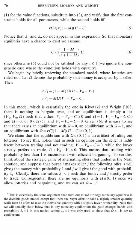
78 BERENTSEN, MOLICO, AND WRIGHT

FIG. 1. Monetary equilibrium, indivisible goods model.
Several comments are in order concerning these results. First, since %� <1,we have { # (0, 1) in a region of parameter space with positive measure.Hence, the implicit restriction made in the previous literature, that lotteriesare not allowed, is indeed restrictive. Second, there is an asymmetry in themodel: money may change hands randomly, but goods either change handswith probability 1 or not at all. This is depicted in Fig. 1, which plots { and* as functions of %. As is clear, for %>%� goods trade with probability 1 andmoney trades randomly, for intermediate % # [%
�, %� ] both objects trade with
probability 1, and for %<%�
monetary equilibria do not exist. We discussthis asymmetry further below.
Note that { measures the price level��it is the average number of unitsof money that it takes to buy a good. One can show { is decreasing in %,increasing in r, increasing in C, and decreasing in U, for both the modelwith Tj=Vj and the model with Tj=0. The effects of changes in M dependon which version of the model we use, however: one can show �{1 ��M>0,but, perhaps surprisingly, �{0��M>0 iff r and M are not too small. Also,as r � 0 we have { � 0 for all %>%� (the { curve in Fig. 1 becomes verticalat %=%� ); thus, if % is big and agents are very patient buyers get the goodvirtually for free, which sellers are willing to go along with since on thesmall but positive chance they get the money it will convey exactly thesame benefit to them.8
79INDIVISIBILITIES, LOTTERIES, AND MONEY
8 The thresholds also depend on r; in particular, as r � 0, we have %� 1 � M and%�
1 � CM�[(1&M) U+MC] in the model with Tj=Vj , and %� 0 � 1�2 and %�
0 � C�(U+C) inthe model with Tj=0. Other differences between the models with different threat pointsinclude the following. When Tj=0, %� 0>1�2 for all r>0, and so lotteries are not used whenbuyers and sellers have equal bargaining power; but when Tj=Vj , it is possible to have {<1when %=1�2. Also, as long as {1 and {0 are in (0, 1), we have {0<{1 iff M>1�2.

Finally, we mention welfare. For low % there is no monetary equilibrium,and the only possible equilibrium is autarchy, where V1=V0=0. If lot-teries are ruled out then there is an equilibrium where money is acceptedand V1>V0>0 for all parameters satisfying (6). Hence, allowing lotteriescan actually reduce welfare. This should not be too surprising, however, asit simply says that agents may be better off if they can commit to *=1rather than bargaining in each bilateral meeting. In any case, we will seebelow that there is a welfare-improving role for lotteries in a slight variantof this model, where we consider commodity money, and where rather thanlooking for equilibria for an arbitrary value of the bargaining weight % welook for incentive-feasible allocations that a social planner might choose.Also, we will soon see that lotteries can only enhance welfare in thedivisible goods version of the model presented in the next section.
4. THE DIVISIBLE GOODS MODEL
When q # R+ , a lottery is generally described by { and two conditionalprobability distributions, *q | 0 and *q | 1 . However, we claim the amount ofgoods that changes hand is degenerate and independent of whether moneychanges hands.
Proposition 3. There is a value for q, say q=q$ (that depends onparameter values), such that *q | 0 (q$)=*q | 1 (q$)=1.
Proof. The Nash bargaining problem is to choose { # [0, 1] and prob-ability measures *q | 0 and *q | 1 to solve
max {{ _| u(q) *q | 1 (dq)+V0 &+(1&{) _| u(q) *q | 0 (dq)+V1&&T1=%
_{{ _&| c(q) *q | 1 (dq)+V1&+(1&{) _&| c(q) *q | 0 (dq)+V0&&T0=
1&%
subject to the incentive constraints in (3), taking V0 and V1 as given. Sup-pose that the solution implies *q | 0 and *q | 1 are nondegenerate, and letq0=� q*q | 0 (dq) and q1=� q*q | 1 (dq). Since u(q) is concave and c(q)convex, and at least one is strictly so, by Jensen's inequality the incentiveconstraints are still satisfied and the Nash product is higher when*q | 0 (q0)=*q | 1 (q1)=1, which is a contradiction. Hence, *q | 0 and *q | 1 aredegenerate at q0 and q1 , respectively. Now suppose q0 {q1 , and let
80 BERENTSEN, MOLICO, AND WRIGHT

Eq={q1+(1&{) q0 . Again by Jensen's inequality the incentive constraintsare still satisfied and the Nash product is higher at Eq, another contradic-tion. So q must be degenerate at some value q$. K
The above result makes the analysis much simpler because we can nowrestrict attention to lotteries that are completely characterized by twonumbers, { and q (in what follows we use q to denote the quantity ratherthan the random variable). Given any such lottery, one can, as in the previoussection, solve (1) for the value functions, substitute in (3), and verify thatthe first constraint is never binding and the second is satisfied iff
rc(q)&{(1&M)[u(q)&c(q)]�0. (9)
In particular, if {=1, then (9) holds iff
.(q)#rc(q)&(1&M)[u(q)&c(q)]�0. (10)
It is easy to see that .(0)=0, .$(0)<0, ."(q)�0 for all q, and .(q)>0for large q; hence, if {=1 the constraints are satisfied iff q is below somecritical value q̂. Also, let q* be the efficient quantity, defined byu$(q*)=c$(q*). It is easy to verify that q* is the quantity that maximizeswelfare, W=MV1+(1&M) V0 . If q=q* then (9) holds iff
{�{̂#rc(q*)
(1&M)[u(q*)&c(q*)], (11)
which can hold iff r is not too big.The following proposition characterizes the set of equilibria for the
model with threat points equal to continuation values.
Proposition 4. Assume Tj=Vj . If %=0, there does not exist amonetary equilibrium. If %>0, then there is a critical value %� 1 constructedin the proof, where %� 1>0 for all parameter values and %� 1<1 iffr<(1&M)[u(q*)&c(q*)]�c(q*), such that the following is true: if %<%� 1
there exists a unique monetary equilibrium and it entails {=1 and q<q*,with �q��%>0 and lim% � %� 1
q=q*; and if %>%� 1 there exists a uniquemonetary equilibrium and it entails q=q* and {={~ 1 # (0, 1), where
{~ 1=r[%c(q*)+(1&%) u(q*)](%&M)[u(q*)&c(q*)]
.
Proof. If %=0 then the bargaining solution is equivalent to take-it-or-leave-it offers by the seller, which implies u(q)={(V1&V0). Inserting this
81INDIVISIBILITIES, LOTTERIES, AND MONEY

into (1), we find V1=0, and therefore V0<0 by (4). But a seller canalways achieve V0=0 by not trading. Hence, there cannot exist a monetaryequilibrium when %=0.
Now assume %>0. Then (2) reduces to choosing ({, q) # [0, 1]_R+ tosolve
max(61&V1)% (60&V0)1&%,
where 61=u(q)+{V0+(1&{) V1 and 60=&c(q)+{V1+(1&{) V0 .Necessary and sufficient conditions for a solution are
%u$(q)(60&V0)&(1&%) c$(q)(61&V1)�0, = if q>0
(12)
%(V0&V1)(60&V0)+(1&%)(V1&V0)(61&V1)&'{�0, = if {>0,
where '{ is the nonnegative multiplier on the constraint {�1. We are look-ing for monetary equilibria, which implies that both conditions hold withequality.
First consider the case where {<1, which implies that '{=0. Then com-bining the two first order conditions yields u$(q)=c$(q), and so q=q*.Solving (1) for the Vj 's and inserting the solutions, as well as q=q*, intothe second condition in (12), we can solve for {={~ 1 where {~ 1 is defined inthe statement of the proposition. Notice that {~ 1 # (0, 1) iff %>%� 1 where
%� 1=(r+M) u(q*)&Mc(q*)(1+r)[u(q*)&c(q*)]
.
One can check that {~ 1� {̂, where {̂ is defined in (11), and therefore theincentive condition (9) holds at {={~ 1 and q=q*. Hence, we conclude thatthere exists an equilibrium with {={~ 1 and q=q* iff %>%� 1 .
Now consider the case where {=1, which implies '{�0. By combiningthe two conditions in (12), we get u$(q)�c$(q), and this implies q�q* inany equilibrium with {=1, with strict inequality as long as '{>0. Insertingthe Vj 's and {=1, we can rewrite the first order condition for q as
(1&%) c$(q)%u$(q)
=1&M&(r+1&M) c(q)�u(q)
r+M&Mc(q)�u(q). (13)
The left hand side of (13) is zero at q=0 and it is strictly increasing. Asq � 0, the right hand side approaches (1&M)�(r+M)>0, becausec(q)�u(q) � 0 by l'Hopital's rule, and it is strictly decreasing and equals 0when q=q̂, where recall that q̂ is the solution to (10) at equality. Hence,
82 BERENTSEN, MOLICO, AND WRIGHT

there exists an unique solution to (13), call it /=/(%), in (0, q̂). Moreover,it is easy to check that /$(%)>0 and that /(%� 1)=q*. Since we need/(%)�q* for an equilibrium with {=1, an equilibrium of this type cannotexist if %>%� 1 . If %<%� 1 then /(%)<q*, and we now show that this alsoimplies the first order condition for { is satisfied at {=1. To see this,rearrange the first order condition for { as
%�(r+M) u(q)&Mc(q)(1+r)[u(q)&c(q)]
. (14)
The right hand side of (14) is decreasing in % and approaches(r+M)�(1+r)>0 as q � 0. Also, (14) is satisfied at equality when %=%� 1 .Hence, (14) is satisfied iff %�%� 1 . We conclude that {=1 and q=/(%)satisfy the first order conditions iff %�%� 1 . Moreover, since /(%)<q̂, itsatisfies the incentive condition (10), and hence satisfies all of the condi-tions for an equilibrium.
Finally, it is obvious that %� 1>0, and that %� 1<1 iff r<(1&M) [u(q*)&c(q*)]�c(q*). This completes the proof. K
The model with Tj=0 has the same qualitative properties, and so as inthe previous section we state the results here without proof.
Proposition 5. Assume Tj=0. If %=0 there does not exist a monetaryequilibrium. If %>0 then there is a critical value %� 0 , where %� 0>0 for allparameter values and %� 0<1 iff r<(1&M)[u(q*)&c(q*)]�c(q*), such thatthe following is true: if %<%� 0 there exists a unique monetary equilibrium andit entails {=1 and q<q*, with �q��%>0 and lim% � %� 0
q=q*; and if %>%� 0
there exists a unique monetary equilibrium and it entails q=q* and{={~ 0 # (0, 1), where
{~ 0=r[(1&%)(1&M+r) u(q*)+%(M+r) c(q*)]
[r(%&M)+M(1&M)(2%&1)][u(q*)&c(q*)].
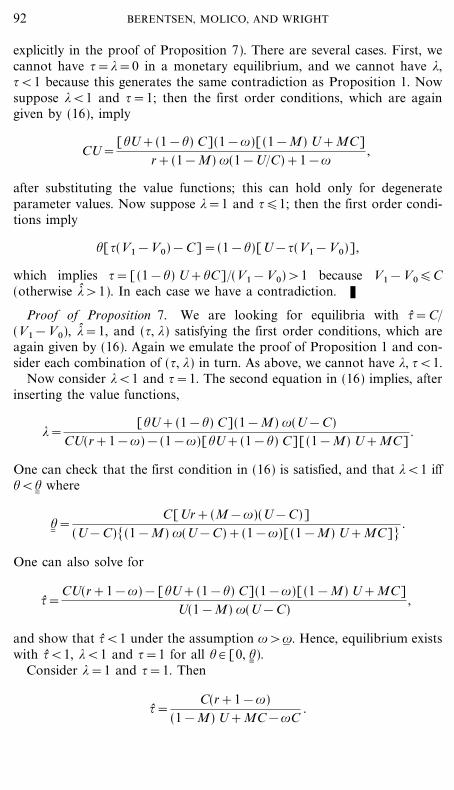
The first thing we want to emphasize about the above two propositionsis that although there is a monetary equilibrium for all %>0 and nomonetary equilibrium for %=0, there is no real discontinuity because q � 0as % � 0 in monetary equilibrium. Next, notice that as in the previous sec-tion the two objects are traded asymmetrically: randomization may be usedfor trading money but not for trading goods. Figure 2 shows { and q asfunctions of % (the figure shows %� <1, which holds iff r is not too big).Notice that q�q* for all % with strict inequality iff %<%� , where q* is theefficient quantity: u$(q*)=c$(q*). It is argued in Trejos and Wright [21]that it is natural to have q below q* in a monetary economy, although inthe model in that paper, without lotteries, the result does not actually hold
83INDIVISIBILITIES, LOTTERIES, AND MONEY

FIG. 2. Monetary equilibrium, divisible goods model.
very generally��it holds when %=1�2 in the model where Tj=0, but it maynot hold for other values of %, and it may not hold in the model whereTj=Vj even if %=1�2. With lotteries, q can never exceed q* irrespective ofthreat points or bargaining power.
Some results for this model are similar to those for the indivisible goodsmodel. For example, the behavior of { with respect to the parameters is thesame. There are also differences. For one thing, in the indivisible goodsmodel we have %� <1, and hence we definitely have {<1 for high %, whilein the divisible goods model we can guarantee {<1 for high % iff r is nottoo big. Also, in the indivisible goods model monetary equilibria do notexist for low %, while in the divisible goods model a monetary equilibriumexists for all %>0. Finally, recall that lotteries could reduce welfare in theindivisible goods model. Lotteries can only improve welfare here: for %�%� ,q and therefore welfare are the same with or without lotteries; for %>%� ,q=q* with lotteries and q>q* without lotteries, and therefore welfare isstrictly higher with lotteries.9
5. DISCUSSION
We have seen that although agents may agree to a lottery where moneychanges hands with probability less than 1, they will never agree to
84 BERENTSEN, MOLICO, AND WRIGHT
9 Lotteries (sometimes) reduce welfare in the indivisible goods model by causing monetaryequilibrium to break down; this never happens in the divisible goods model, and moreoverlotteries can enhance welfare by eliminating overproduction��i.e., q is at rather than above theefficient quantity q*.

a lottery where goods change hands with probability less than 1. What liesbehind this asymmetry? It is not due to the assumption that money isindivisible while goods are divisible, because the same asymmetry ariseswhen goods and money are both indivisible. One conjecture is that asym-metry is due to the fiat nature of the money��i.e., to the fact that it has nointrinsic worth and derives value only from its role as a medium ofexchange. To investigate this, and some other things, we consider severalvariations on the basic theme.
One approach is to consider a model with direct barter instead ofmonetary exchange. For example, suppose some agents consume good 1and produce good 2, while some consume good 2 and produce good 1.Goods are indivisible, production of good j costs Cj>0, and consumptionyields utility Uj . Assume Ui>Cj , for all i, j. When two agents of theopposite type meet they bargain over lotteries. Let % be the bargainingpower of type 1, and let {j be the probability that type j gives up hisproduction good.10 It is easy to prove the following (details available uponrequest): there are critical values %
�and %� , with 0<%
�<%� <1, such that: if
%<%�
then {1=1 and {2 # (0, 1); if %��%�%� then {1={2=1; and if %>%�
then {2=1 and {1 # (0, 1).Hence, agents get their consumption goods with probability less than 1
iff they have sufficiently low bargaining power, in a model with directbarter, while it was not possible to get goods with probability less than 1when agents were trading with fiat money. So it seems there is somethingto the notion that asymmetry is due to the nature of fiat money. To explorethings further, consider a model with one indivisible good and money, asin Section 3, but assume now that the money is a commodity money, in thesense that it yields a direct utility flow #>0 to an agent holding it.
Let { and * be the probabilities that money and goods change hands (wedo not need two conditional probabilities *0 and *1 because one can show,as above, that *0=*1). The value functions satisfy
rV0=M[{(V1&V0)&*C](15)
rV1=(1&M)[*U+{(V0&V1)]+#.
The bargaining solution is exactly as above. Then we have the followinggeneralization of Proposition 1 (for brevity we only present results for thecase Tj=Vj , but the other case is essentially the same).
85INDIVISIBILITIES, LOTTERIES, AND MONEY
10 After trading, one can assume agents return to the market, as in the money model, orthat they exit the economy, as in Rubinstein and Wolinsky [17], say. We have explored theseand several other sets of assumptions, some that generate models very similar to the one inRubinstein and Wolinsky; the same qualitative results held for all the barter models weexplored. Note that lotteries are not useful in the basic model presented by Rubinstein andWolinsky, but only because that model assumes utility is linear.

Proposition 6. Let #� =(r+M) U&MC. If #>#� then for all % thereexists a unique monetary equilibrium and it entails *=1 and {={~ # (0, 1). If# # (0, #� ) then there are critical values %
�and %� , with 0<%
�<%� <1, such that
the following is true: if %<%�
there exists a unique monetary equilibrium andit entails {=1 and *=*� # (0, 1), where
*� =#[%U+(1&%) C]
(U&C)[M(1&%) C&%(1&M) U]+rCU;
if % # [%�, %� ] there exists a unique monetary equilibrium and it entails {=1
and *=1; and if %>%� there exists a unique monetary equilibrium and itentails *=1 and {={~ # (0, 1), where
{~ =r[%C+(1&%) U]
#+(%&M)(U&C).
Proof. See the Appendix.
We emphasize first that #>0 implies that a monetary equilibrium existsfor all %, while with fiat money there was no monetary equilibrium forsmall % (there is no discontinuity, however, since * � 0 as # � 0). However,the key result is that when #>0 we can have * # (0, 1); i.e., goods can tradewith probability less than 1 against commodity money, even though theycould not trade with probability less than 1 against fiat money. So it seemsthat it is not money per se that generates the asymmetry, but fiat money.Before pursuing this issue further, however, we want to highlight somesubstantive results that emerge from the commodity money model.
First, note that for large # we must have { # (0, 1), and indeed, as # � �we have { � 0. This is a version of Gresham's Law: very valuable moneywill be hoarded, in the sense that the probability it changes hands will besmall. However, even though the money is hoarded, the good still changeshands with probability 1. Moreover, one can show that in the divisiblegoods version of the model with commodity money, with lotteries, for big# we have q=q* with probability 1. Hence, a sufficiently valuable moneymay probabilistically stop circulating, but the outcome is neverthelessefficient. By contrast, without lotteries, a sufficiently valuable money alsowill be hoarded, but in this case trade will shut down, and welfare will bereduced.11
Returning to the issue of asymmetry, we have seen that goods can tradewith probability less than 1 against a money that has some exogenouslyspecified commodity value #. In fact, we will now show that goods can
86 BERENTSEN, MOLICO, AND WRIGHT
11 Velde, Weber and Wright [22] discuss Gresham's Law in search models withheterogeneous currencies, without allowing lotteries.

trade with probability less than 1 against a fiat money if there is somevalue to the fiat money that arises endogenously due to, in this case,heterogeneity in bargaining. In particular, consider a generalization of themodel with indivisible goods and fiat money where we now assume thatwith probability | the buyer gets to make a take-it-or-leave-it offer to theseller, while with probability 1&| they bargain according to the Nashsolution, with bargaining power % and threat points Tj=Vj , as above. Thechance of meeting a seller and making a take-it-or-leave-it offer generatesan endogenous return to holding fiat money that will play a role analogousto the role of # in the commodity money model.12
Let ({, *) be the lottery that results from the Nash solution and ({̂, *� )that which results from the take-it-or-leave-it offer (again we do not needconditional probabilities *0 and *1 , or *� 0 and *� 1 , since it turns out that*0=*1=* and *� 0=*� 1=*� ). The value functions satisfy
rV1=(1&M)[|[*� U+{̂(V0&V1)]+(1&|)[*U+{(V0&V1)]]
rV0=M(1&|)[{(V1&V0)&*C].
In the equation for V0 we have used the fact that the seller gets no surpluswhen the buyer makes a take-it-or-leave-it offer: {̂(V1&V0)&*� C=0.Moreover, this condition also implies that either {̂=1 and *� =
V1&V0C , or
{̂= CV1&V0
and *� =1. In the Appendix we show that generically we cannothave {̂=1 and *� =
V1&V0C ; hence we proceed to characterize equilibria with
{̂= CV1&V0
and *� =1.In the interest of manageability, and since we are only interested in
showing that it is possible to have * # (0, 1) we assume in what follows that|�|
�=(U&C)[(1&M) U+CM]�C[rU+M(U&C)], which serves to
guarantee that for all parameter values monetary equilibria exists.
Proposition 7. Assume Tj=Vj , and |�|�. Then for all parameters
there exists an equilibrium with {̂<1, *� =1, and { and * described as follows.There are critical values %
��and %�� constructed in the proof, with 0<%
��<%�� <1,
such that: if %<%��
then {=1 and *<1; if %��<%<%�� then {=1 and *=1; and
if %>%�� then {<1 and *=1.
Proof. See the Appendix.
The key part of this result is that we can have *<1 in this model, justlike in the commodity money model. One way to understand what is going
87INDIVISIBILITIES, LOTTERIES, AND MONEY
12 This model was inspired by comments of the associate editor, although his suggestionwas actually to endow different agents with permanently different bargaining powers. Thisalso works, but things turn out to be a lot cleaner if we assume agents are identical in an exante sense and have different bargaining powers in different meetings.

on is to think about the model in the following way. Agents believe thatthere is some economy-wide probability * with which they can get goodsfor a unit of money. Then, when a particular buyer-seller pair meet, theybargain over the probability *$ that they will use to trade, taking * as given.This generates a version of a best response function, of which an equi-librium is a fixed point. For the commodity money model, the bestresponse function can easily be shown to be *$ =min[4(*), 1], where 4(*)is linear:
4(*)=%U+(1&%) C
CU(1+r)[#+[(1&M) U+MC] *].
If #=0 (fiat money), the intercept of 4(*) is zero. When % is small, theslope of 4 is less than 1, and given any economy-wide * our particularbuyer-seller pair will bargain to *$ <*, so the only fixed point is *=0.When % is big, the slope of 4(*) is greater than 1, and given *>0 our pairwill bargain to *$ >*, so *=1 is fixed point, as well as *=0. With #>0,however, the intercept of 4(*) is strictly positive, and so there is a uniquefixed point, it is always positive, and it less than 1 iff % is small. Intuitively,the idea is that even if other agents are giving goods with probability *=0in exchange for money, as long as #>0 you would be willing to trade yourgood with some positive probability to get a unit of money. This is why themodel with #>0 always has *>0, and can have *<1. The idea is essen-tially the same when |>0. Any value to money outside of the Nashbargain that determines * could play the same role.
To close this section we address one final concern: does the nontrivialrole for lotteries arise when we solve a social planner's problem, or onlywhen we impose an arbitrary bargaining solution, in the sense of anarbitrary value of %? Consider a world with an exogenous supply of Munits of commodity money with return #>0. Goods as well as money areindivisible and there is a unit storage capacity. The social planner gets tochoose a lottery ({, *). Welfare is given by
W=MV1+(1&M) V0=M(1&M) *(U&C)+M#,
which is increasing in *, and independent of { (since it does not matter inthe aggregate who holds the asset and therefore it cannot matter if moneychanges hands).
The planner is faced with the following incentive constraints:
{(V1&V0)&*C�0 which holds iff r�_#+(1&M) *(U&C)*C & {
*U+{(V0&V1)�0 which holds iff r�_#&M*(U&C)*U & {.
88 BERENTSEN, MOLICO, AND WRIGHT

FIG. 3. Incentive feasible allocations in lottery space.
Notice that if #=0, then the second constraint is not binding and the firstholds iff r�{(1&M)(U&C)�C, which does not depend on *. Thus, with#=0 there is no role for lotteries, since: (i) * does not affect the incentiveconditions and {<1 only makes them less likely to hold; and (ii) the objec-tive function W is unaffected by { and increasing in *. This means thateither *=1 is feasible, in which case we can always set {=1, or *=1 is notfeasible, in which case we cannot do better than autarchy. So if there is arole for lotteries here it must be that #>0.
Figure 3 shows the set of points in lottery space satisfying the incentiveconditions for various parameter configurations.13 The cases are similar
89INDIVISIBILITIES, LOTTERIES, AND MONEY
13 The figure is drawn by solving for the {={0 (*) and {={1 (*) that solve the two incentiveconditions with equality. The values for r
�and r� in the figure are given by r
�=[#&
M(U&C)]�U and r� =[#+(1&M)(U&C)]�C.

except for the location of (1, 1) relative to this set. In case 1a, for instance,(1, 1) is not feasible; it is feasible to choose *=1 only if {<1. This casecorresponds to a large value of #, which means money holders will not giveup money with probability 1 to get the good, but they would give it upwith some probability {<1. In case 1b, *=1 is feasible for { in some rangethat includes 1, which means we do not need lotteries. In case 1c, we can-not have *=1; the best * we can achieve is attained by setting {=1, butthis entails *<1. In this case, # is small, so again we need lotteries but nowit is the good that trades with probability less than 1. The bottom line isthat if #>0 there can be a nontrivial role for lotteries in the planner'sproblem, either because we need to set {<1 to achieve *=1, or becausethe best * we can achieve is less than 1.14
6. CONCLUSION
This paper has introduced lotteries into search-theoretic models ofmonetary exchange. It has been shown that, in general, private agents (ora planner) may want to use randomized trading in this environment. In themodel with indivisible goods, we discussed how lotteries give us a way toanalyze prices, and also how lotteries eliminate mixed strategy equilibria.When goods are divisible, we found that the quantity produced is nevermore than the efficient quantity��something that is not generally truewithout lotteries. Also, we found that as a commodity money gets moreand more valuable, it drops out of circulation probabilisitically but the out-come is still efficient��again something that is not true without lotteries. Ageneral conclusion is that future work should take into account the factthat lotteries can have a nontrivial role to play in monetary economics.
APPENDIX
1. Proof of Proposition 6. The argument is similar to the proof ofProposition 1, although here we use the fact that *0=*1=*. First orderconditions for the bargaining problem are:
90 BERENTSEN, MOLICO, AND WRIGHT
14 Note that there is no discontinuity at #=0: as # � 0, {1 (*) approaches the vertical axisand {0 (*) approaches a line which coincides with the vertical axis up to {=rC�(1&N)(U&C)and then becomes horizontal, which gives exactly the set of incentive feasible lotteries with#=0.

&%[{(V1&V0)&*C](V1&V0)
+(1&%)[{(V0&V1)+*U](V1&V0)&'{�0, = if {>0
(16)
%[{(V1&V0)&*C]U&(1&%)[{(V0&V1)+*U]C&'*�0, = if *>0.
Given {>0, the first condition in (16) holds with equality. Consider thecase {<1, which implies *=1, as in Proposition 1. Substituting the Vj 'sinto first condition in (16), we can solve for {={~ , where {~ is defined above,and show {~ # (0, 1) iff
%>%� =(r+M) U&MC&#
(1+r)(U&C).
Notice %� >0 iff (r+M) U&MC>#. The incentive conditions are satisfiedat {={~ and *=1. Hence, there exists an equilibrium with *=1 and{={~ # (0, 1) iff %>%� .
Now consider the case where {=1. Inserting the Vj 's into the secondequation in (16) at equality and rearranging, we have
*[%U[(1&M) U&(r+1&M) C+#]
&(1&%) C[(r+M) U&MC&#�*]]=(1+r) '* .
Consider the case *<1, which implies '*=0 and {=1. Given this, we cansubstitute the Vj 's into second condition in (16) at equality and solve for*=*� , where *� is defined above. Notice *� # (0, 1) iff %<%
�, where
%�=
C[rU+M(U&C)&#](U&C)[U(1&M)+CM+#]
.
The incentive conditions are satisfied at *=*� . Hence, there exists an equi-librium with {=1 and *=*� iff %<%
�.
Finally, consider *={=1. Note that {=1 satisfies the first condition in(16) iff %�%� and *=1 satisfies the second condition iff %�%
�. Also, the
incentive compatibility constraints are satisfied at {=*=1. Hence, thereexists an equilibrium with *=1 and {=1 iff %
��%�%� . Also, it is easy to see
that #<#� implies 0<%�<%� <1 and #>#� implies %� <0. K
2. Proof that we cannot have {̂=1 and *� =(V1&V0)�C. Assuming {̂=1and *� =(V1&V0)�C, we will derive a contradiction from the first orderconditions from the Nash bargaining problem for ({, *) (these are given
91INDIVISIBILITIES, LOTTERIES, AND MONEY
explicitly in the proof of Proposition 7). There are several cases. First, wecannot have {=*=0 in a monetary equilibrium, and we cannot have *,{<1 because this generates the same contradiction as Proposition 1. Nowsuppose *<1 and {=1; then the first order conditions, which are againgiven by (16), imply
CU=[%U+(1&%) C](1&|)[(1&M) U+MC]
r+(1&M) |(1&U�C)+1&|,
after substituting the value functions; this can hold only for degenerateparameter values. Now suppose *=1 and {�1; then the first order condi-tions imply
%[{(V1&V0)&C]=(1&%)[U&{(V1&V0)],
which implies {=[(1&%) U+%C]�(V1&V0)>1 because V1&V0�C(otherwise *� >1). In each case we have a contradiction. K
Proof of Proposition 7. We are looking for equilibria with {̂=C�(V1&V0), *� =1, and ({, *) satisfying the first order conditions, which areagain given by (16). Again we emulate the proof of Proposition 1 and con-sider each combination of ({, *) in turn. As above, we cannot have *, {<1.
Now consider *<1 and {=1. The second equation in (16) implies, afterinserting the value functions,
*=[%U+(1&%) C](1&M) |(U&C)
CU(r+1&|)&(1&|)[%U+(1&%) C][(1&M) U+MC].
One can check that the first condition in (16) is satisfied, and that *<1 iff%<%
��where
%��=
C[Ur+(M&|)(U&C)](U&C)[(1&M) |(U&C)+(1&|)[(1&M) U+MC]]
.
One can also solve for
{̂=CU(r+1&|)&[%U+(1&%) C](1&|)[(1&M) U+MC]
U(1&M) |(U&C),
and show that {̂<1 under the assumption |>|�. Hence, equilibrium exists
with {̂<1, *<1 and {=1 for all % # [0, %��).
Consider *=1 and {=1. Then
{̂=C(r+1&|)
(1&M) U+MC&|C.
92 BERENTSEN, MOLICO, AND WRIGHT

The first order conditions can be shown to hold iff %���%�%�� , where
%�� =rU+(M&|)(U&C)
(1&|+r)(U&C).
Hence, equilibrium exists with {̂<1 and {=*=1 for all % # [%��, %�� ].
Now consider *=1 and {<1. The first equation in (16) implies
{=r[(1&%) U+%C]
[%&M+|(1&%)](U&C).
The second condition in (16) is satisfied iff %>%��, and {<1 iff %>%�� . Also,
{̂=rC[U(%&M)+C(M&|%)]
[(1&M) U+(M&|) C][%&M+|(1&%)](U&C).
One can show that {̂<1. Hence, equilibrium exists with {̂<1, {<1 and*=1 for all %>%�� . K
REFERENCES
1. A. Berentsen, Money inventories in search equilibrium, J. Money, Credit, Banking 32(2000), 168�178.
2. K. Binmore, A. Rubinstein, and A. Wolinsky, The Nash bargaining solution in economicmodeling, Rand J. Econ. 17 (1986), 176�188.
3. G. Camera and D. Corbae, Money and price dispersion, Int. Econ. Rev. 40 (1999),985�1008.
4. S. Chatterjee and D. Corbae, Valuation equilibria with transactions costs, Amer. Econ.Rev. 85 (1995), 287�290.
5. M. Coles and R. Wright, A dynamic equilibrium model of search, bargaining, and money,J. Econ. Theory 78 (1998), 32�54.
6. P. Diamond, Pairwise credit in search equilibrium, Quart. J. Econ. 105 (1990), 285�319.7. E. Green and R. Zhou, A rudimentary model of search with divisible money and prices,
J. Econ. Theory 81 (1998), 252�271.8. N. Kiyotaki and R. Wright, On money as a medium of exchange, J. Polit. Econ. 97 (1989),
927�954.9. N. Kiyotaki and R. Wright, A contribution to the pure theory of money, J. Econ. Theory
53 (1991), 215�235.10. N. Kiyotaki and R. Wright, A search-theoretic approach to monetary economics, Amer.
Econ. Rev. 83 (1993), 63�77.11. M. Molico, The distribution of money and prices in search equilibrium, manuscript
(1996).12. M. J. Osborne and A. Rubinstein, ``Bargaining and Markets,'' Academic Press, San Diego,
1990.13. E. C. Prescott and R. M. Townsend, Pareto optima and competitive equilibrium with
adverse selection and moral hazard, Econometrica 52 (1984), 21�45.
93INDIVISIBILITIES, LOTTERIES, AND MONEY

14. E. C. Prescott and R. M. Townsend, General competitive analysis in an economy withprivate information, Int. Econ. Rev. 25 (1984b), 1�20.
15. R. D. Rogerson, Indivisible labor, lotteries and equilibrium, J. Monet. Econ. 21 (1988),3�16.
16. A. Rubinstein, Perfect equilibrium in bargaining model, Econometrica 50 (1982), 97�109.17. A. Rubinstein and A. Wolinsky, Equilibrium in a market with sequential bargaining,
Econometrica 53 (1985), 1133�1150.18. K. Shell and R. Wright, Indivisibilities, lotteries, and sunspot equilibria, Econ. Theory 3
(1993), 1�17.19. S. Shi, Money and prices: A model of search and bargaining, J. Econ. Theory 67 (1995),
467�496.20. A. Taber and N. Wallace, A matching model with bounded holdings of indivisibile money,
Int. Econ. Rev. 40 (1999), 961�984.21. A. Trejos and R. Wright, Search, bargaining, money and prices, J. Polit. Econ. 103 (1995),
118�141.22. F. Velde, W. Weber, and R. Wright, A model of commodity money, with applications to
Gresham's law and the debasement puzzle, Rev. Econ. Dynam. 2 (1999), 291�323.23. R. Zhou, Individual and aggregate real balances in a random matching model, Int. Econ.
Rev. 40 (1999), 1009�1038.
94 BERENTSEN, MOLICO, AND WRIGHT
Copyright © 2022 FDOKUMEN