Monetary EconomicsAn Integrated Approach to Credit,Money, Income, Productionand Wealth

Wynne Godley

and

Marc Lavoie

Contents

Notations Used in the Book ix

List of Tables xviii

List of Figures xx

Preface xxxiv

1 Introduction 11.1 Two paradigms 11.2 Aspiration 41.3 Endeavour 91.4 Provenance 111.5 Some links with the ‘old’ Yale school 131.6 Links with the post-Keynesian school 161.7 A sketch of the book 18A1.1 Compelling empirical failings of the neo-classical

production function 20A1.2 Stock-flow relations and the post-Keynesians 21

2 Balance Sheets, Transaction Matrices and the Monetary Circuit 232.1 Coherent stock-flow accounting 232.2 Balance sheets or stock matrices 252.3 The conventional income and expenditure matrix 332.4 The transactions flow matrix 372.5 Full integration of the balance sheet and the transactions

flow matrices 432.6 Applications of the transactions flow matrix: the monetary

circuit 47

3 The Simplest Model with Government Money 573.1 Government money versus private money 573.2 The service economy with government money and no

portfolio choice 583.3 Formalizing Model SIM 613.4 A numerical example and the standard Keynesian multiplier 683.5 Steady-state solutions 713.6 The consumption function as a stock-flow norm 743.7 Expectations mistakes in a simple stock-flow model 783.8 Out of the steady state 833.9 A graphical illustration of Model SIM 88

v

vi Contents

3.10 Preliminary conclusion 91A3.1 Equation list of Model SIM 91A3.2 Equation list of Model SIM with expectations (SIMEX ) 92A3.3 The mean lag theorem 92A3.4 Government deficits in a growing economy 95

4 Government Money with Portfolio Choice 994.1 Introduction 994.2 The matrices of Model PC 994.3 The equations of Model PC 1024.4 Expectations in Model PC 1074.5 The steady-state solutions of the model 1114.6 Implications of changes in parameter values on temporary

and steady-state income 1164.7 A government target for the debt to income ratio 124A4.1 Equation list of Model PC 126A4.2 Equation list of Model PC with expectations (PCEX) 126A4.3 Endogenous money 127A4.4 Alternative mainstream closures 129

5 Long-term Bonds, Capital Gains and Liquidity Preference 1315.1 New features of Model LP 1315.2 The value of a perpetuity 1315.3 The expected rate of return on long-term bonds 1325.4 Assessing capital gains algebraically and geometrically 1345.5 Matrices with long-term bonds 1365.6 Equations of Model LP 1375.7 The short-run and long-run impact of higher interest rates

on real demand 1505.8 The effect of household liquidity preference on long rates 1535.9 Making government expenditures endogenous 160A5.1 Equations of Model LP 165A5.2 The liquidity trap 167A5.3 An alternative, more orthodox, depiction of the bond market 168

6 Introducing the Open Economy 1706.1 A coherent framework 1706.2 The matrices of a two-region economy 1716.3 The equations of a two-region economy 1736.4 The steady-state solutions of Model REG 1766.5 Experiments with Model REG 1806.6 The matrices of a two-country economy 1876.7 The equations of a two-country economy 1916.8 Rejecting the Mundell–Fleming approach and adopting

the compensation approach 194

Contents vii

6.9 Adjustment mechanisms 2016.10 Concluding thoughts 207A6.1 Equations of Model REG 209A6.2 Equations of Model OPEN 211A6.3 Historical and empirical evidence concerning the

compensation principle 213A6.4 Other institutional frameworks: the currency board 214A6.5 How to easily build an open model 215

7 A Simple Model with Private Bank Money 2177.1 Private money and bank loans 2177.2 The matrices of the simplest model with private money 2187.3 The equations of Model BMW 2227.4 The steady state 2277.5 Out-of-equilibrium values and stability analysis 2337.6 The role of the rate of interest 2407.7 A look forward 247A7.1 The equations of Model BMW 247

8 Time, Inventories, Profits and Pricing 2508.1 The role of time 2508.2 The measure of profits 2528.3 Pricing 2638.4 Numerical examples of fluctuating inventories 276A8.1 A Numerical example of inventory accounting 278

9 A Model with Private Bank Money, Inventories and Inflation 2849.1 Introduction 2849.2 The equations of Model DIS 2859.3 Additional properties of the model 2939.4 Steady-state values of Model DIS 2959.5 Dealing with inflation in (a slightly modified) Model DIS 300A9.1 Equation list of Model DIS 308A9.2 The peculiar role of given expectations 310A9.3 Equation list of Model DISINF 312

10 A Model with both Inside and Outside Money 31410.1 A model with active commercial banks 31410.2 Balance sheet and transaction matrices 31510.3 Producing firms 31810.4 Households 32210.5 The government sector and the central bank 33110.6 The commercial banking system 33310.7 Making it all sing with simulations 34210.8 Conclusion 374

viii Contents

A10.1 Overdraft banking systems 374A10.2 Arithmetical example of a change in portfolio preference 376

11 A Growth Model Prototype 37811.1 Prolegomena 37811.2 Balance sheet, revaluation and transactions-flow matrices 37911.3 Decisions taken by firms 38311.4 Decisions taken by households 39211.5 The public sector 39711.6 The banking sector 39911.7 Fiscal and monetary policies 40411.8 Households in the model as a whole 42211.9 Financial decisions in the model as a whole 43511.10 A concluding recap 441

12 A More Advanced Open Economy Model 44512.1 Introduction 44512.2 The two matrices 44612.3 Equations of the generic model 45012.4 Alternative closures 46212.5 Experiments with the main fixed exchange rate closure 46612.6 Experiments with alternative fixed exchange rate closures 47212.7 Experiments with the flexible exchange rate closure 47812.8 Lessons to be drawn 487A12.1 A fundamental and useful open-economy flow-of-funds

identity 490A12.2 An alternative flexible exchange rate closure 492

13 General Conclusion 49313.1 Unique features of the models presented here 49313.2 A summary 499

References 501

Index 514

Notations Used in the Book

Ad Advances demanded by private banksA, As Central bank advances made to private banksadd Random change in liquidity preferenceaddbL Spread of bond rate over the bill rateaddl Spread of bill rate over the deposit rateadd2 Random change in government expendituresAF Amortization funds

B$£ Bills held by £ households but issued by the

$ countryB£

$ Bills held by $ households but issued by the £ country

B$cb£ Bills held by the £ central bank but issued by the

$ country (foreign reserves of country £)B$

cb$ Bills held by $ central bank and issued by the$ country

B£cb£ Bills held by the £ central bank and issued by the

£ countryBd, Bhd Bills demanded by households (ex ante)Bb, Bbd Bills actually demanded by banksBbdN Bills notionally demanded by banksBcb Bills held by the central bankBh, Bhh Bills held by householdsBs Treasury bills supplied by governmentbandB, bandT Lower and upper range of the flat Phillips curveBLd Long-term bonds demanded by householdsBLh Long-term bonds held by householdsBLs Long-term bonds issued by governmentBLR Bank liquidity ratio, actual or gross valueBLRN Bank liquidity ratio, net of advancesBLPR Banks liquidity pressure ratiobot Bottom of an acceptable rangebotpm Bottom of the acceptable range of the profitability

margin of banks

ix

x Notations Used in the Book

BP Balance of paymentsBPM Bank profit marginBUR Relative burden of interest payments on loans taken by

households

c, cd Consumption goods demand by households, in realterms

Cd Consumption goods demand by households, in nominalterms

C, Cs Consumption goods supply by firms, in nominal termsCAB Current account balanceCAR Realized capital adequacy ratio of banksCF Cash flow of firmsCG Capital gainsCGe Expected capital gains of the current period

DA Depreciation allowanceDEF Government deficitDS Nominal domestic salesds Real domestic salesdxre Expected change in the exchange rate

E, Ef , Eb Value of equities, issued by firms, issued by bankseb Number of equities supplied by banksed Number of firms’ equities demanded by householdses, ef Number of equities supplied by firmsER Employment rate (the complement of the

unemployment rate)ERrbL Expected rate of return on long-term bonds

F Sum of bank and firm profitsF, Ff Realized entrepreneurial profits of production firmsFb Realized profits of banksFT

b Target profits of banksFcb Profits of central bankFe Expected entrepreneurial profits of firmsFf Realized entrepreneurial profits of production firmsFe

f Expected profits of firmsFT

f Target entrepreneurial profits of production firmsFT Total profits of firms, inclusive of interest payments on

inventoriesFnipa Profits, as measured by national accountantsFD Business dividends

Notations Used in the Book xi

FDb Dividends of banksFDf Realized dividends of production firmsFU Business retained earningsFUb Retained earnings of banksFUT

b Target retained earnings of banksFUf Realized retained earnings of production firmsFUT

f Target retained earnings of production firmsfs Real fiscal stance

g Pure government expenditures in real termsg ′ Real total government expenditures (inflation

accounted)G Pure government expenditures in nominal termsGs, Gd Services supplied to and demanded by governmentGNT Total government expenditures, including interest

payments net of taxesgd Real government debtGT Total government expenditures, inclusive of

interest payments on debtGTD Total domestic government expendituresGD Government debt (public debt), in nominal termsGL Gross flow of new loans made to the household

sectorgr Steady-state growth rate of the economygrk Growth rate of net capital accumulationgrg Growth rate of real pure government expendituresgrpr Growth rate of trend labour productivity

Hbd Reserves demanded by banksHb, Hbs Reserves supplied to banks by the central bankHd, Hhd Cash money demanded by householdsHd, Hh, Hhh Cash money held by householdsHg Cash money held by governmentHhs Cash money supplied to households by the central

bankH , Hs High-powered money, or cash money, supplied by

the central bankHC Historic costsHCe Expected historic costsHUC Historic unit costHUCe Expected historic unit costHWC Historic wage cost

xii Notations Used in the Book

id New fixed capital goods demanded by firms(investment flow), in real terms

Id New fixed capital goods demanded by firms(investment flow), in nominal terms

Ih Residential investment of householdsIs, I , If New fixed capital goods supplied by firms,

in nominal termsin Realized stock of inventories, in real termsine Short-run target level (expected level) of

inventories, in real termsinT Long-run target level of inventories, in real

termsIN Realized stock of inventories, at current unit

costsim Real importsIM Imports, in nominal termsIMT Total imports, inclusive of interest payments

made abroadINTb Interest payments paid by banksINTf Interest payments paid by firmsINTh Interest payments received by households

k, kf , kb Fixed capital stock, in real terms (number ofmachines), of firms, of banks

K, Kf , Kb, Kh Value of fixed capital stock, in nominalterms, of firms, of banks, of households

KT Targeted capital stockKABOSA Capital account balance, inclusive of the

official settlements accountKAB Capital account balance, excluding official

transactions

Ld, Lfd Loans demanded by firms from banksL, Ls, Lfs, Lf Loans supplied by banks to firmsLg Loans to government sectorLhd Loans demanded by households from banksLhs, Lh Loans supplied by banks to households

M , Mh, Mhh Money deposits actually held by householdsM1, M1h Checking account money deposits held by

households

Notations Used in the Book xiii

M1d Checking account money deposits demandedM1s Checking account money deposits suppliedM2, M2h Time or term money deposits held by

householdsM2d Time or term money deposits demandedM2s Time or term money deposits suppliedM1hN The notional amount of bank checking

account deposits that households would holdMd, Mhd Money deposits demanded by householdsMf Financial assets of firmsMg Bank deposits of governmentmh Real money balances held by householdsMs Money supplied by the government (ch. 3) or

the banksML Mean lag

N, Nd Demand for labourNfe The full-employment labour forceNe

s Expected supply of labourNs Supply of labourNT Target level of employment by firmsNAFA Net accumulation of financial assets by the

household sector (financial saving)NCAR Normal capital adequacy ratio of banks

(Cooke ratio)NHUC Normal historic unit costNL Net flow of new loans made to the household

sectornl Real amount of new personal loansnpl Proportion of non-performing loansnple Expected proportion of non-performing loansNPL Amount of non-performing loans (defaulting

loans of firms)NUC Normal unit costsNW, NWh, NWf ,NWg, NWb

Net worth (of households, firms,government, banks)

or Gold unitsOFb Own funds (equity capital) of banksOFe

b Short-run own funds target of banks

OFTb Long-run own funds target of banks

xiv Notations Used in the Book

p Price levelpbL Price of long-term bonds (perpetuities)pe

bL Expected price of long-term bonds in the nextperiod

pds Price index of domestic salespe, pef Price of firms’ equitiespeb Price of banks’ equitiespg Price of goldpk Price of fixed capital goodspm Price index of importsps Price index of salespx Price index of exportspy GDP deflatorPE Price-earnings ratioPERbL Pure expected rate of return on long-term bondspr Labour productivity, or trend labour productivityPSBR Public sector borrowing requirement (government

deficit)

q The valuation ratio of firms (Tobin’s q ratio)

REP Repayment by household borrowers (payment onprincipal)

r, rb Rate of interest on billsr, re Actual and expected yield on perpetuities

(Appendix 5.2)ra Rate of interest on central bank advancesrbL Yield on long-term bondsrk Dividend yieldrl Rate of interest on bank loansrlN Normal rate of interest on bank loans that firms use

to set the markuprm Rate of interest on depositsrrb Real rate of interest on billsrrT

b Target real bill rateRrbl Rate of return on bondsrrbL Real yield on long-term bondsrrc Real rate of interest on bank loans, deflated by the

cost of inventories indexrrl Real rate of interest on bank loansrrm Real rate of interest on term deposits

Notations Used in the Book xv

r̆ Average rate of interest payable on overallgovernment debt

Ra Random number modifying expectationss Realized real sales (in widgets)se Expected real salesS Sales in nominal termsSe Expected sales in nominal termsSA Stock appreciation (inventory valuation

adjustment IVA)SAVh, SAVf ,SAVg, SAV

Household, business, government, and overallsaving

T TaxesTh Income taxes of householdsTf Indirect taxes on firmsTd Taxes demanded by governmentTs, Te

s Taxes supplied or expected to be suppliedtop Top of a target rangetoppm Top of a target range of bank profitabilityTP Target proportion of bonds in national debt held

by households

UC Unit cost of production

v Wealth of households in real termsV , Vh Wealth of households, in nominal termsVT Target level of household wealthVe Expected wealth of households, in nominal termsVf Wealth of firms, in nominal termsVfma Wealth of households devoted to financial market

assetsVg Wealth of government, in nominal termsVnc Wealth of households, net of cashVe

nc Expected wealth of households, net of cash

W Nominal wage rateWB The wage bill, in nominal termswb Real wage bill

x Real exportsX Exports in nominal termsXT Total exports, inclusive of interest payments

received from abroad

xvi Notations Used in the Book

xr Exchange ratexr$ Dollar exchange rate: value of one dollar expressed

in poundsxr£ Sterling exchange rate: value of one pound sterling

expressed in dollarsxre Expected level of the future exchange rate

Y National income, in nominal termsYfc Full-capacity outputYT National income plus government debt serviceYD Disposable income of householdsYDe Expected disposable incomeYDhs Haig–Simons nominal disposable income

(including all capital gains)YDr Regular disposable incomeYDe

r Expected regular disposable incomeYP Nominal personal incomey Real outputyd Deflated regular incomeydhs Haig–Simons realised real disposable incomeyde Expected real disposable incomeydhse Haig–Simons expected real disposable incomeydr Realized real regular disposable incomeyde

r Expected real regular disposable income

z Dichotomic variable or some numerical parameterzm Proportional response of the money deposit rate

following a change in the bill rate

Greek Letters

α (alpha) Consumption parametersα0 Autonomous consumptionα1 Propensity to consume out of regular incomeα2 Propensity to consume out of past wealthα3 Implicit target wealth to disposable income ratio of

householdsα4 Long-run government debt to GDP ratioβ (beta) Reaction parameter related to expectationsγ (gamma) Partial adjustment function that applies to

inventories and fixed capitalδ (delta) Rate of depreciation on fixed capitalδrep Rate of amortization on personal loansε (epsilon) Another reaction parameter related to expectations

Export parameter of a country

Notations Used in the Book xvii

ζ (zeta) Reaction parameter related to changes ininterest rates

η (eta) New loans to personal income ratioθ (theta) Personal income tax rateθ ′ Taxes to GDP ratioι (iota) Parameter tied to the impact of interest rates

on the propensity to consumeκ (kappa) Target fixed capital to output ratioλ (lambda) Reaction parameters in the portfolio choice of

householdsλc Cash to consumption ratioμ (mu) Import propensity or parameterv (nu) Parameter tied to import pricesξ (xi) Reaction parameter tied to changes in interest

rateso (omicron)π (pi) Price inflation rateπc Inflation rate of unit costsρ (ro) Compulsory reserve ratios on bank depositsσ (sigma) Various measures of inventories to output (or

sales) ratioσs Realized (past period) inventories to sales

ratioσse Expected (past period) inventories to sales

ratioσN Normal (past period) inventories to sales ratioσT Target (current) inventories to sales ratioτ (tau) Sales tax rateυ (upsilon) Parameter tied to export pricesϕ (phi) Costing margin in pricingϕT Ideal costing marginϕ′/(1 + ϕ′) Realized share of entrepreneurial profits in

salesχ (chi) Weight of conviction in expected bond pricesψ (psi) Target retained earnings to lagged investment

ratioω (omega) Real wage rateωT Real wage target� (OMEGA) Reaction parameters related to real wage

targeting(hebrew letter) = �p/p (nearly price inflation, but not quite)

$ dollar£ pound sterling

List of Tables

1.1 Standard textbook simplified national income matrix 51.2 Transactions-flow matrix 71.3 Balance-sheet matrix 81.4 Suggested reading sequence 202.1 Household balance sheet 262.2 Balance sheet of production firms at market prices, with

equities as a liability 282.3 Balance sheet of production firms at market prices, without

equities as a liability 312.4 A simplified sectoral balance sheet matrix 322.5 Conventional Income and expenditure matrix 332.6 Transactions-flow matrix 392.7 Full-integration matrix 442.8A First step of the monetary circuit with private money 482.8B The second step of the monetary circuit with private money 492.9A The first step of government expenditures financed by

central bank money 522.9B The second step of government expenditures financed by

central bank money 522.9C The third step of government expenditures financed by

central bank money 532.10A The first step of government expenditures financed by

private money 542.10B The third step of government expenditures financed by

private money 542.11A First step of government expenditures in overdraft system 552.11B Second step of government expenditures in overdraft system 553.1 Balance sheet of Model SIM 593.2 Accounting (transactions) matrix for Model SIM 603.3 Behavioural (transactions) matrix for Model SIM 623.4 The impact of $20 of government expenditures, with perfect

foresight 693.5 Behavioural (transactions) matrix for Model SIM, with

mistaken expectations 803.6 The impact of $20 of government expenditures, with

mistaken expectations 814.1 Balance sheet of Model PC 1004.2 Transactions-flow matrix of Model PC 1015.1 Balance sheet of Model LP 137

xviii

List of Tables xix

5.2 Transactions-flow matrix of Model LP 1385.3 Integration of household flow and stock accounts, within

Model LP 139A5.1 Changes required to achieve an alternative orthodox

Liquidity Preference model (LPNEO) 1696.1 Balance sheet of two-region economy (Model REG) 1716.2 Transactions-flow matrix of two-region economy (Model REG) 1726.3 Balance sheet of two-country economy (Model OPEN) 1886.4 Transactions-flow matrix of two-country economy (Model

OPEN) 1906.5 First-period effect of the jump in imports on the balance

sheet of the South central bank 2007.1 Balance sheet of Model BMW 2197.2 The accounting transactions-flow matrix of Model BMW 2207.3 The behavioural transactions matrix of Model BMW 2217.4 Stability conditions 2378.1 The operations of production firms in a simplified setting 2538.2 Starting from scratch: all produced goods enter inventories 2548.3 A numerical example of varying sales, without inflation 2778.4 A numerical example of varying sales, with cost inflation 278A8.1 A numerical example with inventories 279A8.2 A numerical example of the national accounts 2829.1 Balance sheet of Model DIS 2859.2 The transactions-flow matrix of Model DIS 28510.1 The balance sheet of Model INSOUT 31510.2 Transactions matrix of Model INSOUT 316A10.1 Arithmetical example of a change in portfolio preference 37611.1 The balance sheet of Model GROWTH 37911.2 Revaluation matrix of Model GROWTH: Changes in assets

arising from revaluation gains 38011.3 Transactions matrix of Model GROWTH 38212.1 Balance sheets of the two economies 44712.2 Transactions-flow matrix of the two economies 449

List of Figures

2.1 Total internal funds (including IVA) to gross investment ratio,USA, 1946–2005 35

3.1 Impact on national income Y and the steady state solutionY∗, following a permanent increase in governmentexpenditures (�G = 5) 72

3.2 Disposable income and consumption starting from scratch(Table 3.4) 73

3.3 Wealth change and wealth level, starting from scratch(Table 3.4) 75

3.4 Evolution of wealth, target wealth, consumption anddisposable income following an increase in governmentexpenditures (�G = 5) – Model SIM . 76

3.5 Disposable income and expected disposable income startingfrom scratch with delayed expectations (Table 3.6) – ModelSIMEX 82

3.6 Impact on national income Y and the steady state solutionY∗, following an increase in government expenditures(�G = 5), when expected disposable income remains fixed 84

3.7 Evolution of wealth, consumption and disposable incomefollowing an increase in government expenditures (�G = 5),when expected disposable income remains fully fixed 84

3.8 Evolution of consumption, disposable income and wealthfollowing an increase in the propensity to consume out ofcurrent income (α1 moves from 0.6 to 0.7) 86

3.9 The stability of the dynamic process 883.10 Temporary versus stationary equilibria 89A3.1 The mean lag theorem: speed at which the economy adjusts 94A3.2 Adjustment of national income on different assumptions

about the marginal propensity to consume out of currentincome (MPC), for a given target wealth to disposableincome ratio 95

A3.3 The transition from a stationary to a growing economy:impact on the government debt to GDP ratio (continuouscurve) and on the government deficit to GDP ratio (dottedcurve) 97

A3.4 Discrepancy between the target wealth to income ratio andthe realized wealth to income ratio with economic growth 98

4.1 Money demand and held money balances, when theeconomy is subjected to random shock 110

xx

List of Figures xxi

4.2 Changes in money demand and in money balances held (firstdifferences), when the economy is subjected to random shocks 110

4.3 Evolution of the shares of bills and money balances in theportfolio of households, following an increase of 100 pointsin the rate of interest on bills 112

4.4 Evolution of disposable income and household consumptionfollowing an increase of 100 points in the rate of intereston bills 113

4.5 Rise and fall of national income (GDP) following an increasein the propensity to consume out of expected disposableincome (α1) 118

4.6 Evolution of consumption, expected disposable income andlagged wealth, following an increase in the propensity toconsume out of expected disposable income (α1) 119

4.7 Short-run effect of an increase in the interest rate 1204.8 Short-run effect of a fall in the propensity to consume 1214.9 Evolution of GDP, disposable income, consumption and

wealth, following an increase of 100 points in the rate ofinterest on bills, in Model PCEX2 where the propensity toconsume reacts negatively to higher interest rates 123

4.10 Evolution of tax revenues and government expendituresincluding net debt servicing, following an increase of 100points in the rate of interest on bills, in Model PCEX2 wherethe propensity to consume reacts negatively to higherinterest rates 123

A4.1 Evolution of the rate of interest on bills, following a stepdecrease in the amount of Treasury bills held by the centralbank (Model PCNEO) 129

5.1 The Ostergaard diagram 1355.2 Evolution of the wealth to disposable income ratio, following

an increase in both the short-term and long-term interestrates, with Model LP1 152

5.3 Evolution of household consumption and disposable income,following an increase in both the short-term and long-terminterest rates, with Model LP1 152

5.4 Evolution of the bonds to wealth ratio and the bills to wealthratio, following an increase from 3% to 4% in the short-terminterest rate, while the long-term interest rate moves from 5%to 6.67%, with Model LP1 153

5.5 Evolution of the long-term interest rate (the bond yield),following an increase in the short-term interest rate (the billrate), as a result of the response of the central bank and theTreasury, with Model LP2 156

xxii List of Figures

5.6 Evolution of the target proportion (TP), that is the share ofbonds in the government debt held by households, followingan increase in the short-term interest rate (the bill rate) andthe response of the central bank and of the Treasury, withModel LP2 156

5.7 Evolution of the long-term interest rate, following ananticipated fall in the price of bonds, as a consequence of theresponse of the central bank and of the Treasury, with ModelLP2 157

5.8 Evolution of the expected and actual bond prices, followingan anticipated fall in the price of bonds, as a consequence ofthe response of the central bank and of the Treasury, withModel LP2 158

5.9 Evolution of the target proportion (TP), that is the share ofbonds in the government debt held by households, followingan anticipated fall in the price of bonds, as a consequence ofthe response of the central bank and of the Treasury, withModel LP2 158

5.10 Evolution of national income (GDP), following a sharpdecrease in the propensity to consume out of current income,with Model LP1 163

5.11 Evolution of national income (GDP), following a sharpdecrease in the propensity to consume out of current income,with Model LP3 163

5.12 Evolution of pure government expenditures and of thegovernment deficit to national income ratio (the PSBR toGDP ratio), following a sharp decrease in the propensity toconsume out of current income, with Model LP3 164

6.1 Evolution of GDP in the North and the South regions,following an increase in the propensity to import of theSouth region 181

6.2 Evolution of the balances of the South region – netacquisition of financial assets by the household sector,government budget balance, trade balance – following anincrease in the propensity to import of the South region 182

6.3 Evolution of GDP in the South and the North regions,following an increase in the government expenditures in theSouth region 184

6.4 Evolution of the balances of the South region – netacquisition of financial assets by the household sector,government budget balance, trade balance – following anincrease in the government expenditures in the South region 184

6.5 Evolution of GDP in the North and South regions, followingan increase in the propensity to save of South regionhouseholds 185

List of Figures xxiii

6.6 Evolution of the balances of the South region – netacquisition of financial assets by the household sector,government budget balance, trade balance – following anincrease in the propensity to save of South regionhouseholds 186

6.7 Evolution of the balances of the South region – netacquisition of financial assets by the household sector,government budget balance, trade balance – following adecrease in the liquidity preference of South region households 187

6.8 Evolution of GDP in the North and in the South countries,following an increase in the South propensity to import 194

6.9 Evolution of the balances of the South country – netacquisition of financial assets by the household sector,government budget balance, trade balance – following anincrease in the South propensity to import 195

6.10 Evolution of the three components of the balance sheet of theSouth central bank – gold reserves, domestic Treasury billsand money – following an increase in the South propensity toimport 198

6.11 Evolution of the components of the balance sheet of theSouth central bank, following an increase in the Southpropensity to consume out of current income 201

6.12 Evolution of the balances of the South country – netacquisition of financial assets by the household sector,government budget balance, trade balance – following anincrease in the South propensity to import, with fiscal policyreacting to changes in gold reserves 204

6.13 Evolution of GDP in the South and the North countries,following an increase in the South propensity to consume,with fiscal policy reacting to changes in gold reservess 204

6.14 Evolution of interest rates, following an increase in the Southpropensity to import, with monetary rules based on changesin gold reserves 206

6.15 Evolution of the trade accounts and government balances ofboth countries, following an increase in the South propensityto import, with monetary rules based on changes in goldreserves 207

6.16 Evolution of interest rates, following an increase in the Southpropensity to import, with interest rates acting onpropensities to consume and reacting to changes in goldreserves 208

6.17 Evolution of trade accounts and government balances,following an increase in the South propensity to import, withinterest rates acting on propensities to consume and reactingto changes in gold reserves 208

xxiv List of Figures

7.1 Evolution of household disposable income and consumption,following an increase in autonomous consumptionexpenditures, in Model BMW 231

7.2 Evolution of gross investment and disposable investment,following an increase in autonomous consumptionexpenditures, in Model BMW 231

7.3 Evolution of household disposable income and consumption,following an increase in the propensity to save out ofdisposable income, in Model BMW 232

7.4 Evolution of the output to capital ratio (Y/K−1), following anincrease in the propensity to save out of disposable income,in Model BMW 240

7.5 Evolution of the real wage rate (W), following an increase inthe propensity to save out of disposable income, in Model BMW 242

7.6 The relationship between the real wage and the interest rateon loans 242

7.7 The maximum capital to output ratio that can be attainedduring the transition, for a given interest rate on loans 243

7.8 Evolution of Gross Domestic Income (Y), following anincrease in the interest rate, in Model BMWK 247

8.1 Evolution of price inflation and the inventories to expectedsales ratio, following a decrease in autonomous demand 269

9.1 Evolution of (Haig–Simons) real disposable income and ofreal consumption, following a one-shot increase in thecosting margin 296

9.2 Evolution of (Haig–Simons) real disposable income and ofreal consumption, following an increase in the targetinventories to sales ratio 299

9.3 Evolution of the desired increase in physical inventories andof the change in realized inventories, following an increase inthe target inventories to sales ratio 299

9.4 Evolution of (Haig–Simons) real disposable income and ofreal consumption, following an increase in the rate ofinflation, in a variant where households are blind to thecapital losses inflicted by price inflation 306

9.5 Evolution of real wealth, following an increase in the rate ofinflation, in a variant where households are blind to thecapital losses inflicted by price inflation 306

9.6 Evolution of the rate of price inflation, following a one-shotincrease in the target real wage of workers 307

A9.1 Evolution of real output and real sales following a permanentupward shift in the level of expected real sales 311

A9.2 Convergence of the overestimate of real sales with the desiredreduction in physical inventories following a permanentupward shift in the level of expected sales 311

List of Figures xxv

10.1A Evolution of inventories (and hence bank loans), followingan increase in the target inventories to sales ratio 344

10.1B Evolution of real output and real consumption, relative totheir initial steady state values, following an increase in thetarget inventories to sales ratio 344

10.1C Evolution of household wealth and of its variouscomponents, relative to their initial steady state values,during the first periods that follow an increase in the targetinventories to sales ratio 345

10.1D Evolution of the interest rate on term deposits, following anincrease in the target inventories to sales ratio 346

10.1E Evolution of the various components of the balance sheetof commercial banks, relative to their initial steady statevalues, during the first periods that follow an increase in thetarget inventories to sales ratio 346

10.1F Evolution of the net bank liquidity ratio, relative to itstarget range, following an increase in the target inventoriesto sales ratio 347

10.1G Evolution of the bank profitability margin, relative to itstarget range, following an increase in the target inventoriesto sales ratio 348

10.1H Evolution of the government budget balance, relative to itsinitial steady state value, following an increase in the targetinventories to sales ratio 349

10.1I Evolution of the stock of Treasury bills held by the centralbank, following an increase in the target inventories to salesratio 349

10.2A Evolution of household real wealth, real disposable incomeand real consumption, following a one-step permanentincrease in real government expenditures 350

10.2B Evolution of the public sector borrowing requirement,deflated by the price level, following a one-step permanentincrease in real government expenditures 351

10.2C Evolution the price inflation rate, following a one-steppermanent increase in real government expenditures 352

10.2D Evolution of the real government budget balance, takinginto account the capital gains due to the erosion of thepublic debt by price inflation, following aone-step permanent increase in real governmentexpenditures 353

10.2E Evolution of the debt to GDP ratio, following a one-steppermanent increase in real government expenditures 353

xxvi List of Figures

10.2F Evolution of interest rates on bank loans and term deposits,relative to short and long-term rates on governmentsecurities, following a one-step permanent increase in realgovernment expenditures 354

10.2G Evolution of the various components of the balance sheetof private banks, relative to their initial steady state values,during the first periods that follow an increase in the realgovernment expenditures 354

10.2H Evolution of the net bank liquidity ratio, relative to itstarget range, following a one-step permanent increase inreal government expenditures 355

10.2I Evolution of the bank profitability margin, relative to itstarget range, following a one-step permanent increase inreal government expenditures 355

10.2J Period-by-period changes in the stock of Treasury bills heldby the central bank and in the advances granted tocommercial banks, following a one-step permanent increasein real government expenditures 356

10.3A Evolution of the various components of the balance sheetof commercial banks, relative to their initial steady statevalues, during the first periods that follow an increase in thecompulsory reserve ratios 357

10.3B Evolution of the net bank liquidity ratio, following anincrease in the compulsory reserve ratios 358

10.3C Evolution of the interest rate on deposits and the interestrate on loans, for a given interest rate on bills, following anincrease in the compulsory reserve ratios 359

10.3D Evolution of the bank profitability margin, following anincrease in the compulsory reserve ratios 359

10.3E Evolution of the stock of money deposits, following anincrease in the compulsory reserve ratios 360

10.4A Evolution of the bank liquidity ratio, following an increasein the liquidity preference of banks, proxied by an upwardshift of the liquidity ratio target range 361

10.4B Evolution of the interest rates on deposits and loans,following an increase in the liquidity preference of banks,proxied by an upward shift of the liquidity ratio target range 362

10.4C Evolution of the bank profitability margin, following anincrease in the liquidity preference of banks, proxied by anupward shift of the liquidity ratio target range 362

10.4D Evolution of the various components of the balance sheetof commercial banks, relative to their initial steady statevalues, following an increase in the liquidity preference ofbanks, proxied by an upward shift of the liquidity ratiotarget range 363

List of Figures xxvii

10.5A Evolution of real regular disposable income and of realconsumption, following a decrease in the propensity toconsume out of (expected) real regular disposableincome 364

10.5B Evolution of the real government budget balance, followinga decrease in the propensity to consume out of (expected)real regular disposable income 364

10.6A Evolution of the rate of price inflation, following a one-stepincrease in the target real wage rate 365

10.6B Evolution of real sales and real output following a one-stepincrease in the target real wage that generates an increase inthe rate of inflation 366

10.6C Evolution of the public sector borrowing requirement,deflated by the price level, following a one-step increase inthe target real wage that generates an increase in the rate ofinflation 366

10.6D Evolution of the real government budget deficit, taking intoaccount the capital gains due to the erosion of the publicdebt by price inflation, following a one-step increase in thetarget real wage that generates an increase in the rate ofinflation 367

10.7A Evolution of real sales and real output following a one-stepincrease in the target real wage that generates an increase inthe rate of inflation, accompanied by an increase innominal interest rates that approximately compensates forthe increase in inflation 372

10.7B Evolution of real household debt and real government debtfollowing a one-step increase in the target real wage thatgenerates an increase in the rate of inflation, accompaniedby an increase in nominal interest rates that approximatelycompensates for the increase in inflation 372

10.7C Evolution of the deflated government budget balance,adjusted and unadjusted for inflation gains, following aone-step increase in the target real wage that generates anincrease in the rate of inflation, accompanied by an increasein nominal interest rates that approximately compensatesfor the increase in inflation 373

11.1 Phillips curve with horizontal mid-rangesegment 387

11.2A Evolution of wage inflation and price inflation, followingan autonomous increase in the target real wage 406

11.2B Evolution of real gross fixed investment, real output andreal consumption, all relative to the base line solution,following an autonomous increase in the target realwage 406

xxviii List of Figures

11.2C Evolution of the real interest rate on bills, following anautonomous increase in inflation, when the nominal billrate is set so as to ensure a long-run real rate which is nodifferent from the real rate of the base line solution 407

11.2D Evolution of real output, relative to the base line solution,following an autonomous increase in inflation, when thenominal bill rate rate is set so as to ensure a long-run realrate which is no different from the real rate of the base linesolution 408

11.3A Evolution of real output and real consumption, relative tothe base line solution, following an increase in the rate ofgrowth of real pure government expenditures for only oneyear 409

11.3B Evolution of the employment rate, assumed to be at unityin the base line solution, following an increase in the rate ofgrowth of real pure government expenditures for only oneyear 409

11.3C Evolution of the government deficit to GDP ratio and of thegovernment debt to GDP ratio, relative to the base linesolution, following an increase in the rate of growth of realpure government expenditures for only one year 410

11.3D Evolution of the bank liquidity ratio and of the loans toinventories ratio of firms, relative to the base line solution,following an increase in the rate of growth of real puregovernment expenditures for only one year 411

11.3E Evolution of real consumption and real output, relative tothe base line solution, following a permanent one-shotdecrease in the income tax rate 412

11.4A Evolution of the employment rate and of the inflation rate,with the growth rate of real pure government expendituresbeing forever higher than in the base line solution 413

11.4B Evolution of the real rate of capital accumulation and of thegrowth rate of real output, with the growth rate of real puregovernment expenditures being forever higher than in thebase line solution 413

11.4C Evolution of the government deficit to GDP ratio and of thegovernment debt to GDP ratio, with the growth rate of realpure government expenditures being forever higher than inthe base line solution 414

11.5A Evolution of the lending rate, the deposit rate, and thebond rate, when the (nominal) bill rate is being hiked up insteps and then kept at this higher level 415

List of Figures xxix

11.5B Evolution of real consumption and real output, relative tothe base line solution, when the (nominal) bill rate is set ata higher level 416

11.5C Evolution of the government debt to GDP ratio, when the(nominal) bill rate is set at a higher level 416

11.5D Evolution of the personal loans to regular disposableincome ratio, when the (nominal) bill rate is set at a higherlevel 417

11.5E Evolution of the burden of personal debt (the weight ofinterest payments and principal repayment, as a fraction ofpersonal income), when the (nominal) bill rate is set at ahigher level 418

11.6A Evolution of the growth rate of real output, with the growthrate of real pure government expenditures being foreverhigher than in the base line solution, when the centralbank attempts to keep the real interest rate on bills at aconstant level, but with a partial adjustmentfunction 419

11.6B Evolution of the nominal bill rate, with the growth rate ofreal pure government expenditures being forever higherthan in the base line solution, when the central bankattempts to keep the real interest rate on bills at a constantlevel, but with a partial adjustment function 420

11.6C Evolution of real pure government expenditures and of theemployment rate, relative to the base line solution, with thegrowth rate of real pure government expenditures beingforever higher than in the base line solution, when thecentral bank attempts to keep the employment rate at aconstant level in a forward-looking manner 421

11.6D Evolution of the lending rate, the bill rate and the depositrate, with the growth rate of real pure governmentexpenditures being forever higher than in the base linesolution, when the central bank attempts to keep theemployment rate at a constant level in a forward-lookingmanner 421

11.7A Evolution of real consumption and real output, relative tothe base line solution, following a one-step permanentincrease in the propensity to consume out of regularincome 423

11.7B Evolution of real household wealth, relative to the base linesolution, following a one-step permanent increase in thepropensity to consume out of regular income 424

xxx List of Figures

11.7C Evolution of the inflation rate, relative to the base linesolution, following a one-step permanent increase in thepropensity to consume out of regular income 424

11.7D Evolution of the costing margin of firms and of theirnormal historic unit costs, relative to the base line solution,following a one-step permanent increase in the propensityto consume out of regular income 425

11.7E Evolution of the retained earnings to gross fixed investmentratio and of real inventories, relative to the base linesolution, following a one-step permanent increase in thepropensity to consume out of regular income 426

11.7F Evolution of government deficit to GDP ratio and of thegovernment debt to GDP ratio, relative to the base linesolution, following a one-step permanent increase in thepropensity to consume out of regular income 426

11.7G Evolution of Tobin’s q ratio and of the price-earnings ratio,relative to the base line solution, following a one-steppermanent increase in the propensity to consume out ofregular income 427

11.8A Evolution of the personal loans to personal income ratioand of the burden of personal debt, following an increase inthe gross new loans to personal income ratio 428

11.8B Evolution of real output and real consumption, relative tothe base line solution, following an increase in the grossnew loans to personal income ratio 429

11.8C Evolution of the bank capital adequacy ratio and of thebank liquidity ratio, relative to the base line solution,following an increase in the gross new loans to personalincome ratio 430

11.8D Evolution of the lending rate set by banks, following anincrease in the gross new loans to personal income ratio 430

11.8E Evolution of the government deficit to GDP ratio and of thegovernment debt to GDP ratio, relative to the base linesolution, following an increase in the gross new loans topersonal income ratio 431

11.9A Evolution of Tobin’s q ratio, the price-earnings ratio and theshare of equities in household wealth held in the form offinancial market assets, all relative to the base line solution,following an increase in the household desire to hold stockmarket equities 432

11.9B Evolution of real wealth, real consumption, real output andreal gross investment, all relative to the base line solution,following an increase in the household desire to hold stockmarket equities 433

List of Figures xxxi

11.9C Evolution of the lending rate and the deposit rate,following an increase in the household desire to hold stockmarket equities, when this desire is offset by a drop in thedesire to hold bank deposits 434

11.9D Evolution of the lending rate and the deposit rate,following an increase in the household desire to hold stockmarket equities, when this desire is offset by a drop in thedesire to hold bills and bonds 434

11.10A Evolution of the costing margin of firms, following anincrease in the target proportion of gross investment beingfinanced by gross retained earnings 436

11.10B Evolution of the wage inflation rate, following an increasein the target proportion of gross investment being financedby gross retained earnings 436

11.10C Evolution of the employment rate and of real consumption,relative to the base line solution, following an increase inthe target proportion of gross investment being financed bygross retained earnings 437

11.10D Evolution of Tobin’s q ratio and of the price earnings ratio,relative to the base line solution, following an increase inthe target proportion of gross investment being financed bygross retained earnings, which also corresponds to adecrease in the proportion of investment being financed bynew equity issues 438

11.10E Evolution of the deflated averaged growth rate of theentrepreneurial profits of firms and of the deflated growthrate of equity prices, following an increase in the targetproportion of gross investment being financed by grossretained earnings and no new equity issues 438

11.11A Evolution of the actual bank capital adequacy ratio,following an increase the percentage of non performingloans (defaulting loans) 439

11.11B Evolution of the lending rate and deposit rate, relative tothe base line solution, following an increase thepercentage of non-performing loans (defaultingloans) 440

11.11C Evolution of the actual bank capital adequacy ratio,following a one-time permanent increase in the normalcapital adequacy ratio 440

11.11D Evolution of the interest rate on loans set bybanks, following a one-time permanent increase in thenormal capital adequacy ratio 441

xxxii List of Figures

12.1A Effect of an increase in the US propensity to import on UKvariables, within a fixed exchange rate regime withendogenous foreign reserves: net accumulation of financialassets, current account balance, trade balance andgovernment budget balance 467

12.1B Effect of an increase in the US propensity to import, withina fixed exchange rate regime with endogenous foreignreserves, on the UK current account balance and elementsof the balance sheet of the Bank of England (the UK centralbank): change in foreign reserves, stock of money, holdingsof domestic Treasury bills 468

12.1C Effect of an increase in the US propensity to import on theUS debt to GDP ratio and on the UK debt to income ratio,within a fixed exchange rate regime with endogenousforeign reserves 471

12.2A Effect of an increase in the UK propensity to import, withina fixed exchange rate regime with endogenous UK interestrates, on UK variables: capital account balance, tradebalance, and current account balance 473

12.2B Effect of an increase in the UK propensity to import, withina fixed exchange rate regime with endogenous UK interestrates, on the UK interest rate and on the UK debt to GDP ratio 473

12.3A Effect of an increase in the UK propensity to import, withina fixed exchange rate regime with endogenous UKgovernment expenditures, on the US and UK real GDP 474

12.3B Effect of an increase in the UK propensity to import, withina fixed exchange rate regime with endogenous UKgovernment expenditures, on various UK variables: thecapital account balance, the current account balance andthe trade balance 475

12.3C Effect of an increase in the UK propensity to import, withina fixed exchange rate regime with endogenous UKgovernment expenditures, on various UK variables: thecurrent account balance, the government budget balance,and the net accumulation of financial assets 475

12.3D Effect of an increase in the UK propensity to import, withina fixed exchange rate regime with endogenous UKgovernment expenditures, on the UK and US debt to GDPratios 476

12.4A Effect on the UK current account balance and trade balanceof a successful one-step devaluation of the sterling pound,following an increase in the UK propensity to import,within a fixed exchange rate regime with endogenousforeign reserves 477

List of Figures xxxiii

12.4B Effect of a successful one-step devaluation of the sterlingpound on UK real GDP, following an increase in the UKpropensity to import, within a fixed exchange rate regimewith endogenous foreign reserves 477

12.5A Effect of a decrease in the UK propensity to export, within aflexible exchange rate regime, on various UK variables:current account balance, trade balance and governmentbudget deficit 479

12.5B Effect on the sterling exchange rate of a decrease in the UKpropensity to export, within a flexible exchange rate regime 479

12.5C Effect of a decrease in the UK propensity to export, within aflexible exchange rate regime, over various UK price indices:export prices, import prices, and domestic sales prices 480

12.5D Effect of a decrease in the UK propensity to export, within aflexible exchange rate regime, on the UK and US real GDP 480

12.6A Effect of a step increase in real US governmentexpenditures, within a flexible exchange rate regime, on theUS and UK real GDP 482

12.6B Effect of a step increase in real US governmentexpenditures, within a flexible exchange rate regime, on themain US balances: net accumulation of financial assets,government budget deficit, current account balance 482

12.6C Effect of a step increase in real US government expenditures,within a flexible exchange rate regime, on the share of thewealth of UK residents held in the form of US Treasury bills,when denominated in dollars and then in sterling 483

12.6D Effect on the dollar exchange rate of a step increase in realUS government expenditures, within a flexible exchangerate regime 483

12.7A Effect on the dollar exchange rate of an increase in thedesire to hold US Treasury bills, within a flexible exchangerate regime 485

12.7B Effect of an increase in the desire to hold US Treasury bills,within a flexible exchange rate regime, on the share of thewealth of UK residents held in the form of US Treasury bills,when denominated in dollars and then in sterling 485

12.7C Effect on UK and US real GDP of an increase in the desire tohold US Treasury bills, within a flexible exchange rate regime 486

12.7D Effect of an increase in the desire to hold US Treasury bills,within a flexible exchange rate regime, on various USvariables: net accumulation of financial assets, governmentbudget deficit, current account balance and trade balance 487

Preface

The premises underlying this book are, first, that modern industrialeconomies have a complex institutional structure comprising productionfirms, banks, governments and households and, second, that the evolutionof economies through time is dependent on the way in which these insti-tutions take decisions and interact with one another. Our aspiration is tointroduce a new way in which an understanding can be gained as to howthese very complicated systems work as a whole.

Our method is rooted in the fact that every transaction by one sectorimplies an equivalent transaction by another sector (every purchase implies asale), while every financial balance (the difference between a sector’s incomeand its outlays) must give rise to an equivalent change in the sum of itsbalance-sheet (or stock) variables, with every financial asset owned by onesector having a counterpart liability owed by some other. Provided all thesectoral transactions are fully articulated so that ‘everything comes fromsomewhere and everything goes somewhere’ such an arrangement of con-cepts will describe the activities and evolution of the whole economic system,with all financial transactions (including changes in the money supply) fullyintegrated, at the level of accounting, into the processes which generate factorincome, expenditure and production.

As any model which includes the whole range of economic activitiesdescribed in the national income and flow-of-funds accounts must beextremely complicated, we start off by imagining economies which haveunrealistically simplified institutions, and explore how these would work.Then, in stages, we add more and more realistic features until, by the end,the economies we describe bear a fair resemblance to the modern economieswe know. In the text we shall employ the narrative method of expositionwhich Keynes and his followers used, trying to infuse with intuition ourconclusions about how particular mechanisms (say the consumption or assetdemand functions) work, one at a time, and how they relate to other partsof the economic system. But our underlying method is completely different.Each of our models, before we started to write it up, was set up with its ownstock and flow transactions so comprehensively articulated that, howeverlarge or small the model, the nth equation was always logically implied bythe other n − 1 equations. The way in which the system worked as a wholewas then explored via computer simulation, by first solving the model inquestion for its steady state and then discovering its properties by changingassumptions about exogenous variables and parameters.

xxxiv

Preface xxxv

The text which follows can do no more than provide a narrative supple-mented with equations, but we believe that readers’ understanding will beenhanced, if not transformed, if they reproduce the simulations for them-selves and put each model through its paces as we go along. It should be easyto download each model complete with data and solution routine.1

In Chapters 3–5 we present very elementary models, with drasticallysimplified institutional structures, which will illustrate some basic prin-ciples regarding the functioning of dynamic stock-flow consistent (SFC)models, and which incorporate the creation of ‘outside’ money into theincome–expenditure process.

Chapter 6 introduces the open economy, which is developed seamlessly outof a model describing the evolution of two regions within a single country.

Chapters 7–9 present models with progressively more realistic featureswhich, in particular, introduce commercial banks and discuss the role ofcredit and ‘inside’ money.

The material in Chapters 10–11 constitutes a break, in terms of com-plexity and reality, with everything that has gone before. We first presentmodels which describe how inside money and outside money interact, howfirms’ pricing decisions determine the distribution of the national incomeand how the financial sector makes it possible for firms and households tooperate under conditions of uncertainty. The Chapter 11 model includes arepresentation of growth, investment, equity finance and inflation.

Finally, in Chapter 12, we return to the open economy (always conceivedas a closed system comprising two economies trading merchandise and assetswith one another) and flesh-out the Chapter 6 model with additional realisticfeatures.

It has taken many years to generate the material presented here. But weare painfully aware that this is only a beginning which leaves everything toplay for.

W.G. and M.L.

Background memories (by W.G.)

My first significant memory as an economist was the moment in 1944 whenP.W.S Andrews, my brilliant teacher at Oxford, got me to extrude a questionfrom my mind: Is output determined by the intersection of marginal revenuewith marginal cost curves or is it determined by aggregate demand? Thus Iwas vouchsafed a precocious vision of the great divide which was to obsessme for years.

1 At http.gennaro.zezza.it/software/models.

xxxvi Preface

My apprenticeship was served in the British Treasury, where, from 1956to 1970, I mainly worked on the conjuncture2 and short-term forecasting.This was the heyday of ‘stop–go’ policies, when we tried to forecast whatwould happen during the following 18 months and then design a budgetwhich would rectify anything likely to go wrong. Forecasting consisted ofscratching together estimates of the component parts of real GDP and addingthem up using, so far as we could, a crude version of the Keynesian multiplier.I now think the theoretical and operational principles we used were seriouslydefective, but the whole experience was instructive and extremely exciting.The main thing I derived from this work was an expertise with statisticalconcepts and sources while gathering a considerable knowledge of stylizedfacts – for instance concerning the (non) response of prices to fluctuationsin demand (Godley 1959; Godley and Gillion 1965) and the response ofunemployment to fluctuations in output (Godley and Shepherd 1964). I alsogot a lot of contemporary history burned into my mind – what kind of year1962 was and so on – and, always waiting for the next figure to come out,I learned to think of the economy as an organism which evolves throughtime, with each period having similarities as well as differences from previousperiods. I came to believe that advances in macro-economic theory couldusefully take place only in tandem with an improved knowledge of whatwas actually happening in the real world – an endless process of iterationbetween algebra and statistics. My perspective was very much enlarged bymy close friendship with Nicholas Kaldor, who worked in the Treasury fromthe mid-sixties. Kaldor was touched by genius and, contrary to what onemight suppose, he had an open mind, being prepared to argue any questionthrough with anyone at any time on its merits and even, very occasionally,to admit that he was wrong.

In 1970 I moved to Cambridge, where, with Francis Cripps, I foundedthe Cambridge Economic Policy Group (CEPG). I remember a damascenemoment when, in early 1974 (after playing round with concepts devised inconversation with Nicky Kaldor and Robert Neild), I first apprehended thestrategic importance of the accounting identity which says that, measured atcurrent prices, the government’s budget deficit less the current account deficitis equal, by definition, to private saving net of investment. Having alwaysthought of the balance of trade as something which could only be analysed interms of income and price elasticities together with real output movements at

2 I believe myself, perhaps wrongly, to have coined this word and its variants in1967 when I was working on devaluation. Bryan Hopkin had given me a cutting froma French newspaper describing the work of a ‘conjoncturiste’, adding ‘This is whatyou are.’

Preface xxxvii

home and abroad, it came as a shock to discover that if only one knows whatthe budget deficit and private net saving are, it follows from that informationalone, without any qualification whatever, exactly what the balance of pay-ments must be. Francis Cripps and I set out the significance of this identityas a logical framework both for modelling the economy and for the formula-tion of policy in the London and Cambridge Economic Bulletin in January 1974(Godley and Cripps 1974). We correctly predicted that the Heath Barber boomwould go bust later in the year at a time when the National Institute was infull support of government policy and the London Business School (i.e. JimBall and Terry Burns) were conditionally recommending further reflation! Wealso predicted that inflation could exceed 20% if the unfortunate threshold(wage indexation) scheme really got going interactively. This was importantbecause it was later claimed that inflation (which eventually reached 26%)was the consequence of the previous rise in the ‘money supply’, while othersput it down to the rising pressure of demand the previous year.

However, far more important than any predictions we then made wasour suggestion that an altogether different set of principles for managingthe economy should be adopted, which did not rely nearly so much onshort-term forecasting. Our system of thought, dubbed ‘New Cambridge’by Richard Kahn and Michael Posner (1974), turned on our view that inthe medium term there were limits to the extent to which private net sav-ing would fluctuate and hence that there was a medium-term functionalrelationship between private disposable income and private expenditure.Although this view encountered a storm of protest at the time it has graduallygained some acceptance and is treated as axiomatic in, for example, Garrattet al. (2003).

We had a bad time in the mid-1970s because we did not then understandinflation accounting, so when inflation took off in 1975, we underestimatedthe extent to which stocks of financial assets would rise in nominal terms.We made some bad projections which led people to conclude that New Cam-bridge had been confuted empirically and decisively. But this was neithercorrect nor fair because nobody else at that time seems to have understoodinflation accounting. Our most articulate critic, perhaps, was John Bispham(1975), then editor of the National Institute Economic Review, who wrote anarticle claiming that the New Cambridge equation had ‘broken down mas-sively’. Yet the National Institute’s own consumption function under-forecastthe personal saving rate in 1975 by 6 percentage points of disposable income!And no lesser authority than Richard Stone (1973) made the same mistakebecause in his definition of real income he did not deduct the erosion, due toinflation, of the real value of household wealth. But no one concluded thatthe consumption function had ‘broken down’ terminally if at all.

It was some time before we finally got the accounting quite right. We gotpart of the way with Cripps and Godley (1976), which described the CEPG’s

xxxviii Preface

empirical model and derived analytic expressions which characterized itsmain properties, and which included an early version of the conflictual,‘target real wage’ theory of inflation. Eventually our theoretical model wasenlarged to incorporate inflation accounting and stocks as well as flows andthe results were published in Godley and Cripps (1983)3 with some furtherrefinements regarding inflation accounting in Coutts, Godley and Gudgin(1985). Through the 1970s we gave active consideration to the use of importcontrols to reverse the adverse trends in trade in accordance with principlesset out in Godley and Cripps (1978). And around 1984 James Tobin spent apleasant week in Cambridge (finding time to play squash and go to the opera)during which he instructed us in the theory of asset allocation, particularlyBackus et al. (1980), which thenceforth was incorporated in our work.

In 1979 Mrs Thatcher came to power largely on the grounds that, withunemployment above one million, ‘Labour [wasn’t] working’, and Britainwas subjected to the monetarist experiment. We contested the policies andthe theory underlying them with all the rhetoric we could muster, predict-ing that there would be an extremely severe recession with unprecedentedunemployment. The full story of the Thatcher economic policies (taking theperiod 1979–92) has yet to be told. Certainly the average growth rate was byfar the lowest and least stable of the post-war period while unemploymentrose to at least four million, once the industrial workers in Wales and theNorth who moved from unemployment to invalidity benefit are counted in.

In 1983 the CEPG and several years of work were destroyed, and discreditedin the minds of many people, by the ESRC decision to decimate our funding,which they did without paying us a site visit or engaging in any significantconsultation.

Still, ‘sweet are the uses of adversity’, and deprived of Francis Cripps (per-haps the cleverest economist I have so far encountered) and never havingtouched a computer before, I was forced to spend the hours (and hours) nec-essary to acquire the modelling skills with which I invented prototypes ofmany of the models in this book.

In 1992, I was invited to join the Treasury’s panel of Independent Forecast-ers (the ‘Six Wise Men’). In my contributions I wrongly supposed that thedevaluation of 1992 would be insufficient to generate export-led growth fora time. But I did steadfastly support the policies pursued by Kenneth Clarke(the UK Chancellor of the Exchequer) between 1993 and 1997 – perhapsthe best time for macro-economic management during the post-war period.Unfortunately a decision was made not to make any attempt to explain,

3 A rhetorically adverse and unfair review of this book, by Maurice Peston (1983),appeared in the Times simultaneously with its publication.

Preface xxxix

let alone reconcile, the divergent views of the Wise Men, with the result thattheir reports, drafted by the Treasury, were cacophonous and entirely withoutvalue.

Through most of the 1990s I worked at the Levy Economics Institute ofBard College, in the United States, where I spent about half my time build-ing a simple ‘stock-flow consistent’ model of the United States – with a greatdeal of help from Gennaro Zezza – and writing a number of papers on thestrategic problems facing the United States and the world economies. Wecorrectly argued (Godley and McCarthy 1998; Godley 1999c), slap contraryto the view held almost universally at the time, that US fiscal policy wouldhave to be relaxed to the tune of several hundred billion dollars if a majorrecession was to be avoided. And in Godley and Izurieta (2001), as well as insubsequent papers, we forecast correctly that if US output were to rise enoughto recover full employment, there would be, viewed ex ante, a balance of pay-ments deficit of about 6% of GDP in 2006 – and that this would pose hugestrategic problems both for the US government and for the world. The otherhalf of my time was spent developing the material contained in this book.In 2002 I returned to the United Kingdom where I continued doing simi-lar work, initially under the benign auspices of the Cambridge Endowmentfor Research in Finance, and more recently with the financial support ofWarren Mosler, who has also made penetrating comments on drafts ofthis book.

My friendship with Marc Lavoie started with an email which he sent meout of the blue saying that he could not penetrate one of the equations in apaper I had written called ‘Money and Credit in a Keynesian Model of IncomeDetermination’ which was published by the Cambridge Journal of Economicsin 1999. The reason, I could immediately explain, was that the equationcontained a lethal error! And so our collaboration began. Marc brought to theenterprise a superior knowledge of how the monetary system works, togetherwith scholarship and a knowledge of the literature which I did not possessand without which this book would never have been written. Unfortunately,we have not been able to spend more than about two weeks physically in oneanother’s presence during the past five years – and this is one of the reasonsit has taken so long to bring the enterprise to fruition.

Joint authorship background (by M.L.)

The present book is the culminating point of a long collaboration that startedin December 1999, when Wynne Godley made a presentation of his 1999Cambridge Journal of Economics paper at the University of Ottawa, followingmy invitation. I had been an avid reader of Godley and Cripps’s innovative

xl Preface

book, Macroeconomics, when it came out in 1983, but had been put off some-what by some of its very difficult inflation accounting sections, as well as bymy relative lack of familiarity with stock-flow issues. Nonetheless, the bookclearly stood out in my mind as being written in the post-Keynesian tra-dition, being based on effective demand, normal-cost pricing, endogenousmoney, interest rate targeting by the monetary authorities and bank financeof production and inventories. I could also see ties with the French circuittheory, as I soon pointed out (Lavoie 1987: 77). Indeed, I was later to dis-cover that Wynne Godley himself felt very much in sync with the theoryof the monetary circuit and its understanding of Keynes’s finance motive, aspropounded by Augusto Graziani (1990, 2003). A great regret of mine is thatduring my three-week stint at the University of Cambridge in 1985, under thetutelage of Geoff Harcourt, I did not take up the opportunity to meet WynneGodley then. This led to a long span during which I more or less forgot aboutWynne’s work, although it is cited and even quoted in my post-Keynesiantextbook (Lavoie 1992).

As an aside, it should be pointed out that Wynne Godley himself hasalways seen his work as being part of the Cambridge school of Keynesianeconomics. This was not always very clear to some of his readers, especiallyin the 1970s or 1980s.4 For instance, Robert Dixon (1982–83: 291) arguedthat the ideas defended by the New Cambridge School, of which Godley wasa leading figure, were virtually tantamount to a monetarist vision of incomedistribution, concluding that ‘Doctrines associated with the New CambridgeSchool represent a dramatic break with the ideas of Keynes. New Cambridgetheory seems to be more pertinent to long-run equilibrium than the worldin which we have our being’ (1982–83: 294). In addition, during a discus-sion of Godley (1983), two different conference participants claimed thatGodley’s model ‘had a real whiff of monetarism about it’ (in Worswick andTrevithick, 1983: 174), so that Francis Cripps, Godley’s co-author, felt obligedto state that ‘what they were doing was Keynesian monetary economics; itwas not neoclassical let alone general equilibrium monetary economics’ (inWorswick and Trevithick, 1983: 176). In retrospect, the confusion arose, soit seems, as a result of the insistence of New Cambridge School membersupon stock-flow consistency and the long-run relationships or medium-runconsequences that this required coherence possibly entailed. It is this focuson possible long-run results that led some readers to see some parallels withmonetarism. But as is clearly explained by Keith Cuthbertson (1979), New

4 And even more recently, as Godley is virtually omitted from King’s (2003) historyof post-Keynesianism. By contrast, Hamouda and Harcourt (1988: 23–4) do devote afull page to his work.

Preface xli

Cambridge authors were opposed to monetarists on just about every policyissue, and the underlying structure of their model was clearly of Keynesianpedigree. Godley himself, more than once, made very clear that he associ-ated himself with the post-Keynesian school. For instance, in a paper thatcan be considered to be the first draft of Chapter 10 of the present book,Godley (1997: 48) claimed ‘to have made, so far as I know for the first time,a rigorous synthesis of the theory of credit and money creation with that ofincome determination in the (Cambridge) Keynesian tradition. My belief isthat nothing the paper contains would have been surprising or new to, sayKaldor, Hicks, Joan Robinson or Kahn’.5

In the late 1990s Anwar Shaikh, who had been working at the Levy Insti-tute, brought my attention to a working paper that had been written thereby Wynne Godley (1996), saying that this was innovative work that was ofutmost importance, although hard to follow. I did get a copy of the workingpaper, and remember discussing it with my long-time friend and colleagueat the University of Ottawa – Mario Seccareccia – and arguing that this wasthe kind of work that we ought to be doing if we wanted to move ahead withcircuit theory and post-Keynesian monetary economics, which at the timeseemed to me to be in a sort of an impasse with its endless and inconclusivedebates. When a substantially revised version of the working paper came outin June 1999 in the Cambridge Journal of Economics, I was now ready to diginto it and put it on the programme of the four-person monthly seminar thatwe had set up in the autumn of that year, with Mario Seccareccia, Tom Rymes(TK), Colin Rogers (visiting from Adelaide), and myself. From this came outthe invitation for Wynne to give a formal presentation at the end of 1999.

Wynne himself looked quite excited that some younger scholars wouldonce more pay attention to his work. What I found stimulating was thatWynne’s working paper and published article had managed to successfullyintegrate the flow aspects of production and bank credit with the stock fea-tures of portfolio choice and money balances – an integration that had alwaysevaded my own efforts – while offering a definite post-Keynesian model,which I felt was in the spirit of one of my favourite authors – NicholasKaldor. Indeed, in contrast to other readers of the 1999 article, I thoughtthat Godley’s model gave substantial (but indirect) support to the so-calledKaldor–Moore accommodationist or horizontalist position, of which I wasone of the few supporters at the time, as I have tried to explain in great detailrecently (Lavoie 2006a).

5 Elsewhere, in Godley (1993: 63), when presenting what I believe to be a prelimi-nary version of his 1999 Cambridge Journal of Economics article, Wynne mentions thathis new work is based on his ‘eclectic understanding’ of Sylos Labini, Graziani, Hicks,Keynes, Kaldor, Pasinetti, Tobin and Adrian Wood.

xlii Preface

Around that time I was working on improving Kaldor’s (1966) well-knownneo-Pasinetti growth model, in which corporate firms keep retained earn-ings and issue stock market shares. I had successfully managed to incorporateexplicit endogenous rates of capacity utilization (Lavoie 1998), but was expe-riencing difficulties in introducing money balances into the model, whiletaking care adequately of capital gains on the stock market. These accountingintricacies were child’s play for Wynne, who offered to help out and build amodel that would provide simulations of this modified Kaldorian model. Thisbecame our first published joint effort – the Lavoie and Godley (2001–2) paperin the Journal of Post Keynesian Economics. This gave rise to a very neat ana-lytical formalization, with a variety of possible regimes, provided by LanceTaylor (2004b: 272–8, 303–5), another keen admirer of the methodologypropounded by Wynne Godley. In my view, these two papers taken together,along with the extension by Claudio Dos Santos and Gennaro Zezza (2005),offer a very solid basis for those who wish to introduce debt and stock marketquestions in demand-led models, allowing them, for instance to tackle theissues brought up by Hyman Minsky with his financial fragility hypothesis.

At the time of our first meeting Wynne himself was trying to put togethera small book that would summarize his main methodological and economicideas, by lining up a string of elementary models that would emphasize thekey relationships between producers, banks and households, as well as thegovernment and the external sectors. The first draft of this book was sentto a number of friends and researchers in February 2000. The models ofChapters 3–6 in the present book very closely resemble the models of thedraft. Towards the end of 2000, as our collaboration on the Kaldorian modelseemed to be going very well, Wynne asked me to embark on his book projectand to become a co-author. In particular, I was to provide the links with theexisting post-Keynesian literature.

A substantial portion of the book was written during 2001–03, but progressgot bogged down by other commitments, the difficulties of communicatingfrom a distance, some disagreements on contents, a slowdown due to illnessand some unexpected problems encountered when trying to model and sim-ulate what seemed at first sight like simple and obvious concepts (for instancethe model of Chapter 11 had to be completely revamped). In the end both ofus had to recognize that we would never achieve a perfect product, and thatit was better to publish a book with some imperfections than no book at all.The completion of the book was also both helped and slowed down by thefact that after 2003 we worked very hard at writing together three papers onstock-flow consistent open-economy models.

I would like to take the opportunity to acknowledge, both in my name andin that of Wynne, the support and keen interest of a variety of colleagues

Preface xliii

(such as Ken Coutts, Anwar Shaikh, Tom Palley, Duncan Foley, Mario Secca-reccia) who induced us to move forward and achieve our task. By giving usthe opportunity to present our work and/or by asking us regularly whetherwe had completed the manuscript, many colleagues helped us realize that itwas important that we did so. Alex Izurieta provided encouragement and alot of very helpful technical advice, without which in particular we could nothave imported the charts; Claudio Dos Santos made a lot of suggestions andprovided references to previous related literature of which we were unaware;Gennaro Zezza organized a conference on stock-flow-consistent modelling,and gave his time to translate our models into Eviews; Fernando Pelleranoand Juan Carlos Moreno-Brid provided an everlasting dose of enthusiasmabout the importance and relevance of our work for economists in semi-industrialized or less developed countries; Jacques Mazier, thanks to hisstudent Mickaël Clévenot, provided both of us with generous opportunitiesto present our work on several occasions to a large number of seminar partic-ipants. And finally, Geoffrey Harcourt offered his support and gave us a coupde pouce, inducing us to submit a book proposal and complete the project,while two PhD students of mine, Jung-Hoon Kim and Jun Zhao, made surethat no reference and no notation were omitted and that the bibliographywas in proper form.

To close this preface, it should be pointed out that all the models wererun and figures charted with the MODLER software, which was provided tous free of charge by Charles G. Renfro. MODLER is a wonderful tool to doeconometrics, simulations and charts.

This page intentionally left blank

1Introduction

I have found out what economics is; it is the science of confusingstocks with flows.

A verbal statement by Michal Kalecki,circa 1936, as cited by Joan Robinson, in

‘Shedding darkness’, Cambridge Journal ofEconomics, 6(3), September 1982, 295–6.

1.1 Two paradigms

During the 60-odd years since the death of Keynes there have existed two,fundamentally different, paradigms for macroeconomic research, each withits own fundamentally different interpretation of Keynes’s work.1 On the onehand there is the mainstream, or neo-classical, paradigm, which is based onthe premise that economic activity is exclusively motivated by the aspirationsof individual agents. At its heart this paradigm requires a neo-classical produc-tion function, which postulates that output is the result of combining labourwith capital in such a way that, provided all markets clear, there will be noinvoluntary unemployment while the national income is distributed opti-mally and automatically between wages and profits. If markets do not clearbecause wages or prices are ‘sticky’, the same structure will generate determi-nate, if sub-optimal, disequilibrium outcomes and, for many economists, it isthe possibility of such stickiness that defines Keynesian economics. The keyassumption that individual welfare maximization is the universal mainspringis not consistent with the view that firms have an independent existencewith distinct motivations, because optimum prices, output and employmentare all decided for them by the location of aggregate demand and supply

1 For a masterly survey of the entire field see Lance Taylor (2004b).

1

2 Monetary Economics

schedules. And as production is instantaneous, while supply is brought intoequivalence with demand through the market-clearing process, there is nosystemic need and therefore no essential place for loans, credit money orbanks. The concept of ‘money’ is indispensable, yet money is an asset towhich there is not, in general, a counterpart liability and which often hasno accounting relationship to other variables. Mainstream macroeconomictheory is a deductive system which needs no recourse to facts (though it maybe ‘calibrated’ with numbers) and lends itself to analytic solutions.

The alternative paradigm, which has come to be called ‘post-Keynesian’or ‘structuralist’, derives originally from those economists who were more orless closely associated personally with Keynes such as Joan Robinson, RichardKahn, Nicholas Kaldor, and James Meade, as well as Michal Kalecki whoderived most of his ideas independently. So, far from being a deductivesystem, the post-Keynesian vision is underpinned by ‘stylised facts’ recog-nizing the manifest existence of institutions, together with regularities andmagnitudes in the economic data which can be checked out empirically.Central to this system of ideas is that, in a modern industrial economy,firms have a separate existence with a distinct set of objectives, for example,to make enough profits to pay for growth-maximizing investment. Reject-ing as chimerical the concept of the neo-classical production function,2

post-Keynesians hold that, in an uncertain world, firms, operating underconditions of imperfect competition and increasing returns, must decide howmuch to produce and how many workers to employ, what prices to charge,how much to invest, and how to obtain finance. It will be the pricing deci-sion which, in general, determines the distribution of the national incomebetween wages and profits. And as production and investment take timewhile expectations are in general falsified, there is a systemic need for loansfrom outside the production sector which generates acceptable credit moneyendogenously – in other words (in accordance with common observation)there must exist a banking sector. According to post-Keynesian ideas, thereis no natural tendency for economies to generate full employment, and forthis and other reasons growth and stability require the active participationof governments in the form of fiscal, monetary and incomes policy. And itwill probably be impossible to derive analytic solutions which describe howeconomies as a whole evolve, particularly as institutions and behaviouralpatterns change drastically through historic time.

Luigi Pasinetti (2005) laments the fact that post-Keynesians haveprogressively failed to establish ‘a permanent winning paradigm’. Andindeed, while pockets of stubborn resistance remain, the post-Keynesian tra-dition has now been virtually written out of the literature; it has lost out tothe mainstream in terms of how the subject is taught, what the ‘top’ learnedjournals will accept, where research money is allocated, how appointments

2 Appendix 1.1 provides compelling reasons for this rejection.

Introduction 3

are made and how empirical models are built. Pasinetti attributes this collapsein large part to the personal characters of the formidable economists whodirectly succeeded Keynes, maintaining (correctly in our opinion), that theydid not admit outsiders to their circle or sponsor their work. But Pasinetti alsopoints to ‘a lack of theoretical cohesion in the various pieces which emergedfrom the Keynesian School’, which ‘paid scant attention to the fundamentalson which an alternative, but coherent, paradigm could be built’. He sug-gests that ‘a satisfactory blueprint that could house, beneath one single roof,the development of the existing ideas along the Keynesian lines … is stilllacking’ … and that there is a need for ‘an account of what happens – asKeynes put it – in a “monetary production economy”, which is more com-plex than a pure exchange stationary economy, because it is intrinsicallydynamic, continually affected by history subject to changes both in scaleand structure’. This is an admission that post-Keynesian economics up to thepresent time simply does not cover the ground.

Geoffrey Harcourt (2001: 277) in similar vein observes that post-Keynesianshave been following the Marshallian/Keynesian method which ‘consists atlooking at parts of the economy in sequence, holding constant or abstractingfrom what is going on, or at least the effects of what is going on elsewhere,for the moment’, in the hope that it would be possible eventually ‘to bringall our results together to give a full, overall picture’. Harcourt thinks that‘this may be one of the reasons why ultimately both Marshall and JoanRobinson thought that they had failed – not from realizing that by followingthe procedure they were attempting the impossible, but because the procedureitself was at fault’. While neo-classical economists have general equilibriumtheory and computable general equilibrium models that helped capture theoverall implications of their vision and the interdependence between mar-kets and sectors, post-Keynesian economics could only offer the Sraffianmodel as a formal tool to tackle production interdependencies and relativeprices, but which, ironically, did not and could not deal with the crucialKeynesian issues of output, unemployment, inflation, financial flows anddebts. Post-Keynesian models that dealt with these topics lay in spreadoutpieces, with no account of how the system as a whole worked. There is nostatement which characterizes how post-Keynesian theory can underlie theway in which an industrial capitalist economy works as an organic whole.Despite valiant efforts, such as the book by Eichner (1987), there is no post-Keynesian textbook which covers all of the monetary macro ground as acoherent whole.3

3 This was already pointed out in Godley (1993: 63), where the author deplored theabsence of a Kaldorian textbook, stating that ‘Kaldorian ideas in their positive modehave not been put together in a way which covers the syllabus’. In a footnote to this,the author added that an exception to this generalization was the 1987 (unfortunatelyunfinished) Eichner book (Godley 1993: 80).

4 Monetary Economics

1.2 Aspiration

In writing this book it has been our aspiration to lay the foundations for amethodology which will make it possible to start exploring rigorously howreal economic systems, replete with realistic institutions, function as a whole.Our starting point, though a little intricate for an introduction, is yet sosimple that we propose to plunge straightaway in medias res.4

The standard textbook introduces macroeconomic concepts via thenational income identity. Thus total production, or gross domestic product(GDP), is defined as the sum of all expenditures on goods and services or,alternatively, as the sum of all incomes paid for production of goods andservices. More precisely, the GDP (assuming the economy to be closed) ismade up of personal consumption, investment and government expendi-ture on goods and services; looked at from the income side, it is made upof income from employment and profits. All these concepts are introducedas ‘real’ variables, the GDP being an economy’s total volume of production.Writing these identities formally we have:

C + I + G = Y = WB + F (1.1)

where C is consumption, I is investment, G is government expenditure, Y isGDP, WB is the wage bill and F is profits.

And that is about it, so far as accounting goes, though when it comes tostudying the consumption function the student will quickly have to learnthat personal disposable income is given by:

YD = Y − T (1.2)

where YD is personal disposable income and T describes all taxes and transfersreceived or paid by the government. Equation (1.2) builds in the implicit (butcounterfactual) assumption that all profits are instantaneously distributed tohouseholds.

Decomposing the wage bill into a quantity of employment times a wagerate and postulating the existence of a rate of interest, a stock of money,a price of real product and a stock of fixed capital equipment, we haveenough concepts to erect the ‘core’ model of the so-called neo-classical syn-thesis, which constituted mainstream macroeconomics at least until the1980s and from which more recent schools of thought (e.g. Rational Expec-tations, Real Business Cycles, New Keynesian) are directly descended. Bythis model, in its most basic manifestation, the demand for output is deter-mined by consumption and investment functions, the profit-maximizing

4 Latin for ‘into the middle of things’.

Introduction 5

Table 1.1 Standard textbook simplified national income matrix

Business

Households Current Capital Government �

Consumption −C +C 0Govt. expenditure +G −G 0Investment +I −I 0[GDP (memo)] [Y]Wages +WB −WB 0Profits +F −F 0Tax net of transfers −T +T 0� SAVING 0 INVESTMENT (−) GOVT SURPLUS 0

supply of output is determined by the marginal product of labour and thereal wage. The demand and supply for labour are both determined by thereal wage. The demand for real money balances is determined by incomeand the rate of interest, while the supply of money is exogenous and given.The entire system is in market-clearing equilibrium when all three demandsare in equivalence with all three supplies, yielding determinate values for allthe components of the national income as well as for employment and foreach ‘price’.

Although every author will have his or her own gloss on how exactly thismodel works, and what happens if in various ways it doesn’t work, we haveno doubt whatever that this account does fairly summarize the core modelwhich dominated the scene for so long.5 The purpose of reproducing it hereis not to criticize it, but rather to set up a clear reference point in terms ofwhich we can clearly deploy a radically different way of viewing the worldand setting up a research agenda to explore it.

The difference between the world to be deployed in the following chaptersand that introduced in most textbooks is well introduced by first fitting thevariables described in equation (1.1) into a matrix such as that shown inTable 1.1, which brings out the fact that each variable is a transaction betweentwo sectors which takes place in some given period of time.

5 The classic expositions are to be found in Patinkin (1965) and Modigliani (1944,1963). The basic model is not changed when markets fail to clear. It is, for instance,commonly argued that ‘Keynesian economics’ – using this model – is encapsulated byassuming that the nominal wage is exogenously determined, in which case the supplyof labour can exceed the demand, causing, and suggesting a cure for, unemployment –in advance of any empirical investigation whatever.

6 Monetary Economics

The second column of Table 1.1 does nothing more than reproduceequation (1.1) in a vertical arrangement. The other columns show the trans-actions implied by the component parts of equations (1.1) and (1.2). Thus, forinstance, consumption is a receipt by the business sector and a payment bythe household sector. The only thing which might be unfamiliar to a studentis the third column, which describes the capital account of the businesssector. But there should be no difficulty about the meaning and significanceof this; sales of investment goods give rise to receipts by the business sectorlike any other sales. But these receipts will all have to come (at this level ofabstraction) from payments by the business sector itself, which is assumedto do all the investing.

But now it is easy to see that this system of concepts is seriously incomplete.Consideration of the matrix immediately poses the following questions.What form does personal saving take? Where does any excess of sectoralincome over expenditure actually go to – for it must all go somewhere? Whichsector provides the counterparty to every transaction in assets? Where doesthe finance for investment come from? And how are budget deficits financed?

There is an obvious answer to these questions, which follows from anelementary knowledge of the way the real world works and which can bequickly verified by inspecting the Flow-of-Funds tables published by theFederal Reserve in the United States, which provide data relating to everyquarter since 1952.

Table 1.2 completes and rectifies the story adumbrated in Table 1.1, show-ing a relatively simple comprehensive system of accounts which describesall the intersectoral transactions implied by the Table 1.1 concepts but notshown there.

The upper, national income, part of the table reproduces Table 1.1, withthe important difference that the usual assumption that all profits are dis-tributed has been dropped. Instead some proportion of profits is transferredto firms’ capital account, where it may be used to finance investment.6 Thelower, flow of funds, part of the table could have been completed in vari-ous different ways depending on the degree of detail and the simplificationsdeemed appropriate. However, it will be a cardinal principle applying hereand to every array of concepts we shall deploy in the future that all rows andall columns sum to zero,7 thus ensuring, in the catch-phrase, that ‘everythingcomes from somewhere and everything goes somewhere’.

6 Table 1.2, although an improvement over Table 1.1, still omits several relevant fea-tures, such as interest payments, and it assumes that the central bank is amalgamatedwith the government. A more complete matrix will be introduced in Chapter 2.

7 For this reason the closed economy described above could not be ‘opened’ byadding a column describing exports and imports since this will not normally sum tozero. The solution will be to include all trading partners in the matrix, as will be shown

Introduction 7

Table 1.2 Transactions flow matrix

Production firmsHouseholds Banks Government �

(1) Current (2) Capital (3) (4) (5)

Consumption −C +C 0

Investment +I −I 0

Govt. expenditures +G −G 0

Wages +WB −WB 0

Profits +FDf −Ff +FUf 0

Taxes-transfers −T +T 0

Change in loans +�Lf −�L 0

Change in cash −�Hh −�Hb −�H 0

Change in deposits −�M +�M 0

Change in bills −�Bh −�Bb +�B 0

Change in equities −�e · pe +�e · pe 0

� 0 0 0 0 0 0

However, no sooner does one contemplate filling in the assets which areacquired by households than a second important inadequacy of Table 1.1immediately becomes manifest. Households may (for instance) acquire creditmoney as an asset, but where is the counterpart acquisition of liabilities tobe found? And firms may require loans to finance investment in excess ofretained profits, but from where are these to come? The answers are obviousas soon as the questions are asked. The matrix cannot be completed unlessa whole new sector – a banking sector – is introduced into the elementarysystem of concepts.

In column 1 the saving of the personal sector is assumed to go entirelyinto cash, credit money, government securities and newly issued equities.There are no entries in column 2 because profits are defined as the residualbetween current inflows and outflows. In line 5 profits are in part distributedand in part – in practice by far the greater part – undistributed. In column 3the funds in excess of retained profits required for investment are assumed tocome in part from the issue of equities, with the balance coming from loans.In column 5 the government is assumed to finance any deficit by the issue ofsecurities and cash. Finally in column 4 we have the banks’ transactions inassets which comprise the genesis of loans and credit money and which bring

in Chapters 6 and 12, making a larger closed system in which there is no place for abalance of payments column.

8 Monetary Economics

Table 1.3 Balance-sheet matrix

Households Production firms Banks Government �

Loans −L +L 0Cash +Hh +Hb −H 0Deposits +M −M 0Bills +Bh +Bb −B 0Equities +e · pe −ef · pe −eb · pe 0Tangible capital +Kh +Kf +KSum (net worth) NWh NWf NWb NWg K

these concepts firmly into the most basic accounting structure, and theyalso say, non-trivially, that any gap between these two supplies must alwaysbe matched exactly by net accumulation by banks of cash and governmentbills – for the balance of banks’ transactions in assets must sum to zero if onlybecause every other row and column in the table sums to zero.

All entries in the flow-of-funds sections of Table 1.2 describe changesin stock variables between the beginning and end of the period beingdescribed.8 Thus the evolution of historic time is introduced into the basicsystem of concepts. The transactions in asset stocks in Table 1.2 imply theexistence of an interlocking system of balance sheets, described in Table 1.3.These balance sheets measure the levels of all stock variables at some givenpoint of time. And it is the configuration of stock variables which is providingthe link between each period of time and that which follows it.

The evolution of the entire system may be characterized (at the level ofaccounting) by saying that at the beginning of each period, the configurationof stock variables (i.e. all physical stocks together with the interlocking systemof financial assets and liabilities) is a summary description of (relevant9) pasthistory. Then the transactions described in Table 1.2 heave the stock variablesfrom their state at the beginning of each period to their state at the end,10towhich capital gains will have to be added.

For this system of accounting identities to hold, all variables must be mea-sured at current prices, since they describe the sums of money that actuallychange hands each period – otherwise, unless there is no change in any price,

8 The variables are defined in the matrix. The term e in the final line describes thenumber of equity titles and pe describes their price.

9 A more comprehensive definition would comprehend human capital, naturalresources and many other items.

10 Capital gains and losses, which are not transactions, will have to be accountedfor when we come to examine the relationship between the two matrices.

Introduction 9

the columns would not add up to zero.11 Yet a number of key decisionsregarding, in particular, production, consumption, investment and manykinds of government expenditure are taken in terms of real, physical quan-tities. So we shall at some stage have to describe, at the level of accounting(i.e. before considering behaviour) how prices translate nominal into realvariables, thereby determining the distribution of the national income.

1.3 Endeavour

We can now disclose in a nutshell the nature of the task we have set forourselves. We are going to define a series of evolutionary models, each ofwhich describes an economy moving forward non-ergodically in historictime, as Paul Davidson (1988) would put it. We start with truly primitivemodels containing a mere handful of equations and end up with relativelyelaborate models containing one hundred or more equations. Each modelmust account for every single one of the variables contained in the relevanttransactions and balance sheet matrices. So in sharp contrast with the Mar-shallian method, we shall always be exploring the properties of completesystems, never assuming that we can consider one topic at a time in thehope that the rest of the world stays in place while we do so.

The method will be to write down systems of equations and accountingidentities, attribute initial values to all stocks and all flows as well as tobehavioural parameters, using stylized facts so well as we can to get appropri-ate ratios (e.g. for the proportion of the national income taken by governmentexpenditure). We then use numerical simulation to check the accounting andobtain a steady state for the economy in question. Finally we shock the sys-tem with a variety of alternative assumptions about exogenous variables andparameters and explore the consequences. It will be our contention that viathe experience of simulating increasingly complex models it becomes possi-ble to build up knowledge, or ‘informed intuition’,12 as to the way monetaryeconomies must and do function.

The use of logically complete accounts (with every row and every columnin the transactions matrix summing to zero) has strong implications forthe dynamics of the system as a whole. This completeness carries theimplication that once n−1 equations are satisfied then the nth equation willbe found to be satisfied as well and for this reason must always be droppedfrom the computer model to avoid overdetermination. If the accountingis less than complete in the sense we use, the system dynamics will be

11 Put another way, conventional real disposable income less real consumption doesnot equal the change in the real stock of wealth – a major contention in inflationaccounting to be discussed in Chapter 9.

12 An expression of James Tobin to describe the IS/LM model!

10 Monetary Economics

subverted – rather as though we were trying to operate a hydraulic machinewhich had leaky pipes.

Yet what we offer is no more than a beginning. We are not writing asexperts with special knowledge concerning, say, the investment or consump-tion functions. Our accounting will always be solid and comprehensive – andthis by itself will carry us a considerable distance, particularly when it comesto characterizing the interactions between the real and financial parts ofthe more elaborate models. But we leave every functional relationship ina primitive state yelling to be more thoroughly explored. For instance, wemake the assumption that some small fixed proportion of investment isfinanced by the issue of equity in accordance, very broadly, with the factsas revealed in the flow-of-funds accounts. But industry finance, as it changesradically in the course of time, is a major subject worth deep and ongoinganalysis though always, we argue, in the context of how the system as a wholemust be behaving. It is an implication of our method that, by virtue of itscomprehensive nature, it will ultimately enforce empirical study of the entirerange of macroeconomic relationships, both accounting and functional, alldancing together as one.

Although we shall be writing down postulated ‘parameters’ for all func-tional relationships in the service of grinding out numerical simulations, wedoubt whether these have, in the real world, anything remotely like thestability we have perforce attributed to them. We take the view, on the con-trary, that all behavioural relationships are contingent in the technical sensethat they ‘may or may not happen’. The elementary models presented inChapters 3–6 of this book achieve steady states and use stable ‘parameters’ inorder to obtain comprehensible simulation results, but we have not yet hadtime to explore alternative possibilities thoroughly. Steady states are theo-retical constructs which would be achieved ‘if all parameters and functions ofthe model are taken as given. Since in reality they are not given, the real-worldcounterparts of such constructs do not imply that the economy is at a positionof rest’ (Dutt 1997: 450). The steady state is just an analytical device neverin practice reached, because parameters and exogenous variables are actuallychanging all the time. This implies that steady states should be treated as areference point (Turnovsky 1977: 7). With the simulations advocated here,one ends up knowing something about the initial effects of some change(in the early periods of the dynamic response) as well as the terminal effects(in the steady state). These terminal effects will eventually arise as long asthe structure of the model is left unchanged, although we know that this isunlikely. However, the far more complex later models, described, for exam-ple, in Chapter 11, do not spontaneously achieve steady states in any usefulway, because sensible solutions to them require one to make assumptionsabout how the government reacts – for instance to an increase in inflation.

The only thing about which we are really certain at this stage is that thevarious items must always and everywhere add up appropriately. For instance

Introduction 11

in those models where households have a choice as to how their wealth isto be allocated, we have followed the procedure suggested by Tobin wherebythe proportion of wealth held in any particular form is determined in a reg-ular way by the rate of return on that asset compared with the return onall other assets. However, we do not for a moment suppose that the coef-ficients determining the relevant proportions are fixed through time anddo not, therefore, believe that the theory is confuted because econometri-cians have so far failed to discover coefficients which are stable. All we canbe sure of at this stage is that all (exactly all) wealth must go somewhereand that expected rates of return have something to do with this allocation.We should, however, be able to think coherently about the nature of thedifference made to the outcome if the proportions change in various ways.Similarly we are certain that the finance for investment comes in some pro-portion from undistributed profits, issues of securities and bank loans, andthe changing proportions merit empirical study. But for the time being wemay, through simulation, develop a sense of the difference which alternativefinancing methods may make to the solutions obtained. And so on.

Our method guarantees that we will always be learning to live in a logicallycoherent world. And we are prepared to conjecture that, given that thereare limits to the extent to which stock-flow ratios can change, the systemdynamics of whole economies will pin down their overall behaviour in a waythat can override the findings of econometrics as to the putative behaviourof bits and pieces.

A final obiter dictum. We have no compunction whatever about aspir-ing to describe the behaviour of whole sectors, in defiance of the putativemaximization of utility by individual agents.

1.4 Provenance

Over the past few years, centred along the axis of the New School Universityand the Levy Economics Institute, both located in New York State, there hasbeen a revival of interest in the stock-flow consistent approach to macroe-conomic modelling, or what we could call a sectoral monetary stock-flowconsistent approach.13 The purpose of the present book is to feed thisrevival, in the hope that an accessible introduction to stock-flow consistent

13 This revival is exemplified by the works of Godley (1996, 1997, 1999a,b) andGodley and Shaikh (2002), but also those of Dos Santos (2002a,b, 2005, 2006), Izurieta(2003), Lavoie and Godley (2001–2), Lavoie (2003), Moudud (2007), Taylor (2004a,b),Foley and Taylor (2004), Zezza and Dos Santos (2004), who all explicitly refer to asocial accounting matrix (SAM) approach or to stock-flow consistency (SFC). One mayalso include as part of this revival the works of Willi Semmler, also partly located atthe New School, and his associates (Flaschel, Franke and Semmler 1997; Chiarellaand Flaschel 2000; Flaschel, Gong and Semmler 2001). In addition one can note the

12 Monetary Economics

macroeconomic modelling will induce more students and more colleagues toadopt and develop such an approach. Our belief is that, if such an adoptionoccurs, macroeconomics in general and heterodox economics in particularshould become sounder and more transparent.

A relatively small group of authors in the past have suggested thatsuch a coherent financial stock-flow accounting framework be part ofmacroeconomic theory. In broad terms, one can identify two schools ofthought which actively developed a series of models based on the stock-flow consistent approach to macroeconomic modelling, one located at YaleUniversity and led by the Nobel Prize winner James Tobin, and the otherlocated at the Department of Applied Economics at Cambridge Universityand led by one of the present authors (Wynne Godley). To a large extent, bothgroups worked independently, at least until a conference on Keynes that wasorganized in Cambridge (UK) in 1983, most of their papers and articles havingbeen written in the 1970s and early 1980s. The Yale group, also known as the‘pitfalls approach’ or the New Haven school, focused its attention on portfo-lio and asset choice; its inspiration was essentially neo-classical and based ona practical variant of general equilibrium theory. The Cambridge UK group,which was known as the Cambridge Economic Policy Group (CEPG) or theNew Cambridge school, used the stock-flow consistent framework mainlyfor forecasting whether an expansion was sustainable, as Godley (1999c) stilldoes today, and to discuss the balance of payments problems that were thenplaguing the United Kingdom.

Both research groups faded in the middle of the 1980s, as their funding wascut off, and their ideas, whatever their importance or their relevance, wereput on the back-burner, and overtaken by research based on the representa-tive agent, as in New Classical and New Keynesian economics.14 But thesenew models are devoid of the comprehensive outlook that characterizes theapproach advocated by the Yale school and the CEPG, as could be seen froma reading of Tobin (1982a) and Godley and Cripps (1983) respectively, or bythe reading of other outstanding individual contributions to the stock-flowconsistent approach, such as that of Turnovsky (1977) or Fair (1984).

The more recent work of Godley (1996, 1997, 1999a), which has led to thecreationofthepresentbook, owesasubstantialdebttoTobin, mostparticularlythe work of Tobin as it appears in Backus, Brainard, Smith and Tobin (1980),which presented the most explicit and most empirically-oriented version of

work of students and colleagues from various countries, such as Lequain (2003), Kim(2006a,b), Mouakil (2005), Le Héron (2006), Tymoigne (2006), Clévenot and Mazier(2005), Firmin (2006), Zhao (2006) and Charpe (2006).

14 It is true that mainstream economists have retained the intertemporal budgetconstraints of the representative agent, which is a form of stock-flow consistency inter-nal to a single sector, but the stock-flow consistency required throughout the varioussectors of the economy has been left in the void.

Introduction 13

theresearchprogrammethatwasbeingpursuedatYaleUniversityonthestock-flowconsistentapproachtomacroeconomicmodelling.15 Indeed, becausethepaper was empirically oriented, it contains many heterodox features which arenot present in the other Tobin papers. The present book, in some directions,goes further than those previously enlightened authors, or so we believe, andit also treks along paths that were not suggested by these precursors – pathsthat generally have a post-Keynesian flavour.16

1.5 Some links with the ‘old’ Yale school17

In his Nobel lecture, Tobin (1982a: 172–3) identified the main features thatdistinguished his work. Four features stood out, and they certainly apply tothe present book.

1. Tracking of stocks and precision regarding time;2. Several assets and rates of return;3. Modelling of financial and monetary policy operations;4. The budget constraint and the adding-up constraint.

We have already extensively discussed feature (1). It is simply the ideathat one should adopt a stock-flow coherent approach to modelling. Thisimplies, as was pointed out by Turnovsky (1977: 3), that there are intrinsicdynamics, that reflect ‘the dynamic behaviour stemming from certain logi-cal relationships which constrain the system; specifically the relationshipsbetween stocks and flows’, and which cause the modelled system to evolveover time. The short-run determination of macroeconomic variables is oneamong several steps of a dynamic sequence. These intrinsic dynamics mustbe distinguished from the lag dynamics, which are involved with the passageof time. These lags insure that causes precede effects, so that we keep thetime-sequence right and understand the processes at work. Lags, even smallones, are required to avoid telescoping time (Hicks 1965: 66–7), and they willbe extensively used in our models – more so than in Tobin’s own models. Aswell, we shall often be appealing to the existence of stock-flow norms, bothfor firms and for households. These norms are well known in the case of gov-ernments, where political discussions often centre around sustainable publicdebt to GDP ratios.

15 ‘The paper could not have been written without Tobin’s monumental contributionto the subject’ (Godley 1997: 48).

16 See Chapter 13 for a more detailed assessment of the specific behaviouralequations and closures used in our models, compared with those of Tobin.

17 This section has strongly benefited from the assessment provided by Dos Santos(2002a,b).

14 Monetary Economics

Feature (2) says that a comprehensive model should have several assetsand several rates of return. Tobin objected to the standard representation ofthe IS/LM model, which has only one explicit rate of return, the bill rate,and one explicit asset, money. Since financial relations are so important ina modern economy, a sophisticated financial framework must be developedto understand the various interactions between borrowers and lenders, aswell as the role of the banking system. In our book, we shall experiment withvarious numbers of assets, and various kinds of assets. In some models, wherewe wish to emphasize other blocks of the economy, we shall stick to a singlemonetary asset. However, in most chapters, there will be indeed a multiplicityof assets and liabilities, each with their own rate of return. The portfoliochoice of households will follow the tracks laid out by Brainard and Tobin(1968) in their famous ‘pitfalls’ article. This hypothesis has been abandonedby the profession (on the grounds that its econometric performance, due tocollinearity problems, was ‘a mixed success at best’ (Buiter 2003: 7), but, aswe have already argued, there is no theoretical reason to assume that Tobin’sasset demands are (stable enough to be) amenable to econometric treatmentin the first place.

Feature (3), the modelling of financial and monetary policy, will be a keypart of our book. How the stocks of the various assets are supplied, in par-ticular by the monetary authorities and the government, will be describedin detail. Whatever financial or monetary rule must be followed will bemodelled precisely. Indeed, how the banking and financial systems are pre-cisely being modelled constitutes one of the major differences between theYale approach on the one hand and the New Cambridge approach which isbeing advocated here.

Finally, there is feature (4), which says that agents must respect theirbudget constraint, both in regard to their expectations and when they assessrealized results. In the case of expected results, this is sometimes referredto as Walras’ Law, as does Tobin in his Nobel lecture, but we would ratherrefer to a budget constraint or to a system-wide consistency requirement. Ina water-tight accounting framework, the transaction flows of the ultimatesector are entirely determined by the transaction flows of the other sectors.Indeed, we shall see that this consistency requirement always implies a redun-dant equality. Feature (4) means that there cannot be any black hole. In thewords of Godley and Cripps (1983: 18), ‘the fact that money stocks andflows must satisfy accounting identities in individual budgets and in an econ-omy as a whole provides a fundamental law of macroeconomics analogousto the principle of conservation of energy in physics’. While consistency isrequired at the accounting level, it is also required at the behavioural level.This consistency requirement is particularly important and useful in the caseof portfolio choice with several assets, where any change in the demand foran asset, for a given amount of expected or end-of-period wealth, must bereflected in an overall change in the value of the remaining assets which isof equal size but opposite sign.

Introduction 15

The above four features distinguish the work of Tobin and that of theNew Haven school, along with the work of individuals such as Turnovsky(1977), compared with that of standard mainstream macroeconomics.18 Thesame features apply to the work and the approach being presented in thisbook. Thus, on the method – consistent accounting, consistent stock-flowanalysis and consistent adding-up constraints on behavioural relationships –the New Haven school and the New Cambridge school are in agreement.19 Inaddition, as already pointed out, the modelling of portfolio behaviour byhouseholds in the present book is essentially being inspired by the methodpropounded by Brainard and Tobin (1968).

However, agreement on the method does not preclude disagreement onthe model. While it is crucial to have coherent accounting and stock-flowconsistency, the behaviour of the model and its results depend as well on theclosure and the causality of the model, that is, on the behavioural equationsthat will be associated with the accounting equations. More precisely, asdefined by Lance Taylor (1991: 41): ‘Formally, prescribing closure boils downto stating which variables are endogenous or exogenous in an equation sys-tem largely based upon macroeconomic accounting identities, and figuringout how they influence one another … . A sense of institutions and historynecessarily enters into any serious discussion of macro causality’. It is at thisstage of modelling that the work that we pursue can be best distinguishedfrom that of the New Haven school. As we shall see our book is essentiallypost-Keynesian or heterodox, rather than neo-classical Keynesian as is thecase of Tobin’s work. Still, as was advocated by Thomas Palley (1996: 2), to

18 For instance, in Hicks’s (1937) famous IS/LM model of Keynes’s General Theory(1936), investment is carried on, and saving occurs, while the supply of money isassumed to be exogenous to the model. What happens to wealth or debt at the end ofthe period is never discussed. Whereas the money stock ought to be an endogenousvariable, determined by the system, it is assumed to be exogenous and controlled by themonetary authorities. As pointed out by Tobin (1982a: 187), ‘the conventional strategyis to model the determination of asset prices and interest rates as a temporary stockequilibrium independent of flows of new saving’. The stock-flow consistent approachto macroeconomic modelling, advocated here and advocated by Tobin, precisely goesbeyond this temporary equilibrium, where time seems to be frozen and the flows ofinvestment and household saving have no impact on fixed capital, debt, wealth, andmoney stocks. The IS/LM model is only one slice of time (Tobin 1982a: 172), and abad one at that.

19 We thus disagree with a statement by Victoria Chick (1992: 81), who said that‘economics is not about the logical consistency of models – mercifully, as very fewmodels are logically consistent and those which are, are sterile’. However we do agreewith the rest of her paragraph, when she writes that ‘models involve compromise,and the trick [is] to find the right compromise for the problem at hand’. All sortsof simplifications must be introduced, and different simplifications will be neededdepending on the problem at hand. However, compromise cannot involve a lack ofstock-flow consistency.

16 Monetary Economics

add some aspects of Yale Keynesianism to heterodox post-Keynesian theorymay yield a good mix.

1.6 Links with the post-Keynesian school

In contrast to neo-classical economics, the adjustment processes towards thesteady state will be based on simple reaction functions to disequilibria. Therewill be no need to assume that firms maximize profit or that agents opti-mize some utility function, nor will there be any need to assume that agentshave perfect information or know perfectly how the macroeconomic sys-tem behaves. In other words, there is no need nor no room for the rationalexpectations hypothesis. Still agents in our models are rational: they displaya kind of procedural rationality, sometimes misleadingly called weak rationalityor bounded rationality, or more appropriately named reasonable rationality.20

They set themselves norms and targets, and act in line with these and theexpectations that they may hold about the future. These norms, held byagents, produce a kind of autopilot. Mistakes, or mistaken expectations, bringabout piled-up (or depleted) stocks – real inventories, money balances, orwealth – that signal a required change in behaviour. With stock-flow norms,the exact way in which expectations are formed generally is not crucial. Inaddition, except in the simplest models, agents will be assumed to know onlythe values taken by the various key variables of the previous period, and notthose of the current period. This information about the past will allow themto make predictions about future values, but in a world of uncertainty. Therequired behavioural assumptions are not very strong. What is needed is anappropriate knowledge of the structure of the economy and the functioningof its main institutions.21

This kind of epistemology, that is, this theory of available knowledge,is quite in line with a brand of economics which has become known aspost-Keynesian or Post Keynesian economics. Post-Keynesian economics isassociated with a fundamentalist reading of John Maynard Keynes’s GeneralTheory but it is also associated with the work of the Polish economist Michal

20 Several psychologists now argue that people take their decisions on the basis ofsatisficing, that is when thresholds have been met as Herbert Simon (1959) would putit, and on the basis of fast and frugal heuristics, and that these heuristics give riseto decisions which are as valid if not better than decisions that would be based oncompensatory criteria or linear regressions. See Gigerenzer and Todd (1999).

21 As shown in Lavoie (2006b), our views on this are very close to those of Duméniland Lévy (1993: ch. 10), who advocate the principle of adjustment to observed disequilib-ria by decentralized agents or institutions, in opposition to the optimization principleused by neo-classical authors , and in opposition to the centralized tâtonnementof the Walrasian commissaire-priseur. As Duménil and Lévy (1995: 372) point out,‘adjustment concerns all behaviour. … It can serve to describe the behaviour of an indi-vidual … it applies to an institution, like a firm. We can also apply it to the bankingsystem and the entire system that governs monetary policy.’

Introduction 17

Kalecki, who is said to have discovered Keynes’s principle of effective demandon his own. The other features of Kalecki’s models – imperfect competition,imperfect information, mark-up pricing, fixed technical coefficients, the rel-evance of income distribution, the role of capacity utilization and corporateretained profits, the importance of lags and time, long-run trends being con-ceived as ‘a slowly changing component of a chain of short period situations’(1971: 165) – are all characteristics that have been taken over by the better-known Cambridge economists, in particular Joan Robinson and NicholasKaldor. Most of these features are incorporated into the present book, andthey have been discussed at length in the past by both authors (Godley andCripps 1983; Lavoie 1992).

It should be pointed out that Kaleckian mark-up pricing is a specific vari-ant of the more generic cost-plus pricing (Lee 1998; Lavoie 2001a). Cost-pluspricing asserts that prices are determined by unit costs, somehow mea-sured, to which is added a costing margin. For a long time, heterodoxCambridge economists denied that Kaleckian mark-up pricing had anythingto do with full-cost pricing or normal-cost pricing as developed by membersof the Oxford Economists’ Research Group, such as Hall and Hitch (1939),P.W.S. Andrews (1949) and Andrews and Brunner (1975). It is now generallyacknowledged that Kaleckian markup pricing and Andrewsian normal costpricing are based on the same general conceptual cost-plus framework. Oneof us studied under Andrews and worked under Hall, and has done a substan-tial amount of empirical work vindicating their theories (Coutts, Godley andNordhaus 1978), which may help to explain why full-cost pricing or normalpricing is such an integral part of the more realistic models to be deployedin the latter chapters. Because cost-plus pricing ties together labour costs,interest costs and normal profits, it is also crucial in determining incomedistribution, which is of such importance in heterodox economics.

Our book also has links with post-Keynesian theory because of its emphasison monetary macroeconomics. Post-Keynesians attribute great importance tothe fact that Keynes wished to deal with a monetized economy of production,an entrepreneur economy in the words of Keynes. This means that productionis made possible by bank advances, while firms go into debt before attemptingto recover monetary proceeds. It also means that households hold financialassets, as well as real ones, and that this feature has to be taken into consider-ation when dealing with their behaviour. In particular, it should be clear, aswas already pointed out by Davidson (1968a), that although households holdproperty rights to corporations, in the form of equities which carry a certainrate of return, they do not directly hold the physical capital goods used inthe production process, and hence do not make their portfolio decisions onthe basis of the profit rate generated by these capital goods.

This focus on the monetary side of production, debt and portfoliobehaviour requires a serious examination of the banking system and of thefinancial system more generally. Banks and their balance sheets have to befully integrated to the production process, and interest flows have to be taken

18 Monetary Economics

into account explicitly. Our accounting framework will allow us to do justthat. In addition, this framework will allow us to describe and understand themonetary circuit, that is, the monetary creation, circulation and destructionthat accompanies production and wealth creation. The role of governmentexpenditures, and their link with monetary creation and interest rates pre-vailing on government securities will also be understood through the use ofthe same rigorous accounting framework. In particular, that the money stockis endogenous, as post-Keynesians such as Kaldor (1970a, 1982) and Robinson(1956, ch. 23) have long asserted, will be a crucial element of our models.

Another feature of post-Keynesian models, which can be associated withthe principle of effective demand, is that market clearing through prices doesnot usually occur except in financial markets. The real markets, those forproducts and labour, are assumed to be demand-led. Full employment oflabour is not assumed, nor is full employment of capacity, although, in thelater chapters, where the possibility of inflation is introduced, high levels ofemployment or capacity will be assumed to generate inflationary pressures.In that sense, one can say that our later models will be demand-led but even-tually supply constrained. Post-Keynesians believe that if market forces basedon price clearing were to act on the labour market, they would generate insta-bility. As to product markets, when dealing with the simplest models it willbe assumed that supply adjusts to demand – the reverse of Say’s law – whilewhen dealing with more realistic models there will be another sort of quantityadjustment, a partial one, through inventories. It follows that the models tobe described are typically Keynesian: product markets clear through quantityadjustments, and the models are demand-led. The lack of production capac-ity, brought about by insufficient past investments will not be discussed herealthough it may provide a possible explanation of current unemployment.

Our claim is thus that the present modelling approach is an integral part ofthe post-Keynesian school.22 Indeed, as emphasized by Dos Santos (2005),there is a long tradition among post-Keynesian authors in attempting to anal-yse flows and financial stocks together, as can be seen from the works ofDavidson (1968a,b), Minsky (1975, 1986) and Eichner (1987), just to mentiona few well-known authors, and more recently from Dalziel (2001).23 Thepurpose of our book is to make this concern more explicit.

1.7 A sketch of the book

1.7.1 How the book was written

Our approach is to present a series of models, starting from very simple onesso that the reader can fully comprehend the methodology which is being

22 See Harcourt (2006) for a recent review of post-Keynesian thought.23 See appendix 1.2 for more details on the links with previous post-Keynesian

authors.

Introduction 19

advocated here, as well as its implications. Gradually, various complicationswill be added to the basic model, and these complications will make themodel richer and more realistic, enabling us to understand more features ofthe real world surrounding us. Initially, some of the added complicationswill be removed, leaving room for yet other realistic complications, whichwill allow us to deal with new facets of reality. To give two instances, priceinflation, and its adequate accounting, will not be considered in the initialstages of the book; similarly, open economies will only be considered at firstwithin a highly simplified setting. As a result, we shall present first a series ofhighly simplified models, the behaviour of which shall be simple enough tobe understood intuitively. Only towards the end of the book shall we considersome of these complications all at the same time.

All the descriptions of models in the text were preceded by the constructionof a numerical simulation model which the computer solved successfully anddisplayed. This procedure guaranteed that each model was complete and thatthe accounting was correct, that is to say that the model endogenized allthe relevant variables, that it yielded a stable solution and that the missingequation was satisfied. We found the simulation experiments, some of whichwill be illustrated later on, to be extremely instructive. It has to be admittedthat the text does not always do justice to the insights we obtained.

1.7.2 And how it should be used

As most of our models do not lend themselves to analytic solution,we strongly recommend readers to carry out simulations for themselves(Table 1.4). It will be via the experience of trying out alternative values forexogenous variables and parameters – and, indeed, by changing the modelsthemselves – that major intuitions will be achieved. It will be found thatkey results will be far less arbitrary (less open to the ‘garbage in garbage out’gibe) than one might suppose. The reader will be able quite easily to verifyour results and conduct his or her own experiments because our colleagueGennaro Zezza has set up every one of our models (complete with data andsolution routine) in a form that can be readily accessed.24

The material to be covered in Chapter 2, is undoubtedly difficult for under-graduates. But this material is also of the utmost importance, because it willclearly illustrate why the method and the approach advocated in this bookis different from that to be found in standard macroeconomics. There isthus some dilemma here. As a strategic move, undergrads may prefer to skipChapter 2, and jump right away into Chapter 3, where a very simple model –the simplest we could imagine – illustrates some of the principles which havebeen evoked in this introductory chapter. After having worked out the modelspresented in the next three chapters, where these principles appear time andtime again, in various simplified economies, usually with several assets, the

24 At www.gennaro.zezza.it/software/models.

20 Monetary Economics

Table 1.4 Suggested reading sequence

Undergraduate students Graduate students and professors

Chapter 1 Chapter 1Chapter 3 Chapter 2Chapter 4 Chapter 4Chapter 5 Chapter 5Chapter 6 Chapter 6Chapter 2 Chapter 7

Chapter 8Chapter 9Chapter 10Appendices 3.3 and 3.4Chapter 11Chapter 12Chapter 13

reader should become drilled enough to understand the material presentedin Chapter 2. It would then be quite advisable to track back to that chapter,where the reader will find the answers to some of the queries that could havearisen while dealing with the formal models see (Table 1.4).

Appendix 1.1: Compelling empirical failings of theneo-classical production function

Felipe and McCombie (2006) have brilliantly demonstrated that the neo-classical pro-duction function is an artefact. They start off from a world with mark-up pricingprocedures, made up of firms producing a unique good under the laws of identicalCobb-Douglas production functions (so there is no problem of aggregation as such).Regressions run on physical data confirm that the output elasticity of capital is equalto 0.75, as assumed in the production functions. However, when regressions are run ondeflated monetary values, as they must be since macroeconomists do not have directaccess to physical data, the coefficient representing the apparent output elasticity ofcapital turns out to be equal to 0.25, a value that corresponds to the 25% share of profitincome embedded in the assumed costing margin. Thus Felipe and McCombie showthat regressions on production functions assessed in deflated values yield coefficientsthat measure the share of profits in national income, instead of the output elasticityof capital as neoclassical authors maintain. Such econometric estimates of the produc-tion function simply reproduce the national account identities, as Shaikh (1974) hadshown earlier.

Thus, whereas neo-classical authors believe that the estimates of the output elas-ticities of capital and labour turn out to be nearly equal to the shares of profit andwages in national income because neoclassical theory predicts that this will be so ina competitive economy with diminishing returns and constant returns to scale whereproduction factors are paid at the value of their marginal product, the reality is thatestimates of the production function based on deflated values simply reproduce theidentities of the national accounts and that the pseudo estimates of the output elas-ticity of capital are really approximations of the profit share. Even when diminishing

Introduction 21

returns do rule, the true output elasticities are most likely to be completely unrelated totheir pseudo econometric estimates. Indeed, Shaikh (2005) shows that even when theeconomy has a fixed-coefficient technology with mark-up pricing and Harrod-neutraltechnical progress, so that neither marginal productivity nor marginal cost pricingexist, regressions will yield econometric estimates that seem to support the existenceof a neo-classical production function with factors of production being paid at marginalproductivity, provided technical progress is specified appropriately.

These critiques have serious consequences for nearly all of neo-classical appliedaggregate work, since most of it relies on constant price monetary estimates of ’well-behaved’ production functions. Even when setting aside problems of aggregation, theseestimates are either completely off target (if the world is made up of neo-classical pro-duction functions) or imaginary (if economies are run on fixed technical coefficients,as we believe they are essentially).

Appendix 1.2: Stock-flow relations and the post-Keynesians

In her survey of post-Keynesian economics, Chick (1995) considers that stock-flowanalysis is among its achievements. Chick refers to the works of Hyman Minsky, whoshe says was always concerned by the gap between flow analysis and its stock implica-tions. The influence of Minsky can also be felt in Wray (1990: ch. 9), where a balancesheet approach including firms, banks and households is being proposed to explainthe appearance of endogenous money. Chick (1995) also refers to the balance-sheetapproach of Godley and Cripps (1983), which elsewhere, in Chick (1992: 81), she called‘a very successful integration of stocks and flows’. In an article originally published in1973, Chick (1992) challenged the separation of IS from LM and said that the IS/LMmodel only made sense in a stationary equilibrium, arguing that if one could ignorethe impact of investment on output capacity, one could not ignore the immediatefinancial consequences of investment financing. In this article, Chick also directs thereader towards two articles of Paul Davidson. In the first one, Davidson (1968a) crit-icizes Kaldor (1966) for omitting money balances in his famous neo-Pasinetti growthmodel with stock equities, which is at the origin of an important and successful attemptat integrating growth of output flows and portfolio analysis, that of Peter Skott (1989).In his second paper, Davidson (1968b) provides an excellent critique of Tobin’s growthmodel and portfolio analysis. Davidson underlines the fact that that Tobin does notintroduce an independent investment function, which is the hallmark of Keynesiananalysis, so as to avoid Say’s law, thus assuming that households choose betweenmoney balances and real capital, whereas their choice ought to be between moneybalances and placements, that is, securities or equities. While putting forward his ownq-theory of investment, before Tobin, while not attaching much faith in it, Davidsonpoints out that more household saving would lead to higher valuation ratios, andhence, lower long-term yields or dividend yields, but that this will not in general leadto faster investment. Both of these Davidson papers show a substantial concern forstock-flow consistency.

Another post-Keynesian author who is clearly concerned with stock-flow consis-tency is Alfred Eichner (1987), in his synthesis of post-Keynesian economics. Eichner(1987: ch. 12) also presents the endogeneity of money, the creation of loans, as well asclearinghouse and central bank operations through a balance-sheet approach, wherehe makes a distinction between the financial sector and two non-financial sectors.Eichner explicitly ties this approach to the flow-of-funds approach of Jacob Cohen(1986) and to the work of Godley and Cripps (1983). The post-Keynesian theoryand the flow-of-funds approach also intersect in a paper by Alan Roe (1973), who

22 Monetary Economics

also worked with Richard Stone in the early 1970s to establish flow-of-funds mea-sures of financial interdependence, in a way which closely resembles the coefficientsof Leontief’s input-output analysis, as recently advocated by Lawrence Klein (2003).Roe (1973) believes that individuals and institutions generally follow stock-flow normsrelated to their assets, liabilities, income or sales, but that during expansion, because ofimproved expectations, they may agree to let standards deteriorate. Roe is particularlyconcerned with brisk attempts at changing the composition of portfolios, when cashflows or expectations return to normal values. This sounds very much like Minskyaneconomics, and indeed it is, as Roe explicitly refers to the work of Minsky on financialfragility, showing that a stock-flow consistent framework is certainly an ideal methodto analyse the merits and the possible consequences of Minsky’s financial fragilityhypothesis.25

Minsky himself certainly paid attention to stock-flow consistency. This is not sur-prising since he underlined the fact that stocks of assets and debts led to cash flows anddebt payments through time. Minsky, just like Eichner, had a clear understanding ofthe relationships between the various sectoral balance sheets. As the following quotedemonstrates, he was fully aware of the all-important quadruple entry principle, whichwe will discuss in Chapter 2.26

The structure of an economic model that is relevant to a capitalist economy needsto include the interrelated balance sheets and income statements of the units of theeconomy. The principle of double entry bookkeeping, where financial assets andliabilities on another balance sheet and where every entry on a balance sheet has adual in another entry on the same balance sheet, means that every transaction inassets requires four entries (Minsky 1996: 77).

The ties between flow-of-funds analysis and post-Keynesian economics arereinforced by the fact that most proponents of financial flows analysis were het-erodox economists, associated more or less closely with (old) Institutionalism. Forinstance, in the preface to his handbook on flow-of-funds analysis, Dawson (1996:xx) says that ‘the book will reveal me as an institutionalist, practical in orientation,and skeptical of economic doctrine’. Dawson (1996: 5) points out that ‘the accep-tance of … flow-of-funds accounting by academic economists has been an uphill battlebecause its implications run counter to a number of doctrines deeply embedded inthe minds of economists’, and he adds that Morris A. Copeland, who is considered tobe the inventor of flow-of-funds accounts, ‘himself was at pains to show the incom-patibility of the quantity theory of money with flow-of-funds accounting’. Indeed,James Millar (1996: 85) claims that ‘Copeland always proudly proclaimed his com-mitment to institutionalism’ even though he is not ‘fully recognized today as aninstitutionalist’. He can surely be recognized as some early radical post-Keynesianauthor, since Copeland argued that ‘the changes Keynes introduced represented mod-ifications of neoclassicism, not its rejection’, adding, as early as the late 1950s that‘Keynes was being brought back into the neoclassical church’ – an assessment whichlooks quite similar to those that Cambridge Keynesians such as Robinson and Kaldorwere also making at that time.

25 On this specific issue, see the recent efforts of Dos Santos (2005) andTymoigne (2006).

26 Tarik Mouakil brought our attention to this quote.

2Balance Sheets, Transaction Matricesand the Monetary Circuit

2.1 Coherent stock-flow accounting

Contemporary mainstream macroeconomics, as it can be ascertained fromintermediate textbooks, is based on the system of national accounts that wasput in place by the United Nations in 1953 – the so-called Stone accounts.At that time, some macroeconomists were already searching for some alter-native accounting foundations for macroeconomics. In the United States,Morris A. Copeland (1949), an institutionalist in the quantitative Mitchelltradition of the NBER, designed the first version of what became the flow-of-funds accounts now provided by the Federal Reserve since 1952 – the Z.1accounts. Copeland wanted to have a framework that would allow him toanswer simple but important questions such as: ‘When total purchases ofour national product increase, where does the money come from to financethem? When purchases of our national product decline, what becomes of themoney that is not spent?’ (Copeland 1949 (1996: 7)).

In a macroeconomic textbook that was well-known in France, Jean Denizet(1969) also complained about the fact that standard macroeconomic account-ing, designed upon Richard Stone’s social accounting, as eventually laidout in the 1953 United Nations System of National Accounts, left mon-etary and financial phenomena in the dark, in contrast to the approachthat was advocated from the very beginning by some accountants (amongwhich Denizet) in the Netherlands and in France. In the initial standardnational accounting – as was shown in its most elementary form with thehelp of Table 1.1 – little room was left for banks and financial intermedi-aries and the accounts were closed on the basis of the famous Keynesianequality, that saving must equal investment. This initial system of accountsis a system that presents ‘the sector surpluses that ultimately finance realinvestment’, but it does not present ‘any information about the flows infinancial assets and liabilities by which the saving moves through the finan-cial system into investment. These flows in effect have been consolidated out’(Dawson 1991 (1996: 315)). In standard national accounting, as represented

23

24 Monetary Economics

by the National Income and Product Accounts (NIPA), there is no room todiscuss the questions that Copeland was keen to tackle, such as the changesin financial stocks of assets and of debts, and their relation with the transac-tions occurring in the current or the capital accounts of the various agentsof the economy. In addition, in the standard macroeconomics textbook,households and firms are often amalgamated within a single private sec-tor, and hence, since financial assets or debts are netted out, it is ratherdifficult to introduce discussions about such financial issues, except forpublic debt.

The lack of integration between the flows of the real economy and its finan-cial side greatly annoyed a few economists, such as Denizet and Copeland.For Denizet, J.M. Keynes’s major contribution was his questioning of theclassical dichotomy between the real and the monetary sides of the econ-omy. The post-Keynesian approach, which prolongs Keynes’s contributionon this, underlines the need for integration between financial and incomeaccounting, and thus constitutes a radical departure from the mainstream.1

Denizet found paradoxical that standard national accounting, as was initiallydeveloped by Richard Stone, reproduced the very dichotomy that Keynes hadhimself attempted to destroy. This was surprising because Stone was a goodfriend of Keynes, having provided him with the national accounts data thatKeynes needed to make his forecasts and recommendations to the BritishTreasury during the Second World War, but of course it reflected the initialdifficulties in gathering enough good financial data, as Stone himself latergot involved in setting up a proper framework for financial flows and balancesheet data (Stone 1966).2

By 1968 a new System of National Accounts (SNA) was published by thenational accountants of the UN. This new system provided a theoreticalscheme that stressed the integration of the national income accounts withfinancial transactions, capital stocks and balance sheet (as well as input-output accounts), and hence answered the concerns of economists such asCopeland and Denizet. The new accounting system was cast in the formof a matrix, which started with opening assets, adding or subtracting pro-duction, consumption, accumulation and taking into account reevaluations,to obtain, at the bottom of the matrix, closing assets. This new integratedaccounting system has been confirmed with the revised 1993 SNA.

1 Such an integration of financial transactions with real transactions, within anappropriate set of sectors, was also advocated by Gurley and Shaw (1960: ch. 2) intheir well-known book, as it was by a number of other authors, inspired by the workof Copeland, Alan Roe (1973) for instance, whose article was appropriately titled ‘thecase for flow of funds and national balance sheet accounts’.

2 Various important surveys of flow-of-funds analysis and a stock-flow-consistentapproach to macroeconomics can be found, among others in Bain (1973), Davis (1987),Patterson and Stephenson (1988), Dawson (1996).

Balance Sheets, Transaction Matrices, Monetary Circuit 25

Several countries now have complete flow-of-funds accounts or financialflows accounts, as well as national balance sheet accounts, so that by combin-ing the flow-of-funds account and the national income and product account,and making a few adjustments, linked in particular to consumer durablegood, it is possible to devise a matrix that accomplishes such an integration,as has been demonstrated by Backus et al. (1980: 270–1). The problem nowis not so much the lack of appropriate data, as shown by Ruggles (1987), butrather the unwillingness of most mainstream macroeconomists to incorpo-rate these financial flows and capital stocks into their models, obsessed asthey are with the representative optimizing microeconomic agent. The con-struction of this integrated matrix, which we shall call the transactions flowmatrix, will be explained in a later section. But before we do so, let us examinea simpler financial matrix, one that is better known, the balance sheet matrixor the stock matrix.

2.2 Balance sheets or stock matrices

2.2.1 The balance sheet of households

Constructing the balance sheet matrix, which deals with asset and liabilitystocks, will help us understand the typical financial structure of a moderneconomy. It will also give clues as to the elements that ought to be found inthe transaction flow matrix.

Let us consider a simple closed economy. Open economies will not beexamined at this stage because, for the model to be fully coherent, one wouldneed to consider the whole world, that is, in the simplest open-economymodel, one would need to consider at least two countries.

Our simple closed economy contains the following four sectors: the house-hold sector, the production sector (made up of firms), the financial sector(essentially banks) and the government sector. The government sector canitself be split into two subsectors: the pure government sector and the cen-tral bank. The central bank is a small portion of the government sector, butbecause it plays such a decisive role with respect to monetary policy, andbecause its impact on monetary aggregates is usually identified on its own, itmay be preferable to identify it separately.

Before we describe the balance sheet matrix of all these sectors, that is,the sectoral balance sheet matrix, it may be enlightening, in the first stage,to look at the balance sheet of individual sectors. Let us deal for instancewith the balance sheet of households and that of production firms. First itshould be mentioned that this is an essential distinction. In many accounts ofmacroeconomics, households and firms are amalgamated into a single sector,that is, the private sector. But doing so would lead to a loss in comprehendingthe functioning of the economy, for households and production firms takeentirely different decisions. In addition, their balance sheets show substantial

26 Monetary Economics

differences of structure, which reflect the different roles that each sector plays.For the same reasons, it will be important to make a distinction betweenproduction firms (non-financial businesses) and financial firms (banks andthe so-called non-banking financial intermediaries).

We start with the balance sheet of households, since it is the most intu-itive as shown in Table 2.1. Households hold tangible assets (their tangiblecapital Kh). This tangible capital mainly consists of the dwellings that house-holds own – real estate – but it also includes consumer durable goods, such ascars, dishwashing machines or ovens. An individual may also consider thatthe jewellery (gold, diamonds) being kept at home or in a safe is part of tan-gible assets. But in financial flow accounts, jewellery is not included amongthe tangible assets. Households also hold several kinds of financial assets, forinstance bills Bh, money deposits Mh, cash Hh and a number e of equities,the market price of which is pe. Households also hold liabilities: they takeloans Lh to finance some of their purchases. For instance households wouldtake mortgages to purchase their house, and hence the remaining balance ofthe mortgage would appear as a liability.

The difference between the assets and the liabilities of households con-stitutes their net worth, that is, their net wealth NWh. The net worth ofhouseholds is a residual, which is usually positive and relatively substan-tial. This is because households usually spend much less than they receiveas income, and as a result they accumulate net financial assets and tangible(or real) assets. Note, however, that if equity prices (or housing prices) wereto fall below the value at which they were purchased with the help of loanstaken for pure speculative purposes – as would happen during a stock mar-ket crash that would have followed a stock market boom – the net worth ofhouseholds taken overall could become negative. This is because household

Table 2.1 Household balance sheet

Assets 64,000 Liabilities 64,000

Tangible capital Kh 25,500 Loans Lh 11,900Equities e · pe Net Worth NWh 52,100Bills BhMoney deposits Mh 5,900Cash Hh

Source: Z.1 statistics of the Federal Reserve, www.federalreserve.gov/releases/z1, Table B.100, ‘Balance sheet of households and nonprofitorganizations’, March 2006 release; units are billions of dollars.

Balance Sheets, Transaction Matrices, Monetary Circuit 27

assets, in particular real estate and shares on the stock market, are valued attheir market value in the balance sheet accounts.3

In the case of American households, this is not likely to happen, basedon the figures presented in Table 2.1, which arise from the balance sheet ofhouseholds and nonprofit organizations, as assessed by the Z.1 statistics ofthe Federal Reserve for the last quarter of 2005. Loans represent less than 20%of net worth. Tangible assets – real estate and consumer durable goods – plusdeposits account for nearly 50% of total assets. The other financial assetsare not so easy to assign, since a substantial portion of these other assets,including equities and securities, are held indirectly, by pension funds, trustfunds and mutual funds.

In general net worth turns out to be positive. A general accounting principleis that balance sheets ought to balance, that is, the sums of all the items oneach side of the balance sheet ought to equal each other. It is obvious thatfor the balance sheet of households to balance, the item net worth must beadded to the liability side of the household balance sheet, since net worth ispositive and the asset value of households is larger than their liability value.

In the overall balance sheet matrix, all the elements on the asset side will beentered with a plus sign, since they constitute additions to the net worth ofthe sector. The elements of the liability side will be entered with a negativesign. This implies that net worth will be entered with a negative sign inthe balance sheet matrix, since it is to be found on the liability side. Theseconventions will insure that all the rows and all the columns of the balancesheet matrix sum to zero, thus providing consistency and coherence in ourstock accounting.

2.2.2 The balance sheet of production firms

It could be sufficient to deal with the household sector, since the balancesheets of all sectors respond to the same principles. The balance sheet of firms,however, suffers from one additional complication, which is worth lookingat. The complication arises from the existence of corporate equities. In somesense, the value of these shares is something which the firm owes to itself, butsince the owners consider the value of these shares to be part of their assets,it will have to enter the liability side of some other sector, since we wishto be fully consistent. Equities pose a problem ‘because they are financialassets to whoever holds them, but they are not, legally, liabilities of theissuing corporation’ (Ritter 1963 (1996: 123)), in contrast to corporate paperor corporate bonds issued by the firm. This implies that interest payments

3 This is how it should be; but some statistical agencies still register real estate orstock market shares at their acquisition value.

28 Monetary Economics

are a contractual obligation, whereas the payment of dividends is not – it isat the discretion of the board of directors.

However, in practice, as pointed out by Joan Robinson (1956: 247–8), thisdistinction becomes fuzzy since directors are reluctant to cut off dividends(because of the negative signal that it sends to the markets) and becausecreditors often will accept to forego interest payments temporarily to avoidthe bankruptcy of their debtor. As a result, as suggested by Ritter (1963 (1996:123)), ‘for most purposes the simplest way to handle this is to assume thatcorporate stocks and bonds are roughly the same thing, despite their legaldifferences and treat them both as liabilities of the corporation’.

This is precisely what we shall do. The current stock market value of thestock of equities which have been issued in the past shall be assessed as beingpart of the liabilities of the firms. By doing so, as will be clear in the nextsubsection, we make sure that a financial claim is equally valued whetherit appears among the assets of the households or whether it appears on theliability side of the balance sheet of firms. This will insure that the row ofequities in the overall sectoral balance sheet sums to zero, as all other rowsof the matrix. The balance sheet of production firms in our framework, willthus appear as shown in Table 2.2.

It must be noted that all the items on this balance sheet (except inventories)are evaluated at market prices. This distinction is important, because the itemson balance sheets of firms, or at least some items, are often evaluated athistorical cost, that is, evaluated at the price of acquisition of the assets andliabilities (the price paid at the time that the assets and liabilities were purchased).In the present book, balance sheets at market prices will be the rule. Thismeans that every tangible asset is evaluated at its replacement value, that is,the price that it would cost to produce this real asset now; and every financialasset is evaluated at its current value on the financial markets. For instance,a $100 bond issued by a corporation or a government may see its price risetemporarily to $120. With balance sheets evaluated at market prices, thebond will be entered as a $120 claim in the balance sheets of both the holder

Table 2.2 Balance sheet of production firms at market prices, with equities as a liability

Assets 2001 2005 Liabilities 2001 2005Total 17,500 22,725 Total 17,500 22,725

Tangible capital Kf 9,200 11,750 Loans Lf 9,100 10,125Financial assets Mf 8,300 11,975 Equities issued ef · pef 10,900 10,925

Net Worth NWf −2,500 +1,675

Source: Z.1 statistics of the Federal Reserve, www.federalreserve.gov/releases/z1, Table B.102,‘Balance sheet of nonfarm nonfinancial corporate business’, March 2002 and 2006 releases, lastquarter data; units are billions of dollars.

Balance Sheets, Transaction Matrices, Monetary Circuit 29

and the issuer of the bond, although the corporation or the government stilllook upon the bond as a $100 liability.

However, in the case of firms, the combination of equities treated as a debtof firms with market-price balance sheets yields counter-intuitive results. Thisis why it becomes important to study in detail the balance sheets of firms.Balance sheets computed at market prices and treating equities issued by firmsas a liability of the firm are the only ones that will be utilized in the bookbecause they are the only balance sheets which can be made coherent withinthe matrix approach which is advocated here.

In the example given by Table 2.2, firms have an array of tangible capital –fixed capital, real estate, equipment and software, and inventories, which,evaluated at production prices or current replacement cost, that is, at the pricethat it would cost to have them replaced at current prices, are worth Kf .

4

The numbers being provided are in billions of dollars and are those of theUnited States economy at the end of the fourth quarters of 2001 and 2005, asthey can be found in the flow-of-funds Z.1 statistics of the Federal Reserve. In2005, tangible assets thus held by nonfinancial corporate business amountedto $11,750 billions. Financial assets of various sorts amounted to $11,975billions, and hence total assets were worth $22,725 billions.

On the liability side, liabilities are split into two kinds of liabilities. Firstthere are liabilities to ‘third parties’, which we have summarized under thegeneric term loans Lf , but which, beyond bank loans, comprises notablycorporate paper, corporate bonds and all other credit market instruments.Second, there are liabilities to ‘second parties’, that is, the owners of theequity of firms. In our table, all these liabilities are valued at market prices.In the case of equities, an amount of ef shares have been issued over theyears, and the current price of each share on the stock market is pef . Themarket value of shares is thus Ef = ef · pef . In 2005, ‘loans’ Lf amountedto $10,125 billions, while equities Ef were worth $10,925 billions, for anapparent total liability amount of $21,050 billions. Compare this to the totalasset amount of $22,725 billions. This implies, to insure that the value oftotal liabilities is indeed equal to the value of total assets, that in 2005 thenet worth of the firm, NWf as shown in Table 2.2, is positive and equal to+$1675 billions.

But the situation could be quite different and net worth as measured herecould be negative, as we can observe from the 2001 data, where we see thatnet worth then was negative and equal to $2500 billions. Such a negative

4 Real estate, as in the case of residential dwelling, is evaluated at market prices, butit will enter none of our models. Capital goods are valued at their replacement price.Inventories are valued at their current cost of production. All these assets are valued neitherat their historical cost of acquisition, nor at the price which firms expect to fetch whenthese goods will be sold. This will be explained in greater detail in Chapter 8.

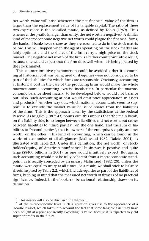
30 Monetary Economics

net worth value will arise whenever the net financial value of the firm islarger than the replacement value of its tangible capital. The ratio of thesetwo expressions is the so-called q-ratio, as defined by Tobin (1969). Thuswhenever the q-ratio is larger than unity, the net worth is negative.5 A similarkind of macroeconomic negative net worth could plague the financial firms,the banks, if banks issue shares as they are assumed to do in the stock matrixbelow. This will happen when the agents operating on the stock market arefairly optimistic and the shares of the firm carry a high price on the stockmarket. The negative net worth of the firm is a rather counter-intuitive result,because one would expect that the firm does well when it is being praised bythe stock market.

This counter-intuitive phenomenon could be avoided either if account-ing at historical cost was being used or if equities were not considered to bepart of the liabilities for which firms are responsible. Obviously, accountingat historical cost in the case of the producing firms would make the wholemacroeconomic accounting exercise incoherent. In particular the macroe-conomic balance sheet matrix, to be developed below, would not balanceout. Also, such accounting at cost would omit price appreciation in assetsand products.6 Another way out, which national accountants seem to sup-port, is to exclude the market value of issued shares from the liabilitiesof the firms. This is the approach taken by the statisticians at the FederalReserve. As Ruggles (1987: 43) points out, this implies that ‘the main break,on the liability side, is no longer between liabilities and net worth, but ratherbetween liabilities to “third parties”, on the one hand, and the sum of lia-bilities to “second parties”, that is, owners of the enterprise’s equity and networth, on the other’. This kind of accounting, which can be found in theworks of economists of all allegiances (Malinvaud 1982; Dalziel 2001), isillustrated with Table 2.3. Under this definition, the net worth, or stock-holders’equity, of American nonfinancial businesses is positive and quitelarge ($8400 billions in 2001), as one would intuitively expect. But again,such accounting would not be fully coherent from a macroeconomic stand-point, as is readily conceded by an uneasy Malinvaud (1982: 20), unless theq-ratio were equal to unity at all times. As a result, we shall stick to balancesheets inspired by Table 2.2, which include equities as part of the liabilities offirms, keeping in mind that the measured net worth of firms is of no practicalsignificance. Indeed, in the book, no behavioural relationship draws on itsdefinition.

5 This q-ratio will also be discussed in Chapter 11.6 At the microeconomic level, such a situation gives rise to the appearance of a

‘goodwill’ asset, which takes into account the fact that some tangible asset may havebeen bought at a price apparently exceeding its value, because it is expected to yieldsuperior profits in the future.

Balance Sheets, Transaction Matrices, Monetary Circuit 31

Table 2.3 Balance sheet of production firms at market prices, without equities as aliability

Assets 2001 2005 Liabilities 2001 2005Total 17,500 22,725 Total 17,500 22,725

Tangible capital Kf 9,200 11,750 Loans Lf 9,100 10,125Financial assets Mf 8,300 11,975 Net Worth NWf 8,400 12,600

Source: Z.1 statistics of the Federal Reserve, www.federalreserve.gov/releases/z1, Table B.102,‘Balance sheet of nonfarm nonfinancial corporate business’, March 2002 and 2006 releases, lastquarter data; units are billions of dollars.

2.2.3 The overall balance sheet matrix

We are now ready to consider the composition of the overall balance sheetmatrix, to be found in Table 2.4. We could assume the existence of an almostinfinite amount of different assets; we could also assume that all sectors owna share of all assets, as is true to some extent, but we shall start by assuminga most simple outfit. The assets and liabilities of households and productionfirms have already been described, and we shall further simplify them byassuming away the financial assets of firms. Government issues short-termsecurities B (Treasury bills). These securities are purchased by the central bank,the banks, and households. Production firms and financial firms (banks) issueequities (shares), and these are assumed to be purchased by households only.We suppose that production firms (and households, as already pointed out)need loans, and that these are being provided by the banks. The major coun-terpart to these loans are the money deposits held by households, who alsohold cash banknotes H , which are provided by the central bank. This specialkind of money issued by the central bank is often called high-powered money,hence the H notation being used. This high-powered money is also usuallybeing held by banks as reserves, either in the form of vault cash or as depositsat the central bank.

In models that will be developed in the later chapters, it will generallybe assumed that households take no loans and the value of their dwellingswill not be taken into consideration, but here we shall do otherwise forexpository purposes. Finally, it will be assumed that the real capital accu-mulated by financial firms or by government is too small to be worthmentioning.

As already mentioned, all assets appear with a plus sign in the balance sheetmatrix while liabilities, including net worth, are assigned a negative sign.The matrix of our balance sheet must follow essentially one single rule: allthe columns and all the rows that deal with financial assets or liabilities mustsum to zero. The only row that may not sum to zero is the row dealing with

32 Monetary Economics

Table 2.4 A simplified sectoral balance sheet matrix

Households Production Banks Government Centralfirms bank �

Tangible capital +Kh +Kf +KBills +Bh +Bb −B +Bcb 0Cash +Hh +Hb −H 0Deposits +Mh −M 0Loans −Lh −Lf +L 0Equities +Ef −Ef 0Equities +Eb −Eb 0Net worth −NWh −NWf −NWb −NWg 0 −K

� 0 0 0 0 0 0

tangible capital – the actual stock of machines and inventories accumulatedby the firms in the production sector and the dwellings of households. A tan-gible asset – a real asset – only appears in a single entry of the sectoral balancesheet, that of its owner. This is in contrast to financial assets and all liabilities,which are a claim of someone against someone else.

Reading now the column of each sector, the sum of all the components ofa column represents the net worth of that sector. Thus adding the net worth,with a negative sign, to all the other elements of the column must by necessityyield a zero result. This guarantees the coherence of the balance sheet matrix.It should be noted that the net worth of the economy, as shown in the lastentry of the penultimate row, is equal to the value of tangible capital assets K(Coutts, Godley and Gudgin 1985: 97; Patterson and Stephenson 1988: 792).If there were only financial assets in an economy, the macroeconomic networth would be nil.

A few additional remarks may be in order. As already mentioned, financialfirms, that is, the banks, will also experience some net worth, NWb, unlesswe assume by construction that they issue no shares and make no profits,as we shall sometimes do to simplify our earlier models. On the other hand,the government sector usually runs a large negative net worth (therefore,in Table 2.4, −NWg is a positive entry). This negative net worth NWg isbetter known as the public debt, which arises as a result of past deficits. Itmay be noticed that the government public debt is the same whether or notwe include the central bank in the government sector. This is because theprofits of the central bank are always returned to the general revenues ofgovernment, so that the net worth of the central bank is zero (provided thecentral bank does not hold long-term bonds, the value of which can changethrough time, as we shall see later, and provided the central bank started tobe run with no capital of its own).

Balance Sheets, Transaction Matrices, Monetary Circuit 33

2.3 The conventional income and expenditure matrix

2.3.1 The NIPA matrix

While the balance sheet matrix has its importance, the really interestingconstruct is the transactions flow matrix. This matrix records all the mone-tary transactions that are occurring in an economy. The matrix provides anaccounting framework that will be highly useful when defining behaviouralequations and setting up formal models of the economy. The transactionsmatrix is the major step in fully integrating income accounting and finan-cial accounting. This full integration will become possible only when capitalgains are added to the transactions matrix. When this is done, it will bepossible to move from the opening stocks of assets, those being held at thebeginning of the production period, to the closing stocks of assets, thosebeing held at the end of the production period.

But before we do so, let us consider the conventional income and expen-diture matrix, that is, the matrix that does not incorporate financial assets.This matrix arises from the consideration of the standard National Incomeand Product Accounts, the NIPA. We have already observed a very similarmatrix, when we examined the national accounts seen from the perspectiveof the standard mainstream macroeconomics textbook. Consider Table 2.5.Compared with the previous balance sheet matrix, the financial sector hasbeen scotched, amalgamated to the business sector, while the central bankhas been reunited with the government sector. We still have the double entryconstraint that the sum of the entries in each row ought to equal zero. Thisis a characteristic of all social accounting matrices.

It should be pointed out that all the complications that arise as a resultof price inflation, for instance the fact that the value of inventories mustbe adjusted to take into account changes in the price level of these inven-tories, have been assumed away. In other words, product prices are deemed

Table 2.5 Conventional Income and expenditure matrix

Business

Households Current Capital Government �

Consumption −C +C 0Govt expenditure +G −G 0Investment +I −If 0[GDP (memo)] [Y]Wages +WB −WB 0Net Profits +FD −F +FU 0Tax net of transfers −Th −Tf +T 0Interest payments +INTh −INTf −INTg 0

� SAVh 0 FU − If −DEF 0

34 Monetary Economics

to remain constant. Unless we make this assumption we shall have to faceup, at far too early a stage, to various questions concerning the valuationof capital, both fixed and working, as well as price index problems. Thesecomplications will be dealt with starting with Chapter 8.

Before we start discussing the definition of gross domestic product, theperceptive reader may have noted that capital accumulation by householdsseems to have entirely disappeared from Table 2.5. It was already the case inTable 1.1, but then such an omission was tied to the highly simplified natureof the standard mainstream model, where only investment by firms was con-sidered. Why would investment in residential housing be omitted from amore complete NIPA? What happens is that, in the standard NIPA, automo-biles or household appliances purchased by individuals are not part of grosscapital formation; rather they are considered as part of current expenditures.In addition, to put home-owners and home-renters on an identical footing,‘home ownership is treated as a fictional enterprise providing housing ser-vices to consumer-occupants’ (Ruggles and Ruggles 1992 (1996: 284)). As aresult, purchases of new houses or apartments by individuals are assignedto fixed capital investment by the real estate industry; and expendituresassociated with home ownership, such as maintenance costs, imputed depre-ciation, property taxes and mortgage interest, ‘are considered to be expensesof the fictional enterprise’, and ‘are excluded from the personal outlays ofhouseholds’. In their place, there is an imputed expenditure to the fictionalreal estate enterprise. This is why there is no Ih entry in Table 2.5 that wouldrepresent investment into housing.

2.3.2 GDP

In this matrix, the expenditure and income components of gross domesticproduct (GDP), appear in the second column. The positive and negative signshave a clear meaning. The positive items are receipts by businesses as a resultof the sales they make – they are the value of production – , while the negativeitems describe where these receipts ‘went to’: they are the product of theeconomy. It has been assumed that every expenditure in the definition ofGDP (consumption C, investment I , and government expenditures on goodsand services G) is a sale by businesses, although in reality this is not quitetrue, government employment – which is a form of expenditure which isnot a receipt by firms – being the major exception. And as a counterpart,every payment of factor income included in the income definition of GDP isa disbursement by businesses in the form of wages WB, distributed profits FDand undistributed profits FU, interest payments INTf , and indirect taxes Tf .From the second column, we thus recover the two standard definitions ofincome:

Y = C + I + G = WB + F + INTf + Tf (2.1)

Balance Sheets, Transaction Matrices, Monetary Circuit 35

We must now confront the fact that firms’ receipts from sales of investmentgoods, which from the sellers’ point of view are no different from any otherkind of sales, do not arise from outside the business sector itself.7 So thedouble entry principle that regulates the use of accounting matrices requiresus to postulate a new sector – the capital account of businesses – which makesthese purchases. As we work down the capital account column, we shalleventually discover where all the funds needed for investment expenditurecome from.

There is no need to assume that all profits are distributed to householdsas is invariably assumed, without question, in mainstream macroeconomics.In the transactions matrix shown above, part of the net profits earned bybusiness are distributed to households (FD) while the rest is undistributed(FU) and (considered to be) paid into their capital accounts to be used as asource of funds – as it happens, the principal source of funds – for investment.Figure 2.1 shows that in the United States total internal funds of non-financialbusinesses exceeds their gross investment expenditures in nearly every year

19460.6

0.8

1

1.2

1.4

1.6

1.8

2

2.2

1951 1956 1961 1966 1971 1976 1981 1986 1991 1996 2001 2005

Total internal funds to Gross investment ratio

Figure 2.1 Total internal funds (including IVA) to gross investment ratio, USA,1946–2005.

Source: Z.1 statistics of the Federal Reserve, www.federalreserve.gov/releases/z1, table F102,Non-farm non-financial corporate business. The curve plots the ratio of lines 9 and 10.

7 As pointed out above, households’ investment in housing is imputed to the realestate industry.

36 Monetary Economics

since 1946. In fact, it would seem that in many instances retained earningsare even used to finance the acquisition of financial assets.

To complete the picture, we include transfer payments between the varioussectors. These are divided into two categories, payments of interest (INT witha lower case suffix to denote the sector in question) that are made on assetsand liabilities which were outstanding at the beginning of the period andtherefore largely predetermined by past history; and other ‘unilateral’ trans-fers (T), of which the most important are government receipts in the formof taxes and government outlays in the form of pensions and other transferslike social insurance and unemployment benefits.

All this allows us to compute the disposable income of households –personal disposable income – which is of course different from GDP. It canbe read off the first column. Wages, distributed dividends, interest payments(from both the business and the government sector, minus interest paid onpersonal loans), minus income taxes, constitute this disposable income YD.8

YD = WB + FD + INTh − Th (2.2)

2.3.3 The saving = investment identity

Matrix 2.5 has now become a neat record of all the income, expenditure andtransfer payments which make up the national income accounts, showinghow the sectoral accounts are intertwined. The first column shows all cur-rent receipts and payments by the household sector, including purchases ofdurable goods, hence the balance at the bottom is equal to household saving(SAVh) as defined in NIPA. The second column shows current receipts andpayments by firms which defines business profits as the excess of receiptsfrom sales over outlays. The third column shows firms’ investment and theundistributed profits (FU) which are available to finance it, the balance atthe bottom showing the firms’ residual financing requirement – what theymust find over and above what they have generated internally. The entriesin the fourth column give all the outlays and receipts of the general govern-ment, and the balance between these gives the government’s budget surplusor deficit. The fact that every row until the bottom row, which describesfinancial balances, sums to zero guarantees that the balances’ row sums tozero as well. It is this last row which has attracted the undivided attention ofnational accountants and of Keynesian economists. This last line says that:

SAVh + (FU − If) − DEF = 0 (2.3)

Considering that the retained earnings of firms constitute the savings of thefirm’s sector, we can write FU = SAVf ; similarly, the surplus of the government

8 Note that interest payments from government are not included in GDP.

Balance Sheets, Transaction Matrices, Monetary Circuit 37

sector is equivalent to its saving, so that SAVg = −DEF. From these newdefinitions, and from the definition implicit to the investment row, we canrewrite equation (2.3) in its more familiar form:

I = SAVh + SAVf + SAVg = SAV (2.4)

Equation (2.4) is nothing else than the famous Keynesian equality betweeninvestment and saving. This is the closest that most mainstream accountsof macroeconomics will get from financial issues.9 What happens to thesesavings, how they arise, what is their composition, how they link up thesurplus sectors to the deficit sectors, is usually not discussed nor modelled.In Matrix 2.5, until the final row, the nature of the transactions is pretty clear:households buy goods and firms sell them, etc.10 However, the transfer offunds ‘below the (bold) line’ requires a whole new set of concepts, which arenot part of the conventional income and expenditures national accounts.The answers to the questions that were put to the reader in section 1.2 ofthe previous section are to be found quite straight forwardly, using conceptswhich are familiar and easy to piece together so long as the double entryprinciple continues to be observed and so long as we always live up to ourmotto that everything must go somewhere and come from somewhere. Inother words, we need to bring in the transactions flow matrix.

2.4 The transactions flow matrix

2.4.1 Rules governing the transactions flow matrix

We shall require the reintroduction of the financial sector, the banks that hadbeen introduced in the balance sheet matrix but that had been amalgamated

9 Note that neo-classical economists don’t even get close to this equation, for other-wise, through equation (2.4), they would have been able to rediscover Kalecki’s (1971:82–3) famous equation which says that profits are the sum of capitalist investment,capitalist consumption expenditures and government deficit, minus workers’ saving.Rewriting equation (2.3), we obtain:

FU = If + DEF − SAVh

which says that the retained earnings of firms are equal to the investment of firmsplus the government deficit minus household saving. Thus, in contrast to neo-liberalthinking, the above equation implies that the larger the government deficit, the largerthe retained earnings of firms; also the larger the saving of households, the smaller theretained earnings of firms, provided the left-out terms are kept constant. Of course thegiven equation also features the well-known relationship between investment and prof-its, whereby actual investment expenditures determine the realized level of retainedearnings.

10 The nature of these transactions is not, in reality, so simple as this. In many,perhaps most cases, the contract to purchase and sell something is separated from thetransfer of money one way and the goods themselves going the other.

38 Monetary Economics

to the business sector in the conventional income and expenditure matrix.Similarly, the operations of the central bank will reappear explicitly in thenew transactions flow matrix which is the corner stone of our approach.These additions to the conventional income and expenditure matrix willallow us to assess all transactions, be they in goods and services or in theform of financial transactions, with additions to assets or liabilities.

As in the balance sheet matrix, the coherence of the transactions flowmatrix is built on the rule that each row and each column must sum to zero.The rule enforcing that all rows must sum to zero is rather straightforward:each row represent the flows of transactions for each asset or for each kind offlow; there is nothing new here. The top part of the matrix, as described inTable 2.6 resembles the income and expenditure matrix, with a few additionsand new notations. In particular, the flow of interest payments, which wasnoted INT in Table 2.5, is now explicit. The flow of interest on an asset ora liability now depends on the relevant rate of interest and on the stock ofasset at the opening of the production period, that is, the stock accumulatedat the end of the previous period, at time t −1. The lagged variable rm standsfor the rate of interest prevailing on money deposits. Similarly rl and rb standfor the rates of interest prevailing on loans and Treasury bills.

The bottom part of the matrix is the flow equivalent of the balance sheetmatrix. When we describe purchases and sales of assets of which the nominalvalue never changes, there is no problem of notation. We simply write �Hor �M (for instance) to describe the increase in the stock of cash, or moneydeposits, between the beginning and end of the period being characterized.When the capital value of the asset can change – that is, when capital gainsand losses can occur, as is the case with long-term bonds and equities – wekeep the convention that the assets are pieces of paper, say e for equities,which have a price, pe. The value of the piece of paper is then e · pe at a pointof time, and the value of transactions in equities – new issues or buy-backs –is given by the change in the number of pieces of paper which are issued (orwithdrawn) times their price, �e · pe.

The rule enforcing that all columns, each representing a sector, must sumto zero as well is particularly interesting because it has a well-defined eco-nomic meaning. The zero-sum rule for each column represents the budgetconstraint of each sector. The budget constraint for each sector describes howthe balance between flows of expenditure, factor income and transfers gen-erate counterpart changes in stocks of assets and liabilities. The accounts ofthe transactions flow matrix, as shown by Table 2.6, are comprehensive inthe sense that everything comes from somewhere and everything goes some-where. Without this armature, accounting errors may pass unnoticed andunacceptable implications may be ignored. With this framework, ‘there areno black holes’ (Godley 1996: 7).

There is no substitute for careful perusal of the matrix at this stage. It is arepresentation, not easily come by, of a complete system of macroeconomic

39

Table 2.6 Transactions flow matrix

Production firms Banks Government Central BankHouseholds

(1) Current (2) Capital (3) Current (4) Capital (5) (6) Current (7) Capital (8) �

Consumption −C +C 0Investment −Ih +I −If 0Govt. exp. +G −G 0Wages +WB −WB 0Profits, firms +FDf −Ff + FUf 0Profits, banks +FDb −Fb +FUb 0Profit, central Bk +Fcb −Fcb 0Loan interests −rl(−1) · Lh(−1) −rl(−1) · Lf(−1) +rl(−1) · L(−1) 0Deposit interests +rm(−1) · Mh(−1) −rm(−1) · M(−1) 0Bill interests +rb(−1) · Bh(−1) +rb(−1) · Bb(−1) −rb(−1) · B(−1) +rb(−1) · Bcb(−1) 0Taxes – transfers −Th −Tf −Tb +T 0Change in loans +�Lh +�Lf −�L 0Change in cash −�Hh −�Hb +�H 0Change, deposits −�Mh +�M 0Change in bills −�Bh −�Bh +�B −�Bcb 0Change, equities −(�ef · pef + �eb · peb) +�ef · pef +�eb · peb 0

� 0 0 0 0 0 0 0 0 0

40 Monetary Economics

transactions. The best way to take it in is by first running down each columnto ascertain that it is a comprehensive account of the sources and uses of allflows to and from the sector and then reading across each row to find thecounterpart of each transaction by one sector in that of another. Note thatall sources of funds in a sectoral account take a plus sign, while the uses ofthese funds take a minus sign. Any transaction involving an incoming flow,the proceeds of a sale or the receipts of some monetary flow, thus takes a pos-itive sign; a transaction involving an outgoing flow must take a negative sign.Uses of funds, outlays, can be either the purchase of consumption goods orthe purchase (or acquisition) of a financial asset. The signs attached to the‘flow of funds’ entries which appear below the horizontal bold line are stronglycounter-intuitive since the acquisition of a financial asset that would add to theexisting stock of asset, say, money, by the household sector, is described with anegative sign. But all is made clear so soon as one recalls that this acquisition ofmoney balances constitutes an outgoing transaction flow, that is, a use of funds.

2.4.2 The elements of the transactions flow matrix

Let us first deal with column 1 of Table 2.6, that of the household sector. Thatcolumn represents the budget constraint of the households. In contrast to thestandard NIPA, investment in housing is taken into account. Households canconsume goods (−C) or purchase new residential dwellings (−Ih), but only aslong as they receive various flows of income or provided they take in new loans(+�Lh) – consumer loans or home mortgages – or reduce their holdings ofassets, for instance by dishoarding money balances (+�Hh or +�Mh). At theaggregate scale, at least as a stylized fact, households add to their net wealth,through their saving. The excess of household income over consumption willtake the form of real purchases of dwellings (Ih), and the form of financialacquisitions: cash (�Hh), bank money (�Mh), fixed interest securities (�Bh),and equities (�e · pe), less the net acquisition of liabilities, in the form of loans(�Lh) from banks. The change in the net financial position of the householdsector, which will require counterpart changes in the net financial positionof the other sectors, appears in the rows below the bold line. The categoriesshown are simplified: there are other important ways in which people save –for example, through life insurance, mutual funds and compulsory pensionfunds; but for the time being these acquisitions will be treated as though theywere direct holdings, perhaps subject to advice from a manager.11

11 It has been shown by Ruggles and Ruggles (1992 (1996)) that once the fictitiousreal estate enterprises of NIPA that take care of households new purchases of residentialunits have been taken out, and once pension fund schemes are considered as saving byfirms rather than that of their employees, then the change in the net financial positionof the household sector is virtually nil, and even negative on the average in the UnitedStates since 1947.

Balance Sheets, Transaction Matrices, Monetary Circuit 41

Column 2 is no different from the one discussed in Table 2.5: it showsthe receipts and the outlays of production firms on their current account.Column 3 now shows how production firms ultimately end up financingtheir capital expenditures, fixed capital and inventories. These capital expen-ditures, at the end of the period, appear to be financed by retained profits,new issues of securities (here assumed to be only equities, but which couldbe bonds or commercial paper) and bank loans.

Columns 4 and 5 describe a relatively sophisticated banking sector. Oncemore, the accounts are split into a current and a capital account. The currentaccount describes the flows of revenues and disbursements that the banksget and make. Banks rake in interest payments from their previous stocks ofloans and securities, and they must make interest payments to those holdingbank deposits. The residual between their receipts and their outlays, net oftaxes, is their profit Fb. This profit, as is the case for production firms, issplit between distributed dividends and retained earnings. These retainedearnings, along with the newly acquired money deposits, are the counterpartsof the assets that are being acquired by banks: new granted loans, newlypurchased bills, or additional vault cash. Column 5 shows how the balancesheets of banks must always balance in the sense that the change in theirassets (loans, securities and vault cash) will always have a counterpart in achange in their liabilities.

Finally, the last columns deal with the government sector and its cen-tral bank. The latter is split from the government sector, as it allows for amore realistic picture of the money creation process, although it adds oneslight complication. Let us first deal with Column 7, the current account ofthe central bank. From the balance sheet of Table 2.4, we recall that centralbanks hold government bills while their typical liabilities are in the form ofbanknotes, that is, cash, which carries no interest payment. As a result, cen-tral banks make a profit, Fcb, which, we will assume, is entirely returned togovernment. This explains the new entry in column 6 of the governmentsector, +Fcb, compared with that of Table 2.5. The fact that the central bankreturns all of its profits to government implies that the while the govern-ment gross interest disbursements on its debt are equal to rb(−1) · B(−1), itsnet disbursements are only rb(−1) · [B(−1) − Bcb(−1)].

Column 6 is the budget constraint of government. It shows that any gov-ernment expenditure which is not financed by taxes (or the central bankdividend), must be financed by an issue of bills. These newly issued billsare purchased by households, banks and the central bank, directly or indi-rectly. Column 8 shows the highly publicized accounting requirement thatany addition to the bond portfolio of the central bank must be accompaniedby an equivalent increase in the amount of high-powered money, +�H . Thisrelationship, which is at the heart of the monetarist explanation of inflation –also endorsed by most neo-classical economists – as proposed by authors suchas Milton Friedman, has been given considerable attention in the recent past,

42 Monetary Economics

since it seems to imply that government deficits are necessarily associatedwith high-powered money increases, and hence through some money mul-tiplier story, as told in all elementary textbooks, to an excess creation ofmoney. A quite different analysis and interpretation of these accountingrequirements will be offered in the next chapters.

2.4.3 Key features of the transactions flow matrix

It is emphasized that so far there has been no characterization of behaviourbeyond what is implied by logical constraints (e.g. that every buyer musthave a seller) or by the functions that have been allocated to the varioussectors (e.g. that firms are responsible for all production, banks for makingall loans) or by the conventional structure and significance of asset portfolios(e.g. that money is accepted as a means of payment).

Reconsider now the system as a whole. We open each period with stocksof tangible assets and a tangle of interlocking financial assets and liabilities.The whole configuration of assets and liabilities is the legacy of all transac-tions in stocks and flows and real asset creation during earlier periods whichconstitute the link between past, present and future. Opening stocks inter-act with the transactions which occur within each period so as to generate anew configuration of stocks at the end of each period; these will constitutepast history for the succeeding period. At the aggregate level, whatever isproduced and not consumed will turn up as an addition to the real capitalstock. At the sectoral level, the sum of all receipts less the sum of all outlaysmust have an exact counterpart in the sum of all transactions (by that sector)in financial assets less financial liabilities.

The only elements missing for a full integration are the capital gains thatought to be added to the increases in assets and liabilities that were assessedfrom the transactions matrix. Thus what is missing is the revaluation account,or what is also known as the reconciliation account. When this is done, itbecomes possible to move from the opening stocks of assets, those beingheld at the beginning of the production period, to the closing stocks of assets,those being held at the end of the production period. This will be done inthe next section.

The system as a whole is now closed in the sense that every flow and everystock variable is logically integrated into the accounting to such a degreethat the value of any one item is implied by the values of all the otherstaken together; this follows from the fact that every row and every columnsums to zero. This last feature will prove very useful when we come to modelbehaviour; for however large and complex the model, it must always be thecase that one equation is redundant in the sense that it is implied by all theother equations taken together.

As pointed out in the first part of this chapter, other authors have previ-ously underlined the importance of the transactions flow matrix. In his book,Jean Denizet (1969: 19) proposed a transactions flow matrix that has implicitly

Balance Sheets, Transaction Matrices, Monetary Circuit 43

all the features of the matrix that has been presented here. Malinvaud (1982:21) also presents a nearly similar transactions flow matrix. The article writtenby Tobin and his collaborators (Backus et al. 1980), has a theoretical transac-tion flow matrix, nearly identical to the one advocated here, with rows andcolumns summing to zero; they also have presented the empirical version ofsuch a matrix, including capital gains, with actual numbers attached to eachcell of our transaction flow matrix, derived from the national income andproduct accounts and the flow-of-funds accounts, thus demonstrating thepractical usefulness of this approach. The transactions flow matrix has beenutilized systematically and amalgamated to behavioural equations by Godleyin his more recent work (1996, 1999a). It was not present in Godley’s earlierwork (Godley and Cripps 1983).

2.5 Full integration of the balance sheet andthe transactions flow matrices

We are now in a position to integrate fully the transactions flow matrix tothe balance sheet. Table 2.7 illustrates this integration (Stone 1986: 16). Asbefore, we consider five sectors: households, production firms, banks, gov-ernment, and the central bank. The first row represents the initial net worthof each sector, as they appear in the penultimate row of Table 2.6. We assumeagain that the net worth of the central bank is equal to nil, as a result of thehypothesis that any profit of the central bank is returned to government. Weshall also see that a central bank zero net worth requires that the central bankholds no bonds, only bills, the price of which does not change. We may alsonote, as was mentioned earlier, that the aggregate net worth of the economy,its macroeconomic net worth, is equal to the value of tangible capital, K.Finally, it should be pointed out once more that the net worth of any sector,at the end of the previous period, is considered to be the same thing as the networth of that sector at the beginning of the current period, and in what followswe shall make use of the (−1) time subscript whenever beginning-of-periodwealth is referred to.

The change in the net worth of any sector is made up of two components,as is clearly indicated in the first column of Table 2.7: the change in net assetsarising from transactions, and the change arising from revaluations, that is,changes in the prices of assets or liabilities. These two components of change,added to the net worth of the previous period, yield the new net worth ofeach sector. This new net worth – the net worth at the end of the currentperiod – appears in the last row of Table 2.7.

The first component of the change in net worth arises from the transactionsflow matrix. The first five rows of these changes are the exact equivalent of thelast five rows (the last row of zeros having been set aside) of the transactionsflow matrix 2.6. They reflect the financial transactions that occurred during

44

Table 2.7 Full-integration matrix

Production Centralfirms Banks Government bank

Households(1) (2) (3) (4) (5) �

Net worth, end ofprevious period

NWh−1 NWf−1 NWb−1 NWg−1 0 K−1

Change in net Change in loans −�Lh −�Lf +�L 0assets arising from Change in cash +�Hh +�Hb −�H 0transactions Change in deposits +�Mh −�M 0

Change in bills +�Bh +�Bh −�B +�Bcb 0Change in equities +�ef · pef + �eb · peb −�ef · pef −�eb · peb 0Change in tangible +�kh · pk +�kf · pk +�k · pk

capital

Change in net Capital gains in +�pef · ef−1 −�pef · ef−1 −�peb · eb−1 0assets arising from equities +�peb · eb−1revaluations Capital gains in +�pk · kh−1 +�pk · kf−1 �pk · (kh−1 + kf−1)

tangible capitalNet worth, end of NWh NWf NWb NWg 0 K

period

Balance Sheets, Transaction Matrices, Monetary Circuit 45

the period. The only difference between these five rows as they appear inTable 2.7 compared to those of Table 2.6 is their sign. All minus signs inTable 2.6 are replaced by a plus sign in Table 2.7, and vice versa. In thetransactions flow matrix of Table 2.6, the acquisition of a financial asset, saycash money �Hh by households, is part of the use of funds, and hence carriesa minus sign. However, in Table 2.7, the acquisition of this cash money addssomething to household wealth, and hence it must carry a plus sign, in orderto add it to the net worth of the previous period. Similarly, when householdsor firms take loans, these new loans provide additions to their sources of funds,and hence carry a plus sign in the transactions flow matrix of Table 2.6. Bycontrast, in the integration matrix of Table 2.7, loans taken by householdsor firms, all other things equal, reduce the net worth of these sectors, andhence must carry a minus sign.

The last element of the first block of six rows arising from the transactionsflow matrix, as shown in Table 2.7, is the row called ‘change in tangiblecapital’. The counterpart of this row can be found in the ‘investment’ rowof Table 2.6. Households, for instance, can augment their net wealth byacquiring financial or tangible capital. In their case, tangible capital is essen-tially made up of residential dwellings (since, in contrast to financial flowsaccountants, we do not consider purchases of durable goods as capital accu-mulation). This was classified as investment in the transactions flow matrix,and called Ih, whereas in the full-integration matrix, it is called �kh · pk,where pk is the price of tangible capital, while �kh is the flow of new residen-tial capital being added to the existing stock, in real terms. In other words,�kh is the number of new residential units which have been purchased byhouseholds. It follows that we have the equivalence, Ih = �kh · pk. Similarly,for firms, their investment in tangible capital (essentially machines, plants,and additions to inventories) was called If in the transactions matrix of Table2.6. Setting aside changes in inventories,12 the value of new investment in tan-gible capital is now called �kf · pk in Table 2.7, so that we have the otherequivalence, If = �kf · pk. Note that for simplification, we have assumed thatthe price of residential tangible capital and the price of production capital isthe same and moves in tandem.

The second major component of the change in net worth arises from capitalgains. For exposition purposes, we assume that only two elements of wealthcan have changing prices, and hence could give rise to capital gains or capitallosses. We assume that the prices of equities can change, those issued byproduction firms and those issued by banks; and we also assume that the

12 This is an important restriction, because, as already pointed out, inventories arevalued at current replacement cost, while fixed capital is valued at current replacementprice, and hence they cannot carry the same price variable. See Chapter 11 for anin-depth study of this issue, which is briefly dealt with in section 2.6.2.

46 Monetary Economics

price of tangible capital, relative to consumer prices, can change. We assumeaway changes in the price of securities. The implicit assumption here is thatall securities are made up of bills – short-term securities that mature withinthe period length considered here. In the case of bonds – long-term securitiesthe prices of which change from period to period, before they mature andcome up for redemption – capital gains or losses would have to be taken intoaccount. Capital gains on bonds will be explicitly taken into considerationin Chapter 5.

The study of capital gains underlines an important principle: any changein the value of an asset may be made up of two components: a componentassociated with a transaction, for instance when new equities are issued andbought up for instance, thus involving additional units of the asset in ques-tion; and a component associated with a change in the price of the asset,when for instance, existing (and newly issued) equities carry a higher price.In the case of equities issued by production firms, as shown in Table 2.7,the change in the value of equities arising from transactions is �ef · pef whilethe change in the value of equities arising from capital gains is �pef · ef−1. InChapter 5, we shall provide a precise proof of this result in discrete time (withtime subscripts, as done here). In the meantime, it is sufficient to remem-ber first-year university calculus, deal with continuous time, and recall that,given two functions, u and v, the derivative of the product of these functionsis such that d(u · v) = du · v + u · dv. In the present case, with e and pe actingas the two functions u and v, we have:

d(e · pe) = de · pe + e · d(pe) (2.5)

The first term represents the change arising from transactions, while thesecond term represents capital gains due to the change in prices. The samerules apply to the changes in the value of tangible capital, where a real termcomponent and a price component can be identified.

Thus, adding the capital gains component so defined and the transac-tions component to the net worth of the previous period, we obtain thenet worth at the end of the current period, as shown in the last row ofTable 2.7. The integration of the flow of funds financial transactions andthe sector balance sheets with the national income accounts is thus com-plete. It should be pointed out however that it is no easy matter to producean empirical version of Tables 2.6 or 2.7. While the flow of funds publishedby the Federal Reserve in the United States, or by other statistical agencies inother countries, contain a vast amount of information about transactions infinancial assets, the sectoral classification and to some extent the conceptsemployed in NIPA are sufficiently different to make any simple junctionof the two data sets. Although the Z.1 accounts themselves provide somereconciliation (in tables F.100 and higher), relatively large discrepanciesremain.

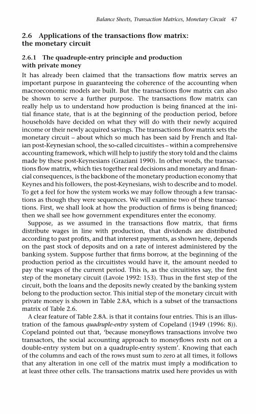
Balance Sheets, Transaction Matrices, Monetary Circuit 47

2.6 Applications of the transactions flow matrix:the monetary circuit

2.6.1 The quadruple-entry principle and productionwith private money

It has already been claimed that the transactions flow matrix serves animportant purpose in guaranteeing the coherence of the accounting whenmacroeconomic models are built. But the transactions flow matrix can alsobe shown to serve a further purpose. The transactions flow matrix canreally help us to understand how production is being financed at the ini-tial finance state, that is at the beginning of the production period, beforehouseholds have decided on what they will do with their newly acquiredincome or their newly acquired savings. The transactions flow matrix sets themonetary circuit – about which so much has been said by French and Ital-ian post-Keynesian school, the so-called circuitistes – within a comprehensiveaccounting framework, which will help to justify the story told and the claimsmade by these post-Keynesians (Graziani 1990). In other words, the transac-tions flow matrix, which ties together real decisions and monetary and finan-cial consequences, is the backbone of the monetary production economy thatKeynes and his followers, the post-Keynesians, wish to describe and to model.To get a feel for how the system works we may follow through a few transac-tions as though they were sequences. We will examine two of these transac-tions. First, we shall look at how the production of firms is being financed;then we shall see how government expenditures enter the economy.

Suppose, as we assumed in the transactions flow matrix, that firmsdistribute wages in line with production, that dividends are distributedaccording to past profits, and that interest payments, as shown here, dependson the past stock of deposits and on a rate of interest administered by thebanking system. Suppose further that firms borrow, at the beginning of theproduction period as the circuitistes would have it, the amount needed topay the wages of the current period. This is, as the circuitistes say, the firststep of the monetary circuit (Lavoie 1992: 153). Thus in the first step of thecircuit, both the loans and the deposits newly created by the banking systembelong to the production sector. This initial step of the monetary circuit withprivate money is shown in Table 2.8A, which is a subset of the transactionsmatrix of Table 2.6.

A clear feature of Table 2.8A. is that it contains four entries. This is an illus-tration of the famous quadruple-entry system of Copeland (1949 (1996: 8)).Copeland pointed out that, ‘because moneyflows transactions involve twotransactors, the social accounting approach to moneyflows rests not on adouble-entry system but on a quadruple-entry system’. Knowing that eachof the columns and each of the rows must sum to zero at all times, it followsthat any alteration in one cell of the matrix must imply a modification toat least three other cells. The transactions matrix used here provides us with

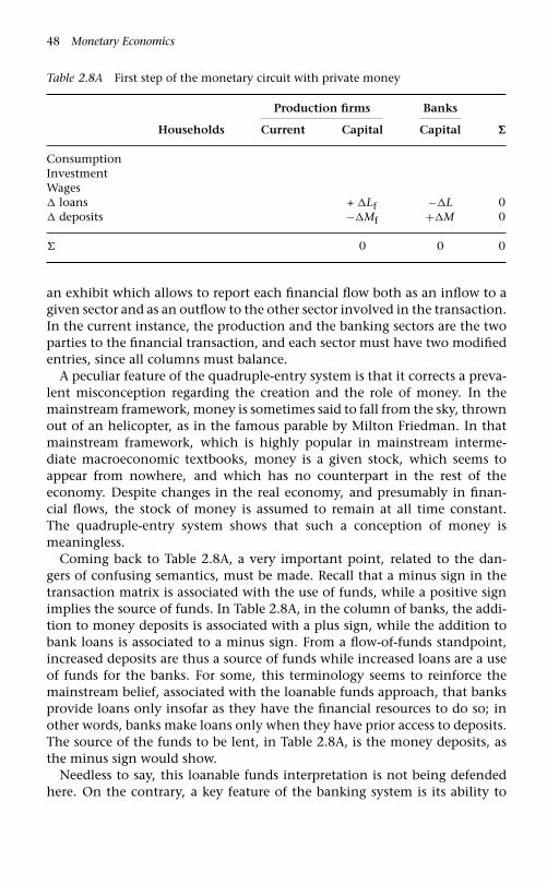
48 Monetary Economics

Table 2.8A First step of the monetary circuit with private money

Production firms Banks

Households Current Capital Capital �

ConsumptionInvestmentWages� loans + �Lf −�L 0� deposits −�Mf +�M 0

� 0 0 0

an exhibit which allows to report each financial flow both as an inflow to agiven sector and as an outflow to the other sector involved in the transaction.In the current instance, the production and the banking sectors are the twoparties to the financial transaction, and each sector must have two modifiedentries, since all columns must balance.

A peculiar feature of the quadruple-entry system is that it corrects a preva-lent misconception regarding the creation and the role of money. In themainstream framework, money is sometimes said to fall from the sky, thrownout of an helicopter, as in the famous parable by Milton Friedman. In thatmainstream framework, which is highly popular in mainstream interme-diate macroeconomic textbooks, money is a given stock, which seems toappear from nowhere, and which has no counterpart in the rest of theeconomy. Despite changes in the real economy, and presumably in finan-cial flows, the stock of money is assumed to remain at all time constant.The quadruple-entry system shows that such a conception of money ismeaningless.

Coming back to Table 2.8A, a very important point, related to the dan-gers of confusing semantics, must be made. Recall that a minus sign in thetransaction matrix is associated with the use of funds, while a positive signimplies the source of funds. In Table 2.8A, in the column of banks, the addi-tion to money deposits is associated with a plus sign, while the addition tobank loans is associated to a minus sign. From a flow-of-funds standpoint,increased deposits are thus a source of funds while increased loans are a useof funds for the banks. For some, this terminology seems to reinforce themainstream belief, associated with the loanable funds approach, that banksprovide loans only insofar as they have the financial resources to do so; inother words, banks make loans only when they have prior access to deposits.The source of the funds to be lent, in Table 2.8A, is the money deposits, asthe minus sign would show.

Needless to say, this loanable funds interpretation is not being defendedhere. On the contrary, a key feature of the banking system is its ability to

Balance Sheets, Transaction Matrices, Monetary Circuit 49

create deposits ex nihilo. More precisely, when agents in the economy arewilling to increase their liabilities, banks can increase the size of both sides oftheir balance sheet, by granting loans and simultaneously creating deposits.As neatly summarized by Earley, Parsons and Thomson (1976, 1996: 159), ‘toencapsulate, we see fluctuations in borrowing as the primary cause of changesin spending’. It may be that, in flow-of-funds terminology, money depositsis the source of funds allowing the use of bank loans. But the cause of thisincrease in deposits and loans is the willingness to contract an additionalliability and the desire of the borrower, here the production firm, to expandits expenditures.

2.6.2 Initial finance versus final finance

This situation as shown in Table 2.8A, however, can only last for a splitsecond. Firms only draw on their lines of credit when they are required tomake payments. In the second step of the circuit, the deposits of the firms aretransferred by cheques or electronic payment to the workers who providedtheir labour to the firms. The moment these funds are transferred, they con-stitute households’ income. Before a single unit is spent on consumer goods,the entire amount of the bank deposits constitutes savings by households,and these are equal to the new loans granted to production firms.

This is all shown in Table 2.8B. The matrix requirement that all rows andcolumns must sum to zero makes clear the exigencies of the second step ofthis monetary circuit. Because of these zero-sum requirements, the followingthree equations must hold:

I − WB = 0 (2.6)

I − �Lf = 0 (2.7)

�Mh − �Lf = 0 (2.8)

At that stage of the circuit, output has been produced but not yet sold. Theunsold production constitutes an increase in inventories (which will later be

Table 2.8B The second step of the monetary circuit with private money

Production firms Banks

Households Current Capital Capital �

ConsumptionInvestment +I −I 0Wages +WB −WB 0� loans +�Lf −�L 0� deposits −�Mh +�M 0� 0 0 0 0 0

50 Monetary Economics

associated with the symbol IN). This increase in inventories is accounted asinvestment in working capital. Staying faithful to our requirement that allrows and all columns must sum to zero, inventories must necessarily riseby an amount exactly equal to the production costs, the wages paid WB,as in equation (2.6).13 The zero-sum column requirement, as applied to thecurrent account of firms makes it so. This demonstrates a very importantpoint: that inventories of unsold goods should be valued at cost, and notaccording to the price that the firm believes it can get for its goods in thenear future.

On the side of the capital account, it is clear that the value of this invest-ment in inventories must be financed by the new loans initially obtained, asin equation (2.7). Table 2.8B, contrasted with Table 2.6, helps us understandthe distinction between initial and final finance which has been underlined bythe circuitistes (Graziani 1990). Initial finance, or what Davidson (1982: 49)calls construction finance, appears in Tables 2.8A: it is the bank loans that firmsusually ask to finance the initial stages of production and hence to financeinventories. Final finance, or Davidson’s investment funding, is to be foundin the last rows of Table 2.6. Final finance are the various means by whichinvestment expenditures are being ultimately financed by the end of the pro-duction period; the retained earnings of corporations constitute the greatestpart of gross investment funding.

The transition from Tables 2.8A and 2.8B, which represent the first andsecond steps of the monetary circuit, to Table 2.6, which represents the thirdand last step of the monetary circuit, is accomplished by households gettingrid of the money balances acquired through wages, and eventually the addi-tional money balances received on account on their dividend and interestpayments. As the households get rid of their money balances, firms gradu-ally recover theirs, allowing them to reimburse the additional loans that hadbeen initially granted to them, at the beginning of the period.

The key factor is that, as households increase their consumption, theirmoney balances fall and so do the outstanding amount of loans owed by thefirms. Similarly, as households get rid of their money balances to purchasenewly issued equities by firms, the latter are again able to reduce their out-standing loans. In other words, at the start of the circuit, the new loansrequired by the firms are exactly equal to the new deposits obtained byhouseholds. Then, as households decide to get rid of their money balances,the outstanding loans of firms diminish pari passu, as long as firms use theproceeds to pay back loans instead of using the proceeds to beef up theirmoney balances or their other liquid financial assets. Although determinedby apparently independent mechanisms, the supply of loans to firms and

13 Note that it is assumed as well that the new fixed investment goods have not yetbeen sold to the corporations which ordered them.

Balance Sheets, Transaction Matrices, Monetary Circuit 51

the holdings of deposits by households (and firms) cannot but be equal, asthey are at the beginning of the circuit, as in equation (2.8). This mechanismwill be observed time and time again in the next chapters, when behaviouralrelations are examined and formalized.

The primary act is best thought of as a decision to produce something.This induces firms to take up a loan to start up the production process. Thebuild up of initial inventories, when production begins, is the result of such aproduction decision, made with the agreement of a bank. It is this act whichbrings a bank loan into existence and simultaneously brings a bank balanceof equal size into existence (that of the firm asking for a loan). As soon ashouseholds are paid for their services, the money deposits are transferred tothe bank accounts of the newly employed labour force.14 We can already seehow it is that the household sector comes to ‘lend’ its surplus to the produc-tion sector, as mainstream economists would say. In the example just given,the mere holding of the money paid out as wages has a loan as its exactcounterpart. When the household sector buys something from the produc-tion sector, this destroys money and loans by an exactly equal amount. Whilethe loan-granting activity created an efflux of money into the economy, thepurchase of goods by households creates a reflux – the destruction of money.Thus, any series of transactions can be conceived as the creation, circulationand destruction of money.

2.6.3 Production with central bank money

The steps of the monetary circuit can once again be used to help us under-stand how money creation and government deficits are related to each other.Suppose that, at the beginning of the circuit, the government sector ordersthe production of some goods to the private production sector. Once thesegoods have been produced, they must be purchased by government. The sim-plest course of action would be for government to draw on its line of creditat the central bank: the government sector would get high-powered moneyas the central bank would grant a loan to its government. But such creditfacilities are now regarded as inflationary by mainstream economists andpoliticians, and as a result, these direct credit facilities are often forbidden bylaw. The alternative is for government to issue new bills, which can eitherbe purchased by the central bank or by a private bank. Direct governmentbond sales to the central bank are also feared by mainstream economists, andas a result, in some countries, they are either forbidden or highly restricted.But let us assume that such a sale occurs anyway. The counterpart of thenewly purchased bills, in the books of the central bank, is the amount ofhigh-powered money credited to the government account. This is, once

14 There is some resemblance with Moore’s (1997: 426) point that ‘depositors canonly “supply” banks with deposits if they have somehow previously acquired them’.

52 Monetary Economics

more the first step of the monetary circuit, and it is shown with the help ofTable 2.9A. This money will circulate, first to pay the producing firms. Thesefirms get cheques, drawn on the account of the government sector at the cen-tral bank. Once cashed at the private banks, these cheques give rise to bankdeposits. This is shown in Table 2.9B. The firms then use these bank depositsto pay their workers and remunerate their owners. Here for simplification,the income so created is to be found on a single row, as Y .15 The moneybalances so created will thus wind up in the deposit accounts of households.This is illustrated with the help of Table 2.9C.

Table 2.9A The first step of government expenditures financed by central bank money

Production Centralfirms Banks bank

Households Current Capital Government Capital �

Govt. exp.Income [GDP]Change in cash −�Hg +�H 0Change in deposits 0Change in bills +�B −�Bcb 0

� 0 0 0

Table 2.9B The second step of government expenditures financed by central bankmoney

Production Centralfirms Banks bank

Households Current Capital Government Capital �

Govt. exp. +G −G 0Income [GDP]Change in cash −�Hb +�H 0Change in deposits −�Mf + �M 0Change in bills +�B −�Bcb 0

� 0 0 0 0 0

15 Here we have slightly cheated, assuming that all profits are distributed tohouseholds.

Balance Sheets, Transaction Matrices, Monetary Circuit 53

Table 2.9C The third step of government expenditures financed by central bankmoney

Production Centralfirms Banks bank

Households Current Capital Government Capital �

Govt. exp. +G −G 0Income [GDP] +Y −Y 0Change in cash −�Hb +�H 0Change in deposits −�Mh +�M 0Change in bills +�B −�Bcb 0

� 0 0 0 0 0 0

Once again, all rows and columns must sum to zero. Before households decidewhat to do with their newly acquired money balances, spending them onconsumption or acquiring interest-earning assets – including governmentbills – all accounts must balance. As a consequence, the deficit cannot but be‘monetized’ initially, in line with what neo-chartalist post-Keynesians havebeen recently arguing (Wray 1998: ch. 4–5; Mosler and Forstater 1999). Thematrices of Tables 2.9B and 2.9C also show the standard result, so oftenunderlined in mainstream textbooks, that private banks now wind up withadditional reserves, the �Hb entry in the capital account of banks. These extrareserves do not mean however that a multiple amount of money depositswill be created, as the standard money multiplier has it. If banks do not findany credit-worthy borrower – and the fact that they now have additionalreserves implies in no way that additional credit-worthy borrowers will beforthcoming – they always have the choice to purchase government bills.16

As we shall see more formally in Chapter 4, if the central bank is to keep theinterest rate at its target level, the central bank must sell to the banks (andto households) the bills that they look for, and by so doing, the central bankwill absorb the money balances that neither the banks nor the householdswish to hold.

We said before that the government sector, to finance its expenditures,could also have sold its bills to private banks. The transactions matrix thatcorresponds to such a transaction, with the ensuing deposits ending up inthe hands of workers and stockholders is even simpler, as illustrated withthe help of Tables 2.10A and 2.10B. Private banks buy the bills and granta bank deposit to the government, as shown in Table 2.10A. This depositthen moves on to the household sector, after having transited through the

16 There is another possibility that will be examined in the next subsection.

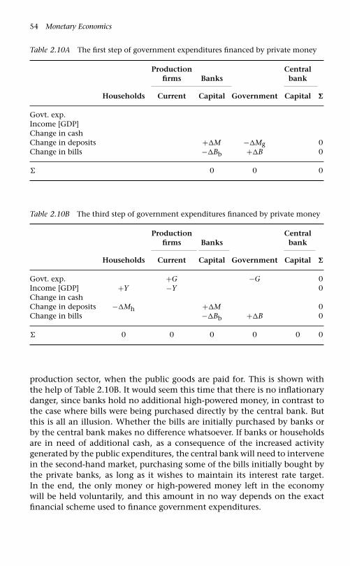
54 Monetary Economics

Table 2.10A The first step of government expenditures financed by private money

Production Centralfirms Banks bank

Households Current Capital Government Capital �

Govt. exp.Income [GDP]Change in cashChange in deposits +�M −�Mg 0Change in bills −�Bb +�B 0

� 0 0 0

Table 2.10B The third step of government expenditures financed by private money

Production Centralfirms Banks bank

Households Current Capital Government Capital �

Govt. exp. +G −G 0Income [GDP] +Y −Y 0Change in cashChange in deposits −�Mh +�M 0Change in bills −�Bb +�B 0

� 0 0 0 0 0 0

production sector, when the public goods are paid for. This is shown withthe help of Table 2.10B. It would seem this time that there is no inflationarydanger, since banks hold no additional high-powered money, in contrast tothe case where bills were being purchased directly by the central bank. Butthis is all an illusion. Whether the bills are initially purchased by banks orby the central bank makes no difference whatsoever. If banks or householdsare in need of additional cash, as a consequence of the increased activitygenerated by the public expenditures, the central bank will need to intervenein the second-hand market, purchasing some of the bills initially bought bythe private banks, as long as it wishes to maintain its interest rate target.In the end, the only money or high-powered money left in the economywill be held voluntarily, and this amount in no way depends on the exactfinancial scheme used to finance government expenditures.

Balance Sheets, Transaction Matrices, Monetary Circuit 55

2.6.4 The case of the overdraft economy

Up to now, we have assumed that government expenditures were financedeither by selling securities to the private banks, or by selling securities to thecentral bank. This corresponds however to a particular institutional set-up,that Hicks (1974: 51) has called the pure auto-economy. It turns out howeverthat the pure auto-economy, or what Lavoie (2001b: 216) has called theasset-based economy, is only one of the possible institutional set-ups. Whilethe asset-based economies have been described in great detail in mainstreamtextbooks, specially in Anglo-saxon textbooks, the other institutional set-upshave been usually ignored. It turns out, however, that most financial systemsin the world are not of the asset-based type, but rather can be described as

Table 2.11A First step of government expenditures in overdraft system

Production Centralfirms Banks bank

Households Current Capital Government Capital �

Govt. exp.Income [GDP]Change in cashChange in deposits +�M −�Mg 0Change in bank loans −�L +�Lg 0Change in central

bank advances

� 0 0 0

Table 2.11B Second step of government expenditures in overdraft system

Production Centralfirms Banks bank

Households Current Capital Government Capital �

Govt. exp. +G −G 0Income [GDP] +Y −Y 0Change in cash −�Hh +�H 0Change in deposits −�Mh +�M 0Change in bank loans −�L +�Lg 0Change in centralbank advances

+�A −�A 0

� 0 0 0 0 0 0

56 Monetary Economics

overdraft economies, making use once more of the terminology proposed byHicks (1974: 53).

In the pure overdraft economy, as defined by Hicks, firms hold no financialassets, and are thus ‘wholly dependent, for their liquidity, on the banks’. Thenotion of a pure overdraft economy can however be extended to the relationsbetween the private banks and the central bank, as is done in Lavoie (2001b).In pure overdraft financial systems, private banks hold little or no govern-ment securities. On the contrary, private banks in such overdraft economiesare permanently in debt vis-á-vis the central bank, having borrowed fundsfrom the central bank to acquire the reserves that they are legally requiredto hold, and to obtain the central bank banknotes that their customers havebeen asking for.

The impact of new government expenditures on the transactions flowmatrix, or at least a part of it, is shown in Tables 2.11A and 2.11B. As before,we assume new government expenditures of an amount G. This is nowfinanced by a loan from the private banks to the government. This is shown inTable 2.11A, which is very similar to Table 2.8A. These government expendi-tures generate an income of Y , which we assume as before to be kept initiallyin the form of money balances by households. A new assumption, comparedwith Tables 2.9 or 2.10, is that households wish to hold a certain portion oftheir new money balances in the form of cash money. In the pure overdrafteconomy, private banks must borrow all cash money from the central bank.Private banks obtain advances A from the central bank, to cover the needsin cash money of the public, as shown in Table 2.11B. Within such a systemwithout government securities, the determination of interest rates is quitestraightforward. The central bank simply needs to set the rate of interest onthe advances made to private banks. This rate of interest on advances is thenthe base rate of interest, that sets the standard for all other rates of interestin the financial system. The study of overdraft financial systems thus helpsto pierce through the veil of the asset-based financial systems, showing withobvious simplicity that central banks do have the ability to set short-terminterest rates.

3The Simplest Model withGovernment Money

3.1 Government money versus private money

Money is created in two fundamentally different ways. On the one handthere is outside money, which is created whenever a government pays forsomething by making a draft on its central bank or by paying for somethingwith banknotes, and which is extinguished when a payment is made by amember of the public to the government, typically in the form of taxes. Thiskind of money we may call government money, since it is issued by publicinstitutions, namely the central bank or the Treasury department of centralgovernment. Government money is usually called central bank money or high-powered money in the literature. On the other hand there is inside money,which is created by commercial banks when they make loans, and whichceases to exist when loans are repaid. This second kind of money will becalled private money, since it is issued by private institutions, namely privatebanks.

We shall eventually cover both types of money creation and destruction.But we have reluctantly come to the conclusion that it is impossible to deploya really simple model of a complete monetary economy in which inside andoutside money both make their appearance at the outset. We have there-fore decided to start by constructing and studying a hypothetical economyin which there is no private money at all, that is, a world where there areno banks, where producers need not borrow to produce, and hence a worldwhere there are no interest payments. We have done this while fully recog-nising that money generated by loans from private banks (e.g. to financeinventories when production takes time) is of the utmost importance in thereal world of monetized economies. This detour will enable the student tomaster the main principles inherent in fully coherent stock-flow macroeco-nomics, including the principles of portfolio behaviour within a simple butyet complete stock-flow framework. Very strong simplifying assumptions willhave to be made initially and the reader is asked to suspend disbelief untilmore realistic systems are introduced.

57

58 Monetary Economics

In the chapters which follow, we shall present a series of increasinglycomplex models. Each model will be complete in its own terms, with itswhole set of equations. And for each model, we shall present the balancesheet and the transactions matrix which belong to it. Each model will thenbe subjected to experiments, that is, parameters or exogenous variables will bemodified, and we shall observe the consequences of these changes for therelevant endogenous variables.

3.2 The service economy with governmentmoney and no portfolio choice

3.2.1 Assumptions

Let us start with the simplest meaningful model that can be built – Model SIM,for simplest. The economy is closed to the outside world: there are neitherexports nor imports, nor foreign capital flows. We postulate a monetary econ-omy in which economic agents, beyond the institution of government, canbe divided conceptually into their business activities on the one hand, sellingservices and paying out wages and, on the other, receiving income, consum-ing and accumulating assets when they act as households. All productionis undertaken by providers of services, who have no capital equipment andno intermediate costs of production. Production of services is assumed to beinstantaneous, so that inventories do not exist. Finance for inventory accu-mulation is thus unnecessary a fortiori. There are no private banks, no firmsand no profits whatsoever. We are in a pure labour economy, à la Adam Smith,where production is carried out by labour alone.1

The government buys services and pays for them with money, which con-sists of pieces of paper which it prints. Money is made acceptable as a meansof payment because there is a law which makes it legal tender, which meansthat creditors are legally obliged to accept money in settlement of debts. Thegovernment also levies taxes and ordains that these be paid in money, whichpeople therefore have to obtain by selling their services for it.2 In other words,all transactions occur in government money, that is, banknotes issued by gov-ernment. This government money is the vehicle via which people receiveincome, settle their debts, pay their taxes, and store their wealth.

It will further be assumed that the government fixes the price for an hour’slabour and that there is an unlimited quantity of labour which is poten-tially available. In other words, it will be assumed initially that the supplyof labour never constitutes a constraint on production. The economy is not

1 See the book by Pasinetti (1993), for the formal description of a multi-sectoreconomy, with pure labour processes.

2 This is sometimes called the cartalist or chartalist view (Wray 1998). Some mayregard it as an artificial assumption, others as an important and realistic principle.

The Simplest Model with Government Money 59

Table 3.1 Balance sheet of Model SIM

1. Households 2. Production 3. Government �

Money stock +H 0 −H 0

supply-constrained; it is demand-led. Production responds immediately todemand. Whatever is demanded will be produced.

3.2.2 Balance sheet and transactions matrix

Model SIM (and every subsequent model) will be introduced with a balancesheet matrix which describes each sector’s stocks of assets and liabilities andtheir logical inter-relationship with those of other sectors – each financialasset owned by one sector always having a counterpart financial liability inone or more other sectors. The balance sheet matrix for Model SIM, given byTable 3.1, is extremely simple as there is only one item – money (H) – whichis a liability of the government and an asset of households. This money isprinted by government: we can assume it consists of banknotes, that is, whatis usually called cash money. Because economists often call this high-poweredmoney, we shall let the letter H stand for it.

Here, as everywhere else, stocks of assets will be entered with a plus signand stocks of liabilities with a minus sign. Since the stock of money is anasset for households – it constitutes their accumulated wealth at a point oftime – it appears with a plus sign (+) in the column allotted to households.On the other hand, the outstanding stock of money constitutes a liability forgovernment. It is the public debt, the debt of government. Thus it is enteredwith a minus sign (−) in the government column.

In this elementary model, people in their capacity as producers and payersof income (shown in column 2 have been treated distinctly from the samepeople in their capacity as consumers, receivers of income and savers (shownas ‘households’ in column 1). People as producers are assumed to holdno cash at all, while they do hold cash when they act as consumers; at alater stage this will become a straightforward distinction between firms andhouseholds.

The second matrix, given in Table 3.2, describes all the transactions whichtake place between the sectors in any given period of time.

As pointed out in Chapter 2, it is impossible to overestimate the useful-ness, when deploying a macroeconomic model, however simple, of usinga system of accounts like that of Table 3.2. The system is comprehensive,in the sense that ‘everything comes from somewhere and everything goessomewhere’. Or, to put it more formally, all flows can be fitted into amatrix in which columns and rows all sum to zero. Without this armature,

60 Monetary Economics

Table 3.2 Accounting (transactions) matrix for Model SIM

1. Households 2. Production 3. Government �

1. Consumption −C +C 02. Govt. expenditures +G −G 03. [Output] [Y]4. Factor income(wages) +WB −WB 05. Taxes −T +T6. Change in the stockof money −�H +�H 0� 0 0 0 0

accounting errors may pass unnoticed and unacceptable implications may beignored.

The first five lines of the transactions matrix describe the variables whichcorrespond, in principle, to the components of the National Income andProduct Accounts (NIPA) arranged as transactions between sectors and whichtake place in some defined unit of time, such as a quarter or a year. Theseare the transactions which are usually to be found in standard macroeco-nomic textbooks. The sixth line, row 6, describes the changes in stocks offinancial assets and liabilities which correspond, in principle, to the Flow-of-Funds Accounts and which are necessary to complete the system of accountsas a whole. The inclusion of stock variables (as in Table 3.1) and transac-tions in stock variables (the last line of Table 3.2) in the basic system ofconcepts is an important distinguishing feature of our approach. It will leadus to conclusions about motivation and the ‘equilibrium’ (or steady state) towhich economic systems tend which are fundamentally at odds with thosepostulated in conventional textbooks.

Reading horizontally, the matrix shows that every component of thetransaction-flow matrix must have an equivalent component, or a sum ofequivalent components, elsewhere. For instance, reading row 5, we seethat the tax revenues collected by the government sector must, by logicalnecessity, be equal to the sum of the taxes paid by the other sectors of theeconomy.

Reading vertically, the matrix shows how any sector’s financial balance –that is, the difference between inflows of income and outflows ofexpenditure – must be exactly matched by the sum of its transactions instocks of financial assets. Note that the first difference symbol (�) describeschanges in a stock variable between the beginning and end of the period,that is �H = H −H−1 where the time subscript refers to the end of the previ-ous period. It is assumed that the stock of an asset, at the end of a period, is

The Simplest Model with Government Money 61

identical to the stock of that asset at the beginning of the next period. Thestock that you end up with is the same as the stock that you next start with.3

As was the case in Chapter 2, the reader should recall that all sources of fundsappear with a plus sign – these are incoming flows of money; on the otherhand, all uses of funds appear with a minus sign. Take for instance the house-hold column. In this simple model, households have only one source offunds, namely wages (the wage bill WB), which arise from sales of their work.4

They have three ways in which they can use their funds: they pay taxes (T),they purchase consumer services (C) and they accumulate additional finan-cial assets (�H). Thus the acquisition of new financial assets takes a minussign, because the purchase or the acquisition of a financial asset is part of theuse of the income they have received.

The matrix shows one item in square brackets which will prove crucial,namely total production (Y), which is not a transaction between two sectorsand hence only appears once, in the production Column 2. Total productionis here defined in the standard way used in all national accounts, either as thesum of all expenditures on goods and services or as the sum of all paymentsof factor income.

Y = C + G = WB (3.10A)

3.3 Formalizing Model SIM

3.3.1 The behavioural transactions matrix

As with all the models which will follow, the coherent system of accounts aris-ing from the balance sheet and the transactions-flow matrices provides thebackbone of the model now to be developed. Although the model isextremely simple, it will enable us to lay down some fundamental principlesand theorems which will remain useful later on.

The accounting matrices shown in Tables 3.1 and 3.2, since every row andevery column sum to zero, describe the identities that must be satisfied inevery solution to the model. However, beyond displaying the universe to be

3 Some authors prefer to call Ht the stock of money being held at the beginningof the period, but the convention that we adopt is more akin to the use of computersimulations.

4 It has been assumed that the government sector only purchases services fromproducing agents. There are no state employees and hence no civil servants. If thissimplification is too hard to swallow, the reader may imagine that all civil servantshave taken early retirement and have been replaced by contractuals. These contractu-als, many of them previously forced into early retirement, have organized themselvesas self-employed workers, setting up companies specialized in providing governmentservices, and as a result the individuals hired to provide government services are partof the production sector.

62 Monetary Economics

Table 3.3 Behavioural (transactions) matrix for Model SIM

1. Households 2. Production 3. Government �

1. Consumption −Cd +Cs 02. Govt. expenditures +Gs −Gd 03. [Output] [Y]4. Factor income(wages) +W · Ns −W · Nd 05. Taxes −Ts +Td 06. Change in the stockof money −�Hh +�Hs 0� 0 0 0 0

considered, these matrices do no more than show how all columns and rowsmust in the end ‘add up’. By themselves they can say nothing at all abouthow the system is motivated or how it works. To understand the behaviourof the system as a whole we first have to make sure that every entry indi-vidually makes behavioural sense in the place where it appears. The agentbuying a service is engaged in a completely different activity from that per-formed by the seller of that service and the motivation behind the two typesof activity is completely different. The vertical columns must necessarily sumto zero, because the change in the amount of money held must always beequal to the difference between households’ receipts and payments, how-ever these are determined. Similarly the change in the amount of moneycreated must always, by the laws of logic, be equal to the difference betweenthe government receipts and outlays. And, as they are assumed to hold nocash, producers receipts from sales must equal their outlays on wages. Butit may not be assumed in advance that the horizontal entries sum to zero;we have to specify the mechanisms by which these equalities come about.These mechanisms will be extremely simple ones in our first models, but theprinciple is theoretically fundamental; and as we advance to more complexmodels the equalizing mechanisms will be far more complex.

In Table 3.3 we show a modified version of Table 3.2 in which each transac-tion now has a suffix, s, d and h. The suffixes s and d, denote what, in a broadsense, may be called ‘supply’ and ‘demand’ while the suffix h attached to H ,describes households’ end period holdings of cash. The ‘wage bill’ has beenmodified so that it reads W · N, that is, a wage rate (W) times employment(N). The production sector supplies services to the household sector and thegovernment, and it ‘demands’ a certain volume of employment at a wagerate assumed to be exogenously determined – from outside the model. Thehousehold sector ‘demands’ consumption services, supplies labour and paystaxes. The government ‘demands’ services and taxes. It ought to be empha-sized that Table 3.3 is a ‘behavioural’ transactions matrix, and not an ‘ex ante’

The Simplest Model with Government Money 63

matrix. The behavioural matrix does not describe what is expected by the vari-ous agents before the period opens. Rather it describes the behaviour of agentsat the time of the transactions. This distinction will become clearer in a latersection.

3.3.2 Mechanisms adjusting supply and demand

The equations that describe Model SIM are to be found in Appendix 3.1.Because it is so very much simplified, only eleven equations are required tocomplete it and make it work.

We start with the equations which equalize demands and supplies.

Cs = Cd (3.1)

Gs = Gd (3.2)

Ts = Td (3.3)

Ns = Nd (3.4)

These four equations imply that whatever is demanded (services, taxes andlabour) is always supplied within the period. These (apart possibly from (3.3))are strong assumptions implying, obviously enough, that we are describ-ing an economy that has no supply constraints of any kind. In particular,equation (3.4) implies that there is a reserve army of unemployed work-ers, all eager to work at the going wage, whenever their labour services arebeing demanded.5 The equalities of equations (3.1) and (3.2) require moreattention, as some delicate points need to be emphasized. The rest of thissubsection is devoted to the product and service markets.

First, it needs to be emphasized that, from the transactions matrix pointof view, Cs and Gs represent the sales of consumption and government ser-vices. Cs and Gs both carry a positive sign in the production column of thebehavioural transactions matrix. Cs and Gs thus represent sources of income –revenues that are collected by the production sector. Similarly, Cd and Gdrepresent the purchases of consumption goods and government services. Ofcourse, we know that the sales have to equal purchases; this is nearly a tautol-ogy. But starting from a situation where production could be different fromsupply, and where supply could be different from demand, how do we arriveat the equality between sales and purchases?

There are several mechanisms that could lead to such a result, thus ensur-ing that the first two rows of the behavioural matrix sum to zero. The

5 Thus equation (3.4) must certainly not be interpreted as implying that there isfull employment. On the opposite, it is the amount of supplied labour that adjusts tolabour demand.

64 Monetary Economics

first mechanism is mainly associated with mainstream theory, that is, neo-classical theory: variations in prices clear the market. Excess demand leadsto higher prices, which is assumed to reduce excess demand.6 This mecha-nism is put into effect within the period, before transactions are made. Whentransactions occur, as reflected in the transactions-flow matrix, supply anddemand have already been equated through the price clearing mechanism.We believe that such a market clearing mechanism, based on price varia-tions, is only appropriate in the case of financial markets. In the case ofgoods and services markets, and in the case of the so-called labour market,we believe that the hypothesis of market-clearing equilibrium prices is whollycounterfactual, inappropriate and misleading.

The second mechanism is associated with the so-called rationing theory,also called constrained equilibrium theory.7 Despite being based on an essen-tially neo-classical view of markets, this approach eschews market clearingprices, by imposing some rigid prices. It says that whenever supply anddemand are different, because of these rigid prices, the adjustment is done onthe short side of the market. For instance, if demand is less than supply, saleswill equate demand; if supply is less than demand, sales (and purchases) willequate supply. In this approach however, it is still the case that prices andnominal wages give the signals and what happens to unsold commodities iswaived aside. For these reasons, we shall not pursue this line of thought.

The third mechanism is linked to the existence of inventories. Firms hold abuffer of finished goods, which can be called upon whenever demand exceedsproduction. Sales are always equal to demand because it is assumed thatinventories are always large enough to absorb any discrepancy between pro-duction and demand. In this approach it is necessary to track the evolutionof inventories from period to period, and to pay meticulous attention to theway in which they are measured, in particular to how they are valued. Ithas been advocated by authors of various heterodox traditions, in particularGodley and Cripps (1983) and Duménil and Lévy (1993: 95), who call it the

6 Although elementary and intermediate textbooks often claim that excess demandis always eliminated by rising prices, things are not so simple in a world with severalcommodities: demand curves may not be downward sloping; they may not be ‘well-behaved’. In the world of produced commodities, this problem is included amongwhat are known as the Cambridge capital controversies (Harcourt 1972; Garegnani1990). In general equilibrium theory, it is known as the Impossibility theorem, orthe Sonnenschein-Debreu-Mantel theorem (Kirman 1989); despite starting with all theconditions associated with rational consumers, it is impossible to demonstrate thatthe market excess demand curve of every good is downward sloping. In other words,the equilibrium may not be stable, and there might be a multiplicity of them.

7 The names of Clower, Barro and Grossman, Bénassy, Malinvaud are usuallyassociated with this particular school of neoclassical Keynesians.

The Simplest Model with Government Money 65

‘general disequilibrium approach’. This mechanism – which we consider tobe the most realistic one – will be described in detail, but only when we dealwith private money, for reasons that will become obvious.

Finally, there is a fourth mechanism, the so-called Keynesian, or Kaleckian,quantity adjustment mechanism. This is the mechanism that is being calledupon in the present model. With the previous three adjustment mecha-nisms, production was assumed to be given, set at some constant level atthe beginning of the period. In the Keynesian and Kaleckian approach, pro-duction is the flexible element of the model. Producers produce exactly whatis demanded. In this approach, there are no inventories. In the nationalaccounts, variations in inventories adjust national expenditures to nationaloutput whenever sales differ from production. Here there is no such account-ing adjustment mechanism, since inventories cannot change by assumption.Sales are equal to production. The equality between demand and supply,the latter being here defined as production, is achieved by an instantaneousquantity adjustment process, as is always the case in standard Kaleckian andKeynesian models. In the words of the mainstream, equations (3.1) and (3.2)embody the equilibrium between aggregate supply and aggregate demand,that is, between produced output and sales, being understood that the equal-ity is achieved by a quantity process, and not by variations in prices. Thismechanism is more likely to be appropriate in a service industry, where theservice often is being provided right away, as soon as it is demanded. In thecase of manufacturing, where production takes time, such an instantaneousquantity adjustment process is unlikely; the third mechanism, that based oninventory adjustments, is much more realistic.

In Model SIM, we are thus making two behavioural assumptions: first, thatfirms sell whatever is demanded (there is no rationing) – an assumption thatwe shall make throughout the book; and second, that there are no invento-ries, which implies that sales are equal to output – an assumption that willbe abandoned in Chapters 8–11, where production will be equal to sales pluschanges in inventories. It is best not to confuse these two assumptions.

3.3.3 Other equations of Model SIM

We next define disposable income (YD) as the wage bill earned by householdsless paid taxes:

YD = W · Ns − Ts (3.5)

We may now enter two behavioural equations. First, taxes are levied assome fixed proportion of money income, θ , which the government decides.The tax rate on (taxable) income is thus θ . This yields equation (3.6):

Td = θ · W · Ns θ < 1 (3.6)

66 Monetary Economics

Second, we must specify the consumption function. At what rate dohouseholds spend on consumption? We know that they open each periodwith a stock of wealth inherited from the previous period (H−1) and duringthe period they receive post tax income equal to YD. There are many waysto portray consumption behaviour. We suggest that households consume onthe basis of two influences: their current disposable income YD, which wemust assume is accurately known to households when they make their deci-sions, and the wealth they have accumulated over the past, H−1. This yieldsequation (3.7), which says that consumption is determined as some propor-tion, α1, of the flow of disposable income and some smaller proportion, α2,of the opening stock of money. Consumption functions have been subjectedto intense debates, and more will be said about the relative merits and theimplicit features of the one chosen here.

Cd = α1 · YD + α2 · Hh−1 0 < α2 < α1 < 1 (3.7)

The next two equations arise once more from the transaction-flow matrix.Equation (3.8) is an identity, taken from column 3 of either of the transac-tion matrices. It says that the change in the stock of money issued by thegovernment in each period, that is, the change in the supply of money Hs,is given by the difference between government receipts and outlays in thatperiod. Both the change in the stock of money and the government deficitare endogenous; once the government has determined its own expenditureand the tax rate, the actual tax take will be determined as part of the solutionof the model. When government expenditures exceed government revenues(taxes), the government issues debt to cover the difference. The debt, in oursimplified economy, is simply cash money, which carries no interest pay-ment. Thus equation (3.8) represents the budget constraint of government.The government expenditures that are not covered by taxes must be coveredby the issue of a debt. Cash money is that debt.

�Hs = Hs − Hs−1 = Gd − Td (3.8)

Next, there is the third equation arising from the transactions-flow matrix,that given by equation (3.9). It corresponds to column 1 of the transactions-flow matrices. This identity describes the budget constraint of households.The accumulation of households’ wealth is determined by their financialbalance – the excess of disposable income over expenditure. Because there isonly a single financial asset, and because there are no tangible assets in thiseconomy, additions to cash holdings constitute the saving of households.

It follows that Hh stands for the cash held by households and also for thelevel of wealth which they possess. The h subscript is there to indicate thatthe cash is being held by households.

�Hh = Hh − Hh−1 = YD − Cd (3.9)

The Simplest Model with Government Money 67

Finally, we need the expressions which describe the determination ofoutput and the determination of employment. This is the national incomeidentity:

Y = Cs + Gs (3.10)

which, seen from the point of view of income, is rewritten as:

Y = W · Nd (3.11A)

or rather as:

Nd = YW

(3.11)

The elementary model is now complete. We have 11 equations and 11unknowns, Y , YD, Td, Ts, Hs, Hh, Gs, Cs, Cd, Ns and Nd. Each of the elevenunknowns has been set on the left-hand side of an equation. There are threeexogenous variables, Gd, θ , and W , the first two of which are set by theautonomous decisions of government – fiscal policy in other words. Wageswill be determined largely by conditions in the labour market but are assumedat this stage to be fully exogenous.8 All these, together with initial (stock)conditions and the parameters of the consumption function, make it possibleto solve the model as a sequence proceeding through time. In sharp contrastwith the conventional treatment, the solution for each period will dependcrucially on stock variables created the previous period; and it will createthe stock variables necessary for the solution of the model in the followingperiod.

It should finally be noted that two separate equations (3.8) and (3.9)describe respectively the issue of money by the government and the addi-tional amount of money which people decide to hold as two distinctprocesses; yet the model contains no equilibrium condition which makes the twoequal to one another. The two (changes in Hh and Hs) must however turnout to be the same once the model is solved, as can be inferred from thebehavioural matrix (Table 3.3). The vertical columns all sum to zero by therules of logic, and we have described behaviour which will guarantee thatall the rows except the bottom row (which contains Hh and Hs) also sumto zero. By virtue of the watertight accounting of the model, combined withbehavioural assumptions which guarantee the equality between demand andsupply for services and labour, we have stumbled on the Walrasian principle,which is not to be gainsaid, that any properly constructed model must con-tain one equation which is redundant, in the sense that it is logically implied

8 In this highly simplified model, as written, it would be meaningless to change thewage rate W .

68 Monetary Economics

by all the others and which can – indeed must – be ‘dropped’ out of the modelif a solution of the model is not to be over-determined. The computer couldnot solve the model if this additional equation were to be included in the pro-gram. We shall encounter time and time again this quasi-Walrasian principle.Here, the redundant equation is:

�Hh = �Hs (3.12)

We draw attention here to a fundamental difference between the modelwhich we are beginning to set forth compared with that which sees clear-ing (or non clearing) markets as the determinants of macro phenomena. Inthis, our elementary model, the equality between the demand and supplyof money is the logically inevitable consequence of using a comprehensivesystem of accounts. By contrast, the identical equation in the neo-classicalmodel is an equilibrium condition which somehow brings the demand formoney into equivalence with the ‘money supply’ determined exogenously.

The equality expressed by equation (3.12) contains nothing surprising froma Keynesian point of view. It simply expresses the well-known Keynesianidentity that says that investment must be equal to saving. In Model SIM,there is no investment. This implies that social saving, the saving of theoverall economy, must sum to zero. Here the term �Hh represents householdsaving; the term �Hs stands for the government fiscal deficit, and hencegovernment dissaving. For overall saving to be zero, the two terms mustequal each other.

3.4 A numerical example and the standardKeynesian multiplier

3.4.1 A numerical example

It may help to give a numerical example of how this whole model evolvesthrough time, starting with the beginning of the world.

Assume the tax rate is 20%, while the parameters of the consumption func-tion, α1 and α2, are 0.6 and 0.4, respectively. We start from a situation wherethere is no economic activity whatsoever, and where none has ever existed.Households have no income, and they never accumulated any wealth. Thecausal chain is set off by a stream of payments by the government. Thesegovernment expenditures generate income, a tax yield, a money supply anda consumption stream. The government has suddenly come in, and decidesto order $20 worth of services from the production sector. These services arepaid for by the creation of 20 units of cash money, that is $20. The moneycreated is then circulated within the system in the following way.

First, producers will pay households with these 20 units of cash. House-holds will then be forced to pay taxes on 20% of that, that is, they will haveto pay 4 units in taxes. These 4 units of money are thus destroyed, as soon

The Simplest Model with Government Money 69

Table 3.4 The impact of $20 of governmentexpenditures, with perfect foresight

Period 1 2 3 ∞

G 0 20 20 20Y = G + C 0 38.5 47.9 100T = θ · Y 0 7.7 9.6 20YD = Y − T 0 30.8 38.3 80C = α1 · YD + α2 · H−1 0 18.5 27.9 80�Hs = G − T 0 12.3 10.4 0�Hh = YD − C 0 12.3 10.4 0H = �H + H−1 0 12.3 22.7 80

as the taxes are paid back to government. Households then purchase con-sumer services from one another, using 60% of the remaining 16 units ofcash money, that is, 9.6 units, while the rest, 40% of the 16 units, will be putaside to accumulate wealth, in the form of cash balances. But the 9.6 unitsof consumption now generate production and an income equal to 9.6 units.Out of this income, more taxes will be paid, more cash will be accumulated,and more consumer expenditures will be carried out. But these expenditureswill lead to more production and more income being distributed, all thiswithin the very same period.

The initial $20 government injection thus has ripple effects throughout theeconomy. The government injection has a multiple effect on income. Thisis the well-known Keynesian multiplier process, to be found in all elemen-tary macroeconomics textbooks. Because perfect foresight has been assumed,households must know precisely how much will be produced and how muchincome the initial injection of government expenditures is able to generate.They must also know with certainty the various parameters of the overalleconomy (the average tax rate and the average propensity to consume out ofdisposable income) and they must know the initial injection. Here, all thesemultiplier effects are assumed to take place within the single period. Startingwith no economic activity at all in period 1, the government expenditurestaking place at the beginning of period 2 along with the standard multiplierprocess will bring about the numbers given at the end of period 2, as shownin Table 3.4.

Since mechanisms equating the various supply and demand variables havebeen provided, the suffixes s and d have been omitted.

3.4.2 The standard Keynesian multiplier

How did the economy achieve the numbers of period 2? The standardKeynesian analysis – precisely the analysis beyond which we wish to go –provides the explanation.

Since there is no past accumulated wealth at the beginning of period 2, theconsumption function given by equation (3.7) comes down to the standard

70 Monetary Economics

textbook consumption function (with no autonomous term):

Cd = α1 · YD (3.13)

The national expenditures equation (3.10), given equations (3.1) to (3.4),and equations (3.5) and (3.6), omitting the subscripts becomes:

Y = C + G = α1 · {Y · (1 − θ)} + G

With perfect foresight national income in the consumption function mustbe identical to national income defined as production. Solving for Y , weobtain the equilibrium value of Y at the end of period 2:

Y∗ = G1 − α1 · (1 − θ)

(3.14)

For the assumed parameter values, the multiplier 1/{1 − α1 · (1 − θ)} isequal to 1.92, and hence, for G = 20, Y∗ = 38.5, as shown in period 2 ofTable 3.4.

In the standard story, for instance that told by the well-known IS/LMmodel, the expression of Y∗ given by equation (3.14) would be the end ofthe story. The reader of the standard textbook would be told that Y∗ is theequilibrium national income. The textbook would then consider whether themultiplier should be interpreted as a logical relationship, occurring withinthe period, as has been done here, or as a dynamic relationship, occurringover several periods, possibly using trial and error. The reader would then betold that provided government expenditures are kept at the same level (here20) in the following periods, national income would remain forever at its Y∗value (here 38.5).

3.4.3 The drawbacks of the standard multiplier analysis

This view of the multiplier process lacks coherence however. The equilibriumvalue of Y∗ is only a short-run equilibrium. It is not a long-run equilibrium,that is, it is not a steady state in the sense that it is a solution that canrepeat itself for a large number of periods. Once we think of it, the factthat equation (3.14) cannot be a steady-state is quite obvious. If the expres-sion of Y∗ provided by equation (3.14) and the numbers provided in period2 of Table 3.4 were to be the algebraic and numerical long-run solutionsof our model, then there would be absurd consequences. In particular, inperiod 2, the government is running a deficit: government expenditures Gminus taxes T are equal to 20−7.7 = 12.3. Since the level of national incomeis deemed to be constant at Y∗, the constant deficit of every period wouldadd to one another, so that government debt would rise forever. The publicdebt to income ratio would rise to infinity. This, of course, is impossible. Thesolution of equation (3.14) and the numbers of period 2 can only provide uswith a temporary solution, a short-run one.

The Simplest Model with Government Money 71

The problem with the standard textbook story is that it deals with flows,while not taking into account the impact of flows on stocks – and the sub-sequent impact of stocks on flows. Until a steady state has been reached,short-run flows will generate changes in stocks. In the case of Model SIM theshort-run solution reached in period 2 gives rise to a government deficit andto a flow of saving on the part of households. The government deficit eachperiod adds to the stock of debt owed by government. Similarly the saving ofhouseholds adds cash money to their existing stock of cash balances. Unlesseverything else grows at the same rate, this cannot go on forever. The wayout of this puzzle is offered by the formulation of the consumption functiongiven by equation (3.7). As households accumulate wealth – as they accu-mulate more and more cash balances – they become richer, and consumepart of their accumulated wealth. This gives rise to the second term of theconsumption function (3.7), the α2 · Hh−1 term, which says that householdsconsume a proportion α2 of the wealth Hh−1 which they have accumulatedin the past. This is why the level of income in period 3, and in successiveperiods is now higher than what it was in period 2, despite the fact that theautonomous government expenditures remain fixed at 20. Consumers spendout of their current income but also out of the money balances which theyhave accumulated in previous periods.

3.5 Steady-state solutions

We may now explore the steady-state solutions of Model SIM, those givenby the last column of Table 3.4. First we define what we mean by a steady-state. It is a state where the key variables remain in a constant relationshipto each other. This must include both flows and stocks, and not flows onlyas with short-run (temporary) equilibria . When, in addition, the levels ofthe variables are constant, the steady state is a stationary state. In general,the steady state will be a growing economy, where ratios of variables remainconstant. Whether we are in a stationary state or a steady state with growth,we may then speak of the long-run solutions. But most of our models will omitgrowth, and hence will deal with stationary states, as is the case with ModelSIM. In the stationary steady state of the model, in which neither stocks norflows change, government expenditure must be equal to tax receipts, that is,there is neither a government deficit nor a government surplus. This is thecondition for a zero change in the stock of money (i.e. government debt).Formally, still omitting subscripts, we have:

G = T∗ = θ · W · N∗ = θ · Y∗

Hence the stationary state flow of aggregate income must be:

Y∗ = Gθ

(3.15)

72 Monetary Economics

1957

125.0

Income Y

Steady-state solution Y *

120.0

115.0

110.0

105.0

100.0

1961 1965 1969 1973 1977 1981 1985 1989 1993 1997 2001

Figure 3.1 Impact on national income Y and the steady state solution Y∗, followinga permanent increase in government expenditures (�G = 5)

where stars now denote a steady state solution.9 In the numerical example,the stationary level of income is 100, as can be seen in the last column ofTable 3.4, since G = 20, while θ = 0.2.

The G/θ ratio we call the fiscal stance. This is the ‘ratio of governmentexpenditure to its income share’ (Godley and Cripps 1983: 111). It plays afundamental role in all of our models with a government sector, since itdetermines GDP in the steady state.

This fundamental property of the model is also illustrated in Figure 3.1which shows how the stationary solution G/θ is modified following a per-manent step addition of $5 to the flow of government expenditure. As theaverage tax rate is assumed to be 20%, the addition to the stationary stateaggregate flow, by (3.10), is $25. As Figure 3.1 shows, the addition to aggregateincome does actually converge to this number. Income Ygradually increasesfrom its $100 steady state value until it finally reaches $125, which is thenew value of G/θ – the new stationary value.10

9 This result was first achieved by Ott and Ott (1965). See also Christ (1968) andGodley and Cripps (1983: 111)

10 Not too much attention should be paid to the numerical years which are shownon the x-axis of the chart. These really represent periods: they could be years, quarters,months.

The Simplest Model with Government Money 73

80

75

60

45

30

15

1957 1961 1965 1969 1973 1977 1981 1985 1989 1993 1997 20010

80

75

60

45

30

15

0

Consumption C

Disposableincome YD

Figure 3.2 Disposable income and consumption starting from scratch (Table 3.4)

Another property of the stationary state is that consumption must be equalto disposable income. In other words, in a model without growth, the averagepropensity to consume must be equal to unity. This property of fully coherentstock-flow models – which is often forgotten – can be easily derived, becausein the stationary state there is no change in financial stocks, that is, there isno saving. Thus, by virtue of equation (3.9), we have:

�H∗h ≡ YD∗ − C∗ = 0

where the stars once more denote steady state values. This implies that:

YD∗ = C∗

and hence, given equations (3.5)–(3.7), (3.11A) and (3.15):

YD∗ = C∗ = G · (1 − θ)

θ(3.16)

In the numerical example of Table 3.4, we can see in the last column thatdisposable income and consumption are equal to each other in the stationarystate only, when they reach 80. Figure 3.2 also illustrates how the changein disposable income responds to the addition to government expenditure;and how consumption responds to disposable income, eventually convergingonto it, as implied by equation (3.16).

74 Monetary Economics

Finally, we may compute the stationary value of the stock of householdwealth, that is the stationary value of cash money balances which is alsothe stationary value of the stock of government debt. In the consumptionfunction (3.7), we substitute the equality YD∗ = C∗. Knowing that in thesteady state, H = H−1, we obtain:

H∗ ={

(1 − α1)

α2

}· YD∗ = α3 · YD∗ = α3 · G · (1 − θ)

θ(3.17)

where α3 = (1 − α1)/α2.With numerical values attributed to the various parameters, we note that

α3 = 0.4/0.4 = 1. Thus, in the numerical simulation given by Table 3.4, thestationary value of the stock of money balances is identical to the value takenby disposable income, and equal to 80. Figure 3.3 also shows how, consistentwith equation (3.17), wealth – here the stock of money – converges ontoits steady state value. The chart also shows that household saving – hereadditions to money balances – converges to zero, as it should in a model thatconverges to a stationary state.11

3.6 The consumption function as a stock-flow norm

The definition of the steady-state solution for household wealth is theoccasion to discuss further the meaning of the consumption function (3.7),and to reach a very important result. When first presented, the consumptionfunction was viewed as a consumption decision based on both the flow ofincome and the stock of past accumulated wealth. Another interpretationof this relationship can now be offered, in terms of a wealth accumulationfunction, thus showing that consumers’ behaviour can be represented ineither of two, logically equivalent, ways. First note that equation (3.9) can berewritten as:

C = YD − �Hh (3.9A)

This simply says that consumption is disposable income minus changesin cash money (i.e. minus the household saving of the period). This iden-tity may be substituted back into (3.7), which, after rearrangement, turnsthe consumption function into a saving function or a wealth accumulationfunction. We have:

C = YD − �Hh = α1 · YD + α2 · Hh−1

11 From the identities of the balance sheet and of the transactions matrix, we knowthat the two curves of Figure 3.3 also trace out the evolution of government deficit andgovernment debt.

The Simplest Model with Government Money 75

1957 1961 1965 1969 1973 1977 1981 1985 1989 1993 1997 2001

80

75

60

45

30

15

0

Wealth change Wealth level

Wealth level H (money stock)

Household saving(the change in the money stock)

12.5

10.0

7.5

5.0

2.5

0.0

Figure 3.3 Wealth change and wealth level, starting from scratch (Table 3.4)

and hence:

�Hh = (1 − α1) · YD − α2 · Hh−1

from which we obtain:

�Hh = α2 · (α3 · YD − Hh−1) (3.7A)

where once again α3 = (1 − α1)/α2.Equation (3.7A) is a partial adjustment function. It says that wealth is

being accumulated at a certain rate, determined by the partial adjustmentparameter α2, towards some desired proportion α3 of disposable income.Thus households are saving, wishing, we may suppose, to end the periodwith some well defined quantity of accumulated wealth. In other words, theexisting wealth of households, when any period begins, is equal to H−1, andgiven the disposable income of the period, households now have a targetlevel of wealth, given by VT = α3 · YD. The α3 coefficient is the stock-flownorm of households. It is the assumed wealth to income target ratio whichis implicitly embedded into the so-called Modigliani consumption functionproposed with equation (3.7). Thus whenever the target level of wealth ishigher than the realized level, households save, in an attempt to reach theirtarget.

76 Monetary Economics

1957 1961 1965 1969 1973 1977 1981 1985 1989 1993 1997 2001

100.0

96.0

92.0

88.0

84.0

80.0

Target wealth (and disposable income)ConsumptionWealth

Figure 3.4 Evolution of wealth, target wealth, consumption and disposable incomefollowing an increase in government expenditures (�G = 5) – Model SIM.

This is illustrated with the help of Figure 3.4, which starts off from thestationary state identified in the previous graphs, which is shocked by a stepincrease in government expenditures. We see that target wealth (here alsoequal to disposable income since α3 = 1) remains higher than realized wealth,so that households save in their attempt to adjust their historically given levelof wealth to their target wealth. As a result, consumption is systematicallybelow disposable income, until the new stationary state is reached, at whichpoint Hh = VT = YD = C.

The fact that the wealth accumulation function (3.7A) can be directlyobtained from consumption function (3.7), by the simple addition ofequation (3.9A) which identically defines consumption, is very important.It shows that the assumption of stock-flow norms in the case of house-holds is not far-fetched, at least within a Keynesian research programme,for the existence of the stock-flow norm is equivalent to the existence of awell-accepted Keynesian consumption function with lagged wealth, that ofequation (3.7). In Godley and Cripps (1983: 41), it was argued that the pro-posed theory, which is roughly similar to the one advocated in the presentbook, was ‘a conditional theory as to how whole economic systems function’.Godley and Cripps argued that ‘the main results are conditional on thebehavioural axiom that stock variables will not change indefinitely as ratiosto related flow variables’. In other words, the theory presented was condi-tional on the existence of stock-flow norms. But equations (3.7) and (3.7A)

The Simplest Model with Government Money 77

show that these stock-flow norms can be extracted directly from (nearly)standard Keynesian consumption functions. All that needs to be assumed,as did Modigliani (1986), is that consumption depends on lagged wealthbesides current disposable income. If one believes in the relative stability ofconsumption functions, that is if one agrees that the α coefficients are fairlystable, then one accepts the relative stability of stock-flow norms in the caseof households.

For instance, in period 3 of Table 3.4, since α3 = 1, the target level of wealthis VT = 38.3, whereas the previously achieved level of wealth is H−1 = 12.3.Rather obviously households do not attempt to reach their wealth target atonce as this might leave them consuming nothing at all for a time. Onlya proportion α2 of the discrepancy will be remedied within a single period.The adjustment to the target level is partial. Again, in the case of period 3 ofTable 3.4, with α2 = 0.4, and with a discrepancy between the target and theachieved wealth of 26, the saving of period 3, �Hh, equals 10.4. Only 40%of the discrepancy is remedied at once.

In general, dissaving will occur when the wealth target has been surpassed.Also, as is clear from equation (3.7A), once the target has been reached, that is,when H∗ = VT = α3 ·YD∗, no more saving will occur and the stationary statedefined by equations (3.14–3.17) is reached.

It may finally be useful to add something about what, in a properly articu-lated stock-flow system, the consumption function is not and cannot possiblybe. It cannot be:

C = α1 · YD 0 < α1 < 1 (3.13)

The reason why this version of the consumption function must be cate-gorically rejected is that, in models without growth, its use renders the modelunstable.12 Why? Because, as shown in section 3.4, if α1 is less than unitythe equation implies that if ever a flow stationary state were reached, therewould have to be a stock disequilibrium; with C and YD constant, the moneystock and government debt must be rising for ever (by an amount equal ineach period to YD − C).

There is however another consumption function, very similar toequation (3.13), which is admissible, although it does not have all the nice

12 In models with growth, the standard consumption function, without a wealthterm, does not lead to formal instability. Thus there is nothing wrong, from a purelylogical viewpoint, with all the Cambridge growth models (à la Kaldor, Robinson,Pasinetti, and even Lavoie and Godley (2001–2)), that exclude a wealth term, beingbased on specific propensities to save out of profits and out of wages. Such modelsachieve a determinate wealth to income ratio, although there is no explicit wealth toincome target ratio.

78 Monetary Economics

properties of equation (3.7). It is:

C = α0 + α1 · YD (3.13A)

with α0 a positive constant, which represents autonomous consumption,independent of current income.

This is, of course, the consumption function to be found in Samuelson’selementary 45 degree-line model – the workhorse of principles ofmacroeconomics – and in the IS-LM model – the workhorse of most inter-mediate macro textbooks. Consumption function (3.13A) is also often to befound in the work of various post-Keynesians. For instance, it can be foundin the textbook of Paul Davidson (1994: 39), who, in the footsteps of Keyneshimself, deals with short-run equilibria, without growth. With consumptionfunction (3.13A), it is possible to achieve a coherent stationary state. Theaverage propensity to consume can be unity, that is we can have C = YD inthe stationary state, even though the marginal propensity to consume outof disposable income, given by α1, is below one. What happens is that theconstant term in equation (3.13A) plays a role similar to that of the con-sumption out of wealth. When we deal with private money, in Chapter 8,we shall introduce a mixture of these two coherent consumption functions,those given by equations (3.7) and (3.13A).

3.7 Expectations mistakes in a simple stock-flow model

3.7.1 Introducing expectations into the model

In this section we introduce uncertainty into the model by making consump-tion depend on expected income – not actual income, which households canonly guess. In the process we shall discover a new and extremely importantfunction for money – that it acts as a ‘buffer’ whenever expectations turn outto be incorrect.

Model SIM used the strong assumption that consumers have perfect fore-sight with regard to their income – something which is inconceivable in aworld dominated by uncertainty, where the future states of nature are them-selves uncertain, and where agents have unreliable knowledge and limitedcapacity in processing information.13 Yet if consumers do not know pre-cisely what their income is going to be, the only change which has to bemade to the model is to substitute expected for actual disposable income inthe consumption function. But we must then have some way of describinghow expectations are formed.

13 Those two aspects of uncertainty are respectively called ontological and epistemo-logical uncertainty.

The Simplest Model with Government Money 79

The new consumption function is:

Cd = α1 · YDe + α2 · Hh−1 (3.7E)

where the superscript e denotes an expected value.It is assumed that households make some estimate of the income they will

receive during the period, and that they base their consumption over thecurrent period on this estimate. Since agents decide what to spend on thebasis of their expected income, this implies that households correctly esti-mate the money stock they will end up with only when they have correctlyanticipated their disposable income. In general, households can only makean estimate of the amount of money which they desire to hold. This con-ditional demand for money, the amount of money desired by householdsconditional on their expectations regarding disposable income, we shall callHd. At the beginning of the period, households decide on the amount ofadditional money which they desire to hold by the end of the period. Thenew stock of money which they wish to hold is their demand for money.We thus add one variable to the model, Hd , the demand for money at thebeginning of the period (based on expectations), and one extra equation:

�Hd = Hd − Hh−1 = YDe − Cd (3.18)

To the extent that expectations about disposable income are falsified, theend period stock of money must differ to an equal extent from what wasinitially demanded. Subtracting equation (3.18) from (3.9), we obtain:

Hh − Hd = YD − YDe (3.19)

The above equation shows that if realized income is above expectedincome, households will hold the difference in the form of larger thanexpected cash money balances. The reason for this is that households havealready decided on the amount they would consume. Any additional income,additional to what was expected, will thus be saved and added to cash bal-ances. The stock of cash people find themselves holding at the end of eachperiod is not the outcome of a plan which they have made. We have reacheda point here where our model of money holding differs fundamentally fromthat in conventional macroeconomics; we could hardly be further from asituation in which there is a difference between the supply and demand formoney which must be resolved via an equilibrating mechanism. The quan-tity of cash households end up with will bear some relationship to what theyplanned but this will be modified by any error in their expectations. Thusmoney provides a function which is sometimes called ‘buffering’ – apart frombeing the form in which wealth is held, money provides an essential flexibleelement which enables people to transact although they never quite knowwhat their income or their expenditure is going to be. This is one reason why

80 Monetary Economics

Table 3.5 Behavioural (transactions) matrix for Model SIM, with mistakenexpectations

1. Households 2. Production 3. Government �

1. Consumption −Cd +Cs 02. Govt.

expenditures +Gs −Gd 03. [Output] [Y]4. Factor income(wages) +W · Ne

s −W · Nd W · Nes − W · Nd

5. Taxes −Tes +Td Td − Te

s6. Change in thestock of money −�Hd +�Hs �Hs − �Hd� 0 0 0 0

the term ‘demand’ for money is so misleading and why we have given it thesubscript h from the very beginning to mean ‘holding’ rather than the usuald subscript.

The appearance of mistaken expectations on the part of households can bedescribed within the framework of another behavioural transactions matrix,shown here in Table 3.5. Let us include, however, within this matrix, theadjustment processes of equations (3.1–3.4), that guarantee that the sums ofsome rows are equal to zero. Then the new behavioural transactions matrixappears as in Table 3.5.

Because only households are assumed to have mistaken expectations, onlythe column of households and that of summations are changed compared toTable 3.3. However, as before, the column of households must sum to zero,for otherwise the plans and the expectations of households would be incom-patible with their budget constraint. The budget constraint of householdsas it appears in the first column of Table 3.5 is reflected in equation (3.18).Similarly, equation (3.19) can be extracted from the last column, by recallingthe definition of disposable income and by recalling equation (3.12) – theredundant equation – which says that �Hs = �Hh.

3.7.2 A more recursive system

The inclusion of expected income, rather than realized income, in the con-sumption function yields a more recursive picture of the system. Recall thedifficulties that we had in identifying income in the very first stage of ournumerical example in Table 3.4, what we called then the second period of themodel. Because all was simultaneously happening at once, we required theshort-term solutions of the multiplier process to achieve the required com-putations. In other words we had to assume that households knew what the

The Simplest Model with Government Money 81

Table 3.6 The impact of $20 of governmentexpenditures, with mistaken expectations

Period 1 2 3 ∞

G 0 20 20 20Y = C + G 0 29.6 39.9 100T = θ · Y 0 5.9 8.0 20YD = Y − T 0 23.7 31.9 80YDe = YD−1 0 16.0 23.7 80C = α1 · YDe + α2 · H−1 0 9.6 19.9 80�Hs = G − T 0 14.1 12.0 0�Hh = YD − C 0 14.1 12.0 0H = Hs = Hh = �H + H−1 0 14.1 26.1 80�Hd = YDe − C 0 6.4 3.8 0Hd = �Hd + H−1 0 6.4 17.9 80

equilibrium level of income was, hence assuming that they had knowledgeof the multiplier process and of the various parameters of the economy.

Here things are much simpler. For instance, starting again from scratch,as we did with the numerical example of Table 3.4, we can suppose that, inthe second period, households only expect as income the services purchasedby government. In the following periods, let us for the time being assumethat expected income is equal to the realized income of the previous period,that is, we have:

YDe = YD−1. (3.20)

The four new equations now help to define model SIMEX. From it, we canbuild a numerical example, as shown in Table 3.6. In period 2, householdsassume an income level of 20, and hence expected disposable income is equalto 16. Since there is a marginal propensity to consume of 0.6, this implies thatactual consumption is 9.6 and hence income is 29.6(= G+C = 20+9.6). Thereader can verify that equation (3.19) is satisfied: the discrepancy betweendesired and realized holdings of money is equal to the discrepancy betweenexpected and realized disposable income. Also, one can see that the expecteddisposable income at period 3 is the same as realized disposable income atperiod 2. Despite the mistakes in expectations, as time goes on, the samestationary state as that of Table 3.4 will be achieved, as shown in the lastcolumn of Table 3.6. The evolution of disposable income YD and expecteddisposable income YDe are specifically charted in Figure 3.5, where it is shownthat both series eventually converge to 80, as they did without the mistakenexpectations.

As period succeeds period, people amend their consumption decisions asthey find their wealth stocks unexpectedly excessive (or depleted), and as

82 Monetary Economics

1957

75

80

60

45

30

15

01961 1965 1969 1973 1977 1981 1985 1989 1993 1997 2001

Expected disposable income

Disposableincome

Figure 3.5 Disposable income and expected disposable income starting from scratchwith delayed expectations (Table 3.6) – Model SIMEX

their expectations about future income get revised. In sequences, the realizedstock of money links each period to the period which comes after. We thushave some kind of autopilot.

3.7.3 An extreme illustration of mistakenexpectations: inert expectations

Mistaken expectations concerning income are relatively unimportant in astock-flow model, that is, in a model where changes in stocks are takeninto consideration and where some flows depend on the values taken bythe stocks, as is the case here with the consumption function. This is wellillustrated by the following numerical simulation with extreme assumptionsregarding income expectations. We assume the same step addition to gov-ernment expenditure takes place, but expectations about future disposableincome are inert: they remain obstinately and permanently unchanged atthe level which existed before the shock (YDe is a constant). Even using theserather exotic assumptions, the new steady state GDP will be exactly what itwas under the assumption of perfect foresight. So long as a stationary stateis reached at all it must be one in which government liabilities are constantand hence where Y∗ = G/θ .

What has happened is that, because income turns out to be continuallyhigher than expected, the accumulation of wealth also continues to be largerthan expected and it is this which makes consumption grow. Growth ceaseswhen wealth has risen to the level at which additional consumption out of

The Simplest Model with Government Money 83

wealth is exactly equal to consumption which is lost because of mistakenexpectations about income.

Although the fact that expectations are invariably falsified has great impor-tance for the theoretical and practical role of money, this doesn’t make ahuge difference to how the model actually solves. It doesn’t matter much ifexpectations are falsified, because we have a sequential system with a builtin mechanism for correcting mistakes.

The consequence of making extreme assumptions about persistently wrongexpectations is illustrated in the next two charts. Assume that the economyhas achieved a stationary state where Y∗ = 100, and where YD∗ = C∗ = 80.Assume now a permanent step increase in government expenditures (�G = 5,G = 25), as was done to obtain Figures 3.1 and 3.4, but this time withthe assumption that the expected disposable income remains fixed at theold stationary equilibrium (YDe = 80). Figure 3.6 shows that despite thecompletely fixed expectations about future disposable income, the actualnational income Y converges towards the steady state level of income, givenby Y∗ = G/θ = 125, as in the case of perfect foresight. Comparing Figure 3.6with Figure 3.1, what we observe is that this convergence is much slowerthan in the perfect foresight case, as it takes many more periods to approachthe steady state solution. In other words, the traverse is different but thestationary equilibrium is no different from what it had been in the previousexperiment.

Figure 3.7 helps to explain why this is so. Because people act on wrongexpectations – underestimating disposable income – saving is higher thanexpected and hence the stock of wealth grows faster than in the perfectforesight case. Consumption eventually reaches the same steady state value(C∗ = 100) that it would have reached in a perfect foresight model. Expec-tations about income never adapt at all to the new circumstances – soconsumption out of (expected) income never changes. However wealth doesrise – faster than it would otherwise have done – and it is this which causesconsumption to rise. The rise only tails off as consumption reaches its newsteady state. This happens at the point when the budget is once again bal-anced. Indeed, actual wealth in the new steady state is much higher than itwould have been in a perfect foresight model (or in the adaptive expectationsmodel), as we can see by comparing the evolution of wealth in Figures 3.4and 3.7. Thus in an economy where agents systematically underestimatetheir incomes, public debt would be larger than that of an economy whereforecasts are correct.

3.8 Out of the steady state

3.8.1 Difference equations

To finish the chapter, let us come back to the model with perfect foresight.The discussion of the properties of the model has so far concentrated entirely

84

1957 1961 1965 1969 1973 1977 1981 1985 1989 1993 1997 2001

125.0

120.0

115.0

110.0

105.0

100.0

Income Y

Steady-state solution Y *

Figure 3.6 Impact on national income Y and the steady state solution Y∗, followingan increase in government expenditures (�G = 5), when expected disposable incomeremains fixed

1957 1961 1965 1969 1973 1977 1981 1985 1989 1993 1997 2001

130

120

110

100

90

80

Wealth H

Disposable income YD

Consumption C

Expected disposable income

Figure 3.7 Evolution of wealth, consumption and disposable income following anincrease in government expenditures (�G = 5), when expected disposable incomeremains fully fixed

The Simplest Model with Government Money 85

on steady states. The solution for Y in all intermediate situations can beobtained by putting the consumption function back into the national incomeidentity to obtain the difference equation:

Y = G + α2 · H−11 − α1 · (1 − θ)

(3.21)

The fact that current income is determined by the stock of money thatwas held in the previous period gives some credence to Keynes’s claim thatmoney is the link between each period and the next, between the past andthe future.

The analogue solution for the stock of money in every intermediatesituation (in this perfect foresight model) – a rearrangement of (3.9A) – is:

Hh = (1 − α1) · (1 − θ) · Y + (1 − α2) · H−1 (3.22)

Substituting Y for its value taken in equation (3.21), the current valueof wealth, H , can be fully assessed in terms of the parameters of the sys-tem, the past values of the variables, and the policy decisions regarding thelevel of government expenditures and the tax rate. The stocks of financialassets at the beginning of each period constitute the legacy from past his-tory. Given that history, and with appropriate knowledge of the parameters,we can follow through future flows and future increments in financial stocks.The numerical example of Table 3.4 can be built sequentially from these twoout-of-equilibrium equations.

Note that from our point of view, the solutions given by equations (3.21)and (3.22) are out-of-equilibrium values. But many economists would saythat these intermediate solutions are short-run equilibria, or temporaryequilibria. They are short-run or temporary equilibria, because, given theparameters and past values of wealth, these are the values that would beachieved in each period.

It should also be noted that while the propensities to save (out of incomeor accumulated wealth) have no impact on the stationary solutions of themodel, they do have a temporary or short-run impact. As can be ascertainedfrom equation (3.21), it is clear that, all else equal, an increase in the propen-sity to consume out of current income – the α1 parameter – leads to an initialrise in national income, due to the increase in consumption expenditure.This initial rise, however, will be cancelled eventually by the accompanyingdecline in accumulated money balances, and hence the decline in con-sumption expenditures out of wealth. The evolution of aggregate income,consumption and wealth, following the increase in the propensity to con-sume, is shown in Figure 3.8. Wealth falls off, since consumption is above

86 Monetary Economics

1957 1961 1965 1969 1973 1977 1981 1985 1989 1993 1997 2001

97.5

90.0

82.5

75.0

67.5

60.0

Consumption

Wealth

Disposableincome

Figure 3.8 Evolution of consumption, disposable income and wealth following anincrease in the propensity to consume out of current income (α1 moves from 0.6 to 0.7).

disposable income during the transition, and the latter two variables eventu-ally revert to their previous steady state levels.14 More on this peculiar effectof the propensities to consume over the long run will be discussed in the nextchapter.

3.8.2 Stability analysis

One important question in economics, although it is a question that is toooften ignored, is whether the model is stable. More often than not, text-books show that there exists an equilibrium solution to the model, thenproceed with some comparative statics – by taking the partial derivative ofthe equilibrium solution, but omit any stability analysis. In other words,textbooks often ‘make the arbitrary assumption that the process of economicadjustment inevitably leads to an equilibrium’ (Chiang 1984: 435). Stabilityanalysis checks whether the equilibrium can be attained. It checks whetherthere is some path leading, say from the old to the new equilibrium.

Stability analysis is closely linked to economic dynamics, as understoodhere. Our models are dynamic, because they take time into consideration.

14 The wealth to disposable income ratio falls down since the α1 consumptionparameter moves up while the α2 parameter stays put, thus driving down the α3parameter which defines this wealth to disposable income ratio.

The Simplest Model with Government Money 87

For instance, as shown in the previous subsection, current income dependson the stock of money that was held in the previous period. Our simulationstrace out the time paths of the various key variables. These simulations allowus to verify whether the model converges to a definite solution, at least forsome parameter values.

In the present case, however, the model is so simple that it is an easytask to verify that the model converges to its equilibrium solution for all(economically meaningful) parameter values. Take the value of H given byequation (3.22), and replace Y by its value in equation (3.21). We obtain asimple difference equation in H and H−1:

H =G · (1 − α1) · (1 − θ)

1 − α1 · (1 − θ)+ H−1 ·

{1 − α1 · (1 − θ) − α2 · θ

1 − α1 · (1 − θ)

}(3.23)

Equation (3.23) is of the form H = A + BH−1. This difference equationyields a non-oscillatory convergent path whenever B takes a positive valuewhich is less than one, that is, whenever 0 < B < 1. In the present case,by comparing the numerator to the denominator of the coefficient tied tothe H−1 variable (the B coefficient), we see that this coefficient is neces-sarily smaller than one. The coefficient is also larger than zero. This canbe seen by noting that the numerator can be rewritten in the followingmanner:

1 − α1 · (1 − θ) − α2 · θ = (1 − α1) + (α1 − α2) · θ

The first term on the left-hand side is the propensity to save out of currentincome, which is always assumed to be positive, while the sign of the secondterm depends on the difference between the propensity to consume out ofcurrent income and the propensity to consume out of past wealth. Thus,provided we have:

(1 − α1) > 0 (3.22)

and

α1 > α2 (3.23)

– two inequalities that are considered to be met in all economically signif-icant models – the B coefficient tied to the H−1 variable is always positive.This means that, when out-of-equilibrium, the model takes a non-oscillatoryconvergent path towards its stationary solution.

Thus knowing that the B coefficient tied to H−1 is positive and smallerthan unity, we can draw Figure 3.9, which represents the phase diagram ofour little model, for the money variable. Equation (3.23) is represented bythe upward-sloping line, called the h curve, which originates from point A.The stationary solution of the model, H∗, as given by equation (3.17), is to be

88 Monetary Economics

H h45°

A

H1

H–1

H*

H1H0 H*

Figure 3.9 The stability of the dynamic process

found at the intersection of this line and the 45-degree line. It is the stationarystate, since at that point we have H = H−1. At all other points on the hcurve, the current and the past money balances are different. Starting froman out-of-equilibrium amount of money balances H0, the figure illustratesthe evolution of money balances through time, as it increases in step until itreaches its stationary value. For instance, if in the initial period the amountof money balances is H0, in the next period it will be H1, and so on.

3.9 A graphical illustration of Model SIM

Because Model SIM is so simple, it is possible to provide a further, moreconventional, graphical representation of it. But despite its simplicity, themodel still requires four quadrants to be fully closed.

Let us consider the first quadrant of Figure 3.10, the north-east quadrant.This is nearly similar to the standard 45◦ graph, which can be found in mostintroductory texts in economics. The horizontal axis represents disposableincome YD, while the vertical axis features national income Y . Since weknow that Y = YD/(1 − θ), we trace out the YD/(1 − θ) line. This line isthe equivalent of the 45◦ line in the Keynesian model of the introductorytextbooks. Along this line, a production level of Y is equivalent to a dispos-able income level of YD = (1− θ)Y . The question now is the following: giventhe various household consumption parameters and the fiscal policy param-eters set by government, what is the level of production compatible withaggregate demand? In other words, for what level of income is the equalityof equation (3.1) verified?

We already know that there are two answers to this question. There is ashort-run answer and there is a long-run answer. In the short-run, we takethe level of wealth as a parameter, given by the amount of cash moneybalances that have been accumulated by the end of the previous period. In

The Simplest Model with Government Money 89

YDYD*YD3

Y

H–1,V T

45°

AD3

AD*

Y*

G

Y3

H2

V3T

2H–1+ G

2H–1

3YD= V T

1YD

YD/(1– )

α

α

α

α

θ

Figure 3.10 Temporary versus stationary equilibria

the long-run, the level of wealth is itself an endogenous variable, such thathousehold saving and government deficit are both nil.

Let us consider the short-run solution first. Consumption demand, out ofcurrent income, is given by the line α1 ·YD. The AD3 line represents aggregatedemand (say at period 3), which is the sum of induced consumption demand,α1 · YD, and of autonomous demand. In other words, aggregate demandAD = Cd + Gd. There are two components of autonomous demand in ModelSIM: autonomous consumption demand, which arises from consumption outof previously accumulated wealth, α2 ·H−1; and government expenditures, G.The amount of government expenditures is shown explicitly on the verticalaxis. The sum of these two autonomous demand components is shown bythe intersection of the AD3 curve with the Y vertical axis. This implies thatconsumption out of wealth is given by the difference between this interceptand the G level. Consumption out of wealth, and the intercept of the AD3curve, will be explained when we deal with the fourth quadrant.

For the moment, note that the aggregate demand curve, the AD line, onlycuts the production line YD/(1 − θ) once. The point of intersection of thesetwo lines is the short-run equilibrium of the model. At that level of income,called here Y3 and corresponding to a level of disposable income YD3, what-ever is being produced is being sold. The level of income Y3 arising from thepoint of intersection is the temporary equilibrium obtained from equation(3.14). It could be, for instance, the level of income achieved in period 3 ofTable 3.4, on the basis of wealth that had been accumulated in period 2.

Let us now come back to the graphical depiction of autonomous demand.Autonomous expenditures are explained in the fourth quadrant, thenorth-west quadrant, where the horizontal axis represents the previouslyaccumulated amount of wealth H−1. The line arising from the origin

90 Monetary Economics

represents consumption demand out of accumulated wealth, α2 · H−1. Theline above it, and parallel to it, represents total autonomous demand. Ithas been shifted up by the autonomous component of demand arising fromgovernment expenditures, G. Here, since we wish to know the short-runequilibrium in period 3, the relevant wealth is H2, the wealth accumulatedat the end of period 2. With wealth H2, and government expenditures G,autonomous demand is given by the intercept of the aggregate demandcurve AD3.

The second quadrant, the south-east quadrant, now allows us to figurewhether the equilibrium found is a temporary or a steady-state one. The sec-ond quadrant illustrates equation (3.7A), the wealth accumulation function.The horizontal axis is disposable income, while the vertical axis representswealth. The curve appearing in the quadrant represents the targeted level ofwealth, VT = α3 · YD, while previously accumulated wealth H−1 is obtainedby a straightforward translation of its value in the fourth quadrant, throughthe 45◦ line of the third quadrant.

In the case corresponding to income and disposable income Y3 andYD3, we see that the previously accumulated wealth H2 is smaller thanthe target wealth level VT

3 corresponding to the realized disposable incomeYD3 of period 3. As a result, households will be saving in this period,and hence we know that the equilibrium given by Y3 and YD3 is atemporary one.

Because households have saved part of their current income, theiraccumulated wealth at the beginning of the next period will now be higher.As a result, consumption demand arising out of accumulated wealth willbe higher in the next period, and this will lead to an upward shift ofthe aggregate demand curve AD, and hence to an increase in incomeand disposable income. The AD curve thus drifts upwards, period byperiod, pushed up by consumption demand out of a growing accumu-lated wealth. Eventually, the new aggregate demand curve will be AD∗, andthe economy will reach the income levels Y∗ and YD∗. This will be thesteady-state of the model – the long-run equilibrium. This can be seen bychecking the second quadrant: at a level of disposable income YD∗, theachieved level of wealth H∗ and the target level of wealth VT∗ are iden-tical. There is no need to save anymore. The stationary state has beenreached.

The reader can also figure out what would happen if government expen-ditures G were to rise. The AD curve would shift up, and this would inducea higher temporary income level. However, at the new higher disposableincome, the new target level of wealth would exceed the previously achievedstationary wealth level. This discrepancy would induce wealth accumulation,the effect of which would be to further reinforce the impact of governmentexpenditures over national income, until a new, higher, stationary incomelevel would be reached.

The Simplest Model with Government Money 91

3.10 Preliminary conclusion

There is a stupendous difference between the world which we are now settingout to explore and the neo-classical world. In one way our models will all besuper-rigorous, in another they will be super-contingent.

With no need to make the strange assumption that there is a given, fixed,exogenous stock of money in order to obtain a solution for any kind of generalequilibrium (market clearing or otherwise), we can freely restore to moneyits natural attributes. We have a plausible story about how money enters andleaves the system. And money is the vehicle via which people receive income,settle their debts, pay their taxes and store their wealth, thus linking eachperiod to the next. In a world of uncertainty, money permits glitches andmistakes. So far from being fixed, money is as volatile as Tinker Bell – as anybook of monetary statistics will immediately reveal. Add finally that moneyin the stock-flow model, unlike ‘money’ in the mainstream model, is an assetwhich does, and always, must have a counterpart liability.

In what follows, we shall eventually be describing the role and operationof financial markets in some detail. Paradoxically it is with regard to the roleof financial markets in macroeconomic systems that neo-classical economicshas very little to say, because, if labour and product markets worked the wayneo-classical economics would like them to work, there would be no needand even no place for finance.

Appendix 3.1: Equation list of Model SIM

Cs = Cd (3.1)

Gs = Gd (3.2)

Ts = Td (3.3)

Ns = Nd (3.4)

YD = W · Ns − Ts (3.5)

Td = θ · W · Ns θ < 1 (3.6)

Cd = α1 · YD + α2 · Hh−1 0 < α2 < α1 < 1 (3.7)

�Hs = Hs − Hs−1 = Gd − Td (3.8)

�Hh = Hh − Hh−1 = YD − Cd (3.9)

Y = Cs + Gs (3.10)

Nd = YW

(3.11)

The redundant, or hidden, equation is:

�Hh = �Hs (3.12)

92 Monetary Economics

G = 20

α1 = 0.6

α2 = 0.4

θ = 0.2

W = 1

Appendix 3.2: Equation list of Model SIM with expectations

SIMEX Model

Cs = Cd (3.1)

Gs = Gd (3.2)

Ts = Td (3.3)

Ns = Nd (3.4)

YD = W · Ns − Ts (3.5)

Td = θ · W · Ns θ < 1 (3.6)

Cd = α1·YDe + α2·Hh−1 0 < α2 < α1 < 1 3.7E

�Hs = Hs − Hs−1 = Gd − Td (3.8)

�Hh = Hh − Hh−1 = YD − Cd (3.9)

Y = Cs + Gs (3.10)

Nd = YW

(3.11)

�Hd = Hd − Hh−1 = YDe − Cd 3.18

YDe = YD−1 3.20

The hidden equation is still:

�Hh = �Hs (3.12)

SIMEXF model

Replace equation (3.20) by equation (3.20F)

YDe = YDe 3.20F

Appendix 3.3: The mean lag theorem

The system dynamics of a fully consistent stock-flow model are largely pinned downby stock-flow norms, if these exist and if they are reasonably small. The intuition hereis perhaps best conveyed by a water analogy. Imagine a cistern containing a certainquantity of water into which and out of which there is a steady inflow and a steady

The Simplest Model with Government Money 93

outflow of equal size. The question now arises: suppose the rate of inflow is raised byx units so that after a certain period of time the rate of outflow is raised to the sameextent. How long does it take before the outflow rises? It will hopefully be obviousthat the time taken will be longer, for any given change in the inflow, the larger is theinitial quantity of water. If this is not intuitive to the reader, consider the relationshipbetween the stock of people queuing to buy tickets and the flows of people joining andleaving the queue. If the stock of people in the queue is long the time taken for a newarrival to actually buy a ticket will be longer than if it is short (given the time it takesfor the ticket to actually be bought at the box office).

The systematic inclusion of stock variables, with steady-state stock to flow ratios,imposes certain constraints on the speed at which the system as a whole will respondto shocks. In this very simple model there is a precise answer to the question of howrapidly the system responds to shocks which, though it must be modified as thingsproceed, will resonate through much of what follows. We are able to assess the time ittakes on average for the effects of a change in government expenditures to take place.This is the mean lag.

To illustrate the relationship between stock/flow norms and the system dynamics ofModel SIM, consider Figure A3.1.15 Up until period A is reached, the system is assumedto be in a stationary steady state where Y∗ = G1/θ and the stock of wealth (that is,government debt) is V = α3 · (1 − θ)Y∗. Now suppose that government expenditureis raised to G2 in a step from A to B. A new steady state is eventually found at C,where Y∗∗ = G2/θ . The curve AC describes the flow of additional tax payments on theway between the two steady states and also acts as a proxy for the flow of additionaloutput since Y = T/θ . There is no way of telling, from this information, how longis the distance between B and C, that is, the total length of time taken by the entireadjustment process. It could be two minutes or 100 years. However the average lengthof time for a unit of additional inflow to re-emerge as outflow is exactly pinned down.

The average lag between inputs and output is equal to the average of the horizontaldistances between the vertical straight line AB and the AC curve. In other words themean lag is given by the area ABC divided by the vertical line AB – a quotient whichis easy to calculate.

The area ABC, whatever the shape of the response of the tax flow, is equal to theaddition to government debt during the whole period between the two steady states(during each of which debt is not changing and therefore G = T = θ · Y). The changein debt between the steady-states, by (3.17) is α3 · �YD = α3 · (1 − θ)�Y . But �Y , by(3.15), is equal to �G/θ . Therefore the area ABC is given by: ABC = α3 · �G · (1 − θ)/θ .And the mean lag, the area ABC divided by the line AB (which describes the step ingovernment expenditure), is:

ML = α3 · �G ·

{(1 − θ)

θ

}�G

= α3 · (1 − θ)

θ

where ML is the mean lag.With the parameters which we have used up to now, this implies that on average

the effects of the increase of government expenditures on tax revenues and national

15 What follows is an illustration. For a more extensive discussion, see Godley andCripps (1983, ch. 3).

94 Monetary Economics

1957

5.0

Path of additional tax revenuesC

B

A

Path of additional government expenditures

4.0

3.0

2.0

1.0

0.01961 1965 1969 1973 1977 1981 1985 1989 1993 1997 2001

Figure A3.1 The mean lag theorem: speed at which the economy adjusts

income would occur within four periods (four quarters for instance).16 Thus if thestock-flow norm is small, as is normally the case with government debt, the theoremhas a powerful implication for the system response to changes in fiscal policy.

The equation defining the mean lag may appear as a slightly surprising result,because it is entirely independent of the lag profile and a fortiori of the total lag. It issaying that the lag in the response of the economy to a shock in the form of increasedgovernment expenditure is determined solely by the long-run aspiration to acquiregovernment debt quite irrespective of the short-run parameters of the consumptionfunction, specifically the α1 parameter.17 In the case of government expenditures,the stock-flow ratio that determines the mean lag is given by the government debt togovernment revenues ratio.18

The invariance of the mean lag to the size of the short-term marginal propensityto consume is illustrated in Figure A3.2 where the identical shock from governmentexpenditure is applied in two different situations. While by construction the wealthaspiration (α3) is the same in each case, the short-run propensities to consume arewildly different; the propensity to consume out of current income, given by α1, is0.6 in one case and 0.9 in the other. When the propensity to consume out of currentincome is high, tax revenues initially increase much faster, so that the governmentdeficit is initially smaller than when the propensity to consume out of current incomeis low; however, as time passes on, the reverse occurs, so that in the end the increasein government debt is the same whatever the propensities to consume (provided α3remains the same).

16 α3 = 1, θ = 0.2, and (1−θ) = 0.8, so that the mean lag is equal to 1(0.8)/(0.2) = 4.With the tax rate at 40%, the mean lag would only be 1.5 periods.

17 It should be noted however, that, for a given propensity to consume out of pastwealth, that is, for a given α2, a higher propensity to consume out of current income– the α1 parameter – implies a lower wealth to income ratio, and hence a shortermean lag.

18 With our parameter values, the initial steady state government debt is 80, whiletaxes are 20, so that the ratio is indeed 4, as pointed out in footnote 16.

The Simplest Model with Government Money 95

1957

125.0

120.0

115.0

110.0

105.0

100.0

1961 1965 1969 1973 1977 1981 1985 1989 1993 1997 2001

Steady state solution Y *

Income Y with highMPC out of currentincome (0.9)

Income Y with lowMPC out of currentincome (0.6)

Figure A3.2 Adjustment of national income on different assumptions about themarginal propensity to consume out of current income (MPC), for a given target wealthto disposable income ratio

The full significance of the mean lag theorem will only become clear when we havesome empirical numbers to look at. The point to remember at this stage is that in aproperly specified stock-flow model, the dynamics of the system as a whole will tosome extent be pinned down by stock-flow norms, that is, the wealth to disposableincome target ratio, α3. The smaller the stock-flow norms the shorter the time lagswill be.19

A word of warning should be added. The mean lag theorem is valid as long as theincome path converges monotonically to its new equilibrium. In the case of the SIMmodel, as was seen in section 3.8, the section that dealt with stability analysis, thiscondition is always fulfilled as long as the propensity to consume out of regular incomeis larger than the propensity to consume out of wealth. In more complex modelswith cyclical or oscillatory variations, the mean lag theorem would lose its usefulness(Godley and Cripps 1983: 124; cf. Malinvaud 1983: 159 , and Solow 1983: 165).

Appendix 3.4: Government deficits in a growing economy

Model SIM was built under the assumption of a stationary steady state. We saw thatin such a steady state, the government budget had to balance. What happens if thesteady state happens to be an economy growing at a constant rate?

In a growing system the private sector will be accumulating wealth, here cash money.The rate of accumulation of wealth will be equal to the rate of growth of GDP. Thisimplies that, in the steady state, the government budget position must be such thatcash money is continuously being issued by government. In a growing steady state, in

19 We add the observation, which at this stage readers may take or leave, that thenormal scale of government liabilities is so small that we shall be able to infer that inthe real world these processes work themselves out quite rapidly.

96 Monetary Economics

a model such as ours, the government has to be in deficit. Combining equations (3.9)and (3.7), and knowing that Hs = Hh = H , we need to have:

�H = YD − C = YD − (α1 · YD + α2 · H−1)

Making use of the definitions of T and YD, this yields:

�H = Y · (1 − θ) · (1 − α1) − α2 · H−1 (A3.3.1)

Divide now the whole equation by �H . One obtains:

�H�H

=(

Y�H

)· (1 − θ)(1 − α1) − α2 ·

(H−1�H

)

Note that the expression �H/H−1 is the rate of growth of the government deficitand the rate of growth of cash money, that is the rate of accumulation of wealth. Letus call gr this rate of growth. The equation above may then be rewritten as:

1 =(

Y�H

)· (1 − θ) · (1 − α1) − α2

gr

Rearranging we get:

�H∗Y∗ = gr · (1 − θ) · (1 − α1)

gr + α2(A3.3.2)

Equation (A3.3.2) tells us that the government deficit to national income ratio has to bepositive in a growing steady state. It is obvious that in the particular case where gr = 0,the deficit to income ratio must be zero, that is in the stationary state the governmentbudget must be balanced. It can also easily be verified, by taking the derivative ofexpression (A3.3.2) with respect to gr, that the higher the growth rate of the economygr, the higher the permanent deficit to income ratio �H∗/Y∗. Similarly, it is easily seenthat an increase in either α1 or α2, the propensities to consume out of current incomeand lagged wealth, would lead to a fall in the required steady-state deficit to incomeratio. Since higher propensities to consume are associated with a lower target wealth toincome ratio, this implies that a higher target wealth to income ratio α3 is associatedwith a higher steady state deficit to income ratio.

Thus, to sum up, ‘if nominal income is growing, the appropriate equilibriumcondition calls not for a balanced budget but for a deficit big enough to keep thedebt growing in proportion to income, the proportion being determined by port-folio considerations’ (Solow in Worswick and Trevithick 1983: 165). The larger thegrowth rate or the target wealth to income ratio, the larger the required deficit toincome ratio.

Similarly, we may wish to compute the steady-state public debt to income ratio,H/Y . This of course is no different from the wealth to income ratio of households.Take equation (A3.3.1) and divide through by H−1, to obtain:

�HH−1

=(

YH−1

)· (1 − θ) · (1 − α1) − α2 ·

(H−1H−1

)

The term on the left-hand side is gr, the steady rate of growth of the economy. Byrecalling that H = (1 + gr)H−1 and rearranging the above equation, we obtain:

H∗Y∗ = (1 + gr) · (1 − θ) · (1 − α1)

gr + α2(A3.3.3)

The Simplest Model with Government Money 97

This is the steady-state government debt to national income ratio. By taking thederivative of expression (A3.3.3) with respect to gr we can verify that a faster growthrate is associated with a lower steady state debt to income ratio. When gr = 0, we getthe special case of the stationary state, as exemplified by the ratios of equations (3.16)and (3.14).

Notwithstanding the extreme simplicity of this model we are already able to reacha supremely important policy conclusion which will survive throughout this book.Given the level of activity, the quantity of private wealth and the rate at which it accu-mulates are determined entirely by the propensities of the private sector, which thegovernment cannot change. But this is to imply (again given the level of activity) thatgovernment deficits and debts (being identically equal to, respectively, private savingand wealth) are endogenous variables which cannot be controlled by governments.This conclusion totally contradicts many influential, or even statutory, proposalsregarding the regulation of fiscal policy which are made in abstraction from any con-sideration of how economies actually work – for instance the European Maastrichtrules, Gordon Brown’s Golden Rule in the United Kingdom and, most important, theview widely held by ignorant politicians and members of the public that governmentbudgets should be balanced.

Figure A3.3 illustrates what happens when the economy moves from a stationaryequilibrium, with no growth, to a steady state with growth, led by an exogenouslyimposed growth rate of 3% in government expenditures. The government debt tonational income ratio decreases until it reaches its new steady state value, below the oldstationary ratio, somewhere below 80% in our example. By contrast, the governmentdeficit to national income ratio, which was zero in the initial stationary state, graduallymoves up in a growing economy, until it reaches a new steady state ratio, somewhereabove 2%.

0.8025Debt to GDP ratio (left-hand scale)

Deficit to GDP ratio (right-hand scale) 0.0250

0.0200

0.0150

0.0100

0.0050

0.0000

0.7950

0.7875

0.7800

0.7725

0.7650

1957 1961 1965 1969 1973 1977 1981 1985 1989 1993 1997

Figure A3.3 The transition from a stationary to a growing economy: impact on thegovernment debt to GDP ratio (continuous curve) and on the government deficit toGDP ratio (dotted curve)

98 Monetary Economics

0.960

1957

0.970

0.980

0.990

1.000Target wealth to disposable income ratio_

Realized wealth to disposable income ratio

1.010

1961 1965 1969 1973 1977 1981 1985 1989 1993 1997 2001

Figure A3.4 Discrepancy between the target wealth to income ratio and the realizedwealth to income ratio with economic growth

What about the wealth to disposable income ratio? In the stationary state, as seen insection 3.5, the target ratio is the realized ratio, and it is equal to:

VT

YD∗ = H∗YD∗ = α3 = (1 − α1)

α2(A3.3.4)

where VT is the target level of wealth.In a growing steady state, the realized wealth to disposable income ratio would be:

H∗YD∗ = (1 + gr) · (1 − α1)

gr + α2(A3.3.5)

and hence the target wealth to disposable income ratio α3 would never be achieved.This is illustrated with the help of Figure A3.4. Once again it is assumed that the

economy starts from a stationary equilibrium, where the target wealth to disposableincome ratio is achieved. However, once government expenditures and then the restof the economy grow at a 3% rate, it can be seen that the realized wealth to disposableincome ratio diverges from its target ratio, finally stabilizing at a lower than targetedvalue in the steady state.

A word of warning is perhaps required concerning the relationships just established.We are not claiming that economic growth invariably requires continuously growinggovernment deficits. There may be long periods of economic growth during which thegovernment budget is balanced or even experiencing large surpluses, as in the UnitedStates at the end of the 1990s. But such periods of growth cannot be approximationsof ‘balanced growth’ or steady-state growth. When there is economic growth withoutgovernment deficits, this implies that the balance sheets of the private agents are get-ting modified, as more private claims are being accumulated, while the private sectoris holding less claims over government liabilities. In other words, private debt mustgrow faster than the rate of growth of the flow of output.

4Government Money withPortfolio Choice

4.1 Introduction

The present chapter combines the circular flow approach to money (featuredin the last chapter) with the stock approach. In the circular flow approach,money is a device allowing transactions between agents to take place andillustrates Keynes’s famous ‘transactions’ motive for holding money. In thestock approach, money is seen as a financial asset which agents hold forinvestment purposes, or more precisely, as a placement as French scholarsand Joan Robinson (1956: 8) say. The quantity of money held depends, inparticular, on the rate of interest that can be obtained on other assets – anapproach associated with Keynes’s ‘speculative’ and ‘precautionary’ motives.Agents make a portfolio choice between money and other possible financialassets. For this reason, the model developed in Chapter 4 is called Model PC,for portfolio choice.

4.2 The matrices of Model PC

Model PC introduces government bills and interest payments into Model SIM.It also takes a major step in the direction of realism by introducing a centralbank. Bills (B) are short-term government securities which pay interest at arate r. These bills are often called Treasury bills, since they are usually issuedby the Treasury Department of central governments. It is assumed that eachbill has a price of one unit, and that its price does not change during theduration of its life.1 As a result, we need not worry about possible capital

1 The assumption could be, for instance, that Treasury bills are three-month assets,and that each period lasts three months (one quarter) or more. Provided bills are issuedonce every three months, interest rates are not changed within the period, so therecannot be any change in the price of bills.

99

100 Monetary Economics

Table 4.1 Balance sheet of Model PC

Households Production Government Central Bank �

Money +H −H 0Bills +Bh −B +Bcb 0Balance (net worth) −V +V 0

� 0 0 0 0

gains that could arise from price changes in financial assets. This assumptionwill be relaxed when we introduce long-term government liabilities, that is,when we introduce bonds in the next chapter. We can imagine that eco-nomic agents purchase government bills at that unit price, and then, onemonth or three months later, when the bills reach maturity, householdsreceive back the principal plus the interest. In the real world, things usu-ally go the other way around. Treasury bills are discount bonds, which statethat a given amount of money will be paid, say three months later: this isthe face value of the bond. The price which the market determines, that is,the price which agents are willing to pay for such a promise, which will belower than the face value (at a discount), implies a yield to maturity – theinterest rate.

We start, as always, with a pair of matrices which describe the whole systemof stocks and flows. Table 4.1 shows the new balance sheet matrix. Here wehave added, in the lowest row, balance items that ensure that all columns,as well as all rows, sum to zero. Column 1 shows the assets of households:they may hold either money H or bills Bh. The sum of the two is privatewealth (V).

The production sector has no entry in the balance sheet. This is because, asin Model SIM, we assume the existence of a pure service economy, with nei-ther circulating nor fixed capital. As a result, the net worth of the householdsector is also the net worth of the private sector.

The counterpart of the net worth of the private sector is public debt. Itfollows that private wealth, in Model PC, is equal to the sum of cash moneyand bills held by households. Also, as can be read from column 3, publicdebt is equal to the amount of outstanding bills B issued by government tohouseholds and the central bank combined.

Column 4 introduces the central bank. The central bank is sometimes amal-gamated with the government sector, and indeed, this is what was doneimplicitly in Model SIM. Here, the central bank is considered as an insti-tution in its own right. The central bank purchases bills from government,thereby adding to its stock of assets (Bcb). On its liability side, the centralbank provides money to households. This money can take the form of either

Government Money with Portfolio Choice 101

Table 4.2 Transactions-flow matrix of Model PC

Central bank

Households Production Government Current Capital �

Consumption −C +C 0Government

expenditures +G −G 0Income = GDP +Y −Y 0Interest payments +r−1 · Bh−1 −r−1 · B−1 +r−1 · Bcb−1 0Central bank profits +r−1 · Bcb−1 −r−1 · Bcb−1 0Taxes −T +T 0

Change in money −�H +�H 0Change in bills −�Bh +�B −�Bcb 0

� 0 0 0 0 0 0

cash or deposits at the central bank. In either case, it would be high poweredmoney. It is assumed that central banks have zero net worth.

The flow matrix in Table 4.2 is similar to that in Table 3.2 – most impor-tantly all rows and columns once more sum to zero to ensure that alltransactions are taken into account – but there are two important differences.First, the flow-of-funds accounts – the two rows inserted between the twolines at the bottom of the table – now comprise two financial assets. Second,there are now interest payments arising from government debt. These interestpayments, made by the government sector, are paid both to households andto the central bank. Interest payments each period are generated by stocks ofassets in existence at the end of the previous period. Because of this time lag,the rate of interest on bills relevant in period t is the rate of interest that wasset at the end of the previous period, at time t−1.2

Interest payments on government debt are not part of national income Y ,as can be checked by looking at column 2. National income consists solely ofincome derived from the sales to households and to the government. Inter-est payments on government debt, though part of government outlays, aretransfer payments, not part of GDP.3

Finally, there is the new central bank sector. Note that this sector hastwo components – a current account and a capital account. The distinction

2 Several authors write, in our view mistakenly, that interest payments at time t areequal to r · B(−1). Some other writers recognize however that the time lag must applyas well to the interest rate on bills. See Turnovsky (1977: 74), and Flaschel, Gong andSemmler (2001: 111).

3 This is now universal practice in national accounting, although this was not alwaysthe case.

102 Monetary Economics

between the current and the capital account will become more importantand more interesting when we deal with industrial firms, which undertakeinvestment and have to find finance to pay for it. But let us see here how thedistinction applies to the central bank sector. The current account describesthe inflows and the outflows that form the current operations of the cen-tral bank, for instance interest payments on existing assets or liabilities,and salaries paid to the employees of the central bank (in our simplifiedaccount, the latter have been omitted). The capital account describes changesin the balance sheet of the central bank, for instance when it purchasesnew bills.

We have taken the central bank’s net worth to be zero, which implies thatany profit it makes is always distributed. Here, the central bank obviouslydoes make profits since it owns bills which yield interest payments, whereasits liabilities – cash money H – pay no interest.4 In line with the currentpractice of most central banks of the world, we have assumed that profitsare all paid to the government. This is shown in the row called ‘central bankprofits’. The consequence of this rule, as a moment’s reflection makes obvi-ous, is that, once central bank profit is taken into account, the public sectoras a whole does not pay interest on its overall debt B; rather net interest pay-ments are made only on the part of the debt Bh which is being held by theprivate sector, that is, the household sector.

In order to slim down the exposition, we shall not use a ‘behavioural’transactions flow matrix but we again assume that firms sell whatever goodsor services are demanded by the consumers and by government, and thathouseholds supply the labour that is demanded by firms.

4.3 The equations of Model PC

4.3.1 Old wine and new bottles

Although there are strong similarities between models SIM and PC, the struc-ture of the two models is not identical. All the equations of Model PC are tobe found separately, in Appendix 4.1, so that we can count equations andunknowns more easily. The first model in this chapter, as in the last, is builton the assumption of perfect foresight, that is, it is assumed that producerssell whatever is demanded, no more and no less, and that households havecorrect expectations regarding their incomes.

4 In the case where H would represent households deposits at the central bank (insome countries, individuals are allowed to hold deposits at the central bank), thesedeposits would carry no interest.

Government Money with Portfolio Choice 103

We start with three equations that are closely related to those of ModelSIM.

Y = C + G (4.1)

YD = Y − T + r−1 · Bh−1 (4.2)

T = θ · (Y + r−1 · Bh−1

)(4.3)

The national income identity, which equates production to sales, isunchanged, as shown in equation (4.1): production is equal to consumptionplus government expenditure on services.

Equation (4.2) defines disposable income. As pointed out in our discussionof matrix 4.2, the definition of households’ disposable income is enlargedby adding interest payments on government debt. As a result, as can beseen from equation (4.3), taxable income is also enlarged by adding interestpayments on bills held by households. The state takes back with one handpart of what it has paid out with the other.

4.3.2 The portfolio decision

We now move to the household sector. A key behavioural assumption madehere, as well as in the chapters to follow, is that households make a two-stage decision (Keynes 1936: 166). In the first step, households decide howmuch they will save out of their income. In the second step, householdsdecide how they will allocate their wealth, including their newly acquiredwealth. The two decisions are made within the same time frame in the model.However, the two decisions are distinct and of a hierarchical form. The con-sumption decision determines the size of the (expected) end-of-period stockof wealth; the portfolio decision determines the allocation of the (expected)stock of wealth. This behavioural hypothesis makes it easier to understandthe sequential pattern of household decisions.5

Equation (4.4) below simply says that the difference between disposableincome and consumption is equal to the change in total wealth – not justmoney as was the case of equation (3.4) of Model SIM. Similarly, as shown inequation (4.5) below, the new consumption function now has total wealth,

5 In his simulation work, but not in his theoretical work, Tobin endorsed thesequential decision that has been proposed here: ‘In the current version of the modelhouseholds have been depicted as first allocating income between consumption andsavings and then making an independent allocation of the saving among the severalassets’ (Backus et al. 1980: 273). Skott (1989: 57) is a concrete example where such asequential process is not followed in a model that incorporates a Keynesian multiplierand portfolio choice.

104 Monetary Economics

instead of money, as its second argument.

V = V−1 + (YD − C) (4.4)

C = α1 · YD + α2 · V−1 0 < α2 < α1 < 1 (4.5)

How is wealth to be allocated between money and bonds? This is a questionthat has elicited several answers over the years. As was pointed out in theintroduction, two traditions have prevailed, one, related to the Quantitytheory of money, links money balances to the flow of income, and theother, of more recent vintage, makes money balances some proportion oftotal wealth. The latter idea was given some early empirical support byH.F. Lydall (1958) and is related to the Keynesian notion of liquidity pref-erence. The lower is liquidity preference, the lower is the money to wealthratio (Boulding 1944). The transactions demand for money and the liquiditypreference story may both be comprised within a single model, as was shownby Brainard and Tobin (1968) and Tobin (1969) in two famous articles. Thetwo equations below, (4.6A) and (4.7), embody the Brainard-Tobin formula,slightly amended.

HhV

= (1 − λ0) − λ1 · r + λ2 ·(

YDV

)(4.6A)

BhV

= λ0 + λ1 · r − λ2 ·(

YDV

)(4.7)

The main point is that households wish to hold a certain proportion λ0 oftheir wealth in the form of bills, and hence, because there is no third asset, aproportion equal to (1−λ0) in the form of money. This proportion, however,is modulated by two elements: the rate of return r on Treasury bills andthe level of disposable income YD relative to wealth. For instance, equation(4.6A) says that the share of wealth which people wish to hold in the form ofmoney is negatively related to the interest rate;6 and that it will be positivelyrelated to disposable income because of the transactions demand for moneyto which this gives rise. Equation (4.7) shows what has to be the share thatpeople wish to hold in the form of bills – given equation (4.6A) and giventhat there is no third asset available. Because portfolio decisions are forward-looking, the relevant rate of interest for these portfolio decisions is the rateof interest r – the rate of interest that equalizes the supply of and the demandfor bills at the end of the current period. In the current period, in period t ,the interest payments depend on the stock of bills of the previous period andon the rate of interest r−1 that was promised in the previous period, as shown

6 Remember that money is assumed to carry no interest, either because it is madeup of cash or because the central bank does not pay any interest on its deposits.

Government Money with Portfolio Choice 105

in equation (4.2). On the other hand, the rate of interest r arrived at or set inthe current period will generate interest payments equal to r · Bh in the nextperiod, in period t + 1.

The coefficients in (4.6A) and (4.7) follow from the assumption that peoplemake consistent plans with regard to the allocation of their wealth. Thus thesum of the ‘constants’ ((1 − λ0) and λ0) must be unity because the decisionto hold some proportion of wealth in the form of cash implies a decisionto hold the rest in the form of bills. And the sum of the coefficients withrespect to each of the arguments of the portfolio equations must be zero foran analogous reason; if a change in interest rates (or incomes) causes people towish to hold a higher proportion of their wealth in the form of money, theymust simultaneously be wishing to hold an equivalently lower proportionin the form of bills. This is why the same λ1 and λ2 coefficients are respec-tively attached (with opposite signs) to the interest rate and income in boththe money demand and the bill demand functions. This is the all-importantwealth constraint or adding-up constraint, emphasized by Tobin (1969), whichwill be discussed in more detail in the next chapter. The two fractions identi-fied with equations (4.6A) and (4.7) must sum to unity, whatever the valuestaken by the variables.

Note that income – the last term in each equation – must be scaled bywealth if the share going to cash is not to rise without limit in a growingsystem. As written, since in a steady state wealth will always revert to somegiven relationship to disposable income, equation (4.6A) guarantees that thestock of cash does the same thing; so the transactions demand for cash ulti-mately ‘wears off’ as the ratio of consumption to income becomes normal.7

Indeed, as we saw in the previous chapter, the target V/YD ratio constitutesa key stock-flow norm, and hence in the steady state we should expect thetarget ratio to be realized.

When we come to solve the model, equations (4.6A) and (4.7) cannot bothbe included because either one of them is obviously a logical implication ofthe other. It has been decided to model cash holdings as the residual equationbecause when there is imperfect foresight the amount of cash held will, in avery real sense, be a residual. With the demand for cash a residual, equation(4.6A) is dropped, and we use equation (4.6) instead. This equation, as shownbelow, simply says that money holdings are the discrepancy between total

7 The failure to scale income by wealth was a slip in the original Brainard and Tobin(1968) article. This was remedied in Tobin (1969), but not in many subsequent formu-lations. Other slips appear in some suggested portfolio equations, as in B. Friedman(1978) and Karacaoglu (1984). These slips can give rise to artificial results, for instancethat as income rises households wish to hold a larger proportion of their wealth in theform of money balances, thus setting up the stage for rising interest rates even whenmoney grows in line with income.

106 Monetary Economics

household wealth and the demand for bills by households. We shall need toverify, in the simulations, that equation (4.6A) is indeed always found to besatisfied.

Hh = V − Bh (4.6)

4.3.3 The endogeneity of the money supplyand the closure of the model

We now consider equations which deal with the government sector and thecentral bank.

�Bs = Bs − Bs−1 = (G + r−1 · Bs−1

) − (T + r−1 · Bcb−1

)(4.8)

�Hs = Hs − Hs−1 = �Bcb (4.9)

Bcb = Bs − Bh (4.10)

r = r (4.11)

Equation (4.8) describes the government budget constraint, which is anidentity illustrated by column 3 of the transactions matrix. The equationsimply says that the government deficit is financed by bills newly issued bythe Treasury department (over and above bills which are renewed as theymature). The first term in parentheses on the right-hand side of equation(4.8) represents the total outlays of the government: expenditures on services,purchased from the production sector and interest payments that must bemade on the overall outstanding debt. The second term in parenthesis onthe right-hand side represents the revenues of the government: its incometax revenue, and the profits which it receives from the central bank.

Equation (4.9) describes the capital account of the central bank, as givenin column 4 of the transactions matrix. It says that additions to the stock ofhigh-powered money �Hs, by accounting logic, are equal to the additionsin the demand for bills by the central bank, �Bcb. Equation (4.10) must beunderstood in tandem with equation (4.11). It explains how the demandfor bills by the central bank is determined. The central bank is the residualpurchaser of bills: it purchases all the bills issued by the government thathouseholds are not willing to hold given the interest rate. Equations (4.8) to(4.10) are three crucial equations within the post-Keynesian framework. Theyimply that, when the central bank acts as a residual purchaser, it provides cashmoney on demand. By reason of equation (4.6), the fact that households failto purchase outstanding bills implies that households wish to hold part oftheir wealth in the form of cash money. Equation (4.10), as is more obviouswhen combined with equation (4.9), thus means that the central bank isproviding cash money to those who demand it. The amount of cash money

Government Money with Portfolio Choice 107

in the system is endogenous and demand-led, while the rate of interest onbills is the exogenous variable, as shown explicitly through equation (4.11).8

If we treat as exogenous the rate of interest, r, and also the two fiscal policyvariables G and θ , we now have, with the parameters describing private sectorresponses (the α’s and λ’s), an equation in every variable, that is, we have10 independent equations and 10 unknowns. The unknowns are Y , YD, T ,C, V , Hh, Bh, Hs, Bcb and Bs. The rate of interest represents monetary policy,and is a given of that policy.9

Whether it is the interest rate or the demand for bills by the central bankwhich is treated as exogenous, we are again left with Hs and Hh on the left-hand-side of two different equations. As in Model SIM, Model PC containsno equilibrium condition that makes Hs and Hh equal to each other. Butthere will always be equivalence between these two variables by virtue ofthe watertight accounting of the system as a whole, namely by virtue of thefirst row of the balance sheet of Table 4.1. This is again an illustration of theWalrasian principle, according to which any properly constructed model con-tains one equation that is redundant, in the sense that it is logically impliedby the others. Here, the redundant equation, which cannot be included in thecomputer program, for otherwise the model would not solve, is the following:

Hh = Hs (4.12)

Given the other equations of the model, the amount of cash money thathouseholds hold is always found to be equal to the amount of cash moneysupplied by the central bank.

4.4 Expectations in Model PC

4.4.1 Expectations and portfolio choice

In the following section we introduce, as we did in the previous chapter, theidea that consumption will depend on expected income, and that expecta-tions will in general turn out to be wrong. As in Model SIM , the consumptionfunction is now

C = α1 · YDe + α2 · V−1 (4.5E)

where YDe is the expected disposable income.

8 More on this can be found in Appendix 4.3.9 An exogenous interest rate is also a feature of the so-called New Consensus macroe-

conomic models (see Fontana 2002; Lavoie and Seccareccia 2004). However, mostother mainstream models have assumed an exogenous stock of money or an exoge-nous amount of central bank assets, in which case there is one less degree of freedom,and one constant has to give way. In mainstream models, it is the rate of interestthat becomes an endogenous variable. The rate of interest becomes a price equilibriummarket mechanism. See Appendix 4.4 for more details.

108 Monetary Economics

The portfolio equations must also be changed because, as households donot know exactly what their income will be, they cannot know what theirend-period wealth will be. We must thus rewrite equations (4.7) and (4.6A)in terms of expectations. With these hypotheses, consumption and portfoliodecisions carry a truly hierarchical relationship. Consumption decisions areirreversible (the decided amount of consumption will be the actual amount)while portfolio decisions are tentative (the desired proportions need not bethe actual ones). Now, because the amounts of financial assets that house-holds will end up with might not be the same as those that they initiallydemanded, one has to be careful to distinguish between assets that aredemanded, at the beginning of the period, from those that will be held bythe end of the period. Once again, we use the subscript d for the assets thatare demanded at the beginning of the period, and the subscript h for theassets that are effectively held at the end of the period. We thus have:

BdVe = λ0 + λ1 · r − λ2 ·

(YDe

Ve

)(4.7E)

HdVe = (1 − λ0) − λ1 · r + λ2 ·

(YDe

Ve

)(4.6E)

where Ve is the level of wealth that is expected to be accumulated by the endof the period.

This means that, in addition to equation (4.6), which tells us how actualassets will be distributed at the end of the period, we need an additionalequation that constitutes an adding-up constraint when households maketheir portfolio plans at the beginning of the period. This additional equation,which takes the place of equation (4.6E), is:

Hd = Ve − Bd (4.13)

And to be internally consistent, household expectations with regard tothe amount of wealth to be accumulated by the end of the period must besuch that:

Ve = V−1 + (YDe − C

)(4.14)

What happens when expectations regarding current income and hence theamount of wealth accumulated by the end of the period are incorrect? Thecrucial assumption which is made here, and which will be used time and timeagain, is that money balances are the element of flexibility in a monetary systemof production. Money balances are the buffer that absorbs unexpected flows offunds.

Suppose for instance that realized disposable income is higher thanexpected. According to the consumption function (4.5E), the additional dis-posable income will not be spent within the period. That unexpected portion

Government Money with Portfolio Choice 109

of disposable income will be entirely saved. But how will this affect the struc-ture of the household portfolio? The assumption we make is that the entireamount of unexpected saving will be kept in the form of additional cashmoney balances. Errors in expectations are entirely absorbed by unexpectedfluctuations in money balances. Money balances act as a buffer against mis-takes in expectations. Any mistake regarding expected disposable income isentirely absorbed by an equivalent unexpected change in money balances.This implies that, regardless of whether they are realized or not, householdsactually invest in bills on the basis of their expectations with respect to dis-posable income that were made at the beginning of the period. This meansthat the amount of bills held by households at the end of the period isexactly equal to the amount of bills that were demanded by households atthe beginning of the period. We have:

Bh = Bd (4.15)

With the added expectations, excluding the rate of interest which canbe considered as an exogenous policy parameter, Model PC thus consistsof 13 equations and 14 variables. We have equations (4.1) to (4.4), (4.5E),(4.6), (4.7E), (4.8) to (4.10), and (4.13 to 4.15).We also have the original 10unknowns, which are Y , YD, T , C, V , Hh, Bh, Hcb, Bcb, Bs, to which we nowadd YDe, Ve, Hd and Bd. We thus have 13 equations and 14 unknowns. Allthat is lacking is an equation defining expected disposable income YDe. Thesimplest such equation would be one of the adaptative type, where expecteddisposable income would simply depend on the realized level of disposableincome achieved in the previous period:

YDe = YD−1 (4.16A)

But the model will easily accommodate any other scheme of expectations-formation so long as it is not systematically perverse as would be the caseif an error in one period were to be larger and in the same direction in thesubsequent period. In Figures 4.1 and 4.2 we show the effect of assuming thatexpectations are subject to a random process, such as the one described bythe following equation.

YDe = YD · (1 + Ra) (4.16)

where Ra is a random series normally distributed with a mean equal to zero.10

The model with expectations (PCEX) is thus complete (and is to be foundin compact form in Appendix 4.2). Once again, as in equation (3.19), thedifferential between the amount of money held by households Hh and the

10 Once again, as pointed out in Chapter 3, readers should not pay any attention tothe precise numbering of the periods as indicated on the horizontal axis of the charts.These periods could be years, quarters or months.

110

1977 1979 1981 1983 1985 1987 1989 1991 1993 1995 1997 1999

35.0

30.0

25.0

20.0

15.0

10.0

Held money balances(continuous line)

Money demand(dotted line)

Figure 4.1 Money demand and held money balances, when the economy is subjectedto random shocks

1977 1979 1981 1983 1985 1987 1989 1991 1993 1995 1997 1999

22.5

15.0

7.5

0.0

–7.5

–15.0

Change in money held(continuous line)

Changein money demand(dotted line)

Figure 4.2 Changes in money demand and in money balances held (first differences),when the economy is subjected to random shocks

Government Money with Portfolio Choice 111

amount of money demanded by households at the beginning of the periodHd, conditional on their expectations regarding their income of the currentperiod, is equal to the difference between realized and expected income. Wehave once again:

Hh − Hd = YD − YDe (4.17)

This equality arises from equation (4.15) and the fact that, from equations(4.13) and (4.14) we know that:

Hd = V−1 + (YDe − C

) − Bd

while from equations (4.4) and (4.6) we also know that:

Hh = V−1 + (YD − C) − Bh

Once more we have shown, through equation (4.17), that the amount ofmoney households will hold at the end of each period differs from what theywere expecting to hold by the size of their mistake about what their incomewill be. Money plays a buffering role.

Once again, also, there is a left-out equation, equation (4.12), such that:Hh = Hs. Whether households make mistakes or not, the central bank willalways be found to provide the amount of cash money that the public findsitself holding at the end of the period, without any need for an additionalequilibrating mechanism.

The buffering role of money is illustrated with the help of Figures 4.1and 4.2. These two charts show how the mistakes about what disposableincome will be show up as fluctuations in the demand for cash money. Thereader will notice that the fluctuations of the actual stock of money – themoney balances held at the end of each period by households – are greaterthan the fluctuations in money demand, which have regular components.Held money balances do act as a buffer, absorbing the consequences of mis-taken expectations. But it should be remembered that the stock of cash whichhouseholds end up with at the end of each period will provide a correctivesignal telling them how to modify their consumption next period.

4.5 The steady-state solutions of the model

4.5.1 The puzzling impact of interest rates

It is now time to examine some properties of Model PC by simulating itnumerically. The main difference with Model SIM, as one can easily imagine,is that the interest rate set by the central bank will play a substantial role.This can be seen immediately, by experimenting with Model PC. The nexttwo charts illustrate the effects of adding 100 basis points to the interestrate (moving it from 2.5% to 3.5%), starting from a full stationary state andassuming no change in other exogenous variables.

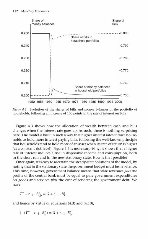
112 Monetary Economics

1950 1955 1960 1965 1970 1975 1980 1985 1990 1995 2000

0.800

0.790

0.780

0.770

0.760

0.750

0.250

0.240

0.230

0.220

0.210

0.200

Share ofmoney balances

Share ofbills

Share of bills inhousehold portfolios

Share of money balancesin household portfolios

Figure 4.3 Evolution of the shares of bills and money balances in the portfolio ofhouseholds, following an increase of 100 points in the rate of interest on bills

Figure 4.3 shows how the allocation of wealth between cash and billschanges when the interest rate goes up. As such, there is nothing surprisinghere. The model is built in such a way that higher interest rates induce house-holds to hold more interest paying bills, following the well-known principlethat households tend to hold more of an asset when its rate of return is higher(at a constant risk level). Figure 4.4 is more surprising: it shows that a higherrate of interest induces a rise in disposable income and consumption, bothin the short run and in the new stationary state. How is that possible?

Once again, it is easy to ascertain the steady-state solutions of the model, bynoting that in the stationary state the government budget must be in balance.This time, however, government balance means that state revenues plus theprofits of the central bank must be equal to pure government expenditureson goods and services plus the cost of servicing the government debt. Wehave:

T∗ + r−1 · B∗cb = G + r−1 · B∗

s

and hence by virtue of equations (4.3) and (4.10),

θ · (Y∗ + r−1 · B∗

h) = G + r−1 · B∗

h

Government Money with Portfolio Choice 113

1950 1955 1960 1965 1970 1975 1980 1985 1990 1995 2000

91.0

90.0

89.0

88.0

87.0

86.0

Consumption

Disposableincome

Figure 4.4 Evolution of disposable income and household consumption following anincrease of 100 points in the rate of interest on bills

Solving for the steady-state value of national income, we get:

Y∗ = G + r · B∗h · (1 − θ)

θ= GNT

θ(4.18)

where, as before, the asterisk indicates a long-run steady-state solution, andassuming that in the steady state r−1 = r. The term GNT stands for totalgovernment expenditures, including interest payments net of taxes.11 Theexpression GNT/θ is the fiscal stance, first introduced in Chapter 3, wheninterest payments on government debt are taken into consideration.

The steady-state solution for disposable income can likewise be obtained.Recall that in the stationary state households make no saving. This impliesthat consumption is equal to disposable income. In formal terms:

C∗ = YD∗ = Y∗ + r · B∗h − T∗ = Y∗ + r · B∗

h − θ · (Y∗ + r · B∗

h)

11 As far as we know, the addition of interest payments in the multiplicand was firstpointed out by Blinder and Solow (1973).

114 Monetary Economics

Substituting Y∗ by its value in equation (4.18), and with some manipulations,we obtain:

C∗ = YD∗ = (G + r · B∗

h) · (1 − θ)

θ(4.19)

Equations (4.18) and (4.19) have the counterintuitive property that in thefull stationary state, the aggregate income flow and the disposable incomeflow are an increasing function of the interest rate. This explains why, inFigure 4.4, the higher interest rate is associated with a higher steady-statenational income. As higher interest payments on government debt buildsup, disposable income rises and so do consumption and national income. Asdisposable income rises, this induces households to hold ever greater wealth,and hence a larger absolute amount of bills, provided the α3 ratio, redefinedbelow, does not drop. In addition, with higher interest rates, households areencouraged to hold a larger proportion of their wealth in the form of bills, aswe saw with Figure 4.3. All this leads to ever larger interest payments on debt.

It follows, in contrast to what most students of principles of economics aretaught, that higher interest rates generate more economic activity, not less,unless high interest rates have a detrimental impact on some components ofaggregate demand.

4.5.2 Fully developed steady-state solutions

Though interesting, the stationary solutions in (4.18) and (4.19) are notentirely satisfying because one of the components of the solutions, B∗

h isitself an endogenous variable. Thus, although we can presume, by intuitivereasoning, that an increase in the rate of interest will lead to an increase inthe amount of bills held by households, and hence to an increase in the over-all interest payments received by households, this still needs to be formallydemonstrated. In other words, we need to find the value of B∗

h in terms ofthe various parameters, and then substitute this value in equations (4.18) and(4.19) to get the fully-developed stationary solutions of Model PC.

This is not too hard a task, although it involves some tedious algebra. First,recall that we can turn the consumption function (4.5) into a wealth accumu-lation function. We pulled a similar trick with the consumption function (3.7)via equation (3.7A). Here, combining equations (4.4) and (4.5), we obtain thewealth accumulation function:

�V = α2 · (α3 · YD − V−1

)(4.20)

where α3 = (1 − α1)/α2.Once again, we know that in the stationary steady state (with no growth),

households accumulate no additional wealth, and hence �V = 0. Thus inthe stationary state, the target level of wealth is achieved, and wealth and

Government Money with Portfolio Choice 115

disposable income are in a constant ratio given by:

V∗YD∗ = α3 (4.21)

Combining equations (4.21) and (4.7) – the equation that defines theportfolio decision of the households – and after some manipulation, wethus have:

B∗h = {(λ0 + λ1 · r) · α3 − λ2} · YD∗ (4.22)

We may now replace in equation (4.19) the value of B∗h given by (4.22). Solv-

ing for YD∗, we obtain its fully determined solution in terms of the variousparameters and constants. We obtain:

YD∗ = G[θ

(1 − θ)

]− r · [(λ0 + λ1 · r) · α3 − λ2]

(4.23)

This can be reinterpreted in a slightly different way. Recall that the last termin square brackets is equal to:

[(λ0 + λ1 · r) · α3 − λ2] = α3 · B∗h

V∗Recall also that V is the total debt of the government sector, and that B∗

h isthe portion of the debt upon which the state has to pay a rate of interest r.It follows that r̆, where,

r̆ = r · B∗h

V∗is the average rate of interest payable on the overall amount of governmentliabilities.

With that interpretation, the steady-state disposable income may also berewritten as:

YD∗ = G[θ

(1 − θ)

]− α3 · r̆

(4.24)

Then, since in the steady state T∗ = G + r · B∗h, we have Y∗ = YD∗ + G, and

hence:

Y∗ = G · (1 − α3 · (1 − θ) · r̆)(θ − α3 · (1 − θ).)

(4.25)

Obviously, in the special case where r̆ = 0, we are back to the simple casedescribed by Model SIM and equation (3.15):

Y∗ = Gθ

(3.15)

116 Monetary Economics

Equation (4.25) can also be rewritten in a form that is reminiscent ofequation (3.15), and which highlights the fact that the steady-state levelof GDP depends on the fiscal stance, which, whatever the target wealth todisposable income ratio and the average rate of interest payable on the over-all amount of government liabilities, depends on the G/θ ratio. After somemanipulations, we get:

Y∗ =(

Gθ

) ⎧⎪⎪⎨⎪⎪⎩

1 + α3 · (1 − θ) · r̆(θ

(1 − θ)

)− α3 · r̆

⎫⎪⎪⎬⎪⎪⎭ (4.26)

4.6 Implications of changes in parameter valuesfor temporary and steady-state income

4.6.1 Some puzzling results

We can now see what are the implications of various changes in the valuesof the parameters. Some of these effects are intuitive, others are not. To startwith the former, obviously an increase in the permanent level of governmentexpenditures G will lead to an increase in the stationary level of income anddisposable income: dY∗/dG > 0. Similarly, any permanent decrease in theoverall tax rate θ leads to an increase in the stationary level of income anddisposable income: dY∗/dθ < 0.

On the other hand, an increase in the rate of interest r, or in the average rateof interest r̆ payable on the overall amount of government liabilities, leads toan increase in the steady-state level of disposable income (and income). Thiscan be seen by computing the derivative dY∗/dr > 0, from equation (4.23), orthe derivative dY∗/dr̆ > 0 from equation (4.24). What happens is that higherrates of interest on government debt increase the flow of payments that arisefrom the government sector, and this leads to more consumer spending onthe part of households. In addition, the higher rate of return on bills induceshouseholds to hold more interest-paying government debt. In the presentmodel, national income is the result of a multiplier effect over a multipli-cand. This multiplicand is government expenditures, and these include pureexpenditures on goods and services as well as the expenditures needed forservicing the debt.12 Because the multiplicand includes interest paymentson the debt, the puzzling positive long-run effect of higher interest rates on

12 This positive impact of higher interest rates on economic activity was noted inItaly during the 1980s. The effect noted in the model was noticeable in Italy, becauseits debt to GDP ratio exceeded 100% while the entire debt was being held by Italians.As a result, an increase in interest rates led to Italians being flooded with additionalinterest revenues arising from their government’s efforts to service the public debt.

Government Money with Portfolio Choice 117

national income still arises in more sophisticated models where interest ratesdo have strong negative short-run effects, as we shall see later in the chapterand in other chapters.

It should also be noted that an increase in the desire to hold bills, that is,an increase in the parameter λ0 of the portfolio equations, would increasethe proportion of government debt taking the form of bills, and hence itwould raise r̆, thus leading to an increase in the steady-state value of nationalincome. Thus, in this model, a reduction in liquidity preference leads to anincrease in national income.

There is another surprising feature of Model PC. We can see that anyincrease in the α3 parameter – the wealth to disposable income ratio – alsoeventually leads to an increase in stationary income or disposable income.For instance, from both equations (4.18) and (4.19), we obtain the derivativedY∗/dα3 > 0. Remember however that α3 is defined as: α3 = (1 − α1)/α2,where α1 and α2 are respectively the propensities to consume out of currentincome and out of accumulated wealth. The smaller these two propensitiesto consume, the larger the α3 parameter. Thus the smaller the propensities toconsume, the larger the steady-state levels of income and disposable income.In other words, if households are more thrifty – if they decide to save a largerproportion of their income and of their wealth – the steady-state income willbe higher.

Although this puzzling result is in line with what many mainstreameconomists would claim today, it contradicts the well-known paradox of thrift,that had been advanced by Keynes (1936) and emphasized over the last sixtyyears or so by Keynesians and post-Keynesians alike. Once again, the reasonfor which higher thrift leads to a higher stationary level of income is that alarger α3 parameter implies that households are aiming at a higher wealth tar-get, for a given income ratio. But a higher wealth target, all else being equal,implies larger interest payments on government debt held by households,and hence, ultimately, higher absolute consumption and income levels oncethe steady-state has been achieved.

4.6.2 A graphical analysis

The effects of an increase in the rate of interest have already been shown inFigures 4.3 and 4.4. The effect of an increase in the propensity to consumeout of disposable income (α1) are shown in the next two figures, built withthe help of model PCEX, under the assumption that expectations about cur-rent disposable income are based on actual disposable income in the previousperiod (equation 4.16A, YDe = YD−1). Recall that an increase in any of thepropensities to consume implies a decrease in the target wealth to disposableincome ratio. Figure 4.5 shows that the effect of a higher propensity to con-sume out of expected disposable income is positive in the short run, withGDP rising; however, in the long run GDP converges to a new steady-statevalue which is lower than the initial steady state.

118 Monetary Economics

1957 1961 1965 1969 1973 1977 1981 1985 1989 1993 1997 2001

120.0

117.0

114.0

111.0

108.0

105.0

National income (GDP)

Figure 4.5 Rise and fall of national income (GDP) following an increase in thepropensity to consume out of expected disposable income (α1)

Figure 4.6 helps us to understand this behaviour of national income. Thechart traces the evolution of household consumption, along with the twoarguments of the consumption function – expected disposable income andlagged wealth. National income first rises in the short run, because, for a givenamount of accumulated wealth, the increase in consumption expendituresout of current income leads to an increase in aggregate demand; howeverthis effect is only temporary. The lower propensity to save leads to a gradualreduction in the stock of wealth, as consumption exceeds disposable income.Eventually, the reduced consumption out of this shrinking wealth fully com-pensates for the higher consumption out of current income. Then, as wealthcontinues to drop, consumption keeps falling, along with the reduced inter-est income on government debt (the counterpart of household wealth), sothat, as shown with the derivatives of the steady-state solutions, nationalincome keeps falling – until it reaches a new stationary state the level ofwhich is ultimately lower than what existed in the previous steady state.

Readers may wonder why, with a higher propensity to consume, both thewealth of households and the debt of government decrease. Remember thatwe start from a situation where the economy is in a stationary state, whichimplies that the private sector is neither saving nor dissaving, while the gov-ernment budget is balanced, neither in deficit nor in surplus. As householdsdecide to consume more, targeting a lower wealth to disposable income ratio,this means that households are now dissaving, which explains why their

Government Money with Portfolio Choice 119

1957 1961 1965 1969 1973 1977 1981 1985 1989 1993 1997 2001

105.0

97.5

90.0

82.5

75.0

67.5

Consumption

Lagged wealth

Expecteddisposableincome

Figure 4.6 Evolution of consumption, expected disposable income and lagged wealth,following an increase in the propensity to consume out of expected disposableincome (α1)

wealth would be falling. In addition, as the households are spending more,there is a boost in economic activity, which generates more tax revenue forthe government; as a result, the government budget goes into a surplus whichallows the government sector to reduce its debt. Thus both household wealthand government debt decrease together, by exactly the same amount, as theymust (in this simplified model).

The short-run effects shown in the previous figures can also be illustratedusing a modified version of Figure 3.10 from Chapter 3. Figure 4.7 illustratesthe case of an increase in the rate of interest set by the central bank. Figure 4.7keeps the first two quadrants of Figure 3.10. The Y line illustrates the rela-tionship between disposable income YD, on the horizontal axis, and nationalincome Y on the vertical axis. The relationship is more complicated than itwas with Model SIM, because, beyond taxes, we must also take into accountinterest payments on debt. Given these, from equations (4.2) and (4.3), wemay write:

YD = Y(1 − θ) + r−1 · Bh−1(1 − θ)

Rearranging this equation, we obtain the relationship between nationalincome and disposable income that we need to equate production to

120 Monetary Economics

aggregate demand, arising out of disposable income and government expen-ditures. We have:

Y = −r−1 · Bh−1 + YD(1 − θ)

(4.27)

This is the line that arises from below the origin. Aggregate demand AD,as shown in the first quadrant of Figure 4.7, is the sum of consumptionexpenditures and government expenditures, and is given by equations (4.1)and (4.5). We may write it as:

YAD = α1 · YD + α2 · V−1 + G (4.28)

The short-run, or temporary, solution of Model PC is given at the intersectionof these two curves. In other words, the out-of-equilibrium level of disposableincome is given by the following difference equation, obtained by puttingtogether equations (4.27) and (4.28):

YD = (1 − θ) · (α2 · V−1 + r−1 · Bh−1 + G)

1 − α1 · (1 − θ)(4.29)

The same short-run, or temporary, solution, for aggregate income can beobtained from (4.27) and (4.29). We get another difference equation:

Y = G + α2 · V−1 + α1 · (1 − θ) · r−1 · Bh−11 − α1 · (1 − θ)

(4.30)

These equations show clearly that any increase in the rate of interest or in thepropensities to consume lead to a temporary increase in disposable incomeand national income. In Figure 4.7, the increase in the rate of interest is

YDV–1

V–1, VT

Y

r.B

V*

YD*

Y

45°

AD*Y*

G

2V–1+ G

2V–1

3YD = VT

1YD

α

α

α

α

Figure 4.7 Short-run effect of an increase in the interest rate

Government Money with Portfolio Choice 121

YD

V–1, VT

Y

VT

V–1

r.B

V*

YD*

Y

45°

AD*

Y*

G

2V–1+ G

2V–1

3YD = VT

1YDα α

α

α

Figure 4.8 Short-run effect of a fall in the propensity to consume

represented by a shift downwards of the Y curve, thus leading to a highertemporary national income and disposable income. Assuming we had startedfrom a stationary position, where accumulated wealth is the targeted levelof wealth, we can see in the bottom quadrant of the graph that the newtarget level of wealth is now higher than the level previously achieved. Thisimplies that within the period households will be saving, accumulating largeramounts of wealth and larger amounts of bills. As a result, in the next peri-ods, consumption will be rising and so will income, until the new, higher,stationary level of income is reached.13

A similar analysis is provided with Figure 4.8, in the case where the propen-sity to consume out of current income would fall, and hence when the targetwealth to income ratio would rise. The decrease in the propensity to consumeis illustrated by the downward rotations of the aggregate demand curve and ofthe target wealth curve. The figure shows that this reduction in the propen-sity to consume would initially lead to a fall in national income, but thatthis would be accompanied by a discrepancy between the new target level ofwealth and the current level of wealth, thus inducing households to accumu-late new wealth and hence purchase bills. The increase in interest paymentswould push down the Y curve, eventually pushing its point of intersectionwith the new AD curve beyond the initial stationary levels of income anddisposable income.

13 Similarly, a difference equation can also be obtained for wealth. Given equations(4.4) and (4.5), it turns out that: V = (1 − α2) · V−1 + (1 − α1)YD. Also, from equation(4.7), we can deduce Bh as a function of V and YD.

122 Monetary Economics

4.6.3 The puzzling impact of interest rates reconsidered

The purpose of this subsection is to reconsider the puzzling impact of interestrates on national income. We saw previously that higher interest rates have apositive impact both on the temporary and the steady-state values of nationalincome. Is this a necessary result? What if propensities to save were positivefunctions of the interest rate, as is often assumed in mainstream textbooks?

Let us suppose then that the propensity to save is not constant anymore,but rather assumes a value which depends negatively on the rate of intereston bills, with the Greek letter ι being the reaction parameter. Formally, thisimplies that:

α1 = α10 − ι · r−1 (4.31)

Since we know that α3 = (1−α1)/α2, this implies that a higher rate of interestwill generate a higher target wealth to income ratio. In other words, withequation (4.31) and a constant propensity to consume out of the openingstock of wealth, α2, it follows that:

α3 = (1 − α10 + ι · r−1)

α2(4.32)

With the addition of equation (4.31), an increase in the rate of interest r canonce more be simulated with Model PC (here PCEX2). This experiment isillustrated with the help of Figure 4.9. The initial impact of the increase ininterest rate on economic activity is negative, as central banks claim. Thereis a fall in consumption, disposable income and national income, as stan-dard short-run macro models would claim (based on some negative interestelasticity of investment). However, our model goes beyond flows and takesstocks into account. The reduction in the propensity to consume and hencethe associated increase in the target wealth to income ratio leads to a gradualincrease in the stock of wealth, through the partial wealth adjustment func-tion, as households now spend less than they earn. Figure 4.9 shows thatconsumption demand is lower than disposable income as long as householdwealth keeps increasing.

Figure 4.9 shows that, when comparing steady states, the aggregate incomeflow is still an increasing function of the interest rate, even though the short-run impact of higher interest rates is to reduce consumption and henceincome as we would expect. Thus, even when the temporary solutions aresubjected to the standard Keynesian effects, that is, when the paradox ofthrift is being observed in the short run, stationary income is an increasingfunction of the rate of interest. Of course, we already knew this from theobservation of equation (4.24), since the term α3 · r̆ which appears with anegative sign in the denominator, is now larger.

The increase in the wealth of households has, as a counterpart, an increasein the debt of government. Figure 4.10 shows why this is so. The short-run

123

1957 1961 1965 1969 1973 1977 1981 1985 1989 1993 1997 2001

120.0

112.5

105.0

97.5

90.0

82.5

National income (GDP)

Household wealth

Consumption

Disposableincome

Figure 4.9 Evolution of GDP, disposable income, consumption and wealth, followingan increase of 100 points in the rate of interest on bills, in Model PCEX2 where thepropensity to consume reacts negatively to higher interest rates

1957 1961 1965 1969 1973 1977 1981 1985 1989 1993 1997 2001

22.80

22.40

22.00

21.60

21.20

20.80

Tax revenues

Government expenditures plus net debt service

Figure 4.10 Evolution of tax revenues and government expenditures including netdebt servicing, following an increase of 100 points in the rate of interest on bills,in Model PCEX2 where the propensity to consume reacts negatively to higherinterest rates

124 Monetary Economics

recession caused by the negative impact of higher interest rates on consump-tion demand drives down government tax revenues. This negative effect onthe government budget position is reinforced by the brisk increase in overallgovernment expenditures, caused by the higher cost in debt servicing aris-ing from the higher interest rates. This immediately creates a governmentdeficit. This deficit gets shrunk gradually, while both government expendi-tures and taxes rise, until they reach a stationary level, at which point thegovernment budget is balanced. The deficit flow is eventually wiped out asa result of the rising consumption expenditures induced by rising house-hold wealth, as we saw in Figure 4.9. Our model thus shows clearly theshort-run perverse effects of higher interest rates on the government budgetposition.

4.7 A government target for the debt to income ratio

In the 1980s and 1990s, governments became concerned about the relativeamount of public debt which they had piled up in their attempt to save theircountries from the oil supply shocks and the slowdown of the economy. Therelative amount of public debt was usually measured as a ratio, the public debtto GDP ratio. In terms of our notation, this is measured by the expressionV/Y , where V is the wealth of households, which corresponds to the debtowed by government to the private sector, while Y is national income orGDP. Can governments do anything about this debt to income ratio in thelong run?14

First it should be pointed out the steady-state wealth to disposable incomeratio – the V/YD ratio – is determined by the behaviour of households. Asstated in equation (4.21), this wealth to disposable income ratio, which alsoturns out to be equal to the public debt to disposable income ratio, is preciselyequal to the α3 ratio which arises from the saving behaviour of households.It follows that governments can do nothing, in the present model, to modifythe public debt to disposable income ratio. If governments were to reducegovernment expenditures, in an attempt to produce a budgetary surplus andinduce a fall in the public debt to disposable income, they would be unsuc-cessful, since this would only lead to a reduction in income and disposableincome, but no change in the targeted ratio, unless the reduction in dispos-able income led households to reduce their saving propensities, and henceled them to reduce their targeted wealth to disposable income ratio.

Governments, and securities grading agencies, however, are not really con-cerned with public debt as a ratio of disposable income, but rather with public

14 A question put by Creel and Sterdyniak (1999: 138), among others.

Government Money with Portfolio Choice 125

debt as a ratio of GDP. Is it possible for governments to modify the steady-state level of the public debt to GDP ratio – the V/Y ratio – although theywould be hopeless in their attempts to modify the public debt to dispos-able income ratio? To answer this question, we can compute the steady-statepublic debt to GDP ratio. Making use of the property that in the stationarystate, Y∗ = YD∗ + G, and using equation (4.23), we obtain the steady-stateratio:

V∗Y∗ = α3

1 +[

θ

(1 − θ)

]− r · [(λ0 + λ1 · r) · α3 − λ2]

(4.33)

It follows that if households are targeting too high a wealth ratio, one thatis higher than the maximum debt to GDP ratio that government officialsjudge to be bearable, it is possible for government to reduce its stationarydebt to GDP ratio by acting on two parameters that are under its control.By inspection of equation (4.33), it can be easily seen that an increase inthe tax rate θ leads to a reduction in the stationary V∗/Y∗ ratio. Similarly,equation (4.33) also reveals that a reduction in the rate of interest on billswill lead to a reduction in the public debt to GDP ratio.15 This reductionwill even be achieved if the propensities to save of households react posi-tively to changes in interest rates, for an autonomous or induced reductionin the α3 coefficient – a proxy for an overall saving propensity – will alsoreduce the V∗/Y∗ ratio. In other words, equation (4.31) may apply. To sum-marize, government officials that would like to induce a reduction in thepublic debt to GDP ratio would need to increase tax rates or reduce interestrates. However both of these actions will lead to a reduced level of station-ary income. Thus if governments wish to sustain full-employment income,they have to disregard the debt to income ratio, which, as we saw, is essen-tially determined by the target wealth to disposable income ratio set by thehouseholds.

In the next chapter, more will be said about the dire consequences of gov-ernment obsession with public deficit reduction and the reduction of the sizeof the public sector, the effect of which has been to encourage reductions inpure government expenditures.

15 This can also be seen, in reverse gear, by inspecting Figure 4.9. The increase ininterest rates led to a large increase in household wealth, and hence net governmentdebt, while GDP decreased only later to rise slightly. As a result, one can say thatincreases in interest rates lead to an increase in the debt to GDP ratio.

126 Monetary Economics

Appendix 4.1: Equation list of Model PC

Y = C + G (4.1)

YD = Y − T + r−1 · Bh−1 (4.2)

T = θ · (Y + r−1 · Bh−1) θ < 1 (4.3)

V = V−1 + (YD − C) (4.4)

C = α1 · YD + α2 · V−1 0 < α2 < α1 < 1 (4.5)

Hh = V − Bh (4.6)

BhV

= λ0 + λ1 · r − λ2 ·(

YDV

)(4.7)

HhV

= (1 − λ0) − λ1 · r + λ2 ·(

YDV

)(4.6A)

�Bs = Bs − Bs−1 = (G + r−1 · Bs−1) − (T + r−1 · Bcb−1) (4.8)

�Hs = Hs − Hs−1 = �Bcb (4.9)

Bcb = Bs − Bh (4.10)

r = r (4.11)

The redundant, or hidden, equation is:

Hh = Hs (4.12)

Appendix 4.2: Equation list of Model PC

with expectations (PCEX)

Y = C + G (4.1)

YD = Y − T + r−1 · Bh−1 (4.2)

T = θ · (Y + r−1 · Bh−1) θ < 1 (4.3)

V = V−1 + (YD − C) (4.4)

C = α1 · YDe + α2 · V−1 (4.5E)

BdV e = λ0 + λ1 · r − λ2 ·

(YDe

V e

)(4.7E)

HdV e = (1 − λ0) − λ1 · r + λ2 ·

(YDe

V e

)(4.6E)

Hd = V e − Bd (4.13)

V e = V−1 + (YDe − C) (4.14)

Hh = V − Bh (4.6)

Government Money with Portfolio Choice 127

Bh = Bd (4.15)

�Bs = Bs − Bs−1 = (G + r−1 · Bs−1) − (T + r−1 · Bcb−1) (4.8)

�Hs = Hs − Hs−1 = �Bcb (4.9)

Bcb = Bs − Bh (4.10)

r = r (4.11)

YDe = YD · (1 + Ra) (4.16)

The redundant equation is still:

Hh = Hs (4.12)

Model PCEX1

Replace equation (4.16) with:

YDe = YD−1 (4.16A)

Model PCEX2

Transform the parameter α1 into a variable, and add to Model PCEX1:

α1 = α10 − ι · r−1 (4.31)

Appendix 4.3: Endogenous money

There is a school of thought that has long been arguing in favour of endogenousmoney. This line of thought goes back to the writings of Thomas Tooke and the BankingSchool, and has been present in the history of economic thought ever since. It can beassociated with the Swedish economist Knut Wicksell as well as several economists ofthe Austrian tradition, such as von Mises and Friedrich Hayek in the 1920s and 1930s.The endogenous money tradition was eclipsed for a long time by the Quantity theoryof money, which was defended by David Ricardo and the Currency School in the 1830s,and then later by the marginalists who needed an exogenous stock of money to makesense of their models. While Keynes and Keynesianism brought back momentarilythe idea that monetary policy was essentially based on an interest rate decision, theQuantity theory of money regained momentum with the arrival of Milton Friedmanand his ‘Monetarism’, who claimed that the central bank only needed to, and could,control the rate of growth of the money supply. The response of heterodox economiststo this far-fetched claim was that the money supply has no stable relationship withoutput or prices – the unstable velocity argument, and that, in any case, the moneysupply is endogenous – the so-called reverse-causation argument.

The equations presented here endorse the reverse-causation argument. It is arguedthat central banks cannot control the money supply directly. What central banks cando is set the rate of interest, and hope that high interest rates will slow down the

128 Monetary Economics

economy and abate inflation in the long run. This view of the monetary process, inparticular the reverse-causation argument, was put forward in very clear terms by theFrench economist Jacques Le Bourva (1992), in two articles published in 1959 and 1962.The well-known British economist Nicholas Kaldor (1964) first endorsed the unstablevelocity argument in his 1958 memorandum to the Radcliffe Committee, only to sup-port twelve years later the much more powerful reverse-causation argument (1970a),when it became clear that the views of Friedman and of monetarism were sweepingthe profession. In the 1970s and the 1980s, heterodox economists (post-Keynesianones in particular), were the only academic economists defending the view that cen-tral banks were essentially setting short-term interest rates, letting the supply of moneyfind its level determined by portfolio demand (Moore 1988). Only practitioners – someeconomists working at central banks such as Goodhart (1984) – seemed to realize thathigh powered money and money were endogenous variables, not under the directcontrol of the central bank.

For a long time mainstream textbooks have faithfully reflected the Quantity the-ory of money and its modern incarnation, Monetarism. Even today, this is still thecase. There is however a clear schizophrenia in the mainstream economics profession.On the one hand, textbook writers claim that monetary policy acts through changesin the money supply. On the other hand, all press releases relative to the actions ofcentral banks speak of rates of interest being set or targeted by the central bank. Thefinancial press is full of reports about the possible changes in rates of interest under thecontrol of the central bank. There is hardly ever any indication about the supply ofmoney or its rate of growth. In addition, the working papers issued by central banksto explain the procedures followed by central bankers very explicitly show that centralbanks set a ‘discount rate’ and a ‘deposit rate’ – which constitutes the interventionband. The same central bank papers show that the overnight rate – the one-day ratethat banks charge to each other – is usually right in the middle of that band.

Some mainstream economists are starting to recognize that fact, and build modelsthat explicitly rely on real interest targeting rather than money supply targeting (Romer2000). Indeed, such models are now part of what some call the New Consensus inmacroeconomics ( J.B. Taylor 2000; Meyer 2001). This change of mind among academiceconomists seems to have arisen out of the more transparent operating proceduresadopted by a number of central banks throughout the world, in particular in Australia,Canada, Sweden and the United States (Lavoie 2005; Fullwiler 2006). Whereas, at leastaccording to our view, central banks always operated monetary policy by relying onchanges in the short-term interest rates under their control, the interest rate targets arenow explicit and publicly announced at regular intervals. Many, perhaps most centralbanks, with the important exception of the European Central Bank, have completelyabandoned any reference to monetary targets. This is usually justified on the groundsthat money demand is too unstable for monetary targets, whatever they are, highpowered money or wider monetary aggregates, to be of any help. Although the moneysupply seems to play no useful role in these new consensus models, it is not yet clear,however, whether these mainstream authors clearly see the money supply as beingendogenous and demand determined. One could argue that New Consensus authorsperceive the money supply to be endogenous by default, whereas post-Keynesiansbelieve that the money supply is endogenous because it cannot be otherwise in awell-functioning monetary system.

Government Money with Portfolio Choice 129

Appendix 4.4: Alternative mainstream closures

An exogenous stock of moneyAn alternative way to close Model PC would be to consider the demand for securitiesby the central bank to be the exogenous policy variable, in which case the rate ofinterest becomes endogenous. This corresponds to what we believe to be a standardneo-classical closure, and it has been incorporated into Model PCNEO. This new closurecan be obtained from Model PC by first writing an additional equation:

Bcb = Bcb (A4.3.1)

By reason of equation (4.9), which says that �Hs = �Bcb, the above equation impliesthat the supply of cash money is also an exogenous variable. In other words, we have:

Hs = Bcb (A4.3.2)

The choice of equation (A4.3.1), instead of (4.11), should be taken to mean that thedemand for bills by households is forced to adjust to the exogenously determinedsupply of bills, net of the demand for bills by the central bank. This means that equation(4.10), is rewritten in the following way:

Bh = Bs − Bcb (A4.3.3)

There are now two equations, instead of one, that determine the holdings of bills byhouseholds (the other one is equation (4.7)). This implies the need for an equilibriumcondition. The net supply of bills and the demand by households are brought intoequivalence by a market clearing price – the rate of interest. The rate of interest thatclears the bill market is given by equation (4.7), which could be rewritten as r = r(Bh/V ,

19571961 1965 1969 1973 1977 1981 1985 1989 1993 1997 2001

0.0300

0.0290

0.0280

0.0270

0.0260

0.0250

Rate of interest on bills

Figure A4.1 Evolution of the rate of interest on bills, following a step decrease in theamount of Treasury bills held by the central bank (Model PCNEO)

130 Monetary Economics

YD/V , λ0, λ1, λ2 ). This market-clearing rate of interest r, determined at the end ofperiod t , is the rate that will be used to define the interest payments r · Bh received byhouseholds in period t + 1.

According to Walras’ Law, if the securities market clears so does the money market(or if the money market clears so does the securities market), so that equation (4.12)is still fulfilled: Hh = Hs. The difference with the post-Keynesian closure advocated inChapter 4, is that the money market clears thanks to a price-equilibrating mechanism,whereas no such equilibrating mechanism was required in the post-Keynesian closureof Model PC.

Figure A4.1 shows what happens when the central bank decides to reduce theamount of bills it is holding within such a setup. The interest rate briskly increasesin the period where the reduction occurs, so that households voluntarily take up thebills that the central bank does not want to hold any more. As the chart shows, there issome further adjustment down the line, since the higher interest rates generate slightlymore economic activity, thus requiring larger money balances for transaction purposes,balances that the central bank refuses to provide. As a result, there are some furtherincreases in the level of interest rates, until the stationary state is reached.

It should be pointed out however that in a model with expectations and additionalrealistic features, the introduction of a fixed money supply rule would create havoc inthe system, as interest rates would sharply rise or fall. An exogenous stock of moneyis not really an alternative.

An exogenous share of government deficitSome authors assume that the government, in cooperation with the monetary author-ities, decides that a fixed proportion of the government deficit is being financed byissuing cash money, while the rest gets financed by issuing bonds or bills. Tobin (1982a:182) makes such an assumption. He supposes that ‘the budget deficit in dollars … isfinanced in fraction γB by selling bonds … and in fraction γH by printing high-poweredmoney (γH + γB = 1)’ (Backus et al. 1980: 267). Such an assumption, which can alsobe found in Ott and Ott (1965), is just a variant of the previous assumption of anexogenous stock of money or bills. Here, for a given budget deficit, what is exogenousis the change in the stock of money. Clearly, this closure again requires endogenousrates of interest and is consistent with an exogenous money view.

This Backus et al. assumption is inconsistent with the post-Keynesian view of endoge-nous money. This must be pointed out, because some authors such as Moudud (1999:22–3) and Franke and Semmler (1991: 340) claim to be working within an endogenousmoney framework, whereas in reality they are not, since they are assuming that a pre-determined percentage of the government deficit is being financed by the issue of cashmoney. The same remark applies to Dalziel (2001: 104), who claims that ‘the govern-ment must decide what portion of the deficit will be funded by the central bank, andwhat portion will be funded by selling government securities to savers in the economy’,and who then assumes that a constant proportion m ‘is funded with central bank lia-bilities’.This assumption allows these authors to reintroduce the conventional notionof an excess supply of money, with its monetarist inflationary consequences.

5Long-term Bonds, Capital Gainsand Liquidity Preference

5.1 New features of Model LP

The definition of wealth in Model PC in Chapter 4 comprised only two assets,money and bills. In this chapter a third asset, long-term government bonds,is introduced and this will provide an opportunity to discuss the notion ofliquidity preference – hence the name Model LP – and also to introduce capitalgains and losses into the system of accounts. An important feature of the newmodel will be that an increase in long-term interest rates will have a short-runnegative effect on demand.

5.2 The value of a perpetuity

Long bonds are here defined as consols, also called perpetuities because theyare never redeemed. It is assumed that each consol is a piece of paper whichpays the owner one dollar after one period has elapsed, this one dollar pay-ment being the coupon of the perpetuity. If there are BL such pieces of paperin existence at the end of the previous period, it follows that the total flow ofinterest payments on these assets in the current period is simply BL−1, sinceeach piece of paper provides an interest revenue of one dollar. The value ofa bond is the piece of paper times its price (pbL) – that is, BL · pbL and thelong rate of interest rbL is simply the reciprocal of the bond price. To obtainthat answer formally, we can look at it the other way: how much would youpay for an asset that would guarantee a payment of one dollar, from nextperiod into eternity, if you discount these future payments at the rate rbL?Mathematically, we have:

pbL =∑ 1

(1 + rbL)t

where the sum is from period one to infinity, and where the price pbL is theprice at period zero. It turns out that the sum of this geometric series is simply

131

132 Monetary Economics

1/rbL, so that:

pbL =∑ 1

(1 + rbL)t= 1

rbL

or:

rbL = 1pbL

In common parlance, rbL is the long-term rate of interest, when the pricepbL has been determined by financial markets. But rbL, among financial mar-ket operators, is better known as the yield (to maturity) of long-term bonds.In our models, which use discrete time, bonds that give rise to an interestincome in the current period must have been owned and valued in the pre-vious period. For instance, in the geometric sum, the price of bonds pbL isthe price of bonds this period, given the interest payments of the future. Thisimplies that the rate of interest on long-term bonds that applies to the cur-rent period is given by the yield of the previous period, based on the pricepaid for bonds in the previous period.

That this relationship is the correct one can be verified by recalling thatthe interest income of the perpetuity is just one dollar, and hence that theoverall interest income on long-term bonds must be equal to the number oflong-term bonds at the end of the previous period, BL−1. As is the case forany asset, this overall interest income must be equal to the product of therate of interest times the value of the overall stock of long-term bonds, buthere both elements are computed at the end of the previous period. In otherwords, we must have the equality:

BL−1 = rbL−1 · pbL−1 · BL−1

This implies, once more, that: rbL−1 = 1/pbL−1. In other words, the long-termbond rate relevant to the present period is the bond yield rbL−1 of the previousperiod. This is symmetrical with the statement made in Chapter 4, accordingto which the rate of interest on bills r−1, determined at the end of the pre-vious period, was the rate of interest that determined the amount of interestpayments on bills r−1 · B−1 that was made in the current period.

5.3 The expected rate of return on long-term bonds

This long rate of interest is not the same thing as the rate of return on long-termbonds. In contrast to bills, the price of which was assumed to remain con-stant until it was redeemed, the price of a long-term bond can change. Theoverall rate of return thus consists of two components: the interest rev-enue, represented by the yield rbL−1; and the capital gain, represented by

Long-term Bonds, Capital Gains, Liquidity Preference 133

the change in the value of the bond between the last period and the currentperiod. The rate of return RrbL on a bond that was purchased (or owned) inthe previous period is thus equal to:

RrbL = rbL−1 + �pbLpbL−1

= 1pbL−1

+ �pbLpbL−1

= 1 + �pbLpbL−1

= 1 + pbL − pbL−1pbL−1

This rate of return can only be known at the end of the current period,when the current price of long-term bonds has settled to its final value.Whether the individual who bought the bond in the previous period decidesto sell or to keep the bond in the current period will not change the rate ofreturn. When the bond is sold, the capital gain is realized. When the bond iskept in the portfolio, the capital gain is only a ‘paper’ gain. The capital gainis not realized; it only accrues to the owner of the asset.

When households make their portfolio choice, three features matter. Firstfinancial investors are concerned with the price that the long-term bondfetches in the current period, for this defines the yield of the asset which willarise in the next period. Second, what also matters is the expected price of thebond in the next period, when it will be possible to sell the bond. These twoprices help define what we shall call the pure expected rate of return on bondspurchased or held in the current period. This pure expected rate of return onbonds purchased now is equal to:

PERrbL = 1 + pebL − pbL

pbL

or

PERrbL = rbL + (pebL − pbL)

pbL

where PERrbL is the rate of return which is expected on long-term bondspurchased this period at the price pbL, while pe

bL is the price of bonds that isexpected to arise by the end of the next period, an expectation which is madein the current period, as households make their portfolio decisions.

However there is an additional factor, a third factor, that plays a role in suchportfolio decisions. This third factor is the confidence with which house-holds hold their expectations about future bond prices. It is a measure ofthe degree of confidence of financial investors, or a measure of the weightthat household investors attribute to the validity of their expectations. In

134 Monetary Economics

other words, households may believe that bond prices will be pebL in the next

period, but they may attribute little weight or conviction to this belief. Weshall call χ (chi) this weight. It reflects the fact that although householdsexpect the future bond price pe

bL to be somewhat different from the presentprice pbL, their portfolio decisions will only partly reflect their belief in thisdiscrepancy. In standard terms, one could say that they assign a probability χ

that such a change in bond prices will actually occur. We shall call ERrbL theexpected rate of return that takes into account either such probabilities orthe conviction with which future bond price changes are being held. Hencewe have:

ERrbL = rbL + χ · (pebL − pbL)

pbL

In a world where there is a multiplicity of opinions, one could assume thatχ reflects the proportion of agents who believe a priori that bond prices willchange towards pe

bL, while (1 − χ) reflects the proportions of agents whobelieve a priori that bond prices will remain where they are at pbL. A posteriori,in a Bayesian world, agents should expect the price change to be χ ·(pe

bL−pbL).If agents expect no future change in the price of bonds, the expected rate

of return ERrbL on bonds is simply the current yield rbL on bonds. In generalthe expected rate of return on bonds, rather than the pure expected rateof return, will be the relevant concept when comparing the profitability ofvarious assets within portfolio choice.

5.4 Assessing capital gains algebraicallyand geometrically

The introduction of capital gains brings to the fore a distinction that we shallhave to make time and time again, with all sorts of assets the value of whichcan change while they are being held.

The value of the stock of bonds at the beginning of the period is given by thestock of bonds held at the end of the previous period, say pbL−1 ·BL−1, whilethe value of the stock of bonds held at the end of the current period is pbL ·BL.Hence the overall change in the value of the stock of bonds, that is, theincrease in the amount of wealth held in this form is given by: (pbL·BL−pbL−1·BL−1). This difference is made up of two components. Part of the increasein the value of wealth held in the form of bonds is due to the fact that morebonds have been purchased in the current period; this is described by thenumber of bonds which change hands times their price (that is, (�BL) · pbL).These will appear in the transactions flow matrix. But there will also be capitalgains or losses on existing holdings when the price of bonds changes, whichare described by (�pbL) · BL−1. This capital gain is equal to the change inprice times the opening number of bonds, to which no transaction between

Long-term Bonds, Capital Gains, Liquidity Preference 135

BL–1 ΔBL

ΔpbL

BL

pbL

pbL–1

Figure 5.1 The Ostergaard diagram

agents of different sectors corresponds. Hence capital gains are included inthe transactions matrix below as a memorandum item only.

It is worth stopping for a moment to demonstrate that changes in thevalue of stock variables are indeed made up in this way. The breakdown ofchanges in the value of stock variables is going to turn up again and again, andthe formula will greatly assist the understanding of some tiresome conceptswhich will simply have to be mastered at some stage, for example, stockappreciation and, more generally, inflation accounting.

The simplest proof is a geometrical one, as can be found in Figure 5.1,which we shall call the Ostergaard figure.1 The end-period value of a stockof bonds is given by the area of the large rectangle in bold, that is pbL · BL.The end-of-previous-period stock is given by the area of the small rectanglein bold, pbL−1 · BL−1; hence the change in the value of the stock is given bythe sum of the two remaining rectangles. Algebraically, we have:

�(pbL · BL) = (pbL · BL − pbL−1 · BL−1) = (�BL) · pbL + (�pbL) · BL−1

1 In 1987, one of us (WG) was berated by an undergraduate class at AalborgUniversity in Denmark for fudging the proof of this expression so he offered a bot-tle of whisky to anyone who could do it better. After less than 24 hours this geometricproof was produced by Jorgn Ostergaard who was, of course, appropriately rewarded.The proof, which has a straightforward three dimensional counterpart for use whenthere are two sources of capital gain (Godley 1999b: 18), has proved extraordinarilyuseful.

136 Monetary Economics

where the two terms on the right-hand side correspond to the two remainingrectangles of the Ostergaard figure. The first term on the right-hand sidedescribes transactions in bonds during the current period, while the seconddescribes the capital gain.

The above can also be proved algebraically. By definition, the differencebetween the new value of the stock of bonds and the old value that was heldis equal to:

(pbL · BL − pbL−1 · BL−1)

= (pbL−1 + �pbL) · (BL−1 + �BL) − (pbL−1 · BL−1)

= (pbL−1 · BL−1) + (�pbL) · BL−1 + (pbL−1 · �BL)

+ (�pbL · �BL) − (pbL−1 · BL−1)

= (pbL−1 · �BL) + (�pbL · �BL) + (�pbL) · BL−1

= (pbL−1 + �pbL) · �BL + (�pbL) · BL−1

= (�BL) · pbL + (�pbL) · BL−1

The algebraic and the geometric proofs have here been conducted in termsof bonds. But these proofs apply to any asset stock, tangible or financial,subject to appreciation or depreciation, and the breakdown will be used timeand time again.

5.5 Matrices with long-term bonds

To obtain the balance sheet of Model LP, shown in Table 5.1, the balance sheetmatrix of Model PC in Chapter 4 has been amended simply by including thevarious stocks of long-term bonds as an additional asset for the householdsector and as a liability for the government sector. We have assumed thatcentral banks do not deal in long-term bonds (to avoid being concerned withcapital losses).2

2 It has been assumed that the central bank does not hold long-term bonds, pre-sumably on the basis that central banks would dislike taking the risk of making capitallosses when interest rates rise; but this is a simplification, as central banks do havelong-term securities on the asset side of their balance sheet, although they generallydeny any attempt to influence long-term rates. For instance, in early 2005, nearly 75%of the domestic assets held by the Bank of Canada were bonds rather than bills, whilenearly half of the domestic securities held had maturity dates going over three years(data drawn from the Bank’s Weekly Financial Statistics).

Long-term Bonds, Capital Gains, Liquidity Preference 137

Table 5.1 Balance sheet of Model LP

Households Production Government Central bank �

Money +H −H 0Bills +Bh −B +Bcb 0Bonds +BL · pbL −BL · pbL 0Balance (net worth) −V +V 0 0

� 0 0 0 0

Similarly, to obtain Table 5.2 and the transactions-flow matrix of ModelLP, the flow matrix of Model PC is amended by including interest paymentson bonds to the household sector. Since each long-term bond pays a singledollar to its owner, the total amount of interest payments made on long-termbonds is exactly equal to BL−1 (= rbL−1 ·pbL−1 ·BL−1), as shown in Table 5.2.The rate of interest on bills is now called rb , to make sure it is distinguishablefrom the rate of interest on long-term bonds rbL. Finally, capital gains havebeen added to the current transactions matrix, but only as a memo item.The matrices of Model LP thus read as follows.

Table 5.3 below fully integrates the household sector’s flow accountswith its stock accounts, thus achieving full consistency between the twoaccounts.

5.6 Equations of Model LP

5.6.1 Regular income versus Haig–Simons income

The equations of Model LP are all to be found in Appendix 5.1. Equation (5.1)is the same as equation (4.1), which states that all goods and servicesdemanded are provided.

Y ≡ C + G (5.1)

The next two equations deal with household income and taxation.

YDr ≡ Y − T + rb−1 · Bh−1 + BLh−1 (5.2)

T = θ · (Y + rb−1 · Bh−1 + BLh−1) θ < 1 (5.3)

Equations (5.2) and (5.3) incorporate the fact that current disposable incomenow includes interest payments on both bills and long-term bonds. It shouldbe noted that capital gains have not been included within the definition ofdisposable income, but this of course is a matter of convention. Disposableincome YDr as defined here only incorporates the flow of regular income, and

138

Table 5.2 Transactions flow matrix of Model LP

Central bank

Households Production Government Current Capital �

Consumption −C +C 0Government expenditures +G −G 0Income = GDP +Y −Y 0Interest payments on bills +rb−1 · Bh−1 −rb−1 · B−1 +rb−1 · Bcb−1 0Interest payments on bonds +BL−1 −BL−1 0Central bank profits +rb−1 · Bcb−1 −rb−1 · Bcb−1 0Taxes −T +T 0

Change in money −�H +�H 0Change in bills −�Bh +�B −�Bcb 0Change in bonds −�BL · pbL +�BL · pbL 0

� 0 0 0 0 0 0Memo: Capital gains −�pbL · BL−1 +�pbL · BL−1 0

139

Table 5.3 Integration of household flow and stock accounts, within Model LP

Money Bills Bonds � assets

Initial assets (end of previous period) Hh−1 Bh−1 pbL−1 · BLh−1 V−1

Consumption −C 0Income = GDP +Y 0Interest payments on bills +rb−1 · Bh−1 0Interest payments on bonds +BLh−1 0Taxes −T 0

Change in money −�Hh +�Hh 0Change in bills −�Bh +�Bh 0Change in bonds −�BLh · pbL +�BLh · pbL 0

� 0 Hh Bh pbL−1 · BLh−1 + �BLh · pbL Hh + Bh + �BLh · pbL+pbL−1 · BLh−1

Capital gains +�pbL · BLh−1 +�pbL · BLh−1

Final assets (end of period) Hh Bh pbL · BLh V

140 Monetary Economics

this is why it carries the subscript r. To make it consistent with the conventionwe have adopted, capital gains have not been included in taxable incomeeither, as can be read from (5.3). Only income arising from business activityand the interest payments received from held assets are assumed to be taxed.It is indeed the case that, for reasons of convenience, capital gains are nottaxed in several countries, or they are taxed at a lower rate. Even in countrieswhere capital gains are taxed, they are usually taxed only if they have beenrealized, that is, if the asset which has benefitted from price appreciation hasbeen sold (a transaction has occurred). Here it is implicitly assumed that thecapital gains that have accrued in favour of the household sector have notbeen realized.

We now move to household wealth accumulation, as given by equation(5.4).

V = V−1 + (YDr − C) + CG (5.4)

with:

CG = �pbL · BLh−1 (5.5)

Equation (5.4) is an important equation reproducing the results exhibited inTable 5.3. It tells us that the increase in household wealth is equal to thedifference between regular disposable income and consumption, plus thecapital gains of households, as assessed in section 4 in the case of bonds andas assessed here in equation (5.5). Equation (5.4) generates an alternativedefinition of income, that of Haig (1921) and Simons (1938), who defineincome as consumption plus the change in wealth. This is a very crucialdefinition of income which we shall often use in models with capital gainsand price inflation. Denoting this Haig–Simons disposable income as YDhs,equation (5.4) can be rewritten as:

YDhs = �V + C = YDr + CG (5.4a)

This implies that the Haig–Simons definition of income is equal to regulardisposable income plus capital gains. Equation (5.4a) is not part of ModelLP – the Haig–Simons income plays no role in Model LP. But it is importantto understand the link between disposable income based on regular flowsand the Haig–Simons definition of income, which incorporates capital gains.

Equation (5.6), which describes the consumption function, again assumesthat consumption depends on expected (regular) disposable income and onpast accumulated wealth,

C = α1 · YDer + α2 · V−1 0 < α2 < α1 < 1 (5.6)

Long-term Bonds, Capital Gains, Liquidity Preference 141

But what about capital gains then? Here we implicitly assume that capitalgains in the current period have no impact on consumption. Capital gainsonly have an impact in the next period, since they then appear in the wealthaccumulated in previous periods. Thus, capital gains or losses feed into theconsumption function with a lag, via the term in wealth (V−1). This isnot the only way to incorporate capital gains into the consumption func-tion. They could have been included as part of disposable income or givena separate entrance all their own. Empirical research alone can determinethe appropriate specification. But empirical studies seem to show that onlylagged measures of capital gains have a significant impact on consumption(Baker 1997: 65), which justifies partially our treatment of capital gains inthe consumption function (equation 5.6).

Finally we introduce another equation, which is the exact equivalent inthe realm of expectations of equation (5.4). This latter equation describedthe evolution of realized wealth. Equation (5.7) below describes the expectedevolution of wealth. We have:

Ve = V−1 + (YDer − C) + CG (5.7)

The wealth that households expect to acquire by the end of the period, inexcess of their wealth of the previous period, is equal to the differencebetween expected regular disposable income and consumption expenditures,plus the capital gains of the current period.

5.6.2 Portfolio behaviour in matrix form

We now come to the equations defining the portfolio behaviour of house-holds. But before we deal with the behavioural equations, let us lay out twoidentities related to the stocks of assets held by households. Just as we definedtwo equations dealing with the realized and the expected accumulation ofwealth, we again write out two equations that define the various componentsof wealth – actual (at the end of the period) and expected (at the start of theperiod). We have:

Hh = V − Bh − pbL · BLh (5.8)

Hd = Ve − Bd − pbL · BLd (5.9)

Equation (5.8) says that household wealth at the end of the current period ismade up of the money balances Hh actually held by households, the bills Bhthey hold, and the value pbL ·BLh of the bonds that they have. Note that theseactual values carry the subscript h to indicate that they are indeed being heldby households at the end of the period. By contrast equation (5.9) outlinesthe various components of expected wealth, and carries subscripts ‘e’ or ‘d’.

142 Monetary Economics

Money balances, bills and the volume of bonds in equation (5.9) all carrythe subscript d for they represent the traditional meaning of the demandfor assets – the demand for assets at the beginning of the period, based onexpectations. These expectations are made up of the expected total amountof wealth Ve, as defined in equation (5.7).

The behavioural equations of the portfolio choice model, in line withthe model first proposed by Tobin (1969) are similar to those in Model PCexcept that they comprise three different assets, cash money, bills and long-term bonds. With so many assets, it becomes neater to present portfoliobehaviour in the form of matrix algebra, and the notations of the parame-ters, accompanied by plus signs only, reflect this possibility. In matrix form,equations (5.9A), (5.10), and (5.11) – which are found in their usual form inAppendix 5.1 – could be rewritten as:

⎡⎢⎢⎣

Hd

Bd

BLd · pbL

⎤⎥⎥⎦ =

⎡⎢⎢⎣

λ10

λ20

λ30

⎤⎥⎥⎦ Ve +

⎡⎢⎢⎣

λ11λ12λ13

λ21λ22λ23

λ31λ32λ33

⎤⎥⎥⎦

⎡⎢⎢⎣

0

rb

ERrbL

⎤⎥⎥⎦ Ve

+

⎡⎢⎢⎣

λ14

λ24

λ34

⎤⎥⎥⎦ YDe

r

Once again, households are assumed to hold a certain proportion λi0 of theirexpected wealth in the form of asset i but this proportion is modified by the(expected) rates of return on these assets and by the level of expected regulardisposable income. The reader may notice that one of the elements of therate of return vector has a 0 element in it. The zero corresponds to the rateof return on cash money. It reflects the fact that cash money H providesno interest payment, and as a consequence, the rate of return is zero.3 Aswith model SIM, when households make their portfolio decision, they areconcerned about rb, the rate of interest on bills to be determined at the endof the current period, but which will generate the interest payments in thefollowing period. We have further assumed that it is the expected rate ofreturn on bonds, ERrbL , rather than the yield on bonds, rbL, that enters intothe determination of portfolio choice. More will be said about this ERrbL ratea bit further. But in the meantime, we note that indeed portfolio decisionsof households are forward-looking.

3 If we were to take price inflation into account, the rate of return on cash would benegative and its absolute value would be approximately equal to the rate of inflation.See Chapter 10.

Long-term Bonds, Capital Gains, Liquidity Preference 143

As was the case before, we cannot keep all three of equations (5.9A), (5.10)and (5.11) as given in the above matrix form, otherwise we would run intoa problem of over-identification. Equation (5.9A) is thus replaced, in thecomputer model, by equation (5.9), which simply says that the share ofexpected wealth which households do not wish to have in bills and bondsmust be held in the form of cash money.

Before we examine the various parameters of the asset demand function,one problem must be dealt with right away. The asset demand functionsdetermine the value of money balances, bills and bonds that householdswould like to hold, given their expectations about income and end-of-periodwealth. Following Turnovsky (1977: 134), we assume, in contrast to Brainardand Tobin (1968), that households are able to achieve within the period theshares of assets that they desire, provided they make no forecasting mistakes.4

The intuitive assumption is that financial markets carry low transaction costs,and hence agents can quickly recover the asset distribution that they want.But what happens when their expectations turn out to be mistaken?

As in Chapter 4, we shall assume that any mistakes in expectations are fullyabsorbed by fluctuations in money balances. That this assumption seems tobe the best one, given the limitations of modelling, seems to be recognized byBackus et al. (1980: 288) when they write that ‘in the case of demand depositsand currency, which serve as buffers or “temporary abodes of purchasingpower”, the partial adjustment mechanism seems particularly inappropriate.’Hence, it is best to assume that any unexpected income flows into the moneybalances of households, as happens here. This is why the money balancesactually held by households at the end of the period, given by Hh, appear asa residual in equation (5.8). The implications of such an assumption is thathouseholds end up holding other assets on the scale that they expected. Thus:

Bh = Bd (5.12)

BLh = BLd (5.13)

5.6.3 The adding-up constraints of portfolio behaviour

As before the adding-up constraints, underlined by Tobin (1969), must hold.This implies the following five vertical conditions:

λ10 + λ20 + λ30 = 1 (ADUP.1)

4 Brainard and Tobin (1968) as well as Backus et al. (1980) focus their atten-tion on the dynamics of adjustment from an arbitrary distribution of assets to theone desired by agents. They are rather silent about the macroeconomic implicationsdeveloped here.

144 Monetary Economics

λ11 + λ21 + λ31 = 0 (ADUP.2)

λ12 + λ22 + λ32 = 0 (ADUP.3)

λ13 + λ23 + λ33 = 0 (ADUP.4)

λ14 + λ24 + λ34 = 0 (ADUP.5)

Equation (ADUP.1) simply says that the total of the shares of each asset mustsum to unity, whatever the actual values taken by the rates of return anddisposable income. Thus the sum of the exogenous components must sumto unity. The rule is that in a completely coherent system, people can onlyhave more of one thing by having less of another. The same rule applies tothe other vertical constraints. In reality, the λ parameters will be shiftingaround like mad, as people change opinions on what is appropriate, but theyare always subject to the adding-up constraints.

Given the first condition ADUP.1, the next three ADUP equations implythat the vertical sum of the coefficients in the rates of return matrix must bezero. These equations ensure that the sum over all assets of responses to achange in any of the rates of return is zero. Similarly, the ADUP.5 equationimplies that the response of assets in total to a change in disposable income iszero. These vertical conditions imply that if the change in one of the relevantvariables of the portfolio matrix induces an increase in the share devoted toone asset, the shares of the other two assets must decrease. The adding-uprequirements thus imply, of course, that some coefficients of the (3 × 3)

matrix above need to be negative. Indeed, here, only λ11, λ22, λ33 and λ14are positive.5 The first three positive coefficients imply that an increase in the‘own’ rate of return has a positive impact on the share of wealth held in thatform. For instance, a higher rate of interest on bills induces households tohold more bills, while a higher expected rate of return on bonds induces themto hold more bonds. Finally, greater disposable income push households tohold more cash money, by reason of the transactions demand for money.

There is another constraint which, surprisingly, is explicitly present nei-ther in Tobin (1969) nor in the following literature (as far as we know). Thisadditional constraint, which is proposed by Godley (1996: 18), is that thesum of all the coefficients on rates of return, reading horizontally, should alsosum to zero; more precisely, the coefficient on each positive ‘own’ rate ofreturn should equal the (negative of) the sum of all the other coefficients inthe row. The grounds for introducing this constraint are that the effect ondemand for the asset in question of an increase in the own rate of interest,

5 Here λ11 is an irrelevant parameter since the return on money is zero. But in amodel with deposit money instead of cash money, where deposit money would bringin interest income, the coefficient λ11 would also be positive.

Long-term Bonds, Capital Gains, Liquidity Preference 145

with all the other rates remaining constant, should not be any different fromthat of a fall, of the same size, in all the other rates, with the own rate stayingput. We thus have the following horizontal constraints:

λ11 = −(λ12 + λ13) (ADUP.6)

λ22 = −(λ21 + λ23) (ADUP.7)

λ33 = −(λ31 + λ32) (ADUP.8)

Some authors, such as Benjamin Friedman (1978) and Karacaoglu (1984),impose instead what they call symmetry constraints on the asset demandfunctions, in addition to Tobin’s vertical constraints. These symmetry con-ditions are of the kind λij = λji,for all i �= j. In our case, since the rate ofreturn on cash money is nought, only one of these symmetry constraintsremains: λ23 = λ32. This equality implies that an increase in the expectedrate of return on bonds will generate a drop in the holdings of bills that willbe of the same amplitude as the drop in the holdings of bonds generatedby a similar increase in the rate of interest on bills. In the general case of athree-asset portfolio choice, the symmetry conditions would imply that:

λ12 = λ21 (ADUP.9)

λ13 = λ31 (ADUP.10)

λ23 = λ32 (ADUP.11)

In such a three-asset model, starting from the above symmetry conditions,assigning a value to each of the above three equations (to the six parametersinvolved), and taking the vertical adding-up constraints into account, willinsure that the horizontal conditions are also respected. Thus, the authorswho add the symmetry conditions (ADUP.9 to ADUP.11) to the verticaladding-up conditions of the rate-of-return matrix (ADUP.2 to ADUP.4) implic-itly fulfil the requirements of the horizontal adding-up conditions (ADUP.6to ADUP.8).

On the other hand, incorporating the horizontal and the vertical adding-up conditions does not necessarily lead to the symmetric conditions. Withthree arbitrarily given parameters, and both the vertical and horizontal con-ditions, there is an infinity of possible sets of parameters, one of which is aset responding to the symmetric conditions. By contrast, starting with threearbitrary parameters, and either vertical or horizontal conditions associatedto the symmetry conditions, there is a single set of possible parameters. Mak-ing use of the symmetry conditions thus allows one to easily build up a setof rates of return parameters that are consistent with the horizontal and thevertical adding-up constraints.

146 Monetary Economics

As an instance take the following numerical values for the symmetricconditions:

λ12 = λ21 = −0.3

λ13 = λ31 = −0.2

λ23 = λ32 = −0.1

Making use in this case of the horizontal sum constraints, we obtain:

λ11 = −(λ12 + λ13) = (0.3 + 0.2) = 0.5

λ22 = −(λ21 + λ23) = (0.3 + 0.1) = 0.4

λ33 = −(λ31 + λ32) = (0.2 + 0.1) = 0.3

and hence the rate of return matrix would look like:

⎡⎢⎢⎣

0.5 −0.3 −0.2

−0.3 0.4 −0.1

−0.2 −0.1 0.3

⎤⎥⎥⎦

The reader can verify that both the horizontal (by construction) and thevertical adding-up conditions are fulfilled.

5.6.4 The closure of Model LP

We now present equations describing the behaviour of the central bank andthe government. Equation (5.14) is none other than the government budgetconstraint.

�Bs ≡ Bs − Bs−1 = (G + rb−1 · Bs−1 + BLs−1)

− (T + rb−1 · Bcb−1) − �BLs · pbL (5.14)

This constraint is expressed in terms of the additional Treasury bills that areissued within the period. The bills that need to be newly issued are equalto government expenditures, including its interest payments, minus the

Long-term Bonds, Capital Gains, Liquidity Preference 147

government revenues – taxes and central bank profits – plus the value ofthe newly issued long-term bonds. Needless to say, when there is a govern-ment surplus, or when the government deficit is financed by new issues oflong-term bonds, the change in Treasury bills will be negative and bills willbe redeemed.

�Hs ≡ Hs − Hs−1 = �Bcb (5.15)

Bcb = Bs − Bh (5.16)

BLs = BLh (5.17)

Equation (5.15) above reflects the capital account constraint of the centralbank. As pointed out earlier, we assume that central banks only purchasebills, and not bonds. The amount of cash money supplied by central banksis simply equal to the amount of bills purchased by the central bank. Inturn, as shown by equation (5.16), the amount of bills purchased by thecentral bank is equal to the difference between the outstanding amount ofbills supplied by government and the amount of bills that households endup holding. Finally, equation (5.17) says that the amount of bonds suppliedby government is equal to the amount of bonds demanded by households.These last two equations are thus saying that the (net) supply of bills and thesupply of bonds are provided passively, in response to demand.

One way to interpret equations (5.15)–(5.17) is to rely on the followingstory. Suppose that households do not want to hold so many bonds, eitherbecause of a change in their liquidity preference (the parameter λ30 goes upwhile parameter λ20 goes down), or because they expect a fall in the priceof bonds. Households will thus offer part of their holdings of bonds for sale.We can assume that the central bank purchases the offered bonds at thepreviously set price, and immediately turns around, asking the Treasury toredeem the bonds so obtained, exchanging them for new issues of bills of anequivalent amount. This story is compatible with equation (5.14), which saysthat the government issues new bills as a response to a government deficitand as a response to changes in the value of newly issued or newly retiredbonds. With this story, the quantity of bonds outstanding depends on thedemand for bonds, so that we do have BLs = BLh, while the central bank stillonly hold bills.

We now come to various definitions or relations which relate to variablesthat have been used in previous equations, but without our having definedwhat they were equal to. We start with the definitions that were explained atthe beginning of the chapter, in sections 5.2 and 5.3. Equation (5.18) definesthe expected rate of return on bonds, while equation (5.19) defines the yieldon bonds, as a function of the price that the bond carries at the end of the

148 Monetary Economics

current period.6

ERrbL = rbL + χ · (pebL − pbL)

pbL(5.18)

rbL = 1pbL

(5.19)

We need also to define some expected values. First, it should again be statedthat pe

bL represents the price of bonds which, with some given conviction χ ,is expected to occur in the future (in the next period, at time t+1). The expec-tation is entertained during the current period (at time t), and this is why itcarries no time subscript. Second, we could assume that expectations regard-ing the price of bonds in the next period is a given in the model, a parameterthat we do not try to explain, something that depends on a convention firmlyestablished among households, and which may not be moved or modifiedeasily by the monetary authorities. That would be equation (5.20A).

pebL = p̄e

bL (5.20A)

However, as a means of freezing the implications of bond price expectations,we shall initially assume that households expect the current bond price toremain the same in the next period. This implies the following equality:

pebL = pbL (5.20)

In general, if bond price expectations differ from current prices, expecta-tions regarding capital gains to be realized or accrued in the next period areassumed to be based on the calculations made in the current period to assessthe expected rate of return on bonds. The expected capital gains CGe arethus given by the χ weighted product of the expected change in bond prices(relative to the bond price of the current period) and the acquired numberof bonds. Naturally, if equation (5.20) rather than (5.20A) applies, expectedcapital gains or losses are nil, and equation (5.21) plays no role.

CGe = χ · (pebL − pbL) · BLh (5.21)

Finally, there remains the expected level of regular disposable income YDer .

One assumption we make, as in Chapter 4, is that expected regular incomeis simply the regular income of the previous period:

YDer = YDr−1 (5.22)

6 See Appendix 5.2 for some implications about the so-called liquidity trap.

Long-term Bonds, Capital Gains, Liquidity Preference 149

Another assumption we have made in simulations is that expectations aregoverned by a random process. Alternative assumptions will give yet otherresults, but it is a property of all these models that errors in expectationshave counterparts in end-period stock variables which will correct matters insucceeding periods.7

We now have 22 equations and 24 possible variables: Y , YDr, YDer , T , V ,

Ve, C, Hh, Hd, Bh, Bd, BLh, BLd, Hs, Bs, Bcb, BLs, pbL, pebL, CG, CGe, ERrbL, rbL

and rb. There are thus two equations that are needed to complete the model.The remaining two equations, equations (5.23) and (5.24) indicate that insuch a world, it is possible in this preliminary exposition for the governmentsector to fix both the rate of interest on bills and the rate of interest on bonds,the latter by fixing the price of government bonds (in the simulations, thebill rate and the price of bonds are treated as parameters).

rb = r̄b (5.23)

pbL = p̄bL (5.24)

The equivalence between the supply of cash and holdings of cash, that is,the equality Hs = Hh which arises from the balance sheet matrix of Table 5.1,will again be treated as the missing or redundant equation.

The assumption that both the short and the long rates of interest may be setexogenously contradicts the usual presumption that central banks or centralgovernments are only able to influence short-term rates, such as the Treasurybill rate, while long-term rates are necessarily market-determined. We seethat this need not be the case. It is possible under these assumptions forthe monetary authorities, here defined generally as the central bank plus theTreasury department, to fix both the short and the long rates, rb and rbL. Inother words, it is possible for the monetary authorities to set the yield curve.Indeed, for a long time, monetary authorities were keen in fixing both the billrate and the bond rate. This was particularly the case right after the SecondWorld War, when government debts were enormous, as a result of the hugewar effort that had produced large annual government deficits. It was thenimportant for rates of interest to be pegged at low rates, to avoid an excessive

7 Expectations in a discrete time model, by contrast to a continuous time model, canbe tricky. What we assume here is that there is a time sequence in household decisions.Households make their consumption decisions early on during the current period, ata time when they don’t know yet what their exact regular income for the period willbe, and when they don’t yet have information about the bond prices of the currentperiod. This is why they rely on the regular income of the previous period and on thewealth that they had accumulated at the end of the previous period. By contrast, whenhouseholds decide to allocate their wealth, we assume this is done towards the end ofthe current period, at which point they have proper information about the interestrates that they are being offered and the current bond prices.

150 Monetary Economics

amount of debt servicing. Because investors knew that the long-term interestrate was pegged, it could be set at very low levels, because investors did notfear capital losses.

In the United States, the Treasury-Fed Accord of 1951 freed the FederalReserve from its obligation to peg both short and long rates (Hetzel and Leach2001). Gradually, elsewhere in the world, monetary authorities renouncedintervention so as to fix the long-term rate of interest, letting it fluctuateaccording to the so-called market forces. Central banks kept a direct controlon short rates only – the Treasury bill rate initially, and then the inter-bankovernight rate (called the federal funds rate in the United States).

But the present model implies that it is quite possible for monetary author-ities to set both the short and the long rates, as the chairman of the Fed,Alan Greenspan, reminded us in 2003. All that is needed, as shown byequations (5.13) and (5.14), is for the central bank to purchase the Treasurybills left over by the households, at the set bill rate, while the Treasury supplieswhatever long-term bonds are demanded by households, matching demandwhatever it is at the bond price (and hence bond rate) set by the Treasury orthe monetary authorities. Things are made easier when the public accepts thenew bond price (equation 5.20 then applies), but we shall see later what hap-pens when the public holds on to its expectations about future bond prices(when equation 5.20A applies).

5.7 The short-run and long-run impact ofhigher interest rates on real demand

Suppose there is an unexpected increase in the interest rates set by the mone-tary authorities, taking all participants in financial markets by surprise. Thereis no difficulty in incorporating such an increase in the bill rate, but thingsare a bit more tricky with respect to bonds. We emphasized that the demandfor bonds depends on the expected rate of return. If financial participantsexpect a fall in the price of bonds, that is, they expect high rates of intereston bonds, this implies a low, possibly, a negative rate of return on existingbonds. Households, expecting such a low rate of return, would reduce thesize of their bond holdings. However, if the Treasury unexpectedly decides tolower the price of long-term bonds, thus increasing the long rate, then thereought to be an increase in the demand for bonds, since, as long as no furthernegative changes in bond prices are anticipated, the expected rate of return isnow higher, equal to the new rate of interest on long-term bonds. Indeed thisis precisely what will occur if equation (5.20) holds, that is, when pe

bL = pbLat all times.

Assume that this is what occurs, with the Treasury bill rate rising from 3%to 4%, while the new price of bonds is such that the long rate is hiked from 5%to 6.66% (the price of bonds drops from 20 to 15 dollars), with the expected

Long-term Bonds, Capital Gains, Liquidity Preference 151

rate of return on bonds rising by the same amount, due to the assumedexpectation that no further change in bond prices will be forthcoming.

The most important point of this experiment is that the fall in bondprices induces an immediate reduction in wealth. Interest rates have a bigeffect on asset prices and this is one of the main conduits for monetarypolicy – working in the conventional way. A rise in interest rates reducesdemand for a time – in Model LP this is achieved by a reduction in consump-tion expenditures, with a lag, through the reduction in the wealth term thatappears in the consumption function. And this puts the earlier unconven-tional result of Chapter 4 into a proper perspective. Model LP shows thatinterest rate increases do have a negative effect on real demand, but thisnegative effect is only a temporary one (which may still last for quite a longtime). In a longer period, the effect of higher interest rates is positive as wesaid before.

Once again, it is easy to ascertain the steady-state (implicit) solutions of themodel, by noting that in the stationary state the government budget mustbe in balance. Starting from equations (5.14) and (5.3), a balanced budgetimplies that:

(G + rb · B∗h + BL∗

s ) = T = θ · (Y + rb · B∗h + BL∗

h)

Therefore GDP in the stationary state is equal to:

Y∗ = {G + (rb · B∗h + BL∗

s ) · (1 − θ)}θ

= GNTθ

where, as in Chapter 4, GNT stands for total government expenditures,including all interest payments to households, net of taxes, and where GNT/θ

is the fiscal stance.The following figures, which should be considered together, illustrate what

happens. Figure 5.2 shows the effect on the wealth to disposable incomeratio. There is an extremely large initial reduction because the fall in theprices of long-term bonds has caused a huge capital loss for households. Thefall in this ratio is quickly made good because, one period later, as Figure 5.3shows, there is a large fall in disposable income (and GDP) – the result oflower consumption via the wealth effect. However, as with Model PC ofChapter 4, the long-run effect of increasing interest rates is to raise aggregateincome, despite the initial negative wealth effect. The steady-state incomelevel (GDP or household disposable income) is still a positive function of therates of interest, for reasons similar to those detailed in Chapter 4. Finally,

152 Monetary Economics

1950 1955 1960 1965 1970 1975 1980 1985 1990 1995 2000

0.980

1.000

0.960

0.940

0.920

0.900

Wealth to disposable income ratio

Figure 5.2 Evolution of the wealth to disposable income ratio, following an increasein both the short-term and long-term interest rates, with Model LP1

1950 1955 1960 1965 1970 1975 1980 1985 1990 1995 2000

99.0

100.5

97.5

96.0

94.5

93.0

Disposableincome

Consumption

Figure 5.3 Evolution of household consumption and disposable income, followingan increase in both the short-term and long-term interest rates, with Model LP1

Figure 5.4 shows how wealth is allocated between the two kinds of securi-ties. The share taken by long-term securities rises, since we assumed a moresubstantial increase in the yield on bonds, notwithstanding the capital losson the opening stock, so the government must be held to issue long-termsecurities on a potentially massive scale to match increased demand.

Long-term Bonds, Capital Gains, Liquidity Preference 153

1950 1955 1960 1965 1970 1975 1980 1985 1990 1995 2000

0.4040

0.4080

0.4000

0.3960

0.3920

0.3880

Bonds to wealth ratio

Bills to wealth ratio

Figure 5.4 Evolution of the bonds to wealth ratio and the bills to wealth ratio,following an increase from 3% to 4% in the short-term interest rate, while thelong-term interest rate moves from 5% to 6.67%, with Model LP1

5.8 The effect of household liquiditypreference on long rates

5.8.1 Targeted proportions of the liabilities of Government

The Treasury must issue or retire long bonds on a massive scale wheneverthere is a substantial change in the price of bonds targeted by the Treasury,or alternatively, when the public modifies its expectations about the futurelevel of bond prices. This may help to explain why, in the real world, long-term rates of interest tend to be under the control of market forces. Thepurpose of this section is to explain how the preferences or the expectationsof households could have an impact on the differential between the Treasurybill rate and the bond rate.

In the previous sections, with equation (5.20), it was assumed that house-holds never considered a change in the future price of bonds relative to thecurrent price. It is now time to give more leeway to household liquidity prefer-ence. Assume that the evolution of expectations regarding future bond pricesfollows the following rule:

�pebL = −βe(pe

bL−1 − pbL) + add (5.20B)

This difference equation insures that in the long run realized and expectedvalues are equal. The random element add gives a boost one way or another,

154 Monetary Economics

when we wish to introduce some independent change in liquidity preferenceon the part of households (meaning here a change in what householdsconsider future normal bond yields will be). The future bond price that isexpected by households may thus differ from the current bond price, eitherbecause the current price was modified by a decision of the government, orbecause households have modified their views with regard to the future.

We now introduce a mechanism that would explain how the liquidity pref-erence of the public could have an impact on the price of long-term bonds,even when the central bank is trying to set both the bill rate and the priceof bonds. The mechanism, one among many possible ones, is described withthe help of four equations, one that replaces a previous equation of ModelLP, and three new equations. We now assume that the price of bonds set bythe Treasury is not a constant anymore, so that we drop the last equation ofModel LP, equation (5.24), and replace it by the following equations:

pbL = (1 + z1 · β − z2 · β) · pbL−1 (5.24A)

z1 = 1 iff TP > top (5.25)

z2 = 1 iff TP < bot (5.26)

TP = BLh−1 · pbL−1BLh−1 · pbL−1 + Bh−1

(5.27)

The price of bonds depends on whether a certain target proportion, herecalled TP, is kept within its target range. The proportion in question is theratio of the value of long-term bonds outstanding to the total value of bondsand bills in the hands of households, as defined by equation (5.27). Whenthe targeted proportion exceeds the top of the range, called top, the Treasurylets bond prices float upwards. When the targeted proportion falls below thebottom of the range, called bot, the Treasury lets bond prices float downwards.

The logic behind this behaviour is the following. Although the monetaryauthorities passively provide households with the assets of their choice, at theinterest rates set by the monetary authorities or the Treasury, it is presumedthat the Treasury prefers to preserve the composition of its debt towards thegeneral public within a certain range, preferring not to have all of its eggs inthe same basket. The value of its long-term debt should not exceed a certaintarget value as a ratio of its total debt held by households; and similarly,the value of its short-term debt, as a percentage of its total debt vis-à-vis thehouseholds, should not exceed a certain percentage.

The reader may note a certain degree of similarity with the assumptionwhich is sometimes entertained in some macroeconomic models, where it is

Long-term Bonds, Capital Gains, Liquidity Preference 155

assumed that the government or the monetary authorities wish to restrainthe proportion of the government deficit that is financed by issuing money,as was recalled in Chapter 4. Here it is assumed that government wishesto restrain the proportion of its stock of debt which is financed by billsissued to the private sector. In both cases, interest rates (here long-termrates only) become endogenous, because the preferences of households maynot be consistent with the proportions set as a target by the governmentsector.

So what happens is the following. Suppose, for some reason, that the shareof the value of outstanding long-term bonds is exceeding the upper part ofthe range targeted by the monetary authorities, called top. Since this share isessentially demand determined, this implies that there is a high demand, byhouseholds, for such a kind of asset. The monetary authorities will respondby letting the prices of bonds drift upwards, thus moving along the linesdrawn by market forces. The Treasury is thus leaning with the wind. Whendemand is low and the share of long-term bonds is falling below the lowerpart of the range, below bot, the Treasury will respond by letting bond pricesdrift downwards.

We may conduct two different experiments. In the first experiment, assumethat the government decides to increase the bill rate, but this time withoutmodifying bond yields. This should lead to a fall in the demand for bondsand hence a fall in the TP ratio, the bonds to bills ratio. If the ratio falls belowthe bottom range, this will induce the central bank to let the price of bondsfall. This will drive up the bond yield rbL and generate temporary expectedcapital gains; these two effects in turn will induce households to hold morebonds, thus driving the economy back towards the target TP range. As aresult, in this model, a permanent one-shot increase in the bill rate generatesin the end a higher bond rate, as one would expect. There is a link betweenthe two interest rates. All this is shown in Figures 5.5 and 5.6 which illustratethe consequences of the initial increase in the bill rate.

As a second experiment, assume that household portfolio holders nowexpect a fall in the price of bonds, believing that a new, higher, long rate ofinterest ought to rule the economy. The random element of equation (5.20A)now kicks in. This change in the value of the expected price of bonds impliesthat long-term bond holders expect a capital loss. The expected rate of returnon bonds is thus lower than the yield on bonds. We have the inequal-ity: ERrbL < rbL. This implies, from equations (5.9A), (5.10) and (5.11), thathouseholds now desire to hold fewer bonds, and more bills and cash money.As long as we assume that the government and the central bank are imper-vious to any change in the composition of the debt, this would have noeffect whatsoever on the long-term rate of interest. However, in the modifiedmodel – Model LP2 – the change in the expectations of households, if largeenough, will have repercussions on the price of bonds and hence on the longinterest rate. With expectations of a fall in the price of bonds, less long-term

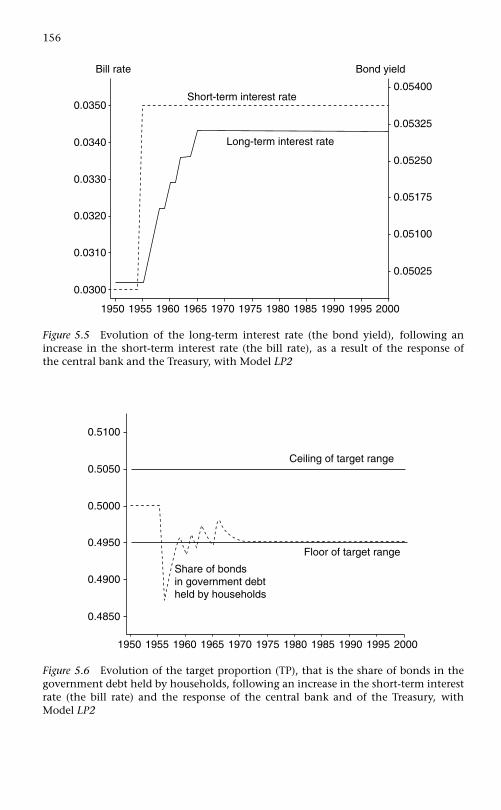
156

1950 1955 1960 1965 1970 1975 1980 1985 1990 1995 2000

0.0300

0.0340

0.0350

0.0330

0.0320

0.0310

0.05025

0.05325

0.05400

Bill rate Bond yield

Short-term interest rate

Long-term interest rate

0.05250

0.05175

0.05100

Figure 5.5 Evolution of the long-term interest rate (the bond yield), following anincrease in the short-term interest rate (the bill rate), as a result of the response ofthe central bank and the Treasury, with Model LP2

1950 1955 1960 1965 1970 1975 1980 1985 1990 1995 2000

0.5050

0.5100

0.5000

0.4950

0.4900

0.4850

Floor of target range

Ceiling of target range

Share of bondsin government debtheld by households

Figure 5.6 Evolution of the target proportion (TP), that is the share of bonds in thegovernment debt held by households, following an increase in the short-term interestrate (the bill rate) and the response of the central bank and of the Treasury, withModel LP2

Long-term Bonds, Capital Gains, Liquidity Preference 157

1950 1955 1960 1965 1970 1975 1980 1985 1990 1995 2000

0.05150

0.05200

Long-term interest rate

0.05100

0.05050

0.05000

0.04950

Figure 5.7 Evolution of the long-term interest rate, following an anticipated fall inthe price of bonds, as a consequence of the response of the central bank and of theTreasury, with Model LP2

bonds will be demanded by households, and if this change is large enough,the proportion TP of bonds to total securities held by households will fallbelow the bottom of the targeted range, inducing the Treasury to reduce theprice of bonds that it sets.

The reduction in the price of bonds will have two stabilizing effects thatwill take place in the next period. First, the fall in bond prices will lead to anincrease in the rate of interest on long-term bonds rbL as is well-known, and asillustrated with Figure 5.7. Second, since households adjust their expectationswith regard to future bond prices only gradually, the expected capital loss willhave been reduced by virtue of the decrease in the actual bond price. Thisis shown in Figure 5.8. As a result, in the next period, the expected rate ofreturn on long-term bonds will have risen, and the demand for bonds byhouseholds will pick up, eventually leading the proportion TP back inside itstarget range, as shown in Figure 5.9.

Figures 5.7 and 5.9 shows that market expectations may have an impacton realized financial outcomes, if the monetary authorities are swayed by thepressures exercised by market participants. It should be emphasized howeverthat this is a discretionary decision of the monetary authorities, based ona convention – the target range of long-term bonds as a proportion of thegovernment debt towards the public. Long-term interest rates react to mod-ifications in the liquidity preference of households because the monetaryauthorities and the Treasury wish to enforce the convention that they haveimposed upon themselves.

158

1950 1955 1960 1965 1970 1975 1980 1985 1990 1995 2000

20.25

21.00

19.50

18.75

18.00

17.25

Actual price of bonds

Expected price of bonds

Figure 5.8 Evolution of the expected and actual bond prices, following an anticipatedfall in the price of bonds, as a consequence of the response of the central bank and ofthe Treasury, with Model LP2

1950 1955 1960 1965 1970 1975 1980 1985 1990 1995 2000

0.500

0.520

0.480

0.460

0.440

0.420

Ceiling of target range

Floor of target range

Share of bonds ingovernment debtheld by households

Figure 5.9 Evolution of the target proportion (TP), that is the share of bonds in thegovernment debt held by households, following an anticipated fall in the price ofbonds, as a consequence of the response of the central bank and of the Treasury, withModel LP2

Long-term Bonds, Capital Gains, Liquidity Preference 159

5.8.2 Various explanations of the yield curve

The above exercise clearly shows that the liquidity preference of householdscan have an impact on real flows and the distribution of asset stocks. Withthe expanded model, Model LP2, we understand more easily why long-termbond rates may be left to the vagaries of the conventions used by privateagents: governments may have decided in advance the proportions of short-and long-term debt that they wish to be responsible for, and hence they willaccept to lean with the wind when these proportions threaten to get outof range.

The above model also shows that, as long as assets are not perfect substi-tutes, which is an assumption embedded in the Tobin portfolio model thatwe use here, there are relative asset supply effects. If the Treasury provides morelong-term securities, the long-term yield diminishes compared to the bill rate.In our model, it is possible for the monetary authorities and the Treasury tomodify the yield curve by changing relative asset supplies.8

Model LP thus potentially illustrates all possible explanations of the inter-est rate term structure, also called the time yield curve. On the one hand,there is the expectations theory, which says that long-term rates should reflectexpected future short-term rates. On the other hand, there is the marketsegmentation theory or the preferred habitat theory, which claim that agentshave strong preferences for some types of assets, for instance short-termassets, in which case these theories can also be associated with a liquidity pre-mium theory, which asserts that the yield curve is normally upward-sloping.In the case of the segmentation theory, because assets are far from being per-fect substitutes, ‘the shape of the yield curve will be affected by “local” supplyand demand conditions’ (Howells and O’Hara 1999: 555), as is the case here.

In our portfolio equations, as shown in their matrix form, the segmentationor liquidity theories are reflected by the presence of the λi0 vector of coeffi-cients, which indicates the proportions in which agents would like to holdthe various assets, regardless of their rates of return. By contrast, the λij matrixthat applies to the various rates of return reflects the impact of expectationsregarding future interest rates on asset demand functions. With the expecta-tions theory of the yield curve, if agents expect a string of higher short-terminterest rates on bills, they will be indifferent to purchasing bonds only iflong-term interest rates rise as well. On the basis of such a rise in long-termrates, they will expect falling bond prices, and hence agents will entertaina lower expected rate of return on bonds. This, as we have seen in the pre-vious simulation with our expanded Model (LP2), should indeed lead to asteeper yield curve. Hence the steeper yield curve could be explained by futureinterest rate expectations, or by a change in liquidity preference.

8 The extreme version of this model, whereby governments fix the supply of bonds,rather than the price of bonds, can be found in Appendix 5.3.

160 Monetary Economics

5.9 Making government expenditures endogenous

A key feature of all the models presented up to now is that pure governmentexpenditures G are assumed to be exogenous. In fact, this assumption isrequired for a determinate solution of the model to exist. Without exogenouspure government expenditures, there would be no multiplicand.

Still, there is no reason to believe that pure government expenditures areimpervious to what is going on in the rest of the economy. For instance, inan otherwise growing economy, one would believe that pure governmentexpenditures would also be growing. What we want to underline in thepresent context is the sensitivity of pure government expenditures to thebudget position of government. Previous experiments have shown, as onewould expect, that increased interest rates on long-term bonds initially leadto a fall in the value of long-term bonds and in the value of household wealth.The increase in interest payments on bills also leads, initially, to an increasein the budget deficit of government. This effect on public deficits is furtherreinforced, in the initial stages, by the negative effects that high interest rateshave on wealth. Because consumption depends on wealth, the large capitallosses induced by the higher interest rates induce a reduction in consump-tion and national income, and this in turn leads to falling tax revenues forthe government sector, and hence to even larger deficits.

These negative effects on the government budget are eventually reversed,because households gradually reconstruct their wealth through saving, sothat government revenues rise again, so much that in the new steady state,national income is now higher, due to the larger payments on the debt.But this result is achieved because it has been assumed all along that puregovernment expenditures were impervious to the apparition of large budgetdeficits.

But this may not necessarily be so. Atul Sood (1999) has shown that highreal interest rates lead to higher government deficits in the short-run, as mustobviously be the case, but he has also shown that these higher interest ratesoften lead to reduced primary deficits, that is to higher primary surpluses,which are defined as the difference between government tax income andpure government expenditures (T − G). In other words, at some point, whenthe deficit gets too large, governments aim at controlling public deficits, andto do so they reduce their pure government expenditures – the services thatthey offer on education, wealth, transport and so on.

Sood (1999) shows these results using the so-called Granger-causality anal-ysis. This econometric method attempts to assess causality from a temporalpoint of view. For instance, interest rates are said to ‘cause’ deficits if it canbe shown that past values of interest rates add some explanatory power tothe past values of deficits in explaining current deficit values. In that spe-cific meaning of causality, Sood shows that higher real interest rates ‘cause’larger overall deficits, more precisely higher deficit to GDP ratios, but then

Long-term Bonds, Capital Gains, Liquidity Preference 161

also ‘cause’ larger primary surpluses and larger primary surplus to GDP ratios,when governments decide to cut down on pure government expenditures inan effort to fight off the public deficits. Of course, such behaviour does notnecessarily occur in all countries, but Sood shows that it describes fairly wellthe evolution of the fiscal stance of major countries such as the United States,Canada, France and Germany, as well as that of a few less developed countriessuch as India, over the last thirty years of the twentieth century.

Such government behaviour can be easily modelled within the frame-work of Model LP – in LP3. This behaviour is described by equations (5.28)to (5.31).

PSBR = (G + rb−1 · Bs−1 + BLs−1) − (T + rb−1 · Bcb−1) (5.28)

z3 = 1 iff(

PSBR−1Y−1

)> 3% (5.29)

z4 = 1 iff(

PSBR−1Y−1

)< −3% (5.30)

G = G−1 − (z3 + z4) · βg · PSBR−1 + add2 (5.31)

It has been assumed that politicians are concerned with the deficit to GDPratio, here called PSBR/Y .9 When this ratio exceeds a certain threshold, thistriggers fiscal austerity, as governments reduce their pure government expen-ditures relative to the level achieved in the previous period. The reductionis assumed to be a certain fraction βg of the deficit incurred in the previ-ous period. In the current case, this occurs automatically when the ratioexceeds 3%, as suggested in various documents pertaining the Europeanunion, in particular in the Treaty of Maastricht. We also assume that there isa symmetric response when there is a large budget surplus.

All this could have been made more complicated. We could have assumedfor instance that government expenditures are also reduced whenever thegovernment has a large debt ratio, for instance 60%, once again as suggestedin the Maastricht Treaty, even when it is running modest deficits relative to

9 Since the deficits of governments involve the issue of assets, government deficitsare often known under the name of public sector borrowing requirement. From hencearises the acronym PSBR that is often used in discussions of public policy and that wehave also picked up to designate the size of government budget deficits.

162 Monetary Economics

the size of GDP.10 We could also have further assumed that governmentstrigger ever harsher austerity policies when both the debt and the deficitratios are being exceeded. Possibilities can quickly be multiplied with thesesorts of conditional reaction functions.

What is important to note is that the model so developed, Model LP3, isan instance of hysteresis. The model offers determinate steady-state solutionsonly as long as the austerity measures are not triggered. As soon as theseare triggered, pure government expenditures G, which in all the previousformalizations were the key multiplicand exogenous variable, also become anendogenous variable. As a result there is no determinate steady-state solutionto the model. The system does tend towards a long-run equilibrium, but thissteady-state solution is not independent of the path taken by the system.The steady state depends on the past history of the economic system understudy. It depends on the values taken by the various endogenous variables, inparticular the deficit to income ratio (and the debt to disposable income ratioif this ratio were to be taken into account). The model is now path-dependent.To find out the steady-state values to be taken by the various endogenousvariables, one needs to know the exact path taken by the economy. Sucha system, where the exogenous variables become in fact endogenous anddependent on the previous values taken by the main endogenous variables,is an instance of deep endogeneity. In such a case, the ‘evolution of a systemmay be best described, not by equilibria, but by “contemporaneous” valuesof variables, expressed in terms of their own past history’ (Setterfield 1993).

In previous formalizations of Model LP, the amplitude of the recessioninduced by a negative shock had no impact whatsoever on the final steady-state equilibrium. This stationary state only depended on the new rate ofinterest, the level of government expenditures, the tax rate, and various sav-ing and portfolio parameters. Eventually, the economy would get to this pre-defined new stationary state. For instance, as shown by Figure 5.10, decreasein the propensity to save has a negative short-run impact on gross domes-tic product, but eventually, as was discussed in great detail in Chapter 4,the larger amounts of government debt payments lead to higher householddisposable income and national income in the new stationary state.

With the present formalization, as described by equations (5.28) to (5.31),the amplitude and possibly the length of the recession might have an impact

10 Dealing with the debt of government is however more complicated than dealingwith its deficit since the recorded debt, based on historical accounts, will be differentfrom the value of debt, as measured here, since the latter depends on its market value,which will be different from its historically measured value whenever there have beenchanges in the prices of long-term bonds. Presumably, it is this historically measureddebt – the sum of past deficits – which is of concern to accountants, rating agenciesand government bureaucrats.

Long-term Bonds, Capital Gains, Liquidity Preference 163

1950 1955 1960 1965 1970 1975

Gross domestic product

1980 1985 1990 1995 200090.0

120.0

127.5

112.5

105.0

97.5

Figure 5.10 Evolution of national income (GDP), following a sharp decrease in thepropensity to consume out of current income, with Model LP1

1950 1955 1960 1965 1970 1975

Gross domestic product

1980 1985 1990 1995 2000

90.0

120.0

127.5

112.5

105.0

97.5

Figure 5.11 Evolution of national income (GDP), following a sharp decrease in thepropensity to consume out of current income, with Model LP3

on the final stationary state. If the recession induced by higher rates of interesttrigger large government deficits, relative to income, these deficits will inducethe politicians and bureaucrats to cut into government expenditures. As aresult, the new stationary state might turn out to be one with lower national

164 Monetary Economics

1950 1955 1960 1965 1970 1975 1980 1985 1990 1995 2000

16.50

19.50

20.25

18.75

18.00

17.25

0.000

0.040

0.050

0.030

0.020

0.010

Pure government expenditures (LHS)

Deficit to national income ratio (RHS)

G PSBR to Y ratio

Figure 5.12 Evolution of pure government expenditures and of the government deficitto national income ratio (the PSBR to GDP ratio), following a sharp decrease in thepropensity to consume out of current income, with Model LP3

income, rather than one with higher national income, as was the case withprevious formalizations of Models PC and LP.

This is illustrated with the help of Figures 5.11 and 5.12. Figure 5.11 showsthe evolution of national income. Gross domestic product falls into a reces-sion, but the recovery is insufficient to reach the initial steady state, or evento go beyond it, in contrast to the situation described by Figure 5.10. WithModel LP3, what happens is that the recovery is hindered by the austeritytriggered by the high deficit to income ratio (PSBR/Y). Figure 5.12 shows theevolution of the deficit to income ratio, and that of government expenditures(measured on a different scale). Government expenditures start to drop in theperiod that follows the exceedingly high deficit to income ratio, that is when-ever that ratio exceeds the 3% rate. The final equilibrium – the new steadystate – will thus depend on the reaction parameter of the government, and itwill depend on what governments consider to be an unacceptable deficit toGDP ratio. There is thus time-dependence. The new stationary state dependson what happens in the transitional states.

Standard Keynesian policy requires that governments increase their expen-ditures (or reduce tax rates) when the economy enters a recession, or evenbetter, whenever the economy threatens to slow down. This is Abba Lerner’sfunctional finance. While it is far from certain that governments followedthese principles even in the heyday of Keynesianism, in the 1980s severalgovernments (but not the American governments of Ronald Reagan and

Long-term Bonds, Capital Gains, Liquidity Preference 165

John W. Bush!) have reverted to the so-called Treasury view, that Keynesobjected so much to in the 1930s. When following the Treasury view, govern-ments reduce their pure expenditures when their tax revenues decrease, thusacting like most households would when their incomes drop. The advocatesof the Treasury view argued that governments ought to reduce their expendi-tures and the fiscal deficit in a slowdown because by doing so, the governmentwould provide room for the private sector, allowing the private sector to col-lect the funds and the saving necessary for its investment expenditures – sothat it does not crowd-out the private sector. In the models presented up tonow, there is no private sector investment, so this kind of argument cannotreally be debated. However, we have seen that it is possible for the centralbank to set the interest rate of its choice, whatever the budgetary position ofgovernment. The rate of interest on bills or bonds can be made independentof the deficit or the debt ratios. In other words, in our models, the rate ofinterest is not determined by debt or deficit ratios; rather, changes in inter-est rates will have an impact on the evolution of government deficits andgovernment debt.

Appendix 5.1: Equations of Model LP

Y ≡ C + G (5.1)

YDr ≡ Y − T + rb−1 · Bh−1 + BLh−1 (5.2)

T = θ · (Y + rb−1 · Bh−1 + BLh−1) θ < 1 (5.3)

V ≡ V−1 + (YDr − C) + CG (5.4)

CG = �pbL · BLh−1 (5.5)

C = α1 · YDer + α2 · V−1 0 < α2 < α1 < 1 (5.6)

Ve ≡ V−1 + (YDer − C) + CG (5.7)

Hh = V − Bh − pbL · BLh (5.8)

Hd = Ve − Bd − pbL · BLd (5.9)

HdVe = λ10 + λ12 · rb + λ13 · ERrbL + λ14 ·

(YDe

rVe

)(5.9A)

BdVe = λ20 + λ22 · rb + λ23 · ERrbL + λ24 ·

(YDe

rVe

)(5.10)

166 Monetary Economics

BLd · pbLVe = λ30 + λ32 · rb + λ33 · ERrbL + λ34 ·

(YDe

rVe

)(5.11)

Bh = Bd (5.12)

BLh = BLd (5.13)

�Bs ≡ Bs − Bs−1 ≡ (G + rb−1 · Bs−1 + BLs−1) − (T + rb−1 · Bcb−1)

− �BLs · pbL (5.14)

�Hs ≡ Hs − Hs−1 ≡ �Bcb (5.15)

Bcb = Bs − Bh (5.16)

BLs = BLh (5.17)

ERrbL = rbL + χ · (pebL − pbL)

pbL(5.18)

rbL = 1pbL

(5.19)

pebL = pbL (5.20)

CGe = χ · (pebL − pbL) · BLh (5.21)

YDer = YDr−1 (5.22)

rb = r̄b (5.23)

pbL = p̄bL (5.24)

Hidden equation: Hs = Hh

Expanded Model LP2:

�pebL = −βe · (pe

bL−1 − pbL) + add (5.20b)

pbL = (1 + z1 · β − z2 · β) · pbL−1 + add1 (5.24A)

z1 = 1 iff TP > top (5.25)

z2 = 1 iff TP < bot (5.26)

TP = BLh−1 · pbL−1(BLh−1 · pbL−1 + Bh−1)

(5.27)

Long-term Bonds, Capital Gains, Liquidity Preference 167

Expanded Model LP3:

PSBR = (G + rb · Bs−1 + BLs−1) − (T + rb · Bcb−1) (5.28)

z3 = 1 iff(

PSBR−1Y−1

)> 3% (5.29)

z4 = 1 iff(

PSBR−1Y−1

)< −3% (5.30)

G = G−1 − (z3 + z4) · βg · PSBR−1 + add2 (5.31)

Appendix 5.2: The liquidity trap

We first assume that it is possible for the monetary authorities to set any interestrate on long-term bonds although we have already identified possible qualificationto this hypothesis: what if the Treasury is targeting a certain range with regard to theproportion of its debt that ought to be held in the form bills by the general public? Wehave seen that if households entertain expectations about the price of bonds which aredifferent from the actual price, this will imply possibly massive switches of holdingsbetween bonds and bills, thus inducing the monetary authorities to change bond pricesin the direction expected by households.

It should also be pointed out that, when long-term interest rates are low, massivetransfers from bonds to bills are more likely. The reason for this is that a very smalldifferential between the expected rate and the current rate, when the current rate islow, is bound to engineer large capital losses for those holding bonds, and hence leadto a large negative expected rate of return on long-term bonds. This can be seen quiteeasily. Recall that the holder of a perpetuity is to receive one dollar of interest revenueat the end of the following year. What change in bond prices would be sufficient for theexpected capital loss to wipe out the actual interest revenue? Obviously, the requiredchange in bond prices is just one dollar. If the actual bond price is $25, a fall in theexpected bond price to $24 will do the trick; and similarly, an expected bond price of$9 when the actual price is 10$ will also bring the expected rate of return down to zero.The implications for the expected change in the long-term rate of interest are quitedifferent in both cases, however. With a $25 bond price, the long-term rate is 4%, andthe required change is 16.6 percentage points, or an expected interest rate of 4.166%;when the bond price is $10, the long-term rate is 10%, and the required change in thelong-term rate is 111 percentage points, or an expected long-term rate of 11.11%. Thisis the so-called squares law that Keynes (1936: 202, 207) associated with the possibilityof a liquidity trap in the case of long-term assets.

At low long-term rates of interest, a small variation in the expected future rate willcause a substantial drop in the expected rate of return on long-term securities, andhence massive transfers from bonds to bill holdings by households. If the monetaryauthorities wish to peg low long-term rates, they must be willing to absorb these mas-sive transfers. At higher rates of interest, the effects of a similar variation in expectedfuture rates will have much a minor impact on the expected rate of return and onportfolio allocation. Thus it will be much more difficult for the monetary authoritiesto peg low long-term interest rates compared to high long-term rates. The cause of

168 Monetary Economics

this is not the low yield, but rather the fear of a substantial capital loss that a smallvariation in the actual long-term rate could impose (Kregel 1985: 136).

Keynes’s squares law can easily be shown. Start with the definition of the relationshipof the yield of a bond (call it simply r) and its price:

r = 1pbL

(5.19)

and recall the definition of the expected rate of return on long-term bonds:

ERrbL = r + (pebL − pbL)

pbL(5.18)

From these two equations we obtain:

ERrbL = r +(

1re − 1

r

)· r = [r · re + (r − re)]

re

where re is the long rate expected to be realized in the next period.What we now want to know is the size of the expected change in long-term interest

rates which is sufficient to bring the expected rate of return down to zero. Setting tozero the above equation, we obtain:

(r − re) = −r · re

or

re = r(1 − r)

And since,

re = r + �re

we obtain:

�re = r2

(1 − r)

The expected change in the long-term interest rate which is required to create a cap-ital loss that wipes out interest income from a perpetuity is roughly equal to the squareof the current long-term interest rate. This justifies the two examples given above.

Appendix 5.3: An alternative, more orthodox,depiction of the bond market

As was pointed out in the main text, while it is possible for governments and monetaryauthorities to control both the short rates and the long rates of interest, control overlong rates has been relinquished by most central banks in the 1950s. It is quite possibleto set forth a model of the economy where central banks set the bill rate, while theylet market forces determine the price of long-term bonds. What we need to assume isthat the supply of bonds is a given, rather than assume, as was done in Model LP, that

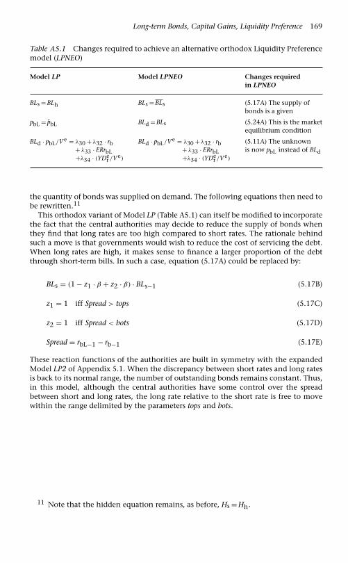
Long-term Bonds, Capital Gains, Liquidity Preference 169

Table A5.1 Changes required to achieve an alternative orthodox Liquidity Preferencemodel (LPNEO)

Model LP Model LPNEO Changes requiredin LPNEO

BLs = BLh BLs = BLs (5.17A) The supply ofbonds is a given

pbL = p̄bL BLd = BLs (5.24A) This is the marketequilibrium condition

BLd · pbL/Ve = λ30 + λ32 · rb BLd · pbL/Ve = λ30 + λ32 · rb (5.11A) The unknown+ λ33 · ERrbL + λ33 · ERrbL is now pbL instead of BLd+λ34 · (YDe

r /Ve) +λ34 · (YDer /Ve)

the quantity of bonds was supplied on demand. The following equations then need tobe rewritten.11

This orthodox variant of Model LP (Table A5.1) can itself be modified to incorporatethe fact that the central authorities may decide to reduce the supply of bonds whenthey find that long rates are too high compared to short rates. The rationale behindsuch a move is that governments would wish to reduce the cost of servicing the debt.When long rates are high, it makes sense to finance a larger proportion of the debtthrough short-term bills. In such a case, equation (5.17A) could be replaced by:

BLs = (1 − z1 · β + z2 · β) · BLs−1 (5.17B)

z1 = 1 iff Spread > tops (5.17C)

z2 = 1 iff Spread < bots (5.17D)

Spread = rbL−1 − rb−1 (5.17E)

These reaction functions of the authorities are built in symmetry with the expandedModel LP2 of Appendix 5.1. When the discrepancy between short rates and long ratesis back to its normal range, the number of outstanding bonds remains constant. Thus,in this model, although the central authorities have some control over the spreadbetween short and long rates, the long rate relative to the short rate is free to movewithin the range delimited by the parameters tops and bots.

11 Note that the hidden equation remains, as before, Hs = Hh.

6Introducing the Open Economy

6.1 A coherent framework

This chapter extends the closed economy framework developed in previ-ous chapters to describe two economies which trade merchandise with oneanother. Our methodology differs from the usual textbook approach, accord-ing to which models of individual closed economies are eventually ‘opened’,but which give no consideration to what other countries must be held tobe doing and how a full set of interactions between all countries might becharacterized. The excuse is that the open economy under study is presumedto be small compared to the rest of the world, so that the feedback effectscan be assumed to negligible. But then not much can be said about theUS economy, the size of which surely guarantees large feedback effects onthe rest of the world, nor about the European community or the block ofAsian countries including Japan. This partial equilibrium approach is themore surprising because international trade theory is usually treated withina relatively sophisticated two-country and two-good framework. We shalldiscuss open economy macro-economics using models of an economic sys-tem which, taken as a whole, is closed, with all flows and all stocks fullyaccounted for wherever they arise.1

One devastating feature of one-country-open-macro is that in the arrayof asset demand functions, which will be developed later in this book, thedemand for overseas assets must be treated net; yet net overseas assets maymove from positive to negative, making it impossible to construct a sen-sible array of asset demand functions. What is required, here again, is a

1 This method is put forward in particular in Godley (1999b). It was first adumbratedin Tobin and De Macedo (1980), and later developed in Allen and Kenen (1980), Kenen(1985), and Branson and Henderson (1985), although all of this work, in our view,falls short of solving a dynamic model which evolves through time with multiplefeedbacks.

170

Introducing the Open Economy 171

Table 6.1 Balance sheet of two-region economy (Model REG)

North South Centralhouseholds households Government bank �

Cash money +HNh +HS

h −H 0

Bills +BNh +BS

h −B +Bcb 0

Wealth (balancing item) −VNh −VS

h −Vg 0 0

� 0 0 0 0 0

systemic approach, methodologically identical with the closed economymodels already presented.2

Our open-economy models will evolve organically in stages from modelPC in Chapter 4. We start off with the very same (closed) economy describedby model PC, and then imagine how the economies of two componentregions, which together make up the total, interact with one another andwith the government. This will be Model REG. In subsequent sections we dealwith a two-country system, each with its own currency. This will be ModelOPEN.

6.2 The matrices of a two-region economy

We introduce open-economy macroeconomics by splitting a closed economyinto two parts, the ‘North’ and the ‘South’ but retaining a single government,a single fiscal and monetary system and (of course) a single currency. Theeconomy described here is the very same economy as in Model PC; we justdisaggregate it into two regions, which will be differentiated by adding theS superscript sign to symbols describing one (the ‘South’) and N to describethe other (the ‘North’).

Table 6.1 shows the balance sheet of this two-region economy. Table 6.1is no different from Table 4.1, except that households have been subdividedinto two groups, the households living in the North and those in the South.Vg represents the net wealth of the federal government and it takes on anegative value, since the government has no asset and only a liability, repre-sented by B. As a consequence Vg describes total net wealth acquired by thehouseholds of both regions.

2 See also Gray and Gray (1988–89: 241) for the advantages of adopting a flow-of-funds matrix for the world, thus identifying the ‘constraints and interdependencieswhich must characterize the international financial system’ and transforming ‘balance-of-payments analysis from a partial to a general framework’.

172

Table 6.2 Transactions-flow matrix of two-region economy (Model REG)

North North South South Centralhouseholds production households production Government bank �

Consumption −CN +CN −CS +CS 0

Govt. exp. +GN +GS −G 0

North Exports to South +XN −IMS 0

South Exports to North −IMN +XS 0

GDP +YN −YN +YS −YS 0

Interest payments +r−1 · BNh−1 +r−1 · BS

h−1 −r−1B−1 +r−1 · Bcb−1 0

Profits of central bank +r−1 · Bcb−1 −r−1 · Bcb−1 0

Taxes −TN −TS +T 0

Change in cash −�HNh −�HS

h +�H 0

Change in bills −�BNh −�BS

h +�B −�Bcb 0

� 0 0 0 0 0 0 0

Introducing the Open Economy 173

Table 6.2 shows the transactions-flow matrix of our two-region economy.There are two main changes compared to the single-region economy ofTable 4.2. First, as was the case with the balance sheet, households and pro-duction firms are subdivided into two groups. Second, there are two newrows in the matrix which represent the exports that each region expeditesto the other. As with all other rows, each of these two rows must sum tozero, and here they do by definition. The addition of the export and importentries does not modify the all-important principle that all columns of thetransactions-flow matrix must sum to zero.3

Exports from the North are denoted as XN. From the point of view of theimporting region, these exports are denoted as IMS, since they are the importsinto the South. Thus, by definition, XN = IMS, and this explains why therow ‘North exports to the South’ must sum to zero. Similarly, the exports ofthe South are the imports of the North, and hence we have XS = IMN, whichexplains why the next row also sums to zero.

There is another delicate accounting point that should be mentioned. InTable 6.2, imports (into the North, say), only appear in the column of pro-ducing firms, and not in the column of the household sector. It seems, then,that only firms import goods from the other region, while households inthe North only consume goods produced by firms located in the North. Inother words, it would seem that imports are only made up of intermedi-ate goods, while households do not directly consume imported goods. Nowthis would be a rather bizarre assumption for we know that consumers dopurchase imported goods. Another interpretation of Table 6.2 is possible.Remembering that most goods are purchased in shops, one can say that allimported goods transit through firms of the North, which act as intermedi-aries, purchasing these goods from the firms of the South, and then sellingthem to the Northern household consumers.

6.3 The equations of a two-region economy

It turns out to be surprisingly easy to adapt Model PC from Chapter 4 todescribe the behaviour of the two-region system which constitutes ModelREG. The equations can all be found in Appendix 6.1.

The first two equations define national income in an open economy,as the transactions matrix shows. Equation (6.1) defines national incomein the North. It equals consumption and government expenditures, plusnet exports, that is, the exports of the North to the South minus theimports of the North from the South, where X and IM stand for exports andimports. Exports are part of production and income, whereas imports are

3 To save space, the current and the capital accounts of the central bank have beenamalgamated.

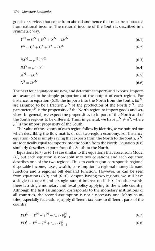
174 Monetary Economics

goods or services that come from abroad and hence that must be subtractedfrom national income. The national income of the South is described in asymmetric way.

YN = CN + GN + XN − IMN (6.1)

YS = CS + GS + XS − IMS (6.2)

IMN = μN · YN (6.3)

IMS = μS · YS (6.4)

XN = IMS (6.5)

XS = IMN (6.6)

The next four equations are new, and determine imports and exports. Importsare assumed to be simple proportions of the output of each region. Forinstance, in equation (6.3), the imports into the North from the South, IMN,are assumed to be a fraction μN of the production of the North YN. Theparameter μN is the propensity of the North region to import goods and ser-vices. In general, we expect the propensities to import of the North and ofthe South regions to be different. Thus, in general, we have μN �= μS, whereμS is the import propensity of the South.

The value of the exports of each region follow by identity, as we pointed outwhen describing the flow matrix of our two-region economy. For instance,equation (6.5) is simply saying that exports from the North to the South, XN,are identically equal to imports into the South from the North. Equation (6.6)similarly describes exports from the South to the North.

Equations (6.7) to (6.18) are similar to the equations that arose from ModelPC, but each equation is now split into two equations and each equationdescribes one of the two regions. Thus to each region corresponds regionaldisposable income, taxes, wealth, consumption, a regional money demandfunction and a regional bill demand function. However, as can be seenfrom equations (6.9) and (6.10), despite having two regions, we still havea single tax rate θ and a single rate of interest on bills r. In other words,there is a single monetary and fiscal policy applying to the whole country.Although the first assumption corresponds to the monetary institutions ofall countries, the second assumption is not a necessary one. Many coun-tries, especially federations, apply different tax rates to different parts of thecountry.

YDN = YN − TN + r−1 · BNh−1 (6.7)

YDS = YS − TS + r−1 · BSh−1 (6.8)

Introducing the Open Economy 175

TN = θ · (YN + r−1 · BNh−1) 0 < θ < 1 (6.9)

TS = θ · (YS + r−1 · BSh−1) 0 < θ < 1 (6.10)

VN = VN−1 + (YDN − CN) (6.11)

VS = VS−1 + (YDS − CS) (6.12)

CN = αN1 · YDN + αN

2 · VN−1 0 < α2 < α1 < 1 (6.13)

CS = αS1 · YDS + αS

2 · VS−1 0 < α2 < α1 < 1 (6.14)

HNh = VN − BN

h (6.15)

HSh = VS − BS

h (6.16)

BNh

VN = λN0 + λN

1 · r − λN2 ·

(YDN

VN

)(6.17)

BSh

VS = λS0 + λS

1 · r − λS2 ·

(YDS

VS

)(6.18)

We have differentiated the behaviour of households of the North from thatof households in the South so the various parameters describing consumerbehaviour (α1 and α2) and portfolio behaviour (λ0, λ1 and λ2), as theyappear in equations (6.9) and (6.10), as well as (6.17) and (6.18), carryan exponent identifying each region. When building the data bank of themodel we assumed symmetric behaviour in each region. We shall how-ever conduct one experiment changing this assumed symmetry, since wedo not, in general, expect households from different regions to behaveidentically.

The next four equations, equations (6.19) to (6.22) are definitions, theaggregates T , G, Bh and Hh being made up of two regional components. Inparticular, pure government expenditures, G, must now be split into twocomponents. Government expenditure takes place partly in the North andpartly in the South, and how much is spent in each region is a policy deci-sion. In the model the two pure governmental flows are separate exogenousvariables. On the other hand, as could be seen in equations (6.7) and (6.8),the expenditures arising from servicing the debt are split according to theamount of bills held by the households of each region.

T = TN + TS (6.19)

G = GN + GS (6.20)

176 Monetary Economics

Bh = BNh + BS

h (6.21)

Hh = HNh + HS

h (6.22)

Finally, the last group of four equations closes the model. All ofthese equations are the same as the equivalent equations in ModelPC. Equation (6.23) is the overall budget constraint of the governmentsector. Equation (6.24) reflects the balance-sheet constraint of the centralbank. Equation (6.25) tells us that the central bank is the residual purchaserof bills. Any outstanding bill not purchased by the households of both regionswill be purchased by the central bank. This behavioural equation allows us toclose the model with equation (6.26), that is, it allows us to assume that thecentral bank sets the rate of interest on bills of its choice. The rate of inter-est on bills is an exogenous variable in this model, as it was in the previousmodels.

�Bs = Bs − Bs−1 = (G + r−1 · Bs−1) − (T + r−1 · Bcb−1) (6.23)

�Hs = Hs − Hs−1 = �Bcb (6.24)

Bcb = Bs − Bh (6.25)

r = r (6.26)

As in all our previous models, there is a ‘missing’ or ‘redundant’ equation,that is, an equation that arises from the complete accounting framework putforth here. This last equation, which can be deduced from all the others, is,once again:

Hs = Hh (6.27)

The supply of money, and the end-of-period demand for money, are nec-essarily equal, without any price-equilibrating mechanism. Once more, weemphasize that the redundant equation cannot be incorporated into thecomputer model, for otherwise the model would be over-determined.

To sum up, there are 26 variables in Model REG, all to be found on the left-hand side of the 26 equations of Appendix 6.1. The fiscal position of centralgovernment is given by three parameters: the tax rate θ , and the regional(pure) expenditures, GN and GS.

6.4 The steady-state solutions of Model REG

How will such a two-region economy behave? Due to the large number ofvariables, the discussion is perhaps best organized by considering the steadystate to which the model will converge. Assuming away continuous growth,this model, like previous models, implies that a stationary state is reached

Introducing the Open Economy 177

when household wealth remains constant. In other words, a stationary stateis reached when the change in household wealth is equal to nil, that is when�V = 0. Naturally in such a stationary state, the government budget ofthis two-region economy is also in balance and issues no further liability.However, as we shall see, while the government taken overall has a balancedbudget, unless a very special and unlikely stationary state has been reached,its operations in one region will carry a deficit while its operations in theother region will carry a surplus of equal size.

Take the case of the North. Making use of equations (6.11) and (6.7), andas can be read from the first row of Table 6.2, the change in the wealth ofNorthern households is equal to:

�VN = YN + r−1 · BN−1 − TN − CN

Substituting YN by its value in equation (6.1), we obtain another expressionfor the change in household wealth:

�VN = (GN + r−1 · BN−1) + XN − TN − IMN (6.28)

Making the following definition:

GNT = GN + r−1 · BN

h−1 (6.29)

hence defining GNT as the total government expenditures injected in the

North region, including both pure government expenditures and the costof servicing the debt held by Northern households, we obtain the followingequation:

�VN = (GNT + XN) − (TN + IMN) = (GN

T − TN) + (XN − IMN) (6.30)

This equation is a very important one in flow-of-funds analysis. It saysthat at all times the change in household wealth is equal to the sum of twoterms: the government deficit and the trade surplus. This equation generatesconstraints as to what can be said or what cannot be said when analysingmacroeconomic sectoral balances, and we shall pay particular attention tothese when conducting simulations.

In the meantime note that there is no more change in the wealth ofhouseholds living in the North, �VN = 0, when the following conditionis fulfilled:

GNT + XN = TN + IMN (6.31)

Condition (6.31) can also be rewritten as:

GNT − TN = IMN − XN (6.32)

178 Monetary Economics

Equation (6.32) is a well-known expression, which has given rise toconsiderable debate, under the name of the twin-deficit situation. Fromequation (6.32), we can see that, in the stationary state, a government budgetdeficit is necessarily accompanied by an equivalent trade deficit. If the left-hand side of equation (6.32) is negative, so must be the right-hand side. Thisequation, which necessarily arises in the stationary state, has sometimes beeninterpreted to imply that government deficits generate trade deficits. No suchcausality is implied here. On the contrary, we mostly emphasize causationrunning in the opposite direction. With our experiments, trade deficits causegovernment deficits.

Equation (6.31) gives rise to another important relationship. First, asan intermediate step, we define net total government expenditures in theNorth as:

GNNT = GN + r−1 · BN

h−1 − θ · r−1 · BNh−1 = GN + (1 − θ) · r−1 · BN

h−1(6.33)

implying that net total government expenditures include interest paymentsto Northern households net of taxes on these interest payments.

From equation (6.9) we know that the value of TN is a direct functionof YN

T . If imports IMN were also a direct function of this total income, YNT ,

we could easily derive an equation defining the steady-state level of totalincome. Things are slightly more complicated because imports are a functionof GDP, that is YN. Making use of equations (6.9) and (6.3), equation (6.31)can be rewritten as a function of GDP, so that we obtain the followingrelationship, taking into account our new definition of net governmentexpenditures:4

YN∗ = (GNNT + XN)

(θ + μN)(6.34)

This says that, in a stationary state, GDP in the North depends on ‘total’government expenditures (net of income taxes on interest payments) in theNorth plus the exports of the North, divided by the sum of the general tax

4 The proof is simple. Start off with equation (6.31), linking the right-hand side toequations (6.9) and (6.3):

GNT + XN = θ · (YN + r−1 · BN

h−1) + μYN

(GNT − θ · r−1 · BN

h−1) + XN = θYN + μYN

and now recall the definition of net total government expenditures:

GNNT + XN = (θ + μ)YN

Introducing the Open Economy 179

rate and the import propensity of the North. This important relationship isthe foreign trade multiplier, or Harrod multiplier, since it was first suggestedby Roy Harrod (1933).5

Equation (6.34), as is the case of the previous equations, is not a fully devel-oped solution, since total income and total government expenditures dependon the amount of bills held by Northern households. In addition, the exportsof the North themselves depend on the income of the South region. How-ever, equation (6.34) is informative, since it gives us the main elements thatdetermine regional income: the higher government expenditures, on goodsand in servicing the debt, and the higher the exports, the higher regionalincome; the higher the tax rate and the propensity to import, the lowerregional income.

While economic forces will drive the economy to the point where the gov-ernment budget deficit (or surplus) for the North region is exactly equal tothe trade deficit (or surplus) of the North region, nothing will lead the systemtowards balanced trade. For a steady state in which regional trade is balanced,it must be the case that XN = IMN and therefore, by (6.32), that GN

T = TN.In that peculiar steady state, we have a kind of super stationary state sincetrade and government regional budget are both balanced, so we have thefollowing equality:6

YN ∗∗ = GNNTθ

= XN

μN (6.35)

This is to say that each region’s ‘trade performance ratio’, defined for theNorth as XN/μN – exports relative to import penetration – must be exactlyequal to the fiscal stance (GN

NT/θ for the North) if trade is to be balanced inthe stationary state. But there is nothing in the model to make this happen.

So what, in general, does the stationary state look like? Needless to say,all the additional equations presented for the North – equation (6.28) to(6.35) – could be rewritten for the South, with the appropriate superscripts.In the general case, there will be a convergence to the state described byequation (6.31) and (6.32) – that is, the sum of government expendituresand exports must equal the sum of tax receipts plus imports. The govern-ment’s regional budget deficit (surplus) in the stationary state will exactlyequal that region’s trade deficit (surplus) with the other region. Each region

5 The relationship was resurrected in the 1970s by the work of the Cambridge Eco-nomic Policy Group (which included Wynne Godley), that of Kaldor, and by thegrowth equations unveiled by Tony Thirlwall (1979) and McCombie and Thirlwall(1994).

6 Obviously XN = IMN implies that YN ∗∗ = XN/μN. In addition, GNT = TN implies

that GNT = θ · (YN + r−1 · BN

h−1), and hence that GNT − θ · r−1 · BN

h−1 = θ · YN, which is:

GNNT = θ · YN.

180 Monetary Economics

achieves its own wealth target, with no need for any adjustment to monetarypolicy – at given interest rates – by virtue of the fact that the government isexactly replenishing (or for the surplus region depleting) the stock of wealthwhich is being lost (gained) through inter-regional transactions with exactlycompensating fiscal transfers (Kaldor 1970b).

While the ‘balance of payments’ of a relatively unsuccessful region dete-riorates as its imports rise, no balance of payments financing problem canpossibly arise. This is because in any new stationary state, as well as in anyperiod of transition, the regionally differentiated government deficit (sur-plus) makes good, or finances, any part of the payments deficit that theprivate sector does not wish to finance and ditto mutatis mutandis for thesurplus region. Not only is there no balance of payments financing problem,the inhabitants of each region have no knowledge of any surplus or deficitbeyond, perhaps, some generally perceived change of prosperity because theirincome and wealth have changed.

6.5 Experiments with Model REG

6.5.1 An increase in the propensity to import of the South

Various simulations can be conducted, to illustrate how Model REG works. Allwe need to do is to change some parameters. The most obvious experimentto conduct is to increase the propensity to import of one of the regions. Letus assume, then, that the propensity to import of the South region, μS, isincreased. The simulations illustrate the interdependence between the tworegions.

The reader may recall that, by identity and hence in all circumstances, asshown in equation (6.30), the private sector surplus (�V) in each regionis necessarily equal to the government’s regional deficit (GT − T) plus thebalance-of-payments surplus of the region (X − IM). Figure 6.1 shows thegovernment’s regional budget balance: when the budget balance is negative,as shown in Figure 6.1, the government is running a deficit in that region.The figure shows that, in the new stationary state, the government’s regionaldeficit is exactly equal to the region’s balance of payments deficit. Thus, in thenew stationary state of the South, the propensity to import which underwentan increase in its value, generates a twin-deficit situation. During the interven-ing, transitional, period, the balance of payments of the deficit region (theSouth) recovers somewhat after its initial fall, because output in the surplusregion (the North) rises, thanks to the North’s higher exports induced bythe South’s higher propensity to import. But the higher level of output inthe North, in due course, brings about some recovery in the deficit region’sexports. During the transitional period the government regional deficit auto-matically makes up any difference between the other two balances of theregion.

Introducing the Open Economy 181

1951

0.00

–0.25

–0.50

–0.75

–1.00

–1.25

1956 1961 1966 1971 1976 1981 1986 1991 1996 2001

Government balance with the South region

Trade balance of the South region

Change in household wealthof the South region

Figure 6.1 Evolution of the balances of the South region – net acquisition of financialassets by the household sector, government budget balance, trade balance – followingan increase in the propensity to import of the South region

The evolution of output in each region, as described in the precedingparagraph, is illustrated in Figure 6.2. It shows that the step increase in thepropensity to import of the South generates a sudden increase in output inthe North, and a corresponding decrease in the South’s output. The changes,however, quickly taper off, because the model incorporates the counter-activefeedback effects that each region is imposing upon the other. These feedbackeffects are such that a new steady state is soon reached, each region producinga constant output.

While demand in the South region falls when its import propensity rises,demand in the North region rises, and this may be inflationary if it startsoff fully employed. This may induce a central government to take deflation-ary fiscal measures even though output and employment in the South havefallen. It should be possible to draw conclusions along Kaldorian lines aboutthe beneficial effect of regionally differentiated fiscal policy (Kaldor 1970b).Note too that in reality taxes are progressive and that government outlays areautomatically differentiated because the central government is responsiblefor all unemployment benefit. This implies, de facto, some kind of regionallydifferentiated fiscal policy, provided the tax system is sufficiently progressiveand the unemployment benefits are sufficiently generous.

These are, we believe, important ‘real’ results which, with only a little imag-ination, can be applied to the current discussion of the European MonetaryUnion (EMU) and its common currency – the Euro. It sheds light on the vexed

182 Monetary Economics

1950 1955 1960 1965 1970 1975

North region GDP

South region GDP

1980 1985 1990 1995 2000102.0

108.0

109.5

106.5

105.0

103.5

Figure 6.2 Evolution of GDP in the North and the South regions, following an increasein the propensity to import of the South region

question of what is the difference between a balance-of-payments deficitwhich exists between two parts of a single country which has a unitary fiscaland monetary system – not, however, the current euro zone arrangements –and one which exists between two different economies. These differenceswill be clearer when we present a similar model of two economies, each withits own currency.

In the meantime, the dramatic consequences of the twin-deficit accountingproposition in all stationary states should be noted, especially within thecontext of the EMU. In the example illustrated with Figures 6.1 and 6.2, itis clear that any region, or country within the EMU, which experiences anincrease in the propensity to import, will end up with a regional governmentdeficit, even though it started out with a balanced budget. In the steady state,or rather, in a stationary steady state without growth, and excluding any thirdparty, it is impossible for both regions of a country, or for both countries ofa monetary union, to simultaneously enjoy government budget surpluses orbalanced budgets.

This proposition is rarely understood, in contrast to another, more obviousproposition, that says that all countries in the world cannot simultaneouslyenjoy a trade surplus or a balance-of-payments surplus. In Model REG, it isobvious that the South and the North regions cannot simultaneously, in orout of the stationary state, enjoy a positive trade balance. One of them musthave a deficit, since the conditions required for balanced trade, as seen withequation (6.35), are so stringent.

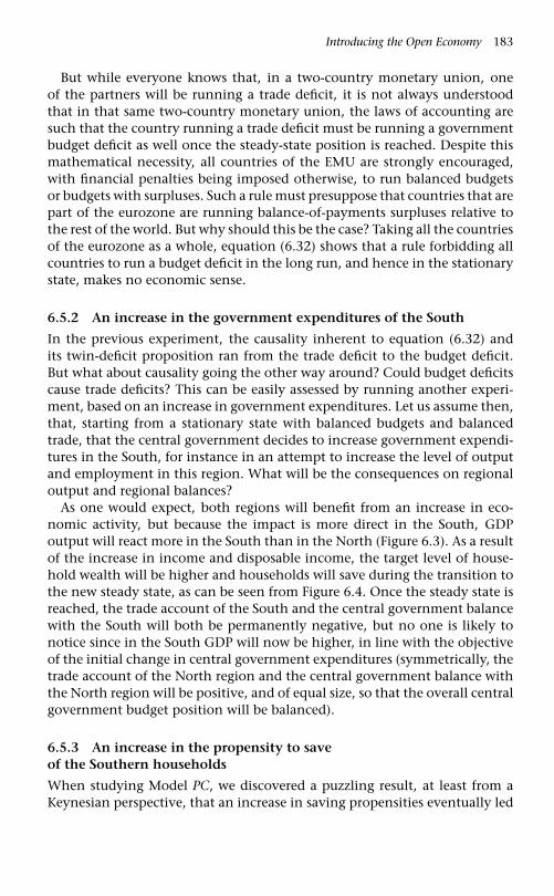
Introducing the Open Economy 183

But while everyone knows that, in a two-country monetary union, oneof the partners will be running a trade deficit, it is not always understoodthat in that same two-country monetary union, the laws of accounting aresuch that the country running a trade deficit must be running a governmentbudget deficit as well once the steady-state position is reached. Despite thismathematical necessity, all countries of the EMU are strongly encouraged,with financial penalties being imposed otherwise, to run balanced budgetsor budgets with surpluses. Such a rule must presuppose that countries that arepart of the eurozone are running balance-of-payments surpluses relative tothe rest of the world. But why should this be the case? Taking all the countriesof the eurozone as a whole, equation (6.32) shows that a rule forbidding allcountries to run a budget deficit in the long run, and hence in the stationarystate, makes no economic sense.

6.5.2 An increase in the government expenditures of the South

In the previous experiment, the causality inherent to equation (6.32) andits twin-deficit proposition ran from the trade deficit to the budget deficit.But what about causality going the other way around? Could budget deficitscause trade deficits? This can be easily assessed by running another experi-ment, based on an increase in government expenditures. Let us assume then,that, starting from a stationary state with balanced budgets and balancedtrade, that the central government decides to increase government expendi-tures in the South, for instance in an attempt to increase the level of outputand employment in this region. What will be the consequences on regionaloutput and regional balances?

As one would expect, both regions will benefit from an increase in eco-nomic activity, but because the impact is more direct in the South, GDPoutput will react more in the South than in the North (Figure 6.3). As a resultof the increase in income and disposable income, the target level of house-hold wealth will be higher and households will save during the transition tothe new steady state, as can be seen from Figure 6.4. Once the steady state isreached, the trade account of the South and the central government balancewith the South will both be permanently negative, but no one is likely tonotice since in the South GDP will now be higher, in line with the objectiveof the initial change in central government expenditures (symmetrically, thetrade account of the North region and the central government balance withthe North region will be positive, and of equal size, so that the overall centralgovernment budget position will be balanced).

6.5.3 An increase in the propensity to saveof the Southern households

When studying Model PC, we discovered a puzzling result, at least from aKeynesian perspective, that an increase in saving propensities eventually led

184

1950 1955 1960 1965 1970 1975 1980 1985 1990 1995 2000

124.0

128.0

120.0

116.0

112.0

108.0

South region GDP

North region GDP

Figure 6.3 Evolution of GDP in the South and the North regions, following an increasein the government expenditures in the South region

1951

2.0

1.0

0.0

–1.0

–2.0

–3.0

1956 1961 1966 1971 1976 1981 1986 1991 1996 2001

Government balancewith the South region

Trade balance of the South region

Change in household wealthof the South region

Figure 6.4 Evolution of the balances of the South region – net acquisition of financialassets by the household sector, government budget balance, trade balance – followingan increase in the government expenditures in the South region

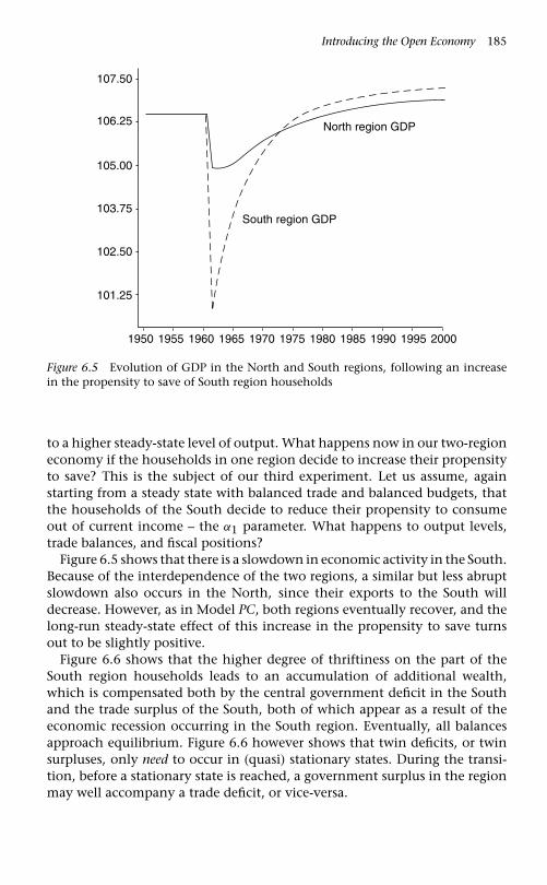
Introducing the Open Economy 185

1950 1955 1960 1965 1970 1975 1980 1985 1990 1995 2000

106.25

107.50

105.00

103.75

102.50

101.25

South region GDP

North region GDP

Figure 6.5 Evolution of GDP in the North and South regions, following an increasein the propensity to save of South region households

to a higher steady-state level of output. What happens now in our two-regioneconomy if the households in one region decide to increase their propensityto save? This is the subject of our third experiment. Let us assume, againstarting from a steady state with balanced trade and balanced budgets, thatthe households of the South decide to reduce their propensity to consumeout of current income – the α1 parameter. What happens to output levels,trade balances, and fiscal positions?

Figure 6.5 shows that there is a slowdown in economic activity in the South.Because of the interdependence of the two regions, a similar but less abruptslowdown also occurs in the North, since their exports to the South willdecrease. However, as in Model PC, both regions eventually recover, and thelong-run steady-state effect of this increase in the propensity to save turnsout to be slightly positive.

Figure 6.6 shows that the higher degree of thriftiness on the part of theSouth region households leads to an accumulation of additional wealth,which is compensated both by the central government deficit in the Southand the trade surplus of the South, both of which appear as a result of theeconomic recession occurring in the South region. Eventually, all balancesapproach equilibrium. Figure 6.6 however shows that twin deficits, or twinsurpluses, only need to occur in (quasi) stationary states. During the transi-tion, before a stationary state is reached, a government surplus in the regionmay well accompany a trade deficit, or vice-versa.

186 Monetary Economics

1951

3.00

2.25

1.50

0.75

0.00

–0.75

1956 1961 1966 1971 1976 1981 1986 1991 1996 2001

Government balance in South region

Tradebalance

Change in household wealthof the South region

Figure 6.6 Evolution of the balances of the South region – net acquisition of financialassets by the household sector, government budget balance, trade balance – followingan increase in the propensity to save of South region households

6.5.4 A change in the liquidity preferenceof the Northern households

A final experiment with Model REG assumes that the Southern householdsreduce their liquidity preference. Within the context of our model, thismeans that households from the South now wish to hold a larger proportionof their portfolio in the form of bills, which implies that the λS

0 coefficient inthe bill demand equation (6.17) is now higher. This difference in the valuestaken by the two parameters λN

0 and λS0 is in fact what one would expect

when comparing a rich and a poor region, assuming now the richer area isthe South region. The rest of the parameters can remain as they are. Whatwill now happen to output, trade balances and fiscal positions?

In this model even a fairly large reallocation of wealth towards bills willonly generate a small increase in the output of the South (and an even smallerone – hardly distinguishable – in the North). What happens, as can be seen inFigure 6.7, is that central government will now be compelled to make moreinterest payments to the households residing in the South. This increasesboth the government deficit and disposable income in the South. This inturn leads to higher consumption and higher GDP in the South, the latterinducing both wealth accumulation and a trade deficit for the South. Boththe government deficit in the South and the trade deficit of the South willbe sustained in the (quasi) steady state. The conclusion is that the reduction

Introducing the Open Economy 187

1951

0.120

0.080

0.040

0.000

–0.040

–0.080

1956 1961 1966 1971 1976 1981 1986 1991 1996 2001

Government deficit with the South region

Trade deficit of the South region

Increase in household wealthof the South region

Figure 6.7 Evolution of the balances of the South region – net acquisition of financialassets by the household sector, government budget balance, trade balance – followinga decrease in the liquidity preference of South region households

in liquidity preference by Southern households has some positive economicrepercussions on the South, as it now benefits from higher total governmentexpenditures. But all these effects are of a second-order magnitude.

6.6 The matrices of a two-country economy

The next stage is to turn Model REG into a two-country model with no over-arching or federal, government. This will be Model OPEN. However, movingin steps, it will for the time being be assumed that the private residents ofeach country are not allowed to hold any kind of foreign asset. The matri-ces for the regional model must be changed so that each country has itsown government and its own central bank. The main change, however, isthat we now assume that the currencies in the two countries are differentfrom one another; hence all transactions between them require conversionso that the transaction can be made in common units. It will also be assumedthat exchange rates are fixed, so any discrepancy between sales and pur-chases on the exchange market are made good by transactions of the centralbanks.

As always we introduce this new model by presenting the balance sheetmatrix and the transactions-flow matrix. These are shown in Tables 6.3and 6.4.

188 Monetary Economics

Table 6.3 Balance sheet matrix of two-country economy (Model OPEN)

North North South Southhouse- North central house- South centralholds Govt. bank holds Govt. bank �

Cash money +HNh −HN

h +HSh −HS

h 0

Bills +BNh −BN +BN

cb +BSh −BS +BS

cb 0

Gold orN · pNg · xr

reserves + orN · pNg · xr + orS · pS

g + orS · pSg

Wealth(balancing − (orN · pN

g · xritem) −VN

h −VNg 0 −VS

h −VSg 0 + orS · pS

g)

� 0 0 0 0 0 0 0

Each country now has its own government which issues bills, and eachcountry has a central bank which issues its own currency. But in addition,each central bank owns a stock of gold reserves which, not being financialassets, have no liability as their counterpart. This is why the value of thegold reserves appearing in the � column is not zero. Despite that, centralbanks have zero net worth, as they did in the previous model without goldreserves.

As with Model REG, all the variables relevant to the North have an N super-script, while all the variables relevant to the South have an S superscript. Thevalue of gold reserves is given by a physical quantity (‘or’) times the priceof gold (pg) expressed in the appropriate currency.7 The exchange rate xris defined as the number which converts North values and prices into theirequivalents in the currency ruling in the South. For example, if North valuesare in dollars, while South values are in yen, with one dollar being exchangedfor 100 yen, then the exchange rate xr is equal to 100.

When adding items in a given column, we need not worry about theexchange rate, because all items are in the same currency. This is not thecase when dealing with rows. However, because, as a simplification device,we have assumed that the inhabitants of each country can only purchasedomestic assets, each half of each row sums to zero (the half dealing withdomestic assets), so that we need not worry about the exchange rate when

7 In French, or means gold.

Introducing the Open Economy 189

summing the elements of each row, except for the row dealing with goldreserves. In the case of gold reserves, we must add gold reserves which arevalued in different currencies. To avoid adding apples and oranges, the goldreserves of the North must be converted in the currency of the South country,so that the gold reserves of the North and of the South can be added together.This is done by multiplying the value of the gold reserves of the North by theexchange rate xr, as shown in the middle column, so as to obtain a measureof these gold reserves valued with the South currency.

In the absence of inter-country fiscal transfers (such as took place withoutanyone knowing or noticing when there was a federal government) theremust be a means by which international debts can be settled. As the resi-dents of neither country hold the currency of the other, when they receivepayments denominated in foreign currency for their exports, they are con-sidered to exchange the proceeds into their own currency; and when theymake payments in foreign currency for imports, they must obtain the meansof payment from the central bank. Any excess of (private sector) paymentsfor imports over receipts from exports must therefore have an identicalcounterpart in transactions involving the two central banks, using someinternationally acceptable means of payment – assumed here to be sales orpurchases of gold bars valued at some fixed rate in terms of its own currency.With a fixed exchange rate and no restrictions on trade, each central bankmust be willing to buy or sell gold on any scale at that fixed rate.

Within the present international monetary system, gold bars are not tradedanymore. Although some central banks still hold gold reserves, the reservesof central banks are mainly made up of foreign currencies, mainly US dollars,and it is these foreign currencies that are used whenever central banks decideto intervene in foreign exchange markets to maintain the exchange rate oftheir home currency vis-à-vis some other currency (often the US dollar) or bas-ket of currencies. There was a time, however, where gold reserves providedthe main international acceptable means of payment. This time is known asthe gold standard period, which occurred between 1880 and 1913 – the hey-day of the gold standard – and then again from 1922 to 1938. The modelto be presented here, Model OPEN, can thus either be understood as a rep-resentation of the gold standard period, or be understood as a rough andover-simplified version of the current international monetary system.

Whatever the chosen interpretation, we may now examine thetransactions-flow matrix of this two-country economy, which appears inTable 6.4. As with all transactions-flow matrices, each row and column ofTable 6.4 must sum to zero. As in Table 6.3, we need not worry about the cur-rency in use when summing the items in each column, since all such itemsare in domestic currency. Summing the rows is a bit more complicated. Aswas the case with the balance sheet, there is no problem for many of the rows,since each half of these rows, linked to domestic transactions only, sums tozero anyway. However, this is not the case of all rows, and in particular this

190Table 6.4 Transactions-flow matrix of two-country economy (Model OPEN)

North country South country

Central CentralHouseholds Producers Govt. bank Households Producers Govt. bank �

Consumption −CN +CN −CS +CS 0

Govt. exp. +GN −GN +GS −GS 0

North Exportsto South +XN ·xr −IMS 0

South Exportsto North −IMN ·xr +XS 0

GDP +YN −YN +YS −YS 0

Interestpayments +r−1 · BN

h−1 −r−1 · BN−1 +r−1 · BNcb +r−1 · BS

h−1 −r−1 · BS−1 +r−1 · BScb−1 0

Profits ofcentral bank +r−1 · BN

cb−1 −r−1 · BNcb−1 +r−1 · BS

cb−1 −r−1 · BScb−1 0

Taxes −TN +TN −TS +TS 0

Change in cash −�HNh +�HN −�HS

h +�HS 0

Change in bills −�BNh +�BN −�BN

cb −�BSh +�BS −�BS

cb 0

Change inreserves −�orN · pN

g ·xr −�orS · pSg 0

� 0 0 0 0 0 0 0 0 0

Introducing the Open Economy 191

is not the case with the export rows and the row dealing with changes ingold reserves. For these rows, an additional column must be introduced, thatmultiplies the domestic values of the North country by the exchange rate xr,to obtain values measured in the South currency. All the items in the rowmay then be summed, since they are being expressed in the same numéraire.As all other rows, the rows dealing with exports and changes in gold holdingsmust then all sum to zero, thanks to this currency adjustment.8

It is a feature of Table 6.4 which may surprise for an instant that neithercountry has or needs a column describing its current balance of payments.However the coherence enforced by double entry accounting ensures thattotal flows in each country always exactly equal total outflows. Thus tradeflows, which are to be found in the two rows describing exports, make upthe balance of payments on current account, which is, in turn, exactly equalto the sum of each country’s transfers of gold described in the row called‘change in reserves’. The logic of the double entry system implies that theentries in the final line sum to zero; hence as both entries in the ‘change inreserves’ row have a negative sign, one country’s gold stock can only rise ifthe other’s falls to an exactly equal extent.

6.7 The equations of a two-country economy

It is easy to adapt the equation system from Model REG, to transform it intoa two-country model. This is done in Appendix 6.2, where equations havebeen renumbered starting with equation (6.O.1) to underline the fact thatwe are now dealing with Model OPEN.

A lot of the equations of Model OPEN are identical to those of Model REG.Thus, equations (6.O.1) to (6.O.4), (6.O.7), (6.O.8), and (6.O.11) to (6.O.18)are identical to equations (6.1) to (6.4), (6.7), (6.8), and (6.11) to (6.18).9

Only a few changes are required to complete the model. First, the export andimport identities must reflect the fact that there now exist two currenciesinstead of one. The imports and exports of the North are thus adjusted bybeing multiplied by the exchange rate, as shown in equations (6.O.5) and(6.O.6).

XN = IMS

xr(6.O.5)

XS = IMN · xr (6.O.6)

8 Changes in gold holdings must also sum to zero. If gold was being produced bythe production sector, and purchased by one of the central banks, this would have toenter the matrix, but we would still be left with zero-sum columns and rows.

9 It cannot be assumed however that the consumption and the portfolio parametersare identical in the two regions, which are now two separate countries.

192 Monetary Economics

Next, one must delete from Model REG all references to a general governmentand a unique central bank. We now have two separate governments and twodifferent central banks. Each government can set its own tax rate, as shownin equations (6.O.9) and (6.O.10).

TN = θN · (YN + rN−1 · BNh−1) 0 < θN < 1 (6.O.9)

TS = θS · (YS + rS−1 · BSh−1) 0 < θS < 1 (6.O.10)

Third, the four equations of Model REG that were defining the aggregates ofthe two-region economy – equations (6.19) to (6.23) – are now meaninglessin the two-country economy of Model OPEN, and must be deleted. Becausethere are now two governments and two central banks, the financial variablesrelated to these institutions double in size: there are now eight such variables,namely the supply of bills by each of the two governments, the demand forbills and the supply of cash money by each central bank, and finally the rate ofinterest set by each central bank. There are also four additional variables, thatdid not exist in Model REG: the change in gold holdings by each central bank,and the price of gold in each country. The exchange rate may be consideredas the last additional variable, but we have assumed fixed exchange rates, sothat the exchange rate is a constant. We thus have 13 additional variables,and so we must define 13 extra equations to determine Model OPEN. This isthe task that we now tackle.

�BNs = BN

s − BNs−1 = (GN + rN−1 · BN

s−1) − (TN + rN−1 · BNcb−1) (6.O.19)

�BSs = BS

s − BSs−1 = (GS + rS−1 · BS

s−1) − (TS + rS−1 · BScb−1) (6.O.20)

BNcb = BN

s − BNh (6.O.21)

BScb = BS

s − BSh (6.O.22)

�orN. · pNg = �HN

s − �BNcb (6.O.23)

�orS. · pSg = �HS

s − �BScb (6.O.24)

HNs = HN

h (6.O.25)

HSs = HS

h (6.O.26)

Equations (6.O.19) and (6.O.20) describe the budget constraint of each gov-ernment; there is nothing new here. Equations (6.O.21) and (6.O.22) arenot new either: they say that each central bank is ready to purchase anybill outstanding which is not bought by households of its constituency.Equations (6.O.23) and (6.O.24) reflect the balance-sheet constraint of thecentral bank. While the balance sheet constraint of the central bank was

Introducing the Open Economy 193

already used in Model PC and Model REG, these two equations are new inso-far as they incorporate changes in gold holdings by each central bank. Butnow, because gold holdings appear on the left-hand side of the equations,while the supply of cash money by the central bank appears on the right-hand side of these two equations, we need two new equations in deter-mining the supply of cash money in each country. These two equationsare equations (6.O.25) and (6.O.26). They indicate that each central bankis supplying the amount of cash money which is demanded by house-holds and explicitly reflect the proposition that money is endogenous, inthe sense that it is demand-led, determined by the portfolio choice ofhouseholds.

Five more equations need to be found. Two of these are straightfor-ward. The price of gold in each country must be determined. Withequation (6.O.27) we assume that the price of gold in the North is a given,expressed in the currency ruling in the North and set by the North centralbank. By the law of one price, the price of gold in the South is deter-mined by the exchange rate, given the price of gold in the North, asshown in equation (6.O.28). Since we have room for three more equations,this means that, in addition to a fixed exchange rate, as shown byequation (6.O.29), it is possible for both central banks to set the rate ofinterest of their choice, as reflected by equations (6.O.30) and (6.O.31). Inother words, despite each country being an open economy with a fixedexchange rate, the rates of interest in each country can be set exoge-nously. The rates of interest do not need to play any price-equilibratingmechanism.

pNg = pN

g (6.O.27)

pSg = pN

g · xr (6.O.28)

xr = xr (6.O.29)

rN = rN (6.O.30)

rS = rS (6.O.31)

The redundant equation is now the one which describes the equivalencebetween reserve gains by one country and reserve losses by the other, as canbe assessed from the row ‘Change in reserves’ in the transactions-flow matrixof Table 6.4. That is to say, the structure of the model implies that:

�orS = −�orN (6.O.32)

and in the simulations this is invariably found to be true, although it doesnot appear as an equation in the model.

194 Monetary Economics

1950 1955 1960 1965 1970 1975 1980 1985 1990 1995 2000

108.0

109.5

106.5

105.0

103.5

102.0

South country GDP

North country GDP

Figure 6.8 Evolution of GDP in the North and in the South countries, following anincrease in the South propensity to import

6.8 Rejecting the Mundell–Fleming approach andadopting the compensation approach

6.8.1 Ever-falling gold reserves

When the two-country model is simulated, we find that a rise in the propen-sity to import of the South country has effects which, initially, are identicalwith those in the regional model. The two countries reach a kind of station-ary state, which we shall call a quasi stationary state, where there is no changein the financial assets held by the households of each country, and wherethere is no change in the income level of both countries. The income of theNorth country is now higher, and that of the South country is now lower, asshown in Figure 6.8, which is identical to Figure 6.2.

Once again the South is subjected to the twin-deficit situation. The effectson the balance of trade, the private sector’s financial balance and thebudget deficit are identically the same as those illustrated in Figure 6.1 –reproduced here as Figure 6.9 with obvious small amendments to theheadings.

However, whereas in the regional model the balance-of-paymentsdeficit is automatically financed by fiscal transfers between regions bythe central government and which can continue for ever, in the two-country model the deficit is financed by a loss of reserves which exactlymatches its trade deficit, step by step, in the quasi stationary state.This must be the case, by the laws of logic, since changes in reserves

Introducing the Open Economy 195

1951

–1.25

–1.00

–0.75

–0.50

–0.25

0.00

1956 1961 1966 1971 1976 1981 1986 1991 1996 2001

South trade balance

South government balance

Change in South household wealth

Figure 6.9 Evolution of the balances of the South country – net acquisition of financialassets by the household sector, government budget balance, trade balance – followingan increase in the South propensity to import

are the only international transactions on capital account. The readerwill recall that when building our transactions and balance sheet matri-ces, we assumed capital flows away – implying fully fledged capitalcontrols.

In the country with the trade surplus, the gold reserves are continuouslyrising, while in the trade deficit country they are diminishing. In addition,the government of the deficit country sees the size of its public debt contin-uously rising, thus facing a rising public debt to income ratio. This is whywe may call the resulting situation a quasi stationary state, since some ofthe main variables or ratios are still changing, and also because it is impos-sible for the situation to persist indefinitely. ‘As a long-term proposition thehypothesis of ever-increasing government debt relative to income accom-panied by continuous external deficits is implausible’ (Godley and Cripps1983: 297).

The interesting thing to emerge from the simulations is that, beyond reduc-ing income in the weaker country via the mechanism of the foreign trademultiplier, as shown in Figure 6.8, the private sector receives no signal thatanything is wrong at all. Yet the central bank is suffering an unsustainableloss of reserves which can only go on for as long as there are reserves to lose.As there are no private international capital transactions and as we have, sofar, a strictly fixed exchange rate system, the government will be forced even-tually to do one of three things: to deflate demand to the point where the

196 Monetary Economics

external deficit is eliminated; to borrow reserves from abroad; or adminis-tratively to restrict imports to what can be paid for with exports.10 It wouldbe possible to work out how much deflation there would have to be – if thisis the route adopted – by setting the change in reserves to zero and endog-enizing government expenditures (or the tax rate). This would ensure thatthe economy must be deflated to the point where the balance of payments isalso zero.

Until a government runs out of reserves and has to take drastic restric-tive action, the signals the private sector receives are almost identical to theones it gets in the regional model; the deficit country suffers a loss of incomeand a generalised loss of wealth and employment, as in the regional model.The only other additional information is that the government running thecountry with the trade deficit is facing a permanent budget deficit, despitea constant national income. The rising public debt to income ratio mightinduce households to reduce their holdings of government bills. But this,in itself, cannot stop the central bank from keeping the interest rates at aconstant level. Indeed, in the (quasi) stationary state, the new public debtis all being financed by the sales of bills to the central bank. The value ofbills purchased by the central bank is exactly equal to the value of gold lossesthat it incurs, as indicated by equations (6.O.23) and (6.O.24). Otherwise,there is no automatic correction mechanism of any kind to stem the tradedeficit.

This finding is profoundly at odds with the influential body of lit-erature which has its genesis in the Mundell–Fleming models of fixedexchange rate economies and the body of doctrine known as ‘the mone-tary approach to the balance-of-payments’, which turn out to be modernextensions of the ‘price-specie flow’ mechanism outlined by David Hume,back in the eighteenth century. A central contention of these theories isthat there is some automatic feedback mechanism that gradually bringsback an equilibrium balance-of-payments whenever a surplus or a deficitposition occurs, even if nominal exchange rates are fixed. The feedbackmechanism is usually presented with the following arguments. A balance-of-payments deficit in a fixed exchange rate regime means a loss of reserves.In Hume’s time, the balance-of-payments deficit meant a loss of gold, andthis was said to lead to a fall in prices, which made the products of thedeficit country more competitive and hence allowed it to recover balancedtrade.

In the modern world, claim the proponents of the Mundell–Flemingapproach, this loss of reserves, which appears on the asset side of the bal-ance sheet of the central bank, is said to induce an equivalent depletion of

10 Another option would be devaluation, or a decision to move to a flexibleexchange rate regime.

Introducing the Open Economy 197

the monetary base, which constitutes the liability side of the central bank.The falling monetary base – the falling supply of high-powered money – leadsto a falling money supply, and hence to higher interest rates. These rates willkeep on rising until balance-of-payments equilibrium is restored, because aslong as the external balance is not restored the monetary base keeps beingdepleted. These feedback mechanisms mimic the ‘price-specie flow’ mech-anism that was said to rule in Hume’s time and in the heyday of the goldstandard regime of international settlements, when gold was the main if notthe only instrument of foreign reserves. Despite the neat graphical represen-tations of the mainstream models via the well-known IS/LM/BP framework,these standard models are difficult to penetrate, precisely because they arenever set forth in a comprehensive system of accounts, with every equationand every equilibrium condition made explicit.

6.8.2 A gold standard with non-existent rules of the game

The interesting thing to emerge from Model OPEN is that although a deficitcountry loses gold reserves, this loss has no independent effect on anythingelse at all. This is the more surprising because Model OPEN retains the mainfeatures of the gold exchange standard, which provides the institutional back-ground which is said to be the most favourable to the functioning of the rulesof the game, that is, the mechanism which ensures that a balance-of-paymentsdeficit will lead to a fall in base money and the money supply, as well as arise in interest rates, and hence to the recovery of a balanced external posi-tion. Model OPEN runs under the gold standard, since any trade deficit mustbe made good by a transfer of gold between central banks. Still, the rulesof the game just do not and cannot apply. There is no endogenous mecha-nism eliminating the balance-of-payments deficit. Hume’s ‘price-specie flow’mechanism just does not seem to have any bite. 11

The point that mainstream authors seem to be missing is that when there isa loss of reserves, as illustrated in Figure 6.9, there will be, after the first kerfuf-fle as the private sector adapts, a budget deficit which is exactly equal to thisloss of reserves. The asset stocks adjust to a new, lower level, in line with thelower income flow but thereafter they exhibit no change at all. The compen-satory mechanism from the budget deficit thus removes all leverage which

11 It must be pointed out that Mundell (1961), whose other works are often invokedto justify the relevance of the rules of the game in textbooks and the IS/LM/BP model,was himself aware that the automaticity of the rules of the game relied on a particularbehaviour of the central bank. Indeed he lamented the fact that modern central bankswere following the banking principle instead of the bullionist principle, and hence adjust-ing ‘the domestic supply of notes to accord with the needs of trade’ (1961: 153), whichis another way to say that the money supply was endogenous and that central bankswere concerned with maintaining the targeted interest rates. This was in 1961!

198 Monetary Economics

1951

1.00

0.50

0.00

–0.50

–1.00

–1.501956 1961 1966 1971 1976 1981 1986 1991 1996 2001

Value ot the change in gold reservesheld by the South central bank

Change in the South country stock of money

Change in stock of bills heldby the South central bank

Figure 6.10 Evolution of the three components of the balance sheet of the Southcentral bank – gold reserves, domestic Treasury bills and money – following an increasein the South propensity to import

the loss of reserves is supposed to be exercising on the monetary system.Although there is no deliberate ‘sterilization’ of falling reserves by the cen-tral bank, the fall in foreign reserves is nonetheless continuously offset bythe increase in the amount of bills held by the central bank, as is shown inFigure 6.10. This increase is entirely endogenous to the behaviour of the cen-tral bank and of the entire economic system. One could say that it arises asa consequence of the decision by the central bank to keep the rate of inter-est on bills constant. But beyond that, the relative constancy of the moneysupply in the new steady state is not the result of a discretionary decisionmade in an attempt to keep the money supply constant, as ‘sterilization’ isportrayed by mainstream authors.

A very similar process is arising in the North, which, with its trade surplus,sees its foreign reserves rise continuously. The rise in these reserves is coun-terbalanced by the fall in the amount of bills that the North central bankis required to hold. This is known as the compensation thesis (Lavoie 2001b:206). The compensation principle asserts that changes in foreign reserveswill generally be compensated by endogenous mechanisms that are tied tothe normal behaviour of the central bank and to that of the other economicagents in the economy. The compensation principle would also operate inan open economy with private bank money.

6.8.3 Two kinds of money supply endogeneity

Mainstream economists usually hold that, whereas otherwise it may be con-sidered to be an exogenous variable, the money supply is endogenous in

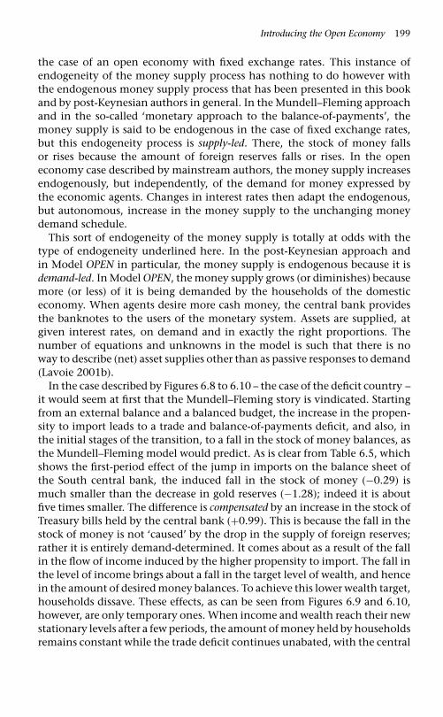
Introducing the Open Economy 199

the case of an open economy with fixed exchange rates. This instance ofendogeneity of the money supply process has nothing to do however withthe endogenous money supply process that has been presented in this bookand by post-Keynesian authors in general. In the Mundell–Fleming approachand in the so-called ‘monetary approach to the balance-of-payments’, themoney supply is said to be endogenous in the case of fixed exchange rates,but this endogeneity process is supply-led. There, the stock of money fallsor rises because the amount of foreign reserves falls or rises. In the openeconomy case described by mainstream authors, the money supply increasesendogenously, but independently, of the demand for money expressed bythe economic agents. Changes in interest rates then adapt the endogenous,but autonomous, increase in the money supply to the unchanging moneydemand schedule.

This sort of endogeneity of the money supply is totally at odds with thetype of endogeneity underlined here. In the post-Keynesian approach andin Model OPEN in particular, the money supply is endogenous because it isdemand-led. In Model OPEN, the money supply grows (or diminishes) becausemore (or less) of it is being demanded by the households of the domesticeconomy. When agents desire more cash money, the central bank providesthe banknotes to the users of the monetary system. Assets are supplied, atgiven interest rates, on demand and in exactly the right proportions. Thenumber of equations and unknowns in the model is such that there is noway to describe (net) asset supplies other than as passive responses to demand(Lavoie 2001b).

In the case described by Figures 6.8 to 6.10 – the case of the deficit country –it would seem at first that the Mundell–Fleming story is vindicated. Startingfrom an external balance and a balanced budget, the increase in the propen-sity to import leads to a trade and balance-of-payments deficit, and also, inthe initial stages of the transition, to a fall in the stock of money balances, asthe Mundell–Fleming model would predict. As is clear from Table 6.5, whichshows the first-period effect of the jump in imports on the balance sheet ofthe South central bank, the induced fall in the stock of money (−0.29) ismuch smaller than the decrease in gold reserves (−1.28); indeed it is aboutfive times smaller. The difference is compensated by an increase in the stock ofTreasury bills held by the central bank (+0.99). This is because the fall in thestock of money is not ‘caused’ by the drop in the supply of foreign reserves;rather it is entirely demand-determined. It comes about as a result of the fallin the flow of income induced by the higher propensity to import. The fall inthe level of income brings about a fall in the target level of wealth, and hencein the amount of desired money balances. To achieve this lower wealth target,households dissave. These effects, as can be seen from Figures 6.9 and 6.10,however, are only temporary ones. When income and wealth reach their newstationary levels after a few periods, the amount of money held by householdsremains constant while the trade deficit continues unabated, with the central

200 Monetary Economics

Table 6.5 First-period effect of the jump in imports on the balance sheet ofthe South central bank

Assets Liabilities

Change in gold reserves −1.28 Change in high-powered money −0.29Change in Treasury bills +0.99

bank experiencing a continuous drain on its gold reserves. The Mundell–Fleming story, or the ‘income-specie flow’ mechanism as Mundell (1961: 159)calls it, and the ‘price-specie flow’ mechanism both turn out to be erroneousafter all.

This finding is in line with the claim made by Arestis and Eichner (1988:1015) that ‘so long as it is recognized that money supply is credit-drivenand demand-determined, the exchange rate regime is of absolutely no con-sequence in the determination of money and credit’. Interest rates can be setby the central bank and money is demand-determined in this fixed exchangerate regime.12

6.8.4 A further example of the compensation thesis:increasing the propensity to save

Let us assume that South households decide to increase their propensity tosave, thus increasing their target wealth to income ratio. The impact of sucha decision on GDP is identical to what was described with Figure 6.5 in thecase of the two regions, with both the South and the North countries GDPdropping briskly, only to rise to a slightly higher level in the new stationarystate. Similarly, the impact on the household financial balance, trade bal-ance and government budget of the South are identical to that described inFigure 6.6. In other words, the short-term recession in the South initially gen-erates a government deficit and a trade surplus. This trade balance howevergets reversed in the long run, since the higher steady-state GDP in the Southgenerates constant trade deficits and government deficits of equal size.

The new results of this two-country economy, relative to the two-regioneconomy, can be found in Figure 6.11, which illustrates what happens tothe three components of the balance sheet of the South central bank. Theevolution of gold holdings reflect the evolution of the trade balance. Gold

12 This was recognized by earlier Keynesian authors, such as Meade. As Allen andKenen (1980: 8), point out, ‘Meade instructs the central bank to maintain a constantinterest rate; the bank’s open market operations offset changes in the supply of moneycaused by movements of reserves and offset changes in the demand for money causedby the movements in domestic income’.

Introducing the Open Economy 201

1951

0.80

1.20

0.40

0.00

–0.40

–0.80

1956 1961 1966 1971 1976 1981 1986 1991 1996 2001

Value of change in gold reserves

Change inthe money stock

Change in bills held

Figure 6.11 Evolution of the components of the balance sheet of the South centralbank, following an increase in the South propensity to consume out of currentincome

holdings initially rise, but this is gradually replaced by an outflow of gold,since a quasi stationary state is reached, with a constant trade deficit. Thestock of high-powered money initially increases, reflecting the increase indesired wealth by Southern households, and it then remains constant reflect-ing the quasi stationary state with no change in the wealth of households.As to the amount of bills held by the central bank, it is this component ofthe central bank that adjusts to the fluctuations in the other componentsof its balance sheet. To maintain a given rate of interest, the South centralbank compensates the quasi steady-state outflow of gold reserves by increas-ing domestic credit, that is by increasing its holdings of domestic Treasurybills. By contrast, during the recession, the inflow of gold, which was accom-panied by a modest increase in the money supply arising from the decisionof Southern households to increase their two wealth components, was com-pensated by a reduction in the stock of bills held by the South central bank,thus illustrating once more the compensation principle.

6.9 Adjustment mechanisms

6.9.1 The super stationary state

Over recent years, a group of heterodox economists (see McCombie andThirlwall 1994) has been arguing, both for theoretical and empirical rea-sons, that the long-run rate of growth of any open economy is essentially

202 Monetary Economics

constrained by a ratio, which is the rate of growth of its exports divided bythe income elasticity of imports of that country. This implies that, over thelong run, the trade account of these countries is roughly balanced. In fact, inthe original study of Thirlwall (1979), Japan was the only country the actualrate of growth of which did not turn out to be closely related to the predic-tion of his simple equation because Japan had a large trade account surplusover a large number of years.

We have claimed above that no automatic economic forces would push theeconomy towards a balanced trade account. But this of course is true only aslong as there are spare foreign reserves. When a country with a balance-of-payments deficit runs out of reserves, something must be done. As pointedout earlier, the government of the deficit country can decide to pursue fiscalausterity in order to establish a balanced trade position, by reducing nationalincome and hence imports. This kind of decision is particularly likely, becauseof the twin-deficit problem: the country with a trade deficit will also be fac-ing, at least when the steady state is reached, a government budget deficit.Recalling equation (6.35), modified to take into account the fact that the taxrate now applies to a single country, it is quite simple to understand whatwill occur.

YN = GNNT

θN = XN

μN (6.35A)

Assuming that exports are exogenous, and that the propensity to importcannot be modified, the only way to reach the super stationary state, for acountry with a trade deficit, is to reduce pure government expenditures or toincrease the tax rate. This will be done until the GN

NT/θN ratio, which is toohigh relative to the XN/μN ratio, is reduced to the level of the latter. If suchpolicies are indeed pursued, it is clear that the world economy suffers from arecession bias, since the reduction in autonomous expenditures in one coun-try eventually leads to the reduction in the exports of the other countries. Asto the countries with a trade and budget surplus, they will have little incentiveto speed up pure government expenditures, although lately, strong pressureshave been exerted, to use any government surplus to reduce tax rates. Thesepressures ought to be successful in keeping the recession bias at bay, but at thesame time, the forces in play are asymmetrical. In the case of vanishing for-eign reserves, something must be done to slow down imports and deflate theeconomy. In the case of the economy with a trade surplus, there is no suchurgency. Politicians and bureaucrats are quite content with trade and govern-ment budget surpluses. They probably feel that nothing needs to be done tocorrect the trade surplus, and they can easily withstand pressures to increasegovernment services or to cut tax rates. This is because, among other factors,some of the constituencies which are so enthusiastic about tax cuts – the

Introducing the Open Economy 203

rentiers – are also worried about the consequences of such tax cuts, fearingthat the cuts would generate an overheated economy and accelerating priceinflation.

6.9.2 Adjustment through pure government expenditures

Still, let us consider the possibility of an adjustment through changes inpure government expenditures. Let us first model some partially symmetricadjustment mechanism, that leads to a decrease in pure government expendi-tures whenever gold reserves are falling, and that leads to a relatively smallerincrease in pure government expenditures whenever gold reserves are rising.This adjustment mechanism may be written in a quite simple way. We couldhave:

GN = GN−1 + ϕN · (�orN−1 · pNg−1) (6.O.33)

GS = GS−1 + ϕS.(�orS−1 · pSg−1) (6.O.34)

where the ϕs are positive.Such an adjustment mechanism is stabilizing, as can be seen from Figure

6.12. As in the previous figures, we assume that, having started from a superstationary state, there is an increase in the South propensity to import. Asits net exports decrease, the South economy slows down and must face bothlosses of gold reserves and government deficits. However, this time round,the losses and the budget deficits do not last forever, for the decreasing puregovernment expenditures slow down the economy and bring it back both toa balanced trade position and to a balanced budget – with some overshootingas can be seen from Figure 6.12.

The only problem with this stabilizing mechanism is that the economymust slow down, so that, in the new steady state, the income level in thedeficit country – the South – is lower than what it was before or than whatit would have been had pure government expenditures been left at a con-stant level. This can be verified by comparing the new steady-state valuetaken by the GDP of the South country in Figure 6.13 with that of Figure6.8, where an identical experiment was conducted, but without the adjust-ment mechanism. Of course, in the North economy, the reverse occurs: theincome level rises, both because of its improved trade position, and becauseof its increased government expenditures. If there had been no symmetri-cal process, (i.e. had the North not reacted to its trade surplus by increasingits government expenditures) income in the South would have fallen evenmore, but balanced trade would have been achieved nonetheless.

As the use of fiscal policy to curb trade imbalances yields strong stabilizingproperties, it is no surprise to discover that the World Bank and the IMF arequite keen on using such an adjustment tool and in imposing it when they

204

1951

0.30

0.00

–0.30

–0.60

–0.90

–1.20

1956 1961 1966 1971 1976 1981 1986 1991 1996 2001

Government account

Change in household wealth

Trade account

Figure 6.12 Evolution of the balances of the South country – net acquisition of finan-cial assets by the household sector, government budget balance, trade balance –following an increase in the South propensity to import, with fiscal policy reactingto changes in gold reserves

1950 1955 1960 1965 1970 1975 1980 1985 1990 1995 2000

110.0

112.5

107.5

105.0

102.5

100.0

South country GDP

North country GDP

Figure 6.13 Evolution of GDP in the South and the North countries, following anincrease in the South propensity to consume, with fiscal policy reacting to changes ingold reserves

Introducing the Open Economy 205

propose adjustment packages to third-world countries that have balance-of-payments disequilibria. The danger is that all balance-of-payments deficitcountries use such an adjustment mechanism while all surplus countriesdecline to inflate their economies, in which case the world economy willbe biased towards depression.

6.9.3 Adjustments through interest rates

World Bank adjustment packages usually contain another element – interestrate hikes. Are these interest rate increases stabilizing? In standard WorldBank adjustment packages, the higher (real) interest rates are there to slowdown the economy, so as to help solving a negative trade balance, and theyare intended to attract foreign capital as well as to induce domestic assetholders to keep their assets in the domestic financial markets. Within thepresent model, it is clear that interest rate hikes would serve no purpose.There are two reasons for this. In Model OPEN, private economic activity doesnot depend on interest rates; in addition, capital flows between countries areruled out, so there are no foreign capital flows to attract or no domestic capitalflows to keep within.

Still, what would happen if interest rates were to react to changes in goldreserves? We can put forward an adjustment equation which is similar to theone proposed above. We would have:

rN = rN−1 − ϕN · (�orN−1 · pNg−1) (6.O.30A)

rS = rS−1 − ϕS · (�orS−1 · pSg−1) (6.O.31A)

The rate of interest is not set exogenously anymore; however, within theframework that we have set up, it is still possible for the monetary author-ities to set the rate of interest at their discretion. In other words, equations(6.O.30A) and (6.O.31A), which replace equations (6.O.30) and (6.O.31), arethe reaction functions of the central banks.

One would normally suppose that the change in the rate of interest oughtto be a negative function of the change in gold reserves. This is why thereis a minus sign in front of the ϕ parameters. For instance, a decrease in goldreserves ought to lead to an increase in the rate of interest.

It would seem that we are back to the ‘price-specie’ mechanism, and to theMundell–Fleming automatic adjustment mechanism. As pointed out in pre-vious sections, these mechanisms lead to spontaneous increases in rates ofinterest whenever gold reserves are falling. But precisely, the above equationshave nothing automatic or natural about them. They are reaction func-tions, which require a discretionary decision and a purposeful action fromthe central bank. Rates of interest move up, not as a result of some spon-taneous market mechanism, but rather as a consequence of the deliberate

206 Monetary Economics

1950 1952 1954 1956 1958 1960 1962

0.125

0.150

0.100

0.075

0.050

0.025

South interest rate(deficit country)

North interest rate(surplus country)

Figure 6.14 Evolution of interest rates, following an increase in the South propensityto import, with monetary rules based on changes in gold reserves

policy choice of the monetary authorities. Equations (6.O.30) are monetaryrules that the central banks have decided to put in place.

The other key question is whether such an increase in interest rates, when-ever a trade deficit arises, will have stabilizing effects. It turns out that suchan adjustment mechanism is fundamentally non self-righting. It is formallyunstable, as simulation experiments quickly reveal. Figure 6.14 shows thatthis is so because the interest rate in the South rises ever faster (while interestrates in the North keep falling, more slowly, on the basis of an asymmetricrule). Figure 6.15 shows that the trade imbalances between the South andthe North only worsen, with the government deficit in the South gettingever worse. Indeed, when submitted to such monetary adjustment rules, theprogram crashes.

Such a result is not surprising. High rates of interest cannot attract foreigncapital, since capital flows have been excluded by assumption. High interestrates do not slow down the economy either, and hence cannot reduce thetrade deficit, since interest rates are assumed not to have any negative impacton the private economy. Indeed, an increase in interest rates worsens thebudget deficit of government, and it fuels the consumption expendituresand the imports of the private economy, by reason of equations (6.O.3) and(6.O.7), thus leading to a further deterioration of the balance of trade.

The instability of this interest rate adjustment still occurs if we let interestrates have a negative impact on aggregate consumption. Assume for instancethat, as was done with Model PC of Chapter 4, a higher interest rate leads to

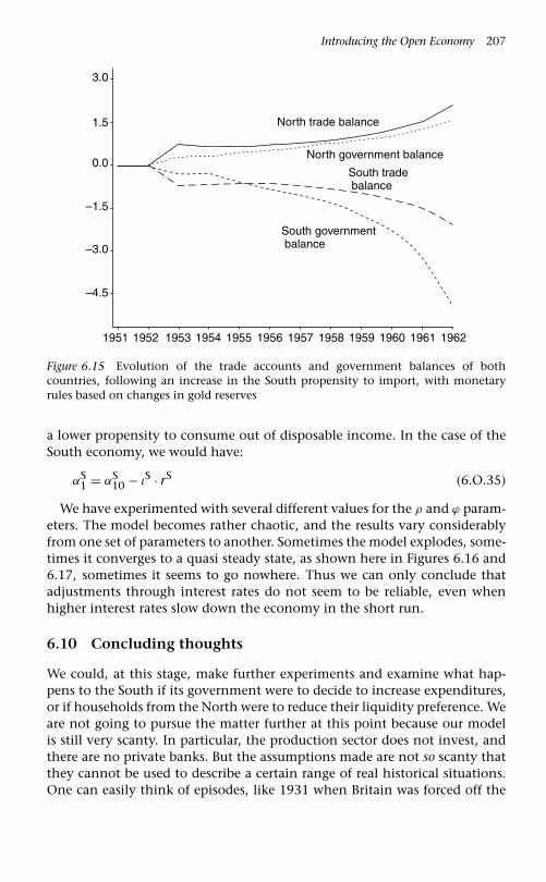
Introducing the Open Economy 207

1951 1952

3.0

1.5

0.0

–1.5

–3.0

–4.5

1953 1954 1955 1956 1957 1958 1959 1960 1961 1962

North trade balance

South trade balance

South government balance

North government balance

Figure 6.15 Evolution of the trade accounts and government balances of bothcountries, following an increase in the South propensity to import, with monetaryrules based on changes in gold reserves

a lower propensity to consume out of disposable income. In the case of theSouth economy, we would have:

αS1 = αS

10 − ιS · rS (6.O.35)

We have experimented with several different values for the ρ and ϕ param-eters. The model becomes rather chaotic, and the results vary considerablyfrom one set of parameters to another. Sometimes the model explodes, some-times it converges to a quasi steady state, as shown here in Figures 6.16 and6.17, sometimes it seems to go nowhere. Thus we can only conclude thatadjustments through interest rates do not seem to be reliable, even whenhigher interest rates slow down the economy in the short run.

6.10 Concluding thoughts

We could, at this stage, make further experiments and examine what hap-pens to the South if its government were to decide to increase expenditures,or if households from the North were to reduce their liquidity preference. Weare not going to pursue the matter further at this point because our modelis still very scanty. In particular, the production sector does not invest, andthere are no private banks. But the assumptions made are not so scanty thatthey cannot be used to describe a certain range of real historical situations.One can easily think of episodes, like 1931 when Britain was forced off the

208

1950 1955 1960 1965 1970 1975 1980 1985 1990 1995 2000

0.040

0.050

0.030

0.020

0.010

0.000

North interest rate

South interest rate

Figure 6.16 Evolution of interest rates, following an increase in the South propensityto import, with interest rates acting on propensities to consume and reacting to changesin gold reserves

1951

1.00

0.50

0.00

–0.50

–1.00

–1.50

1956 1961 1966 1971 1976 1981 1986 1991 1996 2001

South trade account

South government account

North trade account

North governmentaccount

Figure 6.17 Evolution of trade accounts and government balances, following anincrease in the South propensity to import, with interest rates acting on propensitiesto consume and reacting to changes in gold reserves

Introducing the Open Economy 209

gold standard because she ran clean out of reserves at a particular hour andminute, which gives us courage to believe that we are on the right track. Inaddition, there is a large amount of empirical and descriptive evidence sup-porting the compensation principle which can be found for periods duringwhich the gold exchange standard was ruling – the regime considered to bemost favourable to enforce the so-called rules of the game. Studies have pro-vided data that run contrary to what would occur if the rules of the gamehad been followed during the gold exchange standard era.13 This shows thatthe price-specie flow mechanism and the rules of the game are bad theoriesand bad descriptions of what occurs in the real world. The point made hereis that these theories are failures because they lack a proper and coherentaccounting framework.

The current framework can be easily extended to include capital flowsor other institutional set-ups. For instance, in Lavoie (2003), the presentframework is modified by including private capital flows between coun-tries in a world with two governments and one central bank (somethingakin to Europe). Also, in Lavoie (2006c), there is a discussion within a two-country framework of the currency board institution, so popular before theArgentinian debacle.14 Izurieta (2003) also develops the case of dollarizationalong similar lines.

One could argue that the OPEN model or these offsprings are over-simplified and omit too many realistic features. We shall show in Chapter 12however, that the main mechanisms and results of the OPEN model are stillvindicated in more sophisticated models, for instance when there is free cap-ital mobility between countries, and when central banks hold foreign assetsinstead of gold as foreign reserves. In that chapter, we shall also go beyondfixed exchange rates, by analysing what occurs when the model is trans-formed into a flexible exchange rate model, with changing exchange rateshaving an impact on various price indices. A simplified version of that modelhas been presented in Godley and Lavoie (2005–6), where a slightly differentpedagogical approach has been followed to help readers understand the logicof the compensation principle or that of endogenous sterilization.

Appendix 6.1: Equations of Model REG

YN = CN + GN + XN − IMN (6.1)

YS = CS + GS + XS − IMS (6.2)

IMN = μN · YN (6.3)

13 See Appendix 6.3 for further details.14 More is said about this in Appendix 6.4.

210 Monetary Economics

IMS = μS · YS (6.4)

XN = IMS (6.5)

XS = IMN (6.6)

YDN = YN − TN + r−1 · BNh−1 (6.7)

YDS = YS − TS + r−1 · BSh−1 (6.8)

TN = θ · (YN + r−1 · BNh−1) 0 < θ < 1 (6.9)

TS = θ · (YS + r−1 · BSh−1) 0 < θ < 1 (6.10)

VN = VN−1 + (YDN − CN) (6.11)

VS = VS−1 + (YDS − CS) (6.12)

CN = αN1 · YDN + αN

2 · VN−1 0 < αN2 < αN

1 < 1 (6.13)

CS = αS1 · YDS + αS

2 · VS−1 0 < αS2 < αS

1 < 1 (6.14)

HNh = VN − BN

h (6.15)

HSh = VS − BS

h (6.16)

BNh

VN = λN0 + λN

1 · r − λN2 ·

(YDN

VN

)(6.17)

BSh

VS = λS0 + λS

1 · r − λS2 ·

(YDS

VS

)(6.18)

HNh

VN = (1 − λN0 ) − λN

1 · r + λN2 ·

(YDN

VN

)(6.15A)

HSh

VS = (1 − λS0) − λS

1 · r + λS2 ·

(YDS

VS

)(6.16A)

T = TN + TS (6.19)

G = GN + GS (6.20)

Bh = BNh + BS

h (6.21)

Hh = HNh + HS

h (6.22)

�Bs = Bs − Bs−1 = (G + r−1 · Bs−1) − (T + r−1 · Bcb−1) (6.23)

�Hs = Hs − Hs−1 = �Bcb (6.24)

Bcb = Bs − Bh (6.25)

r = r (6.26)

Introducing the Open Economy 211

Hidden equation:

Hs = Hh (6.27)

Appendix 6.2: Equations of Model OPEN

YN = CN + GN + XN − IMN (6.O.1)

YS = CS + GS + XS − IMS (6.O.2)

IMN = μN · YN (6.O.3)

IMS = μS · YS (6.O.4)

XN = IMS

xr(6.O.5)

XS = IMN · xr (6.O.6)

YDN = YN − TN + rN−1 · BNh−1 (6.O.7)

YDS = YS − TS + rS−1 · BSh−1 (6.O.8)

TN = θN · (YN + rN−1 · BNh−1) 0 < θN < 1 (6.O.9)

TS = θS · (YS + rS−1 · BSh−1) 0 < θS < 1 (6.O.10)

VN = VN−1 + (YDN − CN) (6.O.11)

VS = VS−1 + (YDS − CS) (6.O.12)

CN = αN1 · YDN + αN

2 · VN−1 0 < α2 < α1 < 1 (6.O.13)

CS = αS1 · YDS + αS

2 · VS−1 0 < α2 < α1 < 1 (6.O.14)

HNh = VN − BN

h (6.O.15)

HSh = VS − BS

h (6.O.16)

BNh

VN = λN0 + λN

1 · rN − λN2 ·

(YDN

VN

)(6.O.17)

BSh

VS = λS0 + λS

1 · rS − λS2

(YDS

VS

)(6.O.18)

HNh

VN = (1 − λN0 ) − λN

1 · rN + λN2 ·

(YDN

VN

)(6.O.15A)

HSh

VS = (1 − λS0) − λS

1 · rS + λS2 ·

(YDS

VS

)(6.O.16A)

212 Monetary Economics

�BNs = BN

s − BNs−1 = (GN + rN−1 · BN

s−1) − (TN + rN−1 · BNcb−1) (6.O.19)

�BSs = BS

s − BSs−1 = (GS + rS−1 · BS

s−1) − (TS + rS−1 · BScb−1) (6.O.20)

BNcb = BN

s − BNh (6.O.21)

BScb = BS

s − BSh (6.O.22)

�orN. · pNg = �HN

s − �BNcb (6.O.23)

�orS. · pSg = �HS

s − �BScb (6.O.24)

HNs = HN

h (6.O.25)

HSs = HS

h (6.O.26)

pNg = pN

g (6.O.27)

pSg = pN

g · xr (6.O.28)

xr = xr (6.O.29)

rN = rN (6.O.30)

rS = rS (6.O.31)

Redundant or hidden equation:

�orS = −�orN (6.O.32)

Possible additional equations to Model OPEN

OPENG

GN = GN−1 + ϕN(�orN−1 · pNg−1) (6.O.33)

GS = GS−1 + ϕS(�orS−1 · pSg−1) (6.O.34)

OPENM

rN = rN−1 − ϕN · (�orN−1 · pNg−1) (6.O.30A)

rS = rS−1 − ϕS · (�orS−1 · pSg−1) (6.O.31A)

OPENM3

rN = rN−1 − ϕN · (�orN−1 · pNg−1) (6.O.30A)

rS = rS−1 − ϕS · (�orS−1 · pSg−1) (6.O.31A)

Introducing the Open Economy 213

αN1 = αN

10 − ιN · r (6.O.35)

αS1 = αS

10 − ιS · r (6.O.37)

Appendix 6.3: Historical and empirical evidenceconcerning the compensation principle

Some authors advocate a return to the gold standard, believing that it would restorethe rules of the game, and hence that it would help to restore stability and balance-of-payments equilibria throughout the world. This is not the opinion however of themain modern proponents of the compensation principle, who point out that the com-pensation phenomenon which can be observed in modern economies could alreadybe observed in the nineteenth century.

This opinion is confirmed by studies on the gold standard period, between1880–1913 and 1922–38. Bloomfield (1959: 49) shows that when looking at year-to-year changes in the period before the First World War – the heyday of the goldstandard – the foreign assets and the domestic assets of central banks moved in oppo-site directions 60% of the time. Foreign assets and domestic assets moved in the samedirections only 34% of the time for the eleven central banks under consideration. Theprevalence of a negative correlation thus shows that the so-called rules of the game wereviolated more often than not, even during the heyday of the gold standard. Indeed, ‘inthe case of every central bank the year-to-year changes in international and domesticassets were more often in the opposite than in the same direction’ (Bloomfield 1959:49–50).

Almost identical results were obtained in the case of the 1922–38 period. RagnarNurkse (1944: 69) shows that the foreign assets and the domestic assets of twenty-sixcentral banks moved in opposite direction in 60% of the years under consideration,and that they moved in the same directions only 32% of the time. Studying the variousepisodes of inflows or outflows of gold and exchange reserves, Nurkse (1944: 88) con-cludes that ‘neutralization was the rule rather than the exception’. Without saying so,Nurkse adopts the compensation principle as the phenomenon ruling central banks inan open economy. The rules of the game as they were to be endorsed in the modernIS/LM/BP models of Mundell are an erroneous depiction of reality.

There is nothing automatic about the mechanism envisaged in the ‘rules of thegame’. We have seen that automatic forces, on the contrary, may make for neu-tralization. Accordingly, if central banks were to intensify the effect of changes intheir international assets instead of offsetting them or allowing them to be offset byinverse changes in their domestic assets, this would require not only deliberate man-agement but possibly even management in opposition to automatic tendencies.(Nurkse 1944: 88)

Nurkse’s account of the negative correlation between foreign and domestic assetsof central banks in various dramatic instances is particularly interesting becausehe rejects the standard interpretation in terms of a ‘sterilization’ operation initiatedby the central bank. Nurkse considers that it would be ‘quite wrong to interpret [theinverse correlation] as a deliberate act of neutralization’ on the part of the central bank.

214 Monetary Economics

Instead, Nurkse considers that the neutralization (or sterilization) of shifts in foreignreserves is caused by ‘normal’ or ‘automatic’ factors.

Well-known authors have implicitly or explicitly endorsed the principle of com-pensation. Nicholas Kaldor (1980: 309) has provided some econometric evidence insupport of the principle. When speaking of the various determinants of the monetarybase within the balance sheet of the central bank, Charles Goodhart (1984: 192) pointsout that there is ‘some tendency towards negative covariation in these flows, that is,they seem to interact in a way that produces some partial compensation, which alle-viates some of the difficulties facing the authorities. A large foreign exchange inflowusually encourages sales of gilts and also reduces company demand for bank credit’.

Appendix 6.4: Other institutional frameworks:the currency board

Currency boards are central banks deprived of the power to grant credit to domes-tic borrowers. Their sole responsibility is to make sure that the amount of domesticcurrency issued is fully covered by their foreign reserves. Such currency boards werefirst set up in colonial times, in the first half of the nineteenth century, when Britainwished to reduce the costs and inconvenience generated by the use of its currency bythe far-away colonies of its huge empire. Currency boards were highly popular untilthe end of the Second World War, at which stage they went out of fashion, being asymbol of outmoded colonialism, and were replaced by standard central banks. Exceptfor Hong-Kong and Singapore, currency boards virtually disappeared until 1991, whenArgentina adopted a currency board kind of monetary arrangement, which has sincebeen imitated in a few other countries, such as Bulgaria or Lithuania (Ponsot 2002).

Currency boards have been proposed as a quick-fix solution to the recurrent prob-lems that have been met by various countries to maintain price and exchange ratestability, in particular in South America and in Eastern Europe, especially in Russia.Currency boards are said to provide credibility to a currency, since, at least in theory,the issue of currency is limited by the availability of foreign reserves. In other words,domestic currency is backed by foreign reserves. ‘Pure’ currency boards hold a singletype of asset – foreign reserves, gold or foreign currencies such as the American dollar orthe euro. They make no domestic credit and, in contrast to central banks, they makeno advances to the domestic private sector nor do they hold domestic governmentassets. Any increase in the stock of high-powered money must be accompanied by aninflux of foreign reserves, that is, a favourable balance of payments.

Currency boards are thus the means to restore the automatic adjustment mecha-nisms that neo-classical economists have been longing for. According to its proponents,the currency board is said to restore the Rules of the game that ought to regulate anyproperly designed open financial system, notably one based on the gold exchangestandard. Within such a system, any deficit in the balance of payments would gen-erate gold losses, which are then said to induce reductions in the money supply andhigher interest rates, and hence a slowdown in economic activity and in imports, andultimately an equilibrated balance of payments. Lavoie (2006c) shows that a currencyboard does not quite behave in this simple way. Its functioning is barely any differentfrom that of an ordinary central bank; the currency board may also function alongthe lines of a stable endogenous-money economy, but it may do so within a morerestricted zone. Outside this zone, either fiscal policy must be given up or interest ratebehaviour will generate instability.

Introducing the Open Economy 215

More surprisingly, within the stock-flow consistent approach which is advocatedhere, Lavoie (2006c) shows that it is possible for the currency board to set interestrates, even though it is defending a fixed exchange rate on one hand, and refusingon the other hand to grant loans to its domestic economy. This is recognized by theofficials of some currency boards. In the case of Bulgaria again, the Bulgarian NationalBank ‘announces the base interest rate’, whereas the standard belief is that under acurrency board or more generally a fixed exchange rate, ‘the market alone shoulddetermine interest rates’ (Dobrev 1999: 14).

This result is rather remarkable, for it goes against accepted opinions. Take thefollowing statement for instance, drawn from a well-known survey of exchange rateeconomics:

Under a currency board arrangement, the board normally agrees to supply orredeem domestic base money against a foreign currency without limit at a fixedexchange rate. Thus a pure currency board arrangement is essentially equivalentto a fixed exchange rate arrangement in which sterilization is prohibited and themonetary authorities have no autonomy over interest rates. (Isard 1995: 213)

The currency board described by Lavoie (2006c) is indeed a pure currency board; itsustains a fixed exchange rate and it does not engage in standard sterilization opera-tions, that is, it does not engage into open market operations since it neither sells norpurchases bills and bonds. Still, the currency board has full control over interest rates.This is made possible by the fluctuations in the money deposits of government, heldon the books of the currency board, which allow for the flexibility of the currencyboard arrangement. Whenever foreign exchange reserves (gold reserves) are increas-ing faster than the domestic household demand for cash money, the slack betweenthe two is taken by an increase in government deposits held at the currency board.Symmetrically, when the demand for money by households is rising faster than theforeign exchange reserves of the currency board, or when foreign exchange reserves arefalling faster than the household demand for domestic cash money, the discrepancy istaken care of by a reduction in government deposits held at the currency board. Thecompensation principle is just as valid in the case of a currency board as it was in thecase of the OPEN economy model with a central bank compelled to hold constantthe exchange rate.

Appendix 6.5: How to easily build an open model

• Start with two identical economies, both at the super stationary state. Indeed, youmaystartwith the samenumbers thatwereused foraclosedeconomy(thePCmodel).

• Use the super steady-state equations to determine income, net total governmentexpenditures, exports (and imports), from the chosen tax rate and the propensityto import. Use nice rounded numbers.

• Assume some arbitrary level of bills held by households and an exogenous rate ofinterest. This will help set pure government expenditures.

• Compute disposable income.• From the propensities to consume, compute the steady-state wealth to disposable

income ratio, and hence household wealth.• By difference, compute the amount of cash held by households.• This determines the amount of cash issued by the central bank. In the PC model,

this would then determine the amount of bills held by the central bank, and by

216 Monetary Economics

adding bills held by households, this would fix the total amount of governmentdebt.

• But in an open economy, you must proceed differently. You can now set an arbitrarylevel of debt for the government, the residual amount of bills held by the centralbank, and the appropriate value of gold held by the central bank, provided all thesevalues respect the central bank balance-sheet constraints.

• Set the parameters of the portfolio equations in a manner that is consistent withthe values already determined.

• To add some asymmetry to the model, you may modify the propensities to con-sume of one of the two countries, making sure that the α3 coefficient so computedcorresponds indeed to the wealth to disposable income ratio that you started with.

7A Simple Model with PrivateBank Money

7.1 Private money and bank loans

As pointed out earlier, money is created in two fundamentally different ways.In Chapters 3–6, we only dealt with government money – indifferently calledhigh-powered money, central bank money, cash money or outside money.This kind of money had a peculiar characteristic: it carried no interest yield. Itis now time to introduce private money, that is, the money created by privatebanks. Although private, or commercial, banks could also print cash moneyor banknotes, as they indeed were allowed to do in the past before centralbanks were awarded the monopoly, we shall assume that all private moneytakes the form of money deposits. We shall further assume that these bankdeposits carry an interest yield.

In previous chapters we saw that the creation of government money wasassociated with government deficits. In the case of private money, the cre-ation of money is tied to banks granting new loans. Although loans couldbe granted to firms, households or the government sector, we shall sup-pose, at least initially, that all loans are granted to production firms. Theseloans carry an interest yield, which must be paid by the firms which haveborrowed from the banks. The reader may wonder why private moneyhas not been brought into the picture any sooner. These interest pay-ments, which must be made by firms, are the major cause. They add somecomplications to the accounting framework, complications that did notexist when only the government sector had to make interest payments onits debt.

Why do production firms need to borrow from banks? Why are firmsin debt vis-à-vis the banking system, whereas there was no such debt inthe previous chapters? The previous chapters described a service economy,where no capital goods were required for the firms to produce. This serviceeconomy was a kind of pure labour economy, where labour was the onlyinput. Production did not require fixed capital, and it was assumed that all

217

218 Monetary Economics

services could be produced on demand, without any need to hold invento-ries of goods or services. In a sense, production was instantaneous; it didnot require time. These simplifying and artificial assumptions allowed usto move quickly forward in Chapters 3–6. They allowed us to circumventrelatively difficult accounting problems, such as cost accounting, inventoryaccounting, inflation accounting, as well as delicate economic questions,such as investment behaviour and the distribution of property income. It isnow time to face some of these real-world problems. In the real world, firmsrequire fixed capital and working capital. As a result, they need to borrowfrom private banks.

In this chapter, we present the BMW model, the simplest bank-money worldmodel. There is only one kind of financial asset, the money deposits held byhouseholds, and only fixed capital expenditures will be taken into account.This will allow us to circumvent, until the next chapter, the complicationsassociated with inventories valuation and inflation accounting.

7.2 The matrices of the simplest model with private money

7.2.1 The balance sheet matrix

As usual, we start with the balance sheet matrix of Model BMW – the sim-plest model with private money. The entire public sector has been assumedaway, so as to concentrate on the workings of the private economy. Thusboth the pure government sector and the central bank have been taken outof the matrix. We have also reverted to a closed economy. We assume thathouseholds do not borrow, and that they accumulate all their savings inthe form of money deposits. Reciprocally, we assume that firms do not holdmoney balances, and that they borrow from banks to finance their new cap-ital expenditures. Finally, we assume, for simplicity, that neither the firmsnor the banks have any net worth. This means, by implication, that no assetrevaluation has taken place in the past. In other words, prices have beenassumed to remain constant. Indeed, in the equations of the model, theprice level will be a constant, set equal to one.

All these assumptions are reflected in the balance sheet matrix of Table 7.1.As usual, all rows related to financial assets or liabilities sum to zero. This isthe case of the M row, which deals with money deposits at banks; and it is alsothe case of the loans taken by firms, the L row. By contrast, the row relevantto tangible capital, the K row of fixed capital, does not sum to zero. This isa phenomenon that we observed in Chapter 2, when balance sheet matriceswere first presented. Tangible capital appears in the assets of production firms,but they are not counterbalanced by the liabilities of another sector. Tangiblecapital is only an asset; it is not simultaneously an asset and a liability, as isthe case of financial capital.

A Simple Model with Private Bank Money 219

Table 7.1 Balance sheet of Model BMW

Households Production firms Banks �

Money deposits + M −M 0

Loans −L +L 0

Fixed capital +K +K

Balance (net worth) −Vh 0 0 −Vh

� 0 0 0 0

As usual, also, we add a balancing item, net worth, which ensures thatall columns sum to zero. In the very simple model presented here, neitherthe production sector nor the banking sector are assumed to make any netprofits. As a result, the net worth of both the production and the bankingsectors is nil. Only the household sector has a positive net worth, its wealthVh, and by the laws of accounting, that net wealth must be exactly equalto the existing amount of tangible capital K. Thus in the present simplifiedmodel, money deposits are equal to bank loans, and each of these two itemsis equal to the value of tangible capital.

7.2.2 The transactions-flow matrix

Let us now deal with the transactions-flow matrix, as shown in Table 7.2.As with the other transactions matrix, this matrix has components of theNational Income and Product Accounts arranged as transactions betweensectors above the first horizontal line. Below this line are the changesin financial assets and liabilities which correspond to the Flow-of-FundsAccount. Columns and rows all sum to zero.

There are two novelties compared to the transactions-flow matrices of theprevious models. First, there is a private banking sector, with both a cur-rent and a capital account. The current account registers the payments thatthe banking sector must make or receive. The capital account registers theadditions or the subtractions, to assets and liabilities. The other novelty isthe capital account of the sector of production firms. Firms now accumu-late fixed capital goods, so long as a stationary state has not been reached.This accumulation of capital goods, and how it is financed, is registeredin this capital account. The current account only registers output sales andproduction costs.

What happens is that, unlike consumption or government expenditures,investment in fixed capital (or in inventories, when these will be introduced)does not originate from other sectors, so that, in a double entry system ofaccounts, they have to come from a capital account from within the firm

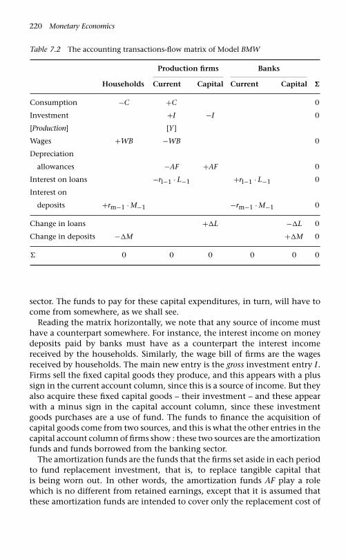
220 Monetary Economics

Table 7.2 The accounting transactions-flow matrix of Model BMW

Production firms Banks

Households Current Capital Current Capital �

Consumption −C +C 0

Investment +I −I 0

[Production] [Y]

Wages +WB −WB 0

Depreciation

allowances −AF +AF 0

Interest on loans −rl−1 · L−1 +rl−1 · L−1 0

Interest on

deposits +rm−1 · M−1 −rm−1 · M−1 0

Change in loans +�L −�L 0

Change in deposits −�M +�M 0

� 0 0 0 0 0 0

sector. The funds to pay for these capital expenditures, in turn, will have tocome from somewhere, as we shall see.

Reading the matrix horizontally, we note that any source of income musthave a counterpart somewhere. For instance, the interest income on moneydeposits paid by banks must have as a counterpart the interest incomereceived by the households. Similarly, the wage bill of firms are the wagesreceived by households. The main new entry is the gross investment entry I .Firms sell the fixed capital goods they produce, and this appears with a plussign in the current account column, since this is a source of income. But theyalso acquire these fixed capital goods – their investment – and these appearwith a minus sign in the capital account column, since these investmentgoods purchases are a use of fund. The funds to finance the acquisition ofcapital goods come from two sources, and this is what the other entries in thecapital account column of firms show : these two sources are the amortizationfunds and funds borrowed from the banking sector.

The amortization funds are the funds that the firms set aside in each periodto fund replacement investment, that is, to replace tangible capital thatis being worn out. In other words, the amortization funds AF play a rolewhich is no different from retained earnings, except that it is assumed thatthese amortization funds are intended to cover only the replacement cost of

A Simple Model with Private Bank Money 221

Table 7.3 The behavioural transactions matrix of Model BMW

Production firms Banks

Households Current Capital Current Capital �

Consumption −Cd +Cs ?

Investment +Is −Id ?

[Production] [Y]

Wages +WBs −WBd ?

Depreciation

allowances −AF +AF 0

Interest on loans −rl−1 · L−1 +rl−1 · L−1 0

Interest on

deposits +rm−1 · M−1 −rm−1 · M−1 0

Change in loans +�Ld −�Ls ?

Change in deposits −�Mh +�Ms ?

� 0 0 0 0 0 0

worn-out capital, whereas retained earnings could be used to finance newadditions to tangible capital. Here, by contrast, any acquisition of fixed capi-tal goods, beyond the amounts required to replenish the existing stock, leadsto an increase in loans of an equivalent amount.1

7.2.3 The behavioural transactions matrix

Because we are now introducing private bank money, no short cut will betaken in the present chapter. Once again, as we did with Model SIM inChapter 3, a fully fledged model is going to be presented, where the supplyand the demand sides of the main variables are distinct from each other. Inorder to do this, we shall once more start off from a behavioural transactionsmatrix, here shown in Table 7.3.

As was the case with Model SIM, the behavioural transactions matrix ofTable 7.3 incorporates suffixes to the main variables. Take the case of the first

1 The introduction of capital depreciation complicates the model somewhat, butadds a great deal of realism. As we shall see, a reduction in the stationary level ofincome requires a smaller stock of capital, but a reduction in the capital stock cannotbe achieved without capital depreciation, unless one assumes the far-fetched possibilityof negative investment output.

222 Monetary Economics

row. Because the demand for consumption goods Cd may be different fromthe sales of consumption goods Cs, the entry in the summation cell carriesa question mark. Until we provide a mechanism explaining how these twovariables turn out to be equal, we cannot be sure that the row sums to zero.Similar question marks arise for the two rows dealing with financial assets. Wemust explain, for instance, why the changes in the supply of loans respond tothe changes in the demand for loans. On the other hand, the rows associatedwith interest payments on loans or on deposits have their summation cellequal to zero. It is rather obvious, for instance, that the interest paymentson deposits made by the banks are by necessity equal to the amounts thatdepositors receive, and no adjusting mechanism is required here.

The behavioural matrix will be particularly useful when we outline theequations that define the model.

7.3 The equations of Model BMW

As mentioned in the previous section, output prices are assumed to remainconstant throughout, to avoid dealing with revaluation complications rightaway. While all variables are expressed in nominal values, these values mayalso be interpreted as real magnitudes, by setting the price level equal to unity.

The model is made up of 19 equations, with 19 variables, excluding theprice variable. These equations can all be seen at a glance in Appendix 7.1.To help handling the system of equations, every variable appears on the left-hand side of an equation. The first four equations describe the mechanismsthat adjust the various supply variables to their demand equivalent. The nextseven equations are drawn from the transactions matrix, while the last eightequations reflect definitions or behaviour.

Once again we start with the four equations that equalize supply todemand.

Cs = Cd (7.1)

Is = Id (7.2)

Ns = Nd (7.3)

�Ls = �Ld (7.4)

Equations (7.1) and (7.2) reflect once more the assumed existence of aninstantaneous quantity adjustment process. Producers supply the consump-tion goods which are being demanded and the investment goods which havebeen ordered. As was explicit in Model 1, equation (7.3) reflects the assump-tion that there is an infinite reserve army of unemployed workers, who areready to work at constant productivity if they are being offered employment,whatever the wage rate. Finally, equation (7.4) reflects the hypothesis that

A Simple Model with Private Bank Money 223

the banks will supply the loans which are being demanded by the firms. Inother words, there is no credit rationing in this model. The supply of loansis whatever the demand for loans is. In this simple world, there is no creditrestrictions, or if there was, it would be reflected in the value taken by theparameter γ in equation (7.18). If production firms knew that some creditrestrictions were existing, they would take this into consideration and wouldadjust more slowly to their targeted stock of capital, thus requesting smalleramounts of loans.

We now move to definitional equations which are implied by the transac-tions matrix, starting with the column of the current account of productionfirms. These definitional equations are given below:

Y = Cs + Is (7.5)

Y = WBd + rl−1 · Ld−1 + δ · K−1 (7.6A)

WBd = Y − rl−1 · Ld−1 − δ · K−1 (7.6)

Total gross production is defined in the standard way used in all nationalaccounts, as the sum of all expenditures on goods and services, here con-sumption and investment goods, as shown in equation (7.5), or as thesum of all payments of factor income, as shown in equation (7.6A). Fac-tor income is made up of three components: the wage bill, the amortizationfunds, and the interest payments of firms on their debt.2 While the wagebill and the interest payments of firms are fairly straightforward, we needto say a bit more about AF – the amortization funds. We shall assumethat these amortization funds are a constant proportion δ of the value ofthe stock of tangible capital at the beginning of the current period. Thuswe write:

AF = δ · K−1 (7.7)

For the purpose of the model, equation (7.6) rather than equation (7.6A) isthe relevant one. It says that, in the present model, the wage bill is a residual.With a given unit price, and a certain level of production, the wage bill mustbe what is left once amortization funds and the interest payments to thebanks have been taken care of. These are set at the beginning of the period,for a given rate of interest on loans, since the stock of debt L−1 and the stockof capital K−1 are given by history.

We still remain with the identities of the firm sector in the transactionsmatrix. Equation (7.8) is the budget constraint of the capital account of the

2 We could say, in broad terms, that the interest payments and the amortizationfunds constitute the profits of the economic system, but the net ‘profits’ – net of interestand amortization – are zero.

224 Monetary Economics

production sector. Since firms make no net profits – amortization funds onlyfinance the replacement of used-up capital – net investment must be entirelyfinanced by loans obtained from the banking sector.

�Ld = Id − AF (7.8)

The transactions matrix also yields the definition of income relevant tohouseholds. Equation (7.9) defines the disposable income of households.Since there is no government and no taxes, the disposable income ofhouseholds is simply the sum of their wages and the interest payments thatthey receive on their deposits. It may be noted that household disposableincome YD is different from national income, because of the presence ofdepreciation allowances in the definition of gross domestic product Y .

YD = WBs + rm−1 · Md−1 (7.9)

The budget constraint of the household sector is shown in equation (7.10).In this simplified world, whatever income is not spent on consumption goodsis added to the existing stock of bank deposits. Equation (7.10) describes thewealth accumulation function of households.

�Mh = Mh − Mh−1 = YD − Cd (7.10)

Finally, equations (7.11) and (7.12) reflect respectively the capital accountconstraint and the current account constraint of the banking sector. Bankshave a single asset – bank loans – and a single liability – bank deposits. Thereare no bonds, no central bank reserves, and private banks do not accumulatecapital reserves since they have been assumed to make zero profits. As a result,the supply of bank money must be precisely equal to the supply of bank loans,and the rate of interest on deposits must be set equal to the rate of intereston loans.

�Ms = �Ls (7.11)

rm = rl (7.12)

We next move to three definitions related to the wage bill. Equation (7.13)makes the obvious definition of the wage bill, as the product of the wagerate times the level of employment. Equation (7.14) tells us what the levelof employment will be, given the production level Y . Recall that Y repre-sents both a nominal magnitude and real production, since the price levelhas been set equal to one. We assume, again for simplicity, a linear rela-tionship between production and employment. The parameter pr represents

A Simple Model with Private Bank Money 225

labour productivity, being equal to output per unit of labour.3 Finally,equation (7.15) tells us what the wage rate is, both in nominal and real terms,since, as already pointed out, the price level is a constant set equal to unity.Given the wage bill, as it appears in equation (7.6), and given the level ofemployment, as implied by equation (7.14), the real wage is determined byequation (7.15). More will be said about this in a later section.

WBs = W · Ns (7.13)

Nd = Ypr

(7.14)

W = WBdNd

(7.15)

We now move to the equations that have some link with the behaviourof the various agents. We start with the behaviour of households,namely their consumption behaviour. The proposed consumption function,equation (7.16), is slightly different from the one that we have used in allprevious models. An autonomous term has been added to our standard con-sumption function. Hence, as before, there are two induced terms, thosethat depend on current disposable income and past accumulated wealth.But consumption depends also in part on an exogenous element. It is thisautonomous component of consumption that will allow our model to remaindeterminate. Otherwise, if consumption were fully induced, there would beno anchor to the model since investment expenditures are also induced, andas we shall see, converge to zero near the stationary state. It turns out thatthe exogenous term α0 in the consumption function of our private moneymodel plays the role of the exogenous government expenditures G, in theclosed models with government money.

Cd = α0 + α1 · YD + α2 · Mh−1 (7.16)

The investment behaviour of firms is dealt with in the next equations.Equation (7.17) is another definition. It recalls that the change in the stockof fixed capital is equal to gross investment in fixed capital Id minus thestock of machines used up during the current period through wear, tear andobsolescence – depreciation allowances – which we note as DA. Normally, amachine would wear out after a certain number of years of use, and so thedepreciation allowance used to compute net investment should depend onthe exact time-path of past investments. For instance, if all machines weredesigned to last for 20 years, with normal use and maintenance, the precise

3 In mainstream terms, both the marginal and the average products of labour areconstant.

226 Monetary Economics

amount of disinvestment, that is, the precise number of machines vanishingfrom the existing tangible capital stock would equal the exact number ofmachines that were put into service 20 years before.

We shall assume otherwise however. For simplicity we shall assume thata constant proportion of the existing stock of machines either wears out orbecomes obsolescent. Thus we have a constant rate of depreciation δ. This rateis applied to the stock of machines existing at the beginning of the currentperiod, which is the stock of machines that ended up remaining at the end ofthe previous period, K−1,, and hence depreciation allowances shall be definedas in equation (7.18). Comparing equations (7.18) and (7.7), it should beobvious that we are assuming, for simplicity once again, that amortizationfunds and depreciation allowances are exactly equal. The funds that firmsset aside to replace their used-up capital is just equal to the amount that isnecessary to replace used-up capital. Combining equations (7.17) and (7.18),we obtain equation (7.18A), which says that the stock of machines at the endof the current period is equal to the stock of capital at the beginning of thecurrent period, plus net investment.

K = K−1 + (Id − DA) (7.17)

DA = δ · K−1 (7.18)

K = (1 − δ) · K−1 + Id = K−1 + (Id − δ · K−1) (7.18A)

Continuing with investment behaviour, equation (7.19) below is sayingthat production firms target a certain capital stock KT. This targeted capitalstock depends on the sales achieved in the previous period. The implicitassumption made here is that entrepreneurs, when they decide on theirorders of investment goods, see overall sales of the previous period as theindicator of the overall sales in the coming period, and attempt to maintaina normal rate of utilization of their capacity.4

KT = κ · Y−1 (7.19)

Finally, there is the investment function itself. The proposed investmentfunction is quite standard: it is the partial adjustment accelerator model.Equation (7.20) says that net investment adjusts partially (γ < 1) to the dis-crepancy between the targeted capital stock KT and the stock of machinesthat was inherited from the end of the previous period. Gross investment Idis the sum of that net investment plus the investment required to replace theused-up machines. When the past stock of machines is larger than the tar-geted stock, gross investment will be smaller than replacement investment,

4 If Y−1 = YN, the normal output, then the capital to full capacity ratio will be κ ·uNwhere uN is the normal rate of capacity utilization.

A Simple Model with Private Bank Money 227

in which case net investment will be negative. Of course, the model must beso constrained that gross investment cannot be negative. Its minimum valueis zero.5

Id = γ · (KT − K−1) + DA (7.20)

The last equation of the model is the equation defining the rate of intereston loans. Because we have a degree of freedom left, the rate of interest onloans can be set by the banking system, at the level that it sees fit. The rateof interest on loans is not the result of a market-clearing price mechanism.

rl = rl (7.21)

As should be the case in all coherent models, there is a redundant equation,which can be deduced from the other equations of the model, but whichneed not to be included within the model, for otherwise it would be over-determined. This equation can be deduced from the all the conditions thathave been imposed on our behavioural transactions matrix. Because we havefound the mechanisms that insure that all the columns and rows, but one,of the behavioural transactions matrix must sum to zero, we know that thelast row must sum to zero as well, despite the absence of such an explicitmechanism for this last row. Here the last row is that of the changes in bankdeposits. The redundant equation is:

�Mh = �Ms (7.22)

There are two distinct processes that explain the issue of new bank depositsby the banking system on the one hand (equation 7.11), and the additionalamount of bank deposits that households decide to hold on the other hand(equation 7.10). By virtue of the tight accounting of the model, these twoprocesses must yield the same answer, without any equilibrium conditionbeing imposed.

7.4 The steady state

7.4.1 Income in the steady state

We now explore the steady-state solutions of our model. Because the modelis so simple, it is possible to obtain analytically the steady-state solutionsof the main variables. The steady state here is a stationary state, with nogrowth. This implies that, in the steady state, net investment is zero whilegross investment is equal to depreciation allowances, and household savingis also zero. This insures, as in our previous models of a closed economy,

5 More will be said about this in a later section.

228 Monetary Economics

that there is no asset accumulation in the steady state, so that stocks do notchange while flows are kept constant.

The fact that household saving is zero in the steady state implies that oncethis state has been reached, household consumption must be equal to dis-posable income, as can be ascertained from the transactions matrix. Thus inthe steady state, the consumption function (7.16) can be rewritten as:

YD∗ = α0 + α1 · YD∗ + α2 · M∗h (7.23)

where the stars denote steady-state values. There is no need to incorporatea time suffix to the money variable Mh, since in the steady state the valuetaken in the current period is the same as that of the previous period.

Another substitution can be made. In the steady state, net investment iszero, which implies, from equation (7.20), that the target level of capital isequal to the achieved stock of capital. This implies that KT∗ = K∗. But we alsoknow from the balance sheet matrix of Table 7.1 that, in our simple model,the wealth of households must never be different from the stock of tangiblecapital. The stock of wealth of households is entirely composed of moneydeposits. This implies that the following equality must hold at all times:

Vh = Mh = K (7.24)

From equation (7.19), we also know that in the steady state the followingequality will hold:

KT∗ = κ · Y∗ (7.25)

so that equation (7.23) can be rewritten as:

YD∗ = α0 + α1 · YD∗ + α2 · κ · Y∗ (7.26)

Before we can find the steady-state value of disposable income YD∗, weneed to establish the relationship between gross domestic product Y andhousehold disposable income YD. In the case of our model, with the vari-ous conditions imposed, the difference is simply that the second variable isequivalent to net domestic product rather than gross domestic product. Thedifference then is the amount of capital depreciation. We may thus write:

Y = YD + δ · K−1 (7.27)

In the steady-state, the previous, current and target stocks of wealth are allequal. Thus, with the help of equation (7.25), we can rewrite equation (7.27)in its steady-state version:

Y∗ = YD∗ + δ · κ · Y∗

A Simple Model with Private Bank Money 229

so that we have:

Y∗ = YD∗(1 − δ · κ)

(7.28)

Substituting equation (7.28) into equation (7.26), we obtain the steadystate value of disposable income:

YD∗ = α0(1 − δ · κ)

(1 − α1) · (1 − δ · κ) − α2 · κ(7.29)

and from there the value of the gross domestic product:

Y∗ = α0(1 − α1) · (1 − δ · κ) − α2 · κ

(7.30)

Obviously, for these values to be positive, there must be some restrictionson the values taken by the various parameters. For gross domestic product Y∗to be positive, its denominator needs to be positive, which implies that thepropensities to consume out of disposable income and out of wealth need tobe small enough. Similarly, the target capital to income ratio κ and the rate ofdepreciation of capital δ cannot be too large.6 Thus, the model makes senseonly if the following restriction on the values taken by the various parametersis fulfilled:

(1 − α1)

α2>

κ

(1 − δ · κ)(7.31)

In words, the ratio of the households’ marginal propensity to save outof disposable income to the marginal propensity to consume out of wealthneeds to be large enough compared to the values taken by the other(production) parameters of condition (7.31).7

7.4.2 The paradox of thrift recovered

A quick look at equation (7.30) is enough to verify the factors that have noimpact and those that have an impact on the steady state level of income(and employment). It is remarkable that the rate of interest on deposits orloans has no impact whatsoever on the steady state level of income. Neitherdoes the real wage level. This result is quite obvious, since the target level ofcapital is the result of a straightforward accelerator mechanism, which does

6 Obviously, in the simplified case without depreciation, δ = 0, and equation (7.30)simplifies to: Y∗ = α0/(1 − α1 − α2 · κ), while condition (7.31) below becomes: κ <

(1 − α1)/α2 = α3. The target capital to sales ratio set by firms must be smaller than thetarget wealth to disposable income set by households.

7 This implies, if κ = 2 for instance, that the propensity to save out of disposableincome must be more than twice the propensity to consume out of wealth.

230 Monetary Economics

not depend on the rate of interest being charged on loans, as could be seenfrom equation (7.19). In addition, there is a single propensity to consume outof disposable income, whether this income comes from wages or from interestrevenue. Similarly, it may noticed that the γ parameter of the investmentfunction (7.20), which represents the reaction speed of entrepreneurs whenfacing any discrepancy between the target and the actual capital stock, doesnot determine the steady state level of income.

Equation (7.30) shows quite clearly the role played by the α0 param-eter, which represents autonomous consumption expenditures. Theseautonomous consumption expenditures play the role previously played bygovernment expenditures. They are the multiplicand of the model. Themultiplier depends on the values taken by the propensities to consume α1and α2, the target capital to income ratio κ, and the depreciation rate δ. Itis obvious that the higher any of these parameters, the higher the steadystate level of income, for a given amount of autonomous consumptionexpenditures.

Post-Keynesian authors have long underlined the role played byautonomous demand. The exogenous component of demand was of courseemphasized by Keynes himself, but his followers have been struck by thekey role that it plays in modern economies (Godley and Cripps 1983;Davidson 1994). Kaldor (1983: 9) has argued that, precisely because ofautonomous demand, a capitalist economy is not necessarily self-adjusting.An increase in potential output will not ‘automatically induce a corre-sponding growth of actual output. This will only be the case if exogenousdemand expands at the same time to the required degree; and this cannot betaken for granted ...’. In our model, α0 represents the autonomous compo-nent of demand. Figure 7.1 illustrates the obvious fact that any increase inautonomous consumption α0 leads to an increase in disposable income andin overall consumption.

Figure 7.1 also illustrates the cyclical dynamics generated by investmentbehaviour. Income or disposable income overshoot their new steady statevalues because the increase in output during the transition induces posi-tive net investment in fixed capital, these investments being made to insurethat future capacity stays in line with expected demand. When the econ-omy approaches its new steady state, net investment falls back towards zero,and as a result national income and disposable income drop below the val-ues attained during part of the transition. Figure 7.2 illustrates the cyclicalbehaviour of investment, as generated by the accelerator equation. In theinitial steps of the transition, net investment quickly moves up, first as a reac-tion to the increased sales induced by the hike in autonomous consumptionexpenditures, and then by the increased investment expenditures needed toreplace the worn-out machines of the growing stock of capital; eventuallyhowever, net investment falls to zero, and all investment is replacementinvestment.

231

1950 1955 1960 1965 1970 1975 1980 1985 1990 1995 2000

200.0

205.0

195.0

190.0

185.0

180.0

Disposable income

Consumption

Figure 7.1 Evolution of household disposable income and consumption, followingan increase in autonomous consumption expenditures, in Model BMW

1951

24.00

23.25

22.50

21.75

21.00

20.25

1956 1961 1966 1971 1976 1981 1986 1991 1996 2001

Gross investment

Replacement investment(capital depreciation)

Figure 7.2 Evolution of gross investment and disposable investment, following anincrease in autonomous consumption expenditures, in Model BMW

232 Monetary Economics

The positive impact of a higher propensity to consume on the steady statelevel of income is also worthy of being noted. In Model SIM of Chapter 3,an increase in the propensity to consume only had a temporary positiveimpact on national income, and no impact whatsoever on the steady statelevel of income. In Model PC of Chapter 4, an increase in the propensity toconsume had a negative impact on the steady state level of income. Theseresults contradicted the famous paradox of thrift, that had been highlightedby Bernard Mandeville in his famous Fable of the Bees and by Keynes in hisGeneral Theory. In the model with private money and no government thatis developed in the current chapter, the paradox of thrift is recovered. Anincrease in thrift, that is, an increase in the propensity to save out of currentincome or out of wealth will reduce the current level of income as well as thesteady state level of income.

What occurs is that the reduction in consumption reduces income, whichleads in the next period to a reduction in the target stock of fixed capital,and in investment. In the end, provided the model is stable, the lower stockof tangible capital will be associated with lower financial wealth on the partof households, and this will generate a lower stationary level of income. Allthis is shown in Figure 7.3. Starting from a stationary state, it is assumed thata campaign of thrift is successful, so that households decide to decrease per-manently their propensity to consume out of disposable income. The figureshows the negative impact on gross domestic income and disposable income,both at the beginning of the thrift campaign and in the new stationary state.

1950

180.0

177.0

174.0

171.0

168.0

165.01955 1960 1965 1970 1975 1980 1985 1990 1995 2000

Consumption

Disposable income

Figure 7.3 Evolution of household disposable income and consumption, followingan increase in the propensity to save out of disposable income, in Model BMW

A Simple Model with Private Bank Money 233

7.4.3 Capital and the money stock in the steady state

We have not yet discussed the values taken by tangible capital and moneydeposits. From the balance sheet of Table 7.1, we know that all times K =Mh = L. Therefore, it must be the case that K∗ = M∗

h in the stationary state.However, this equality is not an obvious one, since capital accumulation andthe accumulation of financial assets appear to be determined by two entirelydifferent processes. In the case of capital accumulation, we have already seenwith equation (7.25) that:

KT∗ = K∗ = κ · Y∗ (7.25)

so that in the steady state the amount of tangible capital, followingequation (7.30), must be equal to:

K∗ = κ · α0(1 − α1) · (1 − δ · κ) − α2 · κ

(7.32)

Seen from the household point of view, the accumulation of financial assetsseems to follow a completely independent path. We know that in the station-ary state C∗ = YD∗ and Mh = Mh−1, so that, from the consumption function,equation (7.16), we obtain:

M∗h =

{(1 − α1)

α2

}· YD∗ − α0

α2(7.33)

Equations (7.32) and (7.33) appear to be entirely different determinants ofwealth. Still, the endogenous values of Y∗ and YD∗ will be such that K∗ = M∗

h.

7.5 Out-of-equilibrium values and stability analysis

7.5.1 Out-of-equilibrium values

As we pointed out in Chapter 3, a key question is whether the solution ofthe model, when it exists, will ever be attained if the economy starts awayfrom it. This is the issue of stability. To study it, we must first obtain theout-of-equilibrium values for the two main variables – the level of incomeand the stock of wealth. We can proceed in a way which at first is similar tothat followed when we searched for the stability conditions of Model SIM inChapter 3. That is, we identify a difference equation for the stock of tangiblecapital, and another one for the income level.

The difference equation for the stock of capital is fairly simple toobtain. We simply combine the relations relevant to investment behaviour,

234 Monetary Economics

equations (7.17) to (7.20), to obtain:

K = (1 − γ ) · K−1 + γ · κ · Y−1 (7.34)

The present capital stock (or money balances, since, by equation (7.27),these need to be the same), is a function of the stock of tangible capital andincome level from the previous period.

Let us now find the difference equation relevant to the gross nationalproduct. By combining equations (7.5), (7.16) and (7.20), that is by makinguse of the fact that gross national product is the sum of consumption andinvestment expenditures, we obtain present income as a function of presentdisposable income, past wealth, the past stock of tangible capital, and thecapital stock target.

Y = α0 + α1 · YD + α2 · Mh−1 + γ · (KT − K−1) + δ · K−1

Recalling equations (7.19), (7.24) and (7.27), that is, recalling that thetarget stock of capital depends on the realized income level of the previousperiod, that the gross domestic product is disposable income plus the depre-ciation allowances, and that the held money balances are exactly equal to thevalue of tangible capital, the above equation becomes equation (7.35), whichdescribes national income in the current period as a function of nationalincome and of the stock of capital of the previous period.

Y = α0 + {(1 − α1) · δ + (α2 − γ )} · K−1 + γ · κ · Y−1(1 − α1)

(7.35)

This is the second of our two difference equations. Thus given the capitalstock of the previous period, and the level of income that was achieved in theprevious period, it would be possible to figure out the income level and themoney balances held in the next period, if all parameters, given variables andreaction coefficients were to remain the same. Starting from some randomposition, it is thus possible, with the help of equations (7.34) and (7.35),to follow the path taken by the economy in all these out-of-equilibriumpositions.

7.5.2 Stability conditions

Now things are more complicated than they were when the stability of ModelSIM was studied in Chapter 3, because there current income was only a func-tion of previous wealth, so that everything could be brought back to a singleequation in one variable. Here, current income is also a function of its pastvalue. So what we have is a system of two difference equations, with twovariables, both based on the past value taken by each variable. Thus we have

A Simple Model with Private Bank Money 235

a recursion with two variables, which in general could be written as:

zt = A · zt−1 + c (7.36)

where z is a vector of two variables (here capital and income), while A is amatrix of coefficients and c is a vector that represents the constant terms.

In the matrix form given by (7.36), the two recursion equations (7.34) and(7.35) may thus be written as:

[K

Y

]=

⎡⎢⎣

1 − γ γ κ

(1 − α1)δ + (α2 −γ )

1 − α1

γ κ

1 − α1

⎤⎥⎦

[K−1

Y−1

]+

⎡⎣ 0

α01 − α1

⎤⎦

The stability conditions are more difficult to handle in the case of differenceequations than they are in the case of differential equations.8 Let us first usethe following notation to represent the two-variable system,

A =[

a11 a12

a21 a22

]

The determinant of the system is:

detA = a11 · a22 − a21 · a12;

the trace is:

trA = a11 + a22;

the discriminant is:

� = (trA)2 + 4 · detA.

The system is unstable if the absolute value of the determinant is equal toor greater than one (|detA| ≥ 1). A necessary condition for stability is thus thatthe absolute value of the determinant be less than unity. In the case of ourmodel, stability requires the following condition:

(1 − α1) >(1 − α2)γ κ

(1 + δγ κ)(7.37)

8 See Gandolfo (1977: 136–9, 273–9) for more precise conditions in the case ofdifference and differential equation systems respectively.

236 Monetary Economics

If this is verified, then the system will be stable whenever the discriminantis non-negative (� ≥ 0). But this is difficult to verify with algebraic values,because of the squared term of the discriminant. In addition, the system canbe stable with a negative discriminant, provided the trace is smaller than2 (trA < 2), if and only if −detA < 1 − |trA|. It is not obvious that the lattercondition would be fulfilled at all times in our model. But assuming that theparameters are such that this condition is realized, the only remaining issuewould be whether the trace is sufficiently small, that is smaller than 2 as saidabove, and thus stability may also involve the following condition:

(1 − α1) >γ · κ

(1 + γ )(7.38)

Condition (7.38) essentially says that the model converges to its sta-ble solution provided the propensity to save is larger than the product ofthe capital/output ratio κ and the γ reaction parameter, with the prod-uct being deflated by (1 + γ ). This is a classic result with this kind of amodel based on an accelerator theory of investment.9 Had we dealt withdifferential equations instead, condition (7.38) would have been a necessaryand sufficient condition for stability, since the other condition for stabilityin a differential system is identical to the existence condition, as definedin (7.31).10

The lesson to be drawn from this stability analysis, by looking at bothconditions (7.37) and (7.38), is that some weighted product of the target cap-ital to output ratio κ and the reaction parameter γ need be small enough,compared to the saving ratio on disposable income. When working capital isconsidered, that is, inventories of finished goods, the capital to output ratio isrelatively small, much smaller than unity, so that firms are often assumed torespond quite quickly to any discrepancy between the existing stock of inven-tories and the desired stock (the γ parameter may be near unity). By contrast,when fixed capital is taken into account, this involves capital to output ratiosthat are much larger than unity, around 3 perhaps; if models based on some

9 The accelerator model, and its more general variant – the capital stock adjustmentmodel – are studied in great detail in many works, in particular Gandolfo (1977). Wedo not attempt to find out how the model is approaching its long run solution. Inother words, we do not attempt to find the parameter values that will guarantee thatthe model converges without exhibiting oscillations. Our simulations will demonstratewhether the chosen parameter values lead or not to oscillations. For instance, when γ

is moved up from 0.15 to 0.25, the model converges but oscillates.10 In other words, in a system of differential equations, condition (7.31) corre-

sponds to the stability condition that the determinant of the system be positive, whilecondition (7.38) corresponds to the stability condition that the trace be negative.

A Simple Model with Private Bank Money 237

Table 7.4 Stability conditions

Eq. (7.31) Eq. (7.37) Eq. (7.38)α1 α2 γ κ δ Existence Determinant Trace

BMW model 0.75 0.10 0.15 1 0.10 0.25 > 0.111 0.25 > 0.133 0.25 > 0.130

Gandolfo 0.75 0.10 0.10 3 0.10 0.25 < 0.428

Alternative 0.75 0.10 0.10 2 0.10 0.25 = 0.25 0.25 > 0.176 0.25 > 0.182

Alternative 0.75 0.10 0.15 1.916 0.10 0.25 > 0.237 0.25 < 0.251 0.25 = 0.25

form of the accelerator are to yield stable solutions, one needs to assumethat entrepreneurs are responding slowly to any discrepancy between actualand desired capacity (the γ parameter has to be a small percentage). Indeed,Gandolfo (1977: 157) claims that empirically, ‘the value of the reaction coeffi-cient has been found to be normally about 0.10’. This is only partly reassuringregarding whether conditions (7.37) and (7.38) are normally fulfilled, becauseeven when γ = 0.10, the required conditions are rather stringent, as can beseen in Table 7.4 above.11

Our BMW model is set up in such a way that all conditions are fulfilled.Introducing a target capital output ratio of 3 in that model would negate theexistence condition. Jacking up the reaction parameter of producers in sucha way that the trace condition is respected could still leave the existencecondition unfulfilled. And finally, in the last line of Table 7.3, we have acase where the determinant condition only would go unfulfilled if the targetcapital to output ratio were raised sufficiently.

7.5.3 An approximate and intuitive stability condition

Condition (7.38) is the result of the simultaneous interaction of two differ-ence equations. If one only wishes to get some estimate of the conditionrequired for stability, then one may use a short-cut. An approximate stabilitycondition – a partial equilibrium stability condition so to speak – can be eas-ily obtained by following a method put forth by Keynesian economists. Thetrick is that a model should be stable if saving reacts more strongly to changesthan does investment. Here for instance, investment reacts to a change inincome through the target capital stock. Similarly, any change in disposableincome will also induce a change in saving. Thus in general, a model is stableprovided dSAV/dY > dI/dY , where SAV represent saving (if positive solutionsexist). We must thus compare how the investment function and the savingfunction react to a change in income.

11 Readers may wish to derive more intuitive results by assuming that δ = 0.

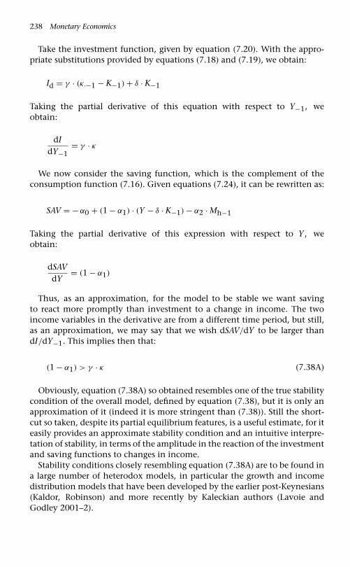
238 Monetary Economics

Take the investment function, given by equation (7.20). With the appro-priate substitutions provided by equations (7.18) and (7.19), we obtain:

Id = γ · (κ·−1 − K−1) + δ · K−1

Taking the partial derivative of this equation with respect to Y−1, weobtain:

dIdY−1

= γ · κ

We now consider the saving function, which is the complement of theconsumption function (7.16). Given equations (7.24), it can be rewritten as:

SAV = − α0 + (1 − α1) · (Y − δ · K−1) − α2 · Mh−1

Taking the partial derivative of this expression with respect to Y , weobtain:

dSAVdY

= (1 − α1)

Thus, as an approximation, for the model to be stable we want savingto react more promptly than investment to a change in income. The twoincome variables in the derivative are from a different time period, but still,as an approximation, we may say that we wish dSAV/dY to be larger thandI/dY−1. This implies then that:

(1 − α1) > γ · κ (7.38A)

Obviously, equation (7.38A) so obtained resembles one of the true stabilitycondition of the overall model, defined by equation (7.38), but it is only anapproximation of it (indeed it is more stringent than (7.38)). Still the short-cut so taken, despite its partial equilibrium features, is a useful estimate, for iteasily provides an approximate stability condition and an intuitive interpre-tation of stability, in terms of the amplitude in the reaction of the investmentand saving functions to changes in income.

Stability conditions closely resembling equation (7.38A) are to be found ina large number of heterodox models, in particular the growth and incomedistribution models that have been developed by the earlier post-Keynesians(Kaldor, Robinson) and more recently by Kaleckian authors (Lavoie andGodley 2001–2).

A Simple Model with Private Bank Money 239

7.5.4 An additional condition to achieve smoothly the steady state

Achieving steady states requires an additional condition however. Whenparameters are such that the new stationary capital stock is higher thanbefore, no additional condition is needed. But when the new stationary levelof capital is lower than before, the new stationary state will be achieved byhaving negative net investment. Under such circumstances, part of the used-up capital will not be replaced. In other words, replacement investment willbe below disinvestment – what we called depreciation allowances.

Still, while net investment can be negative when firms decide not to replaceall the tangible capital stock that has vanished because of obsolescence andwear and tear, gross investment can never be negative. Gross investmentmust thus be zero or a positive amount. Putting together equations (7.17A)and (7.19), we obtain the following condition:

(γ − δ) ·(

K−1Y−1

)≤ γ · κ (7.39)

Obviously, such a condition is always fulfilled when the γ parameter issmaller than the δ parameter. In words, this means that gross investmentwould never become negative provided the percentage of the gap betweenthe target and the existing stock of capital that the entrepreneurs wish toclose in every period is smaller than or equal to the percentage of tangiblecapital that gets used up in every period. Otherwise the following conditionhas to be fulfilled:

Y−1K−1

>(γ − δ)

(γ · κ). (7.40)

What this means is that, when the economy takes a negative shock, theshock needs to be not too large and the rate of capacity utilization mustnot fall below a certain level, for otherwise entrepreneurs would wish for anegative amount of gross investment. This would induce a forced adjustmentin the γ parameter. The new steady state would still eventually be reached, butthe parameter structure of the model would need to be changed, to take intoaccount the non-negative constraint on gross investment. In other words,the desired negative adjustment to the capital stock could not be achieved.This could be handled in a simulation package, and it would introduce non-linearities.

In the meantime, Figure 7.4 illustrates the evolution of the output tocapital ratio (Y/K−1), which is some proxy of the rate of utilization ofcapacity, following a decrease in the propensity to consume, which, as wealready know, entails a negative shock on the economy. As can be seenfrom Figure 7.4, the recession generated by the increase in the propensityto save is accompanied by a drop in the rate of capacity utilization, but as

240 Monetary Economics

1951

1.0000

0.9875

0.9750

0.9625

0.9500

0.9375

1956 1961 1966 1971 1976 1981 1986 1991 1996

Output to capital ratio(a proxy for the output

to capacity ratio)

Figure 7.4 Evolution of the output to capital ratio (Y/K−1), following an increase inthe propensity to save out of disposable income, in Model BMW

the economy goes towards its new steady state, the output to capital ratiogoes back to its desired level, and hence the rate of utilization goes back toits initial level.

7.6 The role of the rate of interest

7.6.1 The rate of interest and the real wage

Having shown that the model converges to its solution, at least for somerestricted set of parameter values, we may now pursue further the question ofcomparative statics. In section 7.4.2, it was already pointed out that the para-dox of thrift had been recovered, both in the short run and while comparingsteady states. However, it was also pointed out that the rate of interest had noimpact whatsoever, neither on the short-run solution nor on the steady stateone. This was attributed mainly to the fact that the rate of interest had noimpact on the target stock of capital (i.e. on the target capital/output ratio)and was not a component of the consumption function. It is now time toreconsider the latter assumption.

However, before we do so, it is interesting to study the relationship in themodel between prices, interest rates, and real wages. This will give rise toa version of the famous wage/profit frontier which has been developed byclassical economists, and which underlines the possible conflict over incomedistribution between wage recipients and profit-recipients, in the present caseinterest-recipients. It will also allow us to note the lack of realism of thesimple model without residual profits which has been suggested here, which

A Simple Model with Private Bank Money 241

will lead us in future chapters to propose a pricing behaviour which is morereasonable and more realistic.

Let us recall the equations which define the real wage:

WBd = Y − rl · Ld−1 − δ · K−1 (7.6)

WBs = W · Ns (7.13)

Nd = Ypr

(7.14)

W = WBdNd

(7.15)

Ns = Nd (7.3)

The last of these five equations shows that we can ignore the distinctionbetween Ns and Nd, and WBs and WBd. Combining equations (7.13) and(7.14), we equalize the two expressions of the wage bill, seen from the supplyand the demand side:

Y − rl · Ld−1 − δ · K−1 = W · Ypr

so that, recalling that at all times L = K, we have:

W = pr{

1 − (rl + δ) ·(

K−1Y

)}(7.41)

It is now obvious that the real wage is directly proportional to the produc-tivity of labour, measured by pr, and that it is inversely related to the rate ofinterest on loans, the rate of depreciation of capital, and to the capital/outputratio of the period. Thus, for a given productivity of labour, the higher the rateof interest, the rate of depreciation, and the capital/output ratio, the lowerthe real wage must be. The evolution of the real wage rate, as represented byequation (7.41) is illustrated in the case of an increase in the propensity tosave, with the help of Figure 7.5. As we saw with Figure 7.4, the slowdown inthe economy induces a temporary reduction in the rate of capacity utiliza-tion, more precisely in the Y/K−1 ratio. This means a temporary increase inthe K−1/Y ratio and hence a reduction in the real wage rate W . By contrast,in the steady state, the real wage takes a specific constant value, for in thesteady state the actual capital/output ratio is the target capital/output ratio.Formalized, this implies that the steady-state real wage is equal to, as shownin Figure 7.6:

W∗ = pr{1 − (rl + δ) · κ} (7.42)

242 Monetary Economics

1954 1958 1962 1966 1970 1974 1978 19861982 1990 1994 1998

0.7050

0.7125

0.6975

0.6900

0.6825

0.6750

Real wage rate

Figure 7.5 Evolution of the real wage rate (W), following an increase in the propensityto save out of disposable income, in Model BMW

rl

W *

δκ

δκ

κ

Figure 7.6 The relationship between the real wage and the interest rate on loans

It may be noted that equations (7.41) and (7.42) represent the classicalwage/profit frontiers, the latter one being the steady state wage/profit fron-tier. The wage/profit frontier illustrates the negative relationship which isnecessarily said to exist between the real wage and the rate of profit. Here,since there is no net profit, the relationship exhibited by equations (7.41) and(7.42) is the negative relation between the real wage and the rate of interest.An increase in one must lead to the reduction of the other, all other thingsequal. In other words, the increase in interest payments must necessarily leadto a fall in the wage bill and in the real wage. This is in perfect symme-try to the arguments that were made by neo-classical authors and that were

A Simple Model with Private Bank Money 243

rl +

(K–1/Y)max

10

0.10

5

0.20δ

Figure 7.7 The maximum capital to output ratio that can be attained during thetransition, for a given interest rate on loans

criticized by Keynes in The General Theory, according to which ‘profits willnecessarily go up because wages have gone down’ (Keynes 1936: 258). As wehave seen with equations (7.30) and (7.35), the interest rate has no impacton either short-run income or its steady state value, although it reduces thereal wage.

The relationship between the real wage and the rate of interest on loansintroduces another constraint on the values that can take the various param-eters and variables, both in the steady state and during any transition pathtowards the steady state. Since the real wage is a residual, the real wage is anendogenous variable that depends on the values taken by the other parame-ters and variables. The real wage however, just like gross investment, cannotbe negative. In the steady state, as illustrated in Figure 7.7, the rate of inter-est on loans cannot be larger than a certain value, such that the maximumsteady-state rate of interest on loans is:

rl−max = (1 − κ · δ)

κ(7.43)

Thus, the larger the target capital to output ratio, and the greater the rateof capital depreciation, the smaller the maximum level of the rate of interest(here the real rate, since price inflation has been assumed away).

Similar limits can be imposed when the economy has not yet reached thesteady state. The conditions imposed by the fact that the wage rate cannotfall to zero can be drawn from equation (7.42). Considering now the rate ofinterest on loans and the rate of depreciation as given variables, let us seewhat maximum value can be taken by the capital to output ratio in any timeduring the transition path. The real wage rate will not fall to zero providedthe following condition is fulfilled:(

K−1Y

)max

= 1(rl + δ)

(7.44)

244 Monetary Economics

Thus the larger the rate of interest and the rate of depreciation, the smallerthe maximum value that can be taken during the transition by the capital tooutput ratio. This relationship is illustrated with the help of Figure 7.7. Thecurve drawn there is a rectangular hyperbola. If the sum of the rate of interestand the rate of depreciation doubles, the maximum capital to output ratio ishalved. This implies, once more, that for the model to make sense, negativeshocks on the economy cannot be too large, for otherwise they would propelthe utilization of capital to very low rates. As a result of these very low rates,firms would be unable to pay their workers, for interest payments on theirdebt would be so large, relative to production, that they would take over theentire national product. In the real world, such circumstances are unlikely,but equation (7.41) clearly shows that real wages are under threat when-ever real interest rates rise, whenever capital becomes rapidly outmoded,and whenever there is a fall in production relative to the existing stock ofcapital.

7.6.2 The interest rate and the mark-up

Now, what is the relationship between these wage–profit frontiers and themark-up pricing formula? Students who are familiar with the post-Keynesianor Kaleckian literature know that prices there are often expressed as a mark-upover unit costs. In the simplest models, prices are said to arise from a mark-upover unit labour costs, more precisely their variable unit labour costs. Firmshave their accountants compute these unit costs, and multiply the found unitcost by some conventional constant to arrive at prices. Formally we have:

p = (1 + ϕ) ·(

Wpr

)(7.45)

where p is the price and ϕ is the percentage costing mark-up on unit labourcosts W/pr.

Our model has a peculiar feature, however, which is that it is assumedthat prices are equal to unity, that is, p = 1 at all times. This assumptionwas made, it may be recalled, to avoid all the complications associated withprice re-evaluations. However, because of the fixed prices assumption, it fol-lows that the real wage, starting from the mark-up equation (7.45), can berewritten as:

W = pr(1 + ϕ)

(7.46)

We thus have two equations that determine the real wage: equation (7.41)which follows from the structure of the model, and equation (7.46), whicharises from a mark-up procedure. Combining these two equations, we obtain

A Simple Model with Private Bank Money 245

the value of the mark-up:

ϕ =(rl + δ) ·

(K−1Y

)

1 − (rl + δ) ·(

K−1Y

) (7.47)

In the present model, the mark-up is not a constant, it is an endogenousvariable, which depends on the exact value taken by the capital/output ratio.This result lacks realism, of course, because we need to assume one of twounlikely hypotheses, either that firms know their sales Y in advance or thatthe real wage of workers is set as they reach out for consumer goods. However,there is no other way out, until the model becomes more sophisticated andallows for the presence of residual profits, something that will be done in thenext chapters. In the meantime, we may note that the mark-up becomes aconstant only in the steady state, in which case it is equal to:

ϕ∗ = (rl−1 + δ) · κ

1 − (rl−1 + δ) · κ(7.48)

Obviously, in symmetry to the real wage, the higher the rate of interest,the rate of depreciation, and the target capital/output ratio, the higher is themark-up.

7.6.3 The rate of interest with a modified consumption function

We now come back to the singular feature of our model, which says thatchanges in the rate of interest charged on firms or paid to depositors willhave no impact on the level of income, neither in the short-run nor in thesteady state. This feature was attributed to the fact that changes in the inter-est rate had no impact on either the demand for capital or the demand forconsumption goods.

It is easy however to remedy to this. Let us assume that households make adistinction between their labour income and their interest income, and thatthe propensity to consume out of wages is larger than their propensity toconsume out of interest payments. Let us call α1w the former and α1r thelatter. The consumption function now becomes:

Cd = α0 + α1w.WBs + α1r · rm−1 · Mh−1 + α2 · Mh−1 (7.16A)

which may also be rewritten as:

Cd = α0 + α1w · WBs + (α1r · rm−1 + α2) · Mh−1 (7.16B)

246 Monetary Economics

or:

Cd = α0 + α1w · WBs + {α2(rm−1)} · Mh−1 (7.16C)

Consumption function (7.16C) is often to be found in mainstream text-books. It says, as interpreted from equation (7.16B), that households consumea proportion α2 of their wealth. However, here in contrast to what is usuallyassumed in mainstream theory, the consumed proportion α2 is a posi-tive function, instead of a negative one, of the rate of return on wealth,given by rm.

But let us go back to equation (7.16A). It is in effect a modified Kaldorianconsumption function, or a Cambridge consumption function, for it distin-guishes between labour income and property income, attributing a differenti-ated propensity to consume to each kind of income. This distinction betweenlabour income and property income has led to a whole series of models,mainly models of growth and distribution, as can be found in Kaldor (1956),Robinson (1956), Kalecki (1971) and many other Cambridge authors. Thesemodels, because they embody both the multiplier effects and class or incomedistinctions, are in the Keynesian and Marxist traditions. A key assumptionin these models is that the propensity to consume out of labour income islarger than the propensity to consume out of property income. Thus, withequation (7.16A), we must add:

α1w > α1r (7.49)

Condition (7.49) is in line with the so-called classical consumption func-tion, where the propensity to save out of wages is zero, while the propensityto save out of interest or profit income is equal to one, or at least positive.

What will now be the impact of an increase in interest rates in such aKaldorian model (called BMWK)? The impact is almost obvious, followingthe analysis of the preceding sub-section. The increase in the interest rate onloans forces firms to reduce the real wage rate, in line with equations (7.42)and (7.43), and Figure 7.6. This redistribution of income, away from workersand towards rentiers (since the interest rate on deposits rises with that ofthe rate on loans), reduces consumption demand. Thus the impact of anincrease in interest rates is a negative one. Income and employment fall,and this reduction also remains when steady states are compared. By takingincome distribution into account in the consumption function, we have thusrecovered what is considered to be an intuitive result. Increases in interestrates reduce aggregate demand and output, but not through the investmentfunction. The negative impact of the increase in interest rates, when incomedistribution enters the consumption function, is illustrated with the help ofFigure 7.8.

A Simple Model with Private Bank Money 247

1972 1975 1978 1981 1984 1987 1990 1993 1996 1999 2002

128.0

132.0

124.0

120.0

116.0

112.0

National income

Figure 7.8 Evolution of Gross Domestic Income (Y), following an increase in theinterest rate, in Model BMWK

7.7 A look forward

The present chapter has introduced privately issued money created by banks.We have examined in detail some of the stability issues and existence issuesthat are linked with stock-flow models. These questions could be analyticallydealt with precisely because of the relative simplicity of Model BMW. Wehave seen that the dynamics of models that ignore the government sector arequite different from those that take into account government debt in a stock-flow consistent manner. The main drawback of our model, however, wasthe unavoidable implicit hypothesis that the wage rate was an endogenousvariable of the model, the value of which could only be known once theequilibrium level of income of the period had been reached. This was forcedupon us because we needed to assume that the price level was set at a constantlevel, to avoid dealing with price changes. This hypothesis is obviously incontradiction with the real world. The next chapters will remedy to this, byintroducing additional realistic features, in particular the residual profits andthe inventories of firms.

Appendix 7.1: The equations of Model BMW

Basic behavioural equations

Cs = Cd (7.1)

Is = Id (7.2)

248 Monetary Economics

Ns = Nd (7.3)

�Ls = �Ld (7.4)

Transactions of the firms

Y = Cs + Is (7.5)

WBd = Y − rl−1 · Ld−1 − AF (7.6)

AF = δ · K−1 (7.7)

�Ld = Id − AF (7.8)

Transactions of households

YD = WBs + rm−1 · Md−1 (7.9)

�Mh = Mh − Mh−1 = YD − Cd (7.10)

Transactions of the banks

�Ms = �Ls (7.11)

rm = rl (7.12)

The wage bill

WBs = W · Ns (7.13)

Nd = Ypr

(7.14)

W = WBdNd

(7.15)

Household behaviour

Cd = α0 + α1 · YD + α2 · Mh−1 (7.16)

The investment behaviour

�K = Id − DA (7.17)

DA = δ · K−1 (7.18)

KT = κ · Y−1 (7.19)

Id = γ · (KT − K−1) + DA (7.20)

A Simple Model with Private Bank Money 249

The behaviour of banks

rl = rl (7.21)

Model BMWK

Replace equation (7.16) by

Cd = α0 + α1w · WBs + α1r · rm−1 · Mh−1 + α2 · Mh (7.16A)

8Time, Inventories, Profitsand Pricing

8.1 The role of time

We shall not present a model in this chapter. Instead the chapter willbe entirely devoted to the measurement of profits, costs and inventories,together with an analysis of the way in which firms’ pricing decisions dis-tribute the national income. The subject matter is intricate and potentiallycontroversial because there are so many ways in which accounts are kept.Our guiding light will be that the concepts and definitions will always meetthe consistency requirements of the double entry matrices which underlie allour work. In particular, the definition of profits and the way in which appro-priations are recorded must fit into a transactions matrix describing a wholeeconomy so that all rows and all columns sum to zero. This will guaranteethat our concepts are sufficiently good even if they are occasionally contro-versial since we shall ensure that the sum of all inflows will always be equalto the sum of all outflows.

The behavioural and accounting problems we shall encounter stem largelyfrom the fact that, in contrast with all the models so far presented, weshall not assume any more that whatever is being produced will be soldwithin the accounting period. We now deal with the more general casewhere, except in the stationary state, the amount of goods produced ina given period will be different from the amount sold in the same period.This will allow us to take the concept of time much more seriously.1 Intro-ducing time in economic models forces the economist to take into accountaspects of the economy which are often brushed aside, such as uncertainty,credit finance and inventories. The following is a good statement of thatclaim.

1 Some economists argue that this concern with time is a defining tenet of post-Keynesian economics (Davidson 1982: 14; Henry 1993).

250

Time, Inventories, Profits and Pricing 251

Firms require revolving finance from banks, not only because productionand distribution take time while wages have to be paid in advance of salesbeing made, but also because they cannot know exactly what their salesare going to be … . It is unrealistic to suppose … that what is produced inone period will automatically be sold in the next. (Godley 1999a: 396)

It will be a very important part of our story that firms initiate production,that the production process takes time and therefore that firms need financein advance of their receiving anything from sales. Firms engage in productionin the expectation that they will be able to set a price and achieve enoughsales at that price to generate some target level of profits.

In each period, there is thus a possibility that what has been produced willnot be sold. This can arise for three major reasons. First, production takestime, and hence what has been produced during the accounting period mayyet be unfinished and not ready for sale. The unfinished product will thus beadded to the stock of goods that are carried by the firm – it will be added tothe inventories of the firm. Second, the product may be finished within theaccounting period, but it may require some time to be distributed and sold(the market period is not simultaneous with the production period).2 Ourmodel will underline a third cause of the discrepancy between productionand sales within a period, which is uncertainty.

Because production takes time, firms must anticipate their sales for thecurrent or the next period. They can only rely on their best estimates ofthese sales, and they cannot forecast them with perfect certainty. Becauseproduction takes time, the goods that they expect to sell must be producedin advance. Because demand by customers may exceed production, firmsmust set aside stocks of produced goods that will generally make it possible tosatisfy demand whenever it exceeds production. These precautionary stocksof goods are the inventories of the firm. Based on their past experience andbest-practice management techniques, firms will set a target inventories tosales ratio, which should allow them to respond fully to any peak in demand,while minimizing the costs which are associated with the carry of finishedbut unsold goods. Consumers see examples of these every day: in groceryshops, in furniture stores, in the lots of auto dealers.

In any period, except in a stationary steady state, even without forecastingmistakes, there will be a discrepancy between the production and the salesof the period. This is because firms are continuously building up or reducing

2 Some economists (e.g. Shaikh (1989); Smithin (1986)) assume that goods producedat time t − 1 are all sold at time t. We are uncomfortable with this assumption becausepart of what is sold in period t may also have been produced in period t. Also theassumption denies to inventories their ‘buffering’ role to which we attach so muchimportance.

252 Monetary Economics

the size of their inventories, in an attempt to achieve their inventory targets.In addition, when forecasting mistakes occur, there is a discrepancy betweenwhat is sold and what was expected to be sold when the production decisionhad to be taken. This implies a change in actual inventories, even if the targetinventories to sales ratio had been previously reached.

In general, forecasting errors will occur. The main exception is when firmsproduce to order. In some industries firms only engage in production whenorders have been received from customers, where the latter enter into a con-tract which ensures that they can purchase the ordered goods as soon asthey are ready. This occurs mainly in the case of fixed investment goodsand specific intermediate or finished goods. In the industries that produceto order, the key issue is that of capacity output: these firms must make surethat they have enough capacity and a wide enough labour pool to respondto any additional order, for otherwise they are likely to lose that order toa competitor. In general, a firm might produce some goods on order, andthe rest in advance, based on a forecast. In the case of diaries for instance,some companies order thousands of diaries for their employees and faithfulcustomers. The diary producer produces these on order, months in advance.On the other hand, the diaries sold to individuals in retail outlets are notproduced to order; they must also be produced in advance, way before thebeginning of the New Year, but the production run will be based on demandforecasts and past sales. Here stocks of finished products are being held forprecautionary reasons, to ensure that unanticipated fluctuations in sales canbe absorbed without any disruption.

The analysis which follows involves some concepts (including profits,3

inventories and inventory valuation) which are not usually given muchattention. The presence of inventories complicates the analysis and theaccounting, but they add a dose of realism to our understanding of bothmacroeconomics and the business firm.

8.2 The measure of profits

8.2.1 The conceptual framework

We usually open our analysis with balance sheet and transaction matriceswhich define the institutional structure of a model. In the present case,because we wish to focus on features of firms operating in the production sec-tor, we start with a partial transaction matrix, indeed that part of the matrixthat is relevant to the operations of the production firms. This is shown inTable 8.1.

3 It is standard practise to assume that profits are timelessly equal to the marginalproduct of capital times the stock of capital. Inventories play no role in market-clearingmodels – nor in ‘disequilibrium’ non-market clearing models!

Time, Inventories, Profits and Pricing 253

Table 8.1 The operations of production firms in a simplified setting

Production firms

Components Current account Capital account

Sales +SChange in the value of inventories +�IN −�INWages −WBInterest on loans −rl−1 · L−1Entrepreneurial profits −FChange in loans +�L� 0 0

The above matrix offers the simplest accounts involving a firm that holdsinventories. As was pointed out in previous chapters, we deal with a ver-tically integrated sector, and hence ignore all intermediate goods. This hasthe advantage of simplification, but of course it sets aside all the produc-tion and pricing interdependencies between goods that are to be found in aLeontief input-output model or in the Sraffian model.4 Be that as it may, weassume in what follows that the only production costs of firms are their labourcosts.

In the period under consideration, the firm makes sales to customers, thevalue of which is S. This item carries a plus sign, of course, since it is a sourceof funds. These are sales of goods that have been produced in the current or inthe previous period. Some produced goods are not sold. From the standpointof accountants, these yet-to-be-sold goods are considered as if they had beensold by the production department of the firm (linked to the current account)to another department, the acquisition department of the firm (linked to thecapital account). This is why they appear with a plus sign as well. On theother hand, the opening stock of inventories is assumed to be disposed of, inother words it has been repurchased by the production department to be soldto customers. So the net transaction here involves the change in the valueof inventories, which is given by �IN. In the capital account, the changein the value of inventories �IN appears with a negative sign, because theacquisition department of the firm acquires the unsold goods, and so fromthat angle it is a use of funds. And how are the unsold goods acquired? Theymust be purchased with the help of bank loans, because at this stage this isthe only source of finance; firms do not have retained earnings. This means

4 This is underlined by Lee (1998: ch. 12). Eichner (1987) offers a completepresentation of these input-output links in the context of macroeconomics.

254 Monetary Economics

Table 8.2 Starting from scratch: all produced goods enter inventories

Production firms

Components Current account Capital account

Sales 0Change in the value of inventories +�IN −�INWages −WBInterest on loansEntrepreneurial profits 0Change in loans +�L� 0 0

that in the balance sheet of our simple firm, the value of inventories IN hasto be exactly equal to the value of bank loans L.5

Why do inventories need to be financed through bank loans? It is simplythe result of the fact that the costs of obtaining inventories are not offsetby some other income flow, unless a money flow is provided by bank loans.This is best shown with the help of Table 8.2, which reproduces Table 8.1, butstarting from scratch, at the very beginning of the life of a producing firm,in its very first period of operation. Assume that all the goods that have beenproduced in this first period, at cost WB, have not yet been sold. There areno sales (S = 0), but wages have been paid, and all produced goods appearas increases in the value of inventories. These inventories are temporarilyacquired by the firm itself. Since the firm is just starting from scratch, allof the inventories must obviously be financed by advances – bank loans.Table 8.2 also makes clear a principle that was established in Chapter 2, thatinventories must be valued at cost, since that is what production actuallydid cost, thereby measuring the amount of finance which was needed. Thisprinciple will soon be put to use.

8.2.2 Entrepreneurial profits versus total business profits

Going back to the current account of Table 8.1, we turn to the negativeelements of the column. During the period, the firms have engaged in pay-ing out wages WB (as already pointed out). But because of operations thatoccurred in previous periods, they also had to pay interest on their out-standing stock of loans, which, as claimed above, means they had to makeinterest payments by reason of their holdings of inventories. The difference

5 When accountants realize that the goods in stock cannot ever be sold (as whendiaries are outdated), or must be dumped at a price which is lower than their cost, thevalue of inventories fall, and hence firms must announce a one-time loss.

Time, Inventories, Profits and Pricing 255

between the sources of funds of the producing firms and their uses of fundsconstitutes the entrepreneurial profits F, which as said before, is assumedto be entirely distributed as dividends to households, so that no profits areretained within the firm. Hence, directly from the matrix describing the oper-ations of producing firms, we get the first definition of profits – entrepreneurialprofits:

F = S − (WB − �IN + rl−1 · IN−1) (8.1)

In the present case, what is being assumed is that the interest costs on heldinventories are considered as unavoidable costs.6 Even if an individual firm(like Microsoft) were able to self-finance its interest costs on inventories, itwould be facing an opportunity cost, given by the interest payments it couldreceive if it were lending these funds.

Entrepreneurial profits, F, as given by equation (8.1), is our preferred def-inition of profit. First, it is our contention that profit is the sum of moneywhich can be periodically extracted from a set of business operations anddistributed while leaving the balance sheet of the concern unchanged.7 Sec-ond, entrepreneurial profits are directly derived from the transactions-flowmatrix, as shown by a subset of it – Table 8.1. Third, we shall argue laterthat when firms make pricing decisions they are primarily concerned withentrepreneurial profits.

There are however other possible definition of profits besides equation (8.1).If we consider gross business profits, before interest payments, then we get asecond definition of profits, that of total business profits, which we find lessrelevant:8

FT = S − (WB − �IN) (8.2)

6 It is assumed that the value of inventories is the same as the value of loans. Inreal life this may not be the case, as inventories may be financed by reductions incash balances or short-term financial assets, in which case the cost of financing assetsmust be interpreted as an opportunity cost – the interest payments foregone to financeinventories. In addition, within a more general framework, firms have to make interestpayments on bank loans obtained for the initial finance of investment or on issuedsecurities (corporate paper, corporate bonds). These interest payments will not be dis-tinguished from interest payments on inventories in the accounts of firms. We shallsuggest a way of handling this problem in Chapter 11.

7 Entrepreneurial profits for firms are here defined by analogy with the Haig–Simonsdefinition of disposable income. Households’ income is the amount that can be con-sumed without diminishing their wealth; entrepreneurial profit is the amount that canbe distributed without diminishing the assets of the firm.

8 This would correspond to EBITDA, or earnings before interest, (corporate) taxes,and depreciation allowances. As we know since the scandals of Enron or Nortel, amongother accounting tricks, managers of these firms used this defective concept to hidethe huge losses that they were suffering because of their high interest payments.

256 Monetary Economics

These two definitions, as given by equations (8.1) and (8.2), are far from intu-itive. In a world without changes in the value of inventories, when �IN = 0,we get the standard result that profits are the discrepancy between sales andcosts. In the case of gross profits, it is the discrepancy between sales and thewage bill, and in the case of entrepreneurial profits, the interest cost is addedto the wage cost. Why are changes in the value of inventories subtractedfrom the wage bill cost of the current period? A full answer will soon beforthcoming.

The above formula defining profits is occasionally, though mistakenly,taken to imply that a physical addition to inventory accumulation adds toprofits. But this it cannot possibly do. If the addition to inventories takesplace with no addition to sales, no difference at all is made to profits; theincreased inventory must be exactly matched by an addition to outlays. Ifthe physical rise in inventory takes place because of a fall in sales, this mustreduce profits. There will be an increase in inventories but this will have alower value than the sales foregone. In particular, when there are no sales,profits are nil, as we saw in Table 8.2.

8.2.3 The definition of historic costs

In an attempt to understand the meaning of profits, let us define as the historicwage cost the terms which are in parentheses in equation (8.2) above. In otherwords, the historic wage cost HWC is defined as:

HWC = (WB − �IN) (8.3)

In addition, let us define as the total historic costs the terms which are foundin the parentheses of equation (8.1). Total historic costs HC are thus historicwage costs plus the interest costs on inventories:

HC = (WB − �IN) + rl−1 · IN−1 (8.4)

What these equations are thus implying is that gross business profits (totalbusiness profits) are the difference between sales and historic wage costs,while entrepreneurial profits are the difference between sales and total his-toric costs. While defining profits in a general way as the difference betweensales and costs, the definition of historic costs or of historic wage costs is notso obvious. Why should the historic wage cost HWC be equal to the sum ofthe current wage bill WB and the change in the value of inventories �IN?

To help us answer this question let us consider two further identities. First,let us consider an identity in the realm of physical objects. Let us assumethat all firms produce ‘widgets’, which can be counted as identical physicalobjects. These physical objects, which can be expressed in real units, willalways be identified with the help of lower case letters. By contrast their valueequivalents, in dollars, will be identified, as they were before, with upper caseletters. Then there is an identity that says that any change in the physical

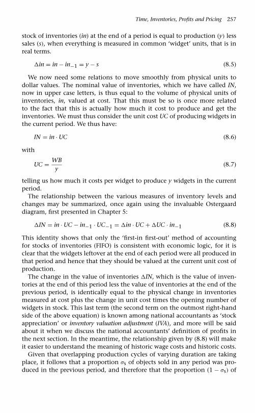
Time, Inventories, Profits and Pricing 257

stock of inventories (in) at the end of a period is equal to production (y) lesssales (s), when everything is measured in common ‘widget’ units, that is inreal terms.

�in = in − in−1 = y − s (8.5)

We now need some relations to move smoothly from physical units todollar values. The nominal value of inventories, which we have called IN,now in upper case letters, is thus equal to the volume of physical units ofinventories, in, valued at cost. That this must be so is once more relatedto the fact that this is actually how much it cost to produce and get theinventories. We must thus consider the unit cost UC of producing widgets inthe current period. We thus have:

IN = in · UC (8.6)

with

UC = WBy

(8.7)

telling us how much it costs per widget to produce y widgets in the currentperiod.

The relationship between the various measures of inventory levels andchanges may be summarized, once again using the invaluable Ostergaarddiagram, first presented in Chapter 5:

�IN = in · UC − in−1 · UC−1 = �in · UC + �UC · in−1 (8.8)

This identity shows that only the ‘first-in first-out’ method of accountingfor stocks of inventories (FIFO) is consistent with economic logic, for it isclear that the widgets leftover at the end of each period were all produced inthat period and hence that they should be valued at the current unit cost ofproduction.

The change in the value of inventories �IN, which is the value of inven-tories at the end of this period less the value of inventories at the end of theprevious period, is identically equal to the physical change in inventoriesmeasured at cost plus the change in unit cost times the opening number ofwidgets in stock. This last term (the second term on the outmost right-handside of the above equation) is known among national accountants as ‘stockappreciation’ or inventory valuation adjustment (IVA), and more will be saidabout it when we discuss the national accountants’ definition of profits inthe next section. In the meantime, the relationship given by (8.8) will makeit easier to understand the meaning of historic wage costs and historic costs.

Given that overlapping production cycles of varying duration are takingplace, it follows that a proportion σs of objects sold in any period was pro-duced in the previous period, and therefore that the proportion (1 − σs) of

258 Monetary Economics

objects sold this period was made this period. By definition, we have:

s = σs · s + (1 − σs) · s (8.9)

The objects made, but not sold, last period (the first term on the right-handside of 8.9) constitute the number of objects in stock with which firms startedthe period. In other words, they were the physical inventories left at the endof the previous period. The proportion σs is thus a stock-flow ratio in realterms; it is the inventories to sales ratio (bearing in mind that σs is an ex postratio, not a target parameter, since sales s are only known after the fact, atthe end of the period). Formally we have:

σs = in−1s

(8.10)

We now can give an intuitive definition of historic wage costs HWC. Thehistoric wage cost is the wage cost encountered when producing the goodsthat have been sold this period. Since a proportion σs were produced in theprevious period, their wage cost is given by the unit cost of the previousperiod, UC−1. The rest, the proportion (1−σs), were produced in the currentperiod, at the unit cost UC. The historic wage cost is thus:

HWC = σs · s · UC−1 + (1 − σs) · s · UC (8.11)

It still needs to be shown that this intuitive definition, equation (8.11), isidentical to the definition that arose from total business profits and the studyof Table 8.1, that is equation (8.3). In other words, is the following equalitytrue?

σs · s · UC−1 + (1 − σs) · s · UC = (WB − �IN)

From equations (8.7) and (8.8), we can rewrite the RHS of the aboveequation as:

(WB − �IN) = y · UC − (�in · UC + �UC · in−1)

Because of equation (8.5), we have:

(WB − �IN) = s · UC + �in · UC − (�in · UC + �UC · in−1)

Expanding �in and �UC, this can be further rewritten as:

(WB − �IN) = s · UC + in · UC − in−1 · UC − in · UC + in−1 · UC

− UC · in−1 + UC−1 · in−1

= (s − in−1) · UC + UC−1 · in−1

= (1 − σs) · s · UC + σs · s · UC−1

because of equation (8.9).

Time, Inventories, Profits and Pricing 259

We thus have demonstrated that equation (8.3) is identical to (8.11). Thisshows that the wage costs encountered by firms historically, over their volumeof sales of the current period, is indeed equal to the expression (WB − �IN).It follows that the difference between the value of realized sales S and thisexpression is indeed equal to the gross business profits of the firm.

If we add interest costs on inventories to this expression, (WB − �IN), weget total historic costs HC over sales of the current period, as was claimed inequation (8.4), so that we may write:

HC = (1 − σs) · s · UC + (1 + rl−1) · σs · s · UC−1 (8.12)

We may also wish to define the historic unit cost, HUC, which is the totalhistoric cost per sold unit. Dividing equation (8.12) by s, we get:

HUC = HCs

= (1 − σs) · UC + (1 + rl−1) · σs · UC−1 (8.13)

8.2.4 Entrepreneurial profits as a share of sales

We now show that entrepreneurial profits can be defined as a share of sales.What we wish to show is that ‘if prices are in a fixed ratio to the historiccost of producing what is sold, then profits in any period will be a constantproportion of the value of sales in that period’ (Godley and Cripps 1983:74–5). From equations (8.1) and (8.4) we know that:

S = F + HC (8.14)

Ex post it is always possible to claim that entrepreneurial profits are a fractionϕ’ of the total historic costs encountered in the production of the goods thatwere sold in the current period. We have:

F = ϕ′ · HC (8.15)

so that combining the last two equations we get:

S = (1 + ϕ′) · HC (8.16)

which implies that:

FS

= ϕ′(1 + ϕ′) (8.17)

Finally, combining (8.12) and (8.16), we have:

S = (1 + ϕ′){(1 − σs) · s · UC + (1 + rl−1) · σs · s · UC−1} (8.18)

Dividing through by s, and remembering that:

S = s · p (8.19)

260 Monetary Economics

we have at last an expression which defines the price level as a mark-up oncurrent and lagged unit costs, with weights determined by their respectiveshares in total sales:

p = (1 + ϕ′) · HUC = (1 + ϕ′) · {(1 − σs) · UC + (1 + rl−1) · σs · UC−1}(8.20)

It cannot be too strongly emphasized that (8.20) is nothing more than adefinition, though one that is very suggestive. It is saying, for instance, thatif firms wished to collar a proportion of the value of sales equal to ϕ′/(1+ϕ′),this would exactly be achieved if they were to set prices as a mark-up equal toϕ′ on actual historic unit costs. We shall see later why target markups may notbe achieved in practice, although (in our opinion) they do come pretty close.

Equation (8.20) is useful for the measurement of markups becauseentrepreneurial profits and business sales can be looked up in accountsdirectly whereas the historic wage costs can only be estimated by indirectcalculations. ‘The theorem holds irrespective of how prices are actually fixed.For example, if competitive market processes cause prices to settle at levelswhich yield a constant share of profits in the value of sales, then prices mustmove in exactly the same manner as if they had been set by adding constantpercentage markups to historic costs’ (Godley and Cripps 1983: 75).

8.2.5 The distinction between entrepreneurialprofit and cash flow

We have shown that entrepreneurial profit is the difference between salesand the total historic cost of producing what was sold. We have, repeated forconvenience:

F = S − THC = S − (WB − �IN + rl−1 · IN−1) (8.2)

In all likelihood the accountants of the entrepreneurs tell them that theirfirm has made a profit equal to the above amount. The entrepreneurs thendecide to distribute the entire profit amount to their families. Will they beable to do so?

The answer is that in general they will not, unless there is no increasein the value of inventories, or unless the increase is entirely financed byborrowing. To distribute the entire amount of entrepreneurial profits in theform of dividends, firm owners need to borrow from banks the equivalentof the change in the value of inventories. This brings forth the importantdistinction between entrepreneurial profits and cash flow. The cash flow ofthe firm is equal to:

CF = S − WB − rl−1 · IN−1 (8.21)

The cash flow of firms within a period is equal to its sales minus the costs thatwere encountered within the period – the wage bill and the interest payments

Time, Inventories, Profits and Pricing 261

on the stock of inventories. The cash flow is the net inflow of money intothe firm, disregarding any bank loan or other financial transactions. The dif-ference between the entrepreneurial profit and the cash flow is the increasein the value of inventories (F −CF = �IN). In most standard models this dis-tinction plays no role since the existence of inventories is assumed away. Thedistinction between entrepreneurial profits and cash flow becomes relevantonly when there are changes in the value of inventories.

The discrepancy between the cash flow and entrepreneurial profits becomesan important issue when the value of inventories changes quickly. Fromequation (8.8), �IN = �in · UC + �UC · in−1, we know that this will happenunder two sets of conditions. First, it can arise because the cost of inventoriesis rising at a high pace – the case of inflation (�UC · in−1). Second, it can alsohappens when fast-growing firms require fast-growing volumes of invento-ries (�in· UC). Under these circumstances, while firms may be making largeprofits, they are continuously required to borrow large amounts from outsidesources if they wish to distribute all of their entrepreneurial profits. Indeed,examples can be easily built where profitable firms, with looming profits,face negative cash flows because of their fast-rising inventories (Godley andCripps 1983: 70).

The distinction between cash flow and entrepreneurial profits helps toexplain the role of credit money. Without credit money – unless inven-tories valued at cost are matched one for one for loans from the banks –it would be impossible for firms to distribute dividends or at least todistribute as dividends the entire amount of their entrepreneurial prof-its. Bank loans are a systemic requirement of the monetary productioneconomy.

8.2.6 The definition of National account profits

Up to now we have focussed our attention on profits as perceived by businessaccountants. National accountants, as exemplified in the National Incomeand Product Accounts, or NIPA for short, have however a different defini-tion of profits. Their definition derives from the fact that the whole nationalaccounting system is being built around the concept of production. The pointof view of the national accountants is that national income should remainthe same if production and sales – measured in real terms, here measured inunits of widgets – do not change. Recalling that the whole of output is madeup of real sales and the value of the increase in physical inventories:

y = s + �in (8.5)

nominal GDP must be made up of these two components, valued at theirappropriate price. In the case of inventories, this means that they must bevalued at their unit cost. GDP in a closed economy without governmentthus starts from the value of consumption and investment (here investment

262 Monetary Economics

in new inventories):

Y = C + I = p · s + UC · (�in) = S + �IN − �UC · in−1 (8.22)

The first two components on the outmost right-hand side of equation (8.22)are identical to the first two components of the current account column ofTable 8.1. However, there is also a third component, the �UC · in−1 term,which is known among national accountants as ‘stock appreciation’ (SA) orinventory valuation adjustment (IVA), and which represents the increase in thevalue of the opening stock of inventories.

SA = �UC · in−1 (8.23)

Net investment, in our world without fixed investment, is thus equal to thevalue of the change in physical inventories, UC · (�in), and not to the changein the value of inventories, �IN. It follows that total profits, as measured bythe national accountants, must also be reduced by the amount of this ‘stockappreciation’. When computing national account profits, national accoun-tants behave as if all sold output had been produced at the current cost – thereplacement cost. For national accountants, total profits are thus equal to:

Fnipa = S − WB + �IN − SA (8.24)

so that the sum of factor incomes (wages plus profits) is indeed equal to thevalue of production:

Y = WB + Fnipa (8.25)

The current treatment of profits in NIPA is thus consistent with the generalprinciple that holding gains or losses, real or nominal, whatever their origin,should not influence the measure of income, saving or value added, whichare flows, and hence should be relegated to revaluation accounts. In theview of the national accountants, stock appreciation SA is akin to a capitalgain, and cannot be included within national income, which measures flows.Thus the overriding justification for deducting stock appreciation both fromprofits and changes in the value of inventories is that national accountantsneed a concept both of aggregate income and aggregate expenditure whichis conceptually identical to production – as there is no counterpart to stockappreciation in production.

This is the national accounts definition of profits that has been adoptedby the SNA since 1953. It must be said however that when the first nationalaccounts came out, their progenitor, Richard Stone (1947: 45,62), did includestock appreciation in the profits of productive firms, using FT as in equation(8.2), presumably as a direct transposition of business accounting. This isbecause from the point of view of the firm stock appreciation is not reallya capital gain. Although a revaluation has taken place, there is no capital

Time, Inventories, Profits and Pricing 263

gain in the ordinary sense because all inventories are valued at cost and allhave been be paid for by the firm as they were accumulated, giving rise toadditional borrowing – just as much as the accumulation of physical stocksgave rise to borrowing. What is actually happening is that the objects instock, even if stationary in aggregate, are all the time revolving; so invento-ries purchased at one time are continuously being used up and replaced byobjects newly purchased at a different price. If this is not perfectly clear, wehave written out in an Appendix an elaborate arithmetical example which,hopefully, illustrates the whole issue with precision.

While the deduction of stock appreciation from NIPA profits achieves con-sistency of one kind, it is defective from another viewpoint because it doesnot conform with a definition of profits as a distributable surplus and because,since stock appreciation is not a transaction, it cannot be fitted into a trans-actions matrix. This criticism of the NIPA definitions does not apply to theUS flow-of-funds accounts where, in the table describing firms’ appropriationaccounts, IVA is added back to ‘book’ profits to obtain total funds availableto firms and then included again in investment expenditure as a componentof firms’ outlays.9In a sense this is not surprising since financial accountsare based on the same logic as our transactions-flow matrix, from which ourdefinition of entrepreneurial profits has arisen.

8.3 Pricing

8.3.1 Generic cost-plus pricing

Up till now, we have described the values that various variables ought totake – in particular the profit variables – at given production costs and prices.Thus we dealt with realized or actual values. We now wish to tackle an entirelydifferent issue, that of price setting. What are firms trying to do when theyset prices? Our general answer to this question is that they aim, taking oneyear with the next, to make enough profits to pay for fixed investment andto distribute enough to satisfy shareholders. But for present purposes, inthis initial step, we assume that their objective is to secure profits equal tosome proportion of sales. Thus we tackle the following question: At givenproduction costs, if firms wish to achieve a certain level of profits, what pricewill they have to set?

The pricing decision is based on expectations and conventions. Price set-ting is based on some measure of unit cost, to which is added a costingmargin. This is the generic principle of cost-plus pricing, which is generallyendorsed by heterodox economists, who reject marginal cost pricing. Here,as in other heterodox works, prices are assumed to be based on the principleof cost-plus pricing. Prices are seen as an income distribution mechanism, in

9 See Flow-of-Funds Table F.102, lines 7 and 13.

264 Monetary Economics

the hands of the firms. By marking up costs, firms attempt to achieve a certainamount of profits, or a certain profit share, which will allow them to meettheir goals. Prices are not the anonymous result of a market-clearing mech-anism where prices rise rapidly when demand rises and fall when demandfalls. We know that in reality noting at all like this happens, except in auctionmarkets.10 Prices do not exist to clear markets, as they are conceived in theWalrasian story of the commissaire-priseur who calls prices, to find the onethat will perfectly equate demand and supply. As Hicks (1965: 79) points out:‘The existence of stocks has a great deal to do, in practice, with the possibil-ity of keeping prices fixed. If, when demand exceeds output, there are stocksthat can be thrown in to fill the gap, it is obvious that the price does not haveto rise; a market in which stock changes substitute for price changes (at leastup to a point) is readily intelligible’.

Firms have two kinds of decisions to make, costing and pricing. ‘Cost-ing refers to the procedures that a business enterprise employs to determinethe costs that will be used in setting the selling price of a good beforeactual production takes place and hence the actual costs of production areknown… . Pricing refers to the procedures the business enterprise uses to setthe price of a good before it is produced and placed on the market. That is,starting with the costs determined by its costing procedures, the businessthen adds a costing margin to costs or marks up the costs to set the price’(Lee 1998: 10).

Another important decision of the firm is whether it sets a gross or a netcosting margin. This depends on whether firms are concerned with totalbusiness profits FT or entrepreneurial profit F, as defined in the previoussection. Assuming that firms target a certain costing margin on their sales, isthat margin gross or net of the unavoidable interest costs that must be metto carry inventories? In other words, for a given amount of expected sales,do firms target a certain amount of total business profits or do they target anamount of entrepreneurial income, net of the interest cost?

10 Godley and Gillion (1965) went through the individual quotations making upthe United Kingdom’s wholesale price index. We took a serial sample (every tenthobservation) and found that individual quotations only changed at rare intervals andthat the monthly changes, when they did occur, clustered around 5%. It could be said,by and large, that changes in the overall index were determined by the number ofindividual quotations which had increased by 5% that month. This finding conformswith the common observation that firms issue price lists at discrete intervals of time.Indeed any other behaviour would be disorderly and expensive. These findings havebeen confirmed by more recent survey studies initiated by Alan Blinder (1991) andreproduced in several countries (see Amirault et al. 2004–2005). While the survey resultsseem to be anomalies from a neo-classical point of view, they are fully consistent withpost-Keynesian pricing theory (Downward and Lee 2001).

Time, Inventories, Profits and Pricing 265

It is clear that different answers to this question will generate different priceand income share dynamics. If entrepreneurs target their entrepreneurialincome, any increase in interest costs will be carried into higher prices.11

In other words, increases in interest rates will not lead to a fall in the shareof income going to entrepreneurial profit, but it will lead to a fall in thereal wage rate and in the share of wages, as we assumed it did in section 6of Chapter 7. By contrast, if entrepreneurs target total business profits, anincrease in interest cost will lead neither to an increase in prices nor to a fallin the real wage rate; it will only lead, ceteris paribus, to a decrease in the shareof entrepreneurial income. In this world, interest income is limited by theextent of total business profit. This is the hypothesis that has been endorsedby a majority of post-Keynesian authors, who omit the impact of interestcosts on the costing margin, implicitly assuming that firms are concernedwith total business profits rather than entrepreneurial profits. In the modelsof the next chapters, by contrast, we shall assume that entrepreneurs set theircosting margins and prices while targeting entrepreneurial income.

8.3.2 Mark-up pricing

Let us first deal with the simplest of all pricing methods, that of mark-up pric-ing. As pointed out above, this method is particularly appropriate if firms areonly concerned with their total business profits, gross of interest payments,or if firms are generally unable to pass on interest costs. It is also appropri-ate under the assumption that unit costs are constant, whatever the level ofoutput or the level of sales. This is the assumption which is usually foundin post-Keynesian mark-up models. In most post-Keynesian models, costingis done on the basis of variable costs, which, are approximately the samething as the so-called direct or prime costs. In that case, unit costs are usuallyconstant or nearly so, at a moment of time, for different levels of output.In the simple vertically integrated models with which we deal, the constantunit cost is the unit labour cost.12 We already presented this simple mark-uppricing model in Chapter 7 as:

p = (1 + ϕ) ·(

Wpr

)= (1 + ϕ) · UC (8.26)

11 What is meant here is any increase in unavoidable interest costs on inventories.In the more general case where firms borrow for other purposes, such as purchasesof fixed capital goods, then a target return pricing formula could apply, with sometarget rate of return on capital. An increase in interest rates may or may not induce anincrease in the target rate of return.

12 As already pointed out, this does not mean that we believe that firms set priceson the basis of labour unit costs only; we do recognize that firms base their prices onunit direct costs, which include the cost of intermediate goods (see Coutts, Godley andNordhaus 1978). But the model here is a vertically integrated model.

266 Monetary Economics

where ϕ is a percentage costing margin, and where W/pr is the unit labour costof producing one widget, or what we called UC in the previous subsections –the unit cost.

Even when unit labour costs are changing from one period to the next,it could be that firms are still using formula (8.26) to set prices. This wouldbe the case of replacement cost pricing, whereby firms adjust the selling priceinstantaneously to changes in unit costs (Coutts, Godley and Nordhaus1978: 36). This form of pricing would go hand in hand with last-in first-out(LIFO) accounting principles.

In the present chapter, and in most chapters to follow, we emphasize thefact that unit labour costs may change from one period to the next. Wealso showed in the previous subsections how total business profits dependon historic wage costs, and how entrepreneurial profits depend on overallhistoric costs. Because of the existence of inventories, the goods sold in aperiod have been produced in part only during the current period; the rest ofthe goods have been produced in an earlier period. The unit cost of the soldgoods thus varies depending on whether they originate from past inventoriesor current production. As a consequence, the average unit cost of the soldgoods varies as well, depending on the proportion of the sold goods thatcomes out of inventories. For every different level of sales, the average unitcost of producing the sold goods is different. This is true even if we considerlabour costs only.

But even if unit labour costs turned out to be constant from one periodto the next, because there were no wage inflation and no change in labourproductivity, the actual average unit cost would vary depending on the scaleof the sales. This is because total historic costs HC, in contrast to historicwage costs HWC, contain an element of fixed costs – the interest costs linkedto inventory holding. When the level of widget sales is larger, the fixed costsare spread over a larger number of units, and as a result the average unit costis lower.

So, on what basis can these average or unit costs be computed, knowingthat every different level of sales generates a different unit cost? There are twopossible answers to this question: normal-cost pricing and full-cost pricing.13 Westart with full-cost pricing.

8.3.3 Historic full-cost pricing

Godley (1999a) accounts for variations in average unit cost by using what wemay call historic full-cost pricing. This is a variant of full-cost pricing, which wasfirst proposed by Hall and Hitch (1939). In full-cost pricing, prices are basedon average unit costs, including overheads (or fixed costs) such as interest

13 See Lavoie (2001a) and Lee (1998, part 2) for more details on these two pricingviews.

Time, Inventories, Profits and Pricing 267

costs on inventories, computed at the expected volume of output. Here wepropose a variant of full-cost pricing, by assuming that prices are based onaverage unit cost computed at the expected sales volume. More precisely, theaverage unit cost involved is the historic unit cost computed at the expectedor forecast sales volume, or the expected historic unit cost. Calling HUCe thisexpected historic unit cost, the pricing formula that we propose in thischapter is given by:

p = (1 + ϕ) · HUCe (8.27)

where

HUCe = HCe

se (8.28)

The variables se and HCe are the expected sales volume and the total historiccosts that would be encountered at this expected sales volume. Note that ϕ

is the target (ex ante) mark-up, in contrast to the realized (ex post) mark-upϕ′ that was defined in section 8.2.

What is the expected historic unit cost equal to? There are three compo-nents to it. The first two components arise from the historic wage costs, ormore precisely from the expected historic wage costs. The first componentis the unit cost of previously produced goods that will be sold in the currentperiod. Inventories make up this component. The second component is theunit cost of the goods to be produced in the current period. The average wageunit cost is thus a weighted average of these two components. What will theweights be? Note that we can write the following definition:

σse = in−1se (8.29)

At the beginning of the period firms hold inventories of an amount in−1. Ifthey expect a volume of sales se, this implies that they expect a proportionσse of their sales to stem from inventories, at the lagged unit cost UC−1. Theselagged unit costs will thus be factored by the weight σse. By the same token,this also implies that firms expect a proportion (1−σse) of their sales volumeto be provided by goods produced in the current period, at the current unitcost UC. The current unit costs thus carry a weight (1−σse). This is in perfectanalogue with our computations of realized historic wage costs HWC, as wasfound in equation (8.11).

The third component is the interest cost on the value of inventories accu-mulated at the end of the previous period. Thus in analogue with the actualhistoric unit cost, HUC, given by equation (8.13), the expected historic unitcost is:

HUCe = (1 − σse) · UC + σse · (1 + rl−1) · UC−1 (8.30)

268 Monetary Economics

Ultimately, putting together equations (8.28) and (8.30), the price equation,assuming full-cost historic pricing, is given by:

p = (1 + ϕ) · {(1 − σse) · UC + σse · (1 + rl−1) · UC−1} (8.31)

This pricing formula says that prices will be set according to expected sales,on the basis of expected historic unit costs and the percentage mark-up ϕ.14

8.3.4 The possibility of perverse pricing

There are two features of formula (8.31) worth noticing. First, any change inthe expected sales to inventories ratio σse induces a change in prices. Priceswill thus be changing all the time. Another, more annoying feature of pricingformula (8.31) is that if firms expect sales to be higher, assuming no differencebetween UC−1 and UC, this leads to a lower expected historic unit cost, andhence, for a given mark-up ϕ, this yields a lower price p. The culprit, so tospeak, is the σse ratio once again. This is called ‘perverse pricing’. Perversepricing, as Gardiner Means (1991: 326) defined it, implies that higher salesare associated with lower prices, while lower sales are associated with higherprices. This may occur with historic full-cost pricing. It is for this reason –the inverse link between expected demand and the price level – that someheterodox authors are reluctant to use full-cost pricing or any of its variants.15

There are two possible cases of perverse pricing, associated with the denom-inator and the numerator of the σse ratio, as defined in equation (8.29).Obviously, when there is an exogenous increase in expected sales se, theσse ratio is lower, and this leads to falling prices according to formula (8.31),unless unit costs UC increase during the period. Thus, if realized sales areequal to expected sales, higher sales will indeed be associated with lowerprices – a case of perverse pricing. The second case of perverse pricing iscaused by an unanticipated increase in demand in the previous period. Thiswill generate a reduction in the realized level of inventories in−1, and henceonce more a reduction in the σse ratio – the more so if expected sales se

react positively to the realized increase of the previous period. Thus in theexperiments that we have conducted using the historic full-cost formula, an

14 Because costs are related to prices and profits in this very specific way, the lagbetween costs and prices cannot be just anything – as the econometricians assume. Thatis, they assume that the lag can be anything at all and that they are uniquely qualifiedto discover what it is. This is one of the reasons the work of Godley and Nordhaus(1972), who imposed lags based on stock/output ratios in preference to estimatingthem econometrically, was never really influential – it was an implicit challenge toeconometric methodology.

15 It should be pointed out, however, that when current unit costs are higher thanlagged unit costs, the sign of the relation between expected sales and the price levelbecomes uncertain.

Time, Inventories, Profits and Pricing 269

1951 1956 1961 1966 1971 1976 1981 1986 1991 1996 2001

0.00000

0.00200

0.00250

0.00150

0.00100

0.00050

0.200

0.280

0.300

inflation rate inventories ratio

rate ofpriceinflation

inventories toexpected salesratio

0.260

0.240

0.220

Figure 8.1 Evolution of price inflation and the inventories to expected sales ratio,following a decrease in autonomous demand

increase in demand is usually accompanied by a small dip in the price level,or in the level of inflation when an inflation equation is added.16 Figure 8.1shows inversely that when autonomous demand briskly falls, the inflationrate is momentarily boosted up, as a result of the increase in the inventoriesto expected sales ratio (σse = in−1/se).

8.3.5 Normal-cost pricing

The drawback of perverse pricing can be avoided by the use of normal-cost pric-ing, where normal costs are defined in reference to a normal level of outputor a normal level of capacity utilization, as was initially proposed by Andrews(1949) and Andrews and Brunner (1975). Normal-cost pricing is an alterna-tive to historic full-cost pricing, that retains the main positive features of thelatter while avoiding the drawback just mentioned. With normal-cost pric-ing, firms measure costs by reference to a normal or standard level of capacityutilization. Normal costs are then defined as the level at which total costswould be, if output were at its normal or trend level (Coutts, Godley andNordhaus 1978: 22–3). Prices are thus set as a costing margin over normalunit costs, which we can denote as NUC. Formally, this can be written as:

p = (1 + ϕ) · NUC (8.32)

16 The dip is very small, but exists nonetheless. For instance when autonomousdemand goes up by 25%, prices decrease at once by about 0.25% with our numbers.

270 Monetary Economics

With normal-cost pricing, there is no presumption that the normal outputlevel will be the realized output level of the period, nor that sales will beequivalent to this normal output level. In addition, the expected outputlevel and the expected level of sales could both be different from the normaloutput level. As a consequence, both the expected and the realized levelof entrepreneurial profits could be quite different from the profit measureimplicit to the pricing formula based on the normal output level, as given byequation (8.32). This is the main disadvantage of the normal-pricing formula.Its advantage is that firms that use normal-cost pricing can base their pricingdecision on a convention or a rule of thumb – the normal or standard levelof output – and need not make forecasts about future sales volumes whensetting prices.17 Moreover it will always be possible for firms to adjust thecosting margin if actual and normal costs diverge for a long time, as we shallshow in the model deployed in Chapter 11.

Within our simplified framework, what will be the normal unit cost? Withhistoric full-cost pricing, the expected historical unit cost depends on pastand current unit labour costs, the rate of interest, and the current inventoriesto expected sales ratio σse. As was shown above, it is this ratio that causesperverse pricing. A company that would set prices neither on actual costsnor on expected costs would have to forsake σse and use instead what itconsiders to be the normal inventories to sales ratio. What is this normalratio? It is the target inventories to sales ratio, which, as we shall see in thenext chapter, drives the behaviour of firms in inventory accumulation, andwhich is equal to:

σT = inT

se (8.33)

The σT ratio is the ideal end-of-period inventories to expected sales ratio thatfirms would like to achieve in the long run. It is a target parameter that firmsset as a convention. This target parameter is realized only when firms reachthe stationary state – in the long period. We suggest that firms set normal unitcosts on the basis of this convention. Normal unit costs are the same as his-torical unit costs when the target inventories to expected sales parameter σT

is realized. Thus by using normal-cost pricing, firms act as if the target inven-tories to sales ratio was the realized one at all times, or rather they act as if thetarget inventories to sales ratio was realized on average. Normal-cost pricesare thus, in that sense, long-period prices (Lee 1985). They do not reflect

17 One of us has directed a great deal of research effort in an attempt to ascertainwhether prices move up or down relative to ‘normal’ historical unit costs, definedas unit costs as they would be if output were reckoned at a normal, or trend level.See Godley (1959), Neild (1963), Godley and Nordhaus (1972), Coutts, Godley andNordhaus (1978).

Time, Inventories, Profits and Pricing 271

non-systematic forces tied to fortuitous variations in sales or inventories.They are prices that reflect historical unit costs as they would be in the longperiod. With normal-cost pricing, firms know that the income distributionimplicit in the pricing formula will not be realized in general, even whentheir sales forecasts are correct. The only exception is the stationary state.

When fixing prices, firms need not make forecasts about future sales vol-ume. They need only know the past and current unit labour costs, the rateof interest, and the conventional inventories to sales σT ratio. By analogywith the full-cost pricing formula, given by (8.31), we obtain the normal-costpricing equation:

p = (1 + ϕ) · NHUC (8.34)

with the normal historic unit cost NHUC being equal to:

NHUC = (1 − σT) · UC + σT · (1 + rl−1) · UC−1 (8.35)

The only thing still left unexplained is the costing margin ϕ. This will beremedied in Chapter 11.18

8.3.6 Some noteworthy features of historic full-cost pricing and normal-cost pricing

Equations (8.31) and (8.34) have several noteworthy features, at least four. Tostart with, full-cost pricing and normal-cost pricing are based on informationthat firms possess or search for at the time that they must make their pricingdecisions. First, firms give themselves a percentage mark-up ϕ, more aboutwhich will be said in a moment. Second, in the case of normal-cost pricing,the σT parameter is also a convention set by firms themselves. In the case ofhistoric full-cost pricing, firms easily estimate the weight σse, since they knowthe level of inventories accumulated at the end of the previous period, andby making a forecast of sales, based in particular on the sales of the previousperiod. Third, the firms collect information on labour unit costs; accountantshave carefully calculated lagged unit costs, and entrepreneurs know the wagerate to be paid to workers in the current period, and they would have someestimate of their productivity. Fourth, and finally, firms would know whatinterest rate rl−1 they are being charged to finance their inventories, sincethis rate is set at the end of the previous period.

18 Here we assumed that the normal historic unit cost NHUC is based on unit costsproper, UC and UC−1. However, if we were to add more realistic features such as cycli-cally changing productivity growth, so that current unit costs could not be knownat the beginning of the period, when prices are set, NHUC would need to be basedon a conventional normal unit cost, NUC and NUC−1, which would depend on someestimate of trend productivity.

272 Monetary Economics

A second noteworthy feature of our two pricing formulas is that interestcosts come explicitly into these pricing formulas. It is clear that any increasein the rate of interest charged to manufacturing firms that carry and financeinventories with bank loans will be passed on to consumers, through higherprices, provided firms do not simultaneously decrease the mark-up ϕ. Theimpact of the rate of interest is even more obvious, when pricing formulas(8.31) or (8.34) are rewritten while assuming that unit costs do not changefrom one period to the next. Assuming that UC = UC−1, pricing formula(8.31) for instance becomes:

p = (1 + ϕ) · (1 + rl · σse) · UC (8.36)

Equation (8.36) illustrates very clearly the principles of cost-plus pricing. Theprice is based on a measure of direct costs, the labour unit costs given by UC;then there is a percentage mark-up, given by rl · σse, which is designed tocover the overhead costs arising from the unavoidable interest costs; finallythere is the entrepreneurial profit percentage mark-up, given by ϕ.

With such a pricing formula, the monetary and the real sides of the econ-omy are intertwined. All else equal, when interest rates rise, prices rise. Thereis a long tradition of heterodox economists, who, at some time or another,have taken this view: Thomas Tooke and the Banking School, Harrod, Kaldor,Sylos Labini, Graziani, Garegnani, Pivetti and even, for a time, Joan Robin-son. In the United States, it is known as Senator Patman’s view (see Taylor2004a: 88–90). Kaldor (1982: 63), for instance, wrote that ‘interest costs arepassed on in higher prices in much the same way as wage costs’.

What is the meaning of the percentage mark-up ϕ and what economicinterpretation can we attribute to it? The answer is quite obvious once wecompare the pricing equations to the identity derived from the transactions-flow matrix. We have:

p = (1 + ϕ) · HUCe = (1 + ϕ){(1 − σse) · UC + σse · (1 + rl−1) · UC−1}(8.27)

p = (1 + ϕ) · NHUC = (1 + ϕ){(1 − σT) · UC + σT · (1 + rl−1) · UC−1}(8.34)

on one hand, and on the other hand:

p = (1 + ϕ′)HUC = (1 + ϕ′){(1 − σs)UC + σs(1 + rl−1)UC−1} (8.20)

where

FS

= ϕ′(1 + ϕ′) (8.17)

Thus, by saying that firms set a percentage mark-up equal to ϕ over expectedhistoric unit costs (or normal historic unit costs), we imply that firms aimat securing as entrepreneurial profit a proportion ϕ/(1 + ϕ) of the value ofsales. That is, firms set a price such that their expected entrepreneurial profit

Time, Inventories, Profits and Pricing 273

is a proportion ϕ/(1 + ϕ) of the expected value of sales. For instance, ifϕ = 0.5, it implies that firms target entrepreneurial profits that represent(.5)/(1.5) = 33.3% of the expected value of sales.

Another interesting property of the historic cost pricing formula given byequation (8.31) is that the actual share of entrepreneurial profits in the valueof sales, ϕ′/(1 + ϕ′), will always turn out to be a close approximation of thedesired share ϕ/(1 + ϕ), whatever the realized value of sales. Changes in theactual share compared to the targeted share are due either to mistaken esti-mates of the current period productivity of workers or to mistaken forecastsof expected sales.19 The latter make the interest cost per sold unit differentfrom its expected cost, and it also modifies the realized weight between laggedand current unit labour costs, making it different from the one incorporatedinto the pricing equation. This last effect is only relevant when unit costs UCdiffer from one period to the next.

Of course these properties of historic cost pricing extend to normal-costpricing. The normal-cost pricing formula implies that entrepreneurs expectprofits to be a proportion ϕ of sales when the stationary state is reached withthe realized inventories to sales ratio no different from the target inventoriesto sales ratio.

8.3.7 Historic unit costs and inflation

Our historic full-cost and normal-cost pricing formulas have a final note-worthy feature. These formulas are impervious to inflation. To demonstratethis we shall focus on the case of the historic full-cost pricing formula. Evenwhen unit costs UC differ from one period to the next, due to cost inflation forinstance, the pricing formula may still be rewritten as equation (8.36), thatis on the basis of the current unit cost UC only. All that is required is a rein-terpretation of the interest rate rl paid on loans to finance inventories. Therate must now be reinterpreted not as the nominal rate, but rather as the realrate of interest, defined with respect to the rate of cost inflation. To demon-strate this remarkable feature of pricing formulas (8.31) and (8.34) based onexpected or normal historic unit costs, we start by making the following twodefinitions.

First, we define the rate of cost inflation πc as being equal to:

πc = (UC − UC−1)

UC−1=

(UC

UC−1

)− 1 (8.37)

The rate of cost inflation measures the rate of growth of unit costs. Thisrate of growth is (nearly exactly) the difference between the rate of growth of

19 In the model to be built for this chapter, we will assume that when entrepreneursset prices they make correct forecasts of labour productivity pr and that they havefinalized the wage bargain with their workers, hence knowing what the nominalwage W is.

274 Monetary Economics

nominal wages minus the rate of growth of labour productivity. The aboveequation implies that lagged unit costs can be rewritten as:

UC−1 = (UC)

(1 + πc)(8.38)

The real rate of interest, here called rrc to reflect the fact that it is the rateof interest net of cost inflation, is usually given by the equation rrc = rl − πc.This however is only an approximation. To find out the exact real rate ofinterest, let us assume that the agent owns a monetary asset, say M . At theend of the period, thanks to the interest payment, the agent is now left withan amount (1+ rl−1)M . In real terms, however, this amount must be deflatedby (1 + πc) under the assumption that prices have risen at the rate πc. Theinterest income, net of inflation, is thus:{

(1 + rl−1)

(1 + πc)

}· M − M

Dividing the above expression by the initial value of the asset M , we obtainthe real rate of interest, which is defined by the following relation:

rrc−1 = (1 + rl−1)

(1 + πc)− 1 (8.39)

so that we can write:

(1 + rl−1) = (1 + rrc−1) · (1 + πc) (8.40)

We can now substitute the values of equations (8.38) and (8.40) into thehistoric full-cost pricing formula (8.31). We nearly directly obtain:

p = (1 + ϕ) · (1 + rrc−1 · σse) · UC (8.41)

By analogy, the normal-cost pricing equation may also be rewritten in termsof current unit labour costs only, as was done with the historic full-costpricing equation. With the real rate of interest rrc we obtain the simpleequation:

p = (1 + ϕ) · (1 + rrc−1 · σT) · UC (8.42)

Where price inflation and cost inflation are equal, the historic full-cost pric-ing and normal-cost pricing equations may be rewritten strictly in terms ofcurrent unit costs; lagged unit costs need not be taken explicitly into con-sideration. But the nominal rate of interest must be replaced by the realinterest rate in the pricing formulas, with no change whatsoever to the cost-ing mark-up. The new formula is nearly identical to equation (8.36) that wehad obtained when assuming that unit costs did not change. The only differ-ence is that the real rate of interest, as defined in equation (8.39) must nowenter the pricing formula.

Time, Inventories, Profits and Pricing 275

One may wonder whether price inflation and cost inflation are ever equal.They will be equal whenever there is no change in the parameters ϕ, rrc andσse of the pricing formula (8.41).

Equations (8.41) and (8.42) clearly show that the margin over current labourunit costs UC depends on the real rate of interest, and not on the nominalrate of interest.20 Indeed these equations show that one purpose of pricing isto determine the shares of real incomes. This can be seen even more clearlyin the following way. Take equation (8.41), divide it by p, and multiply it byy – the real output. We obtain:

y = (1 + ϕ) · (1 + rrc−1 · σse) · UC · yp

Remembering that unit costs are the wage bill per unit produced, orUC = WB/y, and calling wb the real wage bill, wb = WB/p, the above equationbecomes:

y = (1 + ϕ) · (1 + rrc−1 · σse) · wb (8.43)

This equation is a behavioural equation. It sets forth a relation of fundamentalsignificance. It shows that when firms set prices, they intend to determineexhaustively the distribution of real national income between wage income,entrepreneurial income and rentier income. The intended shares of each ofthese is given by the following ratios:

the share of real wage income:wby

;

the share of rentier income: rrc−1 · σse · wby

the share of entrepreneurial income: ϕ · (1 + rrc−1 · σse) · wby

= ϕ

(1 + ϕ)

As soon as any of these two quantities are determined, the third is automat-ically determined as well. The formula has the very important implicationthat if firms have the power to set a mark-up of their choice, and if bankscan set nominal rates of interest at a level which ensures that the real interestrate does not change, then there is no way in which the real wage bill (for a

20 There seems to be some confusion in this regard among some authors who claimthat higher nominal interest rates could lead to higher prices, in particular in Dutt(1992) and Graziani (2003). See Lavoie (1995: 157) for a clear assertion that real ratesof interest are the correct variable to consider. The proof offered here had already beenprovided by Godley and Cripps (1983: 193).

276 Monetary Economics

given output) or the wage share can be changed as a result of the nominalwage bargain. These results were established with the historic full-cost pric-ing formula. By analogy, identical results would be obtained in the case ofnormal-cost pricing as we defined it.21

8.4 Numerical examples of fluctuating inventories

8.4.1 The impact of changing sales on profits: a numericalexample without inflation

The purpose of this section is to provide readers with two simple examples offluctuating sales. They will underline the impact that fluctuating sales, for agiven amount of production, inflict on various measures of profit and its sharein the value of sales or in the value of national income. In this example, amost simple one, we assume that the unit cost UC is constant from one periodto the next. This implies that there is no inventory valuation adjustment(IVA = 0) and that the price level is constant. We further assume that firmshave reached a stationary level of output, equal to 100 units, and hence thatthe target level of inventories has been achieved. Assuming that firms stillexpect sales to remain at 100, this means that they will produce 100 units,having no intention to increase or diminish their inventories voluntarily. Onthe matter of distribution, we assume that the price level is equal to unity(p = 1), that unit costs are UC = .70, and that the overall interest cost is equalto $2. This could be the case, for instance, if the value of inventories (IN−1)

at the beginning of the period were equal to 40 while the rate of interest onloans was 5%. This implies that the target share of entrepreneurial profits Fin sales is 28%, as indicated at the top of Table 8.3.

One can draw several lessons from this table. First, we note that all butone measure of profit shares rise when sales exceed expectations, that is,when there is a business upswing (case 2). Second, it is quite obvious thatmeasures of shares relative to sales are much more stable than measures ofshares relative to national income. The share of total business profits stay attheir target 30%, while the share of realized entrepreneurial profits ϕ′/(1+ϕ′)stay very close to their target ϕ/(1 + ϕ) = 28%, despite large fluctuations insales and inventories.22 By contrast the share of entrepreneurial profit relativeto GDP oscillates between 25.77% and 30.10%, most of the slack being takenby the share of wages in GDP. The share of interest costs in national income,which is 2% when sales expectations are realized, falls to 1.96% when salesrise to 110 units.

21 We only need to substitute σT for σse in the equations above.22 Note once again that while the percentage net costing margin is ϕ (ex ante), ϕ′ is

the percentage profit margin (the realized, ex post, margin).

Time, Inventories, Profits and Pricing 277

Table 8.3 A numerical example of varying sales, without inflation

Hypotheses:se = 100; UC = UC−1 = .70 ; p = 1; ϕ/(1 + ϕ) = 28%

Case 1 Case 2 Case 3

Production y 100 100 100Sales volume s 100 110 90Value of the change

in inventories�in · UC 0 −7 +7

National income Y = s · p + �in · UC 100 103 97Wage bill WB 70 70 70Historic wage cost HWC 70 77 63Interest costs rl−1 · IN−1 2 2 2Gross profits FT 30 33 27Entrepreneurial

profitsF 28 31 25

Profit shares wrtsales

FT/S 30% 30% 30%

F/S = ϕ′/(1 + ϕ′) 28% 28.18% 27.77%Profit shares wrt

national incomeFT/Y 30% 32.04% 27.97%

F/Y 28% 30.10% 25.77%

Now in reality, sales at the macroeconomic level will never go throughswings as large as those described here. Nevertheless there is a further lessonto be drawn from the table. When carrying out studies of cyclical profit sharesthrough the business cycle, economists would be well advised to look at profitshares relative to sales rather than profit shares relative to national income.These studies often attempt to assess whether workers manage to raise theirbargaining power in a boom. The fact that the profit share relative to GDPrises in the first part of the upswing, and diminishes in the second part of theboom, is no necessary indication of the evolution of the bargaining powerof workers; it may simply reflect unexpected movements in sales relative tooutput. The evolution of profits relative to sales would seem to be a betterpossible indicator of the changes in the relative strength of workers and theiremployers.

8.4.2 The impact of changing sales on profits: a numericalexample with cost inflation

We again explore the impact of changing sales, with a given production level,on the various measure of profits, but this time with a time-varying unitcost, which involves the computation of an inventory valuation adjustment

278 Monetary Economics

Table 8.4 A numerical example of varying sales, with cost inflation

Hypotheses:UC = .70; UC−1 = .66; πc = 6.06%p = 1; ϕ/(1 + ϕ) = 28%; ϕ = .388σse = 0.5; se = 100; in−1 = 50; (1 + rc−1 · σse) = 1.0286rrc−1 = 5.71%rl−1 = 12.12%

Production y 100 100 100Sales volume s 100 110 90Value of the change ininventories

�in · UC 0 −7 +7

National income Y = s · p + �in · UC 100 103 97Stock appreciation SA = �UC · in−1 2 2 2Wage bill WB 70 70 70Historic wage cost HWC 68 75 61Interest costs rl−1 · IN−1 4 4 4Gross profits FT 32 35 29Entrepreneurial profits F 28 31 25NIPA profits Fnipa 30 33 27Profit shares wrt sales FT/S 32% 31.81% 32.22%

F/S = ϕ′/(1 + ϕ′) 28% 28.18% 27.77%NIPA profit shares Fnipa/Y 30% 32.04% 27.83%

Fnipa/S 30% 30% 30%

(IVA), also called stock appreciation (SA). The hypotheses used are insertedin Table 8.4.

Once more we see that profit shares relative to sales do not move or barelymove, whereas the profit share relative to national income experiences largerfluctuations.

Appendix 8.1: A numerical example of inventory accounting

The store: no production, just purchases and salesFirst imagine a store which buys goods from a manufacturer and subsequently sellsthem to the public. Counting merchandise as numbers of identical physical objects,which we shall call ‘widgets’, we may first imagine the store’s operations being recordedin the way shown in the first four columns of Table A8.1. These four columns only dealwith physical objects. Note that we always use upper case letters to designate variablesin nominal values while lower case letters are used for real variables (physical objects,or deflated nominal values, as the case may be).

The store starts operations in the first quarter of year 1. It buys 12 widgets in thatquarter and in each of the subsequent quarters of year 1, shown as y in column 1. Itsells nothing during the first year, so inventories, accounted as the number of physical

279Table A8.1 A numerical example with inventories

Objects Dollars

Row 1 2 3 4 5 6 7 8 9 10 11 12

Quarter, Purchases or Inventories Unit Wage Sales Inventories at cost Historic Profityear production Sales (change and level) costs bill (1×5) Price value (2×7) (level and change) wage costs 8–11

y s �in in UC WB p S IN �IN HWC FT1 12 0 12 12 1 12 – 0 12 12 0 02 12 0 12 24 1 12 – 0 24 12 0 03 12 0 12 36 1 12 – 0 36 12 0 04 12 0 12 48 1 12 – 0 48 12 0 0Year 1 48 0 48 48 1 48 – 0 48 48 0 0

1 12 12 0 48 1 12 1.5 18 48 0 12 62 12 12 0 48 1 12 1.5 18 48 0 12 63 12 12 0 48 1 12 1.5 18 48 0 12 64 12 12 0 48 1 12 1.5 18 48 0 12 6Year 2 48 48 0 48 1 48 1.5 72 48 0 48 24

1 12 24 −12 36 1 12 1.5 36 36 −12 24 122 12 24 −12 24 1 12 1.5 36 24 −12 24 123 24 24 0 24 1 24 2.0 48 24 0 24 244 24 24 0 24 1 24 2.0 48 24 0 24 24Year 3 72 96 −24 24 1 72 1.75 168 24 −24 96 72

1 24 24 0 24 1.2 28.8 2.0 48 28.8 4.8 24 242 24 24 0 24 1.2 28.8 2.0 48 28.8 0 28.8 19.23 24 24 0 24 1.2 28.8 2.0 48 28.8 0 28.8 19.24 24 24 0 24 1.2 28.8 2.0 48 28.8 0 28.8 19.2Year 4 96 96 0 24 1.2 115.2 2.0 192 28.8 4.8 110.4 81.6

280 Monetary Economics

objects in store, rise by 12 widgets every quarter, reaching 48 at the end of the year asshown in columns 3 and 4. These inventories, in real terms, are noted in, while thechange in real inventories is noted �in. Sales (noted s in column 2) begin in the firstquarter of year 2 and continue through the year at the rate of 12 widgets per quarter so,as purchases remain at 12, there is a zero change in inventories and their level is again48 at the end of the year. In year 3, sales jump to 24 per quarter and stay at that levelfor the rest of the example. Purchases remain at 12 for two quarters, so inventoriesinitially fall by 12 per quarter. Then purchases jump to 24 and stay at that level sothere are no further changes in the level of inventories. The level of inventories fallsto 24 in the second quarter of year 3 and remains at that level thereafter.

Beyond introducing an identity linking purchases, sales and increases in physicalinventories, the numbers illustrates an important theorem – that in a stationary steadystate, the inventory to sales ratio measures the average time an object remains in stock.Through years 1 and 2 it obviously takes exactly four quarters for any object to be soldusing a ‘first-in first-out’ method of accounting for stocks of inventories (FIFO). Forinstance, the 12 widgets that had been purchased in the first quarter of year 1 are soldin the first quarter of year 2, and hence they remain in stock for exactly four quarters.Similarly the 12 widgets purchased in the second quarter of year 1 are sold in the secondquarter of year 2. One may think of the objects being put onto a conveyor belt whenthey are bought and later taken off and sold in the order in which they were bought.

If the objects are not sold in the order they were purchased, for instance if theyare sold following the ‘last-in first-out’ principle (LIFO), the mean period they remainin stock is still given by the stock/sales ratio; at the end of year 2 the mean periodis 48:12 (or 4) on a quarterly basis and 48:48 (or 1) on an annual basis. In years 3and 4 the mean lag has shortened to a single quarter. At the end of both these years,the mean period is 24:24 (or 1) on a quarterly basis and 24:96 (or 1/4) on a yearlybasis.

The manufacturing firm and inventory accountingTo interpret the columns which follow, imagine the business to be not a store but amanufacturing firm which produces the widgets it sells; the meaning of the symbol ytherefore changes from purchases to production of widgets. If we assume that producedgoods can only be sold under the ‘first-in first-out’ principle, and assuming away thepresence of precautionary inventories, then the fourth year of the numerical exampleof Table A8.1 describes a case where the goods produced in one quarter, say quarter 1of year 4, can only be sold in the next quarter (in quarter 2 of year 4). A time lag ofone period between production and distribution would indeed be introduced, but thistime lag is of only one quarter. If the accounting period of our model is one year, thenthe inventories to sales ratio is only 0.25, giving the impression that there is no timelag whatsoever between production and sales, and that some of the goods that havebeen consumed in one period had been produced within the same period. But this isan illusion based on the fact that the production and the accounting periods are ofdifferent length.

The dollar amounts in columns 5 and 6 assume, for simplicity, that productivityis fixed at one widget per worker per period, so the number of employees is alwaysequal to the number of widgets produced – y in column 1. The wage rate starts at$1 per quarter and rises in a jump to $1.2 per quarter at the beginning of year 4. Asproductivity is assumed to be constant, the unit cost (UC in column 5) is equal to thewage rate.

Time, Inventories, Profits and Pricing 281

Column 7 gives the selling prices p measured in dollars which firms charge perwidget; and column 8 gives the total dollar value of sales. As shown in the table, thisis column 2 times column 7.

Column 9 gives the dollar value of the inventory of widgets measured at cost, notedIN – what it cost the firm to build those inventories. These measures are pretty straight-forward during the first three years, since there is no change in the unit cost of producedwidgets. Any change in the dollar value of inventories must be attributed to a changein the number of physical widgets in stock. Things are more complicated in the firstquarter of year 4. There, although there is no change in the volume of inventories in,that is, there is no change in the number of widgets in stock, there is a change in theirvalue measured at cost. There is an increase from $24 to $28.8, hence an increase of$4.8 as shown in column 10, because 24 widgets valued at $1 each have been taken outof stock and sold; these have been replaced with an inventory of 24 newly producedwidgets which have cost, and are therefore valued at, $1.2 each. Column 10 gives thechange in the value of the widget stock, once more measured at cost, noted � IN.

The relationship between the various measures of inventory levels and changes maybe summarized by equation (8.8):

�IN = �in · UC + �UC · in−1 (8.8)

�IN (column 10) is identically equal to the physical change in inventories measuredat cost (column 3 times column 5) plus the change in unit cost times the opening num-ber of widgets in stock – the ‘stock appreciation’ or inventory valuation adjustment (IVA).

As there is no change at all in the volume of inventories in the first quarter ofYear 4, the whole of the increase in the value of inventories takes the form of stockappreciation. Note that, notwithstanding the suggestive name ‘stock appreciation’and notwithstanding that the value of inventories has gone up without there beingany change in the volume of inventories, nothing in the nature of capital apprecia-tion has occurred which is in any way comparable with appreciation of shares in thestock market. The reason for this is that we are watching a revolving process in whichold inventories purchased at one price are replaced by new inventories purchased atanother (higher) price. There is no capital appreciation in the ordinary sense becauseeverything comprised within the concept of IN is valued at the price which was actu-ally paid for it. Still, as we shall see later, the increase in the value of inventories has,in some other sense, some similarity with the capital gains on stock market shares.

The measure of profitsWe now address a major question. How much profit has the firm made through thefirst four years of its operations? As pointed out in the main text, the conventionalbusiness answer to this question is that total profits of firms, named FT, in each periodare equal to the dollar value of sales less the value of outlays in the same period plusthe change in the value of inventories between the beginning and end of the period,knowing that inventories are always valued at cost.

FT = S − WB + �IN (8.2)

These profits FT appear in column 12 of Table A8.1. They are the sum of columns 8(sales) and 10 (the change in the value of inventories at cost), from which column 6(the wage bill) has been subtracted. They are also column 8 minus column 11.

We have so far omitted to mention a feature of the transactions described inTable A8.1. In the sequence of events described, firms have to pay out wages for the

282 Monetary Economics

whole of year 1 before they get anything back at all. So the whole process cannot getstarted, nor can it proceed, unless there is an external source of funds to finance theseinitial outlays. It is natural to suppose that this external finance comes from commer-cial banks. At the end of year 1 the firm has made a zero profit, but it has had to layout $48 with no offsetting receipts at all. It will only have been possible to carry outthese operations if a loan of $48 has been obtained; but if such a loan has indeed beenobtained, the firm is fully solvent from a balance sheet point of view, with an asset atthe end of the period (the inventory stock valued at $48) which is exactly equal to theliability (the loan it has received). And for the rest of the example, what are recordedas profits can always be extracted leaving assets equal to liabilities if, and only if, thereis a loan equal to the stock of inventory.

National accountsIt is possible to present another numerical example, which arises from that ofTable A8.1, but which takes into account the national income definitions. This is donein Table A8.2. Column 1 represents sales, which in this case are akin to consumptionexpenditures (it is directly taken from column 8 of Table A8.1). Column 2 measuresthe change in the value of inventories, as measured by businesses, �IN (it is takenfrom column 10 of Table A8.1). Column 3 is the inventory valuation adjustment. Thisadjustment only occurs in the first quarter of year 4, since it is only in that year thatunit costs change. Column 4 is investment, as measured by national accountants,

Table A8.2 A numerical example of the national accounts

Row 1 2 3 4 5 6 7

Quarter C = S �IN SA = −IVA I = �in · UC Y = GDP (1+4) WB FnipaQ1 0 12 0 12 12 12 0Q2 0 12 0 12 12 12 0Q3 0 12 0 12 12 12 0Q4 0 12 0 12 12 12 0Year 1 0 48 0 48 48 48 0

Q1 18 0 0 0 18 12 6Q2 18 0 0 0 18 12 6Q3 18 0 0 0 18 12 6Q4 18 0 0 0 18 12 6Year 2 72 0 0 0 72 48 24

Q1 36 −12 0 −12 24 12 12Q2 36 −12 0 −12 24 12 12Q3 48 0 0 0 48 24 24Q4 48 0 0 0 48 24 24Year 3 168 −24 0 −24 144 72 72

Q1 48 4.8 4.8 0 48 28.8 19.2Q2 48 0 0 0 48 28.8 19.2Q3 48 0 0 0 48 28.8 19.2Q4 48 0 0 0 48 28.8 19.2Year 4 192 4.8 4.8 0 192 115.2 76.8

Time, Inventories, Profits and Pricing 283

since we have excluded fixed investment in the present chapter. Column 5 is the grossdomestic product, GDP, which we have denoted previously by the letter Y . Domesticincome, seen from the side of expenditures, is the sum of consumption and invest-ment; but seen from the side of income, it is the sum of wages and profits. This iswhat the next two columns indicate, since the sum of column 6 (the wage bill, takenfrom column 6 of Table A8.1) and column 7 (NIPA total profits) must equal GDP. Notethat NIPA profits (column 7) are different from total profits (column 12 of Table A8.1)on only one occasion, when the unit cost of widgets changes, in the first quarter ofyear 4. Seen from the national accountant’s point of view, we must have the followingequalities:

Y = C + I = S + (�IN − SA) = s · p + �in · UC = WB + Fnipa (8.22)

It is important to note that the same produced good takes on a different value depend-ing on whether it has been sold or not, as can be seen from the s · p + � in · UC term.When the good is sold, it is valued at its selling price p; when it is unsold, being addedto the stock of inventories, the produced good is valued at its unit cost UC.

The numerical example of Table A8.1 is built in such a way that the unit cost toprice ratio is constant between the first quarter of year 2 and the second quarter ofyear 3, as can be seen by matching columns 5 and 7; similarly the profits to sales ratiois constant at 33% during the same time period, as can be checked with columns 12and 8. By contrast, there are wide swings in the ratio between profits and wages innational income, as can be seen by comparing columns 5 and 6 of Table 8.2. In thelast quarter of year 2, profits represent 33% of national income, whereas in the firstquarter of year 3, they represent 50% of national income. These swings arise as a resultof the large fluctuations in sales relative to production; when sales exceed production,as in the first quarter of year 3, the profit share rises.

9A Model with Private Bank Money,Inventories and Inflation

9.1 Introduction

The present chapter applies the accounting lessons and the pricing behaviourthat we discussed in Chapter 8. A preliminary model describing a closed econ-omy with no government is deployed, based on ‘inside’ money created bybanks. After having explored its main features, we will be able to move on totwo more realistic models of a whole modern industrial monetary economy,those of Chapters 10 and 11, that deal simultaneously with privately issuedmoney and government-issued money.

Three propositions are central to the argument of this chapter. First, as weare now describing an industrial economy which produces goods as well asservices, we must recognize that production takes time. As workers have tobe paid as soon as production starts up, while firms cannot simultaneouslyrecover their costs through sales, there arises a systemic need for financefrom outside the production sector. Second, when banks make loans to payfor the inventories which must be built up before sales can take place, theymust simultaneously be creating the credit money used to pay workers whichthey, and the firms from which they buy goods and services, find acceptableas a means of payment. Third, we are about to break decisively with the stan-dard assumption that aggregate demand is always equal to aggregate supply.Aggregate demand will now be equal to aggregate supply plus or minus anychange in inventories. Hicks (1989) noted the high theoretical importanceof this proposition because it destroys the market clearing condition whichis central to general equilibrium theory, though he did so with a marked lackof rhetoric. For this reason our new model will be called Model DIS becauseit deals with disequilibrium (of a kind) in the goods market.

As always, we start with balance sheet and transactions matrices whichdescribe the accounting structure of the model and define the nominal vari-ables which it comprises. As Table 9.1 shows, the only form of wealth ownedby households is (credit) money. Firms are assumed to operate without anyfixed capital but they own a stock of finished goods and work-in-progress

284

Private Bank Money, Inventories and Inflation 285

Table 9.1 Balance sheet of Model DIS

Households Production firms Banks �

Money deposits +M −M 0Loans −L +L 0Inventories +IN +INBalance (net worth) −Vh 0 0 −Vh

� 0 0 0 0

Table 9.2 The transactions-flow matrix of Model DIS

Production firms Banks

Households Current Capital Current Capital �

Consumption −C + C 0Change in the value +� IN −� IN 0

of inventoriesWages + WB − WB 0Interest on loans −rl−1 · L−1 +rl−1 · L−1 0Entrepreneurial profits +F −F 0Bank profits +Fb −Fb 0Interest on deposits +rm−1 · M−1 −rm−1 · M−1 0Change in loans +�L −�L 0Change in deposits −�M +�M 0� 0 0 0 0 0 0

(inventories) which is exactly matched by a liability in the form of bankloans.1 The banks ‘owe’ money and their assets consist entirely of loans.Table 9.2 – the transactions-flow matrix of Model DIS – is nearly identical toTable 7.2. The only difference is that entrepreneurial profits and bank profitsare now distributed to households.

9.2 The equations of Model DIS

The present model, like all our models, is a representation of a complete,interdependent dynamic system. We shall break into the causal circle at a

1 The core of Model DIS is similar to that of Model BMW. As a result, there is justone essential difference between the balance sheet of Table 7.1 and that of Table 9.1.The tangible capital item previously called fixed capital is replaced by the item thatrepresents inventories.

286 Monetary Economics

critical point and discuss the behaviour of each part of the model individually.We then solve the model and learn how it works as a whole, bolstering suchanalytic results as we can grind out with numerical simulations.

9.2.1 The production decision

Two fundamental postulates of this model are, first, that firms decide eachperiod, in advance of knowing what their sales will be, how much (in termsof physical quantities) they will produce; second, that they set the unit pricewhich they are going to charge. These production and price decisions areinterdependent; the firm must believe that the price it charges is consis-tent with its expectation about how many units it will sell, while the wholeoperation generates profits which are some target share of sales.

Since there is a lag between firms’ outlays and their receipts from sales,the whole production/sales process necessarily involves the accumulation ofinventories. However, inventories do not come into existence solely becauseproduction takes time, they also rise and fall because firms make mistakesabout the amount they are going to sell.

Accordingly we write the production decision as:

y = se + ine − in−1 = se + �ine (9.1)

where y, s, and in are respectively output, sales and inventories, measuredas physical objects. The superscript e means that the number in question iswhat firms expect to happen, or, in the case of inventories, what they plan.The equation says that firms decide to produce what they expect to sell plusany planned increase in inventories.

We assume that there is some long-run desired ratio of inventories toexpected sales, just as in Chapter 7 we had a fixed capital to output targetratio, which we shall call σT. Thus, on the basis of their expected sales forthe period, firms set a long run target for inventories, inT, such that:

inT = σT · se (9.2)

However firms know that their expectations may be mistaken, so they aimto recover only a proportion γ of the distance between the targeted and theactual inventory levels in any one period. The level of inventories ine thatfirms desire to hold at the end of the period is given by:

ine = in−1 + γ (inT − in−1) (9.3)

No problem of stability can in practise arise, as it did in Chapter 7, becausethe inventory to sales ratio is so small.2

2 In the United States, the inventory/sales ratio is below 0.2. We will say no moreabout stability, considering that the issue has been dealt in sufficient detail for a verysimilar model, in Chapter 7.

Private Bank Money, Inventories and Inflation 287

Any change in the physical stock of inventories is equal to production lesswhat is actually sold:

in = in−1 + (y − s) (9.4)

Putting (9.1) and (9.4) together, it follows that realized inventories differfrom expected inventories by the difference between expected and actualsales. Inventories will turn out to be lower than expected to the extent thatsales turn out to be higher than expected, and vice versa, so we have thefollowing additional equation, which we can use instead of equation (9.4):

in − ine = se − s (9.4A)

Expected sales could be randomly distributed around past sales. Alterna-tively sales expectations could be adaptive, which is the form that we adopthere, where entrepreneurs revise their past sales expectations in light of thesales that occurred in the previous period:

se = βs−1 + (1 − β) · se−1 (9.5)

What about realized sales? As in previous models, we assume that firmssell the exact amount of consumer goods demanded by households but thisassumption has now become realistic because firms carry stocks into whichthey can dig whenever demand exceeds production. We need only assumethat households never demand more in a period than the sum of inventoriesaccumulated at the beginning of the period plus current production. Providedthis condition is fulfilled, rationing will never occur so it is legitimate toassume that:

s = c (9.6)

where c is the real demand for consumer goods by households.3

We next define four variables related to production which have alreadybeen discussed extensively. The number of people employed N is determinedby the number of physical units firms decide to produce divided by labourproductivity pr, which is assumed to be constant.

N = ypr

(9.7)

The wage bill WB is given by the number of people employed times thenominal wage rate W (measured by dollars per employee per period), thelatter assumed initially to be exogenous.

WB = N · W (9.8)

3 In other words, we assume that at all times: (y + in−1) > c.

288 Monetary Economics

The unit cost of production, UC, is the wage bill divided by the quantityproduced.

UC = WBy

(9.9)

This definition of unit costs enables us to infer the total value (measuredat cost) of the goods in stock, which have so far been measured in physicalunits, so long as the accounting period is longer than the production period.

IN = in · UC (9.10)

All the variables which make up unit cost will be known to the firm.

9.2.2 The pricing decision

The previous chapter was mainly devoted to an analysis of the pricing deci-sion, so we only briefly present the relevant equations here. The key relationis that firms aim to secure as entrepreneurial profit, net of interest costs, acertain proportion, ϕ/(1 + ϕ), of the value of sales S defined as the numberof objects sold s times their price p measured as dollars per object.

S = p · s (9.11)

To achieve their objective, firms use normal-cost pricing, with a percentagemark-up ϕ over normal historical unit costs such that:

p = (1 + ϕ) · NHUC (9.12)

where normal historical unit costs, NHUC, are defined as:

NHUC = (1 − σT) · UC + σT · (1 + rl−1) · UC−1 (9.13)

with σT being the conventional inventories to sales target ratio which firmswould like to achieve over the long run.

Realized profits F, as shown in the previous chapter, are equal to:

F = S − WB + �IN − rl−1 · IN−1 (9.14)

all of which are immediately distributed to households.

9.2.3 Banks, loans and money

If production takes time and if firms are to distribute profits in full, they musthave recourse to borrowing, and we assume that loans from banks are indeedobtained on a scale which exactly corresponds to the level of inventories.

But what exactly does this mean? From the workers’ point of view thereceipt of income consists of an accumulating credit balance at the bankwhich is exactly equal to the loans taken on by firms; it is implied that

Private Bank Money, Inventories and Inflation 289

workers find the acquisition of credit balances at banks a credible meansof payment for their services, and that they have confidence that businesseswill, in turn, accept payment in the form of cheques which draw down thosecredit balances when they buy goods.

The banks’ operations in this simplified world are easily characterized. Ascan be seen from the balance sheet matrix of Table 9.1, the demand for loansby firms is:

Ld = IN (9.15)

We assume that banks open lines of credit to firms such that the stock ofloans is automatically increased when inventories grow and automaticallyrepaid when they fall.

Ls = Ld (9.16)

The quantity of credit money outstanding or (in neo-classical terminology)‘supplied’ is always exactly equal to the stock of loans, as implied by the banks’balance sheet:

Ms = Ls (9.17)

Banks charge interest on loans and pay interest on money. We shall assumethat both rates of interest are determined by banks and that the lending rateis above the deposit rate, so that banks make profits.

rl = r̄l (9.18)

rm = rl − add (9.19)

Banks’ profits, Fb, arise from the difference between the interest thatthey receive on loans and the interest they pay on deposits. As with non-financial firms, we assume that banks distribute all their profits to householdsimmediately.

Fb = rl−1 · L−1 − rm−1 · Mh−1 (9.20)

9.2.4 Household behaviour

Total personal income, YD, the disposable income of households, there beingno taxes, consists of wages, profits paid over by firms and banks, and receiptsof interest on money held at the beginning of the period

YD = WB + F + Fb + rm−1 · Mh−1 (9.21)

The stock of money which households find themselves holding at the endof each period is determined by the opening stock plus total income less the

290 Monetary Economics

value of consumption, C. As in Chapters 3 and 4, we use the h subscript todenote the actual stock of money held, measured ex post. Thus we have:

�Mh = YD − C (9.22)

Our hypothesis regarding consumers expenditure is identical with that pro-posed in Chapter 3, namely that households consume a certain proportionof their expected income each period subject to their eventually achiev-ing some desired level of wealth (in this case entirely consisting of bankdeposits) relative to their income. There is, however, an important differencebetween the Chapter 3 formulation and the present one in that the presentmodel incorporates the idea that prices change, either because the mark-up changes or (potentially) because wage rates or interest rates change. Ourmodified hypothesis regarding household behaviour is that the wealth targetis formulated in real terms; if the price level goes up this reduces the real valueof the existing stock of wealth/money pro tanto, making it necessary to save alittle more in nominal terms in order to achieve a given amount of wealth inreal terms. In other words, households are assumed not to suffer from moneyillusion. This will be explained in more detail in the next subsection.

To incorporate these ideas, we may start by reformulating the Haig–Simonsdefinition of income, which was first presented in Chapter 5 when discussingcapital gains. Here there are no capital gains, but households are experienc-ing a real capital loss on their past accumulated wealth when prices rise.As a result, the Haig–Simons definition of income will come very handywhen prices change. According to Haig (1921) and Simons (1938), incomeis defined as the sum of consumption and the increase in wealth. Up to thepresent chapter, however, we assumed output prices would be constant, andhence we did not need to distinguish between real and nominal income. Howis the Haig–Simons definition of income to be reinterpreted in a world whereoutput prices change? In other words, what is the Haig–Simons definitionof real income? In symmetry to our previous definition, we shall define realdisposable income as the sum of real consumption plus the increase in thestock of real wealth. In other words, real disposable income is the flow ofincome measured in real terms, which, if entirely consumed, will leave thereal stock of wealth intact. Hence we have the Haig–Simons definition of realdisposable income:

ydhs = c + (mh − mh−1) (9.23)

where:

C = c · p (9.24)

and

mh = Mhp

(9.25)

Private Bank Money, Inventories and Inflation 291

The variables c and mh are the straightforward values of the flow of con-sumption C and the stock of money Mh, both deflated by the price level ofthe current period.4 Since we assume that the only assets held by householdsare their money balances at banks, these money deposits make up the entirestock of household wealth.

To complete the model, we only need two additional equations. As before,we shall assume that consumption depends on disposable income and thereal stock of accumulated wealth. In the present context, with the possibilityof price changes, we assume, as already said, that consumption or savingdecisions are taken in real terms. If households had perfect foresight, theirreal consumption demand would depend on their realized real (Haig–Simons)income and on the past accumulated real stock of money. We would have:

c = α0 + α1 · ydhs + α2 · mh−1 (9.26A)

However we assume that households make their consumption decisions onthe basis of their expected real disposable income, yde

hs, so the consumptionfunction is:

c = α0 + α1 · ydehs + α2 · mh−1 (9.26)

We now have to say how expectations about real disposable income areformed. As usual, a multitude of possibilities are open. In a well-wroughtstock-flow model, expectations by firms and households about sales andincome have a secondary practical importance. We could assume entirelyexogenous and constant expectations.5 We could assume that these expecta-tions are randomly formed around the past level of real disposable income.We shall assume here that expectations about the current period real dispos-able income is a weighted average of the past realized level of real disposableincome and the past level of expected real disposable income, so that we have:

ydehs = ε · ydhs−1 + (1 − ε) · yde

hs−1 (9.27)

The model of inventories with private bank money is now complete. Wehave 27 equations and 27 variables. If we wish to deal with national income,as defined by the national accountants, we could add an auxiliary equationof definition, which would play no causal role in the model:

Y = s · p + �in · UC

The reader should note once again that national income is not such thatY = p · y, since the nominal value of output y is different depending onwhether output has been sold (s) or has been added to inventories (� in).

4 It should be noted, as will be pointed out later, that: �mh �= �Mh/p.5 In this case, however, real output in the stationary state would depend on how

optimistic entrepreneurs are. See Appendix 9.2.

292 Monetary Economics

9.2.5 The redundant equation

Although the model is now complete, there is no equation which makes the‘demand’ for money, Mh in (9.22 ), equal to its ‘supply’, Ms in (9.17). Thedemand for credit money is determined by the spending and saving decisionsof households while the supply of money is determined by a quite differentprocess, namely the need of firms to build and finance adequate inventoriesand their decision to distribute all their profits. Yet once again the equivalenceof money ‘supplied’ by banks with the money which households ‘demand’ isguaranteed by the coherence of the system as a whole. There is neither neednor place for an equilibrium condition which makes the demand for moneyequal to supply. So in this model the hidden equation is:

Ms = Mh (9.28)

The so-called money supply Ms, which is created as a result of the banksgranting loans to finance the inventories of firms, always turns out to beexactly equal to money held by households. And once again, this equationcannot be included in the computer program for otherwise the model wouldbe over determined.

In general, the stock of money that households end up holding at the endof the period will be different from the end-of-period amount of money thatthey expected to hold when they took their consumer decisions at the begin-ning of the period. Any error in expectations about income will have, as itsprecise counterpart, an error in the expected end-of-period stock of nominalmoney. Just as errors in sales expectations by firms have, as their counterpart,deviations in inventories (and hence loans) from their expected values, so doerrors in expectations about incomes by households have as their counterpartdeviations in money stocks from their expected values. It is inventories on theone hand, and money stocks on the other, which provide the essential flexi-ble elements – the ‘buffers’ – which enable the whole system to function in aworld of uncertainty. What occurs essentially is that when households over-estimate their disposable income, they spend more than they should have,and hence end up with bank balances smaller than expected. And becausehouseholds have spent more than expected, firms wind up with smallerthan expected inventories, and hence with smaller requirements for loansto finance inventories. This ‘buffering’ does not merely enable the systemto function, it also generates a kind of auto pilot whereby unexpected (andunwanted) stocks of money and inventories result in a corrective mechanismwhich comes into play during subsequent periods.

Two final points are in order, before we tackle a few simulations. The modelin its present form implies that firms can collar any proportion whatever ofthe national income by raising the mark-up. But this is a consequence of ourassumption up to this point that nominal wages are exogenous. Second, ourassumption that firms seek to make profits equal to some proportion of sales

Private Bank Money, Inventories and Inflation 293

is only appropriate to a world in which there is no fixed capital investment.In future models firms will have different objectives and we shall have tomodify the mark-up formula to accommodate these.

9.3 Additional properties of the model

9.3.1 An inflation-accounted definition of household’sreal disposable income

Now that we have introduced the possibility of price changes, and the Haig–Simons definition of real disposable income, we must make an importantpoint about the properties of this definition of real income. What we wish todemonstrate is that the real income of households, using the Haig–Simonsdefinition, which we called ydhs, is not simply the deflated value of theirnominal income YD. Formally, what we wish to show is that ydhs �= YD/p.To demonstrate this, we must take a somewhat roundabout route.

First, let us again resort to the Ostergaard diagram to decompose �Mh onthe basis of equation (9.24), which says that: Mh = mh · p. We get:

�Mh = �mh · p + �p · mh−1 (9.29)

However, from the definition of nominal disposable income, given byequation (9.22), we also know that the change in money balances and hencethe above expression are equal to:

�mh · p + �p · mh−1 = YD − C

Dividing through by p we obtain:

�mh + (�p) · mh−1p

= YDp

− Cp

Recalling the definitions of equations (9.22) and (9.23), we obtain:

�mh· + c = ydhs = YDp

− (�p) · mh−1p

If we multiply and divide the last term on the right-hand side by p−1, wefurther obtain:

ydhs = YDp

−(

�pp−1

)·(

p−1 · mh−1p

)

= YDp

−(

�pp−1

)·(

Mh−1p

)= YD

p− π · Mh−1

p(9.23A)

294 Monetary Economics

with π the rate of price inflation. Or alternatively, we can write:

ydhs = YDp

− · mh−1 (9.23B)

with = �p/p defining an expression which is close to the proper definitionof the inflation rate π , while not being quite identical.

The above two equations show quite clearly that the Haig–Simons defi-nition of real income is indeed such that ydhs �= YD/p when there is priceinflation. These equations also yield an explicit ‘inflation accounted’ defini-tion of real disposable income ydhs. The first term – the positive one – is theflow of regular income (wages plus profits plus interest receipts), deflated byp – the current price level. The second term – the negative one – as shownin equation (9.23A), is the nominal stock of money of the previous period,deflated by the current price level and multiplied by the rate of inflationin output prices, given by �p/p−1. This second term is sometimes referredas the ‘inflation tax’ or the ‘inflation loss’. Thus in general the real dispos-able income is equal to the deflated flow of regular income less the loss,properly deflated, in the purchasing power of the stock of wealth/moneyinherited from the previous period.6 In simple terms, Haig–Simons real dis-posable income is the deflated flow of regular income minus the deflatedinflation loss.7

9.3.2 A real wealth target

Under the assumption that households have a wealth target expressed in realterms, what is this targeted level of wealth? As was the case with nominalmagnitudes in Chapter 3, it is a simple matter to compute the targeted levelof real wealth. First, note that by similarity with the realized real dispos-able income of equation (9.23), we may write the expected real disposableincome as:

c = ydehs − �md = yde

hs − (md − mh−1) (9.30)

where md is the desired real amount of money balances, or what is oftencalled the demand for real money balances.

Combining equation (9.30) with the consumption function in real terms,given by equation (9.26), and collecting terms, we obtain a wealth adjustmentfunction, as we had in Chapter 3, but this time with all variables expressedin real terms:

�md = α2 ·{[

(1 − α1)

α2

]· yde

hs − mh−1

}− α0 (9.31)

6 A slightly different generalization will be needed with capital gains, as we shall seein Chapter 10.

7 The inflation loss in nominal terms is π ·Mh−1 while the deflated loss is π ·Mh−1/p.

Private Bank Money, Inventories and Inflation 295

In the stationary, where �md = 0, and where ydhs = ydehs, we have the

following relation between the real money stock desired by households, andreal disposable income:

m∗d =

{(1 − α1)

α2

}· yd∗

hs −(

α0α2

)= α3 · yd∗

hs −(

α0α2

)(9.32)

where α3 = (1 − α1)/α2.The relationship between the steady-state real money stock and the real

disposable income of households is the same as that established in nominalterms with the help of equation (7.33) of Chapter 7.

9.4 Steady-state values of Model DIS

9.4.1 The impact of an increase in the mark-up ϕ

Let us now proceed with a simple experiment with Model DIS. Let us imposean increase in the costing mark-up ϕ. The obvious impact of such a changeis an increase in the price p relative to unit labour costs UC (which areunchanged), as is obvious from equations (9.12) and (9.13).

The less obvious impact of the increased costing margin is illustratedin Figure 9.1, where the change is imposed upon a stationary state. Theimmediate impact is a reduction in Haig–Simons real income and in realconsumption. Indeed, because the fall in real disposable income was unex-pected, real consumption falls one period later and it does not fall as much asreal income. What happens is that the one-time price increase has deflation-ary short-run consequences, because the price hike leaves households witha lower real stock of money balances, and hence a lower real Haig–Simonsincome, as can be seen from equation (9.23A).

Figure 9.1 also shows that the price increase generated by the higher cost-ing margin ϕ induces a new – lower – stationary level of real income andconsumption. In other words, the long-run consequences of the relative priceincrease is a lower real income, and also, as could be shown, lower real moneybalances and lower employment. Why is this so, when we have argued thatintroducing the Haig–Simons definition of real income in the consumptionfunction ought to make the model impervious to nominal changes?

9.4.2 The steady-state value of real output

To find out, it is best to derive the steady-state value of the real income vari-able, as we did for the steady-state value of disposable income in Chapter 7.To do so, we shall use the consumption function (recalling that in the sta-tionary state the expected and realized values will be the same) and both

296 Monetary Economics

1960 1964 1968 1972 1976 1980 1984 1988 1992 1996 2000

81.75

82.50

81.00

80.25

79.50

78.75

Real consumption

Haig–Simons real disposable income

Figure 9.1 Evolution of (Haig–Simons) real disposable income and of real consump-tion, following a one-shot increase in the costing margin

definitions of real Haig–Simons income.

c = α0 + α1 · ydhs + α2 · mh−1 (9.26A)

ydhs = YDp

− · mh−1 (9.23B)

ydhs = c + (mh − mh−1) (9.23)

Putting the first two equations together we obtain:

c = α0 + α1 · {yd − · mh−1} + α2 · mh−1 (9.35)

where we define yd to be the deflated flow of regular income:

yd = YDp

(9.36)

Recalling that in the steady state there is no change in real wealth, from thetwo equations (9.23) we must have in the stationary state only:

c∗ = yd∗ − · m∗h = yd∗

hs (9.37)

Equation (9.37) implies that in the stationary state there is no real savingby households, although households save nominal amounts of money ineach period when prices increase (recall that = �p/p). In the stationarystate, households receive a flow of nominal income YD (which grows withinflation), and they set aside an amount �Mh = �p · Mh−1. But this amountonly serves to replenish real cash balances and preserve the existing level of

Private Bank Money, Inventories and Inflation 297

real wealth. There is no real saving. Real consumption is equal to real incomecorrectly measured, that is measured with the Haig–Simons lens, and hencein that sense there is no saving by households.

Putting together equations (9.35) and (9.37), and remembering that welook for the stationary state, we obtain:

yd∗hs = α0 + α1 · yd∗

hs + α2 · m∗h (9.38)

We now only need to express mh in terms of ydhs. It must be rememberedthat, at all times, the nominal wealth of households in this model is exactlyequal to the nominal value of inventories, as can be deduced from equations(9.15) to (9.17). Thus we have:

IN = Mh

with:

IN = in · UC (9.10)

Mh = p · mh (9.25)

These three equations imply that:

mh = in · UCp

Assuming a stationary state where expected sales are equal to realized sales,8

equation (9.2) becomes:

in = inT = σT · s∗ = σT · c∗ = σT · yd∗hs

and hence we obtain:

mh = σT · ydhs ·(

UCp

)

Substituting this value of mh back into the consumption function, weobtain the stationary value of real disposable income.

yd∗hs = α0

1 − α1 − α2 · σT · (UC/p)(9.39)

In the present experiment, the increase in prices is a one-time increase;this implies that in this stationary state there is no permanent inflation, that

8 This assumption is not as obvious as it looks. With exogenous sales expectations, asteady state will be reached even though realized sales are not equal to expected sales.See Appendix 9.2.

298 Monetary Economics

is �p = π = 0. So the Haig–Simons definition of real income is no differentfrom the deflated flow of income in this steady state.

The stationary solution of real Haig–Simons income given by equation(9.39) is very close to that obtained in Chapter 7 with equation (7.29). Themultiplicand is given by the autonomous real consumption expenditures α0,and the multiplier is given by the inverse of the denominator. The maindifference with the solution given by nominal magnitudes is that real dis-posable income depends as well on the level of prices p relative to unit costsUC. In other words, in deriving the solution, one must be careful to distin-guish between the nominal value of inventories, which is real inventoriesevaluated at unit costs, and the nominal value of sold finished goods, whichare evaluated at price, as it appears in equations (9.10) and (9.25) above.

Equation (9.39) shows that an increase in the mark-up, which leads toa fall in the UC/p ratio, ultimately leads to a fall in the stationary level ofreal income, and hence to a fall in the stationary level of consumption, pro-duction and employment. The cause of this decrease is the change in thelong-run multiplier effect of inventory accumulation, which is reduced byan increase in the costing margin ϕ.

9.4.3 Long-run impact of other parameter changes

The long-run effects of changing other parameters are obvious, once we makeuse of equation (9.39). Obviously, an increase in autonomous consumptionexpenditures will lead to an increase in real disposable income and in theother real quantity variables. Also, an increase in the propensities to consumewill lead to an increase in real quantities. Similarly, as shown in Figure 9.2,a higher target inventories to sales ratio (σT) will generate a brisk increase inreal income and then in consumption. These two variables will keep increas-ing for a while, with a bit of overshooting, until a new stationary state, withhigher economic activity is reached. Figure 9.3 helps to explain why incomekeeps increasing for a while: firms do not try to achieve the new inventoriestarget right away, since inventories follow a partial adjustment process, asdescribed by equation (9.3). While there is a brisk increase in desired invento-ries and realized inventories, firms continue to desire an increase in physicalinventories for a number of periods. Figure 9.3 also shows that the change inrealized inventories is systematically inferior to the desired change, because ofthe adaptative expectations of households. Naturally, in this model, changesin the money stock and in the stock of loans fully espouse – to the tuneof a multiplicative constant – the changes in realized inventories. Physicalinventories, loans and money balances all play the role of a buffer.

Why is steady-state real output higher when the target inventories to salesratio is higher? The answer is not immediately obvious. Initially, during thetransition, the higher level of output is due to the investment in inventoriesrequired by the gradual attempt to achieve the higher inventories to salesratio. But in the stationary state, this investment in inventories is brought

Private Bank Money, Inventories and Inflation 299

1960 1964 1968 1972 1976 1980 1984 1988 1992 1996 2000

84.00

84.75

83.25

82.50

81.75

81.00

Real consumption

Haig–Simonsreal disposableincome

Figure 9.2 Evolution of (Haig–Simons) real disposable income and of real consump-tion, following an increase in the target inventories to sales ratio

1960 1964 1968 1972 1976 1980 1984 1988 1992 1996 2000

1.60

2.00

1.20

0.80

0.40

0.00

Change inrealized inventories

Desired increasein physical inventories

Figure 9.3 Evolution of the desired increase in physical inventories and of the changein realized inventories, following an increase in the target inventories to sales ratio

back down to zero, since investment and saving are back to zero in thenew stationary state. So higher investment cannot be the cause of the highersteady-state real output. Why does the economy end up with a higher steady-state real income? The reason is quite simple. While transitory income ishigher, firms accumulate new circulating capital and households save part oftheir income, thus accumulating wealth. It is this higher accumulated wealth,

300 Monetary Economics

which is one of the arguments of the consumption function, which in theend drives up the stationary level of real consumption and real income.

On the other hand, a one-time increase in the wage rate W will not generateany steady-state change, since such a change will have no impact on theparameters contained in equation (9.39). For the same reasons, an increasein productivity will have no long-run impact on all real variables save one:employment will be reduced since an equal amount of goods can be producedwith less labour.

Not so obvious is the fact that an increase in the rate of interest will also leadto a reduction in real variables and in real disposable income in particular.Again, this can be attributed to the role played by the UC/p term in equation(9.39). A one-time increase in the rate of interest leads to an increase inhistoric unit costs, and hence to prices, relative to unit labour costs. As aresult, the ratio UC/p falls whenever interest rates rise, and this reduces thestationary value of real disposable income, as can be read from equation(9.39). But this effect is negligible in model DIS, given reasonable parameters,even for substantial changes in the rate of interest.

9.5 Dealing with inflation in (a slightly modified)Model DIS

9.5.1 Nominal and real interest rates

The final paragraph of the previous section introduces the importance ofinterest rate setting in a world of inflation. While the rate of interest has nodirect impact on consumption or investment in Model DIS – it enters nei-ther the consumption function nor the target inventories function – it hashowever an indirect impact on income, through the UC/p ratio, by chang-ing the value of the multiplier. As long as there is no inflation, we needonly be concerned with nominal rates and one-time changes in these rates.However, with inflation, as we saw in the previous chapter, it is the realrate of interest that determines the unit labour cost to price ratio. Therefore,thanks to equation (9.39), we know that any change in the real rate of inter-est that would have been generated by an inflation process has an impact onsteady-state real output and employment. A lower real interest rate would beassociated with a larger stationary level of output.

We could tackle inflation with Model DIS as it exists. But given the factthat a constant nominal rate of interest modifies the UC/p ratio wheneverthere is a change in the rate of inflation, it might be better at this stage tointroduce the hypothesis of a constant real rate of interest on loans (andhence on money deposits). To make this assumption however, we need tomodify somehow the logic of the model. In particular, we need to assumethat the banking system automatically modifies the nominal interest ratesthat apply to the stock of loans (and deposits) outstanding at the end of the

Private Bank Money, Inventories and Inflation 301

previous period, in line with the rate of inflation on unit labour costs of thecurrent period. We have already defined the rate of cost inflation πc as:

πc =(UC − UC−1

)UC−1

=(

UCUC−1

)− 1 (9.I.1)

The real rate of interest on loans, rather than the nominal rate, is now aconstant:

rrc = rrc (9.I.2)

And the nominal rate of interest on loans is given by the Fisher formula:

rl = (1 + rrc) · (1 + πc) − 1 (9.I.3)

while as before the nominal rate of interest on deposits is equal to the nominalrate of interest on loans.

This means that the nominal rate of interest on loans, set by the banksin period t , are now effective in period t (rather than in period t + 1, as inModel DIS), meaning that interest payments that have to be made in period tdepend on the rate of cost inflation which has occurred in period t . In otherwords, both the ex ante and the ex post real rates of interest are exogenous.The nominal lending rate is now assumed to be floating, being adjusted tothe rate of inflation of costs immediately.9

As was shown in the previous chapter, with continuously changing costs,the pricing equations (9.12) and (9.13) can be replaced by equation (9.I.4),where the price level only depends on current unit labour costs and the realrate of interest on loans, and, as before, on the costing margin and theinventories to sales target ratio.

p = (1 + ϕ) ·(1 + rrc · σT

)· UC (9.I.4)

All these changes insure that, in our forthcoming discussion of the impactof inflation on the real variables of the economy, the ratio UC/p does notchange when the rate of inflation is modified, and hence does not bias theachieved results.

9.5.2 Endogenous inflation and the supply side

Until the present chapter, inflation was carefully kept aside. This may haveannoyed a number of readers, first because inflation and inflation control

9 This seems to correspond to current monetary policy since central banks, in theirfight against inflation, focus their attention on real rates of interest rather than onnominal ones.

302 Monetary Economics

is an important feature of modern economies and current monetary pol-icy, and second because the inflationary process is viewed as a kind of supplyconstraint on output, so that these constraints have been assumed away alto-gether in all of our previous models. We could not do otherwise however. Thisis due to the fact that changes in unit costs and in prices, along with changesin inventories, create substantial and complex accounting difficulties, whichwe wished to avoid in order to focus on the main elements of a formalizedmonetary macro economy. But now that price changes are being considered,there is no obstacle to considering continuous price changes, that is priceinflation.

How are wage rates determined? We assume, realistically, that wage ratesonly change at discrete intervals of time and, for convenience, that they onlychange at the beginning of each period. In what follows we propose a sim-plified version of a wage inflation theory which has been broadly espousedby a large number of economists (Cripps and Godley 1976; Rowthorn 1977;Sawyer 1982; Layard et al. 1991).10 We assume that workers and their unionstarget a real wage, which is a function of the productivity level and the levelof effective demand – here proxied by the rate of employment compared tothe level of full employment, Nfe.11 In addition, we suppose that the rate ofgrowth of nominal wages is a function of the difference between this targetreal wage rate and the real wage actually achieved in the previous period.These two ideas are formalized by the two following equations, which pro-vide the simplified component of an endogenous determination of inflationin our model.

ωT =(

Wp

)T= �0 + �1 · pr + �2 ·

(N

Nfe

)(9.I.5)

W = W−1 ·(

1 + �3 ·(

ωT−1 − W−1p−1

))(9.I.6)

where ωT is the target real wage of workers.Taking these wage equations in combination with the price equations, we

can now establish a coherent series of sequences in time. Workers obtain

10 Although our little model of conflict inflation does resemble the one of Layard,Nickell and Jackman (1991), we think it contrasts with their approach which concen-trates on a putative wish of firms to engineer a desired real wage, or real wage share,without any regard at all to what will be the effects on profits – or what profits needor desire to achieve.

11 Of course, it should be admitted that our definition of full employment is onewhere statistical agencies would still find unemployed labour. Full employment is heredefined as the rate of unemployment which neither encourages nor discourages thepopulation to enter the labour force.

Private Bank Money, Inventories and Inflation 303

awards at discrete intervals. They have a real wage target, in principlemeasurable as a money wage rate divided by the price level. Workers suc-ceed in getting a money award which goes some way towards meetingtheir immediate real wage aspiration. Then firms fix prices as a mark-upon normal historic costs which will erode some part of the real wage atthe time the last bargain was struck. This sequence of events ensures thatfirms get the profits they need and that real wages always rise by some-thing close to the normal rise in productivity in the economy as a whole.In our simulation models we assume that firms always successfully applythat mark-up which secures the share of real output they need to carry onbusiness, normally making real wages the residual. But it is recognized thatlots of things can change the story. If the economy is an open one, firms maybe unable to retain the mark-up without a reduction in sales while importprices may affect the total cost of production. Wages may come to be par-tially or wholly indexed in which case the whole process may accelerate outof control.12

The fact that the real value of the money wage bargain is partially erodedbetween settlements does not necessarily mean that workers’ expectationsabout their real wages over the forthcoming period have been disappointed. Itis more likely that they come to expect the thing that normally does actuallyhappen, given that settlements occur at discrete intervals while inflation iscontinuous, namely that there turns out to be a rise in real wages whichroughly matches the rise in productivity in the economy as a whole. Theoutcome of the wage bargaining processes in terms of inflation will obviouslybe dependent on the quasi-parameters �i which may be very different atdifferent times.

This inflation story is based on the notion that workers look for a fairpay (Wood 1978). As shown by equation (9.I.5), productivity increases leadworkers to target a higher real wage, since they might feel that these increasesare partially the result of their hard work. These are the normative pressures.However, what Wood calls the anomic pressures, essentially the pressures ofsupply and demand, also have an impact on the fair real wage. High ratesof unemployment will lead to a reduction of the target real wage, and hencein the level of wage inflation negotiated between the workers and the firms.Equation (9.I.6) says that workers try to catch up. Wage inflation depends onhow large is the discrepancy between what workers perceive to be fair pay(based on economic information collected at the end of the previous period)and the actual real wage rate of the previous period.13

12 On this see Godley and Cripps (1983: ch. 10) and Taylor (2004b: 68–78).13 In contrast to mainstream authors who assume that wage inflation depends on

the expected rate of price inflation, we assume instead that wage inflation depends onthe previous evolution of prices. In other words, post-Keynesians believe that workers’

304 Monetary Economics

Inflation under these assumptions does not necessarily accelerate ifemployment stays in excess of its ‘full employment’ level. Everythingdepends on the parameters and whether they change. Inflation will acceler-ate if the value of �2 rises through time or if the interval between settlementsshortens. If �2 turns out to be constant then a higher pressure of demandwill raise the inflation rate without making it accelerate. An implication ofthe story proposed here is that there is no vertical long-run Phillips curve.There is no NAIRU. When employment is above its full-employment level,unless the parameter �2 moves up there is no acceleration of inflation, onlya higher rate of inflation.

The following quote reflects fairly well the beliefs and the understandingof both authors regarding empirical literature on this topic: ‘Indeed if it istrue that there is a unique NAIRU, that really is the end of discussion ofmacroeconomic policy. At present I happen not to believe it and that thereis no evidence of it. And I am prepared to express the value judgment thatmoderately higher inflation rates are an acceptable price to pay for lowerunemployment. But I do not accept that it is a foregone conclusion that inflationwill be higher if unemployment is lower’ (Godley 1983: 170).

Adding the above two equations to the equations that set real and nominalrates of interest yields a modified DIS model, which we shall call the DISINFmodel, to be described extensively in Appendix 9.2.

9.5.3 The possibility of non-neutral inflation

The stationary solution that we have derived in section 9.4 allows us to dealexplicitly with the consequences of price inflation. Equation (9.39) yields thestationary solution for real disposable income, real consumption and realoutput in an inflationary environment. For convenience, it is repeated here:

yd∗hs = α0

1 − α1 − α2 · σT(UC/p)(9.39)

Since these real variables only depend on given parameters, plus theendogenous UC/p ratio equation, we can assert that equation (9.39) shows,as long as real interest rates are kept constant so that the UC/p ratio remainsunchanged, that price inflation has no impact whatsoever on real variablesin our modified DIS model – the DISINF model.

It is important to point out that such a result was achieved because we madethe hypothesis that households are not being fooled by inflation. Householdstake consumption decisions based on expected real Haig–Simons disposableincome. It is this notion of income which enters the consumption function.When making consumption or saving decisions, households take full account

organizations try to recover past increases in cost-of-living indices; they do not attemptto forecast future increases.

Private Bank Money, Inventories and Inflation 305

of the inflation loss, or inflation tax, which takes its toll on the existing stockof wealth held by households. With these hypotheses, in particular the keyconsumption equation (9.26), price inflation has neither a positive nor anegative impact on real variables, such as real consumption, production, oremployment.14 Generating an exogenous continuous increase in unit costsand prices, without any change in the costing margin ϕ, will have no impactwhatsoever on the relevant real variables.

Could it be otherwise? Indeed it could be. Let us examine the case wherehouseholds are blind to the capital losses that are being inflicted by contin-uously rising prices. This would imply that households are being fooled byinflation. To incorporate such a behaviour, one only needs to modify theconsumption function, and assume that households consume a proportionof their deflated regular income, yd = YD/p, rather than a proportion of their(expected) Haig–Simons real income. In this case, the consumption functionbecomes:

c = α0 + α1 · yd + α2 · mh−1 (9.26B)

We may now find again a steady-state solutions. As before, a steadystate is achieved when real wealth does not change anymore, that is whenreal consumption equates the Haig–Simons real disposable income. Withthe inflation-blind consumption function given by equation (9.26B), thesteady-state real consumption and real Haig–Simons disposable income areequal to:

yd∗hs = α0 + α1 · · m∗

h1 − α1 − α2 · σT · (UC/p)

(9.40)

Obviously the inflation term ( = �p/p) appears in the numerator witha positive coefficient. Thus, with inflation-blind households, inflation leadsto an increase in the steady-state values taken by the real variables. Inflationin this case leads to an increase in real consumption and real (Haig–Simons)disposable income, as shown in Figure 9.4. Naturally this implies that outputand employment rise as well. This simulation is done with Model DISINF,using the revised consumption function (9.26B). Figure 9.5 shows how thisincrease was accomplished. Since households are blind to the capital lossesinflicted by inflation, they do not quite realize that they spend more thanwhat is required to keep their real wealth constant – in other words theirpropensity to save out of properly measured real disposable income is lower,

14 It was also assumed that the target inventories to sales ratio, in volumes, given byequation (9.2), remained unaffected by inflation (see Godley and Cripps 1983: 238).

306 Monetary Economics

1952 1957 1962 1967 1972 1977 1982 1987 1992 1997 2002

83.25

84.00

82.50

81.75

81.00

80.25

Realconsumption

Haig–Simons real disposable income

Figure 9.4 Evolution of (Haig–Simons) real disposable income and of real consump-tion, following an increase in the rate of inflation, in a variant where households areblind to the capital losses inflicted by price inflation

1950 1955 1960 1965 1970 1975 1980 1985 1990 1995 2000

13.125

13.250

13.000

12.875

12.750

12.625

Real wealth

Figure 9.5 Evolution of real wealth, following an increase in the rate of inflation, ina variant where households are blind to the capital losses inflicted by price inflation

and as a result their real wealth initially decreases. However, this lowerpropensity to save, as predicted by Keynesian economics, leads to higher realincome and output, and hence the new value of steady-state wealth becomeshigher than its initial value.

Private Bank Money, Inventories and Inflation 307

1950 1955 1960 1965 1970 1975 1980 1985 1990 1995 2000

0.0160

0.0200

0.0120

0.0080

0.0040

0.0000

Inflation rate

Figure 9.6 Evolution of the rate of price inflation, following a one-shot increase inthe target real wage of workers

In the simulation, the move from zero inflation to a positive inflation rate,here approximately 2% as charted in Figure 9.6, arises from imposing a one-time increase in the autonomous term �0 in the target real wage equation(9.I.5). As a result, workers ask for higher nominal wages, and this translatesinto permanent cost and price inflation. What happens is that the target realwage becomes higher than the one which is made possible by the costingmargin set by firms and the real rate of interest. Inflation picks up slightlyduring the transition period, since equation 9.I.5 assumes that the target realwage rate reacts positively to increases in the employment rate, with the lattervariable increasing until the new steady state is reached.

9.5.4 Implications of endogenous money

The fact that exogenously imposed inflation has no effect or a positive impacton real income and employment contradicts the well-known Pigou effect.As some readers may recall, Pigou (1943) had argued that full employmentin a stationary state – which is precisely the steady state described here –could be recovered if wage costs and hence prices could fall enough. Hisidea was that unemployment, if there was no impediment to competitionbetween workers, would lead to a continuous fall in money wages, and con-sequently in prices. Pigou’s argument was that real money balances werepart of the consumption function, as they have in all our own consump-tion functions, in particular equations (9.26) and (9.26B). With falling prices,Pigou argued, real money balances would become larger and would generatehigher consumption expenditures; this real balance effect on consumption

308 Monetary Economics

would push up production and employment until the latter reached its fullemployment level.

It was quickly pointed out by Kalecki (1944: 131) that one of Pigou’skey assumptions is that the nominal stock of money is a constant in hisframework. This assumption lacks consistency in a fully determined macroe-conomic model, as we have tried to show with even the simplest modelof Chapter 3. As also pointed out by Kalecki (1944), money deposits arebacked by loans made to firms. These loans, within our simple framework,are determined by the value of inventories required by firms. If the cost ofinventories diminishes, so will the required nominal amounts of loans, andhence so will the nominal amounts of money balances held by households.In other words, money is endogenous, and cannot be assumed to remainconstant when unit labour costs and prices are diminishing. Thus the errorof Pigou and of all those who rely on a real cash balances effect through theconsumption function is to assume that nominal money balances are exoge-nous variables which remain at a constant level whatever happens to unitcosts and prices. As pointed out by Moore (1988: 327), ‘in a credit moneyeconomy there is no Pigou effect’.

The analysis of the previous section, and the analysis presented here, clearlyshows that falling unit labour costs and prices have no positive effect on out-put and employment in a closed economy with only private agents. ButModel DISINF is a highly simplified model, which omits any reference to agovernment sector. We shall see in the next chapter that when governmentexpenditures are taken into consideration, the possible effects of inflation ordeflation are contingent on several factors, besides the behaviour of house-holds. But whatever the long-run impact of inflation on the real economythat will be ascertained in Chapter 10, it cannot be attributed to some versionof the Pigou effect since money is endogenous in our models.

Appendix 9.1: Equation list of Model DIS

The production decision

y = se + ine − in−1 = se + �ine (9.1)

inT = σT · se (9.2)

ine = in−1 + γ · (inT − in−1) (9.3)

in = in−1 + (y − s) (9.4)

se = βs−1 + (1 − β) · se−1 (9.5)

s = c (9.6)

N = ypr

(9.7)

Private Bank Money, Inventories and Inflation 309

WB = N · W (9.8)

UC = WBy

(9.9)

IN = in · UC (9.10)

The pricing decision

S = p · s (9.11)

p = (1 + ϕ) · NHUC (9.12)

NHUC = (1 − σT) · UC + σT · (1 + rl−1) · UC−1 (9.13)

F = S − WB + �IN − rl−1 · IN−1 (9.14)

The banking system

Ld = IN (9.15)

Ls = Ld (9.16)

Ms = Ls (9.17)

rl = r̄l (9.18)

rm = rl − add (9.19)

Fb = rl−1 · L−1 − rm−1 · Mh−1 (9.20)

The consumption decision

YD = WB + F + Fb + rm−1 · Mh−1 (9.21)

�Mh = YD − C (9.22)

ydhs = c + (mh − mh−1) (9.23)

C = c · p (9.24)

mh = Mhp

(9.25)

c = α0 + α1 · ydehs + α2 · mh−1 (9.26)

ydehs = ε · ydhs−1 + (1 − ε) · yde

hs−1 (9.27)

The redundant equation is

Ms = Mh

310 Monetary Economics

Appendix 9.2: The peculiar role of given expectations

In Chapter 3, we found that expectations in a stock-flow model did not play any role indefining steady-state values. The stationary state depended on more fundamental vari-ables. However, in the current model, when pursuing steady-state values, as obviousas it may look, we cannot just assume that planned inventories will be realized in thestationary state, unless expectations are endogenized. With exogenous expected sales(se = s̄e), we could reach a steady state where expected and realized sales are different,and hence where desired, targeted and realized inventories are different. For instance,exogenous over-optimistic sales expectations lead to a rise in steady-state output andsales. The new steady-state sales would be below sales expectations, and realized steady-state inventories would exceed expected and targeted inventories. Indeed, in thestationary state, we would have the following relation: (se −s) = (ine − inT) ·(γ /(1−γ )).Here, entrepreneurs wind up with inventories that are higher than expected (desired inthe period), and expected inventories are higher than the level targeted over the longrun. In every period they try to reduce their inventories (by the amount γ ·(in−1−inT)),but the amount by which they try to reduce their inventories, in the stationary state,is just equal to the amount by which they overestimate sales (se − s), so that outputand inventories remain constant.

The proof is the following. In the stationary state, sales equal output and inventoriesremain constant:

Let us start by noting that at all times:

in − ine = se − s (9.4A)

and

ine = in−1 + γ · (inT − in−1

)(9.3)

This last equation can be rewritten as:

in−1 − ine = −γ · (inT − in−1) (A9.1)

Solving for in−1, we get:

in−1 = ine − γ · inT

1 − γ(A9.2)

Note also that in the stationary state, inventories must remain constant, so that:

in = in−1 (A9.3)

From (A9.3), equations (A9.1) and (9.4A) have the same terms on the left-hand side,so that their right-hand sides are equal. We get:

se − s = γ · (in−1 − inT) (A9.4)

As pointed out above, the difference between expected and actual sales is just equalto the amount by which entrepreneurs try to reduce their inventories. In other words,equation (A9.4) can be rewritten as:

se + �ine = s (A9.5)

Private Bank Money, Inventories and Inflation 311

But this, through equation (9.1) that defines the output decision, implies that salesand output are equal. Despite the fact that sales expectations always turn out to bemistaken, we do have:

y = s (A9.6)

1950 1955 1960 1965 1970 1975 1980 1985 1990 1995 2000

84.00

84.75

83.25

82.50

81.75

81.00

Real output y

Real sales s

Expected real sales

Figure A9.1 Evolution of real output and real sales following a permanent upwardshift in the level of expected real sales

1950 1955 1960 1965 1970 1975 1980 1985 1990 1995 2000

3.00

3.75

2.25

1.50

0.75

0.00

Overestimate of real sales

Desired reduction in physical inventories

Figure A9.2 Convergence of the overestimate of real sales with the desired reduc-tion in physical inventories following a permanent upward shift in the level ofexpected sales

312 Monetary Economics

Putting the value of in−1 given by equation (A9.4) into equation (A9.5), we get whatwe are looking for, that is:

(se − s) = (ine − inT) ·

{γ

(1 − γ )

}(A9.6)

All this is illustrated with Figures A9.1 and A9.2, which start from a stationary stateperturbed by a higher level of expected sales, which in the experiment moves up, per-manently, to se = 85. Figure A9.1 shows that in the new stationary state output andsales converge to each other, even though sales diverge from expected sales. Figure A9.2illustrates the convergence towards the equality described by equation (A9.4): theoverestimate of real sales and the desired reduction in physical inventories convergetowards each other.

Appendix 9.3: Equation list of Model DISINF

The production decision

y = se + ine − in−1 = se + �ine (9.1)

inT = σT · se (9.2)

ine = in−1 + γ (inT − in−1) (9.3)

in = in−1 + (y − s) (9.4)

se = βs−1 + (1 − β)se−1 (9.5)

s = c (9.6)

N = ypr

(9.7)

WB = N · W (9.8)

UC = WBy

(9.9)

IN = in · UC (9.10)

The pricing decision

S = p · s (9.11)

F = S − WB + �IN − rl · IN−1 (9.14)

p = (1 + ϕ) · (1 + rrc · σT) · UC (9.I.4)

The banking system

Ld = IN (9.15)

Ls = Ld (9.16)

Ms = Ls (9.17)

rm = rl − add (9.18)

Private Bank Money, Inventories and Inflation 313

Fb = rl−1 · L−1 − rm−1 · Mh−1 (9.20)

πc = (UC − UC−1)

UC−1=

(UC

UC−1

)− 1 (9.I.1)

rrc = r̄rc (9.I.2)

rl = (1 + rrc) · (1 + πc) − 1 (9.I.3)

The consumption decision

YD = WB + F + Fb + rm · Mh−1 (9.21)

�Mh = YD − C (9.22)

ydhs = c + (mh − mh−1) (9.23)

yd = YD

p(9.36)

C = c · p (9.24)

mh = Mhp

(9.25)

c = α0 + α1 · ydehs + α2 · mh−1 (9.26)

c = α0 + α1 · yd + α2 · mh−1 (9.26B)

ydehs = ε · ydhs−1 + (1 − ε) · yde

hs−1 (9.27)

The inflation process

ωT =(

W

p

)T= �0 + �1 · pr + �2 ·

(N

Nfe

)(9.I.5)

W = W−1

(1 + �3 ·

(ωT

−1 − W−1p−1

))(9.I.6)

10A Model with both Inside andOutside Money

10.1 A model with active commercial banks

The following chapter combines Model PC, which described an economy inwhich there was portfolio choice but only with government (or ‘outside’)money, with Model DIS in which there were inventories but only credit(or ‘inside’) money. We shall call the model to be developed the INSOUTModel, since it combines inside and outside money. In the process we shalldescribe the main ways in which the central bank exercises control overcommercial banks. In addition, the description of commercial banks willgo beyond the simple equality between loans and deposits, with which wewere content in the previous chapters. In the present chapter, commercialbanks will actually need to take decisions of their own.

The contents of this chapter have a special interest because now, for the firsttime in this book, we describe a whole monetary economy which, thoughstill very much simplified and mechanical, begins to approach the one whichexists in the real world. It stands in stark opposition to that deployed inthe mainstream literature and in mainstream textbooks – which have it that‘outside’ money is directly under the control of the authorities and that adeterminate amount of credit money is created via the ‘money multiplier’ asbanks ‘loan up’. In these mainstream models, the ‘demand for money’ hasto be brought into equivalence with the exogenous ‘money supply’ via anequilibrium condition which determines the rate of interest.1

This chapter will repeat much material from earlier chapters. But what wenow have is a core model of such importance that it has seemed desirable to

1 As pointed out in earlier chapters, some mainstream authors, for example Romer(2000), now argue that this model of exogenous money supply with endogenousinterest rates should be forsaken and replaced by another model where money isendogenous and where the central bank sets real interest rates as a function of thediscrepancy between the actual and the targeted rates of inflation. This is actually whatJohn B. Taylor (2004) does in his chapter on monetary policy. However, in the chapter

314

Model with Inside and Outside Money 315

include, at this stage, a complete statement which has a unified focus. Mostof the originality of the present chapter, beyond bringing together insideand outside money, resides in developing a more sophisticated and realisticportfolio choice for households and in extending the role of commercialbanks.

10.2 Balance sheet and transaction matrices

The two matrices below (See Tables 10.1 and 10.2) describe the accountingstructure of our new model. So far as households are concerned, the differ-ence, compared with our earlier models, is that the array of assets whichthey can choose to hold – or find themselves holding – has been extended toinclude three kinds of money (cash H , checking accounts M1, and depositaccounts M2) in addition to bills and bonds, with counterpart flows of invest-ment income. Firms are not different from those in Model DIS, except thatthey collect indirect taxes (now the only form of taxation) and pay themover to the government. Stocks and flows generated by the government nowinclude a number of transactions with commercial banks. First of all, on occa-sion, commercial banks have to obtain advances A from the central bank.Commercial banks, in addition to loans made to firms, have two more assets:

Table 10.1 The balance sheet of Model INSOUT

CentralHouseholds Firms Govt. bank Banks �

Inventories +IN +INHPM +Hh −H +Hb 0

+A −AChecking deposits +M1h −M1 0Time deposits +M2h −M2 0Bills +Bh −B +Bcb +Bb 0Bonds +BLh · pbL −BL · pBL 0Loans −L +L 0Balance −V 0 +GD 0 0 −IN

� 0 0 0 0 0 0

on money creation, Taylor reverts to the traditional story based on money multipli-ers and reserve-constrained creation – seemingly not realizing that this is inconsistentwith his previous institutional description of the central bank.

316Table 10.2 Transactions matrix of Model INSOUT

Firms Central bank Banks

Households Current Capital Govt. Current Capital Current Capital �

Consumption −C +C 0Government

expenditures +G −G 0� in the value

of inventories +�IN −IN 0Sales tax −T +T 0Wages +WB −WB 0Entrepreneurial

profits +Ff −Ff 0Bank profits +Fb −Fb 0Central bank

profits +Fcb −Fcb 0Interest on advances +ra−1 · A−1 −ra−1 · A−1

loans −rl−1 · L−1 +rl−1 · L−1 0deposits +rm−1 · M2−1 −rm−1 · M2−1 0bills +rb−1 · Bh−1 −rb−1 · B−1 +rb−1 · Bcb−1 +rb−1 · Bb−1 0bonds +BLh−1 −BL−1 0

Change in advances −�A +�Athe stocks of loans +�L −�L 0

cash −�Hh +�H −�Hb 0checking deposits −�M1h +�M1 0time deposits −�M2h +�M2 0bills −�Bh +�B −�Bcb −�Bb 0bonds −�BLh · pbL +�BL · pbL 0

� 0 0 0 0 0 0 0 0 0 0

Model with Inside and Outside Money 317

Treasury bills Bb and cash balances Hb which they hold at the central bank –the latter constituting the banks’ reserves. And banks ‘owe’ two kinds ofmoney – checking and time deposit accounts, of which only the latter areassumed to bear interest. As before, banks earn profits, called Fb,which arethe excess of their interest receipts over their interest payments, and which,like the profits Ff of producing firms, are assumed to be distributed instanta-neously to households. As was the case with some of the previous models, thecentral bank is making a profit, called Fcb, because its assets generate inter-est revenues while its liabilities pay no interest, and the profit of the centralbank is pocketed by the government sector. Otherwise the two matrices herereplicate the features that have been observed in the previous chapters.

Already, at the level of concepts, the system deployed here differs sharplyfrom the mainstream model – which makes no reference either to bank profitsor to the rather obvious fact that, in order to explain bank profits, there mustbe several different rates of interest; in addition to the bill rate of interest theremust be a money rate which banks pay on deposits and a loan rate whichbanks charge on what they lend. We shall find that without the profits ofbanks and banks’ adjustment of those rates of interest over which they havedirect control (i.e. those on loans and deposit money) it would be impossibleto solve the model.

It is not too early to emphasize two key features of the logical structuredisplayed in the transactions matrix. Every column sums to zero – fromwhich it follows that once every variable in a column bar one has been deter-mined that last variable is logically implicit. It might be supposed that thislogical constraint on the sum of a sector’s activities has no causal impli-cations at all. However it will be found, with all decisions having to bemade in an uncertain world, that there has to be, for every sector, somecomponent of their transactions which flexibly takes on the character ofa residual and which cannot be directly controlled. Thus (to let the catstraight out of the bag) for households the residual process will be mainly theway in which their holdings of non-interest bearing credit money (checkingaccounts) change; for firms the residual will be the amount of loans fromthe banking system; for banks it will be holdings of bills and on occasionthe advances that they take from the central bank; for the government, itwill be new issues of bills; for the central bank, it will be the issue of base,or high-powered, money to banks, as well as the amount of its advances tocommercial banks.

Second, this model like all our models is a complete system with all rowsas well as columns summing to zero so that once every variable bar oneis determined (in the model as a whole not just the sectoral columns), thevalue of that last variable is logically implied by all the others. In other words,there must always be an implicit equation, which has to be ‘dropped’ whenthe model comes to be solved.

318 Monetary Economics

10.3 Producing firms

The model is now so complex and has such a high degree of dynamic inter-dependence that its exposition in words presents considerable difficulties.While each individual outcome will always be heavily dependent on whathappens in other sectors, we proceed by initially discussing each sector sep-arately. By the standard of textbook models ours is large, having eighty oddequations. Yet the economic assumptions are still crude and restrictive. Thereader is asked to exercise imagination.

The following four sections discuss in turn firms, households, thegovernment and its central bank, and commercial banks. Each subsectionopens with a list of the model equations which are most relevant to the sec-tor in question. Then each sector’s motivation, the system properties whichconstrain it and the determinants of what actually happens are discussed ver-bally. Having run through the sectors individually, we discuss how the systemas a whole behaves. Simulation experiments will provide a solid armaturearound which a narrative can be rigorously set forth.

The reader may take note of the following conventions. The super-script ‘e’ denotes an expected value, the superscript ‘T’ denotes a target, whilefor households we still distinguish between on the one hand demanded,expected or planned values, which are denoted by a ‘d’ subscript, and onthe other hand realized values, which carry an ‘h’ subscript. Stars still denotesteady-state values. Capital letters for income and expenditure componentsdenote current prices, the lower case denotes volumes (the number of phys-ical objects in the case of production and expenditures) or deflated values(such as would be the case for wealth). Variables without subscripts are allrealized values. Greek letters are parameters (or what are considered as suchin the model).

10.3.1 Equations describing the decisions of firms

Box 10.1 Firms’ equations

y = se + (ine − in−1) y is output, s sales, ininventories (measured asphysical objects); (10.1)

N = ypr

N is employment, prproductivity; (10.2)

WB = N · W WB is the wage bill, Wthe nominal wage rate; (10.3)

UC = WBy

UC is the unit cost ofproducing one object; (10.4)

se = β · s−1 + (1 − β) · se−1 Adaptative expectations,or the followingalternative: (10.5)

Model with Inside and Outside Money 319

se = [s−1 · (1 + RA1)] RA1 is a random variablewith mean = 0, normallydistributed; (10.5A)

inT = σT · se inT is long-run targetedinventories of widgets; (10.6)

σT = σ0 − σ1 · rl The target inventories tosales ratio depends on rl,the nominal rate ofinterest on loans; (10.7)

rrl = (1 + rl)(1 + π)

− 1 the Fisher discrete timeformula for the real rateof interest where π is theinflation rate; (10.8)

ine = in−1 + γ · (inT − in−1) ine is the short-runplanned level of widgetinventories; (10.9)

p = (1 + τ) · (1 + ϕ) · NHUC NHUC is the normalhistoric unit cost,defined as: (10.10)

NHUC = (1 − σT) · UC+σT ·(1+rl·)·UC−1

where σT is defined asin (10.7);

(10.11)

Fef =

{ϕ

(1 + ϕ)

}·{

1(1 + τ)

}· p · se Expected profits of firms. (10.11A)

The equations in Box 10.1 that describe the behaviour of firms are no differentfrom those that we used in Chapter 9. Firms produce what they expect to sellplus any change in the stock of inventories which they plan to bring about(10.1). The production decisions of firms imply a demand for labour whichis determined by production in combination with exogenous productivity(10.2). The wage bill is determined by employment and exogenous wage rates(10.3). The unit cost of producing objects is defined as in the two previouschapters (10.4). The volume of inventories is assumed to adjust towards somedesired ratio to sales, which, as a slight complication, is inversely related tothe nominal rate of interest on loans (10.6, 10.7, 10.9). The assumptionis that higher interest rates induce firms to economize on their inventories(Malinvaud 1982: 208; Trivedi 1970).2

Sales expectations depend on some adaptative behaviour (10.5); or we maywish to introduce random variations in the volume of expected sales (10.5A).

2 There is a lot of contradictory empirical evidence on this, with many studies show-ing that the nominal rate of interest seems to be the relevant rate, rather than the realrate as theory would tell us.

320 Monetary Economics

We do not have much to say about how expectations are formed. With ran-domly generated variations in expectations, which have been tested in modelsimulations, one can observe how a system can operate if actual and expectedvalues differ from one another all the time in an unpredictable way – there isno suggestion that expectations are indeed formed like this (that is the reasonwhy equation 10.5A has been put into square brackets). If sales are above orbelow expectation, there will be a corresponding fall or rise in inventorieswhich will give a quantity signal to firms to raise or reduce output in laterperiods (if there has been no further change in sales expectations).

We now come to a slight variation compared to Model DIS of Chapter 9.Firms are still assumed to set their prices as a mark-up on normal historic unitcosts (10.11, 10.12), which are defined with the help of the target invento-ries to sales ratio parameter σT, as defined in equation (10.7). But we nowassume away personal income taxes, and introduce instead a sales tax. Thisindirect tax is levied on the ex-tax value of sales at a proportional rate of τ .For instance, if τ = 0.1 a widget the value of which is $10 before tax, has afinal sale price of $11. The share of taxes in the value of sales is thus τ/(1+τ).In the present instance, the share of taxation would be 9.09%. As a result,firms set prices at a level which, if their sales expectations and inventoriesto sales target ratio are fulfilled, ensure that they will realize, in the form ofentrepreneurial profits, some proportion ϕ/(1+ϕ) of the total ex-tax value ofsales, that is, a proportion ϕ/(1 + ϕ) of the value of sales left over once salestaxes have been deducted, as shown in equation (10.11A).3

10.3.2 Equations describing realized outcomes

Box 10.2 Firms’ equations

s = c + g Realized sales volume equalsconsumption plus governmentexpenditures; (10.12)

S = s · p Realized sales value, in $; (10.13)

3 The assumption that prices are a mark-up on expected or normal historic unitcosts is very much weaker than it might appear. It was explained in Chapter 9 whythe ratio of the value of sales to the historic cost of producing what was sold (whichdetermines the profit margin) is equal to the ratio of the price level to the historic unitcost of production (HUC). In other words, whenever it is the case that profits are aconstant proportion of (ex-tax) sales it is also the case that prices are a constant mark-up on historic unit cost. Econometric studies of ‘the price equation’ very commonlytreat lags as entirely contingent phenomena, to be discovered by econometric criteriaalone, with no regard for the implied distribution of income between profits and otherfactor incomes.

Model with Inside and Outside Money 321

in − in−1 = y − s Realized change in inventories; (10.14)

σs = in−1s

Realized inventories to sales ratio; (10.15)

IN = in · UC Realized inventories valued atcurrent unit cost; (10.16)

Ld = IN Amount of loans required by firms; (10.17)Ff = S − T − WB Realized entrepreneurial profits of

firms; (10.18)+�IN − rl·IN−1

π = (p − p−1)

p−1π is the rate of price inflation.

(10.19)

Up to equation (10.11) we have discussed the way in which firms’ keydecisions – that is, decisions about output, employment and prices – aremade. The remaining equations in this section describe how realized out-comes come about, although these cannot be justified comprehensively untilwe have completed our account of how other sectors behave. For instancehouseholds’ consumption seems at this stage to be exogenously determinedbut that will change when we get to the household sector.

Realized sales by firms are equal to the sum of personal and governmentconsumption demand (10.12, 10.13) (Box 10.2). As usual we assume thatwhat is demanded is provided by firms, the more so since firms now letinventories respond to unexpected fluctuations in demand. Realized inven-tories are equal to the opening stock of inventories plus (realized) sales lessproduction (10.14). This of course can be tied to the inventories to realizedsales ratio, σs, which we defined in Chapter 8 (here equation 10.15).

That there is a difference between expected and actual sales, which leadsto unexpected changes in inventories, has enormous theoretical importancebecause it removes any need (for either the businessman or the economist)to seek an equilibrium condition which would clear the market for goods byfinding the right price. The price of goods, in our model, is not a market-clearing mechanism. The purpose of pricing is to assign shares of income tothe various constituents. There should be no argument about how inven-tories ought to be valued in the present context since inventories valuedat historic cost correctly measure the scale of the costs incurred and there-fore of the finance which has been required (equation 10.16). As inventoriesfluctuate violently in the short term, their equivalence with loans impliesthat the latter are available, instantaneously, to match these fluctuations(equation 10.17). For reasons of convenience (to economize on equationsand functions) it is assumed, finally, that firms never hold any money orsecurities; it is not strictly necessary for them to do so given our assumptionsthat loans match inventories one-for-one instantaneously and that all profitsare immediately distributed.

322 Monetary Economics

Realized profits (10.18) are a residual quantity over which firms have nodirect control. Profits are equal to the value of sales less wages, indirect taxesand interest charges paid in respect of inventories during the period plusthe change during the period in inventories valued at historic cost. We havealready explained (in great detail in Chapter 8) that this definition is logicallyequivalent to saying that profits are the difference between the ex-tax valueof sales and the historic cost of producing what was sold. As it is only possiblefor firms to distribute all their profits if inventories valued at cost are matchedone for one by loans from outside the sector, inventory fluctuations generatea systemic need for finance, all of which is assumed to be provided by thebanking system. This implies, as already mentioned above, that firms uselines of credit to finance inventories automatically.4

Finally, equation (10.19) defines the rate of price inflation π that couldarise as a result, for instance, of an exogenous and continuous rise in thenominal wage rate.

10.4 Households

10.4.1 Equations describing realized or ex post outcomes

Box 10.3 Households’ equations

YDr = F + WB + rm−1 · M2h−1 YDr is the realized nominalregular income ofhouseholds – the sum offactor income plus interestreceipts; (10.20)

+rb−1 · Bhh−1 + BLh−1

CG = �pbL·BLh−1 CG is the capital gain onlong-term bonds; (10.21)

YDhs = YDr + CG YDhs is the Haig–Simonsnominal disposable income; (10.22)

F = Ff + Fb Ff and Fb are the net profitsof firms and of banks; (10.23)

�V = YDhs − C This is the change inrealized nominal wealth; (10.24)

Vnc = V − Hhh Vnc is realized wealth, net ofcash; (10.25)

4 The issue of credit rationing will be discussed in Chapter 11. Suffice it to say at thisstage that, as discussed in Chapter 2, if firms are to start up production and accumulateinventories, these will need to be financed. Thus, in our view, which is that of theFrench circuitists, if credit rationing occurs, it will occur at the very beginning of theproduction process, stopping entrepreneurs from producing.

Model with Inside and Outside Money 323

ydr = YDr

p− π · V−1

pydr is realized real regular

disposable income; (10.26)ydhs = c + �v = c + (v − v−1) ydhs is realized real

Haig–Simons income; (10.27A)

ydhs = YDr

p− π · V−1

pThe extended version; (10.27)

+�pbL · BLh−1p

v = Vp

v is realized real wealth; (10.28)

This time we start with the realized outcomes. Nominal disposable incomeis once again given two possible definitions. First, there is regular disposableincome YDr, given by equation (10.20) (Box 10.3), which only includes reg-ular flows – wage income, three kinds of interest income, and distributedprofits F, including both the realized profits of firms Ff and those of banksFb as shown in equation (10.23). All these sources of income can be found inthe first column of the transactions matrix of Table 10.2. Capital gains CG onbonds, as defined in equation (10.21), are excluded from this regular income.The sum of regular income and capital gains constitutes the Haig–Simonsdefinition of nominal income Ydhs, as shown in equation (10.22).

Changes in the stock of household wealth, in equation (10.24), are equal tothe gap between actual disposable income, in its Haig–Simons measure, andthe value of consumption. As shown in equation (10.25), from this stock ofwealth, we deduct transactions-determined cash (banknotes) Hhh to obtainwealth net of cash, Vnc, which is available for asset allocation. Thus weassume that there is a strict transactions demand for cash money – for pettytransactions – which when realized is given by Hhh. This arises as a result ofthe use of banknotes when making some daily consumption expenditures.It is assumed (given modern transactions technology) that the amount ofcash held by households is not part of the wealth allocation process andis determined entirely by the need to finance transactions. In other words,while banknotes are part of household wealth, they are not part of the wealththat households allocate to various assets on the basis of rates of return.

The next three equations define real values. Equation (10.26) defines therealized real regular disposable income of households. As was explained indetail in section 3 of Chapter 9, real regular disposable income is not simply adeflated nominal regular income, in other words, ydr �= YDr/p. Consistencymakes it necessary to deduct the loss in real wealth caused by price inflation,which is what equation (10.26) says. The Haig–Simons definition of incomeis at the origin of this consistency requirement. Equation (10.27A) providesthe standard Haig–Simons definition of realized real disposable income ydhs,which is the sum of real consumption and the realized change in real wealth.

324 Monetary Economics

Equation (10.27) defines the same Haig–Simons real disposable income, butthis time in an extensive manner, with the help of equations (10.21) and(10.22). Equation (10.28) defines real household wealth, which is simply thedeflated amount of nominal wealth.

10.4.2 Equations describing the decisions of households

Box 10.4 Households’ equations

c = α0 + α1·yder + α2·v−1 c is real consumption, that

depends on expected realdisposable regular income, andpast real wealth; (10.29)

yder = ε·ydr−1 + (1 − ε)yde

r−1 Expected real disposable regularincome; (10.30)

yder = [ydr−1(1 + RA2)] An alternative to 10.30 using a

random variation; (10.30A)C = p·c C is the $ value of consumptions; (10.31)

YDer = p·yde

r + π ·V−1p Expected nominal regular

disposable income; (10.32)Ve = V−1 + (YDe

r − C) Expected nominal wealth; (10.33)Hhd = λc · C Households’ demand for cash; (10.34)Ve

nc = Ve − Hhd Expected nominal wealth net ofcash. (10.35)

We now move to the equations describing the decisions of households(Box 10.4). Their decisions to consume are assumed to depend on the stockof real wealth inherited from the previous period in combination with thereal regular disposable income they expect to receive during the period(equation 10.29). Alternatively stated, it is assumed that households have atarget for their regular income-wealth ratio towards which they move, subjectto temporary deviations owing to mistaken expectations, at a rate consistentwith theirneed forconsumptionduring thecurrentperiod.5 Equations (10.30)and (10.30A) explain how households arrive at their expected real regular dis-posable income. Two variants are offered. The first is based on some adaptativeprocess, while the second assumes some random process.

The next equations define nominal variables that will be useful when wereach the portfolio decisions. Consumption expenditures, in nominal terms,are given by equation (10.31). Equation (10.32) yields expected nominal

5 As �v = ydr − c, equation (10.29) implies �v = α2 · [α3 · yder − v−1) where α3 =

(1 − α1)/α2 which in turn implies v∗ = α3 · yd∗r . Targeted real wealth depends on real

regular disposable income.

Model with Inside and Outside Money 325

regular disposable income, which depends on both expected real regularincome and the inflation loss on wealth, in symmetry with equation (10.26).The actual current price level and inflation rate are assumed to be knownwhen such expected incomes are formulated. The assumption is that outputprices are set by firms at the beginning of the period, on the basis of normalhistoric unit costs, as explained in the previous subsection, and hence thatprice stickers are out when households make their consumption and portfoliodecisions during the period.

Once households have planned their consumption expenditures in nom-inal terms, and having made forecasts with regard to their nominal regulardisposable income, they are able to make an estimate of the wealth they willhave accumulated by the end of the period. This expected wealth Ve dependson past wealth V−1. It should also depend on expected capital gains of thecurrent period, as was the case in Chapter 5, but we shall simplify this part ofthe model by assuming away expectations about capital gains and changingbond prices.

Finally, as mentioned when discussing realized outcomes, households’desire to hold a certain quantity of banknotes Hhd. This cash is propor-tional to the consumption expenditures that occur, and constitutes thestrict transactions demand for money (equation 10.34). Deducting thiscash money from expected wealth yields expected wealth net of cash, Ve

nc(equation 10.35). This net amount of wealth will be the key variable in thedescription of the households’ allocation of their wealth.

Box 10.5 Households’ portfolio equations, based on nominal rates

M1dVe

nc= λ10 + λ12 · rm + λ13 · rb + λ14

· ERrbL + λ15 ·(

YDer

Venc

)(10.36)

M2dVe

nc= λ20 + λ22 · rm + λ23 · rb + λ24

· ERrbL + λ25 ·(

YDer

Venc

)(10.37)

BhdVe

nc= λ30 + λ32 · rm + λ33 · rb + λ34

· ERrbL + λ35 ·(

YDer

Venc

)(10.38)

(pbL·BLd)

Venc

= λ40 + λ42 · rm + λ43 · rb + λ44

· ERrbL + λ45 ·(

YDer

Venc

)(10.39)

326 Monetary Economics

While our account of household behaviour up to this point has already beencovered in Model DIS, new ground is broken with respect to the array of assetsbetween which households can allocate their wealth, although we adopt thesame methodology for asset allocation as that described in Chapter 5 withModel LP – that is, we use the ‘adding-up’ constraint and various other con-straints originally proposed by James Tobin. In addition to cash, householdscan now hold checking account money, time deposit money, governmentbills and government bonds (here assumed once more to be perpetuities).It is a profoundly important feature both of households’ wealth allocationplans, and of the subsequent outcome, that all wealth goes into one or otherof these five categories. Households cannot, given their income and theirconsumption, reduce their holdings of one type of asset without increasingthe sum of all their other holdings; nor can they consistently plan to reduceone without increasing the other.

There is a positive transactions demand for checking account money, basedon expected income relative to expected wealth net of cash, (YDe

r /Venc), with

corresponding negative effects on other asset demands. The planned alloca-tion of expected wealth (net of cash holdings) between each kind of moneyand each type of government security is determined principally by the rateof return on each asset: rm the current rate of interest on time deposits M2(which is implicitly assumed to prevail in the next period), rb the short-termof interest or the rate of return on bills, and rbL the long-term interest ratewhich will also be the rate of return on bonds as long as bond prices donot change. We assume that checking account deposits M1 carry no interest.The nominal rate of return on checking deposits is thus zero. This is why therate of return on checking balances is nowhere to be found in the portfolioequations (10.36) to (10.39). But as we shall soon see, it is of the greatestimportance to assign a consistent value to the four λi1 parameters that areimplicitly attached to this zero nominal rate of return on checking depositsin the four portfolio equations (Box 10.5).

As expressed, the four portfolio equations take the nominal rates of returnon all four assets. The question naturally arises as to whether the realrates of return or the nominal ones ought to be taken into considera-tion into the portfolio equations. In Godley (1999a), for instance, realrates of return appear in the portfolio equations. In the PC and LP mod-els of Chapters 4 and 5, we did not deal with this issue, because wewere assuming a world with constant prices. But in the present model,where price and wage inflation could arise, the question has to be squarelyfaced.

Our answer is that, as long as the portfolio set-up is consistent and thevarious adding-up constraints are respected, we may indifferently use realor nominal rates of return. Either sort of rates of return will yield the sameresults with the same set of parameters. From a purely realistic point of view,households will be comparing nominal rates; and hence from that point

Model with Inside and Outside Money 327

of view it may seem better to use nominal rates, as in equations (10.42) to(10.45). From a formal point of view, some economists may prefer to use realrates of return, as shown in Box 10.6, or in the following matrix, because thispresentation carries explicitly the rate of return on checking deposits and itsassociated λ coefficients.

As is well-known, ideally, it is the rate of inflation expected now for the nexttime period that should enter into the portfolio equations, since portfoliodecisions are always forward looking. We shall simplify however, and assumethat the expected rate of inflation of the next period is precisely equal to therealized rate of price inflation of the current period.

In a world with price inflation, non-interest bearing money has a negativerate of return – approximately equal to the inflation rate π . The real rateof return on checking deposits is exactly equal to −π/(1 + π), accordingto Fisher’s discrete time formula that we developed in Chapter 8. The realrates of return used in this alternative representation of the portfolio decision(Box 10.6) which appears in equations (10.36A) to (10.39A) are defined inequations (10.36B) to (10.39B). The advantage of this presentation using realrates of return, as already pointed out, is that it highlights the importance ofassigning consistent values to the λi1 parameters that only appear implicitlyin the equations defining portfolio choice in nominal terms.

Box 10.6 Households’ portfolio equations, based on real rates

M1dVe

nc= λ10 + λ11 ·

(− π

(1 + π)

)+ λ12 · rrm + λ13 · rrb

+ λ14 · rrbL + λ15 ·(

YDer

Venc

)(10.36A)

M2dVe

nc= λ20 + λ21 ·

(− π

(1 + π)

)+ λ22 · rrm + λ23 · rrb

+ λ24 · rrbL + λ25 ·(

YDer

Venc

)(10.37A)

BhdVe

nc= λ30 + λ31 ·

(− π

(1 + π)

)+ λ32 · rrm + λ33 · rrb

+ λ34 · rrbL + λ35 ·(

YDer

Venc

)(10.38A)

Continued

328 Monetary Economics

Box 10.6 Continued

(pbL · BLd)

Venc

= λ40 + λ41 ·(

− π

(1 + π)

)+ λ42 · rrm + λ43 · rrb

+ λ44 · rrbL + λ45 ·(

YDer

Venc

)(10.39A)

− π

(1 + π)= (1 + 0)

(1 + π)− 1 the negative rate of return on

M1 deposits;

(10.36B)

rrm = (1 + rm)

(1 + π)− 1 real rate on term deposits; (10.37B)

rrb = (1 + rb)

(1 + π)− 1 real rate on bills; (10.38B)

rrbL = (1 + rbL)

(1 + π)− 1 real rate on long-term bonds. (10.39B)

10.4.3 The adding-up constraints

As we found in Chapter 5, it may be prudent to indicate explicitly whatthe adding-up constraints must be. First we have the following two verticalsummation constraints, that are relevant to the constant shares of assets innet wealth and to the impact of the regular income to net wealth ratio:

λ10 + λ20 + λ30 + λ40 = 1 (ADUP.1)

λ15 + λ25 + λ35 + λ45 = 0 (ADUP.2)

The next four vertical adding-up constraints deal with the parameters ofthe rates of return matrix:

λ11 + λ21 + λ31 + λ41 = 0 (ADUP.3)

λ12 + λ22 + λ32 + λ42 = 0 (ADUP.4)

λ13 + λ23 + λ33 + λ43 = 0 (ADUP.5)

λ14 + λ24 + λ34 + λ44 = 0 (ADUP.6)

We could also include the horizontal adding-up constraints underlined byGodley (1996). But as we saw in Chapter 5, the horizontal adding-up con-straints can be replaced by the more restrictive symmetry constraints suggested

Model with Inside and Outside Money 329

by Friedman (1978), since the symmetry constraints, given the vertical con-straints above, also fulfil the horizontal adding-up constraints. We thus alsoimpose the following six symmetry constraints:

λ12 = λ21 (ADUP.7)

λ13 = λ31 (ADUP.8)

λ23 = λ32 (ADUP.9)

λ14 = λ41 (ADUP.10)

λ24 = λ42 (ADUP.11)

λ34 = λ43 (ADUP.12)

Readers can build any example that fits all these adding-up constraints.6

They will find that the representations in terms of the real and nominal ratesof return yield the same results.

10.4.4 Realized portfolio asset holdings

Box 10.7 Households’ equations

Hhh = Hhd intentions regarding cash arefulfilled; (10.40)

Bhh = Bhd intentions regarding bills arefulfilled; (10.41)

BLh= BLd intentions regarding bonds arefulfilled; (10.42)

M1hN = Vnc − M2d The notional amount of bankchecking accounts people wouldfind themselves holding; (10.43)

−Bhd − pbL · BLd

Continued

6 The horizontal constraints would be:

λ11 = −(+λ12 + λ13 + λ14) (ADUP.13)

λ22 = −(+λ21 + λ23 + λ24) (ADUP.14)

λ33 = −(+λ31 + λ32 + λ34) (ADUP.15)

λ44 = −(+λ41 + λ42 + λ43) (ADUP.16)

330 Monetary Economics

Box 10.7 Continued

M1h = M1hN · z1 These two equations say that (10.44)z1 = 1 iff M1hN ≥ 0 the bank checking deposits held are

zero if they would turn out to benegative according to equation(10.43);

(10.45)

M2h = M2d · z1 + (Vnc − Bhh − pbL · BLd) · z2 (10.46)z2 = 1 iff M1hN < 0 if checking deposits were to be

negative, households wouldadjust them back to zero bydecreasing time deposits. (10.47)

It is assumed that all plans with regard to the disposition of expected netwealth between cash, time deposit money, bills and bonds are generally real-ized (equations 10.41, 10.42, and 10.43) as shown in Box 10.7. Hence allmistaken expectations about income and wealth determine the deviations,from what was originally planned, in checking account money deposits(equation 10.43). We have here, in fluctuations in checking account deposits,an exact analogue to the fluctuations in inventory accumulation consequentupon firms never knowing exactly what their sales are going to be. As is thecase of firms’ expectations about sales, the way expectations by householdsabout their real disposable income are actually formed is no big deal; if actualincome is lower than expected, this will show up instantaneously as lower-than-expected wealth in the form of checking account money and result (bythe consumption equation 10.29) in corrective action in subsequent peri-ods. The stocks of money and wealth which are created put households on akind of autopilot. Mistakes about income get communicated and hopefullyrectified by the arrival of a bank statement!

Equations 10.43 to 10.47 however take into account the possibility of thechecking account balance getting into the red. With some large mistakesin expectations, it could be the case that the notional amount of checkingdeposits M1hN falls to a negative number. We assume that households areforbidden to borrow, that they benefit from no credit line, and that bankswill not allow the checking accounts of their individual customers to becomenegative. If this were to happen, the banks would take funds away from thetime deposits of households and transfer them to the checking account of thesame customers. Equations 10.43 to 10.47 provide a (slightly complicated)mechanism that insures that checking account deposits M1h actually held byhouseholds are either positive or equal to zero. When this mechanism mustbe put into action, actual checking deposits are brought back to zero and

Model with Inside and Outside Money 331

time deposits become the residual element that adjusts realized outcomes toexpected ones.

10.5 The government sector and the central bank

10.5.1 The government sector

Box 10.8 Government’s equations

T = τ · (S − T) = S · τ

(1 + τ)Realized tax revenue from

sales tax; (10.48)G = p · g Nominal and real pure

government expenditures; (10.49)PSBR = G + rb−1 · Bs−1 Government deficit; (10.50)

+ BLs−1 − (T + Fcb)

Bs = Bs−1 + PSBR − �(BLs) · pbL New issues of bills; (10.51)BLs = BLd Bonds are supplied on

demand; (10.52)

pbL = 1rbL

The price of long-term bondsis the inverse of their yield; (10.53)

rbL = r̄bL The yield on long-term bondsis set exogenously. (10.54)

The government collects revenues through a sales tax (Box 10.8), the rateof which is τ/(1 + τ), as discussed earlier (equation 10.48). The governmentalso buys part of the output of firms, g in terms of widgets, at the price setby firms (equation 10.49). The government’s fiscal deficit, which we calledPSBR for public sector borrowing requirement, as per equation (10.50), is equalto the balance between all outlays (pure expenditures plus interest paymentson both kinds of debt) and all revenues, which include tax receipts and theprofits Fcb of the central bank which are returned to the government.

There are different ways in which the government’s management of itsdebts can be described. We assume that the government and the mone-tary authorities hold both the long and the short interest rate constant –something that was shown could conceivably be done with Model LPin Chapter 5 – which is another way of saying that they buy and sellbills and bonds without limit at those rates of interest. So, at fixedinterest rates, we shall see that the central bank acts as the residualsupplier or purchaser of Treasury bills. Likewise the government sup-plies bonds on demand to households, as shown by equation (10.52),which implies that the long-term interest rate (or the price of bonds)is set exogenously (equations 10.53 and 10.54). The supply of bills bygovernment is determined by its budget constraint. The change in thesupply of bills is the difference between the public sector borrowing

332 Monetary Economics

requirement and the yield value of the current period issue of long-termbonds, as shown in equation (10.51).

10.5.2 The central bank

Box 10.9 The central bank’s equations

Hs = Bcb + As the balance sheet of thecentral bank; (10.55)

Hbs = Hs − Hhs the supply of cash (HPM) hastwo components: thesupply to banks and thesupply to households; (10.56)

Bcb = Bs − Bhh − Bbd the central bank is theresidual purchaser of bills; (10.57)

rb = rb The rate of interest on bills isset exogenously; (10.58)

As = Ad Advances to commercialbanks are provided ondemand; (10.59)

ra = rb For simplification, the rate onadvances is the same as therate on Treasury bills; (10.60)

Fcb = rb−1 · Bcb−1 + ra−1 · As−1 The profits of the centralbank.

(10.61)

We now turn to the equations which are directly tied to the central bank.Equation (10.55) reflects the very simple balance-sheet constraint of thecentral bank (Box 10.9). The value of its assets – the bills that it holds and theadvances that it has made to commercial banks – must be equal to the totalamount of high-powered money Hs that it supplies. High-powered money ismade up of two components: the cash that is supplied to households, indi-rectly, through the banking system, for their transactions when purchasingconsumer goods, and the reserves which private banks must hold in the formof deposits at the central bank, as shown in equation (10.56).

On the bills market, the central bank is a residual purchaser, at the rateof interest on bills that the monetary authorities have decided to enforce.The central bank buys any bill which is not demanded by banks or thehouseholds. These two hypotheses are formalized with the help of equations(10.57) and (10.58).

In addition, the central bank provides, on demand, advances to com-mercial banks, as reflected by equation (10.59). Within our framework, asdiscussed in the next section, those loans to commercial banks are required

Model with Inside and Outside Money 333

when systemic conditions in the financial system are such that commercialbanks would otherwise wind up with fewer liquid assets (Treasury bills) thanthey minimally desire (or possibly with negative holdings). Central banksthen provide advances to banks, which allow banks to keep their minimalamount of bills instead of selling them on the open market to fulfill theirclearing obligations. In so doing the size of the balance sheet of central banksdoes not change, but that of commercial banks does. For simplification pur-poses, and also because in the real world they are virtually equal, the rate ofinterest on advances is assumed to take the same value as the interest rateon Treasury bills (equation 10.60). Knowing the balance sheet of the centralbank allows us to deduce the profit equation of the central bank, given byequation (10.61).

Why can’t the monetary authority determine the issue of base moneyand make some other component of its balance sheet the residual, flexible,variable? In theory this is indeed a possibility, at least in the context of amechanical model such as ours. However, it will be found that in practisethe issue of base money could only be exogenously determined as a policyinstrument if there were unbelievably large fluctuations in interest rates – solarge that the simple linear functions which we have used to describe assetdemands would break down, as would the system itself.

Thus, to sum up the situation of the government sector with that ofits central bank, the fiscal and monetary authorities determine their pureexpenditures, the rate of taxation, and interest rates – both short and long.

The government has a further instrument of policy in that it can (at leastin theory) change the reserve requirement of banks. This is discussed in thefollowing section.

10.6 The commercial banking system

10.6.1 The duties of the commercial banks

We now arrive at the most innovative part of Model INSOUT, at least com-pared with all our previous models, the origins of which can be found inGodley (1997, 1999a).7 This subsection is original because it goes muchbeyond the simple one-asset and one-liability commercial bank that had beenfirst introduced in Chapters 7 and 9, with models BMW and DIS. Here weintroduce a more sophisticated commercial banking system, closer to reality,with two kinds of deposits, two assets and compulsory reserve requirements(although such reserve requirements no longer exist in several countries, such

7 A further discussion about the difference between the present representation ofbank behaviour and that of neo-classical economists can be found in Lavoie and Godley(2006).

334 Monetary Economics

as Canada). The behaviour of banks is given particular attention and is alsoan original feature of Model INSOUT

In other models that attempt to integrate bank behaviour to a full-fledgedmacroeconomic model, specifically that of Brainard and Tobin (1968) andTobin (1969), banks are essentially agents operating in financial marketswho do nothing but make an asset choice exactly like the asset choice ofhouseholds and conducted according to the same principles. The role ofbanks is thus nothing more than to extend the range of asset and liabil-ity choice open to households. Tobinesque banks are treated like financialintermediaries. Their main function is not to create loans which make pos-sible the expansion of production and the financing of inventories. Theirmain role rather is to allocate assets and to decide whether they are pre-pared to take on any additional liabilities. This view of banks is a ratherartificial one, and it leads Tobin (1969: 337) to make some strange construc-tions, such as a deposit supply function which describes ‘the quantity ofdeposits banks wish to accept at any given deposit rate’, or to argue thatthe rate of interest on loans adjusts to clear the credit market (Backus et al.1980: 265). As pointed out by Goodhart (1984: 268), the concept of a supplyfunction for bank deposits is a dubious one and does not seem to properlydescribe the activity of banks: ‘In what manner do banks supply demanddeposits?’.

We are proposing something entirely different here. We are saying thatbanks respond passively to the needs of business for loans (within the lim-its imposed by creditworthiness, which will not be modelled here however)and to the asset allocation activities of households, as well as providingthe means of payment. Banks make profits not by deciding what kind ofasset to invest in, but rather by setting prices that insure a profit margin;they do this by setting the loan and deposit rates of interest relative to thebill rate and relative to each other in such a way that profits will be forth-coming. In addition, banks modify the interest rates over which they havesome control in response to quantity signals relative to the ‘liquidity ratio’or profitability rules of thumb that they assign themselves, presumably onthe basis of past experience. In short, banks are price takers with regardto the interest rates they receive on bills and price makers with regard tothe interest rates they charge on loans and pay on money deposits (God-ley 1999a: 397). It is our view, and also that of Goodhart (1984: 195–6)and Docherty (2005), that such a depiction of commercial banks is muchmore realistic than as an asset allocator, and it yields much more pro-found insights. How exactly banks decide on the amount of profit that theycan reasonably expect will not be discussed here, and will await the nextchapter. In the meantime, despite this lack of precision, we believe that thepresent model of bank behaviour offers enough innovations to be worthpresenting.

Model with Inside and Outside Money 335

Box 10.10 Commercial banks’ equations

Hhs = Hhd cash supplied on demand; (10.62)M1s = M1d checking deposits supplied on

demand; (10.63)M2s = M2d time deposits supplied on

demand; (10.64)Ls = Ld loans supplied on demand; (10.65)Hbd = ρ1 · M1s + ρ2 · M2s the reserve requirements of banks. (10.66)

The first three equations (10.62–10.64) in Box 10.10 describe ‘supplies’ of allthree kinds of money to households, which are assumed to passively match‘demands’, which are all determined in the way explained in the householdsection above. Equations (10.63) and (10.64) say banks passively accept themoney that is being deposited with them. With equation (10.62), we assumethat the central bank provides all the cash that is demanded by consumers.The central bank never refuses to provide commercial banks with the ban-knotes that their clients need for transacting. As in the real world, banknotescan always be obtained through automatic teller machines. Hence in reality,banknotes issued by the central bank are supplied to households who demandthem through the services of private banks, in exchange for bank deposits.

We retain the word ‘supply’ because this accords with conventional usage,although it does not properly convey the nature of the processes we are tryingto depict. What these equations are saying is something very simple, withwhich everyone is familiar – that banks will exchange any of three kinds ofmoney for one another on demand; that they will always accept deposits,and that they will always transfer money paid by households as a whole toanother sector in exchange for goods (purchased from firms) or for bills andbonds (purchased from the government or from banks themselves). Theremay in reality be some restriction on the speed with which money in timedeposit accounts can be spent for any purpose, but we assume for presentpurposes that there is no delay.

Equation (10.65) makes the strong assumptions that loans are instanta-neously available for the finance of inventories as these fluctuate; also thatloans are made for no other purpose. Obviously loans in the real world aremade for many other reasons. But here, as we begin to build up towardsa realistic picture, we concentrate on what we believe to be the most basicrationale for the existence of commercial banks; without finance, productionin an industrial economy could not function. Hence we assume that all firmsare provided with a line of credit – overdrafts – that is sufficiently large torespond to any fluctuation in inventories. Consumer credit will figure in thenext chapter.

336 Monetary Economics

It is assumed in equation (10.66) that banks are obliged, by order, to holdreserves in the form of ‘vault cash’ or balances with the central authoritieswhich are equivalent to cash; and that these reserves must always be someproportion of their liabilities – that is, there is a compulsory reserve ratio ρ1 onchecking deposits M1, and another such ratio ρ2 on time deposit M2. In mostcountries where such reserve requirements are imposed, the required ratio ontime deposits is much smaller, and hence generally we have ρ2 < ρ1, but thereis no harm is supposing that ρ1 = ρ2 = ρ. The banks’ reserves, together withbanknotes in the hands of private agents, make up what is called base moneyor high-powered money. It is always open to the government, at least intheory, to change the compulsory reserve requirement from one proportionto another. As the mainstream account of how credit money is created hingesentirely upon the way in which an increase in banks’ reserves leads to arise in the money supply via the so-called ‘money multiplier’, we shall beparticularly interested in simulations of what happens following a change inthe statutory reserve requirements.

10.6.2 The balance-sheet constraint of commercial banks

We reach now a key point in our exposition of the way banks function.Equation (10.67) describes the collective balance-sheet restraint of commer-cial banks. We can ascertain from the transactions matrix at the head ofthis chapter that changes in the sum of banks’ assets must always equalchanges in the sum of banks’ liabilities. The foregoing paragraphs of thissection have argued that levels and therefore changes in all the compo-nents of banks’ consolidated balance sheet except for one are determinate;the determined variables are money (all kinds) held by households, loans tofirms and banks’ own reserves with the central bank. It follows by the lawsof logic that the remaining variable – banks’ holdings of (or, if you must,‘demand’ for) bills is determined as well. Each of the other components ofthe banks’ balance sheet is likely to be bobbing around, individually subjectto quite distinct influences. It now turns out that it is banks’ holdings of billswhich has to be the fluctuating counterpart of the sum of all these diversetransactions. Checking deposits played the role of a buffer for households;in the case of the banking system, Treasury bills play the role of a buffer.8 AsGoodhart (1984: 196) says, ‘the demand by banks for bonds [bills] emerges asa residual’.

Commercial banks must hold a sufficiently large stock of bills to absorbany fluctuation in money deposits or in loans. There will be circumstances

8 In Appendix 10.1, we show that such a financial system is often called an ‘asset-based’ financial system, and is typical of the Anglo–Saxon world. Typically, in mostother countries, private banks carry no bills and are freely allowed to borrow from thecentral bank, provided they can show some collateral, usually in the form of discountedcommercial paper.

Model with Inside and Outside Money 337

however where the fluctuations in the assets and liabilities of banks are suchthat the stock of bills will fall below the minimum level targeted by banks.Under some circumstances, the stock of bills held by commercial banks wouldeven have to turn negative, if it weren’t for the advances of the central bank.Thus equation (10.67) represents the notional (rather than the actual) stock ofbills that would be left in the hands of commercial banks, because the stockof bills held by banks cannot become negative (Box 10.11).

Box 10.11 Commercial banks’ equations

BbdN = M1s + M2s − Ls − Hbd Notional balance-sheetconstraint of banks; (10.67)

BLRN = BbdN(M1s + M2s)

Net bank liquidity ratio; (10.68)

Ad = {bot · (M1s + M2s) − BbdN} · z4 Advances neededby banks; (10.69)

z4 = 1 iff BLRN < bot (10.70)Bbd = Ad + M1s + M2s − Ls − Hbd Actual balance-sheet

constraint of banks; (10.71)

BLR = Bbd(M1s + M2s)

Actual (or gross) bankliquidity ratio. (10.72)

The financial system taken as a whole thus needs an additional buffer,and that will be the advances provided by the central bank to the bankinginstitutions. Indeed, here we will further assume that banks do wish to hold aminimum amount of bills under all circumstances, and hence advances fromthe central bank will be used both to ensure that the stock of bills held bycommercial banks does not turn negative, but also to ensure that the amountof bills that they hold is at least equal to the targeted minimum. When, forinstance, agents wish to transform their money deposits into an excessiveamount of bills or high powered money, the banks manage to hold on totheir bills by getting advances from the central bank. In other words thebanks are acquiring high-powered money by borrowing it from the centralbank. What we called the notional stock of bills is in fact the stock of billsheld by banks net of the amount of advances taken from the central bank.

All this is represented with the help of equations (10.67 – 10.72). We assumethroughequation(10.68)thatbanksareconcernedwithanetbankliquidityratio,BLRN. The denominator of this ratio is the overall amount of bank depositswhile the numerator is the net amount of bills held by banks, that is the actualamount of bills they hold minus the advances taken by the private banks atthe central bank. As indicated by equations (10.69) and (10.70), when thisnotional bank liquidity ratio falls below a minimum value, a bottom valuecalled bot, banks get advances Ad from the central bank, thus allowing them

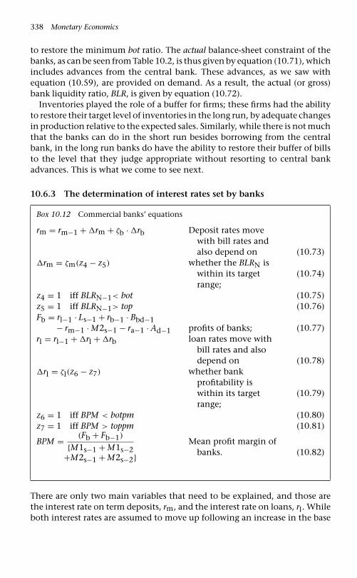
338 Monetary Economics

to restore the minimum bot ratio. The actual balance-sheet constraint of thebanks, as can be seen from Table 10.2, is thus given by equation (10.71), whichincludes advances from the central bank. These advances, as we saw withequation (10.59), are provided on demand. As a result, the actual (or gross)bank liquidity ratio, BLR, is given by equation (10.72).

Inventories played the role of a buffer for firms; these firms had the abilityto restore their target level of inventories in the long run, by adequate changesin production relative to the expected sales. Similarly, while there is not muchthat the banks can do in the short run besides borrowing from the centralbank, in the long run banks do have the ability to restore their buffer of billsto the level that they judge appropriate without resorting to central bankadvances. This is what we come to see next.

10.6.3 The determination of interest rates set by banks

Box 10.12 Commercial banks’ equations

rm = rm−1 + �rm + ζb · �rb Deposit rates movewith bill rates andalso depend on (10.73)

�rm = ζm(z4 − z5) whether the BLRN iswithin its targetrange;

(10.74)

z4 = 1 iff BLRN−1< bot (10.75)z5 = 1 iff BLRN−1> top (10.76)Fb = rl−1 · Ls−1 + rb−1 · Bbd−1

− rm−1 · M2s−1 − ra−1 · Ad−1 profits of banks; (10.77)rl = rl−1 + �rl + �rb loan rates move with

bill rates and alsodepend on (10.78)

�rl = ζl(z6 − z7) whether bankprofitability iswithin its targetrange;

(10.79)

z6 = 1 iff BPM < botpm (10.80)z7 = 1 iff BPM > toppm (10.81)

BPM = (Fb + Fb−1)

{M1s−1 + M1s−2Mean profit margin of

banks. (10.82)+M2s−1 + M2s−2}

There are only two main variables that need to be explained, and those arethe interest rate on term deposits, rm, and the interest rate on loans, rl. Whileboth interest rates are assumed to move up following an increase in the base

Model with Inside and Outside Money 339

rate set by the central bank9 – here the Treasury bill rate rb – we shall furtherassume that two different mechanisms are at work to explain the possiblydiverging evolution of these two administered interest rates (Box 10.12). Weshall assume that variations of the rate of interest on term deposits, relativeto the bill rate, depend on the evolution of the notional bank liquidity ratioBLRN. By contrast variations in the rate of interest on loans, relative to thebill rate, depend on the evolution of some measure of bank profits.

Embedded in the model is a hierarchy of interest rates. This hierarchy wasput forth by Godley and Cripps (1983: 160). They argued that banks wouldbe looking for ‘an appropriate or sensible’ composition of their portfolios ofassets. The bill rate would determine what the rates set by banks ought to be.‘Thus bank lending rates must be higher than [bill rates] (otherwise bankswould not want to lend to the private sector) and rates on interest-bearingbank deposits must be lower than [bill rates] (otherwise neither the publicnor banks would want to hold [bills])’.

How is the rate on deposit money determined? The mechanism to bedescribed closely follows the rules suggested in Godley (1997, 1999a). Ourkey assumption, as pointed out in the previous subsection, is that banks keepthe bank liquidity ratio a positive number above some minimum target, ask-ing for central bank advances if needed. In the longer run however, we shallassume that banks do not wish to be indebted to the central bank, and hencethat banks aim to keep the notional or net bank liquidity ratio BLRN withinsome quite narrow range, the floor and the ceiling of this range being botand top. If the sum of the other balance sheet items has driven the bill hold-ings of banks below the bottom of this range, they must raise the depositrate. This mechanism, described by equations (10.73) to (10.76), will havethe effect of inducing people to sell a proportion of their holdings of govern-ment securities and invest the proceeds in term deposit accounts. This leadsto an expansion in the liabilities of the commercial banks, who can then pur-chase government securities and obtain an equivalent increase in their assets(or reduce the amount of advances that they took from the central bank, inwhich case there is no expansion in the balance sheet of commercial banks),as can be checked from the balance sheet identity of banks (equations 10.67and 10.71). The bank liquidity ratio will now be higher.10

9 Lending rates increase or decrease one-for-one with changes in the bill rate, whilechanges in deposit rates only represent a proportion ζb of the change in the bill rate,as shown in equation (10.73).

10 This behaviour seems to be compatible with the evidence uncovered by Forman,Groves and Eichner (1985), who show that the higher the degree of liquidity pressure,relative to its trend value, the higher the interest rates. Since the degree of liquiditypressure is defined by Forman et al. as the ratio of loans to deposits, it is nearly thecomplement of the bank liquidity ratio defined here.

340 Monetary Economics

Conversely if the bank liquidity ratio rises above the safety range so thatbanks are holding more bills than they need, banks will reduce the interestrate on term deposits so that people hold a smaller share of wealth in moneydeposits and a higher share in securities. Banks will wish to hold as few billsas they safely can, because the rate of interest on these is lower than that onloans to the private sector. In our simulation model we have made up cruderules governing the banks’ responses which will always keep the net bankliquidity ratio moving towards the designated safety band, while the actualbank liquidity ratio is always at or above the minimum ratio.

And so we come to banks’ profits, defined in equation (10.77) as the sum ofall interest receipts less the sum of all interest payments. Our argument is thatbanks can ensure that all their operations are profitable, notwithstanding thepassivity in their responses which we have assumed, by appropriate adjust-ments in at least one of the rates of interest over which they have control. Weshall assume that banks raise the rate they charge on loans, relative to the billrate, whenever their profitability falls below a certain threshold, here calledbotpm. Similarly, when profitability exceeds some upper threshold – calledtoppm – they reduce their lending rates, for fear of government legislation orconsumer outrage.

The behaviour of lending rates, as expressed in equations (10.78)–(10.81),is symmetric to that of deposit rates. The fluctuations of lending rates, relativeto those of the bill rate, do not however depend on the bank liquidity ratio;rather they depend on the value taken by the bank profit margin – calledBPM. This bank profit margin is defined as the ratio of banks’ profits relativeto the stock of deposits of the previous period. We shall assume, as appears inequation (10.82), that banks check the mean value of this profitability indexover two periods, instead of acting on the basis of the value of a single year,so as to avoid unnecessary gyrations in the lending rate.

Our model is now complete in the sense that, with government expen-diture, the tax rate, the short and the long rates of interest, as well asproductivity taken as exogenous variables, there is an equation to explainthe behaviour of every other variable (the nominal wage will be explainednext). As in all of our models, there is one additional equation, the redundantequation, that need not be incorporated in the model. To find it, note thatthere are equations both in banks’ demand for reserves (equation 10.66) andin the supply of reserves to banks (equation 10.56). And here we have, at last,our redundant equation for the system as a whole:

Hbs = Hbd the redundant equation: supplies of reserves are foundto be equal to demand (10.83A)

Banks’ demand for cash and the central bank’s supply of cash to bankswill invariably be found to be of identical magnitude although there is noequation to make this happen. Banks demand reserves on the basis of legalrequirements tied to the size of their deposit liabilities; central banks provide

Model with Inside and Outside Money 341

reserves apparently on the sole basis of their balance-sheet constraint. Stillthe amount supplied will necessarily be equal to the amount demanded. Itis our belief that this is a finding which confirms the imaginative insightsof some post-Keynesian monetary economists, such as Le Bourva, Kaldorand Moore, who did not use formal methods of exposition. The quantity ofreserves supplied by the government to banks cannot be directly controlled.All that the government can control is the rate of interest it charges when itfinds itself making funds available.11

The redundant equation of the model – equation (10.83A) – helps us tounderstand why some countries, such as Canada or Switzerland, are able torun monetary policy and keep control over interest rates despite the com-pulsory reserve ratio being equal to zero. In Canada, for instance, there areno reserve requirements whatsoever. Canadian chartered banks are providedwith the banknotes that they need to operate the automatic teller machinesand their counter operations. Canadian banks do not hold any deposits atthe Bank of Canada. Still, despite the lack of compulsory (and free) reserves,the Bank of Canada is able to set the overnight rate at which individualchartered banks lend or borrow from each other. In our model, if the ρ ratiosrepresenting the required reserve ratios were equal to zero, nothing in howthe model functions would be changed. It is true that the stock of high-powered money Hb held by banks would be zero, and hence that the liabilityside of private banks would be further simplified. But this would have noeffect on the ability of the central bank to set the bill rate, and it would haveno direct effect on how banks set interest rates on loans and deposits.

10.6.4 Introducing inflationary forces

The INSOUT model may be finalized by introducing the same determinantsof inflation that we added to the DIS model of Chapter 9. We can assumethat workers or their unions have some real wage target in mind, whichdepends positively on labour productivity of the previous period as well onthe observed lagged employment rate. The rate of wage inflation will dependon how wide is the discrepancy between the target real wage and real wageof the previous period, as workers try to catch up by raising nominal wages.The following two equations describe this mechanism.

ωT =(

Wp

)T= �0 + �1 · pr + �2 ·

(N

Nfe

)(10.84)

W = W−1

(1 + �3 ·

(ωT−1 − W−1

p−1

))(10.85)

11 See Appendix 10.2 for an arithmetical example illustrating how the monetarymerry-go-round can work.

342 Monetary Economics

Since the focus of the present chapter is the ability of the private banksto absorb short-run fluctuations in the components of their balance sheet,while still maintaining, in the long run, both their profitability and theirliquidity ratio within their desired range, not too much will be said aboutinflation rates. Furthermore, since we have assumed that central banks setnominal rates, without introducing a central bank reaction function thatwould include inflation rates and employment rates – as in the Taylor rule –the true consequences of inflation cannot be taken fully into account.

Finally, for accounting purposes, we should recall the definition of grossdomestic product, Y , which, as we saw in Chapter 8, is the sum of the dollarvalue of sales and of the value of the change in inventories:

Y = p · s + UC · �in (10.86)

10.7 Making it all sing with simulations

10.7.1 The steady state

In this section we try to convey, by simulation experiments, how the systemas a whole behaves. It may be as well first to recall that the model has a welldefined stationary steady state to which it will tend if all the exogenous vari-ables are held constant. This full steady state must be one in which all stocksand all flows are constant. But if stocks of government debt are constant itwould seem to be the case that all outflows from the government are equalto all inflows (that is, tax receipts). Using the above notation it would seemto be the case that:

G + rb · B∗ + BL∗ = T (10.87)

where rb = rb−1.We shall see in a latter subsection that equation (10.87), as a condition for

stationarity, only holds when prices are constant. When there is inflation,real variables must be taken into account rather than nominal magnitudes,and hence the equilibrium level of output derived in equation (10.89) belowonly holds in a world without inflation.

As taxes are levied on the ex-tax, current price, value of sales, and as, inthe stationary state, there is zero investment in inventories so that output isequal to sales (y = s) it follows that:

T = s · p · τ

(1 + τ)(10.88)

We can therefore infer that, assuming away continuous inflation, thestationary value for real output is:

y∗ = (G + rb · B∗ + BL∗) · (1 + τ)

(p · τ)(10.89)

Model with Inside and Outside Money 343

The stationary real level of output depends on the tax rate, pure govern-ment expenditures and debt servicing, but the number of bills and bondsissued are themselves endogenous variables.12 To find out exactly what isgoing on in the model, we need to use simulations.

10.7.2 Simulation 1: An increase in the targetedinventories to sale ratio

In our first simulation experiment we explore what would happen if, start-ing from a stationary steady state, the inventory to sales target ratio σT wereto move up in a step, following an increase in the parameter σ0 of equation(10.7). This change will give us the opportunity to handle nearly all the inter-esting features of our more sophisticated financial system. Note first that, incontrast to the large steady-state increase that was observed with the help ofFigure 9.2 in the case of a pure private economy, the real output of this mixedeconomy will move back after the disturbance to a new steady-state whichshould be close to the original one, by reason of equation (10.89) above,which defines stationary real output. As we shall see, real output will not ingeneral move back to exactly its original level because stocks of governmentdebt will have changed. After a detour through a pure private economy with-out government, we see that the main result obtained in our most simplifiedmodels of Chapters 3 or 4 with only government money, returns to haunt usin the present complex mixed economy.

Figure 10.1A shows the evolution of the dollar value of inventories, andhence the evolution of the stock of bank loans granted to firms (since inven-tories are financed by bank loans). An approximate 10% increase in the targetinventory to sales ratio does lead to a substantial increase in inventories andbank loans, with some overshooting, as inventory investment (the change inthe stock of inventories) first jumps up, then declines, even reaching negativevalues. The response of consumption and total output follows the character-istic pattern generated by the multiplier process; both of them rise and bothgradually fall back, consumption initially trailing output, tracking the impe-tus given by inventory investment, as can be seen in Figure 10.1B, where realoutput and real consumption are charted as a ratio of their original valuesbefore the change.13

12 Equation (10.89) is not entirely correct since we have omitted the revenues thatthe government collects out of the profits of the central bank. But this is a second-ordererror.

13 A credible reason as to why the increase in the target inventories to sales ratiogenerates a slight reduction in the long-run value of real output will have to await thederivation of equation (10.98).

344 Monetary Economics

1955 1960 1965 1970 1975 1980 1985 19951990 2000 2005 2010

42.50

43.75

41.25

40.00

38.75

37.50

Value of inventories = Bank loans

Figure 10.1A Evolution of inventories (and hence bank loans), following an increasein the target inventories to sales ratio

1955 1960 1965 1970 1975 1980 1985 19951990 2000 2005 2010

1.020

1.030

1.010

1.000

0.990

0.980

Real output

Real consumption

Figure 10.1B Evolution of real output and real consumption, relative to their initialsteady state values, following an increase in the target inventories to sales ratio

Next consider what happens to the balance sheet of households and banks.Figure 10.1C tracks the additions, relative to the original steady state, to thevarious components of household wealth immediately after the step increasein the target inventories to sales ratio that was imposed (in the 1960 period,as shown in the chart). This increase, as we saw in the previous figure, ledto a brisk increase in output. As the addition to income was unexpected,no active portfolio choice is immediately made (in 1960) and consequently

Model with Inside and Outside Money 345

1958 1959 1960 1961 1962 1963 1964

3.0

4.0

2.0

1.0

0.0

–1.0

Wealth

Checkingdeposits

Timedeposits

BillsCash

Bonds

Figure 10.1C Evolution of household wealth and of its various components, relativeto their initial steady state values, during the first periods that follow an increase inthe target inventories to sales ratio

the entire accretion to wealth fetches up in the first period as an additionto holdings of checking bank deposits (non-interest bearing money). In thepresent instance, the notion of the initial rise in money being a response toan increase in the ‘demand’ for it is particularly wide of the mark; holdingsof non-interest bearing money have gone up by default, because incomerecipients have been taken by surprise.

In the next period (in 1961), the process of active asset reallocation begins.There is a tiny addition to holdings of cash by households which is neededfor transactions purposes. Besides this, there is, at least in 1961, an increasein the holdings of bills and bonds of households that echoes the increasein wealth. The most noticeable change is that of the interest-bearing moneybalances – the term deposits. It can be observed that there is a sharp rise in theterm deposits held by households, to the point that by 1963, their increaseeven exceeds the increase in wealth, implying a decrease in the absoluteamounts of checking deposits, bills and bonds held by households.14 Thisnew change in the structure of the household portfolio is due to the increasein the interest rate on term deposits, an increase illustrated in Figure 10.1D.But why does this rate increase?

14 All these changes, besides those of the first period, are indicative of what couldhappen; their magnitude depends on the exact values taken by the portfolio param-eters. For instance it could be that checking deposits remain above their startingvalue.

346 Monetary Economics

1956 1961 1966 1971 1976 1981 1986 19961991 2001 2006 2011

0.02240

0.02280

0.02200

0.02160

0.02120

00.02080

Interest rate on bills

Interest rate on term deposits

Figure 10.1D Evolution of the interest rate on term deposits, following an increase inthe target inventories to sales ratio

1958 1959 1960 1961 1962 1963 1964

4.0

5.0

3.0

2.0

1.0

0.0

Loans

Bills

Reserves

Central bank advances

All moneydeposits

Figure 10.1E Evolution of the various components of the balance sheet of commercialbanks, relative to their initial steady state values, during the first periods that followan increase in the target inventories to sales ratio

Figure 10.1E gives us clues as to why this could happen. The figure chartsthe changes, relative to the original steady state, of the various componentsof the balance sheet of banks. Loans, tracking inventories, briskly increase.The stock of money deposits, in the first period (1960), increases by theexact same amount, as the French circuitists and Basil Moore (1988) would

Model with Inside and Outside Money 347

argue. But in the second period (1961), households reallocate their newlyacquired wealth and rectify their consumption behaviour in accordance withtheir higher incomes, thus getting rid of part of the newly acquired deposits,which do not keep up with the rising level of loans made to firms. The banks’compulsory reserves move upwards, in proportion to the overall amount ofmoney deposits. Since banks only have a limited amount of bills to absorbthese fluctuations in their balance sheet, they are forced to take advancesfrom the central bank. This then induces banks to raise interest rates on termdeposits, as was shown in Figure 10.1D, in an effort to attract depositors, sothat money deposits catch up somewhat with bank loans.

Figure 10.1F shows that these actions initiated by banks will eventually besuccessful in reestablishing an acceptable bank liquidity ratio. As pointed outin the previous section, the notional bank liquidity ratio is the net amountof bills held by banks divided by the amount of banks’ deposits. The netamount of bills is the actual amount held minus the value of the advancestaken at the central bank. The large increase in loans granted by the banks isonly partially absorbed by an increase in bank deposits, and as a result the netbank liquidity ratio drops below its minimum acceptable level – the bottomof the target range – as can be seen in Figure 10.1F. Advances from the centralbank keep the actual or gross bank liquidity ratio at this minimum level. Butwith time, thanks to the higher deposit rates, plus the fact that inventoriesand hence loans drop back somewhat, banks manage to recover a net bankliquidity ratio which stands within the target range. This is when the interestrate on deposits becomes constant once again.

1956 1961 1966 1971 1976 1981 1986 19961991 2001 2006 2011

0.030

0.040

0.020

0.010

0.000

–0.010

top of range

bottom of range

Net and actualliquidity ratiosare the same withinthe range

Net bank liquidity ratio

Figure 10.1F Evolution of the net bank liquidity ratio, relative to its target range,following an increase in the target inventories to sales ratio

348 Monetary Economics

1955 1960 1965 1970 1975 1980 1985 19951990 2000 2005 2010

0.00525

0.00600

0.00450

0.00375

0.00300

0.00225

Top of target range

Bank profitability margin

Bottom oftarget range

Figure 10.1G Evolution of the bank profitability margin, relative to its target range,following an increase in the target inventories to sales ratio

We did not show the evolution of interest rates on loans, because the simu-lation did not induce any change in them. The cause of this is that, althoughthe transformation of the balance sheet of banks has led to variations in theprofits of banks, and in the new steady state to lower profits, mostly as a con-sequence of the higher interest rates on deposits, at no point did the bankprofit margin fall below the minimally acceptable level. This is shown inFigure 10.1G. Of course, all of this is indicative. Had the premia on lendingrates been any different, or had the profitability thresholds been any tighter,lending rates would have followed the upward movement of deposit rates.

In the new steady state, inventories, loans and deposit accounts are allhigher than before. The stock of government securities is lower than beforehowever. Total government debt has been reduced because, through most ofthe transition period, the government has been running a budget surplus, asshown in Figure 10.1H. With lower government debt, the steady-state flow ofaggregate income, expenditure and output are all (very slightly) lower thanbefore the shock, as illustrated in Figure 10.1B.

The central bank also has to adapt its balance sheet to the changing needsof the financial system, as well as the desires of portfolio holders and thepublic sector borrowing requirement. Figure 10.1I illustrates the evolution.By responding to the demands of the financial system, that is by allowingfluctuations in its holdings of Treasury bills, and also by granting advancesto banks on demand, the monetary authorities are able to keep control overthe bill rate (and, to a lesser degree, over all the other rates that move in syncwith it), keeping it exactly at its target level.

Model with Inside and Outside Money 349

1955 1960 1965 1970 1975 1980 1985 19951990 2000 2005 2010

0.300

0.375

0.225

0.150

0.075

0.000

Government budget balance

Figure 10.1H Evolution of the government budget balance, relative to its initial steadystate value, following an increase in the target inventories to sales ratio

1955 1960 1965 1970 1975 1980 1985 19951990 2000 2005 2010

20.00

20.50

19.50

19.00

18.50

18.00

Bills held by the central bank

Figure 10.1I Evolution of the stock of Treasury bills held by the central bank, followingan increase in the target inventories to sales ratio

In our model, notwithstanding that there is a fractional reserve rule inplace, the entire chain of causality is reversed compared with the standardtextbook neo-classical story. And although the supply of credit leads to anendogenous creation of money while the demand for money appears to bedetermined by a completely independent process, at no stage of the analysis

350 Monetary Economics

can we say that there is an excessive supply of money. The reason for this isthat we have formalized the existence of buffer mechanisms, which precludethe necessity of continuous equilibrium relationships.

10.7.3 Simulation 2: An increase in puregovernment expenditures

In our second simulation, we repeat an experiment that was made in ourvery first model, Model SIM. We suppose that the fiscal authorities decideto increase (permanently) pure real government expenditures g in a singlestep. The steady-state impact of such a change is quite obvious, if we lookat the steady-state determinant of real output, as given by equation (10.89).Figure 10.2A shows the evolution of real (Haig–Simons) disposable incomeand that of real consumption. In the initial stages following the change,consumption lags behind disposable income, but then catches up and evengoes beyond disposable income. As a result, real wealth increases in theearly stages, but decreases in the later stages, where it converges towardsreal disposable income since we assumed a real wealth to real disposableincome target ratio equal to unity. This cyclical behaviour, following anincrease in government expenditures, is not a necessary feature of the model;running a similar model with different parameters yields a smooth conver-gence between real wealth and disposable income (Godley 1997). But Figure10.2A shows that more complex models, compared to the simpler model ofChapter 3 for instance, where oscillations could not arise, can yield morecomplicated trajectories.

1955 1960 1965 1970 1975 1980 1985 19951990 2000 2005 2010

130.0

135.0

125.0

120.0

115.0

110.0

Real wealth

Real disposable income

Real consumption

Figure 10.2A Evolution of household real wealth, real disposable income andreal consumption, following a one-step permanent increase in real governmentexpenditures

Model with Inside and Outside Money 351

1955 1960 1965 1970 1975 1980 1985 19951990 2000 2005 2010

3.00

3.75

2.25

1.50

0.75

0.00

Public sector borrowing requirementdeflated by the price level

Figure 10.2B Evolution of the public sector borrowing requirement, deflated by theprice level, following a one-step permanent increase in real government expenditures

In the stationary state, as discussed time and again, real consumption isequal to real (Haig–Simons) disposable income, and hence real householdwealth is constant. In the stationary state, we would also expect the govern-ment budget balance to be zero. Figure 10.2B illustrates the evolution of thedeflated value of the public sector borrowing requirement (PSBR/p). As onewould expect, the more expansionary fiscal stance initially generates a largebudget deficit, with the government being forced to borrow.15 The charthowever indicates that the borrowing requirement in real dollars convergesto a positive number in the stationary state. Isn’t there a contradiction witheverything we have claimed in the previous chapters and in equation (10.87)?In the stationary state, when the wealth of the private sector is constant,shouldn’t the public debt be constant as well?

What happens is that the INSOUT model entertains an inflation mecha-nism, found in equations (10.84) and (10.85). In the base stationary state, theinflation rate has been set at zero. However, the larger real government expen-ditures generate higher outputs and higher levels of employment. These inturn generate higher rates of inflation, which mimic the higher output, asshown in Figure 10.2C. Inflation however modifies public sector accountingsince inflation erodes public debt. Inflation reduces real debt, where real debtis nominal debt deflated by current prices. One must thus make a distinction

15 The fiscal stance, as it was already defined in Chapter 3, is the ratio of overallgovernment expenditures to the share of tax revenues in national income (the averagetax rate).

352 Monetary Economics

1955 1960 1965 1970 1975 1980 1985 19951990 2000 2005 2010

0.0160

0.0200

0.0120

0.0080

0.0040

0.0000

Inflation rate

Figure 10.2C Evolution the price inflation rate, following a one-step permanentincrease in real government expenditures

between nominal and real debt, and between a nominal and a real budget bal-ance. A stationary state with permanent inflation implies a constant stock ofreal debt, and hence a zero real budget balance, but a nominal budget deficit.This is the exact counterpart of the situation of households, who, becausethey hold assets that are being eroded by inflation, must have zero real sav-ing in the stationary state, but a positive nominal amount of saving to keeptheir real wealth intact. While the government is running a nominal bud-get deficit, either measured in current dollars (PSBR) or measured in deflateddollars (PSBR/p), its real budget stance must take inflation gains on debt intoconsideration. Thus the real government budget balance is given by:

−PSBR + (�p) · (Bs−1 + BLs−1 · pbL−1)

p

When the government balance is measured in this manner, as shownin Figure 10.2D, it does indeed converge towards zero as the economyapproaches the steady state. This implies that the real debt of government,is constant. Indeed, when we check the evolution of the public debt to GDPratio in this closed economy, looking at Figure 10.2E, we observe that thediscretionary increase in government expenditures has led to a temporaryincrease in the public debt to GDP ratio, but that this ratio is driven back toits original level when all the dynamic effects of this change have run theircourse, when the economy reaches the new stationary state. Still, output,income, consumption and employment all stand at a higher level in thisnew stationary state. And of course, so do the stocks of loans, money andsecurities.

Model with Inside and Outside Money 353

1956 1961 1966 1971 1976 1981 1986 19961991 2001 2006 2011

0.0

1.0

–1.0

–2.0

–3.0

–4.0

Real government budget balance

Figure 10.2D Evolution of the real government budget balance, taking into accountthe capital gains due to the erosion of the public debt by price inflation, following aone-step permanent increase in real government expenditures

1955 1960 1965 1970 1975 1980 1985 19951990 2000 2005 2010

0.680

0.700

0.660

0.640

0.620

0.600

Debt to GDP ratio

Figure 10.2E Evolution of the debt to GDP ratio, following a one-step permanentincrease in real government expenditures

As in the previous experiment, we can look at the consequences of thehigher activity and the larger financial stocks on interest rates and on theprofitability of banks. Figure 10.2F shows the evolution of the main interestrates. Initially, there is a drop in inventories and hence in bank loans, asfirms get surprised by the amplitude of aggregate demand, caused by thebrisk increase in government expenditures. One period later, as firms react

354 Monetary Economics

1955 1960 1965 1970 1975 1980 1985 19951990 2000 2005 2010

0.0255

0.0270

0.0240

0.0225

0.0210

0.0195

Interest rate on deposits

Long-term interest rate (on bonds)

Interest rate on loans

Short-term interest rate (on bills)

Figure 10.2F Evolution of interest rates on bank loans and term deposits, relative toshort and long-term rates on government securities, following a one-step permanentincrease in real government expenditures

1958 1959 1960 1961 1962 1963 1964

6.0

9.0

3.0

0.0

–3.0

–6.0

Bills

Reserves

Loans

Term deposits

Checking deposits

Figure 10.2G Evolution of the various components of the balance sheet of privatebanks, relative to their initial steady state values, during the first periods that followan increase in the real government expenditures

to this drop in inventories by jacking up production, households are alsotaken by surprise, as their actual income turns out to be much greater thantheir expected income, leading to a substantial increase in checking deposits.Both of these effects, shown in Figure 10.2G, drive up the bank liquidityratio beyond the top of its target range as illustrated in Figure 10.2H, thus

Model with Inside and Outside Money 355

1955 1960 1965 1970 1975 1980 1985

Top of range

Net bank liquidity ratio

Bottom of range

19951990 2000 2005 2010

0.160

0.200

0.120

0.080

0.040

0.000

Figure 10.2H Evolution of the net bank liquidity ratio, relative to its target range,following a one-step permanent increase in real government expenditures

1955 1960 1965 1970 1975 1980 1985 19951990 2000 2005 2010

0.00525

0.00600

0.00450

0.00375

0.00300

0.00225

Top of target range

Bottom of target range

Bank profitability margin

Figure 10.2I Evolution of the bank profitability margin, relative to its target range,following a one-step permanent increase in real government expenditures

inducing reductions in the interest rate on term deposits. In the meantime, asa consequence of the changes in the composition of bank balance sheets, andalso as a result of the lower deposit rates, bank profitability also shoots up,beyond the top of its target range (Figure 10.2I). This drives down interestrates on loans. Eventually, as expectations adapt to actual conditions, andas the government deficit vanishes, both deposit rates and lending rates are

356 Monetary Economics

driven back to their original steady-state levels, and banks are even driven tothe discount window, being forced to take advances from the central bankon occasion (on Figure 10.2H the net bank liquidity ratio drops below thebottom of the target range, implying that banks borrow from the central bankto keep the actual bank liquidity ratio at its minimal level).

It is interesting to note that, in the new steady state, with higher activityand higher loans and money stocks, both in nominal and in real terms, inter-est rates are no higher than they were in the starting steady state. This occurseven though we have assumed that banks are concerned by the levels of theirbills to money ratio – the net bank liquidity ratio. This goes against the claim,made by proponents of structural endogeneity such as Chick and Dow (2002)or Wray (1990), that an economy in a boom or with higher activity oughtto be associated with higher interest rates since the bank liquidity ratio ofbanks would need to be lower. Things are much more complex in a fullyconsistent model which has several interdependencies that cannot always befully appreciated within the context of a partial analysis. A fortiori, in a worldwhere banks would be little concerned by such a ratio, as some horizontalistauthors like John Smithin or Le Bourva (1992) would put it, there is littleevidence that interest rates ought to rise. In fact, as we can see from Figure10.2F, despite the huge increase in government debt, the central bank andthe government have no difficulty in keeping the bill rate and the bond rateat the constant level of their choice. But this requires, as can be seen in Figure10.2J, that the central bank accept wide variations in the composition of its

1956 1961 1966 1971 1976 1981 1986 19961991 2001 2006 2011

2.25

3.00

1.50

0.75

0.00

–0.75

Change in the stock of billsheld by the central bank

Change in the advances granted to the commercial banks

Figure 10.2J Period-by-period changes in the stock of Treasury bills held by the cen-tral bank and in the advances granted to commercial banks, following a one-steppermanent increase in real government expenditures

Model with Inside and Outside Money 357

balance sheet, so as to accommodate changes in the demand for reservesand in the demand for bills, and granting advances to commercial banks ondemand.

10.7.4 Simulation 3: An increase in the compulsoryreserve ratios

In our third experiment, the banks’ statutory reserve requirement is assumedto rise from 10% to 20%, for both checking and term deposits. It would appearthat, according to the ubiquitous ‘money multiplier’ model, such a changeshould cut the ‘money supply’ in half. Our view is that nothing remotely likethat could possibly happen.

Figure 10.3A shows changes, compared with what would otherwise havehappened, in the banks’ balance sheet in the periods immediately followingthe postulated change. According to our model, the immediate consequenceof raising the reserve requirement is that reserves themselves do all the adjust-ing. In advance of any change in interest rates, households have no motiveto change any of their asset holdings and firms have no motive to cut theirborrowing. So the instantaneous counterpart of the change in the reserverequirement is a 100% increase in reserves. This should be accompanied byan equivalent fall, measured in dollars, in the net stock of bills held by banks.However, as can be seen in Figure 10.3A, advances from the central bank playthe main buffer role in the first period (1960) and in the following two peri-ods. In the system as configured here, banks are initially forced to borrow

1958 1959 1960 1961 1962 1963 1964

3.75

5.00

2.50

1.25

0.00

–1.25

Bills

Reserves

Loans

All moneydeposits

Central bankadvances

Figure 10.3A Evolution of the various components of the balance sheet of commercialbanks, relative to their initial steady state values, during the first periods that followan increase in the compulsory reserve ratios

358 Monetary Economics

1955 1960 1965 1970 1975 1980 1985 19951990 2000 2005 2010

0.025

0.050

0.000

–0.025

–0.050

–0.075

Top of target range

Bottom of target range

Net bank liquidity ratio

Figure 10.3B Evolution of the net bank liquidity ratio, following an increase in thecompulsory reserve ratios

most of the newly required reserves. Instead of depleting their stock of Trea-sury bills, commercial banks prefer to take advances from the central bank.

In the second period (1961), banks having seen their bank liquidity ratiofall below the bottom of its target range, as shown in Figure 10.3B, they willraise their interest rate on deposits, in an effort to attract more householdterm deposits and restore their bank liquidity ratio. The consequence of this,as can be seen in Figure 10.3A, is that the stock of money deposits – includingboth checking and term deposits – increases instead of briskly decreasing, incontrast to the traditional money multiplier story. This will lead to a furtherincrease in the amount of reserves, since compulsory reserves are a fractionof money deposits.

Furthermore, Figure 10.3A also shows that there is a small drop in theamount of loans. This can be attributed to the increase of the interest rateon loans, in the third period, as shown in Figure 10.3C. This increase inlending rates leads to a reduced target inventories to sales ratio, which inducesa reduction in inventories and hence in bank loans needed by firms. Thisincrease in the lending rate is due to the fall in the bank profitability margin,as shown in Figure 10.3D, that has been induced by the large unfavourablechanges in the structure of the balance sheet of the banks, imposed by themore severe compulsory reserve requirements. In addition, bank profits gethurt by the higher deposit rates needed to reestablish an adequate net bankliquidity ratio. As bank profits get mauled, banks need to raise lending ratesto get the bank profitability margin back to its target range.

In the new stationary state, as there has been a switch from governmentsecurities to money deposits, there will actually be more money in existence

Model with Inside and Outside Money 359

1955 1960 1965 1970 1975 1980 1985 19951990 2000 2005 2010

0.0270

0.0285

0.0255

0.0240

0.0225

0.0210

Interest rate on loans

Interest rate on bills

Interest rate on deposits

Figure 10.3C Evolution of the interest rate on deposits and the interest rate on loans,for a given interest rate on bills, following an increase in the compulsory reserve ratios

1955 1960 1965 1970 1975 1980 1985 19951990 2000 2005 2010

0.00375

0.00450

0.00300

0.00225

0.00150

0.00075

Top of target range

Bottom of target range

Bank profitability margin

Figure 10.3D Evolution of the bank profitability margin, following an increase in thecompulsory reserve ratios

as a result of the whole operation than there would have been without it!This can be seen in Figure 10.3E. Although the stock of money deposits getssomewhat reduced, as firms reduce the size of their inventories, the newsteady-state stock of money deposits remains higher than in the originalsteady state. The higher compulsory reserve ratio has had no negative impacton the stock of money, and no impact to speak of on real output. Its only

360 Monetary Economics

1955 1960 1965 1970 1975 1980 1985 19951990 2000 2005 2010

48.0

49.0

47.0

46.0

45.0

44.0

Money deposits(Checking and time deposits)

Figure 10.3E Evolution of the stock of money deposits, following an increase in thecompulsory reserve ratios

noticeable impact, as observed in Figure 10.3B, is a larger spread betweendeposit rates and lending rates. The compulsory reserve requirements onbank deposits act as a tax, which banks pass on to borrowers, as banks retaintheir profitability by raising lending rates when the compulsory reserve ratiois hiked up by the monetary authorities.

10.7.5 Simulation 4: An increase in the acceptablebank liquidity ratio

Our fourth experiment describes what happens when banks turn out to showa higher preference for liquidity. What will be the consequences of bankstargeting a higher bank liquidity ratio? What if banks wish to hold a saferportfolio? Recall that the bank liquidity ratio is the ratio of bills to deposits, or,as an approximation, the ratio of bills to total liabilities. Since total liabilitiesmust be equal to total assets, this implies that banks wish to hold a largerproportion of their assets in the form of bills. In other words, it means thatbanks wish to hold more bills relative to loans than they held before.16 Interms of equations (10.75) and (10.76), this means that banks set the bot and

16 This hopefully answers some of the queries made by some authors such as SheilaDow (1997: 66) and Jörg Bibow (2000). They insist that banks show some liquiditypreference. This can either mean that banks wish to modify the ‘disposition of the assetside of the bank’s balance sheet’ (Dow 1997: 66), substituting government securitiesin place of loans to the private sector, or it could imply that banks wish to change thesize of their balance sheet altogether. Here we illustrate the case where an increasedbank liquidity preference can be tied to bigger balance sheets.

Model with Inside and Outside Money 361

1955 1960 1965 1970 1975 1980 1985 19951990 2000 2005 2010

0.150

0.180

0.120

0.090

0.060

0.030

Top of new target range

Bottom of new target range

Bottom of initial target range

Top of initial target range

Bank liquidity ratio

Figure 10.4A Evolution of the bank liquidity ratio, following an increase in the liq-uidity preference of banks, proxied by an upward shift of the liquidity ratio targetrange

the top parameters to higher levels – in other words the bottom and top ofthe target range of the bank liquidity ratio are set at a higher level.

Now that we understand the structure of the model, we can guess at leastsome of the consequences of such a change in the liquidity preference ofbanks. Since banks wish to hold a larger proportion of bills among theirassets, as shown in Figure 10.4A, they will have to increase interest rates onmoney deposits relative to those on bills to induce households to relinguishthe bills that banks desire to acquire. The consequences on interest ratesare pretty straight-forward. Despite a constant bill rate, still set by the centralbank, the deposit rate rises. If this increase is large enough, and if the requiredchanges in the balance sheet of banks is important enough, the higher bankliquidity ratio targets will draw the bank profitability margin below its targetrange, and as a consequence the lending rates will also be raised, as is the casein Figure 10.4B, so that the bank profitability margin comes back towards itstarget range, as shown in Figure 10.4C. Thus, higher bank liquidity preferencewill mean both a higher bank liquidity ratio and higher deposit and lendingrates relative to the bill rate.

In our model, it is assumed that when banks do decide to raise the min-imum acceptable bill to deposit ratio, this minimum ratio will be achievedregardless of what needs to be done to achieve it. In the present case, asshown in Figure 10.4D, banks will even take advances from the central bankto modify the composition of their assets. Generally speaking, the attemptby banks to increase their target liquidity ratio will induce an increase in thesize of their balance sheet, as either larger central bank advances or money

362 Monetary Economics

1955 1960 1965 1970 1975 1980 1985 19951990 2000 2005 2010

0.02625

0.02750

0.02500

0.02375

0.02250

0.02125

Interest rate on loans

Interest rate on bills

Interest rate on term deposits

Figure 10.4B Evolution of the interest rates on deposits and loans, following anincrease in the liquidity preference of banks, proxied by an upward shift of the liquidityratio target range

1955 1960 1965 1970 1975 1980 1985 19951990 2000 2005 2010

0.00450

0.00525

0.00375

0.00300

0.00225

0.00150

Top of target range

Bottom of target range

Bank profitability margin

Figure 10.4C Evolution of the bank profitability margin, following an increase in theliquidity preference of banks, proxied by an upward shift of the liquidity ratio targetrange

deposits will accompany the larger amounts of Treasury bills held by privatebanks. Loans, which are a systemic requirement, cannot be called back orcut down at the initiative of the banks; indeed, when they do diminish at alater stage, as shown in Figure 10.4D, it is as a result of the negative impactof lending rates on the inventories to sales ratio.

Model with Inside and Outside Money 363

1955 1960 1965 1970 1975 1980 1985 19951990 2000 2005 2010

8.0

10.0

6.0

4.0

2.0

0.0

Checking and term deposits

Advances from the central bank

Reserves

Bills

Loans

Figure 10.4D Evolution of the various components of the balance sheet of commer-cial banks, relative to their initial steady state values, following an increase in theliquidity preference of banks, proxied by an upward shift of the liquidity ratio targetrange

10.7.6 Simulation 5: A decrease in the propensity to consumeout of real disposable regular income

We now repeat an experiment which we did on a number of occasions inprevious chapters. We assume that some campaign in favour of thriftinesshas been successful, and that the propensity to consume out of expectedreal disposable regular income suddenly drops down permanently in a step(this is the parameter α1 in equation 10.29). It turns out that the results thatwe obtained in smaller and simpler models, notably in Chapter 4 and 5,still hold up with the more complete model – the INSOUT model. We hadalready observed with the help of Figure 5.10 that a decrease in the propensityto consume out of income initially leads to a fall in output and disposableincome, as Keynesians would expect, but in the long run, when compar-ing steady states, this change leads to higher output and disposable income,provided no other parameter changes. Figure 10.5A, which illustrates thediscrepancy between real disposable income and consumption, and thus thepositive change in households’ wealth, is very similar to Figure 5.10, despitethe fact that the INSOUT model takes into account a much more complexprivate sector. As a counterpart to the rising household wealth, the short-runslowdown in economic activity provoked by reduced consumption generatesa deficit in the government budget balance (see Figure 10.5B). This enlargesthe size of the public debt and that of the interest payments on public debt,thus leading ultimately, in the long run, to an increase in economic activity,

364 Monetary Economics

1955 1960 1965 1970 1975 1980 1985 19951990 2000 2005 2010

112.0

116.0

108.0

104.0

100.0

96.0

Real consumption

Real regulardisposable income

Figure 10.5A Evolution of real regular disposable income and of real consumption,following a decrease in the propensity to consume out of (expected) real regulardisposable income

1956 1961 1966 1971 1976 1981 1986 19961991 2001 2006 2011

0.0

1.0

–1.0

–2.0

–3.0

–4.0

Real government budget balance

Figure 10.5B Evolution of the real government budget balance, following a decreasein the propensity to consume out of (expected) real regular disposable income

as per equation (10.89).17 Whether there are no private banks and no pri-vate investment, as in Chapters 4 and 5, or whether these exist as in thecurrent model, does not alter this fundamental principle arising from therequirements of stock-flow consistency.

17 Equation (10.98) will demonstrate this more formally.

Model with Inside and Outside Money 365

10.7.7 Simulation 6: An exogenous increase in therate of inflation

In this last simulation, we reproduce an experiment that we carried out inChapter 9. Once again we impose a one-time increase in the autonomousterm �0 in the target real wage equation (10.84). As a consequence, althoughnothing else has changed, workers ask for higher nominal wages, and thistranslates after some adjustment into permanent cost and price inflation.The results that we obtain in the current chapter, with a more completeINSOUT model that incorporates a government sector, are however quite dif-ferent from those that were obtained with the Chapter 9 DISINF model wherethe government sector was simply assumed away. In Chapter 9, persistentinflation had either a positive effect on the stationary level of real income ifhouseholds were blind to the capital losses inflicted by inflation, or no effectat all if households were aware of these losses. In the INSOUT model withthe government sector, where it is assumed that households are fully awareof inflation losses, persistent inflation is likely to have no effect or a nega-tive impact on the stationary level of real income. The explanations of whythis new result emerges will give us another opportunity to check the evo-lution of the real government budget balance, which we briefly discussed insubsection 10.7.3.

Figure 10.6A shows the boost in the rate of price inflation generated by thehigher target real wage rate. Figure 10.6B shows that the higher inflation rategenerates a lower stationary real national income. This is accompanied, asillustrated in Figure 10.6C, by a government budget deficit that exists even

1952 1957 1962 1967 1972 1977 1982 19921987 1997 2002 2007

0.0200

0.0250

0.0150

0.0100

0.0050

0.0000

Inflation rate

Figure 10.6A Evolution of the rate of price inflation, following a one-step increase inthe target real wage rate

366 Monetary Economics

1952 1957 1962 1967 1972 1977 1982 19921987 1997 2002 2007

132.0

134.0

130.0

128.0

126.0

124.0

Real outputRealsales

Figure 10.6B Evolution of real sales and real output following a one-step increase inthe target real wage that generates an increase in the rate of inflation

1952 1957 1962 1967 1972 1977 1982 19921987 1997 2002 2007

1.20

1.50

0.90

0.60

0.30

0.00

Public sector borrowing requirementdeflated by price level

Figure 10.6C Evolution of the public sector borrowing requirement, deflated by theprice level, following a one-step increase in the target real wage that generates anincrease in the rate of inflation

in the stationary state. But Figure 10.6D demonstrates that this is a nominalbudget deficit, and that when the budget balance is measured in the appro-priate way, by taking into account the inflation gains on the existing stock ofdebt, the real budget stance does converge towards zero. In other words, inthe stationary state, where the real wealth of households remains constant,the real debt of the government also remains constant, meaning that the realdeficit, net of the inflation capital gains on the existing debt, is zero.

Model with Inside and Outside Money 367

1953 1958 1963 1968 1973 1978 1983 19931988 1998 2003 2008

1.50

2.00

Real government budget deficit

1.00

0.50

0.00

–0.50

Figure 10.6D Evolution of the real government budget deficit, taking into accountthe capital gains due to the erosion of the public debt by price inflation, followinga one-step increase in the target real wage that generates an increase in the rate ofinflation

As we have seen in the earlier chapters which were based on state money, thestationary state in a closed economy is achieved when the financial positionof the public sector is such that the public sector does not create new liabilitiesany more. Thus the stationary state is achieved when the public sector is inbalance. In a world without inflation, this meant that the government sectorrannobudgetdeficit (norasurplus), andhence thatgovernmentexpenditures,including interest payments, were equal to its revenues (mainly taxes).

In a world with inflation, things are slightly more complicated, since infla-tion erodes the burden of a given stock of public debt. In other words,inflation reduces real debt, where real debt is nominal debt deflated by cur-rent prices. One must thus make a distinction between nominal and realdebt, and between a nominal and a real budget balance. A stationary statewith permanent inflation implies a constant stock of real debt, and hence azero real budget balance, but a nominal budget deficit. This is the exact coun-terpart of the situation of households, who, because they hold assets that arebeing eroded by inflation, must have zero real saving in the stationary state,but a positive nominal amount of saving to keep their real wealth intact.

10.7.8 The steady state with price inflation

Let us derive once more the stationary value of real output (as was donein equation 10.89), but this time by taking into account the possibility ofprice inflation. Let us start from an identity arising from the balance sheet ofTable 10.1. Reading off from the ‘Balance’ line, we see that:

V = GD + IN (10.90)

368 Monetary Economics

which says that nominal household wealth has two counterparts, nominalgovernment debt GD and nominal private debt, IN, which is the value ofinventories that firms must carry as debt in the form of bank loans. Thisof course also implies that the value of public debt is exactly equal to theamount of household wealth, from which we must subtract the value of theinventories of firms:

GD = V − IN (10.90A)

The same equation can be rewritten in differences:

�GD = �V − �IN (10.91)

Assuming away capital gains or losses arising from changes in interest rates, asin any event we shall concern ourselves with the steady-state solution wheresuch changes will be excluded, the change in nominal government debt canbe written as:

�GD = G + r̆ · GD − T = G + r̆ · (V − IN) − T (10.92)

where r̆, as in Chapter 4, is the average interest rate on government debt.Making use again of the Ostergaard formula, the changes in wealth and

in inventories, once again assuming away capital gains or losses arising fromchanging interest rates, can be written as:

�V = p · �v + �p · v−1 (10.93)

�IN = UC · �in + �UC · in−1 (10.94)

Focussing on the stationary state, we know that in such a state real wealthand real inventories remain constant, so that �v = �in = 0.

Applying this condition to equations (10.93) and (10.94), making use ofequation (10.92), and using real variables times their price, equation (10.91)can be rewritten as:

g · p + r̆ · p[v − in ·

(UCp

)]− T = �p · v − �UC · in (10.95)

or better still, by moving taxes on the right-hand side, dividing by p, andtaking note that in the steady-state �p/p = �UC/UC, we obtain:

g + r̆[v − in ·

(UCp

)]−

(�pp

) [v − in ·

(UCp

)]= T

p(10.96)

This equation demonstrates that, once the stationary state has beenreached, the overall level of tax revenues (in real terms) will be equal to

Model with Inside and Outside Money 369

real government expenditures, including debt servicing, minus the infla-tion gain on government debt.18 With inflation, ceteris paribus, the real fiscalstance gets reduced, since ‘the government receives an inflation gain on itsdebt which makes the inflation-adjusted government deficit smaller than itscash deficit’ (Godley and Cripps 1983: 244). In other words, the governmentshare of real national income exceeds the tax revenues, because of the infla-tion gain (or alternatively real outlays are diminished by the inflation gain).This explains why the public sector borrowing requirement (PSBR) is positive(there is a nominal government deficit, as expenditures exceed tax revenues)once a stationary state with positive price inflation is reached, as was thecase in Figures 10.2B and 10.6B. As pointed out by Godley and Cripps (1983:245), ‘what emerges is that the faster the rate of inflation the larger the gov-ernment’s cash deficit must be in order to keep real debt constant’. In thenew stationary state, the higher the rate of inflation, the larger is the discrep-ancy between deflated government expenditures and deflated governmentrevenues, that is the larger the apparent deflated deficit.

But now we are in a position to find the stationary level of real outputbecause we know that in the stationary state, s∗ = y∗ and c∗ = yd∗

r = yd∗hs.

Furthermore, we know that:

T = s · p · τ

(1 + τ)(10.88)

in∗ = σT · s∗ (10.6A)

v∗ = α3 · yd∗r (10.97)

s = c + g (10.13)

Using the four above equations, from equation (10.96) we derive the sta-tionary level of real output of Model INSOUT when taking into account priceinflation. This long-run equilibrium level of income is:

y∗ = g − α3 · (r̆ − )[τ

1 + τ

]−

[α3 − σT ·

(UCp

)](r̆ − )

(10.98)

where = �p/p, as defined in Chapter 9.19

18 ‘The government’s real fiscal stance may be defined, by analogy with the moneyfiscal stance, as the ratio of real government spending ... to the government’s share ofreal national income. This differs from the money fiscal stance not only because spend-ing is measured in real rather than in money terms but also because the government’sshare of real income includes the inflation gain mentioned above which is ignored inthe money accounts’ (Godley and Cripps 1983: 244).

19 It is also possible to calculate the stationary government debt to real GDP ratio,which we may wish to call gd∗/y∗, where gd is the real government debt, by recalling

370 Monetary Economics

The possible long-run implications of price inflation are now clear.20

Taking the partial derivatives, we find:

dy∗d

< 0

and

dy∗dr̆

> 0

Suppose we move from a stationary equilibrium with no inflation(π = = 0) to a new stationary equilibrium with inflation. If there is nochange in the nominal rate of interest (and no change in the distribution ofpublic debt), then r̆ remains at its initial value, and inflation then generates adecrease in the stationary level of real output, and hence a fall in real incomeand employment.21

The cause of this fall is that real government expenditures, when net-ting out the capital gains that have occurred on the public debt becauseof inflation, have decreased, thus leading to a fall in the multiplicand ofthe multiplier process. To avoid such a decrease in the multiplicand, thealternative is for the government to increase its expenditures on debt servic-ing. Indeed, we can see from equation (10.98) that provided that �(r̆ − ) iszero, that is provided the increase in the average interest rate r̆ is equal tothe inflation proxy value , and also provided there is no change in real puregovernment expenditures g, inflation will generate no change in the long-runvalue of real output.22 In this case, an inflation-neutral fiscal stance could

that gd = v − in · (UC/p), and making use of the stationary values and equations (10.12)and (10.97). We obtain that:

gd∗ = α3(y∗ − g) − in∗ · (UC/p)

while the gd∗/y∗ expression can be obtained by substituting the value of y∗ fromequation (10.98).

20 And so of course are the implications of changes in the other parameters ofequation (10.98). An increase in the target inventories to sales ratio σT leads to alower long-run real output, as long as (r̆ − ) > 0, which is what we assumed in ourfirst experiment. Also an increase in the target wealth to regular disposable incomeratio α3 leads to a higher long-run real output, as was observed in Figure 10.1B and10.5A, also as long as (r̆ − ) > 0.

21 There will be a small second-order change in the UC/p ratio. See Chapter 8.

22 Here we thus recover the result that was achieved in Model DISINF of Chapter 9,which did not include a government sector. It should be recalled that consump-tion equation (10.29), based on the definition of real regular disposable income(equation 10.26), assumes that households are fully aware of inflation losses. If, as

Model with Inside and Outside Money 371

be achieved.23 ‘Provided the real interest rate is maintained ... this happensautomatically through the variation in nominal interest payments’ (Godleyand Cripps 1983: 245).

While an inflation-neutral fiscal stance seems something that could eas-ily be achieved by governments, especially now with modern central banksbeing keen on increasing nominal interest rates in line with inflation rates, sothat real interest rates and the expression (r̆− ) would remain approximatelyunchanged, reality is often otherwise, at least judging by the experience of the1970s. One important cause for this is the fact that the increase in nominalinterest rates will generate a slowdown of the economy during the transi-tion to the new steady state. The higher interest rates imply a fall in theprices of long-term bonds, and hence inflict large capital losses to the bondholders. As a result household real consumption will drop and the economywill slow down. In the INSOUT model, in addition, the target inventories tosales ratio is sensitive to the value taken by the nominal interest rate, so thathigher interest rates will also induce a reduction in planned investment ininventories, and hence a further reduction in short-run output.

All these effects are illustrated in Figures 10.7, which reproduce the impacton Model INSOUT of an autonomous increase in the rate of inflation, as wasshown in Figures 10.6, but this time under the assumption that both theshort-term and the long-term interest rates are increased approximately inline with the increase in inflation. Figure 10.7A tracks the short-run drop inreal sales and their long-run recovery towards the initial steady-state level.Figure 10.7B shows the evolution of the real wealth of households and thegovernment stock of real debt, both of which diminish considerably in theshort run following the increase in long-term interest rates. Finally, Figure10.7C shows the deflated government budget balance, adjusted and unad-justed for inflation gains. In the short run, the former moves into a surplusposition while the latter goes into an apparent deficit.

As a result of the slowdown, the nominal government deficit will be evenhigher than it would be in its steady state with inflation, and this may inducethe government to take restrictive fiscal measures, raising tax rates or reduc-ing pure real government expenditures. As pointed out by Godley and Cripps(1983: 245, 247), ‘the increased cash deficit required in the presence of infla-tion are regarded with suspicion by adherents of the “balanced budget” ... .The real fiscal stance may tighten in response to inflation, while the cash

in Chapter 9, we assume that households are blind to inflation losses, it is as ifthe α3 parameter were revised upwards. The revised α3 parameter takes the value:α3/(1−(α1/α2) · ). In this case inflation would have a positive impact on the long-runlevel of real output.

23 However there will be a small second-order effect on σT, since the value of thisparameter will be pushed down by the higher nominal interest rate. See equation (10.7).

372

1952 1958 1964 1970 1976 1982 19941988 2000 2006

133.75

135.00

132.50

131.25

130.00

128.75

Real sales

Figure 10.7A Evolution of real sales and real output following a one-step increase inthe target real wage that generates an increase in the rate of inflation, accompanied byan increase in nominal interest rates that approximately compensates for the increasein inflation

1952 1957 1962 1967 1972 1977 1982 19921987 1997 2002 2007

97.5

105.0

90.0

82.5

75.0

67.5

Real household wealth

Real government debt

Figure 10.7B Evolution of real household debt and real government debt followinga one-step increase in the target real wage that generates an increase in the rate ofinflation, accompanied by an increase in nominal interest rates that approximatelycompensates for the increase in inflation

Model with Inside and Outside Money 373

1953 1958 1963 1968 1973 1978 1983 19931988 1998 2003 2008

0.50

1.00

0.00

–0.50

–1.00

–1.50

Real government budget balance(adjusted for inflation gains)

Deflated government budget balance(unadjusted for inflation gains)

Figure 10.7C Evolution of the deflated government budget balance, adjusted andunadjusted for inflation gains, following a one-step increase in the target realwage that generates an increase in the rate of inflation, accompanied by anincrease in nominal interest rates that approximately compensates for the increase ininflation

deficit expands’. This we believe is what happened in a large number ofcountries in the 1970s and early 1980s, and it may have contributed to theappearance of stagflation.

With the growth of nominal deficits and nominal debt, governmentsdecided to reduce their operating expenditures, reducing health and edu-cation services, in an effort to control what seemed like an uncontrollableexpansion of debt ratios. Thus, while in the mid 1970s real interest rates fell,thus reducing the contribution of the government sector to effective demand,thereafter it was the reductions in g that directly weakened the contributionof the public sector to real demand.

Governments were thus caught in a Catch-22 situation. With rising infla-tion rates and no increase in nominal interest rates, the real fiscal stancebecomes more restrictive on its own, and this drives down the long-run realoutput level. If governments do raise nominal interest rates in line withinflation rates, a neutral real fiscal stance can be achieved, so there is nodecrease in the long-run output level, but the higher interest rates will gener-ate large capital losses on long-term bonds which, in the short run, will causean economic recession and large government deficits. The only way out isfor the government to increase its operating expenditures in real terms, butthis is unlikely in a situation where nominal government deficits are alreadyrising.

374 Monetary Economics

10.8 Conclusion

We have gone a long way with the introduction of realistic banks whichmake decisions. But the model still lacks some key features of the real world.For instance, in the INSOUT model producing firms and banks distributeall of profits and have no retained earnings. In addition, the stock marketwith its equities and speculators has been left out. These important featuresof the real world are introduced in the growth model of the next chapter,since retained earnings, for instance, are a major characteristic of a growingcorporate economy.

Appendix 10.1: Overdraft banking systems

Anglo–saxon textbooks typically describe what we can be called asset-based financialsystems, which are characterized by a large government debt, some of which is heldby all sectors of the economy. Adjustments in the liquidity of both firms and banks isdone, or is presumed to be done, through changes in the assets, namely changes in theholdings of government bills. This is said, probably rightly so, to characterize financialsystems of the Anglo–Saxon world.

As was pointed out in Chapter 2 however, most countries fail to have asset-basedadjustment mechanisms. Both firms and banks adjust their liquidity position bychanges on their liability side. Indeed, even Anglo-Saxon financial systems have expe-rienced such a kind of adjustment over the last twenty or thirty years, and indeedsuch a phenomenon has been called liability management. Now it should be noted thatliability management has always been pursued by large New York banks, which areindebted towards the rest of the American banking systems. Most of the adjustmentin their liquidity position is done by varying the size of their advances that they bor-row from the rest of the financial system. These banks only keep a minimum amountof Treasury bills – the minimum required to conduct their clearing operations safely.Other countries also experience this division in bank tasks: some banks seem to spe-cialize in collecting deposits, and carry large amounts of bills, thus adjusting theirliquidity position on the asset side; other banks specialize in making loans, are largelyin debt vis-à-vis other banks, and adjust their liquidity position on the liability side,by discharging debt or adding debt. Because the banking sector is represented by asingle homogeneous sector, we cannot model this institutional distinction within ourframework.

There are also countries where the entire banking system is structurally in debtvis-à-vis the central bank. These banking systems are the so-called overdraft sys-tems. In these overdraft systems, banks carry no bills, or no bills in excess of theamounts required to operate safely and conveniently within the bank payments clear-ing system.24 Since bills cannot be used as a buffer, the entire adjustment mechanismrelies on liability management, whereas private banks obtain advances from the central

24 Indeed, large value payment clearing systems, which operate in real time,instead of clearing on the books of the central bank at the end of the day, requirethe possession of these Treasury bills as a guarantee for the finality of the payment.Indeed such use of Treasury bills has generated the generalization of the use of repos,

Model with Inside and Outside Money 375

bank. For instance, if households decide to reduce their bank deposits in exchange forcash money, without any change in loans, private banks obtain the additional cashmoney that households long for by borrowing it from the central bank. In that case,the advances of the central bank to the commercial banking system increase. Mostcountries of the world, including a large number of European countries, have theirbanking system in an overdraft position.

In our INSOUT model we have taken the decision to describe a banking system thathas some functions of both financial systems – the asset-based and the overdraft finan-cial system.25 We have assumed that banks in the short-run are free to get advancesfrom the central bank, paying no specific penalty relative to short-term assets of similarduration, hence describing features of overdraft economies. But we have also assumedthat banks desire to hold a certain proportion of their assets in the form of Treasurybills, and that in the long run they will act in such a manner that this proportion willbe achieved without being structurally indebted to the central bank, thus describingfeatures that are more pertinent to the asset-based system. It is our belief that, withglobalization and the new operating procedures followed by a large number of centralbanks, financial systems are gradually moving towards this hybrid structure, and hencethat the reaction rules that we attribute to central banks and private banks go a longway towards describing actual processes.

The modelling of the pure asset-based system is to be found in Godley (1999a). Zezzaand Dos Santos (2004) take on the case of the pure overdraft system, where banks holdno bills whatsoever. Within this framework, it is possible to see how deposit rateswould evolve endogenously. We could assume that private banks in a pure overdraftsystem keep a check on a bank liquidity pressure ratio – BLPR. This variable would bethe ratio of the funds that banks have borrowed from the central bank to the sumof the deposits being held in banks. The higher the liquidity pressure ratio, the morebanks must rely on the funds borrowed from the central bank. In general we wouldexpect the central bank rate on advances ra to be higher than the rate of interest rmpaid on time deposits of households. Hence, if banks are to hold on to their prof-its, there is an inducement for them to raise the rate of interest on time depositswhenever the bank liquidity pressure ratio exceeds what is considered to be its normalrange.

This procedure should help to bring the ratio back to its normal range. The mech-anism that leads to such a result is the following. By raising the interest rate on timedeposits, banks induce households to switch from checking deposits to time deposits,thus reducing the overall amount of compulsory reserve requirements, and hencereducing the demand of banks for high-powered money as long as the reserve require-ments on time deposits are less stringent than those on checking deposits. In addition,the increase in the rate on time deposits induces households to sell their bills and toacquire time deposits instead. This, by virtue of the balance-sheet constraint of banks,allows them to reduce their advances from the central bank, thus bringing the bankliquidity pressure ratio back towards its normal range.

whereby Treasury bills are sold with a promise to repurchase them back within 24 or48 hours. Thus, in fact, Treasury bills are lent for a day or two.

25 See Levy-Garboua and Maarek (1978) for a more traditional formalization of anoverdraft financial system.

376 Monetary Economics

Appendix 10.2: Arithmetical example of a changein portfolio preference

It may help readers if we provide an arithmetical example of the interdependenciesthat occur when there is a change in the portfolio preferences of households. This willalso help us to understand the quadruple entry system advocated by Copeland (1949),as discussed in Chapter 2. Start by assuming that for some reason, everything elsebeing held constant, households decide to hold $100 more in the form of money,splitting this into a $90 increase in bank deposits (denoted [1] in Table A10.1, which isa simplified balance sheet matrix of model INSOUT) and a $10 increase in cash (denoted[2]). This implies that households have reduced their holding of government securities,and we will assume here that households sold $80 worth of bills [3] and $20 worth oflong-term bonds [4].

If this happens, there have to be no less than seven simultaneous changes in thebalance sheets of commercial banks, the central bank and the government. First themoney deposits ‘owed’ by banks to their depositors must obviously rise by $90, which,being a liability, appear as a negative item [5] in the balance sheet of the banks. Assum-ing the existence of a compulsory fractional reserve ratio, set at 10%, commercial banksmust acquire additional central bank deposits equal to $9 to fulfill their reserve require-ments [6]. By their (vertical) balance sheet identity, this means that banks can nowacquire $81 worth of Treasury bills [7]. Banks will acquire bills, which act as the residualbuffer for banks, instead of granting loans, because post-Keynesians assume that banksgrant loans on demand, to all credit-worthy borrowers, which implies that the appear-ance of new bank deposits does not, in contrast to the mainstream money multiplierstory, induce or allow commercial banks to grant more loans since there is no reasonto believe that the additional deposits will transform unworthy potential borrowersinto credit-worthy ones.

Turning now to the central bank, the horizontal row at the top tells us that thecentral bank must issue additional amounts of high-powered money (HPM), the sumof the demanded cash and central bank deposits, that is $19 [8]. Once again, as theseare liabilities to the central bank, this amount appears with a negative sign. Since thesize of the central bank liabilities has increased by $19, the asset side must increase byan identical amount, leading the central bank to purchase $19 worth of bills [9]. Tokeep the interest rate on bills constant, the demand for and the supply of bills mustremain equal to one another, and hence, since the net demand for bills has grown

Table A10.1 Arithmetical example of a change in portfolio preference

Households Firms Govt. Central bank Banks �

HPM +10 [2] −19 [8] +9 [6] 0Bank deposits +90 [1] −90 [5] 0Bills −80 [3] −20 [10] +19 [9] +81 [7] 0Bonds −20 [4] +20 [11] 0Loans 0

� 0 0 0 0 0 0

Model with Inside and Outside Money 377

by $20, the government must issue $20 worth of new bills [10], which appear witha negative sign since this is a liability for the government. Finally, the last changein the matrix, [11], can be inferred in two ways. Reading vertically, since the size ofthe government debt is among the ceteris paribus variables, the government must retire$20 worth of government bonds to compensate for the $20 increase in the outstandingamount of bills (this will appear with a plus sign, since this is a reduction in liabilities).Alternatively, reading horizontally, to keep bond prices constant, the government mustreduce the value of its debt denominated in bonds since the household demand forbonds has been reduced by $20, purchasing back the bonds that households do notwish to hold anymore.

11A Growth Model Prototype

11.1 Prolegomena

This is by far the most ambitious chapter of the book. It sets out a rig-orous basis for the integration of Keynesian–Kaleckian macroeconomics(with constant or increasing returns to labour, growth, mark-up pricing,etc.) with a model of the financial system comprising banks, loans, creditmoney and equities, together with a model of inflation. Central contentionsof the chapter are that, with trivial exceptions, there are no equilibriaoutside financial markets and that the role of prices is to distribute thenational income, with inflation sometimes playing a key role determiningthe outcome.

The model deployed here describes a growing economy which does notspontaneously find a steady state even in the long run, but which requiresactive management of fiscal and monetary policy if full employment withoutinflation is to be achieved. Its main new features are as follows.

As the model describes a growing economy, firms now undertake fixedinvestment and their pricing mark-up is endogenous, depending on the rateat which dividends are paid and the proportion of investment that firms wishto finance through retained earnings. Second, firms now issue stock marketshares – equities.1 Third, there is now a distinction between unit costs andnormal unit costs, the former being actual labour costs per unit produced.When production is above normal, actual unit costs will be lower than nor-mal unit costs, which depend on trend productivity. It will now be assumedthat households as well as firms borrow from banks, and that the gross flowof new personal loans (before repayments) is exogenously determined as a

1 We first introduced retained earnings and stock equities in a growth model inLavoie and Godley (2001–2). See also Taylor (2004a: ch. 8) for an analytical version ofthat model.

378

A Growth Model Prototype 379

proportion of disposable income.2 As a result, consumption will depend onnet lending as well as real disposable income and wealth. Finally banks willhave to face the fact that some corporate borrowers default on their loans.As a result, banks retain part of their profits, accumulating own funds thatallow them to absorb capital losses while fulfilling regulation obligationsrelated to capital adequacy ratios. The loan rate will once more be determinedendogenously as a mark-up on the deposit rate.

As in any growth model, some of the most crucial equations are those deter-mining how growth arises. First, we assume an exogenous – unexplained –trend rate of growth in labour productivity, while the potential labour forceis assumed to be constant. Second, we initially assume that real pure govern-ment expenditure (excluding interest payments) – grows at a constant rate,initially the same rate at which labour productivity is growing. Third, weassume that the rate of accumulation of fixed capital is a function of the rateof capacity utilisation and of the real rate of interest. The rate of growth offixed capital is thus an endogenous variable, which adjusts to the growth rateof pure government expenditures.

11.2 Balance sheet, revaluation andtransactions-flow matrices

As always, we start the description of the model with its balance sheet andtransactions-flow matrices to which we add a revaluation matrix. Table 11.1

Table 11.1 The balance sheet of Model GROWTH

CentralHouseholds Firms Govt. bank Banks �

Inventories +IN +INFixed capital +K +KHPM +Hh −H +Hb 0Money +M −M 0Bills +Bh −B +Bcb +Bb 0Bonds +BL · pbL −BL · pBL 0Loans −Lh −Lf +L 0Equities +e · pe −e · pe 0Bank capital +OFb −OFb 0

Balance −Vh −Vf −Vg 0 0 −(IN + K)

� 0 0 0 0 0 0

2 Households nowadays borrow substantial amounts from banks, as much if notmore than firms, so any realistic account of what is going on in modern economiesshould incorporate personal bank loans. See Howells (1999).

380 Monetary Economics

provides the balance-sheet of the model, which we shall call Model GROWTH.The economy is again divided into five sections – households, firms, banks,a central bank and a government, each of which has distinct functions andobjectives. The household column has three new features. First, householdsare now indebted to banks. Second, they now hold stock market equities (orshares) issued by firms, e shares each valued at price pe. The third new featureof this column is the term OF which describes the own funds of banks –the value of their equity. It is assumed that whereas production firms arecorporations valued by the stock market, banks are privately held companies,which do not issue stocks. As a result, the net worth of these banks belongsto the private owners of the banks, and must appear as part of the net wealthof households.

It may be useful to recall some accounting issues which were discussedat the beginning of Chapter 2. The description of the Firms column herecorresponds with that in Table 2.2 where the net worth of firms is definedas the difference between all their assets and all their liabilities includingthe market value of equities. As a consequence the net worth of firms Vfcan be either positive or negative. By contrast, the Banks column corre-sponds to the one in Table 2.3 where the net worth of banks is calculatedas the difference between all assets and liabilities, excluding equities (sincewe assumed away their existence!). This is the own funds of banks, or theirequity capital. For the bank to be solvent, this net worth must be positive.However these own funds of the bank, OFb, belong to the owners of thebanks, and for this reason, while they enter with a negative sign in the bal-ance sheet of the banks they also enter with a plus sign in the balance sheet ofhouseholds.

The other components of the balance sheet have already been introducedin previous models. Firms own both kinds of tangible asset needed forproduction – inventories and fixed capital.

We now move to a new matrix, the revaluation matrix, given by Table 11.2which was also discussed in Chapter 2. In previous models, the revaluation

Table 11.2 Revaluation matrix of Model GROWTH: Changes in assets arising fromrevaluation gains

CentralHouseholds Firms Government bank Banks �

Bonds +�pbL · BL−1 −�pbL · BL−1 0Equities

of firms +�pe · e−1 −�pe · e−1 0Bank equity +�OFb −�OFb 0Fixed capital +�p · k−1 +�p · k−1

A Growth Model Prototype 381

matrix comprised only one entry, the capital gains or capital losses onholdings of long-term bonds. In the GROWTH model, four components maybe revalued. Besides bonds, stock market equities are also liable to capitalgains and losses. Third, banks accumulate own funds, but these funds belongto the owners of the banks, so that they are treated as a liability of the banks.From the standpoint of the bank owners, since this is a closed rather than apublicly owned corporation, the own funds accumulated by the bank duringa period are treated as a capital gain. From a Haig–Simons point of view, thebank’s own funds are part of the wealth of household owners, because if thebank were to be liquidated, their owners would be left with the bank capital –the own funds of the bank. Finally, the fourth line of the matrix shows anautomatic revaluation of the value of firms’ fixed capital, arising from priceinflation.

Table 11.3 describes net transactions between all five sectors in some givenperiod of time, measured at current prices. Start with the first seven itemsin the top half of the second column, written in bold characters. This listis the national income identity comprising the major expenditure categories(government expenditure, personal consumption and investment) and flowsof factor income (wages and profits). Every item in this column is a transac-tion with another sector or with a different part of the same sector (e.g. whenfirms buy investment goods from other firms or profits are retained in thebusiness), so a new column, the capital account column has been created torecord these capital transactions.

The columns describing the government and central bank are no differentfrom those of Table 10.2. Indeed, every entry in the top half of the matrixhas already been encountered in previous chapters and is self-explanatory,except for two unusual features relating to national income accounting con-ventions. First, in the row called ‘financing cost of inventories’, in column 2,the loan rate of interest multiplied by the opening stock of inventories hasbeen substituted for conventional stock appreciation (or IVA). Second, inter-est payments by firms, other than with respect to loans for the finance ofinventories, are included in line seven as a component of distributed profits.The reasons for making these entries have already been explained in detailin Chapter 8, where we dealt with various possible definitions of profits, andthe distinction between the requirements of business and national accounts.Banks and producing firms distribute dividends to their owners (FDb andFDf), and keep part of their profits undistributed, in the form of retainedearnings (FUb and FUf).

The bottom of the first half of the Table describes the various interest pay-ments on deposits, bills, bonds and personal loans. The latter is a new entry.It is assumed that households obtain personal loans from banks (Lh) onwhich they make interest payments. These payments carry a negative sign,since they are a use of funds, being subtracted from the personal income ofhouseholds.

382Table 11.3 Transactions matrix of Model GROWTH

Firms Central bank Banks

Households Current Capital Govt. Current Capital Current Capital �

Consumption −C +C 0Government expenditures +G −G 0Fixed investment +I −I 0Inventory accumulation +�IN −�IN 0Income tax −T +T 0Wages +WB −WB 0Inventory financing cost −rl−1 · IN−1 +rl−1 · IN−1 0Entrepreneurial Profits +FDf −Ff +FU f +rl−1 · (Lf−1 −

IN−1) − rl−1 · NPL0

Bank profits +FDb −Fb +FUb 0Central bank profits +Fcb −Fcb 0

Interest on personalloans

−rl−1 · Lh−1 +rl−1 · Lh−1 0

deposits +rm−1 · M−1 −rm−1 · M−1 0bills +rb−1 · Bh−1 −rb−1 · B−1 +rb−1 · Bcb−1 +rb−1 · Bb−1 0bonds +BL−1 −BL−1 0

Change in loans +�L +�L −�L 0the stocks of cash −�Hh +�H −�Hb 0

moneydeposits

−�M +�M 0

bills −�Bh +�B −�Bcb −�Bb 0bonds −�BL · pbL +�BL · pbL 0equities −�e · pe +�e · pe 0

Loan defaults +NPL −NPL 0� 0 0 0 0 0 0 0 0 0 0

A Growth Model Prototype 383

The lower part of the transactions-flow matrix describes the flow-of-funds.Checking the first column, that of households, there are two new items.Besides acquiring cash balances, money deposits, bills and bonds, house-holds purchase stock market shares newly issued (�e). In addition, whenhouseholds increase their borrowing, they have a new source of funds in theform of personal bank loans. The other new entry is ‘Loan defaults’ (NPL)which describe non-performing loans. It is assumed that a certain propor-tion of loans made to firms turn bad. The new loans (�Lf) that firms obtainas residual finance for changes in inventories and fixed investment will bereduced by the amount of defaulted loans. These non-performing loans willalso appear in the capital account of banks.

11.3 Decisions taken by firms

11.3.1 An overview of firms decisions

The following sections outline the behaviour and motivation of each of thefive sectors. These will be followed by an assessment of how the postulatedeconomy as a whole functions.

Firms continuously have to take a complex and interdependent set ofdecisions regarding output, investment, costing, prices, employment andfinance. As was argued earlier, firms must continuously decide how much theyare going to produce and what prices they will charge. These decisions willbe based on the quantity they expect to sell at those prices and the change ininventories they intend to achieve. Firms must also decide how much fixedinvestment they will undertake depending (for instance) on their ‘animalspirits’ and the existing pressure on capacity together with expectations aboutfinancial conditions and profitability. The stylized facts are that, subject to anupward trend in productivity, there are roughly constant returns to labour inthe long run and increasing returns in the short run. The demand for labourhas an obvious implication for the wage bill which firms have to pay. Fur-ther stylized facts are that the prices which firms charge are insensitive toshort-run fluctuations in aggregate demand, as argued in Coutts, Godley andNordhaus (1978). As a result, pro-cyclical fluctuations in demand and outputtend to be associated with pro-cyclical fluctuations in profits. The prices setby firms must be consistent, not only with their expectation about the quan-tity they will sell (at those prices), it must also be such, relative to wage costs,as to generate enough profit to pay for some target proportion of their fixedinvestment while distributing enough to satisfy shareholders and creditors.3

3 The line of argument here accords with an enormous body of theoretical work,notably by Kalecki, Kaldor and Tobin. One of the authors derived his arguments frompersonal conversations with the last two of these characters. The link between retainedearnings and investment can also be found in the works of Wood (1975), Eichner (1976)

384 Monetary Economics

Finally, the prices which firms charge, and the profits they hope to makeand distribute, are not independent of the recourse which they must have tobanks and financial markets as a residual source of funds for investment infixed and working capital.

This whole syndrome of firms’ decisions is presented in the following for-mal model. We shall discuss, in turn, firms’ decisions regarding output andemployment, investment, pricing and financing requirements. While themodelling of behaviour is crude, the accounting is solid and we shall reachconclusions which, when integrated into sub-models of other parts of a closedeconomy, will reveal some key features of the modus operandi of a modernindustrial economy together with an account of the financial system andcredit money. The main purpose of having a formal model, based on trans-actions accounts which have no black holes, is that one is forced to considerhow each part of an economy is interconnected with every other part.4 Forinstance, pro-cyclical productivity combined with normal-cost pricing musthave counterparts in the monetary system since the sudden increase in prof-its when demand rises is likely to reduce the demand for loans without therebeing a comparable fall in the demand for money, thereby threatening banks’profits.

In the sections that immediately follow we divide the decisions of firmsinto four components: those related to output, inventories and investment;costing decisions; pricing decisions; and financing implications. We close thesection with accounting identities describing realized outcomes.

11.3.2 Output and investment decisions

Box 11.1 shows the equations relevant to output, inventories and fixedinvestment. The first five equations are familiar, since they were describedin Chapter 9. The only new equation is (11.2), where it is assumed thatexpected sales are a weighted average of current sales and past sales, the latterbeing augmented by trend productivity growth which is deemed to representsecular tendencies in sales.

Equation (11.6) says that fixed capital accumulates at the rate grk. Thisgrowth rate, as can be seen in the next equation, depends on some constantreflecting animal spirits, on the real rate of interest on loans rrl, as well as aproxy for the rate of utilization of capacity u (here really an output to capitalratio, as shown in equation 11.7). This choice of investment function is arbi-trary. The purpose here is not to argue for one specification against another

and Harcourt and Kenyon (1976). See also Godley (1993) and Lavoie (1992: 109–18)for descriptions of such a link.

4 Keynes (1936: 297) knew all about this since he emphasizes that when analysing aparticular problem we should keep all related problems ‘at the back of our heads’. Weare hoping that the computer makes it possible to do this in a formal way and even tobring those problems round to the front of the heads of lesser mortals.

A Growth Model Prototype 385

Box 11.1 Firms’ equations

y = se + (ine − in−1) Real output decision; (11.1)

se = β · s + (1 − β) · s−1· Expected real sales; (11.2)

(1 + grpr)

inT = σT · se Long-run inventory target; (11.3)

ine = in−1 + γ · (inT − in−1) Short-run inventory target; (11.4)

in = in−1 + (y − s) Actual (real) inventory; (11.5)

k = k−1 · (1 + grk) Real capital stock; (11.6)

grk = gr0 + γu · u − γr · rrl Growth of real capital stock; (11.7)

u = yk−1

Capacity utilization proxy; (11.8)

rrl ={

(1 + rl)(1 + π)

}− 1 Real interest rate on loans; (11.9)

π = (p − p−1)

p−1Rate of price inflation; (11.10)

i = (grk + δ) · k−1 Real gross investment. (11.11)

but to show how, given the investment decision, firms have to validate it bysuccessfully generating the needed finance.5 Finally, equation (11.11) definesreal gross investment, which depends on the rate of accumulation and therate of depreciation of capital δ.

We end this section with a few identities, found in Box 11.2. Sales are madeup of consumption, government and gross investment (equation 11.12). Theother identities transform quantities into values taking note, once more,that goods in stock are valued at their cost of production UC, not at theprice that they could fetch if they were sold in the current period. Thishas the implications for the measure of nominal GDP first discussed inChapter 9.

5 Here we simply follow Dos Santos and Zezza (2005). Lavoie and Godley (2001–2)propose a more sophisticated investment function. Empirical work seems to show thatan essential component of all investment functions is the rate of capacity utilization,either for reasons related to the standard accelerator, or because rates of capacity utiliza-tion are a fair proxy for the realized rate of profit, thus alleviating liquidity constraintson producing firms.

386

Box 11.2 Firms’ equations

s = c + g + i Actual real sales; (11.12)

S = s · p Nominal value of realized sales; (11.13)

IN = in · UC Inventories valued at current cost; (11.14)

I = i · p Nominal gross investment; (11.15)

K = k · p Nominal value of fixed capital; (11.16)

Y = s · p + �in · UC Nominal GDP. (11.17)

11.3.3 Costing decisions

Box 11.3 Firms’ equations

ωT =(

Wp

)T= �0 + �1 · pr

+�2 · {ER + z3(1 − ER) − z4· bandT + z5 · bandB}

Real wage aspirationassessed atbargaining table; (11.18)

ER = N−1Nfe −1

Employment rate ; (11.19)

z3 = 1 if 1 − bandB ≤ ER≤1 + bandT (11.20)

z4 = 1 if ER > 1 + bandT

z5 = 1 if ER < 1 − bandB

W = W−1+�3 ·(ωT ·p−1−W−1) Nominal wage; (11.21)

pr = pr−1 · (1 + grpr) Labour productivity (grpris productivitygrowth);

(11.22)

NT = ypr

Desired employment; (11.23)

N = N−1 + η · (NT − N−1) Actual employment; (11.24)

WB = N · W Nominal wage bill; (11.25)

UC = WBy

Actual unit cost; (11.26)

A Growth Model Prototype 387

NUC = Wpr

Normal (trend) unit cost; (11.27)

NHUC = (1 − σN) · NUC + σN·(1 + rlN·) · NUC−1 Normal historic unit cost. (11.28)

The costing decisions that firms need to take are to be found in Box 11.3.As discussed in Chapter 9, inflation is essentially a conflicting-claims phe-nomenon, with workers coming to the bargaining table with an aspirationto obtain a real wage rate ωT, the size of which depends on trend labourproductivity and on the pressure of demand for labour.6 The nominal wagethen reacts to the discrepancy between the target wage and the actual nom-inal wage (equation 11.21). However, we believe the real-world process tobe highly contingent, going beyond mechanical equations. Indeed the evi-dence relating to the UK with regard to the years prior to 1975 as well as theevidence in several countries over the last few years supports the view thatthere is quite a range of employment or unemployment values within whichthe inflation rate will be unmoved (or even move perversely).

We thus complicate equation (11.18) by adding a logical function (11.20),which says that when the rate of employment ER (as defined in equation11.19), is within a certain band, there will be no additional pressures on thetarget real wage and hence on the rate of inflation. What these equations aresaying is represented in Figure 11.1, which shows a kind of Phillips curve witha horizontal segment, which corresponds to the situation where z3 = 1. Sucha horizontal segment has been suggested recently, among others, by Tobin(1995), Hein (2002) and Palascio-Vera (2005). There is also an ever-growing

Target real wage(wage inflation rate)

1– bandB 1+ bandT100%Employment rate ER

Figure 11.1 Phillips curve with horizontal mid-range segment

6 In the actual model, equation (11.18) is expressed in logarithmic form.

388 Monetary Economics

number of empirical studies that support middle-range flat segments (Eisner1996; Filardo 1998; Barnes and Olivei 2003).

The growth rate of trend labour productivity is still assumed to be an exoge-nous variable (equation 11.22).7 This trend productivity level and the outputdecision have a direct implication for desired employment, NT (equation11.23). By contrast, actual employment, N, follows a partial adjustmentprocess towards its normal relationship to output, as described by equation(11.24). In this way there will be a short-term increase in productivity whenoutput rises above trend in accordance with a well established stylized fact.As total output fluctuates about its trend, there is a tendency for labour pro-ductivity to move pro-cyclically. This may be simply because there is a lagbetween unusual movements in output (which may turn out to be temporary)and the response of firms in terms of hiring. It may alternatively come aboutbecause the total labour force comprises a category of ‘overhead’ employ-ees which does not respond – only sluggishly – to short- and medium-termfluctuations in output (Lavoie 1992: ch. 5).

The distinction between trend and actual productivity allows us to make adistinction between actual unit costs UC, as defined by equation (11.25) and(11.26), and trend or normal unit costs NUC, as given by equation (11.27).We assume that normal unit costs enter into the determination of normalhistoric unit costs NHUC, (11.28), which is based on past and current normalunit costs, and on what firms consider to be the normal inventories to salestarget σN and the normal interest rate rlN.8 It is this normal historic unitcost which will be the multiplicand upon which the costing margin will beapplied when firms set prices.

11.3.4 Pricing decisions

Box 11.4 Firms’ equations

p = (1 + ϕ) · NHUC Normal-cost pricing; (11.29)

ϕ = ϕ−1 + ε · (ϕT−1 − ϕ−1) Actual mark-up; (11.30)

7 Thus, although we believe that the rate of technical progress is influenced byeffective demand, we disregard for simplicity the point made by both Kaldor (1960:237) and Robinson (1956: 96), that ‘the natural rate of growth is ultimately endogenousto the demand-determined actual rate of growth … . The natural rate is not an attractorin demand-led growth models’ (Setterfield 2002: 5). See also Lavoie (2006d: 180–1) andGodley and Cripps (1983: 253–4).

8 In a static model, this normal ratio σN would be the long-run inventories to salestarget σT already defined in equation (11.3), as it was in Chapter 10. However, withgrowth this long-run target is never achieved, so that the realized inventories to salesratio in steady-state growth is always different from this target σT. Thus in the baserun, we have set σN = {σT/(1+grpr)}/( in/inT).

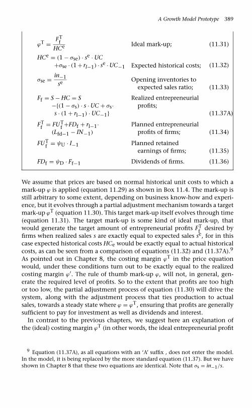
A Growth Model Prototype 389

ϕT = FTf

HCe Ideal mark-up; (11.31)

HCe = (1 − σse) · se · UC+σse · (1 + rl−1) · se · UC−1 Expected historical costs; (11.32)

σse = in−1se Opening inventories to

expected sales ratio; (11.33)

Ff = S − HC = S−{(1 − σs) · s · UC + σs·s · (1 + rl−1) · UC−1}

Realized entrepreneurialprofits;

(11.37A)

FTf = FUT

f +FDf + rl−1·(Lfd−1 − IN−1)

Planned entrepreneurialprofits of firms; (11.34)

FUTf = ψU · I−1 Planned retained

earnings of firms; (11.35)

FDf = ψD · Ff−1 Dividends of firms. (11.36)

We assume that prices are based on normal historical unit costs to which amark-up ϕ is applied (equation 11.29) as shown in Box 11.4. The mark-up isstill arbitrary to some extent, depending on business know-how and experi-ence, but it evolves through a partial adjustment mechanism towards a targetmark-up ϕT (equation 11.30). This target mark-up itself evolves through time(equation 11.31). The target mark-up is some kind of ideal mark-up, thatwould generate the target amount of entrepreneurial profits FT

f desired byfirms when realized sales s are exactly equal to expected sales se, for in thiscase expected historical costs HCe would be exactly equal to actual historicalcosts, as can be seen from a comparison of equations (11.32) and (11.37A).9

As pointed out in Chapter 8, the costing margin ϕT in the price equationwould, under these conditions turn out to be exactly equal to the realizedcosting margin ϕ′. The rule of thumb mark-up ϕ, will not, in general, gen-erate the required level of profits. So to the extent that profits are too highor too low, the partial adjustment process of equation (11.30) will drive thesystem, along with the adjustment process that ties production to actualsales, towards a steady state where ϕ = ϕT, ensuring that profits are generallysufficient to pay for investment as well as dividends and interest.

In contrast to the previous chapters, we suggest here an explanation ofthe (ideal) costing margin ϕT (in other words, the ideal entrepreneurial profit

9 Equation (11.37A), as all equations with an ‘A’ suffix , does not enter the model.In the model, it is being replaced by the more standard equation (11.37). But we haveshown in Chapter 8 that these two equations are identical. Note that σs = in−1/s.

390 Monetary Economics

share, ϕT/(1+ϕT)). Given historic costs, the target mark-up depends on targetentrepreneurial profits. Target entrepreneurial profits, as shown by equation(11.34), must cover target retained earnings FUT

f , distributed dividends FDfand interest payments on loans other than those generated by inventories(which have already been taken into account as part of historic costs). We sup-pose, in line with stylized facts and as several previous post-Keynesian authorshave claimed, that firms attempt to finance most of their gross fixed invest-ment expenditures through their gross retained earnings. Indeed, equation(11.35) sets target undistributed profits as a proportion ψU of gross nomi-nal investment in fixed capital of the previous period. Distributed dividendsare a fraction ψD of entrepreneurial profits earned in the previous period(equation 11.36), and this, actual distributed dividends, rather than a targetamount, enters into the target profits equation. It is assumed that firms willdistribute dividends only once they have obtained verified accounts of theiractivities.10

11.3.5 Financial implications for the firms

Box 11.5 Firms’ equations

Ff = S − WB + �IN − rl· Realized entrepreneurialIN−1 profits of firms; (11.37)

FU f = Ff − FDf − rl−1·(Lfd−1 − IN−1) Retained earnings+ rl−1 · NPL of firms; (11.38)

Lfd = Lfd−1 + I + �IN Demand for loans− FU f − �es · pe − NPL by firms; (11.39)

NPL = npl · Lfd−1 Defaulted (non-performing) loans; (11.40)

es = es−1 + (1 − ψU) · I−1pe

Supply of equitiesissued by firms; (11.41)

10 Final sales will be known at best on the 31st of December, and the income andprofit statement of the firm needs to be verified by accountants before any dividenddecision can be taken. Indeed, in many countries, dividends are announced only onthe 30th of June, after attorneys and accountants have checked the numbers, becauseit would be illegal to distribute dividends that are greater than profits (Vallageas 2001).Thus the dividends distributed in period t arise from the activity of period t − 1.

A Growth Model Prototype 391

rK = FDf(es−1 · pe−1)

Dividend yield of firms; (11.42)

PE = pe(Ff/es−1

) Price earnings ratio; (11.43)

q = (es · pe + Ld)

(K + IN)Tobin’s q ratio or

Kaldor’s valuation ratio. (11.44)

The rules of thumb which firms adopt will never exactly generate requiredprofits because sales, inventories and interest rates will all undergo unex-pected short-term variations. Realized entrepreneurial profits Ff , as definedin equation (11.37), which reproduces the analysis conducted in Chapter 8,will thus, in general, be different from targeted profits (Box 11.5). Becausedistributed dividends and interest payments on bank debt are set amounts,dependent on values taken in the previous period, any windfalls inentrepreneurial profits will go into actual retained earnings FUf . Equation(11.38), which describes undistributed profits, includes an additional term,rl−1 ·NPL. Those are the interest payments that firms defaulting on their loansdid not pay to banks. As a result entrepreneurial profits are enlarged by thisamount, ceteris paribus.11 It is assumed that a proportion npl of previous bankloans default every year (equation 11.40).

Finally coming to the firm sector’s financial requirements, equation (11.39)describes required bank loans, Lfd. The change in loans that firms require canbe computed from their capital account column in Table 11.3. Loans, onceagain, act as a buffer, absorbing unexpected changes in financial require-ments. Any (positive) windfall in entrepreneurial profits will be reflectedin a decrease in the demand for loans. Required loans will also be dimin-ished when some firms default on their loans (NPL), and when firms makenew stock issues (�es · pe). We have assumed that if firms plan that a pro-portion ψU of nominal investment expenditures will be financed throughretained earnings, then a proportion (1 − ψU) – this expression being a smallpercentage – will be financed through new issues of shares (equation 11.41).

11 The ceteris paribus clause normally would not apply because the inventories usu-ally provide the collateral backing the bank loans provided to firms. If firms defaulton their loans, either the banks should get hold of the inventories or these inventorieshave become worthless (because they are outdated merchandise), and hence, if non-performing loans amount to NPL dollars, this implies that firms should lose NPL/UCunits of real inventories. In other words, equation (11.5) ought to be written as:

in = in−1 + (y − s) − NPLUC

392 Monetary Economics

As a result, on average, only additional investment expenditures, relative tothose of the previous period, will be financed through bank loans, so thatapart from these, bank loans are essentially financing inventories.

The last three equations of Box 11.5 yield some well-known financial ratios.The dividend yield, rk, is the ratio of the dividends distributed this period overthe stock market value of the shares outstanding at the end of the previousperiod. This ratio will enter the portfolio decisions of households. Equation(11.43) gives the price earnings ratio, which is the current equity price dividedby profits per share. It is also interesting to define the (average) q ratio, asTobin called it, or the valuation ratio under Kaldor’s terminology (equation11.44). In our model, as we believe also in the real world, there is no mech-anism to make the q ratio converge towards unity. The evolution of the qratio, as well as that of the price earnings ratio, will depend to a large extenton the desire of households to hold equities compared to their desire to holdother financial assets, an issue which is discussed in the next section.

11.4 Decisions taken by households

The decisions of households will be split into three subsections. The firstsubsection is by now familiar and deals with personal income, disposableincome, changes in wealth and consumption. The second is new, describinghow households get into debt. The third deals with usual portfolio decisions.

11.4.1 Income and consumption decisions

Box 11.6 Households’ equations

YP = WB + FDf + FDb+ rm−1 · Mh−1 + rb−1·Bhd−1 + BLd−1 Nominal personal income; (11.45)

T = θ · YP Income taxes; (11.46)

YDr = YP − T

− rl−1 · Lhd−1 Nominal regulardisposable income; (11.47)

YDhs = YDr + CG Haig–Simons nominaldisposable income; (11.48)

CG = �pbL · BLd−1+ �pe · ed−1 + �OF Capital gains; (11.49)

A Growth Model Prototype 393

V = V−1 + YDhs − C Nominal wealth; (11.50)

v = Vp

Real stock of wealth; (11.51)

C = p · c Nominal consumption; (11.52)

c = α1 · (yder + nl)

+ α2 · v−1 Real consumption; (11.53)

yder = ε · ydr + (1 − ε) · Expected real regular

ydr−1 · (1 + grpr) disposable income; (11.54)

ydr = YDr

p− π · V−1

pReal regular

disposable income. (11.55)

This subsection is familiar territory, but it contains a few innovations as aconsequence of the introduction of personal loans to households (Box 11.6).Nominal personal income YP is the sum of wages, dividends and interestpayments received on deposits, bills and bonds (equation 11.45). Incometaxes, the only kind of taxes in Model GROWTH, are paid on this personalincome (equation 11.46). Nominal regular disposable income YDr is whathouseholds are left with once they have paid their income taxes and oncethey have made their interest payments on the personal loans they havetaken from banks (equation 11.47). Haig-Simons nominal disposable incomeYDhs is the sum of regular disposable income and capital gains (equation11.48). The latter, as mentioned in our discussion of the revaluation matrix,comprises capital gains on bonds and equities, as well as the increase in theown funds of banks, which belong to households (equation 11.49). As aresult, the change in nominal wealth is defined in the usual way, as the sumof Haig-Simons disposable income and capital gains (equation 11.50).

As in our other models with changing prices, we suppose that consumptiondecisions are taken in real terms. Real consumption, as shown by equation(11.53) depends on expected real regular disposable income and on a newelement, nl, which is the deflated net lending to households by banks. Inother words, it is assumed that a portion of the funds obtained from banksby households are consumer loans, while the rest is used to purchase financialassets. The nl variable will be explained in the next subsection. As to expectedreal regular disposable income yde

r , in symmetry with expected real sales, wesuppose that it is a weighted average of the real regular disposable incomeof the current period and that of the previous period, augmented by thesecular trend in the growth rate of productivity (equation 11.54). Real regulardisposable income ydr, in line with previous chapters, is itself defined as

394 Monetary Economics

deflated regular disposable income minus the capital losses inflicted by priceinflation (equation 11.55).

11.4.2 Personal loans decisions

Box 11.7 Households’ equations

GL = η · YP Gross amount of newpersonal loans; (11.56)

η = η0 − ηr · rrl New loans to personalincome ratio; (11.57)

NL = GL − REP Net amount of newpersonal loans; (11.58)

REP = δrep · Lhd−1 Personal loanrepayments; (11.59)

Lhd = Lhd−1 + NL Demand forpersonal loans; (11.60)

nl = NLp

Real amount of newpersonal loans; (11.61)

BUR = (REP + rl−1 · Lhd−1)

YPBurden of personal debt. (11.62)

Box 11.7 shows the operations linked to personal loans. Equation (11.56) saysthat the gross flow of new personal loans is a fraction η of nominal personalincome. This fraction may be interpreted as some limit which householdsassign to themselves or as a limit which banks impose on households, fol-lowing some rule of thumb. The fraction η is itself inversely related to thereal rate of interest on loans, as shown in equation (11.57), in line with thenow vast literature on credit rationing.

As equation (11.58) shows, net lending to households within a period isequal to gross new loans minus repayments, (REP). Principal repayments area fraction δrep of the outstanding stock of personal loans (equation 11.59).The end-of-period stock of loans of the current period is thus equal to thestock of loans at the beginning of the period, Lhd−1, plus the net flow of newloans NL (equation 11.60).

The last two equations of Box 11.7 define ratios. The nl variable that weencountered in the equation describing real consumption is here definedas the nominal flow of net lending NL, deflated by the price index.Equation (11.62) yields a potentially useful measure of the burden of debt

A Growth Model Prototype 395

on households. This burden, BUR, is the sum of interest payments and prin-cipal repayments as a fraction of personal income. It is the debt-serviceburden.

11.4.3 Portfolio decisions

Box 11.8 Households’ equations

MdVfma−1

= λ10 + λ11 · rm − λ12 · rb

− λ13 · rbL − λ14 · rK + λ15 ·(

YPVfma−1

); (11.63)

BhdVfma−1

= λ20 − λ21 · rm + λ22 · rb

− λ23 · rbL − λ24 · rK − λ25 ·(

YPVfma−1

); (11.64)

(pbL · BLd)

Vfma−1= λ30 − λ31 · rm − λ32 · rb

+ λ33 · rbL − λ34 · rK − λ35 ·(

YPVfma−1

); (11.65)

(pe · ed)

Vfma−1= λ40 − λ41 · rm − λ42 · rb

− λ43 · rbL + λ44 · rK − λ45 ·(

YPVfma−1

); (11.66)

Mh = Vfma − Bhd − pbL·BLd − pe · ed Money deposits - a residual; (11.67)

Vfma = Md + Bhd

+ pbL · BLd + pe · ed [11.66 rewritten]; (11.68A)

Vfma = V + Lhd Financial market asset− Hhd − OF (investible) wealth; (11.68)

Hhd = λc · C Households’ demandfor cash; (11.69)

ed = es Stock market equilibrium. (11.70)

396 Monetary Economics

Households’ allocate expected disposable income between consumption andwealth accumulation while simultaneously allocating wealth between thevarious assets listed in the accounting matrices. As households’ expectedincome is always different from realized income there must be a flexible com-ponent in the wealth allocation process which takes on a buffering role. Cashis not a good candidate for this role in the days of credit cards and electronicpayments from and into bank deposit accounts. A better candidate is bankdeposits which act as the passive variable giving signals in much the sameway as inventories give signals to firms and reconciles actual with expectedsales.

Financial assets, or rather what we now call market financial assets, Vfma,are allocated in line with Tobinesque principles, with the appropriate adding-up constraints, as described by equations (11.63) to (11.66) (Box 11.8).Financial market assets comprise four kinds of assets: money deposits, bills,bonds and equities, as shown by equation (11.68A). The financial marketasset component of household wealth Vfma can be read off from the first col-umn of Table 11.1. Because the gross wealth of households is equal to theirnet wealth V plus their liabilities, in this case bank loans Lhd, the wealththat can be invested in market financial assets is equal to the net wealth ofhouseholds V , plus the funds borrowed from the banks Lhd, minus house-hold wealth which is stuck in the own funds, OF, of the banks and the wealthwhich is kept in the form of cash, Hhd. This identity arising from Table 11.1is found in equation (11.68).

In this model we do away with complex calculations of expected wealthand simply assume that expected investible wealth is the market financialasset wealth of the previous period (Vfma−1). We further assume that thedemands for financial assets are always realized, except for the demand formoney Md, since money deposits held by households are a residual whichreconciles expected with actual outcomes . The stock of money deposits thathouseholds end up with is thus Mh (not Md), and its value is defined byequation (11.67) instead of equation (11.63).12 By contrast, the demandfor cash Hhd is always realized, being related to transactions arising fromnominal consumption (equation 11.69).

Finally, equation (11.70) reflects the fact that the demand for equities,given in (11.66), has to be confronted with the supply of equities arisingfrom firms’ needs, as determined in equation (11.41), which gives rise tothe model’s only equilibrium condition. Since the number of shares on thestock market is determined by decisions made by firms, it is the number ofshares demanded, ed, that has to adjust to the supply of shares es, and notthe reverse. A change in stock market prices pe is the mechanism that will

12 More specifically, due to the adding up properties, we have: Md = Vfma−1 −Bhd −pbL · BLd − pe · ed, and in general Vfma−1 and Vfma will be different.

A Growth Model Prototype 397

bring demand into equivalence with supply, and hence in that case, and inthat case only, we have a true price-clearing mechanism. In other words, inthe portfolio equation (11.66), the right-hand side variable – the endoge-nous variable – is the price of equities, pe, which will make ed equal to es by(11.70).

11.5 The public sector

11.5.1 The government sector

Box 11.9 Government’s equations

T = θ · YP Income taxes [already given]; (11.46)

G = p · g Nominal pure governmentexpenditures; (11.71)

g = g−1(1 + grg) Real pure governmentexpenditures; (11.72)

PSBR = G + rb−1·(Bhs−1 + Bbs−1)

+ BLs−1 − T Nominal government deficit; (11.73)

Bs = Bs−1 + PSBR

− �BLs · pbL New issues of bills; (11.74)

GD = Bhs + BLs + Hs Nominal government debt. (11.75)

We now move to the public sector, composed of the government and the cen-tral bank (Box 11.9). All the equations relevant to the government sector willbe familiar to readers, except equation (11.72) which defines the evolution ofreal pure government expenditures. It is initially assumed these expendituresgrow at the rate grg, a rate that the government can change in a discretionaryattempt to raise its share of national expenditures or to raise the growth rateof the economy.13 In addition, the government may wish to change the taxrate θ .

13 It will be found that, in our model, with no population growth, pure governmentexpenditures, over a long period, must grow at the trend rate of productivity growth(grg = grpr).

398 Monetary Economics

11.5.2 The central bank

Box 11.10 The central bank’s equations

Fcb = rb−1 · Bcbd−1 Central bank profits; (11.76)

BLs = BLd Bonds are suppliedon demand; (11.77)

Bhs = Bhd Household bills suppliedon demand; (11.78)

Hhd = Hhs Cash supplied on demand; (11.79)

Hbs = Hbd Reserves supplied on demand; (11.80)

Hs = Hbs + Hhs Supply of high powered money; (11.81)

Bcbd = Hs Central bank bills(balance sheet); (11.82)

Bcbs = Bcbd Central bank buys billsthat it demands; (11.83)

rb = rb The rate of interest on billsis set exogenously; (11.84)

rbL = rb + addBL The long-term interest rate; (11.85)

pbL = 1rbL

Price of long-term bonds. (11.86)

In Model GROWTH, central banks have been simplified compared to theINSOUT model. The central bank only holds Treasury bills as assets while itsliabilities are only made up of bank reserves and banknotes. As a result theprofits of central banks, as given by equation (11.76), are equal to the inter-est payments they receive on their bill holdings. The next seven equationsof Box 11.10, equations (11.77) to (11.83) are ‘supply equals demand’ condi-tions, in other words all supplies of assets passively match all demands. Thevarious equations that describe how government securities or central bankliabilities are supplied on demand, allow the interest rates on Treasury billsand government bonds to be treated as exogenous variables, which is whatequations (11.84) and (11.85) are saying, with the long-term rate assumedequal to the short-term rate plus a fixed mark-up.14

14 This is obviously a simplifying assumption. A more complex representation ofthe evolution of the bond rate was presented in Chapter 5.

A Growth Model Prototype 399

11.6 The banking sector

11.6.1 Deposit rates, monetary and credit aggregates

Box 11.11 Commercial banks’ equations

Ms = Md Bank deposits suppliedon demand; (11.87)

Lfs = Lfd Loans to firms suppliedon demand; (11.88)

Lhs = Lhd Personal loans suppliedon demand; (11.89)

Hbd = ρ · Ms Reserve requirementsof banks; (11.90)

Bbs = Bs − Bhs − Bcbs Bills supplied to banks; (11.91)

Bbd = Ms − Lfs − Lhs Balance-sheet constraint− Hbd + OFb of banks; (11.92)

Bbs = Bbd The redundant equation; (11.110A)

BLR = BbdMs

Bank liquidity ratio; (11.93)

rm = rm−1 + �rm Deposit interest rate; (11.94)

�rm = ζm · (z1 − z2) Change in deposit rate; (11.95)

z1 = 1 iff BLR < bot Logical functions dependenton whether the bank; (11.96)

z2 = 1 iff BLR > top liquidity ratio is within itsbot and top range. (11.97)

We now tackle the banking sector. The innovative part is mainly to be foundin the equations of Box 11.12. All of the equations of Box 11.11 are familiarto readers of Chapter 10. Equation (11.87) indicates that money deposits areendogenous, being created on demand, which is to say that banks will alwayscredit (debit) the account of a householder who receives (pays) a cheque from(to) another party, including the government, or exchange credit money forcash and vice versa. But when we say that banks accommodate households inthis way, their function is not well described by saying that they are ‘supply-ing’ money to households, and the whole notion of a supply of credit money

400 Monetary Economics

which is distinct from demand is chimerical, as Kaldor used to maintain sovehemently.

Equations (11.88) and (11.89) tell us that loans, both personal and corpo-rate ones, are also supplied on demand to all creditworthy borrowers (firmsthat cannot get loans would not even be able to start production). Banksmust also accumulate reserves proportional to their deposits, either in theform of deposits at the central bank or as banknotes in vaults and automaticteller machines (equation 11.90).

The stock of bills held by banks can be seen from two points of view,both arising from the identities of the balance sheet matrix. On one handthe supply of bills to banks can be seen as the supply left over after tak-ing into account the bills supplied to households and the central bank(equation 11.91). On the other hand, there is a demand for bills by banks thatarises from the balance sheet constraint of banks, given by equation (11.92).This equation is helpful for it establishes a link between the aggregates in thebanks’ balance sheet and the interest rate which is paid on bank deposits.Since deposits and loans are supplied on demand, while banks’ reserves arepredetermined and while banks’ own funds OFb are not under the full con-trol of the banks, as we shall see with Box 11.12, it follows that the banks’holdings of bills, Bbd, must be the buffer that absorbs unequal fluctuationsin the assets and liabilities of the banks.

But while banks have no direct control over the number of bills theyhold, they have an indirect control, through changes in the spread betweenthe deposit interest rate (which they administer) and the bill rate (which isadministered by the central bank). As we saw with experiments of Chapter 10,the banks are able to bring back the bank liquidity ratio – the bill to depositratio – within an acceptable range, and this is the justification for equations(11.93) to (11.97). If the liquidity ratio drops below the acceptable range,the banks’ response must be to raise the rate of interest they pay on moneydeposits relative to the given bill rate.

11.6.2 The determination of lending rates

Box 11.12 Commercial banks’ equations

rl = rm + addl Loan interest rate; (11.98)

OFTb = NCAR · (Lfs−1 + Lhs−1) Long-run own funds

target; (11.99)

OFeb = OFb−1 + βb ·(OFT

b − OFb−1) Short-run own fundstarget; (11.100)

A Growth Model Prototype 401

FUTb = OFe

b − OFb−1 + nple · Lfs−1 Target retainedearnings of banks; (11.101)

nple = εb · nple−1 +(1 − εb)npl−1 Expected proportionof non-performingloans; (11.102)

FDb = λb · Y−1 Dividends of banks; (11.103)

FTb = (FDb + FUT

b) Target profits of banks; (11.104)

Fb = rl−1 · (Lfs−1 + Lhs−1−NPL) + rb−1 · Bbd−1−rm−1 · Ms−1 Actual profits of banks; (10.105)

addl = {FTb − rb−1 · Bbd−1 + rm−1 · (Ms−1 − (1 − nple) · Lfs−1 − Lhs−1)}

{(1 − nple) · Lfs−1 + Lhs−1}Lending mark-up over

deposit rate; (11.106)FUb = Fb − FDb Actual retained

earnings; (11.107)

OFb = OFb−1 + FUb − NPL Own funds of banks; (11.108)

CAR = OFb(Lfs + Lhs)

Actual capitaladequacy ratio; (11.109)

Bbd = Bbs Redundant equation. (11.110A)

We now arrive at an innovative part of Model GROWTH, at least when com-pared to the model of the previous chapter. As pointed out earlier in thechapter, banks target a certain level of profits, they retain part of these prof-its, and they accumulate equity capital so that they can manage fluctuationsin the proportion of defaulting loans and also to fulfil the capital adequacyratios which have been imposed on internationally-active banks by the Bankfor International Settlements (BIS). Similar rules have also been imposed onbanks operating domestically by most central banks or national regulatoryagencies. As a result of these, banks are forced to hold a minimum amount oftheir own funds as a proportion of their liabilities. With this protection, theBIS hopes that any payment default will not spread to international banks,thus avoiding domino effects that could have devastating effects on the worldfinancial system. Thus banks need to make enough profits to cover dividendpayments that their private owners deem desirable, and to augment their ownfunds in line with the BIS rules on capital adequacy ratios. These two require-ments, given the interest rates administered by the central bank, determine

402 Monetary Economics

the spread between the rate of interest on loans and the rate of interest ondeposits. Equation (11.98) of Box 11.12 says precisely this: the lending rate isequal to the deposit rate plus a spread, addl, which remains to be determined.

The next equation (11.99) specifies required own funds, according to therules set forth by the BIS in 1988. These rules say that banks must secure a mini-mum amount of capital (own funds) relative to their assets. The value of assets,for the purpose of this regulation, is weighted according to the presumed riskof these assets. In the case of our banks, there are only three kinds of asset:cash reserves held at the central bank, bills issued by central government, andloans made to the private sector. Cash reserves and Treasury bills carry a 0%risk weight, since they are liabilities of a sovereign government. Loans madeto private firms and individuals carry a 100% risk weight.15 Thus in our case,the minimum amount of required own funds must be a certain percentage ofcorporate and personal loans. This ratio, called the capital adequacy ratio or thetarget standard ratio, was initially set at 8%.16 We assume that banks attemptto fulfil this ratio by targeting a ratio that is slightly higher than 8%, this ratiobeing the normal capital adequacy ratio, NCAR. The NCAR applies to the loansoutstanding at the beginning of the current period (the loans owed at the endof the previous period), as shown in equation (11.99), because, when banksset their targets and take their interest rate decisions, they do not yet know thestocks of loans and deposits that will be realized at the end of the period. Inthis way, there is a strong likelihood that they will achieve the target standardratio set by the BIS. We also assume that firms do not attempt to achieve thenormal capital adequacy ratio all at once, and that they respond to a partialadjustment mechanism described by equation (11.100). Thus, in symmetrywith the inventory adjustment process, OFT

b is the own funds long-run target,while OFe

b is the short-run target for the current period.

To increase their own funds, firms need to set aside undistributed profits.17

As shown by equation (11.101), banks decide on a target for retained earnings

15 Things have become more complicated in the New Capital Adequacy Framework,issued for comments by the BIS in March 2000, with its latest update in November 2005(Basel Committee 2005). The new framework, called Basel II, is scheduled to be oper-ational at the end of 2007. In Basel II, a lower risk weight is attributed to claims oncorporations with AAA, AA and A ratings by rating agencies, while sovereign govern-ments without a AAA or AA rating carry a positive risk weight (instead of a zero weightas was the case for OECD governments in Basel I). Other measures were already in placeto take into account off-balance items, such as guaranteed credit lines arrangements orsecuritization of loans.

16 ‘The Committee confirms that the target standard ratio of capital to weighted riskassets should be set at 8% … .’ (Basel Committee, 1988: 14).

17 We assume that bank owners do not put up funds of their own any more. Indeed,the BIS defines bank capital as equity capital and the past accumulation of retainedearnings.

A Growth Model Prototype 403

FUTb by computing the additional amount of own funds needed to fulfil the

own funds short-run target and by making an estimate of the amount ofown funds that will be lost through bad loans. Retained earnings must coverthese two elements. The estimate of the percentage of non-performing loans,npee, is assumed to be based on past estimates and the past proportion ofnon-performing loans (equation 11.102).

On this basis, banks set themselves a target level of profits, FTb , which

includes the target retained earnings that they need, plus additional prof-its to pay out distributed dividends FDb, as seen in equation (11.103), thislatter amount here being crudely assumed to be some fraction of the previousperiod’s GDP (equation 11.104).18

So far we have only dealt with target profits. What then are realized prof-its? They are given by equation (11.105). Banks get revenues from the billsthey hold and the loans they have made (more exactly those loans thatdid not default), while they must pay out interest on money deposits. Allthese rates are predetermined, since they were set in the previous period.Similarly, all stocks of assets and liabilities are predetermined, except forthe size of non-performing loans that will not be known in the currentperiod. As a consequence, bank profits in the current period are (nearlycompletely) predetermined from the actions and pricing decisions that weretaken in the previous period. It follows that when banks are assessingtheir target of profits, they are really making an attempt to achieve prof-its and retained earnings for the next period. There is nothing they cando about the profits that will be announced at the end of the currentperiod.

On the other hand banks can compute the spread between the deposit rateand the lending rate that would have generated the targeted level of profitshad there been no mistake in their estimates. The formula for this spread isgiven by equation (11.106). This spread, on average, will allow the banks tomeet their profit and capital adequacy objectives. To compute the requiredinterest spread addl, we equate the profit targets with the expected bankprofits, thus obtaining:

FTb = rl−1 · (Lfs−1 + Lhs−1 − nple · Lfs−1)

+ rb−1 · Bbd−1 − rm−1 · Ms−1

18 Indeed, it has been shown by Hubbard, Kuttner and Palia (2002) that banks withlow realized capital adequacy ratios are prone to set higher lending rates, thus providingdirect empirical justification for the equation determining the interest rate on loansthat we suggest further down.

404 Monetary Economics

We then rewrite the loan rate rl as a function of the deposit rate and thespread, as in equation (11.98). We get:

FTb = (rm−1 + addl) · (Lfs−1 + Lhs−1 − nple · Lfs−1)

+ rb−1 · Bbd−1 − rm−1 · Ms−1

Rearranging and solving for the spread addl, we obtain equation (11.106).Actual retained earnings of the current period will turn out to be the

difference between actual bank profits and distributed dividends (11.107).Knowing this, it is possible to compute the actual own funds of the banksat the end of the current period. The banks’ capital will be equal to theirown funds of the previous period, plus the retained earnings of the currentperiod, minus the actual amount of defaulting loans in the current period,as shown by equation (11.108). Finally, at the end of the period, it will bepossible to compute the actual capital adequacy ratio, CAR, the end-of-periodown funds to loans ratio given by equation (11.109), and compare it with thetarget capital ratio set by the BIS or with the normal capital adequacy ratiotargeted by banks.

We cannot close the presentation of Model GROWTH without mention-ing the redundant equation of the model. A quick look at Box 11.11 willreveal that we have two equations dealing with the stock of bills held bybanks, Bbs given by equation (11.91), while Bbd is given by equation (11.92).These two quantities, the supply of and the demand for bills, are reached byquite distinct routes. It might for a moment, be supposed that an equilib-rium condition, equation (11.110A) of Box 11.11, is required to bring supplyinto equivalence with demand and thereby, conceivably, making the bill rateof interest endogenous. But no such equilibrium condition is required. Wehave reached the point at which every other demand has been matched bysupply, and therefore under quasi-Walrasian principles, this last must holdas well by the logic of the comprehensive accounting system, without anyequation to making this happen. So the solution to the problem, as usual, issimply to drop (11.110A) from the computer model. The equality betweendemand and supply for bills from and to banks (verified in every simula-tion experiment) provides the inconspicuous headstone which validates theentire logical structure of the model.

11.7 Fiscal and monetary policies

11.7.1 Preliminaries

Up to now our style of exposition has not been enormously different from thenarrative style used by most post-Keynesian authors as well as by Keynes him-self. Equations have been attached to all substantial propositions, but therehas been little suggestion that these are more than decorations. However

A Growth Model Prototype 405

the building of a fully articulated simulation model has been the fundamen-tal tool which has made this work possible. Starting from models similar toGodley (1999a), Lavoie and Godley (2001–2), Dos Santos and Zezza (2005)and Godley and Lavoie (2006), the computer model underlying this paperhas grown by accretion; and without it, it would have been impossible to beeven remotely sure that the system functioned as an organic whole when theindividual propositions were strung together.

Not only does the model exist, it solves freely, it satisfies all the accountingconstraints (including the identity between demand and supply of the bank’sholdings of bills, although there is no equation to make this happen) and ithas, when simulated, all the properties claimed for it. For instance, whenshocked from its steady state, prices do not immediately respond either way,yet profits are generated which in due course are sufficient to pay for fixedinvestment and to make adequate distributions to creditors and shareholders.

We end by describing some of the main findings, noting that alternativesolutions to the model all start from a ‘base line’ solution extending overseventy odd ‘years’ in which a steady state has been reached with all stocksand all flows rising at the same rate – namely 3% per period (per annum).The nominal wage rate rises by about 3.25% per annum, normal productivityby exactly 3% and prices by about 0.25%. All shocks to the system will beimposed in the ‘year’ 1965.

11.7.2 An autonomous increase in wage inflation

We conduct our first experiment by considering the case of an autonomousincrease in the rate of wage inflation, because it will be of some relevance forall the experiments that follow. Such an experiment was also conducted inChapter 10, where we concluded that an autonomous increase in the targetreal wage rate, generating a persistent higher rate of inflation, would inducea fall in the level of real output, as long as nominal interest rates remainconstant and households are aware of the capital losses inflicted by inflation.Does a similar result occur in our growth model, where households do takeinflation losses into account?

To find out, we impose an exogenous increase in the real wage aspirationof workers, hiking up the �0 parameter of equation (11.18). This induces asomewhat symmetric increase in wage inflation and price inflation, whichpersists in the long run, as shown in Figure 11.2A. The impact on real out-put and its main components, relative to their base line solutions, can beobserved in Figure 11.2B. While real investment is barely affected, because ofthe fall in the real interest rate which is part of the argument of the invest-ment function, real consumption is greatly diminished (relative to the baseline case), and hence real output remains below its base line solution in thesteady state. Thus, in our growth model, inflation generates a persistentlylower real GDP level.

406 Monetary Economics

1954 1961 1968 1975 1982 1989 1996 20102003 2017 2024 2031

5.00

6.25

3.75

2.50

1.25

0.00

Wage inflation percentage rate

Price inflation percentage rate

Figure 11.2A Evolution of wage inflation and price inflation, following anautonomous increase in the target real wage

1953 1960 1967 1974 1981 1988 1995 20092002 2016 2023 2030

0.990

1.005

0.975

0.960

0.945

0.930

Real fixed investment

Real output

Real consumption

Figure 11.2B Evolution of real gross fixed investment, real output and realconsumption, all relative to the base line solution, following an autonomous increasein the target real wage

The lower real output, relative to the base line solution, can be attributedto the fact, already identified in Chapter 10, that the real balance of thegovernment sector gets reduced by inflation, thus reducing its contributionto effective demand.

A Growth Model Prototype 407

1953 1960 1967 1974 1981 1988 1995 20092002 2016 2023 2030

0.0450

0.0500

0.0400

0.0350

0.0300

0.0250

Real interest rate on bills

Figure 11.2C Evolution of the real interest rate on bills, following an autonomousincrease in inflation, when the nominal bill rate is set so as to ensure a long-run realrate which is no different from the real rate of the base line solution

In a second experiment, with the same autonomous increase in wage infla-tion, we simultaneously modify the nominal rate of interest on bills, to insurethat the real bill rate and the real bond rate, in the new steady state, areapproximately equal to what they were in the original steady state. This isshown in Figure 11.2C, where after some sharp fluctuations, the real bill rateconverges to its starting value. However, the negative consequences of infla-tion remain, as can be seen in Figure 11.2D. Indeed, real output relative to itsbase line solution barely changes compared with the situation described inFigure 11.2B, where the nominal bill rate was constant. This can be ascribedto the brisk fall in the real wealth of households (which enters the consump-tion function). This fall can be attributed to two effects. First, the increasein the nominal bond rate that accompanies inflation reduces bond pricesand hence the wealth of households. Second, the higher rates of return ondeposits, bills and bonds reduce the demand for equities, as can be readfrom portfolio equation (11.66), thus inducing capital losses on the stockmarket.

Thus, in the case of a growth model, the negative effects of inflation onreal output remain, whether nominal interest rates stay constant or move upwith inflation.19 And this must be kept in the back of our mind as we analyse

19 Assuming that households do not take inflation losses into account does notchange this conclusion.

408 Monetary Economics

1953 1960 1967 1974 1981 1988 1995 20092002 2016 2023 2030

0.990

1.000

0.980

0.970

0.960

0.950

Real output

Figure 11.2D Evolution of real output, relative to the base line solution, following anautonomous increase in inflation, when the nominal bill rate rate is set so as to ensurea long-run real rate which is no different from the real rate of the base line solution

the impact of parameter changes that may involve substantial changes in theinflation rate.

11.7.3 A one-period increase in the growth rateof pure government expenditures

We start our various fiscal experiments by imposing a one-period boost tothe growth rate in real pure government expenditures g. In other words, thegrowth rate in real pure government expenditures moves from 3% to 3.5%in 1965, only to come back right away to 3% in all the following years. Thissimply means that the share of real government expenditures in real outputmoves up in 1965. The implications of such a change are illustrated with aseries of Figures 11.3.

In Figure 11.3A, real pure government expenditure and real output y areexpressed relative to the levels which these two variables take in the base linesolution. From 1965 on, government expenditures are nearly one percenthigher than the value that they took in the base line case. The immediateeffect on real output is less than the addition to government expenditurebecause the shock was unexpected so inventory accumulation turns nega-tive, but the multiplier effects gradually take effect. Real output also becomesnearly one percent higher than its base line solution. The graph indicatesthat fiscal policy can be quite successful in increasing the level of output.

The following Figure 11.3B, illustrates the same outcome, but seen fromthe labour market. The one-year increase in government expenditures thatwas imposed achieves a permanent increase in the employment rate, which

409

1953 1960 1967 1974 1981 1988 1995 20092002 2016 2023 2030

1.020

1.030

1.010

1.000

0.990

0.980

real output

real pure government expenditure

Figure 11.3A Evolution of real output and real consumption, relative to the baseline solution, following an increase in the rate of growth of real pure governmentexpenditures for only one year

1958 1965 1972 1979 1986 1993 2000 20142007 2021 2028 2035

1.020

1.030

1.010

1.000

0.990

0.980

Employment rate

Figure 11.3B Evolution of the employment rate, assumed to be at unity in the baseline solution, following an increase in the rate of growth of real pure governmentexpenditures for only one year

410 Monetary Economics

1958 1965 1972 1979 1986 1993 2000 20142007 2021 2028 2035

1.030

1.040

1.020

1.010

1.000

0.990

Government debt to GDP ratio

Government defict to GDP ratio

Figure 11.3C Evolution of the government deficit to GDP ratio and of the governmentdebt to GDP ratio, relative to the base line solution, following an increase in the rateof growth of real pure government expenditures for only one year

rises gradually nearly one percent above the value of its base line solution(which was assumed to be 100%, i.e. ‘full’ employment). In the present case,the employment rate remains within the range where higher employmentdoes not generate any additional change in the target real wage rate, and asa consequence there is no change to speak of in the rate of price inflation.This insures that the problems linked with higher inflation rates, evokedin the previous subsection, are being avoided. Fiscal policy is thus able togenerate a moderate increase in the rate of employment, or a reduction inthe unemployment rate.

Figure 11.3C shows the implications of this one-time expansionary fiscalpolicy on the fiscal indicators which are being watched by financial analysts.Once again these two indicators are shown relative to the base line solution,where both the deficit to GDP ratio and the debt to GDP ratio reach steadypercentages. Somewhat surprisingly, both of these ratios go back to their baseline values. In other words, as long as the rate of inflation remains unaffected,the one-shot increase in the growth rate of government expenditures willhave no long-run impact on the debt to GDP ratio and the deficit to GDPratio, although it will generate a brisk increase in the short-run deficit to GDPratio. What this demonstrates is that, to a large extent, these two ratios aredetermined by factors that are out of the direct control of the government.

Finally Figure 11.3D gives some further, less obvious, implications of theone-time increase in government expenditures. The expansion of output and

A Growth Model Prototype 411

1958 1965 1972 1979 1986 1993 2000 20142007 2021 2028 2035

1.060

1.080

1.040

1.020

1.000

0.980

Bank liquidity ratio

Loans to inventories ratio of firms

Figure 11.3D Evolution of the bank liquidity ratio and of the loans to inventories ratioof firms, relative to the base line solution, following an increase in the rate of growthof real pure government expenditures for only one year

employment during the transition to a new steady state improves the debtposition of firms temporarily. Their loans to inventories ratio becomes lowerthan in the base line case, in particular because the loans needed by firmsdecrease relative to the base line solution. The implication for banks is thattheir liquidity ratio – their bill to deposit ratio – rises relative to the base linesolution in the early steps of the transition, because of the relative fall in loansto firms and because of the relative increase in the quantity of bills whichthey hold. However, in the later steps of the transition, the banks’ liquidityratio gradually converges back to its initial level, endogenously, without anyneed to change the interest rate on deposits.

We conclude this subsection with a reminder that tax policy could achievesimilar results. Figure 11.3E illustrates the relative impact on consumptionand output of a one-shot permanent decrease in the income tax rate θ . Theimpact on relative output is similar to that described in Figure 11.2A. Inaddition, there is virtually no long-run impact on the government deficitto GDP ratio and on the government debt to GDP ratio. Thus, fiscal policy,meaning here taxation, is able to bring back the economy to full employmentor keep it there.

11.7.4 A permanent increase in the growth rateof pure government expenditures

We now pursue a similar but different experiment, assuming that the growthrate of real pure government expenditures g moves up permanently from

412 Monetary Economics

1953 1960 1967 1974 1981 1988 1995 20092002 2016 2023 2030

1.030

1.040

1.020

1.010

1.000

0.990

Real output

Real consumption

Figure 11.3E Evolution of real consumption and real output, relative to the base linesolution, following a permanent one-shot decrease in the income tax rate

3.0% to 3.5% in 1965. Since the labour force is constant, while the rate ofgrowth of normal labour productivity remains at 3%, the rate of employmentrises forever, as is illustrated in Figure 11.4A. This is accompanied by a risein the rate of inflation, also shown in the right-hand side vertical axis ofFigure 11.4A, as the rise in the employment rate encourages workers to targetreal wage increases that go beyond productivity increases.

Figure 11.4B only shows growth rates of real variables. Initially, all threereal variables (pure government expenditures, capital and output) grow atthe same rate. The growth rate of real pure government expenditures is thenforever hiked up. Surprisingly, while the rate of output growth initially seemsto follow the tracks of pure government expenditures, it then drops andoscillates towards a steady growth rate at about 3.1%, much below the 3.5%growth rate of real pure government expenditures, and this despite the factthat the real rate of capital accumulation does seem to be moving towardsthe 3.5% figure.

There is nothing surprising about the rise in the rate of capital accumula-tion, since the rising inflation rate generates falling real interest rates, whichare part of the argument of the investment function, given by equation (11.7),remembering that by construction the nominal bill rate (the king-pin of themonetary system) is exogenous and, in this simulation, fixed.20 What is

20 Since the growth rate of output in the later years is lower than the growth rate ofcapital, this implies that the rate of capacity utilization is gradually falling.

413

1953 1961 1969 1977 1985 1993 2001 20172009 2025 2033

1.065

1.080

1.050

1.035

1.020

1.005

0.060

0.075

0.045

0.030

0.015

0.000

Employmentrate

Employment rate

Inflationrate

Inflation rate

Figure 11.4A Evolution of the employment rate and of the inflation rate, with thegrowth rate of real pure government expenditures being forever higher than in thebase line solution

1958 1965 1972 1979 1986 1993 2000 20142007 2021 2028 2035

0.0340

0.0350

0.0330

0.0320

0.0310

0.0300

Real pure government expenditures growth rate

Real output growth rate

Real rate of capitalaccumulation

Figure 11.4B Evolution of the real rate of capital accumulation and of the growth rateof real output, with the growth rate of real pure government expenditures being foreverhigher than in the base line solution

414 Monetary Economics

1953 1961 1969 1977 1985 1993 2001 20172009 2025 2033

0.0750

0.0875

0.0625

0.0500

0.0375

0.0250

0.740

0.760

0.720

0.700

0.680

0.660

Deficit to GDP ratio

Deficit to GDP ratio

Debt to GDP ratio

Debt to GDP ratio

Figure 11.4C Evolution of the government deficit to GDP ratio and of the governmentdebt to GDP ratio, with the growth rate of real pure government expenditures beingforever higher than in the base line solution

surprising is the fact that the growth rate of output would not converge tothe growth rate of real pure government expenditures. This is due to the fact,already noted in Chapter 10, that government expenditures are made up oftwo components: pure expenditures and debt servicing expenditures. Witha constant nominal interest rate, the debt servicing expenditures cannot riseat the pace set by pure expenditures.

The consequences for the financial ratios of the government sector are quitedevastating. These are shown in Figure 11.4C. The government deficit to GDPratio, as shown on the left-hand side of the vertical axis, rises continuouslythrough time, showing no tapering sign. Similarly, the debt to GDP ratiokeeps moving up, thus indicating that the overall government expendituresgrow faster than national income.

One may wonder what would occur if the real bill rate, rather than thenominal bill rate, were the exogenous variable. Before we examine this case,let us first see what happens when there is an increase in the nominal billrate. This will help us to understand the case of an endogenous interest rate.

11.7.5 A permanent increase in the bill rate of interest

In this third experiment, we assume that the central bank decides to crankup the interest rate on bills by 25 basis points every two periods, with fourconsecutive hikes, starting in 1965. The bill rate thus moves from 3.5% in1964 up to 4.5% in 1971, where it remains thereafter. The evolution of the bill

A Growth Model Prototype 415

1958 1965 1972 1979 1986 1993 2000 20142007 2021 2028 2035

0.060

0.070

0.050

0.040

0.030

0.020

Lending rate

Bond rate

Bill rate

Deposit rate

Figure 11.5A Evolution of the lending rate, the deposit rate, and the bond rate, whenthe (nominal) bill rate is being hiked up in steps and then kept at this higher level

rate is shown in Figure 11.5A, which also illustrates the bond rate, the depositrate and the lending rate, which all follow, to a greater or lesser degree, theincrease in the bill rate.

Since investment and new personal loans are a function of the real lendingrate (which also rises, since inflation is either steady or initially decreases),and since consumption depends on wealth, the value of which is negativelyinfluenced by the increase in the bond rate, the restrictive monetary policyinitially does its work, as can be seen from Figure 11.5B. Real output and realconsumption (as well as the employment rate) relative to the base line casedecrease rapidly, as most economists would expect, but the negative effectsonly last for a few periods. In the medium run real consumption and realoutput (as well as the employment rate) overtake the base line solutions untila new steady state is reached, with higher relative levels. Thus, just as we hadobserved on many occasions in our previous models with stationary long-run equilibria, the short-run impact of higher interest rates is negative, butthe long-run impact is positive. There is no change in the long-run growthrate of the economy, but once the transition period is over, real GDP valuesare higher than the base line solutions. This surprising result can once againbe attributed to the fact that overall government expenditures, which are themultiplicand of the multiplier process, are now larger because of the largerinterest payments that are necessary to service the government debt.

Let us now look at some of the financial implications of the central bankdecision to hike up interest rates. Figure 11.5C shows that in the medium

416 Monetary Economics

1958 1965 1972 1979 1986 1993 2000 20142007 2021 2028 2035

1.020

1.030

1.010

1.000

0.990

0.980

Real consumption

Real output

Figure 11.5B Evolution of real consumption and real output, relative to the base linesolution, when the (nominal) bill rate is set at a higher level

1958 1965 1972 1979 1986 1993 2000 20142007 2021 2028 2035

0.740

0.760

0.720

0.700

0.680

0.660

Government debt to GDP ratio

Figure 11.5C Evolution of the government debt to GDP ratio, when the (nominal)bill rate is set at a higher level

and long run, higher interest rates lead to rising government debt to GDPratios, starting at 66.7%, dropping temporarily at 65.6% because of the fallin the value of bonds, then peaking at 75.2% until it converges to a steadystate around 74%. One can guess that if the increase in interest rates had

A Growth Model Prototype 417

1958 1965 1972 1979 1986 1993 2000 20142007 2021 2028 2035

0.3900

0.3975

0.3825

0.3750

0.3675

0.3600

Personal loans to regular disposable income ratio

Figure 11.5D Evolution of the personal loans to regular disposable income ratio, whenthe (nominal) bill rate is set at a higher level

been more than 100 basis points, the impact on public debt ratios wouldhave been quite devastating.21

The impact on the finances of households can also be examined. First,Figure 11.5D shows that higher interest rates discourage households fromborrowing, as assumed in equation (11.57). The personal loans to regulardisposable income ratio drops through time. As to the debt-service burdenof personal debt, BUR, which is defined in equation (11.62) as the weight ofinterest payments and debt repayment, it is initially driven up as shown inFigure 11.5E, because of higher interest payments, but then driven down ashouseholds decline to take on new loans.

11.7.6 Expansionary fiscal policy and neutralized monetary policy

Let us now come back to our second experiment, where the growth rate ofreal pure government expenditures was pushed up permanently from 3% to3.5%. We now assume that the central bank abandons its nominal peg of thebill rate. We shall be assuming two different kinds of behaviour on the partof the central bank.

21 With our parameters, when the bill rate moves from 3.5% to 8.5%, the kind ofincrease that OECD countries have experienced in the 1980s or early 1990s, the steady-state public debt to GDP ratio moves from 66% to 99% – a change which has also beenexperienced by several countries in those years.

418 Monetary Economics

1958 1965 1972 1979 1986 1993 2000 20142007 2021 2028 2035

0.06375

0.06450

0.06300

0.06225

0.06150

0.06075

The burden of personal debt

Figure 11.5E Evolution of the burden of personal debt (the weight of interestpayments and principal repayment, as a fraction of personal income), when the(nominal) bill rate is set at a higher level

First, we assume that the central bank attempts to keep real rates, moreprecisely the bill rate, at a constant level. Will this be helpful and help theeconomy to stabilize towards the growth rate engineered by the fiscal author-ities? We insert into Model GROWTH an adjustment mechanism by whichthe central bank retains an approximately constant real bill rate, quicklyadjusting the nominal bill rate to any realized change in the inflation rate.We have the following equations:

rb = (1 + rrb) · (1 + π) − 1 (11.111)

rrTb = (1 + rb)

(1 + π) − 1(11.112)

rrb = rrb−1 + εb · (rrTb − rrb−1) (11.113)

with rb the nominal bill rate, rrTb the target real bill rate, and rrb the actual

real bill rate.22

Such a mix of fiscal and monetary policies will be rather unsuccessful, asit generates a wild oscillating pattern in real output and in nominal interest

22 We are aware that these equations do not adequately the forward-lookingbehaviour of central banks nowadays, but we are doubtful that central banks are ableto correctly predict future inflation rates anyway.

A Growth Model Prototype 419

1954 1961 1968 1975 1982 1989 1996 20102003 2017 2024 2031

4.50

5.25

3.75

3.00

2.25

1.50

The growth rateof real output

Figure 11.6A Evolution of the growth rate of real output, with the growth rate of realpure government expenditures being forever higher than in the base line solution,when the central bank attempts to keep the real interest rate on bills at a constantlevel, but with a partial adjustment function

rates (Figures 11.6A and 11.6B). This cyclical behaviour can be explained inthe following way. The increase in nominal rates of interest at first generatesnegative effects, but these are wiped out by the positive effects arising fromthe larger multiplicand associated with larger government debt servicing. Butas further increases in interest rates are required, new negative effects arise,followed by still more new positive effects, thus generating the cycle.23

Let us now assume a different behaviour on the part of the central bank.The central bankers may figure that the fiscal authorities are mistaken intheir decision to have real pure government expenditures growing at 3.5%,and attempt to rectify the situation by raising interest rates in such a waythat monetary restrictions exactly counter-balance the expansionary effectsof fiscal policy. In other words, by trial and error we construct a series of billrate changes that keeps the employment rate at its initial full employmentlevel, with the additional goal of keeping the inflation rate constant, despite

23 A similar cyclical pattern emerges if we repeat our very first experiment, with atemporary boost in the rate of growth of real pure government expenditures which,this time, is sufficient to get the employment rate outside the flat range of the Phillipscurve. The oscillations in the employment rate (and consequently in the inflation rate)generated by the attempt of the central bank to keep the real interest rate constant willbecome ever larger, despite the fact that real pure government expenditures are growingat the appropriate 3% rate.

420 Monetary Economics

1953 1960 1967 1974 1981 1988 1995 20092002 2016 2023 2030

0.120

0.140

0.100

0.080

0.060

0.040

Nominal bill rate

Figure 11.6B Evolution of the nominal bill rate, with the growth rate of real puregovernment expenditures being forever higher than in the base line solution, whenthe central bank attempts to keep the real interest rate on bills at a constant level, butwith a partial adjustment function

the overly expansionary fiscal policy. Thus we grant the central bank thepower to forecast correctly future real output and real employment, and toact accordingly in a forward-looking way, managing to keep the employmentrate constant (as shown in Figure 11.6C). What then will happen?

Figure 11.6D traces the evolution of nominal interest rates. It is assumedthat expansionary fiscal policy starts in 1960, but that the central bank avoidsoverheating by making a pre-emptive strike and raising the bill rate in 1959.As the fiscal authorities maintain an expansionary stance, interest rates mustbe raised again in the following years. It is visually clear that this combinationof fiscal and monetary policies forces the central bank to raise the bill rateexponentially, with accelerating real rate increases.24 The model is in anexploding mode.

We are far from being able at this stage to draw conclusions about theconduct of fiscal and monetary policy in the real world, in particular becausethe model under discussion describes a closed economy which is not beingbuffeted by external, or other, shocks. Nevertheless, the results illustrated in

24 Indeed, despite the employment rate being constant, the rate of inflationdecreases after a while, since the higher real lending rates reduce the incentive toaccumulate capital, thus leading to a reduction in the ideal mark-up (since relativelyless retained earnings are needed), and hence to a reduction in price inflation.

421

1953 1955 1957 1959 1961 1963 1965 1967 1969

1.0500

1.0625

1.0375

1.0250

1.0125

1.0000

Employment rate

Real pure governmentexpenditures

Figure 11.6C Evolution of real pure government expenditures and of the employmentrate, relative to the base line solution, with the growth rate of real pure governmentexpenditures being forever higher than in the base line solution, when the centralbank attempts to keep the employment rate at a constant level in a forward-lookingmanner

1953 1955 1957 1959 1961 1963 1965 1967 1969

0.075

0.090

0.060

0.045

0.030

0.015

Lending rate

Bill rate

Deposit rate

Figure 11.6D Evolution of the lending rate, the bill rate and the deposit rate, withthe growth rate of real pure government expenditures being forever higher than in thebase line solution, when the central bank attempts to keep the employment rate at aconstant level in a forward-looking manner

422 Monetary Economics

Figure 11.6D are interestingly suggestive. They carry the implication, usingthis particular model, that, given average tax rates, government expendituremust normally be made to grow at the same rate as the (growing) steadystate of the economy and that there is a (nearly) unique level of governmentexpenditure which is the counterpart of full employment. If fiscal policy (therelationship between government expenditure and tax rates) is set in someother way, monetary policy is unable to keep the economy on an even keelfor more than a short time.

Despite the misgivings that have been expressed over the last thirty years orso, fiscal policy, in our opinion, is the key instrument to drive and maintainthe economy to a full employment position with low inflation.25

11.8 Households in the model as a whole

We now move on to experiments involving changes in household deci-sions. We shall do three of these. The experiments will revolve around thepropensity to consume, the willingness to acquire new loans, and portfoliopreferences.

11.8.1 An increase in the propensity toconsume out of regular income

In this subsection, we repeat an experiment that was conducted with severalearlier models. We impose an increase in the propensity to consume outof the regular disposable income that households expect to obtain in thecurrent period. This propensity is parameter α1 in equation (11.53). Indeed,the parameter applies not only to regular disposable income but also to thevalue of net new loans that households obtained in the current period.

The reader may recall that in models devoid of a government sector,Keynes’s paradox of thrift held up: an increase in the propensity to con-sume led to an increase in national income; by contrast, in models with agovernment sector, a higher propensity to consume led, in the long run, toreduced national income. What will be the result of a higher propensity toconsume in a growth model such as ours?

The answer is provided by Figure 11.7A. The higher propensity to consumeinitially propels consumption and real GDP upwards relative to the base linesolution. In the long run, however, real consumption and real output go

25 We believe that central banks have been able to keep inflation under control as aresult of a combination of factors, including the high rates of unemployment that mostOECD countries have faced in the 1980s and early 1990s and the modified competitiveenvironment arising from world globalization, both of which have restricted the abilityand willingness of labour unions and employees to demand higher wages, even in timesof high employment and high economic activity.

A Growth Model Prototype 423

1953 1960 1967 1974 1981 1988 1995 20092002 2016 2023 2030

1.030

1.040

1.020

1.010

1.000

0.990

Real output

Real consumption

Figure 11.7A Evolution of real consumption and real output, relative to the base linesolution, following a one-step permanent increase in the propensity to consume outof regular income

back to the levels that they would have achieved in the base line case. Thisimplies that the growth rates of real output and consumption are temporarilyabove 3%, then temporarily below 3%, and back to 3% in the long run.What has happened is that, for a time, consumers’ intake is more than theywould have had, had the propensity to consume remained at its initial level.And similarly, the employment rate, which roughly follows the path of realoutput, is higher than in the base line case for a number of periods, goingback to its ‘full employment’ level in the long run. We may thus concludethat a higher propensity to consume has a positive impact on the economy(meaning real GDP) in the short run, and no impact (or no discernible impact)in the long run. In other words, in this model, there is no trade off betweenpresent consumption and future consumption.

Figure 11.7B, shows how this consumer binge can be achieved. The realwealth of households relative to the base line case diminishes during thetransition, until real wealth starts growing once more at the rate given bythe base line case. The long-run impact of the increase in the propensity toconsume is thus a smaller amount of household wealth.

Figure 11.7C illustrates the impact of a higher propensity to consume onthe inflation rate. When consumption and production are speeded up, withthe employment rate going beyond the upper limit of the flat portion of thePhillips curve, the inflation rate moves up; but it gradually falls back to a levelwhich is comparable to that of the base line case. It is interesting to note thatthe initial increase in economic activity leads to a small decrease in the rate of

424

1953 1960 1967 1974 1981 1988 1995 20092002 2016 2023 2030

0.980

1.000

0.960

0.940

0.920

0.900

Real household wealth

Figure 11.7B Evolution of real household wealth, relative to the base line solution,following a one-step permanent increase in the propensity to consume out of regularincome

1953 1960 1967 1974 1981 1988 1995 20092002 2016 2023 2030

3.75

4.50

3.00

2.25

1.50

0.75

Inflation rate

Figure 11.7C Evolution of the inflation rate, relative to the base line solution,following a one-step permanent increase in the propensity to consume out of regularincome

A Growth Model Prototype 425

1953 1960 1967 1974 1981 1988 1995 20092002 2016 2023 2030

1.060

1.080

1.040

1.020

1.000

0.980

Costing margin

Normal historic unit cost

Figure 11.7D Evolution of the costing margin of firms and of their normal historicunit costs, relative to the base line solution, following a one-step permanent increasein the propensity to consume out of regular income

inflation (in the ‘year’ 1966, one period after the demand shock). The causeof this decrease is to be found in Figure 11.7D. While the costing margin offirms stays put in the first one or two periods, for a number of years thereis a decrease in the normal historic unit cost NHUC relative to the base linesolution. The cause of this is mainly that, as output rises above trend, there isa short-term increase in labour productivity which reduces the normal unitcost NUC relative to the base line case – a well-known stylized fact that ourmodel is able to reproduce.

The short-run speed-up in economic activity is also reflected in the financialratios of producing firms. As shown in Figure 11.7E, the retained earnings tofixed investment ratio, both terms being expressed in gross terms, movesup in the short run, as firms achieve higher than trend profits due to therelative increase in economic activity. Figure 11.7E also shows that this canbe attributed in part to the fact that stocks of inventories (relative to the baseline case) decline in the upward part of the business cycle. Both of these seriesget back to normal when the economy goes back to its new steady state.

What are the other implications for the economy as a whole? Figure 11.7Fcharts the relative evolution of the government deficit to GDP ratio and thegovernment debt to GDP ratio. Both decrease in the short run, and bothreach a new steady state, at levels that are lower than the base line solution.While this is something that is to be expected, it is noteworthy, as it showsthat the evolution of these government financial ratios depend to a largeextent on the saving desires of the community. If households increase their

426

1953 1960 1967 1974 1981 1988 1995 20092002 2016 2023 2030

1.020

1.035

1.005

0.990

0.975

0.960

Retained earnings to gross fixed investment ratio

Real inventories

Figure 11.7E Evolution of the retained earnings to gross fixed investment ratio andof real inventories, relative to the base line solution, following a one-step permanentincrease in the propensity to consume out of regular income

1953 1960 1967 1974 1981 1988 1995 20092002 2016 2023 2030

0.950

1.000

0.900

0.850

0.800

0.750

Government debt to GDP ratio

Government deficit to GDP ratio

Figure 11.7F Evolution of government deficit to GDP ratio and of the governmentdebt to GDP ratio, relative to the base line solution, following a one-step permanentincrease in the propensity to consume out of regular income

A Growth Model Prototype 427

1953 1960 1967 1974 1981 1988 1995 20092002 2016 2023 2030

0.975

0.990

0.960

0.945

0.930

0.915

Price earnings ratio

Tobin's q ratio

Figure 11.7G Evolution of Tobin’s q ratio and of the price-earnings ratio, relative tothe base line solution, following a one-step permanent increase in the propensity toconsume out of regular income

propensity to consume out of regular income, or in other words reduce theirimplicit wealth to disposable income target ratio, this will have consequencesfor the government steady-state debt to GDP ratio. The relationship betweenhousehold wealth and government debt is not a one-to-one relation, sincethe private sector, most notably the producing sector, also holds debt, andsince part of this debt is liable to capital gains, but there is a close relationnonetheless.26

Finally in Figure 11.7G we draw the implications of the fall in the propen-sity to consume out of regular income for two private financial ratios – Tobin’sq ratio (or Kaldor’s valuation ratio) and the price-earnings ratio, which is astandard measure in financial economics. These two ratios are defined inequations (11.44) and (11.43). Both ratios drop to a lower value in the newsteady state. The cause of this drop is that the higher propensity to consumereduces the flow of placements into financial assets, thus reducing the priceof equities on the stock market relative to the base line case,27 and helpingto explain the fall in real wealth that was observed in Figure 11.7B.

26 More precisely, it can be assessed from Table 11.1 that:

V = DG + Lfd + ed · pe,

and more will be said about this in the conclusion of the chapter.27 This result is identical to the one found in the Kaleckian growth model of Godley

and Lavoie (2001–2: 298).

428 Monetary Economics

11.8.2 An increase in the gross new loansto personal income ratio

We now proceed to a new experiment, making use of the equations of Box11.7 devoted to the determination of personal loans. The major parameterof household behaviour with respect to debt is η. This parameter representsthe gross value of new loans as a portion of personal income that householdsare willing to take on, or are allowed to take on, in every period, as definedby equations (11.56) and (11.57). The parameter η is itself dependent on thereal rate of interest on loans, so that the true exogenous parameter is η0, andthis is the parameter that is augmented in the next experiment.

Figure 11.8A shows, as one would expect, that the increase in the willing-ness to take on new loans leads to an increase in both the personal loansto personal income ratio and the debt-service burden of personal debt, BUR.Households thus decide to take on more debt as a proportion of their per-sonal income, and this debt carries a heavier weight – interest and principalrepayment – relative to their personal income. What are the consequences ofthis greater household willingness to go into debt (or the greater willingnessof banks to grant credit to the household sector)?

Figure 11.8B shows the consequences for real consumption and real output.In the short run, this greater willingness to borrow leads to higher consump-tion and higher real GDP relative to the base line case. This positive effect,however, is only temporary. It is followed by a reversal, so that in the new

1958 1965 1972 1979 1986 1993 2000 20142007 2021 2028

0.0975

0.1050

0.0900

0.0825

0.0750

0.0675

0.600

0.650

0.550

0.500

0.450

0.400

Personal loans to personal income ratio

Loans to income ratio

Debt burden ratio

Burden

Figure 11.8A Evolution of the personal loans to personal income ratio and of theburden of personal debt, following an increase in the gross new loans to personalincome ratio

A Growth Model Prototype 429

steady state, real consumption and real output (and hence the employmentrate) are lower than they would have been in the base line scenario. Theseresults thus give support to the arguments advanced by Palley (1996: 213),who wrote that, in the case of household debt, ‘the crux of the argument isthat borrowing initially serves to increase aggregate demand and output, butthat debt service payments subsequently serve to reduce them’.

The picture shown in Figure 11.8B has interesting repercussions for the evo-lution of many OECD countries, most notably the United States and Canada,where aggregate demand over the last ten years or so has been sustained bya continuous expansion in the personal debt of households relative to theirpersonal income (Godley 1999c; Godley and Zezza 2006; Papadimitriou et al.2005; Papadimitriou et al. 2006; Seccareccia 2005). Several authors have won-dered whether such a regime, where the growth of the economy is essentiallydriven by the willingness of households to accept ever higher debt to incomeratio, could go on much longer. Figure 11.8B illustrates the fact that, evenif households do nothing to reduce their debt to personal income ratio ortheir debt-servicing ratio, letting them rise towards their steady-state levels,there is some likelihood that aggregate demand in the future will be nega-tively affected by past decisions to increase the flow of new loans relative topersonal income.

We next explore the implications of higher personal debt ratios for othersectors of the economy. Figure 11.8C shows what happens to the main ratiosof the banking sector. Despite the increase in loans to the private sector,

1953 1960 1967 1974 1981 1988 1995 20092002 2016 2023 2030

1.010

1.020

1.000

0.990

0.980

0.970

Real consumption

Real output

Figure 11.8B Evolution of real output and real consumption, relative to the base linesolution, following an increase in the gross new loans to personal income ratio

430 Monetary Economics

1953 1960 1967 1974 1981 1988 1995 20092002 2016 2023 2030

1.00

1.10

1.20

0.90

0.80

0.70

Bank liquidity ratio

Bank capital adequacy ratio

Figure 11.8C Evolution of the bank capital adequacy ratio and of the bank liquidityratio, relative to the base line solution, following an increase in the gross new loans topersonal income ratio

1958 1965 1972 1979 1986 1993 2000 20142007 2021 2028 2035

0.0620

0.0640

0.0600

0.0500

0.0560

0.0540

Interest rate on loans

Figure 11.8D Evolution of the lending rate set by banks, following an increase in thegross new loans to personal income ratio

banks have no trouble keeping their capital adequacy ratios at the properlevel (indeed the lending rate does not even need to be raised; it falls as shownin Figure 11.8D). On the other hand, there are some large fluctuations in thebank liquidity ratio, but this ratio returns to its initial position endogenously,

A Growth Model Prototype 431

1953 1960 1967 1974 1981 1988 1995 20092002 2016 2023 2030

1.125

1.200

1.050

0.975

0.900

0.825

Debt to GDP ratio

Government deficit to GDP ratio

Figure 11.8E Evolution of the government deficit to GDP ratio and of the governmentdebt to GDP ratio, relative to the base line solution, following an increase in the grossnew loans to personal income ratio

without any change in the deposit interest rate. Thus the banking sector isable to absorb quite large fluctuations in loans to the personal sector.

The consequences for the finances of the public sector are shown inFigure 11.8E. In the short run, when the economy speeds up thanks to theborrowing binge of the household sector, the government deficit to GDP ratiodrops, and so does the government debt to GDP ratio. However, as the nega-tive effects of increased household borrowing take their toll on the economy,the government deficit ratio moves back up to an even higher level than inthe base line case. Thus once more, we can see that the evolution of thefinancial ratios of the government sector do depend heavily on the saving orborrowing decisions of households.

11.8.3 An increase in the desire to hold equities

We now discuss changes in household liquidity preference. The innovativefeature of this chapter with respect to portfolio choices is the introduction ofequity prices. We thus shock our growth model by introducing an increase inthe preference for liquidity. This implies a higher λi0 parameter in portfolioequation (11.68). Since the sum of the λi0 parameters must be equal to one,this implies that at least one of the other λi0 parameters must be reduced. Weassume for simplicity that only the λ10 parameter is correspondingly reduced,implying that households reduce their money deposits to acquire more stockmarket equities.

432 Monetary Economics

1953 1960 1967 1974 1981 1988 1995 20092002 2016 2023 2030

1.275

1.350

1.200

1.125

1.050

0.975

Price-earnings ratio

Tobin’s q ratio

Share of equities in financial market assets

Figure 11.9A Evolution of Tobin’s q ratio, the price-earnings ratio and the share ofequities in household wealth held in the form of financial market assets, all relativeto the base line solution, following an increase in the household desire to hold stockmarket equities

The implications of such a change, relative to the base line solution, areillustrated in Figure 11.9A. First, the share of equities in the wealth of house-holds which is held in the form of financial market assets (money deposits,bills, bonds and equities) does rise, nearly by definition. The increase in thedemand for equities gets reflected in higher equity prices. Hence, as a result,the price-earnings ratio jumps, and so does Tobin’s q ratio. There is some over-shooting in the reaction of all these ratios, but long-run steady-state valuesare all greater than in the base line case, as one would expect.

The reduction in liquidity preference leads to other substantial conse-quences. As shown in Figure 11.9B, real consumption and real output relativeto the base line case increase, since real wealth, which has increased consid-erably because of large capital gains on stock market equities, is an argumentof the consumption function. Surprisingly, in the long-run, the level of realoutput, relative to the base line case, is not any higher – indeed it is some-what lower. This would seem to be best explained by the fact that gross realinvestment, relative to the base line case, is dropping.

Why is the rate of accumulation dropping below the trend rate of growth?The answer must be found within the banking system. A quick look at thebanking system reveals that the bank liquidity ratio has taken a hard hit,due to the fact that households have reduced the size of their bank depositholdings in their attempt to purchase additional stock market shares. Bankscan absorb this deposit drain, but the buffer is made up of their bill holdings,

A Growth Model Prototype 433

1953 1960 1967 1974 1981 1988 1995 20092002 2016 2023 2030

1.200

1.275

1.125

1.050

0.975

0.900

Real output

Real wealth

Consumption

Real grossinvestment

Figure 11.9B Evolution of real wealth, real consumption, real output and real grossinvestment, all relative to the base line solution, following an increase in the householddesire to hold stock market equities

which must decline drastically.28 To recover a proper bank liquidity ratio,banks must raise the deposit rate, and this is what they do, as can be seenin Figure 11.9C. But since banks must also preserve their profitability andtheir own funds, banks must also raise the lending rate, thus driving up thereal rate of interest that enters into the accumulation function. This is whyinvestment drops relative to the base case.

But things would have been completely different had households switchedto stock market equities by reducing their holdings of government bondsand bills instead of reducing the size of their bank deposits. Figure 11.9Dshows what would have had happened in this case. The bank liquidity ratiois driven up, as households sell their bonds and bills, with some of the latterbeing acquired by banks. As a result, with the liquidity ratio beyond the upperthreshold, banks reduce the deposit rate in an attempt to get the liquidityratio back to its normal range, and the lending rate follows the decrease indeposit rates.

Comparison of Figures 11.9C and 11.9D explains why it is important tobe explicit about all portfolio equations. The implications for interest ratesof an increase in the propensity to hold stock market equities turn out to be

28 In the present experiment, the number of bills held by banks even becomesnegative, which implies that banks must borrow them from the central bank, butthe mechanism has not been made explicit, in contrast to the system described inChapter 10.

434

1958 1965 1972 1979 1986 1993 2000 20142007 2021 2028 2035

0.075

0.090

0.060

0.045

0.030

0.015

Lending rate

Deposit rate

Figure 11.9C Evolution of the lending rate and the deposit rate, following an increasein the household desire to hold stock market equities, when this desire is offset by adrop in the desire to hold bank deposits

1953 1960 1967 1974 1981 1988 1995 20092002 2016 2023 2030

0.050

0.060

0.040

0.030

0.020

0.010

Bill rate

Lending rate

Deposit rate

Figure 11.9D Evolution of the lending rate and the deposit rate, following an increasein the household desire to hold stock market equities, when this desire is offset by adrop in the desire to hold bills and bonds

A Growth Model Prototype 435

quite different depending on whether the counterpart to this increase is to befound in a decrease in the propensity to hold money deposits, which was theresidual equation in the portfolio system, or in a decrease in the propensityto hold bills and bonds. If the last portfolio equation is not explicit, thenany increase in the desire to hold equities will be automatically reflected ina desire to hold a smaller proportion of money deposits. As Brainard andTobin (1968: 103) point out, ‘if this is an assumption one would not makedeliberately, neither should he make it inadvertently’.

11.9 Financial decisions in the model as a whole

We close this chapter by making experiments related to financial issues. Wediscuss the target proportion of investment to be financed by internal funds;the proportion of loans that default; and the normal capital adequacy ratioof banks.

11.9.1 An increase in the target proportion of grossinvestment financed by retained earnings

Recall that it was assumed, in Box 11.4, that the ideal or target mark-up isa positive function of planned retained earnings of firms which are set as aproportion ψU of gross investment expenditures undertaken in the previousperiod. The complement of this proportion, (1 − ψU), is to be raised onthe capital markets, by issuing new shares. A possible experiment is thus toassume an increase in the target proportion of investment to be financed byinternal funds. Such an increase simultaneously implies a reduction in thenew issue of equities issues, thus reducing the relative quantity of equitieson the stock market. Under such circumstances, we would expect the priceof equities to rise, as when the preference for equities was on the rise. Is thiswhat is observed?

Let us first deal with the ideal mark-up. Since the mark-up is now designedto generate more profits, a higher target proportion of gross investmentfinanced by retained earnings generates a higher ideal costing margin.Indeed, in the experiment we move the ψU proportion up to 100%, implyingthat no new shares are issued from 1965 on.

The increase in the ideal costing margin can indeed be observed with thehelp of Figure 11.10A, with the brisk increase in the actual costing marginϕ. The increase in prices and price inflation, and hence the reduction inthe real wage caused by this higher costing margin immediately generateswage inflation, as shown in Figure 11.10B, thus yielding another exampleof conflict inflation, where inflation is driven by conflicting claims over thedistribution of income. In the present case, the real wage target of workersis being frustrated by the increase in the costing margin. Wage demands arehowever tempered by the slowdown in economic activity, but still, in the

436 Monetary Economics

1953 1960 1967 1974 1981 1988 1995 20092002 2016 2023 2030

0.2925

0.3000

0.2050

0.2775

0.2700

0.2625

Costing margin

Figure 11.10A Evolution of the costing margin of firms, following an increase in thetarget proportion of gross investment being financed by gross retained earnings

1954 1961 1968 1975 1982 1989 1996 20102003 2017 2024 2031

Wage inflation rate

4.00

4.20

3.80

3.60

3.40

3.20

Figure 11.10B Evolution of the wage inflation rate, following an increase in the targetproportion of gross investment being financed by gross retained earnings

long run, wages rise at about 4.25% whereas they were rising at 3.25% in theinitial steady state.

Figure 11.10C shows that real consumption and the employment rate (andhence real output) drop like a rock in the short run, only to partially recover

A Growth Model Prototype 437

1953 1960 1967 1974 1981 1988 1995 20092002 2016 2023 2030

0.990

1.000

0.980

0.970

0.960

0.950

Employment rate

Real consumption

Figure 11.10C Evolution of the employment rate and of real consumption, relativeto the base line solution, following an increase in the target proportion of grossinvestment being financed by gross retained earnings

in the following periods, reaching new steady-state levels which are still lowerthan those of the base line solutions, most likely because of the increase in theinflation rate as we demonstrated with our very first experiment. Even thoughwe have not assumed propensities to consume that are differentiated on thebasis of income sources or social classes, the reduction in the real wage arisingfrom the higher costing margin does have negative consequences for outputand the employment rate. The lesson to be drawn from this is that for highercosting margins to have no negative impact on the economy, they mustbe accompanied by higher investment expenditures that sustain effectivedemand or that speed up productivity growth.

Finally, as mentioned at the beginning of this subsection, the smaller issuesof stock market shares do lead to an increase in the price earnings ratio, andto a more obvious increase in Tobin’s q ratio, as shown in Figure 11.10D.Figure 11.10E shows the evolution of the growth rate in equity prices, deflatedby the overall price index, as well as that of some weighted average of thegrowth rate in entrepreneurial profits of firms, deflated in the same manner.As one would expect, deflated profits start by growing at 3%, as all real vari-ables do in the base line steady state, and they end back growing at 3% in thenew steady state. By contrast, it may noted that equity prices were initiallygrowing at only 1.50%, and that they hiked up to above 5% when firms tookthe decision not to issue shares anymore. The (deflated) growth rate of equityprices then gravitates towards a 3% rate. Why then didn’t equity prices growat 3% in the base line steady state? It is because, in a steady state, the value

438

1953 1960 1967 1974 1981 1988 1995 20092002 2016 2023 2030

1.075

1.100

1.050

1.025

1.000

0.975

Price-earnings ratio

Tobin’s q ratio

Figure 11.10D Evolution of Tobin’s q ratio and of the price-earnings ratio, relative tothe base line solution, following an increase in the target proportion of gross invest-ment being financed by gross retained earnings, which also corresponds to a decreasein the proportion of investment being financed by new equity issues

1958 1965 1972 1979 1986 1993 2000 20142007 2021 2028 2035

4.50

5.25

3.75

3.00

2.25

1.50

Deflated averaged growth rateof entrepreneurial profits

Deflated growth rate of equity prices

Figure 11.10E Evolution of the deflated averaged growth rate of the entrepreneurialprofits of firms and of the deflated growth rate of equity prices, following an increasein the target proportion of gross investment being financed by gross retained earningsand no new equity issues

A Growth Model Prototype 439

of all portfolio assets must grow at the same rate. But the value of equitiesis made up of a price times the number of equities. The growth rate of thevalue of equities is thus made up of three components, the growth rate ofequity prices, the growth rate of equity numbers, and the product of thesetwo growth rates. In the base line solution, firms did issue new equities, andas a consequence the deflated growth rate of equity prices had to be smallerthan 3%.

11.9.2 Banks capital adequacy ratios

Another innovative feature of Model GROWTH is that it contains a parameterthat tracks the percentage of bank loans to firms that default every period.This is the parameter npl first introduced in equation (11.40). What happenswhen this percentage rises?

The answer is provided in Figure 11.11A. The increase in the percentageof non-performing loans brings about a sharp decline in the banks capitaladequacy ratio. Banks however manage to bring back the actual capital ade-quacy ratio towards its normal level within a short-time period. How is thisaccomplished? Figure 11.11B shows us how. The spread between the lendingrate and the deposit rate is pushed up. Surprisingly however, while the capitaladequacy ratio falls, the bank liquidity ratio rises, and this is why the depositrate moves down, thus allowing the banks to keep the lending rate at a levelwhich is not much higher than the base line solution lending rate.

1953 1960 1967 1974 1981 1988 1995 20092002 2016 2023 2030

0.0920

0.0960

0.0880

0.8040

0.0800

0.760

Bank capital adequacy ratio

Figure 11.11A Evolution of the actual bank capital adequacy ratio, following anincrease the percentage of non-performing loans (defaulting loans)

440

1953 1960 1967 1974 1981 1988 1995 20092002 2016 2023 2030

1.10

1.20

1.00

0.90

0.80

0.70

Deposit rate

Lending rate

Figure 11.11B Evolution of the lending rate and deposit rate, relative to the base linesolution, following an increase the percentage of non-performing loans (defaultingloans)

1958 1965 1972 1979 1986 1993 2000 20142007 2021 2028 2035

0.1080

0.1120

0.1040

0.1000

0.0960

0.0920

Actual capital adequacy ratio

Normal capital adequacy ratio

Figure 11.11C Evolution of the actual bank capital adequacy ratio, following aone-time permanent increase in the normal capital adequacy ratio

A Growth Model Prototype 441

1958 1965 1972 1979 1986 1993 2000 20142007 2021 2028 2035

0.0680

0.0690

0.0670

0.0660

0.0650

0.0640

Interest rate on loans

Figure 11.11D Evolution of the interest rate on loans set by banks, following aone-time permanent increase in the normal capital adequacy ratio

Similarly, if higher compulsory capital adequacy ratios were to be imposedon banks, or if they were to self-impose higher normal capital adequacyratios, actual capital adequacy ratios could very quickly adapt to these newnorms, described as NCAR in the model, as shown in Figure 11.11C. Thehigher actual ratio would be achieved by raising the interest rate, as shownin Figure 11.11D. In this case, however, in contrast to the case describing anincrease in the percentage of defaulting loans, the increase in the lendingrate would only be of a temporary nature.

11.10 A concluding recap

Our model is rooted in a solid, comprehensive and realistic accounting frame-work and, as we believe, accords with many stylized facts backed up by a lotof theory well grounded in the post-Keynesian tradition. In short, our conjec-ture is that subject to admitted major simplifications, the model does indeedprovide important insights regarding the evolution of a modern industrialeconomy through historical time and the way in which the financial systemfulfils an essential role, given that production takes time and all decisionshave to be taken under conditions of uncertainty. Still, we are concernedbecause our most realistic model, which has been described in detail and illus-trated with simulations, remains rather indigestible. Is it possible to grind outsome analytic propositions which convey simply how the system as a wholeworks? Here is a suggestion.

442 Monetary Economics

The balance sheet matrix given in Table 11.1 tells us that household wealthturns out to be equal to the liabilities of the other two non-financial sectors,that is government debt and the liabilities of the producing firms. As pointedout in an earlier footnote, we have:

V = GD + Lfd + ed · pe (11.114)

The liabilities of firms can be rewritten in terms of their assets (fixed capitaland inventories), through Tobin’s q ratio equation. The previous equation,with the help of equation (11.44), can thus be rewritten as:

V = GD + q · (K + IN) (11.115)

so that the nominal government debt, by definition, has to be equal to:

GD = V − q · (K + IN) (11.116)

Dividing through by the price level, and recalling that IN = in · UC, thisidentity becomes:

gd = v − q ·[k + in

(UCp

)](11.117)

where gd is the real government debt. Dividing through by real output y, weobtain the government debt to GDP ratio:

gdy

= vy

− q ·[(

ky

)+

(iny

)·(

UCp

)](11.118)

But every one of the ratios on the right hand-side of the equation is per-fectly determined, or nearly perfectly determined in the case of v/y, bya stock-flow norm in the steady state. In the case of in/y, making use ofequations (11.3) and (11.5), we have:

in∗y∗ = (1 + gr) · σT

{1 + gr · (1 + σT)} (11.119)

where gr is the steady-rate of growth of the economy. The ratio k∗/y∗ arisesfrom equations (11.6)–(11.8):

k∗y∗ = (1 + gr) · γu

(gr − gr0 + γr)(11.120)

As to the v/y ratio, it is a rather complicated expression, but we can moreeasily get a similar ratio in terms of yp where yp = YP/p. With the help of

A Growth Model Prototype 443

equations (11.47)–(11.55), and omitting interest payments on personal loans,we obtain:29

v∗yp∗ = (1 − θ) · (1 − α1) · (1 + gr)

α2 + gr + π − [(1 + gr) · (cg − α1 · nl)]v

(11.121)

where cg are the deflated capital gains (besides inflation losses).As a reasonable approximation, we can say that the main difference

between personal income and national income is made up of the internalfunds retained by firms. As an approximation, with the help of equation(11.35) we an say that:

yp =[1 + gr − ψU · gr

(ky

)]· y (11.122)

so that:

v∗y∗ =

(1 − θ) · (1 − α1) · (1 + gr) ·[1 + gr − ψU · gr ·

(k∗y∗

)]

α2 + gr + π − [(1 + gr) · (cg − α1 · nl)]v

(11.123)

Thus in the steady state with growth the ratio of government debt to GDPis given by the following expression,

gd∗y∗ = v∗

y∗ − q∗ ·[(

k∗y∗

)+

(in∗y∗

)·(

UC∗p∗

)]= α4 (11.124)

where the ratio gd∗/y∗ is in no degree an aspiration or policy decision of thegovernment but a logical implication of the sum of private sector aspirations(mainly stock-flow norms), over which the government has no direct control.

This ratio, α4, can be evaluated, using the numbers in our simulationmodel, as 0.667, from which it follows that the real budget deficit (the growthof real government debt), since the postulated economy is growing at 3%,is just under 2% of real GDP and the nominal deficit a bit more than 2% ofnominal GDP.

We can use the formula given in the appendix of Chapter 3 to calculatethe mean lag between the changes in the real fiscal stance and real output.We define the real fiscal stance, fs, as

fs = g ′θ ′ (11.125)

29 When capital gains, personal loans and inflation losses are omitted, this equationcomes down to equation A3.3.3 of Chapter 3.

444 Monetary Economics

where g ′ is total government outlays in real terms (inflation accounted) andθ ′ describes the ratio of tax receipts to GDP.

The mean lag, ML, is given by the expression:

ML = α4θ ′ (11.126)

which can be evaluated as a bit over 3 years.Readers who reproduce the steady state of our simulation model will be able

to verify that real output does indeed track the fiscal stance one for one witha lag of three years. While the mean lag formula is quite general, as pointedout by Godley and Cripps (1983: 125), it normally has no descriptive powerduring any transition to the steady state, if one occurs, when the fiscal stanceis given a shock, as some of the lag weights typically become negative.

We conclude that the level and growth rate of the fiscal stance is prede-termined if economic growth at full employment is to be achieved. But thegovernment’s budget deficit is equal, by identity, to personal saving plusfirms’ net saving (undistributed profits less investment in fixed and workingcapital) which we call ‘private net saving’. There is no way in which the gov-ernment can change private net saving measured at full employment, whichwill normally be positive. It necessarily follows that the steady state budgetdeficit is determined by private net saving, rather than the other way round,and that the budget balance must normally be in deficit. This is in accor-dance (or at least consistent) with one of Minsky’s major contentions, butit is quite inconsistent with the ignorant assumption often made by politi-cians that the budget balance should be zero; it is also inconsistent with theMaastricht fiscal rules. It is a major anomaly that governments’ fiscal policies,throughout the world, are judged by their budget deficits, measured ex post,over which they have little more control than over the money supply, whilethe fiscal stance itself is a number which is not often calculated, let aloneadmitted to the public discussion.

12A More Advanced OpenEconomy Model

12.1 Introduction

The open economy model deployed in Chapter 6 was very much simplified,with fixed exchange rates and no private transactions in foreign assets, whilecentral banks held all their foreign exchange reserves in the form of gold. Inthis chapter we add a number of realistic features.1 Private agents trade for-eign assets. Official account imbalances are settled normally by transactionsin dollar-denominated assets, with gold only playing a small role. Interna-tional trade depends both on national output and relative prices, implying adistinction between nominal and real values.2 A minimum of five prices areconsidered: export prices, import prices, the price of sales, a domestic salesprice and a GDP deflator. Fixed and flexible exchange rate regimes will both

1 Our methodology, which is based on stock and flow matrices which embody alltransactions within and between two or three countries, was developed by Godleyduring the nineties. The first paper published was Godley (1999b) which formed thebasis for Taylor (2004a). There are now some models with three countries. Lequain(2003) has built a model with two countries sharing a single central bank (Europe),operating with a fixed exchange rate regime with a third country (the USA), the moneyof which is the international currency. Godley and Lavoie (2006b) have built a similarmodel, but operating with a flexible exchange rate regime. Zhao (2006) built a modelwith the first two countries (China and the USA) tied up by a fixed exchange rate,while a third country (Europe) is on a flexible exchange rate regime with these othertwo countries. None of these models (apart from Godley (1999b)) deal explicitly withprices. We have benefited from Lequain’s formalization of a dollar exchange regime(an international monetary system based on the dollar rather than on gold), as can beseen in Godley and Lavoie (2003).

2 This explains why a flexible exchange rate regime was not considered in Chapter 6.A flexible exchange rate regime implies changing price indices, and these could bestbe handled only after Chapter 8, where prices were first introduced. See Godley andLavoie (2005–6) for a more heuristic but less formal attempt at handling a flexibleexchange rate regime, without making use of prices.

445

446 Monetary Economics

be explored. But many simplifying assumptions remain. There are only twocountries, there is no domestic or foreign investment in fixed or workingcapital,3 firms do not hold financial assets, there is no endogenous wageinflation, there are no commercial banks or credit money, and the treat-ment of expectations is rudimentary. Yet we already need nearly one hundredequations to close the model and for inclusion of further realistic features wewould require several more.

The present model, like all our previous models, evolves through time,solving dynamically from one period to the next. There are two parties toeach transaction, while every financial balance has a counterpart change inbalance sheets, making the model complete in the vitally important sensethat the nth equation is logically implied by the other n − 1. This complete-ness provides some ostensive justification for the model by comparison withothers which do not use a comprehensive accounting framework. Indeed thelogical structure of the model and the need to find an equation for each of itsone hundred odd variables brings some degree of inevitability to its overallproperties, which might survive alternative specifications of key behaviouralrelationships, for instance the equations describing international trade or theconsumption function.4

As in other chapters, we start by setting out the model’s balance sheet andthe transactions-flow matrices. We then present sets of equations describinghow individual components of the model work on various different assump-tions about how it is closed (fixed versus floating exchange rates). Varioussimulation experiments are then conducted which illustrate how the systemsas a whole work.

12.2 The two matrices

Table 12.1 sets out the balance sheets of two economies, which will be called‘the United States’ and ‘the United Kingdom’, as a single complete system.As no physical capital exists apart from foreign exchange reserves held inthe form of gold, every asset is a financial asset which has a counterpartliability. Household wealth in each country has three components: cash (inthe domestic currency only), bills issued at home and bills issued abroad. Weuse notations that are similar to those of Chapter 6, but instead of a Northand South terminology, we have recourse to a dollar ($) and pound sterlingdenomination (£).

Bills issued by the government of one country can be held either by house-holds or by the central bank of the other country. When describing bills,

3 So we can revert to using stationary models without a major loss of insight.4 The model presented here is a heavily revised version of Godley (1999b) and

Godley and Lavoie (2003).

447

Table 12.1 Balance sheets of the two economies

Households Firms Govt. Central bank Households Firms Govt. Central bank

UK (£ country) Exch. rate US ($ country) Sum

Money +H£ −H£ +H$ −H$ 0

£ Bills +B££ −B£ +B£

cb£ ·xr£ +B£$ · xr£ 0

$ Bills +B$£ · xr$ +B$

cb£ · xr$ ·xr£ +B$$ −B$ +B$

cb$ 0

Gold +or£ · p£g ·xr£ +or$ · p$

g �or · p$g

Balance −V£ −NW£g −NW£

cb ·xr£ −V$ −NW$g 0 −�or · p$

g

Sum 0 0 0 ·xr£ 0 0 0 0

448 Monetary Economics

a symbol indicating the issuing country will appear as a superscript, whilethe country where the asset is held will be indicated by a subscript. Thus,for instance, B$

£ describes a bill owned by a UK household but issued in the

United States and B$cb £ denotes a bill held by the UK central bank (the Bank of

England) and issued in the United States. Second, supplies of bills are alwaysdenominated in the currency where the bills were issued while demand isalways denominated in the currency of the country where the asset is held.Thus the supply of bills described by B$

£ is denominated in dollars but thedemand for them is denominated in pounds.

In the balance sheets shown in Table 12.1, every entry in the US sectionon the right is denominated in dollars ($), and every entry in the UK sectionon the left is denominated in pounds (£). To obtain stocks of US bills heldin United Kingdom and valued in pounds, their supply must be multipliedby the value of the US dollar in pounds (the exchange rate xr$). So the sum-mation of rows (apart from cash which is not exchanged internationally)requires a multiplicative factor, the exchange rate xr£, which represents thevalue of one unit of the £ currency (the pound) in terms of dollars (the num-ber of dollars per pound), and stands between the two halves of the matrix.Thus all the sterling data in the left half of the matrix are transformed intodollars, which can then be added to the dollar values on the right half. Toget the hang of the accounting it may be useful to follow the trek taken byB$

£, that is UK holdings of dollar bills B$ in Table 12.1. This variable starts off

life as part of the total supply of dollar bills B$, denominated in dollars, incolumn 8. When it shows up as an asset owned by UK households incolumn 1 it has had to be multiplied by xr$ to convert it to pounds. Butthen to bring all items in row 3 into equivalence with one another it mustbe multiplied by xr£ in the middle of the table to convert it back to dollars.

Table 12.1 shows that firms hold no assets or liabilities and that govern-ments issue only bills to finance their deficits. The liabilities of central banksconsist of cash money while their assets consist of bills and gold (describedby ‘or’, as in Chapter 6). On the assumption that the price of gold in USdollars remains constant, the net worth of the US central bank has to bezero. By contrast, the net worth of the UK central bank may become positive(negative) when exchange rates vary, because of capital gains (losses) whenthe dollar currency appreciates (depreciates). This is because the price of goldis assumed to be set in dollars, and because the UK central bank holds billsdenominated in dollars.

The flow matrix in Table 12.2 uses a double entry format to describe alltransactions within and between the two economies and defines all thenominal variables which we shall use. All rows and all columns must sumto zero by accounting identity. As with the stock matrix, the left half ofTable 12.2 describes all UK transactions measured in pounds (the £ cur-rency); the right half describes US transactions measured in dollars (the $

449

Table 12.2 Transactions-flow matrix of the two economies

Households Firms Govt. Central bank Households Firms Govt. Central bank Sum

UK (£ country) Exch. rate US ($ country) 0Consumption −C£ +C£ −C$ +C$ 0Govt. Exp. +G£ −G£ +G$ −G$ 0Trade −IM£ ·xr£ +X$ 0

+X£ ·xr£ −IM$ 0GDP +Y£ −Y£ +Y$ −Y$ 0Taxes −T£ +T£ −T$ +T$ 0Interest payments +r£ · B£

£ −r£ · B£ +r£ · B£cb£ ·xr£ +r£ · B£

$ · xr£ 0

+r$ · B$£ · xr$ +r$ · B$

cb£ · xr$ ·xr£ +r$ · B$$ +r$ · B$ +r$ · B$

cb$ 0

CB profits +F£cb −F£

cb +F$cb −F$

cb 0Changes in:Money −�H£ +�H£ −�H$ +�H$ 0£ Bills −�B£

£ +�B£ −�B£cb£ ·xr£ −�B£

$ · xr£ 0

$ Bills −�B$£ · xr$ −�B$

cb£ · xr$ ·xr£ −�B$$ +�B$ −�B$

cb$ 0

Gold −�or£ · p£g ·xr£ −�or$ · p$

g 0

Sum 0 0 0 0 0 0 0 0 0

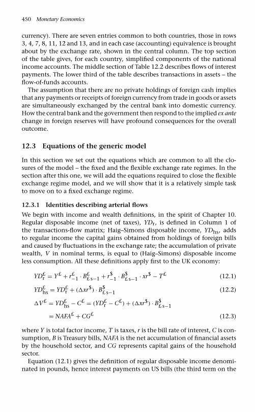
450 Monetary Economics

currency). There are seven entries common to both countries, those in rows3, 4, 7, 8, 11, 12 and 13, and in each case (accounting) equivalence is broughtabout by the exchange rate, shown in the central column. The top sectionof the table gives, for each country, simplified components of the nationalincome accounts. The middle section of Table 12.2 describes flows of interestpayments. The lower third of the table describes transactions in assets – theflow-of-funds accounts.

The assumption that there are no private holdings of foreign cash impliesthat any payments or receipts of foreign currency from trade in goods or assetsare simultaneously exchanged by the central bank into domestic currency.How the central bank and the government then respond to the implied ex antechange in foreign reserves will have profound consequences for the overalloutcome.

12.3 Equations of the generic model

In this section we set out the equations which are common to all the clo-sures of the model – the fixed and the flexible exchange rate regimes. In thesection after this one, we will add the equations required to close the flexibleexchange regime model, and we will show that it is a relatively simple taskto move on to a fixed exchange regime.

12.3.1 Identities describing arterial flows

We begin with income and wealth definitions, in the spirit of Chapter 10.Regular disposable income (net of taxes), YDr, is defined in Column 1 ofthe transactions-flow matrix; Haig–Simons disposable income, YDhs, addsto regular income the capital gains obtained from holdings of foreign billsand caused by fluctuations in the exchange rate; the accumulation of privatewealth, V in nominal terms, is equal to (Haig–Simons) disposable incomeless consumption. All these definitions apply first to the UK economy:

YD£r = Y£ + r£−1 · B£

£ s−1 + r$−1 · B$

£ s−1 · xr$ − T£ (12.1)

YD£hs = YD£

r + (�xr$) · B$£ s−1 (12.2)

�V£ = YD£hs − C£ = (YD£

r − C£) + (�xr$) · B$£ s−1

= NAFA£ + CG£ (12.3)

where Y is total factor income, T is taxes, r is the bill rate of interest, C is con-sumption, B is Treasury bills, NAFA is the net accumulation of financial assetsby the household sector, and CG represents capital gains of the householdsector.

Equation (12.1) gives the definition of regular disposable income denomi-nated in pounds, hence interest payments on US bills (the third term on the

A More Advanced Open Economy Model 451

right-hand side) is converted from dollars into pounds using the exchangerate, as can be read off from Column 1 in Table 12.2. Capital gains, whichare included in equation (12.2), describe the change in the pound value ofpreviously issued US bills measured in dollars; note once again that capitalgains are not transactions and therefore have no place in the columns of thetransactions-flow matrix given by Table 12.2.

Equations (12.4) to (12.6) give exactly comparable definitions for the USeconomy.

YD$r = Y$ + r$

−1 · B$$ s−1 + r£−1 · B£

$ s−1 · xr£ − T$ (12.4)

YD$hs = YD$

r + (�xr£) · B£$ s−1 (12.5)

�V$ = YD$hs − C$ = (YD$

r − C$) + (�xr£) · B£$ s−1

= NAFA$ + CG$ (12.6)

We assume that governments only tax regular income, ignoring capitalgains, so

T£ = θ£ · (Y£ + r£−1 · B££ s−1 + r$

−1 · B$£ s−1 · xr$) (12.7)

T$ = θ$ · (Y$ + r$−1 · B$

$ s−1 + r£−1 · B£$ s−1 · xr£) (12.8)

The identities describing the national income at current prices (Columns 2and 6) are:

Y£ = C£ + G£ + X£ − IM£ (12.9)

Y$ = C$ + G$ + X$ − IM$ (12.10)

where G is (pure) government expenditure, X is exports and IM is imports.As central banks have no interest-paying liabilities, their profits (Fcb) are

equal to total interest receipts from any domestically issued bills, plus, as isthe case for the UK central bank, any foreign Treasury bills, B$

cb £, which theyhold, as shown in Columns 4 and 9 of the matrix.

F£cb = r£−1 · B£

cb £ s−1 + r£−1 · B$cb £ s−1 · xr$ (12.11)

F$cb = r$

−1 · B$cb$ s−1 (12.12)

Given that central bank profits are all paid back to the government, we canwrite the (government) budget constraints (Columns 3 and 8) as:

�B£s = G£ − T£ + r£−1 · B£

s−1 − F£cb (12.13)

�B$s = G$ − T$ + r$

−1 · B$s−1 − F$

cb (12.14)

452 Monetary Economics

where, recall, Bs is the total outstanding stock of bills – the sole liability of thegovernment, as distinct from the whole public sector including the centralbank.

Payments by the US government on US Treasury bills held by the UK centralbank are comprised within total interest payments by the US government,r$−1 · B$

s−1, the third term on the right-hand side of (12.10), as is clear fromline 8 of the transactions matrix. Hence interest payments on US Treasurybills appear as a credit to the UK central bank but not as a debit to the UScentral bank.

It is a feature of Table 12.2 which may seem surprising that neither coun-try has a column describing its balance of payments. However the coherenceenforced by double entry accounting ensures that total flows into each coun-try always exactly equal total outflows, whether measured as current (tradeetc.) flows or as capital account transactions. Thus trade flows (lines 3 and 4of the transactions matrix) plus interest payments (lines 7 and 8) make upthe balance of payments on current account which is, in turn, exactly equalto the sum of each country’s transactions in capital assets shown in lines11–13. To link the transactions described in Table 12.2 to the balance sheetsin Table 12.1, it is necessary to take into account capital gains (or losses) aris-ing from changes in the exchange rate. The balance of payments identities,which are not shown in the matrix, are:

CAB£ = X£ − IM£ + r$−1 · B$

£ s−1 · xr$

− r£−1 · B£$ s−1 + r$

−1 · B$cb £ s−1 · xr$ (12.15)

KABOSA£ = +�B£$ s − �B$

£ s · xr$ − {�B$cb £ s · xr$ + �or£ · p£

g} (12.16)

CAB$ = X$ − IM$ + r£−1 · B£$ s−1 · xr£

− r$−1 · B$

£ s−1 − r$−1 · B$

cb £ s−1 (12.17)

KABOSA$ = +�B$£ s + �B$

cb £ s − �B£$ s · xr£ − {�or$ · p$

g} (12.18)

CAB is the current account balance, which by the normal NIPA conventions,only records transactions and takes no account of capital gains. The currentaccount balance is equal to the trade balance (X − IM) plus the balanceof ‘invisibles’ – the balance in investment income from and to the foreigneconomy.

KABOSA is the capital account balance, defined such that CAB +KABOSA = 0. In other words, KABOSA includes the official settlementsaccount (OSA), which itself includes the negative of changes in officialreserves, this change being the term between French brackets. Once again,as long as the US dollar, rather than gold, is the international currency,increases in the official reserves of United Kingdom (the £ country) willnot be matched by a decrease in the foreign reserves of the Fed (the

A More Advanced Open Economy Model 453

central bank of the $ country), as can be observed by checking the termsinside the brackets in equations (12.16) and (12.18). There is thus an asym-metry here, which impacts on the definition of a non-tautologic balance ofpayments (one which is not always equal to zero by definition). If we excludecapital account transfers involving any of the two central banks, that is takingaway the payments related to what is usually called the official settlementsaccount, then we get another definition of the capital account balance:

KAB£ = +�B£$ s − �B$

£ s · xr$ (12.19)

KAB$ = +�B$£ s − �B£

$ s · xr£ (12.20)

12.3.2 Trade

We now enter a subsection which will look familiar to students of interna-tional trade, but which will be given an original twist. Trade prices, heremore specifically the trade prices of the United Kingdom, are assumed to bedetermined in the following way:

p£m = v0 − v1 · xr£ + (1 − v1) · p£

y + v1 · p$y 0 < v1 < 1 (12.21)

p£x = υ0 − υ1 · xr£ + (1 − υ1) · p£

y + υ1 · p$y 0 < υ1 < 1 (12.22)

where pm is import prices, px is export prices, py is the GDP deflator, whilebold characters denote natural logs of these variables.

The justification for the constraints on the parameters derives from thefollowing thought experiments:

1. If there were a simultaneous additions of some given amount to domesticinflation in both countries with no change in the exchange rate, thenthere would surely be an equivalent addition to export and (therefore)import prices in each country – hence the constraint that the coefficientson domestic and foreign inflation sum to unity. This explains the (1−v1) ·p£

y + v1 · p$y part of the price of imports equation, and its equivalent terms

in the export price equation.2. If currency depreciation (a negative change in xr£) were accompanied by a

simultaneous and equal addition to domestic inflation, it is reasonable toexpect that import prices would rise by the full amount of the depreciation– hence the sum of the (absolute values) of the coefficients on the exchangerate and domestic inflation should also sum to unity. This explains theconstraint on the−v1 ·xr£ + (1−v1) ·p£

y part of the import price equation.3. It is well established empirically that, following depreciation, and given no

immediate effect on domestic inflation, export and import prices denomi-nated in home currency rise, but there will normally be some deteriorationin the terms of trade (i.e. υ1 > v1 > 0 implying that import prices willrise faster than export prices) and vice versa for appreciation. Presumablyexporters in both countries adjust prices in order to maintain or achieve

454 Monetary Economics

some desired market share when exchange rates change (as shown byBloch and Olive 1996).

Import and export prices for the United States now follow by symmetry,since, for instance, the export prices of the United Kingdom are the importprices of the United States, once exchange rates are taken into consideration:

p$x = p£

m · xr£ (12.23)

p$m = p£

x · xr£ (12.24)

Trade flows, measured at constant prices, are determined, very conven-tionally, by relative price and income elasticities, with bold variables againrepresenting logs.

x£ = ε0 − ε1 · (p$m−1−p$

y−1) + ε2 · y$ (12.25)

im£ = μ0 − μ1 · (p£m−1−p£

y−1) + μ2 · y£ (12.26)

Equation (12.25) says that the volume of UK exports (x£) responds with anelasticity of ε1 with respect to US import prices (p$

m) relative to US domesticprices (p$

y ) – both expressed in dollars – and ε2 with respect to US domestic

output (y$). Equation (12.26) says that UK imports (im£) respond with elas-ticities μ1 with respect to import prices (p£

m) relative to domestic prices (p£y ) –

both expressed in pounds – and μ2 with respect to domestic output (y£).As with prices, these equations imply, logically, what dollar export and

import volumes must be since the exports of one country are the imports ofthe other:

x$ = im£ (12.27)

im$ = x£ (12.28)

Finally the four identities generating the values of trade flows in owncurrency are:

X£ = x£ · p£x (12.29)

X$ = x$ · p$x (12.30)

IM£ = im£ · p£m (12.31)

IM$ = im$ · p$m (12.32)

It is often assumed that the sum of the elasticities with respect to relativeprices must sum to at least one if the trade balance is to improve followingdevaluation (the Marshall-Lerner condition). But in verity the sum of these

A More Advanced Open Economy Model 455

elasticities need be no greater than the elasticity of terms of trade with respectto devaluation. If there were no change at all in the terms of trade following a10% devaluation – for instance if both import and export prices in US dollarswent up by 6%, not an impossible outcome – the sum of the elasticitiesneed be no greater than positive for the balance of trade to improve.5 If thedeterioration in the terms of trade were 40% of the devaluation, then thesum of the price elasticities need be no more than 0.4. This would occur ifthe 10% devaluation in the value of the dollar caused import prices in theUS, p$

m, to rise by 7% while export prices in US dollars, p$x , rose by 3%.

12.3.3 Income and expenditures

The consumption function, with the wealth acquisition function that thisimplies, is central to the way in which the system is driven towards a station-ary state, as with our other models. We still assume that households set theirreal consumption decisions as a function of their real disposable income andpast accumulated real wealth. But how are these to be measured? In particu-lar what is the relevant price index? We suggest that the relevant price is thatof domestic sales, pds, since this is the price that consumers face when theypurchase goods. It is, in our model, the nearest equivalent to consumer prices.

Real wealth will thus be defined as nominal wealth V , as already definedin equations (12.3) and (12.6), deflated by domestic prices.

v£ = V£

p£ds

(12.33)

v$ = V$

p$ds

(12.34)

Real (inflation accounted) disposable income (ydhs), once again in linewith the Haig–Simons definition of disposable income, must take possibleinflation losses into account, and is therefore given by:

yd£hs = YD£

hs

p£ds

− v£−1 · �p£ds

p£ds

(12.35)

yd$hs = YD$

hs

p$ds

− v$−1 · �p$

ds

p$ds

(12.36)

5 The standard interpretation of the Marshall-Lerner condition seems to be based onthe assumption that export prices, expressed in the domestic currency, won’t changefollowing a depreciation of the home currency, while import prices will increase inline with the depreciation. In other words, prices are assumed to be always fixed in thecurrencies of the exporters. This implies that the terms of trade go down by the fullamount of the depreciation.

456 Monetary Economics

since we know that, properly measured, Haig–Simons disposable incomemust be such that: ydhs = c + (v − v−1).

Real consumption is determined by expected real disposable income andthe opening stock of (real) wealth. As before, we assume a two-stage decision,where households decide on an overall flow of saving, and then choose howthey will allocate their expected wealth.

c£ = α£1 · yd£

hse + α£2 · v£−1 (12.37)

c$ = α$1 · yd$

hse + α$2 · v$

−1 (12.38)

where the subscript ‘e’ denotes an expected value.The formation of expectations about income (and therefore wealth) is no

big deal in a well wrought stock-flow model. Any way of forming expectationsthat is not downright perverse (such as would be the case if expectations wereto move in a way that ignores or compounds previous errors) will eventuallylead to the same result. This is because errors lead to unwanted changes instocks of wealth which lead, in turn, to self-correcting adjustments in subse-quent periods. We shall assume for simplicity that expected real disposableincome is some average of this and last period’s income.

yd£hse = (yd£

hs + yd£hs−1)

2(12.39)

yd$hse = (yd$

hs + yd$hs−1)

2(12.40)

The limited role of expectations is made clearer when one notices, oncemore, that the consumption function may alternatively be written as a wealthadjustment function, �ve = α2(α3 ·ydhse −v−1), where α3 = (1−α1)/α2. Thesystem will come to rest (of a kind) when the changes in the real stock ofwealth are zero, implying that wealth targets, v∗, have been met, that is,when v = α3 · yd.

For the rest of this section we have a raft of equations, most of them iden-tities, which set out how real wealth accumulation and real consumption areinter-related with all the current price variables.

The total volume of sales,s, is equal to the sum of its components:

s£ = c£ + g£ + x£ (12.41)

s$ = c$ + g$ + x$ (12.42)

The value of sales is:

S£ = s£ · p£s (12.43)

S$ = s$ · p$s (12.44)

A More Advanced Open Economy Model 457

where ps is the average price of all sales.The price level of sales, ps, is determined as a mark-up, ϕ, on unit costs:

p£s = (1 + ϕ£) · (W£ · N£ + IM£)

s£ (12.45)

p$s = (1 + ϕ$) · (W$ · N$ + IM$)

s$(12.46)

where W is the nominal wage rate and N is employment. All profits earnedas a result of the mark-up are assumed to be distributed immediately to thehousehold sector.

The price of domestic sales is:

p£ds = (S£ − X£)

(s£ − x£)(12.47)

p$ds = (S$ − X$)

(s$ − x$)(12.48)

The remaining relationships in this section are those necessary to completethe income/expenditure flow system. They are tedious but necessary steps.They describe, in turn, domestic sales value, DS; domestic sales volume,ds; nominal GDP, Y ; real GDP, y; the GDP deflator, py ; the value of con-sumption, C; the value of government expenditure, G; the tax yield, T , andemployment, N.

DS£ = S£ − X£ (12.49)

DS$ = S$ − X$ (12.50)

ds£ = c£ + g£ (12.51)

ds$ = c$ + g$ (12.52)

Y£ = S£ − IM£ (12.53)

Y$ = S$ − IM$ (12.54)

y£ = s£ − im£ (12.55)

y$ = s$ − im$ (12.56)

p£y = Y£

y£ (12.57)

p$y = Y$

y$(12.58)

C£ = c£ · p£ds (12.59)

458 Monetary Economics

C$ = c$ · p$ds (12.60)

G£ = g£ · p£ds (12.61)

G$ = g$ · p$ds (12.62)

T£ = θ£ · (Y£ + r£−1 · B££s−1 + r$

−1 · B$£s−1 · xr$) (12.63)

T$ = θ$ · (Y$ + r$−1 · B$

$s−1 + r£−1 · B£$s−1 · xr£) (12.64)

N£ = y£

pr£ (12.65)

N$ = y$

pr$(12.66)

where pr is labour productivity.

12.3.4 Asset demands

Up to this point, thanks mainly to the simplifying assumption that there isno inventory investment, we have been able to assume that the supply ofoutput, as well as the supply of labour, is instantaneously equal to demand.How about asset demands and supplies?

Outside a stationary steady state, all stocks and flows will be changing.Demands for assets will originate from the private sectors’ wealth accumu-lation and asset allocation. Supplies of assets originate from the balance ofboth governments’ transactions. The way in which demands are brought intoequivalence with supplies will determine how the system as a whole behaves.The manner of this reconciliation, which can take many forms, comprisesthe core of what this chapter has to say.

The equations summarizing how nominal wealth is created for the privatesector were given right at the beginning of this section. The private sector’sex ante allocation of wealth between the three categories of available finan-cial assets is determined according to Tobin’s principles, as should now bestandard for the reader:

B££ d = V£ · (λ10 + λ11 · r£ − λ12 · (r$ + dxr$

e )) (12.67)

B$£ d = V£ · (λ20 − λ21 · r£ + λ22 · (r$ + dxr$

e )) (12.68)

H£d = V£ · (λ30 − λ31 · r£ − λ32 · (r$ + dxr$

e )) (12.69A)

B$$ d = V$ · (λ40 + λ41 · r$ − λ42 · (r£ + dxr£

e )) (12.70)

B£$ d = V$ · (λ50 − λ51 · r$ + λ52 · (r£ + dxr£

e )) (12.71)

H$d = V$ · (λ60 − λ61 · r$ − λ62 · (r£ + dxr£

e )) (12.72A)

A More Advanced Open Economy Model 459

where, for each country, the sum of the constants is equal to one and thesum of the coefficients in each remaining column is equal to zero, bearing inmind that for bills the assumption is that the coefficient on its own interestrate will be positive and that on other interest rates will be negative.6 As weknow, when consumption is based on expectations which will typically befalsified, these conditions can best be taken into account by removing one ofthe portfolio equations for each country (those identified with an A suffix),and rewriting them as

H£d = V£ − B£

£ d − B$£ d (12.69)

H$d = V$ − B$

$ d − B£$ d (12.72)

The subscript ‘d’ denotes demand and, where the asset is issued abroad,this subscript signifies that the asset is denominated in the currency wherethe asset is held and this is why exchange rates do not enter the portfolioequations. The subscript ‘e’ denotes an expected value, while the prefix ‘d’denotes a proportional rate of change – thus the expected rate of return onbills issued abroad equals the foreign rate of interest plus the change in theexchange rate which is expected to occur by the next period – and hence wehave by definition:

dxr£e = �xr£

exr£ (12.75)

dxr$e = �xr$

e

xr$(12.76)

We could make the conventional assumption that the expected rate ofexchange is equal to the difference between domestic and foreign ratesof interest, thereby establishing equivalence between expected total ratesof return on the two assets. This would imply:

xr£e = xr£−1 + (r$ − r£) · xr£−1

xr$e = xr$

−1 + (r£ − r$) · xr$−1

These equations imply that uncovered interest parity (UIP) holds. Butaccording to the views of foreign exchange traders, they give no indicationof the expected future spot rate; rather they define the forward rate, as setby bankers and traders for their clients (Isard 1995: 78). The forward rate,

6 To cut down the number of equations and focus on the essential elements, portfo-lio equations are assumed to depend on realized wealth rather than expected wealth.The transactions demand for money, dependent on disposable income, has beenomitted.

460 Monetary Economics

relative to the spot rate, gives no indication of how the spot rate will movein the future, as has been repeatedly shown in empirical tests (Moosa 2004).7

As traders say – this is the so-called cambist view – the forward rate cannot bethe expected future spot rate, and hence the conventional closure based onUIP is not helpful (Lavoie 2000; 2002–3).8

We are thus left with two (simple) possibilities. We can assume that theexpected exchange rate is a given (xre = a constant), which might cor-respond to some fundamental exchange rate that investors believe will berealized sooner or later; or we can assume, as we implicitly did in the port-folio equations, that investors have an opinion about possible changes in theexchange rate, in which case the term dxre may be positive or negative, andwill be nil in the neutral case.

12.3.5 Asset supplies

What of asset supplies? The government, having taken decisions about taxrates and public expenditure authorizations and commitments, has no con-trol over its surplus/deficit nor over the issue of bills to which this givesrise, as shown in equations (12.13) and (12.14); nor has it any control overwhere the bills go to. Central banks will always exchange cash for bills andvice versa. This is equivalent to saying that the supply of all assets to theprivate sector of each country passively matches demand. This is the closurewhich corresponds to the assertion that the money supply is endogenous anddemand-led, with central banks setting or steering interest rates rather thanattempting to target money supplies or the supply of securities, an assump-tion which we believe to be realistic and best able to describe the actualbehaviour of central banks.

There are many different ways to arrange the equilibrium conditions forassets, since we are free to choose the appropriate redundant equation – theequation that arises from the fulfilment of every other equation of the model.

7 Isard (1995: 81–2) says that it is ‘widely acknowledged that interest differentialsexplain only a small proportion of subsequent changes in exchange rates’ and ‘oftenmispredict the direction of change’. Tobin (1982b: 124) himself provides some anec-dotal evidence against the view that the forward rate is a predictor of future spotrates.

8 While the method that we use is similar to the one used by Taylor (2004a; 2004b,ch. 10) in his open-economy models, there is a crucial difference: Taylor still assumesendogenously determined interest rates, while ours are set exogenously by centralbanks. Thus these target rates of interest act as an anchor. This difference may helpexplain why Taylor (2004b, p. 333) believes that, in contrast to what we claim, ‘theexchange rate is not set by temporary macro equilibrium conditions. It must evolveover time subject to rules based on expectations about its future values in the future’.This forces Taylor to introduce UIP to close his model, on the basis that UIP relies on‘arbitrage arguments that “should be true” ’ (ibid, p. 333), while acknowledging earlierthat UIP ‘does not fit the data’ (ibid, p. 315)!

A More Advanced Open Economy Model 461

And accounting identities can also be arranged in different ways. Here wechoose the set of equations that we used for the fixed exchange rate variantof our model in Godley and Lavoie (2005–6).

We start with those assets issued by US institutions, government and cen-tral bank, which are acquired by the domestic central bank and by thedomestic private sector, thus writing the following issuing requirements:

H$s = H$

h (12.77)

B$$ s = B$

$ d (12.78)

B$cb $ s = B$

cb $ d (12.79)

where the subscript ‘s’ denotes supply.In the case of assets issued by UK institutions, and acquired by the domestic

central bank and the domestic private sector, we may write, symmetrically:

H£s = H£

h (12.80)

B££ s = B£

£ d (12.81)

B£cb £ s = B£

cb £ d (12.82)

Le us now deal with the components of the balance sheet identity of thecentral banks. In the case of the US central bank, column 9 of the balancesheet matrix (Table 12.1) yields the following identity:

B$cb $ d = H$

s − or$ · p$g (12.83)

while in the case of the UK central bank, column 4 of the transactions-flowmatrix (Table 12.2) gives:

�B£cb £ d = �H£

s − �B$cb £ s · xr$ − �or£ · p£

g (12.84)

The US central bank’s equation can be represented using levels, becausethere is no possibility of capital gains (or losses) within the Fed’s balancesheet. The Fed has no foreign asset or liability, and we shall assume for sim-plicity that the price of gold in dollars, p$

g, is pegged at some constant value.By contrast, the balance sheet of the Bank of England must be set in differ-ences, because it includes bills issued abroad, which are susceptible to capitalgains when the dollar appreciates. In addition, if this occurs, the price of goldin pounds (p£

g) rises, creating a second possible source of appreciation for theBank of England.

The model is nearly complete. In all variants we shall assume that no gold istraded between central banks (�or = 0), gold being kept simply as a remnant

462 Monetary Economics

of the long-gone Bretton Woods regime.9 The law of one price is appliedto the price of gold, under the assumption, already mentioned above, thatthe price of gold in dollars, p$

g, is given. Thus the price of gold in poundsdepends on the exchange rate, as shown in equation (12.85). Also, obviously,the dollar exchange rate, that is the number of pounds per dollar, is thereciprocal of xr£.

p£g = p$

g · xr$ (12.85)

xr$ = 1

xr£ (12.86)

We now deal with conditions of supply and demand that involve theexchange rate, and that we had voluntarily omitted when we dealt withconditions of supply and demand that only involved domestic agents. Threeconditions need to be realized, the third one, equation (12.89) being in factpart of the equations that will identify a closure.

B£$ s = B£

$ d · xr$ (12.87)

B$cb £ d = B$

cb £ s · xr$ (12.88)

B$£ s = B$

£ d · xr£ (12.89)

The generic model as such is complete. We now move to the differentpossible closures.

12.4 Alternative closures

12.4.1 A flexible exchange rate closure

We first deal with the flexible exchange rate closure. The £ central bank,faced with a step-up in imports, refuses to intervene in foreign exchangemarkets, so that it does not lose any of its foreign exchange reserves. Theexchange rate xr£ is endogenous (equation 12.89FL), while the amount offoreign reserves, measured in dollars, becomes a constant (equation 12.91FL).US Bills supplied to foreign bond holders are a residual (equation 12.90FL).The closure is made up of the following three equations, plus the redundant

9 Otherwise, we need another equation, �or$ = −�or£.

A More Advanced Open Economy Model 463

equation, equation (12.82A).10

xr£ = B$£ s

B$£ d

(12.89FL)

B$£ s = B$

s − B$cb £ s − B$

$ s − B$cb $ s (12.90FL)

B$cb£ s = constant (12.91FL)

B£cb£ s = B£

s − B££ s − B£

$ s (12.82A)

while equation (12.84) simplifies down to:

�B£cb £ d = �H£

s (12.84FL)

These four FL equations, with the other 87 remaining equations, consti-tute the OPENFLEX model. This model has over ninety equations, despitecommercial banks having been assumed away!

Equations (12.82A) and (12.90FL) are accounting identities which can beread from rows 2 and 3 of the balance sheet matrix given by Table 12.1.

Equation (12.89FL) might seem to imply that the exchange rate is deter-mined in a unique market, the market for B$

£ bills. But this is not the case.The exchange rate, like every other endogenous variable, is only allowed toappear a single time on the left hand side of an equation. But the system isa fully interdependent one such that the solution of the model as a wholerequires and ensures that every equation in which the exchange rate appearsis satisfied at the same time. Thus equations (12.89FL) and (12.87) must simul-taneously be satisfied. And the exchange rate determined in (12.89FL) willbe found to satisfy all the trade equations in which it appears and also toinfluence personal consumption through its effect on capital gains.

12.4.2 A fixed exchange rate closure, with endogenousforeign reserves

We shall define three different closures of the fixed exchange rate regime.Here we show that it is a simple task to move from the flexible exchangerate closure to a fixed exchange rate closure with freely changing endoge-nous reserves, that is, what most people would consider to be the standardfixed exchange rate regime. This closure constitutes what we can call ModelOPENFIX. There are many different ways to bump successive equationsto arrive at the new fixed exchange rate closure, but here we suggest a

10 This is now the redundant equation because equation (12.82) already has anequation with B£

cb £ s, the supply of domestic bills to the Bank of England (the UKcentral bank), on the left-hand side.

464 Monetary Economics

particularly simple one, that involves inverting only three equations. Thethree equations to be inverted are the ones we identified in the previoussubsection,

xr£ = B$£ s

B$£ d

(12.89FL)

B$£ s = B$

s − B$cb £ s − B$

$ s − B$cb $ s (12.90FL)

B$cb £ s = constant (12.91FL)

which become:

xr£ = constant (12.91F)

B$£ s = B$

£ d · xr£ (12.89F)

B$cb £ s = B$

s − B$£ s − B$

$ s − B$cb $ s (12.90F)

Equation (12.91F) specifies explicitly that the exchange rate is an exoge-nous variable, and hence that we are within a fixed exchange regime closure.Equation (12.89F) inverts equation (12.89FL). As to equation (12.90F), itdescribes the evolution of UK foreign reserves. Alternatively expressed,equation (12.90F) describes the purchases of US Treasury bills which the UKcentral bank must make in order to prevent its exchange rate from floatingup or down.

12.4.3 An alternative fixed exchange rateclosure: the deficit country lets its interestrate become endogenous

An alternative way of fending off devaluation, in theory, is to raise the interestrate. Once again, it is easy to adapt the equations of the model to showhow this would have to happen. We start from the main fixed exchange rateclosure, but impose upon it that the central bank declines to use its foreignreserves, as if the country were on a flexible exchange rate. Hence anothervariable, which was previously assumed to be constant, now needs to bemade endogenous and that will be the rate of interest on UK bills r£. As inthe previous subsection, we show the four equations of the fixed exchangerate closure that need to be modified, and the four new equations of this newclosure, plus equation (12.91F) which defines a fixed exchange rate regimeand remains as is. These equations are:

B$£ s = B$

£ d · xr£ (12.89F)

B$cb £ s = B$

s − B$£ s − B$

$ s − B$cb $ s (12.90F)

A More Advanced Open Economy Model 465

xr£ = constant (12.91F)

r£ = constant (12.92)

B$£ d = V£ · (λ20 − λ21 · r£ + λ22 · (r$ + dxr$

e )) (12.68)

which become:

B$£ d = B$

£ s · xr$ (12.89R)

B$£ s = B$

s − B$cb £ s − B$

$ s − B$cb $ s (12.90R)

xr£ = constant (12.91)

B$cb £ s = constant (12.92R)

r£ = −dxr$e +

⎧⎨⎩λ22 · r$ − λ20 + B$

£ dV£

⎫⎬⎭

λ21(12.68R)

so that once more all variables can only be found once on the left-hand side.This would be Model OPENFIXR.

12.4.4 Another alternative fixed exchangerate closure: one country sets its governmentexpenditures endogenously

Governments can also avoid devaluation by reducing public expenditures.The second possible additional fixed exchange rate closure is also very simpleto arrive at. It is relatively easy to rearrange the equations, following theprocedure outlined in the previous subsection, so as to show how fiscal policycould be adjusted to preserve a fixed rate of exchange despite a deterioratedtrade balance. The new fiscal stance has to be such that after allowing for alllags and feedbacks, the level of domestic output is reduced to such an extentthat the value of imports exactly equals that of exports.

Once more we start from the main closure with a fixed exchange rate, butimpose upon it that the central bank declines to use its foreign reserves, as ifthe country were on a flexible exchange rate. Hence another variable, whichwas previously assumed to be constant, now needs to be made endogenousand that will be the (pure) government expenditures in the UK, g£. As in theprevious section, we can show the equations of the generic model that needto be changed, as well as the equations that define the main fixed exchangeregime closure. The following equations

g£ = constant (12.93)

G£ = g£ · p£ds (12.61)

466 Monetary Economics

�B£s = G£ − T£ + r£−1 · B£

s−1 − F£cb (12.13)

B$£ s = B$

£ d · xr£ (12.89F)

B$cb£ s = B$

s − B$£ s − B$

$ s − B$cb $ s (12.90F)

xr£ = constant (12.91F)

B£cb £ s = B£

s − B££ s − B£

$ s (12.82A)

become:

B$cb£ s = constant (12.93G)

g£ = G£

p£ds

(12.61G)

G£ = �B£s + T£ + F£

cb − r£−1 · B£s−1 (12.13G)

B$£ s = B$

£ d · xr£ (12.89F)

xr£ = constant (12.91F)

B£s = B£

$ s + B££ s + B£

cb £ s (12.82AG)

B$cb£ s = B$

s − B$£ s − B$

$ s − B$cb $ s (12.90GA)

Here, nominal government expenditures are constrained by equation(12.13G). Real government expenditures are thus adjusted to accord withthe nominal amount, through equation (12.61G). We use the redundantequation (12.82A) of the fixed exchange rate model to determine the sup-ply of bills of the UK government (as in 12.82AG), and hence as a result,we must find a new redundant equation for our new closure, which willbe equation (12.90GA). Equations (12.89F) and (12.91F) that defined a fixedexchange rate closure are still part of this new closure, which we can callModel OPENFIXG.

12.5 Experiments with the main fixedexchange rate closure

12.5.1 An increase in the US propensity to import

We now run some experiments, starting with the main fixed exchange rateclosure, which assumes that foreign reserves are endogenous, so that read-ers can compare the results with those achieved in the simpler model ofChapter 6. Our simulation procedure is to start from a full stationary state,with all government budget balances and current account balances at zero,introduce a disturbance, and then inspect a sequence of solutions which willlead either to a new full stationary state or to a hopefully intelligible form of

A More Advanced Open Economy Model 467

instability. In the first exhibit we assume that ‘the United Kingdom’ achievesan uncovenanted addition to exports in a step which is maintained indef-initely (ε0 in equation (12.25) moves up). Assuming that fiscal policy (theparameters θ and g for each country), monetary policy (the rates of interestin both countries), the exchange rate and gold reserves are all fixed, the conse-quences for the UK trade account balance and current account balance (CAB),as well as for the government budget balance and the net accumulation offinancial assets (NAFA) by the private sector are shown in Figure 12.1A.

We already know from Chapter 6 that the GDP of the successful exporter –here United Kingdom – will rise to a new stationary level, while the GDP ofthe other country will decrease to a new lower constant level. The increase indomestic income will generate an increase in UK wealth, which is reflected inthe positive net accumulation of financial assets by UK households, shown bythe NAFA continuous line in Figure 12.1A. As GDP reaches its new constantlevel, this accumulation of financial assets tapers back to zero, and when itactually does reach zero, the quasi stationary state has been reached. The UKtrade balance rises to a surplus position. Because monetary and fiscal policyand also the exchange rate are all fixed, there is no corrective mechanism inoperation, so the trade balance remains indefinitely at its new higher level.But the current account balance, which includes interest flows on foreignassets or liabilities, while initially improving by the same amount as the tradebalance, proceeds thereafter to increase by ever larger – and accelerating –amounts as the Bank of England holdings of US Treasury bills increase, gen-erating ever larger flows of interest payments. The UK government’s budget

1955 1959 1963 1967 1971 1975 1979 19871983 1991 1995 1999

1.60

2.00

1.20

0.80

0.40

0.00

UK current account balance

UK trade balance

UK NAFA

UK governmentbudget balance

Figure 12.1A Effect of an increase in the US propensity to import on UK variables,within a fixed exchange rate regime with endogenous foreign reserves: net accumula-tion of financial assets, current account balance, trade balance and government budgetbalance

468 Monetary Economics

1955 1959 1963 1967 1971 1975 1979 19871983 1991 1995 1999

1.50

2.25

0.75

0.00

–0.75

–1.50

UK current account balance

Change in the Bank of England foreign reserves

Change in theBank of England holdingsof domestic Treasury bills

Change in the UK stock of money

Figure 12.1B Effect of an increase in the US propensity to import, within a fixedexchange rate regime with endogenous foreign reserves, on the UK current accountbalance and elements of the balance sheet of the Bank of England (the UK centralbank): change in foreign reserves, stock of money, holdings of domestic Treasury bills

balance, after a period of transition, moves into surplus which is exactly equalto the UK current account surplus, thus getting into a twin-surplus situation.These two variables increase exponentially.11 Exactly the same thing is hap-pening in reverse in the United States. The US government deficit and the UScurrent account deficit are both increasing without limit, even though thetrade deficit remains constant.

Figure 12.1B shows the current account balance and the change in the valueof US Treasury bills held by the Bank of England (its foreign reserves). Initiallythe two series differ because there is a change in the private income flows inboth countries which leads to a counterpart adjustment in stocks of US assetsheld privately in the United Kingdom and vice versa. In particular, sinceUK households earn higher revenues, they purchase additional bills, amongwhich are bills issued in the United States. As a result, the negative capitalaccount balance (net of the acquisition of official foreign reserves), partlycompensates for the current account surplus for a while. Eventually, however,the income flow settles down at a new constant level and the changes inprivate wealth revert to zero. But the UK current account balance remainsin surplus, while the overall government sector (including the central bank)

11 This result is also achieved by Lequain (2003). This is the main difference fromprevious models where gold stocks, carrying no interest, were the only means to holdforeign reserves, as in Godley (1999b) or Chapter 6. In those models, the currentaccount surplus remained constant, so that foreign reserves rose linearly.

A More Advanced Open Economy Model 469

keeps accumulating foreign assets on an equivalent scale, so the amount ofreserves (US bills) being acquired by the Bank of England comes to exactlymatch the UK current account surplus.

There is no intrinsic limit to these processes. The Bank of England doesnot lose control of its own monetary policy as it buys US Treasury bills, andthere is no flooding of their economy with liquidity. This again can be seenin Figure 12.1B, by checking the continuous line illustrating changes in cashmoney issued by the Bank of England, which quickly reverts to zero. Thisroughly constant stock of money occurs despite the enormous and exponen-tial increase in foreign reserve assets. This is because the increase in holdingsof US Treasury bills is being compensated by the decrease in the UK centralbank holdings of domestic bills, as can also be seen in Figure 12.1B. Theincreases in private disposable income, consumption, output and the pres-sure of demand in the United Kingdom are no more than can be accountedfor by the increase in exports and the multiplier effects of this. The increase inprivate wealth, and its allocation between cash and bills of each kind, is in noway different from what would have taken place had the increase in incomeoriginated in a quite different way, for instance as a result of a relaxation offiscal policy.

All the same things are happening in reverse to the US economy. Initially,there is a slight reduction in the stock of cash and the stock of US bills heldby the Fed, as a result of a decrease in GDP, but afterwards all these remainconstant, despite the current account deficit. Because the US dollar is theinternational currency, there is no need for the Fed to ‘sterilize’ anything.There is no fall in the foreign reserves of the US central bank; the financialassets that have to be provided, as a counterpart to the current account deficit,are being provided by the US Treasury, the debt of which is increasing. Theaccumulation of US Treasury bills by the Bank of England, and the payment ofinterest on these bills to it by the US government, is an entirely self-containedprocess which at no point affects private stocks and flows in either country.That this is the case can actually be observed in the introductory systemdescribing arterial flows, in equations (12.11)–(12.14) together with the textwhich immediately follows, where it is shown that receipts by the UK govern-ment derived from bills issued by the US government (r$

−1 · B$cb£ −1 · xr$) are

components of both governments’ budget balance and also of both countries’current account balance (equations 12.15 and 12.17) – but they do not enterthe flows of private disposable income which are comprehensively given byequations (12.1) and (12.4).

To judge from its recent behaviour (in the early years of 2000), it is notimplausible to suppose that under such circumstances the US governmentwould, in practise, relax fiscal policy enough to keep the level of GDP whereit would otherwise have been, thereby generating an even larger trade deficitand an even larger public sector deficit. Under these circumstances the ‘real’thing that would be happening is that US residents would be producing the

470 Monetary Economics

same amount as before but absorbing more goods and services than they areproducing. UK residents would be producing more but absorbing less thanthey produce.12 There may be solid political or strategic reasons why bothcountries are happy to let the whole thing go on indefinitely.13

The situation being described here with the help of Figures 12.1 seems toapproximate the current situation of the Chinese economy. Hence let us nowattribute to China what is being described in the charts under the name of UK.Is it right to call such accumulation of reserves by the Chinese central bank‘intervention’; and is it right to describe the process as one in which the USis ‘having to attract $x billion per day’ to finance its deficit? Not really. What ishappening, surely, is that Chinese exporters receive, for their increased salesabroad, an additional flow of dollars which they exchange with their centralbank for their own currency. The Chinese central bank (the People’s Bank ofChina) finds itself with an equivalently rising stock of dollar balances whichit exchanges for US Treasury bills. Beyond these two exchanges the People’sBank of China neither needs nor wants to do anything at all.

12.5.2 Theoretical implications

These findings are profoundly at odds with much conventional wisdom andwith the received view that arises from the standard Mundell–Fleming model.Peter Kenen (1985: 669) writes, as many others: ‘ … Reserve flows alter themoney stock, undermining the influence of monetary policy … . The mone-tary approach to the balance of payments is built on this basic proposition’.14

But the monetary approach does not have a fully articulated monetary sys-tem in which the private sector allocates its wealth between money and otherassets. In both countries, the private sector’s accumulation of wealth and itsallocation between available assets is not in any way affected by these centralbank operations beyond what is implied by the step change in disposableincome.

Some would say that the People’s Bank of China will be ‘sterilizing’ foreignreserves, by selling Chinese Treasury bills on the open market. In a way, thisis true. While the Chinese central bank’s foreign reserves are sky-rocketing,its holdings of domestic bills are dwindling, as already pointed out. But this

12 We are grateful to Randy Wray for pointing this out.13 It could be argued, as we did in Chapter 6, that at some point domestic and

foreign investors will be scared by the rising debt to GDP ratio of the US government,or by the large foreign debt to GDP ratio of the US economy, and hence will reducetheir demand for US bills. But as long as the Bank of England is willing to hold itsforeign reserves in the form of US bills, this portfolio reshuffle can be handled withinthe described system, that is, with fixed exchange rates and unchanged interest rates.

14 Similarly, in a recent IMF paper, Prasad and Wei (2005: 13) write that ‘the cap-ital inflows that are reflected in reserve accumulation could increase liquidity in thebanking system, creating potential problems’.

A More Advanced Open Economy Model 471

is not the result of any intentional policy, where central bankers are activelyintervening in financial markets. The Chinese central bank, just like the USone, is simply attempting to keep interest rates constant. Bills are provided tothose who demand them at the set rate of interest. The central bank providescash on demand to its citizens. The reduction in domestic bills holdings bythe People’s Bank of China is essentially the consequence of the reduction inthe amount of outstanding debt of the Chinese government. This can go onindefinitely without any negative implication for the Chinese economy.

Others argue that sterilization in countries with external surpluses cannotgo on forever because rates of interest on the liabilities of the central bankare bound to be higher than rates of interest on US T-bills; this, it is argued,would lead to operating losses (or opportunity costs) to the sterilizing centralbank. As Prasad and Wei (2005: 13) put it: ‘Sterilization of capital inflowsto avoid this outcome [increased liquidity] could generate fiscal costs as therate of return on domestic sterilization instruments is typically higher thanthat earned on reserve holdings’. This argument certainly does not apply tocountries such as China, as Prasad and Wei (2005) recognize, since Chineseinterest rates are administered and can be set at levels lower than in the UnitedStates. Also, why would interest rates in surplus countries be any higher thaninterest rates in countries facing current account deficits? One would havethought that countries faced with external deficits would be the ones whomight be tempted by high or rising interest rates!

Indeed, as can be seen in Figure 12.1C, the surplus country (the UK, asshown, or China, as is currently the case) sees its debt to GDP ratio fall

1955 1959 1963 1967 1971 1975 1979 19871983 1991 1995 1999

1.80

2.00

1.60

1.40

1.20

1.00

UK debt to GDP ratio

US debt to GDP ratio

Figure 12.1C Effect of an increase in the US propensity to import on the US debt toGDP ratio and on the UK debt to income ratio, within a fixed exchange rate regimewith endogenous foreign reserves

472 Monetary Economics

continuously, while the deficit country (the US) has a rising debt to GDPratio. If anything, we would expect, based on standard risk analysis, that(long-term) interest rates in the US would be pressured up, while interestrates in the surplus countries would be pressured down by market forces.From the standpoint of the surplus country, there is thus nothing to stop thesituation from continuing.

12.6 Experiments with alternative fixedexchange rate closures

12.6.1 An endogenous interest rate

If surplus countries can accumulate foreign reserves without any restriction,the reverse case is not possible. Deficit countries losing foreign reserves willeventually run out of them. Faced with dwindling foreign reserves, manycentral banks raise interest rates. We have described such a possible mecha-nism in the first of our alternative fixed exchange rate closure, in section 4,whereby the central bank – let us call it the UK central bank (or the Bankof England) from now on – lets interest rates become endogenous, in itsattempt to preserve the existing fixed exchange rate without losing any addi-tional foreign reserves, in the hope of attracting foreign capital. A rise indomestic interest rates will thus generate positive capital account flows thatwill compensate for the negative trade and current accounts.

But a single adjustment to interest rates of this kind will only keep theasset market and the balance of payments in equilibrium for a single period.If the ‘UK’ goes on having an external deficit – in other words, as long asthere is no slowdown of the economy or as long as exports don’t becomemore competitive – there will have to be a further rise in the UK interest rate,to induce yet higher foreign inflows of capital. As there is no mechanism inplay to correct the trade deficit, we end up with an unstable situation – theinterest rate has to go on rising for ever to maintain an adequate inflow ofcapital. Meanwhile, the trade balance remains negative, while the currentaccount keeps getting ever more negative, at an exponential rate, due to therising burden of interest payments that need to be made abroad. This is allshown in Figures 12.2A and 12.2B, where in addition it is shown that thedeficit country will be faced with a rising debt to GDP ratio that mirrors theexponential rise in domestic interest rates.

The attempt to stabilize the system through interest rate changes generatesinstability, as is always the case in our kind of open economy models (Izurieta2003; Godley and Lavoie 2006b), and as we already observed towards the endof Chapter 6.

12.6.2 Endogenous real government expenditures

To avoid devaluation without losing reserves, governments may decide touse fiscal rather than monetary policy. This alternative closure, where foreign

A More Advanced Open Economy Model 473

1955 1959 1963 1967 1971 1975 1979 19871983 1991 1995 1999

15.0

22.5

7.5

0.0

–7.5

–15.0

UK capital accountbalance

UK tradebalance

UK current accountbalance

Figure 12.2A Effect of an increase in the UK propensity to import, within a fixedexchange rate regime with endogenous UK interest rates, on UK variables: capitalaccount balance, trade balance, and current account balance

1955 1960 1965 1970 1975 1980 1985 19951990 2000

2.50

2.75

2.25

2.00

1.75

1.50

0.090

0.105

0.075

0.060

0.045

0.030

UK debt to GDP ratio

UK interest rate

Debt to GDP ratio Interest rate

Figure 12.2B Effect of an increase in the UK propensity to import, within a fixedexchange rate regime with endogenous UK interest rates, on the UK interest rate andon the UK debt to GDP ratio

reserves are assumed to remain constant, implies that nominal governmentexpenditures are now an endogenous variable, as described in section 5. Thefiscal stance of the UK government depends on how many extra bills can beunloaded on financial markets (as determined by equation 12.82AG). The UK

474 Monetary Economics

government is financially constrained. It is as if there existed some kind ofloanable funds constraint. The intuition is that fiscal policy always adjustsso that the total supply of UK bills is such that the market absorbs themwillingly at given interest rates. Fiscal policy is adjusted in such a way thatthe UK government is running a deficit only if the financial markets areready to take in more UK bills at the given interest rate. Alternatively, thisnew closure can be understood as a situation where the rising debt of thedeficit country is judged to be unsustainable by ‘the markets’, and that, asa result of this, fiscal policy of the deficit country and the amount of newgovernment debt issued is ‘constrained’ by the financial markets.

This kind of fiscal policy response by the deficit country will have a negativeimpact on the surplus country, as shown in Figure 12.3A. While real GDPobviously falls in the trade-deficit ridden UK, real GDP also ends up beinglower in the US, despite its initial export-led boost. Thus, as pointed outby a large number of observers, the current IMF-led international monetarysystem where deficit countries are encouraged to cut down on governmentexpenditures imposes a deflationary bias to the world economy as a whole.

Second, as a counterpart, this type of fiscal policy does achieve what isintended. As UK imports progressively fall because of lower UK incomes, thecurrent account imbalance goes towards zero, and so does the trade balancewhich even becomes positive at some point, because during the transitionalperiod the country has increased its net foreign debt, which now has to beserviced. Figure 12.3B shows all this, as it also illustrates how the balance ofpayments problems of the UK get alleviated.

1955 1959 1963 1967 1971 1975 1979 19871983 1991 1995 1999

97.5

100.0

95.0

92.5

90.0

87.5

US real GDP

UK real GDP

Figure 12.3A Effect of an increase in the UK propensity to import, within a fixedexchange rate regime with endogenous UK government expenditures, on the US andUK real GDP

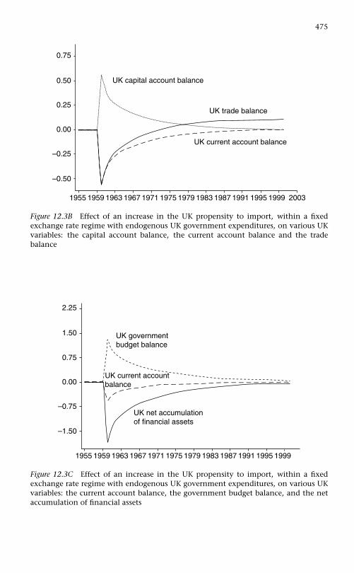
475

1955 1959 1963 1967 1971 1975 1979 19871983 1991 1995 1999 2003

0.50

0.75

0.25

0.00

–0.25

–0.50

UK capital account balance

UK trade balance

UK current account balance

Figure 12.3B Effect of an increase in the UK propensity to import, within a fixedexchange rate regime with endogenous UK government expenditures, on various UKvariables: the capital account balance, the current account balance and the tradebalance

1955 1959 1963 1967 1971 1975 1979 19871983 1991 1995 1999

1.50

2.25

0.75

0.00

–0.75

–1.50

UK governmentbudget balance

UK current accountbalance

UK net accumulationof financial assets

Figure 12.3C Effect of an increase in the UK propensity to import, within a fixedexchange rate regime with endogenous UK government expenditures, on various UKvariables: the current account balance, the government budget balance, and the netaccumulation of financial assets

476 Monetary Economics

1955 1959 1963 1967 1971 1975 1979 19871983 1991 1995 1999

1.540

1.560

1.520

1.500

1.480

1.460

UK debt to GDP ratio

US debt to GDP ratio

Figure 12.3D Effect of an increase in the UK propensity to import, within a fixedexchange rate regime with endogenous UK government expenditures, on the UK andUS debt to GDP ratios

Figure 12.3C helps us to understand how such an improvement can arise. Itis due to the fact that UK households, through their lower disposable incomesgenerated by the fiscal austerity policies (which propel the government bud-get balance into a surplus position), are being forced to dissave, thus sellingsome of their holdings of both domestic and foreign securities. Mainly as aresult of this, the capital account balance becomes positive. Finally, as shownwith Figure 12.3D, while the debt to GDP ratio of the UK rises at first (despitegovernment surpluses), because of the large fall in domestic output, the aus-tere fiscal policy eventually stabilizes the debt to GDP ratios of both countries,in contrast to what was occurring in Figures 12.1C and 12.2B.

12.6.3 A one-step devaluation

In this subsection we simulate what happens when a country gets into a tradedeficit situation, with falling foreign reserves and resolves its predicament bydevaluing currency in a step. As in previous experiments, we assume that theUK suddenly starts importing more foreign goods, and hence is faced witha trade and balance of payments deficit. The government believes that thepressures on the existing parity are too strong, and decides to devalue. Whatwill then happen?

Figure 12.4A describes the evolution of the UK trade balance and currentaccount balance. As the trade deficit is on its way to settling towards a sta-tionary level, the UK government decides to devalue. In the first two periodsfollowing the devaluation, there is no improvement in the trade and the

477

1955 1959 1963 1967 1971 1975 1979 19871983 1991 1995 1999 2003

–0.25

0.00

0.25

–0.50

–0.75

–1.00

–1.25

UK trade balanceUK current account balance

Figure 12.4A Effect on the UK current account balance and trade balance of asuccessful one-step devaluation of the sterling pound, following an increase in the UKpropensity to import, within a fixed exchange rate regime with endogenous foreignreserves

1955 1960 1965 1970 1975 1980 1985 19951990 2000

99.0

100.0

98.0

97.0

96.0

95.0

0.960

0.990

0.930

0.900

0.870

0.840Value of UK currency in dollars

UK real rate

real output Exchange rate

Figure 12.4B Effect of a successful one-step devaluation of the sterling pound on UKreal GDP, following an increase in the UK propensity to import, within a fixed exchangerate regime with endogenous foreign reserves

478 Monetary Economics

current account balances; actually both of them worsen.15 However, startingwith the third period, external deficits decrease. Here, with the simulationshown in Figure 12.4A, the government has properly identified the size of thedevaluation that is required to get the economy back to a balanced currentaccount position. Figure 12.4B shows that, in the circumstances describedby the parameters of the model, the UK economy escapes the stagnationthat would otherwise have been in prospect due to its poor trading perfor-mance. With its currency devaluation, GDP in the UK rises and even achievesa long-term level which is higher than that of the original stationary state.

12.7 Experiments with the flexible exchange rate closure

12.7.1 A step fall in the UK exports

We now turn to the other main closure, the one with a flexible exchangerate regime. Let us assume once more that the UK experiences a downturn inits exports. This will initially create a trade and current account deficit andthe economic slowdown will create as well a government budget deficit. Theincrease in the supply of assets abroad causes sterling (the £ currency) to fallin order to clear the market in all assets simultaneously. This is shown inFigure 12.5A and 12.5B

But the dynamic response of the system as a whole is only just beginning.A train of sequences ensues – and continues until the balance of paymentsand all changes in stock variables revert to zero. For as long as the balance ofpayments is non-zero this must be generating a change in the net supply offoreign denominated assets in each country causing a further change in theexchange rate. When exchange rates change, the absolute and relative pricesof exports and imports all change, so trade volumes and values, income flowsand accumulations of wealth all change. Some of these processes are shownin Figure 12.5C, where we see how export and import prices both rise mea-sured in sterling, accompanied by a deterioration in the terms of trade, assterling depreciates at a decelerating rate until a new equilibrium is restored(Figure 12.5B).

Figure 12.5A shows how the current account balance deteriorates initiallybut then reverts to zero, while the trade balance, thanks to the depreciatingcurrency, becomes positive. As a result, as shown in Figure 12.5D, the fall inUK domestic output, as a result of the direct and indirect (multiplier) effectof the fall in net export demand, is only temporary. The deterioration in theterms of trade and the rise in import prices act so as to make real exports

15 This is in part due to the lagged effect on imports, some of the price effectsarising before the quantity effects. The evolution of the trade balance in Figure 12.4Ais a representation of the famous J-curve effect, whereby the trade deficit widens atfirst, and gets narrowed only after a delay.

479

1953 1962 1971 1980 1989 1998 2007 20252016 2034 2043 2052

0.00

0.20

–0.20

–0.40

–0.60

–0.80

UK budget deficitUK trade balance

UK current account balance

Figure 12.5A Effect of a decrease in the UK propensity to export, within a flexibleexchange rate regime, on various UK variables: current account balance, trade balanceand government budget deficit

1952 1961 1970 1979 1988 1997 2006 20242015 2033 2042 2051

1.000

1.050

0.950

0.900

0.850

0.800

UK currency in dollars

Figure 12.5B Effect on the sterling exchange rate of a decrease in the UK propensityto export, within a flexible exchange rate regime

480

1952 1961 1970 1979 1988 1997 2006 20242015 2033 2042 2051

1.120

1.160

1.080

1.040

1.000

0.960Price of UK domestic sales

Price of UK exports

Price of UK imports

Figure 12.5C Effect of a decrease in the UK propensity to export, within a flexibleexchange rate regime, on various UK price indices: export prices, import prices anddomestic sales prices

1952 1961 1970 1979 1988 1997 2006 20242015 2033 2042 2051

99.0

100.0

98.0

97.0

96.0

95.0

UK real GDP

US real GDP

Figure 12.5D Effect of a decrease in the UK propensity to export, within a flexibleexchange rate regime, on the UK and US real GDP

A More Advanced Open Economy Model 481

exceed real imports in the new steady state. As the trade balance goes into asurplus position, the total demand for domestic product rises above what itwas in the first place (with our parameters).

12.7.2 A step increase in US government expenditures

Let us now turn to the US economy, and assume that the US governmentdecides to increase it real public expenditures g$. Real output in the US rises,as can be seen in Figure 12.6A. As a result, US imports rise and the US cur-rent account balance becomes briskly negative, as shown in Figure 12.6B.16

In addition, taxes collected in the US rise (because of the rise in GDP) butless that government expenditures, so the US government budget goes intodeficit. This means that there has to be an increase in the stock of bills issuedby the US Treasury. Because B$

$ d/V$ and H$d/V$ are fixed (there being no

change in interest rates by assumption, and since we simplified by assum-ing away the transactions demand for money), the net accumulation offinancial assets by US households is insufficient to absorb all the bills beingnewly issued by the US Treasury. As a result, there has to be an increase inB$

£ s, the amount of US Treasury bills which are supplied abroad. But a sim-ilar situation is occurring in the United Kingdom. Because interest rates arefixed, B$

£ d/V£ and B££ d/V£ are also both fixed, as shown in Figure 12.6C. In

addition, because the one-period change in UK output is small, the demandby UK households for Treasury bills issued by the US government, B$

£ d, hardlychanges. The increase in the supply of these US Treasury bills to foreign house-holds, as can be seen also in Figure 12.6C, must thus be absorbed through achange in the exchange rate. The exchange rate, xr$, as can be deduced fromequation (12.89FL), must fluctuate in a way which makes the supply of USTreasury bills abroad equal to the overseas demand for them, when expressedin the same currency. In other words, xr$ – the dollar exchange rate (the valueof the dollar in £ currency) depreciates, as shown in Figure 12.6D.

Next, the change in the exchange rate feeds into both import functions,reducing the import propensity in the United States and raising it in theUnited Kingdom, thus eventually generating a balanced current account(Figure 12.6B). In addition, the falling dollar generates capital losses for UKresidents and capital gains for US residents. These revaluations of wealthstocks will feed into the asset demands in both countries in the same period,and affect consumption expenditures in the succeeding period, through awealth effect. While the responses in the two countries are symmetrical they

16 There is initially a relatively small increase the output of the UK because its exportshave increased, as can be seen in Figure 12.6A. Its budget position improves, but onlyby a very small amount.

482

1952 1961 1970 1979 1988 1997 2006 20242015 2033 2042 2051

103.5

105.0

102.0

100.5

99.0

97.5 UK real output

US real output

Figure 12.6A Effect of a step increase in real US government expenditures, within aflexible exchange rate regime, on the US and UK real GDP

1953 1962 1971 1980 1989 1998 2007 20252016 2034 2043 2052

0.60

0.80

0.40

0.20

0.00

–0.20

US government budget deficit

NAFAin the US

US current account balance

Figure 12.6B Effect of a step increase in real US government expenditures, within aflexible exchange rate regime, on the main US balances: net accumulation of financialassets, government budget deficit, current account balance

483

1952 1961 1970 1979 1988 1997 2006 20242015 2033 2042 2051

0.2775

0.2850

0.2700

0.2625

0.2550

0.2475

US Treasury bills held by UK residents(denominated in dollars)as share of the wealthof UK residents

US Treasury bills held by UK residents(denominated in sterling)as share of the wealth of UK residents

Figure 12.6C Effect of a step increase in real US government expenditures, within aflexible exchange rate regime, on the share of the wealth of UK residents held in theform of US Treasury bills, when denominated in dollars and then in sterling

1952 1961 1970 1979 1988 1997 2006 20242015 2033 2042 2051

0.975

1.000

1.025

0.950

0.925

0.900

Dollar exchange rate(value of the dollar in sterling (£) units)

Figure 12.6D Effect on the dollar exchange rate of a step increase in real USgovernment expenditures, within a flexible exchange rate regime

484 Monetary Economics

will not in general be identical. The coefficients in the asset demand func-tions will in general be entirely different as between the two countries, yetthere has to be only a single exchange rate to satisfy all the relevant responses.

The one-period solution which this model generates when shocked doesnot, in general, simultaneously generate a new overall stationary state inwhich the balance of payments imbalance is eliminated. Rather a new cur-rent account deficit/surplus will occur which will in turn generate a new, andsimilar, set of responses. So long as the exogenous variables do not change,the exchange rate will go on falling at a reducing rate until a new full sta-tionary state is achieved. Fiscal policy and also monetary policy in the formof interest rates both remain under the full control of each government.

The result that we achieved with fiscal policy could be derived from thestandard IS-LM-BP graph of a modified Mundell–Fleming model. Assume thatthe LM curve is flat, while the other two curves have their usual shapes. Anincrease in government expenditures shifts the IS curve to the right, thusleading to a new internal equilibrium which is situated below the BP curve,inducing a depreciation of the domestic currency and hence inducing furtherrightward shifts of the IS and BP curves. This reverses the standard resultsachieved with the Mundell–Fleming model, where fiscal policy is relativelyineffective with flexible exchange rates. In addition, higher governmentexpenditures here lead to a depreciation of the domestic currency, becauseof the induced trade deficit. By contrast (provided the BP curve is flat, whensecurities are perfect substitutes, or at least flatter than the LM curve), theMundell–Fleming model concludes that higher government expenditureslead to an appreciation of the domestic currency, arising from a capitalaccount surplus. This surplus is generated by higher interest rates, causedby crowding-out, a result that arises from the unrealistic assumption thatcentral banks hold the money supply constant despite an increased demandfor money.

12.7.3 Liquidity preference and exchange rate expectations

Changes in interest rates, liquidity preference or exchange rate expecta-tions can all be represented within a similar framework. An increase in theliquidity preference of asset holders in favour of US Treasury bills (throughthe constants λi0) and an expected increase in the dollar exchange rate, justas an increase in the interest rate on US Treasury bills, lead to an attempt byhouseholds to increase their share of US securities in their portfolios.

The rise in the desire of investors to hold US assets immediately leads toa brisk hike in the dollar exchange rate, the value of the dollar in sterlingunits. In other words, there is a sudden appreciation of the dollar, as can beseen in Figure 12.7A. As Figure 12.7B shows, and as is implied by the portfolioequations, the share of dollar bills in UK resident portfolios immediately risesand that of UK bills in UK resident portfolios falls by an equivalent amount solong as both shares are measured in sterling. However this conceals the fact

485

1955 1964 1973 1982 1991 2000 2009 20272018 2036 2045 2054

1.080

1.120

1.040

1.000

0.960

0.920

Dollar exchange rate(Value of the dollar in sterling units)

Figure 12.7A Effect on the dollar exchange rate of an increase in the desire to hold USTreasury bills, within a flexible exchange rate regime

1955 1964 1973 1982 1991 2000 2009 20272018 2036 2045 2054

0.280

0.290

0.270

0.260

0.250

0.240

US Treasury bills held by UK residents(denominated in dollars)as share of the wealthof UK residents

US Treasury bills held by UK residents(denominated in sterling)as share of the wealth of UK residents

Figure 12.7B Effect of an increase in the desire to hold US Treasury bills, within aflexible exchange rate regime, on the share of the wealth of UK residents held in theform of US Treasury bills, when denominated in dollars and then in sterling

486 Monetary Economics

that because the exchange rate has changed, the share of US bills measuredin dollars initially falls, rising only at a later stage. The initial fall is due tothe fact that, since there is an approximately constant supply of US Treasurybills in the entire world, not all households will succeed in increasing theirshare of wealth held in the form of US Treasury bills, when measured indollars, since US residents are also increasing their share of US Treasury bills.UK residents will thus initially hold fewer US Treasury bills, when measuredin dollars, but they will succeed in holding more of them, when measured intheir domestic currency. This will be achieved through an appreciated dollar.

Such changes induce a momentary slowdown of the US economy (and amomentary boost of the UK economy) through the exchange rate channel(Figure 12.7C). The stronger dollar will disturb the whole system by generat-ing fiscal and trade imbalances (Figure 12.7D). US residents will experiencecapital losses on their holdings of foreign Treasury bills due to the deprecia-tion of the sterling currency. US residents will thus save more on their regularincome, generating a net accumulation of financial assets that will also slowdown the US economy. One period later, because the stronger dollar induceshigher US imports, the US economy will start running a current accountdeficit. The latter, along with the slowdown in US consumption, reduce USGDP and propel the US government budget into deficit. Because of this,US Treasury bills will have to be newly issued. The system, by inducing aUS government deficit (see Figure 12.7D), creates the US government assetsthat the investors desire. The outstanding stock of B$

s will rise gradually, andthus respond to the higher demand for this security.

1955 1964 1973 1982 1991 2000 2009 20272018 2036 2045 2054

98.75

100.00

97.50

96.25

95.00

93.75

UK real output

US real output

Figure 12.7C Effect on UK and US real GDP of an increase in the desire to hold USTreasury bills, within a flexible exchange rate regime

A More Advanced Open Economy Model 487

1955 1963 1971 1979 1987 1995 2003 20192011 2027 2035 2043 2051

0.40

0.60

0.20

0.00

–0.20

–0.40

US trade balance

NAFAin the US

US current account balance

US government budget deficit

Figure 12.7D Effect of an increase in the desire to hold US Treasury bills, within aflexible exchange rate regime, on various US variables: net accumulation of financialassets, government budget deficit, current account balance and trade balance

As a result, the value of the dollar will revert towards its original value(Figure 12.7A), and so will US real output (Figure 12.7C). Indeed, because ofthe additional costs of servicing the now larger external debt, the US currentaccount balance will be brought back to zero only if the trade balance remainspositive, as can be seen from Figure 12.7D. As a consequence, the new steadystate value of the dollar exchange rate is lower than its original steady statevalue, and the new US GDP steady state value is higher than what it wasbefore the change in portfolio preferences.

12.8 Lessons to be drawn

We have presented a model of a two-country economy that makes up awhole world. The model is set up with one country, the ‘US’, which pro-vides Treasury bills which are accepted as a reserve asset by the central bankof the other country. Goods are freely traded, and financial assets, althoughthey are not perfect substitutes, are freely exchanged between countries. Themain model and its alternative closures are all based on a rigorous and water-tight system of stock and flow accounts. Income, consumption, governmentdeficits, exports and imports of both countries are all endogenous variablesin these models, as are the various price indices. In addition, wealth, thestock of money and the stock of bills held by households, or the stock of billsheld by the central banks are all endogenous variables. Depending on thechosen closure, foreign reserves, the exchange rate or one rate of interest can

488 Monetary Economics

be made endogenous. The model evolves through time, solving dynamicallyfrom one period to the next.

In the main model with fixed exchange rates, we have shown that it isperfectly feasible for a country like the United States to run a trade deficit, aswell as a current account deficit, while setting the rate of interest of its choiceand without losing any control over the supply of high-powered money.Reciprocally, when other countries are running current account surplusesor balance of payments surpluses, their central banks can also peg interestrates at the level of their choice while still keeping the supply of money inline with the demand for it arising from private agents. Despite the fact thatgrowing interest payments will enlarge the US current account deficit at anexponential rate, GDP and the stock of high-powered money will convergeto constant levels in both countries. On the other hand, when countriesother than the US run balance of payments deficits, pressures to modify fis-cal or monetary policy, or to move unto a floating exchange regime will bemounting, as official reserves gradually vanish and approach some minimallevel.

Our view of the impact of balance of payments surpluses or deficits on themoney stock can be contrasted with the standard view, which is conveyed bythe authors of most textbooks and in the usual Mundell–Fleming IS/LM/BPmodel. Of course it could be objected to us that the Mundell–Fleming modelis not anymore the model in use in top-tiered journals, but Isard (1995: 116)in his recent survey points out that ‘the Mundell–Fleming model remainsthe “workhorse” in academic discussions of stabilization policy for the openeconomy’.

The standard view is generally justified on the basis of a partial analy-sis of the balance sheet of the central bank, where its assets, among themforeign reserves, are said to supply-determine the stock of money. One ofthese authors for instance says: ‘Let us conclude this section by reiterating itscentral and fundamental message: in order to maintain a fixed exchange rate,a central bank must engage in foreign exchange transactions that prevent itfrom managing the monetary base so as to achieve other macroeconomicobjectives’ (McCallum 1996: 139). Our complete stock-flow model showsthat such a statement is far from the truth. When the US is running a deficitand the rest of the world a surplus, central banks can clearly set interest ratesat the level they feel is most appropriate. In our view, there is no ‘price-specieflow’ mechanism of any kind at work.

It is of course recognized by textbook authors that ‘central bank inter-ventions in the foreign exchange market may not affect the home-countrymoney stock if they are sterilized’ (McCallum 1996: 138). But such steril-ization is then said to be ‘weak and short-lived’, or it is claimed that such‘sterilization’ will lead to modified holdings by the private sector of claimson the US government or on foreign governments (Isard 1995: 140–3). Wehave argued in contrast that the so-called sterilization process is entirely

A More Advanced Open Economy Model 489

self-contained and affects neither the flows nor the stocks of the private econ-omy. In addition, we object to such a process being called sterilization, andbelieve that the expression ‘compensation’ process is much more appropriate.At most, one can speak of ‘endogenous sterilization’.

As long as the central bank wishes to peg the exchange rate and its maininterest rate, a compensation mechanism will operate quite automatically,as part of the defensive operations conducted daily to maintain clearingbalances at their required level. The central bank will neutralize the netimpact of any public flow between its balance sheet and that of the financialsystem (through repos or any other means at its disposal) in order to keepthe overnight rate (the federal funds rate) at or near its target rate (Eichner1986; Howard 1998). In one of its background papers, the Bank of Canada(2004) explains that when it conducts exchange rate operations, moderatinga decline in the Canadian dollar for instance, it must sterilize its purchases ofCanadian dollars by ‘redepositing the same amount of Canadian-dollar bal-ances in the financial system’, in order ‘to make sure that the Bank’s purchasesdo not take money out of circulation and create a shortage of Canadian dol-lars, which could put upward pressures on Canadian interest rates’. Thussterilization is not a matter of choice, it is a necessity as long as the centralbank wants to keep the interest rate at its target level.

In the rest of the paper, we have shown that the main model could bequickly modified to yield alternative closures, using the same method, withno black holes. Flexible fiscal policy yielded a stable model, while endogenousinterest rates generated instability, as they did in Chapter 6. Flexible exchangerates also seemed to be conducive to stabilizing external disequilibria, as longas speculative capital markets were not taken into consideration. With theflexible exchange rate closure, we had to be very careful in distinguishingshort-run effects from long-run ones.

It must be emphasized that the use of the different closures, as presentedhere, does not correspond in any straightforward way to different policyregimes. The closures are not in any general sense alternatives to one another.It would, for instance, be perfectly possible for a country which had a depre-ciating currency to switch course and use fiscal policy or put up interestrates. Government expenditures would be gradually reduced, or interest rateswould be pushed up, as long as the depreciation goes on. One could alsoassume a fixed exchange regime, where government expenditures and inter-est rates are gradually modified by the fiscal and the monetary authoritiesin an attempt to reduce the balance of payments deficit. Our experiencewith various closures is that, whatever the institutional background, someresults are being systematically achieved when any particular closure is beingadopted.

The important thing to bring out is that, there is not, in general,as Lance Taylor (2004a) has forcefully argued, an equilibrium towardswhich economies and exchange rates are moving. Any attempt to model

490 Monetary Economics

econometrically the behaviour of exchange rates on the assumption thatthey are moving towards some underlying rate which conforms with ‘funda-mentals’ is likely to be doomed to failure.

Appendix 12.1: A fundamental and useful open-economyflow-of-funds identity

Here we establish a link between our theoretical framework and its practical use thatone of us has pursued over the years (Godley 1999c, Godley et al. 2005). Flow-of-fundsaccounts introduce a constraint on what can happen to external and governmentbudget deficits, once we know what is the financial position of the private sector.This constraint can be very useful when assessing the reliability of predictions madeby forecasting or government agencies, and in assessing the sustainability of possiblescenarios. This crucial constraint is the following relationship, here calculated for theUK (£) country:

NAFA£ = PSBR£ + CAB£ (B12.1)

which can also be written as:{NAFA£ − PSBR£} − CAB£ = 0 (B12.2)

where NAFA is the net accumulation of financial assets by the private sector, PSBR isthe public sector borrowing requirement (as already noted elsewhere) and CAB is thecurrent account balance.

The first two terms, inside the French brackets, account for domestic financial saving(the net financial saving of the private sector plus that of the public sector), while thethird term accounts for funds lent abroad, since we know that CAB + KABOSE = 0,where KABOSE is the overall capital account balance, or the amount of funds lentfrom abroad. Therefore −KABOSE = CAB represents funds lent abroad. By definition,domestic financial saving must equal funds lent abroad, or funds borrowed from abroadmust equal domestic financial dissaving.17

We already know what two of these three terms stand for algebraically, since weknow, in the case of the UK economy, that:

CAB£ = X£ − IM£ + r$−1 · B$

£ s−1 · xr$ + r£−1 · B$cb £ s−1 · xr$ − r£−1 · B£

$ s−1 (12.15)

while PSBR is nothing else than the amount of new bills that must be issued by the(UK) government to finance its budget deficit:

PSBR£ = �B£s = G£ − T£ + r£−1 · B£

s−1 − F£cb (12.13)

As to NAFA, the ‘net accumulation of financial assets’ or NAFA for short, it stands herefor the net financial saving of the household sector. In the real world, it also includes

17 We find again the twin-deficit proposition that arises in a quasi stationary state.Assuming that households accumulate no new asset, that is with NAFA = 0, equation(B12.1) becomes: PSBR£ = −CAB£. The public budget deficit equals the current accountdeficit.

A More Advanced Open Economy Model 491

the net financial saving of the corporate sector (which itself in turn could be split intonon-financial and financial firms). Financial saving has to be distinguished from savingas such, since investment in tangible capital has to be subtracted from overall savingto obtain NAFA. In addition, even in our simplified OPEN models without tangibleinvestment, NAFA is different from the increase in the wealth of households, �V , sinceit does not incorporate capital gains. NAFA thus depends on the difference betweenregular disposable income and consumption:

NAFA£ = (YD£

r − C£)(B12.3)

We can provide two proofs that derive the flow-of-funds identity, equation (B12.1).The first one is more heuristic, while the second one closely follows the definitionsgiven above. The heuristic proof starts from the definition of GNP, Gross NationalIncome by contrast to GDP. GNP is:

GNP = PX + G + X − IM + YF

where PX stands for private expenditures and YF is net foreign income. Subtract taxesand government transfers from both sides and rearrange to get:

(GNP − PX − T) = (G − T) + (X − IM + YF)

which is identity (B12.1), since the three terms in brackets are equivalent to:

NAFA = PSBR + CAB

If we wish to get a more formal proof, we start with our previously defined NAFAand regular disposable income (equation 12.1), obtaining:

NAFA£ = {Y£ + r£−1 · B£

£ s−1 + r$−1 · B$

£ s−1 · xr$ − T£} − C£

From the definition of national income Y£, given by equations (12.45) and (12.55),we obtain:

NAFA£ = {C£ + G£ + X£ − IM£} + { − T£ + r£−1 · B£

£ s−1 + r$−1 · B$

£ s−1 · xr$} − C£

Add and subtract r£−1 · B£s , remembering the extended definition of B£

s , as given by theredundant equation:

B£s = B£

£ s + B£$ s + B£

cb £ s (12.82A)

and add and subtract as well the interest payments on foreign reserves r$−1 ·B$

cb £ s−1 ·xr$

to obtain:

NAFA£ = {G£ + r£−1 · B£

s−1 − T£ − (r£−1 · B£

cb £ s−1 + r£−1 · B$cb £ s−1 · xr$)}

+ {(X£ − IM£) + (

r$−1 · B$

£ s−1 · xr$ + r$−1 · B$

cb £ s−1 · xr$)+ (

r£−1 · B££ s−1 − r£−1 · (

B££ s + B£

$ s))}

492 Monetary Economics

Rearranging, and taking note that the term in brackets inside the first French bracketrepresents central bank profits, as given by equation (12.11),

F£cb = r£−1 · B£

cb £ s−1 + r£−1 · B$cb £ s−1 · xr$ (12.11)

we do get:

NAFA£ = {G£ + r£−1 · B£

s−1 − T£ − F£cb

}+ {(

X£ + r$−1 · B$

£ s−1 · xr$ + r£−1 · B$cb £ s−1 · xr$) − (IM£ + r£−1 · B£

$ s−1)}

where the two terms in French brackets turn out to be PSBR£ and CAB£ as described inequations (12.13) and (12.15), and hence we have proved the flow-of-funds identity:

NAFA£ = PSBR£ + CAB£ (B12.1)

Appendix 12.2: An alternative flexible exchange rate closure

In view of the fact that the UK central bank holds part of its foreign reserves in theform of US bills that carry interest payments in dollars, it could be objected (as wasdone by Mathieu Lequain) that foreign reserves need not stay constant in a flexibleexchange rate closure. The UK central bank could decide to retain the interest paymentsthat it receives in US dollars from the US government, thus purchasing additional USTreasury bills in every period and making additions to its stock of foreign reserves. Sucha closure will lead to a quasi stationary state, since some stocks of assets will be slowlychanging through time, but the logic of the flexible exchange rate model will remainthe same. Three equations need to be modified to complete this alternative closure.First, the stock of foreign reserves becomes endogenous instead of being constant, sothat equation (12.91FL) becomes:

�B$cb£s = r$

−1 · B$cb£s−1

Since the UK central bank is using its inflow of foreign interest payments to acquireforeign reserves, this interest flow is not used anymore to distribute profits to theUK government. As a result, the interest income paid out to the UK government,previously given by equation (12.11), gets reduced to the interest payments obtainedfrom domestic sources:

F£cb = r£−1 · B£

cb£s−1

Finally, we must incorporate the fact that the net wealth of the UK central bankincreases whenever it declines to distribute all of its profits. The best way to take thisinto account is to revert once again to the constraint of the transactions-flow matrix(Table 12.2). Equation (12.84), under the new conditions, now becomes:

�B£cb£d = �H£

s − �B$cb£s · xr$ − �or£ · p£

g + r$−1 · B$

cb£s−1 · xr$

so that, given the first of our three equations, this reverts back to equation (12.84FL).

13General Conclusion

13.1 Unique features of the models presented here

We now wish to recapitulate the main features of our method and of ourmodels. Since it was argued in Chapter 1 that our method shared many fea-tures with Tobin’s New Haven approach, we shall emphasize here how andwhy our models are still distinct from those of Tobin. Indeed, we stronglybelieve that the closure of our models, as well as their spirit, make them indeedquite distinct. The reader having now gone through the various chapters andexperiments that were conducted there should be able to appreciate the dis-tinctions that we are about to claim. It should be understood that in severalinstances it is the features of the more sophisticated and realistic models,those presented in the later chapters, that are under consideration. We shallrefer to the models enclosed in the present book as the G&L models.

13.1.1 General features

We first start with general considerations, which in fact transpire fromthe general statements regarding post-Keynesian theory that were madein the previous section.

G1. The G&L models provide a fully explicit traverse towards the stationarystate. This point has already been made. In the works of Tobin,one-period models are still given an enormous amount of attention; thesteady state solution is assessed, but how it is reached is usually left rathervague.1

G2. The G&L models rely on procedural rationality, with agents reacting to pastdisequilibria relative to norms. This point has also been made in the

1 This is also the opinion of Randall Wray (1992: 86), who writes that in Tobin’sapproach, ‘flow variables are exogenous, so that the model focus is solely on portfoliodecisions’.

493

494 Monetary Economics

preceding subsection. Tobin’s models usually assume profit maximiza-tion and access to an unlikely amount of information.

G3. In the G&L models, institutions are not ‘veils’. Institutions have a life anda rationality of their own. They are not intermediaries acting on behalfof individuals. Several instances will be offered below, and contrasted tothe Tobinesque veils.

G4. In the G&L models, market clearing through prices only occurs in some specificfinancial markets. Prices are generally administered, by business firms,financial institutions or even the monetary authorities. In the goodsmarket, there is no market clearing at all: produced goods may be unsold,and fluctuations of inventories are a key part of the analysis. This is inclear contrast to the standard Tobinesque closure, where changes in assetprices and changes in rates of return provide the main market-clearingmechanism.

G5. The G&L models are demand-led. Supply constraints are convention-ally modelled as fuelling inflation, at least when the rates of capacityutilization or the rates of unemployment move out of a certain range.

G6. G&L models provide inflation-accounted measures of the main variables.Besides real output measures, the real counterparts of disposable income,assets and liabilities in periods of inflation are computed. The preciseconditions under which inflation is neutral are being assessed.

13.1.2 Features tied to households

We now move to some exemplars of the general statements made above.We shall divide these examples along sector lines. We start with households,and then move on to business firms and finally to banks and the monetarysystem.

H1. In G&L models, households make their consumption and portfolio decisionssequentially. The consumption decision is made on the basis of aModigliani-type consumption function, with disposable income orexpected disposable income and past accumulated wealth as the maintwo arguments of the function. This generates an expected saving levelfor the period, which, once added to past wealth, generates the expectedend-of-period wealth. Portfolio decisions – the relative proportions of thedifferent assets – are then taken on the basis of this expected wealth. Thisframework allows us to keep a fairly standard consumption function, asdoes Fair (1984: ch. 3), but in contrast to Fair it also allows us to keep alarge set of distinct financial assets. Broadly speaking, this was also theframework advocated by Backus et al. (1980: 273) in the US empirical ver-sion of Tobin’s model. In his theoretical work however, Tobin assumesthat consumption is a residual: it is the amount of income which isleft over once households have purchased all the additional financial

General Conclusion 495

assets that they desire to acquire (their saving of the period). In thattheoretical framework, everything seems to happen at once: time is con-densed by the need for market clearing. One would achieve the steadystate at once. To reintroduce some duration, Tobin is forced to introducethe hypothesis that households cannot achieve the desired asset ratiosimmediately, due to the existence of high transaction costs – a hypoth-esis that appears highly artificial and unlikely in today’s computerizedworld.

H2. In G&L models, households can make mistakes or make errors in expectations.As pointed out above, households make consumption and asset pur-chase decisions on the basis of expectations. Adaptative expectationsor random errors can be modelled. No such mistakes appear in Tobin’smodels.

H3. In G&L models, cash money or money deposits act as a buffer for households.Whenever there are mistaken expectations, something must give way. Inour models, when revenues are overestimated for instance, householdcash balances or deposit balances at the bank get reduced to absorb theunexpected shortfall, as would happen in real life. No such mechanismexists in Tobin’s world, although this drawback is recognized by Backuset al. (1980: 288) when they mention that demand deposits and currencyought to serve as ‘buffers or temporary abodes of purchasing power’,pointing out that ‘the partial adjustment assumption seems particularlyinappropriate’ in this case.

13.1.3 Features tied to producing firms

Let us now move to the description of business firms – non-financial firmsto be explicit – to show that business firms in our models are institutionsthat have a life of their own, rather than simply being veils. Because produc-ing firms are institutions, they must take a variety of decisions, which, weassume, are not based on standard profit-maximizing principles, and whichmay become intertwined nevertheless.

F1. In G&L models, firms must take a production decision. In the simplest mod-els, firms simply produce what is demanded. In the more sophisticatedmodels with inventories, firms must assess the demand of the period andthey must also decide on the additional inventories that they would liketo hold. The decision to produce is thus intertwined with the decisionto accumulate circulating capital. Mistakes in expectations can also beintroduced at this stage.

F2. In G&L models, firms must decide on fixed capital investment and/orinvestment in inventories. In Tobin’s models, as well as in several otherneo-classical models, fixed capital investment relies on q theory. In anon-growing world, it is claimed that net investment should be positive

496 Monetary Economics

whenever the q ratio is above unity, that is, whenever the stock mar-ket values equities at more than the replacement cost of tangible capital.The logic of such an investment behaviour is that it would be conduciveto the shareholders potentially maximizing the value of their equity.Clearly, in that instance, firms act as a veil, acting in the interest of house-holds. By contrast, in G&L models, firms invest on the basis of stock-flownorms, assessed on the basis of expected sales. Investment behaviour isessentially demand-led, as is the rest of the model.

F3. In G&L models, firms must make pricing decisions. In the simplest G&Lmodels and in some variants of Tobin’s models, the price level is arbitraryand fixed. In the rest of Tobin’s models, the price level is determined bya market-clearing mechanism, which clears the demand for and the sup-ply of goods. In all these models, no pricing decision needs to be taken;the market does it or it is entirely arbitrary. In the more sophisticatedG&L models, the pricing mechanism is essentially an income distri-bution mechanism, which distributes income between labour wages,entrepreneurial profits and creditors’ interest receipts. Pricing arbitratesthe income distribution conflicts between different categories of stake-holders. As pointed out earlier, pricing is based on cost-plus principles,whereby unit costs are assessed and a costing margin is calculated to yielda share of sales or a target profit level. In our ultimate closed-economymodel, this target profit level is designed to provide a reasonable dividendyield as well as to provide internal funds to finance capital accumulation.

F4. In G&L models, firms must make costing decisions. These decisions arerelatively simple when production takes no time and when wage ratesremain constant. However, when wage inflation sets in, when there existsinventories, and hence when time must be taken into consideration, thecomputation of varying unit costs becomes a more complicated task.The more sophisticated G&L models provide what we believe to be fullycoherent answers to this costing issue.

F5. In G&L models, firms must take financial decisions. In a Tobinesque world,firms are indifferent between finance by loans or finance by issuing equi-ties. Only expected financing costs matter. In our models, there is ahierarchy of financing means, and decisions do have consequences. Firmscan decide whether they wish to issue more shares or issue or retire corpo-rate paper or simply draw on their banking line of credit. Producing firmsalso accumulate retained earnings, as do firms in Backus et al. (1980).The problem with the Backus et al. presentation, however, is that nosooner were retained earnings and financial decisions introduced as ahighly realistic element of their model that another hypothesis cancelledthe realism of their firms. Indeed, Backus et al. (1980: 266) assume thatretained earnings are ‘dividends paid matched by sales of shares’. In otherwords, ‘business retained earnings … are imputed to shareowners … as ifthey were dividends … . Retention of earnings is an issue of equity by

General Conclusion 497

business and a purchase of equity by households and other shareowners’(ibid: 268) – a view which can be attributed to Miller and Modigliani(1961). The water-tight accounting of our models, as well as the pres-ence of institutions qua institutions, does not require such a strangehypothesis.

13.1.4 Features tied to banks and the monetary system

Dealing with financial decisions leads us to discuss the role of banks in G&Land in Tobin’s models. We now move to the last set of key features thatdifferentiate the revived New Cambridge school, as presented in this book,and the New Haven approach. Once again, the emphasis will reside in thefact that banks are institutions qua institutions, and not a veil.

B1. In G&L models, banks are creators of credit-money, and they play an essentialsystemic role. This must be contrasted to the role of banks in most ofTobin’s models. Banks in his models are presented as a simple veil,that provide households with the opportunity to enhance their choiceof assets. As is clear in Brainard and Tobin (1968), banks, like house-holds, are assumed to make portfolio asset choices, based on rates ofreturn, among free reserve assets, loans and government bills. Loansplay no special role in this approach – they have no priority – andbanks could as well be a non-banking financial institution.2 This impres-sion is reinforced by a reading of Tobin (1982a), where bank loans areomitted altogether from the formal model. When banks are mentioned,it is claimed that the ‘traditional business of commercial banks is toaccept deposits … and to acquire assets of less liquidity and maturity … .Other intermediaries likewise transform their assets into forms bettertailored … to the preferences and circumstances of their creditors’ (1982:193).3 Backus et al. (1980: 265) also formally describe banks as pure inter-mediaries, but they do concede that, more realistically, bank loans play

2 ‘In the perception I at present have, and which may turn out to be quite misguided,Tobin never makes the final step – essential to my story here – where bank loans arerequired to enable industry to function at all; the raison d’être of Tobin’s banks, so faras I can see, is to enlarge the asset choice of households and facilitate the agility withwhich it can be made’ (Godley 1997: 49).

3 Once again Wray (1992: 87) views Tobin’s work in the same light as we do. Wraywrites: ‘Although Tobin argues that his model incorporates an endogenously deter-mined money supply, money is not endogenous in any meaningful sense. Tobin allowsfor portfolio decisions of wealth holders to affect the ability of banks to lend by deter-mining the size of the “deposit multiplier”. However, because he has assumed thatspending is exogenously determined, the money supply in his model is not endoge-nously increased as spending rises. Banks in his model passively accept the quantityof deposits, then allocate these deposits among excess reserves, bonds and loans

498 Monetary Economics

a special role in monetary production economy, admitting that ‘banksregard business loans as a prior claim on their disposable funds, andmeet these demands at the prevailing rate, only later adjusting this ratein the direction that brings loan demand closer to the bank’s desiredsupply’. This ‘more realistic’ accommodating bank behaviour is morein line with the role of banks in G&L models, which to some extentresemble the banks described by Fair (1984: 72).

B2. In G&L models, bank loans to firms act as a buffer for the fluctuations ininventories and are required for dividends to be distributed. In our models,inventories or unsold production, must be financed by bank loans, oth-erwise the profits of producing firms, as assessed by accountants, justcould not be distributed to shareholders. The money to be distributedwould not be there. G&L models are consistent with the monetary cir-cuit view of the economy, where production must be initially financedby bank loans to get the ball rolling (Graziani 1990). Under this view,the predominant role of banks is to create loans, providing credit tofirms who carry on production in a world where goods take time to beproduced and sold. In the simplest models, bank loans have to financeinventories of producing firms.

B3. In G&L models, banks take pricing decisions: they set deposit and lendingrates. By contrast, in Tobinesque models, deposit and lending rates aremarket clearing prices, which adjust the demand for and supply ofdeposits and loans respectively. In the simplest G&L models, lendingrates are set as a mark-up over deposit rates. In the more realistic model,lending rates are such that they allow banks to attain their target levelof profits, as was the case with the prices set by producing firms. As todeposit rates, it is assumed, as in Godley (1999a), that deposit rates arehiked up or pushed down whenever the banks liquidity ratio goes out-side its target range. There is thus some relationship with the Tobinesqueassumption that banks target some loans to asset ratio, but the depositrate is not market clearing in any sense.

B4. In G&L models, various institutional features can be easily introduced. It ispossible to introduce compulsory reserve requirements, capital ade-quacy ratios, central bank advances, bank profits, bank retained earningsand bank equity issues. It is also possible to introduce consumer creditby banks to households or to assume that firms hold monetary orfinancial assets besides their fixed tangible capital. One could also triggerthresholds, whereby consumer credit or bank loans to firms would be cutoff whenever some ratio is exceeded, as in Le Héron (2006) and Charpe

(Tobin [and Brainard 1969]). Thus Tobin’s approach really does not deviate signifi-cantly from the exogenous approach, in which “deposits make loans”. In contrast thepost-Keynesian endogenous money approach insists that “loans make deposits” (Wray,1990; Moore, 1988)’.

General Conclusion 499

(2006). The simulation method is highly flexible as long as properaccounting is taken care of.

M1. In G&L models, monetary authorities take pricing decisions. In our models,just as in the real world, central banks set the bill rate.4 To achievethis, the central bank must be prepared to purchase or sell any residualamount of Treasury bills. This is clearly consistent with the approachtaken by central banks nowadays, since they now attach very littleimportance to monetary aggregates, while all of their announcementsare concerned with interest rate setting (and inflation rate targets). Webelieve that it never was any different, even at the height of mon-etarism, since central banks tried to achieve the announced moneytargets by modifying short-term interest rates, on the basis of elusivemoney demand functions.

M2. In G&L models, the entire monetary system is ‘accommodative’ or ‘passive’:financial liabilities are supplied on demand. We believe this is a requirementof a well-functioning capitalist economy. It is a systemic requirement.To assume that high-powered money and the money supply are givenis a serious mistake. Even though the system is accommodative, inter-est rates may still fluctuate provided the various financial actors, suchas banks or the monetary authorities, entertain norms with regard tovarious liquidity ratios. In Tobin’s models, although the money supplyappears to be endogenous, ultimately it is not: the New Haven models, asin Tobin (1982a: 182) and Backus et al. (1980: 267), assume that a givenfixed proportion of the government deficit is being monetized, whichgoes against the principle of a truly demand-led endogenous supply ofmoney.

13.2 A summary

The sketch of what an alternative monetary theory ought to look like, as hasbeen presented in this book, had been put forward by Godley (1992: 199–200). We reproduce below its ten main elements, without further comment,in the belief that they provide a fair summary of the content of the book andof our intentions when writing it.

1. Institutions, in particular industrial corporations and banks, have adistinct existence and motivation;

2. The production process must be seen as taking time, and hence requirescredit and is tied to the monetary system;

4 In reality, central banks set the target overnight rate (or target one-day repo rate),with the overnight rate closely tracking this target rate, leaving the bill rate adjust tothe overnight rate. But the introduction of the overnight rate in a model such as ourswould require at least two sets of banks, so that one set could borrow from the other.

500 Monetary Economics

3. A realistic model must start with a comprehensive system of nationalaccounts, flows of funds and balance sheets, which are coherently related;

4. Hypothetical equilibrium conditions should be conceived in terms of realstock-flow ratios;

5. The entire system of accounts needs to be inflation accounted;6. Both closed and open economies should be modelled, so as to highlight

different features;7. Firms operate under conditions of imperfect competition and non-

decreasing returns;8. Pricing decisions are inter-related with growth and adequate finance;9. Government budgetary policy plays a key role;

10. Inflation may be generated out of a struggle for shares of the real nationalincome.

References

Allen, P.R. and P.B. Kenen (1980) Asset Markets and Exchange Rates: Modelling an OpenEconomy (Cambridge: Cambridge University Press).

Amirault, D., C. Kwan and G. Wilkinson (2004–2005) ‘A survey of the price-settingbehaviour of Canadian companies’, Bank of Canada Review, Winter, pp. 29–40.

Andrews, P.W.S. (1949) ‘A reconsideration of the theory of the individual business’,Oxford Economic Papers, 1 (1) (January), pp. 54–89.

Andrews, P.W.S. and E. Brunner (1975) Studies in Pricing (London: Macmillan).Arestis, P. and A.S. Eichner (1988) ‘The post-Keynesian and Institutionalist theory of

money and credit’, Journal of Economic Issues, 22 (4), pp. 1003–21.Backus, D., W.C. Brainard, G. Smith and J. Tobin (1980) ‘A model of U.S. financial and

nonfinancial economic behavior’, Journal of Money, Credit, and Banking, 12 (2) (May),pp. 259–93.

Bain, A.D. (1973) ‘Survey in applied economics: Flow of funds analysis’, EconomicJournal, 322 (December), pp. 1055–93.

Baker, D. (1997) ‘Conceptual and accounting issues in the analysis of saving, invest-ment, and macroeconomic activity’, in R. Pollin (ed.), The Macroeconomics of Saving,Finance, and Investment (Ann Harbor: Michigan University Press), pp. 35–82.

Bank of Canada (2004) ‘Intervention in the foreign exchange market’, http://www.bankofcanada.ca/en/backgrounders/bg-e2.htm

Barnes, M.L. and G.P. Olivei (2003) ‘Inside and outside bounds: Estimates of the Phillipscurve’, New England Economic Review, pp. 3–18.

Basel Committee on Banking Supervision (1988) International Convergence of CapitalMeasurement and Capital Standards (Basel: Bank for International Settlements).

Basel Committee on Banking Supervision (2005) Basel II: International Convergenceof Capital Measurement and Capital Standards: A Revised Framework (Basel: Bank forInternational Settlements) http://www.bis.org/

Bibow, J. (2000) ‘On exogenous money and bank behaviour: The Pandora’s boxkept shut in Keynes’s theory of liquidity preference?’, European Journal of Historyof Economic Thought , 7 (4) (Winter), pp. 532–68.

Bispham, J. (1975) ‘The “New Cambridge” and “Monetarist” criticisms of“Conventional” economic policy making’, National Institute Economic Review,November, pp. 39–55.

Blinder, A.S. (1991) ‘Why are prices sticky? Preliminary results from an interview study’,American Economic Review, 81 (2) (May), pp. 89–96.

Blinder, A.S. and R.M. Solow (1973) ‘Does fiscal policy matter?’, Journal of PublicEconomics, 2 (4) (November), pp. 319–37.

Bloch, H. and M. Olive (1996) ‘Can simple rules explain pricing behaviour in Australianmanufacturing’, Australian Economic Papers, 35 (June), pp. 1–19.

Bloomfield, A.I. (1959) Monetary Policy under the International Gold Standard: 1880–1914(New York: Federal Reserve Bank of New York).

Boulding, K.E. (1944) ‘A liquidity preference theory of market prices’, Economica, 11(May), pp. 55–63.

Brainard, W.C. and J. Tobin (1968) ‘Pitfalls in financial model building’, AmericanEconomic Review, 58 (2) (May), pp. 99–122.

501

502 References

Branson, W.H. and D.W. Henderson (1985) ‘The specification and influence of assetmarkets’, in R. Jones and P.B. Kenen (eds), Handbook of International Economics,volume 2 (Amsterdam: North Holland), pp. 749–805.

Buiter, W.H. (2003) ‘James Tobin: An appreciation of his contribution to economics’,http://www.nber.org/%7Ewbuiter/tobin.pdf

Charpe, M. (2006) ‘Credit rationing, debt deflation and non performing loans in adetailed banking system: A stock-flow consistent model’, Working paper, Ecole desHautes Etudes en Sciences Sociales, Paris.

Chiang, A.C. (1984) Fundamental Methods of Mathematical Economics, 3rd edition(London: McGraw-Hill).

Chiarella, C. and P. Flaschel (2000) The Dynamics of Keynesian Monetary Growth:Macrofoundations (Cambridge: Cambridge University Press).

Chick, V. (1992) ‘Financial counterparts of saving and investment and inconsistency ina simple macro model’, in P. Arestis and S.C. Dow (eds), On Money, Method and Keynes:Selected Essays (London: Macmillan), pp. 81–94 (first published in WeltwirtschaftlichesArchive, 109 (4), 1973, pp. 621–43).

Chick, V. (1995) ‘Is there a case for Post Keynesian economics?’, Scottish Journal ofPolitical Economy, 42 (1) (February), pp. 20–36.

Chick, V. and S.C. Dow (2002) ‘Monetary policy with endogenous money and liquiditypreference: a nondualistic treatment’, Journal of Post Keynesian Economics, 24 (4)(Summer), pp. 587–608.

Christ, C.F. (1968) ‘A simple macroeconomic model with a government budgetrestraint’, Journal of Political Economy, 76 (1) (January–February), pp. 53–67.

Clévenot, M. and J. Mazier (2005) ‘Investment and the rate of profit in a financialcontext: The French case’, University of Paris-Nord.

Cohen, J. (1986) Money and Finance: A Flow-of-Funds Approach (Ames: Iowa StateUniversity Press).

Copeland, M.A. (1949) ‘Social accounting for moneyflows’, The Accounting Review, 24(July), pp. 254–64, in J.C. Dawson (ed.) (1996), Flow-of-Funds Analysis: A Handbookfor Practioners (Armonk, NY: M.E. Sharpe).

Coutts, K.J., W. Godley and G.D. Gudgin (1985) ‘Inflation accounting of whole eco-nomic systems’, Studies in Banking and Finance [Supplement to Journal of Bankingand Finance] (Amsterdam: North Holland), pp. 93–111.

Coutts, K.J., W. Godley and W. Nordhaus (1978) Industrial Pricing in the UK (Cambridge:Cambridge University Press).

Creel, J. and H. Sterdyniak (1999) ‘La politique monétaire sans monnaie’, Revue del’OFCE, 70 (July), pp. 111–53.

Cripps, F. and W. Godley (1976) ‘A formal analysis of the Cambridge economic policygroup model’, Economica, 43 (November), pp. 335–48.

Cuthbertson, K. (1979) Macroeconomic Policy: The New Cambridge, Keynesian andMonetarist Controversies (London: Macmillan).

Dalziel, P. (2001) Money, Credit and Price Stability (London: Routledge).Davidson, P. (1968a) ‘Money, portfolio balance, capital accumulation, and economic

growth’, Econometrica, 36 (2) (April), pp. 291–321.Davidson, P. (1968b) ‘The demand and supply of securities and economic growth and

its implications for the Kaldor-Pasinetti versus Samuelson-Modigliani controversy’,American Economic Association, 58 (2) (May), pp. 252–69.

Davidson, P. (1982) International Money and the Real World (London: Macmillan).Davidson, P. (1988) ‘A technical definition of uncertainty and the long-run non-

neutrality of money’, Cambridge Journal of Economics, 12 (3) (September), pp. 329–37.Davidson, P. (1994) Post Keynesian Macroeconomic Theory (Aldershot: Edward Elgar).

References 503

Davis, E.P. (1987) ‘A stock-flow consistent macro-econometric model of theUK economy – Part I’, Journal of Applied Econometrics, 2 (2) (April),pp. 111–32.

Dawson, J.C. (1991) ‘The conceptual relation of flow-of-funds accounts to the SNA’, inJ.C. Dawson (ed.) (1996), Flow-of-Funds Analysis: A Handbook for Practioners (Armonk,NY: M.E. Sharpe), pp. 313–23.

Dawson, J.C. (ed.) (1996) Flow-of-Funds Analysis: A Handbook for Practioners (Armonk,NY: M.E. Sharpe).

Denizet, J. (1969) Monnaie et financement: Essai de théorie dans un cadre de comptabilitééconomique (Paris: Dunod).

Dixon, R. (1982-83) ‘On the new Cambridge school’, Journal of Post KeynesianEconomics, 5 (2) (Winter), pp. 289–94.

Dobrev, D. (1999) ‘The currency board in Bulgaria: Design, peculiarities and manage-ment of foreign exchange cover’, Discussion Paper 9/1999 (August).

Docherty, P. (2005) Money and Employment: A Study of the Theoretical Implications ofEndogenous Money (Cheltenham: Edward Elgar).

Dos Santos, C.H. (2002a) ‘Notes on the stock-flow consistent approach to macroeco-nomic modelling’, Three Essays in Stock-Flow Consistent Macroeconomic Modeling, PhDDissertation, New School University (November).

Dos Santos, C.H. (2002b) ‘Cambridge and Yale on stock-flow consistent macroeco-nomic modelling’, Three Essays in Stock-Flow Consistent Macroeconomic Modeling, PhDDissertation, New School University (November).

Dos Santos, C.H. (2005) ‘A stock-flow consistent general framework for formal Min-skyan analyses of closed economies’, Journal of Post Keynesian Economics 27 (4)(Summer), pp. 711–36.

Dos Santos, C.H. (2006) ‘Keynesian theorising during hard times: stock-flow consis-tent models as an unexplored “frontier” of Keynesian macroeconomics’, CambridgeJournal of Economics, 30 (4) (July), pp. 541–65.

Dos Santos, C.H. and G. Zezza (2005) ‘A simplified stock-flow consistent Post-Keynesiangrowth model’, Working Paper No. 421, The Levy Economics Institute of BardCollege, Annandale-on-Hudson.

Dow, S.C. (1997) ‘Endogenous money’, in G.C. Harcourt and P.A. Riach (eds), A SecondEdition of The General Theory, volume 2 (London: Routledge), pp. 61–78.

Downward, P. and F. Lee (2001) ‘Post Keynesian pricing theory “reconfirmed”? A criticalreview of Asking About Prices’, Journal of Post Keynesian Economics, 23 (3) (Spring),pp. 465–84.

Duménil, G. and D. Lévy (1993) The Economics of the Profit Rate: Competition, Crises andHistorical Tendencies in Capitalism (Aldershot: Edward Elgar).

Duménil, G. and D. Lévy (1995) ‘Vrais et faux dilemmes’, Recherches économiques deLouvain, 61 (3), pp. 359–94.

Dutt, A.K. (1992) ‘Rentiers in Post-Keynesian models’, in P. Arestis and V. Chick(eds), Recent Developments in Post-Keynesian Economics (Aldershot: Edward Elgar),pp. 95–122.

Dutt, A.K. (1997) ‘Profit-rate equalization in the Kalecki-Steindl model andthe over-determination problem’, The Manchester School, 65 (4) (September),pp. 443–51.

Earley, J.S., R.J. Parsons and F.A. Thompson (1976) ‘Source and use analytics’, inJ.C. Dawson (ed.) (1996), Flow-of-Funds Analysis: A Handbook for Practioners (Armonk,NY: M.E. Sharpe).

Eichner, A.S. (1976) The Megacorp & Oligopoly: Micro Foundations of Macro Dynamics(Cambridge: Cambridge University Press).

504 References

Eichner, A.S. (1986) ‘The demand curve for money further considered’, in A.S. Eichner(ed.), Toward a New Economics: Essays in Post-Keynesian and Institutionalist Theory(London: Macmillan), pp. 98–112.

Eichner, A.S. (1987) The Macrodynamics of Advanced Market Economics (Armonk, NY:M.E. Sharpe).

Eisner, R. (1996) ‘The retreat from full employment’, in P. Arestis (ed.), Employment ,Economic Growth and the Tyranny of the Market: Essays in Honour of Paul Davidson,volume 2 (Cheltenham: Edward Elgar), pp. 106–30.

Fair, R. (1984) Specification, Estimation and Analysis of Macroeconometric Models(Cambridge: Harvard University Press).

Felipe, J. and J. McCombie (2006) ‘The tyranny of identity: growth accountingrevisited’, International Review of Applied Economics, 20 (3) (July), pp. 283–99.

Filardo, A.J. (1998) ‘New evidence on the output cost of fighting inflation’, FederalReserve Bank of Kansas City Quarterly Review, 83 (3), pp. 33–61.

Firmin, C. (2006) ‘Financiarisation, accumulation et État social libéral: quelles perspec-tives pour les politiques keynésiennes’, University of Paris-1, Paper presented at theParis conference on État et régulation sociale.

Flaschel, P., R. Franke and W. Semmler (1997) Dynamic Macroeconomics: Instability,Fluctuations and Growth in Monetary Economics (Cambridge MA: MIT Press).

Flaschel, P., G. Gong and W. Semmler (2001) ‘A Keynesian macroeconometric frame-work for the analysis of monetary policy rules’, Journal of Economic Behavior andOrganization, 46 (January), pp. 101–36.

Foley, D. and L. Taylor (2004) ‘A heterodox growth model’, Working Paper, CEPA, NewSchool University (June).

Fontana, G. (2002) ‘The making of monetary policy in endogenous moneypolicy: An introduction’, Journal of Post Keynesian Economics, 24 (2) (Summer),pp. 503–10.

Forman, L., M. Groves and A.S. Eichner (1985) ‘The demand curve for money furtherreconsidered’, in A.S. Eichner (ed.), Toward a New Economics: Essays in Post-Keynesianand Institutionalist Theory (Armonk, NY: M.E. Sharpe), pp. 98–112.

Franke, R. and W. Semmler (1991) ‘A dynamical macroeconomic growth modelwith external financing of firms: A numerical stability analysis’, in E.J. Nelland W. Semmler (eds), Nicholas Kaldor and Mainstream Economics: Confrontation orConvergence? (London: Macmillan), pp. 335–59.

Friedman, B. (1978) ‘Crowding out or crowding in? Economic consequencesof financing government deficits’, Brookings Papers on Economic Activity,pp. 593–641.

Fullwiler, S.T. (2006) ‘Setting interest rates in the modern money era’, Journal of PostKeynesian Economics, 28 (3) (Spring), pp. 495–526.

Gandolfo, G. (1977) Economic Dynamics: Methods and Models (Amsterdam: North-Holland).

Garegnani, P. (1990) ‘Quantity of capital’, in J. Eatwell, M. Milgare and P. Newman(eds), The New Palgrave: Capital Theory (London: Macmillan), pp. 1–78.

Garratt, A., K. Lee, M.H. Pesaran and Y. Shin (2003) ‘A long run structural macroeco-nomic model of the UK’, Economic Journal, 82 (April), pp. 412–55.

Gigerenzer, G. and P.M. Todd (1999) Simple Heuristics that Make Us Smart (New York:Oxford University Press).

Godley, W. (1959) ‘Costs, prices and demand in the short run’, in M.J. Surrey (ed.),Macroeconomic Themes (Oxford: Oxford University Press), pp. 306–9.

References 505

Godley, W. (1983) ‘Keynes and the management of real national income and expen-ditures’, in D. Worswick and J. Trevithick (eds), Money and the Modern World(Cambridge: Cambridge University Press), pp. 135–78.

Godley, W. (1992) ‘Wynne Godley (born 1926)’, in P. Arestis and M. Sawyer(eds), A Biographical Dictionary of Dissenting Economists (Aldershot: Edward Elgar),pp. 193–201.

Godley, W. (1993) ‘Time, increasing returns and institutions in macroeconomics’,in S. Biasco, A. Roncaglia and M. Salvati (eds), Market and Institutions in EconomicDevelopment: Essays in Honour of Paolo Sylos Labini (New York: St Martin’s Press),pp. 59–82.

Godley, W. (1996) ‘Money, finance and national income determination: An inte-grated approach’, Working Paper No. 167, The Levy Economics Institute of BardCollege.

Godley, W. (1997) ‘Macroeconomics without equilibrium or disequilibrium’, WorkingPaper No. 205, The Levy Economics Institute of Bard College.

Godley, W. (1999a) ‘Money and credit in a Keynesian model of income determination’,Cambridge Journal of Economics, 23 (4) (July), pp. 393–411.

Godley, W. (1999b) ‘Open economy macroeconomics using models of closed systems’,Working Paper No. 285, The Levy Economics Institute of Bard College.

Godley, W. (1999c) Seven Unsustainable Processes: Medium-Term Prospects and Policies forthe United States and the World, Strategic Analysis, The Levy Economics Institute ofBard College.

Godley, W. and F. Cripps (1974) ‘Demand, inflation and economic policy’, London andCambridge Economic Bulletin, 84 (January).

Godley, W. and F. Cripps (1978) ‘Control of Imports as a means to full employ-ment and the expansion of world trade’, Cambridge Journal of Economics, 2 (2),pp. 327–34.

Godley, W. and F. Cripps (1983) Macroeconomics (London: Fontana).Godley, W. and C. Gillion (1965) ‘Pricing behaviour in manufacturing industry’,

National Institute Economic Review, 33, pp. 43–7.Godley, W. and A. Izurieta (2001) ‘Strategic prospects and policies for the U.S.

economy’, Special report, The Levy Economics Institute of BardCollege.

Godley, W. and M. Lavoie (2003) ‘Two-country stock-flow consistent macroeconomicsusing a closed model within a dollar exchange regime’, Cambridge Endowment forResearch in Finance, Working Paper 10, University of Cambridge.

Godley, W. and M. Lavoie (2005–6) ‘Comprehensive accounting in simple open econ-omy macroeconomics with endogenous sterilization or flexible exchange rates’,Journal of Post Keynesian Economics, 28 (2) (Winter), pp. 241–76.

Godley, W. and M. Lavoie (2006a) ‘Prolegomena to realistic monetary macroeco-nomics: A theory of intelligible sequences’, Working Paper No. 441, The LevyEconomics Institute of Bard College.

Godley, W. and M. Lavoie (2006b) ‘A simple model of three economies with twocurrencies: the Eurozone and the USA’, Cambridge Journal of Economics, 10.1093/cje/bel 010.

Godley, W. and G. McCarthy (1998) ‘Fiscal policy will matter’, Challenge, 41 (1),pp. 38–54.

Godley, W. and W. Nordhaus (1972) ‘Pricing in the trade cycle’, Economic Journal,82 (327) (September), pp. 853–82.

506 References

Godley, W., D.B. Papadimitriou, C.H. Dos Santos and G. Zezza (2005) The United Statesand her Creditors: Can the Symbiosis Last?, Strategic Analysis, The Levy EconomicsInstitute of Bard College.

Godley, W. and A. Shaikh (2002) ‘An important inconsistency at the heart of thestandard macroeconomic model’, Journal of Post Keynesian Economics, 24 (3) (Spring),pp. 423–42.

Godley, W. and J.R. Shepherd (1964) ‘Long-term growth and short-term policy’,National Institute Economic Review, 29, pp. 26–33.

Godley, W. and G. Zezza (2006) ‘Debt and lending: a cri de coeur’, Policy Note 2006/4,The Levy Economics Institute of Bard College.

Goodhart, C.A.E. (1984) Monetary Theory and Practice: The UK Experience (London:Macmillan).

Gray, H.P. and J.M. Gray (1988-89) ‘International payments in a flow-of-funds format’,Journal of Post Keynesian Economics, 11 (2) (Winter), pp. 241–60.

Graziani, A. (1990) ‘The theory of the monetary circuit’, Économies et Sociétés, 24 (6)( June), pp. 7–36.

Graziani, A. (2003) The Monetary Theory of Production (Cambridge: Cambridge Univer-sity Press).

Gurley, J.G. and E.A. Shaw (1960) Money in a Theory of Finance (Washington, DC:Brookings Institution).

Haig, R.M. (1921) ‘The concept of income – economic and legal aspects’, in R.M. Haig(ed.), The Federal Income Tax (New York: Columbia University Press), pp. 1–21.

Hall, R.L. and C.L. Hitch (1939) ‘Price theory and business behavior’, Oxford EconomicPapers, 1 (2) (May), pp. 12–45.

Hamouda, O.F. and G.C. Harcourt (1988) ‘Post Keynesianism: From criticism tocoherence?’, Bulletin of Economic Research, 40 (1), pp. 1–33.

Harcourt, G.C. (1972) Some Cambridge Controversies in the Theory of Capital (Cambridge:Cambridge University Press).

Harcourt, G.C. (2001) 50 Years a Keynesian and Other Essays (London: Palgrave).Harcourt, G.C. (2006) The Structure of Post-Keynesian Thought (Cambridge: Cambridge

University Press).Harcourt, G.C. and P. Kenyon (1976) ‘Pricing and the investment decision’,

Kyklos, 29 (3), pp. 449–77.Harrod, R.F. (1933) International Economics (Cambridge: Cambridge University Press).Hein, E. (2002) ‘Monetary policy and wage bargaining in the EMU: Restrictive ECB poli-

cies, high unemployment, nominal wage restraint and inflation above the target’.Banca del Lavoro Quarterly Review, 222, pp. 299–337.

Henry, J. (1993) ‘Post-Keynesian methods and the Post-Classical approach’, Interna-tional Papers in Political Economy, 1 (2), pp. 1–26.

Hetzel, R.L. and R.F. Leach (2001) ‘The Treasury-Fed Accord: A new narrative account’,Federal Reserve Bank of Richmond Economic Quarterly, 87 (1) (Winter), pp. 33–55.

Hicks, J.R. (1937) ‘Mr Keynes and the “Classics”: A suggested interpretation’, Econo-metrica, 5 (April), pp. 147–59.

Hicks, J.R. (1965) Capital and Growth (Oxford: Oxford University Press).Hicks, J.R. (1974) The Crisis in Keynesian Economics (Oxford: Basil Blackwell).Hicks, J.R. (1989) A Market Theory of Money (Oxford: Clarendon Press).Howard, D. (1998) ‘A primer on the implementation of monetary policy in the LVTS

environment’, Bank of Canada Review (Fall), pp. 57–66.Howells, P.G.A. (1999) ‘The source of endogenous money’, Economic Issues, 4 (1)

(March), pp. 101–12.

References 507

Howells, P.G.A. and P. O’Hara (1999) ‘Interest rates: Term structure’, in P.A O’Hara (ed.),The Encyclopedia of Political Economy (London: Routledge), pp. 553–6.

Hubbard, R.G., K.N. Kuttner and D.N. Palia (2002) ‘Are there bank effects in borrowers’costs of funds? Evidence from a matched sample of borrowers and banks’, Journal ofBusiness, 75 (4), pp. 559–81.

Isard, P. (1995) Exchange Rate Economics (Cambridge: Cambridge University Press).Izurieta, A. (2003) ‘Dollarization as a tight rein on the fiscal stance’, in L.P. Rochon and

M. Seccareccia (eds), Dollarization: Lessons from Europe and the Americas (London:Routledge), pp. 143–64.

Kahn, R.F. and M.V. Posner (1974) ‘Cambridge economics and the balance of pay-ments’, London and Cambridge Economic Bulletin, 85 ( July), pp. 19–32.

Kaldor, N. (1956) ‘Alternative theories of distribution’, Review of Economic Studies, 23(92), pp. 83–100.

Kaldor, N. (1960) Essays on Economic Stability and Growth (London: Duckworth).Kaldor, N. (1964) ‘Monetary policy, economic stability and growth’, in Essays on

Economic Policy, volume 1 (London: Duckworth), pp. 128–53.Kaldor, N. (1966) ‘Marginal productivity and the macro-economic theories of distribu-

tion’, Review of Economic Studies, 33 (October), pp. 309–19.Kaldor, N. (1970a) ‘The new monetarists’, Lloyds bank Review, ( July), pp. 1–27.Kaldor, N. (1970b) ‘The case for regional policies’, Scottish Journal of Political Economy,

17 (3) (November), pp. 337–48.Kaldor, N. (1980) ‘Monetarism and UK monetary policy’, Cambridge Journal of

Economics, 4 (4), pp. 293–318.Kaldor, N. (1982) The Scourge of Monetarism (Oxford: Oxford University Press).Kaldor, N. (1983) ‘Keynesian economics after fifty years’, in D. Worswick and J. Tre-

vithick (eds), Money and the Modern World (Cambridge: Cambridge University Press),pp. 1–48.

Kaldor, N. (1985) Economics without Equilibrium (Armonk, NY: M.E. Sharpe).Kalecki, M. (1944) ‘Professor Pigou on “The classical stationary state”: A comment’,

Economic Journal, 54 (213) (April), pp. 131–2.Kalecki, M. (1971) Selected Essays on the Dynamics of the Capitalist Economy (Cambridge:

Cambridge University Press).Karacaoglu, G. (1984) ‘Absence of gross substitution in portfolios and demand for

finance: some macroeconomic implications’, Journal of Post Keynesian Economics,6 (4) (Summer), pp. 576–89.

Kenen, P.B. (1985) ‘Macroeconomics theory and policy: How the closed economymodel was opened’, in R. Jones and P.B. Kenen (eds), Handbook of InternationalEconomics, volume 2 (Amsterdam: North-Holland), pp. 625–77.

Keynes, J.M. (1936) The General Theory of Employment , Interest and Money (London:Macmillan).

Kim, J.-H. (2006a) ‘A two-sector model with target-return pricing in a stock-flowconsistent framework’, Robinson Working Paper WP06–01, University of Ottawa.

Kim, J.-H. (2006b) ‘Demand-led growth and long-run convergence in a two-sectormodel’, Robinson Working Paper WP06–02, University of Ottawa.

King, J.E. (2003) A History of Post Keynesian Economics since 1936 (Cheltenham: EdwardElgar).

Kirman, A. (1989) ‘The intrinsic limits of modern economic theory: The emperor hasno clothes’, Economic Journal, 99 (395) (supplement), pp. 126–39.

Klein, L. (2003) ‘Some potential linkages for input-output analysis with flow-of-funds’,Economic Systems Research, 15 (3) (September), pp. 269–77.

508 References

Kregel, J. (1985) ‘Hamlet without the Prince: Cambridge macroeconomics withoutmoney’, American Economic Review, 75 (2) (May), pp. 133–39.

Lavoie, M. (1987) ‘Monnaie et production: une synthèse de la théorie du circuit’,Économies et Sociétés, 21 (9) (September), pp. 65–101.

Lavoie, M. (1992) Foundations of Post-Keynesian Economic Analysis (Aldershot: EdwardElgar).

Lavoie, M. (1995) ‘Interest rates in post-Keynesian models of growth and distribution’,Metroeconomica, 46 (2) ( June), pp. 146–77.

Lavoie, M. (1998) ‘The neo-Pasinetti theorem in Cambridge and Kaleckian models ofgrowth and distribution’, Eastern Economic Journal, 24 (4) (Fall), pp. 417–34.

Lavoie, M. (2000) ‘A Post Keynesian view of interest parity theorems’, Journal of PostKeynesian Economics, 23 (1) (Summer), pp. 163–79.

Lavoie, M. (2001a) ‘Pricing’, in R.P.F. Holt and S. Pressman (eds), A New Guide to PostKeynesian Economics (London: Routledge), pp. 21–31.

Lavoie, M. (2001b) ‘The reflux mechanism in the open economy’, in L.P. Rochon andM. Vernengo (eds), Credit , Interest Rates and the Open Economy (Cheltenham: EdwardElgar), pp. 215–42.

Lavoie, M. (2002–3) ‘Interest parity, risk premia, and post Keynesian analysis’, Journalof Post Keynesian Economics, 25 (2), pp. 237–50.

Lavoie, M. (2003) ‘A fully coherent post Keynesian model of the euro zone’, in P. Arestis,M. Baddeley and J. McCombie (eds), Globalisation, Regionalism and Economic Activity(Cheltenham: Edward Elgar), pp. 98–126.

Lavoie, M. (2005) ‘Monetary base endogeneity and the new procedures of theasset-based Canadian and American monetary systems’, Journal of Post KeynesianEconomics, 27 (4), (Summer), pp. 689–710.

Lavoie, M. (2006a) ‘Endogenous money: Accommodationist’, in P. Arestis andM. Sawyer (eds), A Handbook of Alternative Monetary Economics (Cheltenham: EdwardElgar), pp. 17–34.

Lavoie, M. (2006b) ‘Do heterodox theories have anything in common? A post-Keynesian point of view’, Intervention. Journal of Economics, 3 (1), pp. 87–112.

Lavoie, M. (2006c) ‘A fully coherent post-Keynesian model of currency boards’,in C. Gnos and L.P. Rochon (eds), Post Keynesian Principles of Economic Policy(Cheltenham, UK and Northampton, USA: Edward Elgar), pp. 185–207.

Lavoie, M. (2006d) ‘A post-Keynesian amendment to the New Consensus on monetarypolicy’, Metroeconomica, 57 (2) (May), pp. 165–92.

Lavoie, M. and W. Godley (2001–2) ‘Kaleckian Growth Models in a Stock and FlowMonetary Framework: A Kaldorian View’, Journal of Post Keynesian Economics, 24 (2)(Winter), pp. 277–312.

Lavoie, M. and W. Godley (2006) ‘Features of a realistic banking system within a post-Keynesian stock-flow consistent model’, in M. Setterfield (ed.), Complexity, Endoge-nous Money and Macroeconomic Theory: Essays in Honour of Basil Moore (Cheltenham:Edward Elgar), pp. 251–68.

Lavoie, M. and M. Seccareccia (eds) (2004) Central Banking in the Modern World:Alternative Perspectives (Cheltenham: Edward Elgar).

Layard, R., S. Nickell and R. Jackman (1991) Unemployment: Macroeconomic Performanceand the Labour Market (Oxford: Oxford University Press).

LeBourva, J. (1992) ‘Money creation and credit multipliers’, Review of Political Economy,4 (4), pp. 447–66.

Lee, F.S. (1985) ‘Full cost prices, classical price theory, and long period method analysis:A critical evaluation’, Metroeconomica, 37 (2) ( June), pp. 199–219.

References 509

Lee, F.S. (1998) Post Keynesian Theory (Cambridge: Cambridge University Press).Le Héron, E. (2006) ‘Liquidity preference and endogenous money: A reconciliation

in a post-Keynesian stock-flow consistent model’, Working paper, University of Bor-deaux, paper presented at the 9th International Post Keynesian conference in KansasCity.

Lequain, M. (2003) ‘A three-country study of the euro zone versus the rest of theworld: The implications of a monetary union in an open environment’, WorkingPaper, University of Ottawa, paper presented at the annual conference of the EasternEconomic Association, in New York (February).

Levy-Garboua, V. and G. Maarek (1978) ‘Bank behavior and monetary policy’, Journalof Banking and Finance, 2, pp. 15–46.

Lydall, H.F. (1958) ‘Income, assets and the demand for money’, Review of Economicsand Statistics, 40 (February), pp. 1–14.

Malinvaud, E. (1982) Théorie macroéconomique, volume 1 (Paris: Dunod).Malinvaud, E. (1983) ‘Comment on Godley’, in D. Worswick and J. Trevithick

(eds), Money and the Modern World (Cambridge: Cambridge University Press),pp. 157–62.

McCallum, B.T. (1996) International Monetary Economics (Oxford: Oxford UniversityPress).

McCombie, J.S.L. and A.P. Thirlwall (1994) Economic Growth and the Balance-of-PaymentsConstraint (New York: St Martin’s Press).

Means, G. C. (1991) ‘Corporate power in the marketplace’, in F.S. Lee and W.J. Samuels(eds), The Heterodox Economics of Gardiner C. Means: A Collection (Armonk, NY: M.E.Sharpe), pp. 318–34.

Meyer, L.H. (2001) ‘Does money matter?’, Federal Reserve Bank of St Louis Review, 83 (5)(September–October), pp. 1–15.

Millar, J.R. (1996) ‘Institutionalist Origins’, in J.C. Dawson (ed.), Flow-of-Funds Analysis:A Handbook for Practioners (Armonk, NY: M.E. Sharpe), pp. 83–92.

Miller, M.H. and F. Modigliani (1961) ‘Dividend policy, growth, and the valuationtheorem’, Journal of Business, 24 (October), pp. 411–33.

Minsky, H.P. (1975) John Maynard Keynes (New York: Columbia University Press).Minsky, H.P. (1986) Stabilizing an Unstable Economy (New Haven: Yale University Press).Minsky, H.P. (1996) ‘The essential characteristics of Post Keynesian economics’, in

G. Deleplace and E.J. Nell (eds), Money in Motion: The Circulation and Post-KeynesianApproaches (London: Macmillan), pp. 532–45.

Modigliani, F. (1944) ‘Liquidity preference and the theory of interest and money’,Econometrica, 12 ( January), pp. 45–88.

Modigliani, F. (1963) ‘The monetary mechanism and its interaction with real phenom-ena’, Review of Economics and Statistics, 45 (February), pp. 79–103.

Modigliani, F. (1986) ‘Life cycle, individual thrift, and the Wealth of Nations’, AmericanEconomic Review, 76 (3) ( June), pp. 297–313.

Moore, B.J. (1988) Horizontalists and Verticalists: The Macroeconomics of Credit Money(Cambridge: Cambridge University Press).

Moore, B.J. (1997) ‘Reconciliation of the supply and demand for endogenous money’,Journal of Post Keynesian Economics, 19 (3) (Spring), pp. 423–8.

Moosa, I.A. (2004) ‘An empirical examination of the Post Keynesian view offorward exchange rates’, Journal of Post Keynesian Economics, 26 (3) (Spring),pp. 395–418.

510 References

Mosler, W. and M. Forstater (1999) ‘A general framework for the analysis ofcurrencies and commodities’, in P. Davidson and J. Kregel (eds), Full Employ-ment and Price Stability in a Global Economy (Cheltenham: Edward Elgar),pp. 166–77.

Mouakil, T. (2005) ‘Les dysfonctionnements du système monétaire international: uneapproche post-keynésienne’, University of Bordeaux.

Moudud, J.K. (1999) ‘Finance in classical and Harrodian cyclical growth models’,Working Paper No. 290, The Levy Economics Institute of Bard College.

Moudud, J.K. (2007) Disequilibrium Dynamics, Stock-Flow Consistency, and EconomicPolicy (Cheltenham: Edward Elgar).

Mundell, R. (1961) ‘The international disequilibrium system’, Kyklos, 14 (2),pp. 153–72.

Neild, R.R. (1963) Pricing and Employment in the Trade Cycle (Cambridge: CambridgeUniversity Press).

Nurkse, R. (1944) International Currency Experience: Lessons of the Inter-War Period(Geneva: League of Nations).

Ott, D.J. and A.F. Ott (1965) ‘Budget balance and equilibrium income’, Journal ofFinance, 20 (1), pp. 71–7.

Palacio-Vera, A. (2005) ‘The “modern” view of macroeconomics: Some critical reflec-tions’, Cambridge Journal of Economics, 29 (5), pp. 747–67.

Palley, T. (1996) Post Keynesian Economics: Debt , Distribution and the Macro Economy(New York: St Martin’s Press).

Papadimitriou, D.B., E. Chilcote and G. Zezza (2006) ‘Are housing prices, householddebt, and growth sustainable?’, Strategic Analysis, Levy Economics Institute of BardCollege, January.

Papadimitriou, D.B., A.M. Shaikh, C.H. Dos Santos and G. Zezza (2005) ‘How fragileis the U.S. economy?’, Strategic Analysis, Levy Economics Institute of Bard College,March.

Pasinetti, L.L. (1993) Structural Economic Dynamics: A Theory of the Economic Conse-quences of Human Learning (Cambridge: Cambridge University Press).

Pasinetti, L.L. (2005) ‘The Cambridge school of Keynesian economics’, CambridgeJournal of Economics, 29 (6) (November), pp. 837–48.

Patinkin, D. (1965) Money, Interest and Prices, 2nd edition (New York: Harper & Row).Patterson, K.D. and M.J. Stephenson (1988) ‘Stock-flow consistent accounting: A

macroeconomic perspective’, Economic Journal, 98 (September), pp. 787–800.Peston, M. (1983) ‘A failed attempt to reconstruct Keynes’, The Times, 12 May 1983.Pigou (1943) ‘The classical stationary state’, Economic Journal, 53 (212) (December), pp.

343–51.Ponsot, J.-F. (2002) Le Currency Board ou la négation de la banque centrale: Une perspective

historique du régime des caisses d’émission, PhD dissertation, Université de Bourgogne(November).

Prasad, E. and A.J. Wei (2005) ‘The Chinese approach to capital inflows: Patterns andpossible explanations’, IMF Working Paper 05/79, IMF.

Ritter, L.S. (1963) ‘A framework for financial analysis’, in J.C. Dawson (ed.), (1996),Flow-of-Funds Analysis: A Handbook for Practioners (Armonk, NY: M.E. Sharpe),pp. 115–23.

Robinson, J. (1956) The Accumulation of Capital (London: Macmillan).Robinson, J. (1982) ‘Shedding darkness’, Cambridge Journal of Economics, 6 (3)

(September), pp. 295–6.

References 511

Roe, A.R. (1973) ‘The case for flow of funds and national balance sheet accounts’,Economic Journal, 83 ( June), pp. 399–420.

Romer, D. (2000) ‘Keynesian macroeconomics without the LM curve’, Journal ofEconomic Perspectives, 14 (2) (Spring), pp. 149–69.

Rowthorn, R.E. (1977) ‘Conflict, inflation and money’, Cambridge Journal of Economics,1 (3) (September), pp. 215–39.

Ruggles, N.D. (1987) ‘Financial accounts and balance sheets: Issues for the revision ofSNA’, Review of Income and Wealth, 33 (1) (March), pp. 39–62.

Ruggles, N.D. and R. Ruggles (1992) ‘A market transactions view of U.S. households’,The Review of Income and Wealth, 38 (2) ( June), pp. 119–27, in J.C. Dawson (ed.)(1996), Flow-of-Funds Analysis: A Handbook for Practioners (Armonk, NY: M.E. Sharpe).

Sawyer, M. (1982) Macro-economics in Question: The Keynesian-Monetarist Orthodoxiesand the Kaleckian Alternative (Armonk, NY: M.E. Sharpe).

Seccareccia, M. (2005) ‘Growing household indebtedness and the plummeting savingrate in Canada: An explanatory note’, Economic and Labour Relations Review, 16 (1)( July), pp. 133–51.

Setterfield, M. (1993) ‘Towards a long-run theory of effective demand: Modellingmacroeconomic systems with hysteresis’, Journal of Post Keynesian Economics, 15 (3)(Spring), pp. 347–64.

Setterfield, M. (2002) ‘Introduction: A dissenter’s view of the development of growththeory and the importance of demand-led growth’, in M. Setterfield (ed.), TheEconomics of Demand-led Growth: Challenging the Supply-side Vision of the Long Run(Cheltenham: Edward Elgar), pp. 1–16.

Shaikh, A. (1974) ‘Laws of algebra and laws of production: The humbug productionfunction’, Review of Economics and Statistics, 56 (1) (February), pp. 115–20

Shaikh, A. (1989) ‘Accumulation, finance, and effective demand in Marx, Keynes, andKalecki’, in W. Semmler (ed.), Financial Dynamics and Business Cycles: New Perspectives(Armonk, NY: M.E. Sharpe), pp. 65–86.

Shaikh, A. (2005) ‘Nonlinear dynamics and pseudo-production functions’, EasternEconomic Journal, 31 (3) (Summer), pp. 447–66.

Simon, H.A. (1959) ‘Theories of decision-making in economics and behavioral science’,American Economic Review, 49 (3) ( June), pp. 253–83.

Simons, H.C. (1938) Personal Income Taxation: The Definition of Income as a Problem ofFiscal Policy (Chicago, Il: Chicago University Press).

Skott, P. (1989) Conflict and Effective Demand in Economic Growth (Cambridge:Cambridge University Press).

Smithin, J. (1986) ‘The length of the production period and effective stabilizationpolicy’, Journal of Macroeconomics, 8 (1) (Winter), pp. 55–62.

Solow, R.M. (1983) ‘Comment on Godley’, in D. Worswick and J. Trevithick (eds),Money and the Modern World (Cambridge: Cambridge University Press), pp. 162–68.

Sood, A. (1999) The Economics of Government Deficits: Some Alternative Formulations withTime Series Evidence, unpublished PhD dissertation, University of Ottawa.

Stone, R. (1947) ‘Definition and measurement of the national income and relatedtotals’, appendix to Measurement of National Income and the Construction of SocialAccounts (UN: United Nations Press).

Stone, R. (1966) ‘The social accounts from a consumer’s point of view’, Review of Incomeand Wealth, 12 (1) (March), pp. 1–33.

Stone, R. (1973) ‘Personal spending and saving in post war Britain’ in H.C. Bos,H. Linneman and P. de Wolff (eds), Economic Structure and Development: Essays inHonour of Jan Tinbergen (Amsterdam: North Holland), pp. 75–98.

512 References

Stone, R. (1986) ‘Nobel Memorial Lecture 1984: The accounts of society’, Journal ofApplied Econometrics, 1 (1) ( January), pp. 5–28.

Taylor, J.B. (2000) ‘Teaching modern macroeconomics at the principles level’, AmericanEconomic Review, 90 (2) (May), pp. 90–4.

Taylor, J.B. (2004) Principles of Macroeconomics, 4th edition (Boston: Houghton Mifflin).Taylor, L. (1991) Income, Distribution, Inflation, and Growth: Lectures on Structuralist

Macroeconomic Theory (Cambridge, MA: MIT Press).Taylor, L. (2004a) ‘Exchange indeterminacy in portfolio balance, Mundell-Fleming,

and uncovered interest rate parity models’, Cambridge Journal of Economics, 28 (2),pp. 205–28.

Taylor, L. (2004b) Reconstructing Macroeconomics: Structuralist Proposals and Critiques ofthe Mainstream (Cambridge, MA: Harvard University Press).

Thirlwall, A.P. (1979) ‘The balance of payments constraint as an explanation of inter-national growth rate differences’, Banca Nazionale del Lavoro Quarterly Review, 32(March), pp. 45–53.

Tobin, J. (1969) ‘A general equilibrium approach to monetary theory’, Journal of Money,Credit , and Banking, 1 (1) (February), pp. 15–29.

Tobin, J. (1982a) ‘Money and finance in the macroeconomic process’, Journal of Money,Credit , and Banking, 14 (2) (May), pp. 171–204.

Tobin, J. (1982b) ‘The state of exchange rate theory: Some skeptical observations’, inR.N. Cooper (ed.), The International Monetary System under Flexible Exchange Rate:Global, Regional and National. Essays in Honor of Robert Triffin (Cambridge, MA:Ballinger), pp. 115–28.

Tobin, J. (1995) ‘The natural rate as new classical macroeconomics’, in R. Cross (ed.),The Natural Rate of Unemployment: Reflections on 25 Years of the Hypothesis (Cambridge:Cambridge University Press), pp. 32–42.

Tobin, J. and J.B. De Macedo (1980) ‘The short-run macroeconomics of floatingexchange rates: An exposition’, in J. Chipman and C. Kindleberger (eds), FlexibleExchange Rates and the Balance of Payments: Essays in the Memory of Egon Sohmen(Amsterdam: North Holland), pp. 5–28.

Trivedi, P.K. (1970) ‘Inventory behavior in U.K. manufacturing, 1956–1967’, Review ofEconomic Studies, 37 (4) (October), pp. 517–36.

Turnovsky, S. (1977) Macroeconomic Analysis and Stabilization Policy (Cambridge:Cambridge University Press).

Tymoigne, É. (2006) ‘System dynamics modeling of a stock-flow consistent Minskianmodel’, paper presented at the ASSA meeting.

Vallageas, B. (2001) Le circuit et le financement de l’économie, Class notes for the course‘Analyse financière des entreprises et théorie économique’, University of Paris-Sud.

Wood, A. (1975) A Theory of Profits (Cambridge: Cambridge University Press).Wood, A. (1978) A Theory of Pay (Cambridge: Cambridge University Press).Worswick D. and J. Trevithick (eds) (1983) Money and the Modern World (Cambridge:

Cambridge University Press).Wray, L.R. (1990) Money and Credit in Capitalist Economies: The Endogenous Approach

(Aldershot: Edward Elgar).Wray, L.R. (1992) ‘Alternative theories of the rate of interest’, Cambridge Journal of

Economics, 16 (1) (March), pp. 69–91.Wray, L.R. (1998) Understanding Modern Money (Cheltenham: Edward Elgar).Zezza, G. and C.H. Dos Santos (2004) ‘The role of monetary policy in post-

Keynesian stock-flow consistent macroeconomic growth models’, in M. Lavoie and

References 513

M. Seccareccia (eds), Central Banking in the Modern World: Alternative Perspectives(Cheltenham, UK, and Northampton, USA: Edward Elgar), pp. 183–208.

Zhao, J. (2006) ‘A three-country model with fixed and flexible exchange ratesunder a stock-flow coherent approach’, Working Paper No. 06-03, University ofOttawa.