

Molecular Spectroscopy - Taylor & Francis eBooks
72
-
Upload
khangminh22 -
Category
Documents
-
view
2 -
download
0
Transcript of Molecular Spectroscopy - Taylor & Francis eBooks


Molecular Spectroscopy
Molecular SpectroscopySecond Edition
Jeanne L. McHaleWashington State University
CRC PressTaylor & Francis Group6000 Broken Sound Parkway NW, Suite 300Boca Raton, FL 33487-2742
© 2017 by Taylor & Francis Group, LLCCRC Press is an imprint of Taylor & Francis Group, an Informa business
No claim to original U.S. Government works
Printed on acid-free paper
International Standard Book Number-13: 978-1-4665-8658-1 (Hardback)
This book contains information obtained from authentic and highly regarded sources. Reasonable efforts have been made to publish reliable data and information, but the author and publisher cannot assume responsibility for the validity of all materials or the consequences of their use. The authors and publishers have attempted to trace the copyright holders of all material repro-duced in this publication and apologize to copyright holders if permission to publish in this form has not been obtained. If any copyright material has not been acknowledged please write and let us know so we may rectify in any future reprint.
Except as permitted under U.S. Copyright Law, no part of this book may be reprinted, reproduced, transmitted, or utilized in any form by any electronic, mechanical, or other means, now known or hereafter invented, including photocopying, microfilming, and recording, or in any information storage or retrieval system, without written permission from the publishers.
For permission to photocopy or use material electronically from this work, please access www.copyright.com (http://www.copy-right.com/) or contact the Copyright Clearance Center, Inc. (CCC), 222 Rosewood Drive, Danvers, MA 01923, 978-750-8400. CCC is a not-for-profit organization that provides licenses and registration for a variety of users. For organizations that have been granted a photocopy license by the CCC, a separate system of payment has been arranged.
Trademark Notice: Product or corporate names may be trademarks or registered trademarks, and are used only for identifica-tion and explanation without intent to infringe.
Library of Congress Cataloging-in-Publication Data
Names: McHale, Jeanne L.Title: Molecular spectroscopy / Jeanne L. McHale.Description: Second edition. | Boca Raton : CRC Press, 2017. | Includes bibliographical references.Identifiers: LCCN 2016038575 | ISBN 9781466586581 (hardback : alk. paper)Subjects: LCSH: Molecular spectroscopy. | Spectrum analysis.Classification: LCC QC454.M6 M38 2017 | DDC 539/.60287--dc23LC record available at https://lccn.loc.gov/2016038575
Visit the Taylor & Francis Web site athttp://www.taylorandfrancis.com
and the CRC Press Web site athttp://www.crcpress.com

Come forth into the light of things,Let Nature be your teacher.
William Wordsworth
vii
Contents
Preface xiii
Physical constants and conversion factors xv
About the author xvii
1 Introduction and review 11.1 Historical perspective 11.2 Definitions, derivations, and discovery 21.3 Review of quantum mechanics 3
1.3.1 The particle in a box: A model for translational energies 51.3.2 The rigid rotor: A model for rotational motion of diatomics 71.3.3 The harmonic oscillator: Vibrational motion 10
1.3.3.1 Classical mechanics of harmonic motion 101.3.3.2 The quantum mechanical harmonic oscillator 121.3.3.3 Harmonic oscillator raising and lowering operators 13
1.3.4 The hydrogen atom 141.3.5 General aspects of angular momentum in quantum mechanics 17
1.4 Approximate solutions to the Schrödinger equation: Variation and perturbation theory 181.4.1 Variation method 181.4.2 Perturbation theory 19
1.5 Statistical mechanics 211.6 Summary 26Problems 26References 27
2 The nature of electromagnetic radiation 292.1 Introduction 292.2 The classical description of electromagnetic radiation 30
2.2.1 Maxwell’s equations 302.2.2 Polarization properties of light 342.2.3 Electric dipole radiation 352.2.4 Gaussian beams 37
2.3 Propagation of light in matter 382.3.1 Refraction and reflection 382.3.2 Absorption and emission of light 412.3.3 Effect of an electromagnetic field on charged particles 42
2.4 Quantum mechanical aspects of light 432.4.1 Quantization of the radiation field 432.4.2 Blackbody radiation and the Planck distribution law 452.4.3 The photoelectric effect and the discovery of photons 47
2.5 Summary 48Problems 48References 49
viii Contents
3 Electric and magnetic properties of molecules and bulk matter 513.1 Introduction 513.2 Electric properties of molecules 52
3.2.1 Review of electrostatics 523.2.2 Electric moments 543.2.3 Quantum mechanical calculation of multipole moments 563.2.4 Interaction of electric moments with the electric field 573.2.5 Polarizability and induced moments 583.2.6 Frequency dependence of polarizability 603.2.7 Quantum mechanical expression for the polarizability 62
3.3 Electric properties of bulk matter 623.3.1 Dielectric permittivity 623.3.2 Frequency dependence of permittivity 643.3.3 Relationships between macroscopic and microscopic properties 66
3.3.3.1 Nonpolar molecules in the gas phase 663.3.3.2 Nonpolar molecules in the condensed phase 673.3.3.3 Polar molecules in condensed phases 68
3.3.4 The local field problem: The Onsager and Kirkwood models 693.3.4.1 Onsager model 703.3.4.2 Kirkwood model 71
3.4 Magnetic properties of matter 723.4.1 Basic principles of magnetism 733.4.2 Magnetic properties of bulk matter 743.4.3 Magnetic moments and intrinsic angular momenta 753.4.4 Magnetic resonance phenomena 77
3.5 Summary 80Problems 81References 81
4 Time-dependent perturbation theory of spectroscopy 834.1 Introduction: Time dependence in quantum mechanics 834.2 Time-dependent perturbation theory 85
4.2.1 First-order solution to the time-dependent Schrödinger equation 854.2.2 Perturbation due to electromagnetic radiation: Momentum versus
dipole operator 864.2.3 Fermi’s Golden Rule and the time–energy uncertainty principle 89
4.2.3.1 Case 1. The limit t → ∞ 894.2.3.2 Case 2. Exact resonance, monochromatic radiation 904.2.3.3 Case 3. Intermediate times and the time–energy
uncertainty principle 904.2.3.4 Case 4. Accounting for the intensity distribution
of the source 914.3 Rate expression for emission 91
4.3.1 Photon density of states 914.3.2 Fermi’s Golden Rule for stimulated and spontaneous emission 92
4.4 Perturbation theory calculation of polarizability 934.4.1 Derivation of the Kramers–Heisenberg–Dirac equation 934.4.2 Finite state lifetimes and imaginary component of polarizability 974.4.3 Oscillator strength 98
4.5 Quantum mechanical expression for emission rate 984.6 Time dependence of the density matrix 1004.7 Summary 105
Contents ix
Problems 106References 107
5 The time-dependent approach to spectroscopy 1095.1 Introduction 1095.2 Time-correlation functions and spectra as Fourier transform pairs 1105.3 Properties of time-correlation functions and spectral lineshapes 1145.4 The Fluctuation–Dissipation Theorem 1165.5 Rotational correlation functions and pure rotational spectra 117
5.5.1 Correlation functions for absorption and light scattering 1185.5.2 Classical free–rotor correlation function and spectrum 119
5.6 Reorientational spectroscopy of liquids: Single-molecule and collective dynamics 1205.6.1 Dielectric relaxation 1205.6.2 Far-infrared absorption 1235.6.3 Depolarized Rayleigh scattering 126
5.7 Vibration-rotation spectra 1285.8 Spectral moments 1305.9 Summary 131Problems 132References 132
6 Experimental considerations: Absorption, emission, and scattering 1336.1 Introduction 1336.2 Einstein A and B coefficients for absorption and emission 1336.3 Absorption and stimulated emission 1356.4 Electronic absorption and emission spectroscopy 137
6.4.1 Atomic spectra 1406.4.2 Molecular electronic spectra 140
6.5 Measurement of light scattering: The Raman and Rayleigh effects 1426.6 Spectral lineshapes 1446.7 Summary 146Problems 147References 148
7 Atomic spectroscopy 1497.1 Introduction 1497.2 Good quantum numbers and not so good quantum numbers 149
7.2.1 The hydrogen atom: Energy levels and selection rules 1507.2.2 Many-electron atoms 1537.2.3 The Clebsch–Gordan series 1577.2.4 Spin–orbit coupling 158
7.3 Selection rules for atomic absorption and emission 1617.3.1 E1, M1, and E2 allowed transitions 1617.3.2 Hyperfine structure 162
7.4 The effect of external fields 1647.4.1 The Zeeman effect 1647.4.2 The Stark effect 167
7.5 Atomic lasers and the principles of laser emission 1677.6 Summary 171Problems 172References 172
8 Rotational spectroscopy 1738.1 Introduction 173
x Contents
8.2 Energy levels of free rigid rotors 1738.2.1 Diatomics 1738.2.2 Polyatomic rotations 175
8.2.2.1 Spherical tops 1798.2.2.2 Prolate symmetric tops 1798.2.2.3 Oblate symmetric tops 1808.2.2.4 Asymmetric tops 1808.2.2.5 Linear molecules 180
8.3 Angular momentum coupling in non-1Σ electronic states 1818.4 Nuclear statistics and J states of homonuclear diatomics 1838.5 Rotational absorption and emission spectroscopy 1868.6 Rotational Raman spectroscopy 1908.7 Corrections to the rigid-rotor approximation 1958.8 Internal rotation 197
8.8.1 Free rotation limit, kBT >> V0 1988.8.2 Harmonic oscillator limit, kBT << V0 199
8.9 Summary 200Problems 201References 202
9 Vibrational spectroscopy of diatomics 2039.1 Introduction 2039.2 The Born–Oppenheimer approximation and its consequences 2039.3 The harmonic oscillator model 2069.4 Selection rules for vibrational transitions 208
9.4.1 Infrared spectroscopy 2089.4.2 Raman scattering 211
9.5 Beyond the rigid rotor-harmonic oscillator approximation 2139.5.1 Perturbation theory of vibration–rotation energy 2139.5.2 The Morse oscillator and other anharmonic potentials 216
9.6 Summary 218Problems 218References 219
10 Vibrational spectroscopy of polyatomic molecules 22110.1 Introduction 22110.2 Normal modes of vibration 222
10.2.1 Classical equations of motion for normal modes 22310.2.2 Example: Normal modes of a linear triatomic 22510.2.3 The Wilson F and G matrices 22710.2.4 Group frequencies 228
10.3 Quantum mechanics of polyatomic vibrations 22910.4 Group theoretical treatment of vibrations 230
10.4.1 Finding the symmetries of normal modes 23010.4.2 Symmetries of vibrational wavefunctions 234
10.5 Selection rules for infrared absorption and Raman scattering: Group theoretical prediction of activity 236
10.6 Rotational structure 23810.7 Anharmonicity 24010.8 Selection rules at work: Benzene 24310.9 Solvent effects on infrared spectra 24410.10 Summary 246
Contents xi
Problems 247References 247
11 Electronic spectroscopy 24911.1 Introduction 24911.2 Diatomic molecules: Electronic states and selection rules 250
11.2.1 Molecular orbitals and electronic configurations for diatomics 25111.2.2 Term symbols for diatomics 25411.2.3 Selection rules 257
11.2.3.1 Electric dipole transitions (E1) 25711.2.3.2 Electric quadrupole transitions (E2) 25811.2.3.3 Magnetic dipole transitions (M1) 25811.2.3.4 Examples of selection rules at work: O2 and I2 258
11.3 Vibrational structure in electronic spectra of diatomics 25911.3.1 Absorption spectra 25911.3.2 Emission spectra 26211.3.3 Dissociation and predissociation 263
11.4 Born–Oppenheimer breakdown in diatomic molecules 26511.5 Polyatomic molecules: Electronic states and selection rules 266
11.5.1 Molecular orbitals and electronic states of H2O 26711.5.2 Franck–Condon progressions in electronic spectra of polyatomics 26811.5.3 Benzene: Electronic spectra and vibronic activity of nontotally
symmetric modes 27011.6 Transition metal complexes: Forbidden transitions and the Jahn–Teller effect 27311.7 Emission spectroscopy of polyatomic molecules 27711.8 Nonradiative relaxation of polyatomic molecules 28011.9 Chromophores 28311.10 Solvent effects in electronic spectroscopy 28411.11 Summary 287Problems 288References 289
12 Raman and resonance Raman spectroscopy 29112.1 Introduction 29112.2 Selection rules in Raman scattering 292
12.2.1 Off-resonance Raman scattering 29412.2.2 Resonance Raman scattering 296
12.3 Polarization in Raman scattering 29912.3.1 Polarization in off-resonance Raman scattering 30012.3.2 Polarization in resonance Raman scattering 302
12.4 Rotational and vibrational dynamics in Raman scattering 30412.5 Analysis of Raman excitation profiles 309
12.5.1 Transform theory of Raman intensity 31012.5.2 Time-dependent theory of resonance Raman and electronic spectra 312
12.6 Surface-enhanced Raman scattering 31912.7 Summary 323Problems 323References 324
13 Nonlinear optical spectroscopy 32713.1 Introduction 32713.2 Classical approaches to nonlinear optical processes 329
13.2.1 Polarization as an expansion in powers of the incident field 329
xii Contents
13.2.2 Three-wave mixing (TWM) 33013.2.3 Four-wave mixing (FWM) 33513.2.4 Classical calculation of χ(2) and χ(3) 33613.2.5 Second-order frequency conversion in the small signal limit 339
13.3 Quantum mechanical approach to nonlinear optical processes 34313.3.1 Time-dependent perturbation theory approach 34313.3.2 Density matrix calculation of χ(2) and χ(3) 346
13.4 Feynman diagrams and calculation of time-dependent response functions 35213.5 Experimental applications of nonlinear processes 359
13.5.1 Examples of χ(2) experiments 35913.5.2 Examples of χ(3) experiments 362
13.5.2.1 Two-photon and multiphoton absorption 36213.5.2.2 Coherent Raman spectroscopy 36513.5.2.3 Spontaneous Raman scattering as a third-order
nonlinear process 36813.5.2.4 Femtosecond stimulated Raman spectroscopy 371
13.6 Summary 373Problems 373References 374
14 Time-resolved spectroscopy 37714.1 Introduction 37714.2 Time-resolved fluorescence spectroscopy 378
14.2.1 Polarization in time-resolved fluorescence spectroscopy 37914.2.2 Time-resolved fluorescence Stokes shift 381
14.3 Time-resolved four-wave mixing experiments 38514.3.1 Third-order nonlinear response function 38714.3.2 Pump-probe spectroscopy 388
14.3.2.1 Transient absorption spectra of excited electronic states 39214.3.2.2 Time-resolved vibrational spectroscopy 396
14.4 Transient grating and photon echo experiments 39914.4.1 Transient grating spectroscopy 40114.4.2 Photon echo spectroscopy 403
14.5 Two-dimensional spectroscopy 40814.6 Summary 412Problems 412References 413
Appendix A: Math review 415
Appendix B: Principles of electrostatics 427
Appendix C: Group theory 433
Index 445
xiii
Preface
The first edition of Molecular Spectroscopy was coaxed from a pile of lecture notes that I had written for my graduate spectroscopy class at the University of Idaho, Moscow, Idaho. At the time it was published in 1999, there were many books about traditional high-resolution spectroscopy of small molecules in the gas phase. Influenced—or, perhaps, biased—by my own research interests, I felt that the topic of condensed phase spec-troscopy was not being adequately covered. It became my pleasure and burden to try to provide this coverage, thus spreading my bias as well as my enthusiasm and modest expertise for the study of the interaction of light and matter. Since the publication of the first edition, spectroscopic applications in fields such as materials science, biology, solar energy conversion, and environmental science have intensified the need for a textbook that prepares researchers to handle systems far more complex than isolated gas phase molecules. The second edition of Molecular Spectroscopy benefits from many years of vetting of the first edition by students and instructors, whose feedback is gratefully acknowledged. As in the first edition, this book aims to present the theoretical foundations of traditional and modern spectroscopy methods and provide a bridge from theory to experimental applications. Emphasis continues to be placed on the use of time-dependent theory to link the spectral response in the frequency domain to the behavior of molecules in the time domain. This link is made stronger by the addition of two new chapters: Chapter 13 on nonlinear optical spectroscopy and Chapter 14 on time-resolved spectroscopy, both of which go beyond the linear spectroscopy regime that is the subject of the first 12 chapters. Chapter 13 provides the quantum mechanical basis for nonlinear spectroscopy from several different theoretical vantage points, whereas Chapter 14 enters the realm of real time to uncover the dynamics concealed in spectral lineshapes.
In addition to correcting pedagogical speedbumps and other glitches discovered by readers over the years, I have added new material that I hope will smooth the transition from the linear (Chapters 1 through 12) to the nonlinear (Chapters 13 and 14) spectroscopy regime. The density matrix is now featured prominently in Chapter 4 and returned to in Chapters 13 and 14. A discussion of magnetic resonance has been added to Chapters 3 and 4 in order to illustrate how the time-dependent density matrix is manifested experimentally. The concepts of population relaxation and dephasing appear throughout this book. A new section on non-radiative relaxation of polyatomic molecules has been added to Chapter 11. The discussion of electromag-netic radiation in Chapter 2 has been augmented by the consideration of the Fresnel equations, important in spectroscopy of surfaces, and a discussion of widely employed Gaussian beams. A new section on surface-enhanced Raman spectroscopy has been added to Chapter 12. The discussion of the third-order underpin-nings of spontaneous Raman spectroscopy has been moved to Chapter 13, where it follows the discussion of the third-order susceptibility.
This book is intended as a resource for researchers and for use in a graduate course in spectroscopy. It would be difficult to cover all 14 chapters in entirety in a single semester. Like the electromagnetic spectrum, the topic of spectroscopy is open ended, and instructors and students can choose where to focus. Depending on their backgrounds, students may be able to skim Chapter 1, which reviews the material taught in a gradu-ate quantum mechanics course. Others may be able to skip Chapter 2 (on electromagnetic radiation) and Chapter 3 (about electric and magnetic properties). I always urge students to read at least the first few sections of Chapter 5 and glean physical intuition from the idea that spectra and dynamics are Fourier-transform pairs. I believe Chapters 4 and 6, which make the link between quantum mechanics and the practice of spectroscopy, are critical to the full appreciation of subsequent chapters. As the order of the field–matter interaction increases, so do the information content, complexity, and number of experiments. I have strived to present the theory that is needed to go beyond what is presented in this book, so that readers can apply
xiv Preface
spectroscopic tools to their own research interests. Particularly in the last two chapters, the examples I have chosen to illustrate fundamental principles are not intended to constitute an exhaustive review; rather, they reflect my pedagogical goals and personal interests.
There are many people to thank for helping me prepare this second edition. Colleagues who provided encouragement, reviewed chapters, answered questions, or generously gave permission to reprint figures include John Bertie, Gregory Scholes, Robert Boyd, Richard Mathies, Mark Johnson, Martin Moskovits, Eric Vauthey, Mark Maroncelli, Lawrence Ziegler, Nancy Levinger, Thomas Elsaesser, Haruko Hosoi, Andrew Hanst, Gerald Meyer, Robert Walker, Susan Dexheimer, Stephen Doorn, Andrew Shreve, Igor Adamovich, Michael Tauber, Erik Nibbering, Henk Fidder, V. Ara Apkarian, Andrei Tokmakoff, Charles Schmuttenmaer, Mary Jane Shultz, and David W. McCamant. Special thanks go to Jahan Dawlaty for his careful and very help-ful review of the two new chapters. On behalf of students and researchers, I thank these colleagues for their commitment to furthering spectroscopy education. I also hold them blameless for any remaining errors, for which I alone am responsible.
In recent years, students in my graduate spectroscopy class and those working in my lab helped to refine draft chapters of this edition. These include McHale group members Christopher Leishman, Riley Rex, Nicholas Treat, Lyra Christianson, Candy Mercado, Greg Zweigle, Deborah Malamen, Christopher Rich, and Stephanie Doan. Extra special thanks are due to Christopher Leishman whose careful review of every chapter was enormously helpful. Graduate students Samuel Battey, Saewha Chong, Sakun Duwal, Elise Held, Adam Huntley, Jason Leicht, Victor Murcia, Junghune Nam, Nathan Turner, and Tiecheng Zhou, who were enrolled in Chem 564 at Washington State University, Pullman, Washington, provided thoughtful comments on draft chapters and helped to find errors.
I am pleased to acknowledge the National Science Foundation for their support of the spectroscopy research that my students, colleagues, and I have had the privilege to engage in. I am grateful to my edi-tor Luna Han for her support and patience. Most of all, I thank my husband and scientific collaborator, Dr. Fritz Knorr. His encouragement and understanding helped to keep me on track. In addition, this book would literally not have been possible without him, because he drew all the figures.
Jeanne L. McHale Moscow, Idaho
August 2016
xv
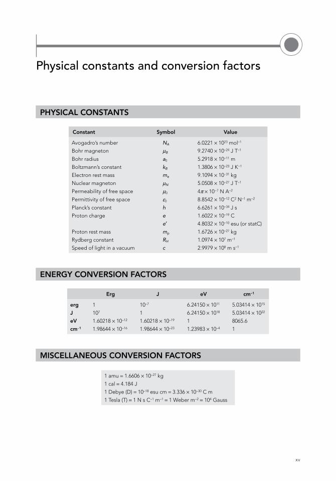
Physical constants and conversion factors
PHYSICAL CONSTANTS
Constant Symbol Value
Avogadro’s number NA 6.0221 × 10²³ mol−1
Bohr magneton μB 9.2740 × 10⁻²⁴ J T−1
Bohr radius a0 5.2918 × 10⁻¹¹ m
Boltzmann’s constant kB 1.3806 × 10⁻²³ J K−1
Electron rest mass me 9.1094 × 10⁻³¹ kg
Nuclear magneton μN 5.0508 × 10⁻²⁷ J T−1
Permeability of free space μ0 4π × 10−7 N A−2
Permittivity of free space ε0 8.8542 × 10⁻¹² C2 N−1 m−2
Planck’s constant h 6.6261 × 10⁻³⁴ J s
Proton charge e 1.6022 × 10⁻¹⁹ C
e′ 4.8032 × 10⁻¹⁰ esu (or statC)
Proton rest mass mp 1.6726 × 10⁻²⁷ kg
Rydberg constant RH 1.0974 × 10⁷ m−1
Speed of light in a vacuum c 2.9979 × 10⁸ m s−1
ENERGY CONVERSION FACTORS
Erg J eV cm−1
erg 1 10−7 6.24150 × 10¹¹ 5.03414 × 10¹⁵
J 107 1 6.24150 × 10¹⁸ 5.03414 × 10²²
eV 1.60218 × 10⁻¹² 1.60218 × 10⁻¹⁹ 1 8065.6
cm−1 1.98644 × 10⁻¹⁶ 1.98644 × 10⁻²³ 1.23983 × 10⁻⁴ 1
MISCELLANEOUS CONVERSION FACTORS
1 amu = 1.6606 × 10⁻²⁷ kg
1 cal = 4.184 J
1 Debye (D) = 10−18 esu cm = 3.336 × 10⁻³⁰ C m
1 Tesla (T) = 1 N s C−1 m−1 = 1 Weber m−2 = 104 Gauss
xvii
About the author
Jeanne L. McHale obtained a BS in chemistry from Wright State University, Dayton, Ohio, where Prof. Paul Seybold ignited her lifelong interest in optical spectroscopy. She earned a PhD in physical chemistry from the University of Utah, Salt Lake City, Utah, in 1979 under the direction of Prof. Jack Simons and then did postdoctoral research there with Prof. C. H. Wang. She began her academic career as a member of the chemistry faculty at the University of Idaho, Moscow, Idaho, in 1980, where she established a research program emphasizing spectro-scopic studies of intermolecular interactions, photoinduced electron transfer, and molecular dynamics of liquids. She is a fellow of the American Association for the Advancement of Science and has been an active member of the American Chemical Society and the Materials
Research Society. She organized the first Telluride Science Center workshop on solar solutions to energy and environmental problems. Dr. McHale served for 12 years as a professor in the Chemistry Department and the Materials Science and Engineering Program at Washington State University (WSU), Pullman, Washington. She has been Professor Emerita at WSU since 2016. Her recent research interests highlight applications of spectroscopy to the study of light-harvesting aggregates, semiconductor nanoparticles, and solar energy conversion.
1
1
Introduction and review
1.1 HISTORICAL PERSPECTIVE
Spectroscopy is about light and matter and how they interact with one another. The fundamental properties of both light and matter evade our human senses, and so there is a long history to the questions: What is light and what is matter? Studies of the two have often been interwoven, with spectroscopy playing an important role in the emergence and validation of quantum theory in the early twentieth century. Max Planck’s analysis of the emission spectrum of a blackbody radiator established the value of his eponymous constant, setting in motion a revolution that drastically altered our picture of the microscopic world. The line spectra of atoms, though they had been employed for chemical analysis since the late 1800s, could not be explained by classical physics. Why should gases in flames and discharge tubes emit only certain spectral wavelengths, while the emission spectrum of a heated body is a continuous distribution? Niels Bohr’s theory of the spectrum of the hydrogen atom recognized the results of Rutherford’s experiments, which revealed previously unexpected details of the atom: a dense, positively charged nucleus surrounded by the diffuse negative charge of the electrons. In Bohr’s atom the electrons revolve around the nucleus in precise paths like the orbits of planets around the sun, a picture that continues to serve as a popular cartoon representation of the atom. Though the picture is conceptually wrong, the theory based on it is in complete agreement with the observed absorption and emission wavelengths of hydrogen! Modern quantum theory smeared the sharp orbits of Bohr’s hydrogen atom into probability distributions, and successfully reproduced the observed spectral transition frequencies. Observations of electron emission by irradiated metals led to Einstein’s theory of photons as packets of light energy, after many hundreds of years of debate on the wave–particle nature of light. Experiments (such as electron diffraction by crystals) and theory (the Schrödinger equation and the Heisenberg uncertainty prin-ciple) gave rise to the idea that matter, like light, has wave-like as well as particle-like properties. Quantum theory and Einstein’s concept of photons converge in our modern microscopic view of spectroscopy. Matter emits or absorbs light (photons) by undergoing transitions between quantized energy levels. This relatively recent idea rests on the foundation built by philosophers and scientists who considered the nature of light since ancient times. The technology of recording spectra is far older than the quantum mechanical theories for interpretation of spectra.
Reference [1] gives an excellent historical account of investigations that led to our present understand-ing of electromagnetic radiation. Lenses and mirrors date back to before the common era, and the ancient Greeks included questions about the nature of light in their philosophical discourses. In 1666, Isaac Newton measured the spectrum of the sun by means of a prism. He speculated that the seven colors he observed (red, orange, yellow, green, blue, indigo, and violet) were somehow analogous to the seven notes of the musical scale. It is interesting that the frequency of violet light is a little less than twice that of red, so we see just less than an octave of this spectrum. We now know that the human eye can discern millions of colors [2] and that the wavelengths spanned by electromagnetic radiation extend indefinitely beyond the boundar-ies of vision. Newton was a proponent of the corpuscular view of light, a theory that held that light was a stream of particles bombarding the viewer. His contemporary, Christian Huygens, proposed a wave theory and showed how the concept could account for refraction and reflection. Newton had considerable influ-ence, and the corpuscular theory dominated the scene for a long time after his death. (Its proponents may have been more zealous then Newton himself had been.) Just a few years after the discovery of the infrared and ultraviolet ranges of the spectrum, Thomas Young in 1802 made the connection between wavelength and color. Young also investigated the phenomenon that is now known as polarization. A. J. Fresnel made
2 Introduction and review
contributions to the emerging wave theory as well, and equations describing the polarization dependence of reflection at a boundary bear his name [1].
The nineteenth century saw many developments in the analysis of spectral lines. Fraunhofer repeated Newton’s measurement of the solar spectrum in 1814, using a narrow slit rather than a circular aperture to admit the light onto the prism. The resolution of this experiment was sufficient to reveal a number of dark lines, wavelengths where the solar emission was missing. Numerous “Fraunhofer lines” are now assigned, thanks to the work of Bunsen, Ångström, and others. They originate from the reabsorption of sunlight by cooler atoms and ions in the outer atmosphere of the sun and that of the earth. In 1859, Kirchhoff demon-strated that two of these dark lines occur at the wavelengths of the yellow emission of hot sodium atoms. This helped to establish the notion that absorption and emission wavelengths of atoms coincide. Fraunhofer made further contributions by fabricating the first diffraction gratings, by wrapping fine silver wires around two parallel screws, and later by etching glass with diamond. By 1885 it was firmly established that elements have characteristic spectral wavelengths. The very discovery of the element helium in 1868 was made by analyzing the wavelengths of the solar spectrum.
The wave theory of light attracted many proponents in the nineteenth century, but it posed problems when light waves were compared to waves in matter, such as sound, which require a medium for support. How could light travel in a vacuum? The luminiferous ether was proposed, and efforts to detect it motivated some historic experiments, such as the accurate measurement of the speed of light by Michelson and Morley in 1887. (Michelson had earlier invented the interferometer while still in his twenties.) Their careful work resulted in rapid evaporation of the ether theory and in the recognition that light propagates in free space. The idea of a transverse wave, where the disturbance is perpendicular to the direction of propagation, was an elusive part of the picture, though it had been appreciated by Young. It took James Clerk Maxwell, whose equa-tions we examine in Chapter 2, to refine the picture of light as a transverse electromagnetic wave. Maxwell’s equations were fertilized by a large body of existing work on electricity and magnetism, particularly that of Michael Faraday. The crown jewel of Maxwell’s theoretical accomplishment was the derivation of the speed of light in terms of two known experimental quantities: the permittivity and permeability of free space. These properties and their interrelation are further discussed in Chapters 2 and 3. The point to be made here is that the result was in agreement with experiment.
Thus the wave theory of light would seem to have been on pretty firm ground as we entered the twentieth century. So too was the idea that matter was composed of particles, although little was known about atomic structure. The quantum upheaval rattled the complacency of classical physics and built the stage on which the field of spectroscopy continues to perform. Looking at things through quantum mechanical goggles, one eye sees the wave and the other the particle. We have to keep both eyes open.
1.2 DEFINITIONS, DERIVATIONS, AND DISCOVERY
As the study of the interaction of light and matter, spectroscopy embraces a wide range of physical and chemi-cal behavior. There is a certain reciprocity in the light–matter interaction. It is often natural to consider an experimental effect to be the result of matter exerting an influence on light (refraction, scattering, absorp-tion, etc.). In other experiments, we may prefer to consider the effect of light on matter (photochemistry, photobleaching, optical trapping, etc.). The range of experimental situations encompassed by this definition is vast, especially considering that by “light” we mean electromagnetic radiation of any frequency, not just the narrow visible region of the spectrum. The emphasis in this book is on spectroscopy as a tool for studying the structure and dynamics of molecules. In Chapters 1 through 12, the experiments to be discussed fall within the range of linear spectroscopy, in which the material response is directly proportional to the amplitude of the electric field vector of the radiation. A typical spectrum consists of the intensity of a certain response, such as absorption of light, as a function of frequency of the light. We shall see that the intensity is a measure of the rate at which molecules make transitions from one energy level to another, while the frequency is directly related to the difference in the initial and final energies of the molecule. In Chapters 13 and 14 we consider spectroscopic effects that come into play with more intense, typically pulsed, sources of electromagnetic
1.3 Review of quantum mechanics 3
radiation. These chapters will delve into nonlinear and time-resolved optical spectroscopy, and the material response will be expressed as a power series expansion in the amplitude of the electric field.
In either the linear or nonlinear regime, we shall take a perturbative approach, in which the zeroth order states are the quantized energy levels of the molecules in the absence of light. These are the stationary states found by solving the time-independent Schrödinger equation. The radiation does not perturb the energy levels themselves; rather, it induces transitions between them. We shall see that the radiation creates a superposition state in which the basis states are those of the system in the dark. In a sense, spectroscopy is applied quantum mechanics: a bridge between experiment and theory. Though in principle the Schrödinger equation permits the energy levels of a molecule to be determined theoretically, exact solutions to chemically interesting problems cannot be attained. Quantum chemists deal with this by developing sophisticated approximation methods to calculate energy levels and wavefunctions. Spectroscopists do their part by using light to discover these energy levels. The two groups keep each other honest, and working together they accomplish more than they could on their own.
Practical applications of spectroscopy routinely deal with large collections of molecules. The interactions among molecules can exert considerable influence on the response of a bulk sample to incident radiation. For example, spectra of isolated (gas phase) molecules reveal numerous spectroscopic transitions in the form of sharp, well-separated lines. Plunk these molecules into a solution, and the lines may broaden or even blur together into a continuous spectrum. How is the Schrödinger equation to help us if we cannot resolve the quantum states? This question begs for a theoretical approach that avoids the need to know molecular eigen-states. The time-dependent theory for interpretation of spectra, introduced in Chapters 5 and 12, will provide such an eigenstate-free approach. Before we can consider this theory, however, we need to understand how isolated molecules respond to light and then see how microscopic physical properties, such as polarizability or dipole moment, sum to give physical properties of matter in bulk. These electric and magnetic properties of molecules and bulk matter are discussed in Chapter 3.
In this chapter, we review some of the basic quantum mechanical principles that enable us to character-ize the translational, rotational, vibrational, and electronic energy states of molecules. The topic of statistical mechanics will then be summarized briefly, in order to discuss the behavior of large collections of molecules on the basis of the quantized states of individual molecules.
A note about derivations in the study of spectroscopy is in order. These derivations, which constitute a large part of this book, provide the foundation for getting microscopic information from spectra. Certainly, one can employ a formula or theoretical concept correctly without having derived it, and there are times when we do this. But having gone through a derivation conveys the scientist with additional insight and power. Knowing the theoretical foundations implies knowing the limits and assumptions behind the equa-tions, so one may avoid incorrect application of a model or theory. Skill and familiarity with derivations enable the practicing spectroscopist to make predictions and perhaps extend the current state of knowledge. Whenever possible, spectroscopic formulas are derived from first principles and the reader is urged to follow along with pencil and scratch paper. Occasionally, it will be necessary to simply say “It turns out that… ,” and the reader will know that the proof of the statement is outside the scope of this book or is just too complex to be worthwhile. When this happens, it is hoped that interested readers will be motivated to consult the refer-ences cited at the end of the chapter.
This chapter is an exception in that no derivations will be presented, except in Section 1.3.3, where raising and lowering operators are discussed. It is assumed that the reader has had some previous exposure to quan-tum mechanics and statistical mechanics. The intent of Section 1.3 is to provide a review and establish some notation and terms that will be employed throughout this book.
1.3 REVIEW OF QUANTUM MECHANICS
Quantum mechanics postulates the existence of a well-behaved wavefunction ψ that describes the state of the system. This function depends on the spatial coordinates of the system, for example, ψ(x, y, z) for a single particle in three dimensions. The wavefunction is not a physical observable; i.e., it cannot be measured
4 Introduction and review
experimentally, and it can be a complex function. However, its complex square, ψ *ψ ≡ |ψ|2, which is real, is interpreted as the probability density and is in principle experimentally observable. In a three-dimensional system, for example, ψ *ψdxdydz is the probability of finding the particle in the infinitesimal volume dxdydz. It is convenient to use the symbol dτ as a generic volume element, in order to write down general expressions that do not depend on the dimension or coordinate system. One condition on the wavefunction is that it be normalizable. A normalized wavefunction gives a total probability of unity when integrated over all space:
ψ ψ τ∗ =∫ d 1 (1.1)
The wavefunction must also be single-valued and continuous.The wavefunction is found by solving the time-independent Schrödinger equation H Eψ ψ= and applying
the appropriate boundary conditions. The Hamiltonian ˆ ˆ ˆH T V= + is the operator for the energy of the sys-tem: the sum of the operators for kinetic energy ( )�T and potential energy ( )�V . It is the latter that makes things interesting, in that it decides whether we are dealing with, say, a harmonic oscillator or a hydrogen atom. For a single particle in three dimensions, the kinetic energy operator is
Tm x y z
=− ∂
∂+
∂∂
+∂∂
�2 2
2
2
2
2
22 (1.2)
The symbol ħ represents h/2π, where h is Planck’s constant, and m is the particle mass.Quantum numbers arise when boundary conditions are applied. The result is that only certain wavefunc-
tions and energies satisfy the time-independent Schrödinger equation.
H En n nψ ψ= (1.3)
The index n in Equation 1.3 represents a quantum number or set of quantum numbers. Equation 1.3 is an eigenvalue equation. The allowed states of the system are specified by the solutions ψn (the eigenfunctions) and the energy of a system in a specific state is the eigenvalue En. If two different states correspond to different energy levels they must be orthogonal:
ψ ψ τn m n md E E∗∫ = ≠0 if (1.4)
Spectroscopy experiments probe differences in these energy levels. The Bohr frequency condition, to be derived in Chapter 4, states that the energy of the photon, hν, must match the energy level difference of the initial and final states:
ν =−E E
h2 1 (1.5)
Equation 1.5 is just one condition that must be met for the transition between states 1 and 2 to be allowed. Not all transitions are permitted, even when the frequency of the light ν satisfies Equation 1.5. We will derive selection rules throughout the book, which enable the allowed transitions to be predicted.
Equation 1.3 is actually a special case that results when the potential energy operator is not a function of time. More generally, we need the time-dependent Schrödinger equation to be discussed in Chapter 4. In later developments, we will account for the time dependence of the applied electromagnetic field. For now, we consider Equation 1.3 to represent the system in the dark.
If the eigenfunctions of Equation 1.3 can be found, then other physical properties can be predicted. It is one of the postulates of quantum mechanics that physical properties are associated with Hermitian opera-tors. For example, the momentum operator in the x direction is
p ix
x = −∂∂� (1.6)
1.3 Review of quantum mechanics 5
The position operator is just x x= . Since the potential energy is a function only of position, the quantum mechanical operator V looks just like the classical expression for the system’s potential energy. A Hermitian operator A obeys the turn-over rule, which states that, for any two well-behaved functions f and g,
f Ag d Af d∗ ∗= ∫∫ ( ) ( )� �τ τg (1.7)
It can be shown that an operator that obeys Equation 1.7 corresponds to a real physical property.A physical property may be calculated in one of two ways. If the system happens to be in a state that is
an eigenfunction of the operator corresponding to physical property A, then the only allowed values of the property are the eigenvalues an of the operator:
�A an n nψ ψ= (1.8)
The an’s are constants and are real. Now, an eigenvalue equation is a special case. What if the system is in a state for which A nψ is not equal to a constant times ψn? In this case we cannot specify the exact value of the physical property; we must resort to calculating the expectation value:
A A dn n= ∗∫ψ ψ τ� (1.9)
⟨A⟩ is the average value of the physical property when the system is in state n. It is often convenient to use Dirac notation in expressions such as 1.9. The wavefunction ψn is represented by the ket vector |ψn⟩ or |n⟩, and its complex conjugate ψ n
∗ is the bra vector ⟨ψn| or ⟨n|. Putting the two together to form a bra-ket (bracket) represents integration over the coordinates of the system. For example, normalization and orthogonality can be summarized by the inner product:
δnm n m= ⟨ ⟩| (1.10)
where the Kronecker delta function δ nm is equal to 1 if n = m and 0 if n ≠ m. The expectation value in Dirac notation is
A n A n Ann= ≡ˆ (1.11)
In many problems we are interested in matrix elements of the operator A connecting two different states: A n A mnm ≡ ˆ . We will also have need for the outer product |m⟩ ⟨n|. This outer product is just the product of ψm and ψ n
∗. Unlike the inner product, no integration is implied. The outer product is “waiting” to meet up with a bra from the left or a ket from the right.
So the good news of quantum mechanics is that we can solve the Schrödinger equation and know all there is to know about a system. The bad news is that this equation can be solved exactly for only a handful of model systems! Fortunately, these exactly solvable models are reasonable approximations to some very relevant chemical problems, and have much to teach us about quantum mechanical systems in general. Let us review the model problems that help us to understand translational, rotational, vibrational and electronic energies of molecules.
1.3.1 The parTicle in a box: a model for TranslaTional energies
This model assumes that a particle is confined to a region of space by a potential energy that rises to infinity at the walls of the container. The problem may seem very simple and perhaps artificial, but it illustrates some general principles that apply to more realistic quantum mechanical systems. Furthermore, it provides the
6 Introduction and review
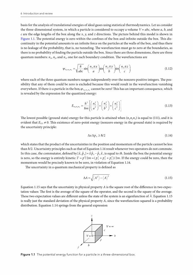
basis for the analysis of translational energies of ideal gases using statistical thermodynamics. Let us consider the three-dimensional system, in which a particle is considered to occupy a volume V = abc, where a, b, and c are the edge lengths of the box along the x, y, and z directions. The picture behind this model is shown in Figure 1.1. The potential energy is zero within the confines of the box and infinite outside the box. This dis-continuity in the potential amounts to an infinite force on the particles at the walls of the box, and thus there is no leakage of the probability, that is, no tunneling. The wavefunction must go to zero at the boundaries, as there is no probability of finding the particle outside the box. Since there are three dimensions, there are three quantum numbers: nx, ny, and nz, one for each boundary condition. The wavefunctions are
ψ π π πn n n
x y zx y z
abc
n x
a
n y
b
n z
c=
8sin sin sin (1.12)
where each of the three quantum numbers ranges independently over the nonzero positive integers. The pos-sibility that any of them could be zero is excluded because this would result in the wavefunction vanishing everywhere. If there is a particle in the box, ψ n n nx y z cannot be zero! This has an important consequence, which is revealed by the expression for the quantized energy:
Eh
m
n
a
n
b
n
cn n n
x y zx y z =
+
+
2 2
2
2
2
2
28 (1.13)
The lowest possible (ground state) energy for this particle is attained when (nxnynz) is equal to (111), and it is evident that E111 ≠ 0. This existence of zero-point energy (nonzero energy in the ground state) is required by the uncertainty principle:
∆ ∆x px ≥ �/2 (1.14)
which states that the product of the uncertainties in the position and momentum of the particle cannot be less than ħ/2. Uncertainty principles such as that of Equation 1.14 result whenever two operators do not commute. In this case, the commutator, defined by [ , ]� � � � � �x p x p p xx x x= − , is equal to iħ. Inside the box the potential energy is zero, so the energy is entirely kinetic: T p m p p p mx y z= = + +2 2 2 22 2/ ( )/ . If the energy could be zero, then the momentum would be precisely known to be zero, in violation of Equation 1.14.
The uncertainty in a quantum mechanical property is defined as
∆A A A= −2 2 (1.15)
Equation 1.15 says that the uncertainty in physical property A is the square root of the difference in two expec-tation values: The first is the average of the square of the operator, and the second is the square of the average. These two expectation values are different unless the state of the system is an eigenfunction of A. Equation 1.15 is really just the standard deviation of the physical property A, since the wavefunction-squared is a probability distribution. Equation 1.14 springs from the general expression
z
yV = 0
V = ∞
b
c
x
a
Figure 1.1 The potential energy function for a particle in a three-dimensional box.
1.3 Review of quantum mechanics 7
∆ ∆A B A B≥
1
2ˆ , ˆ (1.16)
In other words, the product of two uncertainties can be no less than one-half the expectation value of the commutator of the operators for the properties. Equation 1.14 follows directly from 1.16.
The three-dimensional particle in a box illustrates degenerate energy levels. When two or more states (represented by wavefunctions, e.g., Equation 1.12) share the same energy level, they are said to be degen-erate. Suppose that the box is a cube: a = b = c. The ground state, with nx = ny = nz = 1, is nondegenerate with energy 3h2/8ma2. The first excited state, however, is triply degenerate, because the energy 6h2/8ma2 can be achieved by three different combinations of the quantum numbers (nxnynz): (211), (121), and (112). These represent three distinct states since they differ in the position of the nodal plane: ψ211 has a nodal plane at x = a/2, ψ121 has one at y = a/2, and ψ112 has one at z = a/2. Degeneracy is a consequence of symmetry, and if we start with the cubic box and distort it, the degeneracy is lifted and the levels split apart. We can see this effect in molecules; e.g., a degenerate electronic state of a symmetric molecule such as benzene may be split by substitution, which perturbs the sixfold rotation symmetry. An octahedral transition metal complex may tend to distort to a less symmetric form if in doing so it can put electrons in lower energy levels.
Note also the general feature that states of increasing energy have more and more nodes. These nodes, where the wavefunction and thus the probability goes to zero, are one of the many strange aspects of quantum mechanics that would not be expected from the classical analogy to the problem. It is evident that nodes are required in order for two states to be orthogonal to one another. Another lesson is that the energy levels are farther apart for smaller boxes. Conversely, as the box size increases the energy levels get closer together, merging into a continuum in the classical limit. This trend, in which the separation of adjacent energy levels decreases with increasing size, is also seen in atoms, molecules, and nanoparticles.
The particle in a box model is useful for modeling translational energies of molecules in the gas phase. The model is consistent with the ideal gas approximation, in that it neglects intermolecular interactions. As you will show in one of the homework problems, the typical energy level spacings of particles in macroscopic boxes are much smaller than thermal energy at normal temperatures. This means that translational energy levels are essentially continuous and can be treated classically. Translational motion leads to Doppler broad-ening of gas phase spectra and to light scattering by fluids.
1.3.2 The rigid roTor: a model for roTaTional moTion of diaTomics
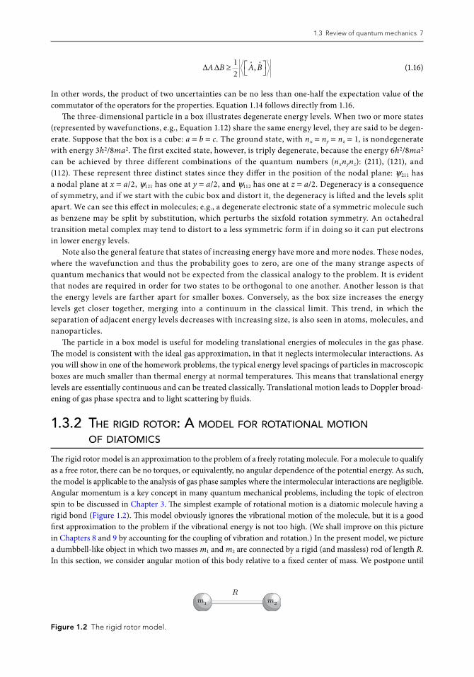
The rigid rotor model is an approximation to the problem of a freely rotating molecule. For a molecule to qualify as a free rotor, there can be no torques, or equivalently, no angular dependence of the potential energy. As such, the model is applicable to the analysis of gas phase samples where the intermolecular interactions are negligible. Angular momentum is a key concept in many quantum mechanical problems, including the topic of electron spin to be discussed in Chapter 3. The simplest example of rotational motion is a diatomic molecule having a rigid bond (Figure 1.2). This model obviously ignores the vibrational motion of the molecule, but it is a good first approximation to the problem if the vibrational energy is not too high. (We shall improve on this picture in Chapters 8 and 9 by accounting for the coupling of vibration and rotation.) In the present model, we picture a dumbbell-like object in which two masses m1 and m2 are connected by a rigid (and massless) rod of length R. In this section, we consider angular motion of this body relative to a fixed center of mass. We postpone until
Rm m
Figure 1.2 The rigid rotor model.
8 Introduction and review
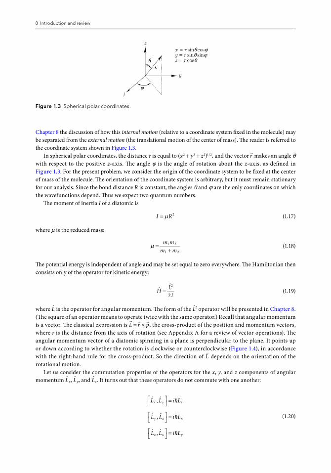
Chapter 8 the discussion of how this internal motion (relative to a coordinate system fixed in the molecule) may be separated from the external motion (the translational motion of the center of mass). The reader is referred to the coordinate system shown in Figure 1.3.
In spherical polar coordinates, the distance r is equal to (x2 + y2 + z2)1/2, and the vector �r makes an angle θ
with respect to the positive z-axis. The angle ϕ is the angle of rotation about the z-axis, as defined in Figure 1.3. For the present problem, we consider the origin of the coordinate system to be fixed at the center of mass of the molecule. The orientation of the coordinate system is arbitrary, but it must remain stationary for our analysis. Since the bond distance R is constant, the angles θ and ϕ are the only coordinates on which the wavefunctions depend. Thus we expect two quantum numbers.
The moment of inertia I of a diatomic is
I R= µ 2 (1.17)
where μ is the reduced mass:
µ =+
m m
m m1 2
1 2
(1.18)
The potential energy is independent of angle and may be set equal to zero everywhere. The Hamiltonian then consists only of the operator for kinetic energy:
ˆˆ
HL
I=
2
2 (1.19)
where L is the operator for angular momentum. The form of the L2 operator will be presented in Chapter 8. (The square of an operator means to operate twice with the same operator.) Recall that angular momentum is a vector. The classical expression is
� � �L r p= × , the cross-product of the position and momentum vectors,
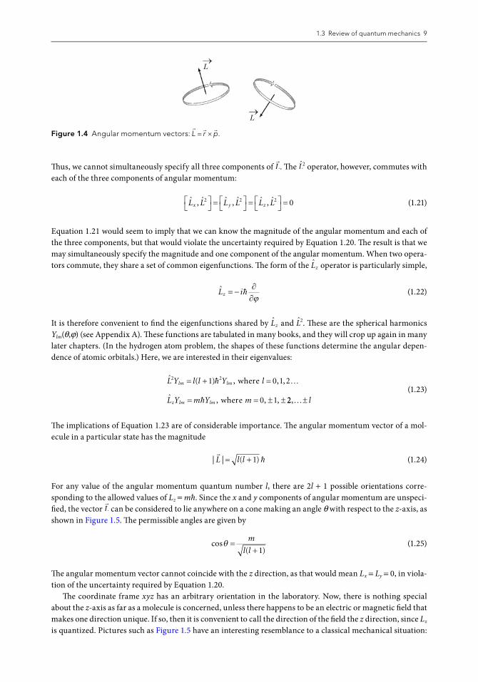
where r is the distance from the axis of rotation (see Appendix A for a review of vector operations). The angular momentum vector of a diatomic spinning in a plane is perpendicular to the plane. It points up or down according to whether the rotation is clockwise or counterclockwise (Figure 1.4), in accordance with the right-hand rule for the cross-product. So the direction of
�L depends on the orientation of the
rotational motion.Let us consider the commutation properties of the operators for the x, y, and z components of angular
momentum Lx, Ly, and Lz . It turns out that these operators do not commute with one another:
ˆ , ˆ
ˆ , ˆ
ˆ , ˆ
L L i L
L L i L
L L i L
x y z
y z x
z x y
=
=
=
�
�
�
(1.20)
z
y
x = r sinθ cosϕy = r sinθ sinϕz = r cosθ
ϕx
θr
Figure 1.3 Spherical polar coordinates.
1.3 Review of quantum mechanics 9
Thus, we cannot simultaneously specify all three components of �L. The L2 operator, however, commutes with
each of the three components of angular momentum:
ˆ , ˆ ˆ , ˆ ˆ , ˆL L L L L Lx y z
2 2 2 0
=
=
=
(1.21)
Equation 1.21 would seem to imply that we can know the magnitude of the angular momentum and each of the three components, but that would violate the uncertainty required by Equation 1.20. The result is that we may simultaneously specify the magnitude and one component of the angular momentum. When two opera-tors commute, they share a set of common eigenfunctions. The form of the Lz operator is particularly simple,
L iz = −
∂∂�
ϕ (1.22)
It is therefore convenient to find the eigenfunctions shared by Lz and L2. These are the spherical harmonics Ylm(θ,ϕ) (see Appendix A). These functions are tabulated in many books, and they will crop up again in many later chapters. (In the hydrogen atom problem, the shapes of these functions determine the angular depen-dence of atomic orbitals.) Here, we are interested in their eigenvalues:
ˆ ( ) , , ,
ˆ , , ,
L Y l l Y l
L Y m Y m
lm lm
z lm lm
2 21 0 1 2
0 1
= + = …
= = ± ±
�
�
where
where 22,…± l (1.23)
The implications of Equation 1.23 are of considerable importance. The angular momentum vector of a mol-ecule in a particular state has the magnitude
| | ( )�
�L l l= + 1 (1.24)
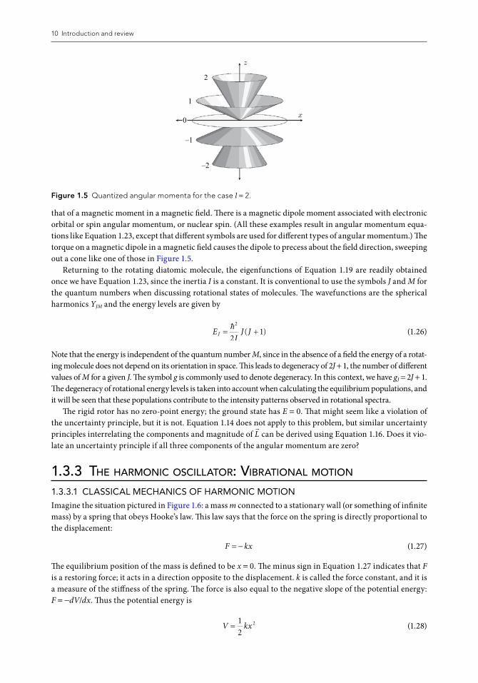
For any value of the angular momentum quantum number l, there are 2l + 1 possible orientations corre-sponding to the allowed values of Lz = mħ. Since the x and y components of angular momentum are unspeci-fied, the vector
�L can be considered to lie anywhere on a cone making an angle θ with respect to the z-axis, as
shown in Figure 1.5. The permissible angles are given by
cos( )
θ =+
m
l l 1 (1.25)
The angular momentum vector cannot coincide with the z direction, as that would mean Lx = Ly = 0, in viola-tion of the uncertainty required by Equation 1.20.
The coordinate frame xyz has an arbitrary orientation in the laboratory. Now, there is nothing special about the z-axis as far as a molecule is concerned, unless there happens to be an electric or magnetic field that makes one direction unique. If so, then it is convenient to call the direction of the field the z direction, since Lz is quantized. Pictures such as Figure 1.5 have an interesting resemblance to a classical mechanical situation:
L
L
Figure 1.4 Angular momentum vectors: � � �L r p= × .
10 Introduction and review
that of a magnetic moment in a magnetic field. There is a magnetic dipole moment associated with electronic orbital or spin angular momentum, or nuclear spin. (All these examples result in angular momentum equa-tions like Equation 1.23, except that different symbols are used for different types of angular momentum.) The torque on a magnetic dipole in a magnetic field causes the dipole to precess about the field direction, sweeping out a cone like one of those in Figure 1.5.
Returning to the rotating diatomic molecule, the eigenfunctions of Equation 1.19 are readily obtained once we have Equation 1.23, since the inertia I is a constant. It is conventional to use the symbols J and M for the quantum numbers when discussing rotational states of molecules. The wavefunctions are the spherical harmonics YJM and the energy levels are given by
EI
J JJ = +�2
21( ) (1.26)
Note that the energy is independent of the quantum number M, since in the absence of a field the energy of a rotat-ing molecule does not depend on its orientation in space. This leads to degeneracy of 2J + 1, the number of different values of M for a given J. The symbol g is commonly used to denote degeneracy. In this context, we have gJ = 2J + 1. The degeneracy of rotational energy levels is taken into account when calculating the equilibrium populations, and it will be seen that these populations contribute to the intensity patterns observed in rotational spectra.
The rigid rotor has no zero-point energy; the ground state has E = 0. That might seem like a violation of the uncertainty principle, but it is not. Equation 1.14 does not apply to this problem, but similar uncertainty principles interrelating the components and magnitude of
�L can be derived using Equation 1.16. Does it vio-
late an uncertainty principle if all three components of the angular momentum are zero?
1.3.3 The harmonic oscillaTor: VibraTional moTion
1.3.3.1 CLASSICAL MECHANICS OF HARMONIC MOTION
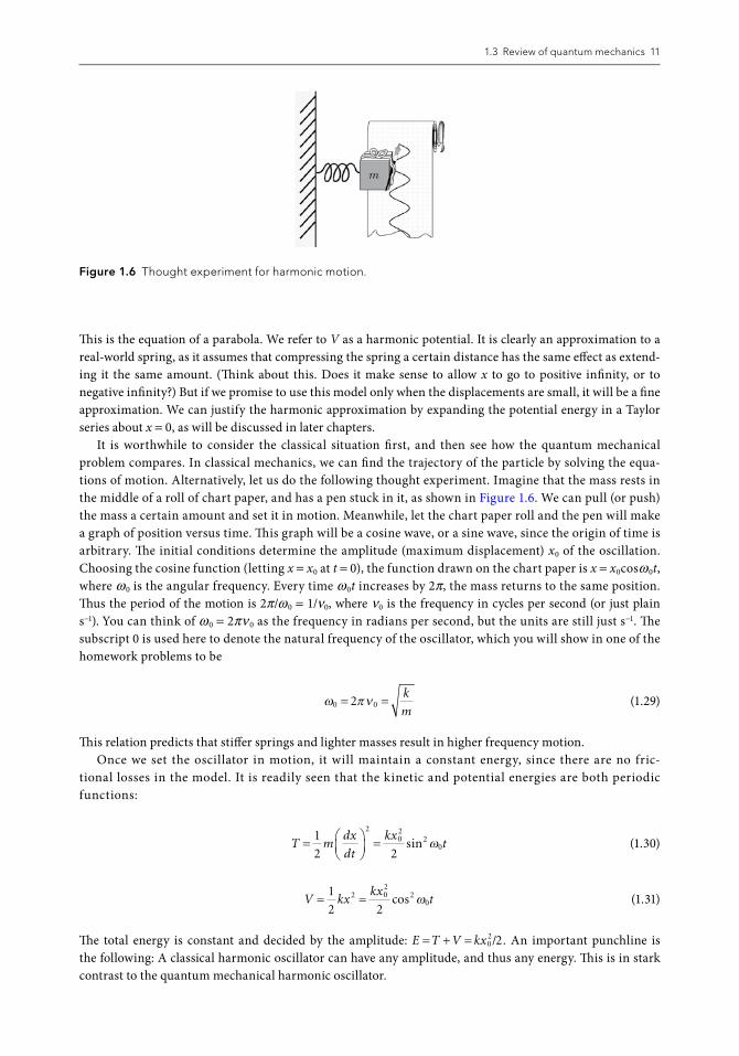
Imagine the situation pictured in Figure 1.6: a mass m connected to a stationary wall (or something of infinite mass) by a spring that obeys Hooke’s law. This law says that the force on the spring is directly proportional to the displacement:
F kx= − (1.27)
The equilibrium position of the mass is defined to be x = 0. The minus sign in Equation 1.27 indicates that F is a restoring force; it acts in a direction opposite to the displacement. k is called the force constant, and it is a measure of the stiffness of the spring. The force is also equal to the negative slope of the potential energy: F = −dV/dx. Thus the potential energy is
V kx=1
22 (1.28)
x
z
2
1
–1
–2
0
Figure 1.5 Quantized angular momenta for the case l = 2.
1.3 Review of quantum mechanics 11
This is the equation of a parabola. We refer to V as a harmonic potential. It is clearly an approximation to a real-world spring, as it assumes that compressing the spring a certain distance has the same effect as extend-ing it the same amount. (Think about this. Does it make sense to allow x to go to positive infinity, or to negative infinity?) But if we promise to use this model only when the displacements are small, it will be a fine approximation. We can justify the harmonic approximation by expanding the potential energy in a Taylor series about x = 0, as will be discussed in later chapters.
It is worthwhile to consider the classical situation first, and then see how the quantum mechanical problem compares. In classical mechanics, we can find the trajectory of the particle by solving the equa-tions of motion. Alternatively, let us do the following thought experiment. Imagine that the mass rests in the middle of a roll of chart paper, and has a pen stuck in it, as shown in Figure 1.6. We can pull (or push) the mass a certain amount and set it in motion. Meanwhile, let the chart paper roll and the pen will make a graph of position versus time. This graph will be a cosine wave, or a sine wave, since the origin of time is arbitrary. The initial conditions determine the amplitude (maximum displacement) x0 of the oscillation. Choosing the cosine function (letting x = x0 at t = 0), the function drawn on the chart paper is x = x0cosω 0t, where ω 0 is the angular frequency. Every time ω 0t increases by 2π, the mass returns to the same position. Thus the period of the motion is 2π/ω 0 = 1/ν0, where ν0 is the frequency in cycles per second (or just plain s−1). You can think of ω 0 = 2πν 0 as the frequency in radians per second, but the units are still just s−1. The subscript 0 is used here to denote the natural frequency of the oscillator, which you will show in one of the homework problems to be
ω πν0 02= =
k
m (1.29)
This relation predicts that stiffer springs and lighter masses result in higher frequency motion.Once we set the oscillator in motion, it will maintain a constant energy, since there are no fric-
tional losses in the model. It is readily seen that the kinetic and potential energies are both periodic functions:
T m
dx
dt
kxt=
=
1
2 2
202
20sin ω
(1.30)
V kx
kxt= =
1
2 22 0
22
0cos ω
(1.31)
The total energy is constant and decided by the amplitude: E T V kx= + = 02 2/ . An important punchline is
the following: A classical harmonic oscillator can have any amplitude, and thus any energy. This is in stark contrast to the quantum mechanical harmonic oscillator.
m
Figure 1.6 Thought experiment for harmonic motion.
12 Introduction and review
1.3.3.2 THE QUANTUM MECHANICAL HARMONIC OSCILLATOR
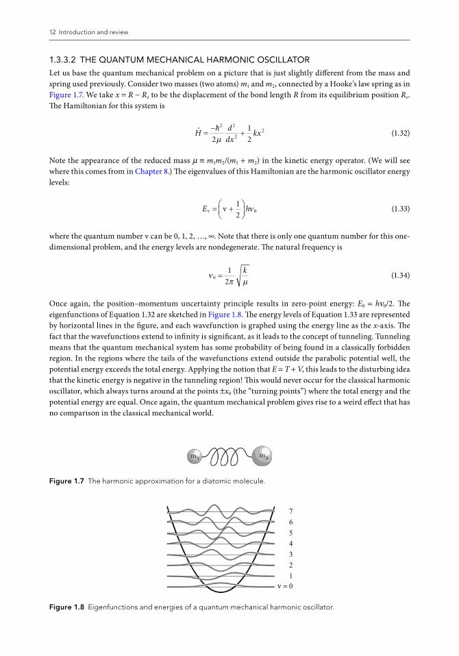
Let us base the quantum mechanical problem on a picture that is just slightly different from the mass and spring used previously. Consider two masses (two atoms) m1 and m2, connected by a Hooke’s law spring as in Figure 1.7. We take x = R − Re to be the displacement of the bond length R from its equilibrium position Re. The Hamiltonian for this system is
Hd
dxkx=
−+
�2 2
22
2
1
2µ (1.32)
Note the appearance of the reduced mass μ ≡ m1m2/(m1 + m2) in the kinetic energy operator. (We will see where this comes from in Chapter 8.) The eigenvalues of this Hamiltonian are the harmonic oscillator energy levels:
E hv v= +
1
20ν (1.33)
where the quantum number v can be 0, 1, 2, …, ∞. Note that there is only one quantum number for this one-dimensional problem, and the energy levels are nondegenerate. The natural frequency is
νπ µ01
2=
k (1.34)
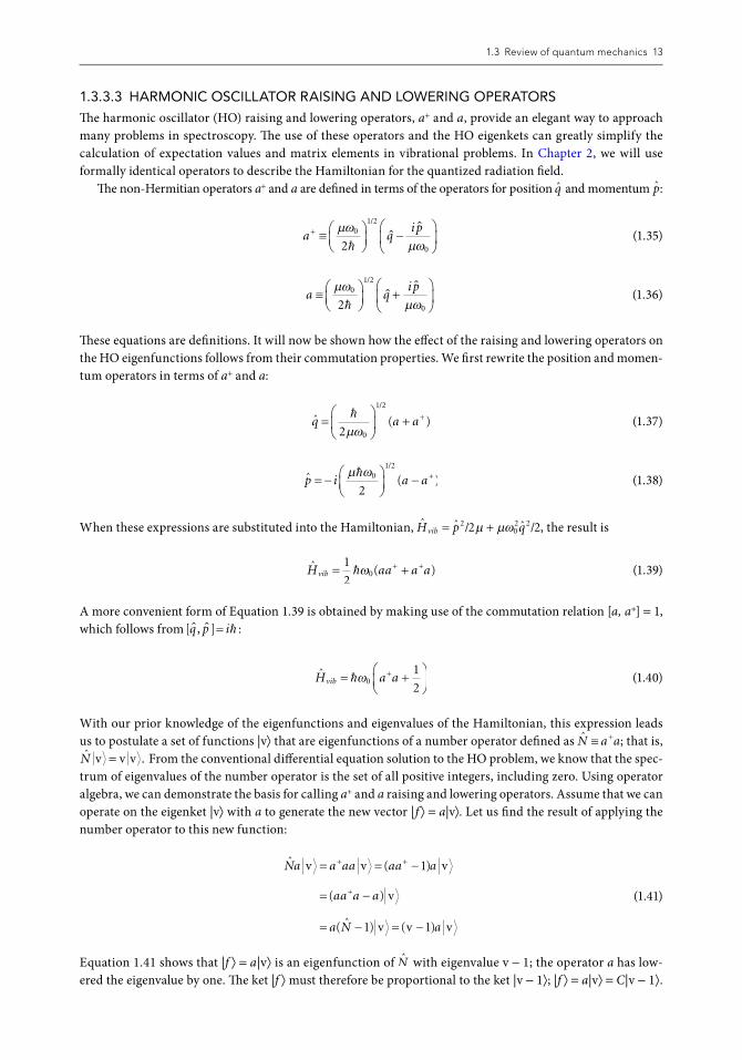
Once again, the position–momentum uncertainty principle results in zero-point energy: E0 = hν0/2. The eigenfunctions of Equation 1.32 are sketched in Figure 1.8. The energy levels of Equation 1.33 are represented by horizontal lines in the figure, and each wavefunction is graphed using the energy line as the x-axis. The fact that the wavefunctions extend to infinity is significant, as it leads to the concept of tunneling. Tunneling means that the quantum mechanical system has some probability of being found in a classically forbidden region. In the regions where the tails of the wavefunctions extend outside the parabolic potential well, the potential energy exceeds the total energy. Applying the notion that E = T + V, this leads to the disturbing idea that the kinetic energy is negative in the tunneling region! This would never occur for the classical harmonic oscillator, which always turns around at the points ±x0 (the “turning points”) where the total energy and the potential energy are equal. Once again, the quantum mechanical problem gives rise to a weird effect that has no comparison in the classical mechanical world.
m m
Figure 1.7 The harmonic approximation for a diatomic molecule.
v = 01234567
Figure 1.8 Eigenfunctions and energies of a quantum mechanical harmonic oscillator.
1.3 Review of quantum mechanics 13
1.3.3.3 HARMONIC OSCILLATOR RAISING AND LOWERING OPERATORS
The harmonic oscillator (HO) raising and lowering operators, a+ and a, provide an elegant way to approach many problems in spectroscopy. The use of these operators and the HO eigenkets can greatly simplify the calculation of expectation values and matrix elements in vibrational problems. In Chapter 2, we will use formally identical operators to describe the Hamiltonian for the quantized radiation field.
The non-Hermitian operators a+ and a are defined in terms of the operators for position q and momentum p:
a q
ip+ ≡
−
µωµω
01 2
02�
/
��
(1.35)
a q
ip≡
+
µωµω
01 2
02�
/
��
(1.36)
These equations are definitions. It will now be shown how the effect of the raising and lowering operators on the HO eigenfunctions follows from their commutation properties. We first rewrite the position and momen-tum operators in terms of a+ and a:
ˆ ( )
/
q a a=
+ +�
2 0
1 2
µω (1.37)
ˆ ( )
/
p i a a= −
− +µ ω� 0
1 2
2 (1.38)
When these expressions are substituted into the Hamiltonian, ˆ ˆ / ˆ /H p qvib = +202 22 2µ µω , the result is
ˆ ( )H aa a avib = ++ +1
20�ω
(1.39)
A more convenient form of Equation 1.39 is obtained by making use of the commutation relation [a, a+] = 1, which follows from [ , ]q p i� � = � :
H a avib = +
+�ω01
2 (1.40)
With our prior knowledge of the eigenfunctions and eigenvalues of the Hamiltonian, this expression leads us to postulate a set of functions |v⟩ that are eigenfunctions of a number operator defined as N a a≡ + ; that is, ˆ .N v v v= From the conventional differential equation solution to the HO problem, we know that the spec-
trum of eigenvalues of the number operator is the set of all positive integers, including zero. Using operator algebra, we can demonstrate the basis for calling a+ and a raising and lowering operators. Assume that we can operate on the eigenket |v⟩ with a to generate the new vector |f ⟩ = a|v⟩. Let us find the result of applying the number operator to this new function:
ˆ ( )
( )
( ˆ ) ( )
Na a aa aa a
aa a a
a N a
v v v
v
v v v
= = −
= −
= − = −
+ +
+
1
1 1
(1.41)
Equation 1.41 shows that |f ⟩ = a|v⟩ is an eigenfunction of N with eigenvalue v − 1; the operator a has low-ered the eigenvalue by one. The ket |f ⟩ must therefore be proportional to the ket |v − 1⟩; |f ⟩ = a|v⟩ = C|v − 1⟩.
14 Introduction and review
The proportionality constant C can be chosen by taking the eigenvectors |v⟩ and |v − 1⟩ to be normalized. Since ⟨v|a+ = (a|v⟩)*,
f f a a v C C= =+ ∗v (1.42)
Using ⟨v|a+a|v⟩ = v⟨v|v⟩ = v, and choosing the constant C to be real, we get
a v v v= − 1 (1.43)
Notice that Equation 1.43 ensures the lower bound of 0 on the eigenvalues v, since applying the lowering operator to the ket |0⟩ returns the value zero, and no negative values of v can be obtained.
Using the same approach on the vector |f ⟩ = a+|v⟩, one can show that
a + = + +v v v1 1 (1.44)
Thus a+ converts an eigenket |v⟩ into a new eigenket having its eigenvalue increased by one. As an example of the utility of this formalism, consider using these operators to derive the following recursion formula for the HO eigenfunctions:
q v v 1 v v v0
=
+ + + −
�2
1 1
1 2
µω
/
(1.45)
Equation 1.45 is obtained by using the position operator q as given in Equation 1.37. It will be useful in future chapters when we consider selection rules for vibrational transitions.
1.3.4 The hydrogen aTom
As a one-electron atom, the hydrogen atom lacks the pairwise inter-electronic repulsion that prevents an exact solution of the Schrödinger equation in the case of many-electron atoms. By examining the quantum mechanical treatment of one-electron atoms, we obtain some general physical concepts and indeed the basis for approximate treatments of the electronic structure of many-electron atoms and molecules. Hydrogen-like (that is, one-electron) atoms require a set of four quantum numbers to fully specify the wavefunction, and only one to define the energy. The number of quantum numbers is consistent with the electron having three spatial and one spin degree of freedom. The variational principle, on which self-consistent field calculations are based, permits us to build approximate wavefunctions for many-electron atoms which assign individual electrons to hydrogenic orbitals with definite spatial and spin quantum numbers, as will be considered in Chapter 7.
The hydrogen atom wavefunctions (which apply to all one-electron atoms or ions by appropriate choice of the atomic number Z) depend on the spatial variables r, θ, and ϕ and an abstract spin coordinate often called σ. The spatial coordinates are the spherical polar coordinates which allow the Schrödinger equation to be solved using separation of variables. They define the position of the electron relative to the center of mass of the atom, which is quite close to the position of the more massive nucleus. The polar coordinates r, θ, ϕ (see Figure 1.3) are related to the Cartesian coordinates x, y, z as follows:
x r= sin cosθ ϕ (1.46)
y r= sin sinθ ϕ (1.47)
z r= cosθ (1.48)
1.3 Review of quantum mechanics 15
The spin coordinate, on the other hand, is a conceptual device to keep track of the two possible states of elec-tron spin, designated α for spin-up and β for spin-down. The wavefunctions for the one-electron atom are represented as follows:
Ψnlm m nl lml s lr R r Y, , , ,θ ϕ σ θ ϕαβ
( ) = ( ) ( )
(1.49)
where Rnl(r) is the radial wavefunction and Ylml θ ϕ,( ) the angular one. The angular wavefunctions are the same spherical harmonics that pertain to the rigid rotator problem. Both are cases of two particles rotating in a coordinate system for which the origin is the center of mass. The two angular variables can be further separated as follows:
Y P elm lmim
l llθ ϕ ∝ θ ϕ, cos( ) ( ) (1.50)
The associated Legendre polynomials Plml ( )x (Appendix A) are tabulated in various books [3,4] and can be generated by a recursion formula. For one-electron atoms we designate the angular momentum quan-tum numbers with the letters l, ml corresponding to the eigenvalues of L2 and Lz respectively (using Dirac notation):
L Y l l Ylm lml l
2 21= +( )� (1.51)
L Y m Yz lm l lml l= � (1.52)
Thus the magnitude of the orbital angular momentum vector is l l +( )1 �, and its projection onto the z direc-tion is ml�.
The one-electron energy levels are given by
EZ e
n a
Z
nn =
−( )
=−
×2 2
02
0
2
24 213 6
πε. eV (1.53)
where n = 1, 2, 3, …∞ is the principal quantum number and a0 = 0.529 Å is the Bohr radius:
aee
00
2
2
4=
πεµ� (1.54)
The quantity μe = memN/(me + mN) is the reduced mass computed from the mass of the electron me and that of the nucleus mN. Because mN is much larger than me, μe is approximately equal to me. The degeneracy of each energy level specified by the principal quantum number n is gn = 2n2, consistent with the number of values of l, ml, and ms that are permitted for each value of n, namely:
l n= … −0 1 1, , , (1.55)
m l l l ll = − − + … … −, , , , , ,1 0 1 (1.56)
ms = ±
1
2 (1.57)
16 Introduction and review
The states having orbital quantum number l = 0, 1, 2, 3, 4… are referred to by the letters s, p, d, f, g…, etc. This quantum number is also called the azimuthal quantum number. The reader may wish to verify that g l nn l
n= + ==−∑2 2 1 2
0
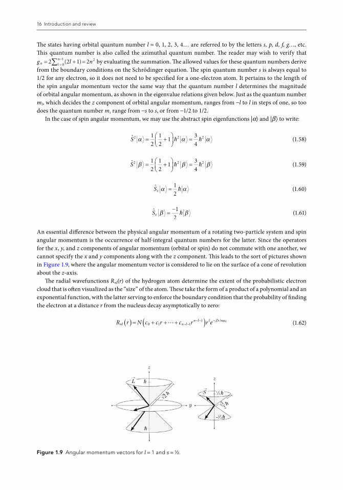
1 2( ) by evaluating the summation. The allowed values for these quantum numbers derive from the boundary conditions on the Schrödinger equation. The spin quantum number s is always equal to 1/2 for any electron, so it does not need to be specified for a one-electron atom. It pertains to the length of the spin angular momentum vector the same way that the quantum number l determines the magnitude of orbital angular momentum, as shown in the eigenvalue relations given below. Just as the quantum number ml, which decides the z component of orbital angular momentum, ranges from −l to l in steps of one, so too does the quantum number ms range from −s to s, or from −1/2 to 1/2.
In the case of spin angular momentum, we may use the abstract spin eigenfunctions |α⟩ and |β ⟩ to write:
S2 2 21
2
1
21
3
4α α α= +
=� � (1.58)
S2 2 21
2
1
21
3
4β β β= +
=� � (1.59)
Sz α α=1
2� (1.60)
Sz β β=−1
2� (1.61)
An essential difference between the physical angular momentum of a rotating two-particle system and spin angular momentum is the occurrence of half-integral quantum numbers for the latter. Since the operators for the x, y, and z components of angular momentum (orbital or spin) do not commute with one another, we cannot specify the x and y components along with the z component. This leads to the sort of pictures shown in Figure 1.9, where the angular momentum vector is considered to lie on the surface of a cone of revolution about the z-axis.
The radial wavefunctions Rnl(r) of the hydrogen atom determine the extent of the probabilistic electron cloud that is often visualized as the “size” of the atom. These take the form of a product of a polynomial and an exponential function, with the latter serving to enforce the boundary condition that the probability of finding the electron at a distance r from the nucleus decay asymptotically to zero:
R r N c c r c r r enl n ln l l Zr na( ) = + + +( )− −
− − −0 1 1
1 0� / (1.62)
h
h h
h
h
h
z
√
z
→
→
L
y
S
3 2
12
1- 2
2√
Figure 1.9 Angular momentum vectors for l = 1 and s = ½.
1.3 Review of quantum mechanics 17
The coefficients cn of each term rn obey a recursion formula which can be found in most quantum chemistry texts [3,4]. As will be shown in Chapter 7, the allowed transitions between energy levels of the hydrogen atom result in absorption and emission frequencies
�ν = −
R
n nH
1 1
12
22
(1.63)
The Rydberg constant is RH = 109,737 cm−1 and n1 < n2. RH can be found using Equations 1.53 and 1.5:
Re
h cH
e=2
4
2 4
02 3
π µπε( )
(1.64)
Equation 1.64 introduces the wavenumber unit �ν , or cm−1, where �ν is the reciprocal of the wavelength of light in cm. �ν = ν/c is equivalent to the frequency of light ν in s−1 divided by the speed of light c = 2.99792 × 1010 cm/s. Wavenumbers are convenient frequency units in spectroscopy.
1.3.5 general aspecTs of angular momenTum in quanTum mechanics
Angular momentum of charged particles leads to magnetic properties as discussed further in Chapter 3. In addition to the orbital l and spin s angular momenta of an electron in a hydrogen atom, it will be seen in Chapter 7 that many-electron atoms possess orbital L and spin S angular momenta which can couple further to give a total angular momentum J. The use of upper case letters for these quantum numbers is to distinguish them from their single electron counterparts. Many nuclei also possess angular momentum as designated by the quantum number I, which can take on nonnegative integer or half-integer values depending on the atomic number and isotope. Despite the variety of symbols for the various angular momentum quantum numbers, s, l, S, J, L, I, etc., their quantum mechanical properties, i.e., commutator relations and eigenvalue expressions, are similar. Owing to the former, the magnitude of the angular momentum and its z-component are quantized while the x and y components are uncertain. We state these generalities here in terms of a generic angular moment quantum number j which can be integral (as in the case of orbital angular momentum) or half-integral (as in the case of s = ½ for an electron). The value of j determines the magnitude of the angular momentum vector, referred to here as
��J j j= +( )1 . A second quantum number m j ranges from j to –j in integral steps and specifies the
z-component of the angular momentum: J mz j= �. There are 2j + 1 values of m j . We can specify the eigenfunc-tions by using Dirac notation and indexing the quantum numbers: j m j, . For example, when this notation is applied to the case of electron spin, the eigenfunctions are expressed as α = 1 2 1 2/ , / and β = −1 2 1 2/ , / . We can then write generic eigenvalue relations for any kind of quantized angular momentum as follows:
ˆ , ( ) ,
ˆ , ,
J j m j j j m
J j m m j m
j j
z j j j
2 21= +
=
�
� (1.65)
It is useful to define ladder operators for angular momentum as follows:
ˆ ˆ ˆ
ˆ ˆ ˆ
J J iJ
J J iJ
x y
x y
+
−
= +
= − (1.66)
The j m j, are not eigenfunctions of these ladder operators. As shown in most quantum mechanics texts, J + and J − act as raising and lowering operators, respectively:
ˆ , [ ( ) ( )] ,
ˆ , [ ( ) (
/J j m j j m m j m
J j m j j m m
j j j j
j j j
+
−
= + − + +
= + − −
1 1 1
1 1
1 2�
))] ,/1 2 1� j m j − (1.67)
18 Introduction and review
The raising operator has the effect of converting an eigenfunction of J z with eigenvalue m j� into a new eigenfunction with eigenvalue ( )m j +1 �, with no effect on the eigenvalue of J 2. Similarly, J − lowers the eigen-value of J z to ( )m j −1 �. Notice that if m j has the maximum value of j, then ˆ ,J j j+ = 0, e.g. it is impossible to raise the eigenvalue of J z any further. Similarly, ˆ ,J j j− − = 0 .
Ladder operators are useful for finding matrix elements of the operators for the x and y components of angular momentum, using the following:
ˆ ( ˆ ˆ )
ˆ ( ˆ ˆ )
J J J
Ji
J J
x
y
= +
= −
+ −
+ −
1
2
1
2
(1.68)
To illustrate this using the spin angular momentum operators (using the letter S in place of J for the relevant operators), it is straightforward to demonstrate the following:
ˆ
ˆ
ˆ
ˆ
S
S
Si
Si
x
x
y
y
α β
β α
α β
β α
=
=
=
=−
�
�
�
�
2
2
2
2
(1.69)
It is seen that the x and y components of the spin operators connect the α and β spin functions, in contrast to Sz which is a diagonal operator.
1.4 APPROXIMATE SOLUTIONS TO THE SCHRÖDINGER EQUATION: VARIATION AND PERTURBATION THEORY
We have now reviewed the exactly solvable quantum mechanical problems. (A fifth example, the hydrogen molecule ion H2
+, can only be solved “exactly” if one makes the Born–Oppenheimer approximation, dis-cussed in Chapter 9.) What of the many problems for which H Eψ ψ= cannot be solved exactly? For example, in atoms and molecules with two or more electrons, the interelectronic repulsions make exact solutions to the Schrödinger equation impossible. In other situations, we might need to find the energy for a problem that is close to one for which we already know the solution. Two methods are commonly employed to address these problems. The variation theorem, which states that there is a lower bound on the energy calculated with an approximate wavefunction, is of great utility in electronic structure calculations. Another approach is per-turbation theory, which is useful whenever the true Hamiltonian is slightly different from one for which the energies and wavefunctions are known.
1.4.1 VariaTion meThod
In this approach, one uses an approximate wavefunction ϕ which has to obey the appropriate boundary con-ditions. The variation theorem states that the energy expectation value calculated using this trial function cannot be any lower than the true ground-state energy E0:
EH
E= ≥ϕ ϕ
ϕ ϕ
ˆ0 (1.70)
1.4 Approximate solutions to the Schrödinger equation: variation and perturbation theory 19
Note that H has to be the exact Hamiltonian operator and ϕ has to be a well-behaved function which satisfies the boundary conditions. The denominator in 1.70 is present in case the trial function ϕ is not normalized. Equation 1.70 says that the lower the energy calculated with some function ϕ, the closer it is to the exact energy. This suggests that a good way to proceed is to build some flexibility into the trial functions, some adjustable parameters that can be varied to obtain the lowest possible energy with that functional form. One way to do this is to use linear variation theory, in which the trial function is taken to be a linear combination of basis functions, say, f1, f2, …, fn. Then we have
ϕ = + + +c f c f c fn n1 1 2 2 � (1.71)
The ci,s are coefficients (just plain numbers) to be determined by minimizing the energy. The basis functions may be any functions appropriate to the boundary conditions. In the calculation of electronic energy levels of molecules, for example, they may be hydrogen-like wavefunctions localized on the atoms. This is the basis for the LCAO-MO (linear combination of atomic orbitals to get molecular orbitals) method, which will be reviewed in Chapter 11.
Equation 1.71 can be used in Equation 1.70 to get an expression for the energy that depends on the coef-ficients. Then, to get the lowest possible energy with the given basis set, we set d⟨E⟩/dci = 0 for each of the n coefficients. This leads to a set of simultaneous linear equations:
H E H ES H ES
H ES H E H ES
H ES H
n n
n n
n n n
11 12 12 1 1
21 21 22 2 2
1 1
− − −− − −
−
��
� � � �
22 2
1
2
0
0
0
0− −
=
ES H E
c
c
cn nn n��
(1.72)
where H f H f Hij i j ji= = ∗˘
and S f f Sij i j ji= = ∗ (Note that, in general, an element of the square matrix on the left-hand side is Hij − ESij, but the overlaps Sii are unity for normalized basis functions. We have dropped the angle brackets around the energy E.) The methods for solving Equation 1.72 are well established (see Appendix A). A solution exists only if the determinant of the matrix of Hij − ESij is zero:
H E H ES H ES
H ES H E H ES
H ES H
n n
n n
n n n
11 12 12 1 1
21 21 22 2 2
1 1
− − −− − −
−
��
� � � �
22 2
0
− −
=
ES H En nn�
(1.73)
Expanding this determinant results in a polynomial of degree n in the energy: thus there are n roots for the energy. We can arrange these in order of increasing energy: E E E En0 ≤ ≤ ≤ 1 2� . Each root in this sequence is a lower bound to the true energy; that is, E0 is no lower than the true ground state energy, E1 is no lower than the energy of the first excited state, etc. For each solution Ek, there is a particular set of coefficients to describe the corresponding wavefunction: ϕk kii ic f= ∑ . (We have to use an additional subscript on the coefficients to keep track of the n different linear combinations.) The cki,s for a particular root are found by substituting the energy Ek into the matrix Equation 1.72 and solving. When this is done, one finds that the coefficients can only be determined to within a multiplicative constant, so it is customary to impose normalization of each ϕk to fix the values of the cki,s.
Linear variation methods are frequently used in electronic structure calculations, and the idea of combin-ing wavefunctions (basis states) to get new wavefunctions (trial functions like ϕ) is a recurring theme. The number of calculated energy levels and states is always equal to the number of basis states combined.
1.4.2 perTurbaTion Theory
We are often interested in molecules which are subject to weak perturbations, such as an external electric or magnetic field. In the study of spectroscopy, we deal with the perturbation resulting from the application
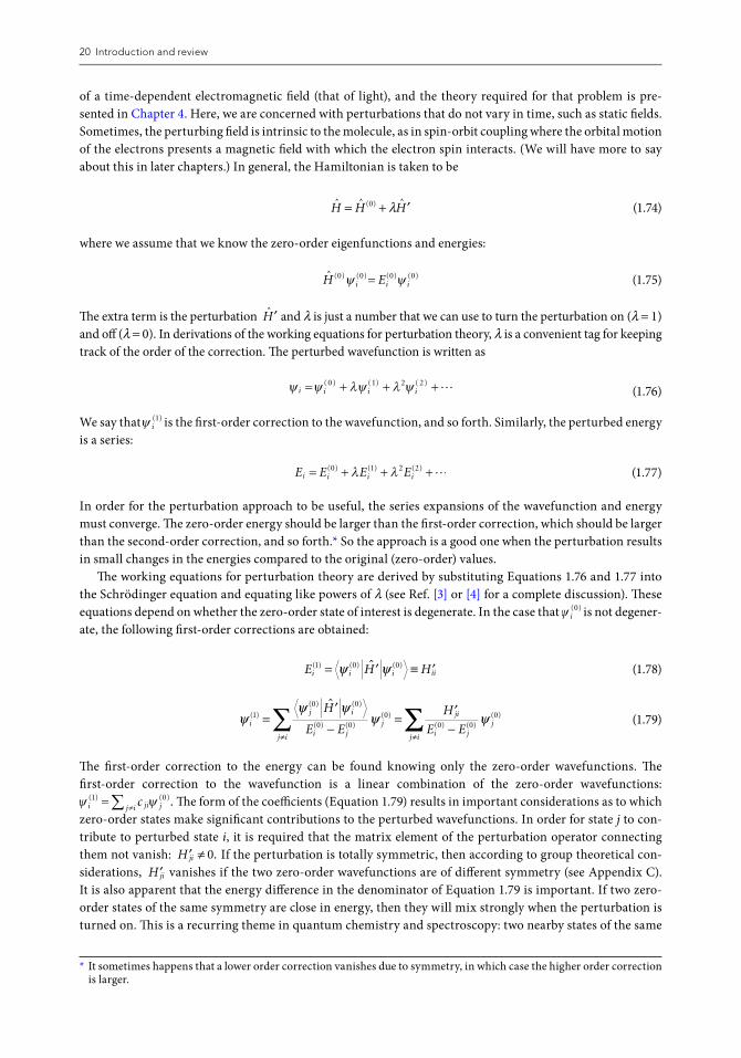
20 Introduction and review
of a time-dependent electromagnetic field (that of light), and the theory required for that problem is pre-sented in Chapter 4. Here, we are concerned with perturbations that do not vary in time, such as static fields. Sometimes, the perturbing field is intrinsic to the molecule, as in spin-orbit coupling where the orbital motion of the electrons presents a magnetic field with which the electron spin interacts. (We will have more to say about this in later chapters.) In general, the Hamiltonian is taken to be
ˆ ˆ ˆ( )H H H= + ′0 λ (1.74)
where we assume that we know the zero-order eigenfunctions and energies:
ˆ ( ) ( ) ( ) ( )H Ei i i
0 0 0 0ψ ψ= (1.75)
The extra term is the perturbation H ′ and λ is just a number that we can use to turn the perturbation on (λ = 1) and off (λ = 0). In derivations of the working equations for perturbation theory, λ is a convenient tag for keeping track of the order of the correction. The perturbed wavefunction is written as
ψ ψ λψ λ ψi i i i= + + +( ) ( ) ( )0 1 2 2 � (1.76)
We say that ψ i( )1 is the first-order correction to the wavefunction, and so forth. Similarly, the perturbed energy
is a series:
E E E Ei i i i= + + +( ) ( ) ( )0 1 2 2λ λ � (1.77)
In order for the perturbation approach to be useful, the series expansions of the wavefunction and energy must converge. The zero-order energy should be larger than the first-order correction, which should be larger than the second-order correction, and so forth.* So the approach is a good one when the perturbation results in small changes in the energies compared to the original (zero-order) values.
The working equations for perturbation theory are derived by substituting Equations 1.76 and 1.77 into the Schrödinger equation and equating like powers of λ (see Ref. [3] or [4] for a complete discussion). These equations depend on whether the zero-order state of interest is degenerate. In the case that ψ i
( )0 is not degener-ate, the following first-order corrections are obtained:
E H Hi i i ii
( ) ( ) ( )1 0 0= ′ ≡ ′ψ ψ�
(1.78)
ψψ ψ
ψi
j i
i jj i
jji
i jj iE E
H
E E( )
( ) ( )
( ) ( )( )
( ) ( )1
0 0
0 00
0 0=′
−= ′
−≠ ≠
∑ H� ∑∑ ψ j( )0
(1.79)
The first-order correction to the energy can be found knowing only the zero-order wavefunctions. The first-order correction to the wavefunction is a linear combination of the zero-order wavefunctions: ψ ψi jij i jc( ) ( ).1 0= ≠∑ The form of the coefficients (Equation 1.79) results in important considerations as to which zero-order states make significant contributions to the perturbed wavefunctions. In order for state j to con-tribute to perturbed state i, it is required that the matrix element of the perturbation operator connecting them not vanish: ′ ≠H ji 0. If the perturbation is totally symmetric, then according to group theoretical con-siderations, ′H ji vanishes if the two zero-order wavefunctions are of different symmetry (see Appendix C). It is also apparent that the energy difference in the denominator of Equation 1.79 is important. If two zero-order states of the same symmetry are close in energy, then they will mix strongly when the perturbation is turned on. This is a recurring theme in quantum chemistry and spectroscopy: two nearby states of the same
* It sometimes happens that a lower order correction vanishes due to symmetry, in which case the higher order correction is larger.
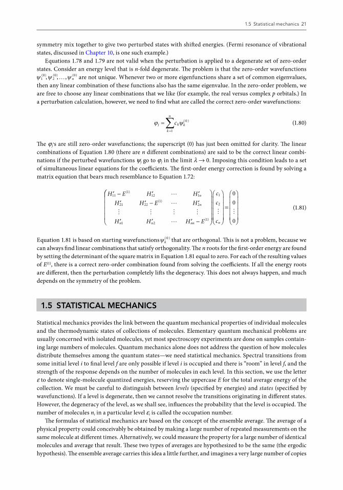
1.5 Statistical mechanics 21
symmetry mix together to give two perturbed states with shifted energies. (Fermi resonance of vibrational states, discussed in Chapter 10, is one such example.)
Equations 1.78 and 1.79 are not valid when the perturbation is applied to a degenerate set of zero-order states. Consider an energy level that is n-fold degenerate. The problem is that the zero-order wavefunctions ψ ψ ψ1
02
0 0( ) ( ) ( ), , ,… n are not unique. Whenever two or more eigenfunctions share a set of common eigenvalues, then any linear combination of these functions also has the same eigenvalue. In the zero-order problem, we are free to choose any linear combinations that we like (for example, the real versus complex p orbitals.) In a perturbation calculation, however, we need to find what are called the correct zero-order wavefunctions:
ϕ ψj k
k
n
kc==
∑1
0( ) (1.80)
The ϕj,s are still zero-order wavefunctions; the superscript (0) has just been omitted for clarity. The linear combinations of Equation 1.80 (there are n different combinations) are said to be the correct linear combi-nations if the perturbed wavefunctions ψj go to ϕj in the limit λ → 0. Imposing this condition leads to a set of simultaneous linear equations for the coefficients. The first-order energy correction is found by solving a matrix equation that bears much resemblance to Equation 1.72:
′ − ′ ′′ ′ − ′
′ ′ ′ −
H E H H
H H E H
H H H E
n
n
n n nn
111
12 1
21 221
2
1 21
( )
( )
( )
��
� � � ��
=
c
c
cn
1
2
0
0
0
� � (1.81)
Equation 1.81 is based on starting wavefunctions ψk( )0 that are orthogonal. This is not a problem, because we
can always find linear combinations that satisfy orthogonality. The n roots for the first-order energy are found by setting the determinant of the square matrix in Equation 1.81 equal to zero. For each of the resulting values of E(1), there is a correct zero-order combination found from solving the coefficients. If all the energy roots are different, then the perturbation completely lifts the degeneracy. This does not always happen, and much depends on the symmetry of the problem.
1.5 STATISTICAL MECHANICS
Statistical mechanics provides the link between the quantum mechanical properties of individual molecules and the thermodynamic states of collections of molecules. Elementary quantum mechanical problems are usually concerned with isolated molecules, yet most spectroscopy experiments are done on samples contain-ing large numbers of molecules. Quantum mechanics alone does not address the question of how molecules distribute themselves among the quantum states—we need statistical mechanics. Spectral transitions from some initial level i to final level f are only possible if level i is occupied and there is “room” in level f, and the strength of the response depends on the number of molecules in each level. In this section, we use the letter ε to denote single-molecule quantized energies, reserving the uppercase E for the total average energy of the collection. We must be careful to distinguish between levels (specified by energies) and states (specified by wavefunctions). If a level is degenerate, then we cannot resolve the transitions originating in different states. However, the degeneracy of the level, as we shall see, influences the probability that the level is occupied. The number of molecules ni in a particular level εi is called the occupation number.
The formulas of statistical mechanics are based on the concept of the ensemble average. The average of a physical property could conceivably be obtained by making a large number of repeated measurements on the same molecule at different times. Alternatively, we could measure the property for a large number of identical molecules and average that result. These two types of averages are hypothesized to be the same (the ergodic hypothesis). The ensemble average carries this idea a little further, and imagines a very large number of copies
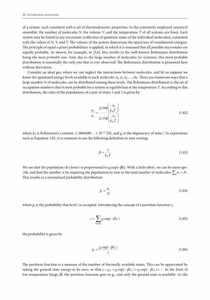
22 Introduction and review
of a system, each consistent with a set of thermodynamic properties. In the commonly employed canonical ensemble, the number of molecules N, the volume V, and the temperature T of all systems are fixed. Each system may be found in any microstate (collection of quantum states of the individual molecules), consistent with the values of N, V, and T. The volume of the system determines the spectrum of translational energies. The principle of equal a priori probabilities is applied, in which it is assumed that all possible microstates are equally probable. As shown, for example, in [5,6], this results in the well-known Boltzmann distribution being the most probable one. And, due to the large number of molecules (or systems), this most probable distribution is essentially the only one that is ever observed! The Boltzmann distribution is presented here without derivation.
Consider an ideal gas, where we can neglect the interactions between molecules, and let us suppose we know the quantized energy levels available to each molecule: ε0, ε1, ε2,…, etc. There are numerous ways that a large number N of molecules can be distributed among these levels. The Boltzmann distribution is the set of occupation numbers that is most probable for a system in equilibrium at the temperature T. According to this distribution, the ratio of the populations of a pair of states 1 and 2 is given by
n
n
gk T
gk T
B
B
1
2
11
22
=
−
−
exp
exp
ε
ε (1.82)
where kB is Boltzmann’s constant, 1.3806488… × 10−23 J/K, and gi is the degeneracy of state i. In expressions such as Equation 1.82, it is common to use the following definition to save writing:
β =
1
k TB (1.83)
We see that the population of a level i is proportional to gi exp(−βεi). With a little effort, we can be more spe-cific and find the number ni by requiring the populations to sum to the total number of molecules: n Nii∑ = . This results in a normalized probability distribution:
p
n
Ni
i=
(1.84)
where pi is the probability that level i is occupied. Introducing the concept of a partition function z,
z g i
i
i= −∑levels
exp( )βε
(1.85)
the probability is given by
p
g
zi
i i=−exp( )βε
(1.86)
The partition function is a measure of the number of thermally available states. This can be appreciated by taking the ground state energy to be zero, so that z g g g= + − + − +0 1 1 2 2exp( ) exp( )βε βε �. In the limit of low temperature (large β), the partition function goes to g0, and only the ground state is available. As the
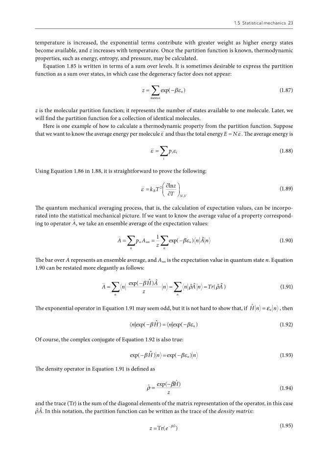
1.5 Statistical mechanics 23
temperature is increased, the exponential terms contribute with greater weight as higher energy states become available, and z increases with temperature. Once the partition function is known, thermodynamic properties, such as energy, entropy, and pressure, may be calculated.
Equation 1.85 is written in terms of a sum over levels. It is sometimes desirable to express the partition function as a sum over states, in which case the degeneracy factor does not appear:
zn
n= −∑ exp( )states
βε (1.87)
z is the molecular partition function; it represents the number of states available to one molecule. Later, we will find the partition function for a collection of identical molecules.
Here is one example of how to calculate a thermodynamic property from the partition function. Suppose that we want to know the average energy per molecule ε and thus the total energy E N= ε . The average energy is
ε ε=∑pi
i
i (1.88)
Using Equation 1.86 in 1.88, it is straightforward to prove the following:
ε =∂∂
k T
z
TB
N V
2 ln
,
(1.89)
The quantum mechanical averaging process, that is, the calculation of expectation values, can be incorpo-rated into the statistical mechanical picture. If we want to know the average value of a property correspond-ing to operator A, we take an ensemble average of the expectation values:
A p Az
n A nn nn
n
n
n
= = −∑ ∑1exp( )βε � (1.90)
The bar over A represents an ensemble average, and Ann is the expectation value in quantum state n. Equation 1.90 can be restated more elegantly as follows:
A nH A
zn n A n Tr A
n n
=−
= =∑ ∑exp( )( )
β ρ ρ� �
� � � � (1.91)
The exponential operator in Equation 1.91 may seem odd, but it is not hard to show that, if H n nn= ε , then
⟨ − = ⟨ −n nH n|exp( ) |exp( )β βε� (1.92)
Of course, the complex conjugate of Equation 1.92 is also true:
exp( ) exp( )− = −β βε�H n nn (1.93)
The density operator in Equation 1.91 is defined as
ˆ exp( ˆ )ρ β= − H
z (1.94)
and the trace (Tr) is the sum of the diagonal elements of the matrix representation of the operator, in this case � �ρA. In this notation, the partition function can be written as the trace of the density matrix:
z e H= −Tr( )β � (1.95)
24 Introduction and review
The value of using Equation 1.91 instead of 1.90 or Equation 1.95 instead of 1.87, is that there is a particularly important property of the trace: It is independent of representation. In the language of linear algebra, we say that the trace of a matrix is preserved by a unitary transformation. In the present context, a change of representation is a change of basis functions. Any convenient orthonormal set of wavefunctions that obey the appropriate boundary conditions can be used to calculate the trace.
Equation 1.94 gives the equilibrium density operator. In nonequilibrium situations, the Hamiltonian depends on time and so does the density operator. The time evolution of the density operator will be consid-ered briefly in Chapter 4 and in more detail in Chapter 13.
In order to apply the methods of this section, we need to be more specific about the form of the energy levels. A great deal of simplification results when the energy of a molecule can be expressed as the sum of translational, rotational, vibrational, and electronic contributions:
ε ε ε ε ε= + + +tr rot vib el (1.96)
When Equation 1.96 holds, the partition function z can be factored:
z z z z z= tr rot vib el (1.97)
The energy contributions on the right-hand side of Equation 1.96 are listed in order of increasing separa-tion of the quantum levels, ranging from the essentially continuous translational levels to the widely spaced electronic levels. The electronic partition function is usually very easy to calculate. Since excited electronic states are usually much higher than thermal energy kBT at ordinary temperatures, zel is equal to the ground state degeneracy. (The exceptions to this occur when molecules have low-lying excited electronic states.) The translational, rotational, and vibrational partition functions can be found using the models discussed in the previous section. For example, the particle in a box model is used to get the translational energies. These are so closely spaced that the sum over nx, ny, and nz can be replaced by an integral. The result is
zmk T
hVB
tr =
22
3 2π /
(1.98)
Note that the mass m is that of a single molecule. The molecular structure is immaterial since translation just involves motion of the center of mass.
We can use the rigid-rotor model to find zrot for a diatomic molecule. The rotational energy-level spacings for many diatomics (and polyatomics, not considered here) are often, but not always, small enough compared to thermal energy that the sum in zrot can be replaced by an integral. In this limit, we find
zIk T
hB
rot =8 2
2
πσ
(1.99)
The symmetry number σ is one for heteronuclear and two for homonuclear diatomics. As will be shown in Chapter 8, the latter have only even or odd J states, but not both, resulting in half as many energy levels as for heteronuclear molecules. Equation 1.99 is valid when h2/8π2IkB is much smaller than T, in other words, when the number of thermally available states is large. When this is not the case, then we have to roll up our sleeves and find the partition function by direct summation.
Using the harmonic oscillator model, the vibrational partition function of a diatomic molecule can also be found. The partition function for vibration is
ze
e
h
hvib =−
−
−
β ν
β ν
0
0
2
1
/
(1.100)
where ν0 is the vibrational frequency. Equation 1.100 is readily extended to polyatomic molecules, in which case the total vibrational partition function is a product of terms like 1.100, one for each normal mode frequency. Normal modes will be considered in Chapter 10.
1.5 Statistical mechanics 25
The partition functions discussed so far are for individual molecules, and we would like to know the partition function for a collection of molecules. If the intermolecular interactions can be neglected, then it is straightforward to find the partition function Z for N molecules from the molecular partition function z. The simplification results from the fact that the total energy E is the sum of the energies of the individual molecules. The total partition function derives from a sum over all possible N molecule states:
Z En
n= −( )∑ expstates
β (1.101)
where En is the total energy for a particular set of molecular quantum states. Using i, j, k, … to label the molecular quantum states and a, b, c, … to index the molecules, we have
En i a j b k c= + + +ε ε ε, , , � (1.102)
Inserting Equation 1.102 in 1.101 and separating the exponentials, Z is found to be
Zi
i a
j
j b
k
k c= −( ) −( ) −(∑ ∑ ∑exp exp exp, , ,
states states states
βε βε βε ))…
= −( )
=∑ exp (,
states
distinguishable partici
i a
N
Nzβε lles)
(1.103)
Equation 1.103 derives from the fact that the particles are all the same, so each sum over molecular states gives the same result. However, there is a limitation to this expression. It only applies to distinguish-able particles. For example, in a crystal we can distinguish particles by the positions in the lattice, and Equation 1.103 is applicable. But for the ideal gas on which we are focusing in this section, Equation 1.103 overestimates the number of states. The reason is that Equation 1.103 counts as distinct microstates those which differ only in the way that the particles are labeled. For example, if we have the microstate where the total energy is ε ε ε7 3 4, , ,a b c+ + +�, it is really the same state as, say, ε ε ε4 3 7, , ,a b c+ + +� if the particles a, b, c, … are indistinguishable. It might seem like keeping track of all possible permutations presents a horrible bookkeeping problem! Fortunately, there an aspect of the problem that makes it easy to correct for over-counting the states. The simplification results from the fact that the number of states greatly exceeds the number of molecules (thanks to the translational energy contribution), so it is highly unlikely that more than one molecule is assigned to the same quantum state. Once we settle on a particular combination of molecular energies, ε ε εi a j b k c, , ,+ + +�, there are N! ways to permute the molecule labels. So we know we have overcounted by N! and the partition function should be
Zz
N
N
=!
( )indistinguishable particles (1.104)
Another condition on the validity of Equation 1.104 is that there be no overlap of the wavefunctions on different molecules. If this condition is met, as we expect for the case of an ideal gas, then the molecules adhere to “Boltzmann statistics.” On the other hand, if the wavefunctions overlap, we must account for the indistinguishability of particles quantum mechanically by placing a restriction on the total wavefunction for the N particle system. If we write a total wavefunction for N particles, it is a function of the coordinates of all N particles: Ψ(1, 2, 3, …, N). Since the probability distribution in terms of the square of the wavefunction cannot depend on the particle labels, we have to be able to exchange any two coordinates and obtain the same probability, for example,
Ψ Ψ( , , , , ) ( , , , , )1 2 3 2 1 32 2… = …N N (1.105)
26 Introduction and review
This leaves two choices for the effect of swapping two coordinates on the wavefunction itself. It may either stay the same or change sign:
Ψ Ψ( , , , , ) ( , , , , )1 2 3 2 1 3… = ± …N N (1.106)
It turns out that there are two kinds of particles in nature. Bosons, which have integral spin quantum numbers, have wavefunctions that stay the same when any two particles are exchanged (the plus sign in Equation 1.106). They are said to adhere to Bose–Einstein (BE) statistics. Fermions, on the other hand, have half-integral spins and wavefunctions that change sign when the labels for two particles are switched. They follow Fermi–Dirac (FD) statistics. The consequences of this difference are dramatic. Bosons can share quantum states, but fermions cannot. Electrons are fermions, and the familiar Pauli exclusion principle is a result of FD statistics. Photons have spin 1 (as will be discussed in Chapter 2) and are bosons. There is no limit to the number of photons that can occupy a given quantum state.
The molecular partition function derived here does not apply to systems of particles having overlapping wavefunctions. There are, however, expressions for the occupation numbers of states that obey BE and FD statistics. In the limit of high temperature or large volume, the BE and FD occupation numbers go over to the same result as obtained using Boltzmann statistics. For our ideal gas, Boltzmann statistics are just fine. In many spectroscopy experiments, however, the symmetry requirements of Equation 1.106 on the molecular wavefunction lead to observable experimental features. We shall examine this in Chapter 8, where rotational spectra are considered.
1.6 SUMMARY
In this chapter, we have reviewed the quantum mechanical and statistical mechanical preliminaries on which much of this book is based. Four simple models provide the basis for approximating the translational, rota-tional, vibrational, and electronic energies of molecules. The corresponding particle-in-a-box, rigid-rotor, harmonic-oscillator, and hydrogen atom problems provide starting points (“zero-order” approximations) for more sophisticated quantum mechanical treatments of molecular energies. In addition, these models illustrate general quantum mechanical principles, such as degeneracy, symmetry, and the uncertainty principle. The stationary states and their energies will provide the basis for understanding spectroscopic transitions, using the time-dependent perturbation theory to be presented in Chapter 4. The rigid-rotor and harmonic-oscillator models will serve as a point of departure for the analysis of rotational and vibrational spectra. The hydrogenic wavefunctions provide a basis for approximating the electronic wavefunctions of many electron atoms and molecules, and give us the familiar chemical concept of orbitals. The techniques of variation theory and per-turbation theory are tools for interpreting molecular properties that are revealed in a myriad of spectroscopy experiments.
The solutions to the Schrödinger equation provide a spectrum of energies that serves as input to the cal-culation of ensemble average properties, following the prescriptions of statistical mechanics. This averaging procedure is fundamental to the understanding of the spectra of collections of molecules. We have intro-duced the concept of the density matrix as a component of the ensemble average calculation. In Chapters 4 and 13, this density matrix will be generalized to allow for time dependence, as we will be concerned with the time evolution of the system undergoing a spectroscopic transition.
PROBLEMS 1. Find the difference between the ground- and first excited-state translational energies of a helium atom
in a 1 mm3 cubic box. Compare this to room temperature energy kBT at 300 K. 2. Find all the possible angles with respect to the z-axis for an angular momentum vector of magnitude
6�.
References 27
3. Show that the uncertainty as defined in Equation 1.15 vanishes when ψ is an eigenfunction of the opera-tor A.
4. The classical harmonic oscillator obeys the equation of motion: F = −kx = md2x/dt2. Use this equation to verify Equation 1.29.
5. Can a harmonic oscillator ever be dissociated? 6. The vibrational frequency of 1H35Cl is ν0 = 8.97 × 10¹³ s−1. Find the force constant for the H–Cl bond. 7. Derive Equation 1.89. 8. Show that if |n⟩ is an eigenfunction of the operator A with eigenvalue an, then e n e nA an
ˆ= . (Hint:
Expand the exponential in a series: e x kx kk
= =∞∑ 0
/ !.) 9. Calculate the fraction of molecules in each of the first ten rotational levels of CO at 300 K, assuming
that it is a rigid rotor with a bond length of 1.13 Å. 10. Calculate the translational partition function for a mole of N2 at 1 atm and 300 K. Verify that the effec-
tive number of available states greatly exceeds the number of molecules. 11. Use the partition functions in Equations 1.98, 1.99, and 1.100 to find the translational, rotational, and
vibrational contributions to the average energy of a diatomic molecule. Compare each result to the prediction of the equipartition theorem, which states that in the classical limit each degree of freedom contributes 1 2( )k TB to the average energy.
12. Hydrides typically have rotational energies that are too widely spaced to be able to use Equation 1.99 at room temperature. Find zrot for HF at 300 K by summing the energies directly. Try to obtain a value that is accurate to three significant figures. Compare the numerical result to the value obtained using Equation 1.99. (Use 0.92 Å for the bond length.)
REFERENCES 1. E. Hecht, and A. Zajac, Optics (Addison-Wesley, Reading, MA, 1974). 2. K. Nassau, The Physics and Chemistry of Color (Wiley, New York, 1983). 3. I. N. Levine, Quantum Chemistry, 5th ed. (Prentice Hall, Upper Saddle River, NJ, 1999). 4. C. Dykstra, Quantum Chemistry and Molecular Spectroscopy (Prentice Hall, Englewood Cliffs, 1992). 5. D. A. McQuarrie, Statistical Mechanics (Harper and Row, New York, 1976). 6. P. W. Atkins, Physical Chemistry, 6th ed. (W. H. Freeman, New York, 1998).
References
1 1. Introduction and review
1. E. Hecht, and A. Zajac, Optics (Addison-Wesley, Reading,MA, 1974).
2. K. Nassau, The Physics and Chemistry of Color (Wiley,New York, 1983).
3. I. N. Levine, Quantum Chemistry, 5th ed. (Prentice Hall,Upper Saddle River, NJ, 1999).
4. C. Dykstra, Quantum Chemistry and Molecular Spectroscopy(Prentice Hall, Englewood Cliffs, 1992).
5. D. A. McQuarrie, Statistical Mechanics (Harper and Row,New York, 1976).
6. P. W. Atkins, Physical Chemistry, 6th ed. (W. H.Freeman, New York, 1998).
2 2. The nature of electromagneticradiation
1. W. Heitler, Quantum Theory of Radiation, 3rd ed. (OxfordUniversity Press, London, 1954).
2. E. Hecht, and A. Zajac, Optics (Addison-Wesley, Reading,MA, 1974).
3. W. S. Struve, Fundamentals of Molecular Spectroscopy(Wiley, New York, 1989).
4. Boyd, R. W. Nonlinear Optics, 3rd ed. (Academic Press,Amsterdam, 2008).
5. Yariv, A. Quantum Electronics, 2nd ed. (John Wiley &Sons, New York, 1975).
6. G. C. Schatz, and M. A. Ratner, Quantum Mechanics inChemistry (Prentice Hall, Englewood Cliffs, NJ, 1993).
7. R. P. Feynman, R. B. Leighton, and M. Sands, The FeynmanLectures on Physics, Vol. III (AddisonWesley, Reading, MA,1965).
8. J. D. Jackson, Classical Electrodynamics (Wiley, NewYork, 1962).
9. A. Yariv, Quantum Optics (Wiley, New York, 1967).
10. R. P. Feynman, R. B. Leighton, and M. Sands, TheFeynman Lecture in Physics, Vol. II, Ch. 21 (AddisonWesley,Reading MA, 1964).
3 3. Electric and magnetic properties ofmolecules and bulk matter
1. J. D. Jackson, Classical Electrodynamics (Wiley, NewYork, 1962).
2. H. Fröhlich, Theory of Dielectrics, 2nd ed. (OxfordUniversity Press, Oxford, 1958).
3. A. Hinchliffe and R. W. Munn, Molecular Electromagnetism(Wiley, New York, 1985).
4. J. G. Kirkwood, The dielectric polarization of polarliquids, J. Chem. Phys. 7, 911 (1939).
5. L. Onsager, Electric moments of molecules in liquids, J.Am. Chem. Soc. 58, 1486 (1936).
6. P. W. Atkins, Molecular Quantum Mechanics, 2nd ed.(Oxford University Press, New York, 1983).
7. J. D. Macomber, The Dynamics of SpectroscopicTransitions (Wiley, New York, 1976).
4 4. Time-dependent perturbation theoryof spectroscopy
1. J. D. Macomber, The Dynamics of SpectroscopicTransitions (John-Wiley and Sons, New York, 1976).
2. C. H. Wang, Spectroscopy of Condensed Media (AcademicPress, Orlando, FL, 1985).
3. G. C. Schatz and M. A. Ratner, Quantum Mechanics inChemistry (Prentice-Hall, Englewood Cliffs, NJ, 1993).
4. W. G. Rothschild, Dynamics of Molecular Liquids (Wiley,New York, 1984).
5 5. The time-dependent approach tospectroscopy
1. R. G. Gordon, Correlation functions for molecularmotion, Adv. Mag. Res. 3, 1 (1968).
2. B. J. Berne and G. D. Harp, On the calculation of timecorrelation functions, Adv. Chem. Phys. 17, 109 (1970).
3. B. J. Berne and R. Pecora, Dynamic Light Scattering(Wiley-Interscience, New York, 1976).
4. H. Fröhlich, Theory of Dielectrics, 2nd ed. (OxfordUniversity Press, New York, 1986).
5. P. A. Madden and D. Kivelson, A consistent moleculartreatment of dielectric phenomena, Adv. Chem. Phys. 56,467 (1984).
6. W. G. Rothschild, Dynamics of Molecular Liquids (Wiley,New York 1984).
7. D. Steele and J. Yarwood, eds., Spectroscopy andRelaxation of Molecular Liquids, (Elsevier SciencePublishers, Amsterdam, 1991).
8. H. D. Dardy, V. Volterra, and T. A. Litovitz, Rayleighscattering: Orientational motion in highly anisotropicliquids, J. Chem. Phys. 59, 4491 (1973).
9. R. Rodriguez and J. L. McHale, First moment of theliquid phase far-infrared absorption cross-section and theR(ω) representation of depolarized Rayleigh scattering, J.Chem. Phys. 88, 2264 (1988).
10. D. A. McQuarrie, Statistical Mechanics (Harper & Row,New York, 1976).
11. R. G. Gordon, Molecular motion in infrared and Ramanspectra, J. Chem. Phys. 43, 1307 (1965).
12. G. R. Fleming and M. Cho, Chromophore-solvent dynamics,Ann. Rev. Phys. Chem. 47, 109 (1996).
13. R. M. Stratt and M. Maroncelli, Nonreactive dynamics insolution: The emerging view of solvation dynamics andvibrational relaxation, J. Phys. Chem. 100, 12981 (1996).
14. M. C. Beard, G.M. Turner, and C. A. Schmuttenmaer,Terahertz spectroscopy, J. Phys. Chem. B 106, 7146 (2002).

15. J. T. Kindt and C. A. Schmuttenmaer, Far-infrareddielectric properties of polar liquids probed byfemtosecond THz pulse spectroscopy, J. Phys. Chem. 100,10373 (1996).
16. D. S. Venables, A. Chiu, and C. A. Schmuttenmaer,Structure and dynamics of nonaqueous mixtures of dipolarliquids: I. Infrared and far-IR spectroscopy, J. Chem.Phys. 113, 3243 (2000).

6 6. Experimental considerations:Absorption, emission, and scattering
1. S. J. Strickler and R. A. Berg, Relationship betweenabsorption intensity and fluorescence lifetimes ofmolecules, J. Chem. Phys. 37, 818 (1962).
2. O. Sonnich-Mortensen and S. Hassing, Advances inInfrared and Raman Spectroscopy 6, Ch. 1 (Heyden, NewYork, 1980).
3. R. Kubo, M. Toda, and N. Hashitsume, Statistical PhysicsII, (Springer-Verlag, New York, 1978).
7 7. Atomic spectroscopy
1. A. R. Edmonds, Angular Momentum in Quantum Mechanics(Princeton University Press, Princeton, NJ, 1974).
2. C. E. Dykstra, Quantum Mechanics and MolecularSpectroscopy (Prentice Hall, Englewood Cliffs, NJ, 1992).
3. I. N. Levine, Quantum Chemistry, 5th ed., (PrenticeHall, Upper Saddle River, NJ, 1999).
4. J. I. Steinfeld, Molecules and Radiation (MIT Press,Cambridge, MA, 1985).
5. R. N. Zare, Angular Momentum, Understanding SpatialAspects in Chemistry and Physics (Wiley, New York, 1988).
6. W. S. Struve, Fundamentals of Molecular Spectroscopy(Wiley, New York, 1989).
7. A. Yariv, Introduction to Optical Electronics (Holt,Rinehart and Winston, New York, 1976).
8. E. U. Condon, and G. H. Shortly, Atomic Spectroscopy(Macmillan Company, New York, 1935).
9. G. Herzberg, Atomic Spectra and Atomic Structure (DoverPublications, New York, 1944).
8 8. Rotational spectroscopy
1. A. R. Edmonds, Angular Momentum in Quantum Mechanics(Princeton University Press, Princeton, NJ, 1974).
2. D. G. Taylor III, and H. L. Strauss, The rotationalRaman spectrum of H 2 in Water J. Chem. Phys. 90, 768(1989).
3. G. Herzberg, Molecular Spectra and Molecular Structure,Vol. I, Spectra of Diatomic Molecules (Van NostrandRienhold, New York 1950).
4. C. H. Townes, and A. L. Schalow, Microwave Spectroscopy(McGraw-Hill, New York, 1955).
5. G. W. Chantry ed., Modern Aspects of MicrowaveSpectroscopy, (Academic Press, New York, 1979).
6. B. J. Berne, and R. Pecora, Dynamic Light Scattering(Wiley, New York, 1976).
7. C. E. Dykstra, Quantum Chemistry and MolecularSpectroscopy (Prentice Hall, Englewood Cliffs, NJ, 1992).
8. I. N. Levine, Molecular Spectroscopy(Wiley-Interscience, New York, 1975).
9 9. Vibrational spectroscopy of diatomics
1. C. E. Dykstra, Quantum Chemistry and MolecularSpectroscopy (Prentice Hall, Englewood Cliffs, New Jersey,1992).
2. I. N. Levine, Molecular Spectroscopy (Wiley, New York,1975).
3. W. S. Struve, Fundamentals of Molecular Spectroscopy(Wiley, New York, 1989).
4. E. T. Branigan, M. N. van Staveren, V. A. Apkarian,Solidlike coherent vibronic dynamics in a room temperatureliquid: Resonance Raman and absorption spectroscopy ofliquid bromine, J. Chem. Phys. 132, 144503 (2010).
5. P. F. Fougere, and R. K. Nesbet, Electronic structure ofC 2 J. Chem. Phys. 44, 285 (1966).
6. P. L. Hanst, and S. T. Hanst, Infrared Spectra forQuantitative Analysis of Gases (Infrared Analysis, Inc., Anaheim, CA, 1992).
10 10. Vibrational spectroscopy ofpolyatomic molecules
1. E. B. Wilson, J. C. Decius, and P. C. Cross, MolecularVibrations (Dover Publications, New York, 1955).
2. F. A. Cotton, Chemical Applications of Group Theory(Wiley-Interscience, New York, 1971).
3. G. Herzberg, Molecular Structure and Molecular SpectraII. Infrared and Raman Spectra of Polyatomic Molecules(Van Nostrand Reinhold, New York, 1945).
4. P. F. Bernath, Spectra of Atoms and Molecules (OxfordUniversity Press, New York, 1995).
5. I. N. Levine, Molecular Spectroscopy(Wiley-Interscience, New York, 1975).
6. B. T. Darling and D. M. Dennison, The water vapormolecule, Phys. Rev. 57, 128 (1940).
7. K. S. Schweizer and D. Chandler, Vibrational dephasingand frequency shifts of polyatomic molecules in solution,J. Chem. Phys. 76, 2296 (1982).
8. J. L. McHale, The influence of angular dependentintermolecular forces on vibrational spectra of solutionphase molecules, J. Chem. Phys. 75, 30 (1981).
9. H. Torii and M. Tasumi, Local order and transitiondipole coupling in liquid methanol and acetone as theorigin of the Raman noncoincidence effect, J. Chem. Phys.99, 8459 (1993).
10. J. E. Bertie, L. Z. Zhang, and C. D. Keefe, Measurementand use of absolute absorption intensities of neatliquids, Vib. Spec. 8, 215 (1995).
11. J. E. Bertie and L. Z. Zhang, Infrared transitions ofliquids. XV. Infrared refractive indices from 8000–350 cm−1 , Absolute integrated intensities, transition moments,and dipole moment derivatives of methanol-d at 25°, Appl.Spec. 48, 176 (1994).
12. J. E. Bertie, L. Z. Zhang, and C. D. Keefe, Infraredintensities of liquids. XVI. Accurate determination ofmolecular band intensities from infrared refractive indexand dielectric constant spectra, J. Mol. Struct. 324, 157(1994).

13. J. E. Bertie and S. L. Zhang, Infrared intensities ofliquids. XVII. Infrared refractive indices from 8000–350cm −1 , absolute intensities, transition moments and dipolemoment derivatives of methan-d 3 -ol and methanol-d 4 at25°, J. Chem. Phys. 101, 8364 (1994).
14. S. A. Steiger, C. Li, C. Campana, and N. R. Natale,Lanthanide and asymmetric catalyzed syntheses ofsterically hindered 4-isoxazolyl-1,4-dihydropyridines and4-isoxazolyl-quinolines, Tet. Lett. 57, 423 (2016).
11 11. Electronic spectroscopy
1. I. N. Levine, Quantum Chemistry, 5th ed. (Prentice Hall,Upper Saddle River, NJ, 1999).
2. C. Dykstra, Quantum Chemistry and Molecular Spectroscopy(Prentice Hall, Englewood Cliffs, NJ, 1991).
3. C. Manneback, Computation of the intensities ofvibrational spectra of electronic bands of diatomicmolecules, Phy sica 17, 1001 (1951) and Physica 20, 497(1954).
4. E. J. Heller, R. L. Sundberg, and D. Tannor, Simpleaspects of Raman scattering, J. Phys. Chem. 86, 1822,(1982).
5. G. Herzberg, Electronic Spectra of Polyatomic Molecules(Van Nostrand Reinhold, New York, 1966).
6. H. Köppel, W. Domcke, and L. S. Cederbaum, Multimodemolecular dynamics beyond the BornOppenheimerapproximation, Adv. Chem. Phys. 57, 59 (1984).
7. L. Salem, Molecular Orbital Theory of Conjugated Systems(W. A. Benjamin, Reading, MA, 1972).
8. A. Streitweiser, Molecular Orbital Theory for OrganicChemists (Wiley, New York, 1961).
9. J. E. Huheey, Inorganic Chemistry (Harper & Row, NewYork, 1972).
10. F. A. Cotton, Chemical Applications of Group Theory(Wiley-Interscience, New York 1971).
11. S. L. Schultz, J. Qian, and J. M. Jean, Separability ofintra- and intermolecular vibrational relaxation processesin trans-stilbene, J. Phys. Chem. A 101, 100 0, (1997).
12. M. L. Horng, J. A. Gardecki, A. Papazyan, and M.Maroncelli, Subpicosecond measurements of polar solvationdynamics: Coumarin 153, J. Phys. Chem 99, 1721 1, (1995).
13. M. Bixon and J. Jortner, Intramolecular radiationlesstransitions, J. Chem. Phys. 48, 715 (1968).
14. K. Nassau, The Physics and Chemistry of Color (Wiley,New York, 1983).
15. C. Reichardt, Solvatochromic dyes as solvent polarityprobes, Chem. Rev. 94, 2319 (1994).
16. N. S. Bayliss and E. G. McRae, Solvent effects inorganic spectra: Dipole forces and the Franck-Condonprinciple, J. Phys. Chem. 58, 100 2 (1954).
17. J. E. Brady and P. W. Carr, An analysis of dielectricmodels of solvatochromism, J. Phys. Chem. 89, 5759 (1985).
18. A. T. Amos and B. L. Burrows, Solvent-shift effects onelectronic spectra and excited state dipole moments, Adv.Quantum Chem. 7, 289 ( 1973).
19. P. Suppan, Solvatochromic shifts: The influence of themedium on the energy of electronic states, J. Photochem.Photobiol. A 50, 293 ( 1990).
20. J. Zeng, J. S. Craw, N. S. Hush, and J. R. Reimers,Solvent effects on molecular spectra. I. normal pressureand temperature Monte Carlo simulations of the structure ofdilute pyrimidine in water, J. Chem. Phys. 99, 1483(1993).
21. N. S. Hush, and J. R. Reimers, Solvent effects on theelectronic spectra of transition metal complexes, Chem.Rev. 100, 775 ( 2000).
22. M. Karelson, T. Tamm, and M. C. Zerner, Multicavityreaction field method for the solvent effect descriptionin flexible molecular systems, J. Phys. Chem 97, 119 01(1993).
23. N. Rösch and M. C. Zerner, Calibration of dispersionenergy shifts in molecular electronic spectra, J. Phys.Chem. 98, 58 17 (1994).
24. J. Motta de Neto, R. B. Alencastro, and M. C. Zerner,Solvent effects on the electronic spectrum of Reichardt’sdye, Int. J. Quantum. Chem. Symp 28, 36 1 (1994).
25. M. Cossi, V. Barone, Time-dependent density functionaltheory for molecules in liquid solutions, J. Chem. Phys.115, 4708 (2001).
26. A. DeFusco, N. Minezawa, L. V. Slipchenko, F. Zahariev,M. S. Gordon, Modeling solvent effects on electronicexcited states, J. Phys. Chem. Lett. 2, 21 84 (2011).
27. M. D. Stephens, J. G. Saven, and J. L. Skinner,

Molecular theory of electronic spectroscopy in nonpolarfluids: Ultrafast solvation dynamics and absorption andemission line shapes, J. Chem. Phys 106, 2129 (1997).
12 12. Raman and resonance Ramanspectroscopy
1. A. C. Albrecht, On the theory of Raman intensities, J.Chem. Phys. 34, 1476 (1961).
2. L. A. Nafie and W. Peticolas, Reorientation andvibrational relaxation as line broadening factors invibrational spectroscopy, J. Chem. Phys. 57, 3145 (1972).
3. O. Sonnich Mortensen and S. Hassing, Polarization andinterference phenomena in resonance Raman scattering,Advances in Infrared and Raman Spectroscopy, 6, Chapter 1(Wiley, New York, 1980).
4. H. Hamaguchi, The resonance Raman effect anddepolarization in vibrational Raman scattering, Advancesin Infrared and Raman Spectroscopy, 12, Chapter 6 (Wiley,New York, 1985).
5. T. G. Spiro and T. C. Strekas, Resonance Raman spectraof hemoglobin and cytochrome c: Inverse polarization andvibronic scattering, Proc. Nat. Acad. Sci. USA 69, 2622(1972).
6. F. Paulat, V. K. K. Praneeth, C. Näther, and N. Lehnert,Quantum chemistry-based analysis of the vibrationalspectra of five-coordinate metalloporphyrins [M(TPP)Cl],Inorg. Chem. 45, 2837 (2006).
7. R. Lynden-Bell, Vibrational relaxation and line widthsin liquids: Dephasing by intermolecular forces, Mol. Phys.33, 907 (1977).
8. A. M. Amorim da Costa, M. A. Norman, and J. H. R. Clark,Reorientational motion in liquids: A comparison of Ramanand Rayleigh scattering, Mol. Phys. 29, 191 (1975).
9. D. W. Oxtoby, Vibrational relaxation in liquids, Ann.Rev. Phys. Chem. 32, 77 (1981).
10. D. W. Oxtoby, Dephasing of molecular vibrations inliquids, Adv. Chem. Phys. 41, 1 (1978).
11. A. Laubereau and W. Kaiser, Vibrational dynamics ofliquids and solids investigated by picosecond lightpulses, Rev. Mod. Phys. 50, 607 (1978).
12. C. H. Wang, Spectroscopy of Condensed Media (AcademicPress, Orlando, FL, 1985).
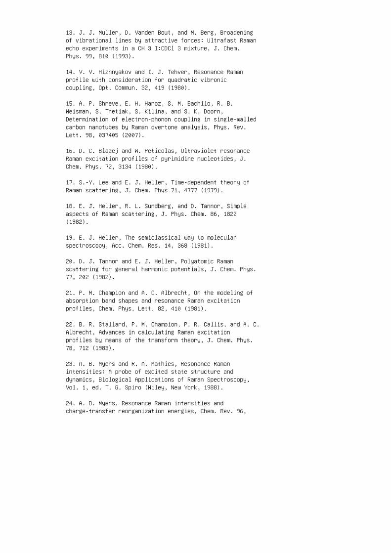
13. J. J. Muller, D. Vanden Bout, and M. Berg, Broadeningof vibrational lines by attractive forces: Ultrafast Ramanecho experiments in a CH 3 I:CDCl 3 mixture, J. Chem.Phys. 99, 810 (1993).
14. V. V. Hizhnyakov and I. J. Tehver, Resonance Ramanprofile with consideration for quadratic vibroniccoupling, Opt. Commun. 32, 419 (1980).
15. A. P. Shreve, E. H. Haroz, S. M. Bachilo, R. B.Weisman, S. Tretiak, S. Kilina, and S. K. Doorn,Determination of electron-phonon coupling in single-walledcarbon nanotubes by Raman overtone analysis, Phys. Rev.Lett. 98, 037405 (2007).
16. D. C. Blazej and W. Peticolas, Ultraviolet resonanceRaman excitation profiles of pyrimidine nucleotides, J.Chem. Phys. 72, 3134 (1980).
17. S.-Y. Lee and E. J. Heller, Time-dependent theory ofRaman scattering, J. Chem. Phys 71, 4777 (1979).
18. E. J. Heller, R. L. Sundberg, and D. Tannor, Simpleaspects of Raman scattering, J. Phys. Chem. 86, 1822(1982).
19. E. J. Heller, The semiclassical way to molecularspectroscopy, Acc. Chem. Res. 14, 368 (1981).
20. D. J. Tannor and E. J. Heller, Polyatomic Ramanscattering for general harmonic potentials, J. Chem. Phys.77, 202 (1982).
21. P. M. Champion and A. C. Albrecht, On the modeling ofabsorption band shapes and resonance Raman excitationprofiles, Chem. Phys. Lett. 82, 410 (1981).
22. B. R. Stallard, P. M. Champion, P. R. Callis, and A. C.Albrecht, Advances in calculating Raman excitationprofiles by means of the transform theory, J. Chem. Phys.78, 712 (1983).
23. A. B. Myers and R. A. Mathies, Resonance Ramanintensities: A probe of excited state structure anddynamics, Biological Applications of Raman Spectroscopy,Vol. 1, ed. T. G. Spiro (Wiley, New York, 1988).
24. A. B. Myers, Resonance Raman intensities andcharge-transfer reorganization energies, Chem. Rev. 96,
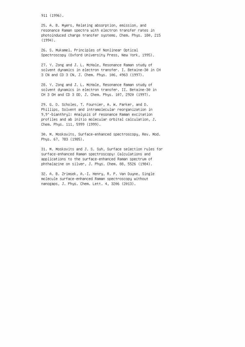
911 (1996).
25. A. B. Myers, Relating absorption, emission, andresonance Raman spectra with electron transfer rates inphotoinduced charge transfer systems, Chem. Phys. 180, 215(1994).
26. S. Mukamel, Principles of Nonlinear OpticalSpectroscopy (Oxford University Press, New York, 1995).
27. Y. Zong and J. L. McHale, Resonance Raman study ofsolvent dynamics in electron transfer. I. Betaine-30 in CH3 CN and CD 3 CN, J. Chem. Phys. 106, 4963 (1997).
28. Y. Zong and J. L. McHale, Resonance Raman study ofsolvent dynamics in electron transfer. II. Betaine-30 inCH 3 OH and CD 3 OD, J. Chem. Phys. 107, 2920 (1997).
29. G. D. Scholes, T. Fournier, A. W. Parker, and D.Phillips, Solvent and intramolecular reorganization in9,9′-bianthryl: Analysis of resonance Raman excitationprofiles and ab initio molecular orbital calculation, J.Chem. Phys. 111, 5999 (1999).
30. M. Moskovits, Surface-enhanced spectroscopy, Rev. Mod.Phys. 67, 783 (1985).
31. M. Moskovits and J. S. Suh, Surface selection rules forsurface-enhanced Raman spectroscopy: Calculations andapplications to the surface-enhanced Raman spectrum ofphthalazine on silver, J. Phys. Chem. 88, 5526 (1984).
32. A. B. Zrimsek, A.-I. Henry, R. P. Van Duyne, Singlemolecule surface-enhanced Raman spectroscopy withoutnanogaps, J. Phys. Chem. Lett. 4, 3206 (2013).
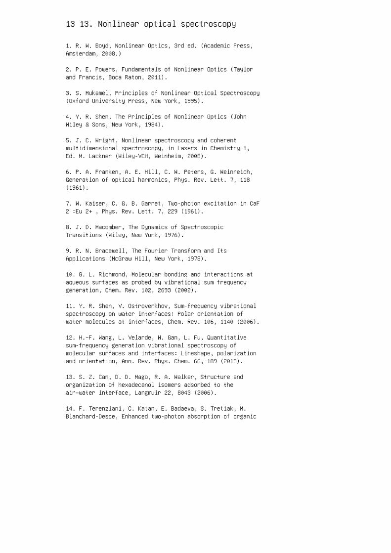
13 13. Nonlinear optical spectroscopy
1. R. W. Boyd, Nonlinear Optics, 3rd ed. (Academic Press,Amsterdam, 2008.)
2. P. E. Powers, Fundamentals of Nonlinear Optics (Taylorand Francis, Boca Raton, 2011).
3. S. Mukamel, Principles of Nonlinear Optical Spectroscopy(Oxford University Press, New York, 1995).
4. Y. R. Shen, The Principles of Nonlinear Optics (JohnWiley & Sons, New York, 1984).
5. J. C. Wright, Nonlinear spectroscopy and coherentmultidimensional spectroscopy, in Lasers in Chemistry 1,Ed. M. Lackner (Wiley-VCH, Weinheim, 2008).
6. P. A. Franken, A. E. Hill, C. W. Peters, G. Weinreich,Generation of optical harmonics, Phys. Rev. Lett. 7, 118(1961).
7. W. Kaiser, C. G. B. Garret, Two-photon excitation in CaF2 :Eu 2+ , Phys. Rev. Lett. 7, 229 (1961).
8. J. D. Macomber, The Dynamics of SpectroscopicTransitions (Wiley, New York, 1976).
9. R. N. Bracewell, The Fourier Transform and ItsApplications (McGraw Hill, New York, 1978).
10. G. L. Richmond, Molecular bonding and interactions ataqueous surfaces as probed by vibrational sum frequencygeneration, Chem. Rev. 102, 2693 (2002).
11. Y. R. Shen, V. Ostroverkhov, Sum-frequency vibrationalspectroscopy on water interfaces: Polar orientation ofwater molecules at interfaces, Chem. Rev. 106, 1140 (2006).
12. H.–F. Wang, L. Velarde, W. Gan, L. Fu, Quantitativesum-frequency generation vibrational spectroscopy ofmolecular surfaces and interfaces: Lineshape, polarizationand orientation, Ann. Rev. Phys. Chem. 66, 189 (2015).
13. S. Z. Can, D. D. Mago, R. A. Walker, Structure andorganization of hexadecanol isomers adsorbed to theair–water interface, Langmuir 22, 8043 (2006).
14. F. Terenziani, C. Katan, E. Badaeva, S. Tretiak, M.Blanchard-Desce, Enhanced two-photon absorption of organic
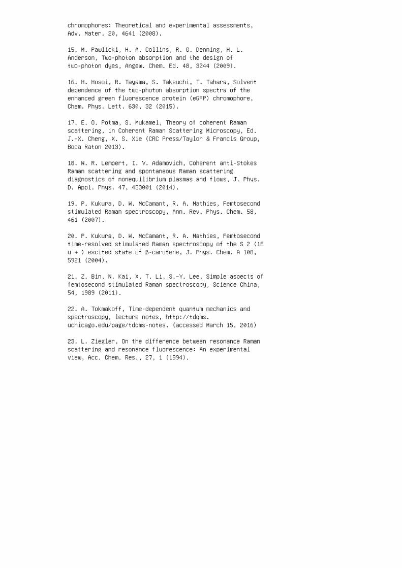
chromophores: Theoretical and experimental assessments,Adv. Mater. 20, 4641 (2008).
15. M. Pawlicki, H. A. Collins, R. G. Denning, H. L.Anderson, Two-photon absorption and the design oftwo-photon dyes, Angew. Chem. Ed. 48, 3244 (2009).
16. H. Hosoi, R. Tayama, S. Takeuchi, T. Tahara, Solventdependence of the two-photon absorption spectra of theenhanced green fluorescence protein (eGFP) chromophore,Chem. Phys. Lett. 630, 32 (2015).
17. E. O. Potma, S. Mukamel, Theory of coherent Ramanscattering, in Coherent Raman Scattering Microscopy, Ed.J.–X. Cheng, X. S. Xie (CRC Press/Taylor & Francis Group,Boca Raton 2013).
18. W. R. Lempert, I. V. Adamovich, Coherent anti-StokesRaman scattering and spontaneous Raman scatteringdiagnostics of nonequilibrium plasmas and flows, J. Phys.D. Appl. Phys. 47, 433001 (2014).
19. P. Kukura, D. W. McCamant, R. A. Mathies, Femtosecondstimulated Raman spectroscopy, Ann. Rev. Phys. Chem. 58,461 (2007).
20. P. Kukura, D. W. McCamant, R. A. Mathies, Femtosecondtime-resolved stimulated Raman spectroscopy of the S 2 (1Bu + ) excited state of β-carotene, J. Phys. Chem. A 108,5921 (2004).
21. Z. Bin, N. Kai, X. T. Li, S.–Y. Lee, Simple aspects offemtosecond stimulated Raman spectroscopy, Science China,54, 1989 (2011).
22. A. Tokmakoff, Time-dependent quantum mechanics andspectroscopy, lecture notes, http://tdqms.uchicago.edu/page/tdqms-notes. (accessed March 15, 2016)
23. L. Ziegler, On the difference between resonance Ramanscattering and resonance fluorescence: An experimentalview, Acc. Chem. Res., 27, 1 (1994).
14 14. Time-resolved spectroscopy
1. R. G. Bennett, Instrument to measure fluorescencelifetimes in the micromillisecond region, Rev. Scient.Instrument. 31, 1275 (1960).
2. S. J. Strickler, and R. A. Berg, Relationship betweenabsorption intensity and fluorescence lifetimes ofmolecules, J. Chem. Phys. 37, 818 (1962).
3. J. R. Lakowicz, Principles of fluorescence spectroscopy,3 rd ed. (Springer, New York, 2006).
4. J. A. Levitt, M. K. Kuimova, G. Yahioglu, P.-H. Chung,K. Suhling, and D. Phillips, Membrane-bound molecularrotors measure viscosity in live cells via fluorescencelifetime imaging, J. Phys. Chem. C 113, 11634 (2009).
5. M. L. Horng, J. A. Gardecki, A. Papazyan, and M.Maroncelli, Sub-picosecond measurements of polar solvationdynamics: Coumarin 153 revisited, J. Phys. Chem. 99, 17311(1995).
6. X.-X. Zhang, M. Liang, N. P. Ernsting, and M.Maroncelli, Complete solvation response of coumarin 153 inionic liquids, J. Phys. Chem. B 117, 4291 (2013).
7. M. Park, C. H. Kim, and T. Joo, Multifaceted ultrafastintramolecular charge transfer dynamics of4-(dimethylamino)benzonitrile (DMABN). J. Phys. Chem. A117, 370 (2013).
8. W. W. Parson, Modern Optical Spectroscopy (Springer, NewYork, 2007).
9. A. Tokmakoff, Time-Dependent Quantum Mechanics andSpectroscopy (University of Chicago),
10. G. Porter, Flash photolysis and some of itsapplications, Science 160, 1299 (1968).
11. T. A. Heimer, E. J. Heilweil, C. A. Bignozzi, and G. J.Meyer, Electron injection, recombination, and halideoxidation dynamics at dye-sensitized metal oxideinterfaces, J. Phys. Chem. A 104, 4256 (2000).
12. J. C. Dean, S. Rafiq, D. G. Oblinksky, E. Casette, C.C. Jumper, and G. D. Scholes, Broadband transientabsorption and two-dimensional electronic spectroscopy ofmethylene blue, J. Phys. Chem. A 119, 9098 (2015).
13. W. T. Pollard, S. L. Dexheimer, Q. Wang, L. A. Peteanu,C. V. Shank, and R. A. Mathies, Theory of dynamicabsorption spectroscopy of nonstationary states. 4.Application to 12-fs resonant impulsive Ramanspectroscopy, J. Phys. Chem. 96, 6147 (1992).
14. S. L. Dexheimer, Q. Wang, L. A. Peteanu, W. T. Pollard,R. A. Mathies, and C. V. Shank, Femtosecond impulsiveexcitation of nonstationary vibrational states inbacteriorhodopsin, Chem. Phys. Lett. 188, 61 (1992).
15. W. T. Pollard, C. H. B. Cruz, C. V. Shank, and R. A.Mathies, Direct observation of the excited statecis-trans photoisomerization of bacteriorhodopsin:Multilevel line shape theory for femtosecond hole burningand its application, J. Chem. Phys. 90, 199 (1989).
16. R. Costard, N. E. Levinger, E. T. J. Nibbering, and T.Elsaesser, Ultrafast vibrational dynamics of waterconfined in phospholipid reverse micelles, J. Phys. Chem. B116, 5752 (2012).
17. M. Rini, A.-K. Holm, E. T. J. Nibbering, and H. Fidder,Ultrafast UV-mid-IR investigation of the ring openingreaction of a photochromic spiropyran, J. Amer. Chem. Soc.125, 3028 (2003).
18. C. Wang and M. J. Tauber, High yield singlet fission ina zeaxanthin aggregate observed by picosecond resonanceRaman spectroscopy, J. Amer. Chem. Soc. 132, 13988 (2010).
19. K. Duppen and D. A. Wiersma, Picosecond multiple-pulseexperiments involving spatial and frequency gratings: Aunifying approach. J. Opt. Soc. Am. B 3, 614 (1986).
20. A. M. Weiner, S. De Silvestri, and E. P. Ippen,Three-pulse scattering for femtosecond dephasing studies:Theory and experiment. J. Opt. Soc. Am. B 2, 654 (1984).
21. E. Vauthey, C. Hogemann, and X. Allonas, Directinvestigation of the dynamics of charge recombinationfollowing the fluorescence quenching of9,10-dicyanoanthracene by various electron donors inacetonitrile, J. Phys. Chem. A 102, 7362 (1998).
22. M. R. Salvador, M. A. Hines, and G. D. Scholes,Exciton-bath coupling and inhomogeneous broadening in theoptical spectroscopy of semiconductor quantum dots, J.Chem. Phys. 118, 9380 (2003).
23. G. R. Fleming and M. Cho, Chromophore-solvent dynamics,Ann. Rev. Phys. Chem. 47, 109 (1996).
24. J. D. Hybl, A. W. Albrecht, S. M. Gallagher Faeder, andD. M. Jonas, Two-dimensional electronic spectroscopy,Chem. Phys. Lett. 297, 307 (1998).
25. M. Cho, Two-dimensional optical spectroscopy, Taylor &Francis group, Boca Raton, 2009.
26. P. Hamm, M. Lim, and R. M. Hochstrasser, Structure ofamide I band of peptides measured by femtosecondnonlinear-infrared spectroscopy, J. Phys. Chem. B 102, 6123(1998).
27. M. Khalil, N. Demirdoven, and A. Tokmakoff, Coherent 2DIR spectroscopy: Molecular structure and dynamics insolution, J. Phys. Chem. A 107, 5258 (2003).
28. N. S. Ginsberg, Y.-C. Cheng, and G. R. Fleming,Two-dimensional electronic spectroscopy of molecularaggregates, Acc. Chem. Res. 42, 1352 (2009).
29. E. Romero, R. Augulis, V. I. Novoderezhkin, M.Ferretti, J. Thieme, D. Zigmantas, and R. van Grondelle,Quantum coherence in photosynthesis for efficientsolar-energy conversion, Nature Physics 10, 676 (2014).
30. S. Garret-Roe and P. Hamm, What can we learn fromthree-dimensional infrared spectroscopy? Acc. Chem. Res.42, 1412 (2009).
31. M. Berg and D. A. Vanden Bout, Ultrafast Raman echomeasurements of vibrational dephasing and the nature ofsolvent-solute interactions, Acc. Chem. Res. 65, 30 (1997).
Appendix A: Math review
1. C. G. Gray and K. E. Gubbins, Theory of MolecularFluids, Volume I, Fundamentals (Oxford University Press,New York, 1984).
2. R. N. Zare, Angular Momentum, Understanding SpatialAspects in Chemistry and Physics (Wiley, New York, 1988).
3. A. R. Edmonds, Angular Momentum in Quantum Mechanics(Princeton University Press, Princeton, NJ, 1974).

Appendix C: Group theory
1. F. A. Cotton, Chemical Applications of Group Theory(Wiley-Interscience, New York, 1971).
2. I. N. Levine, Quantum Chemistry, 5th ed. (Prentice Hall,Upper Saddle River, NJ, 1999).