Modulational instability of Bose-Einstein condensate in a complex polynomial in elliptic Jacobian...

Eur. Phys. J. B (2013) 86: 199 DOI: 10.1140/epjb/e2013-31092-6

Modulational instability of Bose-Einstein condensatein a complex polynomial in elliptic Jacobian functions potential

Emmanuel Kengne, Ahmed Lakhssassi, Remi Vaillancourt and Wu-Ming Liu

Eur. Phys. J. B (2013) 86: 199DOI: 10.1140/epjb/e2013-31092-6

Regular Article

THE EUROPEANPHYSICAL JOURNAL B

Modulational instability of Bose-Einstein condensatein a complex polynomial in elliptic Jacobian functions potential

Emmanuel Kengne1,2,3,a, Ahmed Lakhssassi2, Remi Vaillancourt3, and Wu-Ming Liu1

1 National Laboratory for Condensed Matter Physics, Institute of Physics, Chinese Academy of Sciences,Beijing 100190, P.R. China

2 Departement d’informatique et d’ingenierie, Universite du Quebec en Outaouais, 101 St-Jean-Bosco, Succursale Hull,Gatineau(PQ) J8Y 3G5, Canada

3 Department of Mathematics and Statistics, Faculty of Science, University of Ottawa, 585 King Edward Ave., Ottawa,ON K1N 6N5, Canada

Received 5 December 2012 / Received in final form 30 January 2013Published online 2nd May 2013 – c© EDP Sciences, Societa Italiana di Fisica, Springer-Verlag 2013

Abstract. We consider a Gross-Pitaevskii (GP) equation with cubic-quintic nonlinearities, which governsthe dynamics of Bose-Einstein condensates (BECs) matter waves with time-dependent complex potentialin Jacobian elliptic functions. The complex term of the potential accounts for either the atomic feeding orthe atomic loss of the condensate. Based on a special variable transformation, an integrable condition isobtained and used, firstly, to explicitly express the growth rate of a purely growing modulational instabilityand, secondly, to derive classes of exact solitonic and periodic solutions. Analytical solitonic solutionsdescribe the propagation of both dark and bright solitary waves of the BECs.

1 Introduction

Since Bose-Einstein condensations in a dilute alkali gaswere first observed [1,2], the exploration of their dynam-ical properties through the studies of excitations in thesequantum macroscopic media has been a field of very ac-tive research [3–17]. The first experiments focused on low-energy collective excitations, both in pure condensatesclose to zero temperature [3] and in imperfect ones at fi-nite temperatures [5]; but the latter ones led to a betterunderstanding of the interaction between the condensateand the thermal cloud coupled with it [7]. Some yearsago, experimental and theoretical observations of darkand bright solitons in BECs trapped in optical latticeshave drawn attention to various aspects of the dynam-ics of nonlinear matter waves, such as vortex dynamics,soliton propagation, interference patterns, and modula-tional instability (MI) [9,18–28]. Near zero temperature,the BEC is supposed to be fully condensed and is de-scribed by the mean-field Gross-Pitaevskii equation whichis a time-dependent nonlinear Schrodinger equation withexternal potential; this GP equation takes the effects ofthe particle interactions through an effective meanfieldinto account and describes the condensate dynamics ina confined geometry [25,29–31].

a e-mail: [email protected]; [email protected] Kengne dedicates this valuable work to the memoryof his Father, papa MTOPI FRANCOIS [TAPEKIOU].

The MI is a general feature of continuum as well as ofdiscrete nonlinear wave equations and appears in manynonlinear dispersive systems. It is manifest in diversefields ranging from fluid dynamics and nonlinear optics toplasma physics (see, for example, Refs. [32–36]) and indi-cates that due to the interplay between nonlinearity andthe dispersive effects, a small perturbation on the enve-lope of a plane wave may induce an exponential growth ofthe wave amplitude, resulting in the carrier-wave breakupinto a train of localized waves [27,28,37–44]. In fact, asmany investigators have shown, MI causes an exponentialgrowth of small perturbation of a carrier wave which isa result of the interplay between dispersion and nonlin-earity. More recently, intensive research has been devotedto the study of MI of both single-component BECs anddouble-species BECs in optical lattices: Zhang et al. [45]have studied MI of a single BEC in the presence of athree-body interaction potential through analytical andnumerical methods. In reference [28], Kengne et al. ex-amined the MI for two weakly coupled effective 1D con-densates trapped in a double-well potential. Mohamadouet al. [27] investigated the MI of BECs with both two-and three-body interactions in a repulsive parabolic back-ground with a complex potential and gravitational field.

Motivated by the works [27,28,45], we operate a simpletreatment of MI for a single-component BEC in the pres-ence of both two- and three-body interactions with a com-plex polynomial in elliptic Jacobian functions potential.Therefore, the main purpose of this paper is to investigate

of 15 Eur. Phys. J. B (2013) 86: 199

the MI of quasi-1D single Gross-Pitaevskii (SGP) equa-tions for such systems. Combining a suitable transforma-tion with a similarity transformation, we first reduce theinitial SGP equation describing the condensate dynamicsto a constant-coefficients GP equation. Then, we analyti-cally obtain the dispersion relation with the help of linearstability analysis, which is appropriate for investigatingconstant-amplitude MI of single-component BECs. Thus,we obtain an explicit expression for the growth rate ofthe instability which allows us to derive the criterion forthe MI. The rest of the work is organized as follows. InSection 2, we present the model to which we apply thenecessary transformations. We discuss the question of theMI in Section 3. Analytical solitonic and periodic solutionsof the SGP equations for the system under investigationare given in Section 4. The main results are summarizedin Section 5.

2 Model and suitable transformations

2.1 Nonlinear model

In the mean-field approximation, a condensate in an ex-ternal trap is described by the Gross-Pitaevskii equation,which is a variety of the nonlinear Schrodinger (NLS)equation if only two-body interactions are taken intoconsideration. The one-dimensional GP equation for themacroscopic wavefunctions Ψ(x, t) of the condensate is

normalized in units of√

8πg0�

mω⊥, and generalized to include

three-body interactions given by [10,46,47]:

i∂Ψ

∂t= −∂

2Ψ

∂x2+ v(x, t)Ψ + g0 |Ψ |2 Ψ + χ0 |Ψ |4 Ψ, (1)

where the time and spatial variable t and x are measuredin units of 2/ω⊥ and a⊥, respectively, i.e., in harmonic-oscillator units; a⊥ =

√�/(mω⊥) and a0 =

√�/(mω0)

are linear oscillator lengths in the transverse and cigar-axis direction, respectively; ω⊥ and ω0 are the correspond-ing harmonic-oscillator frequencies. Here, � and m arePlank’s constant and the atomic mass, respectively. Inequation (1), the cubic and quintic nonlinearity coeffi-cients, g0 and χ0, represent the coefficients of two-bodyand three-body interaction potentials, respectively; theirsign determines whether (1) is repulsive (“ + ” sign) orattractive (“ − ” sign). In fact they are positive for re-pulsive interatomic interactions (or defocusing nonlinear-ities) and negative for attractive ones (focusing nonlin-earities). The three-body interaction is expected to havevalue 0 < |χ0| < 1. The real-valued function v(x, t) is anexperimentally generated external macroscopic potential.In the case where the quintic term accounts for the devia-tion from the one dimensionality in the tight cigar-shapedtrap, the three-body interatomic interactions coefficients,χ0, is given by χ0 = −6.9 �ω⊥a2

s, where the numericalfactor corresponds to 24 ln(4/3) [48].

Current BEC experiments require a confining potentialin order to trap the condensate. For theoretical conve-nience, this confinement is often assumed to be harmonic.

Once confined, additional electromagnetic potentials maybe imposed on the BEC [49]. The most relevant exampleof potential v(x, t) used in BECs corresponds to periodicpotential induced by an optical lattice (OL). In opticalmodels with cubic and quintic nonlinearities, two typesof periodic transverse modulations of the refractive in-dex were considered, namely, the Kronig–Penney poten-tial (v(x, t) = v(x) in the form of a chain of rectangularbarriers) [50–52], and the sinusoidal one (a standing lightwave potential) v(x, t) = v(x) = −V0 sin2(μx) [53–55]. Amore general potential of the form v(x, t) = v(x) = −V0

sn2(μx, k) was considered; here sn(x, k) is the Jacobianelliptic sine function with elliptic modulus 0 ≤ k ≤ 1.This potential is a periodic function with period 4K(k) =4∫ π/2

0 dy/√

1 − k2 sin2 y (here, K is the complete ellip-tic integral of first kind). In the limit as k → 0, −V0

sn2(μx, k) → sin2(μx), which means that the above fam-ily of potentials contains the standing light wave potential.In physical units, the period of the elliptic-sine potentialis L =

√2K(k)d/π, d/

√2 being the period of the OL

potential v(x) = −V0 sin2(√

2πx/d) [14].Motivated by the use of the above potentials, in this

work we consider a BEC with a complex periodic poten-tial. We use the more general periodic potential

v (x, t) = γ2 (t)[α0J

2 (x) + β0J (x)]+ iγ(t)h [J (x)] , (2)

where α0 and β0 are two real constants, γ(t) is a real-valued function of time t,

J (x) ∈ {sn (μx, k) , cn (μx, k) , dn (μx, k)} , (3)

and h is a real-valued function of J (x) with nonzero av-erage to be given later. Here, cn (x, k) and dn (x, k) de-note the Jacobian elliptic cosine function and the thirdJacobian elliptic function, respectively. Both cn (x, k) andsn (x, k) have zero average as functions of x and lie in[−1, 1]. On the other hand, dn (x, k) has nonzero av-erage and lies in [

√1 − k2, 1]. Moreover, cn (x, k) and

dn (x, k) are two periodic functions with the same pe-riod, 4K(k). On the other hand, dn (x, k) is a periodicfunction with period 2K(k). Consequently, v (x, t) is a pe-riodic potential of the variable x. We recall that in thelimit as k → 0, cn (x, k) → cos x and dn (x, k) → 1. Onthe other hand, cn (x, k) → cosh x, sn (x, k) → sinh x, anddn (x, k) → tanh x as k → 1− 0. The freedom of choosingthe elliptic modulus k in equation (2) allows for much moregeneral periodic potentials and greater flexibility in con-sidering a wide variety of physically realizable potentials.

The last term of equation (2) makes the system un-der investigation non-conservative. This means that theGP that describes the BECs under consideration con-tains dissipative terms [loss/gain]. Thus, including the ef-fect of loss/gain of atoms, the corresponding SGP equa-tion becomes a non-conservative system and hence thereis no soliton in the conventional sense. However, as weshall see in the next section, one can still look for non-autonomous solitons by suitably tailoring the gain/loss ofatoms [56–60].

Eur. Phys. J. B (2013) 86: 199 Page 3 of 15

When β0 = 0 and h [J (x)] = 0, equation (2) becomes

v (x, t) ∈ {α0γ

2 (t) sn2 (μx, k) , α0γ2 (t) cn2 (μx, k) ,

α0γ2 (t) dn2 (μx, k)

}and coincides with the most physically relevant exampleof external potential in the BECs. This more general peri-odic potential is considered because it allows the inclusionof different regimes of BEC dynamics. In particular, forvalues of k from zero up to 0.9, the shape of the poten-tial is almost indistinguishable from a sinusoidal one. Theproximity of this Jacobian elliptic potential to the sinu-soidal profile (when k ≤ 0.9) is important because the ex-periments reported thus far in BEC have been performedwith harmonic OLs (see, for example, Refs. [61–63]). Onthe other hand, for k close to 1, this more general periodicelliptic potential with positive and negative α0, in manycases, describes a periodic array of well-separated peaksor troughs. Because α0 is of arbitrary sign, the strength ofthe magnetic trap α0γ

2(t) may be positive (confining po-tential) or negative (repulsive potential). The linear realterm β0γ

2(t)J (x) in equation (2) corresponds to some lin-ear periodic potential. The imaginary part γ(t)h [J (x)] inpotential (2) is a (generally small) parameter related tothe feeding (if positive) or loss (if negative) of atoms inthe condensate resulting from the contact with the ther-mal cloud and three-body recombination [64–67].

The time-dependent function γ(t) as well as the con-stants α0 and β0 are potential parameters. The evolutionof the condensate in a time-dependent potential has beenaddressed in many different ways, and the modulationalinstability of a 1D BEC system in a time-dependent har-monic potential has been analyzed [68–70]. Although theSGP equation (1) with external potentials (2) and (3)is a valid model for the dynamics of the BEC with lowmatter wave density at low temperature, knowledge ofthe dynamics of the condensate with time-dependent ex-ternal potential is scarce, and no explicit solutions areknown. In our analysis, we follow [68] and apply a tempo-ral periodic modulation of the potential by using γ(t) =α0 + β0 sin(Ω0t), where α0, β0, and Ω0 are three realnumbers.

2.2 Integrability condition of the SGP equation (1)with potentials (2) and (3)

To get the exact analytical expression that describes theMI and the propagation of both solitary wave-like andperiodic solutions, we first need to find the integrabilitycondition for equation (1) with potentials (2) and (3). Thefirst step in this direction is to introduce a suitable trans-formation that allows us to reduce the SGP equation (1)to a simple cubic-quintic nonlinear Schrodinger equation.On using the ansatz

Ψ(x, t) = u(x = J(x), t), (4)

where x is the new spatial coordinate and u(x, t) thenew unknown function of the variables x and t, it is

easily shown that Ψ(x, t) satisfies equation (1) providedu(x, t) satisfies the spatial variable-coefficients 1D cubic-quintic nonlinear Schrodinger equation with an externaltime-dependent potential containing a derivative linearterm:

i∂u

∂t=F (x)

∂2u

∂x2+

12dF

dx

∂u

∂x+V (x, t) u+g0 |u|2 u+χ0 |u|4 u,

(5)where the potential V (x, t) is given by:

V (x, t) = γ2(t)[α0x

2 + β0x]+ iγ(t)h(x) (6)

and F (x) is defined as:

F (x) =

⎧⎪⎪⎪⎪⎪⎪⎪⎪⎪⎪⎨⎪⎪⎪⎪⎪⎪⎪⎪⎪⎪⎩

μ2[−k2x4 +

(1 + k2

)x2 − 1

],

if J (x) = sn (μx, k) ,

μ2[k2x4 − (

2k2 − 1)x2 + k2 − 1

],

if J (x) = cn (μx, k) ,

μ2[x4 − (

2 − k2)x2 + 1 − k2

],

if J (x) = dn (μx, k) .(7)

It should be noted that x ∈ [−1, 1] for J(x) ∈{sn (μx, k) , cn (μx, k)} and x ∈ [√

1 − k2, 1]

for J(x) =dn(μx, k). Hence, the domain of definition of F (x) is

DF =

{[−1, 1], if J(x) ∈ {sn(μx, k), cn(μx, k)},[√

1 − k2, 1], if J(x) = dn(μx, k).

It is obvious that F (x) < 0 for x in int(DF ), whereint(DF ) stands for the interior of DF . In what follows,we work under the condition that h(x) appearing in po-tential (6) is a nonzero average solution of the integralequation∫ x

a+ε

2h(x)√−F (y)h(y)dy + 2C1h(x) = Y0 − [2α0x+ β0]

×√−F (x), (8)

where Y0 �= 0 and C1 �= 0 are two feeding/loss param-eters to be chosen such that h(x) should have nonzeroaverage; here ε → +0, and a = −1 and a =

√1 − k2

for DF = [−1, 1] and DF =[√

1 − k2, 1], respectively.

We require that Y0 satisfies the condition Y0 �= g(x) =[2α0x+ β0]

√−F (x) for all x ∈ DF , which means thatY0 /∈ [minDF g(x), maxDF g(x)]. Because C1 �= 0, equa-tion (8) is equivalent to the following initial value problemfor h(x):

h′(x) =[4α0F (x) + [2α0x+ β0]F ′(x)] h(x) − 4h3(x)

2(Y0

√−F (x) + [2α0x+ β0]F (x)) ,

x ∈ Int(DF ),

h(a+ ε) =Y0 − [2α0(a+ ε) + β0]

√−F (a+ ε)2C1

.

(9)

of 15 Eur. Phys. J. B (2013) 86: 199

Fig. 1. Effect of the sign of C1 on the feeding/loss parameter: numerical curves of h(x), solution of the Cauchy problem (9)obtained with α0 = −0.1, β0 = 0.2, Y0 = −0.1, μ = 3.08, when C1 = −0.23 (top) and C1 = 0.23 (bottom) for different valuesof the elliptic modulus k : k = 0.03, k = 0.50, k = 0.8, and k = 0.95. The dn-potential plot for k = 0.03 is not visible, becauseof its range (x ∈ [0.9996, 1]).

It is obvious that the initial value problem equation (9)admits one and only one solution.

Generally speaking, Y0 and C1 appearing in the defi-nition of h(x) are feeding/loss control constants. In fact,as we can see from Figures 1 and 2, they allow us to resizeand modify the sign of γ(t)h [J(x)] when α0, β0, and γ(t)are given.

Figure 1 shows numerical curves of h(x) for differentvalues of the elliptic modulus k and for two values of theconstant C1 with data α0 = −0.1, β0 = 0.2, Y0 = −0.1,μ = 3.08. The top and bottom plots are obtained withC1 = −0.23 and C1 = 0.23, respectively. Each panel of thisfigure is obtained with k = 0.03, k = 0.50, k = 0.8, andk = 0.95. Each of the panels corresponding to dn-potential(third column) shows only curves for k = 0.50, k = 0.8,and k = 0.95; because of the size of the range for the plotwith k = 0.03, the corresponding curve for h(x) is not visi-ble (here, x ∈ [0.9996, 1]). The plots of Figure 1 show thatthe sign of h(x) changes with the sign of the constant C1

(in fact, h(x) has the sign of the initial condition h(a+ε)):if negativeC1 gives positive h(x), then positive C1 will givenegative h(x), whence the following conclusion: assumingthe potential modulation γ(t) to have a constant sign, letus say, γ(t) > 0 for example, the sign of C1 defines whetherγ (t)h [J (x)] corresponds to feeding (for positive C1) orloss (for negative C1) of atoms in the condensate resultingfrom the contact with the thermal cloud and three-bodyrecombination. It should be noted that for a given C1,one can change the sign of h(x) by varying Y0(h(x)) withopposite sign of Y0 > [2α0(a + ε) + β0]

√−F (a+ ε) andY0 < [2α0(a + ε) + β0]

√−F (a+ ε)). Thus, both C1 andY0 define the sign of h(x).

Figure 2 shows numerical plots of h(x) with k = 0.1,α0 = −0.1, β0 = 0.2, and μ = 3.08 for different values

of Y0 (top) and different values of C1 (bottom). FixingC1 = −0.23, we generate the top plots for Y0 = −0.01,−0.02, and −0.03. The bottom plots are obtained whenY0 is fixed to Y0 = −0.01 for different values of C1 = −0.1,−0.2, and −0.3. The top plots show that h(x) increaseswith |Y0|. It is seen from the bottom plots that h(x)decreases when |C1| increases. Thus, by readjusting Y0

and C1, one may make h(x) as small as possible. In otherwords, the feeding/loss constants Y0 and C1 in the def-inition of h(x) play the role of control parameters forthe feeding/loss parameter γ(t)h[J(x)]. As a function of|Y0| and |C1|, the feeding/loss parameter |γ(t)h[J(x)]|decreases when |Y0| decreases and |C1| increases. It is im-portant to notice that the use of the function γ(t) to con-trol the imaginary part (feeding/loss parameter) of po-tential (2) will affect the optical potential (real part ofγ2 (t)

[α0J

2 (x) + β0J (x)]. Therefore, it is reasonable, for

this purpose, to use the feeding/loss constants C1 and Y0.The second and last step of finding the integra-

bility condition consists in considering the similaritytransformation (also known as generalized lens-typetransformation)

u (x, t) = ψ (X(x, t), T (t)) ρ (t) exp [iϕ (x, t)] , (10)

which requires ψ(X,T ) to satisfy the cubic-quintic nonlin-ear Schrodinger equation with constant coefficients (calledsimilarity equation)

i∂ψ

∂T= − ∂2ψ

∂X2+ V0ψ +Gc |ψ|2 ψ +Gq |ψ|4 ψ, (11)

where ψ(X,T ) is a complex-valued function of the vari-ables X = X(x, t) and T = T (t) whose relation to theoriginal variables x and t are to be determined, ϕ(x, t)


Fig. 2. Controllability of the feeding/loss functional parameter γ (t)h [J (x)] with the help of parameters Y0 (top plots) and C1

(bottom plots): numerical plots of h(x), solution of the initial problem (9) with k = 0.1, α0 = −0.1, β0 = 0.2, and μ = 3.08 fordifferent values of Y0 (top) and different values of C1 (bottom). C1 = −0.23 and Y0 = −0.01 have been used to generate the topand bottom plots, respectively.

and ρ(t) are two real-valued functions of x and t to bedetermined, V0, Gc and Gq are three real constants.

We, thus, obtain the set of equations

Gc = g0ρ3, Gq = χ0ρ

5, ρdT

dt= 1, (12a)

ρF (x)(∂X

∂x

)2

= −1,∂X

∂t− 2F

∂X

∂x

∂ϕ

∂x= 0, (12b)

12dF

dx

∂X

∂x+ F

∂2X

∂x2= 0, (12c)

ρ

[12dF

dx

∂ϕ

∂x+ γ (t)h (x) + F

∂2ϕ

∂x2− 1ρ

dρ

dt

]= 0, (12d)

ρ

[γ2 (t)

[α0x

2 + β0x]+∂ϕ

∂t− F

(∂ϕ

∂x

)2]

= V0. (12e)

Equations (12a)−(12e) lead to several immediate conclu-sions. It follows from equations (12a) that ρ(t) is a con-stant and T (t) is a linear function of time t. Using thenegativity of F (x), we find that ρ should be a positiveconstant. Solving system (12a)−(12e), we find

T (t) =1ρt+ T0, ρ(t) =

√Gq

χ0

g0Gc

,

X(x, t) = ε

∫ x

a

dy√−ρF (y)+ε

2Y0√ρ

∫ t

0

dκ

∫ κ

a

γ2 (τ) dτ+X0,

ϕ (x, t) = −[ (α0x

2 + β0x)

+

(Y0 − [2α0x+ β0]

√−F (x)2h (x)

)2 ]

×∫ t

0

γ2 (τ) dτ + ϕ0 +V0

ρt, (13)

where T0, X0, and ϕ0 are three constants of integration,ε ∈ {−1, +1}, and a is the same as in equation (8). Inthe special case k = 1, under a temporal periodic modu-lation of the potential of the form γ(t) = α0 + β0 sin(Ω0t),we have

X(x, t) =1

|μ| √ρ ln

√x+ 11 − x

+α2

0Y0√ρt2− 4Y0α0β0

Ω20

√ρ

sin(Ω0t)

+Y0β

20√ρ

(t2

2+

1(2Ω0)

2 cos(2Ω0t)

)+X0

for the sn-potential (i.e., the potential in tanhμx), and

X(x, t) =1

|μ| √ρ lnx

1 +√

1 − x2+α2

0Y0√ρt2

− 4Y0α0β0

Ω20

√ρ

sin(Ω0t)

+Y0β

20√ρ

(t2

2+

1(2Ω0)

2 cos(2Ω0t)

)+X0

for the cn- and dn-potentials (i.e., the potential in1/ coshμx).

of 15 Eur. Phys. J. B (2013) 86: 199

It follows from (13) that the effective nonlinear param-eters Gc and Gq of the similarity equation (11) are to betaken so that

ρ2 =g0χ0

Gq

Gc> 0 ⇐⇒ Gq = ρ2χ0

g0Gc,

(ρ > 0, Gcg0 > 0, Gqχ0 > 0). (14)

Relation (14) is the integrability condition and will beused for the study of the modulational instability of theconstant-amplitude plane wave BECs. The second form,Gq = ρ2 χ0

g0Gc, of the integrability condition (14) ex-

presses the coefficient of the quintic term of similarityequation (11) in terms of its cubic term. Usually, thestrength |Gq| of the three-body interaction is very smallwhen compared with the strength |Gc| of the two-bodyinteraction, as pointed out by Gammal [47]. Consider-ing only the second form, Gq = ρ2 χ0

g0Gc, of the integra-

bility condition (14), we may treat the parameter ρ oftransformation (10) as a parameter which controls thestrength |Gq| of the three-body interaction in the simi-larity equation; in what follows, we call ρ the solvabilityparameter. By adjusting this parameter, one may makethe strength |Gq| of the three-body interaction as small aspossible when compared with the strength |Gc|.

Thus, the virtue of transformation (4) and the gen-eralized lens-type transformation (10) is that, by mini-mizing the complicated calculation, we not only find theintegrability condition (14) for equation (1) with poten-tials (2) and (3), but also retrieve the well-known standardcubic-quintic nonlinear Schrodinger equation (similarityequation) (11) which may admit various solutions such asJacobian elliptic function solutions, solitary wave-like so-lutions, trigonometric function solutions, rational functionsolutions, etc. Thus, under the integrability condition (14),the solution for equation (1) with potentials (2) and (3) isof the form

Ψ(x, t) =

√Gq

χ0

g0Gc

ψ

[ε

∫ x

a+ε

dy√−ρF (y)+ ε

2Y0√ρ

∫ t

0

dκ

×∫

κ

a+ε

γ2 (τ) dτ +X0,

√χ0

Gq

Gc

g0t+ T0

]

× exp

[i

{+ V0

√χ0

Gq

Gc

g0t+ ϕ0 −

[ (α0x

2 + β0x)

+

(Y0 − [2α0x+ β0]

√−F (x)2h (x)

)2 ]

×∫ t

0

γ2 (τ) dτ

}]x=J(x)

, (15)

where ψ(X,T ) is the solution of equation (11), X =X(x, t), T = T (t), F (x) and h(x) are given by relations (7)and (8), and a ∈ Int(DF ).

3 Modulational instability investigation

Based on the constant-amplitude plane wave solution ofsimilarity equation (11), in this section we investigate theMI of constant-amplitude BECs with complex polynomialin Jacobian elliptic functions with both two- and three-body interatomic interactions. For this purpose, we usethe cubic-quintic nonlinear Schrodinger equation (11). Wefirst establish the criteria of the modulational stability andinstability, and then, investigate the effect of the feed-ing/loss functional parameter γ(t)h(x) on the MI.

3.1 Criteria of the modulational stabilityand instability of constant-amplitude BECs

According to linear stability analysis, we perturb theconstant-amplitude plane wave solution

ψ0(X,T ) = R0 exp [iφ0(X,T )]

with

φ0(X,T ) = X − (1 + V0 +GcR

20 +GqR

40

)T

of equation (11) as follows:

ψ(X,T ) = R0 [1 + ε(X,T )] exp [iφ0(X,T )] , (16)

where ε(X,T ) is a small complex modulation perturbationon the carrier wave. Substituting ansatz (16) into equa-tion (11) and linearizing the obtained equation in ε(X,T )and ε∗(X,T ) yields:

i∂ε

∂T= − ∂2ε

∂X2− 2i

∂ε

∂X+ R0cq (ε+ ε∗) , (17)

where ε∗ is the complex conjugate of ε and R0cq =R2

0

(Gc + 2R2

0Gq

). The general solution of equation (17)

can be obtained analytically by assuming a modulation ofthe form

ε(X,T ) = A exp (iqX +ΩT ) +B∗ exp (−iqX +Ω∗T ) ,(18)

where Ω and q are the frequency and the wavenumberof the linear modulation waves, respectively. Now sub-stituting ansatz (18) into equation (17), we obtain thedispersion law

(Ω + 2iq)2 +(2R0cq + q2

)q2 = 0 (19)

which leads to the frequency

Ω = −2iq ± |q|√− [2ρ3R2

0 (g0 + 2χ0ρ2R20) + q2]. (20)

Under condition (19), the complex perturbation on thecarrier wave (18) can be written in the form

ε(X,T ) = exp[Re(Ω)T ]

{A exp[i(qX + Im(Ω)T )]

− R0cq + 2q + q2 + iΩ∗

R0cqA∗ exp[−i(qX + Im(Ω)T )]

}.


It is clearly seen from the above expression of ε(X,T ) thatfor a given carrier wave frequency, a constant-amplitudeplane wave will be unstable to any small modulation ifthe frequency of modulation Ω is complex with a non-nilreal part. In other words, the MI occurs when the waveamplitude |ψ(X,T )| of the perturbed wave (16) increasesexponentially with time T.

For the modulational stability of of BECs describedby equations (1)−(3), it is necessary and sufficient thatRe(Ω) = 0, that is,

g0 + 2ρ2R20χ0 ≥ 0. (21)

As a sufficient condition of modulational stability, weobtain

g0 > 0 and χ0 > 0. (22)

If condition (22) is satisfied, that is, if the similarity equa-tion (11) is a cubic-quintic nonlinear Schrodinger equationwith two- and three-body repulsive interatomic interac-tions, then every constant amplitude BEC will be stableunder modulation. In what follows, condition (22) is calledeither the criterion of absolute MS or absolute criterionof MS.

Let the criterion of absolute MS be violated and let usdenote by qc(ρ) the following critical wavenumber:

qc(ρ) = |R0| ρ√−2ρ (g0 + 2R2

0χ0ρ2). (23)

It is obvious that every wavenumber q satisfying condition|q| < qc, i.e.,

2ρ3R20

(g0 + 2ρ2R2

0χ0

)+ q2 < 0, (24)

leads to two branches of perturbation growth rate

σj(q) = (−1)j |q|√− [2ρ3R2

0 (g0 + 2ρ2R20χ0) + q2]

j = 1, 2, (25)

written in terms of the control parameter ρ.As a general law, the perturbed modulated wave as-

sociated with the perturbation growth rate for whichRe(Ω) < 0 will propagate with a decreasing amplitude,while the one associated with the perturbation growthrate for which Re(Ω) > 0 will propagate with an am-plitude that exponentially grows as t→ +∞. Whence thefollowing MI criterion:

g0 + 2ρ2R20 χ0 < 0. (26)

It is obvious that criterion (26) of the MI occurs for everyreal number R0 as soon as we have:

g0 < 0 and χ0 < 0. (27)

In this situation, we talk of absolute MI of constant-amplitude BECs and condition (27) is called absolute cri-terion of MI.

One natural question is how instability manifests it-self for wave numbers that do or do not satisfy the above

condition (24). Among the two principal ways in which in-stability can be detected, we have chosen the one that con-sists of probing the maxima of the original plane wave. Inthis case, we have plotted in Figure 3, for the sn-potential,the evolution of the maximum amplitude with |g0| = 0.45,|χ0| = 0.1

(3√

4.5)5, ρ = 1

3√4.5, μ = 0.5× 10−3, α0 = −0.1,

β0 = 0.2, k = 0.1, C1 = −0.23, R0 = 2.65, q = 0.001, andY0 = −4 (top) and Y0 = 4 (bottom). For modulationalinstability, we took g0 < 0 and χ0 < 0 (meaning that(g0, χ0) is a point of the region of absolute MI) while,for g0 > 0 and χ0 > 0, (g0, χ0) is a point of the region ofabsolute MS) for the modulational stable case (MS). In or-der to avoid problems with the boundaries, the simulationshown in Figure 3 was performed with periodic boundaryconditions; for the initial condition, we took T (t) suchthat T (0) = 0. In the MI case, we have periodic recur-rence of structures with increasing amplitude, while in themodulationally stable case, the perturbation only causesconstant-amplitude oscillations. Comparing the top andbottom plots allows us to conclude that the enhancementof MI by atomic feeding is stronger than by atomic loss.

3.2 Impact of the feeding/loss parameter γ(t)h(x)on MI

From the above analysis about the MI of constant-amplitude BEC, it is easily seen that neither γ(t) nor h(x)appear explicitly, meaning that it is not possible to con-clude just from the obtained criteria of the MS and MIhow much the feeding/loss parameter γ(t)h(x) affects themodulated wave. Going back to the x and t coordinates,it is seen from equation (13) that, when fixing γ(t), anyvariation of the feeding/loss constant Y0 will affect theamplitude of the modulated wave. In order to show howmuch the feeding/loss parameter γ(t)h(x) affects the mod-ulated wave, we focus on the sn-potential and show in Fig-ures 4 and 5 the evolution of modulational instability andthe temporal development of the condensate maximum forseveral values of the feeding/loss constant Y0, respectively.

Figure 4 shows the evolution of constant-amplitudeBECs under the complex modulation perturbation (18)for Y0 = −0.1 (a) and Y0 = 0.02 (b). Here, we usethe following parameter values: k = 0.1, α0 = −0.1,β0 = 0.2, and μ = 0.5 × 10−3. Moreover, we suppose atemporal periodic modulation of the potential by takingγ(t) = 1 + 0.1 sin(t) [68]. We also use T0 = 0 and X0 = 0to have T (0) = X(a + ε, 0) = 0. The plots of this figureare associated with amplitude R0 = 2.65 and perturba-tion wavenumber q = 0.001. We also add the small initialperturbation

ε(x, 0) = 0.02i exp[∫ x

0.999

iq dy√−ρF (y)

]

+0.02i(R0cq + 2q + q2 + iΩ∗)

R0cq exp[∫ x

0.999iq dy√−ρF (y)

]

of 15 Eur. Phys. J. B (2013) 86: 199

Fig. 3. Evolution of the maximum amplitude (with respect to the spatial variable x) for a modulationally unstable case

(MI) (left plots), g0 = −0.45 and χ0 = −0.1( 3√

4.5)5

and a modulationally stable case (MS) (right plots), g0 = 0.45 and

χ0 = 0.1(

3√

4.5)5

. A small initial perturbation, ε(x, 0) = 0.02i exp[∫ x

0.999iqdy√−ρF (y)

]+

0.02i(R0cq+2q+q2+iΩ∗)

R0cq exp[∫

x0.999

iqdy√−ρF (y)

] , was added to the

uniform solution of R0 = 2.65 with perturbation wavenumber q = 0.001 (it is important to notice that |ε(x, 0)| < 0.0400 13).We have supposed a temporal periodic modulation of the potential by taking γ(t) = 1 + 0.1 sin(t) [68]. The other parametersare ρ = 1

3√4.5, μ = 5 × 10−3, k = 0.1, α0 = −0.1, β0 = 0.2, and C1 = −0.23. The top and bottom plots show the effect of

atomic feeding (obtained with Y0 = −4) and atomic loss (obtained with Y0 = 4) on the MI, respectively. It appears that theenhancement of MI by atomic feeding is stronger than by atomic loss.

to the uniform solution of R0 (it is easy to verify that|ε(x, 0)| < 0.040013). Plots (c) show the time evolutionof the perturbed constant-amplitude wave at the pointx = 0 for Y0 = −0.1 and Y0 = 0.02. The top plots areobtained for perturbed constant wave moving in the re-gion of absolute MI with g0 = −0.45, χ0 = −0.1, andρ =

√45. To generate the bottom plots, the parameters

g0 = 0.45, χ0 = −0.1, and ρ =√

45, which satisfy theMI criterion, are used. It is important to notice that theconstant-amplitude BEC with amplitude R0 = 2.65 andperturbation wavenumber q = 0.001 is stable under modu-lation in both the strong domain of MS ZI

ms and the weakdomain of MS with g0 < 0. Therefore, the top and bottomplots show the evolution of modulational instability in theabsolute and weak regions of MI, respectively. It appearsfrom these plots that the wavelength of the oscillationsdecreases as the feeding/loss constant |Y0| decreases. An-other important conclusion from these two panels of plotsis that the amplitude of perturbed constant-amplitudewave rapidly increases in the absolute region of modu-lational instability.

In Figure 5 where the temporal development of thecondensate maximum density (over the spatial variable x)is shown, we use two sets of feeding/loss constants Y0;Y0 = 3 and Y0 = 4 (top panel) corresponding to posi-tive γ(t)h(x), that is, to atomic feeding, and Y0 = −4and Y0 = −3 (bottom panel) corresponding to negativeγ(t)h(x), that is, to atomic loss. With each value of Y0

from these two sets, we show the evolution of the max-imum amplitude (with respect to the spatial variable x)with the following data: k = 0.1, α0 = −0.1, β0 = 0.2,C1 = −0.23, μ = 0.5 × 10−3, g0 = −0.45, χ0 = −0.1, andρ =

√45. To the uniform solution of R0 = 2.65 with per-

turbation wavenumber q = 0.001, we add the same initialperturbation as in Figure 4. The right panel shows on thesame plot the maximum amplitudes for both Y0 of eachset. One observes that just after a small interval of time,the density of the condensate starts to oscillate almostrandomly. The dynamical process of the spatial patternformation induced by MI can be seen only in the evolu-tion of the overall density. As one can see from the rightplots where the two maxima are given on the same plot,


Fig. 4. Effect of feeding/loss on the MI: evolution of constant-amplitude BECs with amplitude R0 = 2.65 under complexmodulation perturbation (18) for perturbation parameters q = 0.001 and A = 0.02i. The plots are generated with the equationparameters k = 0.1, α0 = −0.1, β0 = 0.2, μ = 0.5 × 10−3 and periodic modulation of the potential γ(t) = 1 + 0.1 sin(t); for

(a) and (b), we used Y0 = −0.1 and Y0 = 0.02, respectively. A small initial perturbation, ε(x, 0) = 0.02i exp

[∫ x

0.999iqdy√−ρF (y)

]+

0.02i(R0cq+2q+q2+iΩ∗)

R0cq exp

[∫x0.999

iqdy√−ρF (y)

] , was added to the uniform solution of R0 = 2.65. The curves of plots (c) show the time evolution of

amplitude of the perturbed constant-amplitude wave at a point x = 0 for Y0 = −0.1 and Y0 = 0.02 (the comparison of the regionof absolute instability with the region of weak instability is also illustrated). The top plots correspond to constant amplitudewaves moving into the region of absolute MI with g0 = −0.45, χ0 = −0.1, and ρ = 1/ 3

√4.5, while the bottom ones are obtained

for constant amplitude waves moving into the weak domain of MI with g0 = 0.45, χ0 = −0.1, and ρ = 1/ 3√

4.5. The top andbottom plots show that the wavelength of the oscillations decreases as the feeding/loss constant |Y0| decreases. Moreover, thetop plots show the strong time-dependence of modulational instability under parameters taken from the absolute domain of MI,while the bottom plots show the weak time-dependence of modulational instability under parameters taken from the domain ofweak MI.

the rate of MI increases with |Y0| in the case of atomicfeeding (top plot) and decreases with |Y0| in the case ofatomic loss (bottom). Thus, the enhancement of MI by theatomic feeding becomes stronger as |Y0| increases while thealleviation of MI by the atomic loss becomes stronger as|Y0| increases.

4 Exact solutions

The single Gross-Pitaevskii equation (1) with nonzero po-tential is usually not integrable, and only small classes ofexplicit solutions can most likely be obtained. In this sec-tion, we use the results of Section 2 to write down exactsolutions of equation (1) with potentials (2), (3) and (9).We focus on traveling wave solutions of the similarityequation (11), that is, solutions whose time-dependenceis restricted to

ψ(X,T ) = r(ξ = a0X − b0T ) exp[−iωT + i

∫ ξ

0

θ(ξ′)dξ′],

(28)where ω is the chemical potential of the condensates, andr(ξ) and θ(ξ) are two real-valued functions to be deter-mined. Substituting ansatz (28) into the similarity equa-tion (11) and integrating the resulting equations yields the

three equations:

θ =C0

r2+

b02a2

0

,(dζ

dξ

)2

= −4C20 + 4r0ζ +

4V0 − 1a20

ζ2 +2Gc

a20

ζ3 +4Gq

3a20

ζ4,

ζ(ξ) = r2(ξ),(29)

where r0 and C0 are two arbitrary real constants. The pa-rameter C0 defined by the first relation in (29) expressesthe conservation of angular momentum [71]. The constantangular momentum solutions, which constitute an impor-tant special case, satisfy C0 = 0 and we have θ(ξ) = b0

2a20;

it is important to notice that the null angular momentumsolutions will correspond to b0 = 0. We write the equationfor ζ as follows:(

dζ

dξ

)2

= αζ4 + 4βζ3 + 6γζ2 + 4δζ + ε = R(ζ), (30)

where

α=4Gq

3a20

, β=Gc

2a20

, γ=4a2

0 (V0−ω) − b206a4

0

, δ=r0, ε=−4C20 .

(31)It follows from condition (14) that α �= 0.

of 15 Eur. Phys. J. B (2013) 86: 199

Fig. 5. Evolution of the maximum amplitude (with respect to the spatial variable x) for a modulationally unstable wavewith k = 0.1, α0 = −0.1, β0 = 0.2, C1 = −0.23, μ = 0.5 × 10−3; different values of Y0 corresponding to either atomicfeeding (top panel) or atomic loss (bottom panel) of the condensate have been used. A small initial perturbation, ε(x, 0) =

0.02i exp[∫ x

0.999iq dy√−ρF (y)

]+

0.02i(R0cq+2q+q2+iΩ∗)

R0cq exp

[∫x0.999

iq dy√−ρF (y)

] , was added to the uniform wave solution of constant-amplitude R0 = 2.65

and perturbation wavenumber q = 0.001; the temporal periodic modulation of the potential, γ(t) = 1 + 0.1 sin(t), has beenused. We observe in the top panel that the enhancement of MI by atomic feeding increases as |Y0| increases; the bottom panelshows that the enhancement of MI by atomic loss becomes stronger as |Y0| decreases.

ζ(ξ) = ζ0 +

√R(ζ0)

d℘(ξ;g2,g3)dξ

+ 12R′(ζ0)[℘(ξ; g2, g3) − 1

24R′′(ζ0)] +

124

R(ζ0)R′′′(ζ0)

2[℘(ξ; g2, g3) − 1

24R′′(ζ0)

]2 − 148

R(ζ0)R(IV )(ζ0)(32)

It is well-known [72–74] that the solutions ζ(ξ) of equa-tion (30) can be expressed in terms of the Weierstrass el-liptic function ℘. Nonzero solutions of equation (30) arewritten in references [72,73] as follows:

see equation (32) above

where R′ = ddζ , ζ0 is any real constant, g2 and g3 are

invariants of the Weierstrass elliptic function ℘(ξ; g2, g3),related to the coefficients of the polynomial R(ζ) by [72],

g2 = αε− 4βδ + 3γ2, (33)

g3 = αγε+ 2βγδ − αδ2 − γ3 − εβ2. (34)

In order to classify the behavior of the solution ζ(ξ) ofequation (30), Whittaker and Watson [72] introduced theso-called discriminant of ℘(ξ; g2, g3) defined in terms ofthe invariants g2 and g3,

Δ = g32 − 27g2

3. (35)

By [72], the conditions

Δ �= 0 or Δ = 0, g2 > 0, g3 > 0, (36)

lead to periodic solutions, whereas, by [73], the conditions

Δ = 0, g2 > 0, g3 ≤ 0, (37)

are associated with solitary wave-like solutions.

Solution (32), in the case ζ0 is a simple root of thepolynomial R(ζ), takes the simplified form

ζ(ξ) = ζ0 +R′(ζ0)

4[℘(ξ; g2, g3) − 1

24R′′(ζ0)

] . (38)

In order to express solitary wave-like solutions, one usesthe Weierstrass elliptic function ℘(ξ; g2, g3) = e1 +3e1 cosh−2

(√3e1 ξ

)which together with (38) gives

ζ(ξ) = ζ0 +R′(ζ0)

4[e1 − R′′(ζ0)

24 + cosh−2(√

3e1 ξ)] , (39)

where e1 = 3√−g3. If ζ0 is a simple root of the polynomial

R′(ζ0), a corresponding periodic solution can be foundby mean of the Weierstrass elliptic function ℘(ξ; g2, g3) =e3 +(e1− e3)sn−2 (

√e1 − e3ξ, k) which together with (38)

gives

ζ(ξ) = ζ0

+R′(ζ0)

4[e3− 1

24R′′(ζ0)+(e1−e3)sn−2 (

√e1−e3ξ, k)

] ,k =

e2 − e3e1 − e3

, (40)

where e1 ≥ e2 ≥ e3 are the roots of the equation

4s3 − g2s− g3 = 0. (41)


δ± =2β

(27γα − 16β2

)±√2 (−729γ3α3 + 1944β2γ2α2 − 1728β4 γα + 512β6)

27α2(46)

δ± = δ(s) =γ − 2βs ±√−4αs3 + 4β2s2 + γ (3αγ − 4β) s + γ2 (1 − αγ)

α(47)

Using well-known relationships between Jacobian ellipticfunctions, one may easily write the periodic cn-wave anddn-wave solutions. When Δ = 0, equation (41) admits twodistinct solutions, e1 = 3g3+g2

√3g2

4g2and e2 = e3 = − 3g3

2g2;

therefore, (40) defines a trigonometric solution ζ(ξ) ofequation (30). Thus, (40) gives a Jacobian elliptic func-tion solution of equation (30) only when Δ �= 0.

In this work, we are interested in real, nonnegative, andbounded solutions ζ(ξ) of equation (30). Conditions forreal and bounded solutions can be obtained by consideringthe phase diagram of R(ζ) (see Refs. [73,75]). Conditionsof the positivity of solutions ζ(ξ) of equation (30) whenε = 0 are investigated in reference [74]. We mention thatcondition ε = 0 is equivalent, according to (31), to C0 = 0,that is, to constant angular momentum θ(ξ) = b0/(2a2

0).Because C0 in equation (29) is an arbitrary constant, wewill consider, for simplicity, only the case C0 = 0; thereforeε = 0. In this special case when ε = 0, discriminant (35)becomes

Δ = δ2[−27α2δ2 + 4β

(27αγ − 16β2

)δ

+18γ2(2β2 − 3αγ

)].

Solving equation Δ = 0 yields either

δ = 0 or

− 27α2δ2 + 4β(27αγ−16β2

)δ+18γ2

(2β2 − 3αγ

)= 0.

When δ = 0, equation (30) then becomes(dζ

dξ

)2

= αζ4 + 4βζ3 + 6γζ2. (42)

We then have R(ζ) = ζ2(αζ2 + 4βζ + 6γ

)with roots

{0,− 2β±√

4β2−6αγ

α }. Moreover, g2 = 3γ2 ≥ 0, g3 = −γ3,Δ = 0, and 4s3 − g2s − g3 = (2s− γ)2 (s+ γ). Becauseγ = 4V0−1

6a20

(see (31)) and V0 is one of the coefficients ofthe similarity equation (11), we can change the sign of γjust by varying V0 in R such that

3G2c −

4Gq

(4a2

0 (V0 − ω) − b20)

a20

> 0. (43)

Therefore, the polynomial R(ζ) will have two simple

roots, ζ±0 = − 2β±√

4β2−6αγ

α . To each of these roots cor-respond a periodic solution and a solitary wave-like so-lution if V0 <

4a20ω+b204a2

0and V0 ≥ 4a2

0ω+b204a2

0, respectively.

Inserting under condition (43) ζ±0 , let us say for example

ζ0 = ζ+0 = − 2β+

√4β2−6αγ

α , into solution (38) and replac-ing g2 and g3 by their expressions yields [74,76]:

ζ(ξ) =

−4[4β +

√(4β)2 − 24αγ

] [γ − 2℘(ξ; 3γ2,−γ3)

]2[4β2 − 5αγ + β

√(4β)2 − 24αγ − 2α℘(ξ; 3γ2,−γ3)

] .(44)

Now, let us consider the case where δ �= 0. Then, ζ0 = 0is a simple root of the polynomial R(ζ) = αζ4 + 4βζ3 +6γζ2 + 4δζ. For this simple root, solution (38) reads

ζ(ξ) =2δ

2℘(ξ; g2, g3) − γ, (45)

where δ �= 0 and


for solitary wave-like solutions, and


for periodic solutions. In equations (46) and (47), the ex-pressions under the square root should be nonnegative. Inexpression (47), the real number s is the same as in equa-tion (41). It is important to mention that every real s0that satisfies the condition:

S(s) = −4αs3 +4β2s2 + γ (3αγ − 4β) s+ γ2 (1 − αγ) ≥ 0,(48)

is a solution of the algebraic equation (41). Using thisparticular solution, one may easily find the other two so-lutions of (41) and have explicit values for e1, e2, and e3appearing in the periodic solution (40). It is obvious thatone of the limits S(s → −∞) and S(s → +∞) is +∞,and this means that inequation (48) admits an infinity ofsolutions. To every solution of this inequation correspondsadditional conditions on α, β, and γ.

Important remark: because δ = r0 (see (31)) is afree parameter (integration constant) in (29), we have alarge flexibility for choosing its values; therefore, insteadof solving the algebraic equation (41) in s, we have pre-ferred to solve it in δ. This procedure enlarges the class ofperiodic solutions (40).

How to operate in practice? In practice, we usethe following algorithm. After choosing s = s0, we im-pose on S(s0) to be nonnegative and set δ = δ(s0);then, we go back to equation (41) and replace g2 and g3by their expressions (see (33) and (34)) in which we re-place δ by δ(s0). For example, for s = 0, we have S(0) =γ2 (1 − αγ) ≥ 0, that is, 9a6

0 − 2Gq[4a20 (V0 − ω)− b20] ≥ 0.

of 15 Eur. Phys. J. B (2013) 86: 199

Replacing in equation (41) s by 0 and g2 and g3 by theirexpression, and δ by δ(0), we obtain β = 1. Accordingto (31), this means that a2

0 = Gc/2, which corresponds toa similarity equation with repulsive two-body interatomicinteractions. Using the above condition on the nonneg-ativity of S(0) yields the following relationship betweenthe two- and three-body interatomic interactions and theconstant potential of the similarity equation (11):

9G3c + 16Gq[b20 − 2Gc (V0 − ω)] ≥ 0. (49)

Seeking the other two solutions of equation (41) yieldse1 =

√g2/2 ≥ e2 = 0 ≥ e3 = −√

g2/2. Therefore, theelliptic modulus appearing in solution (40) is k = (e2 −e3)/(e1 − e3) = 1/2.

The following two subsections describe two classes ofsolutions, namely, solitary wave-like and periodic solutionsof equation (30) in the special case ε = 0. In order toobtain classes of solutions as large as possible, we willwork with δ �= 0. For simplicity, we focus on solutionsthat correspond to the simple root ζ0 = 0 of the polyno-mial R(ζ). For these classes of solitary wave-like and peri-odic solutions we use δ given by equations (46) and (47),respectively.

4.1 Example of solitary wave-like solutionsof equation(30)

In order to give an example of a class of solitary wave-like solutions of equation (30), we focus, as mentionedabove, on the case ε = 0 and either use expression (39)with ζ0 = 0 or insert the Weierstrass elliptic function℘(ξ; g2, g3) = e1 + 3e1 cosh−2

(√3e1ξ

)into solution (45).

As result, we obtain

ζ(ξ) =2δ cosh2

(√3e1 ξ

)6e1 + (2e1 − γ) cosh2

(√3e1 ξ

) , (50)

where δ is given by (46) and

e1 = 3√αδ2 + γ3 − 2βγδ. (51)

The numbers α, β, and γ appearing in (50) and (51) aregiven by relation (31). The requirements that solution (50)be non constant, real, nonnegative, and bounded imposeconditions on different parameters of this solution.

For solution (50) to be non constant and real, it isnecessary and sufficient that e1 > 0, that is, αδ2 + γ3 −2βγδ > 0. For this solution to be bounded it is necessaryand sufficient that either 2e1 − γ > 0 or 2e1 − γ < 0 and8e1 − γ < 0. For the nonnegativity of solution (50), weshould have either 2e1 − γ > 0 and δ > 0 or 2e1 − γ < 0,8e1 − γ < 0, and δ < 0. For solution (50) to be nonconstant, real, nonnegative, and bounded, it is necessaryand sufficient that one of the following two conditions besatisfied:

2 3√αδ2 + γ3 − 2βγδ − γ > 0 and δ > 0 (52)

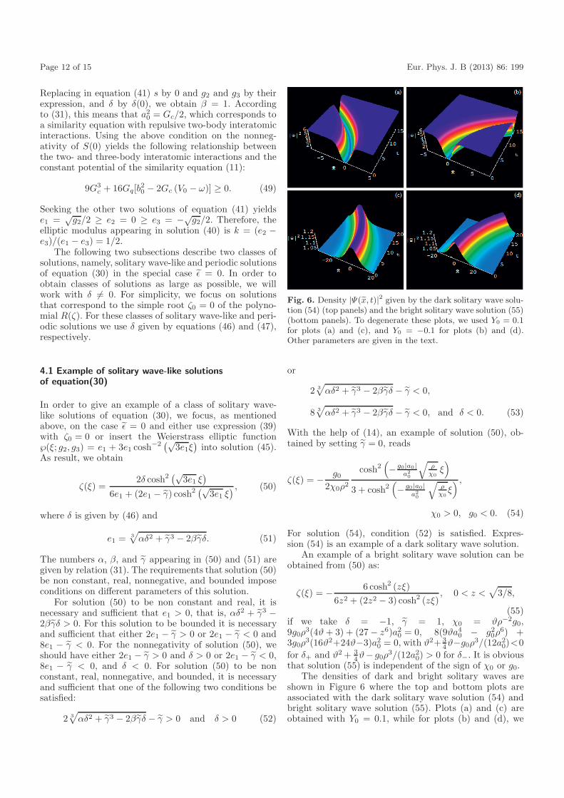
Fig. 6. Density |Ψ(x, t)|2 given by the dark solitary wave solu-tion (54) (top panels) and the bright solitary wave solution (55)(bottom panels). To degenerate these plots, we used Y0 = 0.1for plots (a) and (c), and Y0 = −0.1 for plots (b) and (d).Other parameters are given in the text.

or

2 3√αδ2 + γ3 − 2βγδ − γ < 0,

8 3√αδ2 + γ3 − 2βγδ − γ < 0, and δ < 0. (53)

With the help of (14), an example of solution (50), ob-tained by setting γ = 0, reads

ζ(ξ) = − g02χ0ρ2

cosh2(− g0|a0|

a20

√ρ

χ0ξ)

3 + cosh2(− g0|a0|

a20

√ρχ0ξ) ,

χ0 > 0, g0 < 0. (54)

For solution (54), condition (52) is satisfied. Expres-sion (54) is an example of a dark solitary wave solution.

An example of a bright solitary wave solution can beobtained from (50) as:

ζ(ξ) = − 6 cosh2 (zξ)6z2 + (2z2 − 3) cosh2 (zξ)

, 0 < z <√

3/8,

(55)if we take δ = −1, γ = 1, χ0 = ϑρ−2g0,9g0ρ3(4ϑ+ 3) + (27 − z6)a2

0 = 0, 8(9ϑa40 − g2

0ρ6) +

3g0ρ3(16ϑ2+24ϑ−3)a20 = 0, with ϑ2+ 3

4ϑ−g0ρ3/(12a20)<0

for δ+ and ϑ2 + 34ϑ− g0ρ

3/(12a20) > 0 for δ−. It is obvious

that solution (55) is independent of the sign of χ0 or g0.The densities of dark and bright solitary waves are

shown in Figure 6 where the top and bottom plots areassociated with the dark solitary wave solution (54) andbright solitary wave solution (55). Plots (a) and (c) areobtained with Y0 = 0.1, while for plots (b) and (d), we


ζ(ξ) =6a2

0Gcδsn2(

4√

g2ξ,12

)6a2

04√

g2Gc −(3a2

0Gc√

g2 + 4a20V0 − 4a2

0ω − b20

)sn2

(4√

g2ξ,12

) (61)

δ =

(4a2

0V0 − 4a20ω − b2

0

) [3 |a0|Gc −

√9a2

0G2c − 8Gq(4a2

0V0 − 4a20ω − b2

0)]

24 |a0| a20GcGq

,

a20G

2c

4a20V0 − 4a2

0ω − b20

< Gq < 0 (65)

δ =

(4a2

0V0 − 4a20ω − b2

0

) [3 |a0|Gc −

√9a2

0G2c − 8Gq(4a2

0V0 − 4a20ω − b2

0)]

24 |a0| a20GcGq

,

Gq <a20G

2c

4a20V0 − 4a2

0ω − b20

, 4a20V0 − 4a2

0ω − b20 > 0 (66)

used Y0 = −0.1. For both dark and solitary waves, weused the parameters α0 = 1, β0 = −0.01, C1 = −25,μ = 0.1, g0 = −0.2, χ0 = 0.1, α0 = 1, β0 = 0.1, X0 = 1,a0 = 40. Other parameters used to generate these plotsare Gc = −0.0128 and Gq = 0.001024 for the dark soli-tary wave, and Gc = −0.0706205 and Gq = 0.0176401 forbright solitary wave. The plots of this figure show the ef-fects of parameter Y0 on the solitary wave. It is seen fromthese plots that (i) the trajectory of the solitary wave isparabolic in time; (ii) solitary waves with the same |Y0|(that is, with Y0 = α and Y0 = −α) move with thesame velocity in opposite direction (one along the negativex-axis and another along the positive x-axis); (iii) solitarywaves with the same |Y0| move with the same amplitude.

4.2 Example of periodic solutions of equation (30)

An example of a class of periodic solutions of equation (30)is sought under conditions ε = 0 and δ �= 0 with the use ofthe root ζ0 = 0 of the polynomial R(ζ). Inserting ζ0 = 0into solution (40) yields

ζ(ξ) =2δsn2 (

√e1 − e3 ξ, k)

2(e1 − e3) + (2e3 − γ) sn2 (√e1 − e3 ξ, k)

,

k =e2 − e3e1 − e3

, (56)

where δ is given by (47), and e1 ≥ e2 ≥ e3 are solutionsof the algebraic equation (41), that is,

4s3 − (3γ2 − 4βδ

)s− (

2βγδ − αδ2 − γ3)

= 0. (57)

The solutions e1, e2, and e3 are found using the followingprocedure: choose any s0 satisfying in equation (48), i.e.,S(s0) ≥ 0, impose on s0 to satisfy equation (57) in whichδ is replaced by δ(s0); then, use solution s0 to find theother two solutions of (57) by reducing this equation to aquadratic equation.

For solution (56) to be non constant, nonnegative andbounded, it is necessary and sufficient that one of the

following three conditions be satisfied:

2e3 − γ = 0 and δ(e1 − e3) > 0, (58)sign(δ) = sign(e1 − e3) = sign(2e3 − γ) �= 0, (59)

that is, δ, (e1 − e3), and 2e3 − γ are either three positivenumber or three negative number,

(e1 − e3) (2e3 − γ) < 0 < (e1 − e3) (2e1 − γ)and 0 < δ(e1 − e3). (60)

It should be noted that at least one of conditions (58)–(60)does not depend on the sign of g0 or χ0, nor on their size.We then conclude that equation (1) with potential (2) and(3) and (9) always admits periodic solutions of form (56)in both regions of modulational stability and modulationalinstability.

The simplest example of solution (56) is obtained bytaking s = s0 = 0. As shown above, e1 =

√g2/2 ≥ e2 =

0 ≥ e3 = −√g2/2, and k = 1/2. Therefore,


where

δ =(24 |a0|a2

0GcGq

)−1[3 |a0|Gc

(4a2

0V0 − 4a20ω − b20

)± ∣∣4a2

0V0 − 4a20ω − b20

∣∣×

√9a2

0G2c − 8Gq(4a2

0V0 − 4a20ω − b20)

](62)

g2 =

(4a2

0V0 − 4a20ω − b20

)2 − 12a40G

2cδ

3a40G

2c

, (63)

Gc > 0, 9a20G

2c − 8Gq(4a2

0V0 − 4a20ω − b20) ≥ 0,

0 <(4a2

0V0 − 4a20ω − b20

)2 − 12a40G

2cδ, (64)

with Gc = g0ρ3 and Gq = χ0ρ

5. For solutions (61)−(64),condition (58) cannot occur, while conditions (59)and (60), in terms of the coefficients of the similarityequation (11), become:

see equations (65) and (66) above.

of 15 Eur. Phys. J. B (2013) 86: 199

It is evident that condition (49) occurs as soon as one ofthe conditions (65) and (66) is satisfied.

Because g0ρ3 = Gc > 0, we conclude from condi-

tion (14) that solutions (61)−(64) with condition (65) issuitable only when the cubic and quintic coefficients g0and χ0 describe either two-body attractive (g0 < 0)and three-body repulsive (χ0 > 0) or two-body repulsive(g0 > 0) and three-body attractive (χ0 < 0) bosonic inter-actions BECs. In fact, condition (65) shows thatGcGq < 0and for condition (14) to be satisfied, it is necessary andsufficient that g0χ0 < 0. For such BECs, one may alsouse (61)−(64) with condition (65) by taking only nega-tive χ0. If equation (1) describes the dynamic of BECswith either two- and three-body attractive (g0 < 0 andχ0 < 0) or two- and three-body repulsive (g0 > 0 andχ0 > 0) interatomic interactions, it is reasonable to usesolutions (61)−(64) under condition (66). In fact, for suchBECs, we have g0χ0 > 0, which is equivalent to GqGc > 0;this means that Gq > 0. All χ0ρ

5 = Gq < 0 (i.e., χ0 < 0)satisfying condition (66) are, as mentioned above, suitablefor BECs with negative g0χ0.

5 Conclusion

In conclusion, a cubic-quintic GP equation is used to in-vestigate the modulational instability of BEC in time-dependent potential given by (2) and (3), consisting ofparabolic, linear, and complex terms expressed in termsof Jacobian elliptic functions. With the help of a spe-cial variable transformation and a similarity transforma-tion, we reduced the one-dimensional GP equation (1)to the standard cubic-quintic nonlinear Schrodinger equa-tion under the integrability condition (14). Then, we havederived the exact analytical expression for modulationalinstability of the condensates. We firstly obtained thatthree-body repulsion can overcome two-body attraction,and a stable condensate will appear in the trap; inversely,three-body attraction can overcome two-body repulsion,and a unstable condensate will appear in the trap. Sec-ondly, it is shown that the enhancement and/or the alle-viation of MI can be well controlled by the parameter Y0

of the atomic feeding/loss of the condensate. Further-more, by employing the standard cubic-quintic nonlinearSchrodinger equation (11), we have also presented the ex-act (dark and bright) solitary wave and periodic solutionsof BEC systems. Dark and bright solitary wave solutionsexist for both cases of attractive and repulsive two- andthree-bodies interatomic interactions. By using the pre-sented integrability condition and the derived exact soli-tary wave solutions, we aim to investigate in a nearest fu-ture, the soliton interaction of BECs with both two- andthree-bodies interactions in the presence of feeding/loss ofatoms. It is important to point out that our exact solu-tions can be used as initial condition for investigation thenonlinear dynamics of the BECs under consideration.

This work was supported by Chinese Academy of SciencesVisiting Professorship for Senior International Scientists, the

NKBRSFC under Grants Nos. 2011CB921502, 2012CB821305,2009CB930701, 2010CB922904, NSFC under GrantsNos. 10934010, 60978019, and NSFC-RGC under GrantsNos. 11061160490 and 1386-N-HKU748/10.

References

1. M.H. Anderson, J.R. Ensher, M.R. Matthews, C.E.Wieman, E.A. Cornell, Science 269, 198 (1995)

2. K.B. Davis, M.O. Mewes, M.R. Andrews, N.J. van Druten,D.S. Durfee, D.M. Kurn, W. Ketterle, Phys. Rev. Lett. 75,3969 (1995)

3. D.S. Jin, J.R. Ensher, M.R. Matthews, C.E. Wieman, E.A.Cornell, Phys. Rev. Lett. 77, 420 (1996)

4. M.O. Mewes, M.R. Andrews, N.J. van Druten, D.M. Kurn,C.G. Townsend, W. Ketterle, Phys. Rev. Lett. 77, 988(1996)

5. D.S. Jin, M.R. Matthews, J.R. Ensher, C.E. Wieman, E.A.Cornell, Phys. Rev. Lett. 78, 764 (1997)

6. D.M. Stamper-Kurn, H.J. Meisner, S. Inouye, M.R.Andrews, W. Ketterle, Phys. Rev. Lett. 81, 500 (1998)

7. D.A.W. Hutchinson, R.J. Dodd, K. Burnett, Phys. Rev.Lett. 81, 2198 (1998)

8. F. Dalfovo, S. Giorgini, L.P. Pitaevskii, S. Stringari, Rev.Mod. Phys. 71, 463 (1999)

9. B.B. Baizakov, V.V. Konotop, M. Salerno, J. Phys. B 35,5105 (2002)

10. T. Kohler, Phys. Rev. Lett. 89, 210404 (2002)11. C.J. Pethick, H. Smith, Bose-Einstein Condensation in Di-

lute Gases (Cambridge University Press, Cambridge, 2002)12. W.M. Liu, B. Wu, Q. Niu, Phys. Rev. Lett. 84, 2294 (2000)13. E. Kengne, X.X. Liu, B.A. Malomed, S.T. Chui, W.M. Liu,

J. Math. Phys. 49, 023503 (2008)14. E. Kengne, R. Vaillancourt, B.A. Malomed, J. Phys. B 41,

205202 (2008)15. G.P. Zheng, J.Q. Liang, W.M. Liu, Phys. Rev. A 71,

053608 (2005)16. D.S. Wang, X.-F. Zhang, P. Zhang, W.M. Liu, J. Phys. B.

42, 245303 (2009)17. E. Kengne, P.K. Talla, J. Phys. B 39, 3679 (2006)18. S. Burger, K. Bongs, S. Dettmer, W. Ertmer, K. Sengstock,

Phys. Rev. Lett. 83, 5198 (1999)19. J. Denschlag, J.E. Simsarian, D.L. Feder, C.W. Clark,

L.A. Collins, J. Cubizolles, L. Deng, E.W. Hagley, K.Helmerson, W.P. Reinhardt, S.L. Rolston, B.I. Schneider,W.D. Phillips, Science 287, 97 (2000)

20. K.E. Strecker, G.B. Partridge, A.G. Truscott, R.G. Hulet,Nature 417, 150 (2002)

21. L. Khaykovich, F. Schreck, G. Ferrari, T. Bourdel, J.Cubizolles, L.D. Carr, Y. Castin, C. Salomon, Science 296,1290 (2002)

22. P. Rosenbusch, V. Bretin, J. Dalibard, Phys. Rev. Lett.89, 200403 (2002)

23. Th. Buschand, J.R. Anglin, Phys. Rev. Lett. 84, 2298(2000)

24. W.M. Liu, B. Wu, Q. Niu, Phys. Rev. Lett. 84, 2294 (2000)25. F. Dalfovo, S. Giorgini, L.P. Pitaevskii, S. Stringari, Rev.

Mod. Phys. 71, 463 (1999)26. M. Cristiani, O. Morsch, N. Malossi, M. Jona-Lasino, M.

Andrelini, E. Courtade, E. Arimondo, Opt. Express 12, 4(2004)


27. A. Mohamadou, E. Wamba, S.Y. Doka, T.B. Ekogo, T.C.Kofane, Phys. Rev. A 84, 023602 (2011)

28. E. Kengne, R. Vaillancourt, B.A. Maloned, Int. J. Mod.Phys. B 24, 2211 (2010)

29. L.P. Pitaevskii, Zh. Eksp. Teor. Fiz. 40, 646 (1961)30. L.P. Pitaevskii, Sov. Phys. J. Exp. Theor. Phys. 13, 451

(1961)31. E.P. Gross, Nuovo Cim. 20, 454 (1961)32. T.B. Benjamin, J.E. Feir, J. Fluid Mech. 27, 417 (1967)33. L.A. Ostrovskii, Sov. Phys. J. Exp. Theor. Phys. 24, 797

(1967)34. T.Taniuti, H. Washimi, Phys. Rev. Lett. 21, 209 (1968)35. A. Hasegawa, Phys. Rev. Lett. 24, 1165 (1970)36. G.P. Agrawal, Nonlinear Fiber Optics (Academic Press,

San Diego, 2001)37. L. Fallani, L. DeSarlo, J.E. Lye, M. Modugno, R. Saers,

C. Fort, M. Inguscio, Phys. Rev. Lett. 93, 140406 (2004)38. E. Kengne, C.N. Bame, Phys. Scr. 71, 423 (2005)39. E. Kengne, J. Phys. A 37, 6053 (2004)40. R.J. Deissler, H.R. Brand, Phys. Lett. 146, 252 (1990)41. E.P. Bashkin, A.V. Vagov, Phys. Rev. B 56, 6207 (1997)42. G.R. Jin, C.K. Kim, K. Nahm, Phys. Rev. A 72, 045601

(2005)43. J. Ruostekoski, Z. Dutton, Phys. Rev. A 76, 063607 (2007)44. E. Kengne, S.T. Chui, W.M. Liu, Phys. Rev. E 74, 036614

(2006)45. W. Zhang, M.W. Ewan, H. Pu, P. Meystre, Phys. Rev. A

68, 023608 (2003)46. A. Gammal, T. Frederico, L. Tomio, Phys. Rev. E 60, 2421

(1999)47. A. Gammal, T. Frederico, L. Tomio, F.K. Abdullaev, Phys.

Lett. A 267, 305 (2000)48. A.E. Muryshev, G.V. Shlyapnikov, W. Ertmer, K.

Sengstock, M. Lewenstein, Phys. Rev. Lett. 89, 110401(2002)

49. B. Deconinck, B.A. Frigyik, J.N. Kutz, J. Nonlinear Sci.12, 169 (2002)

50. I.M. Merhasin, B.V. Gisin, R. Driben, B.A. Malomed,Phys. Rev. E 71, 016613 (2005)

51. W.D. Li, A. Smerzi, Phys. Rev. E. 70, 16605 (2004)52. M. Machholm, A. Nicolin, C.J. Pethick, H. Smith, Phys.

Rev. A 69, 043604 (2004)53. J. Wang, F.Ye, L. Dong, T. Cai, Y.-P. Li, Phys. Lett. A

339, 74 (2005)54. D.I. Choi, Q. Niu, Phys. Rev. Lett. 82, 2022 (1999)

55. K. Berg-Sorensen, K. Molmer, Phys. Rev. A 58, 1480(1998)

56. S. Rajendran, P. Muruganandam, M. Lakshmanan, J.Phys. B 42, 145307 (2009)

57. S. Rajendran, P. Muruganandam, M. Lakshmanan,Physica D 239, 366 (2010)

58. V.N. Serkin, A. Hasegawa, T.L. Belyaeva, Phys. Rev. Lett.98, 074102 (2007)

59. V.N. Serkin, A. Hasegawa, T.L. Belyaeva, Phys. Rev. A81, 023610 (2010)

60. U. Roy, R. Atre, C. Sudheesh, C.N. Kumar, P. Panigrahi,J. Phys. B 43, 025003 (2010)

61. D.S. Nicola, B.A. Malomed, R. Fedele, Phys. Lett. A 360,164 (2006)

62. L. Salasnich, A. Cetoli, B.A. Malomed, F. Toigo, L. Reatto,Phys. Rev. A 76, 013623 (2007)

63. B. Paredes, A. Widera, V. Murg, O. Mandel, S. Folling, I.Cirac, G.V. Shlyapnikov, T.W. Hansch, I. Bloch, Nature429, 277 (2004)

64. Y. Kagan, A.E. Muryshev, G.V. Shlyapnikov, Phys. Rev.Lett. 81, 933 (1998)

65. L. Tomio, V.S. Filho, A. Gammal, T. Frederico, Nucl.Phys. A 684, 681 (2001)

66. E. Kengne, P.K. Talla, J. Phys. B 39, 3679 (2006)67. L.-C. Zhao, Z.-Y. Yang, T. Zhang, K.-J. Chi, Chin. Phys.

Lett. 26, 120301 (2009)68. F.Kh. Abdullaev, R. Galimzyanov, J. Phys. B 36, 1099

(2003)69. J.J.G. Ripol, V.M. Perez-Garcia, Phys. Rev. A 59, 2220

(1999)70. G. Theocharis, Z. Rapti, P.G. Kevrekidis, D.J.

Frantzeskakis, V.V. Konotop, Phys. Rev. A 67, 063610(2003)

71. J.C. Bronski, L.D. Carr, B. Deconinck, J.N. Kutz, Phys.Rev. Lett. 86, 1402 (2001)

72. E.T. Whittaker, G.N. Watson, A Course of Modern Analy-sis (Cambridge University Press, Cambridge, 1927), p. 452

73. H.W. Schurmann, Phys. Rev. E 54, 4312 (1996)74. E. Kengne, R. Vaillancourt, Can. J. Phys. 87, 1191 (2009)75. P.G. Drazin, Solitons (Cambridge University Press,

Cambridge, 1983)76. H.W. Schurmann, V.S. Serov, J. Math. Phys. 45, 2181

(2004)77. M. Abramowitz, I.A. Stegun, Handbook of Mathematical

Functions, 9th edn. (Dover Publications, New York, 1972)

Modulational instability of Bose-Einstein condensate in a complex polynomial in elliptic Jacobian...

Documents

Transcript of Modulational instability of Bose-Einstein condensate in a complex polynomial in elliptic Jacobian...