HP ProLiant BL490c Generation 7 (G7) Server Blade - HP-pro ...
Upload
khangminh22Category
view
2download
0
arX
iv:1
110.
2316
v1 [
mat
h.N
A]
11 O
ct 2
011 h-p spectral element methods for three dimensional
elliptic problems on non-smooth domains usingparallel computers
Akhlaq Husain1
DEPARTMENT OF MATHEMATICS AND STATISTICS
INDIAN INSTITUTE OF TECHNOLOGY KANPURJune, 2010
1
1This is a reprint of the PhD thesis of the author, which was submitted on 11th June, 2010 anddefended on 14th January, 2011 at IIT Kanpur, India

h-p spectral element methods for three dimensional
elliptic problems on non-smooth domains usingparallel computers
A Thesis Submittedin Partial Fulfillment of the Requirements
for the Degree of
Doctor of Philosophy
by
Akhlaq Husain2
to the
DEPARTMENT OF MATHEMATICS AND STATISTICS
INDIAN INSTITUTE OF TECHNOLOGY KANPURJune, 2010
1 2
1This is a reprint of the PhD thesis of the author, which was submitted on 11th June, 2010 anddefended on 14th January, 2011 at IIT Kanpur, India
2Dr. Akhlaq HusainLNM Institute of Information TechnologyRupa ki Nangal, Post-Sumel, Via-Jamdoli, Jaipur-302031, Rajasthan, INDIA

CERTIFICATE
It is certified that the work contained in the thesis entitled “h − p spectral element
methods for three dimensional elliptic problems on non-smooth domains using
parallel computers” by Akhlaq Husain, has been carried out under our supervision and
that this work has not been submitted elsewhere for a degree.
Pravir Dutt A.S. Vasudeva Murthy
(Professor) (Professor)
Department of Mathematics TIFR Centre for Applicable
and Statistics Mathematics
Indian Institute of Technology Tata Institute of Fundamental Research
Kanpur Bangalore
June, 2010

ABSTRACT
Elliptic partial differential equations arise in many fields of science and engineering
such as steady state distribution of heat, fluid dynamics, structural/mechanical engineer-
ing, aerospace engineering, medical science and seismology etc.
In three dimensions it is well known that the solutions of elliptic boundary value prob-
lems have singular behaviour near the corners and edges of the domain. The singularities
which arise are known as vertex, edge, and vertex-edge singularities. Due to the pres-
ence of singularities the conventional numerical methods are unable to provide accurate
numerical solutions and the rate of convergence of these methods degrades. In order to
improve efficiency of computations and accuracy of the solutions, it is desirable to find
efficient methods along with standard numerical techniques such as finite element method
(FEM), spectral element method (SEM) and so on.
We propose a nonconforming h−p spectral element method to solve three dimensional
elliptic boundary value problems on non-smooth domains to exponential accuracy.
To overcome the singularities which arise in the neighbourhoods of the vertices, vertex-
edges and edges we use local systems of coordinates. Away from these neighbourhoods
standard Cartesian coordinates are used. In each of these neighbourhoods we use a ge-
ometrical mesh which becomes finer near the corners and edges. The geometrical mesh
becomes a quasi-uniform mesh in the new system of coordinates. Hence Sobolev’s embed-
ding theorems and the trace theorems for Sobolev spaces are valid for spectral element
functions defined on mesh elements in the new system of variables with a uniform con-
stant. We then derive differentiability estimates in these new sets of variables and a
stability estimate, on which our method is based, for a non-conforming h − p spectral
element method.
We choose as our approximate solution the spectral element function which minimizes
the sum of a weighted squared norm of the residuals in the partial differential equations
and the squared norm of the residuals in the boundary conditions in fractional Sobolev
spaces and enforce continuity by adding a term which measures the jump in the function
vi
and its derivatives at inter-element boundaries in fractional Sobolev norms, to the func-
tional being minimized. The Sobolev spaces in vertex-edge and edge neighbourhoods are
anisotropic and become singular at the corners and edges.
The method is essentially a least−squares collocation method and a solution can be
obtained using Preconditioned Conjugate Gradient Method (PCGM). To solve the mini-
mization problem we need to solve the normal equations for the least−squares problem.
The residuals in the normal equations can be obtained without computing and storing
mass and stiffness matrices.
We solve the normal equations using a block diagonal preconditioner where each block
corresponds to the square of H2 norm of the SEF defined on a particular element. More-
over it is shown that there exists a diagonal preconditioner using separation of variables
technique. Let N denote the number of refinements in the geometrical mesh. We shall
assume that N is proportional to W .
For problems with Dirichlet boundary conditions the condition number of the precon-
ditioned system is O((lnW )2), provided W = O(eNα) for α < 1/2. Moreover there exists
a new preconditioner which can be diagonalized in a new set of basis functions, using
separation of variables techniques, in which each diagonal block corresponds to a different
element, and hence it can easily be inverted on each element. For Dirichlet problems
the method requires O(NlnN) iterations of the PCGM to obtain solution to exponen-
tial accuracy and it requires O(N5ln(N)) operations on a parallel computer with O(N2)
processors to compute the solution. For mixed problems with Neumann and Dirichlet
boundary conditions the condition number of the preconditioned system is O(N4), pro-
vided W = O(eNα) for α < 1/2. Hence, it requires O(N3) iterations of the PCGM
to obtain solution to exponential accuracy and requires O(N7) operations on a parallel
computer with O(N2) processors to compute the solution.
Computational results for a number of model problems confirm the theoretical esti-
mates obtained for the error and computational complexity.
Synopsis
Name of the Student : Akhlaq Husain
Roll Number : Y4108061
Degree for which submitted : Ph.D.
Department : Mathematics
Thesis Title : h− p Spectral Element Methods for
Three Dimensional Elliptic Problems
on Non-smooth Domains using
Parallel Computers
Thesis Supervisors : Dr. Pravir K. Dutt and Dr. A. S.
Vasudeva Murthy
Month and year of submission : June, 2010
Elliptic partial differential equations arise in many fields of science and engineering
such as steady state distribution of heat, fluid dynamics, structural/mechanical engineer-
ing, aerospace engineering, medical science and seismology etc. Elliptic boundary value
problems in polygonal and polyhedral domains have been studied in many works in the
literature. Among these, problems on polyhedral domains with corners and edges have
become increasingly important in the last two decades. In many practical situations, the
physical domain often has corners and edges either due to its geometry or created by
unions and intersections of simpler objects such as cylinders, cones and spheres. Hence
singularities of the solutions occur at the corners and edges, and severely affect the regu-
larity of the solutions.
viii
In three dimensions it is well known that the solutions of elliptic boundary value prob-
lems have singular behaviour near the corners and edges of the domain. The singularities
which arise are known as vertex, edge, and vertex-edge singularities. Due to the pres-
ence of singularities the conventional numerical methods are unable to provide accurate
numerical solutions and the rate of convergence of these methods degrades. In order to
improve efficiency of computations and accuracy of the solutions, it is desirable to find
efficient methods along with standard numerical techniques such as finite element method
(FEM), spectral element method (SEM) and so on. Different approaches and methods
have been attempted over the years to find accurate solutions to the elliptic boundary
value problems on polyhedrons containing singularities.
We propose a nonconforming h−p spectral element method to solve three dimensional
elliptic boundary value problems on non-smooth domains to exponential accuracy.
To overcome the singularities which arise in the neighbourhoods of the vertices, vertex-
edges and edges we use local systems of coordinates. These local coordinates are modified
versions of spherical and cylindrical coordinate systems in their respective neighbour-
hoods. Away from these neighbourhoods standard Cartesian coordinates are used. In
each of these neighbourhoods we use a geometrical mesh which becomes finer near the
corners and edges. The geometrical mesh becomes a quasi-uniform mesh in the new
system of coordinates. Hence Sobolev’s embedding theorems and the trace theorems for
Sobolev spaces are valid for spectral element functions defined on mesh elements in the
new system of variables with a uniform constant. We then derive differentiability esti-
mates in these new sets of variables and a stability estimate, on which our method is
based, for a non-conforming h− p spectral element method.
We choose as our approximate solution the spectral element function which minimizes
the sum of a weighted squared norm of the residuals in the partial differential equations
and the squared norm of the residuals in the boundary conditions in fractional Sobolev
spaces and enforce continuity by adding a term which measures the jump in the function
and its derivatives at inter-element boundaries in fractional Sobolev norms, to the func-
tional being minimized. The Sobolev spaces in vertex-edge and edge neighbourhoods are
anisotropic and become singular at the corners and edges.
ix
The spectral element functions are represented by a uniform constant at all the corner
elements in vertex neighborhoods and on the corner-most elements in vertex-edge neigh-
bourhoods which are in the angular direction to the edges. At corner elements which are
in the direction of edges in vertex-edge neighbourhoods and at all the corner elements in
edge neighbourhoods the spectral element functions are represented as one dimensional
polynomials of degree W in the modified coordinates. In all other elements in edge neigh-
bourhoods and vertex-edge neighbourhoods the spectral element functions are a sum of
tensor products of polynomials of degree W in their respective modified coordinates. The
remaining elements in the vertex neighbourhoods and the regular region are mapped to
the master cube and the spectral element functions are represented as a sum of tensor
products of polynomials of degree W in λ1, λ2, and λ3, the transformed variables on the
master cube.
The method is essentially a least−squares collocation method and a solution can be
obtained using Preconditioned Conjugate Gradient Method (PCGM). To solve the mini-
mization problem we need to solve the normal equations for the least−squares problem.
The residuals in the normal equations can be obtained without computing and storing
mass and stiffness matrices.
We choose spectral element functions (SEF) which are non-conforming. We solve the
normal equations using a block diagonal preconditioner where each block corresponds to
the square of H2 norm of the SEF defined on a particular element. Let N denote the
number of refinements in the geometrical mesh. We shall assume that N is proportional
to W .
For problems with Dirichlet boundary conditions the condition number of the precon-
ditioned system is O((lnW )2), provided W = O(eNα) for α < 1/2. Moreover there exists
a new preconditioner which can be diagonalized in a new set of basis functions, using
separation of variables techniques, in which each diagonal block corresponds to a different
element, and hence it can easily be inverted on each element. For Dirichlet problems
the method requires O(NlnN) iterations of the PCGM to obtain solution to exponen-
tial accuracy and it requires O(N5ln(N)) operations on a parallel computer with O(N2)
processors to compute the solution. For mixed problems with Neumann and Dirichlet
x
boundary conditions the condition number of the preconditioned system is O(N4), pro-
vided W = O(eNα) for α < 1/2. Hence, it requires O(N3) iterations of the PCGM
to obtain solution to exponential accuracy and requires O(N7) operations on a parallel
computer with O(N2) processors to compute the solution.
We mention that once we have obtained our approximate solution consisting of non-
conforming spectral element functions we can make a correction to it so that the corrected
solution is conforming and is an exponentially accurate approximation to the actual so-
lution in the H1 norm over the whole domain.
Our method works for non self-adjoint problems too. Computational results for a
number of model problems on non-smooth domains with constant and variable coeffi-
cients having smooth and singular solutions are presented which confirm the theoretical
estimates obtained for the error and computational complexity.
For mixed problems rapid growth of the factor N4 creates difficulty in parallelizing
the numerical scheme. To overcome this difficulty another version of the method may
be defined in which we choose spectral element functions to be conforming only on the
wirebasket of the elements and non-conforming elsewhere. The values of the spectral
element functions at the wirebasket of the elements constitute the set of common boundary
values and an accurate approximation to the Schur complement matrix can be computed.
We plan to consider this in future work.
Contents
Synopsis vii
Contents xi
List of Figures xv
List of Tables xix
1 Introduction 1
1.1 Spectral Methods . . . . . . . . . . . . . . . . . . . . . . . . . . . . . . . . 2
1.2 Types of Spectral Methods . . . . . . . . . . . . . . . . . . . . . . . . . . . 4
1.2.1 Collocation method . . . . . . . . . . . . . . . . . . . . . . . . . . . 4
1.2.2 Galerkin method . . . . . . . . . . . . . . . . . . . . . . . . . . . . 5
1.2.3 Tau method . . . . . . . . . . . . . . . . . . . . . . . . . . . . . . . 6
1.3 Spectral Methods on Non-smooth Domains . . . . . . . . . . . . . . . . . . 6
1.3.1 Gradual h refinement . . . . . . . . . . . . . . . . . . . . . . . . . . 8
1.3.2 Method of auxiliary or conformal mapping . . . . . . . . . . . . . . 8
1.3.3 Advantages and applications of spectral methods: A survey . . . . . 16
1.3.4 Limitations of spectral methods . . . . . . . . . . . . . . . . . . . . 18
1.4 Finite Element Method . . . . . . . . . . . . . . . . . . . . . . . . . . . . . 18
1.4.1 Method of weighted residuals . . . . . . . . . . . . . . . . . . . . . 20
1.4.2 Advantages of FEM . . . . . . . . . . . . . . . . . . . . . . . . . . . 22
1.4.3 Disadvantages of FEM . . . . . . . . . . . . . . . . . . . . . . . . . 23
1.4.4 Spectral vs. finite element methods . . . . . . . . . . . . . . . . . . 23
xii CONTENTS
1.5 Non-conforming Methods . . . . . . . . . . . . . . . . . . . . . . . . . . . . 24
1.6 h− p/Spectral Element Methods on Parallel Computers . . . . . . . . . . 25
1.7 Review of Existing Work . . . . . . . . . . . . . . . . . . . . . . . . . . . . 26
1.8 Review and Outline of the Thesis . . . . . . . . . . . . . . . . . . . . . . . 28
2 Differentiability and Stability Estimates 33
2.1 Introduction . . . . . . . . . . . . . . . . . . . . . . . . . . . . . . . . . . . 33
2.2 Differentiability Estimates in Modified Coordinates . . . . . . . . . . . . . 35
2.2.1 Differentiability estimates in modified coordinates in vertex neigh-
bourhoods . . . . . . . . . . . . . . . . . . . . . . . . . . . . . . . . 36
2.2.2 Differentiability estimates in modified coordinates in edge neigh-
bourhoods . . . . . . . . . . . . . . . . . . . . . . . . . . . . . . . . 38
2.2.3 Differentiability estimates in modified coordinates in vertex-edge
neighbourhoods . . . . . . . . . . . . . . . . . . . . . . . . . . . . . 39
2.2.4 Differentiability estimates in standard coordinates in the regular
region of the polyhedron . . . . . . . . . . . . . . . . . . . . . . . . 41
2.2.5 Function spaces . . . . . . . . . . . . . . . . . . . . . . . . . . . . . 42
2.3 The Stability Theorem . . . . . . . . . . . . . . . . . . . . . . . . . . . . . 44
3 Proof of the Stability Theorem 63
3.1 Introduction . . . . . . . . . . . . . . . . . . . . . . . . . . . . . . . . . . . 63
3.2 Estimates for the Second Derivatives of Spectral Element Functions . . . . 64
3.2.1 Estimates for the second derivatives in the interior . . . . . . . . . 64
3.2.2 Estimates for second derivatives in vertex neighbourhoods . . . . . 71
3.2.3 Estimates for second derivatives in vertex-edge neighbourhoods . . 78
3.2.4 Estimates for second derivatives in edge neighbourhoods . . . . . . 83
3.3 Estimates for Lower Order Derivatives . . . . . . . . . . . . . . . . . . . . 87
3.4 Estimates for Terms in the Interior . . . . . . . . . . . . . . . . . . . . . . 88
3.4.1 Estimates for terms in the interior of Ωr . . . . . . . . . . . . . . . 88
3.4.2 Estimates for terms in the interior of Ωe . . . . . . . . . . . . . . . 89
3.4.3 Estimates for terms in the interior of Ωv . . . . . . . . . . . . . . . 90
CONTENTS xiii
3.4.4 Estimates for terms in the interior of Ωv−e . . . . . . . . . . . . . . 91
3.5 Estimates for Terms on the Boundary . . . . . . . . . . . . . . . . . . . . . 93
3.5.1 Estimates for terms on the boundary of Ωr . . . . . . . . . . . . . . 93
3.5.2 Estimates for terms on the boundary of Ωe . . . . . . . . . . . . . . 95
3.5.3 Estimates for terms on the boundary of Ωv . . . . . . . . . . . . . . 96
3.5.4 Estimates for terms on the boundary of Ωv−e . . . . . . . . . . . . . 96
3.6 Proof of the Stability Theorem . . . . . . . . . . . . . . . . . . . . . . . . . 97
4 The Numerical Scheme and Error Estimates 101
4.1 Introduction . . . . . . . . . . . . . . . . . . . . . . . . . . . . . . . . . . . 101
4.2 The Numerical Scheme . . . . . . . . . . . . . . . . . . . . . . . . . . . . . 102
4.3 Error Estimates . . . . . . . . . . . . . . . . . . . . . . . . . . . . . . . . . 108
5 Solution Techniques on Parallel Computers 117
5.1 Introduction . . . . . . . . . . . . . . . . . . . . . . . . . . . . . . . . . . . 117
5.2 Preconditioning . . . . . . . . . . . . . . . . . . . . . . . . . . . . . . . . . 118
5.2.1 Preconditioners on the regular region . . . . . . . . . . . . . . . . . 118
5.2.2 Preconditioners on singular regions . . . . . . . . . . . . . . . . . . 123
5.3 Parallelization Techniques . . . . . . . . . . . . . . . . . . . . . . . . . . . 129
5.3.1 Integrals on the element domain . . . . . . . . . . . . . . . . . . . . 130
5.3.2 Integrals on the boundary of the elements . . . . . . . . . . . . . . 134
6 Numerical Results 139
6.1 Introduction . . . . . . . . . . . . . . . . . . . . . . . . . . . . . . . . . . . 139
6.2 Test Problems in Regular Regions . . . . . . . . . . . . . . . . . . . . . . . 141
6.3 Test Problems in Singular Regions . . . . . . . . . . . . . . . . . . . . . . 157
6.4 Conclusions and Future Work . . . . . . . . . . . . . . . . . . . . . . . . . 170
6.4.1 Summary and conclusions . . . . . . . . . . . . . . . . . . . . . . . 170
6.4.2 Proposed future work . . . . . . . . . . . . . . . . . . . . . . . . . . 172
Appendix A 173
xiv CONTENTS
Appendix B 181
Appendix C 197
Appendix D 215
Bibliography 245
List of Figures
1.1 Computational domain Ω containing a corner of angle θ = απ. . . . . . . . 7
1.2 Auxiliary mapping of a domain containing a corner to a domain with no
corners. . . . . . . . . . . . . . . . . . . . . . . . . . . . . . . . . . . . . . 9
1.3 Typical three-dimensional singularities. . . . . . . . . . . . . . . . . . . . . 10
2.1 Polyhedral domain Ω in R3. . . . . . . . . . . . . . . . . . . . . . . . . . . 36
2.2 Vertex neighbourhood Ωv. . . . . . . . . . . . . . . . . . . . . . . . . . . . 36
2.3 Edge neighbourhood Ωe. . . . . . . . . . . . . . . . . . . . . . . . . . . . . 39
2.4 Vertex-edge neighbourhood Ωv−e. . . . . . . . . . . . . . . . . . . . . . . . 40
2.5 Division of a tetrahedron into hexahedrons. . . . . . . . . . . . . . . . . . . 45
2.6 Elements in Ωr. . . . . . . . . . . . . . . . . . . . . . . . . . . . . . . . . 46
2.7 Mesh imposed on the spherical boundary Sv. . . . . . . . . . . . . . . . . 48
2.8 Geometrical mesh imposed on Ωv. . . . . . . . . . . . . . . . . . . . . . . 48
2.9 Geometrical mesh imposed on Ωv−e. . . . . . . . . . . . . . . . . . . . . . 51
2.10 Geometrical mesh imposed on Ωe. . . . . . . . . . . . . . . . . . . . . . . 56
3.1 The element Ωrl . . . . . . . . . . . . . . . . . . . . . . . . . . . . . . . . . . 66
3.2 Boundary terms. . . . . . . . . . . . . . . . . . . . . . . . . . . . . . . . . 94
5.1 κ vs. W . . . . . . . . . . . . . . . . . . . . . . . . . . . . . . . . . . . . . . 123
6.1 The domain Ω = Q = standard cube with uniform mesh refinements. . . . 141
6.2 Mesh imposed on Ω = (0, 1)3 with mesh size h = 0.5. . . . . . . . . . . . . 142
6.3 Error vs. p, Iterations vs. p, Error vs. DOF and Error vs. Iterations for
Laplace equation. . . . . . . . . . . . . . . . . . . . . . . . . . . . . . . . . 143
xvi LIST OF FIGURES
6.4 Error vs. p, Iterations vs. p, Error vs. DOF and Error vs. Iterations for
Poisson equation. . . . . . . . . . . . . . . . . . . . . . . . . . . . . . . . . 145
6.5 Error vs. p, Iterations vs. p, Error vs. DOF and Error vs. Iterations for
Poisson equation with mixed boundary conditions. . . . . . . . . . . . . . . 146
6.6 Error vs. p, Iterations vs. p, Error vs. DOF and Error vs. Iterations for
Helmholtz problem. . . . . . . . . . . . . . . . . . . . . . . . . . . . . . . . 149
6.7 Comparison between h and p versions: Error vs. DOF. . . . . . . . . . . . 149
6.8 Error vs. p, Iterations vs. p, Error vs. DOF and Error vs. Iterations for
elliptic problem with variable coefficients. . . . . . . . . . . . . . . . . . . . 151
6.9 Mesh imposed on domain Ω containing 24 brick elements . . . . . . . . . . 152
6.10 Error vs. p, Iterations vs. p, Error vs. DOF and Error vs. Iterations for
elliptic problem on L-shaped domain. . . . . . . . . . . . . . . . . . . . . . 153
6.11 Error as a function of W for different values of h for general elliptic (non
self-adjoint) problem. . . . . . . . . . . . . . . . . . . . . . . . . . . . . . . 155
6.12 Error vs. p, Iterations vs. p, Error vs. DOF and Error vs. Iterations for
general elliptic (non self-adjoint) problem. . . . . . . . . . . . . . . . . . . 156
6.13 The domain Ω(v) containing a vertex singularity. . . . . . . . . . . . . . . . 158
6.14 Geometric mesh imposed on Ω(v) and elements after mapping. . . . . . . . 158
6.15 Error vs. p, Iterations vs. N , Error vs. Ndof and Error vs. Iterations for
Poisson equation containing a vertex singularity. . . . . . . . . . . . . . . . 160
6.16 Error vs. p, Iterations vs. N , Error vs. Ndof and Error vs. Iterations for
mixed problem containing a vertex singularity. . . . . . . . . . . . . . . . . 162
6.17 The domain Ω(e)1 containing an edge singularity. . . . . . . . . . . . . . . . 163
6.18 Error vs. p, Iterations vs. N , Error vs. Ndof and Error vs. Iterations for
Laplace equation containing an edge singularity. . . . . . . . . . . . . . . . 164
6.19 The domain Ω(e)2 containing an edge singularity. . . . . . . . . . . . . . . . 165
6.20 Geometric mesh imposed on Ω(e)2 . . . . . . . . . . . . . . . . . . . . . . . . 166
6.21 Error vs. p, Iterations vs. N , Error vs. Ndof and Error vs. Iterations for
mixed problem containing an edge singularity. . . . . . . . . . . . . . . . . 167
6.22 The domain Ω(v−e). . . . . . . . . . . . . . . . . . . . . . . . . . . . . . . . 168

LIST OF FIGURES xvii
6.23 Geometrical mesh imposed on Ω(v−e) and the elements after mapping. . . . 168
6.24 Error vs. p, Iterations vs. N , Error vs. Ndof and Error vs. Iterations for
Poisson equation containing a vertex-edge singularity. . . . . . . . . . . . . 169
B.1 Interior common boundary face Γvk,i = Γv−eq,r . . . . . . . . . . . . . . . . . . 181
B.2 The face Γvk,i . . . . . . . . . . . . . . . . . . . . . . . . . . . . . . . . . . . 184
B.3 The face Γv−eq,r . . . . . . . . . . . . . . . . . . . . . . . . . . . . . . . . . . 185
B.4 Interior common boundary face Γeu,k = Γv−en,l . . . . . . . . . . . . . . . . . 188
B.5 The face Γeu,k . . . . . . . . . . . . . . . . . . . . . . . . . . . . . . . . . . 190
B.6 The face Γv−en,l . . . . . . . . . . . . . . . . . . . . . . . . . . . . . . . . . . 191
C.1 The element Ωrl and the master cube. . . . . . . . . . . . . . . . . . . . . . 198
C.2 Image of Ωv−el in y-variables. . . . . . . . . . . . . . . . . . . . . . . . . . . 201
C.3 The function r(y3). . . . . . . . . . . . . . . . . . . . . . . . . . . . . . . . 202
C.4 The function s(y3). . . . . . . . . . . . . . . . . . . . . . . . . . . . . . . . 202
C.5 The element Ωv−el . . . . . . . . . . . . . . . . . . . . . . . . . . . . . . . . 206
C.6 Faces f1 and f2. . . . . . . . . . . . . . . . . . . . . . . . . . . . . . . . . . 207
C.7 Sides si, i = 1, · · · , 12 and faces fi, i = 1, · · · , 6 of a typical element in
vertex-edge neighbourhood. . . . . . . . . . . . . . . . . . . . . . . . . . . 208
D.1 A common face in the interior of the edge neighbourhood in xe1 − xe2 plane. 226
D.2 γ, image of γ, in z−coordinates. . . . . . . . . . . . . . . . . . . . . . . . . 227
D.3 A common face in the interior of the edge neighbourhood in xe1 − xe3 plane. 228
D.4 γ, image of γ, in z−coordinates. . . . . . . . . . . . . . . . . . . . . . . . . 229
D.5 Division of Ωem into smaller rectangles. . . . . . . . . . . . . . . . . . . . . 229
D.6 The face Γrm,j of the boundary element Ωrm. . . . . . . . . . . . . . . . . . . 234
D.7 The face Γem,p of the boundary element Ωem. . . . . . . . . . . . . . . . . . . 239
D.8 The edge γ. . . . . . . . . . . . . . . . . . . . . . . . . . . . . . . . . . . . 241
D.9 The edge γ. . . . . . . . . . . . . . . . . . . . . . . . . . . . . . . . . . . . 242


List of Tables
1.1 Weight functions wj(x) used in the method of residual and the method
produced. . . . . . . . . . . . . . . . . . . . . . . . . . . . . . . . . . . . . 21
5.1 Condition number κ as a function of W . . . . . . . . . . . . . . . . . . . . 123
6.1 Performance of the p−version for Laplace equation with Dirichlet bound-
ary conditions . . . . . . . . . . . . . . . . . . . . . . . . . . . . . . . . . . 143
6.2 Performance of the p−version for Poisson equation with homogeneous
boundary conditions . . . . . . . . . . . . . . . . . . . . . . . . . . . . . . 144
6.3 Performance of the p−version for Poisson equation with mixed boundary
conditions . . . . . . . . . . . . . . . . . . . . . . . . . . . . . . . . . . . . 146
6.4 Performance of the h−version for Helmholtz problem . . . . . . . . . . . 148
6.5 Performance of the p−version for Helmholtz problem on Mesh 2 . . . . . 148
6.6 Performance of the p−version for elliptic problem with variable coefficients150
6.7 Performance of the p−version for elliptic problem on L-shaped domain . . 153
6.8 Performance of the p−version on different meshes for general elliptic (non
self-adjoint) problem with variable coefficients . . . . . . . . . . . . . . . 155
6.9 Performance of the p−version for non self-adjoint problem. . . . . . . . . 156
6.10 Performance of the h− p version for Dirichlet problem on Ω(v) containing
a vertex singularity. . . . . . . . . . . . . . . . . . . . . . . . . . . . . . 159
6.11 Performance of the h− p version for mixed problem on Ω(v) containing a
vertex singularity. . . . . . . . . . . . . . . . . . . . . . . . . . . . . . . 161
6.12 Performance of the h− p version for Laplace equation on Ω(e)1 . . . . . . . 163
xx LIST OF TABLES
6.13 Performance of the method for Laplace equation with mixed boundary
conditions on Ω(e)2 containing an edge singularity. . . . . . . . . . . . . . 166
6.14 Performance of the method for Poisson equation on Ω(v−e) containing a
vertex-edge singularity. . . . . . . . . . . . . . . . . . . . . . . . . . . . 169
Chapter 1
Introduction
Many stationary phenomena in science and engineering are modelled by elliptic boundary
value problems for instance, the elasticity problem on polyhedral domains. Usually we do
not have a closed form solution of the problem. So we frequently require the numerical
solution of these problems. In structural mechanics the physical domain often has edges,
vertices, cracks and interface between different materials. It is well known that the so-
lutions of these problems develop singularities due to the presence of corners and edges
in a three-dimensional domain. In the presence of singularities, the standard numerical
methods such as finite element method (FEM) and finite difference method (FDM) fail
to provide accurate solutions and efficiency of computations. The situation is even worse
if the singularity is more severe, for example, a vertex-edge singularity. As a result the
approximation becomes difficult and inefficient and the conventional numerical methods
yield poor convergence results for solutions to these problems. In order to have reliable
and economical approximate solutions with optimal rate of convergence, it is desirable to
find efficient and accurate numerical techniques.
We propose h− p Spectral Element Methods for Three Dimensional Elliptic
Problems on Non-smooth Domains using Parallel Computers. In this chapter,
we give a brief review of the existing numerical methods for such problems and discuss
their computational complexity.
2 Introduction
1.1 Spectral Methods
Spectral Element Methods (SEM) are a class of spatial discretizations that can be utilized
for solving partial differential equations. Spectral methods are one of the most accurate
methods for solving partial differential equations, among others namely Finite Difference
Methods (FDM) and Finite Element Methods (FEM).
Spectral methods are considered as higher order finite element methods due to their
so called spectral/exponential accuracy and use of high order polynomials for computing
numerical solution. The very high accuracy of spectral methods allows us to treat prob-
lems which would require an enormous number of grid points by finite difference or finite
element methods with much fewer degrees of freedom.
Spectral methods were proposed by Blinova [25] and first implemented by Silber-
man [80], but abandoned in the mid-1960s. Orszag [70] and Eliasen et al. [40] resurrected
them again. The formulation of the theory of modern spectral methods was first presented
in the monograph by Gottlieb and Orszag [44] for the numerical solution of partial dif-
ferential equations. Multi-dimensional discretizations were formulated as tensor products
of one-dimensional constructs in separable domains. Since then spectral methods were
extended to a broader class of problems and thoroughly analyzed in the 1980s and entered
the mainstream of scientific computation in the 1990s. The text book of Canuto et al. [27]
focuses on fluid dynamics algorithms and includes both practical as well as theoretical as-
pects of global spectral methods. A companion book Spectral Methods, Fundamentals in
Single Domains by Canuto et al. [28] is focused on the essential aspects of spectral meth-
ods on separable domains. The book Spectral/hp Element Methods for Computational
Fluid dynamics, by Karniadakis and Sherwin [55], deals with many important practical
aspects of computations using spectral methods and summarizes the recent research in
the subject. In the latest book by Bochev and Gunzburger [26] the least-squares finite
element method (LSFEM) for elliptic problems have been described.
The first practitioners of spectral methods were meteorologists studying global weather
modelling and fluid dynamicists investigating isotropic turbulence. The original idea was
to use truncated Fourier series to approximate the (smooth) solution when the problem
1.1 Spectral Methods 3
was specified with (mostly) periodic boundary conditions. In order to tackle problems
with more general boundary conditions (Dirichlet or Neumann type), the set of (algebraic)
polynomials replaced the set of truncated series, but the characterization of the unique
discrete function that would provide the numerical solution was still achieved following
the original strategy.
The key components for spectral methods are the trial functions (also called the expan-
sion or approximating functions) and the test functions (also known as weight functions).
The trial functions, which are linear combinations of suitable trial basis functions, are
used to provide the approximate representation of the solution. The test functions are
used to ensure that the differential equation and some boundary conditions are satisfied
as closely as possible by the truncated series expansion. This is achieved by minimizing,
with respect to a suitable norm, the residual produced by using the truncated expansion
instead of the exact solution. For this reason they may be viewed as a special case of the
method of weighted residuals (Finlayson and Scriven, [41]). An equivalent requirement
is that the residual satisfy a suitable orthogonality condition with respect to each of the
test functions. From this perspective, spectral methods may be viewed as a special case
of Petrov-Galerkin methods (Zienkiewicz and Cheung [93], Babuska and Aziz [6]).
The most frequently used approximation functions (trial functions) are trigonometric
polynomials, Chebyshev polynomials, and Legendre polynomials. Generally, trigonomet-
ric polynomials are used for periodic problems whereas Chebyshev and Legendre polyno-
mials for non-periodic problems. Laguerre polynomials are used for problems on semi-
infinite domains and Hermite polynomials for problems on infinite domains.
Boyd [24] contains a wealth of detail and advise on spectral algorithms and is an
especially good reference for problems on unbounded domains and in cylindrical and
spherical co-ordinate systems. A thorough analysis of the theoretical aspect of spectral
methods for elliptic equations was provided by Bernardi and Maday [23].
4 Introduction
1.2 Types of Spectral Methods
Spectral methods can be broadly classified into two categories: the pseudo-spectral or
collocation methods and the Galerkin methods [55]. The choice of the trial functions
distinguishes between the three early versions of spectral methods, namely, the collocation,
Galerkin and tau versions [28].
1.2.1 Collocation method
In the collocation approach the test functions are translated Dirac delta-functions centered
at special, so-called collocation points. This approach requires the differential equation to
be satisfied exactly at the collocation points. Of course the choice of the set of collocation
points is of fundamental importance for the accuracy of the method and the number
of collocation points must be equal to the dimension of the space of approximation.
Otherwise, the problem could, in general, be over- or under-specified. The collocation
points for both the differential equations and the boundary conditions are usually the
same as the physical grid points. The most effective choice for the grid points are those
that correspond to quadrature formulae of maximum precision.
The collocation approach appears to have been first used by Slater [83] and by Kan-
torovic [54] in specific applications. Frazer et al. [42] developed it as a general method
for solving ordinary differential equations. They used a variety of trial functions and an
arbitrary distribution of collocation points. The work of Lanczos [62] established for the
first time that a proper choice of trial functions and distribution of collocation points is
crucial to the accuracy of the solution. The earliest applications of the spectral colloca-
tion method to partial differential equations were made for spatially periodic problems by
Kreiss and Oliger [59] (who called it the Fourier method) and Orszag [71] (who termed
it pseudo-spectral). Here we choose different spaces of test functions and trial functions.
We approximate u by
uN(x) =
N∑
i=0
aiφi(x) (1.1)
where φii is the space of trial functions.
1.2 Types of Spectral Methods 5
We let the space of test functions ψii be different and impose the orthogonality condition
(LuN , ψi) = 0 for all i. (1.2)
Now if we choose ψi = δ(x − xi) for a suitably chosen set of points xii we obtain the
set of equations
(LuN)(xi) = 0 for all i. (1.3)
The points xi are chosen as the quadrature points of a Gaussian integration formula.
1.2.2 Galerkin method
The Galerkin approach [43], enjoys the aesthetically pleasing feature that the trial and
the test functions are the same, and the discretization is derived from a weak form of the
mathematical problem. The test functions are, therefore, infinitely smooth functions that
individually satisfy some or all of the boundary conditions. The differential equation is
enforced by requiring that the integral of the residual times each test function be zero,
after some integration-by-parts, accounting in the process for any remaining boundary
conditions. Finite element methods customarily use this approach. Moreover, the first
serious application of spectral methods to PDE’s − that of Silberman [80] for meteorolog-
ical modeling − was a Galerkin method. The basic idea is to assume that the unknown
function u(x) can be approximated by a sum of N + 1 basis functions φn(x):
uN(x) =
N∑
i=0
aiφi(x). (1.4)
When this series is substituted into the equation
Lu(x) = f(x) (1.5)
where L is a differential (or integral) operator, the result is the so-called residual function
defined by
RN(x) = LuN(x)− f(x). (1.6)
Since the residual function RN(x; ai) is identically equal to zero for the exact solution, the
challenge is to choose the series coefficients an so that the residual function is minimized.
6 Introduction
1.2.3 Tau method
The spectral tau methods, introduced by Lanczos [62], are similar to Galerkin methods
in the way differential equation is enforced. However, none of the test functions need
satisfy the boundary conditions. Hence, a supplementary set of equations is used to
apply boundary conditions. Tau methods may be viewed as a special case of the so-
called Petrov-Galerkin method and are applicable to problems with nonperiodic boundary
conditions.
1.3 Spectral Methods on Non-smooth Domains
We now present a brief summary of the Section Non-Smooth Domains in the Chapter
Diffusion Equation of [55].
Unlike finite element and finite difference methods, the order of convergence of spectral
methods is not fixed and it is related to the maximum regularity (smoothness) of the
solution. Spectral methods give exponential or spectral convergence if the solution is very
smooth, i.e. possessing a high degree of regularity. In practice, exponential convergence
implies that as the number of collocation points is doubled, the error in the numerical
solution decreases by at least two orders of magnitude and not a fixed factor as in low-order
methods. However, this fast convergence is easily lost if the solution has finite regularity
or if the domain is irregular. For example, the solution of a Helmholtz/Poisson’s equation
may be singular [46].
This singularity in the solution may arise due to non-smooth domains or due to discon-
tinuity in the boundary conditions, or in the specified data (e.g. forcing). Here as in [46],
we assume that all the data, as well as the boundary conditions, are smooth/analytic
and that singularities are only due to non-smoothness of the domain. First derivatives
are unbounded when the angle is reflexive or convex, and the second derivatives are un-
bounded when the angle is acute or obtuse. In this case, not only the fast convergence
of spectral/hp discretization be destroyed, but also the numerical solution obtained (with
any standard method) may be erroneous. In general, theoretical results in three dimen-
1.3 Spectral Methods on Non-smooth Domains 7
sions for vertex, edge and combined vertex-edge singularities are more difficult to obtain,
but work by Guo, Babuska and others [12–16, 51, 52] has addressed these issues.
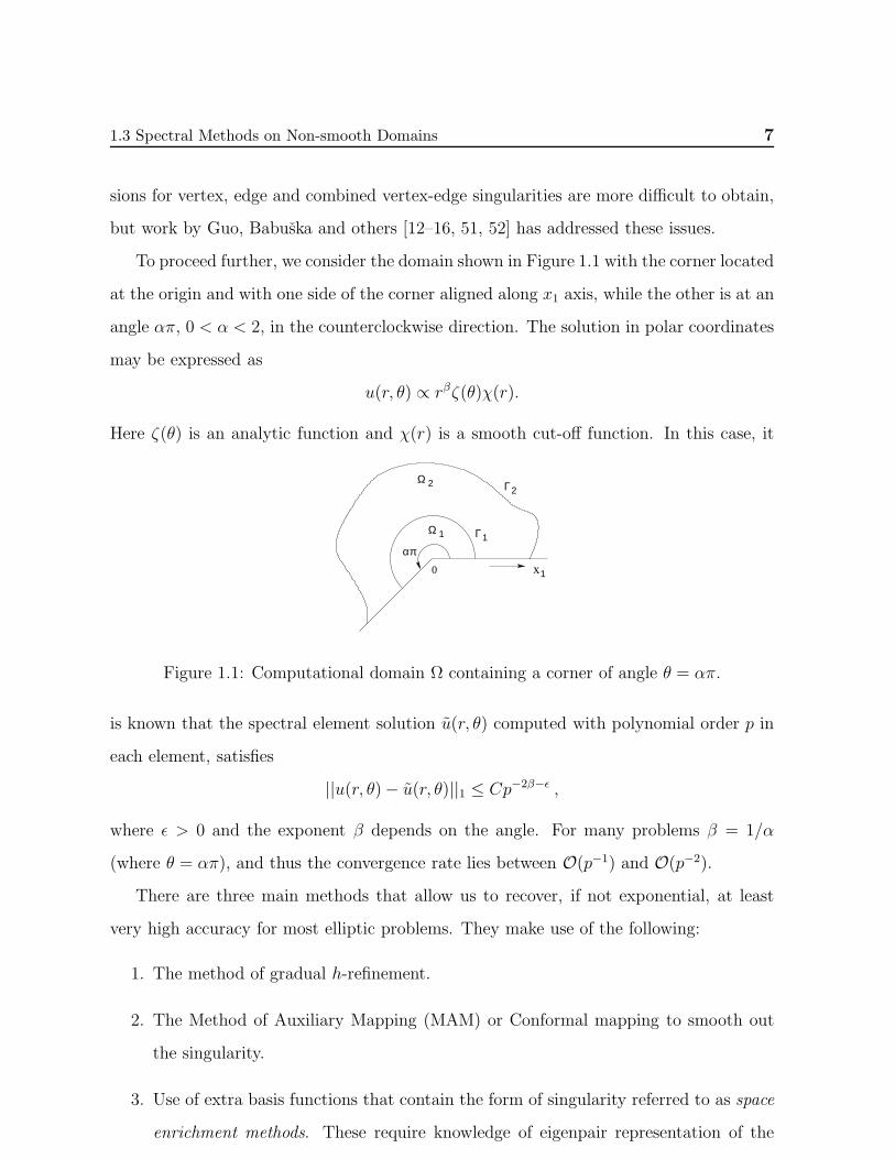
To proceed further, we consider the domain shown in Figure 1.1 with the corner located
at the origin and with one side of the corner aligned along x1 axis, while the other is at an
angle απ, 0 < α < 2, in the counterclockwise direction. The solution in polar coordinates
may be expressed as
u(r, θ) ∝ rβζ(θ)χ(r).
Here ζ(θ) is an analytic function and χ(r) is a smooth cut-off function. In this case, it
0
Ω
Ω
απ
2
1 Γ
Γ2
x1
1
Figure 1.1: Computational domain Ω containing a corner of angle θ = απ.
is known that the spectral element solution u(r, θ) computed with polynomial order p in
each element, satisfies
||u(r, θ)− u(r, θ)||1 ≤ Cp−2β−ǫ ,
where ǫ > 0 and the exponent β depends on the angle. For many problems β = 1/α
(where θ = απ), and thus the convergence rate lies between O(p−1) and O(p−2).
There are three main methods that allow us to recover, if not exponential, at least
very high accuracy for most elliptic problems. They make use of the following:
1. The method of gradual h-refinement.
2. The Method of Auxiliary Mapping (MAM) or Conformal mapping to smooth out
the singularity.
3. Use of extra basis functions that contain the form of singularity referred to as space
enrichment methods. These require knowledge of eigenpair representation of the
8 Introduction
solution.
1.3.1 Gradual h refinement
This approach requires the application of good discretization strategy which is usually
done using radial or geometrically refined meshes (see [19]) and quasi-uniform meshing.
A geometric progression has been found to be effective with a ratio of (√2 − 1)2 ≈ 0.17,
independent of the strength β of the singularity [48, 81]. However, in practice a value of
0.15 is typically adopted.
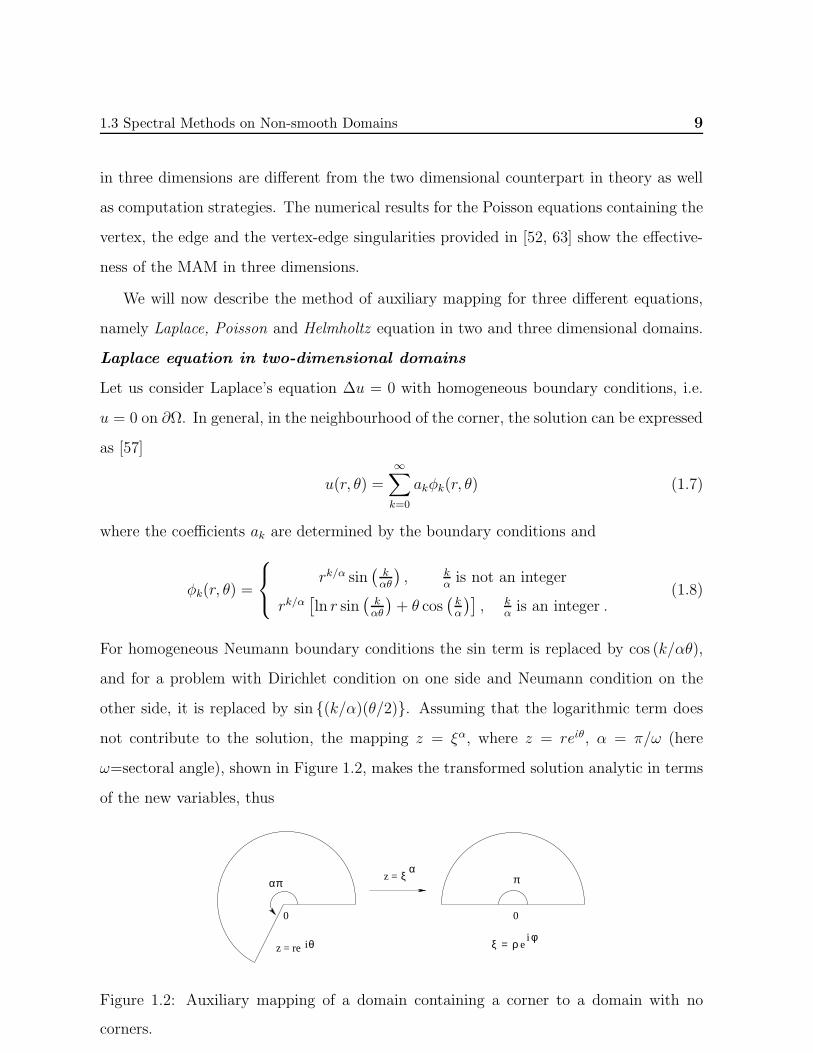
1.3.2 Method of auxiliary or conformal mapping
Babuska and Oh [17] introduced a new approach called the Method of Auxiliary Map-
ping (MAM), to deal with two dimensional elliptic boundary value problems containing
corner singularities. In two dimensions the method adopts an auxiliary mapping of the
type φ(z) = z1/α that maps a region where the solution is singular to a region where the
transformed solution has a higher regularity. Thus, on the mapped domain true solution
has better approximation properties. The method gives highly accurate numerical solu-
tions without destroying the standard band structure of FEM and without increasing the
number of degrees of freedom. The mapping is determined by the known nature of the
singularity in such a way that the exact solution of lower regularity can be transformed
to a function of higher regularity. The MAM, implemented in the p-version of the FEM,
has proven to be successful in dealing with all prominent singularities arising in the two
dimensional case [17, 65, 68, 69]. Benchmark comparisons with other well known numer-
ical methods, reported in [65], show that MAM is more efficient than other numerical
methods.
The MAM was successfully extended and implemented for elliptic PDEs on non-
smooth domains in R3 by Guo and Oh [52] and Lee et al. [63]. However, unlike the
two dimensional case, in R3 there are three different types of singularities, the vertex,
the edge and the vertex-edge. The solutions of three dimensional elliptic problems are
anisotropic in the neighbourhoods of edges and vertex-edges. Thus, the MAM techniques
1.3 Spectral Methods on Non-smooth Domains 9
in three dimensions are different from the two dimensional counterpart in theory as well
as computation strategies. The numerical results for the Poisson equations containing the
vertex, the edge and the vertex-edge singularities provided in [52, 63] show the effective-
ness of the MAM in three dimensions.
We will now describe the method of auxiliary mapping for three different equations,
namely Laplace, Poisson and Helmholtz equation in two and three dimensional domains.
Laplace equation in two-dimensional domains
Let us consider Laplace’s equation ∆u = 0 with homogeneous boundary conditions, i.e.
u = 0 on ∂Ω. In general, in the neighbourhood of the corner, the solution can be expressed
as [57]
u(r, θ) =
∞∑
k=0
akφk(r, θ) (1.7)
where the coefficients ak are determined by the boundary conditions and
φk(r, θ) =
rk/α sin(kαθ
), k
αis not an integer
rk/α[ln r sin
(kαθ
)+ θ cos
(kα
)], k
αis an integer .
(1.8)
For homogeneous Neumann boundary conditions the sin term is replaced by cos (k/αθ),
and for a problem with Dirichlet condition on one side and Neumann condition on the
other side, it is replaced by sin (k/α)(θ/2). Assuming that the logarithmic term does
not contribute to the solution, the mapping z = ξα, where z = reιθ, α = π/ω (here
ω=sectoral angle), shown in Figure 1.2, makes the transformed solution analytic in terms
of the new variables, thus
ξ = ρz = re θi eφ i
z = ξαπ π
0 0
α
Figure 1.2: Auxiliary mapping of a domain containing a corner to a domain with no
corners.
10 Introduction
u(r, θ) =∞∑
k=0
akrk/α sin
(k
αθ
)7→ u(ρ, φ) =
∞∑
k=0
akρk sin(kφ).
For the spectral/hp element discretization this method was first implemented in [17].
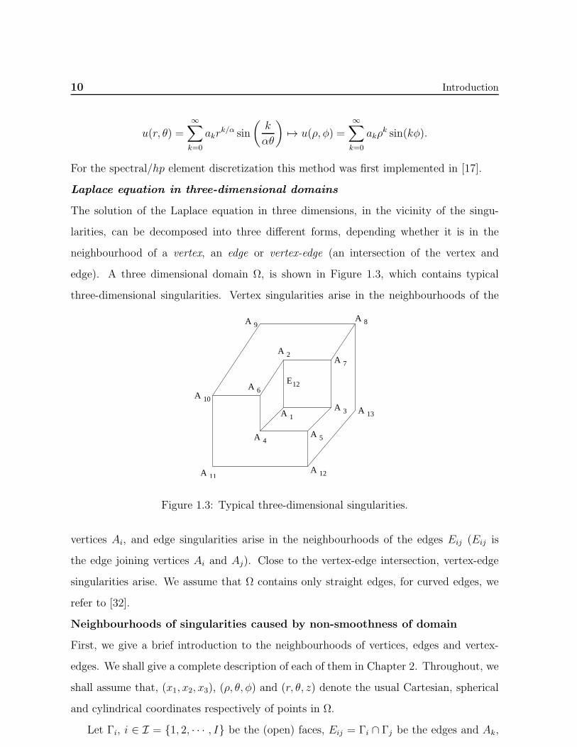
Laplace equation in three-dimensional domains
The solution of the Laplace equation in three dimensions, in the vicinity of the singu-
larities, can be decomposed into three different forms, depending whether it is in the
neighbourhood of a vertex, an edge or vertex-edge (an intersection of the vertex and
edge). A three dimensional domain Ω, is shown in Figure 1.3, which contains typical
three-dimensional singularities. Vertex singularities arise in the neighbourhoods of the
A
A
A
A
A
A
A
A A
A
A
A
1
2
3
4 5
6
7
89
A 10
11 12
13
E12
Figure 1.3: Typical three-dimensional singularities.
vertices Ai, and edge singularities arise in the neighbourhoods of the edges Eij (Eij is
the edge joining vertices Ai and Aj). Close to the vertex-edge intersection, vertex-edge
singularities arise. We assume that Ω contains only straight edges, for curved edges, we
refer to [32].
Neighbourhoods of singularities caused by non-smoothness of domain
First, we give a brief introduction to the neighbourhoods of vertices, edges and vertex-
edges. We shall give a complete description of each of them in Chapter 2. Throughout, we
shall assume that, (x1, x2, x3), (ρ, θ, φ) and (r, θ, z) denote the usual Cartesian, spherical
and cylindrical coordinates respectively of points in Ω.
Let Γi, i ∈ I = 1, 2, · · · , I be the (open) faces, Eij = Γi ∩ Γj be the edges and Ak,

1.3 Spectral Methods on Non-smooth Domains 11
k ∈ K = 1, 2, · · · , K be the vertices of Ω. We also denote a vertex by v and an edge
by e. Without loss of generality, we assume that the vertex v is located at the origin and
the edge coincides with the positive z-axis.
By Ωe we denote an edge-neighbourhood of the edge e = (r, θ, z)|r = 0, 0 < z < le oflength le, which is defined by
Ωe = (r, θ, z) ∈ Ω|0 < r < ǫ, δv < z < le − δv . (1.9)
Here ǫ < 1 and δv < 1 are selected so that Ωe ∩ Γi = ∅ for those faces Γi which do not
contain the edge e.
Consider a neighbourhood Ωvρv of the vertex v(=the origin) defined by
Ωvρv = (ρ, φ, θ) ∈ Ω|ρ < ρv.
Here 0 < ρv < 1 is chosen so that Ωvρv has a void intersection with those edges which do
not pass through the vertex v. Now we decompose Ωvρv into a vertex neighbourhood and
several vertex-edge neighbourhoods. We define, a vertex-edge neighbourhood of the vertex
v and edge e as:
Ωv−e = (ρ, φ, θ) ∈ Ωvρv |0 < φ < φv
where, 0 < φv and ρv < 1 are selected so that Ωv−e1 ∩Ωv−e2 = v for distinct edges e1 and
e2 having v as a common vertex.
A vertex-neighbourhood, Ωv, of the vertex v is defined by
Ωv = Ωvρv \⋃
e∈Ev
Ωv−e , (1.10)
where, Ev denote the set of all edges passing through the vertex v.
Intensities of vertex, edge and vertex-edge singularities
We now give a short outline of the singular solution decomposition in the neighbourhood
of a vertex, an edge, or at a vertex-edge intersection. For corresponding computational
results see [52, 63, 91]. For simplicity, we assume that in the vicinity of vertices or edges
of interest, homogeneous boundary conditions are imposed. The following asymptotic
expansions of the true solution are known:
12 Introduction
Vertex singularities
In a vertex neighbourhood Ωv of the vertex v, the solution has the vertex singularity and
admits an expansion of the form
u(ρ, φ, θ) =L∑
l=1
alργlhl(φ, θ) + v(ρ, φ, θ) , (1.11)
where (ρ, φ, θ) denotes usual spherical coordinates with origin at the vertex v, v(ρ, φ, θ) ∈H2(Ωv), hl(φ, θ) are analytic functions of φ and θ and are referred to as vertex eigenfunc-
tions, and γl is a positive real number (see [21, 45, 46]). In other words, in Ωv, the true
solution has a singularity of type ρλ1 , where λ1 < 1.
Edge singularities
In an edge neighbourhood Ωe of the edge e, the solution has the edge singularity and can
be decomposed as follows:
u(r, θ, z) =M∑
m=1
am(z)rβmhm(θ) + v(r, θ, z) , (1.12)
where (r, θ, z) denotes usual cylindrical coordinates, and the functions am(z) are analytic
in z. The functions v(r, θ, z) ∈ H2(Ωe), hm(θ) are also analytic and hm(θ) are referred to
as edge eigenfunctions (see [21, 45, 88]). In other words, in Ωe, the true solution has a
singularity of type rλ2 , where λ2 < 1.
Vertex-edge singularities
The most complicated decomposition of the solution arises in the case of a vertex-edge
intersection. For example, let us consider the neighbourhood where the edge e approaches
the vertex v. The resulting vertex-edge neighbourhood is denoted by Ωv−e, and the
solution has a singularity caused by the combination of edges and a vertex and has an
expansion of the form
u(ρ, φ, θ) =M∑
m=1
(L∑
l=1
amlργl + fm(ρ)
)(sin φ)βmgm(θ)
+L∑
l=1
alργlhl(φ, θ) + v(ρ, φ, θ) , (1.13)
where the functions fm(ρ) are analytic in ρ, and gm(θ), hl(φ, θ) and v(ρ, φ, θ) ∈ H2(Ωv−e)
are also analytic (see [45–47, 88]). That is, in Ωv−e, the true solution has a singularity of
1.3 Spectral Methods on Non-smooth Domains 13
type ρλ3(sinφ)λ4 , where λ3 < 1 and λ4 < 1.
Poisson equation
The situation becomes more complicated when a forcing function is introduced as in
Poisson’s equation
−∆u = f(x) .
The convergence achieved through auxiliary mapping is no better than algebraic because
the solution may not be analytic after the mapping. Typically, we decompose the solution
into a homogeneous part uH, which has the singularity, and a particular part uP , which
depends on the forcing. Complications arise due to particular part since, even if it is
smooth in the original domain, it may be singular after the transformation. For instance,
consider the following transformed equation which has a singular forcing function
∆u = α2ρ2α−2f(ρ, φ) .
Given the O(ρ−2α) singularity, the spectral element convergence is of the order O(ρ−4α−ǫ)
for any ǫ > 0. In order to enhance the convergence, we separate the two contributions so
that we have an analytic contribution in the z-plane and an analytic contribution in the
ξ-plane.
Helmholtz equation
For the Helmholtz equation
∆u− λu = f(x), λ > 0 ,
the conformal mapping is an effective way of improving convergence, although exponential
convergence cannot be fully recovered. The auxiliary mapping z = ξα, α = ω/π, 0 < α <
2 converts the Helmholtz equation to
∆u− λα2ρ2α−2u = α2ρ2α−2f .
In terms of the original variables, the solution around the corner is
u(r, θ) =∞∑
k=0
akIk/α(√λr) sin
(k
αθ
),
14 Introduction
for k/α not an integer, where I(z) represent the modified Bessel function of the first kind.
After application of the mapping, the solution has the form
u(r, θ) =∞∑
k=0
akρk sin(kθ)
∞∑
j=0
cjρ2jα ,
with a leading singular term of order ρ1+2α. Therefore, the estimated convergence rate is
O(ρ−2−4α−ǫ), which in practise, is adequately fast, though algebraic.
Similar to the Poisson equation, in three dimension there are three different types of
singularities namely, the vertex, the edge and the combined vertex-edge. Furthermore,
solutions of elliptic problems are anisotropic in the neighbourhood of edges and vertex-
edges. However, it is possible to obtain explicitly the form of such singularities [51],
and thus the auxiliary mapping technique can be effectively used in three dimensions.
The difference is that specific auxiliary mappings are required to handle each type of
singularity. Lee et al. [63] have obtained and implemented these mappings successfully for
treating all three types of singularities. The effectiveness of this method was demonstrated
on two polyhedral domains. The results with the mapping method were superior to those
obtained with the p-version of FEM [81] or other low-order methods.
Singular Basis
An alternative approach to using the auxiliary mapping is to use a set of supplementary
basis functions which have the leading behavior of the singularity in conjunction with the
smooth basis Φk(x). For the Helmholtz equation the leading-order singular terms are
r1/α, r2/α(α > 1/2), r3/α(α > 1), · · · ,
which can be included into the expansion basis. However, we can do even better by
supplementing the standard basis in the mapped domain. The transformed solution is
then
u(ρ, φ) =
∞∑
k=1
akIk/α(√λρα) sin(kφ) =
∞∑
k=1
∞∑
l=0
bklρk+2lα sin(kφ), (1.14)
and thus the leading singularities are weaker, i.e.,
ρ1+2α, ρ2+2α(α > 1/2), ρ1+4α, · · · .
1.3 Spectral Methods on Non-smooth Domains 15
A comparison of the effect of adding supplementary basis terms in the original and the
transformed domain is given in [55, 73]. It has been shown in [73] that with one or two
terms included in the transformed domain, a very fast convergence is obtained. To achieve
the exponential accuracy we need to include higher order terms but in the limiting case the
system becomes ill-conditioned as the augmented basis Φ1,Φ2, · · · ,ΦN , ϕ1, ϕ2, · · · , ϕMis nearly linearly dependent if many singular functions are used and as a result the stiffness
matrix is ill-conditioned.
Eigenpair representation: Steklov formulation
A more recent method that treats singular solutions of both scalar and vector elliptic
problems in the neighbourhood of corners was presented for two-dimensional domains by
Yosibash and Szabo [82, 92] and for three-dimensional domains by Yosibash in [90, 91].
As we have already seen, such singular solutions are characterized by the form u = rβh(θ)
close to the corner.
Let us illustrate the basic characteristics of the solution to the Laplace problem over
a two-dimensional domain as shown in Figure 1.2. The Laplace equation over Ω2, with
Dirichlet boundary conditions on its boundary, is cast in cylindrical coordinates as follows:
∆u =∂2u
∂r2+
1
r
∂u
∂r+
1
r2∂2u
∂θ2in Ω2 . (1.15)
The solution in the vicinity of the singular point is sought by separation of variables. We
denote by h+(θ) and h−(θ) the functions associated with the positive and negative values
of β respectively. Although for the Laplace equation h+(θ) ≡ h−(θ), for a general elliptic
equation this is not the case. Thus, the solution to (1.15) admits the expansion
u =∞∑
i=1
airβih+i (θ), h
+i (θ) = sin(βiθ), with βi =
i
α, (1.16)
where βi and hi(θ) denote eigenpairs, and these are determined uniformly by the geometry
and boundary conditions in the neighbourhood of the singular point. Notice that if βi < 1
then the corresponding ith term in the expansion (1.16) for ∇u is unbounded as r → 0.
We say that u is singular at 0 if ∇u tends to infinity as r → 0. The solution u in (1.16)
is therefore singular at 0 if α > 1 for i = 1, . . . , finitely many. The coefficients ai depend
16 Introduction
on the boundary conditions away from the singular points as well as the forcing term in
the Poisson equation.
For general singular points, analytical computation of eigenpairs is not practical, and
numerical approximations are usually sought. One of the most robust and efficient meth-
ods for the computation of eigenpairs is the modified Steklov method, developed by Yosi-
bash [91] and Yosibash and Szabo [92].
1.3.3 Advantages and applications of spectral methods: A sur-
vey
We now briefly describe important features of spectral methods that should be considered
in their formulation and application [44].
1. Rate of convergence : If the solution to a problem is analytic then a properly de-
signed spectral method gives exponential accuracy in contrast to FDM and FEM
which yield finite-order rates of convergence. The important consequence is that
spectral methods can achieve high accuracy with little more resolution than is re-
quired to achieve moderate accuracy in FDM and FEM.
2. Efficiency : In order to be useful the spectral method should be as efficient as dif-
ference methods with comparable number of degrees of freedom. The development
of collocation (pseudospectral) and Galerkin methods permits spectral methods to
be implemented with comparable efficiency to that of FDM with the same num-
ber of independent degrees of freedom. As the required accuracy increases, the
attractiveness of spectral methods increase.
3. Boundary conditions : The mathematical features of spectral methods follow very
closely those of the partial differential equation being solved. Thus the bound-
ary conditions imposed on spectral approximations are normally the same as those
imposed on the differential equation. In contrast, FDM of higher order than the
differential equation require additional “boundary conditions”. Many of the com-
1.3 Spectral Methods on Non-smooth Domains 17
plications of finite-order FDM disappear with the infinite-order-accurate spectral
methods.
Another aspect of the treatment of boundary conditions by spectral methods is their
high resolution of boundary layers. For details we refer to [44, 72].
4. Bootstrap estimation of accuracy : It is often possible to estimate the accuracy of
spectral computations by examination of the shape of the spectrum. Thus, in com-
putations of three-dimensional incompressible flows at high Reynolds numbers, the
mean-square vorticity spectrum must not increase abruptly at large wave numbers.
If the vorticity spectrum decreases smoothly to zero as wave number increases, it is
safe to infer that the calculation is accurate. On the other hand, similar criteria for
finite-difference methods can be misleading.
Let us now survey some applications of spectral methods. We shall classify the method
according to geometry and boundary conditions.
1. Periodic boundary conditions in Cartesian coordinates : Here Fourier series should
be used. Spectral methods have been regularly used in three-dimensions to simulate
homogeneous turbulence using high resolution codes. Most operational codes now
use pseudospectral methods because aliasing errors are usually small.
2. Rigid boundary conditions in Cartesian coordinates : Use of Chebyshev or Legen-
dre polynomials is appropriate is this case. Typical applications include numerical
studies of turbulent shear flows and boundary layer transition.
3. Rigid boundary conditions in Cylindrical geometry : Chebyshev or Legendre poly-
nomials should be used in radial, Fourier series in angular, and either Fourier or
Chebyshev series in the axial direction (depending on boundary conditions).
4. Problems in spherical geometry : Here surface harmonic expansions, generalized
Fourier series, and “associated” Chebyshev expansions all have attractive features.
5. Semi-infinite or infinite geometry : In this case Chebyshev expansions are best
if the domain can be mapped or truncated to a finite domain without serious error.
18 Introduction
There are two cases to be considered: additional boundary conditions may or may
not be required at “infinity”. If additional boundary conditions, such as radiation
or outflow boundary conditions, must be imposed on the truncated domain, then
they should also be applied to the spectral method. On the other hand, if map-
ping without additional boundary conditions does not introduce a singularity in the
exact equations, no boundary conditions at “infinity” are required in the spectral
approximation.
1.3.4 Limitations of spectral methods
The drawbacks of spectral methods are four fold.
1. The main drawback is their inability to handle complex geometries. Different strate-
gies are, however, possible to overcome this difficulty. The idea to couple domain
decomposition techniques to the spectral discretization has been successful in over-
coming this drawback (S. A. Orszag [72]).
2. They are usually more difficult to program than finite difference methods.
3. They are more costly per degrees of freedom than other low-order methods.
1.4 Finite Element Method
The Finite Element Method (FEM) is one of the most widely used numerical methods
for obtaining approximate solutions to a large variety of engineering problems. Although
originally developed for numerical solution of complex problems in structural mechanics,
it has since been extended and applied to the broad field of continuum mechanics. Though
the term finite element was first coined by Clough [30] in 1960 in a paper on plane elasticity
problems, the ideas of finite element analysis date back much further and can be traced
back to the work by Alexander Hrennikoff (1941) and Richard Courant (1942). In the
early 1960s, engineers used the method for approximate solutions of problems in a wide
1.4 Finite Element Method 19
variety of engineering problems such as stress analysis, fluid flow, heat transfer, and other
areas. The first book on the FEM by Zienkiewicz and Chung [93] was published in 1967.
The underlying premise of the method states that a complicated domain can be sub-
divided into a series of smaller regions in which the differential equations are approx-
imately solved. By assembling the set of equations for each region, the behavior over
the entire problem domain is determined. Each region is referred to as an element and
the process of subdividing a domain into a finite number of elements is referred to as
discretization. Elements are connected at specific points, called nodes, and the assembly
process requires that the solution be continuous along common boundaries of adjacent
elements.
When more accuracy is needed, the finite element method has three different versions,
namely h version, p version and h − p version. In the h version, mesh size h is reduced
and polynomials of fixed degree p are used to increase accuracy. In the p version mesh
size h is kept fixed while polynomial degree p is raised. In the h− p version the mesh size
h is reduced and the polynomial degree p is raised simultaneously within the elements
either uniformly over the entire computational domain or selectively depending on the
resolution requirements.
Finite element method is a variational method of approximation, making use of global
or variational statements of physical problems and employing the Rayleigh-Ritz-Galerkin
philosophy of constructing co-ordinate functions whose linear combinations represent the
unknown solutions. It took approximately a decade before the method was recognized as
a form of the Rayleigh-Ritz method. The relation between these two techniques comes
from considering the variational form of a given problem. For instance, the quadratic
functional
F(u) =∫ 1
0
[p(x)(u′(x))2 + q(x)(u(x))2 − 2f(x)u(x)]dx (1.17)
has a minimum with respect to a variation in u(x) given by the Euler equation
− d
dx
(p(x)
du(x)
dx
)+ q(x)u(x) = f(x). (1.18)
Therefore, instead of solving for (1.18) to determine u(x), an alternative but equivalent
20 Introduction
way is to find u(x) which minimizes the functional (1.17).
The Rayleigh-Ritz idea approximates the solution by a finite number of functions
u(x) =∑N
i=1 αiΦi(x) to determine the unknown weights αi, which minimize the functional
(1.17). In the FEM the solution is also approximated by a finite number of functions,
which are typically local in nature as opposed to the global functions used in the Rayleigh-
Ritz approach. However, the starting point for a finite element method is the differential
equation (1.18), which is formulated into an integral form (also known as Galerkin for-
mulation) so that the problem reduces to an algebraic system of equations which can be
solved numerically. This connection between the two methods was made when it was
realized that the integral form of the FEM was exactly same as the functional form used
in the Rayleigh-Ritz method.
This relation between the FEM and Rayleigh-Ritz method was very significant and
it made the finite element technique mathematically respectable. A more general for-
mulation is possible using the method of weighted residuals which leads to the standard
Galerkin formulation.
1.4.1 Method of weighted residuals
The origin of the Method of Weighted Residuals (MWR) dates back prior to development
of the finite element method. The method illustrates how the choice of different test (or
weight) functions may be used to produce many commonly used numerical methods for
solving differential equations.
Suppose we have a linear differential operator L acting on a function u as follows:
L(u(x)) = f(x) for x ∈ Ω.
We wish to approximate u by a function u, which is a linear combination of basis functions
chosen from a linearly independent set. That is,
u ≈ u =
n∑
j=1
ajΦj . (1.19)
Now, when substituted into the differential operator, L, the result of the operations is
1.4 Finite Element Method 21
not, in general, f(x). Hence an error or residual will exist. Define
R(x) = L(u(x))− f(x). (1.20)
The notion in the MWR is to force the residual to zero in some average sense over the
domain Ω. That is, ∫
Ω
R(x)wj(x)dx = 0, j = 1, 2, · · · , n (1.21)
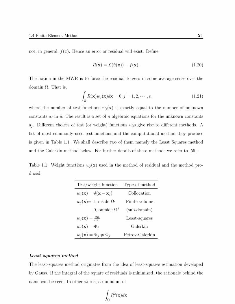
where the number of test functions wj(x) is exactly equal to the number of unknown
constants aj in u. The result is a set of n algebraic equations for the unknown constants
aj . Different choices of test (or weight) functions w′js give rise to different methods. A
list of most commonly used test functions and the computational method they produce
is given in Table 1.1. We shall describe two of them namely the Least Squares method
and the Galerkin method below. For further details of these methods we refer to [55].
Table 1.1: Weight functions wj(x) used in the method of residual and the method pro-
duced.
Test/weight function Type of method
wj(x) = δ(x− xj) Collocation
wj(x)= 1, inside Ωj Finite volume
0, outside Ωj (sub-domain)
wj(x) =∂R∂uj
Least-squares
wj(x) = Φj Galerkin
wj(x) = Ψj 6= Φj Petrov-Galerkin
Least-squares method
The least-squares method originates from the idea of least-squares estimation developed
by Gauss. If the integral of the square of residuals is minimized, the rationale behind the
name can be seen. In other words, a minimum of
∫
Ω
R2(x)dx
22 Introduction
is achieved. Therefore the weight functions for the least-squares method are just the
derivatives of the residual with respect to the unknown constants:
wj(x) =∂R
∂aj.
This formulation using a spectral/hp element discretization has recently increased in pop-
ularity [53, 74, 75].
Galerkin method
This method (also known as Bubnov-Galerkin method) may be viewed as a modification
of the least-squares method. Rather than using the derivative of the residual with respect
to the unknown aj , the derivative of the approximating function is used. It turns out that
the weight/test functions are same as the trial functions. That is,
wj(x) =∂u
∂aj= Φj(x) .
1.4.2 Advantages of FEM
1. Finite element methods convert differential equations into matrix equations that are
sparse because only a handful of basis functions are non-zero in a given sub-interval.
Sparsity of matrix equations allows the stiffness matrix to be stored and inverted
easily thus saving a lot of computational cost.
2. In multi-dimensional problems, the sub-intervals become triangles (in 2D) or tetra-
hedra (in 3D) which can be fitted to irregularly-shaped geometries such as the shell
of an automobile etc.
3. The major advantages of the FEM over FDM and other low-order methods are its
built-in abilities to handle unstructured meshes, a rich family of element choices,
and natural handling of boundary conditions.
4. FEM can handle a wide variety of engineering problems such as problems in solid
mechanics, dynamics, fluids, heat conduction and electrostatics.
1.4 Finite Element Method 23
1.4.3 Disadvantages of FEM
1. Finite element methods are not well suited for open region problems.
2. They suffer low accuracy (for a given number of degrees of freedom N) because each
basis function is a polynomial of low degree.
1.4.4 Spectral vs. finite element methods
Spectral methods are similar to finite element methods in philosophy; the major difference
is that in finite element methods we choose Φn(x) to be local functions which are poly-
nomials of fixed degree and are non-zero only over a couple of sub-intervals. In contrast,
spectral methods use global basis functions in which Φn(x) is a polynomial (or trigono-
metric polynomial) of high degree which is non-zero, except at isolated points, over the
entire computational domain.
Finite element methods convert differential equations into matrix equations that are
sparse because only a handful of basis functions are non-zero in a given sub-interval.
Spectral methods generate algebraic equations with full matrices, but in compensation,
the higher order of the basis functions give high accuracy for a given N . When fast
iterative matrix solvers are used, spectral methods can be much more efficient than FEM
or FDM methods for many classes of problems. However, they are most useful when the
geometry of the problem is fairly smooth and regular.
Spectral Element Methods gain the best of both worlds by hybridizing spectral and
finite element methods. The domain is subdivided into elements, as in finite elements, to
gain the flexibility and matrix sparsity of finite elements. At the same time, the degree of
the polynomial p in each sub-domain is sufficiently high to retain the high accuracy and
low storage of spectral methods.
24 Introduction
1.5 Non-conforming Methods
The formulations presented so far deal with conforming elements where vertices of ad-
joining elements coincide, and correspondingly a C0 continuity condition is satisfied at
the element interfaces. However, design over complex domains often require to refine
the mesh locally. For example, to resolve the geometric singularity in a flow past a half-
cylinder it is desirable to contain the mesh refinement locally as needed and not propagate
the mesh changes globally. Such local refinement is particularly useful in increasing the
computational efficiency of direct and large eddy simulations of turbulent flows.
Non-conforming methods can be used to decompose and recompose such complex do-
mains into sub-domains without requiring the compatibility between the meshes on the
separate components. That is, we will no longer require that the vertices of the adjoining
elements coincide. Instead, we will develop a framework that allows for arbitrary connec-
tion between elements. An added advantage of this idea is that the mesh refinement can
be imposed selectively on the components where it is required. We now present a brief
summary of commonly used non-conforming methods which allow for arbitrary connection
between elements and are highly suitable for parallel implementation (for details see [55]):
Iterative patching
This formulation employs geometrically non-conforming elements but maintains C0
continuity of the global polynomial expansion.
Constrained approximation
The method of constrained approximation was introduced by Oden and his asso-
ciates [34, 67, 76] to deal with geometrically non-conforming discretizations introduced
by refinement. The main idea is to maintain C0 continuity across elemental interfaces by
modifying the unconstrained basis functions appropriately. In other words, the approxi-
mation space is a constrained space which is a subset of H1(Ω) for second order elliptic
problems.
1.6 h− p/Spectral Element Methods on Parallel Computers 25
Mortar element method
In this method C0 continuity is no longer imposed and new weak forms of the problem
are developed. This method was first introduced by Patera and co-workers [2, 22, 66],
who coined the term ‘mortar element methods ’ because the discretization introduces a
set of functions that mortar the brick-like elements together. The method generalizes the
SEM to geometrically nonconforming partitions, to sub-domains with different resolutions
(polynomial degrees) on sub-domain interfaces and allows for the coupling of variational
discretizations of different types in non-overlapping domains, that is, the non-conformity
may be due to geometry, approximation spaces, or both.
Discontinuous Galerkin method
Similar to mortar element method we do not require C0 continuity in this method.
Although original application of most discontinuous Galerkin methods (DGM) was in
solving hyperbolic problems, more recent work has led to formulations for parabolic and
elliptic problems [31]. In an effort to classify all contributions made toward the use of
discontinuous Galerkin methods for elliptic problems, Arnold et al., first in [4] and then
in more generality in [5], published a unified analysis of discontinuous Galerkin methods
for elliptic problems.
1.6 h−p/Spectral Element Methods on Parallel Com-
puters
Spectral element methods function very well on massively parallel machines. One can
assign a single large element with a high order polynomial approximation within it to
a single processor. A three dimensional element of degree N roughly has N3 internal
degrees of freedom, but the number of grid points on its boundary is O(6N2). It is these
boundary values that must be shared with other elements i.e., other processors, so that
the numerical solution is continuous everywhere. As N increases, the ratio of internal grid
points to the boundary grid points increases, implying that more and more of the compu-
26 Introduction
tations are internal to the element, and the shared boundary values become smaller and
smaller compared to the total number of unknowns. This in turn implies inter-processor
communication to be small. To do the same calculation with lower order methods, one
would need roughly eight times as many degrees of freedom in three dimensions. That
would increase the inter-processor communication load by at least a factor of four.
An exponentially accurate h− p/spectral element method for solving two dimensional
general elliptic problems with mixed Neumann and Dirichlet boundary conditions on non-
smooth domains using parallel computers was proposed in [37–39, 84–86]. To resolve the
singularities which arise at the corners an auxiliary map of the form z = log ξ is used
along with a geometric mesh at the corners. In a neighbourhood of the corners, modified
polar coordinates (τk, θk) are used, where τk = ln rk and (rk, θk) denote polar coordinates
with origin at the vertex Ak. Away from the sectoral neighbourhoods of the corners the
usual coordinate system (x1, x2) is used.
With this mesh a numerical method was proposed as follows:
Find a solution which minimizes “the sum of the weighted squared norm of the residuals
in the partial differenital equation and the squared norm of the residuals in the boundary
conditions in fractional Sobolev norms and enforce continuity by adding a term which
measures the jump in the function and its derivatives at inter-element boundaries, in
appropriate Sobolev norms.
The method is a least-squares method and the solution can be obtained by solving the
normal equations using the preconditioned conjugate gradient method (PCGM) without
computing the mass and stiffness matrices [38, 39, 86]. Let N denote the number of layers
in the geometric mesh. Then the method requires O(N lnN) iterations of the PCGM to
obtain the solution to exponential accuracy.
1.7 Review of Existing Work
The h− p version of the finite element method (FEM) for elliptic problems was proposed
by Babuska and his coworkers in the mid 80ies. They unified the hitherto largely separate
1.7 Review of Existing Work 27
developments of fixed order “h-version FEM” in the sense of Ciarlet, which achieve con-
vergence through reduction of the mesh size h, and the so-called “spectral (or p-version)
FEM” achieving convergence through increasing polynomial order p on a fixed mesh.
Apart from unifying these two approaches, a key new feature of hp-FEM was the possi-
bility to achieve exponential convergence in terms of number of degrees of freedom N . A
method for obtaining a numerical solution to exponential accuracy for elliptic problems
in one dimension was first proposed by Babuska and Gui in [48] within the framework
of hp-FEM. Exponential convergence results were shown for the model singular solution
u(x) = xα − x ∈ H10 (Ω) in Ω = (0, 1). Specifically, the error was shown to be bounded
by e−b√Ndof , Ndof is the number of degrees of freedom. This result required σ-geometric
meshes with a fixed mesh ratio σ ∈ (0, 1) while the constant b in the convergence estimate
depends on the singularity exponent α as well as on σ. Among all σ ∈ (0, 1), the optimal
value was shown to be σopt = (√2− 1)2 ≈ 0.17.
In two dimensions, exponential convergence (an upper bound Ce−b3√Ndof ) on the error
for elliptic problems posed on polygonal domains was obtained by Babuska and Guo in
the mid 80ies in a series of landmark papers [8–10]. Key ingredients in the proof were
geometric mesh refinements towards the corners and nonuniform elemental polynomial
degrees which increase linearly with the elements’ distance from corners. We remark that
the proof of elliptic regularity results in terms of countably normed spaces, which con-
stitutes an essential component of the exponential convergence proof, has been a major
technical achievement. This problem has also been examined by Karniadakis and Sher-
win in [55] and Pathria and Karniadakis in [55, 73] in the frame work of spectral/h − pelement methods. In [37–39, 84–86] h − p spectral element methods for solving general
elliptic problems to exponential accuracy on polygonal domains using parallel computers
were proposed. More recently the case of elliptic systems was analyzed in [60] for non-
conforming spectral element functions. Key ingredients were use of geometric mesh at
the corners and use of auxiliary mapping to remove the singularity at the corners. Com-
putational results for least-squares h − p/spectral element method for elliptic problems
on non-smooth domains with monotone singularities of the type rα and rα logδ r as well
28 Introduction
as the oscillating singularities of the type rα sin(ǫ log r) have been obtained in [61].
Starting in the 90ies, efforts to extend the analytic regularity and the hp-convergence
analysis of two dimensional problems to three dimensions in the frame work of finite
element methods were undertaken in [13–15, 49] and the references therein which include
related works in the subject. hp-version of discontinuous Galerkin finite element method
(hp-DGFEM) for second order elliptic problems with piecewise analytic data in three
dimensional polyhedral domains has been analyzed by Schotzau et al. [77, 78]. The
method is shown to be exponentially accurate.
1.8 Review and Outline of the Thesis
As discussed earlier, current formulations of spectral methods to solve elliptic problems on
non-smooth domains allow us to recover only algebraic convergence [28, 55]. The method
of auxiliary mapping, which yields relatively fast convergence makes use of a conformal
mapping of the form ξ = z1/α that maps a neighbourhood of the singularity point (where
the true solution is singular) onto a domain where the true solution is smooth and has
better approximation properties, i.e. we smooth out the singularity that occurs at the
corners [55] using auxiliary map.
In this thesis, we propose an exponentially accurate h−p spectral element method for
elliptic problems on non-smooth polyhedral domains in R3.
In contrast to the two dimensional case, in three dimensions the character of the sin-
gularities is much more complex, not only because of higher dimension but also due to the
different nature of the singularities which are the vertex singularity, the edge singularity
and the vertex-edge singularity. Thus we have to distinguish between the behaviour of
the solution in the neighbourhoods of the vertices, edges and vertex-edges. Unlike the
two dimensional case where weighted isotropic spaces are used, in three dimensions we
have to utilize weighted anisotropic spaces because the solution is smooth along the edges
but singular in the direction perpendicular to the edges [13]. Behaviour of the solution is
even more complex at the vertices where the edges are joined together and the solution
1.8 Review and Outline of the Thesis 29
is not smooth along the edges too.
To overcome the singularities which arise in the neighbourhoods of the vertices, vertex-
edges and edges we use local systems of coordinates. These local coordinates are modified
versions of spherical and cylindrical coordinate systems in their respective neighbour-
hoods. Away from these neighbourhoods standard Cartesian coordinates are used in the
regular region of the polyhedron. In each of these neighbourhoods we use a geometrical
mesh which becomes finer near the corners and edges.
With this mesh we choose our approximate solution as the spectral element function
which minimizes the sum of a weighted squared norm of the residuals in the partial
differential equations and the squared norm of the residuals in the boundary conditions
in fractional Sobolev spaces and enforce continuity by adding a term which measures the
jump in the function and its derivatives at inter-element boundaries in fractional Sobolev
norms, to the functional being minimized. The Sobolev spaces in vertex-edge and edge
neighbourhoods are anisotropic and become singular at the corners and edges.
We then derive differentiability estimates with respect to these new coordinates in
the neighbourhoods of vertices, edges and vertex-edges and in the regular region of the
polyhedron where we retain standard Cartesian coordinate system.
The spectral element functions are represented by a uniform constant at all the corner
elements in vertex neighborhoods and on the corner-most elements in vertex-edge neigh-
bourhoods which are in the direction transverse to the edges of the polyhedron. At corner
elements which are in the direction of edges in vertex-edge neighbourhoods and at all the
corner elements in edge neighbourhoods the spectral element functions are represented
as one dimensional polynomials of degree W in the modified coordinates. In all other
elements in edge neighbourhoods and vertex-edge neighbourhoods the spectral element
functions are a sum of tensor products of polynomials of degreeW in their respective mod-
ified coordinates. The remaining elements in the vertex neighbourhoods and the regular
region are mapped to the master cube and the spectral element functions are represented
as a sum of tensor products of polynomials of degree W in λ1, λ2, and λ3, the transformed
variables on the master cube.
30 Introduction
A stability estimate is then derived for the functional we minimize. We use the stability
estimate to obtain parallel preconditioners and error estimates for the solution of the
minimization problem. Let N denote the number of refinements in the geometrical mesh.
We shall assume that N in proportional toW . Then for problems with Dirichlet boundary
conditions the condition number of the preconditioned system is O((lnW )2) provided
W = O(eNα) for α < 1/2. Moreover it is shown that there exists a new preconditioner
which can be diagonalized in a new set of basis functions using separation of variables
techniques in which each diagonal block corresponds to a different element, and hence it
can easily be inverted on each element. Moreover, if the data is analytic then the error is
exponentially small in N .
For mixed problems the condition number grows like O(N4). The rapid growth of
the factor N4 creates difficulties in parallelizing the numerical scheme. To overcome this
difficulty another version of the method may be defined in which we choose our spectral
element functions to be conforming on the wirebasket (union of vertices and edges) of
elements. It can be shown that a probing parallel preconditioner can be defined for the
minimization problem using the stability estimates which allows the problem to decouple.
We intend to study this in the future.
The method is essentially a least-squares collocation method and a solution can be
obtained using Preconditioned Conjugate Gradient Method (PCGM). To solve the mini-
mization problem we need to solve the normal equations for the least−squares problem.
The residuals in the normal equations can be obtained without computing and storing
mass and stiffness matrices.
For Dirichlet problems we use spectral element functions which are non-conforming
and hence there are no common boundary values. For problems with mixed boundary
conditions the spectral element functions are essentially non-conforming except that they
are continuous only at the wirebasket of the elements. Hence the cardinality of the set of
common boundary values which is equal to the values of the function at the wirebasket
of the elements is much smaller than the cardinality of the common boundary values for
the standard finite element method and so we can compute an accurate approximation
1.8 Review and Outline of the Thesis 31
to the Schur complement matrix. In this dissertation we examine the non-conforming
version of the method. The case when the spectral element functions are conforming on
the wirebasket will be examined in future work.
The method requires O(NlnN) iterations of the PCGM to obtain the solution to
exponential accuracy and requires O(N5ln(N)) operations on a parallel computer with
O(N2) processors for Dirichlet problems. However, for mixed problems it would require
O(N3) iterations of the PCGM to obtain solution to exponential accuracy and O(N7)
operations on a parallel computer with O(N2) processors.
Our method works for non self-adjoint problems too. Results of numerical simulations
for a number of model problems on non-smooth domains are presented with constant
and variable coefficients including the non self-adjoint case which confirm the theoretical
estimates obtained for the error and computational complexity.
We remark here that once we have obtained our approximate solution, consisting of
non-conforming spectral element functions, we can make a correction to the approximate
solution so that the corrected solution is conforming and the error between the corrected
and exact solution is exponentially small in N in the H1 norm over the whole domain.
We now briefly describe the contents of the thesis which is divided into six chapters.
Chapter 1 provides brief descriptions of different methods, namely spectral and finite
element methods, with advantages and disadvantages. Basic properties of these
methods are discussed. An overview of the existing work is also provided.
Chapter 2 introduces the problem under consideration. We define various neighbour-
hoods of vertices, edges and vertex-edges and then derive the differentiability es-
timates and introduce the function spaces in these neighbourhoods which will be
needed in what follows. The main stability estimates are stated here.
Chapter 3 gives the proof of the stability theorem on which our method is based.
Chapter 4 presents the numerical scheme which is based on the stability estimates of
Chapter 2 and error estimates for the approximate solution are obtained.
32 Introduction
Chapter 5 provides preconditioning and parallelization techniques. It is shown that a
preconditioner can be defined for the quadratic form corresponding to the mini-
mization problem which allows the problem to decouple. It is also shown that there
exists another preconditioner which can be diagonalized in a new basis using the
separation of variables technique. Lastly, it briefly describes the steps to compute
the residual.
Chapter 6 gives numerical results to validate the error estimates and bounds on com-
putational complexity. We also briefly outline our plan for future work here.
Chapter 2
Differentiability and Stability
Estimates
2.1 Introduction
In this chapter we shall obtain differentiability estimates and stability estimates for a gen-
eral elliptic boundary value problem posed on a polyhedral domain with mixed Dirichlet
and Neumann boundary conditions. To resolve the singularities which arise at the corners
and edges namely, the vertex, vertex-edge and edge singularities we use geometrical meshes
which become finer near corners and edges. In the neighbourhood of vertices, vertex-edges
and edges we switch to local systems of coordinates (auxiliary mappings). In doing this
the geometrical mesh is reduced to a quasi-uniform mesh and hence Sobolev’s embedding
theorems and trace theorems for Sobolev spaces apply for functions defined on mesh ele-
ments in these new variables with a uniform constant. Away from these neighbourhoods
we retain standard Cartesian coordinates in the regular region of the polydehron. The
use of auxiliary mappings together with geometrical meshes to overcome the singularities
along corners and edges allows us to obtain the solution with exponential accuracy. We
remark that the local systems of coordinates which we use are modified versions of spher-
ical and cylindrical coordinates in the vertex and edge neighbourhoods respectively and
a hybridization of the two coordinate systems in the vertex-edge neighbourhoods.
34 Differentiability and Stability Estimates
We now seek a solution as in [37, 38, 84–86] which minimizes the sum of the squares of a
weighted squared norm of the residuals in the partial differential equation and a fractional
Sobolev norm of the residuals in the boundary conditions and enforce continuity across
inter-element boundaries by adding a term which measures the sum of the squares of
the jump in the function and its derivatives at inter-element boundaries in appropriate
Sobolev norms to the functional being minimized. Since the residuals in the partial
differential equation blow up in the neighbourhoods of vertices, vertex-edges and edges,
we have to multiply these residuals by appropriate weights in various neighbourhoods.
Anisotropic Sobolev norms are used in the neighbourhoods of edges and vertex-edges. All
these computations are done using modified system of coordinates in the neighbourhoods
of corners and edges and a global coordinate system elsewhere.
The differentiability estimates are now obtained with respect to these new coordinates
in the neighbourhoods of vertices, edges and vertex-edges and in the regular region where
standard Cartesian coordinate system is used.
We use spectral element functions which are non-conforming. Let N denote the num-
ber of layers in the geometric mesh. The spectral element functions are represented by a
uniform constant at all the corner elements in vertex neighborhoods and on the corner-
most elements in vertex-edge neighbourhoods which are in the angular direction from the
edges of the domain. At remaining corner elements which are in the direction of the edges
in edge neighbourhoods and vertex-edge neighbourhoods the spectral element functions
are represented as polynomials which are functions of one variable. On elements away
from corners and edges in edge neighbourhoods and vertex-edge neighbourhoods these
spectral element functions are a sum of tensor products of polynomials in the modified
coordinates. The remaining elements in the vertex neighbourhoods and the regular re-
gion are mapped to the master cube Q and the approximate solution is represented as
a sum of tensor products of polynomials of degree W in λ1, λ2 and λ3, the transformed
variables. Here W is chosen proportional to N , the number of layers. A stability estimate
is obtained on which our method is based.
2.2 Differentiability Estimates in Modified Coordinates 35
2.2 Differentiability Estimates in Modified Coordi-
nates
We consider an elliptic boundary value problem posed on a polyhedron Ω in R3 with
mixed Neumann and Dirichlet boundary conditions:
Lw = F in Ω,
w = g[0] for x ∈ Γ[0],(∂w
∂ν
)
A
= g[1] for x ∈ Γ[1]. (2.1)
It is assumed that the differential operator
Lw(x) =
3∑
i,j=1
− ∂
∂xi(ai,jwxj) +
3∑
i=1
biwxi + cw (2.2)
is a strongly elliptic differential operator which satisfies the Lax-Milgram conditions.
Moreover ai,j = aj,i for all i, j and the coefficients of the differential operator are an-
alytic. Let Γi, i ∈ I = 1, 2, ..., I, be the faces of the polyhedron. Let D be a subset
of I and N = I \ D. We impose Dirichlet boundary conditions on the faces Γi, i ∈ Dand Neumann boundary conditions on the faces Γj, j ∈ N . The data F , g[0] and g[1] are
analytic on each open face and g[0] is continuous on ∪i∈D
Γi.
By Hm(Ω), we denote the usual Sobolev space of integer order m ≥ 0 furnished with
the norm
||u||2Hm(Ω) =∑
|α|≤m||Dαu||2L2(Ω)
where α = (α1, α2, α3), |α| = α1 + α2 + α3, and Dαu = Dα1
x1Dα2x2D
α3x3u = uxα1
1 xα22 x
α33
is the
distributional (weak) derivative of u. As usual, H0(Ω) = L2(Ω), H10 (Ω) = u ∈ L2(Ω) :
Du ∈ L2(Ω), u = 0 on ∂Ω. A seminorm on Hm(Ω) is given by
|u|2Hm(Ω) =∑
|α|=m||Dαu||2L2(Ω).
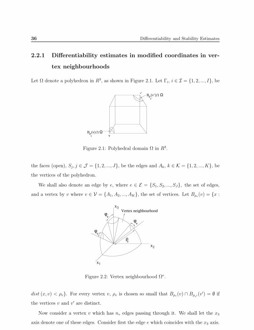
36 Differentiability and Stability Estimates
2.2.1 Differentiability estimates in modified coordinates in ver-
tex neighbourhoods
Let Ω denote a polyhedron in R3, as shown in Figure 2.1. Let Γi, i ∈ I = 1, 2, ..., I, be
v
ρv’
ρv
UΩ
v’B (v’)
B (v)
UΩ
Figure 2.1: Polyhedral domain Ω in R3.
the faces (open), Sj, j ∈ J = 1, 2, ..., J, be the edges and Ak, k ∈ K = 1, 2, ..., K, bethe vertices of the polyhedron.
We shall also denote an edge by e, where e ∈ E = S1, S2, ..., SJ, the set of edges,
and a vertex by v where v ∈ V = A1, A2, ..., AK, the set of vertices. Let Bρv(v) = x :
φφ
ρ
v
v
vx
x
x1
2
3
φv
Vertex neighbourhood
Figure 2.2: Vertex neighbourhood Ωv.
dist (x, v) < ρv. For every vertex v, ρv is chosen so small that Bρv(v) ∩ Bρv′(v′) = ∅ if
the vertices v and v′ are distinct.
Now consider a vertex v which has nv edges passing through it. We shall let the x3
axis denote one of these edges. Consider first the edge e which coincides with the x3 axis.
2.2 Differentiability Estimates in Modified Coordinates 37
Let φ denote the angle which x = (x1, x2, x3) makes with the x3 axis. Let
Vρv,φv(v, e) = x ∈ Ω : 0 < dist (x, v) < ρv, 0 < φ < φv
where φv is a constant. Let us choose φv sufficiently small so that
Vρv,φv(v, e′)⋂Vρv,φv(v, e′′) = ∅
if e′ and e′′ are distinct edges which have v as a common vertex. Now we define Ωv, the
vertex neighbourhood of the vertex v. Let Ev denote the subset of E , the set of edges,
such that Ev = e ∈ E : v is a vertex of e. Then
Ωv =
(Bρv(v) \
⋃
e∈Ev
Vρv,φv(v, e))⋂
Ω .
Here ρv and φv are chosen so that ρv sin(φv) = Z, a constant for all v ∈ V, the set of
vertices. We now introduce a set of modified coordinates in the vertex neighbourhood Ωv.
Let
ρ =√x12 + x22 + x32
φ = cos−1(x3/ρ)
θ = tan−1(x2/x1)
denote the usual spherical coordinates in Ωv. Define
xv1 = φ
xv2 = θ
xv3 = χ = ln ρ . (2.3)
Let wv = w(v), denote the value of w at the vertex v. By Ωv is denoted the image of
Ωv in xv coordinates. We can now state the differentiability estimates in these modified
coordinates in vertex neighbourhoods. The proof is based on the regularity results proved
by Babuska and Guo in [14]. These estimates are obtained when the differential operator
is the Laplacian. However they are valid for the more general situation examined in this
work.
38 Differentiability and Stability Estimates
Unless otherwise stated, as in Babuska and Guo [14–16] we let w(xv), w(xv−e), w(xe)
denote w(x(xv)), w(x(xv−e)), w(x(xe)) respectively. We shall use the same notation for
the spectral element functions u(xv), u(xv−e), u(xe) etc. as well in the ensuing sections
and chapters.
Proposition 2.2.1. There exists a constant βv ∈ (0, 1/2) such that for all 0 < ν ≤ ρv
the estimate∫
Ωv∩xv: xv3≤ ln(ν)
∑
|α|≤mex
v3 |Dα
xv (w(xv)− wv) |2 dxv ≤ C (dmm!)2 ν(1−2βv) (2.4)
holds for all integers m ≥ 1. Here C and d denote constants and dxv denotes a volume
element in xv coordinates.
Proof. The proof is provided in Appendix A.1.
2.2.2 Differentiability estimates in modified coordinates in edge
neighbourhoods
Let e denote an edge, which for convenience we assume to coincide with the x3 axis, whose
end points are the vertices v and v′ as shown in Figure 2.3.
Assume that the vertex v coincides with the origin. Let the length of the edge e
be le, δv = ρv cos(φv) and δv′ = ρv′ cos(φv′). Let (r, θ, x3) denote the usual cylindrical
coordinates
r =√x12 + x22
θ = tan−1(x2/x1)
and Ωe the edge neighbourhood
Ωe = x ∈ Ω : δv < x3 < le − δv′ , 0 < r < Z
as shown in Figure 2.3. We introduce the modified system of coordinates
xe1 = τ = ln r
xe2 = θ
xe3 = x3 . (2.5)
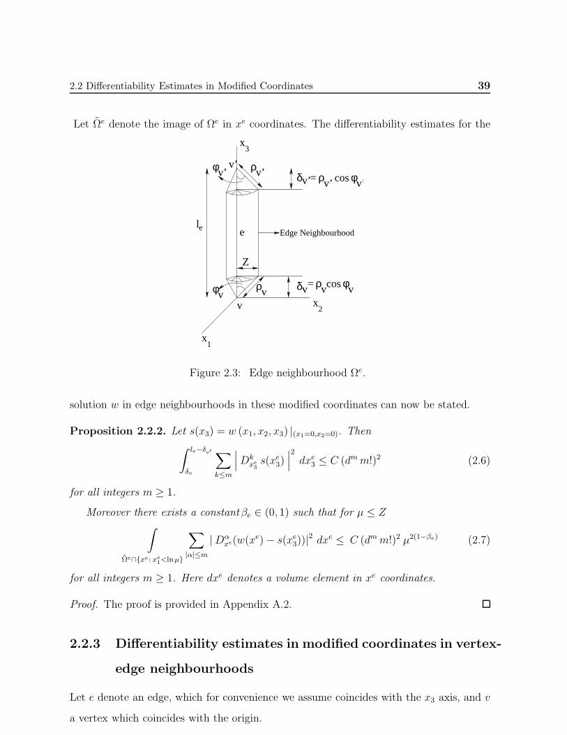
2.2 Differentiability Estimates in Modified Coordinates 39
Let Ωe denote the image of Ωe in xe coordinates. The differentiability estimates for the
Z
x3
v
v’δ
δv= ρρφ
φ= ρ
e Edge Neighbourhood
x1
x2
v
v’ v’ρ
v
v’v’
v cos φ v
cos φ v’
le
Figure 2.3: Edge neighbourhood Ωe.
solution w in edge neighbourhoods in these modified coordinates can now be stated.
Proposition 2.2.2. Let s(x3) = w (x1, x2, x3) |(x1=0,x2=0). Then
∫ le−δv′
δv
∑
k≤m
∣∣∣Dkxe3s(xe3)
∣∣∣2
dxe3 ≤ C (dmm!)2 (2.6)
for all integers m ≥ 1.
Moreover there exists a constantβe ∈ (0, 1) such that for µ ≤ Z∫
Ωe∩xe: xe1<lnµ
∑
|α|≤m|Dα
xe(w(xe)− s(xe3))|2 dxe ≤ C (dmm!)2 µ2(1−βe) (2.7)
for all integers m ≥ 1. Here dxe denotes a volume element in xe coordinates.
Proof. The proof is provided in Appendix A.2.
2.2.3 Differentiability estimates in modified coordinates in vertex-
edge neighbourhoods
Let e denote an edge, which for convenience we assume coincides with the x3 axis, and v
a vertex which coincides with the origin.
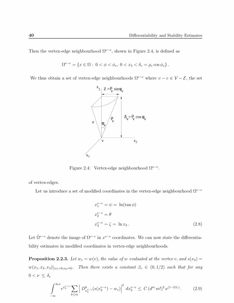
40 Differentiability and Stability Estimates
Then the vertex-edge neighbourhood Ωv−e, shown in Figure 2.4, is defined as
Ωv−e = x ∈ Ω : 0 < φ < φv, 0 < x3 < δv = ρv cosφv .
We thus obtain a set of vertex-edge neighbourhoods Ωv−e where v − e ∈ V − E , the set
v x2
x3
δve
= ρv cosρ
vφv
φv
ρZ = v sin φ v
x1
Figure 2.4: Vertex-edge neighbourhood Ωv−e.
of vertex-edges.
Let us introduce a set of modified coordinates in the vertex-edge neighbourhood Ωv−e
xv−e1 = ψ = ln(tanφ)
xv−e2 = θ
xv−e3 = ζ = ln x3 . (2.8)
Let Ωv−e denote the image of Ωv−e in xv−e coordinates. We can now state the differentia-
bility estimates in modified coordinates in vertex-edge neighbourhoods.
Proposition 2.2.3. Let wv = w(v), the value of w evaluated at the vertex v, and s(x3) =
w(x1, x2, x3)|(x1=0,x2=0). Then there exists a constant βv ∈ (0, 1/2) such that for any
0 < ν ≤ δv
∫
−∞
ln ν
exv−e3
∑
k≤m
∣∣∣Dkxv−e3
(s(xv−e3 )− wv)∣∣∣2
dxv−e3 ≤ C (dmm!)2 ν(1−2βv). (2.9)
2.2 Differentiability Estimates in Modified Coordinates 41
Moreover there exists a constant βe ∈ (0, 1) such that for any 0 < α ≤ tanφv and
0 < ν ≤ δv
∫
Ωv−e∩xv−e: xv−e1 <lnα, xv−e
3 <ln ν
exv−e3
∑
|γ|≤m
∣∣Dγxv−e(w(x
v−e)− s(xv−e3 ))∣∣2 dxv−e
≤ C (dmm!)2 α2(1−βe) ν(1−2βv) (2.10)
for all integers m ≥ 1. Here dxv−e denotes a volume element in xv−e coordinates.
Proof. The proof is provided in Appendix A.3.
2.2.4 Differentiability estimates in standard coordinates in the
regular region of the polyhedron
Let Ωr denote the portion of the polyhedron Ω obtained after the closure of the ver-
tex neighbourhoods, edge neighbourhoods and vertex-edge neighbourhoods have been
removed from it.
Thus let
∆ =
⋃
v∈VΩv
⋃⋃
e∈EΩe
⋃
⋃
v−e∈V−EΩv−e.
Then
Ωr = Ω \ .
We denote the regular region of the polyhedron, in which the solution w is analytic, by Ωr.
In Ωr the standard coordinate system x = (x1, x2, x3) is retained. The differentiability
estimates in these coordinates in the regular region of the polyhedron, are now stated.
Proposition 2.2.4. The estimate
∫
Ωr
∑
|α|≤m|Dα
xw(x)|2 dx ≤ C (dmm!)2 (2.11)
holds for all integers m ≥ 1. Here dx denotes a volume element in x coordinates.
Proof. The proof is provided in Appendix A.4.
42 Differentiability and Stability Estimates
2.2.5 Function spaces
We need to review a set of function spaces described in [14].
Let Ωv denote the vertex neighbourhood of the vertex v and ρ = ρ(x) = dist(x, v) for
x ∈ Ωv and βv ∈ (0, 1/2). We introduce a weight function as in [14] as follows: Define
Φα,lβv(x) =
ρβv+|α|−l, for |α| ≥ l
1, for |α| < l
as in (2.3) of [14]. Let
Hk,lβv(Ωv) =
u| ‖u‖
2H
k,lβv
(Ωv)=∑
|α|≤k
∥∥∥Φα,lβvDαu
∥∥∥2
L2(Ωv)<∞
and
Blβv(Ω
v) =
u| u ∈ Hk,l
βv(Ωv) for all k ≥ l and
∥∥∥Φα,lβvDαu
∥∥∥2
L2(Ωv)≤ C dα α!
denote the weighted Sobolev space and countably normed space defined on Ωv as in [14].
Let us denote by C2βv(Ωv) a countably normed space as in [14, 51] which is the set of
functions u(x) ∈ C0(Ωv) such that for all α, |α| ≥ 0
|Dαx (u(x)− u(v)) | ≤ C dα α! ρ−(βv+|α|−1/2)(x).
Here Ωv denotes the closure of Ωv. Then by Theorem 5.6 of [14], B2βv(Ωv) ⊆ C2
βv(Ωv).
We now cite an important regularity result, viz. Theorem 5.1 of [51] for the solution
of (2.1).
There exists a unique (weak) solution u ∈ H1(Ωv) of (2.1) which belongs to C2βv(Ωv) with
βv ∈ (0, 1/2) satisfying
βv ≥ 1/2− λv, λv =1
2
√1 + 4νvmin − 1 (2.12)
where νvmin is the smallest positive eigenvalue of the Laplace-Beltrami operator on the
spherical boundary Sv.
Next, let Ωe denote an edge neighbourhood of Ω and r = r(x) = dist(x, e) for x ∈ Ωe
and βe ∈ (0, 1). Define the weight function by
Φα,lβe(x) =
rβe+|α′|−l, for |α′| = α1 + α2 ≥ l
1, for |α| < l
2.2 Differentiability Estimates in Modified Coordinates 43
as in (2.1) of [14]. Let
Hk,lβe(Ωe) =
u| ‖u‖
2H
k,lβe
(Ωe)=∑
|α|≤k
∥∥∥Φα,lβeDαu
∥∥∥2
L2(Ωe)<∞
and
Blβe(Ω
e) =
u| u ∈ Hk,l
βe(Ωe) for all k ≥ l and
∥∥∥Φα,lβeDαu
∥∥∥2
L2(Ωe)≤ C dα α!
denote the weighted Sobolev space and countably normed space defined on Ωe as in [14].
We denote by C2βe(Ωe), βe ∈ (0, 1) a countably normed space as in [14, 51], the set of
functions u ∈ C0(Ωe) such that for |α| ≥ 0
∥∥ rβe+α1+α2−1Dαx (u(x)− u(0, 0, x3))
∥∥C0(Ωe)
≤ C dα α!
and for k ≥ 0 ∥∥∥∥dk
(dx3)ku(0, 0, x3)
∥∥∥∥C0(Ωe∩x: x1=x2=0)
≤ C dk k! ,
where Ωe denotes the closure of Ωe. Then by Theorem 5.3 of [14], B2βe(Ω
e) ⊆ C2βe(Ω
e).
We now cite another important regularity result, viz. Theorem 3.1 of [51] for the
solution of (2.1).
There exists a unique (weak) solution u ∈ H1(Ωe) of (2.1) which belongs to C2βe(Ωe) with
βe ∈ (0, 1) satisfying
βe ≥ 1− κe, κe =
π2ωe
if Γs ⊂ Γ[0],Γt ⊂ Γ[1]
πωe, otherwise
(2.13)
where Γs and Γt are such that Γs ∩ Γt = e.
Finally, let ρ = ρ(x) and φ = φ(x) for x ∈ Ωv−e. We define a weight function by
Φα,lβv−e
(x) =
ρβv+|α|−l(sin(φ))βe+|α′|−l, for |α′| = α1 + α2 ≥ l
ρβv+|α|−l, for |α′| < l ≤ |α|1, for |α| < l
as in (2.2) of [14]. Let
Hk,lβv−e
(Ωv−e) =
u| ‖u‖
2H
k,lβv−e
(Ωv−e)=∑
|α|≤k
∥∥∥Φα,lβv−e
Dαu∥∥∥2
L2(Ωv−e)<∞
44 Differentiability and Stability Estimates
and
Blβv−e
(Ωv−e) =
u| u ∈ Hk,l
βv−e(Ωv−e) ∀ k ≥ l and
∥∥∥Φα,lβv−e
Dαu∥∥∥2
L2(Ωv−e)≤ C dα α!
denote the weighted Sobolev space and countably normed space defined on Ωv−e as in [14].
Let us denote by C2βv−e
(Ωv−e), where βv−e = (βv, βe), βv ∈ (0, 1/2) and βe ∈ (0, 1),
the set of functions u(x) ∈ C0(Ωv−e) such that
∥∥ ρβv+|α|−1/2 (sin φ)βe+α1+α2−1 Dαx (u(x)− u(0, 0, x3))
∥∥C0(Ωv−e)
≤ C dα α!
and ∣∣∣∣ |x3|βv+k−1/2 dk
dxk3(u(0, 0, x3)− u(v))
∣∣∣∣C0(Ωv−e∩x: x1=x2=0)
≤ C dk k!
as described in [14, 51]. Here Ωv−e denotes the closure of Ωv−e. Now by Theorem 5.9 of
[14], B2βv−e
(Ωv−e) ⊆ C2βv−e
(Ωv−e).
We cite one last Theorem 4.1 of [51] for the solution of (2.1).
There exists a unique (weak) solution u ∈ H1(Ωv−e) of (2.1) which belongs to C2βv−e
(Ωv−e),
where βv−e = (βv, βe), βv ∈ (0, 1/2) and βe ∈ (0, 1) satisfying (2.12) and (2.13).
2.3 The Stability Theorem
Ω is divided into a regular region Ωr, a set of vertex neighbourhoods Ωv, where v ∈ V,a set of edge neighbourhoods Ωe, where e ∈ E and a set of vertex-edge neighbourhoods
Ωv−e, where v− e ∈ V −E . In the regular region Ωr standard coordinates x = (x1, x2, x3)
are used and in the remaining regions modified coordinates are used as has been described
in Section 2. Ωr is divided into a set of curvilinear hexahedrons, tetrahedrons and prisms.
We impose a geometrically graded mesh in the remaining regions which is described in this
section. We remark that a tetrahedron can always be divided into four hexahedrons [77],
in the same way that a triangle can be divided into three quadrilaterals by joining the
centre of the triangle to the midpoints of the sides (Figure 2.5). Moreover a prism can
be divided into three hexahedral elements. Hence we can choose all our elements to be
hexahedrons. A set of spectral element functions are defined on the elements. In edge
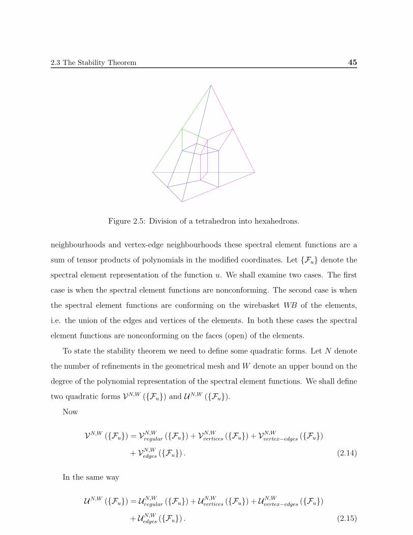
2.3 The Stability Theorem 45
Figure 2.5: Division of a tetrahedron into hexahedrons.
neighbourhoods and vertex-edge neighbourhoods these spectral element functions are a
sum of tensor products of polynomials in the modified coordinates. Let Fu denote the
spectral element representation of the function u. We shall examine two cases. The first
case is when the spectral element functions are nonconforming. The second case is when
the spectral element functions are conforming on the wirebasket WB of the elements,
i.e. the union of the edges and vertices of the elements. In both these cases the spectral
element functions are nonconforming on the faces (open) of the elements.
To state the stability theorem we need to define some quadratic forms. Let N denote
the number of refinements in the geometrical mesh and W denote an upper bound on the
degree of the polynomial representation of the spectral element functions. We shall define
two quadratic forms VN,W (Fu) and UN,W (Fu).Now
VN,W (Fu) = VN,Wregular (Fu) + VN,Wvertices (Fu) + VN,Wvertex−edges (Fu)
+ VN,Wedges (Fu) . (2.14)
In the same way
UN,W (Fu) = UN,Wregular (Fu) + UN,Wvertices (Fu) + UN,Wvertex−edges (Fu)
+ UN,Wedges (Fu) . (2.15)
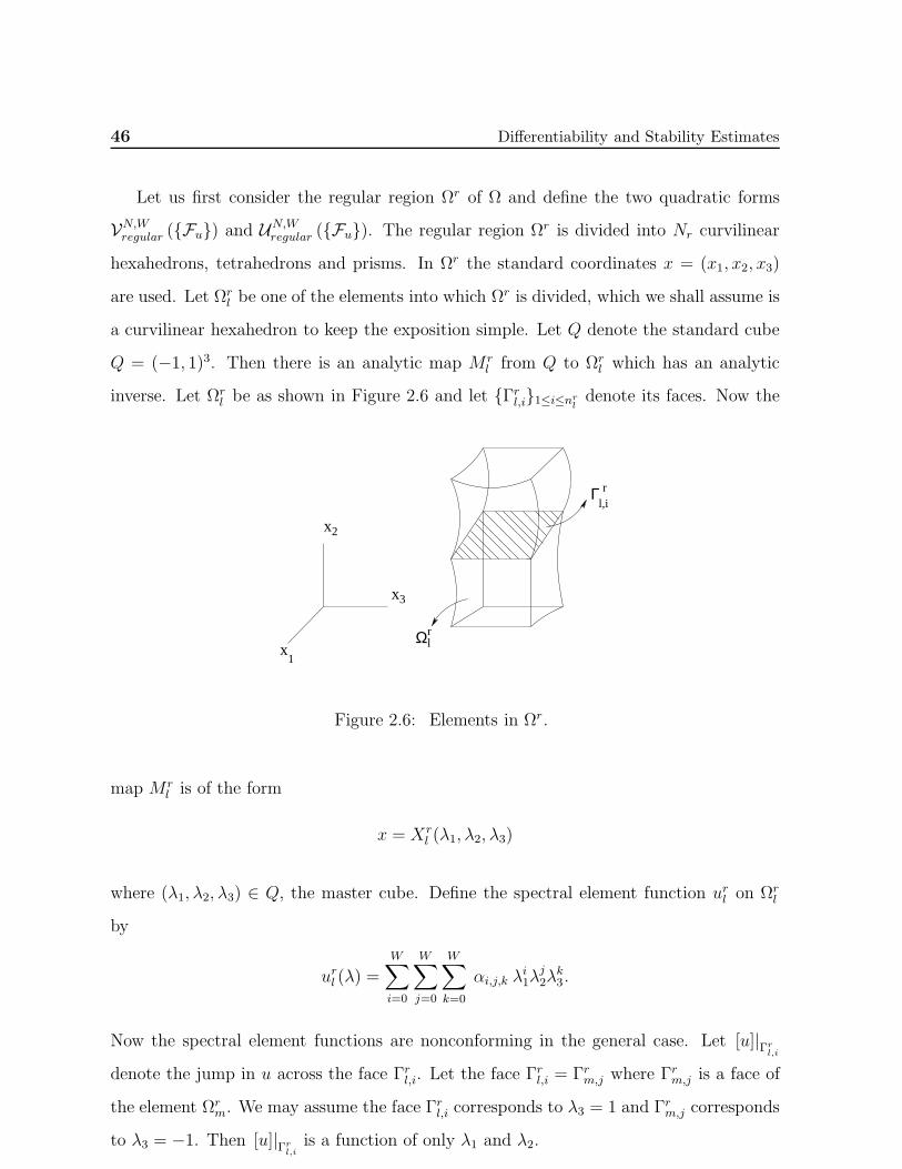
46 Differentiability and Stability Estimates
Let us first consider the regular region Ωr of Ω and define the two quadratic forms
VN,Wregular (Fu) and UN,Wregular (Fu). The regular region Ωr is divided into Nr curvilinear
hexahedrons, tetrahedrons and prisms. In Ωr the standard coordinates x = (x1, x2, x3)
are used. Let Ωrl be one of the elements into which Ωr is divided, which we shall assume is
a curvilinear hexahedron to keep the exposition simple. Let Q denote the standard cube
Q = (−1, 1)3. Then there is an analytic map M rl from Q to Ωrl which has an analytic
inverse. Let Ωrl be as shown in Figure 2.6 and let Γrl,i1≤i≤nrldenote its faces. Now the
Γl,ir
x1
x2
x3
lΩr
Figure 2.6: Elements in Ωr.
map M rl is of the form
x = Xrl (λ1, λ2, λ3)
where (λ1, λ2, λ3) ∈ Q, the master cube. Define the spectral element function url on Ωrl
by
url (λ) =
W∑
i=0
W∑
j=0
W∑
k=0
αi,j,k λi1λ
j2λ
k3.
Now the spectral element functions are nonconforming in the general case. Let [u]|Γrl,i
denote the jump in u across the face Γrl,i. Let the face Γrl,i = Γrm,j where Γrm,j is a face of
the element Ωrm. We may assume the face Γrl,i corresponds to λ3 = 1 and Γrm,j corresponds
to λ3 = −1. Then [u]|Γrl,i
is a function of only λ1 and λ2.
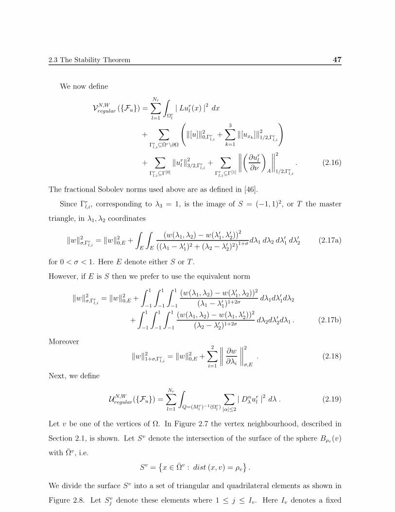
2.3 The Stability Theorem 47
We now define
VN,Wregular (Fu) =Nr∑
l=1
∫
Ωrl
| Lurl (x) |2 dx
+∑
Γrl,i⊆Ωr\∂Ω
(‖[u]‖20,Γr
l,i+
3∑
k=1
‖[uxk ]‖21/2,Γrl,i
)
+∑
Γrl,i⊆Γ[0]
‖url ‖23/2,Γrl,i+
∑
Γrl,i⊆Γ[1]
∥∥∥∥(∂url∂ν
)
A
∥∥∥∥2
1/2,Γrl,i
. (2.16)
The fractional Sobolev norms used above are as defined in [46].
Since Γrl,i, corresponding to λ3 = 1, is the image of S = (−1, 1)2, or T the master
triangle, in λ1, λ2 coordinates
‖w‖2σ,Γrl,i= ‖w‖20,E +
∫
E
∫
E
(w(λ1, λ2)− w(λ′1, λ′2))2
((λ1 − λ′1)2 + (λ2 − λ′2)2)1+σdλ1 dλ2 dλ
′1 dλ
′2 (2.17a)
for 0 < σ < 1. Here E denote either S or T .
However, if E is S then we prefer to use the equivalent norm
‖w‖2σ,Γrl,i= ‖w‖20,E +
∫ 1
−1
∫ 1
−1
∫ 1
−1
(w(λ1, λ2)− w(λ′1, λ2))2(λ1 − λ′1)1+2σ
dλ1dλ′1dλ2
+
∫ 1
−1
∫ 1
−1
∫ 1
−1
(w(λ1, λ2)− w(λ1, λ′2))2(λ2 − λ′2)1+2σ
dλ2dλ′2dλ1 . (2.17b)
Moreover
‖w‖21+σ,Γrl,i= ‖w‖20,E +
2∑
i=1
∥∥∥∥∂w
∂λi
∥∥∥∥2
σ,E
. (2.18)
Next, we define
UN,Wregular(Fu) =Nr∑
l=1
∫
Q=(Mrl )
−1(Ωrl )
∑
|α|≤2
|Dαλu
rl |2 dλ . (2.19)
Let v be one of the vertices of Ω. In Figure 2.7 the vertex neighbourhood, described in
Section 2.1, is shown. Let Sv denote the intersection of the surface of the sphere Bρv(v)
with Ωv, i.e.
Sv =x ∈ Ωv : dist (x, v) = ρv
.
We divide the surface Sv into a set of triangular and quadrilateral elements as shown in
Figure 2.8. Let Svj denote these elements where 1 ≤ j ≤ Iv. Here Iv denotes a fixed
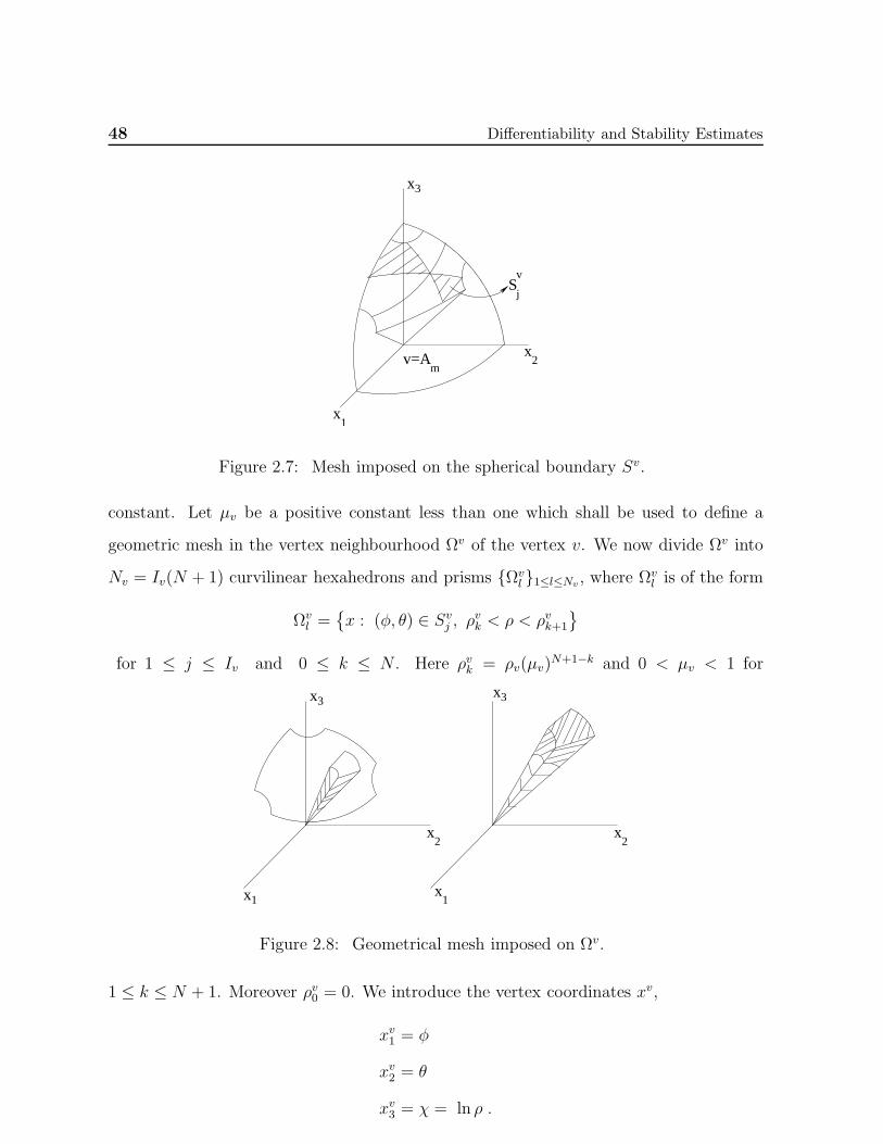
48 Differentiability and Stability Estimates
x
x
x
3
1
2v=Am
Sj
v
Figure 2.7: Mesh imposed on the spherical boundary Sv.
constant. Let µv be a positive constant less than one which shall be used to define a
geometric mesh in the vertex neighbourhood Ωv of the vertex v. We now divide Ωv into
Nv = Iv(N + 1) curvilinear hexahedrons and prisms Ωvl 1≤l≤Nv , where Ωvl is of the form
Ωvl =x : (φ, θ) ∈ Svj , ρvk < ρ < ρvk+1
for 1 ≤ j ≤ Iv and 0 ≤ k ≤ N . Here ρvk = ρv(µv)N+1−k and 0 < µv < 1 for
x
x
x
3
1
2
x
x
x
3
1
2
Figure 2.8: Geometrical mesh imposed on Ωv.
1 ≤ k ≤ N + 1. Moreover ρv0 = 0. We introduce the vertex coordinates xv,
xv1 = φ
xv2 = θ
xv3 = χ = ln ρ .
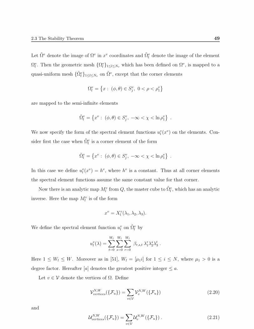
2.3 The Stability Theorem 49
Let Ωv denote the image of Ωv in xv coordinates and Ωvl denote the image of the element
Ωvl . Then the geometric mesh Ωvl 1≤l≤Nv which has been defined on Ωv, is mapped to a
quasi-uniform mesh Ωvl 1≤l≤Nv on Ωv, except that the corner elements
Ωvl =x : (φ, θ) ∈ Svj , 0 < ρ < ρv1
are mapped to the semi-infinite elements
Ωvl =xv : (φ, θ) ∈ Svj , −∞ < χ < ln ρv1
.
We now specify the form of the spectral element functions uvl (xv) on the elements. Con-
sider first the case when Ωvl is a corner element of the form
Ωvl =xv : (φ, θ) ∈ Svj , −∞ < χ < ln ρv1
.
In this case we define uvl (xv) = hv, where hv is a constant. Thus at all corner elements
the spectral element functions assume the same constant value for that corner.
Now there is an analytic mapMvl from Q, the master cube to Ωvl , which has an analytic
inverse. Here the map Mvl is of the form
xv = Xvl (λ1, λ2, λ3).
We define the spectral element function uvl on Ωvl by
uvl (λ) =
Wl∑
t=0
Wl∑
s=0
Wl∑
r=0
βr,s,t λr1λ
s2λ
t3 .
Here 1 ≤ Wl ≤ W . Moreover as in [51], Wl = [µ1i] for 1 ≤ i ≤ N , where µ1 > 0 is a
degree factor. Hereafter [a] denotes the greatest positive integer ≤ a.
Let v ∈ V denote the vertices of Ω. Define
VN,Wvertices(Fu) =∑
v∈VVN,Wv (Fu) (2.20)
and
UN,Wvertices(Fu) =∑
v∈VUN,Wv (Fu) . (2.21)
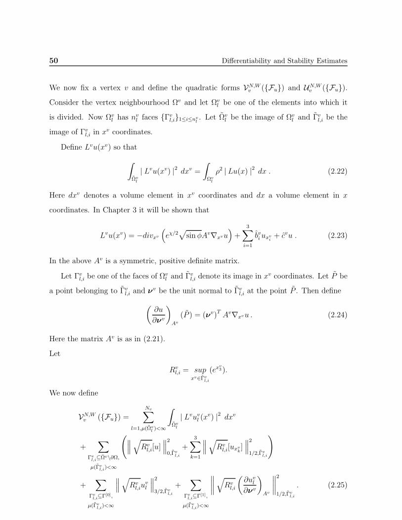
50 Differentiability and Stability Estimates
We now fix a vertex v and define the quadratic forms VN,Wv (Fu) and UN,Wv (Fu).Consider the vertex neighbourhood Ωv and let Ωvl be one of the elements into which it
is divided. Now Ωvl has nvl faces Γvl,i1≤i≤nvl. Let Ωvl be the image of Ωvl and Γvl,i be the
image of Γvl,i in xv coordinates.
Define Lvu(xv) so that
∫
Ωvl
| Lvu(xv) |2 dxv =∫
Ωvl
ρ2 | Lu(x) |2 dx . (2.22)
Here dxv denotes a volume element in xv coordinates and dx a volume element in x
coordinates. In Chapter 3 it will be shown that
Lvu(xv) = −divxv(eχ/2
√sinφAv∇xvu
)+
3∑
i=1
bvi uxvi + cvu . (2.23)
In the above Av is a symmetric, positive definite matrix.
Let Γvl,i be one of the faces of Ωvl and Γvl,i denote its image in xv coordinates. Let P be
a point belonging to Γvl,i and νv be the unit normal to Γvl,i at the point P . Then define
(∂u
∂νv
)
Av
(P ) = (νv)T Av∇xvu . (2.24)
Here the matrix Av is as in (2.21).
Let
Rvl,i = sup
xv∈Γvl,i
(exv3).
We now define
VN,Wv (Fu) =Nv∑
l=1,µ(Ωvl )<∞
∫
Ωvl
| Lvuvl (xv) |2 dxv
+∑
Γvl,i⊆Ωv\∂Ω,µ(Γv
l,i)<∞
(∥∥∥√Rvl,i[u]
∥∥∥2
0,Γvl,i
+3∑
k=1
∥∥∥√Rvl,i[uxvk ]
∥∥∥2
1/2,Γvl,i
)
+∑
Γvl,i⊆Γ[0],
µ(Γvl,i)<∞
∥∥∥√Rvl,iu
vl
∥∥∥2
3/2,Γvl,i
+∑
Γvl,i⊆Γ[1],
µ(Γvl,i)<∞
∥∥∥∥√Rvl,i
(∂uvl∂νv
)
Av
∥∥∥∥2
1/2,Γvl,i
. (2.25)
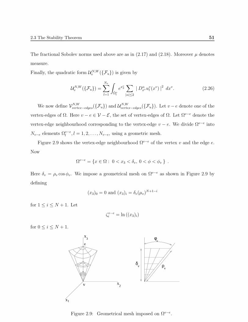
2.3 The Stability Theorem 51
The fractional Sobolev norms used above are as in (2.17) and (2.18). Moreover µ denotes
measure.
Finally, the quadratic form UN,Wv (Fu) is given by
UN,Wv (Fu) =Nv∑
l=1
∫
Ωvl
exv3
∑
|α|≤2
|Dαxvu
vl (x
v) |2 dxv. (2.26)
We now define VN,Wvertex−edges(Fu) and UN,Wvertex−edges(Fu). Let v− e denote one of thevertex-edges of Ω. Here v − e ∈ V − E , the set of vertex-edges of Ω. Let Ωv−e denote the
vertex-edge neighbourhood corresponding to the vertex-edge v − e. We divide Ωv−e into
Nv−e elements Ωv−el , l = 1, 2, . . . , Nv−e, using a geometric mesh.
Figure 2.9 shows the vertex-edge neighbourhood Ωv−e of the vertex v and the edge e.
Now
Ωv−e = x ∈ Ω : 0 < x3 < δv, 0 < φ < φv .
Here δv = ρv cosφv. We impose a geometrical mesh on Ωv−e as shown in Figure 2.9 by
defining
(x3)0 = 0 and (x3)i = δv(µv)N+1−i
for 1 ≤ i ≤ N + 1. Let
ζv−ei = ln ((x3)i)
for 0 ≤ i ≤ N + 1.
v
x
x
x
1
3
2
δ
φ
ρv
ve
v
Figure 2.9: Geometrical mesh imposed on Ωv−e.
52 Differentiability and Stability Estimates
Let us introduce points φv−e0 , . . . , φv−eN+1 such that φv−e0 = 0 and tanφv−ei = µN+1−ie tan(φv),
for 1 ≤ i ≤ N + 1. Here µe is a positive constant less than one. Thus we impose a ge-
ometrical mesh on φ with mesh ratio µe. Finally, θlv−e < θ < θuv−e. A quasi-uniform
mesh
θlv−e = θv−e0 < θv−e1 < · · · < θv−eIv−e= θuv−e
is imposed in θ. We introduce new coordinates in Ωv−e by
xv−e1 = ψ = ln(tanφ)
xv−e2 = θ
xv−e3 = ζ = ln x3 .
Let Ωv−e be the image of Ωv−e in xv−e coordinates. Thus Ωv−e is divided into Nv−e =
Iv−e(N + 1)2 hexahedrons Ωv−en n=1,...,Nv−e, where
Ωv−en =xv−e : ψv−ei < ψ < ψv−ei+1 , θ
v−ej < θ < θv−ej+1 , ζ
v−ek < ζ < ζv−ek+1
.
We now define the spectral element functions on the elements in Ωv−e. Consider an
element
Ωv−en =xv−e : ψv−ei < ψ < ψv−ei+1 , θ
v−ej < θ < θv−ej+1 , −∞ < ζ < ζv−e1
.
Then on Ωv−en
uv−en = hv−e = hv
where hv is the same constant as for the spectral element function uvm defined on the
corner element
Ωvm =xv : (φ, θ) ∈ Svj , −∞ < χ < ln(ρv1)
.
Next, we consider the element
Ωv−ep =xv−e : −∞ < ψ < ψv−e1 , θv−ej < θ < θv−ej+1 , ζ
v−ek < ζ < ζv−ek+1
.
Here k ≥ 1.
Then on Ωv−ep we define
uv−ep (xv−e) =
Wp∑
l=0
βl ζl.
2.3 The Stability Theorem 53
Here 1 ≤Wp ≤W . Moreover Wp = [µ2k] for 1 ≤ k ≤ N , where µ2 > 0 is a degree factor.
Now consider
Ωv−eq =xv−e : ψv−ei < ψ < ψv−ei+1 , θ
v−ej < θ < θv−ej+1 , ζ
v−ek < ζ < ζv−ek+1
for 1 ≤ i ≤ N , 1 ≤ k ≤ N . Then on Ωv−eq we define
uv−eq (xv−e) =
Wq∑
r=0
Wq∑
s=0
Vq∑
t=0
γr,s,t ψrθsζ t.
Here 1 ≤ Wq ≤ W and 1 ≤ Vq ≤ W . Moreover Wq = [µ1i], Vq = [µ2k] for 1 ≤ i, k ≤ N ,
where µ1, µ2 > 0 are degree factors [51].
Let Γv−en,i be one of the faces of Ωv−en such that µ(Γv−en,i ) <∞, where µ denotes measure.
We introduce a norm ||| u |||2Γv−en,i
as follows:
Let Ev−en,i = sup
xv−e∈Γv−en,i
(sinφ) and F v−en,i = sup
xv−e∈Γv−en,i
(exv−e3 ). We also define Gv−e
n,i which is
used in (2.29).
1) If Γv−en,i =xv−e : α0 < xv−e1 < α1, β0 < xv−e2 < β1, x
v−e3 = γ0
then define Gv−e
n,i =
Ev−en,i and
||| u |||2Γv−en,i
= Ev−en,i F
v−en,i
(∫ β1
β0
∫ α1
α0
u2(ψ, θ, γ0) dψ dθ
+
∫ β1
β0
dθ
∫ α1
α0
∫ α1
α0
(u(ψ, θ, γ0)− u(ψ′, θ, γ0))2
(ψ − ψ′)2dψ dψ′
+
∫ α1
α0
dψ
∫ β1
β0
∫ β1
β0
(u(ψ, θ, γ0)− u(ψ, θ′, γ0))2(θ − θ′)2 dθ dθ′
). (2.27a)
2) If Γv−en,i =xv−e : xv−e1 = α0, β0 < xv−e2 < β1, γ0 < xv−e3 < γ1
then define Gv−e
n,i = 1
and
||| u |||2Γv−en,i
= F v−en,i
(∫ γ1
γ0
∫ β1
β0
u2(α0, θ, ζ) dθ dζ
+
∫ γ1
γ0
dζ
∫ β1
β0
∫ β1
β0
(u(α0, θ, ζ)− u(α0, θ′, ζ))2
(θ − θ′)2 dθ dθ′
+ Ev−en,i
∫ β1
β0
dθ
∫ γ1
γ0
∫ γ1
γ0
(u(α0, θ, ζ)− u(α0, θ, ζ′))2
(ζ − ζ ′)2 dζ dζ ′). (2.27b)
3) If Γv−en,i =xv−e : α0 < xv−e1 < α1, x
v−e2 = β0, γ0 < xv−e3 < γ1
then define Gv−e
n,i = 1
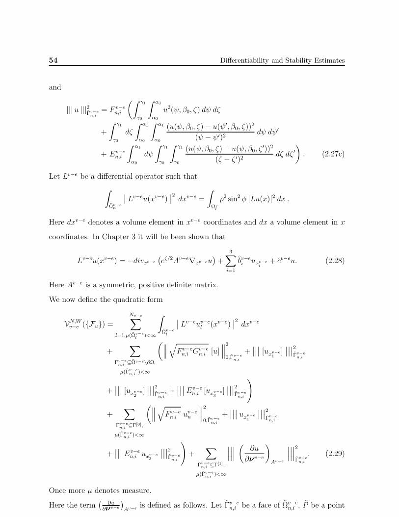
54 Differentiability and Stability Estimates
and
||| u |||2Γv−en,i
= F v−en,i
(∫ γ1
γ0
∫ α1
α0
u2(ψ, β0, ζ) dψ dζ
+
∫ γ1
γ0
dζ
∫ α1
α0
∫ α1
α0
(u(ψ, β0, ζ)− u(ψ′, β0, ζ))2
(ψ − ψ′)2dψ dψ′
+ Ev−en,i
∫ α1
α0
dψ
∫ γ1
γ0
∫ γ1
γ0
(u(ψ, β0, ζ)− u(ψ, β0, ζ ′))2(ζ − ζ ′)2 dζ dζ ′
). (2.27c)
Let Lv−e be a differential operator such that
∫
Ωv−en
∣∣ Lv−eu(xv−e)∣∣2 dxv−e =
∫
Ωvl
ρ2 sin2 φ |Lu(x)|2 dx .
Here dxv−e denotes a volume element in xv−e coordinates and dx a volume element in x
coordinates. In Chapter 3 it will be been shown that
Lv−eu(xv−e) = −divxv−e
(eζ/2Av−e∇xv−eu
)+
3∑
i=1
bv−ei uxv−ei
+ cv−eu. (2.28)
Here Av−e is a symmetric, positive definite matrix.
We now define the quadratic form
VN,Wv−e (Fu) =Nv−e∑
l=1,µ(Ωv−el )<∞
∫
Ωv−el
∣∣ Lv−euv−el (xv−e)∣∣2 dxv−e
+∑
Γv−en,i ⊆Ωv−e\∂Ω,µ(Γv−e
n,i )<∞
(∥∥∥√F v−en,i G
v−en,i [u]
∥∥∥2
0,Γv−en,i
+∣∣∣∣∣∣ [uxv−e
1]∣∣∣∣∣∣2
Γv−en,i
+∣∣∣∣∣∣ [uxv−e
2]∣∣∣∣∣∣2
Γv−en,i
+∣∣∣∣∣∣ Ev−e
n,i [uxv−e3
]∣∣∣∣∣∣2
Γv−en,i
)
+∑
Γv−en,i ⊆Γ[0],
µ(Γv−en,i )<∞
(∥∥∥√F v−en,i uv−en
∥∥∥2
0,Γv−en,i
+∣∣∣∣∣∣ uxv−e
1
∣∣∣∣∣∣2Γv−en,i
+∣∣∣∣∣∣ Ev−e
n,i uxv−e3
∣∣∣∣∣∣2Γv−en,i
)+
∑
Γv−en,i ⊆Γ[1],
µ(Γv−en,i )<∞
∣∣∣∣∣∣∣∣∣(
∂u
∂νv−e
)
Av−e
∣∣∣∣∣∣∣∣∣2
Γv−en,i
. (2.29)
Once more µ denotes measure.
Here the term(
∂u∂νv−e
)Av−e is defined as follows. Let Γv−en,i be a face of Ωv−en,i , P be a point
2.3 The Stability Theorem 55
belonging to Γv−en,i and νv−e denote the unit normal to Γv−en,i at the point P . Then
(∂u
∂νv−e
)
Av−e
(P ) = (νv−e)TAv−e∇xv−eu. (2.30)
Now the quadratic form VN,Wvertex−edges(Fu) is given by
VN,Wvertex−edges(Fu) =∑
v−e∈V−EVN,Wv−e (Fu). (2.31)
Next, we define the quadratic form UN,Wv−e (Fu). Let wv−e(xv−e1 ) be a positive, smooth
weight function such that
wv−e(xv−e1 ) = 1 for xv−e1 ≥ ζv−e1 = ln(tanφv−e1 )
and which satisfies ∫ ζv−e1
−∞wv−e(xv−e1 ) dxv−e1 = 1.
We shall choose
wv−e(xv−e1 ) = 1 for xv−e1 ≥ ζv−e1 − 1
and
wv−e(xv−e1 ) = 0 for xv−e1 < ζv−e1 − 1 .
Then
UN,Wv−e (Fu) =Nv−e∑
l=1,µ(Ωv−el )<∞
∫
Ωv−el
exv−e3
∑
i,j=1,2
(∂2uv−el
∂xv−ei ∂xv−ej
)2
+
2∑
i=1
sin2 φ
(∂2uv−el
∂xv−ei ∂xv−e3
)2
+ sin4 φ
(∂2uv−el(∂xv−e3
)2
)2
+
2∑
i=1
(∂uv−el
∂xv−ei
)2
+ sin2 φ
(∂uv−el
∂xv−e3
)2
+ (uv−el )2
)dxv−e
+
Nv−e∑
l=1,
µ(Ωv−el )=∞
∫
Ωv−el
(uv−el )2exv−e3 wv−e(xv−e1 ) dxv−e . (2.32)
The quadratic form UN,Wvertex−edges(Fu) is then given by
UN,Wvertex−edges(Fu) =∑
v−e∈V−EUN,Wv−e (Fu). (2.33)
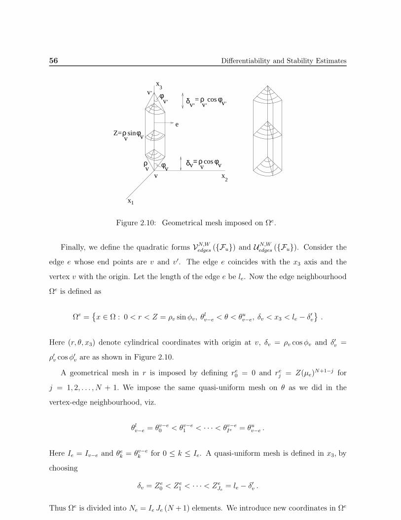
56 Differentiability and Stability Estimates
x
x
xv
v
e
ρ φ
φδ
δv= ρv
vv’’
vv
’
= ρv’
cos
1
3
2
ρvsinφv
φv
’cosφv’
Z=
Figure 2.10: Geometrical mesh imposed on Ωe.
Finally, we define the quadratic forms VN,Wedges (Fu) and UN,Wedges (Fu). Consider the
edge e whose end points are v and v′. The edge e coincides with the x3 axis and the
vertex v with the origin. Let the length of the edge e be le. Now the edge neighbourhood
Ωe is defined as
Ωe =x ∈ Ω : 0 < r < Z = ρv sinφv, θ
lv−e < θ < θuv−e, δv < x3 < le − δ′v
.
Here (r, θ, x3) denote cylindrical coordinates with origin at v, δv = ρv cosφv and δ′v =
ρ′v cos φ′v are as shown in Figure 2.10.
A geometrical mesh in r is imposed by defining re0 = 0 and rej = Z(µe)N+1−j for
j = 1, 2, . . . , N + 1. We impose the same quasi-uniform mesh on θ as we did in the
vertex-edge neighbourhood, viz.
θlv−e = θv−e0 < θv−e1 < · · · < θv−eIe = θuv−e .
Here Ie = Iv−e and θek = θv−ek for 0 ≤ k ≤ Ie. A quasi-uniform mesh is defined in x3, by
choosing
δv = Ze0 < Ze
1 < · · · < ZeJe = le − δ′v .
Thus Ωe is divided into Ne = Ie Je (N +1) elements. We introduce new coordinates in Ωe
2.3 The Stability Theorem 57
by
xe1 = τ = ln r
xe2 = θ
xe3 = x3 .
Let Ωe be the image of Ωe in xe coordinates. Thus Ωe is divided into Ne hexahedrons
Ωemm=1,...,Ne where
Ωem =xe : ln(rei ) < xe1 < ln(rei+1), θ
ej < xe2 < θej+1, Z
ek < xe3 < Ze
k+1
.
We now define the spectral element functions on the elements in Ωe. Consider an element
Ωep =xe : −∞ < xe1 < ln(re1), θ
ej < xe2 < θej+1, Z
en < xe3 < Ze
n+1
.
Then
uep(xe) =
W∑
t=0
αr(xe3)t .
This representation is valid for all j for fixed n.
Next, consider the element
Ωeq =xe : ln(rei ) < xe1 < ln(rei+1), θ
ej < xe2 < θej+1, Z
en < xe3 < Ze
n+1
for 1 ≤ i ≤ N .
Then we define
ueq(xe) =
Wq∑
r=0
Wq∑
s=0
W∑
t=0
αr,s,t (xe1)r(xe2)
s(xe3)t .
Here 1 ≤ Wq ≤ W . Moreover Wq = [µ1i] for all 1 ≤ i ≤ N , where µ1 > 0 is a degree
factor [51].
Let Γem,i be one of the faces of Ωem such that µ(Γem,i) <∞, where µ denotes measure. We
define a norm ||| u |||2Γem,i
as follows:
Let Gem,i = sup
xe∈Γem,i
(eτ ). We also define Hem,i which is needed in (2.38).
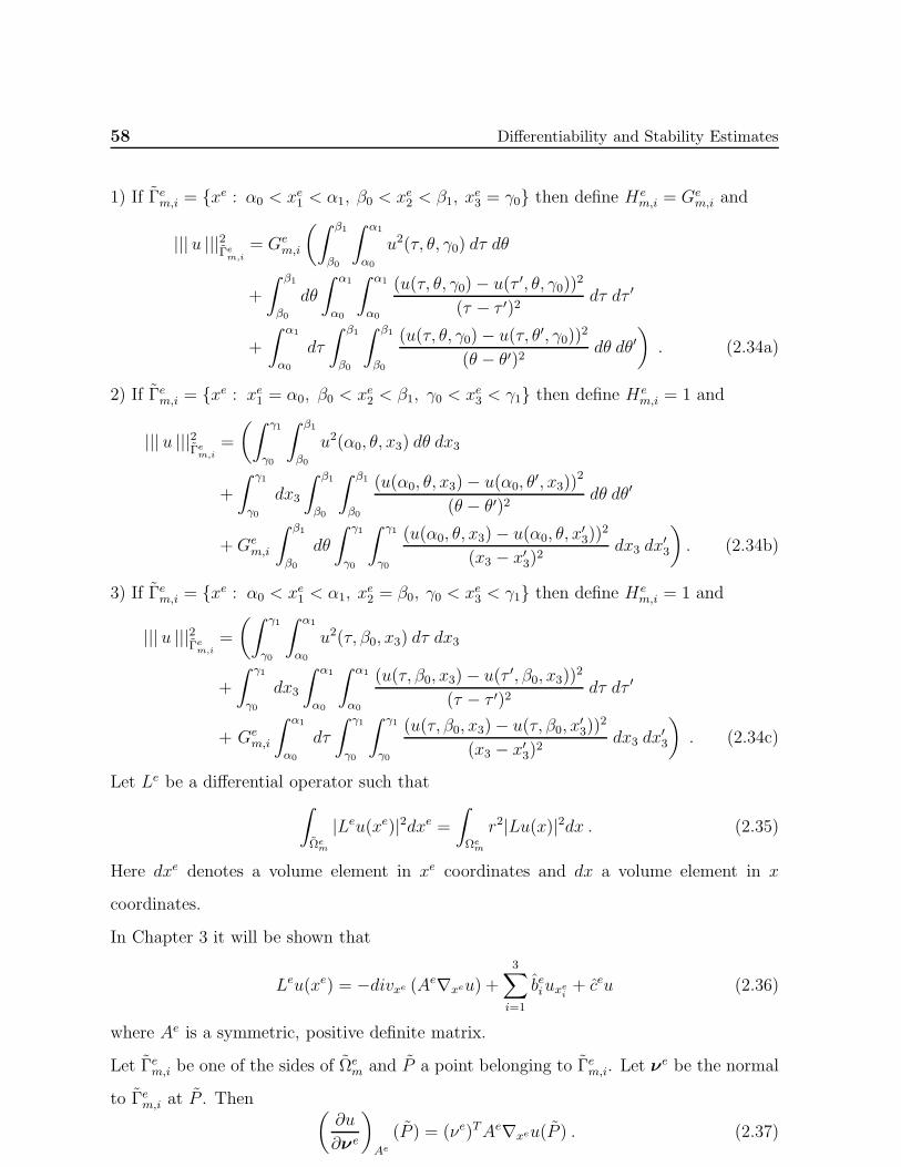
58 Differentiability and Stability Estimates
1) If Γem,i = xe : α0 < xe1 < α1, β0 < xe2 < β1, xe3 = γ0 then define He
m,i = Gem,i and
||| u |||2Γem,i
= Gem,i
(∫ β1
β0
∫ α1
α0
u2(τ, θ, γ0) dτ dθ
+
∫ β1
β0
dθ
∫ α1
α0
∫ α1
α0
(u(τ, θ, γ0)− u(τ ′, θ, γ0))2(τ − τ ′)2 dτ dτ ′
+
∫ α1
α0
dτ
∫ β1
β0
∫ β1
β0
(u(τ, θ, γ0)− u(τ, θ′, γ0))2(θ − θ′)2 dθ dθ′
). (2.34a)
2) If Γem,i = xe : xe1 = α0, β0 < xe2 < β1, γ0 < xe3 < γ1 then define Hem,i = 1 and
||| u |||2Γem,i
=
(∫ γ1
γ0
∫ β1
β0
u2(α0, θ, x3) dθ dx3
+
∫ γ1
γ0
dx3
∫ β1
β0
∫ β1
β0
(u(α0, θ, x3)− u(α0, θ′, x3))
2
(θ − θ′)2 dθ dθ′
+Gem,i
∫ β1
β0
dθ
∫ γ1
γ0
∫ γ1
γ0
(u(α0, θ, x3)− u(α0, θ, x′3))
2
(x3 − x′3)2dx3 dx
′3
). (2.34b)
3) If Γem,i = xe : α0 < xe1 < α1, xe2 = β0, γ0 < xe3 < γ1 then define He
m,i = 1 and
||| u |||2Γem,i
=
(∫ γ1
γ0
∫ α1
α0
u2(τ, β0, x3) dτ dx3
+
∫ γ1
γ0
dx3
∫ α1
α0
∫ α1
α0
(u(τ, β0, x3)− u(τ ′, β0, x3))2(τ − τ ′)2 dτ dτ ′
+ Gem,i
∫ α1
α0
dτ
∫ γ1
γ0
∫ γ1
γ0
(u(τ, β0, x3)− u(τ, β0, x′3))2(x3 − x′3)2
dx3 dx′3
). (2.34c)
Let Le be a differential operator such that∫
Ωem
|Leu(xe)|2dxe =∫
Ωem
r2|Lu(x)|2dx . (2.35)
Here dxe denotes a volume element in xe coordinates and dx a volume element in x
coordinates.
In Chapter 3 it will be shown that
Leu(xe) = −divxe (Ae∇xeu) +
3∑
i=1
beiuxei + ceu (2.36)
where Ae is a symmetric, positive definite matrix.
Let Γem,i be one of the sides of Ωem and P a point belonging to Γem,i. Let ν
e be the normal
to Γem,i at P . Then (∂u
∂νe
)
Ae
(P ) = (νe)TAe∇xeu(P ) . (2.37)
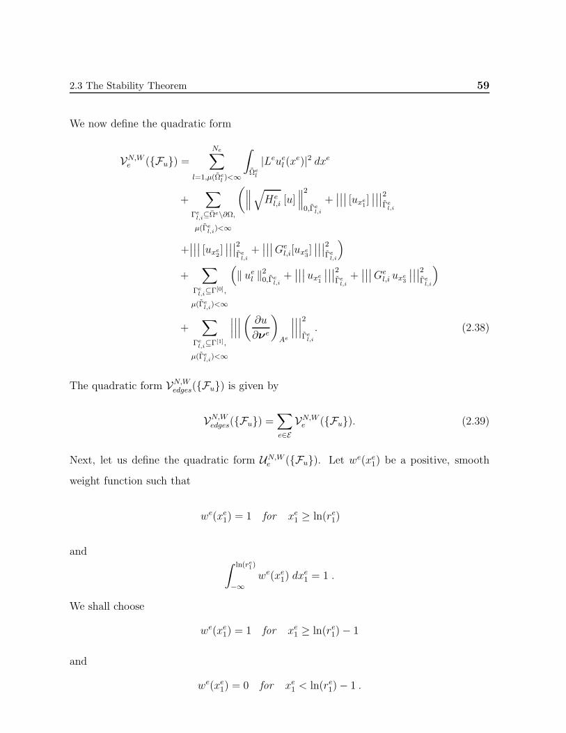
2.3 The Stability Theorem 59
We now define the quadratic form
VN,We (Fu) =Ne∑
l=1,µ(Ωel )<∞
∫
Ωel
|Leuel (xe)|2 dxe
+∑
Γel,i⊆Ωe\∂Ω,µ(Γe
l,i)<∞
(∥∥∥√Hel,i [u]
∥∥∥2
0,Γel,i
+∣∣∣∣∣∣ [uxe1]
∣∣∣∣∣∣2Γel,i
+∣∣∣∣∣∣ [uxe2]
∣∣∣∣∣∣2Γel,i
+∣∣∣∣∣∣Ge
l,i[uxe3]∣∣∣∣∣∣2
Γel,i
)
+∑
Γel,i⊆Γ[0],
µ(Γel,i)<∞
(‖ uel ‖20,Γe
l,i+∣∣∣∣∣∣ uxe1
∣∣∣∣∣∣2Γel,i
+∣∣∣∣∣∣Ge
l,i uxe3∣∣∣∣∣∣2
Γel,i
)
+∑
Γel,i⊆Γ[1],
µ(Γel,i)<∞
∣∣∣∣∣∣∣∣∣(∂u
∂νe
)
Ae
∣∣∣∣∣∣∣∣∣2
Γel,i
. (2.38)
The quadratic form VN,Wedges(Fu) is given by
VN,Wedges(Fu) =∑
e∈EVN,We (Fu). (2.39)
Next, let us define the quadratic form UN,We (Fu). Let we(xe1) be a positive, smooth
weight function such that
we(xe1) = 1 for xe1 ≥ ln(re1)
and∫ ln(re1)
−∞we(xe1) dx
e1 = 1 .
We shall choose
we(xe1) = 1 for xe1 ≥ ln(re1)− 1
and
we(xe1) = 0 for xe1 < ln(re1)− 1 .
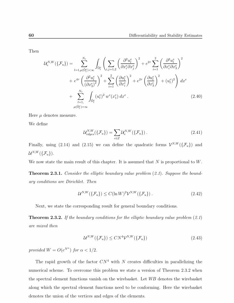
60 Differentiability and Stability Estimates
Then
UN,We (Fu) =Ne∑
l=1,µ(Ωel )<∞
∫
Ωel
(∑
i,j=1,2
(∂2uel∂xei∂x
ej
)2
+ e2τ2∑
i=1
(∂2uel∂xei∂x
e3
)2
+ e4τ(∂2uel(∂xe3)
2
)2
+2∑
i=1
(∂uel∂xei
)2
+ e2τ(∂uel∂xe3
)2
+ (uel )2
)dxe
+Ne∑
l=1,
µ(Ωel )=∞
∫
Ωel
(uel )2 we(xe1) dx
e . (2.40)
Here µ denotes measure.
We define
UN,Wedges(Fu) =∑
e∈EUN,We (Fu) . (2.41)
Finally, using (2.14) and (2.15) we can define the quadratic forms VN,W (Fu) and
UN,W (Fu).We now state the main result of this chapter. It is assumed that N is proportional to W .
Theorem 2.3.1. Consider the elliptic boundary value problem (2.1). Suppose the bound-
ary conditions are Dirichlet. Then
UN,W (Fu) ≤ C(lnW )2VN,W (Fu) . (2.42)
Next, we state the corresponding result for general boundary conditions.
Theorem 2.3.2. If the boundary conditions for the elliptic boundary value problem (2.1)
are mixed then
UN,W (Fu) ≤ CN4VN,W (Fu) (2.43)
provided W = O(eNα) for α < 1/2.
The rapid growth of the factor CN4 with N creates difficulties in parallelizing the
numerical scheme. To overcome this problem we state a version of Theorem 2.3.2 when
the spectral element functions vanish on the wirebasket. Let WB denotes the wirebasket
along which the spectral element functions need to be conforming. Here the wirebasket
denotes the union of the vertices and edges of the elements.
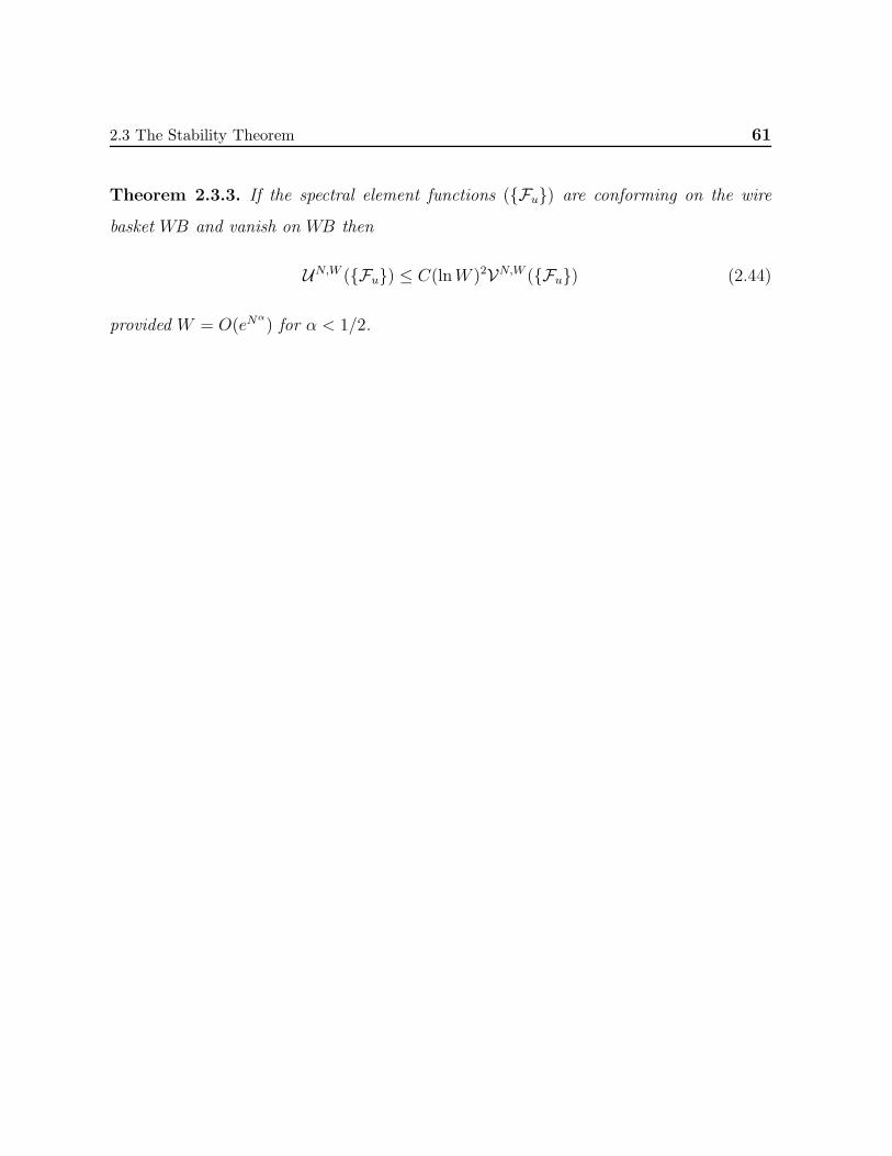
2.3 The Stability Theorem 61
Theorem 2.3.3. If the spectral element functions (Fu) are conforming on the wire
basket WB and vanish on WB then
UN,W (Fu) ≤ C(lnW )2VN,W (Fu) (2.44)
provided W = O(eNα) for α < 1/2.

Chapter 3
Proof of the Stability Theorem
3.1 Introduction
In this chapter we prove the stability estimate, which we use to formulate our numerical
scheme.
In Chapter 2 we have introduced a set of local coordinate systems in various neigh-
bourhoods of the polyhedron Ω, which we referred to as modified coordinates, in the ver-
tex, vertex-edge and edge neighbourhoods. These local coordinates are modified versions
of the spherical and cylindrical co-ordinate systems in vertex and edge neighbourhoods
respectively. In vertex-edge neighbourhoods modified coordinates are a combination of
spherical and cylindrical coordinates. Away from the corners and edges in the regular
region of the domain we use standard Cartesian coordinates. The differentiability esti-
mates for the solution of the elliptic boundary value problem in a polyhedral domain in
terms of these new local coordinates were obtained. We also stated a stability estimate
for a non-conforming spectral element representation of the solution. For problems with
mixed Neumann and Dirichlet boundary conditions the spectral element functions may
be chosen to be continuous on the wirebasket of the elements.
We now briefly describe the contents of this chapter. In Sections 3.2 and 3.3, we derive
estimates for the second order derivatives and the lower order derivatives of the solution
respectively. Estimates for terms in the interior and on the boundary of the polyhedron Ω
64 Proof of the Stability Theorem
are obtained in Sections 3.4 and 3.5. In Section 3.6, we combine all the results of sections
3.2, 3.3, 3.4 and 3.5 to complete the proof of the stability estimate which has been stated
in Chapter 2.
In Chapter 4 we shall give the numerical scheme and error estimates. It will be shown
that the error between the exact and the approximate solution is exponentially small
in N , the number of layers in the geometrical mesh. Optimal rate of convergence with
respect to the number of degrees of freedom is also provided.
3.2 Estimates for the Second Derivatives of Spectral
Element Functions
3.2.1 Estimates for the second derivatives in the interior
We first obtain estimates for elements in the regular region Ωr of Ω. Divide Ωr into
Nr elements, which may consist of curvilinear cubes, prisms and tetrahedrons, Ωrl for
1 ≤ l ≤ Nr.
Let
Lu =
3∑
i,j=1
−(ai,juxj
)xi+
3∑
i=1
biuxi + cu (3.1)
be a strongly elliptic operator that satisfies the Lax-Milgram conditions. Hence there
exists a positive constant µ0 such that
3∑
i,j=1
ai,jζiζj ≥ µ0|ζ |2 .
We consider the mixed boundary value problem
Lw = f in Ω, (3.2a)
γ0w = w|Γ[0] = g[0], (3.2b)
γ1w =
(∂w
∂ν
)
A
∣∣∣∣Γ[1]
= g[1]. (3.2c)
Let
Mu =
3∑
i,j=1
(ai,juxj
)xi. (3.3)
3.2 Estimates for the Second Derivatives of Spectral Element Functions 65
Consider an element Ωrl . Then Ωrl has nl faces Γrl,i1≤i≤nl. Let ∂Γrl,i denote the boundary
of the face Γrl,i.
To proceed we need to review some material in [46]. Let O be a bounded open subset
of R3 with a Lipschitz boundary ∂O. Assume in addition that ∂O is piecewise C2. Let P
be a point on ∂O in a neighbourhood of which ∂O is C2. It is possible to find two curves of
class C2 in a neighbourhood of P , passing through P and being orthogonal there. Let us
denote these curves by C1, C2 and by τ1, τ2 the unit tangent vectors to C1, C2 respectivelyand by s1, s2 the arc lengths along these curves. We assume that τ1,τ2 has the direct
orientation at P . Let ν be the unit normal at P defined as ν = τ1 × τ2. Then at P , BP ,the second fundamental form at P is the bilinear form
(ζ,η)| → −2∑
j,k=1
∂ν
∂sj· τ kζjηk (3.4)
where ζ,η are the tangent vectors to ∂O at P and ζ = (ζ1, ζ2) and η = (η1, η2) in the
basis τ 1, τ 2. In other words,
B(ζ,η) = −∂ν∂ζ· η (3.5)
where ∂
∂ζdenotes differentiation in the ζ direction.
Let w be a vector field defined in a neighbourhood of O. If P is a point on ∂O then
by wν we shall denote the component of w in the direction of ν, while we shall denote
by wT , the projection of w on the tangent hyperplane to ∂O, i.e.
wν = w · ν, (3.6)
wT = w −wνν = wτ1τ 1 +wτ2τ 2. (3.7)
Here wτi = w · τ i for i = 1, 2.
We shall denote by ∇T the projection of the gradient vector on the tangent hyperplane
∇Tu = ∇u− ∂u
∂νν =
2∑
j=1
∂u
∂sjτ j . (3.8)
Let h be a vector field defined on ∂O such that h is tangent to O except on a set of zero
measure. Then
divT (h) =
2∑
j=1
(∂h
∂sj
)· τ j. (3.9)
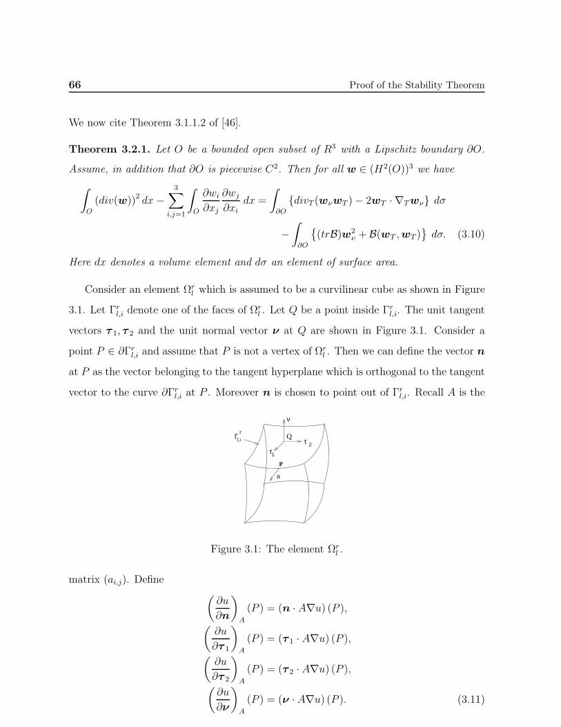
66 Proof of the Stability Theorem
We now cite Theorem 3.1.1.2 of [46].
Theorem 3.2.1. Let O be a bounded open subset of R3 with a Lipschitz boundary ∂O.
Assume, in addition that ∂O is piecewise C2. Then for all w ∈ (H2(O))3 we have
∫
O
(div(w))2 dx−3∑
i,j=1
∫
O
∂wi∂xj
∂wj∂xi
dx =
∫
∂O
divT (wνwT )− 2wT · ∇Twν dσ
−∫
∂O
(trB)w2
ν + B(wT ,wT )dσ. (3.10)
Here dx denotes a volume element and dσ an element of surface area.
Consider an element Ωrl which is assumed to be a curvilinear cube as shown in Figure
3.1. Let Γrl,i denote one of the faces of Ωrl . Let Q be a point inside Γrl,i. The unit tangent
vectors τ 1, τ 2 and the unit normal vector ν at Q are shown in Figure 3.1. Consider a
point P ∈ ∂Γrl,i and assume that P is not a vertex of Ωrl . Then we can define the vector n
at P as the vector belonging to the tangent hyperplane which is orthogonal to the tangent
vector to the curve ∂Γrl,i at P . Moreover n is chosen to point out of Γrl,i. Recall A is the
P
n
ν
τΓ
rl,i Q
τ1
2
Figure 3.1: The element Ωrl .
matrix (ai,j). Define(∂u
∂n
)
A
(P ) = (n · A∇u) (P ),(∂u
∂τ 1
)
A
(P ) = (τ 1 · A∇u) (P ),(∂u
∂τ 2
)
A
(P ) = (τ 2 · A∇u) (P ),(∂u
∂ν
)
A
(P ) = (ν · A∇u) (P ). (3.11)
3.2 Estimates for the Second Derivatives of Spectral Element Functions 67
Let s1, s2 denote arc lengths along τ 1 and τ 2 and s denote arc length measured along
∂Γrl,i.
We can now prove the following result.
Lemma 3.2.1. Let u ∈ H3(Ωrl ). Then
µ20
2ρ2v sin
2(φv)
∫
Ωrl
3∑
i,j=1
∣∣∣∣∂2u
∂xi∂xj
∣∣∣∣2
dx
≤ ρ2v sin2(φv)
∫
Ωrl
|Lu|2dx− ρ2v sin2(φv)
∑
i
∮
∂Γrl,i
(∂u
∂n
)
A
(∂u
∂ν
)
A
ds
− 2∑
i
∫
Γrl,i
2∑
j=1
(∂u
∂τ j
)
A
∂
∂sj
((∂u
∂ν
)
A
)dσ
+ C
∫
Ωrl
∑
|α|≤1
|Dαxu |2 dx . (3.12)
Here C denotes a constant. Moreover dx denotes a volume element, dσ an element of
surface area and ds an element of arc length.
Proof. The proof is similar to the proof of Lemma 3.1 in [38]. We define the vector field
w by w = A∇xu. Then
Mu =
3∑
i,j=1
∂
∂xi
(ai,j
∂u
∂xj
)= div(w), (3.13a)
(∂u
∂ν
)
A
=3∑
i,j=1
νiai,j∂u
∂xj= wν and (3.13b)
(∂u
∂τ j
)
A
=
3∑
i,k=1
(τ j)iai,k∂u
∂xk= wτj . (3.13c)
Applying Theorem 3.2.1
∫
Ωrl
|Mu|2dx−3∑
i,j=1
∫
Ωrl
∂wi∂xj
∂wj∂xi
dx =
∑
i
∫
Γrl,i
divT (wνwT )dσ
− 2∑
i
∫
Γrl,i
2∑
j=1
(∂u
∂τ j
)
A
∂
∂sj
((∂u
∂ν
)
A
)dσ
−∑
i
∫
Γrl,i
(trB)
(∂u
∂ν
)2
A
+ B(
2∑
j=1
(∂u
∂τ j
)
A
τ j,
2∑
j=1
(∂u
∂τ j
)
A
τ j
)dσ. (3.14)
68 Proof of the Stability Theorem
Now by Lemma 3.1.3.4 of [46] the following inequality holds for all u ∈ H2(Ω):
µ20
3∑
i,j=1
∣∣∣∣∂2u
∂xi∂xj
∣∣∣∣2
≤3∑
i,j=1
∂wi∂xj
∂wj∂xi
+ 2
3∑
i,j,k,l=1
∣∣∣∣ ai,k∂2u
∂xj∂xk
∂aj,l∂xi
∂u
∂xl
∣∣∣∣ dx .
a.e. in Ω. Integrating we have
µ20
3∑
i,j=1
∫
Ωrl
∣∣∣∣∂2u
∂xi∂xj
∣∣∣∣2
dx ≤3∑
i,j=1
∫
Ωrl
∂wi∂xj
∂wj∂xi
dx
+ C
∫
Ωrl
3∑
i=1
∣∣∣∣∂u
∂xi
∣∣∣∣3∑
i,j=1
∣∣∣∣∂2u
∂xi∂xj
∣∣∣∣ dx .
The constant C in the above inequality depends on M where M is a common bound for
all C1 norms of the ai,j . Hence
µ20
2
3∑
i,j=1
∫
Ωrl
∣∣∣∣∂2u
∂xi∂xj
∣∣∣∣2
dx ≤3∑
i,j=1
∫
Ωrl
∂wi∂xj
∂wj∂xi
dx
+ C
∫
Ωrl
∑
|α|=1
|Dαxu|2 dx. (3.15)
Here C denotes a generic constant. Now from Lemma 3.2.2 we have
∑
i
∫
Γrl,i
divT (wνwT )dσ =∑
i
∫
∂Γrl,i
wνwn ds .
Herewn = w·n and n is the vector depicted in Figure 3.1 lying on the tangent hyperplane
at the point P and orthogonal to the tangent vector to the curve ∂Γrl,i. Now
Mu = Lu−3∑
i=1
biuxi − cu.
Combining (3.14) and (3.15) and proceeding as in Lemma 3.4 in [38] we obtain
µ20
2ρ2v sin
2(φv)
∫
Ωrl
3∑
i,j=1
∣∣∣∣∂2u
∂xi∂xj
∣∣∣∣2
dx
≤ ρ2v sin2(φv)
∫
Ωrl
|Lu|2dx− ρ2v sin2(φv)
∑
i
∮
∂Γrl,i
(∂u
∂n
)
A
(∂u
∂ν
)
A
ds
− 2∑
i
∫
Γrl,i
2∑
j=1
(∂u
∂τ j
)
A
∂
∂sj
((∂u
∂ν
)
A
)dσ
+ C
∫
Ωrl
∑
|α|≤1
|Dαxu |2 dx+D
∑
i
∫
Γrl,i
∑
|α|=1
|Dαxu |2 dσ . (3.16)
3.2 Estimates for the Second Derivatives of Spectral Element Functions 69
Now for any ǫ > 0 there exists a constant Kǫ such that
∫
Γrl,i
∑
|α|=1
|Dαxu |2 dσ ≤ ǫ
∫
Ωrl
∑
|α|=2
|Dαxu |2 dx+Kǫ
∫
Ωrl
∑
|α|=1
|Dαxu |2 dx .
Using above in (3.16) and choosing ǫ small enough (3.12) follows.
We now prove the following result which we have used in the proof of Lemma 3.2.1.
Lemma 3.2.2. Let w ∈ H2(Ωrl ) and Γrl,k denote one of the faces of Ωrl . Then
∫
Γrl,k
divT (wνwT ) dσ =
∫
∂Γrl,k
wνwn ds. (3.17)
Here dσ denotes an element of surface area and ds an element of arc length.
Proof. We shall use geodesic coordinates to prove the result. For any point P ∈ closure(Γrl,k)
there is an open subset U of R2 containing (0, 0) such that π : U → R3 is an allowable
surface patch for Γrl,k in a neighbourhood of P . Moreover the first fundamental form of
π is dζ2 + G(ζ, η)dη2 where G is a smooth function on U such that G(0, η) = 1 and
Gζ(0, η) = 0 whenever (0, η) ∈ U . Hence for any ǫ > 0 we can choose a fine enough
triangulation of Γrl,k so that on each triangle there is a set of geodesic coordinates such
that |Gζ/G| ≤ ǫ for all (ζ, η) ∈ Ui for all i. Here the curve corresponding to ζ = 0 is
chosen to be a geodesic. All the curves η = constant are geodesics orthogonal to the curve
ζ = 0. This can always be done if the surface patch is small enough. Such a system of
coordinates is called Fermi coordinates [89].
Now integrating over one such triangle we obtain
∫
πi(Ui)
divT (wνwT )dσ =
∫
πi(Ui)
2∑
j=1
∂
∂sj(wν(wT · τ j)) dσ
−∫
πi(Ui)
2∑
j=1
wν
(wT ·
∂τ j∂sj
)dσ. (3.18)
70 Proof of the Stability Theorem
Clearly
∫
πi(Ui)
2∑
j=1
∂
∂sj(wν(wT · τ j)) dσ =
∫
Ui
∂
∂ζ(wν(wT · τ 1))
√G
+∂
∂η(wν(wT · τ 2))
dζ dη
=
∫
Ui
∂
∂ζ
(wν(wT · τ 1)
√G)
+∂
∂η(wν(wT · τ 2))
dζ dη
−∫
Ui
wν(wT · τ 1)
∂√G
∂ζ/√G
√G dζ dη.
Hence∫
πi(Ui)
2∑
j=1
∂
∂sj(wν(wT · τ j)) dσ =
∫
∂Ui
(wν(wT · τ 1)
√Gdη −wν(wT · τ 2) dζ
)
−∫
πi(Ui)
wν(wT · τ 1)
(∂√G
∂ζ/√G
)dσ .
Now
dx
ds= xζ
dζ
ds+ xη
dη
ds= τ 1
dζ
ds+ τ 2
√Gdη
ds.
Hence n = τ 1
√Gdηds− τ 2
dζds
is the unit outward normal to ∂πi(Ui). And so
∫
πi(Ui)
2∑
j=1
∂
∂sj(wν(wT · τ j)) dσ
=
∫
∂πi(Ui)
wνwn ds−∫
πi(Ui)
wν(wT · τ 1)
(∂√G
∂ζ/√G
)dσ .
Summing over all triangular elements of the form πi(Ui) we obtain using (3.18)
∫
Γrl,k
divT (wνwT )dσ =
∫
∂Γrl,k
wνwn ds−∑
i
∫
πi(Ui)
wν(wT · τ 1)
(∂√G
∂ζ/√G
)dσ
−∑
i
∫
πi(Ui)
2∑
j=1
wν
(wT ·
∂τ j∂sj
)dσ. (3.19)
Now∣∣∣∣∣∑
i
∫
πi(Ui)
wν(wT · τ 1)
(∂√G
∂ζ/√G
)dσ
∣∣∣∣∣ ≤ ǫ
∫
Γrl,k
|w|2 dσ (3.20a)
3.2 Estimates for the Second Derivatives of Spectral Element Functions 71
Next at the point P the the ζ parameter curves and the η parameter curves are geodesics.
Hence at P ,∂τ j
∂sj·T ′ = 0 for any vector T ′ which lies on the tangent plane at P . Thus for
any ǫ > 0 we can choose a fine enough triangulation so that∣∣∣∣∣∑
i
∫
πi(Ui)
wν(wT ·∂τ j∂sj
)dσ
∣∣∣∣∣ ≤ ǫ
∫
Γrl,i
(w2ν + |wT |2
)dσ
≤ ǫ
∫
Γrl.i
|w|2 dσ. (3.20b)
Now from (3.19) and (3.20) we obtain the result since ǫ is arbitrary.
3.2.2 Estimates for second derivatives in vertex neighbourhoods
In Figure 2.2 the intersection of Ω with a sphere of radius ρv with center at the vertex
v is shown. On removing the vertex-edge neighbourhoods, which are shaded, we obtain
the vertex neighbourhood Ωv where v ∈ V and V denotes the set of vertices. Choose ρv
and φv so that ρv sin(φv) = Z, a constant, for all v ∈ V . Let Sv denote the intersection
of the closure of Ωv with Bρv(v) = x : |x− v| ≤ ρv. Sv is divided into triangular and
quadrilateral elements Svj for 1 ≤ j ≤ Iv, where Iv is a fixed constant. We define a
geometric mesh in the vertex neighbourhood Ωv of the vertex v as shown in Figure 2.8.
Thus Ωv is divided into Nv curvilinear cubes and prisms Ωvl 1≤l≤Nv . Let us introduce
the new coordinate system
xv1 = φ
xv2 = θ
xv3 = ln ρ = X . (3.21)
Let Ωvl be the image of Ωvl in (xv1, xv2, x
v3) coordinates. Now
∫
Ωvl
ρ2|Lu|2 dx =
∫
Ωvl
eX sinφ|e2XLu|2dφdθ dX . (3.22)
Define
Lvu(xv) = eX
2
√sinφ
(e2XLu
). (3.23)
We have the relation
ρ∇xu = Qv∇xvu . (3.24)
72 Proof of the Stability Theorem
Here
Qv = OvP v (3.25a)
where Ov is the orthogonal matrix
Ov =
cosφ cos θ − sin θ sinφ cos θ
cosφ sin θ cos θ sin φ sin θ
− sinφ 0 cos φ
(3.25b)
and
P v =
1 0 0
0 1/ sinφ 0
0 0 1
. (3.25c)
Define
Av = (Qv)TAQv. (3.25d)
Since φ0 < φ < π − φ0 where φ0 denotes a positive constant, µ0I ≤ Av ≤ µ1I for some
positive constants µ0 and µ1. Let Ωvl be a curvilinear cube and let its faces be denoted
by Γvl,i. We now prove the following result.
Lemma 3.2.3. There exist positive constants Cv such that
µ20
2sin2(φv)
∫
Ωvl
exv3
3∑
r,s=1
∣∣∣∣∂2u
∂xvr∂xvs
∣∣∣∣2
dxv
≤ sin2(φv)
∫
Ωvl
|Lvu(xv)|2dxv
− sin2(φv)
∑
i
∮
∂Γvl,i
exv3 sin(xv1)
(∂u
∂nv
)
Av
(∂u
∂νv
)
Av
dsv
− 2∑
i
∫
Γvl,i
exv3 sin(xv1)
2∑
j=1
(∂u
∂τ vj
)
Av
∂
∂svj
((∂u
∂νv
)
Av
)dσv
+ Cv
∫
Ωvl
∑
|α|≤1
exv3 |Dα
xvu|2 dxv (3.26)
for u ∈ H3(Ωvl ). Here dxv denotes a volume element in xv coordinates, dσv an element
of surface area and dsv an element of arc length in xv coordinates.
3.2 Estimates for the Second Derivatives of Spectral Element Functions 73
Proof. We let f denote a vector field. Then
ρ divx(f) =e−2X
sinφdivxv
(e2X sin φ(Qv)Tf
).
Take f = A∇xu. Hence
∫
Ωvl
|ρ divx(A∇xu)|2 dx =
∫
Ωvl
e−X
sinφ
∣∣divxv(eX sinφ(Qv)TAQv∇xvu)∣∣2 dxv.
Define
Mvu(xv) = divxv(eX/2
√sin φAv∇xvu
). (3.27)
Then
e−X/2√sinφ
divxv(eX sin φAv∇xvu
)= Mvu(xv) +
1
2eX/2
√sin φ
3∑
j=1
av3,j∂u
∂xvj
+1
2eX/2
cos φ√sin φ
3∑
j=1
av1,j∂u
∂xvj.
Here Av is as defined in (3.25d).
Define the vector field w by
w = eX/2√sin φAv∇xvu . (3.28a)
Then
Lvu(xv) = divxv(w) + ηvu(xv)
where
ηvu(xv) = −12eX/2
√sinφ
3∑
j=1
av3,j∂u
∂xvj− 1
2eX/2
cosφ√sinφ
3∑
j=1
av1,j∂u
∂xvj
+3∑
i=1
bvi∂u
∂xvi+ cvu . (3.28b)
Here
‖bvi ‖0,∞,Ωvl= O(e3X/2), (3.29a)
‖cv‖0,∞,Ωvl= O(e5X/2), (3.29b)
74 Proof of the Stability Theorem
and
∥∥∥ (eX/2√
sinφAv)∥∥∥1,∞,Ωv
l
= O(eX/2) . (3.29c)
To obtain (3.26) we shall use Theorem 3.2.1 applied to the vector field w along with
Lemma 3.2.2. Now
2
∫
Γvl,i
wT · ∇Twν dσv
= 2
∫
Γvl,i
2∑
j=1
eX/2√
sinφ
(∂u
∂τ vj
)
Av
∂
∂svj
(eX/2
√sin φ
(∂u
∂νv
)
Av
)dσv
= 2
∫
Γvl,i
2∑
j=1
eX sin φ
(∂u
∂τ vj
)
Av
∂
∂svj
((∂u
∂νv
)
Av
)dσv
+ 2
∫
Γvl,i
2∑
j=1
eX/2√
sinφ
(∂u
∂τ vj
)
Av
(∂u
∂νv
)
Av
∂
∂svj
(eX/2
√sinφ
)dσv . (3.30)
And so using (3.27), (3.28) and (3.30) we obtain
µ20
2sin2(φv)
∫
Ωvl
exv3
3∑
r,s=1
∣∣∣∣∂2u
∂xvr∂xvs
∣∣∣∣2
dxv
≤ sin2(φv)
∫
Ωvl
|Lvu(xv)|2dxv
− sin2(φv)
∑
i
∮
∂Γvl,i
exv3 sin(xv1)
(∂u
∂nv
)
Av
(∂u
∂νv
)
Av
dsv
− 2∑
i
∫
Γvl,i
exv3 sin(xv1)
2∑
j=1
(∂u
∂τ vj
)
Av
∂
∂svj
((∂u
∂νv
)
Av
)dσv
+ Cv
∫
Ωvl
∑
|α|≤1
exv3 |Dα
xvu|2 dxv +Dv
∑
i
∫
Γvl,i
∑
|α|=1
exv3 |Dα
xvu|2 dσv .
Now for any ǫ > 0 there exists a constant Kǫ such that
∫
Γvl,i
∑
|α|=1
exv3 |Dα
xu |2 dσv ≤ ǫ
∫
Ωvl
∑
|α|=2
exv3 |Dα
xu |2 dxv
+Kǫ
∫
Ωvl
∑
|α|=1
exv3 |Dα
xu |2 dxv .
Choosing ǫ small enough (3.26) follows from the above equation.
3.2 Estimates for the Second Derivatives of Spectral Element Functions 75
We now show that the boundary integrals in Lemma 3.2.1 and Lemma 3.2.3 coincide
when Γvk,i = Γrl,m is a portion of the sphere Bρv(v) = x : |x− v| = ρv, except that theyhave opposite signs. Let Qv be the matrix defined in (3.25a). Then by (3.24)
ρ∇xu = Qv∇xvu .
Now if dx is a tangent vector to a curve in x coordinates then its image in xv coordinates
is given by dxv where
dxv =(Qv)T
ρdx . (3.31)
Clearly the first fundamental form ds2 in x coordinates is
ds2 = dxTdx
= ρ2(dxv)T[(Qv)−1(Qv)−T
]dxv
= e2X (dφ2 + sin2 φdθ2 + dX 2) . (3.32)
Moreover on Γrl,m
dσ = ρ2v sinφ dφ dθ . (3.33)
Choose τ v1 = (1, 0, 0)T and τ v2 = (0, 1, 0)T . These are then orthogonal unit tangent vectors
on Γvk,i since (dsv)2 = dφ2 + dθ2 + dX 2. Define
τ 1 = −(Qv)−Tτ v1 = −eφ,
τ 2 =(Qv)−T
sin φτ v2 = eθ . (3.34)
Let νv = (0, 0, 1)T denote the unit normal vector on Γvk,i. Then
ν = −(Qv)−Tνv (3.35)
denotes the unit normal to Γrl,m. Finally let dsv = (dφ, dθ, 0)T denote a tangent vector
field on Γvk,i. Define
dsv =√dφ2 + dθ2,
ds = ρv(Qv)−Tdsv (3.36)
76 Proof of the Stability Theorem
and
ds = ρv
√dφ2 + sin2(φ)dθ2 .
Let
nv =(−dθ, dφ, 0)T√dθ2 + dφ2
(3.37)
be the unit outward normal to ∂Γvk,i. Define
mv =
(− sinφdθ,
dφ
sinφ, 0
)T/
√dφ2 + sin2 φdθ2 . (3.38a)
Then
n = (Qv)−Tmv (3.38b)
is the unit normal vector to ∂Γrl,m. We now prove the following result.
Lemma 3.2.4. Let Γvk,i = Γrl,m. Then the following identities hold.
ρ2v sin2(φv)
∮
∂Γrl,m
(∂u
∂n
)
A
(∂u
∂ν
)
A
ds
= − sin2(φv)
∮
∂Γvk,i
exv3 sin(xv1)
(∂u
∂nv
)
Av
(∂u
∂νv
)
Av
dsv (3.39)
and
ρ2v sin2(φv)
∫
Γrl,m
2∑
j=1
(∂u
∂τ j
)
A
∂
∂sj
((∂u
∂ν
)
A
)dσ
= − sin2(φv)
∫
Γvk,i
exv3 sin(xv1)
2∑
j=1
(∂u
∂τ vj
)
Av
∂
∂svj
((∂u
∂νv
)
Av
)dσv . (3.40)
Proof. We first evaluate ρ2v sin2(φv)
∮∂Γr
l,m
(∂u∂n
)A
(∂u∂ν
)Ads. By (3.24) and (3.35)
(∂u
∂ν
)
A
= νTA∇xu = −(νv)T
ρv
((Qv)−1AQv
)∇xvu
=−((νv)T (Qv)−1(Qv)−T
)
ρvAv∇xvu .
Now by (3.32) and (3.35)
(νv)T (Qv)−1(Qv)−T = (νv)T .
Hence we can conclude that(∂u
∂ν
)
A
=−1ρv
(∂u
∂νv
)
Av
. (3.41)
3.2 Estimates for the Second Derivatives of Spectral Element Functions 77
Now by (3.38b)
(∂u
∂n
)
A
= nTA∇xu =1
ρv
((mv)T (Qv)−1(Qv)−TAv∇xvu
).
Clearly((mv)T (Qv)−1(Qv)−T
)=
sin φ(−dθ, dφ, 0)√dφ2 + sin2 φdθ2
.
Using (3.35), (3.36) and (3.37) gives
1
ρv
((mv)T (Qv)−1(Qv)−T
)= sinφ
dsv
ds(nv)T .
Hence (∂u
∂n
)
A
ds = sin φ
(∂u
∂nv
)
Av
dsv. (3.42)
Thus from (3.41) and (3.42) we obtain (3.39). Finally we evaluate the term
ρ2v sin2(φv)
∫
Γrl,m
2∑
j=1
(∂u
∂τ j
)
A
∂
∂sj
((∂u
∂ν
)
A
)dσ .
Using (3.34) it is easy to show that
(∂u
∂τ 1
)
A
=−1ρv
(∂u
∂τ v1
)
Av
, and
(∂u
∂τ 2
)
A
=sin φ
ρv
(∂u
∂τ v2
)
Av
. (3.43)
Moreover by (3.41) (∂u
∂ν
)
A
=−1ρv
(∂u
∂νv
)
Av
.
Hence
∂
∂s1
((∂u
∂ν
)
A
)=
1
ρ2v
∂
∂sv1
((∂u
∂νv
)
Av
), and
∂
∂s2
((∂u
∂ν
)
A
)= − 1
ρ2v sin φ
∂
∂sv2
((∂u
∂νv
)
Av
). (3.44)
Moreover from (3.32)
dσ = ρ2v sinφ dσv. (3.45)
Combining (3.43), (3.44) and (3.45) we obtain (3.40).
78 Proof of the Stability Theorem
3.2.3 Estimates for second derivatives in vertex-edge neighbour-
hoods
Figure 2.4 shows the vertex-edge neighbourhood Ωv−e of the vertex v and the edge e. As
before we have ρv sinφv = Z. Now
Ωv−e = x ∈ Ω : 0 < x3 < δv, 0 < φ < φv .
A geometric mesh is imposed on Ωv−e as shown in Figure 2.9. To proceed further we
introduce new coordinates in Ωv−e by
xv−e1 = ψ = ln(tanφ)
xv−e2 = θ
xv−e3 = ζ = ln x3 = X + ln(cosφ) . (3.46)
Here
xv1 = φ
xv2 = θ
xv3 = X = ln ρ (3.47)
are the coordinates which have been introduced in the vertex neighbourhood Ωv, adjoining
Ωv−e. Let Ωv−e be the image of Ωv−e in xv−e coordinates. Thus Ωv−e is divided into
Nv−e = Iv−e(N + 1)2 hexahedrons Ωv−en . Now
∇xvu = Jv−e∇xv−eu (3.48)
where
Jv−e =
sec2 φ cotφ 0 − tanφ
0 1 0
0 0 1
. (3.49)
We now need to evaluate ∫
Ωv−en
ρ2 sin2 φ|Lu(x)|2dx .
3.2 Estimates for the Second Derivatives of Spectral Element Functions 79
Let Ωv−en denote the image of Ωv−en in xv coordinates. Then
∫
Ωv−en
ρ2 sin2 φ|Lu(x)|2dx =
∫
Ωv−en
sin2 φ|Lvu(xv)|2dxv.
Now
dxv = sinφ cosφ dxv−e. (3.50)
Let f denote a vector field. Then
divxv(f ) =1
sinφ cosφdivxv−e
(sin φ cosφ(Jv−e)Tf
). (3.51)
Using (3.50) we obtain
∫
Ωv−en
ρ2 sin2 φ | Lu(x) |2 dx =
∫
Ωv−en
sin3 φ cosφ|Lvu(xv)|2 dxv−e .
Define
Lv−eu(xv−e) = (sinφ)3/2(cosφ)1/2Lvu(xv) . (3.52)
Then using (3.27), (3.48) and (3.51)
Lv−eu(xv−e) = (sinφ)1/2(cosφ)−1/2divxv−e
(eX/2(sin φ)3/2 cosφ
(Jv−e)TAvJv−e∇xv−eu)+
2∑
i=1
bv−ei uxv−ei
+ cv−eu . (3.53)
Define
Mv−eu(xv−e) = divxv−e
(eX/2(cosφ)1/2 sin2 φ(Jv−e)TAvJv−e∇xv−eu
).
Or
Mv−eu(xv−e) = divxv−e
(eζ/2Av−e∇xv−eu
). (3.54)
Here
Av−e = sin2 φ(Jv−e)TAvJv−e .
Or using (3.25)
Av−e = (Kv−e)TAKv−e (3.55)
where
Kv−e = OvRv−e
80 Proof of the Stability Theorem
and
Rv−e =
1cosφ
0 − sin2 φcos φ
0 1 0
0 0 sin φ
.
Now
(tanφ)1/2divxv−e
(eX/2(sin φ)3/2 cosφ(Jv−e)TAvJv−e∇xv−eu
)
=Mv−eu(xv−e)− 1
2eζ/2
3∑
j=1
av−e1,j
∂u
∂xv−ej
.
Hence using (3.53)
Lv−eu(xv−e) =Mv−eu(xv−e) + ηv−eu(xv−e) . (3.56)
Here
ηv−eu(xv−e) =−12eζ/2
3∑
j=1
av−e1,j
∂u
∂xv−ej
+ (sin φ)3/2(cos φ)1/2ηvu(xv)
= eζ/23∑
j=1
av−e1,j
∂u
∂xv−ej
+
3∑
i=1
bv−ei
∂u
∂xv−ei
+ cv−eu .
Moreover using (3.28), (3.29) and (3.48), it can be shown that
‖ bv−ei ‖0,∞,Ωv−en
= O(eζ/2) for i = 1, 2,
‖ bv−e3 ‖0,∞,Ωv−en
= O(eζ/2 sinφ), and
‖ cv−e ‖0,∞,Ωv−en
= O(e3ζ/2 sin32 φ) . (3.57)
Now consider the matrix Av−e defined in (3.55). We note that the matrix Av−e becomes
singular as φ → 0. To overcome this problem we introduce a new set of local variables
y = (y1, y2, y3) in
Ωv−en =x : φv−el < φ < φv−el+1 , θ
v−ej < θ < θv−ej+1 , δv(µv)
k < x3 < δv(µv)k−1
by
y1 = xv−e1
y2 = xv−e2
y3 =xv−e3
sin(φv−el+1
) . (3.58)
3.2 Estimates for the Second Derivatives of Spectral Element Functions 81
In making this transformation Ωv−en is mapped to a hexahedron Ωv−en such that the length
of the y3 side becomes large as Ωv−en approaches the edge of the domain Ω. It is important
to note that the trace and embedding theorems in the theory of Sobolev spaces remain
valid with a uniform constant for all the domains Ωv−en . Now
∇xv−eu =
1 0 0
0 1 0
0 0 1sin(φv−e
l+1 )
∇yu, (3.59)
dxv−e = sin(φv−el+1
)dy, (3.60)
and
divxv−e(f) = divy
1 0 0
0 1 0
0 0 1sin(φv−e
l+1 )
f
. (3.61)
Hence
Mv−eu(xv−e) = divy(eζ/2Ay∇yu
)(3.62a)
where
Ay = (Ny)TANy. (3.62b)
Here by (3.54) and (3.55)
Ny = OvQy (3.63)
where
Qy =
1cos(φ)
0 − sin2 φ
sin(φv−el+1 ) cos(φ)
0 1 0
0 0 sin(φ)
sin(φv−el+1 )
.
Clearly, there exist positive constants µ0 and µ1 such that
µ0I ≤ Ay ≤ µ1I (3.64)
for all elements Ωv−en . Moreover there exists a constant C such that ayi,j and its derivatives
with respect to y are uniformly bounded in Ωv−en . Hence we obtain the following result.
82 Proof of the Stability Theorem
Lemma 3.2.5. Let wv−e(xv−e1 ) be a smooth, positive weight function such that wv−e(xv−e1 ) =
1 for all xv−e1 such that
xv−e1 ≥ ψv−e1 = ln(tan(φv−e1 )
)and
∫ ψv−e1
−∞wv−e(xv−e1 ) = 1.
Then there exists a positive constant Cv−e such that the estimate
µ20
2
∫
Ωv−en
exv−e3
2∑
i,j=1
(∂2u
∂xv−ei ∂xv−ej
)2
+2∑
i=1
sin2(φ)
(∂2u
∂xv−ei ∂xv−e3
)2
+ sin4(φ)
(∂2u
∂(xv−e3 )2
)2)dxv−e ≤
∫
Ωv−en
∣∣ Lv−eu(xv−e)∣∣2 dxv−e
−∑
k
∮
∂Γv−en,k
exv−e3
(∂u
∂nv−e
)
Av−e
(∂u
∂νv−e
)
Av−e
dsv−e
− 2∑
k
∫
Γv−en,k
exv−e3
2∑
l=1
(∂u
∂τ v−el
)
Av−e
∂
∂sv−el
(∂u
∂νv−e
)
Av−e
dσv−e
+ Cv−e
(∫
Ωv−en
exv−e3
(2∑
i=1
(∂u
∂xv−ei
)2
+ sin2(φ)
(∂u
∂xv−e3
)2)dxv−e
+
∫
Ωv−en
exv−e3 u2 wv−e(xv−e1 ) dxv−e
)(3.65)
holds for all Ωv−en ⊆ Ωv−e.
Proof. Since the spectral element function u(xv−e) is a function of only xv−e3 if Ωv−en ⊆x : 0 < φ < φv−e1
the result follows. Here we have used the fact that the second funda-
mental form is identically zero.
Now we can prove the following result.
Lemma 3.2.6. Let Γvk,i = Γv−eq,r . Then the following identity holds.
sin2(φv)
∮
∂Γvk,i
exv3 sin(xv1)
(∂u
∂nv
)
Av
(∂u
∂νv
)
Av
dsv
− 2 sin2(φv)
∫
Γvk,i
exv3 sin(xv1)
2∑
j=1
(∂u
∂τ vj
)
Av
∂
∂svj
((∂u
∂νv
)
Av
)dσv
= −∮
∂Γv−eq,r
exv−e3
(∂u
∂nv−e
)
Av−e
(∂u
∂νv−e
)
Av−e
dsv−e
+ 2
∫
Γv−eq,r
exv−e3
2∑
j=1
(∂u
∂τ v−ej
)
Av−e
∂
∂sv−ej
((∂u
∂νv−e
)
Av−e
)dσv−e. (3.66)
3.2 Estimates for the Second Derivatives of Spectral Element Functions 83
Proof. The proof is provided in Appendix B.1.
3.2.4 Estimates for second derivatives in edge neighbourhoods
Consider the edge e whose end points are v and v′. Let the length of e be le. We define
the edge neighbourhood (Figure 2.3)
Ωe =x ∈ Ω : 0 < r < ρv sinφv = Z, θlv−e < θ < θuv−e, δv < x3 < le − δv′
.
Here (r, θ, x3) are polar coordinates with origin at v. We define a geometrical mesh on Ωe
as in Figure 2.10.
Let Ωeu denote an element
Ωeu =x : rej < r < rej+1, θ
ek < θ < θek+1, Z
em < x3 < Ze
m+1
(3.67)
of the geometrical mesh imposed on the edge neighbourhood Ωe. We now introduce a
new set of coordinates in the edge neighbourhood
xe1 = τ = ln r
xe2 = θ
xe3 = x3 . (3.68)
Let Ωeu denote the image of Ωeu in xe coordinate. Now
∇xu = Re∇xeu (3.69)
where
Re =
e−τ cos θ −e−τ sin θ 0
e−τ sin θ e−τ cos θ 0
0 0 1
. (3.70)
Hence
dx = e2τdxe . (3.71)
Moreover
divx(f) = e−2τdivxe(e2τ (Re)Tf ) . (3.72)
84 Proof of the Stability Theorem
Here f denotes a vector field.
We need to evaluate
∫
Ωeu
(ρ2 sin2 φ
)|Lu(x)|2dx =
∫
Ωeu
r2|Lu(x)|2dx .
Clearly ∫
Ωeu
r2|Lu(x)|2dx =
∫
Ωeu
|e2τLu(x)|2dxe. (3.73)
Let
Mu(x) = div(A∇xu)
Now
e2τMu(x) = divxe(e2τ (Re)TARe∇xeu
).
Or
e2τMu(x) = divxe (Ae∇xeu) . (3.74)
Here
Ae = (Se)TASe (3.75)
and
Se =
cos θ − sin θ 0
sin θ cos θ 0
0 0 eτ
. (3.76)
Hence
e2τLu(x) = divxe (Ae∇xeu) +
3∑
i=1
beiuxei + ceu . (3.77)
Now the matrix Ae becomes singular as the element Ωeu approaches the edge e. We note
that
‖be‖0,∞,Ωe = O(eτ ) and
‖ce‖0,∞,Ωe = O(e2τ ) . (3.78)
Now
Ωeu =x : rej < r < rej+1, θ
ek < θ < θek+1, δv < x3 < le − δv′
.
3.2 Estimates for the Second Derivatives of Spectral Element Functions 85
To overcome the singular nature of Ae as j → 0 we once again introduce a set of local
coordinates z in Ωeu defined as
z1 = xe1
z2 = xe2
z3 =xe3rej+1
. (3.79)
Then Ωeu is mapped onto the hexahedron Ωeu such that the length of the z3 side becomes
large as Ωeu approaches the edge of the domain Ω.
Define
Meu(xe) = e2τMu(x) = divxe (Ae∇xeu) . (3.80)
Then
Meu(xe) =Mzu(z) = divz (Az∇zu) . (3.81)
Here
Az = (T z)TAT z (3.82)
where
T z =
cos θ sin θ 0
− sin θ cos θ 0
0 0 eτ
rej+1
. (3.83)
Clearly there exist positive constants µ0 and µ1 such that
µ0I ≤ Az ≤ µ1I . (3.84)
Moreover there exists a constant C such that azi,j and its derivatives with respect to z
are uniformly bounded in Ωeu. Here azi,j denotes the elements of the matrix Az. Hence we
obtain the following result.
Lemma 3.2.7. Let we(xe1) be a smooth, positive weight function such that we(xe1) = 1 for
all xe1 ≥ τ e1 = ln(re1) and∫ τe1−∞we(xe1) dx
e1 = 1. Then there exists a positive constant Ce
86 Proof of the Stability Theorem
such that
µ20
2
∫
Ωeu
(2∑
i,j=1
(∂2u
∂xei∂xej
)2
+ e2τ2∑
i=1
(∂2u
∂xei∂xe3
)2
+ e4τ(∂2u
∂xe32
)2)dxe
≤∫
Ωeu
|Leu(xe)|2 dxe −(∑
k
∮
∂Γeu,k
(∂u
∂ne
)
Ae
(∂u
∂νe
)
Ae
dse
− 2∑
k
∫
Γeu,k
2∑
l=1
(∂u
∂τ el
)
Ae
∂
∂sel
((∂u
∂νe
)
Ae
)dσe
)
+ Ce
(∫
Ωeu
(2∑
i=1
(∂u
∂xei
)2
+ e2τ(∂u
∂xe3
)2)dxe +
∫
Ωeu
u2we(xe1) dxe
)(3.85)
holds for all Ωeu ⊆ Ωe.
Proof. Since the spectral element function u(xe) is only a function of xe3 if Ωeu ⊆ x : r <
re1 the result follows. Here we have used the fact that the second fundamental form is
zero.
Finally we state the following results.
Lemma 3.2.8. Let Γeu,k = Γv−en,l . Then
∮
∂Γv−en,l
exv−e3
(∂u
∂nv−e
)
Av−e
(∂u
∂νv−e
)
Av−e
dsv−e
− 22∑
j=1
∫
Γv−en,l
exv−e3
(∂u
∂τ v−ej
)
Av−e
∂
∂sv−ej
((∂u
∂νv−e
)
Av−e
)dσv−e
= −∮
∂Γeu,k
(∂u
∂ne
)
Ae
(∂u
∂νe
)
Ae
dse
+ 2
2∑
j=1
∫
Γeu,k
(∂u
∂τ ej
)
Ae
∂
∂sej
((∂u
∂νe
)
Ae
)dσe . (3.86)
Proof. The proof is provided in Appendix B.2.
Lemma 3.2.9. Let Γeu,k = Γrl,j. Then
∮
∂Γeu,k
(∂u
∂νe
)
Ae
(∂u
∂ne
)
Ae
dse = −ρ2v sin2(φv)
∮
∂Γrl,j
(∂u
∂n
)
A
(∂u
∂ν
)
A
ds, (3.87)

3.3 Estimates for Lower Order Derivatives 87
and
2∑
m=1
∫
Γeu,k
(∂u
∂τ em
)
Ae
∂
∂sem
(∂u
∂νe
)
Ae
dσe
= −ρ2v sin2(φv)
(2∑
m=1
∫
Γrl,j
(∂u
∂τm
)
A
∂
∂sm
(∂u
∂ν
)
A
dσ
). (3.88)
Proof. The proof is provided in Appendix B.3.
3.3 Estimates for Lower Order Derivatives
Lemma 3.3.1. We can define a set of corrections ηrl l=1,...,Nr , ηvl l=1,...,Nv for v ∈ V,ηv−el l=1,...,Nv−e for v − e ∈ V − E and ηel l=1,...,Ne for e ∈ E such that the corrected
spectral element function p defined as
prl = url + ηrl for l = 1, . . . , Nr,
pvl = uvl + ηvl for l = 1, . . . , Nv and v ∈ V,
pv−el = uv−el + ηv−el for l = 1, . . . , Nv−e and v − e ∈ V − E ,
pel = uel + ηel for l = 1, . . . , Ne and e ∈ E , (3.89)
is conforming and p ∈ H10 (Ω) i.e. p ∈ H1(Ω) and p vanishes on Γ[0]. Define
UN,W(1) (Fs) =Nr∑
l=1
‖ srl (x1, x2, x3) ‖21,Ωrl+∑
v∈V
Nv∑
l=1
∥∥ svl (xv1, xv2, xv3)exv3/2∥∥21,Ωv
l
+∑
v−e∈V−E
(Nv−e∑
l=1
µ(Ωv−el )<∞
∫
Ωv−el
exv−e3
(2∑
i=1
(∂sv−el
∂xv−ei
)2
+ sin2 φ
(∂sv−el
∂xv−e3
)2
+ (sv−el )2
)dxv−e +
Nv−e∑
l=1
µ(Ωv−el )=∞
∫
Ωv−el
exv−e3 (sv−el )2 wv−e(xv−e1 ) dxv−e
)
+∑
e∈E
(Ne∑
l=1
µ(Ωel )<∞
∫
Ωel
(2∑
i=1
(∂sel∂xei
)2
+ e2τ(∂sel∂xe3
)2
+ (sel )2
)dxe
+Ne∑
l=1
µ(Ωel )=∞
∫
Ωel
(sel )2 we(xe1) dx
e
)(3.90)

88 Proof of the Stability Theorem
Then the estimate
UN,W(1) (Fη) ≤ CWVN,W (Fu) (3.91)
holds. Here CW is a constant, if the spectral element functions are conforming on the
wirebasket WB of the elements, otherwise CW = C(lnW ), where C is a constant.
Proof. The proof is provided in Appendix C.1.
Theorem 3.3.1. The following estimate for the spectral element functions holds
UN,W(1) (Fu) ≤ KN,WVN,W (Fu) (3.92)
Here KN,W = CN4, when the boundary conditions are mixed and KN,W = C(lnW )2 when
the boundary conditions are Dirichlet.
If the spectral element functions vanish on the wirebasketWB of the elements then KN,W =
C(lnW )2, where C is a constant.
Proof. The proof is similar to the proof of Theorem 3.1 in [38] and is provided in Appendix
C.2.
3.4 Estimates for Terms in the Interior
3.4.1 Estimates for terms in the interior of Ωr
Lemma 3.4.1. Let Ωrm and Ωrp be elements in the regular region Ωr of Ω and Γrm,i be a
face of Ωrm and Γrp,j be a face of Ωrp such that Γrm,i = Γrp,j. Then for any ǫ > 0 there exists
a constant Cǫ such that for W large enough
∣∣∣∣∣
∫
∂Γrm,i
((∂urm∂ν
)
A
(∂urm∂n
)
A
−(∂urp∂ν
)
A
(∂urp∂n
)
A
)ds
∣∣∣∣∣
≤ Cǫ(lnW )23∑
k=1
‖[uxk ]‖21/2,Γrm,i
+ ǫ∑
1≤|α|≤2
(‖Dα
xurm‖20,Ωr
m+ ‖Dα
xurp‖20,Ωr
p
). (3.93)
Proof. The proof is similar to the proof of Lemma 3.1 in [37] and is provided in Appendix
D.1.
3.4 Estimates for Terms in the Interior 89
Lemma 3.4.2. Let Ωrm and Ωrp be elements in the regular region Ωr of Ω and Γrm,i be a
face of Ωrm and Γrp,j be a face of Ωrp such that Γrm,i = Γrp,j. Then for any ǫ > 0 there exists
a constant Cǫ such that for W large enough∣∣∣∣∣
2∑
j=1
(∫
Γrm,i
(∂urm∂τ j
)
A
∂
∂sj
(∂urm∂ν
)
A
dσ −∫
Γrp,j
(∂urp∂τ j
)
A
∂
∂sj
(∂urp∂ν
)
A
dσ
)∣∣∣∣∣
≤ Cǫ(lnW )23∑
k=1
‖[uxk ]‖21/2,Γrp,j
+ ǫ∑
1≤|α|≤2
(‖Dα
xurm‖20,Ωr
m+ ‖Dα
xurp‖20,Ωr
p
). (3.94)
Proof. The proof is similar to the proof of Lemma 3.3 in [37] and is provided in Appendix
D.2.
3.4.2 Estimates for terms in the interior of Ωe
Lemma 3.4.3. Let Ωem and Ωep be elements in the edge neighbourhood Ωe of Ω and Γem,i
be a face of Ωem and Γep,j be a face of Ωep such that Γem,i = Γep,j and µ(Γem,i) <∞. Then for
any ǫ > 0 there exists a constant Cǫ such that for W large enough∣∣∣∣∣
∮
∂Γem,i
((∂uem∂ne
)
Ae
(∂uem∂νe
)
Ae
−(∂uep∂ne
)
Ae
(∂uep∂νe
)
Ae
)dse
∣∣∣∣∣
≤ Cǫ(lnW )2(∣∣∣∣∣∣ [uxe1]
∣∣∣∣∣∣2Γem,i
+∣∣∣∣∣∣ [uxe2]
∣∣∣∣∣∣2Γem,i
+∣∣∣∣∣∣Ge
m,i[uxe3]∣∣∣∣∣∣2
Γem,i
)
+ ǫ∑
k=m,p
(∫
Ωek
(∑
i,j=1,2
(∂2uek∂xei∂x
ej
)2
+ e2τ2∑
i=1
(∂2uek∂xei∂x
e3
)2
+ e4τ(∂2uek(∂xe3)
2
)2
+2∑
i=1
(∂uek∂xei
)2
+ e2τ(∂uek∂xe3
)2)dxe
). (3.95a)
Here Cǫ is a constant which depends on ǫ but is uniform for all Γem,i ⊆ Ωe, and Gem,i =
supxe∈Γe
m,i
(eτ ).
If µ(Γem,i) =∞ then for any ǫ > 0
∣∣∣∣∣
∮
∂Γem,i
((∂uem∂ne
)
Ae
(∂uem∂νe
)
Ae
−(∂uep∂ne
)
Ae
(∂uep∂νe
)
Ae
)dse
∣∣∣∣∣
≤ ǫ
(∫
Ωem
(uem)2we(xe1) dx
e +
∫
Ωep
(uep)2we(xe1) dx
e
)(3.95b)
provided W = O(eNα) with α < 1/2.
90 Proof of the Stability Theorem
Proof. The proof is provided in Appendix D.3.
Lemma 3.4.4. Let Ωem and Ωep be elements in the edge neighbourhood Ωe of Ω and Γem,i
be a face of Ωem and Γep,j be a face of Ωep such that Γem,i = Γep,j and µ(Γem,i) <∞. Then for
any ǫ > 0 there exists a constant Cǫ such that for W large enough
∣∣∣∣∣
∫
Γem,i
2∑
l=1
((∂uem∂τ el
)
Ae
∂
∂sel
((∂uem∂νe
)
Ae
)−(∂uep∂τ el
)
Ae
∂
∂sel
((∂uep∂νe
)
Ae
))dσe
∣∣∣∣∣
≤ Cǫ(lnW )2(∣∣∣∣∣∣ [uxe1]
∣∣∣∣∣∣2Γem,i
+∣∣∣∣∣∣ [uxe2]
∣∣∣∣∣∣2Γem,i
+∣∣∣∣∣∣Ge
m,i[uxe3]∣∣∣∣∣∣2
Γem,i
)
+ ǫ∑
k=m,p
(∫
Ωek
(∑
i,j=1,2
(∂2uek∂xei∂x
ej
)2
+ e2τ2∑
i=1
(∂2uek∂xei∂x
e3
)2
+ e4τ(∂2uek(∂xe3)
2
)2
+2∑
i=1
(∂uek∂xei
)2
+ e2τ(∂uek∂xe3
)2)dxe
). (3.96a)
If µ(Γem,i) =∞ then for any ǫ > 0
∣∣∣∣∣
∫
Γem,i
2∑
l=1
((∂uem∂τ el
)
Ae
∂
∂sel
((∂uem∂νe
)
Ae
)−(∂uep∂τ el
)
Ae
∂
∂sel
((∂uep∂νe
)
Ae
))dσe
∣∣∣∣∣
≤ ǫ
(∫
Ωem
(uem)2we(xe1) dx
e +
∫
Ωep
(uep)2we(xe1) dx
e
)(3.96b)
provided W = O(eNα) with α < 1/2.
Proof. The proof is provided in Appendix D.4.
We now state estimates for terms in the interior of vertex neighbourhoods and vertex-
edge neighbourhoods the proofs of which are similar to those for Lemma 3.4.1 to Lemma
3.4.4.
3.4.3 Estimates for terms in the interior of Ωv
Lemma 3.4.5. Let Ωvm and Ωvp be elements in the vertex neighbourhood Ωv of Ω and Γvm,i
be a face of Ωvm and Γvp,j be a face of Ωvp such that Γvm,i = Γvp,j. Then for any ǫ > 0 there

3.4 Estimates for Terms in the Interior 91
exists a constant Cǫ such that for W large enough
∣∣∣∣∣
∮
∂Γvm,i
exv3 sin(xv1)
((∂uvm∂nv
)
Av
(∂uvm∂νv
)
Av
−(∂uvp∂nv
)
Av
(∂uvp∂νv
)
Av
)dsv
∣∣∣∣∣
≤ Cǫ(lnW )23∑
k=1
Rvm,i ‖[uxk ]‖21/2,Γv
m,i
+ ǫ∑
1≤|α|≤2
(‖exv3/2Dα
xvuvm‖20,Ωv
m+ ‖exv3/2Dα
xvuvp‖20,Ωv
p
). (3.97)
Here Rvm,i = sup
xv∈Γvm,i
(exv3).
If µ(Γvm,i) =∞ then the integral in left hand side of (3.97) is zero.
Lemma 3.4.6. Let Ωvm and Ωvp be elements in the vertex neighbourhood Ωv of Ω and Γvm,i
be a face of Ωvm and Γvp,j be a face of Ωvp such that Γvm,i = Γvp,j. Then for any ǫ > 0 there
exists a constant Cǫ such that for W large enough
∣∣∣∣∣
2∑
l=1
(∫
Γvm,i
exv3 sin(xv1)
((∂uvm∂τ vl
)
Av
∂
∂svl
((∂uvm∂νv
)
Av
)dσv
−∫
Γvp,j
(∂uvp∂τ vl
)
Av
∂
∂svl
((∂uvp∂νv
)
Av
)dσv
))∣∣∣∣∣
≤ Cǫ(lnW )23∑
k=1
Rvm,i ‖[uxk ]‖21/2,Γv
m,i
+ ǫ∑
1≤|α|≤2
(‖exv3/2Dα
xvuvm‖20,Ωv
m+ ‖exv3/2Dα
xvuvp‖20,Ωv
p
). (3.98)
If µ(Γvm,i) =∞ then the integral in left hand side of (3.98) is zero.
3.4.4 Estimates for terms in the interior of Ωv−e
Lemma 3.4.7. Let Ωv−em and Ωv−ep be elements in the vertex-edge neighbourhood Ωv−e of
Ω and Γv−em,i be a face of Ωv−em and Γv−ep,j be a face of Ωv−ep such that Γv−em,i = Γv−ep,j . Then for
92 Proof of the Stability Theorem
any ǫ > 0 there exists a constant Cǫ such that for W large enough
∣∣∣∣∣
∮
∂Γv−em,i
exv−e3
((∂uv−em
∂nv−e
)
Av−e
(∂uv−em
∂νv−e
)
Av−e
−(∂uv−ep
∂nv−e
)
Av−e
(∂uv−ep
∂νv−e
)
Av−e
)dsv−e
∣∣∣∣
≤ Cǫ(lnW )2(∣∣∣∣∣∣ [uxv−e
1]∣∣∣∣∣∣2
Γv−em,i
+∣∣∣∣∣∣ [uxv−e
2]∣∣∣∣∣∣2
Γv−em,i
+∣∣∣∣∣∣ Ev−e
m,i [uxv−e3
]∣∣∣∣∣∣2
Γv−em,i
)+ ǫ
∑
k=m,p
∫
Ωv−ek
∑
i,j=1,2
(∂2uv−ek
∂xv−ei ∂xv−ej
)2
+ sin2 φ2∑
i=1
(∂2uv−ek
∂xv−ei ∂xv−e3
)2
+ sin4 φ
(∂2uv−ek(∂xv−e3
)2
)2
+2∑
i=1
(∂uv−ek
∂xv−ei
)2
+ sin2 φ
(∂uv−ek
∂xv−e3
)2)ex
v−e3 dxv−e
). (3.99a)
Here Cǫ is a constant which depend on ǫ but is uniform for all Γv−em,i ⊆ Ωv−e, and Ev−em,i =
supxv−e∈Γv−e
m,i
(sin φ).
If µ(Γv−em,i ) =∞ then for any ǫ > 0
∣∣∣∣∣
∮
∂Γv−em,i
exv−e3
((∂uv−em
∂nv−e
)
Av−e
(∂uv−em
∂νv−e
)
Av−e
−(∂uv−ep
∂nv−e
)
Av−e
(∂uv−ep
∂νv−e
)
Av−e
)dsv−e
∣∣∣∣
≤ ǫ
(∑
k=m,p
∫
Ωv−ek
(uv−ek )2exv−e3 wv−e(xv−e1 ) dxv−e
)(3.99b)
provided W = O(eNα) with α < 1/2.
Lemma 3.4.8. Let Ωv−em and Ωv−ep be elements in the edge neighbourhood Ωv−e of Ω and
Γv−em,i be a face of Ωv−em and Γv−ep,j be a face of Ωv−ep such that Γv−em,i = Γv−ep,j . Then for any
3.5 Estimates for Terms on the Boundary 93
ǫ > 0 there exists a constant Cǫ such that for W large enough∣∣∣∣∣
∫
Γv−em,i
exv−e3
(2∑
l=1
((∂uv−em
∂τ v−el
)
Av−e
∂
∂sv−el
((∂uv−em
∂νv−e
)
Av−e
)
−(∂uv−ep
∂τ v−el
)
Av−e
∂
∂sv−el
((∂uv−ep
∂νv−e
)
Av−e
)))dσv−e
∣∣∣∣
≤ Cǫ(lnW )2(∣∣∣∣∣∣ [uxv−e
1]∣∣∣∣∣∣2
Γv−em,i
+∣∣∣∣∣∣ [uxv−e
2]∣∣∣∣∣∣2
Γv−em,i
+∣∣∣∣∣∣ Ev−e
m,i [uxv−e3
]∣∣∣∣∣∣2
Γv−em,i
)+ ǫ
∑
k=m,p
∫
Ωv−ek
∑
i,j=1,2
(∂2uv−ek
∂xv−ei ∂xv−ej
)2
+ sin2 φ
2∑
i=1
(∂2uv−ek
∂xv−ei ∂xv−e3
)2
+ sin4 φ
(∂2uv−ek(∂xv−e3
)2
)2
+
2∑
i=1
(∂uv−ek
∂xv−ei
)2
+ sin2 φ
(∂uv−ek
∂xv−e3
)2)ex
v−e3 dxv−e
). (3.100a)
If µ(Γv−em,i ) =∞ then for any ǫ > 0
∣∣∣∣∣
∫
Γv−em,i
exv−e3
(2∑
l=1
((∂uv−em
∂τ v−el
)
Av−e
∂
∂sv−el
((∂uv−em
∂νv−e
)
Av−e
)
−(∂uv−ep
∂τ v−el
)
Av−e
∂
∂sv−el
((∂uv−ep
∂νv−e
)
Av−e
)))dσv−e
∣∣∣∣
≤ ǫ
(∑
k=m,p
∫
Ωv−ek
(uv−ek )2exv−e3 wv−e(xv−e1 ) dxv−e
)(3.100b)
provided W = O(eNα) with α < 1/2.
3.5 Estimates for Terms on the Boundary
3.5.1 Estimates for terms on the boundary of Ωr
To simplify the presentation we assume the face constituting part of the boundary of Ω
lies on the x2−x3 plane. The contributions from the boundary which have to be estimated
will then consist of terms from the regular region, the vertex region, the vertex-edge region
and the edge region as shown in Figure 3.2. We first examine how to estimate the terms
on the boundary of Ω for the regular region, terms from the other regions can be estimated
similarly.
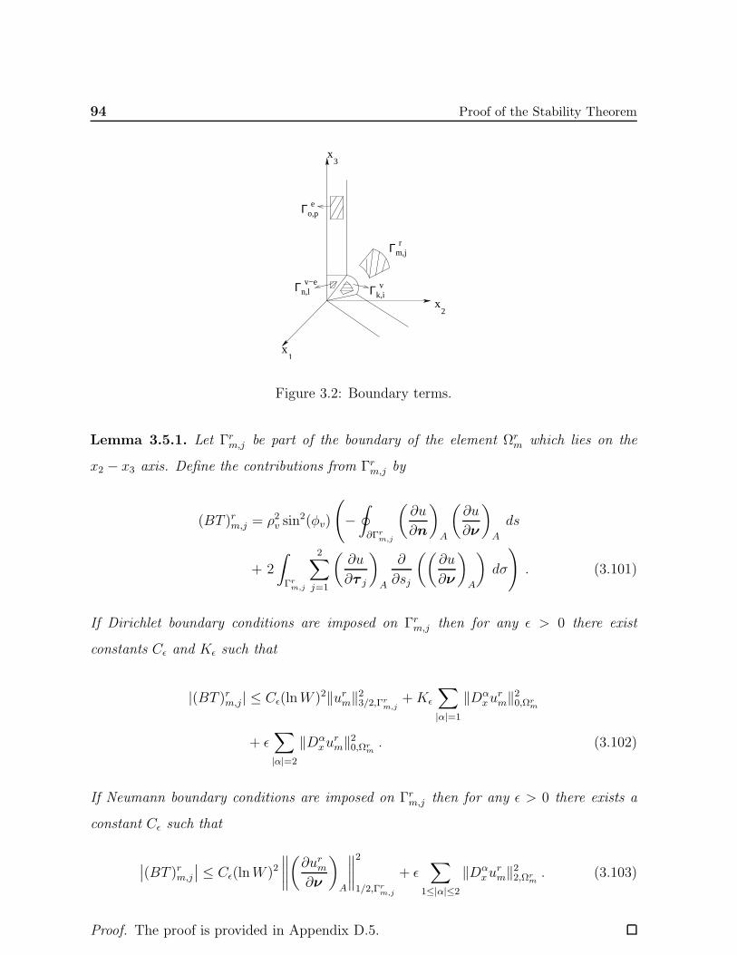
94 Proof of the Stability Theorem
x
x
x1
2
3
Γ
Γ v
rm,j
k,i
Γo,pe
Γn,lv−e
Figure 3.2: Boundary terms.
Lemma 3.5.1. Let Γrm,j be part of the boundary of the element Ωrm which lies on the
x2 − x3 axis. Define the contributions from Γrm,j by
(BT )rm,j = ρ2v sin2(φv)
(−∮
∂Γrm,j
(∂u
∂n
)
A
(∂u
∂ν
)
A
ds
+ 2
∫
Γrm,j
2∑
j=1
(∂u
∂τ j
)
A
∂
∂sj
((∂u
∂ν
)
A
)dσ
). (3.101)
If Dirichlet boundary conditions are imposed on Γrm,j then for any ǫ > 0 there exist
constants Cǫ and Kǫ such that
|(BT )rm,j| ≤ Cǫ(lnW )2‖urm‖23/2,Γrm,j
+Kǫ
∑
|α|=1
‖Dαxu
rm‖20,Ωr
m
+ ǫ∑
|α|=2
‖Dαxu
rm‖20,Ωr
m. (3.102)
If Neumann boundary conditions are imposed on Γrm,j then for any ǫ > 0 there exists a
constant Cǫ such that
∣∣(BT )rm,j∣∣ ≤ Cǫ(lnW )2
∥∥∥∥(∂urm∂ν
)
A
∥∥∥∥2
1/2,Γrm,j
+ ǫ∑
1≤|α|≤2
‖Dαxu
rm‖22,Ωr
m. (3.103)
Proof. The proof is provided in Appendix D.5.
3.5 Estimates for Terms on the Boundary 95
3.5.2 Estimates for terms on the boundary of Ωe
Lemma 3.5.2. Let Γem,j be part of the boundary of the element Ωem which lies on the
x2 − x3 axis. Define the contributions from Γem,j by
(BT )em,j = −∮
∂Γem,j
(∂u
∂ne
)
Ae
(∂u
∂νe
)
Ae
dse
− 2
∫
Γem,j
2∑
l=1
(∂u
∂τ el
)
Ae
∂
∂sel
((∂u
∂νe
)
Ae
)dσe . (3.104)
If Dirichlet boundary conditions are imposed on Γem,j and µ(Γem,j) <∞ then for any ǫ > 0
there exists constants Cǫ, Kǫ such that for W large enough
|(BT )em,j| ≤ Cǫ(lnW )2(‖uem‖20,Γe
m,i+∣∣∣∣∣∣∣∣∣(∂uem∂xe1
) ∣∣∣∣∣∣∣∣∣2
Γem,j
+∣∣∣∣∣∣∣∣∣Ge
m,j
(∂uem∂xe3
) ∣∣∣∣∣∣∣∣∣2
Γem,j
)
+Kǫ
∫
Ωem
(2∑
i=1
(∂uem∂xei
)2
+ e2τ(∂uem∂xe3
)2)dxe
+ ǫ
∫
Ωem
(∑
i,j=1,2
(∂2uem∂xei∂x
ej
)2
+ e2τ2∑
i=1
(∂2uem∂xei∂x
e3
)2
+ e4τ(∂2uem(∂xe3)
2
)2)dxe
(3.105)
If Neumann boundary conditions are imposed on Γem,j and µ(Γem,j) <∞ then for any ǫ > 0
there exists a constant Cǫ such that
∣∣(BT )em,j∣∣ ≤ Cǫ(lnW )2
∣∣∣∣∣∣∣∣∣(∂u
∂νe
)
Ae
∣∣∣∣∣∣∣∣∣2
Γem,j
+ ǫ
(∫
Ωem
(2∑
i,j=1
(∂2uem∂xei∂x
ej
)2
+e2τ2∑
i=1
(∂2uem∂xei∂x
e3
)2
+ e4τ(∂2uem(∂xe3)
2
)2
+
2∑
i=1
(∂uem∂xei
)2
+e2τ(∂uem∂xe3
)2)dxe
). (3.106)
If µ(Γem,j) =∞ then for any ǫ > 0 for N,W large enough
∣∣(BT )em,j∣∣ ≤ ǫ
∫
Ωem
(uem)2we(xe1) dx
e (3.107)
provided W = O(eNα) for α < 1/2.
Proof. The proof is provided in Appendix D.6.
We now state estimates for terms on the boundary of vertex neighbourhoods and
vertex-edge neighbourhoods.
96 Proof of the Stability Theorem
3.5.3 Estimates for terms on the boundary of Ωv
Lemma 3.5.3. Let Γvm,j be part of the boundary of the element Ωvm which lies on the
x2 − x3 axis. Define the contributions from Γvm,j by
(BT )vm,j = sin2(φv)
(−∮
∂Γvm,j
exv3 sin(xv1)
(∂u
∂nv
)
Av
(∂u
∂νv
)
Av
dsv
−2∫
Γvm,j
exv3 sin(xv1)
2∑
l=1
(∂u
∂τ vl
)
Av
∂
∂svl
((∂u
∂νv
)
Av
)dσv
). (3.108)
If Dirichlet boundary conditions are imposed on Γvm,j and µ(Γvm,j) <∞ then for any ǫ > 0
there exists constants Cǫ and Kǫ such that
|(BT )vm,j| ≤ Cǫ(lnW )2Rvm,j‖uvm‖23/2,Γv
m,j+Kǫ
∑
|α|=1
‖exv3/2Dαxvu
vm‖20,Ωe
m
+ ǫ∑
|α|=2
‖exv3/2Dαxvu
vm‖20,Ωv
m. (3.109)
If Neumann boundary conditions are imposed on Γvm,j then
∣∣(BT )vm,j∣∣ ≤ Cǫ(lnW )2Rv
m,j
∥∥∥∥(∂uvm∂νv
)
Av
∥∥∥∥2
1/2,Γvm,j
+ ǫ∑
1≤|α|≤2
‖exv3/2Dαxvu
vm‖20,Ωv
m. (3.110)
If µ(Γvm,j) =∞ then (BT )vm,j = 0.
3.5.4 Estimates for terms on the boundary of Ωv−e
Lemma 3.5.4. Let Γv−em,j be part of the boundary of the element Ωv−em which lies on the
x2 − x3 axis. Define the contributions from Γv−em,j by
(BT )v−em,j = −∮
∂Γv−em,j
exv−e3
(∂u
∂nv−e
)
Av−e
(∂u
∂νv−e
)
Av−e
dsv−e
− 2
∫
Γv−em,j
exv−e3
2∑
l=1
(∂u
∂τ v−el
)
Av−e
∂
∂sv−el
((∂u
∂νv−e
)
Av−e
)dσv−e . (3.111)

3.6 Proof of the Stability Theorem 97
If Dirichlet boundary conditions are imposed on Γv−em,j and µ(Γv−em,j ) <∞ then for any ǫ > 0
there exists constants Cǫ and Kǫ such that
|(BT )v−em,j | ≤ Cǫ(lnW )2(‖uv−em ‖20,Γv−e
m,i+∣∣∣∣∣∣∣∣∣(∂uv−em
∂xv−e1
) ∣∣∣∣∣∣∣∣∣2
Γv−em,j
+∣∣∣∣∣∣∣∣∣Ev−e
m,j
(∂uv−em
∂xv−e3
) ∣∣∣∣∣∣∣∣∣2
Γv−em,j
)
+Kǫ
∫
Ωv−em
(2∑
i=1
(∂uv−em
∂xv−ei
)2
+ sin2 φ
(∂uv−em
∂xv−e3
)2)ex
v−e3 dxv−e
+ ǫ
∫
Ωv−em
∑
i,j=1,2
(∂2uv−em
∂xv−ei ∂xv−ej
)2
+ sin2 φ
2∑
i=1
(∂2uv−em
∂xv−ei ∂xv−e3
)2
+ sin4 φ
(∂2uv−em(∂xv−e3
)2
)2 ex
v−e3 dxv−e. (3.112)
If Neumann boundary conditions are imposed on Γv−em,j and µ(Γv−em,j ) < ∞ then for any
ǫ > 0 there exists a constant Cǫ such that
∣∣(BT )v−em,j
∣∣ ≤ Cǫ(lnW )2∣∣∣∣∣∣∣∣∣(
∂u
∂νv−e
)
Av−e
∣∣∣∣∣∣∣∣∣2
Γv−em,j
+ ǫ
∫
Ωv−em
2∑
i,j=1
(∂2uv−em
∂xv−ei ∂xv−ej
)2
+ sin2 φ2∑
i=1
(∂2uv−em
∂xv−ei ∂xv−e3
)2
+ sin4 φ
(∂2uv−em
(∂xv−e3 )2
)2
+2∑
i=1
(∂uv−em
∂xv−ei
)2
+ sin2 φ
(∂uv−em
∂xv−e3
)2)ex
v−e3 dxv−e
). (3.113)
If µ(Γv−em,j ) =∞ then for any ǫ > 0 for N,W large enough
∣∣(BT )v−em,j
∣∣ ≤ ǫ
∫
Ωv−em
(uv−em )2exv−e3 wv−e(xv−e1 ) dxv−e
provided W = O(eNα) for α < 1/2.
3.6 Proof of the Stability Theorem
We are now in a position to prove the stability estimates stated in Theorems 2.3.1, 2.3.2
and 2.3.3. We recall them again.
Theorem 2.3.1. Consider the elliptic boundary value problem (2.1). Suppose the bound-
ary conditions are Dirichlet. Then
UN,W (Fu) ≤ C(lnW )2VN,W (Fu) .
98 Proof of the Stability Theorem
Theorem 2.3.2. If the boundary conditions for the elliptic boundary value problem (2.1)
are mixed then
UN,W (Fu) ≤ CN4VN,W (Fu)
provided W = O(eNα) for α < 1/2.
Theorem 2.3.3. If the boundary conditions are mixed and the spectral element functions
(Fu) are conforming on the wirebasket WB and vanish on WB then
UN,W (Fu) ≤ C(lnW )2VN,W (Fu)
provided W = O(eNα) for α < 1/2.
Proof. Define
UN,W(2) (Fu) =Nr∑
l=1
∫
Ωrl
3∑
i,j=1
(∂2url∂xi∂xj
)2
dx
+∑
v∈V
Nv∑
l=1,µ(Ωvl )<∞
∫
Ωvl
exv3
3∑
i,j=1
(∂2uvl∂xvi ∂x
vj
)2
dxv
+∑
v−e∈V−E
Nv−e∑
l=1,µ(Ωv−el )<∞
∫
Ωv−el
exv−e3
∑
i,j=1,2
(∂2uv−el
∂xv−ei ∂xv−ej
)2
+ sin2 φ2∑
i=1
(∂2uv−el
∂xv−ei ∂xv−e3
)2
+ sin4 φ
(∂2uv−el
(∂xv−e3 )2
)2)dxv−e
)
+∑
e∈E
(∫
Ωel
(∑
i,j=1,2
(∂2uel∂xei∂x
ej
)2
+ e2τ2∑
i=1
(∂2uel∂xei∂x
e3
)2
+e4τ(∂2uel(∂xe3)
2
)2)dxe
).
Then combining the results in Sections 3.1, 3.2, 3.3 and 3.4 we obtain that for any ǫ > 0
there exist constants Cǫ and Kǫ such that
UN,W(2) (Fu) ≤ Cǫ(lnW )2VN,W (Fu) + ǫ UN,W(2) (Fu)
+Kǫ UN,W(1) (Fu) . (3.114)
Here UN,W(1) (Fu) is as defined in (3.90). Hence choosing ǫ small enough we obtain
UN,W(2) (Fu) ≤ 2(Cǫ(lnW )2VN,W (Fu) +Kǫ UN,W(1) (Fu)
). (3.115)

3.6 Proof of the Stability Theorem 99
At the same time using Theorem 3.3.1 we have
UN,W(1) (Fu) ≤ KN,WVN,W (Fu) . (3.116)
Now
UN,W (Fu) = UN,W(1) (Fu) + UN,W(2) (Fu) . (3.117)
Combining (3.115), (3.116) and (3.117) the result follows.

Chapter 4
The Numerical Scheme and Error
Estimates
4.1 Introduction
In Chapters 2 and 3 we have described a method for solving three dimensional elliptic
boundary value problems on non-smooth domains using h− p spectral element methods.
In this chapter we provide the numerical scheme based on the stability estimates of
Chapters 2 and 3. We shall define a functional which is closely related to the quadratic
forms defined in Chapter 2 in the regular region and in the various neighbourhoods of
vertices, edges and vertex-edges. We seek a solution which minimizes this functional.
The functional which we minimize is the sum of a weighted squared norm of the
residuals in the partial differential equations and the squared norm of the residuals in the
boundary conditions in fractional Sobolev spaces and the sum of the squares of the jumps
in the function and its derivatives across inter-element boundaries in fractional Sobolev
norms. The Sobolev spaces in vertex-edge and edge neighbourhoods are anisotropic and
become singular at the corners and edges.
In section 4.3 we obtain error estimates and show that the error is exponentially small
in terms of the number of degrees of freedom and number of layers in the geometric mesh.
102 The Numerical Scheme and Error Estimates
4.2 The Numerical Scheme
In Chapter 2, we had divided the polyhedral domain Ω into a regular region Ωr, a set
of vertex neighborhoods Ωv, a set of edge neighborhoods Ωe and a set of vertex-edge
neighborhoods Ωv−e. We had further divided each of these sub domains into still smaller
elements as curvilinear hexahedrons, tetrahedrons and prisms and by virtue of the fact
that a tetrahedron can be split into four hexahedrons and a prism can be split into three
hexahedrons we can assume that all our elements are hexahedrons to keep the exposition
simple (and to keep the programming simple).
In Chapter 2, we had introduced a spectral element representation of the function u
on each of these elements in various parts of the domain Ω. To formulate the numerical
scheme we will define a functional RN,W (Fu), closely related to the quadratic form
VN,W (Fu) as follows:
RN,W (Fu) = RN,Wregular (Fu) +RN,W
vertices (Fu) +RN,Wvertex−edges (Fu)
+RN,Wedges(Fu). (4.1)
Let us first consider the regular region Ωr of Ω and define the functionalRN,Wregular(Fu).
Ωr is divided intoNr curvilinear hexahedrons Ωrl , l = 1, 2, . . . , Nr and we map each of these
Ωrl onto the master cube
Q = (−1, 1)3 = λ = (λ1, λ2, λ3)| − 1 ≤ λi ≤ 1, 1 ≤ i ≤ 3
using an analytic map M rl having an analytic inverse.
We now define a non-conforming spectral element representation on each of these
elements as follows:
url (λ) =W∑
i=0
W∑
j=0
W∑
k=0
αi,j,k λi1λ
j2λ
k3.
Let λ = (λ1, λ2, λ3) and let f rl (λ) = f(M rl (λ1, λ2, λ3)) where λ ∈ Q for l = 1, 2, . . . , Nr
and let Jrl (λ) denote the Jacobian of the mapping M rl . Define
F rl (λ) = f rl (λ)
√Jrl (λ) ,
4.2 The Numerical Scheme 103
and
Lrl url (λ) = Lurl (M
rl (λ))
√Jrl (λ) .
Now consider the boundary conditions w = gk on Γk for k ∈ D = Γ[0] and(∂w∂ν
)A=
hk on Γk for k ∈ N = Γ[1]. Let Γri,k = Γk ∩ ∂Ωri be the image of the mapping M ri
corresponding to λ1 = −1. Let gri,k = gk(Mri (−1, λ2, λ3)) and hri,k = hk(M
ri (−1, λ2, λ3))
where −1 ≤ λ2, λ3 ≤ 1.
We now define
RN,Wregular(Fu) =
Nr∑
l=1
∫
Q=(Mrl )
−1(Ωrl )
| Lrl url (λ)− F rl (λ) |2 dλ
+∑
Γrl,i⊆Ωr\∂Ω
(‖[u]‖20,Γr
l,i+
3∑
k=1
‖[uxk ]‖21/2,Γrl,i
)
+∑
Γrl,i⊆Γ[0]
∥∥url − grl,i∥∥23/2,Γr
l,i
+∑
Γrl,i⊆Γ[1]
∥∥∥∥(∂url∂ν
)
A
− hrl,i∥∥∥∥2
1/2,Γrl,i
. (4.2)
Let v be one of the vertices of Ω. Consider the vertex neighborhood Ωv of the vertex
v ∈ V, the set of vertices (defined in Chapter 2). Ωv is divided into Nv curvilinear hexa-
hedrons Ωvl , l = 1, 2, . . . , Nv. We define a non-conforming spectral element representation
as follows: Let Ωvl be the image of Ωvl in xv coordinates. Then there is an analytic map
Mvl : Q→ Ωvl having an analytic inverse. If Ωvl is a corner element of the form
Ωvl = xv : (φ, θ) ∈ Svj ,−∞ < χ < ln(ρv1)
then we define uvl = hv, where hv is a constant.
If Ωvl is of the form
Ωvl = xv : (φ, θ) ∈ Svj , ln(ρvi ) < χ < ln(ρvi+1)
we define
uvl (xv) =
Wl∑
t=0
Wl∑
s=0
Wl∑
r=0
βr,s,t φrθsχt .
Here 1 ≤ Wl ≤ W . Moreover as in [51], Wl = [µ1i] for all 1 ≤ i ≤ N , where µ1 > 0 is a
degree factor. Hereafter [a] denotes the greatest positive integer ≤ a.
104 The Numerical Scheme and Error Estimates
Let Av = (xv1, xv2, x
v3) denote one of the vertices of Ω. Let F
vl (x
v) = e5/2χ√sinφf(x(xv))
for xvl ∈ Ωvl , 1 ≤ l ≤ Nv.
We now consider the boundary conditions w = gi on Γi for i ∈ D = Γ[0] and(∂w∂ν
)A= hi
on Γi for i ∈ N = Γ[1]. Let Γvl,i = Γi ∩ ∂Ωvl and suppose Ωvl is not a corner element.
Moreover it is assumed that Γvl,i lies on the x2 − x3 plane for simplicity. Define
gvl,i(xv) = w = gi(x(x
v)) for Γvl,i ⊆ Γ[0],
hvl,i(xv) =
(∂w
∂νv
)
Av
=eχ
sinφhi(x(x
v)) for Γvl,i ⊆ Γ[1].
Let
Rvl,i = sup
xv∈Γvl,i
(exv3).
We now define the functional
RN,Wv (Fu) =
Nv∑
l=1,µ(Ωvl )<∞
∫
Ωvl
| Lvuvl (xv)− F vl (x
v) |2 dxv
+∑
Γvl,i⊆Ωv\∂Ωµ(Γv
l,i)<∞
(∥∥∥√Rvl,i[u]
∥∥∥2
0,Γvl,i
+
3∑
k=1
∥∥∥√Rvl,i[uxvk ]
∥∥∥2
1/2,Γvl,i
)
+∑
Γvl,i⊆Γ[0],
µ(Γvl,i)<∞
∥∥∥√Rvl,i
(uvl − gvl,i
) ∥∥∥2
3/2,Γvl,i
+∑
Γvl,i⊆Γ[1],
µ(Γvl,i)<∞
∥∥∥∥√Rvl,i
((∂uvl∂νv
)
Av
− hvl,i) ∥∥∥∥
2
1/2,Γvl,i
. (4.3)
The functional RN,Wvertices(Fu) is then given by
RN,Wvertices(Fu) =
∑
v∈VRN,Wv (Fu) . (4.4)
Next, we define RN,Wvertex−edges(Fu). Let Ωv−e denote the vertex-edge neighborhood of
the vertex-edge v−e ∈ V − E . Ωv−e is divided into Nv−e elements Ωv−el , l = 1, 2, . . . , Nv−e.
As in Chapter 2, let us define a non-conforming spectral element representation on each
of these sub-domains as follows:
4.2 The Numerical Scheme 105
Let Ωv−el be the image of Ωv−el in xv−e coordinates. If Ωv−en is a corner element of the
form
Ωv−en = xv−e : ψv−ei < ψ < ψv−ei+1 , θv−ej < θ < θv−ej+1 , −∞ < ζ < ζv−e1
then on Ωv−en we define
uv−en = hv−e = hv .
Next, suppose Ωv−ep is a corner element of the form
Ωv−ep =xv−e : −∞ < ψ < ψv−e1 , θv−ej < θ < θv−ej+1 , ζ
v−en < ζ < ζv−en+1
with k ≥ 1. Then on Ωv−ep we define
uv−ep (xv−e) =
Wp∑
l=0
βl ζl.
Here 1 ≤Wp ≤W . Moreover Wp = [µ2n] for 1 ≤ n ≤ N , where µ2 > 0 is a degree factor.
Finally, suppose Ωv−eq is of the form
Ωv−eq =xv−e : ψv−ei < ψ < ψv−ei+1 , θ
v−ej < θ < θv−ej+1 , ζ
v−en < ζ < ζv−en+1
with i ≥ 1, n ≥ 1. Then on Ωv−eq we define
uv−eq (xv−e) =
Wq∑
r=0
Wq∑
s=0
Vq∑
t=0
γr,s,t ψrθsζ t.
Here 1 ≤ Wq ≤ W and 1 ≤ Vq ≤ W . Moreover Wq = [µ1i], Vq = [µ2n] for 1 ≤ i, n ≤ N ,
where µ1, µ2 > 0 are degree factors [51].
Let F v−el (xv−e) = e2x
v−e1 e
52xv−e3 f(x(xv−e)) for xv−e ∈ Ωv−el , 1 ≤ l ≤ Nv−e.
We now consider the boundary conditions w = gk on Γk for k ∈ D = Γ[0] and(∂w∂ν
)A=
hk on Γk for k ∈ N = Γ[1]. Then(
∂w∂νv−e
)Av−e = ex
v−e3 ex
v−e1 hk(x(x
v−e)). Let Γv−el,k =
Γk ∩ ∂Ωv−el and suppose Ωv−el is not a corner element. Moreover it is assumed that Γv−el,k
lies on the x2 − x3 plane for simplicity and µ(Γv−el,k ) <∞. Define
gv−el,k (xv−e) = w = gk(x(xv−e)) for Γv−el,k ⊆ Γ[0],
hv−el,k (xv−e) =
(∂w
∂νv−e
)
Av−e
= exv−e3 ex
v−e1 hk(x(x
v−e)) for Γv−el,k ⊆ Γ[1].
106 The Numerical Scheme and Error Estimates
We define the functional
RN,Wv−e (Fu) =
Nv−e∑
l=1,µ(Ωv−el )<∞
∫
Ωv−el
∣∣ Lv−euv−el (xv−e)− F v−el (xv−e)
∣∣2 dxv−e
+∑
Γv−el,k ⊆Ωv−e\∂Ω,µ(Γv−e
l,k )<∞
(∥∥∥√F v−el,k Gv−e
l,k [u]∥∥∥2
0,Γv−el,k
+∣∣∣∣∣∣ [uxv−e
1]∣∣∣∣∣∣2
Γv−el,k
+∣∣∣∣∣∣ [uxv−e
2]∣∣∣∣∣∣2
Γv−el,k
+∣∣∣∣∣∣ Ev−e
l,k [uxv−e3
]∣∣∣∣∣∣2
Γv−el,k
)
+∑
Γv−el,k ⊆Γ[0],
µ(Γv−el,k )<∞
(∥∥∥√F v−el,k
(uv−el − gv−el,k
) ∥∥∥2
0,Γv−el,k
+∣∣∣∣∣∣(uxv−e
1− (gv−el,k )
xv−e1
) ∣∣∣∣∣∣2Γv−el,k
+∣∣∣∣∣∣ Ev−e
l,k
(uxv−e
3− (gv−el,k )
xv−e3
) ∣∣∣∣∣∣2Γv−el,k
)
+∑
Γv−el,k ⊆Γ[1],
µ(Γv−el,k )<∞
∣∣∣∣∣∣∣∣∣(
∂u
∂νv−e
)
Av−e
− hv−el,k
∣∣∣∣∣∣∣∣∣2
Γv−el,k
. (4.5)
Here Ev−el,k = sup
xv−e∈Γv−el,k
(sin φ) and Gv−el,k = sup
xv−e∈Γv−el,k
(exv−e3 ). Moreover, Gv−e
l,k is defined in
(2.27).
Then the functional RN,Wvertex−edges(Fu) is defined as follows:
RN,Wvertex−edges(Fu) =
∑
v−e∈V−ERN,Wv−e (Fu) . (4.6)
Finally, we define the functional RN,Wedges(Fu). Let Ωe denote the edge neighborhood
of the edge e ∈ E . Ωe is divided into Ne elements Ωel , l = 1, 2, . . . , Ne. Once again we
define a non-conforming spectral element representation on each of these sub-domains as
follows:
Let Ωem be the image of Ωem in xe coordinates. If Ωep is a corner element of the form
Ωep =xe : −∞ < xe1 < ln(re1), θ
ej < xe2 < θej+1, Z
en < xe3 < Ze
n+1
then we define
uep(xe) =
W∑
t=0
αt(xe3)t .
4.2 The Numerical Scheme 107
Next, let Ωeq be of the form
Ωeq =xe : ln(rei ) < xe1 < ln(rei+1), θ
ej < xe2 < θej+1, Z
en < xe3 < Ze
n+1
with 1 ≤ i ≤ N, 0 ≤ j ≤ Ie, 0 ≤ n ≤ Je .
Then we define
ueq(xe) =
Wq∑
r=0
Wq∑
s=0
W∑
t=0
αr,s,t (xe1)r(xe2)
s(xe3)t .
Here 1 ≤Wq ≤W . Moreover Wq = [µ1i] for 1 ≤ i ≤ N , µ1 > 0 is a degree factor.
Let F el (x
e) = e2xe1f(x(xe)) for xe ∈ Ωel , 1 ≤ l ≤ Ne.
We now consider the boundary conditions w = gk on Γk for k ∈ D = Γ[0] and(∂w∂ν
)A=
hk on Γk for k ∈ N = Γ[1]. Then(∂w∂νe
)Ae = ex
e1hk(x(x
e)). Let Γem,k = Γk ∩ ∂Ωem and
suppose Ωem is not a corner element. Moreover it is assumed that Γem,k lies on the x2 − x3plane for simplicity and µ(Γem,k) <∞. Define
gem,k(xe) = w = gk(x(x
e)) for Γem,k ⊆ Γ[0],
hem,k(xe) =
(∂w
∂νe
)
Ae
= exe1hk(x(x
e)) for Γem,k ⊆ Γ[1] .
We define
RN,We (Fu) =
Ne∑
l=1,µ(Ωel )<∞
∫
Ωel
| Leuel (xe)− F el (x
e) |2 dxe
+∑
Γem,k⊆Ωe\∂Ω,µ(Γe
m,k)<∞
(∥∥∥√Hem,k [u]
∥∥∥2
0,Γem,k
+∣∣∣∣∣∣ [uxe1]
∣∣∣∣∣∣2Γem,k
+∣∣∣∣∣∣ [uxe2]
∣∣∣∣∣∣2Γem,k
+∣∣∣∣∣∣Ge
m,k [uxe3]∣∣∣∣∣∣2
Γem,k
)
+∑
Γem,k⊆Γ[0],
µ(Γem,k)<∞
(∥∥ (uem − gem,k) ∥∥2
0,Γem,k
+∣∣∣∣∣∣(uxe1 − (gem,k)xe1
) ∣∣∣∣∣∣2Γem,k
+∣∣∣∣∣∣Ge
m,k
(uxe3 − (gem,k)xe3
) ∣∣∣∣∣∣2Γem,k
)
+∑
Γem,k⊆Γ[1],
µ(Γem,k)<∞
∣∣∣∣∣∣∣∣∣(∂u
∂νe
)
Ae
− hem,k∣∣∣∣∣∣∣∣∣2
Γem,k
. (4.7)
108 The Numerical Scheme and Error Estimates
Here Gem,k = sup
xe∈Γem,k
(eτ ) and Hem,k is as defined in (2.34).
The functional RN,Wedges(Fu) can now be defined as:
RN,Wedges(Fu) =
∑
e∈ERN,We (Fu) . (4.8)
Finally using (4.2), (4.4), (4.6) and (4.8) in (4.1) we can define RN,W (Fu).Our numerical scheme may now be formulated as follows:
Find Fs ∈ SN,W which minimizes the functional RN,W (Fu) over all Fu ∈ SN,W .
Here SN,W denotes the space of spectral element functions Fu.
4.3 Error Estimates
It is well known that for three dimensional elliptic problems containing singularities in
the form of vertices and edges, the geometric mesh and a proper choice of element degree
distribution leads to exponential convergence and efficiency of computations (see [12, 13,
49, 51] and references therein).
Let N denote the number of refinements in the geometrical mesh and W denote
an upper bound on the degree of the polynomial representation of the spectral element
functions. We assume that N is proportional to W .
In this Section we show that the error obtained from the proposed method is expo-
nentially small in N . The optimal rate of convergence with respect to Ndof , the number
of degrees of freedom is also provided.
Our analysis of error estimates is similar to that in two dimensions (see [8, 11, 60, 86]
and references therein). Here, we briefly describe the main steps of the proof, for details
one may refer to [60].
Let SN,W (Ωv), SN,W (Ωv−e), SN,W (Ωe), and SN,W (Ωr) denote the space of spectral
element functions (SEF) over the set of vertex neighbourhoods Ωv, vertex-edge neigh-
bourhoods Ωv−e, edge neighbourhoods Ωe and regular region Ωr respectively. Let us
denote by SN,W (Ω) the space of SEF over the whole domain Ω whose restrictions to Ωv,
Ωv−e, Ωe and Ωr belong to SN,W (Ωv), SN,W (Ωv−e), SN,W (Ωe), and SN,W (Ωr) respectively.
4.3 Error Estimates 109
Let Fz minimize RN,W (Fu) over all Fu ∈ SN,W (Ω), the space of spectral ele-
ment functions. We write one more representation for Fz as follows:-
Fz =zrl (λ1, λ2, λ3)Nr
l=1 , zvl (φ, θ, χ)Nv
l=1 ,zv−el (ψ, θ, ζ)
Nv−e
l=1, zel (τ, θ, x3)Ne
l=1
.
Here zrl (λ1, λ2, λ3) is a polynomial of degree W in each of its variables.
zvl = av, where av is a constant, on corner elements Ωvl with µ(Ωvl ) = ∞. In all other
elements in the vertex neighbourhoods, zvl (φ, θ, χ) is a polynomial of degree Wl, 1 ≤Wl ≤W,Wl = [µ1i] for all 1 ≤ i ≤ N + 1, in φ, θ and χ variables separately, where µ1 > 0 is a
degree factor.
zv−el = av−e = av, on corner elements Ωv−el of the form
Ωv−el = xv−e : ψv−ei < ψ < ψv−ei+1 , θv−ej < θ < θv−ej+1 , −∞ < ζ < ζv−e1
and zv−el is a polynomial of degree Vl in ζ , 1 ≤ Vl ≤ W,Vl = [µ2n] for all 1 ≤ n ≤ N, µ2 > 0,
on corner elements Ωv−el of the form
Ωv−el =xv−e : −∞ < ψ < ψv−e1 , θv−ej < θ < θv−ej+1 , ζ
v−en < ζ < ζv−en+1
with n ≥ 1.
On the remaining elements in the vertex-edge neighbourhoods, zv−el (ψ, θ, ζ) is a poly-
nomial of degree Wl, 1 ≤ Wl ≤ W,Wl = [µ1i] for all 1 ≤ i ≤ N , in ψ, θ variables and of
degree Vl, 1 ≤ Vl ≤W,Vl = [µ2n] for all 1 ≤ n ≤ N , in ζ variable with µ1 > 0, µ2 > 0.
Finally, on corner elements Ωel with µ(Ωel ) =∞, zel is a polynomial of degree W in x3
and on the remaining elements Ωel away from edges zel (τ, θ, x3) is a polynomial of degree
Wl, 1 ≤Wl ≤W,Wl = [µ1i], 1 ≤ i ≤ N, µ1 > 0 in τ, θ variables and of degree W in the x3
variable.
Approximation in the regular region:
Let us first consider the regular region Ωr of Ω. In Chapter 2, Ωr has been divided
into Ωrl , l = 1, . . . , Nr curvilinear hexahedrons, tetrahedrons and prisms. Let M rl be the
analytic map from Q to Ωrl .
Let ΠW,W,W (w(M rl (λ))) denote the projection of the solution w into the space of poly-
nomials of degree N in each of its variables with respect to the usual inner product in
110 The Numerical Scheme and Error Estimates
H2(Q). Then on Ωrl we define
srl (λ) = ΠW,W,W (w(M rl (λ))) = ΠW,W,W (w(λ)), for λ ∈ Q.
Approximation in vertex neighbourhoods:
Let us now consider the vertex neighbourhood Ωv of the vertex v ∈ V, where V denotes
the set of vertices of Ω (see Figure 2.8). We had divided Ωv into Ωvl , l = 1, . . . , Nv elements
(Chapter 2). If Ωvl is a corner element of the form
Ωvl = xv : (φ, θ) ∈ Svj ,−∞ < χ < ln(ρv1)
then on Ωvl we define
svl = wv,
where wv = w(v) denotes the value of w at the vertex v defined as in our differentiability
estimates of Chapter 2.
If Ωvl is of the form
Ωvl = xv : (φ, θ) ∈ Svj , ln(ρvi ) < χ < ln(ρvi+1)
then on Ωvl we approximate (w(xv)−wv) by its projection, denoted by ΠWl,Wl,Wl, into the
space of polynomials of degree N in each of its variables separately with respect to the
usual inner product in H2(Ωvl ) and define
svl (xv) = ΠWl,Wl,Wl(w(xv)− wv) + wv.
Here 1 ≤ Wl ≤W , Wl = [µ1i] for all 1 ≤ i ≤ N , where µ1 > 0 is a degree factor [51].
Approximation in vertex-edge neighbourhoods:
We now consider the vertex-edge neighborhood Ωv−e of the vertex-edge v− e ∈ V − E(see Figure 2.9). Here, as earlier, V − E denotes the set of vertex-edges of the domain
Ω. Ωv−e is divided into Ωv−eq , q = 1, . . . , Nv−e elements using a geometric mesh in φ, x3
variables and a quasi-uniform mesh in θ variable.
Let Ωv−eq be the image of Ωv−eq in xv−e coordinates. If Ωv−eq is a corner element of the
form
Ωv−eq = xv−e : ψv−ei < ψ < ψv−ei+1 , θv−ej < θ < θv−ej+1 , −∞ < ζ < ζv−e1
4.3 Error Estimates 111
then on Ωv−eq we define
sv−el = wv−e = wv .
Here wv is the value of w at the vertex v (Chapter 2).
Next, suppose Ωv−eq is a corner element of the form
Ωv−eq =xv−e : −∞ < ψ < ψv−e1 , θv−ej < θ < θv−ej+1 , ζ
v−en < ζ < ζv−en+1
with n ≥ 1. Let s(xv−e3 ) = w(x1, x2, x3)|(x1=0,x2=0) be the value of w along the edge e.
Define
σ(xv−e3 ) = s(xv−e3 )− wv.
Let ΠVq(σ(xv−e3 )) be the orthogonal projection of σ(xv−e3 ) into the space of polynomials
in H2(I). Then we define
sv−el (xv−e3 ) = ΠVq(σ(xv−e3 )) + wv = ΠVqs(xv−e3 ).
Here 1 ≤ Vq ≤ W . Moreover Wq = [µ2n] for all 1 ≤ n ≤ N , where µ2 > 0 is a degree
factor.
The remaining elements Ωv−eq in Ωv−e are of the form
Ωv−eq =xv−e : ψv−ei < ψ < ψv−ei+1 , θ
v−ej < θ < θv−ej+1 , ζ
v−en < ζ < ζv−en+1
with i ≥ 1, k ≥ 1. Let us write α(xv−e) = w(xv−e) − s(xv−e3 ). Then on Ωv−eq we
approximate α(xv−e) by its projection, denoted by ΠWq,Wq,Vq , into the space of polynomials
with respect to the usual inner product in H2(Ωv−eq ). We now define
sv−el (xv−e) = ΠWq,Wq,Vq(α(xv−e)) + ΠVq(s(xv−e3 )).
Here 1 ≤ Wq ≤ W and 1 ≤ Vq ≤W . Moreover Wq = [µ1i], Vq = [µ2n] for all 1 ≤ i, n ≤ N ,
where µ1, µ2 > 0 are degree factors [51].
Finally, we discuss approximation in the edge neighbourhood elements and define
comparison functions there.
Approximation in edge neighbourhoods:
112 The Numerical Scheme and Error Estimates
Consider the edge neighborhood Ωe of the edge e ∈ E (see Figure 2.10). Here, as
before, E denotes the set of edges of the domain Ω. In Chapter 2, we had divided Ωe into
Ωep, p = 1, . . . , Ne elements.
Let Ωep be the image of Ωep in xe coordinates. Let Ωep be a corner element of the form
Ωep =xe : −∞ < xe1 < ln(re1), θ
ej < xe2 < θej+1, Z
en < xe3 < Ze
n+1
.
Let s(xe3) = w (x1, x2, x3) |(x1=0,x2=0). Then on Ωep we approximate s(xe3) by its projec-
tion onto the space of polynomials with respect to the usual inner product in H2(I). Let
ΠW (s(xe3)) denote this projection, then we define
sel (xe3) = ΠW (s(xe3)).
Next, let Ωep be of the form
Ωep =xe : ln(rei ) < xe1 < ln(rei+1), θ
ej < xe2 < θej+1, Z
en < xe3 < Ze
n+1
with 1 ≤ i ≤ N, 0 ≤ j ≤ Ie, 0 ≤ n ≤ Je. Let us write β(xe) = w(xe) − s(xe3). Then
on Ωep we approximate β(xe) by its projection, denoted by ΠWp,Wp,W , into the space of
polynomials with respect to the usual inner product in H2(Ωep). Define
sel (xe) = ΠWp,Wp,W (β(xe)) + ΠW (s(xe3)).
Here 1 ≤ Wp ≤ W . Moreover Wp = [µ1i] for all 1 ≤ i ≤ N , where µ1 > 0 is a degree
factor [51].
Now consider the set of functionssrl Nr
l=1, svl Nvl=1, sv−el
Nv−e
l=1 , sel Nel=1
and denote it
by Fs.We will show that the functional defined by
RN,W (Fs) = RN,Wregular (Fs) +RN,W
vertices (Fs)
+RN,Wvertex−edges (Fs) +RN,W
edges(Fs) (4.9)
is exponentially small in N . Here the functionals RN,Wregular (Fs), RN,W
vertices (Fs) etc. aresimilar to those as defined in Section 4.2.
4.3 Error Estimates 113
Using results on approximation theory in [11, 12, 60] it follows that there exist con-
stants C and b > 0 such that the estimate
RN,W (Fs) ≤ Ce−bN (4.10)
holds.
Now Fz minimizes RN,W (Fu) over all Fu ∈ SN,W (Ω), the space of spectral
element functions. Then from (4.10), we have
RN,W (Fz) ≤ Ce−bN . (4.11)
Let VN,W be the quadratic form as defined in Chapter 2. Then from (4.10) and (4.11) we
can conclude that
VN,W(F(s−z)
)≤ Ce−bN (4.12)
where C and b are generic constants.
Hence using the Stability Theorem 2.3.1 we obtain
UN,W(F(s−z)
)≤ Ce−bN . (4.13)
Here the quadratic form UN,W(F(s−z)
)is defined similar to the quadratic form UN,W (Fu)
as in (2.15) of Chapter 2.
Let U rl (λ) = w(Xr
l (λ1, λ2, λ3)) ≡ w(M rl (λ)) for λ ∈ Q, Uv
l (xv) = w(xv) for xv ∈ Ωvl ,
Uv−el (xv−e) = w(xv−e) for xv−e ∈ Ωv−el and Ue
l (xe) = w(xe) for xe ∈ Ωel . Here w is the
solution of the boundary value problem (2.1).
We now define another quadratic form EN,W (z − U) as follows:-
EN,W (z − U) = EN,Wregular(zrl − U rl ) + EN,Wvertices(zvl − Uv
l )
+ EN,Wvertex−edges(zv−el − Uv−el ) + EN,Wedges(zel − Ue
l ) , (4.14)

114 The Numerical Scheme and Error Estimates
where
EN,Wregular(zrl − U rl ) =
Nr∑
l=1
∫
Q=(Mrl )
−1(Ωrl )
∑
|α|≤2
|Dαλ (z
rl − U r
l ) (λ)|2 dλ ,
EN,Wvertices(zvl − Uvl ) =
∑
v∈VEN,Wv (zvl − Uv
l ) ,
EN,Wv (zvl − Uvl ) =
Nv∑
l=1
∫
Ωvl
exv3
∑
|α|≤2
|Dαxv (z
vl − Uv
l ) (xv)|2 dxv ,
EN,Wvertex−edges(zv−el − Uv−el ) =
∑
v−e∈V−EEN,Wv−e (zv−el − Uv−e
l ) ,
EN,Wv−e (zv−el − Uv−el ) =
Nv−e∑
l=1
∫
Ωv−el
exv−e3
∑
|α|≤2
∣∣Dαxv−e
(zv−el − Uv−e
l
)(xv−e)
∣∣2 dxv−e ,
EN,Wedges(zel − Uel ) =
∑
e∈EEN,We (zel − Ue
l ) ,
EN,We (zel − Uel ) =
Ne∑
l=1
∫
Ωel
∑
|α|≤2
|Dαxe (z
el − Ue
l ) (xe)|2 dxe .
It is easy to show that
EN,Wregular(srl − U rl ) ≤ Ce−bN ,
EN,Wvertices(svl − Uvl ) ≤ Ce−bN ,
EN,Wvertex−edges(sv−el − Uv−el ) ≤ Ce−bN ,
EN,Wedges(sel − Uel ) ≤ Ce−bN (4.15)
where the quadratic forms EN,Wregular (srl − U rl ), EN,Wvertices (svl − Uv
l ) etc. are defined similar
to those in (4.14). Now define
EN,W (s− U) = EN,Wregular(srl − U rl ) + EN,Wvertices(svl − Uv
l )
+ EN,Wvertex−edges(sv−el − Uv−el ) + EN,Wedges(sel − Ue
l ) .
Then from (4.15) it follows that
EN,W (s− U) ≤ Ce−bN . (4.16)
Finally, using estimates (4.13) and (4.16), we obtain
UN,W(F(z−U)
)≤ Ce−bN .
4.3 Error Estimates 115
Our main theorem on error estimates is now stated
Theorem 4.3.1. Let Fz minimize RN,W (Fu) over all Fu ∈ SN,W (Ω). Then there
exist constants C and b (independent of N) such that
UN,W(F(z−U)
)≤ Ce−bN . (4.17)
Here UN,W(F(z−U)
)is as defined in (2.15) of Chapter 2.
Remark 4.3.1. After having obtained the non-conforming spectral element solution we
can make a correction to it so that the corrected solution is conforming and the error in
the H1 norm is exponentially small in N . These corrections are similar to those described
in [60, 85, 86] in two dimensions and are explained in the proof of Lemma 3.3.1 in
Appendix C.1.
To end this chapter, let us estimate the error in terms of number of degrees of freedom
in various subregions of the domain Ω.
The regular region Ωr:
The regular region Ωr contains no vertices and edges of the domain Ω. Here the
solution w has no singularity and is analytic.
There are O(1) number of elements in this region and each element has O(W 3) degrees
of freedom. Let Ndof (Ωr) denotes the number of degrees of freedom in Ωr. Then
Ndof (Ωr) = O(W 3) = O(N3) .
The vertex neighbourhoods Ωv:
In a vertex neighbourhood Ωv there are O(N) elements with O(W 3) degrees of freedom
in each element. If Ndof (Ωv) denotes the number of degrees of freedom in Ωv. Then
Ndof(Ωv) = O(NW 3) = O(N4).
The vertex-edge neighbourhoods Ωv−e:
There are O(N2) number of elements in each of the vertex-edge neighbourhoods Ωv−e
and each element has O(W 3) degrees of freedom. Then
Ndof (Ωv−e) = O(N2W 3) = O(N5) .
116 The Numerical Scheme and Error Estimates
Here Ndof (Ωv−e) denotes the number of degrees of freedom in Ωv−e.
The edge neighbourhoods Ωe:
An edge neighbourhood Ωe has O(N) elements with O(W 3) degrees of freedom within
each element. Let Ndof (Ωe) be the number of degrees of freedom in Ωe. Then
Ndof (Ωe) = O(NW 3) = O(N4) .
Hence, the error estimate Theorem 4.3.1 in terms of number of degrees of freedom assumes
the form
Theorem 4.3.2. Let Fz minimizes RN,W (Fu) over all Fu ∈ SN,W (Ω). Then there
exist constants C and b (independent of N) such that
UN,W(F(z−U)
)≤ Ce−bN
1/5dof . (4.18)
Here UN,W(F(z−U)
)is as defined in (2.15) and Ndof = dim(SN,W (Ω)) is the number of
degrees of freedom.
Proof. Follows from Theorem 4.3.1.
Remark 4.3.2. From the above theorem it is clear that the exponential rate of convergence
will be visible only for a large value of Ndof , as a result we need to sufficiently refine the
geometric mesh both in the direction of edges and in the direction perpendicular to the
edges.
Remark 4.3.3. Since the majority of degrees of freedom is present in the vertex-edge
neighbourhoods the factor N1/5dof in the theorem is due to the vertex-edge singularity in the
solution. Hence the optimal convergence rate will be e−bN1/5dof .
Remark 4.3.4. It was conjectured in [13, 51] that for h− p version of the finite element
method in R3 the optimal convergence rate will be e−bN
1/5dof , and it can not be improved
further with any mesh and any anisotropic polynomial order within the elements.
Chapter 5
Solution Techniques on Parallel
Computers
5.1 Introduction
In Chapter 4 we had described the numerical scheme and the error estimates for the
numerical solution were stated.
The method is essentially a least-squares collocation method. To solve the mini-
mization problem we need to solve the normal equations arising from the minimization
problem. We use preconditioned conjugate gradient method (PCGM) to solve the normal
equations using a block diagonal preconditioner which is nearly optimal as the condition
number of the preconditioned system is polylogarithmic in N , the number of refinements
in the geometric mesh. Moreover, to compute the residuals in the normal equations we
do not need to compute mass and stiffness matrices.
We use only non-conforming spectral element functions. We shall examine spectral
element functions which are conforming on the wirebasket in future work.
It is shown that we can define a preconditioner for the minimization problem which
allows the problem to decouple. Construction of preconditioner on each element in various
regions of the polyhedron is also provided. It will be shown as in [36] that there exists
a new preconditioner which can be diagonalized in a new set of basis functions using
118 Solution Techniques on Parallel Computers
separation of variables technique.
The coefficients in the differential operator and the data are projected into the poly-
nomial spaces (we call them filtered coefficients of the differential operator and filtered
data) so that the integrands involved in the numerical formulation are exactly evaluated
using Gauss-Lobatto-Legendre (GLL) quadrature. However, in our computations we do
not need to filter the coefficients of the differential operator and the data. Of course, in
doing so we commit an error and it can be argued as in [86] that this error is spectrally
small.
In section 5.3 we shall describe the steps involved in computing the residuals in the
normal equations without computing mass and stiffness matrices on a distributed mem-
ory parallel computer. The evaluation of these residuals on each processor requires the
interchange of boundary values between neighbouring processors. Hence the communica-
tion involved is quite small. Thus we can compute the residuals in the normal equations
inexpensively and efficiently. Finally, we shall discuss computational complexity of our
method.
5.2 Preconditioning
We now come to the aspect of preconditioning. Our construction of preconditioners is
similar to that for elliptic problems in two dimensions (see [37, 38, 85, 86]).
5.2.1 Preconditioners on the regular region
In the regular region the preconditioner which needs to be examined corresponds to the
quadratic form
B(u) = ||u||2H2(Q) (5.1)
where Q = (−1, 1)3 =master cube, u = u(λ) = u(λ1, λ2, λ3) is a polynomial of degree W
in λ1, λ2 and λ3 separately.
5.2 Preconditioning 119
Let u(λ1, λ2, λ3) be the spectral element function, defined on Q = (−1, 1)3, as
u(λ1, λ2, λ3) =
W∑
i=0
W∑
j=0
W∑
k=0
ai,j,kLi(λ1)Lj(λ2)Lk(λ3). (5.2)
Here Li(·) denotes the Legendre polynomial of degree i.
The quadratic form B(u) can be written as
B(u) =∫
Q
∑
|α|≤2
|Dαλu|2dλ. (5.3)
We shall show that there is another quadratic form C(u) which is spectrally equivalent to
B(u) and which can be easily diagonalized using separation of variables.
Let I denote the interval (−1, 1) and
v(λ1) =
W∑
i=0
βiLi(λ1) . (5.4)
Moreover b = (β0, β1, . . . , βW )T . We now define the quadratic form
E(v) =∫
I
(v2λ1λ1 + v2λ1)dλ1 (5.5)
and
F(v) =∫
I
v2dλ1 . (5.6)
Clearly there exist (W + 1)× (W + 1) matrices E and F such that
E(v) = bTEb (5.7)
and
F(v) = bTFb. (5.8)
Here the matrices E and F are symmetric and F is positive definite.
Hence there exist W + 1 eigenvalues 0 ≤ µ0 ≤ µ1 ≤ · · · ≤ µW and W + 1 eigenvectors
b0, b1, . . . , bW of the symmetric eigenvalue problem
(E − µF )b = 0 . (5.9)
Here
(E − µiF )bi = 0 .
120 Solution Techniques on Parallel Computers
The eigenvectors bi are normalized so that
bTi Fbj = δij . (5.10a)
Moreover the relations
bTi Ebj = µiδij (5.10b)
hold. Let bi = (bi,0, bi,1, . . . , bi,W ). We now define the polynomial
φi(λ1) =
W∑
j=0
bi,jLj(λ1) for 0 ≤ i ≤ W . (5.11)
Next, let ψi,j,k denote the polynomial
ψi,j,k(λ1, λ2, λ3) = φi(λ1)φj(λ2)φk(λ3) (5.12)
for 0 ≤ i ≤W, 0 ≤ j ≤ W, 0 ≤ k ≤W .
Let u(λ1, λ2, λ3) be a polynomial as in (5.2). Define the quadratic form
C(u) =∫
Q
(u2λ1λ1 + u2λ2λ2 + u2λ3λ3 + u2λ1 + u2λ2 + u2λ3 + u2)dλ1dλ2dλ3 . (5.13)
Then the quadratic form C(u) is spectrally equivalent to the quadratic form B(u), de-fined in (5.1). Moreover, the quadratic form C(u) can be diagonalized in the basis
ψi,j,k(λ1, λ2, λ3). Note that ψi,j,k(λ1, λ2, λ3)i,j,k is the tensor product of the polyno-
mials φi(λ1), φj(λ2) and φk(λ3). The eigenvalue µi,j,k corresponding to the eigenvector
ψi,j,k is given by the relation
µi,j,k = µi + µj + µk + 1 . (5.14)
Hence the matrix corresponding to the quadratic form C(u) is easy to invert.
Using the extension theorems in [1] and Lemma 2.1 in [36] we can extend u(λ1, λ2, λ3)
defined in (5.2) to U(λ1, λ2, λ3) by the method of reflection (see Theorem 4.26 of [1]). This
extension U(λ1, λ2, λ3) of u(λ1, λ2, λ3) is such that U(λ1, λ2, λ3) ∈ H2(R3) and satisfies
the estimate
∫
R3
(U2λ1λ1
+ U2λ2λ2
+ U2λ3λ3
+ U2)dλ ≤ K
∫
Q
(u2λ1λ1 + u2λ2λ2 + u2λ3λ3 + u2
)dλ .
5.2 Preconditioning 121
Here K is a constant independent of W . Now making use of Theorem 2.1 of [36] and
extending it to three dimensions it follows that there exists a constant L (independent of
W ) such that
1
L||u||2H2(Q) ≤
∫
Q
(|uλ1λ1 |2 + |uλ2λ2 |2 + |uλ3λ3|2 + |uλ1|2 + |uλ2|2 + |uλ3 |2 + |u|2
)dλ
≤ ||u||2H2(Q) .
i.e. the quadratic forms B(u) and C(u) are spectrally equivalent.
Theorem 5.2.1. The quadratic forms B(u) and C(u) are spectrally equivalent.
We now show that the quadratic form C(u) defined in (5.13) as
C(u) =∫
Q
(u2λ1λ1 + u2λ2λ2 + u2λ3λ3 + u2λ1 + u2λ2 + u2λ3 + u2
)dλ1dλ2dλ3
can be diagonalized in the basis ψi,j,ki,j,k. Here u is a polynomial in λ1, λ2 and λ3 as
defined in (5.2). Let C(f, g) denote the bilinear form induced by the quadratic form C(u).Then
C(f, g) =∫
Q
(fλ1λ1gλ1λ1 + fλ2λ2gλ2λ2 + fλ3λ3gλ3λ3 + fλ1gλ1 + fλ2gλ2
+fλ3gλ3 + fg) dλ1dλ2dλ3 . (5.15)
Let E(v) and F(v) be the quadratic forms defined in (5.5) and (5.6) and let E(f, g) andF(f, g) denote the bilinear forms induced by E(v) and F(v) respectively. Then
E(f, g) =∫
I
(fλ1λ1gλ1λ1 + fλ1gλ1)dλ1 (5.16a)
and
F(f, g) =∫
I
fg dλ1 . (5.16b)
Here I denotes the unit interval and f(λ1), g(λ1) are polynomials of degree W in λ1.
Finally, let φi(λ1) be the polynomial as defined in (5.11). Then relation (5.10a) may
be written as
F(φi, φj) =∫
I
φi(λ1)φj(λ1) dλ1 = δij . (5.17a)
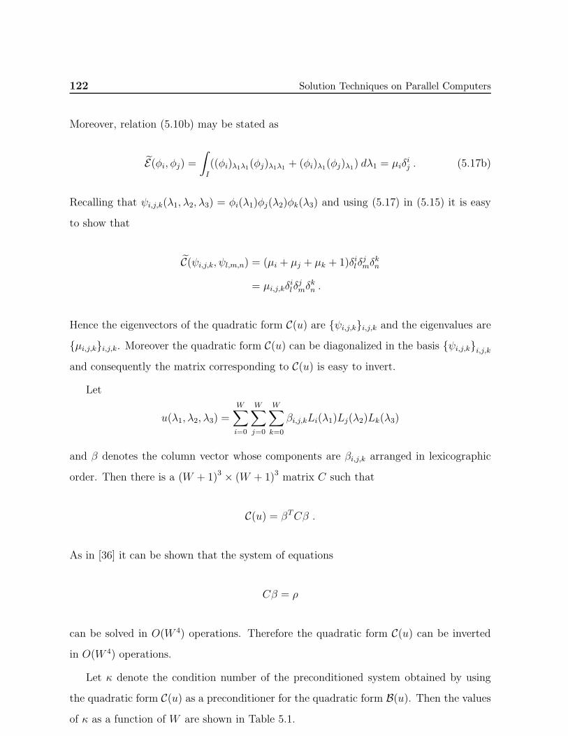
122 Solution Techniques on Parallel Computers
Moreover, relation (5.10b) may be stated as
E(φi, φj) =∫
I
((φi)λ1λ1(φj)λ1λ1 + (φi)λ1(φj)λ1) dλ1 = µiδij . (5.17b)
Recalling that ψi,j,k(λ1, λ2, λ3) = φi(λ1)φj(λ2)φk(λ3) and using (5.17) in (5.15) it is easy
to show that
C(ψi,j,k, ψl,m,n) = (µi + µj + µk + 1)δilδjmδ
kn
= µi,j,kδilδjmδ
kn .
Hence the eigenvectors of the quadratic form C(u) are ψi,j,ki,j,k and the eigenvalues are
µi,j,ki,j,k. Moreover the quadratic form C(u) can be diagonalized in the basis ψi,j,ki,j,kand consequently the matrix corresponding to C(u) is easy to invert.
Let
u(λ1, λ2, λ3) =W∑
i=0
W∑
j=0
W∑
k=0
βi,j,kLi(λ1)Lj(λ2)Lk(λ3)
and β denotes the column vector whose components are βi,j,k arranged in lexicographic
order. Then there is a (W + 1)3 × (W + 1)3 matrix C such that
C(u) = βTCβ .
As in [36] it can be shown that the system of equations
Cβ = ρ
can be solved in O(W 4) operations. Therefore the quadratic form C(u) can be inverted
in O(W 4) operations.
Let κ denote the condition number of the preconditioned system obtained by using
the quadratic form C(u) as a preconditioner for the quadratic form B(u). Then the values
of κ as a function of W are shown in Table 5.1.
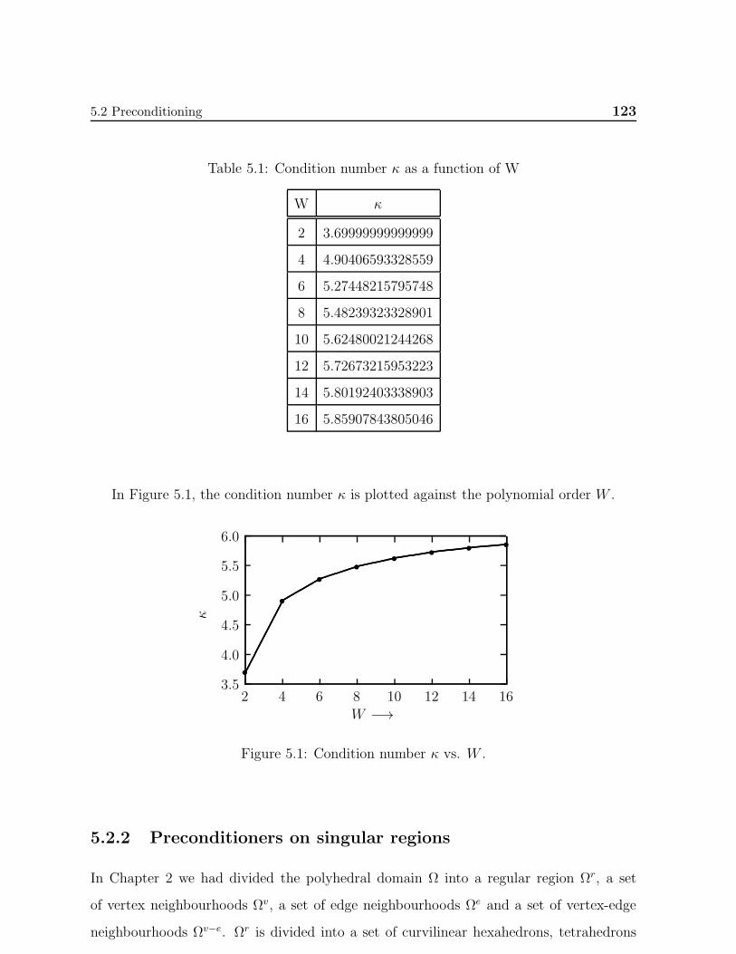
5.2 Preconditioning 123
Table 5.1: Condition number κ as a function of W
W κ
2 3.69999999999999
4 4.90406593328559
6 5.27448215795748
8 5.48239323328901
10 5.62480021244268
12 5.72673215953223
14 5.80192403338903
16 5.85907843805046
In Figure 5.1, the condition number κ is plotted against the polynomial order W .
6.0
5.5
5.0
4.5
4.0
3.5161412108642
W −→
κ
s
s
s
s
ss
ss
Figure 5.1: Condition number κ vs. W .
5.2.2 Preconditioners on singular regions
In Chapter 2 we had divided the polyhedral domain Ω into a regular region Ωr, a set
of vertex neighbourhoods Ωv, a set of edge neighbourhoods Ωe and a set of vertex-edge
neighbourhoods Ωv−e. Ωr is divided into a set of curvilinear hexahedrons, tetrahedrons

124 Solution Techniques on Parallel Computers
and prisms and the singular regions in the neighbourhoods of vertices, edges and vertex-
edges are divided into hexahedrons and prisms using a geometric mesh.
A set of spectral element functions has been defined on all elements in the regular
region and various singular regions.
Let N denote the number of refinements in the geometric mesh. We shall assume that
N is proportional toW . Then the proposed method gives exponentially accurate solution
in N provided the data satisfy usual regularity conditions [51, 52, 86].
We choose our spectral element functions to be fully non-conforming. Let Fu denote
the spectral element representation of the function u. We define the quadratic form
WN,W (Fu) =WN,Wregular(Fu) +WN,W
vertices(Fu) +WN,Wvertex−edges(Fu)
+WN,Wedges(Fu) . (5.18)
Here WN,Wregular(Fu), WN,W
vertices(Fu), WN,Wvertex−edges(Fu) and WN,W
edges(Fu) are defined
similar to the quadratic forms UN,Wregular(Fu), UN,Wvertices(Fu), UN,Wvertex−edges(Fu) and
UN,Wedges(Fu) as in (2.19), (2.21), (2.33) and (2.41) respectively. Then for problems with
Dirichlet boundary conditions by Theorem 2.3.1 it follows that the following estimate is
true
WN,W (Fu) ≤ C(lnW )2VN,W (Fu) (5.19)
provided W = O(eNα) for α < 1/2.
At the same time using trace theorems for Sobolev spaces there exists a constant k
such that1
kVN,W (Fu) ≤ WN,W (Fu) . (5.20)
Hence using (5.19) and (5.20) we conclude that the two quadratic formsWN,W (Fu) andVN,W (Fu) are spectrally equivalent and there exists a constant K such that
1
KVN,W (Fu) ≤ WN,W (Fu) ≤ K(lnW )2VN,W (Fu) (5.21)
provided W = O(eNα) for α < 1/2.
We can now use the quadratic form WN,W (Fu) which consists of a decoupled set of
quadratic forms on each element as a preconditioner. It follows that the condition number
of the preconditioned system is O(lnW )2.
5.2 Preconditioning 125
The other case is when the boundary conditions are of mixed Neumann and Dirichlet
type. In this case, as above, using Theorem 2.3.2 and trace theorems for Sobolev spaces
it follows that for W and N large enough the following estimate holds
1
KVN,W (Fu) ≤ WN,W (Fu) ≤ KN4VN,W (Fu) .
Here K is a constant. It is clear that the quadratic form WN,W (Fu) can be used as a
preconditioner and the condition number of the preconditioned system is O(N4).
We will now construct preconditioners on each of the elements in the neighbourhoods
of vertices, edges, vertex-edges and the regular region. Here u denotes the spectral element
function which is a polynomial of degree W in each of its variables separately defined in
various regions of the polyhedron.
The quadratic forms which need to be examined are
Bregular(u) = ‖u‖2H2(Q) =
∫
Q
∑
|α|≤2
|Dαλ1,λ2,λ3
u|2 dλ1dλ2dλ3 , (5.22)
Bvertices(u) = ‖eχ/2u‖2
H2(Ωvl )=
∫
Ωvl
eχ∑
|α|≤2
|Dαφ,θ,χu|2 dφdθdχ , (5.23)
Bvertex−edges(u) =∫
Ωv−el
eζ(u2ψψ + u2θθ + u2ψθ + sin2 φu2φζ + sin2 φu2θζ
+ sin4 φu2ζζ + u2ψ + u2θ + sin2 φu2ζ + u2) dψdθdζ , (5.24)
Bedges(u) =∫
Ωel
(u2ττ + u2θθ + u2τθ + e2τu2τx3 + e2τu2θx3 + e4τu2x3x3
+ u2τ + u2θ + e2τu2x3 + u2) dτdθdx3 . (5.25)
Here (φ, θ, χ), (ψ, θ, ζ) and (τ, θ, x3) denote the modified systems of coordinates introduced
in Chapter 2 in vertex neighbourhoods, vertex-edge neighbourhoods and edge neighbour-
hoods respectively. Moreover Ωvl , Ωv−el and Ωel denote elements in the vertex neighbour-
hood, vertex-edge neighbourhood and edge neighbourhood respectively.
The construction of preconditioners corresponding to the quadratic forms Bregular(u)and Bvertices(u) is similar to the case of a smooth domain already discussed so we omit
the details. It follows that there exist quadratic forms Cregular(u) and Cvertices(u) which
126 Solution Techniques on Parallel Computers
are spectrally equivalent to Bregular(u) and Bvertices(u) respectively and which can be
diagonalized using separation of variables technique. We will now obtain preconditioners
for edge and vertex-edge neighbourhood elements. For this purpose we observe that for
quadratic forms in edge and vertex-edge neighbourhoods it is enough to examine the
quadratic form
B⋆(u) =∫ 1
−1
∫ 1
−1
∫ 1
−1
(u2xx + u2yy + η2u2xz + η2u2yz + η4u2zz
+ u2x + u2y + η2u2z + u2) dxdydz . (5.26)
Here η = sin φ and η = eτ for vertex-edge and edge neighbourhood elements respectively.
We remark that the factor η becomes smaller towards the vertices and edges of the domain
Ω.
Making the transformation z = zη, so that d
dz= 1
ηddz, the quadratic form B⋆(u) assumes
the form
B⋆(u) =∫ 1
η
− 1η
∫ 1
−1
∫ 1
−1
(u2xx + u2yy + u2xy + u2xz + u2yz + u2zz + u2x + u2y + u2z + u2) dxdydz .
Let us define the quadratic form
C⋆(u) =∫ 1
−1
∫ 1
−1
∫ 1
−1
(u2xx + u2yy + η4u2zz + u2x + u2y + η2u2z + u2) dxdydz . (5.27)
We now show that the quadratic form C⋆(u) is spectrally equivalent to the quadratic
form B⋆(u), defined in (5.26). Moreover, C⋆(u) can be diagonalized using separation of
variables technique.
Let
v(x) =W∑
i=0
βiLi(x), and v(z) =W∑
i=0
γiLi(z) .
Moreover b = (β0, β1, . . . , βW )T and d = (γ0, γ1, . . . , γW )T .
We now define the quadratic form
E(v) =∫
I
(v2xx + v2x)dx (5.28)
and
F(v) =∫
I
v2dx . (5.29)

5.2 Preconditioning 127
We also define the quadratic form
G(v) =∫
I
(η4v2zz + η2v2z)dz (5.30)
and
H(v) =∫
I
v2dz . (5.31)
Here I denotes the unit interval (−1, 1). Clearly there exist (W + 1)× (W + 1) matrices
E,G and F,H such that
E(v) = bTEb , G(v) = dTGd (5.32)
and
F(v) = bTFb , H(v) = dTHd. (5.33)
Here the matrices E,G and F,H are symmetric and F,H are positive definite.
Hence there exist W + 1 eigenvalues 0 ≤ µ0 ≤ µ1 ≤ · · · ≤ µW and W + 1 eigenvectors
b0, b1, . . . , bW of the symmetric eigenvalue problem
(E − µF )b = 0 . (5.34)
Here
(E − µiF )bi = 0 .
Similarly, there exist W + 1 eigenvalues 0 ≤ ν0 ≤ ν1 ≤ · · · ≤ νW and W + 1 eigenvectors
d0, d1, . . . , dW of the symmetric eigenvalue problem
(G− νH)d = 0 . (5.35)
Here
(G− νiH)di = 0 .
The eigenvectors bi and ci are normalized so that
bTi Fbj = δij , and dTi Hdj = δij . (5.36a)
Moreover the relations
bTi Ebj = µiδij and dTi Gdj = νiδ
ij (5.36b)
128 Solution Techniques on Parallel Computers
hold. Let bi = (bi,0, bi,1, . . . , bi,W ) and di = (di,0, di,1, . . . , di,W ). We now define the poly-
nomials
φi(x) =
W∑
m=0
bi,mLm(x) for 0 ≤ i ≤W , (5.37a)
φj(y) =W∑
m=0
bj,mLm(y) for 0 ≤ j ≤W , (5.37b)
θk(z) =
W∑
m=0
dk,mLm(z) for 0 ≤ k ≤W . (5.37c)
Next, let χi,j,k denote the polynomial
χi,j,k(x, y, z) = φi(x)φj(y)θk(z) (5.38)
for 0 ≤ i ≤W, 0 ≤ j ≤ W, 0 ≤ k ≤W .
Note that χi,j,k(x, y, z)i,j,k is the tensor product of the polynomials φi(x), φj(y) and
θk(z). The eigenvalue σi,j,k corresponding to the eigenvector χi,j,k is given by the relation
σi,j,k = µi + µj + νk + 1 . (5.39)
Let C⋆(f, g) be the bilinear form induced by the quadratic form C⋆(u). Then
C⋆(f, g) =∫ 1
−1
∫ 1
−1
∫ 1
−1
(fxxfxx + fyygyy + η4fzzgzz + fxgx + fygy
+ η2fzgz + fg) dxdydz .
It is easy to show that
C⋆(χi,j,k, χl,m,n) = (µi + µj + νk + 1)δilδjmδ
kn
= σi,j,kδilδjmδ
kn .
Hence the eigenvectors of the quadratic form C⋆(u) are χi,j,ki,j,k and the eigenvalues are
σi,j,ki,j,k. Thus, the quadratic form C⋆(u) can be diagonalized in the basis χi,j,ki,j,k.Therefore, the matrix corresponding to the quadratic form C⋆(u) is easy to invert.
Now proceeding as earlier, it can be shown that the quadratic forms B⋆(u) and C⋆(u)are spectrally equivalent. Moreover, the quadratic form C⋆(u) can be inverted in O(W 4)
operations.

5.3 Parallelization Techniques 129
Thus, it follows that there exist quadratic forms Cvertex−edges(u) and Cedges(u) which
are spectrally equivalent to Bvertex−edges(u) and Bedges(u) respectively and which can be
diagonalized using separation of variables technique.
5.3 Parallelization Techniques
In minimizing the functional RN,W (Fv) we seek a solution which minimizes the sum of
weighted norms of the residuals in the partial differential equation and a fractional Sobolev
norm of the residuals in the boundary conditions and enforce continuity by adding a term
which measures the sum of squares of the jumps in the function and its derivatives at inter-
element boundaries in appropriate Sobolev norms, suitably weighted in various regions of
the polyhedron.
In order to obtain a solution using PCGM we must be able to compute residuals
in the normal equations inexpensively. Since we are minimizing RN,W (Fv) over all
Fv ∈ SN,W (space of spectral element functions) we have
RN,W (U + ǫV ) = RN,W (U) + 2ǫV t(XU − Y G) +O(ǫ2)
for all V , where U is a vector assembled from the values of
url (λ)Nr
l=1 , uvl (xv)Nv
l=1 ,uv−el (xv−e)
Nv−e
l=1, uel (xe)Ne
l=1
.
V is a vector similarly assembled and G is assembled from the data. Here X and Y
denote matrices. Thus we have to solve XU − Y G = 0 and so we must be able to
compute XV − Y G economically during the iterative process. We will now explain in
brief how this can be done. The idea is very similar to the case of two dimensional
problems so we refer the reader to [85] for details.
The above minimization amounts to an overdetermined system of equations consisting
of collocating the residuals in the partial differential equation, the residuals in the bound-
ary conditions and jumps in the function and its derivatives at inter-element boundaries
at an over determined set of collocation points, weighted suitably. In fact, we collocate
the partial differential equation on a finer grid of Gauss-Lobatto-Legendre (GLL) points
130 Solution Techniques on Parallel Computers
and then we apply the adjoint differential operator to these residuals and project these
values back to the original grid. Such a treatment obviously involves integration by parts
and hence leads to evaluation of terms at the boundaries. These boundary terms can
be evaluated be a collocation procedure and the other boundary terms corresponding to
jump terms at the inter-element boundaries can be easily calculated.
5.3.1 Integrals on the element domain
We first show how to compute the integrals on the element domain. Since each element
is mapped onto the master cube Q=(−1, 1)3 = (−1, 1)× (−1, 1)× (−1, 1), so we consider
the computations only on Q.
Consider the integral
‖(L)au− F‖2Q . (5.40)
Its variation is ∫
Q
(L)av ((L)au− F ) dξ1 dξ2 dξ3. (5.41)
Here
(L)aw = Awξ1ξ1 + Bwξ2ξ2 + Cwξ3ξ3 + Dwξ1ξ2 + Ewξ2ξ3 + Fwξ3ξ1
+ Gwξ1 + Hwξ2 + Iwξ3 + Jw,
where the coefficients A, B, C etc. are polynomials of degree N and F is a filtered repre-
sentation of F .
Let,
u(ξ1, ξ2, ξ3) =
2N∑
i=0
2N∑
j=0
2N∑
k=0
αi,j,kξ1iξ2
jξ3k
and
v(ξ1, ξ2, ξ3) =2N∑
i=0
2N∑
j=0
2N∑
k=0
βi,j,kξ1iξ2
jξ3k.
The differential operator (L)a is obtained from the differential operator
Lw = Awξ1ξ1 +Bwξ2ξ2 + Cwξ3ξ3 +Dwξ1ξ2 + Ewξ2ξ3 + Fwξ3ξ1
+Gwξ1 +Hwξ2 + Iwξ3 + Jw,
5.3 Parallelization Techniques 131
with analytic coefficients A,B,C etc. We choose the coefficients A, B, C etc. so that they
are the orthogonal projections of A,B,C etc. into the space of polynomials of degree N
with respect to the usual inner product in H2(Q).
Let (La)T denote the formal adjoint of the differential operator (L)a.Then
(La)Tw =(Aw)ξ1ξ1
+(Bw)ξ2ξ2
+(Cw)ξ3ξ3
+(Dw)ξ1ξ2
+(Ew)ξ2ξ3
+(Fw)ξ3ξ1−(Gw)ξ1−(Hw
)ξ2−(Iw)ξ3+ Jw,
Let z denote (L)au− F . Integrating (5.41) by parts we obtain
∫
Q
(L)avz dξ1 dξ2 dξ3
=
∫
Q
v(La)T z dξ1 dξ2 dξ3
+
∫ 1
−1
∫ 1
−1
((Avξ1 + Gv)z− v
((Az)ξ1 + (F z)ξ3 + (Dz)ξ2
))(1, ξ2, ξ3)dξ2 dξ3
−∫ 1
−1
∫ 1
−1
((Avξ1 + Dvξ2 + Gv)z− v
((Az)ξ1 + (F z)ξ3
))(−1, ξ2, ξ3)dξ2 dξ3
+
∫ 1
−1
v(Dz)(1, 1, ξ3)dξ3 −∫ 1
−1
v(Dz)(1,−1, ξ3)dξ3
+
∫ 1
−1
∫ 1
−1
((Bvξ2 + Hv)z− v
((Bz)ξ2 + (Dz)ξ1 + (Ez)ξ3
))(ξ1, 1, ξ3)dξ1 dξ3
−∫ 1
−1
∫ 1
−1
((Bvξ2 + Evξ3 + Hv)z− v
((Bz)ξ2 + (Dz)ξ1
))(ξ1,−1, ξ3)dξ1 dξ3
+
∫ 1
−1
v(Ez)(ξ1, 1, 1)dξ1 −∫ 1
−1
v(Ez)(ξ1, 1,−1)dξ1
+
∫ 1
−1
∫ 1
−1
((Cvξ3 + Iv)z− v
((Cz)ξ3 + (Ez)ξ2 + (F z)ξ1
))(ξ1, ξ2, 1)dξ1 dξ2
−∫ 1
−1
∫ 1
−1
((Cvξ3 + Fvξ1 + Iv)z− v
((Cz)ξ3 + (Ez)ξ2
))(ξ1, ξ2,−1)dξ1 dξ2
+
∫ 1
−1
v(F z)(1, ξ2, 1)dξ2 −∫ 1
−1
v(F z)(−1, ξ2, 1)dξ2 (5.42)
Now u, v and A, B, C etc. are polynomials of degree N in each of the variables ξ1, ξ2 and
ξ3. Moreover F is a polynomial of degree 2N . Hence all the integrands are polynomials
of degree 4N in each of the variables ξ1, ξ2 and ξ3 and so the integral may be exactly
132 Solution Techniques on Parallel Computers
evaluated by the Gauss-Lobatto-Legendre (GLL) quadrature formula with 2N +1 points.
Let ξ2N1,0 , . . . , ξ2N1,2N , ξ
2N2,0 , . . . , ξ
2N2,2N and ξ2N3,0 , . . . , ξ
2N3,2N represent the quadrature points in ξ1,
ξ2 and ξ3 directions respectively and w2N0 , . . . , w2N
2N the corresponding weights.
Proposition 5.3.1. Let the matrix D2N = d2Ni,j denote the differentiation matrix. Then
dl
dξ
(ξ2Ni)=
2N∑
j=0
d2Ni,j l(ξ2Nj)
(5.43)
if l is a polynomial of degree less than or equal to 2N .
Using the GLL quadrature rule we obtain∫
Q
(L)av((L)au− F )dξ1dξ2dξ3
=
2N∑
i=0
2N∑
j=0
2N∑
k=0
v(ξ2N1,i , ξ
2N2,j , ξ
2N3,k
) (w2Ni w2N
j w2Nk LT z
(ξ2N1,i , ξ
2N2,j , ξ
2N3,k
))
+
2N∑
i=0
2N∑
j=0
2N∑
k=0
v(ξ2N1,i , ξ
2N2,j , ξ
2N3,k
) (w2Nj w2N
k d2N2N,iA(1, ξ2N2,j , ξ
2N3,k )z
(1, ξ2N2,j , ξ
2N3,k
))
+2N∑
j=0
2N∑
k=0
v(1, ξ2N2,j , ξ
2N3,k
) (w2Nj w2N
k (Gz− (Az)ξ1 − (F z)ξ3 − (Dz)ξ2)(1, ξ2N2,j , ξ
2N3,k
))
−2N∑
i=0
2N∑
j=0
2N∑
k=0
v(ξ2N1,i , ξ
2N2,j , ξ
2N3,k
) (w2Nj w2N
k
(d2N0,i A(−1, ξ2N2,j , ξ2N3,k )z(−1, ξ2N2,j , ξ2N3,k )
+d2Nj,i D(−1, ξ2N2,j , ξ2N3,k )z(−1, ξ2N2,j , ξ2N3,k )))
−2N∑
j=0
2N∑
k=0
v(−1, ξ2N2,j , ξ2N3,k
) (w2Nj w2N
k (Gz− (Az)ξ1 − (F z)ξ3)(−1, ξ2N2,j , ξ2N3,k
))
+
2N∑
i=0
2N∑
j=0
2N∑
k=0
v(ξ2N1,i , ξ
2N2,j , ξ
2N3,k
) (w2Ni w2N
k d2N2N,jB(ξ2N1,i , 1, ξ2N3,k )z
(ξ2N1,i , 1, ξ
2N3,k
))
+
2N∑
i=0
2N∑
k=0
v(ξ2N1,i , 1, ξ
2N3,k
) (w2Ni w2N
k (Hz− (Bz)ξ2 − (Dz)ξ1 − (Ez)ξ3)(ξ2N1,i , 1, ξ
2N3,j
))
−2N∑
i=0
2N∑
j=0
2N∑
k=0
v(ξ2N1,i , ξ
2N2,j , ξ
2N3,k
) (w2Ni w2N
k
(d2N0,jB(ξ2N1,i ,−1, ξ2N3,k )z(ξ2N1,i ,−1, ξ2N3,k )
+d2Nk,jE(ξ2N1,i ,−1, ξ2N3,k )z(ξ2N1,i ,−1, ξ2N3,k )
))
−2N∑
i=0
2N∑
k=0
v(ξ2N1,i ,−1, ξ2N3,k
) (w2Ni w2N
k (Hz− (Bz)ξ2 − (Dz)ξ1) (ξ2N1,i ,−1, ξ2N3,k )
)
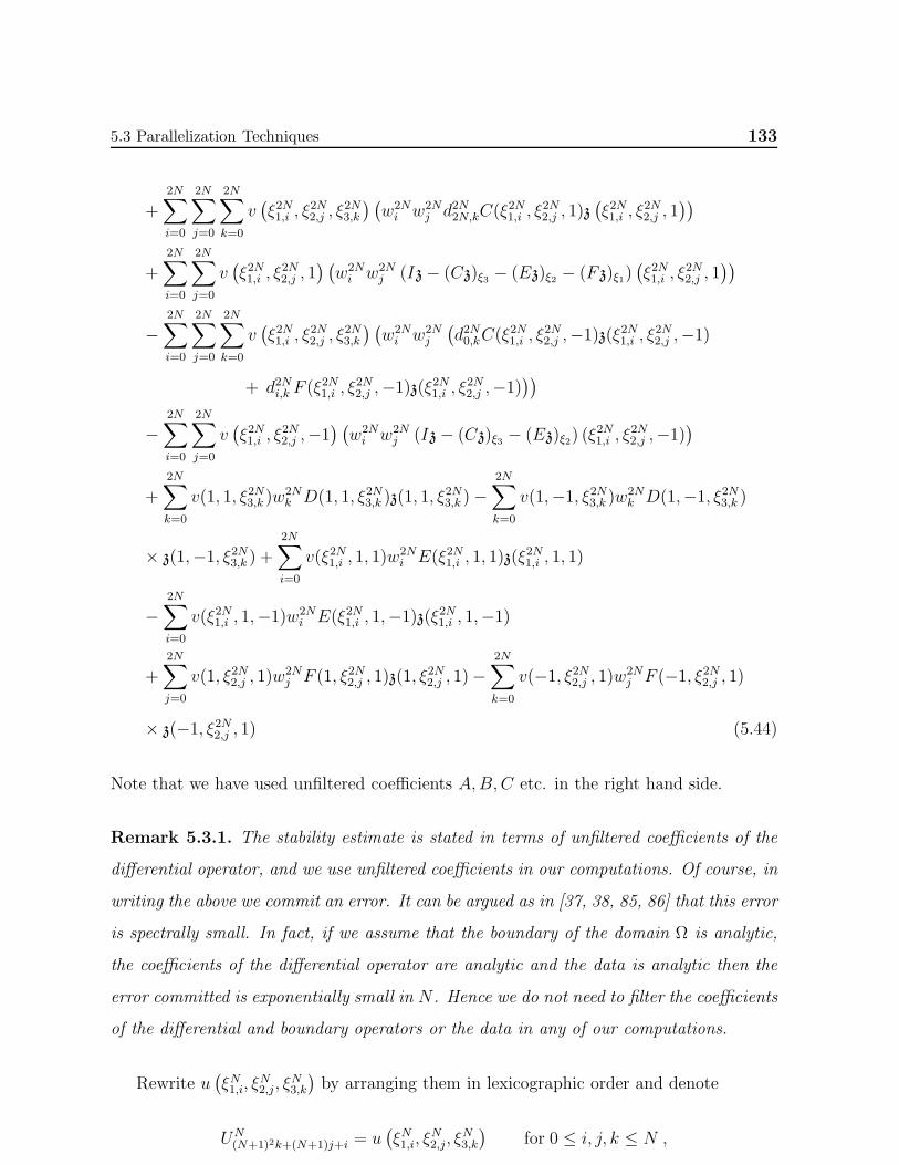
5.3 Parallelization Techniques 133
+
2N∑
i=0
2N∑
j=0
2N∑
k=0
v(ξ2N1,i , ξ
2N2,j , ξ
2N3,k
) (w2Ni w2N
j d2N2N,kC(ξ2N1,i , ξ
2N2,j , 1)z
(ξ2N1,i , ξ
2N2,j , 1
))
+2N∑
i=0
2N∑
j=0
v(ξ2N1,i , ξ
2N2,j , 1
) (w2Ni w2N
j (Iz− (Cz)ξ3 − (Ez)ξ2 − (F z)ξ1)(ξ2N1,i , ξ
2N2,j , 1
))
−2N∑
i=0
2N∑
j=0
2N∑
k=0
v(ξ2N1,i , ξ
2N2,j , ξ
2N3,k
) (w2Ni w2N
j
(d2N0,kC(ξ
2N1,i , ξ
2N2,j ,−1)z(ξ2N1,i , ξ2N2,j ,−1)
+ d2Ni,k F (ξ2N1,i , ξ
2N2,j ,−1)z(ξ2N1,i , ξ2N2,j ,−1)
))
−2N∑
i=0
2N∑
j=0
v(ξ2N1,i , ξ
2N2,j ,−1
) (w2Ni w2N
j (Iz− (Cz)ξ3 − (Ez)ξ2) (ξ2N1,i , ξ
2N2,j ,−1)
)
+
2N∑
k=0
v(1, 1, ξ2N3,k )w2Nk D(1, 1, ξ2N3,k )z(1, 1, ξ
2N3,k )−
2N∑
k=0
v(1,−1, ξ2N3,k )w2Nk D(1,−1, ξ2N3,k )
× z(1,−1, ξ2N3,k ) +2N∑
i=0
v(ξ2N1,i , 1, 1)w2Ni E(ξ2N1,i , 1, 1)z(ξ
2N1,i , 1, 1)
−2N∑
i=0
v(ξ2N1,i , 1,−1)w2Ni E(ξ2N1,i , 1,−1)z(ξ2N1,i , 1,−1)
+2N∑
j=0
v(1, ξ2N2,j , 1)w2Nj F (1, ξ2N2,j , 1)z(1, ξ
2N2,j , 1)−
2N∑
k=0
v(−1, ξ2N2,j , 1)w2Nj F (−1, ξ2N2,j , 1)
× z(−1, ξ2N2,j , 1) (5.44)
Note that we have used unfiltered coefficients A,B,C etc. in the right hand side.
Remark 5.3.1. The stability estimate is stated in terms of unfiltered coefficients of the
differential operator, and we use unfiltered coefficients in our computations. Of course, in
writing the above we commit an error. It can be argued as in [37, 38, 85, 86] that this error
is spectrally small. In fact, if we assume that the boundary of the domain Ω is analytic,
the coefficients of the differential operator are analytic and the data is analytic then the
error committed is exponentially small in N . Hence we do not need to filter the coefficients
of the differential and boundary operators or the data in any of our computations.
Rewrite u(ξN1,i, ξ
N2,j, ξ
N3,k
)by arranging them in lexicographic order and denote
UN(N+1)2k+(N+1)j+i = u
(ξN1,i, ξ
N2,j, ξ
N3,k
)for 0 ≤ i, j, k ≤ N ,
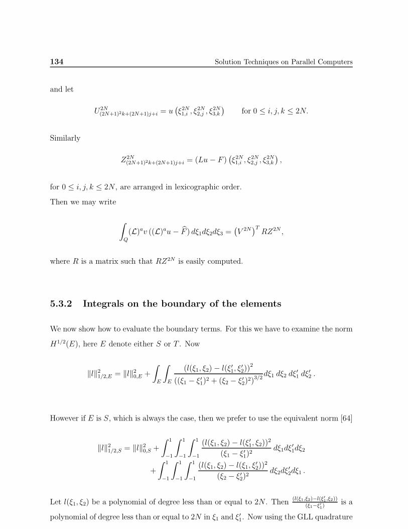
134 Solution Techniques on Parallel Computers
and let
U2N(2N+1)2k+(2N+1)j+i = u
(ξ2N1,i , ξ
2N2,j , ξ
2N3,k
)for 0 ≤ i, j, k ≤ 2N.
Similarly
Z2N(2N+1)2k+(2N+1)j+i = (Lu− F )
(ξ2N1,i , ξ
2N2,j , ξ
2N3,k
),
for 0 ≤ i, j, k ≤ 2N , are arranged in lexicographic order.
Then we may write
∫
Q
(L)av ((L)au− F ) dξ1dξ2dξ3 =(V 2N
)TRZ2N ,
where R is a matrix such that RZ2N is easily computed.
5.3.2 Integrals on the boundary of the elements
We now show how to evaluate the boundary terms. For this we have to examine the norm
H1/2(E), here E denote either S or T . Now
‖l‖21/2,E = ‖l‖20,E +
∫
E
∫
E
(l(ξ1, ξ2)− l(ξ′1, ξ′2))2
((ξ1 − ξ′1)2 + (ξ2 − ξ′2)2)3/2dξ1 dξ2 dξ
′1 dξ
′2 .
However if E is S, which is always the case, then we prefer to use the equivalent norm [64]
‖l‖21/2,S = ‖l‖20,S +∫ 1
−1
∫ 1
−1
∫ 1
−1
(l(ξ1, ξ2)− l(ξ′1, ξ2))2(ξ1 − ξ′1)2
dξ1dξ′1dξ2
+
∫ 1
−1
∫ 1
−1
∫ 1
−1
(l(ξ1, ξ2)− l(ξ1, ξ′2))2(ξ2 − ξ′2)2
dξ2dξ′2dξ1 .
Let l(ξ1, ξ2) be a polynomial of degree less than or equal to 2N . Then(l(ξ1,ξ2)−l(ξ′1,ξ2))
(ξ1−ξ′1)is a
polynomial of degree less than or equal to 2N in ξ1 and ξ′1. Now using the GLL quadrature
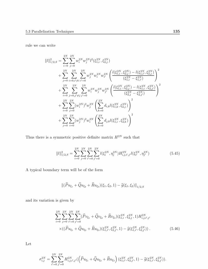
5.3 Parallelization Techniques 135
rule we can write
‖l‖21/2,S =2N∑
i=0
2N∑
j=0
w2Ni w2N
j l2(ξ2N1,i , ξ2N2,j )
+
2N∑
j=0
2N∑
i=0,i′ 6=i
2N∑
i′=0
w2Nj w2N
i w2Ni′
(l(ξ2N1,i , ξ
2N2,j )− l(ξ2N1,i′ , ξ2N2,j )(ξ2N1,i − ξ2N1,i′)
)2
+2N∑
i=0
2N∑
j=0,j′ 6=j
2N∑
j′=0
w2Ni w2N
j w2Nj′
(l(ξ2N1,i , ξ
2N2,j )− l(ξ2N1,i , ξ2N2,j′)(ξ2N2,j − ξ2N2,j′)
)2
+
2N∑
i=0
2N∑
j=0
(w2Ni )2w2N
j
(2N∑
k=0
di,kl(ξ2N1,k , ξ
2N2,j )
)2
+
2N∑
j=0
2N∑
i=0
(w2Nj )2w2N
i
(2N∑
k=0
dj,kl(ξ2N1,i , ξ
2N2,k )
)2
Thus there is a symmetric positive definite matrix H2N such that
‖l‖21/2,S =
2N∑
i=0
2N∑
j=0
2N∑
i′=0
2N∑
j′=0
l(ξ2Ni , η2Nj )H2Ni,j,i′,j′l(ξ
2Ni′ , η
2Nj′ ) (5.45)
A typical boundary term will be of the form
‖(P uξ1 + Quξ2 + Ruξ3)(ξ1, ξ2, 1)− g(ξ1, ξ2)‖1/2,S
and its variation is given by
2N∑
i=0
2N∑
j=0
2N∑
i′=0
2N∑
j′=0
(P vξ1 + Qvξ2 + Rvξ3)(ξ2N1,i , ξ
2N2,j , 1)H
2Ni,j,i′,j′
×((P uξ1 + Quξ2 + Ruξ3)(ξ2N1,i′ , ξ
2N2,j′, 1)− g(ξ2N1,i′ , ξ2N2,j′)) . (5.46)
Let
σ2Ni,j =
2N∑
i′=0
2N∑
j′=0
H2Ni,j,i′,j′(
(P uξ1 + Quξ2 + Ruξ3
)(ξ2N1,i′ , ξ
2N2,j′, 1)− g(ξ2N1,i′ , ξ2N2,j′)).
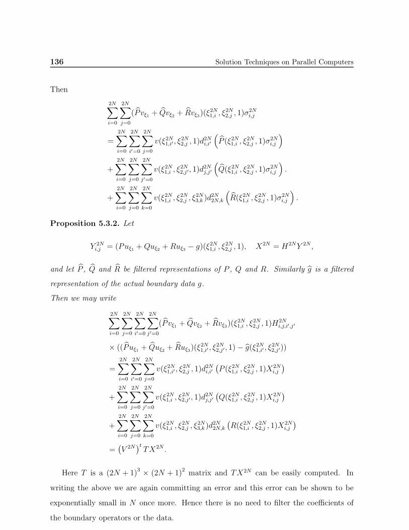
136 Solution Techniques on Parallel Computers
Then
2N∑
i=0
2N∑
j=0
(P vξ1 + Qvξ2 + Rvξ3)(ξ2N1,i , ξ
2N2,j , 1)σ
2Ni,j
=
2N∑
i=0
2N∑
i′=0
2N∑
j=0
v(ξ2N1,i′ , ξ2N2,j , 1)d
2Ni,i′
(P (ξ2N1,i , ξ
2N2,j , 1)σ
2Ni,j
)
+
2N∑
i=0
2N∑
j=0
2N∑
j′=0
v(ξ2N1,i , ξ2N2,j′, 1)d
2Nj,j′
(Q(ξ2N1,i , ξ
2N2,j , 1)σ
2Ni,j
).
+
2N∑
i=0
2N∑
j=0
2N∑
k=0
v(ξ2N1,i , ξ2N2,j , ξ
2N3,k )d
2N2N,k
(R(ξ2N1,i , ξ
2N2,j , 1)σ
2Ni,j
).
Proposition 5.3.2. Let
Y 2Ni,j = (Puξ1 +Quξ2 +Ruξ3 − g)(ξ2N1,i , ξ2N2,j , 1), X2N = H2NY 2N ,
and let P , Q and R be filtered representations of P , Q and R. Similarly g is a filtered
representation of the actual boundary data g.
Then we may write
2N∑
i=0
2N∑
j=0
2N∑
i′=0
2N∑
j′=0
(P vξ1 + Qvξ2 + Rvξ3)(ξ2N1,i , ξ
2N2,j , 1)H
2Ni,j,i′,j′
× ((P uξ1 + Quξ2 + Ruξ3)(ξ2N1,i′ , ξ
2N2,j′, 1)− g(ξ2N1,i′ , ξ2N2,j′))
=2N∑
i=0
2N∑
i′=0
2N∑
j=0
v(ξ2N1,i′ , ξ2N2,j , 1)d
2Ni,i′
(P (ξ2N1,i , ξ
2N2,j , 1)X
2Ni,j
)
+
2N∑
i=0
2N∑
j=0
2N∑
j′=0
v(ξ2N1,i , ξ2N2,j′, 1)d
2Nj,j′
(Q(ξ2N1,i , ξ
2N2,j , 1)X
2Ni,j
)
+
2N∑
i=0
2N∑
j=0
2N∑
k=0
v(ξ2N1,i , ξ2N2,j , ξ
2N3,k )d
2N2N,k
(R(ξ2N1,i , ξ
2N2,j , 1)X
2Ni,j
)
=(V 2N
)tTX2N .
Here T is a (2N + 1)3 × (2N + 1)2 matrix and TX2N can be easily computed. In
writing the above we are again committing an error and this error can be shown to be
exponentially small in N once more. Hence there is no need to filter the coefficients of
the boundary operators or the data.
5.3 Parallelization Techniques 137
Adding all the terms we obtain
∫
Q
(L)av ((L)au− F ) dξ1dξ2dξ3
+
2N∑
i=0
2N∑
j=0
2N∑
i′=0
2N∑
j′=0
(P vξ1 + Qvξ2 + Rvξ3)(ξ2N1,i , ξ
2N2,j , 1)H
2Ni,j,i′,j′
× ((P uξ1 + Quξ2 + Ruξ3)(ξ2N1,i′ , ξ
2N2,j′, 1)− g(ξ2N1,i′ , ξ2N2,j′)) + · · ·
=(V 2N
)t (RZ2N + TX2N + · · ·
)=(V 2N
)tO2N
where O2N = RZ2N + TX2N + · · · is a (2N + 1)3 vector which can be easily computed.
Now there exists a matrix GN such that V 2N = GNV N . Hence
(V 2N
)tO2N =
(V N)T ((
GN)TO2N
).
In [85, 86] it has been shown how(GN)TO2N can be computed for two dimensional
problems without having to compute and store any mass and stiffness matrices. Same
idea extends here and so we just describe the steps involved in brief and refer the reader
to [85, 86] for details.
Let γNm be the normalizing factors used in computing the discrete Legendre transform as
γNm =
(m+ 1/2)−1 if m < N,
2/N if m = N.
Let Oi,j,k0≤i,j,k≤2N be defined as Oi,j,k = O2Nk(2N+1)2+j(2N+1)+i
. Now we perform the fol-
lowing set of operations.
1. Define Oi,j,k ← Oi,j,k/w2Ni w2N
j w2Nk .
2. Calculate ∆i,j,k0≤i,j,k≤2N the Legendre transform of Oi,j,k0≤i,j,k≤2N . Define
∆i,j,k ← γ2Ni γ2Nj γ2Nk ∆i,j,k.
3. Calculate µi,j,k ← ∆i,j,k/γNi γ
Nj γ
Nk , 0 ≤ i, j, k ≤ N.
4. Compute ε, the inverse Legendre transform of µ. Define
εi,j,k ← wNi wNj w
Nk εi,j,k, 0 ≤ i, j, k ≤ N.
138 Solution Techniques on Parallel Computers
5. Define a vector J of dimension (N + 1)3 as
Jk(N+1)2+j(N+1)+i = εi,j,k for 0 ≤ i, j, k ≤ N.
Then J =(GN)tO2N . Thus we see to compute J we do not need to compute and store
any matrices such as the mass and stiffness matrices.
Clearly, O(N4) operations are required to compute the residual vector on a parallel com-
puter. In order to compute the residual vector we need to communicate the values of
the function and its derivatives on the boundary of the element between neighbouring
elements. Moreover, when computing the two global scalars, needed to update the ap-
proximate solution and the search direction during each step of PCGM, some scalars have
to be exchanged among all the processors. Thus we see that inter processor communica-
tion is small.
Chapter 6
Numerical Results
6.1 Introduction
In this chapter we present the results of the numerical simulations which have been per-
formed to validate the asymptotic error estimates and estimates of computational com-
plexity that we have obtained. First, we consider test problems on non-smooth domains
with smooth solutions (i.e. solutions without singularities) which include Laplace, Pois-
son and Helmholtz problems with different types of homogeneous and non-homogeneous
boundary conditions (e.g. Dirichlet, mixed, Neumann and Robin). Next, we consider a
general elliptic equation with mixed boundary conditions. Numerical results for a variable
coefficient problem on L-shaped domain are also presented which confirm the theoretical
estimates obtained.
The method works for non self-adjoint problems too. Computational results for a non
self-adjoint problem with variable coefficients are provided.
In order to show the effectiveness of the method in dealing with elliptic problems
on non-smooth domains containing singularities we shall consider various examples of
Laplace and Poisson equations on a number of polyhedral domains containing all three
types of singularities namely, vertex, edge and vertex-edge singularities with Dirichlet and
mixed type of boundary conditions to include all possible cases of singularities that may
arise due to the presence of corners and edges. We show that the error between the exact
140 Numerical Results
and the approximate solution is exponentially small.
The spectral element functions are nonconforming. The method we have described
is a least-squares collocation method and to obtain our approximate solution we solve
the normal equations using Preconditioned Conjugate Gradient Method (PCGM). The
residuals in the normal equations can be obtained without computing and storing mass
and stiffness matrices. A preconditioner is defined for the method which is a block diagonal
matrix, where each diagonal block corresponds to an element. It is also shown in Chapter 5
that there exists a new preconditioner which is a diagonal preconditioner on each element.
Let N denote the number of refinements in the geometrical mesh and W denote an upper
bound on the polynomial degree. We shall assume that N is proportional toW . Then the
condition number of the preconditioned system is KN,W , where KN,W = O((lnW )2) for
Dirichlet problems and KN,W = O(N4) for mixed problems with Neumann and Dirichlet
boundary conditions, provided W = O(eNα) for α < 1/2.
As stated in previous chapters after obtaining our approximate solution consisting of
non-conforming spectral element functions we can make a correction to it so that the
corrected solution is conforming and is an exponentially accurate approximation to the
true solution in the H1 norm over the whole domain. These corrections are explained in
the proof of Lemma 3.3.1 in Appendix C.1.
We perform the PCGM until a stopping criterion on the relative norm of the residual
vector for the normal equations becoming less than ǫ, a specified number, is satisfied.
Since we would need to perform O(√
κ2| log
(2ǫ
)|)iterations of the PCGM to satisfy the
stopping criterion, we would need to perform O(N(ln(N)) and O(N3) iterations of the
PCGM for Dirichlet and mixed problems respectively to obtain the approximate solution.
Here κ denotes condition number of the preconditioner.
We shall denote by Ω,Ω(v),Ω(e),Ω(v−e) etc. polyhedral domains in R3. Throughout
this chapter, (x1, x2, x3), (φ, θ, ρ) and (r, θ, x3) will denote the Cartesian, the spherical and
the cylindrical coordinates, respectively of points in these domains. In case the solution
is smooth we shall denote the Cartesian coordinates by (x, y, z).
Let uappx. be the spectral element solution obtained from the minimization problem
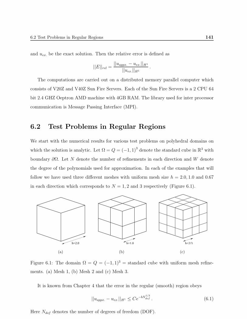
6.2 Test Problems in Regular Regions 141
and uex. be the exact solution. Then the relative error is defined as
||E||rel =||uappx. − uex.||H1
||uex.||H1
.
The computations are carried out on a distributed memory parallel computer which
consists of V20Z and V40Z Sun Fire Servers. Each of the Sun Fire Servers is a 2 CPU 64
bit 2.4 GHZ Oeptron AMD machine with 4GB RAM. The library used for inter processor
communication is Message Passing Interface (MPI).
6.2 Test Problems in Regular Regions
We start with the numerical results for various test problems on polyhedral domains on
which the solution is analytic. Let Ω = Q = (−1, 1)3 denote the standard cube in R3 with
boundary ∂Ω. Let N denote the number of refinements in each direction and W denote
the degree of the polynomials used for approximation. In each of the examples that will
follow we have used three different meshes with uniform mesh size h = 2.0, 1.0 and 0.67
in each direction which corresponds to N = 1, 2 and 3 respectively (Figure 6.1).
h=2.0
(a)
h=1.0
(b)
h=2/3
(c)
Figure 6.1: The domain Ω = Q = (−1, 1)3 = standard cube with uniform mesh refine-
ments. (a) Mesh 1, (b) Mesh 2 and (c) Mesh 3.
It is known from Chapter 4 that the error in the regular (smooth) region obeys
||uappx. − uex.||H1 ≤ Ce−bN1/3dof . (6.1)
Here Ndof denotes the number of degrees of freedom (DOF).
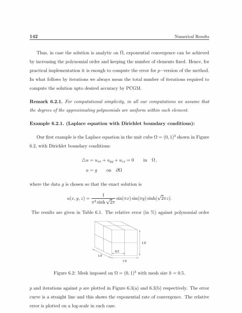
142 Numerical Results
Thus, in case the solution is analytic on Ω, exponential convergence can be achieved
by increasing the polynomial order and keeping the number of elements fixed. Hence, for
practical implementation it is enough to compute the error for p−version of the method.
In what follows by iterations we always mean the total number of iterations required to
compute the solution upto desired accuracy by PCGM.
Remark 6.2.1. For computational simplicity, in all our computations we assume that
the degrees of the approximating polynomials are uniform within each element.
Example 6.2.1. (Laplace equation with Dirichlet boundary conditions):
Our first example is the Laplace equation in the unit cube Ω = (0, 1)3 shown in Figure
6.2, with Dirichlet boundary conditions:
u = uxx + uyy + uzz = 0 in Ω ,
u = g on ∂Ω
where the data g is chosen so that the exact solution is
u(x, y, z) =1
π2 sinh√2π
sin(πx) sin(πy) sinh(√2πz).
The results are given in Table 6.1. The relative error (in %) against polynomial order
1.0
1.0
1.00.5
Figure 6.2: Mesh imposed on Ω = (0, 1)3 with mesh size h = 0.5.
p and iterations against p are plotted in Figure 6.3(a) and 6.3(b) respectively. The error
curve is a straight line and this shows the exponential rate of convergence. The relative
error is plotted on a log-scale in each case.
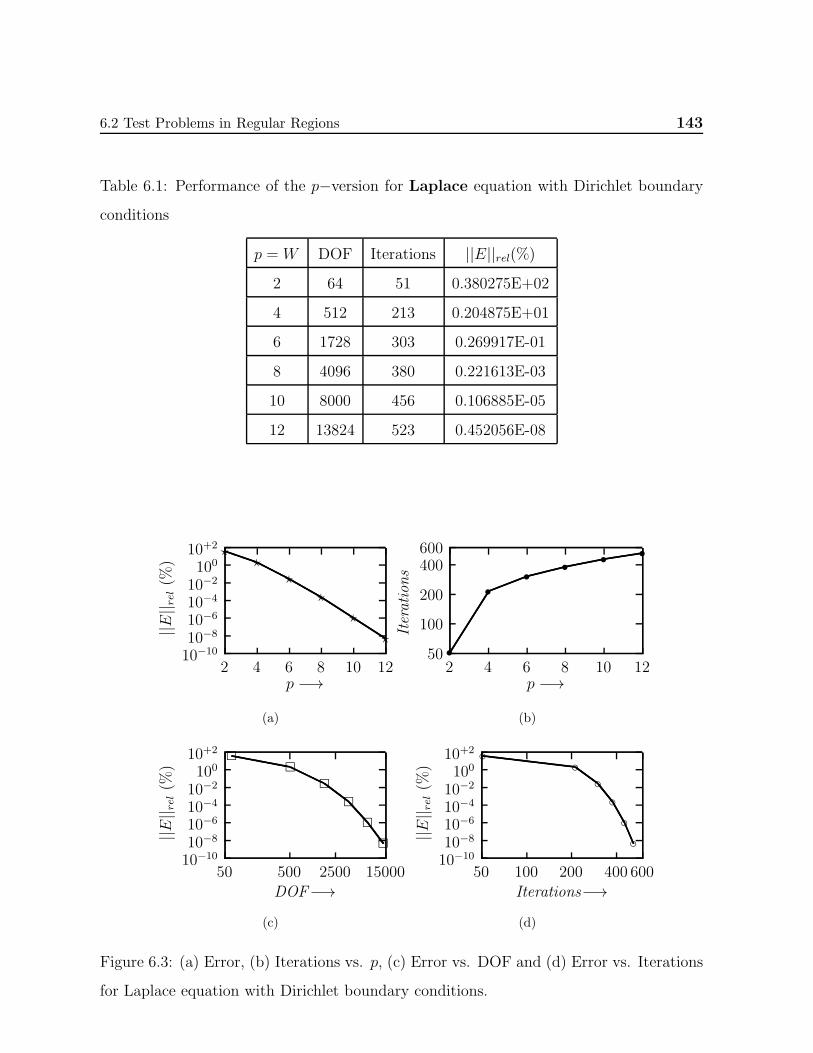
6.2 Test Problems in Regular Regions 143
Table 6.1: Performance of the p−version for Laplace equation with Dirichlet boundary
conditions
p = W DOF Iterations ||E||rel(%)
2 64 51 0.380275E+02
4 512 213 0.204875E+01
6 1728 303 0.269917E-01
8 4096 380 0.221613E-03
10 8000 456 0.106885E-05
12 13824 523 0.452056E-08
10−1010−810−610−410−2100
10+2
12108642p −→
||E|| rel(%
)
⋆⋆
⋆⋆
⋆
⋆
(a)
600400
200
100
5012108642
p −→
Iterations
s
s
s
s
ss
(b)
10−1010−810−610−410−2100
10+2
15000250050050DOF−→
||E|| rel(%
)
(c)
10−1010−810−610−410−2100
10+2
60040020010050Iterations−→
||E|| rel(%
)
(d)
Figure 6.3: (a) Error, (b) Iterations vs. p, (c) Error vs. DOF and (d) Error vs. Iterations
for Laplace equation with Dirichlet boundary conditions.

144 Numerical Results
In Figure 6.3(c) a graph is drawn for ||E||rel against degrees of freedom on a log− log
scale. It is clear that the error obeys (6.1).
Example 6.2.2. (Poisson equation with homogeneous boundary conditions):
We now consider the Poisson equation posed on Ω = Q = (−1, 1)3 with homogeneous
Dirichlet boundary conditions as follows:
Lu = −u = f in Ω ,
u = 0 on ∂Ω
where the right hand side function f is chosen so that the exact solution is
u(x, y, z) = sin(πx) sin(πy) sin(πz).
The performance of the p−version on Mesh 2 of Figure 6.1(b) is given in Table 6.2 for
Table 6.2: Performance of the p−version for Poisson equation with homogeneous bound-
ary conditions
p =W DOF Iterations ||E||rel(%)
2 64 10 0.131056E+02
4 512 56 0.178835E+01
6 1728 87 0.607343E-01
8 4096 100 0.872751E-03
10 8000 109 0.717092E-05
12 13824 116 0.384300E-07
different values of the polynomial order W . In Figure 6.4(a), the relative error (in %)
is plotted against p. The error decays to ≈ 10−8% with p = 12. Figure 6.4(b) depicts
iterations against p. The relative error is plotted on a log-scale. The relative error against
degrees of freedom and iterations is plotted on a log− log scale in Figure 6.4(c) and Figure
6.4(d) respectively.
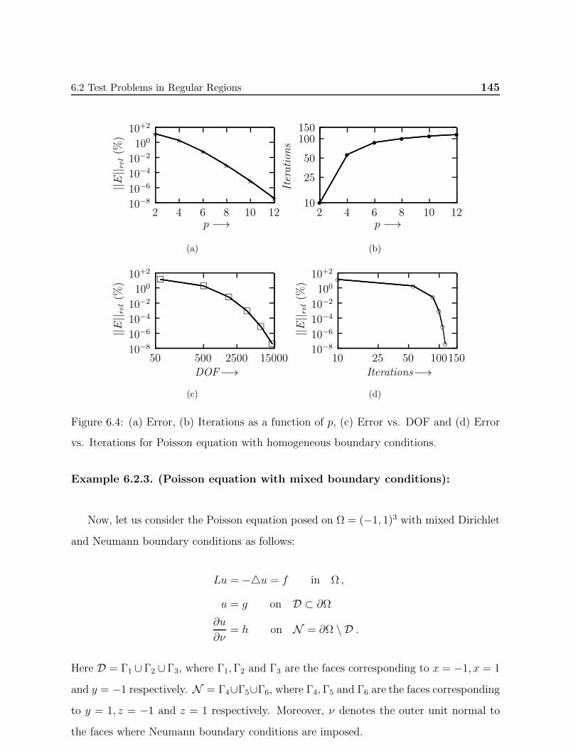
6.2 Test Problems in Regular Regions 145
10−8
10−6
10−4
10−2
10010+2
12108642p −→
||E|| rel(%
) ⋆⋆
⋆⋆
⋆
⋆
(a)
150100
50
25
1012108642
p −→
Iterations
s
s
ss
s s
(b)
10−8
10−6
10−4
10−2
10010+2
15000250050050DOF−→
||E|| rel(%
)
(c)
10−8
10−6
10−4
10−2
10010+2
150100502510Iterations−→
||E|| rel(%
)
(d)
Figure 6.4: (a) Error, (b) Iterations as a function of p, (c) Error vs. DOF and (d) Error
vs. Iterations for Poisson equation with homogeneous boundary conditions.
Example 6.2.3. (Poisson equation with mixed boundary conditions):
Now, let us consider the Poisson equation posed on Ω = (−1, 1)3 with mixed Dirichlet
and Neumann boundary conditions as follows:
Lu = −u = f in Ω ,
u = g on D ⊂ ∂Ω
∂u
∂ν= h on N = ∂Ω \ D .
Here D = Γ1 ∪ Γ2 ∪ Γ3, where Γ1,Γ2 and Γ3 are the faces corresponding to x = −1, x = 1
and y = −1 respectively. N = Γ4∪Γ5∪Γ6, where Γ4,Γ5 and Γ6 are the faces corresponding
to y = 1, z = −1 and z = 1 respectively. Moreover, ν denotes the outer unit normal to
the faces where Neumann boundary conditions are imposed.
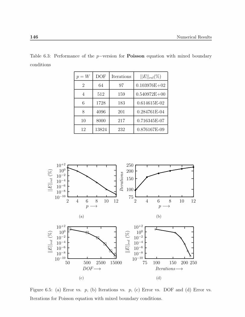
146 Numerical Results
Table 6.3: Performance of the p−version for Poisson equation with mixed boundary
conditions
p =W DOF Iterations ||E||rel(%)
2 64 97 0.103976E+02
4 512 159 0.540972E+00
6 1728 183 0.614615E-02
8 4096 201 0.284761E-04
10 8000 217 0.716345E-07
12 13824 232 0.876167E-09
10−1010−810−610−410−2100
10+2
12108642p −→
||E|| rel(%
) ⋆⋆
⋆
⋆
⋆⋆
(a)
250200
150
100
7512108642
p −→
Iterations
s
s
s
ss
s
(b)
10−1010−810−610−410−2100
10+2
15000250050050DOF−→
||E|| rel(%
)
(c)
10−1010−810−610−410−2100
10+2
25020015010075Iterations−→
||E|| rel(%
)
(d)
Figure 6.5: (a) Error vs. p, (b) Iterations vs. p, (c) Error vs. DOF and (d) Error vs.
Iterations for Poisson equation with mixed boundary conditions.
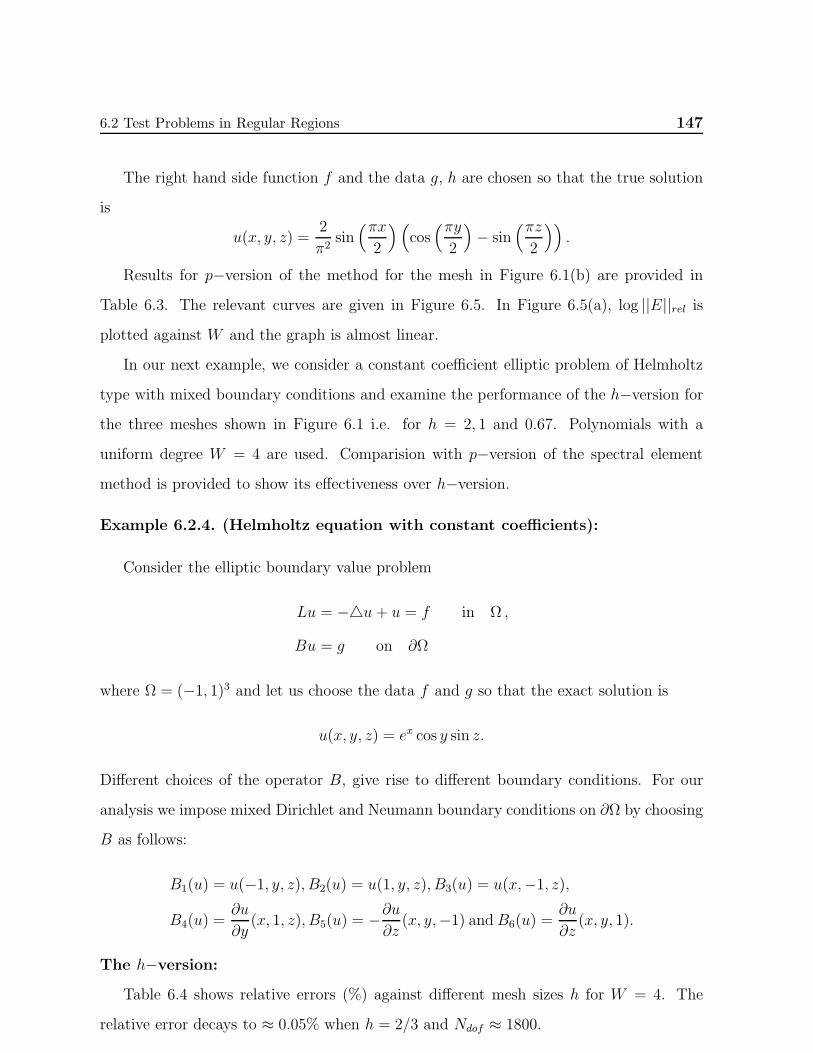
6.2 Test Problems in Regular Regions 147
The right hand side function f and the data g, h are chosen so that the true solution
is
u(x, y, z) =2
π2sin(πx
2
)(cos(πy
2
)− sin
(πz2
)).
Results for p−version of the method for the mesh in Figure 6.1(b) are provided in
Table 6.3. The relevant curves are given in Figure 6.5. In Figure 6.5(a), log ||E||rel isplotted against W and the graph is almost linear.
In our next example, we consider a constant coefficient elliptic problem of Helmholtz
type with mixed boundary conditions and examine the performance of the h−version for
the three meshes shown in Figure 6.1 i.e. for h = 2, 1 and 0.67. Polynomials with a
uniform degree W = 4 are used. Comparision with p−version of the spectral element
method is provided to show its effectiveness over h−version.
Example 6.2.4. (Helmholtz equation with constant coefficients):
Consider the elliptic boundary value problem
Lu = −u+ u = f in Ω ,
Bu = g on ∂Ω
where Ω = (−1, 1)3 and let us choose the data f and g so that the exact solution is
u(x, y, z) = ex cos y sin z.
Different choices of the operator B, give rise to different boundary conditions. For our
analysis we impose mixed Dirichlet and Neumann boundary conditions on ∂Ω by choosing
B as follows:
B1(u) = u(−1, y, z), B2(u) = u(1, y, z), B3(u) = u(x,−1, z),
B4(u) =∂u
∂y(x, 1, z), B5(u) = −
∂u
∂z(x, y,−1) andB6(u) =
∂u
∂z(x, y, 1).
The h−version:Table 6.4 shows relative errors (%) against different mesh sizes h for W = 4. The
relative error decays to ≈ 0.05% when h = 2/3 and Ndof ≈ 1800.
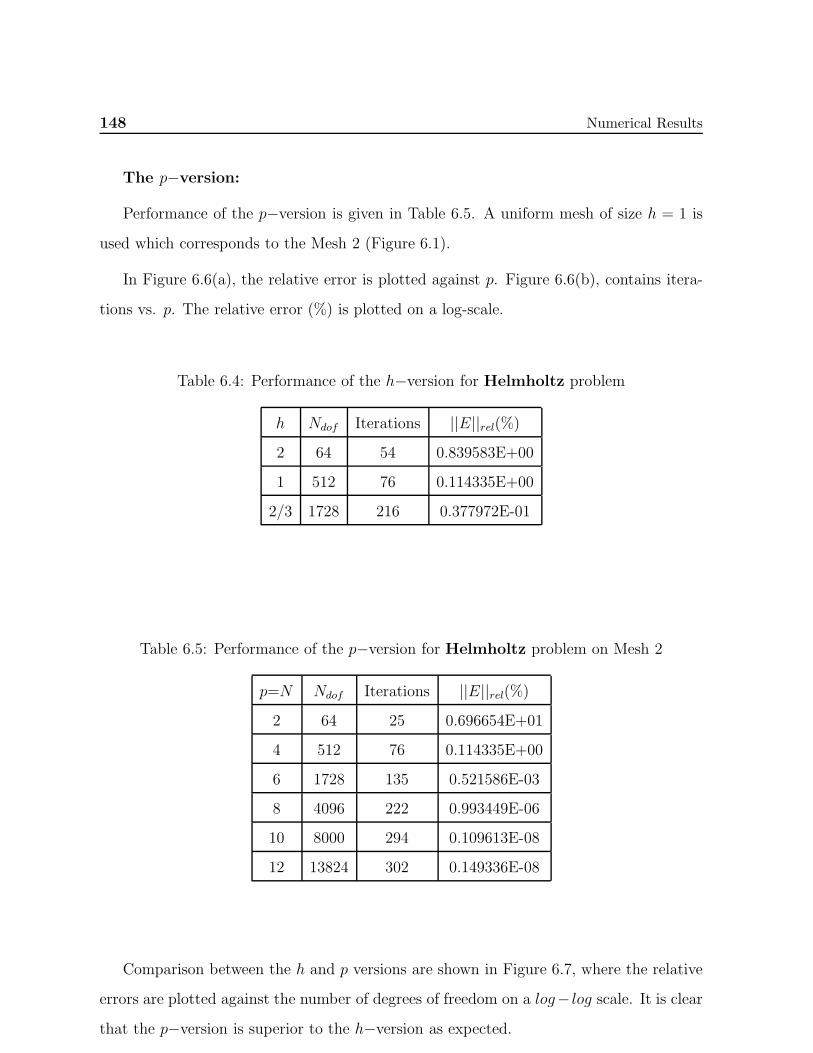
148 Numerical Results
The p−version:
Performance of the p−version is given in Table 6.5. A uniform mesh of size h = 1 is
used which corresponds to the Mesh 2 (Figure 6.1).
In Figure 6.6(a), the relative error is plotted against p. Figure 6.6(b), contains itera-
tions vs. p. The relative error (%) is plotted on a log-scale.
Table 6.4: Performance of the h−version for Helmholtz problem
h Ndof Iterations ||E||rel(%)
2 64 54 0.839583E+00
1 512 76 0.114335E+00
2/3 1728 216 0.377972E-01
Table 6.5: Performance of the p−version for Helmholtz problem on Mesh 2
p=N Ndof Iterations ||E||rel(%)
2 64 25 0.696654E+01
4 512 76 0.114335E+00
6 1728 135 0.521586E-03
8 4096 222 0.993449E-06
10 8000 294 0.109613E-08
12 13824 302 0.149336E-08
Comparison between the h and p versions are shown in Figure 6.7, where the relative
errors are plotted against the number of degrees of freedom on a log− log scale. It is clear
that the p−version is superior to the h−version as expected.
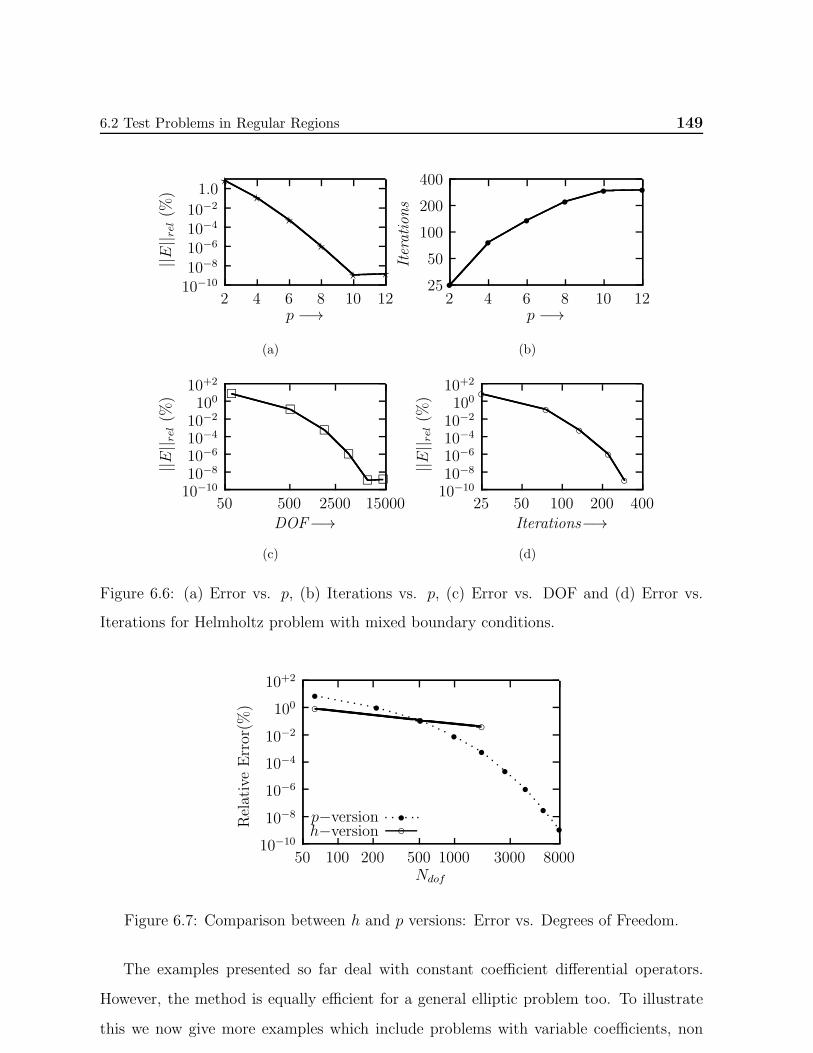
6.2 Test Problems in Regular Regions 149
10−1010−8
10−610−410−2
1.0
12108642p −→
||E|| rel(%
)⋆
⋆
⋆
⋆
⋆ ⋆
(a)
400
200
100
50
2512108642
p −→
Iterations
s
s
s
s
s s
(b)
10−1010−810−610−410−2100
10+2
15000250050050DOF−→
||E|| rel(%
)
(c)
10−1010−810−610−410−2100
10+2
4002001005025Iterations−→
||E|| rel(%
)
(d)
Figure 6.6: (a) Error vs. p, (b) Iterations vs. p, (c) Error vs. DOF and (d) Error vs.
Iterations for Helmholtz problem with mixed boundary conditions.
10+2
100
10−2
10−4
10−6
10−8
10−10
80003000100050020010050Ndof
RelativeError(%
)
p−version
s
s
s
s
s
s
s
s
s
s
h−version
Figure 6.7: Comparison between h and p versions: Error vs. Degrees of Freedom.
The examples presented so far deal with constant coefficient differential operators.
However, the method is equally efficient for a general elliptic problem too. To illustrate
this we now give more examples which include problems with variable coefficients, non
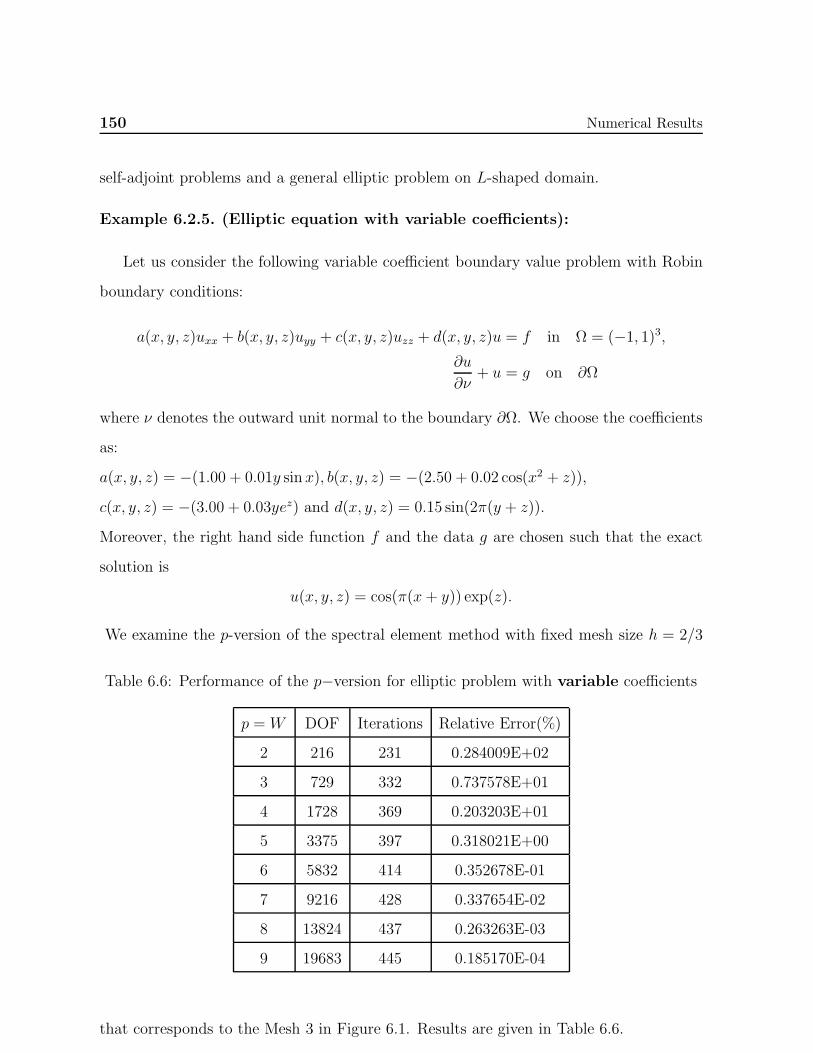
150 Numerical Results
self-adjoint problems and a general elliptic problem on L-shaped domain.
Example 6.2.5. (Elliptic equation with variable coefficients):
Let us consider the following variable coefficient boundary value problem with Robin
boundary conditions:
a(x, y, z)uxx + b(x, y, z)uyy + c(x, y, z)uzz + d(x, y, z)u = f in Ω = (−1, 1)3,∂u
∂ν+ u = g on ∂Ω
where ν denotes the outward unit normal to the boundary ∂Ω. We choose the coefficients
as:
a(x, y, z) = −(1.00 + 0.01y sin x), b(x, y, z) = −(2.50 + 0.02 cos(x2 + z)),
c(x, y, z) = −(3.00 + 0.03yez) and d(x, y, z) = 0.15 sin(2π(y + z)).
Moreover, the right hand side function f and the data g are chosen such that the exact
solution is
u(x, y, z) = cos(π(x+ y)) exp(z).
We examine the p-version of the spectral element method with fixed mesh size h = 2/3
Table 6.6: Performance of the p−version for elliptic problem with variable coefficients
p = W DOF Iterations Relative Error(%)
2 216 231 0.284009E+02
3 729 332 0.737578E+01
4 1728 369 0.203203E+01
5 3375 397 0.318021E+00
6 5832 414 0.352678E-01
7 9216 428 0.337654E-02
8 13824 437 0.263263E-03
9 19683 445 0.185170E-04
that corresponds to the Mesh 3 in Figure 6.1. Results are given in Table 6.6.
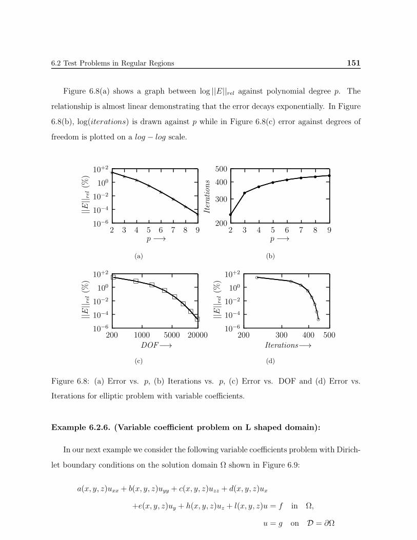
6.2 Test Problems in Regular Regions 151
Figure 6.8(a) shows a graph between log ||E||rel against polynomial degree p. The
relationship is almost linear demonstrating that the error decays exponentially. In Figure
6.8(b), log(iterations) is drawn against p while in Figure 6.8(c) error against degrees of
freedom is plotted on a log − log scale.
10−6
10−4
10−2
100
10+2
98765432p −→
||E|| rel(%
) ⋆ ⋆ ⋆⋆
⋆⋆
⋆⋆
(a)
500
400
300
20098765432
p −→
Iterations
s
s
s
ss
s s s
(b)
10−6
10−4
10−2
100
10+2
2000050001000200DOF−→
||E|| rel(%
)
(c)
10−6
10−4
10−2
100
10+2
500400300200Iterations−→
||E|| rel(%
)
(d)
Figure 6.8: (a) Error vs. p, (b) Iterations vs. p, (c) Error vs. DOF and (d) Error vs.
Iterations for elliptic problem with variable coefficients.
Example 6.2.6. (Variable coefficient problem on L shaped domain):
In our next example we consider the following variable coefficients problem with Dirich-
let boundary conditions on the solution domain Ω shown in Figure 6.9:
a(x, y, z)uxx + b(x, y, z)uyy + c(x, y, z)uzz + d(x, y, z)ux
+e(x, y, z)uy + h(x, y, z)uz + l(x, y, z)u = f in Ω,
u = g on D = ∂Ω
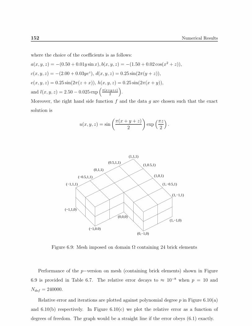
152 Numerical Results
where the choice of the coefficients is as follows:
a(x, y, z) = −(0.50 + 0.01y sin x), b(x, y, z) = −(1.50 + 0.02 cos(x2 + z)),
c(x, y, z) = −(2.00 + 0.03yez), d(x, y, z) = 0.25 sin(2π(y + z)),
e(x, y, z) = 0.25 sin(2π(z + x)), h(x, y, z) = 0.25 sin(2π(x+ y)),
and l(x, y, z) = 2.50− 0.025 exp(π(x+y+z)
2
).
Moreover, the right hand side function f and the data g are chosen such that the exact
solution is
u(x, y, z) = sin
(π(x+ y + z)
2
)exp
(πz2
).
(0,0,0)
(1,1,1)
(1,−1,0)
(1,−1,1)
(0,−1,0)(−1,0.0)
(−1,1,0)
(−1,1,1)
(0,1,1)
(0.5,1,1)
(−0.5,1,1)
(1,0.5,1)
(1,0,1)
(1,−0.5,1)
Figure 6.9: Mesh imposed on domain Ω containing 24 brick elements
Performance of the p−version on mesh (containing brick elements) shown in Figure
6.9 is provided in Table 6.7. The relative error decays to ≈ 10−8 when p = 10 and
Ndof = 240000.
Relative error and iterations are plotted against polynomial degree p in Figure 6.10(a)
and 6.10(b) respectively. In Figure 6.10(c) we plot the relative error as a function of
degrees of freedom. The graph would be a straight line if the error obeys (6.1) exactly.
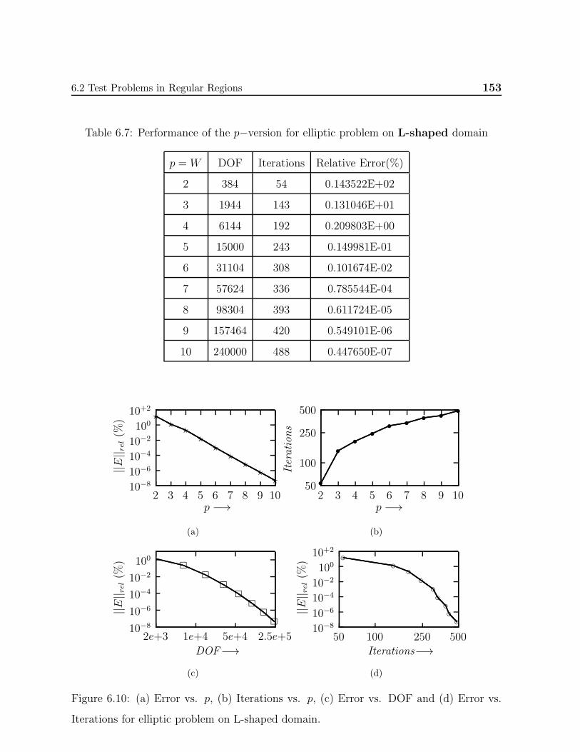
6.2 Test Problems in Regular Regions 153
Table 6.7: Performance of the p−version for elliptic problem on L-shaped domain
p = W DOF Iterations Relative Error(%)
2 384 54 0.143522E+02
3 1944 143 0.131046E+01
4 6144 192 0.209803E+00
5 15000 243 0.149981E-01
6 31104 308 0.101674E-02
7 57624 336 0.785544E-04
8 98304 393 0.611724E-05
9 157464 420 0.549101E-06
10 240000 488 0.447650E-07
10−8
10−6
10−4
10−2
10010+2
1098765432p −→
||E|| rel(%
) ⋆⋆
⋆⋆
⋆⋆
⋆⋆
⋆
(a)
500
250
100
501098765432
p −→
Iterations
s
s
s
s
ss
ss
s
(b)
10−8
10−6
10−4
10−2
100
2.5e+55e+41e+42e+3
DOF−→
||E|| rel(%
)
(c)
10−8
10−6
10−4
10−2
10010+2
50025010050Iterations−→
||E|| rel(%
)
(d)
Figure 6.10: (a) Error vs. p, (b) Iterations vs. p, (c) Error vs. DOF and (d) Error vs.
Iterations for elliptic problem on L-shaped domain.
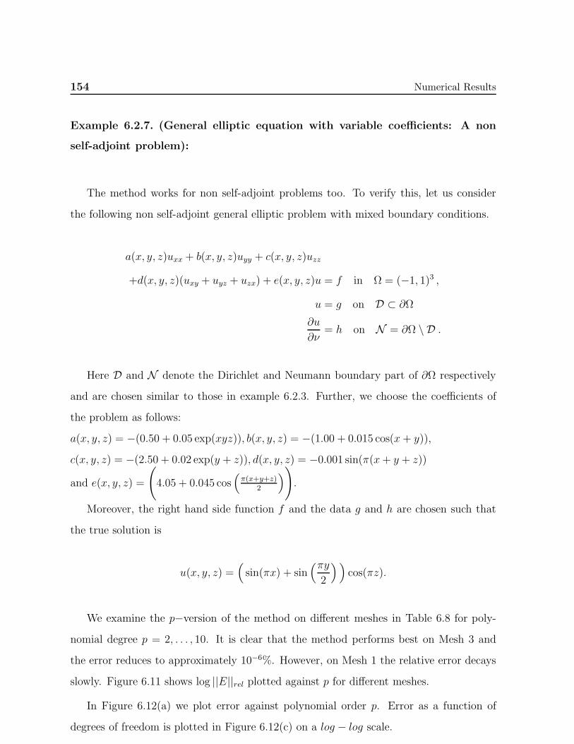
154 Numerical Results
Example 6.2.7. (General elliptic equation with variable coefficients: A non
self-adjoint problem):
The method works for non self-adjoint problems too. To verify this, let us consider
the following non self-adjoint general elliptic problem with mixed boundary conditions.
a(x, y, z)uxx + b(x, y, z)uyy + c(x, y, z)uzz
+d(x, y, z)(uxy + uyz + uzx) + e(x, y, z)u = f in Ω = (−1, 1)3 ,
u = g on D ⊂ ∂Ω
∂u
∂ν= h on N = ∂Ω \ D .
Here D and N denote the Dirichlet and Neumann boundary part of ∂Ω respectively
and are chosen similar to those in example 6.2.3. Further, we choose the coefficients of
the problem as follows:
a(x, y, z) = −(0.50 + 0.05 exp(xyz)), b(x, y, z) = −(1.00 + 0.015 cos(x+ y)),
c(x, y, z) = −(2.50 + 0.02 exp(y + z)), d(x, y, z) = −0.001 sin(π(x+ y + z))
and e(x, y, z) =
(4.05 + 0.045 cos
(π(x+y+z)
2
)).
Moreover, the right hand side function f and the data g and h are chosen such that
the true solution is
u(x, y, z) =(sin(πx) + sin
(πy2
))cos(πz).
We examine the p−version of the method on different meshes in Table 6.8 for poly-
nomial degree p = 2, . . . , 10. It is clear that the method performs best on Mesh 3 and
the error reduces to approximately 10−6%. However, on Mesh 1 the relative error decays
slowly. Figure 6.11 shows log ||E||rel plotted against p for different meshes.
In Figure 6.12(a) we plot error against polynomial order p. Error as a function of
degrees of freedom is plotted in Figure 6.12(c) on a log − log scale.
6.2 Test Problems in Regular Regions 155
Table 6.8: Performance of the p−version on different meshes for general elliptic (non
self-adjoint) problem with variable coefficients
p =W Mesh 1 Mesh 2 Mesh 3
2 0.498666E+02 0.485737E+02 0.291328E+02
3 0.507328E+02 0.107829E+02 0.586317E+01
4 0.227058E+02 0.517751E+01 0.149092E+01
5 0.143968E+02 0.814482E+00 0.237686E+00
6 0.408230E+01 0.234810E+00 0.292025E-01
7 0.184822E+01 0.279261E-01 0.289156E-02
8 0.311612E+00 0.430208E-02 0.236661E-03
9 0.104765E+00 0.377498E-03 0.168223E-04
10 0.136308E-01 0.431639E-04 0.352480E-05
10+2
100
10−2
10−4
10−6
1098765432p −→
||E|| rel(%
)
h = 2.00
s s
ss
s
s
s
s
s
s
h = 1.00
h = 0.67
⋆⋆
⋆⋆
⋆
⋆
⋆
⋆⋆⋆
Figure 6.11: Error as a function of W for different values of h for general elliptic (non
self-adjoint) problem.
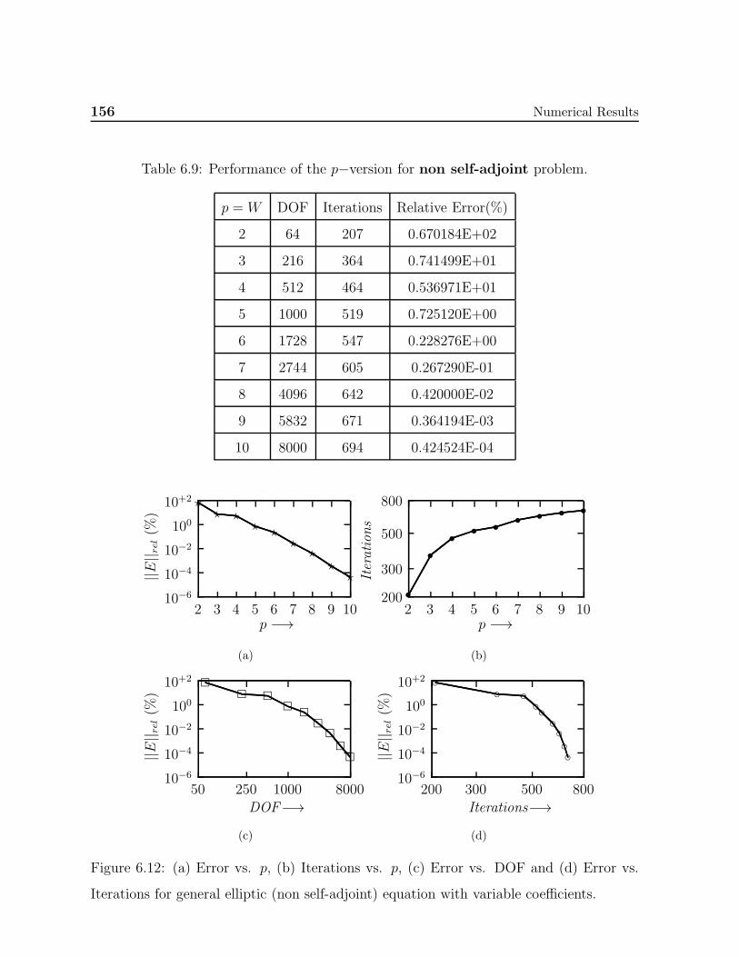
156 Numerical Results
Table 6.9: Performance of the p−version for non self-adjoint problem.
p = W DOF Iterations Relative Error(%)
2 64 207 0.670184E+02
3 216 364 0.741499E+01
4 512 464 0.536971E+01
5 1000 519 0.725120E+00
6 1728 547 0.228276E+00
7 2744 605 0.267290E-01
8 4096 642 0.420000E-02
9 5832 671 0.364194E-03
10 8000 694 0.424524E-04
10−6
10−4
10−2
100
10+2
1098765432p −→
||E|| rel(%
)
⋆⋆ ⋆
⋆ ⋆⋆
⋆⋆
⋆
(a)
800
500
300
2001098765432
p −→
Iterations
s
s
s
ss
ss
s s
(b)
10−6
10−4
10−2
100
10+2
8000100025050DOF−→
||E|| rel(%
)
(c)
10−6
10−4
10−2
100
10+2
800500300200Iterations−→
||E|| rel(%
)
(d)
Figure 6.12: (a) Error vs. p, (b) Iterations vs. p, (c) Error vs. DOF and (d) Error vs.
Iterations for general elliptic (non self-adjoint) equation with variable coefficients.
6.3 Test Problems in Singular Regions 157
6.3 Test Problems in Singular Regions
In order to show the effectiveness of the proposed method in dealing with three dimen-
sional elliptic boundary value problems containing singularities we now present results
of numerical simulations for model problems on various polyhedral domains containing
different types of singularities discussed in the previous chapters which aim to verify the
validity of the asymptotic error estimates and estimates of computational complexity that
have been obtained.
Hereafter N will always denote the number of layers in the geometric mesh
and W , the polynomial order used. It is assumed that N is proportional to
W . In case of examples with vertex and edge singularities all our calculations are based
on a parallel computer with O(N) processors and each element is being mapped onto a
separate processor. However, in case of examples with vertex-edge singularities we have
used a parallel computer with O(N2) processors. The geometric mesh factors in the
neighbourhoods of vertices and edges are chosen as µv = 0.15 and µe = 0.15 which give
optimal results.
The examples reported here will include all three types of singularities. In addition, to
compare our results with those existing in the literature we shall consider a few examples
similar to those of Guo and Oh [52] as well.
Our first example is the Poisson equation containing only a vertex singularity with
Dirichlet boundary conditions. For computational simplicity we shall assume that the
singularity arises only at one vertex of the domain under consideration. However, in
general, a typical domain may contain singularities at more than one corner in which case
the same technique can be applied to each vertex containing a singularity.
Example 6.3.1. (Poisson equation with vertex singularity)
Consider the domain Ω(v) shown in Figure 6.13 defined by
Ω(v) = (φ, θ, ρ) | π/6 ≤ φ ≤ π/3, 0 ≤ θ ≤ 3π/2, ρ ≤ 1.
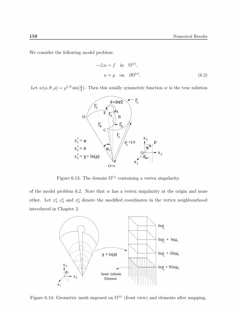
158 Numerical Results
We consider the following model problem:
−u = f in Ω(v),
u = g on ∂Ω(v). (6.2)
Let w(φ, θ, ρ) = ρ1/2 sin(φ2). Then this axially symmetric function w is the true solution
φv
E A
θ=3π/2
= φ
θ =
x
xv
v
2
1
xv3 = χ= ln( )ρ
Γ1
4Γ
O=v
φρ
Oθ
D
Γ
B
x
x
x
1
2
3ρv
=1.0
C3Γ
Γ2
2Γ5
Figure 6.13: The domain Ω(v) containing a vertex singularity.
of the model problem 6.2. Note that w has a vertex singularity at the origin and none
other. Let xv1, xv2 and xv3 denote the modified coordinates in the vertex neighbourhood
introduced in Chapter 2.
ρ ln( )χ =
Semi−infiniteElement
v
µv ln
2
N lnµ
lnµv
v
x
x
1
2
ρ
x3
ρ ln
ln ρv
ln ρv
+
+
+ ln ρv
Figure 6.14: Geometric mesh imposed on Ω(v) (front view) and elements after mapping.
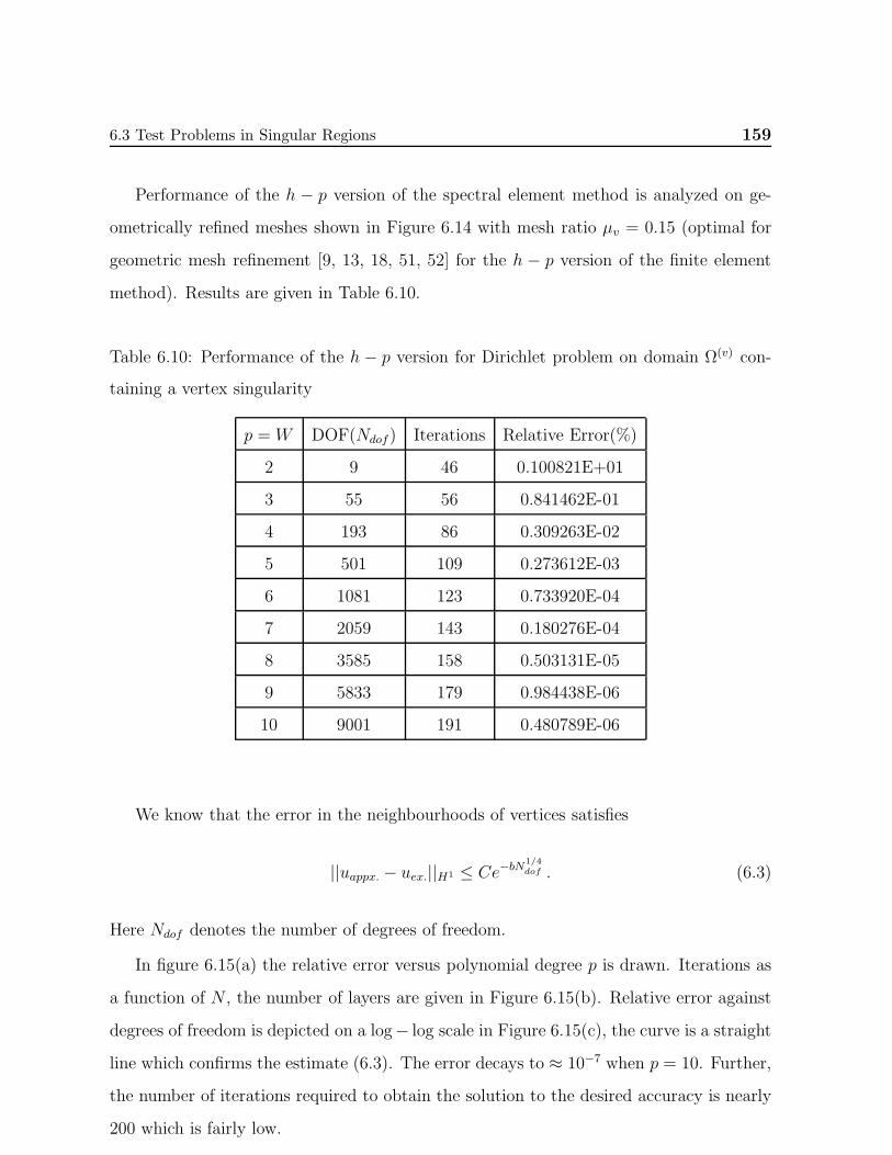
6.3 Test Problems in Singular Regions 159
Performance of the h − p version of the spectral element method is analyzed on ge-
ometrically refined meshes shown in Figure 6.14 with mesh ratio µv = 0.15 (optimal for
geometric mesh refinement [9, 13, 18, 51, 52] for the h − p version of the finite element
method). Results are given in Table 6.10.
Table 6.10: Performance of the h − p version for Dirichlet problem on domain Ω(v) con-
taining a vertex singularity
p =W DOF(Ndof) Iterations Relative Error(%)
2 9 46 0.100821E+01
3 55 56 0.841462E-01
4 193 86 0.309263E-02
5 501 109 0.273612E-03
6 1081 123 0.733920E-04
7 2059 143 0.180276E-04
8 3585 158 0.503131E-05
9 5833 179 0.984438E-06
10 9001 191 0.480789E-06
We know that the error in the neighbourhoods of vertices satisfies
||uappx. − uex.||H1 ≤ Ce−bN1/4dof . (6.3)
Here Ndof denotes the number of degrees of freedom.
In figure 6.15(a) the relative error versus polynomial degree p is drawn. Iterations as
a function of N , the number of layers are given in Figure 6.15(b). Relative error against
degrees of freedom is depicted on a log− log scale in Figure 6.15(c), the curve is a straight
line which confirms the estimate (6.3). The error decays to ≈ 10−7 when p = 10. Further,
the number of iterations required to obtain the solution to the desired accuracy is nearly
200 which is fairly low.
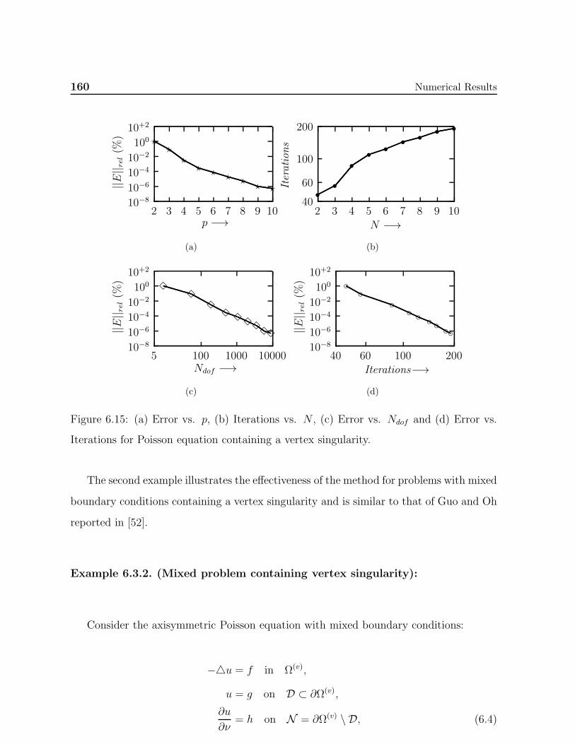
160 Numerical Results
10−8
10−6
10−4
10−2
10010+2
1098765432p −→
||E|| rel(%
) ⋆⋆
⋆⋆ ⋆ ⋆ ⋆ ⋆ ⋆
(a)
200
100
60
401098765432
N −→
Iterations
s
s
s
s
s
ss
ss
(b)
10−8
10−6
10−4
10−2
10010+2
1000010001005Ndof −→
||E|| rel(%
)
(c)
10−8
10−6
10−4
10−2
10010+2
2001006040Iterations−→
||E|| rel(%
)
(d)
Figure 6.15: (a) Error vs. p, (b) Iterations vs. N , (c) Error vs. Ndof and (d) Error vs.
Iterations for Poisson equation containing a vertex singularity.
The second example illustrates the effectiveness of the method for problems with mixed
boundary conditions containing a vertex singularity and is similar to that of Guo and Oh
reported in [52].
Example 6.3.2. (Mixed problem containing vertex singularity):
Consider the axisymmetric Poisson equation with mixed boundary conditions:
−u = f in Ω(v),
u = g on D ⊂ ∂Ω(v),
∂u
∂ν= h on N = ∂Ω(v) \ D, (6.4)
6.3 Test Problems in Singular Regions 161
where the domain Ω(v) is shown in Figure 6.13 and
D = Γ1 ∪ Γ2 ∪ Γ3 ∪ Γ4 = Γ1D ∪ Γ2
D ,
Γ1D = (φ, θ, ρ) : φ = π/6, π/3, 0 ≤ θ ≤ 3π/2, 0 ≤ ρ ≤ 1 ,
Γ2D = (φ, θ, ρ) : π/6 ≤ φ ≤ π/3, θ = 0, 3π/2, 0 ≤ ρ ≤ 1 ,
N = Γ5 = (φ, θ, ρ) : π/6 ≤ φ ≤ π/3, 0 ≤ θ ≤ 3π/2, ρ = 1 .
We choose data f , g and h such that the function w = ρ0.1(1 − ρ) sin 2φ is the true
solution of (6.4) satisfying prescribed boundary conditions. Here ν denotes the exterior
unit normal to the part of the boundary where we impose Neumann boundary conditions.
Table 6.11: Performance of the h − p version for mixed problem on polyhedral domain
Ω(v) containing a vertex singularity
p =W DOF(Ndof) Iterations Relative Error(%)
2 9 16 0.962637E+01
3 55 39 0.252012E+01
4 193 128 0.191490E+00
5 501 176 0.212320E-01
6 1081 314 0.192391E-02
7 2059 409 0.884830E-03
8 3585 743 0.412629E-03
9 5833 814 0.470681E-04
Table 6.11 contains the relative error obtained by applying the method on geometri-
cally refined mesh in ρ. The relative error versus degrees of freedom is depicted in Figure
6.15. It is clear that the method gives exponential accuracy.
Next, we apply our method to an elliptic problem containing an edge singularity.
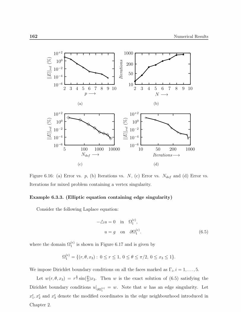
162 Numerical Results
10−6
10−4
10−2
100
10+2
1098765432p −→
||E|| rel(%
) ⋆ ⋆⋆
⋆⋆ ⋆ ⋆
⋆
(a)
1000
200
50
101098765432
N −→
Iterations
s
s
s
s
ss
s s
(b)
10−6
10−4
10−2
100
10+2
1000010001005Ndof −→
||E|| rel(%
)
(c)
10−6
10−4
10−2
100
10+2
10002005010Iterations−→
||E|| rel(%
)
(d)
Figure 6.16: (a) Error vs. p, (b) Iterations vs. N , (c) Error vs. Ndof and (d) Error vs.
Iterations for mixed problem containing a vertex singularity.
Example 6.3.3. (Elliptic equation containing edge singularity)
Consider the following Laplace equation:
−u = 0 in Ω(e)1 ,
u = g on ∂Ω(e)1 . (6.5)
where the domain Ω(e)1 is shown in Figure 6.17 and is given by
Ω(e)1 = (r, θ, x3) : 0 ≤ r ≤ 1, 0 ≤ θ ≤ π/2, 0 ≤ x3 ≤ 1.
We impose Dirichlet boundary conditions on all the faces marked as Γi, i = 1, . . . , 5.
Let w(r, θ, x3) = r13 sin( θ
3)x3. Then w is the exact solution of (6.5) satisfying the
Dirichlet boundary conditions u|∂Ω
(e)1
= w. Note that w has an edge singularity. Let
xe1, xe2 and xe3 denote the modified coordinates in the edge neighbourhood introduced in
Chapter 2.
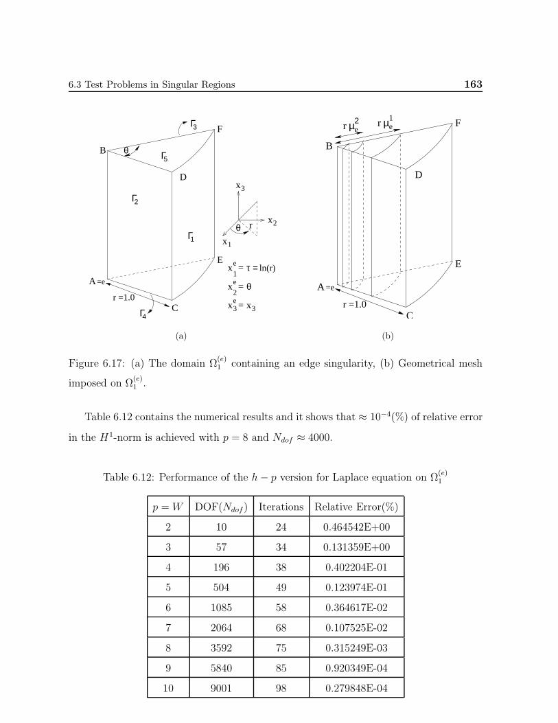
6.3 Test Problems in Singular Regions 163
B
D
E
F
Γ
Γ
Γ
=eA
CΓ
Γ1
2
5
3
4
x2
x3
e
e
xe
1 = ln(r)τ =
= θ
=
θ
r =1.0
x
rθ
x
x
1
2
3
x3
(a)
D
E
F
=eA
C
B
2µr eµr e
1
r =1.0
(b)
Figure 6.17: (a) The domain Ω(e)1 containing an edge singularity, (b) Geometrical mesh
imposed on Ω(e)1 .
Table 6.12 contains the numerical results and it shows that ≈ 10−4(%) of relative error
in the H1-norm is achieved with p = 8 and Ndof ≈ 4000.
Table 6.12: Performance of the h− p version for Laplace equation on Ω(e)1
p =W DOF(Ndof) Iterations Relative Error(%)
2 10 24 0.464542E+00
3 57 34 0.131359E+00
4 196 38 0.402204E-01
5 504 49 0.123974E-01
6 1085 58 0.364617E-02
7 2064 68 0.107525E-02
8 3592 75 0.315249E-03
9 5840 85 0.920349E-04
10 9001 98 0.279848E-04
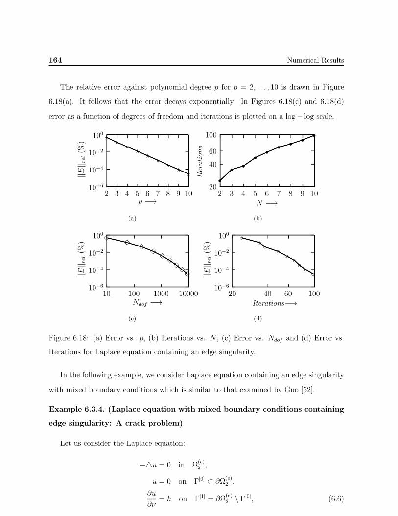
164 Numerical Results
The relative error against polynomial degree p for p = 2, . . . , 10 is drawn in Figure
6.18(a). It follows that the error decays exponentially. In Figures 6.18(c) and 6.18(d)
error as a function of degrees of freedom and iterations is plotted on a log− log scale.
10−6
10−4
10−2
100
1098765432p −→
||E|| rel(%
)
⋆⋆
⋆⋆
⋆⋆
⋆⋆
⋆
(a)
100
60
40
201098765432
N −→Iterations
s
s
s
s
s
ss
s
s
(b)
10−6
10−4
10−2
100
10000100010010Ndof −→
||E|| rel(%
)
(c)
10−6
10−4
10−2
100
100604020Iterations−→
||E|| rel(%
)
(d)
Figure 6.18: (a) Error vs. p, (b) Iterations vs. N , (c) Error vs. Ndof and (d) Error vs.
Iterations for Laplace equation containing an edge singularity.
In the following example, we consider Laplace equation containing an edge singularity
with mixed boundary conditions which is similar to that examined by Guo [52].
Example 6.3.4. (Laplace equation with mixed boundary conditions containing
edge singularity: A crack problem)
Let us consider the Laplace equation:
−u = 0 in Ω(e)2 ,
u = 0 on Γ[0] ⊂ ∂Ω(e)2 ,
∂u
∂ν= h on Γ[1] = ∂Ω
(e)2 \ Γ[0], (6.6)
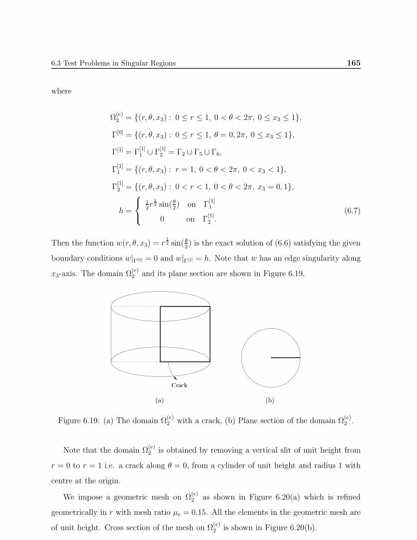
6.3 Test Problems in Singular Regions 165
where
Ω(e)2 = (r, θ, x3) : 0 ≤ r ≤ 1, 0 < θ < 2π, 0 ≤ x3 ≤ 1,
Γ[0] = (r, θ, x3) : 0 ≤ r ≤ 1, θ = 0, 2π, 0 ≤ x3 ≤ 1,
Γ[1] = Γ[1]1 ∪ Γ
[1]2 = Γ2 ∪ Γ5 ∪ Γ6,
Γ[1]1 = (r, θ, x3) : r = 1, 0 < θ < 2π, 0 < x3 < 1,
Γ[1]2 = (r, θ, x3) : 0 < r < 1, 0 < θ < 2π, x3 = 0, 1,
h =
12r
12 sin( θ
2) on Γ
[1]1
0 on Γ[1]2 .
(6.7)
Then the function w(r, θ, x3) = r12 sin( θ
2) is the exact solution of (6.6) satisfying the given
boundary conditions w|Γ[0] = 0 and w|Γ[1] = h. Note that w has an edge singularity along
x3-axis. The domain Ω(e)2 and its plane section are shown in Figure 6.19.
Crack
(a)
.
(b)
Figure 6.19: (a) The domain Ω(e)2 with a crack, (b) Plane section of the domain Ω
(e)2 .
Note that the domain Ω(e)2 is obtained by removing a vertical slit of unit height from
r = 0 to r = 1 i.e. a crack along θ = 0, from a cylinder of unit height and radius 1 with
centre at the origin.
We impose a geometric mesh on Ω(e)2 as shown in Figure 6.20(a) which is refined
geometrically in r with mesh ratio µe = 0.15. All the elements in the geometric mesh are
of unit height. Cross section of the mesh on Ω(e)2 is shown in Figure 6.20(b).
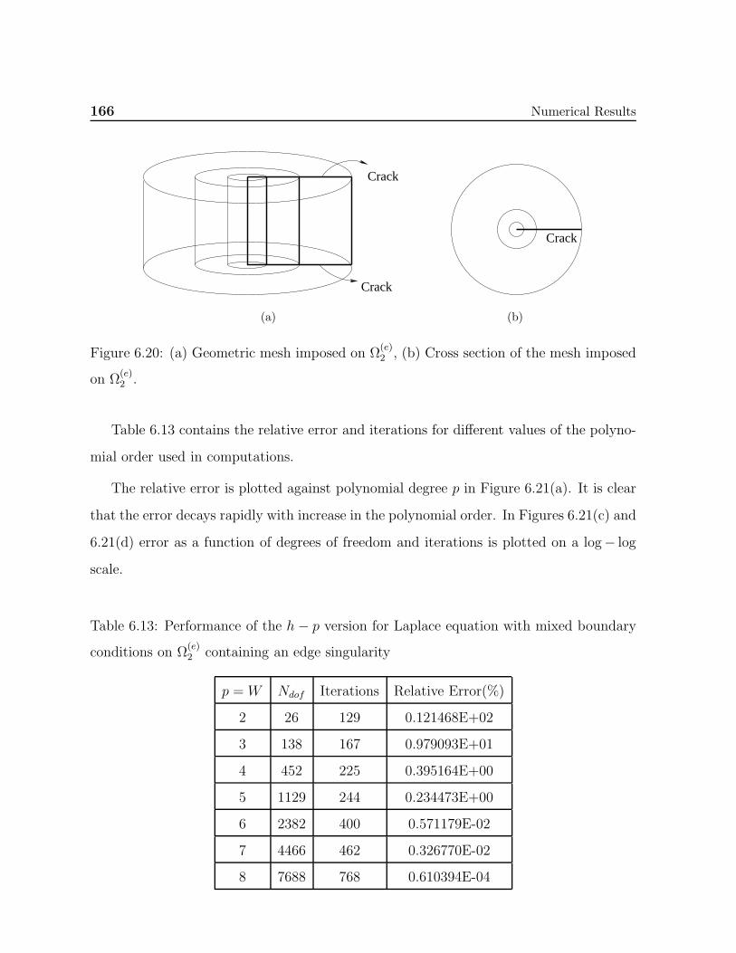
166 Numerical Results
Crack
Crack
(a)
Crack
(b)
Figure 6.20: (a) Geometric mesh imposed on Ω(e)2 , (b) Cross section of the mesh imposed
on Ω(e)2 .
Table 6.13 contains the relative error and iterations for different values of the polyno-
mial order used in computations.
The relative error is plotted against polynomial degree p in Figure 6.21(a). It is clear
that the error decays rapidly with increase in the polynomial order. In Figures 6.21(c) and
6.21(d) error as a function of degrees of freedom and iterations is plotted on a log− log
scale.
Table 6.13: Performance of the h− p version for Laplace equation with mixed boundary
conditions on Ω(e)2 containing an edge singularity
p =W Ndof Iterations Relative Error(%)
2 26 129 0.121468E+02
3 138 167 0.979093E+01
4 452 225 0.395164E+00
5 1129 244 0.234473E+00
6 2382 400 0.571179E-02
7 4466 462 0.326770E-02
8 7688 768 0.610394E-04
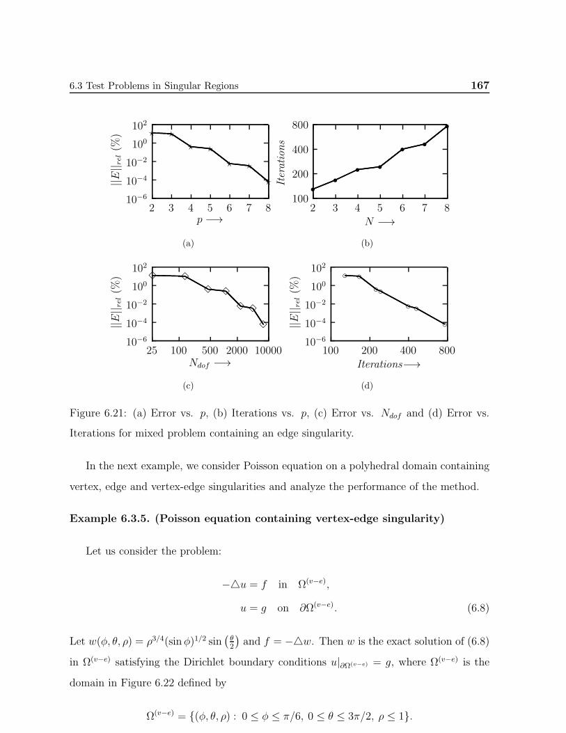
6.3 Test Problems in Singular Regions 167
10−6
10−4
10−2
100
102
8765432p −→
||E|| rel(%
) ⋆ ⋆⋆ ⋆
⋆ ⋆
⋆
(a)
800
400
200
1008765432
N −→
Iterations
s
s
ss
s
s
s
(b)
10−6
10−4
10−2
100
102
10000200050010025Ndof −→
||E|| rel(%
)
(c)
10−6
10−4
10−2
100
102
800400200100Iterations−→
||E|| rel(%
)
(d)
Figure 6.21: (a) Error vs. p, (b) Iterations vs. p, (c) Error vs. Ndof and (d) Error vs.
Iterations for mixed problem containing an edge singularity.
In the next example, we consider Poisson equation on a polyhedral domain containing
vertex, edge and vertex-edge singularities and analyze the performance of the method.
Example 6.3.5. (Poisson equation containing vertex-edge singularity)
Let us consider the problem:
−u = f in Ω(v−e),
u = g on ∂Ω(v−e). (6.8)
Let w(φ, θ, ρ) = ρ3/4(sinφ)1/2 sin(θ2
)and f = −w. Then w is the exact solution of (6.8)
in Ω(v−e) satisfying the Dirichlet boundary conditions u|∂Ω(v−e) = g, where Ω(v−e) is the
domain in Figure 6.22 defined by
Ω(v−e) = (φ, θ, ρ) : 0 ≤ φ ≤ π/6, 0 ≤ θ ≤ 3π/2, ρ ≤ 1.
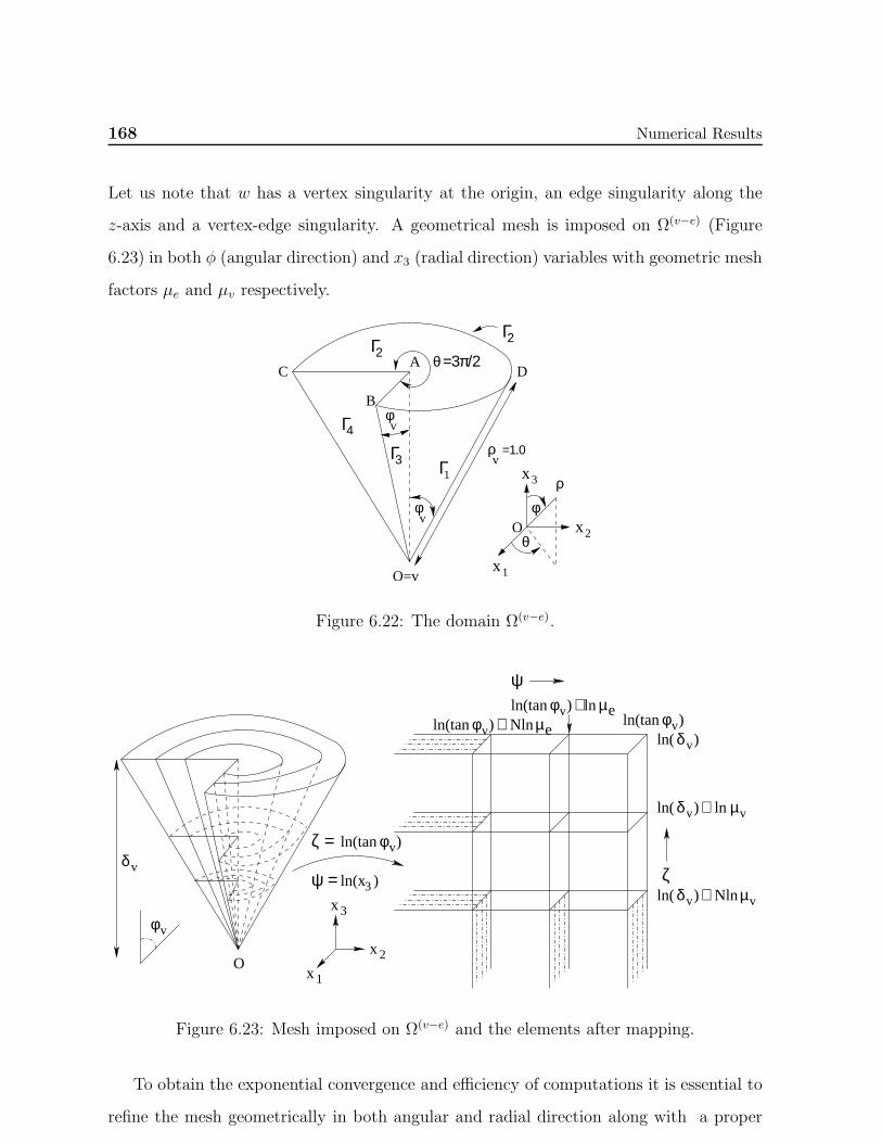
168 Numerical Results
Let us note that w has a vertex singularity at the origin, an edge singularity along the
z-axis and a vertex-edge singularity. A geometrical mesh is imposed on Ω(v−e) (Figure
6.23) in both φ (angular direction) and x3 (radial direction) variables with geometric mesh
factors µe and µv respectively.
B
C
Γ
Γ
Γ
φ
ΓA
3
4
2
O=v
θ
O
ρ
φ
θ
D
ρv
=1.0
=3π/2
φv
v
2
Γ1 x
x
3
2
x1
Figure 6.22: The domain Ω(v−e).
ζ
δv
ln( )
ln( )
δ
δv
ln( )ln(tan )φv
v
ln(tan )φv +ln µe+ Nlnµe
ln(tan )φv
+ Nlnµv
+ ln µv
ψ
O
δv
φv
ζ = φv
ψ = ln(x )3
x
x
3
2
x1
ln(tan )
Figure 6.23: Mesh imposed on Ω(v−e) and the elements after mapping.
To obtain the exponential convergence and efficiency of computations it is essential to
refine the mesh geometrically in both angular and radial direction along with a proper
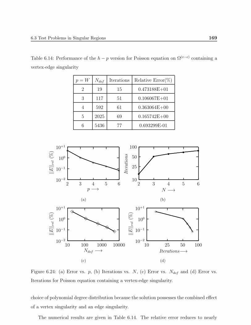
6.3 Test Problems in Singular Regions 169
Table 6.14: Performance of the h− p version for Poisson equation on Ω(v−e) containing a
vertex-edge singularity
p = W Ndof Iterations Relative Error(%)
2 19 15 0.473188E+01
3 117 51 0.106067E+01
4 592 61 0.363064E+00
5 2025 69 0.165742E+00
6 5436 77 0.693299E-01
10−2
10−1
100
10+1
65432p −→
||E|| rel(%
) ⋆
⋆⋆
⋆⋆
(a)
100
50
25
1065432
N −→
Iterations
s
s
ss
s
(b)
10−2
10−1
100
10+1
10000100010010Ndof −→
||E|| rel(%
)
(c)
10−2
10−1
100
10+1
100502510Iterations−→
||E|| rel(%
)
(d)
Figure 6.24: (a) Error vs. p, (b) Iterations vs. N , (c) Error vs. Ndof and (d) Error vs.
Iterations for Poisson equation containing a vertex-edge singularity.
choice of polynomial degree distribution because the solution possesses the combined effect
of a vertex singularity and an edge singularity.
The numerical results are given in Table 6.14. The relative error reduces to nearly
170 Numerical Results
0.07% with p = 6.
Figure 6.24(a) contains the relative error versus polynomial order p. The error is
plotted on a log−scale. The curve is almost a straight line and it confirms the theoretical
estimates obtained. Further in Figure 6.24(b) the error is drawn as a function of Ndof on
a log− log scale.
6.4 Conclusions and Future Work
6.4.1 Summary and conclusions
There are three different types of singularities for elliptic problems on non-smooth domains
in R3, namely, the vertex, the edge and the vertex-edge. In addition, the solutions to these
problems are anisotropic in the neighbourhoods of edges and vertex-edges.
Among many approaches that have been attempted over the past three decades to
provide accurate and economical solutions to the elliptic boundary value problems con-
taining singularities, the two principal approaches are the adaptive mesh refinement (very
small elements near the singularities and large elements elsewhere) and the use of singular
basis functions. In three dimensional problems, the first approach suffers the problems of
limited storage capacity and high computational cost while ill-conditioning occur in the
latter in presence of singularities. As an extension of the second approach, the method of
auxiliary mapping (MAM) was introduced by Babuska and Oh (see [17, 65, 68, 69] and
references therein). The MAM has proven to be highly successful in dealing with elliptic
boundary value problems containing singularities in R2 [17, 65, 68, 69] and R3 [52, 63]
using p-version of the finite element method. However, the success of this method depends
on optimal choices of auxiliary mappings.
In the present work we have proposed an exponentially accurate h−p spectral element
method for three dimensional elliptic problems on non-smooth domains using parallel
computers.
We choose as our solution the spectral element function which minimizes the sum of
a weighted squared norm of the residuals in the partial differential equations and the

6.4 Conclusions and Future Work 171
squared norm of the residuals in the boundary conditions in fractional Sobolev spaces
and enforce continuity by adding a term which measures the jump in the function and
its derivatives at inter-element boundaries in fractional Sobolev norms, to the functional
being minimized.
The present study can be summarized as follows:-
• To resolve the singularities which arise in the neighbourhoods of vertices, edges and
vertex-edges we use modified systems of coordinates that are modified versions of
spherical and cylindrical coordinate systems. These modified coordinates serve as
our auxiliary mappings in different neighbourhoods.
• The Sobolev spaces in vertex-edge and edge neighbourhoods are anisotropic and
become singular at the corners and edges.
• We choose spectral element functions (SEF) which are fully non-conforming. i.e.
there are no set of common boundary values, and hence we do not need to solve the
Schur complement system.
• The method is essentially a least-squares method and to solve the minimization
problem we need to solve the normal equations for the least-squares problem.
• The residuals in the normal equations can be obtained without computing and
storing mass and stiffness matrices.
• We use Preconditioned Conjugate Gradient Method (PCGM) to solve normal equa-
tions using a block diagonal preconditioner. Moreover, there exists a new precon-
ditioner which can be diagonalized in a new set of basis functions, and hence it is
easily inverted on each element.
• For Dirichlet problems the condition number of the preconditioner is O((lnW )2),
provided W = O(eNα) for α < 1/2. However, it grows like O(N4) for mixed
problems.

172 Numerical Results
• For Dirichlet problems the overall complexity of the method is O(N5ln(N)) opera-
tions on a parallel computer with O(N2) processors to compute the solution. For
mixed problems it is equal to O(N7) operations on a parallel computer with O(N2)
processors.
• Computational results for a number of test problems on smooth as well as non-
smooth domains confirm the estimates obtained for the error and computational
complexity.
• In each iteration of the PCGM we need to communicate the values of the function
and its derivatives on the boundary of the element between neighbouring elements.
Moreover, we need to compute two global scalars to update the approximate solution
and search direction. Thus, the inter processor communication involved is small.
• Though the method is efficient and delivers exponential accuracy, more experience is
needed in computations and implementation. e.g. how to implement the distribution
of element degrees, what are the optimal degree factors, etc.
6.4.2 Proposed future work
Rapid growth of the factor N4 for mixed problems creates difficulty in parallelizing the
numerical scheme. To overcome this difficulty another version of the method can be
defined in which we choose spectral element functions to be conforming only on the
wirebasket of the elements.
The values of the spectral element functions at the wirebasket of the elements con-
stitute the set of common boundary values and we need to solve the Schur complement
matrix system corresponding to the common boundary values. We intend to consider this
in future work.
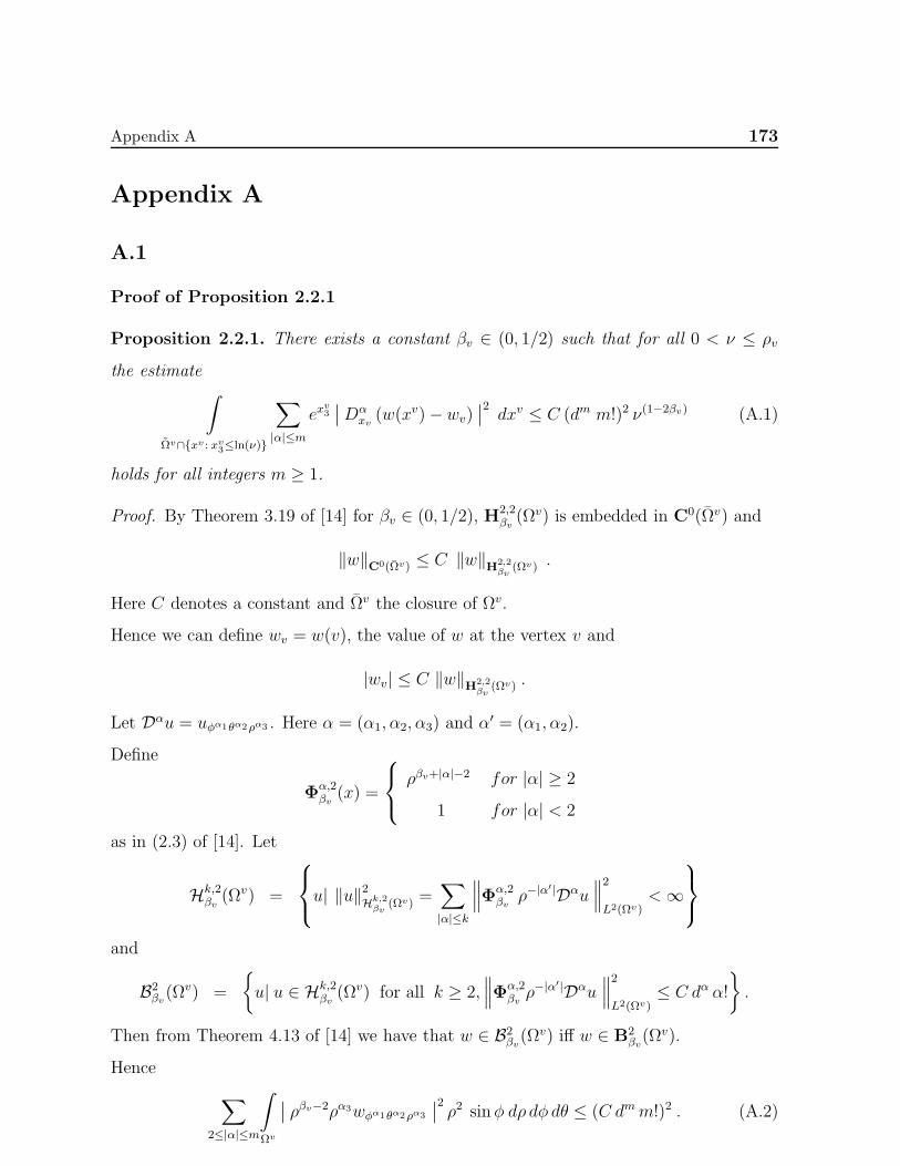
Appendix A 173
Appendix A
A.1
Proof of Proposition 2.2.1
Proposition 2.2.1. There exists a constant βv ∈ (0, 1/2) such that for all 0 < ν ≤ ρv
the estimate∫
Ωv∩xv: xv3≤ln(ν)
∑
|α|≤mex
v3
∣∣Dαxv (w(x
v)− wv)∣∣2 dxv ≤ C (dm m!)2 ν(1−2βv) (A.1)
holds for all integers m ≥ 1.
Proof. By Theorem 3.19 of [14] for βv ∈ (0, 1/2), H2,2βv(Ωv) is embedded in C0(Ωv) and
‖w‖C0(Ωv) ≤ C ‖w‖
H2,2βv
(Ωv) .
Here C denotes a constant and Ωv the closure of Ωv.
Hence we can define wv = w(v), the value of w at the vertex v and
|wv| ≤ C ‖w‖H
2,2βv
(Ωv) .
Let Dαu = uφα1θα2ρα3 . Here α = (α1, α2, α3) and α′ = (α1, α2).
Define
Φα,2βv
(x) =
ρβv+|α|−2 for |α| ≥ 2
1 for |α| < 2
as in (2.3) of [14]. Let
Hk,2βv(Ωv) =
u| ‖u‖
2Hk,2
βv(Ωv)
=∑
|α|≤k
∥∥∥Φα,2βvρ−|α′|Dαu
∥∥∥2
L2(Ωv)<∞
and
B2βv(Ω
v) =
u| u ∈ Hk,2
βv(Ωv) for all k ≥ 2,
∥∥∥Φα,2βvρ−|α′|Dαu
∥∥∥2
L2(Ωv)≤ C dα α!
.
Then from Theorem 4.13 of [14] we have that w ∈ B2βv(Ωv) iff w ∈ B2
βv(Ωv).
Hence
∑
2≤|α|≤m
∫
Ωv
∣∣ ρβv−2ρα3wφα1θα2ρα3
∣∣2 ρ2 sinφ dρ dφ dθ ≤ (C dmm!)2 . (A.2)
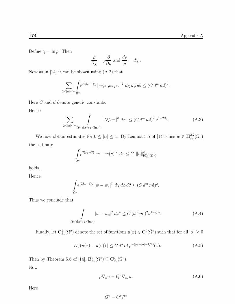
174 Appendix A
Define χ = ln ρ. Then
∂
∂χ= ρ
∂
∂ρand
dρ
ρ= dχ .
Now as in [14] it can be shown using (A.2) that
∑
2≤|α|≤m
∫
Ωv
e(2βv−1)χ | wφα1θα2χα3 |2 dχ dφ dθ ≤ (C dmm!)2.
Here C and d denote generic constants.
Hence∑
2≤|α|≤m
∫
Ωv∩xv: χ≤ln ν
|Dαxvw |2 dxv ≤ (C dmm!)2 ν1−2βv . (A.3)
We now obtain estimates for 0 ≤ |α| ≤ 1. By Lemma 5.5 of [14] since w ∈ H2,2βv(Ωv)
the estimate ∫
Ωv
ρ2(βv−2) |w − w(v)|2 dx ≤ C ‖u‖2H
2,2βv
(Ωv)
holds.
Hence ∫
Ωv
e(2βv−1)χ |w − wv|2 dχ dφ dθ ≤ (C dmm!)2.
Thus we conclude that
∫
Ωv∩xv: χ≤ln ν
|w − wv|2 dxv ≤ C (dmm!)2ν1−2βv . (A.4)
Finally, let C2βv(Ωv) denote the set of functions u(x) ∈ C0(Ωv) such that for all |α| ≥ 0
|Dαx (u(x)− u(v)) | ≤ C dα α! ρ−(βv+|α|−1/2)(x). (A.5)
Then by Theorem 5.6 of [14], B2βv(Ω
v) ⊆ C2βv(Ω
v).
Now
ρ∇xu = Qv∇xvu. (A.6)
Here
Qv = OvP v
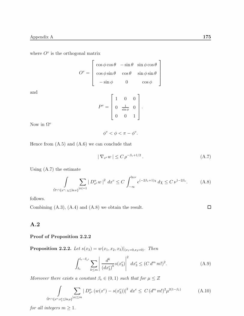
Appendix A 175
where Ov is the orthogonal matrix
Ov =
cosφ cos θ − sin θ sin φ cos θ
cosφ sin θ cos θ sinφ sin θ
− sinφ 0 cosφ
and
P v =
1 0 0
0 1sinφ
0
0 0 1
.
Now in Ωv
φv < φ < π − φv.
Hence from (A.5) and (A.6) we can conclude that
| ∇xvw | ≤ C ρ−βv+1/2 . (A.7)
Using (A.7) the estimate
∫
Ωv∩xv : χ≤ln ν
∑
|α|=1
|Dαxvw |2 dxv ≤ C
∫ ln ν
−∞e(−2βv+1)χ dχ ≤ C ν1−2βv . (A.8)
follows.
Combining (A.3), (A.4) and (A.8) we obtain the result.
A.2
Proof of Proposition 2.2.2
Proposition 2.2.2. Let s(x3) = w(x1, x2, x3)|(x1=0,x2=0). Then
∫ le−δv′
δv
∑
k≤m
∣∣∣∣∣dk
(dxe3)ks(xe3)
∣∣∣∣∣
2
dxe3 ≤ (C dmm!)2. (A.9)
Moreover there exists a constant βe ∈ (0, 1) such that for µ ≤ Z
∫
Ωe∩xe:xe1≤lnµ
∑
|α|≤m|Dα
xe (w(xe)− s(xe3))|2 dxe ≤ C (dmm!)2µ2(1−βe) (A.10)
for all integers m ≥ 1.
176 Appendix A
Proof. We denote by C2βe(Ωe), βe ∈ (0, 1), the set of functions u ∈ C0(Ωe) such that for
|α| ≥ 0∥∥ rβe+α1+α2−1Dα
x (u(x)− u(0, 0, x3))∥∥C0(Ωe)
≤ C dα α! (A.11)
and for k ≥ 0 ∥∥∥∥dk
(dx3)ku(0, 0, x3)
∥∥∥∥C0(Ωe∩x: x1=x2=0)
≤ C dk k! (A.12)
as in (5.1) and (5.2) of [14]. Here Ωe denotes the closure of Ωe.
Then by Theorem 5.3 of [14], B2βe(Ωe) ⊆ C2
βe(Ωe).
Now
xe1 = τ = ln r
xe2 = θ
xe3 = x3 .
Define s(x3) = w(x1, x2, x3)|(x1=0,x2=0). Then (A.9) follows immediately from (A.12) since
w ∈ B2βe(Ωe) and hence w ∈ C2
βe(Ωe).
Let
p(x) = w(x)− s(x3) .
Then by (A.11) we have that
∥∥ rβe+α1+α2−1Dαxp(x)
∥∥C0(Ωe)
≤ C dα α! (A.13)
Now we can show just as in Theorem 4.1 of [14] that
∥∥rβe−1 Dαxep(x
e)∥∥C0(Ωe)
≤ C dα α! (A.14)
using the estimate (A.13).
Hence
|Dαxep(x
e) | ≤ C dα α! e(1−βe)xe1
for xe ∈ Ωe.
Using the above we conclude that∫
Ωe∩xe:xe1≤lnµ
∑
|α|≤m|Dα
xep(xe) |2 dxe ≤ C (dmm!)2
∫ lnµ
−∞e2(1−βe)τ dτ
and this gives the required estimate (A.10).

Appendix A 177
A.3
Proof of Proposition 2.2.3
Proposition 2.2.3. Let wv = w(v), the value of w evaluated at the vertex v, and s(x3) =
w(x1, x2, x3)|(x1=0,x2=0). Then there exists a constant βv ∈ (0, 1/2) such that for any
0 < ν ≤ δv∫
−∞
ln ν
exv−e3
∑
k≤m
∣∣∣Dkxv−e3
(s(xv−e3 )− wv)∣∣∣2
dxv−e3 ≤ C (dmm!)2 ν(1−2βv) . (A.15)
Moreover there exists a constant βe ∈ (0, 1) such that for any 0 < α ≤ tanφv and
0 < ν ≤ δv∫
Ωv−e∩xv−e:xv−e1 <lnα, xv−e
3 <ln ν
exv−e3
∑
|γ|≤m
∣∣Dγxv−e
(w(xv−e3 )− s(xv−e3 )
) ∣∣2 dxv−e3
≤ C (dmm!)2 α2(1−βe) ν(1−2βv) (A.16)
for all integers m ≥ 1.
Proof. By C2βv−e
(Ωv−e), where βv−e = (βv, βe), βv ∈ (0, 1/2) and βe ∈ (0, 1) we denote
the set of functions u(x) ∈ C0(Ωv−e) such that
∥∥ ρβv+|α|−1/2 (sin φ)βe+α1+α2−1 Dαx (u(x)− u(0, 0, x3))
∥∥C0(Ωv−e)
≤ C dα α! (A.17)
and∣∣∣∣ |x3|βv+k−1/2 d
k
dxk3(u(0, 0, x3)− u(v))
∣∣∣∣C0(Ωv−e∩x: x1=x2=0)
≤ C dk k! (A.18)
as described in (5.26) and (5.27) of [14]. Here Ωv−e denotes the closure of Ωv−e.
Now by Theorem 5.9 of [14], B2βv−e
(Ωv−e) ⊆ C2βv−e
(Ωv−e). Since w ∈ B2βv−e
(Ωv−e) we
conclude that w ∈ C2βv−e
(Ωv−e). Let s(x3) = w(0, 0, x3) and wv = w(v). Then
∣∣∣∣ |x3|βv+k−1/2 dk
dxk3(s(x3)− wv)
∣∣∣∣ ≤ C dk k!.
Now xv−e3 = ln x3. Hence it can be shown as before that
∫ ln ν
−∞
∑
k≤m
∣∣∣Dkxv−e3
(s(xv−e3 )− wv
) ∣∣∣2
dxv−e3 ≤ C (dmm!)2 ν(1−2βv).
178 Appendix A
Let p(x) = w(x)− s(x3). Then by (A.17) we have that
∥∥ ρβv+|α|−1/2(sinφ)βe+α1+α2−1 Dαxp(x)
∥∥C0(Ωv−e)
≤ C dα α! .
It can be shown as in Theorem 4.8 of [14] that
∥∥ (ρβv−1/2(sinφ)βe−1)ρα3(sinφ)α1 pφα1θα2ρα3
∥∥C0(Ωv−e)
≤ C dα α! .
Here Ωv−e is the image of Ωv−e in (φ, θ, ρ) coordinates.
From the above the estimate
∥∥ e(βv−1/2)χ (sinφ)βe−1 (sinφ)α1 pφα1θα2χα3
∥∥C0(Ωv−e)
≤ C dα α! (A.19)
follows. Here Ωv−e is the image of Ωv−e in xv coordinates, xv = (φ, θ, χ) and χ = ln ρ.
Now the vertex-edge coordinates are defined as
xv−e1 = ψ = ln(tanφ)
xv−e2 = θ
xv−e3 = ζ = ln(x3) = χ+ ln(cosφ).
Thus
∇xvu = Jv−e∇xv−eu
where
Jv−e =
sec2 φ cotφ 0 − tanφ
0 1 0
0 0 1
.
Hence
∇xv−eu = (Jv−e)−1∇xvu.
Here
(Jv−e)−1 =
cosφ sinφ 0 sin2 φ
0 1 0
0 0 1
.
Hence
∂u
∂ψ= cos φ sinφ
∂u
∂φ+ sin2 φ
∂u
∂χ,
∂u
∂ζ=∂u
∂χ.
Appendix A 179
From the above we obtain
∂mu
∂ψm=
m∑
k=1
∑
α1+α2=k
(∑
j1+j2=2m−α1
amα1,α2,j1,j2(cosφ)j1 (sinφ)j2 ((sin φ)α1)uφα1χα2
)(A.20)
It can be shown that the coefficients amα1,α2,j1,j2satisfy the recurrence relation
am+1α1,α2,j1,j2
= amα1−1,α2,j1−1,j2 + (α1 + j2)amα1,α2,j1−2,j2 (A.21)
− j1amα1,α2,j1,j2−2 + amα1,α2−1,j1,j2−2 (A.22)
for |α| ≤ m.
For |α| = m+ 1
am+1α1,α2,j1,j2
=
1 if j1 = α1, j2 = 2m+ 2− α1
0 otherwise .
Since 0 ≤ φ ≤ φv, where φv < π/2, we can conclude from (A.19) that
∥∥ e(βv−1/2)ζ e(βe−1)ψ (sinφ)α1 pφα1θα2χα3
∥∥C0
(Ωv−e)
≤ C dα α! . (A.23)
Here Ωv−e denotes the image of Ωv−e in xv−e coordinates. From (A.23) the estimate
∥∥∥ e(βv−1/2)xv−e3 e(βe−1)xv−e
1 Dαxv−e p
∥∥∥C0
(Ωv−e)
≤ C dα α! . (A.24)
follows.
As in [14] we show (A.24) for the cases α = (m, 0, 0), α = (0, m, 0) and α = (0, 0, m)
since the general case can be shown in the same way. It is enough to prove (A.24) for
α = (m, 0, 0) since the other two cases are trivial.
Let
Amk =∑
α1+α2=k
∑
j1+j2=2m−α1
∣∣amα1,α2,j1,j2
∣∣ . (A.25)
Then
Amm ≤ 4m. (A.26)
Moreover for k < m
Amk ≤ 4mm!
k!. (A.27)
180 Appendix A
The proof is by induction. Using the recurrence relation (A.21) we obtain
Am+1k ≤ 2mAmk + 2Amk−1
≤ 2m
(4mm!
k!
)+ 2
(4mm!
(k − 1)!
)
≤ 4m+1 (m+ 1)!
k!
(2m
4(m+ 1)+
2k
4(m+ 1)
)
≤ 4m+1
k!(m+ 1)! (A.28)
Now using (A.19), (A.20) and (A.28) it can be shown that
∥∥∥∥ e(βv−1/2)xv−e
3 e(βe−1)xv−e1
∂mp
∂ψm
∥∥∥∥C0(Ωv−e)
≤m∑
k=1
∑
α1+α2=k
∑
j1+j2=2m−α1
∣∣amα1,α2,j1,j2
∣∣ C dα1+α2 α1!α2!
≤m∑
k=1
Amk (C dk k!)
≤ C dmm!
Here C and d denote generic constants.
The inequality (A.24) is obtained in the same way. Now the estimate (A.16) follows
immediately from (A.24).
A.4
Proof of Proposition 2.2.4
Proposition 2.2.4. The estimate
∫
Ωr
∑
|α|≤m|Dα
xw(x) |2 ≤ C (dmm!)2 (A.29)
holds for all integers m ≥ 1.
Proof. Now w(x) is analytic in an open neighbourhood of Ωr. Hence (A.29) follows.
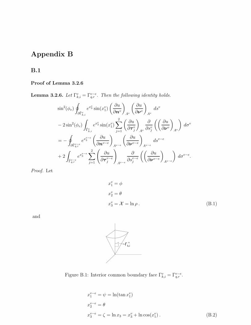
Appendix B
B.1
Proof of Lemma 3.2.6
Lemma 3.2.6. Let Γvk,i = Γv−eq,r . Then the following identity holds.
sin2(φv)
∮
∂Γvk,i
exv3 sin(xv1)
(∂u
∂nv
)
Av
(∂u
∂νv
)
Av
dsv
− 2 sin2(φv)
∫
Γvk,i
exv3 sin(xv1)
2∑
j=1
(∂u
∂τ vj
)
Av
∂
∂svj
((∂u
∂νv
)
Av
)dσv
= −∮
∂Γv−eq,r
exv−e3
(∂u
∂nv−e
)
Av−e
(∂u
∂νv−e
)
Av−e
dsv−e
+ 2
∫
Γv−eq,r
exv−e3
2∑
j=1
(∂u
∂τ v−ej
)
Av−e
∂
∂sv−ej
((∂u
∂νv−e
)
Av−e
)dσv−e.
Proof. Let
xv1 = φ
xv2 = θ
xv3 = X = ln ρ . (B.1)
and
vΓk,i
Figure B.1: Interior common boundary face Γvk,i = Γv−eq,r .
xv−e1 = ψ = ln(tanxv1)
xv−e2 = θ
xv−e3 = ζ = ln x3 = xv3 + ln cos(xv1) . (B.2)
182 Appendix B
Clearly
∇xvu = Jv−e∇xv−eu (B.3)
where
Jv−e =
sec2 φ cotφ 0 − tanφ
0 1 0
0 0 1
. (B.4)
Now if dxv is a tangent vector to a curve in xv coordinates then its image in xv−e coor-
dinates is given by dxv−e where
dxv−e = (Jv−e)Tdxv. (B.5)
Clearly the first fundamental form (dsv)2 in xv coordinates is
(dsv)2 = (dxv)T (dxv) = (dxv−e)T (Jv−e)−1(Jv−e)−Tdxv−e. (B.6)
Now
(Jv−e)−1 =
cosφ sinφ 0 sin2 φ
0 1 0
0 0 1
.
Hence
(dsv)2 = sin2 φ(dxv−e1 )2 + (dxv−e2 )2 + (dxv−e3 )2 + 2 sin2 φdxv−e1 dxv−e3
= sin2 φdψ2 + dθ2 + dζ2 + 2 sin2 φ dψ dζ. (B.7)
Moreover, on Γvk,i,
dσv = dθdζ (B.8)
since by (B.7)
(dsv)2 = dθ2 + dζ2
on Γvk,i. Choose τ v−e1 = (0, 1, 0)T and τ v−e2 = −(0, 0, 1)T . These are orthogonal unit
vectors on Γv−eq,r since
(dsv−e)2 = dψ2 + dθ2 + dζ2. (B.9)
Appendix B 183
Define
τ v1 = (Jv−e)−Tτ v−e1 (B.10)
τ v2 = −(Jv−e)−Tτ v−e2 . (B.11)
Let νv−e = −(1, 0, 0)T denote the unit normal vector on Γv−eq,r and
mv−e = (sec2 φ cotφ, 0,− tanφ)T . (B.12)
Then
νv = (1, 0, 0)T = (Jv−e)−Tmv−e (B.13)
is the unit normal to ∂Γvk,i. Finally let dsv−e = (0, dθ, dζ)T denote a tangent vector field
on Γv−eq,r . Define
dsv−e =√dθ2 + dζ2 (B.14)
dsv = (Jv−e)−Tdsv−e = (0, dθ, dX )T (B.15)
and
dsv =√dθ2 + dX 2. (B.16)
Let
nv−e = (0, dζ,−dθ)T/√dζ2 + dθ2 (B.17)
be the unit outward normal to ∂Γv−eq,r . Then
nv = (Jv−e)−Tnv−e (B.18)
is the unit outward normal to ∂Γvk,i.
Now(∂u
∂nv
)
Av
= (nv)T (Av)∇xvu
= (nv−e)T (Jv−e)−1(Av)∇xvu
=(nv−e)T
sin2 φ
((Jv−e)−1(Jv−e)−T
)(sin2 φ(Jv−e)TAvJv−e)∇xv−eu
=(nv−e)T
sin2 φ
sin2 φ 0 sin2 φ
0 1 0
sin2 φ 0 1
A
v−e∇xv−eu
=(−dθ sin2 φ, dζ,−dθ)Tsin2 φ
√dζ2 + dθ2
Av−e∇xv−eu.
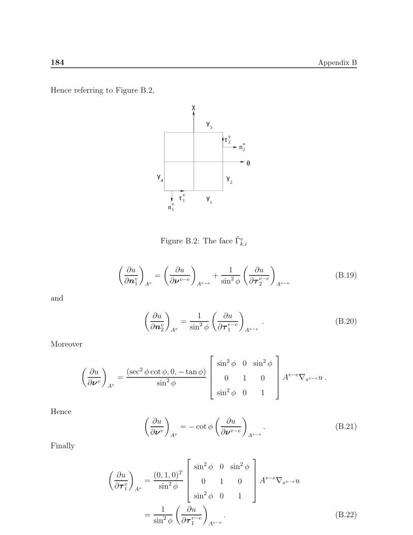
184 Appendix B
Hence referring to Figure B.2,
1τ
τ
γ4
γ
γ
γ
θ
χ
n
n
3
2
1
2
2
v
v
v
v
1
Figure B.2: The face Γvk,i
(∂u
∂nv1
)
Av
=
(∂u
∂νv−e
)
Av−e
+1
sin2 φ
(∂u
∂τ v−e2
)
Av−e
(B.19)
and
(∂u
∂nv2
)
Av
=1
sin2 φ
(∂u
∂τ v−e1
)
Av−e
. (B.20)
Moreover
(∂u
∂νv
)
Av
=(sec2 φ cotφ, 0,− tanφ)
sin2 φ
sin2 φ 0 sin2 φ
0 1 0
sin2 φ 0 1
A
v−e∇xv−eu .
Hence (∂u
∂νv
)
Av
= − cotφ
(∂u
∂νv−e
)
Av−e
. (B.21)
Finally
(∂u
∂τ v1
)
Av
=(0, 1, 0)T
sin2 φ
sin2 φ 0 sin2 φ
0 1 0
sin2 φ 0 1
A
v−e∇xv−eu
=1
sin2 φ
(∂u
∂τ v−e1
)
Av−e
. (B.22)
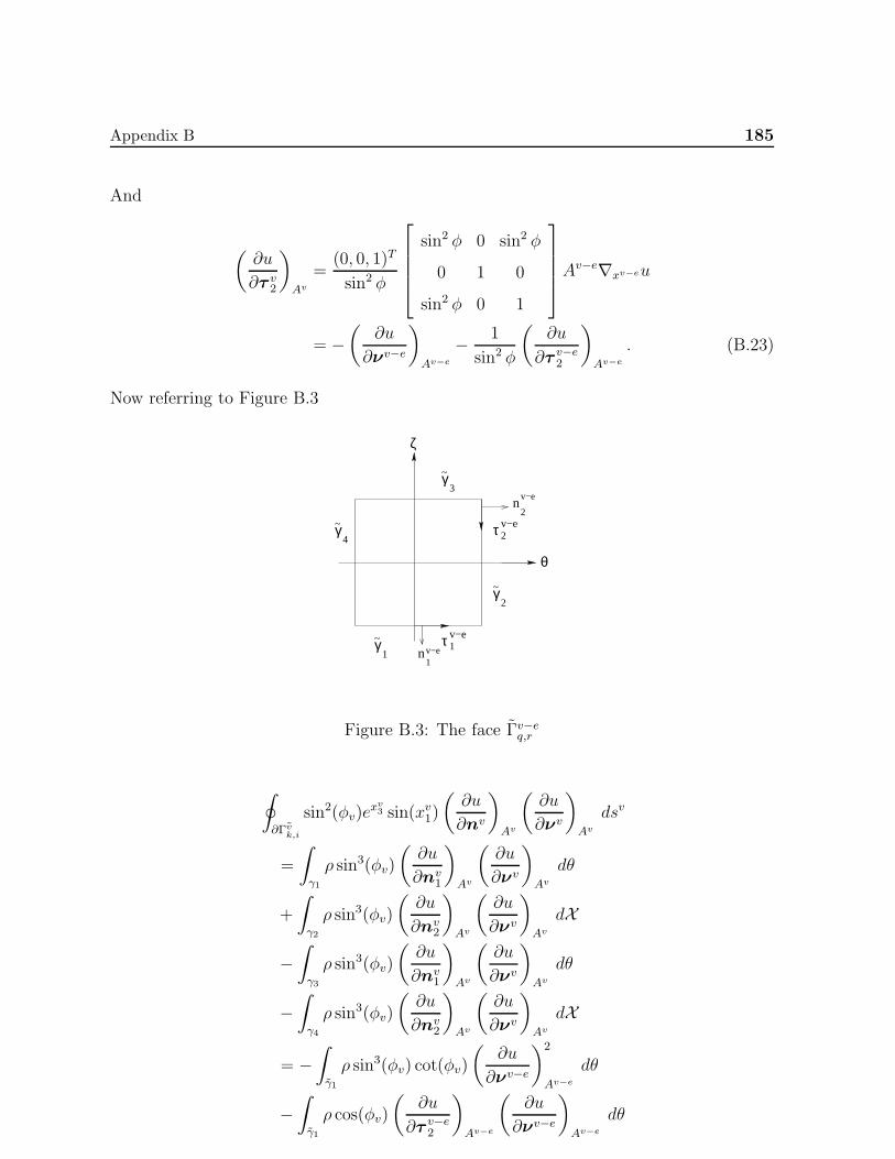
Appendix B 185
And
(∂u
∂τ v2
)
Av
=(0, 0, 1)T
sin2 φ
sin2 φ 0 sin2 φ
0 1 0
sin2 φ 0 1
A
v−e∇xv−eu
= −(
∂u
∂νv−e
)
Av−e
− 1
sin2 φ
(∂u
∂τ v−e2
)
Av−e
. (B.23)
Now referring to Figure B.3
v−eτγ1
1~
γ4
~
γ~2
γ3
~
τ 2v−e
ζ
θ
v−e1
n
n2
v−e
Figure B.3: The face Γv−eq,r
∮
∂ ˜Γvk,i
sin2(φv)exv3 sin(xv1)
(∂u
∂nv
)
Av
(∂u
∂νv
)
Av
dsv
=
∫
γ1
ρ sin3(φv)
(∂u
∂nv1
)
Av
(∂u
∂νv
)
Av
dθ
+
∫
γ2
ρ sin3(φv)
(∂u
∂nv2
)
Av
(∂u
∂νv
)
Av
dX
−∫
γ3
ρ sin3(φv)
(∂u
∂nv1
)
Av
(∂u
∂νv
)
Av
dθ
−∫
γ4
ρ sin3(φv)
(∂u
∂nv2
)
Av
(∂u
∂νv
)
Av
dX
= −∫
γ1
ρ sin3(φv) cot(φv)
(∂u
∂νv−e
)2
Av−e
dθ
−∫
γ1
ρ cos(φv)
(∂u
∂τ v−e2
)
Av−e
(∂u
∂νv−e
)
Av−e
dθ
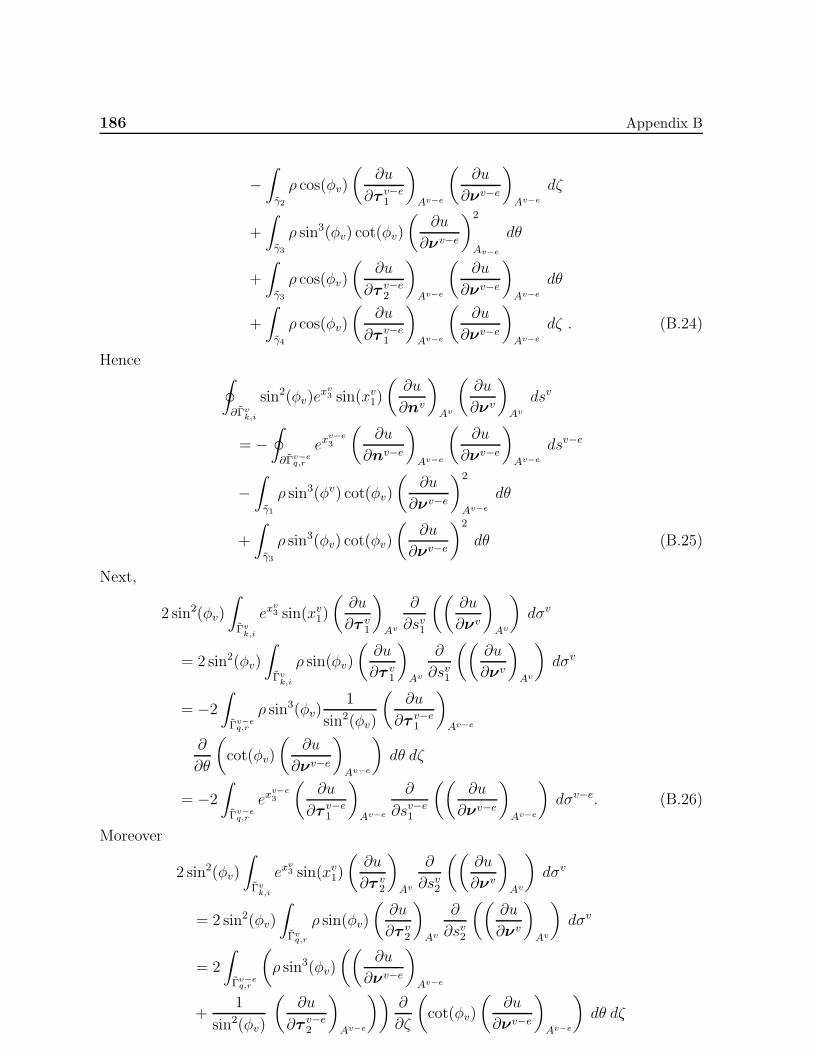
186 Appendix B
−∫
γ2
ρ cos(φv)
(∂u
∂τ v−e1
)
Av−e
(∂u
∂νv−e
)
Av−e
dζ
+
∫
γ3
ρ sin3(φv) cot(φv)
(∂u
∂νv−e
)2
Av−e
dθ
+
∫
γ3
ρ cos(φv)
(∂u
∂τ v−e2
)
Av−e
(∂u
∂νv−e
)
Av−e
dθ
+
∫
γ4
ρ cos(φv)
(∂u
∂τ v−e1
)
Av−e
(∂u
∂νv−e
)
Av−e
dζ . (B.24)
Hence∮
∂Γvk,i
sin2(φv)exv3 sin(xv1)
(∂u
∂nv
)
Av
(∂u
∂νv
)
Av
dsv
= −∮
∂Γv−eq,r
exv−e3
(∂u
∂nv−e
)
Av−e
(∂u
∂νv−e
)
Av−e
dsv−e
−∫
γ1
ρ sin3(φv) cot(φv)
(∂u
∂νv−e
)2
Av−e
dθ
+
∫
γ3
ρ sin3(φv) cot(φv)
(∂u
∂νv−e
)2
dθ (B.25)
Next,
2 sin2(φv)
∫
Γvk,i
exv3 sin(xv1)
(∂u
∂τ v1
)
Av
∂
∂sv1
((∂u
∂νv
)
Av
)dσv
= 2 sin2(φv)
∫
Γvk,i
ρ sin(φv)
(∂u
∂τ v1
)
Av
∂
∂sv1
((∂u
∂νv
)
Av
)dσv
= −2∫
Γv−eq,r
ρ sin3(φv)1
sin2(φv)
(∂u
∂τ v−e1
)
Av−e
∂
∂θ
(cot(φv)
(∂u
∂νv−e
)
Av−e
)dθ dζ
= −2∫
Γv−eq,r
exv−e3
(∂u
∂τ v−e1
)
Av−e
∂
∂sv−e1
((∂u
∂νv−e
)
Av−e
)dσv−e. (B.26)
Moreover
2 sin2(φv)
∫
Γvk,i
exv3 sin(xv1)
(∂u
∂τ v2
)
Av
∂
∂sv2
((∂u
∂νv
)
Av
)dσv
= 2 sin2(φv)
∫
Γvq,r
ρ sin(φv)
(∂u
∂τ v2
)
Av
∂
∂sv2
((∂u
∂νv
)
Av
)dσv
= 2
∫
Γv−eq,r
(ρ sin3(φv)
((∂u
∂νv−e
)
Av−e
+1
sin2(φv)
(∂u
∂τ v−e2
)
Av−e
))∂
∂ζ
(cot(φv)
(∂u
∂νv−e
)
Av−e
)dθ dζ
Appendix B 187
=
∫
Γv−eq,r
ρ sin3(φv) cot(φv)∂
∂ζ
(∂u
∂νv−e
)2
Av−e
dθ dζ
+ 2
∫
Γv−eq,r
eζ(
∂u
∂τ v−e2
)
Av−e
∂
∂ζ
(∂u
∂νv−e
)
Av−e
dθdζ
= −∫
γ1
ρ sin3(φv) cot(φv)
(∂u
∂νv−e
)2
Av−e
dθ
+
∫
γ3
ρ sin3(φv) cot(φv)
(∂u
∂νv−e
)2
Av−e
dθ
− 2
∫
Γv−eq,r
ex3v−e
(∂u
∂τ v−e2
)
Av−e
∂
∂sv−e2
(∂u
∂νv−e
)
Av−e
dσv−e . (B.27)
Combining (B.24)-(B.27) we obtain the result.
B.2
Proof of Lemma 3.2.8
Lemma 3.2.8. Let Γeu,k = Γv−en,l . Then∮
∂Γv−en,l
exv−e3
(∂u
∂nv−e
)
Av−e
(∂u
∂νv−e
)
Av−e
wv−e(xv−e1 ) dsv−e
− 2
2∑
j=1
∫
Γv−en,l
exv−e3
(∂u
∂τ v−ej
)
Av−e
∂
∂sv−ej
((∂u
∂νv−e
)
Av−e
)wv−e(xv−e1 ) dσv−e
= −∮
∂Γeu,k
(∂u
∂ne
)
Ae
(∂u
∂νe
)
Ae
we(xe1) dse
+ 2
2∑
j=1
∫
Γeu,k
(∂u
∂τ ej
)
Ae
∂
∂sej
((∂u
∂νe
)
Ae
)we(xe1) dσ
e.
Proof. We have
xe1 = τ = ln r
xe2 = θ
xe3 = x3 . (B.28)
and
xv−e1 = ψ = ln tanφ
xv−e2 = θ
xv−e3 = ζ = ln x3 . (B.29)
188 Appendix B
Γn,lv−e
Figure B.4: Interior common boundary face Γeu,k = Γv−en,l
Hence
xe1 = xv−e1 + xv−e3 = ψ + ζ
xe2 = xv−e2
xe3 = exv−e3 = eζ . (B.30)
Clearly
∇xv−eu = Je∇xeu . (B.31)
Here
Je =
1 0 0
0 1 0
1 0 x3
. (B.32)
Now if dxv−e is a tangent vector to a curve in xv−e coordinates then its image in xe
coordinates is given by dxe where
dxe = (Je)Tdxv−e. (B.33)
Clearly the first fundamental form (dsv−e)2 in xv−e coordinates is
(dsv−e)2 = (dxv−e)T (dxv−e) = (dxe)T ((Je)−1(Je)−T )dxv−e. (B.34)
Now
(Je)−1 =
1 0 0
0 1 0
− 1x3
0 1x3
. (B.35)
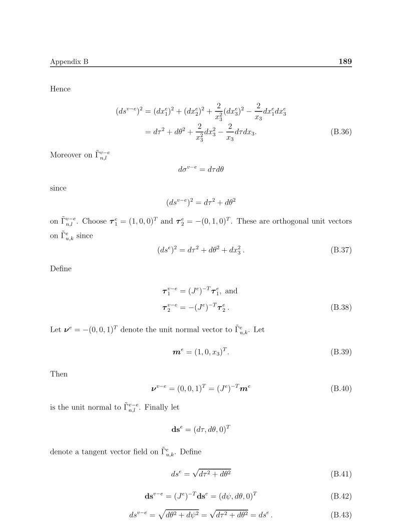
Appendix B 189
Hence
(dsv−e)2 = (dxe1)2 + (dxe2)
2 +2
x23(dxe3)
2 − 2
x3dxe1dx
e3
= dτ 2 + dθ2 +2
x23dx23 −
2
x3dτdx3. (B.36)
Moreover on Γv−en,l
dσv−e = dτdθ
since
(dsv−e)2 = dτ 2 + dθ2
on Γv−en,l . Choose τ e1 = (1, 0, 0)T and τ e2 = −(0, 1, 0)T . These are orthogonal unit vectors
on Γeu,k since
(dse)2 = dτ 2 + dθ2 + dx23 . (B.37)
Define
τ v−e1 = (Je)−Tτ e1, and
τ v−e2 = −(Je)−Tτ e2 . (B.38)
Let νe = −(0, 0, 1)T denote the unit normal vector to Γeu,k. Let
me = (1, 0, x3)T . (B.39)
Then
νv−e = (0, 0, 1)T = (Je)−Tme (B.40)
is the unit normal to Γv−en,l . Finally let
dse = (dτ, dθ, 0)T
denote a tangent vector field on Γeu,k. Define
dse =√dτ 2 + dθ2 (B.41)
dsv−e = (Je)−Tdse = (dψ, dθ, 0)T (B.42)
dsv−e =√dθ2 + dψ2 =
√dτ 2 + dθ2 = dse . (B.43)
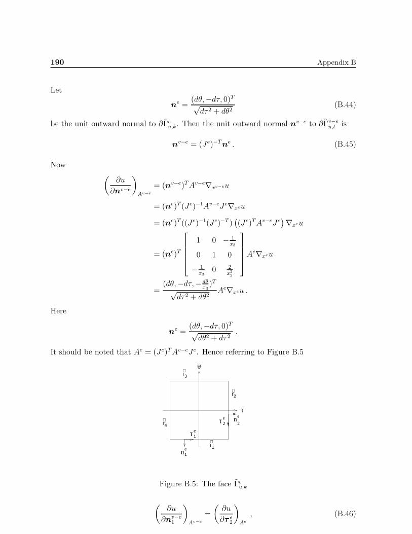
190 Appendix B
Let
ne =(dθ,−dτ, 0)T√dτ 2 + dθ2
(B.44)
be the unit outward normal to ∂Γeu,k. Then the unit outward normal nv−e to ∂Γv−en,l is
nv−e = (Je)−Tne . (B.45)
Now(
∂u
∂nv−e
)
Av−e
= (nv−e)TAv−e∇xv−eu
= (ne)T (Je)−1Av−eJe∇xeu
= (ne)T ((Je)−1(Je)−T )((Je)TAv−eJe
)∇xeu
= (ne)T
1 0 − 1x3
0 1 0
− 1x3
0 2x23
A
e∇xeu
=(dθ,−dτ,− dθ
x3)T
√dτ 2 + dθ2
Ae∇xeu .
Here
ne =(dθ,−dτ, 0)T√dθ2 + dτ 2
.
It should be noted that Ae = (Je)TAv−eJe. Hence referring to Figure B.5
Γ
Γ
Γ
Γ∼
∼
∼
∼
3
4
1
2
θ
τ
τ 1e
τ 2e en
2
n1e
Figure B.5: The face Γeu,k
(∂u
∂nv−e1
)
Av−e
=
(∂u
∂τ e2
)
Ae
, (B.46)
Appendix B 191
and(
∂u
∂nv−e2
)
Av−e
=
(∂u
∂τ e1
)
Ae
+1
x3
(∂u
∂νe
)
Ae
. (B.47)
Moreover
(∂u
∂νv−e
)
Av−e
=[1 0 x3
]
1 0 − 1x3
0 1 0
− 1x3
0 2x23
A
e∇xeu
=
[0, 0,
1
x3
]Ae∇xeu
= − 1
x3
(∂u
∂νe
)
Ae
. (B.48)
Now
Γ
Γ
Γ
Γ3
4
1
2
θ
ψ
τ
n1v−e
v−e1
v−eτ 2
2nv−e
Figure B.6: The face Γv−en,l
∮
∂Γv−en,l
exv−e3
(∂u
∂nv−e
)
Av−e
(∂u
∂νv−e
)
Av−e
dsv−e
=
∫
Γ1
x3
(∂u
∂nv−e1
)
Av−e
(∂u
∂νv−e
)
Av−e
dψ
+
∫
Γ2
x3
(∂u
∂nv−e2
)
Av−e
(∂u
∂νv−e
)
Av−e
dθ
−∫
Γ3
x3
(∂u
∂nv−e1
)
Av−e
(∂u
∂νv−e
)
Av−e
dψ
−∫
Γ4
x3
(∂u
∂nv−e2
)
Av−e
(∂u
∂νv−e
)
Av−e
dθ
= −∫
Γ1
(∂u
∂τ e2
)
Ae
(∂u
∂νe
)
Ae
dτ
192 Appendix B
−∫
Γ2
((∂u
∂τ e1
)
Ae
+1
x3
(∂u
∂νe
)
Ae
)(∂u
∂νe
)
Ae
dθ
+
∫
Γ3
(∂u
∂τ e2
)
Ae
(∂u
∂νe
)
Ae
dτ
+
∫
Γ4
((∂u
∂τ e1
)
Ae
+1
x3
(∂u
∂νe
)
Ae
)(∂u
∂νe
)
Ae
dθ
= −∮
∂Γeu,k
(∂u
∂ne
)
Ae
(∂u
∂νe
)
Ae
dse
−∫
Γ2
1
x3
(∂u
∂νe
)2
Ae
dθ +
∫
Γ4
1
x3
(∂u
∂νe
)2
Ae
dθ (B.49)
Now τ v−e1 = (1, 0, 0)T and τ e1 = (Je)−Tτ v−e1 . Moreover τ v−e2 = (0, 1, 0)T and τ e2 =
−(Je)Tτ v−e2 .
Hence
2
∫
Γv−en,l
exv−e3
(∂u
∂τ v−e1
)
Av−e
∂
∂sv−e1
((∂u
∂νv−e
)
Av−e
)dσv−e
= −2∫
Γeu,k
((∂u
∂τ e1
)
Ae
+1
x3
(∂u
∂νe
)
Ae
)∂
∂τ
((∂u
∂νe
)
Ae
)dτ dθ
= −2∫
Γeu,k
(∂u
∂τ e1
)
Ae
∂
∂se1
((∂u
∂νe
)
Ae
)dσe
−∫
Γ2
1
x3
(∂u
∂νe
)2
Ae
dθ +
∫
Γ4
1
x3
(∂u
∂νe
)2
Ae
dθ . (B.50)
And
2
∫
Γv−en,l
exv−e
3
(∂u
∂τ v−e2
)
Av−e
∂
∂sv−e2
((∂u
∂νv−e
)
Av−e
)dσv−e
= −2∫
Γeu,k
(∂u
∂τ e2
)
Ae
∂
∂θ
((∂u
∂νe
)
Ae
)dτ dθ
= −2∫
Γeu,k
(∂u
∂τ e2
)
Ae
∂
∂se2
((∂u
∂νe
)
Ae
)dσe . (B.51)
Combining (B.49), (B.50) and (B.51) we obtain the result.
B.3
Proof of Lemma 3.2.9
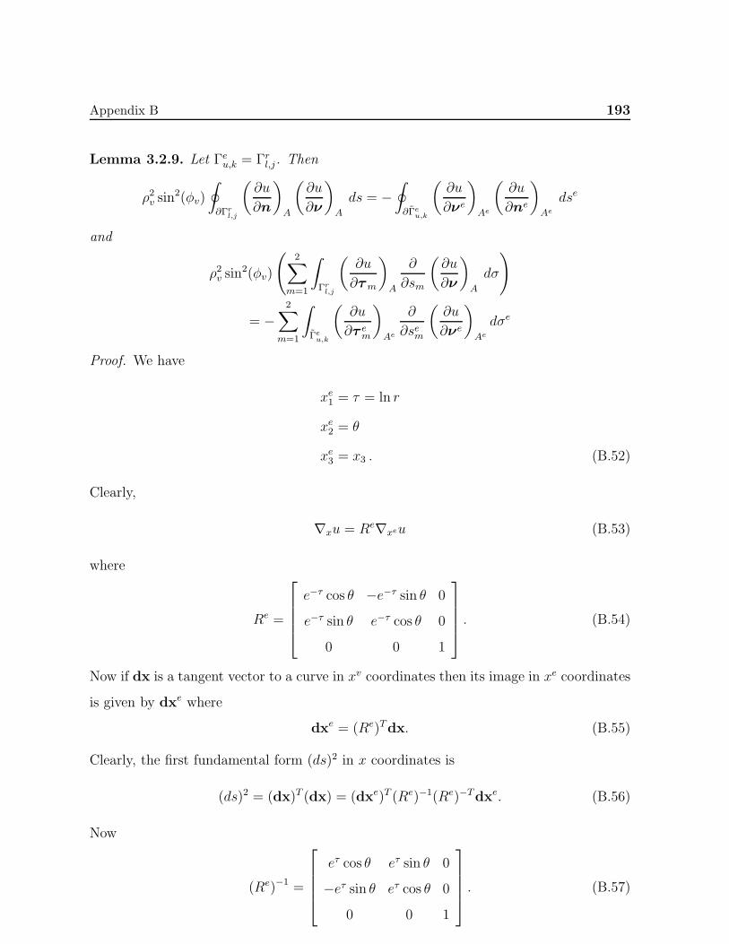
Appendix B 193
Lemma 3.2.9. Let Γeu,k = Γrl,j. Then
ρ2v sin2(φv)
∮
∂Γrl,j
(∂u
∂n
)
A
(∂u
∂ν
)
A
ds = −∮
∂Γeu,k
(∂u
∂νe
)
Ae
(∂u
∂ne
)
Ae
dse
and
ρ2v sin2(φv)
(2∑
m=1
∫
Γrl,j
(∂u
∂τm
)
A
∂
∂sm
(∂u
∂ν
)
A
dσ
)
= −2∑
m=1
∫
Γeu,k
(∂u
∂τ em
)
Ae
∂
∂sem
(∂u
∂νe
)
Ae
dσe
Proof. We have
xe1 = τ = ln r
xe2 = θ
xe3 = x3 . (B.52)
Clearly,
∇xu = Re∇xeu (B.53)
where
Re =
e−τ cos θ −e−τ sin θ 0
e−τ sin θ e−τ cos θ 0
0 0 1
. (B.54)
Now if dx is a tangent vector to a curve in xv coordinates then its image in xe coordinates
is given by dxe where
dxe = (Re)Tdx. (B.55)
Clearly, the first fundamental form (ds)2 in x coordinates is
(ds)2 = (dx)T (dx) = (dxe)T (Re)−1(Re)−Tdxe. (B.56)
Now
(Re)−1 =
eτ cos θ eτ sin θ 0
−eτ sin θ eτ cos θ 0
0 0 1
. (B.57)

194 Appendix B
Hence
(ds)2 = e2τ (dτ)2 + e2τ (dθ)2 + (dxe3)2 . (B.58)
Moreover on Γrl,j
dσ = eτdθdxe3 (B.59)
since
(ds)2 = e2τ (dθ)2 + (dxe3)2
on Γrl,j. Choose τ e1 = (0, 1, 0)T and τ e2 = (0, 0, 1)T . These are orthogonal unit tangent
vectors on Γeu,k since (ds)2 = e2τ (dτ)2 + e2τ (dθ)2 + (dxe3)2.
Define
τ 1 = e−τ (Re)−Tτ e1 ,
τ 2 = (Re)−Tτ e2 . (B.60)
Let νe = (1, 0, 0)T denotes the unit normal vector on Γeu,k. Then
ν = −e−τ (Re)−Tνe
denotes the unit normal to Γrl,j. Finally let
dse = (0, dθ, dxe3)
denotes a tangent vector field on Γeu,k. Define
dse =√(dθ)2 + (dxe3)
2 , (B.61)
ds = (Re)−Tdse (B.62)
and
ds =√e2τ (dθ)2 + (dxe3)
2 . (B.63)
Let
ne =(0,−dxe3, dθ)T√(dθ)2 + (dxe3)
2(B.64)
be the outward unit normal to ∂Γeu,k. Define
me =(0,−e−τdxe3, eτdθ)T√e2τ (dθ)2 + (dxe3)
2. (B.65)
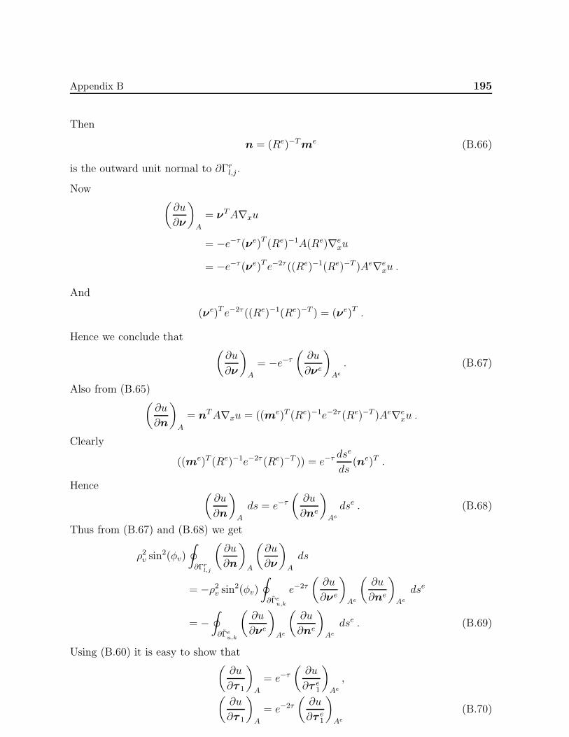
Appendix B 195
Then
n = (Re)−Tme (B.66)
is the outward unit normal to ∂Γrl,j .
Now(∂u
∂ν
)
A
= νTA∇xu
= −e−τ (νe)T (Re)−1A(Re)∇exu
= −e−τ (νe)T e−2τ ((Re)−1(Re)−T )Ae∇exu .
And
(νe)T e−2τ ((Re)−1(Re)−T ) = (νe)T .
Hence we conclude that(∂u
∂ν
)
A
= −e−τ(∂u
∂νe
)
Ae
. (B.67)
Also from (B.65)(∂u
∂n
)
A
= nTA∇xu = ((me)T (Re)−1e−2τ (Re)−T )Ae∇exu .
Clearly
((me)T (Re)−1e−2τ (Re)−T )) = e−τdse
ds(ne)T .
Hence (∂u
∂n
)
A
ds = e−τ(∂u
∂ne
)
Ae
dse . (B.68)
Thus from (B.67) and (B.68) we get
ρ2v sin2(φv)
∮
∂Γrl,j
(∂u
∂n
)
A
(∂u
∂ν
)
A
ds
= −ρ2v sin2(φv)
∮
∂Γeu,k
e−2τ
(∂u
∂νe
)
Ae
(∂u
∂ne
)
Ae
dse
= −∮
∂Γeu,k
(∂u
∂νe
)
Ae
(∂u
∂ne
)
Ae
dse . (B.69)
Using (B.60) it is easy to show that(∂u
∂τ 1
)
A
= e−τ(∂u
∂τ e1
)
Ae
,
(∂u
∂τ 1
)
A
= e−2τ
(∂u
∂τ e1
)
Ae
(B.70)
196 Appendix B
Moreover using (B.67) we get
∂
∂s1
((∂u
∂ν
)
A
)= e−2τ ∂
∂se1
((∂u
∂νe
)
Ae
),
∂
∂s2
((∂u
∂ν
)
A
)= e−τ
∂
∂se2
((∂u
∂νe
)
Ae
). (B.71)
Combining (B.69), (B.70) and (B.71) we obtain the result.
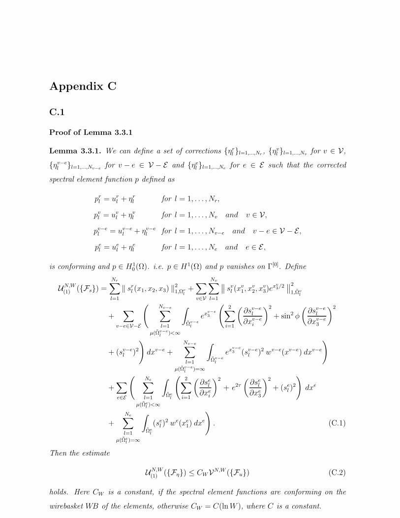
Appendix C
C.1
Proof of Lemma 3.3.1
Lemma 3.3.1. We can define a set of corrections ηrl l=1,...,Nr , ηvl l=1,...,Nv for v ∈ V,ηv−el l=1,...,Nv−e for v − e ∈ V − E and ηel l=1,...,Ne for e ∈ E such that the corrected
spectral element function p defined as
prl = url + ηrl for l = 1, . . . , Nr,
pvl = uvl + ηvl for l = 1, . . . , Nv and v ∈ V,
pv−el = uv−el + ηv−el for l = 1, . . . , Nv−e and v − e ∈ V − E ,
pel = uel + ηel for l = 1, . . . , Ne and e ∈ E ,
is conforming and p ∈ H10 (Ω). i.e. p ∈ H1(Ω) and p vanishes on Γ[0]. Define
UN,W(1) (Fs) =Nr∑
l=1
‖ srl (x1, x2, x3) ‖21,Ωrl+∑
v∈V
Nv∑
l=1
∥∥ svl (xv1, xv2, xv3)exv3/2∥∥21,Ωv
l
+∑
v−e∈V−E
(Nv−e∑
l=1
µ(Ωv−el )<∞
∫
Ωv−el
exv−e3
(2∑
i=1
(∂sv−el
∂xv−ei
)2
+ sin2 φ
(∂sv−el
∂xv−e3
)2
+ (sv−el )2
)dxv−e +
Nv−e∑
l=1
µ(Ωv−el )=∞
∫
Ωv−el
exv−e3 (sv−el )2 wv−e(xv−e) dxv−e
)
+∑
e∈E
(Ne∑
l=1
µ(Ωel )<∞
∫
Ωel
(2∑
i=1
(∂sel∂xei
)2
+ e2τ(∂sel∂xe3
)2
+ (sel )2
)dxe
+Ne∑
l=1
µ(Ωel )=∞
∫
Ωel
(sel )2 we(xe1) dx
e
). (C.1)
Then the estimate
UN,W(1) (Fη) ≤ CWVN,W (Fu) (C.2)
holds. Here CW is a constant, if the spectral element functions are conforming on the
wirebasket WB of the elements, otherwise CW = C(lnW ), where C is a constant.
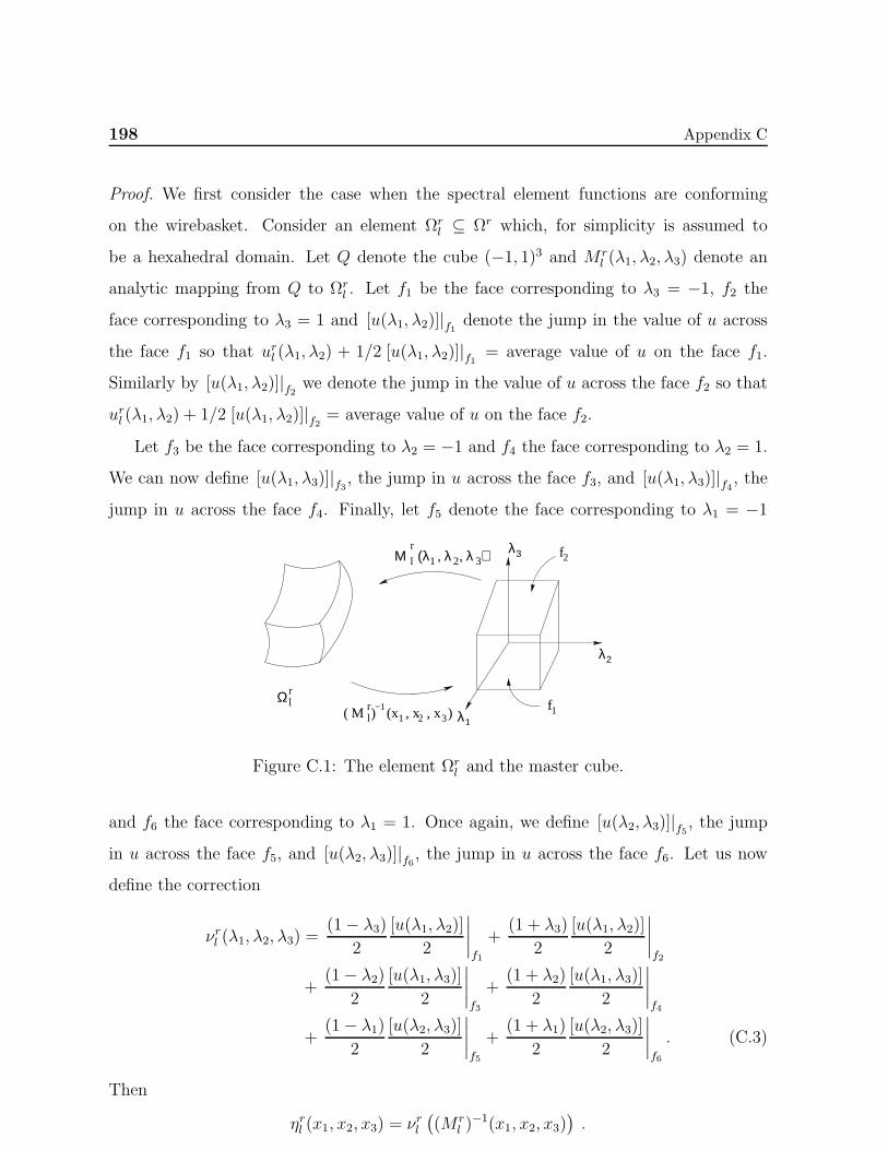
198 Appendix C
Proof. We first consider the case when the spectral element functions are conforming
on the wirebasket. Consider an element Ωrl ⊆ Ωr which, for simplicity is assumed to
be a hexahedral domain. Let Q denote the cube (−1, 1)3 and M rl (λ1, λ2, λ3) denote an
analytic mapping from Q to Ωrl . Let f1 be the face corresponding to λ3 = −1, f2 the
face corresponding to λ3 = 1 and [u(λ1, λ2)]|f1 denote the jump in the value of u across
the face f1 so that url (λ1, λ2) + 1/2 [u(λ1, λ2)]|f1 = average value of u on the face f1.
Similarly by [u(λ1, λ2)]|f2 we denote the jump in the value of u across the face f2 so that
url (λ1, λ2) + 1/2 [u(λ1, λ2)]|f2 = average value of u on the face f2.
Let f3 be the face corresponding to λ2 = −1 and f4 the face corresponding to λ2 = 1.
We can now define [u(λ1, λ3)]|f3 , the jump in u across the face f3, and [u(λ1, λ3)]|f4 , thejump in u across the face f4. Finally, let f5 denote the face corresponding to λ1 = −1
λ
λ
λ3
2
1
Ωrl
( M r)l−1
1 2
1 2Μ (λ , λ , λ )l
r
(x , x , x )3
3f
f
2
1
Figure C.1: The element Ωrl and the master cube.
and f6 the face corresponding to λ1 = 1. Once again, we define [u(λ2, λ3)]|f5 , the jump
in u across the face f5, and [u(λ2, λ3)]|f6 , the jump in u across the face f6. Let us now
define the correction
νrl (λ1, λ2, λ3) =(1− λ3)
2
[u(λ1, λ2)]
2
∣∣∣∣f1
+(1 + λ3)
2
[u(λ1, λ2)]
2
∣∣∣∣f2
+(1− λ2)
2
[u(λ1, λ3)]
2
∣∣∣∣f3
+(1 + λ2)
2
[u(λ1, λ3)]
2
∣∣∣∣f4
+(1− λ1)
2
[u(λ2, λ3)]
2
∣∣∣∣f5
+(1 + λ1)
2
[u(λ2, λ3)]
2
∣∣∣∣f6
. (C.3)
Then
ηrl (x1, x2, x3) = νrl((M r
l )−1(x1, x2, x3)
).
Appendix C 199
Next, we define the corrections in the vertex neighbourhood Ωv for v ∈ V, the set of
vertex neighbourhoods. Suppose Ωvl is not a corner element, nor does it have a face in
common with a corner element. Then the correction ηvl (xv1, x
v2, x
v3) is defined in the same
way as in the regular region.
If Ωvl is a corner element then define
ηvl (xv1, x
v2, x
v3) ≡ 0.
If Ωvl is an element which has a face in common with a corner element, i.e.
Ωvl =xv : (θ, φ) ∈ Svj , ln(ρv1) < χ < ln(ρv2)
then the corrected element function will assume the constant value hv on the side χ =
ln(ρv1). Hence the correction will assume the value [u(φ, θ, ln(ρv1))] instead of 12[u(φ, θ, ln(ρv1))]
on the side χ = ln(ρv1). In the vertex neighbourhood Ωv the vertex coordinates are
xv1 = φ
xv2 = θ
xv3 = χ = ln ρ .
Moreover
∫
Ωvl
| ∇xuvl |2 dx =
∫
Ωvl
(u2φ +
1
sin2 φu2θ + (ρuρ)
2
)sinφ dρ dφ dθ.
Hence ∫
Ωvl
|∇xuvl |2dx
is uniformly equivalent to ∫
Ωvl
exv3 | ∇xvu
vl |2 dxv
for all Ωvl , v ∈ V.Here we have used the fact that
0 < φ0 ≤ φv ≤ π − φ0
for all v ∈ V.

200 Appendix C
Next, we define the corrections in Ωv−e, a vertex-edge neighbourhood, where v − e ∈V − E , the set of vertex edge neighbourhoods. Let Ωv−el be an element which is not a
corner element, nor which has a face in common with a corner vertex-edge element. Then
Ωv−el =xv−e : ψv−ei < ψ < ψv−ei+1 , θ
v−ej < θ < θv−ej+1 , ζ
v−ek < ζ < ζv−ek+1
with 2 ≤ i, 2 ≤ k. If Ωv−el is a corner element then ηv−el (xv−e) = 0. Here
xv−e1 = ψ = ln(tanφ)
xv−e2 = θ
xv−e3 = ζ = ln x3 = χ+ ln(cos(φ)).
We introduce local variables
y1 = xv−e1
y2 = xv−e2
y3 =xv−e3
sin(φv−ei+1
) .
Then Ωv−el is mapped to a rectangular hexahedron Ωv−el in xv−e coordinates and to a
long, thin hexahedron Ωv−el in the local y coordinates such that the length of the y3 side
becomes large as Ωv−el approaches the edge of the domain Ωv−e, as shown in Figure C.2.
Clearly ∫
Ωv−el
| ∇xu |2 dx
is uniformly equivalent to∫
Ωv−el
(u2φ +
1
sin2 φu2θ + u2χ
)eχ sinφ dφ dθ dχ
for all Ωv−el ⊆ Ωv−e, v−e ∈ V − E . Here Ωv−el denotes the image of Ωv−el in xv coordinates.
Now
∇xvu = Jv−e∇xv−eu
where
Jv−e =
sec2 φ cotφ 0 − tanφ
0 1 0
0 0 1
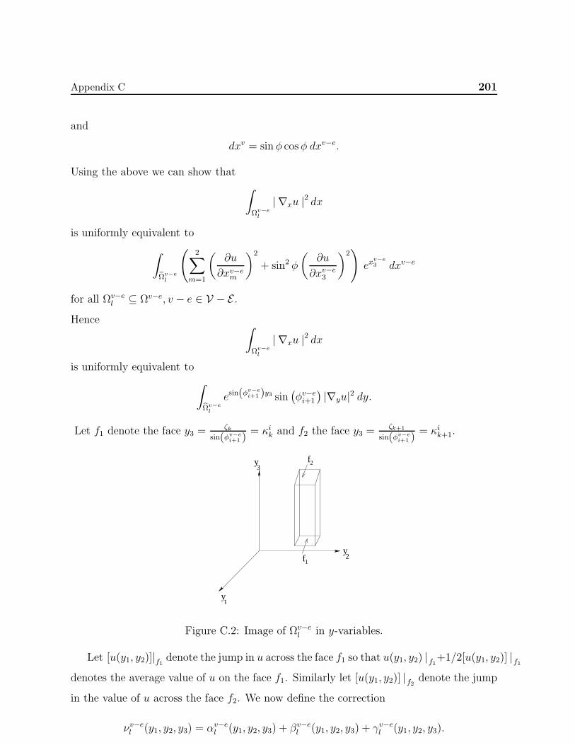
Appendix C 201
and
dxv = sinφ cosφ dxv−e.
Using the above we can show that
∫
Ωv−el
| ∇xu |2 dx
is uniformly equivalent to
∫
Ωv−el
(2∑
m=1
(∂u
∂xv−em
)2
+ sin2 φ
(∂u
∂xv−e3
)2)ex
v−e3 dxv−e
for all Ωv−el ⊆ Ωv−e, v − e ∈ V − E .Hence ∫
Ωv−el
| ∇xu |2 dx
is uniformly equivalent to
∫
Ωv−el
esin(φv−ei+1 )y3 sin
(φv−ei+1
)|∇yu|2 dy.
Let f1 denote the face y3 =ζk
sin(φv−ei+1 )
= κik and f2 the face y3 =ζk+1
sin(φv−ei+1 )
= κik+1.
y
y
y
1
3
2f
f
1
2
Figure C.2: Image of Ωv−el in y-variables.
Let [u(y1, y2)]|f1 denote the jump in u across the face f1 so that u(y1, y2) |f1+1/2[u(y1, y2)] |f1denotes the average value of u on the face f1. Similarly let [u(y1, y2)] |f2 denote the jump
in the value of u across the face f2. We now define the correction
νv−el (y1, y2, y3) = αv−el (y1, y2, y3) + βv−el (y1, y2, y3) + γv−el (y1, y2, y3).
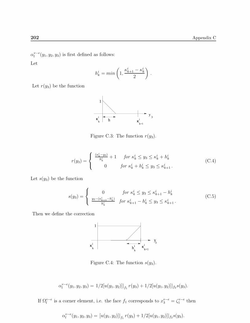
202 Appendix C
αv−el (y1, y2, y3) is first defined as follows:
Let
hik = min
(1,κik+1 − κik
2
).
Let r(y3) be the function
i
y3i
k+1k
κ κh
1
Figure C.3: The function r(y3).
r(y3) =
(κik−y3)hik
+ 1 for κik ≤ y3 ≤ κik + hik
0 for κik + hik ≤ y3 ≤ κik+1 .(C.4)
Let s(y3) be the function
s(y3) =
0 for κik ≤ y3 ≤ κik+1 − hiky3−(κik+1−hik)
hikfor κik+1 − hik ≤ y3 ≤ κik+1 .
(C.5)
Then we define the correction
iκhk
i
y3
κ i
k+1k
1
Figure C.4: The function s(y3).
αv−el (y1, y2, y3) = 1/2[u(y1, y2)]|f1 r(y3) + 1/2[u(y1, y2)]|f2s(y3).
If Ωv−el is a corner element, i.e. the face f1 corresponds to xv−e3 = ζv−e1 then
αv−el (y1, y2, y3) = [u(y1, y2)]|f1 r(y3) + 1/2[u(y1, y2)]|f2s(y3).
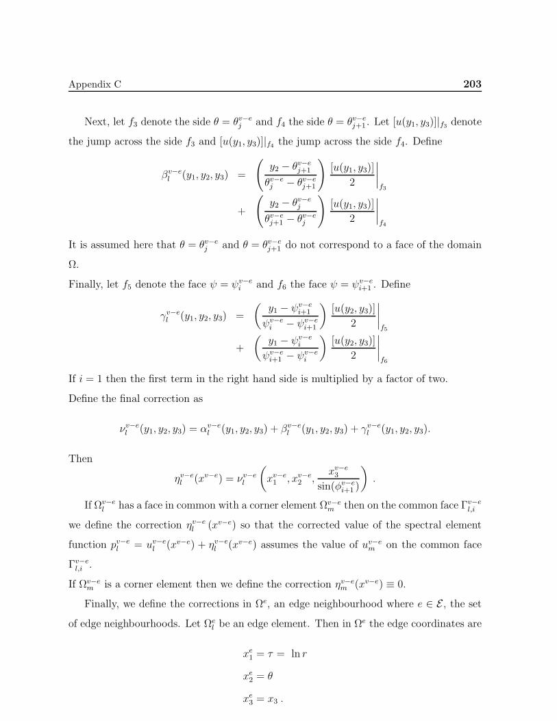
Appendix C 203
Next, let f3 denote the side θ = θv−ej and f4 the side θ = θv−ej+1 . Let [u(y1, y3)]|f3 denotethe jump across the side f3 and [u(y1, y3)]|f4 the jump across the side f4. Define
βv−el (y1, y2, y3) =
(y2 − θv−ej+1
θv−ej − θv−ej+1
)[u(y1, y3)]
2
∣∣∣∣f3
+
(y2 − θv−ej
θv−ej+1 − θv−ej
)[u(y1, y3)]
2
∣∣∣∣f4
It is assumed here that θ = θv−ej and θ = θv−ej+1 do not correspond to a face of the domain
Ω.
Finally, let f5 denote the face ψ = ψv−ei and f6 the face ψ = ψv−ei+1 . Define
γv−el (y1, y2, y3) =
(y1 − ψv−ei+1
ψv−ei − ψv−ei+1
)[u(y2, y3)]
2
∣∣∣∣f5
+
(y1 − ψv−ei
ψv−ei+1 − ψv−ei
)[u(y2, y3)]
2
∣∣∣∣f6
If i = 1 then the first term in the right hand side is multiplied by a factor of two.
Define the final correction as
νv−el (y1, y2, y3) = αv−el (y1, y2, y3) + βv−el (y1, y2, y3) + γv−el (y1, y2, y3).
Then
ηv−el (xv−e) = νv−el
(xv−e1 , xv−e2 ,
xv−e3
sin(φv−ei+1 )
).
If Ωv−el has a face in common with a corner element Ωv−em then on the common face Γv−el,i
we define the correction ηv−el (xv−e) so that the corrected value of the spectral element
function pv−el = uv−el (xv−e) + ηv−el (xv−e) assumes the value of uv−em on the common face
Γv−el,i .
If Ωv−em is a corner element then we define the correction ηv−em (xv−e) ≡ 0.
Finally, we define the corrections in Ωe, an edge neighbourhood where e ∈ E , the set
of edge neighbourhoods. Let Ωel be an edge element. Then in Ωe the edge coordinates are
xe1 = τ = ln r
xe2 = θ
xe3 = x3 .
204 Appendix C
Let Ωel denote the image of Ωe in xe coordinates. Then
Ωel =xe : ln(rej ) < xe1 < ln(rej+1), θ
ek < xe2 < θek+1, Z
en < xe3 < Ze
n+1
.
Once again we introduce a set of local coordinates z in Ωel defined as
z1 = xe1
z2 = xe2
z3 =xe3rej+1
.
Then Ωel is mapped onto the hexahedron Ωel such that the length of the z3 side becomes
large as Ωel approaches the edge of the domain.
Now ∫
Ωeu
|∇xu|2dx =
∫
Ωel
((∂u
∂τ
)2
+
(∂u
∂θ
)2
+ e2τ(∂u
∂x3
)2)dτ dθ dx3 .
Hence ∫
Ωeu
|∇xu|2dx
is uniformly equivalent to ∫
Ωeu
|∇zu|2rej+1 dz .
Here u denotes the spectral element function defined on Ωeu . Now we can define cor-
rections to the spectral element functions so that the corrected element functions are
conforming as we have for vertex-edge elements.
Finally, a further set of corrections can be made so that the corrected element function
p(x) ∈ H10 (Ω), i.e. p vanishes on Γ[0], the Dirichlet portion of the boundary ∂Ω of Ω.
Moreover the estimate (C.1) holds.
We now briefly indicate how the corrections need to be defined in case the spectral
element functions are nonconforming.
The corrections are first described for an element Ωrl ⊆ Ωr, the regular region of Ω.
Let M rl (λ1, λ2, λ3) denote the map from the cube Q = (−1, 1)3 to Ωrl as shown in Figure
C.1.
We first make a correction δrl (λ1, λ2, λ3) =∑1
i=0
∑1j=0
∑1k=0 ai,j,kλ
i1λ
j2λ
k3 such that
(url + δrl )(n) = u(n), where n denotes a node of Q = (M rl )
−1(Ωrl ) and u(n) the average
Appendix C 205
value of u at the node n. Hence the corrected spectral element function is conforming at
the nodes of Ωrl . Here we use the estimate
‖w‖2L∞(R) ≤ C ‖w‖2H3/2(R)
where R is a rectangle in the plane, each of whose sides is of length = Θ(1).
Next, we define a correction ǫrl (λ1, λ2, λ3) such that if t is a point on a side S of
Q = (M rl )
−1 (Ωrl ) then (url + δrl + ǫrl )(t) = u+ δ(t) where u+ δ(t) denotes the average
value of u + δ at t. It should be noted that ǫrl (t) = 0 if t is a node of Q. Consider for
example the side corresponding to λ1 = −1, λ2 = −1, −1 < λ3 < 1 and let the correction
corresponding to the side be g(λ3). Then the contribution of the correction for this side to
ǫrl would be (1−λ1)2
(1−λ2)2
g(λ3). The contributions of the corrections for other sides would
be similarly defined and ǫrl would be the sum of all these contributions. Here we use the
estimate
‖w‖2H1(S) ≤ C lnW‖w‖2H3/2(R)
where R is a rectangle in the plane, each of whose sides is of length Θ(1), and S is a side
of the rectangle R. Moreover w is a polynomial of degree W in each of its two arguments.
Now url + δrl + ǫrl , would be conforming on the portion of the wirebasket contained in
Ωr, the regular region of Ω. We shall next make corrections in Ωv for v ∈ V,Ωv−e for
v − e ∈ V − E and Ωe for e ∈ E , so that the corrected spectral element functions are
conforming on the wire basket of the elements contained in Ω. Once this has been done
a further set of corrections can be made so that the corrected spectral element functions
would be conforming on the faces as well as the wire basket and vanish on the Dirichlet
portion of the boundary Γ[0] of ∂Ω as has already been described. The corrections δvl + ǫvl
that need to be made in the vertex neighbourhood Ωv of Ω so that uvl + δvl + ǫvl would
be conforming on the portion of the wirebasket contained in Ωv are very similar to those
described for the regular region Ωr of Ω and hence are not discussed any further. We now
describe the corrections δv−el +ǫv−el that need to be made in the vertex-edge neighbourhood
Ωv−e of Ω so that uv−el + δv−el + ǫv−el would be conforming on the portion of the wirebasket
contained in Ωv−e.
Let Ωv−el be an element in the vertex-edge neighbourhood Ωv−e, and let Ωv−el be its
206 Appendix C
y
y
y
1
3
2
f
f
1
2
Figure C.5: The element Ωv−el .
image in y coordinates where
y1 = ψ = ln(tanφ)
y2 = θ
y3 =ζ
sin(φv−ei+1
) =ln(x3)
sin(φv−ei+1
) .
Then the length of the y3 side becomes large as the elements approach the edge of the
domain Ω. We define
σ1(y1, y2) =∑
i,j=0,1
h(1)i,j y
i1yj2,
a bilinear function of y1 and y2 so that
uv−el (y1, y2, y3) + σ1(y1, y2)∣∣f1
= w1(y1, y2)
is conforming at the nodes of the face f1. Here w1(y1, y2) assumes the average value of
the spectral element functions at the nodes of f1.
In the same way we define
σ2(y1, y2) =∑
i,j=0,1
h(2)i,j y
i1yj2,
a bilinear function of y1 and y2, so that
uv−el (y1, y2, y3) + σ2(y1, y2)|f2 = w2(y1, y2)
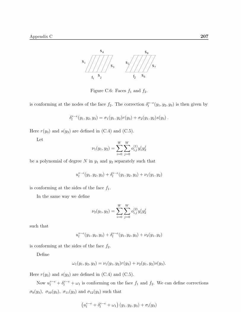
Appendix C 207
f f1 2
s
s
s
s
s
s
s
s
1
2
3
4 8
6
57
Figure C.6: Faces f1 and f2.
is conforming at the nodes of the face f2. The correction δv−el (y1, y2, y3) is then given by
δv−el (y1, y2, y3) = σ1(y1, y2)r(y3) + σ2(y1, y2)s(y3) .
Here r(y3) and s(y3) are defined in (C.4) and (C.5).
Let
ν1(y1, y2) =
W∑
i=0
W∑
j=0
o(1)i,j y
i1yj2
be a polynomial of degree N in y1 and y2 separately such that
uv−el (y1, y2, y3) + δv−el (y1, y2, y3) + ν1(y1, y2)
is conforming at the sides of the face f1.
In the same way we define
ν2(y1, y2) =
W∑
i=0
W∑
j=0
o(2)i,j y
i1yj2
such that
uv−el (y1, y2, y3) + δv−el (y1, y2, y3) + ν2(y1, y2)
is conforming at the sides of the face f2.
Define
ω1(y1, y2, y3) = ν1(y1, y2)r(y3) + ν2(y1, y2)s(y3).
Here r(y3) and s(y3) are defined in (C.4) and (C.5).
Now uv−el + δv−el + ω1 is conforming on the face f1 and f2. We can define corrections
σ9(y3), σ10(y3), σ11(y3) and σ12(y3) such that
(uv−el + δv−el + ω1
)(y1, y2, y3) + σi(y3)
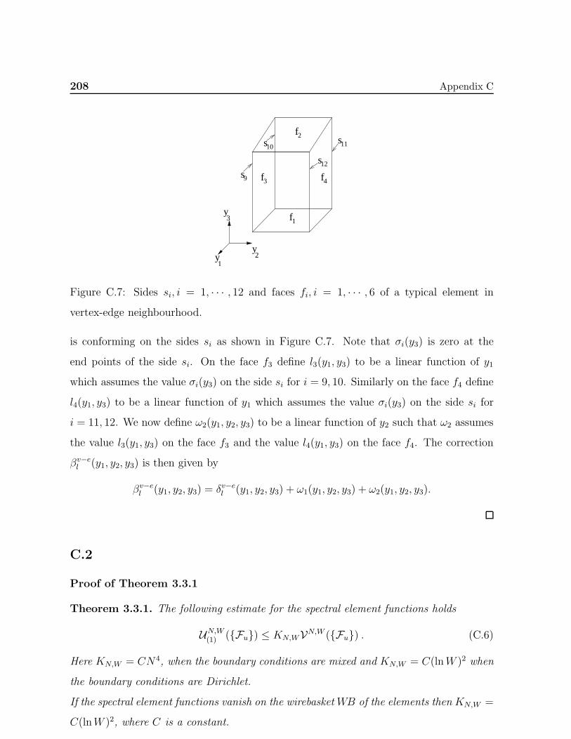
208 Appendix C
yy
y
12
3 f
ffs
s
s
s
3 49
10 11
12
1
f2
Figure C.7: Sides si, i = 1, · · · , 12 and faces fi, i = 1, · · · , 6 of a typical element in
vertex-edge neighbourhood.
is conforming on the sides si as shown in Figure C.7. Note that σi(y3) is zero at the
end points of the side si. On the face f3 define l3(y1, y3) to be a linear function of y1
which assumes the value σi(y3) on the side si for i = 9, 10. Similarly on the face f4 define
l4(y1, y3) to be a linear function of y1 which assumes the value σi(y3) on the side si for
i = 11, 12. We now define ω2(y1, y2, y3) to be a linear function of y2 such that ω2 assumes
the value l3(y1, y3) on the face f3 and the value l4(y1, y3) on the face f4. The correction
βv−el (y1, y2, y3) is then given by
βv−el (y1, y2, y3) = δv−el (y1, y2, y3) + ω1(y1, y2, y3) + ω2(y1, y2, y3).
C.2
Proof of Theorem 3.3.1
Theorem 3.3.1. The following estimate for the spectral element functions holds
UN,W(1) (Fu) ≤ KN,WVN,W (Fu) . (C.6)
Here KN,W = CN4, when the boundary conditions are mixed and KN,W = C(lnW )2 when
the boundary conditions are Dirichlet.
If the spectral element functions vanish on the wirebasketWB of the elements then KN,W =
C(lnW )2, where C is a constant.
Appendix C 209
Proof. Let p denote the corrected spectral element function defined in Lemma 3.3.1 and
B(p, λ) =
∫
Ω
(3∑
i,j=1
ai,jpxiλxj +3∑
i=1
bipxiλ+ cpλ
)dx (C.7)
be a bilinear form for p, λ ∈ H10 (Ω). Here H1
0 (Ω) denotes the subspace of functions ⊆H1(Ω) which vanish on Γ[0]. Moreover there is a constant K such that
K‖q‖2H1(Ω) ≤ B(q, q) (C.8)
for all q ∈ H10 (Ω).
Now
B(p, λ) = Bregular(p, λ) +Bvertices(p, λ) +Bvertex−edge(p, λ) +Bedges(p, λ) . (C.9)
Here
Bregular(p, λ) =
Nr∑
l=1
B(p, λ)Ωrl
and
B(p, λ)Ωrl=
∫
Ωrl
3∑
i,j=1
(ai,jpxiλxj +
3∑
i=1
bipxiλ+ cpλ
)dx .
The other terms are similarly defined.
Now
prl = url + ηrl .
Hence
B(p, λ)Ωrl= B(url , λ)Ωr
l+B(ηrl , λ)Ωr
l.
Integrating by parts we obtain,
B(url , λ)Ωrl=
∫
Ωrl
Lurl λ dx+
∫
∂Ωrl
(∂url∂ν
)
A
λ dσ .
Hence
Bregular(p, p) =Nr∑
l=1
∫
Ωrl
Lurl p dx+∑
Γrl,i⊆Ωr
∫
Γrl,i
(∂u
∂ν
)
A
p dσ
+∑
Γrl,i⊆∂Ωr
∫
Γrl,i
(∂u
∂ν
)
A
p dσ +Nr∑
l=1
B(ηrl , p)Ωrl. (C.10)
210 Appendix C
Now
Bvertices(p, λ) =∑
v∈V
Nv∑
l=1
B(p, λ)Ωvl.
Clearly
B(p, λ)Ωvl= B(uvl , λ)Ωv
l+B(ηvl , λ)Ωv
l.
Once more using integration by parts
B(uvl , λ)Ωvl=
∫
Ωvl
Lvu(xv) λ eχ/2√sin φ dxv +
∫
∂Ωvl
(∂uvl∂νv
)
Av
λ eχ sin φ dσv .
Hence
Bvertices(p, p) =∑
v∈V
(Nv∑
l=1
∫
Ωvl
Lvu(xv) λ eχ/2√sin φ dxv
+∑
Γvl,i⊆Ωv
∫
Γvl,i
[(∂u
∂νv
)
Av
]p eχ sinφ dσv
+∑
Γvl,i⊆∂Ωv
∫
Γvl,i
(∂u
∂νv
)
Av
p eχ sinφ dσv +Nv∑
l=1
B(ηvl , p)Ωvl
. (C.11)
Now if Γvl,i is a face of Ωvl and Γrj,k is a face of Ωrj such that Γvl,i = Γrj,k then
∫
Γrj,k
(∂url∂ν
)
Av
p dσ = −∫
Γvl,i
(∂uvl∂νv
)
Av
peχ sinφ dσv . (C.12)
Next
Bvertex−edge(p, λ) =∑
v−e∈V−E
Nv−e∑
l=1
B(p, λ)Ωv−el.
And
B(p, λ)Ωv−el
= B(uv−el , λ)Ωv−el
+B(ηv−el , λ)Ωv−el.
Integration by parts gives
B(uv−el , λ)Ωv−el
=
∫
Ωv−el
Lv−eu(xv−e)λ(xv−e)eζ/2 dxv−e
+
∫
∂Ωv−el
(∂u
∂νv−e
)
Av−e
λeζ dσv−e .
Appendix C 211
Hence
Bvertex−edge(p, p) =∑
v−e∈V−E
(Nv−e∑
l=1
∫
Ωv−el
Lv−eu(xv−e) p(xv−e) eζ/2 dxv−e
+∑
Γv−el,i ⊆Ωv−e
∫
Γv−el,i
[(∂u
∂νv−e
)
Av−e
]p eχ dσv−e
+∑
Γv−el,i ⊆∂Ωv−e
∫
Γv−el,i
(∂u
∂νv−e
)
Av−e
p eχ dσv−e
+
Nv−e∑
l=1
B(ηv−el , p)Ωv−el
). (C.13)
Now if Γvm,j = Γv−el,i then
∫
Γvm,j
(∂u
∂νv
)
Av
p eχ sinφ dσv = −∫
Γv−el,i
(∂u
∂νv−e
)
Av−e
peζ dσv−e. (C.14)
Finally
Bedges(p, λ) =∑
e∈E
Ne∑
l=1
B(p, λ)Ωel.
Here
B(p, λ)Ωel= B(uel , λ)Ωe
l+B(ηel , λ)Ωe
l.
Integrating by parts we obtain
B(uel , λ)Ωel=
∫
Ωel
Leu(xe)λ dxe +
∫
∂Ωel
(∂u
∂νe
)
Ae
λ dσe.
Hence
Bedges(p, p) =∑
e∈E
(Ne∑
l=1
∫
Ωel
Leu(xe)p dxe
+∑
Γel,i⊆Ωe
∫
Γel,i
[(∂u
∂νe
)
Ae
]p dσe +
∑
Γel,i⊆∂Ωe
∫
Γel,i
(∂u
∂νe
)
Ae
p dσe
+
Ne∑
l=1
B(ηel , p)Ωel
). (C.15)
Let Γv−el,i = Γem,j . Then it can be shown that
∫
Γv−el,i
(∂u
∂νv−e
)
Av−e
peζ dσv−e = −∫
Γem,j
(∂u
∂νe
)
Ae
p dσe (C.16)
212 Appendix C
Also if Γem,j = Γrn,k then
∫
Γem,j
(∂u
∂νe
)
Ae
p dσe = −∫
Γrn,k
(∂u
∂ν
)
A
p dσ (C.17)
Now
B(p, p)Ω = Bregular(p, p) +Bvertices(p, p) +Bvertex−edges(p, p)
+Bedges(p, p) . (C.18)
Substituting (C.10)−(C.17) into the above we obtain
B(p, p)Ω ≤ cd VN,W (Fu) + 1/d G(p) . (C.19)
In the above
G(p) = ‖p(x)‖21,Ωr +∑
v∈V‖p(xv) exv−e
3 /2‖21,Ωv +
∑
v−e∈V−E
∫
Ωv−e
(2∑
i=1
(∂p(xv−e)
∂xv−ei
)2
+ sin2 φ
(∂p(xv−e)
∂xv−e3
)2
+(p (xv−e)
)2)ex
v−e3 wv−e(xv−e1 ) dxv−e
+∑
e∈E
∫
Ωe
(2∑
i=1
(∂p(xe)
∂xei
)2
+ e2τ(∂p(xe)
∂xe3
)2
+(p (xe)
)2)we(xe1)dx
e. (C.20)
Now
K‖p‖2H1(Ω) ≤ B(p, p) .
Moreover if the spectral element functions are not conforming on the wirebasket WB then
G(p) ≤ CN,W‖p‖2H1(Ω) . (C.21)
Here CN,W = EN2 if the boundary conditions are mixed and CN,W = E if the boundary
conditions are Dirichlet. Choosing d = 2EN2
Kin (C.19) gives
B(p, p)Ω ≤c
KCN,WVN,W (Fu) .
Hence combining the above and (C.20) gives
G(p) ≤ 2c
K2(CN,W )2N4 VN,W (Fu) . (C.22)
Now (C.1) and (C.22) yields (C.6).
Appendix C 213
Finally, we consider the case when the spectral element functions are conforming on
the wirebasket WB and vanish on it. Then p vanishes on the wirebasket. Consider p(xe)
on Ωel . Here
Ωel =xe : ln(rei ) < xe1 < ln(rei+1), θj < xe2 < θj+1, Z
ek < xe3 < Ze
k+1
.
Now if s(y1, y2) is a polynomial of degree W in each of its arguments on the unit square
S which vanishes at one of the vertices of S then using a scaling argument as in § 3.4of [87] we obtain
∫
S
(s(y))2 dy ≤ F (lnW )
∫
S
((∂s
∂y1
)2
+
(∂s
∂y2
)2)dy .
Hence, since p(xe1, xe2, .) is a polynomial of degree W in xe1 and xe2
∫
Ωel
(p(xe))2 dxe ≤ F (lnW )
∫
Ωel
(2∑
i=1
(∂p(xe)
∂xei
)2
+ e2τ(∂p(xe)
∂xe3
)2)dxe .
And so it can be shown that
G(p) ≤ F lnW‖p‖2H1(Ω) . (C.23)
Choosing d = 1K
2F lnW
in (C.19) gives
G(p) ≤ 2cF 2
K2(lnW )2 VN,W (Fu) . (C.24)
Now combining (C.1) and (C.24) yields (C.6).

Appendix D 215
Appendix D
D.1
Proof of Lemma 3.4.1
Lemma 3.4.1. Let Ωrm and Ωrp be elements in the regular region Ωr of Ω and Γrm,i be a
face of Ωrm and Γrp,j be a face of Ωrp such that Γrm,i = Γrp,j. Then for any ǫ > 0 there exists
a constant Cǫ such that for W large enough∣∣∣∣∣
∫
∂Γrm,i
((∂urm∂ν
)
A
(∂urm∂n
)
A
−(∂urp∂ν
)
A
(∂urp∂n
)
A
)ds
∣∣∣∣∣
≤ Cǫ(lnW )23∑
k=1
‖[uxk ]‖21/2,Γrm,i
+ ǫ∑
1≤|α|≤2
(‖Dα
xurm‖20,Ωr
m+ ‖Dα
xurp‖20,Ωr
p
). (D.1)
Proof. Let Γrm,i be the image of the mappingM rm from Q to Ωrm corresponding to λ3 = −1
and Γrp,j, the image of the mapping M rm from Q to Ωrp corresponding to λ3 = 1. Then
Γrm,i is the image of the square S = (−1, 1)2 under these mappings. However the proof
remains valid if it is the image of T , the master triangle, too.
Now ∫
∂Γrm,i
(∂u
∂ν
)
A
(∂u
∂n
)
A
ds =
∫
∂S
3∑
i,j=1
αi,j∂u
∂xi
∂u
∂xjds . (D.2)
Here the element of arc length ds in the right hand side denotes either dλ1 or dλ2.
Moreover αi,j is an analytic function of its arguments. Now
∂urm∂xi
=
3∑
j=1
βi,j∂urm∂λj
where βi,j is an analytic function of λ = (λ1, λ2, λ3).
Let βi,j be the projection of βi,j into the space of polynomials of degree W in H3(Q).
Then for any m > 0
‖βi,j − βi,j‖1,∞,Q ≤CmWm
(D.3)
as W →∞.
Define(∂urm∂xi
)a, an approximate representation for ∂urm
∂xi, by
(∂urm∂xi
)a=
3∑
j=1
βi,j∂urm∂λj
.
216 Appendix D
Moreover(∂urm∂xi
)ais a polynomial of degree 2W in each of its arguments λ1, λ2 and λ3.
Now ∥∥∥∥∂urm∂xi−(∂urm∂xi
)a∥∥∥∥0,∂S
≤ C
W 4
3∑
j=1
∥∥∥∥∂urm∂λj
∥∥∥∥0,∂S
≤ C
W 5
3∑
j=1
∥∥∥∥∂urm∂λj
(λ)
∥∥∥∥5/4,Q
by the trace theorem for Sobolev spaces.
Hence ∥∥∥∥∂urm∂xi−(∂urm∂xi
)a∥∥∥∥0,∂S
≤ C
W 4
∑
1≤|α|≤2
(‖Dα
λurm‖20,Q
)1/2. (D.4)
Here we have used the inverse inequality for differentiation∥∥∥∥∂urm∂λi
(λ)
∥∥∥∥5/4,Q
≤ KW
∥∥∥∥∂urm∂λi
(λ)
∥∥∥∥1,Q
.
Now ∥∥∥∥∂urm∂xi
∥∥∥∥2
0,∂S
≤ C
3∑
i=1
∥∥∥∥∂urm∂λi
∥∥∥∥2
0,∂S
.
Moreover (see [87]),
∥∥∥∥∂urm∂xi
∥∥∥∥2
0,∂S
≤ C(lnW )∑
1≤|α|≤2
‖Dαλu
rm‖20,Q . (D.5a)
In the same way it can be shown that
∥∥∥∥(∂urm∂xi
)a∥∥∥∥2
0,∂S
≤ C(lnW )∑
1≤|α|≤2
‖Dαλu
rm‖20,Q . (D.5b)
Now ∫
∂Γrm,i
(∂urm∂ν
)
A
(∂urm∂n
)
A
ds =
∫
∂S
3∑
i,j=1
αi,j
(∂urm∂xi
)(∂urm∂xj
)ds .
Using (D.4) and (D.5) gives∣∣∣∣∣
∫
∂S
3∑
i,j=1
αi,j
((∂urm∂xi
)a(∂urm∂xj
)a− ∂urm
∂xi
∂urm∂xj
)ds
∣∣∣∣∣
≤ C
(3∑
i,j=1
∥∥∥∥(∂urm∂xi
)a∥∥∥∥0,∂S
∥∥∥∥(∂urm∂xj
)a−(∂urm∂xj
)∥∥∥∥0,∂S
+
3∑
i,j=1
∥∥∥∥(∂urm∂xj
)∥∥∥∥0,∂S
∥∥∥∥(∂urm∂xi
)a−(∂urm∂xi
)∥∥∥∥0,∂S
)
≤ C
√lnW
W 4
∑
1≤|α|≤2
‖Dαλu
rm‖20,Q . (D.6)
Appendix D 217
In the same way it can be shown that
∣∣∣∣∣
∫
∂S
3∑
i,j=1
αi,j
((∂urp∂xi
)a(∂urp∂xj
)a−(∂urp∂xi
)(∂urp∂xj
))ds
∣∣∣∣∣
≤ C
√lnW
W 4
∑
1≤|α|≤2
‖Dαλu
rp‖20,Q . (D.7)
Hence∣∣∣∣∣
∫
∂S
3∑
i,j=1
αi,j
((∂urm∂xi
)(∂urm∂xj
)−(∂urp∂xi
)(∂urp∂xj
))ds
∣∣∣∣∣
≤∣∣∣∣∣
∫
∂S
3∑
i,j=1
αi,j
((∂urm∂xi
)a(∂urm∂xj
)a−(∂urp∂xi
)a(∂urp∂xj
)a)ds
∣∣∣∣∣
+C√lnW
W 4
∑
1≤|α|≤2
(‖Dα
λurm‖20,Q + ‖Dα
λurp‖20,Q
) . (D.8)
Now∣∣∣∣∣
∫
∂S
3∑
i,j=1
αi,j
((∂urm∂xi
)a(∂urm∂xj
)a−(∂urp∂xi
)a(∂urp∂xj
)a)ds
∣∣∣∣∣
≤ C
[3∑
i,j=1
(∥∥∥∥(∂urm∂xi
)a∥∥∥∥0,∂S
∥∥∥∥(∂urm∂xj
)a−(∂urp∂xj
)a∥∥∥∥0,∂S
+
∥∥∥∥(∂urp∂xj
)a∥∥∥∥0,∂S
∥∥∥∥(∂urm∂xi
)a−(∂urp∂xi
)a∥∥∥∥0,∂S
)]
Hence for any ǫ > 0 there is a constant Cǫ such that
∣∣∣∣∣
∫
∂S
3∑
i,j=1
αi,j
((∂urm∂xi
)a(∂urm∂xj
)a−(∂urp∂xi
)a(∂urp∂xj
)a)ds
∣∣∣∣∣
≤ Cǫ(lnW )
(3∑
i,j=1
∥∥∥∥(∂urm∂xi
)a−(∂urp∂xi
)a∥∥∥∥2
0,∂S
)
+ ǫ/3
∑
1≤|α|≤2
(‖Dα
λurm‖20,Q + ‖Dα
λurp‖20,Q
) . (D.9)
Here we have used the estimate (D.5)
∥∥∥∥(∂urm∂xi
)a∥∥∥∥2
0,∂S
≤ C(lnW )
∑
1≤|α|≤2
‖Dαλu
rm‖20,Q
.

218 Appendix D
and ∥∥∥∥(∂urp∂xi
)a∥∥∥∥2
0,∂S
≤ C(lnW )
∑
1≤|α|≤2
‖Dαλu
rp‖20,Q
.
Now as in [87]
∥∥∥∥(∂urm∂xi
)a−(∂urp∂xi
)a∥∥∥∥2
0,∂S
≤ C(lnW )
(∥∥∥∥(∂urm∂xi
)a−(∂urp∂xi
)a∥∥∥∥2
1/2,S
)(D.10)
since(∂urm∂xi
)and
(∂urp∂xi
)are polynomials of degree 2W in each of their arguments.
Now combining (D.9) and (D.10) gives∣∣∣∣∣
∫
∂S
3∑
i,j=1
αi,j
((∂urm∂xi
)a(∂urm∂xj
)a−(∂urp∂xi
)a(∂urp∂xj
)a)ds
∣∣∣∣∣
≤ Cǫ(lnW )2
(3∑
i,j=1
∥∥∥∥(∂urm∂xi
)a−(∂urp∂xi
)a∥∥∥∥2
1/2,S
)
+ ǫ/3
∑
1≤|α|≤2
(‖Dα
λurm‖20,Q + ‖Dα
λurp‖20,Q
) . (D.11)
Next∥∥∥∥(∂urm∂xi
)a−(∂urm∂xi
)∥∥∥∥1/2,S
≤3∑
j=1
∥∥∥∥(βi,j − βi,j)∂urm∂λj
∥∥∥∥1/2,S
≤3∑
j=1
∥∥∥(βi,j − βi,j)∥∥∥1,∞,S
∥∥∥∥∂urm∂λj
∥∥∥∥1/2,S
.
Hence ∥∥∥∥(∂urm∂xi
)a−(∂urm∂xi
)∥∥∥∥2
1/2,S
≤ C
W 8
∑
1≤|α|≤2
‖Dαλu
rm‖20,Q
. (D.12a)
In the same way it can be shown that
∥∥∥∥(∂urp∂xi
)a−(∂urp∂xi
)∥∥∥∥2
1/2,S
≤ C
W 8
∑
1≤|α|≤2
‖Dαλu
rp‖20,Q
. (D.12b)
Combining (D.11) and (D.12) and choosing W large enough gives∣∣∣∣∣
∫
∂S
3∑
i,j=1
αi,j
((∂urm∂xi
)a(∂urm∂xj
)a−(∂urp∂xi
)a(∂urp∂xj
)a)ds
∣∣∣∣∣
≤ Cǫ(lnW )2
(3∑
i=1
∥∥∥∥∂urm∂xi− ∂urp∂xi
∥∥∥∥2
1/2,S
)+ 2ǫ/3
∑
1≤|α|≤2
‖Dαλu
rp‖20,Q
. (D.13)
Appendix D 219
Now substituting (D.13) into (D.8) and choosing W large enough yields
∣∣∣∣∣
∫
∂S
3∑
i,j=1
αi,j
((∂urm∂xi
)(∂urm∂xj
)−(∂urp∂xi
)(∂urp∂xj
))ds
∣∣∣∣∣
≤ Cǫ(lnW )2
(3∑
i=1
∥∥∥∥∂urm∂xi− ∂urp∂xi
∥∥∥∥2
1/2,S
)+ ǫ
∑
1≤|α|≤2
‖Dαλu
rp‖20,Q
. (D.14)
And so the required result (D.1) follows.
D.2
Proof of Lemma 3.4.2
Lemma 3.4.2. Let Ωrm and Ωrp be elements in the regular region Ωr of Ω and Γrm,i be a
face of Ωrm and Γrp,j be a face of Ωrp such that Γrm,i = Γrp,j. Then for any ǫ > 0 there exists
a constant Cǫ such that for W large enough
∣∣∣∣∣
2∑
j=1
(∫
Γrm,i
(∂urm∂τ j
)
A
∂
∂sj
(∂urm∂ν
)
A
−∫
Γrp,j
(∂urp∂τ j
)
A
∂
∂sj
(∂urp∂ν
)
A
)dσ
∣∣∣∣∣
≤ Cǫ(lnW )23∑
k=1
‖[uxk ]‖21/2,Γrp,j
+ ǫ∑
1≤|α|≤2
(‖Dα
xurm‖20,Ωr
m+ ‖Dα
xurp‖20,Ωr
p
). (D.15)
Proof. It is enough to show that
∣∣∣∣∣
∫
Γrm,i
((∂urm∂τ j
)
A
∂
∂sj
(∂urm∂ν
)
A
−(∂urp∂τ j
)
A
∂
∂sj
(∂urp∂ν
)
A
)dσ
∣∣∣∣∣
≤ Cǫ(lnW )23∑
k=1
‖[uxk ]‖21/2,Γrp,j
+ ǫ∑
1≤|α|≤2
(‖Dα
xurm‖20,Ωr
m+ ‖Dα
xurp‖20,Ωr
p
)(D.16)
for j = 1.
Let Γrm,i be the image of the mapping M rm from Q to Ωrm corresponding to λ3 = −1
and Γrp,j, the image of the mapping M rm from Q to Ωrp corresponding to λ3 = 1. Then
Γrm,i is the image of the square S = (−1, 1)2 under these mappings. However the proof
220 Appendix D
remains valid if it is the image of T , the master triangle, too.
Now
∫
Γrm,i
(∂u
∂τ 1
)
A
∂
∂s1
(∂u
∂ν
)
A
dσ
=2∑
j=1
3∑
i,k=1
∫
S
(ai,j
∂u
∂xi
)∂
∂λj
(bk∂u
∂xk
)dλ1dλ2 (D.17)
where ai,j(λ1, λ2) and bk(λ1, λ2) are analytic functions of λ1 and λ2.
Now as in Lemma 3.4.1, let ai,j(λ1, λ2) and bk(λ1, λ2) be the projections of ai,j(λ1, λ2)
and bk(λ1, λ2) into the space of polynomials of degree W in H3(S). Moreover, let(∂urm∂xi
)a,
(∂urp∂xi
)abe the approximations to ∂urm
∂xiand
∂urp∂xi
defined in Lemma 3.4.1. Then(∂urm∂xi
)aand
(∂urp∂xi
)aare polynomials of degree 2W in each of the variables λ1, λ2 and λ3.
Now
∣∣∣∣∫
S
(ai,j
(∂urm∂xi
)∂
∂λj
(bk∂urm∂xk
)− ai,j
(∂urm∂xi
)∂
∂λj
(bk∂urm∂xk
))dλ1dλ2
∣∣∣∣
≤∣∣∣∣∫
S
(ai,j − ai,j)∂urm∂xi
∂
∂λj
(bk∂urm∂xk
)dλ1dλ2
∣∣∣∣
+
∣∣∣∣∫
S
ai,j∂urm∂xi
∂
∂λj
((bk − bk)
∂urm∂xk
)dλ1dλ2
∣∣∣∣
≤ C
W 4
3∑
l,m=1
∥∥∥∥∂urm∂λl
∥∥∥∥0,S
(∥∥∥∥∂urm∂λm
∥∥∥∥0,S
+
∥∥∥∥∂2urm∂λm∂λj
∥∥∥∥0,S
)
≤ C
W 4
3∑
l=1
∥∥∥∥∂urm∂λl
∥∥∥∥2
7/4,Q
. (D.18)
To obtain the above inequality we have used the trace theorem for Sobolev spaces. Hence
by the inverse inequality for differentiation
∣∣∣∣∫
S
(ai,j
(∂urm∂xi
)∂
∂λj
(bk∂urm∂xk
)− ai,j
(∂urm∂xi
)∂
∂λj
(bk∂urm∂xk
))dλ1dλ2
∣∣∣∣
≤ C
W
∑
1≤|α|≤2
‖Dαλu
rm‖22,Q . (D.19)
Appendix D 221
Combining (D.17) and (D.19) gives
∣∣∣∣∫
S
(ai,j
∂urm∂xi
∂
∂λj
(bk∂urm∂xk
)− ai,j
∂urp∂xi
∂
∂λj
(bk∂urp∂xk
))dλ1dλ2
∣∣∣∣
≤∣∣∣∣∫
S
(ai,j
∂urm∂xi
∂
∂λj
(bk∂urm∂xk
)− ai,j
(∂urp∂xi
)∂
∂λj
(bk∂urp∂xk
))dλ1dλ2
∣∣∣∣
+C
W
∑
1≤|α|≤2
(‖Dα
λurm‖22,Q +
∥∥Dαλu
rp
∥∥22,Q
) . (D.20)
Next
∣∣∣∣∫
S
(ai,j
∂urm∂xi
∂
∂λj
(bk∂urm∂xk
)− ai,j
(∂urm∂xi
)a∂
∂λj
(bk
(∂urm∂xk
)a))dλ1dλ2
∣∣∣∣
≤∣∣∣∣∫
S
ai,j∂urm∂xi
∂
∂λj
(bk
(∂urm∂xk−(∂urm∂xk
)a))dλ1dλ2
∣∣∣∣
+
∣∣∣∣∫
S
ai,j
((∂urm∂xi
)a− ∂urm
∂xi
)∂
∂λj
((∂urm∂xk
)a)dλ1dλ2
∣∣∣∣
≤ C
(∥∥∥∥∂urm∂xi
∥∥∥∥0,S
(∥∥∥∥∂
∂λj
(∂urm∂xk−(∂urm∂xk
)a)∥∥∥∥0,S
)
+
∥∥∥∥(∂urm∂xi
)a− ∂urm
∂xi
∥∥∥∥0,S
∥∥∥∥∂
∂λj
((∂urm∂xk
)a)∥∥∥∥0,S
). (D.21)
Now
∥∥∥∥∂urm∂xi
∥∥∥∥0,S
≤ C∑
|α|≤1
‖Dαλu
rm‖1,Q . (D.22)
and
∥∥∥∥∂
∂λj
(∂urm∂xk
−(∂urm∂xk
)a)∥∥∥∥0,S
≤ C
W 4
∑
1≤|α|≤2
‖Dαλu
rm‖0,S . (D.23)
Hence
∥∥∥∥∂
∂λj
(∂urm∂xk−(∂urm∂xk
)a)∥∥∥∥0,S
≤ C
W 4
∑
|α|=1
‖Dαλu
rm‖2,Q . (D.24)
Here we have used the trace theorem for Sobolev spaces.
Now using the inverse inequality for differentiation in (D.24) gives
∥∥∥∥∂
∂λj
(∂urm∂xk−(∂urm∂xk
)a)∥∥∥∥0,S
≤ C
W 2
∑
1≤|α|≤2
‖Dαλu
rm‖1,Q . (D.25)
222 Appendix D
Combining (D.22) and (D.25) gives
∥∥∥∥∂urm∂xi
∥∥∥∥0,S
∥∥∥∥∂
∂λj
(∂urm∂xk−(∂urm∂xk
)a)∥∥∥∥0,S
≤ C
W 2
∑
1≤|α|≤2
‖Dαλu
rm‖0,Q . (D.26)
Next ∥∥∥∥(∂urm∂xi
)a− ∂urm
∂xi
∥∥∥∥0,S
≤ C
W 4
∑
|α|=1
‖Dαλu
rm‖0,S .
Hence by the trace theorem for Sobolev spaces
∥∥∥∥(∂urm∂xi
)a− ∂urm
∂xi
∥∥∥∥0,S
≤ C
W 4
∑
1≤|α|≤2
‖Dαλu
rm‖0,Q . (D.27)
And ∥∥∥∥∂
∂λj
((∂urm∂xk
)a)∥∥∥∥0,S
≤ C∑
1≤|α|≤2
‖Dαλu
rm‖0,S .
Using the trace theorem and inverse inequality for differentiation gives
∥∥∥∥∂
∂λj
((∂urm∂xk
)a)∥∥∥∥0,S
≤ CW 3∑
1≤|α|≤2
‖Dαλu
rm‖0,Q . (D.28)
Combining (D.27) and (D.28) we obtain
∥∥∥∥(∂urm∂xi
)a− ∂urm
∂xi
∥∥∥∥0,S
∥∥∥∥∂
∂λj
((∂urm∂xk
)a)∥∥∥∥0,S
≤ C
W
∑
1≤|α|≤2
‖Dαλu
rm‖20,Q
. (D.29)
Substituting (D.26) and (D.29) into (D.21) yields
∣∣∣∣∫
S
(ai,j
∂urm∂xi
∂
∂λj
(bk∂urm∂xk
)− ai,j
(∂urm∂xi
)a∂
∂λj
(bk
(∂urm∂xk
)a))dλ1dλ2
∣∣∣∣
≤ C
W
∑
1≤|α|≤2
‖Dαλu
rm‖20,Q
. (D.30a)
In the same way it can be shown that
∣∣∣∣∫
S
(ai,j
∂urp∂xi
∂
∂λj
(bk∂urp∂xk
)− ai,j
(∂urp∂xi
)a∂
∂λj
(bk
(∂urp∂xk
)a))dλ1dλ2
∣∣∣∣
≤ C
W
∑
1≤|α|≤2
‖Dαλu
rp‖20,Q
. (D.30b)
Appendix D 223
Combining (D.20) and (D.30) gives
∣∣∣∣∫
S
(ai,j
∂urm∂xi
∂
∂λj
(bk∂urm∂xk
)− ai,j
∂urp∂xi
∂
∂λj
(bk
(∂urp∂xk
)))dλ1dλ2
∣∣∣∣
≤∣∣∣∣∫
S
(ai,j
(∂urm∂xi
)∂
∂λj
(bk
(∂urm∂xk
)a)
− ai,j
(∂urp∂xi
)a∂
∂λj
(bk
(∂urp∂xk
)a))dλ1dλ2
∣∣∣∣
+C
W
∑
1≤|α|≤2
(‖Dα
xurm‖20,Q + ‖Dα
xurm‖20,Q
) . (D.31)
Clearly
∣∣∣∣∫
S
(ai,j
(∂urm∂xi
)a∂
∂λj
(bk
(∂urm∂xk
)a)
− ai,j
(∂urp∂xi
)a∂
∂λj
(bk
(∂urp∂xk
)a))dλ1dλ2
∣∣∣∣
≤∣∣∣∣∫
S
ai,j
(∂urm∂xi
)a∂
∂λj
(bk
((∂urm∂xk
)a−(∂urp∂xk
)a))dλ1dλ2
∣∣∣∣
+
∣∣∣∣∫
S
(ai,j
((∂urm∂xi
)a−(∂urp∂xi
)a)∂
∂λj
(bk
(∂urp∂xk
)a))dλ1dλ2
∣∣∣∣ . (D.32)
Now if e(λ1, λ2) and f(λ1, λ2) are polynomials of degree W in λ1 and λ2 then using
Theorem 4.1 of [37]
∣∣∣∣∫
S
e(λ1, λ2)∂
∂λj(f(λ1, λ2)) dλ1dλ2
∣∣∣∣ ≤ C(lnW )‖e‖1/2,S‖f‖1/2,S . (D.33)
The estimate (D.32) remains valid if we replace the square S by the master triangle T .
Hence for any η > 0 there is a constant C such that
∣∣∣∣∫
S
ai,j
(∂urm∂xi
)a∂
∂λj
(bk
((∂urm∂xk
)a−(∂urp∂xk
)a))dλ1dλ2
∣∣∣∣
≤ C
η(lnW )2
∥∥∥∥bk((
∂urm∂xk
)a−(∂urp∂xk
)a)∥∥∥∥2
1/2,S
+ η
∥∥∥∥ai,j(∂urm∂xi
)a∥∥∥∥2
1/2,S
≤ K
(1
η(lnW )2
∥∥∥∥((
∂urm∂xk
)a−(∂urp∂xk
)a)∥∥∥∥2
1/2,S
+ η
∥∥∥∥(∂urm∂xi
)a∥∥∥∥2
1/2,S
). (D.34)
Here we have used the estimate
‖gh‖1/2,S ≤ C‖g‖1,∞,S ‖h‖1/2,S . (D.35)
224 Appendix D
Now
∥∥∥∥(∂urm∂xk
)a−(∂urp∂xk
)a∥∥∥∥2
1/2,S
≤(∥∥∥∥
∂urm∂xk− ∂urp∂xk
∥∥∥∥2
1/2,S
+
∥∥∥∥∂urp∂xk−(∂urp∂xk
)a∥∥∥∥2
1/2,S
+
∥∥∥∥∂urm∂xk−(∂urm∂xk
)a∥∥∥∥2
1/2,S
). (D.36)
By the trace theorem for Sobolev spaces
∥∥∥∥∂urp∂xk−(∂urp∂xk
)a∥∥∥∥1/2,S
≤ C
∥∥∥∥∂urp∂xk−(∂urp∂xk
)a∥∥∥∥1,Q
(D.37)
and ∥∥∥∥∂urp∂xk−(∂urp∂xk
)a∥∥∥∥1,Q
≤ C
W 4
∑
1≤|α|≤2
‖Dαλu
rp‖1,Q
. (D.38)
Substituting (D.37) and (D.38) into (D.36) gives
∥∥∥∥(∂urm∂xk
)a−(∂urp∂xk
)a∥∥∥∥2
1/2,S
≤ C
∥∥∥∥∂urm∂xk− ∂urp∂xk
∥∥∥∥2
1/2,S
+K
W 8
∑
1≤|α|≤2
‖Dαxu
rp‖20,Ωr
p+ ‖Dα
xurm‖20,Ωr
m
. (D.39)
Next by the trace theorem for Sobolev spaces
∥∥∥∥(∂urm∂xi
)a∥∥∥∥2
1/2,S
≤ C
∥∥∥∥(∂urm∂xi
)a∥∥∥∥1,Q
and ∥∥∥∥(∂urm∂xi
)a∥∥∥∥1,Q
≤ C
∥∥∥∥∂urm∂xi
∥∥∥∥1,Q
+C
W 4
∑
1≤‖α‖≤2
‖Dαxu
rm‖1,Q
.
Hence ∥∥∥∥(∂urm∂xi
)a∥∥∥∥1/2,S
≤ C
∑
1≤|α|≤2
‖Dαxu
rm‖Ωr
m
. (D.40)
Substituting (D.39) and (D.40) into (D.34) for any η > 0
∣∣∣∣∫
S
ai,j
(∂urm∂xi
)a∂
∂λj
(bk
((∂urm∂xk
)a−(∂urp∂xk
)a))dλ1dλ2
∣∣∣∣
≤ K
(lnW )2
η
∥∥∥∥∂urm∂xk− ∂urp∂xk
∥∥∥∥2
1/2,S
+ η
∑
1≤|α|≤2
‖Dαxu
rm‖20,Ωr
m
(D.41)
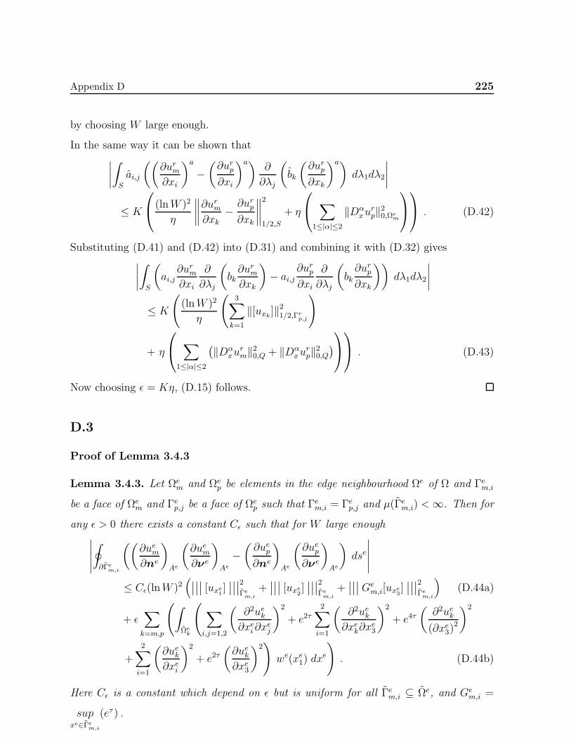
Appendix D 225
by choosing W large enough.
In the same way it can be shown that∣∣∣∣∫
S
ai,j
((∂urm∂xi
)a−(∂urp∂xi
)a)∂
∂λj
(bk
(∂urp∂xk
)a)dλ1dλ2
∣∣∣∣
≤ K
(lnW )2
η
∥∥∥∥∂urm∂xk− ∂urp∂xk
∥∥∥∥2
1/2,S
+ η
∑
1≤|α|≤2
‖Dαxu
rp‖20,Ωr
m
. (D.42)
Substituting (D.41) and (D.42) into (D.31) and combining it with (D.32) gives∣∣∣∣∫
S
(ai,j
∂urm∂xi
∂
∂λj
(bk∂urm∂xk
)− ai,j
∂urp∂xi
∂
∂λj
(bk∂urp∂xk
))dλ1dλ2
∣∣∣∣
≤ K
((lnW )2
η
(3∑
k=1
‖[uxk ]‖21/2,Γrp,j
)
+ η
∑
1≤|α|≤2
(‖Dα
xurm‖20,Q + ‖Dα
xurp‖20,Q
) . (D.43)
Now choosing ǫ = Kη, (D.15) follows.
D.3
Proof of Lemma 3.4.3
Lemma 3.4.3. Let Ωem and Ωep be elements in the edge neighbourhood Ωe of Ω and Γem,i
be a face of Ωem and Γep,j be a face of Ωep such that Γem,i = Γep,j and µ(Γem,i) <∞. Then for
any ǫ > 0 there exists a constant Cǫ such that for W large enough∣∣∣∣∣
∮
∂Γem,i
((∂uem∂ne
)
Ae
(∂uem∂νe
)
Ae
−(∂uep∂ne
)
Ae
(∂uep∂νe
)
Ae
)dse
∣∣∣∣∣
≤ Cǫ(lnW )2(∣∣∣∣∣∣ [uxe1]
∣∣∣∣∣∣2Γem,i
+∣∣∣∣∣∣ [uxe2]
∣∣∣∣∣∣2Γem,i
+∣∣∣∣∣∣Ge
m,i[uxe3]∣∣∣∣∣∣2
Γem,i
)(D.44a)
+ ǫ∑
k=m,p
(∫
Ωek
(∑
i,j=1,2
(∂2uek∂xei∂x
ej
)2
+ e2τ2∑
i=1
(∂2uek∂xek∂x
e3
)2
+ e4τ(∂2uek(∂xe3)
2
)2
+
2∑
i=1
(∂uek∂xei
)2
+ e2τ(∂uek∂xe3
)2)we(xe1) dx
e
). (D.44b)
Here Cǫ is a constant which depend on ǫ but is uniform for all Γem,i ⊆ Ωe, and Gem,i =
supxe∈Γe
m,i
(eτ ) .
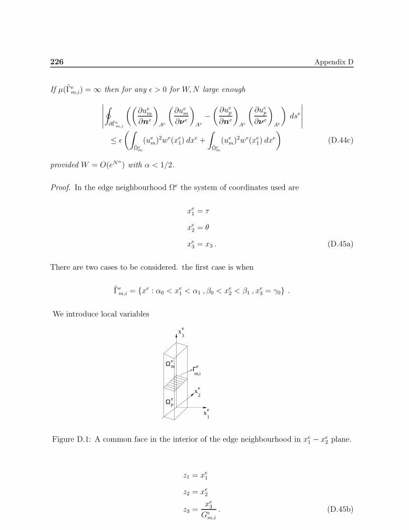
226 Appendix D
If µ(Γem,i) =∞ then for any ǫ > 0 for W,N large enough
∣∣∣∣∣
∮
∂Γem,i
((∂uem∂ne
)
Ae
(∂uem∂νe
)
Ae
−(∂uep∂ne
)
Ae
(∂uep∂νe
)
Ae
)dse
∣∣∣∣∣
≤ ǫ
(∫
Ωem
(uem)2we(xe1) dx
e +
∫
Ωem
(uem)2we(xe1) dx
e
)(D.44c)
provided W = O(eNα) with α < 1/2.
Proof. In the edge neighbourhood Ωe the system of coordinates used are
xe1 = τ
xe2 = θ
xe3 = x3 . (D.45a)
There are two cases to be considered. the first case is when
Γem,i = xe : α0 < xe1 < α1 , β0 < xe2 < β1 , xe3 = γ0 .
We introduce local variables
x
x
x
1
3
2
e
e
e
Γ
Ωp
Ωm
e
e
m,i
e
Figure D.1: A common face in the interior of the edge neighbourhood in xe1 − xe2 plane.
z1 = xe1
z2 = xe2
z3 =xe3Gem,i
. (D.45b)
Appendix D 227
Now
(∂u
∂xe1
)
Ae
=[1 0 0
]Ae
∂u∂xe1
∂u∂xe2
∂u∂xe3
=[1 0 0
]
1 0 0
0 1 0
0 0 1Ge
m,i
A
e
1 0 0
0 1 0
0 0 1Ge
m,i
∂u∂z1
∂u∂z2
∂u∂z3
Hence we obtain
(∂u
∂xe1
)
Ae
=
(∂u
∂z1
)
Ae
(D.46a)
(∂u
∂xe2
)
Ae
=
(∂u
∂z2
)
Ae
(D.46b)
(∂u
∂xe3
)
Ae
= Gem,i
(∂u
∂z3
)
Ae
. (D.46c)
Here using (3.76)
Ae = (Se)TASe (D.47a)
where
Se =
cos θ − sin θ 0
sin θ cos θ 0
0 0 eτ
Gem,i
. (D.47b)
Hence Ae and its derivatives with respect to z are uniformly bounded in Ωem and Ωep. Here
Ωem and Ωep are the images of Ωem and Ωep in z variables respectively. Now
1
23e
e
e
e
γ
n
ν
e
^
zz
z
Figure D.2: γ, image of γ, in z−coordinates.

228 Appendix D
∫
γ
((∂uem∂ne
)
Ae
(∂uem∂νe
)
Ae
−(∂uep∂ne
)
Ae
(∂uep∂νe
)
Ae
)dse
=
∫
γ
((∂uem∂xe1
)
Ae
(∂uem∂xe3
)
Ae
−(∂uep∂xe1
)
Ae
(∂uep∂xe3
)
Ae
)dxe2
= Gem,i
∫
γ
((∂uem∂z1
)
Ae
(∂uem∂z3
)
Ae
−(∂uep∂z1
)
Ae
(∂uep∂z3
)
Ae
)dz2 . (D.48)
Here γ is the image of γ in z coordinates as shown in Figure D.2.
Proceeding as in Lemma 3.4.1 we can prove using the representation (D.48) that for
any η > 0 there exists a constant Cη, which depends on η, but is uniform for all Γem,i ⊆ Ωe
such that∣∣∣∣∣
∫
∂Γem,i
((∂uem∂ne
)
Ae
(∂uem∂νe
)
Ae
−(∂uep∂ne
)
Ae
(∂uep∂νe
)
Ae
)dse
∣∣∣∣∣
≤ Gem,i
(Cη(lnW )2
3∑
k=1
‖[uzk ]‖21/2,Γem,i
+ η
∑
1≤|α|≤2
(‖Dα
z uem‖20,Ωe
m+ ‖Dα
z uep‖20,Ωe
p
) . (D.49)
Here Γem,i is the image of Γem,i in z coordinates and Ωem and Ωep are the images of Ωem and
Ωep in z coordinates. And by a proper choice of η in (D.49) we obtain (D.44).
The other case to be considered is when the boundary Γem,i corresponds to
Γem,i = xe : α0 < xe1 < α1, xe2 = β0, γ0 < xe3 < γ1 .
The case when
x1
x2e
e
x3e
Γem,i
Figure D.3: A common face in the interior of the edge neighbourhood in xe1 − xe3 plane.
Γem,i = xe : xe1 = α0, β0 < xe2 < β1, γ0 < xe3 < γ1
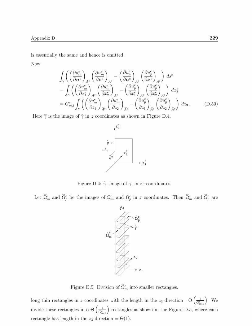
Appendix D 229
is essentially the same and hence is omitted.
Now∫
γ
((∂uem∂ne
)
Ae
(∂uem∂νe
)
Ae
−(∂uep∂ne
)
Ae
(∂uep∂νe
)
Ae
)dse
=
∫
γ
((∂uem∂xe1
)
Ae
(∂uem∂xe2
)
Ae
−(∂uep∂xe1
)
Ae
(∂uep∂xe2
)
Ae
)dxe3
= Gem,i
∫
γ
((∂uem∂z1
)
Ae
(∂uem∂z2
)
Ae
−(∂uep∂z1
)
Ae
(∂uep∂z2
)
Ae
)dz3 . (D.50)
Here γ is the image of γ in z coordinates as shown in Figure D.4.
x
1
2
3
e
e
e
νe
γ
z
z
^
en
Figure D.4: γ, image of γ, in z−coordinates.
Let Ωem and Ωep be the images of Ωem and Ωep in z coordinates. Then Ωem and Ωep are
z
z
z
3
1
2
γ^
Ω^ e p
Ωm
e ^
Figure D.5: Division of Ωem into smaller rectangles.
long thin rectangles in z coordinates with the length in the z3 direction= Θ(
1Ge
m,i
). We
divide these rectangles into Θ(
1Ge
m,i
)rectangles as shown in the Figure D.5, where each
rectangle has length in the z3 direction = Θ(1).
230 Appendix D
Proceeding as in Lemma 3.4.1 we can prove using the representation (D.50) that
∣∣∣∣∣
∫
∂Γem,i
((∂uem∂ne
)
Ae
(∂uem∂νe
)
Ae
−(∂uep∂ne
)
Ae
(∂uep∂νe
)
Ae
)dse
∣∣∣∣∣
≤ Gem,i
(Cη(lnW )2
3∑
k=1
‖[uzk ]‖21/2,Γem,i
+ η
∑
1≤|α|≤2
(‖Dα
z uem‖20,Ωe
m+ ‖Dα
z uep‖20,Ωe
p
) . (D.51)
Here Γem,i is the image of Γem,i in z coordinates and Ωem and Ωep are the images of Ωem and
Ωep in z coordinates. Now by a proper choice of η in (D.51) we obtain (D.44).
D.4
Proof of Lemma 3.4.4
Lemma 3.4.4. Let Ωem and Ωep be elements in the edge neighbourhood Ωe of Ω and Γem,i
be a face of Ωem and Γep,j be a face of Ωep such that Γem,i = Γep,j and µ(Γem,i) <∞. Then for
any ǫ > 0 there exists a constant Cǫ such that for W large enough
∣∣∣∣∣
∫
Γem,i
2∑
l=1
((∂uem∂τ el
)
Ae
∂
∂sel
((∂uem∂νe
)
Ae
)−(∂uep∂τ el
)
Ae
∂
∂sel
((∂uep∂νe
)
Ae
))dσe
∣∣∣∣∣
≤ Cǫ(lnW )2(∣∣∣∣∣∣ [uxe1]
∣∣∣∣∣∣2Γem,i
+∣∣∣∣∣∣ [uxe2]
∣∣∣∣∣∣2Γem,i
+∣∣∣∣∣∣Ge
m,i[uxe3]∣∣∣∣∣∣2
Γem,i
)
+ ǫ∑
k=m,p
(∫
Ωek
(∑
i,j=1,2
(∂2uek∂xei∂x
ej
)2
+ e2τ2∑
i=1
(∂2uek∂xei∂x
e3
)2
+ e4τ(∂2uek(∂xe3)
2
)2
+2∑
i=1
(∂uek∂xei
)2
+ e2τ(∂uek∂xe3
)2)we(xe1) dx
e
). (D.52a)
If µ(Γem,i) =∞ then for any ǫ > 0 for W,N large enough
∣∣∣∣∣
∫
Γem,i
2∑
l=1
((∂uem∂τ el
)
Ae
∂
∂sel
((∂uem∂νe
)
Ae
)−(∂uep∂τ el
)
Ae
∂
∂sel
((∂uep∂νe
)
Ae
))dσe
∣∣∣∣∣
≤ ǫ
(∫
Ωem
(uem)2we(xe1) dx
e +
∫
Ωem
(uem)2we(xe1) dx
e
)(D.52b)
provided W = O(eNα) with α < 1/2.
Appendix D 231
Proof. Let us first consider the case when
Γem,i = xe : α0 < xe1 < α1 β0 < xe2 < β1 xe3 = γ0
which corresponds to Figure D.1.
Now using (D.47)
∫
Γem,i
2∑
l=1
((∂uem∂τ el
)
Ae
∂
∂sel
((∂uem∂νe
)
Ae
)
−(∂uep∂τ el
)
Ae
∂
∂sel
((∂uep∂νe
)
Ae
))dσe
=
∫
Γem,i
2∑
l=1
((∂uem∂xel
)
Ae
∂
∂xel
((∂uem∂xe3
)
Ae
)
−(∂uep∂xel
)
Ae
∂
∂xel
((∂uep∂xe3
)
Ae
))dxe1dx
e2
= Gem,i
∫
Γem,i
2∑
l=1
((∂uem∂zl
)
Ae
∂
∂zl
((∂uem∂z3
)
Ae
)
−(∂uep∂zl
)
Ae
∂
∂zl
((∂uep∂z3
)
Ae
))dz1dz2 . (D.53)
Proceeding as in Lemma 3.4.2 we can prove using the representation (D.53) that for
any η > 0 there exists a constant Cη, which depends on η, but is uniform for all Γem,i ⊆ Ωe
such that
∫
Γem,i
2∑
l=1
((∂uem∂τ el
)
Ae
∂
∂sel
((∂uem∂νe
)
Ae
)−(∂uep∂τ el
)
Ae
∂
∂sel
((∂uep∂νe
)
Ae
))dσe
≤ Gem,i
(Cη(lnW )2
3∑
k=1
‖[uzk ]‖21/2,Γem,i
+ η
∑
1≤|α|≤2
(‖Dα
z uem‖20,Ωe
m+ ‖Dα
z uep‖20,Ωe
p
) . (D.54)
And by a proper choice of η in (D.54) we obtain (D.52).
The next case we consider is when the boundary Γem,i corresponds to
Γem,i = xe : α0 < xe1 < α1, xe2 = β0, γ0 < xe3 < γ1 .
232 Appendix D
The boundary Γem,i is shown in Figure D.3. Now
∫
Γem,i
2∑
l=1
((∂uem∂τ el
)
Ae
∂
∂sel
((∂uem∂νe
)
Ae
)−(∂uep∂τ el
)
Ae
∂
∂sel
((∂uep∂νe
)
Ae
))dσe
=
∫
Γem,i
((∂uem∂xe1
)
Ae
∂
∂xe1
((∂uem∂xe2
)
Ae
)−(∂uep∂xe1
)
Ae
∂
∂xe1
((∂uep∂xe2
)
Ae
))dxe1dx
e3
+
∫
Γem,i
((∂uem∂xe3
)
Ae
∂
∂xe3
((∂uem∂xe2
)
Ae
)−(∂uep∂xe3
)
Ae
∂
∂xe3
((∂uep∂xe2
)
Ae
))dxe1dx
e3 .
Hence∫
Γem,i
2∑
l=1
((∂uem∂τ el
)
Ae
∂
∂sel
((∂uem∂νe
)
Ae
)
−(∂uep∂τ el
)
Ae
∂
∂sel
((∂uep∂νe
)
Ae
))dσe
= Gem,i
(∫
Γem,i
((∂uem∂z1
)
Ae
∂
∂z1
((∂uem∂z2
)
Ae
)
−(∂uep∂z1
)
Ae
∂
∂z1
((∂uep∂z2
)
Ae
))dz1dz3
+
∫
Γem,i
((∂uem∂z3
)
Ae
∂
∂z3
((∂uem∂z2
)
Ae
)
−(∂uep∂z3
)
Ae
∂
∂z3
((∂uep∂z2
)
Ae
))dz1dz3
). (D.55)
Proceeding as in Lemma 3.4.2 we can prove using the representation (D.55) that for
any η > 0 there exists a constant Cη, which depends on η, but is uniform for all Γem,i ⊆ Ωe
such that∣∣∣∣∣
∫
Γem,i
2∑
l=1
((∂uem∂τ el
)
Ae
∂
∂sel
((∂uem∂νe
)
Ae
)−(∂uep∂τ el
)
Ae
∂
∂sel
((∂uep∂νe
)
Ae
))dσe
∣∣∣∣∣
≤ Gem,i
(Cη(lnW )2
3∑
k=1
‖[uzk ]‖21/2,Γem,i
+ η
∑
1≤|α|≤2
(‖Dα
z uem‖20,Ωe
m+ ‖Dα
z uep‖20,Ωe
p
) . (D.56)
Now by a proper choice of η, (D.52) follows.
D.5
Proof of Lemma 3.5.1
Appendix D 233
Lemma 3.5.1. Let Γrm,j be part of the boundary of the element Ωrm which lies on the
x2 − x3 axis. Define the contributions from Γrm,j by
(BT )rm,j = ρ2v sin2(φv)
(−∮
∂Γrm,j
(∂u
∂n
)
A
(∂u
∂ν
)
A
ds
+ 2
∫
Γrm,j
2∑
j=1
(∂u
∂τ j
)
A
∂
∂sj
((∂u
∂ν
)
A
)dσ
). (D.57)
If Dirichlet boundary conditions are imposed on Γrm,j then
|(BT )rm,j| ≤ Cǫ(lnW )2‖urm‖23/2,Γrm,j
+Kǫ
∑
|α|=1
‖Dαxu
rm‖20,Ωr
m
+ ǫ∑
|α|=2
‖Dαxu
rm‖20,Ωr
m. (D.58)
If Neumann boundary conditions are imposed on Γrm,j then
∣∣(BT )rm,j∣∣ ≤ Cǫ(lnW )2
∥∥∥∥(∂urm∂ν
)
A
∥∥∥∥2
1/2,Γrm,j
+ ǫ∑
1≤|α|≤2
‖Drxu
rm‖22,Ωr
m. (D.59)
Proof. In case the boundary conditions on the face corresponding to the x2 − x3 axis are
Neumann we can show that for any ǫ > 0
∣∣(BT )rm,j∣∣ ≤ Cǫ(lnW )2
∥∥∥∥(∂urm∂ν
)
A
∥∥∥∥2
1/2,Γrm,j
+ ǫ∑
1≤|α|≤2
‖Drxu
rm‖22,Ωr
m. (D.60)
We now need to examine the case when Dirichlet boundary conditions are imposed on
the face corresponding to the x2 − x3 plane.
We may choose
τ 1 = (0, 0, 1) ,
τ 2 = (0, 1, 0) ,
ν = (−1, 0, 0) . (D.61)
Now
Aτ 1 = α11τ 1 + α12τ 2 + α13Aν
Aτ 2 = α21τ 1 + α22τ 2 + α23Aν (D.62)
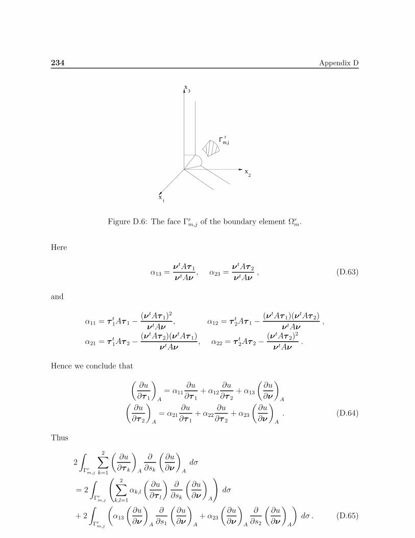
234 Appendix D
x
x
x1
2
3
Γ rm,j
Figure D.6: The face Γrm,j of the boundary element Ωrm.
Here
α13 =νtAτ 1
νtAν, α23 =
νtAτ 2
νtAν, (D.63)
and
α11 = τ t1Aτ 1 −(νtAτ 1)
2
νtAν, α12 = τ t2Aτ 1 −
(νtAτ 1)(νtAτ 2)
νtAν,
α21 = τ t1Aτ 2 −(νtAτ 2)(ν
tAτ 1)
νtAν, α22 = τ t2Aτ 2 −
(νtAτ 2)2
νtAν.
Hence we conclude that
(∂u
∂τ 1
)
A
= α11∂u
∂τ 1+ α12
∂u
∂τ 2+ α13
(∂u
∂ν
)
A(∂u
∂τ 2
)
A
= α21∂u
∂τ 1+ α22
∂u
∂τ 2+ α23
(∂u
∂ν
)
A
. (D.64)
Thus
2
∫
Γrm,j
2∑
k=1
(∂u
∂τ k
)
A
∂
∂sk
(∂u
∂ν
)
A
dσ
= 2
∫
Γrm,j
(2∑
k,l=1
αk,l
(∂u
∂τ l
)∂
∂sk
(∂u
∂ν
)
A
)dσ
+ 2
∫
Γrm,j
(α13
(∂u
∂ν
)
A
∂
∂s1
(∂u
∂ν
)
A
+ α23
(∂u
∂ν
)
A
∂
∂s2
(∂u
∂ν
)
A
)dσ . (D.65)
Appendix D 235
Now
2
∫
Γrm,j
(α13
(∂u
∂ν
)
A
∂
∂s1
(∂u
∂ν
)
A
+ α23
(∂u
∂ν
)
A
∂
∂s2
(∂u
∂ν
)
A
)dσ
=
∫
Γrm,j
(∂
∂s1
(α13
(∂u
∂ν
)2
A
)+
∂
∂s2
(α23
(∂u
∂ν
)2
A
))dσ
−∫
Γrm,j
(∂
∂s1(α13) +
∂
∂s2(α23)
)(∂u
∂ν
)2
A
dσ . (D.66)
Using the divergence theorem we conclude that
2
∫
Γrm,j
(α13
(∂u
∂ν
)
A
∂
∂s1
(∂u
∂ν
)
A
+ α23
(∂u
∂ν
)
A
∂
∂s2
(∂u
∂ν
)
A
)dσ
=
∫
∂Γrm,j
(n · τ 1)α13 + (n · τ 2)α23(∂u
∂ν
)2
A
ds
−∫
Γrm,j
(∂
∂s1(α13) +
∂
∂s2(α23)
)(∂u
∂ν
)2
A
dσ . (D.67)
Here n denotes the unit outward normal to ∂Γrm,j .
Now
(n · τ 1)α13 + (n · τ 2)α23 =(n · τ 1)ν
tAτ 1 + (n · τ 2)νtAτ 2
νtAν
=νtA(n · τ 1)τ 1 + (n · τ 2)τ 2
νtAν=
νtAn
νtAν.
Hence∫
∂Γrm,j
(n · τ 1)α13 + (n · τ 2)α23(∂u
∂ν
)2
A
ds =
∫
∂Γrm,j
νtAn
νtAν
(∂u
∂ν
)2
A
ds . (D.68)
Thus
2ρ2v sin2(φv)
∫
Γrm,j
2∑
k=1
(∂u
∂τ k
)
A
∂
∂sk
(∂u
∂ν
)
A
dσ
= ρ2v sin2(φv)
(∫
Γrm,j
(2∑
k,l=1
2αk,l
(∂u
∂τ l
)∂
∂sk
(∂u
∂ν
)
A
)dσ
−∫
Γrm,j
(2∑
k=1
∂
∂sk(αk3)
)(∂u
∂ν
)2
A
dσ +
∫
∂Γrm,j
νtAn
νtAν
(∂u
∂ν
)2
A
ds
). (D.69)
We now examine the term
ρ2v sin2(φv)
(−∮
∂Γrm,j
(∂u
∂n
)
A
(∂u
∂ν
)
A
ds
). (D.70)
236 Appendix D
Now (∂u
∂n
)
A
= γ11∂u
∂τ 1+ γ12
∂u
∂τ 2+ γ13
(∂u
∂ν
)
A
.
Here
γ13 =νtAn
νtAν,
γ11 = τ t1An−(νtAn)(νtAτ 1)
νtAν,
γ12 = τ t2An−(νtAn)(νtAτ 2)
νtAν. (D.71)
Hence
ρ2v sin2(φv)
(−∮
∂Γrm,j
(∂u
∂n
)
A
(∂u
∂ν
)
A
ds
)
= ρ2v sin2(φv)
(−∮
∂Γrm,j
2∑
k=1
γ1,k∂u
∂τ k
(∂u
∂ν
)
A
ds
−∮
∂Γrm,j
(νtAn
νtAν
)(∂u
∂ν
)2
A
ds
). (D.72)
Combining (D.69) and (D.72) we obtain
(BT )rm,j = ρ2v sin2(φv)
(∫
Γrm,j
(2∑
k,l=1
2αk,l∂u
∂τ l
∂
∂sk
(∂u
∂ν
)
A
)dσ (D.73)
−∫
Γrm,j
(2∑
k=1
∂
∂sk(αk3)
)(∂u
∂ν
)2
A
dσ −∮
∂Γrm,j
2∑
k=1
γ1,k∂u
∂τ k
(∂u
∂n
)
A
ds
).
(D.74)
Using (D.73) we can show that
∥∥(BT )rm,j∥∥ ≤ Cǫ(lnW )2‖urm‖23/2,Γr
m,j+ ǫ/2
∑
1≤|α|≤2
‖Dαxu
rm‖20,Ωr
m
+K|urm|21,Γrm,j
. (D.74)
Now
|urm|21,Γrm,j≤ Kǫ|urm|21,Ωr
m+ ǫ/2|urm|22,Ωr
m. (D.75)
Appendix D 237
Hence
∥∥(BT )rm,j∥∥ ≤ Cǫ(lnW )2‖urm‖23/2,Γr
m,j+Kǫ
∑
|α|=1
‖Dαxu
rm‖20,Ωr
m
+ ǫ∑
|α|=2
‖Dαxu
rm‖20,Ωr
m. (D.76)
D.6
Proof of Lemma 3.5.2
Lemma 3.5.2. Let Γem,j be part of the boundary of the element Ωem which lies on the
x2 − x3 axis. Define the contributions from Γem,j by
(BT )em,j = −∮
∂Γem,j
(∂u
∂ne
)
Ae
(∂u
∂νe
)
Ae
dse
− 2
∫
Γem,j
2∑
l=1
(∂u
∂τ el
)
Ae
∂
∂sel
((∂u
∂νe
)
Ae
)dσe . (D.77)
If Dirichlet boundary conditions are imposed on Γem,j and µ(Γem,j) <∞ then for any ǫ > 0
there exists constants Cǫ, Kǫ such that for W large enough
|(BT )em,j| ≤ Cǫ(lnW )2(‖uem‖20,Γe
m,i+∣∣∣∣∣∣∣∣∣(∂uem∂xe1
) ∣∣∣∣∣∣∣∣∣2
Γem,j
+∣∣∣∣∣∣∣∣∣Ge
m,j
(∂uem∂xe3
) ∣∣∣∣∣∣∣∣∣2
Γem,j
)
+Kǫ
∫
Ωem
(2∑
i=1
(∂uem∂xei
)2
+ e2τ(∂uem∂xe3
)2)dxe + ǫ
∫
Ωem
(∑
i,j=1,2
(∂2uem∂xei∂x
ej
)2
+e2τ2∑
i=1
(∂2uem∂xei∂x
e3
)2
+ e4τ(∂2uem(∂xe3)
2
)2)dxe . (D.78)
If Neumann boundary conditions are imposed on Γem,j and µ(Γem,j) <∞ then for any ǫ > 0
there exists a constant Cǫ such that
∣∣(BT )em,j∣∣ ≤ Cǫ(lnW )2
∣∣∣∣∣∣∣∣∣(∂u
∂νe
)
Ae
∣∣∣∣∣∣∣∣∣2
Γem,j
+ ǫ
(∫
Ωem
(2∑
i,j=1
(∂2uem∂xei∂x
ej
)2
+e2τ2∑
i=1
(∂2uem∂xei∂x
e3
)2
+ e4τ(∂2uem(∂xe3)
2
)2
+
2∑
i=1
(∂uem∂xei
)2
+e2τ(∂uem∂xe3
)2)dxe
). (D.79)
238 Appendix D
If µ(Γem,j) =∞ then for any ǫ > 0 for N,W large enough
∣∣(BT )em,j∣∣ ≤ ǫ
∫
Ωem
(uem)2we(xe1) dx
e
provided W = O(eNα) for α < 1/2.
Proof. In the edge neighbourhood the coordinates used are
xe1 = τ
xe2 = θ
xe3 = x3 . (D.80)
We introduce the variables as in (D.45)
z1 = xe1
z2 = xe2
z3 =xe3Gem,i
. (D.81)
Let us examine the term
(BT )em,j = −2∫
Γem,j
2∑
l=1
(∂u
∂τ el
)
Ae
∂
∂sel
(∂u
∂νe
)
Ae
dσe
+
∮
∂Γem,j
(∂u
∂ne
)
Ae
(∂u
∂νe
)
Ae
dse . (D.82)
If the boundary conditions are Neumann we can prove as in Lemma 3.4.4 that
|(BT )em,j| ≤ Cǫ(lnW )2|||(∂uem∂νe
)
Ae
|||2Γem,j
+ ǫ
(∫
Ωem
∑
i,j=1,2
(∂2uem∂xei∂x
ej
)2
+ e2τ2∑
i=1
(∂2uem∂xei∂x
e3
)2
+ e4τ(∂2uem(∂xe3)
2
)2
+2∑
i=1
(∂uem∂xei
)2
+ e2τ(∂uem∂xe3
)2)we(xe1) dx
e . (D.83)
Let us now examine the case when the boundary conditions are Dirichlet.
Now choose
τ e1 = (1, 0, 0)
τ e2 = (0, 0, 1)
νe = (0,−1, 0) . (D.84)
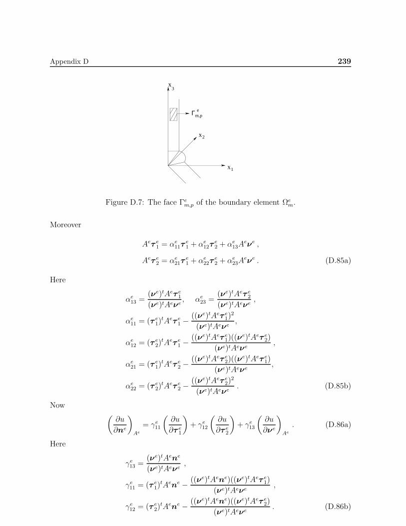
Appendix D 239
x
x3
x2
1
m,pΓ e
Figure D.7: The face Γem,p of the boundary element Ωem.
Moreover
Aeτ e1 = αe11τe1 + αe12τ
e2 + αe13A
eνe ,
Aeτ e2 = αe21τe1 + αe22τ
e2 + αe23A
eνe . (D.85a)
Here
αe13 =(νe)tAeτ e1(νe)tAeνe
, αe23 =(νe)tAeτ e2(νe)tAeνe
,
αe11 = (τ e1)tAeτ e1 −
((νe)tAeτ e1)2
(νe)tAeνe,
αe12 = (τ e2)tAeτ e1 −
((νe)tAeτ e1)((νe)tAeτ e2)
(νe)tAeνe,
αe21 = (τ e1)tAeτ e2 −
((νe)tAeτ e2)((νe)tAeτ e1)
(νe)tAeνe,
αe22 = (τ e2)tAeτ e2 −
((νe)tAeτ e2)2
(νe)tAeνe. (D.85b)
Now(∂u
∂ne
)
Ae
= γe11
(∂u
∂τ e1
)+ γe12
(∂u
∂τ e2
)+ γe13
(∂u
∂νe
)
Ae
. (D.86a)
Here
γe13 =(νe)tAene
(νe)tAeνe,
γe11 = (τ e1)tAene − ((νe)tAene)((νe)tAeτ e1)
(νe)tAeνe,
γe12 = (τ e2)tAene − ((νe)tAene)((νe)tAeτ e2)
(νe)tAeνe. (D.86b)
240 Appendix D
Then it can be shown that
(BT )em,j =
(∫
Γem,j
(2∑
k,l=1
2αek,l∂u
∂τ el
∂
∂sek
(∂u
∂νe
)
Ae
)dσe
−∫
Γem,j
(2∑
k=1
∂
∂sek(αek3)
)(∂u
∂νe
)2
Ae
dσe
−∮
∂Γem,j
2∑
k=1
γe1,k∂u
∂τ ek
(∂u
∂ne
)
Ae
dse
). (D.87)
Now
αe13 =(νe)tAeτ e1(νe)tAeνe
, αe23 =(νe)tAeτ e2(νe)tAeνe
,
αe11 = (τ e1)tAeτ e1 −
((νe)tAeτ e1)2
(νe)tAeνe,
αe12 = (τ e2)tAeτ e1 −
((νe)tAeτ e1)((νe)tAeτ e2)
(νe)tAeνe,
αe21 = αe12, αe22 = (τ e2)tAeτ e2 −
((νe)tAeτ e2)2
(νe)tAeνe. (D.88)
Hence
( I ) =
∫
Γem,j
(2∑
k,l=1
2αek,l∂u
∂τ el
∂
∂sek
((∂u
∂νe
)
Ae
))dσe
= −∫
Γem,j
2
(αe1,1
∂u
∂xe1
∂
∂xe1
((∂u
∂xe2
)
Ae
)+ αe1,2
∂u
∂xe3
∂
∂xe1
((∂u
∂xe2
)
Ae
)
+ αe2,1∂u
∂xe1
∂
∂xe3
((∂u
∂xe2
)
Ae
)+ αe2,2
∂u
∂xe3
∂
∂xe3
((∂u
∂xe2
)
Ae
))dxe1 dx
e3
= −2Gem,j
∫
Γem,j
(αe1,1
∂u
∂z1
∂
∂z1
((∂u
∂z2
)
Ae
)+
αe1,2Gem,j
∂u
∂z3
∂
∂z1
((∂u
∂z2
)
Ae
)
+αe2,1Gem,j
∂u
∂z1
∂
∂z3
((∂u
∂z2
)
Ae
)+
αe2,2(Ge
m,j)2
∂u
∂z3
∂
∂z3
((∂u
∂z2
)
Ae
))dz1 dz3 . (D.89)
Here Γem,j denotes the image of Γem,j in z coordinates.
Now from (3.79), (3.80) and (D.88) αe1,1,αe1,2
Gem,j,
αe2,1
Gem,j
andαe2,2
(Gem,j )
2 are bounded and have
bounded derivatives in z coordinates.
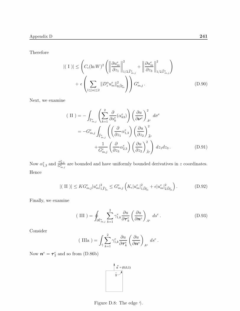
Appendix D 241
Therefore
|( I )| ≤(Cǫ(lnW )2
(∥∥∥∥∂uem∂z1
∥∥∥∥2
1/2,Γem,j
+
∥∥∥∥∂uem∂z3
∥∥∥∥2
1/2,Γem,j
)
+ ǫ
∑
1≤|α|≤2
‖Dαz u
em‖20,Ωe
m
Ge
m,j . (D.90)
Next, we examine
( II ) = −∫
Γem,j
(2∑
k=1
∂
∂sek(αek3)
)(∂u
∂νe
)2
Ae
dσe
= −Gem,j
∫
Γem,j
((∂
∂z1αe1,3
)(∂u
∂z2
)2
Ae
+1
Gem,j
(∂
∂z3αe2,3
)(∂u
∂z2
)2
Ae
)dz1dz3 . (D.91)
Now αe1,3 andαe2,3
Gem,j
are bounded and have uniformly bounded derivatives in z coordinates.
Hence
|( II )| ≤ KGem,j |uem|21,Γe
m≤ Ge
m,j
(Kǫ|uem|21,Ωe
m+ ǫ|uem|22,Ωe
m
). (D.92)
Finally, we examine
( III ) =
∮
∂Γem,j
2∑
k=1
γe1,k∂u
∂τ ek
(∂u
∂ne
)
Ae
dse . (D.93)
Consider
( IIIa ) =
∫
γ
2∑
k=1
γe1,k∂u
∂τ ek
(∂u
∂ne
)
Ae
dse .
Now ne = τ e2 and so from (D.86b)
ne
= (0,0,1)
γ~
Figure D.8: The edge γ.
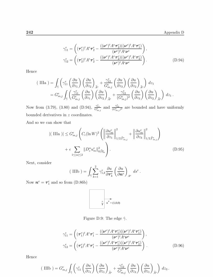
242 Appendix D
γe11 =
((τ e1)
tAeτ e2 −((νe)tAeτ e2)((ν
e)tAeτ e1)
(νe)tAeνe
),
γe12 =
((τ e2)
tAeτ e2 −((νe)tAeτ e2)((ν
e)tAeτ e2)
(νe)tAeνe
). (D.94)
Hence
( IIIa ) =
∫
γ
(γe11
(∂u
∂z1
)(∂u
∂z2
)
Ae
+γe12Gem,j
(∂u
∂z3
)(∂u
∂z2
)
Ae
)dz1
= Gem,j
∫
γ
(γe11Gem,j
(∂u
∂z1
)(∂u
∂z2
)
Ae
+γe12
(Gem,j)
2
(∂u
∂z3
)(∂u
∂z2
)
Ae
)dz1 .
Now from (3.79), (3.80) and (D.94),γe11Ge
m,jand
γe12(Ge
m,j)2 are bounded and have uniformly
bounded derivatives in z coordinates.
And so we can show that
|( IIIa )| ≤ Gem,j
(Cǫ(lnW )2
(∥∥∥∥∂uem∂z1
∥∥∥∥2
1/2,Γem,j
+
∥∥∥∥∂uem∂z3
∥∥∥∥2
1/2,Γem,j
)
+ ǫ∑
1≤|α|≤2
‖Dαz u
em‖20,Ωe
m
. (D.95)
Next, consider
( IIIb ) =
∫
γ
2∑
k=1
γe1,k∂u
∂τ ek
(∂u
∂ne
)
Ae
dse .
Now ne = τ e1 and so from (D.86b)
ne
= (1,0,0)γ^
Figure D.9: The edge γ.
γe11 =
((τ e1)
tAeτ e1 −((νe)tAeτ e1)((ν
e)tAeτ e1)
(νe)tAeνe
),
γe12 =
((τ e2)
tAeτ e1 −((νe)tAeτ e1)((ν
e)tAeτ e2)
(νe)tAeνe
). (D.96)
Hence
( IIIb ) = Gem,j
∫
γ
(γe11
(∂u
∂z1
)(∂u
∂z1
)
Ae
+γe12Gem,j
(∂u
∂z3
)(∂u
∂z1
)
Ae
)dz3 .
Appendix D 243
Now from (3.79), (3.80) and (D.96), γe11 andγe12Ge
m,jare bounded and have uniformly bounded
derivatives in z coordinates.
So we can show that
|( IIIb )| ≤ Gem,j
(Cǫ(lnW )2
(∥∥∥∥∂uem∂z1
∥∥∥∥2
1/2,Γem,j
+
∥∥∥∥∂uem∂z3
∥∥∥∥2
1/2,Γem,j
)
+ ǫ∑
1≤|α|≤2
‖Dαz u
em‖20,Ωe
m
. (D.97)
Combining (D.90), (D.92), (D.95) and (D.97), we obtain
|(BT )em,j| ≤ Gem,j
(Cǫ(lnW )2
(∥∥∥∥∂uem∂z1
∥∥∥∥2
1/2,Γem,j
+
∥∥∥∥∂uem∂z3
∥∥∥∥2
1/2,Γem,j
)
+ Kǫ
∑
|α|=1
‖Dαz u
em‖20,Ωe
m+ ǫ
∑
|α|=2
‖Dαz u
em‖20,Ωe
m
. (D.98)
From this the result follows.

Bibliography
[1] R.A. Adams (1975): Sobolev Spaces, Academic Press, New York.
[2] G. Anagnostou (1991): Non-conforming sliding spectral element method for the un-
steady incompressible Navier-Stokes equations, Ph.D. thesis, Massachusetts Institute
of Technology.
[3] B. Andersson, U. Falk, I. Babuska and T. Von-Petersdorff (1995): Reliable stress and
fracture mechanics analysis of complex components using a h − p version of FEM,
Int. J. Numer. Meth. Eng., 38, 2135.
[4] D.N. Arnold, F. Brezzi, B. Cockburn and D. Marini (2000): The development of
discontinuous Galerkin methods. In Discontinuous Galerkin methods: Theory, com-
putation and applications (ed. B. Cockburn, G.E. Karniadakis and C.W. Shu), p. 89.
Springer, Germany.
[5] D.N. Arnold, F. Brezzi, B. Cockburn and D. Marini (2002): Unified analysis of
discontinuous Galerkin methods for elliptic problems, SIAM J. Numer. Anal., 39,
1794.
[6] A.K. Aziz and I. Babuska (1972): The Mathematical Foundations of the Finite El-
ement Method with Applications to Partial Differential Equations, Academic Press,
New York.
[7] I. Babuska (1994): On the h, p and h− p version of the finite element method, Tatra
Mountains Math. Publ., 4, 5-18.
246 BIBLIOGRAPHY
[8] I. Babuska and B. Guo (1986): The h− p Version of the finite element method, Part
I: The basic approximation results, Comp. Mech., 1, 21-41.
[9] I. Babuska and B. Guo (1986): The h− p Version of the finite element method, Part
II: General results and Applications, Comp. Mech., 1, 203-220.
[10] I. Babuska and B. Guo (1988): Regularity of the solutions of elliptic problems with
piecewise analytic data, Part I: Boundary value problems for linear elliptic equation
of second order, SIAM J. Math. Anal. Vol. 19, No. 1, 172.
[11] I. Babuska and B. Guo (1988): The h − p version of the finite element method on
domains with curved boundaries, SIAM J. Num. Anal., Vol 25, 837.
[12] I. Babuska and B. Guo (1995): The h−p version of the finite element method in R3.
[13] I. Babuska and B. Guo (1996): Approximation properties of the h− p version of the
finite element method, Comp. Methods Appl. Mech. Engrg, 133, 319-346.
[14] I. Babuska and B. Guo (1997): Regularity of the solutions for elliptic problems on
non-smooth domains in R3, Part I: Countably Normed spaces on polyhedral domains;
Proc. of the Royal Society of Edinburgh, 127A, 77-126.
[15] I. Babuska and B. Guo (1997): Regularity of the solutions for elliptic problems on
non-smooth domains in R3, Part II: Regularity in neighbourhoods of edges; Tech.
Note BN-1182, IPST, University of Maryland, College Park, Proc. of the Royal So-
ciety of Edinburgh, 127A, 517-545.
[16] I. Babuska and B. Guo: Regularity of the solutions for elliptic problems on non-
smooth domains in R3, Part III: Regularity in neighbourhoods of vertices. To appear
in Proc. of the Royal Society of Edinburgh.
[17] I. Babuska and S.H. Oh (1990): The p-version of the Finite Element Method for
Domains with Corners and for Infinite Domains, Numer. Meth. PDEs., Vol. 6, pp
371-392.
BIBLIOGRAPHY 247
[18] I. Babuska, B. Guo, B. Andersson, H.S. Oh and J.M. Melenk (1996): Finite element
methods for solving problems with singular solutions, J. Comp. Appl. Math., Vol.
74, 51-70.
[19] I. Babuska and M. Suri (1994): The p and h−p version of the finite element method,
basic principles and properties, SIAM review, Vol. 36, No. 4, 578-632.
[20] I. Babuska, T. Von-Petersdorff and B. Andersson (1994): Numerical treatment of
vertex singularities and intensity factors for mixed boundary value problems for the
Laplace equation in R3, SIAM J. Numer. Anal., 31, 1265.
[21] A.E. Beagles and J.R. Whiteman (1985): Treatment of a reentrant vertex in three
dimensional Poisson problem, Singularities and constructive methods for their threat-
ment, edited by Grisvard et al, Lecture Note No. 1121, Springer-Verlag.
[22] C. Bernardi, Y. Maday, C. Mavriplis and A.T. Patera (1989): The mortar element
method applied to spectral discretizations, In Finite element analysis in fluids, sev-
enth international conference on finite element methods in flow problems (ed. T. J.
Chung and G. R. Karr). UAH Press, Huntsville, TX.
[23] C. Bernardi and Y. Maday (1999): Spectral methods. In Handbook of Numerical
Analysis V, ed. P.G. Ciarlet and J.L. Lions. Amsterdam: Elsevier Sciences.
[24] J.P. Boyd (2001): Chebyshev and Fourier Spectral Methods, 2nd edn. (Dover, New
York).
[25] E.N. Blinova (1944): Hydrodynamic theory of pressure and temperature waves and
center of action of the atmosphere, Trans. No. 113 (Regional Control Office, Second
Weather Region, Patterson Field, OH).
[26] P.B. Bochev, M.D. Gunzburger (2009): Least-Squares Finite Element Methods,
Springer.
[27] C. Canuto, M.Y. Hussaini, A. Quarteroni, T.A. Zang (1987): Spectral methods in
fluid dynamics, Springer, New York.
248 BIBLIOGRAPHY
[28] C. Canuto, M.Y. Hussaini, A. Quarteroni, T.A. Zang (2006): Spectral methods,
Fundamentals in single domains; Scientific computaion, Springer.
[29] C. Canuto, M.Y. Hussaini, A. Quarteroni, T.A. Zang (2007): Spectral methods,
Evolution to Complex geometries and applications to fluid dynamics, Scientific com-
putaion, Springer.
[30] R.W. Clough (1960): The Finite Element Method in Plane Stress Analysis, Proceed-
ings of 2nd ASCE Conference on Electronic Computation, Pittsburgh, PA, September
89.
[31] B. Cockburn, G.E. Karniadakis and C.W. Shu (2000): The development of discon-
tinuous Galerkin methods, In Discontinuous Galerkin methods: theory, computation
and applications (ed. B. Cockburn, G.E. Karniadakis and C.W. Shu), p. 3, Springer,
Germany.
[32] M. Costabel and M. Dauge (1993): General asymptotics of solutions of second-order
elliptic boundary value problems I and II, Proc. R. Soc. Edin., 123A, 109.
[33] M. Dauge (1988): Elliptic boundary value problems in corner domains-Smoothness
and asymptotics of solutions, Lecture Notes in Mathematics 1341. Springer-Verlag,
Heidelberg.
[34] L. Demkowicz, J.T. Oden, W. Rachowicz and O. Hardy (1989): Toward a universal
h− p adaptive finite element strategy, Part I: Constrained approximations and data
structure, Comp. Meth. Appl. Mech. Eng., 77, 79.
[35] P. Dutt and S. Bedekar (2001): Spectral Methods for Hyperbolic Initial Boundary
Value Problems on Parallel Computers, Jour. Comp. Appl. Math., 134, pp 165-190.
[36] P. Dutt, P. Biswas and G. N. Raju (2008): Preconditioners for spectral element
methods for elliptic and parabolic problems, Journal of Computational and Applied
Mathematics, Vol. 215, Issue 1, 152-166.
BIBLIOGRAPHY 249
[37] P. Dutt, S. Tomar and B.V.R. Kumar (2002): Stability estimates for h− p spectral
element methods for elliptic problems, Proc. Indian Acad. Sci. (Math Sci.) Vol. 112,
No. 4, 601-639.
[38] P. Dutt and S. Tomar (2003): Stability estimates for h−p spectral element methods
for general elliptic problems on curvilinear domains, Proc. Indian Acad. Sci. (Math.
Sci.) Vol.113, No.4, 395-429.
[39] P.K. Dutt, N. Kishore Kumar and C.S. Upadhyay (2007): Non-conforming h − p
spectral element methods for elliptic problems, Proc. Indian Acad. Sci. (Math. Sci.)
Vol. 117, No. 1, 109-145.
[40] E. Eliasen, B. Machenhauer and E. Rasmussen (1970): ‘On a Numerical Method
for Integration of the Hydrodynamical Equations with a Spectral Representation of
the Horizontal Fields’, Rep. No. 2 (Institut for Teoretisk Meteorologi, Univ. Copen-
hagen).
[41] B.A. Finlayson and L.E. Scriven (1966): The Method of Weighted Residuals: A
Review, Appl. Mech. Rev., 19, pp 735-748.
[42] R.A. Frazer, W.P. Jones and S.W. Skan (1937): Approximation to Functions and to
the Solution of Differential Equations, Rep. and Mem. 1799 (Aeronautical Research
Council, London).
[43] B. Galerkin (1915): Rods and plates: Series occurring in various questions concerning
the elastic equilibrium of rods and plates, Vestn. Inzhen., 19, pp 897-908.
[44] D. Gottlieb and S.A. Orszag (1986): Numerical analysis of spectral methods, Theory
and applications, SIAM.
[45] P. Grisvard : Singularities des problemes aux limites dans polyhedres, Expose no.
VIII, Ecole Plytechnique Centre de Mathematique, France.
[46] P. Grisvard (1985): Elliptic problems in nonsmooth domains, Monographs and Stud-
ies in Mathematics 24, Pitman Advanced Publishing Program, Boston, MA.
250 BIBLIOGRAPHY
[47] P. Grisvard (1976): Behavior of the solutions of an elliptic boundary value problem
in a polyhedral domain, Numerical solution of PDEs, edited by B. Hubbard, pp
207-274.
[48] W. Gui and I. Babuska (1986): The h, p and h − p versions of the finite element
method for one dimensional problem, Part I: The error analysis of the p version,
Part II: The error analysis of the h and h− p versions, Part III: The adaptive h− pversion; Numer. Math., 49, 577-683.
[49] B. Guo (1994): The h − p Version of the finite element method for solving bound-
ary value problems in polyhedral domains, In Boundary value problems and integral
equations in non smooth domains, volume 167 of Lecture Notes in Pure and Appl.
Math., pages 101-120. eds. M. Costabel, M. Dauge, C. Nicaise and Marcel Dekker
Inc.
[50] B. Guo (1995): Optimal finite element approaches for elasticity problems on non-
smooth domains in R3, Computaional Mechanics’s 95, Vol. 1, 427-432, eds. S.N.
Atluri, G. Yawaga and T.A. Cruse, Springer.
[51] B. Guo (1996): h − p version of the finite element method in R3: Theory and al-
gorithm, In ICOSAHOM 95: Proceedings of the third international conference on
spectral and higher order methods (ed. A.V. Ilin and L.R. Scott), Houston, TX, June
5, 1995, p. 487-500, Houston Journal of Mathematics, 1996.
[52] B. Guo and S.H. Oh (1995): The method of auxiliary mapping for the finite ele-
ment solutions of elliptic partial differential equations on non-smooth domains in R3.
Available at http://home.cc.umanitoba.ca/ guo/publication.htm.
[53] Bo-nan Jiang (1998): Least-Squares Finite Element Method: Theory and Applications
in Computational Fluid Dynamics and Electromagnetics, Springer-Verlag, New York.
[54] L.V. Kantorovic (1934): On a new method of approximate solution of partial differ-
ential equations, Dolk. Akad. Nauk SSSR 4, pp 532-536 (in Russian).
BIBLIOGRAPHY 251
[55] G. Karniadakis and J. Sherwin (1999): Spectral/h-p Element Methods for CFD,
Oxford University Press.
[56] S. Kesavan (1998): Topics in Functional Analysis and Applications, Wiley Eastern.
[57] V.A. Kondratiev (1967): Boundary value problems for elliptic elliptic equations in
domains with conical or angular points, Trans. Moscow Math. Soc., 16, 227.
[58] V.A. Kondratiev (1970): The smoothness of a solution of Dirichlet’s problem for
second order elliptic equations in a region with a piecewise smooth boundary, Differ-
ential’nye Uraneniya, 6(10), 1831-1843. Differential Equations, 6, 1392-1401.
[59] H.O. Kreiss and J. Oliger (1972): Comparison of accurate methods for the integration
of hyperbolic equations, Tellus, 24, pp 199-215.
[60] N.K. Kumar, P.K. Dutt and C.S. Upadhyay (2009): Nonconforming spectral/h − pelement methods for elliptic systems, Journal of Numerical Mathematics, Vol. 17,
Issue 2, pp 119-142.
[61] N. Kishore Kumar, G. Naga Raju (2010): Least-squares h − p/spectral element
method for elliptic problems, Applied Numerical Mathematics, Vol. 60, 38-54.
[62] C. Lanczos (1938): Trigonometric interpolation of empirical and analytical functions,
J. Math. Phys., 67, pp 123-199.
[63] S.J. Lee, H.S. Oh, J.H. Yun (2001): Extension of the method of auxiliary mapping
for three-dimensional elliptic boundary valuse problems, Int. J. Numer. Math. Engg.,
50, pp 1103-1129.
[64] J.L. Lions and E. Magenes (1972): Non-homogeneous boundary value problems and
applications, Vol II; Springer Verlag, Berlin, Heidelberg, New York.
[65] T.R. Lucas and S.H. Oh (1993): The method of auxiliary mappings in the finite
element solutions of elliptic boundary value problems containing boundary or corner
singularities, Journal of Computational Physics, 108, pp 327-342.
252 BIBLIOGRAPHY
[66] C. Mavriplis (1989): Non-conforming discretizations and a posteriori error estimators
for adaptive spectral element techniques, Ph.D. thesis, Massachusetts Institute of
Technology.
[67] J.T. Oden, L. Demkowicz, W. Rachowicz and T. Westermann (1989): Toward a
universal h−p adaptive finite element strategy, Part II: A posteriori error estimation.
Comp. Meth. Appl. Mech. Eng., 77, 113.
[68] S.H. Oh and I. Babuska (1992): The p-version of the finite element method for
the elliptic problems with interfaces, Computer Methods in Applied Mechanics and
Engineering, 97, pp 211-232.
[69] S.H. Oh and I. Babuska (1995): The method of auxiliary mapping for the finite
element solutions of elasticity problems containing singularities, Journal of Compu-
tational Physics, 121, pp 193-212.
[70] S.A. Orszag (1969): Numerical methods for the simulation of turbulence, Phys. Fluids
Suppl. II. 12, pp 250-257.
[71] S.A. Orszag (1972): Comparison of pseudospectral and spectral approximation, Stud.
Appl. Math., 51, pp 253-259.
[72] S.A. Orszag (1980): Spectral methods for problems in complex geometries, J. Com-
put. Phys., 37, pp 70-92.
[73] D. Pathria and G.E. Karniadakis (1995): Spectral element methods for ellptic prob-
lems in non-smooth domains, Journal of Computational Physics, 122, 83-95.
[74] M. Proot (2003): The least-squares spectral element method, Ph.D. thesis, Delft Uni-
versity of Technology, The Netherlands.
[75] M. Proot and M.I. Gerritsma (2002): Least-squares spectral elements applied to the
Stokes problem, J. Comput. Phys., 181, pp 454-477.
BIBLIOGRAPHY 253
[76] W. Rachowicz, J.T. Oden and L. Demkowicz (1989): Toward a universal h − p
adaptive finite element strategy, Part III: Design of h−p meshes. Comp. Meth. Appl.
Mech. Eng., 77, 181.
[77] D. Schotzau, C. Schwab and T.P. Wihler (2009): hp−DGFEM for second order
elliptic problmes in polyhedra, I: Stability and Quasioptimality on Geometric Meshes,
Research Report No. 2009-28, ETH, Zurich.
[78] D. Schotzau, C. Schwab and T.P. Wihler (2009): hp-DGFEM for second order elliptic
problmes in polyhedra, II: Exponential Convergence, Research Report No. 2009-29,
ETH, Zurich.
[79] Ch. Schwab (1998): p and h− p Finite element methods, Clarendon Press, Oxford.
[80] I. Silberman (1954): Planetary waves in the atmosphere, J. Meteorol, 11, pp 27-34.
[81] B. Szabo and I. Babuska (1991): Finite element analysis, Wiley, New york.
[82] B. Szabo and Z. Yosibash (1996): Superconvergent extraction of flux intensity factors
and first derivatives from finite element solutions, Comp. Meth. Appl. Mech. Eng.,
129, 349.
[83] J.C. Slater (1934): Electronic energy bands in metal. Phys. Rev., 45, pp 794-801.
[84] S.K. Tomar, P.Dutt and B.V.Ratish Kumar (2002): An Efficient and Exponentially
Accurate Parallel h − p Spectral Element Method for Elliptic Problems on Polygo-
nal Domains - The Dirichilet Case, Lecture Notes in Computer Science 2552, High
Performance Computing, Springer Verlag.
[85] S.K. Tomar (2002): h − p spectral element methods for elliptic problems on non-
smooth domains using parallel computers, Ph.D. Thesis, IIT Kanpur, India, 2001.
Reprint available as Tec. Rep. no. 1631, Faculty of Mathematical Sciences, University
of Twente, The Netherlands. http://www.math.utwente.nl/publications.

254 BIBLIOGRAPHY
[86] S.K. Tomar (2006): h− p Spectral element methods for elliptic problems over non-
smooth domains using parallel computers, Computing 78, 117-143.
[87] Toselli, Widlund (2005): Domain decomposition methods-Algorithms and theory,
Springer series in computational mathematics.
[88] H. Walden and R.B. Kellogg (1977): Numerical determination of the fundamental
eigenvalue for the Laplace operator in a spherical domain, J. Eng. Math., 11, pp
299-318.
[89] Wolfgang Kuhnel (2005): Differential Geometry, Curves-Surfaces-Manifolds, Student
mathematical library, vol. 96, AMS.
[90] Z. Yosibash (1997): Numerical analysis of edge singularities in three-dimensional
elasticity, Int. J. Numer. Meth. Eng., 40, 4611.
[91] Z. Yosibash (2000): Computing singular solutions of elliptic boundary value problems
in polyhedral domains using p-FEM, Appl. Numer. Math., 33, 71.
[92] Z. Yosibash and B. Szabo (1995): Numerical analysis of singularities in two dimen-
sions, Part 1: Computation of eigenpairs, Int. J. Numer. Meth. Eng., 38, 2055.
[93] O.C. Zienkiewicz, Y.K. Cheung (1967): The Finite Element Method in Structural
and Continuum Mechanics, McGraw-Hill, London.
This figure "logobw.jpg" is available in "jpg" format from:
http://arxiv.org/ps/1110.2316v1
Copyright © 2022 FDOKUMEN