Modi…cations of SEATS'Diagnostic for Detecting Over or Underestimation of Seasonal Adjustment...

Modifications of SEATS’ Diagnostic for Detecting Over- or

Underestimation of Seasonal Adjustment Decomposition

Components

David F. Findley, Tucker S. McElroy and Kellie C. Wills

U.S. Census Bureau

March 23, 2005

Abstract

We consider two modifications of SEATS’ diagnostics for determining whether, for an

estimated seasonal decomposition component, there is underestimation or overestimation,

meaning inadequate or excessive suppression of the other components. The diagnostic

of SEATS depends on variance estimates that assume an infinitely long filter has been

applied. This results in substantial bias toward indicating underestimation. Our modified

diagnostics are calculated from time-varying variances associated with the finite-length

filters actually used. Tests for the statistical significance of any indicated misestimation

are presented and analyzed. Our diagnostics and tests also apply to structural model-

based approaches to seasonal decomposition.

Key Words. Signal Extraction, Auto Regressive Integrated Moving Average model,

Wiener-Kolmogorov Filtering.

Disclaimer. This report is distributed to inform about ongoing research and to

encourage discussion. Any views expressed are those of the authors and not necessarily

those of the U.S. Census Bureau.

1 Introduction

The most widely used ARIMA model-based approach to seasonal decomposition of a time

series is the “canonical” decomposition approach of Hillmer and Tiao (1982) and Burman

(1980), as implemented in SEATS (Gomez and Maravall, 1997) and in other software under

1

development – see Monsell, Aston and Koopman (2003). There are also the “structural”

ARIMA model-based approaches of DECOMP (Kitagawa 1981, 1985) and STAMP (Koopman,

Harvey, Doornik, and Shepherd, 1995). All of these approaches assume that, after a logarithmic

transformation if necessary, and after removal of any trading day, holiday, and outlier effects

estimated with the regression component of the fitted regARIMA model, the time series to be

seasonally adjusted, Yt, 1 ≤ t ≤ N, can be decomposed into a sum of ARIMA seasonal, trend,

and irregular components denoted by St, Tt, and It respectively,

Yt = St + Tt + It, 1 ≤ t ≤ N. (1.1)

The component models lead to estimates St, Tt, and It that are Gaussian conditional means,

e.g.

It = E (It|Ys, 1 ≤ s ≤ N) =t−1∑

j=t−N

cIj,t (N)Yt−j . (1.2)

Specifically, the cIj,t (N) are chosen to minimize E

(It −

∑t−1j=t−N cI

j,tYt−j

)2

under assumptions

that make it possible to evaluate this expectation by treating the values of model parameters

– specified or estimated from the data via maximum likelihood – as if they were correct. St

and Tt are defined analogously. (For simplicity, we shall usually suppress the dependence of

the estimates on N , the models, and the decomposition.) Here and throughout, E denotes

the mean calculated according to the model specified for the data, whether or not this model

is correct. When the model is incorrect, we use Etrue to denote the mean calculated using

the true distribution of the data, which is known for simulated time series. The additivity

property of conditional means yields the seasonal decomposition Yt = St + Tt + It, 1 ≤ t ≤ N.

Model inadequacy can lead to inadequacies in this decomposition. The most fundamental

inadequacy is the presence of an easily detectable seasonal component in the adjusted series,

At = Yt − St, or in the detrended seasonally adjusted series It = At − Tt, i.e., the estimated

irregular component. Therefore seasonal adjustment programs need a diagnostic (or several)

to detect residual seasonality. Spectrum estimates are the most developed and widely used

diagnostics for the detection of essentially periodic components such as seasonality and trading

day effects and are part of the automatic output of X-12-ARIMA, see Findley, Monsell, Bell,

Otto, and Chen (1998).

SEATS (Gomez and Maravall, 1997) does not yet have spectrum diagnostics for detecting

residual seasonality. Instead, it provides a diagnostic for detecting “underestimation” and

2

“overestimation.” Maravall (2003) defines underestimation of the seasonal component heuristi-

cally to mean that its estimate fails to capture all of the seasonal variation, while overestimation

means too much variation has been assigned to this component. To have a heuristic definition

that applies to all components, we interpret underestimation of the component of interest to

mean that signal extraction filters used do not adequately suppress the other component or

components. This would be the case for the seasonal adjustment filters, for example, if the

dips in their squared gain functions at the seasonal frequencies are too narrow. Overestima-

tion means too much suppression, e.g., these dips are too wide. The irregular filters provide

suppression both around the seasonal frequencies and also around near-zero frequencies asso-

ciated with trend, so misestimation of It could also result from inappropriate suppression of

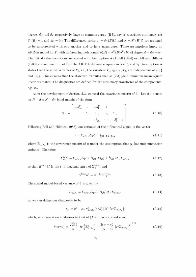
low-frequency (long-period) components. Some examples of squared gains of irregular com-

ponent extraction filters illustrating overestimation and underestimation are given in Figure 1

below. There are no formal studies of the consequences of overestimation and underestimation,

but Table 10 of Findley, Monsell, Shulman, and Pugh (1990) indicates that both can greatly

increase the amount of seasonal adjustment instability observed when more recent observations

are added to the time series and the earliest observations are deleted.

In Section 2, after describing the SEATS diagnostic for detecting underestimation and over-

estimation, we show it is biased toward identifying underestimation even when the estimate

is optimal. Simulation analyses of two modified diagnostics that are essentially unbiased are

provided in Section 3. We develop significance tests for the modified diagnostics in Section

4 and in the Appendix, for the situation in which the distribution of the stationary time se-

ries obtained from differencing operations has neither skewness nor kurtosis. (Specifically, we

assume that all third and fourth cumulants are zero.) In Section 5, the significance tests are

applied with some success to two official time series for which misestimation is suspected. Sec-

tion 6 discusses some conclusions and extensions. Certain required formulas are derived in the

Appendix.

2 The Basic Diagnostic

We focus on detecting misestimation of the irregular component, because the model for this

component is stationary and usually fully specified by a constant variance, σ2I = EI2

t . As a

consequence, the signal extraction filter formulas are simpler than for the other components,

as are the formulas of the over/underestimation diagnostics. (For the seasonal, trend, and

3

seasonally adjusted components, the SEATS diagnostic is calculated for the “stationary trans-

formation” of each component, meaning the output of the differencing operation specified by

the component’s ARIMA model.) Because of this greater simplicity, Agustın Maravall attaches

more importance to the over/underestimation diagnostic of the irregulars than to the corre-

sponding diagnostics for the other components (personal communication). Our study seems to

be the first systematic investigation of this kind of diagnostic.

In SEATS, the term estimator is used for the theoretical Wiener-Kolmogorov estimate that

applies with bi-infinite data. To have a specific formula for the variance of the estimator of the

irregular component used by SEATS, suppose the (estimated or fixed) ARIMA model for the

Yt is written in the usual backshift operator polynomial notation as

δ (B)φ (B)Yt = η (B) at. (2.1)

Thus δ (B) = 1 − δ1B − · · · − δdBd denotes the differencing operator which transforms Yt to

stationarity, e.g. δ (B) = (1 − B)2(1 + B + · · ·+ Bs−1

), at is the one-step-ahead prediction-

error process (with variance parameter σ2a), etc. Here s is the number of observations per year

(s = 12 in our analyses): φ (0) = η (0) = 1, and the zeros of φ (z) have magnitudes exceeding

one. For simplicity, the same will be assumed of η (z). The spectral density of the model for

the differenced series yt = δ(B)Yt is

g(λ) =σ2

a

2π

∣∣∣∣θ(e−iλ)φ(e−iλ)

∣∣∣∣2

. (2.2)

For j = 0,±1, · · · with

cIj =

σ2I

4π2

∫ π

−π

cos jλ

g(λ)|δ(e−iλ)|2 dλ (2.3)

the Wiener-Kolmogorov estimator IWK,t of It from bi-infinite data, i.e., the Gaussian condi-

tional expectation E(It|Ys,−∞ < s < ∞), has the formula IWK,t =∑∞

j=−∞ cIjYt−j SEATS’

variance of the estimator, σ2WK,I = EI2

WK,t, has the formula σ2WK,I = σ2

IcI0. The estimate of

It is the model’s conditional mean from the data:

It = E(It|Ys, 1 ≤ s ≤ N) =t−1∑

j=t−N

cIj,tYt−j . (2.4)

4

SEATS’ variance of the estimate is defined to be the sample second moment1

I2 =1N

N∑t=1

I2t , (2.5)

and, conceptually for SEATS, overestimation is indicated when I2 > σ2WK,I and underesti-

mation when I2 < σ2WK,I . However, the calculations that produce the component models in

SEATS and other software yield variances such as σ2I and σ2

WK,I calculated as though the

innovation variance of (2.1) were equal to one. We shall denote these unscaled variances by

σ2I/σ2

a and σ2WK,I/σ2

a. Thus, in place of σ2WK,I , for some estimate σ2

a, the scaled quantity

σ2aσ2

WK,I/σ2a is used. Let σ2

a,mle denote the maximum likelihood estimate of σ2a given by (A.1)

in the Appendix. Following SEATS, we use the bias-corrected estimate of Ansley and Newbold

(1981),

σ2a =

N − nδ,φ

N − nδ,φ − ncoeffsσ2

a,mle (2.6)

where nδ,φ = d (or d plus the degree of φ(z) if SEATS’ conditional estimate of φ(z) is used), and

ncoeffs is the number of estimated ARMA coefficients in the model. Note that when ncoeffs =

0, e.g. in the fixed-coefficient case, then σ2a = σ2

a,mle. SEATS’ criterion is I2 > σ2aσ2

WK,I/σ2a for

overestimation, and I2 < σ2aσ2

WK,I/σ2a for underestimation.

The following simple Proposition shows that SEATS’ over/underestimation criterion is biased

toward indicating underestimation.

Proposition 1 For the estimates It (2.4) of the stationary irregular component It, we have

EI2 ≤ σ2WK,I (2.7)

with σ2WK,I − EI2 = N−1

∑Nt=1

(E(It − It)

2 − E(It − IWK,t)2)

. Strict inequality necessarily

holds in (2.7) when the moving average polynomial η(B) in (2.1) has positive degree.

Proof. For covariance calculations based on the assumed model, the estimate It and its error

It− It, which sum to It, are treated as uncorrelated. The same is true for IWK,t and It−IWK,t.

Thus we have

σ2I = EI2

t + E(It − It)2

= σ2WK,I + E(It − IWK,t)

2. (2.8)

1Instead of I2, SEATS uses the sample variance,∑

t (It − It)2/(N − 1) where It is the sample mean. This

is N/(N − 1) u 1 times the smaller quantity I2 − (It)2. Therefore, the bias results of Proposition 1 apply to

the sample variance as well as to the sample second moment.

5

It follows from (2.8) that (2.7) is valid, because E(It − IWK,t)2 ≤ E(It − It)

2due to E(It − It)

2=

E(It − IWK,t)2+E(It − IWK,t)

2. This identity holds because, for covariance calculations based

on the assumed model, IWK,t, being the minimum mean square estimator from the larger data

set, is treated as uncorrelated with It − IWK,t. Strict inequality holds in (2.7) whenever (2.1)

has a moving average component, because then infinitely many coefficients in (2.3) are nonzero,

so that E(It − IWK,t)2

> 0. ¤

Suppose the model considered is the Box-Jenkins airline model,

(1−B)(1−B12)Yt = (1− θB) (1−ΘB) at. (2.9)

Let σ2WK,I denote the variance of the canonical irregular component of the sort produced

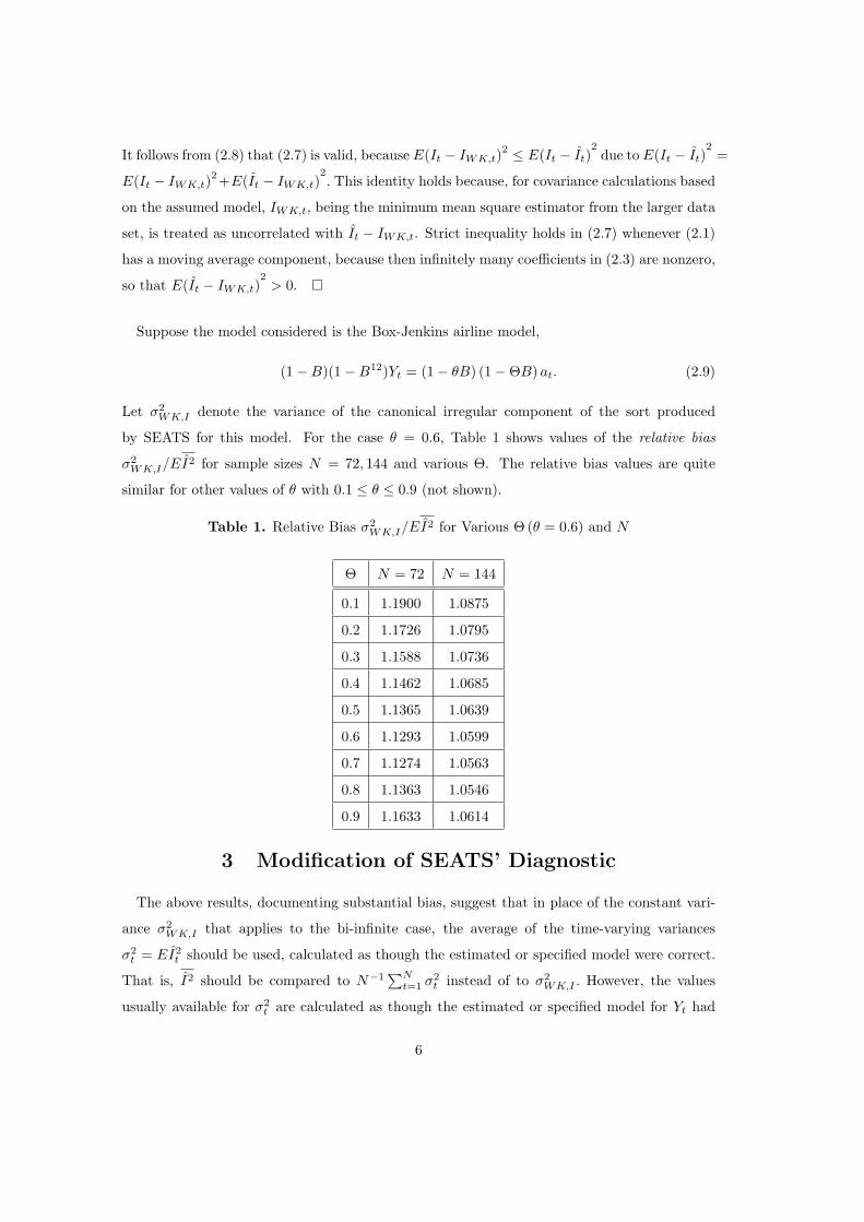
by SEATS for this model. For the case θ = 0.6, Table 1 shows values of the relative bias

σ2WK,I/EI2 for sample sizes N = 72, 144 and various Θ. The relative bias values are quite

similar for other values of θ with 0.1 ≤ θ ≤ 0.9 (not shown).

Table 1. Relative Bias σ2WK,I/EI2 for Various Θ (θ = 0.6) and N

Θ N = 72 N = 144

0.1 1.1900 1.0875

0.2 1.1726 1.0795

0.3 1.1588 1.0736

0.4 1.1462 1.0685

0.5 1.1365 1.0639

0.6 1.1293 1.0599

0.7 1.1274 1.0563

0.8 1.1363 1.0546

0.9 1.1633 1.0614

3 Modification of SEATS’ Diagnostic

The above results, documenting substantial bias, suggest that in place of the constant vari-

ance σ2WK,I that applies to the bi-infinite case, the average of the time-varying variances

σ2t = EI2

t should be used, calculated as though the estimated or specified model were correct.

That is, I2 should be compared to N−1∑N

t=1 σ2t instead of to σ2

WK,I . However, the values

usually available for σ2t are calculated as though the estimated or specified model for Yt had

6

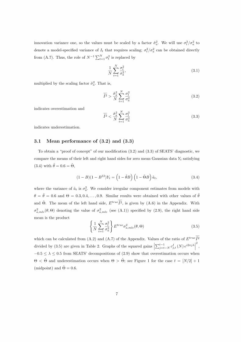
innovation variance one, so the values must be scaled by a factor σ2a. We will use σ2

t /σ2a to

denote a model-specified variance of It that requires scaling; σ2t /σ2

a can be obtained directly

from (A.7). Thus, the role of N−1∑N

t=1 σ2t is replaced by

1N

N∑t=1

σ2t

σ2a

, (3.1)

multiplied by the scaling factor σ2a. That is,

I2 >σ2

a

N

N∑t=1

σ2t

σ2a

(3.2)

indicates overestimation and

I2 <σ2

a

N

N∑t=1

σ2t

σ2a

(3.3)

indicates underestimation.

3.1 Mean performance of (3.2) and (3.3)

To obtain a “proof of concept” of our modification (3.2) and (3.3) of SEATS’ diagnostic, we

compare the means of their left and right hand sides for zero mean Gaussian data Yt satisfying

(3.4) with θ = 0.6 = Θ,

(1−B)(1−B12)Yt =(1− θB

)(1− ΘB

)at, (3.4)

where the variance of at is σ2a. We consider irregular component estimates from models with

θ = θ = 0.6 and Θ = 0.3, 0.4, . . . , 0.9. Similar results were obtained with other values of θ

and Θ. The mean of the left hand side, EtrueI2, is given by (A.6) in the Appendix. With

σ2a,mle(θ, Θ) denoting the value of σ2

a,mle (see (A.1)) specified by (2.9), the right hand side

mean is the product {1N

N∑t=1

σ2t

σ2a

}Etrueσ2

a,mle(θ, Θ) (3.5)

which can be calculated from (A.2) and (A.7) of the Appendix. Values of the ratio of EtrueI2

divided by (3.5) are given in Table 2. Graphs of the squared gains∣∣∣∑t−1

j=t−N cIj,t (N) ei2πjλ

∣∣∣2

,

−0.5 ≤ λ ≤ 0.5 from SEATS’ decompositions of (2.9) show that overestimation occurs when

Θ < Θ and underestimation occurs when Θ > Θ; see Figure 1 for the case t = [N/2] + 1

(midpoint) and Θ = 0.6.

7

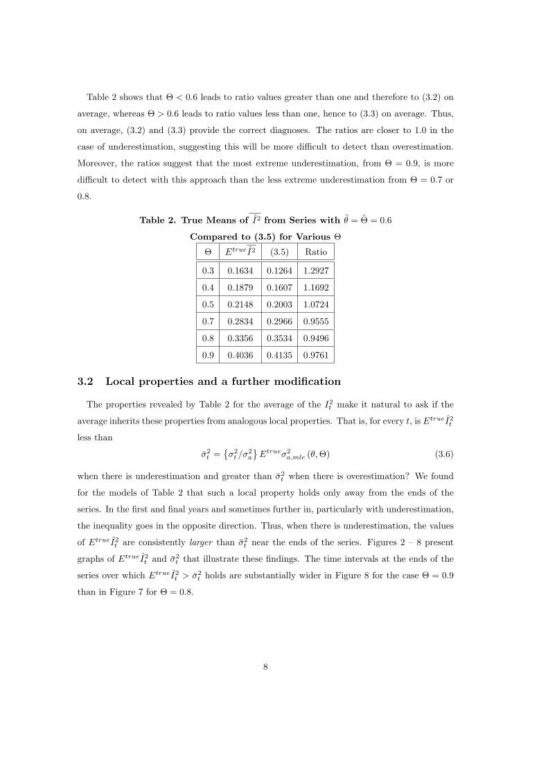
Table 2 shows that Θ < 0.6 leads to ratio values greater than one and therefore to (3.2) on

average, whereas Θ > 0.6 leads to ratio values less than one, hence to (3.3) on average. Thus,

on average, (3.2) and (3.3) provide the correct diagnoses. The ratios are closer to 1.0 in the

case of underestimation, suggesting this will be more difficult to detect than overestimation.

Moreover, the ratios suggest that the most extreme underestimation, from Θ = 0.9, is more

difficult to detect with this approach than the less extreme underestimation from Θ = 0.7 or

0.8.

Table 2. True Means of I2 from Series with θ = Θ = 0.6

Compared to (3.5) for Various Θ

Θ EtrueI2 (3.5) Ratio

0.3 0.1634 0.1264 1.2927

0.4 0.1879 0.1607 1.1692

0.5 0.2148 0.2003 1.0724

0.7 0.2834 0.2966 0.9555

0.8 0.3356 0.3534 0.9496

0.9 0.4036 0.4135 0.9761

3.2 Local properties and a further modification

The properties revealed by Table 2 for the average of the I2t make it natural to ask if the

average inherits these properties from analogous local properties. That is, for every t, is EtrueI2t

less than

σ2t =

{σ2

t /σ2a

}Etrueσ2

a,mle (θ, Θ) (3.6)

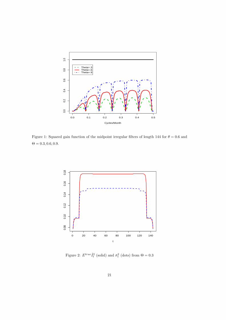
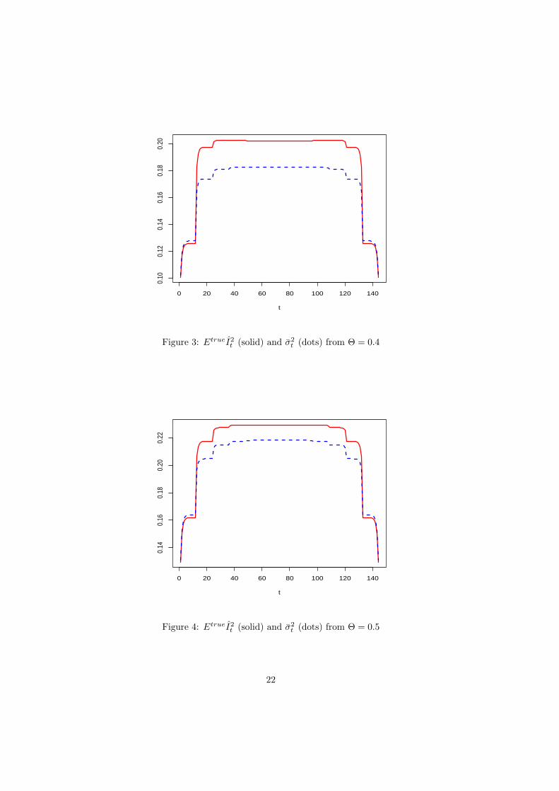
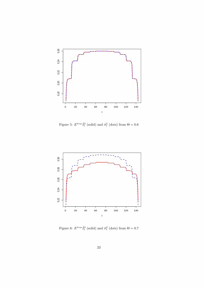
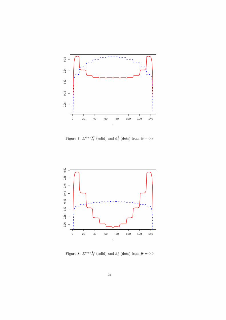
when there is underestimation and greater than σ2t when there is overestimation? We found

for the models of Table 2 that such a local property holds only away from the ends of the

series. In the first and final years and sometimes further in, particularly with underestimation,

the inequality goes in the opposite direction. Thus, when there is underestimation, the values

of EtrueI2t are consistently larger than σ2

t near the ends of the series. Figures 2 – 8 present

graphs of EtrueI2t and σ2

t that illustrate these findings. The time intervals at the ends of the

series over which EtrueI2t > σ2

t holds are substantially wider in Figure 8 for the case Θ = 0.9

than in Figure 7 for Θ = 0.8.

8

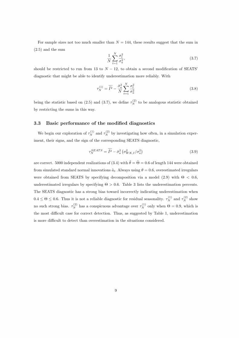
For sample sizes not too much smaller than N = 144, these results suggest that the sum in

(2.5) and the sum1N

N∑t=1

σ2t

σ2a

, (3.7)

should be restricted to run from 13 to N − 12, to obtain a second modification of SEATS’

diagnostic that might be able to identify underestimation more reliably. With

τ(1)N = I2 − σ2

a

N

N∑t=1

σ2t

σ2a

(3.8)

being the statistic based on (2.5) and (3.7), we define τ(2)N to be analogous statistic obtained

by restricting the sums in this way.

3.3 Basic performance of the modified diagnostics

We begin our exploration of τ(1)N and τ

(2)N by investigating how often, in a simulation exper-

iment, their signs, and the sign of the corresponding SEATS diagnostic,

τSEATSN = I2 − σ2

a

(σ2

WK,I/σ2a

)(3.9)

are correct. 5000 independent realizations of (3.4) with θ = Θ = 0.6 of length 144 were obtained

from simulated standard normal innovations at. Always using θ = 0.6, overestimated irregulars

were obtained from SEATS by specifying decomposition via a model (2.9) with Θ < 0.6,

underestimated irregulars by specifying Θ > 0.6. Table 3 lists the underestimation percents.

The SEATS diagnostic has a strong bias toward incorrectly indicating underestimation when

0.4 ≤ Θ ≤ 0.6. Thus it is not a reliable diagnostic for residual seasonality. τ(1)N and τ

(2)N show

no such strong bias. τ(2)N has a conspicuous advantage over τ

(1)N only when Θ = 0.9, which is

the most difficult case for correct detection. Thus, as suggested by Table 1, underestimation

is more difficult to detect than overestimation in the situations considered.

9

Table 3. Percents of Simulated Airline Model Series with θ = Θ = 0.6 for Which

Underestimation is Indicated by Diagnostics of Adjustments Produced from

Estimated θ and Θ and with Specified Incorrect Θ’s

Θ τSEATSN τ

(1)N τ

(2)N

0.3 12.1 1.4 2.1

0.4 32.2 6.9 8.6

0.5 62.7 22.0 24.4

estimated θ, Θ 100 47.4 48.2

0.7 96.6 75.0 73.3

0.8 99.1 84.1 84.0

0.9 98.4 66.7 81.4

4 Tests for the Significance of Over- or Underestimation

For significance testing, we interpret the value of τ(1)N by reference to an estimate σN (τ (1)

N )

of its standard deviation given by the right hand side of (A.9) in the Appendix. This estimate

accounts for the variances of I2 and σ2a and their covariance by treating the model coefficients

as non-random, as they are for the simulation results. An analogous σN (τ (2)N ) is used with

τ(2)N . For a given size (significance level) α, and with z denoting an N (0, 1) variate, let z1−α

denote the value for which P {z > z1−α} = P {z < −z1−α} = 1−α. We performed simulation

experiments to determine, for various α and Θ, the proportion of simulated series for which

τ(i)N > z1−α σN (τ (i)

N ) (4.1)

occurs, which is interpreted to indicate overestimation (at the α level of significance), or for

which

τ(i)N < −z1−α σN (τ (i)

N ) (4.2)

occurs, indicating underestimation, for i = 1, 2; we simulated 1000 series of length N = 144

from the model (3.4) with θ = Θ = 0.6.

10

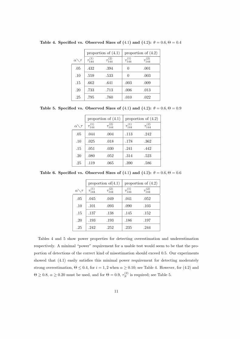
Table 4. Specified vs. Observed Sizes of (4.1) and (4.2): θ = 0.6,Θ = 0.4

proportion of (4.1) proportion of (4.2)

α�τ τ(1)144 τ

(2)144 τ

(1)144 τ

(2)144

.05 .432 .394 0 .001

.10 .559 .533 0 .003

.15 .662 .641 .003 .009

.20 .733 .713 .006 .013

.25 .795 .760 .010 .022


proportion of (4.1) proportion of (4.2)

α�τ τ(1)144 τ

(2)144 τ

(1)144 τ

(2)144

.05 .044 .004 .113 .242

.10 .025 .018 .178 .362

.15 .051 .030 .241 .442

.20 .080 .052 .314 .523

.25 .119 .065 .390 .586


proportion of(4.1) proportion of (4.2)

α�τ τ(1)144 τ

(2)144 τ

(1)144 τ

(2)144

.05 .045 .049 .041 .052

.10 .101 .093 .090 .103

.15 .137 .138 .145 .152

.20 .193 .193 .186 .197

.25 .242 .252 .235 .244

Tables 4 and 5 show power properties for detecting overestimation and underestimation

respectively. A minimal “power” requirement for a usable test would seem to be that the pro-

portion of detections of the correct kind of misestimation should exceed 0.5. Our experiments

showed that (4.1) easily satisfies this minimal power requirement for detecting moderately

strong overestimation, Θ ≤ 0.4, for i = 1, 2 when α ≥ 0.10; see Table 4. However, for (4.2) and

Θ ≥ 0.8, α ≥ 0.20 must be used, and for Θ = 0.9, τ(2)N is required; see Table 5.

11

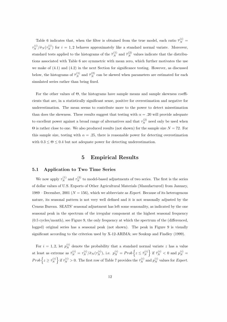
Table 6 indicates that, when the filter is obtained from the true model, each ratio τ(i)N =

τ(i)N /σN (τ (i)

N ) for i = 1, 2 behaves approximately like a standard normal variate. Moreover,

standard tests applied to the histograms of the τ(1)N and τ

(2)N values indicate that the distribu-

tions associated with Table 6 are symmetric with mean zero, which further motivates the use

we make of (4.1) and (4.2) in the next Section for significance testing. However, as discussed

below, the histograms of τ(1)N and τ

(2)N can be skewed when parameters are estimated for each

simulated series rather than being fixed.

For the other values of Θ, the histograms have sample means and sample skewness coeffi-

cients that are, in a statistically significant sense, positive for overestimation and negative for

underestimation. The mean seems to contribute more to the power to detect misestimation

than does the skewness. These results suggest that testing with α = .20 will provide adequate

to excellent power against a broad range of alternatives and that τ(2)N need only be used when

Θ is rather close to one. We also produced results (not shown) for the sample size N = 72. For

this sample size, testing with α = .25, there is reasonable power for detecting overestimation

with 0.3 ≤ Θ ≤ 0.4 but not adequate power for detecting underestimation.

5 Empirical Results

5.1 Application to Two Time Series

We now apply τ(1)N and τ

(2)N to model-based adjustments of two series. The first is the series

of dollar values of U.S. Exports of Other Agricultural Materials (Manufactured) from January,

1989 – December, 2001 (N = 156), which we abbreviate as Export. Because of its heterogenous

nature, its seasonal pattern is not very well defined and it is not seasonally adjusted by the

Census Bureau. SEATS’ seasonal adjustment has left some seasonality, as indicated by the one

seasonal peak in the spectrum of the irregular component at the highest seasonal frequency

(0.5 cycles/month), see Figure 9, the only frequency at which the spectrum of the (differenced,

logged) original series has a seasonal peak (not shown). The peak in Figure 9 is visually

significant according to the criterion used by X-12-ARIMA; see Soukup and Findley (1999).

For i = 1, 2, let p(i)N denote the probability that a standard normal variate z has a value

at least as extreme as τ(i)N = τ

(i)N /σN (τ (i)

N ), i.e. p(i)N = Prob

{z ≤ τ

(i)N

}if τ

(i)N < 0 and p

(i)N =

Prob{

z ≥ τ(i)N

}if τ

(i)N > 0. The first row of Table 7 provides the τ

(i)N and p

(i)N values for Export.

12

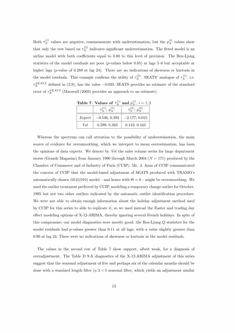
Both τ(i)N values are negative, commensurate with underestimation, but the p

(i)N values show

that only the test based on τ(2)N indicates significant underestimation. The fitted model is an

airline model with both coefficients equal to 0.80 to this level of precision. The Box-Ljung

statistics of the model residuals are poor (p-values below 0.05) at lags 3–6 but acceptable at

higher lags (p-value of 0.289 at lag 24). There are no indications of skewness or kurtosis in

the model residuals. This example confirms the utility of τ(2)N . SEATS’ analogue of τ

(1)N , i.e.

τSEATSN defined in (3.9), has the value −0.033. SEATS provides no estimate of the standard

error of τSEATSN (Maravall (2003) provides an approach to an estimate).

Table 7. Values of τ(i)N and p

(i)N , i = 1, 2

τ(1)N ; p

(1)N τ

(2)N ; p

(2)N

Export −0.546; 0.292 −2.177; 0.015

Vol 0.299; 0.383 0.142; 0.443

Whereas the spectrum can call attention to the possibility of underestimation, the main

source of evidence for oversmoothing, which we interpret to mean overestimation, has been

the opinions of data experts. We denote by Vol the sales volume series for large department

stores (Grands Magasins) from January 1990 through March 2004 (N = 171) produced by the

Chamber of Commerce and of Industry of Paris (CCIP). Mr. J. Anas of CCIP communicated

the concern of CCIP that the model-based adjustment of SEATS produced with TRAMO’s

automatically chosen (012)(010) model – and hence with Θ = 0 – might be oversmoothing. We

used the outlier treatment preferred by CCIP, modeling a temporary change outlier for October,

1995 but not two other outliers indicated by the automatic outlier identification procedure.

We were not able to obtain enough information about the holiday adjustment method used

by CCIP for this series to able to replicate it, so we used instead the Easter and trading day

effect modeling options of X-12-ARIMA, thereby ignoring several French holidays. In spite of

this compromise, our model diagnostics were mostly good: the Box-Ljung Q statistics for the

model residuals had p-values greater than 0.11 at all lags, with a value slightly greater than

0.90 at lag 24. There were no indications of skewness or kurtosis in the model residuals.

The values in the second row of Table 7 show support, albeit weak, for a diagnosis of

overadjustment. The Table D 9.A diagnostics of the X-12-ARIMA adjustment of this series

suggest that the seasonal adjustment of five and perhaps six of the calendar months should be

done with a standard length filter (a 3 × 5 seasonal filter, which yields an adjustment similar

13

to a SEATS adjustment with Θ = 0.6, see Findley and Martin, 2003), whereas a shorter filter

should be used for the remaining months, quite short for some of the months. (A SEATS filter

from Θ = 0 has length about 37 months, slightly shorter than the filter obtained by using the

shortest (i.e., the 3×1) seasonal filter in X-12-ARIMA.) Thus, the indications of overestimation

may be weak because overestimation is a problem only for half or less of the months. For this

series, τSEATSN has the value 0.000 and so gives no indication of overestimation.

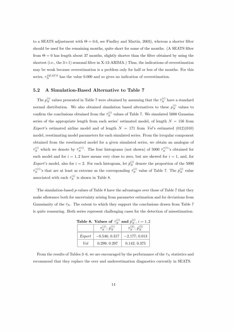
5.2 A Simulation-Based Alternative to Table 7

The p(i)N values presented in Table 7 were obtained by assuming that the τ

(i)N have a standard

normal distribution. We also obtained simulation based alternatives to these p(i)N values to

confirm the conclusions obtained from the τ(i)N values of Table 7. We simulated 5000 Gaussian

series of the appropriate length from each series’ estimated model, of length N = 156 from

Export ’s estimated airline model and of length N = 171 from Vol ’s estimated (012)(010)

model, reestimating model parameters for each simulated series. From the irregular component

obtained from the reestimated model for a given simulated series, we obtain an analogue of

τ(i)N which we denote by τ

∗(i)N . The four histograms (not shown) of 5000 τ

∗(i)N ’s obtained for

each model and for i = 1, 2 have means very close to zero, but are skewed for i = 1, and, for

Export ’s model, also for i = 2. For each histogram, let p(i)N denote the proportion of the 5000

τ∗(i)N ’s that are at least as extreme as the corresponding τ

(i)N value of Table 7. The p

(i)N value

associated with each τ(i)N is shown in Table 8.

The simulation-based p-values of Table 8 have the advantages over those of Table 7 that they

make allowance both for uncertainty arising from parameter estimation and for deviations from

Gaussianity of the τN . The extent to which they support the conclusions drawn from Table 7

is quite reassuring. Both series represent challenging cases for the detection of misestimation.

Table 8. Values of τ(i)N and p

(i)N , i = 1, 2

τ(1)N ; p

(1)N τ

(2)N ; p

(2)N

Export −0.546; 0.317 −2.177; 0.013

Vol 0.299; 0.297 0.142; 0.375

From the results of Tables 3–6, we are encouraged by the performance of the τN statistics and

recommend that they replace the over and underestimation diagnostics currently in SEATS.

14

6 Conclusions and Extensions

By using finite-data signal extraction variances (in conjunction with the bias-corrected es-

timate of Ansley and Newbold (1981) of the innovation variance), one can obtain essentially

unbiased analogues of the diagnostics of SEATS for detecting over- or underestimation and, in

addition, test statistics for one-sided tests of the presence of these phenomena. In the preceding

Sections, this was demonstrated in the context of an extensive analysis of the diagnostic for

the irregular component of a seasonal adjustment decomposition. However, there are broad

generalizations of the diagnostic (3.8) and its standard error, with slightly more complex for-

mulas, that apply to time series which can be modeled as a sum of “independent” components,

each with an ARIMA model. Such formulas are given in (A.15) and (A.16) of Appendix A

for stationary transforms ut = δU (B)Ut of the estimates Ut of the component Ut of a general

two component decomposition Yt = Ut + Vt, 1 ≤ t ≤ N . By specializing these formulas to the

other components of a seasonal decomposition Yt = St +Tt + It, i.e., setting Ut equal to St, Tt,

or Tt + It, (the target seasonal adjustment), analogues of (4.1) and (4.2) can be obtained to

provide tests for replacements for the other over- and under-adjustment diagnostics of SEATS.

The exact formulas needed to implement the analogues of the test statistic (3.8) for the sta-

tionary transforms of the seasonal and trend component estimates are given in Proposition 4

of McElroy and Sutcliffe (2004). A change in the notation of the proof of Proposition 1 shows

that SEATS’ diagnostic for the stationary transforms of the seasonal, trend, and seasonally ad-

justed series are also biased toward indicating underestimation. Feldpausch, Hood, and Wills

(2004) present simulation results that show this bias.

In future work, after these tests are programmed into the X-13 program discussed in Monsell

et al. (2003), we plan to apply them to large numbers of Census Bureau time series to learn more

about what features of series and seasonal decompositions they are sensitive to. Another future

project is the establishment of a central limit theorem for τ(1)N /σN (τ (1)

N ) and its generalizations.

A Appendix: Technical Results

A.1 Formulas for σ2a,mle (θ, Θ) and Etrueσ2

a,mle

(θ, Θ

)

A time series with spectral density g (λ) has autocovariances

γj (g) =∫ π

−π

cos(jλ) g (λ) dλ, j = 0,±1, . . . .

15

Let Σ(g) denote the associated covariance matrix of order N−d, i.e., Σ(g) = [γj−k (g)]1≤j,k≤N−d.

For the model (2.1), the spectral density of yt = δ (B)Yt is g (λ) = (σ2a/2π)

∣∣η (e−iλ

)∣∣2 ∣∣φ (e−iλ

)∣∣−2.

If we define yd+1:N =[

yd+1 · · · yN

]′and g1 (λ) = (1/2π)

∣∣η (e−iλ

)∣∣2 ∣∣φ (e−iλ

)∣∣−2, then it

follows from ΣN−d (g) = σ2aΣN−d (g1) and (3.2) of Ansley and Newbold (1981) that the m.l.e.

of σ2a is

σ2a,mle (η/φ) =

1N − d

y′d+1:NΣ−1 (g1)yd+1:N , (A.1)

and also that, with tr denoting trace of a matrix,

Etrueσ2a,mle (η/φ) =

1N − d

tr{Σ−1 (g1) Σ (g)

}. (A.2)

For (2.9) and (3.5), we denote (A.1) by σ2a,mle (θ, Θ) and (A.2) by Etrueσ2

a,mle (θ, Θ).

A.2 Formulas associated with It

To obtain standard errors of test statistics, variances and covariances of I2 and σ2a,mle (η/φ)

are required. These can be obtained fairly easily if, as usual, the model coefficients are treated

as fixed rather than random. We first need the covariance matrix of the It. In the notation

introduced above, and with ∆ denoting the N − d×N band matrix of the form

∆ =

−δd · · · −δ1 1. . . . . . . . . . . .

−δd · · · −δ1 1

, (A.3)

the formula for the vector I = I (g,N) of estimates It, 1 ≤ t ≤ N from (2.3) under Assumption

A of Bell and Hillmer (1988) – see subsection A.4 – is

I =σ2

I

σ2a

∆′Σ−1 (g1)yd+1:N , (A.4)

when It is white noise with variance σ2I – see (4.3) of Bell and Hillmer (1988). Thus the

covariance matrix ΣtrueI

= ΣI (g, g, N) has the formula

ΣtrueI

=(

σ2I

σ2a

)2

∆′Σ−1 (g1)Σ (g)Σ−1 (g1) ∆. (A.5)

For 1 ≤ t ≤ N , EtrueI2t is the t-th diagonal entry of Σtrue

I, and

EtrueI2 = N−1trΣtrueI

. (A.6)

For 1 ≤ t ≤ N , the scaled model-based variance σ2t /σ2

a is the t-th diagonal entry of

ΣI/σa=

(σ2

I

σ2a

)2

∆′Σ−1 (g1)∆, (A.7)

and (3.7) is given by N−1trΣI/σa.

16

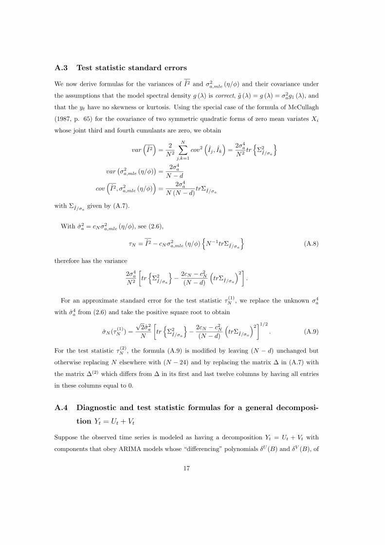
A.3 Test statistic standard errors

We now derive formulas for the variances of I2 and σ2a,mle (η/φ) and their covariance under

the assumptions that the model spectral density g (λ) is correct, g (λ) = g (λ) = σ2ag1 (λ), and

that the yt have no skewness or kurtosis. Using the special case of the formula of McCullagh

(1987, p. 65) for the covariance of two symmetric quadratic forms of zero mean variates Xi

whose joint third and fourth cumulants are zero, we obtain

var(I2

)=

2N2

N∑

j,k=1

cov2(Ij , Ik

)=

2σ4a

N2tr

{Σ2

I/σa

}

var(σ2

a,mle (η/φ))

=2σ4

a

N − d

cov(I2, σ2

a,mle (η/φ))

=2σ4

a

N (N − d)trΣI/σa

with ΣI/σagiven by (A.7).

With σ2a = cNσ2

a,mle (η/φ), see (2.6),

τN = I2 − cNσ2a,mle (η/φ)

{N−1trΣI/σa

}(A.8)

therefore has the variance

2σ4a

N2

[tr

{Σ2

I/σa

}− 2cN − c2

N

(N − d)

(trΣI/σa

)2]

.

For an approximate standard error for the test statistic τ(1)N , we replace the unknown σ4

a

with σ4a from (2.6) and take the positive square root to obtain

σN (τ (1)N ) =

√2σ2

a

N

[tr

{Σ2

I/σa

}− 2cN − c2

N

(N − d)

(trΣI/σa

)2]1/2

. (A.9)

For the test statistic τ(2)N , the formula (A.9) is modified by leaving (N − d) unchanged but

otherwise replacing N elsewhere with (N − 24) and by replacing the matrix ∆ in (A.7) with

the matrix ∆(2) which differs from ∆ in its first and last twelve columns by having all entries

in these columns equal to 0.

A.4 Diagnostic and test statistic formulas for a general decomposi-

tion Yt = Ut + Vt

Suppose the observed time series is modeled as having a decomposition Yt = Ut + Vt with

components that obey ARIMA models whose “differencing” polynomials δU (B) and δV (B), of

17

degrees dU and dV respectively, have no common zeros. (If Ut, say, is covariance stationary, set

δU (B) = 1 and dU = 0.) The differenced series ut = δU (B)Ut and vt = δV (B)Vt are assumed

to be uncorrelated with one another and to have mean zero. These assumptions imply an

ARIMA model for Yt with differencing polynomial δ(B) = δU (B)δV (B) of degree d = dU +dV .

The initial value conditions associated with Assumption A of Bell (1984) or Bell and Hillmer

(1988) are assumed to hold for the ARIMA difference equations for Ut and Vt. Assumption A

states that the initial d values of Yt, i.e., the variables Y1, Y2, · · · , Yd, are independent of {ut}and {vt}. This ensures that the standard formulas such as (2.3) yield minimum mean square

linear estimates. The diagnostics are defined for the stationary transforms of the components,

e.g. ut.

As in the development of Section A.3, we need the covariance matrix of ut. Let ∆V denote

an N − d×N − dU band matrix of the form

∆V =

−δVdV

· · · −δV1 1

. . . . . . . . . . . .

−δVdV

· · · −δV1 1

. (A.10)

Following Bell and Hillmer (1988), our estimate of the differenced signal is the vector

u = Σu/σa∆′V Σ−1(g1)yd+1:N (A.11)

where Σu/σais the covariance matrix of u under the assumption that yt has unit innovation

variance. Therefore,

Σtrueu = Σu/σa

∆′V Σ−1(g1)Σ(g)Σ−1(g1)∆V Σu/σa

(A.12)

so that Etrueu2t is the t-th diagonal entry of Σtrue

u , and

Etrueu2 = N−1trΣtrueu . (A.13)

The scaled model-based variance of u is given by

Σu/σa= Σu/σa

∆′V Σ−1(g1)∆V Σu/σa

. (A.14)

So we can define our diagnostic to be

τN = u2 − cN σ2a,mle(η/φ)

{N−1trΣu/σa

}(A.15)

which, in a derivation analogous to that of (A.9), has standard error

σN (τN ) =√

2σ2a

N

[tr

{Σ2

u/σa

}− 2cN − c2

N

(N − d)(trΣu/σa

)2]1/2

(A.16)

18

where σa comes from (2.6).

Acknowledgement. We thank William Bell and Michael Shimberg for helpful comments

on a draft of this paper and Catherine Hood for supplying the Export series.

References

[1] Ansley, C. F. and Newbold, P. (1981), “On the Bias in Estimates of Forecast Mean Square

Error,” Journal of the American Statistical Association, 76, 569-576.

[2] Bell, W. (1984). Signal Extraction for Nonstationary Time Series. The Annals of Statistics

12, 646 –664.

[3] Bell, W. R. and Hillmer, S. C. (1988), “A matrix approach to likelihood evalua-

tion and signal extraction for ARIMA component time series models,” Bureau of the

Census, Statistical Research Division Report Number: Census/SRD/RR-88/22. Also

www.census.gov/srd/papers/pdf/rr88-22.pdf

[4] Burman, J. (1980), “Seasonal Adjustment by Signal Extraction,” Journal of the Royal

Statistical Society, Ser. A, 143, 321–337.

[5] Feldpausch, R. M., Hood, C., and Wills, K. (2004), “Diagnostics for Model-Based Seasonal

Adjustment,” 2004 Proceedings American Statistical Association [CD-ROM]: Alexandria,

VA

[6] Findley, D. F., Wills, K. C., Aston, J. A., Feldpausch, R. M. and Hood, C. C. (2003),

“Diagnostics for ARIMA-Model-Based Seasonal Adjustment,” 2003 Proceedings American

Statistical Association [CD-ROM]: Alexandria, VA

[7] Findley, D. F. and Martin, D. E. K. (2003), “Frequency Domain Analyses of SEATS and

X-12-ARIMA Seasonal Adjustment Filters for Short and Moderate-Length Time Series,”

Statistical Research Division Research Report Series, Statistics #2003-02, Census Bureau,

Washington, D.C. Also www.census.gov/srd/papers/pdf/rrs2003-02.pdf

[8] Findley, D., Monsell, B., Shulman, H., and Pugh, M. (1990), “Sliding Spans Diagnostics

for Seasonal and Related Adjustments,” Journal of the American Statistical Association,

85, 345–355.

19

[9] Findley, D. F., Monsell, B. C., Bell, W. R., Otto, M. C. and Chen, B. C. (1998). New

Capabilities and Methods of the X-12-ARIMA Seasonal Adjustment Program,” Journal

of Business and Economic Statistics , 16, 127–177 (with discussion).

[10] Gomez, V. and Maravall, A. (1997), “Program SEATS Signal Extraction in ARIMA Time

Series: Instructions for the User (beta version: June 1997),” Working Paper 97001, Minis-

terio de Economıa y Hacienda, Dirrection General de Analysis y Programacion Presupues-

taria, Madrid.

[11] Hillmer, S. and Tiao, G. (1982), “An ARIMA-Model-Based Approach to Seasonal Adjust-

ment,” Journal of the American Statistical Association, 77, 63 – 70.

[12] Kitagawa, G. (1981), “A Nonstationary Time Series Model and its Fitting by a Recursive

Filter,” Journal of Time Series Analysis, 2, 103–116.

[13] Kitagawa, G. (1985), DECOMP. In TIMSAC-84 Part 2, Computer Science Monographs

No. 23, The Institute of Statistical Mathematics, Tokyo.

[14] Koopman, S., Harvey, A., Doornik, J., and Shepherd, N. (1995), Stamp 5.0: Structural

Time Series Analyser, Modeller, and Predictor, London: Chapman and Hall.

[15] Maravall, A. (2003), “A Class of Diagnostics in the ARIMA-Model-Based Decomposition

of a Time Series,” Memorandum, Bank of Spain.

[16] McCullagh, P. (1987), Tensor Methods in Statistics, London: Chapman and Hall.

[17] McElroy, T. S. and Sutcliffe, A. (2004), “An Iterated Parametric Approach

to Nonstationary Signal Extraction,” Statistical Research Division Research

Report Series, Statistics #2004-05, Census Bureau, Washington, D.C. Also

www.census.gov/srd/papers/pdf/rrs2004-05.pdf

[18] Monsell, B., Aston, J. and Koopman, S. (2003), “Toward X-13?” Proceeding of the Busi-

ness and Economic Statistics Section of the American Statistical Association.

[19] Soukup, R. J. and Findley, D. F. (1999). “On the Spectrum Diagnostics Used by X-12-

ARIMA to Indicate the Presence of Trading Day Effects after Modeling or Adjustment,”

Proceedings of the Business and Economic Statistics Section, 144–149, American Statisti-

cal Association. Also www.census.gov/pub/ts/papers/rr9903s.pdf

20

Cycles/Month

0.0 0.1 0.2 0.3 0.4 0.5

0.0

0.2

0.4

0.6

0.8

1.0

Theta=.3Theta=.6Theta=.9

Figure 1: Squared gain function of the midpoint irregular filters of length 144 for θ = 0.6 and

Θ = 0.3, 0.6, 0.9.

t

0 20 40 60 80 100 120 140

0.08

0.10

0.12

0.14

0.16

0.18

Figure 2: EtrueI2t (solid) and σ2

t (dots) from Θ = 0.3

21

t

0 20 40 60 80 100 120 140

0.10

0.12

0.14

0.16

0.18

0.20



t

0 20 40 60 80 100 120 140

0.14

0.16

0.18

0.20

0.22



22

t

0 20 40 60 80 100 120 140

0.18

0.20

0.22

0.24

0.26



t

0 20 40 60 80 100 120 140

0.22

0.24

0.26

0.28

0.30



23

t

0 20 40 60 80 100 120 140

0.28

0.30

0.32

0.34

0.36



t

0 20 40 60 80 100 120 140

0.36

0.38

0.40

0.42

0.44

0.46

0.48

0.50



24

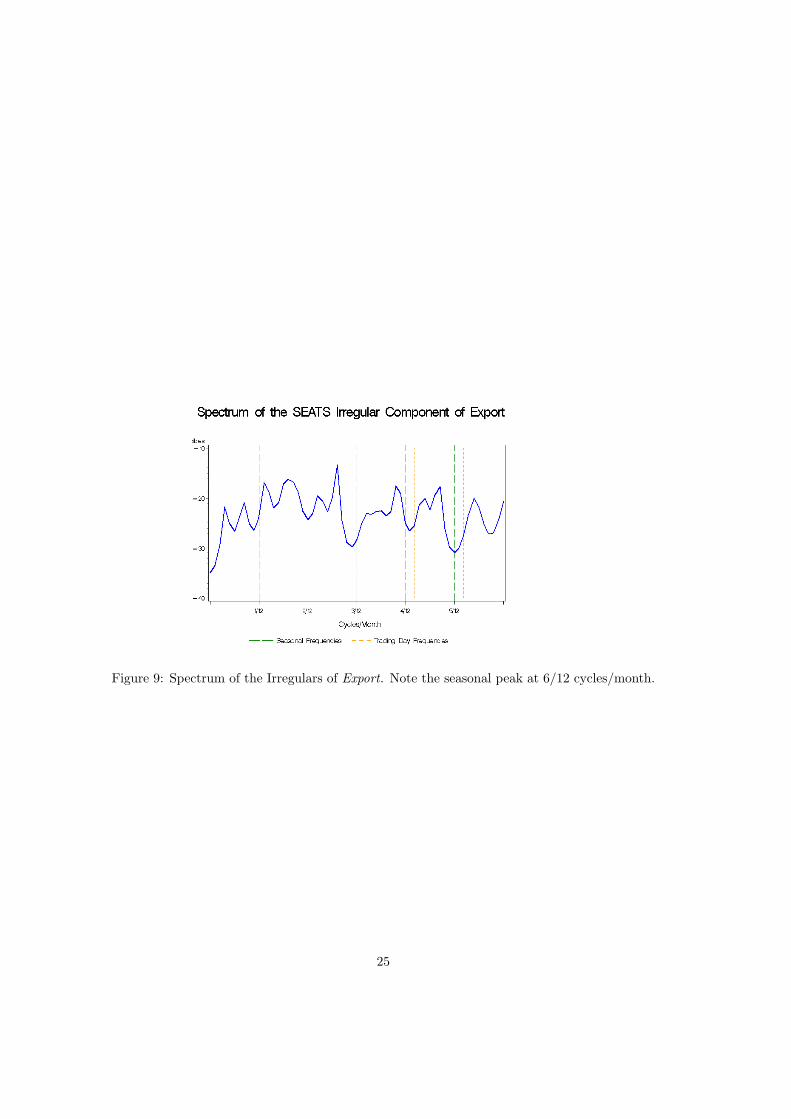
Figure 9: Spectrum of the Irregulars of Export. Note the seasonal peak at 6/12 cycles/month.

25

Modi…cations of SEATS'Diagnostic for Detecting Over or Underestimation of Seasonal Adjustment...

Documents

Transcript of Modi…cations of SEATS'Diagnostic for Detecting Over or Underestimation of Seasonal Adjustment...