Models and methods for analyzing DCE-MRI: A reviewFahmi Khalifa, Ahmed Soliman, Ayman El-Baz, Mohamed Abou El-Ghar, Tarek El-Diasty, Georgy Gimel’farb, Rosemary Ouseph, and Amy C. Dwyer Citation: Medical Physics 41, 124301 (2014); doi: 10.1118/1.4898202 View online: http://dx.doi.org/10.1118/1.4898202 View Table of Contents: http://scitation.aip.org/content/aapm/journal/medphys/41/12?ver=pdfcov Published by the American Association of Physicists in Medicine Articles you may be interested in ADC texture—An imaging biomarker for high-grade glioma? Med. Phys. 41, 101903 (2014); 10.1118/1.4894812 Elastic registration of multimodal prostate MRI and histology via multiattribute combined mutual information Med. Phys. 38, 2005 (2011); 10.1118/1.3560879 Breast MRI: Fundamentals and Technical Aspects Med. Phys. 35, 1163 (2008); 10.1118/1.2840347 An objective method for combining multi-parametric MRI datasets to characterize malignant tumors Med. Phys. 34, 1053 (2007); 10.1118/1.2558301 Automatic identification and classification of characteristic kinetic curves of breast lesions on DCE-MRI Med. Phys. 33, 2878 (2006); 10.1118/1.2210568

Models and methods for analyzing DCE-MRI: A reviewFahmi KhalifaBioImaging Laboratory, Department of Bioengineering, University of Louisville, Louisville, Kentucky 40292and Electronics and Communication Engineering Department, Mansoura University, Mansoura 35516, Egypt

Ahmed Soliman and Ayman El-Baza)

BioImaging Laboratory, Department of Bioengineering, University of Louisville, Louisville, Kentucky 40292

Mohamed Abou El-Ghar and Tarek El-DiastyRadiology Department, Urology and Nephrology Center, Mansoura University, Mansoura 35516, Egypt

Georgy Gimel’farbDepartment of Computer Science, University of Auckland, Auckland 1142, New Zealand

Rosemary Ouseph and Amy C. DwyerKidney Transplantation–Kidney Disease Center, University of Louisville, Louisville, Kentucky 40202

(Received 29 July 2014; revised 11 September 2014; accepted for publication 1 October 2014;published 17 November 2014)

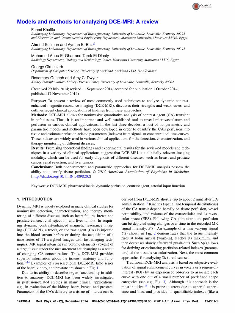
Purpose: To present a review of most commonly used techniques to analyze dynamic contrast-enhanced magnetic resonance imaging (DCE-MRI), discusses their strengths and weaknesses, andoutlines recent clinical applications of findings from these approaches.Methods: DCE-MRI allows for noninvasive quantitative analysis of contrast agent (CA) transientin soft tissues. Thus, it is an important and well-established tool to reveal microvasculature andperfusion in various clinical applications. In the last three decades, a host of nonparametric andparametric models and methods have been developed in order to quantify the CA’s perfusion intotissue and estimate perfusion-related parameters (indexes) from signal- or concentration–time curves.These indexes are widely used in various clinical applications for the detection, characterization, andtherapy monitoring of different diseases.Results: Promising theoretical findings and experimental results for the reviewed models and tech-niques in a variety of clinical applications suggest that DCE-MRI is a clinically relevant imagingmodality, which can be used for early diagnosis of different diseases, such as breast and prostatecancer, renal rejection, and liver tumors.Conclusions: Both nonparametric and parametric approaches for DCE-MRI analysis possess theability to quantify tissue perfusion. C 2014 American Association of Physicists in Medicine.[http://dx.doi.org/10.1118/1.4898202]

Key words: DCE-MRI, pharmacokinetic, dynamic perfusion, contrast agent, arterial input function

1. INTRODUCTION

Dynamic MRI is widely explored in many clinical studies fornoninvasive detection, characterization, and therapy moni-toring of different diseases such as heart failure, breast andprostate cancer, renal rejection, and liver tumors. In acquir-ing dynamic contrast-enhanced magnetic resonance imag-ing (DCE-MRI), a tracer, or contrast agent (CA) is injectedinto the blood stream before or during the acquisition of atime series of T1-weighted images with fast imaging tech-niques. MR signal intensities in volume elements (voxels) ofa target tissue under the measurement are changing as a resultof changing CA concentrations. Thus, DCE-MRI providessuperior information about the tissues’ anatomy and func-tion.1–14 Examples of cross-sectional DCE-MRI time seriesof the heart, kidney, and prostate are shown in Fig. 1.

Due to its ability to describe organ functionality in addi-tion to anatomy, DCE-MRI has been widely investigatedin perfusion-related studies in many clinical applications,e.g., in evaluation of the kidney, heart, breast, and prostate.Parameters of the CA’s delivery to a tissue of interest can be

derived from DCE-MRI shortly (up to about 2 min) after CAadministration.15 Kinetics (spatial and temporal distributions)of the CA transit depend heavily on tissue perfusion, vesselpermeability, and volume of the extracellular and extravas-cular space (EES). Following CA administration, perfusioncan be depicted using changes over time in the recorded MRsignal intensity, S(t). An example of a time varying signalS(t) shown in Fig. 2 demonstrates that the tissue intensityrises at bolus arrival (wash-in), reaches its maximum, andthen decreases slowly afterward (wash-out). Such S(t) allowsfor deriving or estimating perfusion-related indexes (parame-ters) of the tissue’s vascularization. Next, the most commonapproaches for analyzing S(t) are discussed.

Traditional DCE-MRI analysis is based on subjective eval-uation of signal enhancement curves in voxels or a region-of-interest (ROI) by an experienced observer to associate eachcurve with one out of a small number of predefined shapecategories (see e.g., Fig. 3). Although this approach is themost intuitive,16 it is prone to errors due to experts’ experi-ence and bias, and provides no quantifiable indexes (like a

124301-1 Med. Phys. 41 (12), December 2014 0094-2405/2014/41(12)/124301/32/$30.00 © 2014 Am. Assoc. Phys. Med. 124301-1

124301-2 Khalifa et al.: Models and methods for analyzing DCE-MRI 124301-2

F. 1. Cross section DCE-MRI images of the heart, kidney, and prostate at different time instants before and after administering the CA into the blood stream.

rate of tracer uptake or wash-out) or measurements of tis-sue perfusion and permeability. In addition to expert’s expe-rience and bias, qualitative curve pattern analysis can alsobe affected by data acquisition protocols, such as temporalresolution. Therefore, other quantitative methods have beenproposed for the analysis of DCE-MRI.

This paper focuses on the two most well-known groupsof approaches to quantitatively analyze DCE-MRI, namely,nonparametric (model-free) and parametric (analytical) tech-niques. The nonparametric approaches derive empirical in-dexes that characterize the shape and structure of S(t). Typi-cal examples of these parameters are shown in Fig. 2. Straig-htforward and simple definitions and computations of these

F. 2. An example of a S(t) curve showing the time points that quantifythe CA’s dynamics and result in different metrics that qualitatively charac-terize the agent’s perfusion: onset time (To), time-to-peak (TP), peak signalintensity, wash-in slope (initial up-slope), wash-out slope (down-slope), areaunder the curve (AUC), and initial area under the curve (IAUC). Note that S0is the intensity before the administration of CA and Tmax is the time periodof the MR experiment.

empirical parameters are their main advantages. Empirical in-dexes correlate with the physiology of the organ as evidencedby their changes with diseases (e.g., cancer, renal rejec-tion). However, it is difficult to estimate tissue’s physiolog-ical quantities, such as vascular permeability and blood flow,directly from these empirical indexes. Parametric approaches,on the other hand, aim to estimate kinetic parameters directlyby fitting one of the several well-known pharmacokinetic(PK) models to the concentration curves. PK models arepotentially able to extract a set of kinetic parameters that arephysiologically interpretable, e.g., the EES volume and capil-lary permeability.17 However, the underlying assumptions ofeach PK model may not be applicable to all tissue types ortumors. Therefore, the choice of a PK model depends on theclinical application.18

Nonparametric approaches are suited more for fast andsimple noninvasive image-based diagnostics, whereas para-metric ones support studying the CA kinetics in a certain

F. 3. Different enhancement patterns: Type I (persistent)—a progressivesignal intensity increase, Type II (plateau)—an initial peak followed by arelatively constant enhancement, and Type III (wash-out)—a sharp uptakefollowed by an enhancement decrease over time.

Medical Physics, Vol. 41, No. 12, December 2014

124301-3 Khalifa et al.: Models and methods for analyzing DCE-MRI 124301-3

tissue or organ when physiological parameters of the under-lying tissue are required. Strengths and weaknesses of com-mon nonparametric and parametric approaches for analyzingdynamic MRI, together with various clinical applications andfindings using these methods, are discussed in Secs. 2 and 3.

2. NONPARAMETRIC DCE-MRI ANALYSIS

The first category for the analysis of CA perfusion is basedon nonparametric or model-free techniques. The establishednonparametric dynamic perfusion analysis measures empir-ical indexes directly from S(t). The perfusion-related measure-ments, shown in Fig. 2, include the onset (lag or arrival) time,peak signal intensity, wash-in slope (maximum or initial up-slope),15 wash-out slope (down-slope),19 maximum intensitytime ratio (MITR),20 time-to-peak, signal enhancement ratio(SER),21,22 and others. These perfusion-related measurementsare defined as follows:

To the onset (lag or bolus arrival) time of anenhancement curve, i.e., the time from the CAinjection to the appearance of contrast in thetissues.

Sm maxt S(t)—the maximum signal intensity(peak enhancement) of a given time-varyingsignal S(t).

∆S Sm−So—the peak (maximal absolute) enh-ancement of a given signal S(t), i.e., the differ-ence between Sm and baseline (So) intensities.

∆SSo

the relative signal intensity (RSI) or peakenhancement ratio (PER), i.e., the relativepeak enhancement.

TP the time-to-peak, i.e., the time before the CAreaches its highest value in the tissue during thefirst-pass cycle.

T90 the time before the CA in the tissue reaches90% of the maximal signal intensity.

△STP

the MITR, i.e., the ratio between the peakenhancement ∆S and the time-to-peak TP. Al-so, the normalized MITR (nMITR), △S

SoTP, is

used.△S

(TP−To) the wash-in slope (the maximal or initial up-slope), i.e., the slope of the line connecting Soand Sm points.

Smax−Sfinal(Tmax−TP) the wash-out slope (down-slope), i.e., the sl-

ope of the line connecting Sm and the last pointof the signal curve Sfinal.

SE−So(SL−So) the SER is the ratio of early to late contrast

enhancement; where SE and SL are the earlyand late contrast signal intensities measured atpredefined times of TE and TL, respectively.23,24

However, the CA kinetics change rapidly during the tran-sient phase of the CA transit, so that the limited temporalsampling results in noisy measurements. To overcome thisproblem, perfusion can be characterized using several datapoints over the signal intensity time series. This can be achie-ved by calculating the total AUC and the average signal change

during the more slowly varying phase (plateau or tissue distri-bution), as shown in Fig. 2

• Average plateau, i.e., average signal change during thetissue distribution (wash-out) phase= (1/Tmax−Tp)

TmaxTp

S(t)dt, starting approximately at Tp (≈30 s) and extend-ing to approximately Tmax= 2 min for peripheral injec-tions.25

• AUC, i.e., area under S(t) (relative or absolute). Somemethods use AUC of S(t) for a time point t (e.g., AUC60

and AUC90, etc.) and the area under the initial uptakeportion of S(t), called the IAUC.

Obvious advantages of the nonparametric DCE-MRI anal-ysis include (i) less complicated and time-consuming acquisi-tion requirements [e.g., no need for the so-called arterial inputfunction (AIF) measurement], (ii) parameter estimation is per-formed directly from S(t) without converting them into CAconcentrations, and (iii) possibilities to completely describeS(t) curves with a large set of measurements (see Fig. 2). How-ever, since the analysis is based on the signal intensity, MRacquisition parameters and scanner type and settings can influ-ence the measurements. Comparisons of results obtained atdifferent times and/or at different sites are also difficult un-less totally identical settings are used.26 Although the nonpara-metric analysis cannot derive physiological information, e.g.,vascular permeability and blood flow, directly from S(t), thereexists a correlation between the curve-related measurementsand the underlying physiology. For example, increased wash-in slope, AUC, and peak enhancement and decreased time-to-peak are likely related to an improved organ functionality(e.g., renal transplant), bad response to therapy (e.g., canceroustissue), or increased vascular density and/or vascular perme-ability.

2.A. Clinical applications of nonparametricapproaches

The promise of DCE-MRI as a new diagnostic modalityand the feasibility of the nonparametric analysis of perfu-sion MRI for developing noninvasive computer-aided diag-nostic (CAD) systems was investigated in various clinicalstudies. These studies try to correlate the DCE-MRI measure-ments with diseases, as will be discussed below. DCE-MRI-based diagnosis has been explored in different clinical studies,including monitoring the effects of chemotherapy in bone sar-comas or melanoma,27,28 head and neck,29–31 cardiac,5,32–40

pelvic,41 rectal,42–47 pancreatic cancer,48 liver,49 lung,50 co-lon,51 breast,52–68 uterus,69–80 renal,10,81–92 prostate,11,93–104 andbladder105 applications. Recent applications of the nonpara-metric DCE-MRI analysis and their findings for the assess-ment of heart disease, kidney function, and prostate and breastcancers are overviewed below.

Ischemic heart disease is the most common cause of heartfailure, which affects approximately 6 million US patientsannually.106 Therefore, detecting precursors to prevent progr-ession to end-stage disease is of important clinical concern.The nonparametric DCE-MRI analysis has been used for the

Medical Physics, Vol. 41, No. 12, December 2014

124301-4 Khalifa et al.: Models and methods for analyzing DCE-MRI 124301-4

assessment of myocardial perfusion in patients with heart dis-eases in Refs. 5 and 32–40. Schwitter et al.32 detected and sizedthe compromised myocardium by using DCE-MRI, compar-ing with quantitative measures of coronary angiography andpositron emission tomography (PET). The up-slope index wasused to measure the myocardial perfusion. According to theirresults, the MRI measurements could reliably detect and quan-tify perfusion deficits in patients with the coronary artery dis-ease, even when perfusion abnormalities were confined to thesubendocardial layer. Ibrahim et al.33 measured in a similarway the coronary flow reserve (CFR) defined as the stress-to-rest ratio of the maximal up-slope and myocardial peak signalintensity indexes. The MRI-based CFR was underestimatedwith respect to the PET-based one. A semiautomated approachby Positano et al.34 characterized the myocardial perfusionin patients with suspected coronary artery diseases using thewash-in slope, time-to-peak, and peak signal intensity for anumber of user-defined equiangular sectors. Their postpro-cessing pipeline included image alignment, left ventricle wallsegmentation, and extraction of the time/intensity curves andthe related perfusion. However, their study did not provide anycorrelation of the estimated indexes with the disease. Semiau-tomated evaluation of regional myocardial perfusion by Tar-roni et al.5 quantified perfusion regionally with the peak signalintensity, initial up-slope, and the product of the amplitudeand the slope. The up-slope index had the highest diagnosticaccuracy compared to a coronary angiography reference forthe presence of obstructive coronary artery disease. An auto-mated assessment of cardiac perfusion in patients with acutemyocardial infarction by Ólafsdóttir et al.35 used parametricmaps of three perfusion-related indexes (maximum up-slope,time-to-peak, and peak value) to assess coronary artery dis-eases. The maximum up-slope confirmed a severe perfusiondeficit at the anteroseptal and inferoseptal wall for all slices. Asimilar approach by Xue et al.36 employed the scale-space the-ory and the nonmaximal suppression.107 The generated param-eter maps were found to be effective in identifying the hypoen-hanced regions, which are consistent with the signal attenua-tion on the original and motion corrected images. A frameworkfor evaluating the perfusion indexes for normal and ischemicmyocardium was proposed by Su et al.37 The segment-wiseratio of the maximum up-slope (i.e., the up-slope at stress)to the up-slope at rest using the 17-segment model108 differ-entiated between ischemic and nonischemic myocardium. Inaddition to studying ischemic heart diseases, the dynamic MRIwas also employed for evaluating the follow-up on therapy.Khalifa et al.38,39 and Beache et al.40 analyzed myocardialfirst-pass MRI of patients with ischemic damage from heart at-tacks who were undergoing a stem cell myoregeneration ther-apy. The perfusion was quantified using pixel-wise perfusion-related maps of the peak signal intensity, time-to-peak, initialup-slope, and average plateau indexes. The derived perfu-sion maps demonstrated the ability to show regional perfusiondifferences and improvements with treatment, including trans-mural effects.

Breast cancer is one of the most common malignanciesin women worldwide that accounts in total for more than20% of new cancer cases and about 15% of cancer deaths.109

Therefore, its early detection, diagnosis, and treatment areof prime importance. The accuracy of early detection and/ordiagnosis using the nonparametric DCE-MRI measurementshas been tested and improved in a number of CAD sys-tems.52–67 An approach for the extraction and visualization ofperfusion parameters of breast DCE-MRI was proposed byGlaßer et al.52 To reveal the most suspicious region and theheterogeneity of the tumor, their study employed voxel-wiseparametric maps of relative enhancement of breast tumors.Karahaliou et al.53 investigated the feasibility of discrim-inating between the malignant and benign breast tumorsby texture analysis. Discriminatory features quantifying theheterogeneity of the lesion enhancement kinetics were ob-tained from the maps of three indexes [Sm, measured forthe first 3 min after the CA injection; (Sm−Sfinal)/Sm; thesignal enhancement ratio, (Sm−S0)/(Sfinal−S0), see Fig. 2].Discriminating abilities of the texture features were investi-gated using the minimum least-squares distance classifier. Toimprove the diagnostic performance of Type II enhancementcurves of the breast, Fusco et al.55 used the difference be-tween the percentage enhancement at the last time point andthe peak percentage enhancement as a discriminatory feature.In addition to breast cancer detection and diagnosis, nonpara-metric DCE-MRI based evaluation and follow-up on treat-ment have also been explored.54,56–59 A study by Abramsonet al.54 evaluated the ability of the nonparametric DCE-MRIanalysis to predict pathological response after one cycle ofneoadjuvant chemotherapy (NAC) for patient with locallyadvanced breast cancer. Their study concluded that DCE-MRI with high temporal resolution possesses the ability todiscriminate patients with an eventual pathological completeresponse. Martincich et al.56 predicted histological responsesin patients undergoing primary chemotherapy for breast can-cer using the total lesion volume, precontrast uptake (signalintensity over the baseline normalized by the baseline inten-sity), and the enhancement pattern categorized into TypesI, II, and III, shown in Fig. 3. Their study confirmed theability of DCE-MRI to predict the effect of NAC in breastcancer and the tumor volume reduction after two cycles hadthe strongest predictive value. A similar study by El Khouryet al.57 for patients with breast cancer under preoperativechemotherapy quantified the tumors using the wash-out vari-ation maps (i.e., the maps of the difference between Sfinal andSm of the dynamic series in each voxel, see Fig. 2). Nonpara-metric MRI-based indexes were used by Johansen et al.58 forthe early prediction of the response to the NAC and the 5-yrsurvival for patients with locally advanced breast cancer. Inthe baseline DCE-MRI study, which was performed prior tothe start of therapy, the patients surviving for more than 5 yrhad significantly less heterogeneous RSI distribution than thenonsurvivors. The usefulness of the DCE-MRI in analyzingand predicting the survival of the breast cancer patients hasbeen demonstrated also by Tuncbilek et al.59

Renal diseases, including cancer, artery stenosis, and trans-plant rejection, can also be diagnosed with nonparametricDCE-MRI techniques.10,81–92 A semiautomated framework byHo et al.81 evaluated renal lesions, which were identified man-ually by observers, with a percentage of the enhancement ratio

Medical Physics, Vol. 41, No. 12, December 2014

124301-5 Khalifa et al.: Models and methods for analyzing DCE-MRI 124301-5

between the pre- and postcontrast signals in each set of im-ages. A 15% threshold was used to distinguish between cystsand solid renal lesions. All malignancies were accurately diag-nosed between 2 and 4 min after administering the CA (100%sensitivity for true tumors and 6% or fewer false-positive (FP)tumor diagnoses). Michaely et al.82 assessed the feasibilityof the renal MR perfusion for grading renal artery stenosiseffects on parenchymal perfusion. The gamma variate func-tion110 was used to describe the transient (first pass or wash-in)phase of the time varying signal S(t). Then perfusion-relatedindexes after agent bolus, such as the mean transit time (MTT),maximal up-slope, maximum signal intensity, and time-to-peak, were calculated from the fitted S(t). The evaluated perfu-sion reflected the renal function measured with serum creati-nine in a cohort of 73 patients. The peak signal intensity, MTT,initial up-slope, and time-to-peak were also used to analyze theperfusion by Positano et al.83 Other research groups have ex-ploited DCE-MRI for early detection of renal rejection follow-ing kidney transplantation.10,84–86,88–92 A DCE-MRI basedCAD system for early diagnosis of acute renal transplant rejec-tion proposed by Farag et al.85 and El-Baz et al.86,88 clas-sified the kidney status of each patient using four indexes:peak signal intensity, time-to-peak, wash-in slope, and wash-out slope, calculated from the MRI signal for the kidney cor-tex. Similar approaches, but with the perfusion curves for thewhole kidney, rather than only the cortex, were proposed inRefs. 89 and 90. The latter CAD system was tested on 100patients. A nonparametric MRI-based technique for analyzingkidney perfusion by Khalifa et al.10 accounts first for kidneydeformations in order to accurately calculate indexes for theclassification of the transplanted kidney status and evaluationof acute renal rejection. The kidney status is characterized byboth the transient phase indexes (peak signal intensity, initialup-slope, and time-to-peak) and the tissue phase signal changeindex (the average plateau). This technique was extended in92

by applying a simplified gamma variate fit111 to S(t).Prostate cancer is the most frequently diagnosed male

malignancy and the second leading cause (after lung cancer)of cancer-related death in the USA with more than 2 38 000new cases and a mortality rate of about 30 000 in 2013.112

Early diagnosis improves the effectiveness of the treatmentand increases the patient’s chances of survival. NonparametricDCE-MRI analyses have been widely used to identify andclassify prostate cancer.11,93–104 Engelbrecht et al.93 separatedcancerous and normal prostate tissues in the peripheral zone(PZ) and central zone (CZ) by combining the T2-relaxationrate with the DCE-MRI indexes, calculated from the concen-tration curves, rather than S(t). According to receiver operat-ing characteristics (ROC), the relative peak enhancement in-dex was the best for discriminating the prostate carcinoma inthe PZ and CZ. Noworolski et al.94 used the DCE-MRI data toclassify the prostate tissues into cancerous or normal PZ andstromal benign or glandular hyperplasia. Capabilities of theDCE-MRI indexes in diagnosing benign and malignant pros-tate tissues were evaluated by Ren et al.,95 who also investi-gated relationships between characteristics of the S(t)-curvesand angiogenesis. Their studies confirmed that DCE-MRI andhistological findings are correlated. DCE-MRI based CAD

systems introduced by Puech et al.96,97 and Firjani et al.100,101

classified the prostatic tissue using the wash-in and wash-outslopes derived from S(t). Isebaert et al.102 evaluated the corre-lation to histopathology of nonparametric DCE-MRI charac-teristics, such as the time-to-peak, maximal signal enhance-ment, wash-in slope, and the clearance rate of the CA (thewash-out), for detecting prostate carcinoma and separatingmalignant and benign prostate tissue regions. According totheir study, the wash-in slope is the most accurate separatorof the malignant and benign tissues. Niaf et al.103 developeda CAD system using multiple MRI data (namely, T2-weightedMRI, DCE-MRI, and DW-MRI) to diagnose prostate can-cer in the PZ. Four supervised classifiers of malignant andbenign tissues were compared: a nonlinear support vector ma-chine, the linear discriminant analysis, a K-nearest neighbor(KNN), and a naïve Bayes classifier, combining image inten-sity, texture, and gradient with functional features (e.g., PKfeatures, the peak intensity, and the wash-in and wash-outslopes). Based on the ROC analysis, the combined nonlinearSVM classifier with a t-test feature selection approach yieldedthe highest diagnostic performance. In addition to cancer det-ection and classification, DCE-MRI facilitated prostate can-cer therapy evaluations. Haider et al.11 compared the accu-racy of DCE-MRI diagnostic with conventional T2-weightedMRI for detecting and localizing recurrent prostate cancer inthe PZ for patients with biochemical failures after externalbeam radiotherapy. A DCE-MRI based voxel-enhancementcriterion at 46 s after CA injection outperformed T2-weightedMRI. A similar study was conducted by Casciani et al.98

to detect local cancer recurrence after radical prostatectomyusing combined endorectal MRI and DCE-MRI. Their mul-tiparametric MRI analysis showed a higher sensitivity andspecificity in detecting local recurrences after radical pros-tatectomy compared with MRI alone. Multivariate analysisof magnetic resonance spectroscopic imaging (MRSI) andDCE-MRI was used by Valerio et al.99 to differentiate be-tween various prostate diseases, such as chronic inflamma-tion, fibrosis, and adenocarcinoma. Their study showed thatthe multivariate analysis applied on MRSI/DCE-MRI resultsallows to differentiate among the various prostatic diseasesin a noninvasive way with a 100% accuracy. Capabilities ofDCE-MRI, combined with T2-weighted MRI, in staging pros-tate cancer were investigated by Fütterer et al.104 To separatethe stage 2 and stage 3 prostate carcinoma, four perfusion-related indexes were calculated from the concentration curvesof the dynamic MRI data instead of S(t), as shown in Ref. 93.The ROC analysis documented a significant improvement inprostate cancer staging by combining nonparametric DCE-MRI features with unenhanced T2-weighted MRI for lessexperienced observer; with no benefit to the experienced ob-servers.

3. PARAMETRIC DCE-MRI ANALYSIS

Parametric approaches fit mathematical PK models to dyn-amically acquired tissue concentration curves, so that quantita-tive tissue parameters (e.g., permeability and volume fractions)

Medical Physics, Vol. 41, No. 12, December 2014

124301-6 Khalifa et al.: Models and methods for analyzing DCE-MRI 124301-6

that are related to vascularity can be estimated. The pioneeringworks by Larsson,113 Brix,114 and Tofts115 for the study of mul-tiple sclerosis113,115 and brain tumors113,114 showed the poten-tial promise of PK models to better understand the CA perfu-sion kinetics in human tissue. Later on, these initial techniquesenabled modeling of CA kinetics with DCE-MRI and wereused to estimate perfusion and capillary permeability in severalclinical applications.116 Recent PK analyses reveal physiolog-ical characteristics by relating perfusion to the tissue vascularfunctionality, which enables measurement of blood volume andcapillary permeability.117

The literature’s PK models proposed for quantitative anal-ysis of the DCE-MRI data are based on different assump-tions and simplifications. The choice of a particular modelfor solving a certain clinical problem depends on many fac-tors, including:118,119 (i) the unique physiology of the tis-sue of interest (e.g., brain, breast, or prostate) that governsthe CA behavior; (ii) dominant conditions affecting the MRsignal (e.g., fast or limited water exchange); (iii) whetherthe depicted anatomy allows for determining an AIF; (iv)the temporal MRI data resolution needed to accurately cap-ture the CA uptake, etc. Dynamic perfusion data analysis in-volves two main categories of PK models, namely, compart-mental and spatially distributed models. The former categoryincludes the Larsson (LM),113 Brix (BM),114 Tofts and Ker-mode (TK),115 extended TK (ETK),120 two-compartment ex-change (2CXM),6 and Patlak (PM)121 models, whereas thelatter category comprises the distributed parameter (DP),122

tissue homogeneity (TH)123 model, and the adiabatic approx-imation of the TH (AATH) model.124

Compartmental PK models describe complex blood–tissueexchanges of an administered CA with a collection of inter-acting homogeneous components, called compartments. Twoassumptions are sufficient to completely define the CA ki-netics: (i) compartments are well-mixed, i.e., the CA concen-tration is spatially uniform at any given time within the volumeand (ii) an output CA flux of any compartment is directly pro-portional to its concentration. Generally, the larger the numberof compartments, the higher the accuracy of the PK model, butthe higher the analysis complexity.125 Due to simplicity andsmall numbers of parameters to be estimated, compartmentalmodels have gained considerable attention in many clinicalinvestigations over the past two decades.

Spatially distributed kinetic models123,124 are based onmore realistic models for flow (e.g., a plug-flow model),carrying an administered CA through a tube by a flow, whereall particles travel with the same velocity. In these models,the tissue space is considered as a series of infinitesimalcompartments that is allowed to exchange CA with onlynearby locations in the capillary bed with no axial CA trans-portation along the capillary length.117 Unlike compartmentalmodels, spatially distributed models account for both spatialand temporal variations of an administered CA. Therefore,these models correspond more closely to reality, are expectedto reflect the underlying physiology more accurately thanthe compartmental ones, and potentially increase modelingaccuracy and provide additional information.7,126,127 How-ever, their higher complexity requires higher data quality to

maintain the accuracy and precision of the estimated modelparameters and thus limits their widespread popularity.128

Since measuring or determining the CA concentration inthe blood plasma, or the so-called AIF, is a key requirementof most of the PK modeling, most common AIF determina-tion methods are outlined below.

3.A. AIF

The AIF describing the changes of the CA concentrationover time in a blood vessel feeding the tissue of interesthas to be determined or measured for almost all parametricDCE-MRI models.129 However, it is difficult to accuratelydetermine or estimate the true AIF due to problems includ-ing flow artifacts, inflow and nonlinear effects of high CAconcentrations, and partial volume effects.130 The AIF ki-netics differ from the tissue concentration as it is charac-terized by a sharp uptake, followed by a short-lived peakvalue, and subsequently a longer wash-out period. Currenttechniques to measure or to determine the AIF can be strat-ified into five groups: the gold standard, population-based,subject-specific, reference tissue-based, and jointly estimatedAIFs, which are briefly reviewed below.

Gold standard AIF is determined by analyzing blood sam-ples collected during DCE-MRI acquisition from an arterialcatheter inserted into the subject.113,131 Larsson et al.113,131

measured the CA amount in a series of blood samples taken atintervals of 15 s after a CA bolus injection. The main advan-tage of this method for AIF determination is the precise mea-surement of Cp in each sample over time, i.e., accurate char-acterization of the AIF as a function of time. However, thisinvasive approach is inconvenient for patients and its accuracydepends on temporal resolution (the number of samples thatcan be collected), especially for depicting small lesions. Addi-tionally, it is unsuitable for some clinical applications, such asbreast DCE-MRI, due to the lack of big vessels in the field ofview.

Population-based AIF is determined by measuring bloodsamples from a small group of subjects and using their averagemeasurement for subsequent studies.132 Tofts and Kermode115

used a population-based AIF and described it by a sum of twodecreasing exponentials [see Fig. 4(a)] with parameters esti-mated by fitting plasma concentration measurements, takenfrom control subjects, in the earlier work by Weinmann et al.132

Cp(t)=D�a1e−m1t+a2e−m2t

�, (1)

where D is the CA dose (mM kg−1 of body mass), a1= 3.99 kgand a2= 4.78 kg are amplitudes of the exponentials, and m1

= 0.144 min−1 and m2= 0.011 min−1 are their rate constants.115

Parker et al.130 proposed another population-based AIFwhere a mixture of two Gaussian kernels plus an exponentialmodulated with a sigmoid function [see Fig. 4(b)] fits theaverage MRI signal measurements from 23 cancer patients

Cp(t)= Be−m1t

1+e−m2(t−tc) +2

i=1

ai

σi

√2π

e−((t−µi)/σi

√2)2, (2)

Medical Physics, Vol. 41, No. 12, December 2014

124301-7 Khalifa et al.: Models and methods for analyzing DCE-MRI 124301-7

F. 4. The population-based AIFs by (a) Tofts and Kermode (Ref. 115) with D = 0.1mM kg−1 and (b) Parker et al. (Ref. 130). Different time scales are usedto better visualize CA uptake and wash-out phases.

where B = 1.050 mM and m1= 0.1682 min−1 are the amplitudeand the decay constant of the exponential; m2= 38.078 min−1

and tc = 0.1483 min are the sigmoid width and center; a1

= 0.809 mM min, a2= 0.330 mM min, σ1= 0.0563 min, σ2

= 0.132 min, µ1= 0.170 min, and µ2= 0.365 min are the scales,widths, and centers of the Gaussian kernels, respectively.

As demonstrated in Fig. 4, the AIF by Parker et al.130

is closer by kinetics to the true AIF and therefore is morerealistic than the AIF proposed by Tofts and Kermode115

The population-based AIFs are widely used in parametricDCE-MRI studies due to their simplicity and the fact that noadditional MR measurements in other regions of interest arerequired.133 However, ignoring variations of the CA injectionrates and doses, and presuming small intersubject variabilitiesare their main limitations, which can result in large errors inboth the AIF characterization and subsequent PK analysis.

Subject-specific or individual-based AIF is determinedfrom the patient’s DCE-MRI data.134–136 Typically, the MRIsignal from a region, which contains a large feeding arterylocated near the tissue of interest, is monitored and convertedto CA concentration (such a conversion is detailed in Sec. 3.B)to directly characterize the AIF.134,137 This approach is acompletely noninvasive technique and is expected to closelyapproximate the true AIF. However, the required large arte-rial vessel within the depicted field of view may not exist ifsmall lesion areas, e.g., breast cancer, are imaged. Also, theaccuracy of the measured AIF depends on the chosen MRIpulse sequence parameters,138 namely, the optimization oftemporal resolution for determining the AIF accurately couldresult in undesirable spatial resolution and signal-to-noise ra-tio (SNR).133 Additionally, MR signal measurements from alarge feeding artery near the tissue of interest can be distortedby other artifacts, such as the partial volume effect,139,140

inflow effect,141,142 and blood flow pulsatility and turbulenceeffects.143 It is worth mentioning that the AIF obtained from afeeding artery characterizes the whole arterial blood and mustbe corrected to account for the hematocrit factor in order torepresent the plasma concentration.

Reference tissue-based AIF144–148 overcomes limitationsof the subject-specific AIF and inaccuracies of the population-based AIF. Instead of measuring the MRI signal in a nearbyfeeding artery or assuming a particular form of the AIF, the

CA concentration in a well-characterized, healthy referencetissue (e.g., a muscle) is measured to calibrate signal intensitychanges in the tissue of interest. These techniques are strati-fied into two groups called the single and multiple referencetissue-based methods, respectively. The former presume theknown PK parameter values for a single healthy reference tis-sue and use its CA uptake curve to inversely derive the AIF.144

However, this assumption does not necessarily hold due tointerindividual variability of the kinetic parameters,149 whichaffects the accuracy and reduces the reproducibility of the re-sults.147 Additionally, the single reference tissue-based AIF isassumed to be the same for both the reference tissue (e.g., amuscle) and the tissue of interest (e.g., a tumor). Moreover,single reference tissue-based AIF is applicable only for simpleDCE-MRI modeling, which does not include the fractionalvolume of plasma per unit volume of tissue, or vp.150 Thedouble150,151 and multiple152–154 reference tissue-based tech-niques involve no assumptions about the kinetic parametersin the reference tissue. The multiple reference tissue-basedAIFs have demonstrated better PK modeling compared withthe population-based methods.153 Although the double refer-ence tissue-based AIF methods effectively avoid the need ofliterature values for reference tissue kinetic parameters, theyare used in certain types of tissue that can only be describedby a two-compartment PK model.152 Like the single refer-ence tissue methods, the double region-based methods areonly applicable for simple DCE-MRI models which do notinclude vp.153,155 On the other hand, multiple reference tissue-based AIF method can be applied, theoretically, to generalDCE-MRI PK models; however, their practical applicationusing Tofts model120 employed predefinition of the ve in thereference tissue regions.156

Jointly estimated AIF is specified as an acceptable func-tion with adjustable parameters of blood plasma concentra-tion, which can be jointly estimated with the PK param-eters. No measurements of, or assumptions about, an AIFare involved. Both the PK and AIF parameters are jointlyadjusted for fitting the tissue CA concentration curve, whilethe AIF parameters are tuned for obtaining the best fit.157

The main advantage is that no special DCE-MRI protocolfor measuring the AIF is required. As shown in Refs. 158and 159, the joint estimation of both the AIF and PK model

Medical Physics, Vol. 41, No. 12, December 2014

124301-8 Khalifa et al.: Models and methods for analyzing DCE-MRI 124301-8

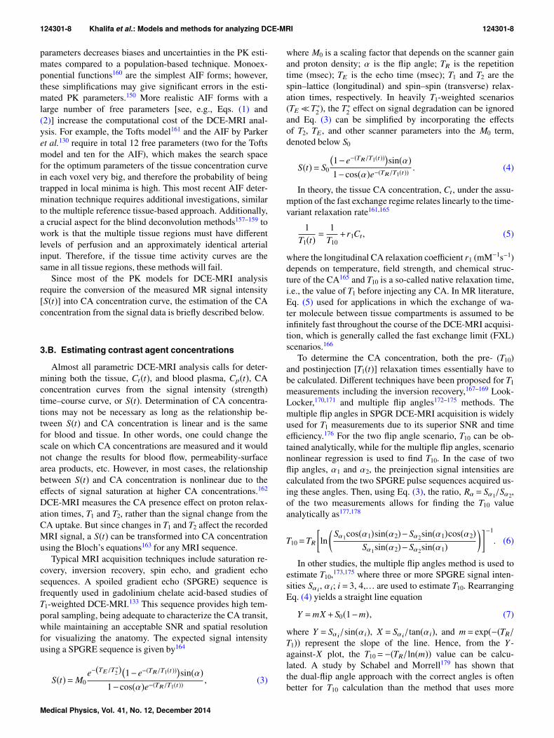
parameters decreases biases and uncertainties in the PK esti-mates compared to a population-based technique. Monoex-ponential functions160 are the simplest AIF forms; however,these simplifications may give significant errors in the esti-mated PK parameters.150 More realistic AIF forms with alarge number of free parameters [see, e.g., Eqs. (1) and(2)] increase the computational cost of the DCE-MRI anal-ysis. For example, the Tofts model161 and the AIF by Parkeret al.130 require in total 12 free parameters (two for the Toftsmodel and ten for the AIF), which makes the search spacefor the optimum parameters of the tissue concentration curvein each voxel very big, and therefore the probability of beingtrapped in local minima is high. This most recent AIF deter-mination technique requires additional investigations, similarto the multiple reference tissue-based approach. Additionally,a crucial aspect for the blind deconvolution methods157–159 towork is that the multiple tissue regions must have differentlevels of perfusion and an approximately identical arterialinput. Therefore, if the tissue time activity curves are thesame in all tissue regions, these methods will fail.

Since most of the PK models for DCE-MRI analysisrequire the conversion of the measured MR signal intensity[S(t)] into CA concentration curve, the estimation of the CAconcentration from the signal data is briefly described below.

3.B. Estimating contrast agent concentrations

Almost all parametric DCE-MRI analysis calls for deter-mining both the tissue, Ct(t), and blood plasma, Cp(t), CAconcentration curves from the signal intensity (strength)time–course curve, or S(t). Determination of CA concentra-tions may not be necessary as long as the relationship be-tween S(t) and CA concentration is linear and is the samefor blood and tissue. In other words, one could change thescale on which CA concentrations are measured and it wouldnot change the results for blood flow, permeability-surfacearea products, etc. However, in most cases, the relationshipbetween S(t) and CA concentration is nonlinear due to theeffects of signal saturation at higher CA concentrations.162

DCE-MRI measures the CA presence effect on proton relax-ation times, T1 and T2, rather than the signal change from theCA uptake. But since changes in T1 and T2 affect the recordedMRI signal, a S(t) can be transformed into CA concentrationusing the Bloch’s equations163 for any MRI sequence.

Typical MRI acquisition techniques include saturation re-covery, inversion recovery, spin echo, and gradient echosequences. A spoiled gradient echo (SPGRE) sequence isfrequently used in gadolinium chelate acid-based studies ofT1-weighted DCE-MRI.133 This sequence provides high tem-poral sampling, being adequate to characterize the CA transit,while maintaining an acceptable SNR and spatial resolutionfor visualizing the anatomy. The expected signal intensityusing a SPGRE sequence is given by164

S(t)=M0e−(TE/T ∗2)�1−e−(TR/T1(t))�sin(α)

1−cos(α)e−(TR/T1(t)) , (3)

where M0 is a scaling factor that depends on the scanner gainand proton density; α is the flip angle; TR is the repetitiontime (msec); TE is the echo time (msec); T1 and T2 are thespin–lattice (longitudinal) and spin–spin (transverse) relax-ation times, respectively. In heavily T1-weighted scenarios(TE≪T∗2 ), the T∗2 effect on signal degradation can be ignoredand Eq. (3) can be simplified by incorporating the effectsof T2, TE, and other scanner parameters into the M0 term,denoted below S0

S(t)= S0

�1−e−(TR/T1(t))�sin(α)1−cos(α)e−(TR/T1(t)) . (4)

In theory, the tissue CA concentration, Ct, under the assu-mption of the fast exchange regime relates linearly to the time-variant relaxation rate161,165

1T1(t) =

1T10+r1Ct, (5)

where the longitudinal CA relaxation coefficient r1 (mM−1s−1)depends on temperature, field strength, and chemical struc-ture of the CA165 and T10 is a so-called native relaxation time,i.e., the value of T1 before injecting any CA. In MR literature,Eq. (5) used for applications in which the exchange of wa-ter molecule between tissue compartments is assumed to beinfinitely fast throughout the course of the DCE-MRI acquisi-tion, which is generally called the fast exchange limit (FXL)scenarios.166

To determine the CA concentration, both the pre- (T10)and postinjection [T1(t)] relaxation times essentially have tobe calculated. Different techniques have been proposed for T1measurements including the inversion recovery,167–169 Look-Locker,170,171 and multiple flip angles172–175 methods. Themultiple flip angles in SPGR DCE-MRI acquisition is widelyused for T1 measurements due to its superior SNR and timeefficiency.176 For the two flip angle scenario, T10 can be ob-tained analytically, while for the multiple flip angles, scenariononlinear regression is used to find T10. In the case of twoflip angles, α1 and α2, the preinjection signal intensities arecalculated from the two SPGRE pulse sequences acquired us-ing these angles. Then, using Eq. (3), the ratio, Rα = Sα1/Sα2,of the two measurements allows for finding the T10 valueanalytically as177,178

T10=TR

ln

Sα1cos(α1)sin(α2)−Sα2sin(α1)cos(α2)

Sα1sin(α2)−Sα2sin(α1)−1

. (6)

In other studies, the multiple flip angles method is used toestimate T10,173,175 where three or more SPGRE signal inten-sities Sαi

, αi; i = 3, 4,. . . are used to estimate T10. RearrangingEq. (4) yields a straight line equation

Y =mX +S0(1−m), (7)

where Y = Sαi/sin(αi), X = Sαi

/tan(αi), and m= exp(−(TR/T1)) represent the slope of the line. Hence, from the Y -against-X plot, the T10=−(TR/ln(m)) value can be calcu-lated. A study by Schabel and Morrell179 has shown thatthe dual-flip angle approach with the correct angles is oftenbetter for T10 calculation than the method that uses more

Medical Physics, Vol. 41, No. 12, December 2014

124301-9 Khalifa et al.: Models and methods for analyzing DCE-MRI 124301-9

flip angles. The T1(t) can be estimated using a postinjectionDCE-MRI scan acquired at a single flip angle α in conjunc-tion with a DCE-MRI preinjection scan, with the assumptionthat proton density does not change due to the CA uptake.180

After all, inaccurate determination of both AIF and T1 cancause significant parameter estimation errors in DCE-MRI.14

Therefore, for a more accurate DCE-MRI analysis and betterevaluation of the PK parameters, the estimated T1(t) and T10values should be compared with the known ones for differenttissues (e.g., muscles, gray matter, and white matter) to ensurethat these estimates are in the acceptable ranges.

Once T10 and AIF are measured or determined, and theS(t) is converted to tissue CA concentration using Eq. (5),the PK model is then used to fit the latter. After fitting, theCA concentration in the tissue, Ct, is described in termsof various rates and volume parameters of the model used.Strengths and weaknesses of the most common compart-mental and distributed tracer-kinetic models that are used foranalyzing DCE-MRI, are outlined below.

3.C. Compartmental models

For the last two decades, many compartmental models ofvarious complexities and under different assumptions havebeen proposed for quantifying the CA uptake in the tissue.Well-known compartmental models are based on the orig-inal principles of the Kety’s model.181 A two-compartmentmodel, widely used for quantitative analysis of tissue perfu-sion, is sketched in Fig. 5. Its compartments specify the CAconcentrations in the EES [i.e., Ce(t)] and the blood plasmaor the intravascular space [i.e., Cp(t)]. An arterial inputCA amount, Ca(t), administered to the system yields a dy-namic concentration, Cp(t), in the first compartment, whereasthe intercompartmental CA exchange results in a dynamicconcentration, Ce(t), in the second compartment. Intercom-partment exchange rates are governed by forward and back-ward volume transfer constants, k12 and k21, respectively, andCA losses from the system are described by an excretionrate, kel. Since, the parameters k12 and k21 control the CAtransfer from the blood plasma to the tissue, they are relatedto capillary permeability.161 The total tissue CA concentra-tion is as follows: Ct(t)= vpCp(t)+ veCe(t), where vp and ve

(0 < vp, ve < 1) are the fractional plasma and EES volumes,

F. 5. Two-compartment model: the function Ca(t) quantifies the arterialinput into the plasma compartment; the peripheral compartment receives theCA from, and returns the CA to, the plasma compartment at the rates k12 andk21, respectively; the rate kel specifies the CA loss from the system.

F. 6. The LM for a capillary–tissue system: blood plasma flows in thecapillary at an Fp rate and exchanges CA with EES at a kep rate.

respectively. The most common compartmental models foranalyzing CA perfusion in the tissue are detailed below.

3.C.1. LM

LM is one of the earliest kinetic models for analyzing DCE-MRI that was developed by Larsson et al.113 In this model,the CA transfer between the blood plasma in the capillary andEES (also called the interstitial water space) is assumed to becontrolled by a single transfer constant kep (min−1) combiningthree parameters: the capillary blood flow, Fp; the extractionfraction, E; the fractional EES volume, see Fig. 6.

To build the model, the CA concentration in the plasmacompartment, Cp(t), is obtained using the gold standard AIF,namely, by measuring the CA amount in a series of bloodsamples taken in 15 s intervals after a bolus CA injection.The measurements are then fitted with a sum of three expo-nentials with the amplitudes ai and time constants mi, respec-tively (i = 1, 2, 3)

Cp(t)=3

i=1

aie−mit . (8)

The temporal tissue CA concentration uptake change in theEES compartment is described using the transfer equation

dCt

dt= kep

�Cp(t)−Ct

�(9)

which can be solved for Ct using Cp(t) in Eq. (8) as follows:

Ct(t)= kep

3i=1

ai

�e−kept−e−mit

�

mi− kep. (10)

The LM assumes that the MR signal S(t) relates linearly tothe CA concentration:

S(t)= S0+

k ′(t)kep

Ct, (11)

where k ′(t)= S′(t)/3i=1ai, S0 is the baseline signal intensity

before the CA injection, and S′(t) is the initial signal slope, orequivalently

Medical Physics, Vol. 41, No. 12, December 2014

124301-10 Khalifa et al.: Models and methods for analyzing DCE-MRI 124301-10

S(t)= S0+ k ′(t)3

i=1

ai

�e−kept−e−mit

�

mi− kep. (12)

The LM is applicable under a very limited tissue perme-ability, i.e., when the permeability is considerably lower thanthe flow, and is fully described by the single transfer constant,kep. The latter can be estimated via optimization, e.g., by theleast-squares techniques. The main limitation of the LM is itsassumed negligible contribution of the plasma (intravascularspace) tracer. Additionally, the work presented in Ref. 113provides only a combined estimation of both permeabilityand the mean extravascular space. However, Larsson and hiscoworkers provisioned a method that allows for separate esti-mation of permeability and ve, using in-vitro value of relaxiv-ity and a measurement of T10.182

3.C.2. BM

Proposed by Brix et al.114 is one of the most well-knowncompartmental models for analyzing DCE-MRI. In the BM,kinetics of the CA exchange between the blood plasma andthe peripheral (interstitial) EES compartments are describedwith several rate and transfer constants, shown in Fig. 7. TheCA is administered at a constant rate of kin over a time-spanτ, exchanged between the plasma and EES compartments atkpe (forward) and kep (reverse) transfer rates, and eliminatedfrom the plasma at a rate of kel. Unlike the LM, which re-quires a predetermined AIF, for the BM, a particular AIF istaken to be known from the infusion rate (the flux) enteringthe body.

Relationships between the intravascular and peripheral co-mpartments in the BM are described using the mass conser-vation principle114

dCp

dt=

kin

Vp(u(t)−u(t−τ))− kelCp(t), (13)

dCt

dt= kpe

Vp

VeCp− kepCp(t), (14)

F. 7. Schematic illustration of the Brix model. The CA is administered at aconstant rate of kin into the plasma compartment, exchanged between the twocompartments at rates of kep and kpe, respectively, and eliminated (cleared)from the plasma at a rate of kel.

where u(t) is the Heaviside step function, and Vp and Ve arethe intravascular plasma and the EES compartment volumes,respectively. Solving Eqs. (13) and (14) under the initialconditions Cp(t)= 0 and Ct(t)= 0 for t = 0 gives the followingCA concentrations in the blood plasma and tissue:12

Cp(t)= kin

Vpkel

ekelt

′

−1

ekelt, (15)

Ct =kinkpe

Vp(kep− kel)

e−kelt

kel

ekelt

′

−1−

e−kept

kep

ekept′−1

, (16)

where t ′= t if 0 ≤ t ≤ τ and t ′= τ if τ ≤ t. To fit the measuredsignal S(t), the BM uses three parameters, namely, the CAexchange rate, kep; the elimination rate, kel; an additionalparameter, ABrix, being an arbitrary constant that depends onthe tissue properties and the MR sequence parameters. Therelationship between the signal S(t) and these free modelparameters at any time is as follows:114

S(t)S0= 1+

ABrix

kep− kel

e−kelt

kel

ekelt

′

−1−

e−kept

kep

ekept′−1

, (17)

where t ′= t if 0 ≤ t ≤ τ and t ′= τ if τ ≤ t. After a CA bolusinjection, Eq. (17) is reduced to

S(t)S0≈ 1+τABrix

e−kelt−e−kept

kep− kel

. (18)

A modified version of the BM proposed by Hoffmannet al.160 reduces the CA infusion length to 1 min. The after-bolus signal S(t) is fitted using

S(t)S0≈ 1+ kepAH

e−kelt−e−kept

kep− kel

(19)

the amplitude parameter, AH approximately corresponds tothe EES size if the CA relaxation properties, the native T1,and the CA dose do not vary significantly.161

Although the BM has been widely used due to its simplicityand proved ability to closely fit the tissue DCE-MRI data,its basic assumption of approximating Cp(t) with a singleexponential function for up to 20 min after the CA injectionis seldom supported by experimental observations.115,132 Ad-ditionally, the BM provides no direct measure of capillarypermeability and is applicable only under specific permeabili-ty-limiting conditions.183 However, the vasculature permeabi-lity can be roughly estimated with the product of the amplitudeparameter, ABrix, and the rate constant, kep.114,184,185

3.C.3. TK model

The most common PK model proposed by TK115 has uni-fied many previous ones and introduced common character-istic parameters and naming conventions.120 It assumes thatthe CA diffuses from and returns to the blood plasma at ratesgoverned by the forward transfer constant, Ktrans (min−1), andthe reverse constant, kep (min−1), respectively (see Fig. 8).

The tissue CA concentration is derived in the TK fromthe EES components only, while the intravascular (plasma)compartment contribution is ignored, i.e., Ct(t)= veCe(t). The

Medical Physics, Vol. 41, No. 12, December 2014

124301-11 Khalifa et al.: Models and methods for analyzing DCE-MRI 124301-11

F. 8. Schematic illustration of the CA transfer in the TK model betweenthe central (plasma) compartment and the EES space with the Ktrans and keprates, respectively.

tissue concentration, Ct(t), is described by the transfer equa-tion

dCt

dt=KtransCp(t)− kepCt(t)=Ktrans

Cp(t)− Ct(t)

ve

, (20)

where kep=Ktrans/ve. The CA concentration in the plasma,Cp(t), after injection specifies the AIF and is used as theinitial condition to estimate Ct(t). Under the initial condi-tions Cp(t)=Ct(t)= 0 at t = 0, Eq. (20) has the followingsolution:120

Ct(t)=Ktrans

t

0Cp(t ′)e−(Ktrans/ve)(t−t′)dt ′. (21)

Alternatively, the TK output, Ct(t), in Eq. (21), can befound by using the convolution theory. Namely, Ct(t) is ob-tained by the convolution (denoted ⊗) of the input signal,Cp(t), with the tissue impulse response, HTK(t), i.e., Ct(t)=Cp(t)⊗HTK(t) where

HTK(t)=Ktranse−(Ktrans/ve)t . (22)

A population-based AIF in the original TK,115 describedby a sum of two exponentials [see Eq. (1) and Fig. 4(a)]results in the following output Ct(t) of Eq. (21):

Ct(t) = DKtrans

a1

m1− kep

e−((Ktrans/ve)t)−e−m1t

+

a2

m2− kep

e−((Ktrans/ve)t)−e−m2t

, (23)

where D is the CA dose (mM kg−1 of body mass) and Ktrans andve are the TK model free parameters that determine the shape ofthe fitted data from which kep=Ktrans/ve is determined. Phys-iologically, Ktrans is the most important and significant tissue-dependent parameter in the TK model. It assesses either plasmaflow Fp in flow-limited scenarios or tissue permeability (rep-resented by the tissue permeability–surface area product, PS)in permeability-limited scenarios for the uptake. In mixed sce-narios, it indicates a combination of the flow and permeabilityproperties of the tissue and acts as a lump measure of their jointeffect.

3.C.4. ETK model

The original TK depends on two parameters, Ktrans and ve,and assumes that the tissue is weakly vascularized (vp= 0).However, this assumption is invalid for many tissues, espe-cially tumors. The generalized TK,161 known commonly asthe extended TK (ETK), includes the intravascular contribu-tion vpCp(t) to the tissue concentration by representing thetotal tissue concentration as

Ct(t) = vpCp(t)+Cp(t)⊗HTK(t)

= vpCp(t)+Ktrans

t

0Cp(t ′)e−((Ktrans/ve)(t−t′))dt ′, (24)

where vp is the fractional plasma volume per unit of tissuevolume. Free ETK parameters, Ktrans, ve, and vp, can be esti-mated by fitting an empirical tissue concentration estimatedfrom the MRI data by the curve Ct(t) of Eq. (24) with ameasured or determined AIF (as described in Sec. 3.A). Forfitting, the signal intensity is converted to the CA concentra-tion using Eq. (5).

Both TK (Ref. 115) and ETK (Ref. 161) models areconsidered the best-established models for analyzing T1-weighted DCE-MR images. However, because the volumetransfer constant, Ktrans, incorporates both the plasma flowand tissue permeability, these latter parameters cannot beestimated separately. The use of a population-based AIFthat was originally introduced by Weinmann et al.132 differssignificantly from the true AIF and is an additional disadvan-tage of both the models. However, individually measured AIFor any other AIF type can be used for TK and ETK models.

3.C.5. PM

Unlike the above PK models, Patlak et al.121 have pro-posed a graphical approach, called Patlak plot, for compart-mental analysis in order to estimate the CA transfer constantbetween the blood plasma and the EES space. The PM as-sumes the reverse vascular transfer constant, kep, from theEES back to the plasma in Fig. 8 and Eq. (20) is negligiblysmall due to low permeability and short measuring time. Thisassumption results in the following tissue concentration:

Ct(t)= vpCp(t)+Ktrans

t

0Cp(t ′)dt ′, (25)

where vp is the vascular fraction. The Patlak plot linearizesEq. (25) as

Y =KtransX + vp, (26)

where Y =Ct(t)/Cp(t) and X = t

0 Cp(t ′)dt ′/Cp(t). Estimationof the parameter Ktrans by constructing visual linear graphicalplots and simple interpretation are the main advantages ofthe PM. This linearized graphical analysis has a widespreadpopularity in certain clinical studies, such as renal applica-tions186–190 where Ktrans is equal to the kidney’s glomerularfiltration rate (GFR). However, this model does not take intoaccount the reverse flow (kep); therefore, its estimates can behighly inaccurate and the analysis results could have somelimitations.191 Moreover, if the model assumption is violated,

Medical Physics, Vol. 41, No. 12, December 2014

124301-12 Khalifa et al.: Models and methods for analyzing DCE-MRI 124301-12

the plotted points are not collinear and the estimation of theparameters is no longer correct.192

Chen et al.192 developed an extended graphical PM, whichis an intermediate between PM and ETK and yields morestable and unbiased Ktrans estimates within short acquisitiondurations. It expands the ETK by correcting for reflux whileretaining the central PM’s advantages, such as linearity inthe parameters estimated, simple graphical interpretation, andstable fitting procedures. Due to accommodating CA efflux,the extended graphical PM became less susceptible to bias.193

3.C.6. 2CXM

The earlier PK models113–115,161 allowed, in principle, forestimating the volume transfer constant, Ktrans, that combinesboth the blood flow and tissue permeability. A recent moregeneral 2CXM (Refs. 6, 127, and 194) allows for separateestimation of the permeability, PS, and the plasma bloodflow, Fp. A block diagram of the 2CXM is schematized inFig. 9, which consists of two compartments: the intravas-cular plasma and the EES compartments. The intravascularcompartment experiences an external flow, Fp, of plasma andthe CA exchanges between both compartments at a symmet-ric rate of PS.

Using mass conservation principle, the CA diffusion be-tween capillary plasma and EES is described by the coupledsystem of differential equations6

dCp

dt=

PSvp

�Ce(t)−Cp(t)�+ Fp

vp

�Ca(t)−Cp(t)�, (27)

dCe

dt=

PSve

�Cp(t)−Ce(t)�, (28)

Ct(t)= vpCp(t)+ veCe(t), (29)

where Cp(t), Ce(t), and Ca(t) are the intravascular plasma,EES space, and arterial plasma CA concentrations, respec-tively. Here, vp and ve are the respective fractional capillary

F. 9. Schematic illustration of the 2CXM. The CA delivered via arteries tothe plasma compartment at a rate of FP is exchanged between the compart-ments at a symmetric rate of PS, and is eliminated subsequently from theplasma compartment.

plasma and EES compartments’ volumes. The Ct(t) is speci-fied by convolving the AIF with the tissue impulse responsefunction, multiplied by the blood plasma flow, Fp

Ct(t)= FpH2CXM(t)⊗Ca(t), (30)

where the tissue response, H2CXM(t), is found by solvingEqs. (27) and (28) for the input delta-function Ca(t)= δ(t) un-der the initial conditions Cp(t)=Ce(t)= 0 for t = 0 and usingEq. (29)194

H2CXM(t)= Be−m1t+ (1−B)e−m2t, (31)

where B, m1, and m2 relate to the model parameters (Fp, PS,vp, and ve) as follows:

m1=12

a+b+

(a+b)2−4bc

,

m2=12

a+b−

(a+b)2−4bc

, B =

m2−cm2−m1

, (32)

where

a =Fp+PS

vp, b=

PSve

, c=Fp

vp. (33)

As a generalization of the 2CXM model, multicompart-ment models with multiple tissue compartments have alsobeen proposed.135,195–199 These models possess the ability toappropriately describe the observed CA dynamics.135 How-ever, the increased complexity of these models, sensitivity tothe choice of initial values, and numerical instability haveprevented the widespread use of these multicompartmentmodels.197 Generally, most of the well-known PK models canbe derived from the 2CXM under specific assumptions. Forexample, the ETK model is derived from the 2CXM modelby assuming that the plasma flow is so high such that the timetaken for the CA to pass through the plasma compartment,i.e., the MTT is negligible. Under this assumption, the intra-vascular plasma concentration cannot be distinguished fromthe AIF, i.e., Cp(t) �Ca(t). However, a study by Donaldsonet al.127 in the carcinoma of the cervix suggested that theassumption of negligible plasma MTT is not appropriate andthe 2CXM is better suited for the analysis than the TK model.Moreover, a breast cancer study by Li et al.200 suggests thatthe TK and ETK models can grossly underestimate bloodflow, vessel wall permeability, and the EES fraction.

As the most general compartmental model, the 2CXMis gradually becoming more common for fitting the MRIdata in many clinical applications.2,127,194 Its main advan-tage is the possibility to estimate both the regional bloodflow and capillary permeability as well as the volume frac-tions of the intravascular (plasma) and the interstitial (EES)space.6 The main limitation of this and other compartmentalmodels is the assumed well-mixed tissue compartments sothat spatial variations of the CA diffusion are not taken intoaccount. In addition, all compartmental models assume aFXL regime, i.e., the intercompartmental water exchange isassumed to be infinitely fast throughout DCE-MRI acquisi-tion. However, this assumption is not always valid or true,

Medical Physics, Vol. 41, No. 12, December 2014

124301-13 Khalifa et al.: Models and methods for analyzing DCE-MRI 124301-13

especially for the high CA concentration in the voxel of in-terest.201 To account for this, other PK models have beendeveloped to allow finite intercompartmental water exchangekinetics.201,202 In these models, the extravascular space isdivided into two separate compartments, namely, the EESand the extravascular-intracellular space (EIS), and a specialshutter speed model is introduced to account for the waterexchange rate between the compartments. Unlike the conven-tional PK models that assume well-mixed compartments witha fast water exchange between them relative to the MRItime frame, the shutter speed model assumes that the tissuecompartments are not well-mixed and the water exchange be-tween the compartments (i.e., between plasma and EES; andbetween EES and EIS) is not sufficiently fast.203 Therefore,the linear relationship between the relaxation rate of the tis-sue and CA concentration in the tissue given by Eq. (5) isno longer valid. It was recently shown that relieving the FXLconstraint leads to a remarkable performance for breast204–208

and prostate166,209 cancer diagnoses using DCE-MRI and theshutter speed model. It is worth mentioning that the waterexchange sensitivity can be minimized by changing the MRIdata acquisition parameters as was shown by Li et al.209,210

More details about these models can be found in Refs. 200,201, 203–207, and 211–214.

3.D. Spatially distributed models

Compartmental models have been widely employed inmany clinical studies due to their simplicity. However, thesemodels do not possess sufficient realism due to the inherentassumptions that the CA gradients within compartments areassumed to be zero at all times. Also, these models assumea fast CA movement and an even distribution throughout thecompartment instantaneously on CA arrival in each compart-ment.126 This makes the CA concentration a function of timeonly, but not space. Advanced spatially distributed kineticmodels, detailed below, that account for both temporal andspatial CA concentration distributions123,124,126,215–217 havebeen introduced for a more complete analysis of the perfu-sion data.

3.D.1. DP model

The DP model122 is the first type of the spatially distrib-uted kinetic models. The DP model is based on a plug-flowmodel, an alternative to a compartmental model, which as-sumes that the administered CA is carried through a tubeby a flow where all particles are traveling with the samevelocity.117,218 In contrast to compartmental models, the DPdoes not assume homogeneous (well-mixed) compartments,but accounts instead for a CA concentration gradient withinthe plasma and EES compartments making their CA concen-trations functions of both the time and distance along thecapillary length (see Fig. 10). The DP is based on three basicassumptions:117 (i) there is no radial (direction perpendicularto the capillary bed) change in CA concentration, such thatthe CA distribution is described by a 1D variation Cp(x,t),

F. 10. Schematic illustration of the DP model. The CA concentrationwithin the capillary decreases with position (x) along the capillary length (L),producing concentration gradients between the arterial (x=0) and venous(x=L) capillary ends. During the CA passage, a portion of the CA moleculesdiffuses between the plasma and EES at a controlled PS rate, so that theplasma, Cp(x, t), and EES, Ce(x, t), concentrations show both the spatialand temporal dependence.

(ii) the EES is modeled as a series of infinitesimal compart-ments exchanging the CA with only nearby locations in thecapillary bed, and (iii) no axial CA transportation (along thex-direction in Fig. 10) is allowed in the EES.

From the mass conservation, the DP can be representedwith a system of differential equations for an elementaryvolume dx along the axial length L of a capillary tube122

vp∂Cp(x,t)

∂t=−LFp

∂Cp(x,t)∂x

−PS�Cp(x,t)−Ce(x,t)�, (34)

ve∂Ce(x,t)

∂t= PS

�Cp(x,t)−Ce(x,t)�. (35)

Similar to the 2CXM, the analytical DP solution is ob-tained by the convolution of Ca(t) (the AIF) with the tissueimpulse response function, multiplied by Fp. The latter func-tion is found again by solving Eqs. (34) and (35) for thedelta-function input of CA (Refs. 117 and 118) as

HDP(t) = u(t)−u(t−Tc)exp−

PSFp

×

1+PS

t−Tc

0

1

t ′Fpve

0.5

e−((PS/ve)t′)

×I1*,2PS

t ′

Fpve

0.5+-

dt ′, (36)

where Tc= vp/Fp is the MTT of the capillary, I1(.) is themodified Bessel function,219 and u(t) is the Heaviside unitstep function. Compared to compartmental models, the DPis more realistic and makes fewer assumptions about micro-circulation. However, like all distributed kinetic models ingeneral, the DP is computationally more intensive and re-quires data with higher temporal resolution in order to derivemeaningful results.128

3.D.2. TH model

Another spatially distributed kinetic model is the THmodel that was first described by Johnson and Wilson123 andapplied in nuclear medicine by Sawada et al.215 The THmodel is a special case of the DP assuming the homogeneous

Medical Physics, Vol. 41, No. 12, December 2014

124301-14 Khalifa et al.: Models and methods for analyzing DCE-MRI 124301-14

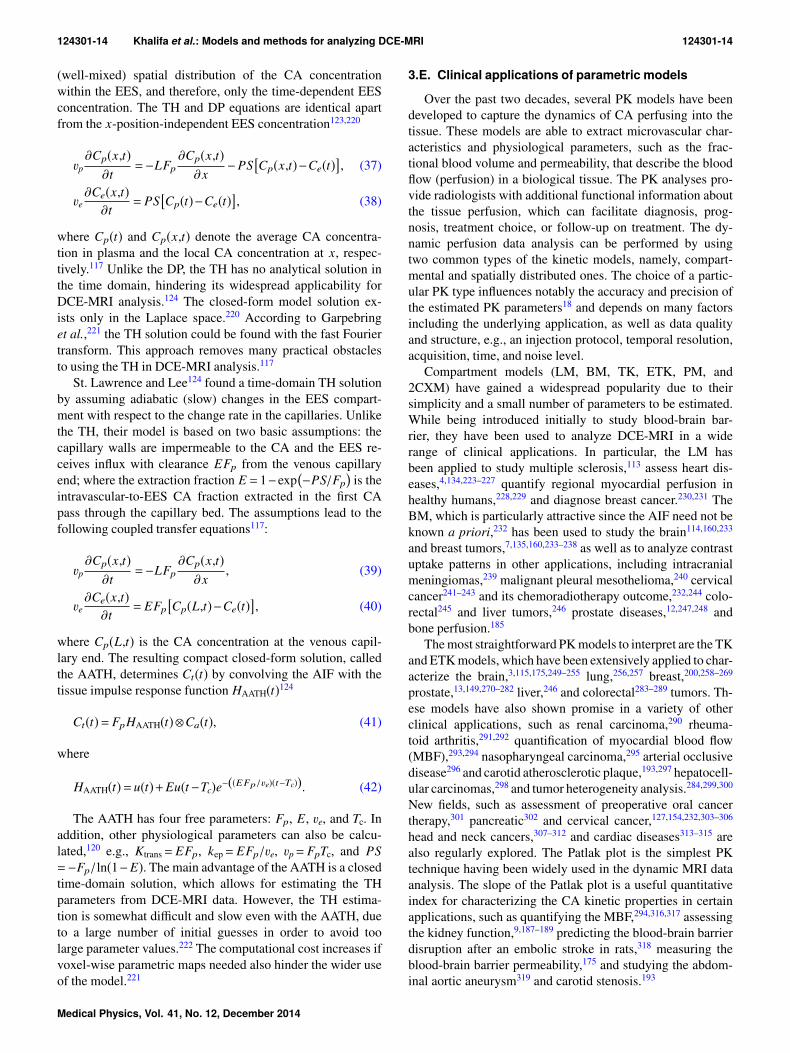
(well-mixed) spatial distribution of the CA concentrationwithin the EES, and therefore, only the time-dependent EESconcentration. The TH and DP equations are identical apartfrom the x-position-independent EES concentration123,220

vp∂Cp(x,t)

∂t=−LFp

∂Cp(x,t)∂x

−PS�Cp(x,t)−Ce(t)�, (37)

ve∂Ce(x,t)

∂t= PS

�Cp(t)−Ce(t)�, (38)

where Cp(t) and Cp(x,t) denote the average CA concentra-tion in plasma and the local CA concentration at x, respec-tively.117 Unlike the DP, the TH has no analytical solution inthe time domain, hindering its widespread applicability forDCE-MRI analysis.124 The closed-form model solution ex-ists only in the Laplace space.220 According to Garpebringet al.,221 the TH solution could be found with the fast Fouriertransform. This approach removes many practical obstaclesto using the TH in DCE-MRI analysis.117

St. Lawrence and Lee124 found a time-domain TH solutionby assuming adiabatic (slow) changes in the EES compart-ment with respect to the change rate in the capillaries. Unlikethe TH, their model is based on two basic assumptions: thecapillary walls are impermeable to the CA and the EES re-ceives influx with clearance EFp from the venous capillaryend; where the extraction fraction E = 1−exp

�−PS/Fp

�is the

intravascular-to-EES CA fraction extracted in the first CApass through the capillary bed. The assumptions lead to thefollowing coupled transfer equations117:

vp∂Cp(x,t)

∂t=−LFp

∂Cp(x,t)∂x

, (39)

ve∂Ce(x,t)

∂t= EFp

�Cp(L,t)−Ce(t)�, (40)

where Cp(L,t) is the CA concentration at the venous capil-lary end. The resulting compact closed-form solution, calledthe AATH, determines Ct(t) by convolving the AIF with thetissue impulse response function HAATH(t)124

Ct(t)= FpHAATH(t)⊗Ca(t), (41)

where

HAATH(t)= u(t)+Eu(t−Tc)e−((EFp/ve)(t−Tc)). (42)

The AATH has four free parameters: Fp, E, ve, and Tc. Inaddition, other physiological parameters can also be calcu-lated,120 e.g., Ktrans= EFp, kep= EFp/ve, vp= FpTc, and PS=−Fp/ln(1−E). The main advantage of the AATH is a closedtime-domain solution, which allows for estimating the THparameters from DCE-MRI data. However, the TH estima-tion is somewhat difficult and slow even with the AATH, dueto a large number of initial guesses in order to avoid toolarge parameter values.222 The computational cost increases ifvoxel-wise parametric maps needed also hinder the wider useof the model.221

3.E. Clinical applications of parametric models

Over the past two decades, several PK models have beendeveloped to capture the dynamics of CA perfusing into thetissue. These models are able to extract microvascular char-acteristics and physiological parameters, such as the frac-tional blood volume and permeability, that describe the bloodflow (perfusion) in a biological tissue. The PK analyses pro-vide radiologists with additional functional information aboutthe tissue perfusion, which can facilitate diagnosis, prog-nosis, treatment choice, or follow-up on treatment. The dy-namic perfusion data analysis can be performed by usingtwo common types of the kinetic models, namely, compart-mental and spatially distributed ones. The choice of a partic-ular PK type influences notably the accuracy and precision ofthe estimated PK parameters18 and depends on many factorsincluding the underlying application, as well as data qualityand structure, e.g., an injection protocol, temporal resolution,acquisition, time, and noise level.

Compartment models (LM, BM, TK, ETK, PM, and2CXM) have gained a widespread popularity due to theirsimplicity and a small number of parameters to be estimated.While being introduced initially to study blood-brain bar-rier, they have been used to analyze DCE-MRI in a widerange of clinical applications. In particular, the LM hasbeen applied to study multiple sclerosis,113 assess heart dis-eases,4,134,223–227 quantify regional myocardial perfusion inhealthy humans,228,229 and diagnose breast cancer.230,231 TheBM, which is particularly attractive since the AIF need not beknown a priori,232 has been used to study the brain114,160,233

and breast tumors,7,135,160,233–238 as well as to analyze contrastuptake patterns in other applications, including intracranialmeningiomas,239 malignant pleural mesothelioma,240 cervicalcancer241–243 and its chemoradiotherapy outcome,232,244 colo-rectal245 and liver tumors,246 prostate diseases,12,247,248 andbone perfusion.185

The most straightforward PK models to interpret are the TKand ETK models, which have been extensively applied to char-acterize the brain,3,115,175,249–255 lung,256,257 breast,200,258–269

prostate,13,149,270–282 liver,246 and colorectal283–289 tumors. Th-ese models have also shown promise in a variety of otherclinical applications, such as renal carcinoma,290 rheuma-toid arthritis,291,292 quantification of myocardial blood flow(MBF),293,294 nasopharyngeal carcinoma,295 arterial occlusivedisease296 and carotid atherosclerotic plaque,193,297 hepatocell-ular carcinomas,298 and tumor heterogeneity analysis.284,299,300

New fields, such as assessment of preoperative oral cancertherapy,301 pancreatic302 and cervical cancer,127,154,232,303–306

head and neck cancers,307–312 and cardiac diseases313–315 arealso regularly explored. The Patlak plot is the simplest PKtechnique having been widely used in the dynamic MRI dataanalysis. The slope of the Patlak plot is a useful quantitativeindex for characterizing the CA kinetic properties in certainapplications, such as quantifying the MBF,294,316,317 assessingthe kidney function,9,187–189 predicting the blood-brain barrierdisruption after an embolic stroke in rats,318 measuring theblood-brain barrier permeability,175 and studying the abdom-inal aortic aneurysm319 and carotid stenosis.193

Medical Physics, Vol. 41, No. 12, December 2014

124301-15 Khalifa et al.: Models and methods for analyzing DCE-MRI 124301-15

The 2CXM model6,127,194 and the more general multicom-partment models135,195,197–199 resolve the ambiguity in inter-preting the Ktrans-estimates from the TK and ETK models.This is a well-known model in classical pharmacokinetics320

and has been applied to analyze nuclear medicine data byLarson et al.126 and adopted for the perfusion analysis byBrix et al.321,322 and Cheong et al.323 Classification of breasttumors by Brix et al.6 was its first DCE-MRI application.Recently, the 2CXM is gradually becoming common invarious applications, such as brain1,2,194 and lung cancer,324

myometrium,325 cervix127 and bladder cancer,326 head andneck tumors,327 and carotid atherosclerotic plaques.193

Compared to compartmental models, the spatially distrib-uted kinetic models (DP, TH, and AATH) account much moreaccurately for the underlying physiology. The DP has beenfirst described by Sangren and Sheppard122 and applied toDCE-MRI by Bisdas et al.328 for studying head and neck can-cer and more recently by Koh et al.329 for studying hepaticmetastases. In contrast to the DP, the TH has not been widelyused for DCE-MRI analysis due to the lack of a closed-formsolution in the time domain. Because the closed-form solu-tion exists only in the Laplace space,220 the fast Fouriertransform was used by Garpebring et al.221 to apply theTH for studying brain tumors. The AATH has been firstapplied to characterize animal brain tumors using DCE-MRIby Henderson et al.330 Among all current models measur-ing Fp and PS separately, the AATH has been most widelyused in a number of DCE-MRI studies, such as detectingviable myocardium331 and lung nodules,257 exploring breasttumors7,332 and prostate cancer,222,333–335 cerebral perfusionmapping,1 and investigating hepatocellular carcinomas in an-imals.298

In summary, the PK modeling capabilities to noninva-sively characterize microvascular physiology have been expl-ored and taken advantage in a wide range of clinical appli-cations. This section covered the clinical applications of thereviewed PK models. There is no uniform consensus forthe choice of an appropriate PK model for specific onco-logic application. Identification of objective criteria for PKmodel selection to fit a given application is a promisingtrend.191,257,336–338 Due to their simplicity, the TK and theETK models have been widely used in many brain, breast,and prostate applications, even by using data with limitedtemporal resolution and without accurate AIF information.18

Based on the reviewed studies (see Table I), the TK and ETKmodels’ parameters have been successfully able to evaluatethe perfusion and permeability of brain tumors,339 discrim-inate between different brain tumors,175,340 detect breast tu-mors,261,266 and evaluate response to treatment.263,300 In car-diac applications, Ktrans is related to the MBF which givesvaluable information about the severity and progression ofcardiac disease, and response to therapy and prognosis. Usu-ally, cardiac applications employ LM and PM models forKtrans estimation. The utility of the Ktrans and ve parame-ters has been found relevant to describe tumor vasculature

perfusion and permeability in several prostate DCE-MRI re-ports. These parameters are known to be elevated in can-cer and therefore are relevant for cancer detection and prog-nosis270,271,273,276,280,299 as well as assessing cancer aggres-siveness.13,278 For renal application, various compartmentalmodels have been proposed for the analysis of kidney DCE-MRI. The GFR measurement is usually obtained using thePM,188 Rutland–Patlak,189 and more advanced models in wh-ich the kidney is modeled as a combination of a vascular andone187 or more tubular compartments.190,341 Table I summa-rizes a number of important findings in a wide range of non-tumor and tumor studies, including tumor detection, charac-terization, and staging, as well as therapy monitoring.

4. SUMMARY AND DISCUSSION

In this paper, we have presented an overview of the exploredDCE-MRI analysis and modeling techniques as well as theirapplications in a wide range of clinical studies in the last twodecades. Promising theoretical findings and experimental re-sults for the reviewed models and techniques in a variety ofclinical applications suggest that DCE-MRI is a clinically rele-vant imaging modality. For example, the classical mammog-raphy has a significantly lower sensitivity (33%–59%) in earlydetection of breast cancer than DCE-MRI analysis (71%–96%).60,65,259,261,263,265,266 Among all MRI modalities, DCE-MRI also offers the highest diagnostic accuracy of small (lessthan 1 cm) breast lesions20,264,342 and the most accurate local-ization and staging of prostate cancer.13,93,100,101,104,247,270,280

Additionally, DCE-MRI has been shown as an effective toolfor evaluating changes in tumor vascular support after ther-apies.343,344 Furthermore, DCE-MRI allows for differentiatingvery accurately between various brain tumors, such as glioma,meningioma, acoustic neuroma, or metastases3,249,340,345 and isa promising noninvasive tool for detecting acute renal rejectionat its earliest stage.10,87–92

As discussed in this paper, both nonparametric and para-metric approaches for DCE-MRI analysis possess the abilityto quantify tissue perfusion. The main advantage of theseanalysis methods is that they reduce the original DCE-MRIdata dimensionality to a small set of parameters that describethe tissue perfusion. The straightforward nonparametric tech-niques characterize shapes and structures of signal enhance-ment curves by computing descriptive indexes (e.g., themaximum enhancement, time-to-peak, and up-slope) directlyfrom these curves. The advantages of these techniques aretwofold: (i) no need to convert the recorded MR signals intoCA concentrations and (ii) the complete analysis of the wholeenhancement curve cycle by computing perfusion-related in-dexes from both wash-in and wash-out phases. However, therelation of the indexes to the underlying physiology is oftenunclear, although some correlation with quantitative or atleast qualitative physiological measurements can be estab-lished. For example, increased wash-in slope, AUC, and peakenhancement and decreased time-to-peak are likely relatedto an improved organ functionality (e.g., renal transplant),bad response to therapy (e.g., cancerous tissue), or increased

Medical Physics, Vol. 41, No. 12, December 2014

124301-16 Khalifa et al.: Models and methods for analyzing DCE-MRI 124301-16

T I. Recent clinical applications of parametric DCE-MRI analysis.

Study PK model Tissue of interest Objectives (o) and conclusions (c)

Harrer et al. (Ref. 339) TK, ETK, andthe first-passleakage profile(Ref. 74)

Brain; 18 patients (o) Characterizing human gliomas with three PK models.(c) Highly correlated ETK- and the first-pass leakage profile-based estimates of Ktrans

and vp validate the use of these models for the evaluation of perfusion andpermeability in tumors.

Haris et al. (Ref. 340) TK Brain; 103 patients (o) Assessing capabilities of various perfusion indexes to separate infective fromneoplastic brain lesions.

(c) Ktrans and ve are useful indexes for discriminating between infective brain lesionsand gliomas.

Bergamino et al.(Ref. 175)

ETK and PM Brain; 25 patients (o) Investigating blood-brain-barrier permeability associated with different braintumors using DCE-MRI.

(c) Different permeability measurements based on Ktrans for different tumor grades:the higher the histological grades, the higher the permeability values.

(c) Significantly different ETK- and PM-related Ktrans-values for the high gradetumors.

Chih-Feng et al.(Ref. 369)

ETK Brain; 10 patients (o) Correlating Ktrans-values and the IAUC of the concentration–time curve forparametric and nonparametric PK modeling, respectively, in clinical patients withbrain tumors.

(c) High correlation coefficient (0.913) between the IAUC and Ktrans suggests theIAUC as an alternative for evaluating physiological condition in DCE-MRI.

Bisdas et al. (Ref. 3) TK Brain; 18 patients (o) Investigating the feasibility of PK modeling to distinguish recurrent high-gradegliomas from radiation injury.

(c) Significantly higher Ktrans-values in recurrent gliomas in comparison toradiation-induced necrosis sites.

(c) 100% sensitivity and 83% specificity of detecting recurrent gliomas on the basisof a cutoff Ktrans-value, compared to 71% sensitivity and 71% specificity of thelike diagnostics with nonparametric AUC.

Lee et al. (Ref. 312) ETK Head and neck; 63patients

(o) Examining DCE-MRI capabilities in differential diagnostics of various head andneck cancers.

(c) Significantly different Ktrans-values obtained by PK analysis between theundifferentiated carcinomas (UDC) and squamous cell carcinoma (SCC), as wellas between the UDC and lymphoma.

(c) The obtained Ktrans-values correlate with the vascular endothelial growth factor(VEGF) expression.

Donaldson et al.(Ref. 327)

2CXM Head and neck; 8patients

(o) Analyzing DCE-MRI data and correlating the obtained PK parameters withmeasurements of hypoxia and VEGF expression in patients with squamous cellcarcinoma.

(c) Negative correlation between the perfusion and both the VEGF expression andhypoxia.

Lee et al. (Ref. 310) ETK Head and neck; 21patients

(o) Investigating the radiation exposure effect on the DCE-MRI parameters andcorrelating the radiation dose and the degree of parotid gland atrophy.

(c) The correlation between the greater glandular atrophy and a lower baseline ve andvp, as well as a higher post-treatment increase in ve showed sound potentialities ofthe DCE-MRI for predicting and assessing the radiation injury in the parotidglands.

Adluru et al. (Ref. 293) TK Heart; 10 patients (o) Assessing the accuracy of a PK-based registration of myocardial DCE-MRI forquantifying the MBF.

(c) Improved estimation of the regional perfusion flow indexes for 77% out of all datasets.

Pärkkä et al. (Ref. 228) LM Heart; 18 patients (o) Assessing myocardial perfusion reserve (MPR) in healthy humans usingDCE-MRI in comparison with PET.

(c) Significant correlation between MRI- and PET-based estimation of MPR.(c) Myocardial perfusion can be quantified by PK modeling of the DCE-MRI.

Medical Physics, Vol. 41, No. 12, December 2014

124301-17 Khalifa et al.: Models and methods for analyzing DCE-MRI 124301-17

T I. (Continued).

Study PK model Tissue of interest Objectives (o) and conclusions (c)

Fritz-Hansen et al.(Ref. 229)

LM Heart; 10 patients (o) Evaluating the MPR in humans by using DCE-MRI and 13N-ammonia PET as areference.

(c) High correlation coefficient (0.96) between the mean perfusion values at rest andhyperemia derived from both DCE-MRI and PET data.

Pack and DiBella(Ref. 294)

TK and PM Heart; 20 subjects (o) Comparing different quantitative techniques for regional myocardial perfusionquantification.

(c) No significant differences between the aggregate Ktrans-values for both the TK andthe Patlak plot analysis.

Kerwin et al. (Ref. 315) ETK Heart; 45 patients (o) Characterizing vasa vasorum in the carotid artery in patients with carotidatherosclerosis disease.

(c) Ktrans-values estimated for the adventitial carotid region are significantlycorrelated with serum inflammation markers, such as C-reactive protein levels(r = 0.57; p = 0.01).

(c) The adventitial Ktrans-value may be a risk marker.

Kurita et al. (Ref. 316) PM Heart; 20 patients (o) Comparing the regional MPR with the CFR found, respectively, byDCE-MRI-based estimation of myocardial perfusion and with the intracoronaryDoppler flow wire.

(c) Significant direct correlations between DCE-MRI-based MPR assessments andDoppler-based CFR assessments (correlation coefficients of 0.87 and 0.86 forculprit and nonculprit arteries, respectively).

Ichihara et al.(Ref. 317)

PM Heart; 10 patients (o) Quantifying DCE-MRI based MBF estimation and comparing it with thatobtained from coronary sinus blood flow.

(c) The means of 86 ± 25 and 89 ± 30 ml/min 100 g−1, for MBFs fromDCE-MRI-related perfusion estimates and coronary sinus blood flow,respectively.

Radjenovic et al.(Ref. 372)

BM Breast; 52 patients (o) Studying the effectiveness of quantitative DCE-MRI parameters for monitoringNAC.

(c) The parameters Ktrans and kep exhibit the highest correlation with the high-gradebreast carcinomas, whereas differ significantly in the low-grade ones.

Schmid et al. (Ref. 332) AATH Breast; 12 patients (o) Evaluating the accuracy of a Bayesian P-spline-based semiparametricquantification of CA concentration curves obtained from DCE-MRI.

(c) The P-spline model demonstrates a superior fit to the observed concentrationcurves and captures accurately the time series up-slope.

Furman-Haran et al.(Ref. 261)

TK Breast; 121 patients (o) Quantifying microvascular perfusion parameters in various breast lesions anddetermining whether the parameters vary between benign and malignant lesions.

(c) High specificity (96%) and sensitivity (93%) of the Ktrans-values for breast cancerdetection.

(c) Significant improvements of breast cancer diagnosis using PK models.

Padhani et al.(Ref. 300)

TK Breast; 25 patients (o) Correlating early changes in the PK parameters’ distribution with treatmentresponse assessments.

(c) Changes in vascular heterogeneity quantified by Ktrans at the end of the secondcycle of systemic chemotherapy can predict both clinical and histopathologicalresponses after three to six cycles of the therapy.

Vincensini et al.(Ref. 263)

TK Breast; 92 patients (o) Studying the effectiveness of quantitative DCE-MRI parameters to characterizemalignant breast lesions.

(c) Excellent classification sensitivity and specificity of the kep-parameter.(c) Monitoring the kep-value may be used to discriminate between lesions that

respond well or poorly to therapy at the early treatment stage.

El Khouli et al.(Ref. 267)

ETK Breast; 95 patients (o) Comparing the ETK model performance with conventional morphology pluskinetic curve type analysis.

(c) The kinetic curve type assessment or PK modeling improve similarly thediagnostic performance.

Medical Physics, Vol. 41, No. 12, December 2014

124301-18 Khalifa et al.: Models and methods for analyzing DCE-MRI 124301-18

T I. (Continued).

Study PK model Tissue of interest Objectives (o) and conclusions (c)

Schabel et al.(Ref. 266)

ETK Breast; 74 patients (o) Prospective investigation of whether PK parameters could provide diagnosticallyuseful information to distinguish between benign and malignant breast lesions.

(c) Higher AUC of 0.915, sensitivity (91%), and specificity (85%) of the Ktrans andkep based classification with respect to mammography (the sensitivity of 88% andspecificity of 68%).

Ah-See et al. (Ref. 265) TK Breast; 28 patients (o) Investigating whether the PK modeling parameters for pre- and post-NAC couldpredict final clinical and pathological response.

(c) According to the ROC analysis, the parameter Ktrans is the best pathologicalnonresponse predictor (the AUC of 0.93, sensitivity of 94%, and specificity of82%).

(c) Correctly identified 94% of nonresponders and 73% of responders, beingcomparable to the change of the MRI-derived tumor size that failed to predict thepathological response.

Fusco et al. (Ref. 7) ETK, BM, andAATH

Breast; 4 patients (o) Analyzing the performance of different DP and compartmental PK models.(o) Comparing TK and BM on real breast DCE-MRI data.(c) The AATH achieved better fit than TK and BM with respect to three

goodness-of-fit metrics: the residual sum of squares, the Bayesian informationcriterion, and Akaike information criterion (AIC).

Naish et al. (Ref. 257) TK, ETK, andAATH

Lung; 6 patients (o) Comparing the performance of the three PK models and a model-free analysis indistinguishing between malignant and nonmalignant lung tissues.

(c) The AATH gives the best description of the lung tumor data with respect to theAIC.

de Senneville et al.(Ref. 9)

PM Kidney; 20 patients (o) Evaluating the effect of DCE-MRI motion correction on the estimated GFR.(c) Significant uncertainty reduction on the computed GFR for native, but not the

transplanted kidneys.

Sourbron et al.(Ref. 190)

Sourbron model(Ref. 190)

Kidney; 15 volunteers (o) Measuring GFR with the gadobenate dimeglumine (Gd-BOPTA) CA using aSourbron mode—the two-compartment PK model with bolus dispersion andtubular outflow.

(c) About 40%-underestimation of GFR (arguably, due to low albumin binding of theGd-BOPTA , which leads to reduced relaxivity in the tubular system andincomplete glomerular filtration).

Anderlik et al.(Ref. 373)

Sourbron model(Ref. 190)

Kidney; 11 volunteers (o) Quantitative assessment of kidney function using DCE-MRI.(c) Promising estimates of the GFR.

Hahn et al. (Ref. 290) ETK Kidney; 56 patients (o) Investigating DCE-MRI as a pharmacodynamic biomarker of a Sorafenibantiangiogenic agent with renal cancer activity.

(c) The derived Ktrans and IAUC90 are pharmacodynamic biomarkers of Sorafenib inmetastatic renal cancer.

(c) The high baseline Ktrans and vp may act as a prognostic or predictive biomarker,which is beneficial to Sorafenib.

Buckley et al.(Ref. 334)

AATH Prostate; 22 patients (o) Prospective evaluation of vascular characteristics of prostate cancer usingDCE-MRI and the DP model.

(c) Increased plasma flow and EES-space fraction within prostate cancer tissue, whencompared to its PZ.

(c) Similar permeability and plasma volume fraction estimates in both regions ofinterest.

Kiessling et al.(Ref. 247)

BM Prostate; 27 patients (o) Evaluating the accuracy of discrimination of prostate cancers from the peripheralgland with descriptive and PK parameters.

(c) Potentialities of the PK parameters (ABrix and kep) in discriminating the prostatecancers from the peripheral prostate tissue.

(c) The nonparametric indexes of early signal enhancement after CA injection, suchas the AUC and up-slopes at 26, 39, 52, and 65 s, have higher sensitivity andspecificity, although at the start of the signal intensity increase, To, these indexesdo not discriminate the carcinomas from the glandular tissue.

Medical Physics, Vol. 41, No. 12, December 2014

124301-19 Khalifa et al.: Models and methods for analyzing DCE-MRI 124301-19

T I. (Continued).

Study PK model Tissue of interest Objectives (o) and conclusions (c)

Kelm et al. (Ref. 12) BM Prostate; 37 patients (o) Assessing the efficacy of spatial prior knowledge for estimating PK parametermaps from DCE-MRI.

(c) The spatial prior knowledge reduces both the bias and variance of the estimatedkep-parameter maps.

van Dorsten et al.(Ref. 374)

LM Prostate; 50 patients (o) Differentiating prostate carcinoma from healthy PZ and CZ using DCE-MRI and2D 1H MRSI.

(c) Excellent potentialities of the combined high-resolution spatio-vascularinformation from the dynamic MRI and metabolic information from the MRSI forimproving the localization and characterization of the prostate cancer in a clinicalsetting.

Jackson et al.(Ref. 271)

TK Prostate; 19 patients (o) Assessing the efficacy of spatial prior knowledge for estimating PK parametermaps from DCE-MRI.

(c) Pixel-wise parametric maps for Ktrans, ve, and kep parameters reveal significantdifferences between benign and malignant tumors in the PZ, while the ROCanalysis shows that the PK parameters are only “fair discriminators” betweencancer and benign gland.

(c) The radiologist interpretation shows similar specificity (85% vs 81%; p = 0.593)and higher sensitivity (50% vs 21%; p = 0.006) of DCE-MRI with respect toT2-weighted MRI for cancer localization.

(c) Guiding the radiotherapy beam with DCE-MRI and PK modeling can improve theoutcome of radiotherapy.

Ocak et al. (Ref. 270) TK Prostate; 50 patients (o) Determining PK parameters, being useful for prostate cancer diagnostics inpatients with biopsy-proven lesions.

(c) Four PK parameters: Ktrans, kep, ve, and the AUC of the gadolinium concentrationcurve were determined and compared for cancer, inflammation, and healthyperipheral.

(c) Improved prostate cancer specificity of the conventional T2-weighted MRI for theKtrans and kep parameters.

Langer et al. (Refs. 273and 276)

TK Prostate; 25 in Ref. 273and 24 in Ref. 276patients

(o) Investigating relationships between the multimodal MRI [diffusion tensor imaging(DTI), T2-weighted, DCE-MRI] measurements and the underlying composition ofnormal and malignant prostate tissues.

(c) Significant differences between cancer and normal PZ tissues for the MRI-derivedapparent diffusion coefficient (ADC), T2, Ktrans, and ve parameters and thepercentage areas of all tissue components except stroma.

Vos et al. (Ref. 275) TK Prostate; 34 patients (o) Developing a multimodality (T2-weighted MRI and DCE-MRI) CAD system witha SVM classifier to diagnose prostate cancer in the PZ.

(c) Using T2-weighted sequence significantly improves the diagnosis performanceobtained with only DCE-MRI PK parameters, namely, the ROC’s AUC increasesfrom 0.83 (0.75–0.92) to 0.89 (0.81–0.95).

Kershaw et al.(Ref. 333)

AATH Prostate; 13 patients (o) Evaluating microvascular and relaxation parameters of prostate and nearbymuscle in patients with benign prostatic hyperplasia and examining measurementreproducibility.

(c) Significantly different bootstrap analysis of the PK parameters (Fp, Tc, Ktrans, andPS) in the prostate’s CZ, comparing with the PZ.

Vos et al. (Ref. 280) TK Prostate; 177patients

(o) Investigating the feasibility of an automated CAD system with a lineardiscriminant analysis (LDA) classifier to detect prostate’s cancer-suspiciousregions.

(c) The CAD system detects 74% of all tumors at a FP level of 5.(c) The system’s sensitivity of 88% for the high-grade tumors at the FP level of 5.

Li et al. (Ref. 281) TK Prostate; 33 patients (o) Investigating and comparing the diagnostic performance of DTI, DCE-MRI, ortheir combination in detecting prostate’s cancerous areas in the PZ.

(c) The combination of DTI and DCE-MRI has better diagnosis in detecting prostatecancer than either technique alone.

Medical Physics, Vol. 41, No. 12, December 2014

124301-20 Khalifa et al.: Models and methods for analyzing DCE-MRI 124301-20

T I. (Continued).

Study PK model Tissue of interest Objectives (o) and conclusions (c)

Vos et al. (Ref. 13) TK Prostate; 45 patients (o) Assessing cancer aggressiveness in the PZ with a combination of kineticparameters, Ktrans and kep, and model-free parameters wash-in and wash-outslopes.

(c) According to the ROC analysis, the 75-percentile of wash-in, Ktrans, and kep

discriminate the best between low-grade and intermediate/high-grade prostatecancer cases.

Chikui et al. (Ref. 301) TK Oral cancer; 29 patients (o) Evaluating usefulness of a PK analysis to monitor the oral cancer response tochemoradiotherapy (CRT).

(c) Statistical analysis reveals that the ve-increase strongly suggests a good tumorresponse to the CRT.

(c) Significantly larger Ktrans-changes for responders, than for nonresponders.

de Lussanet et al.(Ref. 284)

ETK Rectal cancer; 17patients

(o) Evaluating radiation therapy-related microvascular changes in locally advancedrectal cancer using DCE-MRI and histology.

(c) Lower intratumoral heterogeneity in Ktrans and vp for primary rectal cancerpatients receiving the radiation therapy than for those without the radiationtherapy.

de Lussanet et al.(Ref. 296)

TK Thigh; 15 male rabbits (o) Assessing the use of MRI (DCE-MRI and MRA) to evaluate the muscle perfusionrecovery and the growth of collateral arteries in a rabbit femoral artery ligationmodel.

(c) Combined DCE-MRI and MRA data allow for noninvasive serial monitoring ofchanges in the muscle blood flow and growth of submillimeter sized collateralarteries.

Donaldson et al.(Ref. 127)

2CXM and TK Cervix; 30 patients (o) Comparisons of 2CXM and TK models on reporting microvascular parameters inpatients with cervical cancer.

(c) The 2CXM model demonstrated better fit to the data for all patients.(c) Inaccurate PK parameter estimates for TK due to its inherent assumption of

negligible plasma MTT.

Zahra et al. (Ref. 304) TK Cervix; 13 patients(each with three scans)

(o) Evaluate DCE-MRI-based prediction of the response to cervix cancerradiotherapy.

(c) In spite of statistically significant correlation between the percentage tumorregression and both the nonparametric indexes (the peak time, slope, maximumslope, and contrast enhancement ratio) and PK parameters, such as Ktrans

(p = 0.043) and kep (p = 0.022), for the pretreatment DCE-MRI, the samecharacteristics for the second and third scans show no correlation.

Andersen et al.(Ref. 232)

BM and TK Cervix; 81 patients (o) Assessing the prognostic value of the PK parameters derived fromprechemoradiotherapy DCE-MRI of cervical cancer patients.

(c) According to the prognostic significance of the PK parameters [InternationalFederation of Gynecology and Obstetrics (FIGO) stage and tumor volume], beingassessed with the multivariate analysis, the estimated imaging parameters prior tochemoradiotherapy may be used to identify patients at risk of treatment failure.

Akisik et al. (Ref. 302) TK Pancreas; 11patients

(o) Evaluating capabilities of PK modeling of DCE-MRI to predict a pancreaticcancer response to combined chemo and antiangiogenic therapy.

(c) Significant reduction of all parameters, such as Ktrans, ve, the peak concentration,up-slope, and AUC at 60 s, after combined therapy.

(c) The pretreatment Ktrans-measurement in pancreatic tumors can predict response toantiangiogenic therapy.

Ma et al. (Ref. 185) BM Bone perfusion; 165subjects

(o) Investigating PK modeling of bone perfusion in subjects with varying bonemineral density.

(c) Notable reduction of the PK parameter ABrix in osteoporotic subjects compared tothe normal ones.

(c) Less pronounced reductions in the permeability constant, ABrixkep, and theelimination one, kel.

Medical Physics, Vol. 41, No. 12, December 2014

124301-21 Khalifa et al.: Models and methods for analyzing DCE-MRI 124301-21

vascular density and/or vascular permeability. Nevertheless,the indexes can be reproducible at different sites only if anidentical data acquisition protocol is used.346

The parametric techniques fit one of the well-known math-ematical PK models to the concentration curves in orderto estimate physiologically meaningful parameters, e.g., theEES volume and capillary permeability of a tissue of interest.The parametric PK modeling has the following advantages:(i) estimation of a set of kinetic parameters that have phys-iological interpretations, (ii) they provide a way for betterunderstanding of the interaction between drugs (i.e., contrastagent) and human tissue, and (iii) the lesser sensitivity ofparameter estimates to noise, image settings, and data acqui-sition protocols.17 However, both the data acquisition andanalysis become more complicated in comparison with thenonparametric techniques. The complexity arises from therequired conversion of MR signal intensities into CA concen-trations involving the measurements of tissue relaxation time(T1), native relaxation time (T10), and the tissue AIF. Based ontheir mathematical foundations and hypothesis for describ-ing the kinetics of blood flow and capillary-tissue CA ex-change, spatially distributed PK models account much moreaccurately for the underlying physiology and often result ina better fit to the data.127 However, these techniques requiremore investigations and evaluations as other studies showedthat compartment and distributed models result in the sametissue curve331 or distributed models even produce resultsthat are different than expected.1 The PK models are typi-cally refined to more closely reflect physiological processesby including additional parameters, e.g., water exchange andCA diffusion. However, the refinement mostly complicatesDCE-MRI analysis, and its usefulness requires additionalinvestigation.200,326,347–349

It is worth mentioning that the blood flow can also bedetermined using another approach that is based on the Ken-neth L Zierler’s central volume principle.350 Zierler’s tech-nique avoids the use of kinetic models and is based on thedeconvolution theory. Namely, the mean blood perfusion isestimated from a residue function that is derived from thedeconvolution of the tissue response with a measured AIF. De-convolution analysis has been used in many perfusion studies,such as brain351,352 and cardiac applications.353–355 However,it can only determine the blood flow, but not other perfu-sion parameters, such as the vascular volume or the capillarypermeability-surface area product.356

Accurate DCE-MRI analysis is faced with multiple chal-lenges. One of the challenges in gadolinium-based DCE-MRIanalysis is the risk of nephrogenic systemic fibrosis, whichis increased in patients with renal dysfunction.357 Also, thechoice of an appropriate CA dose for the quantitative DCE-MRI analysis is a challenging problem: the high dose in-creases the signal enhancement in the tissue, but may causeoverestimation of the PK parameters due to saturation ornonlinearity of the MRI signal190 or their underestimationdue to transendothelial water exchange effects.358 Investiga-tions of alternative CA types, such as superparamagnetic ironoxide (SPIO) and ultra SPIO (USPIO) particles remain anopen research area. However, it should be pointed out that

those CA agents are mostly intravascular agents and their useprobably will not enable measurement of vessel permeability.

Temporal resolution is another challenge for accurate DCE-MRI data analysis. Compartmental models (other than the2CXM model) are usually used to analyze data sets with longimaging intervals (i.e., low temporal resolution), where theCA movement appears instantaneous and the capillary-tissuecomponents could be approximated as well-mixed compart-ments. On the other hand, spatially distributed PK models arerelevant for DCE-MRI data with short imaging intervals (i.e.,higher temporal resolution) as they do not assume instanta-neous CA movement in the capillary, but rather employ theeffect of the capillary transit time Tc.330 A simulation study byHenderson et al.359 showed that a temporal resolution of 16 sor less is required to ensure that the estimation error in Ktransand kep be less than 10% of their true values. A similar study bySchabel158 found that stable estimates of Ktrans and kep param-eters can be obtained using sampling rates of 12 s. Recently,Larsson et al.360 investigated the effect of variations in tem-poral resolution (between 2.1 and 68 s) on the estimations ofDCE-MRI-derived PK parameters in patients with high-gradegliomas. Their study concluded that for temporal resolutiongreater than 20 s, there is a significant overestimation of Ktransand under estimation of ve. On the other hand, a study by Ker-shaw and Cheng128 concluded that a temporal resolution of1.5 s is required if all parameters of the AATH model are to bemeasured with minimal bias. Therefore, higher temporal reso-lution is desirable, even for compartmental models, to allowfor more accurate modeling and thus more accurate DCE-MRIparameter estimation, particularly for PK models with largenumbers of parameters.128 However, increasing temporal reso-lution greatly affects the spatial resolution and may not be obt-ainable due to hardware limitations. Due to recent technolog-ical progress in rapid MR acquisition, it is expected that DCE-MRI data with sufficient spatial and temporal resolutions willbe obtainable in the near future.

Comparison of different published results is another chal-lenging problem, in part, due to the lack of standardized DCE-MRI acquisition protocols; difficulties of achieving adequatespatial and temporal DCE-MRI resolutions simultaneously;various analytical postprocessing, which sometimes may notdescribe adequately the relevant physiology; different types ofdiseases, subjects’ numbers, and treatment scenarios.

Recent trends to increase the reliability and accuracy ofDCE-MRI-derived perfusion parameters include (i) objectivecriteria for choosing a suitable PK model among the existingones to fit a given application; (ii) a standard consensus fora DCE-MRI data acquisition protocol in each specific appli-cation; (iii) better data normalization techniques that accountfor different physiological and scanning factors, e.g., patientweight/size and scanner type/acquisition parameters, respec-tively; (iv) since the analysis techniques describe a direct rela-tion between the MRI signal and the underlying model, a newtrend is to apply motion correction techniques before analyzingDCE-MRI data10 to remove noise and motion effects in orderto assure that the change in the signal is related to the CA transitin the tissue; (v) including spatial information into voxel-wiseestimation of PK parameters is another trend in DCE-MRI data

Medical Physics, Vol. 41, No. 12, December 2014

124301-22 Khalifa et al.: Models and methods for analyzing DCE-MRI 124301-22

analysis,12,198,199,361,362 which has shown to be very informativein some applications, such as the assessment of tumors’ hetero-geneity;53,348,363–365 (vi) since nonparametric approaches aresimple and fast, a new trend is to develop complete nonin-vasive image-based diagnostic systems for early diagnosis ofdifferent diseases, e.g., lung and prostate cancer; (vii) fusionof parametric and nonparametric approaches is one more newtrend toward more robust diagnostic decisions in each appli-cation.3,92,103,248,254,268,278,282,295,304,366–369 The high correlationbetween the estimated physiological (parametric) and nonpara-metric indexes92,254,268,282,367–369 suggests the nonparametricDCE-MRI analysis can help in avoiding the complexity andlimitations of the parametric methods for evaluation of phys-iological conditions; (viii) distributed-parameter models aremore realistic and make fewer assumptions about microcircu-lation, therefore they are the main focus of research in recentyears and their usefulness requires additional investigation;(ix) in order to account for scanner hardware drift and physio-logical fluctuations, another trend to increase the reliability ofDCE-MRI is to perform reproducibility and repeatability test,especially for longitudinal studies.145,147,193,366,370,371

a)Author to whom correspondence should be addressed. Electronic mail:aselba01@louisville.edu; https://louisville.edu/speed/bioengineering/faculty/bioengineering-full/dr-ayman-el-baz/elbazlab.html/.

1T. S. Koh, C. K. Tan, L. H. Cheong, and C. C. Lim, “Cerebral perfusion map-ping using a robust and efficient method for deconvolution analysis of dy-namic contrast-enhanced images,” Neuroimage 32(2), 643–653 (2006).

2H. B. W. Larsson, F. Courivaud, E. Rostrup, and A. E. Hansen, “Mea-surement of brain perfusion, blood volume, and blood-brain barrier perme-ability, using dynamic contrast-enhanced T1-weighted MRI at 3 tesla,”Magn. Reson. Med. 62(5), 1270–1281 (2009).

3S. Bisdas, T. Naegele, R. Ritz, A. Dimostheni, C. Pfannenberg, M. Reimold,T. S. Koh, and U. Ernemann, “Distinguishing recurrent high-grade gliomasfrom radiation injury: A pilot study using dynamic contrast-enhanced MRimaging,” Acad. Radiol. 18(5), 575–583 (2011).

4G. Nielsen, T. Fritz-Hansen, C. G. Dirks, G. B. Jensen, and H. B. W. Lars-son, “Evaluation of heart perfusion in patients with acute myocardial infarc-tion using dynamic contrast-enhanced magnetic resonance imaging,” J.Magn. Reson. Imaging 20(3), 403–410 (2004).

5G. Tarroni, C. Corsi, P. F. Antkowiak, F. Veronesi, C. M. Kramer, F.H. Epstein, J. Walter, C. Lamberti, R. M. Lang, V. Mor-Avi, and A. R.Patel, “Myocardial perfusion: Near–automated evaluation from contrast-enhanced MR images obtained at rest and during vasodilator stress,” Radi-ology 265(2), 576–583 (2012).

6G. Brix, F. Kiessling, R. Lucht, S. Darai, K. Wasser, S. Delorme, and J.Griebel, “Microcirculation and microvasculature in breast tumors: Phar-macokinetic analysis of dynamic MR image series,” Magn. Reson. Med.52(2), 420–429 (2004).

7R. Fusco, M. Sansone, S. Maffei, N. Raiano, and A. Petrillo, “Dynamiccontrast-enhanced MRI in breast cancer: A comparison between distributedand compartmental tracer kinetic models,” J. Biomed. Graphics Comput.2(2), 23–36 (2012).

8H. Michaely, K. Herrmann, K. Nael, N. Oesingmann, M. Reiser, and S.Schoenberg, “Functional renal imaging: Nonvascular renal disease,” Ab-dom. Imaging 32(1), 1–16 (2007).

9B. D. de Senneville, I. A. Mendichovszky, S. Roujol, I. Gordon, C. Moonen,and N. Grenier, “Improvement of MRI-functional measurement with auto-matic movement correction in native and transplanted kidneys,” J. Magn.Reson. Imaging 28(4), 970–978 (2008).

10F. Khalifa, G. M. Beache, M. A. El-Ghar, T. El-Diasty, G. Gimel’farb, M.Kong, and A. El-Baz, “Dynamic contrast-enhanced MRI-based early detec-tion of acute renal transplant rejection,” IEEE Trans. Med. Imaging 32(10),1910–1927 (2013).

11M. A. Haider, P. Chung, J. Sweet, A. Toi, K. Jhaveri, C. Ménard, P. Warde,J. Trachtenberg, G. Lockwood, and M. Milosevic, “Dynamic contrast-enhanced magnetic resonance imaging for localization of recurrent prostatecancer after external beam radiotherapy,” Int. J. Radiat. Oncol. Biol. Phys.70(2), 425–430 (2008).

12B. M. Kelm, B. H. Menze, O. Nix, C. M. Zechmann, and F. A. Hamprecht,“Estimating kinetic parameter maps from dynamic contrast-enhancedMRI using spatial prior knowledge,” IEEE Trans. Med. Imaging 28(10),1534–1547 (2009).

13E. K. Vos, G. Litjens, T. Kobus, T. Hambrock, C. A. Kaa, J. O. Barentsz, H.Huisman, and T. W. J. Scheenen, “Assessment of prostate cancer aggres-siveness using dynamic contrast-enhanced magnetic resonance imaging at3 T,” Eur. Urol. 64(3), 448–455 (2013).

14M. Bergamino, L. Bonzano, F. Levrero, G. Mancardi, and L. Roccatagliata,“A review of technical aspects of t1–weighted dynamic contrast-enhancedmagnetic resonance imaging (DCE-MRI) in human brain tumors,” Phys.Med. 30(6), 635–643 (2014).

15E. Nagel, C. Klein, I. Paetsch, S. Hettwer, B. Schnackenburg, K. Wegschei-der, and E. Fleck, “Magnetic resonance perfusion measurements for thenon-invasive detection of coronary artery disease,” Circulation 108(4),423–437 (2003).

16P. L. Choyke, J. A. Frank, M. E. Girton, S. W. Inscoe, M. J. Carvlin, J. L.Black, H. A. Austin, and A. J. Dwyer, “Dynamic Gd-DTPA-enhanced MRimaging of the kidney: Experimental results,” Radiology 170(3), 713–720(1989).

17L. Bokacheva, H. Rusinek, J. L. Zhang, Q. Chen, and V. S. Lee, “Esti-mates of glomerular filtration rate from MR renography and tracer kineticmodels,” J. Magn. Reson. Imaging 29(2), 371–382 (2009).

18D. L. Buckley, “Uncertainty in the analysis of tracer kinetics using dynamiccontrast-enhanced T1-weighted MRI,” Magn. Reson. Med. 47(3), 601–606(2002).

19G. J. M. Parker, J. Suckling, S. F. Tanner, A. R. Padhani, J. E. Husband, andM. O. Leach, “MRIW: Parametric analysis software for contrast-enhanceddynamic MR imaging in cancer,” Radiographics 18(2), 497–506 (1998).

20P. Gibbs, G. P. Liney, M. Lowry, P. J. Kneeshaw, and L. W. Turnbull, “Differ-entiation of benign and malignant sub-1 cm breast lesions using dynamiccontrast enhanced MRI,” Breast 13(2), 115–121 (2004).

21N. M. Hylton, J. D. Blume, W. K. Bernreuter, E. D. Pisano, M. A. Rosen,E. A. Morris, P. T. Weatherall, C. D. Lehman, G. M. Newstead, S. Polin, H.S. Marques, L. J. Esserman, M. D. Schnall, and ACRIN 6657 Trial Teamand I-SPY 1 TRIAL Investigators, “Locally advanced breast cancer: MRimaging for prediction of response to neoadjuvant chemotherapy resultsfrom ACRIN 6657/I-SPY TRIAL,” Radiology 263(3), 663–672 (2012).

22V. A. Arasu, R. C. Chen, D. N. Newitt, C. B. Chang, H. Tso, N. M. Hylton,and B. N. Joe, “Can signal enhancement ratio (SER) reduce the numberof recommended biopsies without affecting cancer yield in occult MRI-detected lesions?,” Acad. Radiol. 18(6), 716–721 (2011).

23S. C. Partridge, R. K. Vanantwerp, R. K. Doot, X. Chai, B. F. Kurland, P. R.Eby, J. M. Specht, L. K. Dunnwald, E. K. Schubert, C. D. Lehman, and D.A. Mankoff, “Association between serial dynamic contrast-enhanced MRIand dynamic 18F-FDG PET measures in patients undergoing neoadjuvantchemotherapy for locally advanced breast cancer,” J. Mag. Reson. Imaging32(5), 1123–1131 (2010).

24N. Hylton, “Dynamic contrast-enhanced magnetic resonance imaging as animaging biomarker,” J. Clin. Oncol. 24(20), 3293–3298 (2006).

25G. M. Beache, S. Kulke, H. Kantor, P. N. T. Campbell, D. Chesler, H. Ger-wirtz, B. Rosen, T. Brady, and T. Weisskoff, “Imaging perfusion deficitsin ischemic heart disease with susceptibility–enhanced T2-weighted MRI:Preliminary human studies,” Magn. Reson. Imaging 16(1), 19–27 (1998).

26M. J. Paldino and D. P. Barboriak, “Fundamentals of quantitative dynamiccontrast-enhanced MR imaging,” Magn. Reson. Imaging Clin. North Am.17(2), 277–289 (2009).

27H. J. Van der woude, J. L. Bloem, K. L. Verstraete, A. H. Taminiau, M. A.Nooy, and H. P. C, “Osteosarcoma and Ewing’s sarcoma after neoadjuvantchemotherapy: Value of dynamic MR imaging in detecting viable tumorbefore surgery,” Am. J. Roentgenol. 165(3), 593–598 (1995).

28W. E. Reddick, J. S. Taylor, and B. D. Fletcher, “Dynamic mr imaging(demri) of microcirculation in bone sarcoma.,” J. Magn. Reson. Imaging10(3), 277–285 (1999).

29P. J. Hoskin, M. I. Saunders, K. Goodchild, M. E. Powell, N. J. Taylor, andH. Baddeley, “Dynamic contrast enhanced magnetic resonance scanning asa predictor of response to accelerated radiotherapy for advanced head andneck cancer,” Br. J. Radiol. 72(863), 1093–1098 (1999).

Medical Physics, Vol. 41, No. 12, December 2014

124301-23 Khalifa et al.: Models and methods for analyzing DCE-MRI 124301-23

30A. Semiz oysu, E. Ayanoglu, N. Kodalli, C. Oysu, C. Uneri, and C. Erzen,“Dynamic contrast-enhanced MRI in the differentiation of posttreatmentfibrosis from recurrent carcinoma of the head and neck,” Clin. Imaging29(5), 307–312 (2005).

31N. Tomura, K. Omachi, I. Sakuma, S. Takahashi, J. Izumi, O. Watanabe, J.Watarai, and M. Sageshima, “Dynamic contrast-enhanced magnetic reso-nance imaging in radiotherapeutic efficacy in the head and neck tumors,”Am. J. Otolaryngol. 26(3), 163–167 (2005).

32J. Schwitter, D. Nanz, S. Kneifel, K. Bertschinger, M. Büchi, P. R. Knüsel,B. Marincek, T. F. Lüscher, and G. K. Von schulthess, “Assessment ofmyocardial perfusion in coronary artery disease by magnetic resonancea comparison with positron emission tomography and coronary angiog-raphy,” Circulation 103(18), 2230–2235 (2001).

33T. Ibrahim, S. G. Nekolla, K. Schreiber, K. Odaka, S. Volz, J. Mehilli,M. Güthlin, W. Delius, and M. Schwaiger, “Assessment of coronaryflow reserve: Comparison between contrast-enhanced magnetic resonanceimaging and positron emission tomography,” J. Am. Coll. Cardiol. 39(5),864–870 (2002).

34V. Positano, M. F. Santarelli, and L. Landini, “Automatic characterizationof myocardial perfusion in contrast-enhanced MRI,” EURASIP J. Appl.Signal Process. 5(1), 413–421 (2003).

35H. Ólafsdóttir, M. B. Stegmann, and H. B. W. Larsson, “Automatic assess-ment of cardiac perfusion MRI,” in Proceedings of the Medical ImageComputing and Computer Assisted Intervention (Springer, Berlin Heidel-berg, 2004), pp. 1060–1061.

36H. Xue, S. Zuehlsdorff, P. Kellman, A. Arai, S. Nielles-Vallespin, C. Chefd-hotel, C. H. Lorenz, and J. Guehring, “Unsupervised inline analysis ofcardiac perfusion MRI,” in Proceedings of the Medical Image Computingand Computer Assisted Intervention (Springer, Berlin Heidelberg, 2009),pp. 741–749.

37M.-Y. M. Su, K.-C. Yang, C.-C. Wu, Y.-W. Wu, H.-Y. Yu, R.-Y. Tseng, andW.-Y. I. Tseng, “First-pass myocardial perfusion cardiovascular magneticresonance at 3 Tesla,” J. Cardiovasc. Magn. Reson. 9(4), 633–644 (2007).

38F. Khalifa, G. M. Beache, A. Elnakib, H. Sliman, G. Gimel’farb, K.C. Welch, and A. El-Baz, “A new nonrigid registration framework forimproved visualization of transmural perfusion gradients on cardiac first-pass perfusion MRI,” in Proceedings of the IEEE International Sympo-sium on Biomedical Imaging: From Nano to Macro (IEEE, Piscataway, NJ,2012), pp. 828–831.

39F. Khalifa, G. M. Beache, G. Gimel’farb, and A. El-Baz, “A novel CADsystem for analyzing cardiac first-pass MRI images,” in Proceedings of theIEEE International Conference on Pattern Recognition (IEEE, Piscataway,NJ, 2012), pp. 77–80.

40G. M. Beache, F. Khalifa, G. Gimel’farb, and A. El-Baz, “Fully automatedframework for the analysis of myocardial first-pass perfusion MR images,”Med. Phys. 41(10), 102305 (18pp.) (2014).

41J. M. Hawnaur, X. P. Zhu, and C. E. Hutchinson, “Quantitative dynamiccontrast enhanced MRI of recurrent pelvic masses in patients treated forcancer,” Br. J. Radiol. 71(851), 1136–1142 (1998).

42L. Blomqvist, P. Fransson, and T. Hindmarsh, “The pelvis after surgery andradio-chemotherapy for rectal cancer studied with Gd-DTPA-enhanced fastdynamic MR imaging,” Eur. Radiol. 8(5), 781–787 (1998).

43O. Dicle, F. Obuz, and H. Cakmakci, “Differentiation of recurrent rectalcancer and scarring with dynamic MR imaging,” Br. J. Radiol. 72(864),1155–1159 (1999).

44P. Torricelli, A. Pecchi, G. Luppi, and R. Romagnoli, “Gadolinium-enhanced MRI with dynamic evaluation in diagnosing the local recurrenceof rectal cancer,” Abdom. Imaging 28(1), 0019–0027 (2003).

45N. Tuncbilek, H. M. Karakas, and S. Altaner, “Dynamic MRI in indirectestimation of microvessel density, histologic grade, and prognosis in colo-rectal adenocarcinomas,” Abdom. Imaging 29(2), 166–172 (2004).

46A. de Vries, J. Griebel, C. Kremser, W. Judmaier, T. Gneiting, P. Debbage,T. Kremser, K.-P. Pfeiffer, W. Buchberger, and P. Lukas, “Monitoring of tu-mor microcirculation during fractionated radiation therapy in patients withrectal carcinoma: Preliminary results and implications for therapy,” Radi-ology 217(2), 385–391 (2000).

47X. M. Zhang, D. Yu, H. L. Zhang, Y. Dai, D. Bi, Z. Liu, M. R. Prince,and C. Li, “3D dynamic contrast-enhanced MRI of rectal carcinoma at 3T:Correlation with microvascular density and vascular endothelial growthfactor markers of tumor angiogenesis,” J. Magn. Reson. Imaging 27(6),1309–1316 (2008).

48K. Bol, J. C. Haeck, H. C. Groen, W. J. Niessen, M. R. Bernsen, M.de Jong, and J. F. Veenland, “Can DCE-MRI explain the heterogeneity in

radiopeptide uptake imaged by SPECT in a pancreatic neuroendocrinetumor model?,” PloS one 8(10), e77076 (11pp.) (2013).

49J. Scharf, A. Kemmling, T. Hess, A. Mehrabi, G. Kauffmann, C. Groden,and G. Brix, “Assessment of hepatic perfusion in transplanted livers bypharmacokinetic analysis of dynamic magnetic resonance measurements,”Invest. Radiol. 42(4), 224–229 (2007).

50Y. Ohno, M. Nogami, T. Higashino, D. Takenaka, S. Matsumoto, H. Hatabu,and K. Sugimura, “Prognostic value of dynamic mr imaging for non-small-cell lung cancer patients after chemoradiotherapy,” J. Magn. Reson. Imag-ing 21(6), 775–783 (2005).

51M. Medved, G. Karczmar, C. Yang, J. Dignam, T. F. Gajewski, H. Kindler,E. Vokes, P. MacEneany, M. T. Mitchell, and W. M. Stadler, “Semiquanti-tative analysis of dynamic contrast enhanced MRI in cancer patients: Vari-ability and changes in tumor tissue over time,” J. Magn. Reson. Imaging20(1), 122–128 (2004).

52S. Glaßer, U. Preim, K. Tönnies, and B. Preim, “A visual analytics approachto diagnosis of breast DCE-MRI data,” Comput. Graphics 34(5), 602–611(2010).

53A. Karahaliou, K. Vassiou, N. S. Arikidis, S. Skiadopoulos, T. Kanavou,and L. Costaridou, “Assessing heterogeneity of lesion enhancement ki-netics in dynamic contrast-enhanced MRI for breast cancer diagnosis,” Br.J. Radiol. 83(988), 296–309 (2010).

54R. G. Abramson, X. Li, T. L. Hoyt, P.-F. Su, L. R. Arlinghaus, K. J. Wil-son, V. G. Abramson, A. B. Chakravarthy, and T. E. Yankeelov, “Earlyassessment of breast cancer response to neoadjuvant chemotherapy bysemi-quantitative analysis of high-temporal resolution DCE-MRI: Prelim-inary results,” Magn. Reson. Imaging 31(9), 1457–1464 (2013).

55R. Fusco, S. Filice, V. Granata, Y. Mandato, A. Porto, M. DAiuto, M.Rinaldo, M. Di Bonito, M. Sansone, C. Sansone, A. Rotondo, and A.Petrillo1, “Can semi-quantitative evaluation of uncertain (type II) time-intensity curves improve diagnosis in breast DCE-MRI?,” J. Biomed. Sci.Eng. 6(3A), 418–425 (2013).

56L. Martincich, F. Montemurro, G. De Rosa, V. Marra, R. Ponzone, S. Cir-illo, M. Gatti, N. Biglia, I. Sarotto, P. Sismondi, D. Regge, and M. Agli-etta, “Monitoring response to primary chemotherapy in breast cancer usingdynamic contrast-enhanced magnetic resonance imaging,” Breast CancerRes. Treat. 83(1), 67–76 (2004).

57C. El Khoury, V. Servois, F. Thibault, A. Tardivon, L. Ollivier, M. Meunier,C. Allonier, and S. Neuenschwander, “MR quantification of the washoutchanges in breast tumors under preoperative chemotherapy: Feasibility andpreliminary results,” Am. J. Roentgenol. 184(5), 1499–1504 (2005).

58R. Johansen, L. R. Jensen, J. Rydland, P. E. Goa, K. A. Kvistad, T. F. Bathen,D. E. Axelson, S. Lundgren, and I. S. Gribbestad, “Predicting survival andearly clinical response to primary chemotherapy for patients with locallyadvanced breast cancer using DCE-MRI,” J. Magn. Reson. Imaging 29(6),1300–1307 (2009).

59N. Tuncbilek, F. Tokatli, S. Altaner, A. Sezer, M. Türe, I. K. Omurlu, andO. Temizoz, “Prognostic value DCE-MRI parameters in predicting factordisease free survival and overall survival for breast cancer patients,” Eur. J.Radiol. 81(5), 863–867 (2012).

60S. Mussurakis, D. L. Buckley, S. Bowsley, P. J. Carleton, J. N. Fox, L. W.Turnbull, and A. Horsman, “Dynamic contrast-enhanced magnetic reso-nance imaging of the breast combined with pharmacokinetic analysis ofgadolinium-DTPA uptake in the diagnosis of local recurrence of early stagebreast carcinoma,” Invest. Radiol. 30(11), 650–662 (1995).

61P. C. Stomper, J. S. Winston, S. Herman, D. L. Klippenstein, M. A.Arredondo, and L. E. Blumenson, “Angiogenesis and dynamic MR imaginggadolinium enhancement of malignant and benign breast lesions,” BreastCancer Res. Treat. 45(1), 39–46 (1997).

62L. Esserman, N. Hylton, T. George, and N. Weidner, “Contrast-enhancedmagnetic resonance imaging to assess tumor histopathology and angiogen-esis in breast carcinoma,” Breast J. 5(1), 13–21 (1999).

63C. K. Kuhl, P. Mielcareck, S. Klaschik, C. Leutner, E. Wardelmann, J.Gieseke, and H. H. Schild, “Dynamic breast MR imaging: Are signal inten-sity time course data useful for differential diagnosis of enhancing le-sions?,” Radiology 211(1), 101–110 (1999).

64R. Matsubayashi, Y. Matsuo, G. Edakuni, T. Satoh, O. Tokunaga, andS. Kudo, “Breast masses with peripheral rim enhancement on dynamiccontrast-enhanced MR images: Correlation of MR findings with histologicfeatures and expression of growth factors,” Radiology 217(3), 841–848(2000).

Medical Physics, Vol. 41, No. 12, December 2014

124301-24 Khalifa et al.: Models and methods for analyzing DCE-MRI 124301-24

65F. Sardanelli, F. Podo, G. D’Agnolo, A. Verdecchia, M. Santaquilani, R.Musumeci, G. Trecate, S. Manoukian, S. Morassut, C. de Giacomi, M. Fed-erico, L. Cortesi, S. Corcione, S. Cirillo, V. Marra, A. Cilotti, C. Di Maggio,A. Fausto, L. Preda, C. Zuiani, A. Contegiacomo, A. Orlacchio, M. Cal-abrese, L. Bonomo, E. Di Cesare, M. Tonutti, P. Panizza, and A. Del Mas-chio, “Multicenter comparative multimodality surveillance of women atgenetic-familial high risk for breast cancer (HIBCRIT study): Interim re-sults,” Radiology 242(3), 698–715 (2007).

66C. E. Loo, H. J. Teertstra, S. Rodenhuis, M. J. van de Vijver, J. Hanne-mann, S. H. Muller, M.-J. V. Peeters, and K. G. A. Gilhuijs, “Dynamiccontrast-enhanced MRI for prediction of breast cancer response to neoadju-vant chemotherapy: Initial results,” Am. J. Roentgenol. 191(5), 1331–1338(2008).

67M. Rakoczy, D. McGaughey, M. J. Korenberg, J. Levman, and A. L. Martel,“Feature selection in computer-aided breast cancer diagnosis via dynamiccontrast-enhanced magnetic resonance images,” J. Digital Imaging 26(1),198–208 (2013).

68C. R. Loiselle, P. R. Eby, W. B. DeMartini, S. Peacock, N. Bittner, C. D.Lehman, and J. N. Kim, “Dynamic contrast-enhanced MRI kinetics of inva-sive breast cancer: A potential prognostic marker for radiation therapy,” Int.J. Radiat. Oncol., Biol., Phys. 76(5), 1314–1319 (2010).

69N. A. Mayr, W. T. C. Yuh, V. A. Magnotta, J. C. Ehrhardt, J. A. Wheeler, J.I. Sorosky, C. S. Davis, B. Wen, D. D. Martin, R. E. Pelsang, R. E. Buller, L.W. Oberley, D. E. Mellenberg, and D. H. Hussey, “Tumor perfusion studiesusing fast magnetic resonance imaging technique in advanced cervical can-cer: A new noninvasive predictive assay,” Int. J. Radiat. Oncol., Biol., Phys.36(3), 623–633 (1996).

70N. A. Mayr, W. T. Yuh, J. Zheng, J. C. Ehrhardt, V. A. Magnotta, J. I.Sorosky, R. E. Pelsang, L. W. Oberley, and D. H. Hussey, “Prediction of tu-mor control in patients with cervical cancer: Analysis of combined volumeand dynamic enhancement pattern by MR imaging,” Am. J. Roentgenol.170(1), 177–182 (1998).

71Q. Y. Gong, J. N. Brunt, C. S. Romaniuk, J. P. Oakley, L. T. Tan, N. Roberts,G. H. Whitehouse, and B. Jones, “Contrast enhanced dynamic MRI of cer-vical carcinoma during radiotherapy: Early prediction of tumour regressionrate,” Br. J. Radiol. 72(864), 1177–1184 (1999).

72S. Postema, P. M. T. Pattynama, C. S. P. van Rijswijk, and J. B. Trimbos,“Cervical carcinoma: Can dynamic contrast-enhanced MR imaging helppredict tumor aggressiveness?,” Radiology 210(1), 217–220 (1999).

73R. A. Cooper, B. M. Carrington, J. A. Loncaster, S. M. Todd, S. E. David-son, J. P. Logue, A. D. Luthra, A. P. Jones, I. Stratford, R. D. Hunter,and C. M. L. Weat, “Tumour oxygenation levels correlate with dynamiccontrast-enhanced magnetic resonance imaging parameters in carcinomaof the cervix,” Radiother. Oncol. 57(1), 53–59 (2000).

74K.-L. Li, X. P. Zhu, A. Waterton, and Jackson, “Improved 3D quantitativemapping of blood volume and endothelial permeability in brain tumors,” J.Magn. Reson. Imaging 12(2), 347–357 (2000).

75N. A. Mayr, W. T. C. Yuh, J. C. Arnholt, J. C. Ehrhardt, J. I. Sorosky, V. A.Magnotta, K. S. Berbaum, W. Zhen, A. C. Paulino, L. W. Oberley, A. K.Sood, and J. M. Buatti, “Pixel analysis of MR perfusion imaging in predict-ing radiation therapy outcome in cervical cancer,” J. Magn. Reson. Imaging12(6), 1027–1033 (2000).

76E. A. Boss, L. F. A. G. Massuger, L. A. M. Pop, L. C. G. Verhoef, H.-J. Huis-man, H. Boonstra, and J. O. Barentsz, “Post-radiotherapy contrast enhance-ment changes in fast dynamic MRI of cervical carcinoma,” J. Magn. Reson.Imaging 13(4), 600–606 (2001).

77S. Donaldson, D. L. Buckley, J. O’connor, S. E. Davidson, B. M. Carring-ton, A. P. Jones, and C. M. L. West, “Enhancing fraction measured usingdynamic contrast-enhanced MRI predicts disease-free survival in patientswith carcinoma of the cervix,” Br. J. Cancer 102(1), 23–26 (2009).

78W. T. C. Yuh, N. A. Mayr, D. Jarjoura, D. Wu, J. C. Grecula, S. S. Lo, S.M. Edwards, V. A. Magnotta, S. Sammet, H. Zhang, J. F. Montebello, J.Fowler, M. Knopp, and J. Z. Wang, “Predicting control of primary tumorand survival by DCE MRI during early therapy in cervical cancer,” Invest.Radiol. 44(6), 343–350 (2009).

79N. A. Mayr, W. T. C. Yuh, D. Jajoura, J. Z. Wang, S. S. Lo, J. F. Montebello,K. Porter, D. Zhang, D. S. McMeekin, and J. M. Buatti, “Ultra-early predic-tive assay for treatment failure using functional magnetic resonance imag-ing and clinical prognostic parameters in cervical cancer,” Cancer 116(4),903–912 (2010).

80E. K. Andersen, K. H. Hole, K. V. Lund, K. Sundfør, G. B. Kristensen,H. Lyng, and E. Malinen, “Dynamic contrast-enhanced MRI of cervicalcancers: Temporal percentile screening of contrast enhancement identifies

parameters for prediction of chemoradioresistance,” Int. J. Radiat. Oncol.,Biol., Phys. 82(3), e485–e492 (2012).

81V. B. Ho, S. F. Allen, M. N. Hood, and P. L. Choyke, “Renal masses: Quan-titative assessment of enhancement with dynamic MR imaging,” Radiology224(3), 695–700 (2002).

82H. J. Michaely, S. O. Schoenberg, N. Oesingmann, C. Ittrich, C. Buhlig, D.Friedrich, A. Struwe, J. Rieger, C. Reininger, W. Samtleben, M. Weiss, andM. F. Reiser, “Renal artery stenosis: Functional assessment with dynamicMR perfusion measurements feasibility study,” Radiology 238(2), 586–596(2006).

83V. Positano, I. Bernardeschi, V. Zampa, M. Marinelli, L. Landini, andM. F. Santarelli, “Automatic 2D registration of renal perfusion image se-quences by mutual information and adaptive prediction,” Magn. Reson.Mater. Phys., Biol., Med. 26(3), 325–335 (2013).

84J. A. de Priester, J. A. den Boer, M. H. Christiaans, A. G. Kessels, E. L.Giele, A. Hasman, H. P. van Hooff, and J. van Engelshoven, “Automatedquantitative evaluation of diseased and nondiseased renal transplants withMR renography,” J. Magn. Reson. Imaging 17(1), 95–103 (2003).

85A. A. Farag, A. El-Baz, S. Yuksel, M. A. El-Ghar, and T. El-Diasty, “Aframework for the detection of acute renal rejection with dynamic contrastenhanced magnetic resonance imaging,” in Proceedings of the IEEE Inter-national Symposium on Biomedical Imaging: From Nano to Macro (IEEE,Piscataway, NJ, 2006), pp. 418–421.

86A. El-Baz, A. Farag, R. Fahmi, S. Yuksel, W. Miller, M. Abou El-Ghar,T. El-Diasty, and M. Ghoneim, “A new CAD system for the evaluation ofkidney diseases using DCE-MRI,” in Proceedings of the Medical ImageComputing and Computer Assisted Intervention (Springer, Berlin Heidel-berg, 2006), pp. 446–453.

87A. El-Baz, A. Farag, R. Fahmi, S. Yuksel, M. Abo El-Ghar, and T. El-diasty, “Image analysis of renal DCE-MRI for the detection of acute renalrejection,” in Proceedings of the IEEE International Conference on PatternRecognition (IEEE, Piscataway, NJ, 2006), pp. 822–825.

88A. El-Baz, G. Gimel’farb, and M. Abou El-Ghar, “New motion correctionmodels for automatic identification of renal transplant rejection,” in Pro-ceedings of the Medical Image Computing and Computer Assisted Inter-vention (Springer, Berlin Heidelberg, 2007), pp. 235–243.

89A. El-Baz, G. Gimel’farb, and M. Abo El-Ghar, “A novel image analysisapproach for accurate identification of acute renal rejection,” in Proceed-ings of the IEEE International Conference on Image Processing (IEEE,Piscataway, NJ, 2008), pp. 1812–1815.

90A. El-Baz, G. Gimel’farb, and M. Abo El-Ghar, “Image analysis approachfor identification of renal transplant rejection,” in Proceedings of the Inter-national Conference on Pattern Recognition (IEEE Computer Society,Washington, DC, 2008), pp. 1–4.

91F. Khalifa, A. El-Baz, G. Gimel’farb, and M. Abo El-Ghar, “Non-invasiveimage-based approach for early detection of acute renal rejection,” in Pro-ceedings of the Medical Image Computing and Computer Assisted Inter-vention (Springer, Berlin Heidelberg, 2010), pp. 10–18.

92F. Khalifa, M. Abou El-Ghar, B. Abdollahi, H. B. Frieboes, T. El-Diasty,and A. El-Baz, “A comprehensive non-invasive framework for automatedevaluation of acute renal transplant rejection using DCE-MRI,” NMRBiomed. 26(11), 1460–1470 (2013).

93M. R. Engelbrecht, H. J. Huisman, R. J. F. Laheij, G. J. Jager, G. J. L. H.van Leenders, C. A. Hulsbergen-Van De Kaa, J. J. M. C. H. de la Rosette,J. G. Blickman, and J. O. Barentsz, “Discrimination of prostate cancerfrom normal peripheral zone and central gland tissue by using dynamiccontrast-enhanced MR imaging,” Radiology 229(1), 248–254 (2003).

94S. M. Noworolski, R. G. Henry, D. B. Vigneron, and J. Kurhanewicz, “Dy-namic contrast-enhanced MRI in normal and abnormal prostate tissuesas defined by biopsy, MRI, and 3D MRSI,” Magn. Reson. Med. 53(2),249–255 (2005).

95J. Ren, Y. Huan, H. Wang, Y.-J. Chang, H.-T. Zhao, Y.-L. Ge, Y. Liu,and Y. Yang, “Dynamic contrast-enhanced MRI of benign prostatic hyper-plasia and prostatic carcinoma: Correlation with angiogenesis,” Clin. Ra-diol. 63(2), 153–159 (2008).

96P. Puech, N. Betrouni, R. Viard, A. Villers, X. Leroy, and L. Lemaitre,“Prostate cancer computer-assisted diagnosis software using dynamiccontrast-enhanced MRI,” in Proceedings of the International Conference ofthe IEEE Engineering in Medicine and Biology Society (IEEE, Piscataway,NJ, 2007), pp. 5567–5570.

Medical Physics, Vol. 41, No. 12, December 2014

124301-25 Khalifa et al.: Models and methods for analyzing DCE-MRI 124301-25

97P. Puech, N. Betrouni, N. Makni, A.-S. Dewalle, A. Villers, and L. Lemaitre,“Computer-assisted diagnosis of prostate cancer using DCE-MRI data: De-sign, implementation and preliminary results,” Int. J. Comput. Assisted Ra-diol. Surg. 4(1), 1–10 (2009).

98E. Casciani, E. Polettini, E. Carmenini, I. Floriani, G. Masselli, L.Bertini, and G. F. Gualdi, “Endorectal and dynamic contrast-enhancedMRI for detection of local recurrence after radical prostatectomy,” Am. J.Roentgenol. 190(5), 1187–1192 (2008).

99M. Valerio, V. Panebianco, A. Sciarra, M. Osimani, S. Salsiccia, L. Cas-ciani, A. Giuliani, M. Bizzarri, F. Di Silverio, R. Passariello, and C. Filippo,“Classification of prostatic diseases by means of multivariate analysis on invivo proton MRSI and DCE-MRI data,” NMR Biomed. 22(10), 1036–1046(2009).

100A. Firjani, F. Khalifa, A. Elnakib, G. Gimel’farb, M. Abo El-Ghar, A. El-maghraby, and A. El-Baz, “Non-invasive image-based approach for earlydetection of prostate cancer,” in Proceedings of the Fourth InternationalConference on Developments in E-systems Engineering (IEEE ComputerSociety, Washington DC, 2011), pp. 172–177.

101A. Firjani, F. Khalifa, A. Elnakib, G. Gimel’farb, M. Abo El-Ghar, A. El-maghraby, and A. El-Baz, “A novel image-based approach for early detec-tion of prostate cancer using DCE-MRI,” in Computational Intelligence inBiomedical Imaging, edited by K. Suzuki (Springer Science and BusinessMedia, New York, NY, 2014), Chap. 3, pp. 55–85.

102S. Isebaert, F. De Keyzer, K. Haustermans, E. Lerut, T. Roskams, I.Roebben, H. Van Poppel, S. Joniau, and R. Oyen, “Evaluation of semi-quantitative dynamic contrast-enhanced MRI parameters for prostate can-cer in correlation to whole-mount histopathology,” Eur. J. Radiol. 81(3),217–222 (2012).

103E. Niaf, O. Rouvière, F. Mège-Lechevallier, F. Bratan, and C. Lartizien,“Computer-aided diagnosis of prostate cancer in the peripheral zone usingmultiparametric MRI,” Phys. Med. Biol. 57(12), 3833–3851 (2012).

104J. J. Fütterer, M. R. Engelbrecht, H. J. Huisman, G. J. Jager, C. A.Hulsbergen-van De Kaa, J. A. Witjes, and J. O. Barentsz, “Staging pros-tate cancer with dynamic contrast-enhanced endorectal MR imaging priorto radical prostatectomy: Experienced versus less experienced readers1,”Radiology 237(2), 541–549 (2005).

105M. J. Dobson, B. M. Carrington, C. D. Collins, W. D. J. Ryder, G. Read, C.E. Hutchinson, and J. M. Hawnaur, “The assessment of irradiated bladdercarcinoma using dynamic contrast-enhanced MR imaging,” Clin. Radiol.56(2), 94–98 (2001).

106A. Kalogeropoulos, V. Georgiopoulou, S. Kritchevsky, B. Psaty, N. Smith,A. Newman, N. Rodondi, S. Satterfield, D. Bauer, K. Bibbins-Domingo,A. Smith, P. Wilson, R. Vasan, T. Harris, and J. Butler, “Epidemiologyof incident heart failure in a contemporary elderly cohort: The health, ag-ing, and body composition study,” Archi. Intern. Med. 169(7), 708–715(2009).

107T. Lindeberg, “Edge detection and ridge detection with automatic scaleselection,” Int. J. Comput. Vision 30(2), 117–156 (1998).

108M. D. Cerqueira, N. J. Weissman, V. Dilsizian, A. K. Jacobs, S. Kaul,W. K. Laskey, D. J. Pennell, J. A. Rumberger, T. Ryan, and M. S. Ve-rani, “Standardized myocardial segmentation and nomenclature for tomo-graphic imaging of the heart: A statement for healthcare professionals fromthe cardiac imaging committee of the council on clinical cardiology of theAmerican Heart Association,” Circulation 105(4), 539–542 (2002).

109A. Jemal, F. Bray, M. M. Center, J. Ferlay, E. Ward, and D. Forman, “Globalcancer statistics,” Ca–Cancer J. Clin. 61(2), 69–90 (2011).

110H. K. Thompson, C. F. Starmer, R. E. Whalen, and H. D. McIntosh, “Indi-cator transit time considered as a gamma variate,” Circ. Res. 14(6), 502–515(1964).

111C. Cobelli, G. Toffolo, and D. M. Foster, “A simplified formulation of thegamma variate function,” Phys. Med. Biol. 37(7), 1597–1600 (1992).

112American Cancer Society, Cancer Facts and Figures (American CancerSociety, Atlanta, GA, 2013).

113H. B. W. Larsson, M. Stubgaard, J. L. Frederiksen, M. Jensen, O. Henrik-sen, and O. B. Paulson, “Quantitation of blood-brain barrier defect by mag-netic resonance imaging and gadolinium-DTPA in patients with multiplesclerosis and brain tumors,” Magn. Reson. Med. 16(1), 117–131 (1990).

114G. Brix, W. Semmler, R. Port, L. Schad, G. Layer, and W. Lorenz, “Pharma-cokinetic parameters in CNS Gd-DTPA enhanced MR imaging,” J. Com-put. Assisted Tomogr. 15(4), 621–628 (1991).

115P. S. Tofts and A. G. Kermode, “Measurement of the blood-brain barrierpermeability and leakage space using dynamic MR imaging. 1. Fundamen-tal concepts,” Magn. Reson. Med. 17(2), 357–367 (1991).

116S. P. Sourbron and D. L. Buckley, “Classic models for dynamic contrast-enhanced MRI,” NMR Biomed. 26(8), 1004–1027 (2013).

117S. P. Sourbron and D. L. Buckley, “Tracer kinetic modeling in MRI:Estimating perfusion and capillary permeability,” Phys. Med. Biol. 57(2),R1–R33 (2012).

118T. S. Koh, S. Bisdas, D. M. Koh, and C. H. Thng, “Fundamentals of tracerkinetics for dynamic contrast-enhanced MRI,” J. Magn. Reson. Imaging34(6), 1262–1276 (2011).

119J. R. Ewing and H. Bagher-Ebadian, “Model selection in measures ofvascular parameters using dynamic contrast-enhanced MRI: Experimentaland clinical applications,” NMR Biomed. 26(8), 1028–1041 (2013).

120P. S. Tofsts, G. Brix, D. L. Buckley, J. L. Evelhoch, E. Henderson, M. V.Knopp, H. B. W. Larsson, T. Lee, N. A. Mayr, and G. J. M. Parker, “Esti-mating kinetics parameters from dynamic contrast-enhanced T1-weightedMRI of a diffusible tracer: Standardized quantities and symbols,” J. Magn.Reson. Imaging 10(3), 223–232 (1999).

121C. S. Patlak, R. G. Blasberg, and J. D. Fenstermacher, “Graphical evalua-tion of blood-to-brain transfer constants from multiple-time uptake data,”J. Cereb. Blood Flow Metab. 3(1), 1–7 (1983).

122W. C. Sangren and C. W. Sheppard, “A mathematical derivation of the ex-change of a labeled substance between a liquid flowing in a vessel andan external compartment,” The Bulletin Math. Biophys. 15(4), 387–394(1953).

123J. A. Johnson and T. A. Wilson, “A model for capillary exchange,” Am. J.Physiol. 210(6), 1299–1303 (1966).

124K. S. St Lawrence and T.-Y. Lee, “An adiabatic approximation to the tissuehomogeneity model for water exchange in the brain: I. Theoretical deriva-tion,” J. Cereb. Blood Flow Metab. 18(12), 1365–1377 (1998).

125C. Cobelli, G. Toffolo, and D. M. Foster, “Tracer to tracee ratio for analysisof stable isotope tracer data: Link with radioactive kinetic formalism,” Am.J. Phys. 262(6), 968–975 (1992).

126K. B. Larson, J. Markham, and M. E. Raichle, “Tracer-kinetic models formeasuring cerebral blood flow using externally detected radiotracers,” J.Cereb. Blood Flow Metab. 7(4), 443–463 (1987).

127S. B. Donaldson, C. M. L. West, S. E. Davidson, B. M. Carrington, G.Hutchison, A. P. Jones, S. P. Sourbron, and D. L. Buckley, “A compar-ison of tracer kinetic models for T1-weighted dynamic contrast-enhancedMRI: Application in carcinoma of the cervix,” Magn. Reson. Med. 63(3),691–700 (2010).

128L. E. Kershaw and H.-L. M. Cheng, “Temporal resolution and SNR require-ments for accurate DCE-MRI data analysis using the AATH model,” Magn.Reson. Med. 64(6), 1772–1780 (2010).

129T. E. Yankeelov and J. C. Gore, “Dynamic contrast enhanced magneticresonance imaging in oncology: Theory, data acquisition, analysis, andexamples,” Curr. Med. Imaging Rev. 3(2), 91–107 (2009).

130G. J. M. Parker, C. Roberts, A. Macdonald, G. A. Buonaccorsi, S. Che-ung, D. L. Buckley, A. Jackson, Y. Watson, K. Davies, and G. C. Jayson,“Experimentally-derived functional form for a population-averaged high-temporal-resolution arterial input function for dynamic contrast-enhancedMRI,” Magn. Reson. Med. 56(5), 993–1000 (2006).

131H. B. W. Larsson and P. S. Tofts, “Measurement of blood-brain bar-rier permeability using dynamic Gd-DTPA scanning–A comparison ofmethods,” Magn. Reson. Med. 24(1), 174–176 (1992).

132H. J. Weinmann, M. Laniado, and W. Mutzel, “Pharmacokinetics ofGdDTPA/dimeglumine after intravenous injection into healthy volunteers,”Physiol. Chem. Phys. Med. NMR 16(2), 167–172 (1984).

133D. De Naeyer, “Algorithm development and protocol optimization for phar-macokinetic modeling of dynamic contrast-enhanced magnetic resonanceimaging,” Ph.D. dissertation, Ghent University, Ghent, Belgium, 2011.

134T. Fritz-Hansen, E. Rostrup, H. B. W. Larsson, L. Søndergaard, P. Ring,and O. Henriksen, “Measurement of the arterial concentration of Gd-DTPAusing MRI: A step toward quantitative perfusion imaging,” Magn. Reson.Med. 36(2), 225–231 (1996).

135R. E. Port, M. V. Knopp, U. Hoffmann, S. Milker-Zabel, and G. Brix, “Mul-ticompartment analysis of gadolinium chelate kinetics: Blood-tissue ex-change in mammary tumors as monitored by dynamic MR imaging,” J.Magn. Reson. Imaging 10(3), 233–241 (1999).

136M. J. P. van Osch, E.-J. Vonken, M. A. Viergever, J. van der Grond, andC. J. G. Bakker, “Measuring the arterial input function with gradient echosequences,” Magn. Reson. Med. 49(6), 1067–1076 (2003).

137S. L. Barnes, J. G. Whisenant, M. E. Loveless, and T. E. Yankeelov, “Prac-tical dynamic contrast enhanced MRI in small animal models of cancer:Data acquisition, data analysis, and interpretation,” Pharmaceutics 4(3),442–478 (2012).

Medical Physics, Vol. 41, No. 12, December 2014

124301-26 Khalifa et al.: Models and methods for analyzing DCE-MRI 124301-26

138G. O. Cron, C. Foottit, T. E. Yankeelov, L. I. Avruch, M. E. Schweitzer, andI. Cameron, “Arterial input functions determined from MR signal magni-tude and phase for quantitative dynamic contrast-enhanced MRI in the hu-man pelvis,” Magn. Reson. Med. 66(2), 498–504 (2011).

139I. Van der Schaaf, E.-J. Vonken, A. Waaijer, B. Velthuis, M. Quist, and T.van Osch, “Influence of partial volume on venous output and arterial inputfunction,” Am. J. Neuroradiol. 27(1), 46–50 (2006).

140B. F. Kjølby, I. K. Mikkelsen, M. Pedersen, L. Østergaard, and V. G. Kise-lev, “Analysis of partial volume effects on arterial input functions usinggradient echo: A simulation study,” Magn. Reson. Med. 61(6), 1300–1309(2009).

141M. K. Ivancevic, I. Zimine, X. Montet, J.-N. Hyacinthe, F. Lazeyras, D.Foxall, and J.-P. Vallée, “Inflow effect correction in fast gradient-echoperfusion imaging,” Magn. Reson. Med. 50(5), 885–891 (2003).

142F. Peeters, L. Annet, L. Hermoye, and B. E. Van Beers, “Inflow correctionof hepatic perfusion measurements using T1-weighted, fast gradient-echo,contrast-enhanced MRI,” Magn. Reson. Med. 51(4), 710–717 (2004).

143J. L. Zhang, H. Rusinek, L. Bokacheva, Q. Chen, P. Storey, and V. S. Lee,“Use of cardiac output to improve measurement of input function in quan-titative dynamic contrast-enhanced MRI,” J. Magn. Reson. Imaging 30(3),656–665 (2009).

144D. A. Kovar, M. Lewis, and G. S. Karczmar, “A new method for imag-ing perfusion and contrast extraction fraction: Input functions derived fromreference tissues,” J. Magn. Reson. Imaging 8(5), 1126–1134 (1998).

145T. E. Yankeelov, L. M. DeBusk, D. D. Billheimer, J. J. Luci, P. C. Lin, R.R. Price, and J. C. Gore, “Repeatability of a reference region model foranalysis of murine DCE-MRI data at 7T,” J. Magn. Reson. Imaging 24(5),1140–1147 (2006).

146T. E. Yankeelov, G. O. Cron, C. L. Addison, J. C. Wallace, R. C. Wilkins,B. A. Pappas, G. E. Santyr, and J. C. Gore, “Comparison of a reference re-gion model with direct measurement of an AIF in the analysis of DCE-MRIdata,” Magn. Reson. Med. 57(2), 353–361 (2007).

147S. Walker-Samuel, C. C. Parker, M. O. Leach, and D. J. Collins, “Repro-ducibility of reference tissue quantification of dynamic contrast-enhanceddata: Comparison with a fixed vascular input function,” Phys. Med. Biol.52(1), 75–89 (2007).

148M. Heisen, X. Fan, J. Buurman, N. A. W. van Riel, G. S. Karczmar, and B.M. ter Haar Romeny, “The use of a reference tissue arterial input functionwith low-temporal-resolution DCE-MRI data,” Phys. Med. Biol. 55(16),4871–4883 (2010).

149A. R. Padhani, C. Hayes, S. Landau, and M. O. Leach, “Reproducibility ofquantitative dynamic MRI of normal human tissues,” NMR Biomed. 15(2),143–153 (2002).

150C. Yang, G. S. Karczmar, M. Medved, and W. M. Stadler, “Estimatingthe arterial input function using two reference tissues in dynamic contrast-enhanced MRI studies: Fundamental concepts and simulations,” Magn. Re-son. Med. 52(5), 1110–1117 (2004).

151T. E. Yankeelov, J. J. Luci, M. Lepage, R. Li, L. DeBusk, P. C. Lin, R. R.Price, and J. C. Gore, “Quantitative pharmacokinetic analysis of DCE-MRIdata without an arterial input function: A reference region model,” Magn.Reson. Imaging 23(4), 519–529 (2005).

152C. Yang, G. S. Karczmar, M. Medved, and W. M. Stadler, “Multiple refer-ence tissue method for contrast agent arterial input function estimation,”Magn. Reson. Med. 58(6), 1266–1275 (2007).

153C. Yang, G. S. Karczmar, M. Medved, A. Oto, M. Zamora, and W. M.Stadler, “Reproducibility assessment of a multiple reference tissue methodfor quantitative DCE-MRI analysis,” Magn. Reson. Med. 61(4), 851–859(2009).

154C. Yang, W. M. Stadler, G. S. Karczmar, M. Milosevic, I. Yeung, and M. A.Haider, “Comparison of quantitative parameters in cervix cancer measuredby dynamic contrast–enhanced MRI and CT,” Magn. Reson. Med. 63(6),1601–1609 (2010).

155T. E. Yankeelov, J. J. Luci, L. M. DeBusk, P. C. Lin, and J. C. Gore, “Incor-porating the effects of transcytolemmal water exchange in a reference re-gion model for DCE-MRI analysis: Theory, simulations, and experimentalresults,” Magn. Reson. Med. 59(2), 326–335 (2008).

156A. Steingoetter, J. Svensson, Y. Kosanke, R. M. Botnar, M. Schwaiger,E. Rummeny, and R. Braren, “Reference region-based pharmacokineticmodeling in quantitative dynamic contract-enhanced MRI allows robusttreatment monitoring in a rat liver tumor model despite cardiovascularchanges,” Magn. Reson. Med. 65(1), 229–238 (2011).

157J. U. Fluckiger, M. C. Schabel, and E. V. R. DiBella, “Model-based blindestimation of kinetic parameters in dynamic contrast enhanced (DCE)-MRI,” Magn. Reson. Med. 62(6), 1477–1486 (2009).

158M. C. Schabel, J. U. Fluckiger, and E. V. R. DiBella, “A model-constrainedMonte Carlo method for blind arterial input function estimation in dy-namic contrast-enhanced MRI: I. Simulations,” Phys. Med. Biol. 55(16),4783–4806 (2010).

159M. C. Schabel, E. V. R. DiBella, R. L. Jensen, and K. L. Salzman, “Amodel-constrained Monte Carlo method for blind arterial input functionestimation in dynamic contrast-enhanced MRI: II. In vivo results,” Phys.Med. Biol. 55(16), 4807–4823 (2010).

160U. Hoffmann, G. Brix, M. V. Knopp, T. Heβ, and W. J. Lorenz, “Pharmaco-kinetic mapping of the breast: A new method for dynamic MR mammog-raphy,” Magn. Reson. Med. 33(4), 506–514 (1995).

161P. S. Tofts, “Modeling tracer kinetics in dynamic Gd-DTPA MR imaging,”J. Magn. Reson. Imaging 7(1), 91–101 (1997).

162D. Gadian, J. Payne, D. Bryant, I. Young, D. Carr, and G. Bydder,“Gadolinium-DTPA as a contrast agent in mr imaging-theoretical projec-tions and practical observations,” J. Comput. Assisted Tomogr. 9(2),242–251 (1985).

163F. Bloch, “Nuclear induction,” Phys. Rev. 70(7–8), 460–474 (1946).164D. W. McRobbie, E. A. Moore, M. J. Graves, and M. R. Prince, MRI from

Picture to Proton (Cambridge University Press, Cambridge, UK, 2006).165G. J. Stanisz and R. M. Henkelman, “Gd-DTPA relaxivity depends on

macromolecular content,” Magn. Reson. Med. 44(5), 665–667 (2000).166X. Li, R. A. Priest, W. J. Woodward, I. J. Tagge, F. Siddiqui, W. Huang,

W. D. Rooney, T. M. Beer, M. G. Garzotto, and C. S. Springer, “Feasibilityof shutter-speed DCE-MRI for improved prostate cancer detection,” Magn.Reson. Med. 69(1), 171–178 (2013).

167R. Ordidge, P. Gibbs, B. Chapman, M. Stehling, and P. Mansfield, “High-speed multislice T1 mapping using inversion-recovery echo-planar imag-ing,” Magn. Reson. Med. 16(2), 238–245 (1990).

168U. Studler, L. M. White, G. Andreisek, S. Luu, H.-L. M. Cheng, and M.S. Sussman, “Impact of motion on T1 mapping acquired with inversionrecovery fast spin echo and rapid spoiled gradient recalled-echo pulse se-quences for delayed gadolinium-enhanced MRI of cartilage (dGEMRIC)in volunteers,” J. Magn. Reson. Imaging 32(2), 394–398 (2010).

169D. C. Zhu and R. D. Penn, “Full-brain T1 mapping through inversion re-covery fast spin echo imaging with time-efficient slice ordering,” Magn.Reson. Med. 54(3), 725–731 (2005).

170E. Henderson, G. Mckinnon, T.-Y. Lee, and B. K. Rutt, “A fast 3D look-locker method for volumetric t1 mapping,” Magn. Reson. Imaging 17(8),1163–1171 (1999).

171A. Freeman, P. Gowland, and P. Mansfield, “Optimization of the ultra-fast look-locker echo-planar imaging t1 mapping sequence,” Magn. Reson.Imaging 16(7), 765–772 (1998).

172H. Z. Wang, S. J. Riederer, and J. N. Lee, “Optimizing the precision in T1relaxation estimation using limited flip angles,” Magn. Reson. Med. 5(5),399–416 (1987).

173H.-L. M. Cheng and G. A. Wright, “Rapid high-resolution T1 mapping byvariable flip angles: Accurate and precise measurements in the presence ofradiofrequency field inhomogeneity,” Magn. Reson. Med. 55(3), 566–574(2006).

174G. Andreisek, L. M. White, Y. Yang, E. Robinson, H.-L. M. Cheng, andM. S. Sussman, “Delayed gadolinium-enhanced MR imaging of articularcartilage: Three-dimensional T1 mapping with variable flip angles and B1correction,” Radiology 252(3), 865–873 (2009).

175M. Bergamino, L. Saitta, L. Barletta, L. Bonzano, G. L. Mancardi, L.Castellan, J. L. Ravetti, and L. Roccatagliata, “Measurement of blood-brainbarrier permeability with T1-Weighted dynamic contrast-enhanced MRI inbrain tumors: A comparative study with two different algorithms,” ISRNNeurosci. 2013, 1–6.

176J. Yuan, S. K. K. Chow, D. K. W. Yeung, A. T. Ahuja, and A. D. King,“Quantitative evaluation of dual-flip-angle T1 mapping on DCE-MRI ki-netic parameter estimation in head and neck,” Quant. Imaging Med. Surg.2(4), 245–253 (2012).

177B. Whitcher and V. J. Schmid, “Quantitative analysis of dynamiccontrast-enhanced and diffusion-weighted magnetic resonance imaging foroncology in R,” J. Stat. Software 44(5), 1–29 (2011).

178J. A. Brookes, T. W. Redpath, F. J. Gilbert, A. D. Murray, and R. T. Staff,“Accuracy of T1 measurement in dynamic contrast-enhanced breast MRIusing two-and three-dimensional variable flip angle fast low-angle shot,” J.Magn. Reson. Imaging 9(2), 163–171 (1999).

Medical Physics, Vol. 41, No. 12, December 2014

124301-27 Khalifa et al.: Models and methods for analyzing DCE-MRI 124301-27

179M. C. Schabel and G. R. Morrell, “Uncertainty in T1 mapping using thevariable flip angle method with two flip angles,” Phys. Med. Biol. 54(1),1–8 (2009).

180J. Brookes, T. Redpath, F. Gilbert, G. Needham, and A. Murray, “Measure-ment of spin-lattice relaxation times with FLASH for dynamic MRI of thebreast,” Br. J. Radiol. 69(819), 206–214 (1996).

181S. S. Kety, “The theory and applications of the exchange of inert gas at thelungs and tissues,” Pharmacol. Rev. 3(1), 1–41 (1951).

182H. B. W. Larsson, P. Christiansen, M. Stubgaard, C. Thomsen, J. Frederik-sen, and O. Henriksen, “In vivo calculation of the unidirectional inflow con-stant across the blood-brain barrier using MRI,” in Proceedings of the An-nual Meeting of the Society for Magnetic Resonance in Medicine (ISMRM,Berkeley, CA, 1990), pp. 752.

183G. Brix, J. Griebel, F. Kiessling, and F. Wenz, “Tracer kinetic modellingof tumour angiogenesis based on dynamic contrast-enhanced CT and MRImeasurements,” Eur. J. Nucl. Med. Mol. Imaging 37(1), 30–51 (2010).

184J. H. Lee, J. P. Dyke, D. Ballon, D. Ciombor, M. P. Rosenwasser, and R.K. Aaron, “Subchondral fluid dynamics in a model of osteoarthritis: Useof dynamic contrast-enhanced magnetic resonance imaging,” Osteoarthritisand Cartilage 17(10), 1350–1355 (2009).

185H. T. Ma, J. F. Griffith, D. K. Yeung, and P. C. Leung, “Modified Brix modelanalysis of bone perfusion in subjects of varying bone mineral density,” J.Magn. Reson. Imaging 31(5), 1169–1175 (2010).

186M. D. Rutland, “A comprehensive analysis of renal DTPA studies. I. Theoryand normal values,” Nucl. Med. Commun. 6(1), 11–20 (1985).

187N. Hackstein, J. Heckrodt, and W. S. Rau, “Measurement of single-kidneyglomerular filtration rate using a contrast-enhanced dynamic gradient-echosequence and the Rutland-Patlak plot technique,” J. Magn. Reson. Imaging18(6), 714–725 (2003).

188N. Hackstein, H. Kooijman, S. Tomaselli, and W. S. Rau, “Glomerularfiltration rate measured using the Patlak plot technique and contrast-enhanced dynamic MRI with different amounts of gadolinium-DTPA,” J.Magn. Reson. Imaging 22(3), 406–414 (2005).

189D. L. Buckley, A. E. Shurrab, C. M. Cheung, A. P. Jones, H. Mamtora,and P. A. Kalra, “Measurement of single kidney function using dynamiccontrast-enhanced MRI: Comparison of two models in human subjects,” J.Magn. Reson. Imaging 24(5), 1117–1123 (2006).

190S. P. Sourbron, H. J. Michaely, M. F. Reiser, and S. O. Schoenberg, “MRI-measurement of perfusion and glomerular filtration in the human kidneywith a separable compartment model,” Invest. Radiol. 43(1), 40–48 (2008).

191H. Bagher-Ebadian, R. Jain, S. P. Nejad-Davarani, T. Mikkelsen, M. Lu, Q.Jiang, L. Scarpace, A. S. Arbab, J. Narang, H. Soltanian-Zadeh, R. Paudyal,and J. R. Ewing, “Model selection for DCE-T1 studies in glioblastoma,”Magn. Reson. Med. 68(1), 241–251 (2012).

192H. Chen, F. Li, X. Zhao, C. Yuan, B. Rutt, and W. S. Kerwin, “Extendedgraphical model for analysis of dynamic contrast-enhanced MRI,” Magn.Reson. Med. 66(3), 868–878 (2011).

193M. E. Gaens, W. H. Backes, S. Rozel, M. Lipperts, S. N. Sanders, K. Jaspers,J. P. M. Cleutjens, J. C. Sluimer, S. Heeneman, M. J. A. P. Daemen, R.T. J. Welten, J.-W. H. Daemen, J. E. Wildberger, R. M. Kwee, and M.E. Kooi, “Dynamic contrast-enhanced MR imaging of carotid atheroscle-rotic plaque: Model selection, reproducibility, and validation,” Radiology266(1), 271–279 (2013).

194S. Sourbron, M. Ingrisch, A. Siefert, M. Reiser, and K. Herrmann, “Quan-tification of cerebral blood flow, cerebral blood volume, and blood-brain-barrier leakage with DCE-MRI,” Magn. Reson. Med. 62(1), 205–217(2009).

195J. Kärcher and V. J. Schmid, “Two tissue compartment model in DCE-MRI:A Bayesian approach,” in Proceedings of the IEEE International Sympo-sium on Biomedical Imaging: From Nano to Macro (IEEE, Piscataway, NJ,2010), pp. 724–727.

196M. Mescam, M. Kretowski, and J. Bezy-Wendling, “Multiscale model ofliver DCE-MRI towards a better understanding of tumor complexity,” IEEETrans. Med. Imaging 29(3), 699–707 (2010).

197A. Steingoetter, D. Menne, and R. F. Braren, “Assessing antiangiogenictherapy response by DCE-MRI: Development of a physiology driven multi-compartment model using population pharmacometrics,” PloS one 6(10),e26366 (2011).

198J. C. Sommer and V. J. Schmid, “Spatial two-tissue compartment model fordynamic contrast-enhanced magnetic resonance imaging,” J. R Stat. Soc.:Ser. C (Appl. Stat.) 63, 695–713 (2014).

199J. C. Sommer, J. Gertheiss, and V. J. Schmid, “Spatially regularized esti-mation for the analysis of dynamic contrast-enhanced magnetic resonanceimaging data,” Stat. Med. 33(6), 1029–1041 (2014).

200X. Li, E. B. Welch, A. B. Chakravarthy, L. Xu, L. R. Arlinghaus, J. Farley, I.A. Mayer, M. C. Kelley, I. M. Meszoely, J. Means-Powell, V. G. Abramson,A. M. Grau, J. C. Gore, and T. E. Yankeelov, “Statistical comparison ofdynamic contrast-enhanced MRI pharmacokinetic models in human breastcancer,” Magn. Reson. Med. 68(1), 261–271 (2012).

201C. S. Landis, X. Li, F. W. Telang, J. A. Coderre, P. L. Micca, W. D. Rooney,L. L. Latour, G. Vétek, I. Pályka, and C. S. Springer, “Determination ofthe MRI contrast agent concentration time course in vivo following bolusinjection: Effect of equilibrium transcytolemmal water exchange,” Magn.Reson. Med. 44(4), 563–574 (2000).

202T. E. Yankeelov, W. D. Rooney, and C. S. Springer, “CR bolus-trackingpharmacokinetic parameters: The effects of equilibrium transcytolemmalwater exchange,” in Proceedings of the 9th Annual Meeting of the Inter-national Society for Magnetic Resonance in Medicine (ISMRM, Berkeley,CA, 2001), pp. 2251.

203X. Li, W. D. Rooney, and C. S. Springer, “A unified magnetic resonanceimaging pharmacokinetic theory: Intravascular and extracellular contrastreagents,” Magn. Reson. Med. 54(6), 1351–1359 (2005).

204W. Huang, L. A. Tudorica, X. Li, S. B. Thakur, Y. Chen, E. A. Mor-ris, I. J. Tagge, M. E. Korenblit, W. D. Rooney, J. A. Koutcher, and C.S. Springer, “Discrimination of benign and malignant breast lesions byusing shutter-speed dynamic contrast-enhanced MR imaging,” Radiology261(2), 394–403 (2011).

205X. Li, W. Huang, T. E. Yankeelov, A. Tudorica, W. D. Rooney, and C. S.Springer, “Shutter-speed analysis of contrast reagent bolus-tracking data:Preliminary observations in benign and malignant breast disease,” Magn.Reson. Med. 53(3), 724–729 (2005).

206X. Li, W. Huang, E. A. Morris, L. A. Tudorica, V. E. Seshan, W. D. Rooney,I. Tagge, Y. Wang, J. Xu, and C. S. Springer, “Dynamic NMR effects inbreast cancer dynamic-contrast-enhanced MRI,” Proc. Natl. Acad. Sci. U.S. A. 105(46), 17937–17942 (2008).

207W. Huang, X. Li, E. A. Morris, L. A. Tudorica, V. E. Seshan, W. D.Rooney, I. Tagge, Y. Wang, J. Xu, and C. S. Springer, “The magnetic reso-nance shutter speed discriminates vascular properties of malignant andbenign breast tumors in vivo,” Proc. Natl. Acad. Sci. U. S. A. 105(46),17943–17948 (2008).

208C. S. Springer, L. A. Tudorica, X. Li, S. Thakur, E. A. Morris, K. Y. Oh,M. D. Kettler, Y. Chen, I. J. Tagge, S. L. Hemmingson, M. Korenblit, J. W.Grinstead, G. Laub, J. Koutcher, and W. Huang, “Meta-population breastcancer screening with the δk trans DCE-MRI parameter,” in Proceedings ofthe International Society for Magnetic Resonance in Medicine (ISMRM,Berkeley, CA, 2011), pp. 3097.

209X. Li, R. A. Priest, W. J. Woodward, F. Siddiqui, T. M. Beer, M. G. Garzotto,W. D. Rooney, and C. S. Springer, Jr., “Cell membrane water exchangeeffects in prostate DCE-MRI,” J. Magn. Reson. 218, 77–85 (2012).

210X. Li, C. S. Springer, and M. Jerosch-Herold, “First-pass dynamic contrast-enhanced MRI with extravasating contrast reagent: Evidence for humanmyocardial capillary recruitment in adenosine-induced hyperemia,” NMRBiomed. 22(2), 148–157 (2009).

211T. E. Yankeelov, W. D. Rooney, X. Li, and C. S. Springer, “Variation of therelaxographic ‘shutter-speed’ for transcytolemmal water exchange affectsthe CR bolus-tracking curve shape,” Magn. Reson. Med. 50(6), 1151–1169(2003).

212R. Zhou, S. Pickup, T. E. Yankeelov, C. S. Springer, and J. D. Glickson,“Simultaneous measurement of arterial input function and tumor pharma-cokinetics in mice by dynamic contrast enhanced imaging: Effects of tran-scytolemmal water exchange,” Magn. Reson. Med. 52(2), 248–257 (2004).

213T. E. Yankeelov, W. D. Rooney, W. Huang, J. P. Dyke, X. Li, A. Tudorica,J.-H. Lee, J. A. Koutcher, and C. S. Springer, “Evidence for shutter-speedvariation in CR bolus-tracking studies of human pathology,” NMR Biomed.18(3), 173–185 (2005).

214S. Kim, H. Quon, L. A. Loevner, M. A. Rosen, L. Dougherty, A. M. Kil-ger, J. D. Glickson, and H. Poptani, “Transcytolemmal water exchange inpharmacokinetic analysis of dynamic contrast-enhanced MRI data in squa-mous cell carcinoma of the head and neck,” J. Magn. Reson. Imaging 26(6),1607–1617 (2007).

215Y. Sawada, C. S. Patlak, and R. G. Blasberg, “Kinetic analysis of cerebro-vascular transport based on indicator diffusion technique,” Am. J. Physiol.256(3), H794–H812 (1989).

216T. Koh, V. Zeman, J. Darko, T. Lee, M. Milosevic, M. Haider, P. Warde,and I. Yeung, “The inclusion of capillary distribution in the adiabatic tis-sue homogeneity model of blood flow,” Phys. Med. Biol. 46(5), 1519–1538(2001).

Medical Physics, Vol. 41, No. 12, December 2014

124301-28 Khalifa et al.: Models and methods for analyzing DCE-MRI 124301-28

217T. Koh, L. Cheong, C. Tan, and C. Lim, “A distributed parameter model ofcerebral blood-tissue exchange with account of capillary transit time distri-bution,” Neuroimage 30(2), 426–435 (2006).

218M. Ingrisch and S. Sourbron, “Tracer-kinetic modeling of dynamiccontrast-enhanced MRI and CT: A primer,” J. Pharmacokinet. Pharmaco-dyn. 40(3), 281–300 (2013).

219W. H. Press, B. P. Flannery, S. A. Teukolsky, and W. T. Vetterling, Numer-ical Recipes in FORTRAN: The Art of Scientific Computing (CambridgeUniversity Press, Cambridge, England, 1992).

220G. R. Moran and F. S. Prato, “Modeling tissue contrast agent concentration:A solution to the tissue homogeneity model using a simulated arterial inputfunction,” Magn. Reson. Med. 45(1), 42–45 (2001).

221A. Garpebring, N. Ostlund, and M. Karlsson, “A novel estimation methodfor physiological parameters in dynamic contrast-enhanced MRI: Applica-tion of a distributed parameter model using Fourier-domain calculations,”IEEE Trans. Med. Imaging 28(9), 1375–1383 (2009).

222L. E. Kershaw and D. L. Buckley, “Precision in measurements of perfu-sion and microvascular permeability with T1-weighted dynamic contrast-enhanced MRI,” Magn. Reson. Med. 56(5), 986–992 (2006).

223H. B. W. Larsson, M. Stubgaard, L. Søndergaard, and O. Henriksen, “Invivo quantification of the unidirectional influx constant for Gd-DTPA diffu-sion across the myocardial capillaries with MR imaging,” J. Magn. Reson.Imaging 4(3), 433–440 (1994).

224H. B. Larsson, T. Fritz-Hansen, E. Rostrup, L. Søndergaard, P. Ring, andO. Henriksen, “Myocardial perfusion modeling using MRI,” Magn. Reson.Med. 35(5), 716–726 (1996).

225T. Fritz-Hansen, E. Rostrup, L. Sørndergaard, P. B. Ring, O. Amtorp, andH. B. W. Larsson, “Capillary transfer constant of Gd-DTPA in the myocar-dium at rest and during vasodilation assessed by MRI,” Magn. Reson. Med.40(6), 922–929 (1998).

226J.-P. M. Vallée, H. D. Sostman, J. R. Macfall, T. R. Degrado, J. Zhang, L.Sebbag, F. R. Cobb, T. Wheeler, L. W. Hedlund, T. G. Turkington, C. E.Spritzer, and R. E. Coleman, “Quantification of myocardial perfusion byMRI after coronary occlusion,” Magn. Reson. Med. 40(2), 287–297 (1998).

227J. H. S. Cullen, M. A. Horsfield, C. R. Reek, G. R. Cherryman, D. B. Bar-nett, and N. J. Samani, “A myocardial perfusion reserve index in humansusing first-pass contrast-enhanced magnetic resonance imaging,” J. Am.Coll. Cardiol. 33(5), 1386–1394 (1999).

228J. P. Pärkkä, P. Niemi, A. Saraste, J. W. Koskenvuo, M. Komu, V. Oiko-nen, J. O. Toikka, T. O. Kiviniemi, J. Knuuti, H. Sakuma, and J. J. Har-tiala, “Comparison of MRI and positron emission tomography for measur-ing myocardial perfusion reserve in healthy humans,” Magn. Reson. Med.55(4), 772–779 (2006).

229T. Fritz-Hansen, J. D. Hove, K. F. Kofoed, H. Kelbaek, and H. B. W.Larsson, “Quantification of MRI measured myocardial perfusion reservein healthy humans: A comparison with positron emission tomography,” J.Magn. Reson. Imaging 27(4), 818–824 (2008).

230C. A. Hulka, B. L. Smith, D. C. Sgroi, L. Tan, W. B. Edmister, J. P. Semple,T. Campbell, D. B. Kopans, T. J. Brady, and R. M. Weisskoff, “Benign andmalignant breast lesions: Differentiation with echo-planar MR imaging,”Radiology 197(1), 33–38 (1995).

231C. A. Hulka, W. B. Edmister, B. L. Smith, L. Tan, D. C. Sgroi, T. Camp-bell, D. B. Kopans, and R. M. Weisskoff, “Dynamic echo-planar imagingof the breast: Experience in diagnosing breast carcinoma and correlationwith tumor angiogenesis,” Radiology 205(3), 837–842 (1997).

232E. K. Andersen, K. H. Hole, K. V. Lund, K. Sundfør, G. B. Kristensen,H. Lyng, and E. Malinen, “Pharmacokinetic parameters derived from dy-namic contrast enhanced MRI of cervical cancers predict chemoradiother-apy outcome,” Radiother. Oncol. 107(1), 117–122 (2013).

233P. Hayton, M. Brady, L. Tarassenko, and N. Moore, “Analysis of dynamicMR breast images using a model of contrast enhancement,” Med. ImageAnal. 1(3), 207–224 (1997).

234M. V. Knopp, G. Brix, H. J. Junkermann, and H. P. Sinn, “MR mammog-raphy with pharmacokinetic mapping for monitoring of breast cancer treat-ment during neoadjuvant therapy,” Magn. Reson. Imaging Clin. North Am.2(4), 633–658 (1994).

235M. Müller-Schimpfle, K. Ohmenhäuser, J. Sand, P. Stoll, and C. D.Claussen, “Dynamic 3D-MR mammography: Is there a benefit of sophis-ticated evaluation of enhancement curves for clinical routine?,” J. Magn.Reson. Imaging 7(1), 236–240 (1997).

236M. V. Knopp, E. Weiss, H. P. Sinn, J. Mattern, H. Junkermann, J. Radeleff,A. Magener, G. Brix, S. Delorme, I. Zuna, and G. van Kaick, “Pathophys-iologic basis of contrast enhancement in breast tumors,” J. Magn. Reson.Imaging 10(3), 260–266 (1999).

237P. Armitage, C. Behrenbruch, M. Brady, and N. Moore, “Extracting andvisualizing physiological parameters using dynamic contrast-enhancedmagnetic resonance imaging of the breast,” Med. Image Anal. 9(4),315–329 (2005).

238M. D. Pickles, M. Lowry, D. J. Manton, P. Gibbs, and L. W. Turnbull, “Roleof dynamic contrast enhanced MRI in monitoring early response of locallyadvanced breast cancer to neoadjuvant chemotherapy,” Breast Cancer Res.Treat. 91(1), 1–10 (2005).

239H. Hawighorst, R. Engenhart, M. V. Knopp, G. Brix, M. Grandy, M. Essig,P. Miltner, I. Zuna, M. Fuss, and G. van Kaick, “Intracranial meningeo-mas: Time-and dose-dependent effects of irradiation on tumor microcircu-lation monitored by dynamic MR imaging,” Magn. Reson. Imaging 15(4),423–432 (1997).

240F. L. Giesel, P. L. Choyke, A. Mehndiratta, C. M. Zechmann, H. von Tengg-Kobligk, K. Kayser, H. Bischoff, C. Hintze, S. Delorme, M. A. Weber,M. Essig, H.-U. Kauczor, and M. V. Knopp, “Pharmacokinetic analysis ofmalignant pleural mesothelioma initial results of tumor microcirculationand its correlation to microvessel density (CD-34),” Acad. Radiol. 15(5),563–570 (2008).

241H. Hawighorst, P. G. Knapstein, W. Weikel, M. V. Knopp, I. Zuna, A. Knof,G. Brix, U. Schaeffer, C. Wilkens, S. O. Schoenberg, M. Essig, P. Vaupel,and G. van kaick, “Angiogenesis of uterine cervical carcinoma: Character-ization by pharmacokinetic magnetic resonance parameters and histolog-ical microvessel density with correlation to lymphatic involvement,” Can-cer Res. 57(21), 4777–4786 (1997).

242H. Hawighorst, W. Weikel, P. G. Knapstein, M. V. Knopp, I. Zuna, S. O.Schönberg, P. Vaupel, and G. van kaick, “Angiogenic activity of cervicalcarcinoma: Assessment by functional magnetic resonance imaging-basedparameters and a histomorphological approach in correlation with diseaseoutcome,” Clin. Cancer Res. 4(10), 2305–2312 (1998).

243J. A. Loncaster, B. M. Carrington, J. R. Sykes, A. P. Jones, S. M. Todd, R.Cooper, D. L. Buckley, S. E. Davidson, J. P. Logue, R. D. Hunter, and C.M. L. West, “Prediction of radiotherapy outcome using dynamic contrastenhanced MRI of carcinoma of the cervix,” Int. J. Radiat. Oncol., Biol.,Phys. 54(3), 759–767 (2002).

244C. Halle, E. Andersen, M. Lando, E.-K. Aarnes, G. Hasvold, M. Holden, R.G. Syljuåsen, K. Sundfør, G. B. Kristensen, R. Holm, E. Malinen, and H.Lyng, “Hypoxia-induced gene expression in chemoradioresistant cervicalcancer revealed by dynamic contrast-enhanced MRI,” Cancer Res. 72(20),5285–5295 (2012).

245M. Müller-Schimpfle, G. Brix, G. Layer, P. Schlag, R. Engenhart, S.Frohmuller, T. Hess, I. Zuna, W. Semmler, and G. van Kaick, “Recurrentrectal cancer: Diagnosis with dynamic MR imaging,” Radiology 189(3),881–889 (1993).

246X. Yang, J. Liang, J. T. Heverhagen, G. Jia, P. Schmalbrock, S. Sammet,R. Koch, and M. V. Knopp, “Improving the pharmacokinetic parametermeasurement in dynamic contrast-enhanced MRI by use of the arterialinput function: Theory and clinical application,” Magn. Reson. Med. 59(6),1448–1456 (2008).

247F. Kiessling, M. Lichy, R. Grobholz, M. Heilmann, N. Farhan, M. S.Michel, L. Trojan, J. Ederle, U. Abel, H.-U. Kauczor, W. Semmler, andS. Delorme, “Simple models improve the discrimination of prostate can-cers from the peripheral gland by T1-weighted dynamic MRI,” Eur. Radiol.14(10), 1793–1801 (2004).

248Y. S. Sung, H.-J. Kwon, B.-W. Park, G. Cho, C. K. Lee, K.-S. Cho, andJ. K. Kim, “Prostate cancer detection on dynamic contrast-enhanced MRI:Computer-aided diagnosis versus single perfusion parameter maps,” Am.J. Roentgenol. 197(5), 1122–1129 (2011).

249X. P. Zhu, K. L. Li, I. D. Kamaly-Asl, D. R. Checkley, J. J. L. Tessier, J.C. Waterton, and A. Jackson, “Quantification of endothelial permeability,leakage space, and blood volume in brain tumors using combined T1 andT2* contrast-enhanced dynamic MR imaging,” J. Magn. Reson. Imaging11(6), 575–585 (2000).

250H. C. Roberts, T. P. Roberts, R. C. Brasch, and W. P. Dillon, “Quantita-tive measurement of microvascular permeability in human brain tumorsachieved using dynamic contrast-enhanced MR imaging: Correlation withhistologic grade,” Am. J. Neuroradiol. 21(5), 891–899 (2000).

Medical Physics, Vol. 41, No. 12, December 2014

124301-29 Khalifa et al.: Models and methods for analyzing DCE-MRI 124301-29

251D. J. Covarrubias, B. R. Rosen, and M. H. Lev, “Dynamic magneticresonance perfusion imaging of brain tumors,” Oncologist 9(5), 528–537(2004).

252M. Bergamino, L. Barletta, L. Castellan, L. Saitta, G. L. Mancardi, andL. Roccatagliata, “Evaluation of IAUGC indices and two DCE-MRI phar-macokinetic parameters assessed by two different theoretical algorithms inpatients with brain tumors,” Clin. Imaging 38(6), 808–814 (2014).

253S. P. Cramer and H. B. W. Larsson, “Accurate determination of blood-brainbarrier permeability using dynamic contrast-enhanced T1-weighted MRI:a simulation and in vivo study on healthy subjects and multiple sclerosispatients,” J. Cereb. Blood Flow Metab. 34(10), 1655–1665 (2014).

254C. Lavini, J. J. C. Verhoeff, C. B. Majoie, L. J. A. Stalpers, D. J. Richel,and M. Maas, “Model-based, semiquantitative and time intensity curveshape analysis of dynamic contrast-enhanced MRI: A comparison in pa-tients undergoing antiangiogenic treatment for recurrent glioma,” J. Magn.Reson. Imaging 34(6), 1303–1312 (2011).

255M. Haris, N. Husain, A. Singh, R. Awasthi, R. K. Singh Rathore, M. Hu-sain, and R. K. Gupta, “Dynamic contrast-enhanced (DCE) derived trans-fer coefficient (ktrans) is a surrogate marker of matrix metalloproteinase9 (MMP-9) expression in brain tuberculomas,” J. Magn. Reson. Imaging28(3), 588–597 (2008).

256G. J. Hunter, L. M. Hamberg, N. Choi, R. K. Jain, T. McCloud, and A. J. Fis-chman, “Dynamic T1-weighted magnetic resonance imaging and positronemission tomography in patients with lung cancer: Correlating vascularphysiology with glucose metabolism,” Clin. Cancer Res. 4(4), 949–955(1998).

257J. H. Naish, L. E. Kershaw, D. L. Buckley, A. Jackson, J. C. Waterton,and G. J. M. Parker, “Modeling of contrast agent kinetics in the lung usingT1-weighted dynamic contrast-enhanced MRI,” Magn. Reson. Med. 61(6),1507–1514 (2009).

258P. S. Tofts, B. Berkowitz, and M. D. Schnall, “Quantitative analysis ofdynamic Gd-DTPA enhancement in breast tumors using a permeabilitymodel,” Magn. Reson. Med. 33(4), 564–568 (1995).

259S. Mussurakis, D. L. Buckley, P. J. Drew, J. N. Fox, P. J. Carleton, L. W.Turnbull, and A. Horsman, “Dynamic MR imaging of the breast combinedwith analysis of contrast agent kinetics in the differentiation of primarybreast tumours,” Clin. Radiol. 52(7), 516–526 (1997).

260C. Hayes, A. R. Padhani, and M. O. Leach, “Assessing changes in tumourvascular function using dynamic contrast-enhanced magnetic resonanceimaging,” NMR Biomed. 15(2), 154–163 (2002).

261E. Furman-Haran, E. Schechtman, F. Kelcz, K. Kirshenbaum, and H.Degani, “Magnetic resonance imaging reveals functional diversity ofthe vasculature in benign and malignant breast lesions,” Cancer 104(4),708–718 (2005).

262S. B. Wedam, J. A. Low, S. X. Yang, C. K. Chow, P. Choyke, D. Danforth, S.M. Hewitt, A. Berman, S. M. Steinberg, D. J. Liewehr, J. Plehn, A. Doshi,D. Thomasson, N. McCarthy, H. Koeppen, M. Sherman, J. Zujewski, K.Camphausen, H. Chen, and S. M. Swain, “Antiangiogenic and antitumoreffects of bevacizumab in patients with inflammatory and locally advancedbreast cancer,” J. Clin. Oncol. 24(5), 769–777 (2006).

263D. Vincensini, V. Dedieu, P. A. Eliat, C. Vincent, C. Bailly, J. de Certaines,and F. Joffre, “Magnetic resonance imaging measurements of vascularpermeability and extracellular volume fraction of breast tumors by dynamicGd-DTPA-enhanced relaxometry,” Magn. Reson. Imaging 25(3), 293–302(2007).

264J. Veltman, M. Stoutjesdijk, R. Mann, H. J. Huisman, J. O. Barentsz, J. G.Blickman, and C. Boetes, “Contrast-enhanced magnetic resonance imagingof the breast: The value of pharmacokinetic parameters derived from fastdynamic imaging during initial enhancement in classifying lesions,” Eur.Radiol. 18(6), 1123–1133 (2008).

265M.-L. W. Ah-See, A. Makris, N. J. Taylor, M. Harrison, P. I. Richman, R.J. Burcombe, J. J. Stirling, J. A. d’Arcy, D. J. Collins, M. R. Pittam, D.Ravichandran, and A. R. Padhani, “Early changes in functional dynamicmagnetic resonance imaging predict for pathologic response to neoadju-vant chemotherapy in primary breast cancer,” Clin. Cancer Res. 14(20),6580–6589 (2008).

266M. C. Schabel, G. R. Morrell, K. Y. Oh, C. A. Walczak, R. B. Barlow,and L. A. Neumayer, “Pharmacokinetic mapping for lesion classification indynamic breast MRI,” J. Magn. Reson. Imaging 31(6), 1371–1378 (2010).

267R. H. El khouli, K. J. Macura, I. R. Kamel, M. A. Jacobs, and D. A.Bluemke, “3-T dynamic contrast-enhanced MRI of the breast: Pharma-cokinetic parameters versus conventional kinetic curve analysis,” Am. J.Roentgenol. 197(6), 1498–1505 (2011).

268X. Li, L. R. Arlinghaus, G. D. Ayers, A. B. Chakravarthy, R. G. Abramson,V. G. Abramson, N. Atuegwu, J. Farley, I. A. Mayer, M. C. Kelley, I. M.Meszoely, J. Means-Powell, A. M. Grau, M. Sanders, S. R. Bhave, and T.E. Yankeelov, “DCE-MRI analysis methods for predicting the response ofbreast cancer to neoadjuvant chemotherapy: Pilot study findings,” Magn.Reson. Med. 71(4), 1592–1602 (2014).

269A. Jena, S. B. Mehta, and S. Taneja, “Optimizing MRI scan time in thecomputation of pharmacokinetic parameters (k trans) in breast cancer diag-nosis,” J. Magn. Reson. Imaging 38(3), 573–579 (2013).

270I. Ocak, M. Bernardo, G. Metzger, T. Barrett, P. Pinto, P. S. Albert, andP. L. Choyke, “Dynamic contrast-enhanced MRI of prostate cancer at3T: A study of pharmacokinetic parameters,” Am. J. Roentgenol. 189(4),W192–W201 (2007).

271A. S. N. Jackson, S. A. Reinsberg, S. A. Sohaib, E. M. Charles-Edwards, S.Jhavar, T. J. Christmas, A. C. Thompson, M. J. Bailey, C. M. Corbishley, C.Fisher, M. O. Leach, and P. Dearnaley, “Dynamic contrast-enhanced MRIfor prostate cancer localization,” Br. J. Radiol. 82(974), 148–156 (2009).

272M. Lowry, B. Zelhof, G. P. Liney, P. Gibbs, M. D. Pickles, and L. W. Turn-bull, “Analysis of prostate DCE-MRI: Comparison of fast exchange limitand fast exchange regimen pharmacokinetic models in the discriminationof malignant from normal tissue,” Invest. Radiol. 44(9), 577–584 (2009).

273D. L. Langer, T. H. van der Kwast, A. J. Evans, J. Trachtenberg, B. C. Wil-son, and M. A. Haider, “Prostate cancer detection with multi-parametricMRI: Logistic regression analysis of quantitative T2, diffusion-weightedimaging, and dynamic contrast-enhanced MRI,” J. Magn. Reson. Imaging30(2), 327–334 (2009).

274S. F. Riches, G. S. Payne, V. A. Morgan, S. Sandhu, C. Fisher, M. Germuska,D. J. Collins, A. Thompson, and N. M. desouza, “MRI in the detection ofprostate cancer: Combined apparent diffusion coefficient, metabolite ratio,and vascular parameters,” Am. J. Roentgenol. 193(6), 1583–1591 (2009).

275P. C. Vos, T. Hambrock, J. O. Barenstz, and H. J. Huisman, “Computer-assisted analysis of peripheral zone prostate lesions using T2-weighted anddynamic contrast enhanced T1-weighted MRI,” Phys. Med. Biol. 55(6),1719–1734 (2010).

276D. L. Langer, T. H. van der Kwast, A. J. Evans, A. Plotkin, J. Trachten-berg, B. C. Wilson, and M. A. Haider, “Prostate tissue composition and MRmeasurements: Investigating the relationships between ADC, T2, K trans,ve, and corresponding histologic features,” Radiology 255(2), 485–494(2010).

277A. Oto, C. Yang, A. Kayhan, M. Tretiakova, T. Antic, C. Schmid-Tannwald,S. Eggener, G. S. Karczmar, and W. M. Stadler, “Diffusion-weighted anddynamic contrast-enhanced MRI of prostate cancer: Correlation of quanti-tative MR parameters with gleason score and tumor angiogenesis,” Am. J.Roentgenol. 197(6), 1382–1390 (2011).

278Y.-J. Chen, W.-C. Chu, Y.-S. Pu, S.-C. Chueh, C.-T. Shun, and W.-Y. I.Tseng, “Washout gradient in dynamic contrast-enhanced MRI is associatedwith tumor aggressiveness of prostate cancer,” J. Magn. Reson. Imaging36(4), 912–919 (2012).

279K. Røe, L. T. G. Mikalsen, A. J. van der Kogel, J. Bussink, H. Lyng, A.H. Ree, L. Marignol, and D. R. Olsen, “Vascular responses to radiotherapyand androgen-deprivation therapy in experimental prostate cancer,” Radiat.Oncol. 7(1), 75–87 (2012).

280P. C. Vos, J. O. Barentsz, N. Karssemeijer, and H. J. Huisman, “Automaticcomputer-aided detection of prostate cancer based on multiparametricmagnetic resonance image analysis,” Phys. Med. Biol. 57(6), 1527–1542(2012).

281C. Li, M. Chen, S. Li, X. Zhao, C. Zhang, X. Luo, and C. Zhou, “Detec-tion of prostate cancer in peripheral zone: Comparison of MR diffusiontensor imaging, quantitative dynamic contrast-enhanced MRI, and the twotechniques combined at 3.0 T,” Acta. Radiol. 55(2), 239–247 (2014).

282A. B. Rosenkrantz, A. Sabach, J. S. Babb, B. W. Matza, S. S. Taneja,and F.-M. Deng, “Prostate cancer: Comparison of dynamic contrast-enhanced MRI techniques for localization of peripheral zone tumor,” Am.J. Roentgenol. 201(3), W471–W478 (2013).

283M. L. George, A. S. K. Dzik-Jurasz, A. R. Padhani, G. Brown, D. M. Tait, S.A. Eccles, and R. I. Swift, “Non-invasive methods of assessing angiogen-esis and their value in predicting response to treatment in colorectal cancer,”Br. J. Surg. 88(12), 1628–1636 (2001).

284Q. G. de Lussanet, W. H. Backes, A. W. Griffioen, A. R. Padhani, C. I.Baeten, A. van Baardwijk, P. Lambin, G. L. Beets, J. van Engelshoven,and R. G. H. Beets-Tan, “Dynamic contrast-enhanced magnetic resonanceimaging of radiation therapy-induced microcirculation changes in rectalcancer,” Int. J. Radiat. Oncol., Biol., Phys. 63(5), 1309–1315 (2005).

Medical Physics, Vol. 41, No. 12, December 2014

124301-30 Khalifa et al.: Models and methods for analyzing DCE-MRI 124301-30

285G. Atkin, N. J. Taylor, F. M. Daley, J. J. Stirling, P. Richman, R. Glynne-Jones, J. A. d’Arcy, D. J. Collins, and A. R. Padhani, “Dynamic contrast-enhanced magnetic resonance imaging is a poor measure of rectal cancerangiogenesis,” Br. J. Surg. 93(8), 992–1000 (2006).

286W. Ceelen, P. Smeets, W. Backes, N. van Damme, T. Boterberg, P. Demetter,I. Bouckenooghe, M. De Visschere, M. Peeters, and P. Pattyn, “Noninvasivemonitoring of radiotherapy-induced microvascular changes using dynamiccontrast enhanced magnetic resonance imaging (DCE-MRI) in a colorectaltumor model,” Int. J. Radiat. Oncol., Biol., Phys. 64(4), 1188–1196 (2006).

287K. Mross, U. Fasol, A. Frost, R. Benkelmann, J. Kuhlmann, M. Büchert,C. Unger, H. Blum, J. Hennig, T. P. Milenkova, J. Tessier, A. D. Krebs, A.J. Ryan, and R. Fischer, “DCE-MRI assessment of the effect of vandetanibon tumor vasculature in patients with advanced colorectal cancer and livermetastases: A randomized phase I study,” J. Angiog. Res. 1(5), 1–12 (2009).

288J. Gu, P.-L. Khong, S. Wang, Q. Chan, E. X. Wu, W. Law, R. K. Liu, and J.Zhang, “Dynamic contrast-enhanced MRI of primary rectal cancer: Quan-titative correlation with positron emission tomography/computed tomog-raphy,” J. Magn. Reson. Imaging 33(2), 340–347 (2011).

289W. W. Yao, H. Zhang, B. Ding, T. Fu, H. Jia, L. Pang, L. Song, W. Xu, Q.Song, K. Chen, and Z. Pan, “Rectal cancer: 3D dynamic contrast-enhancedMRI; correlation with microvascular density and clinicopathological fea-tures,” La Radiol. Med. 116(3), 366–374 (2011).

290O. M. Hahn, C. Yang, M. Medved, G. Karczmar, E. Kistner, T. Karri-son, E. Manchen, M. Mitchell, M. J. Ratain, and W. M. Stadler, “Dy-namic contrast-enhanced magnetic resonance imaging pharmacodynamicbiomarker study of sorafenib in metastatic renal carcinoma,” J. Clin. Oncol.26(28), 4572–4578 (2008).

291R. J. Hodgson, T. Barnes, S. Connolly, B. Eyes, R. S. D. Campbell, and R.Moots, “Changes underlying the dynamic contrast-enhanced MRI responseto treatment in rheumatoid arthritis,” Skeletal Radiol. 37(3), 201–207(2008).

292R. Hodgson, P. OConnor, and R. Moots, “MRI of rheumatoid arthritis–image quantitation for the assessment of disease activity, progression andresponse to therapy,” Rheumatology 47(1), 13–21 (2008).

293G. Adluru, E. V. DiBella, and M. C. Schabel, “Model-based registrationfor dynamic cardiac perfusion MRI,” J. Magn. Reson. Imaging 24(5),1062–1070 (2006).

294N. A. Pack and E. V. R. DiBella, “Comparison of myocardial perfusion esti-mates from dynamic contrast-enhanced magnetic resonance imaging withfour quantitative analysis methods,” Magn. Reson. Med. 64(1), 125–137(2010).

295B. Huang, C.-S. Wong, B. Whitcher, D. L.-W. Kwong, V. Lai, Q. Chan, andP.-L. Khong, “Dynamic contrast-enhanced magnetic resonance imaging forcharacterising nasopharyngeal carcinoma: Comparison of semiquantitativeand quantitative parameters and correlation with tumour stage,” Eur Radiol.23(6), 1495–1502 (2013).

296Q. G. de Lussanet, J. C. G. van Golde, R. G. H. Beets-Tan, M. J. Post, M. S.Huijberts, N. C. Schaper, A. G. H. Kessels, J. van Engelshoven, and W. H.Backes, “Dynamic contrast-enhanced MRI of muscle perfusion combinedwith MR angiography of collateral artery growth in a femoral artery ligationmodel,” NMR Biomed. 20(8), 717–725 (2007).

297L. Dong, W. S. Kerwin, M. S. Ferguson, R. Li, J. Wang, H. Chen, G. Canton,T. S. Hatsukami, and C. Yuan, “Cardiovascular magnetic resonance in ca-rotid atherosclerotic disease,” J. Cardiovasc. Magn. Reson. 11, 53 (15pp.)(2009).

298N. Michoux, L. Huwart, J. Abarca-Quinones, M. Dorvillius, L. Annet, F.Peeters, and B. E. Van Beers, “Transvascular and interstitial transport in rathepatocellular carcinomas: Dynamic contrast-enhanced MRI assessmentwith low-and high-molecular weight agents,” J. Magn. Reson. Imaging28(4), 906–914 (2008).

299D. Checkley, J. J. Tessier, J. Kendrew, J. C. Waterton, and S. R. Wedge,“Use of dynamic contrast-enhanced MRI to evaluate acute treatment withZD6474, a VEGF signalling inhibitor, in PC-3 prostate tumours,” Br. J.Cancer 89(10), 1889–1895 (2003).

300A. R. Padhani, C. Hayes, L. Assersohn, T. Powles, A. Makris, J. Suckling,M. O. Leach, and J. E. Husband, “Prediction of clinicopathologic responseof breast cancer to primary chemotherapy at contrast-enhanced MR imag-ing: initial clinical results,” Radiology 239(2), 361–374 (2006).

301T. Chikui, E. Kitamoto, S. Kawano, T. Sugiura, M. Obara, A. W. Simon-etti, M. Hatakenaka, Y. Matsuo, S. Koga, M. Ohga, K. Nakamura, and K.Yoshiura, “Pharmacokinetic analysis based on dynamic contrast-enhancedMRI for evaluating tumor response to preoperative therapy for oral cancer,”J. Magn. Reson. Imaging 36(3), 589–597 (2012).

302M. F. Akisik, K. Sandrasegaran, G. Bu, C. Lin, G. D. Hutchins, and E.G. Chiorean, “Pancreatic cancer: Utility of dynamic contrast-enhancedMR imaging in assessment of antiangiogenic therapy,” Radiology 256(2),441–449 (2010).

303Y. Yamashita, T. Baba, Y. Baba, R. Nishimura, S. Ikeda, M. Takahashi,H. Ohtake, and H. Okamura, “Dynamic contrast-enhanced MR imagingof uterine cervical cancer: Pharmacokinetic analysis with histopathologiccorrelation and its importance in predicting the outcome of radiation ther-apy,” Radiology 216(3), 803–809 (2000).

304M. A. Zahra, L. T. Tan, A. N. Priest, M. J. Graves, M. Arends, R. A. F. Craw-ford, J. D. Brenton, D. J. Lomas, and E. Sala, “Semiquantitative and quan-titative dynamic contrast-enhanced magnetic resonance imaging measure-ments predict radiation response in cervix cancer,” Int. J. Radiat. Oncol.,Biol., Phys. 74(3), 766–773 (2009).

305S. I. Semple, V. N. Harry, D. E. Parkin, and F. J. Gilbert, “A com-bined pharmacokinetic and radiologic assessment of dynamic contrast-enhanced magnetic resonance imaging predicts response to chemoradia-tion in locally advanced cervical cancer,” Int. J. Radiat. Oncol., Biol., Phys.75(2), 611–617 (2009).

306C. Ellingsen, T. A. M. Egeland, K. Gulliksrud, J.-V. Gaustad, B. Mathiesen,and E. K. Rofstad, “Assessment of hypoxia in human cervical carcinomaxenografts by dynamic contrast-enhanced magnetic resonance imaging,”Int. J. Radiat. Oncol., Biol., Phys. 73(3), 838–845 (2009).

307S. Kim, L. A. Loevner, H. Quon, A. Kilger, E. Sherman, G. Weinstein, A.Chalian, and H. Poptani, “Prediction of response to chemoradiation therapyin squamous cell carcinomas of the head and neck using dynamic contrast-enhanced MR imaging,” Am. J. Neuroradiol. 31(2), 262–268 (2010).

308C. Roberts, G. J. M. Parker, C. J. Rose, Y. Watson, J. P. O’Connor, S.M. Stivaros, A. Jackson, and V. E. Rushton, “Glandular function in sjö-gren syndrome: Assessment with dynamic contrast-enhanced MR imagingand tracer kinetic modeling initial experience,” Radiology 246(3), 845–853(2008).

309Y. Cao, A. Popovtzer, D. Li, D. B. Chepeha, J. S. Moyer, M. E. Prince, F.Worden, T. Teknos, C. Bradford, S. K. Mukherji, and A. Eisbruch, “Earlyprediction of outcome in advanced head-and-neck cancer based on tumorblood volume alterations during therapy: A prospective study,” Int. J. Ra-diat. Oncol., Biol., Phys. 72(5), 1287–1290 (2008).

310F. K.-H. Lee, A. D. King, M. K.-M. Kam, B. B.-Y. Ma, and D. K.-W. Ye-ung, “Radiation injury of the parotid glands during treatment for head andneck cancer: Assessment using dynamic contrast-enhanced MR imaging,”Radiat. Res. 175(3), 291–296 (2011).

311S. Agrawal, R. Awasthi, A. Singh, M. Haris, R. K. Gupta, and R. K. S.Rathore, “An exploratory study into the role of dynamic contrast-enhanced(DCE) MRI metrics as predictors of response in head and neck cancers,”Clin. Radiol. 67(9), e1–e5 (2012).

312F. K.-H. Lee, A. D. King, B. B.-Y. Ma, and D. K.-W. Yeung, “Dynamiccontrast enhancement magnetic resonance imaging (DCE-MRI) for differ-ential diagnosis in head and neck cancers,” Eur. J. Radiol. 81(4), 784–788(2012).

313W. Kerwin, A. Hooker, M. Spilker, P. Vicini, M. Ferguson, T. Hatsukami,and C. Yuan, “Quantitative magnetic resonance imaging analysis of neo-vasculature volume in carotid atherosclerotic plaque,” Circulation 107(6),851–856 (2003).

314W. S. Kerwin, K. D. O’Brien, M. S. Ferguson, N. Polissar, T. S. Hatsukami,and C. Yuan, “Inflammation in carotid atherosclerotic plaque: A dynamiccontrast-enhanced MR imaging study,” Radiology 241(2), 459–468 (2006).

315W. S. Kerwin, M. Oikawa, C. Yuan, G. P. Jarvik, and T. S. Hatsukami, “MRimaging of adventitial vasa vasorum in carotid atherosclerosis,” Magn. Re-son. Med. 59(3), 507–514 (2008).

316T. Kurita, H. Sakuma, K. Onishi, M. Ishida, K. Kitagawa, T. Yamanaka, T.Tanigawa, T. Kitamura, K. Takeda, and M. Ito, “Regional myocardial perfu-sion reserve determined using myocardial perfusion magnetic resonanceimaging showed a direct correlation with coronary flow velocity reserve byDoppler flow wire,” Eur. Heart J. 30(4), 444–452 (2009).

317T. Ichihara, M. Ishida, K. Kitagawa, Y. Ichikawa, T. Natsume, N. Yamaki,H. Maeda, K. Takeda, and H. Sakuma, “Quantitative analysis of first-passcontrast-enhanced myocardial perfusion MRI using a patlak plot methodand blood saturation correction,” Magn. Reson. Med. 62(2), 373–383(2009).

318Q. Jiang, J. R. Ewing, G. L. Ding, L. Zhang, Z. G. Zhang, L. Li, P. Whitton,M. Lu, J. Hu, Q. J. Li, R. A. Knight, and M. Chopp, “Quantitative evalua-tion of BBB permeability after embolic stroke in rat using MRI,” J. Cereb.Blood Flow Metab. 25(5), 583–592 (2005).

Medical Physics, Vol. 41, No. 12, December 2014

124301-31 Khalifa et al.: Models and methods for analyzing DCE-MRI 124301-31

319V. L. Nguyen, M. E. Kooi, W. H. Backes, R. H. M. van Hoof, A. E. C. M.Saris, M. C. J. Wishaupt, F. A. M. V. I. Hellenthal, R. J. van der Geest, A.G. H. Kessels, G. W. H. Schurink, and T. Leiner, “Suitability of pharma-cokinetic models for dynamic contrast-enhanced MRI of abdominal aorticaneurysm vessel wall: A comparison,” PLoS One 8(10), e75173 (2013).

320J. A. Jacquez, Compartmental Analysis in Biology and Medicine (Univer-sity of Michigan Press, Ann Arbor, MI, 1985).

321G. Brix, M. L. Bahner, U. Hoffmann, A. Horvath, and W. Schreiber,“Regional blood flow, capillary permeability, and compartmental volumes:Measurement with dynamic CT-initial experience,” Radiology 210(1),269–276 (1999).

322G. Brix, M. Salehi Ravesh, S. Zwick, J. Griebel, and S. Delorme, “On im-pulse response functions computed from dynamic contrast-enhanced imagedata by algebraic deconvolution and compartmental modeling,” Phys. Med.28(2), 119–128 (2012).

323L. H. D. Cheong, C. C. T. Lim, and T. San Koh, “Dynamic contrast-enhanced CT of intracranial meningioma: Comparison of distributed andcompartmental tracer kinetic models initial results,” Radiology 232(3),921–930 (2004).

324S. Metz, C. Ganter, S. Lorenzen, S. van Marwick, K. Herrmann, F. Lordick,S. G. Nekolla, E. J. Rummeny, H.-J. Wester, G. Brix, M. Schwaiger, andA. Beer, “Phenotyping of tumor biology in patients by multimodality mul-tiparametric imaging: Relationship of microcirculation, αvβ3 expression,and glucose metabolism,” J. Nucl. Med. 51(11), 1691–1698 (2010).

325I. Thomassin-Naggara, D. Balvay, C. A. Cuenod, E. Daraï, C. Marsault, andM. Bazot, “Dynamic contrast-enhanced MR imaging to assess physiologicvariations of myometrial perfusion,” Eur. Radiol. 20(4), 984–994 (2010).

326L. J. Bains, D. M. McGrath, J. H. Naish, S. Cheung, Y. Watson, M. B. Tay-lor, J. P. Logue, G. J. M. Parker, J. C. Waterton, and D. L. Buckley, “Tracerkinetic analysis of dynamic contrast-enhanced MRI and CT bladder cancerdata: A preliminary comparison to assess the magnitude of water exchangeeffects,” Magn. Reson. Med. 64(2), 595–603 (2010).

327S. B. Donaldson, G. Betts, S. C. Bonington, J. J. Homer, N. J. Slevin, L.E. Kershaw, H. Valentine, C. M. L. West, and D. L. Buckley, “Perfusionestimated with rapid dynamic contrast-enhanced magnetic resonance imag-ing correlates inversely with vascular endothelial growth factor expressionand pimonidazole staining in head-and-neck cancer: A pilot study,” Int. J.Radiat. Oncol., Biol., Phys. 81(4), 1176–1183 (2011).

328S. Bisdas, M. Baghi, J. Wagenblast, T. J. Vogl, C. H. Thng, and T. S.Koh, “Gadolinium-enhanced echo-planar t2-weighted MRI of tumors in theextracranial head and neck: Feasibility study and preliminary results usinga distributed-parameter tracer kinetic analysis,” J. Magn. Reson. Imaging27(5), 963–969 (2008).

329T. Koh, C. Thng, S. Hartono, J. Kwek, J. Khoo, K. Miyazaki, D. Collins, M.Orton, M. Leach, V. Lewington, and D. Koh, “Dynamic contrast-enhancedMRI of neuroendocrine hepatic metastases: A feasibility study using adual-input two-compartment model,” Magn. Reson. Med. 65(1), 250–260(2011).

330E. Henderson, J. Sykes, D. Drost, H.-J. Weinmann, B. K. Rutt, and T.-Y.Lee, “Simultaneous MRI measurement of blood flow, blood volume, andcapillary permeability in mammary tumors using two different contrastagents,” J. Magn. Reson. Imaging 12(6), 991–1003 (2000).

331G. R. Moran, R. E. Thornhill, J. Sykes, and F. S. Prato, “Myocardialviability imaging using Gd-DTPA: Physiological modeling of infarctedmyocardium, and impact on injection strategy and imaging time,” Magn.Reson. Med. 48(5), 791–800 (2002).

332V. J. Schmid, B. Whitcher, A. R. Padhani, and G.-Z. Yang, “Quantita-tive analysis of dynamic contrast-enhanced MR images based on BayesianP-splines,” IEEE Trans. Med. Imaging 28(6), 789–798 (2009).

333L. E. Kershaw, C. E. Hutchinson, and D. L. Buckley, “Benign prostatichyperplasia: Evaluation of T1, T2, and microvascular characteristics withT1-weighted dynamic contrast-enhanced MRI,” J. Magn. Reson. Imaging29(3), 641–648 (2009).

334D. L. Buckley, C. Roberts, G. J. M. Parker, J. P. Logue, and C. E. Hutchin-son, “Prostate cancer: Evaluation of vascular characteristics with dynamiccontrast-enhanced T1-weighted MR imaging initial experience,” Radiol-ogy 233(3), 709–715 (2004).

335J. G. Korporaal, M. van Vulpen, C. A. van den Berg, and U. A. van derHeide, “Tracer kinetic model selection for dynamic contrast-enhancedcomputed tomography imaging of prostate cancer,” Invest. Radiol. 47(1),41–48 (2012).

336G. Brix, S. Zwick, F. Kiessling, and J. Griebel, “Pharmacokinetic analysisof tissue microcirculation using nested models: Multimodel inference andparameter identifiability,” Med. Phys. 36(7), 2923–2933 (2009).

337R. Luypaert, M. Ingrisch, S. Sourbron, and J. de Mey, “The akaike informa-tion criterion in DCE-MRI: Does it improve the haemodynamic parameterestimates?,” Phys. Med. Biol. 57(11), 3609–3628 (2012).

338M. Ingrisch, S. Sourbron, D. Morhard, B. Ertl-Wagner, T. Kümpfel, R.Hohlfeld, M. Reiser, and C. Glaser, “Quantification of perfusion and perme-ability in multiple sclerosis: Dynamic contrast-enhanced MRI in 3D at 3T,”Invest. Radiol. 47(4), 252–258 (2012).

339J. U. Harrer, G. J. M. Parker, H. A. Haroon, D. L. Buckley, K. Embelton, C.Roberts, D. Balériaux, and A. Jackson, “Comparative study of methods fordetermining vascular permeability and blood volume in human gliomas,”J. Magn. Reson. Imaging 20(5), 748–757 (2004).

340M. Haris, R. K. Gupta, A. Singh, N. Husain, M. Husain, C. M. Pandey, C.Srivastava, S. Behari, and R. K. S. Rathore, “Differentiation of infectivefrom neoplastic brain lesions by dynamic contrast-enhanced MRI,” Neu-roradiology 50(6), 531–540 (2008).

341V. S. Lee, H. Rusinek, L. Bokacheva, A. J. Huang, N. Oesingmann, Q.Chen, M. Kaur, K. Prince, T. Song, E. L. Kramer, and E. F. Leonard, “Renalfunction measurements from mr renography and a simplified multicom-partmental model,” Am. J. Physiol.-Renal Physiol. 292(5), F1548–F1559(2007).

342L. Tabar, H.-H. T. Chen, S. W. Duffy, and U. B. Krusemo, “Primary andadjuvant therapy, prognostic factors and survival in 1053 breast cancersdiagnosed in a trial of mammography screening,” Jpn. J. Clin. Oncol.29(12), 608–616 (1999).

343M. Leach, B. Morgan, P. Tofts, D. Buckley, W. Huang, M. Horsfield, T.Chenevert, D. Collins, A. Jackson, D. Lomas, B. Whitcher, L. Clarke, R.Plummer, I. Judson, R. Jones, R. Alonzi, T. Brunner, D. Koh, P. Murphy,J. Waterton, G. Parker, M. Graves, T. Scheenen, T. Redpath, M. Orton, G.Karczmar, H. Huisman, and P. A. J. Barentsz, “Imaging vascular functionfor early stage clinical trials using dynamic contrast-enhanced magneticresonance imaging,” Eur. Radiol. 22(7), 1451–1464 (2012).

344J. P. O’Connor, A. Jackson, G. J. Parker, C. Roberts, and G. C. Jayson, “Dy-namic contrast-enhanced mri in clinical trials of antivascular therapies,”Natl. Rev. Clin. Oncol. 9(3), 167–177 (2012).

345C. Andersen and F. T. Jensen, “Differences in blood-tumour-barrier leakageof human intracranial tumours: Quantitative monitoring of vasogenicoedema and its response to glucocorticoid treatment,” Acta Neurochir.140(9), 919–924 (1998).

346S. Sourbron, “Technical aspects of MR perfusion,” Eur. J. Radiol. 76(3),304–313 (2010).

347M. Pellerin, T. E. Yankeelov, and M. Lepage, “Incorporating contrast agentdiffusion into the analysis of DCE-MRI data,” Magn. Reson. Med. 58(6),1124–1134 (2007).

348G. Jia, C. O’Dell, J. T. Heverhagen, X. Yang, J. Liang, R. V. Jacko, S.Sammet, T. Pellas, P. Cole, and M. V. Knopp, “Colorectal liver metastases:Contrast agent diffusion coefficient for quantification of contrast enhance-ment heterogeneity at MR imaging,” Radiology 248(3), 901–909 (2008).

349D. L. Buckley, L. E. Kershaw, and G. J. Stanisz, “Cellular-interstitial waterexchange and its effect on the determination of contrast agent concentra-tion in vivo: Dynamic contrast-enhanced MRI of human internal obturatormuscle,” Magn. Reson. Med. 60(5), 1011–1019 (2008).

350K. L. Zierler, “Theoretical basis of indicator-dilution methods for measur-ing flow and volume,” Circ. Res. 10(3), 393–407 (1962).

351L. Østergaard, R. M. Weisskoff, D. A. Chesler, C. Gyldensted, and B. R.Rosen, “High resolution measurement of cerebral blood flow using intra-vascular tracer bolus passages. Part I: Mathematical approach and statisticalanalysis,” Magn. Reson. Med. 36(5), 715–725 (1996).

352F. Calamante, D. Gadian, and A. Connelly, “Quantification of perfu-sion using bolus tracking magnetic resonance imaging in stroke assump-tions, limitations, and potential implications for clinical use,” Stroke 33(4),1146–1151 (2002).

353M. Jerosch-Herold, C. Swingen, and R. T. Seethamraju, “Myocardial bloodflow quantification with MRI by model-independent deconvolution,” Med.Phys. 29(5), 886–897 (2002).

354S. E. Petersen, M. Jerosch-Herold, L. E. Hudsmith, M. D. Robson, J. M.Francis, H. A. Doll, J. B. Selvanayagam, S. Neubauer, and H. Watkins, “Ev-idence for microvascular dysfunction in hypertrophic cardiomyopathy newinsights from multiparametric magnetic resonance imaging,” Circulation115(18), 2418–2425 (2007).

Medical Physics, Vol. 41, No. 12, December 2014

124301-32 Khalifa et al.: Models and methods for analyzing DCE-MRI 124301-32

355C. A. Miller, J. H. Naish, M. P. Ainslie, C. Tonge, D. Tout, P. Arumugam,A. Banerji, R. M. Egdell, D. Clark, P. Weale, C. D. Steadman, G. P. Mc-Cann, S. G. Ray, G. J. Parker, and M. Schmitt, “Voxel-wise quantificationof myocardial blood flow with cardiovascular magnetic resonance: Effectof variations in methodology and validation with positron emission tomog-raphy,” J. Cardiovasc. Magn. Reson. 16(1), 1–11 (2014).

356M. Jerosch-Herold, “Quantification of myocardial perfusion by cardiovas-cular magnetic resonance,” J. Cardiovasc. Magn. Reson. 12(1), 57 (16pp.)(2010).

357T. Franiel, B. Hamm, and H. Hricak, “Dynamic contrast-enhanced mag-netic resonance imaging and pharmacokinetic models in prostate cancer,”Eur. Radiol. 21(3), 616–626 (2011).

358H. B. W. Larsson, S. Rosenbaum, and T. Fritz-Hansen, “Quantifica-tion of the effect of water exchange in dynamic contrast MRI perfusionmeasurements in the brain and heart,” Magn. Reson. Med. 46(2), 272–281(2001).

359E. Henderson, B. K. Rutt, and T.-Y. Lee, “Temporal sampling requirementsfor the tracer kinetics modeling of breast disease,” Magn. Reson. Imaging16(9), 1057–1073 (1998).

360C. Larsson, M. Kleppestø, I. Rasmussen, R. Salo, J. Vardal, P. Brandal, andA. Bjørnerud, “Sampling requirements in DCE-MRI based analysis of highgrade gliomas: Simulations and clinical results,” J. Magn. Reson. Imaging37(4), 818–829 (2013).

361V. J. Schmid, B. Whitcher, A. R. Padhani, N. J. Taylor, and G.-Z. Yang,“Bayesian methods for pharmacokinetic models in dynamic contrast-enhanced magnetic resonance imaging,” IEEE Trans. Med. Imaging25(12), 1627–1636 (2006).

362V. J. Schmid, “Voxel-based adaptive spatio-temporal modelling of perfu-sion cardiovascular MRI,” IEEE Trans. Med. Imaging 30(7), 1305–1313(2011).

363H. C. Canuto, C. McLachlan, M. I. Kettunen, M. Velic, A. S. Krishnan, A.Neves, M. de Backer, D.-E. Hu, M. P. Hobson, and K. M. Brindle, “Char-acterization of image heterogeneity using 2D minkowski functionals in-creases the sensitivity of detection of a targeted MRI contrast agent,” Magn.Reson. Med. 61(5), 1218–1224 (2009).

364C. J. Rose, S. J. Mills, J. P. O’Connor, G. A. Buonaccorsi, C. Roberts,Y. Watson, S. Cheung, S. Zhao, B. Whitcher, A. Jackson, and G. J. M.Parker, “Quantifying spatial heterogeneity in dynamic contrast-enhancedMRI parameter maps,” Magn. Reson. Med. 62(2), 488–499 (2009).

365L. Alic, M. van Vliet, C. van Dijke, A. Eggermont, J. Veenland, and W.Niessen, “Heterogeneity in DCE-MRI parametric maps: A biomarker fortreatment response?,” Phys. Med. Biol. 56(6), 1601–1616 (2011).

366S. M. Galbraith, M. A. Lodge, N. J. Taylor, G. J. S. Rustin, S. Bentzen,J. J. Stirling, and A. R. Padhani, “Reproducibility of dynamic contrast-enhanced MRI in human muscle and tumours: Comparison of quantitativeand semi-quantitative analysis,” NMR Biomed. 15(2), 132–142 (2002).

367G. Jia, X. Yang, Y. Takayama, S. Sammet, Z. K. Shah, K. K. Shah, P. P.Dangle, W. P. Wang, R. E. Jimenez, V. R. Patel, and M. V. Knopp, “Ass-essment of different quantification approaches of DCE-MRI in prostatecancer at 3T,” in Proceedings of the International Society for MagneticResonance in Medicine (ISMRM, Berkeley, CA, 2008), Vol. 16, pp. 168.

368L. Bokacheva, K. Sheikh, H. Rusinek, A. Mikheev, D. Kim, X. Kong, J.Melamed, and B. Taouli, “Which DCE MRI parameter provides the bestdiscrimination between prostate cancer and benign tissue?,” in Proceed-ings of the International Society for Magnetic Resonance in Medicine(ISMRM, Berkeley, CA, 2009), Vol. 17, pp. 785.

369C. Chih-Feng, H. Ling-Wei, L. Chun-Chung, L. Chen-Chang, W. Hsu-Huei, T. Yuan-Hsiung, and L. Ho-Ling, “In vivo correlation between semi-quantitative hemodynamic parameters and k trans derived from DCE-MRIof brain tumors,” Int. J. Imaging Sys. Technol. 22(2), 132–136 (2012).

370B. Morgan, J. Utting, A. Higginson, A. L. Thomas, W. P. Steward, and M.A. Horsfield, “A simple, reproducible method for monitoring the treatmentof tumours using dynamic contrast-enhanced MR imaging,” Br. J. cancer94(10), 1420–1427 (2006).

371X. Zhang, M. D. Pagel, A. F. Baker, and R. J. Gillies, “Reproducibility ofmagnetic resonance perfusion imaging,” PLoS One 9(2), e89797 (2014).

372A. Radjenovic, B. Dall, J. P. Ridgway, and M. A. Smith, “Measurementof pharmacokinetic parameters in histologically graded invasive breast tu-mours using dynamic contrast-enhanced MRI,” Br. J. Radiol. 81(962),120–128 (2008).

373A. Anderlik, A. Z. Munthe-Kaas, O. K. Oye, E. Eikefjord, J. Rorvik, D.M. Ulvang, F. G. Zollner, and A. Lundervold, “Quantitative assessmentof kidney function using dynamic contrast enhanced MRI-Steps towardsan integrated software prototype,” in Proceedings of the 6th InternationalSymposium on Image and Signal Processing Analysis (IEEE, New York,NY, 2009), pp. 575–581.

374F. A. van Dorsten, M. van der Graaf, M. R. W. Engelbrecht, G. J. L. H.van Leenders, A. Verhofstad, M. Rijpkema, J. J. M. C. H. de la Rosette, J.O. Barentsz, and A. Heerschap, “Combined quantitative dynamic contrast-enhanced MR imaging and 1H MR spectroscopic imaging of human pros-tate cancer,” J. Magn. Reson. Imaging 20(2), 279–287 (2004).

Medical Physics, Vol. 41, No. 12, December 2014