Time-dependent interaction between load rating and reliability of deteriorating bridges
Upload
khangminh22Category
view
3download
0
Avdelningen för Konstruktionsteknik Lunds Tekniska Högskola
Box 118
221 00 LUND
Division of Structural Engineering Faculty of Engineering, LTH
P.O. Box 118
S-221 00 LUND
Sweden
Modelling Time-Dependent Effects for Segmentally Constructed
Prestressed Concrete Bridges
Modellering av tidsberoende effekter för etappvis utbyggda spännarmerade
betongbroar
Joel Sunesson
Niclas Elfving
2021

Rapport TVBK-5285
ISSN 0349-4969
ISRN: LUTVDG/TVBK-21/5285
Examensarbete
Handledare: Jonas Niklewski (LTH), Christoffer Svedholm (ELU), Viktor Eriksson (ELU)
Maj 2021

Modelling Time-Dependent Effects for SegmentallyConstructed Prestressed Concrete Bridges
Niclas ElfvingJoel Sunesson
V16
31st May 2021

Abstract
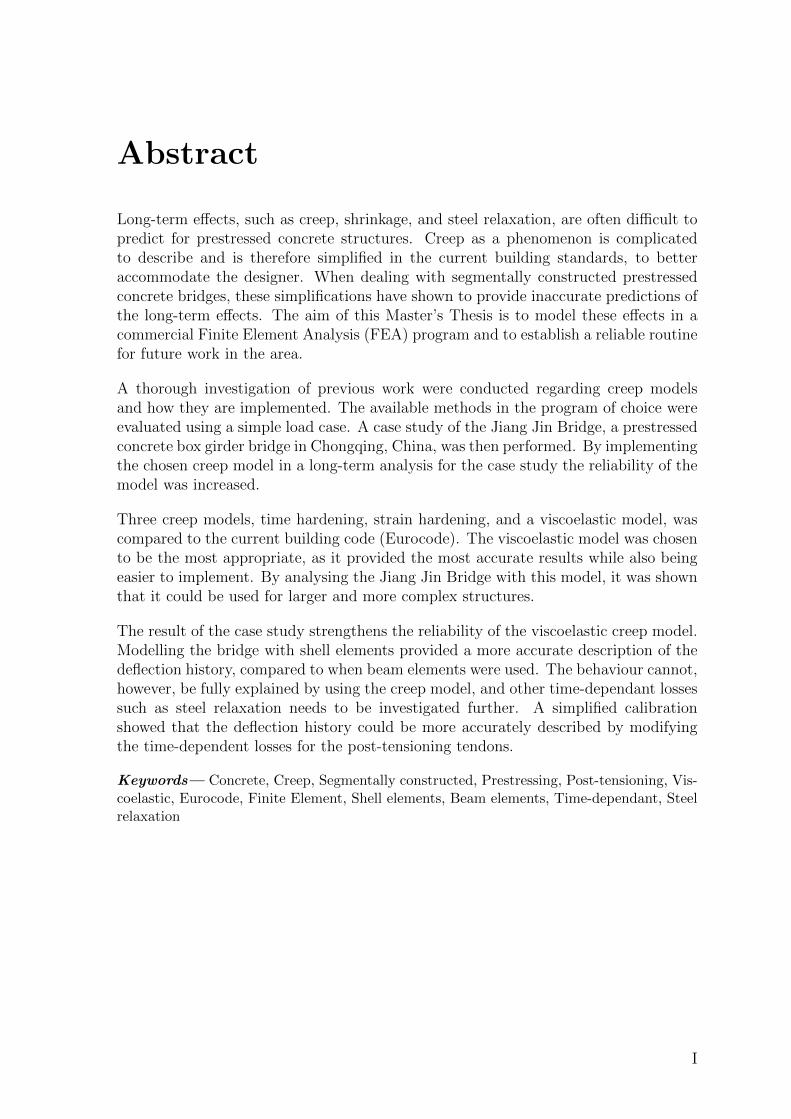
Long-term effects, such as creep, shrinkage, and steel relaxation, are often difficult topredict for prestressed concrete structures. Creep as a phenomenon is complicatedto describe and is therefore simplified in the current building standards, to betteraccommodate the designer. When dealing with segmentally constructed prestressedconcrete bridges, these simplifications have shown to provide inaccurate predictions ofthe long-term effects. The aim of this Master’s Thesis is to model these effects in acommercial Finite Element Analysis (FEA) program and to establish a reliable routinefor future work in the area.
A thorough investigation of previous work were conducted regarding creep modelsand how they are implemented. The available methods in the program of choice wereevaluated using a simple load case. A case study of the Jiang Jin Bridge, a prestressedconcrete box girder bridge in Chongqing, China, was then performed. By implementingthe chosen creep model in a long-term analysis for the case study the reliability of themodel was increased.
Three creep models, time hardening, strain hardening, and a viscoelastic model, wascompared to the current building code (Eurocode). The viscoelastic model was chosento be the most appropriate, as it provided the most accurate results while also beingeasier to implement. By analysing the Jiang Jin Bridge with this model, it was shownthat it could be used for larger and more complex structures.
The result of the case study strengthens the reliability of the viscoelastic creep model.Modelling the bridge with shell elements provided a more accurate description of thedeflection history, compared to when beam elements were used. The behaviour cannot,however, be fully explained by using the creep model, and other time-dependant lossessuch as steel relaxation needs to be investigated further. A simplified calibrationshowed that the deflection history could be more accurately described by modifyingthe time-dependent losses for the post-tensioning tendons.
Keywords— Concrete, Creep, Segmentally constructed, Prestressing, Post-tensioning, Vis-coelastic, Eurocode, Finite Element, Shell elements, Beam elements, Time-dependant, Steelrelaxation
I

II
Sammanfattning
Tidsberoende effekter, sasom krypning, krympning och stalrelaxation, ar ofta svara attprediktera nar det kommer till forspanda betongkonstruktioner. Krypning som ett feno-men ar komplicerat och forenklas darfor i gallande byggnormer (Eurocode), for att un-derlatta konstruktorens arbete. Nar det galler etappvis spannarmerade betongbroar har des-sa forenklingar visat sig ge felaktiga prognoser av de tidsberoende effekterna. Syftet meddenna uppsats ar att modellera dessa effekter i ett kommersiellt Finita Element program ochdarmed skapa en palitlig rutin for framtida arbete inom omradet.
En djupgaende undersokning gjordes kring olika krypmodeller och hur de kan implementeras.De tillgangliga metoderna i det valda programmet utvarderades med ett enkelt lastfall. Enfallstudie av Jiang Jin Bridge, en etappvis spannarmerad betongbro i Chongqing, Kina,genomfordes sedan. Genom att implementera krypmodellen och analysera den valda bronover en tidsperiod pa 10 ar kunde modellens tillforlitlighet okas.
Tre krypmodeller, tidshardande, tojningshardande och en viskoelastisk modell, jamfordesmed hur krypning beaktas i den nuvarande byggnormen (Eurocode). Den viskoelastiskamodellen valdes som den mest lampliga, den gav de mest exakta resultaten samtidigt somden var lattare att implementera. Genom att analysera Jiang Jin Bridge med denna modellvisades det att den kunde anvandas for storre och mer komplexa konstruktioner.
Resultatet av fallstudien starker tillforlitligheten hos den viskoelastiska krypmodellen. Mo-dellering av bron med skalelement gav en mer exakt beskrivning av nedbojningshistorikenjamfort med nar balkelement anvandes. Beteendet kan dock inte forklaras fullstandigt medhjalp av krypmodellen och andra tidsberoende effekter sasom forluster i spannkablar behoverundersokas vidare. En forenklad kalibrering visade att nedbojningshistoriken kunde beskrivasmer exakt genom att andra de tidsberoende forlusterna for de forspanda spannkablarna.
III

IV

Acknowledgements
This Master’s Thesis have been written at the division of Construction Science at the Facultyof Engineering, Lund University and in collaboration with ELU konsult Malmo. We wouldlike to thank our supervisor at ELU, Christoffer Svedholm, and our supervisor from thefaculty, Jonas Niklewski, who has given us continous support throughout the entire process.We would also like thank the ELU office in Malmo and the remaining professionals who haveprovided input on our work.
May 2021
Lund, Sweden
Joel Sunesson and Niclas Elfving
V

VI

Abbrevations
EC Eurocode
FEA Finite Element Analysis
FEM Finite Element Method
VII

VIII

List of Symbols
α Temperature coefficient associating the relative strainα1 Coefficient considering concrete strengthα2 Coefficient considering concrete strengthα3 Coefficient considering concrete strengthβ(fcm) Factor on the notional creep coefficient to allow for con-
crete strengthβ(t0) Factor on the notional creep coefficient to allow for age
at loadingβas Time function of autogenous shrinkage strainβc Time function of the creep coefficientβds Time function of drying shrinkage strainβH Factor on βc to account for relative humidity and no-
tional member sizeχ1000 Stress relaxation after 1000 hoursχ Ageing coefficientχ∞ Stress relaxation factor after long timeχt Stress relaxation factor at time tδ Vertical deflection [m]E Modulus of elasticity [Pa]E0 Modulus of elasticity at time t0 [Pa]Ec Modulus of elasticity for concrete [Pa]Ecm Modulus of elasticity for concrete after 28 days [Pa]Ec,eff Effective modulus of elasticity for concrete [Pa]Ep Modulus of elasticity for prestressing steel [Pa]ε0 Elastic strainεc Total strain in concreteεc,creep Strain in concrete due to creep˙εcr Strain in concrete due to creep, power law parameterεca Autogenous shrinkage strainεca(∞) Final autogenous shrinkage strainεcd Drying shrinkage strainεcd,0 Nominal unrestrained drying shrinkageεcd(∞) Final drying shrinkage strainεcs Total shrinkage strain in concreteεpi Initial strain of prestressing steelεp∞ Total strain in prestressing steel after long timeεvol Total volumetric strainfck Characteristic strength for concrete [Pa]fcm,28d Design strength for concrete after 28 days [Pa]fpuk Ultimate characteristic tensile strength of the prestress-
ing steel [Pa]G0 Shear modulus at time t = 0 [Pa]gR Dimensionless shear relaxation modulusGR Shear relaxation modulus at time t [Pa]γ Total shear strain
IX
h0 Notional size of the concrete member [mm]J Total stress dependant strain from a constant applied
stressjK Normalized bulk complianceJK Bulk compliance [1/Pa]jS Normalized shear complianceJS Shear compliance [1/Pa]k Wobble coefficientK0 Bulk modulus at time t = 0 [Pa]kh Shrinkage coefficient depending on notional size, h0
kR Normalized bulk modulusKR Bulk modulus at time t [Pa]µ Friction coefficientν Poisson’s ratioν0 Poisson’s ratio at time t = 0p0 Constant pressure [Pa]Pmax Maximal force at stressing end in tendon [N]∆Pµ(x) Loss in prestressing force due to friction located at dis-
tance x along the tendon [N]ϕ(∞, t0) Long term creep coefficient for concreteϕ(tc, t0) Creep for coefficient for concrete at age tc where the
structural system changesϕ(t, t0) Creep coefficient for concrete, loading at time t0ϕ(t, ti) Creep coefficient for concrete, loading at time tiϕ0 Notional creep coefficient for concreteϕk(t, t0) Creep coefficient for concrete at high stress levelsϕRH Factor on the notional creep coefficient to allow for re-
lative humidityq Equivalent deviatoric stress [Pa]R Stress response from a constant applied strainRH Relative Humidity (%)s Coefficient describing the hardening rate of cementS Deviatoric stress [Pa]S0 Internal actions from segmental construction sequenceSc Internal actions if the structure was to be cast in one∆S Redistribution of internal actions due to creepσ0 Stress in concrete applied at time t0 [Pa]σc Stress in concrete at time t [Pa]σp Stress in prestressing tendons at time t [Pa]σpi Initial stress in prestressing tendons [Pa]σpsl Loss in prestressing tendons due to anchorage slip [Pa]σpmax Maximal effective stress in prestressing tendon after
tensioning [Pa]∆σ Stress difference [Pa]∆σµ(x) Loss in prestressing tendons due to friction located at
distance x along the tendon [Pa]∆σpr Stress loss in prestressing steel [Pa]t0 Time of loading (curing age) [days]T Temperature [◦C]τ0 Constant shear stress [Pa]θ Rotational angle
X
Contents
Abstract I
Sammanfattning III
Acknowledgements V
Abbrevations VII
List of Symbols IX
Table of Contents XIII
1 Introduction 1
1.1 Background . . . . . . . . . . . . . . . . . . . . . . . . . . . . . . . . . . . . . 1
1.2 Aim and Objectives . . . . . . . . . . . . . . . . . . . . . . . . . . . . . . . . 1
1.3 Method and Research Questions . . . . . . . . . . . . . . . . . . . . . . . . . 2
1.4 Limitations . . . . . . . . . . . . . . . . . . . . . . . . . . . . . . . . . . . . . 2
I Literature Study 3
2 History and Concept 5
2.1 History of Prestressed Concrete . . . . . . . . . . . . . . . . . . . . . . . . . . 5
2.1.1 Concept and Intuitive Designs . . . . . . . . . . . . . . . . . . . . . . 5
2.1.2 Early Development . . . . . . . . . . . . . . . . . . . . . . . . . . . . . 5
2.1.3 Understanding of Time-Dependent Effects . . . . . . . . . . . . . . . . 6
2.2 Case Study Concepts . . . . . . . . . . . . . . . . . . . . . . . . . . . . . . . . 7
2.2.1 Cantilever Bridges . . . . . . . . . . . . . . . . . . . . . . . . . . . . . 7
2.2.2 Balanced Cantilever Method . . . . . . . . . . . . . . . . . . . . . . . 7
3 Basic Theory 11
3.1 Post-Tensioning . . . . . . . . . . . . . . . . . . . . . . . . . . . . . . . . . . . 11
3.1.1 Design of Post-Tensioning System . . . . . . . . . . . . . . . . . . . . 12
XI
3.1.2 Installation of Post-Tensioning System . . . . . . . . . . . . . . . . . . 13
3.1.3 Friction Losses . . . . . . . . . . . . . . . . . . . . . . . . . . . . . . . 15
3.2 Time-Dependent Effects . . . . . . . . . . . . . . . . . . . . . . . . . . . . . . 16
3.2.1 Stress Relaxation of Steel . . . . . . . . . . . . . . . . . . . . . . . . . 16
3.2.2 Shrinkage . . . . . . . . . . . . . . . . . . . . . . . . . . . . . . . . . . 19
3.2.3 Creep . . . . . . . . . . . . . . . . . . . . . . . . . . . . . . . . . . . . 20
3.2.4 Time Hardening (Young’s Modulus) . . . . . . . . . . . . . . . . . . . 22
4 Modelling of Creep 25
4.1 Building Codes to Predict Creep . . . . . . . . . . . . . . . . . . . . . . . . . 25
4.2 Creep Models in Abaqus . . . . . . . . . . . . . . . . . . . . . . . . . . . . . . 26
4.2.1 Time Hardening Model . . . . . . . . . . . . . . . . . . . . . . . . . . 26
4.2.2 Strain Hardening Model . . . . . . . . . . . . . . . . . . . . . . . . . . 30
4.2.3 Calibrating Time and Strain Hardening Parameters . . . . . . . . . . 33
4.2.4 Viscoelastic Model . . . . . . . . . . . . . . . . . . . . . . . . . . . . . 34
4.2.5 Comparison of Creep Models . . . . . . . . . . . . . . . . . . . . . . . 36
4.3 Verification of Creep Models . . . . . . . . . . . . . . . . . . . . . . . . . . . . 37
4.3.1 Time and Strain Hardening Model . . . . . . . . . . . . . . . . . . . . 38
4.3.2 Viscoelastic Model . . . . . . . . . . . . . . . . . . . . . . . . . . . . . 39
4.3.3 Comparing Models when Unloading . . . . . . . . . . . . . . . . . . . 40
4.3.4 Development of Young’s Modulus . . . . . . . . . . . . . . . . . . . . . 40
4.3.5 Conclusion of Model best fit for Predicting Creep According to Eurocode 41
II Case Study 43
5 Jiang Jin Bridge Description 45
5.1 Dimensions and Positioning of Tendons . . . . . . . . . . . . . . . . . . . . . 45
5.2 Properties . . . . . . . . . . . . . . . . . . . . . . . . . . . . . . . . . . . . . . 47
5.3 Construction Sequence . . . . . . . . . . . . . . . . . . . . . . . . . . . . . . . 48
6 Finite Element Model 51
6.1 Modelling of Shrinkage . . . . . . . . . . . . . . . . . . . . . . . . . . . . . . . 52
6.2 Implementation of Creep in Abaqus . . . . . . . . . . . . . . . . . . . . . . . 52
XII
6.3 Modelling of Tendons . . . . . . . . . . . . . . . . . . . . . . . . . . . . . . . 54
6.3.1 Losses due to Stress Relaxation . . . . . . . . . . . . . . . . . . . . . . 54
6.3.2 Instantaneous Losses (Friction/Anchorage Slip) . . . . . . . . . . . . . 55
6.4 Modelling of the Construction Sequence . . . . . . . . . . . . . . . . . . . . . 57
III Results and Discussion 59
7 Case Study Analysis 61
7.1 Deflections . . . . . . . . . . . . . . . . . . . . . . . . . . . . . . . . . . . . . 61
7.2 Analysis of Bending Moments . . . . . . . . . . . . . . . . . . . . . . . . . . . 66
7.2.1 Bending Moment due to Permanent Loads . . . . . . . . . . . . . . . . 66
7.2.2 Influence of Tendons on the Bending Moment . . . . . . . . . . . . . . 67
7.3 Calibration of Parameters . . . . . . . . . . . . . . . . . . . . . . . . . . . . . 68
7.4 Sources of Errors . . . . . . . . . . . . . . . . . . . . . . . . . . . . . . . . . . 69
8 Conclusions 73
9 Further Work 75
Bibliography 77
XIII

XIV
1 Introduction
1.1 Background
When designing prestressed concrete bridges, it is important to consider time-dependenteffects such as creep, shrinkage, and steel relaxation. This is especially important when thebridge is cast and erected in several different stages, as this causes the structure to deformsubstantially and gradually during construction. A general problem with this constructionmethod is that deformations induced by creep are difficult to accurately predict. There arenumerous examples of bridges that have exhibited deformations larger than those predicted indesign. One example is the Koror-Babeldaob bridge in Palau where the mid-span deflectionwas more than double that of what was predicted in the design stage (Bazant et al., 2012a).
The European building code, (Eurocode 2, 2005b), suggests four different methods for design-ing segmentally constructed concrete bridges with regards to creep:
1. General and incremental step-by-step method
2. Methods based on the theorems of linear viscoelasticity
3. The ageing coefficient method
4. Simplified ageing coefficient method
In the designers guide to Eurocode 2 (2005b), see Hendy and Smith (2007), only Method 1and 4 are considered. Method 1 requires an iterative procedure whereas 4 can be performedusing hand calculations. Furthermore, method 2 has been frequently used when more accur-ate modelling has been done for existing bridges, see for example (Canovic and Goncalves,2005) and (Bazant et al., 2012b).
1.2 Aim and Objectives
Time-dependent effects for segmentally constructed concrete bridges are usually consideredusing simplified hand calculations, due to difficulties in describing time-dependent effectsduring the erection process. The overarching aim of this Master’s Thesis is to evaluatethe possibility of using numerical models to determine the long term behaviour of segment-ally constructed prestressed bridges. By establishing a reliable routine, excessive long-termdeformation can be avoided.
Different creep models were analysed for a simple load case to determine the one best suited.Existing measurements from a segmentally cast bridge were then used as a basis to furtherevaluate the performance of the chosen creep model.
1
1.3 Method and Research Questions
A literature study was initially carried out to address the following:
• What are the different mechanical and structural concepts involved in determining thelong-term behaviour of prestressed segmentally constructed concrete bridges? Whatare the existing theories regarding creep, shrinkage, and prestressing losses?
• How can these effects be implemented numerically for segmentally constructed concretebridges? What are the difficulties?
Numerical models (Brigade/PLUS, based on the Abaqus software) was then used to addressthe following:
• What are the available methods to model creep numerically? How, and under whatcircumstances, do they differ in their result?
• How can the creep models be verified by using a simple load case and comparing withthe methods described in Eurocode (EC)?
• How can the global analysis be simplified to facilitate an efficient design process? Isit necessary to use shell elements or is it possible to model the bridge with beamelements?
A case study of the Jiang Jin Bridge was finally carried out using the acquired methods.The results were analysed with respect to long-term deformations and compared to measuredvalues.
1.4 Limitations
The scope of this Master’s Thesis is focused on long-term effects for bridges similar to thecase study. The analysis is therefore limited to prestressed segmentally constructed concretebridges with large spans. Due to the focus on long-term effects the study only considerspermanent loads. It should be noted however, that depending on the frequency, traffic loadscan induce cyclic creep (see for example Teng (2017)).
The analysis is limited to the FEA program of choice, the commercial software Brigade/PLUS.This means that the study will be somewhat limited to the chosen modelling program re-garding the implementation of long-term effects. There will also be limitations regardingcomputational power and therefore simplifications must be made.
2

Part I
Literature Study
3

2 History and Concept
2.1 History of Prestressed Concrete
2.1.1 Concept and Intuitive Designs
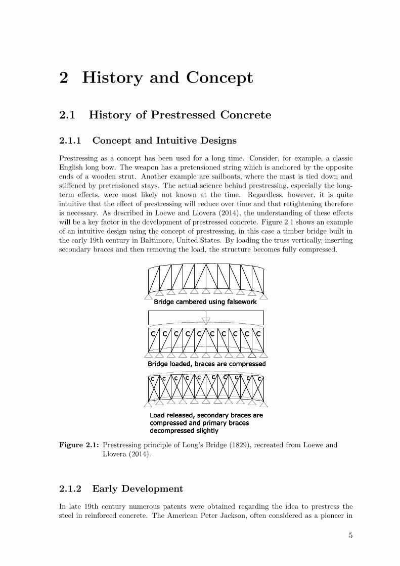
Prestressing as a concept has been used for a long time. Consider, for example, a classicEnglish long bow. The weapon has a pretensioned string which is anchored by the oppositeends of a wooden strut. Another example are sailboats, where the mast is tied down andstiffened by pretensioned stays. The actual science behind prestressing, especially the long-term effects, were most likely not known at the time. Regardless, however, it is quiteintuitive that the effect of prestressing will reduce over time and that retightening thereforeis necessary. As described in Loewe and Llovera (2014), the understanding of these effectswill be a key factor in the development of prestressed concrete. Figure 2.1 shows an exampleof an intuitive design using the concept of prestressing, in this case a timber bridge built inthe early 19th century in Baltimore, United States. By loading the truss vertically, insertingsecondary braces and then removing the load, the structure becomes fully compressed.
Bridge cambered using falsework
CC C C C C C C C C C
Bridge loaded, braces are compressed
Load released, secondary braces arecompressed and primary bracesdecompressed slightly
c c c c c c c c c c
Bridge cambered using falsework
CC C C C C C C C C C
Bridge loaded, braces are compressed
Load released, secondary braces arecompressed and primary bracesdecompressed slightly
c c c c c c c c c c
Bridge cambered using falsework
CC C C C C C C C C C
Bridge loaded, braces are compressed
Load released, secondary braces arecompressed and primary bracesdecompressed slightly
c c c c c c c c c c
Bridge cambered using falsework
CC C C C C C C C C C
Bridge loaded, braces are compressed
Load released, secondary braces arecompressed and primary bracesdecompressed slightly
c c c c c c c c c c
Figure 2.1: Prestressing principle of Long’s Bridge (1829), recreated from Loewe andLlovera (2014).
2.1.2 Early Development
In late 19th century numerous patents were obtained regarding the idea to prestress thesteel in reinforced concrete. The American Peter Jackson, often considered as a pioneer in
5
prestressed concrete, received several patents between 1858 and 1888. The latter one includeda way to handle bonding issues by installing metallic pieces at both ends and turnbuckles sothat that the steel chord could be retightened. These patents were then further developed byfellow countryman Thomas Lee, who also introduced high strength steel. Similar innovationswere made in Europe during this period, for example Doerhing in 1888, although not as wellrecognised or documented. A common driver for prestressing at the time was improved fireresistance. For example, the tie rod in a masonry arch was believed to be better protectedagainst fire if the structure was prestressed (Loewe and Llovera, 2014).
Following the advancements made by American engineers, several Europeans further de-veloped the concept of prestressed concrete. The French engineer, Francois Chaudy, cameup with an effective design of a post-tensioned concrete beam in 1894. The Norwegian JensLund obtained patents in 1907 regarding prestressed concrete slabs, building on the conceptsfrom Jackson and Lee (Loewe and Llovera, 2014).
2.1.3 Understanding of Time-Dependent Effects
At the time when reinforced concrete became widely used the progress of prestressed concretewas still slow. One of the main reasons relate to the lack of high strength steel which reducesthe losses due to steel relaxation and allows for a reduced cross-sectional area. Anotherreason is the lacking understanding of time-dependent effects, in particular those related tocreep deformations.
The effects of shrinkage were known quite early. In 1908 the American Charles Steinerobtained a patent that compensated for the variations in concrete properties over time. Theconcept of prestressing concrete was not successful, however, until the 1930s when thoroughstudies were made regarding creep behaviour. Leading the development in this area was aFrench engineer, Eugene Freyssinet, who studied the subject for about three decades withoutproper recognition (Loewe and Llovera, 2014).
By this time high strength steel was also available. Combined with the understanding ofshrinkage, creep, and steel relaxation the use of prestressed concrete grew substantially. In1932 the German E. Hoyer started producing prestressed concrete elements, an idea laterimplemented by the Swedish company AB Strangbetong in the 1940s. Klockestrand bridgein Kramfors, was the first implementation of prestressed concrete in Sweden. It was builtbetween 1938-1940 by Skanska Cementgjuteriet (now Skanska). Another famous exampleof early prestressed concrete structures are the concrete shells of the Sydney Opera House,designed by danish company Arup in the 1950s (Engstrom, 2011).
6
2.2 Case Study Concepts
2.2.1 Cantilever Bridges
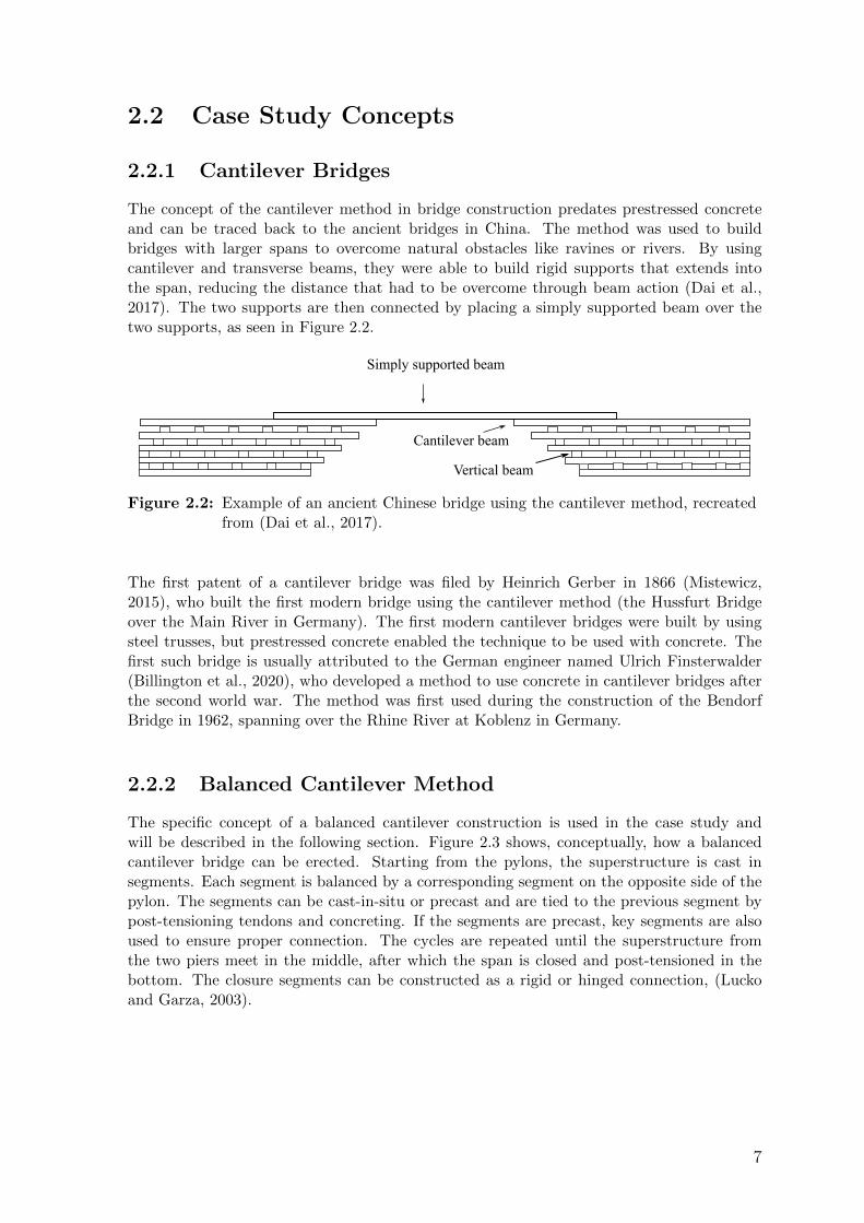
The concept of the cantilever method in bridge construction predates prestressed concreteand can be traced back to the ancient bridges in China. The method was used to buildbridges with larger spans to overcome natural obstacles like ravines or rivers. By usingcantilever and transverse beams, they were able to build rigid supports that extends intothe span, reducing the distance that had to be overcome through beam action (Dai et al.,2017). The two supports are then connected by placing a simply supported beam over thetwo supports, as seen in Figure 2.2.
Simply supported beam
Cantilever beam
Vertical beam
Figure 2.2: Example of an ancient Chinese bridge using the cantilever method, recreatedfrom (Dai et al., 2017).
The first patent of a cantilever bridge was filed by Heinrich Gerber in 1866 (Mistewicz,2015), who built the first modern bridge using the cantilever method (the Hussfurt Bridgeover the Main River in Germany). The first modern cantilever bridges were built by usingsteel trusses, but prestressed concrete enabled the technique to be used with concrete. Thefirst such bridge is usually attributed to the German engineer named Ulrich Finsterwalder(Billington et al., 2020), who developed a method to use concrete in cantilever bridges afterthe second world war. The method was first used during the construction of the BendorfBridge in 1962, spanning over the Rhine River at Koblenz in Germany.
2.2.2 Balanced Cantilever Method
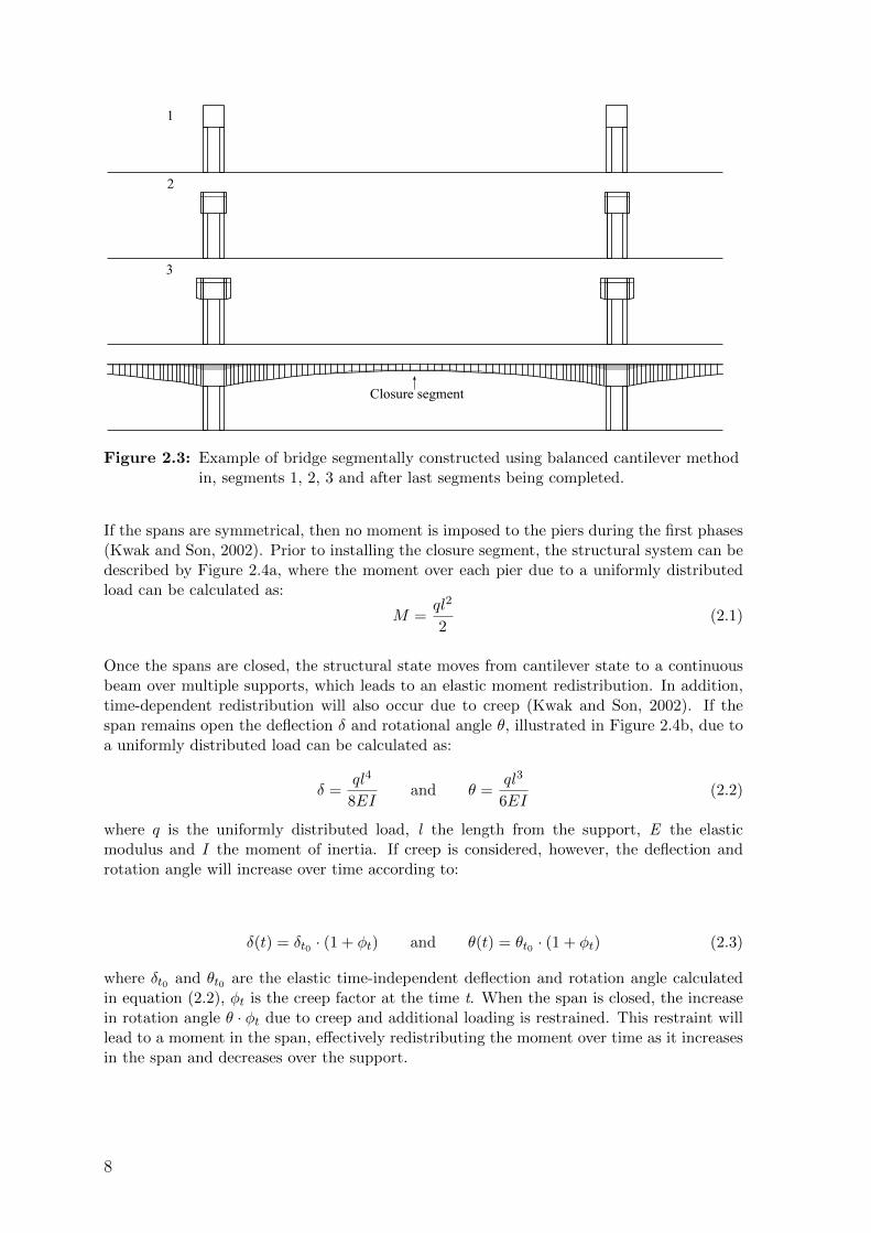
The specific concept of a balanced cantilever construction is used in the case study andwill be described in the following section. Figure 2.3 shows, conceptually, how a balancedcantilever bridge can be erected. Starting from the pylons, the superstructure is cast insegments. Each segment is balanced by a corresponding segment on the opposite side of thepylon. The segments can be cast-in-situ or precast and are tied to the previous segment bypost-tensioning tendons and concreting. If the segments are precast, key segments are alsoused to ensure proper connection. The cycles are repeated until the superstructure fromthe two piers meet in the middle, after which the span is closed and post-tensioned in thebottom. The closure segments can be constructed as a rigid or hinged connection, (Luckoand Garza, 2003).
7
1
2
3
Closure segment
Figure 2.3: Example of bridge segmentally constructed using balanced cantilever methodin, segments 1, 2, 3 and after last segments being completed.
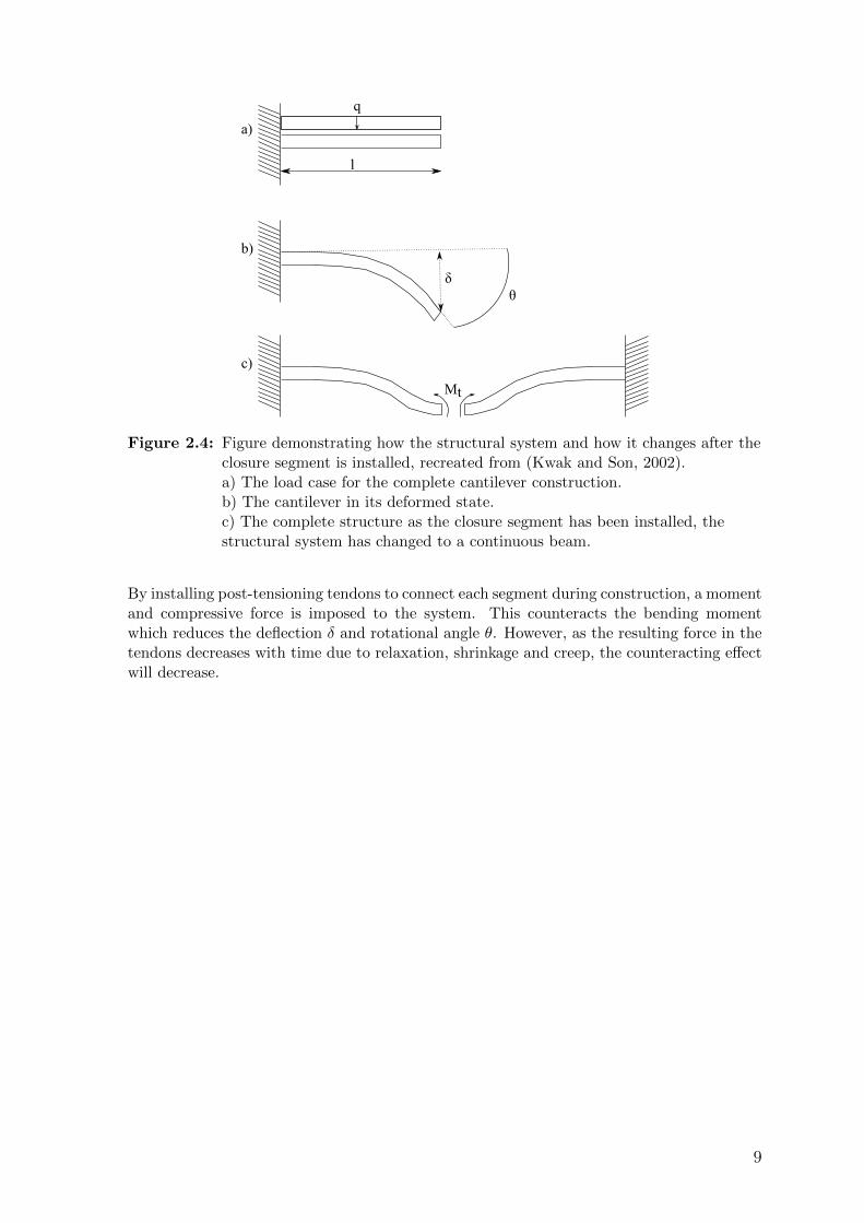
If the spans are symmetrical, then no moment is imposed to the piers during the first phases(Kwak and Son, 2002). Prior to installing the closure segment, the structural system can bedescribed by Figure 2.4a, where the moment over each pier due to a uniformly distributedload can be calculated as:
M =ql2
2(2.1)
Once the spans are closed, the structural state moves from cantilever state to a continuousbeam over multiple supports, which leads to an elastic moment redistribution. In addition,time-dependent redistribution will also occur due to creep (Kwak and Son, 2002). If thespan remains open the deflection δ and rotational angle θ, illustrated in Figure 2.4b, due toa uniformly distributed load can be calculated as:
δ =ql4
8EIand θ =
ql3
6EI(2.2)
where q is the uniformly distributed load, l the length from the support, E the elasticmodulus and I the moment of inertia. If creep is considered, however, the deflection androtation angle will increase over time according to:
δ(t) = δt0 · (1 + φt) and θ(t) = θt0 · (1 + φt) (2.3)
where δt0 and θt0 are the elastic time-independent deflection and rotation angle calculatedin equation (2.2), φt is the creep factor at the time t. When the span is closed, the increasein rotation angle θ · φt due to creep and additional loading is restrained. This restraint willlead to a moment in the span, effectively redistributing the moment over time as it increasesin the span and decreases over the support.
8
δθ
a)
b)
c)
q
l
Mt
Figure 2.4: Figure demonstrating how the structural system and how it changes after theclosure segment is installed, recreated from (Kwak and Son, 2002).a) The load case for the complete cantilever construction.b) The cantilever in its deformed state.c) The complete structure as the closure segment has been installed, thestructural system has changed to a continuous beam.
By installing post-tensioning tendons to connect each segment during construction, a momentand compressive force is imposed to the system. This counteracts the bending momentwhich reduces the deflection δ and rotational angle θ. However, as the resulting force in thetendons decreases with time due to relaxation, shrinkage and creep, the counteracting effectwill decrease.
9

10
3 Basic Theory
3.1 Post-Tensioning
Reinforced concrete is cost effective and durable in a variety of applications and is thereforewidely used. Concrete is normally reinforced by embedded steel to compensate for its poortensile strength. The composite material works exceptionally well since concrete, if designedproperly, is resistant to degradation while steel normally is not. When steel comes in contactwith oxygen and water, corrosion will start to develop over time. Essentially the concretecover protects the steel (Engstrom, 2011).
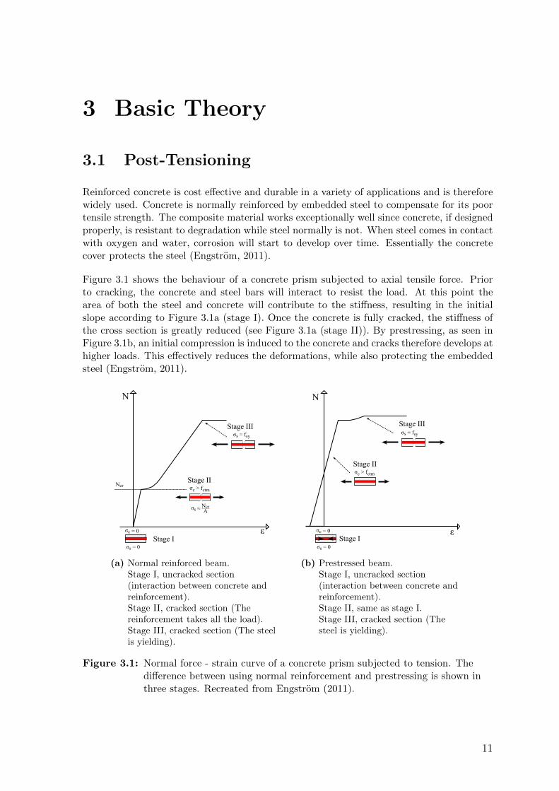
Figure 3.1 shows the behaviour of a concrete prism subjected to axial tensile force. Priorto cracking, the concrete and steel bars will interact to resist the load. At this point thearea of both the steel and concrete will contribute to the stiffness, resulting in the initialslope according to Figure 3.1a (stage I). Once the concrete is fully cracked, the stiffness ofthe cross section is greatly reduced (see Figure 3.1a (stage II)). By prestressing, as seen inFigure 3.1b, an initial compression is induced to the concrete and cracks therefore develops athigher loads. This effectively reduces the deformations, while also protecting the embeddedsteel (Engstrom, 2011).
ε
N
σs = 0
σc > fctm
σs Ncr~~ A
σs = fsy
σc = 0
Ncr
Stage I
Stage II
Stage III
(a) Normal reinforced beam.Stage I, uncracked section(interaction between concrete andreinforcement).Stage II, cracked section (Thereinforcement takes all the load).Stage III, cracked section (The steelis yielding).
σc > fctm
σc = 0
σs = 0
σs = fsy
ε
N
Stage I
Stage II
Stage III
(b) Prestressed beam.Stage I, uncracked section(interaction between concrete andreinforcement).Stage II, same as stage I.Stage III, cracked section (Thesteel is yielding).
Figure 3.1: Normal force - strain curve of a concrete prism subjected to tension. Thedifference between using normal reinforcement and prestressing is shown inthree stages. Recreated from Engstrom (2011).
11
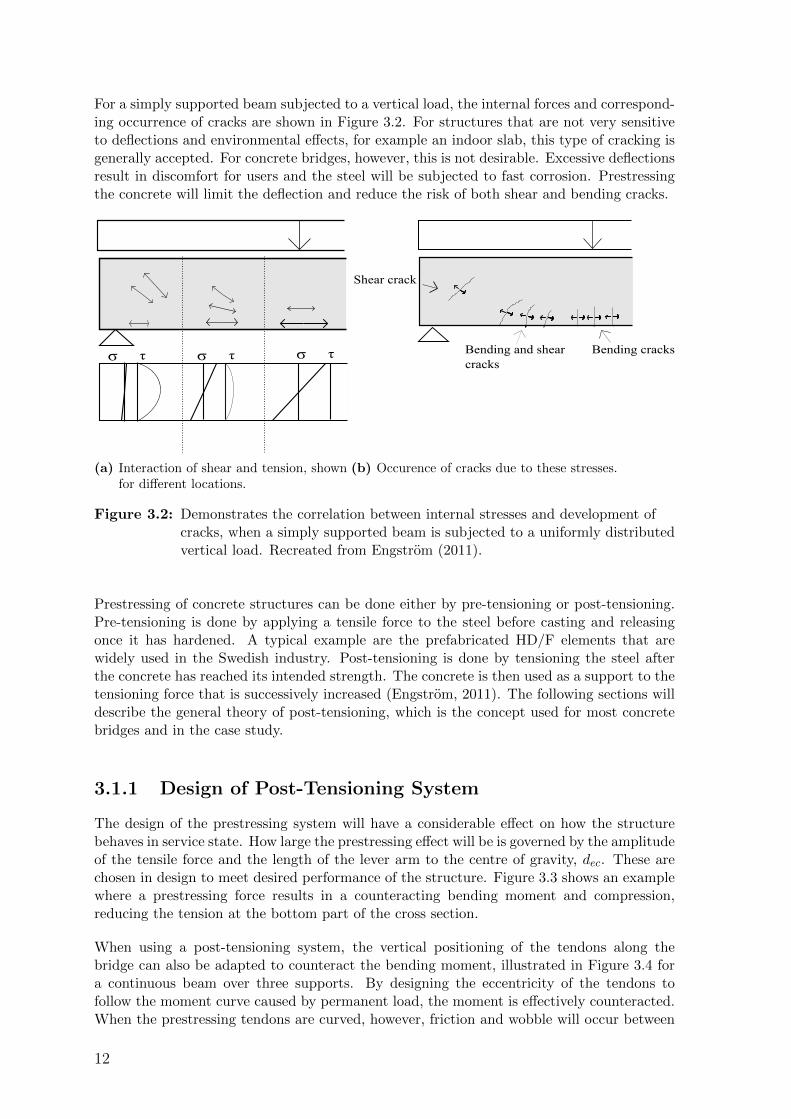
For a simply supported beam subjected to a vertical load, the internal forces and correspond-ing occurrence of cracks are shown in Figure 3.2. For structures that are not very sensitiveto deflections and environmental effects, for example an indoor slab, this type of cracking isgenerally accepted. For concrete bridges, however, this is not desirable. Excessive deflectionsresult in discomfort for users and the steel will be subjected to fast corrosion. Prestressingthe concrete will limit the deflection and reduce the risk of both shear and bending cracks.
(a) Interaction of shear and tension, shownfor different locations.
(b) Occurence of cracks due to these stresses.
Figure 3.2: Demonstrates the correlation between internal stresses and development ofcracks, when a simply supported beam is subjected to a uniformly distributedvertical load. Recreated from Engstrom (2011).
Prestressing of concrete structures can be done either by pre-tensioning or post-tensioning.Pre-tensioning is done by applying a tensile force to the steel before casting and releasingonce it has hardened. A typical example are the prefabricated HD/F elements that arewidely used in the Swedish industry. Post-tensioning is done by tensioning the steel afterthe concrete has reached its intended strength. The concrete is then used as a support to thetensioning force that is successively increased (Engstrom, 2011). The following sections willdescribe the general theory of post-tensioning, which is the concept used for most concretebridges and in the case study.
3.1.1 Design of Post-Tensioning System
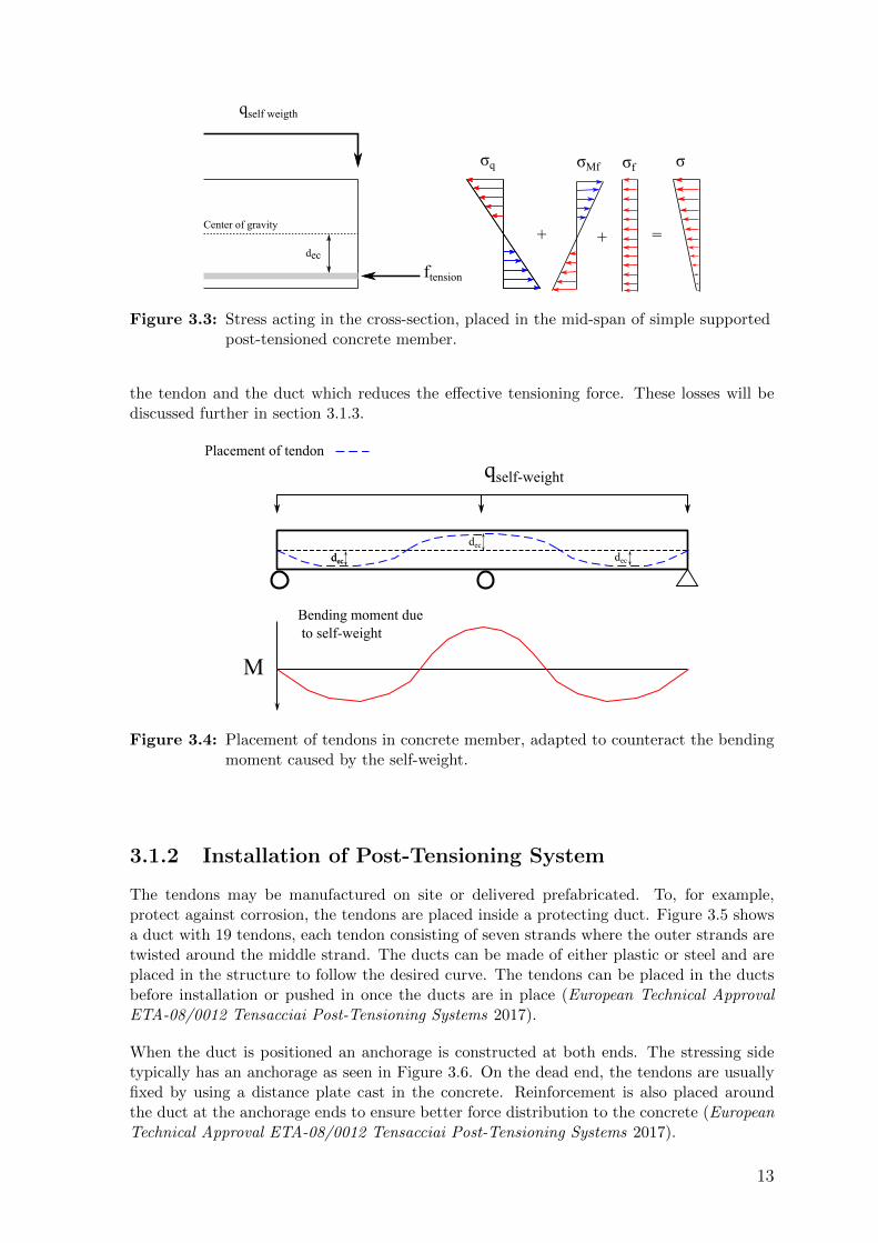
The design of the prestressing system will have a considerable effect on how the structurebehaves in service state. How large the prestressing effect will be is governed by the amplitudeof the tensile force and the length of the lever arm to the centre of gravity, dec. These arechosen in design to meet desired performance of the structure. Figure 3.3 shows an examplewhere a prestressing force results in a counteracting bending moment and compression,reducing the tension at the bottom part of the cross section.
When using a post-tensioning system, the vertical positioning of the tendons along thebridge can also be adapted to counteract the bending moment, illustrated in Figure 3.4 fora continuous beam over three supports. By designing the eccentricity of the tendons tofollow the moment curve caused by permanent load, the moment is effectively counteracted.When the prestressing tendons are curved, however, friction and wobble will occur between
12
dec
ftension
qself weigth
σq σMf
+ =+
σf σ
Center of gravity
Figure 3.3: Stress acting in the cross-section, placed in the mid-span of simple supportedpost-tensioned concrete member.
the tendon and the duct which reduces the effective tensioning force. These losses will bediscussed further in section 3.1.3.
Bending moment due to self-weight
Placement of tendon
decdec
dec
dec
qself-weight
M
Figure 3.4: Placement of tendons in concrete member, adapted to counteract the bendingmoment caused by the self-weight.
3.1.2 Installation of Post-Tensioning System
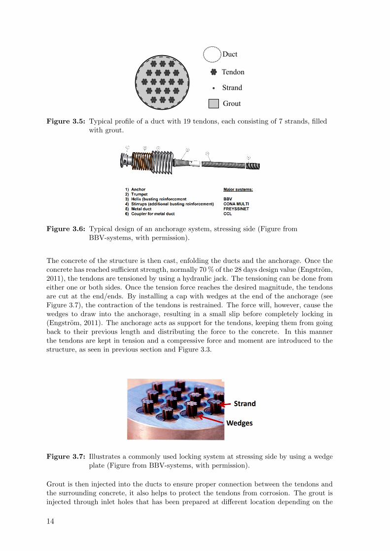
The tendons may be manufactured on site or delivered prefabricated. To, for example,protect against corrosion, the tendons are placed inside a protecting duct. Figure 3.5 showsa duct with 19 tendons, each tendon consisting of seven strands where the outer strands aretwisted around the middle strand. The ducts can be made of either plastic or steel and areplaced in the structure to follow the desired curve. The tendons can be placed in the ductsbefore installation or pushed in once the ducts are in place (European Technical ApprovalETA-08/0012 Tensacciai Post-Tensioning Systems 2017).
When the duct is positioned an anchorage is constructed at both ends. The stressing sidetypically has an anchorage as seen in Figure 3.6. On the dead end, the tendons are usuallyfixed by using a distance plate cast in the concrete. Reinforcement is also placed aroundthe duct at the anchorage ends to ensure better force distribution to the concrete (EuropeanTechnical Approval ETA-08/0012 Tensacciai Post-Tensioning Systems 2017).
13
Duct
Tendon
Strand
Grout
Figure 3.5: Typical profile of a duct with 19 tendons, each consisting of 7 strands, filledwith grout.
Figure 3.6: Typical design of an anchorage system, stressing side (Figure fromBBV-systems, with permission).
The concrete of the structure is then cast, enfolding the ducts and the anchorage. Once theconcrete has reached sufficient strength, normally 70 % of the 28 days design value (Engstrom,2011), the tendons are tensioned by using a hydraulic jack. The tensioning can be done fromeither one or both sides. Once the tension force reaches the desired magnitude, the tendonsare cut at the end/ends. By installing a cap with wedges at the end of the anchorage (seeFigure 3.7), the contraction of the tendons is restrained. The force will, however, cause thewedges to draw into the anchorage, resulting in a small slip before completely locking in(Engstrom, 2011). The anchorage acts as support for the tendons, keeping them from goingback to their previous length and distributing the force to the concrete. In this mannerthe tendons are kept in tension and a compressive force and moment are introduced to thestructure, as seen in previous section and Figure 3.3.
Figure 3.7: Illustrates a commonly used locking system at stressing side by using a wedgeplate (Figure from BBV-systems, with permission).
Grout is then injected into the ducts to ensure proper connection between the tendons andthe surrounding concrete, it also helps to protect the tendons from corrosion. The grout isinjected through inlet holes that has been prepared at different location depending on the
14
length and placement of the duct. Outlet holes are normally placed at the highest pointsof the ducts, ensuring that no air gets trapped and that the duct gets completely filledwith grout. Finally the protruding part of the tendons are cut and the cap is covered in aprotecting layer of grout(Engstrom, 2011).
According to European Technical Approval ETA-08/0012 Tensacciai Post-Tensioning Sys-tems (2017), the value of the anchorage slip should be chosen between 5-6 mm. The slipwill cause the strain in the tendons to decrease, which leads to tension losses. The followingequation can be used to calculate the loss of tension in the tendons due to slip, σpsl.
σpsl = σpi ·dslipLtendon
(3.1)
where σpi is the initial stress, dslip the distance slipped and Ltendon the length of the tendon.
3.1.3 Friction Losses
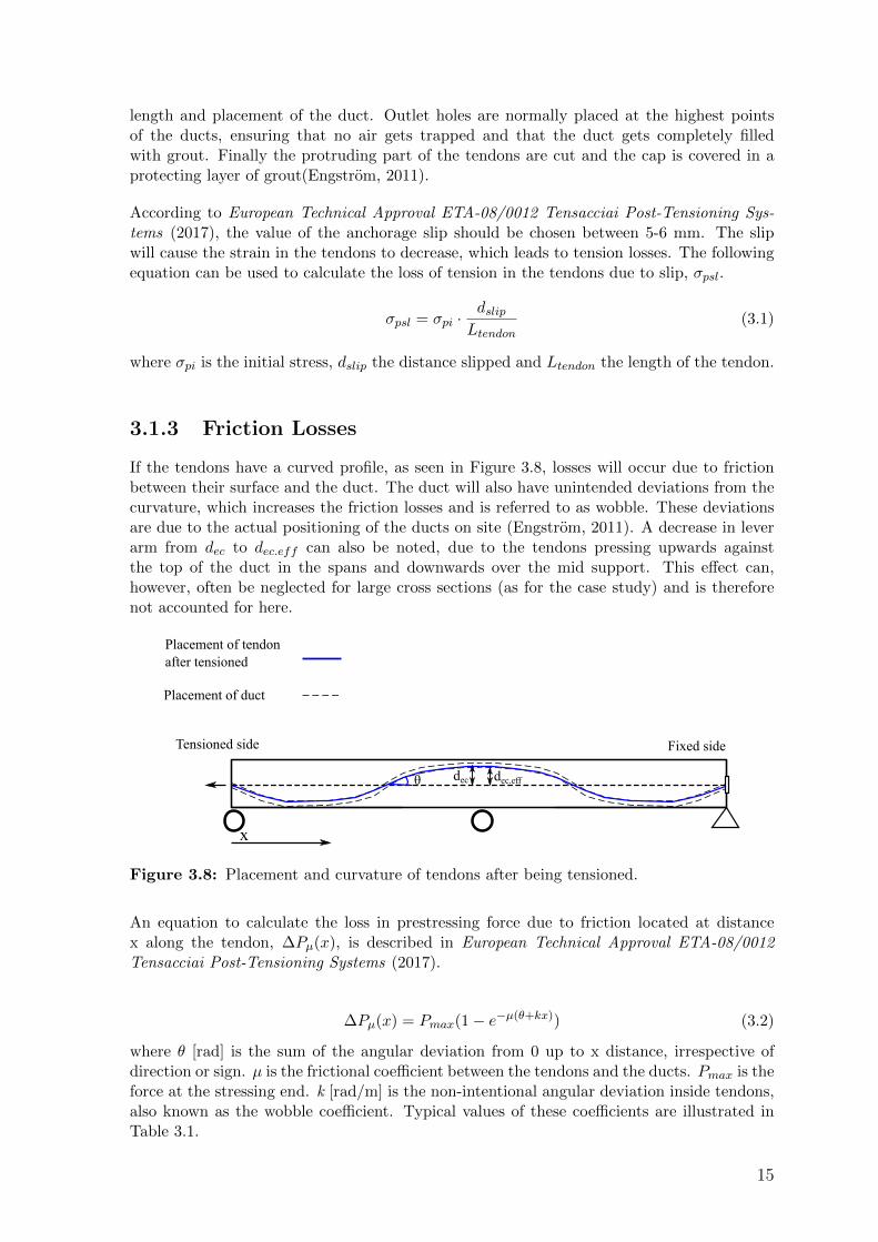
If the tendons have a curved profile, as seen in Figure 3.8, losses will occur due to frictionbetween their surface and the duct. The duct will also have unintended deviations from thecurvature, which increases the friction losses and is referred to as wobble. These deviationsare due to the actual positioning of the ducts on site (Engstrom, 2011). A decrease in leverarm from dec to dec.eff can also be noted, due to the tendons pressing upwards againstthe top of the duct in the spans and downwards over the mid support. This effect can,however, often be neglected for large cross sections (as for the case study) and is thereforenot accounted for here.
Placement of tendon after tensioned
decθ
Placement of duct
Tensioned side Fixed side
x
dec.eff
Figure 3.8: Placement and curvature of tendons after being tensioned.
An equation to calculate the loss in prestressing force due to friction located at distancex along the tendon, ∆Pµ(x), is described in European Technical Approval ETA-08/0012Tensacciai Post-Tensioning Systems (2017).
∆Pµ(x) = Pmax(1− e−µ(θ+kx)) (3.2)
where θ [rad] is the sum of the angular deviation from 0 up to x distance, irrespective ofdirection or sign. µ is the frictional coefficient between the tendons and the ducts. Pmax is theforce at the stressing end. k [rad/m] is the non-intentional angular deviation inside tendons,also known as the wobble coefficient. Typical values of these coefficients are illustrated inTable 3.1.
15
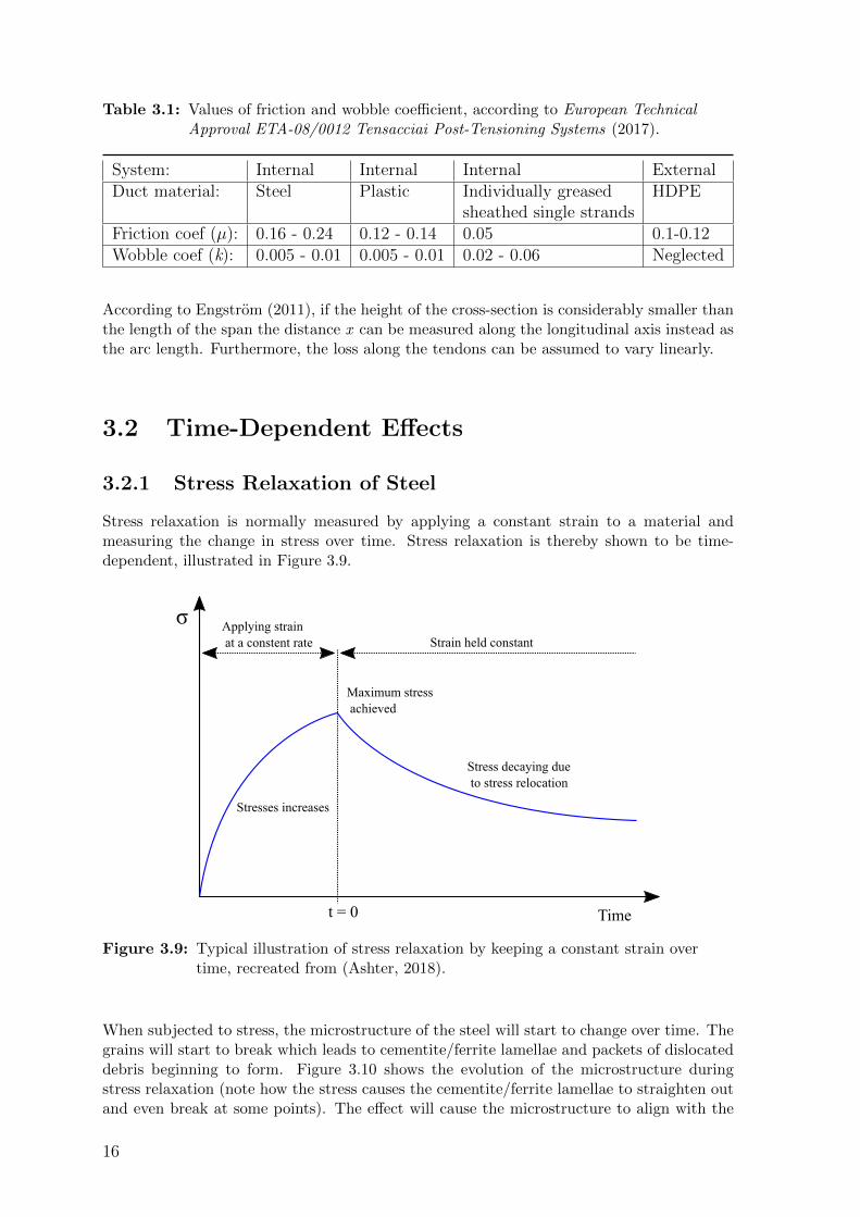
Table 3.1: Values of friction and wobble coefficient, according to European TechnicalApproval ETA-08/0012 Tensacciai Post-Tensioning Systems (2017).
System: Internal Internal Internal ExternalDuct material: Steel Plastic Individually greased HDPE
sheathed single strandsFriction coef (µ): 0.16 - 0.24 0.12 - 0.14 0.05 0.1-0.12Wobble coef (k): 0.005 - 0.01 0.005 - 0.01 0.02 - 0.06 Neglected
According to Engstrom (2011), if the height of the cross-section is considerably smaller thanthe length of the span the distance x can be measured along the longitudinal axis instead asthe arc length. Furthermore, the loss along the tendons can be assumed to vary linearly.
3.2 Time-Dependent Effects
3.2.1 Stress Relaxation of Steel
Stress relaxation is normally measured by applying a constant strain to a material andmeasuring the change in stress over time. Stress relaxation is thereby shown to be time-dependent, illustrated in Figure 3.9.
Figure 3.9: Typical illustration of stress relaxation by keeping a constant strain overtime, recreated from (Ashter, 2018).
When subjected to stress, the microstructure of the steel will start to change over time. Thegrains will start to break which leads to cementite/ferrite lamellae and packets of dislocateddebris beginning to form. Figure 3.10 shows the evolution of the microstructure duringstress relaxation (note how the stress causes the cementite/ferrite lamellae to straighten outand even break at some points). The effect will cause the microstructure to align with the
16
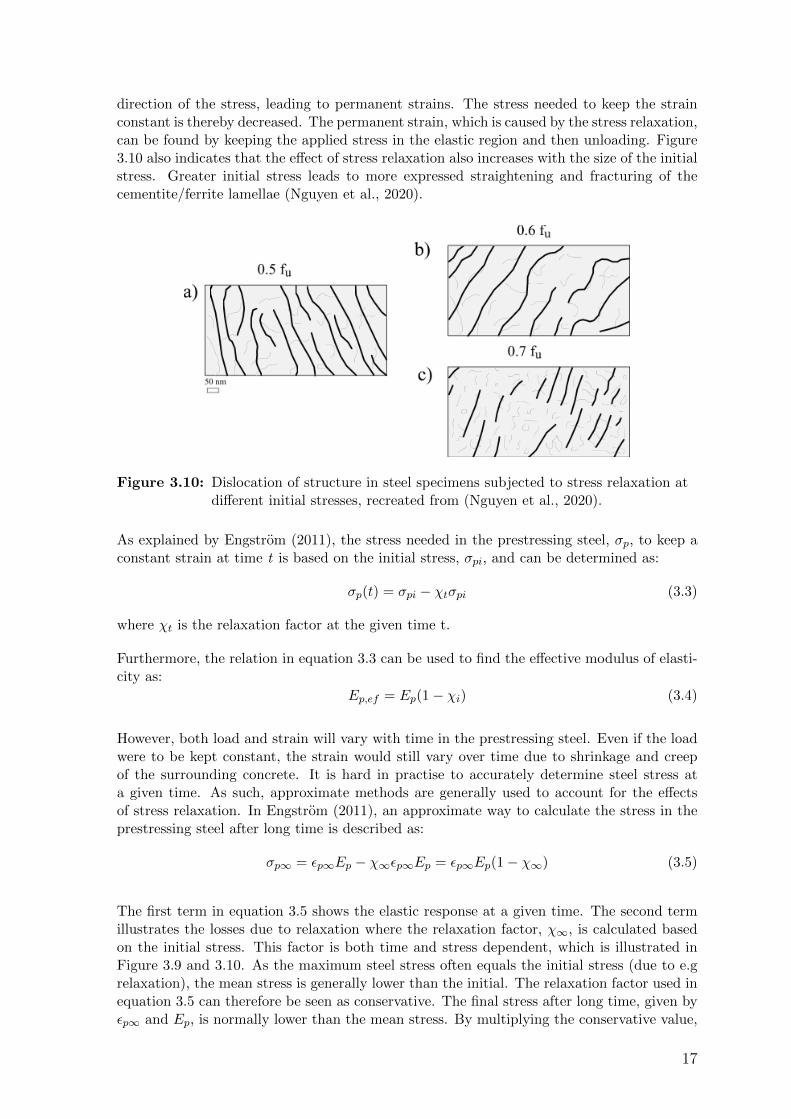
direction of the stress, leading to permanent strains. The stress needed to keep the strainconstant is thereby decreased. The permanent strain, which is caused by the stress relaxation,can be found by keeping the applied stress in the elastic region and then unloading. Figure3.10 also indicates that the effect of stress relaxation also increases with the size of the initialstress. Greater initial stress leads to more expressed straightening and fracturing of thecementite/ferrite lamellae (Nguyen et al., 2020).
Figure 3.10: Dislocation of structure in steel specimens subjected to stress relaxation atdifferent initial stresses, recreated from (Nguyen et al., 2020).
As explained by Engstrom (2011), the stress needed in the prestressing steel, σp, to keep aconstant strain at time t is based on the initial stress, σpi, and can be determined as:
σp(t) = σpi − χtσpi (3.3)
where χt is the relaxation factor at the given time t.
Furthermore, the relation in equation 3.3 can be used to find the effective modulus of elasti-city as:
Ep,ef = Ep(1− χi) (3.4)
However, both load and strain will vary with time in the prestressing steel. Even if the loadwere to be kept constant, the strain would still vary over time due to shrinkage and creepof the surrounding concrete. It is hard in practise to accurately determine steel stress ata given time. As such, approximate methods are generally used to account for the effectsof stress relaxation. In Engstrom (2011), an approximate way to calculate the stress in theprestressing steel after long time is described as:
σp∞ = εp∞Ep − χ∞εp∞Ep = εp∞Ep(1− χ∞) (3.5)
The first term in equation 3.5 shows the elastic response at a given time. The second termillustrates the losses due to relaxation where the relaxation factor, χ∞, is calculated basedon the initial stress. This factor is both time and stress dependent, which is illustrated inFigure 3.9 and 3.10. As the maximum steel stress often equals the initial stress (due to e.grelaxation), the mean stress is generally lower than the initial. The relaxation factor used inequation 3.5 can therefore be seen as conservative. The final stress after long time, given byεp∞ and Ep, is normally lower than the mean stress. By multiplying the conservative value,
17
χ∞, with the underestimated stress given by εp∞ and Ep the two errors partly balance eachother out.
A more accurate model to determine the steel relaxation is described in Eurocode 2 (2005a),which also consider the strain variation in the steel over time:
σp(t) = Epεpi(1− 0.8χt) (3.6)
where εpi is the initial strain of prestressing steel and χt is the relaxation factor at time t.The possibility to define the useful effective modulus of elasticity is, however, lost in equation3.6.
The relaxation factor χt is described in Eurocode 2 (2005a) as:
χt =∆σprσpi
(3.7)
where ∆σpr is the loss in stress due to relaxation and σpi the initial prestressing force. Thisrelation at a certain time can be obtained by using test certificates from the manufactureror alternatively be estimated from Eurocode 2 (2005a).
In EC, prestressing steel is divided into three relaxation classes, where the relaxation factorafter 1000 hours, χ1000, is given in Table 3.2.
Table 3.2: Relaxation factor after 1000 hours according to Eurocode 2 (2005a).
Relaxation class Prestressing steel χ1000
1 Wire and strand with ordinary relaxation 0.082 Wire and strand with low relaxation 0.0253 Hot-rolled and processed bars 0.04
Table 3.2 is based on tests performed with a constant temperature of 20◦C, and with aninitial stress of 70 % of the actual steel strength (Engstrom, 2011). According to the standardspecification by ASTM International (2018) post-tensioning strands comprised of 7 individualwires should have a low relaxation class. This corresponds to relaxation class 2 according toTable 3.2.
The following equation is described in EC to calculate the relaxation factor for tendons ofrelaxation class 2:
χt = 0.66 · χ1000 · e9.1µ · ( t
1000)0.75(1−µ) · 10−3 (3.8)
where t is the time after tensioning in hours and µ is given as:
µ =σpifpuk
(3.9)
where fpuk is the ultimate characteristic tensile strength of the prestressing steel.
18
3.2.2 Shrinkage
As explained in Engstrom (2011) the total shrinkage(εcs) consists of two components: dryingshrinkage, εcd, and autogenous shrinkage, εca.
Autogenous shrinkage
Autogenous shrinkage, also called chemical shrinkage, is due to unhardened cement reactingwith the remaining moisture inside the concrete. It reaches its long term value quicklycompared to drying shrinkage and is described in Eurocode 2 (2005a) as:
εca(t) = βas(t)εca(∞) (3.10)
where βas(t) is the time function of autogenous shrinkage strain, calculated as:
βas(t) = 1− e−0.2t0.5 (3.11)
and εca(∞) is the final autogenous shrinkage strain which increases linearly with higherconcrete classes, calculated as:
εca(∞) = 2.5(fck − 10)10−6 (3.12)
Drying shrinkage
Drying shrinkage is due to moisture exchange between concrete and the surrounding envir-onment. Compared to the autogenous shrinkage this process develops over a longer period.The magnitude of the final strain depends on the amount of water that is stored in the poresafter casting the concrete. The rate depends largely on the relative humidity (RH) of thesurroundings and the area of the exposed surfaces relative to the thickness of the member(Engstrom, 2011). It is defined in Eurocode 2 (2005a) as:
εcd(t) = βds(t)εcd(∞) (3.13)
where βds(t) is the time function of autogenous shrinkage strain and εcd(∞) is the finaldrying shrinkage strain, which decreases with higher concrete classes. These parameters aredescribed in the equations below:
βds(t) =t− t0
(t− t0) + 0.04√h0
3(3.14)
where t0 is the curing age (time at loading), h0 is the notional size of the element.
εcd(∞) = khεcd,0 (3.15)
where kh is a coefficient depending on the notional size, εcd,0 is the nominal unrestraineddrying shrinkage.
19
3.2.3 Creep
In this section general equations to describe creep in all materials are first described. Tocapture the true behaviour, however, the mechanics of the specific material need to bestudied in detail. Different theories to describe the different mechanical behaviours have beenestablished. The behaviour of solid materials is especially complex due to many influencingfactors (Betten, 2008). The most appropriate theories and equations used to simulate thebehaviour of creep depends on the material being studied, the factors involved and theirmagnitude. Simplified methods according EC, commonly used to describe the creep ofconcrete, are finally shown.
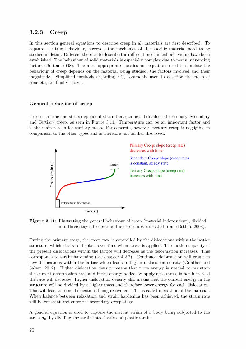
General behavior of creep
Creep is a time and stress dependent strain that can be subdivided into Primary, Secondaryand Tertiary creep, as seen in Figure 3.11. Temperature can be an important factor andis the main reason for tertiary creep. For concrete, however, tertiary creep is negligible incomparison to the other types and is therefore not further discussed.
Primary Creep: slope (creep rate) decreases with time.
Secondary Creep: slope (creep rate) is constant, steady state.
Tertiary Creep: slope (creep rate) increases with time.
Instantaneous deformation
Time (t)
Cre
ep s
trai
n (ε
)
Rapture
Figure 3.11: Illustrating the general behaviour of creep (material independent), dividedinto three stages to describe the creep rate, recreated from (Betten, 2008).
During the primary stage, the creep rate is controlled by the dislocations within the latticestructure, which starts to displace over time when stress is applied. The motion capacity ofthe present dislocations within the lattice will decrease as the deformation increases. Thiscorresponds to strain hardening (see chapter 4.2.2). Continued deformation will result innew dislocations within the lattice which leads to higher dislocation density (Gunther andSalzer, 2012). Higher dislocation density means that more energy is needed to maintainthe current deformation rate and if the energy added by applying a stress is not increasedthe rate will decrease. Higher dislocation density also means that the current energy in thestructure will be divided by a higher mass and therefore lower energy for each dislocation.This will lead to some dislocations being recovered. This is called relaxation of the material.When balance between relaxation and strain hardening has been achieved, the strain ratewill be constant and enter the secondary creep stage.
A general equation is used to capture the instant strain of a body being subjected to thestress σ0, by dividing the strain into elastic and plastic strain:
20
ε0 =σ0
E(T )+ εp(σ0, T ) (3.16)
where T is the temperature and E is the elastic modulus. However, to calculate creep, timeis also an important factor. A simplified equation has been established to capture the creepstrain in Figure 3.11, (Betten, 2008).
εcr = ε(t)− ε0 ∝ tκ (3.17)
where κ < 1 represent the primary, κ = 1 the secondary and κ > 1 the tertiary creep stages.
Due to the creep rate being constant during the secondary stage and tertiary creep not beingrelevant, it is mainly the primary creep behaviour that is of interest. The primary creep willalso govern the magnitude of the final creep.
Creep for concrete
Apart from deforming elastically when stressed, concrete will be subjected to creep deform-ation. The creep strain, εc,creep, increases with the concrete stress, σc, and is defined inEurocode 2 (2005a) as:
εc,creep(t) = ϕ(t, t0)σcEc
(3.18)
where ϕ(t, t0) is the creep function depending on time (t) and time of loading (t0), Ec is theelastic modular ratio for concrete. The magnitude of the creep function depends largely onthe age of the concrete when the structure is loaded (t0) and is determined by:
ϕ(t, t0) = βc(t, t0)ϕ0 (3.19)
where βc(t, t0) determines how the creep function varies with time and ϕ0 is the notionalcreep coefficient, calculated as:
βc(t, t0) =
[(t− t0)
(βH + t− t0)
]0.3
and ϕ0 = ϕRH · β(fcm) · β(t0) (3.20)
where βH , in the left expression, is a factor that depends on the relative humidity and thenotional member size. In the right expression, ϕRH accounts for the relative humidity, β(fcm)for the concrete strength, and β(t0) for the time of loading. These parameters are describedfurther in section 6.2.
An important note is that the above relations apply as long as the compression in theconcrete does not exceeds 0.45fck (fck is the characteristic compressive strength of concrete).In general the long-term compressive stresses should be kept below this value. If this stressis exceeded ϕ(t, t0) is replaced with ϕk(t, t0).
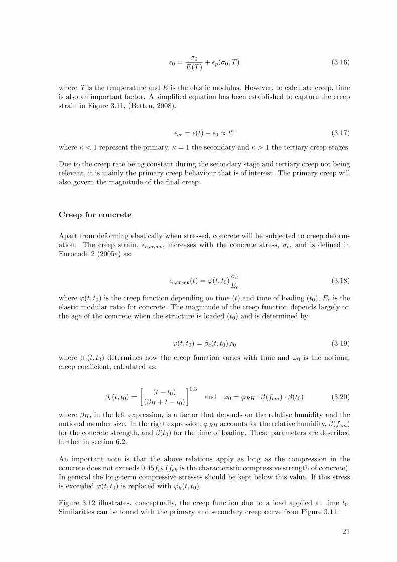
Figure 3.12 illustrates, conceptually, the creep function due to a load applied at time t0.Similarities can be found with the primary and secondary creep curve from Figure 3.11.
21
t0 t
Time
φ
φ(t,t0)
Figure 3.12: Illustrating the general behaviour of creep in concrete using the creepfunction described in EC.
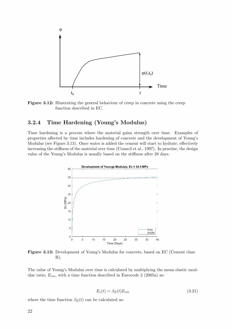
3.2.4 Time Hardening (Young’s Modulus)
Time hardening is a process where the material gains strength over time. Examples ofproperties affected by time includes hardening of concrete and the development of Young’sModulus (see Figure 3.13). Once water is added the cement will start to hydrate, effectivelyincreasing the stiffness of the material over time (Council et al., 1997). In practise, the designvalue of the Young’s Modulus is usually based on the stiffness after 28 days.
Figure 3.13: Development of Young’s Modulus for concrete, based on EC (Cement classR).
The value of Young’s Modulus over time is calculated by multiplying the mean elastic mod-ular ratio, Ecm, with a time function described in Eurocode 2 (2005a) as:
Ec(t) = βE(t)Ecm (3.21)
where the time function βE(t) can be calculated as:
22
βE(t) = (βcc(t))0.3 (3.22)
and
βcc(t) = es−(1−( 28t
)0.5) (3.23)
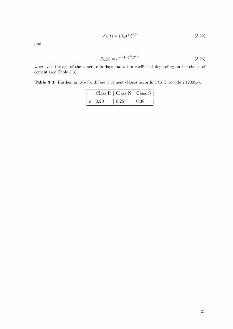
where t is the age of the concrete in days and s is a coefficient depending on the choice ofcement (see Table 3.3).
Table 3.3: Hardening rate for different cement classes according to Eurocode 2 (2005a).
Class R Class N Class S
s 0,20 0,25 0,38
23

24
4 Modelling of Creep
4.1 Building Codes to Predict Creep
The influence of creep in concrete is described in section 3.2.3. With varying long-termloads, such as in the case of segmentally constructed bridges, the behaviour becomes morecomplicated. This report will be limited to the methods described in Eurocode 2 (2005b), itshould be noted that there are several other methods available.
1. General and incremental step-by-step method
• This method requires the designer to carry out structural analysis at severalsteps. The fundamental equation for time-dependent concrete strain is writtenas:
εc(t) =σ0
Ec(t0)+ϕ(t, t0)
σ0
Ec(28)+∑(
1
Ec(ti)+ϕ(t, ti)
Ec(28)
)∆σ(ti)+ εcs(t, ts) (4.1)
where the first term represents the instant deformation from a stress appliedat time t0, the second term represents the corresponding creep, the third termcorresponds to the instant and creep deformation occurring due to variations instress, and the fourth term describes the deformation due to shrinkage.
2. Methods based on the theorems of linear viscoelasticity
• The time-dependent properties of concrete can be described by:
– J(t, t0) which represents the strain response at time ”t” resulting from aconstant applied stress at time ”t0”.
– R(t, t0) which represents the stress response at time ”t” from a constantapplied strain at time ”t0”.
3. The ageing coefficient method
• This method allows for an analysis to be performed without having to take thediscrete time steps into account. It is based on the ageing coefficient, χ, and isuseful when only the long term effects are of interest (Eurocode 2, 2005b).
4. Simplified ageing coefficient method
• The principle of this simplified method is to first calculate the internal forces ofthe structure by modelling the complete construction sequence, and then repeat-ing the calculations assuming the structure was cast-in-one. By interpolatingbetween these two cases the redistribution due to creep can be found as:
∆S = (Sc − S0)ϕ(∞, t0)− ϕ(tc, t0)
1 + χϕ(∞, t0)(4.2)
where Sc are the internal actions from the segmental construction sequence, S0
are the internal actions if the structure was to be cast in one go. According toHendy and Smith (2007) the factor ϕ(∞,t0)−ϕ(tc,t0)
1+χϕ(∞,t0) typically has as value between0.65 and 0.8.
25
4.2 Creep Models in Abaqus
The material properties in Abaqus need to be adjusted to perform a creep analysis. Thereare several ways to do this, see Simulia (2014), but in this report the following models areinvestigated:
• Function *CREEP and the subfunctions time/strain hardening.
• Function *VISCOELASTIC in the time domain where the losses are caused by theinternal damping effect of the material. This corresponds to the method described insection 4.1 (Methods based on the theorems of linear viscoelasticity).
4.2.1 Time Hardening Model
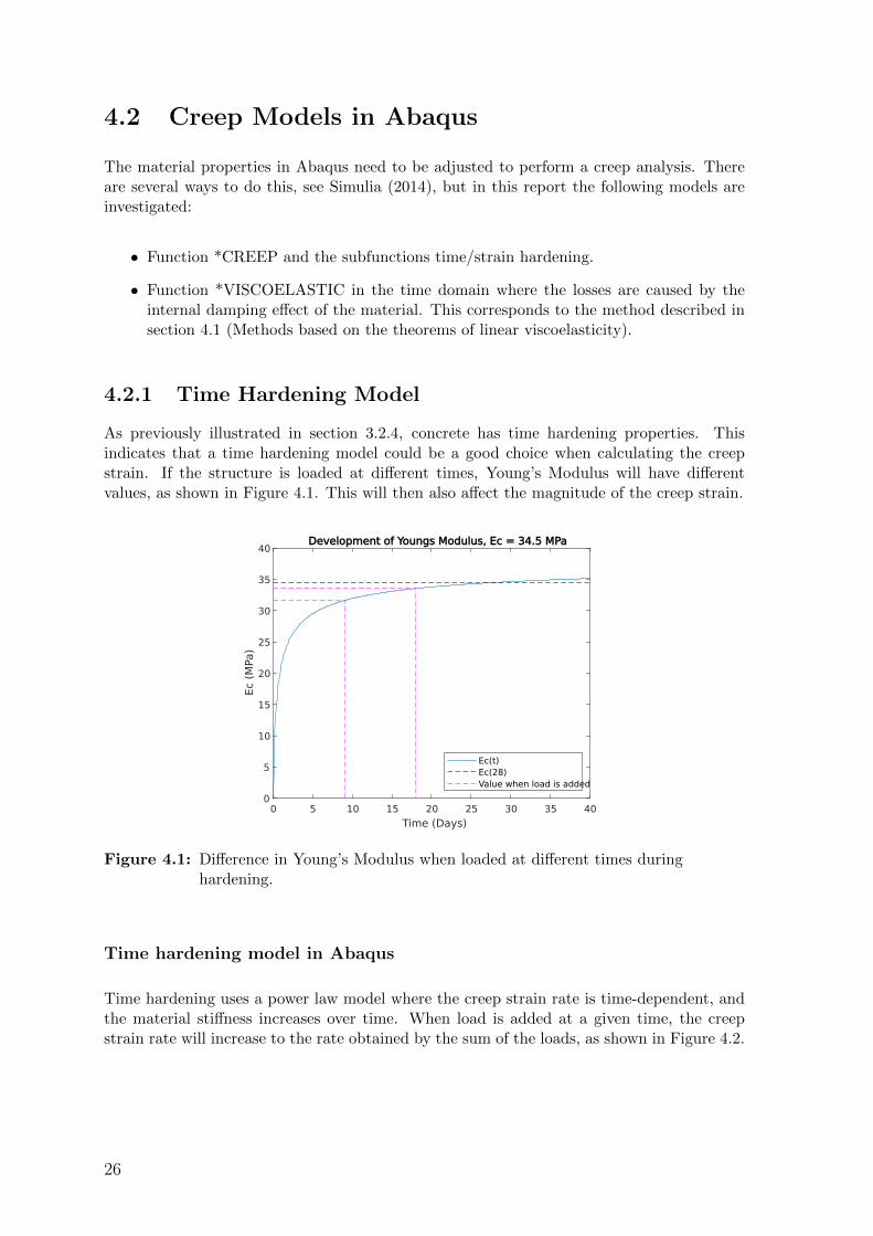
As previously illustrated in section 3.2.4, concrete has time hardening properties. Thisindicates that a time hardening model could be a good choice when calculating the creepstrain. If the structure is loaded at different times, Young’s Modulus will have differentvalues, as shown in Figure 4.1. This will then also affect the magnitude of the creep strain.
0 5 10 15 20 25 30 35 40
Time (Days)
0
5
10
15
20
25
30
35
40
Ec
(MPa
)
Development of Youngs Modulus, Ec = 34.5 MPa
Ec(t)Ec(28)Value when load is added
Figure 4.1: Difference in Young’s Modulus when loaded at different times duringhardening.
Time hardening model in Abaqus
Time hardening uses a power law model where the creep strain rate is time-dependent, andthe material stiffness increases over time. When load is added at a given time, the creepstrain rate will increase to the rate obtained by the sum of the loads, as shown in Figure 4.2.
26
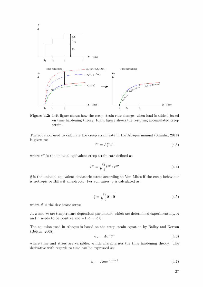
Time
εcr
t0 t1
Time-hardening
Time
εcr
t0 t1
Time-hardening
εcr
ε cr(σ 0,t 1)
.
εcr(σ0+Δσ,t 1)
.
t0 tTime
σ
σ0
Δσ1
t0 t1 t2
Δσ2
t2
εcr(t,σ0)
εcr(t,σ0+Δσ1)
εcr(t,σ0+Δσ1+Δσ2)
εcr(t,σ0+Δσ1+Δσ2)
t2
.
Figure 4.2: Left figure shows how the creep strain rate changes when load is added, basedon time hardening theory. Right figure shows the resulting accumulated creepstrain.
The equation used to calculate the creep strain rate in the Abaqus manual (Simulia, 2014)is given as:
˙εcr = Aqntm (4.3)
where ˙εcr is the uniaxial equivalent creep strain rate defined as:
˙εcr =
√2
3εcr : εcr (4.4)
q is the uniaxial equivalent deviatoric stress according to Von Mises if the creep behaviouris isotropic or Hill’s if anisotropic. For von mises, q is calculated as:
q =
√2
3S : S (4.5)
where S is the deviatoric stress.
A, n and m are temperature dependant parameters which are determined experimentally, Aand n needs to be positive and −1 < m < 0.
The equation used in Abaqus is based on the creep strain equation by Bailey and Norton(Betten, 2008).
εcr = Aσntm (4.6)
where time and stress are variables, which characterises the time hardening theory. Thederivative with regards to time can be expressed as:
εcr = Amσntm−1 (4.7)
27
However, Abaqus refers to the uniaxial equivalent creep strain and equivalent deviatoricstress. The equation developed by Bailey and Norton is also based on uniaxial stress but notthe equivalent and only calculates the strain in one direction. For the one dimensional casewith an isotropic material, the equivalent uniaxial creep strain rate and stress are equal tothe uniaxial creep strain rate and stress ( ˙εcr=εcr and q=σ). If the material is anisotropic therelation between the strains in the different directions need to be established before changingthe variables (Simulia, 2014).
Several variations of the Bailey and Norton equation can be found in the literature, whichleads to different material parameters. The parameters that are to be used needs to bespecifically determined to fit the model in Abaqus. One way to determine the parametersis to perform tests on the material, which will be a time-consuming process. It’s easier tolook at tests already performed or to calibrate them against EC, the latter is chosen in thisreport.
To calibrate the parameters the creep strain is required. The creep strain is derived byintegrating equation 4.3 with respect to time, stress is independent of time in this regard.
εcr = Aqtm+1
m+ 1+ C (4.8)
where C is a constant which corresponds to the elastic strain, ε0. By replacing the equivalentstrain and deviatoric stress with the uniaxial for an isotropic material, the following equationis obtained:
εcr = Aσntm+1
m+ 1+ ε0 (4.9)
For a one-dimensional case, the creep law can be integrated directly to find the solution. Inother cases, numerical methods must be used where the time is divided into time steps inwhich iterations are performed until equilibrium is reached.
Referring to EC
The parameters can be decided by referring to EC and the creep function, ϕ(t, t0), see section3.2.3. The time hardening theory indicates that the creep function is established solely basedon the concrete age when the first load is applied. If further loads are added, the additionalcreep will be based on the creep function caused by the initial load, resulting in a creep rateaccording to Figure 4.2. This method will underestimate deformations, as loads added aftersome time will result in little or no creep.
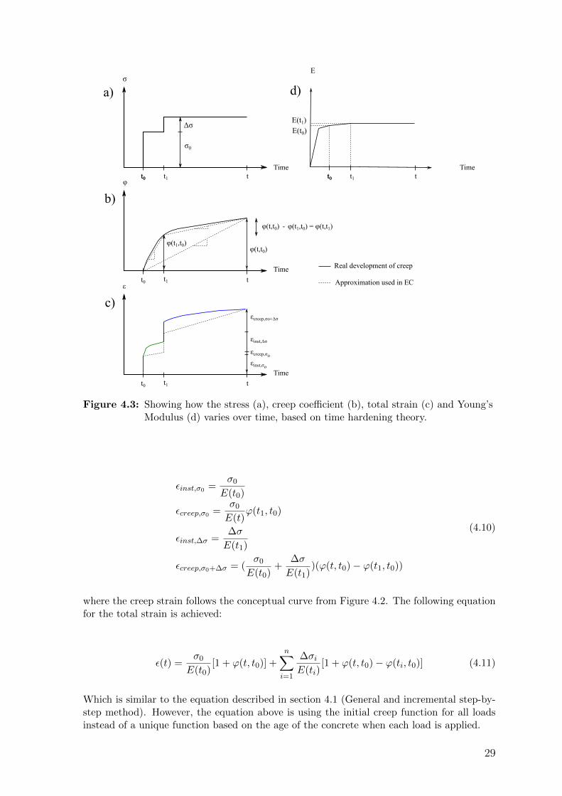
The behaviour of the time hardening model, and how the total strains can be calculatedusing the creep function, is shown in Figure 4.3 and the following relations.
28
t0 t
t0 t
t0 t
Time
Time
Time
σ
ε
φ
σ0
Δσ
t0 t1
t1
t1
φ(t1,t0)φ(t,t0)
Real development of creep
Approximation used in EC
t0 tTime
E
t0 t1
E(t1)E(t0)
φ(t,t0) φ(t1,t0) = φ(t,t1) -
εinst,σo
εcreep,σo
εinst,Δσ
εcreep,σo+Δσ
a)
b)
c)
d)
Figure 4.3: Showing how the stress (a), creep coefficient (b), total strain (c) and Young’sModulus (d) varies over time, based on time hardening theory.
εinst,σ0 =σ0
E(t0)
εcreep,σ0 =σ0
E(t)ϕ(t1, t0)
εinst,∆σ =∆σ
E(t1)
εcreep,σ0+∆σ = (σ0
E(t0)+
∆σ
E(t1))(ϕ(t, t0)− ϕ(t1, t0))
(4.10)
where the creep strain follows the conceptual curve from Figure 4.2. The following equationfor the total strain is achieved:
ε(t) =σ0
E(t0)[1 + ϕ(t, t0)] +
n∑i=1
∆σiE(ti)
[1 + ϕ(t, t0)− ϕ(ti, t0)] (4.11)
Which is similar to the equation described in section 4.1 (General and incremental step-by-step method). However, the equation above is using the initial creep function for all loadsinstead of a unique function based on the age of the concrete when each load is applied.
29
4.2.2 Strain Hardening Model
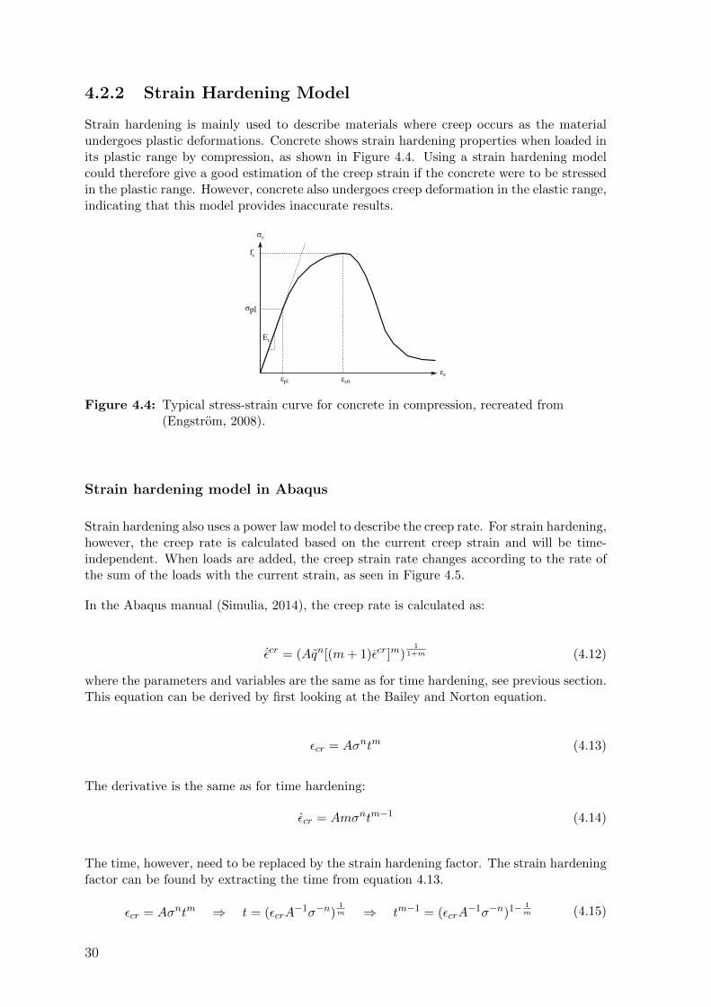
Strain hardening is mainly used to describe materials where creep occurs as the materialundergoes plastic deformations. Concrete shows strain hardening properties when loaded inits plastic range by compression, as shown in Figure 4.4. Using a strain hardening modelcould therefore give a good estimation of the creep strain if the concrete were to be stressedin the plastic range. However, concrete also undergoes creep deformation in the elastic range,indicating that this model provides inaccurate results.
σc
εc
σpl
εpl εc0
fc
Ec
Figure 4.4: Typical stress-strain curve for concrete in compression, recreated from(Engstrom, 2008).
Strain hardening model in Abaqus
Strain hardening also uses a power law model to describe the creep rate. For strain hardening,however, the creep rate is calculated based on the current creep strain and will be time-independent. When loads are added, the creep strain rate changes according to the rate ofthe sum of the loads with the current strain, as seen in Figure 4.5.
In the Abaqus manual (Simulia, 2014), the creep rate is calculated as:
˙εcr = (Aqn[(m+ 1)εcr]m)1
1+m (4.12)
where the parameters and variables are the same as for time hardening, see previous section.This equation can be derived by first looking at the Bailey and Norton equation.
εcr = Aσntm (4.13)
The derivative is the same as for time hardening:
εcr = Amσntm−1 (4.14)
The time, however, need to be replaced by the strain hardening factor. The strain hardeningfactor can be found by extracting the time from equation 4.13.
εcr = Aσntm ⇒ t = (εcrA−1σ−n)
1m ⇒ tm−1 = (εcrA
−1σ−n)1− 1m (4.15)
30
ε cr(ε cr,0,σ0)
.
Time
εcr
t0 t1
Strain-hardening
Time
εcr
t0 t1
Strain-hardening
εcr,1 ε cr(ε cr,1,σ 0+Δσ 1)
.εcr,1
t2 t2
εcr(t,σ0)
εcr(t,σ0+Δσ1)
εcr(t,σ0+Δσ1+Δσ2)
εcr,1
εcr,2 εcr(εcr,2,σ0+Δσ1
+Δσ2)
.εcr,2
t0 tTime
σ
σ0
Δσ1
t0 t1 t2
Δσ2
Figure 4.5: Left figure shows how the creep strain rate changes when load is added, basedon strain hardening theory. Right figure shows the resulting accumulatedcreep strain.
The time in the derivated expression, equation 4.14, is then replaced with the strain harden-ing factor:
εcr = Amσntm−1 ⇒ εcr = Amσn(εcrA−1σ−n)1− 1
m ⇒ εcr = mA1mσ
nm ε
m−1m
cr (4.16)
The equation Abaqus uses as strain hardening can then be derived in the same way asdescribed for Bailey and Norton. First, equation 4.3 is integrated with respect to time toobtain the creep strain.
εcr =
∫Aqntm dt =
Aqntm+1
m+ 1(4.17)
The strain hardening factor is then obtained in the same way as described previously, forBailey and Norton equation 4.15, as:
t = (εcr(m+ 1)A−1q−n)1
m+1 ⇒ tm = (εcr(m+ 1))m
m+1 (A−1q−n)1− 1m+1
= (εcr(m+ 1))m
m+1 (Aqn)−1(Aq)1
m+1
(4.18)
The time in equation 4.3 is then replaced with the strain hardening factor above.
¯εcr = Aqntm = Aqn(εcr(m+ 1))m
m+1 (Aqn)−1(Aq)1
m+1 = (εcr(m+ 1))m
m+1 (Aq)1
m+1 (4.19)
Which is the same equation found in the Abaqus manual, see equation 4.12. Abaqus thensolves equation 4.19 by using a numerical step by step method, same way as described fortime hardening.
31
Referring to EC
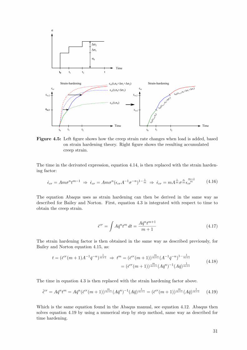
Similar to time hardening, the creep rate can be referred to the creep function described inEC. When load is added the creep rate will change according to Figure 4.5. The behaviourof the strain hardening model, and how the total creep can be calculated using the creepfunction, is shown in Figure 4.6 and in the following relations.
t0 t
t0 t
t0 t
Time
Time
Time
σ
ε
φ
σ0
Δσ
t0 t1
t1
t1
φ(t1,t0)
φ(t,t0)
Real development of creep
Approximation used in EC
t0 tTime
E
t0 t1
φ(t,t0) -
εinst,σo
εcreep,σo
εinst,Δσ
εcreep,σo+Δσ
E(28)
φεcr(t1,t0)
φεcr(t1,t0)
a)
b)
c)
d)
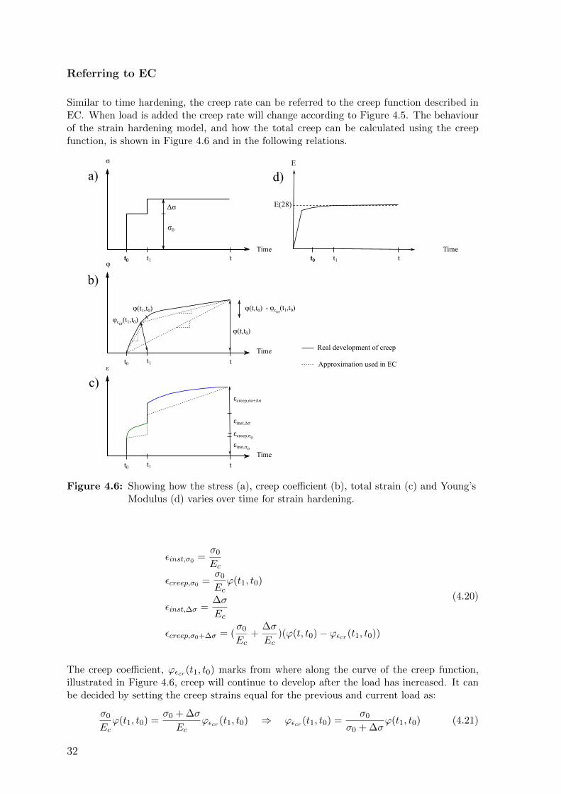
Figure 4.6: Showing how the stress (a), creep coefficient (b), total strain (c) and Young’sModulus (d) varies over time for strain hardening.
εinst,σ0 =σ0
Ec
εcreep,σ0 =σ0
Ecϕ(t1, t0)
εinst,∆σ =∆σ
Ec
εcreep,σ0+∆σ = (σ0
Ec+
∆σ
Ec)(ϕ(t, t0)− ϕεcr(t1, t0))
(4.20)
The creep coefficient, ϕεcr(t1, t0) marks from where along the curve of the creep function,illustrated in Figure 4.6, creep will continue to develop after the load has increased. It canbe decided by setting the creep strains equal for the previous and current load as:
σ0
Ecϕ(t1, t0) =
σ0 + ∆σ
Ecϕεcr(t1, t0) ⇒ ϕεcr(t1, t0) =
σ0
σ0 + ∆σϕ(t1, t0) (4.21)
32
The sum of the strain eq 4.22, can be related to the General and incremental step-by-stepmethod described in EC, similar to time hardening. It should be noted, however, that iffurther loads are applied the creep coefficient ϕεcr becomes complicated to calculate by hand,it can instead be determined numerically.
ε(t) =σ0
Ec[1 + ϕ(t, t0) + ϕεcr ] +
n∑i=1
∆σiEc
[1 + ϕ(t, t0)− ϕεcr(ti, t0)] (4.22)
4.2.3 Calibrating Time and Strain Hardening Parameters
When using time/strain hardening, only one creep function is used to calculate the creepstrain for all loads that are applied over time. The creep function is calculated based on theage of the concrete when the first load is applied, t0. Concrete as a structural member can beseen as isotropic (Reiner, 1949), which entails that the equation used in Abaqus to calculatethe creep strain, can be changed to equation 4.9, according to section 4.2.1. The parametersused in the equation can then be found by comparing it to the general creep strain equationdescribed in Eurocode 2 (2005a):
εcr(t) = Aσntm+1
m+ 1=σ · ϕ(t, t0)
Ec(4.23)
The parameters can be found by using the natural logarithm and dividing the equation intosets:
ln(Aσntm+1
m+ 1) = ln(
σ · ϕ(t, t0)
Ec) (4.24)
ln(A) + n · ln(σ)− ln(m+ 1) + (m+ 1) · ln(t) = ln(σ)− ln(Ec) + ln(ϕ(t, t0)) (4.25)
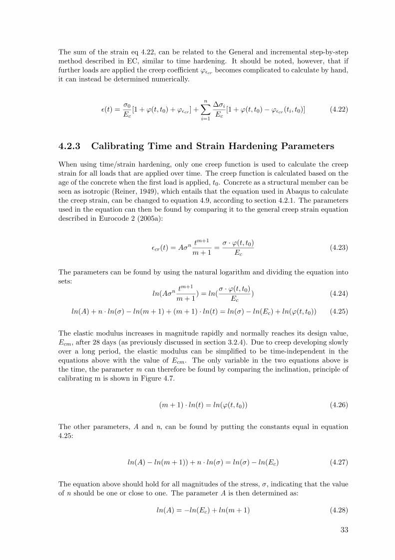
The elastic modulus increases in magnitude rapidly and normally reaches its design value,Ecm, after 28 days (as previously discussed in section 3.2.4). Due to creep developing slowlyover a long period, the elastic modulus can be simplified to be time-independent in theequations above with the value of Ecm. The only variable in the two equations above isthe time, the parameter m can therefore be found by comparing the inclination, principle ofcalibrating m is shown in Figure 4.7.
(m+ 1) · ln(t) = ln(ϕ(t, t0)) (4.26)
The other parameters, A and n, can be found by putting the constants equal in equation4.25:
ln(A)− ln(m+ 1)) + n · ln(σ) = ln(σ)− ln(Ec) (4.27)
The equation above should hold for all magnitudes of the stress, σ, indicating that the valueof n should be one or close to one. The parameter A is then determined as:
ln(A) = −ln(Ec) + ln(m+ 1) (4.28)
33
-5 0 5 10
ln(Time)
-2.5
-2
-1.5
-1
-0.5
0
0.5
1
1.5
2
ln(C
reep C
oeffi
cia
nt)
(m+1) = 0.2807
ln(Creep-coef(t,t0))
(m+1)*ln(t)
0 1000 2000 3000 4000 5000 6000 7000 8000 9000
Time (days)
0
0.5
1
1.5
2
2.5
3
Cre
ep C
oeffi
cia
nt
Creep coefficiant over time
Figure 4.7: Left: development of the creep coefficient over time. Right: comparison of thecreep coefficient and the time dependent part of the equation in Abaqus,using a logarithmic scale.
4.2.4 Viscoelastic Model
A viscoelastic material is characterised by a combination of two theories. Viscosity, whichdescribes how a fluid resists flow (compare for example honey and water) and Elasticity whichdescribes how a material deforms under load (compare for example steel and timber). Thismeans that a viscoelastic material is subject to both instant (Elasticity) and time-dependent(Viscosity) strain (Ohlsson, 2018).
As described in for example Grasley and Lange (2007), the ageing, viscoelastic behaviour ofconcrete is due to the properties of the cement paste. Whereas the aggregates are knownto behave elastically and in a non-aging manner. The studies regarding this subject haveprimarily been performed with the goal to understand the long-term deformations in con-crete. Which is also why it has been considered as an appropriate model to determine thecreep behaviour.
Viscoelastic modelling in Abaqus
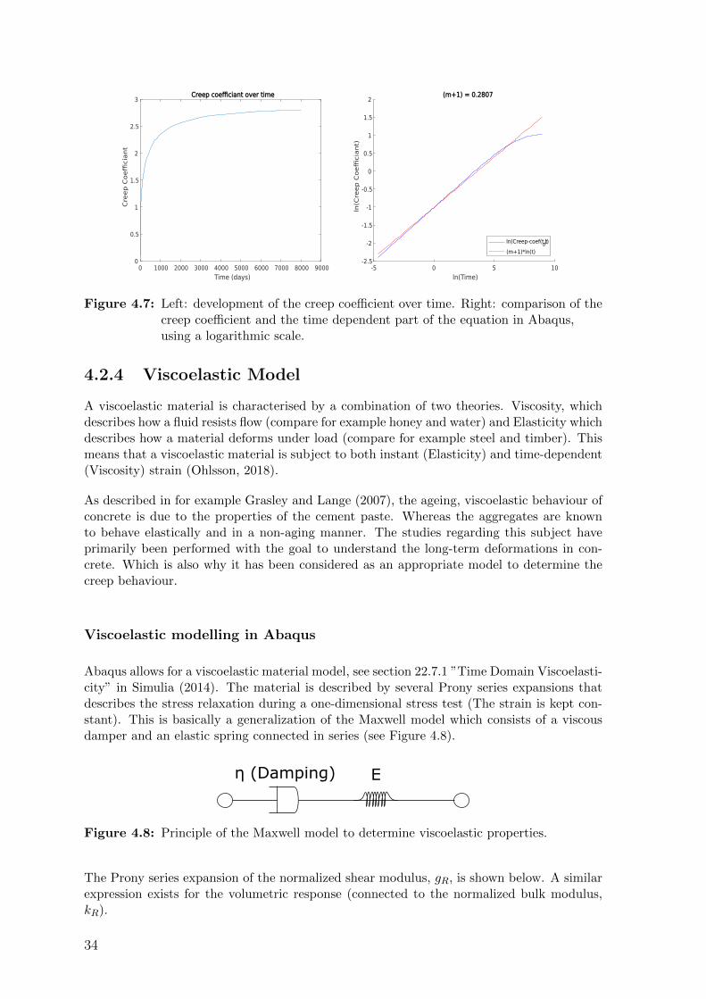
Abaqus allows for a viscoelastic material model, see section 22.7.1 ”Time Domain Viscoelasti-city” in Simulia (2014). The material is described by several Prony series expansions thatdescribes the stress relaxation during a one-dimensional stress test (The strain is kept con-stant). This is basically a generalization of the Maxwell model which consists of a viscousdamper and an elastic spring connected in series (see Figure 4.8).
Eη (Damping)
Figure 4.8: Principle of the Maxwell model to determine viscoelastic properties.
The Prony series expansion of the normalized shear modulus, gR, is shown below. A similarexpression exists for the volumetric response (connected to the normalized bulk modulus,kR).
34
gR(t) = 1−N∑i=1
gPi(1− e−t/τGi
)(4.29)
In Abaqus it is possible to define this behaviour in several ways:
• Direct specification - Define required parameters for each term in the Prony seriesexpansion. Since these are quite difficult to determine this method is not considered.
• Creep test data - The creep test data is converted to relaxation data and then to theProny series parameters using a nonlinear least-square fit.
• Relaxation test data - A nonlinear least-square fit is used to convert the relaxationtest data into the Prony series parameters.
Creep test data
The normalized shear and bulk compliance (jS & jK) are defined as:
jS(t) = G0JS(t) and jK(t) = K0JS(t) (4.30)
where JS(t) = γ(t)/τ0 and JK(t) = εvol(t)/p0 are the shear and bulk compliance. G0 and K0
are the shear/bulk modulus at time t = 0, at t = 0 the factors jS = jK = 1. Furthermore,we recall the following definitions for an isotropic material (Eurocode 2, 2005a).
G0 =E0
2(1 + ν0)and K0 =
E0
3(1− ν0)(4.31)
Relaxation test data
For small strains, the dimensionless shear relaxation modulus, gR, is defined as:
gR(t) = GR(t)/G0 (4.32)
where GR is the time-dependent shear relaxation modulus, GR(0) = G0.
The creep coefficient, ϕ(t, t0), can be implemented according to Eurocode 2 (2005a) section7.4.3 (Using the effective modulus of elasticity, Ec,eff ). It is also recognised that Poisson’sratio, ν, does not change considerably after the concrete has cured (Allos and Martin, 1981).The shear modulus at time t, GR, can then be evaluated as:
GR =Ec,eff
2(1 + v)=
E0
1 + ϕ(t, t0)
1
2(1 + ν0)(4.33)
The dimensionless shear relaxation modulus, gR, can finally be derived according to theequation below, kR is calculated using the same principle.
gR =GRG0
=
E01+ϕ(t,t0)
12(1+ν0)
E02(1+ν0)
=1
1 + ϕ(t, t0)=KR
K0= kR (4.34)
35
4.2.5 Comparison of Creep Models
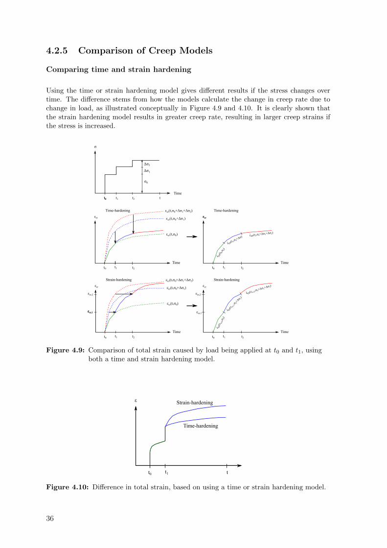
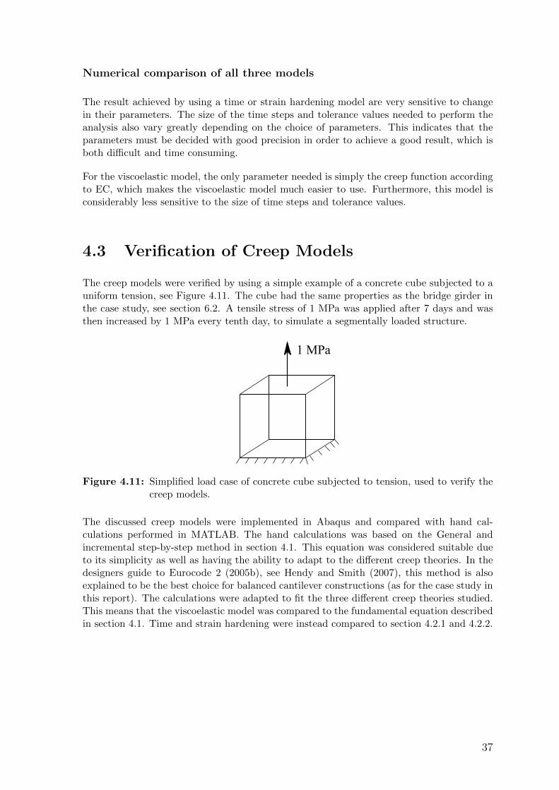
Comparing time and strain hardening
Using the time or strain hardening model gives different results if the stress changes overtime. The difference stems from how the models calculate the change in creep rate due tochange in load, as illustrated conceptually in Figure 4.9 and 4.10. It is clearly shown thatthe strain hardening model results in greater creep rate, resulting in larger creep strains ifthe stress is increased.
Time
εcr
t0 t1
Time-hardening
Time
εcr
t0 t1
Time-hardening
εcrε cr(t 0,σ 0)
.
εcr(t1,σ0+Δσ
)
.
t0 tTime
σ
σ0
Δσ1
t0 t1
ε cr(ε cr,0,σ0)
.
Time
εcr
t0 t1
Strain-hardening
Time
εcr
t0 t1
Strain-hardening
εcr,1 ε cr(ε cr,1,σ 0+Δσ 1)
.εcr,1
t2
Δσ2
t2
t2
εcr(t,σ0)
εcr(t,σ0+Δσ1)
εcr(t,σ0+Δσ1+Δσ2)
εcr(t2,σ0+Δσ1+Δσ2)
t2
t2
εcr(t,σ0)
εcr(t,σ0+Δσ1)
εcr(t,σ0+Δσ1+Δσ2)
εcr,1
εcr,2 εcr(εcr,2,σ0+Δσ1
+Δσ2)
.εcr,2
.
Figure 4.9: Comparison of total strain caused by load being applied at t0 and t1, usingboth a time and strain hardening model.
t0 t
ε
t1
Time-hardening
Strain-hardening
Figure 4.10: Difference in total strain, based on using a time or strain hardening model.
36
Numerical comparison of all three models
The result achieved by using a time or strain hardening model are very sensitive to changein their parameters. The size of the time steps and tolerance values needed to perform theanalysis also vary greatly depending on the choice of parameters. This indicates that theparameters must be decided with good precision in order to achieve a good result, which isboth difficult and time consuming.
For the viscoelastic model, the only parameter needed is simply the creep function accordingto EC, which makes the viscoelastic model much easier to use. Furthermore, this model isconsiderably less sensitive to the size of time steps and tolerance values.
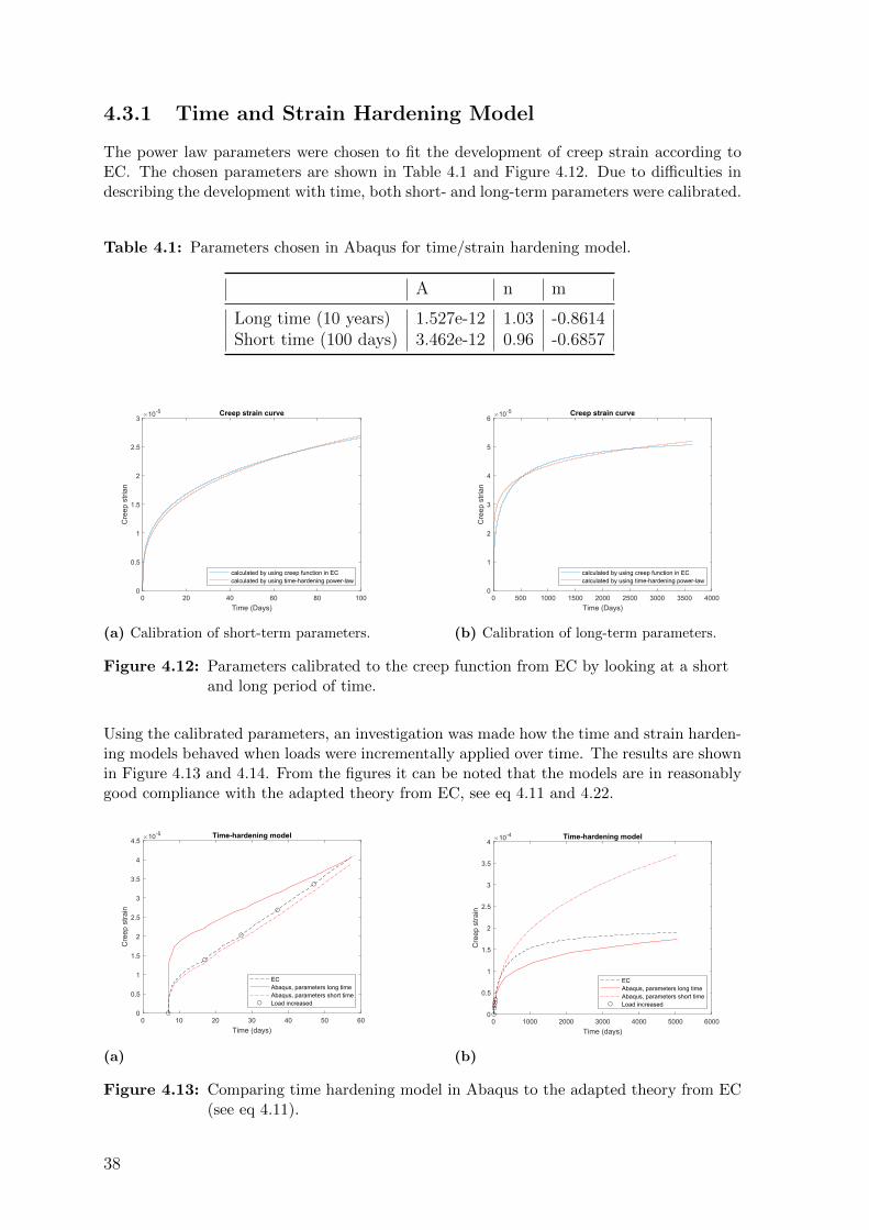
4.3 Verification of Creep Models
The creep models were verified by using a simple example of a concrete cube subjected to auniform tension, see Figure 4.11. The cube had the same properties as the bridge girder inthe case study, see section 6.2. A tensile stress of 1 MPa was applied after 7 days and wasthen increased by 1 MPa every tenth day, to simulate a segmentally loaded structure.
1 MPa
Figure 4.11: Simplified load case of concrete cube subjected to tension, used to verify thecreep models.
The discussed creep models were implemented in Abaqus and compared with hand cal-culations performed in MATLAB. The hand calculations was based on the General andincremental step-by-step method in section 4.1. This equation was considered suitable dueto its simplicity as well as having the ability to adapt to the different creep theories. In thedesigners guide to Eurocode 2 (2005b), see Hendy and Smith (2007), this method is alsoexplained to be the best choice for balanced cantilever constructions (as for the case study inthis report). The calculations were adapted to fit the three different creep theories studied.This means that the viscoelastic model was compared to the fundamental equation describedin section 4.1. Time and strain hardening were instead compared to section 4.2.1 and 4.2.2.
37
4.3.1 Time and Strain Hardening Model
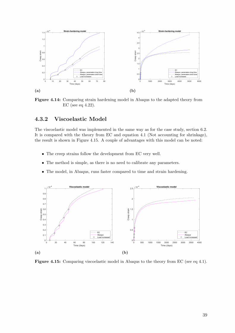
The power law parameters were chosen to fit the development of creep strain according toEC. The chosen parameters are shown in Table 4.1 and Figure 4.12. Due to difficulties indescribing the development with time, both short- and long-term parameters were calibrated.
Table 4.1: Parameters chosen in Abaqus for time/strain hardening model.
A n m
Long time (10 years) 1.527e-12 1.03 -0.8614Short time (100 days) 3.462e-12 0.96 -0.6857
(a) Calibration of short-term parameters. (b) Calibration of long-term parameters.
Figure 4.12: Parameters calibrated to the creep function from EC by looking at a shortand long period of time.
Using the calibrated parameters, an investigation was made how the time and strain harden-ing models behaved when loads were incrementally applied over time. The results are shownin Figure 4.13 and 4.14. From the figures it can be noted that the models are in reasonablygood compliance with the adapted theory from EC, see eq 4.11 and 4.22.
(a) (b)
Figure 4.13: Comparing time hardening model in Abaqus to the adapted theory from EC(see eq 4.11).
38
(a) (b)
Figure 4.14: Comparing strain hardening model in Abaqus to the adapted theory fromEC (see eq 4.22).
4.3.2 Viscoelastic Model
The viscoelastic model was implemented in the same way as for the case study, section 6.2.It is compared with the theory from EC and equation 4.1 (Not accounting for shrinkage),the result is shown in Figure 4.15. A couple of advantages with this model can be noted:
• The creep strains follow the development from EC very well.
• The method is simple, as there is no need to calibrate any parameters.
• The model, in Abaqus, runs faster compared to time and strain hardening.
(a) (b)
Figure 4.15: Comparing viscoelastic model in Abaqus to the theory from EC (see eq 4.1).
39
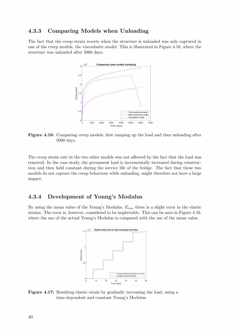
4.3.3 Comparing Models when Unloading
The fact that the creep strain reverts when the structure is unloaded was only captured inone of the creep models, the viscoelastic model. This is illustrated in Figure 4.16, where thestructure was unloaded after 5000 days.
Figure 4.16: Comparing creep models, first ramping up the load and then unloading after5000 days.
The creep strain rate in the two other models was not affected by the fact that the load wasremoved. In the case study, the permanent load is incrementally increased during construc-tion and then held constant during the service life of the bridge. The fact that these twomodels do not capture the creep behaviour while unloading, might therefore not have a largeimpact.
4.3.4 Development of Young’s Modulus
By using the mean value of the Young’s Modulus, Ecm, there is a slight error in the elasticstrains. The error is, however, considered to be neglectable. This can be seen in Figure 4.16,where the use of the actual Young’s Modulus is compared with the use of the mean value.
Figure 4.17: Resulting elastic strain by gradually increasing the load, using atime-dependent and constant Young’s Modulus.
40
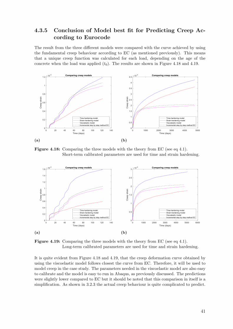
4.3.5 Conclusion of Model best fit for Predicting Creep Ac-cording to Eurocode
The result from the three different models were compared with the curve achieved by usingthe fundamental creep behaviour according to EC (as mentioned previously). This meansthat a unique creep function was calculated for each load, depending on the age of theconcrete when the load was applied (t0). The results are shown in Figure 4.18 and 4.19.
(a) (b)
Figure 4.18: Comparing the three models with the theory from EC (see eq 4.1).Short-term calibrated parameters are used for time and strain hardening.
(a) (b)
Figure 4.19: Comparing the three models with the theory from EC (see eq 4.1).Long-term calibrated parameters are used for time and strain hardening.
It is quite evident from Figure 4.18 and 4.19, that the creep deformation curve obtained byusing the viscoelastic model follows closest the curve from EC. Therefore, it will be used tomodel creep in the case study. The parameters needed in the viscoelastic model are also easyto calibrate and the model is easy to run in Abaqus, as previously discussed. The predictionswere slightly lower compared to EC but it should be noted that this comparison in itself is asimplification. As shown in 3.2.3 the actual creep behaviour is quite complicated to predict.
41

42

Part II
Case Study
43

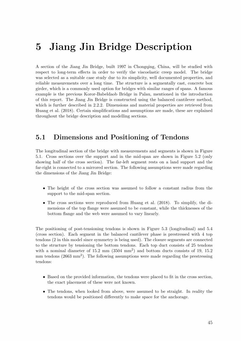
5 Jiang Jin Bridge Description
A section of the Jiang Jin Bridge, built 1997 in Chongqing, China, will be studied withrespect to long-term effects in order to verify the viscoelastic creep model. The bridgewas selected as a suitable case study due to its simplicity, well documented properties, andreliable measurements over a long time. The structure is a segmentally cast, concrete boxgirder, which is a commonly used option for bridges with similar ranges of spans. A famousexample is the previous Koror-Babeldaob Bridge in Palau, mentioned in the introductionof this report. The Jiang Jin Bridge is constructed using the balanced cantilever method,which is further described in 2.2.2. Dimensions and material properties are retrieved fromHuang et al. (2018). Certain simplifications and assumptions are made, these are explainedthroughout the bridge description and modelling sections.
5.1 Dimensions and Positioning of Tendons
The longitudinal section of the bridge with measurements and segments is shown in Figure5.1. Cross sections over the support and in the mid-span are shown in Figure 5.2 (onlyshowing half of the cross section). The far-left segment rests on a land support and thefar-right is connected to a mirrored section. The following assumptions were made regardingthe dimensions of the Jiang Jin Bridge:
• The height of the cross section was assumed to follow a constant radius from thesupport to the mid-span section.
• The cross sections were reproduced from Huang et al. (2018). To simplify, the di-mensions of the top flange were assumed to be constant, while the thicknesses of thebottom flange and the web were assumed to vary linearly.
The positioning of post-tensioning tendons is shown in Figure 5.3 (longitudinal) and 5.4(cross section). Each segment in the balanced cantilever phase is prestressed with 4 toptendons (2 in this model since symmetry is being used). The closure segments are connectedto the structure by tensioning the bottom tendons. Each top duct consists of 25 tendonswith a nominal diameter of 15.2 mm (3504 mm2) and bottom ducts consists of 19, 15.2mm tendons (2663 mm2). The following assumptions were made regarding the prestressingtendons:
• Based on the provided information, the tendons were placed to fit in the cross section,the exact placement of these were not known.
• The tendons, when looked from above, were assumed to be straight. In reality thetendons would be positioned differently to make space for the anchorage.
45
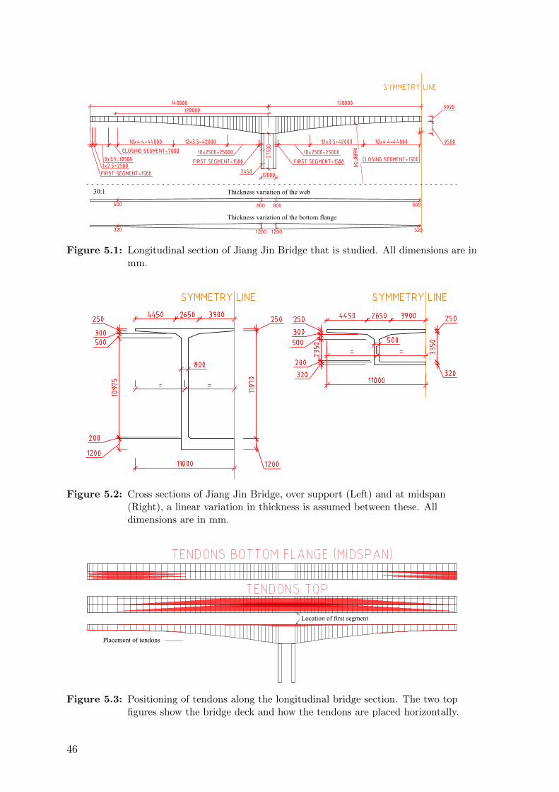
800800500 500
Thickness variation of the web
1200320 1200 320
Thickness variation of the bottom flange
30:1
Figure 5.1: Longitudinal section of Jiang Jin Bridge that is studied. All dimensions are inmm.
Figure 5.2: Cross sections of Jiang Jin Bridge, over support (Left) and at midspan(Right), a linear variation in thickness is assumed between these. Alldimensions are in mm.
Placement of tendons
Location of first segment
Figure 5.3: Positioning of tendons along the longitudinal bridge section. The two topfigures show the bridge deck and how the tendons are placed horizontally.
46
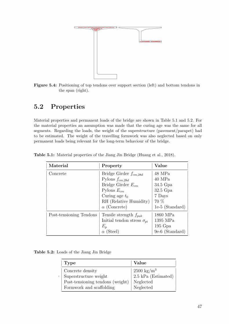
Figure 5.4: Positioning of top tendons over support section (left) and bottom tendons inthe span (right).
5.2 Properties
Material properties and permanent loads of the bridge are shown in Table 5.1 and 5.2. Forthe material properties an assumption was made that the curing age was the same for allsegments. Regarding the loads, the weight of the superstructure (pavement/parapet) hadto be estimated. The weight of the travelling formwork was also neglected based on onlypermanent loads being relevant for the long-term behaviour of the bridge.
Table 5.1: Material properties of the Jiang Jin Bridge (Huang et al., 2018).
Material Property Value
Concrete Bridge Girder fcm,28d 48 MPaPylons fcm,28d 40 MPaBridge Girder Ecm 34.5 GpaPylons Ecm 32.5 GpaCuring age t0 7 DaysRH (Relative Humidity) 70 %α (Concrete) 1e-5 (Standard)
Post-tensioning Tendons Tensile strength fpuk 1860 MPaInitial tendon stress σpi 1395 MPaEp 195 Gpaα (Steel) 9e-6 (Standard)
Table 5.2: Loads of the Jiang Jin Bridge
.
Type Value
Concrete density 2500 kg/m3
Superstructure weight 2.5 kPa (Estimated)Post-tensioning tendons (weight) NeglectedFormwork and scaffolding Neglected
47

5.3 Construction Sequence
The concrete segments were cast-in-situ in a balanced cantilever construction. Regardingthe long-term effects, changes in the timeline of the cantilever construction, prestressingsequence, and closure segments can have a large impact. The matter in which the pylonsand midsection are constructed are less important in this regard. The following timeline isgiven by Huang et al. (2018):
1. The balanced cantilever construction was completed, t = 300 days. Progress is shownin Figure 5.5.
2. The side-span (left) closure segment was cast and bottom tendons were prestressedfrom one side, t = 310 days. Progress is shown in Figure 5.6.
3. The mid-span (right) closure segment was cast and the bottom tendons were prestressedfrom both sides, t = 320 days. Progress is shown in Figure 5.7.
4. The remaining superstructure such as pavement was added, t = 350 days.
In addition to the timeline above, some assumptions had to be made in order to model theconstruction sequence:
• Each segment took 9 days to cast and prestress.
• The segments left of the side-span were assumed to be cast on temporary supports,before the closure segment since these were over land.
• Measurements of the relative elevations were initiated at mid- and side-span after theweight of the remaining superstructure was added, at t = 360 days.
48
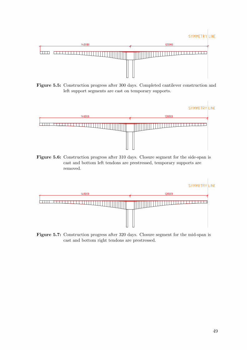
Figure 5.5: Construction progress after 300 days. Completed cantilever construction andleft support segments are cast on temporary supports.
Figure 5.6: Construction progress after 310 days. Closure segment for the side-span iscast and bottom left tendons are prestressed, temporary supports areremoved.
Figure 5.7: Construction progress after 320 days. Closure segment for the mid-span iscast and bottom right tendons are prestressed.
49

50
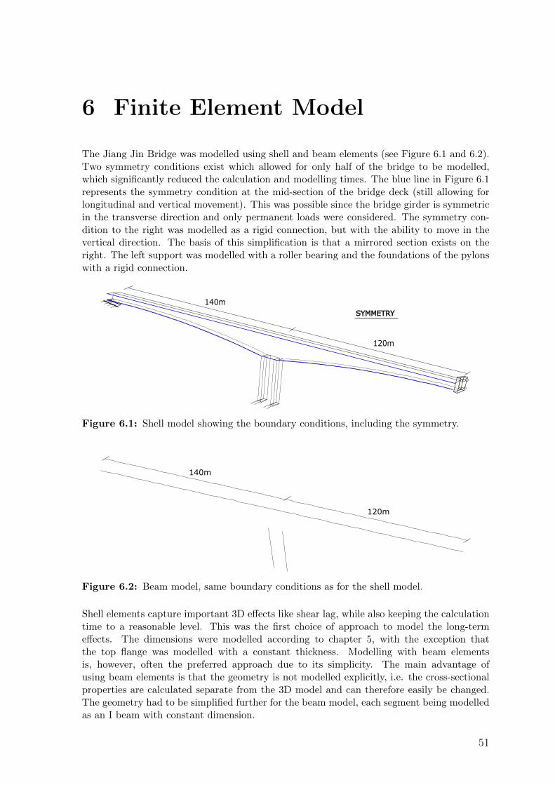
6 Finite Element Model
The Jiang Jin Bridge was modelled using shell and beam elements (see Figure 6.1 and 6.2).Two symmetry conditions exist which allowed for only half of the bridge to be modelled,which significantly reduced the calculation and modelling times. The blue line in Figure 6.1represents the symmetry condition at the mid-section of the bridge deck (still allowing forlongitudinal and vertical movement). This was possible since the bridge girder is symmetricin the transverse direction and only permanent loads were considered. The symmetry con-dition to the right was modelled as a rigid connection, but with the ability to move in thevertical direction. The basis of this simplification is that a mirrored section exists on theright. The left support was modelled with a roller bearing and the foundations of the pylonswith a rigid connection.
140m
120m
SYMMETRY
Figure 6.1: Shell model showing the boundary conditions, including the symmetry.
140m
120m
Figure 6.2: Beam model, same boundary conditions as for the shell model.
Shell elements capture important 3D effects like shear lag, while also keeping the calculationtime to a reasonable level. This was the first choice of approach to model the long-termeffects. The dimensions were modelled according to chapter 5, with the exception thatthe top flange was modelled with a constant thickness. Modelling with beam elementsis, however, often the preferred approach due to its simplicity. The main advantage ofusing beam elements is that the geometry is not modelled explicitly, i.e. the cross-sectionalproperties are calculated separate from the 3D model and can therefore easily be changed.The geometry had to be simplified further for the beam model, each segment being modelledas an I beam with constant dimension.
51
6.1 Modelling of Shrinkage
As described in section 3.2.2, the autogenous shrinkage depends only on the concrete qualityand elapsed time since casting. The drying shrinkage, however, also depends on the notionalsize of the cross section, which means that sections along the bridge girder will have differentshrinkage properties. Table 6.1 shows the total shrinkage strain for different notional sizesand time steps. The calculations were based on the theory described in section 3.2.2, usingthe parameters of the Jiang Jin Bridge. It can be noted that the final shrinkage does notvary a lot with different notional sizes. The rate, however, varies quite significantly (comparethe shrinkage strains at for example t=50 days).
Table 6.1: Total shrinkage strain calculated for different notional sizes and times steps (indays).
εcs[‰]
h0[mm] t=10 t=50 t=250 t=1000 t=∞100 0,052 0,219 0,344 0,381 0,394200 0,037 0,125 0,252 0,315 0,344300 0,033 0,090 0,194 0,268 0,311500 0,031 0,068 0,141 0,222 0,294
Shrinkage strains were modelled by applying a negative temperature corresponding to T =εc/α, where α is the temperature coefficient. The temperature varied with time and wasimplemented by using an amplitude function (tabular). The shrinkage for segment 1 wasadded after the casting of segment 2 had begun, to best match the actual process. Thebridge girder needed to be divided into several different segments, with different notionalsizes. For this case study, the following simplifications were made to reduce modelling time:
• The notional size was assumed to be 500 mm, an average value to represent the wholebridge girder (510 mm according to Huang et al. (2018)).
• Shrinkage in the transverse direction were neglected.
6.2 Implementation of Creep in Abaqus
The Abaqus relaxation test data was used to model the concrete viscoelastically, the para-meters needed were gR, kR and the respective time step t. By using the simplified equationfor these parameters, see section 4.2.4, as well as the basic creep theory in 3.2.3, these couldbe determined for a number of time steps. An example is shown in the calculations belowand in Table 6.2, using the parameters of the Jiang Jin Bridge:
• t0 = 7 (Loading after 7 days), t = 100 days
• Notional size, h0 = 500 mm (Simplification), RH = 70 %, fcm = 48 MPa
• α1/α2/α3 are given in Eurocode 2 (2005a)
52
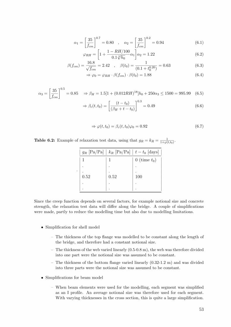
α1 =
[35
fcm
]0.7
= 0.80 , α2 =
[35
fcm
]0.2
= 0.94 (6.1)
ϕRH =
[1 +
1−RH/100
0.1 3√h0
α1
]α2 = 1.22 (6.2)
β(fcm) =16.8√fcm
= 2.42 , β(t0) =1
(0.1 + t0.200 )
= 0.63 (6.3)
⇒ ϕ0 = ϕRH · β(fcm) · β(t0) = 1.88 (6.4)
α3 =
[35
fcm
]0.5
= 0.85 ⇒ βH = 1.5[1 + (0.012RH)18]h0 + 250α3 ≤ 1500 = 995.99 (6.5)
⇒ βc(t, t0) =
[(t− t0)
(βH + t− t0)
]0.3
= 0.49 (6.6)
⇒ ϕ(t, t0) = βc(t, t0)ϕ0 = 0.92 (6.7)
Table 6.2: Example of relaxation test data, using that gR = kR = 11+ϕ(t,t0) .
.
gR [Pa/Pa] kR [Pa/Pa] t− t0 [days]
1 1 0 (time t0). . .. . .0.52 0.52 100. . .. . .
Since the creep function depends on several factors, for example notional size and concretestrength, the relaxation test data will differ along the bridge. A couple of simplificationswere made, partly to reduce the modelling time but also due to modelling limitations.
• Simplification for shell model
– The thickness of the top flange was modelled to be constant along the length ofthe bridge, and therefore had a constant notional size.
– The thickness of the web varied linearly (0.5-0.8 m), the web was therefore dividedinto one part were the notional size was assumed to be constant.
– The thickness of the bottom flange varied linearly (0.32-1.2 m) and was dividedinto three parts were the notional size was assumed to be constant.
• Simplifications for beam model
– When beam elements were used for the modelling, each segment was simplifiedas an I profile. An average notional size was therefore used for each segment.With varying thicknesses in the cross section, this is quite a large simplification.
53
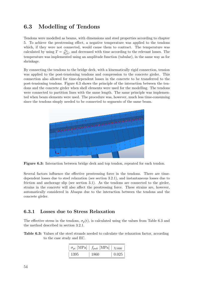
6.3 Modelling of Tendons
Tendons were modelled as beams, with dimensions and steel properties according to chapter5. To achieve the prestressing effect, a negative temperature was applied to the tendonswhich, if they were not connected, would cause them to contract. The temperature wascalculated by using T =
σpEpα
, and decreased with time according to the relevant losses. The
temperature was implemented using an amplitude function (tabular), in the same way as forshrinkage.
By connecting the tendons to the bridge deck, with a kinematically rigid connection, tensionwas applied to the post-tensioning tendons and compression to the concrete girder. Thisconnection also allowed for time-dependent losses in the concrete to be transferred to thepost-tensioning tendons. Figure 6.3 shows the principle of the interaction between the ten-dons and the concrete girder when shell elements were used for the modelling. The tendonswere connected to partition lines with the same length. The same principle was implemen-ted when beam elements were used. The procedure was, however, much less time-consumingsince the tendons simply needed to be connected to segments of the same beam.
Figure 6.3: Interaction between bridge deck and top tendon, repeated for each tendon.
Several factors influence the effective prestressing force in the tendons. There are time-dependent losses due to steel relaxation (see section 3.2.1), and instantaneous losses due tofriction and anchorage slip (see section 3.1). As the tendons are connected to the girder,strains in the concrete will also affect the prestressing force. These strains are, however,automatically considered in Abaqus due to the interaction between the tendons and theconcrete girder.
6.3.1 Losses due to Stress Relaxation
The effective stress in the tendons, σp(t), is calculated using the values from Table 6.3 andthe method described in section 3.2.1.
Table 6.3: Values of the steel strands needed to calculate the relaxation factor, accordingto the case study and EC.
σpi [MPa] fpuk [MPa] χ1000
1395 1860 0.025
54
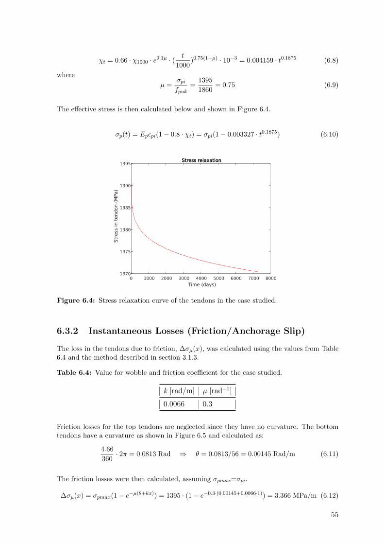
χt = 0.66 · χ1000 · e9.1µ · ( t
1000)0.75(1−µ) · 10−3 = 0.004159 · t0.1875 (6.8)
where
µ =σpifpuk
=1395
1860= 0.75 (6.9)
The effective stress is then calculated below and shown in Figure 6.4.
σp(t) = Epεpi(1− 0.8 · χt) = σpi(1− 0.003327 · t0.1875) (6.10)
0 1000 2000 3000 4000 5000 6000 7000 8000
Time (days)
1370
1375
1380
1385
1390
1395
Str
ess
in t
endon (
MPa
)
Stress relaxation
Figure 6.4: Stress relaxation curve of the tendons in the case studied.
6.3.2 Instantaneous Losses (Friction/Anchorage Slip)
The loss in the tendons due to friction, ∆σµ(x), was calculated using the values from Table6.4 and the method described in section 3.1.3.
Table 6.4: Value for wobble and friction coefficient for the case studied.
k [rad/m] µ [rad−1]
0.0066 0.3
Friction losses for the top tendons are neglected since they have no curvature. The bottomtendons have a curvature as shown in Figure 6.5 and calculated as:
4.66
360· 2π = 0.0813 Rad ⇒ θ = 0.0813/56 = 0.00145 Rad/m (6.11)
The friction losses were then calculated, assuming σpmax=σpi.
∆σµ(x) = σpmax(1− e−µ(θ+kx)) = 1395 · (1− e−0.3·(0.00145+0.0066·1)) = 3.366 MPa/m (6.12)
55
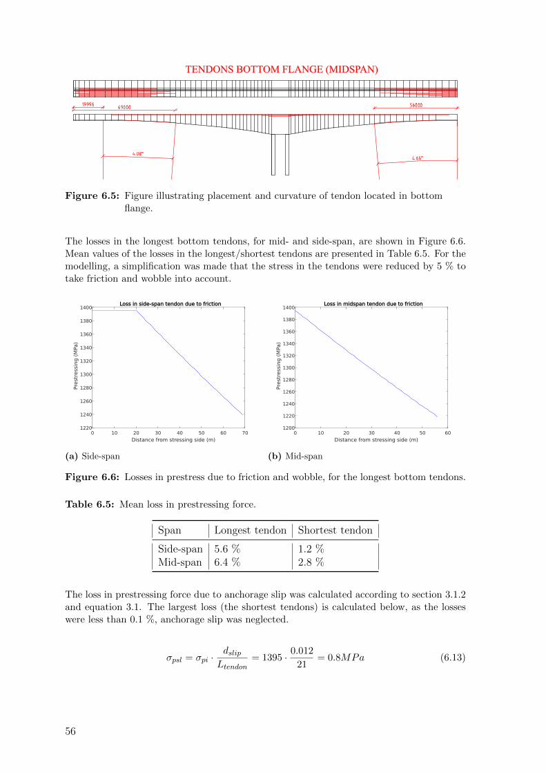
TENDONS BOTTOM FLANGE (MIDSPAN)
Figure 6.5: Figure illustrating placement and curvature of tendon located in bottomflange.
The losses in the longest bottom tendons, for mid- and side-span, are shown in Figure 6.6.Mean values of the losses in the longest/shortest tendons are presented in Table 6.5. For themodelling, a simplification was made that the stress in the tendons were reduced by 5 % totake friction and wobble into account.
0 10 20 30 40 50 60 70
Distance from stressing side (m)
1220
1240
1260
1280
1300
1320
1340
1360
1380
1400
Pre
stre
ssin
g (
MPa
)
Loss in side-span tendon due to friction
(a) Side-span
0 10 20 30 40 50 60
Distance from stressing side (m)
1200
1220
1240
1260
1280
1300
1320
1340
1360
1380
1400
Pre
stre
ssin
g (
MPa
)
Loss in midspan tendon due to friction
(b) Mid-span
Figure 6.6: Losses in prestress due to friction and wobble, for the longest bottom tendons.
Table 6.5: Mean loss in prestressing force.
Span Longest tendon Shortest tendon
Side-span 5.6 % 1.2 %Mid-span 6.4 % 2.8 %
The loss in prestressing force due to anchorage slip was calculated according to section 3.1.2and equation 3.1. The largest loss (the shortest tendons) is calculated below, as the losseswere less than 0.1 %, anchorage slip was neglected.
σpsl = σpi ·dslipLtendon
= 1395 · 0.012
21= 0.8MPa (6.13)
56
6.4 Modelling of the Construction Sequence
To assemble the segmentally constructed bridge in Abaqus, the following steps were per-formed:
1. Deactivate the whole bridge with its tendons (except pylons and mid-section).
2. Activate segment.
• Activate concrete casting.
• Activate top tendons associated with current segment.
• Repeat for the whole cantilever construction.
3. Activate the segments by the left support and activate the temporary supports.
4. Activate left closing segments and deactivate the temporary supports.
• Activate concrete casting.
• Activate bottom tendons.
• Repeat for right closure segment.
5. Add additional permanent loads and creep for required number of days.
The correct way to model with respect to creep, would be to add the self-weight of theconcrete as a load to the previous segment without activating the current casting. Thisis due to the concrete segment being cast not actually carrying load until the formwork isremoved and the tendons tensioned. In the model used for the case study, however, theconcrete segment instantly started to carry its own load.
57

58

Part III
Results and Discussion
59

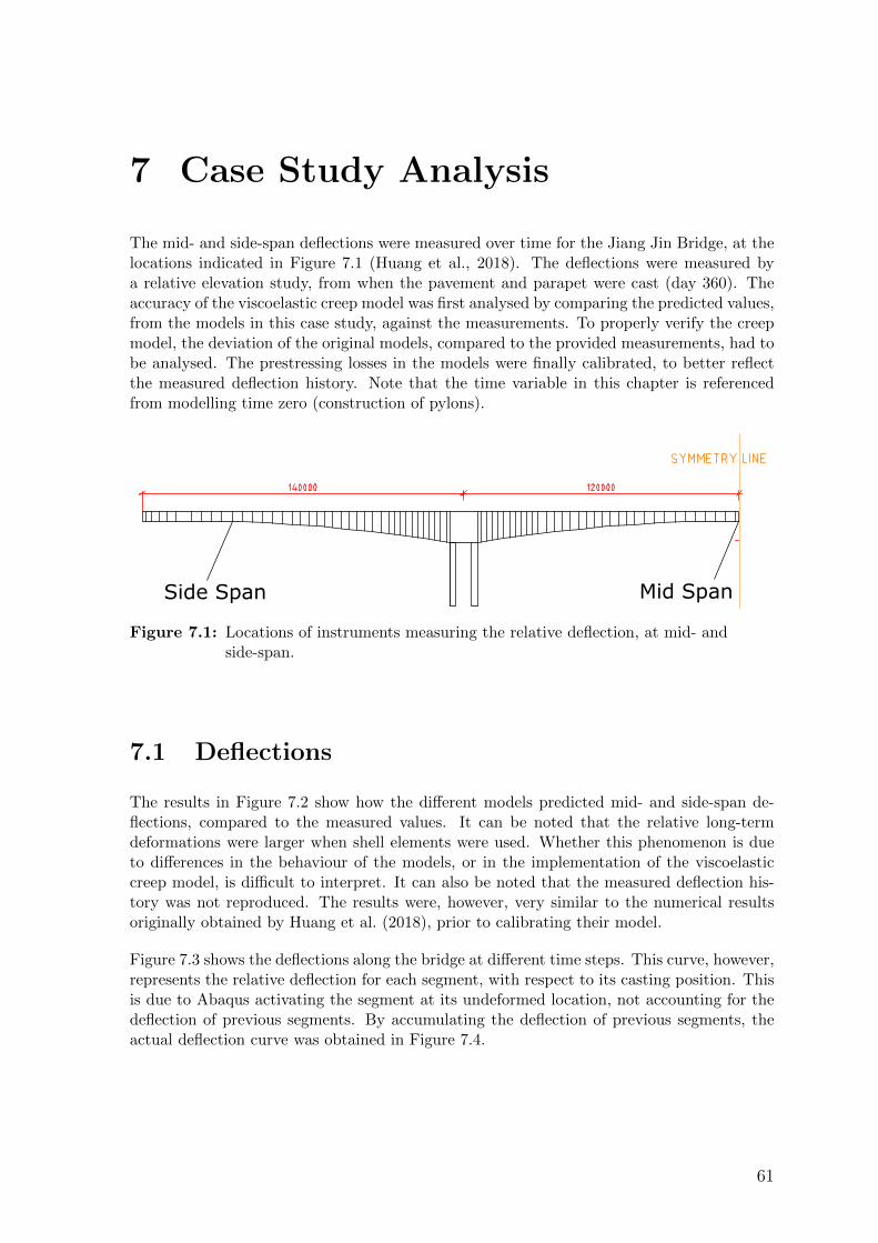
7 Case Study Analysis
The mid- and side-span deflections were measured over time for the Jiang Jin Bridge, at thelocations indicated in Figure 7.1 (Huang et al., 2018). The deflections were measured bya relative elevation study, from when the pavement and parapet were cast (day 360). Theaccuracy of the viscoelastic creep model was first analysed by comparing the predicted values,from the models in this case study, against the measurements. To properly verify the creepmodel, the deviation of the original models, compared to the provided measurements, had tobe analysed. The prestressing losses in the models were finally calibrated, to better reflectthe measured deflection history. Note that the time variable in this chapter is referencedfrom modelling time zero (construction of pylons).
Side Span Mid Span
Figure 7.1: Locations of instruments measuring the relative deflection, at mid- andside-span.
7.1 Deflections
The results in Figure 7.2 show how the different models predicted mid- and side-span de-flections, compared to the measured values. It can be noted that the relative long-termdeformations were larger when shell elements were used. Whether this phenomenon is dueto differences in the behaviour of the models, or in the implementation of the viscoelasticcreep model, is difficult to interpret. It can also be noted that the measured deflection his-tory was not reproduced. The results were, however, very similar to the numerical resultsoriginally obtained by Huang et al. (2018), prior to calibrating their model.
Figure 7.3 shows the deflections along the bridge at different time steps. This curve, however,represents the relative deflection for each segment, with respect to its casting position. Thisis due to Abaqus activating the segment at its undeformed location, not accounting for thedeflection of previous segments. By accumulating the deflection of previous segments, theactual deflection curve was obtained in Figure 7.4.
61
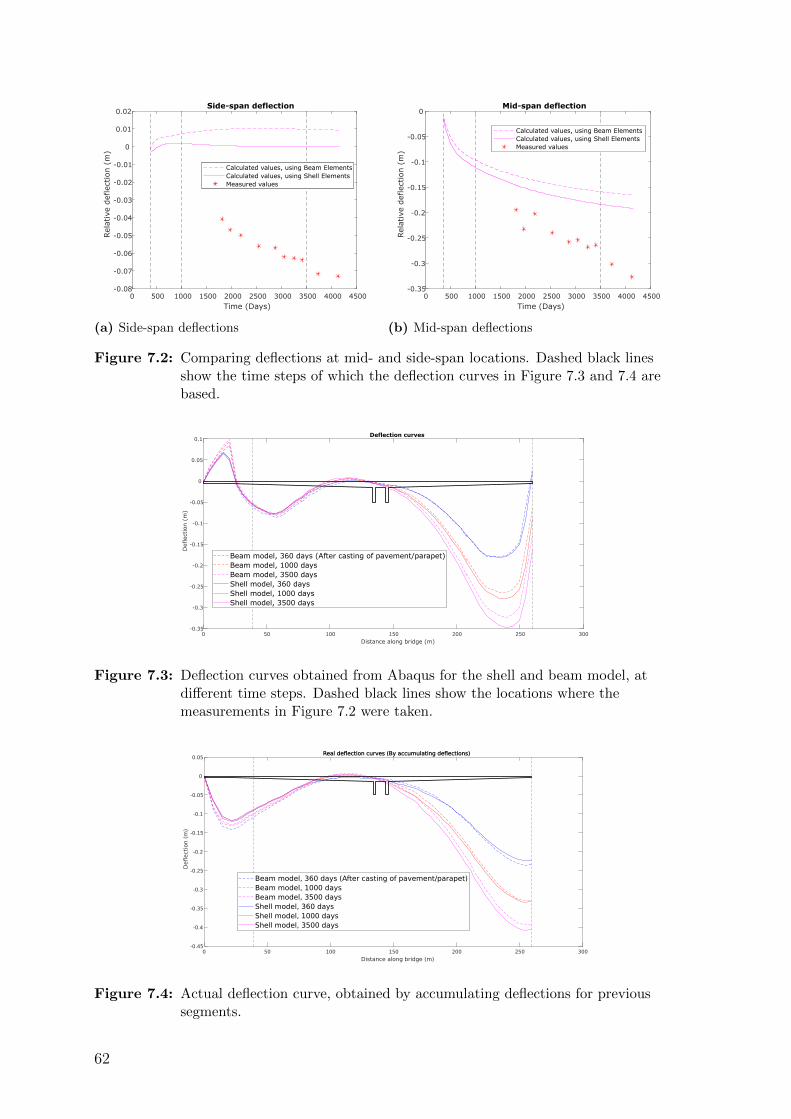
0 500 1000 1500 2000 2500 3000 3500 4000 4500Time (Days)
-0.08
-0.07
-0.06
-0.05
-0.04
-0.03
-0.02
-0.01
0
0.01
0.02Rel
ativ
e def
lect
ion (
m)
Side-span deflection
Calculated values, using Beam ElementsCalculated values, using Shell ElementsMeasured values
(a) Side-span deflections
0 500 1000 1500 2000 2500 3000 3500 4000 4500Time (Days)
-0.35
-0.3
-0.25
-0.2
-0.15
-0.1
-0.05
0
Rel
ativ
e def
lect
ion (
m)
Mid-span deflection
Calculated values, using Beam ElementsCalculated values, using Shell ElementsMeasured values
(b) Mid-span deflections
Figure 7.2: Comparing deflections at mid- and side-span locations. Dashed black linesshow the time steps of which the deflection curves in Figure 7.3 and 7.4 arebased.
0 50 100 150 200 250 300Distance along bridge (m)
-0.35
-0.3
-0.25
-0.2
-0.15
-0.1
-0.05
0
0.05
0.1
Def
lect
ion (
m)
Deflection curves
Beam model, 360 days (After casting of pavement/parapet)Beam model, 1000 daysBeam model, 3500 daysShell model, 360 daysShell model, 1000 daysShell model, 3500 days
Figure 7.3: Deflection curves obtained from Abaqus for the shell and beam model, atdifferent time steps. Dashed black lines show the locations where themeasurements in Figure 7.2 were taken.
0 50 100 150 200 250 300
Distance along bridge (m)
-0.45
-0.4
-0.35
-0.3
-0.25
-0.2
-0.15
-0.1
-0.05
0
0.05
Deflect
ion (
m)
Real deflection curves (By accumulating deflections)
Beam model, 360 days (After casting of pavement/parapet)Beam model, 1000 daysBeam model, 3500 daysShell model, 360 daysShell model, 1000 daysShell model, 3500 days
Figure 7.4: Actual deflection curve, obtained by accumulating deflections for previoussegments.
62
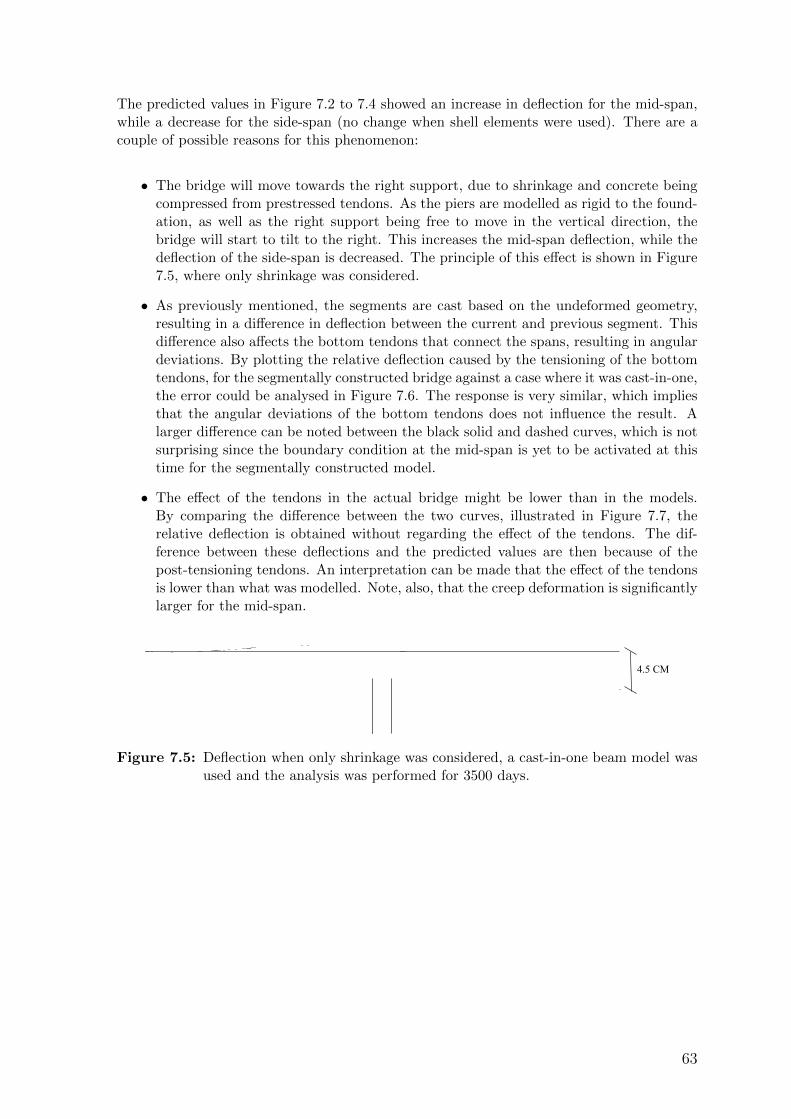
The predicted values in Figure 7.2 to 7.4 showed an increase in deflection for the mid-span,while a decrease for the side-span (no change when shell elements were used). There are acouple of possible reasons for this phenomenon:
• The bridge will move towards the right support, due to shrinkage and concrete beingcompressed from prestressed tendons. As the piers are modelled as rigid to the found-ation, as well as the right support being free to move in the vertical direction, thebridge will start to tilt to the right. This increases the mid-span deflection, while thedeflection of the side-span is decreased. The principle of this effect is shown in Figure7.5, where only shrinkage was considered.
• As previously mentioned, the segments are cast based on the undeformed geometry,resulting in a difference in deflection between the current and previous segment. Thisdifference also affects the bottom tendons that connect the spans, resulting in angulardeviations. By plotting the relative deflection caused by the tensioning of the bottomtendons, for the segmentally constructed bridge against a case where it was cast-in-one,the error could be analysed in Figure 7.6. The response is very similar, which impliesthat the angular deviations of the bottom tendons does not influence the result. Alarger difference can be noted between the black solid and dashed curves, which is notsurprising since the boundary condition at the mid-span is yet to be activated at thistime for the segmentally constructed model.
• The effect of the tendons in the actual bridge might be lower than in the models.By comparing the difference between the two curves, illustrated in Figure 7.7, therelative deflection is obtained without regarding the effect of the tendons. The dif-ference between these deflections and the predicted values are then because of thepost-tensioning tendons. An interpretation can be made that the effect of the tendonsis lower than what was modelled. Note, also, that the creep deformation is significantlylarger for the mid-span.
4.5 CM
Figure 7.5: Deflection when only shrinkage was considered, a cast-in-one beam model wasused and the analysis was performed for 3500 days.
63
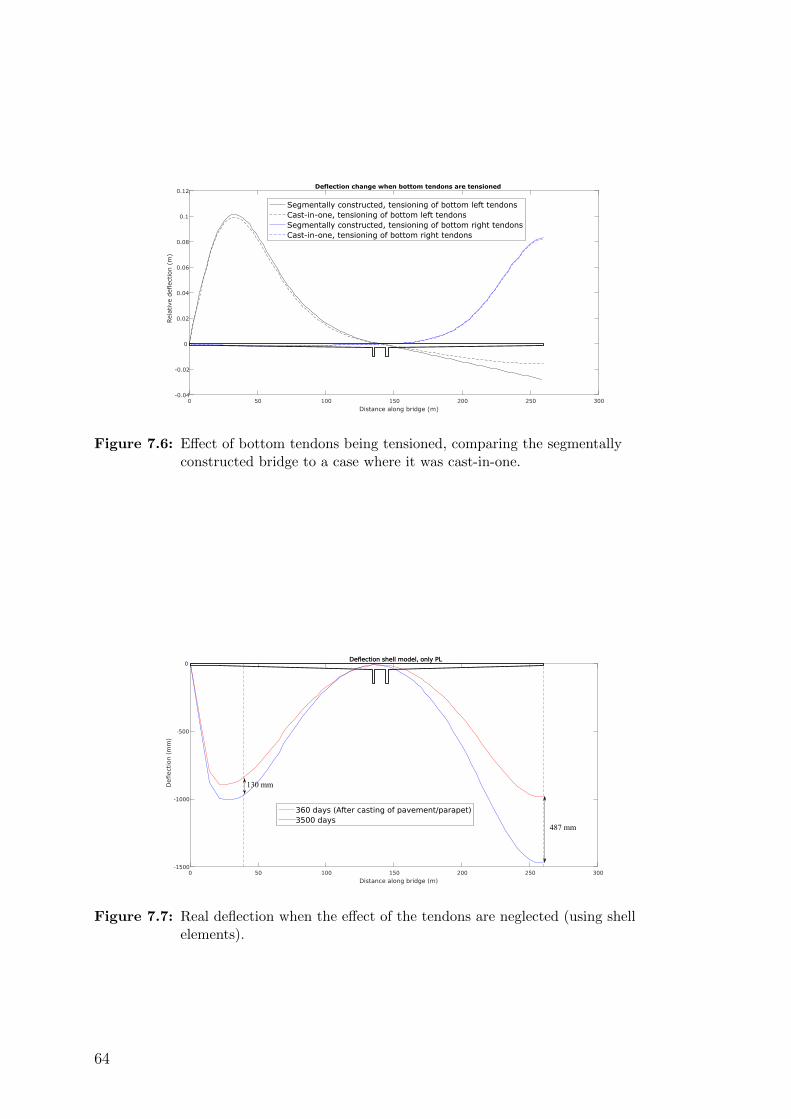
0 50 100 150 200 250 300Distance along bridge (m)
-0.04
-0.02
0
0.02
0.04
0.06
0.08
0.1
0.12
Rel
ativ
e def
lect
ion (
m)
Deflection change when bottom tendons are tensioned
Segmentally constructed, tensioning of bottom left tendonsCast-in-one, tensioning of bottom left tendonsSegmentally constructed, tensioning of bottom right tendonsCast-in-one, tensioning of bottom right tendons
Figure 7.6: Effect of bottom tendons being tensioned, comparing the segmentallyconstructed bridge to a case where it was cast-in-one.
0 50 100 150 200 250 300
Distance along bridge (m)
-1500
-1000
-500
0
Deflect
ion (
mm
)
Deflection shell model, only PL
360 days (After casting of pavement/parapet)3500 days
487 mm
130 mm
Figure 7.7: Real deflection when the effect of the tendons are neglected (using shellelements).
64
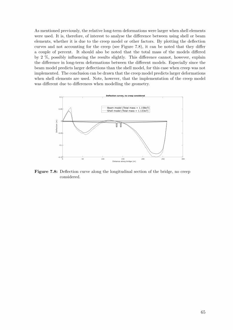
As mentioned previously, the relative long-term deformations were larger when shell elementswere used. It is, therefore, of interest to analyse the difference between using shell or beamelements, whether it is due to the creep model or other factors. By plotting the deflectioncurves and not accounting for the creep (see Figure 7.8), it can be noted that they differa couple of percent. It should also be noted that the total mass of the models differedby 2 %, possibly influencing the results slightly. This difference cannot, however, explainthe difference in long-term deformations between the different models. Especially since thebeam model predicts larger deflections than the shell model, for this case when creep was notimplemented. The conclusion can be drawn that the creep model predicts larger deformationswhen shell elements are used. Note, however, that the implementation of the creep modelwas different due to differences when modelling the geometry.
0 50 100 150 200 250 300Distance along bridge (m)
-0.15
-0.1
-0.05
0
0.05
0.1
Def
lect
ion (
m)
Deflection curves, no creep considered
Beam model (Total mass = 1.158e7)Shell model (Total mass = 1.133e7)
Figure 7.8: Deflection curve along the longitudinal section of the bridge, no creepconsidered.
65
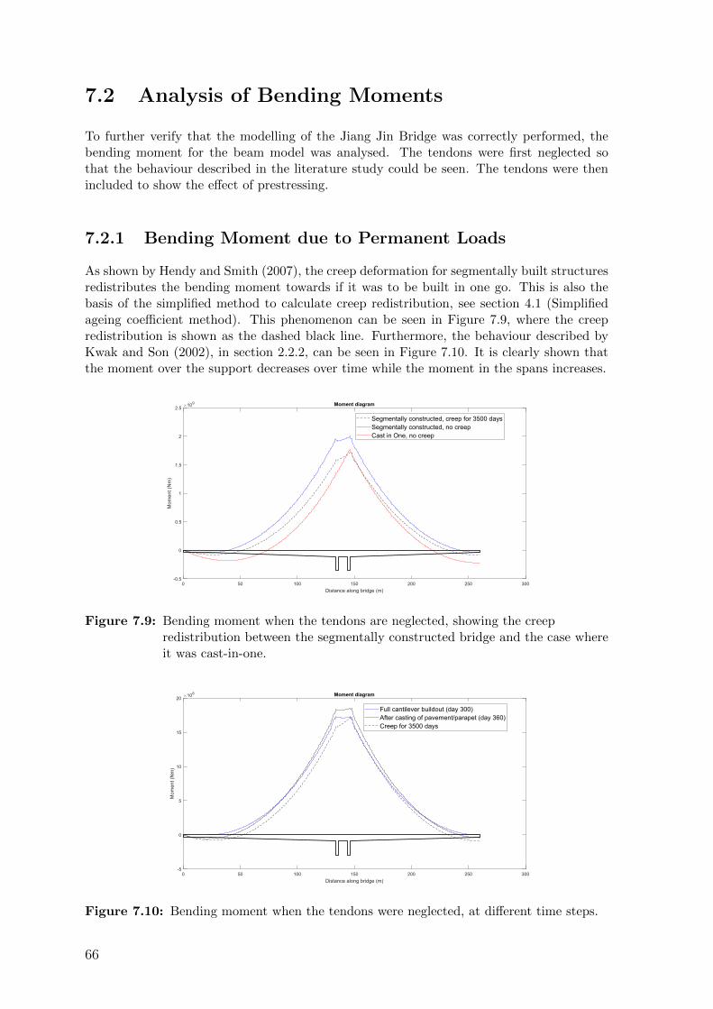
7.2 Analysis of Bending Moments
To further verify that the modelling of the Jiang Jin Bridge was correctly performed, thebending moment for the beam model was analysed. The tendons were first neglected sothat the behaviour described in the literature study could be seen. The tendons were thenincluded to show the effect of prestressing.
7.2.1 Bending Moment due to Permanent Loads
As shown by Hendy and Smith (2007), the creep deformation for segmentally built structuresredistributes the bending moment towards if it was to be built in one go. This is also thebasis of the simplified method to calculate creep redistribution, see section 4.1 (Simplifiedageing coefficient method). This phenomenon can be seen in Figure 7.9, where the creepredistribution is shown as the dashed black line. Furthermore, the behaviour described byKwak and Son (2002), in section 2.2.2, can be seen in Figure 7.10. It is clearly shown thatthe moment over the support decreases over time while the moment in the spans increases.
Figure 7.9: Bending moment when the tendons are neglected, showing the creepredistribution between the segmentally constructed bridge and the case whereit was cast-in-one.
Figure 7.10: Bending moment when the tendons were neglected, at different time steps.
66
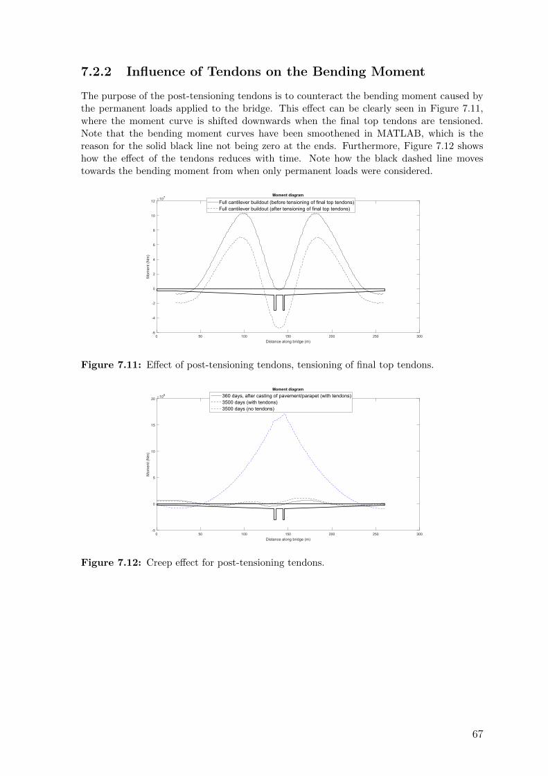
7.2.2 Influence of Tendons on the Bending Moment
The purpose of the post-tensioning tendons is to counteract the bending moment caused bythe permanent loads applied to the bridge. This effect can be clearly seen in Figure 7.11,where the moment curve is shifted downwards when the final top tendons are tensioned.Note that the bending moment curves have been smoothened in MATLAB, which is thereason for the solid black line not being zero at the ends. Furthermore, Figure 7.12 showshow the effect of the tendons reduces with time. Note how the black dashed line movestowards the bending moment from when only permanent loads were considered.
Figure 7.11: Effect of post-tensioning tendons, tensioning of final top tendons.
Figure 7.12: Creep effect for post-tensioning tendons.
67
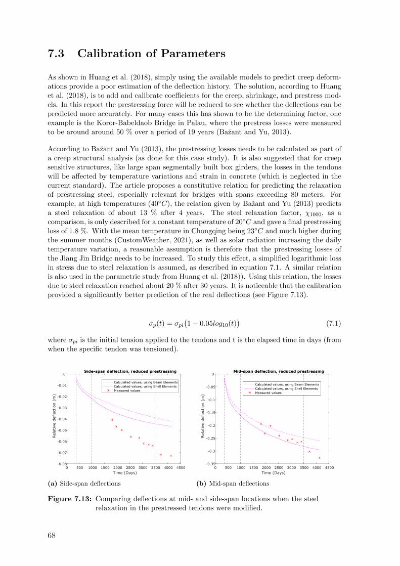
7.3 Calibration of Parameters
As shown in Huang et al. (2018), simply using the available models to predict creep deform-ations provide a poor estimation of the deflection history. The solution, according to Huanget al. (2018), is to add and calibrate coefficients for the creep, shrinkage, and prestress mod-els. In this report the prestressing force will be reduced to see whether the deflections can bepredicted more accurately. For many cases this has shown to be the determining factor, oneexample is the Koror-Babeldaob Bridge in Palau, where the prestress losses were measuredto be around around 50 % over a period of 19 years (Bazant and Yu, 2013).
According to Bazant and Yu (2013), the prestressing losses needs to be calculated as part ofa creep structural analysis (as done for this case study). It is also suggested that for creepsensitive structures, like large span segmentally built box girders, the losses in the tendonswill be affected by temperature variations and strain in concrete (which is neglected in thecurrent standard). The article proposes a constitutive relation for predicting the relaxationof prestressing steel, especially relevant for bridges with spans exceeding 80 meters. Forexample, at high temperatures (40◦C), the relation given by Bazant and Yu (2013) predictsa steel relaxation of about 13 % after 4 years. The steel relaxation factor, χ1000, as acomparison, is only described for a constant temperature of 20◦C and gave a final prestressingloss of 1.8 %. With the mean temperature in Chongqing being 23◦C and much higher duringthe summer months (CustomWeather, 2021), as well as solar radiation increasing the dailytemperature variation, a reasonable assumption is therefore that the prestressing losses ofthe Jiang Jin Bridge needs to be increased. To study this effect, a simplified logarithmic lossin stress due to steel relaxation is assumed, as described in equation 7.1. A similar relationis also used in the parametric study from Huang et al. (2018)). Using this relation, the lossesdue to steel relaxation reached about 20 % after 30 years. It is noticeable that the calibrationprovided a significantly better prediction of the real deflections (see Figure 7.13).
σp(t) = σpi(1− 0.05log10(t)
)(7.1)
where σpi is the initial tension applied to the tendons and t is the elapsed time in days (fromwhen the specific tendon was tensioned).
0 500 1000 1500 2000 2500 3000 3500 4000 4500Time (Days)
-0.08
-0.07
-0.06
-0.05
-0.04
-0.03
-0.02
-0.01
0
Rel
ativ
e def
lect
ion (
m)
Side-span deflection, reduced prestressing
Calculated values, using Beam ElementsCalculated values, using Shell ElementsMeasured values
(a) Side-span deflections
0 500 1000 1500 2000 2500 3000 3500 4000 4500Time (Days)
-0.35
-0.3
-0.25
-0.2
-0.15
-0.1
-0.05
0
Rel
ativ
e def
lect
ion (
m)
Mid-span deflection, reduced prestressing
Calculated values, using Beam ElementsCalculated values, using Shell ElementsMeasured values
(b) Mid-span deflections
Figure 7.13: Comparing deflections at mid- and side-span locations when the steelrelaxation in the prestressed tendons were modified.
68
7.4 Sources of Errors
Regarding the collected data from Huang et al. (2018), a couple of assumptions made in themodelling need to be addressed:
• The cross section was simplified as an I beam with rectangular flanges and web, whichleads to a slight error in the moment of inertia.
• The friction losses for the top tendons were neglected. In reality the top tendonsmight be slightly curved in the transversal direction, and friction losses would need tobe taken into account.
• The measured deflections were described as ”relative elevation surveys placed on thepavement after the Jiang Jin Bridge opened to traffic”. The exact location of theside-span as well as the exact time of installation were not known. In this analysis themeasurements were assumed to start after the pavement/parapet was added. If therelative measurements were to be initiated 10 days later in the model, the mid-spandeflection would be reduced by 1.3 cm.
Regarding boundary conditions and loads the following should be considered:
• If the pylons were to be modelled as pinned, instead of rigid at the foundations, theresults would be slightly different. The angular displacement at the top of the pylonswould be reduced, which leads to an increase in deflection for the side-span and adecrease for the mid-span (see Figure 7.14). This way of modelling could possibly bemore correct and could explain the discrepancy between the relative deflections formid- and side-span.
• The weight of the superstructure (pavement/parapet) had to be estimated to 2.5 kPa.Large changes to this load could have significant effects on the time-dependant de-formations.
• The fact that the weight of the travelling formwork was neglected should not affectthe relative measurements much.
For the implementation of time-dependant losses in Abaqus, the following should be con-sidered:
• The viscoelastic creep model had different input values depending on the notional sizeof the element. With varying thicknesses in the cross section of the concrete girder,as well as along the longitudinal length of the bridge, large simplifications had to bemade. Modelling with shell elements allowed for the most exact implementation.
• For the shrinkage, an average notional size was assumed for the whole bridge girder.This should not affect the long-term deformations much since the notional size mostlyinfluences the rate of the shrinkage. The creep of concrete and losses in prestressingtendons have also shown larger impact during the modelling of the case study.
• As a simplification in the modelling, the concrete segment instantly started to carryits own weight. When considering the long-term effects, however, the error due to thissimplification is considered to be quite small.
69
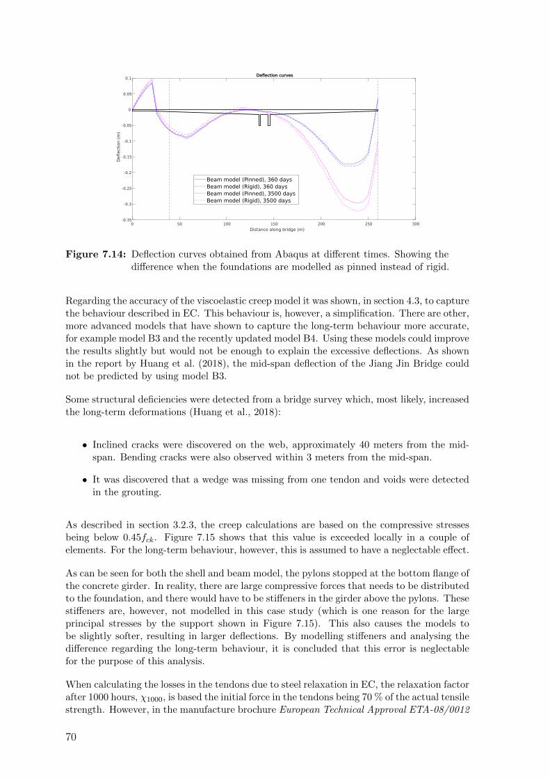
0 50 100 150 200 250 300
Distance along bridge (m)
-0.35
-0.3
-0.25
-0.2
-0.15
-0.1
-0.05
0
0.05
0.1
Deflect
ion (
m)
Deflection curves
Beam model (Pinned), 360 daysBeam model (Rigid), 360 daysBeam model (Pinned), 3500 daysBeam model (Rigid), 3500 days
Figure 7.14: Deflection curves obtained from Abaqus at different times. Showing thedifference when the foundations are modelled as pinned instead of rigid.
Regarding the accuracy of the viscoelastic creep model it was shown, in section 4.3, to capturethe behaviour described in EC. This behaviour is, however, a simplification. There are other,more advanced models that have shown to capture the long-term behaviour more accurate,for example model B3 and the recently updated model B4. Using these models could improvethe results slightly but would not be enough to explain the excessive deflections. As shownin the report by Huang et al. (2018), the mid-span deflection of the Jiang Jin Bridge couldnot be predicted by using model B3.
Some structural deficiencies were detected from a bridge survey which, most likely, increasedthe long-term deformations (Huang et al., 2018):
• Inclined cracks were discovered on the web, approximately 40 meters from the mid-span. Bending cracks were also observed within 3 meters from the mid-span.
• It was discovered that a wedge was missing from one tendon and voids were detectedin the grouting.
As described in section 3.2.3, the creep calculations are based on the compressive stressesbeing below 0.45fck. Figure 7.15 shows that this value is exceeded locally in a couple ofelements. For the long-term behaviour, however, this is assumed to have a neglectable effect.
As can be seen for both the shell and beam model, the pylons stopped at the bottom flange ofthe concrete girder. In reality, there are large compressive forces that needs to be distributedto the foundation, and there would have to be stiffeners in the girder above the pylons. Thesestiffeners are, however, not modelled in this case study (which is one reason for the largeprincipal stresses by the support shown in Figure 7.15). This also causes the models tobe slightly softer, resulting in larger deflections. By modelling stiffeners and analysing thedifference regarding the long-term behaviour, it is concluded that this error is neglectablefor the purpose of this analysis.
When calculating the losses in the tendons due to steel relaxation in EC, the relaxation factorafter 1000 hours, χ1000, is based the initial force in the tendons being 70 % of the actual tensilestrength. However, in the manufacture brochure European Technical Approval ETA-08/0012
70
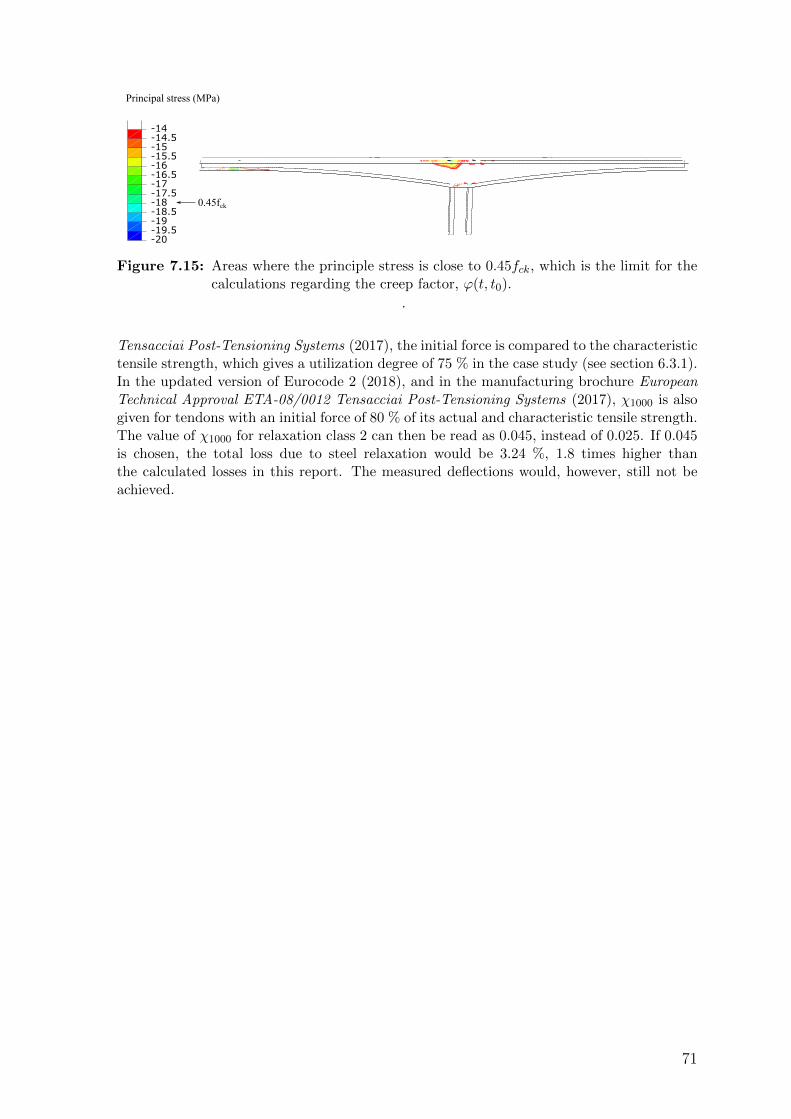
-20-19.5-19-18.5-18-17.5-17-16.5-16-15.5-15-14.5-14
0.45fck
Principal stress (MPa)
Figure 7.15: Areas where the principle stress is close to 0.45fck, which is the limit for thecalculations regarding the creep factor, ϕ(t, t0).
.
Tensacciai Post-Tensioning Systems (2017), the initial force is compared to the characteristictensile strength, which gives a utilization degree of 75 % in the case study (see section 6.3.1).In the updated version of Eurocode 2 (2018), and in the manufacturing brochure EuropeanTechnical Approval ETA-08/0012 Tensacciai Post-Tensioning Systems (2017), χ1000 is alsogiven for tendons with an initial force of 80 % of its actual and characteristic tensile strength.The value of χ1000 for relaxation class 2 can then be read as 0.045, instead of 0.025. If 0.045is chosen, the total loss due to steel relaxation would be 3.24 %, 1.8 times higher thanthe calculated losses in this report. The measured deflections would, however, still not beachieved.
71

72
8 Conclusions
The overarching objective of the present work was to model time-dependent losses in seg-mentally constructed concrete bridges, with special emphasis on the effect of creep. Thiswas done by establishing a routine for numerical modelling. The main conclusions of thesubsequent analysis are summarized as follows:
1. The effect of early and repeated loading is difficult to predict. Numerical simulationof a simple load case indicated that a viscoelastic model, based on the creep functionin EC, was the most accurate. This conclusion is corroborated by similar studies inthe literature, which strengthens the results.
2. Through modelling of the Jiang Jin Bridge, it was shown that the viscoelastic modelcan be useful for modelling creep in more complex structures, specifically segmentallyconstructed bridges. Discrepancy between measured results were however observed,leading to the conclusion that other factors need to be considered.
3. The discrepancies described in the previous point could be partly eliminated throughsignificantly increasing the time-dependent losses of the prestressing tendons. Thispoints towards time-dependent losses being underestimated. This is not surprisingsince measurements have shown large reductions in prestressing force for similar struc-tures, largely due to high temperature variations. To accurately predict the deflectionsthese losses would need to be more accurately studied and implemented along withthe creep model.
4. Modelling with beam elements significantly reduces modelling and computational time,as well as the file size of the actual model. Using shell elements, however, allowed fora more accurate implementation of the viscoelastic creep model and captured thelong-term behaviour better.
5. The viscoelastic creep model can be easily applied to all concrete structures and de-pends solely on the creep function from EC. A conclusion can be drawn that themodel is able to capture the behaviour from EC very well. It should be noted thatthe accuracy of the creep model is limited to the behaviour according to the Generaland incremental step-by-step method (see section 4.1). To assess the accuracy of thecreep model, the General and incremental step-by-step method needs to be studied indetail.
73

74
9 Further Work
The subject studied in this Master’s Thesis is quite extensive, only a specific part wasthoroughly investigated. This leads to further work being required, to reliably predict long-term deformations for segmentally constructed prestressed concrete bridges. Here follows acouple of suggestions:
• This report studies one way of implementing the viscoelastic model in Abaqus. Itwould be of interest to investigate other ways, possibly increasing the accuracy andreducing the modelling time.
• Due to a limited amount of data for the case study, some simplifications and assump-tions have been made. It would be of interest to perform a similar analysis in acase-study where the full and accurate history of the bridge is known.
• For the Jiang Jin Bridge the deflection history was measured over a period of 10 years.It would be of interest to perform the analysis when deflections over a larger periodare available. Continuous measurements of losses in prestressed tendons would alsoallow for a better analysis.
• Shrinkage and prestress losses were in this report implemented using amplitude func-tions (tabular). It would be of interest to investigate the best and easiest way ofimplementing these in Abaqus.
• The viscoelastic creep model predicted larger deformations when shell elements wereused, compared to beam elements. Further analysis is required, however, to determineand isolate the accuracy of the creep model with respect to shell and beam elements.
• It would be of interest to perform the analysis using solid elements, which has notbeen done in this report.
75

76
Bibliography
Articles
Allos, Atheel E and LH Martin (1981). ‘Factors affecting Poisson’s ratio for concrete’.In: Building and environment 16.1, pp. 1–9.
Bazant, Zdene k P, Qiang Yu and Guang-Hua Li (2012a). ‘Excessive long-time deflec-tions of prestressed box girders. I: Record-span bridge in Palau and other paradigms’.In: Journal of structural engineering 138.6, pp. 676–686.
– (2012b). ‘Excessive long-time deflections of prestressed box girders. II: Numericalanalysis and lessons learned’. In: Journal of Structural Engineering 138.6, pp. 687–696.
Bazant, Zdenek P and Qiang Yu (2013). ‘Relaxation of prestressing steel at varyingstrain and temperature: Viscoplastic constitutive relation’. In: Journal of Engineer-ing Mechanics 139.7, pp. 814–823.
Billington, Philip N, David P Billington and Hubert. Shirley-Smith (2020). ‘Bridge’.In: Encyclopedia Britannica. url: https://www.britannica.com/technology/bridge-engineering.
Dai, Gonglian, Hao Ge, Miao Su and Y Frank Chen (2017). ‘Century-old coveredbridge with cantilever beams in China’. In: Structural Engineering International27.2, pp. 255–262.
Grasley, Zachary C and David A Lange (2007). ‘What is balanced Cantilever method ofBridge Construction?’ In: Mechanics of Time-Dependent Materials 11.3-4, pp. 175–198.
Huang, Haidong, Shan-Shan Huang and Kypros Pilakoutas (2018). ‘Modeling forassessment of long-term behavior of prestressed concrete box-girder bridges’. In:Journal of Bridge Engineering 23.3, p. 04018002.
Kwak, H.-G. and J.-K. Son (2002). ‘Determination of design moments in bridges con-structed by balanced cantilever method’. In: Engineering Structures 24.5, pp. 639–648. issn: 0141-0296.
Loewe, Sanabra and Capella Llovera (2014). ‘The four ages of early prestressed con-crete structures’. In: PCI Journal 59.4, pp. 93–121.
Lucko, Gunnar and Jesus M de la Garza (2003). ‘Constructability considerations forbalanced cantilever construction’. In: Practice Periodical on Structural Design andConstruction 8.1, pp. 47–56.
Mistewicz, Marek (2015). ‘First European truss cantilever bridge in the light of numis-matics, iconography and written sources’. In: Kwartalnik Architektury i Urbanistyki.
Reiner, M (1949). ‘On volume-or isotropic flow as exemplified in the creep of concrete’.In: Flow, Turbulence and Combustion 1.1, p. 475.
77
Book Sources
Ashter, Syed Ali (2018). Thermoforming of Single and Multilayer Laminates. Taylor,Francis.
Betten, Josef (2008). Creep mechanics. Springer Science & Business Media.Council, National Research et al. (1997). Nonconventional concrete technologies: re-
newal of the highway infrastructure. Vol. 484. National Academies Press.Engstrom, Bjorn (2008). Restraint cracking of reinforced concrete structures. Chalmers
University of Technology.Hendy, Chris R. and David A. Smith (2007). Designers’ Guide to EN 1992-2 Eurocode
2: Design of concrete structures: Part 2: Concrete bridges. The authors and ThomasTelford Limited 2007.
Nguyen, Ngoc-Vinh, Quoc-Anh Vu and Seung-Eock Kim (2020). Construction andBuilding Materials. Elsevier.
Manuals
ASTM International (2018). Standard Specification for Low-Relaxation, Seven-WireSteel Strand for Prestressed Concrete. ASTM International.
Eurocode 2 (2005a). SS-EN 1992-1-1, Eurocode 2: Design of concrete structures – Part1-1: General rules and rules for buildings. SIS AB.
– (2005b). SS-EN 1992-2, Eurocode 2 – Design of concrete structures – Part 2: Con-crete bridges – Design and detailing rules. SIS AB.
– (2018). SS-EN 1992-1-1, Eurocode 2 – Design of concrete structures (Updated ver-sion) – Part 1-1: General rules and rules for buildings. SIS AB.
Simulia (2014). ABAQUS 6.14 - ANALYSIS USER’S GUIDE VOLUME III: MA-TERIALS. Dassault Systemes.
Websites
CustomWeather (2021). Annual Weather Averages Near Chongqing. url: https://www.timeanddate.com/weather/china/chongqing/climate (visited on 05/05/2021).
Ohlsson, Gabriel (2018). What is a Viscoelastic material? url: https://www.biolinscientific.com/blog/what-is-a-viscoelastic-material (visited on 18/02/2021).
Reports
Engstrom, Bjorn (2011). Design and analysis of prestressed concrete structures. Re-port. CHALMERS UNIVERSITY OF TECHNOLOGY.
European Technical Approval ETA-08/0012 Tensacciai Post-Tensioning Systems (2017).Brochure.
78

Theses
Canovic, Senad and Joakim Goncalves (2005). ‘Modelling of the response of the NewSvinesund Bridge’. Master’s Thesis. CHALMERS UNIVERSITY OF TECHNO-LOGY.
Teng, Tong (2017). ‘Computational Modelling of Concrete Time-Dependent Mechanicsand Its Application to Large-Scale Structure Analysis’. University of Pittsburgh.
79
Copyright © 2022 FDOKUMEN