Zinc-Based Curing Activators: New Trends for Reducing Zinc ...
Upload
khangminh22Category
view
1download
0
Effects of Accelerated Curing on the Time-Dependent Properties of Concrete
Ingimar Johannsson
A thesis
submitted in partial fulfillment of the
requirements for the degree of
Master of Science in Civil Engineering
University of Washington
2018
Committee:
John F. Stanton
Marc O. Eberhard
Donald J. Janssen
Program Authorized to Offer Degree:
Civil and Environmental Engineering

© Copyright 2018
Ingimar Johannsson

University of Washington
Abstract
Effects of Accelerated Curing on the Time-Dependent Properties of Concrete
Ingimar Johannsson
Chair of the Supervisory Committee:
John F. Stanton
Department of Civil and Environmental Engineering
The long-term creep and shrinkage behaviors of concrete can greatly affect the serviceability and
constructability of prestressed concrete structures. To account for these effects, it is necessary to
reliably predict the deformations of the concrete through time. These calculations are particularly
challenging for precast, prestressed girders, for which fabricators often use accelerated curing
regimes (hot-curing) to make the concrete gain strength faster and thus increase girder
production rates. With the exception of a recent study at the University of Washington
(Magnuson 2016), little data previously exists on the creep and shrinkage behavior of concrete
for such a curing regime.
Current prediction models of creep and shrinkage have been calibrated using ambient-cured
concrete tests and assume a constant stress history. They deal with variable stress histories by
applying the principle of superposition. The validity of the application of the principle of
superposition to creep strains has been questioned by many, and it is not computationally
convenient.

The objectives of this research were (1) to collect additional data on the creep and shrinkage of
hot-cured concrete, (2) to study the effect of hot-curing concrete further and (3) to validate the
functionality of a model proposed by Magnuson. The additional data verified that creep is
affected by the hot-curing but it suggested that shrinkage strain are not affected. Several
configurations of the model were calibrated, and a reasonable fit was achieved to creep data from
concrete with a diverse set of loading histories. A previously suggested and simpler version of
the model showed comparable results (but slightly worse), which questions the necessity of the
more complex version of the model.

i
Table of Contents Page
List of Figures ……………………………………………………………………………….…..iv
List of Tables ………………………………………………………………………………….xiii Chapter 1 Introduction ........................................................................................................... 1
1.1 Creep in Concrete Structures............................................................................................ 1
1.2 Deflections of Precast Prestressed Girders....................................................................... 1
1.3 Objectives and Scope of thesis ......................................................................................... 2
Chapter 2 Experimental Program ........................................................................................... 4
2.1 Test Program Overview ................................................................................................... 4
2.2 Concrete Properties .......................................................................................................... 8
2.2.1 Concrete Mix Composition ....................................................................................... 8
2.2.2 Curing Regimes ........................................................................................................ 8
2.3 Creep Rigs ........................................................................................................................ 9
2.4 Test Procedure ................................................................................................................ 14
2.5 Instrumentation and Data Acquisition............................................................................ 15
2.6 Strength and Stiffness Tests ........................................................................................... 16
2.7 Potential Sources of Errors in the Test Program ............................................................ 17
Chapter 3 Data Processing ................................................................................................... 20 3.1 Shrinkage Strain Data..................................................................................................... 21
3.2 Creep Strain Data ........................................................................................................... 26
3.3 Elastic Strains ................................................................................................................. 29
3.4 Identifying of Individual Strain Components................................................................. 30
Chapter 4 Compressive Strength .......................................................................................... 32
4.1 Measured Compressive Strength of Strength Cylinders ................................................ 32
4.2 Measured Compressive Strength of Shrinkage and Creep Cylinders ............................ 34
4.3 Modelling of Compressive Strength Gain with Time .................................................... 37
Chapter 5 Elastic Modulus ................................................................................................... 39
5.1 Elastic Modulus Inferred from Creep Tests ................................................................... 39
5.2 Elastic Modulus Measured at End of Creep and Shrinkage Testing .............................. 45
5.3 Calculation of Elastic Modulus from Direct Measurements .......................................... 46
5.4 Calculation of Elastic Modulus Inferred from Creep Rigs ............................................ 49
Chapter 6 Shrinkage Strains ................................................................................................. 52 6.1 Measured Shrinkage Strains ........................................................................................... 52
ii
6.2 Parametrization of Shrinkage Strains ............................................................................. 56
Chapter 7 Creep ................................................................................................................... 62 7.1 Effects of Curing ............................................................................................................ 62
7.2 Effect of Age at Loading ................................................................................................ 66
7.3 Contribution of Basic Creep to Total Creep................................................................... 71
7.4 Effects of Cyclic Loading .............................................................................................. 74
7.5 Parameterization of Creep Data ..................................................................................... 77
Chapter 8 Creep Recovery ................................................................................................... 81 8.1 Contributions of Basic Creep Recovery to Total ........................................................... 81
8.2 Effects of Duration of Loading ...................................................................................... 84
8.3 Effects of Age of Initial Loading ................................................................................... 85
8.4 Effects of Load Level ..................................................................................................... 86
8.5 Parametrization of Creep Recovery ............................................................................... 87
Chapter 9 Superposition of Creep ........................................................................................ 91
9.1 Effect of Load Level ...................................................................................................... 91
9.1.1 Unsealed Cylinders ................................................................................................. 92
9.1.2 Sealed Cylinders ..................................................................................................... 95
9.2 Load Superposition for Loading/Unloading at 28 days ................................................. 98
Chapter 10 Model Calibration .............................................................................................. 103
10.1 Model and Calibration overview .................................................................................. 103
10.2 Calibration Methodology ............................................................................................. 104
10.3 Number of Kelvin elements ......................................................................................... 107
10.4 Comparison of Models ................................................................................................. 108
10.5 Calibration with Limited Data...................................................................................... 112
Chapter 11 Discussion ......................................................................................................... 114 11.1 Test Setup ..................................................................................................................... 114
11.2 Material Behavior ......................................................................................................... 115
11.3 Model ........................................................................................................................... 117
Chapter 12 Summary, Conclusions and Recommendations ................................................ 120 12.1 Summary ...................................................................................................................... 120
12.2 Conclusions .................................................................................................................. 121
12.2.1 Test Setup ................................................................................................................. 121
12.2.2 Material Behavior .................................................................................................... 122

iii
12.2.3 Model Performance .................................................................................................. 123
12.3 Recommendations ........................................................................................................ 124
References 127 Appendix A Preliminary Work .............................................................................................. 130
A.1 Stiffness of Creep Rigs ................................................................................................. 130
A.2 Temperature and Humidity Measurements .................................................................. 134
A.3 Gage Malfunctions ....................................................................................................... 134
Appendix B Raw Data ........................................................................................................... 139
B.1 Specimen A .................................................................................................................. 139
B.2 Specimen B .................................................................................................................. 141
B.3 Specimen C .................................................................................................................. 143
B.4 Specimen D .................................................................................................................. 145
B.5 Specimen E ................................................................................................................... 147
B.6 Specimen F ................................................................................................................... 149
B.7 Specimen G .................................................................................................................. 151
B.8 Specimen H .................................................................................................................. 153
B.9 Specimen I .................................................................................................................... 155
B.10 Specimen J.................................................................................................................... 157
B.11 Specimen K .................................................................................................................. 159
B.12 Specimen L ................................................................................................................... 161
B.13 Specimen M.................................................................................................................. 163
B.14 Specimen N .................................................................................................................. 165
B.15 Specimen O .................................................................................................................. 167
B.16 Specimen P ................................................................................................................... 169
B.17 Specimen Q .................................................................................................................. 171
B.18 Specimen R .................................................................................................................. 173
B.19 Specimen S ................................................................................................................... 175
Appendix C Processed Data .................................................................................................. 177
C.1 Creep Strains at 7 Days and at the End of Monitoring................................................. 177
C.2 Curve Fits for Creep Strain .......................................................................................... 178
C.3 Elastic Modulus from Creep Rigs ................................................................................ 184
Appendix D Model Fits .......................................................................................................... 187

iv
List of Figures
Figure 2.1. Naming convention for creep cylinders. ...................................................................... 4
Figure 2.2. Experimental program scheme. .................................................................................... 7
Figure 2.3. Curing temperature histories for hot-, weekend- and ambient-cured concrete. ........... 9
Figure 2.4. Creep rig diagram (dimensions in inches). ................................................................. 12
Figure 2.5. A creep rig in the UW lab (Magnusson, 2016). ......................................................... 13
Figure 3.1. Naming convention for gages (Magnusson, 2016)..................................................... 20
Figure 3.2. Individual shrinkage strain measurements for Specimen L, unsealed. ...................... 22
Figure 3.3. Individual shrinkage strain measurements for Specimen A, unsealed. ...................... 23
Figure 3.4. Individual shrinkage strain measurements for Specimen L, sealed. .......................... 24
Figure 3.5. Individual shrinkage strain measurements for Specimen N, unsealed, before and after
correction. ..................................................................................................................................... 25
Figure 3.6. Individual strain measurements from creep cylinder of Specimen L, unsealed. ........ 26
Figure 3.7. Individual strain measurements from creep cylinder of Specimen L, sealed. ............ 27
Figure 3.8. Individual strain measurements from creep cylinder of Specimen N, unsealed. ....... 28
Figure 3.9. Upper and lower bounds of elastic strain. .................................................................. 29
Figure 3.10. Breakdown of strain components for Specimen L. .................................................. 31
Figure 4.1. Measured mean strength of each batch. ..................................................................... 33
Figure 4.2. Measured strength of test cylinders at the end of testing. .......................................... 34
Figure 4.3. Data fit for the time dependent function 𝜿𝒕, modelling strength gain. ...................... 35
Figure 5.1. Elastic modulus measured from creep rigs for hot-cured specimens. ........................ 41
Figure 5.2. Measured elastic modulus from creep rigs – unsealed cylinders. .............................. 44
Figure 5.3. Measured elastic modulus from creep rigs – sealed cylinders. .................................. 44

v
Figure 5.4. Measured elastic modulus at the end of the test period. ............................................. 45
Figure 5.5. Predicted elastic modulus against measured elastic modulus. ................................... 48
Figure 5.6. Predicted elastic modulus against measured elastic modulus from creep rigs. .......... 50
Figure 6.1. Shrinkage measurements, unsealed cylinders (total shrinkage). ................................ 54
Figure 6.2. Shrinkage measurements, sealed cylinders. ............................................................... 55
Figure 6.3. Shrinkage strains after 6 months. ............................................................................... 55
Figure 6.4. Breakdown of shrinkage components for Hot-cured specimens. ............................... 57
Figure 6.5. Breakdown of shrinkage components for the Weekend-cured specimen. ................. 57
Figure 6.6. Breakdown of shrinkage components for an Ambient-cured specimen, Batch 2. ..... 58
Figure 7.1. Total creep strain for specimens with different curing regimes. ................................ 63
Figure 7.2. Total creep coefficient for different curing regimes. .................................................. 64
Figure 7.3. Basic creep coefficient from different curing regimes. .............................................. 65
Figure 7.4. Drying creep coefficient for different curing regimes, unsealed specimens. ............. 66
Figure 7.5. Effect of age at loading on total creep strain. ............................................................. 67
Figure 7.6. Creep coefficient for specimens with different ages of loading – unsealed. .............. 68
Figure 7.7. Creep coefficient for specimens with different ages of loading –sealed. ................... 69
Figure 7.8. Drying creep coefficient for specimens with different ages of loading. .................... 70
Figure 7.9. Effect of age at loading on creep strains after six months of loading. ....................... 71
Figure 7.10. Basic to total creep ratio at 7 days for specimens with constant loading. ................ 72
Figure 7.11. Basic to total creep ratio at 6 months for specimens with constant loading. ............ 73
Figure 7.12. Ratio of basic to total creep for Specimen A against time. ...................................... 74
Figure 7.13. Effect of cyclic loading on total creep. ..................................................................... 75
Figure 7.14. Effect of cyclic loading on basic creep. .................................................................... 76
vi
Figure 7.15. Effect of cyclic loading on drying creep. ................................................................. 77
Figure 7.16. Ultimate total creep strain, predicted from curve fits. .............................................. 79
Figure 8.1. Identification of creep, recovered creep and residual creep. ...................................... 82
Figure 8.2. Ratio of recovered creep for specimens 28 days after unloading. .............................. 83
Figure 8.3. Ratio of recovered creep against load duration. ......................................................... 84
Figure 8.4. Creep-recovery ratio against age at initial loading. .................................................... 85
Figure 8.5. Recovered creep strains 28 days after unloading for variable load levels. ................ 86
Figure 8.6. Creep-recovery ratio against loading stress. ............................................................... 87
Figure 9.1. Elastic strains and creep for different load levels, unsealed cylinders. ...................... 92
Figure 9.2. Superimposed elastic strains and creep for different load levels, unsealed cylinders. 93
Figure 9.3. Superimposed elastic strains for different load level. ................................................ 94
Figure 9.4. Specific creep for different load levels, unsealed cylinders. ...................................... 94
Figure 9.5. Elastic strains and creep for different load levels, sealed cylinders. .......................... 96
Figure 9.6. Elastic strains and creep for different load levels, sealed cylinders. .......................... 97
Figure 9.7. Superimposed creep for different load levels, sealed cylinders. ................................ 97
Figure 9.8. Elastic strains and creep for Specimens L, P and O, unsealed cylinders. .................. 99
Figure 9.9. Superimposed elastic strains and creep for Specimens L-P and O, unsealed cylinders.
..................................................................................................................................................... 100
Figure 9.10. Superimposed elastic strains for L-P and O, unsealed cylinders............................ 100
Figure 9.11. Superimposed creep strains for L-P and O, unsealed cylinders. ............................ 101
Figure 10.1. Diagram of the model. ............................................................................................ 104
Figure 10.2. Comparison of objective function values for each specimen. ................................ 109
Figure 10.3. Comparison of models for Specimen A. ................................................................ 110
vii
Figure 10.4. Comparison of models for Specimen E. ................................................................. 111
Figure 10.5. Comparison of models for Specimen S. ................................................................. 111
Figure 10.6. Value of objective value function against length of calibration. ............................ 113
Figure A.1. Stiffness of Rig 1. .................................................................................................... 130
Figure A.2. Stiffness of Rig 2. .................................................................................................... 131
Figure A.3. Stiffness of Rig 4. .................................................................................................... 131
Figure A.4. Stiffness of Rig 5. .................................................................................................... 132
Figure A.5. Stiffness of Rig 7. .................................................................................................... 132
Figure A.6. Stiffness of Rig 8. .................................................................................................... 133
Figure A.7. Temperature and humidity in the test room............................................................. 134
Figure A.8. Gage malfunctions, creep cylinders A-K. ............................................................... 135
Figure A.9. Gage malfunctions, creep cylinders L-S.................................................................. 136
Figure A.10. Gage malfunctions, shrinkage cylinders. ............................................................... 137
Figure B.1. Specimen A – Sealed Shrinkage Cylinder. .............................................................. 139
Figure B.2. Specimen A – Unsealed Shrinkage Cylinder. .......................................................... 139
Figure B.3. Specimen A – Sealed Creep Cylinder. ..................................................................... 140
Figure B.4. Specimen A – Unsealed Creep Cylinder. ................................................................ 140
Figure B.5. Specimen B – Sealed Shrinkage Cylinder. .............................................................. 141
Figure B.6. Specimen B – Unsealed Shrinkage Cylinder. .......................................................... 141
Figure B.7. Specimen B – Sealed Creep Cylinder. ..................................................................... 142
Figure B.8. Specimen B – Unsealed Creep Cylinder.................................................................. 142
Figure B.9. Specimen C – Sealed Shrinkage Cylinder. .............................................................. 143
Figure B.10. Specimen C – Unsealed Shrinkage Cylinder. ........................................................ 143
viii
Figure B.11. Specimen C – Sealed Creep Cylinder. ................................................................... 144
Figure B.12. Specimen C – Unsealed Creep Cylinder................................................................ 144
Figure B.13. Specimen D – Sealed Shrinkage Cylinder. ............................................................ 145
Figure B.14. Specimen D – Unsealed Shrinkage Cylinder. ........................................................ 145
Figure B.15. Specimen D – Sealed Creep Cylinder. ................................................................... 146
Figure B.16. Specimen D – Unsealed Creep Cylinder. .............................................................. 146
Figure B.17. Specimen E – Sealed Shrinkage Cylinder. ............................................................ 147
Figure B.18. Specimen E – Unsealed Shrinkage Cylinder. ........................................................ 147
Figure B.19. Specimen E – Sealed Creep Cylinder. ................................................................... 148
Figure B.20. Specimen E – Unsealed Creep Cylinder. ............................................................... 148
Figure B.21. Specimen F – Sealed Shrinkage Cylinder.............................................................. 149
Figure B.22. Specimen F – Unsealed Shrinkage Cylinder. ........................................................ 149
Figure B.23. Specimen F – Sealed Creep Cylinder. ................................................................... 150
Figure B.24. Specimen F – Unsealed Creep Cylinder. ............................................................... 150
Figure B.25. Specimen G – Sealed Shrinkage Cylinder. ............................................................ 151
Figure B.26. Specimen G – Unsealed Shrinkage Cylinder. ........................................................ 151
Figure B.27. Specimen G – Sealed Creep Cylinder. ................................................................... 152
Figure B.28. Specimen G – Unsealed Creep Cylinder. .............................................................. 152
Figure B.29. Specimen H – Sealed Shrinkage Cylinder. ............................................................ 153
Figure B.30. Specimen H – Unsealed Shrinkage Cylinder. ........................................................ 153
Figure B.31. Specimen H – Sealed Creep Cylinder. ................................................................... 154
Figure B.32. Specimen H – Unsealed Creep Cylinder. .............................................................. 154
Figure B.33. Specimen I – Sealed Shrinkage Cylinder. ............................................................ 155
ix
Figure B.34. Specimen I – Unsealed Shrinkage Cylinder. ......................................................... 155
Figure B.35. Specimen I – Sealed Creep Cylinder. .................................................................... 156
Figure B.36. Specimen I – Unsealed Creep Cylinder. ................................................................ 156
Figure B.37. Specimen J – Sealed Shrinkage Cylinder. ............................................................. 157
Figure B.38. Specimen J – Unsealed Shrinkage Cylinder. ......................................................... 157
Figure B.39. Specimen J – Sealed Creep Cylinder. .................................................................... 158
Figure B.40. Specimen J – Unsealed Creep Cylinder. ................................................................ 158
Figure B.41. Specimen K – Sealed Shrinkage Cylinder. ............................................................ 159
Figure B.42. Specimen K – Unsealed Shrinkage Cylinder. ........................................................ 159
Figure B.43. Specimen K – Sealed Creep Cylinder. ................................................................... 160
Figure B.44. Specimen K – Unsealed Creep Cylinder. .............................................................. 160
Figure B.45. Specimen L – Sealed Shrinkage Cylinder. ............................................................ 161
Figure B.46. Specimen L – Unsealed Shrinkage Cylinder. ........................................................ 161
Figure B.47. Specimen L – Sealed Creep Cylinder. ................................................................... 162
Figure B.48. Specimen L – Unsealed Creep Cylinder. ............................................................... 162
Figure B.49. Specimen M – Sealed Shrinkage Cylinder. ........................................................... 163
Figure B.50. Specimen M – Unsealed Shrinkage Cylinder. ....................................................... 163
Figure B.51. Specimen M – Sealed Creep Cylinder. .................................................................. 164
Figure B.52. Specimen M – Unsealed Creep Cylinder ............................................................... 164
Figure B.53. Specimen N – Sealed Shrinkage Cylinder. ............................................................ 165
Figure B.54. Specimen N – Unsealed Shrinkage Cylinder. ........................................................ 165
Figure B.55. Specimen N – Sealed Creep Cylinder. ................................................................... 166
Figure B.56. Specimen N – Unsealed Creep Cylinder. .............................................................. 166
x
Figure B.57. Specimen O – Sealed Shrinkage Cylinder. ............................................................ 167
Figure B.58. Specimen O – Unsealed Shrinkage Cylinder. ........................................................ 167
Figure B.59. Specimen O – Sealed Creep Cylinder. ................................................................... 168
Figure B.60. Specimen O – Unsealed Creep Cylinder. .............................................................. 168
Figure B.61. Specimen P – Sealed Shrinkage Cylinder.............................................................. 169
Figure B.62. Specimen P – Unsealed Shrinkage Cylinder. ........................................................ 169
Figure B.63. Specimen P – Sealed Creep Cylinder. ................................................................... 170
Figure B.64. Specimen P – Unsealed Creep Cylinder. ............................................................... 170
Figure B.65. Specimen H – Sealed Shrinkage Cylinder. ............................................................ 171
Figure B.66. Specimen Q – Unsealed Shrinkage Cylinder. ........................................................ 171
Figure B.67. Specimen Q – Sealed Creep Cylinder. ................................................................... 172
Figure B.68. Specimen Q – Unsealed Creep Cylinder. .............................................................. 172
Figure B.69. Specimen H – Sealed Shrinkage Cylinder. ............................................................ 173
Figure B.70. Specimen S – Unsealed Shrinkage Cylinder. ........................................................ 173
Figure B.71. Specimen R – Sealed Creep Cylinder. ................................................................... 174
Figure B.72. Specimen R – Unsealed Creep Cylinder................................................................ 174
Figure B.73. Specimen S – Sealed Shrinkage Cylinder.............................................................. 175
Figure B.74. Specimen S – Unsealed Shrinkage Cylinder. ........................................................ 175
Figure B.75. Specimen S – Sealed Creep Cylinder. ................................................................... 176
Figure B.76. Specimen S – Unsealed Creep Cylinder. ............................................................... 176
Figure C.1. Creep strain data and curve fits – Specimen A. ....................................................... 178
Figure C.2. Creep strain data and curve fits – Specimen B. ....................................................... 178
Figure C.3. Creep strain data and curve fits – Specimen C. ....................................................... 179

xi
Figure C.4. Creep strain data and curve fits – Specimen D. ....................................................... 179
Figure C.5. Creep strain data and curve fits – Specimen F......................................................... 180
Figure C.6. Creep strain data and curve fits – Specimen H. ....................................................... 180
Figure C.7. Creep strain data and curve fits – Specimen J. ........................................................ 181
Figure C.8. Creep strain data and curve fits – Specimen K. ....................................................... 181
Figure C.9. Creep strain data and curve fits – Specimen L. ....................................................... 182
Figure C.10. Creep strain data and curve fits – Specimen M. .................................................... 182
Figure C.11. Creep strain data and curve fits – Specimen P....................................................... 183
Figure C.12. Creep strain data and curve fits – Specimen Q. ..................................................... 183
Figure D.1. Model fits for Specimen A. ..................................................................................... 187
Figure D.2. Model fits for Specimen D. ..................................................................................... 187
Figure D.3. Model fits for Specimen E. ...................................................................................... 188
Figure D.4. Model fits for Specimen F. ...................................................................................... 188
Figure D.5. Model fits for Specimen G. ..................................................................................... 189
Figure D.6. Model fits for Specimen H. ..................................................................................... 189
Figure D.7. Model fits for Specimen I. ....................................................................................... 190
Figure D.8. Model fits for Specimen J. ....................................................................................... 190
Figure D.9. Model fits for Specimen K. ..................................................................................... 191
Figure D.10. Model fits for Specimen L. .................................................................................... 191
Figure D.11. Model fits for Specimen O. ................................................................................... 192
Figure D.12. Model fits for Specimen P. .................................................................................... 192
Figure D.13. Model fits for Specimen Q. ................................................................................... 193
Figure D.14. Model fits for Specimen R..................................................................................... 193

xii
Figure D.15. Model fits for Specimen S. .................................................................................... 194

xiii
List of Tables
Table 2.1. Concrete mix composition. ............................................................................................ 8
Table 2.2. Summary of calculation of stiffness of creep rigs. ...................................................... 11
Table 4.1. Strength of each batch at ages from 0.7 – 28 days, all hot-cured. ............................... 32
Table 4.2. Optimized values for concrete strength parameters ..................................................... 38
Table 5.1. Unit weight of each batch. ........................................................................................... 47
Table 5.2. Parameters for elastic modulus equation (units in lbs). ............................................... 48
Table 5.3. Comparison of Predicted and Measured elastic moduli .............................................. 49
Table 5.4. Accuracy of elastic modulus estimate inferred from creep rigs. ................................. 50
Table 6.1. Summary of shrinkage cylinders. ................................................................................ 52
Table 6.2 Curve Fit Parameters for Total, Autogenous and Drying Shrinkage. ........................... 59
Table 6.3 Predicted ultimate strain and t50 for total, autogenous and drying shrinkage. .............. 60
Table 7.1. Curve fit parameters for creep for each specimen. ...................................................... 78
Table 7.2. Predicted ultimate strain and the t50, yielded from curve fits. ...................................... 80
Table 8.1. Curve fit parameters for creep recovery for each specimen. ....................................... 88
Table 8.2. Predicted ultimate creep recovery strains and 𝒕𝟓𝟎. ..................................................... 89
Table 10.1. Comparison of objective function values. ............................................................... 107
Table 10.2. Calibrated parameters for models. ........................................................................... 108
Table 10.3. Optimized parameters for single specimen calibrations. ......................................... 112
Table A.1. Gage malfunctions. ................................................................................................... 138
Table C.1. Creep strains at 7 days and at the end of monitoring. ............................................... 177
Table C.2. Elastic modulus measured from creep rigs. .............................................................. 184

xiv
Acknowledgements
I would like to thank Professor John F. Stanton and Marc O. Eberhard for their support and
guidance on this project. Thanks to Professor Donald Janssen for serving on my defense
committee.
Thanks to Cameron West and Concrete Technology Corporation for providing concrete and
invaluable support throughout this whole project.
Thanks to the Valle Scholarship and Scandinavian Exchange Program for funding my studies at
the University of Washington.
Thanks to Yiming Liu and Vince Chaijaroen for their help and guidance in the lab.
Thanks to my fellow graduate students and special thanks to Kristjan S. Magnusson for his help.
Last but not least, I want to thank my family, for their tremendous support.

xv
Dedication
I would like to dedicate this thesis to the memory of Andri Finn Sveinsson.

1
Chapter 1 Introduction
1.1 Creep in Concrete Structures
Creep and shrinkage deformations are inevitable in concrete structures. In some cases, creep and
shrinkage deformations can have beneficial consequences, for example, in order to redistribute
forces. In other cases, they can have more detrimental effects, even causing collapse. This was the
case for the B-K bridge in the Republic of Palau, which collapsed in 1996, 19 years after its
construction finished (Bazant, Hubler, & Yu, 2015). More commonly however, engineers face
problems regarding serviceability or complications in construction because of creep and shrinkage,
especially in prestressed structures, such as cast-in-place or precast bridge girders. To identify
these problems, it is necessary to reliably predict the deformation of the concrete through time.
1.2 Deflections of Precast Prestressed Girders
A common method in bridge design is to use precast girders, which has a number of benefits as
opposed to casting on site. It shortens construction time, reduces traffic disruption on construction
time, improves work-zone safety, lessens environmental impacts, improves constructability, and
lowers life-cycle costs (Cohagen, 2008). In order to allow for longer spans these girders are often
prestressed with high-strength steel tendons that apply stress to the girder as the strands are
released from the stressing abutments. When the stress is applied to the girder, the concrete needs
to have gained sufficient strength. To increase the turnover rate of the girders (usually, once per
day), the concrete is cured with an accelerated curing regime, whereby the forms are heated or hot
steam is applied to the girder (hot-cured).

2
For an effective use of the tendon in a prestressed bridge girder, the tendon is usually placed
eccentrically, causing the girder to camber upwards when the stress is applied. The stress in the
tendon then changes with time, due to creep and shrinkage in the concrete, relaxation in the steel
tendon and applied loads on the girder, and the camber varies accordingly. The deformation over
time is therefore dependent on the applied stress, properties of the steel tendon and the shrinkage
and creep behavior of the concrete.
Accurate predictions of the creep and shrinkage deformations over time are critical to avoiding
construction problems. If the camber is too large, the girder may interfere with the deck
reinforcement. If the camber is too small, additional concrete may be needed to bring the roadway
up to the target elevation (Magnusson, 2016).
There is, however, little information available in the literature about the effects of hot-curing on
the time-dependent properties of concrete, which is necessary for these predictions. Furthermore,
the current creep models listed by the American Concrete Institute (ACI) are only formulated for
constant stress, but the stress in prestressed bridge girders changes over time.
1.3 Objectives and Scope of thesis
Previous research by Magnusson (2016) demonstrated that the creep and shrinkage behavior of
concrete is affected by hot-curing, and a model was proposed to predict the creep behavior. The
model was not only developed to account for the different curing regime but also to predict creep
response from variable load histories.
The objectives of this research were (1) to collect additional data on the creep and shrinkage of
hot-cured concrete, (2) to study the effect of hot-curing concrete further and (3) to validate the

3
functionality of the model. In this thesis, a closer look is also taken at variable loading and creep
recovery.
Chapter 2 describes the experimental program, the instrumentation and the test procedure. In this
chapter, the properties of the concrete used are also reported, and potential errors are discussed.
The data processing is described in Chapter 3. The experimental data on strength, elastic modulus,
shrinkage, creep and creep recovery are presented in chapters 4 – 8, respectively. The principle of
superposition, used for creep prediction is examined in Chapter 9, and the creep model is calibrated
in Chapter 10. A discussion of these results is provided in Chapter 11, and summary, conclusions
and research recommendations are provided in Chapter 12.
4
Chapter 2 Experimental Program
In this chapter, the experimental program and its objectives are described, the instrumentation is
documented, and potential sources of error associated with the test program are discussed.
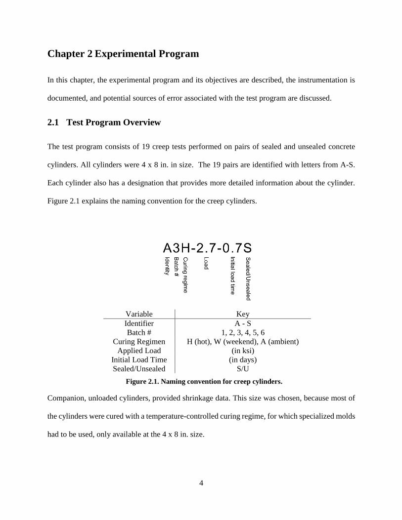
2.1 Test Program Overview
The test program consists of 19 creep tests performed on pairs of sealed and unsealed concrete
cylinders. All cylinders were 4 x 8 in. in size. The 19 pairs are identified with letters from A-S.
Each cylinder also has a designation that provides more detailed information about the cylinder.
Figure 2.1 explains the naming convention for the creep cylinders.
Variable Key
Identifier A - S
Batch # 1, 2, 3, 4, 5, 6
Curing Regimen H (hot), W (weekend), A (ambient)
Applied Load (in ksi)
Initial Load Time (in days)
Sealed/Unsealed S/U
Figure 2.1. Naming convention for creep cylinders.
Companion, unloaded cylinders, provided shrinkage data. This size was chosen, because most of
the cylinders were cured with a temperature-controlled curing regime, for which specialized molds
had to be used, only available at the 4 x 8 in. size.

5
Specimens A-K and their companion shrinkage cylinders were cast in 2016, and were a part of a
research performed by Magnusson (2016). Magnusson reported his findings, from 100 days’ worth
of data in his thesis, but the creep tests continued and the results for the extended data series will
be discussed in this thesis. Furthermore, new creep tests were conducted in 2017, on Specimens
L-S. Some of those specimens were intended to provide insight to unstudied creep properties, but
others were monitored as a duplicate of specimens cast earlier to verify certain results and increase
the reliability of the study.
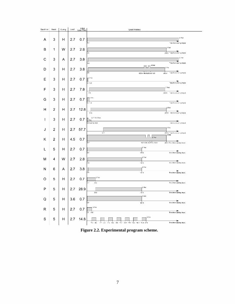
Figure 2.2 describes key characteristics, including the load history for all 19 specimens. The creep
specimens had a variety of curing regimes, loading histories and load levels to test how creep was
affected by those parameters and to be able to use the data to effectively calibrate the model that
was proposed in Magnusson’s thesis. Because early creep behavior is of special interest, as it
affects erection of prestressed girders, most of the creep tests were only performed for 6 to 9
months. Specimens A and C are exceptions. They have not been unloaded yet and provide one
and a half years’ worth of data on the effects of heat curing on long-term creep. The following
discussions illustrates how key parameters were examined within the test program.
Curing regime. Specimens A, B and C (cast in 2016) and L and M (cast in 2017) make it possible
to directly evaluate how different curing regimes affect creep and shrinkage behavior. All five
specimens were loaded to 2.7 ksi. A and L were hot-cured, B and M were weekend-cured and C
was ambient-cured. L and M were intended to duplicate A and B respectively.
Age at first loading. Specimens A, D, F, H, J, L and P can be compared to evaluate the effect of
initial loading times on creep. All seven specimens were hot cured and were subjected to the same
compressive stress of 2.7 ksi.

6
Loading history. Magnusson used Specimen I to effect the effect of step loading on creep and in
this thesis the effect of cyclic loading was examined with Specimen S.
Load superposition. The validity of load history superposition was examined looking at the creep
data from Specimens A, D, F, G, I, L, O and P. Specimens L, O and P will be discussed in this
thesis, but Magnusson did a thorough analysis on the other specimens listed.
Stress amplitude. Specimens A, K, L and Q were all hot cured and loaded at the same age (0.7
days). These specimens were compared to see how the stress amplitude affected the creep behavior
of hot-cured concrete.
Creep recovery. Creep recovery data is available from all specimens, expect for A and C. The data
can be used to analyze the effect of a variety of factors that Yue and Taerwe (1993) have been
found to influence creep recovery. Amongst those are stress level, loading history (for how long
and when specimens are loaded) and curing regime.
7
Figure 2.2. Experimental program scheme.
8
2.2 Concrete Properties
2.2.1 Concrete Mix Composition
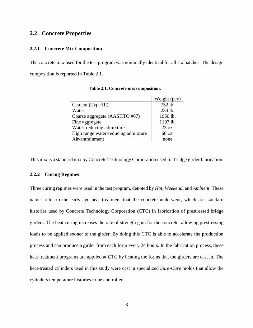
The concrete mix used for the test program was nominally identical for all six batches. The design
composition is reported in Table 2.1.
Table 2.1. Concrete mix composition.
Weight (pcy)
Cement (Type III) 752 lb.
Water 234 lb.
Coarse aggregate (AASHTO #67) 1950 lb.
Fine aggregate 1197 lb.
Water-reducing admixture 23 oz.
High range water-reducing admixture 60 oz.
Air-entrainment none
This mix is a standard mix by Concrete Technology Corporation used for bridge girder fabrication.
2.2.2 Curing Regimes
Three curing regimes were used in the test program, denoted by Hot, Weekend, and Ambient. These
names refer to the early age heat treatment that the concrete underwent, which are standard
histories used by Concrete Technology Corporation (CTC) in fabrication of prestressed bridge
girders. The heat curing increases the rate of strength gain for the concrete, allowing prestressing
loads to be applied sooner to the girder. By doing this CTC is able to accelerate the production
process and can produce a girder from each form every 24 hours. In the fabrication process, these
heat treatment programs are applied at CTC by heating the forms that the girders are cast in. The
heat-treated cylinders used in this study were cast in specialized Sure-Cure molds that allow the
cylinders temperature histories to be controlled.
9
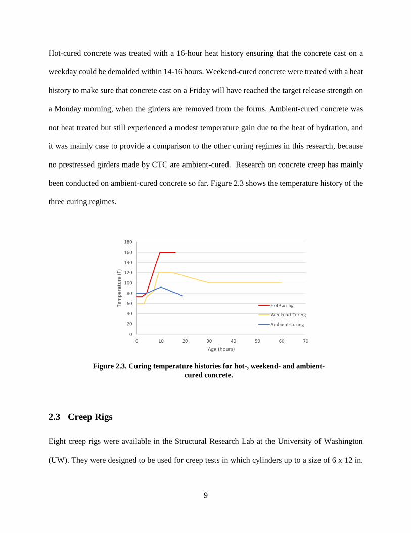
Hot-cured concrete was treated with a 16-hour heat history ensuring that the concrete cast on a
weekday could be demolded within 14-16 hours. Weekend-cured concrete were treated with a heat
history to make sure that concrete cast on a Friday will have reached the target release strength on
a Monday morning, when the girders are removed from the forms. Ambient-cured concrete was
not heat treated but still experienced a modest temperature gain due to the heat of hydration, and
it was mainly case to provide a comparison to the other curing regimes in this research, because
no prestressed girders made by CTC are ambient-cured. Research on concrete creep has mainly
been conducted on ambient-cured concrete so far. Figure 2.3 shows the temperature history of the
three curing regimes.
Figure 2.3. Curing temperature histories for hot-, weekend- and ambient-
cured concrete.
2.3 Creep Rigs
Eight creep rigs were available in the Structural Research Lab at the University of Washington
(UW). They were designed to be used for creep tests in which cylinders up to a size of 6 x 12 in.

10
could be loaded up to a stress of 4.5 ksi. A detailed design description of the creep rigs can be
found in Magnusson (2016).
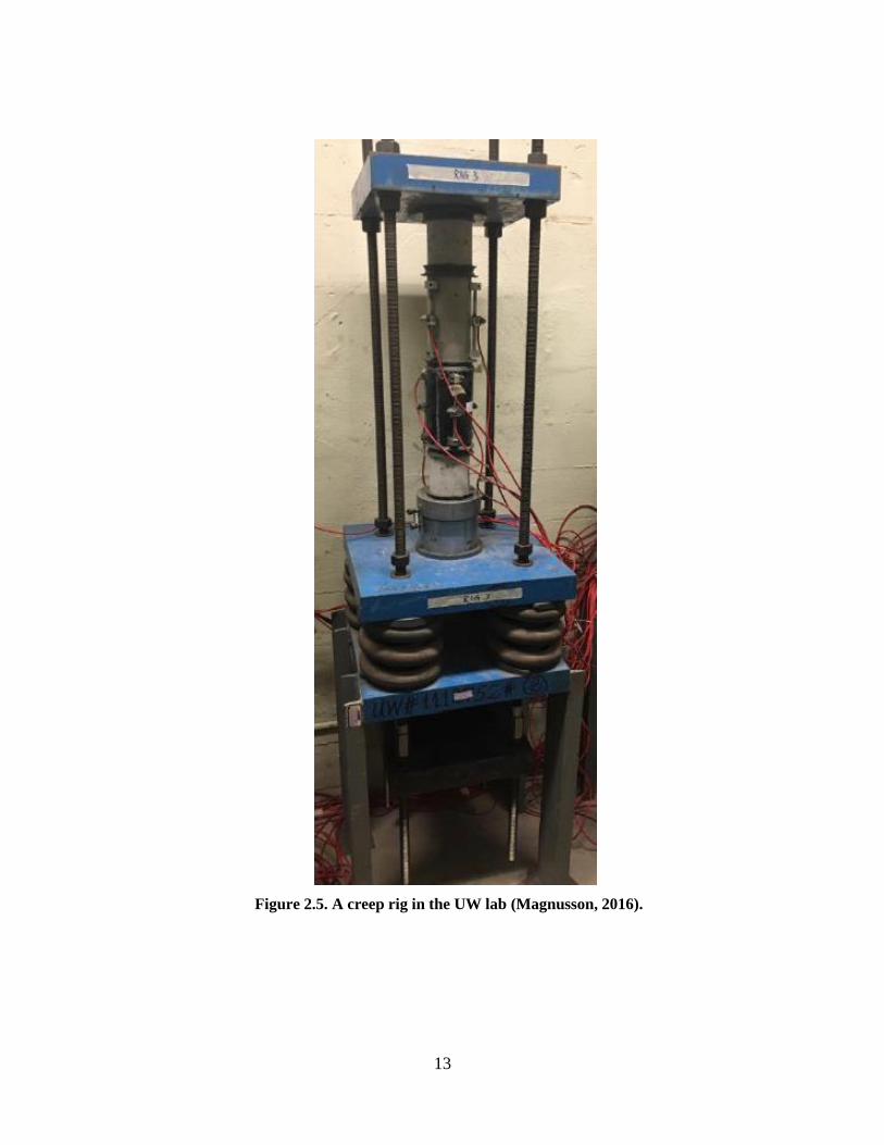
Figure 2.4 and Figure 2.5 show a drawing and a photo of a typical creep rig. Each rig consists of
two steel plates (A and B in Fig. 2.4) with four sets of springs, a set consisting of a spring with an
outside diameter of 4.5 inches inside a spring with an outside diameter of 8 inches, in between
them. The lower plate (A) is attached to four legs. Through these two plates go four threaded-steel
rods. Mounted on these steel rods is a slightly smaller steel plate (C) above the two bigger plates.
High-strength steel nuts hold this assembly together. The sealed and unsealed concrete cylinders
(F) are placed between the small top plate (C) and the upper big plate (B). Two smaller cylinders
(G), made from the same concrete as the other cylinders, are placed on the top and the bottom of
the stack, which sits on a rotating swivel head (D). The purpose of the two smaller cylinders was
to prevent unwanted radial confinement at the ends of the test cylinders that might happen because
of the friction from the creep rig plates. Beneath plates A and B is another steel plate (E) upon
which the hydraulic loading ram sits during application of loads. Between plates A and B is a
displacement dial gage, placed centrally between the springs, that measures the distance between
the two plates. Knowing the stiffness of the springs allows for the stress in the system to be
calculated and monitored over time.
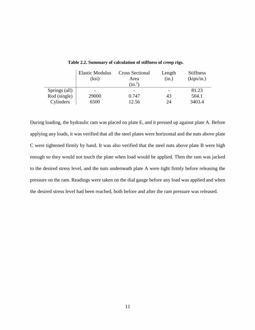
The measured total stiffness of all springs in each rig was 81.23 kips/in. The elastic modulus of
the steel rods is approximately 29000 ksi, and their cross-sectional area and length are 0.747 in2
and 43 in. respectively. The elastic modulus of the concrete varies over time and curing regime
but an average value of 6500 ksi can be used to estimate the stiffness of the cylinder stack. The
cross-sectional area and length of the stack is 12.56 in2 and 24 in. respectively. Table 2.2
summarizes the stiffness calculation for each component of the creep rigs.
11
Table 2.2. Summary of calculation of stiffness of creep rigs.
Elastic Modulus
(ksi)
Cross Sectional
Area
(in.2)
Length
(in.)
Stiffness
(kips/in.)
Springs (all) - - - 81.23
Rod (single) 29000 0.747 43 504.1
Cylinders 6500 12.56 24 3403.4
During loading, the hydraulic ram was placed on plate E, and it pressed up against plate A. Before
applying any loads, it was verified that all the steel plates were horizontal and the nuts above plate
C were tightened firmly by hand. It was also verified that the steel nuts above plate B were high
enough so they would not touch the plate when load would be applied. Then the ram was jacked
to the desired stress level, and the nuts underneath plate A were tight firmly before releasing the
pressure on the ram. Readings were taken on the dial gauge before any load was applied and when
the desired stress level had been reached, both before and after the ram pressure was released.

12
Figure 2.4. Creep rig diagram (dimensions in inches).
13
Figure 2.5. A creep rig in the UW lab (Magnusson, 2016).
14
2.4 Test Procedure
The concrete cylinders were all cast by CTC in their plant in Tacoma, Washington. Heat-cured
cylinders were cast in Sure Cure molds and consolidated with a vibrating table, and ambient-cured
cylinders were cast in plastic molds and consolidated by rodding. All cylinders were 4 x 8 inches.
Batches 1-3 were made during a six-day period in July 2016 whereas batches 4-6 were made during
a three-week period from May until June in 2017. Another nominally identical batch was made
alongside batches 1-3 in 2016, which was used for strength and elastic modulus testing.
Magnusson (2016) analyzed those tests.
When the cylinders had reached their desired maturity, about 15 hours after casting the hot-cured
concrete, the cylinders were transported to the materials lab at the University of Washington (UW).
All cylinders were capped with sulfur caps; half of the cylinders were then sealed with pre-cut 1/8-
in. thick, self-adhesive rubber. Vibrating wire gages were then glued to the cylinders with
superglue, which had proven to be the most effective way after having considered epoxy and other
types of glue. Then any exposed concrete surfaces around the free edges of the rubber, on the
sealed cylinders, were sealed with silicone.
Finally, the cylinders were placed in the creep rigs, as described in Section 2.3 and loaded
according to the appropriate load history in Figure 2.2. Shrinkage cylinders, which were not
loaded, were placed in the same room as the creep rigs, and the top and bottom of sealed cylinders
were sealed with rubber. Those cylinders were otherwise treated the same as the creep cylinders
until the point of loading.
One improvement was made in this procedure between 2016 and 2017 to speed up the process,
because time was critical in order to adhere as closely as possible to the curing regime and concrete
15
maturity that would be used in the production plant by CTC. Instead of bringing the cylinders in
their molds to the UW lab and demolding them there, the demolding was done in Tacoma by an
experienced lab technician, and the cylinders were then transported to the UW in thermally
insulated boxes to minimize any loss of heat.
2.5 Instrumentation and Data Acquisition
Geokon Model 4000 vibrating wire strain gages were used to measure the strains of all concrete
cylinders. One of the main advantages of using this type of gage is their long-term stability. The
gage consists of an encased steel wire tensioned between two mounting blocks that are glued to
the surface of the concrete cylinder. Deformation of the concrete produces relative movement
between the two mounting blocks inducing a change in the wire tension and a corresponding
change in its natural frequency of vibration. The resonant frequency is measured by plucking the
wire using an electromagnetic coil connected through a signal cable to a data analyzer. The active
gage length is 150 mm, its range is 3000 με and its accuracy is 0.5 με (Geokon, 2017).
Two types of analyzers were used to read the strain gages, the CDM-VW305 and the AVW200,
both from Campbell Scientific Inc. The former can read eight channels simultaneously up to a rate
of 333 Hz by using an excitation mechanism that maintains the vibrating steel wire in a
continuously vibrating state (Campbell Scientific, 2016). The latter can be connected to
multiplexers allowing it to read up to 96 channels. It reads one channel at a time by exciting the
vibrating wire with a single pulse. This does not allow a measuring rate as high as the other
mechanism (Campbell Scientific, 2015). It can read each channel once every four minutes. For
consistency, the CDM-VW305 was also set to take readings every four minutes. However, by
using the CDM-VW305 the instantaneous creep behavior right after loading could be examined,
which the AVW200 was not able to do.

16
In total 104 gages were used to monitor the cylinders. Magnusson performed a few preliminary
tests and concluded that using two gages on each shrinkage cylinder and three gages on each creep
cylinder would be sufficient. However, because some eccentricity seemed to be inevitable when
load was applied to the creep cylinders, it was decided in this study, in case of any gage
malfunctions, that using four gages on the creep cylinders would be preferable. Therefore, creep
cylinders tested in 2017 had four gages each, instead of three used the year before. Using two
gages on shrinkage cylinders was still assumed to be sufficient for the tests performed in 2016 and
2017.
2.6 Strength and Stiffness Tests
Magnusson (2016) performed a study on the strength and stiffness of the concrete in 2016; his
analyzes can be found in his thesis in Chapter 5. In addition to the study, strength and stiffness
tests were performed on each batch to verify the consistency of the nominally identical batches.
For every batch that was cast, cylinders were made to be tested for strength. The tests were
performed on the cylinders at the age of 0.7, 7, 14 and 28 days. Some of the tests were performed
by CTC with their fully automatic Forney 400k VFD compression testing machine, and some of
the test were performed in the UW lab with a Forney compression testing machine. The cylinders
tested by CTC were removed from their molds at approximately 15 hours and immersed in a lime-
saturated water curing tank. The cylinders tested in the UW lab were removed from their molds at
approximately 15 hours, then transported in thermal insulated boxes to the UW lab where they
were cured in the same room as the creep tests were performed, at a nominal relative humidity of
40 to 50% and a temperature between 70 and 76 ºF.
17
Stiffness and strength tests were done on all creep and shrinkage cylinders at the end of their test
period. The stiffness tests were performed according to the ASTM standard C469/C469M-14 using
a Baldwin hydraulic ram and vibrating-wire gages in the UW lab. The strength tests were
performed using a Forney compression testing machine in the UW lab.
2.7 Potential Sources of Errors in the Test Program
The reliability of the research is highly dependent on the accuracy of the measurements because
identifying specific creep components can require a subtraction of multiple measured values.
Loading error. Several behaviors contributed to possible inaccuracy in the load. First, the load on
the cylinder stack was found to be somewhat eccentric, despite the best efforts to avoid it. Whether
this was caused by poor centering, non-perpendicular capping or by side sway of the rig during
loading is not known. Second, the dial gauges that measured the deformations of the springs in the
rig (see Figure 2.4) showed about a 1/100 in. “slip back” when the ram force was removed after
having tightened the nuts. A slight deformation as the nuts press against the plates and the threads
of the rods settle in the nuts while the load is being transferred from ram to the rods is assumed to
be the reason for this. The stiffness of all the springs in rig was measured to be 81.23 kip/in. A
deformation of a 1/100 in. therefore corresponds to a loss of about 0.8 kip, about 2.5% of the
nominal load applied to most of the cylinders. The ram force is also somewhat open to question,
because there is inevitably some friction on the piston. This source of error was minimized by
arranging for the smallest possible piston extension, and the ram was calibrated using the same
extension as was used in the creep rigs, but some error is nonetheless inevitable. It is estimated to
be less than 0.5 kip.
18
Concrete cylinders. The variability of the concrete among the cylinders is a potential source for
error, especially when comparing concretes that were cast months apart, considering that the
fabricator might have gotten new deliveries of cement and aggregates in the meantime and the
moisture content of the aggregates could vary. Another potential source for errors is if some of the
sealed cylinders were not sealed properly and are therefore losing moisture. This error is assumed
to be small as great care was taken to seal the cylinder.
Laboratory conditions. If the temperature and relative humidity where the creep rigs are located
vary by a large amount over the test period, that can be a potential source for error. The temperature
and relative humidity of the room where the creep rigs in this project were located were recorded
for a part of the duration of the tests. This data is shown in Appendix A.
Strain gages. The manufacturer of the strain gages claims that their accuracy is within ±0.5%. The
gages are claimed to be able to correct for strains induced by temperature changes. This was tested
by Magnusson. The thermal coefficient obtained in that test was around 10% of the thermal
coefficient for stainless steel, of which the gages are made, and thus the self-compensation for
temperature was deemed good enough.
Gage reading rate. Readings were taken on the vibrating wire gages every four minutes, thus it is
impossible to separate the elastic deformation from the early creep exactly. This is discussed more
closely in Section 3.3. The error of the elastic strain is estimated to be smaller than 0.5%.
Attachment of gages. Potentially there was creep in the superglue that was used to attach the gages
to the concrete, but no data suggested that. Several gage malfunctions were however evident,
especially on the sealed cylinders, whether that can be traced back to the superglue is not known.
Another source of error related to the attachment of the strain gages is their positioning, for the

19
measurements to be accurate the gages need to be perfectly in line with the cylinder and the
application of load. This error is assumed to be small, because great caution was taken to aligning
them correctly.
20
Chapter 3 Data Processing
In this chapter, the processing of the data acquired from the concrete specimens is described. First,
the key test variables are explained for the shrinkage cylinders and the creep cylinders. Then, using
the data obtained, the details are shown for identifying the individual strain components for each
specimen.
The general process for all specimens was the same, but, in case of gage malfunctions, some
specimens had to be treated differently. This chapter focuses mainly on specimens L – S, as
Magnusson (2016) discussed the procedure for the other specimens in his thesis. Specimen L will
be used as an example to describe the data processing, and some data from other specimens will
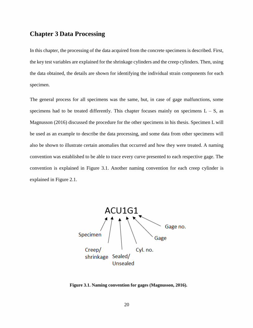
also be shown to illustrate certain anomalies that occurred and how they were treated. A naming
convention was established to be able to trace every curve presented to each respective gage. The
convention is explained in Figure 3.1. Another naming convention for each creep cylinder is
explained in Figure 2.1.
Figure 3.1. Naming convention for gages (Magnusson, 2016).

21
3.1 Shrinkage Strain Data
The processing of the shrinkage data is described in this section.
A pair of shrinkage specimens consisted of one unsealed cylinder and one sealed cylinder. On each
cylinder, there were two vibrating wire gages, placed directly opposite one another. For each hot-
cured batch two pairs of shrinkage specimens were made, but for the weekend- and ambient-cured
batches, only one pair of cylinders was made and monitored. This decision was made to optimize
the usage of gages. Every hot-cured batch had at least three pairs of companion creep cylinders,
and it was therefore important that the shrinkage data was available for those batches, otherwise
the data from all corresponding creep specimens would be unusable. On the other hand, all
weekend- and ambient-cured batches had only one pair of creep cylinders, and it was therefore
deemed sufficient to have only one pair of shrinkage cylinders for each of those batches. In total,
there were ten pairs of shrinkage cylinders cast, six hot-cured, two weekend-cured and two
ambient-cured. The experimental program scheme is shown in Figure 2.2.
Figure 3.2 shows the raw strain measurements for the two unsealed shrinkage cylinders
corresponding to Specimen L5H_2.7_0.7. The same shrinkage specimens were used in considering
the other hot-cured specimens from Batch 5 (seen in Figure 2.2). In Figure 3.2, time begins at the
age at loading of Specimen L.

22
Figure 3.2. Individual shrinkage strain measurements for Specimen L,
unsealed.
Great internal consistency is seen in the measurements, which verifies the reliability of the gages
used. At 6 months the average strain value is 450 με, and the coefficient of variation (COV) is
under 5%. The average strains of the two cylinders are almost the same, but the variance is much
higher for Cylinder 2. The difference of the two gages after 6 months is about 70 με, whether this
represents a gage error or a difference in real strain on the two sides is not known. The total
shrinkage of Specimen L was taken to be the average of all four gages.
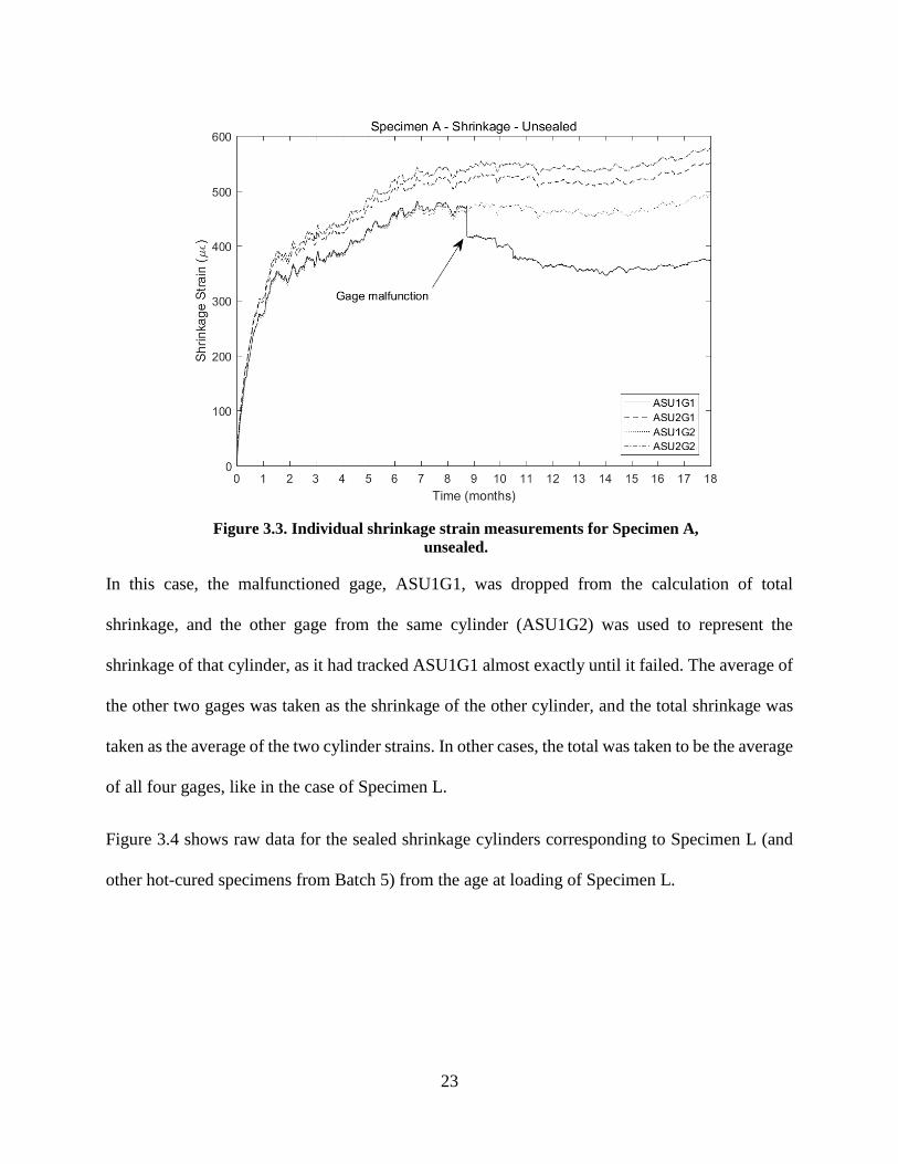
A gage malfunction was observed on an unsealed hot-cured shrinkage cylinder for Batch 3
(specimens A, D, E, F, G and I), as shown in Figure 3.3.
23
Figure 3.3. Individual shrinkage strain measurements for Specimen A,
unsealed.
In this case, the malfunctioned gage, ASU1G1, was dropped from the calculation of total
shrinkage, and the other gage from the same cylinder (ASU1G2) was used to represent the
shrinkage of that cylinder, as it had tracked ASU1G1 almost exactly until it failed. The average of
the other two gages was taken as the shrinkage of the other cylinder, and the total shrinkage was
taken as the average of the two cylinder strains. In other cases, the total was taken to be the average
of all four gages, like in the case of Specimen L.
Figure 3.4 shows raw data for the sealed shrinkage cylinders corresponding to Specimen L (and
other hot-cured specimens from Batch 5) from the age at loading of Specimen L.
24
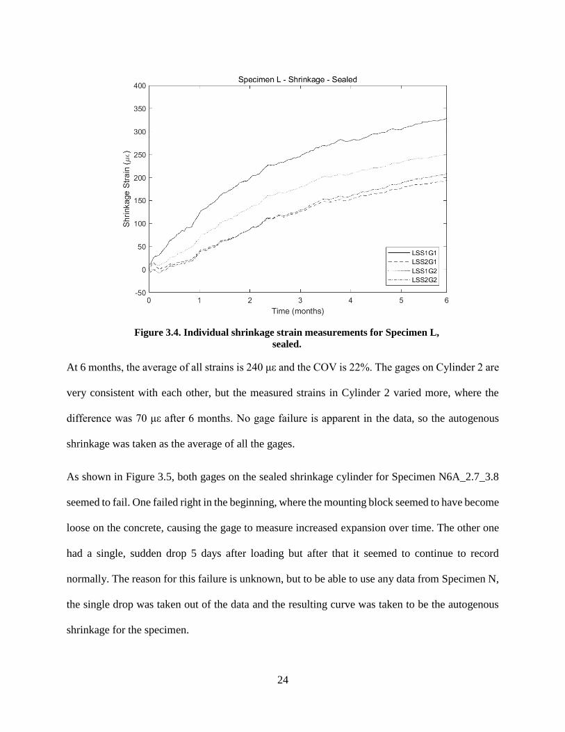
Figure 3.4. Individual shrinkage strain measurements for Specimen L,
sealed.
At 6 months, the average of all strains is 240 με and the COV is 22%. The gages on Cylinder 2 are
very consistent with each other, but the measured strains in Cylinder 2 varied more, where the
difference was 70 με after 6 months. No gage failure is apparent in the data, so the autogenous
shrinkage was taken as the average of all the gages.
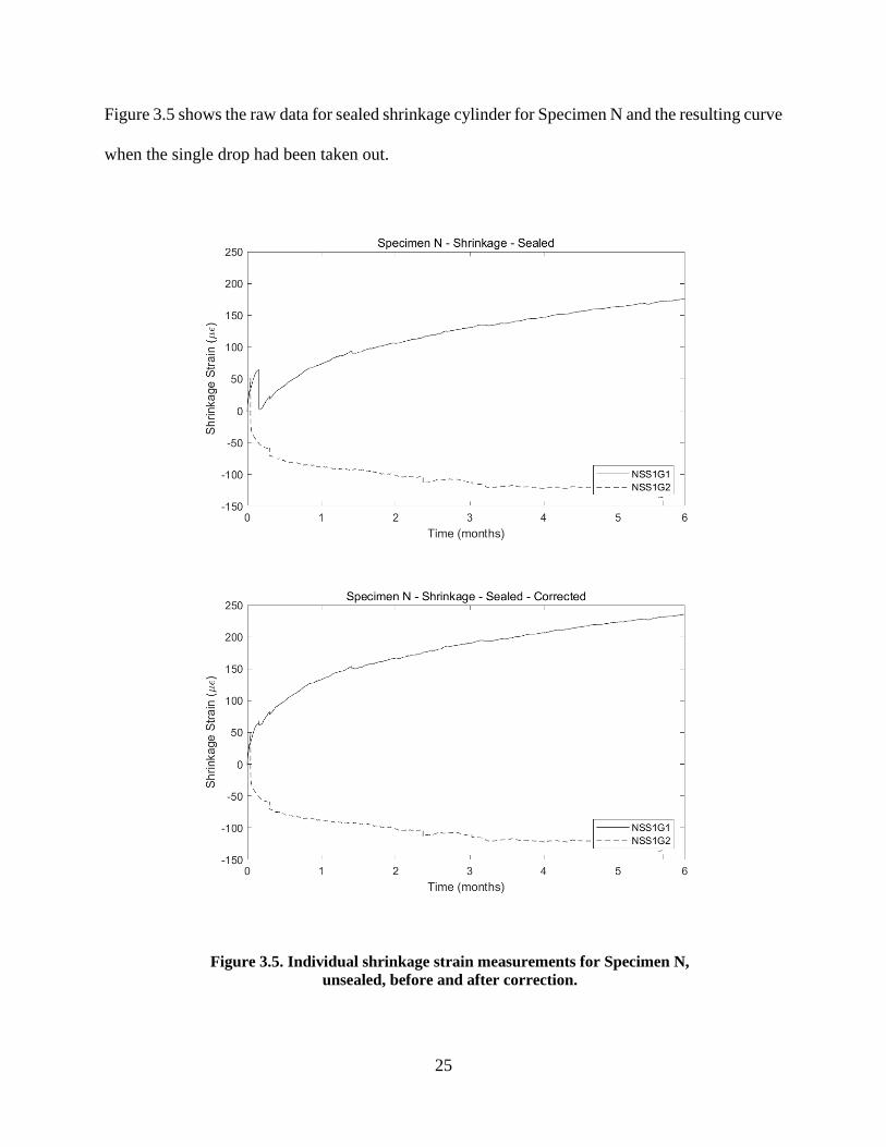
As shown in Figure 3.5, both gages on the sealed shrinkage cylinder for Specimen N6A_2.7_3.8
seemed to fail. One failed right in the beginning, where the mounting block seemed to have become
loose on the concrete, causing the gage to measure increased expansion over time. The other one
had a single, sudden drop 5 days after loading but after that it seemed to continue to record
normally. The reason for this failure is unknown, but to be able to use any data from Specimen N,
the single drop was taken out of the data and the resulting curve was taken to be the autogenous
shrinkage for the specimen.
25
Figure 3.5 shows the raw data for sealed shrinkage cylinder for Specimen N and the resulting curve
when the single drop had been taken out.
Figure 3.5. Individual shrinkage strain measurements for Specimen N,
unsealed, before and after correction.
26
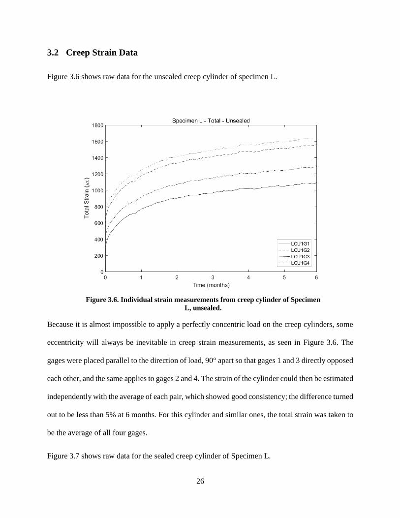
3.2 Creep Strain Data
Figure 3.6 shows raw data for the unsealed creep cylinder of specimen L.
Figure 3.6. Individual strain measurements from creep cylinder of Specimen
L, unsealed.
Because it is almost impossible to apply a perfectly concentric load on the creep cylinders, some
eccentricity will always be inevitable in creep strain measurements, as seen in Figure 3.6. The
gages were placed parallel to the direction of load, 90° apart so that gages 1 and 3 directly opposed
each other, and the same applies to gages 2 and 4. The strain of the cylinder could then be estimated
independently with the average of each pair, which showed good consistency; the difference turned
out to be less than 5% at 6 months. For this cylinder and similar ones, the total strain was taken to
be the average of all four gages.
Figure 3.7 shows raw data for the sealed creep cylinder of Specimen L.

27
Figure 3.7. Individual strain measurements from creep cylinder of Specimen
L, sealed.
Similar eccentricity is apparent on both the sealed and the unsealed creep cylinders of Specimen
L, seen by comparing Figure 3.6 and Figure 3.7, which verifies that it is the eccentricity that causes
the apparent variation among the gages but not gage failures or other experimental mishaps. The
strain in the sealed cylinders (basic creep strain) was taken to be the average of all four gages.
Where three gages or two non-opposing gages failed on the same cylinder, the measured strains
were unreliable and effectively useless. This was unfortunately the case for the sealed creep
cylinders of specimens O5H_2.7_0.7 and P. A figure showing all gage failures can be found in
Appendix A.
When a single gage failure was apparent on a cylinder, that gage and the opposing gage were
dropped from the calculations and the average of the remaining two gages was taken to be the total
strain for the specimen. This was done in the case of unsealed creep cylinders of specimens N and
28
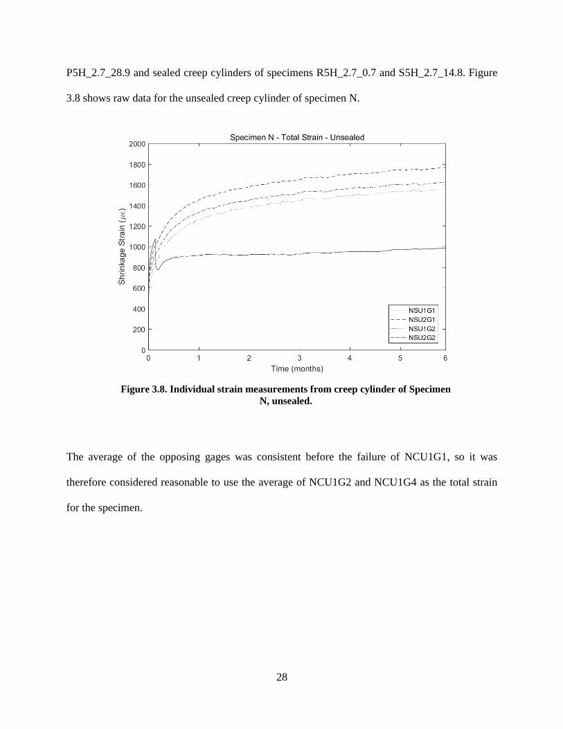
P5H_2.7_28.9 and sealed creep cylinders of specimens R5H_2.7_0.7 and S5H_2.7_14.8. Figure
3.8 shows raw data for the unsealed creep cylinder of specimen N.
Figure 3.8. Individual strain measurements from creep cylinder of Specimen
N, unsealed.
The average of the opposing gages was consistent before the failure of NCU1G1, so it was
therefore considered reasonable to use the average of NCU1G2 and NCU1G4 as the total strain
for the specimen.
29
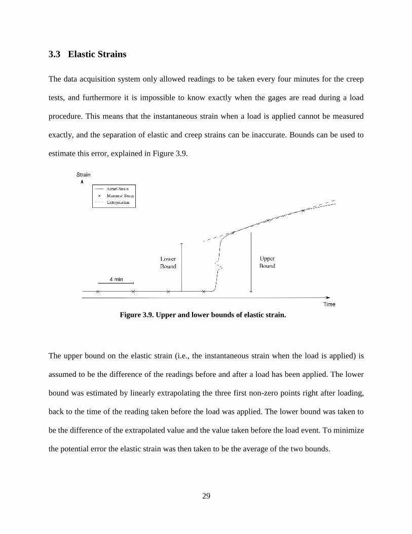
3.3 Elastic Strains
The data acquisition system only allowed readings to be taken every four minutes for the creep
tests, and furthermore it is impossible to know exactly when the gages are read during a load
procedure. This means that the instantaneous strain when a load is applied cannot be measured
exactly, and the separation of elastic and creep strains can be inaccurate. Bounds can be used to
estimate this error, explained in Figure 3.9.
Figure 3.9. Upper and lower bounds of elastic strain.
The upper bound on the elastic strain (i.e., the instantaneous strain when the load is applied) is
assumed to be the difference of the readings before and after a load has been applied. The lower
bound was estimated by linearly extrapolating the three first non-zero points right after loading,
back to the time of the reading taken before the load was applied. The lower bound was taken to
be the difference of the extrapolated value and the value taken before the load event. To minimize
the potential error the elastic strain was then taken to be the average of the two bounds.

30
3.4 Identifying of Individual Strain Components
The process of identifying individual strain components is described in detail by Magnusson
(2016) and is summarized here.
In processing the data, the values for the gages on each cylinder were averaged, unless one or more
had to be discarded due to faulty behavior as described above. This left the following average
curves and values.
A single curve for elastic + total creep + total shrinkage from the unsealed, loaded cylinder,
A single curve for elastic + basic creep + autogenous shrinkage from the sealed, loaded
cylinder,
A single curve for total shrinkage from the unsealed, unloaded cylinder(s), and
A single curve for autogenous shrinkage from the sealed, unloaded cylinder(s).
A single value for elastic strain from the unsealed, loaded cylinder.
Keeping all the data points for all the curves led to large datasets. To reduce the amount of data
but to weight the points towards the early parts of the curves, it was decided to use points of equal
intervals of 0.1 in log time, i.e. the first point was taken at 100.1 days, then at 100.2 days, and so on,
from every stress change event. Two points were also taken on each side of a stress change event,
to capture elastic strains as well. The curves obtained by this procedure were used to produce the
plot shown in Figure 3.10 for Specimen L. It shows the breakdown of the measured strains into
different phenomena listed above. The smaller number of data points also sped up the model fitting
described in Chapter 10.

31
Figure 3.10. Breakdown of strain components for Specimen L.

32
Chapter 4 Compressive Strength
From each of the six batches, companion 4”x8”cylinders were tested for strength. Those strength
tests were performed at the ages of 0.7, 7, 14 and 28 days. Strength tests were also done on all
creep and shrinkage cylinders at the end of their test period. The results and analyzes of these tests
are reported in this chapter.
4.1 Measured Compressive Strength of Strength Cylinders
Table 4.1 shows the measured strength of each pair of cylinders tested that was hot-cured. Most
of the test were conducted by Concrete Technology Corporation (CTC), while those in the table
marked with an asterisk were tested at the University of Washington (UW). The 7-day strength is
not available for batches 1-3, and the 14-day strength is also unavailable for Batch 5. The tests on
Batch 5 were done in the UW lab, along with a pair of cylinders from Batch 4 that was tested for
the 7-day strength. The measured values for the 7-day strength of Batch 4, for both cylinders tested
at the UW and at CTC, show great consistency and suggest that the result performed at both labs
are comparable. CTC uses Neoprene caps, while the UW uses sulfur caps.
Table 4.1. Strength of each batch at ages from 0.7 – 28 days, all hot-cured.
Strength of hot-cured cylinders (psi)
Cast
date Batch 0.7 day 7 day 14 day 28 day
06/08/16 CTC
Study 10,240/9,730 11240/11200 11,960/11,440 12,222/13,505
07/05/16 1 9,170/9,250 - 11,090/11,380 11,620/12,510
07/06/16 2 9,680/9,680 - 11,360/11,260 12,430/12,020
07/11/16 3 9,650/9,460 - 12,110/11,870 12,900/12,620
05/23/17 4 8,000/8,270 9,730/9,330/
9,780*/9,460* 10,590/10,220 11,500/10,900
05/25/17 5 8,910*/8,460* 8,940*/9,490* - 10,710*/11,230*
06/12/17 6 8,220/8,390 9,690/9,370 10,400/10,700 11,360/11,120
*Cylinders cured and tested in the UW lab.
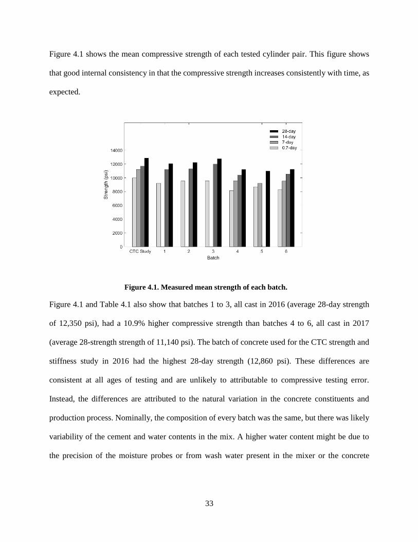
33
Figure 4.1 shows the mean compressive strength of each tested cylinder pair. This figure shows
that good internal consistency in that the compressive strength increases consistently with time, as
expected.
Figure 4.1. Measured mean strength of each batch.
Figure 4.1 and Table 4.1 also show that batches 1 to 3, all cast in 2016 (average 28-day strength
of 12,350 psi), had a 10.9% higher compressive strength than batches 4 to 6, all cast in 2017
(average 28-strength strength of 11,140 psi). The batch of concrete used for the CTC strength and
stiffness study in 2016 had the highest 28-day strength (12,860 psi). These differences are
consistent at all ages of testing and are unlikely to attributable to compressive testing error.
Instead, the differences are attributed to the natural variation in the concrete constituents and
production process. Nominally, the composition of every batch was the same, but there was likely
variability of the cement and water contents in the mix. A higher water content might be due to
the precision of the moisture probes or from wash water present in the mixer or the concrete

34
delivery vehicle (West, 2017). These results show that such natural variations limit the accuracy
with which strength can be predicted based on the concrete mix composition alone.
4.2 Measured Compressive Strength of Shrinkage and Creep Cylinders
Figure 4.2 shows the measured compressive strengths of all cylinders after their creep and
shrinkage tests had been completed. Batches 1-3 were tested a year after casting, whereas batches
4-6 were tested eight months after casing. Each bar corresponds to the measured strength of a
single cylinder, because pairs of cylinders were not available from the creep rigs. The concrete
compressive strengths are plotted versus time in Figure 4.3 for all compressive strengths measured
at CTC or UW.
Figure 4.2. Measured strength of test cylinders at the end of testing.
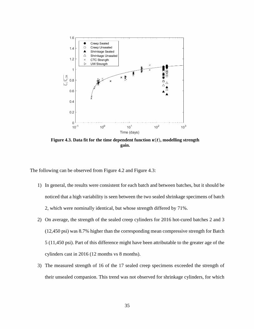
35
Figure 4.3. Data fit for the time dependent function 𝜿(𝒕), modelling strength
gain.
The following can be observed from Figure 4.2 and Figure 4.3:
1) In general, the results were consistent for each batch and between batches, but it should be
noticed that a high variability is seen between the two sealed shrinkage specimens of batch
2, which were nominally identical, but whose strength differed by 71%.
2) On average, the strength of the sealed creep cylinders for 2016 hot-cured batches 2 and 3
(12,450 psi) was 8.7% higher than the corresponding mean compressive strength for Batch
5 (11,450 psi). Part of this difference might have been attributable to the greater age of the
cylinders cast in 2016 (12 months vs 8 months).
3) The measured strength of 16 of the 17 sealed creep specimens exceeded the strength of
their unsealed companion. This trend was not observed for shrinkage cylinders, for which

36
the strength of the sealed cylinders exceeded the strength of the unsealed cylinders for only
4 of the 7 tests.
4) The measured strength of the unsealed creep cylinders tested after monitoring is in only
one case higher than the 28-day strength of the strength test cylinders from the same batch
(reported in Figure 4.1), and even then the strength is less than 1% higher. These
measurements suggest that the concrete strength diminished with time, due to either
sustained load or simply the passage of time. Some unstressed specimens (e.g. the unsealed
shrinkage specimens of Batch 5) also suggest a strength reduction with time. Their average
strength was 30% lower than that of the 28-day strength cylinders from the same batch
5) The shrinkage specimens had generally lower strengths than their companion creep
specimens from the same batch. Both were tested at the same age. The difference is larger
for hot- or weekend-cured specimens than for the ambient-cured specimens. These results
suggest that sustained load increases the concrete strength, which is the opposite of the
evidence in (4) above
6) The data hints that ambient-curing results in higher ultimate strength than hot- and
weekend-curing, but more data on ambient curing would be needed to confirm that
conclusion. This trend is in agreement with the experience of precasters and experiments
on strength development of heat-treated concrete (Kim, Han, & Song, 2002; Kim, Moon,
& Eo, 1998).
7) The compressive strength did not appear to vary consistently with the loading time or
duration of loading.

37
4.3 Modelling of Compressive Strength Gain with Time
Magnusson (2016) analyzed data from a set of compressive strength tests that was performed by
CTC on both hot- and ambient-cured cylinders. The test were done on a nominally identical, but
separate, batch of concrete as the creep tests. To model the compressive strength gain of hot-cured
specimens, he suggested using an equation on the following form:
𝒇𝒄 (𝒕) = 𝜿(𝒕) 𝒇𝒄
(𝟐𝟖) 4.1
where 𝑓��(28) is the strength at 28 days, and 𝜅(𝑡) is a time dependent function with the following
form:
𝜿(𝒕) = 𝒂
(𝒂 − 𝟏) (𝟐𝟖 − 𝒕𝟎
𝒕 − 𝒕𝟎)
𝟏/𝒏
+ 𝟏
4.2
where 𝑎 is the ratio between ultimate strength (i.e., at infinite time) and the strength at 28 days, 𝑛
is a parameter that controls the rate of strength gain, 𝑡 is the time in days since mixing the concrete,
and 𝑡0 is a time offset parameter that reflects the time taken for the initial set to take place. The
28-day strength value for each batch was taken as the average of the two cylinders tested at that
age. The value of 𝑡0 was rounded to the nearest hour.
Equation 4.1 represents a generalization of the equation used in ACI 209 (ACI Committee 209,
2008), which is:
𝒇𝒄 (𝒕) = [
𝒕
𝒂 + 𝒃𝒕] 𝒇𝒄
(𝟐𝟖) 4.3
where 𝑓��(28) is the strength at 28 days and a and b are constants dependent on the cement type
and the curing regime of the concrete. Because the time function must equal 1.00 at t = 28, a and

38
b are not independent and the function has only one free parameters, which means that the initial
strength gain rate and the ratio of strengths at 28 days and infinite time are inextricably linked.
By contrast, if 𝑡0 is ignored, Equation 4.2 has two free parameters, and those two features can be
matched independently.
Using the data from the strength study, the data reported in Table 4.1 and the data from the sealed
creep cylinders tested at the end of the test period, the 𝜅(𝑡) function was fitted. The optimized
parameters are reported in Table 4.2 and are compared with the parameters Magnusson (2016)
reported. As more tests are included in the data base than when before, the results should be more
reliable. Figure 4.3 shows the fitted time-dependent function and the measured strength from all
tests.
Table 4.2. Optimized values for concrete strength parameters
Current
Study
Magnusson
𝒂 1.112 1.114
𝒏 3.13 2.44
𝒕𝟎 (days) 0.375 0.208
The value of a is consistent with what Magnusson (2016) reported and indicates that the hot-cured
concrete does not gain much strength after 28 days. This small strength gain is expected (Wight
and MacGregor (2009). By having 𝑡0 equal to 9 hours a better fit was gotten for the whole dataset,
particularly for the early measurements.

39
Chapter 5 Elastic Modulus
In order to predict deformations of concrete under loading, it is important to be able to predict the
initial strain, i.e. the elastic strain. The ratio of the applied stress to the “instantaneous” strain is
referred to as the elastic modulus and has conventionally been related to the strength and the unit
weight of the concrete with various relationships (Branson, 1977). Interestingly, Bazant, ASCE
and Kim (1979) stated that a sustained compressive stress of low (service) level would make the
response to subsequent load increments markedly stiffer. There is little information available about
this phenomenon in the literature, so the test program was extended to investigate it.
In this chapter, measured values of elastic modulus will be analyzed. For every loading and
unloading event for the creep cylinders, a value for the elastic modulus was obtained. In addition,
at the end of the test period an elastic modulus test was performed, in a conventional test machine,
on every cylinder to get a more accurate value than could be obtained from the creep rigs.
5.1 Elastic Modulus Inferred from Creep Tests
Each time a creep specimen was either loaded or unloaded, changes in the strains in the sealed and
unsealed cylinders were measured, and values for the elastic modulus were calculated. These
estimates of 𝐸𝑐 were computed because the stress and strain data were available. However, they
are considered less reliable than values obtained in a conventional test machine. The primary
reasons are:
The stress values were obtained the digital oil pressure in the jack, rather than a load cell.
While the pressure gage could easily be read to within 1% accuracy, some other sources of
potential error remained. For example, Magnusson found that the reliability of the jack
force depended on how far the piston was extended, and attributed the differences to

40
friction in the piston. It was also necessary to judge the exact load at which the plates in
the rig lifted off from the nuts securing the rods. These features are not found in a
conventional test machine.
The data acquisition system used with the creep rigs was capable of recording 104
channels, but was programmed to read at four minute intervals, whereas a different reader,
capable of reading fewer channels but much faster, was used for the tests in the
conventional test machine. Thus some uncertainty existed about the exact time that the
strain readings were taken in the creep rigs, and about the amount of strain to be attributed
to elastic behavior and creep, respectively.
Figure 5.1 shows the measured elastic modulus for all of the hot-cured specimens for all load
changes with time; Appendix C tabulates the data numerically. The time shown is time since
casting. Partially unloading Specimen I at 3.8 days shows anomaly high values and are not
considered reliable because of relatively high uncertainty in the measured stress change.
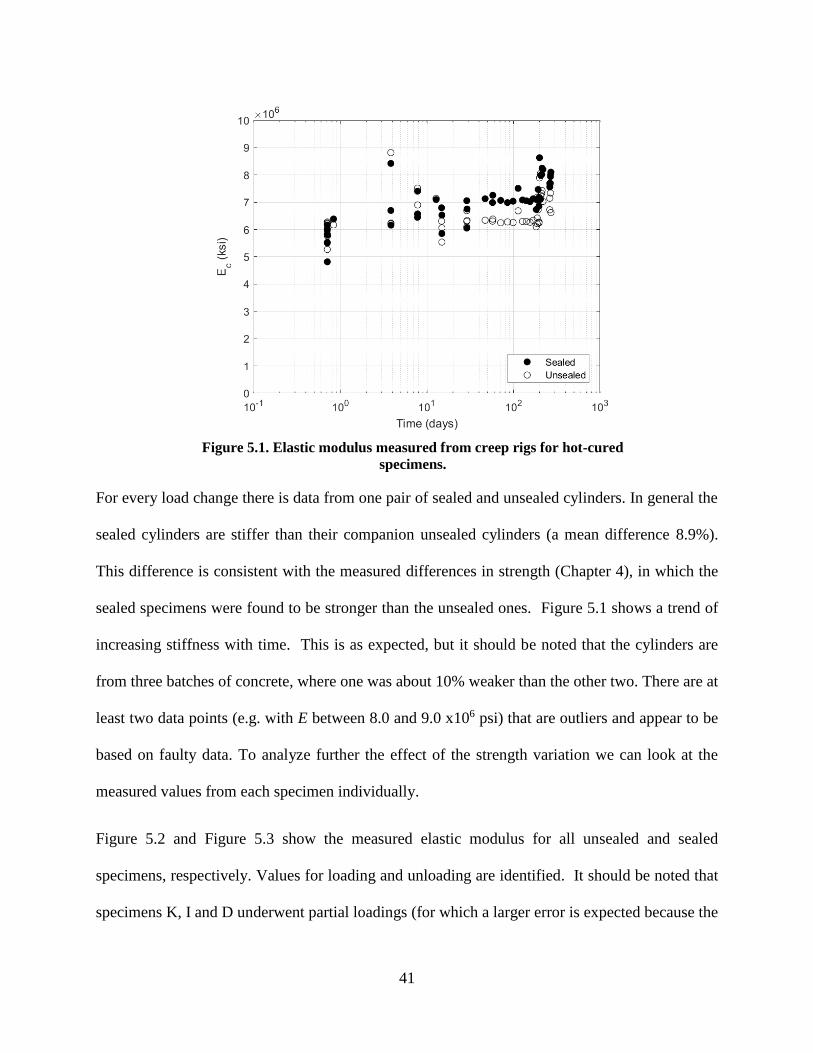
41
Figure 5.1. Elastic modulus measured from creep rigs for hot-cured
specimens.
For every load change there is data from one pair of sealed and unsealed cylinders. In general the
sealed cylinders are stiffer than their companion unsealed cylinders (a mean difference 8.9%).
This difference is consistent with the measured differences in strength (Chapter 4), in which the
sealed specimens were found to be stronger than the unsealed ones. Figure 5.1 shows a trend of
increasing stiffness with time. This is as expected, but it should be noted that the cylinders are
from three batches of concrete, where one was about 10% weaker than the other two. There are at
least two data points (e.g. with E between 8.0 and 9.0 x10⁶ psi) that are outliers and appear to be
based on faulty data. To analyze further the effect of the strength variation we can look at the
measured values from each specimen individually.
Figure 5.2 and Figure 5.3 show the measured elastic modulus for all unsealed and sealed
specimens, respectively. Values for loading and unloading are identified. It should be noted that
specimens K, I and D underwent partial loadings (for which a larger error is expected because the
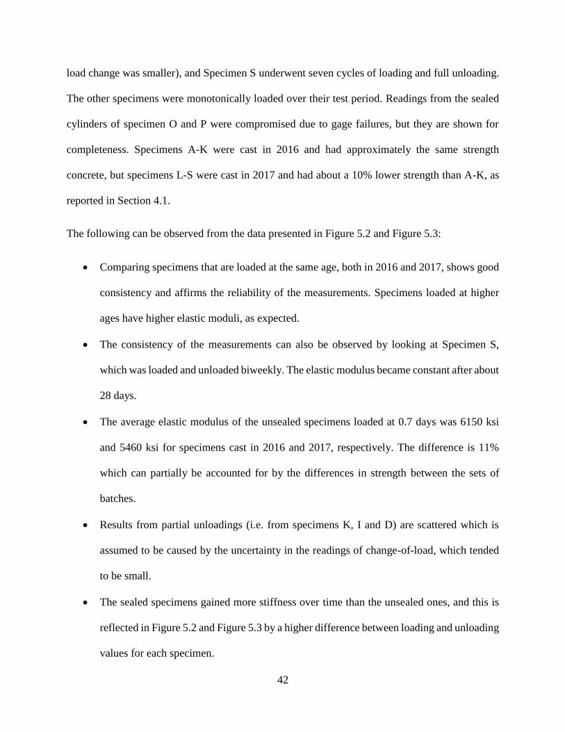
42
load change was smaller), and Specimen S underwent seven cycles of loading and full unloading.
The other specimens were monotonically loaded over their test period. Readings from the sealed
cylinders of specimen O and P were compromised due to gage failures, but they are shown for
completeness. Specimens A-K were cast in 2016 and had approximately the same strength
concrete, but specimens L-S were cast in 2017 and had about a 10% lower strength than A-K, as
reported in Section 4.1.
The following can be observed from the data presented in Figure 5.2 and Figure 5.3:
Comparing specimens that are loaded at the same age, both in 2016 and 2017, shows good
consistency and affirms the reliability of the measurements. Specimens loaded at higher
ages have higher elastic moduli, as expected.
The consistency of the measurements can also be observed by looking at Specimen S,
which was loaded and unloaded biweekly. The elastic modulus became constant after about
28 days.
The average elastic modulus of the unsealed specimens loaded at 0.7 days was 6150 ksi
and 5460 ksi for specimens cast in 2016 and 2017, respectively. The difference is 11%
which can partially be accounted for by the differences in strength between the sets of
batches.
Results from partial unloadings (i.e. from specimens K, I and D) are scattered which is
assumed to be caused by the uncertainty in the readings of change-of-load, which tended
to be small.
The sealed specimens gained more stiffness over time than the unsealed ones, and this is
reflected in Figure 5.2 and Figure 5.3 by a higher difference between loading and unloading
values for each specimen.
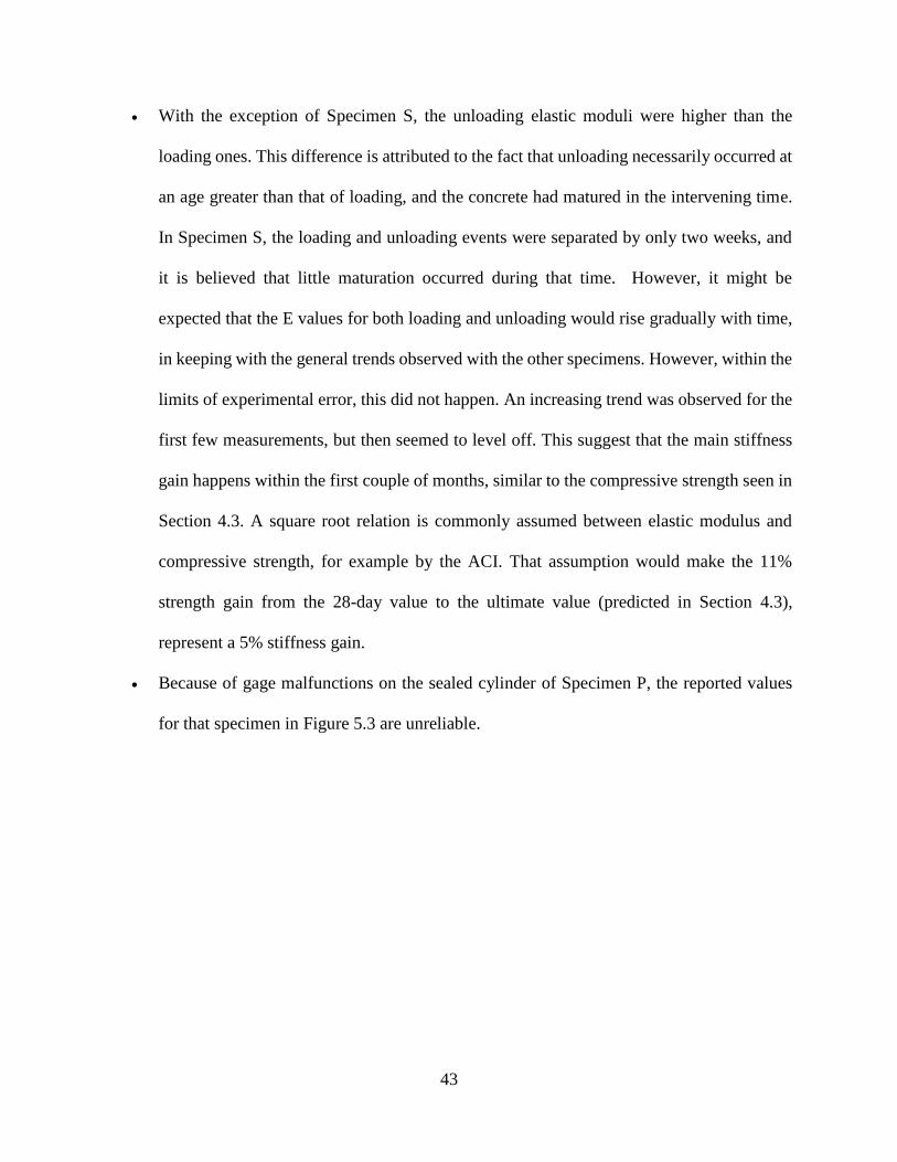
43
With the exception of Specimen S, the unloading elastic moduli were higher than the
loading ones. This difference is attributed to the fact that unloading necessarily occurred at
an age greater than that of loading, and the concrete had matured in the intervening time.
In Specimen S, the loading and unloading events were separated by only two weeks, and
it is believed that little maturation occurred during that time. However, it might be
expected that the E values for both loading and unloading would rise gradually with time,
in keeping with the general trends observed with the other specimens. However, within the
limits of experimental error, this did not happen. An increasing trend was observed for the
first few measurements, but then seemed to level off. This suggest that the main stiffness
gain happens within the first couple of months, similar to the compressive strength seen in
Section 4.3. A square root relation is commonly assumed between elastic modulus and
compressive strength, for example by the ACI. That assumption would make the 11%
strength gain from the 28-day value to the ultimate value (predicted in Section 4.3),
represent a 5% stiffness gain.
Because of gage malfunctions on the sealed cylinder of Specimen P, the reported values
for that specimen in Figure 5.3 are unreliable.
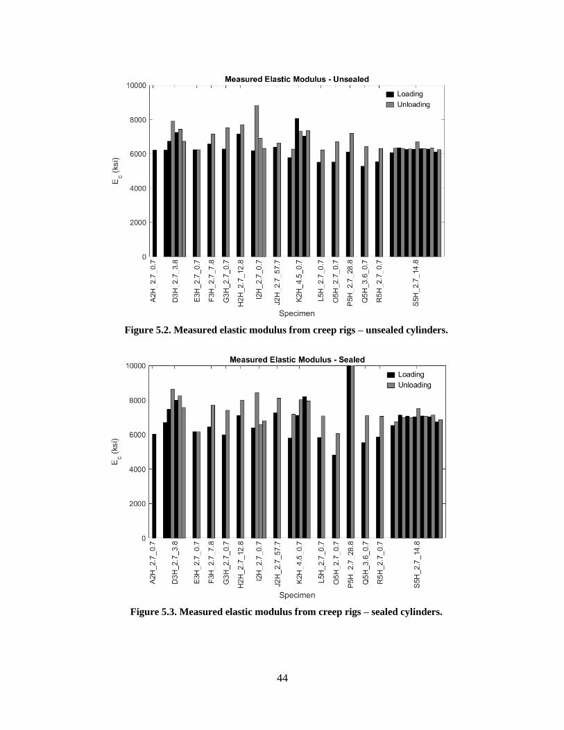
44
Figure 5.2. Measured elastic modulus from creep rigs – unsealed cylinders.
Figure 5.3. Measured elastic modulus from creep rigs – sealed cylinders.
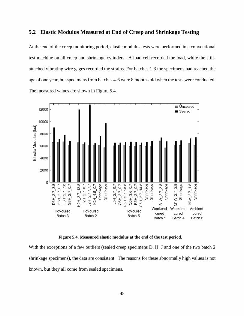
45
5.2 Elastic Modulus Measured at End of Creep and Shrinkage Testing
At the end of the creep monitoring period, elastic modulus tests were performed in a conventional
test machine on all creep and shrinkage cylinders. A load cell recorded the load, while the still-
attached vibrating wire gages recorded the strains. For batches 1-3 the specimens had reached the
age of one year, but specimens from batches 4-6 were 8 months old when the tests were conducted.
The measured values are shown in Figure 5.4.
Figure 5.4. Measured elastic modulus at the end of the test period.
With the exceptions of a few outliers (sealed creep specimens D, H, J and one of the two batch 2
shrinkage specimens), the data are consistent. The reasons for these abnormally high values is not
known, but they all come from sealed specimens.

46
The sealed specimens are in all cases (24 out of 24) stiffer than their unsealed companion; this is
in an agreement with Figure 5.1. The average of all unsealed specimens was 6190 ksi and the
coefficient of variation was less the 5%. If the four highest values are disregarded from the sealed
dataset, the average becomes 6880 ksi and the coefficient of variation is 5%. Disregarding the four
cylinders with suspiciously high elastic moduli, the mean ratio of the elastic modulus of the sealed
and unsealed cylinders together is 1.115. The creep specimens and shrinkage specimens from the
same batch gave comparable values in all cases, which suggests that a sustained load does not
affect the stiffness of concrete. In Chapter 4, the evidence for sustained load affecting strength was
inconclusive.
5.3 Calculation of Elastic Modulus from Direct Measurements
Magnusson analyzed data from a set of 11 elastic modulus tests that were performed by CTC, and
related the elastic modulus to the corresponding strength. Using a generalized form of the
equations used by ACI (2014) and AASHTO (2014) a best fit was made to the combined dataset.
The equation is as follows:
𝑬𝒄(𝒕) = 𝒄 𝒘𝒏𝒘 𝒇𝒄 (𝒕)𝒏𝒇 5.1
where 𝑐, 𝑛𝑤 and 𝑛𝑓 are dimensionless parameters to be determined by a least-squares fit to data.
𝑤 is the unit weight of the concrete in pounds per cubic foot, and 𝑓�� is the concrete compressive
strength at the time of measuring the elastic modulus, in pounds per square inch. For the study
done in 2016, the strength and elastic modulus were measured on separate cylinders from the same
batch that had been treated with identical curing regimes.
The model was re-calibrated here using not only the CTC data (11 tests), but also the data from
the elastic modulus tests performed in this study on the 11 sealed and 14 unsealed creep cylinders
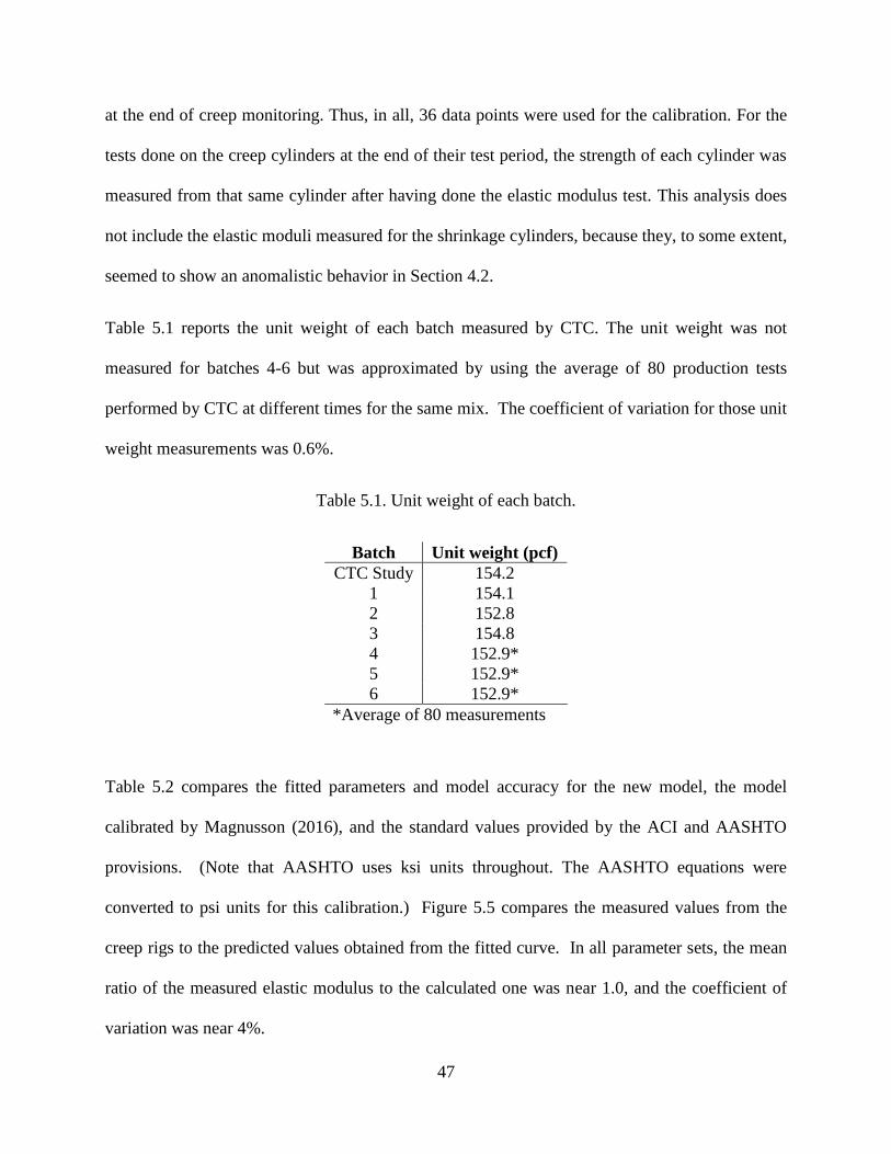
47
at the end of creep monitoring. Thus, in all, 36 data points were used for the calibration. For the
tests done on the creep cylinders at the end of their test period, the strength of each cylinder was
measured from that same cylinder after having done the elastic modulus test. This analysis does
not include the elastic moduli measured for the shrinkage cylinders, because they, to some extent,
seemed to show an anomalistic behavior in Section 4.2.
Table 5.1 reports the unit weight of each batch measured by CTC. The unit weight was not
measured for batches 4-6 but was approximated by using the average of 80 production tests
performed by CTC at different times for the same mix. The coefficient of variation for those unit
weight measurements was 0.6%.
Table 5.1. Unit weight of each batch.
Batch Unit weight (pcf)
CTC Study 154.2
1 154.1
2 152.8
3 154.8
4 152.9*
5 152.9*
6 152.9*
*Average of 80 measurements
Table 5.2 compares the fitted parameters and model accuracy for the new model, the model
calibrated by Magnusson (2016), and the standard values provided by the ACI and AASHTO
provisions. (Note that AASHTO uses ksi units throughout. The AASHTO equations were
converted to psi units for this calibration.) Figure 5.5 compares the measured values from the
creep rigs to the predicted values obtained from the fitted curve. In all parameter sets, the mean
ratio of the measured elastic modulus to the calculated one was near 1.0, and the coefficient of
variation was near 4%.
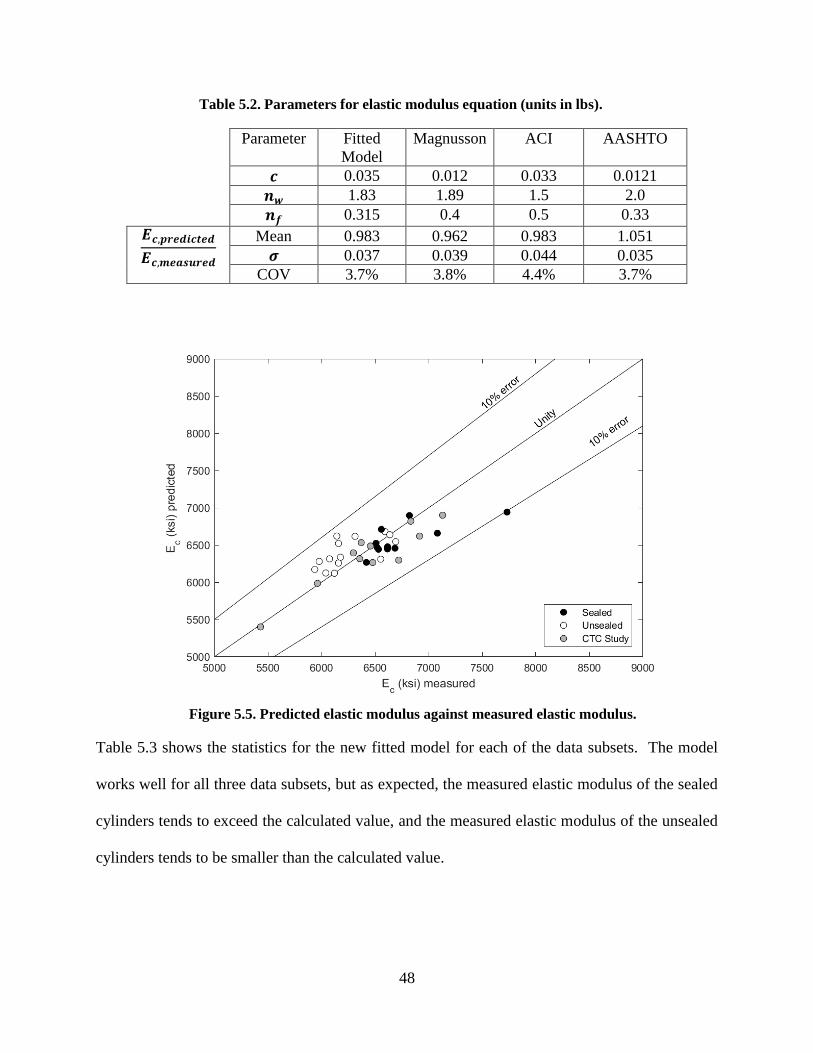
48
Table 5.2. Parameters for elastic modulus equation (units in lbs).
Parameter Fitted
Model
Magnusson ACI AASHTO
𝒄 0.035 0.012 0.033 0.0121
𝒏𝒘 1.83 1.89 1.5 2.0
𝒏𝒇 0.315 0.4 0.5 0.33
𝑬𝒄,𝒑𝒓𝒆𝒅𝒊𝒄𝒕𝒆𝒅
𝑬𝒄,𝒎𝒆𝒂𝒔𝒖𝒓𝒆𝒅
Mean 0.983 0.962 0.983 1.051
𝝈 0.037 0.039 0.044 0.035
COV 3.7% 3.8% 4.4% 3.7%
Figure 5.5. Predicted elastic modulus against measured elastic modulus.
Table 5.3 shows the statistics for the new fitted model for each of the data subsets. The model
works well for all three data subsets, but as expected, the measured elastic modulus of the sealed
cylinders tends to exceed the calculated value, and the measured elastic modulus of the unsealed
cylinders tends to be smaller than the calculated value.

49
Table 5.3. Comparison of Predicted and Measured elastic moduli
𝑬𝒄,𝒎𝒆𝒂𝒔𝒖𝒓𝒆𝒅
𝑬𝒄,𝒑𝒓𝒆𝒅𝒊𝒄𝒕𝒆𝒅
# Measurements Mean Std. Dev. COV
Sealed Cyl. 11 1.004 0.037 3.7%
Unsealed Cyl. 14 0.959 0.030 3.1%
CTC Study 11 0.993 0.027 2.8%
All 36 0.983 0.037 3.7%
5.4 Calculation of Elastic Modulus Inferred from Creep Rigs
A value for the elastic modulus was obtained from the creep rigs every time the load on the
specimen changed, but the concrete strength was not known at all of those times. However, the
strength can be estimated using Equation 4.1 and the coefficients reported in the first column of
Table 4.2, and that strength estimate can then be used to calculate a predicted value for the elastic
modulus using Equation 5.1 and Table 5.2. Figure 5.6 plots the estimated elastic modulus against
the measured elastic modulus from the creep rigs. All partial loading events (on specimens K, I
and D) not included in the plot, because this data was considered unreliable.
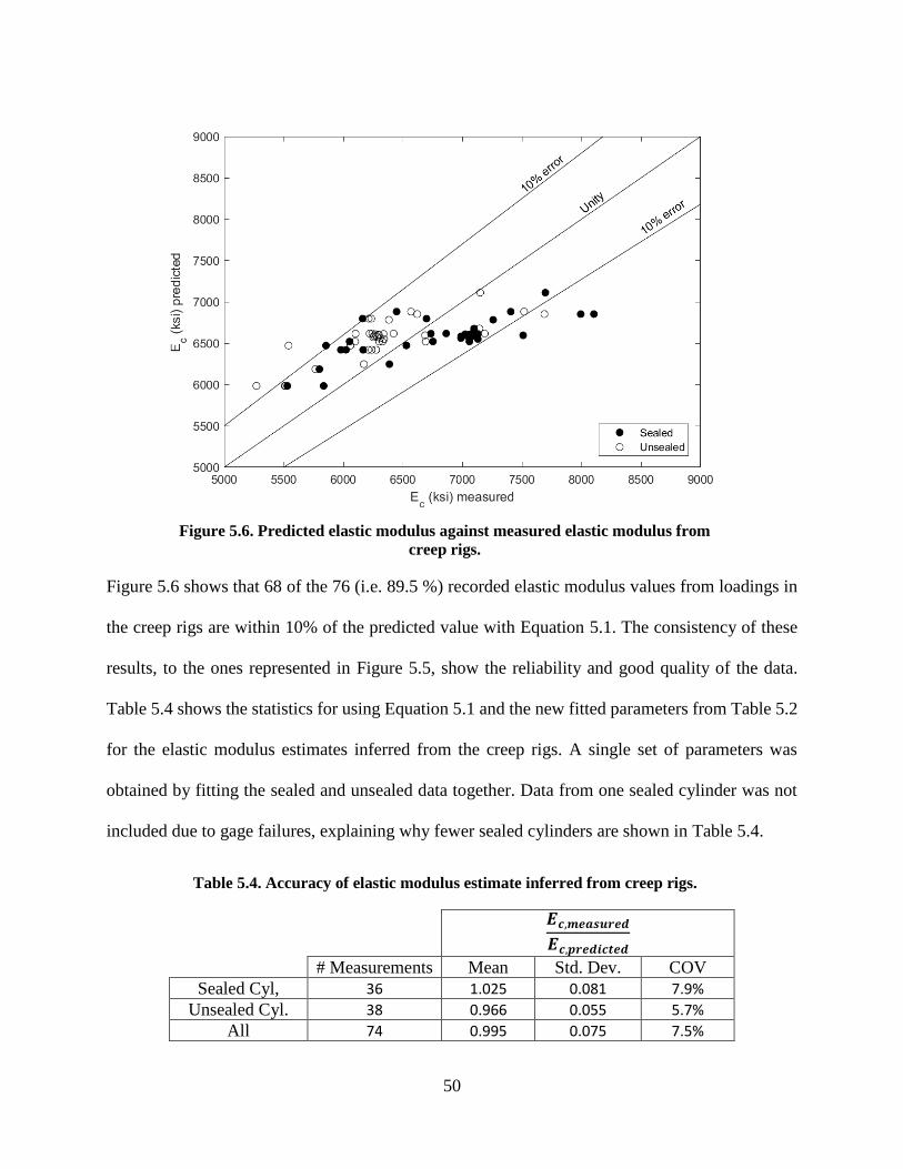
50
Figure 5.6. Predicted elastic modulus against measured elastic modulus from
creep rigs.
Figure 5.6 shows that 68 of the 76 (i.e. 89.5 %) recorded elastic modulus values from loadings in
the creep rigs are within 10% of the predicted value with Equation 5.1. The consistency of these
results, to the ones represented in Figure 5.5, show the reliability and good quality of the data.
Table 5.4 shows the statistics for using Equation 5.1 and the new fitted parameters from Table 5.2
for the elastic modulus estimates inferred from the creep rigs. A single set of parameters was
obtained by fitting the sealed and unsealed data together. Data from one sealed cylinder was not
included due to gage failures, explaining why fewer sealed cylinders are shown in Table 5.4.
Table 5.4. Accuracy of elastic modulus estimate inferred from creep rigs.
𝑬𝒄,𝒎𝒆𝒂𝒔𝒖𝒓𝒆𝒅
𝑬𝒄,𝒑𝒓𝒆𝒅𝒊𝒄𝒕𝒆𝒅
# Measurements Mean Std. Dev. COV
Sealed Cyl, 36 1.025 0.081 7.9%
Unsealed Cyl. 38 0.966 0.055 5.7%
All 74 0.995 0.075 7.5%

51
Table 5.4 shows that the new fitted model, on average, overestimates the elastic modulus of
unsealed cylinders and underestimates the elastic modulus of sealed cylinders. The overestimate
of unsealed values is not large but could partially be explained by that fact that Equation 4.1 is
used to predict the strength of both sealed and unsealed cylinders. In Section 4.3, the parameters
used in the equation were calibrated using data from the sealed cylinders meanwhile unsealed
cylinders showed generally lower strength.
Overall, the mean of the ratio of measured and predicted values is very close to unity indicating
that the fitted model does a good job and overestimates about as many data points as it
underestimates.

52
Chapter 6 Shrinkage Strains
Shrinkage measurements were performed on 10 sets of cylinders; six hot-cured (from three
different batches), two weekend-cured and two ambient-cured (each from two different batches).
Table 6.1 shows the number of cylinders from each batch.
Table 6.1. Summary of shrinkage cylinders.
Curing Batch Companion
creep specimens
Number of
cylinder
sets
Hot-cured
2 A, D, E, F, G, I 2
3 H, J, K 2
5 L, O, P, Q, R, S 2
Weekend-
cured
1 B 1
4 M 1
Ambient-cured 2 C 1
6 N 1
Each cylinder set had one unsealed and one sealed cylinder from which total and autogenous
shrinkage were measured, respectively. Drying shrinkage was estimated by subtracting the
autogenous shrinkage from the total shrinkage. The average of the two gages on each cylinder was
taken to be the shrinkage of the cylinder. The room in which the cylinders where stored was kept
at a nominal relative humidity of 40 to 50% and a temperature between 70 and 76 ºF. The humidity
and temperature records can be found in Appendix A.
6.1 Measured Shrinkage Strains
Figure 6.1 and Figure 6.2 plots the variation of the measured shrinkage strains with time for the
unsealed and sealed cylinders of each batch for the three curing regimes. The dark lines show the
average for each curing regime. In all cases the curves have a similar form, in which the rate of
shrinkage slows down considerably after about 50 days.
53
Figure 6.3 summarizes the results of the shrinkage measurements after 6 months. After 6 months,
the total shrinkage (unsealed cylinders) varied from 390 – 500 με across all curing regimes. The
averages of all curing regimes were almost identical: 495, 442 and 443 με for the hot-, weekend-
and ambient-cured, respectively. This difference is less than 4% of the measured strain. The
variance within each curing regime was highest for the ambient-cured specimens but lowest for
the hot-cured ones. As shown in Figure 6.3, both the lowest and highest total shrinkage strains
were measured on ambient.
After 6 months, the autogenous shrinkage (sealed cylinders) varied from 230 – 310 με across all
curing regimes. Again the averages of all curing regimes were very similar, being 262, 263 and
238 με for the hot-, weekend- and ambient-cured, respectively. This reflects a difference of 10%.
The variability within each curing regime was highest for the hot-cured specimens but lowest for
the ambient-cured ones, which had almost exactly the same strain for both batches. The hot-cured
specimen from batch 2 might be considered an anomaly in which the autogenous shrinkage is
about 25% larger than the average of the other specimens (which are all consistent with a
coefficient of variance of 5%).
After 6 months, the drying shrinkage varied from 150 – 260 με across all curing regimes, the
averages being 195, 178 and 206 με for the hot-, weekend- and ambient-cured, respectively. The
variability within each curing regime was highest for the ambient-cured specimens but lowest for
the hot-cured ones.
Results from Chapter 4 show that the nominally identical concrete cylinders cast in 2016 (batches
1-3) were considerably stronger than the concrete cylinders cast in 2017 (batches 4-6). This
difference does not seem to have had a considerable effect on the shrinkage of the hot- and
weekend-cured concrete. The large difference in drying shrinkage of the ambient specimens
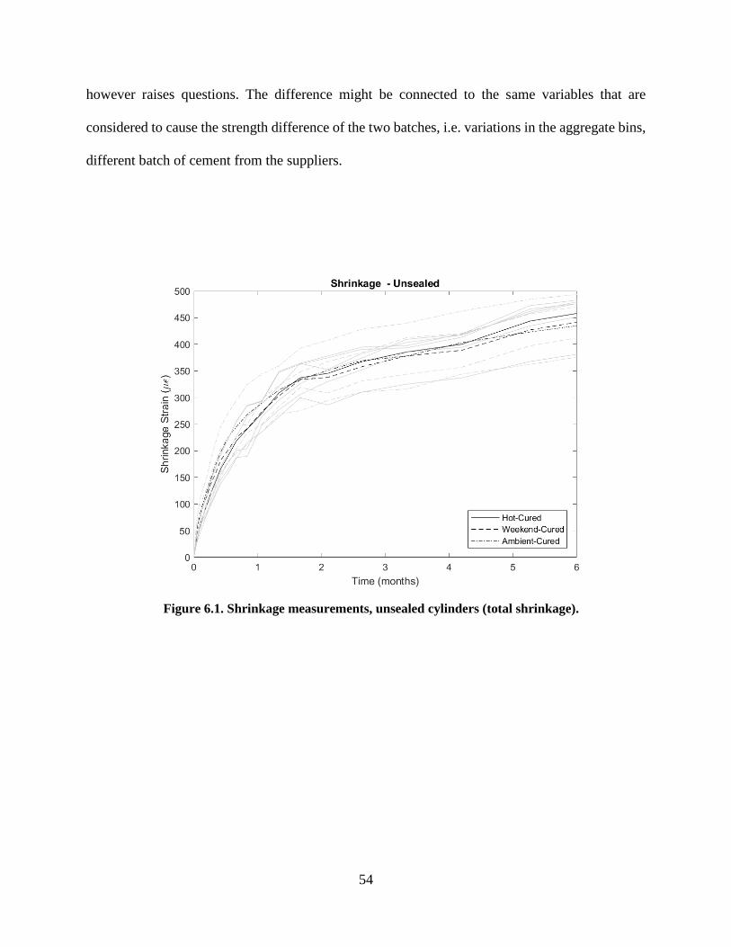
54
however raises questions. The difference might be connected to the same variables that are
considered to cause the strength difference of the two batches, i.e. variations in the aggregate bins,
different batch of cement from the suppliers.
Figure 6.1. Shrinkage measurements, unsealed cylinders (total shrinkage).
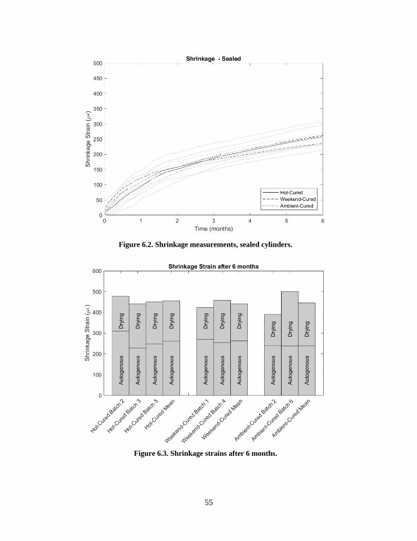
55
Figure 6.2. Shrinkage measurements, sealed cylinders.
Figure 6.3. Shrinkage strains after 6 months.

56
6.2 Parametrization of Shrinkage Strains
A time-dependent relationship was fitted to the average measured shrinkage strains for each case.
The functional form of the relationship was:
𝝐(𝒕) = 𝛋(𝐭) ∙ 𝜺(𝟐𝟖) 6.1
where
𝛋(𝐭) = 𝒂
(𝒂 − 𝟏) ∙ (𝟐𝟖 𝒕⁄ )𝟏 𝒏⁄ + 𝟏
6.2
where ε(t) is the shrinkage strain at time t, ε(28) is the shrinkage strain after 28 days, a is the ratio
between the ultimate strain value and the strain value at 28 days, and n is a parameter that controls
the rate of strain gain with time. The function has a value of 1.0 at 28 days and a slope of 0.0 at
infinite time. The time it takes to reach half of the ultimate strain can be computed as:
𝒕𝟓𝟎 = 𝟐𝟖 ∙ (𝒂 − 𝟏)𝒏 6.3
The form of this equation was originally developed to describe strength gain with time but, because
it is dimensionless, it can be applied to any time-dependent characteristic.
Figure 6.4 – Figure 6.6 show the average shrinkage strains for each curing regime fitted with the
time-dependent relationship. The error bars show the standard deviation of the measurements taken
from the unsealed and sealed shrinkage cylinders.
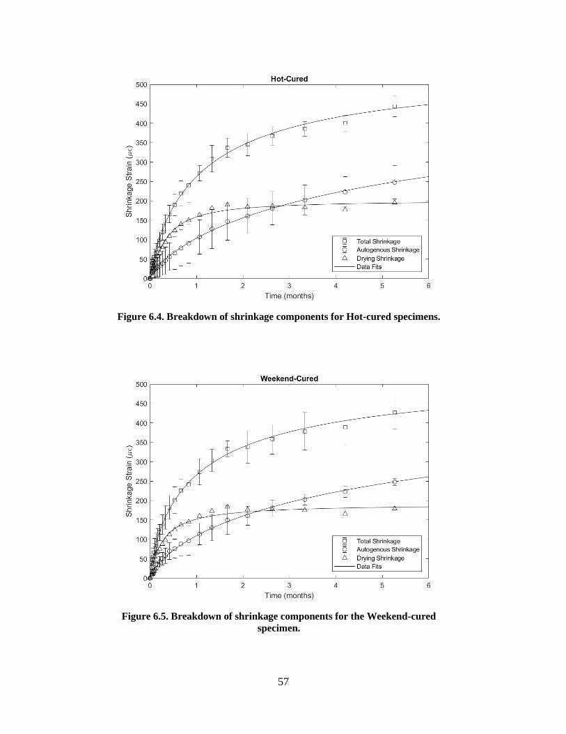
57
Figure 6.4. Breakdown of shrinkage components for Hot-cured specimens.
Figure 6.5. Breakdown of shrinkage components for the Weekend-cured
specimen.
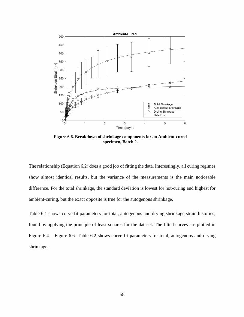
58
Figure 6.6. Breakdown of shrinkage components for an Ambient-cured
specimen, Batch 2.
The relationship (Equation 6.2) does a good job of fitting the data. Interestingly, all curing regimes
show almost identical results, but the variance of the measurements is the main noticeable
difference. For the total shrinkage, the standard deviation is lowest for hot-curing and highest for
ambient-curing, but the exact opposite is true for the autogenous shrinkage.
Table 6.1 shows curve fit parameters for total, autogenous and drying shrinkage strain histories,
found by applying the principle of least squares for the dataset. The fitted curves are plotted in
Figure 6.4 – Figure 6.6. Table 6.2 shows curve fit parameters for total, autogenous and drying
shrinkage.
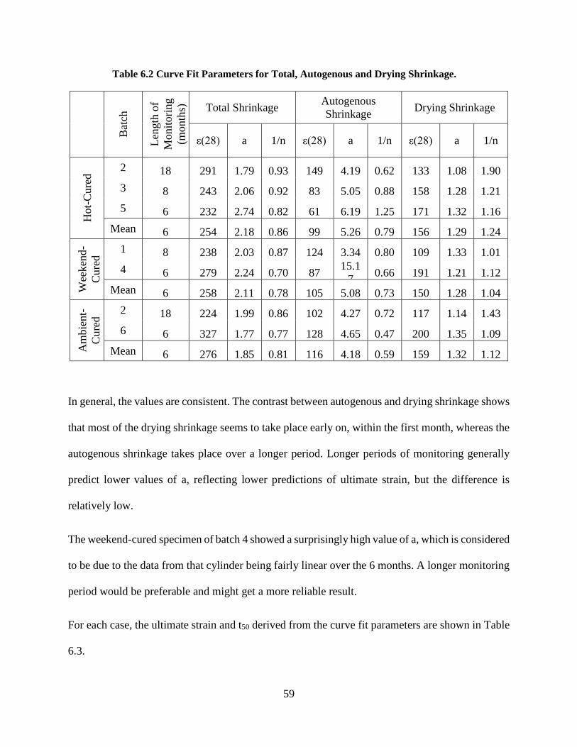
59
Table 6.2 Curve Fit Parameters for Total, Autogenous and Drying Shrinkage.
Bat
ch
Len
gth
of
Monit
ori
ng
(month
s)
Total Shrinkage Autogenous
Shrinkage Drying Shrinkage
ε(28) a 1/n ε(28) a 1/n ε(28) a 1/n
Hot-
Cure
d 2 18 291 1.79 0.93 149 4.19 0.62 133 1.08 1.90
3 8 243 2.06 0.92 83 5.05 0.88 158 1.28 1.21
5 6 232 2.74 0.82 61 6.19 1.25 171 1.32 1.16
Mean 6 254 2.18 0.86 99 5.26 0.79 156 1.29 1.24
Wee
ken
d-
Cure
d 1 8 238 2.03 0.87 124 3.34 0.80 109 1.33 1.01
4 6 279 2.24 0.70 87
15.1
7
0.66 191 1.21 1.12
Mean 6 258 2.11 0.78 105 5.08 0.73 150 1.28 1.04
Am
bie
nt-
Cure
d 2 18 224 1.99 0.86 102 4.27 0.72 117 1.14 1.43
6 6 327 1.77 0.77 128 4.65 0.47 200 1.35 1.09
Mean 6 276 1.85 0.81 116 4.18 0.59 159 1.32 1.12
In general, the values are consistent. The contrast between autogenous and drying shrinkage shows
that most of the drying shrinkage seems to take place early on, within the first month, whereas the
autogenous shrinkage takes place over a longer period. Longer periods of monitoring generally
predict lower values of a, reflecting lower predictions of ultimate strain, but the difference is
relatively low.
The weekend-cured specimen of batch 4 showed a surprisingly high value of a, which is considered
to be due to the data from that cylinder being fairly linear over the 6 months. A longer monitoring
period would be preferable and might get a more reliable result.
For each case, the ultimate strain and t50 derived from the curve fit parameters are shown in Table
6.3.

60
Table 6.3 Predicted ultimate strain and t50 for total, autogenous and drying
shrinkage.
B
atch
Len
gth
of
Monit
ori
ng
(month
s) Total
Shrinkage
Autogenous
Shrinkage
Drying
Shrinkage
Autogenous +
Drying
εult t50 εult t50 εult t50 εult
Hot-
Cure
d 2 18 520 22 623 184 144 8 767
3 8 502 30 418 139 202 10 620
5 6 637 55 375 104 226 11 602
Mean 6 554 34 522 177 201 10 723
Wee
ken
d-
Cure
d 1 8 484 29 413 81 145 9 558
4 6 623 38 1317 1509 231 7 1548
Mean 6 546 32 533 190 191 8 725
Am
bie
nt-
Cure
d 2 18 444 28 436 145 133 7 569
6 6 578 20 594 436 270 11 864
Mean 6 510 23 483 200 210 10 693
Comparing each curing regime, the fits for batches 4-6 (all cast in 2017) predict about 25 - 30%
higher total ultimate strains than the fits for batches 1-3 (all cast in 2016). This suggests that the
variance in the nominally identical concrete cast a year apart, noticed in Chapter 4, has an effect
on the ultimate shrinkage, even though the results in Section 6.1 do not show a clear connection.
The difference between the individual batches was larger than the differences between the curing
regimes, which suggests that hot-curing does not affect the shrinkage more than the natural
variations in the concrete. The results however suggest that the total ultimate shrinkage of hot-
cured concrete is about 10% higher than of ambient-cured concrete.

61
Adding the ultimate autogenous shrinkage to the ultimate drying shrinkage does generally not
agree with the predicted total ultimate shrinkage, as it should. The summation gives higher values
in all cases, except for hot-cured Batch 5.
62
Chapter 7 Creep
This chapter analyzes the creep strains measured in the unsealed and sealed cylinders. Chapter 3
describes the procedure that was followed to convert the raw data into the processed creep data.
Appendix D provides strain histories for all test cylinders and reports values of creep strains for
all specimens at the ages of 7 days and 6 months.
The total creep strains were separated into basic and drying creep components. Basic creep is the
creep that happens in the absence of drying (i.e., taken as the creep strains measured in the sealed
specimens), and the drying creep is the additional creep that occurs when the concrete can dry (i.e.,
difference between the creep strains in the sealed and unsealed specimens).
7.1 Effects of Curing
To examine the effect of the three curing regimes, five specimens can be compared. All specimens
were loaded to the same load level of 2.7 ksi at the time they were estimated to have gained
sufficient strength, 10 ksi. Three of these specimens were cast in 2016: Specimen A3H_2.7_0.7
was hot-cured (H), specimen B1W_2.7_2.8 was weekend-cured (W), and C3A_2.7_3.8, was
ambient-cured. Specimens L (H) and M (W) were cast in 2017 to provide duplicates of specimens
A and B. Figure 7.1 plots the variation of the total creep strains with time for these five specimens.
The creep strain histories were calculated by subtracting the elastic and shrinkage strains from the
total strain from the unsealed cylinders. The shrinkage strains were obtained from the companion,
unsealed cylinders. For easier comparison, solid lines show the average of each curing regime.
Only data from one ambient cured specimen (cast in 2016) is however available, in which case the
average is simply the creep of that single specimen.
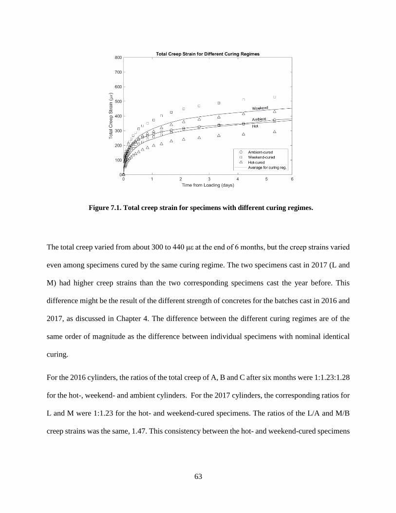
63
Figure 7.1. Total creep strain for specimens with different curing regimes.
The total creep varied from about 300 to 440 με at the end of 6 months, but the creep strains varied
even among specimens cured by the same curing regime. The two specimens cast in 2017 (L and
M) had higher creep strains than the two corresponding specimens cast the year before. This
difference might be the result of the different strength of concretes for the batches cast in 2016 and
2017, as discussed in Chapter 4. The difference between the different curing regimes are of the
same order of magnitude as the difference between individual specimens with nominal identical
curing.
For the 2016 cylinders, the ratios of the total creep of A, B and C after six months were 1:1.23:1.28
for the hot-, weekend- and ambient cylinders. For the 2017 cylinders, the corresponding ratios for
L and M were 1:1.23 for the hot- and weekend-cured specimens. The ratios of the L/A and M/B
creep strains was the same, 1.47. This consistency between the hot- and weekend-cured specimens
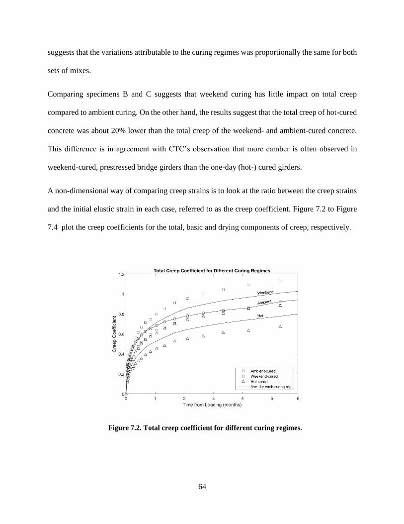
64
suggests that the variations attributable to the curing regimes was proportionally the same for both
sets of mixes.
Comparing specimens B and C suggests that weekend curing has little impact on total creep
compared to ambient curing. On the other hand, the results suggest that the total creep of hot-cured
concrete was about 20% lower than the total creep of the weekend- and ambient-cured concrete.
This difference is in agreement with CTC’s observation that more camber is often observed in
weekend-cured, prestressed bridge girders than the one-day (hot-) cured girders.
A non-dimensional way of comparing creep strains is to look at the ratio between the creep strains
and the initial elastic strain in each case, referred to as the creep coefficient. Figure 7.2 to Figure
7.4 plot the creep coefficients for the total, basic and drying components of creep, respectively.
Figure 7.2. Total creep coefficient for different curing regimes.
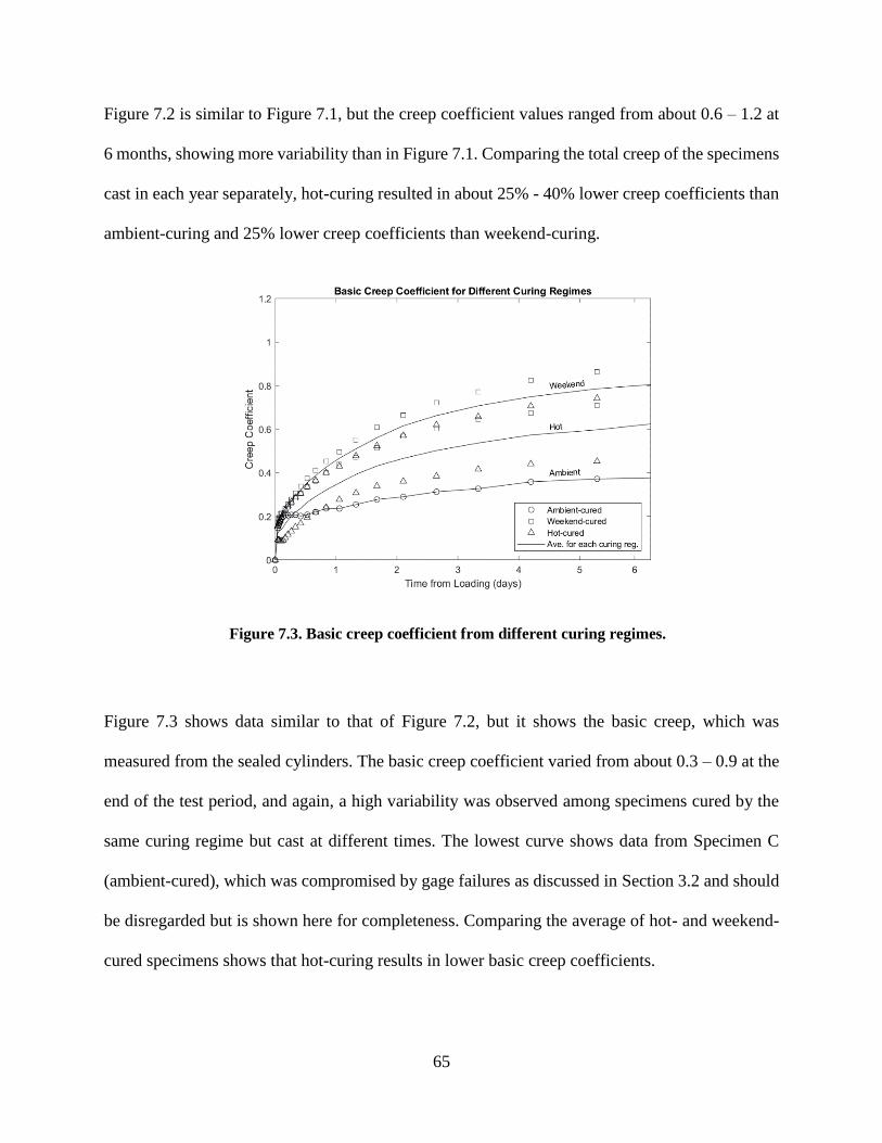
65
Figure 7.2 is similar to Figure 7.1, but the creep coefficient values ranged from about 0.6 – 1.2 at
6 months, showing more variability than in Figure 7.1. Comparing the total creep of the specimens
cast in each year separately, hot-curing resulted in about 25% - 40% lower creep coefficients than
ambient-curing and 25% lower creep coefficients than weekend-curing.
Figure 7.3. Basic creep coefficient from different curing regimes.
Figure 7.3 shows data similar to that of Figure 7.2, but it shows the basic creep, which was
measured from the sealed cylinders. The basic creep coefficient varied from about 0.3 – 0.9 at the
end of the test period, and again, a high variability was observed among specimens cured by the
same curing regime but cast at different times. The lowest curve shows data from Specimen C
(ambient-cured), which was compromised by gage failures as discussed in Section 3.2 and should
be disregarded but is shown here for completeness. Comparing the average of hot- and weekend-
cured specimens shows that hot-curing results in lower basic creep coefficients.
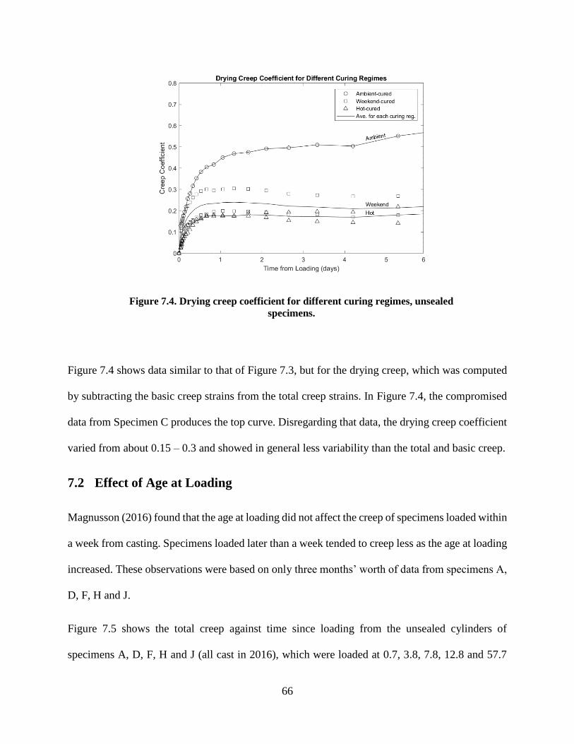
66
Figure 7.4. Drying creep coefficient for different curing regimes, unsealed
specimens.
Figure 7.4 shows data similar to that of Figure 7.3, but for the drying creep, which was computed
by subtracting the basic creep strains from the total creep strains. In Figure 7.4, the compromised
data from Specimen C produces the top curve. Disregarding that data, the drying creep coefficient
varied from about 0.15 – 0.3 and showed in general less variability than the total and basic creep.
7.2 Effect of Age at Loading
Magnusson (2016) found that the age at loading did not affect the creep of specimens loaded within
a week from casting. Specimens loaded later than a week tended to creep less as the age at loading
increased. These observations were based on only three months’ worth of data from specimens A,
D, F, H and J.
Figure 7.5 shows the total creep against time since loading from the unsealed cylinders of
specimens A, D, F, H and J (all cast in 2016), which were loaded at 0.7, 3.8, 7.8, 12.8 and 57.7
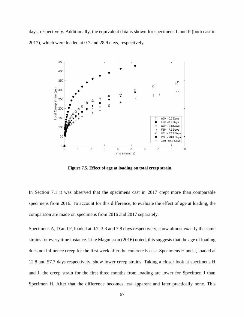
67
days, respectively. Additionally, the equivalent data is shown for specimens L and P (both cast in
2017), which were loaded at 0.7 and 28.9 days, respectively.
Figure 7.5. Effect of age at loading on total creep strain.
In Section 7.1 it was observed that the specimens cast in 2017 crept more than comparable
specimens from 2016. To account for this difference, to evaluate the effect of age at loading, the
comparison are made on specimens from 2016 and 2017 separately.
Specimens A, D and F, loaded at 0.7, 3.8 and 7.8 days respectively, show almost exactly the same
strains for every time instance. Like Magnusson (2016) noted, this suggests that the age of loading
does not influence creep for the first week after the concrete is cast. Specimens H and J, loaded at
12.8 and 57.7 days respectively, show lower creep strains. Taking a closer look at specimens H
and J, the creep strain for the first three months from loading are lower for Specimen J than
Specimen H. After that the difference becomes less apparent and later practically none. This
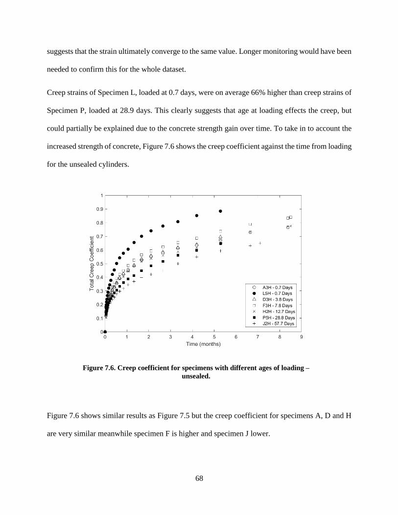
68
suggests that the strain ultimately converge to the same value. Longer monitoring would have been
needed to confirm this for the whole dataset.
Creep strains of Specimen L, loaded at 0.7 days, were on average 66% higher than creep strains of
Specimen P, loaded at 28.9 days. This clearly suggests that age at loading effects the creep, but
could partially be explained due to the concrete strength gain over time. To take in to account the
increased strength of concrete, Figure 7.6 shows the creep coefficient against the time from loading
for the unsealed cylinders.
Figure 7.6. Creep coefficient for specimens with different ages of loading –
unsealed.
Figure 7.6 shows similar results as Figure 7.5 but the creep coefficient for specimens A, D and H
are very similar meanwhile specimen F is higher and specimen J lower.

69
Figure 7.7 similarly shows the basic creep coefficient, measured from the sealed cylinders of the
specimens in discussion, against time. Because of many gage malfunctions on the sealed cylinders
not much meaning can be derived from the figure.
Figure 7.8 shows the drying creep coefficient, obtained by subtracting the basic creep coefficient
from the total creep coefficient, against time. Again, because of many gage malfunctions on the
sealed cylinders not much meaning can be derived from the figure but it is shown for completeness.
Figure 7.7. Creep coefficient for specimens with different ages of loading –
sealed.

70
Figure 7.8. Drying creep coefficient for specimens with different ages of loading.
Figure 7.9 shows the total (from unsealed cylinders) and basic (from sealed cylinder) creep strains
at the end of six months against the age at loading.
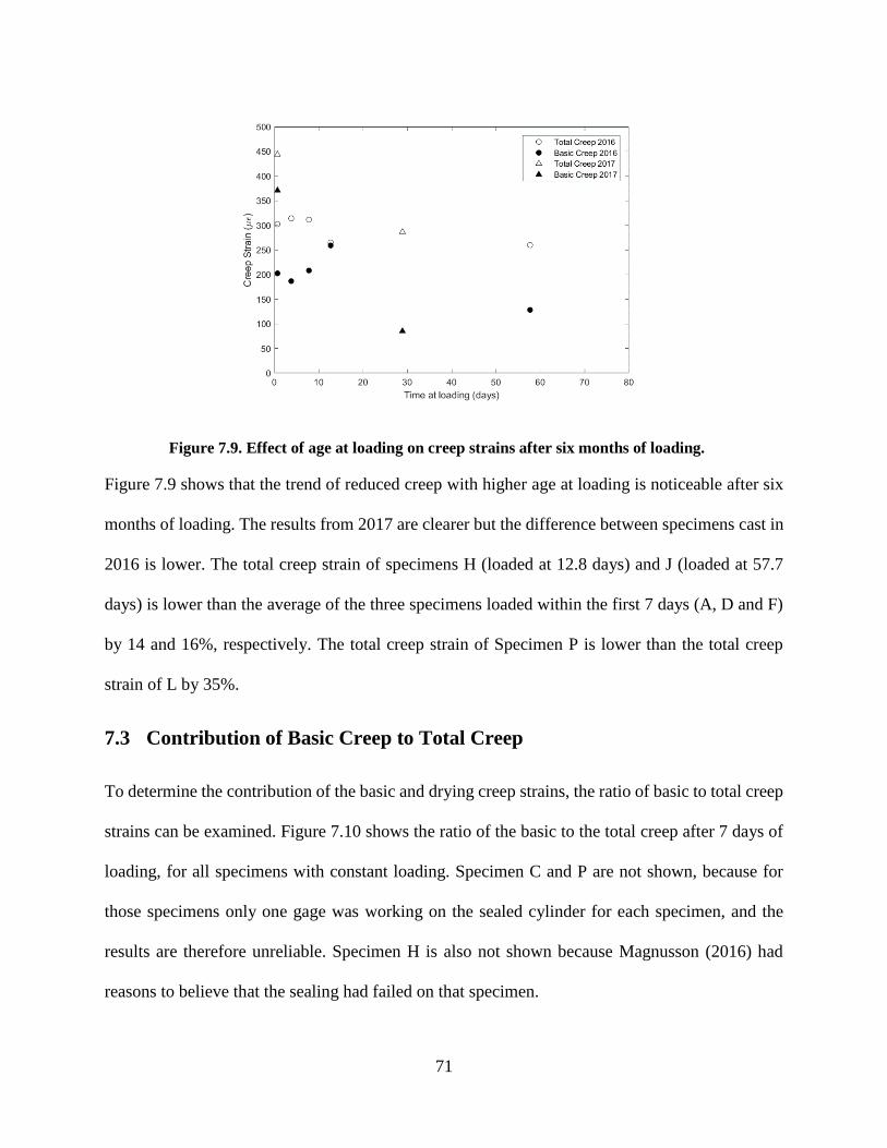
71
Figure 7.9. Effect of age at loading on creep strains after six months of loading.
Figure 7.9 shows that the trend of reduced creep with higher age at loading is noticeable after six
months of loading. The results from 2017 are clearer but the difference between specimens cast in
2016 is lower. The total creep strain of specimens H (loaded at 12.8 days) and J (loaded at 57.7
days) is lower than the average of the three specimens loaded within the first 7 days (A, D and F)
by 14 and 16%, respectively. The total creep strain of Specimen P is lower than the total creep
strain of L by 35%.
7.3 Contribution of Basic Creep to Total Creep
To determine the contribution of the basic and drying creep strains, the ratio of basic to total creep
strains can be examined. Figure 7.10 shows the ratio of the basic to the total creep after 7 days of
loading, for all specimens with constant loading. Specimen C and P are not shown, because for
those specimens only one gage was working on the sealed cylinder for each specimen, and the
results are therefore unreliable. Specimen H is also not shown because Magnusson (2016) had
reasons to believe that the sealing had failed on that specimen.
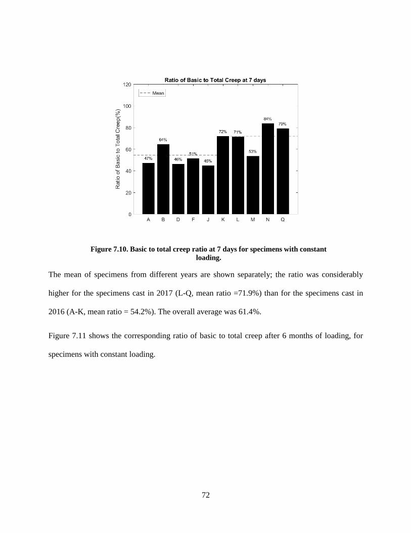
72
Figure 7.10. Basic to total creep ratio at 7 days for specimens with constant
loading.
The mean of specimens from different years are shown separately; the ratio was considerably
higher for the specimens cast in 2017 (L-Q, mean ratio =71.9%) than for the specimens cast in
2016 (A-K, mean ratio = 54.2%). The overall average was 61.4%.
Figure 7.11 shows the corresponding ratio of basic to total creep after 6 months of loading, for
specimens with constant loading.

73
Figure 7.11. Basic to total creep ratio at 6 months for specimens with
constant loading.
Again, it is observed that the ratio of basic creep is higher for specimens L-Q (81.8%) than for
specimens A-K (68.8%). The overall average increased from the 7-day average (61.4%) to 72.6%
at 6 months. For every specimen, the ratio increased between the two times.
Figure 7.12 shows the variation basic-to-total creep ratio against time for Specimen A, to illustrate
how this ratio behaved over time.

74
Figure 7.12. Ratio of basic to total creep for Specimen A against time.
In Figure 7.12 the ratio seems to level off after about 40 days. This suggests that the drying creep
is a larger component for early creep than for long-term creep. Here, the results suggest the drying
creep and the basic creep increase proportionally after 40 days (for the 4”-diameter cylinders used
in this study). The drying depends on the surface-volume ratio, so it would be expected to affect
the time variation of the basic to total creep ratio. This would have to be examined with different
size test cylinders.
7.4 Effects of Cyclic Loading
The effect of cyclic loading on creep can be examined using data from Specimen S. Through the
course of 6 months, Specimen S underwent seven, two-week-long cycles of loading and unloading,
the total creep that took place in each load cycle is shown in Figure 7.13.

75
Figure 7.13. Effect of cyclic loading on total creep.
From Figure 7.13, a decreasing trend can be observed for the first three cycles, and then the total
creep for every cycle seems to about be the same after that. This decreasing trend can be considered
a result of two things; different times of loading and the effect of repetitive loading and unloading
on creep. Magnusson (2016) found that loading at a later ages reduced the total creep.
The basic creep for each load cycle is shown in Figure 7.14. Figure 7.14 shows that the basic creep
decreases, like the total creep, noticeably for the first three cycles, then it keeps on decreasing
consistently, but the difference between each cycle gets lower. Cycle 7 is the only cycle that does
not show lower basic creep than the cycle before. This suggests that the basic creep reduces with
every load cycle when concrete experiences cyclic loading.
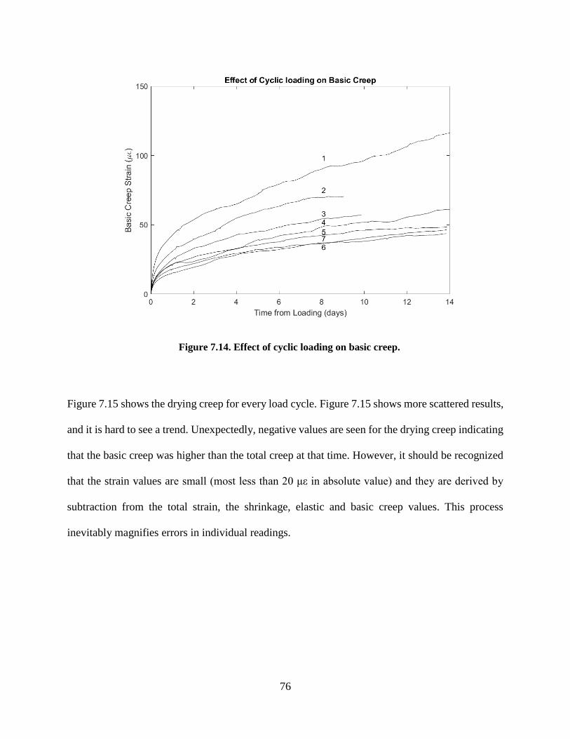
76
Figure 7.14. Effect of cyclic loading on basic creep.
Figure 7.15 shows the drying creep for every load cycle. Figure 7.15 shows more scattered results,
and it is hard to see a trend. Unexpectedly, negative values are seen for the drying creep indicating
that the basic creep was higher than the total creep at that time. However, it should be recognized
that the strain values are small (most less than 20 με in absolute value) and they are derived by
subtraction from the total strain, the shrinkage, elastic and basic creep values. This process
inevitably magnifies errors in individual readings.
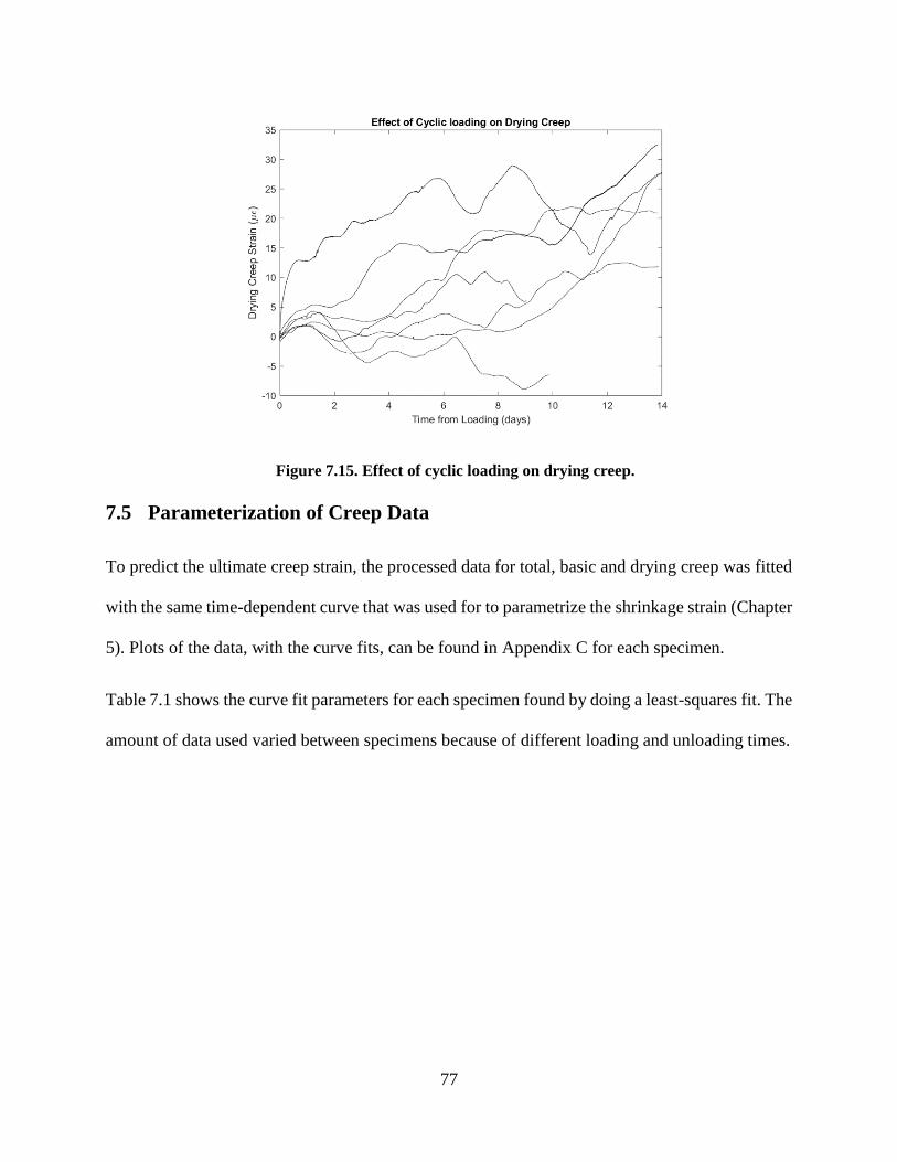
77
Figure 7.15. Effect of cyclic loading on drying creep.
7.5 Parameterization of Creep Data
To predict the ultimate creep strain, the processed data for total, basic and drying creep was fitted
with the same time-dependent curve that was used for to parametrize the shrinkage strain (Chapter
5). Plots of the data, with the curve fits, can be found in Appendix C for each specimen.
Table 7.1 shows the curve fit parameters for each specimen found by doing a least-squares fit. The
amount of data used varied between specimens because of different loading and unloading times.
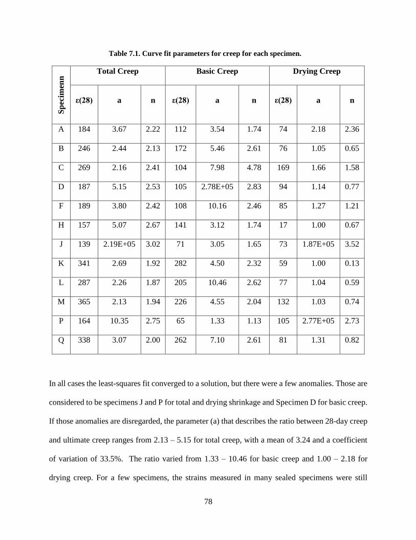
78
Table 7.1. Curve fit parameters for creep for each specimen. S
pec
imen
n Total Creep Basic Creep Drying Creep
ε(28) a n ε(28) a n ε(28) a n
A 184 3.67 2.22 112 3.54 1.74 74 2.18 2.36
B 246 2.44 2.13 172 5.46 2.61 76 1.05 0.65
C 269 2.16 2.41 104 7.98 4.78 169 1.66 1.58
D 187 5.15 2.53 105 2.78E+05 2.83 94 1.14 0.77
F 189 3.80 2.42 108 10.16 2.46 85 1.27 1.21
H 157 5.07 2.67 141 3.12 1.74 17 1.00 0.67
J 139 2.19E+05 3.02 71 3.05 1.65 73 1.87E+05 3.52
K 341 2.69 1.92 282 4.50 2.32 59 1.00 0.13
L 287 2.26 1.87 205 10.46 2.62 77 1.04 0.59
M 365 2.13 1.94 226 4.55 2.04 132 1.03 0.74
P 164 10.35 2.75 65 1.33 1.13 105 2.77E+05 2.73
Q 338 3.07 2.00 262 7.10 2.61 81 1.31 0.82
In all cases the least-squares fit converged to a solution, but there were a few anomalies. Those are
considered to be specimens J and P for total and drying shrinkage and Specimen D for basic creep.
If those anomalies are disregarded, the parameter (a) that describes the ratio between 28-day creep
and ultimate creep ranges from 2.13 – 5.15 for total creep, with a mean of 3.24 and a coefficient
of variation of 33.5%. The ratio varied from 1.33 – 10.46 for basic creep and 1.00 – 2.18 for
drying creep. For a few specimens, the strains measured in many sealed specimens were still
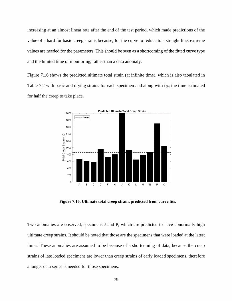
79
increasing at an almost linear rate after the end of the test period, which made predictions of the
value of a hard for basic creep strains because, for the curve to reduce to a straight line, extreme
values are needed for the parameters. This should be seen as a shortcoming of the fitted curve type
and the limited time of monitoring, rather than a data anomaly.
Figure 7.16 shows the predicted ultimate total strain (at infinite time), which is also tabulated in
Table 7.2 with basic and drying strains for each specimen and along with t50; the time estimated
for half the creep to take place.
Figure 7.16. Ultimate total creep strain, predicted from curve fits.
Two anomalies are observed, specimens J and P, which are predicted to have abnormally high
ultimate creep strains. It should be noted that those are the specimens that were loaded at the latest
times. These anomalies are assumed to be because of a shortcoming of data, because the creep
strains of late loaded specimens are lower than creep strains of early loaded specimens, therefore
a longer data series is needed for those specimens.
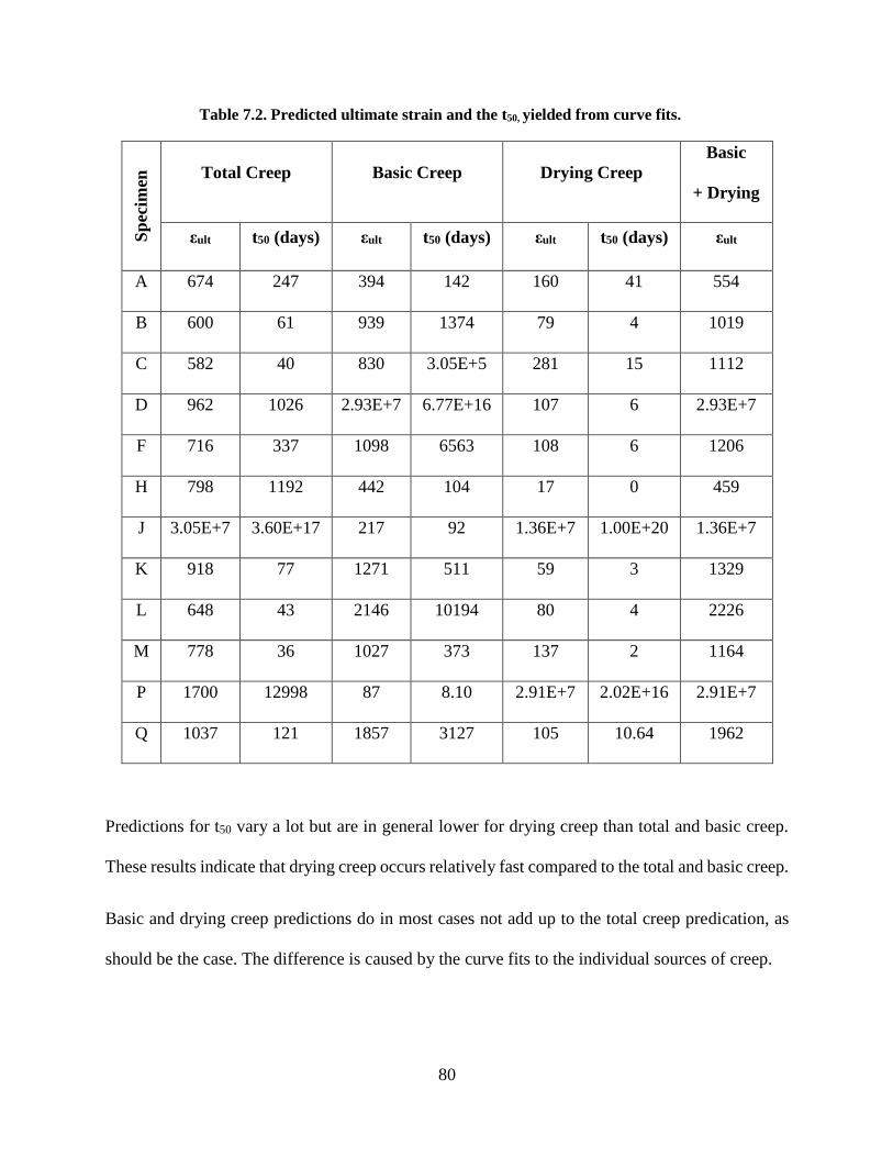
80
Table 7.2. Predicted ultimate strain and the t50, yielded from curve fits.
Sp
ecim
en
Total Creep Basic Creep Drying Creep
Basic
+ Drying
εult t50 (days) εult t50 (days) εult t50 (days) εult
A 674 247 394 142 160 41 554
B 600 61 939 1374 79 4 1019
C 582 40 830 3.05E+5 281 15 1112
D 962 1026 2.93E+7 6.77E+16 107 6 2.93E+7
F 716 337 1098 6563 108 6 1206
H 798 1192 442 104 17 0 459
J 3.05E+7 3.60E+17 217 92 1.36E+7 1.00E+20 1.36E+7
K 918 77 1271 511 59 3 1329
L 648 43 2146 10194 80 4 2226
M 778 36 1027 373 137 2 1164
P 1700 12998 87 8.10 2.91E+7 2.02E+16 2.91E+7
Q 1037 121 1857 3127 105 10.64 1962
Predictions for t50 vary a lot but are in general lower for drying creep than total and basic creep.
These results indicate that drying creep occurs relatively fast compared to the total and basic creep.
Basic and drying creep predictions do in most cases not add up to the total creep predication, as
should be the case. The difference is caused by the curve fits to the individual sources of creep.

81
Chapter 8 Creep Recovery
To be able to predict the behavior of concrete submitted to stress variations over time, it is
important to analyze the creep recovery. This phenomenon has not been studied as thoroughly as
creep under sustained loads, even though many investigations on creep behavior include recorded
data after specimens have been unloaded. The main reason for this is that most experimental data
have not resulted from a systematic investigation of creep recovery, but instead, as a side product
of creep experiments (Yue & Taerwe, 1992). In this study, the unloading data can be used to give
an insight on the parameters that effect the creep recovery of hot-cured concrete and how it should
be modeled.
8.1 Contributions of Basic Creep Recovery to Total
When a specimen is unloaded, the creep that had previously been developed is typically partially
or fully recoverable. The creep recovery is measured from the time right after unloading until a
specified time instance. The sustained strain at that time instance is referred to as the residual
creep. The creep-recovery ratio is the ratio of the recovered creep to the previously developed
creep before unloading. This is shown graphically in Figure 8.1, where the unsealed cylinder of
Specimen O is used as an example to explain these different phenomena.

82
Figure 8.1. Identification of creep, recovered creep and residual creep.
Figure 8.2 shows the ratio of the creep-recovery ratio at 28 days after unloading for 15 specimens.
These 15 specimens represent all of the specimens that were subject to a nominally constant axial
stress and then unloaded. Specimens A and C were not unloaded. Specimens I and S were
subjected to axial loads that varied with time. Specimen G, O and P only show bars for total creep,
because gage failures on the sealed cylinders compromised the creep data for basic and drying
creep.
It should also be noted that Specimen E was loaded at 0.7 days and unloaded at an early age (2.8
days) when not much total and basic creep had yet developed (158 and 73 µε). The basic creep
recovery for this specimen exceeded the basic creep measured prior to unloading, resulting in a
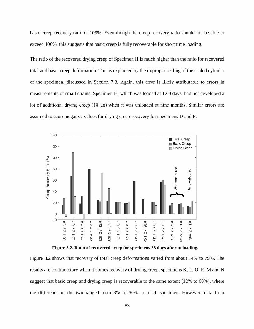
83
basic creep-recovery ratio of 109%. Even though the creep-recovery ratio should not be able to
exceed 100%, this suggests that basic creep is fully recoverable for short time loading.
The ratio of the recovered drying creep of Specimen H is much higher than the ratio for recovered
total and basic creep deformation. This is explained by the improper sealing of the sealed cylinder
of the specimen, discussed in Section 7.3. Again, this error is likely attributable to errors in
measurements of small strains. Specimen H, which was loaded at 12.8 days, had not developed a
lot of additional drying creep (18 µε) when it was unloaded at nine months. Similar errors are
assumed to cause negative values for drying creep-recovery for specimens D and F.
Figure 8.2. Ratio of recovered creep for specimens 28 days after unloading.
Figure 8.2 shows that recovery of total creep deformations varied from about 14% to 79%. The
results are contradictory when it comes recovery of drying creep, specimens K, L, Q, R, M and N
suggest that basic creep and drying creep is recoverable to the same extent (12% to 60%), where
the difference of the two ranged from 3% to 50% for each specimen. However, data from
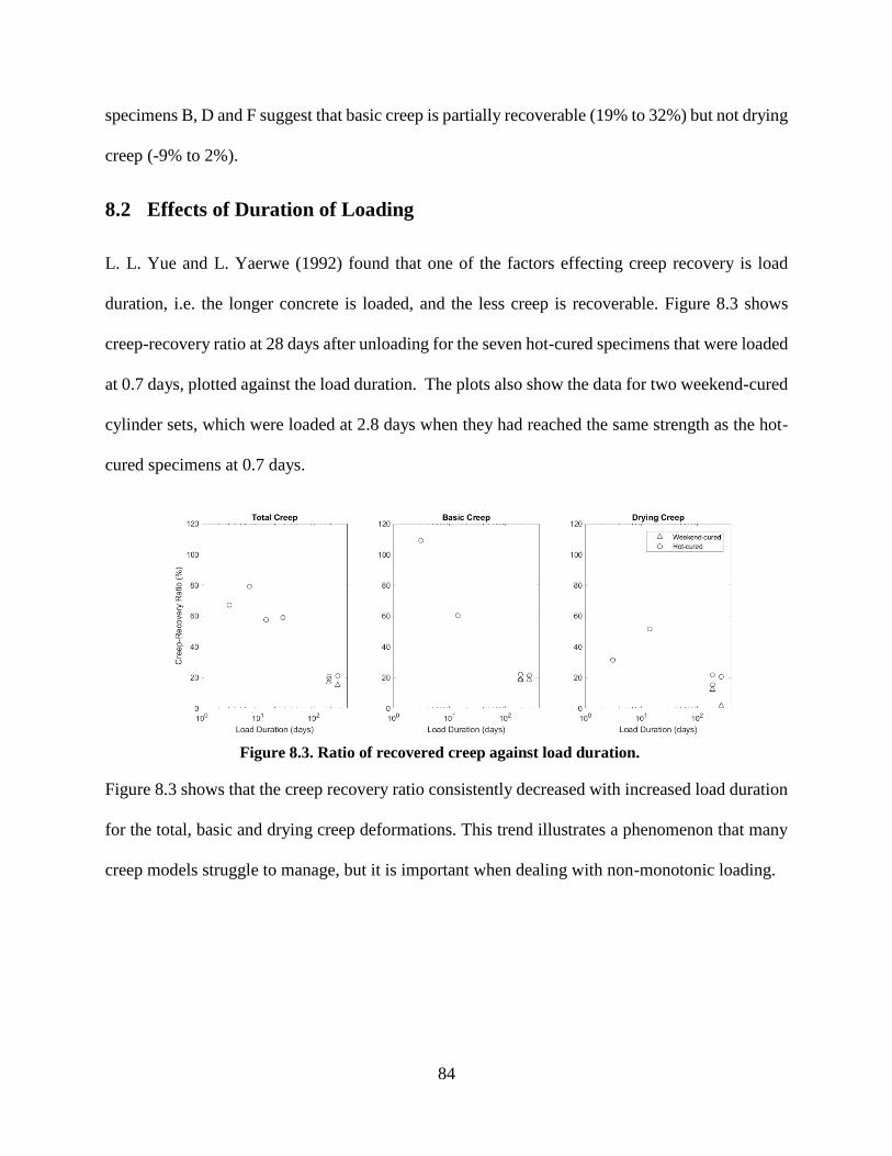
84
specimens B, D and F suggest that basic creep is partially recoverable (19% to 32%) but not drying
creep (-9% to 2%).
8.2 Effects of Duration of Loading
L. L. Yue and L. Yaerwe (1992) found that one of the factors effecting creep recovery is load
duration, i.e. the longer concrete is loaded, and the less creep is recoverable. Figure 8.3 shows
creep-recovery ratio at 28 days after unloading for the seven hot-cured specimens that were loaded
at 0.7 days, plotted against the load duration. The plots also show the data for two weekend-cured
cylinder sets, which were loaded at 2.8 days when they had reached the same strength as the hot-
cured specimens at 0.7 days.
Figure 8.3. Ratio of recovered creep against load duration.
Figure 8.3 shows that the creep recovery ratio consistently decreased with increased load duration
for the total, basic and drying creep deformations. This trend illustrates a phenomenon that many
creep models struggle to manage, but it is important when dealing with non-monotonic loading.

85
8.3 Effects of Age of Initial Loading
The age of initial loading is considered to affect creep recovery and according to Mei, Zhang,
Wang and Zou (2017) the creep recovery is expected to decrease with the increase of loading age.
Figure 8.4 shows the creep-recovery ratio plotted against the age of initial loading for specimens
D, F, H, J, L and P, which were all loaded for more than five months. Specimen P was loaded for
five months, L for six months, J for seven months and D, F and H for nine months. Specimen P
results are not shown for basic and drying creep recovery because of gage failures on the sealed
cylinder of that specimen. It should be noted that the sealing on the sealed cylinder of Specimen
H was considered to have failed, which explains the anomalistic behavior in the graph for basic
and drying creep recovery.
Figure 8.4. Creep-recovery ratio against age at initial loading.
Surprisingly, the total and basic creep-recovery ratio seems to increase with age at initial loading,
contrary to what Mei, Zhang, Wang and Zou (2017) stated. Results for drying creep-recovery ratio,
on the other hand, suggest that drying creep is not recoverable if the specimen is loaded at 3.8 days
or later (if the anomalistic behavior of Specimen H is ignored). More data is needed to confirm
these findings.
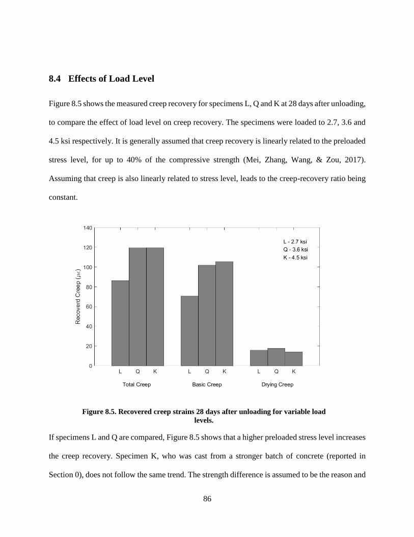
86
8.4 Effects of Load Level
Figure 8.5 shows the measured creep recovery for specimens L, Q and K at 28 days after unloading,
to compare the effect of load level on creep recovery. The specimens were loaded to 2.7, 3.6 and
4.5 ksi respectively. It is generally assumed that creep recovery is linearly related to the preloaded
stress level, for up to 40% of the compressive strength (Mei, Zhang, Wang, & Zou, 2017).
Assuming that creep is also linearly related to stress level, leads to the creep-recovery ratio being
constant.
Figure 8.5. Recovered creep strains 28 days after unloading for variable load
levels.
If specimens L and Q are compared, Figure 8.5 shows that a higher preloaded stress level increases
the creep recovery. Specimen K, who was cast from a stronger batch of concrete (reported in
Section 0), does not follow the same trend. The strength difference is assumed to be the reason and
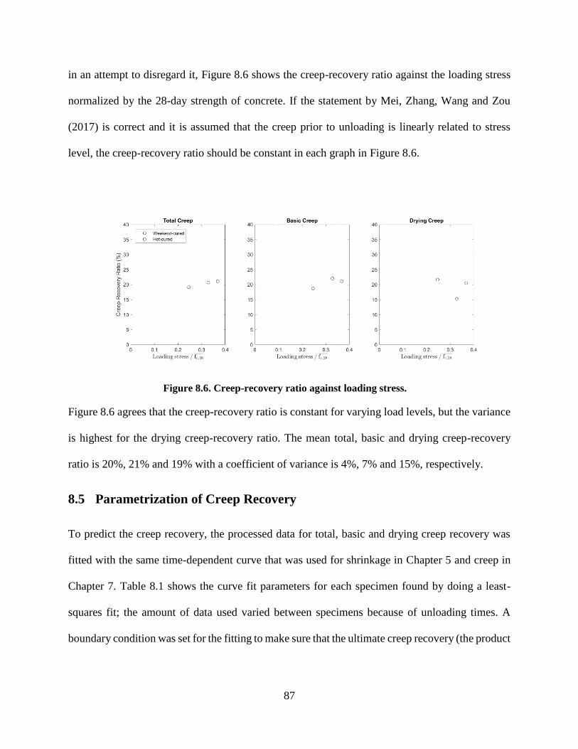
87
in an attempt to disregard it, Figure 8.6 shows the creep-recovery ratio against the loading stress
normalized by the 28-day strength of concrete. If the statement by Mei, Zhang, Wang and Zou
(2017) is correct and it is assumed that the creep prior to unloading is linearly related to stress
level, the creep-recovery ratio should be constant in each graph in Figure 8.6.
Figure 8.6. Creep-recovery ratio against loading stress.
Figure 8.6 agrees that the creep-recovery ratio is constant for varying load levels, but the variance
is highest for the drying creep-recovery ratio. The mean total, basic and drying creep-recovery
ratio is 20%, 21% and 19% with a coefficient of variance is 4%, 7% and 15%, respectively.
8.5 Parametrization of Creep Recovery
To predict the creep recovery, the processed data for total, basic and drying creep recovery was
fitted with the same time-dependent curve that was used for shrinkage in Chapter 5 and creep in
Chapter 7. Table 8.1 shows the curve fit parameters for each specimen found by doing a least-
squares fit; the amount of data used varied between specimens because of unloading times. A
boundary condition was set for the fitting to make sure that the ultimate creep recovery (the product
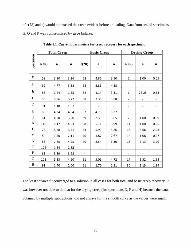
88
of ε(28) and a) would not exceed the creep evident before unloading. Data from sealed specimens
G, O and P was compromised by gage failures.
Table 8.1. Curve fit parameters for creep recovery for each specimen.
Sp
ecim
en Total Creep Basic Creep Drying Creep
ε(28) a n ε(28) a n ε(28) a n
B 59 3.90 3.26 58 4.86 3.50 2 1.00 0.05
D 62 4.77 3.38 68 3.86 4.33 - - -
E 85 1.24 1.55 64 1.14 3.31 1 26.25 0.53
F 58 5.86 3.72 68 3.35 3.98 - - -
G 91 1.18 1.57 - - - - - -
H 68 4.24 4.54 57 4.76 3.37 - - -
J 61 4.50 3.20 59 2.33 3.05 2 1.00 0.09
K 110 5.17 4.03 98 5.11 3.99 11 1.00 0.05
L 78 5.78 3.71 63 5.99 3.86 15 3.66 2.93
M 84 1.50 2.11 70 1.87 2.67 14 1.08 0.97
N 88 7.85 4.95 70 8.54 5.30 18 5.13 3.79
O 122 1.84 2.85 - - - - - -
P 66 3.69 3.28 - - - - - -
Q 108 5.33 4.50 91 5.06 4.72 17 1.52 1.93
R 91 1.40 2.00 61 1.70 2.51 30 1.15 1.34
The least squares fit converged to a solution in all cases for both total and basic creep recovery, it
was however not able to do that for the drying creep (for specimens D, F and H) because the data,
obtained by multiple subtractions, did not always form a smooth curve as the values were small.
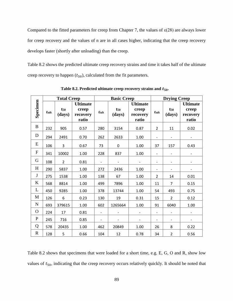
89
Compared to the fitted parameters for creep from Chapter 7, the values of ε(28) are always lower
for creep recovery and the values of n are in all cases higher, indicating that the creep recovery
develops faster (shortly after unloading) than the creep.
Table 8.2 shows the predicted ultimate creep recovery strains and time it takes half of the ultimate
creep recovery to happen (𝑡50), calculated from the fit parameters.
Table 8.2. Predicted ultimate creep recovery strains and 𝒕𝟓𝟎.
Sp
ecim
en Total Creep Basic Creep Drying Creep
εult t50
(days)
Ultimate
creep
recovery
ratio
εult t50
(days)
Ultimate
creep
recovery
ratio
εult t50
(days)
Ultimate
creep
recovery
ratio
B 232 905 0.57 280 3154 0.87 2 11 0.02
D 294 2491 0.70 262 2633 1.00 - - -
E 106 3 0.67 73 0 1.00 37 157 0.43
F 341 10002 1.00 228 837 1.00 - - -
G 108 2 0.81 - - - - - -
H 290 5837 1.00 272 2436 1.00 - - -
J 275 1538 1.00 138 67 1.00 2 14 0.01
K 568 8814 1.00 499 7896 1.00 11 7 0.15
L 450 9285 1.00 378 13744 1.00 54 493 0.75
M 126 6 0.23 130 19 0.31 15 2 0.12
N 693 379615 1.00 602 1265664 1.00 91 6040 1.00
O 224 17 0.81 - - - - - -
P 245 716 0.85 - - - - - -
Q 578 20435 1.00 462 20849 1.00 26 8 0.22
R 128 5 0.66 104 12 0.78 34 2 0.56
Table 8.2 shows that specimens that were loaded for a short time, e.g. E, G, O and R, show low
values of 𝑡50, indicating that the creep recovery occurs relatively quickly. It should be noted that

90
these specimens were monitored for a much longer time after unloading than the other specimens
which increased the reliability of the results.
The data for other specimens show that it takes the creep recovery a long time to occur, and the
creep is predicted to be fully recoverable. This is assumed to be caused by a shortage of data in
light of the observations from specimens monitored for a longer time.
91
Chapter 9 Superposition of Creep
The principle of superposition of creep strains of concrete is commonly used in engineering
calculations in which complex load histories are analyzed. The validity of the superposition
principle for creep behavior has been investigated by many experiments and has been heavily
debated. It was originally suggested by McHenry (1943), where he showed that the performance
of the principle was satisfactory for experiments on creep recovery of sealed concrete. ACI
Committee 209 (2008) lists a few causes for major deviations from the principle of superposition
and references the following for a comprehensive summary for the debate about the validity of the
principle of superposition for creep; (Bažant, 2000; Bažant, 1999; Al-Manaseer, Espion, & and
Ulm, 1999; TC-107, 1995; Jirasek & Bazant, 2002; Gardner & Tsuruta, 2004; Bažant, 1975).
It should be noted that almost all experiments on the principle of superposition for creep, found in
the literature, were conducted on ambient-cured concrete rather than heat-treated concrete.
Magnusson (2016) found the principle of superposition tended to overestimate the creep recovery
of hot-cured concrete, but the accuracy was nonetheless deemed sufficient for practical purposes.
9.1 Effect of Load Level
If superposition is applicable to elastic and creep behavior, the effects of loading will be
proportional to the level of loading. To test this hypothesis, four specimens that were all loaded at
0.7 days can be compared. Specimens A and L were loaded to 2.7 ksi, Specimen Q was loaded to
3.6 ksi, and Specimen K was loaded to 4.5 ksi.
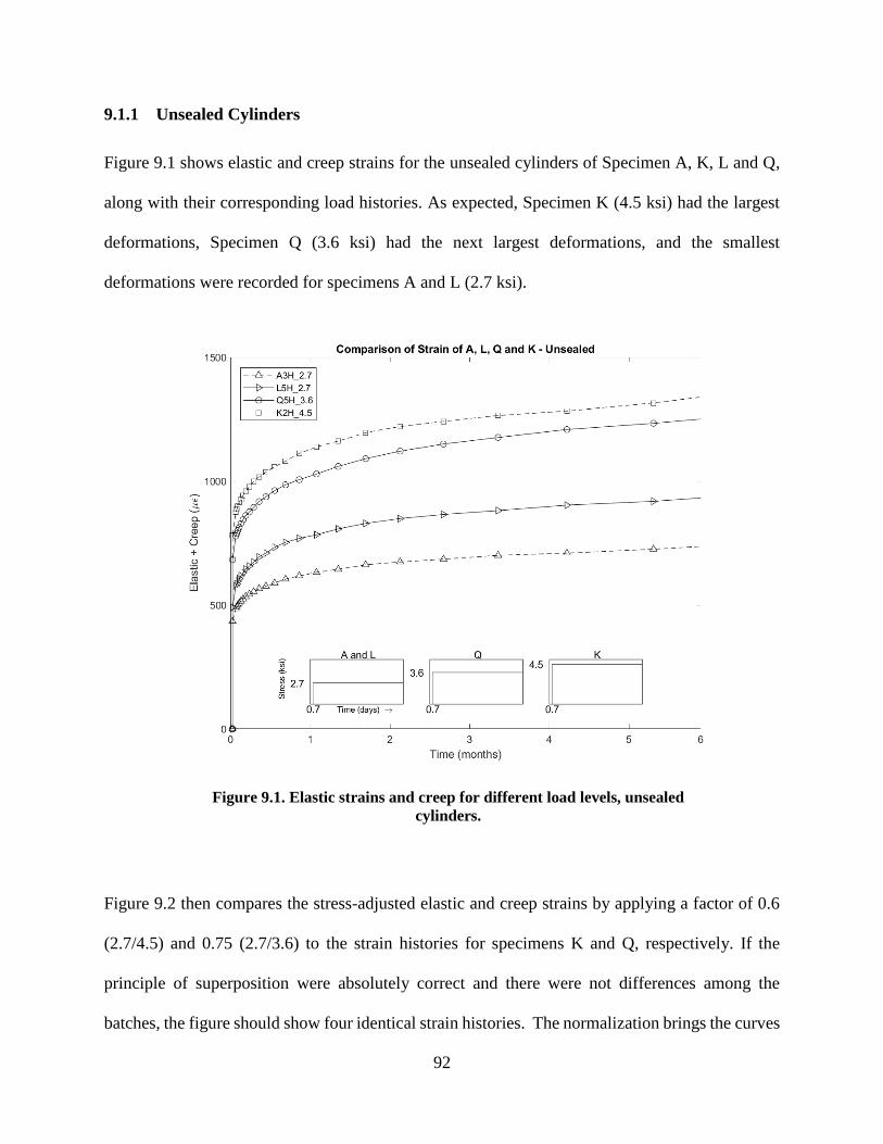
92
9.1.1 Unsealed Cylinders
Figure 9.1 shows elastic and creep strains for the unsealed cylinders of Specimen A, K, L and Q,
along with their corresponding load histories. As expected, Specimen K (4.5 ksi) had the largest
deformations, Specimen Q (3.6 ksi) had the next largest deformations, and the smallest
deformations were recorded for specimens A and L (2.7 ksi).
Figure 9.1. Elastic strains and creep for different load levels, unsealed
cylinders.
Figure 9.2 then compares the stress-adjusted elastic and creep strains by applying a factor of 0.6
(2.7/4.5) and 0.75 (2.7/3.6) to the strain histories for specimens K and Q, respectively. If the
principle of superposition were absolutely correct and there were not differences among the
batches, the figure should show four identical strain histories. The normalization brings the curves
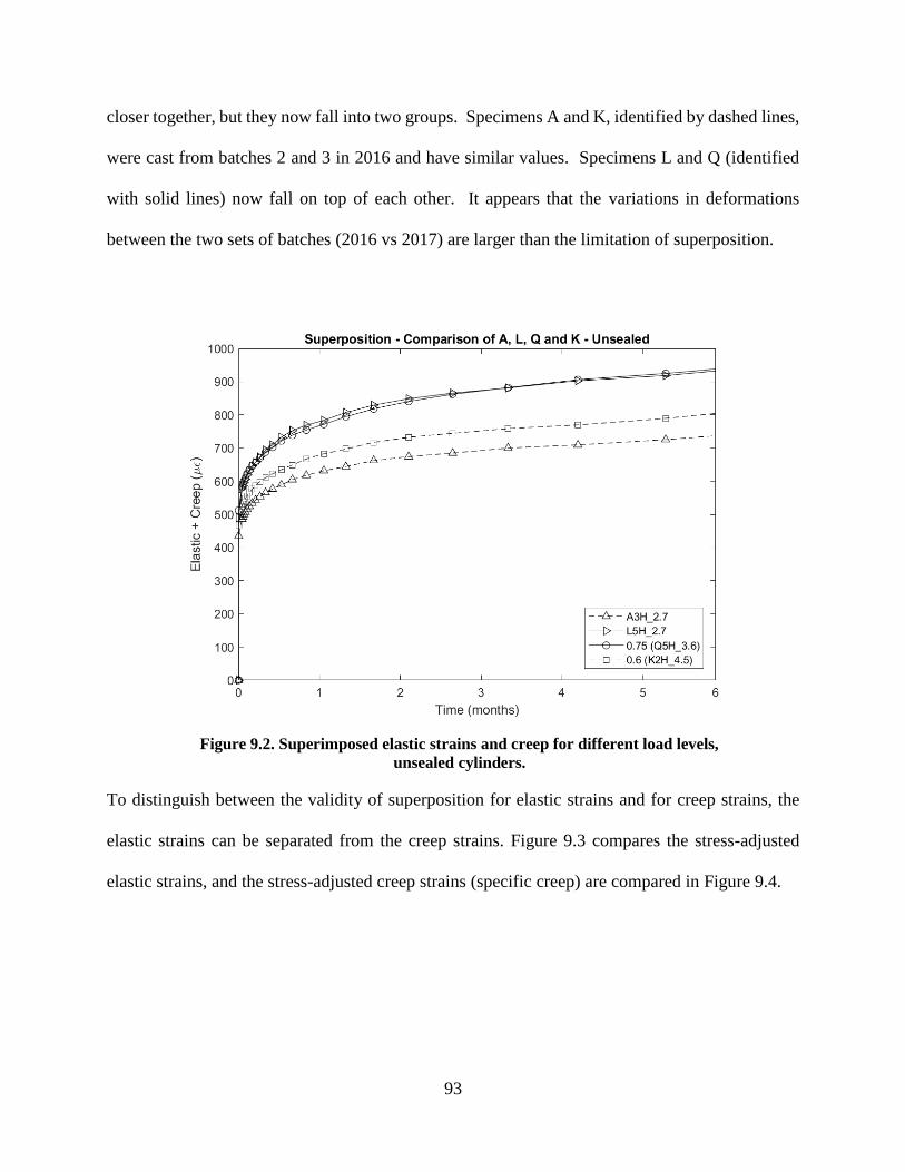
93
closer together, but they now fall into two groups. Specimens A and K, identified by dashed lines,
were cast from batches 2 and 3 in 2016 and have similar values. Specimens L and Q (identified
with solid lines) now fall on top of each other. It appears that the variations in deformations
between the two sets of batches (2016 vs 2017) are larger than the limitation of superposition.
Figure 9.2. Superimposed elastic strains and creep for different load levels,
unsealed cylinders.
To distinguish between the validity of superposition for elastic strains and for creep strains, the
elastic strains can be separated from the creep strains. Figure 9.3 compares the stress-adjusted
elastic strains, and the stress-adjusted creep strains (specific creep) are compared in Figure 9.4.
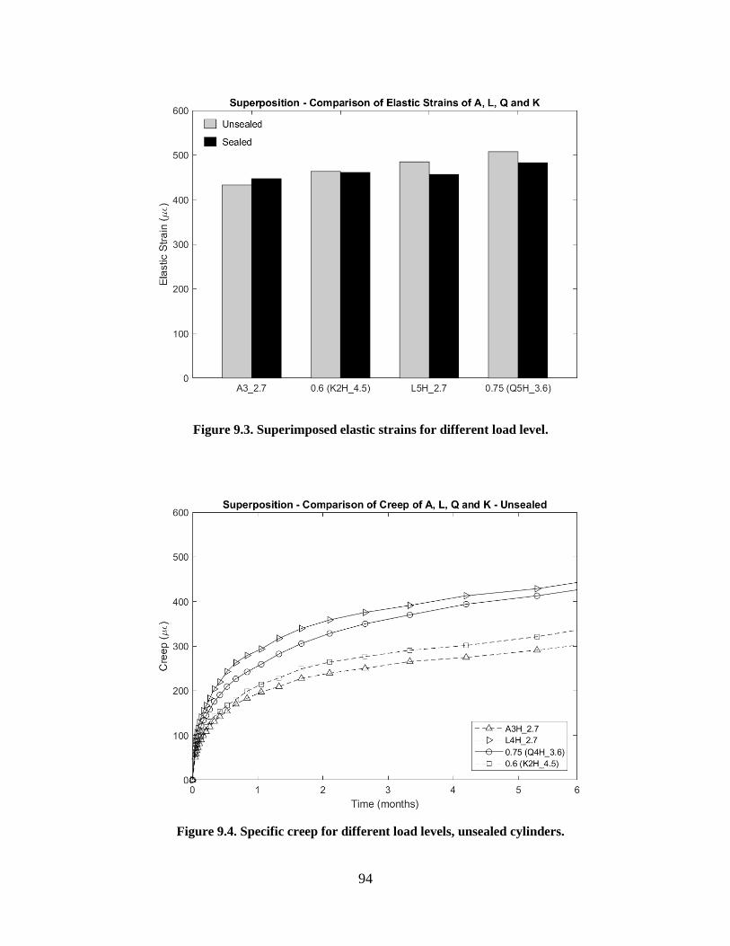
94
Figure 9.3. Superimposed elastic strains for different load level.
Figure 9.4. Specific creep for different load levels, unsealed cylinders.
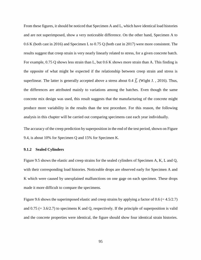
95
From these figures, it should be noticed that Specimen A and L, which have identical load histories
and are not superimposed, show a very noticeable difference. On the other hand, Specimen A to
0.6 K (both cast in 2016) and Specimen L to 0.75 Q (both cast in 2017) were more consistent. The
results suggest that creep strain is very nearly linearly related to stress, for a given concrete batch.
For example, 0.75 Q shows less strain than L, but 0.6 K shows more strain than A. This finding is
the opposite of what might be expected if the relationship between creep strain and stress is
superlinear. The latter is generally accepted above a stress about 0.4 𝑓�� (Wight J. , 2016). Thus,
the differences are attributed mainly to variations among the batches. Even though the same
concrete mix design was used, this result suggests that the manufacturing of the concrete might
produce more variability in the results than the test procedure. For this reason, the following
analysis in this chapter will be carried out comparing specimens cast each year individually.
The accuracy of the creep prediction by superposition in the end of the test period, shown on Figure
9.4, is about 10% for Specimen Q and 15% for Specimen K.
9.1.2 Sealed Cylinders
Figure 9.5 shows the elastic and creep strains for the sealed cylinders of Specimen A, K, L and Q,
with their corresponding load histories. Noticeable drops are observed early for Specimen A and
K which were caused by unexplained malfunctions on one gage on each specimen. These drops
made it more difficult to compare the specimens.
Figure 9.6 shows the superimposed elastic and creep strains by applying a factor of 0.6 (= 4.5/2.7)
and 0.75 (= 3.6/2.7) to specimens K and Q, respectively. If the principle of superposition is valid
and the concrete properties were identical, the figure should show four identical strain histories.
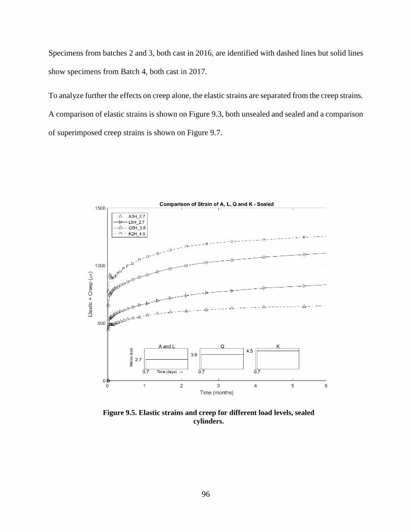
96
Specimens from batches 2 and 3, both cast in 2016, are identified with dashed lines but solid lines
show specimens from Batch 4, both cast in 2017.
To analyze further the effects on creep alone, the elastic strains are separated from the creep strains.
A comparison of elastic strains is shown on Figure 9.3, both unsealed and sealed and a comparison
of superimposed creep strains is shown on Figure 9.7.
Figure 9.5. Elastic strains and creep for different load levels, sealed
cylinders.
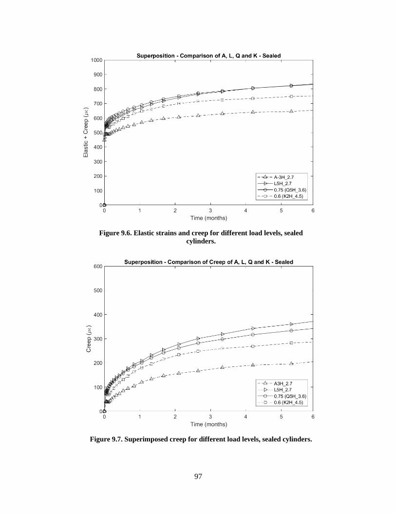
97
Figure 9.6. Elastic strains and creep for different load levels, sealed
cylinders.
Figure 9.7. Superimposed creep for different load levels, sealed cylinders.
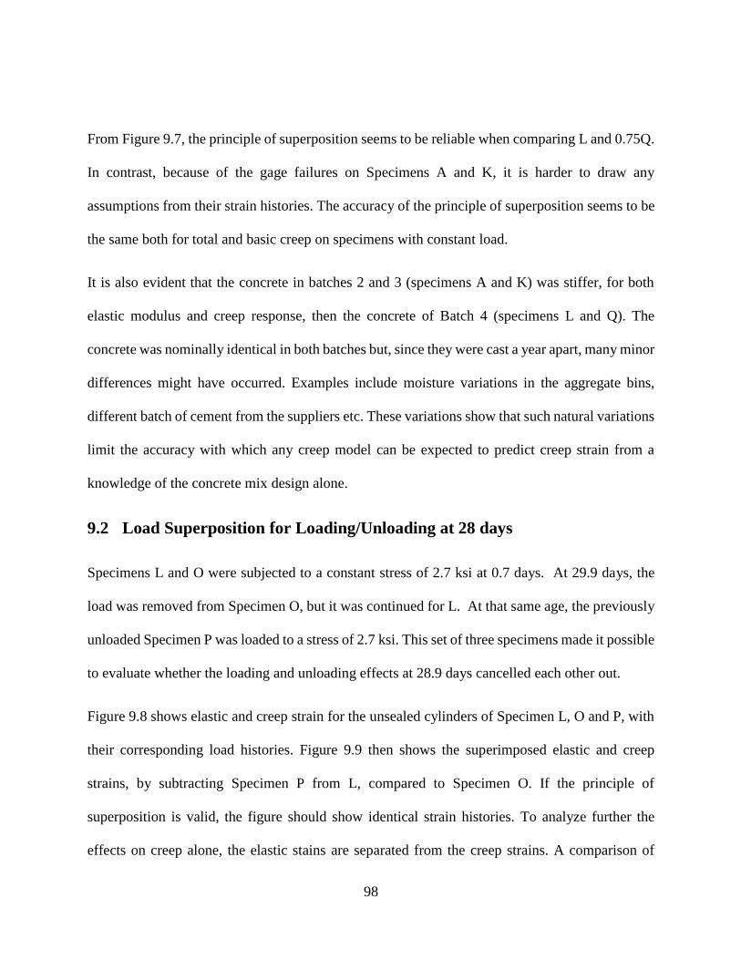
98
From Figure 9.7, the principle of superposition seems to be reliable when comparing L and 0.75Q.
In contrast, because of the gage failures on Specimens A and K, it is harder to draw any
assumptions from their strain histories. The accuracy of the principle of superposition seems to be
the same both for total and basic creep on specimens with constant load.
It is also evident that the concrete in batches 2 and 3 (specimens A and K) was stiffer, for both
elastic modulus and creep response, then the concrete of Batch 4 (specimens L and Q). The
concrete was nominally identical in both batches but, since they were cast a year apart, many minor
differences might have occurred. Examples include moisture variations in the aggregate bins,
different batch of cement from the suppliers etc. These variations show that such natural variations
limit the accuracy with which any creep model can be expected to predict creep strain from a
knowledge of the concrete mix design alone.
9.2 Load Superposition for Loading/Unloading at 28 days
Specimens L and O were subjected to a constant stress of 2.7 ksi at 0.7 days. At 29.9 days, the
load was removed from Specimen O, but it was continued for L. At that same age, the previously
unloaded Specimen P was loaded to a stress of 2.7 ksi. This set of three specimens made it possible
to evaluate whether the loading and unloading effects at 28.9 days cancelled each other out.
Figure 9.8 shows elastic and creep strain for the unsealed cylinders of Specimen L, O and P, with
their corresponding load histories. Figure 9.9 then shows the superimposed elastic and creep
strains, by subtracting Specimen P from L, compared to Specimen O. If the principle of
superposition is valid, the figure should show identical strain histories. To analyze further the
effects on creep alone, the elastic stains are separated from the creep strains. A comparison of
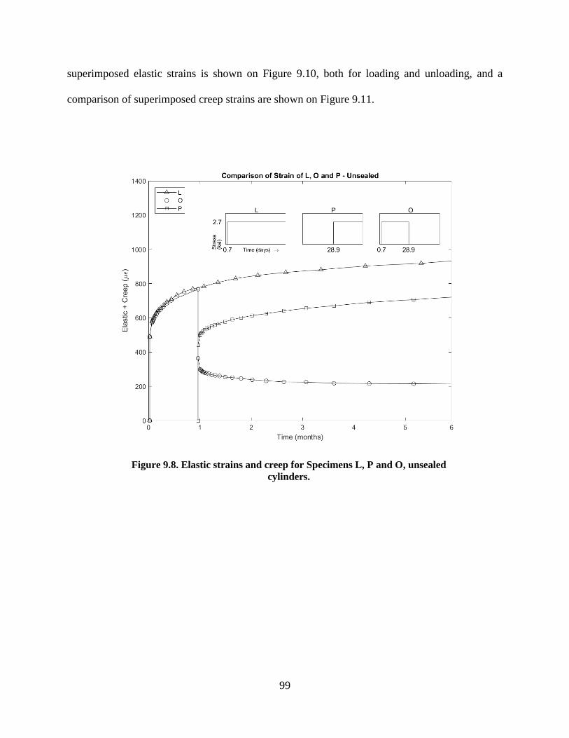
99
superimposed elastic strains is shown on Figure 9.10, both for loading and unloading, and a
comparison of superimposed creep strains are shown on Figure 9.11.
Figure 9.8. Elastic strains and creep for Specimens L, P and O, unsealed
cylinders.
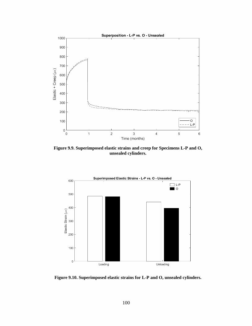
100
Figure 9.9. Superimposed elastic strains and creep for Specimens L-P and O,
unsealed cylinders.
Figure 9.10. Superimposed elastic strains for L-P and O, unsealed cylinders.
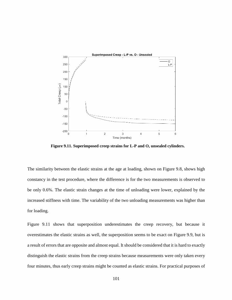
101
Figure 9.11. Superimposed creep strains for L-P and O, unsealed cylinders.
The similarity between the elastic strains at the age at loading, shown on Figure 9.8, shows high
constancy in the test procedure, where the difference is for the two measurements is observed to
be only 0.6%. The elastic strain changes at the time of unloading were lower, explained by the
increased stiffness with time. The variability of the two unloading measurements was higher than
for loading.
Figure 9.11 shows that superposition underestimates the creep recovery, but because it
overestimates the elastic strains as well, the superposition seems to be exact on Figure 9.9, but is
a result of errors that are opposite and almost equal. It should be considered that it is hard to exactly
distinguish the elastic strains from the creep strains because measurements were only taken every
four minutes, thus early creep strains might be counted as elastic strains. For practical purposes of

102
evaluating strains, Figure 9.9 shows that superposition gives a very good estimate of the actual
strains for the unsealed cylinders.
Both sealed cylinders of Specimen O and P had too many gage failures for their data to be usable.
Data from those specimens were therefore not analyzed.

103
Chapter 10 Model Calibration
In this chapter, the model put forward by Magnusson is calibrated against the test data from this
study. The objective is to obtain a set of material parameters that allow the model to predict the
time-dependent response of hot-cured concrete to time-varying loads.
10.1 Model and Calibration overview
The model is shown schematically in Figure 10.1. It is a one-dimensional rate-type model based
on visco-elastic behavior. It consists of a linear spring element attached to a chain of Kelvin
elements; the number of Kelvin elements can be chosen arbitrarily but three are shown on Figure
10.1 for illustration. Each Kelvin element consists of a linear spring and a linear dashpot in parallel.
In practice, the Kelvin elements imitate the creep behavior of the concrete and the linear spring
element, the elastic stiffness. Bazant and Asghari (1974), among others, have previously put forth
models with this setup, but what is novel in this case is that the element properties can vary with
time. By this feature, the change in elastic modulus over time can be included, for example. This
is however not the first time that a Kelvin-model with non-constant parameters has been suggested;
for example Schutter (1999) suggested using a degree of hydration based Kelvin model for basic
creep of early age concrete A detailed description of the model and its formulation can be found
in Magnusson’s thesis (2016). One of the difficulties associated with non-constant element
properties is ensuring that the model is thermodynamically valid, such that it cannot create energy.
The model used here satisfies that criterion.

104
Figure 10.1. Diagram of the model.
Data from all the hot-cured specimens were used in the calibration; a description of their load
histories can be found in Section 2.1. The data set provides 6 – 9 months of creep data and more
varied load histories than have been used before in calibration of the model.
The investigation concentrated on four aspects of the model.
Number of Kelvin elements. Models with up to four elements were tried to investigate the
benefits and drawbacks of using more elements.
Time-varying parameters. Models with parameters that did and did not vary with time were
compared to observe the gains achieved by the time-variation.
Parameter identification. The parameters that gave the best fit to various sub-sets of the
test data were then identified.
Long-term response prediction. The model’s ability to predict long-term response, after
calibration against only short-term creep data, was investigated. This ability is likely to be
needed in practice, when limited time is available for a creep study of a particular concrete.
10.2 Calibration Methodology
The data sets were obtained for each specimen, as described in Section 3.4, by taking the average
strain from the unsealed loaded cylinder and subtracting the average strain of the companion
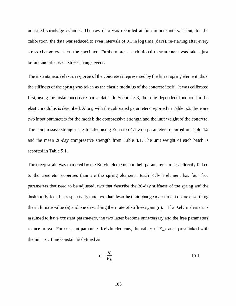
105
unsealed shrinkage cylinder. The raw data was recorded at four-minute intervals but, for the
calibration, the data was reduced to even intervals of 0.1 in log time (days), re-starting after every
stress change event on the specimen. Furthermore, an additional measurement was taken just
before and after each stress change event.
The instantaneous elastic response of the concrete is represented by the linear spring element; thus,
the stiffness of the spring was taken as the elastic modulus of the concrete itself. It was calibrated
first, using the instantaneous response data. In Section 5.3, the time-dependent function for the
elastic modulus is described. Along with the calibrated parameters reported in Table 5.2, there are
two input parameters for the model; the compressive strength and the unit weight of the concrete.
The compressive strength is estimated using Equation 4.1 with parameters reported in Table 4.2
and the mean 28-day compressive strength from Table 4.1. The unit weight of each batch is
reported in Table 5.1.
The creep strain was modeled by the Kelvin elements but their parameters are less directly linked
to the concrete properties than are the spring elements. Each Kelvin element has four free
parameters that need to be adjusted, two that describe the 28-day stiffness of the spring and the
dashpot (E_k and η, respectively) and two that describe their change over time, i.e. one describing
their ultimate value (a) and one describing their rate of stiffness gain (n). If a Kelvin element is
assumed to have constant parameters, the two latter become unnecessary and the free parameters
reduce to two. For constant parameter Kelvin elements, the values of E_k and η are linked with
the intrinsic time constant is defined as
𝝉 =𝜼
𝑬𝒌 10.1

106
which can be envisioned and expected to lie within a certain range (Bazant & Asghari, 1974). For
that reason, the model was calibrated by varying 𝐸𝑘 and 𝜏, which both represent physical entities,
rather than the fundamental properties Ek and . It was also decided, to simplify the calibration, to
keep 𝜏 constant for the time-dependent Kelvin models as well. This means that the same time
variation function was assigned to both the spring and dashpot of the Kelvin elements.
If the model parameters are constant with time, the ultimate creep coefficient can be calculated as
𝑪𝒄,𝒖𝒍𝒕 =𝑬𝒄
𝑬𝒌 10.2
Where 𝐸𝑘 is the stiffness of the Kelvin spring and 𝐸𝑐 is the stiffness of the elastic element.
The objective cost function that was used to optimize the set of parameters for all 15 specimen had
the following form:
𝒇(𝜺𝒑, 𝜺𝒎, 𝒏𝒅, 𝒏𝒔) =
∑ √∑ (𝜺𝒎 − 𝜺𝒑)
𝟐𝒏𝒅𝒊=𝟏
𝒏𝒅,𝒋
𝒏𝒔𝒋=𝟏
𝒏𝒔
10.3
where
𝜀𝑝 – Strain calculated with model (micro-strain)
𝜀𝑚 – Strain measured (micro-strain)
𝑛𝑑,𝑗 – Number of data points for specimen j
𝑛𝑠 – Number of specimens (15)
For each specimen, the root mean squared (rms) error between measured and predicted values
during the loading history was calculated. These resulting values were then added up for all

107
specimens and divided by the number of specimens. The model was only calibrated for the creep
strains; elastic strains were predicted using Equation 4.1 and parameters from Table 4.2.
Matlab (2017) was used to for the calculation, using a built-in function that performed the
optimization by an interior-point algorithm. The following sections show result for each of the
four configurations considered in this thesis.
10.3 Number of Kelvin elements
To identify the most efficient number of Kelvin elements to use for the model a comparison was
made for eight configurations: 1-4 elements with either all constant parameters or all time-
dependent parameters. It should be noted that time-dependent elements can converge to a constant
parameter element, allowing all combinations of constant and time-dependent configurations.
Table 10.2 shows a comparison of objective function values for all configurations where the
models are fitted with data series from hot-cured specimens. The value of the cost function is
equal to the root-mean-square (RMS) error between predicted and measured strains (in micro-
strain.)
Table 10.1. Comparison of objective function values.
Constant (µε) Time-Dependent (µε)
1 Kelvin 64.1 44.7
2 Kelvin 53.4 35.8
3 Kelvin 53.1 35.8
4 Kelvin 53.1 35.8
Adding elements can never lead to less accurate predictions, so the criterion for selecting the best
model combined the improvement in the fit and the ease of finding the optimum parameters. For
the time-dependent model configuration, the use of more than two elements provided no noticeable

108
improvement, while adding a third element only increased the difficulty of calibration by adding
two extra parameters. The same result was found for the constant-element model. The table shows
that the time-dependent configuration provided a fit that was better than that available with
constant parameters.
10.4 Comparison of Models
Table 10.2 shows the calibrated parameters for the two-element constant model and the two-
element time-dependent model.
Table 10.2. Calibrated parameters for models.
Constant Time-dependent
Kelvin 1 Kelvin 2 Kelvin 1 Kelvin 2
𝑬𝒌,𝟐𝟖 (ksi) 27700 8280 43300 7740
𝝉 (days) 2.17 109.5 1.89 86.3
a - - 3010 848000
n - - 0.50 0.72
To provide a visual representation of how well these two configurations fit the data, Figure 10.2
compares the objective function values for each specimen where the models are calibrated for the
whole dataset.

109
Figure 10.2. Comparison of objective function values for each specimen.
For a more detailed illustration, Figure 10.3 shows the measured data for specimen A, which was
subjected to monotonic loading, along with the values predicted by the two models (constant and
time-varying) calibrated using the whole dataset. The remaining two curves show the predictions
of both models calibrated against data from Specimen A alone. It is evident that a better fit can be
achieved by calibrating against data from a single specimen.
Similarly, Figure 10.4 compares the model fits for a specimen that was unloaded at an early age
(E). It illustrates on one of the shortcomings of the constant-property model, namely that it always
predicts complete creep recovery on unloading, whereas the variable-property model can model
irreversible creep strain. Figure 10.5 shows data for a specimen with a variable load history (S).
To improve the readability of that figure, it is divided into two graphs and only one model fit is
shown on each; one for the time-dependent and one for the constant parameter configuration. In

110
both cases the models are fitted only with the data from Specimen S. Similar plots, showing
individual model fits for all fifteen specimens, can be found in Appendix D.
Table 10.3 shows the optimized parameters for specimens A, E and S.
Figure 10.3. Comparison of models for Specimen A.
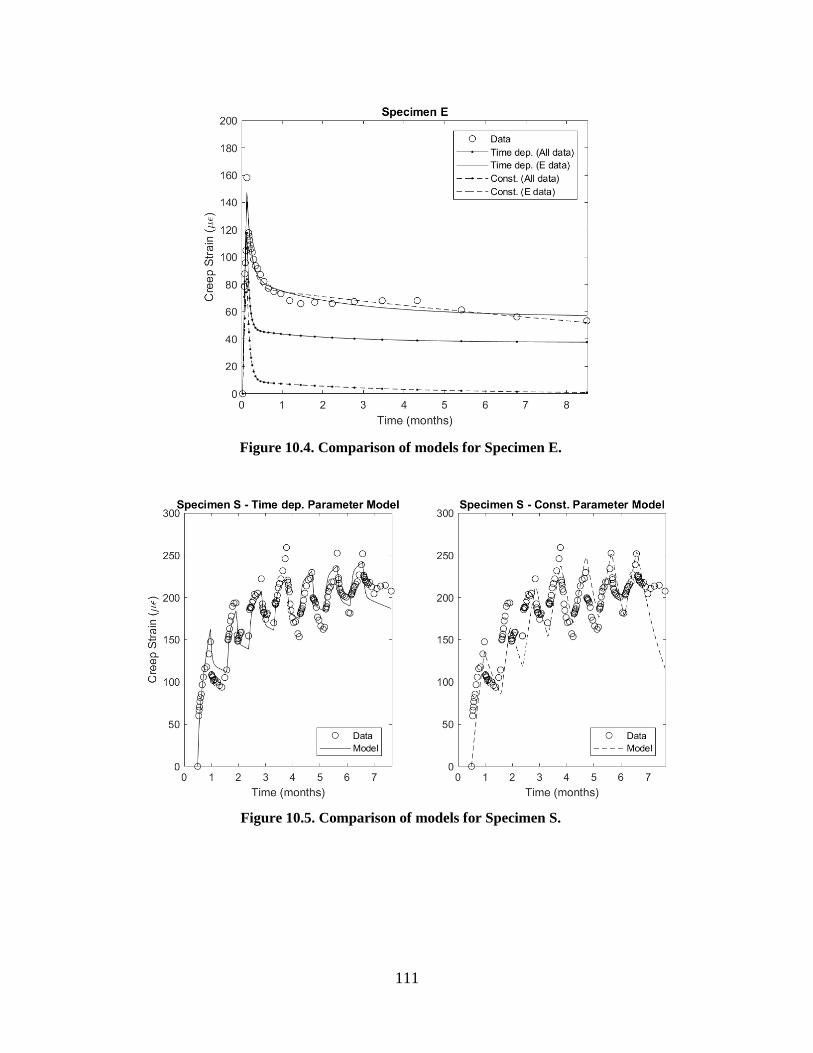
111
Figure 10.4. Comparison of models for Specimen E.
Figure 10.5. Comparison of models for Specimen S.
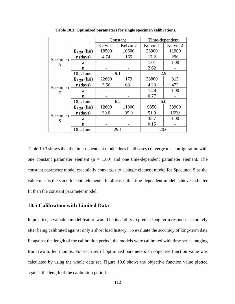
112
Table 10.3. Optimized parameters for single specimen calibrations.
Constant Time-dependent
Kelvin 1 Kelvin 2 Kelvin 1 Kelvin 2
Specimen
A
𝑬𝒌,𝟐𝟖 (ksi) 18500 10600 23900 11900
𝝉 (days) 4.74 165 17.2 296
a - - 1.01 1.00
n - - 2.62 -
Obj. func. 9.1 2.9
Specimen
E
𝑬𝒌,𝟐𝟖 (ksi) 22600 173 23800 313
𝝉 (days) 3.56 631 4.23 473
a - - 1.28 1.00
n - - 0.77 -
Obj. func. 6.2 6.0
Specimen
S
𝑬𝒌,𝟐𝟖 (ksi) 12600 11800 9350 53900
𝝉 (days) 39.0 39.0 51.9 1650
a - - 35.7 1.00
n - - 0.15 -
Obj. func. 29.1 20.0
Table 10.3 shows that the time-dependent model does in all cases converge to a configuration with
one constant parameter element (a = 1.00) and one time-dependent parameter element. The
constant parameter model essentially converges to a single element model for Specimen S as the
value of 𝜏 is the same for both elements. In all cases the time-dependent model achieves a better
fit than the constant parameter model.
10.5 Calibration with Limited Data
In practice, a valuable model feature would be its ability to predict long term response accurately
after being calibrated against only a short load history. To evaluate the accuracy of long-term data
fit against the length of the calibration period, the models were calibrated with time series ranging
from two to ten months. For each set of optimized parameters an objective function value was
calculated by using the whole data set. Figure 10.6 shows the objective function value plotted
against the length of the calibration period.
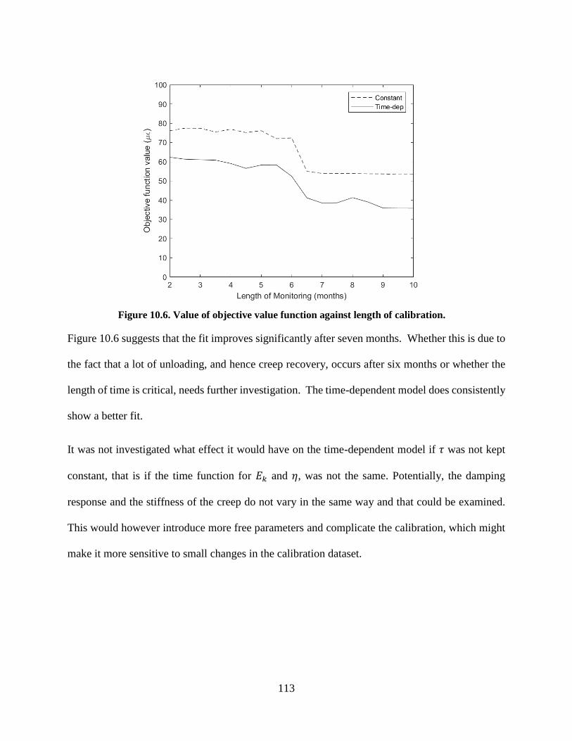
113
Figure 10.6. Value of objective value function against length of calibration.
Figure 10.6 suggests that the fit improves significantly after seven months. Whether this is due to
the fact that a lot of unloading, and hence creep recovery, occurs after six months or whether the
length of time is critical, needs further investigation. The time-dependent model does consistently
show a better fit.
It was not investigated what effect it would have on the time-dependent model if 𝜏 was not kept
constant, that is if the time function for 𝐸𝑘 and 𝜂, was not the same. Potentially, the damping
response and the stiffness of the creep do not vary in the same way and that could be examined.
This would however introduce more free parameters and complicate the calibration, which might
make it more sensitive to small changes in the calibration dataset.
114
Chapter 11 Discussion
In this chapter, the main findings of the research will be discussed, first regarding the test setup,
then the material behavior and finally the performance of the model.
11.1 Test Setup
The main improvement made on the test setup, from the previous creep research done at the
University of Washington, was adding an extra gage on all creep cylinders. Four gages were used
instead of three. This was done because even mild eccentricity was inevitable when applying loads
in the creep rigs. Having four gages increased the reliability of the results, because a comparison
could be made on two pairs of opposing gages, instead of having to average three gages to get the
creep of the cylinder. Good consistency was seen when comparing the averages of opposing gages
on individual cylinders. Therefore, in the case of gage malfunctions the faulty gage and its
opposing gage could be dropped from the data processing without serious effects on the
consistency of the data which was not the case when only three gages were on a cylinder.
When hot-cured cylinders were loaded at an early age the sealed and unsealed cylinders had been
handled the same way up until that point and should have identical material properties. Good
consistency of initial (elastic) strains was seen in those cases for all cylinders, both in the same
creep rig and in separate ones. This verified the consistency of both the loading procedure and the
strain measurements.
It should be noted, however, that significant logistical challenges must be overcome in order to
remove all sources of potential error. In this case, the primary difficulties were associated with
getting the concrete from the precaster’s yard to the test site and then preparing the cylinders and
loading them into the test rigs, all in the shortest possible time so the concrete would be loaded at

115
the same time in its curing history as would the concrete in a real girder. The cylinders were
prepared by Concrete Technology Corporation and transported to the University of Washington
early in the morning (to avoid traffic), and a team of helpers worked to cap, seal and gage the
cylinders, but the time from picking up the cylinders to loading them in the creep rigs was still
between 2 and 3 hours. That time is not negligible compared to the total curing time, but reducing
it would be difficult.
Gage malfunctions were evident on 18 gages of a total of 170 gages used; 15 of the 18 happened
on sealed cylinders. Most of these were due to gages becoming loose on the cylinders at various
ages after loading. The fact that most of the failures happen on the sealed specimens makes the
sealing suspect but no cause for the failures could be identified.
11.2 Material Behavior
The strength data from each batch showed that the natural variability in the nominally identical
concrete batches can result in a strength variation of about 10%. It shows that natural variations
limit the accuracy with which strength can be predicted by knowledge of the concrete mix alone.
This variability also seemed to effect the creep.
Bazant, ASCE and Kim (1979) have suggested that a sustained load affects the stiffness of
concrete. The elastic modulus tests done at the end of the creep test period did not indicate that the
loaded creep specimens had gained stiffness over the test period compared to the unloaded
shrinkage specimens.
Shrinkage measurements showed some variation. It is considered to be caused by changes in
relative humidity and natural variations in the concrete but overall no distinction could be made
between the shrinkage of hot-, weekend- ambient-cured cylinders. Total shrinkage was on the
116
order of 500 micro-strain after 6 months. Most of the drying shrinkage seemed to occur within the
first month, and it had essentially stabilized after 6 months. The autogenous shrinkage occurred
more slowly and did not stabilize during the test period. The use of larger test cylinders, with a
lower surface-volume ratio, might be expected to slow the drying shrinkage. This should be
considered in further research as the 4x8” cylinders have a lower surface-volume ratio than normal
bridge girders.
Autogenous shrinkage gain was expected to slow down like the strength gain because it is related
to the same chemistry. The autogenous shrinkage seemed to be still increasing at the end of six
months and it might therefore be questioned whether the sealed cylinders were sufficiently sealed.
It should however be noticed that strength was also increasing at the end of six months and great
care was taken to prevent any moisture loss from the cylinders. Furthermore, it was noticed that
the autogenous shrinkage was consistent for all measurements which implies that the sealing
procedure was at least consistent, and therefore likely reliable. The measurements from the sealed
cylinders are therefore assumed dependable but unit weight measurements could be done in future
experiments, before and after the test period, to verify the assumption.
Creep of weekend- and ambient cured concrete showed similar results but hot-cured concrete
showed about 20% less total creep.
The one specimen that was loaded and unloaded biweekly showed reducing creep for the first three
loadings but after that the creep curves for every cycle kept fairly similar. This suggests that creep
reduces with age at loading, but that it does not vanish completely. However, that finding is
derived from a single specimen.
117
The amount of recoverable creep proved to be dependent on the load duration, and reduced with
longer duration.
Magnusson (2016) suggested that basic creep was fully recoverable while drying creep was not.
Branson (1977) also claims this is the case. The data from this study is inconclusive; about half of
the unloaded specimens showed no drying creep recovery but the other half showed comparable
recovery for both drying and basic creep.
Applying the principle of superposition to predict creep response gave good results, both where it
was applied to examine a variable load history and in the case of different load levels. The results
were not exact but were deemed sufficient for practical design, in accordance with conclusions
from Magnusson (2016). Validity of Superposition implies that creep is a linear process. Almost
all of the specimens were loaded to a stress less than 40% of their estimated strength at the time
and many authors (e.g .Wight 20xx) agree that the stress-strain curve is linear up to that point.
In general, the total creep coefficient for all specimens was low, with an average of 0.80 (varying
from 0.57 to 1.16) at the end of 6 months. The total creep coefficient for the only two specimens
still loaded was 0.92 and 1.07 for the hot- and ambient-cured, respectively, at the end of 18 months.
11.3 Model
A configuration of the model with two time-dependent Kelvin elements turned out to give the best
results when the whole dataset was fitted. Having more elements did not seem to improve the fit
and only added more parameters to be calibrated. When the model was fitted to individual
specimens the model converged to a solution with one time-dependent Kelvin element and one
constant Kelvin element. This suggest that this configuration might be sufficient for simpler
datasets. Furthermore, use of a large number of parameters results in potentially large changes in

118
parameter values for only small changes in the data. This behavior renders the calibration process
very sensitive.
Using datasets with limited amount of monitoring time showed that in order to get the best fit to
the whole dataset it was necessary to have data from seven months of monitoring. The reason for
this length of time is assumed to be that, after six months, about half of the specimens were
unloaded, which gave the necessary data to allow the model to predict the creep recovery. From
this observation it is furthermore assumed that, in order to predict a history of variable applied
stress, unloading data needs to be included in the calibration dataset. When the later set of
unloadings (at eight months) were included in the calibration it did not noticeably improve the
model fit to the whole data set. Further study is needed to determine whether the necessary creep
recovery data could be obtained from specimens unloaded at an age earlier than six months. It
was also found that prediction of long-term creep response from short-term creep data is very
difficult. This difficulty is caused partly by sensitivity to data, whereby a small change in the short-
term data implies large differences in long-term response, and partly by the form of the time-
dependence equations used in the model. The latter represent an improvement over the equations
advocated in ACI 209, but they have difficulty tracking faithfully the presumed rates of maturity
change during and after hot curing.
Using time-dependent Kelvin elements opposed to constant ones allows the model to distinguish
between creep behaviors due to early and late loadings. It also eliminates the full creep recovery,
which is inevitable when using constant Kelvin elements. These are two of the main reasons for
adding the factor of time-dependency to the elements of the Kelvin model. It improved the fit to
the whole dataset but it also converged to a solution where it predicted that essentially no creep
would occur in response to a load applied at 1 year or more.

119
For both the constant and the time-dependent models use of parameters optimized for the whole
dataset still resulted in bad fits for some individual specimens. The time-dependent model showed
better results than the constant model in eleven out of fifteen cases.

120
Chapter 12 Summary, Conclusions and Recommendations
12.1 Summary
The objectives of this research were to collect additional data on the creep and shrinkage of hot-
cured concrete, to study the effects of hot-curing concrete and to validate the functionality of the
creep model but forth in an earlier research at the University of Washington. In this thesis, a closer
look is also taken at variable loading, creep recovery and long-term strength and stiffness
development of concrete under loading.
Creep tests were performed on 19 specimens, which were all made from nominally identical
batches of concrete. Each specimen consisted of two pairs of unsealed and sealed cylinders, one
pair of which was not loaded to be compared with the other pair which was loaded. These
specimens were cured with different heat treatments and subjected to various loading cases to get
an insight on as many characteristics of the creep behavior as possible. At the end of the test period,
all cylinders were tested for their elastic modulus and then strength to estimate the effect of
loading, from the creep test, on these properties of the concrete. These specimens were cast in six
batches of concrete. Alongside the creep and shrinkage cylinders, cylinders were also cast to
investigate the natural variations in concrete strength.
Previously a study was done on strength and elastic modulus development of nominally identical
hot-cured concrete, where eleven pairs were tested for a period of 56 days. The data from that
study and the strength and elastic modulus tests performed on creep cylinders in the present study
was used to develop a model to predict how the elastic modulus varied with time.
The results from the creep tests and the elastic modulus study were used to develop and calibrate
a one-dimensional rate-type model based on visco-elastic behavior to predict creep strains for hot-
121
cured concrete subjected to a variable stress history. The model consists of a single elastic spring
in series with any number of Kelvin elements, all of which have time-varying properties. A Kelvin
element consist of a linear spring in series with a linear dashpot and all the springs and dashpots
may have time-dependent properties. Kelvin models have been used to predict concrete creep
before but allowing them to have varying properties has not been common. Having varying
properties allows the model to follow the time variations in the concrete and to model non-
recoverable creep which constant-parameter Kelvin models cannot.
The conclusions, regarding the test setup, material behavior and the model performance are
discussed in this chapter and recommendations for further research are presented.
12.2 Conclusions
12.2.1 Test Setup
The data recorded with the VW gages shows good consistency both for the short term (elastic
modulus tests) and the long term (creep and shrinkage tests) measurements. The consistency
verifies the reliability of the gages, which are also very convenient for long-time monitoring
because of their automation. The usage of automated gages also eliminates the measurement error,
opposed to using traditional manual gages. Being able to control the reading rate and take reading
up to 300 times a second also allows for a closer look to be taken at the short time creep behavior
during and directly after the application of load. A few gage malfunctions were however evident,
mainly on sealed specimens. The reasons are unknown but are assumed to be related to improper
attachment of the gages.

122
12.2.2 Material Behavior
The following conclusions regarding the material behavior were drawn from the study:
Variations in strength gain. A natural strength variation of 10% can be expected in the
concrete, even with the good QC exercised by the precaster. This difference was observed
from the nominally identical batches cast in 2016 and 2017.
Effect of sealing on strength. Sealed specimens showed more strength gain over time than
their unsealed companion.
Consistency of elastic modulus data. Measured elastic modulus from sealed and unsealed
cylinders of the same specimens showed good consistency for initial loading. This verified
the reliability of the data as the concrete in the two types of cylinder should have identical
properties at that point. Great internal consistency was also observed from elastic modulus
tests that were performed at the end of the test period as well.
Effect of sealing on stiffness. The sealed specimens showed more stiffness gain over time
than their unsealed companion, in accordance with the strength gain.
Effect of loading on stiffness. No significant stiffness gain was observed from loaded creep
specimens compared to the unloaded shrinkage ones at the end of the test period.
Effect of curing regimes on shrinkage. Different curing regimes did not seem to effect the
shrinkage behavior of the concrete, this is contrary to what Magnusson (2016) concluded,
where he reported more shrinkage due to hot-curing. In general, the total creep coefficient
for all specimens was low, with an average of 0.80 at the end of 6 months
Effect of curing regimes on creep. When the same load level was applied to cylinders which
were estimated to have gained the same strength, results suggest that creep behavior of

123
ambient-cured and weekend-cured concrete was comparable meanwhile hot-cured
concrete showed lower creep strains.
Creep due to cyclic loading. Creep due to repeated loading reduced noticeably during the
first load cycles and stabilized as the number of cycles increased. The behavior is mainly
considered to be the result of two factors: the concrete being loaded at a higher age and
residual creep. Presumably, residual creep might reduce the creep capacity of the concrete,
but this would have to be examined futher.
Creep recovery. Creep recovery ratio reduced with longer load duration and lower
preloaded stress. The results were inconclusive about drying creep’s being recoverable but
they showed that basic creep was at least partially recoverable.
Validity of the principle of superposition. Use of the principle of superposition to predict
creep response to time-varying load gave results close to, but exactly equal to, the
measured values.
12.2.3 Model Performance
The following conclusions regarding the model performance were drawn from the study:
Number of Kelvin-elements. Using two Kelvin elements was shown to be sufficient, using
more only complicated calibration.
Time-dependent vs constant parameters. Using time-dependent parameters showed better
performance than using constant parameters for the Kelvin model.
Calibration data. To predict creep response to variable load histories it is necessary to
include unloading data in the calibration dataset.

124
The model involves less book-keeping than superposition and is therefore more convinient
when variable load cases are analyzed.
12.3 Recommendations
Following are recommendations for further research:
Examine effect of surface-volume ratio. The surface-volume ratio is generally considered
to effect the development of creep (Branson, 1977) and the 4x8 in. cylinders, used in the
study, have a considerably higher surface-volume ratio than a standard bridge girder. It
would therefore be valuable to examine the effect off surface-volume ratio by using a range
of different cylinder sizes.
Application to practice. The variable-viscosity Kelvin model should be incorporate into a
camber program for prestressed, precast bridge girders.
Relating model parameters to concrete properties. To allow the model to be used without
having to calibrate it using experimental data it should be examined whether associating
the model parameters to measurable properties of concrete, is possible.
Allowing non-constant intrinsic time. Potentially, the damping response and the stiffness
of the creep do not vary in the same way and that should be examined by allowing the
intrinsic time constant, = Ek/, to vary over time. This would however introduce more
free parameters and complicate the calibration, which might make it more sensitive to small
changes in the calibration dataset.

125
Notation
a = Ratio between ultimate value and 28-day value in new time-dependent function
a = Strength gain constant for concrete in the ACI 209R-92 model
b = Strength gain constant for concrete in the ACI 209R-92 model
c = Multiplication constant for the equation predicting elastic modulus with time
𝐶𝑐𝑢 = Creep coefficient
E = Modulus of elasticity
𝐸𝑐 = Modulus of elasticity of concrete
𝐸𝑒= Modulus of elasticity of elastic spring
𝐸𝑘 = Modulus of elasticity of Kelvin-element spring
𝑓��(𝑡) = Compressive strength of concrete
n = Exponent in new time-dependent function
𝑛𝑑,𝑗 = Number of data points for Specimen j
𝑛𝑓 = Compressive strength exponent
𝑛𝑠 = Number of specimens
𝑛𝑤 = Unit weight exponent
t = time
𝑡0 = Time offset from zero in new time-dependent function

126
𝑡50 = Time it takes to reach 50% of ultimate strain value
w = Unit weight of concrete
𝜀 = Strain
𝜅 = Time-dependent function for concrete strength in the Kelvin-element model
𝜂 = Dashpot viscosity
𝜎 = Stress
𝜏 = Intrinsic time constant of Kelvin-element

127
References
ACI Committee 209. (2008). Guide for Modeling and Calculating Shrinkage and Creep in
Hardened Concrete (ACI 209.2R-08). Farmington Hills: American Concrete Institute.
Al-Manaseer, A., Espion, B., & and Ulm, F. J. (1999). Conclusions: ACI Paris Chapter Workshop
on Creep and Shrinkage in Concrete Structures. Revue Française de Génie Civil, 15-19.
American Association of State Highway and Transporation Officials (AASHTO). (2014). LRFD
Bridge Design Specifications 7th Edition. Washington: AASHTO.
American Concrete Institute (ACI). (2014). Building Code Requirements for Structural Concrete
(ACI 318-14). Farmington Hills: American Concrete Institute.
Bažant, Z. P. (1975). Theory of Creep and Shrinkage in Concrete Structures: a Précis of Recent
Developments. Mechanics Today, 1-93.
Bažant, Z. P. (1999). Criteria for Rational Prediction of Creep and Shrinkage of Concrete. Revue
Française de Génie Civil, 61-89.
Bažant, Z. P. (2000). Criteria for Rational Prediction of Creep and Shrinkage of Concrete. In A.
Al-Manaseer, The Adam Neville Symposium: Creep and Shrinkage-Structural Design
Effects (pp. 237-260). Farmington Hills, MI: American Concrete Institute.
Bazant, Z. P., & Asghari, A. (1974). Computation of Kelvin chain retardation spectra of aging
concrete. Cement and Concrete Resarch, Vol. 4, 797-806.
Bazant, Z. P., & Kim, S.-S. (1979). Nonlinear Creep of Concrete - Adaption and Flow. ASCE
Journal of the Engineering Mechanics Division, 429-446.
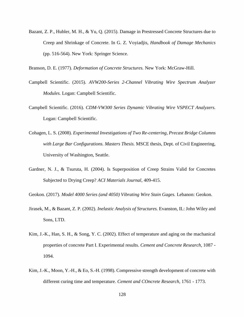
128
Bazant, Z. P., Hubler, M. H., & Yu, Q. (2015). Damage in Prestressed Concrete Structures due to
Creep and Shrinkage of Concrete. In G. Z. Voyiadjis, Handbook of Damage Mechanics
(pp. 516-564). New York: Springer Science.
Branson, D. E. (1977). Deformation of Concrete Structures. New York: McGraw-Hill.
Campbell Scientific. (2015). AVW200-Series 2-Channel Vibrating Wire Spectrum Analyzer
Modules. Logan: Campbell Scientific.
Campbell Scientific. (2016). CDM-VW300 Series Dynamic Vibrating Wire VSPECT Analyzers.
Logan: Campbell Scientific.
Cohagen, L. S. (2008). Experimental Investigations of Two Re-centering, Precast Bridge Columns
with Large Bar Configurations. Masters Thesis. MSCE thesis, Dept. of Civil Engineering,
University of Washington, Seattle.
Gardner, N. J., & Tsuruta, H. (2004). Is Superposition of Creep Strains Valid for Concretes
Subjected to Drying Creep? ACI Materials Journal, 409-415.
Geokon. (2017). Model 4000 Series (and 4050) Vibrating Wire Stain Gages. Lebanon: Geokon.
Jirasek, M., & Bazant, Z. P. (2002). Inelastic Analysis of Structures. Evanston, IL: John Wiley and
Sons, LTD.
Kim, J.-K., Han, S. H., & Song, Y. C. (2002). Effect of temperature and aging on the machanical
properties of concrete Part I. Experimental results. Cement and Concrete Research, 1087 -
1094.
Kim, J.-K., Moon, Y.-H., & Eo, S.-H. (1998). Compressive strength development of concrete with
different curing time and temperature. Cement and COncrete Research, 1761 - 1773.
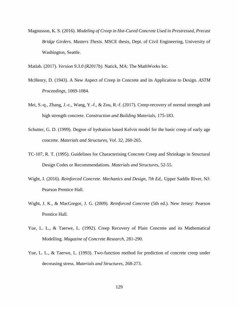
129
Magnusson, K. S. (2016). Modeling of Creep in Hot-Cured Concrete Used in Prestressed, Precast
Bridge Girders. Masters Thesis. MSCE thesis, Dept. of Civil Engineering, University of
Washington, Seattle.
Matlab. (2017). Version 9.3.0 (R2017b). Natick, MA: The MathWorks Inc.
McHenry, D. (1943). A New Aspect of Creep in Concrete and its Application to Design. ASTM
Proceedings, 1069-1084.
Mei, S.-q., Zhang, J.-c., Wang, Y.-f., & Zou, R.-f. (2017). Creep-recovery of normal strength and
high strength concrete. Construction and Building Materials, 175-183.
Schutter, G. D. (1999). Degree of hydration based Kelvin model for the basic creep of early age
concrete. Materials and Structures, Vol. 32, 260-265.
TC-107, R. T. (1995). Guidelines for Characterising Concrete Creep and Shrinkage in Structural
Design Codes or Recommendations. Materials and Structures, 52-55.
Wight, J. (2016). Reinforced Concrete. Mechanics and Design, 7th Ed,. Upper Saddle River, NJ:
Pearson Prentice Hall.
Wight, J. K., & MacGregor, J. G. (2009). Reinforced Concrete (5th ed.). New Jersey: Pearson
Prentice Hall.
Yue, L. L., & Taerwe, L. (1992). Creep Recovery of Plain Concrete and its Mathematical
Modelling. Magazine of Concrete Research, 281-290.
Yue, L. L., & Taerwe, L. (1993). Two-function method for prediction of concrete creep under
decreasing stress. Materials and Structures, 268-273.
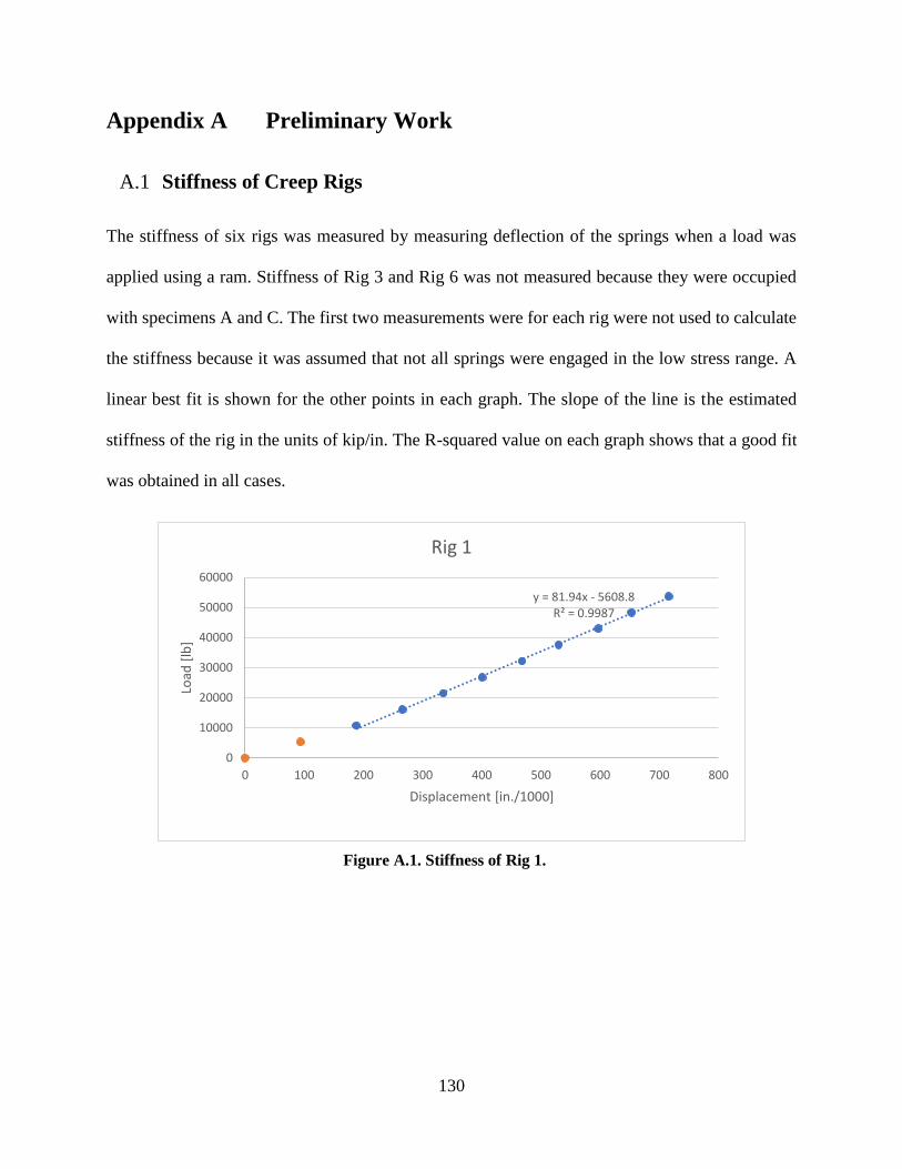
130
Appendix A Preliminary Work
A.1 Stiffness of Creep Rigs
The stiffness of six rigs was measured by measuring deflection of the springs when a load was
applied using a ram. Stiffness of Rig 3 and Rig 6 was not measured because they were occupied
with specimens A and C. The first two measurements were for each rig were not used to calculate
the stiffness because it was assumed that not all springs were engaged in the low stress range. A
linear best fit is shown for the other points in each graph. The slope of the line is the estimated
stiffness of the rig in the units of kip/in. The R-squared value on each graph shows that a good fit
was obtained in all cases.
Figure A.1. Stiffness of Rig 1.
y = 81.94x - 5608.8R² = 0.9987
0
10000
20000
30000
40000
50000
60000
0 100 200 300 400 500 600 700 800
Load
[lb
]
Displacement [in./1000]
Rig 1
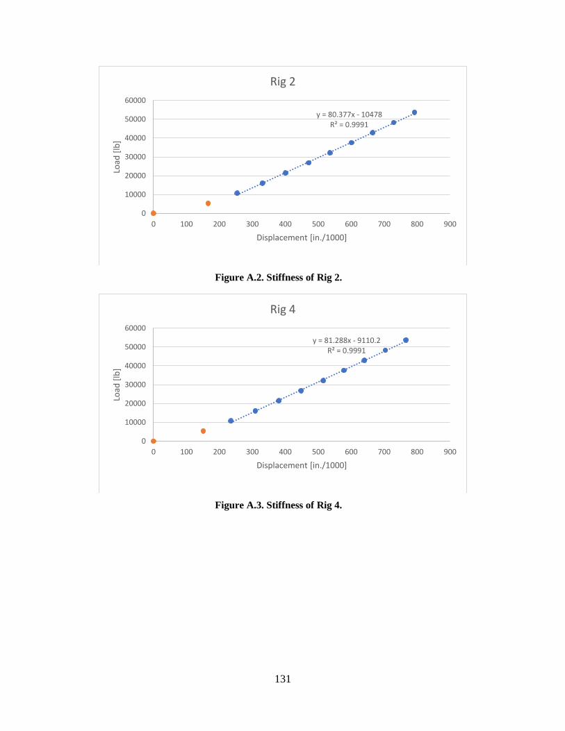
131
Figure A.2. Stiffness of Rig 2.
Figure A.3. Stiffness of Rig 4.
y = 80.377x - 10478R² = 0.9991
0
10000
20000
30000
40000
50000
60000
0 100 200 300 400 500 600 700 800 900
Load
[lb
]
Displacement [in./1000]
Rig 2
y = 81.288x - 9110.2R² = 0.9991
0
10000
20000
30000
40000
50000
60000
0 100 200 300 400 500 600 700 800 900
Load
[lb
]
Displacement [in./1000]
Rig 4
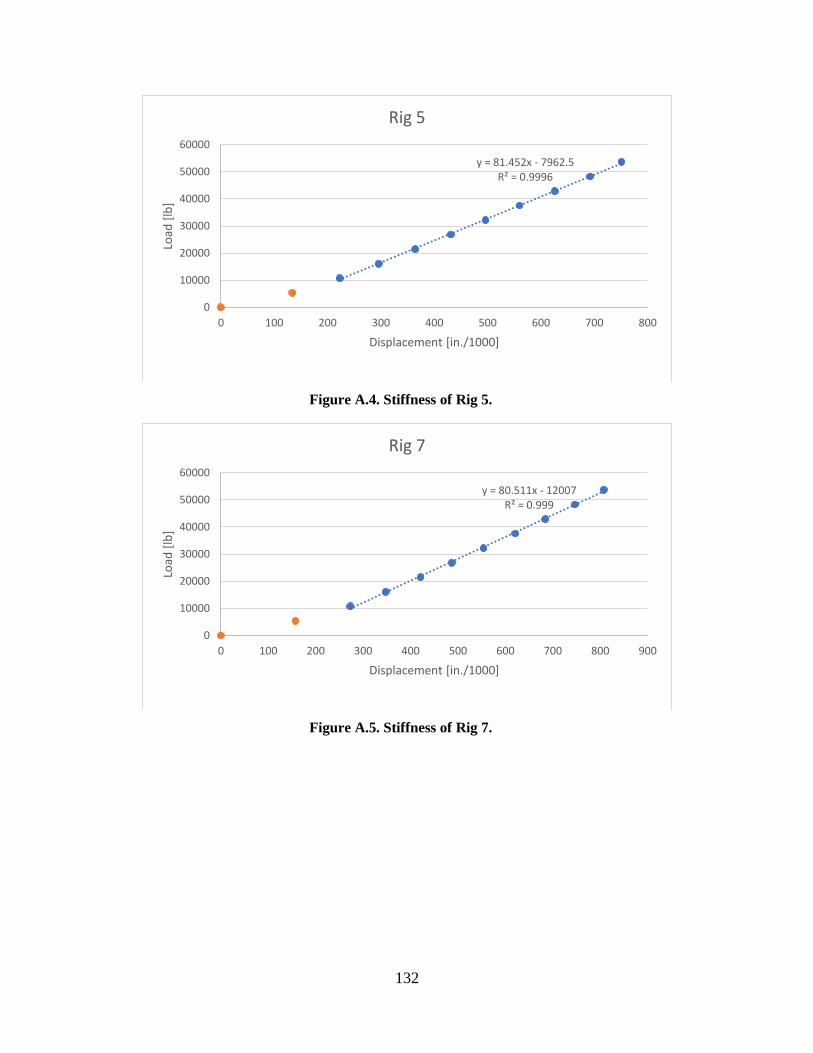
132
Figure A.4. Stiffness of Rig 5.
Figure A.5. Stiffness of Rig 7.
y = 81.452x - 7962.5R² = 0.9996
0
10000
20000
30000
40000
50000
60000
0 100 200 300 400 500 600 700 800
Load
[lb
]
Displacement [in./1000]
Rig 5
y = 80.511x - 12007R² = 0.999
0
10000
20000
30000
40000
50000
60000
0 100 200 300 400 500 600 700 800 900
Load
[lb
]
Displacement [in./1000]
Rig 7
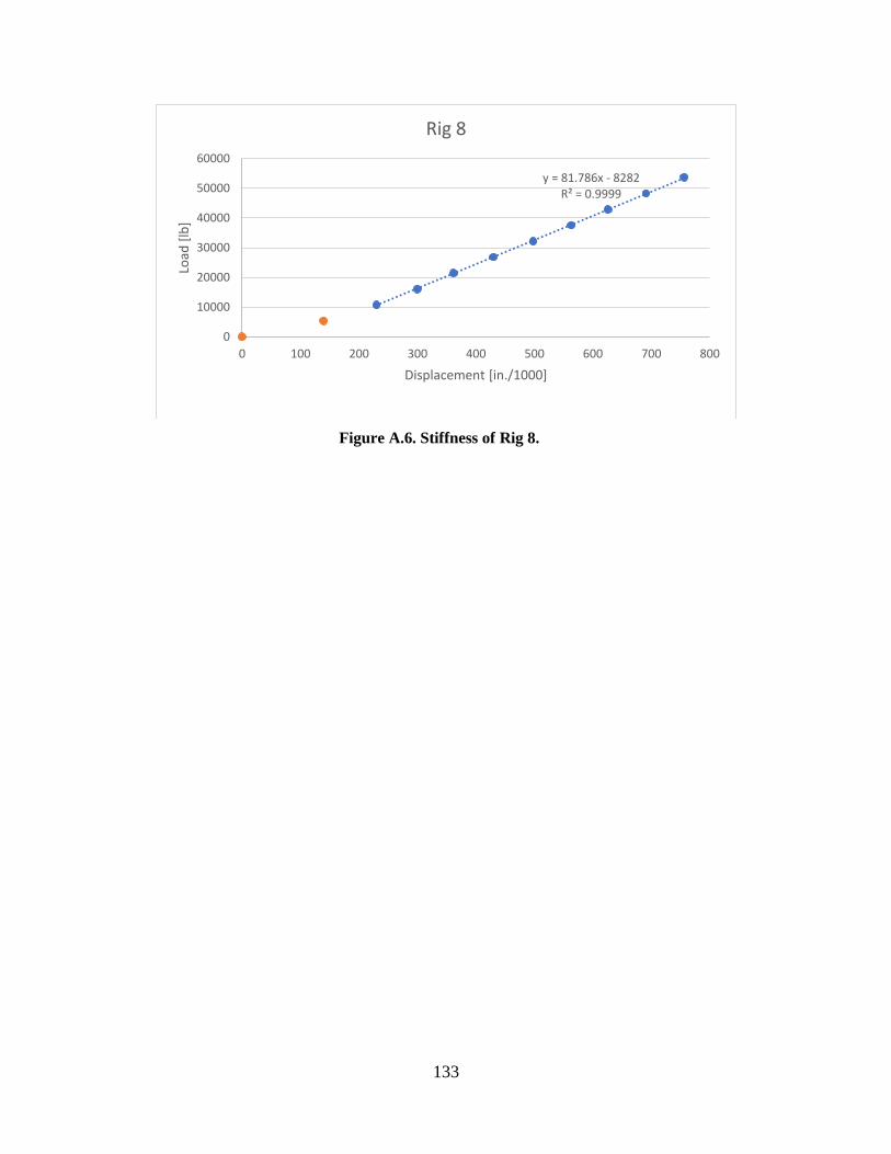
133
Figure A.6. Stiffness of Rig 8.
y = 81.786x - 8282R² = 0.9999
0
10000
20000
30000
40000
50000
60000
0 100 200 300 400 500 600 700 800
Load
[lb
]
Displacement [in./1000]
Rig 8
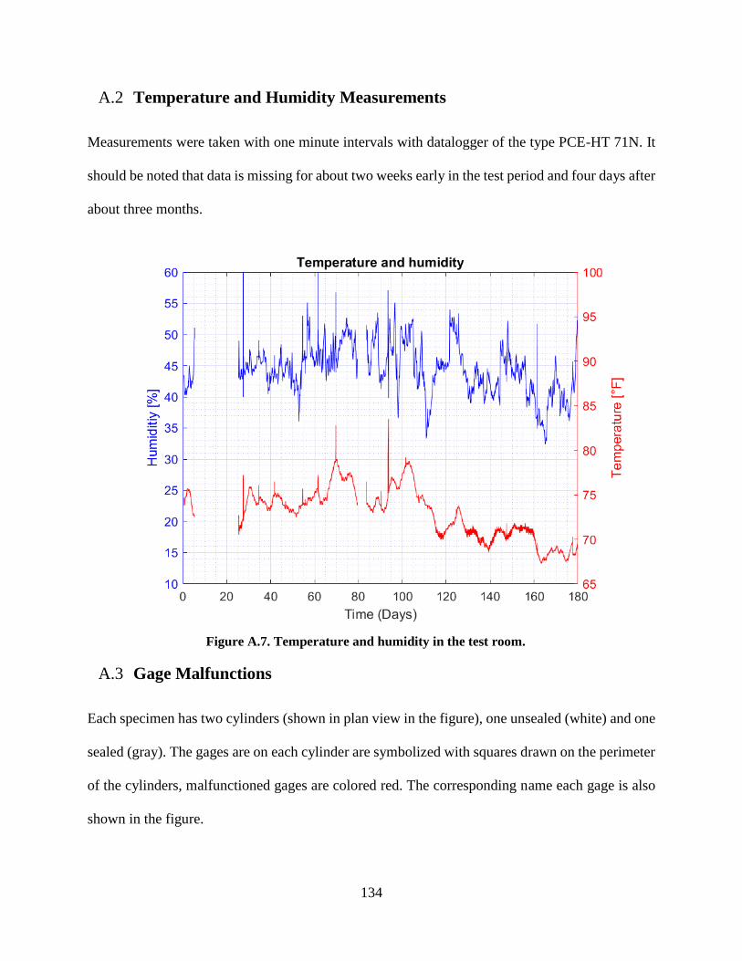
134
A.2 Temperature and Humidity Measurements
Measurements were taken with one minute intervals with datalogger of the type PCE-HT 71N. It
should be noted that data is missing for about two weeks early in the test period and four days after
about three months.
Figure A.7. Temperature and humidity in the test room.
A.3 Gage Malfunctions
Each specimen has two cylinders (shown in plan view in the figure), one unsealed (white) and one
sealed (gray). The gages are on each cylinder are symbolized with squares drawn on the perimeter
of the cylinders, malfunctioned gages are colored red. The corresponding name each gage is also
shown in the figure.
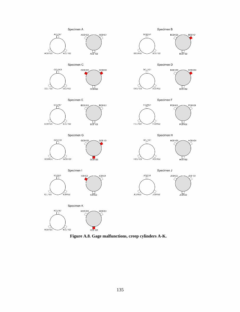
135
Figure A.8. Gage malfunctions, creep cylinders A-K.
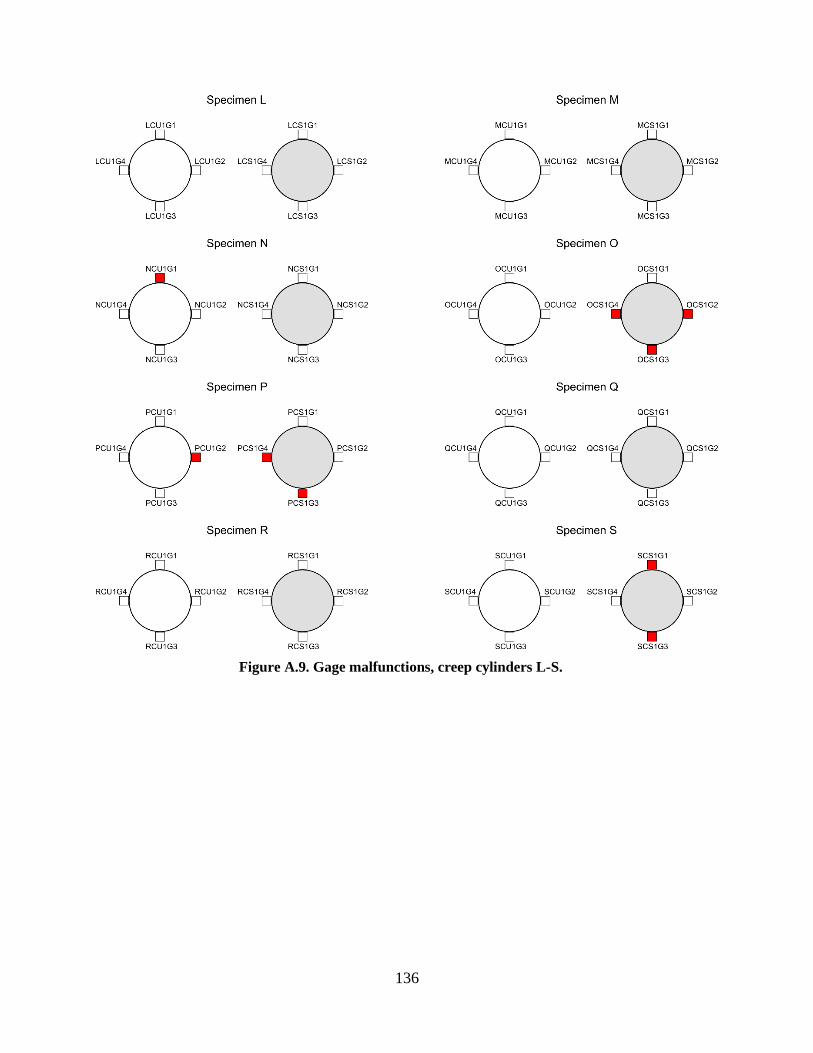
136
Figure A.9. Gage malfunctions, creep cylinders L-S.

137
Figure A.10. Gage malfunctions, shrinkage cylinders.

138
Table A.1. Gage malfunctions.
Gage ID List of Malfunction Gages Fate
ASS1G1/ESS1G1/GSS1G1/ISS1G1 Shrinkage Scrapped
BSS1G2 Shrinkage Scrapped
BCS1G1 Creep Kept
CCS1G1 Creep Scrapped
CCS1G3 Creep Scrapped
DCS1G1 Creep Kept
GCS1G1 Creep Kept
GCS1G2 Creep Kept
ICS1G3 Creep Kept
KSS1G2 Shrinkage Scrapped
KCS1G2 Creep Kept
NCU1G1 Creep Scrapped
NSS1G1 Shrinkage Kept
NSS1G2 Shrinkage Scrapped
OCS1G2 Creep Scrapped
OCS1G3 Creep Scrapped
OCS1G4 Creep Scrapped
PCU1G2 Creep Scrapped
PCS1G3 Creep Scrapped
PCS1G4 Creep Scrapped
SCS1G1 Creep Scrapped
SCS1G3 Creep Scrapped
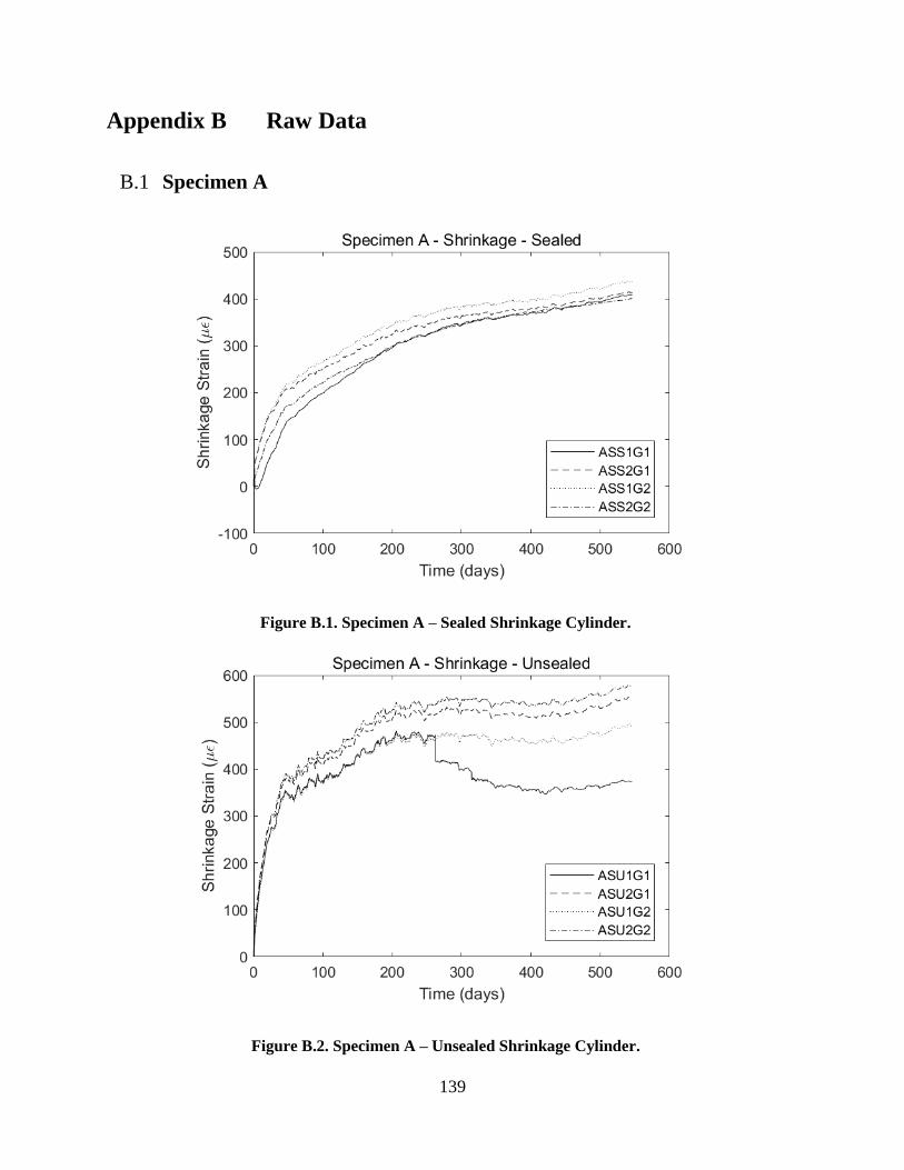
139
Appendix B Raw Data
B.1 Specimen A
Figure B.1. Specimen A – Sealed Shrinkage Cylinder.
Figure B.2. Specimen A – Unsealed Shrinkage Cylinder.
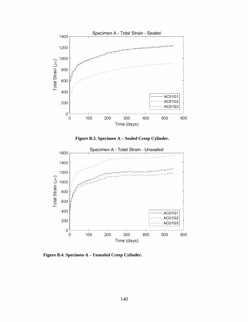
140
Figure B.3. Specimen A – Sealed Creep Cylinder.
Figure B.4. Specimen A – Unsealed Creep Cylinder.
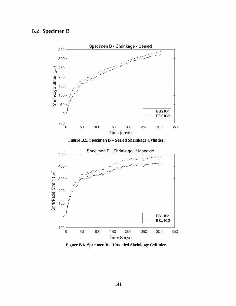
141
B.2 Specimen B
Figure B.5. Specimen B – Sealed Shrinkage Cylinder.
Figure B.6. Specimen B – Unsealed Shrinkage Cylinder.
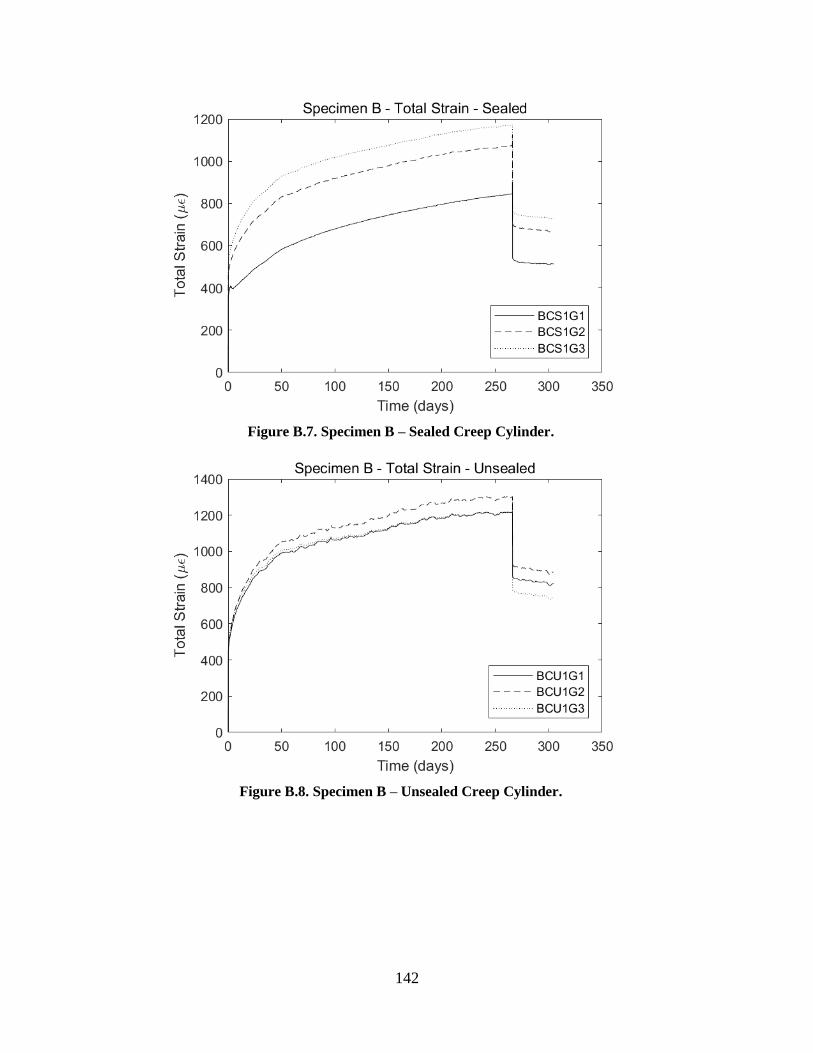
142
Figure B.7. Specimen B – Sealed Creep Cylinder.
Figure B.8. Specimen B – Unsealed Creep Cylinder.

143
B.3 Specimen C
Figure B.9. Specimen C – Sealed Shrinkage Cylinder.
Figure B.10. Specimen C – Unsealed Shrinkage Cylinder.
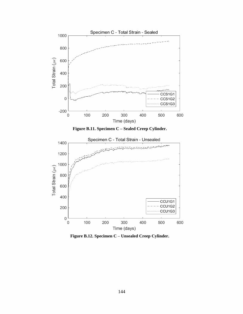
144
Figure B.11. Specimen C – Sealed Creep Cylinder.
Figure B.12. Specimen C – Unsealed Creep Cylinder.
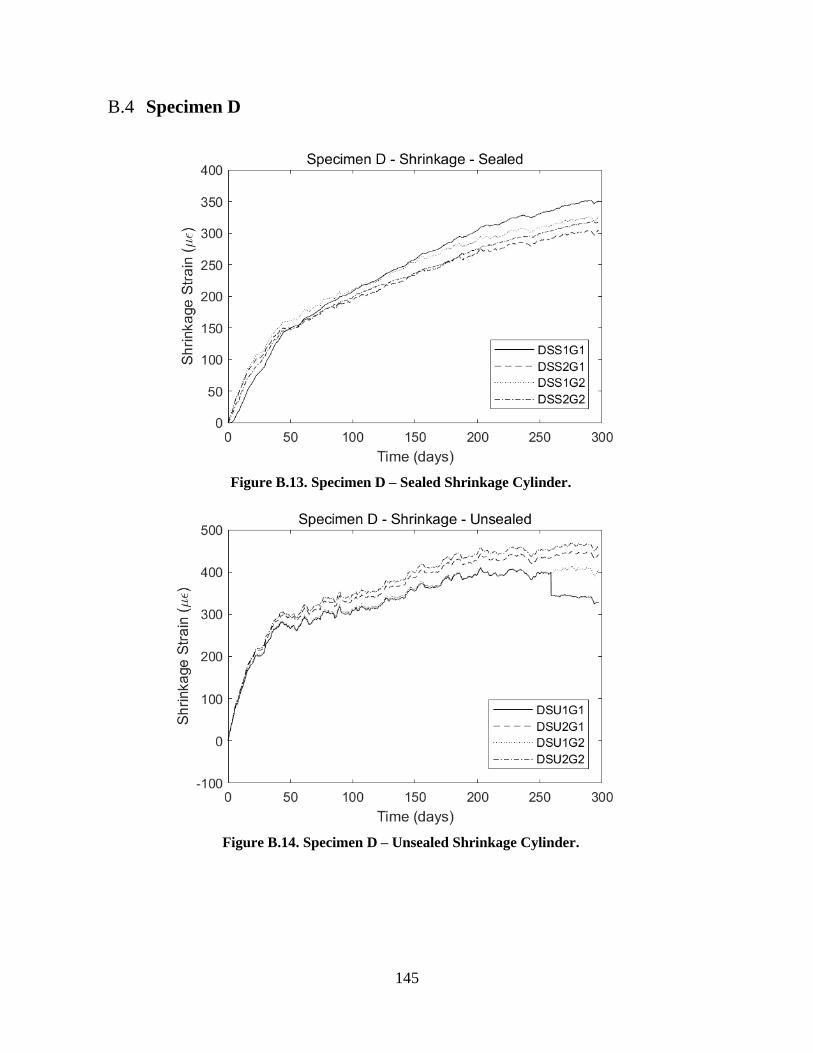
145
B.4 Specimen D
Figure B.13. Specimen D – Sealed Shrinkage Cylinder.
Figure B.14. Specimen D – Unsealed Shrinkage Cylinder.
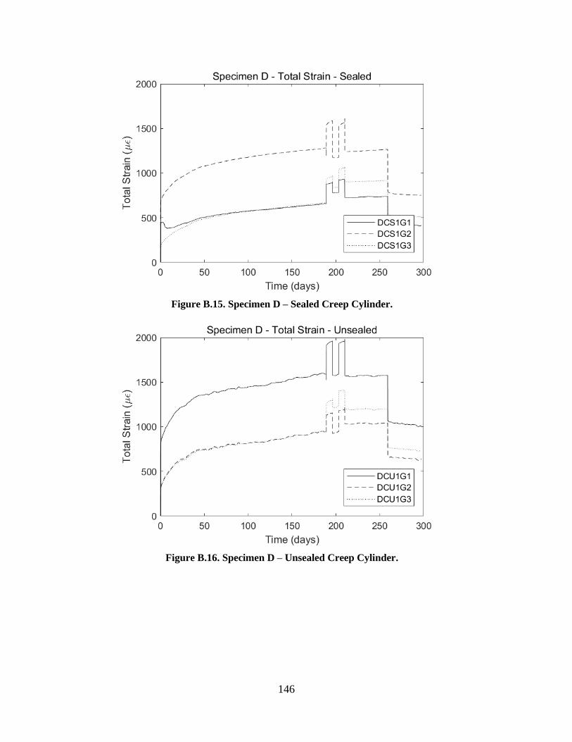
146
Figure B.15. Specimen D – Sealed Creep Cylinder.
Figure B.16. Specimen D – Unsealed Creep Cylinder.

147
B.5 Specimen E
Figure B.17. Specimen E – Sealed Shrinkage Cylinder.
Figure B.18. Specimen E – Unsealed Shrinkage Cylinder.
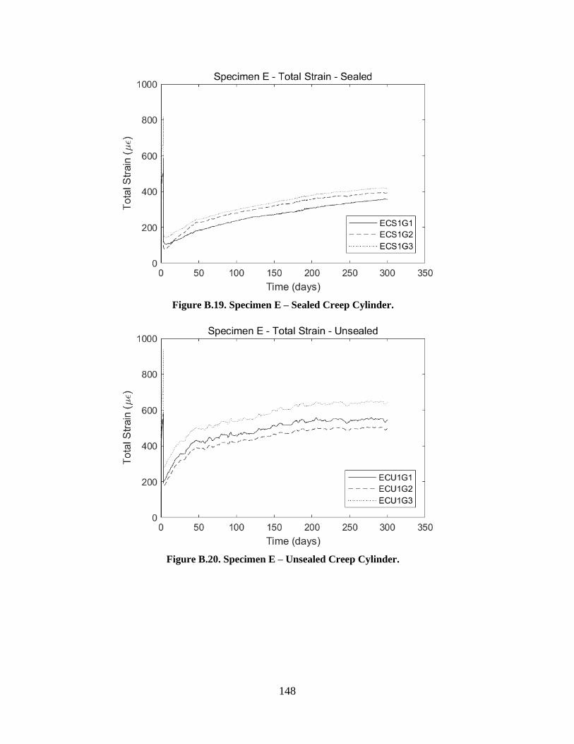
148
Figure B.19. Specimen E – Sealed Creep Cylinder.
Figure B.20. Specimen E – Unsealed Creep Cylinder.
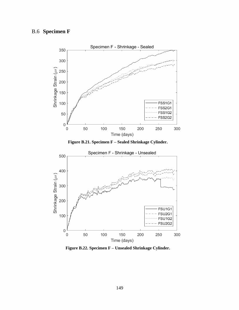
149
B.6 Specimen F
Figure B.21. Specimen F – Sealed Shrinkage Cylinder.
Figure B.22. Specimen F – Unsealed Shrinkage Cylinder.

150
Figure B.23. Specimen F – Sealed Creep Cylinder.
Figure B.24. Specimen F – Unsealed Creep Cylinder.
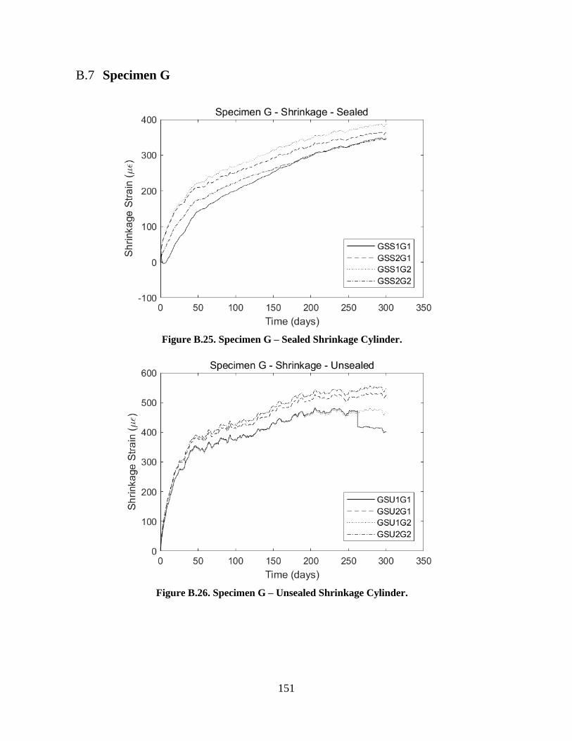
151
B.7 Specimen G
Figure B.25. Specimen G – Sealed Shrinkage Cylinder.
Figure B.26. Specimen G – Unsealed Shrinkage Cylinder.
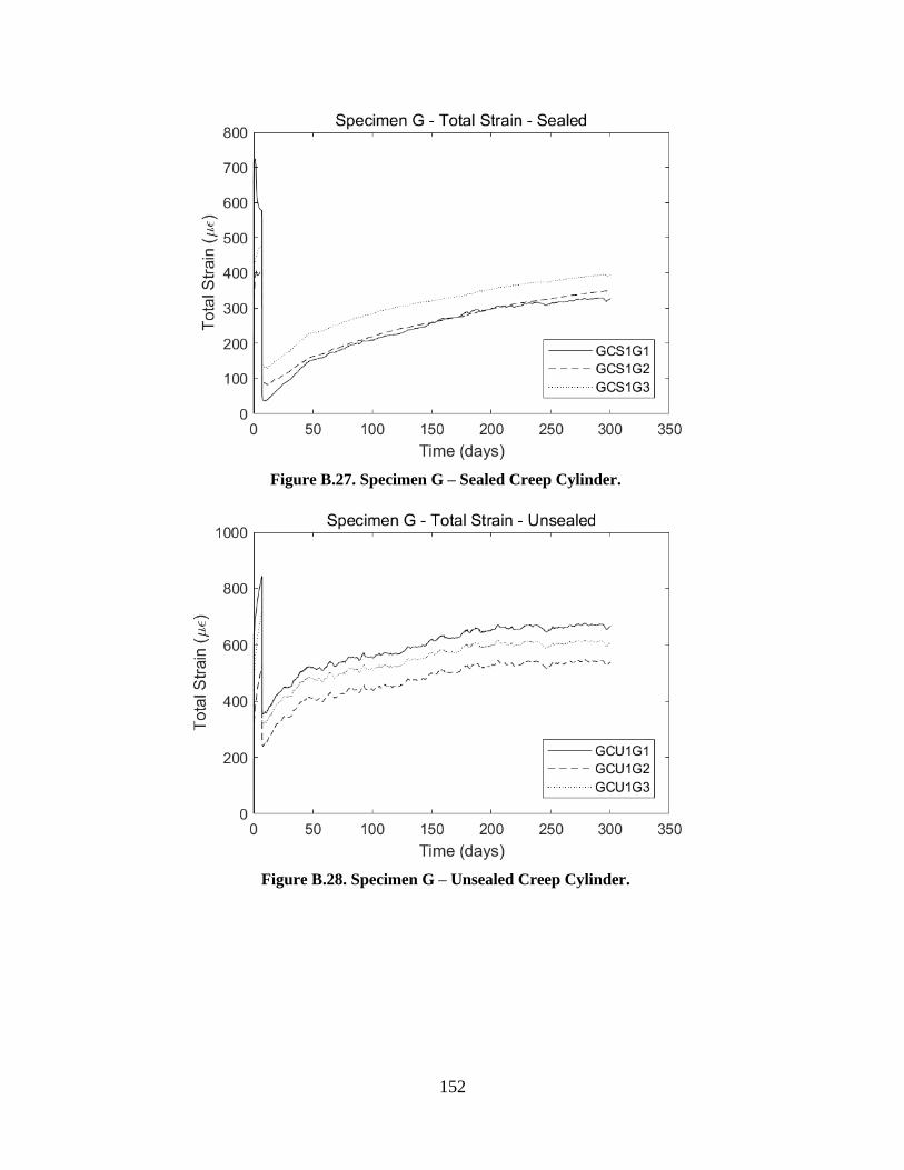
152
Figure B.27. Specimen G – Sealed Creep Cylinder.
Figure B.28. Specimen G – Unsealed Creep Cylinder.
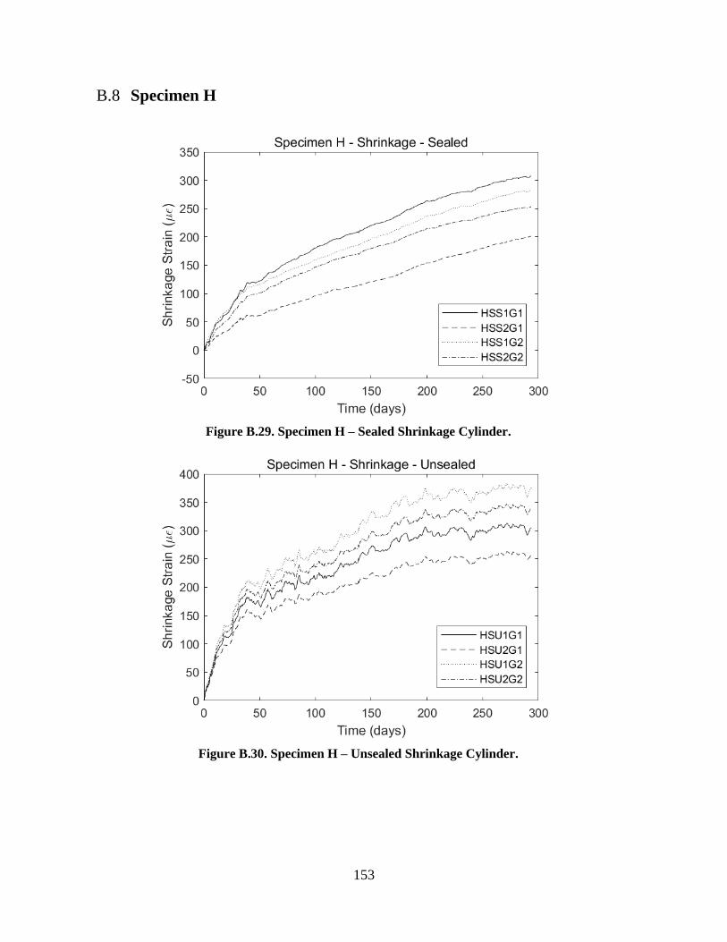
153
B.8 Specimen H
Figure B.29. Specimen H – Sealed Shrinkage Cylinder.
Figure B.30. Specimen H – Unsealed Shrinkage Cylinder.
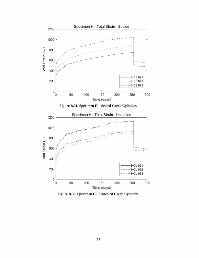
154
Figure B.31. Specimen H – Sealed Creep Cylinder.
Figure B.32. Specimen H – Unsealed Creep Cylinder.

155
B.9 Specimen I
Figure B.33. Specimen I – Sealed Shrinkage Cylinder.
Figure B.34. Specimen I – Unsealed Shrinkage Cylinder.

156
Figure B.35. Specimen I – Sealed Creep Cylinder.
Figure B.36. Specimen I – Unsealed Creep Cylinder.
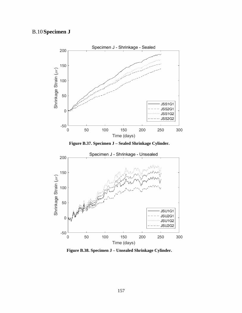
157
B.10 Specimen J
Figure B.37. Specimen J – Sealed Shrinkage Cylinder.
Figure B.38. Specimen J – Unsealed Shrinkage Cylinder.
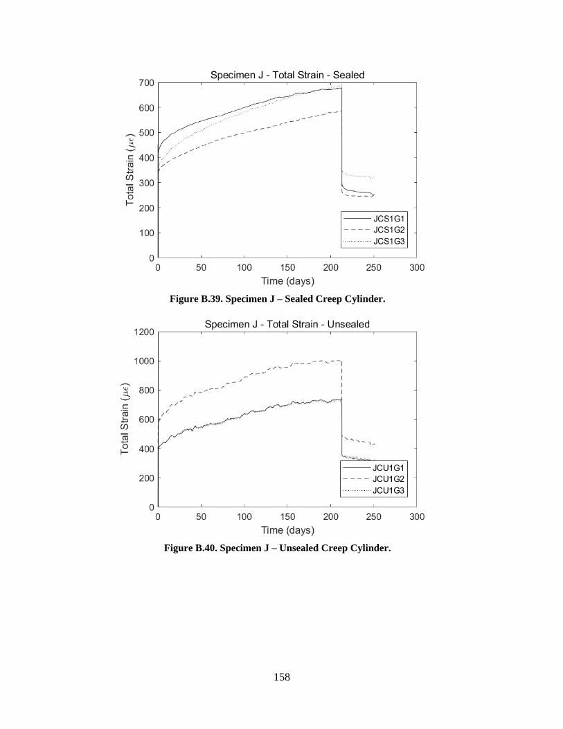
158
Figure B.39. Specimen J – Sealed Creep Cylinder.
Figure B.40. Specimen J – Unsealed Creep Cylinder.
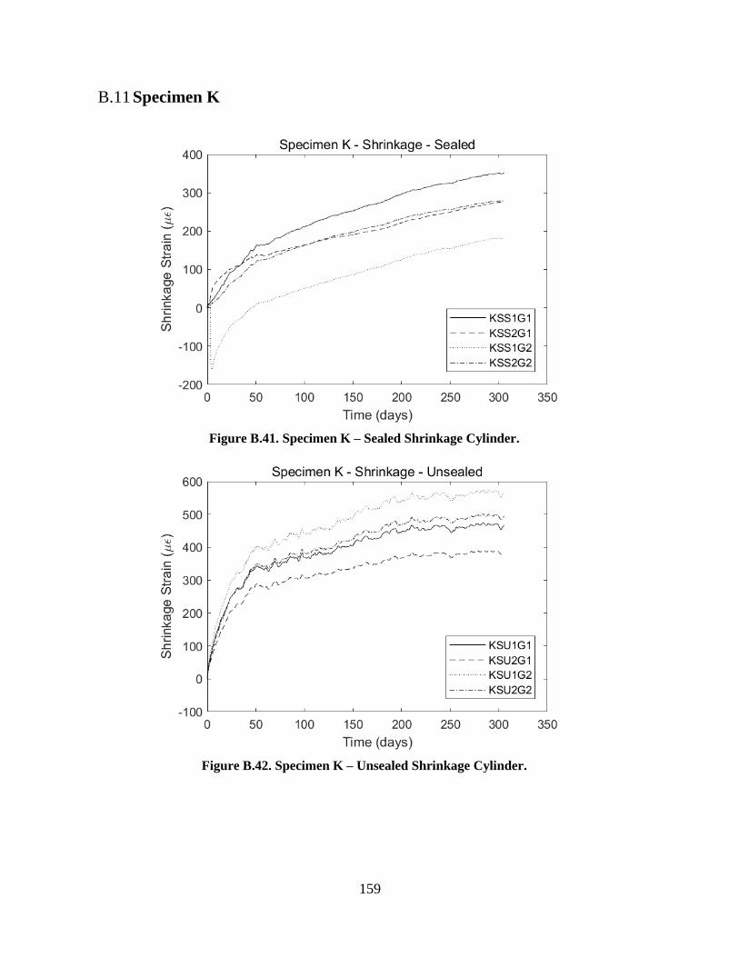
159
B.11 Specimen K
Figure B.41. Specimen K – Sealed Shrinkage Cylinder.
Figure B.42. Specimen K – Unsealed Shrinkage Cylinder.
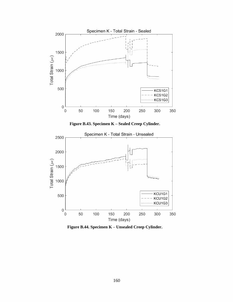
160
Figure B.43. Specimen K – Sealed Creep Cylinder.
Figure B.44. Specimen K – Unsealed Creep Cylinder.
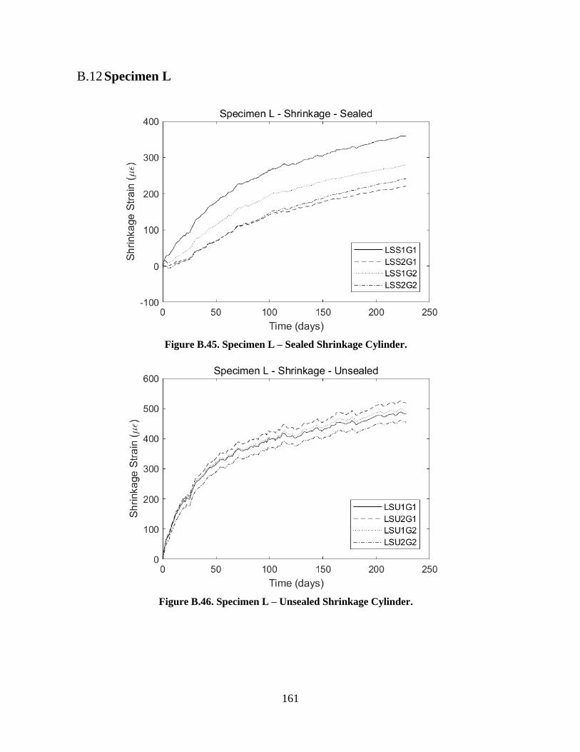
161
B.12 Specimen L
Figure B.45. Specimen L – Sealed Shrinkage Cylinder.
Figure B.46. Specimen L – Unsealed Shrinkage Cylinder.
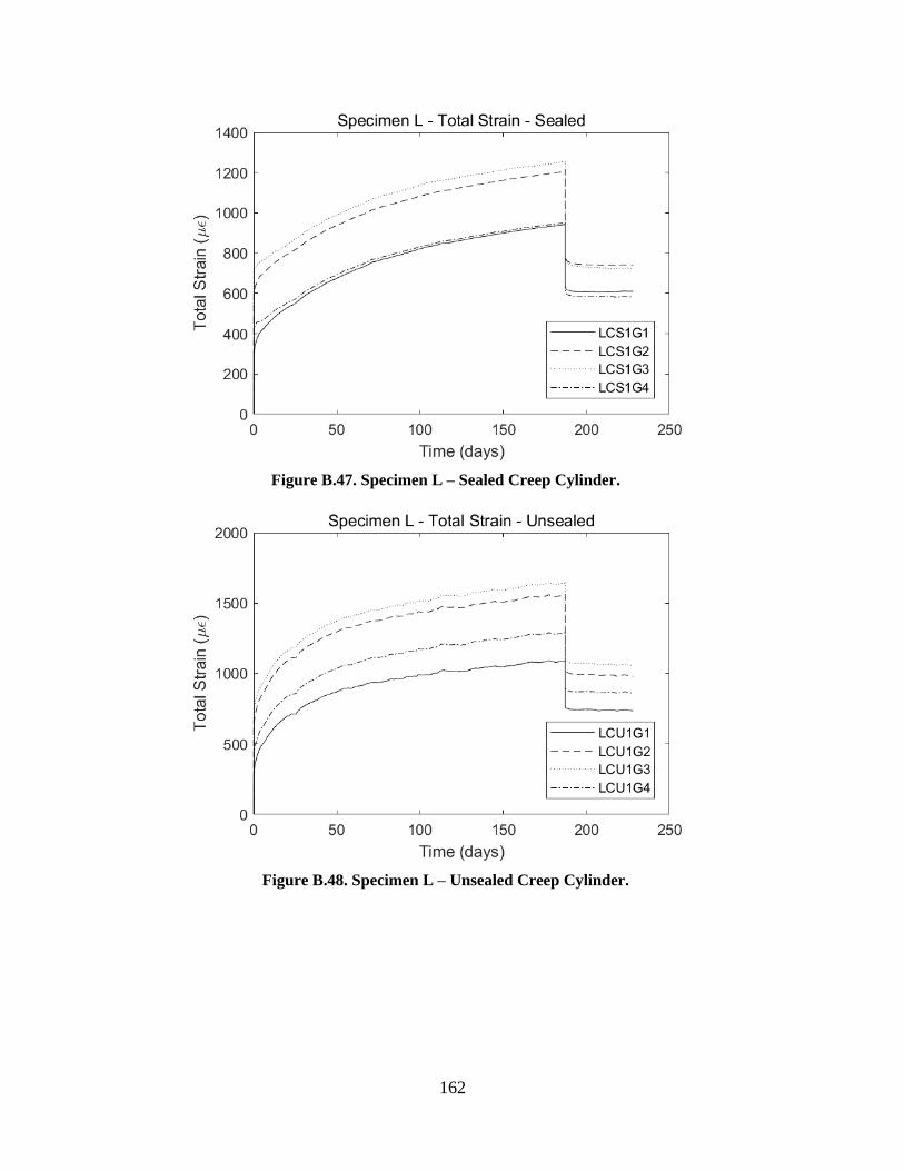
162
Figure B.47. Specimen L – Sealed Creep Cylinder.
Figure B.48. Specimen L – Unsealed Creep Cylinder.

163
B.13 Specimen M
Figure B.49. Specimen M – Sealed Shrinkage Cylinder.
Figure B.50. Specimen M – Unsealed Shrinkage Cylinder.
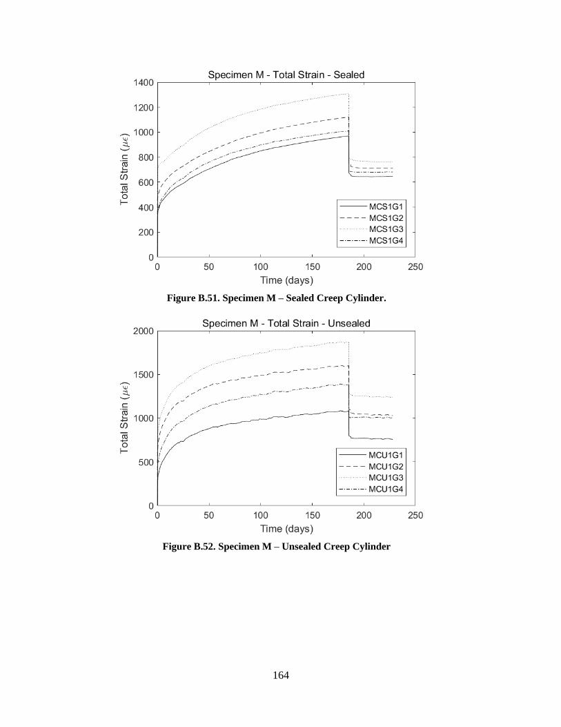
164
Figure B.51. Specimen M – Sealed Creep Cylinder.
Figure B.52. Specimen M – Unsealed Creep Cylinder
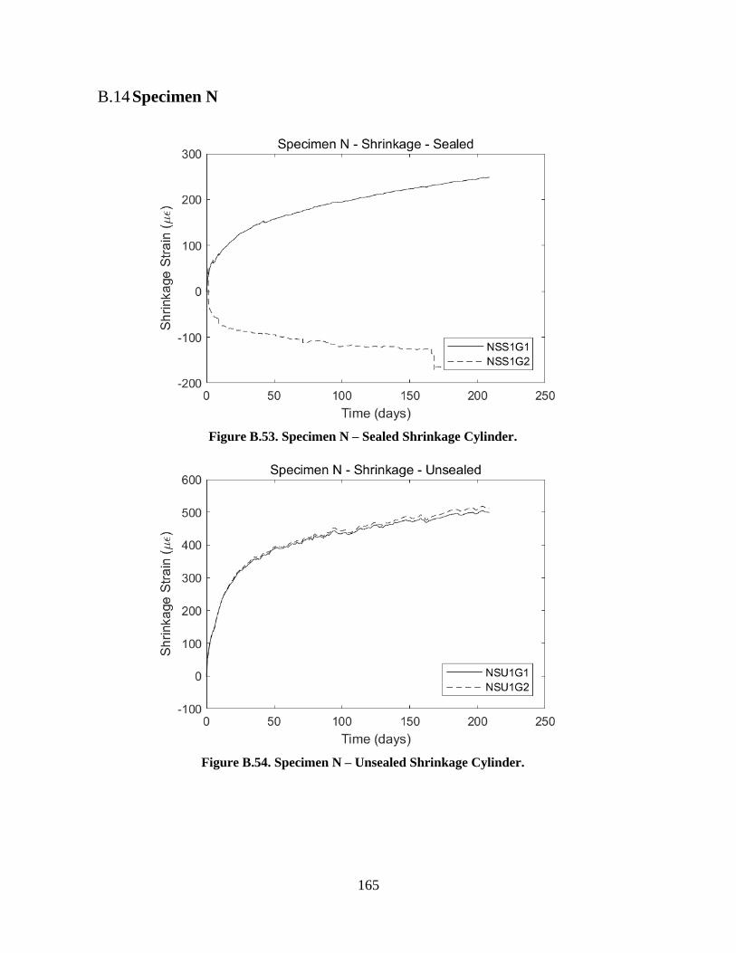
165
B.14 Specimen N
Figure B.53. Specimen N – Sealed Shrinkage Cylinder.
Figure B.54. Specimen N – Unsealed Shrinkage Cylinder.
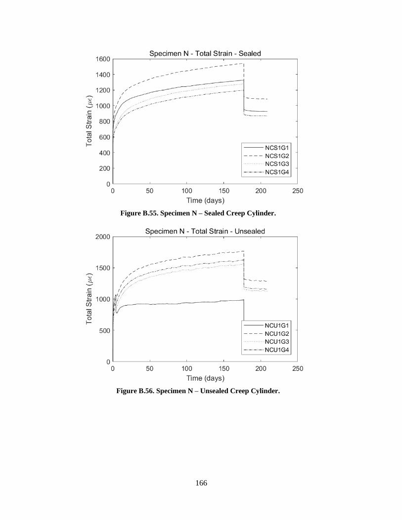
166
Figure B.55. Specimen N – Sealed Creep Cylinder.
Figure B.56. Specimen N – Unsealed Creep Cylinder.

167
B.15 Specimen O
Figure B.57. Specimen O – Sealed Shrinkage Cylinder.
Figure B.58. Specimen O – Unsealed Shrinkage Cylinder.
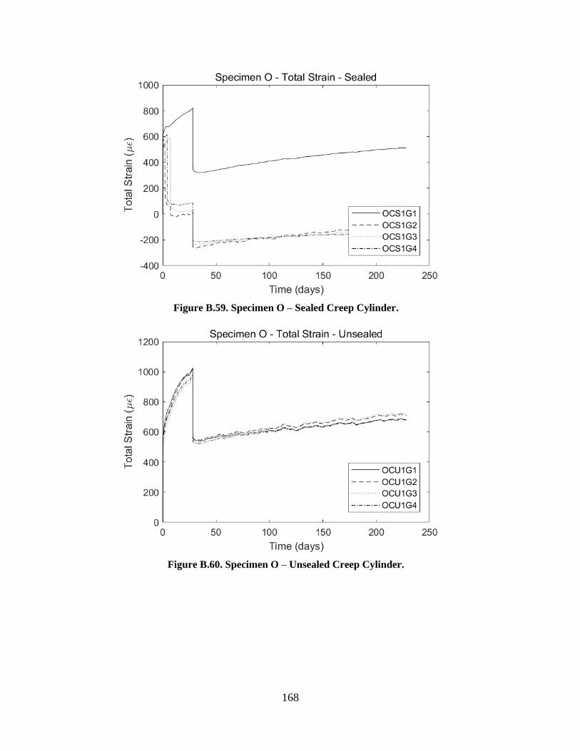
168
Figure B.59. Specimen O – Sealed Creep Cylinder.
Figure B.60. Specimen O – Unsealed Creep Cylinder.

169
B.16 Specimen P
Figure B.61. Specimen P – Sealed Shrinkage Cylinder.
Figure B.62. Specimen P – Unsealed Shrinkage Cylinder.
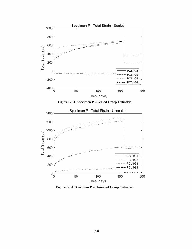
170
Figure B.63. Specimen P – Sealed Creep Cylinder.
Figure B.64. Specimen P – Unsealed Creep Cylinder.
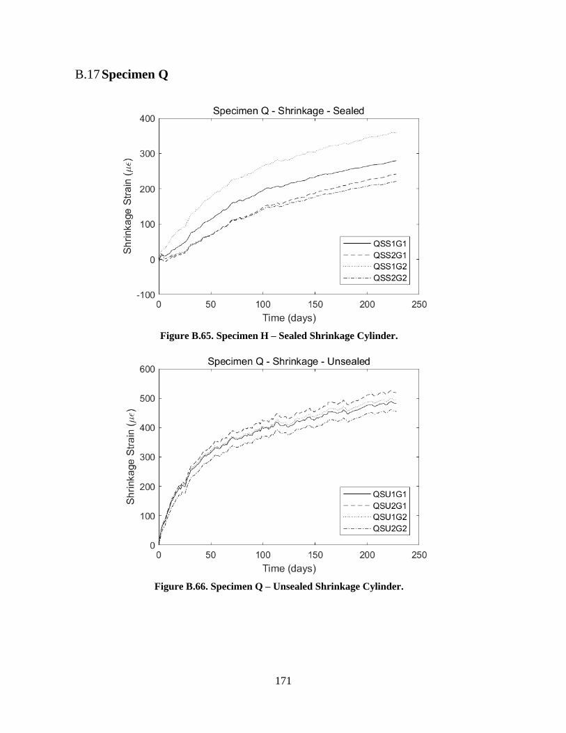
171
B.17 Specimen Q
Figure B.65. Specimen H – Sealed Shrinkage Cylinder.
Figure B.66. Specimen Q – Unsealed Shrinkage Cylinder.
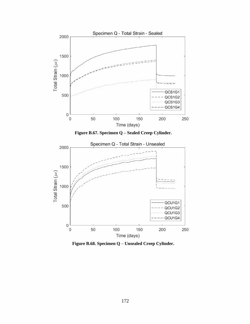
172
Figure B.67. Specimen Q – Sealed Creep Cylinder.
Figure B.68. Specimen Q – Unsealed Creep Cylinder.
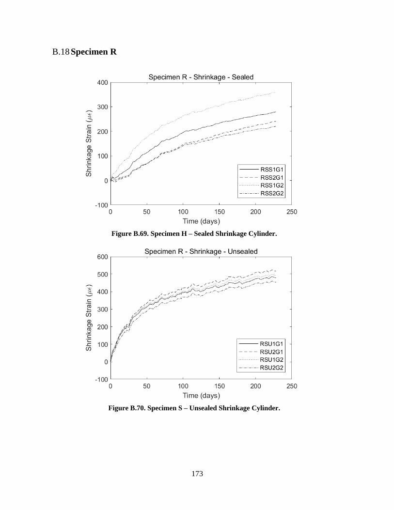
173
B.18 Specimen R
Figure B.69. Specimen H – Sealed Shrinkage Cylinder.
Figure B.70. Specimen S – Unsealed Shrinkage Cylinder.
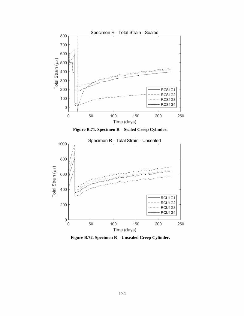
174
Figure B.71. Specimen R – Sealed Creep Cylinder.
Figure B.72. Specimen R – Unsealed Creep Cylinder.
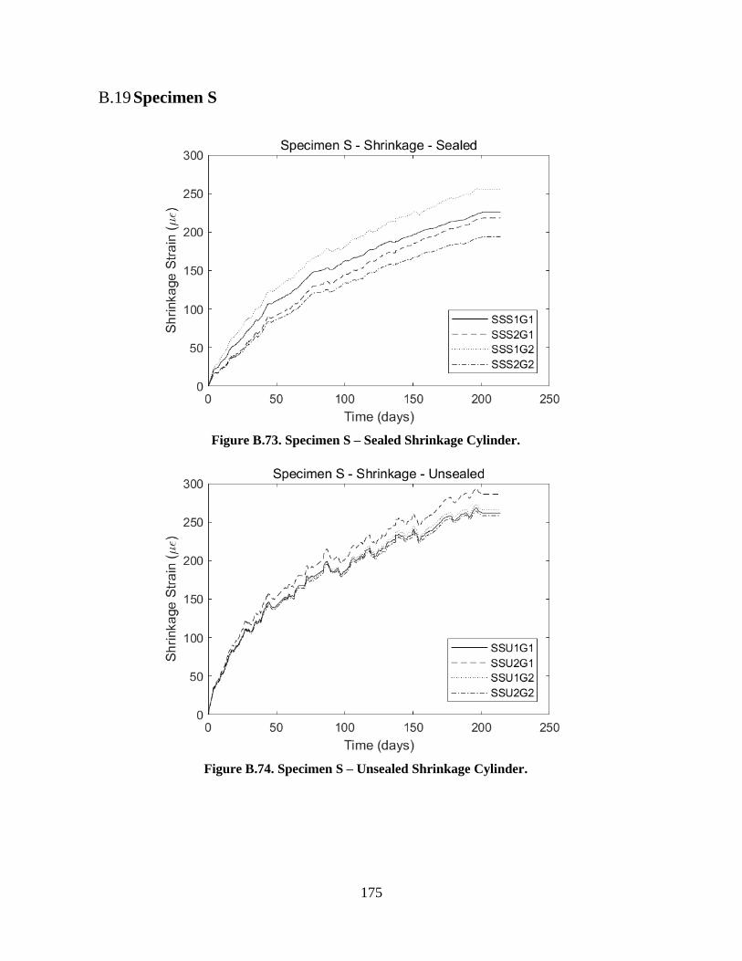
175
B.19 Specimen S
Figure B.73. Specimen S – Sealed Shrinkage Cylinder.
Figure B.74. Specimen S – Unsealed Shrinkage Cylinder.
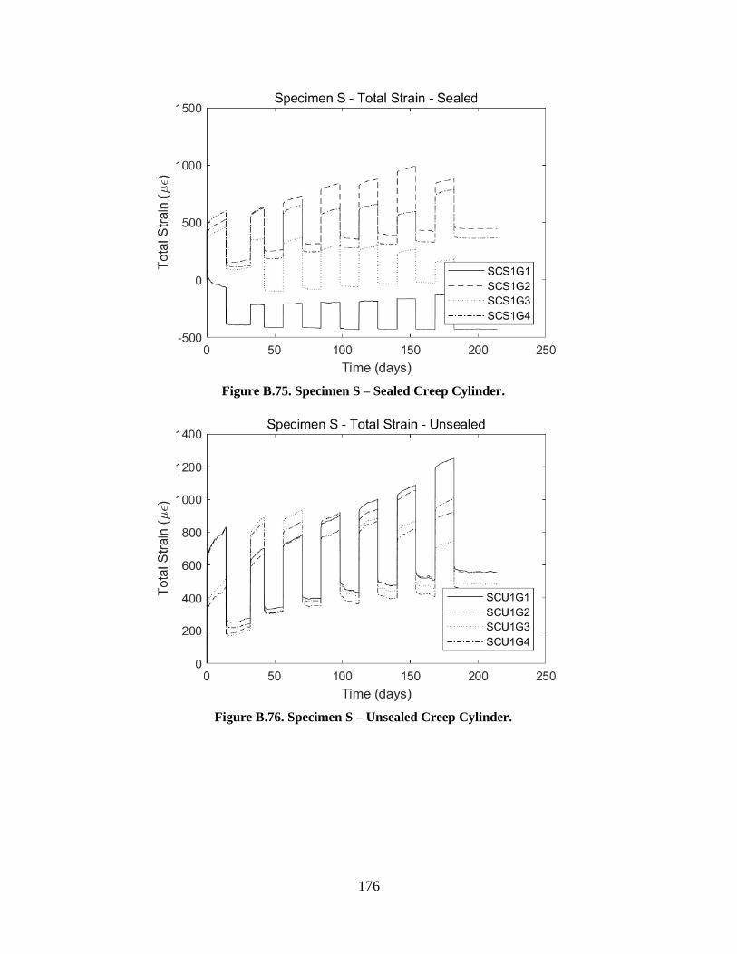
176
Figure B.75. Specimen S – Sealed Creep Cylinder.
Figure B.76. Specimen S – Unsealed Creep Cylinder.
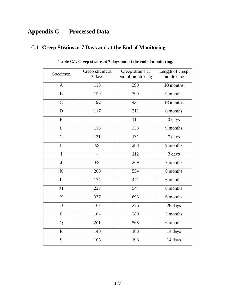
177
Appendix C Processed Data
C.1 Creep Strains at 7 Days and at the End of Monitoring
Table C.1. Creep strains at 7 days and at the end of monitoring.
Specimen Creep strains at
7 days
Creep strains at
end of monitoring
Length of creep
monitoring
A 113 399 18 months
B 159 399 9 months
C 192 434 18 months
D 117 311 6 months
E - 111 3 days
F 118 338 9 months
G 131 131 7 days
H 99 288 9 months
I - 112 3 days
J 89 269 7 months
K 208 554 6 months
L 174 441 6 months
M 233 544 6 months
N 377 693 6 months
O 167 276 28 days
P 104 280 5 months
Q 201 568 6 months
R 140 188 14 days
S 105 198 14 days
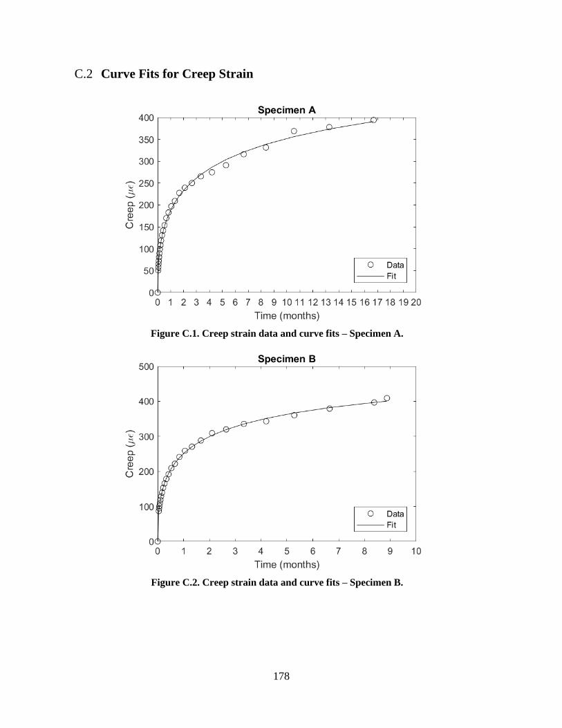
178
C.2 Curve Fits for Creep Strain
Figure C.1. Creep strain data and curve fits – Specimen A.
Figure C.2. Creep strain data and curve fits – Specimen B.
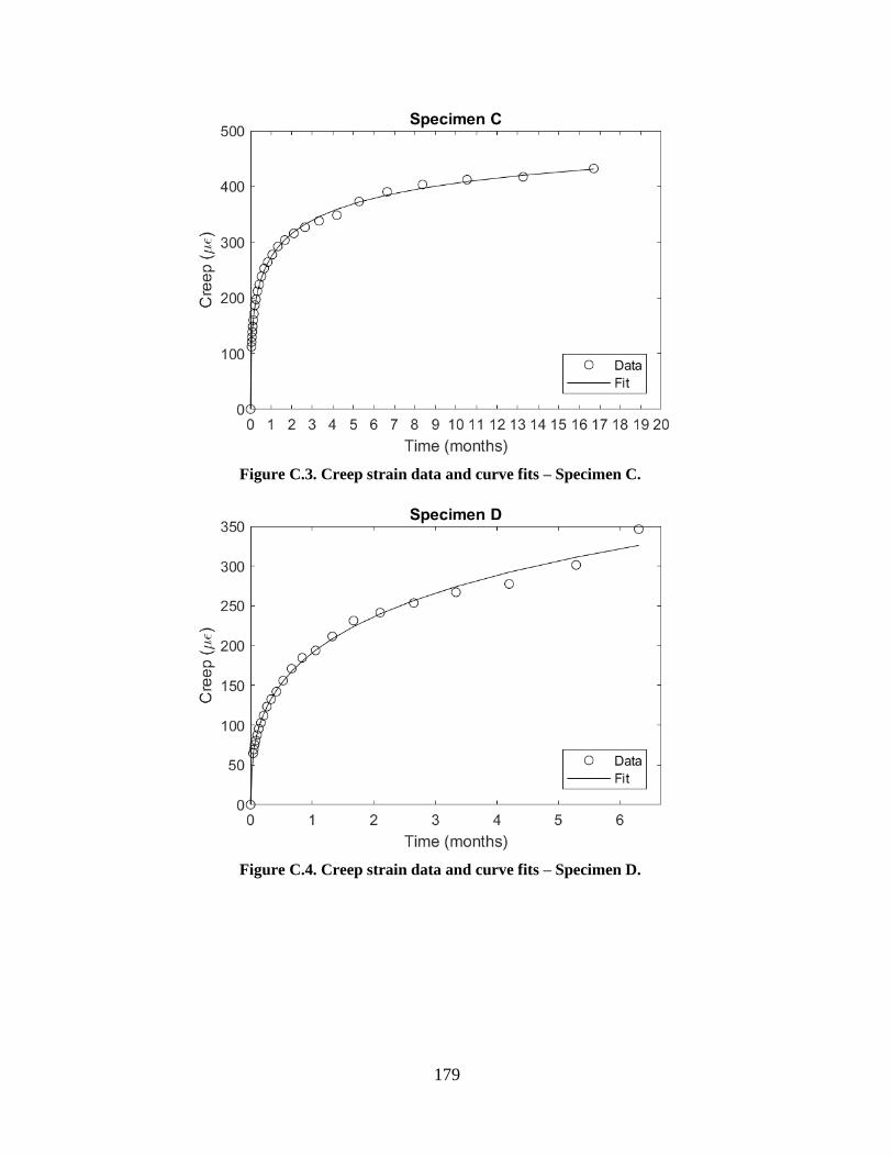
179
Figure C.3. Creep strain data and curve fits – Specimen C.
Figure C.4. Creep strain data and curve fits – Specimen D.
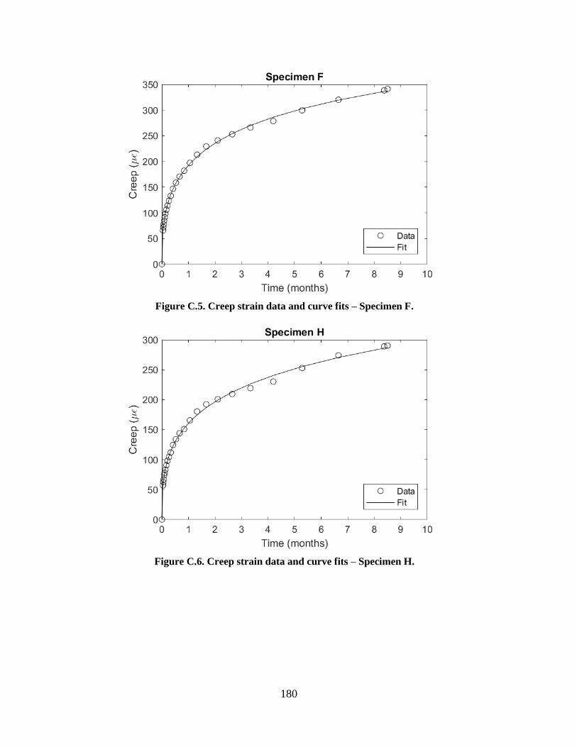
180
Figure C.5. Creep strain data and curve fits – Specimen F.
Figure C.6. Creep strain data and curve fits – Specimen H.

181
Figure C.7. Creep strain data and curve fits – Specimen J.
Figure C.8. Creep strain data and curve fits – Specimen K.

182
Figure C.9. Creep strain data and curve fits – Specimen L.
Figure C.10. Creep strain data and curve fits – Specimen M.
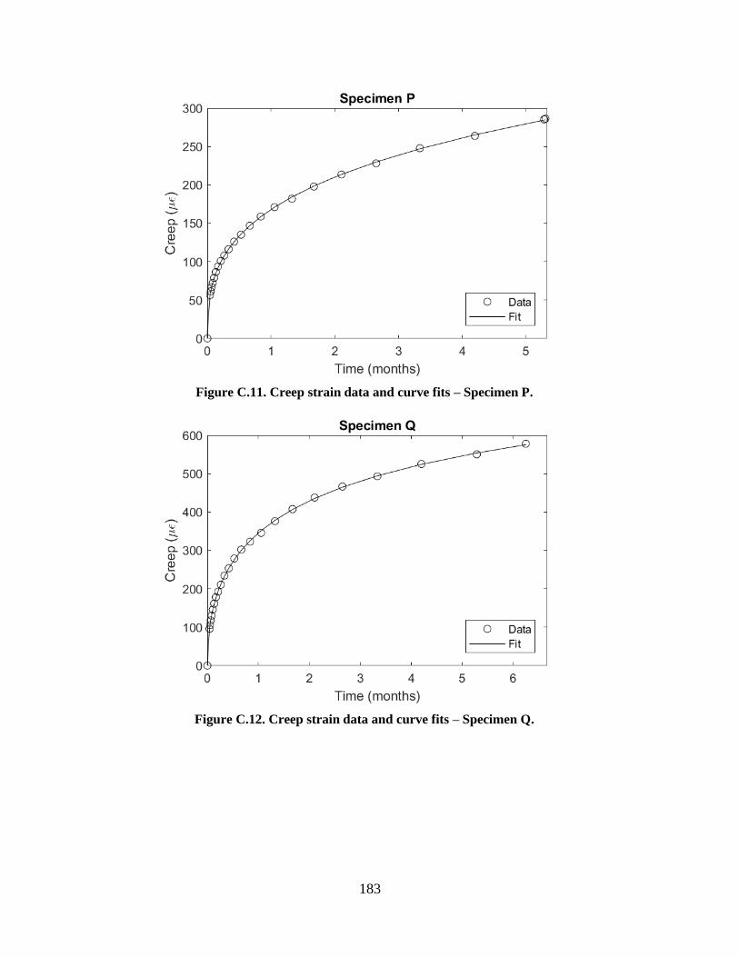
183
Figure C.11. Creep strain data and curve fits – Specimen P.
Figure C.12. Creep strain data and curve fits – Specimen Q.
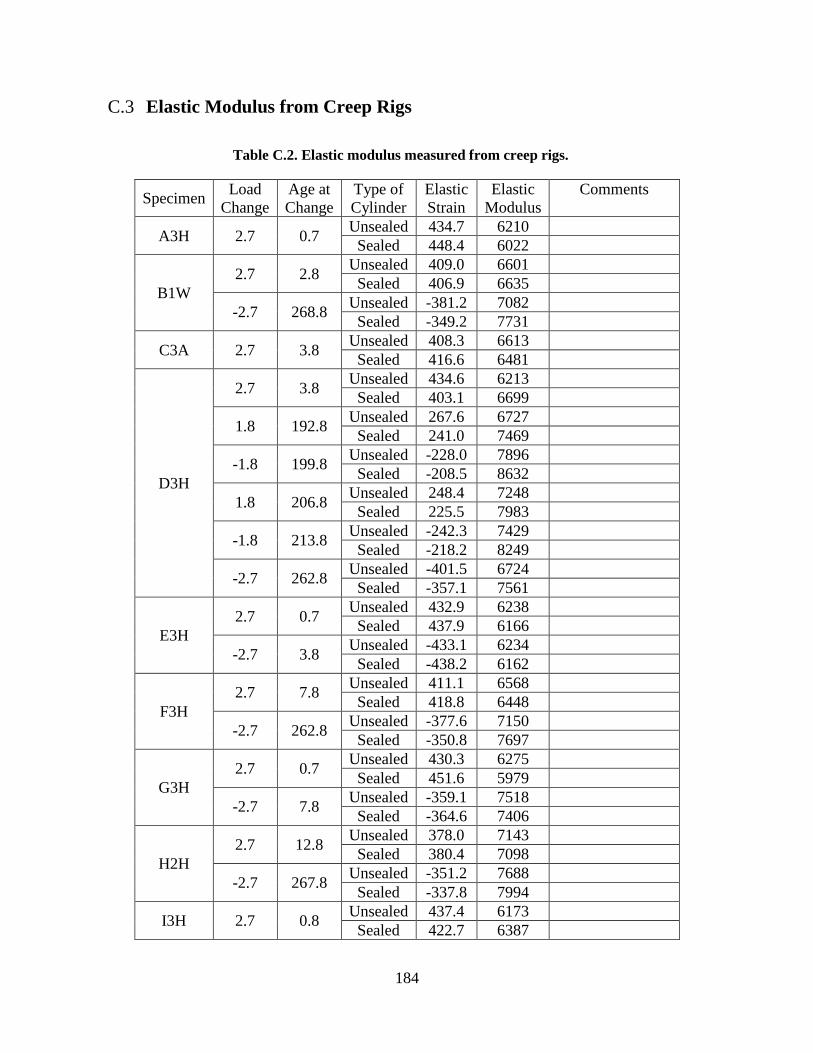
184
C.3 Elastic Modulus from Creep Rigs
Table C.2. Elastic modulus measured from creep rigs.
Specimen Load
Change
Age at
Change
Type of
Cylinder
Elastic
Strain
Elastic
Modulus
Comments
A3H 2.7 0.7 Unsealed 434.7 6210
Sealed 448.4 6022
B1W
2.7 2.8 Unsealed 409.0 6601
Sealed 406.9 6635
-2.7 268.8 Unsealed -381.2 7082
Sealed -349.2 7731
C3A 2.7 3.8 Unsealed 408.3 6613
Sealed 416.6 6481
D3H
2.7 3.8 Unsealed 434.6 6213
Sealed 403.1 6699
1.8 192.8 Unsealed 267.6 6727
Sealed 241.0 7469
-1.8 199.8 Unsealed -228.0 7896
Sealed -208.5 8632
1.8 206.8 Unsealed 248.4 7248
Sealed 225.5 7983
-1.8 213.8 Unsealed -242.3 7429
Sealed -218.2 8249
-2.7 262.8 Unsealed -401.5 6724
Sealed -357.1 7561
E3H
2.7 0.7 Unsealed 432.9 6238
Sealed 437.9 6166
-2.7 3.8 Unsealed -433.1 6234
Sealed -438.2 6162
F3H
2.7 7.8 Unsealed 411.1 6568
Sealed 418.8 6448
-2.7 262.8 Unsealed -377.6 7150
Sealed -350.8 7697
G3H
2.7 0.7 Unsealed 430.3 6275
Sealed 451.6 5979
-2.7 7.8 Unsealed -359.1 7518
Sealed -364.6 7406
H2H
2.7 12.8 Unsealed 378.0 7143
Sealed 380.4 7098
-2.7 267.8 Unsealed -351.2 7688
Sealed -337.8 7994
I3H 2.7 0.8 Unsealed 437.4 6173
Sealed 422.7 6387
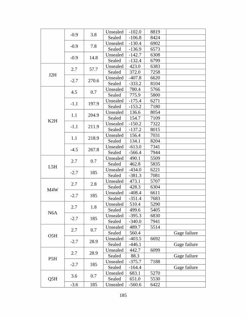
185
-0.9 3.8 Unsealed -102.0 8819
Sealed -106.8 8424
-0.9 7.8 Unsealed -130.4 6902
Sealed -136.9 6573
-0.9 14.8 Unsealed -142.7 6308
Sealed -132.4 6799
J2H
2.7 57.7 Unsealed 423.0 6383
Sealed 372.0 7258
-2.7 270.6 Unsealed -407.8 6620
Sealed -333.2 8104
K2H
4.5 0.7 Unsealed 780.4 5766
Sealed 775.9 5800
-1.1 197.9 Unsealed -175.4 6271
Sealed -153.2 7180
1.1 204.9 Unsealed 136.6 8054
Sealed 154.7 7109
-1.1 211.9 Unsealed -150.2 7322
Sealed -137.2 8015
1.1 218.9 Unsealed 156.4 7031
Sealed 134.1 8204
-4.5 267.8 Unsealed -613.0 7341
Sealed -566.4 7944
L5H
2.7 0.7 Unsealed 490.1 5509
Sealed 462.8 5835
-2.7 185 Unsealed -434.0 6221
Sealed -381.3 7081
M4W
2.7 2.8 Unsealed 473.1 5707
Sealed 428.3 6304
-2.7 185 Unsealed -408.4 6611
Sealed -351.4 7683
N6A
2.7 1.8 Unsealed 510.4 5290
Sealed 499.6 5405
-2.7 185 Unsealed -395.3 6830
Sealed -340.0 7941
O5H
2.7 0.7 Unsealed 489.7 5514
Sealed 560.4 Gage failure
-2.7 28.9 Unsealed -403.5 6692
Sealed -446.1 Gage failure
P5H
2.7 28.9 Unsealed 442.7 6099
Sealed 88.3 Gage failure
-2.7 185 Unsealed -375.7 7188
Sealed -164.4 Gage failure
Q5H 3.6 0.7
Unsealed 683.1 5270
Sealed 651.0 5530
-3.6 185 Unsealed -560.6 6422
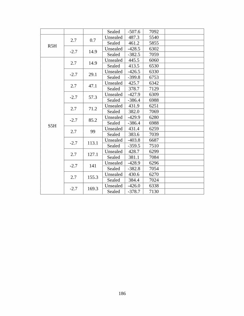
186
Sealed -507.6 7092
R5H
2.7 0.7 Unsealed 487.3 5540
Sealed 461.2 5855
-2.7 14.9 Unsealed -428.5 6302
Sealed -382.5 7059
S5H
2.7 14.9 Unsealed 445.5 6060
Sealed 413.5 6530
-2.7 29.1 Unsealed -426.5 6330
Sealed -399.8 6753
2.7 47.1 Unsealed 425.7 6342
Sealed 378.7 7129
-2.7 57.3 Unsealed -427.9 6309
Sealed -386.4 6988
2.7 71.2 Unsealed 431.9 6251
Sealed 382.0 7069
-2.7 85.2 Unsealed -429.9 6280
Sealed -386.4 6988
2.7 99 Unsealed 431.4 6259
Sealed 383.6 7039
-2.7 113.1 Unsealed -403.8 6687
Sealed -359.5 7510
2.7 127.1 Unsealed 428.7 6299
Sealed 381.1 7084
-2.7 141 Unsealed -428.9 6296
Sealed -382.8 7054
2.7 155.3 Unsealed 430.6 6270
Sealed 384.4 7024
-2.7 169.3 Unsealed -426.0 6338
Sealed -378.7 7130
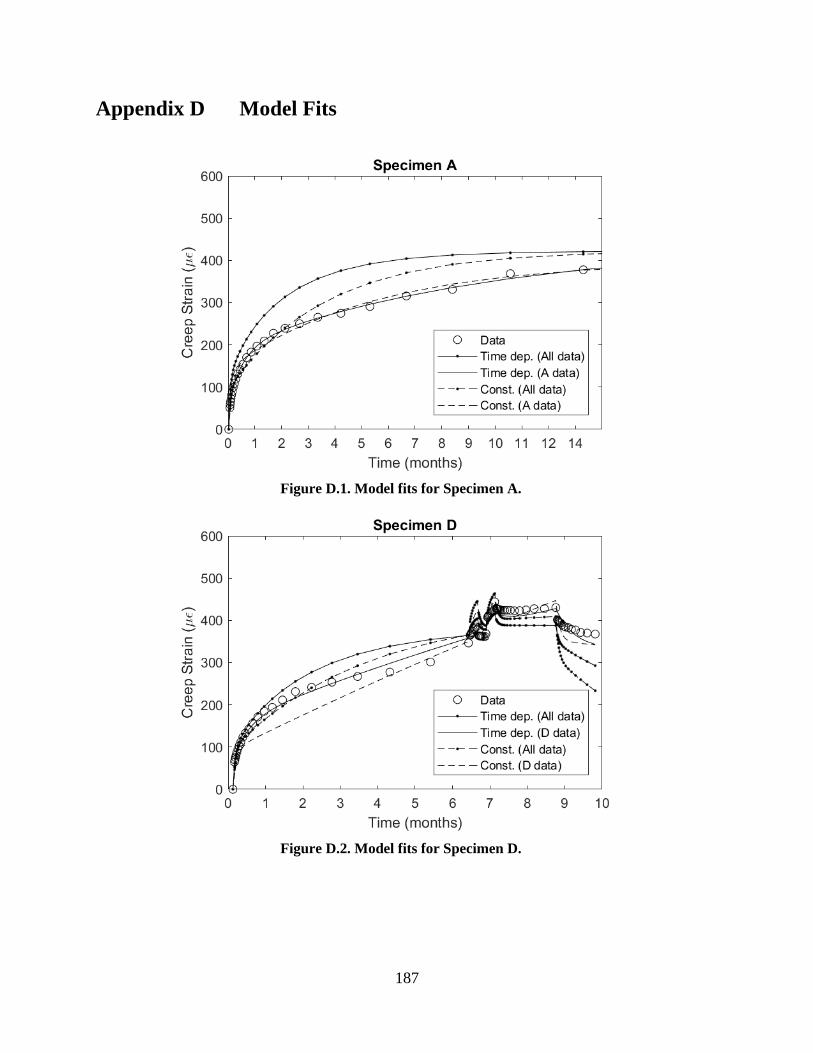
187
Appendix D Model Fits
Figure D.1. Model fits for Specimen A.
Figure D.2. Model fits for Specimen D.

188
Figure D.3. Model fits for Specimen E.
Figure D.4. Model fits for Specimen F.
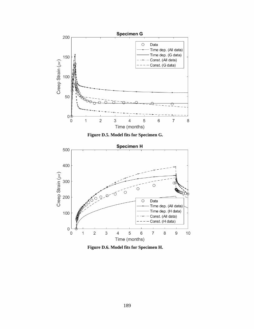
189
Figure D.5. Model fits for Specimen G.
Figure D.6. Model fits for Specimen H.
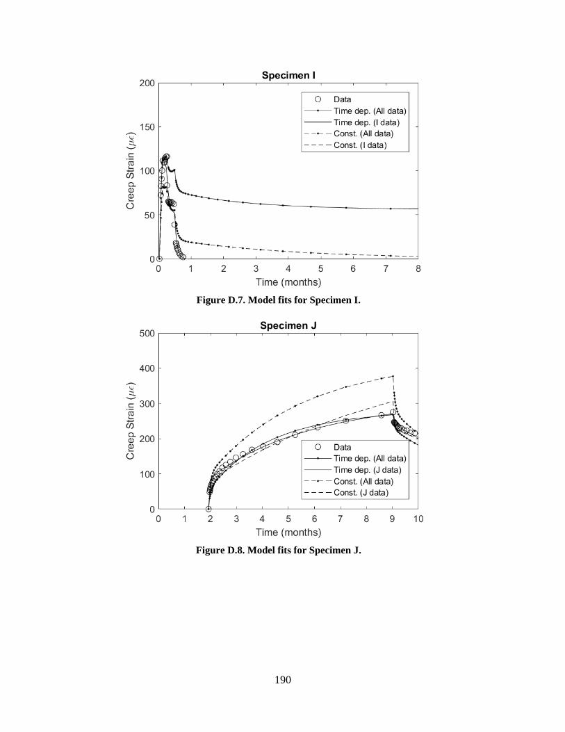
190
Figure D.7. Model fits for Specimen I.
Figure D.8. Model fits for Specimen J.
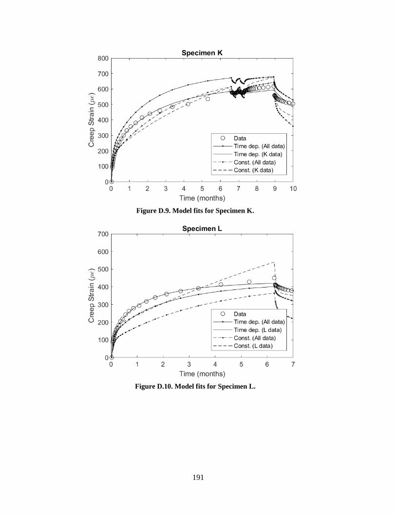
191
Figure D.9. Model fits for Specimen K.
Figure D.10. Model fits for Specimen L.
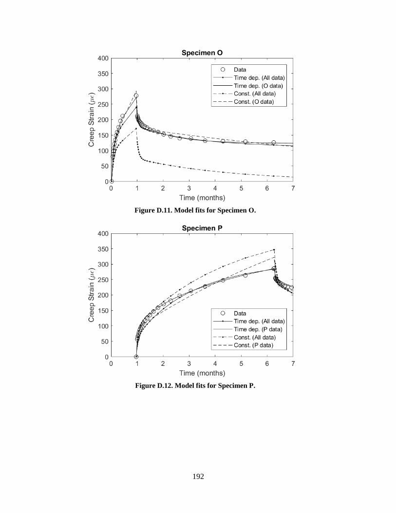
192
Figure D.11. Model fits for Specimen O.
Figure D.12. Model fits for Specimen P.

193
Figure D.13. Model fits for Specimen Q.
Figure D.14. Model fits for Specimen R.
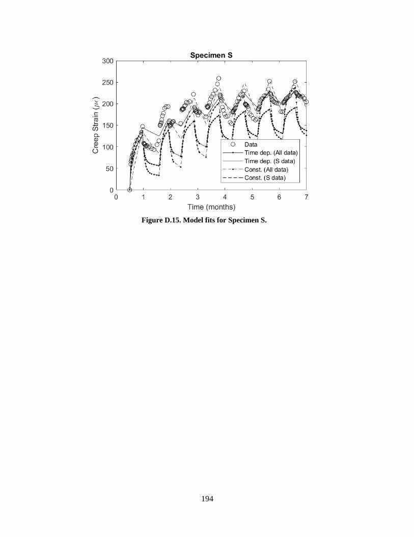
194
Figure D.15. Model fits for Specimen S.
Copyright © 2022 FDOKUMEN