Modelling of Thermal Magnesium Processes

Modelling of Thermal Magnesium Processes

Winny Wulandari

A Thesis Presented for the Degree of Doctor of Philosophy

Faculty of Engineering and Industrial Sciences Swinburne University of Technology

2013

i

Declaration The author declares that this thesis:

• contains no material which has been accepted for the award to the

candidate of any other degree or diploma, except where due reference is

made in the text of the thesis;

• to the best of the candidate’s knowledge contains no material previously

published or written by another person except where due reference is

made in the text of the thesis; and

• where the work is based on joint research or publications, discloses the

relative contributions of the respective workers or authors.

Winny Wulandari February 2013

ii

This Page Intentionally Left Blank

iii

Abstract The current dominant route for producing magnesium is via the Pidgeon

process, a batch pyrometallurgical route that uses silicothermic reduction for

extracting magnesium in the form of metal vapour. While this process is

versatile and offers simple operation, the productivity of this process is very

low. Other silicothermic processes such as the Magnetherm and the Mintek

process attempt to increase the productivity of the silicothermic reduction

process by carrying out the reduction at higher temperatures in a liquid oxide

phase. The higher temperature and correspondingly increased productivity is

likely to lead to greater impurities in the magnesium metal. While the

silicothermic processes has been operative over seventy years, there is limited

information on the thermodynamics and kinetics of the process. In particular,

there is limited information on the behaviour of magnesium vapour and its

impurities in these processes. The purpose of this study is to investigate the

fundamental chemistry associated with the silicothermic processes, with

emphasis on the behaviour of impurities in the process, by using

thermodynamic modelling and kinetics analysis, and test the predictions from

thermodynamic modelling by performing an experimental study.

The first stage of the study focused on the thermodynamic modelling of

silicothermic processes using the Gibbs energy minimisation method.

Thermodynamic modelling predicted the limit of magnesium recovery from the

process at specific operating condition. The results showed the model over-

predict experimental and industrial data from literature: For example between

1100 and 1200 °C, the model predicted 99 wt% of conversion while data

showed that conversion varied between 87 and 89 wt%. A solution model for

the metallic phases was developed using data from critically analysed literature

to describe the interaction between binary metals involved in the magnesium-

impurities system. A multistage equilibrium model of vapour condensation

predicted impurities to segregate in the process at temperature ranges between

iv

the reaction and condenser zone; that is between 482 and 1100 °C, with

impurities comprising of the species Fe, FeSi, CaO, and Mg2Ca.

In the next stage of research, a kinetics study was carried out to analyse the

kinetics of the process under a flowing inert gas atmosphere. The experimental

data used for this study was from a previous work on the silicothermic reaction

under argon atmosphere. The kinetics analysis considered a number of kinetic

models with different controlling factors and the mass transfer kinetics of

magnesium vapour from the briquettes to the bulk gas phase. Based on the

analysis, it was concluded that the silicothermic process under inert

atmosphere was controlled by solid state diffusion of reactants, with the Jander

and Ginstling-Brounshtein models being the best models to describe the kinetics

of the process. The analysis also predicted that gas-film mass transfer of

magnesium to the bulk gas phase was not limiting the overall kinetics of the

process.

In order to test prediction of the thermodynamic modelling study, an

experimental apparatus was developed and experimental work was performed

using the Pidgeon process’s chemistry to investigate the behaviour of impurities

in the process. Some condensates were found in the cooler part of the furnace,

with MgO as the major phase. The magnesium metal condensate had been

purposedly oxidised after formation. The variation of concentration of the

condensates as predicted from the thermodynamic modelling study was not

observed in the experimental study. The Classical Nucleation Theory predicts

that homogeneous nucleation for the species occurs at different temperature,

which corresponds to different position in the horizontal tube. However, due to

very low vapour pressure of Ca, SiO, and Fe in this temperature range, these

species would not to be expected to be observed in the experimental study,

which was consistent with the experimental results.

In conclusion, there is no evidence that impurities present in magnesium vapour

can be practically separated by selective condensation, eventhough it is

thermodynamically feasible. Experimental work at higher concentrations and

temperature range are required to fully explore this option.

v

Acknowledgments I would like to express my gratitude to Allah, the Almighty, who guides me

throughout my PhD study and beyond.

I am truly indebted and obliged to my supervisor, Professor Geoffrey Brooks, for

his guidance and support, and countless reading revisions of this thesis. He has

been supporting me throughout this challenging journey while I has been

juggling between PhD journeys and becoming a young mother. I really admire

his enthusiasm on research and his contribution to the society, which also

motivates me do this research. I would like to thank him for introducing me to

this field of research and the high temperature processing research community.

I also would like to express my gratitude my second supervisors, Dr. M. Akbar

Rhamdhani, for his valuable discussions. To my external supervisor, Dr. Brian J.

Monaghan, I would like to thank for his valuable discussions and suggestions on

my research. I always gain more insight on this project from my corresponding

supervisors, especially about the analytical skills as well as experimental skills.

I owe sincere thankfulness to technical staffs at the Faculty of Engineering and

Industrial Sciences: Phil Watson, Alec Papanicolaou, David Vass, and Andrew

Moore for assisting me to construct experimental rig and help me technically.

Without their assistances, it was very challenging to construct and develop a

new laboratory and experimental rig in the early growth of this research group.

I also would like to thanks Dr. James Wang for assisting me conducting

SEM/EDS analysis, and Dr. Francois Malherbe from Faculty of Life and Social

Sciences for assisting me conducting XRD analysis and also introducing me to

his research group.

Thanks to all my colleagues of the High Temperature Processing group (in no

special order): Neslihan Dogan, Nazmul Huda, Behrooz Fateh, Morshed Alam,

vi

Bernard Xu, Reiza Mukhlis, Abdul Khaliq, Saiful Islam, and Shabnam Sabah. In

particular, I would like to thank Neslihan, Nazmul, and Morshed for all

wonderful discussions and sharing of knowledge and experiences during the

duration of my PhD journey.

I am honestly thankful to my husband, Muhammad Agus Kariem, who always

supports me in any way to finish my study. It has been a great experience to

share PhD journey with him and have scientific discussions along trips to

campus. To my sons, Affan and Arfa, who has been grown up with this project,

thanks being so patient and understanding their mum working and very busy

on her PhD. And also to my parents, sisters, and my parents in law (Hasan Basri

and Nor Rosyidah) in my home country whose support and encourage me to

finish this study, I would like to thank them.

This thesis is dedicated to my beloved parents, Nina Indrakirana and Nandang

Apipudin. They have raised me with a love of science and always support me in

any conditional way to help me achieve my success since my childhood until

now.

vii

To my parents, Mas Kariem, Affan, and Arfa

viii


ix

Table of Contents Declaration ......................................................................................................................................... i

Abstract ............................................................................................................................................. iii

Acknowledgments .......................................................................................................................... v

Table of Contents ........................................................................................................................... ix

List of Figures .............................................................................................................................. xvii

List of Tables ................................................................................................................................xxv

Nomenclatures .......................................................................................................................... xxix

1 Introduction ............................................................................................................................ 1

2 Fundamental of Silicothermic Processes ..................................................................... 5

2.1 The Pidgeon Process .................................................................................................... 5

2.1.1 Thermodynamics of the Pidgeon Process ................................................... 9

2.1.2 Reaction Kinetics of the Pidgeon Process ................................................ 12

2.1.2.1 Reaction in Vacuum Condition ............................................................ 12

2.1.2.1.1 Effect of Temperature and Pressure ............................................. 17

2.1.2.1.2 Effect of Silicon Grade ......................................................................... 18

2.1.2.1.3 Effect of Silicon Stoichiometry ........................................................ 19

2.1.2.1.4 Effect of Catalyst.................................................................................... 19

2.1.2.1.5 Effect of Particle Size and Distribution ........................................ 20

2.1.2.1.6 Effect of Briquetting Pressure ......................................................... 20

2.1.2.2 Reaction under Flowing Inert Gas Atmosphere ........................... 20

2.1.3 Reaction Mechanism of the Pidgeon Process ......................................... 22

2.2 Bolzano Process .......................................................................................................... 27

2.3 Magnetherm Process ................................................................................................ 29

2.3.1 Magnetherm Process Description ............................................................... 29

2.3.2 Magnetherm Refining Operation ................................................................. 32

2.3.3 Modified Magnetherm Processes ................................................................ 33

2.4 Mintek Process ............................................................................................................ 34

2.4.1 Mintek Process Description .......................................................................... 34

2.4.2 Mintek Refining Operation ............................................................................ 39

2.4.3 Prospects of the Mintek Process.................................................................. 40

x

2.5 Purity Requirement for Commercial Magnesium .......................................... 41

3 Review of Thermodynamics and Kinetics of High Temperature System ..... 45

3.1 Thermodynamic Modelling .................................................................................... 45

3.1.1 Gibbs Energy Minimisation ........................................................................... 45

3.1.2 Database Development ................................................................................... 48

3.1.3 Solution Models .................................................................................................. 48

3.1.3.1 Ideal Solution Model ................................................................................ 49

3.1.3.2 Dilute Solution Model .............................................................................. 49

3.1.3.3 Regular Solution Model .......................................................................... 50

3.1.3.4 Random Mixing Solution Model .......................................................... 51

3.1.3.5 Sublattice Model ........................................................................................ 52

3.1.3.6 Compound Energy Formalism Model ............................................... 53

3.1.3.7 Modified Quasichemical Model ........................................................... 53

3.1.4 Thermochemical Packages ............................................................................ 55

3.1.4.1 Chemix-Thermodata ................................................................................ 55

3.1.4.2 HSC ................................................................................................................. 56

3.1.4.3 FactSage ........................................................................................................ 56

3.1.4.4 MTDATA ....................................................................................................... 57

3.2 Reaction Kinetics ........................................................................................................ 58

3.2.1 Kinetics of Heterogeneous Reaction .......................................................... 58

3.2.2 Kinetics Theory of Gas-Solid Reaction ...................................................... 60

3.2.3 Kinetics Theory of Solid-Solid Reaction ................................................... 62

3.2.3.1 Solid-State Diffusion ................................................................................ 66

3.2.3.2 Gas-Phase Mass Transfer ....................................................................... 67

3.2.4 Kinetics of Vapour Condensation ................................................................ 70

3.2.4.1 Homogeneous Nucleation ..................................................................... 71

3.2.4.1.1 Classical Nucleation Theory (CNT) ................................................ 73

3.2.4.1.2 Scaled Nucleation Theory (SNT) ..................................................... 74

3.2.4.1.3 Internally Consistent Classical Nucleation Theory (ICCT) ... 75

3.2.4.2 Heterogeneous Nucleation .................................................................... 76

3.2.4.3 Growth of Particles................................................................................... 77

3.3 Experimental Techniques ....................................................................................... 78

xi

3.3.1 Experimental Techniques on the Kinetics of Silicothermic Processes ............................................................................................................................... 78

3.3.2 Experimental Studies on Homogeneous Nucleation ........................... 84

4 Research Issues ................................................................................................................... 87

5 Thermodynamic Modelling of Silicothermic Processes ...................................... 89

5.1 Methodology of Modelling ...................................................................................... 89

5.2 Thermodynamic Analysis of Silicothermic Processes ................................. 92

5.2.1 Thermodynamic Simulation of the Pidgeon Process ........................... 94

5.2.1.1 Modelling Development ......................................................................... 94

5.2.1.2 Results ........................................................................................................... 97

5.2.2 Thermodynamic Simulation of the Magnetherm Process ................. 99

5.2.2.1 Modelling Developments ....................................................................... 99

5.2.2.2 Results ......................................................................................................... 100

5.2.3 Thermodynamic Simulation of the Mintek Process ........................... 101

5.2.3.1 Modelling Development ....................................................................... 101

5.2.3.2 Results ......................................................................................................... 102

5.2.4 Impurities in the Silicothermic Processes ............................................. 103

5.2.4.1 Modelling Development ....................................................................... 104

5.2.4.2 Modelling of Impurities Behaviour of Vapour produced from the Pidgeon Process .................................................................................................... 105

5.2.4.3 Modelling of Impurities Behaviour of Vapour produced from the Magnetherm Process ........................................................................................... 107

5.2.4.4 Modelling of Impurities Behaviour of Vapour produced from the Mintek Process ....................................................................................................... 107

5.2.5 Analysis of Preliminary Study .................................................................... 109

5.3 Detailed Thermodynamic Analysis of the Pidgeon Process .................... 111

5.3.1 Development of Thermodynamic Model for Metallic Phases ........ 112

5.3.1.1 Mg-Ca System ........................................................................................... 112

5.3.1.2 Mg-Si System ............................................................................................ 114

5.3.1.3 Ca-Si System ............................................................................................. 115

5.3.1.4 Fe-Si System .............................................................................................. 116

5.3.1.5 Other Systems .......................................................................................... 117

5.3.1.6 Construction of Metallic Phases Solution Model Database .... 117

xii

5.3.1.7 Note on Built-In Metallic Solution Database from FactSage ..119

5.3.2 Modelling Formulation ..................................................................................121

5.3.3 Results .................................................................................................................123

5.3.3.1 Effect of Some Variables on Magnesium Recovery ....................123

5.3.3.1.1 Effect of Temperature .......................................................................123

5.3.3.1.2 Effect of Pressure ................................................................................124

5.3.3.2 Single Stage Condensation Model.....................................................126

5.3.3.3 Multistage Condensation Model .......................................................129

5.3.3.3.1 Modelling of Vapour Condensation from 1160 °C Reaction Temperature ..............................................................................................................129

5.3.3.3.2 Modelling of Vapour Condensation from 1360 °C Reaction Temperature ..............................................................................................................134

5.4 Discussion ...................................................................................................................137

5.4.1 Effect of Operating Condition to Magnesium Recovery....................137

5.4.2 Equilibrium Models of Vapour Condensation ......................................138

5.5 Concluding Remarks ...............................................................................................141

6 Kinetics of Silicothermic Process under Flowing Argon Atmosphere .........143

6.1 Introduction ...............................................................................................................143

6.2 Kinetics of Reaction .................................................................................................144

6.2.1 Model Formulation .........................................................................................146

6.2.2 Results .................................................................................................................151

6.3 Kinetics of Mass Transfer ......................................................................................156

6.3.1 Model Formulations .......................................................................................158

6.3.1.1 Gas-Film Mass Transfer ........................................................................158

6.3.1.2 Pore Diffusion...........................................................................................160

6.3.2 Results .................................................................................................................161

6.3.2.1 Effect of Argon Gas Flow Rate ............................................................162

6.3.2.2 Effect of Time and Temperature .......................................................163

6.4 Discussion ...................................................................................................................165

6.4.1 Kinetics of Reaction ........................................................................................165

6.4.2 Kinetics of Mass Transfer .............................................................................167

6.5 Conclusion ...................................................................................................................168

xiii

7 Experimental: Impurities Study in Magnesium Produced via Silicothermic Process ........................................................................................................................................... 171

7.1 Experimental Methodology .................................................................................. 171

7.1.1 Experimental Rig ............................................................................................. 172

7.1.1.1 Argon Gas System ................................................................................... 172

7.1.1.2 Reduction System ................................................................................... 173

7.1.1.3 Condenser Design ................................................................................... 175

7.1.2 Sample Preparation ........................................................................................ 176

7.1.2.1 Reactants .................................................................................................... 176

7.1.2.2 Sample Preparation Procedures ....................................................... 176

7.1.2.3 Temperature Profile Measurement ................................................. 179

7.1.3 Main Experimental Program ....................................................................... 179

7.1.4 Material Characterisations .......................................................................... 181

7.1.4.1 Scanning Electron Microscope (SEM) ............................................. 181

7.1.4.2 Energy Dispersive Spectroscopy (EDS) ......................................... 183

7.1.4.3 X-Ray Diffraction (XRD) ....................................................................... 184

7.1.4.4 Inductively Couple Plasma – Atomic Emission Spectroscopy (ICP-AES) 186

7.1.4.5 Error Analysis .......................................................................................... 186

7.2 Experimental Results.............................................................................................. 187

7.2.1 Reactant Characterisations ......................................................................... 187

7.2.2 Post-Reaction Characterisation ................................................................. 192

7.2.3 Condensates Characterisation .................................................................... 193

7.2.4 Summary of Results ........................................................................................ 200

8 Analysis of Homogeneous Nucleation of Vapours from Silicothermic Process ........................................................................................................................................... 203

8.1 Model Formulation .................................................................................................. 205

8.1.1 Properties Data ................................................................................................ 206

8.1.2 Supersaturation ............................................................................................... 208

8.2 Results .......................................................................................................................... 211

8.2.1 Condensation of Magnesium ....................................................................... 211

8.2.2 Condensation of Silicon Monoxide ........................................................... 215

8.2.3 Condensation of Calcium .............................................................................. 217

xiv

8.2.4 Condensation of Iron ......................................................................................219

8.3 Discussion ...................................................................................................................220

8.4 Conclusion ...................................................................................................................223

9 Discussion ...........................................................................................................................225

10 Conclusions and Recommendations .....................................................................233

References ....................................................................................................................................237

Appendixes

Appendix A: Species and Phases in the Silicothermic System................................... A-1

A.1 Calcined Dolomite........................................................................................................... A-1

A.2 Ferrosilicon....................................................................................................................... A-2

A.3 Flux........................................................................................................................................A-3

A.4 Dicalcium Silicate.......................................................................................................... ..A-3

Appendix B: FactSage Program............................................................................................... B-1

B.1 Description of Program................................................................................................ B-1

B.2 Customised Solution Models...................................................................................... B-4

B.3 Examples of Computational Thermodynamics.................................................. B-7

B.3.1 Pidgeon Process Equilibrium at 1100 °C and 7 Pa.................................. B-7

B.3.2 Condensation of Magnesium Vapour at 1050 °C...................................... B-7

Appendix C: Temperature Profile Measurement............................................................. C-1

C.1 Temperature Profile with and without Condenser.......................................... C-1

C.2 Temperature Profile with Different Argon Gas Flow...................................... C-2

C.3 Temperature Profile at 1140 – 1145 °C ................................................................ C-2

C.4 Temperature Profile at Different Set Point Temperature.............................. C-3

C.5 Isothermal Position inside Horizontal Tube Furnace......................................C-3

Appendix D: Error Analysis...................................................................................................... D-1

D.1 Errors in Experimental Procedures....................................................................... D-1

D.1.1 Weighing Error....................................................................................................... D-1

D.1.2 Temperature Measurement Error.................................................................. D-1

D.1.3 Error in Sample Position inside Furnace.................................................... D-2

D.1.4 Flow Rate Errors.................................................................................................... D-2

D.2 Errors in Analytical Technique................................................................................. .D-2

D.2.1 Error in EDS Analysis............................................................................................D-2

xv

D.2.1 Error in XRD Analysis...........................................................................................D-2

Appendix E: Sample Calculations.......................................................................................... E-1

E.1 Kinetic Analysis................................................................................................................ .E-1

E.1.1 Determination of Mass Transfer Coefficient.............................................. .E-1

E.2 Experimental Study......................................................................................................... E-2

E.2.1 Calculation of Required Amount of Reactant............................................. E-2

xvi


xvii

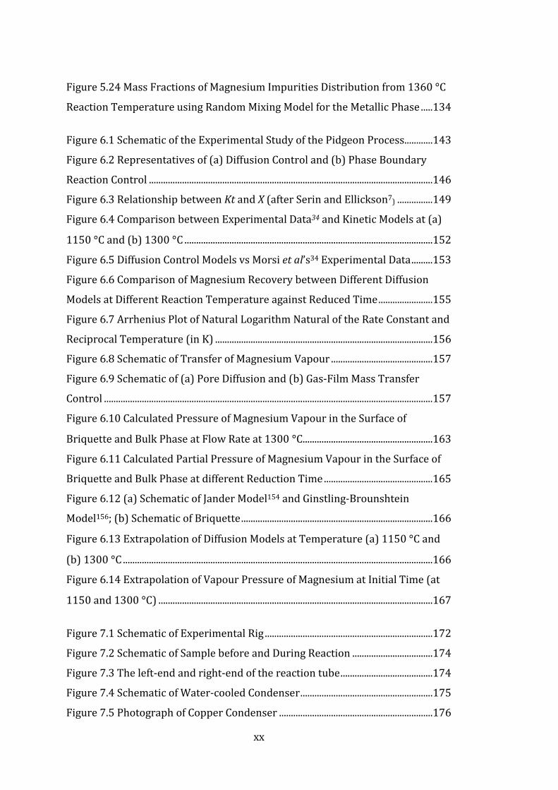
List of Figures Figure 2.1 The Pidgeon Process Flow Diagram15 ............................................................... 7

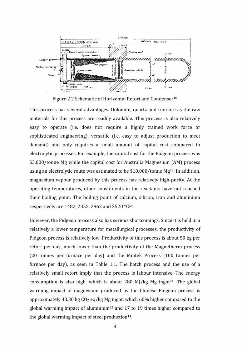
Figure 2.2 Schematic of Horizontal Retort and Condenser18 ........................................ 8

Figure 2. 3 Silicon Activities (aSi) for the Fe-Si System: a. aSi at 1200 °C,

Reference State to Solid Silicon23, b. aSi at 1500 °C, Reference State to Molten

Silicon24, and c. aSi at 1600 °C, Reference State to Molten Silicon25 ............................ 9

Figure 2. 4 Gibbs Energy of Reaction26 Calculated using FactSage 6.2 ................... 11

Figure 2. 5 Kinetics of Silicothermic Reaction at Vacuum Condition of 0.5 mmHg

(After Toguri and Pidgeon16, 35) ............................................................................................. 13

Figure 2.6 Magnesium Recovery from the Pidgeon Process. Dolomite type A:

white, hard and macrocrystalline; Dolomite B: brown, friable to hard,

microcrystalline ........................................................................................................................... 15

Figure 2.7 Arrhenius Plot for the Jander Constants (Wynnyckyj et al36) .............. 16

Figure 2.8 Effect of Pressure on Conversion of Magnesium (after Pidgeon12 and

Toguri and Pidgeon35) ............................................................................................................... 17

Figure 2.9 Effect of Ferrosilicon Grade on Magnesium Conversion ........................ 18

Figure 2.10 Effect of Silicon (75%FeSi) Stoichiometry on Magnesium Conversion

............................................................................................................................................................ 19

Figure 2. 11 Effect of Time and Temperature on Conversion of Magnesium in

Argon Atmosphere at 2.5×10-4 m3/min (After Morsi et al34) ..................................... 21

Figure 2.12 Effect of Hydrogen Flow Rate on Magnesium Conversion.

Temperature: 1150 °C; pellet radius: 9 mm; Compaction pressure: 68 MPa.

(after Barua and Wynnyckyj37) .............................................................................................. 22

Figure 2.13 The presence of CaSi2 in MgO-CaO-Si system. C: CaSi2, γ : γ-Ca2SiO4

(after Wynncykyj and Pidgeon28) .......................................................................................... 24

Figure 2.14 Predicted Conversion Profile for Typical Experimental Condition.

Radius: 1.0 cm, Temperature: 1177 °C, ke = 418 J/msK36 ............................................ 25

Figure 2.15 Effect of Pellet Radius on the Conversion Profile and Temperature

Distribution within the Briquette, Predicted by the Model. Temperature: 1177

°C, ke= 418 J/msK, Time: 60 min36 ........................................................................................ 26

xviii

Figure 2.16 Calculated Magnesium Pressure on the Briquette Surface and Bulk

Gas37 .................................................................................................................................................. 27

Figure 2. 17 Bolzano Reactor48 ............................................................................................... 28

Figure 2.18 The Schematic of Magnetherm Process53 .................................................. 29

Figure 2.19 The Phase Diagram of CaO-MgO-SiO2-Al2O3 System at 10%

Al2O3(Temperature is in K)61. The Grey Area is the Magnetherm Operation

Condition ......................................................................................................................................... 31

Figure 2.20 Phase Diagram of CaO-MgO-Al2O3-SiO2 System at 10 wt%

Al2O3(Temperature in K)61. The black area is the Mintek Operating Condition . 35

Figure 2.21 Layout of the MTMP Pilot Plant70 .................................................................. 37

Figure 3.1 Different Modes of Diffusion133 ........................................................................ 59

Figure 3.2 Representation of a Reacting Particle when Diffusion through Gas

Film is the Controlling Resistance136. .................................................................................. 60

Figure 3.3 Diffusion of Species A from a Solid Surface into a Moving Gas

Stream134 ......................................................................................................................................... 69

Figure 3.4 Basic Steps of Crystal Growth from Condensation of Vapours. A.

Generation. B. Bulk Transport. C. Boundary Layer Transport. D.

Adsorption/Desorption. E. Migration. F. Nucleation165 ................................................ 71

Figure 3.5 The Schematic of Graphite Retort (After Toguri and Pidgeon)38 ........ 79

Figure 3.6 Experimental Configuration in Horizontal Tube Furnace (After

Hughes et al29) .............................................................................................................................. 80

Figure 3.7 Effect of Hydrogen Flow Rate on the Apparent Reaction Pressure at

1159 °C (after Pidgeon and King27) ...................................................................................... 80

Figure 3.8 The Schematic of Vapour Pressure Measurement (after Pidgeon and

King27) .............................................................................................................................................. 82

Figure 3.9 Magnesium Reduction Apparatus (after Morsi et al40) ........................... 83

Figure 3.10 Schematic of Experimental Study (after Misra et al32) ......................... 83

Figure 3.11 Schematic of Experimental Study of Mg Vapour Condensation183 ... 84

Figure 5.1 Thermodynamic Modelling Methodology .................................................... 91

Figure 5.2 Schematic of Equilibrium Calculations .......................................................... 96

Figure 5.3 Equilibrium Calculation of the Pidgeon Process at 1100 °C and 7 Pa 97

xix

Figure 5.4 Equilibrium calculations for the Magnetherm Process at 1550 °C and

5 kPa. .............................................................................................................................................. 101

Figure 5.5 Equilibrium Calculation for the Mintek Process at 1750 °C and 85

kPa. .................................................................................................................................................. 103

Figure 5.6 Schematic of Multistage Equilibrium modelling ...................................... 105

Figure 5.7 Predicted Impurities Distribution from Multistage Equilibrium

Calculations using Vapour Predicted from the Pidgeon Process ............................ 105


Calculations using Vapour Predicted from the Magnetherm Process .................. 106

Figure 5.9 Impurity distribution of the Mintek Process ............................................. 108

Figure 5. 10 Phase Diagram of Mg Rich Region in Mg-Ca System211 ..................... 112

Figure 5. 11 Activity of Mg and Ca106 at 550 °C .............................................................. 113

Figure 5.12 (a) Phase Diagram of Mg-Si system, (b) Phase Diagram of Mg-rich

Region on Mg-Si System217 .................................................................................................... 114

Figure 5. 13 Activity of Mg and Si217 at 550 °C .............................................................. 115

Figure 5. 14 Phase Diagram of Mg-Si System (after Grobner et al220) .................. 115

Figure 5.15 Phase Diagram of Fe-Si (after Lacaze and Sundman221) .................... 116

Figure 5.16 Schematic of Model Representations ........................................................ 121

Figure 5.17 Schematic of Thermodynamic Modelling of the Pidgeon Process.. 121

Figure 5.18 Effect of Temperature to Magnesium Recovery via the Pidgeon

Process ........................................................................................................................................... 124

Figure 5.19 Effect of Pressure to Magnesium Recovery via the Pidgeon process

.......................................................................................................................................................... 125

Figure 5.20 Effects of Pressure and Temperature to Magnesium Recovery

Predicted by Thermodynamic Modelling ......................................................................... 125

Figure 5.21 The Predicted Fugacity of Magnesium Vapour in the Pidgeon

Process System at Various Temperature and Presssure ........................................... 126

Figure 5.22 Magnesium Impurities by Single Stage Equilibrium ........................... 127

Figure 5.23 Comparison between (a) Ideal Solution Model and (b) Random

Mixing Solution Model from the Modelling of the Pidgeon Process Impurities at

1160 °C Temperature. ............................................................................................................. 130

xx

Figure 5.24 Mass Fractions of Magnesium Impurities Distribution from 1360 °C

Reaction Temperature using Random Mixing Model for the Metallic Phase .....134

Figure 6.1 Schematic of the Experimental Study of the Pidgeon Process............143

Figure 6.2 Representatives of (a) Diffusion Control and (b) Phase Boundary

Reaction Control ........................................................................................................................146

Figure 6.3 Relationship between Kt and X (after Serin and Ellickson7) ...............149

Figure 6.4 Comparison between Experimental Data34 and Kinetic Models at (a)

1150 °C and (b) 1300 °C .........................................................................................................152

Figure 6.5 Diffusion Control Models vs Morsi et al’s34 Experimental Data .........153

Figure 6.6 Comparison of Magnesium Recovery between Different Diffusion

Models at Different Reaction Temperature against Reduced Time .......................155

Figure 6.7 Arrhenius Plot of Natural Logarithm Natural of the Rate Constant and

Reciprocal Temperature (in K) ............................................................................................156

Figure 6.8 Schematic of Transfer of Magnesium Vapour ...........................................157

Figure 6.9 Schematic of (a) Pore Diffusion and (b) Gas-Film Mass Transfer

Control ...........................................................................................................................................157

Figure 6.10 Calculated Pressure of Magnesium Vapour in the Surface of

Briquette and Bulk Phase at Flow Rate at 1300 °C.......................................................163

Figure 6.11 Calculated Partial Pressure of Magnesium Vapour in the Surface of

Briquette and Bulk Phase at different Reduction Time ..............................................165

Figure 6.12 (a) Schematic of Jander Model154 and Ginstling-Brounshtein

Model156; (b) Schematic of Briquette .................................................................................166

Figure 6.13 Extrapolation of Diffusion Models at Temperature (a) 1150 °C and

(b) 1300 °C ...................................................................................................................................166

Figure 6.14 Extrapolation of Vapour Pressure of Magnesium at Initial Time (at

1150 and 1300 °C) ....................................................................................................................167

Figure 7.1 Schematic of Experimental Rig .......................................................................172

Figure 7.2 Schematic of Sample before and During Reaction ..................................174

Figure 7.3 The left-end and right-end of the reaction tube .......................................174

Figure 7.4 Schematic of Water-cooled Condenser ........................................................175

Figure 7.5 Photograph of Copper Condenser .................................................................176

xxi

Figure 7.6 Sample Preparation Technique ...................................................................... 177

Figure 7.7 Sample Arrangement .......................................................................................... 178

Figure 7.8 SEM/EDS Equipment .......................................................................................... 182

Figure 7.9 Bruker AXS X-Ray Diffraction......................................................................... 185

Figure 7.10 SEM of MgO (Signal: Secondary Electron, EHT: 3.00 kV, Working

Distance: 6 mm) ......................................................................................................................... 187

Figure 7.11 SEM of CaO (Signal: Secondary Electron, EHT: 8.0 kV, working

distance: 4 mm) .......................................................................................................................... 187

Figure 7.12 SEM of FeSi (Signal: Secondary Electron, EHT: 3.0 kV, working

distance: 6 mm) .......................................................................................................................... 188

Figure 7.13 XRD Pattern of Preheated Pellet in Inert Atmoshere .......................... 188

Figure 7. 14 EDS Analysis of Surface of Reactants ........................................................ 189

Figure 7. 15 SEM of Pellet at 94.5 MPa Compaction Pressure ................................. 190

Figure 7. 16 SEM of Pellet at 54.5 MPa Compaction Pressure ................................. 190

Figure 7. 17 SEM of pellet at 13.3 MPa Compaction Pressure (5000×) ............... 191

Figure 7. 18 XRD Pattern of Reacted Samples ................................................................ 192

Figure 7.19 XRD Pattern of Reacted Samples at Different Time ............................. 193

Figure 7.20 Magnesium Condensates at (a) Condenser, (b) Wire Attached to

Sample Boat, ................................................................................................................................ 193

Figure 7. 21 Photograph of Quartz Tube Condenser after Reduction Experiment

.......................................................................................................................................................... 194

Figure 7. 22 Inside Wall of Quartz Tube Condenser Containing Condensates .. 194

Figure 7.23 XRD of Magnesium Condensate Run II (2 hour) ................................... 195

Figure 7.24 XRD of Magnesium Condensates Run III (3 hour). Red line: MgO;

Blue Line: Ca2SiO4 ...................................................................................................................... 195

Figure 7.25 XRD of Magnesium Condensates Run IV (4 hour): at 0-5 cm (red:

MgO, blue: Mg3CaO.(SiO3)4, green: CaMgSi2O6) .............................................................. 196

Figure 7.26 XRD of Magnesium Condensates Run IV (4 hour): at 6-12 cm (blue:

MgO, green: magnesium calcium iron silicate) .............................................................. 196

Figure 7.27 SEM of Magnesium Condensates from Wall (1500× Magnification)

.......................................................................................................................................................... 197

xxii

Figure 7.28 SEM of Different Morphology of Magnesium Condensate Collected

from Copper Condenser. (left: SE image, right: QBSD image) (1,500×

magnification) .............................................................................................................................197

Figure 7.29 SEM of “Snow” Condensate Collected from Inside Mullite Tube (left:

SE image, right: QBSD image) (1,500 × magnification) ..............................................197

Figure 7.30 SEM of “Dense” Condensate Collected from Copper Condenser left:

SE image, right: QBSD image) (1,500 × magnification) ..............................................198

Figure 7.31 Elemental Mapping of Magnesium Condensate Run IV (4 hour) ....199

Figure 7.32 Elemental Mapping of Magnesium Condensate Run IV ......................200

Figure 8.1 Schematic of Diagram of Experimental Apparatus to Produce

Condensate from Silicothermic Reduction of CaO-MgO .............................................203

Figure 8.2 Temperature Profile of System between position 30 and 58 cm at

Reaction Temperature of 1140 °C at Centerline ...........................................................204

Figure 8.3 Schematic of Thermocouple Measurement ...............................................210

Figure 8.4 (a) Supersaturation of Mg Vapour Versus Temperature, (b) Plot of (ln

S)2/3 vs T for Mg Homogeneous Nucleation ....................................................................212

Figure 8.5 Plot of Nucleation Rate (/m3.s) and Radius of Cluster (× 10-9 m) of Mg

Homogeneous Nucleation ......................................................................................................213

Figure 8.6 Temperature Profile, Nucleation Rate of Mg, and Critical Radius of

Nucleus along the Position .....................................................................................................214

Figure 8.7 Plot of (ln S)2/3 of SiO with Temperature ....................................................215

Figure 8.8 Temperature Profile, Nucleation Rate of SiO, and Critical Radius of


Figure 8.9 Plot of lnS 2/3 of Ca Vapour with 1000/T ....................................................218

Figure 8.10 Temperature Profile, Nucleation Rate of Ca, and Critical Radius of


Figure 8.11 Plot of lnS 2/3 of Fe Vapour with Temperature.......................................219

Figure 8.12 Temperature Profile, Nucleation Rate of Fe, and Critical Radius of


Figure 8.13 Vapour Pressure of Metals198........................................................................222

xxiii

Figure A.1 The CaO-MgO Phase Diagram after Doman et al253. The dashed lines

is the assestment results of Hillert and Wang 254 …………………………………...........A-1

Figure A.2 Fe-Si Phase Diagram (after Masallski and Okamoto258)...………...........A-3

Figure A.3 CaO-SiO2 Phase Diagram14…………………………………………...………...........A-4

Figure A.4 Phase Diagram of Ca2SiO4-Mg2SiO4 System119 …...………..........................A-5

Figure B.1 FactSage Program Version 6.1 ……………………………………………...........B-1

Figure B.2 Reactant Menu …………………………………………………………………………B-2

Figure B.3 List of Thermodynamic Databases ……………………………………………. B-3

Figure B.4 Equilib Menu Window ………………………………………………………………. B-4

Figure B.5 Binary Excess Parameters in the FCC Solution Model …………………B-5

Figure B.6 Binary Excess Parameter in the HCP Solution Model ………………… B-6

Figure B.7 Binary Excess Parameter in the BCC Solution Model ………………… B-6

Figure B.8 Input Species for the Pidgeon Process Reaction …………………………. B-7

Figure B.9 Details of Species Considered in the Equilibrium calculation ……… B-7

Figure B.10 Solution Models and Equilibrium Conditions …………………………… B-8

Figure B.11 Input Species for the Vapour Condensation ……………………………. B-10

Figure B.12 Solution Species and Final Conditions for the Vapour Condensation

………………………………………………………………………………………………………………...B-10

Figure C. 1 Temperature Profile Measurement at Set Point of 1190 oC, Ar gas

Flow Rate of 0.3 L/min, and Cooling Water Rate of 3 L/min …………………………C-1

Figure C. 2 Temperature Profile at Different Condenser Position ………………….C-1

Figure C. 3 Temperature Profile Measurement at Set Point of 1140 oC, Ar gas

Flow Rate of 0.3 L/min, and Cooling Water Rate of 3 L/min …………………………C-2

Figure C. 4 Temperature Profile Measurement at Set Point of 1145 oC under Ar

Gas Flow Rate of 0.3 L/min. The Position of Water-cooled Condenser is 30 cm

from the right-end of tube. ………………………………………………………………………….C-2

Figure C. 5 Temperature Profile Measurement at Set-Point Temperatures of

1130 oC, 1145 oC and 1160 oC. Sample is put inside the Tube Furnace at 25 cm

Position. …………………………………………………………………………………………………….C-3

xxiv

Figure C. 6 The Isothermal Position inside Tube Furnace at Set Point

Temperature of 1130 oC, 1145 oC and 1160 oC ……………………………………………..C-3

Figure C. 7 Temperature Calibration between Set Point and Actual Temperature

…………………………………………………………………………………………………… ……………..C-4

xxv

List of Tables Table 1.1 Operating Conditions and Impurities in Magnesium Extracted from the

Silicothermic Processes ............................................................................................................... 2

Table 2.1 Comparison of Some Reductions of Magnesium Oxide 11 ........................... 6

Table 2.2 Dolomite and Calcined Dolomite Composition, at wt% ............................... 7

Table 2.3 Summaries of Briquette Properties and Experimental Conditions Used

by Previous Investigators ......................................................................................................... 14

Table 2.4 Impurities in the Magnesium Produced from the Magnetherm Process

Before and After Refining (using MgCl2 and KCl fluxs) process, in wt%59 ............ 32

Table 2.5 Composition of Magnesium Process in Heggie-Iolaire Process64 ......... 34

Table 2.6 Composition of Calcined Dolomite (Cal.dol) and Reducing Agent

(%wt)67 ............................................................................................................................................ 34

Table 2. 7 Composition of Condensed Magnesium (wt%)66 ....................................... 38

Table 2.8 Slag Composition in Mintek Process (wt%)66 ............................................... 38

Table 2.9 Chemical Analyses of Various Fluxes, Mass per Cent8 ............................... 39

Table 2. 10 Chemical Analyses of Crude and Clean Magnesium, wt%8 .................. 40

Table 2.11 Physical Properties of Magnesium48 .............................................................. 42

Table 2. 12 Pure Magnesium – Specification and Mean Impurity Content9 ......... 42

Table 2. 13 Composition of Magnesium Alloys ................................................................ 43

Table 5.1 Operating Condition of Silicothermic Processes ......................................... 92

Table 5.2 FactSage204 Built-in Compound Database Used in This Study ............... 93

Table 5.3 FactSage204 Built-in Solution Database Used in This Study ..................... 94

Table 5.4 Possible Species for The Pidgeon Process System in Gas and

Condensed Phases ....................................................................................................................... 96

Table 5.5 Possible Species for The Magnetherm and Mintek process Systems 100

Table 5.6 Predicted Vapour Compositions of Silicothermic Process from

Thermodynamic Modelling ................................................................................................... 104

Table 5.7 Comparison of Element Composition Calculated from the Present

Study, Previous Modelling Work73 and Actual Chemical Analysis8, 35, 59 .............. 109

xxvi

Table 5.8 Interaction Parameters for Solid Solution Models ....................................118

Table 5.9 Database for Metallic System in FTlite database225 ..................................119

Table 5.10 Database for Some Metal System in SGTE alloy 2007 database .......120

Table 5.11 Input Data in the Pidgeon Process System35 ............................................122

Table 5.12 Details of Composition and Phase Present predicted from Model II

Single stage Condensation (per 100 mol Mg) using random Mixing Solution

Model for the Metallic Phases ...............................................................................................128

Table 5.13 Details of Phase Present predicted from Model II Single stage

Condensation (per 100 mol Mg) using Ideal Solution for the Metallic Phases ..128

Table 5.14 The Predicted Vapour Phase in the Pidgeon Process ............................129

Table 5.15 Mass of the Vapour Phase and Condensed Phases from Multistage

Condensation Model at Different Temperature (in gram per 100 moles Mg)

Calculated using Ideal Solution for the Metallic Phases .............................................131



Calculated using Random Mixing Solution model for the Metallic Phases ..........132



Calculated using Random Mixing Solution model for the Metallic Phases ..........136

Table 5.18 Comparison of Magnesium and Impurities Concentrations Calculated

from Present Study and from Chemical Analyses at Reaction Temperature of

1160 °C (in wt %) ......................................................................................................................139

Table 6.1 Parameter of Experimental Work (after Morsi et al34) ...........................145

Table 6.2 Models for Mixed Powder Reactions133 ........................................................147

Table 6.3 Parameters from Nucleation Model ...............................................................152

Table 6.4 R2 of Kinetic Models ..............................................................................................152

Table 6.5 Correlation Coefficient, R2, of Diffusion Models .........................................154

Table 6.6 Magnesium Conversion at 1300 °C and 1 Hour34 ......................................158

Table 6.7 Magnesium Conversion at 0.25 L/min Argon Gas Flow Rate34 ............158

Table 6.8 Mass Transfer Coefficient, kc, of Mg-Ar System at 1300 °C ....................162

Table 6.9 Magnesium Vapour Pressure at 1300 °C at Surface and Bulk Gas .....162

xxvii

Table 6.10 Magnesium Vapour Pressure at 1150 °C at Surface and Bulk Gas

(Argon Gas Flow Rate: 0.25×10-3 m3/min) ...................................................................... 163


(Argon Gas Flow Rate: 0.25×10-3 m3/min) ...................................................................... 164

Table 7.1 Purity and Composition of Raw Materials ................................................... 176

Table 7. 2 Silicothermic Experiments in Vacuum Conditions .................................. 191

Table 7.3 Semi-quantitative Analysis of Condensates using EDS analysis.......... 198

Table 8.1 Properties Data of Species183, 243, 245, 246 ........................................................ 207

Table 8.2 Surface energy of Condensing Species .......................................................... 207

Table 8.3 Equilibrium Vapour Pressure Constants (as per Equation 8.7) .......... 209

Table 8.4 Molar Partial Fraction of Vapours Predicted from Thermodynamic

Modelling at 1140 °C using FACT53 database ............................................................... 211

Table 8.5 Summary of T* ........................................................................................................ 221

Table 8.6 Summary of Condensation of Vapour ............................................................ 221

xxviii


xxix

Nomenclatures Initial concentration of reactant

C Concentration of reactant

Cp Heat capacity

D Diffusivity (or Diffusion coefficient)

∗ Self-diffusion coefficient

Interdiffusivity of species A and B

Knudsen Diffusion

δ Inter-atomic spacing

EA Activation energy

G Gibbs energy of system

∆ Gibbs energy of reaction

Standard Gibbs energy of pure component i

Gibbs energy of mixing

Partial Gibbs energy or chemical potential of component i

φ Gibbs energy of ideal mixing

φ Excess Gibbs energy

γi Activity coefficient of species i

γ Henrian activity coefficient of species i

∆ Enthalpy of reaction

∆S the entropy change of the process

σAB Collision diameter of species A and B

ε Lennard-Jones potential of species A and B

ΩAB Collision integral of A-B mixture at dimensionless temperature TAB

Ω Excess surface entropy per molecule (in homogeneous nucleation

theory)

j Mass transfer flux

J Nucleation rate

k Rate constant

kc Mass transfer coefficient

xxx

kB/k Boltzmann constant (1.380648×10-23 J/K)

Equilibrium constant

,,φ Binary interaction parameter of species i and j

L Thickness of product layer; characteristic length

M Molecular mass

NA Mass transfer rate per unit solid surface area

ai Activity of species i

Pi Partial pressure of species i

pi: 3.14159 …

R Gas constant (8.314 J/mol.K)

r Radius

Re Reynolds number; Re = UL/v

ρi Density of species i

Supersaturation/supercooling

Sc Schmidt Number; Sc = v/D

Sh Sherwood number; Sh = kcL/D

σ Surface tension

T Temperature

t Time

U Velocity

v Kinematic viscosity

wt% Weight percent

X Conversion

xi Composition of species i

yi Fractional site composition of i

Z Correction in the Valensi-Carter model

1

1 Introduction

Magnesium is a light metal that has a density of 1783 kg/m3, which is two thirds

of aluminium and one sixth of steel. It also has a number of other desirable

properties including good ductility, excellent castability and high specific

strength1. The strength-to-weight ratio of magnesium, 158 kNm/kg, is 17%

higher than the strength-to-weight ratio of aluminium. These attractive

properties have ensured a steady increase in the consumption of magnesium in

the recent years with a growth rate of 7% per annum2. It is used as an alloying

element in aluminium alloys, die casting, for steel desulphurisation, and as an

industrial chemicals3. The aluminium industry utilises magnesium to increase

the strength, ductility and corrosion resistance of aluminium alloys.

Magnesium’s use in both aluminium and steel production strongly links its

demand to these two other metal commodities.

Magnesium is produced commercially via two general routes: electrolytic and

metallothermic routes. The electrolytic process routes are based on the

electrolysis of molten magnesium chloride. A number of process steps are

needed to purify magnesium chloride prior to the electrolytic operation. Hence,

these routes are complex and capital intensive. Metallothermic routes utilise a

metal as the reducing agent to extract magnesium from calcined dolomite in a

thermal reduction process. In the silicothermic route, such as the Pidgeon

process, ferrosilicon reduces calcined dolomite in a horizontal retort. The

produced magnesium vapour condenses as a dense metal.

While the Pidgeon Process is slow and energy intensive, this process has

become the dominant process for producing magnesium in the world, with

China over 70% of all magnesium4. This process suits the local economy of

China, where the labour costs are cheap and raw materials are available. The

growing demand for magnesium has stimulated research into new methods of

producing magnesium. The Magnetherm process had been operated in the past

2

at higher temperature than the Pidgeon process in order to increase

productivity. The Mintek process is another silicothermic process that also

operates at higher temperature and high productivity. The development of this

process is still underway.

Table 1.1 Operating Conditions and Impurities in Magnesium Extracted from the

Silicothermic Processes

Operating

Condition Pidgeon5, 6 Magnetherm7 Mintek8

Pressure 13-67 Pa 0.05- 0.1 atm ~1 atm

Temperature (°C) 1100 - 1200 1550 - 1600 1700 – 1750

Productivity per retort per day

50 kg 20 tonne 100 tonne

Impurities

(wt%) Pidgeon9 Magnetherm7 Mintek8

Crude Clean

Al 0.004 0.01 0.066 0.04

Si 0.01 0.05 0.281 0.095

Ca 0.005 N.A. 0.385 0.023

Fe 0.007 0.005 0.25 0.047

Mn 0.01 0.05 N.A. N.A.

The productivity of the process has strong correlation with the impurities found

in the magnesium. Table 1.1 shows the typical impurities of magnesium resulted

from various silicothermic processes. The Pidgeon process typically produces

50 kg of magnesium per retort per day, while the Magnetherm process and the

Mintek process produce approximately 20 and 100 tonnes per retort per day,

respectively. While a higher temperature process offer higher productivity, the

increase in operating temperature results in higher impurities. The Pidgeon

process, which operates between a temperature of 1100 and 1200 °C, produces

the highest purity of magnesium (>99.96 wt%). Conversely, the Mintek process

which operates at a temperature between 1700 and 1750 °C produces a low

purity of magnesium (less than 99 wt% for the crude magnesium). The purity

required for 9980 A-grade commercial magnesium is a minimum of 99.80 wt%

Mg, with the impurities such as Ca, Al, Si, and Fe are below 0.05 wt% each10.

3

As the silicothermic reaction involves a number of reactants in different phases,

the physical chemistry associated with this process is complex. The fundamental

thermodynamics of the Pidgeon process has been established6 and some papers

on the kinetics of the process are available. However, while a number of

parameters affecting the process have been examined, there is no general

conclusion on the kinetics of the process. The knowledge on the behaviour of

impurities in magnesium produced by silicothermic process is also quite

limited. In the current practice, the impurities in magnesium metal produced

from the silicothermic processes are removed in a separate refining operation.

This study is concerned with the fundamental physical chemistry associated

with the silicothermic processes, including the behaviour of impurities in the

process. This achieved by using thermodynamics and kinetics modelling, as well

as high temperature experiments to validate the predictions. Accordingly, this

study will address the following questions:

- What is the effect of parameters such as temperature and pressure to the

conversion of magnesium and the impurities included in the magnesium

vapour?

- What is the controlling factor in the kinetics of silicothermic process?,

and

- What is the distribution of impurities in the silicothermic processes?

Overview of this study

In the first two chapters, the literature on the fundamentals of silicothermic

processes and the thermodynamics and kinetics of high temperature processes

are examined. In Chapter 2, different type of silicothermic processes, such as the

Pidgeon process, the Magnetherm process, the Mintek process, and the Bolzano

process are explored, including the available literature on their basic

thermodynamics and kinetics. In Chapter 3, theories on computational

thermodynamics and kinetic modelling are described.

4

Based on the literature review, the research issues are identified in Chapter 4.

The thermodynamic modelling results are described in Chapter 5, while the

kinetic modelling results are described in Chapter 6. The results of experiments

are described in Chapter 7. Chapter 8 provides analysis based on the Classical

Nucleation theory on the condensation behaviour. The general discussion is

provided in Chapter 9, while Chapter 10 will provide conclusions and

recommendation for further studies.

The following papers have resulted from this study:

1. W. Wulandari, M. A. Rhamdhani, G. A. Brooks, and B. J. Monaghan:

'Distribution of Impurities in Magnesium Production via Silicothermic

Reduction', Proceedings of the Inaugural High Temperature Processing

Symposium, Hawthorn, Victoria, Australia, 09 February 2009.

2. W. Wulandari, M. A. Rhamdhani, G. A. Brooks, and B. J. Monaghan:

'Distribution of Impurities in Magnesium Production via Silicothermic

Reduction', Proceedings of European Metallurgical Conference 2009,

Innsbruck, Austria, 28 June - 1 July 2009, 2009, GDMB, pp. 1401-1417

(refereed).

3. W. Wulandari, G. Brooks, M. A. Rhamdhani, and B. J. Monaghan:

'Thermodynamic Modelling of High Temperature Systems', Proceedings of

the Chemeca 2009 Annual Conference, Perth, Western Australia, 27-30

September 2009, Engineers Australia (refereed).

4. W. Wulandari, G. Brooks, M. A. Rhamdhani, and B. J. Monaghan: 'Magnesium:

Current and Future Production Routes', Proceedings of 'Engineering at the

edge', the 2010 Chemeca Annual Conference (Chemeca 2010), Adelaide,

South Australia, Australia, 26-29 September 2010, Engineer Australia

(refereed).

5. W. Wulandari, M. A. Rhamdhani, G. A. Brooks, and B. J. Monaghan: “Kinetics

of Silicothermic Reduction of Calcined Dolomite in Flowing Argon

Atmosphere”, Proceedings of the 2nd Annual High Temperature Processing

Symposium, Hawthorn, Victoria, Australia, 08-09 February 2010 / Geoffrey

Brooks, M. Akbar Rhamdhani and Xiadong Xu (eds.), pp. 77-80.

5

2 Fundamental of Silicothermic Processes Silicothermic process refers to a method of extracting metal by reducing the

metal oxide using silicon as a reducing agent. This reaction is endothermic, as

energy is required to process and break down the bond between metal and

oxygen in the reaction. In the silicothermic process for magnesium production,

calcined dolomite (CaO.MgO) is mixed with ferrosilicon before being charged

into the retort for the reduction process. The silicothermic reaction can be

expressed as follows:

2. !" → $ % 2& !" (2. 1)

In this chapter, a comprehensive literature review of the silicothermic processes

is presented. The initial section of this chapter reviews the physical chemistry of

the Pidgeon process, which includes the thermodynamics and kinetics of this

process. This is followed by the description of various silicothermic processes,

such as the Bolzano, the Magnetherm and the Mintek processes. The last section

reviews the purity requirement of magnesium metal for commercial purposes.

2.1 The Pidgeon Process

Thermal based processes to produce magnesium metal from its oxide have been

studied by Pidgeon11, 12. Based on Table 2.1, which lists the reaction enthalpy

and the theoretical amount of required reducing agent for each reaction, silicon

is found to be an excellent reducing agent to produce magnesium compared to

calcium carbide, aluminium and carbon. 113 g of ferrosilicon (80wt%Si) is

required to produce a gram of magnesium at 1200 °C compared to 120 g of CaC2

at 1700 °C13. Reaction between MgO and carbon is feasible at 1900 °C; however,

the reaction is reversible and forming carbon and MgO at temperatures between

400 and 1700 °C. Thermal reduction of MgO using CaC2 has been known and

must be carried out below temperatures at which CaO is reduced by carbon13.

Aluminium is more effective compared with silicon as the reducing agent (55 g

6

of aluminium is required to produce 1 g of magnesium); however, the high cost

of aluminium makes it is unsuitable for a commercial process. In addition, the

high energy required to produce aluminium would only add to a high energy

consumption associated with magnesium processing14.

Table 2.1 Comparison of Some Reductions of Magnesium Oxide 11

Reductant T (°°°°C) Reaction Enthalpy and Amount of

Reductant

Carbon 1900 MgO(s) + C(s) = Mg(g) + CO(g) ∆H = 604.76 kJ/mol Mg

Calcium Carbide

1700 MgO(s) + CaC2(s) = Mg(g) + CaO(s) + 2C(s)

∆H = 153.23 kJ/mol Mg

CaC2 = 120 g/g Mg (80% CaC2)

Aluminium 1700 3MgO(s) +Al(s) = Al2O3(s) + 3Mg(g)

∆H = 166.67 kJ/g Mg

Al = 55 g/g Mg (90% Al)

Silicon

1200 2MgO(s) + Si(s) = SiO2(s) + 2Mg(g)

∆H = 285.79 kJ/g Mg

Si = 57.5 g/g Mg (80% Si)

1200 2CaO(s) +2MgO(s) +Si(s) = Ca2SiO4(s) + 2Mg(g)

∆H = 229.21 kJ /g Mg

Si = 113 g/g Mg (80% Si)

Pidgeon developed a process to extract magnesium from calcined dolomite

using ferrosilicon (75%Si) as the reducing agent based on reaction in Equation

(2.1). The process flow diagram is given in Figure 2.115. Calcined dolomite

(CaO.MgO) is mixed with powdered ferrosilicon and fluorspar as a catalyst.

Table 2.2 lists a typical chemical composition of calcined dolomite used in the

Pidgeon process. A typical calcined dolomite contained 38.8 wt% of MgO, 57.5

wt% of CaO, and a number of impurities.

Prior to reduction process, the briquetted charge is placed inside a horizontal

Ni-Cr steel retort, which is shown in Figure 2.2. The retort is heated to a

temperature between 1100 and 1200 °C under a vacuum pressure between 10

to 76 Pa5. Magnesium vapour evolves from the briquettes and precipitates

inside a removable condenser sleeve. Magnesium deposit is removed after eight

hour of batch processing. Typically 20 kg of magnesium is produced per batch

from 120 kg of raw materials5.

7

Figure 2.1 The Pidgeon Process Flow Diagram15

Table 2.2 Dolomite and Calcined Dolomite Composition, at wt%

Dolomite Calcined Dolomite16

Compounds Dolomite from Haley,Ontario17

Theoretical CaMg(CO3)2

Compounds Compositions

MgO 21.12 21.86 CaO 57.5

CaO 31.27 30.41 MgO 38.8

CO2 47.22 47.73 L.O.I 1.38

SiO2 0.12 - Insoluble 0.48

FeO 0.22 - R2O3 0.4

H2O 0.02 - Minor 1.44

Crushing

Ring roller mills

Sizing

Storage

Jaw crusher

Ball mill

Storage

RAW DOLOMITE

Mixer

Briquetting press

Retort

FERROSILICON 75%

CALCINATED DOLOMITE (via calcining kilns)

Magnesium crown to melting

Residue to waste

8

Figure 2.2 Schematic of Horizontal Retort and Condenser18

This process has several advantages. Dolomite, quartz and iron ore as the raw

materials for this process are readily available. This process is also relatively

easy to operate (i.e. does not require a highly trained work force or

sophisticated engineering), versatile (i.e. easy to adjust production to meet

demand) and only requires a small amount of capital cost compared to

electrolytic processes. For example, the capital cost for the Pidgeon process was

$3,000/tonne Mg while the capital cost for Australia Magnesium (AM) process

using an electrolytic route was estimated to be $10,000/tonne Mg19. In addition,

magnesium vapour produced by this process has relatively high-purity. At the

operating temperatures, other constituents in the reactants have not reached

their boiling point. The boiling point of calcium, silicon, iron and aluminium

respectively are 1482, 2355, 2862 and 2520 °C20.

However, the Pidgeon process also has serious shortcomings. Since it is held in a

relatively a lower temperature for metallurgical processes, the productivity of

Pidgeon process is relatively low. Productivity of this process is about 50 kg per

retort per day, much lower than the productivity of the Magnetherm process

(20 tonnes per furnace per day) and the Mintek Process (100 tonnes per

furnace per day), as seen in Table 1.1. The batch process and the use of a

relatively small retort imply that the process is labour intensive. The energy

consumption is also high, which is about 280 MJ/kg Mg ingot21. The global

warming impact of magnesium produced by the Chinese Pidgeon process is

approximately 43.30 kg CO2 eq/kg Mg ingot, which 60% higher compared to the

global warming impact of aluminium22 and 17 to 19 times higher compared to

the global warming impact of steel production14.

9

2.1.1 Thermodynamics of the Pidgeon Process

The equilibrium of reaction in Equation (2.1) can be expressed as the following:

' ()*+ ,-.+/012,-.1+ ,)*1+ ,/0 (2. 2)

where K is equilibrium constant, PMg is the vapour pressure of Mg, and ai

corresponds to activities of species i. Assuming that CaO, MgO and Ca2SiO4 are

pure condensed phases, which have a unit activity, the equilibrium of

silicothermic reaction will be a function of vapour pressure of magnesium and

activity of silicon, as written in Equation (2.3).

' ()*+,/0

(2. 3)

Figure 2. 3 Silicon Activities (aSi) for the Fe-Si System: a. aSi at 1200 °C, Reference State to Solid Silicon23, b. aSi at 1500 °C, Reference State to Molten Silicon24, and c. aSi at 1600 °C, Reference State to Molten Silicon25

Ellingsaeter and Rosenqvist23 measured the activities of solid silicon of the Fe-Si

alloy in the silicothermic reaction system. This silicon activity was compared

with the activity of molten silicon in the Fe-Si system at 1500 °C24-25 and

described in Figure 2.3. These curves show a similar trend as the curve of solid

10

alloys, except for the stepwise increase in activity at the composition of

intermediates solid phases. The drops in the silicon activity at 70, 50 and 30

atomic % Si corresponds to the ζ-phase (Fe2Si5), the ε-phase (FeSi) and the

saturation limit for the α-phase (Fe2Si)23.

The equilibrium constant correlates with the Gibbs energy at the corresponding

temperature with this relationship:

∆3 ' 45678 (2.4)

where R is gas constant, 8.314 J/mol.K, T is temperature (in K), and K is

equilibrium constant.

Since the reaction in Equation (2.1) is a sum of the reaction in Equations (2.5) to

(2.7) as in the following:

2 ' 2 $& (2. 5)

$& ' $ (2. 6)

$ 2 ' 2$ % (2. 7),

the Gibbs free energy of reaction in Equation (2.1) can be calculated to be:

∆$.: ' ∆$.; ∆$.< ∆$.= (2. 8)

11

Figure 2. 4 Gibbs Energy of Reaction26 Calculated using FactSage 6.2

Figure 2.4 shows the Gibbs free energy of reaction of Equations (2.1), (2.5), (2.6)

and (2.7) for temperature range between 1080 to 1260 °C. The Gibbs energy of

silicothermic reaction is between 72 to 90 kJ/mol at this temperature range.

Pidgeon and King27 have measured the equilibrium vapour pressure of

magnesium over the CaO-MgO-Si system as in reaction of Equation (2.1) using

transpiration/entrainment method. At 1100 °C, the pressure of magnesium was

found to be 1.3 kPa. This has been confirmed by several further works23, 28, 29,

including using a Knudsen cell technique28. This value is significantly higher

than the previous work30 which reported a value of 0.25 kPa over the MgO-Si

system. The theoretical magnesium vapour pressure associated with reaction in

Equation (2.1) based on Kubaschewski and Alcock31 had been found one thirds

lower than measured value27. Some investigators16, 23 suspected this

discrepancy was based on the uncertainty of thermodynamic data or a

formation of a complex silicate compound. However, the most recent

thermodynamic data26 shows that the calculated magnesium vapour pressure

over silicothermic system is 1.4 kPa at a temperature of 1100 °C, which is

comparable to Pidgeon and King27.

12

Magnesium vapour removal from silicothermic system drives the reaction

between calcined dolomite and ferrosilicon. There are two methods available to

remove magnesium vapour: using vacuum and a stream of inert gas or ambient

atmosphere. Vacuum has been used extensively both in experimental and

commercial scale5, 6, 18, 32, 33. The second method, using a stream of inert gas34, 35,

is more suitable for continuous operation. The utilisation of inert gas system

offers the possibility of condensing the magnesium to liquid, although it needs a

complex gas system configuration in a large scale operation.

The use of vacuum has been found more effective to remove magnesium from

the briquettes compared with utilising a streaming inert gas16. An experimental

study on the silicothermic reaction in argon atmosphere34 found that the overall

yield of magnesium is lower than those in vacuum. This is supported by the

determination of a lower apparent activation energy of silicothermic in

vacuum35 compared to in a stream of inert gas34. The morphologies of

magnesium collected from those two methods are also different. Silicothermic

in vacuum produces a dense condensate while silicothermic in streaming gas

produces a loose powdered condensate16.

2.1.2 Reaction Kinetics of the Pidgeon Process

2.1.2.1 Reaction in Vacuum Condition

Silicothermic reaction involves three solids (i.e. CaO, MgO and Si) to produce a

vapour and another solid (i.e. Ca2SiO4). The kinetics of this reaction has been

subject of interest to a number of researchers12, 29, 32-37. The experimental

studies of the silicothermic reaction were carried out using thermogravimetry.

Pidgeon12 studied the silicothermic reaction in an ambient atmosphere and a

vacuum. At ambient atmosphere, the system was heated under hydrogen at

atmospheric pressure. The crucible began to lose weight when temperature

reached 1450 to 1570 °C. In the vacuum condition, the system was evacuated to

13 Pa prior to reduction. The reaction proceeded successfully with 78 wt%

conversion after an hour operation at 1155 °C12.

13

Several investigations29, 32, 35 provide additional details on the effect of

parameters such as temperature, pressure, ferrosilicon, particle size and time

on the rate of silicothermic reaction in vacuum condition. Toguri and Pidgeon 35,

38 studied silicothermic reaction by varying temperature from 1050 to 1560 °C,

and pressure between 0.13 Pa and 35 kPa. The results of magnesium conversion

over time at different reaction temperature are shown in Figure 2.5. They

reported that the magnesium recovery increased by a factor of 1.55 for a 50 °C

increase in temperature over the range 1050 to 1560 °C.

Figure 2. 5 Kinetics of Silicothermic Reaction at Vacuum Condition of 0.5 mmHg (After Toguri and Pidgeon16, 35)

A summary of the process parameters and briquette properties used by

previous studies is given in Table 2.3. Misra et al32 studied the reduction rate of

the Pidgeon process in the range of 1100 to 1200 °C, and reported that the

highest magnesium recovery (92.07 wt%) was obtained at a temperature of

1200 °C and pressure of 13 Pa. Hughes et al29 conducted a study at 1000 to 1180

°C, reported the importance of the characteristics of different calcined dolomite,

and suggested that the rate of magnesium evolution from single briquette was

partly controlled by briquette permeability and partly by chemical reaction.

14

Table 2.3 Summaries of Briquette Properties and Experimental Conditions Used by Previous Investigators

Investigators Reactant size

FeSi grade/ excess

Briquette Pressure

Reactor

Pressure

(Pa) Catalyst

Time

(h) Silicon Dolime

Pidgeon12 44-853 µm: 28%

<44µm: 38.5% 178-221µm: 43% 44-221µm:15%

75.7%Si/ 0 N.A. 0.13 N.A. 1

Toguri and Pidgeon35

N.A. N.A. 75%Si/15% 20 MPa 0.13 None 1

Misra et al32 <74µm -147µm 81%Si/18% 20 MPa 13 0.8% CaF2 2 Hughes et al29

<74µm: 90% >147µm: 19% <74µm: 65%

78.6%Si/17% 200 MPa 0.13 CaF2 4

Peirce et al18 N.A. N.A. 75%Si/0 13.7 MPa 13 CaF2 2.5% 8 Yucel et al33 N.A. N.A. FeSi 75% N.A. 100 CaF2 3

15

Pidgeon and Alexander5 reported the development of Pidgeon Process in pilot

plant scale, while Pierce et al18 reported commercial scale results. More

recently, Yucel et al33 studied the production of magnesium metal from Turkish

calcined dolomite and ferrosilicon by the vacuum silicothermic method. The

reaction was investigated over a temperature range of 1100 to 1300 °C and

pressure of 100 Pa. They found that magnesium recovery increases with FeSi

addition, CaF2 addition and reduction time. A recovery of 80 to 96.46 wt% over

the range of conditions studied was achieved33.

Figure 2.6 shows the magnesium recovery of silicothermic under vacuum

condition from a number of investigators at different reduction temperatures.

The pressure of the system vary between 0.13 to 100 Pa, while the reduction

time varies from one to four hours at an experimental scale12, 29, 32, 33, 35 to eight

hours at a commercial scale18.

Figure 2.6 Magnesium Recovery from the Pidgeon Process. Dolomite type A: white, hard and macrocrystalline; Dolomite B: brown, friable to hard, microcrystalline

Based on Figure 2.6, there is some appreciable magnesium recovery at 1000 °C,

i.e. 13 to 40 wt%12, 29, 32. At the commercial operating temperatures of

silicothermic process, 1100 to 1200 °C, magnesium recovery was found to be

between 75 to 95 wt%12, 29, 32, 33, 35.

16

The rate of the silicothermic reaction was found to follow first order kinetics16.

The general equation integrates to:

>? ' 78 @ A0A0BA C (2. 9)

where Ci is initial concentration of reactant, C is final concentration of reactant,

and k is a rate constant. Based on the kinetic analysis conducted by Wynnyckyj

et al36, Jander model for solid-state diffusion has been found to represent a

number of experimental data on the Pidgeon process reaction. The briquettes

used for the reaction was cylindrical. The Jander model can be written as

follows:

D1 4 1 4 F:/$H$ ' $IJKL+ ' >? (2. 10)

where ro2 is initial radius of pellet, k is a rate constant, t is time, and X is

magnesium conversion, which is obtained from the following expression:

F ' MOP&QJRK&P SPKPJJQPKPJT,MOP&QJUV&KP,TJ,J (2. 11)

Figure 2.7 Arrhenius Plot for the Jander Constants (Wynnyckyj et al36)

17

The Arrhenius plot for experimental data based on Jander model is described in

Figure 2.7. The activation energy was calculated from the following Arrhenius

equation:

> ' Wexp @B[\]3 C (2. 12)

where A is the pre-exponential constant, EA is the activation energy, R is the gas

constant (8.314 J/mol.K), and T is temperature in Kelvin. The activation energy

of silicothermic reaction was found between 226.35 and 238.49 kJ/mol. The

values suggest that the reaction is controlled by a solid state diffusion, as the

solid-solid diffusion has activation energy typically between 200 and 400

kJ/mol39.

2.1.2.1.1 Effect of Temperature and Pressure

It has been established that the rate of reaction increases as the increasing

temperature as clearly shown in Figures 2.5 and 2.6. For the reaction which

utilises vacuum condition, pressure of the system also has significant effect to

the kinetics of the reaction. Some investigators12, 32, 35 found that the magnesium

recovery is decreased linearly when the pressure of system is increased up to

10 kPa, with the trend shown in Figure 2.8.

Figure 2.8 Effect of Pressure on Conversion of Magnesium (after Pidgeon12 and Toguri and Pidgeon35)

18

2.1.2.1.2 Effect of Silicon Grade

The effect of silicon grades5, 23, 32, 35 ranges from 15.73 to 96.7 wt% Si is shown

in Figure 2.9. The term “silicon efficiency” was introduced by Pidgeon and

Alexander5 which refer to the following ratio:

"^^ _ "8_` ' OP&QJUTMMPTJPV&OP&QJUV&PaRb,MPJUcSKPPJ d100% (2. 13)

Figure 2.9 Effect of Ferrosilicon Grade on Magnesium Conversion

In general, magnesium conversion increases with the utilisation of higher grade

ferrosilicon. However, there is a reduction in silicon efficiency after utilisation of

75% Si ferrosilicon. A higher grade ferrosilicon beyond 75% Si does not

improve the silicon efficiency. Therefore, it is agreed that 75% Si grade

ferrosilicon is sufficient, as well as being a cost-effective for commercial

operation. This has been supported by earlier work which showed that the

silicon activity of 75% Si grade ferrosilicon is similar to 90 wt% Si grade

ferrosilicon23.

19

2.1.2.1.3 Effect of Silicon Stoichiometry

The effect silicon stoichiometry on the silicon efficiency and magnesium

conversion is shown in Figure 2.10. Silicon stoichiometry is defined as mole

ratio of silicon to calcined dolomite. The value “1.0” is the stoichiometric

amount of ferrosilicon required for calcined dolomite, i.e. one mole of silicon to

two moles of calcined dolomite. Misra et al32 showed that while the magnesium

conversion increases up to 86 wt% as silicon stoichiometry rise to 2.4, the

silicon efficiency decreased to 30 wt%. The utilisation of silicon has been found

to be optimal for silicon stoichiometry values between 1.0 and 1.1032.

Figure 2.10 Effect of Silicon (75%FeSi) Stoichiometry on Magnesium Conversion

2.1.2.1.4 Effect of Catalyst

Alkali and alkaline earth fluoride have been known to accelerate the solid-state

reaction in oxide systems. Toguri and Pidgeon35 investigated the effect of CaF2,

BaF2 and MgF2 on the reaction rate of silicothermic reaction by adding 2.5 wt%

catalyst to a mixture of calcined dolomite and ferrosilicon. It is found that CaF2

is the most effective catalyst, with the 58 wt% magnesium conversion being

achieved in the first ten minutes in a 1300 °C reduction, compared with 52 and

51 wt% for BaF2 and MgF2, respectively35. This catalytic effect has been

accounted from the formation of a liquid phase which creates a faster diffusion

media for reactants35.

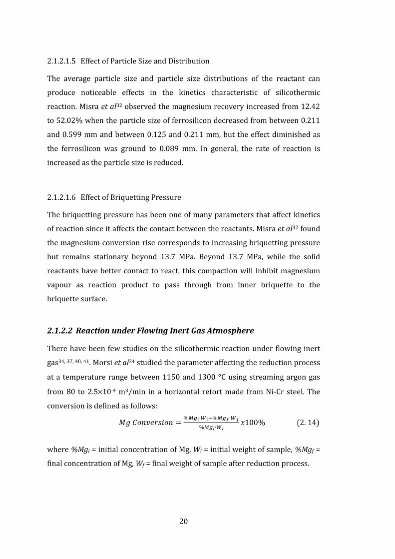
20

2.1.2.1.5 Effect of Particle Size and Distribution

The average particle size and particle size distributions of the reactant can

produce noticeable effects in the kinetics characteristic of silicothermic

reaction. Misra et al32 observed the magnesium recovery increased from 12.42

to 52.02% when the particle size of ferrosilicon decreased from between 0.211

and 0.599 mm and between 0.125 and 0.211 mm, but the effect diminished as

the ferrosilicon was ground to 0.089 mm. In general, the rate of reaction is

increased as the particle size is reduced.

2.1.2.1.6 Effect of Briquetting Pressure

The briquetting pressure has been one of many parameters that affect kinetics

of reaction since it affects the contact between the reactants. Misra et al32 found

the magnesium conversion rise corresponds to increasing briquetting pressure

but remains stationary beyond 13.7 MPa. Beyond 13.7 MPa, while the solid

reactants have better contact to react, this compaction will inhibit magnesium

vapour as reaction product to pass through from inner briquette to the

briquette surface.

2.1.2.2 Reaction under Flowing Inert Gas Atmosphere

There have been few studies on the silicothermic reaction under flowing inert

gas34, 37, 40, 41. Morsi et al34 studied the parameter affecting the reduction process

at a temperature range between 1150 and 1300 °C using streaming argon gas

from 80 to 2.5×10-4 m3/min in a horizontal retort made from Ni-Cr steel. The

conversion is defined as follows:

g8h"ij g8 ' %V&0∙l0B%V&m∙lm%V&0∙l0 d100% (2. 14)

where %Mgi = initial concentration of Mg, Wi = initial weight of sample, %Mgf =

final concentration of Mg, Wf = final weight of sample after reduction process.

21

Figure 2. 11 Effect of Time and Temperature on Conversion of Magnesium in Argon Atmosphere at 2.5×10-4 m3/min (After Morsi et al34)

Figure 2.11 shows the effect of time and temperature on conversion of

magnesium in argon athmosphere at 25×10-4 m3/min. At 1150 °C, the

magnesium conversion reaches 55 wt% after five hour reduction time; while 90

wt% of conversion can be achieved from reduction for five hour at 1300 °C.

Barua and Wynnyckyj37 studied silicothermic reduction under flowing hydrogen

atmosphere in the temperature ranges between 1070 and 1250 °C using a

single spherical pellets. The effect of hydrogen rate on magnesium conversion is

shown in Figure 2.12. Barua and Wynnyckyj37 concluded that the overall rates

were higher than vacuum under equivalent conditions, and were limited by

combined factors: intrinsic chemical rate, heat transfer, pore diffusion of

magnesium, as well as mass transfer across the boundary layer of the pellets.

22

Figure 2.12 Effect of Hydrogen Flow Rate on Magnesium Conversion. Temperature: 1150 °C; pellet radius: 9 mm; Compaction pressure: 68 MPa. (after Barua and Wynnyckyj37) As shown in Figures 2.11 and 2.12, there are significant differences in

magnesium conversion between silicothermic reduction under argon34 and

hydrogen atmospheres37. Under argon atmosphere, 14 wt% of magnesium

conversion was achieved after an hour reduction, while under 1000 cm3/min

hydrogen flow atmosphere and similar time frame, the magnesium conversion

reaches 70 wt%. This difference may be likely caused by the flow rate of inert

gas and the diffusivity difference of magnesium in those two different

atmospheres. Diffusion of magnesium in hydrogen is faster than that in argon.

The diffusivity of magnesium in argon is 1×10-3 m2/s37, while the diffusivity of

magnesium in hydrogen which calculated using the Chapman-Enskog theory is

5×10-4 m2/s.

2.1.3 Reaction Mechanism of the Pidgeon Process

The knowledge of reaction kinetics and reaction mechanisms of the Pidgeon

process in vacuum condition is generally understood12, 35, while the knowledge

of reaction mechanism of the Pidgeon process in inert flowing gas is limited.

23

In the reaction between MgO and Si, Mg2SiO4 is formed instead of SiO230, 38. This

reaction can be represented by:

4 ' 2 $ % (2. 15)

The vapour pressure of magnesium associated with reaction (2.15) was 253 Pa

at 1200 °C30. When CaO is added to the system (in the form of calcined

dolomite), the solid product becomes Ca2SiO4. Ca2SiO4 formation is favoured

since it has a lower Gibbs energy formation. The Gibbs energy formation of

Ca2SiO4 and Mg2SiO4 are −1513 and −1666 kJ/mol, respectively. The addition of

CaO has several advantages. First is the optimisation of MgO utilisation to

produce Mg. In a CaO-MgO-Si system, 1 mole MgO will produce 1 mole of Mg

instead of 1 mole MgO to 0.5 Mole Mg on the MgO-Si as in reaction of Equation

(2.15). Secondly, since the Gibbs energy of reaction in the CaO-MgO-Si system is

lower than the MgO-Si system (48 kJ/mol for CaO-MgO-Si system and 174

kJ/mol for MgO-Si system at 1100 °C), the vapour pressure of magnesium in

CaO-MgO-Si system is significantly higher than the vapour pressure in the MgO-

Si system.

The mechanism of silicothermic reaction has been postulated by a number of

authors. Pidgeon and King12, 27 postulated that the nature of reaction mechanism

in silicothermic caused primarily from solid diffusion between reactants. In

their experiment, when a briquette of calcined dolomite and a briquette of

silicon were placed closely in the retort, no magnesium appeared in the

condenser. This was in contrast with intimate mixture of silicon and calcined

dolomite, in which the briquetted mixtures completely reacted in a few hours27.

Wynnyckyj and Pidgeon28 investigated the role of CaO in the CaO-MgO-Si

system. It has been known that reaction between CaO and Si occurs at 1000 °C30,

which is represented by the following reaction:

4 5 ' 2 $M $ % (2. 16)

∆Go1000 C = -41.05 kJ/mole

24

Thus, silicon as reducing agent may present in liquid alloy phase as in Equation

(2.17) rather than as a solid phase:

4 2 M → 2& $ % (2. 17)

Therefore, when a system contains CaO, MgO and Si species, it is likely that

different competing reactions such as reaction in Equations (2.17) and (2.1)

take place.

This phenomenon was then confirmed with the presence of CaSi2 when a

mixture of MgO, CaO and Si was heated to 1150 °C and no magnesium vapour

removed either by vacuum or entrainment gas28. Figure 2.13 shows the

presence of CaSi2 from XRD analysis of the reacted briquettes28. This was in

contrast with when magnesium was removed by entrainment method, where γ-

Ca2SiO4 was the dominant phase in the briquettes that detected by XRD.

Figure 2.13 The presence of CaSi2 in MgO-CaO-Si system. C: CaSi2, γ : γ-Ca2SiO4 (after Wynncykyj and Pidgeon28) Wynnyckyj42 suggested that the reaction mechanism of the Pidgeon process was

started by a primary reaction which occurs between CaO and Si. The liquid alloy

spreads over the surfaces of the oxide particles thus distributing the silicon

throughout the mass. Secondly, initial reaction to produce magnesium gas

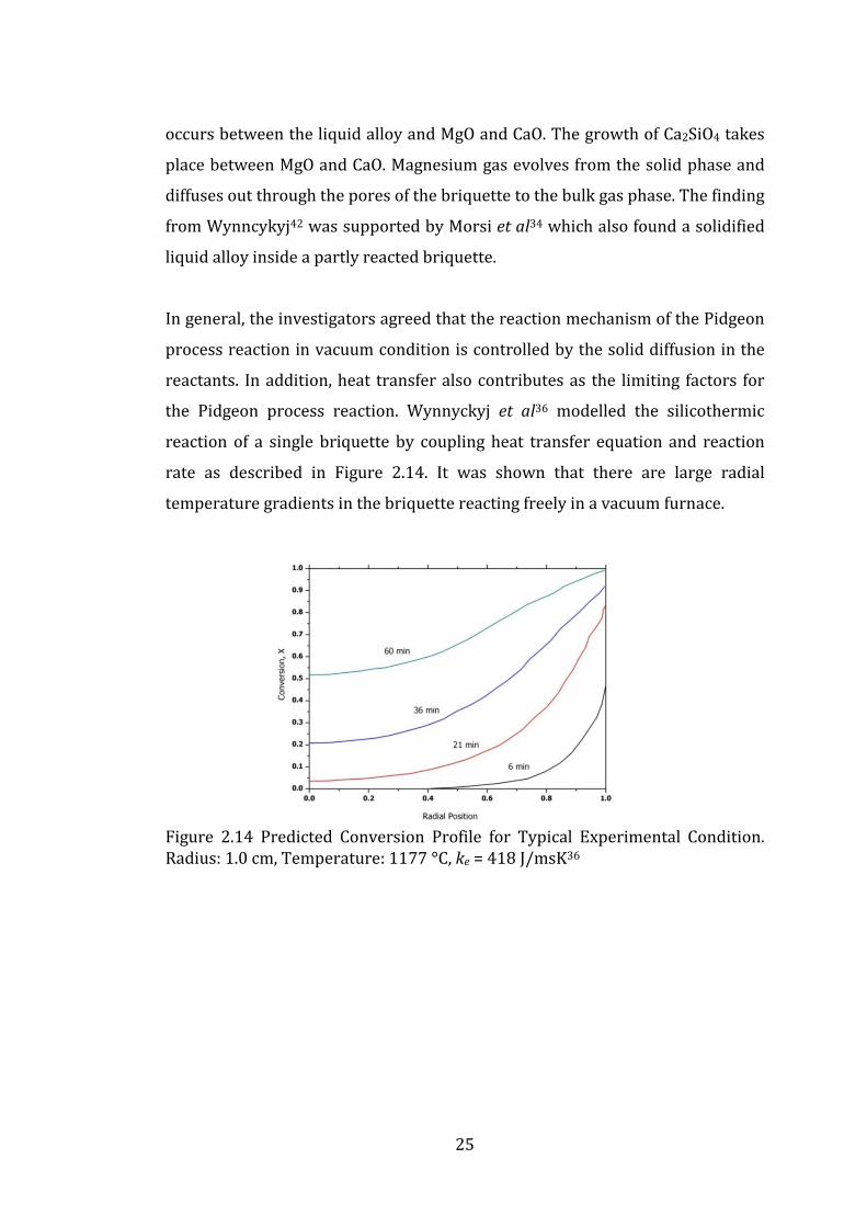
25

occurs between the liquid alloy and MgO and CaO. The growth of Ca2SiO4 takes

place between MgO and CaO. Magnesium gas evolves from the solid phase and

diffuses out through the pores of the briquette to the bulk gas phase. The finding

from Wynncykyj42 was supported by Morsi et al34 which also found a solidified

liquid alloy inside a partly reacted briquette.

In general, the investigators agreed that the reaction mechanism of the Pidgeon

process reaction in vacuum condition is controlled by the solid diffusion in the

reactants. In addition, heat transfer also contributes as the limiting factors for

the Pidgeon process reaction. Wynnyckyj et al36 modelled the silicothermic

reaction of a single briquette by coupling heat transfer equation and reaction

rate as described in Figure 2.14. It was shown that there are large radial

temperature gradients in the briquette reacting freely in a vacuum furnace.

Figure 2.14 Predicted Conversion Profile for Typical Experimental Condition. Radius: 1.0 cm, Temperature: 1177 °C, ke = 418 J/msK36

26

Figure 2.15 Effect of Pellet Radius on the Conversion Profile and Temperature Distribution within the Briquette, Predicted by the Model. Temperature: 1177 °C, ke= 418 J/msK, Time: 60 min36 Figure 2.15 also shows that there are gradual conversion and temperature

profiles within the briquette at different radial positions. Since there is a

gradient in the temperature and conversion profile, Wynnyckyj et al36

concluded that the conduction through briquette and the intrinsic reaction are

slow and limit the reaction.

The available literature about the reaction mechanism focused on what is

occuring inside the briquette. While the rate of effusion of magnesium from the

surface of briquette is often assumed to be rapid in a vacuum condition36, it is

not the case with the streaming inert gas condition. Barua and Wynncykyj37

analysed the role of gas-film mass transfer of magnesium vapour from the

briquette surface to the bulk gas during silicothermic reduction of calcined

dolomite in a streaming hydrogen gas, using the following equation:

p ' V]3 >Tq 4 qc (2. 18)

where kc is mass transfer coefficient, which was predicted from Ranz and

Marshall correlation43, PB and PS are the vapour pressures of gas in bulk stream

and surface, respectively.

27

Figure 2.16 Calculated Magnesium Pressure on the Briquette Surface and Bulk Gas37 Figure 2.16 shows the calculated magnesium vapour pressure on the surface of

briquette and the bulk hydrogen gas. These calculations show that there is

significant resistance on the gas-film mass transfer of magnesium vapour,

especially at the beginning of the reaction.

2.2 Bolzano Process

A number of modifications of the Pidgeon process include utilisation of vertical

retort44 and using internally heated retort. The latter is called the Bolzano

process, which is similar to the Pidgeon process in terms of ferrosilicon

utilisation to extract magnesium from calcined dolomite. In the Bolzano process,

which is described schematically in Figure 2.17, the briquettes are charged into

an internally heated and brick-lined cylindrical reactor.

This process was developed in Bolzano, Italy by Societa Italiana per il Leghe di

Magnesio (SAIM)45, 46 and operated by Bragmag (Minas, Girvas, Brazil). Bettatini

et al45 patented the process of extracting magnesium by this process, while the

reactor furnace was patented by Ravelli et al46. The homogenously mixed

calcined dolomite and ferrosilicon briquettes (d) are loaded and stacked on a

charge support system (e) with electrical heating conductors (f). The top section

is cooled and acts as a condenser for the magnesium vapors generated in the

furnace47.

28

Figure 2. 17 Bolzano Reactor48

The process operates at a temperature of 1200 °C and pressure less than 400

Pa48. Magnesium vapour evolves from the briquettes and condenses at the inner

wall of a water-cooled condenser at a temperature between 400 and 500 °C.

Each reactor has a production capacity of two tonnes of magnesium per 20-24

hours reaction cycle, with a shutdown time of 0.5 to 0.75 hour per cycle. After

the process is shut down, the reactor is opened at the flange and the metal is

removed. It is reported that magnesium with 99.9 to 99.99% of purity can be

obtained48. The procedure of charge handling and slag removal is difficult in this

process. However, there is little information about the physical chemistry of this

process in the literature.

The global warming potential (GWP) for this process was calculated to be 13.80

kg CO2/kg Mg ingot, which is approximately about a third of the Pidgeon

process’s GWP49. The main reason for such diverging result lies in the fact that

the Bolzano process utilises an electric-heated reactor, where more than 80% of

the total used electricity comes from hydropower while the Pidgeon process

relies on a low-efficient coal-fired reactor49.

29

2.3 Magnetherm Process

2.3.1 Magnetherm Process Description

The development of the Magnetherm process begun in France in 19487. The

commercial production has been established from the 1960s until 1990s50. At

the present time, the only operational plant utilising the Magnetherm process is

in the Bela Stena (Serbia) magnesium plant51. This process differs from the

Pidgeon process in a number of ways52: 1) the reduction process is carried out

in a molten slag bath, and 2) alumina/bauxite is used to produce calcium-silico-

aluminate slag, and the magnesium vapour produced is condensed to its liquid

state, before it is further processed in the refining operation. The starting

materials for the Magnetherm process are calcined dolomite, ferrosilicon and

bauxite7. The Magnetherm process, as schematically illustrated in Figure 2.18,

involves a silicothermic reduction of MgO from the calcined dolomite (CaO.MgO)

in a molten slag bath.

Figure 2.18 The Schematic of Magnetherm Process53

30

The overall reaction may be written as follows:

. d!" 8W7$r' 2$ %. 8W7$rM,& 2& d!"M

(2. 19)

The calcined dolomite, ferrosilicon and alumina dissolve in the slag phase

before the silicothermic reaction occurs. The process is operated at a

temperature of 1550 °C and pressure of 5 kPa in an electric arc furnace. The slag

composition is maintained at 55 wt% of CaO, 25 wt% of SiO2, 14 wt% of Al2O3

and 6 wt% of MgO. A phase diagram for the CaO-SiO2-Al2O3-MgO system is given

in Figure 2.19. The slag composition lies on the dicalcium silicate area close to

the periclase border.

A simplified silicothermic reduction in the Magnetherm process can be written

as follows:

M,& M ' $M,& 2& (2. 20)

The thermodynamics of this process has been described by Christini54 and

Cameronet al55. The key feature of the Magnetherm process to this process is to

develop a low-silica activity in the molten slag and maintain the composition of

the slag on the dicalcium silicate and periclase phase-boundary in the

quaternary CaO-Al2O3-SiO2-MgO system54. The molten magnesium oxide is kept

at fully saturated; therefore, the activity of MgO is unity. A slag analysis using

SEM, XRD and DTA-TG51 showed that the MgO content in the slag is in the range

of 7.02 to 8.82 wt% with γ-Ca2SiO4 as the dominant phase.

There are few kinetic studies on the fundamental aspects of reduction of MgO in

the molten slag. Most of the studies only give a description7, 52, 56-59 of the

process kinetics of the Magnetherm process. Christini54 pointed that the

reaction between MgO in the slag and FeSi only occurs when the two phases are

in contact: that is the contact between freshly-charged FeSi and the slag; and

between the surface of residual FeSi and the molten slag at the bottom of the

furnace. An experimental study on the kinetics of MgO reduction by ferro-

31

aluminium alloy in the MgO-Al2O3-CaO slag60 also found that the mass

transport in the slag/metal interfacial area controlled the overall reaction.

Figure 2.19 The Phase Diagram of CaO-MgO-SiO2-Al2O3 System at 10% Al2O3(Temperature is in K)61. The Grey Area is the Magnetherm Operation Condition

The vacuum condition in the reactor results in some operational problems. The

ingress of air during slag tapping was reported to cause the loss of 20% of the

production due to the formation of MgO and Mg3N2 in the condenser55.

Magnesium loss was also caused by the carbothermic reduction of MgO in the

reactor lining and electrode which forms carbon monoxide, according to the

following reaction:

' & & (2. 21)

The direction of reaction in Equation (2.21) reverses at a lower temperature.

Hence, at the low temperature of the condenser, the carbon monoxide vapour

will re-oxidise the magnesium vapour and form magnesium oxide.

32

2.3.2 Magnetherm Refining Operation

Magnesium vapour produced from the Magnethem process reaction is

condensed then refined in another unit process. Table 2.4 shows the impurities

in the magnesium before and after refining process as reported by Bowman59.

The impurities in the magnesium originate from:

1. Particulate matter carried by magnesium vapour, e.g. MgO and CaO;

2. Physical and chemical interactions between species inside the reactor; and

3. Vaporisation of volatilised materials, such as Mn, Zn, Pb, and Ni.

The details of the refining process are as follows59. A flux containing 45% of

MgCl2 and 55% of KCl is added and stirred into the molten metal. At the end of

the refining process, the flux is allowed to settle before molten magnesium is

tapped and casted. The chemical reaction in the refining can be written as:

7$M PJ,M ' PJ,M 7$ (2. 22)

In addition to remove Ca, the flux also captures oxide inclusion and forms a

sludge of heavy oxy-chloride8. The refining practice can produce a magnesium

ingot with a standard composition as required by ASTM B92. However, the

refining stage means a higher production cost and less magnesium metal yield.

There is about 5-8% magnesium lost in the refining stage59.

Table 2.4 Impurities in the Magnesium Produced from the Magnetherm Process Before and After Refining (using MgCl2 and KCl fluxs) process, in wt%59

Impurities Before refining After refining

Calcium 0.77 – 1.05 0.005

Silicon 0.11 – 0.16 0.063 – 0.11

Aluminium 0.037 – 0.088 < 0.05

33

2.3.3 Modified Magnetherm Processes

In the mid of 1980s, the raw material in the Magnetherm process was modified

by adding aluminium skim and aluminium shot in addition to ferrosilicon as the

reducing agent62. This concept is similar to the aluminothermic route, which

reduces magnesium oxide using aluminium as a reducing agent. This route was

first studied by Grjotheim et al63, which measured the equilibrium vapour

pressure of magnesium over the MgO-Al system by means of transpiration at

the temperature ranges between 870 and 1141°C. The vapour pressure of

magnesium in the MgO-Al system was found to be higher than the MgO-Si

system, which is 19.73 kPa compared to 2.49 kPa at a temperature of 1150 °C.

The development of this process has been limited by the higher price of

aluminium compared to magnesium. Low grade and recycled aluminium have

been suggested as possible reducing agent62, but their availability is not reliable

for use in commercial scale production.

The modified Magnetherm process is conducted at a high temperature (1550

°C) and a low pressure (10 kPa)62. In the original Magnetherm process, alumina

is added to lower the liquidus temperature of the slag. A modification was

carried out to replace alumina with alumina balls, aluminium shot, or

aluminium skim (mixture of Al-Al2O3). Christini and Ballain62 found that the

conversion of magnesium produced by using aluminium skim as reducing agent

was better compared to the magnesium recovery from a normal Magnetherm

operation.

Another variation of modified aluminothermic is the Heggie-Iolaire Process64.

The aluminothermic reduction of magnesium oxide, in the form of calcined

dolomite or magnesia, is employed at near atmospheric pressure in a thermal-

plasma arc furnace using scrap aluminium as the reducing agent. Wadsley64

conducted a 10 kg/hr test of this process. Magnesium oxide, aluminium

reactants, and calcium oxide were fed into a plasma arc furnace up to 180

minutes at near atmospheric pressure and a temperature between 1500 and

1600 °C to produce magnesium vapour at rate 2.5 kg per hour.

34

Table 2.5 shows the typical composition of magnesium vapour produced via the

Heggie-Iolaire process. Whilst the best individual run may produce 99.06 wt%

of pure magnesium, the average purity of the product is similar to those from

the Magnetherm process.

Table 2.5 Composition of Magnesium Process in Heggie-Iolaire Process64

Element Average Product, wt% Best Individual Product, wt%

Mg 97.4 99.06

Ca 1.28 0.46

Al 0.68 <0.06

Si < 0.07 0.05

2.4 Mintek Process

2.4.1 Mintek Process Description

The Mintek Thermal Magnesium Process (MTMP)65 has been developed in the

last twenty five years. During the 1980s, Mintek, a South African research

council, began a small-scale test work in order to develop a continuous thermal

magnesium process66, 67. Mintek has carried out the development test work at a

pilot plant scale68-70. The principle of the Mintek process was based on the

Magnetherm process whereas silicothermic reduction is carried out in a molten

slag. The raw materials used in the process are magnesia (MgO), calcined

dolomite (CaO.MgO), ferrosilicon, and aluminium. The composition of the raw

materials for the Mintek process is shown in Table 2.6.

Table 2.6 Composition of Calcined Dolomite (Cal.dol) and Reducing Agent (%wt)67

Material MgO CaO SiO2 Al2O3 FeO MnO LOI*

Cal.dol 1 38 57.8 1.1 0.4 0.4 0.2 0.3 Cal.dol 2 35 55.5 2.6 1 1.4 1.5 0.5 Alumina - 0.1 0.1 99.3 0.1 - -

Material Si Fe Al C Ca Mg Mn

Aluminium 0.06 0.15 99.8 N.A. N.A 0.0025 0.13 FeSi 75.5 18.1 2.4 0.1 0.7 0.03 0.1

*Loss of Ignition

35

MgO is obtained by calcining magnesite in a tunnel kiln at a temperature of

1720 °C, while calcined dolomite is obtained by calcining dolomite ores in a

rotary kiln at 1650 °C. The reducing agents utilised in this process are

ferrosilicon and aluminium. Ferrosilicon and aluminium reduces magnesium

oxide via silicothermic and aluminothermic reactions, respectively. These

reducing agents are provided in different quantities and had a particle range

size between 3 and 25 mm.

The main reactions in the Mintek process are as follows71:

2 2 !" ' & $ % !" (2. 23)

12 21 14W7 ' 21& 12. 7W7$rM (2. 24)

Figure 2.20 Phase Diagram of CaO-MgO-Al2O3-SiO2 System at 10 wt% Al2O3(Temperature in K)61. The black area is the Mintek Operating Condition

36

Magnesium vapour is generated in a heated reaction zone which consists of

aluminosilicate slag from solid reactants fed continuously to such reaction zone.

The reaction zone is heated by thermal plasma. The volatilised magnesium

condenses in a condenser in liquid form. The total pressure in the system, which

consists of partial pressure of argon plasma and the magnesium vapour, is kept

at nearly atmospheric pressure. The partial pressure of magnesium is in the

range between 0.3 and 0.5 atm67.

Besides the operating conditions, the differences between the Mintek and the

Magnetherm processes lie in the slag chemistry. The Mintek process has a

higher liquidus temperature compared to the Magnetherm process. As

illustrated in Figure 2.20, the slag composition of the Mintek process (black

area) has a liquidus temperature of 1700 °C. When MgO is reduced using

ferrosilicon and carried out at atmospheric pressure, the reaction is predicted

by thermodynamics to occur at temperatures above 1950 °C. Barcza et al66

suggested that by adding bauxite, the liquidus temperature of the slag can be

lowered to between 1700 and 1750 °C, so the furnace operating temperature

can be reduced as well. In a pilot scale plant, Abdellatif70 reported that the

temperature range of the system can adjusted to be in the range of 1600 to 1700

°C with bauxite addition70.

While there are a number of papers from Mintek that explains the process

description, whether it is in a small scale67 or in a pilot plant scale69, 70, there is

no fundamental thermodynamics or kinetics study of this process in the

literature. A study based on a thermodynamic simulation of the Mintek process

using PyroSim (in-house thermochemical software owned by Mintek) was

carried out to determine the theoretical operating condition and slag

composition in the Mintek process69. However, there is no published article

explaining the detail of the work on the thermodynamics of the Mintek Process.

Cameron et al55, 72 who analysed on the Magnetherm process provided some

physical and chemical details to the silicothermic reaction in molten slag such as

the Mintek process.

37

Figure 2.21 Layout of the MTMP Pilot Plant70 A schematic layout of the Mintek Process in a pilot plant scale is described in

Figure 2.21. The calcined dolomite is heated up in an electrical operated kiln at a

temperature between 1000 and 1100 °C. The feed rate varies between 250 and

400 kg/h. The heated calcined dolomite is collected in refractory-lined transfer

bins and then discharged into the furnace feed system. The average feed rate is

about 525 kg/h (10.7% FeSi, 5.5% Al, the remainder being calcined dolomite)

and the feed duration is about 2.5 hours, giving a batch size of 1300 kg. The slag

tapping is carried out by drilling through a tap-hole at average temperature of

1650 °C. The batch period is about 2.5 to 3.0 hours70.

Magnesium condensation takes place in the elbow compartment and inside

crucible. A stirrer is used to create a central vortex that drew the magnesium

vapour from the arc furnace. The temperature inside the condenser is in the

range between 680 and 720 °C70.

38

Barcza et al66 explained the work of small scale test of magnesium production at

nearly atmospheric pressure. They claimed that the produced magnesium has a

purity of 99.80 wt%. The typical composition of metallic element in the

magnesium metal based on this work is shown in Table 2.7, while the resulted

slag composition is presented in Table 2.8. In the test 1, the magnesium

produced contains 0.1 wt % of Ca, 0.03 wt % of Si, 0.01 wt% of Al, 0.01 wt% of

Fe and 0.02 wt% of Mn. The slag composition contains 6.3 to 8.5 wt% of MgO,

47.7 to 56.2 wt% of CaO, 22.3 to 31.9 wt% of SiO2 and 10.8 to 12.7 wt% of Al2O3.

This composition is comparable with the Magnetherm’s slag composition.

Abdellatif69 argued that the Mintek process has several advantages compared to

the Pidgeon and the Magnethem process. The potential risk of air-ingress into

the system is largely eliminated because the operation is carried out at

atmospheric pressure. Condensation to a liquid phase reduces the energy

requirements in the cleaning and refining operation, as the remelting of the

crude magnesium is not be been required69. However, condensing to a liquid

phase also implies that the condensing surface needs to be maintained at

relatively high temperatures (greater than 650 °C)69 and requires a large

condensing area.

Table 2. 7 Composition of Condensed Magnesium (wt%)66

Test Mg Ca Si Al Fe Mn

1 99.81 0.10 0.03 0.01 0.01 0.02

2 99.84 0.08 0.02 0.01 0.01 0.03

3 99.80 0.09 0.02 0.02 0.02 0.04

4 99.80 0.10 0.02 0.02 0.02 0.02

Table 2.8 Slag Composition in Mintek Process (wt%)66

Test MgO CaO SiO2 Al2O3

1 7.9 53.3 23.3 12.7

2 8.5 52.5 24.6 10.9

3 4.7 56.2 22.3 12.9

4 6.3 47.7 31.9 10.8

39

2.4.2 Mintek Refining Operation

Magnesium produced from the Mintek process requires a refining operation in

order to remove impurities in the condensed metal. The impurities are

originated from the particulate matters in the feed entrain in the gas stream and

settle inside the condenser and from physical and chemical interaction between

the electric arc and the furnace bath73.

Table 2.9 Chemical Analyses of Various Fluxes, Mass per Cent8

Component M130 Flux Fluorspar KCl

Mg 9.69 NA NA

Al 0.08 0.44 0.12

Si 0.37 0.215 0.94

Ca 2.13 48.45 0.019

Fe 0.20 0.236 0.03

Cl 56.15 0.0144 47.55

Na NA 0.01 0.01

K 27.10 0.011 50.90

F 1.95 51.29 NA

The crude magnesium produced by MTMP is refined in two stages8. In the first

step, crude metal is melted and M130 flux is added to the melt. M130 flux is an

MgCl2-KCl flux which has compositions listed in Table 2.9. M130 flux captures

the oxide and nitride inclusions of Mg, Al, Ca, and Si, and forms a thick chloride

sludge which settles out at the bottom of the refining crucible8. Calcium is

removed by following reaction:

7$M PJ,M ' PJ,M 7$ (2. 25)

M130 Flux is believed to be ineffective in removing the iron and silicon in

magnesium metal8; therefore, it is essential to conduct further refining in the

second stage.

The subsequent refining uses mixtures of M130 flux and FeCl3. This stage is

carried out between temperature 715 and 760 °C. Ferric chloride is used to

capture silicon impurity in the molten magnesium metal and convert it into a

40

FeSi alloy8. The refining reaction to remove Si impurities in the magnesium

metal can be written as follows:

PJ,M r$ PJ,M !"7rM ' !" r

$ 7$M (2. 26)

This refining is not only reducing the silicon content of the metal, but also

lowering metallic impurities such as Fe, Mn, Cr, Ni, and Al. Table 2.10 shows the

chemical analysis of the crude and the refined magnesium. The refining

operation was claimed to reduce the impurities content in the magnesium, such

as Al, Si, Ca and Fe to be less that 0.01 wt%8.

Table 2. 10 Chemical Analyses of Crude and Clean Magnesium, wt%8

Element ASTM B92

Grade 9980A Crude Mg

Clean Mg

Avg. Max. Min.

Al 0.05 max 0.066 0.040 0.253 0.003

Si 0.05 max 0.281 0.095 0.500 0.014

Ca 0.05 max 0.385 0.023 0.102 0.005

Fe 0.05 max 0.250 0.047 0.100 0.002

2.4.3 Prospects of the Mintek Process

Barcza et al74 examined the potential benefits of the Mintek Process. The

economic analysis of the Mintek process was compared to the Magnetherm and

the electrolytic process. Several advantages of the Mintek process are:

1. Less capital intensive compared to electrolytic process. The estimated

capital cost for the Mintek process is $US 5000/ annual tonne magnesium75

(data per 2006), while the estimated cost for the electrolytic plant is $US

8000/annual tonne magnesium76 (data per 2004).

2. The treatment of raw material is less sophisticated when compared to the

electrolytic process. The raw material preparation for the Mintek process

includes calcination of dolomite, while the feed preparation for the

electrolytic process may comprise a number of steps to ensure a high-purity

magnesium chloride as the feed for electrolytic operation.

41

The Mintek Process has potential future for magnesium production. In 2004,

Gossan Resources Ltd. which holds a high-purity dolomite property at Inwood,

Manitoba, Canada conducted a preliminary study to produce magnesium using

Mintek Process77. The development of this process leads to the Gossan-Zuliani

process, which operates at temperature higher than 1550 °C at atmosphere

pressure. The utilisation of hydro power gives a great advantage over the

Chinese Pidgeon process in terms of greenhouse emissions78.

2.5 Purity Requirement for Commercial Magnesium

Table 2.11 provides the physical properties of magnesium metal. Magnesium

melts at 651 °C and has a boiling point of 1107 + 10 °C at 1 atm79. The crystal

structure of magnesium is close-packed hexagonal (h.c.p), with a density of

1738 kg/m3 at room temperature. Magnesium has pyrophoric properties,

which may react spontaneously in normal atmospheric pressure resulting an

intense white flame79. Magnesium also reacts violently with water.

In the industrial process, from both electrolytic and pyrometallurgical

processes, magnesium metal is remelted and refined in order to meet the purity

requirement of commercial magnesium. Table 2.12 shows the specification of

magnesium produced by Timminco. In general, the magnesium content should

be 99.80 wt% min and less for more advanced application. The ultra-purity

grade requires 99.98 % purity of magnesium. The presence of iron in the

magnesium metal will reduce the corrosion resistance properties of the metal.

42

Table 2.11 Physical Properties of Magnesium48

Physical Properties Value

Melting point 650 + 2 °C Boiling point 1107 + 10 °C Latent heat of fusion 0.37 MJ/kg Latent heat of evaporation 5.25 MJ/kg Heat of combustion 25.1 MJ/kg Specific heat at 20 °C 1030 J.kg-1K-1 Specific heat at 600 °C 1178 J.kg-1K-1 Electrical resistivity at 20 °C 4.45 μΩ.cm Thermal conductivity at 25 °C 155 Wm-1K-1 Thermal expansion at 20 °C 25.2 × 10-6 K-1 Thermal expansion at 20 – 300 °C 27-28 × 10-6 K-1 Density (solid) at 600 °C 1622 gcm-3 Standard redox potential -2.372 V

Table 2. 12 Pure Magnesium – Specification and Mean Impurity Content9

Element

Commercial

99.80

Grade

% max

Timminco High-purity Grades

High-purity

99.80 Grade Super Purity

99.95 Grade Ultra Purity

99.98 Grade

% max Spec %

max Mean %

Spec %

max Mean %

Aluminum (1) (1) (1) 0.0040 0.004 0.0030 Zinc (1) (1) (1) 0.0045 0.007 0.0045 Manganese 0.10 0.01 0.01 0.0030 0.002 0.0015 Iron (1) 0.0070 0.03 0.0015 0.002 0.0015 Nickel 0.001 0.001 0.001 <0.0005 0.0005 <0.0005 Copper 0.02 0.005 0.002 <0.0005 0.0005 <0.0005 Silicon (1) 0.010 0.010 0.0045 0.003 0.0025 Lead 0.01 0.005 0.003 0.0010 0.001 <0.0010 Calcium 0.010 0.005 0.003 0.0012 0.003 0.0012 Tin 0.01 0.001 0.001 <0.001 0.001 <0.0010 Cadmium - - - - - <0.0001 Others, each 0.05 0.012 0.01 - 0.005 - Others, total 0.20 0.100 0.03 - 0.02 -

Controlled by limits for other, each

Magnesium ingot is the main material to produce magnesium alloy AZ91 D. The

composition of magnesium alloys AZ91D and AM60A is listed in Table 2.13.

Elements such as Fe, Ni, and Cu are harmful to corrosion properties, and strict

specification limits apply for these elements 80. Fe is removed by adding other

materials to precipitate Fe. For AZ91D (8.3-9.7% Al, 0.15% Mn, 0.35 – 1.0% Zn),

after Mn, Al, and Zn is added to molten Mg, the temperature of molten alloy is

lowered to the casting temperature. During alloying and equilibrating process,

Fe precipitated as intermetallic compounds that settle in the bottom of furnace.

43

Ni also can be removed but at present there are no established methods to

control Cu and Ni other than controlling the purity of basic alloy constituents80.

Table 2. 13 Composition of Magnesium Alloys

Element AZ91D (wt%) AM60A (wt%)

Al 8.3 to 9.7 5.5 to 6.5

Mn 0.15 min. 0.13 min

Zn 0.35 to 1.0 0.22

Si 0.10 max. 0.50 Si max.

Fe 0.005 max. N.A.

Cu 0.030 max. 0.35 max.

Ni 0.002 max. 0.03

Zn N.A. 0.22

others 0.02 max (each) N.A.

Mg balance Mg. balance Mg

44


45

3 Review of Thermodynamics and Kinetics of

High Temperature System

3.1 Thermodynamic Modelling

Thermodynamic modelling has been widely used in high temperature

processing to predict multiphase equilibrium, identify the limits of a process

and provide a better understanding of complex processes. In this chapter, the

fundamental of thermodynamic modelling will be described, in particular with

reference to the modelling of high temperature systems, where the assumption

of equilibrium is usually effective because of the fast chemical kinetics and high

rates of mass and heat transfer associated with these conditions.

3.1.1 Gibbs Energy Minimisation

In a reaction between A and B which produces C and D as in Equation (3.1):

W tu ' _ v (3. 1)

The enthalpy of reaction, which is the heat absorbed or evolved by reaction in

Equation (3.1), ∆Ho, is defined by:

∆° ' _∆T v∆ 4 ∆, 4 t∆x (3. 2)

The function which decides whether a process will occur is called the free

energy change, ∆G, which is defined by:

∆ ' ∆ 4 6∆ (3. 3)

where ∆G = the free energy or Gibbs energy change of the process,

∆H = the enthalpy change of the process, and

∆S = the entropy change of the process.

The equilibrium of reaction in Equation (3.1) can be written as follows:

' ,-y,z,\.,| (3. 4)

46

The Gibbs energy of reaction in Equation (3.1) relates with equilibrium

constant, K, with the following equation:

∆ ' 45678 (3. 5)

When there is more than one compounds in a solution, a partial Gibbs energy,

, is introduced. The partial Gibbs energy is related to the activity of

component i in the solution, ai, which is defined as follows:

' 5678 (3. 6)

where R is the gas constant, T is temperature, and ai is the activity of component

i in the solution. The activity of component i, ai, corresponds to the

concentration of i in the solution by the following correlation:

' ~d (3. 7)

where γi is the activity coefficient of component i.

When a mixture of components in a multiphase system is not in equilibrium, the

Gibbs energy of such a system is high. The reactions that will reduce the total

free energy of the system to a minimum are thermodynamically favoured.

In the Gibbs minimisation method81-83, the total Gibbs energy of all phases in the

system is kept at a minimum. The total Gibbs energy can be calculated either

from knowledge of chemical potential of component i, , by:

' ∑ 8 (3. 8)

where ni is the amount of component i, or alternatively by:

' ∑ φ φφ (3. 9)

where φ is the amount of phase φ and φ its Gibbs energy:

φ ' ∑ ∑ d ' ∑ ∑ d 5678 (3. 10)

is the Gibbs energy of pure species i and xi is the composition of component i.

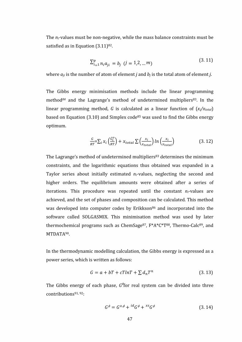
47

The ni-values must be non-negative, while the mass balance constraints must be

satisfied as in Equation (3.11)82.

∑ 8 ' t p ' 1,2, … S: (3. 11)

where aji is the number of atom of element j and bj is the total atom of element j.

The Gibbs energy minimisation methods include the linear programming

method84 and the Lagrange’s method of undetermined multipliers83. In the

linear programming method, G is calculated as a linear function of (xi/xtotal)

based on Equation (3.10) and Simplex code85 was used to find the Gibbs energy

optimum.

]3=∑ d @0L]3C dJJ,M ∑ @ 0

L.C 78 @ 0 L.C (3. 12)

The Lagrange’s method of undetermined multipliers83 determines the minimum

constraints, and the logarithmic equations thus obtained was expanded in a

Taylor series about initially estimated ni-values, neglecting the second and

higher orders. The equilibrium amounts were obtained after a series of

iterations. This procedure was repeated until the constant ni-values are

achieved, and the set of phases and composition can be calculated. This method

was developed into computer codes by Erikkson86 and incorporated into the

software called SOLGASMIX. This minimisation method was used by later

thermochemical programs such as ChemSage87, F*A*C*T88, Thermo-Calc89, and

MTDATA90.

In the thermodynamic modelling calculation, the Gibbs energy is expressed as a

power series, which is written as follows:

' t6 _6786 ∑ v6 (3. 13)

The Gibbs energy of each phase, Gφfor real system can be divided into three

contributions91, 92:

φ ' ,φ φ φ (3. 14)

48

where Go is the Gibbs energy of pure element in φ phase, φ corresponds to the

Gibbs energy of mixing of an ideal solution, and φ is the so-called excess

term, which relates to real behaviour of the solution91, 92. The detail of different

solution models will be described in Section 3.1.3.

3.1.2 Database Development

Reliable thermochemical databases for species are the vital inputs for

thermodynamic calculations. Thermochemical databases were developed from

critical analysis of a number set of experimental data. The Gibbs energy was

expressed mathematically as a function of temperature, as shown in Equation

(3.12). Entropy, enthalpy, and heat capacity data are expressed as per Equations

(3.15) to (3.17), respectively.

' 4t 4 _ 4 _786 4 ∑ 8v6B: (3. 15)

' 4 _6 4 ∑8 4 16 (3. 16)

' 4_ 4 ∑ 88 4 1v6B: (3. 17)

These databases were collected and critically assessed before included in the

thermochemical software as data sources for thermodynamic calculations. Some

established database are JANAF thermochemical tables26, SGTE (Scientific

Group Thermodata Europe)93, NPL, and FACT database94.

3.1.3 Solution Models

In a high temperature system, it is common for species to dissolve into each

other to form multi-component phases such as slag, mattes, and alloys. In some

cases, this solution behaviour is quite complex, with interactions between

different species in the phase strongly influencing the distribution of elements

between different phases. Unfortunately, there is no single approach to

modelling multi-component solution behaviour that will satisfy all systems.

49

There is also no comprehensive scientific treatment of solution behaviour;

instead, a combination of theory and empiricism is used to deal with the

thermodynamics of these systems95. The following section describes some of

common models used for high temperature systems.

3.1.3.1 Ideal Solution Model

In an ideal solution, the volumetric changes and enthalpy resulting from mixing

are zero. Ideal solution model assumes that there is no interaction between

different molecules. Ideal solution follows Raoult’s law96, which states that the

vapour pressure of an ideal solution is function of the vapour pressure of each

chemical component and the mole fraction of the component present in the

solution. In the case of an ideal solution of A and B species in a condensed phase,

the Gibbs energy of solution is written as follows:

φ ' P,M (3. 18)

φ ' d d 56d78d d78d (3. 19)

The ideal solution model is often used for a mixture of vapour in atmospheric

pressure, as the behaviour of vapour in this condition follows Raoult’s law96.

While it is common for many researchers to use the ideal solution model as a

starting point for their calculation, the complex condensed phase such as slag

and metallic phase necessitate more sophisticated models.

3.1.3.2 Dilute Solution Model

Dilute solution often follows Henry’s law97, whereas the solute activity has

linear correlation with its concentration. This correlation can be described as:

' γd (3. 20)

where γoi is Henrian activity coefficient or Henrian Constant.

50

The partial Gibbs energy in dilute solution model is defined as follows:

' 5678d (3. 21)

where has a constant value based on the Henrian concentration range and

may be obtained directly from γ . Interaction coefficients98 are introduced to

allow this model to be applied to higher order systems. The partial Gibbs energy

is then defined as follows:

' 5678d 56 ∑ εd (3. 22)

where xi is the concentration of solute i and εis an interaction parameter

involving component i and j in the solvent. This approach is commonly used in

molten metal applications, for example, in calculating the equilibrium between

liquid steel and inclusion chemistry99, 100.

3.1.3.3 Regular Solution Model

Regular solution is a non-ideal solution that has “regular solution behaviour”101.

The correlation of the activity coefficient to the concentration in the regular

solution is as follows:

5678γ ' α′d$ (3. 23)

5678γ ' α′d$ (3. 24)

The excess Gibbs energy for a regular solution is described as follows:

' 56αdd ' Ωdd (3. 25)

Activity coefficient of species in the regular solution model is a function of

temperature with the following correlation:

γ\,JJPSPK,JRKP3 γ|,JJPSPK,JRKP3+ ' 3

3+ (3. 26)

51

Some examples of the application of the regular solution model are in the MgO-

FeO solid solution102, Thallium-Tin system103, and Iron-Nickel system104.

A sub-regular model is used for a more complex systems, where the interaction

coefficients at certain temperature are considered to change linearly with

composition101:

' ddΩ d Ω d (3. 27)

3.1.3.4 Random Mixing Solution Model

The random mixing solution model or substitutional solution model is non-ideal

solution model, which the excess Gibbs energy formula is represented by a

power series of composition dependence. This solution model assumes that

different species occupy random positions within a defined lattice101. The Ω in

Equation (3.28) is usually represented using the Redlich-Kister equation105:

Ω ' ∑ ,,φd 4 d (3. 28)

with ,,φ ' t6 (3. 29)

where Li,j is a binary interaction parameter, while an and bn are the model

parameters. When n = 0, the excess Gibbs energy become regular and is similar

to the regular solution model. When n = 1, the excess Gibbs energy become

subregular.

The Gibbs energy of binary compounds following the Redlich-Kister equation

can be expanded into:

' ∑ d 56 ∑ d78d ∑ ∑ dd ∑ ,,φ d 4 d (3. 30)

The Redlich-Kister polynomial equation is widely used in metallic systems for

substitutional phase, such as liquid, b.c.c and f.c.c106. However, when there is

short-range ordering in the liquid (such as in a slag and in the molten metal

with a tendency to form intermetallics), this model is not sufficient92.

52

The thermodynamic properties of multi-component systems are calculated

based on the summation of the binary and ternary excess paramaters.

Muggianu, Kohler, and Toop’s equations are amongst the method to extrapolate

the Gibbs energy of ternary system from binary systems. The details of this

methods are described elsewhere107.

3.1.3.5 Sublattice Model

In a random mixing solution model, all lattice sites are assumed to be

equivalent. However, some crystalline species are formed in two or more

different lattice structures. Therefore, it is advantageous to model the multi-

component solution of crystalline species using a sublattice model.

In a sublattice model, a fractional site, yi, is defined as the total number of

component i (nis) in sublattice S divided by the total component (NS) in the same

sublattice108 as in Equation (3.31).

` ' 0 (3.31)

The relationship between mole fraction (xi) and fractional site (yi) is described

by the following equation:

d ' ∑ 0∑ :B. (3. 32)

where yVa indicates the vacancy site fraction. The interaction parameter of the

excess Gibbs energy is also described using the Redlich-Kister polynomial. The

Gibbs energy of solution is defined by the following equation:

' ∑ 8 56 ∑ ∑ ` 78` ` ∑ ` 4 II (3. 33)

The application of the sublattice model includes interstitial phases and complex

intermetallic compounds92, for example in the Fe-Cr-C steel and Ni-Al solid

solution109. Fe and Cr in f.c.c crystal form with C as intersititial, the phase can be

modelled as (Fe,Cr)1(C,Va)2110. There are also several models which developed

based on the sublattice models, such as Compound Energy Formalism108 and

ionic liquid models111.

53

3.1.3.6 Compound Energy Formalism Model

Compound Energy Formalism (CEF) was developed based on the sublattice

model108. While the sublattice models consist of two set of positions (e.g. anions

and cations) that are distinguishable by different fractional occupancies of each

component, the CEF model incorporates the detailed of crystallographic data

into the sublattice model. This corresponds to the use of multiple sublattices.

The Compound Energy Formalism is beneficial to describe complex phase, such

as Laves phase, and cubic Frank-Kasper phase112.

The Gibbs energy expression in the CEF per formula unit of solution is written

as follows:

' ∑ ∑ `V$ V: 4 6A P (3. 34)

A ' ∑ `V$78`:V$ V: V: (3. 35)

where M is the sites and SC is configurational entropy.

The variation for different phases has been constructed by a number of

researchers with wide-range applications110, which include vacancies, anti-sites

and ordering, reciprocal phases, ionic melts113, and short range orders in

crystals114. It can also be applied to an ionic solution with application for solid

oxides, such as spinel and pyroxenes 115.

3.1.3.7 Modified Quasichemical Model

In some phases, the species in solution are not randomly distributed. For

example, in molten CaO-SiO2 slags, there is a tendency for short range ordering

to occur at around specific conditions and compositions. Modified

quasichemical models for short-range ordering liquid solution has been

developed and derived from quasichemical theory116. For a liquid binary

solution, atoms or molecules A and B are distributed over the sites of the

quasilattice. If a pair exchange reaction is considered:

W 4 W u 4 u ' 2W 4 u; ∆ (3. 36)

54

The Gibbs energy for the liquid using this model can be written as follows:

Ma ' 8Ma 8Ma 4 6∆A 0$ P ,Ma (3. 37)

where ni and nj are the number of moles of the component i and j, nij is the

number of (i-j) pairs, and ∆SC is the configurational entropy of mixing given for

randomly distributing the (i-i), (i-j), and (i-j) pairs. The configurational entropy

is defined as:

∆TU& ' 45D8 lnd 8 lndH 4 5 878 000+

878 +

878 00

(3. 38)

The molar and entropy change ∆gAB is noted as (ω-ηT). Coordination-equivalent

fractions, yi, and Z, coordination number is introduced in the model, which is

describes as follows:

` ' 0000 (3. 39)

while pair fraction, xii, is introduced as follows:

d ' 00000 (3. 40)

The excess Gibbs energy is expanded as a polynomial in terms of the pair

fraction, which is represented in the following equation:

' ∆ ∑ °d ∑ °d:,::,: (3. 41)

The parameters such as ∆ , ° and °is optimised using experimental data.

This idea can be extended to multi-component systems117. Important

applications of the Modified Quasichemical Models are for molten slag118, 119 and

molten salts120.

There are also some other approaches which have been adapted to described an

ordered system, such as Cluster Varian Method (CVM)121, Monte Carlo (MC) and

Bragg-William-Gosrsky (BWG)122, 123 treatments. Order parameters are

introduced to describe the degree of order in solution at various temperatures.

55

The free energy of the system is then described in terms of these order

parameters, and the equilibrium of the system is determined by minimising the

free energy of the system with respect to the order parameter.

3.1.4 Thermochemical Packages

Development of thermochemical packages has had a significant impact on

material and metallurgical processing, and the use is now common among

engineers and researchers alike. Some of the thermochemical packages

commonly available are FactSage, HSC, Chemix (CSIRO-SGTE Thermodata)., and

MTDATA. In essence, thermochemical packages have the following content:

1. Thermochemical database (Cp, G, H, S)

2. Solution models

3. Solution model database

4. Gibbs energy minimisation subroutine

3.1.4.1 Chemix-Thermodata

Chemix was a part of the CSIRO-SGTE Thermodata System, which was

developed by CSIRO minerals in the 1980s. The databases used in Chemix are

SGTE 1977, JANAF, NPL, and CSIRO. This module uses Solgasmix minimisation

subroutine to calculate equilibrium of multi-component and multiphase system.

A number of applications in extractive metallurgy has been reported, such as

direct smelting of zinc concentrate124, bauxite purification system125, solid

solution formation between arsenic and antimony oxides126, and carbothermic

of magnesium production127.

The activity coefficient models which are available in Chemix include fixed

activity coefficient, polynomial, Redlich-Kister, Margules, Virial, Redlich-Kwong,

and Pitzer dilute solution. The activity coefficient for each phase must be

entered by user, which can be obtained from a private database or available

literature. Whilst widely used in Australia during the 1990s, CSIRO has stopped

providing technical support for the software.

56

3.1.4.2 HSC

HSC Chemistry was developed by Outokumpu Technology in 1974. The

database used in HSC are taken from Barin128 and JANAF26 thermochemical

database. The Solgasmix routine83 based on Gibbs energy minimisation is also

used in the equilibrium module. In HSC, definition of system is crucial step and

carried out by the user. The users must specify the species that may be present

at equilibrium, though the software can readily identify the possible

combinations. The activity coefficients for individual species may be entered as

a constant number, or as a polynomial function of composition and

temperature. HSC has wide applications and is widely used in industry because

of its user-friendliness and calculating power. It is also used extensively for

calculating heat and mass balances for process flowsheets.

3.1.4.3 FactSage

FactSage is an integrated database computing system for chemical

thermodynamic. This package has optimized database for solutions, such as

alloys, liquid and solid oxides, and slags. For pure components, the data are

taken from JANAF Thermochemical Tables26, FACT data, and SGTE data128. The

details of this thermochemical package, which includes the databases and

various calculation modules, can be found elsewhere94. The solution models and

database for common systems have been optimised by the developer, such as

for oxide systems, slag, matte, salt, and light metals.

The user can use his/her own private database in FactSage software using the

“Compound” module for the species properties (G, H, S, Cp) and the “Solution”

module for solution interaction parameters. Thermochemical solution models

for various systems are available, for example random solution model, CEF, and

modified quasichemical models.

In the “Equilib” module, the Gibbs energy minimisation technique is used to

calculate the concentration of chemical species when specified elements or

57

compounds are react to reach the state of equilibrium. Phases from the

compound and solution databases are retrieved and listed as possible products

in the equilibrium result. “React” module calculates the enthalpy and Gibbs

energy of reaction, and a “Phase Diagram” module for generating phase

diagram.

3.1.4.4 MTDATA

MTDATA (Metallurgical and Thermochemical Databank) was developed by

National Physical Laboratory, England. The principle of MTDATA is similar with

other thermochemical packages, which is a software/data package for the

calculation of phase equilibria in multi-component and multiphase systems

using critically assessed thermodynamic data129. Computational interface for

thermodynamic calculations with MATLAB also has been reported130. It uses

Gibbs energy minimisation routine to predict equilibrium and has a number of

different modules allowing presentation and analysis of its predictions in

different formats such as Pourbaix, Kellogg or phase diagrams. It primary

calculation module for complex equilibria in metallurgical systems is called

Multiphase. The specifics of the minimisation routine used are dependent on the

level of accuracy required in the calculation. The highest accuracy minimisation

routine is essentially consistent with Solgasmix131.

Each different thermochemical packages has its different features and

limitations. These thermochemical packages may be used for different purposes

and systems. For example, HSC can be used for simple processes that do not

require multi-component solutions. FactSage and MTDATA can be utilised to

generate phase diagram as predictive tools for alloy development. One

important part that cannot be neglected in all thermodynamic calculation is the

definition of phases and possible species to be considered by the

thermodynamic model132. These choices will have a significant influence on the

results generated and the repercussions of these choices need to be considered

when using these tools.

58

3.2 Reaction Kinetics

Knowledge of reaction kinetics is essential for a better operation and control of

processes. While thermodynamics deals with equilibrium condition and

considers the feasibility of a reaction under a particular condition, kinetics give

information about the rate at the equilibrium state is approached. The rate of

reaction also depends on the path between initial states to final states, which is

not considered by equilibrium thermodynamics.

The kinetics of reaction is highly dependent on the condition of the system. The

reaction is called homogeneous when it includes one phase and heterogeneous

when involves two or more phases. Metallurgical reactions are largely

heterogeneous reactions, for example gas-solid reactions and slag-metal

reactions. A number of parameters may influence the kinetics of reaction,

including temperature, pressure and interfacial area. The analysis of overall

reaction kinetics of a system has been based on the expressions that either

involve a number of assumptions or are empirical133. This section will describe

the fundamental kinetics of heterogeneous reaction, with an emphasis to the

solid-solid reaction and gas-solid reaction.

3.2.1 Kinetics of Heterogeneous Reaction

In a heterogeneous reaction, the reaction occur at the interface of difference

phases, for example at gas-solid interface or at a solid A – solid B interface. The

overall kinetics of heterogeneous reaction may be governed by various steps. In

the case of a solid-solid reaction between AO and B2O3 species, the reaction

follows a number of steps 133: self-diffusion of reactant B2O3 species, diffusion of

reactant B2O3 species through product layer, reaction between AO and B2O3 in

the interface, and growth of product layer.

Figure 3.1 shows two schematically different types of diffusion. When the

diffusion is one-sided, i.e. diffusion of B2O3 is much faster than diffusion of AO,

the product growth of the reaction will occur only on one-side interface, which

59

is in the interface between the product (AB2O4) and AO. Conversely, when

counter-diffusion is involved, the product growth will occur on both side of the

interface.

Figure 3.1 Different Modes of Diffusion133

For a reaction between a solid and a gas, the overall reactions should involve

these steps134:

1. Gas phase mass transfer of the gaseous reactant from the bulk of the gas

stream to the external surface of the solid particle,

2. Several steps that may take simultaneously in a diffuse spatial domain:

a. Diffusion of the gaseous reactant through the pores of the solid

matrix, which could consist of a mixture of solid reactants and

products,

b. Adsorption of the gaseous reactant on the surface of the solid

matrix,

c. Chemical reaction at the surface of the solid matrix,

d. Desorption of the gaseous product from the surface of the solid

matrix, and

e. Diffusion of gaseous reaction product through pores of the solid

matrix; and

3. Gas phase mass transfer of the gaseous product from the external surface

of the solid to the bulk of the gas stream.

In a heterogeneous reaction, phenomena such as diffusion, mass transfer, and

heat transfer must be considered besides the intrinsic chemical reaction.

60

3.2.2 Kinetics Theory of Gas-Solid Reaction

The fundamentals of gas-solid reaction have been comprehensively explained

by Szekely et al135. A general type of non-catalytic gas-solid reaction may be

represented as the following reaction:

W& tu& ' q& _ (3. 42)

When the resistance of the gas film controls the overall reaction, as described in

Figure 3.2, the concentration of gaseous reactant is zero at the surface of

particle. Hence, the concentration driving force is constant during the reaction.

Figure 3.2 Representation of a Reacting Particle when Diffusion through Gas Film is the Controlling Resistance136.

The derivation of the model concludes to the following relationship:

>? ' 1 4 @Ky]Cr ' F (3. 43)

where rc=radius of core, R = radius of particle, X = conversion, and k = rate

constant, which equals to:

> ' rxI*A\*|] (3. 44)

61

where b = mole coefficient of particle, kg = rate constant, CAg = concentration of

the gaseous reactant and ρB = density of particle

A number of models have been proposed to predict the behaviour of gas-solid

reaction based on different assumptions137, 138. In which the solid is assumed to

be nonporous, the kinetics model of gas-solid reaction is generally modelled by

the Sharp Interface model or the Shrinking Core model139-142. While the

Shrinking Core model is the simplest, this model is one of the earliest models

and has been used as a basis for development of more sophisticated models. A

number of modifications based on the Shrinking Core Model have been modified

over the years. Some of the modification took account of the effect of bulk gas

flow of gaseous reactant143, 144, Knudsen diffusion in the ash layer145, 146,

structural changes in pellet systems in isothermal147 and non-isothermal

system148.

Other gas-solid reaction models include the Volume Reaction model149, the

Particle-Pellet/Grain model150, 151, the Modified Volume reaction models142, 149

and the Modified Grain model152, 153. The Volume Reaction Model149 was

proposed to describe gas-solid reaction in a porous solid. When the solid is

porous, the gas can penetrate into the solid; hence, the reaction may be assumed

to be carried out in all over the volume of pellet. In the Grain model150, 151, the

solid pellet is visualised as consisting of a number of small particles. The

reaction occurs in the surface of each particle and treated as the Shrinking Core

model. The Modified Volume Reaction models are based on the Volume Reaction

model which accounts the structural changes due to reaction142, 149. The

Modified Grain model also takes account the structural changes, where the

radius of the grain is assumed to change due to the differences in the molal

volume of the products and reactants152, 153. The details of these models are

provided elsewhere138.

62

3.2.3 Kinetics Theory of Solid-Solid Reaction

The kinetics of solid-solid reaction is affected by the form of solid (i.e.

nonporous, porous, or a mixed powder), particle size distribution, undefined

geometry and sintering. Powder reactions are substantially more complex and

not as yet amenable to treatments based on “ first principles”36. In any powder

reaction, the solid particles of reactants should contact one another, and at least

one of them must diffuse though an increasing product shell after initial surface

reaction133.

There are several reaction models for mixed powder reaction based on three

different rate-limiting controls:

1. Product-layer diffusion control

Once the product layer has formed by the solid-solid reaction at the phase

boundary, reactant must diffuse through this product layer. Product-layer

diffusion control model assumes that this step limit the overall reaction.

There are several variations of this type of model, including Jander model154,

Serin-Ellickson model155, Ginstling-Brounshtein156, and Carter model157.

a. Jander Model.

Jander154 assumed a sphere radius r of components A and B, which

reacting and developing a reaction product of thickness y. The rate of

reaction product thickness was assumed to be inversely proportional to

its thickness:

J ' I

(3. 45)

The correlation between thickness of reaction product and conversion

based on the sphere volume is represented as follows:

` ' i 1 4 1 4 d¡¢ (3. 46)

63

The integration of Equation (3.45) and substitution with Equation (3.46)

obtain the Jander relationship:

1 4 1 4 F¡¢$ ' $IJ

K+ ' >? (3. 47)

where X is conversion, r is radius of pellet, and k is reaction constant.

b. Serin-Ellickson model

This model is based on the derivation of governing unsteady state

diffusion in solids under various boundary conditions155. For a slab of

infinite length and thickness of L, in which the concentration of the

diffusing material is zero at t = 0 and is placed in a region where the

concentration is maintained at a value Co at the boundaries of the slab,

the completion fraction of the diffusion process, X, has been defined as

follows:

1 4 F ' @ £π+C ∑ :

+¤¥¥ exp@4 +π+¦J§+ C (3. 48)

where t is the time, D is the diffusion coefficient, which is defined by

Fick’s law, and L is the thickness of product layer. A similar expression

was obtained for the case of a sphere, where the expression of X

becomes155:

1 4 F ' @ <π+C ∑ :

+ exp@4 +π+¦J§+ C (3. 49)

where K = π2D/L2.

c. Ginstling-Brounshtein model

Ginstling-Brounshtein model156 is based on the radial steady-state

diffusion in a sphere using a constant reactant concentration on the

phase boundaries. In this model, product thickness is assumed as a

spherical shell. Fick’s equation in the case of spherical symmetry and in

spherical coordinates has the following form:

¨A¨J ' @¨+A

¨K+ $K

¨A¨KC (3. 50)

64

From the derivation with specific boundary conditions, it is found that

the concentration gradient of reaction to radius has the following

correlation:

¨A¨K ' A]]B

K+ (3. 51)

where x is the product thickness, and defined as follows:

d ' 51 4 √1 4 F¡ (3. 52)

The integration of Equation (3.51) with a substitution from Equation

(3.52) at x = 0 and t = 0 results the Ginstling-Brounshtein correlation,

which can be written as follows:

1 1 4 F$/r 4 21 4 F:/r ' I¡JKL+ ' ? (3. 53)

d. Valensi-Carter model

Valensi-Carter157 pointed that Jander model154 has two simplifications.

First, the thickness of the product layer in the Jander model is assumed

to be a planar surface. The second simplification was made from the

assumption that the specific volume of the product is similar to the

specific volume of reactant. Both simplifications will result in

inconsistency between Jander model and experimental data at a large

conversion157.

Valensi-Carter then introduced Z, which represent the volume of product

formed per unit volume of component reactant consumed. The

integrated Valensi-Carter equation can be expressed as follows:

1 ª 4F¢+¡ ª 4 11 4 F+

¡ ' ª $:BI2JKL+ ' ª 21 4 ª>?

(3. 54)

2. Phase Boundary Reaction Control

The phase boundary reactions models have been developed for different

geometry and different boundary conditions. Some of these models are as

follow:

65

a. For a sphere reacting from surface inwards, the conversion versus time

can be written as follows:

>? ' 1 4 1 4 F¢:/r (3. 55)

This equation is similar to the Sharp-Interface model or Shrinking Core

Model for gas solid reaction137, 138, where reaction proceeds from the

outer skin to the central of pellet.

b. For a circular disk reacting from the edge inwards, the correlation is

described as follows:

>? ' 1 4 1 4 F¢:/$ (3. 56)

c. For contracting cube, the equation is described as follows:

F ' 8>r?r 4 12>$?$ 6>? (3. 57)

3. Chemical Kinetics Control

Chemical reaction control occurs when the reaction of the interface, which

also includes adsorption and desorption steps, is much slower than the

various mass transfer step. Chemical control can normally be described

using a simple rate equation. The order of reaction with respect to particular

reactant is defined as the power to which its concentration term in the rate

equation is raised.

:

B: ::B®¯° 4 1± ' >? (3. 58)

4. Nucleation Growth Control

This model was initially formulated to analyse the kinetics of phase

transformation. However, it has been successful to described solid-solid

reaction, in particular for decomposition processes. The nucleation growth

controlled model, or commonly called the Avrami equation158, has several

simplifications159, such as:

a. Nucleation occurs randomly and homogeneously,

b. The growth rate does not depend on the extent of transformation,

and

c. Growth occurs at the same rate in all directions.

66

The expression for conversion and time, relationship of nuclei growth

controlled model can be written as follows:

ln1 4 F ' 4>? (3. 59)

The determination of kinetic constants, such as Arrhenius constant (A) and

activation energy (EA) is generally carried out using the isothermal model-

fitting method. k, reaction rate, is determined by fitting the “best” model to

the experimental data.

3.2.3.1 Solid-State Diffusion

Diffusion is the movement of a species from a high concentration region to a low

concentration region. Diffusion occurs because of chemical potential gradient in

the system. Fick’s first law of diffusion160 states the rate of diffusion of one

material in another is proportional to the negative of the concentration gradient

of the first material. This can be expressed as the following equation:

p ' 4 @¨A\¨ C (3. 60)

where jAx is the molar rate of flux A in the x-direction (mol.s-1.cm-2), DA is the

diffusion coefficient or diffusivity of A (cm2s-1) and CA is the concentration of A

(mol.cm-3).

Fick’s second law describes the accumulation or depletion of concentration

when steady-state is not achieved, and is obtained from spatial derivation of

flux:

¨A\¨J ' 4 ¨\²

¨ ' 4 @¨+A\¨ + C (3. 61)

Fick’s second law can be solved using appropriate boundary conditions that

determined by experiment.

67

Self-diffusion occurs in a solid metal. Self-diffusion rate is defined as the rate at

which atom moves through the lattice of a pure metal161. It is be measured using

radioactive atoms as tracers161. The self-diffusion coefficient in a simple cubic

lattice based on the probabilistic approach may be expressed by162:

∗ ' :< δ

$h (3. 62)

where δ is the inter-atomic spacing and v is jump frequency of the atom. Self-

diffusion may also apply to a homogeneous alloy.

When a concentration gradient present, inter-diffusion coefficient (³ is used to

determine the rate of flux A or B atom in the A-B system. The diffusion of atom

in non-metals similar with the diffusion in metals, but there is additional effects

applied due to the varying degrees of polarisation between cations and

anions163. The diffusion coefficient in solids is a function of temperature based

on the Arrhenius law161:

' "B[\/]3 (3. 63)

where EA is the activation energy and Do is the frequency factor, which is

constant over a wide temperature range.

3.2.3.2 Gas-Phase Mass Transfer

Based on the kinetic theory of gases, diffusion of spherical A atoms diffusing in

pure A is defined as follows161:

∗ ' $r @ κ|

´¡\C:/$ 3¡/+(+ (3. 64)

whereκB is the Boltzmann constant (1.38×10-16 ergs-molecule-1.K-1), T is the

temperature (K), d is the molecular diameter (cm) and mA is the molecular mass

(g.cm-1).

Gas diffusion studies have been concerned with measuring and predicting

diffusion coefficients in gaseous mixtures161. In a multi-component gas,

diffusivity of species A in A-B gas mixture is similar to the diffusivity of species B

68

in the mixture. Hence, DA = DB = DAB= ³. Interdifusivity of A-B species for

monoatomic gas can be determined using the Chapman-Enskog theory:

' .:::£;£r3¡(σ\|+Ωz,\| µ :

V\ :V|

(3. 65)

where σAB is collision diameter, that obtained from ¶ ' :$ σ σ. ΩAB is

defined as the collision integral for A-B mixture at dimensionless temperature,

TAB, for the Lennard-Jones potential (a function of KT/εAB), where ε ':$ ε ε.

Diffusion of gaseous species in porous solid is more complicated and much less

well understood. The actual diffusion path will not follow the straight line but

will quite tortuous. In addition, the pores that may be small enough to the

species and the pressure gradient may affect the actual diffusion134. Hence, the

rate of pore diffusion is smaller than that of the molecular diffusion for

comparable driving force. The effective diffusivity is introduced to describe

diffusion in porous medium, which is a function of porosity, ε, and tortuosity, τ :

,PUU ' ·¸

(3. 66)

If gas diffusion occurs in a very fine pore, particularly at low pressure, the ‘mean

free path’ of the molecules may be larger than the diameter of the passage. Thus,

collision with the wall becomes much frequent compared to the collision with

other molecules. This diffusion is called ‘Knudsen diffusion’134. Knudsen

diffusivity, DK, is defined as the following equation:

' @$rC iSh3 (3. 67)

where rp is the radius of the pore and vT is the average velocity of molecules.

Mason et al164 proposed the diffusion flux of species A in an isothermal porous

solid to be represented by the following equation:

69

' 4,PUU¹ dº 4 d~3u/»¹ (3. 68)

The first term represents effective diffusion, the second term represents bulk

flow due to diffusion, and the third term represents transport due to gradient in

pressure. º ' PUU/PUU, γ ' PUU/I, and :

,PUUB: ' B: PUUB: (3. 69)

DAK is the “”Knudsen diffusivity” of species A while DABeff is the effective

diffusivity for the gas mixture AB as shown in Equation (3.65).

Figure 3.3 Diffusion of Species A from a Solid Surface into a Moving Gas Stream134

Figure 3.3 shows the schematic representation of diffusion from a solid surface

into the gas stream. The rate of mass transfer of species A from the solid into the

gas stream is given by:

' >T 4 (3. 70)

where NA is the mass transfer rate per unit solid surface area, kc, is the mass

transfer coefficient, CAs and CAo are the concentration of species A at the solid

surface and the gas stream, respectively.

The mass transfer coefficient is obtained empirically in majority of practical

cases and influenced by the gas flow and physical properties of the particle. The

70

mass transfer coefficient is often expressed in a dimensionless form of

Sherwood number, Sh, where Sh = kcL/D. For convection, such as diffusion of

species A into a stream of gas, Sherwood number is a function of Reynold

number (Re = UL/v) and Schmidt number (Sc = v/D). L is the characteristic

dimension, v is the kinematic viscosity and U is the linear velocity of gas stream.

There are a number expression of correlation between a system of particle and

gas. An expression that widely used for the system of particle and gas are the

Ranz and Marshall correlation, which is derived empirically based on the

evaporation of drops43. Szekely et al134 noted that, “indeed the “rate expression”

for gas-solid mass transfer constitutes an area where most investigators appear to

be in quite good agreement”.

3.2.4 Kinetics of Vapour Condensation

When gaseous solution, pure gases, pure liquids, or liquids reach some degree of

supersaturation or supercooling, e.g. gas stream that reaches below its

condensation temperature, condensation will occur. Supersaturation is defined

as the partial pressure of compound per its equilibrium partial pressure, which

can be expressed as follows:

' ((¼½ (3. 71)

The condensation process from vapour streams, as schematically described in

Figure 3.4, comprises of several steps:

a. generation of reactants, which can be from a reaction or vaporisation of

pure condensed phase,

b. transport of vapours to the growth surface,

c. boundary layer transport,

d. formation of crystal nuclei, and

e. growth of crystal.

71

Figure 3.4 Basic Steps of Crystal Growth from Condensation of Vapours. A. Generation. B. Bulk Transport. C. Boundary Layer Transport. D. Adsorption/Desorption. E. Migration. F. Nucleation165 In order for gaseous compound to condense and growth its crystal, the

condition of supersaturation must be supported with the existent of nuclei.

Nuclei are the first formed embryos, possibly of only a few nanometers in size,

which subsequently grow to produce tangible crystals166. Nucleation can be

divided into two types:

1. Primary nucleation, which is nucleation without crystalline matter. This

is also divided into homogeneous nucleation andheterogeneous

nucleation.

2. Secondary nucleation. Secondary nucleation is induced by the presence

of existing crystals.

3.2.4.1 Homogeneous Nucleation

Homogeneous nucleation is determined by the formation stable nuclei in a

supersaturated solution. Classical Nucleation Theory has been widely used to

predict nucleation rate in a wide range system. This theory originates from the

work of Gibbs167 on thermodynamics, and developed by Volmer and Weber168 to

describe vapour condensation. Other pioneers of the Classical Nucleation

Theory include Becker and Doring169, Volmer170, and Turnbull and Fischers171.

When a group of molecules becomes aggregated to more condensed state, in

which the molecular movement is restricted, a quantity of energy is released. On

72

the other hand, the formation of solid particle demands a quantity of energy to

form solid surface. Therefore, the quantity of work required to form a stable

nucleus can be written and expanded as follows:

¾ ' 4πi$σ4 %r πir $σ

K ' £r πi$σ (3. 72)

where σ and r is the surface tension and radius of nucleus, respectively. Supersaturation, S, is also defined as follows:

78 ' $Vσ

]3ρK (3. 73)

where M, ρ, and T is molecular mass, density, and temperature, respectively. By

substituting r in Equation (3.73) to Equation (3.72), the work, W, can be defined

as follows:

¾ ' :<π¿¡V+r]3¿Mc+ (3. 74)

This expression indicates that when the system is completely saturated, with

supersaturation reaches one, the amount energy for nucleation is infinite. The

system need to be supersaturated in order to create a homogeneous nucleation.

The free energy associated with the homogeneous nucleation comprises the

surface excess free energy,∆, and the volume excess free energy, ∆À. In a

supersaturated condition, this becomes:

∆ ' ∆ ∆À ' 4iσ %r ir∆b (3. 75)

where ∆b is the free energy of the transformation per unit volume.

The critical free energy to form homogeneous nucleation is obtained by setting

d∆/dr=0 in Equation (3.75), which becomes:

∆TKJ ' :<´¿y¡r∆Á+ ' %´¿y¡

r (3. 76)

where rc is the critical nucleus, which represent the minimum size of a stable

nucleus. Correspondingly, the critical radius of nucleus is defined as follows:

73

iT ' $σÀI3Mc (3. 77)

Particles smaller than rc will dissolve, or evaporate if the particle is in a

supersaturated vapour. Similarly, particle larger than rc will continue to grow.

The rate of nucleation, J, e.g. the number of nuclei formed per unit time per unit

volume, can be expressed as Arrhenius equation:

Â ' W"d 4 ∆yÃ0I3 ± ' "d 4 :<´¿¡b+

rI¡3¡Mc+± (3. 78)

3.2.4.1.1 Classical Nucleation Theory (CNT)

The Classical Nucleation Theory, or Becker-Doring theory169, predicts that the

nucleation rate is defined as follows:

Â ' @$σπC:/$ Ä:$"d B:<πσ¡À+

rI¡3¡Mc+± (3. 79)

where σ is the surface free energy of molecule, m is the mass of the condensing

molecule, V is the volume of condensing molecule, N1 is the number density of

the monomer, and k is Boltzmann’s constant (1.380×10-23 J/K). This equation

indicates that the rate of nucleation is affected by three variables: temperature,

degree of saturation, and interfacial tension.

While the Classical Nucleation Theory (CNT) has been widely used as a main

tool for calculations of nucleation rates in practically relevant systems, the

magnitude and temperature dependence of the Classical Nucleation Rate is

often contradicted with experiments172. The discussion of the failure of CNT has

been focused on two explanations: (1) CNT miscalculates the degrees of

freedom of cluster, (2) the use of macroscopic thermodynamic properties to

molecular-size system is inaccurate173, 174, and (3) assuming steady state at the

liquid/solid-gas interface175. There have been various corrections to this

theory176, 177, as well as other method to study nucleation rates, including

74

density functional methods178, Monte Carlo methods172 and molecular

dynamics179, 180. However, often the corrected theories only predict the rates

well for some substances and conditions, but fail in other cases just like the

original theory181.

3.2.4.1.2 Scaled Nucleation Theory (SNT)

An example of a correction of the Classical Nucleation Theory is the Scaled

Nucleation Theory176. It utilised critical quantities to writes the equations for

nucleation in a material independent form. The Scaled Nucleation Theory

presents an expression for the Classical Nucleation Rate in terms of scaled

surface tension, σ06 4 6, excess surface entropy and critical point quantities

to describe the homogeneous nucleation rate into an approximate material

independent form.

The nucleation rate of Scaled Nucleation Theory is defined as follows:

Â ' ÂSKPc3"d @4 ∆I3C (3. 80)

where: ÂSKPc3 ' ÂAÅ @c(.(- C$

(3. 81)

ÂT ' @(-Q C λy

ρy ρyI3yλy (3. 82)

Å ' Æ@ %r√´C:/r @r<´/¡σ

ρ+/¡I3 C:/$ @3y3Cr/$ @ρy

ρC$/rÇ (3. 83)

Tc, Pc, ρT , and λT are the critical temperature, pressure, density, and inverse

thermal wavelength of material, respectively. By replacing the bulk surface

tension with scaled surface tension, σ06 4 6, the exponential term is

expressed as a reduced form :

4 ∆I3 ' 4 @:<´

r C Ωr @3y3 4 1Cr @ :

Mc+C (3. 84)

where Ω is excess surface entropy per molecule (Ω ' σÉIρ+/¡). The typical range of

Ω is 1.5 to 2.2 for most simple and associated liquid176 and 0.8 for most metallic

liquids182.

75

For a flux of 1 cm3/s, this model predicts the critical supersaturation ratio, Scr,

correlates to:

ln TK Ê ΓΩr/$ 3-3 4 1±r/$

(3. 85)

where Γ is defined as follows:

Γ ' @:<´r C:/r 78 ËÌÃ¼/ÍÎ

Ë B:/$ ( 3. 86)

Γ is a weak function of the temperature and saturation, approximately equal to

0.53.

For fluxes larger than 1 cm3 s-1, the critical supersaturation is modified as follows:

ln ' ln TK 1 MË$MË-Ã±

r/$ ' 78TK . Ï (3. 87)

where Q represents the bracketed terms. The Scaled Nucleation Theory has

been reported to be consistent with experimental study of nucleation of several

vapours to solid, such as magnesium, silicon monoxide, and cesium vapour141,

183-185. According to the SNT, the surface energy can be estimated by the scaled

formalism with the quantity of Ω such as follows:

σ

I/ρ+/¡ ' Ω 6A 4 6¢ (3. 88)

3.2.4.1.3 Internally Consistent Classical Nucleation Theory (ICCT)

ICCT, or often called Self Consistent Classical Nucleation Theory, was developed

to correct certain inconsistencies apparent in CNT, such as law of mass action

and error expression of the cluster distribution177, 186. ICCT removes the

inconsistency results by the addition of term 1/S in the pre-exponential of the

CNT rate expression. Term θ is also added into the exponential form of the free

energy for the limiting consistency modification177.

The nucleation rate of ICCT model is written as follows:

Â ' ÂA3 ÐÑÒθc (3. 89)

76

where JCNT is the CNT expression for the homogeneous nucleation rate J, and θ

is:

θ ' r<´/¡σρ+/¡I3 (3. 90)

The supersaturation of ICCT model can be described in term of SNT model as

follows182:

ln ' Ωr/$βÓAA3 3-3 4 1±r/$

(3. 91)

where

βÓAA3 ' @:<´r C:/$ 78 ËÌÃ¼/ÍÎ

Ëc 36:/r @3y3 4 1CB:/$

(3. 92)

3.2.4.2 Heterogeneous Nucleation

Heterogeneous occurs when nucleation takes place in the special sites in the

materials that can be capable to lowering the Gv. To form heterogeneous

nucleation, the overall free energy change associated with the formation of

critical nucleus under heterogeneous condition, ∆Gcrit, must be less than

corresponding homogeneous free enery change, ∆Gcri:

∆TKJÕ ' φ∆TKJÕ (3. 93)

Where φ is less than unity. The factor that controlling heterogeneous nucleation

is interfacial energy, σ, that closely related to contact angle.

The factor φ can be expressed as187:

φ ' $Tθ:BTθ+% (3. 94)

where θ is contact angle.

In analogy to homogeneous nucleation, the rate of heterogeneous nucleation

can be predicted from the following correlation187:

Â ' @$σπC:/$ Ä:$"d B:<πσ¡À+Uφ

rI¡3¡Mc+ ± (3. 95)

77

with the factor f(φ) accounting for the decreased energy barrier to nucleation

due to a foreign solid phase.

In practice, nucleation rate must be measured and correlated empirically for

each system. Giesen et al188 employed nucleation model and surface

condensation model to determine the kinetic parameter of thermal dissociation

of Fe(CO)5 to Fe atom. The formation of monomer n1 follows the equation:

J ' >:8SKPT 4 Â∗ 4 Ö:,S8: 4 8:,P,S (3. 96)

where k1 is the rate coefficient of thermal decomposition of precursor, nprec is

precursor concentration, J is the nucleation rate, g* is a critical cluster and β1,p is

the collision frequency between monomer and particle. This nucleation model

has been used to interpret Fe condensation behaviour188.

3.2.4.3 Growth of Particles

As soon as stable nuclei have been form in supercooled system, they will grow

to a larger crystal. There have been several theories attempted to describe the

growth of single crystal. Surface energy theories comes from Gibbs167 who

suggested that the growth of a crystal could be considered based on the

principle that the total of free energy of a crystal in equilibrium with its

surrounding at constant temperature and pressure would be a minimum for a

given volume. Wulff189 suggested that crystal faces would grow proportionally

to the surface energy, and in addition Laue190 pointed that all possible

combination of faces must be considered. Adsorption layer theories from

Volmer’s theory170 states that when units of crystallising substance arrive at the

crystal face they are not merely integrated to lattice and then migrate over the

crystal face through surface diffusion. Therefore, there will be a loosely

adsorbed layer at the interface, which play important role in growth

phenomena.

78

The physical properties and environment condition such as pressure and

temperature of the species will affect the growth, direction, crystal morphology,

and structure. These effect of properties and environment are well described by

Mullin187.

3.3 Experimental Techniques

3.3.1 Experimental Techniques on the Kinetics of Silicothermic

Processes

The experimental methods used to study the silicothermic processes were

based on thermogravimetric techniques with different configurations. There are

two standard configurations in the thermogravimetry techniques134. First, is by

placing several identical pellets into an environment at the temperature under

investigation for a given period of time and calculate the weight change on a

standard laboratory balance. This procedure relies on being able to keep exactly

the same condition (temperature, pressure, compaction pressure) for all pellets.

Secondly, a more satisfactory approach is to suspend a pellet with the particular

environment from one arm of a laboratory beam balance. The weight change

can be followed as the reaction of one pellet proceeds, giving different points on

a weight versus time from which the whole curve may be interpolated. This

later approach is particularly useful to determine the kinetics of magnesium

generated from the reactants.

There are a number of experimental studies on the silicothermic reaction. Some

of the studies are focused on the measurement of the vapour pressure of

magnesium for different system27, 63, 191, 192, while others concentrate on the

kinetics of the silicothermic processes29, 32, 33, 35, 38.

79

Figure 3.5 The Schematic of Graphite Retort (After Toguri and Pidgeon)38

Toguri and Pidgeon38 determined the reaction rate by measuring the weight

loss of briquette reactants in a high-temperature vacuum furnace incorporating

a thermo-balance, as illustrated in Figure 3.5. This arrangement enables the

monitoring of weight loss of the reactants over the time without opening the

furnace.

Some experimental configurations resemble the industrial system. For example,

Hughes et al29 conducted the experiments in a horizontal furnace with the

charge contained in the steel boat situated inside the hot zone of the furnace

under vacuum, as illustrated in Figure 3.6. The magnesium condensate was

collected on a water-cooled copper condenser. Other studies32-34, 40 also

employed a horizontal tube furnace to heat the reactants and collected the

magnesium condensate at the cooler part of the apparatus.

80

Figure 3.6 Experimental Configuration in Horizontal Tube Furnace (After Hughes et al29)

The experimental studies utilising inert carries gas32, 33, 40 are usually applied in

a “transpiration” method. In the transpiration method, which generally applies

to the measurement of vapour pressure of metals, a measured flow of inert gas

is passed over the substance under investigation, which is maintained at a

constant temperature193. The gas removes the vapour or volatile component of

the substance at a rate which is dependent upon the relative pressures and

upon the rate of gas flow. The vapour is then condensed at a cooler part of the

apparatus.

In the interest of experimental study in an equilibrium system, the saturation

between the vapour and the carrier gas should be achieved. This was usually

attained by applying a low flow rate of the carrier gas. Figure 3.7 shows an

example of the saturation achieved in the MgO-CaO-Si equilibrium system. The

saturation was achieved at the hydrogen rate less than 0.2×10-3 m3/min27.

Figure 3.7 Effect of Hydrogen Flow Rate on the Apparent Reaction Pressure at 1159 °C (after Pidgeon and King27)

81

Kubaschewski and Alcock193 noted a few points regarding the technical details

of the transpiration method. A constriction should be made in the furnace tube

to minimise the counter-diffusion of vapour. A heavier gas, such as argon, is

preferred to minimise this occurrence. Whist the transporting gas must be quite

pure, the total gas flow should be measured by a volume rather than a flow

meter, since the fundamental quantity being measured is the total volume over

a known time193.

An example of interest is a study of magnesium vapour pressure measurement

by Pidgeon and King27, which is schematically described in Figure 3.8.

Magnesium vapours saturate the hydrogen in the reaction zone (25) and are

carried to an iron tube condenser (34) containing a steel wool mesh (34a). The

retort tube (20) made of 28 wt% chromium steel is 0.90 m long with 2.5×10-2 m

inside diameter and 3×10-3 m thick. The condenser, a 0.23 m length of malleable

iron pipe, was machined to give a close tight the retort to prevent magnesium

vapours from passing between it and retort tube. A strip of steel wool (34a),

weighing 1.00 g and 0.1 m in length, fills the cross-sectional area with the

condenser at the area where condensation takes place. This configuration

enables a pure magnesium vapour pressure measured from the calculation

derived from the weight loss of the reactant.

82

Figure 3.8 The Schematic of Vapour Pressure Measurement (after Pidgeon and King27) The horizontal configuration is usually applied for the study of the Pidgeon

process. Another essential factor in the experimental study, in particular to

examine the magnesium condensate, is the design of condenser. The condenser

material used to cool magnesium vapour varies from steel to copper, with

usually use water as a cooling fluid. Morsi et al34 used a U-shaped copper cooling

tube at the end of the furnace tube. This is described in Figure 3.9.

Misra et al32 employed a specially designed split type condenser with perforated

stainless steel discs. These were placed at regular intervals for collection of

deposits of magnesium at different temperature zones. In this way, the

condensation characteristic of magnesium can be studied. Iron wool was placed

at the cooler end of the condenser to collect traces of alkalies present in the

dolomite. The experimental design from Misra et al 32 is shown in Figure 3.10.

83

Figure 3.9 Magnesium Reduction Apparatus (after Morsi et al40)

Figure 3.10 Schematic of Experimental Study (after Misra et al32)

84

3.3.2 Experimental Studies on Homogeneous Nucleation

The rate of nucleation cannot be determined by a priori, but need to be

determined empirically using experimental studies. In interest of vapour

condensation, there have been a number of studies to investigate homogeneous

nucleation of metallic vapour141, 175, 183-185, 188, 194-196. Nagahara et al197 vaporised

olivine in hydrogen stream and succeeding in condensing olivine, pyroxene and

silica mineral. Giesen et al188 conducted nucleation studies of Fe atom from

Fe(CO)5 gas by using shock wave tube over the temperature range of 477 to 877

°C. The concentration of Fe was monitored by using Atomic Resonance

Absorption (ARAS) at the wavelength of 271.9 nm. These data has been

modelled and fit the nucleation model.

Figure 3.11 Schematic of Experimental Study of Mg Vapour Condensation183 Brooks et al196 studied the condensation of magnesium in supersonic quenching

nozzle while Koo et al175 modelled 1D classical nucleation and growth

phenomena of particular system. The model predicted that 99% of the

condensation is due on the growth of particles nucleated during an initial high

nucleation stage.

85

Nuth and Donn184 developed experimental apparatus to observe nucleation of

SiO vapour. SiO was vaporised in a quartz chamber at different temperature

around its vaporisation temperature, where the smoke evolved is detected by a

monochromators. This method was able to generate a quantification of data

over different temperature. This approach was adapted by Ferguson et al183 to

study homogeneous nucleation on magnesium vapour. The schematic of

experimental rig is shown in Figure 3.6. Temperature is recorded at the source

and the condensation point. The equilibrium vapour pressure of magnesium is

obtained from the magnesium vapour data198:

7gqPa ' 4 3 u 67g6 (3. 97)

Thus, supersaturation of magnesium vapour can be obtained from this

experimental configuration. The supersaturation of magnesium vapour was

modelled based on the Scaled Nucleation Theory176 and found to have the

following correlation with temperature:

78$/r ' $%;3 4 1.206 (3. 98)

86


87

4 Research Issues

Review of literatures covering the fundamental of silicothermic processes

suggests that the fundamental thermodynamics of the Pidgeon process has been

established, while previous works have been focused to ascertain the kinetics of

this process, especially in vacuum. While a number of parameters affecting the

process have been examined, there is no general conclusion what really controls

the kinetics of the process. Previous studies of the Pidgeon process’s

thermodynamics did not include a thorough treatment of solid solution

behaviour. The knowledge of thermodynamics and kinetics of other

silicothermic processes is also inadequate. It is known that the Pidgeon process

has a relatively low impurities compared to the silicothermic processes

conducted at higher temperatures, such as the Magnetherm and the Mintek

process. However, there is limited information on the behaviour of magnesium

vapour and its impurities in these processes.

The aim of this project is to investigate the fundamental physical chemistry

associated with the silicothermic processes. This study is also concerned with

the behaviour of impurities in the process.

A number of research questions arise from literature review, which includes

the following questions:

- What is the effect of parameters such as temperature and pressure to the

conversion of magnesium and the impurities included in the magnesium

vapour?

- What is the controlling factor in the kinetics of silicothermic process?,

and

- What is the distribution of impurities in the silicothermic processes?

88

The approach used in the study was to first develop thermodynamic modelling

of the silicothermic processes using the Gibbs energy minimisation. Defining the

species involved in the phases and system, identifying the appropriate solution

models for the system and applying a number of assumptions were required in

the development of the thermodynamic modelling. Thermodynamic modelling

was used to predict the variation of magnesium produced from the processes,

including the impurities at different operating conditions.

The second part of the study was to analyse the kinetics of silicothermic

reduction of calcined dolomite, in particular under a flowing gas atmosphere.

Fortunately, there is a set of experimental data for this condition34, which will

be used as the data for kinetics analysis. The kinetics analysis of the process

includes the kinetics of reaction and the mass transfer kinetics of magnesium

vapour from the briquettes to the bulk gas phase.

In the following step of the study, experimental works was performed to

investigate whether the predictions from thermodynamic modelling can be

observed experimentally. This included development of experimental apparatus

to carry out reactions that produce magnesium vapour via the Pidgeon process,

including development of appropriate analytical techniques to characterise the

nature of condensates. The condensation behaviour of vapour was also analysed

by using Classical Nucleation Theory.

89

5 Thermodynamic Modelling of Silicothermic

Processes

In this chapter, the effect of several parameters such as temperature, pressure,

and slag compositions were incorporated in the thermodynamic analysis of

silicothermic processes: the Pidgeon, the Magnetherm, and the Mintek. Based on

the thermodynamic calculation results, multistage condensation model was

constructed to study the condensation behaviour of magnesium vapour from

silicothermic reactions. In the case of the Pidgeon process, a detailed

thermodynamic analysis of the reduction process and the condensation

behaviour of vapour incorporate an ideal and non-ideal solution models.

5.1 Methodology of Modelling

Thermodynamic modelling study was based on the approach of the Gibbs free

energy minimisation technique82, 83, which has been described in Section 3.1.

The term “thermodynamic modelling” as means to optimise thermodynamic

data and phase diagram of binary or ternary system, as in CALPHAD method199,

is not part of this study. The equilibrium calculation was carried out using

FactSage thermochemical software200.

In the Gibbs energy Minimisation method, the total of Gibbs energy of

multiphase at equilibrium is at a minimum as in Equation (5.1):

' ∑ ∑ 8S:φ (5. 1)

where ni is the mole of species i and× is the partial Gibbs energy of i in φ phase.

Mass balance constraints, an equation summing up the total moles of that

element, must satisfy Equation (5.2).

∑ 8 ' t p ' 1,2, … S: (5. 2)

90

where aij is the number of atoms of element j and bj is the total atom of element j. The methodology of thermodynamic modelling is schematically described in

Figure 5.1. The thermodynamic modelling was carried out based on these

orders:

1. Definition of species and phases in the system

In order to conduct appropriate thermodynamic modelling, it is essential

to evaluate the possible species and phases in a particular system. When

an important species or phase is not considered, the thermodynamic

calculation may result a deviation from the correct finding. The definition

of species and phases in silicothermic system was carried by evaluating

the available literature.

2. Database definition

Thermodynamic properties database which include H, S, Cp, and G is

important elements in the thermodynamic calculation. Most

thermodynamic database has been established and available in widely

used software such as FactSage200, HSC201 and Thermocalc202. In this

study, the thermodynamic data, such as ∆Hf, So, and Cp data for species

and elements in their standard states were taken from FACT53 data,

which were mainly obtained from JANAF thermochemical tables26.

Thermodynamic data for solid condensates containing oxygen atom,

such as silicates and oxides were obtained from FTOxid compound

database, which has been evaluated by FACT group and consistent with

FTOxid solution model. The references of FTOxid database were mainly

obtained from Barin 128 and from Berman et al203.

91

Figure 5.1 Thermodynamic Modelling Methodology

3. Selection of Solution Models

Ideal solution is preferred as a starting point of thermodynamic

calculation. A number of established solution models also used to

describe the thermodynamic properties of a particular chemical system.

4. Selection of Operating Condition

This operating condition is referred from the existing experimental or

industrial data. Different ranges of operating condition, in particular

temperature, pressure, and composition is applied to examine the effect

of different conditions to the process.

5. Equilibrium Calculation

Equilibrium calculation based on Gibbs energy minimisation is carried

using “Equilib Module” in the FactSage software. The calculation details

are described in Appendix E.

92

5.2 Thermodynamic Analysis of Silicothermic

Processes

This section describes a preliminary study carried out in the early research

work. The purpose of this preliminary study is to identify the compounds and

species of the multiphase system resulted from the equilibrium

thermodynamics at various silicothermic processes and at specified operating

conditions.

The calculation for this thermodynamic analysis was based on 1000 kg calcined

dolomite. Each process had different compositions and raw materials. As listed

in Table 5.1, the input for the Pidgeon process was calcined dolomite and

ferrosilicon, while the alumina and aluminium were added as the additional

input for the Magnetherm and the Mintek process. Fluorspar (CaF2) as catalyst

was not used in this study35.

Table 5.1 Operating Condition of Silicothermic Processes

Process Pidgeon Magnetherm Mintek

Raw Materials

Calcined Dolomite Ferrosilicon

Calcined Dolomite Ferrosilicon

Alumina

Calcined dolomite Ferrosilicon Aluminium

Alumina Operating conditions

T: 1100 to 1200 °C P: 7 – 20 Pa

T: 1550 °C P: 5 kPa

T: 1700 to 1800 °C P: 85 kPa (atmospheric)

93

Table 5.2 FactSage204 Built-in Compound Database Used in This Study

Compound Database Description

FTOxid118, 119, 205,

206(FToxid53Base.cdb) The FToxid compound database contains all stoichiometric solid and liquid oxide compounds evaluated/optimized by the FACT group to be thermodynamically consistent with the FToxid solution database.

FTMisc FACT Miscellaneous databases contain various databases such as liquid Fe with dilute solutes, liquid Sn, liquid Pb, light metal alloys etc.

FACT5326, 93, 128 This database contains data for over 4500 compounds. Most of the data for those compounds which have been evaluated/optimized to be thermodynamically consistent with the FToxid, FTsalt, FThall, . . . etc. solution databases.

Table 5.2 shows the description of thermodynamic database which are used in

this study, while the solution models used in the thermodynamic modelling of

silicothermic processes are listed in Table 5.3. The FACT53 compound database

contains thermochemical properties of thousands of compounds from standard

compilations, while the FToxid compound database contain data for pure oxides

and oxide solutions of 20 elements (as well as for dilute solutions of S, SO4, PO4,

H2O/OH, CO3, F, Cl, I, C, N and CN in the molten slag phase). FTMisc contain

databases for various liquid alloys and mattes.

94

Table 5.3 FactSage204 Built-in Solution Database Used in This Study

Solution

Database

Description Type of Solution

Model

FTOxid-MeO118,

119, 205, 206 Monoxide solution with rock salt (NaCl) structure. Compounds: Fe(II)O,CaO,MgO,Mn(II)O,NiO,CoO at all compositions + (Al,Fe(III),Cr(III),Ti(IV),Zn,Zr in dilute amounts)

These models take into account the mixing of various cations on crystallographically different sublattices.

FToxid-bC2S51, 170

αÕ 4Ca2SiO4 solid solution. Temperature range: 25 to 1437 °C Compounds: Ca2SiO4 + (Mg2SiO4, Fe2SiO4, Mn2SiO4, Pb2SiO4, Zn2SiO4, Ca3B2O6 in dilute amounts). Ca2SiO4 must be present.

Substitutional model

FToxid-aC2S119, 207 α-Ca2SiO4 solid solution. Temperature range: 1437 to 5000 °C Ca2SiO4 + (Mg2SiO4, Fe2SiO4, Mn2SiO4, Ca3B2O6 in dilute amounts) Ca2SiO4 must be present.

Substitutional model

FToxid-SLAGA51,167-169

Liquid oxide solution. Major oxide components: Oxides of Al,Ca,Fe(II),Fe(III),Mg,Si

Modified Quasichemical model

FTmisc_FeLQ208 Liquid steel solution. Don't use with any other liq metal phase. For Iron/Steelmaking Processes, not solidification. Fe-rich(not for stainless) Compounds: Fe, Mg, MgO, Ca, Al, Si, O, SiO, AlO, Al2O

Associate Model

5.2.1 Thermodynamic Simulation of the Pidgeon Process

5.2.1.1 Modelling Development

In the equilibrium calculation of the Pidgeon process, the chemical composition

of reactants and the ratio between calcined dolomite and ferrosilicon were

based on Toguri and Pidgeon’s work35. Calcined dolomite contained 36.13 wt%

MgO, 61.74% CaO, 1.34 wt% FeO, 0.42 wt% SiO2 (as an insoluble compound),

and 0.37 wt%Al2O3; while ferrosilicon contained 75 wt% Si and 25% Fe.

95

Database used for equilibrium calculation of the Pidgeon process were FACT53

and FACT-Oxid database. The description of these databases is given in Table

5.2. In the event of duplication of compound database (FACT53 and FTOxid),

FTOxid database was preferentially selected with regards to FACT53 since

FTOxid compound database had been evaluated to be consistent with FTOxid

Solution database.

The solution models used for the Pidgeon process equilibrium calculation were

as follows:

1. Vapour phase : ideal gas

2. Oxides in calcined dolomite: Built-in Monoxide solution model with

rocksalt (NaCl) type crystal structure (FTOxid-MeO).

3. Dicalcium silicate: α’-Ca2SiO4 solution model (FT-Oxid-b’C2S). Ca2SiO4 is

the dominant species, while the minor species includes Mg2SiO4 and

Fe2SiO4. The description of the FTOxid-MeO and FT-Oxid-b’C2S solution

models are given in Table 5.3.

4. Metallic phase: ideal solution. Metallic phase contains magnesium and its

metallic impurities.

The description of these phases is provided in Appendix A.

In the FactSage software, defining the species resulted from equilibrium

calculation is not necessary since by default, FactSage will include all possible

combinations of species existing in its database for the equilibrium calculation.

Table 5.4 shows the possible species for the Pidgeon process system generated

by FactSage.

The equilibrium calculation was divided into two parts. First, equilibrium was

evaluated at reduction condition, i.e. at 1100 °C and 7 Pa. The condition of

equilibrium replicated the practical operation5, 35. The equilibrium calculation at

the reaction temperature resulted a vapour phase and a number of solid phases.

96

Table 5.4 Possible Species for The Pidgeon Process System in Gas and Condensed Phases

Species in theGas Phase

(FACT53 Database)

Condensed Phases

(FTOxid and FACT53 Database)

SiO, Si3, Si2, Si, O3, O2, O, MgO, Mg2, Mg, FeO, Fe, CaO, Ca2, Ca, AlO2, Al2O, Al2, Al, (AlO)2

SiO2, MgSiO3, MgO, MgAl2O4, Mg4Al10Si2O3, Mg2Al2Si3O2, Mg2SiO4, Mg2Si, Mg FeSiO3, FeSi2, FeSi, FeO, FeAl3, FeAl2O4, Fe3Si, Fe3O4, Fe3Al2Si3O12, Fe2SiO4, Fe2O3, Fe2Al4Si5O18, Fe CaSiO3, CaSi2, CaSi, CaOMgOSiO2, CaO2, CaO, CaMgSi2O6, CaMg2Al16O27, Mg2Ca, CaFeSi2O6, CaFe4O7, CaAl4O7, CaAl2Si2O8, CaAl12O19, Ca3SiO5, Ca3Si2O7, Ca3MgSi2O8, Ca3MgAl4O10, Ca3Fe2Si3o12, Ca3Al2O6, Ca2SiO4, Ca2Si, Ca3MgSi2O7, Ca2FeSi2O7, Ca2FeAl2O7, Ca, Al8Mg5, Al4Ca, Al2SiO5, Al2Si2O7, Al2O3, Al2Fe2O6, Al2Ca, Al

Figure 5.2 Schematic of Equilibrium Calculations

The equilibrium calculation for the process is schematically described in Figure

5.2. The second calculation comprised of single stage equilibrium of vapour

cooling, which used the predicted vapour phase from the first equilibrium

calculation as the input data. The second equilibrium calculation was carried

out at the condensation temperature of magnesium and similar pressure as the

preceding calculation.

97

5.2.1.2 Results

The result of the equilibrium calculations were combined and shown in Figure

5.3. From the equilibrium calculation, the product of silicothermic reduction of

calcined dolomite predicted from thermodynamic calculation at a temperature

of 1100 °C and 7 Pa are a vapour phase, solid phases, and a number of single

phases (pure compounds). The vapour phase consists of magnesium vapour

with 99.63% purity and consists of the following impurities: Ca(g), Fe(g), SiO(g)

and Al(g). Calcium vapour was found to be the dominant impurity in the vapour

phase with a concentration of 0.35 wt%. The solid phases include α’-Ca2SiO4

phase as a side product, oxide phase (which contains 99.62% CaO); while the

predicted pure solid compounds are FeSi, Fe, and calcium aluminate (Ca3Al2O6).

Figure 5.3 Equilibrium Calculation of the Pidgeon Process at 1100 °C and 7 Pa

It was estimated from thermodynamic calculation that magnesium rich vapour

condenses at 482 °C at 7 Pa pressure. This temperature is somewhat lower than

the melting point of magnesium at atmospheric temperature (650 °C). This

operating condition resulted to solid metallic magnesium. The condensation of

Silicothermic reduction at

1100 °°°°C & 7 Pa

Dolime 1000 kg SiO2 0.42% FeO 1.34% MgO 36.13% CaO 61.74% Al2O3 0.37%

FeSi 194 kg Fe 25% Si 75% αααα’ - Ca2SiO4 796 kg

Ca2SiO4 99.44% Mg2SiO4 0.56 % Oxide 95 kg MgO 0.13% CaO 99.62% Al2O3 0.25%

FeSi 52 kg

Fe 24 kg

Ca3Al2O6 9 kg

Condensation of

vapour at 482 °°°°C, 7 Pa

Vapour 218 kg Mg(g) 99.63% Ca (g) 0.35 % Fe (g) 0.01% SiO(g) 21.1 ppm Al (g) 0.5 ppm

Total amount: 218 kg % Mg to total: Mg(s) 98.63% Single Phases Mg2Ca1.29% Fe_b.c.c 0.02% Fe3Si 0.02% MgO 34.8ppm FeAl3 0.6 ppm

98

vapour predicted from thermodynamic modelling results in solid metallic

magnesium and several pure compounds: Mg2Ca, Fe3Si, Fe, MgO and FeAl3.

As illustrated in Figure 5.3, the vapour phase generated from the reduction

process is predicted to have 99.63 wt% purity of magnesium, while the metallic

magnesium resulting in equilibrium calculation at 482 °C has a purity of

98.63wt%.

The purity of metallic magnesium is lower than its vapour. The thermodynamic

calculation predicts that calcium vapour interacts with magnesium to form

Mg2Ca inter-metallic compound, while aluminium vapour interact with iron

vapour to form FeAl3. This inter-metallic compounds may be formed by the

following reactions:

2& & ' $; ∆%£$A ' 4251.822>Â/g7 (5. 3)

3W7& !"& ' !"W7r; ∆%£$A ' 41493.96>Â/g7 (5. 4)

Silicon monoxide vapour dissociates to be silicon vapour and reacts with iron to

form Fe3Si with the following reactions:

& & ' & ; ∆%£$A ' 476.395>Â/g7 (5. 5)

& 3!"& ' !"r ; ∆%£$A ' 41321.11>Â/g7 (5. 6)

99

5.2.2 Thermodynamic Simulation of the Magnetherm Process

5.2.2.1 Modelling Developments

The reactant data for thermodynamic modelling of the Magnetherm process

were taken from a typical feed composition in the industrial operation7, 54. In

this analysis, the slag had been initially included in the “reactor”, which was

indicated by a slag phase as the input material into thermodynamic calculation

of Magnetherm reduction process.

The initial composition of slag was a typical slag composition of the

Magnetherm process54, which consisted of 55 wt% CaO, 25 wt% SiO2, 6 wt%

MgO and 14 wt% Al2O3. FACT53, FTOxid, and FTMisc compound databases (as

described in Table 5.2) were also used as the thermochemical properties data of

species used in this calculation.

The possible species resulted from the multiphase equilibria of the Magnetherm

process is shown in Table 5.5. The solution models employed in the

thermodynamic analysis of the Magnetherm process were as follows:

1. Vapour phase: ideal gas

2. Oxides in calcined dolomite: Monoxide solution model with rocksalt

(NaCl) type crystal structure (FTOxid-MeO).

3. Slag phase: liquid oxide solution (FToxid-SLAGA).

4. Dicalcium silicate phase: Alpha dicalcium silicate (α-Ca2SiO4) solution

model phase was included in the equilibrium calculation. Based on the

literature, α-Ca2SiO4 is stable above 1420 °C 209 (see Appendix A for the

phase description).

5. Liquid metal in the reduction process: FT-Misc FeLQ solution model208

was included in the model to describe liquid Fe-rich phase.

6. Liquid magnesium: pure liquid magnesium

100

Table 5.5 Possible Species for The Magnetherm and Mintek process Systems

Phase Species

Gas Phase (FACT53 and FTOxid Database)

SiO, Si3, Si2, Si, O3, O2, O, MgO, Mg2, Mg, FeO, Fe, CaO, Ca2, Ca, AlO2, Al2O, Al2, Al, (AlO)2

Slag-liquid (FTOxid Database) Al2O3, SiO2, CaO, Fe2O3, MgO a-Ca2SiO4 Mg2SiO4, Ca2SiO4, Fe2SiO4 Condensed Phases (FACT and FTOxid Database)

FeSi, MgO, Ca2SiO4_alpha, Ca2SiO4_alpha, Fe_b.c.c, Fe_f.c.c, CaO_lime, Ca3SiO5, CaAl2O4, Ca3MgSi2O8, Ca3Al2O6, Ca2SiO4_gamma,Mg2AlO4, CaOMgOSiO2, Ca2Al2SiO7, Ca3MgAl4O10, CaSiO3, Ca3Si2O7, Al2O3, CaAl4O7, Al2O3, Fe3Si, Ca2MgSi2O7, Mg2SiO4, Mg, Si, MgSiO3, Mg2SiO4, Al, SiO2, CaMgSi2O6, Ca, MgSiO3,FeSi2, FeO, CaAl2Si2O8, Al2SiO5, Mg2Si, Ca3Al2Si3O12

The Magnetherm process equilibrium was carried out at a temperature of 1550

°C and a pressure of 5 kPa. The equilibrium calculation was also divided into

two parts as in the previous section: First is the equilibrium calculation at the

Magnetherm operating condition; and secondly, equilibrium at the

condensation temperature of magnesium. At the Magnetherm condensation

condition (i.e. a pressure of 5 kPa and temperature of 650 °C), magnesium

vapour produced from the reaction condensed as a liquid.

5.2.2.2 Results

The results of thermodynamic analysis of a typical Magnetherm operation are

shown in Figure 5.4. The predicted purity of magnesium vapour from the

Magnetherm process at 1550 °C and 5 kPa is 99.59 wt%. The major impurities

predicted from the thermodynamic calculation are Ca(g), SiO(g) and Fe(g). This

results are similar to a previous investigation that found SiO(g) has an

appreciable vapour pressure above 1300 °C38.

101

Figure 5.4 Equilibrium calculations for the Magnetherm Process at 1550 °C and 5 kPa.

The liquid magnesium predicted from equilibrium calculation at 650 °C has a

purity of 98.98 wt%. The 650 °C condensation temperature was chosen from

typical condenser temperature in the Magnetherm process. The impurities

predicted from the calculations are in the form of inter-metallic compounds,

which includes CaMgSi (1.18 wt%), MgO(0.44 wt%), CaO (0.15 wt%), FeSi (706

ppm) and CaAl2 (144 ppm).

5.2.3 Thermodynamic Simulation of the Mintek Process


For the equilibrium calculations of the Mintek process, the input data for the

calcined dolomite, ferrosilicon, and aluminium were referred from a typical feed

composition in a pilot scale operation69. While it is possible to have a continuous

operation in the Mintek process, the calculation in this study used a condition

that relevant to a batch small scale trial operation70. In this operation, no

additional flux was added in the process besides Al2O3.

Bauxite 154 kg Al2O3 100% Reduction at 1550 °°°°C

and 5 kPa

Dolime 1000 kg SiO2 0.23% FeO 0.42% MgO 38.88% CaO 60.40%

α - Ca2SiO4 448 kg Ca2SiO4 97.12% Mg2SiO4 2.88%

Slag 953 kg MgO 6.52% CaO 52.96 % Al2O3 21.12% SiO2 19.40% FeSi 79 kg

Condensation of

magnesium at

650°°°°C, 5 kPa

Vapour 206 kg Mg(g) 99.59 % Ca (g) 0.28% SiO(g) 0.075% Fe (g) 0.05% Al (g) 14.5 ppm Mg2(g) 8.07 ppm Al2O(g) 0.6 ppm Si(g) 0.2ppm

Mg(l) Metal 206 kg % Mg to total: 98.98% Single Phases CaMgSi 1.18% MgO 0.44% CaO 0.15% FeSi 706ppm CaAl2 144 ppm

Slag 338 kg SiO2 25% Al2O3 14% MgO 6% CaO 55%

FeSi 194 kg Fe 25% Si 75%

102

The compound database and solution model database were similar with those

employed in the Magnetherm process simulation. The compound databases

include FACT53, FTMisc and FTOxid database. The possible species included in

the equilibrium calculation of the Mintek process is given in Table 5.5. The

solution models used in the equilibrium calculation were as follows:

1. Vapour phase: ideal gas

2. Oxides in calcined dolomite: monoxide solution model

3. Slag phase: liquid oxide solution (FToxid-SLAG A).

4. Dicalcium silicate phase: alpha dicalcium silicate (α-Ca2SiO4)

5. Liquid metal in the reduction process: FT-Misc FeLQ solution model208

was included in the model to describe liquid Fe-rich phase.

6. Liquid magnesium: pure liquid magnesium

The calculation equilibrium was carried out at a temperature of 1750 °C and a

pressure of 85 kPa69.

5.2.3.2 Results

The results of thermodynamic analysis of the Mintek process are shown in

Figure 5.5. Thermodynamic calculation predicts magnesium vapour with the

purity of 98.15 % resulted from equilibrium of the Mintek process system at a

temperature of 1750 °C and atmospheric pressure. The major impurities are

similar with those in the Magnetherm case, which includes Ca(g), SiO(g) and Fe(g).

The compositions of produced slag are predicted to be as follows: 60.41 wt%

CaO, 15.11 wt% Al2O3, 21.32 wt% SiO2 and 3.14% MgO.

103

Figure 5.5 Equilibrium Calculation for the Mintek Process at 1750 °C and 85 kPa.

The produced vapour is further condensed into a liquid phase at 750 °C, which

is a typical Mintek condenser temperature. The liquid magnesium is predicted

to have a purity of 93.49 wt%. This prediction is the lowest purity compared to

the Pidgeon process and the Magnetherm process prediction, which is

consistent with available data. Calcium is predicted to be the most dominant

impurity in the vapour phase with 1.64 wt% composition and is followed by SiO

vapour with 0.18 wt% composition.

5.2.4 Impurities in the Silicothermic Processes

The thermodynamic calculation of those three processes gives some insight

particularly in terms of equilibrium vapour composition. In Table 5.6, the

compiled predicted vapour compositions of three different processes are

compared. The overall trend is clear. As the temperature condition increases,

the magnesium vapour has lower purity. This is consistent with experimental

and plant work, as listed in Table 1.1.

Dolime 1000 kg SiO2 1.07% Fe2O3 0.32% MgO 40.31% CaO 57.94% Al2O30.36%

Slag 194 kg MgO 3.14% CaO 60.41% Al2O3 15.11% SiO2 21.32%

Condensation of

magnesium at

750°°°°C, 85 kPa Vapour 239 kg Mg(g) 98.15% Ca (g) 1.64% SiO(g) 0.18% Al (g) 0.01 % Mg2(g) 0.01% Al2O(g)11 ppm Si(g)6 ppm Fe (g)1 ppm Mn(g) 1 ppm

Metal 239 kg Mg metal: 225 kg %Mg to total metal: 93.49% Single Phases Mg2Ca 5.21% CaO 0.42% Fe_b.c.c 0.02% FeSi 0.6 % FeAl3 0.03 %

FeSi 227 kg Fe 25% Si 75%

α - Ca2SiO4 702 kg Ca2SiO4 98.76% Mg2SiO4 1.23%

Liquid Metal 32 kg Fe 20.47 % Si 46.16% Al 14.95 % Mg 14.53 % Ca 3.54 %

Aluminium 18.5kg Fe 0.15% Si 0.06% Al 99.75% Mn 0.002%

FeSi 79 kg

Silicothermic reduction at

1750 °°°°C and 85 kPa

104

Table 5.6 Predicted Vapour Compositions of Silicothermic Process from Thermodynamic Modelling

Species Pidgeon Magnetherm Mintek

Temperature 1100 °C 1550 °C 1750 °C Mg(g) 99.63 wt% 99.89 wt% 98.15 wt% Ca(g) 0.35 wt% 0.28 wt% 1.64 wt% SiO(g) 21.1 ppm 0.075 wt% 0.18 wt% Fe(g) 0.01 wt% 0.05 wt% 1 ppm Al(g) 0.5 ppm 14.5 ppm 0.01 wt%

Mg2(g) - 8 ppm 0.01 wt% Al2O(g) - 0.6 ppm 11 ppm

Si(g) - 0.2 ppm 6 ppm Mn(g) - - 1 ppm


In order to study the behaviour of impurities during condensation, a multistage

equilibrium modelling approach was applied. In this model, the equilibrium was

carried out at different temperatures (gradually from high to lower

temperatures).

A schematic of multistage equilibrium modelling for the Pidgeon process system

is shown in Figure 5.6. The bulk composition was started with the vapour phase

produced from the reduction process modelling at 1100 °C. The system was

cooled in 50 °C increments to 1050 °C. In this new condition, the system

contained a vapour phase with new composition and several condensed/solid

phases. The solid phases were then removed from the system, while the vapour

phases became the input for subsequent equilibrium calculation at 1000 °C. The

procedure was repeated for the equilibrium calculations in the subsequent

stages (where at each stage the temperature is decreased by 50 °C) until the

magnesium metal was condensed.

105

Figure 5.6 Schematic of Multistage Equilibrium modelling The multistage equilibrium calculation for each processes used the predicted

vapour phase produced from the reduction process simulation as listed in Table

5.3 as the input data. In the study, the vapour phase was assumed as ideal gas,

and the solid phase, i.e. solid condensate, were treated as pure

element/compounds (single phase). The solid solution behaviour in condensed

solid was not considered in this model.

5.2.4.2 Modelling of Impurities Behaviour of Vapour produced from

the Pidgeon Process

The results of multistage condensation of vapour produced from the Pidgeon

process simulation is shown in Figure 5.7.


Calculations using Vapour Predicted from the Pidgeon Process

Stage 1

1050 °C

Stage 2

1000 °C

solid impurities

solid impurities

vapour

1000 °C

Stage ..

482 °C …

vapour

500 °C

vapour

1050 °C

Vapour

1100 °C

metal

106

At temperature range between 950 and 1100 °C, there are significant amount of

FeSi and CaO compounds which condensed from the system, while the

condensation of Fe is predicted to occur between 850 and 1100 °C.

Condensation of Fe vapour is favoured at this temperature range.

The Gibbs energy condensation of Fe is 207.3 kJ/mol at 1050 °C. FeSi and CaO

are the results of Ca, Fe, and SiO vapour interaction:

& & !"& ' !" (5. 7)

∆:;A ' 604.9>Â/g7 Al2Ca inter-metallic is predicted to precipitate below 900 °C. At temperature

ranges between 650 and 850 °C, it is predicted that magnesium and calcium are

equilibrium in the vapour phase. The calcium vapour begins to precipitate and

interact with magnesium forming Mg2Ca at 650 °C, and magnesium metal is

predicted to condense together with the impurity of Mg2Ca compound.


Calculations using Vapour Predicted from the Magnetherm Process

107


the Magnetherm Process

In the case of the Magnetherm’s process vapour condensation, as shown in

Figure 5.8, some significants amount of solid phases such as FeSi, Ca2SiO4 and

other aluminates were formed at temperature range between 1100 and 1500

°C. At 850 °C, prior to condensation of magnesium, the vapour only contained

Mg and Ca as the remaining impurities. Thus, magnesium metal was predicted

at higher purity with Ca as the only impurities.


the Mintek Process

In the case of the results from the modelling of the Mintek process impurities,

which is shown in Figure 5.9, calcium silicate, FeSi and CaO are predicted to

precipitate between 1300 and 1700 °C. From the model, it is found that the

inter-metallics precipitate below 1600 °C. The inter-metallic compounds such as

CaSi, Al2Ca and Mg2Ca were predicted to form at lower temperatures between

1000 and 1500 °C.

The multistage modellings of vapour produced from various silicothermic

processes have similar behaviours. At moderate temperatures, Ca, Fe, Si, and O

elements condensed as CaO, Fe and FeSi, while in the higher temperature ranges

(for example for the case of the Magnetherm and the Mintek Process), Ca, Fe, Si,

and O elements will condense as FeSi and Ca2SiO4. If the amount of Al element is

sufficient in the vapour phase, calcium silicate and calcium aluminate also

would be predicted to form.

108

Figure 5.9 Impurity distribution of the Mintek Process

After Fe and O element diminish in the vapour phase in the lower temperature

range, inter-metallic compounds such as CaSi and Al2Ca are formed. The

condensation of solid compounds containing Fe, Si, O, and Al impurities are

predicted to take place at a 200 °C temperature higher than the condensation

temperature of magnesium. Ca is predicted to be the remaining impurities that

stable with magnesium vapour prior to condensation of magnesium. The

condensation of this vapour results a pure magnesium species and Mg2Ca inter-

metallic compound.

The order of condensed compound with the decreasing vapour temperature can

generally be written as follows:

FeSi > Fe > CaO/Ca2SiO4/CaAl3O6> CaSi > Al2Ca > Mg2Ca > Mg

109

5.2.5 Analysis of Preliminary Study

Table 5.7 shows the magnesium, calcium, silicon, and aluminium concentrations

calculated from the present study which are compared to previous

thermodynamic modelling73 and the actual chemical analysis8, 35, 59. Single stage

equilibrium refers to a direct-cooling as described in Figures 5.3 to 5.5, while

the multistage equilibrium refers to the final results of vapour condensation as

described in Figures 5.7 to 5.9. The results provide information on the

behaviour of species during condensation of vapour produced from

silicothermic processes determined from chemical equilibrium.

Table 5.7 Comparison of Element Composition Calculated from the Present Study, Previous Modelling Work73 and Actual Chemical Analysis8, 35, 59

Element Pidgeon Magnetherm Mintek

Magnesium (wt %)

Single Stage Equilibrium

Multistage equilibrium

99.63 99.98

99.59 99.89

98.15

99.42

Calcium (wt %)


Multistage equilibrium Previous Work 73

Actual Data

0.35 0.02

- 0.02 – 0.06

0.28 0.11

0.44 – 1.11 0.77–1.05

1.69

0.58

-

0.03 – 0.385

Silicon (wt %)


Multistage equilibrium Previous Work73

Actual Data

0.0002 N.A

- 0.03 – 0.07

0.075 N.A.

0.44 - 1.19 0.11 – 0.16

0.18

N.A

-

0.1 – 1.1

Aluminium (wt %)


Multistage equilibrium Previous Work 73

Actual Data

0.00005

N.A

-

0.007 – 0.02

0.0014

N.A

0.0012 – 0.0034

0.037 – 0.088

0.01

N.A. -

0.01 – 0.066

*previous modelling work and actual data were taken from the literatures

110

From the current thermodynamic study of silicothermic processes, it is found

that the magnesium metal resulted from multistage equilibrium model has a

higher purity than predicted by the single stage equilibrium model. Magnesium

purity predicted from the Pidgeon process by single stage and multistage

equilibrium model are 99.63 and 99.98 wt%, respectively. The magnesium

purity predicted from the Magnetherm process are 99.59 and 99.89 wt%,

respectively; while the magnesium predicted from the Mintek process are 98.15

and 99.42 wt%, respectively.

For the Pidgeon process, the impurities (such as Ca, Si, and Al) predicted by

current multistage model is in agreement or even lower compared with actual

data. The impurities predicted from the Magnetherm and the Mintek processes

are in the range impurities from actual plant data.

The multistage equilibrium models predict significant solid condensates which

precipitate prior to the condensation of magnesium metal; therefore, the purity

of magnesium resulted from the multistage equilibrium model is higher than

those from the single stage equilibrium model.

The thermodynamic calculations from the present study also suggest that

calcium is the main impurity (assuming all the precipitated solids end up in

magnesium product), which is in agreement with the experimental and plant

data8, 35, 59. The calcium is present in collected magnesium metal in the form of

calcium inter-metallic and calcium oxide 59. This study also shows that solid

impurities are predicted from multi stage condensation of magnesium vapour,

regardless the initial composition and condition.

This result leads to a hypothesis:

“Can impurities be removed from magnesium vapour by selective

condensation or multistage condensation?”

“If in reality, impurities can be removed by selective condensation, is

there a possibility to obtain higher purity magnesium for high

temperature smelting process such as the Mintek process”

111

It should be noted that this analysis has not included a detailed literature

evaluation of thermodynamic properties of elements in the system, instead has

only used available thermodynamic data and solution models included in the

FactSage software. The metallic system used in the study was assumed as ideal,

i.e. there is no solid solution behaviour in the metallic system. However, in the

reality, there may be a solid solution between elements in the condensed phase.

The scope of this study and the rest of this thesis will be limited to the Pidgeon

process. While the Pidgeon system is simpler compared to the Magnetherm and

Mintek process, the distribution of impurities predicted from thermodynamic

calculation for the Pidgeon process will have similar tendency with the other

silicothermic processes. This choice is consistent with the goals of this thesis.

5.3 Detailed Thermodynamic Analysis of the Pidgeon

Process The Pidgeon process system consists of several phases: vapour phase, calcined

dolomite (oxide phase), ferrosilicon phase, dicalcium silicate phase, and metallic

phase. Thermodynamic solution model for each phase involved in the system is

essential for thermodynamic modelling analysis. Thermodynamic solution for

oxide phase has been established and available from FactSage. At the time when

this study was started, there was limited thermodynamic database for metallic

solutions.

This section describes the implementation of modelling methodology to a

detailed analysis of the Pidgeon process. An in-house thermodynamic model of

the metallic phases was developed based on an extensive literature review. This

thermodynamic model will be implemented to the equilibrium calculation of the

Pidgeon process.

112

5.3.1 Development of Thermodynamic Model for Metallic

Phases

Magnesium metal produced by the silicothermic process has some metallic

impurities; such as calcium, silicon, aluminium, and iron. It is essential to

include solid solution assumption in the thermodynamic calculation of

magnesium condensation which involves metallic impurities. For this reason,

available thermodynamic data of the concerned metallic system was evaluated.

The solid solutions for the metallic phases incorporate the binary interactions

between two elements in the metallic phases. The following section describes

the literature review of metallic system incorporated in the Pidgeon process

system.

5.3.1.1 Mg-Ca System

Mg has an h.c.p (hexagonal closed packaged) crystal structure, while Ca has a

cubic crystal structure. Mg-Ca system has a liquid solution and a terminal solid

solution in the magnesium rich composition, which is called the Mg-h.c.p

phase210. The phase diagram of Mg-Ca system in the magnesium rich

composition is shown in Figure 5.10.

Figure 5. 10 Phase Diagram of Mg Rich Region in Mg-Ca System211

113

The thermochemical system of Mg-Ca system has been optimised by several

researchers210-213. Agarwal et al213 measured the thermodynamic properties of

Mg2Ca and liquid Mg-Ca at 750 °C system using calorimetric method. Islam dan

Medraj106 optimised thermodynamic data of Mg-Ca system and applied a

random mixing model to Mg-h.c.p solid solution and liquid solution, while

others211 re-modelled these system using the Modified Quasichemical Model116

for the liquid phase and therandom mixing model for the solid phase. The

thermodynamic solution model of Mg-Ca solid solution was described as a

regular solution model; with the interaction parameter is a function of

temperature.

The excess Gibbs energy for solid solution in Mg-Ca system based on regular

solution model (random mixing solution model) was defined as follows106:

P V&BQTS ' dV&dA,7150.90 4 9.40126 (5. 8)

The activity of Ca and Si in Mg-Ca system based on Equation (5.8) is shown in

Figure 5.11.

Figure 5. 11 Activity of Mg and Ca106 at 550 °C

114

5.3.1.2 Mg-Si System

Si has a diamond cubic crystal structure. Thermodynamic optimisation of Mg-Si

by Chakraborti et al214, Feufel et al 215 and Yan et al216 was recalculated by

Kevorkov et al217 since the previous studies showed exhibited inverted

miscibility gaps in the liquid phase at higher temperature. Figure 5.12 shows the

recalculated phase diagram of Mg-Si. It has a terminal Mg-h.c.p solid solution, a

liquid solution and an Mg2Si inter-metallic phase216. Recent study218 remodelled

liquid solution using Modified Quasichemical model since the binary liquid Mg-

Si phases show a strong interaction and ordering tendency around the Mg2Si

composition218.

Figure 5.12 (a) Phase Diagram of Mg-Si system, (b) Phase Diagram of Mg-rich Region on Mg-Si System217

The solid solution and liquid solution of Kevorkov et al’s work 217were

described by a regular solution model. The excess Gibbs energy for solid

solution in Mg-Ca system based on regular solution model was defined as

follows217:

P V&BQTS ' dV&dc41375.63 0.458556 (5. 9)

The activity of Mg-Si system at 550 °C is illustrated in Figure 5.13.

(a) (b)

115

Figure 5. 13 Activity of Mg and Si217 at 550 °C

5.3.1.3 Ca-Si System

Many authors have investigated the phase diagram of binary Ca-Si system191, 219,

220. The phase diagram of Ca-Si system, as shown in Figure 5.14, has the

following phases: liquid phase, Ca-b.c.c and Ca-f.c.c phases, and Si-diamond

phases. The compounds involved in the Ca-Si system include Ca2Si, CaSi and

CaSi2 inter-metallic compounds.

Figure 5. 14 Phase Diagram of Mg-Si System (after Grobner et al220)

116

The Ca-Si f.c.c and b.c.c solid solution has been described by means of regular

solution model219. The excess Gibbs energy of this system is described by:

P A,BUTT ' dA,dc806 (5. 10)

P A,BxTT ' dA,dc806 (5. 11)

5.3.1.4 Fe-Si System

Fe and Si have several terminal solid solutions such as Fe-b.c.c, Fe-f.c.c and Si-

diamond. Figure 5.15 shows the phase diagram of Fe-Si System. The inter-

metallic compounds involved in the Fe-Si system are Fe2Si, FeSi and FeSi2. The

activity of liquid Si in Fe-Si system has been measured by Chipman et al24 at

temperature range of 1290 to 1600 °C. Lacaze and Sundman221 modelled solid

solution and liquid of Fe-Si system using the random mixing solution model,

while Miettinen222 added a two-lattice model beside the random mixing model

to the solution phases.

Figure 5.15 Phase Diagram of Fe-Si (after Lacaze and Sundman221)

117

The excess Gibbs energy for Fe-Si solid solution based on random mixing model

are as follows221:

P ÙPBc,UTT 'dÙPdc @4125247.7 41.1166 4142707.6dÙP4dc 89907.3dÙP4dcÚC (5. 12)

P ÙPBc,xTT ' dÙPdc @427809 11.626 411544dÙP4dc 3890dÙP4dcÚC (5. 13)

5.3.1.5 Other Systems

Thermodynamic data for other binary systems in the metallic phases can be

summarised as follows:

• Al-Mg system: random mixing solution model for Al (f.c.c and b.c.c) solid

solution112

• Al-Ca system: random mixing solution model for Al (f.c.c and b.c.c) solid

solution219

• Ca-Fe system: no solid solution observed from this system223

• Mg-Fe System: no solid solution observed from this system223

5.3.1.6 Construction of Metallic Phases Solution Model Database

Solution models for the metallic phase (Mg-Ca-Fe-Si-Al) were then developed

and put into a Solution Module in the FactSage program. The details of

procedure are explained in the Appendix E. The solid solutions were divided

into three different solution models based on their crystal structure, which are:

a. hexagonal closed package (h.c.p) solid solutions

Components: Mg, Ca, Al, Si

Binary interaction: Mg-Ca, Mg-Si, Al-Ca

b. face centered cubic (f.c.c) solid solutions

Components: Mg, Ca, Al, Fe, Si

Binary interactions: Al-Mg, Fe-Si, Al-Fe

118

c. body centered cubic (b.c.c) solid solutions

Components: Mg, Ca, Al, Fe, Si

Binary interactions: Al-Mg, Fe-Si, Al-Fe

The thermodynamic properties for pure compounds in this system were

obtained from FACT53 compound database. The metallic phase solution models

used a random mixing solution model, where the interaction parameters that

described the excess Gibbs energy are written in the form of Redlich Kister

equation:

Ω ' ∑ ,,φd 4 d (5. 14)

with ,,φ ' t6 (5. 15)

Li,j is a binary interaction parameter which is linearly dependent on the

temperature, based on Equation (5.15), where an and bn are the model

parameters that have been optimised in the literature. Table 5.8 summarises the

interaction parameter for Redlich Kister equation for the random mixing

solution models for the metallic system used in this study.

Table 5.8 Interaction Parameters for Solid Solution Models

System Interaction Parameter

oL 1L 2L

h.c.p solid solutions

Ca-Mg106 7150.9 + 4.4724T Mg-Si217 -7148.79 + 0.894T Al-Mg224 1950 – 2T 1480 – 2.08T 3500 f.c.c solid solutions

Ca-Si219 80T Al-Mg224 4971 – 3.5T 900 + 0.423T 950 Al-Ca219 80T Fe-Si221 -125247.7 + 41.116T -142707.6 89907.3 Al-Fe219 -74000 + 27.67T 12500 b.c.c solid solutions

Al-Ca219 80T Al-Fe219 -114600 + 29.67T -3975 - 5T Al-Si219 80T Ca-Fe219 120705 Ca-Si219 80T Fe-Si221 -27809 + 11.62T -11544 3890

119

5.3.1.7 Note on Built-In Metallic Solution Database from FactSage

In the updated FactSage version 6.1200, there was significant developments of

solution database, in particular for the light metal database such as FTlite and

SGTE alloy database.

The FTlite database is compiled from European COST 507 and FACT Consortium

Project 2000-2003-NSERC204. The binary systems have all been completely

assessed, modelled and optimised for all phases at all compositions. The model

used for the liquid phase is indicated for each system. All binary systems using

the Modified Quasichemical Model in the Pair Approximation (MQMP) for the

liquid are unique to FactSage.

The SGTE alloy database was based on SGTE database204. In the assessments,

the liquid phase has been described using a simple substitutional solution

approach based on the Redlich-Kister-Muggianu polynomial expression. Most of

the solid phases have been described using sub-lattice models which include

interstitials and vacancies where appropriate. The references used for FTLite

and SGTE alloy database are shown in Tables 5.9 and 5.10, respectively.

Table 5.9 Database for Metallic System in FTlite database225

System Model Source Data

Ca-Mg MQMP Unpublished report, P.-A. Anctil, Projet de fin d’etudes, CRCT, 2003 (VLAB project)

Mg-Si MQMP with volumetric data

J.-P. Harvey, M.A.Sc. thesis, Ecole Polytechnique, 2006 (VLAB Project); Vol. Data F. Gemme, CRCT, 2003 (VLAB project)

Ca-Si MQMP Unpublished report, M. Heyrman, CRCT, 2005 (VLAB project)

Al-Ca MQMP Unpublished report, P.-A. Anctil, Projet de fin d’etudes, CRCT, 2003

Ca-Fe Bragg-Williams R-K Polynomial

Unpublished report, P.J. Spencer, 2001 (FACT Consortium)

Mg-Fe MQMP Unpublished report, P. Chartrand, CRCT, 2006 (GM project)

Al-Si MQMP with molar volume J.-P. Harvey, M.A.Sc. thesis, Ecole Polytechnique, 2006 (VLAB Project); Vol. Data F. Gemme, CRCT, 2003 (VLAB project)

*MQMP: Modified Quasichemical Model in the Pair Approximation

120

Table 5.10 Database for Some Metal System in SGTE alloy 2007 database

Binary System References

Ca-Mg

Agarwal R, Lee J J, Lukas H L, Sommer F, Z. Metallkde 1995, 86, 103-108 “Calorimetric Measurements and Thermodynamic Optimization of the Ca-Mg system”)

Mg-Si Heufel H, Godecke T, Lukas H L, Sommer F, J. Alloys Compds., 1997, 247(1-2), 31-42 “Investigation of the Al-Mg-Si system by experiments and thermodynamic calculations”)215

Ca-Si

Anglezio J C, Servant C, Ansara I; CALPHAD, 1994, 18(3), 273-309 “Contribution to the experimental and thermodynamic assessment of the Al-Ca-Fe-Si, Al-Ca-Si, Al-Fe-Si and Ca-Fe-Si systems219

Al-Ca

J C Anglezio, C Servant, I Ansara; CALPHAD, 1994, 18(3), 273-309. “Contribution to the experimental and thermodynamic assessment of the Al-Ca-Fe-Si, Al-Ca-Si, Al-Fe-Si and Ca-Fe-Si systems219

Ca-Fe Not available

Mg-Fe Not available

Al-Si Unpublished report, COST507 Thermochemical database for light metal alloys, Volume 2 eds I Ansara, A T Dinsdale and M H Rand, July 1998, EUR18499

While in the duration of this study, there have been some improvements on

FactSage database, especially on the light metal system that has important

element, it has been considered that this study uses an “in-house” solution

database which has been constructed from literature evaluation. Some of the

original references of the FTLite and SGTE Alloy databases were not available to

public, which made difficult to assess.

121

5.3.2 Modelling Formulation

The schematic of Pidgeon’s retort is shown in Figure 5.16. Based on this figure,

the thermodynamic modelling of the Pidgeon process is divided into three

models, which are schematically shown in Figure 5.17.

Figure 5.16 Schematic of Model Representations

Figure 5.17 Schematic of Thermodynamic Modelling of the Pidgeon Process

122

The equilibrium models include:

• Model I: Equilibrium at Reaction Condition

This model calculates equilibrium at the process condition

• Model II: Single stage Equilibrium of Vapour Cooling

The second model performed a single stage condensation model of

vapour resulting from Model I. The output was a condensed magnesium

metal with impurities.

• Model III: Multistage Equilibrium of vapour Cooling

The third model (Model III) used a multistage condensation approach to

predict the composition of condensate formed during cooling. The

vapour phase from the hot reacting zone at 1160 °C was cooled in 50 °C

decrements, with an equilibrium calculation at each stage performed to

predict the composition of the condensate. After each calculation, the

remaining vapours were used in the subsequent calculations at cooler

temperatures. These steps were repeated until all the magnesium

vapour condensed.

Table 5.11 Input Data in the Pidgeon Process System35

Species Amount (g) Species Amount (g)

Calcined Dolomite (Oxides Phase)

CaO MgO Al2O3 SiO2

(Carbonate Phase) FeCO3

5972 (57.5%) 4030 (38.8%)

42 (0.4%) 50 (0.48%)

150 (1.44%)

Ferrosilicon (75%Si)

Fe Si

535 1605

Calcined Dolomite : FeSi = 82.72% : 17.28%

The details of the input data used in this study are listed in Table 5.11. The ratio

of calcined dolomite and ferrosilicon is stoichiometric (i.e. 2 moles of calcined

dolomite to 1 mole of silicon). FACT53 and FTOxid compound database were

used for the thermodynamic properties of species involved in the modelling.

123

The solution models used for thermodynamic modelling of the Pidgeon process

comprise the following models:

1. Vapour phase : ideal solution

2. Oxides in calcined dolomite: Built-in Monoxide solution model (FTOxid-

MeO).

3. Dicalcium silicate: built-in α’-Ca2SiO4 solution model (FT-Oxid-b’C2S).

4. Metallic phase:

a. Ideal solution

b. In-house metallic solution models, as explained in Section 5.3.1.6,

which includes h.c.p solution models, f.c.c solution models, b.c.c

solution models

5.3.3 Results

5.3.3.1 Effect of Some Variables on Magnesium Recovery

5.3.3.1.1 Effect of Temperature

Figure 5.18 shows the predicted magnesium recovery compared with data from

literatures. The predicted value is based on the amount of magnesium vapour

produced by reaction in Equation (2.1) at pressure of 7 Pa calculated using

thermodynamic modelling, while the data are obtained from several previous

works at different time, ranging between one and eight hours, where the details

of their process conditions have been given in Table 2.3.

The recovery of magnesium of the published data was calculated from the

following equation:

l0¯%V&0¯Blm0¯.%V&m0¯.

l0¯ d100% (5. 16)

where Win and Wfinal is the weight of initial and final charge, while %Mgin is the

composition of magnesium in the initial charge and %Mgfinal is the composition

of magnesium in the reacted charge.

124

It can be seen that the predicted magnesium conversion increases sharply after

900 °C. At a temperature between 1100 and 1200 °C, Model I over-predict the

published data by 10 to 12%. At a higher temperature, i.e. 1300 °C,

thermodynamic model agrees well with the data.

Figure 5.18 Effect of Temperature to Magnesium Recovery via the Pidgeon Process

5.3.3.1.2 Effect of Pressure

Thermodynamic analysis was carried out by varying the pressure of the system

in order to see the effect of pressure to magnesium recovery. The pressure

condition were 0.07 and 666 Pa12.

Figure 5.19 shows the effect of pressure and temperature to the magnesium

recovery. At 0.07 Pa, some discrepancies were observed between the

thermodynamic calculation and the experimental data. Thermodynamic

calculation predicts that significant magnesium is obtained at 800 °C and above,

while experimental data12 shows 76 wt% of magnesium recovery is obtained at

1100 °C.

125

Thermodynamic calculation predicts well at 666 Pa pressure condition, where

approximately 90 wt% of magnesium recovery is obtained at 1200 °C

temperature condition.

Figure 5.19 Effect of Pressure to Magnesium Recovery via the Pidgeon process

Figure 5.20 Effects of Pressure and Temperature to Magnesium Recovery Predicted by Thermodynamic Modelling Figure 5.20 shows the prediction of magnesium recovery with the increasing

temperature at different pressure condition. At 7 Pa, a typical vacuum pressure

condition in commercial operation, the predicted magnesium in the vapour

phase reaches 88.7 wt% at 850 °C and increases to 99.2 wt% at a temperature

0

20

40

60

80

100

600 800 1000 1200

Ma

gn

esi

um

Re

cov

ery

(%

)

Temperature (oC)

0.07 Pa

0.7 Pa

7 Pa

67 Pa

667 Pa

126

of 1100 °C. The predicted magnesium recovery in Figure 5.20 correlates to the

fugacity of magnesium vapour in the system, as predicted in Figure 5.21. At a

lower pressure condition, the fugacity of magnesium vapours reaches the

system pressure at lower temperature. Hence, the magnesium vapour will be

generated at a lower temperature compared to the magnesium vapour at a

higher pressure condition.

Figure 5.21 The Predicted Fugacity of Magnesium Vapour in the Pidgeon Process System at Various Temperature and Presssure

5.3.3.2 Single Stage Condensation Model

In the single stage condensation, the predicted vapour phase obtained from

Model I was used as the input data for Model II. The equilibrium condition of the

thermodynamic modelling was carried at the condensation temperature of

magnesium (which is 482 °C) and a pressure of 7 Pa. Mass fraction of species

were then calculated and plotted in the logarithmic scale against available

data35. These are described in Figure 5.22.

Model II predicts a higher Ca content to the Toguri and Pidgeon’s data35, i.e.

0.001 to 1 wt% compared to 0.0008 to 0.0003 wt%. The predicted Si and Fe

content are also higher than the Si and Fe from the data35. Conversely, it

predicts a lower Al content in magnesium, i.e. 10-4 compared to 10-2 wt% in the

data.

127

Figure 5.22 Magnesium Impurities by Single Stage Equilibrium

As seen in Figure 5.22, the impurities predicted from thermodynamic

calculation increases with the increasing reduction temperature condition,

while the impurities from Toguri and Pidgeon’s data35 fluctuates with regards to

temperature.

Table 5.12 lists the detail of impurities composition resulted from the single

stage equilibrium model of vapour condensation. The random mixing solution

model for the metallic phase was used in the modelling. The phases that present

at condensation temperature of magnesium and pressure of 7 Pa based on the

single stage equilibrium model are Mg (h.c.p phase), Fe (b.c.c phase), Mg2Ca, Fe,

Fe3Si, MgO and CaSi inter-metallic compound. Mg h.c.p mainly consists of 99.90

wt% of Mg, 0.10 wt% of Ca with a trace amount of Al and Si. Fe b.c.c phase

consists of 94 wt% of Fe and 6 wt% of Al. In general, the amount of impurities,

both in the form of solid solution and intermetallic compound, increases with

the increasing temperature.

128

Table 5.12 Details of Composition and Phase Present predicted from Model II Single stage Condensation (per 100 mol Mg) using random Mixing Solution Model for the Metallic Phases

Condensed Species Reduction Temperature (°°°°C)

1100 1150 1200 1250

Mg h.c.p phase, g 2330 2321 2245 2116 Mg, wt % 99.90 99.90 99.90 99.90 Ca, wt % 0.10 0.10 0.10 0.10 Al, wt% 0.0042 0.0127 - - Si, wt% 0.0101 0.0163 0.101 0.101 Fe b.c.c phase, g 0.01 0.05 0.39 1.43 Fe, wt % 94.09 92.54 94.09 94.09 Al, wt % 5.91 7.46 5.91 5.91 Single Phase, g

Mg2Ca 33 93 271 525 Fe 0.46 - 3.43 6.03 Fe3Si 0.32 0.82 5.05 19.57 MgO 0.07 1.84 1.04 4.04 Ca2Si - 4.48 - -

Table 5.13 Details of Phase Present predicted from Model II Single stage Condensation (per 100 mol Mg) using Ideal Solution for the Metallic Phases

Condensed Species Reduction Temperature (°°°°C)

1100 1150 1200 1250

Mg 2324.80 2316.60 2240.40 2111.40 Mg2Ca 38.17 97.96 276.42 529.80 Fe 0.46 - 3.77 7.30 Fe3Si 0.34 0.87 5.06 59.59 MgO 0.07 1.84 1.04 4.04 FeAl3 2.62×10-3 1.07×10-3 4.05×10-3 0.14

Ca2Si - 4.47 - -

As for comparison, the single stage modelling of vapour condensation were also

carried out by using ideal solution for the metallic phase. The result is presented

in Table 5.13. The amounts of condensed single phase such as Fe3Si, MgO, FeAl3,

and Ca2Si are similar with the results from single stage condensation model

using random mixing solution model for the metallic phase. The different lies in

the Mg and Fe phase, where Mg h.c.p phase and Fe b.c.c phase have some

impurities dissolved in the phase. Mg h.c.p phase also has a maximum capacity

to dissolve Ca. This is consistent with the phase diagram of Mg-Ca system, which

is shown in Figure 5.10. At 97 to 99 wt% of Mg (the remaining is Ca), typical

purity of Mg produced the Pidgeon process simulation, and the stable phase at

equilibrium is Mg h.c.p and Mg2Ca.

129

5.3.3.3 Multistage Condensation Model

5.3.3.3.1 Modelling of Vapour Condensation from 1160 °C Reaction Temperature

The input of this calculation was the predicted vapour phase from the

silicothermic process equilibrium (Model I) at 1160 °C and 7 Pa. The

composition of the vapour phase is listed in Table 5.14. The vapour phase at

1360 oC was also used as an input to observe the effect of temperature.

Table 5.14 The Predicted Vapour Phase in the Pidgeon Process

Species Mole (per 100 mol Mg) Mass Fraction (%)

1160 °°°°C 1360 °°°°C 1160 °°°°C 1360 °°°°C

Mg(g) 97.76 99.07 97.49 79.70 Ca(g) 1.45 7.40 2.38 9.81 SiO(g) 3.075×10-4 2.46 6×10-4 3.59 Al(g) 3.074×10-4 2.635×10-2 3×10-4 0.024 Fe(g) 5.79×10-2 3.7197 0.1327 6.88

Al2O(g) - 6.22×10-4 - 1.4×10-4 Si(g) - 1.66×10-4 - -

The multistage condensation calculations were carried out in two different

ways in order to assess the impact of solution models on the results:

1. In the first approach, the equilibrium calculations were based on the

assumption of an ideal solution in the metal phase.

2. Secondly, the calculations were re-done assuming that the condensed

phase comprises of substitutional solution between magnesium and its

impurities. This is indicated by using a random mixing solution model

for the metal phases, which are f.c.c.m b.c.c and h.c.p phases (refer to

Section 5.3.1.6).

The mass and mass fraction of impurities/condensed phase over the range of

temperatures calculated using ideal solution for the metallic phase are plotted

in Figure 5.23 (a). The mass of condensed phase is based on 100 moles of Mg;

while the mass fraction of the condensed phases is with reference to total mass

of condensed phase at correlating temperature. The details of mass of each

130

species at different temperature for the multistage condensation calculated

using ideal solution is provided in Table 5.15.

Figure 5.23 Comparison between (a) Ideal Solution Model and (b) Random Mixing Solution Model from the Modelling of the Pidgeon Process Impurities at 1160 °C Temperature. Figure 5.23(b) shows the predicted condensed phase calculated using the

random mixing model for the metallic phase, which are represented by mass

and mass fraction of the condensed phase. Fe f.c.c and Fe b.c.c in the graph

refer to f.c.c and b.c.c solution model. The details of mass of species at different

temperature calculated using random mixing model for the metallic phase are

given in Table 5.16.

131

Table 5.15 Mass of the Vapour Phase and Condensed Phases from Multistage Condensation Model at Different Temperature (in gram per 100 moles Mg) Calculated using Ideal Solution for the Metallic Phases

Temp

(°°°°C) 1160 1100 1050 1000 950 900 850 800 750 700 650 600 550 500 482

GAS ideal

Mg 2376.01 2376.01 2376.01 2376.01 2376.01 2376.01 2376.01 2376.01 2376.01 2376.01 2376.01 2376.01 2355.01 2355.01 Ca 57.92 57.77 57.69 57.69 57.69 57.69 57.69 57.69 57.69 57.69 57.69 57.69 39.56 0.33 Fe 3.23 7.63×10-1 2.07×10-1 5.05×10-2 1.10×10-2 2.09×10-3 SiO 0.40 0.02 0.01 Al 8.3×10-3 7.96×10-3 1.12×10-3 1.12×10-3 1.12×10-3 1.12×10-3 1.12×10-3 1.12×10-3 TOTAL 2437.58 2434.57 2433.92 2433.75 2433.71 2433.70 2432.70 2433.70 2433.70 2433.70 2433.70 2433.70 2394.56 2355.34

Oxide

CaO 0.48 0.03 0.02 MgO 1.57×10-4 5.57×10-6 1.91×10-6 Al2O3 1.01×10-3 4.42×10-5 2.75×10-6 Total

0.48 0.03 0.02

Single Phase

FeSi 0.72 0.04 0.02 Fe_b.c.c 1.99 0.53 0.14 0.04 0.01

Al2Ca

1.79×10-3

40.18 86.81 87.54 Mg2Ca

Mg(s)

2307.18

132

Table 5.16 Mass of the Vapour Phase and Condensed Phases from Multistage Condensation Model at Different Temperature (in gram per 100 moles Mg) Calculated using Random Mixing Solution model for the Metallic Phases

Temp (°°°°C) 1160 1100 1050 1000 950 900 850 800 750 700 650 600 550 500 482

GAS ideal

Mg 2376.01 2376.01 2376.01 2376.01 2376.01 2376.01 2376.01 2376.01 2376.01 2376.01 2376.01 2376.01 2355.01 2355.15 Ca 57.92 57.77 57.71 57.71 57.71 57.71 57.71 57.71 57.71 57.71 57.71 57.71 39.56 0.33 Fe 3.23 0.76 0.21 0.05 1.10×10-2 2.09×10-3

SiO 0.40 0.02 1.84×10-3 Al 8.3×10-3 1.56×10-3 4.32×10-4 Total 2437.58 2434.56 2434.91 2434.77 2433.73 2433.72 2433.72 2433.72 2433.72 2433.72 2433.72 2433.72 2394.56 2329.80

Monoxide

CaO 0.48 0.03 2.19×10-3 MgO 1.62×10-4 5.78×10-6 2.68×10-7 Al2O3 2.05×10-4 2.52×10-6

Total 0.48 0.03 2.19×10-3 F.C.C phase Mg

Ca 2.55×10-5 1.28×10-5 3.24×10-6 Al 1.65×10-5 8.97×10-6 2.84×10-2 Fe 3.46×10-6 1.08×10-6 1.74×10-6 Si 11.36 0.43 Total

1.36 0.43 2.84×10-2

B.C.C phase Ca

Al 6.61×10-3 1.12×10-3 3.26×10-4 Fe 0.63 0.10 0.03 Si 2.62×10-5 3.01×10-6 5.91×10-7 Total

0.64 0.10 0.03

H.C.P Phase Mg 2328.42 Ca 0.33 Total

2328.75

Single Phase

Fe_b.c.c

8.91×10-3 1.75×10-3 FeSi_solid (s) 0.72 0.04 3.28×10-3

Al2Ca Mg2Ca

40.18 86.80

133

Both models show a similar trend. Significant amount of impurities, consisting

of FeSi, oxide phase, and Fe, were predicted to precipitate at a higher

temperature. FeSi and oxide phase predicted to condense between 900 and

1000 °C. The amount of FeSi predicted to condense is between 3.28×10-3 g and

0.78 g per 100 g. The amount of oxide phase predicted to condense is between

1.57×10-2 g to 48.2×10-2 g. The oxide phase consists of CaO, MgO, and Al2O3, with

CaO as the major species, 99.92 wt%.

Fe is predicted to condense between 950 and 1100 °C, with the amount between

1.75 mg and 2 g per 100 moles Mg. The amount of condensed Fe, along with FeSi

oxide phase, decreases with the decreasing of temperature.

When the random mixing solution model for the metal phases is applied, iron

makes up most of the f.c.c. and b.c.c phases. Silicon and aluminium precipitated

in the b.c.c solid solution at the temperature range of 1000 and 1100 °C.

At the temperature range between 750 and 850 °C, there is no solid phase

predicted from the ideal solution model, while the latter model predicts inter-

metallic Al2Ca which condenses at 750 °C. Both models predict that significant

amount of impurities, at approximately 3.706 g per 100 moles Mg (equal to 0.15

wt% of total metal), has condensed prior to temperature of 750 °C. The vapour

phase at below 750 °C only contains magnesium and calcium. Using the random

mixing solution model, magnesium was predicted to condense with 99.986 wt%

purity. The model that adopts ideal solution model for the metal phase predicts

some purity of 98.331 wt% magnesium.

134

5.3.3.3.2 Modelling of Vapour Condensation from 1360 °C Reaction Temperature

To study the effect of reaction temperature to the impurities in magnesium,

multistage condensation model was carried out from the vapour composition

predicted from equilibrium of the process at 1360 °C. This calculation used

random mixing solution model for the metallic phase as described in Section

5.3.1.6.

Figure 5.24 shows the mass (in logarithmic value) and mass fraction of

condensed solid over range of temperature, starting from 1300 °C to the

condensation temperature of magnesium, while Table 5.18 provides the details

of mass of each phase at specific temperature.

Figure 5.24 Mass Fractions of Magnesium Impurities Distribution from 1360 °C Reaction Temperature using Random Mixing Model for the Metallic Phase As per the previous predictions, significant amount of solid is predicted to form

in the temperature range between 1000 and 1360 °C. Approximately 100 g of

dicalcium silicate phase from 3000 g stream of vapour is predicted to condense

between 1250 and 1300 °C. The condensation of oxide phase, which consists of

99 wt% of CaO, takes place between 1000 and 1200 °C, with the total amount of

approximately 10 g of solids. B.c.c and f.c.c phase, which consists of 99 wt% of

Fe is predicted to condense between 950 and 1250 °C. The total of condensed

b.c.c and f.c.c phase are approximately 87 and 27 g, respectively.

135

Below a temperature of 950 °C, the predicted vapour consists of Mg and Ca. The

condensation of Mg2Ca is predicted to take place between 500 and 550 °C, with

the total amount of 541 g of Mg2Ca intermetallic. Mg in h.c.p phase is predicted

to condense at 482 °C with 99.99 wt% of Mg purity.

136

Table 5.17 Mass of the Vapour Phase and Condensed Phases from Multistage Condensation Model at Different Temperature (in gram per 100 moles Mg) Calculated using Random Mixing Solution model for the Metallic Phases

Temp (°°°°C) 1360 1300 1250 1200 1150 1100 1050 1000 950 900-600 550 500 482

GAS_ideal

Mg 2407.92 2408.60 2408.63 2408.63 2408.63 2408.63 2408.63 2408.63 2408.63 2408.63 2155.03 2112.32 Ca 296.41 256.49 249.35 245.81 245.30 245.22 245.30 245.28 245.28 245.28 36.20 0.30 Fe 207.73 65.03 24.24 8.42 2.72 0.81 0.22 0.05 0.01

SiO 108.44 20.17 4.44 0.62 6.82×10-2 6.31×10-3 7.5×10-4 Al 0.71 0.18 0.04 0.02 5.32×10-3 1.65×10-3 2.98×10-4 Al2O 0.04 5.1×10-3

Si 4.6×10-3 1.01×10-3 Total 3021.27 2750.48 2686.69 2663.69 2656.72 2654.66 2654.12 2653.91 2653.91 2653.90 2191.2 2112.62

a-Ca2SiO4

Mg2SiO4

0.08 0.02 Ca2SiO4

86.15 15.37 Total

86.23 15.39 Monoxide

CaO

4.86 5.57 0.08 7.4×10-3 9.14×10-4 MgO

9.34×10-4 7.06×10-4 6.36×10-6 3.65×10-7

Al2O3

3.9×10-3 1.23×10-3 4.22×10-6

Total

4.87 5.58 0.08 0.01 0.00

F.C.C phase Mg

2.38×10-5 6.52×10-5 1.45×10-4 2.66×10-5 1.36×10-5 6.93×10-6 3.28×10-6

Ca

4.98×10-5 1.43×10-4 3.4×10-4 6.72×10-5 3.73×10-5 2.09×10-5 1.1×10-5 Al

9.98×10-6 2.02×10-5 3.13×10-5 3.79×10-6 1.2×10-6 3.63×10-7

Fe

4.28 8.15 12.27 1.48 0.48 0.15 0.04 Total

4.28 8.15 12.27 1.48 0.48 0.15 0.04

B.C.C phase Ca

Al

0.56 0.15 0.02 0.03 3.66×10-3 1.19×10-3 Fe

58.86 21.31 2.82 3.69 0.35 0.1

Si

5.82×10-3 1.86×10-3 1.95×10-4 1.99×10-4 1.45×10-5 3.2×10-6 Total

55.42 21.45 2.84 3.73 0.35 0.1

H.C.P Phase Mg 2112.10 Ca 0.18 Total

2112.29

SinglePhase

Fe_b.c.c

0.01 FeSi_solid (s) 126.03 22.49 8.35 0.12 0.01

Mg2Ca

462.67 79.42

137

5.4 Discussion

5.4.1 Effect of Operating Condition to Magnesium Recovery

Thermodynamic modelling can determine the amount of particular phases or

compounds at equilibrium. In Figure 5.18, thermodynamic modelling prediction

is compared to magnesium recovery from some published data. The percentage

of magnesium recovery from the model and the data increases with the

increasing process temperature. As the Pidgeon process reaction is

endothermic, the increasing temperature will increase the equilibrium constant

of the reaction, which will increase the magnesium recovery.

However, there is some discrepancy between the prediction and the model in

the lower temperature range. For example, between 1100 and 1200 °C, the

model predicts 99 wt% conversions; while the data shows some conversion

between 87 and 89 wt%12, 29, 32, 33, 35. This discrepancy becomes smaller with the

increasing temperature.

This discrepancy may be explained as follows. The Pidgeon process reaction

involves a solid-solid reaction between calcined dolomite and ferrosilicon. The

nature of solid state reaction has a relatively slow kinetics with a fluid-solid

reaction, in particular at a low or moderate temperature. As the temperature

increases, the kinetics of the process also increases, which contributes to a

higher recovery at higher temperature. This explains why the disparity between

the model and data is greater at lower process temperature; while at a higher

temperature (i.e. 1300 °C), the model prediction is comparable to the data. The

complexity of the Pidgeon process’s kinetics at near completion also prevents a

complete reduction of magnesium oxide in the reactant. Several researchers34, 36

found merwinite, Ca3Mg(SiO4)2, in the reacted charge. The presence of

merwinite was caused by the reaction between MgO and dicalcium silicate

(Ca2SiO4) 34, 36. Therefore, not all the magnesium in the charge can be extracted

to the vapour phase via the reduction.

138

In essence, thermodynamic model is useful to predict the limit of magnesium

recovery from the Pidgeon process at a specific condition. However, kinetic of

this process must be considered to predict an accurate magnesium recovery.

The effect of temperature and pressure to the magnesium recovery as predicted

by the thermodynamic model has been shown in Figure 5.19. At 7 Pa,

magnesium vapour is predicted to be in equilibrium in the vapour phase at a

temperature of 850 °C, while at 667 Pa, the model shows that magnesium

vapour is predicted to evolve at 1100 °C.

The equilibrium constant (K), which correlates with the Gibbs energy of

reaction by∆] ' 45678, is a function of magnesium vapour partial pressure

(fugacity of Mg, PMg) based on the following relationship (assuming other

species are pure condensed solid with unit activity):

' ()*+ ,-.+/012,/0,)*1+ ,-.1+ ' "d @4 ∆Û

]3 C (5. 17)

When a decrease in pressure is applied to the modelling, the thermodynamic

equilibrium is displaced according to le Chatelier’s principle226 to cause a higher

fugacity of magnesium vapour. As shown in Figure 5.21, when lower pressure is

used, the fugacity of magnesium vapour reaches the system pressure at a lower

temperature. Hence, a higher magnesium recovery will be obtained at a lower

pressure.

5.4.2 Equilibrium Models of Vapour Condensation

Model II simulates single stage equilibrium of magnesium condensation. This

model does not describe the real condensation phenomena, but can predict

what solid species will be formed when a vapour phase is cooled to the

condensation temperature.

139

It is obvious that as the process temperature increases, the purity of magnesium

vapour will decrease as some impurities will be generated in the vapour phase.

Calcium is the main impurities because of its high vapour pressure compare to

other element. At 600 °C, the vapour pressure of Ca is 1.27 Pa, much higher than

Al which is 1.86×10-8 Pa227. This model can give the maximum impurities

generated along with magnesium in the Pidgeon process.

The multistage equilibrium model (Model III) aims to study the distribution of

impurities in the magnesium condensation. The thermodynamic modelling

predicts that significant impurities such Fe, CaO and MgO have condensed at a

higher temperature than the condensation temperature of magnesium. This

indicates that the impurities are likely to condense before reaching the main

condenser, where magnesium vapour condensed.

The predicted magnesium purity based on Model III is is higher than 99.98 wt%,

with calcium is the main impurity. Besides forming Mg2Ca intermetallic, calcium

dissolves in the magnesium h.c.p solid solution.

Table 5.18 Comparison of Magnesium and Impurities Concentrations Calculated from Present Study and from Chemical Analyses at Reaction Temperature of 1160 °C (in wt %)

Element Mg Ca Al Si Fe

Model II Single stage Condensation

97.950 1.970 0.0003 0.053 0.031

Model III. Multistage Condensation. (Ideal Solution)

98.331 1.669 N.A. N.A. N.A.

Model III. Multistage Condensation (Random Mixing Solution Model)

99.985 0.014 N.A N.A. N.A.

Actual Analyses35 99.543 – 99.850

0.02 – 0.06

0.03 – 0.07

0.007 – 0.02

0.0014 – 0.019

140

Table 5.18 shows a comparison of magnesium purity calculated using different

models. Single stage condensation (Model II) predicts the lowest purity, i.e.

97.95 wt% with calcium, aluminium, silicon, and iron impurities. This is

expected as it was assumed that all impurities in the vapour phase were

condensed with magnesium. Multistage condensation (Model III) which uses

ideal solution model predicts magnesium purity of 98.33 wt%. The latter Model

III, which applies a random mixing solution model, predicts some purity of

99.985 wt%. The Model III predictions are the closest to the existing

experimental data, i.e. 99.54 to 99.8 wt%.

The results provide information on the impurities in magnesium during

condensation from a thermodynamic modelling approach. The multistage

condensation (Model III) predictions for Mg and Ca composition are consistent

with industrial results. The multistage condensation model predicts 99.985

wt% of Mg, while the magnesium purity in the experimental and industrial scale

are in the range of 99.543 to 99.85 wt%. However, the limitation of this model is

that it does not predict the amounts of aluminium, silicon, and iron measured

from industrial operations. In the Model III condensation calculations,

aluminium, silicon and iron are predicted to precipitate between 950 and 1000

°C. Thus, when magnesium is predicted to condense, it is assumed that the

magnesium vapour was clear from these impurities.

The results from this study suggest that higher purity magnesium can be

achieved in a silicothermic reduction system if equilibrium conditions are

approached in the condensation zone of the reactor. There is a possibility that

the impurities begin to condense in the region between the reactants and the

cooled area where magnesium vapour condenses. Examining the predictions

with the experimental data shown in Table 5.18, it is possible that the

impurities are condensed before magnesium, which is advantageous for the

Pidgeon process system. Detail examination is needed to confirm this

hypothesis since there are no commercial or experimental data available on the

distribution of the impurities in a Pidgeon process retort.

141

5.5 Concluding Remarks

Thermodynamic modelling has been carried out to improve the understanding

of how the Pidgeon process conditions affect the magnesium recovery and

purity of the magnesium. The results obtained from this study are as follows:

1. While magnesium recovery or the yield of magnesium produced from

silicothermic process increases with the increasing temperature

condition, the purity of magnesium vapour is decreased. The magnesium

vapour purity predicted from the equilibrium calculation are as follow:

a. The Pidgeon process (1100 °C, 7 Pa): 99.63 wt%

b. The Magnetherm process (1550 °C, 5 kPa): 99.59 wt%

c. The Mintek process (1750 °C, 85 kPa): 98.15 wt%

Calcium is the most dominant impurities in the vapour phase, followed

by SiO at low process temperature (1100 °C), or Fe at a higher process

temperature (1750 °C).

2. Thermodynamic calculations over-predict the magnesium recovery

when compared to experimental and industrial data. However, it

provides a maximum limit of how much magnesium can be extracted. It

is postulated that temperature gradients and solid state kinetics limit the

actual magnesium recovery.

3. A way to achieve high-purity magnesium based on the thermodynamic

modelling with multistage condensation model has been developed.

Solution models of Mg-Ca-Fe-Si-Al system have been constructed using

literature data. Thermodynamic model predicts that there are formations

of solid impurities at a temperature range between the reaction and

condenser section, which include FeSi, CaO, Al, and Fe in pure species

and dissolved phase.

142

4. The predicted impurities in the magnesium metal consists the following

compounds:

a. Using an ideal solution for the metallic phase: Mg2Ca, CaO, FeSi,

Fe, Al2Ca, CaSi, and Fe3Si,

b. Using a random mixing solution model: Mg2Ca, oxide phase

(majority as CaO), Fe fcc and bcc phase

5. The multistage condensation calculation using ideal solution model

predicts magnesium purity of 98.3314 wt%; while using developed

random solution model for metal phase, 99.98 wt% of magnesium purity

is predicted, with calcium is the main impurity.

6. The formations of impure phases suggest that higher purity magnesium

can be achieved if there is a way to remove these phases from Mg vapour.

However, further fundamental experiments are required to confirm

these predictions and provide insight into the physical chemistry of the

process.

143

6 Kinetics of Silicothermic Process under

Flowing Argon Atmosphere

6.1 Introduction

The kinetics of the Pidgeon process in vacuum condition has been an interest of

several researchers over a number of years29, 32, 34-37, 228. Several researchers

have agreed that the kinetics of this process is controlled by solid-state

diffusion12, 29, 36, while the role of SiO gas as the intermediate gas has also been

discussed for the reaction above 1300 °C 35, 38. In a larger scale operation, such

as in pilot plant and full-scale plant, heat transfer is thought to control the

overall kinetics of the process229, 230.

The motivation of this study stems from the thermodynamic analysis study in

Chapter 5, which found that thermodynamic analysis over-predicts the

magnesium recovery in the Pidgeon process. This discrepancy, especially at

lower temperature (i.e. at 1100 to 1200 °C), leads to a hypothesis that it may be

possible that kinetic barriers prevent the magnesium from evolving from

calcined dolomite – ferrosilicon system in the silicothermic process.

This kinetic study will focus on the silicothermic system under flowing inert

atmosphere, which is relevant to the experimental work which will be described

in Chapter 7. This study will concentrate on a small inert gas flow rate in order

to assess the condition of the system, whether it is controlled by mass transfer

or chemical kinetics. This study may also applicable to systems with a flowing

inert atmosphere, such as the new silicothermic processes, i.e. the Mintek

processes which utilising streaming argon gas at atmospheric pressure.

Figure 6.1 Schematic of the Experimental Study of the Pidgeon Process

Water cooled condenser

A

B

C D

144

In the Pidgeon process, ferrosilicon reduces calcined dolomite to produce

magnesium vapour which then condenses in condenser unit. As shown

schematically in Figure 6.1, the kinetics of the Pidgeon process can be divided

into four parts:

A. kinetics of the chemical reaction,

B. mass transfer of magnesium vapour, which can be categorised into:

a. Mass transfer of magnesium vapour through briquette, and

b. Mass transfer of magnesium vapour from surface to the bulk

phase,

C. transport of gaseous product to condense, and

D. kinetics of condensation: homogeneous and heterogeneous

condensation, which include the nucleation and crystal growth.

The kinetics of reaction (A) is complex since it involves three solids reacting to

form a vapour and another solid. The mass transfer of magnesium vapour (B)

requires a mass transfer through the briquette and a mass transfer to the bulk

gas phase from the surface of the briquette. The magnesium vapour is

transported from the interface of the pellets to the condenser section in an

argon gas stream (C) before it nucleates and condenses as the temperature is

lowered on condenser unit (D).

The interests of the phenomena studied in this chapter are (A), kinetics of

reaction, and (B), the kinetics of transfer of magnesium vapour. The general

explanation of condensation phenomena such nucleation and growth of

magnesium vapour will be included in Chapter 8.

6.2 Kinetics of Reaction

There have been few studies about the kinetics of silicothermic reaction under

flowing inert gas34, 37, 40, 41, 231. Morsi et al34 used argon as a carrier gas between

8×10-5 and 100×10-5 m3/min to study the kinetics of silicothermic reduction of

calcined dolomite. They investigated the effect of flow rate of argon gas,

temperature, time and preheating conditions, and suggested that the

145

silicothermic reaction was controlled by solid-state diffusion (based on the

Ginsting-Brounshtein model) with the apparent activation energy of 306

kJ/mol34. The analysis of mass transfer of magnesium vapour was not

conducted in Morsi et al’s study34.

The kinetics of silicothermic reduction of calcined dolomite using hydrogen as

the carrier gas at 1 to 6×10-3 m3/min has been studied by Barua and

Wynnyckyj37. From the study which involves different pellet size and porosity, it

was concluded that the overall rates were limited by combined factors: intrinsic

chemical rate, heat transfer, pore diffusion and mass transfer across the

boundary layer37.

Another study involved a non-isothermal thermogravimetric study which used a

flowing argon gas in reduced pressure condition of 30.4 kPa and 40.5 kPa41. It

was obtained that the effect of diffusion in the boundary layer is minimal and

the reaction may be limited by diffusion magnesium vapour in pores. However,

no detailed study on pore diffusion was conducted.

The purpose of current work is to extend the kinetic analysis of silicothermic

reduction of calcined dolomite under flowing argon gas based on the data from

Morsi et al34. The detail of its process parameters are shown in Table 6.1, while

the experimental data has been shown in Figure 2.11.

Table 6.1 Parameter of Experimental Work (after Morsi et al34)

Parameter Value

Reductant Stoichiometry (using 75% FeSi) 2X Si CaF2 in weight % 2.5 % CaO/MgO Molar Ratio 1.6 Rate of Argon Gas 0.25 L/min Pressing Pressure of Briquette 450 MPa Preheating Temperature 800 °C Preheating Time 1 hour Diameter of Briquette, mm 14 Thickness of Briquette, mm 5 Weight of Charges, g 10

146

6.2.1 Model Formulation

In a powdered mixed solid-solid reaction, such as in the Pidgeon process, a

reactant must have contact with another one before reacting and produce and

grow a solid product. Thus, there are several possibilities of rate controlling

factors133, such as the diffusion of reactants through product layer, phase

boundary reactions, chemical reaction, or the growth of product nuclei. These

have been explained in the literature review of this thesis at Section 3.2.3.

Figure 6.2 Representatives of (a) Diffusion Control and (b) Phase Boundary Reaction Control

Based on the possibilities of the rate controlling factors, the kinetic models for

mixed powder reaction is categorised into: product layer diffusion control,

control phase boundary reaction control, nuclei growth control and order of

reaction.

Table 6.2 summarises a set of reaction models based on these different

controlling factors:

1. Product layer diffusion control

The models based on the product layer diffusion control assume that the

rate of reaction is controlled by diffusion of reactant in the product layer.

Figure 6.2 (a) shows the schematic of these models. The concentration of

reactant A is assumes to be constant in the reactant side and decreases

along the product layer.

147

Table 6.2 Models for Mixed Powder Reactions133

Reaction Model Mathematical Model

Product Layer diffusion control (i) Jander154

1 4 1 4 F¡¢$ ' $IKL+ ? ' >? ;

>: ' ¦T+BTS

(ii) Ginstling-Brounshtein156 1 4 $r F 4 1 4 F+

¡ ' I+KL+ ? ' >?

(iii) Valensi-Carter157 1 ª 4F¢+¡ ª 4 11 4 F+

¡ 'ª 21 4 ª>? (iv) Serin-Ellickson155 For slab:

1 4 F ' @ £π+C∑ :

+¤¥¥ exp@4 +π+¦J§+ C

For sphere:

1 4 F ' @ <π+C∑ :

+ exp@4 +π+¦J§+ C

Nuclei Growth Control158 ln1 4 F ' 4>? Phase Boundary Reaction Control

(i) Sphere reacting from

surface inwards232

>? ' 1 4 1 4 F¢:/r

(ii) Circular disk reacting from

edge inwards232

>? ' 1 4 1 4 F¢:/$

(iii) Contracting cube F ' 8>r?r 4 12>$?$ 6>?

Order of reaction (nth order) >? ' :B: @ :

B:¯° 4 1C

The product layer diffusion models can be divided into several models:

a. Jander model154

The rate of thickening of the reaction product was assumed

inversely proportional to its thickness, which is written as

follows:

J ' I

(6. 1)

where k = rate constant; y = thickness of product layer.

The integration of this first order differential equation using a

sphere particle leads to an equation as follows:

1 4 1 4 F¡¢$ ' $I

KL+ ? ' >? (6. 2)

148

where ro = the radius of the particle, X = conversion, k1 = the rate

constant. k1 is a function of diffusivities and concentration:

>: ' ¦A+BAρ

(6. 3)

D = diffusivities of species in the product layer, C2 and C1 =

concentration of the reactant on the inner and outer interface,

respectively; and ρ = molar density of reactant in the core.

b. Ginstling-Brounshtein model156

Ginstling-Brounshtein model is based on the radial steady-state

diffusion in sphere using a constant reactant concentration on the

phase boundaries. In this model, product thickness is assumed as

a spherical shell.

1 4 $r F 4 1 4 F+

¡ ' I+KL+ ? ' >? (6. 4)

where the rate constant, k2 is also expressed as per Equation (6.3).

c. Serin-Ellickson Model155

This model is based on the derivation of governing unsteady state

diffusion in solids under various boundary conditions. For a slab

of infinite length and thickness of L, in which the concentration of

a diffusing material is zero at t=0 and is placed in a region where

the concentration is maintained at a value Co at the boundaries of

the slab, the fraction of completion of the diffusion process, X, has

been defined as follows:

1 4 F ' @ £´+C∑ @ :

+C "d @4 +´+¦J§+ C (6. 5)

where t = time, D = diffusivity coefficient which is defined by

Fick’s law, and L = thickness of product layer.

149

In the case of a sphere, the expression of X is as follows:

1 4 F ' @ <´+C∑ @ :

+C "d @4 +´+¦J§+ C (6. 6)

where K= π2D/L2. The correlation of Kt and X for Serin-Ellickson model has been described as in Figure 6.3155.

Figure 6.3 Relationship between Kt and X (after Serin and Ellickson7)

d. Valensi-Carter Model157

Valensi-Carter introduced Z, which represents the volume of

product formed per unit volume of component reactant

consumed. The integrated Valensi-Carter equation can be

expressed as follows:

1 ª 4F¢+¡ ª 4 11 4 F+

¡ ' ª 21 4 ª>? (6. 7)

2. Phase boundary control

In the phase boundary reaction model232, it is assumed that the diffusion

of reactant species is fast compared to the chemical reaction; hence the

kinetics is controlled by chemical reaction at the boundary layer between

reactant and product, which is described in Figure 6.2 (b).

150

The phase boundary reactions models have been developed for different

geometry and corresponding boundary conditions. Some of these models

are as follows:

a. For a sphere reacting from surface inwards, the conversion, X, and

time, t, relates by equation as follow:

>? ' 1 4 1 4 F¢:/r (6. 8)

This equation is often called the Sharp-Interface model or

Shrinking Core Model for gas solid reaction137, 138 (as described in

Section 3.2.2).

b. For a circular disk reacting from the edge inwards:

>? ' 1 4 1 4 F¢:/$ (6. 9)

c. For contracting cube, the equation is:

F ' 8>r?r 4 12>$?$ 6>? (6. 10)

3. Nucleation growth controlled model.

This model is also called the Avrami equation158. This model assumes (a)

nucleation occurs randomly, and (b) the growth rate does not depend on

the extent of transformation occurs at the same rate in all directions159.

The expression for conversion, X, and time, t, relationship of nuclei

growth controlled model can be written as follows:

ln1 4 F ' 4>? (6. 11)

where m = parameter of model, t = time. The Avrami exponent, m, is a

measure of the crystal growth mechanism. It should be an integer from 1

to 3233, 234, with the integer indicates as follows:

151

Index 1 is for front growth at very high density on the

surface

Index 2 is for disk-like growth

Index 3 is for half sphere growth

4. Chemical kinetics model.

This model assumes that the rate of reaction is controlled by nth order

chemical reaction. For the silicothermic reaction, it was shown that the

extent of reaction follows a first order reaction16.

6.2.2 Results

Several assumptions applied for the first part of kinetic modelling are as follow:

• The product layer diffusion control model used Jander model.

• The particle shape chosen for the phase boundary controlled model is a

sphere reacting from the surface inwards.

• In the case of nucleation growth controlled model, the m parameter is

obtained from the slope of ln ln 1/(1-X) and ln t.

• The chemical kinetic model used a first order reaction model.

The results of different kinetic models compared to the Morsi et al’s

experimental data34 at 1150 and 1300 °C are shown in Figure 6.4 (a) and (b),

respectively. As described in Figure 6.4 (a), the rate of the magnesium

conversion is decelerated as time progress, in particular from three to five hour.

The first order reaction model and phase boundary model tend to have a

constant rate, while the diffusion controlled model (the Jander model) and

nucleation model have a tendency to decelerate.

The differences between first order model and phase boundary reaction model

to the experimental data at 1300 °C are also obvious in Figure 6.4 (b). At

conversion less than 0.8, both models under-predicts experimental data, while

beyond 0.8 conversion, the models over-predicts the data.

152

Figure 6.4 Comparison between Experimental Data34 and Kinetic Models at (a) 1150 °C and (b) 1300 °C The nucleation model appears fit with experimental data, which is noted with

high R2, as listed in Table 6.3. The index m obtained from the plot of ln(ln 1/(1-

X)) and ln t is between 0.6 – 0.7. From the original theory158, the value for m

should be an integer of 1, 2, or 3. When m ~ 0.5, it is empirically shown that

reaction is controlled by diffusion235, while when m ~ 1.0, nucleation occurs

with front growth direction and the reaction is controlled by phase boundary

reaction235. Thus, for this system, with m = 0.6, it is suggested that the reaction

is controlled by diffusion.

Table 6.3 Parameters from Nucleation Model

Temperature (°°°°C) 1150 1200 1250 1300

m 0.59 0.64 0.55 0.69 k 0.0667 0.1570 0.4751 0.7722

R2 0.9663 0.9861 0.9695 0.9979

Table 6.4 R2 of Kinetic Models

Temperature (°°°°C)

Jander154 First Order Phase

Boundary Nucleation158

1150 0.9609 0.8142 0.7639 0.9663

1200 0.9841 0.7615 0.6286 0.9861

1250 0.9628 0.7721 0.5518 0.9695

1300 0.9922 0.883 0.6289 0.9979

153

Since there are a number of diffusion models, the experimental data was also

analysed using different diffusion models. For the case of Serin-Ellickson

model155, the slab condition was chosen for the modelling calculation. The Z

factor chosen for the Carter model was 1.68, which was based on the ratio of the

volumes of spheres of typical powders which have particle sizes below 74 µm

particles157.

Figure 6.5 Diffusion Control Models vs Morsi et al’s34 Experimental Data

The kinetic model calculations using several diffusion models are presented in

Figure 6.5. These results are compared to the existing experimental data34. The

error in magnesium conversion was + 4 wt%, which was estimated from the

error associated with weighing samples and error from chemical analysis by

using complexometric titration.

In general, based on Figure 6.5, diffusion models can be applied to all

experimental data in different reaction temperature from 1150 to 1300 °C.

Magnesium conversion tends to decelerate with the time progressing.

154

The analysis of this isothermal kinetics models was carried out sing the

following methods236:

1. Testing the linearity plots of g(X) against time

The deviation from linearity of conversion, X, versus time plots can be

used to determine which equations merit more detailed analysis.

Standard classical criteria include the correlation coefficient, r; the

standard error of slope of the regression line, sb; or the standard error of

the estimate of X from t can be used to quantify the deviation of a

number of experimental data.

Table 6.5 Correlation Coefficient, R2, of Diffusion Models

T (oC)

Jander154 Ginstling-

Brounshtein156 Serin-

Ellickson155 Valensi-

Carter157 1150 0.9609 0.9619 0.9476 0.9619

1200 0.9841 0.9868 0.9743 0.9855

1250 0.9628 0.9560 0.9188 0.9176

1300 0.9922 0.9691 0.9925 0.9336

Table 6.5 provides the correlation coefficient, R2, of the diffusion-

controlled models to the experimental data. No particular models in this

result that have advanced correlation coefficient at all range of

temperature. However, the Jander154 and Ginstling- Brounshtein156

models have the highest correlation coefficients compared to Serin-

Ellickson155 and Valensi-Carter157 models.

2. Reduced-time scales and plots of X against reduced-time.

Experimental time values, (t-to) can be scaled by reduced time factor, tred:

?KP ' JBJÉJÉ.ÜBJÉ (6. 12)

where t = time of reaction, t0.5 = time required to obtain 50% conversion, and t0 = initial time.

155

Figure 6.6 Comparison of Magnesium Recovery between Different Diffusion Models at Different Reaction Temperature against Reduced Time

The tred in the current study was calculated using equation ?KP ' JBJÉJÉ.2BJÉ, where

t0.4 is the time required to obtain 40% conversion. The result of this testing is

shown in Figure 6.6. All models fit well to experimental data.

The activation energy of this reaction was calculated by plotting ln k with 1/T,

based on the formula:

> ' W"d @4 [,]3C (6. 13)

156

Figure 6.7 Arrhenius Plot of Natural Logarithm Natural of the Rate Constant and Reciprocal Temperature (in K) The intercept corresponds to ln A, which the slope corresponds to –Ea/R. The

results are shown in Figure 6.7. The activation energy of the silicothermic

reaction under flowing argon gas is found to be between 299 and 322 kJ/mol.

The activation energy for the bulk diffusion in a solid-solid diffusion is typically

in the range of 40 to 400 kJ/mol39. Activation energy of silicothermic under

flowing argon is higher than activation energy of silicothermic reduction in a

vacuum, which is 226.6 kJ/mol16.

6.3 Kinetics of Mass Transfer

The magnesium vapour produced from silicothermic reduction will diffuse

through pores before reaching the surface of the briquette and diffuse to bulk

argon gas flow. Thus, there are two phenomena which occur, which are pore

diffusion and gas-film mass transfer. This is schematically shown in Figure 6.8.

On the interface between reactants, such as CaO, MgO, and Si, and Ca2SiO4

product, the vapour pressure of produced magnesium corresponds to the

equilibrium vapour pressure of magnesium from silicothermic reaction at

condition’s temperature.

157

Figure 6.8 Schematic of Transfer of Magnesium Vapour

Figure 6.9 Schematic of (a) Pore Diffusion and (b) Gas-Film Mass Transfer Control When the kinetics is limited by pore diffusion, the pressure of magnesium at the

surface of the pellet is decreased, as shown schematically in Figure 6.9(a). At

this condition, the rate of gas-film mass transfer is high enough compared to the

pore diffusion, so the magnesium vapour pressure in the bulk is similar to the

vapour pressure at the surface of pellet. Conversely, when the kinetics is limited

by gas film mass transfer only, the rate of pore diffusion is high compared to

gas-film mass transfer, as shown in Figure 6.9 (b).

158

The kinetics of mass transfer of magnesium vapours from the briquettes in a

flowing argon atmosphere has not been available in the literature. For this

reason, this section will describe an analysis of the kinetics of mass transfer of

magnesium vapour from the briquettes. The data used in this study were from

experimental data conducted by Morsi et al34. These data includes the

magnesium conversion from silicothermic reaction at different argon gas flow

rate, time, and temperature. These data are shown in Tables 6.6 and 6.7,

respectively.

Table 6.6 Magnesium Conversion at 1300 °C and 1 Hour34

Flow Rate (××××10-3 m3/min) Conversion

0.08 0.36 0.25 0.56 0.5 0.56 0.7 0.59 1 0.59

Table 6.7 Magnesium Conversion at 0.25 L/min Argon Gas Flow Rate34

Time (hour) 1150 °°°°C Conversion 1300 °°°°C Conversion

0.5 - 0.40

1 0.14 0.57

2 0.26 0.75

3 0.34 0.84

4 - 0.88

5 0.40 0.92

6.3.1 Model Formulations

6.3.1.1 Gas-Film Mass Transfer

After magnesium evolved from the mixture of reactant, magnesium vapour

travels through pores to the surface and then diffuses to the bulk gas phase

through gas film on the surface. The mass transfer can be written using the

following equation37:

p ' V]3 >Tq 4 q (6. 14)

159

where PB =pressure of magnesium in the bulk gas phase; Ps = the pressure of

magnesium at the surface; and kc = mass transfer coefficient.

The mass transfer coefficient is determined by empirical equation. M is the

atomic mass, while R and T is the gas constant and temperature (in Kelvin),

respectively. Based on mass balance, Equation (6.14) can be arranged into:

∆q ' ]3VIy

(6. 15)

where ∆P = PS – PB

M = atomic weight of magnesium

N = rate of magnesium (mol/min)

A = cross section area of tube (m)

R = gas constant, 8.314 J/mol.K

Thus, the effect of mass transfer can be examined by calculating the pressure

difference between surface and bulk gas phase.

kc depends on the system. The convective mass transfer from sphere to a free

flowing gas can be calculated using the Ranz and Marshall correlation237 which

is a function of Reynold number, NRe, and Schmidt number, NSc,:

>A ' 2.0 0.6]P:/$cT:/r ¦K (6. 16)

Reynold Number is defined as ]P ' $ρbKµ

while the Schmidt Number is defined

as cT ' µ

ρ¦.

where ρ = the density of gas (kg/m3)

v = mean velocity of gas (m/s)

µ = dynamic viscocity of the gas (Pa.s)

rs = radius of pellet (m)

D = molecular diffusivity, which was calculated using Eq. 6.18

160

In this study, the Warner relation238 was used to determine mass transfer

relationship in a tube where gas passed through annulus form by briquette and

tube in the silicothermic process, which is expressed by:

>A ' 2.0 0.6]P:/$cT:/r :.:;¦$K (6. 17)

Magnesium molecular diffusivity, D, can be calculated using the Chapman-

Enskog equation for monoatomic gas based from kinetic theory of gas239:

' .:£;£r3¡/+(σ\|+Ωz,\| µ :

V\ :V| (6. 18)

where σAB = ½ (σA + σB) = collision diameter, Å

MA and MB = molecular weights of species A and B, g/mol;

p = pressure, atm;

T = temperature, K;

ΩD,AB = collision integral for A-B mixture at dimensionless temperature,

T*AB, for the Lennard-Jones potential;6∗ ' @κ|

εC ∙ 6

κB = Boltzmann’s constant, 1.38×10-16 ergs-molecule-1 K-1

@κ|εC = intermolecular force parameter, K.

The viscosity of gas was calculated from the formula based on the kinetic theory

of gas239:

η ' 2.67d10B; √V3σ+Ω¯ (6. 19)

6.3.1.2 Pore Diffusion

Pore diffusion may be categorised as molecular diffusion, surface diffusion, or

Knudsen diffusion. In the molecular diffusion, the molecules can freely move

and collide with other molecules without any barrier. The diffusivities can be

calculated from Equation (6.18). Knudsen diffusion will occur in a long pore

with a narrow diameter because molecules frequently collide with the pore

wall. Knudsen diffusivities can be calculated from the following formula:

161

' 9700iµ3V (6. 20)

where DK = Knudsen diffusivity, r = radius of pore, m; T = temperature, K; and M

= atomic mass.

An analysis conducted by the author for the CaO-MgO-FeSi briquette that has a

compaction pressure of 13 MPa shows a Knudsen diffusivities (Dk) were in the

range of 0.74 to 78 cm2/s. If compared with the molecular diffusivities of Mg-Ar

(DMg-Ar), which is 4.45 cm2/s, it appears that the pore diffusion inside the

silicothermic briquette is a Knudsen diffusion type.

The mass transfer equation of Knudsen diffusion is similar to the Fick’s law,

which is:

Â ' 4 A\Ý ' 4 ¦Þ

]3(\Ý (6. 21)

where JK = Knudsen mass transfer, CA = concentration of reactant A, Z = length,

and PA = vapour pressure of A.

However, because there was a limitation in the experimental data34 on the

properties of the briquettes, such as pore characteristic, tortuosity, and

porosity, the analysis of mass transfer based on the pore diffusion of magnesium

vapour was not conducted in the current study.

6.3.2 Results

This study examines the effect of some parameters to the mass transfer of

magnesium vapour from the briquette to the bulk gas phase. Based on the

available data, effect of inert gas, time, and temperature to the mass transfer of

magnesium vapour from the briquettes will be examined.

162

6.3.2.1 Effect of Argon Gas Flow Rate

Table 6.8 shows the several variables that affects the mass transfer coefficient,

such as velocity, density, viscocity, Reynold and Schmidt Number, and diffusivity

of Mg-Ar. The mass transfer coefficient for silicothermic reduction in argon at a

temperature of 1300 °C and low flow rates, i.e. 8×10-5 to 100×10-5 m3/min,

calculated using Warner relation238 in Equation (6.17) was found between 0.09

to 0.106 m/s. This value is lower than mass transfer coefficient of magnesium in

hydrogen at a high flow rate (3×10-3 to 8×10-3 m3/min) reported by Barua and

Wynncykyj37, which is between 0.21-0.25 m/s.

Table 6.8 Mass Transfer Coefficient, kc, of Mg-Ar System at 1300 °C

Flow Rate

(××××10-3

m3/min)

v

(m/s)

density

(kg/m3)

viscosity (××××10-5

kg/ms)

Nre

D

(××××10-4

m2/s)

NSc

kc

(××××10-2

m2/s)

0.08 0.007 0.309 7.14 0.4298 5.1725 0.045 9.09 0.25 0.022 0.309 7.14 1.3430 5.1725 0.045 9.55 0.5 0.044 0.309 7.14 2.6860 5.1725 0.045 9.98 0.7 0.062 0.309 7.14 3.7603 5.1725 0.045 10.25 1 0.088 0.309 7.14 5.3719 5.1725 0.045 10.59

From the mass transfer coefficient, partial pressure of magnesium vapour in the

surface of briquette and in the bulk gas phase can be estimated. Table 6.9 shows

the magnesium vapour pressure at the surface and the bulk gas phase calculated

using Equation (6.15) using mass transfer coefficient from Table 6.8. These

results are also illustrated in Figure 6.10.


Flow Rate (××××10-3 m3/min)

kc (××××10-2

m2/s) N (××××10-8

kg/s) V (××××10-5

Mol/s) Pb (kPa)

∆∆∆∆P

(kPa) Ps (kPa)

0.08 9.09 3 1 12.41 0.19 12.60 0.25 9.55 5 3 6.58 0.28 6.86 0.5 9.98 5 6 3.40 0.27 3.67 0.7 10.25 6 9 2.58 0.27 2.86 1 10.59 6 13 1.82 0.27 2.09

163

Figure 6.10 shows the pressure of magnesium vapour at 1300 °C at the bulk gas

phase (straight line) and the briquette surface (dash line). The calculated

pressure drop is between 186 and 266 Pa.

Figure 6.10 Calculated Pressure of Magnesium Vapour in the Surface of

Briquette and Bulk Phase at Flow Rate at 1300 °C

6.3.2.2 Effect of Time and Temperature

The mass transfer coefficient of magnesium vapour from the briquettes in

0.25×10-3 m3/min argon flow rate calculated from Warner relation in Equation

(6.17) are found to be 9.61×10-2 m/s at 1150 °C and 9.55×10-2 m/s at 1300 °C,

respectively. Based on these mass transfer coefficients, the partial pressure of

magnesium vapour on the surface of briquette and the bulk gas phase were

calculated. The details are found in Tables 6.10 and 6.11, respectively.

Table 6.10 Magnesium Vapour Pressure at 1150 °C at Surface and Bulk Gas (Argon Gas Flow Rate: 0.25×10-3 m3/min)

Time (h) kc

(cm/s) N (×10-6 g/s)

V (×10-6

Mol/s) Pb (kPa) ∆∆∆∆P (kPa) Ps (kPa)

1 9.61 13 32 1.68 0.07 1.75 2 9.61 12 32 1.58 0.06 1.64 3 9.61 11 32 1.39 0.06 1.45 5 9.61 8 32 0.99 0.04 1.03

164

Table 6.11 Magnesium Vapour Pressure at 1300 °C at Surface and Bulk Gas (Argon Gas Flow Rate: 0.25×10-3 m3/min)

Time (h) kc

(cm/s) N (×10-6 g/s)

V (×10-6

Mol/s) Pb (kPa) ∆∆∆∆P (kPa) Ps (kPa)

0.5 9.55 77 32 9.18 0.40 9.58

1 9.55 55 32 6.69 0.28 6.98

2 9.55 36 32 4.48 0.19 4.67

3 9.55 27 32 3.42 0.14 3.56

4 9.55 21 32 2.69 0.11 2.80

5 9.55 18 32 2.25 0.09 2.35

These results are plotted in Figure 6.11, which shows the profile of partial

pressure of magnesium at different reduction time. In general, the partial

pressure of magnesium vapours on the surface of briquette and bulk phase

decreases over time. For example, the partial pressure of magnesium vapours in

the bulk gas phase at 1150 °C is 1.68 kPa at an hour reduction time and

decrease to 0.99 kPa after five hour. The partial pressure of magnesium vapours

in the bulk gas phase at 1300 °C is 9.18 kPa at a half hour reduction time and

decrease to 2.25 kPa after five hour.

At reaction temperature of 1150 °C, the pressure at the surface and bulk gas

phase at one hour is 1.75 and 1.68 kPa, respectively. As a comparison, the

equilibrium vapour pressure of magnesium over calcined dolomite-ferrosilicon

system at 1150 °C is 2.4 kPa27.

At reaction temperature of 1300 °C, the pressure at the surface and bulk gas

phase at one hour reaction time is 6.98 and 6.69 kPa, respectively. The

equilibrium vapour pressure of magnesium over calcined dolomite-ferrosilicon

system at temperature of 1300 °C is 14.73 kPa27. These shows that at both

reaction temperatures, the partial pressure of magnesium at the surface at an

hour reaction time is lower than their corresponding equilibrium vapour

pressure.

165

Figure 6.11 Calculated Partial Pressure of Magnesium Vapour in the Surface of Briquette and Bulk Phase at different Reduction Time

6.4 Discussion

6.4.1 Kinetics of Reaction

Based on kinetic analysis, it is concluded that the kinetics of solid-solid reaction

is controlled by diffusion of reactant in the product layer. The result also shows

that diffusion models, although was derived from different assumption on the

shape of the product layer, can be applied to describe experimental data. Jander

model154, for example, as described in Figure 6.12 (a), which was based on the

diffusion in the product layer for a sphere particle and assumes the thickness of

product layer as a plane sheet, represents experimental data well especially at

lower conversion. The Ginstling–Broushtein model156, which is based on

diffusion in the sphere and consider the thickness of product layer as a sphere

shell, can also be applied to this experimental data, even though the shape of

briquette is a short cylinder (Figure 6.12 (b)).

166

Figure 6.12 (a) Schematic of Jander Model154 and Ginstling-Brounshtein Model156; (b) Schematic of Briquette However, these models may not be able to explain the conversion beyond the

experimental data range. For the operating condition which has temperature of

1150 °C, the models can only represent experimental data up to 40%

conversion.

When the models are expanded to the 100% conversion, the estimated

conversion between each model becomes different, as shown in Figure 6.13.

Thus, two models are unreliable. More experimental data should be required,

specifically to predict the completion time for silicothermic reduction at 1150

°C.

Figure 6.13 Extrapolation of Diffusion Models at Temperature (a) 1150 °C and (b) 1300 °C

At 1300 °C, while the models can represent experimental data up to 95%, the

prediction between each model beyond 95% conversion has significant

differences. While Ginstling-Brounshtein156 and Valensi-Carter157 models

(a) (b)

Thickness,in Jander154 Model

Thickness, as shell, in Ginstling-Brounshtein156

167

predict that the conversion of silicothermic reaction reaches 100% at seven

hours, the Jander model predicts that the reaction will be completed after 16

hours.

This behaviour of Jander model has been commented by Szekely et al134. The

behaviour of the diffusion models is readily explained by the fact that, when the

conversion is small, the product layer around sphere or cylinder approximates

an infinite slab reasonably well. However, as conversion increases, this

approximation becomes inaccurate134.

6.4.2 Kinetics of Mass Transfer

Figures 6.10 and 6.11 show that since the pressure drop between bulk phase

and the surface of briquette are small compared to actual vapour pressure, the

external mass transfer is not a limiting factor to the magnesium recovery. This

tendency is similar with the results reported by Barua and Wynncykyj37 who

calculated the magnesium pressure on the surface of briquette and bulk

hydrogen gas phase and reported a vapour pressure drop of 267 to 400 Pa at a

higher hydrogen flow rate, which is between 2×10-3 and 6×10-3 m3/min. The

vapour pressure drop of magnesium pressure inside the briquette due to the

pore diffusion was reported to be between 400 and 1066 Pa37.

Figure 6.14 Extrapolation of Vapour Pressure of Magnesium at Initial Time (at 1150 and 1300 °C)

168

In an attempt to understand the vapour pressure of magnesium at the initial

reaction, the vapour pressure of magnesium on the surface of the pellet was

extrapolated to zero time. The results are shown in Figure 6.14. At 1150 °C, the

estimated vapour pressure of magnesium at the initial reaction time is 1.95 kPa,

0.45 kPa lower than the equilibrium vapour pressure at the corresponding

temperature. In addition, the estimated initial vapour pressure of magnesium at

1300 °C is estimated to be 12.2 kPa, 2.53 kPa lower from the equilibrium vapour

pressure at 1300 °C. These differences may result from the resistance of pore

diffusion (i.e. kinetic barrier).

Current analysis, which extends the Morsi et al’s study34 on the solid-solid

reaction of calcined dolomite and ferrosilicon in a flowing argon gas, predicts

that there is little pressure drop through gas-film on the surface. This can

conclude that the overall reaction was not controlled by gas-film mass transfer.

6.5 Conclusion

The kinetics study conducted in this chapter suggests several conclusions:

1. The rate of silicothermic reduction of calcined dolomite under flowing

gas is predicted to be limited by solid state diffusion. The Jander154 and

Ginstling-Brounshtein156 models can represent the kinetics of the

process, but are only valid within the range of experimental data

available.

2. The activation energy of the silicothermic reaction under flowing argon

gas calculated from Morsi et al’s data34 is between 299 to 322 kJ/mol.

This value also supports the conclusion that the reaction is limited by a

solid state diffusion39

3. The mass transfer coefficient for transfer of Mg to bulk argon gas at flow

rate of 8×10-5 to 100×10-5 m3/min, is found between 0.091 to 0.106 m/s

169

4. Current analysis on the the gas-film mass transfer based on Morsi et al’s

data34 shows that the gas-film mass transfer is not limiting the kinetics of

the process. The pressure difference between magnesium pressure at the

briquette surface and at the bulk gas flow at 1150 °C is found to be 66 Pa.

5. The pressure of magnesium at the surface of briquette at initial

reactionat 1300 °C is estimated to be 12.2 kPa. Considering the

difference between equilibrium vapour pressure of the reaction and the

pressure of magnesium at the surface of briquette, which is 2530 Pa, the

pore diffusion could also play a crucial role in the process. However,

because of limited properties data from Morsi et al34, detail analysis on

effect of pore diffusion is not analysed in the current study.

170


171

7 Experimental: Impurities Study in Magnesium

Produced via Silicothermic Process

7.1 Experimental Methodology

The purpose of the experimental work is to investigate and characterise

magnesium and its impurities from silicothermic reaction. This experimental

work has been designed based on previous studies29, 34 on determining the

kinetics of silicothermic reaction, but it will be focused on investigating and

characterising magnesium metal condensed from silicothermic reaction.

This section describes the details of experimental techniques, including the

preparation of samples, experimental apparatus, procedures, and material

characterisations.

The requirement of the overall design and apparatus were recognised as

follows:

1. The reactions should be carried out in an inert atmosphere under low

flow rate of argon gas to replicate equilibrium.

2. The reaction system inside the tube furnace required a good sealing. A

procedure to put sample in and out of the reactor without breaking the

sealing has been developed by utilising a magnet system to locate the

sample into the heating zone without opening the system.

3. Magnesium vapour must be condensed with enough quantity for

collection. A suitable condenser has been designed in order to fulfil the

function. A quartz tube was also inserted to the cooler zone in order to

collect the condensate.

The reaction was carried out in argon gas at atmospheric pressure. Magnesium

vapour produced from silicothermic reaction condensed in a cooler zone inside

the tube furnace. The range of reaction temperature was the normal working

industrial temperature, which is between 1100 and 1170 °C.

172

7.1.1 Experimental Rig

Experimental rig configuration is shown in Figure 7.1. It consists of argon gas

system, argon deoxidation system, reduction system and exhaust gas system.

Figure 7.1 Schematic of Experimental Rig

7.1.1.1 Argon Gas System

The argon gas has a purity of 99.9995% and supplied from Coregas Australia.

The argon gas was drawn from a pressurised cylinder via a dual-stage regulator

and needle valve through PVC tubing to the inlet of rotameter. The outlet

pressure of gas was 0.25 MPa. The argon gas was preheated to 700 °C inside

deoxidation furnace, which filled with a packed of copper turning inside the

ceramic tube, to oxidise any oxygen content in the argon gas. According to

Ellingham diagram240, the system of Cu-CuO at 700 °C in an equilibrium

condition corresponds to oxygen partial pressure of 10-10 atm. The vertical tube

was mounted on steel support with additional support in the base of furnace.

The copper turnings were replaced after five run of experiments. The preheated

argon gas was passed into a tube containing silica gel to remove any moisture

before entered to the furnace.

173

7.1.1.2 Reduction System

The reduction furnace (Labec, Australia), 600 mm in length and 50 mm in

internal diameter, had a maximum temperature of 1200 °C and equipped with

Kanthal A1 wire element winding, a ferritic iron-chromium-aluminium alloy

(0.23Cr, 0.058 Al, balance Fe), which was surrounded to the alumina tube

furnace. The insulation that surrounded the alumina ceramic tube was made

from thermal ceramic board. The furnace had a recommended maximum

heating rate of 30 °C per minute. The furnace temperature was controlled using

Eurotherm 3216 PID type controller.

The reaction tube was made from mullite (Al6Si2O13). The length of the tube was

1000 mm, which was situated symmetrically with reference to the tube furnace

(the tube position of 200 to 800 mm is situated inside the tube furnace). The

tube is both open at the end. The tube had an outside diameter of 45 mm and

internal diameter of 35 mm. The ends of the retort were closed by using an end-

cap fitting fabricated from brass.

The reduction process was carried out inside the reaction tube. The reactant

charge was placed in an alumina boat (2.1 cm × 10.4 cm × 1.4 cm) inside the

mullite tube, which is schematically shown in Figure 7.2. The steel wire was

attached to a piece of steel at the end and placed inside a borosilicate tube. In

order to move the reactant charger, a ring-type neodymium magnet was placed

outside the borosilicate tube. The steel piece and steel wire as well as the

reactant charge were moved along with the movement of the magnet. In this

way, the reacted charge can be moved by dragging the magnet attached to the

steel wire without necessities to open the left-end.

174

Figure 7.2 Schematic of Sample before and During Reaction

Figure 7.3 The left-end and right-end of the reaction tube

Figure 7.3 shows the end-cap arrangement to accommodate the requirements in

the reaction. The open left horizontal end was made from brass and had three

inlets: argon gas inlet, thermocouple ceramic seal inlet, and stainless wire inside

the borosilicate tubing for moving the reactant inside. The argon gas inlet tubing

material was made from copper with 6 mm diameter, which had length of 20

mm inside the furnace. The ceramic sheathed thermocouple had a diameter of 6

mm. The thermocouple was type K (chromel (0.9Ni,0.1Cr) – alumel (0.95Ni,

0.02Mn, 0.02Al, 0.01Si)). The right end cap had three holes of outlet/inlet:

thermocouple, argon gas outlet, and copper condenser.

before reaction

during reaction

wire

Sample & boat

magnet

heating element

heating element

Ar gas inlet

Thermocouple

Wire to move

sample

Ar gas inlet

Thermocouple

Condenser

175

7.1.1.3 Condenser Design

The condenser is a crucial part of experimental rig. The condenser was designed

to be removable and able to condense magnesium vapour. It was found that

there is significant temperature gradient in the condenser. The temperature

between the furnace heating zone and the condenser reached 800 °C, while the

temperature inside the condenser surface was approximately 13 °C. Therefore,

the condenser material must have a low thermal expansion coefficient. Copper,

which has low thermal expansion coefficient (i.e. 16×10-6 m/m.K) was chosen as

the condenser material. A copper probe-type condenser have also been used

previously to condense magnesium inside a horizontal tube furnace29, 40.

In this experimental study, the condenser was made from copper which has

6.35 mm inside diameter and 13 mm of outside diameter. The schematic and the

picture of water-cooled condenser are shown in Figures 7.4 and 7.5,

respectively. The length of condenser was 500 mm. Cooling water flows through

the 6.35 mm inlet to the edge of condenser then distributes inside 12.7 mm

diameter copper tube. The condenser was situated at the centre of the furnace

tube radius.

In addition to copper condenser, a quartz tube was inserted to the cooler part of

tube furnace. The purpose of quartz tube was to collect condensates in the

cooler part of furnace.

Figure 7.4 Schematic of Water-cooled Condenser

176

Figure 7.5 Photograph of Copper Condenser

7.1.2 Sample Preparation

7.1.2.1 Reactants

The raw materials for these experiments were calcium oxide (CaO), magnesium

oxide (MgO) and ferrosilicon (FeSi) powders. CaO was obtained from Alfa Aesar

with 99.95% purity. The particle size of CaO was less than 10µm. MgO was

obtained from Sigma Aldrich and had a purity of more than 99% and the

particle size less than 325 mesh.

Table 7.1 Purity and Composition of Raw Materials

Raw Material Manufacturer Purity Form

Calcium Oxide Alfa Aesar 99.95 % Fine white powder,

-20 mesh (< 10µm)

Magnesium Oxide Sigma Aldrich 99+ % Fine white powder,

-325 mesh

Ferrosilicon(75% Si) Goodfellow 99.9+ % Fine dark grey

powder, < 45 µm

Fluorspar Alfa Aesar 99+ % Fine white powder,

-20 mesh

7.1.2.2 Sample Preparation Procedures

CaO and MgO as the reactants are excellent absorbents of moisture and carbon

dioxide. A reaction mixture pellet which had been stored in a desiccator for a

week had been found to absorb moisture. Proper handling was required when

weighing, pelleting, and storing in order to minimise moisture and carbon

dioxide in the reactant sample.

water inlet

Water outlet Condenser edge

177

The procedures to prepare samples are shown in Figure 7.6. CaO and MgO were

dried separately at 800 °C for two hours in a muffle furnace to remove hydrate

and carbonate. The average weight loss of CaO and MgO due to the presence

hydrate and carbonate was found to be approximately 14.5 and 10.26 wt%,

respectively.

Figure 7.6 Sample Preparation Technique

178

CaO, MgO, FeSi, and CaF2 were weighed and combined based on its

stoichiometric composition to a total mass of 60 gram and put into a

polyethylene jar. The polyethylene jar was rotated for 48 hours on a ball mill to

mix the powder homogeneously. The absorbed moisture during handing and

mixing was checked by heating a sample of powders at 800 °C. The typical

absorbed moisture is approximately 2.3 wt%.

The homogeneous powder was weighed at about 1.07 g each and put into a

small container. The powder was put inside a pellet die set and pressed for two

minutes at pressures between 13 and 94 MPa using a laboratory scale hydraulic

press. The produced pellets were put inside a desiccator. During this process, it

is unavoidable that some moisture from the atmosphere will enter the sample.

For this reason, the pellets were heated again at 800 °C in inert atmosphere

prior to the reduction process.

Each experiment requires 15 grams of raw materials. The pellet has diameter of

13 mm and height of 5 mm each. For the reduction process, the pellets were

placed on a ceramic boat (100mm long, 24mm wide and 15mm high). The

sample arrangement in ceramic boat is shown in Figure 7.7.

Figure 7.7 Sample Arrangement

The advantages from this sample preparation technique are as follows:

1. The error in determining composition of pellet reactant can be

minimised. The weighing of CaO, MgO, and ferrosilicon is carried out

after the moisture of CaO and MgO is removed during preheating in the

muffle furnace.

2. The presence of moisture is avoided in the pellet. The weight loss of re-

heating of pellet in inert atmosphere is found between 1.5 and 2.5 wt%.

179

7.1.2.3 Temperature Profile Measurement

The thermocouple used in this experiment was a type-K thermocouple

(chromel-alumel) which had temperature range of -180 to 1300 °C.

Temperature profile along the tube furnace was measured at specific operating

condition. The temperature profile was measured inside the tube furnace in

order to find the isothermal zone. At 1190 °C, an isothermal zone can be

achieved between 25 and 35 cm position with the fluctuation of + 1 °C.

The temperature profile also was measured at the end of the tube furnace

parallel to the water-cooled probe condenser in order to characterise the

temperature distribution. The complete profiles of the temperature distribution

are shown in Appendix C.

7.1.3 Main Experimental Program

The reduction process was carried out in the alumina boat inside a horizontal

tube furnace that had a maximum temperature of 1200 °C. The actual

temperature was calibrated using K-type thermocouple. The argon gas was

purified by passing the gas through copper turning at 700 °C.

The schematic of experimental rig has been shown at Figure 7.1. About 10 to 15

g of pellets were put into alumina boat. The charged boat was inserted to the

furnace at the end of the mullite tube at room temperature and the system was

sealed. Some silicon sealants were applied to the edge of tube in order to

prevent any leaking. The furnace temperature was brought to the reaction

temperature (between 1135 and 1180 oC) with the heating rate of 9 to 11 °C per

minute. When the furnace temperature reached the reaction temperature, the

charged boat was pushed into the reaction zone using a magnet system. The

position of reaction had been identified using temperature profile experiment to

determine the position of the isothermal zone in the furnace. After the charged

boat was inserted into the reaction zone, the temperature would drop and

gradually increased to the reaction temperature after few minutes. The starting

180

reaction time was referred when the temperature reached the reaction

temperature after the charged boat was inserted. The reduction process was

performed between 1 to 18 hours.

The produced vapour (Mg and impurities) were transported by the carrier gas

to the condenser section in the direction of decreasing temperature. After the

reduction reaction time was finished, the charged boat was pulled back into its

position using the magnet system. The furnace was brought to cool under

flowing argon atmosphere. Post-oxidation of magnesium metal condensate was

carried out by passing carbon dioxide gas in order to passivate magnesium for

safety reason. After the reactor reached room temperature, left-end cap was

opened and the remaining pellets were weighed and stored in a closed

container.

To recover condensates, the right-end cap was opened and the quartz tube was

removed. Condensates were observed on the surface of copper condenser and

in the inner wall of quartz tube. The condensates from the copper condenser

were removed for further analysis and characterisation. The quartz tube was

sectioned horizontally in order to recover the condensates which were

deposited inside the inner wall. Since the amount of condensate is very small (<

0.1 g), the condensate at different position of the quartz tube or copper

condenser were analysed using XRD analysis to determine the major phase of

condensate and by using EDS for semi-quantitative analysis of condensate

composition.

The experiment variables examined in this study are:

1. Temperature: 1140 to 1160 °C

2. Argon gas flow rate: 0.3 L/min

3. Condenser position: 20 cm, 30 cm, and 40 cm from right-end of tube

furnace.

181

The variables measured in the experimental study included the initial weight of

pellet sample, the final weight of sample after reduction, temperature (based on

the calibration), and elemental bulk analysis by using ICP-AES.

7.1.4 Material Characterisations

The magnesium recovered from reduction experiment was analysed and

characterised by Scanning Electron Microscope (SEM), Energy Dispersive

Spectroscopy (EDS), X-Ray Difraction (XRD), and Inductively Coupled Plasma

Atomic Emission Spectrometry (ICP-AES).

7.1.4.1 Scanning Electron Microscope (SEM)

Scanning Electron Microscope (SEM) was used for observe the morphology of

sample. It also can be used for estimating the particle size of sample. The image

was formed in an SEM by scanning an electron beam across a sample and

collecting some signal from the beam-sample interaction, which was used to

control the intensity of the spot on a monitor which was scanning in

synchronization with the beam on the sample.

There were two signals obtained from SEM analysis for imaging purposes,

namely Secondary Electrons (SE) and Back-Scattered Electron (BSE). Secondary

electron had low energy of order few eV and thought as a surface-sensitive

signal, which allows most high resolution SEM imaging. The back-scattered

electron (BSE) was beam electron that reflected from the sample by elastic

scattering. BSE signal can be used to detect the element distribution in the

sample, since BSE signal has a good correlation to atomic number. The detail of

SEM analysis had been clearly described by Goldstein et al241.

The technique for preparing the sample was by placing the sample (i.e.

powdered condensate, pellet) on a thin membrane coated with carbon

supported on a standard scanning microscope sample powder. To analyse the

cross section of pellet, pellet was sectioned and placed on the carbon tape with

the sectioned area facing up.

182

Charging phenomena are found in images from non-metallic specimen such as

the specimen used in this study. Some of these behaviours are slight

imperfections, such as unexpected brightening/darkening in images with

detectors that collect secondary electrons. To overcome the problems of

charging a thin metal layer was deposited on the surface of sample.

In most cases, the prepared sample was sputtered with a deposit layer of gold in

vacuum condition. This technique prevents a build-up of charge, which can

distort the image on the sample and reduces any effects the beam might have on

the solid sample242. Highly sculptured specimens need more coating material

than flat specimen. The average time required to coat the sample using the

vacuum evaporation method was about three hours.

Figure 7.8 SEM/EDS Equipment

In this study, the SEM analysis was carried out by using ZEISS Supra 40 Field

Emission Scanning Electron Microscope (manufactured by Carl Zeiss) from

Electron and Microscopy Facility in Swinburne University of Technology, which

183

is shown in Figure 7.8. The microscope is incorporated with an energy

dispersive X-Ray Spectrometer unit. The accelerating voltage applied for

imaging ranges between 3 to 10 keV, depending on the nature of sample. The

working distance ranges between 4 to 14 mm.

7.1.4.2 Energy Dispersive Spectroscopy (EDS)

EDS measures X-Rays produced from a sample during bombardment by an

energetic electron beam. The characteristic X-Ray are unique to each atomic

species, this EDS can be used to determine the element composition of the

sample.

EDS analyses the sample using semi-quantitative analysis based on relative line

intensities. The semi-quantitative analysis is a standardless analysis. The steps

in semi-quantitative analysis of EDS are as follows:

1. Comparing between the peaks found in the spectrum and the atomic data

2. Removing backgrounds intensity under peaks

3. Deconvolution to correct peak intensities especially at overlap lines

4. Element concentrations are calculated from deconvolved line intensities

using standardless P/B-ZAF method. ZAF correction method counts for

effect of atomic number, effect of absorbed X-Ray, and x-ray induced

fluorescence within the sample.

The accelerating voltage used for EDS analysis was between 15 and 20 keV. The

EDS analysis comprises the following analysis:

1. Localised elemental information from point analyses

2. Spatial gradient information of elements, which based on the electron

beam analysis that follow a line drawn from the sample image

3. Element mapping distribution, which is a relative intensity of defined

elements over the scanned area.

184

The constraint of EDS analysis were as follows: - Energy resolution: 15 to 25 eV

- Limit of detection: 1000 – 3000 ppm, > 1 wt%

- Spatial resolution: low atomic number: 1 to 5 µm3; high atomic number:

0.2 to 1 µm3.

- Error in accuracy: + 5 wt% for particles and rough surface without

standards.

7.1.4.3 X-Ray Diffraction (XRD)

Phase analysis of starting and product sample was undertaken using X-Ray

Diffraction technique. The X-Ray diffraction pattern was determined using

Bruker AXS-D8 Advance from Electron Microscopy and Characterisation Facility

from Swinburne University of Technology. Additional data for the samples were

also collected with a Siemens D5000 front-loading X-Ray Diffractometer from

the Advanced Analytical Centre in James Cook University.

The samples were prepared as powder mounts: approximately 0.1 to 0.5 g of

each sample was crushed lightly in an agate mortar with a pestle and packed

into a plastic cavity mount suitable for insertion into the X-ray Diffractometer.

For sample less than 0.1 g, the sample was smeared on a glass plate to create

uniform distribution.

A Cu Kα radiation (Cu Kα = 1.54178 Å) was used to scan from 20 to 80 degree

(2θ) at rate 0.02o per 1.5 s time step. This instrument was fitted with a copper

tube, operated at 40 kV and 30 mA, and a post diffraction graphite

monochromator.

185

Figure 7.9 Bruker AXS X-Ray Diffraction

The limitations of XRD analysis were as follows:

1. There was a limit of detection of 1-2% on most minerals. For high-

iron bearing minerals, this rises to 5%.

2. Where there exist multiple mineral phases, overlap of diffracted

reflections can occur, thus rendering some ambiguity into the

interpretation.

3. Some mineral phases cannot be unambiguously identified, as they

were present in minor or trace amounts.

The analysis of XRD pattern was carried out using DIFFRAC software to match

XRD pattern of sample with the reference data from ICDD. Any small peak that

did not match with main phases indicates there were secondary phases in the

sample.

186

7.1.4.4 Inductively Couple Plasma – Atomic Emission Spectroscopy

(ICP-AES)

ICP-AES analytical technique was used to determine the elemental bulk analysis

of sample. The analysis was conducted at Spectrometer Services Pty. Ltd. The

sample for ICP-AES analysis was prepared using lithium metaborate fusion. 0.2

g of sample and 0.6 g LiBO3 was placed in a carbon crucible. The sample was

fused in a muffle furnace at 1100 °C. This was followed by an addition of 30%

nitric acid solution and stirred till all the glassy mass dissolved. The solution

was then diluted to standard volume with distilled water. Standard mixtures

were prepared from analytical grade of the elements, such as magnesium,

calcium, iron, and silicon. The standards were prepared in the same procedures

as the sample.

7.1.4.5 Error Analysis

The sources of experimental error were from temperature measurement,

weighing, chemical analysis, and time recording. The error analysis of this

experimental study is discussed in detail in Appendix D.

187

7.2 Experimental Results

7.2.1 Reactant Characterisations

Morphology of the raw material, such as CaO, MgO, and FeSi was analysed using

SEM. Figures 7.10 to 7.12 show the morphology of MgO, CaO, and FeSi,

respectively. MgO and CaO were in the form of agglomerated powders, while

FeSi was a coarse powder which had particle size about 5 µm.

Figure 7.10 SEM of MgO (Signal: Secondary Electron, EHT: 3.00 kV, Working Distance: 6 mm)

Figure 7.11 SEM of CaO (Signal: Secondary Electron, EHT: 8.0 kV, working distance: 4 mm)

188

Figure 7.12 SEM of FeSi (Signal: Secondary Electron, EHT: 3.0 kV, working distance: 6 mm)

Pellets fabricated for reactants were characterised by means of XRD and

SEM/EDS analysis. Figure 7.13 shows the XRD pattern of preheated pellet in the

inert atmosphere. The major phases identified in the reactant were CaO, MgO,

FeSi2, Fe2Si, and CaSi2.

Figure 7.13 XRD Pattern of Preheated Pellet in Inert Atmoshere

189

Figure 7. 14 EDS Analysis of Surface of Reactants

The distribution of reactants in the pellets was examined using EDS analysis. In

a typical EDS of the reactant surface, as shown in Figure 7.14, Mg and Ca

element spreads uniform throughout the pellet. The distribution of Si and Fe, as

shown in Figure 7.14, was not as uniform as the previous elements. This was

because the particle size of FeSi was much larger compared to particle size of

CaO and MgO.

The effect of compaction pressure on the morphology of the pellet was

examined using SEM analysis. The pellets fabricated at different compaction

pressure were section, and the section area was analysed using SEM analysis.

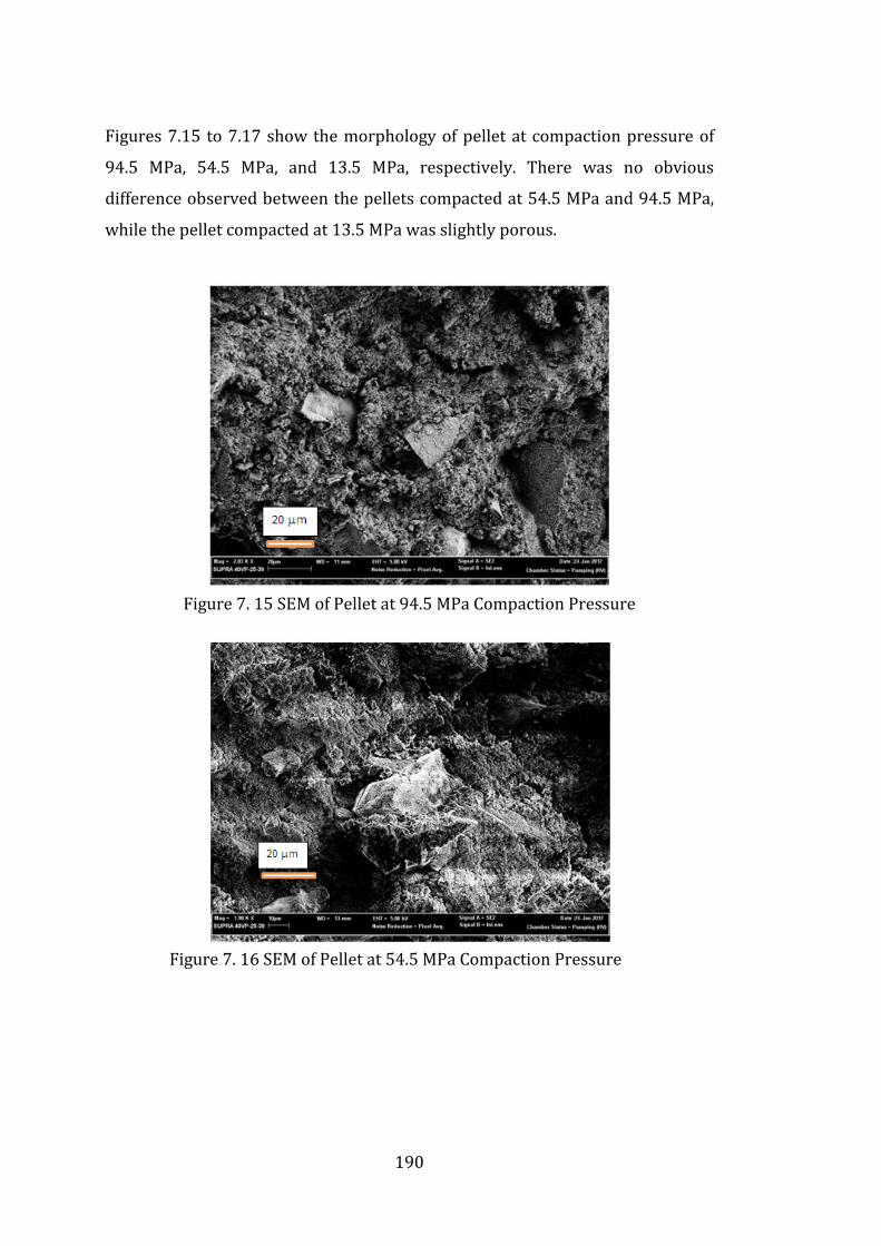
190

Figures 7.15 to 7.17 show the morphology of pellet at compaction pressure of

94.5 MPa, 54.5 MPa, and 13.5 MPa, respectively. There was no obvious

difference observed between the pellets compacted at 54.5 MPa and 94.5 MPa,

while the pellet compacted at 13.5 MPa was slightly porous.

Figure 7. 15 SEM of Pellet at 94.5 MPa Compaction Pressure

Figure 7. 16 SEM of Pellet at 54.5 MPa Compaction Pressure

191

Figure 7. 17 SEM of pellet at 13.3 MPa Compaction Pressure (5000×)

Table 7. 2 Silicothermic Experiments in Vacuum Conditions

Experiments Particle

Sizes Compaction

Pressure Temperature

(°°°°C) Pressure

Magnesium

conversion

Pidgeon12 (varied, with 2.5% CaF2)

CaO.MgO: < 0.25 mm FeSi: < 0.15 mm

2 tonne/inch2 = 27.4 MPa

1045 – 1160 0.006 Pa 80% at 1160 °C with 25% excess calcine

Toguri and Pidgeon 35 (15% excess FeSi, 2.5% CaF2)

CaO.MgO: fine powders FeSi 74%: < 75µm

3000 psi = 20.68 MPa

1165 – 1545 13 Pa 50 % at 1165 °C for 70 minutes

Misra et al 32

CaO: < 152 µm MgO: < 152 µm FeSi: < 66 µm

2000 - 3000 psi = 13.33 to 20.68 MPa

1000 – 1200 13 – 133 Pa

80 % at 1200 °C, 2 hour

Yucel et al 33 (50% excess FeSi)

Calcined dolo-mite, FeSi, CaF2

: N.A.

N.A. 1200 – 1350 101.3 Pa 80% at 1200 °C, 4 hour

Current Work (15% excess FeSi)

CaO: < 10µm MgO: < 44 µm FeSi 75%: < 75µm

94.5 MPa 1140 200 Pa (based on fix output of pressure), 0.1 L/min Ar

1140 °C, 4 hour, 15%. Condensates on quartz condenser

192

7.2.2 Post-Reaction Characterisation

Five experimental run was carried out at a temperature of 1140 °C at different

reaction times. Initially, the reduction process was carried out under flowing

argon at atmospheric pressure. However, the magnesium conversion was low.

Vacuum pressure was later incorporated into the parameters of the

experimental work. The detail parameter of the experimental work is given in

Table 7.2, which is compared to previous works on silicothermic experiments in

vacuum condition. About 15 wt% of conversion was obtained after four hour

reduction process at 1140 °C.

Figures 7.18 to 7.19 show a typical XRD pattern of reacted samples. It is

apparent that the reacted samples still contains MgO. A number silicates

compounds were detected from the reacted samples, such as γ-Ca2SiO4, Ca3SiO5,

and Ca3Mg(SiO4)2 were detected from the XRD pattern of the sample.

Figure 7. 18 XRD Pattern of Reacted Samples

193

Figure 7.19 XRD Pattern of Reacted Samples at Different Time

7.2.3 Condensates Characterisation

Most of deposits were found on the copper condenser. Figure 7.20 shows the

photographs of typical condensates found on the experimental rig. Condensates

also found on the wall of quartz condenser, as pictured in Figures 7.21 and 7.22.

Figure 7.20 Magnesium Condensates at (a) Condenser, (b) Wire Attached to Sample Boat,

(b)

(a)

(c)

194

Figure 7. 21 Photograph of Quartz Tube Condenser after Reduction Experiment

Figure 7. 22 Inside Wall of Quartz Tube Condenser Containing Condensates

Powdered condensates observed inside horizontal tube suggests a condensation

that occurs via homogeneous condensation. Condensates also found on the wall

of copper condenser, wire, and quartz condenser, which may indicate that

heterogeneous nucleation, may also occur during the condensation of vapour.

Figure 7.23 shows XRD pattern of magnesium condensate in different position.

In general, the phases consisted of MgO and some impurities. MgO was resulted

from post-oxidation of magnesium metal which had been purposedly oxidised.

As shown in Figure 7.23, there are broadening peaks between 2-theta of 20 to

30. These broadening peaks indicate some form of of magnesium calcium

silicate. The result also shows that there is no significant difference in phase and

compound of impurities for magnesium condensate at different position.

195

Figure 7.23 XRD of Magnesium Condensate Run II (2 hour)

The following figures show the detail of XRD analysis of condensate collected

from different experiments.

Figure 7.24 XRD of Magnesium Condensates Run III (3 hour). Red line: MgO; Blue Line: Ca2SiO4

196

Figure 7.25 XRD of Magnesium Condensates Run IV (4 hour): at 0-5 cm (red:

MgO, blue: Mg3CaO.(SiO3)4, green: CaMgSi2O6)

Figure 7.26 XRD of Magnesium Condensates Run IV (4 hour): at 6-12 cm (blue:

MgO, green: magnesium calcium iron silicate) The typical morphologies of the condensates from experiments Run I to IV are

shown in Figures 7.27 to 7.30. The condensate was spread along the wall of

quartz tube in a grainy form. The condensate was observed in the form of

needles (Figure 7.27), layers of growing MgO (Figure 7.28), snow and grainy

form (Figure 7.29), and dense form (Figure 7.30).

197

Figure 7.27 SEM of Magnesium Condensates from Wall (1500× Magnification)

Figure 7.28 SEM of Different Morphology of Magnesium Condensate Collected from Copper Condenser. (left: SE image, right: QBSD image) (1,500× magnification)

Figure 7.29 SEM of “Snow” Condensate Collected from Inside Mullite Tube (left: SE image, right: QBSD image) (1,500 × magnification)

198

Figure 7.30 SEM of “Dense” Condensate Collected from Copper Condenser left: SE image, right: QBSD image) (1,500 × magnification) The condensates were scraped at different regions and collected into different

container. From each sample container, a sufficient amount (< 0.01 g) was

analysed using XRD technique to determine the phase and subsequently

analysed using SEM/EDS to determine the morphology, and elemental analysis

and mapping.

Table 7.3 lists typical semi-quantitative results of EDS analysis of magnesium

condensate. The area analysed for EDS analysis were 140 µm × 70 µm with

spatial depth of 2 µm. In general, the condensate has relatively pure magnesium

with calcium and silicon as the impurities. Calcium was found in most of

condensate surfaces, e.g. at condensates from Run II (2 hour) and Run IV (4

hour). Silicon was also found in condensate from Run IV. Iron was not observed

in the condensates.

Table 7.3 Semi-quantitative Analysis of Condensates using EDS analysis

Experiment Position Mg Ca Si Fe

Run II (2 hour) all 99.34 0.65 N.A N.A Run IV (4 hour) 0-5 cm 95.99 3.72 0.3 N.A. Run IV (4 hour) 6-15 cm 98.11 1.89 N.A. N.A. Run V (6 hour) all 99.99 N.A N.A N.A.

The distribution of impurities in the magnesium condensates are shown in

Figures 7.31 and 7.32, which is elemental mapping using EDS analysis. There is

no obvious variation of impurities in the condensates. Based on observation of

199

Figure 7.31, calcium and silicon were localised at different position, while in

Figure 7.32, calcium was uniformly distribution throughout the condensate.

Figure 7.31 Elemental Mapping of Magnesium Condensate Run IV (4 hour)

The formation of calcium and silicon on the magnesium condensate is not

understood. Assuming calcium and silicon monoxide vapour evolve along

magnesium vapour from the briquette and transfer to the cooler part of furnace,

these elements may nucleate in the vapour phase (as in homogeneous

nucleation) and collide due to heterogeneous nucleation before deposited on

the wall of quartz tube and water-cooled condenser. Further study of this

condensation behaviour is required to understand the formation of these

condensates.

Si Mg

Ca O

Samples

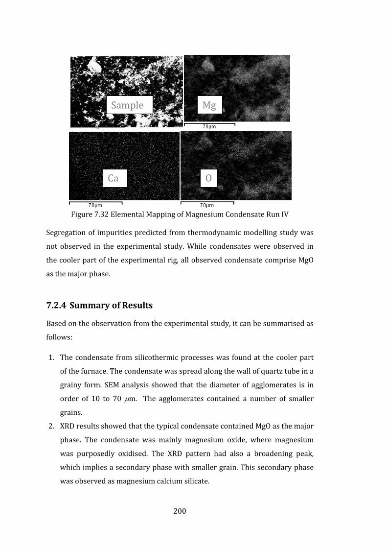
200

Figure 7.32 Elemental Mapping of Magnesium Condensate Run IV

Segregation of impurities predicted from thermodynamic modelling study was

not observed in the experimental study. While condensates were observed in

the cooler part of the experimental rig, all observed condensate comprise MgO

as the major phase.

7.2.4 Summary of Results

Based on the observation from the experimental study, it can be summarised as

follows:

1. The condensate from silicothermic processes was found at the cooler part

of the furnace. The condensate was spread along the wall of quartz tube in a

grainy form. SEM analysis showed that the diameter of agglomerates is in

order of 10 to 70 µm. The agglomerates contained a number of smaller

grains.

2. XRD results showed that the typical condensate contained MgO as the major

phase. The condensate was mainly magnesium oxide, where magnesium

was purposedly oxidised. The XRD pattern had also a broadening peak,

which implies a secondary phase with smaller grain. This secondary phase

was observed as magnesium calcium silicate.

Sample Mg

Ca O

201

3. Magnesium condensates contained calcium and silicon impurities. However,

there was no obvious variation of concentration of impurities observed in

the experimental study.

4. Segregation of impurities predicted from thermodynamic modelling study

was not observed in the experimental study.

5. The formation of impurities in the observed magnesium condensate was

not understood. The kinetics of condensation may help to understand this

formation of impurities. Analysis of vapour condensation is described in

Chapter 8.

202


203

8 Analysis of Homogeneous Nucleation of

Vapours from Silicothermic Process In the experimental study, vapour produced from silicothermic reduction of CaO

and MgO was carried over by argon gas and condensed in the cooler part of the

furnace. The schematic of experimental apparatus to produce condensates from

silicothermic reduction of CaO-MgO is shown in Figure 8.1. In this scheme, the

heating element of horizontal tube furnace was located between position of 0

and 60 cm, while the quartz condenser tube was located between position 40

and 70 cm. Temperature gradients existed in this region due to a temperature

difference between the furnace and ambient atmosphere outside the furnace as

well as the presence of water-cooled copper condenser. The temperature profile

of the system at the reaction temperature of 1140 °C is shown in Figure 8.2. This

temperature profile was measured by a thermocouple with the location at 1.3

cm from the axis centre of the horizontal tube furnace.

Figure 8.1 Schematic of Diagram of Experimental Apparatus to Produce Condensate from Silicothermic Reduction of CaO-MgO

204

Figure 8.2 Temperature Profile of System between position 30 and 58 cm at Reaction Temperature of 1140 °C at Centerline

Condensation of vapours will occur via homogeneous nucleation, reaction

condensation (for example in the case of SiO vapour), heterogeneous nucleation

of particle in the vapour phase, and heterogeneous nucleation of particle on the

surface of copper condenser and quartz tube. Condensates were found on the

surface of water-cooled copper condenser and inner wall surface of the quartz

tube. The morphology of the crystallised products depends on the nucleation

condition, temperature, and condenser materials. This section describes the

vapour nucleation phenomena which are occurred during the condensation of

vapour.

Classical Nucleation Theory (CNT) 169 had been used for predicting the effect of

homogeneous nucleation of vapour to liquid/solid phase. The development of

this theory was based on thermodynamics and kinetics arguments. CNT had

been criticised due to the use of simplifying assumptions, such as the

inappropriateness of using bulk surface tension values to predict behaviour of

clusters and assuming steady state at the liquid/solid-gas interface175. Aside of

this criticism, CNT had some considerable successes to describe and capture

critical aspects of homogeneous nucleation of vapours.

0

200

400

600

800

1000

1200

1400

30 35 40 45 50 55

Te

mp

era

ture

(C

)

position (cm)

Thermocouple 1 Thermocouple 2

205

8.1 Model Formulation

Classical nucleation theory (CNT), or the Becker-Doring theory169, predicts that

the particle formation rate, J, is related to supersaturation, S, and temperature,

T, by the following relationship:

ÂA3 ' @$¿´C:/$ Ä:$"d @ B:<´¿¡À+

rI¡3¡Mc+C (8. 1)

Where σ is the surface free energy of molecule, m is the mass of the condensing

molecule, V is the volume of condensing molecule, N1 is the number density of

the molecule, and k is Boltzmann’s constant (1.380×10-23 J K-1).

The critical radius of nucleus is obtained when the free energy formation of

nucleus reaches maximum. By setting d∆G/dr = 0 for a spherical nucleus, the

critical radius of nucleus is defined as follows:

iT ' $σÀI3Mc (8. 2)

Another theory that attempted to describe the homogeneous nucleation of

vapour is the Scaled Nucleation theory (SNT). SNT describes the nucleation

behaviour of various compounds using a scaled and material independent form

of the CNT nucleation rate equation176, 243. It utilises critical point properties to

rephrase the equation for nucleation rate in a material independent form. The

detail of Scaled Nucleation Theory has been described in Section 3.2.4.1.2.

In the SNT, SCr, or supersaturation at critical point, is predicted as in the

following equation:

78AK ' ΓΩr/$ @3-3 4 1Cr/$

(8. 3)

TC is critical temperature, and Ω is the excess surface entropy which is obtained

from the negative partial derivative with respect to temperature of the surface

tension (Ω ' σÉIρ+/¡). Based on the literatures, Ω has value of 1.5 to 2.0 for liquid

species176, while a recent study has revised the value of Ω specifically for liquid

206

metal to be 0.8182. Γ is defined by Equation (3.86), and is a weak function of the

temperature and supersaturation, which has a value of approximately equals to

0.53183.

Hale176 noted that for fluxes larger than 1 cm-3 s-1, supersaturation can be

defined as follows:

78 Ê 78AK @1 Ë$MË-ÃC ' 78AKÏ (8. 4)

where ln(JCr) is equal to 72 + 3 and Q is the term in bracket. This implies that

based on the SNT, supersaturation has in the form of (lnS)2/3 has linear

relationship with the inverse of temperature, i.e. (ln S)2/3 ~ 1/T.

According to the SNT, the critical radius of nucleus, rc, is defined as follows:

iT ' Æ$r<´/¡Ω@Î-Î B:CrMc Ç

r (8. 5)

8.1.1 Properties Data

Properties data are the important parameters for predicting homogeneous

nucleation. In this study, the species involved in the vapour phase for this

system are Mg, Ca, SiO, and Fe. The properties data which determine the

homogeneous nucleation rate from the Classical Nucleation Theory, such as

mass and volume of condensing molecule, were taken from the well-known

literature (i.e. Barin et al128 and CRC Handbook of Chemistry and Physics244),

while the surface energy of liquid species was obtained from various specific

literatures. The properties data of species are shown in Table 8.1.

207

Table 8.1 Properties Data of Species183, 243, 245, 246

Species Atomic/ Molecular

Mass, m (kg)128

Molecular

Volume (m3)

Number density

of molecule, N1

(1/m3)182

Surface

Energy, σσσσ

(N/m)

Mg 4.04×10-26 2.24×10-29 4.46×1028 0.30 – 0.32

Ca 6.65×10-26 4.07×10-29 2.46×1028 0.470

Fe 9.27×10-29 1.16×10-29 8.64×1028 1.92

SiO 7.32×10-26 2.4×10-29 4.17×1028 0.58 – 0.6

Note: m is obtained from Ar ( or Mr)/ Avogadro Number (6.022×1023 /mol).

Surface energy of condensing species is usually based on the empirical

correlation, such as shown in Table 8.2. There is limited data on the surface

energy used for homogeneous nucleation. As explained in the introductory part

of this chapter, one limitation of the CNT is that this theory is using bulk-phase

surface tension/surface energy value. The surface energy used for this study

was based on the surface energy of liquid metal, with assumption that the

condensation occurs via vapour-liquid-solid phase.

The effective surface energy of Mg was obtained from Ferguson et al183, which

was based on the analysis of homogeneous nucleation of Mg using the SNT. The

surface energy of liquid Ca was obtained from Metal Handbook245. The surface

energy of Fe was obtained from Wille et al246, which was based on the

measurement of surface tension of containerless liquid iron.

Table 8.2 Surface energy of Condensing Species

Species Surface Energy (N/m) References

Mg 0.531 – 2.265×10-4 T Ferguson et al183

Ca 0.472 – 1×10-4 T Metals Handbook245

Fe 2.403 – 2.85×10-4 T Wille et al246

SiO 0.820 – 2.2×10-4 T Hale and Kemper243

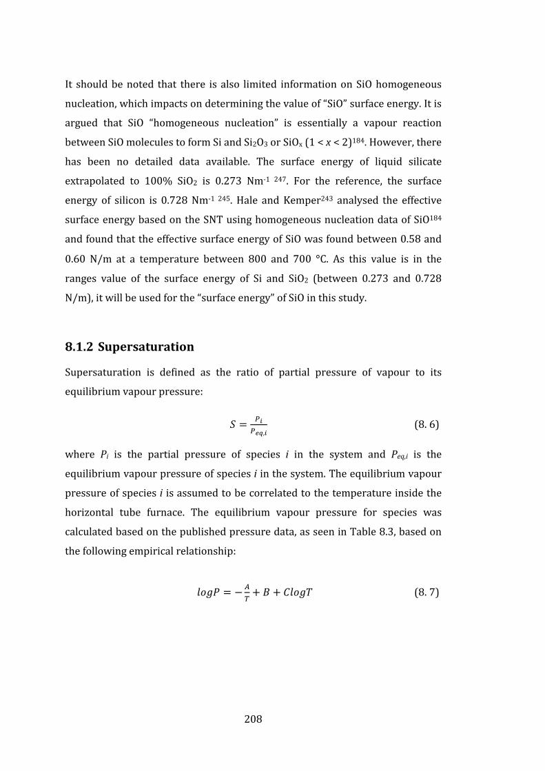
208

It should be noted that there is also limited information on SiO homogeneous

nucleation, which impacts on determining the value of “SiO” surface energy. It is

argued that SiO “homogeneous nucleation” is essentially a vapour reaction

between SiO molecules to form Si and Si2O3 or SiOx (1 < x < 2)184. However, there

has been no detailed data available. The surface energy of liquid silicate

extrapolated to 100% SiO2 is 0.273 Nm-1 247. For the reference, the surface

energy of silicon is 0.728 Nm-1 245. Hale and Kemper243 analysed the effective

surface energy based on the SNT using homogeneous nucleation data of SiO184

and found that the effective surface energy of SiO was found between 0.58 and

0.60 N/m at a temperature between 800 and 700 °C. As this value is in the

ranges value of the surface energy of Si and SiO2 (between 0.273 and 0.728

N/m), it will be used for the “surface energy” of SiO in this study.

8.1.2 Supersaturation

Supersaturation is defined as the ratio of partial pressure of vapour to its

equilibrium vapour pressure:

' (0(¼½,0 (8. 6)

where Pi is the partial pressure of species i in the system and Peq,i is the

equilibrium vapour pressure of species i in the system. The equilibrium vapour

pressure of species i is assumed to be correlated to the temperature inside the

horizontal tube furnace. The equilibrium vapour pressure for species was

calculated based on the published pressure data, as seen in Table 8.3, based on

the following empirical relationship:

7gq ' 4 3 u 7g6 (8. 7)

209

Table 8.3 Equilibrium Vapour Pressure Constants (as per Equation 8.7)

Species A B C T (K) range

Magnesium248 7780 11.41 -0.855 298-923 7550 12.79 -1.41 923-1363

Calcium248 10300 14.97 -1.76 713-1115 9600 12.55 -1.21 1115-1484

SiO (over amorphous

SiO) 194

13.29 + 0.39 17740 + 550 0 1301-1529

SiO (over equimolar Si and SiO2)249

13.25 + 0.89 17900 + 1300 0 1433-1608

Fe195 11.7 + 0.3 21000 + 500 0 1573-1973 P is in mmHg and T is in K

Partial pressure of SiO had been measured over amorphous SiO194 and

equimolar Si and SiO2249. In this study, the partial pressure of SiO used in this

study is over amorphous SiO194 was preferred.

Several assumptions were made to determine supersaturation of species, which

comprises the following:

1. The partial pressure of Mg vapour in the system was calculated on the

basis of the amount of magnesium evolved during silicothermic reaction.

The partial pressure of magnesium was calculated from the correlation

with the total pressure of the system based on a mass balance

relationship, which is written as follows37:

q ' (Î:ÀV/ß (8. 8)

where PB was the partial pressure of magnesium in the bulk gas phase, PT

was the total pressure of the gas phase, V was the molar rate of carrier

gas (mol min-1), M was the atomic mass of magnesium (in g), and ß was

the magnesium generation rate (g min-1). The magnesium generation

rate was assumed to be constant, which was calculated as the average of

magnesium generation rate during the reduction process.

210

2. The temperature of the system was determined based on the

thermocouple measurements at various positions in similar horizontal

position (about 1.3 cm from the axis centre of horizontal mullite tube.

The radius of mullite tube was 1.75 cm).

The schematic of temperature measurement is shown in Figure 8.3. It is

assumed that the equilibrium temperature corresponds to the

temperature recorded at a typical position. The temperature profile

inside mullite tube at temperature set point of 1140 °C and condenser

position at 40 cm is shown Figure 8.2. The effect of temperature gradient

on the cross section of horizontal tube was not considered in the

calculation.

Figure 8.3 Schematic of Thermocouple Measurement

3. The amount of Ca, Si, and Fe in the condensates could not be determined

accurately, since the amount of these species was very small. The partial

pressure of Ca, SiO, and Fe vapour were determined from the equilibrium

prediction of these vapour with Mg vapour in the silicothermic reduction

system.

The partial pressure of other species, such as Ca, SiO, and Fe were

calculated based on the molar ratio of the species to magnesium in the

vapour phase:

q ' qV&d V0V)* (8. 9)

211

where Pi was the partial pressure of species i, Mi and MMg were the molar

fraction of i and Mg in the vapour phase, respectively. The ratio of molar

fraction of vapour phase species was predicted using equilibrium

calculation at the process temperature and pressure, which are

presented in Table 8.4.

Table 8.4 Molar Partial Fraction of Vapours Predicted from Thermodynamic Modelling at 1140 °C using FACT53 database

Species Molar Fraction

P = 1 atm P = 200 Pa

Mg 0.99823 0.99402

Ca 0.00174 0.00572

SiO 1.0618×10-5 2.5063×10-4

Fe 5.7016×10-9 3.2775×10-8

8.2 Results

8.2.1 Condensation of Magnesium

Figure 8.4 (a) shows the profile of supersaturation of magnesium vapour with

temperatures. At the argon gas flow rate of 2.5×10-4 m3/min at atmospheric

pressure and 75 wt% conversion of magnesium being produced from the

silicothermic reaction, the partial pressure of Mg over Mg-Ar system was

estimated to be 1.15 kPa. At temperature of 713 °C, supersaturation reaches

one.

212

(a)

(b) Figure 8.4 (a) Supersaturation of Mg Vapour Versus Temperature, (b) Plot of (ln S)2/3 vs T for Mg Homogeneous Nucleation

Figure 8.4 (b) shows the plot of (ln S)2/3 with the decreasing temperature. This

data was compared to nucleation data of previous work of magnesium smoke at

0.32 atm of static hydrogen pressure183. The data showed a good agreement at

213

temperatures range between 560 to 634 °C. However, at lower temperatures,

Ferguson et al183 observed nucleation of magnesium at a lower supersaturation

compared to the current study.

The supersaturation of Mg vapour in this system followed the SNT, which

predicted that had a linear relationship with temperature. Based on the plot of

(lnS)2/3 of Mg vapour with 1000/T, supersaturation of Mg vapour had the

following correlation:

78$/r ' ;;$3 4 3.73936 à 604 (8. 10)

78$/r ' :rr£<.;3 4 13.3776 á 604 (8. 11)

Figure 8.5 shows the nucleation rate of Mg vapour and the estimated radius of

nucleus/cluster formed from homogeneous nucleation predicted by the CNT

model. The nucleation rate of Mg vapour was calculated using the CNT in

Equation (8.1). The radius of nucleus/cluster was calculated from Equation

(8.2). It was predicted that growth of cluster from homogeneous nucleation of

Mg vapour occurs at temperature below 545 °C, with the critical cluster radius

of less than 0.75 nm.

Figure 8.5 Plot of Nucleation Rate (/m3.s) and Radius of Cluster (× 10-9 m) of Mg Homogeneous Nucleation

214

The nucleation rate of Mg vapour was predicted to increase with the decreasing

temperature. The nucleation rate of Mg vapour was found to be 1028/m3s at 400

°C with a cluster radius of 0.4 nm.

The correlation of the predicted homogeneous nucleation to the observation of

the current experimental study is shown in Figure 8.6. Figure 8.6 shows the plot

of measured temperature profile along the experimental rig, which is compared

to the nucleation rate and critical radius of Mg cluster predicted from the CNT.

Mg vapour was predicted to condense at about position of 55 cm and beyond on

the experimental rig.

Figure 8.6 Temperature Profile, Nucleation Rate of Mg, and Critical Radius of Nucleus along the Position

215

8.2.2 Condensation of Silicon Monoxide

Silicon monoxide is the third major compound in the vapour produced from

silicothermic process. The molar fraction of SiO vapour within the system which

was predicted based on thermodynamic modelling are between 10-4 and 10-5.

The condensation of silicon monoxide was not fully understood. In addition to

the argument that condensation of silicon monoxide actually a vapour phase

reaction of SiO molecules184, 185, in the system contain SiO vapour with addition

of other element, SiO tend to react with other cation to form silicates. A

simulation studied by Paquette et al 250 predicts that in the system contains SiO,

Mg, and Fe, SiO will nucleate with Mg and Fe to form magnesium silicate or iron

silicate grains in proportion to the flux of Mg and Fe atoms out of the gas phase

at the time of nucleation. This also had been observed experimentally that gas-

to-solid condensation in a Fe-Mg-SiO-H2-O2 vapour yields magnesium silicate

and ferrosilicate251.

Figure 8.7 Plot of (ln S)2/3 of SiO with Temperature

Figure 8.7 shows the supersaturation of SiO with temperature. The plot of

(lnS)2/3 with 1000/T was found to be linear. This implied that SiO homogenous

216

nucleation also follows the SNT. Similar as in Mg homogeneous nucleation, the

correlation of supersaturation and temperature based on the Scaled Nucleation

Theory was divided into two regions:

78$/r ' :==3 4 13.8076 à 825 (8. 12)

78$/r ' $â;$$3 4 25.0886 á 825 (8. 13)

The “homogeneous nucleation of SiO” predicted by SNT gave some insight when

the nucleation of SiO occurred. This prediction was sensitive to some the

quantities included in the calculation, such vapour pressure and surface tension

of SiO.

Figure 8.8 Temperature Profile, Nucleation Rate of SiO, and Critical Radius of Nucleus along the Position

217

The measured temperature profile along the experimental rig was plotted

against the nucleation rate critical radius of cluster predicted from CNT of “SiO

homogeneous nucleation” in Figure 8.8. The nucleation rate of “SiO” cluster was

predicted to occur at temperatures below 850 °C, which corresponded to

supersaturation of 12 ((ln S)2/3 is 1.8) and the position of 39 cm in the

experimental rig. The critical radius of “SiO” cluster was predicted between 0.3

to 0.9 nm.

8.2.3 Condensation of Calcium

Calcium is the major impurities in the magnesium vapour. The molar percentage

of calcium in the vapour phase predicted from thermodynamic modelling was

between 0.1 and 0.5 %. Whilst there was no previous study which analyse the

homogeneous nucleation of calcium vapour, by appropriately choosing the

required quantities such as surface energy and number of condensing

molecules, behaviour of homogeneous nucleation of Ca was predicted using the

CNT.

The plot of ln S and temperature is shown in Figure 8.9. The supersaturation of

Ca vapour and temperature follows the SNT. Based on the plot of (ln S)2/3 of Ca

vapour with 1000/T, the supersaturation of Ca vapour had the following

correlation:

78$/r ' <$â$.<3 4 5.3886 T < 490 °C (8. 14)

(78$/r ' ::r;%3 4 12.227 T > 490 °C (8. 15)

The plot of supersaturation, nucleation rate, and critical radius of cluster from

Ca homogeneous nucleation with corresponding to the position in the

experimental rig is shown in Figure 8.10. The nucleation rate of Ca cluster was

predicted to occur at temperature of 620 °C, which corresponded to position of

52.3 cm in the experimental rig. The critical radius of Ca cluster was predicted

to between 0.1 to 0.6 nm.

218

Figure 8.9 Plot of lnS 2/3 of Ca Vapour with 1000/T

Figure 8.10 Temperature Profile, Nucleation Rate of Ca, and Critical Radius of Nucleus along the Position

219

8.2.4 Condensation of Iron

The formation of iron in the vapour phase was mainly caused by the

evaporation of Fe metal in the pellet reactant. Thermodynamic modelling

predicts that the molar composition of Fe was between 3.2×10-8 and 60×10-8.

The plot of ln S and temperature is shown in Figure 8.11. Based on the plot of

(lnS)2/3 of Fe vapour with 1000/T supersaturation of Fe vapour has the

following correlation:

78$/r ' :;$:3 4 10.754 T < 822 °C (8. 16)

(78$/r ' $%£â%3 4 19.549 T > 822 °C (8. 17)

Figure 8.11 Plot of lnS 2/3 of Fe Vapour with Temperature

Figure 8.12 shows the plot of supersaturation, nucleation rate, and critical

radius of cluster from Fe homogeneous nucleation with corresponding to the

position in the experimental rig. The nucleation rate of Fe cluster was predicted

to occur at temperature of 731 °C, which corresponded to position of 36 cm in

the experimental rig. The critical radius of Fe cluster was predicted to between

0.5 to 2 nm.

220

Figure 8.12 Temperature Profile, Nucleation Rate of Fe, and Critical Radius of Nucleus along the Position

8.3 Discussion The analysis of condensation behaviour of species using the CNT enables us to

predict the temperatures and degree of supersaturation /supercooling

condensation will occur. The extent of nucleation rate and particle size radius

can also be predicted from this theory.

In general, the supersaturation of all species in this study correlates with

temperatures and follow the SNT. Using linear regression, the correlation of

supersaturation and temperature can be estimated. In each species, the

correlation between supersaturation and temperature is divided into two

regions, which was separated by temperature, namely T*. Table 8.5 shows the

summary of T* of the species involved in the system, which is compared to the

melting point of each species. T* is below the melting point of species.

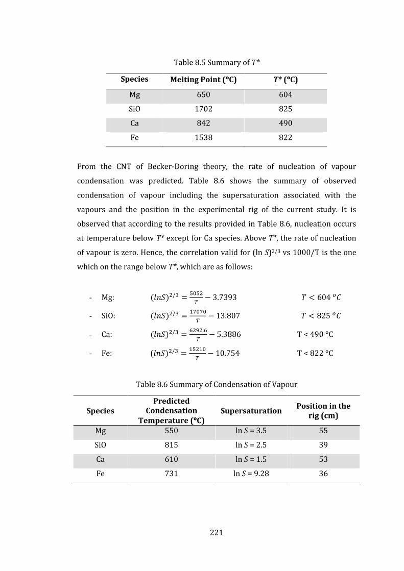
221

Table 8.5 Summary of T*

Species Melting Point (°°°°C) T* (°°°°C)

Mg 650 604

SiO 1702 825

Ca 842 490

Fe 1538 822

From the CNT of Becker-Doring theory, the rate of nucleation of vapour

condensation was predicted. Table 8.6 shows the summary of observed

condensation of vapour including the supersaturation associated with the

vapours and the position in the experimental rig of the current study. It is

observed that according to the results provided in Table 8.6, nucleation occurs

at temperature below T* except for Ca species. Above T*, the rate of nucleation

of vapour is zero. Hence, the correlation valid for (ln S)2/3 vs 1000/T is the one

which on the range below T*, which are as follows:

- Mg: 78$/r ' ;;$3 4 3.73936 à 604

- SiO: 78$/r ' :==3 4 13.8076 à 825

- Ca: 78$/r ' <$â$.<3 4 5.3886 T < 490 °C

- Fe: (78$/r ' :;$:3 4 10.754 T < 822 °C

Table 8.6 Summary of Condensation of Vapour

Species

Predicted

Condensation

Temperature (°°°°C)

Supersaturation Position in the

rig (cm)

Mg 550 ln S = 3.5 55

SiO 815 ln S = 2.5 39

Ca 610 ln S = 1.5 53

Fe 731 ln S = 9.28 36

222

CNT predicts that homogeneous nucleation for the species occurs at different

temperature, which corresponds to different position in the horizontal tube.

While SiO and Fe are predicted to condense at higher temperature, the amount

of these species is very small. This is due to low vapour pressure of the species,

as shown in Figure 8.13. Thus, the segregation of these impurities would not to

be expected to be observed in the experimental study.

Figure 8.13 Vapour Pressure of Metals198 Analysis of homogeneous nucleation of vapours in this study is used as the

starting point to understand the behaviour of vapour condensation in the

Pidgeon process system. It also should be noted that heterogeneous nucleation

is likely to occur in the practice plant.

Heterogeneous nucleation can be considered as a surface catalysed nucleation

process, which forms at the phase boundaries, surfaces, and impurities, and

specifically at the surface of condenser due to the lower temperature of the

surfaces. As the free energy needed for heterogeneous nucleation is equal to the

product of homogeneous nucleation and a function of contact angle, the free

energy of heterogeneous nucleation has lower free energy change compared to

homogeneous nucleation. This implies that in practice, the free energy required

for the vapour condensation is actually lower than predicted in this study. While

the heterogeneous nucleation of vapour is not quantitatively analysed, it can be

implied that the vapour condensation of magnesium and its impurities are

easier to condense compared to the current prediction.

223

8.4 Conclusion

Nucleation model of Mg, SiO, Ca and Fe had been developed using the Classical

Nucleation Theory. It was predicted that Mg, SiO, Ca and Fe condenses at

different temperatures and different location inside the experimental rig. Mg

was predicted to condense at around temperature of 550 °C, which was

corresponded to position of 55 cm on the horizontal tube. This was consistent

with the observation from the experiment where MgO phase was observed that

the positions between 50 and 60 cm on the horizontal tube.

Ca was predicted to condense around position of 53 on the horizontal tube,

while Fe and SiO were predicted to condense at the positions of 36 and 39 cm

on the horizontal tube, respectively. However, due to very low vapour pressure

of these species at the temperature ranges, these species would not to be

expected to be observed in the experimental study, which in fact was the case.

224


225

9 Discussion

Magnesium is dominantly produced via the Pidgeon process, which involves a

solid-solid reaction of calcined dolomite and ferrosilicon at temperature ranges

between 1100 and 1200 °C5, 11, 12. While this process is versatile and offers

simple operation, the productivity of this process is very low. Other processes

attempt to increase the productivity of the silicothermic reduction process by

carrying out the reduction at higher temperatures in a liquid phase, such as the

Magnetherm process7, 52, 56 which operates at 1550 °C and the Mintek process68,

74, 75 which reduces calcined dolomite at 1700 °C. This higher temperature and

correspondingly increased productivity is likely to lead to greater impurities in

the magnesium metal.

The literature on magnesium production has been focused on the kinetics of the

Pidgeon process in an attempt to improve the productivity of the process. While

a number of parameters affecting the process have been examined12, 29, 32, 35,

there is no general conclusion what really controls the kinetics of the process.

The knowledge on the behaviour of impurities in magnesium produced by

silicothermic process is also quite limited. In the current practice, the impurities

in magnesium metal produced from the silicothermic processes are removed by

a refining operation, which causes 5 to 8% loss in magnesium59.

The objective of this study is a detailed study to investigate the fundamental

chemistry associated with the silicothermic process, with emphasis to the

behaviour of impurities in the process, by using thermodynamic modeling and

kinetics analysis of the process, and test the predictions from thermodynamic

modelling by performing an experimental study.

Thermodynamic modelling prediction conducted in this study confirmed that

the amount of magnesium evolved from the silicothermic process increases

with the increasing operating temperature; however, the purity of the

magnesium condensate decreases. Thermodynamic modelling provides a

226

maximum limit of how much is the percentage of magnesium can be extracted

from the reactant at specific operating condition. Thermodynamic calculations

of the Pidgeon process at higher temperature over-predicted the previous

experimental and industrial data, as described in Figure 5.18. For example,

between 1100 and 1200 °C, the model predicts 99 wt% conversions; while the

data shows some conversion between 87 and 89 wt%12, 29, 32, 33, 35. This

discrepancy becomes smaller with increasing temperature. It was postulated

that solid state kinetics and temperature gradients within the furnace limit the

actual magnesium recovery.

A multistage condensation model was developed as the first attempt to study

the behaviour of impurities in magnesium metal produced via silicothermic

processes. A thermodynamic solution model for the metallic phases was

developed using data from critically analysed literature which includes solid

solution behaviour and interaction between binary metals involved in the

magnesium-impurities system.

Impurities were predicted to segregate from magnesium metal in an

equilibrium condition at a temperature range between the reaction and

condenser section (e.g. between 482 to 1100 °C). This predicted segregation

was achieved in the thermodynamic modelling by conducting the equilibrium of

the system at a lower temperature, separate the solid formed from the

equilibrium, and further conducting the subsequent equilibrium at 50 °C

increment. The magnesium vapour predicted from silicothermic processes (at

1160 °C and 7 Pa) has the following compositions: Ca (2.38 wt%), SiO (6 ppm),

Fe (0.13 wt%), and Al (3 ppm). The results from multistage condensation model

predicted that the segregation of impurities from magnesium metal would

proceed as follows: Fe and FeSi was predicted to condense at temperature

ranges between 1000 and 1100 °C, CaO rich phase between 1000 to 1100 °C,

Mg2Ca intermetallics compound between 500 and 550 °C, and finally Mg rich

phase condenses at 482 °C. This study also shows that the segregation of solid

impurities predicted from multi stage condensation of magnesium vapour and is

227

not sensitive to the initial composition of the vapour and operating condition of

the system, i.e. if Mg, Fe, Si, and Ca are present in the vapour; this sequence is

predicted to occur.

Thermodynamic modelling study of has some limitations. A number assumption

was applied to simplify the modelling. The modelling comprises as following

limitations:

1. As in any thermodynamic modelling study, the process was assumed in

equilibrium. In the reality, the silicothermic process is not run at

equilibrium conditions, though it is reasonable to assume it approaches

equilibrium. Condensation of vapour is also non-equilibrium, as the

vapour system need to be in supersaturated condition to nucleate and

form condensate.

2. The thermodynamic solution model of oxide which used FTOxid from

FactSage thermochemical package is a semi-“black box” solution model.

While the description of the solution model and the references of the

data used for FTOxid were provided by FactSage, the details of the data

and the thermodynamic model could not be examined and assessed by

the user.

3. The thermodynamic solution model for the metallic phases was

developed and obtained from various published studies. A

comprehensive assessment of this data was not carried out in this study.

The assessment and optimisation of this set of thermodynamic solution

model should be required in order to be fully confident in the predictions

made.

4. The thermodynamic solution model for the metallic phases only

considered the binary interactions between the metals, e.g. Mg-Ca, Mg-Si,

and Mg-Al.

228

The thermodynamic modelling conducted in this study leads to two main

questions:

1. What does limit magnesium recovery from the Pidgeon process?

2. Can the segregation of impurities from magnesium metal predicted

from thermodynamic modelling be observed in an experimental

study?

Kinetic analysis of Pidgeon process was carried out to address the first

hypotheses, as the thermodynamic modelling over-predicts the magnesium

recovery in the actual experiment and industrial data. As the condition that

approaches equilibrium is required to represent the condition described in

thermodynamic modelling, the kinetic analysis used the data on a study of

silicothermic process in argon gas atmosphere34. For this analysis, different

kinetics models based on various assumption was considered, as well as the

mass transfer of magnesium vapour from the briquette to the bulk gas phase.

The kinetic study shows that the kinetic model based on solid state diffusion

best represents the kinetics of the process, as illustrated in Figure 6.4. In

general, the solid state diffusion models (e.g. Jander154, Ginstling-Brounshtein156,

Serin-Ellickson155, and Valensi-Carter model157) can represent the kinetics of the

process in the range condition where the experimental data are available.

Analysis of isothermal kinetic models carried out using linearity testing as well

as reduced-time testing236 showed that Jander model and Ginstling-Brounshtein

model were among the best models that can be applied to describe the kinetics

of the process at various temperatures.

The mass transfer coefficient of magnesium vapour was estimated by using an

empirical correlation238 and properties data predicted by kinetic theory of gas.

The mass transfer of magnesium vapour from the briquette to the bulk gas

phase at low argon flow rate, i.e. 8×10-5 m3/min to 25×10-4 m3/min, appeared

not to be the limiting factor since the pressure drop in the boundary layer is

very small compared to the actual partial pressure of magnesium, i.e. the

229

calculated partial pressure of magnesium at 1150 °C after 1 hour on the surface

of briquette and the bulk gas phase are 1.75 and 1.68 kPa, respectively. The

kinetic study also found that the partial pressure of magnesium at the initial

reaction was lower that its equilibrium vapours pressure. The extrapolated

partial pressure of magnesium at the initial reaction at 1150 °C was estimated

to be 1.95 kPa, while the equilibrium partial pressure of magnesium over

silicothermic system at 1150 °C was 2.40 kPa27. The difference in these partial

pressures was postulated to be controlled by the mass transfer in the pores.

Because of the limited available information, the kinetic analysis of silicothermic

reduction under flowing inert gas has several limitations, such as the following:

1. The solid state diffusion models applied to describe the kinetics process

seemed not sensitive to the experimental data. This is because of the

models applied curve fitting method the available experimental data. As

the k (rate constant) used in the models is a function of diffusivity, radius

of particles and concentration gradients of reactants, as shown in

Equation (6.3), the models may have provide more insights if the

analysis includes these parameters. However, because of the data

limitation, this analysis could not be carried out.

2. Because of the curve-fitting procedure, these models cannot predict the

conversion beyond the experimental data range. An analysis which

expand the models beyond the experimental data, which is illustrated in

Figure 6.13, shows that the models (i.e. Jander154, Ginstling-

Brounshtein156, and Valensi-Carter model157) predicted different reaction

times for magnesium conversion near 100%. This behaviour had been

noted by Szekely et al134, which pointed that the approximation of

diffusion models, such as Jander model, becomes inaccurate as the

conversion increases. More experimental data at a higher conversion is

required in order to improve the models.

3. Pore diffusion analysis was not conducted in this study, since there is

limited information of the properties of the briquette, such as tortuosity

and radius of the pores. However, the kinetic analysis conducted in this

230

study provides some preliminary hypothesis that pore diffusion is likely

to be significant in the kinetics of the Pidgeon process.

To address the second question based on the finding from thermodynamic

modelling of vapour condensation, an experimental rig was developed. The

experimental rig was designed to replicate the Pidgeon process and the

reactants used in the experimental study followed the Pidgeon process’s

chemistry. The experimental study was carried out in a horizontal tube furnace

at temperatures between 1140 and 1160 °C.

The condensate from silicothermic processes was found at the cooler part of the

furnace. The condensate was spread along the wall of quartz tube in a grainy

form. SEM analysis showed that the diameter of agglomerates is in order of 10

to 70 µm. The agglomerates contained a number of smaller grains. XRD results

showed that the typical condensate contained MgO as the major phase. The

condensate was mainly magnesium oxide, which was formed by the oxidation of

magnesium metal during cooling, storage, and handling prior to analysis. The

XRD pattern had also a broadening peak, which implies a secondary phase with

smaller grain. The experiment results did not indicate any obvious variation of

concentration of elements along the position of condensate in the condenser.

The analysis of Classical Nucleation Theory on the homogeneous nucleation of

magnesium predicted that magnesium condense at temperature around 550 °C.

While Classical Nucleation Theory predicted that SiO2 condensed at 815 °C and

Fe condensed at 713 °C, these condensates were not observed in the

experimental study at those conditions. These may be caused by the following:

1. The amount of element was very small, such as in order of ppm.

Therefore, it was difficult to recover the condensate for further EDS

analysis.

2. The effective vapour pressure of these elements was very small at the

typical operating condition and so the level of impurities predicted in

the condensate cannot be achieved.

231

This imply that in order to observe the segregation of impurities from

magnesium metal, a high vapour pressure of those impurity elements are

needed, and the amounts of vapour element must be increased. This can be

done by performing the experiment at higher temperature and by adding more

reactant.

The limitation of this experimental study comprises as follows:

1. Limited variations of temperature. The furnace used in this study could

not operate above 1170 °C.

2. Reactants used in experimental study were CaO and MgO instead of

calcined dolomite. This choice of reactant was considered in order to

produce high purity magnesium. However, these compounds may have

different reactivity to calcined dolomite, which affect the amount of

magnesium generated from silicothermic reaction in the experimental

study.

3. Limited information in properties data, particularly for analysis of

Classical Nucleation Theory, where the properties data has a crucial

impact on the predicting the onset of nucleation

232


233

10 Conclusions and Recommendations

The physical chemistry of the silicothermic processes have been investigated

through a number of methods. Thermodynamic modelling was used to predict

the behaviour of impurities in the magnesium metal produced from

silicothermic processes. A kinetics analysis has been carried out to examine

what is limiting the recovery in the Pidgeon process. An experimental study was

also conducted to observe the impurities in the process.

From this study, the following conclusions can be drawn:

1. Thermodynamic modelling of the silicothermic processes has been

developed and compared with the existing experimental and industrial

data. The model can predict the variations in the magnesium recovery

and its impurities under defined operating conditions. Thermodynamic

calculations over-predict the magnesium recovery when compared to

actual experimental and industrial data. However, it provides a

maximum limit of how much magnesium can be extracted.

2. A thermodynamic solution model for the metallic phases has been

developed using data from critically analysed literature which includes

solid solution behaviour and interaction between binary metals involved

in the magnesium-impurities system. This thermodynamic solution

model was included in the multistage equilibrium model developed for

studying the behaviour of impurities in the magnesium metal. The model

predicts that impurities were segregated from magnesium metal in an

equilibrium condition at a temperature range between the reaction and

condenser section (e.g. between 482 to 1100 °C).

3. The silicothermic reduction kinetics has been examined using

corresponding kinetics models. The effect of mass transfer of the gas

phase has been included in the analysis. The results show that the rate of

silicothermic reduction of calcined dolomite under flowing argon gas was

234

controlled by solid-state diffusion. The Jander and Ginstling-Brounshtein

model can represent the kinetics of the process, but are only valid within

the range of experimental data available. The predictions also show that

gas-film mass transfer of magnesium vapour to the bulk gas phase is not

limiting the kinetics of the process. It is also postulated that mass

transfer in the pores also partial control the process.

4. An experimental study was carried out to observe the predictions in the

thermodynamic modelling study which suggest that impurities

condenses and segregates within the furnace. Some condensates were

found that the cooler part of the furnace in a grainy form, with contained

MgO as the major phase. The variation of concentration of condensates

was not observed in the experimental study.

5. The Classical Nucleation Theory of homogeneous condensation was used

to analyse the experimental results. The nucleation model of Mg, SiO, Ca,

and Fe has been developed. CNT predicts that homogeneous nucleation

for the species occurs at different temperature, which corresponds to

different position in the horizontal tube. However, due to very low

vapour pressure of Ca, SiO, and Fe at the temperature ranges, these

species would not to be expected to be observed in the experimental

study, which in fact was the case.

This study contributes to knowledge in a way that: the first published study to

use multistage condensation model to predict the distribution and segregation

of elements from condensation of mixture of vapour. As far as the author is

aware, this is the first thorough examination of kinetic models used to analyse

the kinetics of the process. The experimental study also provides evidence that

impurity present do not condense in high temperature regions of the furnace.

In conclusion, there is no evidence that impurities present in magnesium vapour

can be practically separated by selective condensation, eventhough it is

thermodynamically feasible. Experimental work at higher concentrations and

temperature range are required to fully explore this option.

235

The recommendations suggested for future improvement of this study are as

follow:

1. To perform experiment at higher temperature in order to enhance the

kinetics of silicothermic to generate more vapour with greater

impurities

2. To carry out a kinetics study that explores the effect of pore diffusion on

the overall kinetics of silicothermic. At present the knowledge on how

pore diffusion varies with the degree of compaction pressure, particle

size distribution, source of raw materials and their effect to the kinetics

of the process have only been partly explained and further work is

required.

236


237

References

1. B. L. Mordike and T. Ebert: "Magnesium. Properties - Applications -

Potential", Materials Science and Engineering A, 2001, vol. A302(1), pp.

37-45.

2. M. M. Avedesian and H. Baker, 'Magnesium and Magnesium Alloys - ASM

Specialty Handbook'; 1999, Ohio,

3. '2007 Annual Yearbook Magnesium,

http://minerals.usgs.gov/minerals/pubs/commodity/magnesium/myb1

-2007-mgmet.pdf', 2009 [viewed 14 April 2009].

4. 'www.intlmag.org International Magnesium Association', 2010 [viewed

12 April 2009].

5. L. M. Pidgeon and W. A. Alexander: "Thermal Production of Magnesium --

Pilot-plant Studies on the Retort Ferrosilicon Process", Transaction of the

AIME, 1944, vol. 159, pp. 315-351.

6. A. Mayer: "Plant for Production of Magnesium by the Ferrosilicon

Process", Transaction of the AIME, 1944, vol. 159, pp. 363-376.

7. C. Faure and J. Marchal: "Magnesium by the Magnetherm Process",

Journal of Metals, 1964, vol., pp. 721-723.

8. M. A. Abdel-latif: 'Refining Testwork on Crude Magnesium Produced in

the Mintek Thermal Magnesium Process', Southern African

Pyrometallurgy 2006, Johannesburg, 5-8 March, 2006, pp. 343-355.

9. S. G. Hibbins and F. C. Dimayuga: 'Production and Application of Ultra

High Purity Magnesium', The International Symposium on Extraction,

Refining, and fabrication of Light Metals, Ottawa, Ontario, 18-21 August

1991, 1991, Light Metals Section of the Metallurgical Society of CIM, pp.

3-18.

10. ASTM: 'B92/B92N: Standard Specification for Unalloyed Magnesium

Ingot and Stick for Remelting', in pp. 2007, West Conshohocken, PA,

ASTM International.

238

11. L. M. Pidgeon: "New Methods for the Production of Magnesium", The

Canadian Institute of Mining and Metallurgy, 1944, vol. 47, pp. 16-34.

12. L. M. Pidgeon: "Thermal production of magnesium: reduction of

magnesia by silicon, aluminum and calcium carbide", Transactions of the

Canadian Institute of Mining and Metallurgy, 1946, vol. 49, pp. 621-635.

13. F. R. Kemmer: Trans. Electrochem. Soc. , 1942, vol. 81-82.

14. T. E. Norgate and W. J. Rankin: "Assessing The Environmental Impact of

Metal Production Processes", Journal of Cleaner Production, 2007, vol.

15(8-9), pp. 838-848.

15. G. J. Kipouros and D. R. Sadoway: ' in 'Advances in Molten Salt Chemistry',

pp. 127-209; 1987.

16. J. M. Toguri: 'A Study of the Silicothermic Process for the Production of

Magnesium', PhD thesis, University of Toronto, Toronto, 1958.

17. 'http://rruff.geo.arizona.edu/doclib/hom/dolomite.pdf, Dolomite

CaMg(CO3)2', 2005 [viewed 22 May 2009].

18. W. M. Peirce, R. K. Waring, L. D. Fetterolf, and G. T. Mahler: "Some

Developments in the Production of Magnesium from dolomite by the

Ferrosilicon Process", Transaction of the AIME, 1944, vol. 159, pp. 377-

391.

19. S. Das: "Primary Magnesium Production Costs for Automotive

Applications", Journal of the Minerals, Metals, and Materials Society, 2008,

vol. 60(11), pp. 63-69.

20. O. Kubaschewski and C. B. Alcock: 'Heat of Formation, Standard

Entropies and Structures', in 'Metallurgical Thermochemistry', 5th edn,

pp. 269-323; 1979, Oxford, Pergamon Press Ltd. .

21. J. Du, W. Han, and Y. Peng: "Life Cycle Greenhouse Gases, Energy and Cost

Assessment of Automobiles using Magnesium from Chinese Pidgeon

Process", Journal of Cleaner Production, 2010, vol. 18(2), pp. 112-119.

22. S. Ramakrishnan and P. Koltun: "Global Warming Impact of the

Magnesium Produced in China using the Pidgeon Process", Resources

Conservation & Recycling, 2004, vol. 42(1), pp. 49-64.

239

23. B. Ellingsaeter and T. Rosenqvist: "Silicothermic Reduction of Magnesia

and Ferrosilicon Activities", Transaction of the AIME, 1956, vol.

24. J. Chipman, J. C. Fulton, N. Gocken, and J. Caskey, G. R.: "Activity of Silicon

in Liquid Fe-Si and Fe-C-Si Alloys", Acta Metallurgica, 1954, vol. 2, pp.

439-450.

25. A. Tanaka: "The Determination of the Activities in Mn-C and Mn-Si Melts

by the Vapour Pressure Measurement", Transaction of the Japanese

Institute of Metals, 1979, vol. 20, pp. 516 -522.

26. M. W. J. Chase (Ed.), 'JANAF Thermochemical Tables'; 1971, U.S., NSRDS.

27. L. M. Pidgeon and J. A. King: "The Vapor Pressure of Magnesium in the

thermal reduction of MgO by Ferrosilicon", Discussion of Faraday Society,

1948, vol. 4, pp. 197-206.

28. J. R. Wynnyckyj and L. M. Pidgeon: "Equilibria in the Silicothermic

Reduction of Calcined Dolomite", Metallurgical Transactions 1971, vol. 2,

pp. 979-986.

29. W. T. Hughes, C. E. Ransley, and E. F. Emley: "Reaction Kinetics in the

Production of Magnesium by the Dolomite-Ferrosilicon (Pidgeon)

Process", Advances in Extractive Metallurgy, Inst. Min. Met (London),

1968, vol., pp. 429-452.

30. A. Schneider and Hesse: Etachr. Elektrochem. , 1940, vol. 46.

31. O. Kubaschewski and C. B. Alcock: 'Standard Gibbs Energy of Reaction', in

'Metallurgical Thermochemistry', pp. 378-384; 1979, Oxford, Pergamon

Press Ltd. .

32. R. N. Misra, V. S. Sampath, and P. P. Bhatnagar: "Studies on Silicothermic

Reduction of Dolomite for the Production of Magnesium", Transaction of

the Indian Institute of Metals, 1964, vol. 17, pp. 145-154.

33. O. Yucel, S. Yigit, and B. Derin: "Production of Magnesium Metal from

Turkish Calcined Dolomite using Vacuum Silicothermic Reduction

Method", Materials Science Forum, 2005, vol. 488-489, pp. 39-42.

34. I. M. Morsi, K. A. El-Barawy, M. B. Morsi, and S. R. Abdel-Gawad:

"Silicothermic Reduction of Dolomite Ore Under Inert Atmosphere",

Canadian Metallurgical Quarterly, 2002, vol. 41(1), pp. 15-28.

240

35. J. M. Toguri and L. M. Pidgeon: "High Temperature Studies of

Metallurgical Processes. Part II. The Thermal Reduction of Calcined

Dolomite with Silicon", Canadian Journal of Chemistry, 1962, vol. 40, pp.

1769-1776.

36. J. R. Wynnyckyj, D. B. Rao, and G. S. Mueller: "Reaction Kinetics in the

Silicothermic Magnesium Process", Metallurgical Society of CIM Annual

Volume Featuring Molybdenum, 1977, vol., pp. 73-81.

37. S. K. Barua and J. R. Wynnyckyj: "Kinetics of The Silicothermic Reduction

of Calcined Dolomite in Flowing Hydrogen", Canadian Metallurgical

Quarterly, 1981, vol. 20(3), pp. 209-306.

38. J. M. Toguri and L. M. Pidgeon: "High Temperature Studies of

Metallurgical Processes. Part I. Thermal Reduction of Magnesium Oxide

with Silicon", Canadian Journal of Chemistry, 1961, vol. 39, pp. 540-547.

39. A. C. Lasaga, 'Kinetic Theory in Earth Sciences'; 1998, Princeton,

Princeton University Press.

40. I. M. Morsi, K. A. El-Barawy, M. B. Morsi, and S. R. Aldel-Gawad: "Effect of

CaO/CaF2 Addition on Magnesium Production From Dolomite Ore by

The Silicothermic Reduction Process", Transaction of the Indian Institute

of Metals, 2001, vol. 54(5), pp. 199-210.

41. A. N. Kazhikenov, V. V. Yakovlev, and S. V. Komarov: "Kinetic of

Silicothermic Reduction of Magnesium in an Argon Flow", Steel in

Translation, 2000, vol. 30(5), pp. 28-32.

42. J. R. Wynnyckyj: 'Mechanism and Phases Present in the Reduction of

Calcined Dolomite by Silicon', PhD thesis, University of Toronto, Toronto,

1968.

43. W. E. Ranz and W. R. Marshall. Jr: Chemical Engineering Progress, 1952,

vol. 48, pp. 141-146, 173-180.

44. A. Yu, H. Hu, and N. Li: "Mathematical Modelling of Magnesium Reduction

in a Novel Vertical Pidgeon Process", Modelling and Simulation in

Materials Science and Engineering, 2002, vol. 10, pp. 413-423.

241

45. C. Bettanini, S. Zanier, and M. Enrici: 'US Patent No. 4,238,223 Method of

Extracting Magnesium from Magnesium Oxides', Patent US Patent No.

4,238,223, Italy, 1-6, 1980.

46. S. E. Ravelli, C. Bettanini, S. Zanier, and M. Enrici: 'US Patent No.

4,264,778 Extraction Furnace', Patent, Italy, 1981.

47. D. A. Kramer, Magnesium and Magnesium Alloys, in Kirk-Othmer

Encyclopedia of Chemical Technology. 2001, John Wiley & Sons, Inc. .

48. F. Habashi: 'Magnesium', in 'Handbook of Extractive Metallurgy', pp. 981-

1038; 1997, Winheim, Wiley-VCH.

49. F. Cherubini, M. Raugei, and S. Ulgiati: "LCA of Magnesium Production.

Technological Overview and Worldwide Estimation of Environmental

Burdens", Resources Conservation & Recycling, 2008, vol. 52(8-9), pp.

1093-1100.

50. R. A. Christini and M. D. Ballain: "Magnetherm Atmospheric Pressure

Operation: Aluminum Reactivity in Silicate Slag", Light Metals,

proceedings of the technical sessions presented by the TMS Light Metals

Committee at the 120th TMS Annual Meeting, New Orleans, Louisiana,

1991, vol., pp. 1189-1196.

51. D. Minic, D. Manasijevic, J. Dokic, D. Zivkovic, and Z. Zivkovic:

"Silicothermic Reduction Process in Magnesium Production. Thermal

Analysis and Characterization of Slag", Journal of Thermal Analysis and

Calorimetry, 2008, vol. 93(2), pp. 411-415.

52. F. Trocme: 'the Development of the 'Magnetherm' Process', Light Metals

1971, 1971, AIME, pp.

53. G. C. Holywell: "Magnesium: The First Quarter Millenium", Journal of the

Minerals, Metals, and Materials Society, 2005, vol. 57(7).

54. R. A. Christini: "Equlibria among Metals, Slag, and Gas Phases in the

Magnetherm Process", Light Metals, 1980, vol., pp. 982-995.

55. A. M. Cameron, L. A. Lewis, and C. F. Drumm: 'The Thermodynamic and

Economic Modelling of a novel Magnesium Production Process',

Proceeding of the Third International Magnesium Conference,

Manchester, England, 1996, 1996, Institutes of Metals, pp. 7-18.

242

56. F. Trocme: 'Magnetherm Process, Marignac, France', International

Symposium on Advances in Extractive Metal lurgy and Refining, London,

1972, 1972, Institution of Mining and Metallurgy, pp. 517-520, 546-548.

57. R. Sevin: "Manufacture of Mg by the Magnetherm Process", J. Four Elect. ,

1973, vol. 78(5), pp. 105-112.

58. M. P. Lugagne: "The Magnetherm Process for the Production of

Magnesium", Erzmetall., 1978, vol. 31(7/8), pp. 310-313.

59. K. A. Bowman: "Magnesium by the Magnetherm Process -- Process

Contamination and Fused Salt Refining", Light Metals, 1986, vol. 2, pp.

1033-1038.

60. J. D. T. Capocchi and V. Rajakumar: 'Reduction of Molten MgO - Bearing

Slags with Ferroaluminium', Magnesium Technology 2000, 2000, The

Minerals, Metals, and Materials Society, pp. 53-63.

61. V. D. Eisenhuttenleute, ed. Slag Atlas, (ed.2nd), 1995, Verlag Stahleisen

GmbH.

62. R. A. Christini and M. D. Ballain: 'Aluminothermic Magnetherm:

Development of Aluminum Skim and Aluminum Shot as Reductant ',

Reinhardt Schuhmann International Symposium on Innovative

Technology and Reactor Design in Extraction Metallurgy, Colorado

Springs, 1986, pp. 965-986.

63. K. Grjotheim, O. Herstad, and J. M. Toguri: "The Aluminum Reduction of

Magnesium Oxide: I. The Vapor Pressure of Magnesium Over The System

Al-MgO", Canadian Journal of Chemistry, 1961, vol. 39, pp. 443-450.

64. M. W. Wadsley: 'Magnesium Metal by the Heggie-Iolaire Process',

Magnesium Technology, 2000, The Minerals, Metals, and Materials

Society, pp. 65-70.

65. R. T. Jones and T. R. Curr: 'Pyrometallurgy at Mintek ', Southern African

Pyrometallurgy 2006, Johannesburg, 2006, pp. 127-150.

66. N. A. Barcza and A. F. S. Schoukens: 'US Patent 4,699,653 Thermal

Production of Magnesium', Patent, South Africa, 1-5, 1987.

243

67. A. F. S. Schoukens: 'A Plasma-Arc Process for the Production of

Magnesium', Extractive Metallurgy'89, London, UK, 10-13 July, 1989, pp.

209-223.

68. M. A. Abdel-latif: 'Atmospheric Thermal Magnesium Extraction', Pyromet

'05, Cape Town, 14-15 March, 2005, pp. 1-12.

69. M. A. Abdel-latif: 'Mintek Thermal Magnesium Process (MTMP):

Theoretical and Operational Aspects', Southern African Pyrometallurgy

2006, Johannesburg, 5-8 March, 2006, pp. 329-331.

70. M. A. Abdel-latif: 'Pilot Plant Demonstration of the Mintek Thermal

Magnesium Process', Conference of Metallurgist, Montreal, Quebec,

Canada, 1-4 October 2006, 2006, pp.

71. M. A. Abdel-latif: "Review of the Development Work on the Mintek

Thermal Magnesium Process", the Journal of the Southern African

Institute of Mining and Metallurgy, 2011, vol. 111, pp. 393-399.

72. A. M. Cameron: 'US Patent 5,090,996: Magnesium Production', Patent,

United Kingdom, 1-13, 1992.

73. C. S. Ritter and D. R. Sadoway: 'A Thermochemical Study of the Behavior

of Impurities in the Magnetherm Process', Light Metals, Phoenix, Arizona;

USA;, 25-28 Jan. 1988, 1988, pp. 799-805.

74. N. A. Barcza and A. F. S. Schoukens: 'Thermal Magnesium: Is it

Economically Viable?', 2nd Annual Australian Magnesium Conference,

Sydney, Australia, 2000, 2000, pp.

75. A. F. S. Schoukens, M. A. Abdel-latif, and M. J. Freeman: "Technological

Breakthrough of the Mintek Thermal Magnesium Process", The Journal of

South African Institute of Mining and Metallurgy, 2006, vol. 106, pp. 25-

29.

76. Anon, 'The Economics of Magnesium Metal '; 2004, Roskill Information

Services.

77. 'Magnesium', 2004 [viewed 24th January 2008 Available from:

http://www.nrcan.gc.ca/ms/cmy/2004revu/mag_e.htm.

244

78. 'Inwood Project and Zuliani Process, available at

http://www.gossan.ca/projects/inwood.html', 2010 [viewed 15 May

2010].

79. E. F. Emley: 'Extraction of Magnesium', in 'Principles of Magnesium

technology', pp. 25-69; 1966, Oxford, Pergamon Press.

80. H. E. Friedrich and B. L. Mordike, 'Magnesium Technology: Metallurgy,

Design Data, Applications'; 2006,

81. J. W. Gibbs: 'On the Equilibrium of Heterogeneous Substances', in 'The

Scientific Papers of J. Willard Gibbs', pp. 55-353; 1878, New York, Dover

Publication, Inc. .

82. W. B. White, S. M. Johnson, and G. B. Dantzig: "Chemical Equilibrium in

Complex Mixtures", The Journal of Chemical Physics, 1958, vol. 28(5), pp.

751-755.

83. G. Erikkson: "Thermodynamic Studies of High Temperature Equilibria.

XII. SOLGASMIX, a Computer Program for Calculation of Equilibrium

Compositions in Multiphase Systems", Chemica Scripta, 1975, vol. 8, pp.

100-103.

84. G. B. Dantzig, N. M. Johnson, and W. B. White: "The RAND Corporation,

Paper P-1060, April 15.", 1957, vol.

85. N. Saunders and A. P. Miodownik: 'Chapter 9. Computational Methods', in

'CALPHAD (Calculation of Phase Diagram): A Comprehensive Guide ', pp.

261-294; 1998, Burlington, Pergamon.

86. G. Erikkson and K. Hack: 'Calculation of Phase Equilibria in

Multicomponent Alloy Systems using a Specially Adapted Version of the

Program 'Solgasmix'', Proceedings of the International Symposium on

Computer Software in Chemical and Extractive Metallurgy, Montreal,

Canada, 1984, Pergamon Press, pp. 15-29.

87. E. Konigsberger and G. Erikkson: "A New Optimization Routine for

ChemSage", Calphad, 1995, vol. 19(2), pp. 207-214.

88. W. J. Thompson, G. Erikkson, A. D. Pelton, and C. W. Bale: 'Heterogeneous

Calculations with Multicomponent Solution Models - Solgasmix and the

F*A*C*T System', Proceedings of the International Symposium on

245



89. B. Sundman: 'Metallurgical Applications of Thermo-Calc', Proceedings of

the International Symposium on Computer Software in Chemical and

Extractive Metallurgy, Montreal, Canada, 1989, Pergamon Press, pp. 75-

86.

90. R. H. Davies, A. T. Dinsdale, and S. M. Hodson: 'Thermodynamic Modelling

using MTDATA', Proceedings of the International Symposium on



91. U. R. Kattner: "The Thermodynamic Modeling of Multicomponent Phase

Equilibria ", Journal of the Minerals, Metals, and Materials Society, 1997,

vol. 49(12), pp. 14-19.

92. N. Saunders and A. P. Miodownik: 'Chapter 5. Thermodynamic Models for

Solution and Compound Phases', in 'CALPHAD (Calculation of Phase

Diagram): A Comprehensive Guide ', pp. 1998, Burlington, Pergamon.

93. A. T. Dinsdale: "SGTE Data for Pure Elements", Calphad, 1991, vol. 15(4),

pp. 317-425.

94. C. W. Bale, E. Belisle, P. Chartrand, S. A. Decterov, G. Eriksson, K. Hack, I.-

H. Jung, Y.-B. Kang, J. Melancon, A. D. Pelton, C. Robelin, and S. Petersen:

"FactSage thermochemical software and databases - recent

development", CALPHAD, 2008, vol. 33(2), pp. 295-311.

95. N. Saunders: "A Review and Thermodynamic Assessment of the Al-Mg

and Mg-Li Systems", Calphad, 1990, vol. 14(1), pp. 61-70.

96. F.-M. Raoult: "General Law of the Vapour Pressure of Solvents", Comptes

Rendus, 1887, vol. 104, pp. 1430-1433.

97. W. Henry, 'The Elements of Experimental Chemistry'; 1823, Baldwin

98. G. K. Sigworth and J. F. Elliot: "The Thermodynamic of Liquid Dilute Iron

Alloys", Metal Science, 1974, vol. 8, pp. 298-302.

99. I.-H. Jung, S. A. Decterov, and A. D. Pelton: "A Thermodynamic Model for

Deoxidation Equilibria in Steel", Metallurgical and Materials Transaction

B, 2004, vol. 35B, pp. 493-507.

246

100. B. Deo and R. Boom: ' in 'Fundamentals of Steelmaking Metallurgy', pp.

47-53; 1993, UK, Prentice Hall.

101. J. H. Hildebrand: "Solubility, XII, Regular solution", Journal of the

American Chemistry Society, 1929, vol. 51, pp. 66-80.

102. P. Wu, G. Eriksson, and A. D. Pelton: "Critical Evaluation and Optimization

of the Thermodynamic Properties and Phase Diagram of the Calcia-

Iron(II) Oxide, Calcia-Magnesia, Calcia-Manganese(II) Oxide, Iron(II)

Oxide-Magnesia, Iron(II) Oxide-Manganese(II)Oxide, and Magnesia-

Manganese(II) Oxide systems", Journal of American Ceramic Society,

1993, vol. 76, pp. 2065-2075.

103. J. H. Hildebrand and J. N. Sharma: "The Activities of Molten Alloys of

Thallium with Tin and Lead", J. Am. Ceram. Soc., 1929, vol. 51, pp. 462.

104. J. P. Morris and G. R. Zellars: "Vapor Pressure of Liquid Copper and

Activities in Liquid Fe-Cu Alloys", Transaction of the AIME, 1956, vol.

206(1086).

105. O. Redlich and A. T. Kister: "Algebraic Representation of Thermodynamic

Properties and the Classification of Solutions", Industrial and Engineering

Chemistry, 1948, vol. 40(2), pp. 345-348.

106. F. Islam and M. Medraj: 'Thermodynamic Modeling of Mg-Ca and Al-Ca

Binary Systems', CSME Forum, 2004, pp. 921-929.

107. A. D. Pelton: "A General "Geometric" Thermodynamic Model for

Multicomponent Solutions ", Calphad, 2001, vol. 25(2), pp. 319-328.

108. M. Hillert: "The Compound Energy Formalism", Journal of Alloy and

Compounds, 2001, vol. 320, pp. 161-176.

109. I. Ansara, N. Dupin, H. L. Lukas, and B. Sundman: "Thermodynamic

Asssessment of the Al-Ni System", Journal of Alloy and Compounds, 1997,

vol. 247(1-2), pp. 20-30.

110. K. Frisk and M. Selleby: "The Compound Energy Formalism: Application",

Journal of Alloy and Compounds, 2001, vol. 320, pp. 177-188.

111. M. Hillert and X. Wang: "Thermodynamic Calculation of the CaO-MgO

System", Calphad, 1989, vol. 13(3), pp. 267-271.

247

112. P. Liang, T. Tarfa, J. A. Robinson, S. Wagner, P. Ochin, M. G. Harmelin, H. J.

Seifert, H. L. Lukas, and F. Aldinger: "Experimental Investigation and

Thermodynamic Calculation of the Al-Mg-Zn System", Thermochimica

Acta, 1998, vol. 314, pp. 87-110.

113. M. Hillert, B. Jansson, B. Sundman, and J. Agren: "A Two-sublattice Model

for Molten Solutions with Different Tendency for Ionization ",

Metallurgical and Materials Transaction A, 1985, vol. 16(1), pp. 261-266.

114. Y. Dessureault and A. D. Pelton: "Contribution to the Quasichemical

Model of Reciprocal Molten Salt Solutions", Journal de Chimie Physique,

1991, vol. 88, pp. 1811.

115. T. I. Barry, A. T. Dinsdale, J. A. Gisby, B. Hallstedt, M. Hillert, B. Jansson, S.

Jonsson, B. Sundman, and J. Taylor: "The Compound Energy Model for

Ionic Solutions with Applications to Solid Oxides", Journal of Phase

Equilibria and Diffusion, 1992, vol. 13(5), pp. 459-475.

116. A. D. Pelton, S. A. Decterov, G. Eriksson, C. Robelin, and Y. Dessureault:

"The Modified Quasichemical Model I - Binary Solutions", Metallurgical

and Materials Transaction B, 2000, vol. 31B, pp. 651-659.

117. A. D. Pelton and P. Chartrand: "The Modified Quasi-chemical: Part II.

Multicomponent Solutions", Metallurgical and Materials Transaction A,

2001, vol. 32A, pp. 1355-1360.

118. S. A. Decterov, I.-H. Jung, and A. D. Pelton: "Thermodynamic Modeling of

the FeO-Fe2O3-MgO-SiO2 System", Journal of American Ceramic Society,

2002, vol. 85, pp. 2903-2910.

119. I.-H. Jung, S. A. Decterov, and A. D. Pelton: "Critical Thermodynamic

Evaluation and Optimization of ther CaO-MgO-SiO2 System", Journal of

European Ceramic Society, 2005, vol. 25, pp. 313-333.

120. C. Robelin and P. Chartrand: "Thermodynamic Evaluation and

Optimisation of the (NaCl + KCl + MgCl2 + CaCl2 + ZnCl2)", Journal of

Chemical Thermodynamics, 2010, vol. 43(3), pp. 377-391.

121. R. Kikuchi: "A Theory of Cooperative Phenomena ", Physical Review 1951,

vol. 81(6), pp. 988-1003.

248

122. W. L. Bragg and E. J. Williams: "The Effect of Thermal Agitation on Atomic

Arrangement in Alloys", Proceeding of Royal Society of London A, 1934,

vol. 145(699-730).

123. W. L. Bragg and E. J. Williams: "The Effect of Thermal Agitation on Atomic

Arrangement in Alloys II", Proceeding of Royal Society of London A, 1935,

vol. 151(540-566).

124. T. R. A. Davey and A. G. Turnbull: 'The Direct Smelting of Zinc Sulfide

Concentrate', Proceedings, Australia/Japan Extractive Metallurgy

Symposium, Sydney, 16-18 July, 1980, Australasian Institute of Mining

and Metallurgy, Melbourne, pp. 23-29.

125. M. W. Wadsley: 'Use of the CSIRO-NPL Thermodata System in the Design

of Bauxite Purification Process', Proceedings, 2nd Australian

Thermodynamic Conference, Melbourne, 15-19 February, 1981, Royal

Australian Thermodynamics Conference, pp. 112-124.

126. G. A. Brooks and W. J. Rankin: "Thermal Separation of Arsenic and

Antimony Oxides", Metallurgical and Materials Transaction B, 1994, vol.

25(6), pp. 873-884.

127. G. Brooks, M. Nagle, S. Tassios, and S. Trang: 'The Physical Chemistry of

the Carbothermic Route to Magnesium', Magnesium Technology 2006,

Warrendale PA, 2006, TMS, pp. 25-33.

128. I. Barin, 'Thermochemical Data of Pure Substances'; 1993, Weinheim

Germany, VCH Verlagsgesellschaft mbH.

129. R. H. Davies, A. T. Disdale, and J. A. Gisby: "MTDATA - Thermodynamic

and Phase Equilibrium Software from the National Physical Laboratory",

Calphad, 2002, vol. 26(2), pp. 229-271.

130. Z. Huang, P. P. Conway, R. C. Thomson, A. T. Dinsdale, and J. A. Robinson:

"A Computational Interface for Thermodynamic Calculations Software

MTDATA", Computer Coupling of Phase Diagram and Thermochemistry,

2008, vol. 32(6), pp. 129-134.

131. A. T. Dinsdale, S. M. Hodson, and J. R. Taylor: 'Application of MTDATA to

modelling of slag, matte, metal, gas phase equilibria', International

249

Conference on Molten Slags and Fluxes, London, 1989, Institute of

Metals, pp. 246-253.

132. W. Wulandari, G. Brooks, M. A. Rhamdhani, and B. J. Monaghan:

'Thermodynamic Modelling of High Temperature Systems', Chemeca,

Perth, 2009, Engineers Australia, pp.

133. S. S. Tamhankar and L. K. Doraiswamy: "Analysis of Solid-Solid Reactions:

A Review", AIChE Journal, 1979, vol. 25(4), pp. 561-582.

134. J. Szekely, J. W. evans, and H. Y. Sohn, 'Gas-Solid Reactions'; 1976,

London, Academic Press.

135. H. Y. Sohn and J. Szekely: "The Effect of Reaction Order in Non-Catalytic

Gas-Solid Reactions", The Canadian Journal of Chemical Engineering,

1972, vol. 50, pp. 674-676.

136. O. Levenspiel, Chemical Reaction Engineering. 1999, Wiley: New York. p.

569.

137. L. K. Doraiswamy and M. M. Sharma, 'Heterogeneous Reactions: Analysis,

Examples, and Reactor Design'; 1984, John Wiley & Sons.

138. P. A. ramachandran and L. K. Doraiswamy: "Modeling of NonCatalytic

Gas-Solid Reactions", AIChE Journal, 1982, vol. 28(6), pp. 881-900.

139. S. Yagi and D. Kunii: '5th Symposium (Internation) on Combustion', New

York, 1955, Reinhold, pp. 231.

140. G.-S. Cha, H. Uchtmann, J. A. Fisk, and J. L. Katz: "Initial Investigation of

the Homogeneous Nucleation of Cesium Vapour", Journal of Chemical

Physics, 1994, vol. 101(1), pp. 459-467.

141. F. T. Ferguson and J. A. Nuth III: "Experimental Studies of the Vapour

Phase Nucleation of Refractory Compounds. V. The Condensation of

Lithium", Journal of Chemical Physics, 2000, vol. 113(10), pp. 4093-4102.

142. C. Y. Wen: "Non-catalytic Heterogenerous Solid-Fluid Reaction Models",

Industrial and Engineering Chemistry, 1968, vol. 60, pp. 34.

143. G. S. G. Beveridge and P. J. Goldie: "Effectiveness Factors and Instability in

Non Catalytic Gas-Solid Reactions.The Effect of Solid Heat Capacity",

Chemical Engineering Science, 1968, vol. 23, pp. 912.

250

144. H. Y. Sohn and H. J. Sohn: "The Effect of Bulk Flow due to Volume Change

in the Gas Phase on Gas-Solid Reactions: Initially Nonporous Solids",

Industrial and Engineering Chemistry Process Design and Development,

1980, vol. 19, pp. 237.

145. T. Deb Roy and K. P. Abraham: "An Analysis of the Pressure Build-up

Inside a Reacting Pellet during Gas-Solid Reactions", Metallurgical and

Materials Transaction 1974, vol. 5, pp. 349.

146. P. C. Prasannan and L. K. Doraiswamy: "Gas-Solid Reactions:

Experimental Evaluation of the Zone Model", Chemical Engineering

Science, 1982, vol. 37, pp. 925-937.

147. J. Shen and J. M. Smith: "Diffusional Effects in Gas-Solid Reactions",

Industrial and Engineering Chemistry 1965, vol. 4(3), pp. 293-301.

148. A. S. Rehmat, S. C. Saxena, R. Land, and A. A. Jonke: "Non Catalytic Gas-

Solid Reaction with Changing Particle Size: Unsteady State Heat

Transfer", Canadian Journal of Chemical Engineering, 1978, vol. 56, pp.

316.

149. M. Ishida and C. Y. Wen: "Comparison of Kinetic and Diffusional Models

for Solid-Gas Reactions", AIChE Journal, 1968, vol. 144, pp. 311.

150. J. Szekely and J. W. Evans: "A Structural Model for Gas-Solid Reactions

with a Moving Boundary - II. The Effect of Grain Size, Porosity, and

Temperature on the Reaction of Porous Pellet", Chemical Engineering

Science, 1971, vol. 26, pp. 1901-1913.

151. A. Calvelo and J. M. Smith: 'Intrapellet Transport in Gas-Solid Non-

Catalytic Reactions', Chemeca'70, 1970, pp. 1-24.

152. M. Hartman and R. W. Coughlin: "Reaction of Sulfur Oxide with Lime-

Stone and the Influence of Pore Structure", Industrial and Engineering

Chemistry Process Design and Development, 1974, vol. 13, pp. 248.

153. M. Hartman and R. W. Coughlin: "Reaction of Sulfurdioxide with Lime-

Stone and the Grain model", AIChE Journal, 1976, vol. 22, pp. 490.

154. W. Jander: "Reactions in Solid State at High Temperatures: I", Zeitschrift

für anorganische und allgemeine Chemie, 1927, vol. 163, pp. 1-29.

251

155. B. Serin and R. T. Ellickson: "Determination of Diffusion Coefficient ",

Journal of Chemical Physics, 1941, vol. 9, pp. 742-747.

156. A. M. Ginstling and B. I. Brounshtein: "Concerning the Diffusion Kinetics

of Reactions in Spherical Particles", J. Appl. Chem USSR (Engl. Transl.),

1950, vol. 23, pp. 1327-1338.

157. R. E. Carter: "Kinetic Model for Solid-State Reactions", The Journal of

Chemical Physics, 1961, vol. 34(6), pp. 2010-2015.

158. M. Avrami: "Kinetics of Phase Change. I General Theory", Journal of


159. A. K. Jena and M. C. Chaturvedi, 'Phase Transformations in Materials';

1992, Prentice Hall.

160. A. Fick: "Ueber Diffusion", Annalen der Physik 1855, vol. 170(1), pp. 59-

1855.

161. G. H. Geiger and D. H. Poirier, 'Transport Phenomena in Metallurgy';

1973, Addison-Wesley Pub. Co. .

162. P. G. Shewmon, 'Diffusion in Solids'; 1989, Minerals, Metals & Materials

Society.

163. C. Wagner: "The Evaluation of Data Obtained with Diffusion Couples of

Binary Single-Phase and Multiphase Systems", Acta Materialia, 1969, vol.

17, pp. 99.

164. E. A. Mason and T. R. Marrero: 'The Diffusion of Atoms and Molecules', in

'Advances in Atomic and Molecular Physics', (eds. D. R. Bates, et al.), pp.

155-232; 1970, Elsevier.

165. A. W. Vere, 'Crystal Growth Principles and Progress'; 1987, New York,

Plenum Press.

166. A. G. Jones, 'Crystallisation Process Systems'; 2002, Butterworth-

Heinemann.

167. J. W. Gibbs, 'Collected Works'; 1928, London, Longmans Green.

168. M. Volmer and Z. Weber: Seitschrift fur Physicalische Chemie, 1925, vol.

119, pp. 227.

169. R. V. Becker and W. Doring: "Kinetische Behandlung der Keimbildung in

ubersattigen Dampfen", Annln Phys., 1935, vol. 24, pp. 719.

252

170. M. Volmer, 'Kinetik der Phasenbildung'; 1939, Dresden and Leipzig,

Steinkopff.

171. D. Turnbull and J. C. Fischer: Journal of Chemical Physics, 1949, vol. 17, pp.

71.

172. J. Merikanto, E. Zapadinsky, A. Lauri, and H. Vehkamaki: "Origin of the

Failure of Classical Nucleation Theory: Incorrect Description of the

Smallest Clusters", Physical review Letter, 2007, vol. 98.

173. J. Lothe and G. M. Pound: Journal of Chemical Physics, 1962, vol. 26, pp.

2080.

174. A. Dillmann and G. E. A. Meier: Journal of Chemical Physics, 1991, vol. 94,

pp. 3872.

175. A. Koo, G. Brooks, and M. Nagle: "Nucleation and Growth of Mg

Condensate during Supersonic Gas Quenching", Journal of Crystal Growth,

2008, vol. 310, pp. 2659-2667.

176. B. Hale: "Application of a Scaled Homogeneous Nucleation-rate

Formalism to Experimental Data at T << Tc", Physical Review A, 1986, vol.

33(6), pp. 4156 - 4163.

177. S. L. Girshick and C.-P. Chiu: "Kinetic Nucleation Theory: A New

Expression for the Rate of Homogeneous Nucleation from an Ideal

Supersaturated Vapour", Journal of Chemical Physics, 1990, vol. 93, pp.

1273-1276.

178. J. Barrett: "First-Order Correction to Classical Nucleation Thery; A

Density Functional Approach", Journal of Chemical Physics, 1999, vol.

111, pp. 5938-5946.

179. K. Yasuoka and M. Matsumoto: "Molecular Dynamics of Homogeneous

Nucleation in the Vapour Phase. I. Lennard-Jones Fluid", Journal of

Chemical Physics, 1998, vol. 109, pp. 8451-8461.

180. S. Toxvaerd: "Molecular Dynamics Simulation of Homogeneous

Nucleation in the Vapour Phase", Journal of Chemical Physics, 2001, vol.

115(8819-8827).

181. H. Vehkamaki, 'Classical Nucleation Theory in Multicomponent Systems';

2006, Birkhauser.

253

182. D. M. Martinez, F. T. Ferguson, R. H. Heist, and J. A. Nuth III: "Application

of Scaled Nucleation Theory to Metallic Vapor Condensation", Journal of


183. F. T. Ferguson, J. A. Nuth III, and L. U. Lilleleht: "Experimental Studies of

the Vapor Phase Nucleation of refractory Compounds. IV. The

Condensation of Magnesium", Journal of Chemical Physics, 1996, vol.

104(9), pp. 3205-3211.

184. J. A. Nuth III and B. Donn: "Experimental studies of Vapor Phase

Nucleation of refractory Compounds. I. The Condensation of SiO", Journal

of Chemical Physics, 1982, vol. 77(5), pp. 2639-2646.

185. J. A. Nuth and B. Donn: "Laboratory Studies of the Condensation and

Properties of Amorphous Silicate Smokes", Journal of Geophysical

Research, 1983, vol. 88, pp. A847-A852.

186. M. Kulmala, A. Laaksonen, and S. L. Girshick: "The Self-consistency

Correction to Homogeneous Nucleation: Extension to BInary Systems",

Journal of Aerosol Science, 1992, vol. 23(3), pp. 309-312.

187. J. W. Mullin, 'Crystallisation'; 1961, London, Buttersworth

188. A. Giesen, A. Kowalik, and P. Roth: "Iron-atom Condensation Intrepreted

by A Kinetic Model and Nucleation Model Approach", Phase Transitions,

2004, vol. 77(1-2), pp. 115-119.

189. G. Wulff: Z. Kristallogr. , 1901, vol. 34, pp. 449.

190. M. V. Laue: Z. Kristallogr., 1943, vol. 105, pp. 124.

191. J. R. Wynnyckyj and L. M. Pidgeon: "Investigations on the Constitution of

the Calcium-Silicon System", High Temperature Science, 1972, vol. 4, pp.

192-204.

192. K. Grjotheim, J. M. Toguri, and O. Herstad: "The Aluminum Reduction of

Magnesium Oxide: II. The Vapor Pressure of Magnesium over the System

Al-MgO-CaO", Canadian Journal of Chemistry, 1961, vol. 39(11), pp. 2290-

2294.

193. O. Kubaschewski and C. B. Alcock: 'Experimental Methods ', in

'Metallurgical Thermochemistry', pp. 127; 1979, Oxford, Pergamon Press.

254

194. F. T. Ferguson and J. A. Nuth III: "Vapor Pressure of Silicon Monoxide",

Journal of Chemical Engineering Data, 2008, vol. 53, pp. 2824-2832.

195. F. T. Ferguson, J. A. Nuth III, and N. M. Johnson: "Thermogravimetric

Measurement of the Vapour Pressure of Iron from 1573 K to 1973 K ",


196. G. Brooks, S. Trang, P. Witt, M. N. H. Khan, and M. Nagle: "Carbothermic

Route to Magnesium", Journal of Minerals, Metals and Materials Society,

2006, vol. 58(5), pp. 51-55.

197. H. Nagahara, I. Kushiro, B. O. Mysen, and H. Mori: "Experimental

Vaporisation and Condensation of Olivine Solid Solution", Nature, 1988,

vol. 311(11), pp. 516-518.

198. C. J. Smithells, 'Smithells's Metals Reference Book'; 1992, Oxford,

Butterworths-Heinemann.

199. P. J. Spencer: "A Brief History of CALPHAD", Computer Coupling of Phase

Diagram and Thermochemistry, 2008, vol. 32, pp. 1-8.

200. C. W. Bale, E. Belisle, P. Chartrand, S. A. Decterov, G. Eriksson, K. Hack, I.-

H. Jung, Y.-B. Kang, J. Melancon, A. D. Pelton, C. Robelin, and S. Petersen:

"FactSage thermochemical software and databases - recent

development", Computer Coupling of Phase Diagram and

Thermochemistry, 2008, vol. 33(2), pp. 295-311.

201. A. Roine: 'HSC Chemistry 3.0 in Metallurgical Application', Sulfide

Smelting '98: Current and Future Practices, 1998, The Minerals, Metals,

and Materials Society, pp. 49-58.

202. J.-O. Andersson, T. Helander, L. Loglund, P. Shi, and B. Sundman:

"THERMO-CALC & DICTRA, Computational Tools for Materials Science",

Calphad, 2002, vol. 26(2), pp. 273-312.

203. R. G. Berman and T. H. Brown: "Heat Capacity of Minerals in the System

Na2O-K2O-CaO-MgO-FeO-Fe2O3-Al2O3-SiO2-TiO2-H2O-CO2:

Representation, Estimation, and High Temperature Extrapolation",

Contribution to Mineralogy and Petrology, 1985, vol. 89(2-3), pp. 168-

183.

255

204. 'Database Documentation - FactSage(TM).

http://www.crct.polymtl.ca/fact/documentation/', 1976 - 2010

[viewed 10 November 2010].

205. S. A. Decterov, I.-H. Jung, E. Jak, Y.-B. Kang, P. C. Hayes, and A. D. Pelton:

'Thermodynamic Modeling of the Al2O3-CaO-CoO-CrO-Cr2O3-FeO-Fe2O3-

MgO-MnO-NiO2-SiO2-S System and Applications in Ferrous Process

Metallurgy', Proceeding of VII International Conference on Molten Slags,

Fluxes and Salts, Johannesburg, 2004, South African Inst. Mining &

Metallurgy, pp. 839-849.

206. I.-H. Jung, S. A. Decterov, and A. D. Pelton: "Critical Thermodynamic

Evaluation and Optimization of the MgO-Al2O3, CaO-MgO-Al2O3, and MgO-

Al2O3-SiO2 Systems", Journal of Phase Equilibria and Diffusion, 2004, vol.

25(4), pp. 329-345.

207. I.-H. Jung, S. A. Decterov, and A. D. Pelton: "Thermodynamic Modeling of

the Fe-Mg-O system", JOurnal of Physical Chemistry of Solids, 2004, vol.

(65), pp. 1638-1695.

208. I.-H. Jung: "A Thermodynamic Model for Deoxidation Equilibria in Steel",

Metallurgical and Materials Transaction B, 2004, vol. 35B, pp. 493-507.

209. D. K. Smith, A. Majumdar, and F. Ordway: "The Crystal Structure of γ-

Dicalcium Silicate", Acta Crystallica, 1965, vol. 18, pp. 787-795.

210. F. Islam and M. Medraj: "Thermodynamic Modelling of the Mg-Al-Ca

System", Canadian Metallurgical Quarterly, 2005, vol. 44(4), pp. 523-536.

211. M. Aljarrah and M. Medraj: "Thermodynamic Modelling of the Mg-Ca, Mg-

Sr, Ca-Sr, and Mg-Ca-Sr Systems using the Modified Quasichemical

Model", Computer Coupling of Phase Diagram and Thermochemistry,

2008, vol. 32, pp. 240-251.

212. A. Janz, J. Grobner, H. Cao, J. Zhu, Y. A. Chang, and R. Schmid-Fetzer:

"Thermodynamic Modeling of the Mg-Al-Ca System", Acta Materialia,

2009, vol. 57, pp. 682-694.

213. R. Agarwal, J. J. Lee, H. L. Lukas, and F. Sommer: "Calorimetric

Measurements and Thermodynamic Optimisation of the Ca-Mg System",

Zeitschrift für Metalkunde, 1995, vol. 86(2), pp. 103-108.

256

214. N. Chakraborti and H. L. Lukas: "Thermodynamic Optimization of the Mg-

Al-Si Phase Diagram", Calphad, 1992, vol. 16(1), pp. 79-86.

215. H. Feufel, T. Godecke, H. L. Lukas, and F. Sommer: "Investigation of the Al-

Mg-Si System by Experiments and Thermodynamic Calculations", Journal

of Alloy and Compounds, 1997, vol. 247, pp. 31-42.

216. X. Y. Yan, F. Zhang, and Y. A. Chang: "A Thermodynamic Analysis of the

Mg-Si System", Journal of Phase Equilibria, 2000, vol. 21(4), pp. 379-384.

217. D. Kevorkov, R. Schmid-Fetzer, and F. Zhang: "Phase Equilibria and

Thermodynamics of the Mg-Si-Li System and Remodeling of the Mg-Si

System", Journal of Phase Equilibria and Diffusion, 2004, vol. 25(2), pp.

140-151.

218. I.-H. Jung, D.-H. Kang, W.-J. Park, N. J. Kim, and S.-H. Ahn:

"Thermodynamic Modeling of the Mg-Si-Sn", Computer Coupling of Phase

Diagram and Thermochemistry, 2007, vol. 31, pp. 192-200.

219. J. C. Anglezio, C. Servant, and I. Ansara: "Contribution to the Experimental

and Thermodynamic Assessment of the Al-Ca-Fe-Si System. I. Al-Ca-Fe,

Al-Ca-Si, Al-Fe-Si, and Ca-Fe-Si Systems", Calphad, 1994, vol. 18(3), pp.

273-309.

220. J. Grobner, I. Chumak, and S.-F. Rainer: "Experimental Study of Ternary

Ca-Mg-Si Phase Equilibria and Thermodynamic Assessment of Ca-Si and

Ca-Mg-Si Systems", Intermetallics, 2003, vol. 11, pp. 1065-1074.

221. J. Lacaze and B. Sundman: "An Assessment for Fe-C-Si System",

Metallurgical Transactions A, 1991, vol. 22A, pp. 2211-2223.

222. J. Miettinen: "Reassed Thermodynamic Solution Phase Data for Ternary

Fe-Si-C System", Calphad, 1998, vol. 22(2), pp. 231-256.

223. A. A. Nayeb-Hashemi, J. B. Clark, and L. J. Swartzendruber: 'Fe-Mg (Iron-

Magnesium)', in 'Phase Diagram of Binary Iron Alloys', (ed. H. Okamoto),

pp. 200-202; 1993, Materials Park, OH, ASM International.

224. P. Liang, T. Tarfa, J. A. Robinson, S. Wagner, P. Ochin, M. G. Harmelin, H. J.

Seifert, H. L. Lukas, and F. Aldinger: "Experimental Investigation and

Thermodynamic Calculation of the Al-Mg-Zn System", Thermochim. Acta,

1998, vol., pp. 87-110.

257

225. 'The FACT FTLite Light Metal Alloy Database

http://www.crct.polymtl.ca/fact/documentation/', 2011 [viewed 28

February 2011].

226. H. Le Chatelier: "Sur les lois Numeriques des equilibres chimiques",

Comptesrendus de l'Academie des Sciences, 1885, vol. 101, pp. 1005-1007.

227. C. B. Alcock, V. P. Itkin, and M. K. Horrigan: "Vapour Pressure Equations

for the Metallic Elements: 298 - 2500 K", Can. Metall. Q., 1984, vol. 23(3),

pp. 309-313.

228. J. R. Wynnyckyj, E. N. Tackie, and G. Chen: "The Problem of Limited

Recoveries in the Pidgeon Process for Magnesium Production", Canadian

Metallurgical Quarterly, 1991, vol. 30(3), pp. 139-143.

229. R. B. Li, J. J. Wei, L. J. Guo, and S. J. Zhang: 'Numerical Simulation of

Magnesium Production by the Pidgeon Process Part I: A New Model for

Magnesium Reduction Process in a Horizontal Retort ', Seventh

International Conference on CFD in the Minerals and Process Industries,

Melbourne, Australia, 2009, CSIRO, pp.

230. S. J. Zhang, R. B. Li, J. J. Wei, and L. J. Guo: 'Numerical Simulation of

Magnesium Production by the Pidgeon Process Part II: Coupling of the

Magnesium Reduction in the Retorts with the Surrounding Thermal-Flow

Fiels in a Coal-fired Furnace', Seventh International Conference on CFD in

the Minerals and Process Industries, Melbourne, Australia, 2009, CSIRO,

pp.

231. J. R. Wynnyckyj and E. N. Tackie: 'Bench-Scale Investigation of

Magnesium Winning ', Light Metals 1988, Phoenix, Arizona; USA, 25-28

January, 1988, pp.

232. J. Jach: "The Thermal Decomposition of NaBrO3, Part I. Unirradiated

Material", Journal of Physics and Chemistry of Solids, 1963, vol. 24(1), pp.

63-73.

233. Anon, 'IUPAC Compendium of Chemical Terminology '; 1997,

234. H. Janeschitz-Kriegl, 'Crystallisation Modalities in Polymer Melt

Processing. Fundamental Aspects of Structure Formation'; 2010,

Germany, Springer-Verlag.

258

235. A. Putnis, 'Introduction to Mineral Sciences'; 2003, Cambridge,

Cambridge University Press.

236. A. K. Galwey and B. M. E.: 'Kinetic Background to Thermal Analysis and

Calorimetry', in 'Handbook of Thermal Analysis and Calorimetry', (ed. M.

E. Brown), pp. 1998, Amstredam, Elsevier Scientific

237. W. E. Ranz and W. R. Marshall. Jr: Chem. Eng. Prog. , 1952, vol. 48, pp.

141-146, 173-180.

238. N. A. Warner: Transaction of the AIME, 1964, vol. 230, pp. 163-176.

239. E. R. Buckle, J. A. Mawella, and D. J. Hitt: "Particle Condensation in

Metallic Vapour Plumes", Journal of Materials Science, 1984, vol. 19, pp.

3437 - 3442.

240. H. J. T. Ellingham: J. Soc. Chem. Ind., 1944, vol. 63, pp. 125.

241. J. I. Goldstein, D. E. Newbury, P. Echlin, D. C. Joy, C. E. Lyman, E. Lifshin, L.

Sawyer, and J. R. Michael, 'Scanning Electron Microscopy and X-Ray

Microanalysis'; 2003, New York, Kluwer Academic.

242. J. Szekely, J. W. evans, and H. Y. Sohn: 'Gas-Solid Reactions', in pp. 218;

1976, London, Academic Press.

243. B. Hale and P. Kemper: "Analysis of Experimental Nucleation Data for

Silver and SiO using Scaled Nucleation Theory", Journal of Chemical

Physics, 1989, vol. 91, pp. 4314.

244. D. R. Lide, 'CRC Handbook of Chemistry and Physics'; 1997, New York,

CRC.

245. J. R. Davis, ed. Metals Handbook, Desk Edition 1985, Metals Park, Ohio,

The American Society for Metals.

246. G. Wille, F. Millot, and J. C. Rifflet: "Thermophysical Properties of

Containerless Liquid Iron up to 2500 K", International Journal of

Thermophysics, 2002, vol. 23(5), pp. 1197-1206.

247. T. B. King: Trans. Soc. Glass Technol. , 1951, vol. 35, pp. 241.

248. O. Kubaschewski and C. B. Alcock, 'Metallurgical Thermochemistry';

1979, Oxford, Pergamon Press Ltd. .

259

249. F. T. Ferguson and J. A. Nuth III: "Vapour Pressure and Evaporation

Coefficient of Silicon Monoxide over a Mixture of Silicon and Silica",


250. J. A. Paquette, F. T. Ferguson, and J. A. Nuth III: "A Model of Silicate Grain

Nucleation and Growth in Circumstellar Outflows", The Astrophysical

Journal, 2011, vol. 732(62), pp. 1-12.

251. F. J. M. Rietmejer, J. A. Nuth III, and J. M. Karner: "Metastable Eutectic

Condensation in a Mg-Fe-SiO-H2-O2 Vapour: Analogs to Circumstellar

Dust ", The Astrophysical Journal 1999, vol. 527, pp. 395-404.

252. D. Springorum, ed. Slag Atlas, 1995, Dusseldorf, Verlag Stahleisen GmbH.

253. R. C. Doman, J. B. Barr, R. N. McNally, and A. M. Alper: "Phase Equilibria in

the System CaO-MgO", J. Am. Ceram. Soc., 1963, vol. 46, pp. 313-316.

254. X. Wang and M. Hillert: "Thermodynamic Calculation of the CaO-MgO

System", Calphad, 1989, vol. 13(3).

255. I. Srecec, A. Ender, E. Woermann, W. Gans, E. Jacobsson, G. Eriksson, and

E. Rosen: "Activity-Composition Relation to Magnesiowustite Solid

Solution Series in Equilibrium with Metallic Iron in the Temperature

Range 1040-1400 K", Phys. Chem. Minerals, 1987, vol. 14, pp. 492-498.

256. N. K. Batra: "Modelling of Ferrosilicon Smelting in Submerged Arc

Furnaces", Ironmaking and Steelmaking, 2003, vol. 30(5), pp. 399-404.

257. E. H. Myrhaug and H. Tveit: 'Material Balances of Trace Elements in the

Ferrosilicon and Silicon Process', 2000 Electric Furnace Conference

Orlando, 2000, pp.

258. T. B. Massalski and H. Okamoto, 'Binary Alloy Phase Diagram '; 1990,

Ohio, ASM International.

259. G. Erikkson, P. Wu, M. Blander, and A. D. Pelton: "Critical Evaluation and

Optimisation of the Thermodynamic Properties and Phase Diagrams of

the MnO-SiO2 and CaO-SiO2 Systems", Canadian Metallurgical Quarterly,

1994, vol. 33, pp. 13-21.

260. W. Jander and Hoffmann: Zeft energ. Chem. , 1934, vol. 218.

261. W. Gutt: Nature, 1965, vol. 207, pp. 184-185.

260

262. C. W. Bale, P. Chartrand, S. A. Degterov, G. Eriksson, K. Hack, R. B.

Mahfoud, J. Melancon, A. D. Pelton, and S. Petersen: "Factsage

Thermochemical Software and Databases", Calphad, 2002, vol. 26(2), pp.

189-228.

A-1

Appendix A: Species and Phases in the

Silicothermic System

This section provides description on the phases and species involved in the

silicothermic process, in particular for the Pidgeon process. Calcined dolomite

and ferrosilicon are the main raw materials for the silicothermic processes. The

product of this process is dicalcium silicate and magnesium vapour.

A.1. Calcined Dolomite

In the calcinations process, dolomite (CaCO3.MgCO3) decomposes to form

calcined dolomite (CaO.MgO). It has NaCl-cubic (rock salt) type crystal

structure. Figure A.1 illustrates the phase diagram of CaO-MgO system 252. At the

calcined dolomite composition (58.18 wt% CaO and 41.82 wt% MgO), the CaO-

MgO system comprises of a mixture of CaO-rich solid solution and MgO-rich

solid solution phases.

Figure A.1 The CaO-MgO Phase Diagram after Doman et al 253. The dashed lines is the assessment results of Hillert and Wang 254.

A-2

The large difference in cation size, i.e. 1.00 Å for CaO and 0.70 Å for MgO, imply a

limited miscibility in CaO and MgO, especially at a temperature between 1100 to

2200 °C. Limited solid solution of CaO and MgO exist at a temperature above

1600 °C. The maximum solid solution of MgO in the CaO lattice is approximately

17 wt% at 2370 °C, while the maximum solid solution of CaO in the MgO lattice

is approximately 7.8 wt% at 2370 °C 253.

Besides CaO and MgO as the major constituent, calcined dolomite has impurities

such as FeO, Al2O3. Below is the thermodynamic description of the binary

system involved in the calcined dolomite:

- FeO – MgO system: solid solution exist in FeO and MgO system, and the

phase are completely miscible at high temperature255.

- CaO-FeO system: CaO and FeO rich solid solution exist in CaO-FeOwith

miscibility gap102

- CaO – Al2O3 system: a number of calcium aluminate compounds exist in

this system, such as Ca3Al2O6, Ca5Al6O14, CaAl2O4, and Ca3Al10O18

- MgO– Al2O3 system: This binary compounds form spinel solid solution

(Mg2+, Al3+)(Mg2+, Al3+, Va)2O4 206

A.2. Ferrosilicon

Ferrosilicon is an alloy of iron of iron and silicon. Ferrosilicon alloys are

produced by carbothermic reduction of silica or quartzite in submerged electric

arc smelting furnace in the range 700 to 1300 °C 256, 257. Phase diagram of Fe-Si

system is illustrated in Figure A.2. At 75 wt% Si and 1200 °C, the Fe-Si system

contains FeSi2 compounds and pure Si. The melting point of ferrosilicon is 1200

to 1250 °C, while the boiling point of this compound is 2355 °C26.

A-3

Figure A.2 Fe-Si Phase Diagram (After Masalski and Okamoto258)

Commercial grade ferrosilicon contains some impurities, such as P, S, and C.

They originally come from the raw material, which dissolves in ferrosilicon and

form stable silicides 257.

A.3. Flux

In some processes, flux is added to increase the rate of reaction or to modify the

phases present in the system. CaF2 is added as the cataltyst to increase the

reaction rate of silicothermic process. Al2O3 flux is added to reduce the liquidus

temperature of the slag. Al2O3 is originally from bauxite (AlO(OH)4 or

Al2O3.2H2O).

A.4. Dicalcium silicate

Dicalcium silicate (Ca2SiO4 or 2CaO.SiO2) is a white solid product resulting from

the silicothermic reaction. Figure A.3 illustrates the phase diagram of CaO-SiO2

system.

A-4

Dicalcium silicate has five polymorphs, which are: γ- Ca2SiO4, β- Ca2SiO4, α’-

Ca2SiO4, and α- Ca2SiO4 209. γ- Ca2SiO4 is thermodynamically stable at room

temperature up to 725 °C, while α’-Ca2SiO4 is stable at a temperature between

620 °C and 1425 °C. α’-Ca2SiO4 will convert to α-Ca2SiO4 at a temperature above

1425 °C.

Figure A.3 CaO-SiO2 Phase Diagram259

γ-Ca2SiO4 belongs to olivine solid solution along with monticellite (CaMgSiO4)

and fosterite (Mg2SiO4). However, the structure of γ-Ca2SiO4 is slightly

incompatible with olivine Mg2SiO4 because of the larger Ca2+ cation compared

with Mg2+. Smith et al 260 concluded that the structure of γ-Ca2SiO4 is similar

with Al2BeO4-type crystal structure, which is orthorhombic.

Figure A.4 shows the phase diagram of Ca2SiO4-Mg2SiO4 system119. This system

is essential for the silicothermic process, as MgO-CaO-SiO2 compounds are

prominent in this process. Dicalcium silicate forms a limited solid solution with

Mg2SiO4. Gutt 261 found limited solubility of Mg2+ in α’- and γ-Ca2SiO4 and no

solubility of Mg2+ in α-Ca2SiO4.

A-5

Figure A.4 Phase Diagram of Ca2SiO4-Mg2SiO4 System 119

A-6


B-1

Appendix B: FactSage Program

B.1. Description of Program

FactSage© 200, 262 is an integrated database computing system which provides

tool for computational chemical thermodynamics. It was the integration of two

well-known software packages in the field of computational chemistry: Fact-

Win88 and ChemSage86. The FactSage database contains optimised pure

thermodynamic database for inorganic systems and solution databases for

oxides, salts, metals, mattes, etc. Figure B.1 shows the main menu of this

program. FactSage can calculate properties of a reaction, such as Gibbs energy,

enthalpy and entropy in the Reaction Module. Phase Diagram Module can

construct phase diagram of binary, ternary and quaternary system. The most

widely used module, in particular for this thesis, is called the Equilib Module. It

calculates complex equilibrium for multi-component and multiphase system

based on the Gibbs Energy Minimisation technique 83. When the calculation is

finished, the result window will provide the equilibrium products of the

reaction.

Figure B.1 FactSage Program Version 6.1

B-2

User enters the amount of input data in the Reactants Menu, as displayed in

Figure B.2. The thermodynamic data of defined species are retrieved from the

chosen database. The database of particular species has a certain temperature

range. In the case of calculation is carried out outside its temperature range, the

thermodynamic data is extrapolated. FactSage contains pure and solution

databases. The pure databases are FACT53 element database and ELEM

database. There is a number of solution database available, for example FTOxid

for oxides database, FTLite for metal database, FTSalt for salt database, etc.

Figure B.3 shows the list of database in the FactSage program. These databases

have been all developed FactSage developer through valuation and

“optimisation” of thermodynamic data from the primary literature. The

description of each solution model has been clearly described in the manual.

However, the user cannot retrieve the model parameters used in the solution

models. Instead, the user can develop their own solution database using their

data or literature in the Solution Module.

Figure B.2 Reactant Menu

B-3

Figure B.3 List of Thermodynamic Databases

The equilibrium calculation in the Equilib module is achieved through these

steps:

1. Reactant Definition

User enters the amount (in mol/gram) of species and phase in the

reactant menu. The initial temperature and pressure may be required in

order to actual the enthalpy and entropy of the system

2. Selection of Possible Compound and Solution Products

In default, FactSage will include all the possible compound and element

that may form from given reactant. User can refine the compound species

and eliminate unnecessary compound in the product sub-menu in the

Equilib menu window (see Figure E.4). The selection of solution species

based on chosen database is also carried in this menu.

3. Determination of Final Conditions, such Temperature, Pressure, or

Amount of Specific Compound/Element

4. Equilibrium Calculation

5. Result

The result is displayed in the Results Window using FACT format or

SGTE format.

B-4

Figure B.4 Equilib Menu Window

B.2. Customised Solution Models

In the FactSage program, user can enter their own or literature data on the

compound’s thermodynamic property or on the solution model. The

modification of a compound property data is carried out in the Compound

Module, while the modification of solution property in a private database is

carried out in the Solution Module.

There are several types of solution model that can be employed, which are:

1. Polynomial (Kohler/Toop)

2. Wagner Interaction Formalism

3. Quasichemical

4. Sublattice (Kohler/Toop)

5. Sublattice (Muggianu)

6. Pitzer

7. Polynomial (Muggianu) in Redlich-Kister or Legendre polynomial

8. Sublattice (Quasichemical)

9. Compound Energy Formalism

B-5

The solution model developed in thermodynamic modelling study is based on

the polynomial (Muggianu) with Redlich-Kister type polynomial. The name of

solution model for metallic solid solution is called the PIDG Solution. It contains

three sub-models, which are HCP, BCC and FCC. This compounds use

thermodynamic data from FACT53 database. The details of binary excess

parameters in the FCC, HCP and BCC solution models are displayed in Figure E.5

to E.7, respectively.

Figure B.5 Binary Excess Parameters in the FCC Solution Model

B-6

Figure B.6 Binary Excess Parameter in the HCP Solution Model

Figure B. 7 Binary Excess Parameter in the BCC Solution Model

B-7

B.3 Examples of Computational Thermodynamics

B.3.1 Pidgeon Process Equilibrium at 1100 °°°°C and 7 Pa

This sub-chapter provides the details of computational thermodynamic of a

Pidgeon process system at temperature of 1100 °C and pressure of 7 Pa. Figure

B.8 provides the details of the amount of reactants. Figure E.9 provides some of

the elements and compounds as possible species in the reaction product at

equilibrium.

Figure B.8 Input Species for the Pidgeon Process Reaction

Figure B.9 Details of Species Considered in the Equilibrium calculation

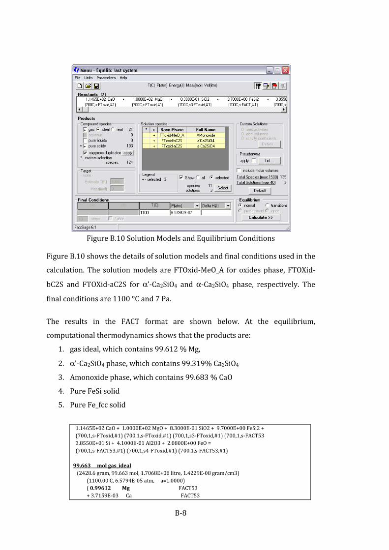
B-8

Figure B.10 Solution Models and Equilibrium Conditions

Figure B.10 shows the details of solution models and final conditions used in the

calculation. The solution models are FTOxid-MeO_A for oxides phase, FTOXid-

bC2S and FTOXid-aC2S for α’-Ca2SiO4 and α-Ca2SiO4 phase, respectively. The

final conditions are 1100 °C and 7 Pa.

The results in the FACT format are shown below. At the equilibrium,

computational thermodynamics shows that the products are:

1. gas ideal, which contains 99.612 % Mg,

2. α’-Ca2SiO4 phase, which contains 99.319% Ca2SiO4

3. Amonoxide phase, which contains 99.683 % CaO

4. Pure FeSi solid

5. Pure Fe_fcc solid

1.1465E+02 CaO + 1.0000E+02 MgO + 8.3000E-01 SiO2 + 9.7000E+00 FeSi2 + (700,1,s-FToxid,#1) (700,1,s-FToxid,#1) (700,1,s3-FToxid,#1) (700,1,s-FACT53 3.8550E+01 Si + 4.1000E-01 Al2O3 + 2.0800E+00 FeO = (700,1,s-FACT53,#1) (700,1,s4-FToxid,#1) (700,1,s-FACT53,#1) 99.663 mol gas_ideal

(2428.6 gram, 99.663 mol, 1.7068E+08 litre, 1.4229E-08 gram/cm3) (1100.00 C, 6.5794E-05 atm, a=1.0000) ( 0.99612 Mg FACT53 + 3.7159E-03 Ca FACT53

B-9

+ 1.3765E-04 Fe FACT53 + 2.1205E-05 SiO FACT53 + 4.5508E-07 Al FACT53) + 51.693 mol a'Ca2SiO4 (8892.4 gram, 51.693 mol) (1100.00 C, 6.5794E-05 atm, a=1.0000) ( 6.8148E-03 Mg2SiO4 FToxid + 0.99319 Ca2SiO4 FToxid) System component Mole fraction Mass fraction Fe 1.1623E-10 2.6413E-10 Ca 0.28377 0.46278 Si 0.14286 0.16326 Mg 1.9471E-03 1.9257E-03 O 0.57143 0.37203 + 10.446 mol AMonoxide (586.12 gram, 10.446 mol) (1100.00 C, 6.5794E-05 atm, a=1.0000) ( 0.99683 CaOFToxid + 1.7901E-03 MgOFToxid + 1.3786E-03 Al2O3 FToxid) System component Mole fraction Mass fraction Fe 7.1758E-09 1.4313E-08 Ca 0.49739 0.71198 Al 1.3757E-03 1.3258E-03 Mg 8.9321E-04 7.7538E-04 O 0.50034 0.28592 + 7.0854 mol FeSi_solid T FACT53 (594.68 gram, 7.0854 mol) (1100.00 C, 6.5794E-05 atm, S1, a=1.0000) + 4.6809 mol Fe_fcc FACT53 (261.41 gram, 4.6809 mol) (1100.00 C, 6.5794E-05 atm, S2, a=1.0000) + 0.39558 mol Ca3Al2O6_solid FACT53 (106.88 gram, 0.39558 mol) (1100.00 C, 6.5794E-05 atm, S1, a=1.0000) + 0.00000 mol Ca3Al2O6_solid FToxid (1100.00 C, 6.5794E-05 atm, S1, a=1.0000) + 0.00000 mol CaO_lime FACT53 (1100.00 C, 6.5794E-05 atm, S1, a=0.99539) + 0.00000 mol CaO_limeFToxid (1100.00 C, 6.5794E-05 atm, S1, a=0.99539) + 0.00000 mol Fe_bcc FACT53 …… …

B-10

B.3.2 Condensation of Magnesium Vapour at 1050 °°°°C

This sub-chapter provides the detail of condensation of magnesium vapour from

1100 to 1050 °C. Figure E.11 shows the input data for the calculation. This is

mixture of vapour, which is based on the results of equilibrium of the

Pidgeonprocess at 1100 °C and 7 Pa. Figure E.12 shows the final condition and

solution models employed in the calculation.

Figure B.11 Input Species for the Vapour Condensation

Figure B.12 Solution Species and Final Conditions for the Vapour Condensation

B-11

The results are shown below. The phase resulted from equilibrium of vapour at

1050 °C are:

1. 99.649 mol of ideal gas (vapour phase), which contains 99.62% Mg

2. 6.8×10-3 mol of fcc phase, which contains 99.99% Fe

3. 1.18×10-3 mol of bcc phase, which contains 99.99% Fe

4. 1.9×10-3 mol of Amonoxide phase, which contains 99.84% CaO

5. 1.9×10-3 mol of pure FeSi

9.9277E+01 Mg + 3.7034E-01 Ca + 1.3718E-02 Fe + 2.1134E-03 SiO + (1100,6.57E-05,g-FACT53,#1) (1100,6.57E-05,g-FACT53,#1) (1100,6.57E-05,g-FAC 4.5355E-05 Al = (1100,6.57E-05,g-FACT53,#1) 99.649 mol gas_ideal (2427.9 gram, 99.649 mol, 1.6444E+08 litre, 1.4764E-08 gram/cm3) (1050.00 C, 6.5794E-05 atm, a=1.0000) ( 0.99626 Mg FACT53 + 3.6969E-03 Ca FACT53 + 3.7315E-05 Fe FACT53 + 1.6472E-06 SiO FACT53 + 1.6108E-07 Al FACT53) + 6.8986E-03 mol FCC (0.38524 gram, 6.8986E-03 mol) (1050.00 C, 6.5794E-05 atm, a=1.0000) ( 6.8475E-05 Mg T PIDG + 5.1558E-06 Al T PIDG + 0.99992 Fe PIDG + 6.8615E-06 Ca PIDG) System component Mole fraction Mass fraction Fe 0.99992 0.99996 Ca 6.8615E-06 4.9244E-06 Si 4.8065E-11 2.4174E-11 Al 5.1558E-06 2.4911E-06 Mg 6.8475E-05 2.9803E-05 + 1.9478E-03 mol AMonoxide#1 (0.10922 gram, 1.9478E-03 mol) (1050.00 C, 6.5794E-05 atm, a=1.0000) ( 0.99849 CaOFToxid + 1.1328E-03 MgOFToxid + 3.7910E-04 Al2O3 FToxid) System component Mole fraction Mass fraction Fe 1.1016E-09 2.1953E-09 Ca 0.49896 0.71362 Al 3.7889E-04 3.6481E-04 Mg 5.6609E-04 4.9099E-04 O 0.50009 0.28553 + 0.00000 mol AMonoxide#2 (1050.00 C, 6.5794E-05 atm, a=0.33100)

B-12

( 6.0862E-04 CaOFToxid + 0.99939 MgOFToxid) + 1.1802E-03 mol BCC (6.5105E-02 gram, 1.1802E-03 mol) (1050.00 C, 6.5794E-05 atm, a=1.0000) ( 2.3525E-02 Al T PIDG + 0.97641 Fe PIDG + 6.0737E-05 Si PIDG) System component Mole fraction Mass fraction Fe 0.97641 0.98846 Ca 9.9692E-11 7.2428E-11 Si 6.0737E-05 3.0923E-05 Al 2.3525E-02 1.1506E-02 + 0.00000 mol a'Ca2SiO4 (1050.00 C, 6.5794E-05 atm, a=0.32340) ( 5.3846E-03 Mg2SiO4 FToxid + 0.99462 Ca2SiO4 FToxid) + 0.00000 mol hcp (1050.00 C, 6.5794E-05 atm, a=2.2781E-04) ( 0.35860 Mg T PIDG + 1.9045E-02 Ca PIDG + 5.9848E-02 Al T PIDG + 0.56250 Si PIDG) + 1.9492E-03 molFeSi_solid T FACT53 (0.16359 gram, 1.9492E-03 mol) (1050.00 C, 6.5794E-05 atm, S1, a=1.0000)

Pidgeon Process, 1100 °°°°C, 7 atm

(gram) 4.2 SiO2 + 13.4 FeO + 361.3 MgO + 617.4 CaO + (gram) 3.7 Al2O3 + 48.5 Fe + 145.5 Si = 8.9283 molgas_ideal (217.54 gram, 8.9283 mol, 1.4562E+07 litre, 1.4939E-08 gram/cm3) (1100.00 C, 6.9084E-05 atm, a=1.0000) ( 0.99631 Mg FACT53 + 3.5395E-03 Ca FACT53 + 1.3109E-04 Fe FACT53 + 2.0191E-05 SiO FACT53 + 4.3363E-07 Al FACT53) + 795.84 gram a'Ca2SiO4 (795.84 gram, 4.6266 mol) (1100.00 C, 6.9084E-05 atm, a=1.0000) ( 0.58104 wt.% Mg2SiO4 FToxid + 99.419 wt.% Ca2SiO4 FToxid) System component Mole fraction Mass fraction Fe 1.1608E-10 2.6381E-10 Ca 0.28368 0.46267 Si 0.14286 0.16327 Mg 2.0297E-03 2.0075E-03 O 0.57143 0.37205 + 95.078 gram AMonoxide#1 (95.078 gram, 1.6945 mol)

B-13

(1100.00 C, 6.9084E-05 atm, a=1.0000) ( 1.8418E-06 wt.% FeOFToxid + 99.615 wt.% CaOFToxid + 0.13508 wt.% MgOFToxid + 0.25019 wt.% Al2O3 FToxid) System component Mole fraction Mass fraction Fe 7.1781E-09 1.4318E-08 Ca 0.49734 0.71194 Al 1.3740E-03 1.3242E-03 Mg 9.3831E-04 8.1456E-04 O 0.50034 0.28592 + 0.00000 gram AMonoxide#2 (1100.00 C, 6.9084E-05 atm, a=0.42232) ( 4.4991E-05 wt.% FeOFToxid + 9.7959E-02 wt.% CaOFToxid + 99.902 wt.% MgOFToxid) + 52.354 gram FeSi_solid T FACT53 (52.354 gram, 0.62378 mol) (1100.00 C, 6.9084E-05 atm, S1, a=1.0000) + 24.016 gram Fe_fcc FACT53 (24.016 gram, 0.43004 mol) (1100.00 C, 6.9084E-05 atm, S2, a=1.0000) + 9.1740 gram Ca3Al2O6_solid FToxid (9.1740 gram, 3.3953E-02 mol) (1100.00 C, 6.9084E-05 atm, S1, a=1.0000)

The Magnetherm Process, 1550 °°°°C, 5 kPa

(gram) 2.3 SiO2 + 4.2 FeO + 388.8 MgO + 604.0 CaO + (gram) 154 Al2O3 + 48.5 Fe + 145.5 Si + 84.5 SiO2 + (gram) 47.32 Al2O3 + 20.38 MgO + 185.9 CaO = 8.4616 molgas_ideal (206.29 gram, 8.4616 mol, 25653. litre, 8.0417E-06 gram/cm3) (1550.00 C, 4.9346E-02 atm, a=1.0000) ( 0.99591 Mg FACT53 + 2.8351E-03 Ca FACT53 + 7.4573E-04 SiO FACT53 + 4.8953E-04 Fe FACT53 + 1.4490E-05 Al FACT53 + 8.0718E-06 Mg2 FACT53 + 5.7844E-07 Al2O FACT53 + 2.0619E-07 Si FACT53) + 953.29 gram ASlag-liq#1 (953.29 gram, 15.598 mol) (1550.00 C, 4.9346E-02 atm, a=1.0000) ( 21.118 wt.% Al2O3 FToxid + 19.389 wt.% SiO2 FToxid + 52.975 wt.% CaOFToxid + 9.9437E-04 wt.% FeOFToxid + 7.6155E-07 wt.% Fe2O3 FToxid + 6.5175 wt.% MgOFToxid) Site fraction of sublattice constituents: Al 0.22472 Si 0.17506 Ca 0.51248 Fe2+ 7.5085E-06 Fe3+ 5.1743E-09 Mg 8.7726E-02 ----------------------------------- O 1.0000

B-14

System component Mole fraction Mass fraction Fe 3.2848E-06 7.7346E-06 Ca 0.22404 0.37861 Si 7.6533E-02 9.0631E-02 Al 9.8241E-02 0.11177 Mg 3.8352E-02 3.9303E-02 O 0.56283 0.37969 + 0.00000 gram ASlag-liq#2 (1550.00 C, 4.9346E-02 atm, a=1.0000) ( 21.118 wt.% Al2O3 FToxid + 19.389 wt.% SiO2 FToxid + 52.975 wt.% CaOFToxid + 9.9437E-04 wt.% FeOFToxid + 7.6155E-07 wt.% Fe2O3 FToxid + 6.5175 wt.% MgOFToxid) Site fraction of sublattice constituents: Al 0.22472 Si 0.17506 Ca 0.51248 Fe2+ 7.5085E-06 Fe3+ 5.1743E-09 Mg 8.7726E-02 ----------------------------------- O 1.0000 System component Mole fraction Mass fraction Fe 3.2848E-06 7.7346E-06 Ca 0.22404 0.37861 Si 7.6533E-02 9.0631E-02 Al 9.8241E-02 0.11177 Mg 3.8352E-02 3.9303E-02 O 0.56283 0.37969 + 448.37 gram a-Ca2SiO4 (448.37 gram, 2.6200 mol) (1550.00 C, 4.9346E-02 atm, a=1.0000) ( 2.8808 wt.% Mg2SiO4 FToxid + 97.119 wt.% Ca2SiO4 FToxid + 2.5905E-05 wt.% Fe2SiO4 FToxid) System component Mole fraction Mass fraction Fe 6.2159E-08 1.4199E-07 Ca 0.27570 0.45197 Si 0.14286 0.16411 Mg 1.0012E-02 9.9534E-03 O 0.57143 0.37396 + 0.00000 gram Fe-liq (1550.00 C, 4.9346E-02 atm, a=0.94899) ( 87.890 wt.% Fe FACT + 0.22754 wt.% Al FACT + 6.7019E-05 wt.% Ca FACT + 7.1394E-06 wt.% O FACT + 11.864 wt.% Si FACT + 1.5764E-02 wt.% Mg FACT + 8.2907E-04 wt.% MgO FACT + 5.7283E-04 wt.% CaO FACT + 3.4171E-04 wt.% AlO FACT + 1.2874E-05 wt.% SiO FACT + 8.4567E-04 wt.% Al2O FACT) + 77.439 gram FeSi_solid T FACT53 (77.439 gram, 0.92266 mol) (1550.00 C, 4.9346E-02 atm, S1, a=1.0000)

B-15

Mintek Process, 1750 °°°°C, 85 kPa

(gram) 9.8 SiO2 + 3.1 Fe2O3 + 391. MgO+ 562. CaO + (gram) 4.8 Al2O3 + 56.75 Fe + 170.25 Si + 0.9 Fe + (gram) 0.02775 Si + 18.45375 Al + 3.7E-4 Mn = 9.4348 molgas_ideal (231.53 gram, 9.4348 mol, 1867.2 litre, 1.2400E-04 gram/cm3) (1750.00 C, 0.83888 atm, a=1.0000) ( 0.98578 Mg FACT + 1.1380E-02 Ca FACT + 2.5832E-03 SiO FACT + 1.1914E-04 Al FACT + 1.0399E-04 Mg2 FACT + 1.7073E-05 Fe FACT + 1.1661E-05 Al2O FACT + 8.1156E-06 Si FACT + 1.1960E-07 Mn FACT) + 203.60 gram ASlag-liq#1 (203.60 gram, 3.4046 mol) (1750.00 C, 0.83888 atm, a=1.0000) ( 13.949 wt.% Al2O3 FToxid + 23.251 wt.% SiO2 FToxid + 58.710 wt.% CaOFToxid + 5.1345E-05 wt.% FeOFToxid + 4.0901 wt.% MgOFToxid) Site fraction of sublattice constituents: Al 0.15125 Si 0.21391 Ca 0.57874 Fe2+ 3.9506E-07 Fe3+ 2.1750E-10 Mg 5.6098E-02 Mn2+ 6.2732E-10 Mn3+ 2.0253E-14 ----------------------------------- O 1.0000 System component Mole fraction Mass fraction Fe 1.7265E-07 3.9933E-07 Mn 2.7400E-10 6.2347E-10 Ca 0.25277 0.41959 Si 9.3431E-02 0.10868 Al 6.6062E-02 7.3825E-02 Mg 2.4502E-02 2.4665E-02 O 0.56323 0.37323 + 0.00000 gram ASlag-liq#2 (1750.00 C, 0.83888 atm, a=1.0000) ( 13.949 wt.% Al2O3 FToxid + 23.251 wt.% SiO2 FToxid + 58.710 wt.% CaOFToxid + 5.1345E-05 wt.% FeOFToxid + 4.0901 wt.% MgOFToxid) + 48.246 gram Fe-liq (48.246 gram, 1.4635 mol) (1750.00 C, 0.83888 atm, a=1.0000) ( 30.756 wt.% Fe FACT + 11.953 wt.% Al FACT + 3.9092 wt.% Ca FACT + 6.3814E-04 wt.% Mn FACT + 6.8867E-05 wt.% O FACT + 43.128 wt.% Si C FACT + 9.6324 wt.% Mg C FACT

B-16

+ 6.8411E-02 wt.% MgO FACT + 0.11507 wt.% CaO FACT + 2.0781E-02 wt.% AlO FACT + 2.7058E-03 wt.% SiO FACT + 0.41356 wt.% Al2O FACT) System component Mole fraction Mass fraction Fe 0.18060 0.30756 Mn 3.8090E-06 6.3815E-06 Ca 3.2658E-02 3.9915E-02 Si 0.50357 0.43130 Al 0.14931 0.12285 Mg 0.13052 9.6737E-02 O 3.3480E-03 1.6335E-03 + 0.00000 gram a'Ca2SiO4 (1750.00 C, 0.83888 atm, a=0.99948) ( 1.6006 wt.% Mg2SiO4 FToxid + 1.1220E-06 wt.% Fe2SiO4 FToxid + 98.399 wt.% Ca2SiO4 FToxid) + 666.12 gram Ca2SiO4_alpha FToxid (666.12 gram, 3.8674 mol) (1750.00 C, 0.83888 atm, S3, a=1.0000) + 67.587 gram FeSi_solid T FACT (67.587 gram, 0.80528 mol) (1750.00 C, 0.83888 atm, S1, a=1.0000)

C-1

Appendix C: Temperature Profile Measurement

C.1 Temperature Profile with and without Condenser

Figure C. 1 Temperature Profile Measurement at Set Point of 1190 oC, Ar gas Flow Rate of 0.3 L/min, and Cooling Water Rate of 3 L/min

Figure C. 2 Temperature Profile At Different Condenser Position

0

200

400

600

800

1000

1200

1400

0 10 20 30 40 50 60 70 80

Measurement without Condenser

Measurement with Condenser

Position, cm

Te

mp

era

ture

,C

Condenser position

Isothermal Zone at 1190 - 1191 C

0

200

400

600

800

1000

1200

1400

30 35 40 45 50 55 60 65

Te

mp

era

ture

( C

)

Position, cm

condenser position: 60 cm

condenser position: 40 cm

C-2

C.2 Temperature Profile with Different Argon Gas Flow

Rate

Figure C. 3 Temperature Profile Measurement at Set Point of 1140 oC, Ar gas Flow Rate of 0.3 L/min, and Cooling Water Rate of 3 L/min

C.3 Temperature Profile at 1140 – 1145 °°°°C

Figure C. 4 Temperature Profile Measurement at Set Point of 1145 °C under Ar Gas Flow Rate of 0.3 L/min. The Position of Water-cooled Condenser is 30 cm from the right-end of tube.

0

200

400

600

800

1000

1200

1400

-10 0 10 20 30 40 50 60 70 80

Ar Flow Rate 0.2 L/min with Condenser

Ar Flow Rate = 0.2 L/min

Ar Flow Rate = 2 L/min

Position, cm

Te

mp

era

ture

,C

Position, cm

Te

mp

era

ture

,C

Condenser position

Isothermal Zone at 1135 - 1136 C

Position, cmPosition, cm

0

200

400

600

800

1000

1200

1400

5 15 25 35 45 55 65

Te

mp

era

ture

(C

)

position (cm)

Thermocouple 1 Thermocouple 2

C-3

C.4 Temperature Profile at Different Set Point

Temperature

Figure C. 5 Temperature Profile Measurement at Set-Point Temperatures of 1130 °C, 1145 °C and 1160 °C. Sample is put inside the Tube Furnace at 25 cm Position.

C.5 Isothermal Position inside Horizontal Tube Furnace

Figure C. 6 The Isothermal Position inside Tube Furnace at Set Point Temperature of 1130, 1145 and 1160 °C

800

850

900

950

1000

1050

1100

1150

1200

0 5 10 15 20 25 30 35

1130 C 1145 C 1160 C

1100

1110

1120

1130

1140

1150

1160

12 15 18 21 24 27 30

1130 C 1145 C 1160 C

C-4

Figure C. 7 Temperature Calibration between Set Point and Actual Temperature

R² = 0.9891

1120

1125

1130

1135

1140

1145

1150

1125 1130 1135 1140 1145 1150 1155 1160 1165

Series1 Linear (Series1)

D-1

Appendix D: Error Analysis In laboratory experiments, the measurements of physical and chemical analysis

are always associated with its uncertainties. The error in experiment is

classified into random errors and systematic error. The random errors arise

from uncertainties in measurement devices. The systematic error may occur

from all other sources of errors such as impure reagent, instrumentation, etc. In

the experiment, every activity such as weighing, flow rate measurement,

temperature measurement, and chemical analysis contribute to uncertainty.

The possible source of error may arise from the weight and size of sample,

initial composition of sample, and temperature inside furnace.

The error of summation or substraction of two quantities of a and b is as

follows263:

δ ' δ δt

where δ, δ, and δt are absolute error of quantities p, a, and b.

The error of product of two quantities of a and b is as follows:

δ ' δ

δtt

D.1 Errors in Experimental Procedures

D.1.1 Weighing Error

All samples are weighed in six figure balance with the error of + 0.0001 g.

D.1.2 Temperature Measurement Error

Temperature was measured using K-type thermocouple and recorded by a

multimeter, which has uncertainty as follows:

- error in temperature below 1000 oC: + 0.1 °C

- error in temperature above 1000 oC is + 1 °C

The temperature profile measurement was carried out by placing ceramic

sheathed thermocouple inside the furnace. Temperature was recorded every 1

D-2

cm position. The error associated with the position of thermocouple estimated

to be + 5 mm. This corresponds to + 1 °C at the hot zone (between 20 to 40 cm

position) and + 15 at the cooler zone (between 0 and 20 cm position and 40 to

80 cm position).

D.1.3 Error in Sample Position inside Furnace

Ceramic boat which contains sample was connected to a steel rod. Ceramic boat

was displaced into a hot zone in the horizontal tube furnace by placing a strong

magnet to the steel rod and moved the magnet along. The error of sample

position was estimated to be + 2 mm.

D.1.4 Flow Rate Errors

Argon gas is measured using BES Flowmeter, which is a type of gas rotameter.

The flow mater has range between 5×10-5 m3/min and 50×10-5 m3/min. The

error in argon gas flow rate measurement is estimated to be + 5×10-5 m3/min.

Cooling water flow rate is also measured using BES flowmeter which has flow

rate range between 1×10-3 m3/min and 3×10-3 m3/min. The error in cooling

water measurement is estimated to be + 2×10-4 m3/min (i.e. half the smallest

scale of the flowmeter).

D.2 Error in Analytical Technique

D.2.1 Error in EDS Analysis

The error in accuracy in EDS analysis was expected to be + 5 wt% for particles

and rough surface without standards (based on Briggs et al264).

D.2.1 Error in XRD Analysis

The source of error in XRD measurements may be caused by misalignment of

the equipment, sample displacement, absorption, and peak distortion due to

Kα2 and Kβ wavelengths. These errors were not important because we were

only performing phase identification.

E-1

Appendix E: Sample Calculations

E.1 Kinetics Analysis

E.1.1 Determination of Mass Transfer Coefficient

σV& ' 3_$/j (from Geiger and Poirer, p.466, Table 13.7)

σK ' 3.418_$/j

σV&BK ' :$ σV& σK ' 3.209_$/j

ε/κ,V& ' 1772.16

ε/κ,K ' 124

ε

κ|,)*°\Ã ' ã ε

κ|,)* ε

κ|,\Ãä+ ' 443.607

κ|3ε

' 3.5459

ΩV&BK ' 0.9 (from Geiger and Poirer, p.464, Figure 13.18)

Diffusivity of Mg-Ar:

' .:::£;£r3¡(σ\|+Ωz,\| µ :

V\ :V| (6.18)

From Equation (6.18), V&BK ' 5.1725_$/j

Mass transfer coefficient of Mg-Ar (Warner relation):

A ' 2.0 0.6]P:/$cQ:/r :.:;¦$K (6.17)

At flow rate of 8×10-5 m3/min, r = 0.7 cm, µ = 7.14×10-5 kg/m.s :

]P ' 2ρhiη

' 20.3090.070.0077.14d10B; ' 0.4298

cT ' η

ρV&BK ' 7.14d10B;0.3095.1725 ' 0.045

By substituting NRe, NSc, and DMg-Ar to Equation (6.17), mass transfer coefficient can be calculated to be : A ' 9.09_/j

E-2

E.2 Experimental Study

E.2.1 Calculation of Required Amount of Reactant

Silicothermic reaction proceeds as follows:

2 2 ' 2& $ % (E. 1)

The atomic mass of the species is as follows: Ar Mg: 24.305

Ar Ca: 40.078

Ar Si: 28.0855

Ar Fe: 55.847,

Ar O: 15.9994

The stoichiometric amounts of reactants are:

CaO = 2 mol x (40.078+ 15.994) g/mol = 112.1548 g

MgO = 2 mol x (24.305+ 15.994) g/mol = 81.6088 g

Si = 1 mol x 28.0855 g/mol = 28.0855 g

FeSi75 = 100/75 x28.0855 g = 37.4775 g

Ratio of CaO: MgO: FeSi75 = 112.1548 : 81.6088: 37.4775

= 48.501 % : 35.292 % : 16.207%

When 10% excess of FeSi75 is incorporated into the samples, the ratio of

reactant becomes:

Ratio of CaO: MgO: FeSi75 = 47.728 % : 34.729 % : 17.545 %

When 2.5% CaF2 is added into the reactants, the ratio of reactants becomes:

Ratio of CaO: MgO: FeSi75: CaF2 = 46.518 % : 33.848 % : 17.100 % : 2.5 %

Modelling of Thermal Magnesium Processes

Documents

Transcript of Modelling of Thermal Magnesium Processes