Modelling of landscape variables at multiple extents to predict fine sediments and suitable habitat...

Modelling of landscape variables at multiple extents topredict fine sediments and suitable habitat for Tubifextubifex in a stream system

KARA J. ANLAUF 1 AND CHRISTINE M. MOFFITT

United States Geological Survey, Idaho Cooperative Fish and Wildlife Research Unit, Department of Fish and Wildlife Resources,

University of Idaho, Moscow, ID, U.S.A.

SUMMARY

1. Aggregations of fine sediments are a suitable proxy for the presence and abundance of

Tubifex tubifex, one of the obligate hosts in the parasitic life cycle that causes salmonid

whirling disease (Myxobolus cerebralis).

2. To determine and evaluate practical approaches to predict fine sediments (<2 mm

diameter) that could support Tubifex spp. aggregations, we measured habitat features in a

catchment with field measures and metrics derived from digital data sets and geospatial

tools at three different spatial extents (m2) within a hierarchical structure.

3. We used linear mixed models to test plausible candidate models that best explained the

presence of fine sediments measured in stream surveys with metrics from several spatial

extents.

4. The percent slow water habitat measured at the finest extent provided the best model to

predict the likely presence of fine sediments. The most influential models to predict fine

sediments using landscape metrics measured at broader extents included variables that

measure the percentage land cover in conifer or agriculture, specifically, decreases in

conifer cover and increases in agriculture.

5. The overall best-fitting model of the presence of fine sediments in a stream reach

combined variables measured and operating at different spatial extents.

6. Landscape features modelled within a hierarchical framework may be useful tools to

evaluate and prioritise areas with fine sediments that may be at risk of infection by

Myxobolus cerebralis.

Keywords: benthos, ecosystem, erosion ⁄sedimentation ⁄ landuse, fish, geospatial, parasites ⁄pathogens,physical habitat modelling

Introduction

Tubifex tubifex Muller (Annelida: Oligochaeta: Tubi-

ficidae) is a tubificid oligochaete found in a variety of

aquatic habitat types (Brinkhurst, 1996). Tubifex

tubifex is one of the obligate hosts in the life cycle

of Myxobolus cerebralis Hofer (Myxozoa: Myxosporea:

Myxobolidae), the causative agent of salmonid

whirling disease. This European fish parasite was

inadvertently introduced to North America within

regions of susceptible and native fish hosts. Inside T.

tubifex, M. cerebralis emerges from spores and

attaches to the lining of the worm intestine (Brink-

hurst, 1996). After approximately 90 days, the para-

site develops into the triactinomyxon (TAM) stage

and is egested from the worm into the water column.

Correspondence: Christine M. Moffitt, United States Geological

Survey, Idaho Cooperative Fish and Wildlife Research Unit,

Department of Fish and Wildlife Resources, University of Idaho,

Moscow, ID 83844-1136, U.S.A. E-mail: [email protected] address: Kara J. Anlauf, Corvallis Research Lab, Oregon

Department of Fish and Wildlife, 28655 Hwy, 34 Corvallis, OR

97333, U.S.A.

Freshwater Biology (2010) 55, 794–805 doi:10.1111/j.1365-2427.2009.02323.x

794 � 2010 Blackwell Publishing Ltd

TAMs released into the water infect susceptible

salmonid hosts by penetrating the epithelial cells.

The parasite migrates through peripheral nerves

ultimately ending in the spinal cord and cranial

region (Hedrick & El-Matbouli, 2002). With no

natural immunity to the parasite, many fish popula-

tions in western North America have been negatively

affected (Bartholomew & Reno, 2002; Krueger et al.,

2006). Since the fish hosts are several, and the

obligate invertebrate host is only T. tubifex, predict-

ing the likely habitat for the oligochaete host may be

a preferred way to determine areas of highest risk

for infection within catchments (Hiner & Moffitt,

2002; Schisler & Bergersen, 2002; Krueger et al., 2006).

Tubificid oligochaetes occur in many aquatic benthic

habitats (Reynoldson, 1987); however, substrate is

believed to be a primary factor influencing the abun-

dance and distribution of T. tubifex (Lazim & Learner,

1987). Fine substrates are favoured by T. tubifex and are

common in stream habitats that have been incised and

widened. Such areas often have reduced riparian shade

and tend to support higher stream temperatures and

lower oxygen concentrations and these conditions

favour T. tubifex over other invertebrate species (Schis-

ler & Bergersen, 2002). Broad-scale landscape features

have been associated with sediment depositions at local

levels (Allan, Erickson & Fay, 1997) and could therefore

influence the likelihood of T. tubifex presence. Stream

habitat variables such as surface slope and sediment

proportions that predict the presence of T. tubifex have

been shown to vary with spatial extent (Anlauf &

Moffitt, 2008). A synergism among measures taken at

several spatial scales may be useful in predicting T.

tubifex. Further, although direct influence of some

variables may not always be discernable, the impact

of certain habitat features can be viewed through

intermediate pathways.

Other researchers have predicted the likely distri-

bution of the fish parasite M. cerebralis using habitat

variables measured within a catchment (Isaak &

Hubert, 1999; Hiner & Moffitt, 2002). The variation in

prevalence and the severity of infection from the

parasite are reliant on the interactions between the

pathogen, its hosts and the environment (Reno,

1998). The features of the physical environment are

probably the least defined components of the M.

cerebralis life cycle, and the benefits of understanding

those gradients will aid in the management of

affected populations and ecosystems as a whole

(Hedrick, 1998; Zendt & Bergersen, 2000; Anlauf &

Moffitt, 2008).

Combining variables measured or estimated at

large spatial scales (landscape) with variables mea-

sured or estimated at finer, local scales (stream

reach) in modelling instream habitat provides a

further opportunity to reveal controlling mechanisms

(Allan & Johnson, 1997). The relationship between T.

tubifex and fine substrates has been documented

(Lazim & Learner, 1987; Kaeser & Sharpe, 2006;

Anlauf & Moffitt, 2008). Our study, therefore, pur-

sued ways to predict and understand variables that

influenced the quantity of fine sediments (particle

size <2 mm diameter), as a surrogate for T. tubifex

populations. We developed and tested habitat mod-

els to predict the quantity of fine sediments in

streams using habitat features measured at multiple

spatial extents: 500-m, 2000-m and the entire extent

of the upstream segment (total length; hereafter

referred to as the TL) above the start of each stream

reach where fine sediments were measured. Our

objectives were to compare model results when

landscape characteristics of the same resolution were

summarised at three spatial extents, and to deter-

mine whether the incorporation of both local and

landscape habitat characteristics improved predictive

models.

Methods

Study area

We conducted this study in the Pahsimeroi River

drainage basin, a tributary of the Salmon River,

located in eastern Idaho, U.S.A., between the Lost

River and Lemhi mountain ranges (Fig. 1). The

Pahsimeroi valley drains approximately 2175 km2

with elevations ranging from 1413 to 3846 m and

average annual flows in the mainstem Pahsimeroi

River during the study period ranging from

6.091 m3 s)1 in 2001 to 4.717 m3 s)1 in 2004. Like

many areas of the western intermountain region, the

Pahsimeroi River is influenced by local land-use

practices including irrigated agriculture and live-

stock grazing (Bureau of Land Management, 1999;

Colvin & Moffitt, 2008). Land cover and vegetation

are comprised mostly of sagebrush steppe, grassland

communities in the valley and conifer communities

in upland mountain drainages (Fig. 1). The Pahsim-

Modelling landscape variables and sediments 795

� 2010 Blackwell Publishing Ltd, Freshwater Biology, 55, 794–805

eroi catchment has been selected as high priority for

restoration to enhance populations of threatened and

endangered salmonids (Shumar, Reaney & Herron,

2001; National Oceanographic and Atmospheric

Administration, 2004).

The underlying geology of the subbasin varies;

much of the valley and adjacent mountain ranges are

composed of metamorphosed gneiss and schist, with

both sedimentary (limestone and dolomite) and vol-

canic (fine grained basalt) rock deposits (Young &

Harenberg, 1973; Alt & Hyndman, 1989). Glacial,

alluvial and fluvial deposits blanket the valley floor,

and the principal aquifer in the valley is contained in

the alluvium (Young & Harenberg, 1973). The main-

stem Pahsimeroi River consists of three distinct

sections disconnected due predominantly to subsur-

face flow. The upper and middle sections of the

Pahsimeroi River are disconnected year-round while

the middle and lower Pahsimeroi River sections have

an intermittent connection during certain times of the

year. The tributaries in the drainage basin exit

confined canyon corridors and enter extensive alluvial

deposits. Due to the highly porous nature of the

coarse alluvium, the majority of the streams within

the subbasin exhibit large percolation losses. As a

result, the majority of these tributaries contribute little

to the surficial flow of the Pahsimeroi River (Bureau of

Land Management, 1999; Colvin & Moffitt, 2008).

Additionally, much of the water from these channels

is diverted to irrigation canals as the streams enter the

large alluvial fans. The water that feeds the baseflow

of the mainstem is derived primarily from subsurface

flow and emerges as springs in the Pahsimeroi valley

(Young & Harenberg, 1973; Colvin & Moffitt, 2008).

Study stream reaches

To estimate and measure instream characteristics, we

created points in a geospatial (GIS) along a 1 : 24 000

scale stream coverage. Each point became the start of a

potential study reach site and had associated with it a

site number and northing and easting UTM coordi-

nates. We then parsed the drainage into six strata

based on stream slopes derived from a 10-m digital

elevation model, and used a stratified random sam-

pling design to select study reach sites from each slope

stratum. The reach slope strata (percent slope) were

defined as follows: I = 0–0.5%; II = >0.5–1.0%;

III = >1.0–1.5%; IV = >1.5–2.0%; V = >2.0–4.0% and

VI = >4.0–6.0%. We selected sixty 100-m stream

reaches for instream surveys. The number of reaches

surveyed by strata were: 17, 15, 5, 9, 10 and 4, for

stratum I, II, III, IV, V and VI respectively. The intensity

of sampling within each stratum was based on the

proportionate distribution of gradients throughout the

drainage. We measured and evaluated the aquatic

habitat during late May–September 2003 using field

methods described in Anlauf & Moffitt (2008).

Fig. 1 Major land cover types represented

in the Pahsimeroi River drainage (Idaho

GAP Analysis 1999) and sample site

locations (n = 56).

796 K. J. Anlauf and C. M. Moffitt


Habitat variables

Instream habitat characteristics were measured with-

in specific habitat units defined and characterised by

similar morphological and hydrological features, i.e.

pools or riffles (Bisson et al., 1982; Frissell et al.,

1986; Hawkins et al., 1993), and summarised within

100-m stream reaches. The 100-m reach served as

our local or finest spatial extent. We obtained an

empirical estimate of fine sediments based on visual

observation of the percent distribution of streambed

area, relative to the total habitat area, consisting of

sediments <2 mm in diameter (Hausle & Coble,

1976; Everest et al., 1987). We obtained an average

value for each reach and this value became our

response variable. We selected three habitat vari-

ables as our local scale predictors, each of which

was measured in the field and summarised within

the 100 m reach: width-depth ratio, percent slow

water habitat and percent slope (Table 1). These

variables were chosen given their perceived influ-

ence over fine sediments and because they are

commonly measured and summarised in stream

habitat surveys.

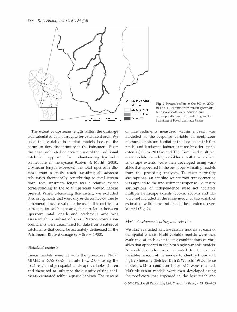
Geospatial habitat data were derived from existing

data sources (Table 1) and measured within a 100-m

stream buffer on either side of the stream at three

stream segment lengths: 500-m, 2000-m and the entire

extent of the upstream segment (TL) above the start of

each stream reach where fine sediments were mea-

sured (Fig. 2). Geospatial data summarised within this

buffered stream segment include land cover ⁄use and

geology variables, total upstream length and stream

slope (Table 1).

Table 1 Description of reach (instream) and landscape (GIS-derived) habitat data used in analyses. Reach habitat was summarised for

a 100-m reach. Landscape habitat was calculated within a 100-m buffer along both sides of specified stream segments. Percent fine

sediments was the dependent variable in all analyses

Habitat variable Description of measure Data source

Instream

Percent fine sediments Proportion of stream bed area

classified as sediments <2 mm

Measured in field

Percent reach slope Average stream slope calculated

for a 100-m reach length

Gradient generated in each grid cell

from a USGS 10-m DEM

Percent slow habitat Proportion of total habitat area

classified as pools or glides

Measured in field

Width : depth ratio Ratio of wetted width and average

depth along transects

Measured in field

GIS-derived

Percent agriculture Area classified as agriculture

(row crops, irrigated pasture

and low intensity urban)

Derived from land cover ⁄ use layer

(Idaho GAP Analysis 1999);

(http://www.wildlife.uidaho.edu/idgap/index.html)

Percent conifer cover Area classified as forest; includes

subalpine fir, Douglas fir, Subalpine

pine, mixed subalpine forests

The land cover variables were combined into

like groupings based on similar flora types

listed in the metadata

Percent shrub ⁄ forb cover Area classified as rangeland (warm

mesic shrubs, curlleaf mountain

mahogany, salt desert shrub,

mountain big sagebrush, low sagebrush,

basin WY sagebrush, mountain low

sagebrush, graminoid-forb riparian

and shrub riparian)

Percent surficial deposits Area classified quaternary surficial

deposits; includes continental

deposit rock type or alluvium fill

(unconsolidated deposits of cobble,

gravel, sand, silt, clay)

Idaho Geological Survey;

(http://www.idahogeology.org)

Upstream length Total channel length upstream

of 100 m reach

1 : 24 000 digitised stream layer

from USGS topographic maps

Percent stream slope Average stream slope calculated

upstream of 100 m reach

Gradient generated in each grid cell

from a USGS 10 m DEM



The extent of upstream length within the drainage

was calculated as a surrogate for catchment area. We

used this variable in habitat models because the

nature of flow discontinuity in the Pahsimeroi River

drainage prohibited an accurate use of the traditional

catchment approach for understanding hydraulic

connections in the system (Colvin & Moffitt, 2008).

Upstream length expressed the total upstream dis-

tance from a study reach including all adjacent

tributaries theoretically contributing to total stream

flow. Total upstream length was a relative metric

corresponding to the total upstream wetted habitat

present. When calculating this metric, we excluded

stream segments that were dry or disconnected due to

ephemeral flow. To validate the use of this metric as a

surrogate for catchment area, the correlation between

upstream total length and catchment area was

assessed for a subset of sites. Pearson correlation

coefficients were determined for data from a subset of

catchments that could be accurately delineated in the

Pahsimeroi River drainage (n = 8; r = 0.980).

Statistical analysis

Linear models were fit with the procedure PROC

MIXED in SAS (SAS Institute Inc., 2000) using the

local reach and geospatial landscape variables chosen

and theorised to influence the quantity of fine sedi-

ments estimated within aquatic habitats. The percent

of fine sediments measured within a reach was

modelled as the response variable on continuous

measures of stream habitat at the local extent (100-m

reach) and landscape habitat at three broader spatial

extents (500-m, 2000-m and TL). Combined multiple-

scale models, including variables at both the local and

landscape extents, were then developed using vari-

ables that appeared in the best approximating models

from the preceding analyses. To meet normality

assumptions, an arc sine square root transformation

was applied to the fine sediment response. To ensure

assumptions of independence were not violated,

multiple landscape extents (500-m, 2000-m and TL)

were not included in the same model as the variables

estimated within the buffers at these extents over-

lapped (Fig. 2).

Model development, fitting and selection

We first evaluated single-variable models at each of

the spatial extents. Multi-variable models were then

evaluated at each extent using combinations of vari-

ables that appeared in the best single-variable models.

A condition index was evaluated for the set of

variables in each of the models to identify those with

high collinearity (Belsley, Kuh & Welsch, 1982). Those

models with a condition index <10 were retained.

Multiple-extent models were then developed using

the predictors that appeared in the best reach and

Fig. 2 Stream buffers at the 500-m, 2000-

m and TL extents from which geospatial

landscape data were derived and

subsequently used in modelling in the

Pahsimeroi River drainage basin.



landscape models. When developing multi-variable

candidate models, a maximum of two predictor

variables were included in each model (with excep-

tion to the global model) due to the instability

associated with overfitting or over-parameterising

(Burnham & Anderson, 2002).

For all models developed at each spatial extent

(100-m, 500-m, 2000-m and TL), we concluded that

the predictive capabilities were effective if the global

model fit the data based on the r-square and root

mean square error (RMSE) values. To select the

most plausible model(s), Akaike Information Criteria

(AIC) were used. We used the small sample

approximation, AICc, because the sample size to

predictor ratio was 18. We considered models with

DAIC values less than or equal to three as compet-

ing models. The relative plausibility of each model

was then obtained based on the weight of evidence

(Akaike weights, wi) relative to the best approxi-

mating model (Burnham & Anderson, 2002; Littell

et al., 2006).

To incorporate probable spatial dependence occur-

ring within the dataset, each reach on the same stream

was assigned to a unique group and the degree of

spatial dependence was modelled within each group.

We examined the residuals of each global model at

each of the four spatial extents within each group to

evaluate the degree of spatial dependence. We

assessed three different covariance structures and

used AICc to select the best fit. The autoregressive

(AR) covariance structure, which considers sites closer

together to be likely more correlated to one another

than sites that are further apart, provided the best fit,

based on the AICc values (Table 2). We therefore

defined this structure for all subsequent analyses.

Results

Fine sediment characterisation

The percent of fine sediments across all the stream

reaches surveyed ranged from 0.10% to 100%. The

highest mean percentage (±SD) was within stratum I

(31.8 ± 22.4%) followed by stratum II (24.8 ± 18.9%)

and lowest for slope stratum IV (4.1 ± 3.6%). At the

finest spatial extent (100-m), the percentage of fine

sediments decreased with increasing reach slope and

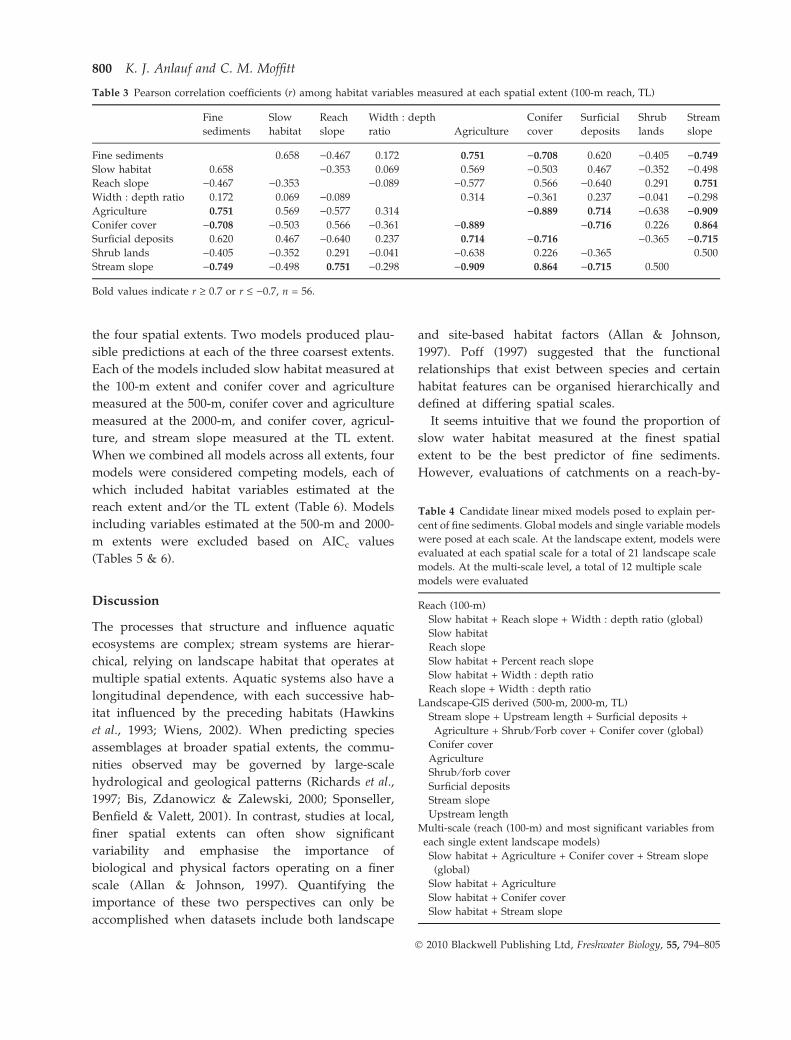
increasing percent of slow habitat. At broader spatial

extents, a strong relationship was also observed

between the percentage of fine sediments and agri-

culture, conifer cover, surficial deposits and the

average stream slope (Table 3). These relationships

are reported in Table 3 for the TL extents only; similar

relationships were observed at the 500-m and 2000-m

spatial extents, although diminished slightly in

magnitude.

Model fitting and selection of plausible models

At the finest spatial extent (100-m), the global model

including all three habitat variables adequately

described the data (r2 = 0.507, RMSE = 0.015). Six

candidate models were then evaluated, and the best

model predicting the percentage of fine sediments

included slow habitat (wi = 0.999) (Tables 4 & 5).

Global models to predict fine sediments using

geospatial habitat variables measured at the three

coarse spatial extents adequately described the data

for the 500-m (r2 = 0.466, RMSE = 0.016), 2000-m

(r2 = 0.498, RMSE = 0.015) and TL (r2 = 0.609,

RMSE = 0.013) scales. At each of the three extents,

we found the best approximating single variable

models predicting the percentage of fine sediments

to include agriculture. Using AICc criteria, we

found a competing model, including conifer cover,

at the 2000-m extent. At the TL extent, two

competing models included conifer cover or stream

slope. None of the multi-variable models evaluated

appeared as competing models when compared

to the single variable models using AICc (Tables 3

& 5).

Multiple-extent models

Multiple-extent models were developed using the

variables that appeared in the best models at each of

Table 2 Covariance structure models evaluated for analysis of

spatial dependence

Scale Covariance structure AICc DAICc wi

500-m Autoregressive )262.0 0.0 0.877

None )257.5 4.5 0.092

Spatial spherical )255.3 6.7 0.030

2000-m Autoregressive )264.2 0.0 0.648

None )262.4 1.8 0.263


Total Autoregressive )271.4 0.0 0.801

Length None )268.0 3.4 0.146




the four spatial extents. Two models produced plau-

sible predictions at each of the three coarsest extents.

Each of the models included slow habitat measured at

the 100-m extent and conifer cover and agriculture

measured at the 500-m, conifer cover and agriculture

measured at the 2000-m, and conifer cover, agricul-

ture, and stream slope measured at the TL extent.

When we combined all models across all extents, four

models were considered competing models, each of

which included habitat variables estimated at the

reach extent and ⁄or the TL extent (Table 6). Models

including variables estimated at the 500-m and 2000-

m extents were excluded based on AICc values

(Tables 5 & 6).

Discussion

The processes that structure and influence aquatic

ecosystems are complex; stream systems are hierar-

chical, relying on landscape habitat that operates at

multiple spatial extents. Aquatic systems also have a

longitudinal dependence, with each successive hab-

itat influenced by the preceding habitats (Hawkins

et al., 1993; Wiens, 2002). When predicting species

assemblages at broader spatial extents, the commu-

nities observed may be governed by large-scale

hydrological and geological patterns (Richards et al.,

1997; Bis, Zdanowicz & Zalewski, 2000; Sponseller,

Benfield & Valett, 2001). In contrast, studies at local,

finer spatial extents can often show significant

variability and emphasise the importance of

biological and physical factors operating on a finer

scale (Allan & Johnson, 1997). Quantifying the

importance of these two perspectives can only be

accomplished when datasets include both landscape

and site-based habitat factors (Allan & Johnson,

1997). Poff (1997) suggested that the functional

relationships that exist between species and certain

habitat features can be organised hierarchically and

defined at differing spatial scales.

It seems intuitive that we found the proportion of

slow water habitat measured at the finest spatial

extent to be the best predictor of fine sediments.

However, evaluations of catchments on a reach-by-

Table 3 Pearson correlation coefficients (r) among habitat variables measured at each spatial extent (100-m reach, TL)

Fine

sediments

Slow

habitat

Reach

slope

Width : depth

ratio Agriculture

Conifer

cover

Surficial

deposits

Shrub

lands

Stream

slope

Fine sediments 0.658 )0.467 0.172 0.751 )0.708 0.620 )0.405 )0.749

Slow habitat 0.658 )0.353 0.069 0.569 )0.503 0.467 )0.352 )0.498

Reach slope )0.467 )0.353 )0.089 )0.577 0.566 )0.640 0.291 0.751

Width : depth ratio 0.172 0.069 )0.089 0.314 )0.361 0.237 )0.041 )0.298

Agriculture 0.751 0.569 )0.577 0.314 )0.889 0.714 )0.638 )0.909

Conifer cover )0.708 )0.503 0.566 )0.361 )0.889 )0.716 0.226 0.864

Surficial deposits 0.620 0.467 )0.640 0.237 0.714 )0.716 )0.365 )0.715

Shrub lands )0.405 )0.352 0.291 )0.041 )0.638 0.226 )0.365 0.500

Stream slope )0.749 )0.498 0.751 )0.298 )0.909 0.864 )0.715 0.500

Bold values indicate r ‡ 0.7 or r £ )0.7, n = 56.

Table 4 Candidate linear mixed models posed to explain per-

cent of fine sediments. Global models and single variable models

were posed at each scale. At the landscape extent, models were

evaluated at each spatial scale for a total of 21 landscape scale

models. At the multi-scale level, a total of 12 multiple scale

models were evaluated

Reach (100-m)

Slow habitat + Reach slope + Width : depth ratio (global)

Slow habitat

Reach slope

Slow habitat + Percent reach slope

Slow habitat + Width : depth ratio

Reach slope + Width : depth ratio

Landscape-GIS derived (500-m, 2000-m, TL)

Stream slope + Upstream length + Surficial deposits +

Agriculture + Shrub ⁄ Forb cover + Conifer cover (global)

Conifer cover

Agriculture

Shrub ⁄ forb cover

Surficial deposits

Stream slope

Upstream length

Multi-scale (reach (100-m) and most significant variables from

each single extent landscape models)

Slow habitat + Agriculture + Conifer cover + Stream slope

(global)

Slow habitat + Agriculture

Slow habitat + Conifer cover

Slow habitat + Stream slope



reach approach are often not feasible. When the

catchment was examined using spatial extents greater

than the 100-m study reach, we found that measures

of landscape cover and land use were important

factors influencing the prediction of fine sediments.

Our best models, based on variables derived from a

GIS, were those that used explanatory variables of

vegetation cover (conifer), land use (agriculture) and

stream slope. Considering the processes occurring

within a catchment, the TL extent appeared to be

important for predicting fine sediments. In this study,

we used the TL extent as a proxy for catchment area.

Catchment area and habitat characterised at this scale

have been shown to be important predictors of

instream habitat by placing the habitat within the

context of the stream network (Allan & Johnson, 1997;

Richards et al., 1997; Feist et al., 2003; Allan, 2004).

Additionally, this scale is often the extent at which

instream data are summarised when prioritising

restoration efforts and salmon recovery (Nehlson,

1997).

The inherent functional and causative relation-

ships present among features and linkages mea-

sured at local and landscape scales have been

emphasised in recent studies (Richards, Johnson &

Host, 1996; Richards et al., 1997; Davies, Norris &

Thomas, 2000; Wang, Seelbach & Hughes, 2006;

Hutchens et al., 2009). A primary objective of our

study was to improve predictions of whirling

disease risk using multi-scale metrics to understand

habitat. Identification of habitat factors influential in

T. tubifex and M. cerebralis proliferation has been

addressed previously (Hiner & Moffitt, 2002; Bar-

tholomew et al., 2005; Kaeser & Sharpe, 2006; Kae-

ser, Rasmussen & Sharpe, 2006), but our novel

contribution identified landscape and GIS-derived

habitat features that influence these local instream

habitat conditions for T. tubifex. We were interested

in predicting fine sediments, due to their direct

influence on aggregations of Tubifex spp, and

implications in the ecology of Myxobolus cerebralis

(Anlauf & Moffitt, 2008). Identification of variables

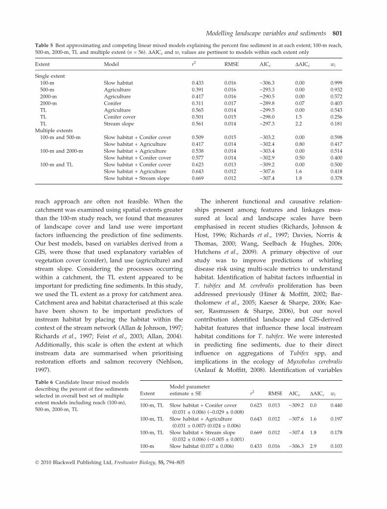
Table 5 Best approximating and competing linear mixed models explaining the percent fine sediment in at each extent; 100-m reach,

500-m, 2000-m, TL and multiple extent (n = 56). DAICc and wi values are pertinent to models within each extent only

Extent Model r2 RMSE AICc DAICc wi

Single extent

100-m Slow habitat 0.433 0.016 )306.3 0.00 0.999

500-m Agriculture 0.391 0.016 )293.3 0.00 0.932

2000-m Agriculture 0.417 0.016 )290.5 0.00 0.572

2000-m Conifer 0.311 0.017 )289.8 0.07 0.403

TL Agriculture 0.565 0.014 )299.5 0.00 0.543

TL Conifer cover 0.501 0.015 )298.0 1.5 0.256

TL Stream slope 0.561 0.014 )297.3 2.2 0.181

Multiple extents

100-m and 500-m Slow habitat + Conifer cover 0.509 0.015 )303.2 0.00 0.598

Slow habitat + Agriculture 0.417 0.014 )302.4 0.80 0.417

100-m and 2000-m Slow habitat + Agriculture 0.538 0.014 )303.4 0.00 0.514

Slow habitat + Conifer cover 0.577 0.014 )302.9 0.50 0.400

100-m and TL Slow habitat + Conifer cover 0.623 0.013 )309.2 0.00 0.500

Slow habitat + Agriculture 0.643 0.012 )307.6 1.6 0.418

Slow habitat + Stream slope 0.669 0.012 )307.4 1.8 0.378

Table 6 Candidate linear mixed models

describing the percent of fine sediments

selected in overall best set of multiple

extent models including reach (100-m),

500-m, 2000-m, TL

Extent

Model parameter

estimate ± SE r2 RMSE AICc DAICc wi

100-m, TL Slow habitat + Conifer cover

(0.031 ± 0.006) ()0.029 ± 0.008)

0.623 0.013 )309.2 0.0 0.440

100-m, TL Slow habitat + Agriculture

(0.031 ± 0.007) (0.024 ± 0.006)

0.643 0.012 )307.6 1.6 0.197

100-m, TL Slow habitat + Stream slope

(0.032 ± 0.006) ()0.005 ± 0.001)

0.669 0.012 )307.4 1.8 0.178

100-m Slow habitat (0.037 ± 0.006) 0.433 0.016 )306.3 2.9 0.103



that specifically promote local increases in fine

sediments in stream habitats in addition to deter-

mining the most appropriate scale at which to draw

inference are invaluable within the context of

whirling disease research and management.

The proportion of slow habitats, a local scale

habitat variable, occurred repeatedly in the set of

best models. Slow water habitats (pools) and fast

water habitats (riffles) represent distinctly different

ecological habitats with notably different biota

inhabiting them. Biota display variations in taxo-

nomic composition, morphology and physiological

traits (Hawkins et al., 1993). At the reach scale, slow

water habitats can often predict the presence of

obligate depositional taxa (Richards et al., 1997) since

they accumulate fine sediments and exhibit a

positive relationship to burrowing invertebrates.

Pools are critical for sediment storage and release

to downstream habitats. Depending on the pool

geometry within a system, sediment transport and

transient sediment storage will vary with gradient,

flow structure and interval, and specific bed topog-

raphy (Rathburn & Wohl, 2003). To understand

sediment dynamics more specifically within a stream

system, an understanding of the major contributors

of sediment is necessary. Further, employing the use

of numerical models to evaluate sediment mobility

and storage given sediment influxes would further

elucidate how sedimentation patterns influence prox-

imal habitats and the aquatic biota inhabitants

(Rathburn & Wohl, 2003). Slow water habitats, along

with other features measured instream, can be

placed in the context of processes occurring at larger

scales thereby mediating the distribution of certain

stream invertebrates through the control over local

habitats (Richards et al., 1997).

Land cover ⁄ land use variables appeared repeatedly

and consistently across spatial extents, emphasising

their importance. Further, models that simultaneously

included reach and landscape predictors were better

than landscape models alone. Townsend et al. (2003)

found that the best prediction of local stream inver-

tebrate diversity was made when variables from

multiple scales were modelled together. In our study,

agriculture and forest cover occurred more frequently

in the competing models at multiple scales. Stream

habitat quality and biotic integrity have been found to

be negatively correlated with agriculture or urbanisa-

tion and positively correlated with the presence of

forest cover (Potter, Cubbage & Schaberg, 2005;

Walters, Roy & Leigh, 2009). Agricultural land use is

frequently associated with increased sedimentation in

stream channels, often altering the invertebrate com-

munities present within the stream (Allan et al., 1997).

Bed substrate characteristics have been shown to be

strongly influenced by land cover patterns at the

scales that extended the entire length of the stream

(Sponseller et al., 2001). Permanent streamside vege-

tation has also been found to explain variation in the

percentage of fines and erosion (Richards et al., 1996)

as well as the variability in benthic invertebrate biotic

index scores (Potter et al., 2005). Forest cover, which

is frequently negatively associated with degraded

stream conditions, was among the most critical habitat

factors. These results testify to the modifying influ-

ence that lateral connections can have on both sedi-

ment delivery and erosional processes.

Intermediate factors or drivers

Although land cover ⁄ land use variables appeared

predominantly in this study, they of course are highly

correlated with other relatively immutable landscape

features such as stream slope, elevation and geology.

These static features exert direct influence over land

cover, and land use is highly influenced by these

geomorphic characteristics. Specifically, land use can

often mask the importance of surficial geology. At

intermediate scales, geology and climate can set

physical limits for subsequent scales and stream

hydrology and riparian vegetation, influenced by

climate and geology contribute to the differences seen

at these finer resolutions (Malmquist, 2002). The

addition of surficial geology can therefore often

account for more variation than inclusion of land

use properties alone (Allan & Johnson, 1997). The

catchment characteristics of the soil porosity (a prod-

uct of surficial geologies), gradient, elevation and

climatic regimes, will influence the variation in loca-

tion and prevalence of particular land use practices

and land cover types. The configuration and compo-

sition of these natural features often influences the

suitability and thereby presence of agricultural land

uses (Allan, 2004).

Although surficial deposits did not appear in any of

the plausible models, geology and groundwater

movement in the Pahsimeroi system are important

features. In the Pahsimeroi River, baseflow of the



mainstem is derived primarily from subsurface flow

and emerges as springs in the Pahsimeroi valley.

Because of this highly groundwater-governed base-

flow, the Pahsimeroi has a fairly stable flow. The

sediments in the lower reaches are rarely disturbed or

reworked providing a secure environment for many

depositional invertebrate taxa to thrive. The geology

of a region gives an indication of the erodibility of the

underlying geologic material, groundwater-surface

water exchange, groundwater chemistry and stream-

bed composition (Gordon, McMahon & Finlayson,

1992). Because of this dynamic situation and the

relatively coarse categorisation of geology in this

study, the lack of prominence of this variable in our

models seems understandable. Further differentiating

between surficial geology formations may have em-

phasised the value of this variable.

Conclusions and management implications

Our study provides insight for managers and other

researchers regarding ways to use multi-scale metrics

and models in a hierarchical fashion to generate

estimates of specific habitat characteristics. Our work

builds on that of others such as Harig & Fausch (2002)

who commented that large-scale variables can be used

as coarse filters in predictive studies to detect differ-

ences in local habitats where needed. Geospatial

techniques such as those used in this study can be

employed to reduce the dependence on costly fine

scale studies. Spatial analysis using GIS technologies

and remote sensing are becoming powerful tools for

restoration planning and site selection (Mollot &

Bilby, 2007; Jorgensen et al., 2009). We used these

tools to supplement invaluable field data collection.

Managers can use GIS-derived metrics to help

prioritise areas of high risk or those best for restora-

tion in a tiered approach (Walters et al., 2009). With a

multi-scale approach, important factors affecting the

hierarchy of habitat relationships can be appropriately

weighted (Hutchens et al., 2009). Because regional

processes influence local stream habitat conditions,

this is a plausible approach to further understanding

of stream structure and communities. The application

of the models for predicting areas of highest likeli-

hood of T. tubifex, and consequently of M. cerebralis

risk, in our study could be validated in drainage

basins throughout the intermountain west. Digitally

available land use characteristics are readily available.

The environmental gradients we observed exist with-

in most drainage basins. The Pahsimeroi River is less

affected by the urban interface and more directly

influenced by the prevalence of agriculture directly

adjacent to the lowland riverine system (Colvin &

Moffitt, 2008). Although the specific composition and

configuration of surficial geology within a drainage

basin will vary, understanding how these feature

correlate to land cover ⁄use, in addition to how these

relationships will affect the distribution of sediments,

will further facilitate the transferable nature of this

model approach.

The presence and distribution of fine sediments

within stream habitats is natural and is a reflection of

both local habitat structure as well as adjacent riparian

composition and upslope processes. Because of the

nature of stream systems, persistent sediment deliv-

ery within the cycle of variable annual flow events,

and persistent sediment deposition within slow water,

low gradient habitats is natural. The conversion of

floodplains to agriculture lands and the elimination of

riparian buffer zones have and will continue to

exacerbate potentially excessive amounts of fine

sediments that not only harbour the intermediate

host for the M. cerebralis parasite, but also provide

little value to spawning and rearing salmonids.

The relative abundance of fine sediments within

these systems can be managed through the use of

erosion control measures and maintenance of riparian

buffers.

Acknowledgments

The Funding was provided by Idaho Department of

Fish and Game, the National Partnership for the

Management of Wild and Native Coldwater Fisheries,

Trout Unlimited, and the Whirling Disease Founda-

tion. M. Colvin, K. Johnson, D. Munson, D. Burton, T.

Garlie, D. Engemann and numerous volunteers pro-

vided logistical support and assistance. R. King, U.S.

Forest Service, B. Shafii, B. Price, M. Colvin and J.

Horne of the University of Idaho provided statistical

assistance. Conceptual approach and assistance was

provided by B. Rieman, J. B. Johnson, A. H. Haukenes,

J. Braatne, J. Trexler and E. Strand. We are grateful to

R. Flitcroft and C. Torgersen for critical review of

earlier drafts. This is contribution 1030 of the Univer-

sity of Idaho Forestry, Wildlife and Range Resources

Experiment Station, Moscow, Idaho.



References

Allan J.D. (2004) Landscapes and riverscapes: the

influence of land use on stream ecosystems. Annual

Review of Ecology, Evolution, and Systematics, 35, 257–

284.

Allan J.D. & Johnson L.B. (1997) Catchment-scale analysis

of aquatic ecosystems. Freshwater Biology, 37, 107–111.

Allan J.D., Erickson D.L. & Fay J. (1997) The influence of

catchment land use on stream integrity across multiple

spatial scales. Freshwater Biology, 37, 149–161.

Alt D. & Hyndman D.W. (1989) Roadside Geology of Idaho.

Mountain Press Publishing Co., Missoula, MT.

Anlauf K.J. & Moffitt C.M. (2008) Models of stream

habitat characteristics associated with tubificid popu-

lations in an intermountain watershed. Hydrobiologia,

603, 147–158.

Bartholomew J.L. & Reno P. (2002) Review: the history

and dissemination of whirling disease. American Fish-

eries Society Symposium, 29, 3–24.

Bartholomew J.L., Kerans B.L., Hedrick R.P., MacDiar-

mid S.C. & Winton J.R. (2005) A risk assessment based

approach for the management of whirling disease.

Reviews in Fisheries Science, 13, 205–230.

Belsley D.A., Kuh E. & Welsch R.E. (1982) Regression

Diagnostics: Identifying Influential Data and Sources of

Collinearity. John Wiley, New York.

Bis B., Zdanowicz A. & Zalewski M. (2000) Effects of

catchment properties on hydrochemistry, habitat com-

plexity and invertebrate community structure in a

lowland river. Hydrobiologia, 422 ⁄423, 369–387.

Bisson P.A., Nielsen J.A., Palmason R.A. & Grove E.L.

(1982) A system for naming habitat types in small

streams, with examples of habitat utilization by

salmonids during low stream flow. In: Acquisition and

Utilization of Aquatic Habitat Inventory Information (Ed.

N.B. Armantrout), pp. 62–73. Western Division,

American Fisheries Society, Portland, OR.

Brinkhurst R.O. (1996) On the role of tubificid oligochaetes

in relation to fish disease with special reference to the

myxozoa. Annual Review of Fish Diseases, 6, 29–40.

Bureau of Land Management (1999) Pahsimeroi Watershed

Biological Assessment. Challis Resource Area, Boise, ID.

Burnham K.P. & Anderson D.R. (2002) Model Selection

and Multimodel Inference: A Practical Information-Theo-

retic Approach. Springer-Verlag, New York.

Colvin M.E. & Moffitt C.M. (2008) Evaluation of irriga-

tion canal networks to assess stream connectivity in a

watershed. River Research and Applications, 25, 486–496.

Davies N.M., Norris R.H. & Thomas M.C. (2000) Predic-

tion and assessment of local stream habitat features

using large-scale catchment characteristics. Freshwater

Biology, 45, 343–369.

Everest F.H., Beschta R.L., Scrivener J.C., Koski K.V.,

Sedell J.R. & Cederholm C.J. (1987) Fine sediment and

salmonid production: A paradox. In: Streamside Man-

agement: Forestry and Fishery Interactions, Contribution

No. 57 (Eds E.O. Salow & T.E. Cundy), pp. 98–142.

Institute of Forest Resources, University of Washing-

ton, Seattle, WA.

Feist B.E., Steel E.A., Pess G.R. & Bilby R.E. (2003) The

influence of scale on salmon habitat restoration prior-

ities. Animal Conservation, 6, 271–282.

Frissell C.A., Liss W.J., Warren C.E. & Hurley M.D.

(1986) A hierarchical framework for stream habitat

classification: viewing streams in a watershed context.

Environmental Management, 10, 199–214.

Gordon N.D., McMahon T.A. & Finlayson B.L. (1992)

Stream Hydrology: An Introduction for Ecologists. John

Wiley and Sons Ltd, West Sussex.

Harig A.L. & Fausch K.D. (2002) Minimum habi-

tat requirements for establishing translocated cutthroat

trout populations. Ecological Applications, 12, 535–551.

Hausle D.A. & Coble D.W. (1976) Influence of sand in

redds on survival and emergence of brook trout

(Salvelinus fontinalis). Transactions of the American

Fisheries Society, 105, 57–63.

Hawkins C.P., Kerchner J.L., Bisson P.A. et al. (1993) A

hierarchical approach to classifying stream habitat

features. Fisheries, 18, 3–12.

Hedrick R.P. (1998) Relationships of the host, pathogen,

and environment: implications for diseases of cultured

and wild fish populations. Journal of Aquatic Animal

Health, 10, 107–111.

Hedrick R.P. & El-Matbouli M. (2002) Recent advances

with taxonomy, life cycle, and development of

Myxobolus cerebralis in the fish and oligochaete hosts.

American Fisheries Society Symposium, 29, 45–53.

Hiner M. & Moffitt C.M. (2002) Epidemiological model-

ing of Myxobolus cerebralis infections in trout: associa-

tions with habitat variables. American Fisheries Society

Symposium, 26, 167–179.

Hutchens J.J. Jr, Schuldt F.A., Richards C., Johnson L.B.,

Host G.E. & Breneman D.H. (2009) Multi-scale

mechanistic indicators of Midwestern USA stream

macroinvertebrates. Ecological Indicators, 9, 1138–1150.

Isaak D.J. & Hubert W.A. (1999) Predicting the effects of

Myxobolus cerebralis across a fifth-order Rocky Moun-

tain watershed. In: Proceedings of the 5th Annual

Whirling Disease Symposium, pp. 151–156. Whirling

Disease Foundation, Bozeman, MT.

Jorgensen J.C., Honea J.M., McClure M.M., Cooney T.D.,

Engie K. & Holzer D.M. (2009) Linking landscape-level

change to habitat quality: an evaluation of restoration

actions on the freshwater habitat of spring-run Chi-

nook salmon. Freshwater Biology, 54, 1560–1575.



Kaeser A.J. & Sharpe W.E. (2006) Patterns of distribution

and abundance of Tubifex tubifex and other aquatic

oligochaetes in Myxobolus cerebralis enzootic areas in

Pennsylvania. Journal of Aquatic Animal Health, 18, 64–

67.

Kaeser A.J., Rasmussen C. & Sharpe W.E. (2006) An

examination of environmental factors associated

with Myxobolus cerebralis infection of wild trout in

Pennsylvania. Journal of Aquatic Animal Health, 18,

90–100.

Krueger R.C., Kerans B.L., Vincent E.R. & Rasmussen C..

(2006) Risk of Myxobolus cerebralis infections to rainbow

trout in the Madison River, Montana, USA. Ecological

Applications, 16, 770–783.

Lazim M.N. & Learner M.A. (1987) The influence of

sediment composition and leaf litter on the distribu-

tion of tubificid worms (Oligochaeta). Oecologia, 72,

131–136.

Littell R.C., Milliken G.A., Stroup W.W., Wolfinger R.D.

& Schabenberger O. (2006) SAS for Mixed Models, 2nd

edn. SAS Institute Inc, Cary, NC.

Malmquist B. (2002) Aquatic invertebrates in riverine

landscapes. Freshwater Biology, 47, 679–694.

Mollot L.A. & Bilby R.E. (2007) The use of Geographic

Information Systems, remote sensing, and suitability

modeling to identify conifer restoration sites with

high biological potential for anadromous fish at the

Cedar River Municipal Watershed in Western

Washington. U.S.A Restoration Ecology, 16, 336–347.

National Oceanographic and Atmospheric Administra-

tion (2004) Endangered and threatened species:

designation of critical habitat for 13 evolutionarily

significant units of Pacific salmon (Oncorhynchus spp.)

and steelhead (O. mykiss) in Washington, Oregon,

and Idaho; proposed rule. Federal Register, 69, 74572–

74846.

Nehlson W. (1997) Prioritizing watersheds in Ore-

gon for salmon restoration. Restoration Ecology, 5, 25–

33.

Poff N.L. (1997) Landscape filters and species traits:

towards mechanistic understanding and prediction in

stream ecology. Journal of the North American Bentho-

logical Society, 16, 391–409.

Potter K.M., Cubbage F.W. & Schaberg R.H. (2005)

Multiple-scale landscape predictors of benthic macro-

invertebrate community structure in North Carolina.

Landscape and Urban Planning, 71, 77–90.

Rathburn S. & Wohl E. (2003) Predicting fine sediment

dynamics along a pool-riffle mountain channel. Geo-

morphology, 55, 111–124.

Reno P.W. (1998) Factors involved in the dissemination

of disease in fish populations. Journal of Aquatic Animal

Health, 10, 160–171.

Reynoldson T.B. (1987) The role of environmental factors

in the ecology of tubificid oligochaetes: an experimen-

tal study. Holarctic Ecology, 10, 241–248.

Richards C., Johnson L.B. & Host G.E. (1996) Land-

scape-scale influences on stream habitats and biota.

Canadian Journal of Fisheries and Aquatic Sciences, 53,

295–311.

Richards C., Haro R.J., Johnson L.B. & Host G.E. (1997)

Catchment and reach-scale properties as indicators of

macroinvertebrate species traits. Freshwater Biology, 37,

219–230.

SAS Institute Inc. (2000) The SAS System for Windows,

Version 8.2. SAS Institute, Cary, NC.

Schisler G.J. & Bergersen E.P. (2002) Evaluation of risk of

high elevation Colorado waters to the establishment of

Myxobolus cerebralis. American Fisheries Society Sympo-

sium, 26, 1–11.

Shumar M.L., Reaney D. & Herron T. (2001) Pahsimeroi

River Subbasin Assessment and Total Maximum Daily

Load. Idaho Department of Environmental Quality,

Boise, ID.

Sponseller R.A., Benfield E.F. & Valett H.M. (2001)

Relationships between land use, spatial scale and

stream macroinvertebrate communities. Freshwater

Biology, 46, 1409–1424.

Townsend C.R., Doledec S., Norris R., Peacock K. &

Arbuckle C. (2003) The influence of scale and geogra-

phy on relationships between stream community

composition and landscape variables: description and

prediction. Freshwater Biology, 48, 768–785.

Walters D.M., Roy A.H. & Leigh D.S. (2009) Environ-

mental indicators of macroinvertebrate and fish assem-

blage integrity in urganizing watersheds. Ecological

Indicators, 9, 1222–1233.

Wang L., Seelbach P.W. & Hughes R.M. (2006) Introduc-

tion to landscape influences on stream habitats and

biological assemblages. In: Landscape Influences on Stream

Habitats and Biological Communities (Eds R. Hughes, L.

Wang & P.W. Seelbach), pp. 1–23. American Fisheries

Society Symposium 48, Bethesda, MD.

Wiens J.A. (2002) Riverine landscapes: taking landscape

ecology into the water. Freshwater Biology, 47, 501–515.

Young H.W. & Harenberg W.A. (1973) A Reconnaissance

of the Water Resources in the Pahsimeroi River Basin,

Idaho. Idaho Department of Water Administration, 73,

Boise, ID.

Zendt J.S. & Bergersen E.P. (2000) Distribution and

abundance of the aquatic oligochaete host Tubifex tubifex

for the salmonid whirling disease parasite Myxobolus

cerebralis in the Upper Colorado River Basin. North Amer-

ican Journal of Fisheries Management, 20, 502–512.

(Manuscript accepted 25 August 2009)



Modelling of landscape variables at multiple extents to predict fine sediments and suitable habitat...

Documents

Transcript of Modelling of landscape variables at multiple extents to predict fine sediments and suitable habitat...