Modelling feeding, growth, and habitat selectionin larval Atlantic cod (Gadus morhua):observations and model predictions in amacrocosm environment

Trond Kristiansen, Øyvind Fiksen, and Arild Folkvord

Abstract: Individual-based models (IBMs) integrate behavioural, physiological, and developmental features and differ-ences among individuals. Building on previous process-based models, we developed an IBM of larval Atlantic cod(Gadus morhua) that included foraging, size-, temperature-, and food-limited growth, and environmental factors such asprey-field, turbulence, and light. Direct comparison between larval fish IBMs and experimental studies is lacking.Using data from a macrocosm study on growth and feeding of larval cod, we forced the model with observed tempera-ture and prey-field and compared model predictions with observed distribution, diet, size-at-age, and specific growthrates. We explored implications of habitat selection rules on predicted growth rates. We analyze the sensitivity ofmodel predictions by the Latin Hypercube Sampling method and individual parameter perturbation. Food limitation pre-vented larvae from growing at their physiological maximum, especially in the period 5–17 days post hatch (DPH). Ac-tive habitat selection had the potential to enhance larval growth rates. The model predicted temperature-limited growthrates for first-feeding larvae (5–20 DPH) when prey density is >5 nauplii·L–1. After age 20 DPH, maximum modelledgrowth required a diet of copepodites. Simulated growth rates were close to observed values except for the period justafter the start of exogenous feeding when prey density was low.

Résumé : Les modèles centrés sur l’individu (IBMs) intègrent les caractéristiques du comportement, de la physiologieet du développement, ainsi que les différences entre les individus. Nous servant de modèles antérieurs basés sur lesprocessus, nous bâtissons un IBM pour les larves de morue franche (Gadus morhua) qui inclut la recherche de nourri-ture, la croissance limitée par la température et l’alimentation, de même que des facteurs du milieu, tels que l’universdes proies, la turbulence et la lumière. Il n’existe pas de comparaisons directes entre les IBM de larves de poissons etles études expérimentales. À l’aide de données provenant d’une étude de la croissance et de l’alimentation de larves demorue en macrocosme, nous avons forcé le modèle avec les températures et les communautés de proies observées;nous avons ensuite comparé les prédictions du modèle à la répartition, au régime alimentaire, à la taille en fonction del’âge et aux taux spécifiques de croissance observés. Nous avons exploré les conséquences des règles de sélection del’habitat sur les taux de croissance prédits. Nous analysons la sensibilité des prédictions du modèle par la méthoded’échantillonnage par hypercubes latins et par la perturbation des paramètres individuels. La pénurie de nourriture em-pêche les larves de croître à leur taux physiologique maximal, particulièrement dans la période des jours 5–17 aprèsl’éclosion (DPH). Une sélection active de l’habitat peut potentiellement améliorer les taux de croissance des larves. Lemodèle prédit des taux de croissance limités par la température chez les larves qui se nourrissent pour la première fois(5–20 DPH), lorsque la densité des proies est >5 nauplius·L–1. À l’âge de 20 DPH, la croissance maximale prédite parle modèle exige un régime composé de copépodites. Les taux de croissance simulés sef rapprochent des valeurs obser-vées à l’exception de la période qui suit immédiatement le début de l’alimentation exogène à un moment où la densitédes proies est basse.

[Traduit par la Rédaction] Kristiansen et al. 151

Introduction

Individual-based models (IBMs) are an important tool thatcan integrate from individual-level properties of environ-mental exposure, behaviour, and physiology to population-

level characteristics of larval fish growth, survival, and spa-tial distribution (Grimm and Railsback 2005). Presently,there are many attempts to develop coupled biophysicalmodels where IBMs of larval fish are embedded in generalcirculation models (Werner et al. 2001; Hinrichsen et al.

Can. J. Fish. Aquat. Sci. 64: 136–151 (2007) doi:10.1139/F06-176 © 2007 NRC Canada

136

Received 24 March 2006. Accepted 9 October 2006. Published on the NRC Research Press Web site at http://cjfas.nrc.ca on30 January 2007.J19240

T. Kristiansen,1 Ø. Fiksen, and A. Folkvord. Department of Biology, University of Bergen, P.O. Box 7800, N-5020 Bergen,Norway.

1Corresponding author (e-mail: trond.kristiansen@bio.uib.no).

2002; Lough et al. 2005). However, direct comparisons be-tween model predictions and the observed growth patternsor feeding habits of larvae in natural or seminatural environ-ments are rare. Therefore, direct comparisons betweenmodel predictions and observations of larval fish feeding,growth, and spatial distribution are warranted. Such effortsmay strengthen our confidence in predictions from large-scale, physical–biological-coupled models. Controlled envi-ronments in macrocosms or landlocked fjords provide a bal-ance between the realism of a natural habitat and thetractability of the laboratory (Folkvord et al. 1994). Informa-tion on the environmental conditions and larval propertiesfrom such studies can be used as forcing data to drive IBMs.

In the pelagic realm, vertical environmental gradients aretypically much stronger than horizontal gradients. Therefore,

when implementing IBMs into circulation models, accuraterepresentation of the vertical distribution is important forpredicting the exposure of larvae to environmental factors.Also, the horizontal dispersal of larvae often depends ontheir vertical positioning (Vikebø et al. 2005). However,little information exists on criteria for habitat selection oflarval Atlantic cod (Gadus morhua). This is particularly sofor larvae facing trade-offs between food availability, tem-perature, advection, and predation risk. Here, we present amechanistic model of foraging and growth of cod larvae.The feeding processes are adopted from Fiksen and Mac-Kenzie (2002), while our formulation of assimilation andtransformation of energy from prey to larval tissue andgrowth is new. It incorporates the empirical models devel-oped by Finn et al. (2002) and Folkvord (2005). Explicit

© 2007 NRC Canada

Kristiansen et al. 137

Fig. 1. (a) Temperature distribution (°C) and (b) average prey abundance (µg·L–1) during the macrocosm experiment and observed(c) day and (d) night distribution (%·m–1) of larval Atlantic cod (Gadus morhua).

R NI NII NIII NIV NV NVI CI CII CIII CIV H M

lpi (mm) 0.10 0.22 0.27 0.40 0.48 0.55 0.61 0.79 1.08 1.38 1.80 0.30 0.60dpi (mm) 0.10 0.10 0.10 0.10 0.15 0.18 0.20 0.22 0.25 0.31 0.40 0.10 0.30wpi (µg) 0.16 0.33 0.49 1.0 1.51 2.09 2.76 4.18 13.24 23.13 63.64 0.30 1.00

Note: R, rotifer; N, nauplius; C, copepodite; H, harpactacoid; M, miscellaneous. Sizes taken from Lough et al. (2005). Image area of prey (Ap, mm2) isestimated as lp × dp × 0.75 (elongate prey).

Table 1. Length (lpi), width (dpi), and dry weight (wpi) for the 13 various zooplankton categories (i) available as prey in the pond.

simulations of the macrocosm experiment by Folkvord et al.(1994) allow for direct comparison between model predic-tions and observed properties of the larvae in a monitored,nearly predator-free environment. We compare modelledand observed growth and diet of larvae for the first 42 daysof their life. In addition, we explore the effects of habitat se-lection by the larvae on realized growth rates in the pond.

Biological background: the macrocosmexperiment

This model effort uses observed temperature and preydensity from a macrocosm experiment (Folkvord et al. 1994)as forcing. Observations of larval growth and weight at datesare compared with model predictions. Below, we provide abrief summary of the Folkvord et al. (1994) experiment.

SamplingIn spring 1983, larval Atlantic cod were released in five

cohorts separated by 10-day intervals into the 5.5 m deepnaturally enclosed 63 000 m3 Hyltropollen (Folkvord et al.1994). Fish larvae were 5 days post hatch (DPH) at the dayof release and still at the yolk-sac stage. A total of 40 000larvae samples were collected between 20 March and 3 May1983, and 4354 larvae were individually measured. The en-vironment was monitored by weekly measurements of tem-perature (Fig. 1a) and zooplankton biomass (Fig. 1b) at 1 mintervals from the surface to the bottom (Folkvord et al.1994). Observations of zooplankton and temperature areavailable to day 42 (47 DPH) of the experiment.

The environmentAn average turbulent dissipation rate was estimated using

the mean wind field obtained from the Meteorological Insti-tute in Norway for a nearby station (Flesland) and the empir-ical relationship between wind and turbulence fromMackenzie and Leggett (1993). Both temperature and zoo-plankton concentrations showed strong vertical and temporalvariation (Fig. 1). Initially, strong vertical gradients charac-terized the hydrography after a cold weather period withpatches of ice at the surface. By mid-April, most of the gra-dients had eroded and the water column was mixed(Fig. 1a).

PreyIn late March, total zooplankton biomass was very low at

the surface but increased towards the bottom (Fig. 1). Astime passed, the zooplankton became distributed homo-genously in the water column. Prey types available in thepond were nauplii and copepodite stages of Calanus finmar-chicus, rotifers, and harpacticoids. Rotifers were an impor-tant prey item for first-feeding larvae (Folkvord et al. 1994).A peak in abundance of rotifers occurred in the beginning ofApril (33·L–1 at the surface). Total prey density rarely ex-ceeded 10·L–1 with an average close to 6·L–1 (Folkvord et al.1994). Mean, standard deviation, minimum, and maximumvalues for the period 20 March – 1 May were 1.0 ± 5.0·L–1

(0.0–33·L–1) for rotifers, 2.1 ± 1.7·L–1 (0.1–8.3·L–1) fornauplii, 0.6 ± 0.4·L–1 (0.1–1.9·L–1) for copepodites, 0.5 ±

1.0·L–1 (0.0 ± 5.8·L–1) for harpacticoids, and 1.7 ± 2.2·L–1

(0.3 ± 13.6·L–1) for miscellaneous species.The sampling only separated between nauplii and cope-

podites. To obtain smaller incremental steps between size-classes of prey, we divided the C. finmarchicus data intodevelopmental stages NI–NVI for nauplii and CI–CIV forcopepods (Table 1). We assumed an exponential decrease innumbers between stages, where prey concentrations and preysize spectra correspond to estimated densities of nauplii andcopepodites (Table 1).

Model description

The model description follows the outline recommendedby Grimm and Railsback (2005) (PSPC + 3).

PurposeThis IBM simulates the early life history of larval cod

based on environmental factors and underlying processesthat we believe are important. Each process is formulatedand parameterized from laboratory experiments conductedon larval cod (Fiksen and MacKenzie 2002). The combina-tion of these processes describes mechanistically how larval

© 2007 NRC Canada

138 Can. J. Fish. Aquat. Sci. Vol. 64, 2007

Fig. 2. Flow chart of the individual-based model (IBM) wheresubmodels are open boxes and state variables are shaded boxes.Each hourly calculations start with estimation of encounter, ap-proach, capture, and ingestion for 13 prey types and sizes. In-gested biomass is stored in the stomach variable and determinestogether with ambient temperature the corresponding growth. Themodel has a spatial and temporal resolution of 1 m. Larval draw-ing by Tamara L. Clark, Woods Hole, Massachusetts.

cod encounter, capture, and ingest food and use the energyfor growth. The main purpose is to evaluate model perfor-mance in a well-studied seminatural situation.

StructureWe simulated growth for a period of 5–47 DPH for 160

individual cod larvae in a closed macrocosm with no preda-tors assuming no mortality and no interactions among indi-vidual larvae. Behavioural responses to changes in theenvironment were restricted to vertical movements with aspatial resolution of 1 m and a temporal resolution of 1 h.

ProcessesSubmodels govern the interaction between environmental

forcing (temperature, turbulence, and zooplankton density)and the dynamic state variables weight, stomach content,and length. These states are updated once every hour(Fig. 2). A key element is the mechanistic foragingsubmodel combined with a stomach as a state variable. In-gested mass or energy results from the successful comple-

tion of sequential processes: encounter, approach, and cap-ture (Fiksen and MacKenzie 2002). The foraging processesare iterated for all prey types and size categories (Fig. 2).Holling’s (1966) disc equation ensures that the total timespent handling prey reduces available search time. Stomachfullness and body mass determine whether growth is onlytemperature dependent or also food limited.

ConceptsAn important and difficult topic for larval fish modelling

is the behavioural positioning of the larvae in environmentalgradients. We expect strong selection pressures on habitatselection in larval fish, since the pelagic environment is typi-cally characterized by strong vertical gradients of variablesrelated to growth (temperature, prey concentrations, light,and turbulence), predation risk (distribution and search effi-ciency of predators), and the probability of being advectedout of favourable areas (Werner et al. 1993; Vikebø et al.2005). Here, we explore the consequences of four differentvertical behavioural rules: (i) larvae move along the depth of

© 2007 NRC Canada

Kristiansen et al. 139

Symbol Description Units Value

SGRa Specific growth rate %·day–1 Eq. 2Rb Respiration rate µg Eq. 1s Stomach size µg·µg–1·individual–1 Eq. 5wpi Weight of prey of type i µg Table 1lpi Length of prey type i mm Table 1dpi Width of prey type i mm Table 1ec Encounter rate Prey·s–1

e fr r Nf u= + +23

23 2 2 2π π λ ω

f c Pause frequency s–1 0.43N Prey density mm3

r d Distance of perception mmr cr E CA

E

E K2

pb

b e

exp( ) = ′+

u Prey swimming speed mm·s–1 100 × lpi

ωe Turbulent velocity mm·s–1ω ε= 3.615 0.667( )r

λc Pause duration s 2.0E ′g Eye sensitivity of larva Dimensionless

ESL

C′ =

× × ×

2

0.1 0.2 0.75

Cd Prey inherent contrast Dimensionless 0.4Ap

f Image of elongate prey mm2 lp × dp × 0.75

Ked Larva half-saturation parameter µmol·m–2·s–1 1.0

Ebd Light µmol·m–2·s–1 Eb(z,h) = E0(h)exp(–zk)

Ah Assimilation efficiency Dimensionless 0.75c Beam attenuation coefficient m–1 3kεe Turbulent dissipation rate kg·m–2·s–3 ε = 5.82 × 10–9W 3

W Windspeed m·s–1 3.0k Attenuation coefficient m–1 0.18

aFolkvord (2005).bFinn et al. (2002).cMacKenzie and Kiørboe (1995).dAksnes and Utne (1997).eMacKenzie and Leggett (1993).fFiksen and Folkvord (1999).gFiksen and MacKenzie (2002).hKiørboe (1989).

Table 2. Variables and parameters from the IBM.

observed larval maximum abundances (ObsD), (ii) larvaefollow the depth of highest temperature (HighT), (iii) larvaemove along the depth with highest prey biomass (HighP),and (iv) larvae find the depth that yields the highest growthrate (HighG). We also included a simulation of larvae with-out active selection, i.e., larvae that move randomly up ordown the water column. Our null hypothesis was that indi-viduals with a strategy would grow faster than individualsmoving randomly in the water column. To test this, we re-corded average weight-at-age and depth distribution of 100individuals for 32 days with random vertical positioning. Alllarvae were initialized with a start weight of 58 µg.

InitializationWe used observed data on each of four dates (26 and 31

March and 6 and 10 April) to describe the initial populationweight distribution. For each date (11, 16, 22, and 26 DPH),we drew 160 (maximum number of larvae sampled at 16DPH) individual weights randomly from the observations toyield averages of 58 ± 9, 112 ± 22, 234 ± 48, and 410 ± 87 µg,respectively. Using the four start dates and 160 individuals,simulations were repeated for the four rules. This resulted in2560 individual realizations.

The simulation initiated on 10 April was run until 47 DPHand was compared with final observations from the pond onday 49, the final day of the Folkvord et al. (1994) experi-ment. This provides us with as many direct comparisonsbetween predictions and observations as possible and alsoallows for identifying under which environmental conditionsthe model failed.

InputObserved (Folkvord et al. 1994) prey density and turbu-

lence were input to the foraging processes and temperaturefor the growth processes. We modelled light as a function ofdate, time of day, and latitude.

Submodels

The IBM was written as an object-oriented Fortran 90code, which allows for tracking properties for every individ-ual. Following is a detailed description of the varioussubmodels.

Larval feeding processesPrey encounter rate, pursuit success, and capture success

determine larval feeding success. We applied the detailedand mechanistic model by Fiksen and MacKenzie (2002)based on earlier developments (MacKenzie and Kiørboe1995; Aksnes and Utne 1997; Caparroy et al. 2000). Thismodel predicts (i) prey encounter rates as a function of preycharacteristics, larval size, ambient light, turbulence, andprey density and the probability that (ii) prey detect the ap-proaching larvae and escape (Psa), (iii) prey are advected outof the larva’s perception range owing to turbulence (Psp),and (iv) prey are successfully captured and ingested (Pca).

Prey ingestion is limited by stomach capacity, while the preyitems that compose the diet are estimated from all preyitems captured within the last time step. Predictions fromthis model generated larval prey size selectivity in agree-ment with observations by Munk (1997). Key variables andparameter values are defined in Table 2. Visual foragers de-pend on light. Light conditions Eb vary with time of day hand depth z and are a function of the surface light E0 and thediffuse light attenuation k (Table 2). Surface light is calcu-lated according to time of day, latitude (60°N), and day ofthe year (here, 20 March – 2 May 1983).

Respiration ratesRoutine respiration rate of larval cod was thoroughly esti-

mated by Finn et al. (2002). Routine respiration R (µg·indi-vidual–1·h–1) varies with dry-weight body mass w (mg) andtemperature T (°C) as

(1) R w T= × −2.38 10 0.0.880.97 exp( )

Respiration rates were measured in light and darkness (Finnet al. 2002). Higher values occurred in light than in dark-ness, indicating that the values from darkness were closer toresting respiration. In the present model, we have applied theaveraged value for R. The metabolism is elevated by a factorof 2.0 (Lough et al. 2005) when light conditions are suitablefor foraging (visual range ≥1.0 mm) and the larvae are ac-tive.

Size- and temperature-limited growth rateIf the larvae ingest more food than they can process and

assimilate, then size- and temperature-dependent physiologi-cal processes will limit their growth. We applied the modelderived from extensive laboratory rearing experiments oncoastal cod by Otterlei et al. (1999) and Folkvord (2005) tofind larval specific growth rates (SGR, %·day–1) under suchconditions:

(2) SGR 2 3( , ) ln( ) ln( ) ln( )w T a b w c w d w= − − +

where SGR is the specific growth rate in percentage per day,expressed as a function of temperature (T) and dry mass(w, mg), and a = 1.08 + 1.79T, b = 0.074T, c = 0.0965T, andd = 0.0112T (Folkvord 2005). The SGR can be expressed asspecific growth rate g per time step (dt, day–1), g =ln[(SGR/100) + 1)/dt].

Larval state variables and food-limited growthLarvae are characterized by the state variables body mass

(w, dry weight) and stomach fullness (s). The maximum en-ergy content of the stomach (s) is set to 6.0% of the totalweight, which corresponds to observations of stomach con-tent and size of cod larvae on Georges Bank (E. Broughton,National Marine Fisheries Service, NOAA, Northeast Fish-eries Science Center, Woods Hole, MA 02543, USA, per-sonal communication) and to the upper limit of ingestedmaterial used by Lough et al. (2005). The amount of food inthe stomach and the growth potential of the larvae determine

© 2007 NRC Canada

140 Can. J. Fish. Aquat. Sci. Vol. 64, 2007

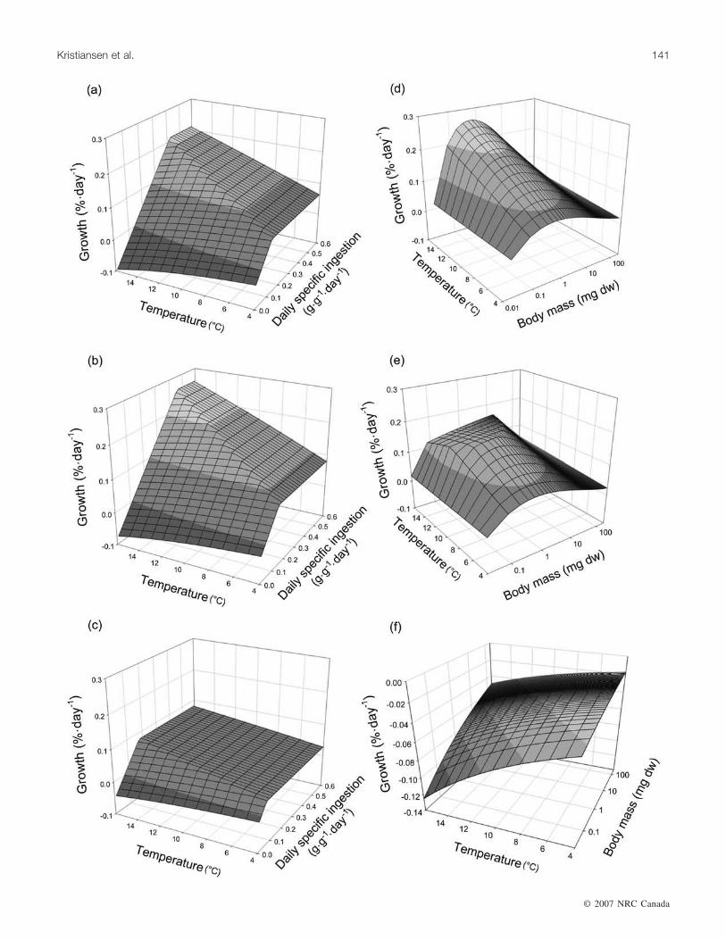
Fig. 3. Growth rates (left panels) for three fish sizes, (a) 0.1, (b) 1.0, and (c) 100 mg, experiencing a range of ingestion rates (0–0.6 g·g–1·day–1) and temperatures (4–16 °C). Also shown are larval and juvenile (0.01–100 mg) growth rates assuming three fixed in-gestion rates (d) 0.8, (e) 0.3, and (f) 0.0 g·g–1·day–1 for different temperatures (4–16 °C).

© 2007 NRC Canada

Kristiansen et al. 141

whether growth is maximal (size and temperature limited) orfood limited.

The mass (or energy) D required to sustain maximalgrowth within each time step is given by

(3) D t gw R A= +d ( )/

Here, A is the assimilation efficiency equal to 0.75, correct-ing for energy losses through feces and specific dynamic ac-tion (Kiørboe 1989). The stomach then acts as a reactor anddynamic storage where mass is withdrawn depending on po-tential growth. The stomach fullness is a function of previ-ous state st, digested material D, and ingestion i:

(4) s s D it t+ = − +1

The change in body mass dw within each time-step is thengiven by

(5)ddwt

gw D s

sA R D st

t

=≤

− >

if

if

This is where growth becomes either food or temperaturelimited. If stomach content st can supply the matter and en-ergy required D (D = st), then growth proceeds at maximumrate. Otherwise, if D > st, then what is in the stomach is pro-cessed and turned into body mass. The predicted growthrates of larval cod under various temperatures, body mass,and prey ingestion rates are presented in Fig. 3. This ap-

proach integrates solid laboratory studies on larval codgrowth and metabolism and a simple, but reasonable, repre-sentation of mass and energy flow through the larvae. Themodel predicts that growth drops linearly with food avail-ability below a threshold that depends on both temperatureand larval weight (Fig. 3c). It captures the general view thatfood requirements are higher when growth rates are high andacts as an interpolation between the food-satiated growthpattern observed by Folkvord (2005) and the starving caseof Finn et al. (2002) (Fig. 3b).

Sensitivity analysis

Trust in model predictions is gained through validationand testing of the IBM. Comparison between simulation re-sults and observations may increase confidence in the hy-potheses formalized in the model, depending on its ability tomatch observed patterns. Also, the importance of submodelsin a complex model can be analyzed through sensitivity anal-yses. If small changes in parameter values generate large re-sponses, the model is sensitive to the parameter.

Sensitivity analysis of the IBM was performed using aMonte Carlo simulation where parameter values are ran-domly selected from a distribution. We implemented thismethod using Latin Hypercube Sampling (Rose 1987; Roseet al. 1991b) and used it to determine the contribution of pa-rameter variation to prediction error (Bartell et al. 1986).First, we assigned a specific distribution for all parameters

© 2007 NRC Canada

142 Can. J. Fish. Aquat. Sci. Vol. 64, 2007

r2

10% increase individualparameter perturbation (%increase in weight from baseafter 48 h)

Parameter–variable

Mean value

(min.–max.) 5 mm 11 mm Submodel 5 mm 11 mm

ExternalTemperature (°C) 7.0 (6.5–7.5) 0.05 0.98 Environment 0.4 1.6Prey density (L–1) 2.5 (0.5–4.5) 0.88 0.02 0.4 0.05Surface wind 3.0 (1.0–5.0) 0.00 0.00 0.1 0.01Surface light (µmol·m–2·s–1) 250 (200–300) 0.00 0.00 0.0 0.0Beam attenuation coefficient (m–1) 0.18 (0.1–0.3) 0.00 0.00 –0.3 0.0Attenuation coefficient (m–1) 0.54 (0.33–0.89) 0.00 0.00 –0.1 0.0Sum 0.94 1.00

InternalInitial perception (mm2) 0.015 (0.014–0.016) 0.00 0.01 Mechanistic foraging –0.5 –0.06Attack speed (m·s–1) 10 (8–12) 0.34 0.08 2.9 0.02Escape speed (m·s–1) 100 (80–120) 0.32 0.08 –0.1 –0.07Mean jump angle (rad) π/6 (0.3–0.7) 0.12 0.01 –0.3 0.0Half-saturation parameter 1.0 (0.001–5) 0.00 0.00 –0.2 0.0Activity (dimensionless) 2.0 (1.5–2.5) 0.00 0.00 Bioenergetic 1.4 0.0Respiration exponent (dimensionless) 0.9 (0.85–0.95) 0.00 0.01 1.4 0.0Gut size (% dry weight) 0.06 (0.05–0.07) 0.03 0.24 0.45 0.5Assimilation (dimensionless) 0.75 (0.6–0.9) 0.00 0.01 3.1 0.0Sum 0.81 0.45

Note: Mean values of the parameter distribution are shown together with the range (min.–max.). The influence (r2) from each parameter on the simu-lated weight (after 48 h) is given for two larval sizes (5 and 11 mm). By increasing the parameter value by 10%, the corresponding increase in weight(% increase from base run) is given in the individual parameter perturbation columns for two sizes of larval cod.

Table 3. Variables and parameters examined in the sensitivity analysis, divided into internal and external variables, and further groupedinto submodel level.

included in the error analysis. The nominal value for eachparameter defines the mean value of the distribution. Wethen drew values randomly from the distributions to create aset of parameter values in each model realization.

A typical approach to sensitivity analysis in IBMs is theindividual parameter perturbation method where eachvariable–parameter in the model is varied ±10% or ±20%between simulations. Model results (weight in this case),with and without this change, determine the impact of the

change in variable value. Although this method leaves uswith an indication of the sensitivity of that particular vari-able, the results can be biased if different processes behavein a nonlinear fashion and interaction exists between vari-ables (Gardner and O’Neill 1981). We included the individ-ual parameter perturbation approach as a companion to theerror analysis.

The Monte Carlo error analysis combined with the LatinHypercube Sampling approach has been used by several au-

© 2007 NRC Canada

Kristiansen et al. 143

Mean density (no.·L–1 ± SD (min.–max.))

Simulation period (DPH) ObsD HighT HighP HighG

5–22 Total prey density 2.4±0.8 (1.0–4.0) 2.7±0.9 (0.9–4.4) 4.8±2.2 (1.2–10.0) 3.5±2.0 (0.9–10.0)Available for larva 1.2±0.6 (1.3–2.9) 1.3±0.5 (0.4–2.6) 2.8±1.7 (0.4–6) 1.9±1.2 (0.7–5.7)

22–47 Total prey density 2.4±0.7 (1.4–4.0) 2.7±1.0 (0.9–4.4) 6.1±1.8 (4.0–10.0) 2.7±0.9 (0.9–4.3)Available for larva 2.1±0.7 (1.0–3.7) 2.1±0.8 (0.9–3.8) 5.4±1.6 (3.3–9.0) 2.1±0.8 (0.9–3.8)

Note: The simulation period for the first 17 days post hatch (DPH) and that for the last 25 DPH are separated, as the size of the larvae in the timewindows differs significantly and thereby the number of available prey types for ingestion. Only C. finmarchicus is considered, as this is the dominantprey item found in gut analysis (Folkvord et al. 1994) both in observations and in simulations. ObsD, depth where maximum abundances of larvae wereobserved during assessment; HighT, depth of highest temperature; HighP, depth with highest prey biomass; HighG, depth that yields the highest growthrate.

Table 4. Density of Calanus finmarchicus (nauplii and copepodites) in the water column as experienced by a larva according to verti-cal behavioural rule and age.

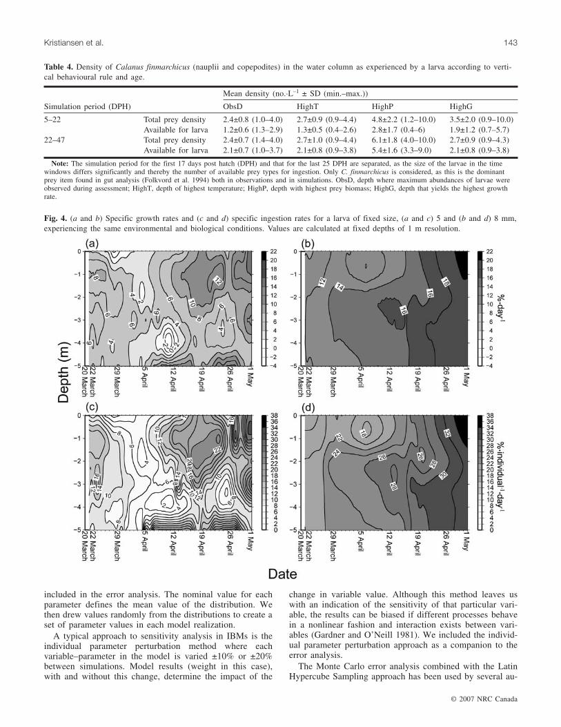
Fig. 4. (a and b) Specific growth rates and (c and d) specific ingestion rates for a larva of fixed size, (a and c) 5 and (b and d) 8 mm,experiencing the same environmental and biological conditions. Values are calculated at fixed depths of 1 m resolution.

thors (Rose et al. 1991a; Letcher et al. 1996; Megrey andHinckley 2001). In general, these studies found the methodsto provide similar results for linear models. We applied theerror analysis to the IBM model in two steps by varying(i) six of the external (environmental) variables and (ii) 10of the internal variables.

We assumed a normal distribution of both internal and ex-ternal parameters by defining a mean, minimum, and maxi-mum value of each parameter (Table 3). Each parameterdistribution was sampled 300 times. During sensitivity anal-ysis of the internal parameters, the environmental variablesare not kept constant but vary according to observations. In-ternal and external parameter analysis resulted in two datasets of size 300 times 11 and 7 (parameters and simulatedlarval weight), respectively. These data sets were further ana-lysed statistically by simple correlation analysis (Pearson).Correlation between parameters and model results deter-mines the individual contribution from each parameter tomodel variance. We repeated the analysis for two sizes oflarval cod (5 and 11 mm).

Results

Sensitivity analysisThe Monte Carlo sensitivity analysis revealed interesting

properties of the model. In particular, growth rates were sen-sitive to variance in certain variables, which differed for

large and small larvae (Table 3). For small larvae (5 mm),prey density strongly influences growth. The range of preydensity varied between 0.8 and 10 nauplii·L–1 depending onchoice of vertical rule. Estimated prey concentration withinedible size range depended on larval size and vertical rule(Table 4), with very low values for age 5–22 DPH larvae(0.4–6 nauplii·L–1). For small larvae, the prey size categoryavailable for capture is limited to rotifers and small nauplii(NI-NIII) (Table 1). The sensitivity of the internal parame-ters revealed that small changes in prey escape speed andlarval attack speed can increase or decrease the range of pos-sible prey items (Table 3). In a food-limited situation, this iscritical to maintain high growth rates. Larger larvae (11 mm)are unaffected by variation in prey density, as long as thevalues exceed 2–3 nauplii·L–1 (Table 4), and variance ingrowth is explained almost solely by the changes in temper-ature (r2 = 0.98) (Table 3). This situation also explains whyparameters related to foraging efficiency are sensitive forsmall but not for larger larvae. Similarly, gut size is impor-tant for larger larvae, since maintaining growth during nightis occasionally dependent on stomach capacity.

Variation in surface light, beam attenuation, and extinctioncoefficient does not influence the result at all, mainly be-cause light conditions limit foraging only at sunset and atnight. The pond is shallow so that light is not the importantlimiting factor; this has been shown to be so in models ofcod in marine environments (Lough et al. 2005).

© 2007 NRC Canada

144 Can. J. Fish. Aquat. Sci. Vol. 64, 2007

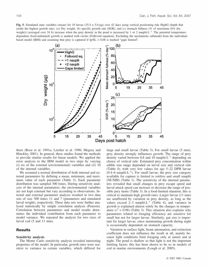
Fig. 5. Simulated state variables (mean) for 10 larvae (35.4 ± 5.6 µg) over 42 days using vertical positioning rule HighG (depth thatyields the highest growth rate). (a) Dry weight, (b) specific growth rate (SGR), and (c) stomach fullness (% of maximum (6% dryweight)) (averaged over 24 h) increase when the prey density in the pond is increased by 1 or 2 nauplii·L–1. The potential temperature-dependent (food-unlimited) growth is marked with circles (Folkvord equation). Excluding the mechanistic submodel from the individual-based model (IBM) and assuming that prey is captured if lp/SL < 0.08 is marked “gape limited”.

Comparison between simulation runs with a 10% increasein parameter values (individual parameter perturbationmethod) produces low impact on the simulated weight over48 h. The growth difference was generally lower than 1%,with the exception of the attack speed of the larvae and theprey escape speed for small larvae.

Vertical behaviour and growth ratesBehavioural conduct in a spatial environment affects the

potential growth rates for small larvae, even in a pond ofonly 5 m depth. Modelled growth and ingestion rates for a5 mm larva vary considerably between depths (Figs. 4a and4c). One of the rules applied for habitat selection is relatedto growth (HighG), and therefore, modelled habitat selectionbecomes dependent on stomach fullness, temperature, andprey density (Figs. 5 and 6). Larvae adapting to rule HighGachieve the highest growth rates. Larvae of size 5 mm aremechanistically restricted to forage on rotifers and copepodnauplii compared with 8 mm larvae that are capable of cap-turing copepodites. This results in large depth-dependent dif-ferences in growth rates for the two sizes of larval cod(Fig. 4) that experience the same habitat. Growth rates aremainly temperature dependent for 8 mm larvae, whilegrowth of a 5 mm larva depends on the correct choice ofhabitat. Given the relatively low prey concentrations foundin the pond (Table 4), a small increase in nauplii (1–2·L–1)increases the growth rates considerably for small larvae, es-pecially at the onset of feeding (Fig. 5). The minimum preydensity necessary to obtain purely temperature-dependent

growth rates was analyzed by increasing the prey concentra-tion of nauplii (NI) in the macrocosm from 1 to 10·L–1

(Fig. 6). A prey density of >10 nauplii·L–1 enables small lar-vae (5 mm) to encounter and capture enough prey to sustainthe energetic demands of temperature-dependent growth(Fig. 6), although at 25 DPH, growth is food limited, and thelarva needs to switch to or include copepodites in the diet tosustain optimal growth rates. Otherwise, the larva is eventu-ally limited by the encounter rate and ceases to captureenough prey. To determine the effect of the mechanisticsubmodel, we modelled growth where foraging is gape lim-ited and where upper prey length to predator length ratio is amaximum of 8%. Corresponding growth increases equal toan increase in prey density of 2 nauplii·L–1 (Fig. 5).

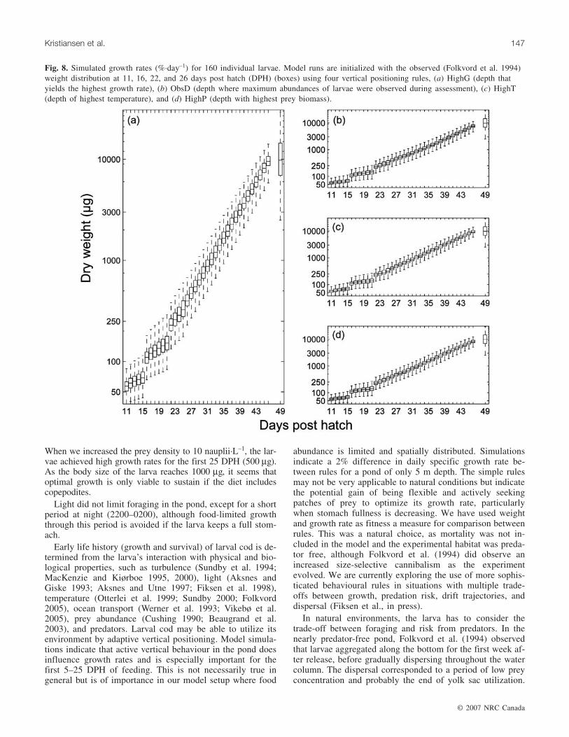
Average observed growth rates for the population aged 5–25 DPH were 12.7%·day–1 (Folkvord et al. 1994), while sim-ulated growth rates depended on the choice of verticalbehavioural rule, 9.1%, 10.5%, 10.7%, and 11.2%·day–1 forObsD, HighT, HighP, and HighG, respectively (Fig. 7). Sim-ulated growth rates for larval age 5–22 DPH were lower thanobserved, but the difference diminished after 22 DPH as thesimulated larvae increased in size and grew close to observa-tions (Figs. 7 and 8).

DietGut analysis of larval cod revealed a diet consisting of ro-

tifers and nauplii for the first 20 DPH (Folkvord et al. 1994)and then switched to a diet composed mainly of copepodites(90% of the energy and 20% of the prey items in the stom-

© 2007 NRC Canada

Kristiansen et al. 145

Fig. 6. Simulated state variables (mean) for 10 larvae (35.4 ± 5.6 µg) over 42 days using vertical positioning rule HighG. (a) Dryweight, (b) specific ingestion rate (before assimilation), and (c) specific growth rate increase gradually as prey concentration is raisedfrom 1 to 10 nauplii·L–1. The potential temperature-dependent (food-unlimited) growth is marked with circles (Folkvord equation).

ach) (Fig. 9, top left panel). Nauplii are the most abundantprey in the pond, which is also reflected in simulated gutcontents (Fig. 9). After day 20, the larger larval size opensup for a wider range of prey items and the importance ofcopepodites increases (Fig. 9).

Rules compared with random walkWeight-at-age varied for larvae following different rules,

and all rules perform better than a random movement strat-egy (Fig. 10a). Larvae moving according to rules HighP andHighG did best. The vertical movement during 32 days for alarva following rule HighG varies considerably over time(Fig. 10b). The frequent vertical repositioning is related tostomach dynamics: which habitat has maximum growth ratesdepends on stomach fullness, temperature, and prey abun-dance (Fig. 10c). The vertical position of the larva followsthe depth where prey abundance satiates maximum growth atthe highest possible temperature (Figs. 10c, 1a, and 1b). Theaverage depth for the random walk converges towards an av-erage of 2.5 m.

Discussion

Sensitivity analysis suggests that small changes in param-eters or variables do not create large differences in simula-

tion results. This reassures us that the model is robust withinthe parameter space, possibly with the exception of the preyjump speed and the cod attack speed for small larva. TheIBM uses the ratio between larva attack speed and prey es-cape speed (1/10), as discussed by Fiksen and MacKenzie(2002) in the calculation of the capture success. A larval at-tack speed of 10 standard lengths·s–1 and a prey escapespeed of 100 prey lengths·s–1 are based on intermediate val-ues from experiments (for details, see Fiksen and Mackenzie2002). An increased ratio results in an increased capture suc-cess (restricted by the gape limitation of the larva) and viceversa. However, the selected ratio simulates a prey prefer-ence size of 5% of larval body length (Fiksen and MacKen-zie 2002) and agrees well with observations by Munk(1997). This indicates that the chosen velocity values aresensible, although an improved version of this IBM wouldgain realism by including differences between prey species,e.g., contrast of prey to the background and difference in es-cape speed between species.

Smaller larvae are sensitive to changes in prey density,which is not surprising, as 2–4 nauplii·L–1 seems to be theminimum values needed for larvae to sustain metabolism.Model results predict that larvae are able to grow at 2%–5%·day–1 at quite low prey density (2 nauplii·L–1), althoughgrowth after 25 DPH at this prey density is severely limited.

© 2007 NRC Canada

146 Can. J. Fish. Aquat. Sci. Vol. 64, 2007

Fig. 7. Simulated growth rates for 160 individual larvae. Model runs are initialized with the observed (Folkvord et al. 1994) weightdistribution at 11, 16, 22, and 26 days post hatch (DPH) (arrows) using four vertical positioning rules, (a) ObsD (depth where maxi-mum abundances of larvae were observed during assessment), (b) HighT (depth of highest temperature), (c) HighP (depth with highestprey biomass), and (d) HighG (depth that yields the highest growth rate). Temperature-limited growth rate is estimated using the aver-age weight distribution for each day (line) and defines the upper physiological restricted growth rate for the given environment.

When we increased the prey density to 10 nauplii·L–1, the lar-vae achieved high growth rates for the first 25 DPH (500 µg).As the body size of the larva reaches 1000 µg, it seems thatoptimal growth is only viable to sustain if the diet includescopepodites.

Light did not limit foraging in the pond, except for a shortperiod at night (2200–0200), although food-limited growththrough this period is avoided if the larva keeps a full stom-ach.

Early life history (growth and survival) of larval cod is de-termined from the larva’s interaction with physical and bio-logical properties, such as turbulence (Sundby et al. 1994;MacKenzie and Kiørboe 1995, 2000), light (Aksnes andGiske 1993; Aksnes and Utne 1997; Fiksen et al. 1998),temperature (Otterlei et al. 1999; Sundby 2000; Folkvord2005), ocean transport (Werner et al. 1993; Vikebø et al.2005), prey abundance (Cushing 1990; Beaugrand et al.2003), and predators. Larval cod may be able to utilize itsenvironment by adaptive vertical positioning. Model simula-tions indicate that active vertical behaviour in the pond doesinfluence growth rates and is especially important for thefirst 5–25 DPH of feeding. This is not necessarily true ingeneral but is of importance in our model setup where food

abundance is limited and spatially distributed. Simulationsindicate a 2% difference in daily specific growth rate be-tween rules for a pond of only 5 m depth. The simple rulesmay not be very applicable to natural conditions but indicatethe potential gain of being flexible and actively seekingpatches of prey to optimize its growth rate, particularlywhen stomach fullness is decreasing. We have used weightand growth rate as fitness a measure for comparison betweenrules. This was a natural choice, as mortality was not in-cluded in the model and the experimental habitat was preda-tor free, although Folkvord et al. (1994) did observe anincreased size-selective cannibalism as the experimentevolved. We are currently exploring the use of more sophis-ticated behavioural rules in situations with multiple trade-offs between growth, predation risk, drift trajectories, anddispersal (Fiksen et al., in press).

In natural environments, the larva has to consider thetrade-off between foraging and risk from predators. In thenearly predator-free pond, Folkvord et al. (1994) observedthat larvae aggregated along the bottom for the first week af-ter release, before gradually dispersing throughout the watercolumn. The dispersal corresponded to a period of low preyconcentration and probably the end of yolk sac utilization.

© 2007 NRC Canada

Kristiansen et al. 147

Fig. 8. Simulated growth rates (%·day–1) for 160 individual larvae. Model runs are initialized with the observed (Folkvord et al. 1994)weight distribution at 11, 16, 22, and 26 days post hatch (DPH) (boxes) using four vertical positioning rules, (a) HighG (depth thatyields the highest growth rate), (b) ObsD (depth where maximum abundances of larvae were observed during assessment), (c) HighT(depth of highest temperature), and (d) HighP (depth with highest prey biomass).

Larval cod that are able to maximize growth (HighG) avoidareas of low prey density. They also tend to find the depthswhere prey densities are able to sustain high growth rates atdepths of high temperature. Small larvae are therefore ableto grow fast, but their energy storage is low. It is also evi-dent from the model results that even simple rules outper-form random vertical behaviour. For the larvae to obtaingrowth rates comparable with what Folkvord et al. (1994)observed, it would therefore be tempting to say that the lar-vae would need some form of strategy. Information on towhat extent larval cod are able to optimize the water columnin this fashion and to migrate vertically is limited. Grønkjærand Wieland (1997) observed vertical distribution of smalllarvae (4–5 mm) in the Baltic Sea. The Baltic Sea is charac-terized by low-density surface water, making the eggs neu-trally buoyant below the halocline (>45 m). Larval cod arevisual feeders, and food and light at the depth of hatchingare limited, causing the larvae to swim upward, closer to thesurface, to forage. This behaviour is observed from the onset

of first feeding (2–5 DPH) and indicates the ability of smalllarvae to be able to adequately assess the environment. Lar-val behaviour is probably connected to environmental gradi-ents, especially the gradient of light in a water column.Light is essential for detecting prey but also for larval expo-sure to predators. As the larvae grow in size, they develop adiel vertical migration pattern based on the trade-offs be-tween feeding and the risk to predation (Lough and Potter1993). Larval cod on Georges Bank, larger than 9 mm, seemto follow a diurnal cycle, moving into the surface layer (up-per 20 m) at night and into deeper water (35 m) during theday (Lough and Potter 1993; Lough et al. 1996). This verti-cal behaviour is probably initiated when larvae reach 6–8 mm (Lough and Potter 1993).

Folkvord et al. (1994) observed that larvae fed mainly onrotifers and nauplii (80% of the stomach content) for thefirst 20 DPH and then switched to a diet of larger cope-podites, contributing up to 90% of the energy and 20% ofthe prey number in the stomach at 48 DPH. Both simula-

© 2007 NRC Canada

148 Can. J. Fish. Aquat. Sci. Vol. 64, 2007

Fig. 9. (a) Observed (Folkvord et al. 1994) and simulated energy content in the stomach according to choice of vertical positioningrule (b) ObsD (depth where maximum abundances of larvae were observed during assessment), (c) HighT (depth of highest tempera-ture), (d) HighP (depth with highest prey biomass), and (e) HighG (depth that yields the highest growth rate). Prey categories are con-fined to rotifers, Calanus finmarchicus nauplii and copepodites, miscellaneous, and harpactacoids. The energetic contribution fromthese five prey categories was estimated using the conversion between prey weight and energy content from Blom et al. (1991).

tions and observations indicate that nauplii are the main preyspecies for smaller larvae. A striking difference between ob-servations and simulations is the high numbers of rotifersfound in the gut analysis. This bias between observationsand simulations could stem from underestimated samplingof rotifers, perhaps caused by patchy distribution of rotifersnot captured by the sampling routines. Also, alternative preysuch as ciliates may have been present in the pond but notdetected in the sampling. Alternatively, the encounter ratewith small prey is severely underestimated in the model, butit is difficult, then, to point out exactly which element of thefeeding model is biased. Rotifers could also be detected atlarger distance and encountered more frequently than antici-pated owing to their movement pattern.

After day 20, the simulated larvae are able to capture anddigest larger copepodites, but the level of copepodites in thestomach is lower in simulations compared with observations.Abundance of copepodites in the pond could have beenhigher than sampling data reveal, or perhaps larvae in thepond actively select larger prey.

The foraging model is biased towards the prey with thehighest encounter rate, given that the size of the prey is fea-sible to capture for the larva. Larvae in natural conditionsare often size selective and favour larger prey (McLaren andAvendano 1995; Munk 1995, 1997) if food is plentiful.Here, the mechanistic model merely includes passive selec-tion resulting from the physical and biological characteris-

tics between the prey and the predator, some of which includefunctions of size.

An energy source for the larvae at the onset of exogenousfeeding was phytoplankton. Dinoflagellates in combinationwith rotifers were observed by Theilacker and McMaster(1971) to provide anchovy larvae with enough energy to growat a physiological optimal rate. Fossum and Ellertsen (1994)observed the dominance of phytoplankton in gut analysis oflarval cod in Lofoten (Norway) for the first 2–3 days after thestart of feeding. Folkvord et al. (1994) observed “greenguts” in the stomach analysis, indicating active foraging onphytoplankton. This extra energy source could be vital forsurvival during the critical first days after hatching, as simu-lations with the observed zooplankton field were too low toprovide the necessary amount of prey of the correct sizerange for the larvae to grow at a rate comparable with obser-vations. It seems that the ability of larvae to utilize potentialenergy of, e.g., protozoans (von Herbing and Gallager 2000)and phytoplankton (Pedersen et al. 1989; van der Meeren1993; Lough and Mountain 1996), in food-limited areas maybe crucial for first-feeding cod larvae.

Simulated and observed growth rates differ considerablyfor the first 17 days (22 DPH). One obvious error concern-ing this comparison is that the IBM does not account forsize-dependent mortality. It is probable that size-dependentmortality removed the smallest individuals in the pond, espe-cially regarding the low prey availability. The overall mortal-

© 2007 NRC Canada

Kristiansen et al. 149

Fig. 10. (a) Average simulated weight for 10 individuals that follow the rules ObsD (depth where maximum abundances of larvae wereobserved during assessment), HighT (depth of highest temperature), HighP (depth with highest prey biomass), and HighG (depth thatyields the highest growth rate) compared with the average weight of 100 individuals that move randomly (Ran) and (b) depth positionand (c) specific stomach content for a 32-day period of an individual that optimize the growth rate (HighG) (6 h running mean).

ity to metamorphosis (12 mm) was very low (60%), butmost effective during the first 2 weeks of the experiment(Folkvord et al. 1994). From the starvation control experi-ment, Folkvord et al. (1994) found that 90% of the totalmortality occurred between day 15 and day 20. Differencesbetween model results and observations are partly explainedby the combination of an extra energy source inphytoplankton and size-dependent mortality. After 22 DPH,there is a strong resemblance to the model and experimentaldata, suggesting that the model is capable of simulating lar-val growth, given the correct input data.

In conclusion, the use of IBMs as tools for bringingknowledge and processes at an individual level to the popu-lation level is becoming increasingly popular (Grimm andRailsback 2005). IBMs as a reliable laboratory can help usunderstand how population patterns emerge from individualtraits, how physical characteristics affect behavior of pelagicfish, and possibly the impact of climatic variability on indi-viduals and populations. It is also a way to bridge experi-mental studies with modelling to generate understanding ofpatterns at a larger scale. However, to obtain reliable pat-terns, we need to develop IBMs that have been tested andused with data from natural conditions. Our model does notprovide results with a perfect fit to observations but providessome hypotheses on the interaction between processes andthe relative importance of processes. It also identifies wherethe model fails, although it is difficult to point exactly toparticular processes. Possibly, the sampling procedure couldalso be the reason for some of the discrepancies. We also re-alize that there are likely to be substantial differences be-tween natural environments and the macrocosm used here.This type of systematic use of IBMs can also give feedbackto future experimental work.

Even in a pond of only 5 m depth, the light, prey, andtemperature gradients are strong, and this research has pin-pointed how larval vertical behaviour influence realizedgrowth rates. Modelling efforts today often strive to explainboth large- and small-scale processes combined by usingcoupled IBMs and three-dimensional physical models. Thetype of behaviour that the larvae inhibit in these model set-ups colours the simulated larval drift, distribution, andgrowth, and it is therefore important to consider implement-ing sound vertical behavior, e.g., as a function of larval con-dition (stomach fullness, larval size) and light (Fiksen et al.,in press). The failure to do so could severely influencemodel results and conclusions.

Acknowledgements

This work was financed by the Norwegian ResearchCouncil (project No. 155930/700) and is part of the ECOBE(NORWAY-GLOBEC) project. The authors thank J.Titelman for comments on early versions of the manuscriptand K.A. Rose for help with the Latin Hypercube Samplingmethod.

References

Aksnes, D.L., and Giske, J. 1993. A theoretical-model of aquaticvisual feeding. Ecol. Model. 67: 233–250.

Aksnes, D.L., and Utne, A.C.W. 1997. A revised model of visualrange in fish. Sarsia, 82: 137–147.

Bartell, S.M., Breck, J.E., Gardner, R.H., and Brenkert, A.L. 1986.Individual parameter perturbation and error analysis of fish bio-energetics models. Can. J. Fish. Aquat. Sci. 43: 160–168.

Beaugrand, G., Brander, K.M., Lindley, J.A., Souissi, S., and Reid,P.C. 2003. Plankton effect on cod recruitment in the North Sea.Nature (London), 426: 661–664.

Blom, G., Otterå, H., Svåsand, T., Kristiansen, T.S., and Serigstad,B. 1991. The relationship between feeding conditions and pro-duction of cod fry (Gadus morhua L.) in a semi-enclosedmarine ecosystem in western Norway, illustrated by use of aconsumption model. ICES Mar. Sci. Symp. 192: 176–189.

Caparroy, P., Thygesen, U.H., and Visser, A.W. 2000. Modellingthe attack success of planktonic predators: patterns and mecha-nisms of prey size selectivity. J. Plankton Res. 22: 1871–1900.

Cushing, D.H. 1990. Plankton production and year-class strengthin fish populations — an update of the match/mismatch hypoth-esis. Adv. Mar. Biol. 26: 249–293.

Fiksen, Ø., and Folkvord, A. 1999. Modelling growth and inges-tion processes in herring Clupea harengus larvae. Mar. Ecol.Prog. Ser. 184: 273–289.

Fiksen, Ø., and MacKenzie, B.R. 2002. Process-based models offeeding and prey selection in larval fish. Mar. Ecol. Prog. Ser.243: 151–164.

Fiksen, Ø., Utne, A.C.W., Aksnes, D.L., Eiane, K., Helvik, J.V.,and Sundby, S. 1998. Modelling the influence of light, turbu-lence and ontogeny on ingestion rates in larval cod and herring.Fish. Oceanogr. 7: 355–363.

Fiksen, Ø., Jørgensen, C., Kristiansen, T., Vikebø, F., and Huse, G.In press. Linking behavioural ecology and oceanography: larvalbehaviour determines growth, mortality, and dispersal. Mar.Ecol. Prog. Ser.

Finn, N., Rønnestad, I., van der Meeren, T., and Fyhn, H.J. 2002.Fuel and metabolic scaling during the early life stages of Atlan-tic cod Gadus morhua. Mar. Ecol. Prog. Ser. 243: 217–234.

Folkvord, A. 2005. Comparison of size-at-age of larval Atlanticcod (Gadus morhua) from different populations based on size-and temperature-dependent growth models. Can. J. Fish. Aquat.Sci. 62: 1037–1052.

Folkvord, A., Øiestad, V., and Kvenseth, P.G. 1994. Growth-patternsof 3 cohorts of Atlantic cod larvae (Gadus morhua L.) studied ina macrocosm. ICES J. Mar. Sci. 51: 325–336.

Fossum, P., and Ellertsen, E. 1994. Gut content analysis of first-feeding cod larvae (Gadus morhua L.) sampled at Lofoten, Nor-way, 1979–1986. ICES Mar. Sci. Symp. 198: 430–437.

Gardner, R.H., and O’Neill, R.V. 1981. A comparison of sensitivityanalysis and error analysis based on a stream ecosystem model.Ecol. Model. 12: 173–190.

Grimm, V., and Railsback, S.F. 2005. Individual based modelingand ecology. 1st ed. Princeton University Press, Princeton, N.J.

Grønkjær, P., and Wieland, K. 1997. Ontogenetic and environmen-tal effects on vertical distribution of cod larvae in the BornholmBasin, Baltic Sea. Mar. Ecol. Prog. Ser. 154: 91–105.

Hinrichsen, H.-H., Möllmann, C., Voss, R., Köster, F.W., andKornilovs, G. 2002. Biophysical modeling of larval Baltic cod(Gadus morhua) growth and survival. Can. J. Fish. Aquat. Sci.59: 1858–1873.

Holling, C.S. 1966. The functional response of invertebrate preda-tors to prey density. Mem. Entomol. Soc. Can. 48: 1–86.

Kiørboe, T. 1989. Growth in fish: are they particularly efficient?Rapp. P.-v. Réun. Cons. Int. Explor. Mer, 191: 383–389.

Letcher, B.H., Rice, J.A., Crowder, L.B., and Rose, K.A. 1996.Variability in survival of larval fish: disentangling components

© 2007 NRC Canada

150 Can. J. Fish. Aquat. Sci. Vol. 64, 2007

with a generalized individual-based model. Can. J. Fish. Aquat.Sci. 53: 787–801.

Lough, R.G., and Mountain, D.G. 1996. Effect of small-scale turbu-lence on feeding rates of larval cod and haddock in stratified wa-ter on Georges Bank. Deep-Sea Res. Part II. Top. Stud. Oceanogr.43: 1745–1772.

Lough, R.G., and Potter, D.C. 1993. Vertical distribution patterns anddiel migrations of larval and juvenile haddock Melanogrammusaeglefinus and Atlantic cod Gadus morhua on Georges Bank. Fish.Bull. 91: 281–303.

Lough, R.G., Caldarone, E.M., Rotunno, T.K., Broughton, E.A.,Burns, B.R., and Buckley, L.J. 1996. Vertical distribution of codand haddock eggs and larvae, feeding and condition in stratifiedand mixed waters on southern Georges Bank, May 1992. Deep-Sea Res. Part II. Top. Stud. Oceanogr. 43: 1875–1904.

Lough, R.G., Buckley, L.J., Werner, F.E., Quinlan, J.A., and Ed-wards, K.P. 2005. A general biophysical model of larval cod(Gadus morhua) growth applied to populations on Georges Bank.Fish. Oceanogr. 14: 241–262.

MacKenzie, B.R., and Kiørboe, T. 1995. Encounter rates and swim-ming behavior of pause–travel and cruise larval fish predators incalm and turbulent laboratory environments. Limnol. Oceanogr.40: 1278–1289.

MacKenzie, B.R., and Kiørboe, T. 2000. Larval fish feeding and tur-bulence: a case for the downside. Limnol. Oceanogr. 45: 1–10.

MacKenzie, B.R., and Leggett, W.C. 1993. Wind-based models forestimating the dissipation rates of turbulent energy in aquatic en-vironments — empirical comparisons. Mar. Ecol. Prog. Ser. 94:207–216.

McLaren, I.A., and Avendano, P. 1995. Prey field and diet of larvalcod on Western Bank, Scotian Shelf. Can. J. Fish. Aquat. Sci.52: 448–463.

Megrey, B., and Hinckley, S. 2001. Effect of turbulence on feedingof larval fish: a sensitivity analysis using an individual-basedmodel. ICES J. Mar. Sci. 58: 1015–1029.

Munk, P. 1995. Foraging behaviour of larval cod (Gadus morhua)influenced by prey density and hunger. Mar. Biol. 122: 205–212.

Munk, P. 1997. Prey size spectra and prey availability of larval andsmall juvenile cod. J. Fish Biol. 51(Suppl. A): 340–351.

Otterlei, E., Nyhammer, G., Folkvord, A., and Stefansson, S.O.1999. Temperature- and size-dependent growth of larval andearly juvenile Atlantic cod (Gadus morhua): a comparativestudy of Norwegian coastal cod and northeast Arctic cod. Can.J. Fish. Aquat. Sci. 56: 2099–2111.

Pedersen, T., Eliassen, J.E., Eilertsen, H.C., Tande, K.S., andOlsen, R.E. 1989. Feeding, growth, lipid composition, and sur-vival of larval cod (Gadus morhua L.) in relation to environ-mental conditions in an enclosure at 70° in northern Norway.Rapp. P.-v. Réun. Cons. Int. Explor. Mer, 191: 409–420.

Rose, K.A. 1987. Sensitivity analysis in ecological simulationmodels. In Systems and control encyclopedia: theory, technol-ogy, applications. Edited by M.G. Singh. Oxford Press, Toronto,Ont. pp. 4230–4235.

Rose, K.A., Brenkert, A.L., Cook, R.B., and Gardner, R.H. 1991a.Systematic comparison of ILWAS, MAGIC, and ETD watershedacidification models 2. Monte Carlo analysis under regionalvariability. Water Resour. Res. 27: 2591–2603.

Rose, K.A., Smith, E.P., Gardner, R.H., Brenkert, A.L., and Bartell,S.M. 1991b. Parameter sensitivities, Monte-Carlo filtering, andmodel forecasting under uncertainty. J. Forecasting, 10: 117–133.

Sundby, S. 2000. Recruitment of Atlantic cod stocks in relation totemperature and advection of copepod populations. Sarsia, 85:277–298.

Sundby, S., Ellertsen, B., and Fossum, P. 1994. Encounter rates be-tween first-feeding cod larvae and their prey during moderate tostrong turbulent mixing. ICES Mar. Sci. Symp. 198: 293–405.

Theilacker, G.H., and McMaster, M.F. 1971. Mass culture of therotifer Brachionus plicatilis and its evaluation as a food for lar-val anchovies. Mar. Biol. 10: 183–188.

van der Meeren, T. 1993. Feeding ecology, nutrition, and growth inyoung cod (Gadus morhua L.) larvae. Dr. Sci., University ofBergen, Bergen, Norway.

Vikebø, F., Sundby, S., Ådlandsvik, B., and Fiksen, Ø. 2005. Thecombined effect of transport and temperature on distribution andgrowth of larvae and pelagic juveniles of Arcto-Norwegian cod.ICES J. Mar. Sci. 62: 1375–1386.

von Herbing, I.H., and Gallager, S.M. 2000. Foraging behavior inearly Atlantic cod larvae (Gadus morhua) feeding on a proto-zoan (Balanion sp.) and a copepod nauplius (Pseudodiaptomussp.). Mar. Biol. 136: 591–602.

Werner, F.E., Page, F.H., Lynch, D.R., Loder, J.W., Lough, R.G.,Perry, R.I., Greenberg, D.A., and Sinclair, M.M. 1993. Influ-ences of mean advection and simple behavior on the distributionof cod and haddock early life stages on Georges Bank. Fish.Oceanogr. 2: 43–64.

Werner, F.E., MacKenzie, B.R., Perry, R.I., Lough, R.G., Naimie,C.E., Blanton, B.O., and Quinlan, J.A. 2001. Larval tropho-dynamics, turbulence, and drift on Georges Bank: a sensitivityanalysis of cod and haddock. Sci. Mar. 65: 99–115.

© 2007 NRC Canada

Kristiansen et al. 151