
Modelling distributions of fossil sampling rates over time, space and taxa: assessment and...
24
UNIFYING FOSSILS AND PHYLOGENIES FOR COMPARATIVE ANALYSES OF DIVERSIFICATION AND TRAIT EVOLUTION Modelling distributions of fossil sampling rates over time, space and taxa: assessment and implications for macroevolutionary studies Peter J. Wagner 1 * and Jonathan D. Marcot 2 1 Department of Paleobiology, National Museum of Natural History, Smithsonian Institution, MRC 121, PO Box 37012, Washington, DC, 20013-7012, USA; and 2 Department of Animal Biology, University of Illinois, 515 Morrill Hall, 505 S. Goodwin Ave., Urbana, IL, 61801, USA Summary 1. Observed patterns in the fossil record reflect not just macroevolutionary dynamics, but preservation patterns. Sampling rates themselves vary not simply over time or among major taxonomic groups, but within time inter- vals over geography and environment, and among species within clades. Large databases of presences of taxa in fossil-bearing collections allow us to quantify variation in per-collection sampling rates among species within a clade. We do this separately not just for different time/stratigraphic intervals, but also for different geographic or ecologic units within time/stratigraphic intervals. We then re-assess per-million-year sampling rates given the distributions of per-collection sampling rates 2. We use simple distribution models (geometric and lognormal) to assess general models of per-locality sam- pling rate distributions given occurrences among appropriate fossiliferous localities. We break these down not simply by time period, but by general biogeographic units in order to accommodate variation over space as well as among species. 3. We apply these methods to occurrence data for Meso-Cenozoic mammals drawn from the Paleobiology Dat- abase and the New and Old Worlds fossil mammal database. We find that all models of distributed rates do vastly better than the best uniform sampling rates and that the lognormal in particular does an excellent job of summarizing sampling rates. We also show that the lognormal distributions vary fairly substantially among biogeographic units of the same age. 4. As an example of the utility of these rates, we assess the most likely divergence times for basal (Eocene–Oligo- cene) carnivoramorphan mammals from North America and Eurasia using both stratigraphic and morphological data. The results allow for unsampled taxa or unsampled portions of sampled lineages to be in either continent and also allow for the variation in sampling rates among species. We contrast five models using stratigraphic like- lihoods in different ways to summarize how they might affect macroevolutionary inferences. Key-words: evolutionary biology, macroevolution, phylogenetics, systematics Introduction A concern expressed in even the oldest studies of evolution using fossil data is that inconsistent sampling might distort evolutionary patterns (Darwin 1859). Inconsistent sampling over time, geography and among taxa affects our perceptions of a wide range of macroevolutionary issues: from more general to more specific, these span from differences in overall richness (Raup 1972; Alroy et al. 2001), to extinction and orig- ination rates (Sepkoski 1975; Foote 1997, 2001; Alroy 2000) and further down to specific ideas about timings of extinctions (Signor & Lipps 1982; Marshall 1995a) and originations (Wagner 1995a, 2000a; Huelsenbeck & Rannala 1997). These issues in turn spill over into other macroevolutionary issues such as whether apparent patterns of punctuated or continu- ous morphological change might reflect sampling (Marshall 1995b) or whether apparent shifts in rates of morphological change reflect differences in sampling affecting how much time lineages might have had to accumulate change (Wagner 1995b, 1997). Thus, being able to model variation in the rates at which we sample taxa from the fossil record transcends simple interest in sampling itself. A key point is that there is no such thing as ‘the quality’ of the fossil record: the probabilities of sampling taxa, either *Correspondence author. E-mail: [email protected] Published 2013. This article is a US Government work and is in the public domain in the USA. Methods in Ecology and Evolution © 2013 British Ecological Society Methods in Ecology and Evolution 2013, 4, 703–713 doi: 10.1111/2041-210X.12088
-
Upload
un-lincoln -
Category
Documents
-
view
2 -
download
0
Transcript of Modelling distributions of fossil sampling rates over time, space and taxa: assessment and...
UNIFYINGFOSSILSANDPHYLOGENIES FORCOMPARATIVEANALYSESOFDIVERSIFICATIONANDTRAIT EVOLUTION
Modelling distributions of fossil sampling rates over
time, space and taxa: assessment and implications
formacroevolutionary studies
Peter J.Wagner1* and JonathanD.Marcot2
1Department of Paleobiology, NationalMuseumof Natural History, Smithsonian Institution,MRC121, POBox 37012,
Washington, DC, 20013-7012, USA; and 2Department of Animal Biology, University of Illinois, 515Morrill Hall, 505 S.Goodwin
Ave., Urbana, IL, 61801, USA
Summary
1. Observed patterns in the fossil record reflect not just macroevolutionary dynamics, but preservation patterns.
Sampling rates themselves vary not simply over time or among major taxonomic groups, but within time inter-
vals over geography and environment, and among species within clades. Large databases of presences of taxa in
fossil-bearing collections allow us to quantify variation in per-collection sampling rates among species within a
clade.We do this separately not just for different time/stratigraphic intervals, but also for different geographic or
ecologic units within time/stratigraphic intervals. We then re-assess per-million-year sampling rates given the
distributions of per-collection sampling rates
2. We use simple distribution models (geometric and lognormal) to assess general models of per-locality sam-
pling rate distributions given occurrences among appropriate fossiliferous localities. We break these down not
simply by time period, but by general biogeographic units in order to accommodate variation over space as well
as among species.
3. We apply these methods to occurrence data forMeso-Cenozoic mammals drawn from the Paleobiology Dat-
abase and the New and Old Worlds fossil mammal database. We find that all models of distributed rates do
vastly better than the best uniform sampling rates and that the lognormal in particular does an excellent job of
summarizing sampling rates. We also show that the lognormal distributions vary fairly substantially among
biogeographic units of the same age.
4. As an example of the utility of these rates, we assess the most likely divergence times for basal (Eocene–Oligo-
cene) carnivoramorphanmammals fromNorthAmerica andEurasia using both stratigraphic andmorphological
data. The results allow for unsampled taxa or unsampled portions of sampled lineages to be in either continent
and also allow for the variation in sampling rates among species.We contrast fivemodels using stratigraphic like-
lihoods in differentways to summarize how theymight affectmacroevolutionary inferences.
Key-words: evolutionary biology, macroevolution, phylogenetics, systematics
Introduction
A concern expressed in even the oldest studies of evolution
using fossil data is that inconsistent sampling might distort
evolutionary patterns (Darwin 1859). Inconsistent sampling
over time, geography and among taxa affects our perceptions
of a wide range of macroevolutionary issues: from more
general to more specific, these span from differences in overall
richness (Raup 1972; Alroy et al. 2001), to extinction and orig-
ination rates (Sepkoski 1975; Foote 1997, 2001; Alroy 2000)
and further down to specific ideas about timings of extinctions
(Signor & Lipps 1982; Marshall 1995a) and originations
(Wagner 1995a, 2000a; Huelsenbeck & Rannala 1997). These
issues in turn spill over into other macroevolutionary issues
such as whether apparent patterns of punctuated or continu-
ous morphological change might reflect sampling (Marshall
1995b) or whether apparent shifts in rates of morphological
change reflect differences in sampling affecting howmuch time
lineagesmight have had to accumulate change (Wagner 1995b,
1997). Thus, being able tomodel variation in the rates at which
we sample taxa from the fossil record transcends simple
interest in sampling itself.
A key point is that there is no such thing as ‘the quality’ of
the fossil record: the probabilities of sampling taxa, either*Correspondence author. E-mail: [email protected]
Published 2013. This article is a US Government work and is in the public domain in the USA.
Methods in Ecology and Evolution © 2013 British Ecological Society
Methods in Ecology and Evolution 2013, 4, 703–713 doi: 10.1111/2041-210X.12088
per-stage or per-million years, vary enormously over time
(Alroy 1999; Foote 2001), among taxonomic groups (Foote &
Sepkoski 1999), across geography and environment (Smith
2001), and among species within clades (Wagner 2000a). Foote
(1997; also Foote & Raup 1996) presents methods that can
assess the first two issues, that is, variation in rates at which we
sample taxa over time (Foote 2001) and among major clades
(Foote & Sepkoski 1999). Thesemethods require only synoptic
compilations of first and last occurrences such as provided by
Sepkoski (2002). However, they provide only single ‘average’
sampling rates for whole taxonomic groups and/or strati-
graphic intervals. These rates themselves reflect two factors:
sampling at the finest stratigraphic levels (i.e. individual collec-
tions of fossils from particular rock layers) and the number of
collections within a stratigraphic or million-year interval.
Assessing variation in per-stage or per-million-year sampling
rates among taxa in the same interval (e.g. different species in a
clade, or species from different habitats or geographic areas)
therefore requires that we assess per-collection sampling rates.
Fortunately,palaeontologistshaveassembled largedatabases
of fossil occurrences anddistributions of sedimentary rock such
as the Paleobiology Database (http://paleodb.org). These pro-
vide information about numbers of finds, numbers of sampling
opportunities, and where those finds and opportunities exist
geographically and environmentally. This opens the door to
modelling sampling as distributions of per-collection rates
rather than single ‘average’ per-stage or per-million-year rates
and then extrapolating distributions of per-stage or per-
million-year sampling rates fromper-collection sampling rates.
The issue of rate variation is hardly specific to sampling rates
from fossil record. Phylogeneticists deal with an analogous
problem when accommodating variations in rates of character
change. Instead of deriving specific rates for individual charac-
ters, phylogeneticists assume that rates are drawn from model
distributions such as the gamma (Yang 1994). Instead of
assuming that single gammas fit all data partitions (e.g. differ-
ent genes), they examine whether different data partitions fit
different gammadistributions (Yang 1996).We adopt the same
approach by first assessing whether model distributions for
sampling rates such as geometrics or lognormals better predict
distributions of fossil occurrences than do single sampling rate
models. We further adapt this by breaking the distributions up
by time and geography in order to better model suspected vari-
ation in the fossil record. Finally, we apply these results to a
particular issue – the likelihood of stratigraphic gaps associ-
ated with divergence times implicit to a hypothesized phylog-
eny – and provide cursory discussion of how these results
might affect macroevolutionary inferences.
Data andmethods
DISTRIBUTIONS OF SAMPLING RATES
Some basic issues concerning the data
Our tests rely on occurrence (=incidence) data of fossil species.In particular, we are interested in how well distributions of
sampling rates predict frequencies of occurrences per-sampling
opportunity (i.e. relevant fossil-bearing collection). This intro-
duces onemajor difference between our goal and the conceptu-
ally similar goal of modelling abundance distributions within
communities (May 1975; Gray 1987). In those studies, the
number of specimens sets the limits on the possible specimens
that might go to Species A, B, C, etc. Thus, if there are 100
specimens, then only one species can have 100 individuals. The
number of possible occurrences is the number of collections.
Thus, if there are 100 collections, then theoretically all species
could have 100 occurrences.
‘Per-sampling opportunity’ leads to our next basic issue:
exactly which fossiliferous collections count as sampling
opportunities? We define ‘sampling opportunities’ as collec-
tions from which a species of interest could have been sampled
had they been present. For example, we do not expect to sam-
ple terrestrial vertebrates from marine sediments; thus, a col-
lection of marine invertebrates is not a sampling opportunity
for terrestrialmammals. This goes beyond basic environmental
differences. For example, a Cenozoic locality preserving only
terrestrial plants almost certainly captures an environment that
hosted mammals, too. However, taphonomic processes (e.g.
factors causing fossilization; Behrensmeyer & Kidwell 1985)
can exclude basic preservational groups. Thus, environmental
and taphonomic controls (Bottjer & Jablonski 1988) are criti-
cal for assessing sampling opportunities: a collection is an
opportunity only if it shows that it could have contained the
species of interest.
Assessedmodels
The first model that we assess is not a distribution, but a single
rate. This represents the simplest (one parameter) model and
thus is the null relative to all others.Many studies estimate glo-
bal sampling rates per-chronostratigraphic unit (e.g. stage or
substage; Foote & Raup 1996). Given a per-stage sampling
rate Rs and N collections in that stage, we can estimate the
per-collection sampling rate to be:
Rc ¼ 1� elnð1�RsÞ
N :
Thus, if one estimatesRs = 0�333 for an interval withN = 100
collections, then one would estimate an ‘average’Rc = 0�004.For numerous reasons, we do not expect a singleRc to sum-
marize all taxa and all collections. Buzas et al. (1982) consider
two models when looking at the distribution of occurrences:
the log-series (Fisher, Corbet &Williams 1943) and the lognor-
mal (Preston 1948). Their primary justification for doing this
was that abundances of fossil taxa within collections often fit
these two distributions well. Although we also are using occur-
rence data, we are modelling underlying sampling rates rather
than occurrence frequencies. Thus, the log-series is unusable as
it models distributions of discrete variables (e.g. taxa with 1, 2,
etc. finds) rather than fractional variables such as rates.
However, we can use geometric distributions (Motomura
1932) as an alternative. Like the log-series, the geometric distri-
bution assumes that the relevant variables follow a uniform
Published 2013. This article is a US Government work and is in the public domain in the USA.
Methods in Ecology and Evolution © 2013 British Ecological Society, Methods in Ecology and Evolution, 4, 703–713
704 P. J. Wagner & J. D. Marcot
exponential distribution. We might expect geometric distribu-
tions of sampling rates if there is no cohesion among the
numerous processes underlying sampling rates (e.g. geographic
ranges, relative abundance and sample size from collections,
local preservation potential and ease of identification and
recovery). Conversely, if there are central tendencies to those
processes that are associated with particular taxa, then we
expect lognormal distributions (Montroll & Shlesinger 1982).
Wagner & Marcot (2010) show that sampling rates among
some Ordovician–Silurian gastropods follow a lognormal dis-
tribution.
Both the geometric and lognormal models have a basic
sampling rate, r, as one parameter. For the geometric distri-
bution, there is an additional ‘decay’ parameter, d, giving
how many times lower the next sampling rate is. For the
taxon with the ith highest sampling rate, the per-collection
sampling rate Rci is
Rci ¼ r1dði�1Þ
where r1 is the sampling rate of the most easily found taxon.
Note that these rates are per-collection, so r1 cannot exceed
1�0. The uniform is a special case of the geometric in which
d = 1, that is, there is no decay in rates over taxa.
For the lognormal, the basic rate r represents the geometric
mean of the rates. The distribution is determined by two more
parameters. One is a magnitude parameter,m, which gives one
standard deviation in magnitude of change around the mean.
The second is true richness (S). For the taxon with the ith high-
est sampling rate,Rci is
Rci ¼ rmnorminvð½Sþ1�i�=½Sþ1�Þ
where norminv(x) gives the number of standard deviations
away from themean for which x is the area under the bell curve
to the left of that point. The latter parameter illustrates the
importance of S. At S = 50 taxa, Rc1 is proportional to m to
the power norminv(50/51) = 2�06; however, at S = 100 taxa,
Rc1 is proportional to m to the power of norminv(100/
101) = 2�33. Note that the uniform is a special case of the log-
normal wherem = 1�0 and S = ∞.There are several other distribution models (e.g. gamma,
Zipf, etc.) that onemight consider. However, we found none of
them to perform as well as the best models considered here,
and there are no particular theoretical reasons to expect these
distributions. Therefore, we do not discuss them here. We do
include the likelihoods of saturated models (Sanderson 2002)
where the expected number of taxa with 1…N finds equals the
observed. Saturated models provide the maximum possible
likelihood of any hypothesis derived from these sorts ofmodels
and thus provide a useful benchmark for evaluating the perfor-
mance of the simplemodels.
Model assessment
We assess hypotheses under any particular model by deriving
the expected frequencies of taxa with 1…N finds and then
using multinomial probability to assess the likelihood of the
rate distribution given occurrence data. For any distribution,
the expected frequencies givenRc are
fðkÞ ¼Psi¼1
Nk
� �� Rcki � ð1� RciÞðN�kÞ
� �Psi¼1
1� 1� Rci½ �N� � :
The numerator sums the binomial probability of k occurrences
given N collections and sampling rate Rc. The denominator
sums binomial probabilities of finding the taxon at all (i.e. one
minus the probability of 0 finds). This conditions ƒ(k) on the
taxa being found, which is appropriate because we can tally
taxa with 1, 2, etc. occurrences, but not those with 0 occur-
rences. The lognormal is the onlymodel for whichS is an expli-
cit parameter (Wagner, Kosnik &Lidgard 2006). In the case of
the geometric, we sum up to the i where until Rci becomes so
low that it no longer elevates the denominator past the 4th dec-
imal point. In the case of the uniform, the summation is unnec-
essary asRci = r for any taxon i; thus, the summations in both
the numerator and denominator can be eliminated (for the sat-
urated model, we forgo this equation and simply set ƒ(x) = Sx/
Sobs where Sx = observed number of taxa with x occurrences
and Sobs is the observed number of taxa).
For any particular Rc from any given model given the data,
the sufficient statistic for the likelihood is
L½Rcjdata� ¼YNx¼1
fðxÞnðxÞ
where n(x) gives the number of taxa with x = 1…N occur-
rences (see Figs S1–S4). Although the uniform represents a
special case of the geometric and the lognormal, the geometric
is not a special case of the lognormal. Therefore, we use
Akaike’s modified information criterion (Sugiura 1978) to
compare the best representatives of each model. We include
comparisons with the saturated model simply to inform the
readers’ intuitions regarding how close simple models come to
maximally explaining the data.
DATA
We use occurrences and collections of terrestrial mammals
from the Campanian through the Pliocene. The bulk of the
data come from the PALEODB (http://paleodb.org), downloaded
on 29 November 2012. We augment these data with the New
and Old Worlds database (formerly Neogene Old World;
http://www.helsinki.fi/science/now/), after vetting the data to
remove duplicate localities and occurrences. Uhen et al. (2013)
review both databases and numerous macroevolutionary stud-
ies that use these data (Alroy 1996, 1998, 1999; Fortelius et al.
1996, 2002; Raia et al. 2012). We include only occurrences
identified to the species level and thus only those collections
with such occurrences. We used species from the Lepidosauro-
morpha (e.g. lizards, snakes and relatives) as a taphonomic
control group. Our justification for this is that terrestrial
localities from which workers can identify lepidosauromorpha
species level have the potential to preserve mammal specimens
Published 2013. This article is a US Government work and is in the public domain in the USA.
Methods in Ecology and Evolution © 2013 British Ecological Society, Methods in Ecology and Evolution, 4, 703–713
Fossil sampling rate distributions 705
that can be identified to the same level. Conversely, our analy-
ses exclude Cetacea and other exclusively marine mammals, as
we do not expect to find terrestrial mammals in fossil beds
yielding those taxa. In total, we use 46612 occurrences of 8129
species from 7871 localities (Table 1) and binned these into
standard stages and substages of the Mesozoic and Cenozoic.
PaleoDBdata represent 5587 references.
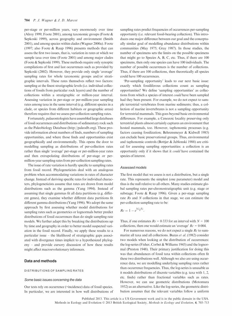
Mammalian localities are not evenly distributed over time
(Fig. 1). In particular, the Miocene and Pliocene have more
localities than expected given their durations, and the Paleo-
cene and Cretaceous have fewer localities than expected. This
pattern becomes more pronounced when we subdivide collec-
tions by continent. Although large proportions of Miocene
and Pliocene collections come from Eurasia, a much smaller
proportion of pre-Miocene collections are from Eurasia.
African sampling not only is less than North American or
Eurasian, but simply quite poor prior to the Miocene. (Both
results likely reflect the NOW database beginning as the Neo-
gene OldWorld database, leading it to still be better populated
with post-Oligocene data than pre-Miocene data.) The bulk of
Campanian–Oligocene localities in our pooled data set come
fromNorthAmerica.
Using the localities per-stratigraphic unit shown in Fig. 1,
we evaluate the different basic models for per-collection sam-
pling rates both globally and then by individual continent.
Results
For every interval considered, the lognormal distribution out-
performs the geometric and (especially) the uniform model
(Table 2; see Table S1 for the parameters of the best represen-
tative of each model). This is not simply due to extra parame-
ters: the lognormal does much better than the geometric and
uniform given AICc scores (Table S2). These simple models
do very good jobs of summarizing the data. The difference in
log-likelihoods between the best uniform rate hypothesis and
the saturated model (i.e. the best possible hypothesis) repre-
sents the maximum improvement in log-likelihood that a
model can offer. If we scale this difference to 1�0, then we find
that in nearly all intervals, lognormals provide over 90% (and
frequently over 95%) of the possible improvement in log-likeli-
hoods over the uniformdistribution (Fig. 2). Thus, lognormals
do not leave huge room for improvement by still more complex
models.
Lognormal sampling rates change perceptions of overall
sampling markedly. Here, we summarize the lognormal using
the midpoint rates associated with four equal-area partitions,
that is, the rates at which 12�5%, 37�5%, 62�5% and 87�5% of
taxa have higher rates (Yang 1994). The most likely uniform
rate frequently is higher than the 4th quartile rate (Fig. 3) sim-
ply because the few commonly occurring taxa are less probable
given low sampling rates than many infrequently occurring
Table 1. General summary of analysed data
Stage/
Substage(s)
Onset
(Millions of
YearsAgo)
Sampled
taxa Occurrences Collections
Campanian +83�5 89 314 133
Maastrichtian +70�6 86 728 198
Danian +65�5 306 1396 253
Selandian–Thanetian
+61�7 363 1668 296
Ypresian +55�8 553 6458 998
Lutetian +48�6 445 1605 328
Bartonian–Priabonian
+40�4 762 2326 374
Rupelian +33�9 484 1778 489
Chattian +28�4 397 871 202
Aquitanian–Burdigalian
+23�0 1429 6875 1082
Langhian–Serravallian
+16�0 1284 7890 1230
Tortonian–Messinian
+11�6 1667 7326 1165
Zanclean +5�3 831 2131 369
Piacenzian–Gelasian
+3�6 1309 5246 754
‘Onset’ gives the beginning of the stratigraphic units in question in mil-
lions of years as per Gradstein, Ogg & Smith (2005). Sampled taxa give
numbers of species sampled.
Fig. 1. Chronology and stratigraphy for Campanian – Pliocene mam-
mals. Time scale is modified from Gradstein, Ogg & Smith (2005).
‘Coll.’ gives the number of collections (taphonomically controlled fos-
siliferous localities) within each stratigraphic unit for the globe, Africa,
Eurasia and North America. Data are from the PALEODB and NOW.
Solid lines divide the stages and substages used in these analyses;
dashed lines separate substages lumped into single units.
Published 2013. This article is a US Government work and is in the public domain in the USA.
Methods in Ecology and Evolution © 2013 British Ecological Society, Methods in Ecology and Evolution, 4, 703–713
706 P. J. Wagner & J. D. Marcot
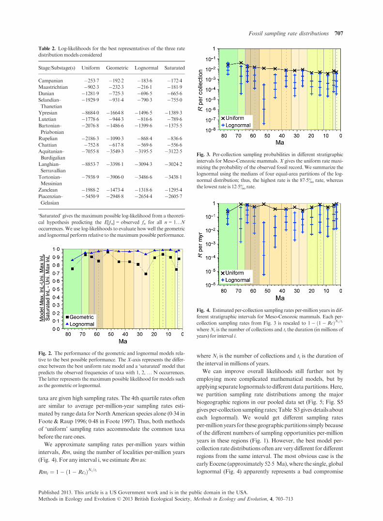
taxa are given high sampling rates. The 4th quartile rates often
are similar to average per-million-year sampling rates esti-
mated by range data for North American species alone (0�34 inFoote & Raup 1996; 0�48 in Foote 1997). Thus, both methods
of ‘uniform’ sampling rates accommodate the common taxa
before the rare ones.
We approximate sampling rates per-million years within
intervals, Rm, using the number of localities per-million years
(Fig. 4). For any interval i, we estimateRm as:
Rmi ¼ 1� ð1� RciÞNi=ti
where Ni is the number of collections and ti is the duration of
the interval inmillions of years.
We can improve overall likelihoods still further not by
employing more complicated mathematical models, but by
applying separate lognormals to different data partitions.Here,
we partition sampling rate distributions among the major
biogeographic regions in our pooled data set (Fig. 5; Fig. S5
givesper-collection sampling rates;Table S3gives details about
each lognormal). We would get different sampling rates
per-millionyears for these geographicpartitions simplybecause
of the different numbers of sampling opportunities per-million
years in these regions (Fig. 1). However, the best model per-
collection rate distributions often are very different for different
regions from the same interval. The most obvious case is the
earlyEocene (approximately 52�5 Ma),where the single, global
lognormal (Fig. 4) apparently represents a bad compromise
Table 2. Log-likelihoods for the best representatives of the three rate
distributionmodels considered
Stage/Substage(s) Uniform Geometric Lognormal Saturated
Campanian �253�7 �192�2 �183�6 �172�4Maastrichtian �902�3 �232�3 �216�1 �181�9Danian �1281�9 �725�3 �696�5 �665�6Selandian–Thanetian
�1929�9 �931�4 �790�3 �755�0
Ypresian �8684�0 �1664�8 �1496�5 �1389�3Lutetian �1778�6 �944�3 �816�6 �789�6Bartonian–Priabonian
�2076�8 �1486�6 �1399�6 �1375�5
Rupelian �2186�3 �1090�3 �868�4 �836�6Chattian �752�8 �617�8 �569�6 �556�6Aquitanian–Burdigalian
�7055�8 �3549�3 �3195�5 �3122�5
Langhian–Serravallian
�8853�7 �3398�1 �3094�3 �3024�2
Tortonian–Messinian
�7938�9 �3906�0 �3486�6 �3438�1
Zanclean �1988�2 �1473�4 �1318�6 �1295�4Piacenzian–Gelasian
�5450�9 �2948�8 �2654�4 �2605�7
‘Saturated’ gives the maximum possible log-likelihood from a theoreti-
cal hypothesis predicting the E[ƒn] = observed fn for all n = 1…N
occurrences.We use log-likelihoods to evaluate howwell the geometric
and lognormal perform relative to themaximumpossible performance.
Fig. 2. The performance of the geometric and lognormal models rela-
tive to the best possible performance. The X-axis represents the differ-
ence between the best uniform rate model and a ‘saturated’ model that
predicts the observed frequencies of taxa with 1, 2, … N occurrences.
The latter represents the maximum possible likelihood for models such
as the geometric or lognormal.
Fig. 3. Per-collection sampling probabilities in different stratigraphic
intervals for Meso-Cenozoic mammals. X gives the uniform rate maxi-
mizing the probability of the observed fossil record. We summarize the
lognormal using the medians of four equal-area partitions of the log-
normal distribution; thus, the highest rate is the 87�5& rate, whereas
the lowest rate is 12�5& rate.
Fig. 4. Estimated per-collection sampling rates per-million years in dif-
ferent stratigraphic intervals for Meso-Cenozoic mammals. Each per-
collection sampling rates from Fig. 3 is rescaled to 1� ð1� RcÞNi=ti
whereNi is the number of collections and ti the duration (in millions of
years) for interval i.
Published 2013. This article is a US Government work and is in the public domain in the USA.
Methods in Ecology and Evolution © 2013 British Ecological Society, Methods in Ecology and Evolution, 4, 703–713
Fossil sampling rate distributions 707
between different regional lognormals (Fig. 5). However, sev-
eral other intervals show marked differences in both geometric
means andvariancesof per-collection sampling rates.
Discussion
APPLICATION OF RESULTS: D IVERGENCE TIMES AMONG
CARNIVORAMORPHAN MAMMALS
In lieu of a traditional discussion, we present an applied
example using mammalian sampling rates in a phylogenetic
context. Phylogenies are particularly useful for our discussion
for two basic reasons. First, phylogenies allow reconstruction
of ancestral geographic distributions (Ree 2005; Ree & Smith
2008), which in turn let us take advantage of different sam-
pling rates for different regions. Second, there is some branch
duration that will maximize the likelihood of any branch on a
phylogeny given some distribution of character state and
some hypothesized rate(s) of change (Felsenstein 1973). This
latter point is particular critical because alternate macroevolu-
tionary hypotheses often predict different rates of morpholog-
ical change over particular time intervals and thus are
optimized at different branch durations. Branch duration
therefore is a critical nuisance parameter for hypotheses rang-
ing from punctuated versus continuous morphological change
(Marshall 1995b) to ‘big bangs’ in morphologic evolution
early in clade histories (Wagner 1995b, 1997; Ruta, Wagner
& Coates 2006). If we can indefinitely extend branch dura-
tions (and thus the time to accumulate change), then we often
can elevate the likelihood of hypotheses of constant rates
when a literal reading of the fossil record suggests rate
decreases. However, the likelihoods of these durations might
be strongly reduced whether the stratigraphic gaps implicit to
those durations are improbable given sampling rates (Huel-
senbeck & Rannala 1997; Wagner 2000a). ‘Molecular clock’
studies reverse the emphasis on the same parameters: charac-
ter rate variation is the nuisance parameter, and branch dura-
tions are the inference (Huelsenbeck, Larget & Swofford
2000; Drummond et al. 2006). Although this traditionally
was restricted to molecular characters, recent divergence-date
studies have extended this to morphological characters when
dating branches leading to fossil taxa (Pyron 2010, 2011;
Ronquist et al. 2012). Marshall (2008) addresses bracketing
divergence times with limited occurrence data; here, we
approach the same general problem using a much broader
range of information from occurrence data.
To explore how our approach might alter inferences, we
calibrate branch durations for early (Eocene – Oligocene) car-
nivoramorphan mammals from North America and Eurasia
under five different models using morphological, biogeograph-
ic and stratigraphic data. Here, we will discuss how different
approaches in general and how branch duration calibrations in
particular might affect conclusions drawn fromWesley-Hunt’s
(2005) analyses of carnivoramorphan dental disparity.
We use character data and a corresponding parsimony tree
from Wesley-Hunt & Flynn (2005). We estimate morphologi-
cal likelihoods using an Mk model assuming continuous
change through time (Lewis 2001), with morphological rates
assumed to follow a lognormal distribution estimated from
compatibility tests (Wagner 2012) and an initial estimate of un-
sampled lineages over which change could accrue based on an
global lognormal preservation rates (Foote 1996). We also use
an Mk model to estimate likelihoods of geographic distribu-
tions (Ree & Smith 2008), with lineages assumed to occupy
either North America or Eurasia, and with the probability of
an unsampled lineage being in North America calculated
simply as:
P½North America�¼ L½North America�=ðL½North America� þ L½Eurasia�Þ:
Given this particular tree we use, ancestral geographies have
very high probabilities for either North America or Eurasia
save for a very few branches near a likely North American ?Eurasian incursion (Fig. S6; see also Table S4).
The stratigraphic likelihood of any branch duration is the
probability of zero finds overXmillion years based on per-col-
lection sampling rates illustrated in Figs 3–5 and collections
per-million years illustrated in Fig. 1:
L½DivergencejStratigraphy�
¼XAreasA¼1
P½A� �YSTs¼st
X4q¼1
1� RmA�s�q� �t
4
! !
where A is a possible ancestral region, st and ST are the first
and last stages (or other chronostratigraphic units) over which
a branch spans, t is the duration within that stage that the
branch spans, and q is one of four quartiles within the lognor-
mal distribution (Wagner &Marcot 2010). Thus,RmA•s•q gives
the per-million-year sampling rate for Area A in stage s from
lognormal quartile q, and (1 � RmA•s•q)t gives the probability
of zero finds over t million years. Branch likelihoods are now
L½DivergencejData�¼ L½DivergencejStratigraphy� � L½DivergencejMorphology�:
Fig. 5. Estimated collection sampling probabilities per-million years in
different stratigraphic intervals for Meso-Cenozoic mammals now
divided into different biogeographic units. Note that intervals with too
few localities are excluded. See Fig. 3 for additional explanation.
Published 2013. This article is a US Government work and is in the public domain in the USA.
Methods in Ecology and Evolution © 2013 British Ecological Society, Methods in Ecology and Evolution, 4, 703–713
708 P. J. Wagner & J. D. Marcot
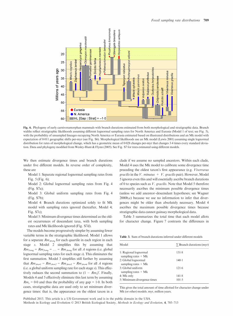
We then estimate divergence times and branch durations
under five different models. In reverse order of complexity,
these are
Model 1: Separate regional lognormal sampling rates from
Fig. 5 (Fig. 6);
Model 2: Global lognormal sampling rates from Fig. 4
(Fig. S7a);
Model 3: Global uniform sampling rates from Fig. 4
(Fig. S7b);
Model 4: Branch durations optimized solely to fit Mk
model with sampling rates ignored (hereafter, Model 4;
Fig. S7c);
Model 5:Minimumdivergence times determined as the old-
est occurrences of descendant taxa, with both sampling
rates andMk likelihoods ignored (Fig. S7d).
Themodels become progressively simpler by assuming fewer
variable terms in the stratigraphic likelihood. Model 1 allows
for a separate RmA•s•q for each quartile in each region in each
stage s. Model 2 simplifies this by assuming that
Rm1•s•q = Rm2•s•q = … = RmA•s•q for all A regions (i.e. global
lognormal sampling rates for each stage s). This eliminates the
first summation. Model 3 simplifies still further by assuming
that RmA•s•1 = RmA•s•2 = RmA•s•3 = RmA•s•4 for all A regions
(i.e. a global uniform sampling rate for each stage s). This effec-
tively reduces the second summation to (1 � Rms)t. Finally,
Models 4 and 5 effectively eliminate this last term by assuming
Rms = 0�0 and thus the probability of any gap = 1�0. In both
cases, stratigraphic data are used only to set minimum diver-
gence times: that is, the appearance on the oldest taxon in a
clade if we assume no sampled ancestors. Within each clade,
Model 4 uses the Mk model to calibrate some divergence time
preceding the oldest taxon’s first appearance (e.g. Viverravus
gracilis in theV. minutus + V. gracilis pair). However,Model
5 ignores even this andwill essentially ascribe branch durations
of 0 to species such as V. gracilis. Note that Model 5 therefore
necessarily ascribes the minimum possible divergence times
(unless we add ancestor–descendant hypotheses; see Wagner
2000b,c) because we use no information to infer that diver-
gences might be older than absolutely necessary. Model 4
ascribes the maximum possible divergence times because
stratigraphic data cannot gainsaymorphological data.
Table 3 summarizes the total time that each model allots
for character change. Figure 7 contrasts the differences in
Fig. 6. Phylogeny of early carnivoramorphan mammals with branch durations estimated from both morphological and stratigraphic data. Branch
widths reflect stratigraphic likelihoods assuming different lognormal sampling rates for North America and Eurasia (Model 1 of text; see Fig. 5),
with the probability of unsampled lineages occupying North America or Eurasia estimated based on illustrated distributions and anMkmodel with
expectation of 0�011 geographic shifts per-myr (see Fig. S6). Morphological likelihoods use an Mk model (Lewis 2001) assuming single lognormal
distribution for rates of morphological change, which has a geometric mean of 0�028 changes per-myr that changes 3�4 times every standard devia-
tion. Data and phylogenymodified fromWesley-Hunt&Flynn (2005). See Fig. S7 for trees estimated using differentmodels.
Table 3. Sumof branch durations inferred under differentmodels
Model ∑Branch durations (myr)
1: Regional lognormal
sampling rates + Mk
131�8
2: Global lognormal
sampling rates + Mk
140�1
3: Global uniform
sampling rates + Mk
121�6
4:Mk only 141�85:Minimumdivergence times 101�5
This gives the total amount of time allotted for character change under
Mk (or other)models. myr,million years.
Published 2013. This article is a US Government work and is in the public domain in the USA.
Methods in Ecology and Evolution © 2013 British Ecological Society, Methods in Ecology and Evolution, 4, 703–713
Fossil sampling rate distributions 709
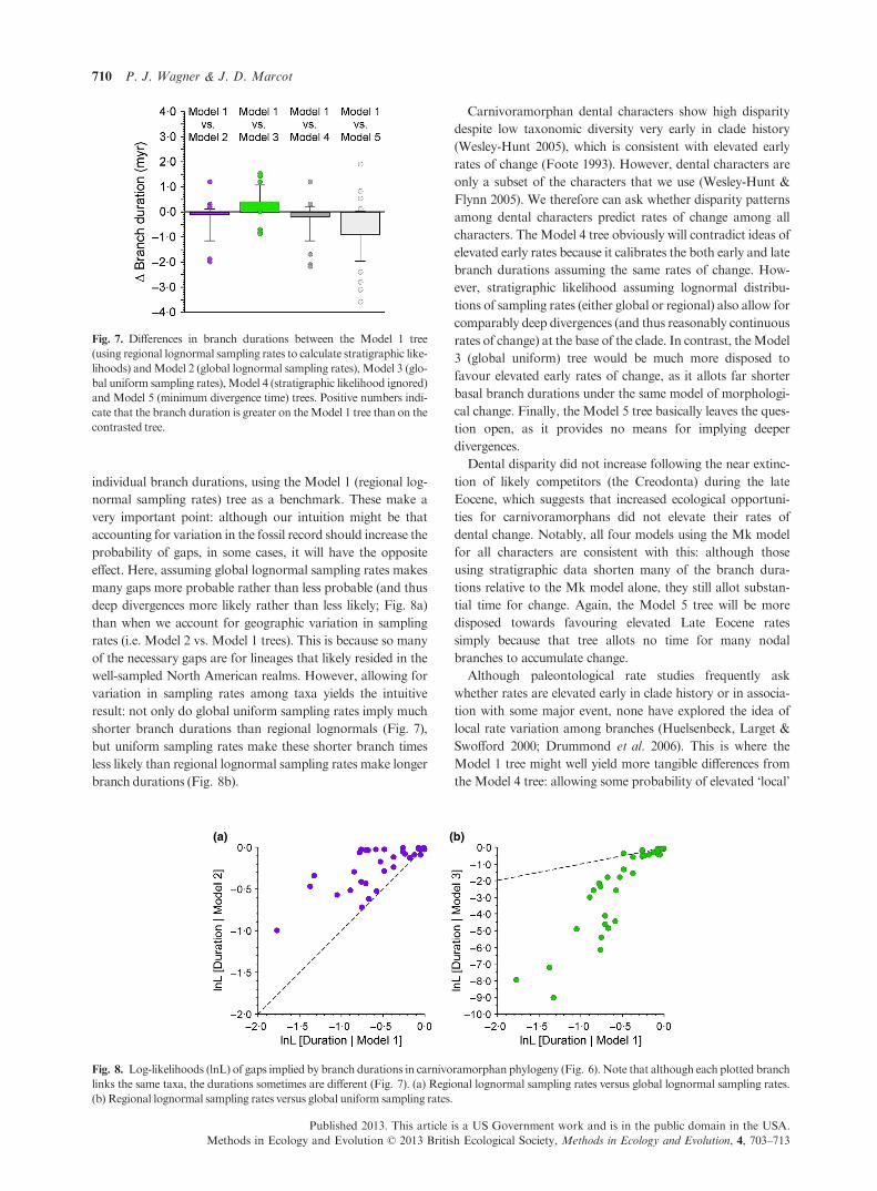
individual branch durations, using the Model 1 (regional log-
normal sampling rates) tree as a benchmark. These make a
very important point: although our intuition might be that
accounting for variation in the fossil record should increase the
probability of gaps, in some cases, it will have the opposite
effect. Here, assuming global lognormal sampling rates makes
many gaps more probable rather than less probable (and thus
deep divergences more likely rather than less likely; Fig. 8a)
than when we account for geographic variation in sampling
rates (i.e. Model 2 vs. Model 1 trees). This is because so many
of the necessary gaps are for lineages that likely resided in the
well-sampled North American realms. However, allowing for
variation in sampling rates among taxa yields the intuitive
result: not only do global uniform sampling rates imply much
shorter branch durations than regional lognormals (Fig. 7),
but uniform sampling rates make these shorter branch times
less likely than regional lognormal sampling rates make longer
branch durations (Fig. 8b).
Carnivoramorphan dental characters show high disparity
despite low taxonomic diversity very early in clade history
(Wesley-Hunt 2005), which is consistent with elevated early
rates of change (Foote 1993). However, dental characters are
only a subset of the characters that we use (Wesley-Hunt &
Flynn 2005). We therefore can ask whether disparity patterns
among dental characters predict rates of change among all
characters. The Model 4 tree obviously will contradict ideas of
elevated early rates because it calibrates the both early and late
branch durations assuming the same rates of change. How-
ever, stratigraphic likelihood assuming lognormal distribu-
tions of sampling rates (either global or regional) also allow for
comparably deep divergences (and thus reasonably continuous
rates of change) at the base of the clade. In contrast, theModel
3 (global uniform) tree would be much more disposed to
favour elevated early rates of change, as it allots far shorter
basal branch durations under the same model of morphologi-
cal change. Finally, the Model 5 tree basically leaves the ques-
tion open, as it provides no means for implying deeper
divergences.
Dental disparity did not increase following the near extinc-
tion of likely competitors (the Creodonta) during the late
Eocene, which suggests that increased ecological opportuni-
ties for carnivoramorphans did not elevate their rates of
dental change. Notably, all four models using the Mk model
for all characters are consistent with this: although those
using stratigraphic data shorten many of the branch dura-
tions relative to the Mk model alone, they still allot substan-
tial time for change. Again, the Model 5 tree will be more
disposed towards favouring elevated Late Eocene rates
simply because that tree allots no time for many nodal
branches to accumulate change.
Although paleontological rate studies frequently ask
whether rates are elevated early in clade history or in associa-
tion with some major event, none have explored the idea of
local rate variation among branches (Huelsenbeck, Larget &
Swofford 2000; Drummond et al. 2006). This is where the
Model 1 tree might well yield more tangible differences from
the Model 4 tree: allowing some probability of elevated ‘local’
Fig. 7. Differences in branch durations between the Model 1 tree
(using regional lognormal sampling rates to calculate stratigraphic like-
lihoods) andModel 2 (global lognormal sampling rates), Model 3 (glo-
bal uniform sampling rates),Model 4 (stratigraphic likelihood ignored)
and Model 5 (minimum divergence time) trees. Positive numbers indi-
cate that the branch duration is greater on theModel 1 tree than on the
contrasted tree.
(a) (b)
Fig. 8. Log-likelihoods (lnL) of gaps implied by branch durations in carnivoramorphan phylogeny (Fig. 6). Note that although each plotted branch
links the same taxa, the durations sometimes are different (Fig. 7). (a) Regional lognormal sampling rates versus global lognormal sampling rates.
(b) Regional lognormal sampling rates versus global uniform sampling rates.
Published 2013. This article is a US Government work and is in the public domain in the USA.
Methods in Ecology and Evolution © 2013 British Ecological Society, Methods in Ecology and Evolution, 4, 703–713
710 P. J. Wagner & J. D. Marcot
rates would elevate the total likelihood of the branch durations
reduced by stratigraphic data (Fig. 7). However, the Model 1
tree would be less prone to doing this than the Model 3 simply
because regional lognormal sampling rates reduce the likeli-
hoods of gaps much less than global uniform rates do. Note
that any stratigraphic likelihood model would be less biased
towards supporting local rate heterogeneity than the Model 5
(minimum divergences) tree. This is not just because all strati-
graphic likelihood trees extend many branches with near-zero
durations given minimum divergences, but also because the
stratigraphic likelihoods reduce the durations of branches link-
ing clades in some cases.
FUTURE DIRECTIONS
Relaxing assumptions about continuous distributions of
localities over time
When assessing sampling rates per-million years, our approach
currently assumes that localities are continuously distributed
throughout an interval. This is rarely, if ever, true. However,
biochronological techniques for ordinating localities based on
constituent species combined with some absolute dates offer
the potential for very high resolution biochronological place-
ment of localities (Alroy 1994; Sadler, Kemple & Kooser
2003). This can allow us to generate different per-myr and even
per-collection sampling rates within intervals.
Origination and extinction
Another advantage to ordinating collections within strati-
graphic units is that these results will often show that species
durations are less than that of whole stratigraphic intervals
(Alroy 1996). This is important because our estimates of
sampling rates do not take into account turnover within strati-
graphic intervals: instead, we assume that any taxon present in
an interval was present throughout the entire interval. For taxa
with true durations less than that of the entire interval, many
collections currently tallied as ‘gaps’ actually come from before
or after the species’ lifetimes: and this biases our method
towards underestimating sampling rates. An obvious next step
in this sort of approach is to add origination and extinction
parameters (Weiss & Marshall 1999). However, we stress that
the approach as done here should be ‘conservative’ with
respect to rejecting null hypotheses because of long strati-
graphic gaps.
Conclusions
The existence of large databases of fossil occurrences such as
the PaleoDB andNOWallows us to assess sampling rates over
time and space in greater detail than ever before. Here, we
show that in the case of fossil mammals at least, lognormal dis-
tributions of sampling rates among taxa prevail. Moreover,
these distributions vary considerably over time and among
contemporaneous geographic areas. Many interesting macro-
evolutionary hypotheses concerning rates of morphological
change, speciation patterns and turnover events differ in the
gaps they require between observed stratigraphic ranges and
either divergence times or extinction times. Combining these
models and these data should allow evolutionary biologists to
more fully exploit the fossil record as a tool for corroborating
or contradicting these hypotheses while at the same time allow-
ing for the uncertainties inherent to the fossil record.
Acknowledgements
We thank the special issue editors for their invitation and their subsequent for-
bearance.We also thank D. Bapst and P. D. Polly for very insightful reviews that
(hopefully) led to clarification of our primary goals and concepts. For discussions
about the appropriate distributions to model sampling rates, we thank J. Alroy.
This represents PaleoDB Publication No. 182. For those data, we thank in
particular J. Alroy,K. Behrensmeyer,M.Uhen,A.Turner, L. v. d.HoekOstende
andM. Carrano. Occurrence data and a C program for estimating per-collection
sampling rates are available at the Dryad Data repository (http://datadryad.org;
doi:10.5061/dryad.3b87j).
References
Alroy, J. (1994) Appearance event ordination: a new biochronologic method.
Paleobiology, 20, 191–207.Alroy, J. (1996) Constant extinction, constrained diversification, and uncoordi-
nated stasis in North American mammals. Palaeogeography, Palaeoclimatolo-
gy, Palaeoecology, 127, 285–311.Alroy, J. (1998) Diachrony of mammalian appearance events: implications for
biochronology.Geology, 26, 23–26.Alroy, J. (1999) The fossil record of North American mammals: evidence for a
Paleocene evolutionary radiation. Systematic Biology, 48, 107–118.Alroy, J. (2000) New methods for quantifying macroevolutionary patterns and
processes.Paleobiology, 26, 707–733.Alroy, J.,Marshall, C.R., Bambach, R.K., Bezusko, K., Foote,M., F€ursich, F.T.
et al. (2001) Effects of sampling standardization on estimates of Phanerozoic
marine diversity.Proceedings of the National Academy of Sciences of the United
States of America, 98, 6261–6266.Behrensmeyer, A.K. & Kidwell, S. (1985) Taphonomy’s contribution to paleobi-
ology.Paleobiology, 11, 105–119.Bottjer, D.J. & Jablonski, D. (1988) Paleoenvironmental patterns in the evolution
of post-Paleozoic benthicmarine invertebrates.Palaios, 3, 540–560.Buzas, M.A., Koch, C.F., Culver, S.J. & Sohl, N.F. (1982) On the distribution of
species occurrence.Paleobiology, 8, 143–150.Darwin,C. (1859)TheOrigin of Species, 6th edn. JohnMurray, London.
Drummond, A.J., Ho, S.Y.W., Phillips, M.J. & Rambaut, A. (2006) Relaxed
phylogenetics and datingwith confidence.PLoSBiology, 4, e88.
Felsenstein, J. (1973) Maximum-likelihood and minimum-steps methods for esti-
mating evolutionary trees from data on discrete characters. Systematic Zool-
ogy, 22, 240–249.Fisher, R.A., Corbet, A.S. & Williams, C.B. (1943) The relation between the
number of species and the number of individuals in a randomsample of an ani-
mal population. Journal of Animal Ecology, 12, 42–48.Foote, M. (1993) Discordance and concordance between morphological and tax-
onomic diversity.Paleobiology, 19, 185–204.Foote, M. (1996) On the probability of ancestors in the fossil record. Paleobiol-
ogy, 22, 141–151.Foote, M. (1997) Estimating taxonomic durations and preservation probability.
Paleobiology, 23, 278–300.Foote, M. (2001) Inferring temporal patterns of preservation, origination,
and extinction from taxonomic survivorship analysis. Paleobiology, 27,
602–630.Foote, M. & Raup, D.M. (1996) Fossil preservation and the stratigraphic ranges
of taxa.Paleobiology, 22, 121–140.Foote, M. & Sepkoski, J.J. Jr (1999) Absolute measures of the completeness of
the fossil record.Nature, 398, 415–417.Fortelius, M., Werdelin, L., Andrews, P., Bernor, R.L., Gentry, A., Humphrey,
L., Mittmann, W. & Viranta, S. (1996) Provinciality, diversity, turnover and
paleoecology in land mammal faunas of the later Miocene of western Eurasia.
TheEvolution ofWestern EurasianNeogeneMammal Faunas (edsR.L. Bernor,
V. Fahlbusch&W.Mittmann), pp. 414–448. ColumbiaUniversity Press, New
York,NewYork,USA.
Published 2013. This article is a US Government work and is in the public domain in the USA.
Methods in Ecology and Evolution © 2013 British Ecological Society, Methods in Ecology and Evolution, 4, 703–713
Fossil sampling rate distributions 711
Fortelius, M., Eronen, J., Jernvall, J., Liu, L., Pushkina, D., Rinne, J. et al.
(2002) Fossil mammals resolve regional patterns of Eurasian climate change
over 20million years.Evolutionary Ecology Research, 4, 1005–1016.Gradstein, F., Ogg, J. & Smith, A. (2005) A Geological Times Scale 2004. Cam-
bridgeUniversity Press, Cambridge.
Gray, J.S. (1987) Species-abundance patterns. Organization of Communities Past
and Present (eds J.H.R.Gee&P.S. Gillier), pp. 53–67. Blackwell, Oxford.Huelsenbeck, J.P., Larget, B. & Swofford, D. (2000) A compound Poisson Pro-
cess for relaxing themolecular clock.Genetics, 154, 1879–1892.Huelsenbeck, J.P. & Rannala, B. (1997) Maximum likelihood estimation of
topology and node times using stratigraphic data. Paleobiology, 23, 174–180.
Lewis, P.O. (2001) A likelihood approach to estimating phylogeny from discrete
morphological character data.Systematic Biology, 50, 913–925.Marshall, C.R. (1995a)Distinguishing between sudden and gradual extinctions in
the fossil record: predicting the position of the iridium anomaly using the
ammonite fossil record on Seymour Island, Antarctica.Geology, 23, 731–734.Marshall, C.R. (1995b) Stratigraphy, the true order of species’ originations and
extinctions, and testing ancestor-descendant hypotheses among Caribbean
bryozoans. New Approaches to Studying Speciation in the Fossil Record (eds
D.H. Erwin & R.L. Anstey), pp. 208–236. Columbia University Press, New
York,NewYork,USA.
Marshall, C.R. (2008) A simple method for bracketing absolute divergence times
on molecular phylogenies using multiple fossil calibration points. The Ameri-
canNaturalist, 171, 726–742.May, R.M. (1975) Patterns of species abundance and diversity. Ecology and Evo-
lution of Communities (edsM.L. Cody& J.M.Diamond), pp. 87–120. The Bel-knap Press ofHarvardUniversity Press, Cambridge.
Montroll, E.W. & Shlesinger, M.F. (1982) On 1/f noise and other distributions
with long tails. Proceedings of the National Academy of Sciences, 79, 3380–3383.
Motomura, I. (1932) A statistical treatment of associations.ZoologicalMagazine,
Tokyo, 44, 379–383.Preston, W.H. (1948) The commonness and rarity of species. Ecology, 29, 254–
283.
Pyron, R.A. (2010) A likelihood method for assessing molecular divergence time
estimates and the placement of fossil calibrations. Systematic Biology, 59, 185–194.
Pyron, R.A. (2011) Divergence time estimation using fossils as terminal taxa and
the origins of Lissamphibia.Systematic Biology, 60, 466–481.Raia, P., Carotenuto, F., Passaro, F., Fulgione, D. & Fortelius, M. (2012) Eco-
logical specialization in fossil mammals explains Cope’s Rule. The American
Naturalist, 179, 328–337.Raup, D.M. (1972) Taxonomic diversity during the Phanerozoic. Science, 177,
1065–1071.Ree, R.H. (2005) Detecting the historical signature of key innovations using sto-
chasticmodelsof character evolutionandcladogenesis.Evolution,59, 257–265.Ree, R.H. & Smith, S.A. (2008) Maximum likelihood inference of geographic
range evolution by dispersal, local extinction, and cladogenesis. Systematic
Biology, 57, 4–14.Ronquist, F., Klopfstein, S., Vilhelmsen, L., Schulmeister, S., Murray, D.L. &
Rasnitsyn, A.P. (2012) A Total-Evidence approach to dating with fossils,
applied to the early radiation of the Hymenoptera. Systematic Biology, 61,
973–999.Ruta, M., Wagner, P.J. & Coates, M.I. (2006) Evolutionary patterns in early tet-
rapods. I. Rapid initial diversification by decrease in rates of character change.
Proceedings of the Royal Society of London, Series B. Biological Sciences, 273,
2107–2111.Sadler, P.M., Kemple, W.G. & Kooser, M.A. (2003) CONOP9 Programs for
Solving the Stratigraphic Correlation and Seriation Problems as Constrained
Optimization. High-Resolution Stratigraphic Approaches in Paleontology (ed.
P.Harries), pp. 461–462. PlenumPress, NewYork,NewYork, USA.
Sanderson, M.J. (2002) Estimating absolute rates of molecular evolution and
divergence times: a penalized likelihood approach.Molecular Biology and Evo-
lution, 19, 101–109.Sepkoski, J.J. Jr (1975) Stratigraphic biases in the analysis of taxonomic survivor-
ship.Paleobiology, 1, 343–355.Sepkoski, J.J. Jr (2002) A compendium of fossil marine animal genera. Bulletins
of American Paleontology, 363, 1–563.Signor, P.W. & Lipps, J.H. (1982) Sampling bias, gradual extinction patterns and
catastrophes in the fossil record. Geological Society of America Special Paper,
190, 291–296.Smith, A.B. (2001) Large-scale heterogeneity of the fossil record: implications for
Phanerozoic biodiversity studies. Philosophical Transactions of the Royal Soci-
ety of London Series B, 356, 351–367.
Sugiura, N. (1978) Further analysis of the data by Akaike’s information criterion
and the finite corrections. Communications in Statistics – Theory andMethods,
A7, 13–26.Uhen, M.D., Barnosky, A.D., Bills, B., Blois, J., Carrano, M.T., Carrasco, M.A.
et al. (2013) From card catalogs to computers: databases in vertebrate paleon-
tology. Journal of Vertebrate Paleontology, 33, 13–28.Wagner, P.J. (1995a) Stratigraphic tests of cladistic hypotheses. Paleobiology, 21,
153–178.Wagner, P.J. (1995b) Testing evolutionary constraint hypotheses with early
Paleozoic gastropods.Paleobiology, 21, 248–272.Wagner, P.J. (1997) Patterns of morphologic diversification among the Rostro-
conchia.Paleobiology, 23, 115–150.Wagner, P.J. (2000a) Likelihood tests of hypothesized durations: determining
and accommodating biasing factors.Paleobiology, 26, 431–449.Wagner, P.J. (2000b) Phylogenetic analyses and the fossil record: tests and infer-
ences, hypotheses and models. Paleobiology Memoir (eds D.H. Erwin & S.L.
Wing), pp. 341–371. Paleontological Society, Deep time – Paleobiology’s
perspective.
Wagner, P.J. (2000c) The quality of the fossil record and the accuracy of
phylogenetic inferences about sampling and diversity. Systematic Biology, 49,
65–86.Wagner, P.J. (2012) Modelling rate distributions using character compatibility:
implications for morphological evolution among fossil invertebrates. Biology
Letters, 8, 143–146.Wagner, P.J., Kosnik,M.A. & Lidgard, S. (2006) Abundance distributions imply
elevated complexity of post-Paleozoic marine ecosystems. Science, 314, 1289–1292.
Wagner, P.J. & Marcot, J.D. (2010) Probabilistic phylogenetic inference in the
fossil record: current and future applications.QuantitativeMethods in Paleobi-
ology (eds J. Alroy & G. Hunt), pp. 195–217. Paleontological Society, New
Haven, Connecticut, USA.
Weiss, R.E. & Marshall, C.R. (1999) The uncertainty in the true end point of a
fossil’s stratigraphic ranges when stratigraphic sections are sampled discretely.
Mathematical Geology, 31, 435–453.Wesley-Hunt, G.D. (2005) The morphological diversification of carnivores in
NorthAmerica.Paleobiology, 31, 35–55.Wesley-Hunt, G.D. & Flynn, J.J. (2005) Phylogeny of the Carnivora: basal rela-
tionships among the carnivoramorphans, and assessment of the position of
“Miacoidea” relative to crown-clade Carnivora. Journal of Systematic Palae-
ontology, 3, 1–28.Yang, Z. (1994) Maximum likelihood phylogenetic estimation from DNA
sequences with variable rates over sites: approximate methods. Journal of
Molecular Evolution, 39, 306–314.Yang, Z. (1996) Maximum-likelihood models for combined analyses of multiple
sequence data. Journal ofMolecular Evolution, 42, 587–596
Received 25 January 2013; accepted 10 June 2013
Handling Editor: GrahamSlater
Supporting Information
Additional Supporting Information may be found in the online version
of this article.
Appendix S1.Additional results andmethodological discussion.
Fig. S1. Lognormal distribution of per-collection sampling rates (Rc)
for 100 taxa.
Fig. S2. Probabilities of X occurrences for the four species with corre-
sponding colors in Fig. 1.
Fig. S3.Expected species withX occurrences.
Fig. S4. Expected rank order plot of numbers of occurrences against
ranked taxa.
Fig. S5.Distributions of per-collection preservation rates forMeso-Ce-
nozoicmammals, broken down by basic geographic units.
Published 2013. This article is a US Government work and is in the public domain in the USA.
Methods in Ecology and Evolution © 2013 British Ecological Society, Methods in Ecology and Evolution, 4, 703–713
712 P. J. Wagner & J. D. Marcot

Fig. S6.Estimated probabilities that unsampled lineages resided in Eur-
asia (red) orNorthAmerica (blue).
Fig. S7. Alternate phylogenies with the same cladistic topology using
differentmethods to calibrate branch durations and divergence times.
Table S1.Parameters from the best hypothesis of eachmodel.
Table S2.AICc for the best representatives of the three rate distribution
models considered for per-collection sampling rates.
Table S3.Parameters from the best hypothesis of eachmodel.
Table S4. Stratigraphic likelihoods given gaps hypothesized by carniv-
oramorphan phylogeny (Fig. 6).
Published 2013. This article is a US Government work and is in the public domain in the USA.
Methods in Ecology and Evolution © 2013 British Ecological Society, Methods in Ecology and Evolution, 4, 703–713
Fossil sampling rate distributions 713
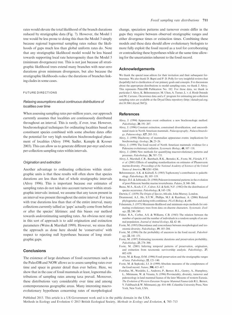
SOM: Sampling Rate Distributions S1 Wagner & Marcot
Supplementary Online Material
Assessing Model Distributions
We assess model distributions using the expected numbers of taxa with 1…N occurrences given
N collections. Here we will
describe how we generate
these expectations when
testing a hypothesized log-
normal distribution rate of
per-collection sampling
rates (Rc) for 100 species
with Rcmodal = 0.01 and the
magnitude parameter, m, =
2.5. In other words, the
geometric mean of the rates
is ln(0.1) and the standard
deviation on the log-transformed rates is ln(2.75). In our example, we will focus on four taxa
shown in separate colors: the three species with the highest Rc and the species with the lowest
Rc.
Now, assume that there are 200 collections from which these species might be sampled. The
single most probable number of occurrences for any species i is the integer closest to 200 x Rci.
However, there is considerable variation simply due to binomial error. Thus, although it is most
probable that we will sample Species 1 (Rc1 = 0.1056) in 21 collections, the exact probability of
this outcome is reasonably low (p = 0.092; Fig. S2). The probabilities of 20 or 21 finds are
Fig. S1. Lognormal distribution of per-collection sampling rates (Rc) for 100 taxa. Species 1, 2, 3 and 100 are set in separate colors to match Fig. S2.
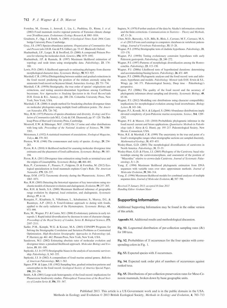
SOM: Sampling Rate Distributions S2 Wagner & Marcot
nearly as great, and there is
even a very remote probability
of 0 occurrences (p = 2x10⁻¹⁰).
As Rci decreases, the
probability curves shift to the
left. Thus, when we look at
Species 100 (Rc = 0.0009), the
single most probable outcome
is that we fail to sample it
altogether (p=0.82).
Another crucial point is the
heavy overlap among
probability curves. Thus, the probability that Species 2 might actually have more occurrences
than Species 1 is non-trivial: and the probability of sampling taxa out-of-order increases as we
approach the mode of the distribution simply because the difference between Rci and Rci+1
becomes very small. What is more relevant to our purposes is that the expected number (and
later expected frequency) of species with 21 occurrences is not based simply on having one
taxon with 21 expected occurrences, but is instead the sum of probabilities of 21 occurrences
over all 100 species. Thus, we do not assume that observed ranks of occurrences match the
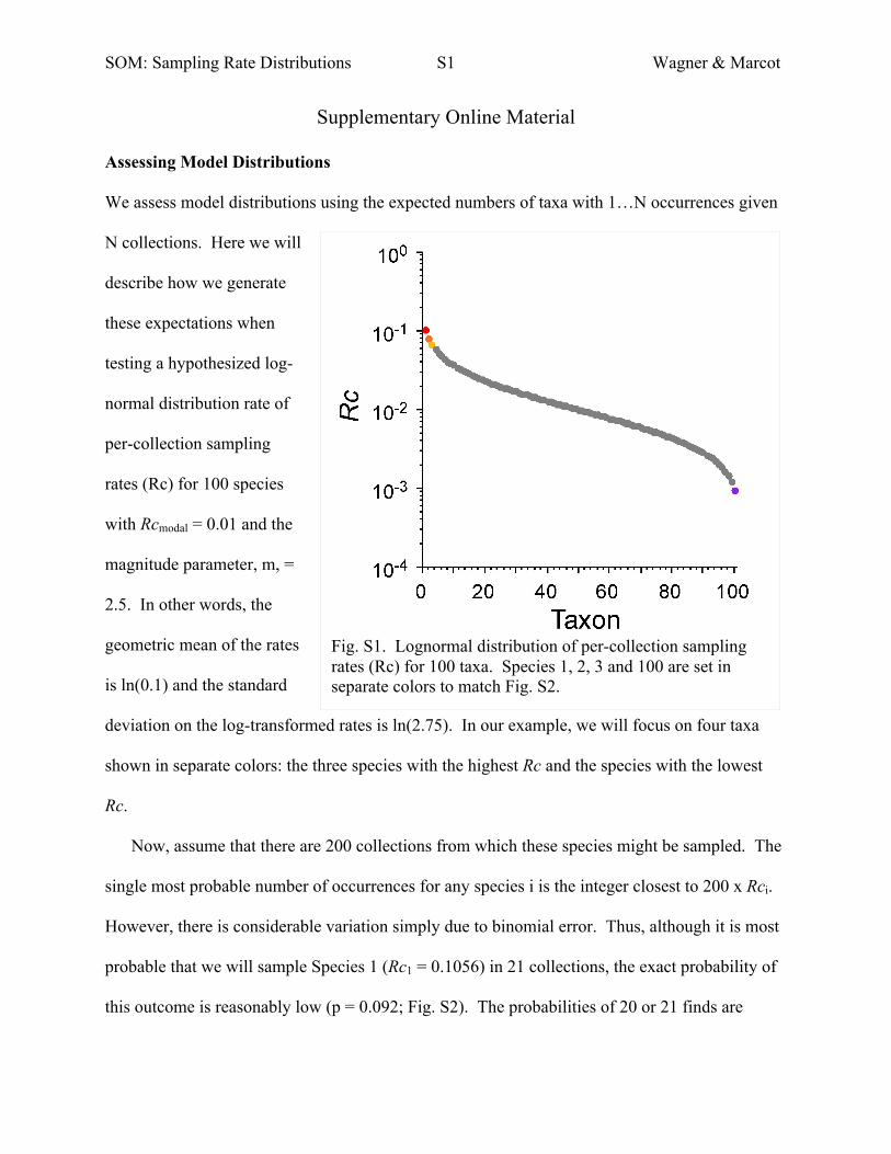
“true” ranks of sampling rates. Doing this now gives us an expected number of species with n
occurrences (Figure S3). We then can transform this to a probability density function by setting
the area under the curve = 1.0 (i.e., by dividing by the expected number of sample species). We
Fig. S2. Probabilities of X occurrences for the 4 species with corresponding colors in Figure 1. The expected number of taxa with X finds is the sum of the height of each curve at X.
SOM: Sampling Rate Distributions S3 Wagner & Marcot
now can evaluate the exact
probability of the observed
numbers of taxa with N
occurrences using multinomial
probability (e.g., Wagner, Kosnik
& Lidgard 2006).
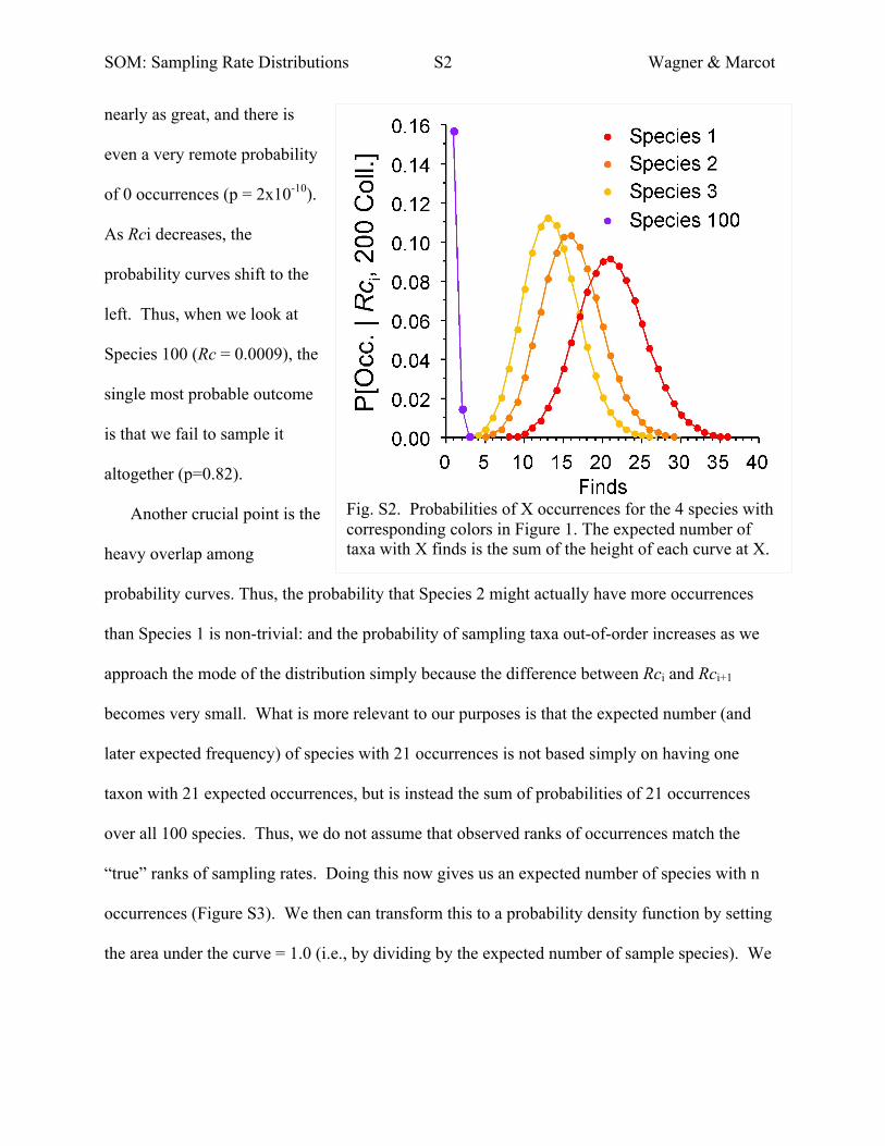
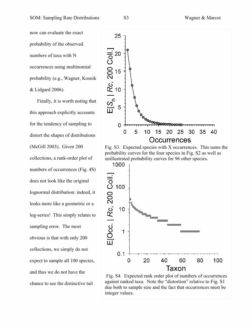
Finally, it is worth noting that
this approach explicitly accounts
for the tendency of sampling to
distort the shapes of distributions
(McGill 2003). Given 200
collections, a rank-order plot of
numbers of occurrences (Fig. 4S)
does not look like the original
lognormal distribution: indeed, it
looks more like a geometric or a
log-series! This simply relates to
sampling error. The most
obvious is that with only 200
collections, we simply do not
expect to sample all 100 species,
and thus we do not have the
chance to see the distinctive tail
Fig. S3. Expected species with X occurrences. This sums the probability curves for the four species in Fig. S2 as well as unillustrated probability curves for 96 other species.
Fig. S4. Expected rank order plot of numbers of occurrences against ranked taxa. Note the “distortion” relative to Fig. S1 due both to sample size and the fact that occurrences must be integer values.
SOM: Sampling Rate Distributions S4 Wagner & Marcot
of a lognormal. The second is that occurrences are integers, resulting in substantial numbers of
taxa with the same number of occurrences. Indeed, if we replot Figure S3 as log-occurrences
(i.e., log the X-axis), then one begins to see a normal distribution that is truncated in the middle
(see, e.g., Preston 1948).
Additional Results
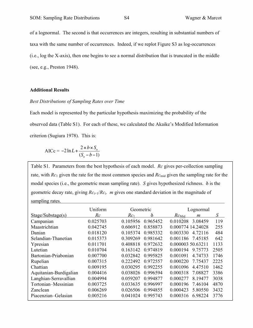
Best Distributions of Sampling Rates over Time
Each model is represented by the particular hypothesis maximizing the probability of the
observed data (Table S1). For each of these, we calculated the Akaike’s Modified Information
criterion (Sugiura 1978). This is:
AICc = !2 lnL + 2"b" Sn(Sn ! b!1)
Table S1. Parameters from the best hypothesis of each model. Rc gives per-collection sampling
rate, with Rc1 given the rate for the most common species and Rcmid given the sampling rate for the
modal species (i.e., the geometric mean sampling rate). S gives hypothesized richness. δ is the
geometric decay rate, giving Rci+1/Rci. m gives one standard deviation in the magnitude of
sampling rates.
Uniform Geometric Lognormal Stage/Substage(s) Rc Rc1 δ RcMid m S Campanian 0.025703 0.105956 0.965452 0.010208 3.08459 119 Maastrichtian 0.042745 0.606912 0.858873 0.000774 14.24028 255 Danian 0.018120 0.105374 0.985332 0.003330 4.72116 484 Selandian-Thanetian 0.015373 0.309269 0.981642 0.001186 7.45185 642 Ypresian 0.011701 0.408818 0.972632 0.000003 50.63211 1133 Lutetian 0.010704 0.163142 0.974819 0.000194 9.75773 2505 Bartonian-Priabonian 0.007700 0.032842 0.995825 0.001091 4.74733 1746 Rupelian 0.007315 0.222492 0.972557 0.000220 7.75437 2225 Chattian 0.009195 0.030295 0.992255 0.001096 4.47510 1462 Aquitanian-Burdigalian 0.004416 0.038026 0.996594 0.000318 7.08827 3386 Langhian-Serravallian 0.004994 0.059207 0.994877 0.000277 8.19477 3038 Tortonian–Messinian 0.003725 0.033635 0.996997 0.000196 7.46104 4870 Zanclean 0.006269 0.026506 0.994855 0.000423 5.80550 3432 Piacenzian–Gelasian 0.005216 0.041024 0.995743 0.000316 6.98224 3776
SOM: Sampling Rate Distributions S5 Wagner & Marcot
where lnL is the log-
likelihood of the best
hypothesis for each
model, b is the number
of parameters for that
model (i.e., the number
of columns in Table S1),
and Sn is the number of
taxa (i.e., the number of
data points). Note that
this precludes
calculating AICc from our hypothetical “best” model simply because the denominator is -1 when
there are as many parameters as data points. In many cases, workers might wish to use Akaike’s
weights to assess the “significance” of these differences. Here, the differences are sufficiently
large that this simply confirms the obvious, i.e., that the lognormal is vastly superior to the
geometric or uniform distributions for modeling per-collection sampling rates.
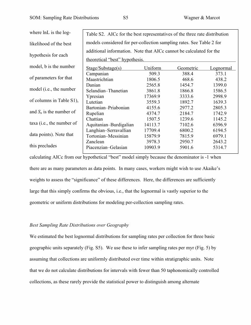
Best Sampling Rate Distributions over Geography
We estimated the best lognormal distributions for sampling rates per collection for three basic
geographic units separately (Fig. S5). We use these to infer sampling rates per myr (Fig. 5) by
assuming that collections are uniformly distributed over time within stratigraphic units. Note
that we do not calculate distributions for intervals with fewer than 50 taphonomically controlled
collections, as these rarely provide the statistical power to distinguish among alternate
Table S2. AICc for the best representatives of the three rate distribution
models considered for per-collection sampling rates. See Table 2 for
additional information. Note that AICc cannot be calculated for the
theoretical “best” hypothesis.
Stage/Substage(s) Uniform Geometric Lognormal Campanian 509.3 388.4 373.1 Maastrichtian 1806.5 468.6 438.2 Danian 2565.8 1454.7 1399.0 Selandian–Thanetian 3861.8 1866.8 1586.5 Ypresian 17369.9 3333.6 2998.9 Lutetian 3559.3 1892.7 1639.3 Bartonian–Priabonian 4155.6 2977.2 2805.3 Rupelian 4374.7 2184.7 1742.9 Chattian 1507.5 1239.6 1145.2 Aquitanian–Burdigalian 14113.7 7102.6 6396.9 Langhian–Serravallian 17709.4 6800.2 6194.5 Tortonian–Messinian 15879.9 7815.9 6979.1 Zanclean 3978.3 2950.7 2643.2 Piacenzian–Gelasian 10903.9 5901.6 5314.7
SOM: Sampling Rate Distributions S6 Wagner & Marcot
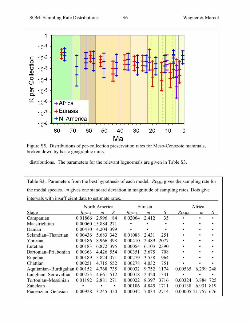
distributions. The parameters for the relevant lognormals are given in Table S3.
Figure S5. Distributions of per-collection preservation rates for Meso-Cenozoic mammals, broken down by basic geographic units.
Table S3. Parameters from the best hypothesis of each model. RcMid gives the sampling rate for
the modal species. m gives one standard deviation in magnitude of sampling rates. Dots give
intervals with insufficient data to estimate rates.
North America Eurasia Africa Stage RcMid m S RcMid m S RcMid m S Campanian 0.01866 2.996 84 0.02064 2.412 35 • • • Maastrichtian 0.00060 15.884 271 • • • • • • Danian 0.00470 4.204 399 • • • • • • Selandian–Thanetian 0.00436 5.683 342 0.01088 2.431 251 • • • Ypresian 0.00186 8.966 398 0.00410 2.489 2077 • • • Lutetian 0.00183 6.872 395 0.00054 6.103 2390 • • • Bartonian–Priabonian 0.00363 4.426 554 0.00351 3.675 708 • • • Rupelian 0.00189 5.824 371 0.00279 3.558 964 • • • Chattian 0.00251 4.715 552 0.00278 4.032 751 • • • Aquitanian–Burdigalian 0.00152 4.768 735 0.00032 9.752 1174 0.00565 6.299 248 Langhian–Serravallian 0.00255 4.661 512 0.00018 12.420 1341 • • • Tortonian–Messinian 0.01192 2.881 271 0.00022 8.397 3716 0.00324 3.884 725 Zanclean • • • 0.00106 4.845 1711 0.00138 6.931 819 Piacenzian–Gelasian 0.00928 3.245 350 0.00042 7.034 2714 0.00005 21.757 676
SOM: Sampling Rate Distributions S7 Wagner & Marcot
Carnivoramorphan Analysis
Analysis of morphological data
We use morphological data for the Carnivoramorpha originally published by Wesley-Hunt and
Flynn (2005). Their analyses include 39 taxa and 113 characters. However, many of these later
taxa are composite codings for derived clades of the Carnivora. To keep the analyses at the
species level, we reduced it to the 21 earliest appearing species and the 86 characters that vary
among those species. We used inverse modeling tests on the compatibility structure of these
characters to establish a base rate of 2.82 changes per character for the entire tree (i.e., about
0.028 changes per myr), with those rates showing lognormal variation in which one standard
deviation equals a magnitude of 3.41 (Wagner 2012). These tests suggest that there are an
additional 17 characters that should be invariant among these species. Thus, the likelihood
analyses included 103 total characters with 17 invariant ones. We converted this to per-million-
year rates by using the sampling rates to estimate the amount of “missing” evolutionary time (see
Foote 1996).
The first appearances and total stratigraphic ranges of each taxon are based on stratigraphic
data from the Paleobiology Database and New and Old World Database. These ranges include
occurrences for species deemed to be junior synonyms in the current taxonomic tables of the
PBDB. Note that we replaced the stratigraphic data for the early mustelid Zodiolestes
daimonelixensis Riggs 1942 with that of Promartes gemmarosae Loomis 1932, the earliest
known mustelid. However, we assumed the same morphological characters for P. gemmarosae
as Welsey-Hunt and Flynn used for Z. daimonelixensis.
SOM: Sampling Rate Distributions S8 Wagner & Marcot
Biogeographic distributions of unsampled lineages
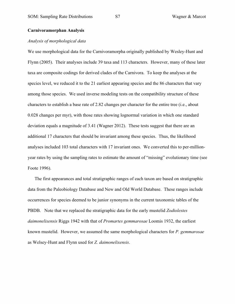
Given the phylogeny proposed by Wesley-Hunt and Flynn (2005), early carnivoramorphans were
exclusive to North America, with one derived clade later emigrating to Eurasia. Instead of
assuming this, we
allowed uncertainty
in the geographic
“state” of
unsampled lineages
in the way allow
for uncertainty in
morphological
states along those
same branches. We
did this assuming a
base rate where there is only one expected change, which means that this rate was very low (i.e.,
0.011 changes per myr). This really affected only that portion of the tree where some transition
necessarily occurred (Fig. S6). The uncertainty is greatest on the branches spanning the longest
amounts of time, but this is in keeping with the idea that there is greater opportunity for “hidden”
changes and reversals along such branches.
Note that the original estimates derive likelihoods for Eurasia or North America as an
ancestral “state.” We convert those to probabilities by dividing each likelihood by the sum of the
two likelihoods. These numbers then are used to weight the likelihoods of gaps given the North
Figure S6. Estimated probabilities that unsampled lineages resided in Eurasia (red) or North America (blue). Bars sum to 1.0.
SOM: Sampling Rate Distributions S9 Wagner & Marcot
American and Eurasian stratigraphic records and sampling rates.
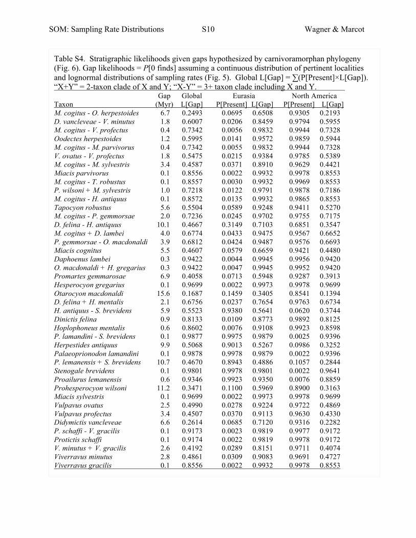
Divergence Time Likelihoods for Carnivoramorphans
We use the phylogenetic relationships among carnivoramorphan species suggested by Wesley-
Hunt and Flynn (2005). For each branch on that tree, we calculate the likelihood of the gap
implicit to that branch given both the morphological data and the stratigraphic data, finding the
branch length that maximizes the probability of both data sets. For branches linking observed
species to nodes, this is the difference between the hypothesized divergence and the species’ first
occurrence. In cases of unsampled hypothetical ancestors, this is the difference between the
hypothesized divergence and the hypothesized divergences of the daughter taxa. For each
lineage, we use the probabilities of the lineage being present in either North America or Eurasia
to weight the stratigraphic likelihood given the sampling rates and numbers of collections from
both areas (Figs. 1, 5). (We do not consider the possibility that a species was present in both.)
Thus, even within clades of species known from only one area, there is some small probability In
other words, the stratigraphic likelihood is:
(P[Present in Eurasia] × L[Gap in Eurasia]) + (P[Present in N. America] × L[Gap in America])
The details for each branch are given in Table S4.
Alternate phylogenies for Carnivoramorphans
The information above corresponds to our Model 1 tree. Here we illustrate our Model 2
(Mk+global lognormal sampling rates), Model 3 (Mk+global uniform sampling rates), Model 4
(Mk only) and Model 5 (minimum divergence times) trees.
SOM: Sampling Rate Distributions S10 Wagner & Marcot
Table S4. Stratigraphic likelihoods given gaps hypothesized by carnivoramorphan phylogeny (Fig. 6). Gap likelihoods = P[0 finds] assuming a continuous distribution of pertinent localities and lognormal distributions of sampling rates (Fig. 5). Global L[Gap] = ∑(P[Present]×L[Gap]). “X+Y” = 2-taxon clade of X and Y; “X-Y” = 3+ taxon clade including X and Y. Gap Global Eurasia North America Taxon (Myr) L[Gap] P[Present] L[Gap] P[Present] L[Gap] M. cogitus - O. herpestoides 6.7 0.2493 0.0695 0.6508 0.9305 0.2193 D. vancleveae - V. minutus 1.8 0.6007 0.0206 0.8459 0.9794 0.5955 M. cogitus - V. profectus 0.4 0.7342 0.0056 0.9832 0.9944 0.7328 Oodectes herpestoides 1.2 0.5995 0.0141 0.9572 0.9859 0.5944 M. cogitus - M. parvivorus 0.4 0.7342 0.0055 0.9832 0.9944 0.7328 V. ovatus - V. profectus 1.8 0.5475 0.0215 0.9384 0.9785 0.5389 M. cogitus - M. sylvestris 3.4 0.4587 0.0371 0.8910 0.9629 0.4421 Miacis parvivorus 0.1 0.8556 0.0022 0.9932 0.9978 0.8553 M. cogitus - T. robustus 0.1 0.8557 0.0030 0.9932 0.9969 0.8553 P. wilsoni + M. sylvestris 1.0 0.7218 0.0122 0.9791 0.9878 0.7186 M. cogitus - H. antiquus 0.1 0.8572 0.0135 0.9932 0.9865 0.8553 Tapocyon robustus 5.6 0.5504 0.0589 0.9248 0.9411 0.5270 M. cogitus - P. gemmorsae 2.0 0.7236 0.0245 0.9702 0.9755 0.7175 D. felina - H. antiquus 10.1 0.4667 0.3149 0.7103 0.6851 0.3547 M. cogitus + D. lambei 4.0 0.6774 0.0433 0.9475 0.9567 0.6652 P. gemmorsae - O. macdonaldi 3.9 0.6812 0.0424 0.9487 0.9576 0.6693 Miacis cognitus 5.5 0.4607 0.0579 0.6659 0.9421 0.4480 Daphoenus lambei 0.3 0.9422 0.0044 0.9945 0.9956 0.9420 O. macdonaldi + H. gregarius 0.3 0.9422 0.0047 0.9945 0.9952 0.9420 Promartes gemmarosae 6.9 0.4058 0.0713 0.5948 0.9287 0.3913 Hesperocyon gregarius 0.1 0.9699 0.0022 0.9973 0.9978 0.9699 Otarocyon macdonaldi 15.6 0.1687 0.1459 0.3405 0.8541 0.1394 D. felina + H. mentalis 2.1 0.6756 0.0237 0.7654 0.9763 0.6734 H. antiquus - S. brevidens 5.9 0.5523 0.9380 0.5641 0.0620 0.3744 Dinictis felina 0.9 0.8133 0.0109 0.8773 0.9892 0.8125 Hoplophoneus mentalis 0.6 0.8602 0.0076 0.9108 0.9923 0.8598 P. lamandini - S. brevidens 0.1 0.9877 0.9975 0.9879 0.0025 0.9396 Herpestides antiquus 9.9 0.5068 0.9013 0.5267 0.0986 0.3252 Palaeoprionodon lamandini 0.1 0.9878 0.9978 0.9879 0.0022 0.9396 P. lemanensis + S. brevidens 10.7 0.4670 0.8943 0.4886 0.1057 0.2844 Stenogale brevidens 0.1 0.9801 0.9978 0.9801 0.0022 0.9641 Proailurus lemanensis 0.6 0.9346 0.9923 0.9350 0.0076 0.8859 Prohesperocyon wilsoni 11.2 0.3471 0.1100 0.5969 0.8900 0.3163 Miacis sylvestris 0.1 0.9699 0.0022 0.9973 0.9978 0.9699 Vulpavus ovatus 2.5 0.4990 0.0278 0.9224 0.9722 0.4869 Vulpavus profectus 3.4 0.4507 0.0370 0.9113 0.9630 0.4330 Didymictis vancleveae 6.6 0.2614 0.0685 0.7120 0.9316 0.2282 P. schaffi - V. gracilis 0.1 0.9173 0.0023 0.9819 0.9977 0.9172 Protictis schaffi 0.1 0.9174 0.0022 0.9819 0.9978 0.9172 V. minutus + V. gracilis 2.6 0.4192 0.0289 0.8151 0.9711 0.4074 Viverravus minutus 2.8 0.4861 0.0309 0.9083 0.9691 0.4727 Viverravus gracilis 0.1 0.8556 0.0022 0.9932 0.9978 0.8553
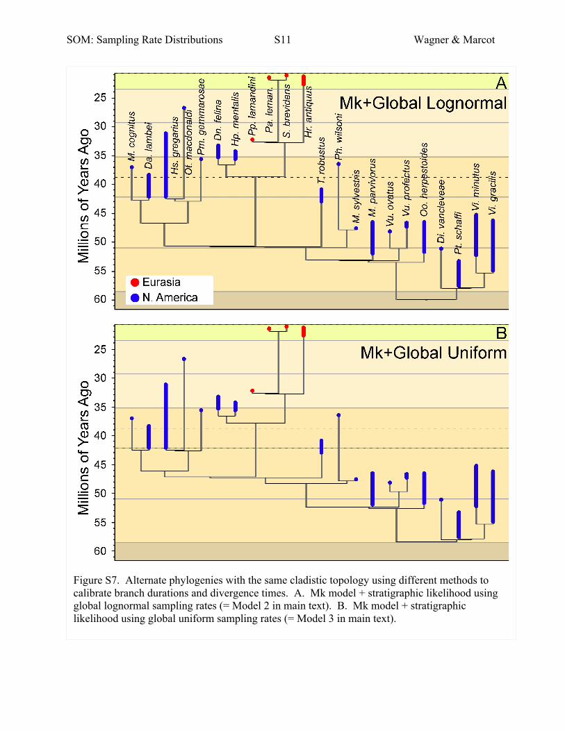
SOM: Sampling Rate Distributions S11 Wagner & Marcot
Figure S7. Alternate phylogenies with the same cladistic topology using different methods to calibrate branch durations and divergence times. A. Mk model + stratigraphic likelihood using global lognormal sampling rates (= Model 2 in main text). B. Mk model + stratigraphic likelihood using global uniform sampling rates (= Model 3 in main text).
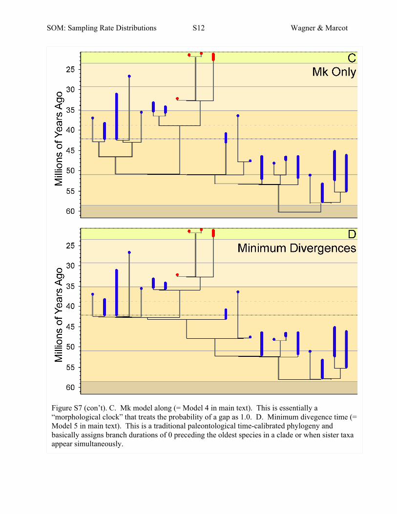
SOM: Sampling Rate Distributions S12 Wagner & Marcot
Figure S7 (con’t). C. Mk model along (= Model 4 in main text). This is essentially a “morphological clock” that treats the probability of a gap as 1.0. D. Minimum divegence time (= Model 5 in main text). This is a traditional paleontological time-calibrated phylogeny and basically assigns branch durations of 0 preceding the oldest species in a clade or when sister taxa appear simultaneously.
SOM: Sampling Rate Distributions S13 Wagner & Marcot
References and Notes
Foote, M. (1996) On the probability of ancestors in the fossil record. Paleobiology, 22, 141 -
151.
McGill, B.J. (2003) Does Mother Nature really prefer rare species or are log-left-skewed SADs a
sampling artefact? Ecology Letters, 6, 766 - 773.
Preston, W.H. (1948) The commonness and rarity of species. Ecology, 29, 254 - 283.
Sugiura, N. (1978) Further analysis of the data by Akaike’s information criterion and the finite
corrections. Communications in Statistics - Theory and Methods, A7, 13 - 26.
Wagner, P.J. (2012) Modelling rate distributions using character compatibility: implications for
morphological evolution among fossil invertebrates. Biology Letters, 8, 143 - 146.
Wagner, P.J., Kosnik, M.A. & Lidgard, S. (2006) Abundance distributions imply elevated
complexity of post-Paleozoic marine ecosystems. Science, 314, 1289 - 1292.
Wesley-Hunt, G.D. & Flynn, J.J. (2005) Phylogeny of the Carnivora: basal relationships among
the carnivoramorphans, and assessment of the position of “Miacoidea” relative to crown-
clade Carnivora. Journal of Systematic Palaeontology, 3, 1 - 28.