Use of neural fuzzy networks with mixed genetic/gradient algorithm in automated vehicle control
Upload
khangminh22Category
view
0download
0
Modelling and Control of Vehicle
Suspension Control Systems
Jiangtao Cao
Institute of Industrial Research
University of Portsmouth
A thesis submitted for the degree of
Doctor of Philosophy
Yet to be decided

2

Acknowledgements
I wish to express my gratitude to my supervisor, Dr. Honghai Liu, for
his constant support, guidance and encouragement. I feel especially
blessed since he is not only my supervisor but also my friend.
Of equal importance are my thanks to Prof. Ping Li and Dr. David
J. Brown. This research was supported in part by PML Flightlink
Ltd., British Council and University of Portsmouth. While everyone
at QED workgroup was supportive of my work, I am particularly
pleased to thank Mr. Martin Boughtwood and Mr. Chris Hilton for
their generous support.
Many thanks to my colleagues at Institute of Industrial Research.
Special thanks go to Dr. Ian Morgan, Mr. Edward Smart, Mr. Zhao-
jie Ju and Mr. Medhi Khoury for sharing their knowledge and exper-
tise with me.
Throughout the past years as a graduate student, there have been
many joyful moments in life, the moments which have been made
more enjoyable by my friends. Of equal importance are my happy
memories of Piyush Goel, Josh Fahimi, Chee Seng Chan, Xin Wen,
Yang Wang, Jian Ma, Jie Ma, Yuhui Shao.
I wish to express thanks to all my family members for their constant
support, encouragement, understanding. I will be short on words to
express my gratitude to my parents, what they have done for me
over the years. They have never stopped loving, even in the hardest
moment. They have always been my biggest inspiration. This work
would not be possible without their love support.

Abstract
In this thesis, firstly, a state of the art on computational intelligence
approaches in active vehicle suspension control systems is surveyed.
With a focus on the problems raised in practical implementations by
their non-linear and uncertain properties, it explores existing methods
in fuzzy inference systems, neural networks, genetic algorithms and
their combination for suspension control issues. Exactly due to these
conclusions of literature review, a new half-vehicle suspension model
is built. A novel framework of type-2 fuzzy control system for vehicle
active suspension is proposed and its closed-loop stability with the
sufficient conditions is carried out.
From a comprehensive consideration of a real car, an improved half-
vehicle suspension model is built in this thesis. The proposed model
can not only describe the real coupling between front and rear vehi-
cle body, but also be convenient to integrate suspension system with
brake control and anti-roll control systems. Hence this model is of
benefit to design the following active suspension control system.
A novel adaptive fuzzy logic controller is designed for vehicle ac-
tive suspension system. The proposed method utilizes interval type-2
fuzzy membership functions to deal with not only non-linearity and
uncertainty caused by irregular road inputs and complex suspension
dynamics, but also the potential uncertainty of experts knowledge and
experience which occur in typical fuzzy logic methods. An adaptive
strategy with closed-loop feedback regulation is proposed to improve
the existed type-reduction methods of type-2 fuzzy system. Simula-
tions on quarter-vehicle and half-vehicle active suspension models are
studied to evaluate the proposed control system. In comparison with

passive and typical fuzzy methods, the proposed method can obtain
better control performance.
For the closed-loop stability analysis of proposed control system, with
the Takagi-Sugeno (T-S) fuzzy consequents, the Lyapunov stabiliza-
tion method is implemented to verify the closed-loop stability. The
sufficient stability conditions for proposed vehicle active suspension
control system are deduced.
To review above all, with the improved vehicle suspension model, the
adaptive fuzzy controller and its stability analysis, this thesis builds
a completely intelligent control system for vehicle active suspension
system. The simulation results demonstrate its efficiency and prac-
ticability. And it is convenient to be implemented for the industrial
applications.

Contents
List of Figures vi
List of Tables ix
1 Introduction 1
1.1 A Brief Background . . . . . . . . . . . . . . . . . . . . . . . . . . 1
1.2 Problems and Challenges . . . . . . . . . . . . . . . . . . . . . . . 3
1.3 Overview of Approaches and Contributions . . . . . . . . . . . . . 4
1.4 Outline of Thesis . . . . . . . . . . . . . . . . . . . . . . . . . . . 5
2 Literature Review 7
2.1 Introduction . . . . . . . . . . . . . . . . . . . . . . . . . . . . . . 7
2.2 Background . . . . . . . . . . . . . . . . . . . . . . . . . . . . . . 12
2.2.1 Active Suspension System Linear Models and Control . . . 12
2.2.1.1 Quarter Vehicle Active Suspension Model . . . . 12
2.2.1.2 Half Vehicle Active Suspension Model . . . . . . 16
2.2.2 Non-linear Model of Active Suspension Model . . . . . . . 21
2.3 Adaptive Fuzzy Control . . . . . . . . . . . . . . . . . . . . . . . 23
2.4 Adaptive Fuzzy Sliding Mode Control . . . . . . . . . . . . . . . . 25
2.4.1 Conventional Sliding Mode Control . . . . . . . . . . . . . 26
2.4.2 Fuzzy Sliding Mode Control System . . . . . . . . . . . . . 29
2.4.2.1 Alleviating SMC Chattering . . . . . . . . . . . . 29
2.4.2.2 Fuzzy Logic Complementary to SMC . . . . . . . 33
2.5 Adaptive Neural Network Control . . . . . . . . . . . . . . . . . . 35
2.6 Genetic Algorithms Based Adaptive Optimization and Control . . 37
iv

CONTENTS
2.7 Integrated Adaptive Control Methods . . . . . . . . . . . . . . . . 41
2.7.1 Adaptive Neuro-fuzzy Control . . . . . . . . . . . . . . . . 41
2.7.2 Adaptive Genetic-based Optimal Fuzzy Control . . . . . . 43
2.7.3 GA-ANNs Combined Control . . . . . . . . . . . . . . . . 45
2.8 Summary . . . . . . . . . . . . . . . . . . . . . . . . . . . . . . . 46
3 Improved Vehicle Active Suspension Model 48
3.1 Introduction . . . . . . . . . . . . . . . . . . . . . . . . . . . . . . 48
3.2 A Rigid Tyre Model . . . . . . . . . . . . . . . . . . . . . . . . . 49
3.3 The Improved Half-vehicle Active Suspension Model . . . . . . . . 52
3.3.1 The Linear Half-vehicle Model . . . . . . . . . . . . . . . . 54
3.3.2 Linear Model Performance Analysis . . . . . . . . . . . . . 56
3.3.3 The Non-linear Half-vehicle Model . . . . . . . . . . . . . 61
3.3.4 Non-linear Model Analysis . . . . . . . . . . . . . . . . . . 62
3.4 The Improved LQG Design . . . . . . . . . . . . . . . . . . . . . . 66
3.4.1 The Improved LQG . . . . . . . . . . . . . . . . . . . . . . 66
3.4.2 Simulation Results . . . . . . . . . . . . . . . . . . . . . . 67
3.4.2.1 Step Road Inputs . . . . . . . . . . . . . . . . . . 67
3.4.2.2 Random Road Inputs . . . . . . . . . . . . . . . 69
3.5 Summary . . . . . . . . . . . . . . . . . . . . . . . . . . . . . . . 71
4 Interval Type-2 Fuzzy Control System 74
4.1 Introduction . . . . . . . . . . . . . . . . . . . . . . . . . . . . . . 74
4.2 Interval Type-2 Fuzzy Systems . . . . . . . . . . . . . . . . . . . . 77
4.2.1 The Interval Type-2 Fuzzy Sets . . . . . . . . . . . . . . . 77
4.2.2 The Interval Type-2 Fuzzy System . . . . . . . . . . . . . 79
4.2.3 Type-reduction and Defuzzification Methods . . . . . . . . 81
4.3 The Adaptive Interval Type-2 FLC . . . . . . . . . . . . . . . . . 84
4.3.1 The Framework of Adaptive IT2 FLC . . . . . . . . . . . . 85
4.3.2 The LMS method . . . . . . . . . . . . . . . . . . . . . . . 86
4.3.3 The PSO method . . . . . . . . . . . . . . . . . . . . . . . 88
4.4 Simulations on the Quarter-vehicle Model . . . . . . . . . . . . . 90
4.4.1 Adaptive IT2 FLC with the LMS method . . . . . . . . . 91
4.4.2 Adaptive IT2 FLC with the PSO method . . . . . . . . . . 100
v

CONTENTS
4.5 Simulations on the Half-vehicle Model . . . . . . . . . . . . . . . 105
4.5.1 The adaptive IT2 FLC with the LMS method . . . . . . . 107
4.5.2 The IT2 FLC with the PSO method . . . . . . . . . . . . 112
4.6 Summary . . . . . . . . . . . . . . . . . . . . . . . . . . . . . . . 117
5 Stability Analysis of Closed-loop Systems 119
5.1 Introduction . . . . . . . . . . . . . . . . . . . . . . . . . . . . . . 119
5.2 Typical T-S Fuzzy Control Systems and the Stability Conditions . 120
5.2.1 T-S Fuzzy Model and Control System . . . . . . . . . . . . 120
5.2.2 The Stability Conditions with Lyapunov Stability Theory . 122
5.3 The General Interval Type-2 T-S Fuzzy System . . . . . . . . . . 124
5.3.1 The Interval Type-2 T-S Fuzzy System . . . . . . . . . . . 124
5.3.2 The Interval Type-2 T-S Fuzzy Control System . . . . . . 126
5.4 Stability Analysis of the IT2 T-S Fuzzy Control System . . . . . . 127
5.5 Summary . . . . . . . . . . . . . . . . . . . . . . . . . . . . . . . 132
6 Conclusions 133
6.1 Overview . . . . . . . . . . . . . . . . . . . . . . . . . . . . . . . . 133
6.2 Contributions . . . . . . . . . . . . . . . . . . . . . . . . . . . . . 133
6.2.1 The Improved Models . . . . . . . . . . . . . . . . . . . . 134
6.2.2 The Interval Type-2 Fuzzy Controller with LMS . . . . . . 134
6.2.3 The Interval Type-2 Fuzzy Controller with PSO . . . . . . 135
6.2.4 Closed-loop Stability Analysis . . . . . . . . . . . . . . . . 135
6.3 Future Work . . . . . . . . . . . . . . . . . . . . . . . . . . . . . . 136
6.3.1 Expansion of Type-2 Fuzzy Inference Engine . . . . . . . . 136
6.3.2 Relaxation on Stability Conditions . . . . . . . . . . . . . 136
6.3.3 Generalization . . . . . . . . . . . . . . . . . . . . . . . . . 136
6.3.4 Application . . . . . . . . . . . . . . . . . . . . . . . . . . 137
6.4 Summary . . . . . . . . . . . . . . . . . . . . . . . . . . . . . . . 137
References 153
A Publications 154
B Fuzzy Rules Table 156
vi

List of Figures
2.1 Six degree-of-freedom vehicle model (Nagai, 1993) . . . . . . . . 13
2.2 Two degree-of-freedom quarter-vehicle model . . . . . . . . . . . . 14
2.3 Half-vehicle suspension model . . . . . . . . . . . . . . . . . . . . 17
2.4 Non-linear properties of suspension system [wheel stroke(m) versus
suspension force(N)](Kim & Ro, 1998) . . . . . . . . . . . . . . . 22
2.5 The adaptive FLC scheme in Huang & Chao (2000) . . . . . . . . 25
2.6 Effects of parameters G and K (Kaynak, 1998) . . . . . . . . . . 30
2.7 Fuzzy adaptive sliding mode control scheme for Active Suspension
Control System (ASCS) in Chen et al. (1995) . . . . . . . . . . . 30
2.8 The fuzzy adaptive controller scheme in Zhang et al. (2007) . . . 32
2.9 The adaptive fuzzy sliding mode controller scheme in Huang & Lin
(2003) . . . . . . . . . . . . . . . . . . . . . . . . . . . . . . . . . 34
2.10 Scheme of the hydraulic active suspension system in Kucukdemiral
et al. (2005) . . . . . . . . . . . . . . . . . . . . . . . . . . . . . . 35
2.11 The scheme of indirect adaptive control based on ANNs in Guo
et al. (2004) . . . . . . . . . . . . . . . . . . . . . . . . . . . . . . 36
2.12 The 5 degree-of-freedom half vehicle model employed in Baumal
et al. (1998) . . . . . . . . . . . . . . . . . . . . . . . . . . . . . . 39
2.13 The force control scheme with skyhook damper, virtual damper
and road-following spring in Tsao & Chen (2001) . . . . . . . . . 40
2.14 The adaptive neural network fuzzy control system with time-delay
compensator in Dong et al. (2006) . . . . . . . . . . . . . . . . . . 42
2.15 The FNNC scheme in Dong et al. (2006) . . . . . . . . . . . . . . 42
2.16 The PBGA fuzzy control system in Nawa et al. (1999) . . . . . . 44
vii

LIST OF FIGURES
2.17 An example of the fuzzy system encoded in a chromosome in Nawa
et al. (1999) . . . . . . . . . . . . . . . . . . . . . . . . . . . . . . 45
3.1 The rigid tyre model . . . . . . . . . . . . . . . . . . . . . . . . . 50
3.2 The half vehicle model . . . . . . . . . . . . . . . . . . . . . . . . 52
3.3 The pitch angles of a vehicle body with different Vcr . . . . . . . . 57
3.4 The accelerations of front vehicle body with different Vcr . . . . . 57
3.5 The accelerations of rear vehicle body with different Vcr . . . . . . 58
3.6 The front suspension travel with different Vcr . . . . . . . . . . . 59
3.7 The rear suspension travel with different Vcr . . . . . . . . . . . . 59
3.8 The front tyre dynamic loading with different Vcr . . . . . . . . . 60
3.9 The rear tyre dynamic loading with different Vcr . . . . . . . . . 60
3.10 The vertical accelerations of front vehicle body with non-linear model 63
3.11 The vertical accelerations of rear vehicle body with non-linear model 63
3.12 The pitch angles of vehicle body with non-linear model . . . . . . 64
3.13 The front suspension travel with non-linear model . . . . . . . . 64
3.14 The rear suspension travel with non-linear model . . . . . . . . . 65
3.15 The front tyre dynamic loading with non-linear model . . . . . . 65
3.16 The rear tyre dynamic loading with non-linear model . . . . . . . 66
3.17 Pitch angle comparison with typical LQG and different rolling ve-
locities . . . . . . . . . . . . . . . . . . . . . . . . . . . . . . . . 68
3.18 Pitch angle comparison with different controller at Vcr= 35 m/s
(upper three lines) and 25 m/s (lower three lines) . . . . . . . . . 69
3.19 Pitch angle comparison with different controller and random road
input ( Vcr=35m/s) . . . . . . . . . . . . . . . . . . . . . . . . . 70
3.20 Pitch angle comparison with different controller and random road
input (Vcr=25m/s) . . . . . . . . . . . . . . . . . . . . . . . . . . 72
4.1 The interval type-2 fuzzy membership functions . . . . . . . . . . 78
4.2 The interval type-2 fuzzy logic system . . . . . . . . . . . . . . . . 80
4.3 The framework of proposed IT2 fuzzy controller . . . . . . . . . . 85
4.4 The structure of adaptive IT2 FLC with LMS method . . . . . . 87
4.5 The structure of adaptive IT2 FLC with PSO method . . . . . . . 89
4.6 The interval type-2 fuzzy membership functions of three inputs . . 91
viii

LIST OF FIGURES
4.7 The membership functions of actuator force fa . . . . . . . . . . . 92
4.8 The frequency response of vehicle body acceleration zb . . . . . . 95
4.9 The frequency response of tyre dynamic load . . . . . . . . . . . . 95
4.10 The frequency response of vehicle body acceleration on B class
road surface . . . . . . . . . . . . . . . . . . . . . . . . . . . . . . 96
4.11 The frequency response of vehicle body acceleration on C class
road surface . . . . . . . . . . . . . . . . . . . . . . . . . . . . . . 96
4.12 The frequency response of vehicle body acceleration on D class
road surface . . . . . . . . . . . . . . . . . . . . . . . . . . . . . . 97
4.13 The frequency response of vehicle body acceleration (1: sprung
mass +50%, 2: sprung mass -50%) . . . . . . . . . . . . . . . . . 98
4.14 The frequency response of vehicle body acceleration (1: Ks1 +10%,
2: Ks1 -10%) . . . . . . . . . . . . . . . . . . . . . . . . . . . . . 100
4.15 The frequency response of vehicle body acceleration zb . . . . . . 101
4.16 The frequency response of tyre dynamic load . . . . . . . . . . . . 102
4.17 The interval type-2 fuzzy membership functions of five inputs . . 105
4.18 The frequency response of vehicle front body acceleration . . . . . 108
4.19 The frequency response of vehicle rear body acceleration . . . . . 108
4.20 The frequency response of front tyre dynamic load . . . . . . . . . 109
4.21 The frequency response of rear tyre dynamic load . . . . . . . . . 109
4.22 The frequency response of pitch angle acceleration . . . . . . . . . 110
4.23 The different pitch dynamics with different vehicle speed . . . . . 111
4.24 The frequency response of vehicle front body acceleration . . . . . 113
4.25 The frequency response of vehicle rear body acceleration . . . . . 113
4.26 The frequency response of front tyre dynamic load . . . . . . . . . 114
4.27 The frequency response of rear tyre dynamic load . . . . . . . . . 114
4.28 The frequency response of pitch angle acceleration . . . . . . . . . 115
4.29 The different pitch dynamics with changing vehicle speed . . . . . 116
ix

List of Tables
2.1 Comparison of capabilities of different adaptive methodologies(Fukuda
& Kubota, 1999) . . . . . . . . . . . . . . . . . . . . . . . . . . . 11
2.2 Road roughness values classified by ISO (Degree of roughness S(Ω)×10−6) 15
3.1 Nominal parameters of half-vehicle active suspension model . . . . 56
3.2 The coefficients of non-linear forces . . . . . . . . . . . . . . . . . 63
3.3 Random road input parameters and the weighting parameters . . 67
3.4 Vehicle performance comparison with Vcr = 30m/s . . . . . . . . 71
3.5 Vehicle performance comparison with Vcr = 35m/s . . . . . . . . 71
3.6 Vehicle performance comparison with Vcr=25 m/s . . . . . . . . . 72
4.1 The parameters of quarter vehicle active suspension . . . . . . . . 91
4.2 The rules of fuzzy controller . . . . . . . . . . . . . . . . . . . . . 93
4.3 The RMS values comparison in time domain . . . . . . . . . . . . 95
4.4 The RMS values comparison on B class road surface . . . . . . . . 97
4.5 The RMS values comparison on C class road surface . . . . . . . . 98
4.6 The RMS values comparison on D class road surface . . . . . . . . 98
4.7 The RMS comparison of body acceleration in time domain . . . . 99
4.8 The RMS comparison of tyre dynamic loads in time domain . . . 99
4.9 The RMS values comparison in time domain . . . . . . . . . . . . 102
4.10 The comparison of RMS values of body acceleration . . . . . . . . 103
4.11 The comparison of RMS values of tyre dynamic load . . . . . . . 103
4.12 The comparison of RMS values of suspension travel . . . . . . . . 104
4.13 The comparison of RMS values of control force . . . . . . . . . . . 104
4.14 The RMS values comparison with constant vehicle speed . . . . . 111
x

LIST OF TABLES
4.15 The RMS values comparison with changing vehicle speed . . . . . 112
4.16 The RMS values comparison with constant vehicle speed . . . . . 116
4.17 The RMS values comparison with changing Vcr . . . . . . . . . . . 117
B.1 The fuzzy rules for half-vehicle active suspension (part 1) . . . . . 156
B.2 The fuzzy rules for half-vehicle active suspension (part 2) . . . . . 157
B.3 The fuzzy rules for half-vehicle active suspension (part 3) . . . . . 158
B.4 The fuzzy rules for half-vehicle active suspension (part 4) . . . . . 159
B.5 The fuzzy rules for half-vehicle active suspension (part 5) . . . . . 160
B.6 The fuzzy rules for half-vehicle active suspension (part 6) . . . . . 161
xi

Chapter 1
Introduction
It is well known that the suspension system performs multiple tasks such as
maintaining contact between vehicle tyres and the road, addressing the stability
of the vehicle, and isolating the frame of the vehicle from road-induced vibration
and shocks. With the development of mechanical and electronics technology, the
requirements of ride comfort and driving performance have been major devel-
opment objectives of modern vehicles to satisfy the expectations of customers.
Hence, the design of an appropriate suspension system is always an important
research topic for achieving the desired vehicle quality.
1.1 A Brief Background
There are many performance parameters which need to be optimized in vehicle
suspension system. Among them there are four main parameters which should be
considered carefully in designing a suspension system, i.e., ride comfort (directly
related to acceleration sensed by passengers), body motion (bounce, pitch and
roll of sprung mass are created by cornering and acceleration or deceleration),
road handling (associated with the contact forces of tyres and road surface),
suspension travel (referring to the displacement between the sprung mass and
unsprung mass) (Hrovat, 1997). It is a challenging issue for one suspension system
to simultaneously minimize all four parameters. Hence, how to obtain a proper
trade-off between these performances is the main task for successfully designing
a vehicle suspension system.
1

1.1 A Brief Background
To improve the vehicle performance, many kinds of suspension systems have
been designed for different types of vehicles. In general, there are three main
branches of suspension system, i.e., a passive, semi-active and active suspension
system. Passive suspension systems consist of conventional springs and dampers
which are used in most cars. The springs and dampers are assumed to have al-
most linear characteristics. In passive suspension systems, these elements have
fixed characteristics, and so, have no mechanism for feedback control(Naude &
Snyman, 2003a,b; Tamboli & Joshi, 1999). Semi-active suspensions provide con-
trolled real-time dissipation of energy(Choi et al., 2001; Margolis, 1982; Oueslati
& Sankar, 1994; Yao et al., 2002). This is achieved through a mechanical device
called an active damper which is used in parallel to a conventional spring. The
main feature of this system is the ability to adjust the damping of the suspension,
without any use of actuators. Active suspension systems employ pneumatic or
hydraulic actuators which in turn creates the desired force in the suspension sys-
tem (Crolla & Abdel, 1991; Hac, 1992; Hrovat, 1997; Thompson & Davis, 1988).
The actuator works in parallel to a spring and damper. An active suspension
system requires sensors to be located at different points of the vehicle to measure
its dynamic information of part of a vehicle. This information is used in the
real-time controller to drive the actuator in order to provide the exact amount of
force required.
Due to fewer mechanical constraints, more degrees of freedom and a stronger
capability to deal with unknown road surfaces, there is an increasing interest in
design and control of active suspension systems for automotive engineers and re-
searchers during the past three decades. Research has shown that a linear optimal
control scheme provides an efficient way to design an active suspension system
which can improve the vehicle ride and handling performance together (Hrovat,
1997; Nagai, 1993). However, it is based on the assumption that there exists a
perfect (broad bandwidth) actuator, which can generate the required force fast
enough and the system can be linearized within some operation regions. For
a real vehicle suspension system, its dynamics are inherently non-linear, even
with some uncertainties. Therefore, adaptive control schemes and robust control
strategies have been proposed to undertake the role of providing self-tuning feed-
back gains and to take the aforementioned four sets of parameters into account
2

1.2 Problems and Challenges
to ensure optimal operation of the system in different driving conditions and road
surfaces(Gordon et al., 1991; Hac, 1987; Sunwoo & Cheok, 1990; Sunwoo et al.,
1991). Much research considered non-linear, uncertain and unmodelled parts of a
real suspension system by using non-linear models and non-linear control meth-
ods(Alleyne & Hedrick, 1995; Alleyne et al., 1993; Gordon et al., 1991). With
the significant development of computational intelligence in the past two decades,
intelligent control methods provide an extensive freedom for control engineers to
deal with practical problems associated with active suspension control systems
(Chen et al., 1995; Cherry & Jones, 1995; Fernando & Viassolo, 2000; Huang &
Chao, 2000; Huang & Lin, 2003; Lian et al., 2005; Rao & Prahlad, 1997; Ting
et al., 1995; Yeh & Tsao, 1994).
1.2 Problems and Challenges
As mentioned in early research about active suspension systems, the dynamics
of suspension and the actuator were assumed to be linear or piecewise linear
and the majority of control laws were built on linear suspension mathematical
models. However, in real applications, there are some issues to bring out the non-
linear and uncertain dynamics of suspension systems, e.g., mechanical non-linear
properties, the coupling with other vehicle control systems and the disturbance by
random road inputs. Furthermore, more and more information from each part of
vehicle components are integrated into one central control unit in modern vehicles,
the problem of obtaining the proper description of suspension information from
other related subsystems becomes more and more complex. So the existed theory
analysis results with assumed models were proved to suffer from severe limitations
(Gao et al., 2006; Li et al., 2006).
For active suspension control systems, the key role is to optimize suspension
performances in real-time with multiple constraints. With the development of
vehicle technology, some devices for special vehicles, such as military vehicles,
can be transferred to normal cars. Meanwhile, some new requirements of the
suspension system have been demanded by customers and vehicle companies,
such as energy saving (Cao et al., 2008). Consequently, a new control framework
needs to be designed to satisfy these new requirements. Alternatively, a more
3

1.3 Overview of Approaches and Contributions
adaptive capability of controller is required to keep satisfied riding and handling
performance on different circumstance.
Almost all of the suspension control systems are closed-loop control systems,
so the closed-loop stability is very important to be guaranteed when they are
employed in real systems. Based on Lyapunov stability methods, some stability
analysis of suspension control systems with linear control strategies have been
studied. However, it is still a challenge for suspension control system to build a
proper surface or systematic analysis method, especially for an intelligent con-
troller (Feng, 2006).
In recent years, research work on improving the active suspension control
systems has been challenged in four major directions: Comprehensive studies on coupling information between suspension systems
and other vehicle control systems, as well as developing the decoupling
methods for suspension control. Achieving more adaptability and appropriate performance active suspension
control methods or control framework while retaining simplicity and real-
time computing efficiency. Development of estimating a platform for active suspension control sys-
tems and stability analysis methods of closed-loop control systems which
considers the effect of uncertainty and non-linearity in applications. Improving the manufacture of high performance actuators and micro control
units, as well as reforming the sensory structures used by information fusion
technology.
1.3 Overview of Approaches and Contributions
To take into account the previous section, this thesis makes contributions to the
first three of the four problem areas described in Section 1.2. The contributions
are driven by three new ideas which are described below:
4

1.4 Outline of Thesis
1. An improved half-vehicle model for active suspension control system is pro-
posed to make up the existing models by considering the coupling of longi-
tudinal motion between the front and the back of vehicle body. This model
can more precisely describe the real dynamics of vehicle suspension system.
2. Based on the improved model, a novel architecture of the interval type-2
fuzzy controller is proposed to control the vehicle non-linear active suspen-
sion system. Under the proposed control framework, the adaptive strategy
with two optimization methods (i.e., Least Means Squares (LMS) and Par-
ticle Swarm Optimization (PSO)) is designed to derive the expected active
control forces which bring better ride comfort and handling performance.
Furthermore, the proposed method has inherent capability to deal with the
potential uncertain information of fuzzy knowledge base which is deduced
from expert experience.
3. With the proposed control framework, the stability of vehicle active sus-
pension closed-loop control system is analysed by the quadratic Lyapunov
stability method. The sufficient conditions are derived for guaranteeing its
global stability.
1.4 Outline of Thesis
To fulfil the proposed approaches, the thesis has been structured as follows.
Chapter 2 provides an overview of computational intelligence approaches in
active vehicle suspension control systems with a focus on the problems raised in
practical implementations by their non-linear and uncertain properties. After a
brief introduction on active suspension models, it explores state of the art in fuzzy
inference systems, neural networks, genetic algorithms and their combination for
suspension control issues. Discussion and comments are provided based on the
reviewed simulation and experimental results. The future research directions and
challenges for active suspension control are discussed.
Chapter 3 proposes an improved half-vehicle active suspension model to
explore the nature longitudinal coupling phenomenon between the front and back
part of vehicle body. It addresses the first idea in Chapter 1. To achieve this
5

1.4 Outline of Thesis
improved model, firstly, a rigid tyre model is introduced to study the vehicle
speed effect on vertical vibration. Secondly, the improved model is built by
integrating the tyre model into the linear and non-linear half-vehicle suspension
models. Finally, the open-loop and closed-loop performances of the improved
model are analysed with step road inputs and random road inputs.
Chapter 4 builds a novel framework of adaptive interval type-2 fuzzy con-
troller for vehicle non-linear active suspension systems. It undertakes the second
approach in Chapter 1. To design the new control architecture, the first is a
brief review of interval type-2 fuzzy system. Subsequently, the proposed adaptive
control framework is built. With the proposed control structure, the adaptive
method is designed to self-tune lower bounds and upper bounds of interval type-
2 fuzzy reasoning results by two optimization methods (i.e., LMS and PSO). The
control aims are not only to improve the ride comfort and handling performance
of vehicle suspension system, but also to reduce the suspension travel and the lon-
gitudinal vibration. Finally, under several different test conditions, case studies
based on quarter-vehicle and half-vehicle models are demonstrated.
Chapter 5 presents the closed-loop stability analysis for proposed control
system. It addresses the third idea in Chapter 1. To address the stability analy-
sis, initially, the typical T-S fuzzy control system and its stability conditions by
the Lyapunov stability theory are revisited. By formalising the proposed control
system into a general interval type-2 fuzzy control system, the closed-loop sta-
bility is analysed with the quadratic Lyapunov method. Finally, the sufficient
conditions for global stability are derived.
Chapter 6 summaries the thesis with a discussion of the methods employed
and future work.
Appendices includes a list of publications and followed by the fuzzy control
rules for half-vehicle active suspension fuzzy controllers.
6

Chapter 2
Literature Review
2.1 Introduction
A suspension system is one of the important components of a vehicle, which plays
a crucial role in handling performance and the ride comfort characteristics of a
vehicle. It has two main functionalities, one is to isolate the vehicle body with its
passengers from external disturbance inputs which mainly come from irregular
road surfaces. It always relates to riding quality. The other is to maintain a firm
contact between the road and the tyres to provide guidance along the track. It
is called handling performance.
In a conventional passive suspension system which comprises of springs and
dampers, a trade-off is needed to resolve the conflicted requirements of ride com-
fort and good handling performance. The reason is that stiff suspension is re-
quired to support the weight of vehicle and to follow the track; on the other
hand, soft suspension is needed to isolate the disturbance from the road. Hence
there exists a significantly growing interest in the design and control of active
suspension systems from automotive engineers and researchers in the past three
decades. An active suspension system is characterized by employing some kind
of suspension force generator using pneumatic, magneto-rheological or hydraulic
actuators. Practical applications of active suspension systems have been facil-
itated by the development of microprocessors and electronics from the middle
of 1980s(Esmailzadeh & Bateni, 1992; Hrovat, 1987; Thompson & Davis, 1988,
1991). Related surveys on theories and applications of active suspension control
7

2.1 Introduction
systems were provided by Hrovat (1997); Nagai (1993), with fast-growing com-
putational intelligence methodologies significantly driving recent advances in this
research area in the past decade.
The design of a vehicle active suspension control system is a long-standing con-
trol engineering problem, which is rooted in multi-parameter optimization with
a real-time requirement. It includes ride comfort, body motion, road handling
and suspension travel (Taghirad, 1997; Taghirad & Esmailzadeh, 1998; Williams,
1997). Ride comfort directly relates to the acceleration sensed by passengers.
Body motion means bounce, pitch and roll of sprung mass which are created
by cornering, acceleration or deceleration. Road handling is associated with the
contact forces of tyres and the road surface. Suspension travel refers to the dis-
placement between a sprung mass and an unsprung mass. It is really a challenging
issue for one active suspension system to simultaneously optimise all four sets of
parameters. Hence, the ability to handle related trade-offs is crucial for success-
fully designing an active suspension control system. Research in the past three
decades has shown that a linear optimal control scheme provides an efficient way
to design an active suspension system which can improve the vehicle ride and
handling performance together (Hrovat, 1997; Nagai, 1993). This is based on the
assumption that there exists a perfect (broad bandwidth) actuator, which can
generate the required force fast enough and the system can be linearized within
some operation regions. However, a real vehicle suspension system is inherently
non-linear, even with some uncertainties. Therefore, adaptive control schemes
have to undertake the role of providing self-tuning feedback gains and to take
the aforementioned four sets of parameters into account to ensure optimal opera-
tion of the system in different driving conditions and road surfaces(Gordon et al.,
1991; Hac, 1987; Sunwoo & Cheok, 1990).
A classical form of adaptive scheme for a vehicle active suspension system was
introduced in the late 1980s by Hac (1987). This is the starting point of the adap-
tive control scheme, in which a set of feedback gains are varied by the change of
power spectral density of terrain roughness obtained by processing the measure-
ment data. Another comparison of adaptive Linear-Quadratic-Gaussian (LQG)
and non-linear controllers for active suspensions was presented by Gordon et al.
(1991). A model reference adaptive control scheme was proposed by Alleyne et al.
8

2.1 Introduction
(1993) which resulted in better performance than the active suspension system
with a non-adaptive controller and passive suspension system. Also in this thesis,
10% to 30% variances of sprung mass and stiffness coefficients were examined to
check the adaptation capability based on a single degree-of-freedom (DOF) quar-
ter vehicle model. Sunwoo & Cheok (1990) proposed an explicit adaptive control
for an active suspension system which is based on a self-tuning controller design.
It consisted of on-line low-order recursive parameters estimation, a closed-form
algebraic gain computation and manipulation of the control parameters. Some
other works on adaptive control of active suspension systems can be found in
Alleyne (1997); Alleyne & Hedrick (1995); Kim (1996); Kim & Ro (1998); Lu &
DePoyster (2002). Up to this point, most researchers have dealt with a linear
model in developing control laws or using adaptive control scheme to conquer
the limited non-linear properties of suspension systems. However, if the system
is highly non-linear over the range of operation, its adaptive schemes may show
severe limitations. For instance, if a wheel stroke is so strong that the stiffness
of a suspension is beyond the linear range, it might be practically impossible to
identify parameters through ordinary identification(Kim & Ro, 1998; Palkovics &
Venhovens, 1992; Sunwoo et al., 1991). In the early 1990s many studies began to
consider the non-linearities, uncertainties and unmodelled parts of a real suspen-
sion system, which requires the use of a non-linear model and some non-linear
forms of control scheme(Alleyne et al., 1993; Slotine & Li, 1991). In practice,
these non-linear models made active suspension control systems so complex and
too challenging to employ.
In industrial applications, control engineers often have to deal with complex
systems, which have multiple variable and multi-parameter models with perhaps
non-linear coupling. The conventional approaches for understanding and predict-
ing the behaviour of such systems based on analytical techniques can be proved
to be inadequate, even at the initial stages of establishing an appropriate math-
ematical model(Kaynak et al., 2001). The computational environment used in
such an analytical approach is perhaps too categorical and inflexible in order to
cope with the intricacy and the complexity of real world industrial systems. It
turns out that, in dealing with such systems, one has to face a high degree of un-
certainty and tolerate imprecision. Trying to increase precision can be very costly.
9

2.1 Introduction
Thanks to the significant development of soft computing or computational intel-
ligence in the past decades, it has provided alternative ways to non-linear system
modelling and control. Generally speaking, the principal constituents of intelli-
gent computing include Fuzzy Logic (FL), artificial neural networks (ANNs) and
evolutionary computing (EC). FL is mainly concerned with imprecision and ap-
proximate reasoning, ANNs are mainly concerned with learning and curve fitting,
and EC is mainly concerned with global optimization based on the natural se-
lection and genetics. These intelligent computing methodologies have resulted in
the development of the “intelligent control” field, which consists of novel control
approaches based on FL, ANNs, EC, and other techniques induced from artificial
intelligence and their combination. These methods provide an extensive freedom
for control engineers to deal with practical problems of vagueness, uncertainty,
or imprecision. These intelligent methods are good candidates for alleviating the
problems associated with active suspension control systems (Zhang et al., 2007).
In comparison with hard computing, soft computing provides the tolerance
for imprecision and uncertainty which is exploited to achieve a practically ac-
ceptable solution at a reasonable cost, tractability, and high machine intelligence
quotient (MIQ). Zadeh argues that soft computing, rather than hard computing,
should be viewed as the foundation of machine intelligence. A full comparison
of their capabilities in different application fields was constructed by Fukuda and
Shimojima in Table 2.1, together with those of control theory and artificial intel-
ligence(Fukuda & Kubota, 1999).
10

2.1
Intro
ductio
n
Table 2.1: Comparison of capabilities of different adaptive methodologies(Fukuda & Kubota, 1999)
Mathematical
Model
Learning
Data
Operator
Knowl-
edge
Real
Time
Knowledge
Repre-
sentation
Non-
linearity
Optimisation
Control
Theory
Good or
Suitable
Unsuitable Needs
other
methods
Good or
Suitable
Unsuitable Unsuitable Unsuitable
Neural
Network
Unsuitable Good or
Suitable
Unsuitable Good or
Suitable
Unsuitable Good or
Suitable
Fair
Fuzzy
Logic
Fair Unsuitable Good or
Suitable
Good or
Suitable
Needs
other
methods
Good or
Suitable
Unsuitable
other
Artificial
Intelli-
gence
Needs other
methods
Unsuitable Good or
Suitable
Unsuitable Good or
Suitable
Needs
other
methods
Unsuitable
Genetic
Algo-
rithms
Unsuitable Good or
Suitable
Unsuitable Needs
other
methods
Unsuitable Good or
Suitable
Good or Suitable
11

2.2 Background
This chapter reviews the necessary background for active suspension control
systems which provides a foundation for the methods proposed in later chap-
ters. It is organized as follows. Section 2.2 revises the modelling of an active
suspension system. Section 2.3 reviews adaptive fuzzy control methods; Section
2.4 presents adaptive fuzzy sliding mode control approaches; Section 2.5 revises
neural networks based control systems, and Section 2.6 presents adaptive genetic
algorithm control methods. Section 2.7 describes combination methods based on
neural networks, fuzzy inference and generic algorithms. Finally it is concluded
in Section 2.8 with discussions and future work.
2.2 Background
A vehicle body is generally a rigid body with six DOF motions shown in Fig.
2.1. It consists of longitudinal, lateral, heave, roll, pitch and yaw motions. These
motions are restricted by suspension geometries in vehicles and are more or less
coupled with one another. Moreover, as the suspensions have a mechanical struc-
ture with unsprung mass, coupling also occurs between the sprung and unsprung
masses. Regardless of such coupling problems, the reduced-order mathematical
model is useful for designing an active suspension control system. Therefore a
quarter-vehicle model or a half-vehicle model is often used for theoretical analysis
and design of active suspension systems (Hrovat, 1997; Nagai, 1993).
In this section, a linear quarter-vehicle model and a linear half-vehicle model
of an active suspension system are introduced. Based on the linear models, their
LQG controllers are designed. Practical active suspension system models are also
analysed in terms of non-linear properties and uncertain dynamic disturbances.
2.2.1 Active Suspension System Linear Models and Con-
trol
2.2.1.1 Quarter Vehicle Active Suspension Model
The quarter-vehicle model was initially developed to explore active suspension
capabilities. It gave birth to the concepts of skyhook damping and fast load
12

2.2 Background
Figure 2.1: Six degree-of-freedom vehicle model (Nagai, 1993)
leveling which are now being developed toward actual, large-scale production ap-
plications. In this section, we define,
mb: quarter body mass (or sprung mass) (Kg);
mw: wheel mass (or unsprung mass) (Kg);
Ks: suspension spring stiffness (N/m)
Kt: tyre stiffness (N/m);
c: damping coefficient (Ns/m);
G0: road roughness coefficient (m3/cycle);
U0: vehicle original forward velocity (m/s);
f0: low cut-off frequency (Hz);
z0: road displacement (m);
zw: wheel displacement (m);
zb: body displacement (m);
fa: control force (N);
The quarter vehicle model is shown in Fig. 2.2. The dynamic differential equa-
tions of this suspension system can be represented as
mbzb = fa + c(zw − zb) + Ks(zw − zb) (2.1)
mwzw = −fa − c(zw − zb) − Ks(zw − zb) − Kt(zw − z0) (2.2)
For better ride comfort, a perfect road surface model is necessary to design vehicle
active suspension control system. There are many possible ways to analytically
13

2.2 Background
Figure 2.2: Two degree-of-freedom quarter-vehicle model
describe the road inputs, which can be classified as shock or vibration (Hrovat,
1997). Shocks are discrete events of relatively short duration and high intensity,
e.g., a pronounced bump or pothole on an otherwise smooth road. Vibrations,
on the other hand, are characterised by prolonged and consistent excitations that
are called “rough” roads. In this section, the rough road is considered. The
International Organization for Standardization (ISO) has proposed a series of
standards of road roughness classification using the Power Spectral Density (PSD)
values (ISO 2631), as shown in Table 2.2. Due to the ISO, the road displacement
PSD can be described as
G(n) = G(n0)(n
n0)−w (2.3)
Here, n is the space frequency (m−1) and time frequency f is f = nv (v is the
vehicle speed), n0 is the reference space frequency, G(n) is the road displacement
PSD, G(n0) is road roughness coefficient shown in Table 2.2, w is the linear fitting
coefficient, always w = 2. Based on the standard road surface description, the
road surface input model is built through an forming filter by Gaussian white
noise and successfully used in many presented works (Taghirad, 1997; Yu et al.,
2000). The equation of the road surface input is:
z0 = −2πf0z0 + 2π√
G0U0w0 (2.4)
14

2.2 Background
where f0 is low cut-off frequency, G0 is road roughness coefficient , w0 is a Gaus-
sian white noise, and U0 is the vehicle speed.
Table 2.2: Road roughness values classified by ISO (Degree of roughness
S(Ω)×10−6)
Road Class Range Geometric mean
A(very good) <8 4
B(good) 8-32 16
C(Average) 32-128 64
D(Poor) 128-512 256
E(very poor) 512-2048 1024
F 2048-8192 4096
G 8192-32768 16384
H > 32768
Equations 2.1, 2.2 and 2.4 are combined to give the state space representation
of the quarter-vehicle model:
X = AX + BU + FW (2.5)
Y = CX + DU (2.6)
where
X =[
zb zw zb zw z0
](2.7)
Y =[
zb zw zw − zb zw − z0
](2.8)
U = [fa] , W = [w0] (2.9)
A =
− cmb
cmb
−Ks
mb
Ks
mb0
cmw
− cmw
Ks
mw−Ks+Kt
mw
Kt
mw
1 0 0 0 00 1 0 0 00 0 0 0 −2πf0
(2.10)
15

2.2 Background
B =
1mb
− 1mw
000
, F =
0000
2π√
G0U0
, D =
1mb
− 1mw
00
(2.11)
C =
− cmb
cmb
−Ks
mb
Ks
mb0
cmw
− cmw
Ks
mw−Ks+Kt
mw− Kt
mw
0 0 −1 1 00 0 0 1 −1
(2.12)
Based on the proposed model, linear optimal control theory is used to design
the active suspension controller. To obtain the better handling performance and
ride comfort, the performance index can be written as a weighted sum of mean
square values of output performance variables including body acceleration, wheel
to body displacement and dynamic tyre deflection.
J = limT→∞
1
T
∫ T
0
q1 (zw − zb)
2 + q2(zw − z0)2 + q3z
2b
dt (2.13)
Changing equation 2.13 into a general matrix format, it follows that
J = limT→∞
1
T
∫ T
0
[XTQX + UTRU + 2XTNU ]dt (2.14)
where Q, R, N can be solved from equation 2.1, 2.2, 2.4. Assuming that an opti-
mal state observer, i.e. Kalman filter, is available to get a satisfactory estimation
of state vector X, based on the separation theorem, an optimal control force is
U = −R−1BTPX = −KX (2.15)
where K represents the gain matrix; and P is the solution of the following classical
algebraic Riccati equation
PA + ATP − (PB + N)R−1(BTP + NT) = −Q (2.16)
2.2.1.2 Half Vehicle Active Suspension Model
The half-vehicle model including pitch and heave modes was invented to simulate
the ride characteristics of a simplified whole vehicle, which led to significant
16

2.2 Background
Figure 2.3: Half-vehicle suspension model
improvement in ride and handling. Let f and r denote the front and rear, x and
z be the longitudinal forward direction and vertical up direction in this thesis,
we define,
df : distance from the front axle to the center of gravity (m);
dr: distance from the rear axle to the center of gravity (m);
Ib: pitch inertia (Kgm2);
U0: vehicle forward speed(m/s);
zf0: road displacement at the front wheel (m);
zr0: road displacement at the rear wheel (m);
zwf : front wheel displacement (m);
zbf : front body displacement (m);
zwr: rear wheel displacement (m);
zbr: rear body displacement (m);
The half-vehicle model is shown in Fig. 2.3.
With the assumption of a small pitch angle, the following are obtained,
zbf = zb − df · θ, zbr = zb + dr · θ (2.17)
From equation 2.17, the pitch angle can be written as:
θ =zbr − zbf
df + dr
(2.18)
17

2.2 Background
and hence the model equations of motion can be written as follows:
zwfmwf = −Ktf (zwf − zf0) − [faf + cf (zwf − zbf )+ Ksf(zwf − zbf )]
(2.19a)
zwrmwr = −Ktr(zwr − zr0) − [far + cr(zwr − zbr)+ Ksr(zwr − zbr)]
(2.19b)
zbmb = faf + cf(zwf − zbf ) + Ksf(zwf − zbf ) + far
+ cr(zwr − zbr) + Ksr(zwr − zbr)(2.19c)
θIb = −df [faf + cf(zwf − zbf ) + Ksf(zwf − zbf )]+ dr[far + cr(zwr − zbr) + Ksr(zwr − zbr)]
(2.19d)
Substituting equation 2.17 into 2.19c and 2.19d, we have the following,
zbf =(
1mb
+d2
f
Ib
)[faf + cf(zwf − zbf ) + Ksf(zwf − zbf )]
+(
1mb
− dfdr
Ib
)[far + cr(zwr − zbr) + Ksr(zwr − zbr)]
(2.20a)
zbr =(
1mb
− dfdr
Ib
)[faf + cf (zwf − zbf ) + Ksf(zwf − zbf )]
+(
1mb
+ d2r
Ib
)[far + cr(zwr − zbr) + Ksr(zwr − zbr)]
(2.20b)
Using filtered white noise w1, w2 as the road inputs, the road input equations for
the front and rear wheels respectively are
zf0 = −2πf0zf0 + 2π√
G0U0w1 (2.21a)
zr0 = −2πf0zr0 + 2π√
G0U0w2 (2.21b)
So far we have a state vector as
Xhalf = [ zbr zwr zbf zwf zbr
zwr zbf zwf zr0 zf0 ]T(2.22)
Combining vehicle model equations 2.18, 2.19a, 2.19b,2.19c, 2.19d 2.20a, 2.20b,
and road input equations 2.21a and 2.21b, the system representation in state
space form is given by,
Xhalf = AXhalf + BUhalf + Fwhalf (2.23a)
18

2.2 Background
Yhalf = CXhalf + DUhalf + vhalf (2.23b)
where A, B, C, D, F are differential equation coefficient matrices, Xhalf is the
state vector, Yhalf is the output vector, here Yhalf is defined in equation 2.24,
Uhalf is control input matrix, whalf is road inputs, vhalf is measurement noise.
Yhalf = [ zbf zbf − zwf zwf − zf0
zbr zbr − zwr zwr − zr0 ]T(2.24)
The matrices A, B, C, D, F , Uhalf , whalf are shown in the following equations 2.25-
2.31,
D =
[α3 0 0 α2 0 0α2 0 0 α1 0 0
]T
(2.25)
F =
[0 0 0 0 0 0 0 0 2π
√G0U0 0
0 0 0 0 0 0 0 0 0 2π√
G0U0
]T
(2.26)
Uhalf =
[faf
far
], whalf =
[w2
w1
](2.27)
where α1 denotes ( 1mb
+ d2r
Ib), α2 denotes ( 1
mb− df dr
Ib) and α3 denotes ( 1
mb+
d2f
Ib).
Based on the proposed model, linear optimal control theory is used here to design
the active suspension controller. For obtaining the better handling and ride
comfort, the performance index can be written as a weighted sum of mean square
values of output performance variables including body acceleration, wheel to body
displacement and dynamic tyres deflection, as shown in equation 2.28.
J = limT→∞
1T
∫ T
0[q1(zwf − zf0)
2+q2(zbf − zwf )2
+ρ1zbf + q3 (zwr − zr0)2 + q4(zbr − zwr)
2 + ρ2zbr]dt(2.28)
The optimal LQ control gain can be found by solving from Riccati equation,
similar to the quarter vehicle model.
19

2.2
Back
gro
und
A =
−α1cr α1cr −α2cf α2cf −α1Ksr α1Ksr −α2Ksf α2Ksf 0 0cr
mwr− cr
mwr0 0 Ksr
mwr−Ksr+Ktr
mwr0 0 Ktr
mwr0
−α2cr α2cr −α3cf α3cf −α2Ksr α2Ksr −α3Ksf α3Ksf 0 0
0 0cf
mwf− cf
mwf0 0
Ksf
mwf−Ksf +Ktf
mwf0
Ktf
mwf
1 0 0 0 0 0 0 0 0 0
0 1 0 0 0 0 0 0 0 0
0 0 1 0 0 0 0 0 0 0
0 0 0 1 0 0 0 0 0 0
0 0 0 0 0 0 0 0 −2πf0 0
0 0 0 0 0 0 0 0 0 −2πf0
(2.29)
B =
[α2 0 α3 − 1
mwf0 0 0 0 0 0
α1 − 1mwr
α2 0 0 0 0 0 0 0
]T
(2.30)
C =
−α2cr 0 0 −α1cr 0 0α2cr 0 0 α1cr 0 0−α3cf 0 0 −α2cf 0 0α3cf 0 0 α2cf 0 0
−α2Ksr 0 0 −α1Ksr 1 0α2Ksr 0 0 α1Ksr −1 1−α3Ksf 1 0 −α2Ksf 0 0α3Ksf −1 1 α2Ksf 0 0
0 0 0 0 0 −10 0 −1 0 0 0
T
(2.31)
20

2.2 Background
2.2.2 Non-linear Model of Active Suspension Model
Many researchers have dealt with a linear model in developing control laws. How-
ever, considering the inherent non-linearities and uncertainties, it is not sufficient
to represent the real system with a linear model as in Section 2.2.1. In the early
1990s many studies began to consider non-linearities, uncertainties and unmod-
elled parts of a real suspension system, which required the use of a non-linear
model and some adaptive or robust form of control scheme (Alleyne & Hedrick,
1995; Alleyne et al., 1993; Gordon et al., 1991; Hrovat, 1997; Kim & Ro, 1998;
Sunwoo & Cheok, 1990). In this section, the non-linear properties are introduced
and the general non-linear models of suspension systems are illustrated.
As Hrovat (1997) remarked, for many operations, the linear system approxi-
mation was appropriate. However, there were some situations which amplify the
non-linear effects. One was created by discrete-event disturbances, such as single
bumps or potholes, which can cause a highly non-linear phenomenon. Another
was dry friction. Based on the quarter-vehicle model shown in Section 2.2.1.1,
Kim & Ro (1998) modelled the connecting forces (e.g., spring force, damping
force) as non-linear functions using measured data. In the linear model, these
connecting forces were described as linear functions of the system states. Fig. 2.4
showed major non-linearities in a real suspension system. In Kim’s paper, the
non-linear spring properties were mainly due to two parts. One was the bump
stop which restricted the wheel travel within a given range and prevents the tyre
from contacting the vehicle body. The other was the strut bushing which con-
nected the strut with the body structure and reduced vibrations from the road
input. These two non-linear effects can be included in the spring force fs with
non-linear characteristics versus suspension rattle space (zw-zb). Based on the
measured data in Kim & Ro (1998), Kim modelled the spring force fs and the
damping force by high-order polynomial functions. The spring force was described
as a third-order polynomial function shown as equation 2.32,
fs = fsl + fsn = k1∆x + (k0 + k2∆x2 + k3∆x3) (2.32)
where fsl is the linear part of the spring force and fsn is the non-linear part of
the spring force. The coefficients can be obtained from fitting the experimental
data.
21

2.2 Background
Figure 2.4: Non-linear properties of suspension system [wheel stroke(m) versus
suspension force(N)](Kim & Ro, 1998)
Also the damping force fd was modelled as a second-order polynomial function
by fitting the measured data, shown as below
fd = fdl + fdn = c1∆x + c2∆x2 (2.33)
where the fdl is the linear part and the fdn is the non-linear part of damper force,
the coefficients can be obtained from fitting the experimental data.
Except for the non-linear properties presented by the spring force and damp-
ing force, the vertical tyre force is highly non-linear, especially when the load
condition changed by a significant amount. Even the vertical tyre force became
zero when the tyre lost contact with the road. Kim et al modeled the tyre force
as:ftl = kt(z0 − zw) when(z0 − zw) > 0ftn = 0 when(z0 − zw) ≤ 0
(2.34)
where ftl denotes the linear tyre force, and ftn denotes the non-linear tyre force.
In order to show the effect of the asymmetric tyre stiffness on the response
of the quarter-car model, some simulation results were shown to investigate the
22

2.3 Adaptive Fuzzy Control
effect of non-linear tyre force under the different amplitudes of road input(Kim
& Ro, 1998). From the results, it was clear that vehicle non-linearities should
be considered in developing a more accurate system model, from which a more
reliable control algorithm can be developed.
In this thesis, two kinds of non-linear suspension system models are provided
for the controller design and performance analysis. Considering the non-linear
parts shown by equations 2.32 and 2.33, the active suspension system can be
written as a multiple-input multiple-output (MIMO) non-linear model:
X = F (X) + BU + d (2.35)
where F (X) is a non-linear function including the non-linear forces fs, ft and fd, U
is the input of the suspension system and d is the unknown external disturbance.
The other non-linear model can be described as a hybrid model with linear part
and non-linear part:
X = AX + BU + d (2.36)
where AX+BU is the linear model of the suspension system based on fsl, fdl and
ftl, d represents the non-linearity and uncertain parts of the suspension system.
2.3 Adaptive Fuzzy Control
The control performance of a traditional controller greatly depends on the accu-
racy of the known system dynamic model according to Section 2.2.1. In order
to meet the practical requirements of an active suspension system, it is crucial
to derive or identify an appropriate model for the traditional controller design.
Estimating uncertain effects is even more challenging due to random noise occur-
ring in road inputs. Hence some model-free intelligent controllers were introduced
to solve these problems, e.g., Fuzzy Logic Control (FLC)(Huang & Chao, 2000;
Huang & Lin, 2004; Rao & Prahlad, 1997; Yeh & Tsao, 1994). The FLC is cred-
ited with being an adequate methodology for designing robust controllers that
are capable of delivering a satisfactory performance in the face of uncertainty and
imprecision. As a result, the FLC has become a popular approach to non-linear
and uncertain system control in recent years.
23

2.3 Adaptive Fuzzy Control
There are different ways to construct FLC for vehicle suspension control. The
most common method to construct the FLC is by eliciting the fuzzy rules and
its membership functions based on expert knowledge or experience. The most
common problem which occurs is that they cannot fully handle or accommo-
date the linguistic and numerical uncertainties associated with dynamic natural
changing road inputs as they use precise fuzzy sets. In order to overcome this
weakness, adaptive FLC was designed to self-tune the fuzzy rules or member-
ship functions(Huang & Chao, 2000; Huang & Lin, 2004; Lian et al., 2005; Rao &
Prahlad, 1997; Yang et al., 2006; Yeh & Tsao, 1994). In this section, the adaptive
FLC designs and applications on active suspension systems are reviewed.
The key components of a FLC are a set of linguistic fuzzy control rules and
an inference engine to comprehend these rules. These fuzzy rules offer a transfor-
mation between the linguistic control knowledge of an expert and the automatic
control strategies of an actuator. Every fuzzy control rule is composed of an
antecedent and a consequent. A general form of the rules, Ri, can be expressed
as,
Ri : IF x1 is Di1 · · · and xn is Di
n , THEN u is Ei
where Ri stands for the ith rule, i = 1 · · ·n, Dij stands for the linguistic value
of the premise variable xj and Ei denotes the linguistic value of the consequence
output u. A mapping from the universe of discourse Dij to the universe of dis-
course Ei is performed by the inference mechanism.
The structures and parameters of control rules dominate the performance of
fuzzy control. From the control point of view, it is crucial that related parameters
or structures are modified automatically by evaluating the results of fuzzy control.
For instance, Huang & Chao (2000) proposed an adaptive FLC for an active
suspension system. This adaptive FLC scheme is shown in Fig. 2.5
The inputs of FLC were the vertical position error and error change of the
vehicle sprung mass. Its output was the control voltage increment. The an-
tecedents membership functions consisted of 11 equal triangular type functions.
The voltage increment membership function was a set of 15 equal triangular type
functions. Its self-tuning property was implemented by tuning the scaling factors
S1, S2, S3. Then the membership functions were adapted to improve the FLC
24

2.4 Adaptive Fuzzy Sliding Mode Control
Figure 2.5: The adaptive FLC scheme in Huang & Chao (2000)
performance. Its 121 fuzzy rules were employed to suppress the sprung mass
vibration amplitude due to road inputs.
In order to evaluate the fuzzy control system, a two DOF quarter-vehicle
suspension model was established. The suspension mechanism included a spring,
mass and a hydraulic control loop. A hydraulic servo system was used to generate
various road surfaces and an optical linear scale and a linear potentiometer were
employed to measure the sprung mass and road surface vertical displacements
respectively. Based on this realistic suspension model, the dynamic response of
active suspension system was provided for vehicle ride performance on a rough
concave-convex road with 25mm obstacles. The maximum displacement of the
vehicle body was less than 5mm and it converged within 0.5s. The control signal
was very smooth and easy to employ in the practical vehicle. However, its ad-
justed scaling factors were chosen by experiments and many simulations, which
limited the flexible and adaptive abilities of the adaptive FLC. In order to over-
come this problem, researchers have compensated for this type of adaptive FLC
by employing non-linear optimal algorithms, such as Genetic Algorithms (GA)
and/or ANNs to self-tune the parameters of their membership functions and fuzzy
rules. These kinds of adaptive FLC will be covered in Section 2.7.
2.4 Adaptive Fuzzy Sliding Mode Control
Sliding Mode Control (SMC) nowadays enjoys a wide variety of application areas,
such as general motion control applications, robotics, process control, aerospace
25

2.4 Adaptive Fuzzy Sliding Mode Control
applications and vehicle active suspension systems. The main reason for this
popularity is its attractive properties including good control performance for
non-linear systems, applicability to MIMO systems, and well-established design
criteria for discrete-time systems. Robustness is its most significant property.
Loosely speaking, when a system is in a sliding mode, it is insensitive to pa-
rameter changes or external disturbances. However, the SMC also suffer from
the following disadvantages in practical application. Firstly, there is the problem
of chattering, which is the high-frequency oscillations of the controller output
which is brought by the high speed switching for the establishment of a sliding
mode. Chattering is very undesirable and dangerous in practice because it may
excite unmodelled high-frequency dynamics resulting in unforeseen instabilities.
Secondly, a SMC is extremely vulnerable to measured noise since its input de-
pends on the sign of a measured variable which is very close to zero. Thirdly, the
SMC may employ unnecessarily large control signals to overcome the paramet-
ric uncertainties. Lastly, there exists difficulty in the calculation of the so-called
equivalent control. The integration of a FL system in a SMC has been witnessed
in many successful applications where an attempt to relieve the implementation
difficulties of the SMC are made by the addition of the FL system (Efe et al.,
2000; Yoo & Ham, 1998). On the other hand, some significant research works
have originated due to different difficulties, i.e., the difficulties in carrying out a
rigorous stability analysis of FLCs.
2.4.1 Conventional Sliding Mode Control
Let us consider the following nth order MIMO non-linear system,
X = F (X) + B(X)U + d (2.37)
where X ∈ Rn denotes the state vector of a system and is assumed to be avail-
able for measurement, U ∈ Rq denote the inputs of the plant, and d represent
the unknown bounded external disturbances, F (X) and B(X) are non-linear,
uncertain, continuous and bounded functions.
26

2.4 Adaptive Fuzzy Sliding Mode Control
Suppose that the functions F (X) and B(X) can be written as the sum of a
well-characterized nominal function and a bounded uncertainty:
F (X) = F0(X) + ∆F (X), ‖∆F (X)‖ < MF
B(X) = B0(X) + ∆B(X), ‖∆B(X)‖ < MB(2.38)
where MF and MB are positive constants, and ‖.‖ denotes the Euclidian norm.
System equation 2.37 can be rewritten in the following form:
X = F0(X) + B0(X)U + D. (2.39)
where D = ∆F (X) + ∆B(X)U + d, and D ≤ αd; αd is a positive constant.
The design of a SMC involves two steps. The first step is to select switching
hyperplane called sliding surface to prescribe the desired dynamic characteristics
of a controlled system; The second step is to design discontinuous control such
that the system enters a sliding surface and remains in it. Regarding to the
system given by equation 2.39, the sliding surface S is generally selected as,
S(X) = GX = 0 (2.40)
where S(X) denotes a set of switching hyperplanes, and G is a constant q × n
matrix to be determined.
The main object in a SMC is to force the system states to the sliding surface.
Once the states are on the sliding surface, the system errors converge to zero
with an error dynamics dictated by the matrix G. The solution S(X) = 0 is
rigorous but in practise difficult to use for a controller design. A better approach
for a controller design is to introduce the equivalent control methods for defin-
ing the system behaviour on its sliding surface. If the dynamic of a system is
exactly known and no disturbance affects the system, the equivalent control can
be defined by equation 2.40 and 2.41:
S(X) = GX = GF0(X) + GB0(X)U + GD = 0. (2.41)
The condition in equation 2.40 is such that the system is on its sliding surface
and the condition in equation 2.41 shows that the system does not leave the
surface. Let us assume GB0 is non-singular, then the equivalent control can be
obtained by
Ueq = −(GB0)−1[GF0(X) + GD]. (2.42)
27

2.4 Adaptive Fuzzy Sliding Mode Control
In order to satisfy the sliding conditions despite uncertainty on the dynamic
F0(X), a term which is discontinuous across the surface S = 0 can be added to
Ueq as in equation 2.43 below:
U = Ueq + Usw (2.43)
where Usw is the switch control and is defined as:
Usw = −(GB0)−1Ksgn(S) (2.44)
where K denotes the switching gain and sgn(S) denotes the sign function and is
defined as,
sgn(S) =
+1, S > 00, S = 0
−1, S < 0.(2.45)
The ability to maintain the stability of a designed control system is determined
by the selection of a Lyapunov function. The control must be chosen such that its
candidate Lyapunov function satisfies Lyapunov stability criteria. For instance,
herein a SMC control’s Lyapunov function is selected as
V =1
2ST (X)S(X). (2.46)
This function is positive definite because V (S = 0) = 0 and V (S) > 0 ∀S 6= 0. It
is such that the derivative of the Lyapunov function is negative definite. That is:
dV
dt=
1
2
d
dt(S2
i ) = SiSi < −ηi |Si| . (2.47)
where Si is a component of vector S, and ηi is positive. Then the derivative of
the sliding parameter is described as:
Si ≤ −ηisgn(Si). (2.48)
Substituting U in equation 2.43, the stable switching condition is reached.
28

2.4 Adaptive Fuzzy Sliding Mode Control
2.4.2 Fuzzy Sliding Mode Control System
Considering the SMC designed by equations 2.40-2.45, its implementation needs
two necessary conditions, one of which is the exact system model or the sys-
tem dynamics and the other is a high frequency switching control. In practical
systems, these conditions will be constrained by the non-linear dynamics or un-
certain disturbance and physical actuators. In the last two decades, fuzzy logic
has been employed to improve SMC in terms of efficiency and practical issues.
Two types of fuzzy sliding mode control are introduced in this section. They are
employed to solve two SMC weaknesses, i.e., alleviation of SMC chattering and
modelling the non-linear or uncertain characteristics of practical systems.
2.4.2.1 Alleviating SMC Chattering
Fuzzy logic is employed to self-tune the discontinuous switching control law in
order to overcome the chattering phenomenon in SMC. Considering the switching
control law in terms of equation 2.44, there are two parameters (G and K) to
be optimised. Their effects on the system performance are shown in Fig. 2.6.
Parameter G determines the slope of the sliding line, which means the larger G
is, the faster the system response. Due to the fact that an over-large value of G
can cause overshoot or instability, it would be advantageous to adaptively vary its
slope in such a way that the slope is increased as the magnitude of its error gets
smaller. Curve labelled “1” corresponds to the case when K is large. The system
states reach the sliding line in a short time, but overshoot it by a considerable
amount. Curve labelled “2” reflects the case with a small K parameter. Neither
curve “1” nor “2” is desired. Curve “3” can be obtained via fuzzy adaptive
algorithms in which parameter “K” is increased only when the states are close
to its sliding line.
For instance, Chen et al. (1995) proposed a fuzzy adaptive sliding mode con-
troller for an active suspension system. The proposed quarter car active suspen-
sion model was as follows,
X = AX + BU + EW + D (2.49)
29

2.4 Adaptive Fuzzy Sliding Mode Control
Figure 2.6: Effects of parameters G and K (Kaynak, 1998)
Its sliding surface was defined as:
S(X) = GX = x2 + λx1 = 0, λ > 0 (2.50)
Likewise, the SMC control Ueq and UN were chosen as below:
Ueq = b−1[−a1x1 − (a2 + λ)x2], UN = b−1Ksgn(S). (2.51)
The proposed fuzzy adaptive SMC scheme is shown in Fig. 2.7. Note that the
actual inputs of this fuzzy adaptive SMC controller are S and its derivative S.
(a) Fuzzy control scheme for active
suspension control system
(b) Self-tuning fuzzy logic controller
Figure 2.7: Fuzzy adaptive sliding mode control scheme for ASCS in Chen et al.
(1995)
The output is the hitting control. Fuzzification and defuzzification stood for
an interface between the crisp values of reality and the linguistic values of in-
30

2.4 Adaptive Fuzzy Sliding Mode Control
ference. A map from the universe of input discourse to the universe of output
discourse was carried out by the inference mechanism. The controller was orga-
nized at two levels. At the basic level, the conventional fuzzy control rule sets
and inference mechanism were constructed to generate a fuzzy control scheme. At
the supervising level, the control performance was evaluated to modify system
parameters, especially for adaptively tuning its scaling factors. The proposed
fuzzy control rules were outlined in Chen et al. (1995). Here, for instance, if Ss
is NB and Sδs is NB, then uf is PB. It represented the fact that “ Ss is NB ”
meant s was far from the sliding surface in the negative and “Sδs is NB” meant
divergent speed was very large, therefore a large amount of positive uf should be
provided to force it backward. On the other hand, if Ss was NB and Sδs was PB,
S currently converged to the sliding surface, hence there was no need to give a
very large output because a small positive uf was able to drive S gently to the
surface and to prevent overshoot.
In order to investigate an active suspension performance based on the above-
mentioned fuzzy SMC, a pseudo-random disturbance road input was employed
to test robustness of the controller under the condition that spring mass distur-
bance was increased by 30% and damping coefficient and spring stiffness were
decreased by 30% from the nominal values. The simulation results demonstrated
that the controlled suspension deflection was smaller than its counterpart of a
LQG optimal control but larger than that of a conventional SMC. Regarding
the riding quality, the fuzzy SMC achieved the best performance of sprung mass
acceleration. The simulation results also illustrated that the road handling abil-
ity maintained by the fuzzy SMC outperformed that of a LQG controller and a
conventional SMC. Similar conclusions were also drawn for the perturbed condi-
tions.
Additionally, Zhang et al. (2007) also proposed a fuzzy adaptive SMC for an
active suspension system. The main difference from Chen’s research was the way
in which a sliding surface was constructed. In Yun’s paper, the sliding surface
was built on the basis of conventional sliding surface s and its derivative s as
below:
σ = s + λs (2.52)
31

2.4 Adaptive Fuzzy Sliding Mode Control
where λ was a positive value, and its Lyapunov stability condition must be sat-
isfied:
V = σσ < 0 (2.53)
The equivalent control can be obtained:
Ueq = −(GB)−1[(GA + λG)AZ + (GA + λG)BU ] (2.54)
UN = −(GB)−1εsgn(σ). (2.55)
Then the SMC control output was achieved:
U = Ueq + UN (2.56)
Finally it led to the controller output:
U(n) = U(n − 1) + U(n). (2.57)
Figure 2.8: The fuzzy adaptive controller scheme in Zhang et al. (2007)
The scheme of a fuzzy adaptive tuning controller is cited in Fig. 2.8. The
simulations in the time domain and the frequency domain were carried out on a
quarter car active suspension system. In the time domain analysis, the compar-
ison between a LQG controller and the fuzzy adaptive SMC controller showed
that the proposed controller can significantly decrease its sprung mass accelera-
tion from peak value to zero. However, the proposed fuzzy adaptive SMC simul-
taneously needed higher active forces than the LQG controller. In the frequency
32

2.4 Adaptive Fuzzy Sliding Mode Control
domain analysis, the fuzzy adaptive SMC improved the frequency response from
the road input to the sprung mass acceleration, especially in the frequency range
4 − 8 Hz. Based on ISO2631, the human body is very sensitive to vertical vibra-
tion in the frequency range 4− 8 Hz. That is to say that the proposed controller
can significantly improve the ride quality. Considering the existence of uncertain
parameters, the sprung mass was assumed to change in a bounded range of ±50%. The simulation results demonstrated that the maximum acceleration of the
active suspension using the proposed controller was on average 54% smaller than
a passive suspension system.
2.4.2.2 Fuzzy Logic Complementary to SMC
Referring to a traditional SMC design, the equivalent control law always depends
on its system model, due to the fact that an exact system model is very diffi-
cult to achieve for a more complex non-linear system. A practical method for a
non-linear problem is linearized around given operation points such that the well-
developed linear control theory can be applied into the local region with apparent
ease. However, it leads to a new problem of how to aggregate each locally lin-
earized model into a global model which represents the corresponding non-linear
system. Fuzzy logic offers a solution to the problem without the need of a mathe-
matical model and constant gain limitation(Chen & Chang, 1998). Huang & Lin
(2003) proposed an adaptive fuzzy sliding mode controller for an active vehicle
suspension system. Its system control block diagram is given in Fig. 2.9. FLC
was employed to approximate the non-linear function of the equivalent control
law, Ueq. The voltage output of an actuator in each sampling step was derived
from fuzzy inference, instead of from the nominal model at the sliding surface.
It significantly diminished the chattering phenomenon of the traditional sliding
mode control.
The input signal of this type of fuzzy logic control was the sliding surface
variable, S in equation 2.58, in terms of its sprung mass position and velocity
deviations. Its output signal was control voltage, U , which was the output of the
hydraulic servo actuator.
S = x2 + λx1. (2.58)
33

2.4 Adaptive Fuzzy Sliding Mode Control
Figure 2.9: The adaptive fuzzy sliding mode controller scheme in Huang & Lin
(2003)
The fuzzy input variable S consisted of eleven equal-span triangular mem-
bership functions, which were employed for the fuzzy output variable U through
eleven fuzzy inference rules. The tunable consequent parameters of those peaks of
the triangular membership functions were initialized to zero by default. A novel
on-line parameters tuning algorithm was proposed to adjust the consequent pa-
rameters and monitor the system control performance. A quarter car 2 DOF
active suspension system was designed and built for investigating its dynamic
performance and control effect. The suspension system was tested under three
different conditions. One was a rough road with 40mm amplitude sinusoidal wave,
the other two were a rough concave-convex road with a randomly dynamic 40mm
height and a rough road with a random amplitude. The experimental results
showed that the proposed method had significantly suppressed the sprung mass
position oscillation amplitude. In addition, the control voltage was smooth and
the speed converged quickly.
Additionally, Kucukdemiral et al. (2005) proposed a fuzzy logic method to
handle the non-linear system model and uncertain disturbance for an active sus-
pension system. The adaptive SMC is shown in Fig. 2.10, where the control
was given by u = ufz + uvs. Here, uvs denoted the switching control which im-
proved by a boundary layer and alleviated the chattering; ufz was obtained from
FLC with the input S. To evaluate the proposed controller, the simulation en-
vironment was controlled as follows: vehicle speed was 72 km/h and two types
of road surfaces were employed for controller performance evaluation including a
34

2.5 Adaptive Neural Network Control
Figure 2.10: Scheme of the hydraulic active suspension system in Kucukdemiral
et al. (2005)
standard bump-type surface profile with 10cm length × 10cm height and a ran-
dom road profile generated to simulate stabilized road with 1cm × 1cm pebbles.
Four types of controllers were employed on the active suspension system. When
the standard bump-type surface profile was used, the proposed controller clearly
produced the shortest response time of 0.85s and the lowest peak value of 0.4
cm. Under the condition of random road input, the adaptive fuzzy SMC had
overwhelming success over other controllers. Besides, since it has a single input
FLC as the main controller, the rule base of FLC drastically decreased when it
was compared with traditional FLCs.
2.5 Adaptive Neural Network Control
Due to their non-linear mapping and learning ability, ANNs have been one of
dominant methods for designing robust, adaptive and intelligent control systems
(Feng et al., 1997b). For further information on ANNs control systems please
refer to Agarwal (1997); Vemuri (1993).
35

2.5 Adaptive Neural Network Control
An adaptive non-linear controller is required for the non-linear and uncertainty
during operation in an active suspension system. For instance, Guo et al. (2004)
designed an adaptive controller with an ANNs-based identifier to control a semi-
active suspension with a magneto-rheological damper based on a quarter vehicle
model. The ANNs control system scheme is shown in Fig. 2.11. In principle, the
direct neural network control takes the error between the ideal reference signal
and the system response as the error of back propagation. However this error does
not offer good information for updating the weights of neural networks because
of potential uncertainty on the non-linear model. In Guo’s paper, an indirect
adaptive ANNs control strategy was proposed to approximate the input error.
The structure of the neural network controller is shown in Fig. 2.11. The NNC
was the neural network controller, the NNI was the neural network identifier,
and the TDL was tapped delay. Due to the unavailability of the inverse model of
the non-linear dynamic system, not only did the NNI trace the system response,
but it also calculated the back propagation error for the NNC. The topological
structure of the NNC consisted of three layers with 4 × 9 × 1 nodes, including
one hidden layer. The NNI structure was the same as the NNC. The sigmoid
function served as the activation function for both the hidden and output layers;
the back propagation algorithm was used to update the weights.
Figure 2.11: The scheme of indirect adaptive control based on ANNs in Guo et al.
(2004)
For evaluating the adaptive NN-based control system, numerical simulations
36
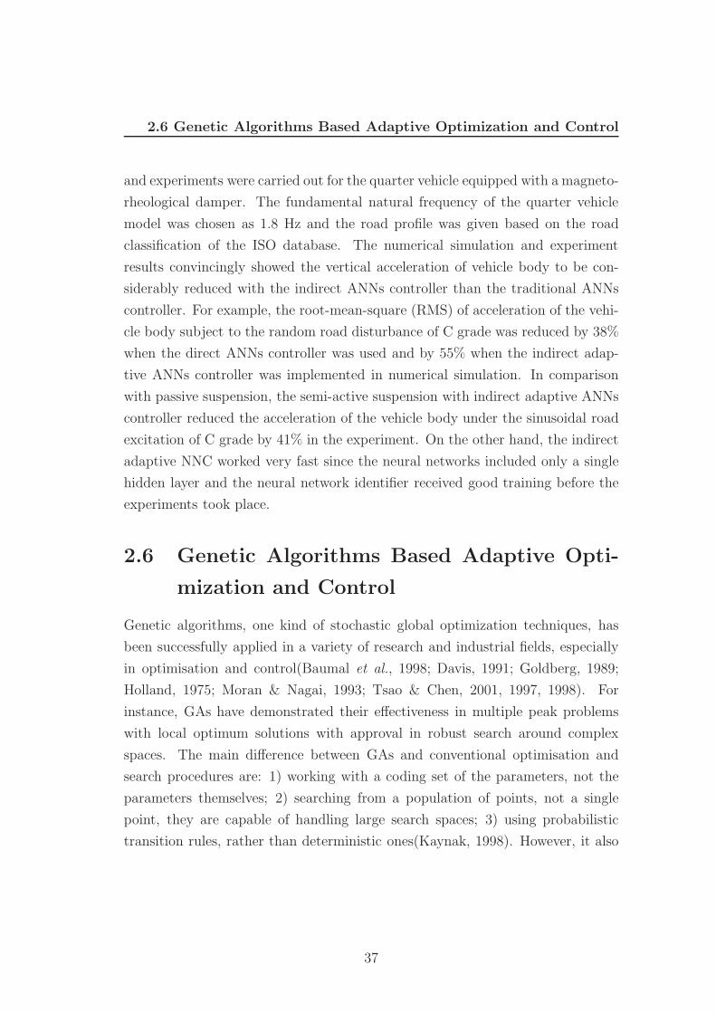
2.6 Genetic Algorithms Based Adaptive Optimization and Control
and experiments were carried out for the quarter vehicle equipped with a magneto-
rheological damper. The fundamental natural frequency of the quarter vehicle
model was chosen as 1.8 Hz and the road profile was given based on the road
classification of the ISO database. The numerical simulation and experiment
results convincingly showed the vertical acceleration of vehicle body to be con-
siderably reduced with the indirect ANNs controller than the traditional ANNs
controller. For example, the root-mean-square (RMS) of acceleration of the vehi-
cle body subject to the random road disturbance of C grade was reduced by 38%
when the direct ANNs controller was used and by 55% when the indirect adap-
tive ANNs controller was implemented in numerical simulation. In comparison
with passive suspension, the semi-active suspension with indirect adaptive ANNs
controller reduced the acceleration of the vehicle body under the sinusoidal road
excitation of C grade by 41% in the experiment. On the other hand, the indirect
adaptive NNC worked very fast since the neural networks included only a single
hidden layer and the neural network identifier received good training before the
experiments took place.
2.6 Genetic Algorithms Based Adaptive Opti-
mization and Control
Genetic algorithms, one kind of stochastic global optimization techniques, has
been successfully applied in a variety of research and industrial fields, especially
in optimisation and control(Baumal et al., 1998; Davis, 1991; Goldberg, 1989;
Holland, 1975; Moran & Nagai, 1993; Tsao & Chen, 2001, 1997, 1998). For
instance, GAs have demonstrated their effectiveness in multiple peak problems
with local optimum solutions with approval in robust search around complex
spaces. The main difference between GAs and conventional optimisation and
search procedures are: 1) working with a coding set of the parameters, not the
parameters themselves; 2) searching from a population of points, not a single
point, they are capable of handling large search spaces; 3) using probabilistic
transition rules, rather than deterministic ones(Kaynak, 1998). However, it also
37

2.6 Genetic Algorithms Based Adaptive Optimization and Control
needs to be pointed out that the main disadvantage of GAs is that their optimal
speed is too slow to use in real-time applications.
Considering the control strategy in active suspension systems, Baumal et al.
(1998) utilised the GA in a five DOF half vehicle model shown in Fig. 2.12. In
their research, all the involved parameters were comprised into one constraint
optimal description with eight unknown parameters and seven constraints. That
means the active control and passive mechanical parameters were the designed
variables to be optimised. Two active elements provided forces proportional
to the absolute vertical velocity of the points on the car body directly above
the rear and front wheels. These devices, characterised by proportionality con-
stants cf and cr, were known as skyhook dampers. The design variables were
the set:x=k1, c1, k3, c3, cr, k4, c4, cf. The constraints were obtained from the
three performances of vehicle suspension systems: 1) ride comfort; 2) road-holding
ability; 3) the suspension working space. Two constraints were for the body ac-
celeration and the seat acceleration. The other five constraints were for the seat,
suspension and tyre deflections. Given the optimised initial set, there were three
steps to implement the genetic algorithm. Firstly, the reproduction, which was
performed by copying a current generation string into a new population (par-
ent pool) according to the chosen fitness. The fitness depended on the objective
function value and constrained violations. Secondly, the crossover, which was
the exchange of design characteristics among randomly selected pairs from the
parent pool. Finally, the mutation was achieved by switching a 0 with a 1, or
vice-versa, at a binary site. The algorithm stopped when the maximum fitness
design comprised at least 30% of a newly created generation. The reproduction
stage itself was a simulation of the survival of the fittest designs. Moreover, in
order to improve the efficiency of the GA, the binary strings and fitness values
for each unique design of the current generation were stored in a linear search
look-up table. If a design string in the next generation matched one in the ta-
ble, then the fitness did not have to be re-calculated. This significantly avoided
the GAs weakness by improving computing time, especially for expensive fitness
evaluations. With five independent runs of the GA, the optimal values were ob-
tained and compared with the local optimisation search technique and the passive
suspension design. The results showed that the proposed GA can carry out the
38

2.6 Genetic Algorithms Based Adaptive Optimization and Control
best parameters with the least computing time among the three methods. The
active and passive suspension system seat acceleration responses were compared
to evaluate its dynamics performance. The response of the active system showed
that the road disturbance had little effect on the seat acceleration, and indicated
that GAs had strong potential to incorporate global optimisation methods for
suspension system design.
Figure 2.12: The 5 degree-of-freedom half vehicle model employed in Baumal
et al. (1998)
Tsao & Chen (2001) also proposed an active suspension force controller using
GAs with maximum stroke constraints based on their former research (Tsao &
Chen, 1997, 1998). In contrast to the traditional approach, the maximum absolute
values of suspension strokes were employed in the objective function to achieve
better ride comfort within the stroke limitation. A GA was employed to search
for the parameters of damping ratios and spring constants to achieve an optimum
trade-off among ride comfort, handling quality and suspension stroke limitation
simultaneously. The force control scheme of a half-vehicle model is shown in Fig.
2.13, where bdf and bdr denote the skyhook damping ratios, krf and krr denote
39

2.6 Genetic Algorithms Based Adaptive Optimization and Control
the road-following spring stiffness coefficients, ktf and ktr denote the known tyre
stiffness coefficients, btf and btr denote the virtual tyre damping ratios, bcf and kcf
denote the damping ratio and spring stiffness for compensating front end dynam-
ics. Utilising this control scheme, the active suspension control was converged into
an optimal problem where eight parameters(bdf , bdr, krf , krr, btf , btr, bcf , kcf) were
optimised simultaneously by GA. Two driving conditions were tested on the ac-
tive force controller. One was a steep ramp road with forward speed V = 10m/s
and the other was a sinusoidal bump road with V = 40m/s. The simulations
were carried out for the three cases in each driving condition. Each case was
ended after 500 generation runs. The comparisons of the performance among
these cases showed that the proposed force controller using GA achieved great
ride and handling quality while the suspension stroke was restricted to be less
than or equal to the passive system. In terms of the dynamic performance, the
heave and pitch angle motions of the suspension system were shown and com-
pared with the passive suspension system. Especially considering the comparison
of the suspension displacement, the summation of the quadratic values of the
suspension displacements in the active system was larger than that of the passive
suspension. But the maximum displacement was smaller and the vibration had
been absorbed during the transient period. These results can explain why the
maximum absolute value instead of the summation quadratic form of suspension
displacement can achieve better performance.
Figure 2.13: The force control scheme with skyhook damper, virtual damper and
road-following spring in Tsao & Chen (2001)
40

2.7 Integrated Adaptive Control Methods
2.7 Integrated Adaptive Control Methods
Control strategies are reviewed in this section based on the combination of pre-
sented methodologies in previous sections.
2.7.1 Adaptive Neuro-fuzzy Control
Much attention has been paid on the combination of ANNs and fuzzy systems
(Nurnberger et al., 1999). The advantage is that the fuzzy systems can compen-
sate the tuning ability of their rules by using the learning algorithms of ANNs;
on the other hand, the ANNs system can also improve the transparency and
interpretability by rule-based fuzzy reasoning construction. Generally speaking,
an ANNs-fuzzy system can be viewed as a special 3-layer feed forward neural
network, and the fuzzy rules are trained by an ANNs algorithm. With both
advantages of neural network and fuzzy logic, the neuro-fuzzy system had been
successfully employed to solve a wide range of industry problems, especially on
non-linear and uncertain systems.
For instance, Dong et al. (2006) employed an adaptive ANNs-fuzzy controller
for a quarter-vehicle magneto-rheological suspension system. The control system
is shown in Fig. 2.14. This controller consisted of a Fuzzy Neural Network Con-
troller(FNNC) and a Time Delay Compensator(TDC). The FNNC calculated the
control force according to error and the change of the error, the TDC was a neu-
ral network model which predicted for compensating the suspension’s time-delay.
For the quarter-vehicle model, the input was the damper force, the output was
the sprung mass vertical acceleration, and road input was treated as a distur-
bance. The FNNC scheme shown in Fig. 2.15, where two linguistic variables
were the inputs of the network and seven fuzzy sets were defined for each input
as NB, NM, ZE, PS, PM, PB in the first layer; the second layer included 14
neurons to correspond to all the fuzzy sets; the third layer contained 49 neurons
to do the fuzzy reasoning based on the defined fuzzy rules. The FNNC output
41

2.7 Integrated Adaptive Control Methods
was defined as:
u =
Rn∑i=1
µiwi
Rn∑i=1
µi
=∑
µiwi (2.59)
where Rn=49, and µ was the chosen Gaussian distribution. Weights wi of the
last layer were learned by back propagation algorithm. The simulation and ex-
perimental results showed that the proposed FNNC with TDC can significantly
reduce the acceleration peak value with 42.3% decrease in comparison of a passive
suspension system.
Figure 2.14: The adaptive neural network fuzzy control system with time-delay
compensator in Dong et al. (2006)
Figure 2.15: The FNNC scheme in Dong et al. (2006)
42

2.7 Integrated Adaptive Control Methods
Additionally, Wu et al. (2005) proposed a fuzzy controller based on the neuro-
fuzzy model for a half-vehicle active suspension system. The half-vehicle active
suspension was modelled as a non-linear system including heave, pitch and motion
of the front and rear wheels. The proposed neuro-fuzzy network was a self-
organizing inference network with 6 layers to derive the corresponding Takagi-
Sugeno (T-S) fuzzy model. The learning structure included both precondition
and consequence identification of fuzzy IF-THEN rules. Based on supervised
learning algorithms, the parameters of linear equations in the consequent parts
were adjusted by recursive least squares(RLS) algorithms, and the parameters in
the precondition part were adjusted by back propagation algorithm to minimize
a given cost function. Based on the T-S fuzzy model, a fuzzy controller was
designed to get the optimal active force. The simulation results showed the
proposed optimal fuzzy controller can improve the ride comfort by minimizing
both the displacements and accelerations of the vehicle centre and the pitch angle
simultaneously.
2.7.2 Adaptive Genetic-based Optimal Fuzzy Control
Due to the fact that IF-THEN rules in a fuzzy inference system are not always
available, automatic design methods and rule acquisition procedures for fuzzy
systems are required and have been proposed mostly based on GA and/or ANNs
in the past four decades. The key advantage of the hybrid system combining GA
and FL is that almost all the tasks of fuzzy system design can be accomplished
automatically. Because the GA can converge to the global optimal solution, FL
parameters of inference rules and membership functions are able to be determined
by a hybrid system itself. For GA-fuzzy control systems please refer to Herrera
et al. (1995, 1998); Homaifar & McCormick (1995); Magdalena et al. (2004).
Nawa et al studied a GA-fuzzy control system with the aid of pseudo bacte-
rial GAs (PBGA) and employed this controller to an active suspension system
shown in Fig. 2.16. Its encoding method is demonstrated in Fig. 2.17. Differ-
ing from the traditional canonical binary encoding, the parameters were put into
the chromosome, each of which encoded the rules of fuzzy system. Since every
43

2.7 Integrated Adaptive Control Methods
Figure 2.16: The PBGA fuzzy control system in Nawa et al. (1999)
rule contained the information of antecedent and consequent variables, each chro-
mosome encoded the parameters of the membership functions. Triangular type
membership functions were employed so that the parameters of the membership
function were in pairs of centre and width as shown in Fig. 2.17. This encod-
ing method gave a high degree of freedom for the GA, which can optimise the
variables to be employed in the rules, the rules themselves, and the parameters
of membership functions. Therefore, this encoding was desirable to simultane-
ously evolve the rules and the membership functions, minimize the probability of
arriving at a local optimal point.
The GA algorithm can be briefly described as follows, 1) generation of the ini-
tial population; 2) genetic operations: mutation-evaluation-selection-replacement;
3) crossover and produce the new generation. An adaptive method was used
in a crossover operation instead of randomly deciding the chromosomes cutting
points. The adaptive crossover operator took into account the moving average
of the degrees of truth values of the fuzzy rules when deciding where to cut the
chromosome. The moving average was defined as the average of the accumulated
truth values of the rules. The accumulated truth value of a fuzzy rule was the
sum of the truth values for each one of the entries in the training data. It was
a measure of quality. If a rule possessed a high value of accumulated truth, it
meant that the rule was intensively and frequently triggered during the evalu-
ation process. Consequently, this was an indication of the utility and possible
44

2.7 Integrated Adaptive Control Methods
effectiveness of that rule. On the other hand, if a rule possessed a low value of
accumulated truth, this was an indication that the rule did not play an important
role in the system. Four approaches were employed on the semi-active suspension
control system. The first method was a GA with fixed membership functions as
defined in Goldberg (1989). The second method is a GA with the possibility of
defining the membership functions and rules of a fuzzy controller simultaneously.
The third approach used the PBGA with a traditional crossover operator and
the fourth approach was the PBGA with adaptive crossover operation. The sim-
ulation results showed the proposed adaptive PBGA fuzzy controller worked well
to find out better rules and obtained the best performance of these four control
strategies. The results also indicated that this PBGA fuzzy controller focused
more on the actuation but the encoding methods increased the total number of
membership functions in the system.
Figure 2.17: An example of the fuzzy system encoded in a chromosome in Nawa
et al. (1999)
2.7.3 GA-ANNs Combined Control
A combination of a genetic algorithm and a neural network was employed to
design an active suspension controller by Tang & Zhang (2005). The GA searched
for the optimal acceleration of the vehicle body, which served as the objective
output of the ANNs control system. The neural network had two hidden layers
and the input, hidden and output neurons were 1, 10, 3 and 1, respectively. An
adaptive leaning rate was applied to decrease the training by keeping the learning
reasonably high, while insuring stable learning. The input of the ANNs was the
time response of the acceleration of the sprung mass, the objective output was the
optimised suspension control force. The proposed GA-ANNs combined controller
45

2.8 Summary
and a LQG controller were employed to evaluate the control performance. The
simulation results demonstrated that the NN controller with optimal acceleration
parameters computed by GA-based optimisation provided better ride comfort in
the time domain.
2.8 Summary
Computational intelligence based adaptive control approaches are required due
to the real-time, non-linear and uncertain nature properties of active suspension
systems. This chapter provided an account of state of the art of adaptive ac-
tive suspension control systems with intelligent methodologies. Their advantages
and disadvantages are concluded based on theoretical analysis, analysing simu-
lations and the experimental results of the reviewed systems. In what follows,
we enumerate some open questions and scientific problems that suggest following
chapters and future research.
1. Employing intelligent control based on a more practical suspension model or
hybrid model with other vehicle control subsystems. Most of the reported
research on active suspension intelligent control has studied the suspension
performance under the linear quarter-vehicle or half-vehicle model. A com-
prehensive consideration of a real car can lead to a more practical model
which will bring further distinct functional and safety-related benefits. Also
a hybrid model will be convenient to integrate the other control subsystems,
such as brake control, steering control and anti roll control, etc., to a hy-
brid intelligent system and it will be benefit for analysis of a unit vehicle
performance.
2. Integration of multi-objective optimisation methods and fuzzy logic rea-
soning. Considering the trade-off between ride comfort and road handling
quality, the optimal objective will be changed with the requirements of
different road surfaces. Then the adaptive multi-objective optimisation
methods with high real-time computing efficiency need to be researched,
especially for the application of modern vehicle active suspension systems.
46

2.8 Summary
Some new intelligent methods, such as the type-2 fuzzy logic system, have
provided an alternative way for vehicle active suspension control.
3. Pursuing the balance of accuracy and interpretability in an active suspen-
sion intelligent control system such as FLC, ANNs or their integrating meth-
ods. Though intelligent systems have been widely investigated in many do-
mains, their future will lie in the careful integration of the best constituent
technologies beyond simply combining individual methods.
4. Evaluating intelligent control methodologies from the perspective of prac-
tical applications. It is necessary to build an evaluating system to compare
the different intelligent systems according to application requirements such
as computing cost, number of tuning parameters, closed-loop stability con-
ditions and the interface to faulty diagnosis, etc. The comparison results
will be beneficial to intelligent control system applications and to the future
research.
47

Chapter 3
Improved Vehicle Active
Suspension Model
3.1 Introduction
With the development of electronics technology, the requirements of ride comfort
and driving performance are major objectives in designing modern vehicles to
satisfy the expectations of customers. It is well known that the suspension system
is important when considering the ride comfort and handling capability. Hence,
the design of an appropriate suspension system is always an important research
topic for achieving the desired vehicle ride quality.
Three types of mathematical vehicle models consisting of a quarter-vehicle
model, half-vehicle model and full-vehicle model have been developed for analyz-
ing and designing active suspension control systems. These models have inves-
tigated the trade-off between the ride comfort and safety. Firstly, the quarter-
vehicle model was initially developed to explore active suspension capabilities
and gave birth to the concepts of skyhook damping and fast load leveling which
are now being developed toward actual, large-scale production applications(Gao
et al., 2006; Hrovat, 1997). Furthermore, the half-vehicle model including pitch
and heave modes was invented to simulate ride characteristics of a simplified
whole vehicle, which led to significant improvement in ride and handling (EI-
Demerdash et al., 1999; Mansour & Crolla, 2000; Wang et al., 2006; Yu et al.,
2000; Yu & Ma, 2005). The full-vehicle model had been proposed with the aim
48

3.2 A Rigid Tyre Model
of closely studying coupled states of four quarter-vehicle models and handling
trade-offs between ride comfort and safety (Hrovat, 1997; Yoshimura & Emoto,
2003).
Although the above three mathematical suspension models have been imple-
mented to design different active suspension control systems, few models con-
sidered the effect of vehicle speed change, such as acceleration or deceleration.
In fact, when the vehicle speed is significantly changed by braking or acceler-
ating, the variant rolling torque on wheels will break down the existed torque
balance of suspension system and affect the vehicle ride comfort and handling
performance. The key reason is the coupling phenomenon between the suspen-
sion system and the braking or driving system (Pacejka, 2006; Trachtler, 2004;
Yoshimura & Watanabe, 2003). Some research has been done on the effect of
latitude speed change for heavy vehicles, especially when the vehicles turned a
sharp corner (Lin et al., 1996; Sampson & Cebon, 2003; Wang & Shen, 2008).
Here, from a longitudinal speed change point, a rigid tyre model is built and in-
tegrated into a half vehicle model to present a more real and practical dynamics
for later research in Chapter 4.
This chapter is organized as follows: Section 3.2 analyses a rigid tyre model
and its non-linear dynamics by braking or accelerating are presented; by integrat-
ing the tyre model into the existing half-vehicle suspension model, an improved
half-vehicle active suspension model is proposed in Section 3.3; Section 3.4 de-
signs a linear optimal controller for evaluating the improved model; finally we
conclude this chapter with discussions in Section 3.5.
3.2 A Rigid Tyre Model
The kinematics of a pneumatic tyre are important for the vehicle performance
of ride comfort and handling. Generally speaking, there are three major sources
of tyre vibrations. They are brake torque fluctuations, road unevennesses, and
horizontal and vertical oscillations of the axle (Zegelaar & Pacejka, 1996). In this
section, the first two sources are considered to analysis the dynamics of the tyre
and build a proper model for later research on active suspension system.
49

3.2 A Rigid Tyre Model
The diagram of a simplified tyre model is shown in Fig. 3.1, which has been
used in research reported by Zegelaar & Pacejka (1996). This tyre model can
generate the typical tyre vibrations in the frequency range 0-100 Hz which ensures
the tyre tread-band behaves as a rigid body. The whole wheel is separated into
three parts, one is the rim and axle with index a, the second part is the tyre belt
with index b and the third part is the contact patch with index c. For consistency
with the coordinates used in Chapter 2, the vertical direction is noted as Z, the
latitudinal direction is noted as Y and the longitudinal direction is noted as X.
The rotational speed is defined as Ω. The motion equations of this tyre model
are described as follows.
Figure 3.1: The rigid tyre model
mwAc = Ffx (3.1)
mwzw = Fz (3.2)
Iayθa = Tby − Tay (3.3)
Iby θb = −rFcx − Tby. (3.4)
where mw is the mass of whole wheel, Ac is the longitudinal acceleration, Ffx is
the longitudinal resultant force, zw is the vertical displacement of the wheel, and
50

3.2 A Rigid Tyre Model
Fz is the vertical resultant force seen in Chapter 2. Iay and Iby are the inertia
about the y-axis of the rim and tyre belt, respectively. The torques of rim and
tyre belt are Tay and Tby. Fcx is the longitudinal force in the contact patch.
The main aim is to build the relation between the longitudinal force Fcx and
vehicle forward speed V or wheel rotational velocity Ω. Since the longitudinal
force is related with vertical force and the tyre slip conditions, here, the tyre slip
characteristics are presented by a brush type model which describes the realistic
slip performance using three parameters: half the contact length la, the tread
element stiffness per unit of length cpx and the friction coefficient lµ. Then the
longitudinal force Fcx is presented as:
Fcx =
lµFz
3 |θxζcx| − 3 |θxζcx|2 + |θxζcx|3
sgn(ζcx), |ζcx| ≤ 1
θx
lµFzsgn(ζcx), |ζcx| > 1θx
(3.5)
where, the tyre parameters θx is:
θx =2cpxl
2a
3lµFz
(3.6)
and the slip function ζcx can be solved by the first order slip model:
σcζcx + Vcrζcx = −Vcsx (3.7)
Here, the rolling velocity Vcr=rΩ, r is defined as effective rolling radius, and
the slip velocity Vcsx can described as:
Vcsx = V − Vcr = V − rΩ (3.8)
Only considering the case of full adhesion, the relaxation length of contact patch
σc is given by
σc =1
2la. (3.9)
From the equations 3.5 - 3.9, based on the tyre model, the relationship is
built between the longitudinal force of the tyre and the vehicle forward speed.
The longitudinal force will affect the vehicle body pitch motion induced by the
suspension system. Then a more faithful vehicle suspension model is proposed in
Section 3.3 to integrate the pitch motion with the vertical dynamic.
51

3.3 The Improved Half-vehicle Active Suspension Model
3.3 The Improved Half-vehicle Active Suspen-
sion Model
Compared with the typical half-vehicle active suspension model which has been
shown in Chapter 2.2.1, an improved model is presented and its structure is shown
in Fig. 3.2. Let f and r denote the front and rear, x and z be the longitudinal
forward direction and vertical up direction, and additional variables are defined
as,
h: body center of gravity height from ground(m);
Ac: vehicle longitudinal forward acceleration(m/s2);
Fx: longitudinal force from tyre(N);
Fz: vertical force from road surface(N);
The vertical and longitudinal dynamics of this half-vehicle active suspension
Figure 3.2: The half vehicle model
system are represented and the motion equations of force balance and torque
balance can be written as follows:
zwfmwf = ftf − Ff (3.10a)
52

3.3 The Improved Half-vehicle Active Suspension Model
zwrmwr = ftr − Fr (3.10b)
zbmb = Ff + Fr (3.10c)
θIb = −dfFf + drFr − dtfFxf − dtrFxr. (3.10d)
Here, ftf and ftr are the front and rear vertical tyre forces, Ff and Fr are the
front and rear resultant forces of the suspension system, and Ff = faf +fsf +fdf ,
Fr = far +fsr +fdr. faf and far are front and rear actuator forces, fsf and fsr are
front and rear spring forces, fdf and fdr are front and rear damping forces. Fxf and
Fxr are the longitudinal forces from the front tyre and rear tyre, dtf = zbf−zwf +h
and dtr = zbr − zwr + h, θ is the pitch angle which is described by equations 3.11
- 3.12, θ is the pitch angle acceleration of the vehicle body.
zbf = zb − df · θ, zbr = zb + dr · θ (3.11)
From equation 3.11, the pitch angle can be written as:
θ =zbr − zbf
df + dr
(3.12)
Based on the half-vehicle active suspension structure in Fig. 3.2, the equations
3.10a - 3.10d are rewritten as follows:
zwfmwf = Ktf (zf0 − zwf ) − [faf + cf (zwf − zbf ) + Ksf(zbf − zwf)] (3.13a)
zwrmwr = Ktr(zr0 − zwr) − [far + cr(zwr − zbr) + Ksr(zbr − zwr)] (3.13b)
zbmb = faf + cf(zwf − zbf ) + Ksf(zwf − zbf ) + far
+ cr(zwr − zbr) + Ksr(zwr − zbr)(3.13c)
θIb = −df [faf + cf(zwf − zbf ) + Ksf(zwf − zbf )] − Fxf(zbf − zwf + h)+ dr[far + cr(zwr − zbr) + Ksr(zwr − zbr)] − Fxr(zbr − zwr + h).
(3.13d)
Different from the typical model in Chapter 2, the torque balance equation
3.13d includes the tyre dynamics which are described in Section 3.2. With the
53

3.3 The Improved Half-vehicle Active Suspension Model
equation 3.5, the relation between the longitudinal force and vehicle speed is non-
linear. In order to evaluate the improved suspension model, the improved linear
half-vehicle model with linearized longitudinal force is described in Section 3.3.1
and its performance is analysed in Section 3.3.2. With the non-linear longitudinal
force, the improved non-linear half-vehicle model is implemented in Section 3.3.3
and its performance is analysed in Section 3.3.4.
3.3.1 The Linear Half-vehicle Model
A linear half-vehicle model with linear longitudinal force is proposed in this sec-
tion. The non-linear longitudinal force with the rigid tyre model is described in
equations 3.5 - 3.9. For simplicity, the longitudinal force is linearized by ignoring
the high order terms and it can be rewritten as:
Fx = lµFz · 3θxζcx (3.14)
With the normal stationary solution of the first order slip model (i.e. ζcx=-
Vcsx/Vcr), substituting the equations 3.6 - 3.9 into the equation 3.14, then the
linear longitudinal force is defined in equation 3.15.
Fx = −2cpxl2a
Vcr
V + 2cpxl2a (3.15)
Assuming the longitudinal force from front tyre (Fxf) is the same as the force
from the rear tyre (Fxr) (i.e., Fxf = Fxr = Fx), substituting equation 3.15 into the
equations 3.13a - 3.13d, the active suspension dynamic equations are rewritten
as follows,
zbf = ( 1mb
+d2
f
Ib)[faf + cf(zwf − zbf ) + Ksf(zbf − zwf)] + ( 1
mb− df dr
Ib)[far
+cr(zwr − zbr) + Ksr(zbr − zwr)] +Fxdf
Ib(zbf − zbr − zwf + zwr)
(3.16a)
zbr = ( 1mb
− df dr
Ib)[faf + cf (zwf − zbf) + Ksf(zbf − zwf)] + ( 1
mb+ d2
r
Ib)[far
+cr(zwr − zbr) + Ksr(zbr − zwr)] − Fxdr
Ib(zbf − zbr − zwf + zwr)
(3.16b)
which incorporate the relationship between vehicle suspension vertical dynamics
and pitch motion into the model.
54

3.3 The Improved Half-vehicle Active Suspension Model
Using the same road inputs as in equations 2.21a - 2.21b, the state vector of
the half-vehicle active suspension system is defined by equation 3.17.
X =[
zbr zwr zbf zwf zbr
zwr zbf zwf zr0 zf0
]T (3.17)
Combining the improved half-vehicle active suspension motion equations 3.16a,
3.16b, and road input equations 2.21a and 2.21b, the system equation and output
equation in state space form can be rewritten in equations 3.18a and 3.18b.
X(t) = AnewX(t) + BU(t) + Fw(t) (3.18a)
Y (t) = CnewX(t) + DU(t) + v(t) (3.18b)
In comparison to the typical state space model in equations 2.23a - 2.23b, only
matrices Anew, Cnew are changed due to the introduction of longitudinal force
changes, given in equations 3.19 and 3.20.
Anew =
0 0 0 0 α1Ksr − α5 −α1Ksr + α5
0 0 0 0 − Ksr
mwr
Ksr−Ktr
mwr
0 0 0 0 α2Ksr + α4 −α2Ksr − α4
0 0 0 0 0 01 0 0 0 0 00 1 0 0 0 00 0 1 0 0 00 0 0 1 0 00 0 0 0 0 00 0 0 0 0 0
α2Ksf − α5 −α2Ksf + α5 0 00 0 Ktr
mwr0
α3Ksf + α4 −α3Ksf − α4 0 0
− Ksf
mwf
Ksf−Ktf
mwf0
Ktf
mwf
0 0 0 00 0 0 00 0 0 00 0 0 00 0 −2πf0 00 0 0 −2πf0
(3.19)
55

3.3 The Improved Half-vehicle Active Suspension Model
Cnew =
0 0 0 0 0 00 0 0 0 0 00 0 0 0 0 00 0 0 0 0 0
α2Ksr + α4 0 0 α1Ksr − α4 1 0−α2Ksr + α4 0 0 −α1Ksr − α4 −1 1α3Ksf − α5 1 0 α2Ksf + α5 0 0−α3Ksf − α5 −1 1 −α2Ksf + α5 0 0
0 0 0 0 0 −10 0 −1 0 0 0
T
(3.20)
where α4 denotes (df Fx
Ib) and α5 denotes (drFx
Ib), and B, D, F, U, W, α1, α2, α3, α4
are described in Chapter 2, Section 2.2.1.
3.3.2 Linear Model Performance Analysis
For evaluating this improved linear half-vehicle active suspension model, some
simulations are done to demonstrate the vertical and pitch vibrations which are
not repeated by other existing models. The nominal parameters of half-vehicle
active suspension system are given in Table 3.1.
Table 3.1: Nominal parameters of half-vehicle active suspension model
parameters values parameters values
mb (Kg) 1794.4 Ktf (N/m) 101115
mwf (Kg) 87.15 Ktr (N/m) 101115
mwr (Kg) 140.04 df (m) 1.3
Ib (Kg m2) 3443.05 dr (m) 1.5
Ksf (N/m) 66824.2 cf (N s/m) 1190
Ksr (N/m) 18615 cr (N s/m) 1000
f0 (Hz) 0.1 cpx (N/s2) 1.7 × 10⁶
la (m) 0.053 h (m) 0.5
In the field of suspension control analysis, researchers use various common
indexes to compare the performance of different systems. Differences in perfor-
mance might be due to damper type, suspension category, or even the suspension
56

3.3 The Improved Half-vehicle Active Suspension Model
control method. The most commonly used benchmarking indexes for ride com-
fort, road handling, and pitch motion performances are used in this thesis. That
is, the performance of ride comfort is indexed by the vehicle body vertical acceler-
ations, the performance of handling is embodied by the suspension displacements
(e.g., the suspension travel and tyre dynamic loading), and the pitch angle is
used to compare the pitch motion of suspension system (Crolla & Abdel, 1991;
EI-Demerdash et al., 1999; Liu et al., 2008b).
0 0.5 1 1.5 2 2.5 3 3.5 4 4.5 5−0.02
−0.015
−0.01
−0.005
0
0.005
0.01
0.015
0.02
Time(s)
θ (
rad)
Vcr=20
Vcr=17
Vcr=14
Figure 3.3: The pitch angles of a vehicle body with different Vcr
0 0.5 1 1.5 2 2.5 3 3.5 4 4.5 5−1
−0.5
0
0.5
1
1.5
Time(s)
Ve
hic
le b
od
y a
cce
lera
tio
ns (
m/s
2)
Vcr=20
Vcr=17
Vcr=14
Figure 3.4: The accelerations of front vehicle body with different Vcr
57

3.3 The Improved Half-vehicle Active Suspension Model
0 0.5 1 1.5 2 2.5 3 3.5 4 4.5 5−0.6
−0.4
−0.2
0
0.2
0.4
0.6
0.8
1
1.2
1.4
Time(s)
Ve
hic
le b
od
y a
cce
lera
tio
ns (
m/s
2)
Vcr=20
Vcr=17
Vcr=14
Figure 3.5: The accelerations of rear vehicle body with different Vcr
In order to analyse the natural vertical and pitch dynamics of the improved
half-vehicle suspension model, the active forces are ignored, the average forward
speed V is 20 m/s and the rolling velocity Vcr are chosen as 20 m/s, 17 m/s
and 14 m/s. From the longitudinal tyre force in equation 3.15, when the forward
speed V is the same as the rolling velocity Vcr, the longitudinal effect to pitch
motion disappears and the improved model is reduced to the typical model. With
step road inputs (z0 = 0.1 m ), the pitch angles of a vehicle body with different
rolling velocities are shown in Fig. 3.3. The comparison of accelerations of the
front and rear vehicle body with different rolling velocities are shown in Fig. 3.4
and Fig. 3.5. The front and rear suspension travel and tyre dynamic loadings
are compared in Fig. 3.6 - 3.9. These simulation results demonstrate that the
longitudinal tyre force can significantly affect the pitch angles of a vehicle body
which are not presented by the existing typical model. Also it is evident that
the longitudinal tyre force has a very small effect on the vertical vibration of
the vehicle body because the vertical accelerations, suspension travels and tyre
dynamic loadings of the improved model are similar with the typical model.
58

3.3 The Improved Half-vehicle Active Suspension Model
0 0.5 1 1.5 2 2.5 3 3.5 4 4.5 5−0.06
−0.04
−0.02
0
0.02
0.04
0.06
0.08
0.1
Time(s)
The s
uspensio
n tra
vel (m
)
Vcr=20
Vcr=17
Vcr=14
Figure 3.6: The front suspension travel with different Vcr
0 0.5 1 1.5 2 2.5 3 3.5 4 4.5 5−0.06
−0.04
−0.02
0
0.02
0.04
0.06
0.08
0.1
0.12
Time(s)
The s
uspensio
n tra
vel (m
)
Vcr=20
Vcr=17
Vcr=14
Figure 3.7: The rear suspension travel with different Vcr
59

3.3 The Improved Half-vehicle Active Suspension Model
0 0.5 1 1.5 2 2.5 3 3.5 4 4.5 5−12
−10
−8
−6
−4
−2
0
2
4x 10
−3
Time(s)
Th
e t
yre
dyn
am
ic lo
ad
ing
(m
)
Vcr=20
Vcr=17
Vcr=14
Figure 3.8: The front tyre dynamic loading with different Vcr
0 0.5 1 1.5 2 2.5 3 3.5 4 4.5 5−10
−8
−6
−4
−2
0
2
4x 10
−3
Time(s)
Th
e t
yre
dyn
am
ic lo
ad
ing
(m
)
Vcr=20
Vcr=17
Vcr=14
Figure 3.9: The rear tyre dynamic loading with different Vcr
60

3.3 The Improved Half-vehicle Active Suspension Model
3.3.3 The Non-linear Half-vehicle Model
It is evident that a linear system approximation is not appropriate for highly non-
linear systems with uncertain input factors. This is because non-linear effects are
usually amplified in such systems.
For a vehicle suspension system, except for the tyre longitudinal non-linear
dynamics mentioned in Section 3.2, the non-linear dynamics could be created
by dry friction and discrete-event disturbances (e.g., single bumps or potholes),
which cause a highly non-linear phenomenon. The non-linear properties mainly
arise from two sources. The first is the bump stop which restricts the wheel travel
within a given range and prevents the tyre from contacting the vehicle body; the
other is the strut bushing which connects the strut with the body structure and
reduces harshness from the road input. Based on the method in Kim & Ro
(1998), the connecting forces (e.g., spring force, damping force, tyre force) can
be modelled as non-linear functions using measured data. Here, the spring force
fs is estimated by high-order polynomial functions as shown in equation 3.21,
fs = fsl + fsn = k1∆zs + (k0 + k2∆z2s + k3∆z3
s ), (3.21)
where fsl is the linear term of the spring force and fsn is the non-linear term
of the spring force, ∆zs is the displacement of suspension. The coefficients were
obtained by fitting the equation to experimental data. The damping force fd were
also modelled as a second-order polynomial function by fitting the measured data,
as given below,
fd = fdl + fdn = c1∆zs + c2∆zs2, (3.22)
where fdl is the linear term and fdn is the non-linear term of the damper force.
Besides the non-linear properties presented by the spring force and damping
force, the vertical tyre force is also highly non-linear, especially when there are
substantial load changes. The vertical tyre force becomes zero when the tyre loses
contact with the road surface. The tyre force was modelled as below,
ft :
ftl = kt∆zt, zt > 0ftn = 0, zt ≤ 0.
(3.23)
61

3.3 The Improved Half-vehicle Active Suspension Model
where ft is the vertical tyre force, ftl denotes the linear tyre force, ftn denotes
the non-linear tyre force and ∆zt is the tyre displacement.
Integrating all the above mentioned non-linear dynamics in an active suspen-
sion system, this non-linear model is provided below for the further research in
this thesis. Also this non-linear model is built as a reference model of real vehicle
active suspension system for all further simulations of this thesis.
With the non-linearity shown in equations 3.5, 3.21, 3.22, 3.23, the active
suspension system can be written as a MIMO non-linear model:
X = F (X, U) (3.24)
where X denotes the state matrices which includes the displacements and
velocity of the vehicle body (i.e., Zb and Zb), suspension (i.e., Zw and Zw) and
road surface input (i.e., Z0 and Z0) and U denotes the actuator force matrices
(i.e., faf and far), F (X, U) is a non-linear function which presents the suspension
non-linear dynamic description which can be obtained by integrating the linear
model and the non-linear forces (i.e., fs ,ft, fd and Fx). The performance analysis
of this non-linear model is presented in Section 3.3.4.
3.3.4 Non-linear Model Analysis
In order to demonstrate the non-linear characteristics of a vehicle suspension
model described in Section 3.3.3, the simulations without active control forces
are done to show the natural vertical and pitch motions. Since most of the non-
linear dynamics occur around the suspension minimum and maximum travel, a
0.2m step road input is used to simulate a very sharp bump. The parameters
of the vehicle suspension can be found in Table 3.1 and the coefficients of the
non-linear forces are given in Table 3.2. Here, subscript f and r denote the front
and rear.
The vertical accelerations of the front and rear vehicle body are shown in Fig.
3.10 - Fig. 3.11. In comparison with the linear model described in Section 3.3.2,
the non-linear dynamics occurred in the first second when the suspension travel
was close to reaching its maximum expansion and contraction. With the passage
of time, when the vertical vibrations are reduced into the linear ranges by the
62

3.3 The Improved Half-vehicle Active Suspension Model
Table 3.2: The coefficients of non-linear forcesparameters values parameters values
k0f (N) -236 k1f (N/m) 66824
k2f (N/m2) -403 k3f (N/m3) 104
k0r (N) -146 k1r (N/m) 18615
k2r (N/m2) -265 k3r (N/m3) 284
c1f (N s/m) 1190 c2f (N s2/m) 426
c1r (N s/m) 1000 c2r (N s2/m) 215
0 0.5 1 1.5 2 2.5 3 3.5 4 4.5 5−2
−1.5
−1
−0.5
0
0.5
1
1.5
2
2.5
3
Time(s)
Ve
hic
le b
od
y a
cce
lera
tio
ns (
m/s
2)
linear
nonlinear
Figure 3.10: The vertical accelerations of front vehicle body with non-linear model
0 0.5 1 1.5 2 2.5 3 3.5 4 4.5 5−1.5
−1
−0.5
0
0.5
1
1.5
2
2.5
3
Time(s)
Ve
hic
le b
od
y a
cce
lera
tio
ns (
m/s
2)
linear
nonlinear
Figure 3.11: The vertical accelerations of rear vehicle body with non-linear model
63

3.3 The Improved Half-vehicle Active Suspension Model
0 0.5 1 1.5 2 2.5 3 3.5 4 4.5 5−0.06
−0.04
−0.02
0
0.02
0.04
0.06
Time(s)
θ (
rad)
linear
nonlinear
Figure 3.12: The pitch angles of vehicle body with non-linear model
dampers, the vertical dynamics of this non-linear model are similar to the linear
dynamics. The other performance indexes of a non-linear model, that is, the
suspension travel and tyre dynamic loading, shown in Fig. 3.13 - Fig. 3.16, can
also demonstrate similar dynamics from non-linear to linear.
0 0.5 1 1.5 2 2.5 3 3.5 4 4.5 5−0.15
−0.1
−0.05
0
0.05
0.1
0.15
0.2
Time(s)
The s
uspensio
n tra
vel (m
)
linear
nonlinear
Figure 3.13: The front suspension travel with non-linear model
Fig. 3.12 shows the pitch angles of a non-linear model and a linear model.
From these pitch motion dynamics, the non-linear model can represent the pitch
motion as a linear model.
64

3.3 The Improved Half-vehicle Active Suspension Model
0 0.5 1 1.5 2 2.5 3 3.5 4 4.5 5−0.2
−0.15
−0.1
−0.05
0
0.05
0.1
0.15
0.2
0.25
Time(s)
The s
uspensio
n tra
vel (m
)
linear
nonlinear
Figure 3.14: The rear suspension travel with non-linear model
0 0.5 1 1.5 2 2.5 3 3.5 4 4.5 5−0.02
−0.015
−0.01
−0.005
0
0.005
0.01
Time(s)
The tyre
dynam
ic loadin
g (
m)
linear
nonlinear
Figure 3.15: The front tyre dynamic loading with non-linear model
65

3.4 The Improved LQG Design
0 0.5 1 1.5 2 2.5 3 3.5 4 4.5 5−0.02
−0.015
−0.01
−0.005
0
0.005
0.01
Time(s)
The tyre
dynam
ic loadin
g (
m)
linear
nonlinear
Figure 3.16: The rear tyre dynamic loading with non-linear model
Since all the above dynamics of the proposed non-linear suspension model
are closer to the real physical dynamics, further research in this thesis will use
this non-linear model as the reference suspension model to design the intelligent
active suspension control system and evaluate its ride comfort, handling and pitch
motion performance.
3.4 The Improved LQG Design
In order to further test the proposed suspension model, especially closed-loop
evaluation with a controller, an improved LQG controller is designed to improve
not only the ride comfort and handling performance, but also the pitch motion.
3.4.1 The Improved LQG
Considering the improved model in Section 3.3.1 and the typical LQG design in
Chapter 2, a new term is added to the control performance index, and shown in
equation 3.25
J = limT→∞
1T
∫ T
0[q1(zwf − zf0)
2+q2(zbf − zwf)2
+ρ1zbf + q3 (zwr − zr0)2 + q4(zbr − zwr)
2
+ρ2z2br + q5(zbr − zbf )
2]dt
(3.25)
66

3.4 The Improved LQG Design
where q5 is a new weight value to the control performance of pitch angle. With
this new control performance equation 3.25 and the state space model in Section
3.3.1, the improved optimal control force can be described by equation 3.26.
U(t) = −R−1BTPX(t) = −KnewX(t). (3.26)
where Knew represents the control gain matrix; and P is the solution of the
classical algebraic Riccati equation in equation 2.16.
3.4.2 Simulation Results
Initially, the response of the improved active suspension model to a step road in-
put is investigated with different acceleration values based on an LQG controller,
as this provides an insight into the relation between vehicle body pitch angle and
longitudinal tyre forces. Furthermore, the control performance of three control
strategies (LQG, Improved LQG (ILQ) and Wheelbase preview LQG (WLQ)) are
assessed on the improved model with a step road input and different longitudinal
acceleration values. More detail about the WLQ can be found in paper (Yu et al.,
2000). With the random road input, three control strategies are also used on the
improved model to compare their control performance.
The nominal values of parameters for the half-vehicle suspension model are
given in Table 3.1, and the coefficients of calculating control gains used in the
simulation are given in Table 3.3.
Table 3.3: Random road input parameters and the weighting parameters
parameters G0 U0 ρ1 ρ2 q1 q2 q3 q4
values 5 × 10⁻⁶ 30 1 1 80000 100 80000 100
3.4.2.1 Step Road Inputs
In order to examine the dynamic effect of speed changes to the vehicle body
pitch angle, the response of the improved linear half-vehicle suspension model
to step road input is carried out under different rolling velocities. The typical
LQG controller is used and the original forward velocity is 30m/s. A step input
67

3.4 The Improved LQG Design
of 0.1m is applied on the vehicle model to simulate the sharp road vibration.
Fig. 3.17 shows pitch angle comparison with different rolling velocities as 35m/s,
34m/s, 32m/s, 30m/s, 28m/s, 26m/s, 25m/s. The simulation results showed
that different rolling velocities caused different pitch angles. Higher velocity gap
values brought larger additional pitch angle from zero-velocity-gap pitch angle,
and vice versa.
0 0.5 1 1.5 2 2.5 3 3.5 4 4.5 5−0.03
−0.02
−0.01
0
0.01
0.02
0.03
0.04
0.05
pitch a
ngle
(ra
d)
time(second)
Vcr
=35
Vcr
=34
Vcr
=32
Vcr
=30
Vcr
=28
Vcr
=26
Vcr
=25
Figure 3.17: Pitch angle comparison with typical LQG and different rolling ve-
locities
For constraining the additional pitch angle to obtain better vehicle pitch mo-
tion performance, the second simulation is carried out under the improved lin-
ear half-vehicle suspension model, the same rolling velocity and different control
strategies. One controller is the typical LQG controller without considering the
pitch motion information in control performance index as in equation 2.28. Its
control results of pitch angle are shown in Fig. 3.18 by a solid line. The second
controller is the ILQ based on equation 3.25, and weight value q5 is 1. Its control
results of pitch angle are shown in Fig. 3.18 by dot line. The third controller is
the WLQ. The control results are shown in Fig. 3.18 by dash dot line.
68

3.4 The Improved LQG Design
0 0.5 1 1.5 2 2.5 3 3.5 4 4.5 5−0.02
−0.01
0
0.01
0.02
0.03
0.04
0.05
time(second)
pitch a
ngle
(ra
d)
wheelbase preview LQ
basical LQ
improved LQ
wheelbase preview LQ
improved LQ
basical LQ
Figure 3.18: Pitch angle comparison with different controller at Vcr= 35 m/s
(upper three lines) and 25 m/s (lower three lines)
As shown in Fig. 3.18, regarding vehicle body pitch angle, the proposed ILQ
controller obtained smaller overshoot and stable values than the other two con-
trollers. The WLQ controller obtained nearly the same stable values as the LQG
controller. But it is sensitive to velocity changing and the dynamic performance
became unsatisfactory when the vehicle speed was significantly changed.
3.4.2.2 Random Road Inputs
In order to provide approximate road input conditions, a random road surface
model is used, which is mentioned in Chapter 2, Section 2.2.1. The road surface
with a roughness coefficient of 5 × 10⁻⁶ is used. The vehicle forward speed is
30m/s. With different Vcr values and different controllers, the pitch angle vari-
ance were shown in Fig. 3.19 and Fig. 3.20, and the RMS values of Body
Vertical Acceleration (BVA), Suspension Displacement (SD), Tyres Dynamic
Loading (TDL) and Body Pitch Angle (BPA) were shown in Table 3.4, Table
3.5, Table 3.6.
As shown in Fig. 3.19 and Fig. 3.20, the ILQ controller obtained smaller
69

3.4 The Improved LQG Design
dynamic and stable values than the other two controllers. The wheel-based pre-
view controller was sensitive to velocity changing and the dynamic performance
became unsatisfactory.
As shown in Table 3.4, all the control performance of the ILQ controller were
the same as LQG controller without considering the longitudinal force. The WLQ
controller obtained better control performance, especially in the rear wheel and
suspension.
Table 3.5 and Table 3.6 showed the effects of the tyre longitudinal force chang-
ing to the vehicle performance, especially to vehicle body pitch angle. The ILQ
controller obtained smaller pitch angle than LQG and WLQ with the rolling ve-
locities 35m/s and 25m/s. The other performance of the vehicle (i.e., BVA, SD,
TDL ) changed a little by using three controllers under different rolling velocities.
0 0.5 1 1.5 2 2.5 3 3.5 4 4.5 5−0.03
−0.02
−0.01
0
0.01
0.02
0.03
time (second)
pitch a
ngle
(ra
d)
wheelbase preview LQ
basical LQ
improved LQ
Figure 3.19: Pitch angle comparison with different controller and random road
input ( Vcr=35m/s)
70

3.5 Summary
Table 3.4: Vehicle performance comparison with Vcr = 30m/s
BV Af SDf TDLf BV Ar
LQ 0.7731 0.0079 0.0030 0.8349
ILQ 0.7731 0.0079 0.0030 0.8349
WLQ 0.7668 0.0079 0.0030 0.7716
SDr TDLr BPA Vcr
LQ 0.0080 0.0032 0.0025 30
ILQ 0.0080 0.0032 0.0025 30
WLQ 0.0052 0.0027 0.0026 30
Table 3.5: Vehicle performance comparison with Vcr = 35m/s
BV Af SDf TDLf BV Ar
LQ 0.7708 0.0076 0.0030 0.8400
ILQ 0.7707 0.0079 0.0030 0.8401
WLQ 0.7636 0.0077 0.0030 0.7709
SDr TDLr BPA Vcr
LQ 0.0084 0.0031 0.0049 35
ILQ 0.0083 0.0032 0.0044 35
WLQ 0.0072 0.0027 0.0108 35
3.5 Summary
In this chapter, the improved half-vehicle active suspension models which inte-
grate tyre longitudinal dynamics were proposed. Their dynamic open-loop and
closed-loop response to different road surfaces have been demonstrated.
To more precisely describe the suspension dynamics, a tyre dynamic model
was introduced to connect the tyre longitudinal forces with the vehicle suspension
model. The effect of tyre longitudinal dynamics were represented by two improved
half-vehicle active suspension models. One was the linear model to demonstrate
the typical linear response to road vibrations. It was also used to design the linear
controller, such as the LQG controller. The other was the non-linear model which
can show the real spring, damping forces and tyre non-linear dynamics, especially
when the suspension travel reached its physical limitations.
71

3.5 Summary
Table 3.6: Vehicle performance comparison with Vcr=25 m/s
BV Af SDf TDLf BV Ar
LQ 0.7636 0.0081 0.0031 0.8306
ILQ 0.7664 0.0081 0.0031 0.8307
WLQ 0.7708 0.0082 0.0030 0.7731
SDr TDLr BPA Vcr
LQ 0.0076 0.0032 0.0105 25
ILQ 0.0077 0.0032 0.0096 25
WLQ 0.0062 0.0027 0.0137 25
0 0.5 1 1.5 2 2.5 3 3.5 4 4.5 5−0.04
−0.03
−0.02
−0.01
0
0.01
0.02
time (second)
pitch a
ngle
(ra
d)
wheelbase preview LQ
basical LQ
improved LQ
Figure 3.20: Pitch angle comparison with different controller and random road
input (Vcr=25m/s)
72

3.5 Summary
All the proposed suspension models were evaluated from open-loop point
(without the active forces) to the closed-loop system (with the linear controller
for active suspension). The simulation results have shown that the improved
models provided a more accurate representation of the pitch motion dynamics of
an active suspension system than existing models. Also the non-linear model can
present more accurate vertical dynamics than the linear models. However, it was
hard to obtain satisfied control performances by the LQG controller because it
was designed to work with a linear model.
Then Chapter 4, a novel intelligent control strategy is proposed to deal with
these non-linear dynamics in the active suspension system and to improve the
capability of constraining the vertical and longitudinal vibrations to the vehicle
body.
73

Chapter 4
Interval Type-2 Fuzzy Control
System
4.1 Introduction
In order to improve the capability of active suspension systems, a lot of research
has been carried out on the design and control of active suspension systems in
the past two decades (Hrovat, 1997; Nagai, 1993; Sun, 2003). Simultaneously, the
control strategies of an active suspension system have been developed in a wide
range from initially linear quadratic controllers (e.g., LQG) to intelligent con-
trollers based on recently new findings in the field of computational intelligence.
To control an active suspension, the control algorithms must be able to deal
with mechanical non-linear dynamics and to operate under imprecise and uncer-
tain conditions, mainly caused by road surfaces. The mechanism behind FLCs
are credited with being a feasible methodology for designing robust controllers
that are able to deliver a satisfactory performance in face of non-linearity, un-
certainty and imprecision. The FLC has been successfully employed in some
practical suspension systems. Chen et al. (1995) proposed a FLC for an active
suspension under the sliding mode control (SMC) frame. The FLC was designed
to reduce the chattering of the SMC and to supervise the control performance to
self-tuning parameters of the control system. Zhang et al. (2007) also proposed
an adaptive fuzzy sliding mode controller for an active suspension system but its
sliding surface was different from Chen’s. Rao & Prahlad (1997) also presented a
74

4.1 Introduction
tunable FLC to bring down the suspension acceleration and deflection to a level
that of a hypothetical reference model. The suspension deflection and velocity
were the two input variables to the FLC while the desired force as its output.
Fernando & Viassolo (2000) proposed a controller consisting of two control loops
to minimize the vehicle body acceleration and to avoid hitting the suspension
limit. The outer loop was as same as Rao’s work, but additional inner loop was
designed to deal with the non-linear hydraulic actuator. More recent research
results can be found in (Cao et al., 2007, 2008; Chen & Huang, 2008; Gao et al.,
2006; Li et al., 2006, 2008; Lin & Lian, 2008; Liu et al., 2008b; Wang & Shen,
2008).
Though there are different ways to construct FLCs for a vehicle active sus-
pension, the most common way is to construct a FLC by eliciting the fuzzy rules
and the Membership Function (MF)s based on expert knowledge or experience.
A FLC handles the uncertainty associated with the inputs and outputs by using
precise and crisp MFs. This means that, once the MFs have been chosen, all
the uncertainty disappears (Hagras, 2004; Mendel & John, 2002). Then there is
the common problem that such a FLC limits introducing uncertain factors from
linguistic rules through predefined membership functions. Recently, fuzzy type-2
methods, which were introduced by Zadeh (1975), have been further developed
to improve the FLCs performance for handling the high level uncertainty (Karnik
& Mendel, 2001; Wu & Mendel, 2009).
Fuzzy type-2 method is that its fuzzy set is further defined by a typical fuzzy
membership function, i.e., the membership degree of belonging for each element
of this set is a fuzzy set in [0, 1], not a crisp number (Liang & Mendel, 2000).
Then the Interval Type-2 Fuzzy Membership Function (IT2MF) is three dimen-
sional and include a footprint of uncertainty, which provided additional degrees of
freedom that made it possible to directly model and handle uncertainty (John &
Coupland, 2007; Mendel, 2007a; Wu & Mendel, 2007, 2008). In comparison with
the type-1 Fuzzy Logic System (FLS), a type-2 FLS has the two-fold advantages
as follows. Firstly, it has the capability of directly handling the uncertain factors
of fuzzy rules caused by expert experience or linguistic description. Secondly, it
is efficient to employ a type-2 FLS to cope with scenarios in which it is difficult or
impossible to determine an exact membership function and related measurement
75

4.1 Introduction
of uncertainties. These strengths have made researchers consider type-2 FLS as
the preference for real-world applications (Astudillo et al., 2007; Hagras, 2007;
Liang et al., 2000; Liu, 2008a; Sepulveda et al., 2007).
About the type-2 FLS, some research has been done to study the set theoretic
operations, properties of membership grades and the uncertainty bounds of type-
2 fuzzy sets(John, 1998; Karnik & Liang, 1999; Mendel et al., 2007). From the
viewpoint of real-time application, Interval Type-2 (IT2)FLS has been widely
studied and utilized in many research fields, such as autonomous mobile robots
control, adaptive control of nonlinear system, noise cancellation, quality control
and wireless communications, etc. That is mainly due to the IT2FLS’s simple
computing methods and less computational expense on type reduction which is
still a bottleneck for other type-2 FLSs to be used in real-time applications.
According to the research of type-2 FLC, considering the real-time control
requirements, many researchers used interval type-2 fuzzy sets to solve the com-
putational complexity of general type-2 fuzzy sets and have brought some appli-
cations(Julio & Alberto, 2007; Wu & Mendel, 2002). However, the computational
expense on type reduction of type-2 FLS also is a bottleneck for a type-2 FLC in
real-time control applications(Mendel, 2007b). Some new alternative ways have
been provided to reduce the computational expense of type-2 FLC, such as the
method proposed by Wu & Mendel (2002). In Wu’s approach, they replaced the
type reduction with lower and upper bounds for the end-points of the type re-
duction sets, and those bounds can be computed without having to perform the
type reduction. But its drawback is the type reduction will be performed during
the design step. However, designing an efficient type-2 FLC with less calculation
and strong adaptive ability to overcome uncertainty of industrial applications is
still an open question.
Due to the difficulties of building proper crisp MFs from uncertainty of ex-
pert knowledge or experience for an active suspension system, inspiring from the
idea of type-2 fuzzy methods, an adaptive FLC with IT2MFs is proposed in this
chapter. A general structure to aggregate uncertainty bounds to the defuzzified
outputs through further optimization is built to improve the vehicle performance.
The main control aims are to minimize vehicle body acceleration to improve ride
76

4.2 Interval Type-2 Fuzzy Systems
comfort and reduce the tyre dynamic loadings to enhance the handling perfor-
mance. The further optimal goals are to reduce the suspension displacements
and tyre dynamic loadings with less control force.
In Section 4.2 the general background of interval type-2 FLS is introduced.
The framework of adaptive interval type-2 FLC is proposed in Section 4.3. Simu-
lation results on quarter and half vehicle active suspension systems are provided
in Section 4.4 and Section 4.5. This chapter is concluded in the Section 4.6.
4.2 Interval Type-2 Fuzzy Systems
The interval type-2 FLS has been widely studied in recent decade. Compared to
the general type-2 FLS, its primary advantage is its computational tractability
(Mendel, 2007a). In order to clearly describe the later controller design, the
background of IT2 fuzzy sets and fuzzy systems are introduced in this section.
4.2.1 The Interval Type-2 Fuzzy Sets
An interval type-2 fuzzy set is defined as below:
A =
∫
x∈X
∫
u∈Jx⊆[0,1]
1/(x, u) =
∫
x∈X
∫
u∈Jx⊆[0,1]
1/u
/x (4.1)
where x is the primary variable with domain X, u ∈ U is the secondary variable
with domain Jx at each x ∈ X. Jx is the primary membership of x and it is
defined in equation 4.2. The secondary grades of A are all equal 1.
Jx =
(x, u) : u ∈[µ
A(x), µ
A(x)]
(4.2)
As shown in Fig. 4.1, for a crisp input value a, its primary membership
grade µx(a) belongs to an interval:[µx(a), µx(a)] and all the secondary grades
f(µx(a)), f(µx(a)) are all equal to 1.
77

4.2 Interval Type-2 Fuzzy Systems
(a) The primary membership functions of crisp in-
put a(describing an interval type-2 fuzzy set)
(b) The secondary membership function of crisp in-
put a(describing an interval type-1 fuzzy set)
Figure 4.1: The interval type-2 fuzzy membership functions
By this interval type-2 fuzzy set, uncertainty about type-1 fuzzy set will be
conveyed by all the primary MFs. The primary MF can be separated into two
type-1 MFs, i.e., the Upper Membership Function (UMF) and the Lower Mem-
bership Function (LMF). The footprint of uncertainty of A can be described as:
FOU(A) =⋃
∀x∈X
Jx =⋃
∀x∈X
[µ
A(x), µA(x)
](4.3)
With two interval type-2 fuzzy sets A and B in equations 4.4 and 4.5, the interval
type-2 fuzzy set theory operations of union, intersection and complement can be
78

4.2 Interval Type-2 Fuzzy Systems
written in equations 4.6- 4.8.
A = 1/FOU(A) = 1/⋃
∀x∈X
[µA(x), µA(x)] (4.4)
B = 1/FOU(B) = 1/⋃
∀x∈X
[µB(x), µB(x)] (4.5)
A ∪ B = 1/⋃
∀x∈X
[µA(x) ∨ µ
B(x), µA(x) ∨ µB(x)] (4.6)
A ∩ B = 1/⋃
∀x∈X
[µA(x) ∗ µ
B(x), µA(x) ∗ µB(x)] (4.7)
A = 1/⋃
∀x∈X
[1 − µA(x), 1 − µA(x)] (4.8)
4.2.2 The Interval Type-2 Fuzzy System
With IT2 fuzzy sets, the framework of the IT2 fuzzy logic system is shown in Fig.
4.2. Basically, an IT2 fuzzy system is composed of five functional blocks: the Fuzzification interface which transforms the crisp inputs into fuzzy
values with linguistic knowledge. the Knowledge base which includes the rule base and database; the rule
base contains fuzzy if-then rules and the database defines the IT2 fuzzy
membership functions of IT2 fuzzy sets. the Decision-making unit which performs the inference operations on the
fuzzy rules; that is the fuzzy reasoning process. the Type-reduction which combines the output sets and performs a cen-
troid calculation to obtain the type-reduced sets (Type-1 fuzzy sets). the Defuzzification interface which transforms the fuzzy reasoning re-
sults to crisp outputs.
Based on this framework, the IT2 fuzzy system will work as follows:
79

4.2 Interval Type-2 Fuzzy Systems
Figure 4.2: The interval type-2 fuzzy logic system
1. The crisp inputs are fuzzified into IT2 fuzzy sets which are described by
IT2 membership functions. Then each crisp value will be transferred into a
fuzzy value.
2. These fuzzy values can active the fuzzy inference engine with the fuzzy rule
base to produce the fuzzy reasoning results. The fuzzy rules are same as
type-1 fuzzy system, but all fuzzy values are defined by interval membership
grades obtained from their IT2 fuzzy sets. Then the reasoning results are
all IT2 fuzzy values.
3. With a specially designed type-reduction and defuzzification method, the
IT2 fuzzy reasoning results are combined and calculated to the expected
crisp outputs. Then the IT2 reasoning process is implemented.
A simplified IT2 fuzzy system with ν inputs and one output is considered to
show the basic existed research results about the IT2 fuzzy systems. Assume
there are m IF-THEN fuzzy rules with the form:
R(l): IF x1 is F l1 and x2 is F l
2, . . ., and xν is F lν , THEN y is Gl.
where, l ∈ L := 1, 2, . . . , m.
80

4.2 Interval Type-2 Fuzzy Systems
The IT2 MFs for all antecedent IT2 fuzzy sets are defined as µF lk(xk) (k =
1, . . . , ν) and the IT2 MFs for consequent is defined as µGl(y). The major result
is concluded by the following theorem (Liang & Mendel, 2000).
Theorem 1: In an interval singleton type-2 fuzzy system, using product or min-
imum t-norm, for input X = X ′:
1. The result of the antecedent operations is an interval type-1 fuzzy set as
follows.
F l(X ′) =[f l(X ′), f
l(X ′)
]≡[f l, f
l]
=[µ
F l1
(x′1) ∗ µ
F l2
(x′2) ∗ · · · ∗ µ
F lν
(x′ν), µF l
1(x′
1) ∗ µF l2(x′
2) ∗ · · · ∗ µF lν(x′
ν)]
(4.9)
2. The rule Rl fired output consequent set, µBl(y), is the IT2 fuzzy set:
µBl =
∫
bl∈[f l∗µGl(y),f
l∗µ
Gl (y)]
1/bl, y ∈ Y (4.10)
where µGi
(y) and µGl(y) are the lower and upper membership grades of
µGi(y).
3. Supposing that n of the m rules in the IT2 fuzzy system are fired, where
n < m, and the combined output fuzzy set, µB(y), is obtained as:
µB =
∫
b∈[(f1∗µ
G1 (y))∨···∨(fn∗µGn (y)),(f
1∗µ
G1 (y))∨···∨(fn∗µGn (y))
] 1/bl, y ∈ Y
(4.11)
4.2.3 Type-reduction and Defuzzification Methods
With the structure of IT2 system and Theorem 1 in Section 4.2.2, the type-
reduction process provides an IT2 fuzzy set which presents an interval of uncer-
tainty for the output of an IT2 FLS. That is, the uncertain information from
inputs and fuzzy rules can be transferred into the fuzzy results by the IT2 fuzzy
reasoning process. Meanwhile, as mentioned by Mendel & John (2002), the more
uncertainties that occur in an IT2 FLS, the larger the type-reduced fuzzy set
will be, vice-versa. The type-reduction method is important to fully present the
81

4.2 Interval Type-2 Fuzzy Systems
capability of covering uncertainty and directly relates to the computational cost
of the IT2 FLS. In this section, two kinds of existing type-reduction methods are
represented.
A general IT2 fuzzy output with different type-reduction methods can be
expressed as:
YTR(X ′) = [yLE(X ′), yRI(X′)] ≡ [yLE , yRI ]
=∫
y1∈[y1LE
,y1RI
]· · ·∫
ym∈[ymLE
,ymRI
]
∫f1∈[f1,f
1]· · ·∫
fm∈[fm,fm
]1/
∑ml=1
f lyl
∑ml=1 f l
(4.12)
where the multiple integral signs denote the union operation. In this thesis, the
center-of-set method is used for type-reduction. yiLE and yi
RI are the left and
right end-points of the centroid of the consequent of the ith rule, f i and fiare
the lower and upper firing degrees of the ith rule. They can be solved by the
equation 4.9.
There are no closed-form formula for yLE and yRI . For computing these two
values, two different methods are introduced.
The KM algorithm:
This method was introduced by Karnik and Mendel (Karnik & Mendel, 2001).
The end-point yRI :
1. The pre-computed yiRI are arranged in ascending order, i.e., y1
RI ≤ y2RI ≤
. . . ≤ ymRI .
2. Compute yRI by equation 4.14. The initial f iRI is (f i + f
i)/2.
yRI =∑m
l=1 f lRIy
lRI
/∑ml=1 f l
RI(4.13)
3. Let y′RI = yRI , find R (1 ≤ R ≤ m − 1) which can satisfy the condition:
yRRI ≤ y′
RI ≤ yR+1RI .
4. Compute the yRI by equation 4.14 with f iRI = f i for i ≤ R and f i
RI = fi
for i > R.
5. Let y′′RI = yRI , if y′′
RI 6= y′RI , then set y′
RI equal to y′′RI and turn to step 3.
6. If y′′RI = y′
RI , then let y′′RI = yRI , stop.
82

4.2 Interval Type-2 Fuzzy Systems
The end-point yLE:
1. The pre-computed yiLE are arranged in ascending order, i.e., y1
LE ≤ y2LE ≤
. . . ≤ ymLE.
2. Compute yLE by equation 4.14. The initial f iLE is (f i + f
i)/2.
yLE =∑m
l=1 f lLEyl
LE
/∑ml=1 f l
LE(4.14)
3. Let y′LE = yLE, find L (1 ≤ L ≤ m − 1) which can satisfy the condition:
yLLE ≤ y′
LE ≤ yL+1LE .
4. Compute the yLE by equation 4.14 with f iLE = f i for i ≤ L and f i
LE = fi
for i > L.
5. Let y′′LE = yLE, if y′′
LE 6= y′LE, then set y′
LE equal to y′′LE and turn to step 3.
6. If y′′LE = y′
LE, then let y′′LE = yLE , stop.
The WM algorithm:
This method was proposed by Wu and Mendel (Wu & Mendel, 2002).
The end-point yRI(yRI(x′) ≤ yRI(x
′) ≤ yRI(x′)):
yRI(x′) =
yr(x′) + yr(x
′)
2(4.15)
here,
yr(x′) = max
m∑i=1
fiyi
RI
m∑i=1
fi
,
m∑i=1
f iyiRI
m∑i=1
f i
(4.16)
yr(x′) = y
r(x′)+
m∑i=1
(fi − f i)
m∑i=1
fi
m∑i=1
f i
×
m∑i=1
fi(yi
RI − y1RI)
m∑i=1
f i(ymRI − yi
RI)
m∑i=1
fi(yi
RI − y1RI) +
m∑i=1
f i(ymRI − yi
RI)
. (4.17)
The end-point yLE(yLE
(x′) ≤ yLE(x′) ≤ yLE(x′)):
yLE(x′) =y
LE(x′) + yLE(x′)
2(4.18)
83

4.3 The Adaptive Interval Type-2 FLC
here,
yl(x′) = min
m∑i=1
f iyiLE
m∑i=1
f i
,
m∑i=1
fiyi
LE
m∑i=1
fi
(4.19)
yl(x′) = yl(x
′) −
m∑i=1
(fi − f i)
m∑i=1
fi
m∑i=1
f i
×
m∑i=1
f i(yiLE − y1
LE)m∑
i=1
fi(ym
LE − yiLE)
m∑i=1
f i(yiLE − y1
LE) +m∑
i=1
fi(ym
LE − yiLE)
.
(4.20)
With the above two methods, the yLE(x′) and yRI(x′) are solved and the crisp
output of IT2 FLS can be obtained by the equation 4.21.
y(x′) =yLE(x′) + yRI(x
′)
2. (4.21)
4.3 The Adaptive Interval Type-2 FLC
By analyzing the general reasoning process of the IT2 FLS and the two main
kinds of type-reduction methods in Section 4.2, the crisp output is calculated
by averaging the end-points which are reasoning results from the interval fuzzy
inference engine. In fact, this interval between two end-points includes all possible
reasoning results. The average value of this interval region is not guaranteed to be
the expected one for control aim. Also considering the fact that all the uncertain
information is finally embodied into this interval domain, the method of deducing
a better output is very important to show the advantage of IT2 fuzzy system in
dealing with uncertain information.
In this section, a framework for adaptive IT2 FLC is designed to deal with
the uncertainty and imprecision in the vehicle active suspension system. With
designed feedback structure, two optimal algorithms are used to adaptively opti-
mise the interval region and to obtain a crisp output which can bring the better
control performance.
Firstly, a framework of proposed method is designed for control the non-
linear and uncertain active suspension system in Section 4.3.1. Then two optimal
algorithms are described in the adaptive control scheme and undertake the role to
84

4.3 The Adaptive Interval Type-2 FLC
provide self-tuning feedback gains changing with different suspension performance
in Section 4.3.2 and Section 4.3.3.
4.3.1 The Framework of Adaptive IT2 FLC
The framework of adaptive IT2 FLC is shown in Fig. 4.3. In comparison with
Figure 4.3: The framework of proposed IT2 fuzzy controller
the conventional IT2 FLS in Fig. 4.2, the proposed structure builds a more
general framework to represent the type-reduction and defuzzification process. If
an optimal goal of the proposed IT2 FLS can be described by equation 4.21, the
convergence of the optimization method is guaranteed, the proposed method is
shrunk to the same form as the conventional IT2 FLS.
In comparison of two kinds of type-reduction methods, the first type of meth-
ods calculate the exact solutions monotonically and super-exponentially fast with
simple formula and they can be run in parallel, but the time delay caused by algo-
rithmic iteration is the bottleneck for real-time applications. On the other hand,
the second type of methods replaces the TR by four uncertainty bounds. These
bounds only depend on the lower and upper firing levels of each rule and the cen-
troid of each rule’s consequent set. For the purpose of computational efficiency,
the proposed method in this thesis uses the second type-reduction method to
calculate the end-points of reasoning results.
85

4.3 The Adaptive Interval Type-2 FLC
Furthermore, under the proposed structure, the crisp output of the IT2 FLS
represents twofold information. One is the fuzzy reasoning result which is based
on fuzzy rules extracted from expert knowledge or industrial experience; the
other is the further optimal goal which is required by practical issues (e.g., saving
energy) or is impossible to be combined into the fuzzy rules.
Optimization algorithms can be selected in terms of domain-dependent goals
and practical requirements. Here, for real-time control, two optimization algo-
rithms are used, one is the LMS method which is a gradient-based method and
the other is the PSO method which is a recently invented high-performance non-
linear optimizer and requires less computational cost in real-time applications.
4.3.2 The LMS method
The Least Mean Square (LMS) algorithm, introduced by Widrow & Hoff (1960) is
an adaptive gradient-based algorithm. It incorporates an iterative procedure that
makes successive corrections to the weight vector in the direction of the negative
of the gradient vector that eventually leads to the minimum mean square error.
Compared to other optimization algorithms, LMS algorithm is relatively simple
and it does not require correlation function calculation or matrix inversions.
For an active suspension system, considering the natural variability of the
road conditions and the human sensation to vibration in different environments,
an adaptive strategy used in a control system will improve the self-tuning and
robustness of an active suspension system. Also the structure of the proposed
IT2 FLS means that it is possible to use an adaptive strategy on the interval
results. That is, the designed adaptive solution can self-tune the weight value of
end-points or boundaries to minimize optimal performance index. The structure
of this adaptive algorithm on quarter-vehicle suspension system is shown in Fig.
4.4.
The crisp output of proposed IT2 FLC is described as weighted sum of two
end-points. It can be written as:
y = αyLE + (1 − α)yRI (4.22)
86

4.3 The Adaptive Interval Type-2 FLC
Figure 4.4: The structure of adaptive IT2 FLC with LMS method
So the LMS optimization method is employed to construct the optimal weight
value α of fuzzy reasoning results. According to the linear quarter-vehicle sus-
pension model in Chapter 3, the sprung mass acceleration with the adaptive FLC
can be rewritten as
y(k) = W T · X(k) (4.23)
where y(k) is the measurable system output(i.e., active suspension sprung mass
acceleration), W is a coefficient vector of α, the vector is [ αmb
(1−α)mb
cmb
Ks
mb]T , X(k)
is a vector including the measurable system inputs and fuzzy control force given
by [yo yo zw − zb zw − zb]. Consider:
e(k) = d(k) − y(k) (4.24)
where d=0 is the reference value of y(k) and e is the error of sprung mass accel-
eration.
The LMS algorithm can be used to compute the weight matrix coefficients
W by minimum the squared error criterion. Since the system total mean square
value can not be obtained, the LMS algorithm adaptive tunes the coefficients
according to the negative gradient of single sample mean square. The iterative
optimal formula of weight coefficient is
W (k + 1) = W (k) − µ∇e2(k) (4.25)
87

4.3 The Adaptive Interval Type-2 FLC
where µ is gain coefficient which related to adaptive speed and stability, ∇e2(k)
is the gradient of single error sample square. Generally, for efficient calculation,
∇e2(k) can be approximated as the gradient of theerror mean square E[e2(k)].
That is
∇e2(k) = −2e(k)X(k) (4.26)
The weight coefficient iterative adaptive optimal algorithm comprises of equations
4.23-4.26. When the gradient is zero, the mean square of the error is minimum and
the weight coefficient is optimum at the same time. Additionally, α is only tunable
weight value in W and all the variables in X can be measured or calculated. Then
the adaptive strategy can optimize the weight coefficients by using the feedback
of the vehicle body acceleration.
The half-vehicle suspension system can be divided into front quarter and rear
quarter suspension for using this adaptive strategy. The coupling between front
and rear vehicle suspension will be presented by fuzzy rules and an antecedent
part, not the consequent part (i.e., control outputs). Simulations on non-linear
quarter-vehicle and half-vehicle suspension models are described in Section 4.4
and Section 4.5.
4.3.3 The PSO method
Although the LMS method can optimize the IT2 fuzzy reasoning results with a
simple iterative process, it depends on a linear model of the suspension system. It
can only work on a linear optimization performance because it is a kind of linear
optimizer. In other words, the optimal solutions by LMS method are obtained
with a linear reference model and they can not be guaranteed to have optimal
solutions for the non-linear models. Furthermore, if the optimization performance
is non-linear, the LMS method can not work.
For dealing with the non-linear optimization problems and satisfying the real-
time control requirements, the PSO method is used to optimize the IT2 fuzzy
reasoning results. The PSO is a population-based stochastic evolutionary al-
gorithm, noted for its capability to search for the global optimum of complex
problems. Since its inception in 1995 (Kennedy & Eberhart, 1995), PSO has
attracted a lot of attention from a variety of engineering fields. In this thesis,
88

4.3 The Adaptive Interval Type-2 FLC
the PSO method is integrated into the adaptive strategy of the proposed IT2
FLC. The structure of this adaptive algorithm on the quarter-vehicle suspension
system is shown in Fig. 4.5.
Figure 4.5: The structure of adaptive IT2 FLC with PSO method
Initially, assume that the interval results of IT2 fuzzy reasoning are discretized
to D values by equation 4.27-4.29.
y∗ = min
yLE
, yRI
, y∗ = max yLE , yRI , (4.27)
yd = y∗ + d∆y∗, d = 1, 2, . . . , D (4.28)
∆y∗ =y∗ − y∗
D(4.29)
Then each discrete value yd is regarded as the d-th particle of a swarm and
represented by the vector Yd=(yi1, yi2, . . . , yiD), i = 1, 2, . . . , N , where N is the
size of population. The best particle of the swarm, i.e., the particle with the
lowest function value, is denoted by index g. The best previous position (i.e., the
position corresponding to the best function value) of the d-th particle is recorded
and represented as Pd = (pi1, pi2, . . . , piD), and the position change (velocity) of
the d-th particle is Vd = (vi1, vi2, . . . , viD).
The particles are manipulated with the equations below.
V k+1d = λ(ωV k
d + c1rki1(P
kd − Y k
d ) + c2rki2(P
kg − Y k
d )) (4.30)
89

4.4 Simulations on the Quarter-vehicle Model
Y k+1d = Y k
d + V k+1d (4.31)
λ is a constriction factor which is used to control and constrict velocities, ω is the
inertia weight, c1 and c2 are two positive constants, called the cognitive and social
parameter respectively, ri1 and ri2 are random numbers uniformly distributed
within the range [0,1]. Equation 4.30 is used to determine the i-th particle’s
new velocity at each iteration, while equation 4.31 provides the new position
of the i-th particle. The performance of each particle is measured according
to a problem-dependent optimal objective function. In this thesis, the optimal
objective functions for quarter-vehicle and half-vehicle suspension systems are
defined in Section 4.4 and 4.5.
The inertia weight ω is considered important for the convergence of PSO
(Parsopoulos & Vrahatis, 2002). In fact, the parameter ω regulates the trade-off
between the global (wide-ranging) and the local (nearby) exploration abilities of
the swarm. Experimental results implied that it was preferable to initially set
the inertia to a large value, to promote global exploration of the search space,
and gradually decrease it to obtain refined solutions(Shi & Eberhart, 1998). In
simulation sections, this method is used off-line to choose a proper inertia weight
for proposed IT2 FLC.
4.4 Simulations on the Quarter-vehicle Model
For evaluating the control performance of the proposed controller, the numerical
simulations have been carried out on the quarter vehicle active suspension system
shown in Fig. 2.2. The parameters of active suspension are selected from Taghirad
(1997) and presented on the Table 4.1. Compared to the typical quarter-vehicle
suspension system, this model integrates the non-linear dynamics which have
been described in Chapter 3. Then, based on the nominal spring stiffness Ks
and damper coefficient c in Table 4.1, the related coefficients of their high-order
polynomial functions are also given in Table 4.1.
The simulations of the proposed adaptive IT2 FLC with LMS method is pre-
sented in Section 4.4.1. With similar testing conditions, the adaptive IT2 FLC
90

4.4 Simulations on the Quarter-vehicle Model
Table 4.1: The parameters of quarter vehicle active suspension
mb(Kg) mw(Kg) Ks1(N/m) c1(Ns/m) Kt (N/m)
897.2 87.15 66824.2 1190 101115
Ks0(N) Ks2(N/m2) Ks3(N/m3) c0(N) -
-236 -403 104 426 -
with PSO method is demonstrated and simulation results are shown in Section
4.4.2.
4.4.1 Adaptive IT2 FLC with the LMS method
For the purposes of minimizing the vehicle body acceleration, reducing the tyre
dynamic loads and avoiding hitting the suspension physical limit, the vehicle body
displacement zb, velocity zb and the deflection between body and wheel zb − zw
are chosen as the input variables. Scaling factors are used for these three inputs
to appropriately map them to their respective universes of discourse, denoted
by S1, S2 and S3. Considering noise and construct uncertainty in these inputs,
their MFs are designed as the interval type-2 fuzzy membership functions which
is shown in Fig. 4.6.
(a) The membership functions of vehicle
body displacement zb and velocity zb
(b) The membership functions of deflection
between body and wheel zb − zw
Figure 4.6: The interval type-2 fuzzy membership functions of three inputs
The output is the actuator force fa and its membership functions are shown
in Fig. 4.7. A rule base developed by heuristics with suspension displacement,
velocity and deflection between body and wheel as input variables is designed.
91

4.4 Simulations on the Quarter-vehicle Model
Figure 4.7: The membership functions of actuator force fa
The rules are governed by three main cases. Firstly, when the body displacement
is around big (positive or negative) and its derivative has a large magnitude, the
power of the vibration is strong and the chief task of control is to improve the
dynamic response with fast and strong force. Secondly, when the body displace-
ment and its derivative is small or zero, stability will be the key aim to control
and the output force will be small or zero. Thirdly, considering the physical real-
ity of the suspension system, the input of the suspension deflection will be used
in the rules only when the suspension displacement is positive big or negative
big. Here, define zb − zw as ∆z, the rules are shown in Table 4.2. In the table,
“NV” means negative very big, “NB” means negative big, “NM” means negative
middle, “N” means negative, “NS” means negative small, “ZE” means zero, “PS”
means positive small, “P” means positive, “PM” means positive middle, “PB”
means positive big, “PV” means positive very big. A typical type-1 FLC (TFC)
designed in Huang & Chao (2000) is reconstructed to compare with the proposed
method and the passive suspension system. In the TFC, the inputs of fuzzy con-
troller were the vehicle body displacement and velocity, their crisp membership
functions are chosen as the center of the interval type-2 fuzzy MFs in Fig. 4.6(a).
The TFC output is the actuator force fa and its MFs are chosen as the center of
the interval type-2 fuzzy MFs in Fig. 4.7.
Generally, the scaling factors are chosen based on the range of related param-
eters of passive suspension obtained from numerical simulations. Here, the S1,
S2, S3 are 10, 3, 12 in this section, respectively.
92

4.4 Simulations on the Quarter-vehicle Model
Table 4.2: The rules of fuzzy controller
zb zb ∆z fa zb zb ∆z fa zb zb ∆z fa
NB NB N PV P NB - ZE NB Z P PS
NB N N PB P N - NS NB P Z ZE
NB Z N PM P Z - NM NB P P NS
NB P N PS P P - NB NB PB Z NS
NB PB N ZE P PB - NV NB PB P NM
N NB - PV PB NB N PS PB NB Z ZE
N N - PM PB N N ZE PB NB P ZE
N Z - PM PB Z N NS PB N Z NS
N P - PS PB P N NM PB N P NS
N PB - NS PB PB N NB PB Z Z NB
Z NB - PM NB NB Z PB PB Z P NB
Z N - PS NB NB P PM PB P Z NV
Z Z - ZE NB N Z PM PB P P NV
Z P - NS NB N P PM PB PB Z NV
Z PB - NM NB Z Z PS PB PB P NV
93

4.4 Simulations on the Quarter-vehicle Model
In this section, firstly, the C class road as the road roughness 2.56 × 10⁻⁴
m3/cycle is used to test the non-linear control capability of proposed method.
Secondly, a persistent total 15s simulation with three different road surfaces is
carried out to test the adaptive ability of proposed controller. The B class road
surface with roughness G0 = 6.4 × 10⁻⁵m3/cycle is implemented from 0 to 5 s,
the C class road surface is used from 6 to 10 s, and the D class road surface with
roughness G0 = 1.024 × 10⁻³m3/cycle is utilized from 11 to 15 s. Thirdly, the
±50% changes of nominal mass mb and ±10% changes of nominal spring stiffness
Ks1 are implemented to test the robust performance of proposed method. The
vehicle speed is 20 m/s.
Generally speaking, the ride comfort related to frequency sensitive (vehicle
body acceleration frequency response), and the handling performance related to
the tyre dynamic load. Additionally, from ISO 2361, the human body is very
sensitive to vertical vibration in the frequency range 4-8 Hz. Then the simulation
results are shown by frequency response and RMS values.
The first testing condition:
With the C class road surface, the frequency response of body acceleration
with the proposed IT2 FLC are compared with passive and the TFC shown in
Fig. 4.8. The result has shown that the proposed adaptive IT2 FLC has achieved
a significant decrease of body acceleration in the system low syntonic frequency
8.63Hz.
Fig. 4.9 shows the tyre dynamic loads of the quarter-vehicle suspension system
with passive, proposed method and TFC. With smaller tyre dynamic loads, the
quarter-vehicle suspension by the proposed method can obtain better handling
performance.
The RMS values of vehicle body accelerations and dynamic load are shown in
Table 4.3. It is clear that the proposed active suspension control system achieves
better time response.
The second testing condition:
With a persistent total 15 seconds simulation with three different road sur-
faces, the adaptive ability of proposed controller to variant road conditions is
tested. The frequency responses of body accelerations compared in three parts
94

4.4 Simulations on the Quarter-vehicle Model
100
101
102
103
0
0.05
0.1
0.15
0.2
0.25
0.3
0.35
Frequency [Hz]
Accele
ration [m
/s2]
passive
AFC
TFC
Figure 4.8: The frequency response of vehicle body acceleration zb
100
101
102
103
0
0.5
1
1.5
2
2.5
Frequency [Hz]
Tyre
dyn
am
ic lo
ad
[K
N]
passive
AFC
TFC
Figure 4.9: The frequency response of tyre dynamic load
Table 4.3: The RMS values comparison in time domain
Control performance passive TFC IT2 FLC
Acceleration[m/s2] 0.4912 0.3202 0.2825
Dynamic Load [KN ] 0.4730 0.3616 0.3298
95

4.4 Simulations on the Quarter-vehicle Model
are shown in Fig. 4.10, Fig. 4.11 and Fig. 4.12. From the comparison of fre-
quency response, the proposed IT2 FLC significantly reduced body acceleration
in the low syntonic frequency 8.63Hz, especially on the B class and C class road.
100
101
102
103
0
0.005
0.01
0.015
0.02
0.025
0.03
0.035
Frequency [Hz]
Bo
dy a
cce
lera
tio
n [
m/s
2]
passive
TFC
AFC
Figure 4.10: The frequency response of vehicle body acceleration on B class road
surface
100
101
102
103
0
0.05
0.1
0.15
0.2
0.25
Frequency [Hz]
Bo
dy a
cce
lera
tio
n [
m/s
2]
passive
TFC
AFC
Figure 4.11: The frequency response of vehicle body acceleration on C class road
surface
The RMS values of accelerations and tyre dynamic loads are shown in Table
4.4, Table 4.5 and Table 4.6. The comparisons of RMS values also show the
96

4.4 Simulations on the Quarter-vehicle Model
100
101
102
103
0
0.05
0.1
0.15
0.2
0.25
0.3
0.35
Frequency [Hz]
Bo
dy a
cce
lera
tio
n [
m/s
2]
passive
AFC
TFC
Figure 4.12: The frequency response of vehicle body acceleration on D class road
surface
proposed IT2 FLC can hold the best ride comfort and handling performance on
changing road surface than the conventional TFC and the passive suspension.
Table 4.4: The RMS values comparison on B class road surface
RMS values (1-5 s) passive TFC IT2 FLC
Acceleration[m/s2] 0.2309 0.1449 0.1338
Tyre dynamic load[N ] 230.96 159.62 152.61
The third testing condition:
For testing the adaptive and robust properties of the active suspension with
proposed controller, the case for different sprung mass and the spring coefficient
are considered. The sprung mass changes ± 50 percent of nominal value. The
system low syntonic frequency changes to 7.046Hz and 12.205Hz. The frequency
control performances are shown in Fig. 4.13, and the RMS values comparison of
body acceleration and tyre dynamic load are shown in Table 4.7 and Table 4.8.
According to the comparison of body acceleration and tyre dynamic loads, the
97

4.4 Simulations on the Quarter-vehicle Model
Table 4.5: The RMS values comparison on C class road surface
RMS values (6-10 s) passive TFC IT2 FLC
Acceleration[m/s2] 0.5882 0.4504 0.3963
Tyre dynamic load[KN ] 0.5611 0.4464 0.4056
Table 4.6: The RMS values comparison on D class road surface
RMS values (11-15 s) passive TFC IT2 FLC
Acceleration[m/s2] 0.6780 0.5267 0.5011
Tyre dynamic load[KN ] 0.6606 0.5382 0.5117
100
101
102
103
0
0.05
0.1
0.15
0.2
0.25
0.3
0.35
Frequency [Hz]
Bo
dy a
cce
lera
tio
n [
m/s
2]
1
2
passive
TFC
AFC
Figure 4.13: The frequency response of vehicle body acceleration (1: sprung mass
+50%, 2: sprung mass -50%)
98

4.4 Simulations on the Quarter-vehicle Model
Table 4.7: The RMS comparison of body acceleration in time domain
RMS values[m/s2] passive TFC IT2 FLC
Body mass +50% 0.4654 0.2994 0.2663
Body mass -50% 0.6489 0.5329 0.4870
Ks1 +10% 0.5553 0.4009 0.3871
Ks1 -10% 0.4596 0.3452 0.3427
Table 4.8: The RMS comparison of tyre dynamic loads in time domain
RMS values[KN ] passive TFC IT2 FLC
Body mass +50% 0.5309 0.3854 0.3460
Body mass -50% 0.3209 0.2751 0.2575
Ks1 +10% 0.5553 0.4009 0.3871
Ks1 -10% 0.4596 0.3452 0.3427
99

4.4 Simulations on the Quarter-vehicle Model
proposed method achieves better control performance than the passive suspension
and the TFC suspension.
The value of Ks1 changes ± 10 percent of nominal value. The system low
syntonic frequency changes to 9.051Hz and 8.187Hz. Fig. 4.14 and Table 4.7
all show the robust and adaptive ability of the proposed controller is stronger
and also has a better trade-off between riding comfort and handling performance
when the Ks is changed.
100
101
102
103
0
0.05
0.1
0.15
0.2
0.25
0.3
0.35
0.4
0.45
Frequency [Hz]
Body a
ccele
ration [m
/s2]
1
2
passive
TFC
AFC
Figure 4.14: The frequency response of vehicle body acceleration (1: Ks1 +10%,
2: Ks1 -10%)
The simulation results have demonstrated the proposed adaptive IT2 FLC
can well deal with the uncertainty and non-linearity of an quarter-vehicle active
suspension system than a conventional fuzzy controller and a passive suspension
system.
4.4.2 Adaptive IT2 FLC with the PSO method
In this section, considering the purpose of not only riding comfort and handling,
but also energy consumption or reducing the suspension travel, the proposed
adaptive IT2 FLC with PSO optimizer is used to control the non-linear quarter-
vehicle suspension system. By designing the additional optimal performance, the
100

4.4 Simulations on the Quarter-vehicle Model
proposed method aims to find a new trade-off point which can improve more
suspension performance to satisfy more expectations of customers.
With the same fuzzy inputs, output and fuzzy rules, an optimal performance
for reducing the suspension travel is designed as below.
Γ = minfa∈(y∗,y∗)
[1
m2b
f 2a +
K2s
m2b
(zb − zw)2
](4.32)
The C class road is used to test the control capability of proposed method.
The parameters of PSO are chosen as: λ = 0.75, c1 = c2 = 2 and ω = 0.9. The
size of particle D is 20.
The frequency response of body acceleration with the proposed IT2 FLC is
compared with the passive and the TFC as shown in Fig. 4.15. The result has
verified that the proposed adaptive IT2 FLC has achieved a significant decrease
of body acceleration in the system low syntonic frequency 8.63Hz.
100
101
102
103
0
0.05
0.1
0.15
0.2
0.25
0.3
0.35
Frequency (Hz)
Accele
ration (
m/s
2)
passive
TFC
Proposed(PSO)
Figure 4.15: The frequency response of vehicle body acceleration zb
Fig. 4.16 shows the tyre dynamic loads of the quarter-vehicle suspension
system with the passive method, the proposed method and TFC. With smaller
tyre dynamic loads, the quarter-vehicle suspension using the proposed method
can obtain better handling performance.
The RMS values of vehicle body accelerations, dynamic load, suspension travel
and control force are shown in Table 4.9. It is clear that the proposed active sus-
pension control system can not only achieve better riding comfort and handling
101

4.4 Simulations on the Quarter-vehicle Model
100
101
102
103
0
0.5
1
1.5
2
2.5
Frequency (Hz)
Tyre
dyn
am
ic lo
ad
(K
N)
passive
TFC
proposed(PSO)
Figure 4.16: The frequency response of tyre dynamic load
performance, but also decrease the suspension travel which will reduce the pos-
sibility of the strut hitting phenomenon. Meanwhile, compared with TFC, the
proposed method need more active control forces.
Table 4.9: The RMS values comparison in time domain
Control performance passive TFC IT2 FLC
Acceleration[m/s2] 0.4912 0.3202 0.2931
Dynamic Load [KN ] 0.4730 0.3616 0.3599
Suspension travel [m] 0.006498 0.004522 0.004035
Control force [KN ] - 0.1653 0.2038
For testing the adaptive and robust properties of the active suspension with
proposed controller, the case for different sprung mass and the spring coefficient
are considered. The sprung mass changes ± 50 percent of its nominal value and
102

4.4 Simulations on the Quarter-vehicle Model
the spring stiffness changes ±10%. The RMS values of vehicle body acceleration,
dynamic load, suspension travel and control force are shown in Table 4.10-4.13.
Table 4.10: The comparison of RMS values of body acceleration
Condition passive TFC IT2 FLC
Body mass (1+50%)mb 0.4654 0.2994 0.2845
Body mass (1-50%)mb 0.6489 0.5329 0.5067
Spring stiffness (1+10%) Ks1 0.5849 0.3935 0.3901
Spring stiffness (1-10%) Ks1 0.4728 0.3370 0.3228
Table 4.11: The comparison of RMS values of tyre dynamic load
Condition passive TFC IT2 FLC
Body mass (1+50%)mb 0.5309 0.3854 0.3650
Body mass (1-50%)mb 0.3209 0.2751 0.2641
Spring stiffness (1+10%) Ks1 0.5553 0.4009 0.3882
Spring stiffness (1-10%) Ks1 0.4596 0.3452 0.3433
It is clear that the proposed method with the PSO optimizer obtained smaller
suspension travel without losing better riding comfort and handling performance
under these different suspension parameters. The force comparison results showed
that the proposed method need higher control forces.
103

4.4 Simulations on the Quarter-vehicle Model
Table 4.12: The comparison of RMS values of suspension travel
Condition passive TFC IT2 FLC
Body mass (1+50%)mb 0.009252 0.005318 0.005227
Body mass (1-50%)mb 0.004146 0.003558 0.003450
Spring stiffness (1+10%) Ks1 0.007016 0.004455 0.004341
Spring stiffness (1-10%) Ks1 0.006871 0.004566 0.004499
Table 4.13: The comparison of RMS values of control force
Condition TFC IT2 FLC
Body mass (1+50%)mb 152.14 180.29
Body mass (1-50%)mb 174.26 186.16
Spring stiffness (1+10%) Ks1 173.26 211.17
Spring stiffness (1-10%) Ks1 157.14 201.46
104

4.5 Simulations on the Half-vehicle Model
4.5 Simulations on the Half-vehicle Model
The proposed adaptive IT2 FLC in Section 4.3 is implemented into the non-linear
half-vehicle active suspension system as shown in Chapter 3 whose mathematical
model is given in Section 3.3. Parameters of the model are provided in Table 3.1
and Table 3.2.
For the purposes of minimizing the vehicle body acceleration and reducing
the tyre dynamic loads, the vehicle body displacement zbf and zbr, velocity zbf
and zbr and pitch angle θ are chosen as the input variables. Scaling factors are
used for these five inputs to appropriately map them to the respective universe of
discourses and are respectively called Szbf, Szbr
, Szbf, Szbr
and Sθ. Their MFs are
designed as the IT2 fuzzy membership functions which are shown in Fig. 4.17.
(a) The membership functions of vehicle
body displacements zbf , zbr
(b) The membership functions of vehicle
body velocities zbf ,zbr and the pitch angle
θ
Figure 4.17: The interval type-2 fuzzy membership functions of five inputs
The output is the actuator force Ua = [faf , far]. Considering the stability
of the control system and computational cost, a T-S fuzzy model is used as the
consequent of the fuzzy controller. For example, one of the fuzzy rules can be
presented as:
Ri : If zbf is PB and zbr is PB and zbf is P and zbr is N and θ is N, then Ua
=−K0Xhalf ;
where Xhalf is the measurement matrix and K0 is one of local linear control
gains, which can be solved by using LQG control strategy on piecewise linear
105

4.5 Simulations on the Half-vehicle Model
models (Cao et al., 2007). In this section, with five local operation points, the
non-linear half-vehicle suspension model in Chapter 3 is piecewise linearized to
five local linear models and the local control gains are solved as follows.
K0 =
[−63.854−5966
28.493 −7265.3 5276.2 −55.9585935.3 −84.927 33.582 −34321
1430.2 −103100 295110 −1384.4 −192180196960 −84.892 2315.8 −161790 −2248.2
] (4.33)
K1 =
[−63.854−5966
28.493 −7265.3 5276.2 −55.9585935.3 −84.927 33.582 −30598
1430.2 −89731 281740 −1384.4 −192180193240 −84.892 2315.8 −161790 −2248.2
] (4.34)
K2 =
[−63.854−5966
28.493 −7265.3 5276.2 −55.9585935.3 −84.927 33.582 −26875
1430.2 −76366 268380 −1384.4 −192180189520 −84.892 2315.8 −161790 −2248.2
] (4.35)
K3 =
[−63.854−5966
28.493 −7265.3 5276.2 −55.9585935.3 −84.927 33.582 −23152
1430.2 −63001 255010 −1384.4 −192180185790 −84.892 2315.8 −161790 −2248.2
] (4.36)
K4 =
[−63.854−5966
28.493 −7265.3 5276.2 −55.9585935.3 −84.927 33.582 −19429
1430.2 −49636 241650 −1384.4 −192180182070 −84.892 2315.8 −161790 −2248.2
] (4.37)
With similar consideration of vertical dynamics in the quarter-vehicle sus-
pension system, additional pitch dynamics and coupling information in the half-
vehicle suspension system, a rule base is developed for the half-vehicle suspension
system. There are total 225 fuzzy rules for the half-vehicle suspension control sys-
tem as shown in Appendix B.
The typical type-1 T-S FLC (TFC) designed by Feng (2006) is modified to
compare with the proposed method and the passive suspension system. The
inputs of the TFC were the same as the proposed adaptive IT2 FLC; their crisp
membership functions are chosen as the center of interval type-2 fuzzy MFs in
Fig. 4.17. The TFC T-S consequent is same as the proposed method.
106

4.5 Simulations on the Half-vehicle Model
The simulations of the proposed adaptive IT2 FLC with the LMS method are
presented in Section 4.5.1. With similar testing conditions, the adaptive IT2 FLC
with PSO method is demonstrated and simulation results are shown in Section
4.5.2.
4.5.1 The adaptive IT2 FLC with the LMS method
For testing the adaptive ability of proposed controller to random road conditions,
a poor road surface (C class in ISO 2361) G0 = 2.56 × 10⁻⁴m3/cycle is used.
The ride comfort and handling performance of the half-vehicle suspension system
are tested from frequency and time domain in comparison with the TFC and the
passive suspension system. Furthermore, with the improved suspension model,
the response to different vehicle forward speed is investigated.
First testing condition: constant vehicle speed V = Vcr = 20m/s
The frequency responses of the front and rear body accelerations are shown
in Fig. 4.18 and Fig. 4.19. From the comparison of frequency response, the
proposed IT2 FLC significantly reduced the front and rear body acceleration in
the human sensitive frequency band. The RMS values of front and rear vehicle
body accelerations are compared in Table 4.14. With the TFC and proposed IT2
FLC, the front body acceleration has been reduced by 37.4% and 51.8% compared
with the passive suspension system respectively. By the TFC and proposed IT2
FLC, the rear body acceleration has been reduced by 54.6% and 71.8% over the
passive suspension system .
Fig. 4.20 and Fig. 4.21 showed the frequency responses of the front and
rear tyre dynamic loads. The comparisons clearly verified the proposed method
achieved better handling performance in the frequency domain. From the time
domain, the RMS values of front and rear tyre dynamic loads were compared in
Table 4.14. In terms of the front tyre dynamic loads, the TFC and proposed IT2
FLC showed a 36.2% and 52.3% reduction over the passive suspension system.
Meanwhile, with the TFC and proposed IT2 FLC, the rear tyre dynamic loads
have been reduced by 46.1% and 57.1% over the passive suspension system re-
spectively. The frequency responses of pitch angle acceleration are compared in
Fig. 4.22. From the comparison result, the proposed control method reduced the
107

4.5 Simulations on the Half-vehicle Model
100
101
102
103
0
0.05
0.1
0.15
0.2
0.25
0.3
0.35
Frequency (Hz)
Acce
lera
tio
n (
m/s
2)
Passive
TFC
Proposed
Figure 4.18: The frequency response of vehicle front body acceleration
100
101
102
103
0
0.02
0.04
0.06
0.08
0.1
0.12
0.14
0.16
0.18
Frequency (Hz)
Acce
lera
tio
n (
m/s
2)
Passive
TFC
Proposed
Figure 4.19: The frequency response of vehicle rear body acceleration
108

4.5 Simulations on the Half-vehicle Model
100
101
102
103
0
0.5
1
1.5
2
2.5
3
Frequency (Hz)
Tyre
dyn
am
ic lo
ad
(K
N)
Passive
TFC
Proposed
Figure 4.20: The frequency response of front tyre dynamic load
100
101
102
103
0
0.1
0.2
0.3
0.4
0.5
0.6
0.7
0.8
0.9
1
Frequency (Hz)
Tyre
dyn
am
ic lo
ad
(K
N)
Passive
TFC
Proposed
Figure 4.21: The frequency response of rear tyre dynamic load
109

4.5 Simulations on the Half-vehicle Model
pitch vibration and achieved better attitude performance. From the comparison
of RMS value in Table 4.14, with the TFC and proposed IT2 FLC, it has been
reduced by 61.8% and 72.2% over the passive suspension system respectively.
100
101
102
103
0
1
2
3
4
5
6x 10
−3
Frequency (Hz)
Pitch
an
gle
(ra
d)
Passive
TFC
Proposed
Figure 4.22: The frequency response of pitch angle acceleration
Second testing condition: different vehicle forward speeds
By using different vehicle rolling speeds (i.e., Vcr=16m/s, 20m/s and 24m/s),
the pitch angle dynamics were tested by the improved non-linear half-vehicle
model with the proposed IT2 FLC method. The simulation time was 4 seconds.
The road input was same as the first testing condition. The testing aim was to
verify the effect of the vehicle acceleration or deceleration on vehicle body pitch
dynamics. Fig. 4.23 showed the comparison of pitch angle accelerations with
the proposed IT2 FLC. It was clear that different vehicle rolling speed brought
different vehicle accelerations and different pitch dynamics. These comparisons
showed the improved model presented more accurate suspension dynamics and it
will be helpful to support the application of proposed model and control methods.
The RMS values of pitch angle acceleration were compared in Table 4.15.
When the vehicle accelerated (i.e., Vcr=16m/s), the pitch angle acceleration in-
creased 38.0% over the constant vehicle speed(i.e., V =20m/s). When the vehicle
decelerated (i.e.,Vcr=24m/s), there was 18.7% reduction over the constant vehicle
speed in the pitch angle acceleration. Because of the non-linear relation between
110

4.5 Simulations on the Half-vehicle Model
Table 4.14: The RMS values comparison with constant vehicle speed
RMS values passive TFC IT2 FLC
Front body acceleration[m/s2] 0.6739 0.4217 0.3248
Rear body acceleration[m/s2] 0.5271 0.2395 0.1486
Front tyre dynamic load[KN ] 0.6812 0.4346 0.3248
Rear tyre dynamic load[KN ] 0.4044 0.2179 0.1733
Pitch angle acceleration [rad/s2] 0.2744 0.1046 0.0764
0 0.5 1 1.5 2 2.5 3 3.5 4−2
−1.5
−1
−0.5
0
0.5
1
1.5x 10
−4
time(s)
pitch a
ngle
accele
ration(r
ad/s
2)
Vcr
=16m/s
Vcr
=24m/s
Vcr
=20m/s
Figure 4.23: The different pitch dynamics with different vehicle speed
111

4.5 Simulations on the Half-vehicle Model
vehicle speed and pitch angle, the rate of increase was not same as the rate of
decrease.
Table 4.15: The RMS values comparison with changing vehicle speed
Vcr pitch angle acceleration (rad/s2)
16 m/s 0.06966
24 m/s 0.04101
20 m/s 0.05047
4.5.2 The IT2 FLC with the PSO method
Under similar testing conditions as in Section 4.5.1, the proposed IT2FLC with
the PSO method was implemented on the non-linear half-vehicle suspension sys-
tem and its control performance was investigated. An optimal performance for
constraining the pitch vibration was designed for the PSO optimizer in equation
4.38.
Γhalf = minfaf∈(y∗
f,y∗
f),far∈(y∗
r,y∗
r)
[(1
mb+
d2f
Ib
)f 2
af+
df−dr
Ib(zbf − zbr)
2 +(
1mb
+ d2r
Ib
)f 2
ar
] (4.38)
The parameters for the PSO method were chosen as: λf = 0.75, λr = 0.75,
c1f = c2f = 2 ,c1r = c2r = 2, ωf = 0.9 and ωr = 0.9. The size of particles Df and
Dr was 20. They are all chosen by initial tests.
First testing condition: constant vehicle speed
The frequency responses of front and rear body accelerations are shown in
Fig. 4.24 and Fig. 4.25. From the comparison of frequency response, the pro-
posed IT2 FLC significantly reduced the front and rear body acceleration in the
human sensitive frequency band. The RMS values of front and rear vehicle body
accelerations are compared in Table 4.16. With the TFC and proposed IT2 FLC,
112

4.5 Simulations on the Half-vehicle Model
the front body acceleration has been reduced by 37.4% and 51.4% over the pas-
sive suspension system respectively. With the TFC and proposed IT2 FLC, the
rear body acceleration has been reduced by 54.6% and 71.3% over the passive
suspension system respectively.
100
101
102
103
0
0.05
0.1
0.15
0.2
0.25
0.3
0.35
Frequency (Hz)
Acce
lera
tio
n (
m/s
2)
Passive
TFC
Proposed
Figure 4.24: The frequency response of vehicle front body acceleration
100
101
102
103
0
0.02
0.04
0.06
0.08
0.1
0.12
0.14
0.16
0.18
Frequency (Hz)
Acce
lera
tio
n (
m/s
2)
Passive
TFC
Proposed
Figure 4.25: The frequency response of vehicle rear body acceleration
Fig. 4.26 and Fig. 4.27 showed the frequency responses of front and rear tyre
dynamic loads. The comparisons clearly verified the proposed method achieved
better handling performance in the frequency domain. From the time domain,
the RMS values of front and rear tyre dynamic loads were compared in Table
113

4.5 Simulations on the Half-vehicle Model
4.16. By the controller of TFC and proposed IT2 FLC, the front tyre dynamic
loads have been reduced by 36.2% and 49.9% over the passive suspension system
respectively. Meanwhile, the rear tyre dynamic loads have been reduced by 46.1%
and 57.6% over the passive suspension system respectively.
100
101
102
103
0
0.5
1
1.5
2
2.5
3
Frequency (Hz)
Tyre
dyn
am
ic lo
ad
(K
N)
Passive
TFC
Proposed
Figure 4.26: The frequency response of front tyre dynamic load
100
101
102
103
0
0.1
0.2
0.3
0.4
0.5
0.6
0.7
0.8
0.9
1
Frequency (Hz)
Tyre
dyn
am
ic lo
ad
(K
N)
Passive
TFC
Proposed
Figure 4.27: The frequency response of rear tyre dynamic load
The frequency responses of the pitch angle acceleration are compared in Fig.
4.28. From the comparison results, the proposed control method reduced the pitch
vibration and achieved better attitude performance. From the comparison of
114

4.5 Simulations on the Half-vehicle Model
RMS values in Table 4.16, by the TFC and proposed IT2 FLC, it has been reduced
by 61.8% and 76.2% over the passive suspension system respectively. Compared
100
101
102
103
0
1
2
3
4
5
6x 10
−3
Frequency (Hz)
Pitch
an
gle
(ra
d)
Passive
TFC
Proposed
Figure 4.28: The frequency response of pitch angle acceleration
with the results in Section 4.5.1, the ride comfort and handling performance of the
suspension system were similar. But the pitch angle acceleration by the proposed
IT2 FLC with the PSO was reduced by 14.5% over the proposed IT2 FLC with
LMS because of the further optimization.
Second testing condition: different vehicle forward speed
By using different vehicle rolling speeds (i.e., Vcr=16m/s, 20m/s and 24m/s),
the pitch angle dynamics were tested by the improved non-linear half-vehicle
model with the proposed IT2 FLC method with PSO. The simulation time was
4 seconds. The road input was same as the first testing condition. The testing
aim was to verify the effect of vehicle moving acceleration or deceleration on
vehicle body pitch dynamics. Fig. 4.29 showed the comparison of pitch angle
accelerations with the proposed IT2 FLC with PSO. Similar conclusions in Section
4.5.1 were verified.
The RMS values of pitch angle acceleration were compared in Table 4.15.
When the vehicle accelerated (i.e., Vcr=16m/s), the pitch angle acceleration in-
creased 42.75% over the constant vehicle speed(i.e., V = Vcr=20m/s). When
the vehicle decelerated (i.e.,Vcr=24m/s), there was a 21.06% reduction over the
constant vehicle speed in the pitch angle acceleration. Because of the non-linear
115

4.5 Simulations on the Half-vehicle Model
Table 4.16: The RMS values comparison with constant vehicle speed
RMS values passive TFC IT2 FLC
Front body acceleration[m/s2] 0.6739 0.4217 0.3275
Rear body acceleration[m/s2] 0.5271 0.2395 0.1511
Front tyre dynamic load[KN ] 0.6812 0.4346 0.3411
Rear tyre dynamic load[KN ] 0.4044 0.2179 0.1716
Pitch angle acceleration [rad/s2] 0.2744 0.1046 0.0653
0 0.5 1 1.5 2 2.5 3 3.5 4−2
−1.5
−1
−0.5
0
0.5
1
1.5
2x 10
−4
time(s)
pitch a
ngle
accele
ration(r
ad/s
2)
Vcr
=16m/s
Vcr
=24m/s
Vcr
=20m/s
Figure 4.29: The different pitch dynamics with changing vehicle speed
116

4.6 Summary
relation between vehicle speed and pitch angle, the rate of increase was not same
as the rate of decrease.
Table 4.17: The RMS values comparison with changing Vcr
Vcr pitch angle acceleration (rad/s2)
16 m/s 0.07593
20 m/s 0.05319
24 m/s 0.04199
4.6 Summary
This chapter has presented the adaptive IT2 FLC with two optimization methods
(i.e., LMS and PSO), which is not only aimed at improving the ride comfort and
handling performance of a vehicle suspension system, but also aimed at reducing
suspension travel and longitudinal vibrations. In comparison with the passive
suspension system and the typical fuzzy control suspension system, the results
showed that the proposed methods are better at constraining vertical vibrations,
pitch angle changes and suspension travels. The simulation results on non-linear
quarter-vehicle and half-vehicle suspension models can be summarized as follows, The simulation results by the adaptive IT2 FLC with LMS method have
shown that the proposed method can significantly reduce the vehicle body
accelerations and tyre dynamic loads on quarter-vehicle suspension model.
Under a C class road surface, the vehicle body acceleration was reduced by
42.5% over passive suspension system and by 11.7% over the TFC on the
quarter-vehicle suspension model. The tyre dynamic load was reduced by
42.5% over the passive suspension system and by 8.8% over the TFC. Under
117

4.6 Summary
different class random road surfaces, using nominal parameters of suspen-
sion components and significant variations from their nominal parameters,
the proposed method has been found to offer a better solution to handle
the trade-off between ride comfort and handling performance. Also its po-
tential adaptive ability in dealing with linguistic uncertainty and non-linear
dynamics was verified to be superior to the typical fuzzy control method. On the half-vehicle suspension model, the simulation results by the adaptive
IT2 FLC with the LMS method have shown the proposed method achieved
better ride comfort and handling performance with random road surfaces.
Furthermore, with the additional optimization part, the longitudinal vibra-
tion was constrained and the pitch angle acceleration was reduced by 61.8%
over passive suspension system and by 26.9% over the TFC method. With non-linear optimal performance functions, the adaptive IT2 FLC with
the PSO method obtained additional expected performance without losing
the ride comfort and handling performance. On the quarter-vehicle model,
the suspension travel was reduced to avoid the strut hitting phenomenon.
On the half-vehicle model, the pitch angle acceleration was reduced to im-
prove the longitudinal stability. Based on the improved half-vehicle suspension model, the simulation re-
sults have presented the effect of vehicle moving acceleration. With the
proposed controller, when the vehicle accelerated, the pitch angle accelera-
tion increased, and vice versa.
With the simulation results on the quarter-vehicle and the half-vehicle sus-
pension model, the proposed method obtained better control performance than
the passive suspension and the typical fuzzy control method. In the next chapter,
the stability of the closed-loop fuzzy control system with the proposed method is
analysed and the stability conditions for the proposed method are given.
118

Chapter 5
Stability Analysis of Closed-loop
Systems
5.1 Introduction
Stability is one of the most important issues in analysis and design of control
systems. Stability analysis of fuzzy control system has been more difficult because
the system is essentially non-linear. Reviewing the existing stability analysis
results of typical fuzzy control systems, T-S fuzzy-model-based control systems
provided great development of systematic approaches to stability analysis and
controller design of fuzzy control systems in view of powerful conventional control
theory and techniques (Feng, 2006). The most acceptable method is to design a
feedback controller for each local model and to construct a global controller from
the local controllers in such a way that global stability with/without various
performance indexes of the closed-loop fuzzy control system is guaranteed (Akar
& Ozguner, 2000; Assawinchaichote et al., 2004; Cao & Frank, 2001; Cao & Lin,
2003; Chen et al., 2007; Feng et al., 1997a; Guerra & Vermeiren, 2004; Kiendl &
Ruger, 1995; Kiriakidis et al., 1998; Kosko, 1998; Lam et al., 2001; Ting, 2006).
The major techniques that have been used include quadratic stabilization, linear
matrix inequalities (LMI), Lyapunov stability theory, bilinear matrix inequalities.
Inspired from the above stability analysis approaches, in this chapter, for
the proposed framework of adaptive IT2 FLC for the vehicle active suspension
system, its closed-loop stability is analysed. Firstly, the typical T-S fuzzy control
119

5.2 Typical T-S Fuzzy Control Systems and the Stability Conditions
system and its stability analysis results are reviewed in Section 5.2. Secondly,
the general form of interval type-2 fuzzy system is built in Section 5.3. With the
proposed framework of control system, the IT2 FLC system is demonstrated. In
Section 5.4, the stability of proposed fuzzy control system is analysed and the
sufficient stability conditions are obtained. Concluding remarks, perspectives and
challenges are discussed in Section 5.5.
5.2 Typical T-S Fuzzy Control Systems and the
Stability Conditions
T-S fuzzy model was proposed by Takagi & Sugeno (1985). This model is based
on using a set of fuzzy rules to describe a global non-linear system in terms of a set
of local linear models which are smoothly connected by fuzzy membership func-
tions. A lot of theoretical results on function approximation, stability analysis,
and controller synthesis have been developed for T-S fuzzy model during recent
decades (Fang et al., 2006; Feng, 2006; Guan & Chen, 2004; Tanaka & Wang,
2001; Taniguchi et al., 2000; Tseng et al., 2001). The research results have shown
that T-S fuzzy model is able to approximate any smooth non-linear functions to
any degree of accuracy in any convex compact region (Ke et al., 2000). In this
section, the T-S fuzzy model is represented and the T-S model-based fuzzy con-
troller by parallel distributed compensation (PDC) method is rebuilt in Section
5.2.1. The main approaches of stability analysis and their stability conditions are
reviewed in Section 5.2.2.
5.2.1 T-S Fuzzy Model and Control System
The T-S fuzzy dynamic model is described by fuzzy IF-THEN rules, which rep-
resent local linear input-output relations of non-linear systems. The ith rule of
T-S fuzzy model is shown as follows.
R(i): IF z1 is M i1 and z2 is M i
2, . . ., and zg is M ig THEN x(t + 1) = Aix(t) +
Biu(t). (i = 1, 2, . . . , m).
where M is the typical fuzzy set, x(t)=[x1(t), x2(t), . . . , xn(t)]T denotes the
state vector , u(t) denotes the input vector, m denotes the number of fuzzy rules,
120

5.2 Typical T-S Fuzzy Control Systems and the Stability Conditions
and z1, z2, . . . , zg denote measurable variables.
x(t) ∈ ℜn, u(t) ∈ ℜp, Ai ∈ ℜn×n, Bi ∈ ℜn×p (5.1)
Assume that, g=n, z1=x1(t), . . ., zn=xn(t). For a pair of inputs (x(t), u(t)), the
output of T-S fuzzy system is presented as follows:
x(t + 1) =
m∑i=1
ωi[Aix(t)+Biu(t)]
m∑i=1
ωi
=m∑
i=1
hi [Aix(t) + Biu(t)]
(5.2)
where
ωi =n∏
j=1
Mij(xj(t))
hi = ωim∑
i=1
ωi
(5.3)
here, Mij(xj(t)) is the membership grade of xj(t) in the fuzzy set Mij. For general,
the normalized form of ωi and hi are defined as:
ωi ≥ 0, i = 1, 2, · · · , mm∑
i=1
ωi ≥ 0
hi ≥ 0, i = 1, 2, · · · , mm∑
i=1
hi = 1
(5.4)
The T-S fuzzy controller can be designed by the method PDC. The ith control
rule is described as:
R(i): IF z1 is M i1 and z2 is M i
2, . . ., and zn is M in THEN u(t) = Kix(t).
(i = 1, 2, . . . , m).
The control rules have linear state feedback control laws in its consequent
parts. The final output of this fuzzy controller is:
u(t) =
m∑
i=1
hiKix(t), i = 1, 2, · · · , m (5.5)
Substitute equation 5.5 into equation 5.2, the closed-loop T-S fuzzy control system
is presented as follows.
x(t + 1) =
m∑
i=1
m∑
j=1
hihj (Ai − BiKj)x(t) (5.6)
121

5.2 Typical T-S Fuzzy Control Systems and the Stability Conditions
5.2.2 The Stability Conditions with Lyapunov Stability
Theory
As mentioned by Feng (2006), based on the above T-S fuzzy control system in
equation 5.6, the existing main methods for stability analysis include quadratic
stabilization, linear matrix inequalities and bilinear matrix inequalities, and so
on. Most of these methods will require a Lyapunov function V (x) = xT Px (e.g.,
common quadratic Lyapunov function, piecewise quadratic Lyapunov function
and fuzzy Lyapunov function). The basic stability condition for the open-loop
T-S fuzzy system can be presented by the following Theorem 5.1.
Theorem 5.1: The equilibrium of system in 5.2 (with u=0) is asymptotically
stable in the large if there exists a common positive definite matrix P such that
ATi P + PAi < 0 (5.7)
for all subsystems, that is, i=1, 2, . . . , m.
A common Lyapunov function in equation 5.7 can be solved numerically by
convex programming algorithms (e.g., LMI method). More details can be found
in the book by Tanaka & Wang (2001). For the further stability analysis of T-S
fuzzy control system, several stability conditions were summarized by Wang et al.
(1996). These stability conditions are rearranged by using the general T-S fuzzy
control system in the equation 5.6.
Firstly, the T-S fuzzy control system 5.6 can be represented in a general form
as follows.
x(t + 1) = G0x(t) +m∑
i=1
m∑j=1
hihj∆Gijx(t)
= G0x(t) +m∑
i=1
hihi∆Giix(t)
+m∑
i<j
hihj∆Fijx(t)
= G0 + W∆(t)Zx(t)
(5.8)
here,
G0 =1
m
m∑
i=1
(Ai + BiKi) (5.9)
∆Gij = Ai + BiKj − G0
∆Gii = QiiΦiiSTii
∆Fij = ∆Gij + ∆Gji = QijΦijSTij , i < j
(5.10)
122

5.2 Typical T-S Fuzzy Control Systems and the Stability Conditions
Q and S are unitary matrix, and W ∈ ℜn×γ, ∆(t) ∈ ℜγ×γ , Z ∈ ℜγ×n, γ =
[n × m × (m + 1)]/2, the matrices W ,Z are as follows:
W =[
Q1 Q2 · · · Qm
]
Z =[
S1 S2 · · · Sm
]T
∆(t) = block − diag[
Φe1 Φe
2 · · · Φem
] (5.11)
whereQi =
[Qii Qii+1 · · · Qim
]
Si =[
Sii Sii+1 · · · Sim
]
Φei = block − diag
[eiiΦii eii+1Φii+1 · · · eimΦim
]
eii = hihj
(5.12)
Based on the equation 5.11, the matrices M and N are defined as follows:
M = N = block − diag[
Φd1 Φd
2 · · · Φdm
](5.13)
whereΦd
i = block − diag[
dii
2Φii
dii+1
2Φii+1 · · · dim
2Φim
]
dij = maxhihj
(5.14)
Theorem 5.2: The equilibrium of a general T-S fuzzy control system as given in
equation 5.6 is quadratically stable in the large if and only if one of the following
conditions is satisfied.
C1) There exists a positive definite matrix P such that
P (G0 + WMZ) + (G0 + WMZ)TP+PWNNTWTP + ZTZ < 0
C2) G0 + WMZ is a stable matrix and
∥∥Z(sI − G0 − WMZ)−1WN∥∥∞
< 1
C3) If defined
H =
[G0 + WMZ −WNNTWT
ZTZ −(G0 + WMZ)
]
the condition is
Reλi(H) 6= 0, i = 1, 2, · · · , 2 × n.
C4) There exists a positive definite matrix P such that
[P (G0 + WMZ) + (G0 + WMZ)TP + ZTZ PWN
NTWTP −I
]< 0
123

5.3 The General Interval Type-2 T-S Fuzzy System
C5) There exists a positive definite matrix P such that
P (G0 + WMZ) + (G0 + WMZ)TP PWN ZT
NTWTP −I 0Z 0 −I
< 0
Remark 5.1: The condition C1 is obtained by using the common quadratic
method which finds the positive definite solution P from Riccati equation. The
condition C2 connects the global stability with the H∞ control performance. By
the research of Khargonekar et al. (1990), the conditions C3 - C5 are equivalent
to C1 and C2, however they are described by LMI methods. There have been
some efficient algorithms to check the global stability by LMI methods (Li et al.,
2000; Tanaka & Wang, 2001).
Remark 5.2: All these conditions can be fitted for the deterministic T-S fuzzy
systems, but not for the stochastic T-S fuzzy systems (Feng, 2006). That is means,
if the membership grades are not crisp values ( e.g., uncertain or interval vari-
ables), these above conditions can not directly work. Several authors have made
attempt to address these issues (Chen et al., 2003; Liu & Li, 2005). However, the
existing results are not enough for stability analysis of the proposed adaptive IT2
FLC in this thesis.
5.3 The General Interval Type-2 T-S Fuzzy Sys-
tem
A brief introduction on general interval type-2 T-S fuzzy system is firstly pre-
sented in this section, then the type-2 reasoning methods and proposed adaptive
optimization structure are demonstrated, finally the section is concluded with the
general formulation of proposed IT2 T-S fuzzy control system.
5.3.1 The Interval Type-2 T-S Fuzzy System
Considering an interval type-2 T-S fuzzy model with m rules represented as the
general form:
R(l): IF z1 is F l1 and z2 is F l
2, . . ., and zν is F lν THEN x(t + 1) is gl(X, U).
(l ∈ L := 1, 2, . . . , m).
124

5.3 The General Interval Type-2 T-S Fuzzy System
where R(l) denotes the lth fuzzy inference rule, m denotes the number of
fuzzy rules, F lj(j = 1, 2, . . . , ν) denote the interval type-2 fuzzy sets, z(t) :=
[z1, z2, . . . , zν ] denote measurable variables, x(t) ∈ ℜn denotes the state vector,
u(t) ∈ ℜp denotes the input vector, and the T-S consequent terms gl is defined
in equation 5.15.
gl(X, U ; θl) = Alx(t) + Blu(t) + al
l ∈ L := 1, 2, . . . , m(5.15)
where Al, Bl and al are the parameter matrices of the lth local model.
Its firing strength of the lth rule belongs to the following interval set:
ωl(x) ∈ [ωl(x), ωl(x)]; l = 1, 2, · · · , m (5.16)
where
ωl(x) = µF l
1
(x) ∗ µF l
2
(x) · · · ∗ µF l
m
(x) (5.17)
ωl(x) = µF l1(x) ∗ µF l
2(x) · · · ∗ µF l
m(x) (5.18)
in which, µF l
i
(x) and µF li(x) denote the lower and upper membership grades,
respectively. Then the inferred IT2 T-S fuzzy model is defined as
x(t + 1) =m∑
l=1
(α · ωl(x) + β · ωl(x))(Alx + Blu)
=m∑
l=1
ωl(x)(Alx + Blu)(5.19)
whereωl(x) = α · ωl(x) + β · ωl(x) ∈ [0, 1]m∑
l=1
ωl(x) = 1(5.20)
Herein, the values of α and β are both depend on the uncertainty which poten-
tially existed in parameters and fuzzy rules.
As mentioned before, the non-linear suspension model includes parameter and
linguistic uncertainties, then these uncertainties will lead to the uncertainty of
ωl(x) by the two variables α and β. Furthermore, the interval type-2 T-S fuzzy
model is just used as a tool to aid the controller design and it is not necessary
implemented.
125

5.3 The General Interval Type-2 T-S Fuzzy System
5.3.2 The Interval Type-2 T-S Fuzzy Control System
In order to control the non-linear system based on the IT2 T-S fuzzy model
described by equation 5.19, an adaptive IT2 T-S fuzzy controller is designed and
its fuzzy rules are given as below,
R(r): IF z1 is F r1 and z2 is F r
2 , . . ., and zν is F rν , THEN u(t) is Krx(t).
(r ∈ L := 1, 2, . . . , m).
where Kr stands for the rth local linear control gain. The output of this
controller is defined as
u(t) =m∑
r=1
f(ωLr (x), ωU
r (x))Kr · x (5.21)
here,
ωLr (x) =
ωr(x)m∑
r=1
(ωr(x) + ωr(x))(5.22)
ωUr (x) =
ωr(x)m∑
r=1
(ωr(x) + ωr(x))(5.23)
ωLr and ωU
r are satisfied with
m∑
r=1
(ωLr (x) + ωU
r (x)) = 1 (5.24)
and the value of f(ωLr (x), ωU
r (x)) depends on the type reduction methods and
belongs to an interval.
In the recent research of Lam & Seneviratne (2008), with the normalized cen-
tral method(i.e., f(ωLr (x), ωU
r (x)) = (ωLr (x) + ωU
r (x))/2), the stability of interval
type-2 T-S fuzzy control system was studied and the stability condition was con-
ducted. However, it can not work on the proposed methods in this thesis because
the type reduction method is different. That is, based on the proposed adaptive
IT2 FLC system, the interval fuzzy outputs were optimised by LMS and PSO
methods with the equation 4.22 and equation 4.28. Then related with the equa-
tion 5.21, a general formula for the control output of proposed method is written
126

5.4 Stability Analysis of the IT2 T-S Fuzzy Control System
as:
u(t) =
m∑
r=1
(αωLr (x) + βωU
r (x))Kr · x (5.25)
For general, the coefficients α and β should be satisfied with the condition: α+β =
1. Since the stability analysis methods for typical fuzzy systems will require the
crisp or precise value of ωl(x), these approaches cannot be directly used to analyse
the stability of IT2 fuzzy control systems. So in this chapter, the stability analysis
approach will be restructured by integrating the lower and upper membership
grades.
5.4 Stability Analysis of the IT2 T-S Fuzzy Con-
trol System
In this section, the stability of the proposed closed-loop IT2 T-S fuzzy control
system is analysed. With the IT2 T-S fuzzy model in equation 5.19 and the
proposed controller in equation 5.25, the closed-loop IT2 T-S fuzzy control system
can be described as follows,
x(t + 1) =m∑
i=1
m∑
j=1
Gij(Ai + BiKj)x(t) (5.26)
where, Gij denotes the fixed membership grade from the IT2 antecedents and
T-S consequent, it is described as,
Gij =[αωL
r (x) + βωUr (x)
]ωj = ωiωj (5.27)
where ωLr (x), ωU
r (x) and ωj are defined in equations 5.22,5.23 and 5.20.
With the closed-loop IT2 T-S fuzzy control system in equation 5.26, a Lya-
punov function candidate is defined as:
V (t) = x(t)TPx(t) (5.28)
here, the matrix P is positive definite, and this function satisfies the following
properties:V (0) = 0, V (x(t)) > 0 for x(t) 6= 0 and V (x(t)) approaches infinity as
‖x(t)‖ → ∞.
127

5.4 Stability Analysis of the IT2 T-S Fuzzy Control System
Then
V (t) = x(t)TPx(t) + x(t)TP x(t) (5.29)
Substituting the equation 5.26 into the equation 5.29, we have
V (t) =
(m∑
i=1
m∑j=1
[αωL
j (x) + βωUj (x)
]ωi(Ai + BiKj)x(t)
)T
Px(t)
+x(t)TP
(m∑
i=1
m∑j=1
[αωL
j (x) + βωUj (x)
]ωi(Ai + BiKj)x(t)
)
= xT(t)
(m∑
i=1
m∑j=1
ωi(αωLj + βωU
j )((Ai + BiKj)TP + P (Ai + BiKj)
)x(t)
(5.30)
For using the general formulations by Lam & Seneviratne (2008); Sala & Arino
(2007), the equation 5.30 can be rewritten as
V (t) =m∑
i=1
m∑j=1
[αωL
j (x) + βωUj (x)
]ωi(Ai + BiKj)Z(t)TQijZ(t)
= Z(t)TΨZ(t)(5.31)
where Z(t) = Px(t), Qij = AiP−1 + P−1AT
i + BiKjP−1 + (KjP
−1)TBTi , Ψ =
m∑i=1
m∑j=1
[αωL
j (x) + βωUj (x)
]ωiQij .
Based on the Lyapunov stability theory, if the condition V (t) ≤ 0 is satisfied,
the related IT2 fuzzy control system is asymptotic stable. From equation 5.31,
Ψ ≤ 0 should be satisfied. Considering the well-known expression of stability
analysis (Arino & Sala, 2008; Sala & Arino, 2007; Sala & AriNo, 2008; Takagi &
Sugeno, 1985), let Ξ = −Ψ and Qij = −Qij . If the following condition is proved,
− ˙V (t) = −Z(t)TΨZ(t) = Z(t)TΞZ(t) ≥ 0 (5.32)
V (t) ≤ 0 can be obtained.
Most of existing stability analysis results for typical T-S fuzzy control system
considered the Qij in the case of same membership grades of fuzzy controller and
fuzzy model(i.e., µi = ηi, here, µi is one of membership grade of fuzzy model
and ηi is one of membership grade of fuzzy controller). However, in the proposed
IT2 fuzzy control system, the membership grades of fuzzy model ωi are not same
128

5.4 Stability Analysis of the IT2 T-S Fuzzy Control System
as the membership grades of fuzzy controller αωLj (x) + βωU
j (x). So some new
conditions must be reconsidered.
Since the interval type-2 fuzzy membership grades belong to an interval, there
will be some constraints between these membership grades of fuzzy model and
fuzzy controller.
ηi −ωU
i
ωi
µi = ηi + aiµi ≤ 0 (5.33)
−ηi +ωL
i
ωi
µi = −ηi + biµi ≤ 0 (5.34)
here, ηi = αωLj (x) + βωU
j (x) and µi = ωi.
The conditions in equation 5.33 and 5.34 can be rewritten as,
m∑i=1
(ηi + aiµi) ≤ 0
m∑i=1
(−ηi + biµi) ≤ 0(5.35)
The positive definite matrices Γk(k = 1, 2) are defined as:
Γ1 =m∑
j=1
(µjRj1 + ηjRj1) ≥ 0
Γ2 =m∑
j=1
(µjTj2 + ηjTj2) ≥ 0(5.36)
Multiplying the first condition in equation 5.35 by Γ1, we get a negative-
semidefinite matrix:
H1 =
m∑
i=1
m∑
j=1
(ηiµjRj1 + ηiηjRj1 + aiµiµjRj1 + aiµiηjRj1) ≤ 0 (5.37)
Multiplying the second condition in equation 5.35 by Γ2, we get another
negative-semidefinite matrix:
H2 =m∑
i=1
m∑
j=1
(−ηiµjTj2 − ηiηjTj2 + biµiµjTj2 + biµiηjTj2) ≤ 0 (5.38)
129
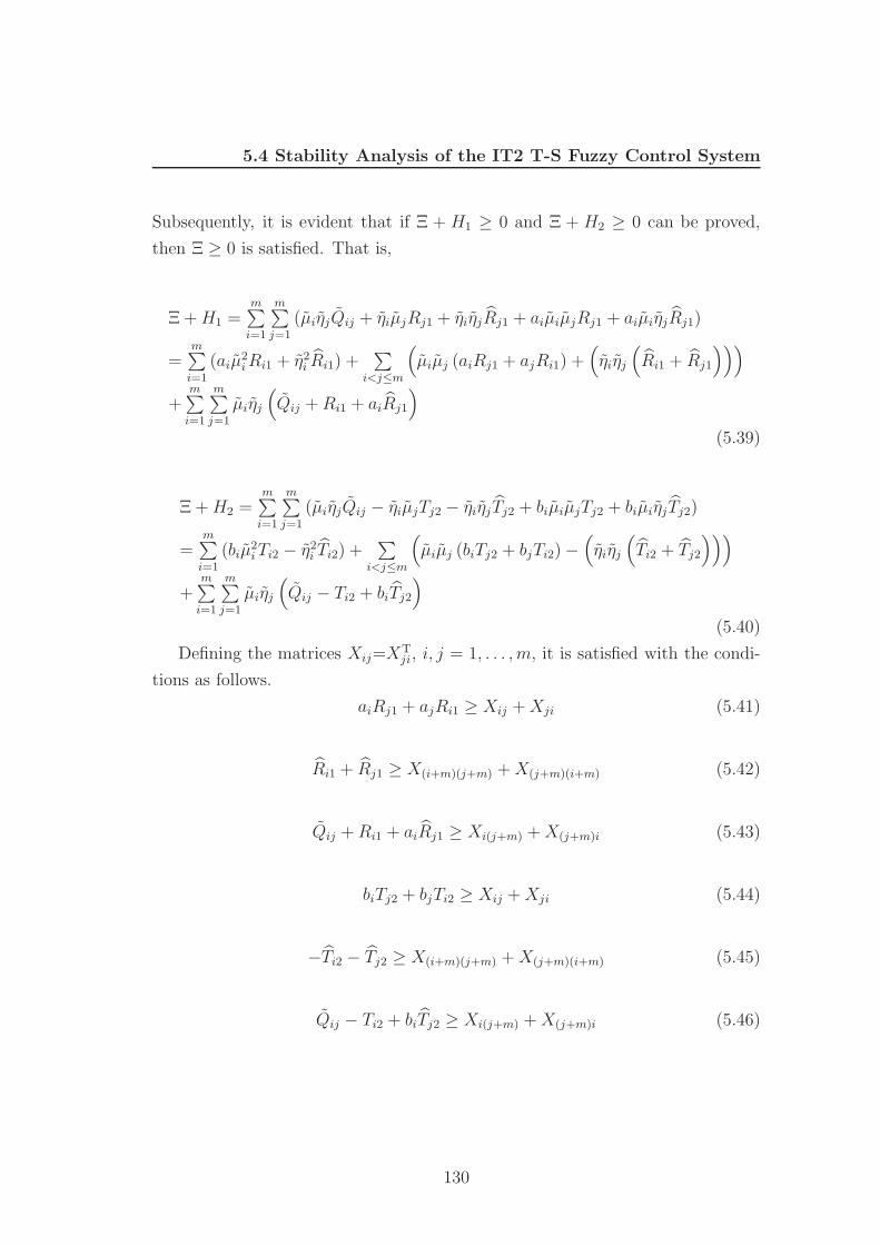
5.4 Stability Analysis of the IT2 T-S Fuzzy Control System
Subsequently, it is evident that if Ξ + H1 ≥ 0 and Ξ + H2 ≥ 0 can be proved,
then Ξ ≥ 0 is satisfied. That is,
Ξ + H1 =m∑
i=1
m∑j=1
(µiηjQij + ηiµjRj1 + ηiηjRj1 + aiµiµjRj1 + aiµiηjRj1)
=m∑
i=1
(aiµ2i Ri1 + η2
i Ri1) +∑
i<j≤m
(µiµj (aiRj1 + ajRi1) +
(ηiηj
(Ri1 + Rj1
)))
+m∑
i=1
m∑j=1
µiηj
(Qij + Ri1 + aiRj1
)
(5.39)
Ξ + H2 =m∑
i=1
m∑j=1
(µiηjQij − ηiµjTj2 − ηiηjTj2 + biµiµjTj2 + biµiηjTj2)
=m∑
i=1
(biµ2i Ti2 − η2
i Ti2) +∑
i<j≤m
(µiµj (biTj2 + bjTi2) −
(ηiηj
(Ti2 + Tj2
)))
+m∑
i=1
m∑j=1
µiηj
(Qij − Ti2 + biTj2
)
(5.40)
Defining the matrices Xij=XTji, i, j = 1, . . . , m, it is satisfied with the condi-
tions as follows.
aiRj1 + ajRi1 ≥ Xij + Xji (5.41)
Ri1 + Rj1 ≥ X(i+m)(j+m) + X(j+m)(i+m) (5.42)
Qij + Ri1 + aiRj1 ≥ Xi(j+m) + X(j+m)i (5.43)
biTj2 + bjTi2 ≥ Xij + Xji (5.44)
−Ti2 − Tj2 ≥ X(i+m)(j+m) + X(j+m)(i+m) (5.45)
Qij − Ti2 + biTj2 ≥ Xi(j+m) + X(j+m)i (5.46)
130

5.4 Stability Analysis of the IT2 T-S Fuzzy Control System
X11 · · · X1(2r)...
. . ....
X(2r)1 · · · X(2r)(2r)
> 0 (5.47)
With the conditions in equations 5.41 - 5.43, the equation 5.39 can be extended
as:
Ξ + H1 ≥m∑
i=1
(µ2i Xii + η2
i Xii)
+m∑
i=1
∑i<j≤m
(µiµj (Xij + Xji) + ηiηj
(X(i+m)(j+m) + X(j+m)(i+m)
))
+m∑
i=1
m∑j=1
(µiηj
(Xi(j+m) + X(j+m)i
))(5.48)
With the different conditions in equations 5.44 - 5.46, the equation 5.40 can
be extended as the same formula as equation 5.48.
Hence, with the equation 5.48, Ξ + H ≥ 0. Then Ξ ≥ 0. And based on the
condition 5.32, ˙V (t) ≤ 0. The proposed interval type-2 fuzzy control system is
asymptotic stable.
Furthermore, the conditions of equations 5.41 - 5.46 can be rewritten as:
aiRj1 + ajRi1 + biTj2 + bjTi2 ≥ Xij + Xji (5.49)
Ri1 + Rj1 − Ti2 − Tj2 ≥ X(i+m)(j+m)X(j+m)(i+m) (5.50)
Qij + Ri1 + aiRj1 − Ti2 + biTj2 ≥ Xi(j+m) + X(j+m)i (5.51)
The stability analysis result is summarized in the following theorem.
Theorem 5.3: With the known conditions of equations 5.33 and 5.34, if there
exist matrices Xij=XTji, i, j = 1, . . . , 2m and symmetric definite positive matrices
Rj1, Rj1, Tj2 and Tj2 for all j = 1, . . . , r, which satisfy the conditions in equations
5.49- 5.51 and equation 5.47, the proposed interval type-2 fuzzy control system
in equation 5.26 is asymptotic stable.
Remark 5.3: When all the membership functions in fuzzy control system are
typical membership functions, the closed-loop system is reduced to a typical T-S
fuzzy control system. The constraints of membership grades in equations 5.33 and
131

5.5 Summary
5.34 will be changed to µi = ηj. The process of stability analysis in this section
will be shrunk to the general formulation for typical T-S fuzzy system. So this
stability analysis method is an extension of existing typical stability results to
consider the interval membership grades in type-2 fuzzy system. Furthermore,
the stability analysis can not only be utilized for proposed adaptive IT2 fuzzy
control system, but also for the general interval type-2 fuzzy systems.
Remark 5.4: Since the stability result in this section is deducted from Lya-
punov stability theory, a common quadratic Lyapunov function need to be found
for all the local subsystems in T-S fuzzy model. And this stability conditions are
sufficient conditions. Less conservative methods about interval type-2 T-S fuzzy
control system will be studied in future.
5.5 Summary
With the proposed framework of adaptive IT2 FLC in Chapter 4, a closed-loop
model of interval type-2 fuzzy control system was presented. Its closed-loop sta-
bility has been investigated by quadratic Lyapunov stability theory. Under the
constraints of interval membership grades in the T-S fuzzy model, the proposed
control system has been proved to be asymptotic stable. And the stability con-
ditions have been carried out to guarantee its stability.
According to the vehicle non-linear suspension system, since the proposed
control method has been guaranteed to be stable with required conditions, it
provides a theoretical foundation for further experimental study and industrial
application development.
132

Chapter 6
Conclusions
6.1 Overview
This thesis started by considering three key aims as the main objectives of this
research project. The first aim was to study the non-linear performance of a
vehicle active suspension system and build the proper model to represent the
effect of changing vehicle speed and random road vibrations. This task involves
the modelling of tyres and numerical simulations on an improved half-vehicle
suspension model. The second aim was to design intelligent control strategies
to minimize the vertical and longitudinal vibrations of vehicle body to improve
the ride comfort and handling performance. The uncertainties from road inputs
and suspension parameters were considered. The third aim was to analyse the
closed-loop system stability of the proposed intelligent controller on the vehicle
suspension system.
6.2 Contributions
In this thesis, an improved non-linear half-vehicle suspension model has been built
to more accurately represent suspension dynamics. With the proposed model,
this thesis has presented a novel framework to adaptively control the vehicle
active suspension system by using interval type-2 fuzzy logic. The bounded in-
terval fuzzy reasoning results have been obtained to cover more general non-linear
133

6.2 Contributions
and uncertain information in the suspension control system. Two optimization
methods have been integrated into the interval type-2 fuzzy control structure to
self-tune the control forces. Simulations with different road conditions and vary-
ing suspension coefficients have been done to verify the efficiency of the proposed
control methods. The closed-loop stability of the proposed system has been anal-
ysed and the stability conditions have been derived. These are addressed in turn
in the following subsections.
6.2.1 The Improved Models
In Chapter 3, two improved half-vehicle active suspension models which inte-
grated tyre longitudinal dynamics, linear and non-linear spring and damper dy-
namics were proposed. By introducing a rigid tyre dynamic model, the tyre
longitudinal vibration and its effect on pitch motion in the suspension were rep-
resented in the improved system model. The improved model has been evaluated
using the open-loop system (not considering the active force) and the closed-
loop system (with linear controller). The simulation results have shown that the
improved models represent more accurate pitch motion dynamics in comparison
with the existing models. Also the non-linear model represents more accurate
vertical vibrations than the linear models.
6.2.2 The Interval Type-2 Fuzzy Controller with LMS
In Chapter 4, Section 4.3.2, an adaptive IT2 FLC with LMS was proposed to con-
trol the vehicle non-linear suspension system. Compared with existed methods,
the proposed method can not only deal with the non-linear dynamics and uncer-
tain information from road vibration and linguistic expert knowledge, but also
make use of the interval reasoning results to do further optimization to reduce
the system error. In Chapter 4, Section 4.4.1 and Section 4.5.1, the simulation
results have shown that the proposed method can significantly reduce the vehicle
body accelerations and tyre dynamic loads on the quarter-vehicle and half-vehicle
suspension models. Furthermore, on the half-vehicle suspension model, with the
additional optimization structure, the longitudinal vibration was constrained and
134

6.2 Contributions
the pitch angle acceleration was reduced by 61.8% over the passive suspension
system and by 26.9% over the TFC method. Also its potential adaptive ability
of dealing with linguistic uncertainty and non-linear dynamics was verified to be
superior than the TFC method. The results have also clearly showed the rela-
tionship between the pitch motion dynamics and different vehicle forward speeds.
6.2.3 The Interval Type-2 Fuzzy Controller with PSO
In Chapter 4, Section 4.3.3, an adaptive IT2 FLC with PSO was proposed to con-
trol the vehicle non-linear suspension system. Different from the LMS method,
the PSO method can solve non-linear optimisation problem. With the same
framework as the adaptive IT2 FLC, this method has dealt with the required
aim of constraining the suspension travel and reducing the pitch vibration. In
Chapter 4, Section 4.4.2 and Section 4.5.2, the simulation results have shown
that the proposed method can not only improve the riding comfort and handling
performance, but also limit the suspension travel to avoid strut hitting on the
quarter-vehicle suspension model. It achieved the aim of reducing the pitch an-
gle accelerations on the half-vehicle suspension model. Also its adaptive ability
of dealing with linguistic uncertainty and non-linear dynamics was verified to be
superior than the typical fuzzy control method. The effect of different vehicle for-
ward speed on suspension pitch motion dynamics has been verified by simulation
results.
6.2.4 Closed-loop Stability Analysis
In Chapter 5, based on existing stability analysis results on the T-S fuzzy con-
trol system and by extending the constraints of membership grades to interval
domains, the quadratic Lyapunov stability theory has been restructured to anal-
yse the closed-loop stability of the proposed interval type-2 fuzzy control system.
Sufficient conditions have been derived by a theorem in Chapter 5, Section 5.3,
to guarantee that the proposed fuzzy control system was asymptotic stable.
135

6.3 Future Work
6.3 Future Work
6.3.1 Expansion of Type-2 Fuzzy Inference Engine
This thesis is the first to design an interval type-2 fuzzy controller for a vehicle
active suspension system. Since the type-2 fuzzy logic system is still an emerging
area of vigorous research activities, its outstanding feature on handling uncer-
tainty need to be verified from theory and applications. Based on the further
optimization structure on the interval type-2 fuzzy reasoning results, the pro-
posed method indirectly optimise the interval fuzzy membership functions and
inference engine performance. Furthermore, this kind of optimal action can be
transferred to the inference engine and directly optimise the fuzzy membership
functions, fuzzy rules and fuzzy reasoning process. With the proposed frame-
work, the probabilistic and fuzzy qualitative reasoning methods can be merged
to expand the properties of type-2 fuzzy system (Liu, 2008b; Liu et al., 2007,
2008a).
6.3.2 Relaxation on Stability Conditions
Using the well developed quadratic Lyapunov stability theory on T-S fuzzy sys-
tems, sufficient conditions were deduced to guarantee the global stability of pro-
posed control methods. As is usual for this approach, a quadratic Lyapunov
function for all local subsystems in a T-S fuzzy model need to be found and this
is conservative in some cases. Recent work has been done to relax the restrictive
conditions by using piecewise quadratic Lyapunov functions or fuzzy Lyapunov
functions (Chen et al., 2005; Feng, 2004). However, ways of extending these
results to type-2 fuzzy systems have not been well studied.
6.3.3 Generalization
To analyse the benefit of the proposed control framework, it should be generalised
to a number of different situations. In this thesis, the generalisation for this
framework was only tested upon the quarter-vehicle and half-vehicle suspension
136

6.4 Summary
system. For closely studying the coupled states of four quarter-vehicle models,
the whole-vehicle model need to be considered. Furthermore, by integrating other
control subsystems in the vehicle(e.g., anti-brake control, steering control or anti-
roll control), a hybrid model will be studied under the proposed control framework
in the future.
6.3.4 Application
The numerical simulations with the proposed control method on the improved
suspension model have strongly supported its practical applications. However,
before the proposed method is used for a real vehicle active suspension system,
some extended research needs to be done to include actuators and physical limits
into the model. Additionally, a solid model of a vehicle active suspension system
will be designed to verify the numerical simulation results.
6.4 Summary
In this dissertation, an improved suspension model was proposed to integrate
the tyre longitudinal dynamics into suspension motion. An overall adaptive IT2
fuzzy control framework has been built to improve the ride comfort and handling
performance by efficiently overtaking non-linear dynamics and uncertainty from
random road surfaces and expert linguistic knowledge. The simulations have
demonstrated that proposed method outperform the passive and typical fuzzy
control methods. Using quadratic Lyapunov stability theory, the global asymp-
totic stability of the proposed method has been proved and the sufficient stability
conditions have been derived.
137

References
Agarwal, M. (1997). A systematic classification of neural-network-based con-
trol. IEEE Control Systems Magazine, 17, 75–93. 35
Akar, M. & Ozguner, U. (2000). Decentralized techniques for the analysis and
control of Takagi-Sugeno fuzzy systems. IEEE Transactions on Fuzzy Systems ,
8, 691–704. 119
Alleyne, A. (1997). Improved vehicle performance using combined suspension
and braking forces. Vehicle System Dynamics , 27, 235–265. 9
Alleyne, A. & Hedrick, J. (1995). Nonlinear adaptive control of active sus-
pensions. IEEE Transactions on Control Systems Technology , 3, 94–101. 3, 9,
21
Alleyne, A., Neuhaus, P. & Hedrick, J. (1993). Application of nonlinear
control theory to electronically controlled suspensions. Vehicle System Dynam-
ics , 22, 309–320. 3, 8, 9, 21
Arino, C. & Sala, A. (2008). Extensions to ”Stability analysis of fuzzy control
systems subject to uncertain grades of membership”. IEEE Transactions on
Systems, Man, and Cybernetics. Part B , 38, 558–563. 128
Assawinchaichote, W., Nguang, S. & Shi, P. (2004). H-infinity output
feedback control design for uncertain fuzzy singularly perturbed systems: an
LMI approach. Automatica, 40, 2147–2152. 119
138

REFERENCES
Astudillo, L., Castillo, O. & Aguilar, L. (2007). Intelligent control for
a perturbed autonomous wheeled mobile robot: a type-2 fuzzy logic approach.
Journal of Nonlinear Studies, 14, 37–48. 76
Baumal, A., McPhee, J. & Calamai, P. (1998). Application of genetic
algorithms to the design optimization of an active vehicle suspension system.
Computer Methods in Applied Mechanics and Engineering , 163, 87–94. vii, 37,
38, 39
Cao, J., Liu, H., Li, P. & Brown, D. (2007). Study on active suspension
control system based on an improved half-vehicle model. International Journal
of Automation and Computing , 4(3), 236–242. 75, 106
Cao, J., Liu, H., Li, P. & Brown, D. (2008). State of the art in vehicle
active suspension adaptive control systems based on intelligent methodologies.
IEEE Transactions on Intelligent Transportation Systems, 9, 392–405. 3, 75
Cao, Y. & Frank, P. (2001). Stability analysis and synthesis of nonlinear time-
delay systems via linear Takagi–Sugeno fuzzy models. Fuzzy Sets and Systems ,
124, 213–229. 119
Cao, Y. & Lin, Z. (2003). Robust stability analysis and fuzzy-scheduling control
for nonlinear systems subject to actuator saturation. IEEE Transactions on
Fuzzy Systems , 11, 57–67. 119
Chen, B., Lee, B. & Guo, L. (2003). Optimal tracking design for stochastic
fuzzy systems. IEEE Transactions on Fuzzy Systems , 11, 796–813. 124
Chen, B., Liu, X. & Tong, S. (2007). New delay-dependent stabilization
conditions of T-S fuzzy systems with constant delay. Fuzzy Sets and Systems ,
158, 2209–2224. 119
Chen, C. & Chang, M. (1998). Optimal design of fuzzy sliding-mode control:
a comparative study. Fuzzy Sets and Systems , 93, 37–48. 33
Chen, C., Feng, G. & Guan, X. (2005). Delay-dependent stability analysis
and controller synthesis for discrete-time T-S fuzzy systems with time delays.
IEEE Transactions on Fuzzy Systems , 13, 630–643. 136
139

REFERENCES
Chen, H. & Huang, S. (2008). A new model-free adaptive sliding controller for
active suspension system. International Journal of Systems Science, 39, 57–69.
75
Chen, S., Tzuu, S. & Fan, C. (1995). Design of fuzzy controller for active
suspension system. Mechatronics, 5(4), 365–383. vii, 3, 29, 30, 31, 74
Cherry, A. & Jones, R. (1995). Fuzzy logic control of an automotive suspen-
sion system. IEE Proceedings-Control Theory and Applications, 142, 149–160.
3
Choi, S., Lee, H. & Chang, E. (2001). Field test results of a semi-active
ER suspension system associated with skyhook controller. Mechatronics, 11,
345–353. 2
Crolla, D. & Abdel, M. (1991). Active suspension control: performance
comparisons using control laws applied to a full vehicle model. Vehicle System
Dynamics , 20, 107–120. 2, 57
Davis, L. (1991). Handbook of genetic algorithms. Van Nostrand Reinhold New
York . 37
Dong, X., Yu, M., Liao, C., Chen, W., Zhang, H. & Huang, S. (2006).
Adaptive fuzzy neural network control for transient dynamics of magneto-
rheological suspension with time-delay. Lecture Notes in Computer Science,
3972, 1046–1051. vii, 41, 42
Efe, M., Kaynak, O. & Wilamowski, B. (2000). Stable training of com-
putationally intelligent systems by using variable structure systems technique.
IEEE Transactions on Industrial Electronics , 47, 487–496. 26
EI-Demerdash, S., Selim, A. & Crolla, D. (1999). Vehicle body attitude
control using an electronically controlled active suspension. SAE Transactions,
108, 1232–1242. 48, 57
Esmailzadeh, E. & Bateni, H. (1992). Optimal active vehicle suspensions
with full state feedback control. SAE Transactions, 101, 784–795. 7
140

REFERENCES
Fang, C., Liu, Y., Kau, S., Hong, L. & Lee, C. (2006). A new LMI-based
approach to relaxed quadratic stabilization of TS fuzzy control systems. IEEE
Transactions on Fuzzy Systems , 14, 386–397. 120
Feng, G. (2004). Stability analysis of discrete-time fuzzy dynamic systems based
on piecewise Lyapunov functions. IEEE Transactions on Fuzzy Systems , 12,
22–28. 136
Feng, G. (2006). A survey on analysis and design of model-based fuzzy control
systems. IEEE Transactions on Fuzzy Systems , 14, 676–697. 4, 106, 119, 120,
122, 124
Feng, G., Cao, S., Rees, N. & Chak, C. (1997a). Design of fuzzy control
systems with guaranteed stability. Fuzzy Sets and Systems , 85, 1–10. 119
Feng, X., Lin, C., Yu, T. & Coleman, N. (1997b). Intelligent control design
and simulation using neural networks. AIAA Guidance, Navigation and Control
Conference, Part 1, 294–299. 35
Fernando, J. & Viassolo, D. (2000). Fuzzy control for active suspensions.
Mechatronics, 10, 897–920. 3, 75
Fukuda, T. & Kubota, N. (1999). Intelligent robotic systems: Adaptation,
learning, and evolution. Artificial Life and Robotics , 3, 32–38. x, 10, 11
Gao, B., Darling, J., Tilley, D., Williams, R., Bean, A. & Donahue,
J. (2006). Control of a hydropneumatic active suspension based on a non-linear
quarter-car model. Proceedings of the Institution of Mechanical Engineers, Part
I: Journal of Systems and Control Engineering , 220, 15–31. 3, 48, 75
Goldberg, D. (1989). Genetic algorithms in search, optimization, and machine
learning. 37, 45
Gordon, T., Marsh, C. & Milsted, M. (1991). A comparison of adaptive
LQG and nonlinear controllers for vehicle suspension systems. Vehicle System
Dynamics , 20, 321–340. 3, 8, 21
141

REFERENCES
Guan, X. & Chen, C. (2004). Delay-dependent guaranteed cost control for
TS fuzzy systems with time delays. IEEE Transactions on Fuzzy Systems , 12,
236–249. 120
Guerra, T. & Vermeiren, L. (2004). LMI-based relaxed nonquadratic sta-
bilization conditions for nonlinear systems in the Takagi-Sugeno’s form. Auto-
matica, 40, 823–829. 119
Guo, D., Hu, H. & Yi, J. (2004). Neural network control for a semi-active
vehicle suspension with a magnetorheological damper. Journal of Vibration
and Control , 10, 461–471. vii, 36
Hac, A. (1987). Adaptive control of vehicle suspension. Vehicle System Dynam-
ics , 16, 57–74. 3, 8
Hac, A. (1992). Optimal linear preview control of active vehicle suspension.
Vehicle System Dynamics , 21, 167–195. 2
Hagras, H. (2004). A hierarchical type-2 fuzzy logic control architecture for
autonomous mobile robots. IEEE Transactions on Fuzzy Systems,, 12(4), 524–
539. 75
Hagras, H. (2007). Type-2 flcs: a new generation of fuzzy controllers. IEEE
Computational Intelligence Magazine, 2(1), 30–44. 76
Herrera, F., Lozano, M. & Verdegay, J. (1995). Tuning fuzzy logic con-
trollers by genetic algorithms. International Journal of Approximate Reason-
ing , 12, 299–315. 43
Herrera, F., Lozano, M. & Verdegay, J. (1998). A learning process for
fuzzy control rules using genetic algorithms. Fuzzy Sets and Systems , 100,
143–158. 43
Holland, J. (1975). Adaptation in natural and artificial systems. University of
Michigan press, Ann Arbor, MI . 37
142

REFERENCES
Homaifar, A. & McCormick, E. (1995). Simultaneous design of membership
functions and rule sets for fuzzy controllers using genetic algorithms. IEEE
Transactions on Fuzzy Systems,, 3, 129–139. 43
Hrovat, D. (1987). Ride improvements with unsprung mass dynamic absorbers
for active suspension vehicles. Ford Motor Company Research Report SR-87-
120 . 7
Hrovat, D. (1997). Survey of advanced suspension developments and related
optimal control applications. Automatica, 33(10), 1781–1817. 1, 2, 8, 12, 14,
21, 48, 49, 74
Huang, S. & Chao, H. (2000). Fuzzy logic controller for a vehicle active sus-
pension system. Proceedings of the Institution of Mechanical Engineers, Part
D, Journal of Automobile Engineering , 214, 1–12. vii, 3, 23, 24, 25, 92
Huang, S. & Lin, C. (2003). Adaptive fuzzy controller with sliding surface for
vehicle suspension control. IEEE Transactions on Fuzzy Systems , 11, 550–559.
vii, 3, 33, 34
Huang, S. & Lin, C. (2004). Application of a fuzzy enhance adaptive control
on active suspension system. International Journal of Computer Applications
in Technology , 20, 152–160. 23, 24
John, R. (1998). Type 2 fuzzy sets: An appraisal of theory and applications. In-
ternational Journal of Uncertainty, Fuzziness and Knowledge-Based Systems ,
6, 563–576. 76
John, R. & Coupland, S. (2007). Type-2 fuzzy logic: A historical view. IEEE
Computational Intelligence Magazine, 2, 57–62. 75
Julio, R. & Alberto, V. (2007). Calculating functions of interval type-2
fuzzy numbers for fault current analysis. IEEE Transactions on Fuzzy Systems ,
15(1), 31–40. 76
Karnik, N. & Liang, J. (1999). Type-2 fuzzy logic systems. IEEE Transactions
on Fuzzy Systems , 7, 643–658. 76
143

REFERENCES
Karnik, N. & Mendel, J. (2001). Centroid of a type-2 fuzzy set. Information
Sciences , 132, 195–220. 75, 82
Kaynak, O. (1998). Computational Intelligence: Soft Computing and Fuzzy-
Neuro Integration with Applications. Springer. vii, 30, 37
Kaynak, O., Erbatur, K. & Ertugnrl, M. (2001). The Fusion of Compu-
tationally Intelligent Methodologies and Sliding-mode Control-A Survey. IEEE
Transactions on Industrial Electronics, 48, 4–17. 9
Ke, Z., Nai, Z. & Wen, X. (2000). A comparative study on sufficient conditions
for Takagi-Sugeno fuzzy system as universal approximators. IEEE Transactions
on Fuzzy Systems , 8, 773–780. 120
Kennedy, J. & Eberhart, R. (1995). Particle swarm optimization. IEEE
International Conference on Neural Networks, Proceedings,, 4. 88
Khargonekar, P., Petersen, I. & Zhou, K. (1990). Robust stabilization of
uncertain linear systems: quadraticstabilizability and H infinity control theory.
IEEE Transactions on Automatic Control , 35, 356–361. 124
Kiendl, H. & Ruger, J. (1995). Stability analysis of fuzzy control systems
using facet functions. Fuzzy Sets and Systems , 70, 275–285. 119
Kim, C. (1996). A comparative study of active suspension systems using adaptive
self-tuning control and sliding mode control schemes. Master thesis, Mechanical
and Aerospace Engineering Department, North Carolina State University . 9
Kim, C. & Ro, P. (1998). A sliding mode controller for vehicle active suspen-
sion systems with non-linearities. Proceedings of the Institution of Mechanical
Engineers, Part D, Journal of Automobile Engineering , 212, 79–92. vii, 9, 21,
22, 23, 61
Kiriakidis, K., Grivas, A. & Tzes, A. (1998). Quadratic stability analysis
of the Takagi-Sugeno fuzzy model. Fuzzy Sets and Systems , 98, 1–14. 119
Kosko, B. (1998). Global stability of generalized additive fuzzy systems. IEEE
Transactions on Systems, Man and Cybernetics, Part C , 28, 441–452. 119
144

REFERENCES
Kucukdemiral, I., Engin, S., Omurlu, V. & Cansever, G. (2005). A
robust single input adaptive sliding mode fuzzy logic controller for automotive
active suspension system. Lecture Notes in Computer Science, 3613, 981. vii,
34, 35
Lam, H. & Seneviratne, L. (2008). Stability analysis of interval type-2 fuzzy-
model-based control systems. IEEE Transactions on Systems, Man and Cyber-
netics, Part B , 38, 617–628. 126, 128
Lam, H., Leung, F. & Tam, P. (2001). Nonlinear state feedback controller for
nonlinear systems: Stability analysis and design based on fuzzy plant model.
IEEE Transactions on Fuzzy Systems , 9, 657–661. 119
Li, J., Wang, H., Niemann, D. & Tanaka, K. (2000). Dynamic parallel
distributed compensation for takagi–sugeno fuzzy systems: An lmi approach.
Information Sciences, 123, 201–221. 124
Li, L., Wang, F. & Zhou, Q. (2006). Integrated longitudinal and lateral
tire/road friction modeling and monitoring for vehicle motion control. IEEE
Transactions on Intelligent Transportation Systems, 7, 1–19. 3, 75
Li, Z., Yang, Y., Gong, X., Lin, Y. & Liu, G. (2008). Fuzzy control of
the semi-active suspension with MR damper based on µGA. In IEEE Vehicle
Power and Propulsion Conference (VPPC’08), 1–6. 75
Lian, R., Lin, B. & Sie, W. (2005). Self-organizing fuzzy control of active
suspension systems. International Journal of Systems Science, 36, 119–135. 3,
24
Liang, Q. & Mendel, J. (2000). Interval type-2 fuzzy logic systems: theory
and design. IEEE Transactions on Fuzzy Systems , 8, 535–550. 75, 81
Liang, Q., Karnik, N. & Mendel, J. (2000). Connection admission control
in atm networks using survey-based type-2 fuzzy logic systems. IEEE Trans-
actions on Systems, Man, and Cybernetics, Part C , 30, 329–339. 76
145

REFERENCES
Lin, J. & Lian, R. (2008). DSP-based self-organising fuzzy controller for active
suspension systems. Vehicle System Dynamics , 46, 1123–1139. 75
Lin, R., Cebon, D. & Cole, D. (1996). Active roll control of articulated
vehicles. Vehicle System Dynamics , 26, 17–43. 49
Liu, F. (2008a). An efficient centroid type-reduction strategy for general type-2
fuzzy logic system. Information Sciences, 178, 2224–2236. 76
Liu, H. (2008b). A fuzzy qualitative framework for connecting robot qualitative
and quantitative representations. IEEE Transactions on Fuzzy Systems , 16,
1522–1530. 136
Liu, H., Coghill, G. & Brown, D. (2007). Qualitative kinematics of planar
robots: intelligent connection. International Journal of Approximate Reason-
ing , 46, 525–541. 136
Liu, H., Brown, D. & Coghill, G. (2008a). Fuzzy qualitative robot kine-
matics. IEEE Transactions on Fuzzy Systems , 16, 808–822. 136
Liu, H., Nonami, K. & Hagiwara, T. (2008b). Active following fuzzy output
feedback sliding mode control of real-vehicle semi-active suspensions. Journal
of Sound and Vibration, 314, 39–52. 57, 75
Liu, Z. & Li, H. (2005). A probabilistic fuzzy logic system for modelling and
control. IEEE Transactions on Fuzzy Systems , 13(6), 848–859. 124
Lu, J. & DePoyster, M. (2002). Multiobjective optimal suspension control
to achieve integrated ride and handling performance. IEEE Transactions on
Control Systems Technology , 10, 807–821. 9
Magdalena, L., Cordon, O., Gomide, F., Herrera, F. & Hoffmann,
F. (2004). Ten years of genetic fuzzy systems: Current framework and new
Trends. Fuzzy Sets and Systems , 141, 5–31. 43
Mansour, A. & Crolla, D. (2000). Analysis and design of limited bandwidth
active hydropneumatic vehicle suspension systems. SAE Transactions, 109,
2100–2108. 48
146

REFERENCES
Margolis, D. (1982). Semi-active heave and pitch control for ground vehicles.
Vehicle System Dynamics , 11, 31–42. 2
Mendel, J. (2007a). Advances in type-2 fuzzy sets and systems. Information
Sciences , 177, 84–110. 75, 77
Mendel, J. (2007b). New results about the centroid of an interval type-2 fuzzy
set, including the centroid of a fuzzy granule. Infromation Sciences, 117, 360–
377. 76
Mendel, J. & John, R. (2002). Type-2 fuzzy sets made simple. IEEE Trans-
actions on Fuzzy Systems , 10, 117–127. 75, 81
Mendel, J., Hagras, H. & John, R. (2007). Standard background material
about interval type-2 fuzzy logic systems that can be used by all authors.
http://ieee-cis.org/files/standards.t2.win.pdf . 76
Moran, A. & Nagai, M. (1993). Optimal preview control of rear suspension
using nonlinear neural networks. Vehicle System Dynamics , 22, 321–334. 37
Nagai, M. (1993). Recent researches on active suspensions for ground vehicles.
JSME International Journal. Series C, Mechanical Systems, Machine Elements
and Manufacturing , 36, 161–170. vii, 2, 8, 12, 13, 74
Naude, A. & Snyman, J. (2003a). Optimisation of road vehicle passive sus-
pension systems. Part 1. Optimisation algorithm and vehicle model. Applied
Mathematical Modelling , 27, 249–261. 2
Naude, A. & Snyman, J. (2003b). Optimisation of road vehicle passive sus-
pension systems. Part 2. Qualification and case study. Applied Mathematical
Modelling , 27, 263–274. 2
Nawa, N., Furuhashi, T., Hashiyama, T. & Uchikawa, Y. (1999). A study
on the discovery of relevant fuzzy rules using pseudobacterial genetic algorithm.
IEEE Transactions on Industrial Electronics , 46, 1080–1089. vii, viii, 44, 45
147

REFERENCES
Nurnberger, A., Nauck, D. & Kruse, R. (1999). Neuro-fuzzy control based
on the NEFCON-model: Recent developments. Soft Computing-A Fusion of
Foundations, Methodologies and Applications , 2, 168–182. 41
Oueslati, F. & Sankar, S. (1994). A class of semi-active suspension schemes
for vehicle vibration control. Journal of Sound and Vibration, 172, 391–411. 2
Pacejka, H. (2006). Tyre and Vehicle Dynamics. Butterworth-Heinemann. 49
Palkovics, L. & Venhovens, P. (1992). Investigation on stability and possible
chaotic motions in the controlled wheel suspension system. Vehicle System
Dynamics , 21, 269–296. 9
Parsopoulos, K. & Vrahatis, M. (2002). Particle swarm optimization
method for constrained optimization problems. In Proceedings of the Euro-
International Symposium on Computational Intelligence 2002 , 214–220, IOS
Press. 90
Rao, M. & Prahlad, V. (1997). A tunable fuzzy logic controller for vehicle-
active suspension systems. Fuzzy Sets and Systems , 85, 11–21. 3, 23, 24, 74
Sala, A. & Arino, C. (2007). Asymptotically necessary and sufficient condi-
tions for stability and performance in fuzzy control: Applications of Polya’s
theorem. Fuzzy Sets and Systems , 158, 2671–2686. 128
Sala, A. & AriNo, C. (2008). Relaxed stability and performance LMI condi-
tions for Takagi–Sugeno fuzzy systems with polynomial constraints on mem-
bership function Shapes. IEEE Transactions on Fuzzy Systems , 16, 1328–1336.
128
Sampson, D. & Cebon, D. (2003). Active roll control of single unit heavy road
vehicles. Vehicle System Dynamics , 40, 229–270. 49
Sepulveda, R., Castillo, O., Melin, P., Rodrıguez-Dıaz, A. & Mon-
tiel, O. (2007). Experimental study of intelligent controllers under uncertainty
using type-1 and type-2 fuzzy logic. Information Sciences, 177, 2023–2048. 76
148

REFERENCES
Shi, Y. & Eberhart, R. (1998). Parameter selection in particle swarm opti-
mization. Lecture Notes in Computer Science, 591–600. 90
Slotine, J. & Li, W. (1991). Applied nonlinear control. NJ: Prantice-Hall,
Englewood Cliffs . 9
Sun, J. (2003). Study on control technique for vehicle active suspension system.
PhD thesis, Harbin Engineering University . 74
Sunwoo, M. & Cheok, K. (1990). An application of rxplicit self-tuning con-
troller to vehicle active suspension systems. Proceedings of the 29th IEEE Con-
ference on Decision and Control , 2251–2257. 3, 8, 9, 21
Sunwoo, M., Cheok, K. & Huang, N. (1991). Model reference adaptive
control for vehicle active suspensionsystems. IEEE Transactions on Industrial
Electronics , 38, 217–222. 3, 9
Taghirad, H. (1997). Automobile passenger comfort assured through lqg/lqr
active suspension. Journal of Vibration and Control , 3, 1–19. 8, 14, 90
Taghirad, H. & Esmailzadeh, E. (1998). Automobile passenger comfort as-
sured through LQG/LQR active suspension. Journal of Vibration and Control ,
4, 603–618. 8
Takagi, T. & Sugeno, M. (1985). Fuzzy identification of systems and its
applications to modeling and control. IEEE Transactions on Systems, Man,
and Cybernetics, 15, 116–132. 120, 128
Tamboli, J. & Joshi, S. (1999). Optimum design of a passive suspension system
of a vehicle subjected to actual random road excitations. Journal of Sound and
Vibration, 219, 193–205. 2
Tanaka, K. & Wang, H. (2001). Fuzzy control systems design and analysis: a
linear matrix inequality approach. Wiley-Interscience. 120, 122, 124
Tang, C. & Zhang, T. (2005). The research on control algorithms of vehicle
active suspension system. IEEE International Conference on Vehicular Elec-
tronics and Safety , 320–325. 45
149

REFERENCES
Taniguchi, T., Tanaka, K. & Wang, H. (2000). Fuzzy descriptor systems
and nonlinear model following control. IEEE Transactions on Fuzzy Systems ,
8, 442–452. 120
Thompson, A. & Davis, B. (1988). Optimal linear active suspensions with
derivative constraints and output feedback control. Vehicle System Dynamics ,
17, 179–192. 2, 7
Thompson, A. & Davis, B. (1991). A technical note on the Lotus suspension
patents. Vehicle System Dynamics , 20, 381–383. 7
Ting, C. (2006). Stability analysis and design of Takagi–Sugeno fuzzy systems.
Information Sciences, 176, 2817–2845. 119
Ting, C., Li, T. & Kung, F. (1995). Design of fuzzy controller for active
suspension system. Mechatronics, 5, 365–383. 3
Trachtler, A. (2004). Integrated vehicle dynamics control using active brake,
steering and suspension systems. International Journal of Vehicle Design, 36,
1–12. 49
Tsao, J. & Chen, R. (2001). The design of an active suspension force controller
using genetic algorithms with maximum stroke constraints. Proceedings of the
Institution of Mechanical Engineers, Part D, Journal of Automobile Engineer-
ing , 215, 317–327. vii, 37, 39, 40
Tsao, Y. & Chen, R. (1997). Parameters searching for force control of active
suspension design by using genetic algorithm. Automatic Control Conference,
Taipei , 695–699. 37, 39
Tsao, Y. & Chen, R. (1998). Force control for active suspension design with a
half car model by using genetic algorithms. Proceedings of Fourth International
Symposium on Advanced Vehicle Control, AVEC’98, Nagoya, Japan,, 243–248.
37, 39
Tseng, C., Chen, B. & Uang, H. (2001). Fuzzy tracking control design for
nonlinear dynamic systems via TS fuzzy model. IEEE Transactions on Fuzzy
Systems , 9, 381–392. 120
150

REFERENCES
Vemuri, V. (1993). Artificial neural networks in control applications. Advances
in Computers, 36, 203–254. 35
Wang, H., Tanaka, K. & Griffin, M. (1996). An approach to fuzzy control
of nonlinear systems: stability and design issues . IEEE Transactions on Fuzzy
Systems , 4, 14–23. 122
Wang, J. & Shen, S. (2008). Integrated vehicle ride and roll control via active
suspensions. Vehicle System Dynamics , 46, 495–508. 49, 75
Wang, J., Wilson, D., Xu, W. & Crolla, D. (2006). Integrated vehicle ride
and steady-state handling control via active suspensions. International Journal
of Vehicle Design, 42, 306–327. 48
Widrow, B. & Hoff, M. (1960). Adaptive switching circuits. New York: IRE ,
4, 96–104. 86
Williams, R. (1997). Automotive active suspensions Part 2: practical consider-
ations. Proceedings of the Institution of Mechanical Engineers, Part D: Journal
of Automobile Engineering , 211, 427–444. 8
Wu, D. & Mendel, J. (2007). Uncertainty measures for interval type-2 fuzzy
sets. Information Sciences, 177(23), 5378–5393. 75
Wu, D. & Mendel, J. (2008). A vector similarity measure for linguistic ap-
proximation: Interval type-2 and type-1 fuzzy sets. Information Sciences, 178,
381–402. 75
Wu, D. & Mendel, J. (2009). A comparative study of ranking methods, simi-
larity measures and uncertainty measures for interval type-2 fuzzy sets. Infor-
mation Sciences , 179, 1169–1192. 75
Wu, H. & Mendel, J. (2002). Uncertainty bounds and their use in the design
of interval type-2 fuzzy logic systems. IEEE Transactions on Fuzzy Systems ,
10, 622–639. 76, 83
151

REFERENCES
Wu, S., Wu, C. & Lee, T. (2005). Neural-network-based optimal fuzzy con-
trol design for half-car active suspension systems. IEEE Intelligent Vehicles
Symposium, Proceedings , 376–381. 43
Yang, J., Li, J. & Du, Y. (2006). Adaptive fuzzy control of lateral semi-active
suspension for high-speed railway vehicle. Lecture Notes in Computer Science,
4114, 1104–1115. 24
Yao, G., Yap, F., Chen, G., Li, W. & Yeo, S. (2002). MR damper and its
application for semi-active control of vehicle suspension system. Mechatronics,
12, 963–973. 2
Yeh, E. & Tsao, Y. (1994). A fuzzy preview control scheme of active suspension
for rough road. International Journal of Vehicle Design, 15, 166–180. 3, 23, 24
Yoo, B. & Ham, W. (1998). Adaptive fuzzy sliding mode control of nonlinear
system. IEEE Transactions on Fuzzy Systems , 6, 315–321. 26
Yoshimura, T. & Emoto, Y. (2003). Steering and suspension system of a
full car model using fuzzy reasoning and disturbance observers. International
Journal of Vehicle Autonomous Systems, 1, 363–386. 49
Yoshimura, T. & Watanabe, K. (2003). Active suspension of a full car model
using fuzzy reasoning based on single input rule modules with dynamic ab-
sorbers. International Journal of Vehicle Design, 31, 22–40. 49
Yu, F., Zhang, J. & Crolla, D. (2000). A study of a Kalman filter active
vehicle suspension system using correlation of front and rear wheel road inputs.
Proceedings of the Institution of Mechanical Engineers, Part D, Journal of
Automobile Engineering , 214, 493–502. 14, 48, 67
Yu, Q. & Ma, J. (2005). Analysis of automotive acceleration performance im-
provement due to active suspension. Journal of Vehicle Technology , 37, 20–23.
48
Zadeh, L. (1975). The concept of a linguistic variable and its application to
approximate reasoning-1. Information Sciences, 8, 199–249. 75
152

REFERENCES
Zegelaar, P. & Pacejka, H. (1996). Dynamic tyre responses to brake torque
variations. Vehicle System Dynamics , 27, 65–79. 49, 50
Zhang, Y., Zhao, Y., Yang, H. & Chen, L. (2007). A dynamic sliding-
mode controller with fuzzy adaptive tuning for an active suspension system.
Proceedings of the Institution of Mechanical Engineers, Part D, Journal of
Automobile Engineering , 221, 417–428. vii, 10, 31, 32, 74
153

Appendix A
Publications
1. Cao, J., Liu, H. and Li, P. An Interval Fuzzy Controller for Vehicle Ac-
tive Suspension Systems (under review), IEEE Transactions on Intelligent
Transportation Systems.
2. Cao, J., Li, P., and Liu, H. An Extended Fuzzy Controller for Vehicle Active
Suspension System (under review), Vehicle System Dynamics.
3. Cao, J., Li, P., Liu, H. An Extended Fuzzy Logic System for Uncertainty
Modelling (accepted), IEEE International Conference on Fuzzy Systems,
Jeju Island, Korea, 2009.
4. Cao, J., Ju, Z., Ji, X. and Liu, H. A Switching Fuzzy Control Method
for the Magnetic Active Suspension System (accepted), IEEE International
Conference on Fuzzy Systems, Jeju Island, Korea, 2009.
5. Cao, J., Liu, H., Li, P. and Brown, D.J. State of the Art in Vehicle Active
Suspension Adaptive Control Systems Based on Intelligent Methodologies,
IEEE Transactions on Intelligent Transportation Systems, 2008, 9(3), 392-
405.
6. Cao, J., Liu, H., Li, P. and Brown, D.J. An Interval Type-2 Fuzzy Logic
Controller for Quarter Vehicle Active Suspensions, Proceedings of the Insti-
154

tution of Mechanical Engineers, Part D, Journal of Automobile Engineer-
ing, 2008, 222(8), 1361-1374.
7. Cao, J., Li, P., Liu, H. and Brown, D.J. Adaptive Fuzzy Logic Controller for
Vehicle Active Suspensions with Interval Type-2 Fuzzy Membership Func-
tions, Proc. 2008 IEEE World Congress on Computational Intelligence,
Hong Kong, China, 2008.
8. Cao, J., Li, P., Liu, H. and Brown, D.J. Adaptive Fuzzy Controller for
Vehicle Active Suspensions with Particle Swarm Optimization, Proc. 7th
International Symposium on Instrumentation and Control Technology, Bei-
jing, China, 2008.
9. Cao, J., Liu, H., Li, P., Brown, D.J. and Dimirovski, G.M. Study on Ac-
tive Suspension Control System Based on an Improved Half-Vehicle Model,
International Journal of Automation and Computing, 2007, 4(3), 236-242.
10. Cao, J., Liu, H., Li, P., Brown, D.J. and Dimirovski, G.M. An Improved
Active Suspension Model for Attitude Control of Electric Vehicles, IEEE
International Conference on Mechatronics and Automation, Harbin, China,
2007.
155

Appendix B
Fuzzy Rules Table
Table B.1: The fuzzy rules for half-vehicle active suspension (part 1)
zbf ˙zbf zbr zbr θ Ua zbf ˙zbf zbr zbr θ Ua
NB P PB P Z -K0Xhalf NB P PM N Z -K1Xhalf
NB Z PB P P -K0Xhalf NB Z PM N Z -K1Xhalf
NB N PB P P -K0Xhalf NB N PM N Z -K0Xhalf
NB P PB Z Z -K1Xhalf NB P Z P Z -K1Xhalf
NB Z PB Z P -K0Xhalf NB Z Z P Z -K1Xhalf
NB N PB Z P -K0Xhalf NB N Z P P -K0Xhalf
NB P PB N Z -K1Xhalf NB P Z Z Z -K1Xhalf
NB Z PB N P -K1Xhalf NB Z Z Z Z -K1Xhalf
NB N PB N P -K0Xhalf NB N Z Z P -K0Xhalf
NB P PM P Z -K1Xhalf NB P Z N Z -K0Xhalf
NB Z PM P Z -K1Xhalf NB Z Z N Z -K1Xhalf
NB N PM P P -K0Xhalf NB N Z N Z -K0Xhalf
156

Table B.2: The fuzzy rules for half-vehicle active suspension (part 2)
zbf ˙zbf zbr zbr θ Ua zbf ˙zbf zbr zbr θ Ua
NB P PM Z Z -K1Xhalf NB P NM P Z -K1Xhalf
NB Z PM Z Z -K1Xhalf NB Z NM P Z -K1Xhalf
NB N PM Z P -K0Xhalf NB N NM P P -K0Xhalf
NB P NM Z Z -K2Xhalf NM P PB Z Z -K1Xhalf
NB Z NM Z Z -K2Xhalf NM Z PB Z Z -K1Xhalf
NB N NM Z Z -K0Xhalf NM N PB Z P -K0Xhalf
NB P NM N Z -K2Xhalf NM P PB N Z -K2Xhalf
NB Z NM N Z -K0Xhalf NM Z PB N P -K1Xhalf
NB N NM N Z -K0Xhalf NM N PB N P -K0Xhalf
NB P NB P Z -K1Xhalf NM P PM P Z -K2Xhalf
NB Z NB P Z -K1Xhalf NM Z PM P Z -K2Xhalf
NB N NB P P -K0Xhalf NM N PM P P -K3Xhalf
NB P NB Z Z -K2Xhalf NM P PM Z Z -K2Xhalf
NB Z NB Z Z -K2Xhalf NM Z PM Z Z -K4Xhalf
NB N NB Z Z -K0Xhalf NM N PM Z P -K2Xhalf
NB P NB N Z -K1Xhalf NM P PM N Z -K2Xhalf
NB Z NB N Z -K1Xhalf NM Z PM N Z -K2Xhalf
NB N NB N Z -K0Xhalf NM N PM N P -K3Xhalf
NM P PB P Z -K0Xhalf Z P PM Z Z -K4Xhalf
NM Z PB P P -K0Xhalf Z Z PM Z Z -K4Xhalf
NM N PB P P -K0Xhalf Z N PM Z Z -K3Xhalf
157

Table B.3: The fuzzy rules for half-vehicle active suspension (part 3)
zbf ˙zbf zbr zbr θ Ua zbf ˙zbf zbr zbr θ Ua
NM P Z P Z -K2Xhalf NM P NB Z Z -K2Xhalf
NM Z Z P Z -K4Xhalf NM Z NB Z Z -K2Xhalf
NM N Z P P -K3Xhalf NM N NB Z Z -K0Xhalf
NM P Z Z Z -K2Xhalf NM P NB N Z -K2Xhalf
NM Z Z Z Z -K4Xhalf NM Z NB N Z -K0Xhalf
NM N Z Z P -K3Xhalf NM N NB N P -K0Xhalf
NM P Z N Z -K2Xhalf Z P PB P Z -K0Xhalf
NM Z Z N Z -K4Xhalf Z Z PB P Z -K1Xhalf
NM N Z N P -K3Xhalf Z N PB P P -K0Xhalf
NM P NM P Z -K2Xhalf Z P PB Z Z -K1Xhalf
NM Z NM P Z -K2Xhalf Z Z PB Z Z -K1Xhalf
NM N NM P P -K3Xhalf Z N PB Z Z -K0Xhalf
NM P NM Z Z -K2Xhalf Z P PB N Z -K1Xhalf
NM Z NM Z Z -K4Xhalf Z Z PB N Z -K1Xhalf
NM N NM Z Z -K3Xhalf Z N PB N Z -K0Xhalf
NM P NM N Z -K2Xhalf Z P PM P Z -K3Xhalf
NM Z NM N Z -K2Xhalf Z Z PM P Z -K3Xhalf
NM N NM N Z -K3Xhalf Z N PM P P -K2Xhalf
NM P NB P Z -K1Xhalf PM P PM P Z -K3Xhalf
NM Z NB P Z -K1Xhalf PM Z PM P Z -K3Xhalf
NM N NB P P -K0Xhalf PM N PM P N -K2Xhalf
158

Table B.4: The fuzzy rules for half-vehicle active suspension (part 4)
zbf ˙zbf zbr zbr θ Ua zbf ˙zbf zbr zbr θ Ua
Z P PM N Z -K4Xhalf Z P NB P Z -K1Xhalf
Z Z PM N Z -K4Xhalf Z Z NB P Z -K1Xhalf
Z N PM N Z -K3Xhalf Z N NB P N -K0Xhalf
Z P Z P Z -K4Xhalf Z P NB Z Z -K1Xhalf
Z Z Z P Z -K4Xhalf Z Z NB Z Z -K1Xhalf
Z N Z P P -K4Xhalf Z N NB Z Z -K1Xhalf
Z P Z Z Z -K4Xhalf Z P NB N N -K0Xhalf
Z Z Z Z Z -K4Xhalf Z Z NB N Z -K0Xhalf
Z N Z Z Z -K4Xhalf Z N NB N Z -K0Xhalf
Z P Z N Z -K4Xhalf PM P PB P Z -K0Xhalf
Z Z Z N Z -K4Xhalf PM Z PB P Z -K0Xhalf
Z N Z N Z -K4Xhalf PM N PB P Z -K1Xhalf
Z P NM P Z -K2Xhalf PM P PB Z Z -K0Xhalf
Z Z NM P Z -K2Xhalf PM Z PB Z Z -K0Xhalf
Z N NM P P -K2Xhalf PM N PB Z Z -K1Xhalf
Z P NM Z Z -K4Xhalf PM P PB N Z -K0Xhalf
Z Z NM Z Z -K4Xhalf PM Z PB N Z -K1Xhalf
Z N NM Z Z -K4Xhalf PM N PB N Z -K1Xhalf
Z P NM N N -K3Xhalf PB P PB N Z -K0Xhalf
Z Z NM N Z -K3Xhalf PB Z PB N Z -K0Xhalf
Z N NM N Z -K2Xhalf PB N PB N Z -K0Xhalf
159

Table B.5: The fuzzy rules for half-vehicle active suspension (part 5)
zbf ˙zbf zbr zbr θ Ua zbf ˙zbf zbr zbr θ Ua
PM P PM Z Z -K2Xhalf PM P NM N N -K3Xhalf
PM Z PM Z Z -K4Xhalf PM Z NM N N -K2Xhalf
PM N PM Z Z -K3Xhalf PM N NM N Z -K3Xhalf
PM P PM N Z -K2Xhalf PM P NB P N -K1Xhalf
PM Z PM N Z -K3Xhalf PM Z NB P N -K1Xhalf
PM N PM N Z -K2Xhalf PM N NB P Z -K0Xhalf
PM P Z P Z -K3Xhalf PM P NB Z N -K1Xhalf
PM Z Z P Z -K4Xhalf PM Z NB Z Z -K1Xhalf
PM N Z P Z -K4Xhalf PM N NB Z Z -K1Xhalf
PM P Z Z Z -K3Xhalf PM P NB N N -K0Xhalf
PM Z Z Z Z -K4Xhalf PM Z NB N N -K0Xhalf
PM N Z Z Z -K4Xhalf PM N NB N N -K0Xhalf
PM P Z N N -K2Xhalf PB P PB P Z -K0Xhalf
PM Z Z N N -K3Xhalf PB Z PB P Z -K0Xhalf
PM N Z N Z -K3Xhalf PB N PB P Z -K0Xhalf
PM P NM P Z -K2Xhalf PB P PB Z Z -K0Xhalf
PM Z NM P Z -K2Xhalf PB Z PB Z Z -K0Xhalf
PM N NM P Z -K2Xhalf PB N PB Z Z -K0Xhalf
PM P NM Z N -K2Xhalf PB P NB N N -K0Xhalf
PM Z NM Z N -K4Xhalf PB Z NB N N -K0Xhalf
PM N NM Z Z -K2Xhalf PB N NB N Z -K0Xhalf
160
Table B.6: The fuzzy rules for half-vehicle active suspension (part 6)
zbf ˙zbf zbr zbr θ Ua zbf ˙zbf zbr zbr θ Ua
PB P PM P Z -K0Xhalf PB P NM Z N -K0Xhalf
PB Z PM P Z -K1Xhalf PB Z NM Z N -K1Xhalf
PB N PM P Z -K2Xhalf PB N NM Z Z -K1Xhalf
PB P PM Z Z -K0Xhalf PB P NM N N -K0Xhalf
PB Z PM Z Z -K1Xhalf PB Z NM N N -K0Xhalf
PB N PM Z Z -K1Xhalf PB N NM N N -K0Xhalf
PB P PM N N -K0Xhalf PB P NB P Z -K0Xhalf
PB Z PM N N -K0Xhalf PB Z NB P N -K1Xhalf
PB N PM N Z -K0Xhalf PB N NB P N -K1Xhalf
PB P Z P Z -K0Xhalf PB P NB Z N -K0Xhalf
PB Z Z P Z -K1Xhalf PB Z NB Z N -K0Xhalf
PB N Z P Z -K1Xhalf PB N NB Z Z -K1Xhalf
PB P Z Z Z -K1Xhalf - - - - - -
PB Z Z Z Z -K1Xhalf - - - - - -
PB N Z Z Z -K1Xhalf - - - - - -
PB P Z N N -K0Xhalf - - - - - -
PB Z Z N N -K0Xhalf - - - - - -
PB N Z N Z -K0Xhalf - - - - - -
PB P NM P N -K0Xhalf - - - - - -
PB Z NM P Z -K1Xhalf - - - - - -
PB N NM P Z -K2Xhalf - - - - - -
161
Copyright © 2022 FDOKUMEN