Automatica 53 (2015) 188–194

Contents lists available at ScienceDirect

Automatica

journal homepage: www.elsevier.com/locate/automatica

Brief paper

A clipped-optimal control algorithm for semi-active vehiclesuspensions: Theory and experimental evaluation✩

Panos Brezas a, Malcolm C. Smith a,1, Will Hoult ba University of Cambridge, Cambridge, UKb McLaren Automotive Ltd., Woking, Surrey, UK

a r t i c l e i n f o

Article history:Received 8 December 2013Received in revised form1 August 2014Accepted 8 November 2014

Keywords:Optimal controlSemi-active suspensionObserver designState-space methods

a b s t r a c t

This paper addresses the problem of optimal control for semi-active vehicle suspensions. A specific goalis to develop an algorithm which is capable of optimising ride and handling behaviour simultaneouslyin an experimental situation. A time-domain optimal control approach is adopted in which ride andhandling are modelled as exogenous disturbances acting on the vehicle: road disturbances (modelledstochastically), and driver inputs (treated as deterministic quasi-static disturbances). A control algorithmis derived from a solution of the stochastic Hamilton–Jacobi–Bellman equation for the finite horizon case.The advantages of the approach are demonstrated experimentally on a test vehicle performing a steeringmanoeuvre on a bumpy roundabout.

© 2014 The Authors. Published by Elsevier Ltd.This is an open access article under the CC BY license

(http://creativecommons.org/licenses/by/4.0/).

1. Introduction

This paper is concerned with the design and experimentalimplementation of a clipped-optimal Linear Quadratic (LQ) semi-active suspension system. We focus on a suspension designframework which aims to insulate the body simultaneously fromboth road irregularities and handling disturbances (driver inputs,e.g. due to cornering, braking, etc.). Recent work on LQ semi-active suspension design – see for example Butsuen and Hedrick(1989), Du, Sze, and Lam (2005), Gordon (1995), Hrovat (1997),Savaresi, Poussot-Vassal, Spelta, Sename, andDugard (2010), Sharpand Peng (2011) and Tseng and Hedrick (1994) and referencestherein – has often concentrated on the vehicle’s response toroad disturbances only. The incorporation of load disturbancesinto an LQ optimal control and estimation framework wasproposed in Brezas and Smith (2013) in the context of activevehicle suspensions to deal with handling inputs. There, it wasdemonstrated, in simulation examples, that the use of a quasi-static model of the load forces is necessary both for effective

✩ This work was supported in part by J.S. Latsis Foundation, Greece, EPSRC indus-trial case studentship (07002200) and EPSRC programme grant EP/G066477/1. Thematerial in this paper was not presented at any conference. This paper was rec-ommended for publication in revised form by Associate Editor Peng Shi under thedirection of Editor Toshiharu Sugie.

E-mail addresses: pb448@cam.ac.uk (P. Brezas), mcs@eng.cam.ac.uk(M.C. Smith), will.hoult@mclaren.com (W. Hoult).1 Tel.: +44 1223 3 32745; fax: +44 1223 3 32662.

http://dx.doi.org/10.1016/j.automatica.2014.12.0260005-1098/© 2014 The Authors. Published by Elsevier Ltd. This is an open access artic

control and to ensure good performance of the estimator. In thepresent work this approach is extended to the case of semi-activesuspensions. We approach the optimal control problem by solvinga stochastic Hamilton–Jacobi–Bellman (HJB) equation on a finitehorizon, which motivates a constant gain clipped-optimal controllaw. This paper presents an experimental implementation of thealgorithm on a prototype vehicle (made available as a test platformfor this research) which clearly demonstrates the advantages ofthe approach (i.e., incorporating a model of the load disturbancesin the control and estimator design). The vehicle was subjectedto a slalom-type manoeuvre involving large steering inputs andsignificant road undulations. We provide a comparison with thestandard LQG control in the literature (i.e., ignoring the loaddisturbance modelling), as well as a comparison with two fixeddamping policies.

2. Quarter-car model and problem formulation

A typical semi-active suspension has a fixed spring ks in parallelwith a rapidly adjustable damper with damping coefficient u(t)that satisfies an inequality of the form0 < cmin ≤ u(t) ≤ cmax. (1)As usual for the control design, we take the suspension springto be linear and we approximate the tyre by a linear spring. Theequations of motion are given bymszs = Fs − ks(zs − zu)− u(zs − zu) (2a)muzu = ks(zs − zu)+ u(zs − zu)− kt(zu − zr), (2b)

le under the CC BY license (http://creativecommons.org/licenses/by/4.0/).

P. Brezas et al. / Automatica 53 (2015) 188–194 189

where zs, zu, zr are the displacements of the sprungmass, unsprungmass and road, ms, mu, ks, kt are the respective mass and springconstants. In this section we assume that zr is a Wiener process,i.e. zr is Gaussian white noise. (For the full-car vehicle model wetake a more realistic coloured noise road disturbance excitation.)As in Brezas and Smith (2013), Smith (1995) and Smith and Wang(2002) we include a load disturbance Fs on the sprung mass toapproximatelymodel the effect of handling inputs. More precisely,Fs effectively models the inertial forces induced by handlingmanoeuvres (such as cornering, braking, etc.) on the body, changesto static loads, as well as the aerodynamical loads and is treateddeterministically. We can write the bilinear model in state-spaceform as

x = Ax + BNT xu + Fd + Gw, (3)where x = [zs − zr , zs, zu − zr , zu]T ∈ R4, u ∈ U , [cmin,cmax], d = Fs ∈ R, andw = zr ∈ R. Displacements are chosenrelative to the road (rather than as absolute displacements) andthe corresponding state-spacematrices can be found in Brezas andSmith (2013). This has certain advantages in case the model issubjected to ramp inputs in zr .

We make the common assumption that the adjustable dampercan deliver the requested (admissible) damping instantaneously.Practical limitations would apply but these depend on the typeof adjustable damper used (see Poussot-Vassal, Spelta, Sename,Savaresi, & Dugard, 2012 formore details). The reader is referred toElmadany, Abduljabbar, and Foda (2003), Fialho and Balas (2002),Hac (1994), Hrovat (1990), Ray (1992), Ulsoy, Hrovat, and Tseng(1994), Williams and Haddad (1997), Wilson, Sharp, and Hassan(1986) and Youn, Im, and Tomizuka (2006) for further backgroundon LQ active suspensions.

We consider the performance index

J = E12

T

0

q0z2s + q1(zs − zr)2 + q2z2s

+ q3(zu − zr)2 + q4z2u + ru2 dt, (4)

which is to be minimised over u. We take an initial condition x0which is a Gaussian randomvector independent ofw. We note thatJ includes the sprungmass acceleration, tyre deflection and sprungmass displacement weightings (which are directly related to themain objectives), but also the sprung and unsprung velocity andcontrolweightingswhich can in general be used formore flexibilityin tuning (e.g. to achieve well-damped responses). We can writethe performance index as

J = E T

0l(x, u)dt

, (5)

where

l(x, u) =12

xud

T Q S1x S2xT ST1 xTR1x S3xST2 xT ST3 R2

xud

,

S1 = M1NT , S2 = M2,

S3 = M3NT , and R1 = RNNT .

The entries of Q , M1, M2, M3, R and R2 can be found in Brezas andSmith (2013).

3. Clipped-optimal stationary control

In this section we provide a treatment of the optimal semi-active suspension control problem for the quarter-car modelthat also includes a deterministic load disturbance acting on thesprung mass. We first show that an optimal control exists, andsubsequently we apply the sufficient conditions for optimality toobtain an optimal control.

3.1. Optimal control formulation

For l(x, u) defined in Section 2we formalise our optimal controlproblem as follows:

Minimise E T

0l(x, u)dt

over measurable u : [0, T ] → R

and loc. abs. continuous x : [0, T ] → R4, s.t.x = Ax + BNT xu + Fd + Gw,x(0) = E [x0] , u(t) ∈ U .

.

(P)

In this section we assume that the full state x is available forfeedback. In Section 4.3 we describe the use of a Kalman filter toestimate the state for a full-car vehicle model.

3.2. Existence of an optimal control

Lemma 1. The problem (P) has an optimal solution.

Proof. It is straightforward to see that the conditions for existenceof solutions in Fleming and Rishel (1975, Theorem 6.3, p. 170) aresatisfied by the problem (P). �

3.3. Sufficient conditions for optimality

Theorem 2. Consider the problem (P). Assume that, for a given initialstate x0, it is possible to find a control

u = sat [cmin,cmax]

−(NT x)−1R−1

(BTP + M1)x

− BTσ + M3d, (6)

and a solution to the following boundary value problem:

x =

(A + BNT cmin)x + Fd, u = cmin

(A − BR−1(BTP + M1))x− BR−1BTσ + (F − BR−1M3)d, u ∈ (cmin, cmax)

(A + BNT cmax)x + Fd, u = cmax

where P(t) is a symmetric positive-definite matrix and σ(t) a vectorsatisfying

P =

φ1(P), u = cminφ2(P), u ∈ (cmin, cmax)φ3(P), u = cmax

(7)

σ =

ψ1(σ ), u = cminψ2(σ ), u ∈ (cmin, cmax)ψ3(σ ), u = cmax

(8)

where

φ1(P) = −P(A + BNT cmin)− (A + BNT cmin)TP − Q

− 2M1NT cmin − Rc2min,

φ2(P) = −P(A − BR−1MT1 )− (A − BR−1MT

1 )TP

+ PBR−1BTP − Q + M1R−1MT1 ,

φ3(P) = −P(A + BNT cmax)− (A + BNT cmax)TP − Q

− 2M1NT cmax − Rc2max,

ψ1(σ ) = −(AT+ NBT cmin)σ − (PF + M3NT cmin + M2)d,

ψ2(σ ) = −AT

− M1R−1BT− PBR−1BT σ

−M2 − M1R−1M3 + P(F − BR−1M3)

d,

ψ3(σ ) = −(AT+ NBT cmax)σ − (PF + M3NT cmax + M2)d,

with boundary conditions x(0) = x0, P(T ) = 0, and σ(T ) = 0.Then, u is an optimal control.

190 P. Brezas et al. / Automatica 53 (2015) 188–194

Proof. The stochastic Hamilton–Jacobi–Bellman (HJB) equation isgiven by

−∂V (t, x)∂t

= minu

l(x, u)+

∂V (t, x)∂x

T

(Ax + Bu + Fd)

+12Tr

∂2V (t, x)∂x2

GΓ GT, (9)

with V (T , x) = 0, where V (t, x) is a value function (Bryson & Ho,1975, p. 434). It is well known that solvability of theHJB equation isa sufficient condition for optimality. Following Whittle (1996) weseek a value function of the form V (t, x) = xTPx + σ T x + τ . Theleft-hand side of the HJB equation above is quadratic in the scalaruwhich has an unconstrained minimum given by

u∗= −(xTR1x)−1

xTM1NT x + xTNBT (Px + σ)+ M3NT xd

= −(NT x)−1R−1 (BTP + M1)x − BTσ + M3d

. (10)

If u∗∈ U then the optimal control u equals u∗, otherwise it equals

cmin or cmax and therefore u is given by (6). Given the optimalcontrol u, the HJB can be written as

− (xT Px + σ T x + τ ) = l(x, u)+ (xTP + σ T )(Ax + Bu + Fd)

+12Tr

PGΓ GT . (11)

We can have the following three cases:(i) u = u∗

∈ (cmin, cmax). Substituting u from (10) in (11) weobtain

xTP + P(A − BR−1MT

1 )+ (A − BR−1MT1 )

TP

− PBR−1BTP + Q − M1R−1MT1

x

+ xTσ +

AT

− M1R−1BT− PBR−1BT σ

+M2 − M1R−1M3 + P(F − BR−1M3)

d

+ τ −12σ TBR−1

1 BTσ + σ T (F − BR−11 M3)d

+12dT (R2 − M3R−1

1 M3)d +12Tr[PGΓ GT

] = 0.

(ii) u = sat[cmin,cmax][u∗] = cmin. From (11) we obtain

xTP + P(A + BNT cmin)+ (A + BNT cmin)

TP + Q

+ 2M1NT cmin + Rc2min

x + xT

σ + (AT

+ NBT cmin)σ

+ (PF + M3NT cmin + M2)d

+ τ −12σ TBR−1

1 BTσ + σ T (F − BR−11 M3)d

+12dT (R2 − M3R−1

1 M3)d +12Tr[PGΓ GT

] = 0.

(iii) u = sat[cmin,cmax][u∗] = cmax. As in the previous equation but

with cmax in place of cmin.A sufficient condition for the above equations to hold for all x(t)

is that (7), (8) and

τ −12σ TBR−1

1 BTσ + σ T (F − BR−11 M3)d

+12dT (R2 − M3R−1

1 M3)d +12Tr[PGΓ GT

] = 0

hold for all t ∈ [0, T ]. Note that the latter equation is not needed inthe theorem statement, since the optimal control does not dependon τ . From the terminal constraint it follows that P(T ) = 0,σ(T ) =

0, τ(T ) = 0. �

Since we are mainly concerned with the infinite horizon casewe do not formally establish the existence of solutions of thesystem of differential equations in Theorem 2. However, we notethat the system can be integrated forwards in time in a well-behaved manner with initial conditions specified on x, P , σ . Itis therefore expected that shooting methods could be deployedto obtain numerical solutions of the two-point boundary valueproblem (Keller, 1976).

3.4. Linear Quadratic clipped-optimal control

Considering the infinite horizon, we remark that the controllaw of Theorem 2 does not tend to a well-defined steady-state asT → ∞. Nevertheless, the form of the control law in Theorem 2motivates the ‘‘clipped-optimal’’ control law stated below. Acontrol law of similar form has been suggested in the literature(Butsuen &Hedrick, 1989; Karnopp, 1983;Margolis, 1983; Tseng &Hedrick, 1994) for the casewhere the load disturbance d is ignored.As in previous work we do not formally establish any optimalityproperties of this control law.Clipped-optimal control. Consider the problem (P) on an infinitehorizon.We define the ‘‘clipped-optimal’’ control law by

u = sat[cmin,cmax]

(NT x)−1u∗

, (12)

where

u∗= −R−1

(BTP + M1)x − BTσ + M3d, (13)

where a symmetric positive-definite P and σ are the unique solutionsof the following algebraic equations:

P(A − BR−1MT1 )+ (A − BR−1MT

1 )TP

− PBR−1BTP + Q − M1R−1MT1 = 0, (14)

AT− M1R−1BT

− PBR−1BT σ+

M2 − M1R−1M3 + P(F − BR−1M3)

d = 0. (15)

We note that under the usual assumptions that (A− BR−1MT1 , B) is

controllable,Q−M1R1MT1 ≥ 0,R1 > 0 and (A−BR−1

1 MT1 , Q ) (where

Q Q T= Q −M1R−1

1 MT1 ) is observable, existence and uniqueness of

(14) and (15) are guaranteed.Note that the above equations are still valid for half-car and

full-car models with the division of the NT x term in (12) occurringelementwise (Hadamard product).

4. Vehicle modelling and controller structure

4.1. Vehicle model

The full-car model and road disturbance model used for thecontrol design can be found in Brezas and Smith (2013), with theonly difference that u will be element-wise multiplied by a termNT x (cf. (3)), where

N =

0 1 0 −lf 0 tf 0 −1 0 0 0 0 0 00 1 0 −lf 0 −tf 0 0 0 −1 0 0 0 00 1 0 lr 0 tr 0 0 0 0 0 −1 0 00 1 0 lr 0 −tr 0 0 0 0 0 0 0 −1

T

.

Due to left–right symmetry, the full-car model was furtherdecomposed into two half car models (namely, bounce/pitch androll/warp half-car models) as in Smith and Wang (2002) by asymmetric transformation

Lf =12

1 1 0 00 0 1 11 −1 0 00 0 1 −1

,

P. Brezas et al. / Automatica 53 (2015) 188–194 191

such that,(x)bf , (x)br , (x)ρf , (x)ρr

T= Lf [x1, x2, x3, x4]T ,

where x can represent any of the variables zu, zr , u, whereas thesubscripts bf , br denote the front and rear bounce componentsand ρf , ρr the front and rear roll components respectively. Thisallows two independent controllers to be designed which offersmore flexibility in tuning.

4.2. Clipped-optimal control

The performance index for the bounce/pitch half-car model ischosen as

Jb =12

∞

0q0z2s + q1z2θ + q2z2s + q3z2s + q4z2θ + q5z2θ

+ q6(zu)2bf + q7(zu)2bf + q8(zu)2br + q9(zu)2br

+ r(u)2bf + (u)2br

dt

and for the roll/warp half-car is chosen as

Jρ =12

∞

0q0z2φ + q1z2φ + q2z2φ + q3(zu)2ρf + q4(zu)2ρf

+ q5(zu)2ρr + q6(zu)2ρr + r(u)2ρf + (u)2ρr

dt.

In state-space terms each of the half-car costs can be written ina general form as in (5). Note that the zs, zθ , zφ , zs and zu denotethe ‘‘relative-displacement’’ states as defined in Brezas and Smith(2013).

The clipped-optimal control for the full-car model is thencomputed by

[u1, u2, u3, u4]T = sat[cmin,cmax]

(NT x)−1

◦u∗

1, u∗

2, u∗

3, u∗

4

T,

where ◦ denotes the Hadamard product (i.e., elementwise multi-plication) andu∗

1, u∗

2, u∗

3, u∗

4

T= L−1

f

(u)∗bf , (u)

∗

br , (u)∗

ρf, (u)∗ρr

T,

where ((u)∗bf , (u)∗

br ) (resp. ((u)∗ρf, (u)∗ρr )) are computed from (13)

corresponding to the bounce/pitch (resp. roll/warp) half-carmodel.

4.3. State estimation

A straightforward approach to the state estimation is to com-pute the (deterministic) body load disturbances Fs, Tθ , Tφ directlyfrom the equations of motion. This is feasible in typical cases, e.g. ifsuspension deflection and body acceleration measurements areavailable. The (stochastic) Gaussian input to the road disturbancelow-pass filter is treated as the input noise with covariance matrixΓ in the Kalman filter and output noisewith covariancematrix∆ isassumed on the sensor measurements, with a full-car model writ-ten in the form˙x = Ax + Bu + F d + Gwr ,

y = Cx + Du + Hd,

where x denotes the vector comprised of the state vector x and theroad model state as in Brezas and Smith (2013).

It can be checked, with the available measurements and thebody loads calculated as above, that (C, A) is detectable. Also, thepair (A, G

√Γ ) is stabilisable. The observer then takes the form

xe = Axe + Bu + F d + Ke(y − ye), (16)

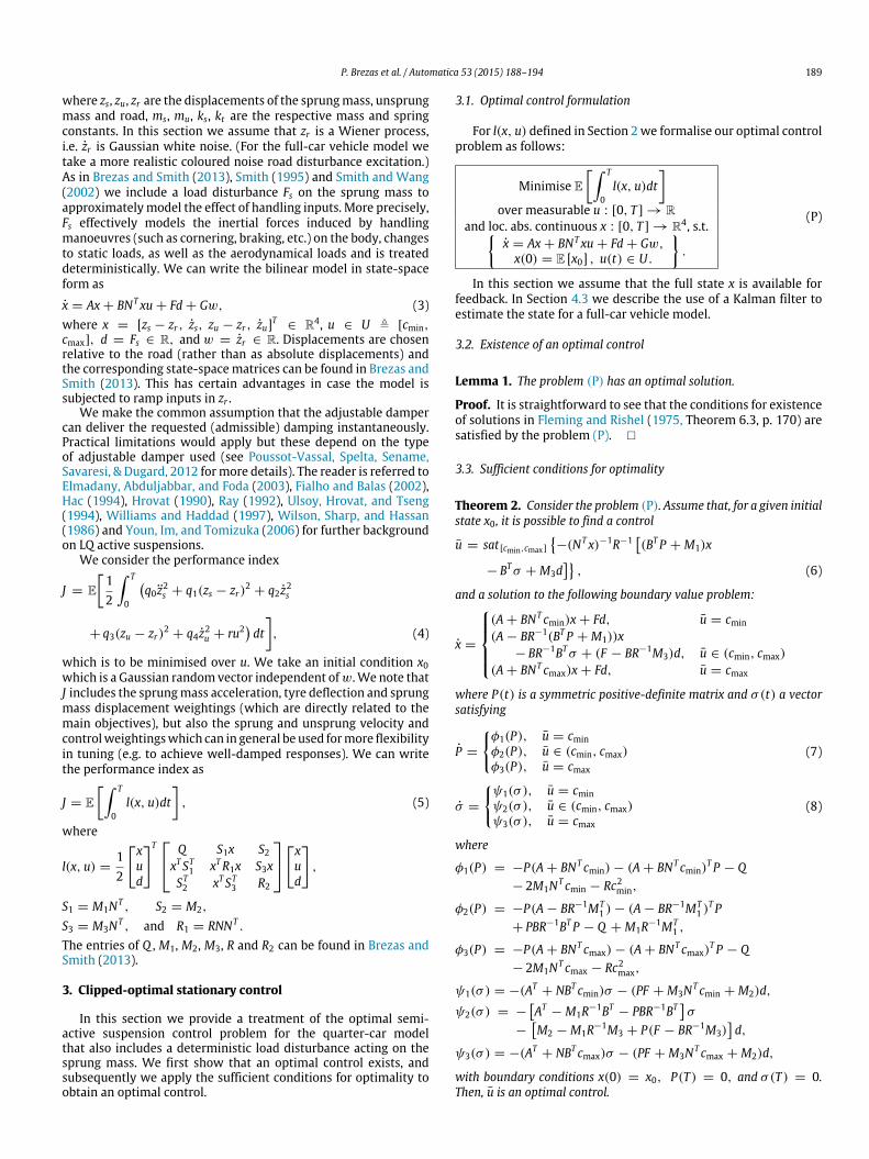
Fig. 1. Steeringwheel angle, (solid) measured suspension deflections and (dashed)estimated suspension deflections for the estimator with no disturbance modellingfor a roundabout manoeuvre (60 km/h).

where xe is the estimation of the state vector,

ye = Cxe + Du + Hd, (17)

and Ke = PeCT∆−1 is the standard Kalman filter gain where Pesatisfies the Riccati equation

APe + PeAT− PeCT∆−1CPe + GΓ GT

= 0.

5. Experimental results

The algorithm developed in this paper was evaluated experi-mentally on a test vehicle (high-performance sports car) with sus-pension consisting of a continuously adjustable damper in parallelwith a passive spring. The damper is of variable-orifice type andhas a bandwidth of 60 Hz. In the test setup the physical damperhas a nonlinear velocity–force characteristic. In the experimentsreported here the bounds cmin and cmax are velocity-dependent,effectively to allow the damper to provide its maximum force inthe saturation region, rather than restricting to an artificial max-imum given by predetermined fixed cmin and cmax. This practicewas followed in all experiments for a fair comparison. The test ve-hicle parameters were in the typical range for a high-performancesports car. The costweightingswere chosen to adjust the trade-offsfor ride comfort, tyre grip, handling etc., for achieving satisfactoryperformance for different driving modes. The weights on the bodyaccelerations and tyre deflections gave good authority for achiev-ing a good compromise between ride comfort and tyre grip duringobjective tests like a bumpy road profile or symmetric and asym-metric bumps. The roll angle and roll velocity weights were foundto be useful tuning parameters for handling behaviour. Note thatin the comparison between the proposed control scheme and thestandard clipped optimal approach the performance weights arethe same. The available measurements are the suspension deflec-tions and the body and hub accelerations. The control algorithm isimplemented in discrete formwith a 1ms sampling period. Experi-mental results are now presented for a steeringmanoeuvre around

192 P. Brezas et al. / Automatica 53 (2015) 188–194

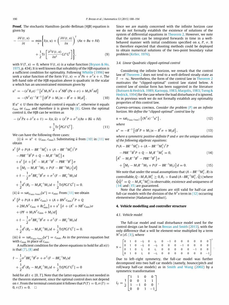
Fig. 2. Steeringwheel angle, (solid) measured suspension deflections and (dashed)estimated suspension deflections for the estimator with disturbance modelling fora roundabout manoeuvre (60 km/h). Note that the measured and estimated signalscoincide in the plot.

70

60

505.5 6 6.5 7

5.5 6 6.5 7

5.5 6 6.5 7

5.5 6 6.5 7

5.5 6 6.5 7

5.5 6 6.5 7

100

50

–50

0

0.02

0

–0.02

–0.04

0.02

0

–0.02

–0.04

0.02

0

–0.02

–0.04

0.02

0

–0.02

–0.04

RL

susp

. def

l. (m

)R

R s

usp.

def

l. (m

)F

L su

sp. d

efl.

(m)

FR

sus

p. d

efl.

(m)

Ste

erin

g an

gle

(deg

)C

ar s

peed

(km

/h)

Time (s)

Time (s)

Time (s)

Time (s)

Time (s)

Time (s)

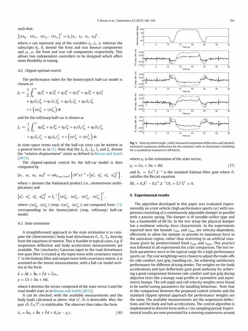
Fig. 3. Car speed, steering wheel angle andmeasured suspension deflections whenusing the observer with disturbance modelling (black-dashed) and when usingthe observer with no disturbance modelling (red-solid). (For interpretation of thereferences to colour in this figure legend, the reader is referred to the web versionof this article.)

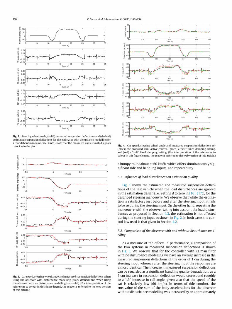
Fig. 4. Car speed, steering wheel angle and measured suspension deflections for(black) the proposed semi-active control, (green) a ‘‘stiff’’ fixed damping setting,and (red) a ‘‘soft’’ fixed damping setting. (For interpretation of the references tocolour in this figure legend, the reader is referred to the web version of this article.)

a bumpy roundabout at 60 km/h, which offers simultaneously sig-nificant ride and handling inputs, and repeatability.

5.1. Influence of load disturbances on estimation quality

Fig. 1 shows the estimated and measured suspension deflec-tions of the test vehicle when the load disturbances are ignoredin the estimation design (i.e., setting d to zero in (16), (17)), for thedescribed steering manoeuvre. We observe that while the estima-tion is satisfactory just before and after the steering input, it failsto be so during the steering input. On the other hand, repeating themanoeuvre with the observer taking into account the load distur-bances as proposed in Section 4.3, the estimation is not affectedduring the steering input as shown in Fig. 2. In both cases the con-trol law used is that given in Section 4.2.

5.2. Comparison of the observer with and without disturbance mod-elling

As a measure of the effects in performance, a comparison ofthe two systems in measured suspension deflections is shownin Fig. 3. We observe that for the controller with Kalman filterwith no disturbance modelling we have an average increase in themeasured suspension deflections of the order of 1 cm during thesteering input, whereas after the steering input the responses arealmost identical. The increase in measured suspension deflectionscan be regarded as a significant handling quality degradation, as a1 cm increase in suspension deflection would correspond roughlyto a 1.5° increase in roll angle, given also that the speed of thecar is relatively low (60 km/h). In terms of ride comfort, therms value of the sum of the body accelerations for the observerwithout disturbancemodellingwas increased by an approximately

P. Brezas et al. / Automatica 53 (2015) 188–194 193

100

50

0

–50

415 420 425 430 435

415 420 425 430 435

0.02

–0.02

0.01

–0.01

0

0.4

–0.4

0.2

0

–0.2

0.05

–0.05

0

0.2

–0.2

0.1

–0.10

Zφ

(rad

/s)

Zφ

(rad

)Z

s (m

)Z

s (m

/s)

Ste

erin

g an

gle

(deg

)

Time (s)

Time (s)

415 420 425 430 435Time (s)

415 420 425 430 435Time (s)

415 420 425 430 435Time (s)

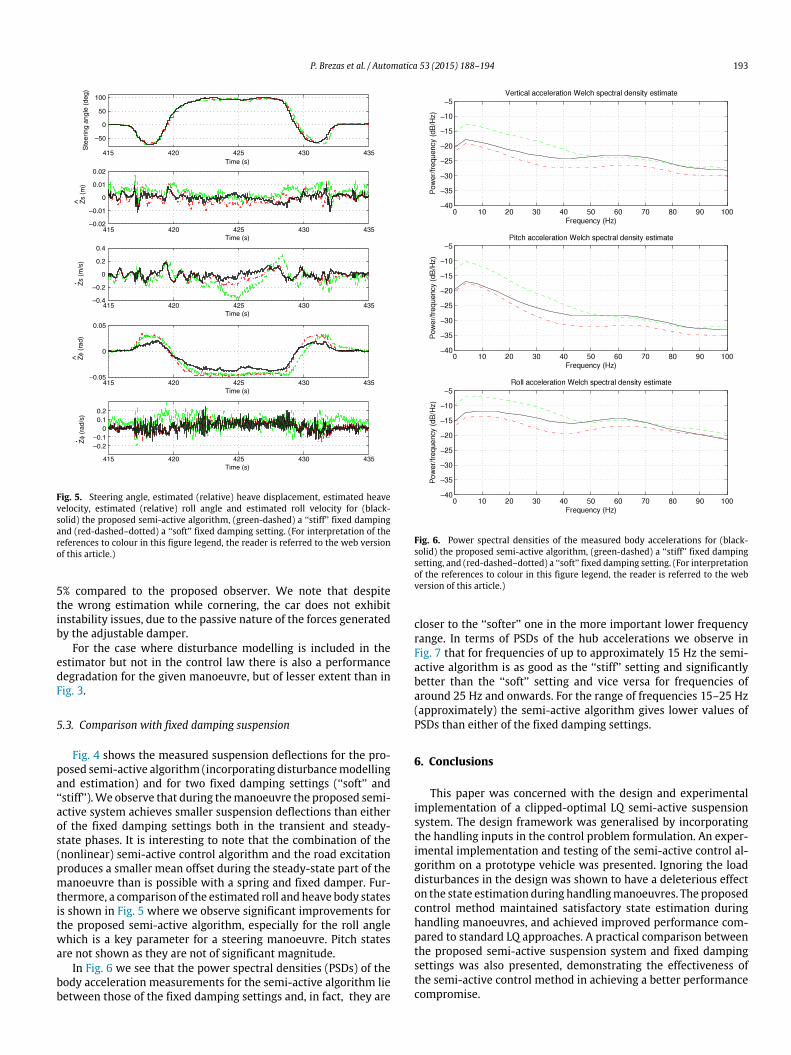
Fig. 5. Steering angle, estimated (relative) heave displacement, estimated heavevelocity, estimated (relative) roll angle and estimated roll velocity for (black-solid) the proposed semi-active algorithm, (green-dashed) a ‘‘stiff’’ fixed dampingand (red-dashed–dotted) a ‘‘soft’’ fixed damping setting. (For interpretation of thereferences to colour in this figure legend, the reader is referred to the web versionof this article.)

5% compared to the proposed observer. We note that despitethe wrong estimation while cornering, the car does not exhibitinstability issues, due to the passive nature of the forces generatedby the adjustable damper.

For the case where disturbance modelling is included in theestimator but not in the control law there is also a performancedegradation for the given manoeuvre, but of lesser extent than inFig. 3.

5.3. Comparison with fixed damping suspension

Fig. 4 shows the measured suspension deflections for the pro-posed semi-active algorithm (incorporating disturbancemodellingand estimation) and for two fixed damping settings (‘‘soft’’ and‘‘stiff’’).We observe that during themanoeuvre the proposed semi-active system achieves smaller suspension deflections than eitherof the fixed damping settings both in the transient and steady-state phases. It is interesting to note that the combination of the(nonlinear) semi-active control algorithm and the road excitationproduces a smaller mean offset during the steady-state part of themanoeuvre than is possible with a spring and fixed damper. Fur-thermore, a comparison of the estimated roll and heave body statesis shown in Fig. 5 where we observe significant improvements forthe proposed semi-active algorithm, especially for the roll anglewhich is a key parameter for a steering manoeuvre. Pitch statesare not shown as they are not of significant magnitude.

In Fig. 6 we see that the power spectral densities (PSDs) of thebody acceleration measurements for the semi-active algorithm liebetween those of the fixed damping settings and, in fact, they are

Fig. 6. Power spectral densities of the measured body accelerations for (black-solid) the proposed semi-active algorithm, (green-dashed) a ‘‘stiff’’ fixed dampingsetting, and (red-dashed–dotted) a ‘‘soft’’ fixed damping setting. (For interpretationof the references to colour in this figure legend, the reader is referred to the webversion of this article.)

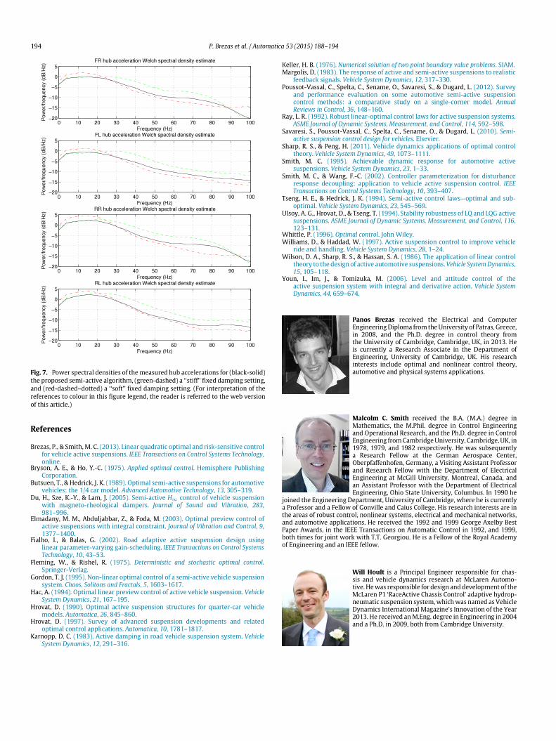
closer to the ‘‘softer’’ one in the more important lower frequencyrange. In terms of PSDs of the hub accelerations we observe inFig. 7 that for frequencies of up to approximately 15 Hz the semi-active algorithm is as good as the ‘‘stiff’’ setting and significantlybetter than the ‘‘soft’’ setting and vice versa for frequencies ofaround 25 Hz and onwards. For the range of frequencies 15–25 Hz(approximately) the semi-active algorithm gives lower values ofPSDs than either of the fixed damping settings.

6. Conclusions

This paper was concerned with the design and experimentalimplementation of a clipped-optimal LQ semi-active suspensionsystem. The design framework was generalised by incorporatingthe handling inputs in the control problem formulation. An exper-imental implementation and testing of the semi-active control al-gorithm on a prototype vehicle was presented. Ignoring the loaddisturbances in the design was shown to have a deleterious effecton the state estimation during handlingmanoeuvres. The proposedcontrol method maintained satisfactory state estimation duringhandling manoeuvres, and achieved improved performance com-pared to standard LQ approaches. A practical comparison betweenthe proposed semi-active suspension system and fixed dampingsettings was also presented, demonstrating the effectiveness ofthe semi-active control method in achieving a better performancecompromise.

194 P. Brezas et al. / Automatica 53 (2015) 188–194

Fig. 7. Power spectral densities of themeasured hub accelerations for (black-solid)the proposed semi-active algorithm, (green-dashed) a ‘‘stiff’’ fixed damping setting,and (red-dashed–dotted) a ‘‘soft’’ fixed damping setting. (For interpretation of thereferences to colour in this figure legend, the reader is referred to the web versionof this article.)

References

Brezas, P., & Smith, M. C. (2013). Linear quadratic optimal and risk-sensitive controlfor vehicle active suspensions. IEEE Transactions on Control Systems Technology,online.

Bryson, A. E., & Ho, Y.-C. (1975). Applied optimal control. Hemisphere PublishingCorporation.

Butsuen, T., & Hedrick, J. K. (1989). Optimal semi-active suspensions for automotivevehicles: the 1/4 car model. Advanced Automotive Technology, 13, 305–319.

Du, H., Sze, K.-Y., & Lam, J. (2005). Semi-active H∞ control of vehicle suspensionwith magneto-rheological dampers. Journal of Sound and Vibration, 283,981–996.

Elmadany, M. M., Abduljabbar, Z., & Foda, M. (2003). Optimal preview control ofactive suspensions with integral constraint. Journal of Vibration and Control, 9,1377–1400.

Fialho, I., & Balas, G. (2002). Road adaptive active suspension design usinglinear parameter-varying gain-scheduling. IEEE Transactions on Control SystemsTechnology, 10, 43–53.

Fleming, W., & Rishel, R. (1975). Deterministic and stochastic optimal control.Springer-Verlag.

Gordon, T. J. (1995). Non-linear optimal control of a semi-active vehicle suspensionsystem. Chaos, Solitons and Fractals, 5, 1603–1617.

Hac, A. (1994). Optimal linear preview control of active vehicle suspension. VehicleSystem Dynamics, 21, 167–195.

Hrovat, D. (1990). Optimal active suspension structures for quarter-car vehiclemodels. Automatica, 26, 845–860.

Hrovat, D. (1997). Survey of advanced suspension developments and relatedoptimal control applications. Automatica, 10, 1781–1817.

Karnopp, D. C. (1983). Active damping in road vehicle suspension system. VehicleSystem Dynamics, 12, 291–316.

Keller, H. B. (1976). Numerical solution of two point boundary value problems. SIAM.Margolis, D. (1983). The response of active and semi-active suspensions to realistic

feedback signals. Vehicle System Dynamics, 12, 317–330.Poussot-Vassal, C., Spelta, C., Sename, O., Savaresi, S., & Dugard, L. (2012). Survey

and performance evaluation on some automotive semi-active suspensioncontrol methods: a comparative study on a single-corner model. AnnualReviews in Control, 36, 148–160.

Ray, L. R. (1992). Robust linear-optimal control laws for active suspension systems.ASME Journal of Dynamic Systems, Measurement, and Control, 114, 592–598.

Savaresi, S., Poussot-Vassal, C., Spelta, C., Sename, O., & Dugard, L. (2010). Semi-active suspension control design for vehicles. Elsevier.

Sharp, R. S., & Peng, H. (2011). Vehicle dynamics applications of optimal controltheory. Vehicle System Dynamics, 49, 1073–1111.

Smith, M. C. (1995). Achievable dynamic response for automotive activesuspensions. Vehicle System Dynamics, 23, 1–33.

Smith, M. C., & Wang, F.-C. (2002). Controller parameterization for disturbanceresponse decoupling: application to vehicle active suspension control. IEEETransactions on Control Systems Technology, 10, 393–407.

Tseng, H. E., & Hedrick, J. K. (1994). Semi-active control laws—optimal and sub-optimal. Vehicle System Dynamics, 23, 545–569.

Ulsoy, A. G., Hrovat, D., & Tseng, T. (1994). Stability robustness of LQ and LQG activesuspensions. ASME Journal of Dynamic Systems, Measurement, and Control, 116,123–131.

Whittle, P. (1996). Optimal control. John Wiley.Williams, D., & Haddad, W. (1997). Active suspension control to improve vehicle

ride and handling. Vehicle System Dynamics, 28, 1–24.Wilson, D. A., Sharp, R. S., & Hassan, S. A. (1986). The application of linear control

theory to the design of active automotive suspensions.Vehicle SystemDynamics,15, 105–118.

Youn, I., Im, J., & Tomizuka, M. (2006). Level and attitude control of theactive suspension system with integral and derivative action. Vehicle SystemDynamics, 44, 659–674.

Panos Brezas received the Electrical and ComputerEngineeringDiploma from theUniversity of Patras, Greece,in 2008, and the Ph.D. degree in control theory fromthe University of Cambridge, Cambridge, UK, in 2013. Heis currently a Research Associate in the Department ofEngineering, University of Cambridge, UK. His researchinterests include optimal and nonlinear control theory,automotive and physical systems applications.

Malcolm C. Smith received the B.A. (M.A.) degree inMathematics, the M.Phil. degree in Control Engineeringand Operational Research, and the Ph.D. degree in ControlEngineering fromCambridgeUniversity, Cambridge, UK, in1978, 1979, and 1982 respectively. He was subsequentlya Research Fellow at the German Aerospace Center,Oberpfaffenhofen, Germany, a Visiting Assistant Professorand Research Fellow with the Department of ElectricalEngineering at McGill University, Montreal, Canada, andan Assistant Professor with the Department of ElectricalEngineering, Ohio State University, Columbus. In 1990 he

joined the Engineering Department, University of Cambridge, where he is currentlya Professor and a Fellow of Gonville and Caius College. His research interests are inthe areas of robust control, nonlinear systems, electrical and mechanical networks,and automotive applications. He received the 1992 and 1999 George Axelby BestPaper Awards, in the IEEE Transactions on Automatic Control in 1992, and 1999,both times for joint work with T.T. Georgiou. He is a Fellow of the Royal Academyof Engineering and an IEEE fellow.

Will Hoult is a Principal Engineer responsible for chas-sis and vehicle dynamics research at McLaren Automo-tive. Hewas responsible for design and development of theMcLaren P1 ‘RaceActive Chassis Control’ adaptive hydrop-neumatic suspension system,whichwas named as VehicleDynamics International Magazine’s Innovation of the Year2013. He received anM.Eng. degree in Engineering in 2004and a Ph.D. in 2009, both from Cambridge University.