![[tel-00004681, v1] Modélisation géométrique de surfaces lisses](https://static.fdokumen.com/doc/165x107/631b636f5e4c963afd06d345/tel-00004681-v1-modelisation-geometrique-de-surfaces-lisses.jpg)
[tel-00004681, v1] Modélisation géométrique de surfaces lisses
Upload
khangminh22Category
view
2download
0
HAL Id: tel-00961182https://tel.archives-ouvertes.fr/tel-00961182
Submitted on 19 Mar 2014
HAL is a multi-disciplinary open accessarchive for the deposit and dissemination of sci-entific research documents, whether they are pub-lished or not. The documents may come fromteaching and research institutions in France orabroad, or from public or private research centers.
L’archive ouverte pluridisciplinaire HAL, estdestinée au dépôt et à la diffusion de documentsscientifiques de niveau recherche, publiés ou non,émanant des établissements d’enseignement et derecherche français ou étrangers, des laboratoirespublics ou privés.
Modélisation thermomécanique et analyse de ladurabilité d’échangeurs thermiques à plaques soudées
Mathieu Laurent
To cite this version:Mathieu Laurent. Modélisation thermomécanique et analyse de la durabilité d’échangeurs thermiquesà plaques soudées. Autre. Université de Grenoble, 2013. Français. �NNT : 2013GRENI019�. �tel-00961182�

THÈSE Pour obtenir le grade de
DOCTEUR DE L’UNIVERSITÉ DE GRENOBLE Spécialité : Ingénierie - Matériaux, Mécanique, Energétique, Environnement, Procédés de production
Arrêté ministériel : 7 août 2006 Présentée par
Mathieu LAURENT Thèse dirigée par Rafael ESTEVEZ et codirigée par Damien FABREGUE préparée au sein du Laboratoire SIMAP dans l'École Doctorale IMEP2
Modélisation thermomécanique et analyse de la durabilité d’échangeurs thermiques à plaques soudées Thèse soutenue publiquement le 14 janvier 2012 , devant le jury composé de :
Rafael ESTEVEZ Professeur des Universités, Université Joseph Fourier,Directeur de thèse Damien FABREGUE Maitre de conférences, INSA Lyon, co-Directeur de thèse Michel CORET Professeur des Universités, Ecole Centrale de Nantes, Rapporteur Véronique FAVIER Professeur des Universités, ENSAM Paris, Rapporteur Franck MOREL Professeur des Universités, ENSAM Angers, Examinateur Eric AYAX Docteur, Ingénieur, Alfa Laval Vicarb, Examinateur

Preamble
Preamble-1
Preamble
This PhD project has been carried out in both SIMAP (Science et ingénierie des matériaux et des procédés) and MATEIS (Matériaux, Ingénierie et Science) Laboratories respectively directed by Michel Pons and Joël Courbon, and more precisely in the “Métal” Team of the MATEIS Laboratory directed by Xavier Kleber. I would like to thank them all for having given me the opportunity to write this report today.
My greatest thanks are naturally addressed to my thesis directors Rafael Estevez and Damien Fabrègue who have always been able to encourage, advise and guide me during these three years.
This project would have not been performed without a strong partnership with Alfa Laval Vicarb. In this way, I would like to deeply thank Eric Ayax for having supported and organized this project, then for having trusted me all the time to lead it until the end. I don’t forget here Pascal Vernay for having devoted a part of its time to the project. In a second time, I would also like to thank the Research Office of the parent company, Alfa Laval AB in Lund, and mainly Lars Fogelberg and its team for the time spent on the two thermal tests performed on real heat exchangers. Finally, it is important for me to thank Sandrine Chabanet, Sylvie Pelenc and Franck Alenda for their respective contribution and influence in the project.
Finally I would like to express my gratitude to all the other persons having bring me their knowledge and technical know-low as Florian Mercier (MATEIS Laboratory), Jean Gillibert, Aymen Ben Kaabar and Bassem El Zoghbi (SIMAP Laboratory), Daniel Maisonnette (Mecanium, INSA Lyon).

General Introduction
Introduction-1
GENERAL INTRODUCTION
Thermo-mechanical modelling and durab
For several years, the part of the
increasing. A large panel of dom
simulation is used at several st
validation. It involves various so
cycle can be actually multiple:
- the innovation and the ind
- the improvement of the p
- time and costs cutting in
- the opportunity to investi
- the supply of arguments f
In this context, Alfa Laval Vica
initiated an extension of the us
conditions in terms of temperatur
to be warrant, or at least evalua
insight on the heat exchanger me
work during long times, critical
mainly for maintenance operatio
numerical methodology allowing
of a given welded heat exchange
the customer about the maximal
way, this could allow to provide
possible better redesigning of the
In order to reach this goal, the f
welded heat exchanger at the ma
thin rolled plates constituted of 31
mechanical response of a unit in
have been carefully identified. D
basic rules as a mesh optimisati
parameterize this latter to permi
kind of exchanger involved. The
on the unit in operating condition
(Lund, Sweden) for future applica
The second step of the study w
previous numerical response of t
realistic elastic-plastic constitut
rability analysis of welded heat exchangers
Introduction-2
the simulation in the industrial environment has b
omains is concerned as aeronautic, automobile or e
stages of the industrial product design and ma
software technologies whose interest during the p
industrial competitiveness,
e products quality and security,
in comparison with the prototypes manufacturing,
stigate original solutions during the design phase,
ts for the product use specifications to the customer.
icarb, world leader as welded plate heat exchange
use of the heat exchangers produced to new m
ture fields have a larger magnitude and reliability
luated. The present work contribute to this as wel
mechanical response to shape its future design. If
al loadings occur when a shut down and a new st
tions. The expected issue of this PhD project wa
ng from input data as fluid temperature to give a cor
ger before failure. Actually, it is necessary to give
al fluid temperature generating damage as late as p
ide some recommendations or at least useful infor
he structure.
e first main stage consists in the thermo-mechanic
macroscopic scale using the FEM by ANSYS sof
f 316L stainless steel, the model should be able to r
in operating conditions. Thus, the mechanical prop
. Due to its industrial application, the model shoul
ation faced to the large volume of the structure.
mit an easy adaption of some important paramete
he determination of thermal fields representative of
ions is finally performed in both design offices of A
lications.
will permit to establish a damage criterion direct
f the exchanger for simple experimental configura
tutive law for repeated loadings characterizatio
s been actually always
r energetic. Numerical
manufacturing process
e product development
er.
nger manufacturer, has
markets. The loading
ty of the product needs
ell as aims at gaining
If a unit is designed to
start up are necessary
was thus to develop a
corresponding life time
ive accurate advises to
s possible. In the same
formation concerning a
nical description of the
software. Composed of
o represent thermal and
operties of the material
ould also respect some
It is then needed to
eters depending on the
of the loading working
of Alfa Laval Lund AB
ectly applicable to the
urations. To this end, a
tion is necessary. Its

General Introduction
Introduction-3
identification is performed and the response of the material for various case studies reported. This has
helped in designing the experimental test for the identification of the fatigue criterion. The values
obtained are in agreement with available data in the literature. A mythology is then provided to
combine the results from the stress distribution across the structure together with the estimation of the
local plastic strain amplitude value. This latter will finally allows a prediction of the exchanger
lifetime when subjected to thermal cyclic loadings through the identified fatigue criterion.
This manuscript has been divided into three parts. In Chapter 1, the company Alfa Laval and the
industrial context of the study is presented. A main part is devoted to the analysis of the welded heat
exchanger design under consideration in this study. Some cases for which failures have been observed
in bench tests in different units are then reported. The investigations localises the regions
corresponding to large stress concentrations in the heat exchanger. The next step consists inn
introducing a damage analysis by borrowing a oligocyclic fatigue criterion in the literature and
identifying the parameters for the material under consideration. A rapid literature survey about the heat
exchanger failure analysis is given to situate the context of the study.
The finite element model construction of the heat exchanger at the scale of the structure has been
carried out in a step by step approach in Chapter 2. From several assumptions verified experimentally,
the thermo-elastic response of the heat exchanger under uniform thermal loading has been firstly
investigated. The region of the exchangers where the stress concentrates has been identified. Two
thermo-mechanical tests have been performed to validate the thermo-elastic description of the heat
exchanger.
In Chapter 3, the elastic-plastic mechanical response of the 316L steel is identified, which exhibits a
combined isotropic and kinematic hardening. An energy equivalent method is proposed to estimate the
magnitude of the equivalent plastic deformation from the analysis at the level of the structure. This
estimation is used to predict the exchanger life from a Manson-Coffin criterion identified in the low
cycle fatigue regime. The prediction is finally compared to experimental data.

State of the art
I-1
I. STATE OF THE ART
In this chapter, the company Alfa Laval as well as the industrial context of the study is firstly
introduced. A main part is devoted to the analysis of the welded heat exchanger design about to be
studied. The next step of this part then introduces the involved damage mechanics in the reported
failure cases as well as the material properties needed for the study. Finally a literature review about
the heat exchanger failure analysis is given to situate the context of the study

Thermo-mechanical modelling and durab
I.1. Table of conten
I. State of the art ......................
I.1. Table of contents .........
I.2. Alfa Laval Group .........
I.3. Generalities about heat
I.3.1. Global functionali
I.3.2. Design description
I.3.3. Heat exchanger cla
I.4. Welded heat exchanger
I.4.1. General considerat
I.4.2. Design of the exch
I.5. Context of the study ....
I.5.1. Failure cases repor
I.5.2. Generalities on the
I.6. Introduction of fatigue
I.6.1. Generalities on dam
I.6.2. Fatigue damage ....
I.6.3. Loading condition
I.6.4. Classical fatigue m
I.7. Plasticity theory in the f
I.7.1. Cyclic material be
I.7.2. Observations in m
I.7.3. Tridimensional yie
I.7.4. Specific plasticity
I.8. Heat exchanger analysi
I.9. Goal of the study .........
I.10. References ...................
rability analysis of welded heat exchangers
I-2
tents
...................................................................................
...................................................................................
...................................................................................
at exchangers ...........................................................
ality ...........................................................................
ion .............................................................................
classification in the market ......................................
gers of Alfa Laval Vicarb ..........................................
rations ......................................................................
changer ....................................................................
..................................................................................
ported ........................................................................
the involved damage mechanics ...............................
ue phenomenon .........................................................
damage .....................................................................
..................................................................................
ons ............................................................................
e models parameters .................................................
e fatigue material behaviour ....................................
behaviour ..................................................................
multiaxial ................................................................
yield stress criterion .................................................
ity laws ......................................................................
ysis in the literature ...................................................
...................................................................................
..................................................................................
................................ I-1
................................. I-2
................................. I-3
................................. I-4
................................. I-4
................................. I-5
................................. I-5
................................. I-7
................................. I-7
................................ I-7
............................... I-11
............................... I-11
............................... I-13
............................... I-14
............................... I-14
............................... I-15
............................... I-16
............................... I-17
.............................. I-18
............................ I-18
............................... I-20
............................... I-20
............................... I-21
............................... I-24
............................... I-27
............................... I-28

State of the art
I-3
I.2. Alfa Laval Group
Gustaf de Laval (cf. Figure I.1) and his partner, Oscar Lamm, founded the company AB Separator in
1883, six years after the beginning of his work on the development of a centrifugal separator and four
after its first demonstration in Stockholm. In 1890 the world’s first continuous separator using an Alfa-
disc technology is introduced in order to manufacture the first Milk pasteurizer. The first French
Subsidiary of the current Alfa Laval Company called “La Société des Ecrémeuses Alfa Laval” is
founded in 1907 by H.H Mac Coll. Until 1938 the company developed different kind of separator,
particularly for farm’s application and oil purification. Nevertheless AB Separator already introduced
its first heat exchanger the same year. From this time, Lund has become the development and
production’s centre of heat exchangers. It is only in 1963 that the company changed its name to Alfa-
Laval. In 2008, the group represents 20 production sites and almost 11500 employees around the
world (with more than 800 in France). In 1998, Alfa Laval acquired Vicarb based at Le Fontanil and
Nevers in France, and Packinox based at Chalon-sur-Saone in 2005. Those two companies are
specialised in the fabrication of welded plate heat exchangers.
Nowadays, the Alfa Laval group develops three key technologies in the world market, namely the heat
transfer the separation and the fluid handling. Up to 3% of sales are today invested annually in
Research & Development and from which the company can suggest technological solutions in
different applications area such as:
- energy,
- environment conservation,
- food and water supplies,
- Pharmaceuticals.
Figure I.1 - Gustaf de Laval / Old heat exchanger model
The project being focused on the heat exchanger durability analysis, the next part particularly deals
with the presentation of their structure and functionalities.

Thermo-mechanical modelling and durab
I.3. Generalities ab
Heat exchangers have a large
conditioning, refrigeration, cryog
day to day life of everybody such
I.3.1. Global functionali
Typically, the major role of a hea
more fluids at different temperat
which avoids the fluids to mix t
conduction.
Figure
Figu
T1
T2
Fluid
distribution
rability analysis of welded heat exchangers
I-4
about heat exchangers
ge industrial scope (energy, petroleum industry
ogenic, heat recovery, alternate fuels, etc.), as the
ch as the car conditioning or the heater in the house
ality
heat exchanger is to transfer an internal thermal flu
ratures. In principle, the fluids are separated by a
x together (cf. Figure I.2) and allows both media
re I.2 - Definition of the thermal exchange notion
gure I.3 - Current welded plate heat exchanger
T1 > T
2
e
Q
try, transportation, air
hey can be used in the
use.
flux Q between two or
a heat transfer surface
ia to exchange heat by

State of the art
I-5
I.3.2. Design description
A classical heat exchanger consists of the assembly of two main parts such as a core or a matrix
containing the heat transfer surfaces and fluid distribution elements (as headers and tank, inlet and
outlet nozzles and pipes for instance, cf. Figure I.3).
Generally all the components of an exchanger are fixed, except for particular cases such as rotary
generator (in which the matrix is able to rotate). In all cases, the fluids are in contact with the transfer
surface permitting the heat to be transferred from the hot fluid to the cold one. As a consequence, the
fluid becomes hotter or colder, wins or loses energy. Therefore it is clear that the exchanger efficiency
strongly depends on its exchange surface.
I.3.3. Heat exchanger classification in the market
Industrial heat exchangers are classified according to different aspects and criterion which are given in
the paragraphs below.
I.3.3.1. Classification according to the heat exchangers design
It concerns the global geometry of the heat exchanger, which can be classified into four main parts:
- Tubular heat exchangers (double pipe, shell and tube, coiled tube),
- Plate heat exchangers (produced by the Alfa Laval group),
- Extended surface heat exchangers (fin-tube, thin-sheet),
- Regenerators (fixed matrix, rotary).
Alfa Laval Group mostly produces plate heat exchangers classified in three groups:
- Gasketed plate heat exchangers,
- Spiral heat exchangers ,
- Welded plate heat exchangers which are considered in this study.
I.1.1.1. Classification according to transfer process
Two types of thermal transfer are distinguished:
- An indirect contact type (direct transfer type, storage type, fluidized bed),
- A direct contact type (the two fluids are note separate by a wall).
The project deals with the indirect transfer type exchangers in which there is a continuous flow of the
heat from the hot to the cold fluid through a separating wall. The fluids’ mixing is prevented by
separated fluid passages.

Thermo-mechanical modelling and durab
Figure I.4 - Thermal pa
I.1.1.2. Classific
Compact heat exchangers are use
service conditions are involved.
transfer area A to its volume V,
Compact heat exchangers. By thi
than shell and tube exchangers
exchangers very useful in intensiv
to a smaller weight, an easier tran
I.1.1.3. Classific
Tree main flow arrangements are
- parallel flow arrangement
- counter flow arrangement
- cross-flow arrangement (
This design parameter is very
criterion. Thus, the cross-flow ar
the most common used for the ex
rability analysis of welded heat exchangers
I-6
path inside the exchanger core through a cross-flow arra
ification according to surface compactness
used in most cases when restrictions on the structur
d. The interesting feature here is the area densit
V, noted β). The value of β is particularly high (a
this way, a compact surface often offers a higher t
rs (95% vs. 60 until 80%). This advantage make
sive energy industries. Moreover small volumes are
ransport, a better temperature control...
ification according to flow and pass arrangeme
re available in the heat exchanger market:
ent,
ent,
t (cf. Figure I.4).
ry important, heat exchanger efficiency strongly
arrangement allowing to increase considerably th
extended heat exchanger surfaces.
Cross-
arrange
Thermal path
directed by baffles
arrangement
ture size and weight in
sity (ratio of the heat
(about 700 m2/m3) for
r thermal effectiveness
kes the Compact heat
are naturally correlated
ment
gly depending on this
the fluid turbulence is
-flow
gement

State of the art
I-7
Figure I.5 - Isometric view of the welded heat exchanger
Depending on the thermal specifications given by the customers, a heat exchanger can contain odd or
even number of passes. A pass is created by installing baffles through channels. Typically, its role is to
define a thermal circuit within the exchanger (cf. Figure I.4).
I.3.3.2. Classification according to the heat transfer mechanism
Although the heat transfer through the plates is made by conduction, the fluids temperature is then
able to change by a liquid/solid or liquid/stream contact, permitting the exchange in the full structure.
Convection force can be thus seen as the major heat transfer mechanism involved in the exchanger.
I.4. Welded heat exchangers of Alfa Laval Vicarb
I.4.1. General considerations
The welded heat exchanger of Alfa Laval Vicarb belongs to the Compact exchanger family. This one
called “Compabloc” has been developed by the company for more than 20 years. The major interest of
using this exchanger is to get optimal performances when the operating conditions become severe as
in chemical aggressive environment or/and under high temperature’s variations (from ΔT = -50 to
400°C) with extreme pressure conditions (up to 40 bars).
I.4.2. Design of the exchanger
The Figure I.5 shows an isometric view of the welded heat exchanger depicting the different
constitutive parts of this heat exchanger. As it is shown, the structure is typically composed of two
mains parts which are presented in more details in the following.

Thermo-mechanical modelling and durab
I.4.2.1. Heart o
The core of the system is compo
500). These latter are welded
perpendicular channels crossing t
number m of pass which are lim
heat exchanger (cf. Figure I.4 an
according to the size of the heat
plates. Seven designs exist in Al
number corresponding to the w
exchanger can offer 330 m2 of e
0.8mm until CP40, 1mm for CP5
assembly of an Alfa Laval welde
welded together along their right
Baffle
Smooth
Zone
“Papillote”
Ledges of both
plates welded
together
rability analysis of welded heat exchangers
I-8
Figure I.6 - Heart of the exchanger
Figure I.7 - Double plate patterns
t of the exchanger
posed of a stack of N plates (plates pack being abl
d together alternatively from side to the other
g themselves according to a cross-flow arrangemen
imited by baffles, driving the fluid along a “therm
and Figure I.6). Welded heat exchangers are desig
at exchanger heart, in other words the heat transfe
Alfa Laval Vicarb: CP15, CP20, CPL30, CP40, C
width of the exchanger plates). For informatio
f exchange’s area. The plate thickness depends on
P50 and CP75 and 1.2mm for CP120. Figure I.7 sh
ded heat exchanger. Typically, this assembly is com
ht and left sides.
1 pass
C
le
Flow direction
able to vary from 30 to
er in order to create
ent. N is then split in a
rmal” circuit inside the
signed by the company
sfer area of the welded
, CP50 and CP120 (the
tion, the biggest heat
on the surface’s area:
shows a double plates’
composed of two plates
Girder
Corrugated
Zone
Upper
ledge of the
State of the art
I-9
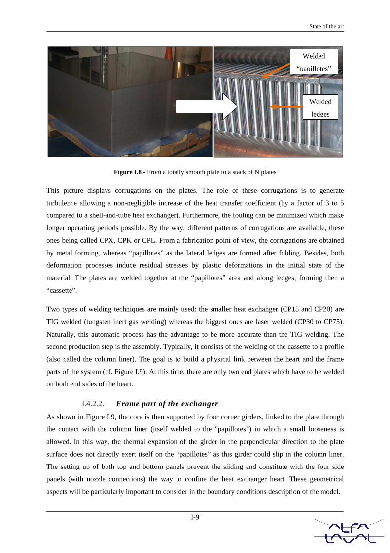
Figure I.8 - From a totally smooth plate to a stack of N plates
This picture displays corrugations on the plates. The role of these corrugations is to generate
turbulence allowing a non-negligible increase of the heat transfer coefficient (by a factor of 3 to 5
compared to a shell-and-tube heat exchanger). Furthermore, the fouling can be minimized which make
longer operating periods possible. By the way, different patterns of corrugations are available, these
ones being called CPX, CPK or CPL. From a fabrication point of view, the corrugations are obtained
by metal forming, whereas “papillotes” as the lateral ledges are formed after folding. Besides, both
deformation processes induce residual stresses by plastic deformations in the initial state of the
material. The plates are welded together at the “papillotes” area and along ledges, forming then a
“cassette”.
Two types of welding techniques are mainly used: the smaller heat exchanger (CP15 and CP20) are
TIG welded (tungsten inert gas welding) whereas the biggest ones are laser welded (CP30 to CP75).
Naturally, this automatic process has the advantage to be more accurate than the TIG welding. The
second production step is the assembly. Typically, it consists of the welding of the cassette to a profile
(also called the column liner). The goal is to build a physical link between the heart and the frame
parts of the system (cf. Figure I.9). At this time, there are only two end plates which have to be welded
on both end sides of the heart.
I.4.2.2. Frame part of the exchanger
As shown in Figure I.9, the core is then supported by four corner girders, linked to the plate through
the contact with the column liner (itself welded to the ”papillotes”) in which a small looseness is
allowed. In this way, the thermal expansion of the girder in the perpendicular direction to the plate
surface does not directly exert itself on the “papillotes” as this girder could slip in the column liner.
The setting up of both top and bottom panels prevent the sliding and constitute with the four side
panels (with nozzle connections) the way to confine the heat exchanger heart. These geometrical
aspects will be particularly important to consider in the boundary conditions description of the model.
Welded
“papillotes”
Welded
ledges

Thermo-mechanical modelling and durab
Figure I.9 - F
Figure I.10 - Fin
Therefore both girders and fram
which classically the heart is com
the panels allows to carry out d
eventual waterproofness problem
in order to seal it. It is moreov
according to different criterion (f
…) and may play a possible role
supporting the nozzle is thicker
takes into account the preparation
nozzles welding on the panel ...).
rability analysis of welded heat exchangers
I-10
Final view of the exchanger heart on the bending bench
inal view of the whole exchanger delivered to the custom
ame panels are bolted together in order to form o
compressed with a 12t pressure. Furthermore, the p
t different non-destructive controls as leak tests
ems. A joint is finally included between the panel a
over worth noticing that the nozzle can have a
(frame width and height, number of plates per pa
ole in the total rigidity of the frame. Therefore in m
er than the other. In Alfa Laval Vicarb, a special
ion of the frame panels (Nozzle components weldin
..).
Stack of
plates
ch
tomer
one compact bloc in
e progressive fixing of
in order to localize
el and the column liner
a very large diameter
pass, state of the fluid
n most cases, the panel
ial production activity
ding, panels machining,
Column
liner

State of the art
I-11
I.5. Context of the study
This PhD project concerns the problematic of heat exchangers durability and more particularly the
study of the cyclic thermo-mechanical loading influence on the mechanical response on these kinds of
systems. In fact, the trouble shooting analysis available in Alfa Laval Vicarb reports the occurrence of
recent failure cases in their 316L welded heat exchangers due to a new use in severe operating
conditions (The unit being subjected to thermal fields highly anisothermal). Although having a long
experience in the understanding of these possible damages, this department needs available tools to
advise customer concerning the appropriate temperature range in which the unit can be used and to
avoid definitively these troubles by optimizing its design in the future.
I.5.1. Failure cases reported
The most often reported failure cases are reported just below. The damaged zones will be observed
thanks to a penetrant testing (PT) fluid which is a widely used method for the detection of open and
surface breaking discontinuities. The main advantage of this non-destructive testing method is that we
can easily detect the position, direction and size of the defect by colorizing the damaged zones (in red).
I.5.1.1. Along the column liner and at the inner angles
In Figure I.11, a failure along the column liner is shown. It involves the appearance of leaks between
heat exchanger plates and “papillotes” connecting both heart and frame parts. Several abrupt angles
can be effectively observed in this zone making it very sensitive to the temperature variations.
Similarly as in the foregoing case, leaks appear at the inner angle in the corners of the core where the
“papillotes” is even subjected to deformations strongly heterogenic due to the proximity of particular
end plate surrounded by the frame.
These two failure cases correspond to more than the half the reported cases. In the sequel, the heat
exchanger response in the vicinity of the “papillotes” will be carefully analysed, since it seems to be
the weakest zone of the structure. It will be important to build a sufficient precise model in these
regions to show that they are particularly highly stress concentrated.
I.5.1.2. Corner of the head plates and loss of contact points
A damaged zone has also been reported in the seam weld between the column liner and the head plate.
This induces loss of the contact points between the corrugated zones of two plates thus reducing
noticeably the heat exchanger efficiency.
I.5.1.3. Welded zone in column liner and at head plates
Additional damage cases are also reported at the seam weld in the column liner and at the head plates
as depicted in the figures below. These concerns some damage outside the heat exchanger’s heart, in
zone related to the body part.

Thermo-mechanical modelling and durab
Fi
Figure I.13 - Fa
F
rability analysis of welded heat exchangers
I-12
Figure I.11 - Failure along the column liner
Figure I.12 - Failure at the inner angles
Failure in the head plate corner and loss of contact poin
Figure I.14 - Failure in two welded zones
oints

State of the art
I-13
I.5.2. Generalities on the involved damage mechanics
Welded heat exchangers are subjected to both thermal and mechanical loadings. The first one comes to
the material temperature variation due to the fluid flow, involving a heterogeneous thermal field. The
second is due to in duty pressure. Pressure measurements inside the exchanger revealed intensities
relatively small (around 15MPa) compared to mechanical properties of the material (as the yield stress
of magnitude order at least twenty times bigger, cf. chapter 2). In this context, thermal loading appears
to be the most detrimental effects particularly during transient regimes including start up and shut
down of the exchanger. Thermo-mechanical fatigue phenomenon is involved in a lot of industrial
domains such as aeronautics, nuclear, railroad and of course heat exchange. During their life time,
mechanical structures are so subjected to repeated thermal loads leading to the cracks nucleation
damageable for installations where the process implied both thermal and mechanical stresses
according to Auger.
More precisely, Spera specifies that thermo-mechanical fatigue corresponds to the gradual
deterioration of the material induced by a progressive cracking during successive alternated heating
and cooling in which free deformation is partially or entirely impeded. Thus mechanical stresses result
from thermal loading associated to the boundary conditions of the structure. More generally (thermal)
fatigue phenomenon is particularly insidious due to its progressive and discreet character. Industrial
experience has already shown that cracks occurring by fatigue can lead to the brutal failure of the
component. Thus the design of these components needs need to take into account thermo-mechanical
fatigue aspects. Before considering it in the domain of the heat exchange, the next paragraph
introduces more carefully the fatigue phenomenon.

Thermo-mechanical modelling and durab
I.6. Introduction of
I.6.1. Generalities on da
Damage phenomenon is classica
for micro-cracks or cavities. Th
deformation, although causes ap
dislocation in metals. Macroscop
several criterions characterizing
component (Von Mises, Tresca, M
It is nevertheless only in 1958 t
parameter (for metals creep fract
of the material progressive deteri
then seen new studies describing
Chaboche, in Japan by Murakam
developed the generalization to th
irreversible processes anisotropic
Regarding the physics of dam
phenomenon will be studied. Wh
is present at the microscopic scale
since the initial stage of the mate
final stage is defined as the mom
mesoscopic crack size of the s
considered. Damage theory take s
The nature of the evolution mode
or to interact together. Knowing
integration) damage evolution un
point of the structure. As a result
This methodology is the basis p
design, verification and control
described by different laws in th
continuity of the project, the last m
rability analysis of welded heat exchangers
I-14
of fatigue phenomenon
damage
ically characterized by a surface or volume discont
The rheological process involved is so relatively
appear to be identical such as the displacement a
copic fracture has been studied for a long time wi
ng the volume element fracture and depending
a, Mohr, Coulomb, Rankine…).
8 that Kachanov published the first memory on a
acture in one dimension). This historical date point
terioration modeling happening before macroscopic
ing also ductile behavior performed mainly in Fra
kami, in England by Leckie… In the end of the
o the 3 dimensional isotropic case in the domain of
pic damage is finally more recent.
amage, it is previously essential to introduce
hatever the material, damage exists only if at leas
ale. In practical cases, this affirmation is often neve
aterial damage is the moment from which strain hi
oment when the volume element fracture occurs by
same order of magnitude. Then, crack propaga
e so into account every kind of materials under eve
odels will help to transpose different phenomenon a
g stress and strain story of one volume element, da
until the macroscopic crack nucleation at the highes
lt, corresponding time or number of cycles to failur
s principle of the modern structure resistance est
ol (in service) levels. In this context, four type
the literature such as elastic brittle, ductile, creep
st mentioned is now going to be developed.
ontinuities respectively
ely different from the
t and accumulation of
with the suggestion of
ng on stress or strain
a continuous damage
inted out the beginning
pic fracture. 70’s have
France by Lemaitre &
he 70’s, has been also
of thermodynamics of
e the scale at which
ast one crack or cavity
ever objective and right
history is known. The
by the appearance of a
agation theory can be
every kind of loadings.
n able to be cumulated
, damage laws give (by
hest stress concentrated
lure is deduced.
estimation used at the
pes of damage are so
eep and fatigue. In the

State of the art
I-15
Figure I.15 - SN curve description
I.6.2. Fatigue damage
Fatigue damage is characterized by the damage resulting for a cyclic loading whose amplitude can
remain constant or be able to vary. Fatigue test data are mainly presented through the SN curve of the
material (also called the Wöhler curve, cf. Figure I.15), stress level being depicted as the function of
the number of cycle to failure under a logarithmic scale. This phenomenon can be induced by different
levels of stress intensity on the Wöhler curve:
- The oligocyclic fatigue or low cycle fatigue (LCF) regime corresponds to a number of cycles
to fracture lower than almost 104 in which thermal fatigue is habitually classified. Here plastic
strains are generally induced. At high temperatures, this fatigue phenomenon could be merged
with eventual creep damage [1,4]
- The unlimited endurance domain involves strength implying no plastic deformation, at least at
the macroscopic level. Fracture will occur after a high number of cycles, almost from 106 to
109 ). Fatigue is thus qualified as gigacyclic.
- Between both domains, high cycle fatigue is characterized by deformation mainly elastic,
where fracture occurs after a certain number of cycles, increasing with the stress decrease.
Fatigue strength describes the stress below which fracture is supposed to never occur. The knowledge
of such stress level is obviously interesting for the engineer who normally uses it as a reference stress
to design a structure. This threshold is nevertheless often difficult to identify through experiments
making the use of SN curves necessary. In some other cases (as for problems involving corrosion)
where the horizontal asymptote does not exist, a conventional threshold (107) is considered.
Oligocyclic
fatigue
Limited endurance or fatigue area
Unlimited endurance
or security zone
Fatigue strength

Thermo-mechanical modelling and durab
Fi
A the microstructure level, thr
nucleation, growth and propagatio
Usually nucleation occurs when t
crack nucleate from an inclusion
bands can also appear where stra
ductility and the stress level. Hig
material will be able to accomm
Under high stresses application,
90% of the total fatigue life.
Two stages of propagation are the
cracks appear being able to propa
microstructure and particularly
microstructural obstacle. Concer
reached a mesoscopic scale. Du
shearing effects. In a second stag
direction from the maximal princi
I.6.3. Loading condition
Most of the fatigue tests are then
whereas thermal fatigue for ex
temperature and strain through th
εmax or σm
Maximal strain o
ε or σ
rability analysis of welded heat exchangers
I-16
Figure I.16 - Loading parameters in fatigue
hree steps in the damage process are distingui
ation of micro-cracks and sudden fracture.
n the material is subjected to local stresses sufficien
ion or a surface default. After a certain number of
strains concentrate. Crack propagation mainly depe
Higher is the ductility, slower is the propagation v
modate strain. Nucleation phase is function of the
n, this time can represent only 10 %, whereas low
then classically considered. It is firstly during the n
opagate and eventually to coalesce. Here it is mainl
rly to the grain size, grain boundaries effecti
cerning steels, micro-cracks are generally intra-g
During this first stage, crack nucleation is in an
stage crack trajectory can change and propagate al
ncipal stress direction.
ons
en force driven as it corresponds to the main indust
example is normally displacement driven due t
the thermal expansion coefficient (cf. Chapter 2).
One cycle of loading
max
n or stress
Δε or Δσ
Range of strain or stress varia
εm or σm
Mean value of strain or stress
guished known as the
ciently high and fatigue
of cycles, some shear
epends on the material
n velocity as more the
the loading conditions.
lower intensities imply
e nucleation that micro-
inly due to the material
ctively constituting a
granular until having
any case governed by
along a perpendicular
strial fatigue analysis,
e to the link between
riation
Δε/2 or Δσ/2
Strain or stress
amplitude
Time
State of the art
I-17
Different parameters used to describe a fatigue loading are thus recapitulated in Figure I.16. Loading is
in principle mainly characterized by the amplitude (σm/ εm) or the mean value (σm/ εm). The fatigue life
is then predicted for a given frequency or R ratio defined by the difference between σMax and σmin. Four
types of load are thus distinguished:
- R = -1 implying alternated symmetric stresses,
- -1 < R < 0 making alternated stresses asymmetric,
- R = 0 corresponding to the application of repeated stresses (σm = Δσ/2),
- 0 > R > 1 simply corresponding to the application of repeated stresses.
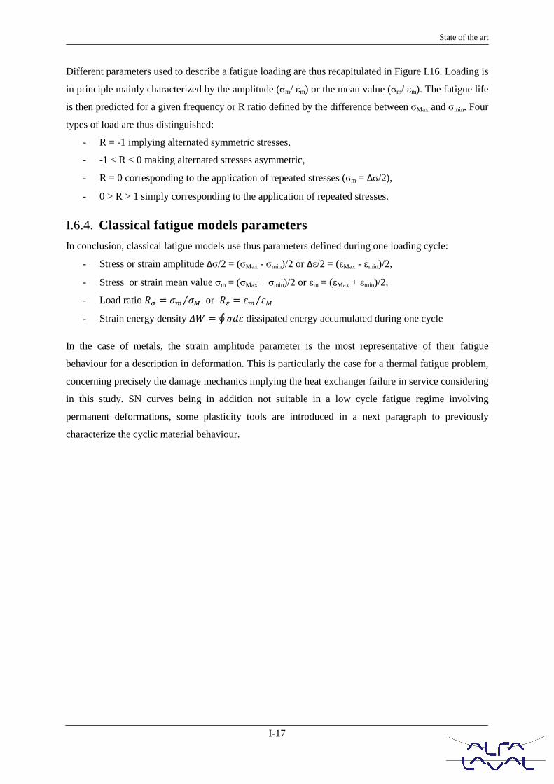
I.6.4. Classical fatigue models parameters
In conclusion, classical fatigue models use thus parameters defined during one loading cycle:
- Stress or strain amplitude Δσ/2 = (σMax - σmin)/2 or Δε/2 = (εMax - εmin)/2,
- Stress or strain mean value σm = (σMax + σmin)/2 or εm = (εMax + εmin)/2,
- Load ratio �� = �� ��⁄ or �� = � �⁄
- Strain energy density � = ∮ � dissipated energy accumulated during one cycle
In the case of metals, the strain amplitude parameter is the most representative of their fatigue
behaviour for a description in deformation. This is particularly the case for a thermal fatigue problem,
concerning precisely the damage mechanics implying the heat exchanger failure in service considering
in this study. SN curves being in addition not suitable in a low cycle fatigue regime involving
permanent deformations, some plasticity tools are introduced in a next paragraph to previously
characterize the cyclic material behaviour.

Thermo-mechanical modelling and durab
I.7. Plasticity theor
I.7.1. Cyclic material be
I.7.1.1. Descrip
Cyclic behaviour generally involv
and more precisely the Bausching
yield stress in compression after
domain is translated in the deviat
kinematic hardening is linked to
the microscopic scale. Dependin
accompanied by its expansion. T
of the dislocation density.
In cyclic tests at applied deformat
- A material hardening (cf.
- A material softening duri
Different material responses to a
will normally occur only if the
adaptation or a plastic accommod
material involving no more pla
stabilization. Once the stabilisatio
a second time (cf. Figure I.18-b).
In the case of non-symmetric ap
cause a non-negligible number of
I.19). In multiaxial conditions, ra
stress and strains for equivalent lo
I.7.1.2. Influen
As a consequence, all these result
I.17-b, the middle (X) evolution o
by elastic unloading at a given pl
definition of both isotropic (siz
translation) allows to introduce th
In this way, plastic flow law can
rability analysis of welded heat exchangers
I-18
ory in the fatigue material beha
behaviour
iption
olves material memory able to be described by the
inger effect. It corresponds to a material softening
fter a first load in tension (cf. Figure I.17-ii). As
iatoric plane without other transformation after defo
to the residual micro stresses due to the heterogene
ing on the studied cases, the translation of the el
. This characterizes the isotropic hardening, resultin
ation, two types of material behaviour are classical
cf. Figure I.18-i) where stress increases with the num
uring which, on the contrary, stress decreases with t
a cyclic loading are depicted in Figure I.19. A hy
the loading is perfectly periodic, corresponding
odation. The first case implies a limit value of the
lastic strain after a certain time, when the seco
tion reached, another one can occur by increasing t
.
applied stress, Ratchetting effect can be observed
of structural failures by generating progressive def
ratchtting effect is generally less visible and so im
t loadings.
ences on the material description
ults make yield surface representation not fixed wit
n of the segment 2(σ0+R) characterizes the called
plastic deformation εp (R being an isotropic harden
size evolution of the elastic domain) and kinem
the yield surface description:
� = |� � �| � � � ��
n only occur if �� � 0 or � = 0.
haviour
he kinematic hardening
ng by a decrease of the
As a result, the elastic
eformation. In general,
neity of the material at
elastic domain can be
lting from the increase
ically observed:
number of cycle,
h the time.
hysteresis stabilisation
either to an elastic
he energy stored by the
cond leads to a cycle
g the load amplitude in
ed. It is considered to
deformation (cf. Figure
implies less Von Mises
with the time. In Figure
ed kinematic hardening
dening parameter). The
ematic (elastic domain
(1.1)

State of the art
I-19
Figure I.17 - Linear kinematic hardening (i) in the deviatoric plane, (ii) in the σ = f(εp) response
Figure I.18 - (i) predicted strain memory effect by three different strain amplitude and (ii) predicted cyclic
plasticity behaviour (50cycles) for nickel base alloy under tension-compression (from Dieng et al., 2004)
Figure I.19 - Cyclic material response under different force loadings with (i) the elastic adaptation, (ii) the
plastic accommodation and (iii) the Ratchetting effect
(iii) Ratchetting (ii) Accommodation (i) Adaptation
(i) (ii)
(i) (ii)
X

Thermo-mechanical modelling and durab
I.7.1.3. Accumu
Classical hardening laws take in
noted p in an uniaxial case. This
careful look at Figure I.17. In
applied, the opposite unload BA g
Under N cycle(s) of loading-unlo
� = ��Isotropic hardening is mainly a f
whose utilisation mainly depends
about to be used in a future applic
values p (1.6), the power law
kinematic hardening, two main
hardening parameters, X as R bein
I.7.2. Observations in m
The loading path can play a criti
other metallic alloys. A load intr
points of a structure is so calle
parameters. On the contrary, con
From equal amplitude loadings,
loading path.
I.7.3. Tridimensional yie
The unidirectional plasticity thres
��� and ��� represent respectively
(�� = 0) in the domain. ��� � �elastic domain of the material
generalization in Tridimensiona
describing a domain in the 2, 3
generates elastic strains.
In the case of metals, physical me
tensor. Here the well-known Von
plate anisotropy appears to be ver
rability analysis of welded heat exchangers
I-20
mulated plastic deformation and hardenin
into account the plastic strain εp but or the accum
his term after N identical cycles can be pointed ou
fact, plastic deformation increases when a load
A giving the same results in absolute value.
� ! = |! � | = �
loading, total accumulated uniaxial plastic strain ca
�"�!→ " $ "� →!"% = 2�� = ' "�� " (�)
a function of p with R = R(p) and 3 different laws
nds on the material. Voce law is classically used t
plication. It shows its ability to saturate for high cum
w being more in adequacy with aluminium beh
in laws are introduced in Table I.2. C and γ are
eing functions of the plastic deformation history.
multiaxial
ritical role in the mechanical response of some ma
introducing no variation of the principal stress tens
alled proportional. It allows generally to determi
considering non-proportional loading introduced th
, they can lead to an additional hardening depen
yield stress criterion
reshold defines the elastic domain in the one dimen
ly yield stress in traction and compression, no plas
� ���. Considering the particular case of identica
ial can be described by the criteria function�nal case is the yield stress criterion still formu
3 or 6 dimensions stress space, in which a stress
mechanics can justify the convexity of the criteria f
on Mises isotropic criterion will be used for the s
very negligible (cf. experimental tensile curves in C
ing laws
umulated plastic strain
out by having a more
oad on the path AB is
(1.2)
can be defined as
(1.3)
ws exist (cf. Table I.1)
d to study steels and is
cumulated plastic strain
ehaviour. Considering
re known as kinematic
materials as steels and
ensor directions in any
minate elastic domain
the hardening notion.
ending strongly on the
ension stress space. If
lastic flow is observed
tical yield stress, initial
= |�| � �� � 0 . Its
ulated by � � 0 and
ess variation will only
ia function of the stress
e study as the eventual
Chapter 2).
State of the art
I-21
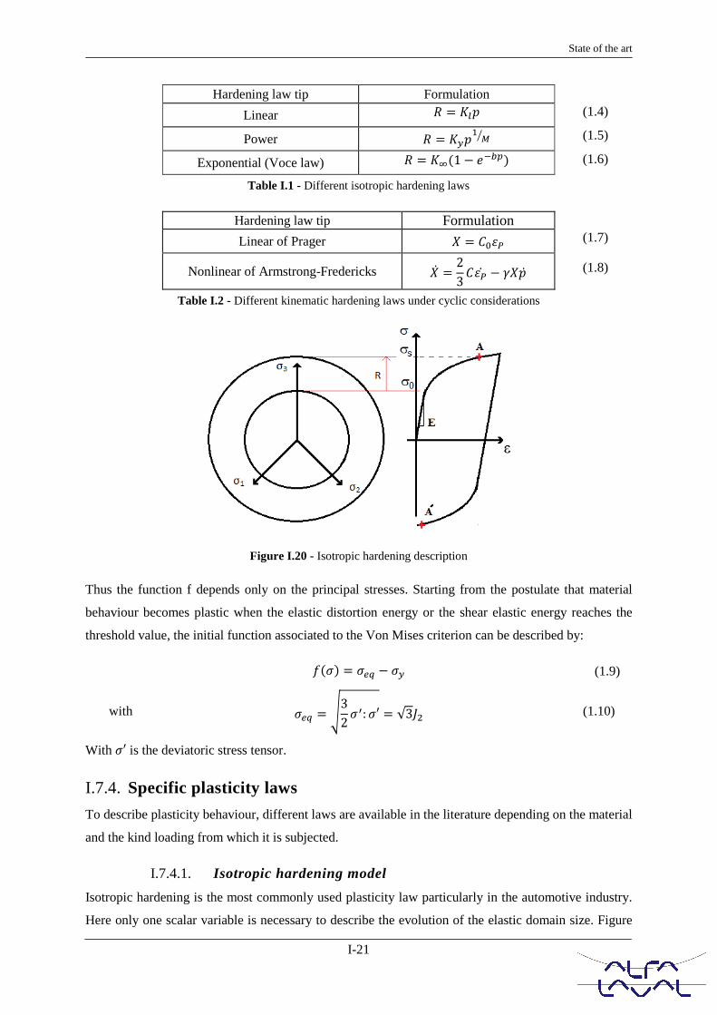
Hardening law tip Formulation
Linear � = *+� (1.4)
Power � = *��, �- (1.5)
Exponential (Voce law) � = *.(1 � 123�) (1.6)
Table I.1 - Different isotropic hardening laws
Hardening law tip Formulation
Linear of Prager 5 = 6)7 (1.7)
Nonlinear of Armstrong-Fredericks 5� = 23 67� � 95�� (1.8)
Table I.2 - Different kinematic hardening laws under cyclic considerations
Figure I.20 - Isotropic hardening description
Thus the function f depends only on the principal stresses. Starting from the postulate that material
behaviour becomes plastic when the elastic distortion energy or the shear elastic energy reaches the
threshold value, the initial function associated to the Von Mises criterion can be described by:
�(�) = �:; � �� (1.9)
with �:; = <32 �=: �′ = √3AB (1.10)
With �′ is the deviatoric stress tensor.
I.7.4. Specific plasticity laws
To describe plasticity behaviour, different laws are available in the literature depending on the material
and the kind loading from which it is subjected.
I.7.4.1. Isotropic hardening model
Isotropic hardening is the most commonly used plasticity law particularly in the automotive industry.
Here only one scalar variable is necessary to describe the evolution of the elastic domain size. Figure

Thermo-mechanical modelling and durab
I.20 schematically shows the crit
curve.
In addition, the curve points out t
cumulated plastic strain p, confir
isotropic make easier its mathem
defined by deformation partition,
And
and by a linear elasticity. Free ene
And
State laws give then
And
Where G(p) defines the hardenin
exponential law.
I.7.4.2. Linear
Kinematic hardening correspond
I.17) introduces it in the descripti
�From this definition (1.17), the a
linearity from which the hardenin
It is not possible to introduce a no
to the criteria function. It would
experimental observations. Thus
Mises criterion, the variable beco
rability analysis of welded heat exchangers
I-22
riteria evolution in the stress space and the corres
ut the fact that A (after loading) and A’ (after unloa
firming its ability to be used here as parameter. Su
ematic description as shown by the classical Pran
n, the general normality law is:
�� = C� D�D�
E�F = C� D�DGF
energy and yield criterion are respectively:
HI = HI: $ HI� = HI: $ J(�)
� = �:; � � � ��
� = H DID = K: � � �%
� = H DID� = DJD� = �(�)
ning R(p). Equation (1.6) gives identification exa
r Kinematic hardening of Prager
nds to the translation of the yield surface. The X
ption of the yield surface by the use of the Von Mis
� = ‖� � 5‖ � �� = AB(� � 5) � ��
e assumption of generalized normality implies the
ning variable is equal to the plastic strain.
�� = �C� D�D5 = C� D�D� = ��
non-linear relation between 5 and � considering a
uld lead to a one-to-one non-linearity which is n
us using specific free energy under a quadratic form
comes
responding stress-strain
loading) have the same
Supposing a hardening
randtl-Reuss law. It is
(1.11)
(1.12)
(1.13)
(1.14)
(1.15)
(1.16)
example of R(p) by an
X variable (cf. Figure
ises criterion:
(1.17)
he kinematic hardening
(1.18)
g a flow potential equal
not in adequacy with
orm in the case of Von
State of the art
I-23
5 = H DID� = 6)� = 6)ε� = 23 6ε� (1.19)
The linear kinematic hardening law of Prager could be thus summarized by equations (1.11) and
(1.19) where the hardening modulus is constant and equals to C.
I.7.4.3. Non-linear Kinematic hardening of Armstrong -Fredericks
Hardening law linearity certainly implies easier and faster calculation resolution. Nevertheless in case
of cyclic loading, Bauschinger effect could not be precisely represented, stress state will accommodate
from the first cycle and Ratchetting effects are moreover not described. In this way, non-linear
kinematic hardening of Armstrong-Frederick is going to be used. This model is curiously very famous
although its publication had been more recent. Until 2007, it has been limited to an internal report of
the Central Energy Generating Board (CEGB). The yield surface remains defined here by (1.17). In
order to get round the disadvantage of the proportionality between 7� and 5� , a third term is added in
(1.8), �� is the cumulated plastic strain velocity and (C, γ) material parameters. This third term is
known as dynamic restoration due to its one degree homogeneity against the time. Generally, 5 tensor
is supposed equal to 0 at the initial stage as the other plasticity theory elements are not modified.
Thus, one of the main characteristic of this model corresponds to the classic plasticity formulation
with two surfaces (allowing the description of a continuous hardening modulus evolution):
- The elasticity limit surface merged with the yield surface,
- A limit surface induced by the variables re-actualisation, the state (N2,� , 5N2,) being the
consequence of the prior plastic flow.
I.7.4.4. Combined hardening law
Although isotropic hardening alone remains the most widely used model in the industry, taking into
account Bauschinger effect recently showed beneficial influence on numerical prediction reliability,
particularly in the case of spring back. In this way, a new standard of models is emerging. It is a matter
of a superposition of a non-linear kinematic hardening to an isotropic one, implying both translation
and dilatation of the elasticity domain. This combination will be particularly recommended in case of
reversed strain path. It is described with two state variables: the cumulated plastic strain p and the
associated thermodynamical force R (inducing the size variation of the yield surface). Always
considering a Von Mises criterion, the yield surface is now defined in term of:
� = AB(� � 5) � � � �� (1.20)
R varies as a function of the accumulated plastic strain taking into account the progressive hardening.
As it will be pointed out later, regarding cyclic behaviour, this evolution is in principle relatively slow.
It can increase, the term of cyclic hardening is thus introduced, or decrease for the cyclic softening

Thermo-mechanical modelling and durab
cases. This variation can be de
definition.
Where ∞R gives the asymptotic v
to reach this stabilization. Assum
last relation would give (1.16).
For applied strain, this last equ
superpose several isotropic harde
region on the stress-strain curve.
on kinematic variables dependi
becomes:
In conclusion, it is also importa
describes an evanescence memo
loading. More generally, this m
applied in the heat exchanger fail
I.8. Heat exchanger
Fatigue has been widely studied f
applications received also a lot o
[2], [3]. However, surprisingly fa
of the recent references concer
approach in order to mainly iden
In these studies, the fracture of
microstructural feature such as th
back to the 90’s to find some num
[7] suggested a way to include
exchanger. This leads to a possi
supposed to appear at welded joi
including residual thermal stre
distribution has been used to v
boundary conditions. The study
mechanism corresponds to therm
involving a thermal cyclic loadin
rability analysis of welded heat exchangers
I-24
described by a formulation which looks like k
�� = O(�. � �)�� ic value corresponding to the stabilized cyclic regim
ming that R is equal to 0 for a p value also equal to
quation represents nicely the cyclic hardening. It
rdening variables� = ∑ �Q, often necessary to study
Isotropic hardening taken as cyclic hardening effe
ding on the cumulated plastic strain. In this w
5� = 23 6(�)7� � 9(�)5�� rtant to note that non-linear kinematic hardening
mory, that is to say the stabilized cycle is unique
material behaviour theory presented is going to
ailure analysis in Chapter 3.
ger analysis in the literature
d from a general and scientific point of view during
t of attention such as in bearings or structural mate
fatigue in the case of heat exchanger has been bar
cerning the failure analysis of exchanger deal w
entify the damage mechanics involved in industria
of heat exchanger has been associated to therma
s the presence of defects (i.e. sulphides in [5]). It i
umerical approach of a heat exchanger failure. Fer
de a fatigue model in a thermo-elastic analysis
ssible estimation of the fatigue life of this type o
joints after a relatively short time, hypothesizing s
tresses from welding and especially thermal fa
o validate finite elements model geometry, mat
dy of the thermal load in duty has led to the co
rmal fatigue. Indeed, every day the unit is started
ding. In addition, once the unit reaches maximal te
e kinematic hardening
(1.21)
gime and b the rapidity
l to 0, integration of the
. It is also possible to
udy small deformations
effect could also induce
way, equation (1.18)
(1.22)
ng model nevertheless
que for a given cyclic
to be introduced and
ring last decades. Some
aterials for aeronautics
barely addressed. Most
l with a metallurgical
trial problems [4, 5, 6].
mal fatigue coupled to
It is necessary to come
erguson and Gullapalli
is of a gas fired heat
of exchanger. Cracks
g several failure modes
fatigue failure. This
aterial properties and
conclusion that failure
ted up and shut down,
temperature, an actual

State of the art
I-25
cook cycle occurs. A linear FE (Nastran) shell analysis has been so conducted. A thermal load
corresponding to the worst in duty one in terms of stress concentration identified by a first study is
applied to the heat exchanger model. The stress in each node is thus extracted. In order to predict the
fatigue behaviour, a failure criterion is then used. This failure criterion is based on the maximal stress
admissible. This empirical criterion stated that the maximal load is given by the endurance limit at
infinite life corrected by factors taking into account the surface finish, the size, the temperature effects,
etc…:
R: = STS3S�SUS:R:= With Se the modified endurance limit, ka the surface finish factor (taking into account the thermo
mechanical treatments experienced by the base material), kb the size factor and kc the load factor (the
value of these two parameters are set and there real significance is not expressly given), kd the
temperature factor (taking onto account the evolution of the base material properties with the
temperature), ke the stress concentration factor. At last Se’ the endurance limit at infinite life.
Moreover, the authors added a Palmgren-Miner equation to take into account the different types of
load experienced by the heat exchanger on the total damage. This approach permits to obtain a fair
idea of the fatigue life of this type of heat exchanger. However, it is clear that the failure criterion
proposed is more an ad-hoc fitting parameter only describing the case studied. Thus any prediction of
fatigue life in an other configuration seems to be not possible with this approach.
Carter P and TJ [8] have then suggested a metallurgical failure analysis of aluminium plate fin
exchanger to identify the involved damage mechanism in a first approach. In that case, the material is
composed of a core material namely 3003 Al-Mn alloy and a clad made of Al-Si. This clad permits to
braze the structure when a thermal cycle is imposed due to the lower melting temperature of the Al-Si
alloy. It is shown that fracture occurs due to the presence of brittle phases in the solidified clad. In a
second time, the study has been followed by a life prediction through a numerical analysis and the
application of a fatigue model. This structure normally also works in a steady state, being submitted to
significant pressure and thermal loads cycles occurring this time irregularly during start-up and shut
down of the unit. Thermal fatigue failure was confirmed. Linear FE (Abaqus) shell analysis of a corner
piece was performed in steady and transient state followed by stress analysis in which the weakest
zone has been identified. A version of Manson-Coffin law taking into account total strain and stress
amplitude (corresponding partially to Basquin’s method) has been used to predict the final fatigue life.
The authors consider that fracture is determined by the behaviour of the brazed materials. Thus only
the mechanical strength of this one is considered. The finite element model developed here predicts
that the transient regime seems to be more detrimental for the structure considering fatigue. The
fatigue life is reduced to less than 100 cycles for a transient with a difference in temperature of 130°C.
Moreover this model predicts also the right location of the fracture. Even if the model presented here
Thermo-mechanical modelling and durab
is quite coarse in terms of me
materials are not taken in to acco
are not considered), this approac
study. It is interesting to note tha
for automotive applications. The
Xray tomography studies [9].
In the same way, Nakaoka, Naka
strength of plate-fib heat excha
supposed to be involved, a coarse
is calculated probably with a pu
results giving the number of cyc
test. This comparison is used to
life seems to be correctly predict
account the plastic behavior of
clearly not the case in the real ca
provide a more predictive mod
configurations or base materials.
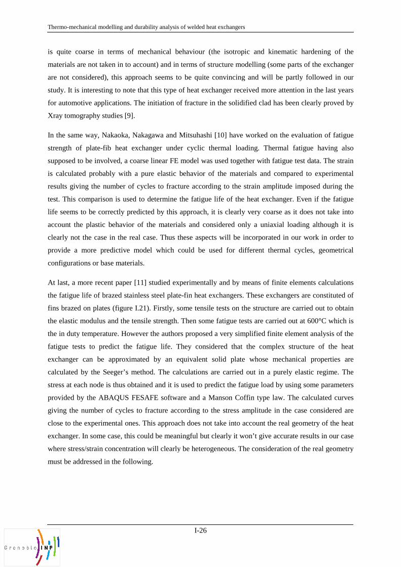
At last, a more recent paper [11]
the fatigue life of brazed stainless
fins brazed on plates (figure I.21
the elastic modulus and the tensil
the in duty temperature. However
fatigue tests to predict the fatig
exchanger can be approximated
calculated by the Seeger’s metho
stress at each node is thus obtaine
provided by the ABAQUS FESA
giving the number of cycles to f
close to the experimental ones. T
exchanger. In some case, this cou
where stress/strain concentration
must be addressed in the followin
rability analysis of welded heat exchangers
I-26
mechanical behaviour (the isotropic and kinemat
count) and in terms of structure modelling (some pa
oach seems to be quite convincing and will be pa
that this type of heat exchanger received more atten
he initiation of fracture in the solidified clad has be
akagawa and Mitsuhashi [10] have worked on the e
changer under cyclic thermal loading. Thermal
rse linear FE model was used together with fatigue
pure elastic behavior of the materials and compa
ycles to fracture according to the strain amplitude
to determine the fatigue life of the heat exchanger
icted by this approach, it is clearly very coarse as
f the materials and considered only a uniaxial lo
l case. Thus these aspects will be incorporated in o
odel which could be used for different thermal
ls.
1] studied experimentally and by means of finite e
less steel plate-fin heat exchangers. These exchange
21). Firstly, some tensile tests on the structure are
sile strength. Then some fatigue tests are carried o
ver the authors proposed a very simplified finite ele
atigue life. They considered that the complex st
ted by an equivalent solid plate whose mecha
thod. The calculations are carried out in a purely
ined and it is used to predict the fatigue load by us
SAFE software and a Manson Coffin type law. T
fracture according to the stress amplitude in the
. This approach does not take into account the real
ould be meaningful but clearly it won’t give accura
on will clearly be heterogeneous. The consideration
ing.
atic hardening of the
parts of the exchanger
partly followed in our
tention in the last years
been clearly proved by
e evaluation of fatigue
al fatigue having also
ue test data. The strain
pared to experimental
de imposed during the
ger. Even if the fatigue
as it does not take into
loading although it is
in our work in order to
al cycles, geometrical
e elements calculations
ngers are constituted of
re carried out to obtain
out at 600°C which is
element analysis of the
structure of the heat
hanical properties are
ely elastic regime. The
using some parameters
. The calculated curves
he case considered are
al geometry of the heat
urate results in our case
on of the real geometry

State of the art
I-27
Figure I.21 – Real geometry of the heat exchanger (a) and the equivalent solid plate considered for finite
element calculations (b) [11]
I.9. Goal of the study
Although some studied cases exist in the literature, all projects can obviously differ in the approach
simply due to the differences of design or industrial application for example. Thus the aim of this PhD
project has been to provide insight of the welded heat exchanger response in use in order to explain the
most common failure cases reported in the Trouble Shooting Department of Alfa Laval. In this way, a
methodology has been thought to answer this given problem with the:
- Linear FE description of the full exchanger by locating the weakest zones thanks to
assumptions in adequacy with the reality and physics of the problem. It is something already
innovative as references previously presented (paragraph 1.8) had the tendency to consider
only a small part of the exchanger in the modelling. Here the model is supposed to be able to
describe a structure weight of almost 50,000kg, composed of 500 plates,
- Validation of boundary conditions and numerical results by comparing the simulation with
thermal fatigue test performed one or several prototypes,
- Identification of the material cyclic response to be able to get the real material behaviour
involved in the working unit and proposition of a way to incorporate in the FE model,
- Suggestion a fatigue model able to make a link between local material response and fatigue
life predication, easily usable in an industrial environment.

Thermo-mechanical modelling and durab
I.10. References
“Heat exchanger design handbook
[1] Lemaitre J, Chaboche J-L, B
Editions Dunod.
[2] Tonicello E, Girodin D., Sid
trends in materials and heat treatm
[3] Delacroix J., Buffière JY.,Fou
and Fretting crack processes in A
[4] Otegui J.L, Fazzini P. Failur
Engineering failure analysis 11 (2
[5] Azevedo C.R.F, Alves G.S.
analysis 12 (2005) 193-200.
[6] Usman A, Nusair Khan A. Fa
15 (2008) 118-228.
[7] Ferguson G.L, Gullapalli S.R
failure analysis, Vol 2, No. 3 (199
[8] Carter P, Carter T.J, Viljoen
heat exchanger, Engineering failu
[9] Buteri A, Buffiere JY, Fabrèg
Al-Mn brazed used in heat exchan
[10] Nakaoka T, Nakagawa T, M
under thermal loading, Internation
[11] Jiang W., Gong JM., Tu ST
equivalent-homgeneous-solid me
rability analysis of welded heat exchangers
I-28
ook”, T. Kuppan
Benallal A, Desmorat R. Mécanique de matériaux
Sidoroff C, Fazekas A., Perez M., Rolling bearing
atments, Materials Science and Technology 28 (201
ouvry S., Daniellou A., Effets of microstructure on
Al-Cu-Li alloys, Journal of the ASTM Internationa
lure analysis of tube-tubesheet welds in cracked g
(2004) 903-913.
Failure analysis of a heat exchanger serpentine
Failure analysis of a heat exchanger tubes, Enginee
.R. Thermo-elastic finite element fatigue failure a
1995) 197-207.
en A. Failure analysis and life prediction of a larg
ilure analysis, Vol 3, No. 1 (1996) 29-43
règue D., Perrin E., Rethore J., Havet P., fatigue M
hanger, Materials Science Forum, ICAA12, Yokoha
Mitsuhashi K. Evaluation of fatigue strength of plat
tional Conference on Pressure Vessel Technology, V
ST., Fatigue life predction of a stainless steel plat
ethod, Materials and Design 32 (2011) 4936-4942
aux solides, 3e édition,
ing applications: some
012) 23-26.
on the incipient fatigue
nal 7 (2010).
d gas heat exchangers,
ne, Engineering failure
neering failure analysis
e analysis, Engineering
arge, complex plate fin
Mechanismsof brazed
ohama 2010.
late-fin heat exchanger
, Vol 1, ASME 1996.
late-fin structure using
42.

Structure modelling description
II-1
II. STRUCTURE MODELLING DESCRIPTION
The finite element model construction of a heat exchanger has been carried out in a step by step
approach. From several assumptions verified experimentally, the thermo-elastic response of the heat
exchanger under uniform thermal loading has been firstly investigated. Regions of the exchangers
where the stress concentrates have been identified. Two thermo-mechanical tests have been performed
to validate the thermo-elastic description of the heat exchanger.

Thermo-mechanical modelling and durab
II.1. Table of conten
II. Structure modelling descriptio
II.1. Table of contents .............
II.2. Motivation and methodo
II.3. Mechanical characterizat
II.4. Mesoscopic analysis of th
II.4.1. Mechanical characte
II.4.2. Governing equations
II.4.3. Simplified plate desc
II.4.4. A two plates assemb
II.4.5. Introduction of a mo
II.5. Construction of a full 3D F
II.5.1. Repetition of the ele
II.5.2. Account for the end
II.5.3. Influence of the end
II.6. First validation of the 3D
II.6.1. Exchanger design an
II.6.2. Boundary conditions
II.6.3. Validation of the FE
II.7. Second thermal test for e
II.7.1. Design of the protot
II.7.2. Results analysis ........
II.7.3. Comparison with line
II.7.4. Thermal tests summ
rability analysis of welded heat exchangers
II-2
tents
escription ............................................................................
...........................................................................................
ethodology .......................................................................
acterization of the material ................................................
ysis of the plates assembly .................................................
characterization of a heat exchanger plate .......................
quations for the thermo-mechanical problem ..................
late description and thermo-mechanical simulation .........
embly ...........................................................................
of a more realistic boundary conditions case ..................
full 3D FE model of the exchanger ................................
f the elementary model .....................................................
the end plates to reach a full structure description ..........
the end plate on the stress distribution ............................
f the 3D FE model ...............................................................
esign and thermal fatigue test introduction ......................
onditions justification by local temperature analysis .........
f the FE model ................................................................
test for evaluating the FE model .........................................
e prototype and test specifications ................................
......................................................................................
with linear FE simulation and discussion ..........................
ts summary .........................................................................
................................... II-1
...................................... II-2
.............................. II-3
...................................... II-5
...................................... II-6
...................................... II-6
...................................... II-8
................................ II-9
................................ II-12
.................................... II-13
.................................... II-18
.................................... II-18
............................... II-18
.................................... II-20
.................................... II-22
.................................... II-22
.............................. II-22
.................................... II-25
.............................. II-35
.................................... II-35
.................................... II-39
.................................... II-42
.............................. II-43

Structure modelling description
II-3
II.2. Motivation and methodology
This chapter deals with the construction of a simplified 3D description of the heat exchanger,
something never made until now mainly due to the difficulty to easily take into account structure size,
boundary conditions, thermal loading, transitory effects, among other aspects. The aim is to build a FE
model that allows thermo-elastic calculations to point out zones of stress concentration in the corners
of the heat exchanger core, where some vulnerability may be observed. It is here necessary to have a
good balance between a realistic description of the mechanical fields that are responsible for damage
and a low cost simulation time. To the end, a bottom-up approach has been adopted, starting with a
simple description of the plate (i) and their assembly through “papillotes”. Using simple boundary
conditions and homogeneous thermal loading, regions that are potentially critical have been identified.
Then more realistic boundary conditions have been considered by a detailed analysis of the plates pack
environment (iii). From a balance between a refined description where stress partially concentrate and
a simplification (where heterogeneous fields are found), the final macroscopic FE model is reached by
the last consideration of the core extremities (iv). It is finally compared to experimental tests to check
its validity.
Regarding thermal loading, it is in practice generated by fluid flows in the whole exchanger. It is
assumed that it is the only load supposed to be detrimental for the structure resistance, internal
pressure effect being here neglected, although the model could be used for burst test (pressure
resistance). If thermal loading has been considered as the existing data of the methodology, real
temperature distribution calculation have been performed by Alfa Laval research center. Throughout
the construction of the 3D FE model of the exchanger core, it has been supposed during heating (resp.
cooling) transient step, thermal inertia between core and external frame panels is different enough to
consider frame part as a rigid while the core deforms thermo-mechanically. Thin plates (1mm) of the
core (in red) should have tendency to heat and expand very quickly when it is expected that thicker
frame panels (almost 120mm, in blue) and girders need much more time to reach the asymptotic
temperature by conduction. In this way, throughout the project, whole frame part will be fixed,
applying rigidity effect on the core. It is in addition during these first instant that boundary conditions
applied on the core are supposed to be the strongest through this assumption. This important postulate
should be verified experimentally. At each step, thermo-mechanical calculations have been so carried
out to identify regions where a defined description is necessary and those where a simplified one is
allowed by the observation of the stress distribution under a simple uniform temperature field. ANSYS
finite element code has been used for all simulations in this study. From a technical point of view, the
FE model has been parameterized so that the future user can vary plate size, plates and passes number,
column liner and girder dimensions and size of “papillotes” as desired. The sequel of the chapter
follows the bottom um approach depicted in Figure II.1.

Thermo-mechanical modelling and durab
Figure II.1 - (a) Picture of the heat e
pack corner showing the assembl
depicting the strategy adopted to co
assembly with another one with perp
panels,
The mechanical characterization
Basic plates assembly and bou
description of the full 3D FE mod
(iii ) Accurthe boun
(iv) Final model o
(a) CPK75
Plates pColumn liner
Girder
rability analysis of welded heat exchangers
II-4
t exchanger core with the pill-up of corrugated plates, (b
bly of the “papillotes”, column liner and the end plate, (
construct the FE model with (i) description of a single co
erpendicular corrugations orientation, (iii) the account fo
ls, (iv) the final FE model at the macroscopic scale
on of the smooth and corrugated material has be
oundary conditions influence have been then an
odel is provided. Predictions have been compared w
(i) One plate mo
(ii) Introduction of the papillote
curate description of undary conditions
l of the core
75 core prototype
s pack End plate
(b) zon
b) zoom along the plate
e, (i) to (iv) snapshots
corrugated plate, (ii) its
t for connection to frame
been firstly gets onto.
analysed. Finally the
d with experiments.
model
Papillote
b) Zoom on the zone of interest

Structure modelling description
II-5
Figure II.2 - Uniaxial tensile test stress-strain response of the rolled 316L steel under consideration in this study
along the rolling direction (long), at 45° and transversely
II.3. Mechanical characterization of the material
The material involved in the project has been here previously characterised. Plates are made from a
laminated 316 L steel whose basis composition is a high Chromium content (17%) for corrosion
problem, from 11 to 13% of Nickel and around 2% of Molybdenum (elements particularly adapted for
aggressive environments). Cr-Ni alloy is here characteristic of an austenitic stainless steel. In a
mechanical point of view, this material is ductile and presents high tensile strength and creep
resistance. Nevertheless it cannot be subjected to a thermal treatment and its forming should be made
at room temperature (as the plate embossing or lamination). Regarding the external frame part, panels
and girders are manufactured in low carbon content steel, not characterized here the frame has been
only considered as rigid body displacements applying at its contact with the core.
The mechanical material properties of rolled 316L steel have been identified in uniaxial monotonic
tensile tests performed at 0°, 45° and 90°C to the rolling direction, allowing to also point out a
possible plate plastic anisotropy. Specimen thickness is 1mm and all tensile tests have been conducted
at a strain rate of 1x10⁻⁴s-1. Longitudinal and transverse strains have been recorded with a non-
contacting video method. Cauchy stress was finally calculated from the load assuming an isochorus
transformation during the plastic deformation. Figure II.2 shows material responses along the three
directions (Long, 45° and transverse) in the same σ-ε plot and it is shown here that plastic anisotropy
is relatively low. Added to the fact, plate rolling direction is oriented randomly in the manufacturing
process of the exchanger, material plasticity has been simply supposed isotropic in Chapter 3.
0
200
400
600
800
1 000
1 200
0,00 0,05 0,10 0,15 0,20 0,25 0,30 0,35 0,40 0,45 0,50
Tru
e s
tress
σv
(MP
a)
True strain εv = ln(L/L0)
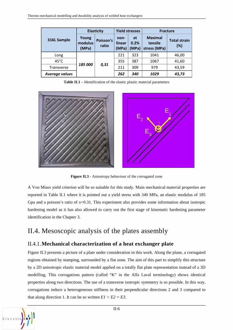
Thermo-mechanical modelling and durab
316L Sample Youn
modul
(MPa
Long
185 0045°C
Transverse
Average values
Table II.1 – I
Figure II
A Von Mises yield criterion will
reported in Table II.1 where it is
Gpa and a poisson’s ratio of υ=0
hardening model as it has also a
identification in the Chapter 3.
II.4. Mesoscopic ana
II.4.1. Mechanical charac
Figure II.3 presents a picture of a
regions obtained by stamping, sur
by a 2D anisotropic elastic materi
modelling. This corrugations pa
properties along two directions. T
corrugations induce a heterogene
that along direction 1. It can be so
rability analysis of welded heat exchangers
II-6
Elasticity Yield stresses Fracture
Young
modulus
(MPa)
Poisson's
ratio
non-
linear
(MPa)
at
0.2%
(MPa)
Maximal
tensile
stress (MPa)
185 000 0,31
221 323 1041
355 387 1067
211 309 979
262 340 1029
Identification of the elastic plastic material parameters
II .3 - Anisotropy behaviour of the corrugated zone
ill be so suitable for this study. Main mechanical m
t is pointed out a yield stress with 340 MPa, an ela
=0.31. This experiment also provides some inform
allowed to carry out the first stage of kinematic
analysis of the plates assembly
racterization of a heat exchanger plat
f a plate under consideration in this work. Along th
surrounded by a flat zone. The aim of this part to si
terial model applied on a totally flat plate representa
pattern (called “K” in the Alfa Laval terminolo
. The use of a transverse isotropic symmetry is so
eneous stiffness in their perpendicular directions 2
so written E1 > E2 = E3.
E2
E
E3
Fracture
Total strain
(%)
46,00
41,60
43,59
43,73
ers
material properties are
elastic modulus of 185
rmation about isotropic
ic hardening parameter
late
the plane, a corrugated
simplify this structure
ntation instead of a 3D
ology) shows identical
o possible. In this way,
2 and 3 compared to
E1

Structure modelling description
II-7
Figure II.4 - Uniaxial stress-strain response of the 316L steel along the direction perpendicular to the
corrugations and corresponding samples
Figure II.5 - Zoom on the beginning of the stress-strain response of the 316L steel along the direction
perpendicular to the corrugations
In this way, Figure II.4 shows the uniaxial stress-strain response of the corrugated 316L steel. The
curve can be split in three parts. The reaction along direction 2 shows (i) a reduced stiffness up to (ii) a
plateau corresponding to a geometrical accommodation of the corrugations. The third part (iii) finally
points out material hardening of the flattened material. In order to estimate the stiffness E2 along the
direction normal to the corrugations, the first slope of the curve has been considered (cf. Figure II.5).
�� = �(�)�(�) =
230.002 = 11500��� (2.1)
Strain (10-2 %)
Strain (10-2 %)
Stress (MPa)
Stress (MPa)
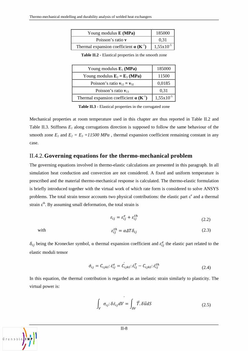
Thermo-mechanical modelling and durab
Y
Therma
Table
Y
You
Therma
Table I
Mechanical properties at room t
Table II.3. Stiffness E1 along cor
smooth zone E1 and E2 = E3 =11
case.
II.4.2. Governing equatio
The governing equations involved
simulation heat conduction and
prescribed and the material therm
is briefly introduced together wit
problems. The total strain tensor
strain εth. By assuming small defo
with
��� being the Kronecker symbol,
elastic moduli tensor
�
In this equation, the thermal con
virtual power is:
rability analysis of welded heat exchangers
II-8
Young modulus E (MPa) 185000
Poisson’s ratio ν 0,31
al expansion coefficient α (K -1) 1,55x10⁻⁵
ble II.2 - Elastical properties in the smooth zone
Young modulus E1 (MPa) 185000
oung modulus E2 = E3 (MPa) 11500
Poisson’s ratio ν12 = ν32 0,0185
Poisson’s ratio ν13 0,31
mal expansion coefficient α (K -1) 1,55x10⁻⁵
II .3 - Elastical properties in the corrugated zone
temperature used in this chapter are thus reporte
corrugations direction is supposed to follow the sa
11500 MPa , thermal expansion coefficient remai
tions for the thermo-mechanical prob
ved in thermo-elastic calculations are presented in
d convection are not considered. A fixed and uni
rmo-mechanical response is calculated. The thermo
ith the virtual work of which rate form is conside
or accounts two physical contributions: the elastic
eformation, the total strain is
��� = ���� � �����
����� = ������
ol, α thermal expansion coefficient and ���� the elast
���� = ��� !: ����� = ��� !: ����# $ ��� !: �������
ontribution is regarded as an inelastic strain simila
% ���: �����&'(= % �)*. �+)*&,
-(
�
orted in Table II.2 and
same behaviour of the
aining constant in any
roblem
in this paragraph. In all
uniform temperature is
rmo-elastic formulation
dered to solve ANSYS
ic part εe and a thermal
(2.2)
(2.3)
astic part related to the
(2.4)
ilarly to plasticity. The
(2.5)
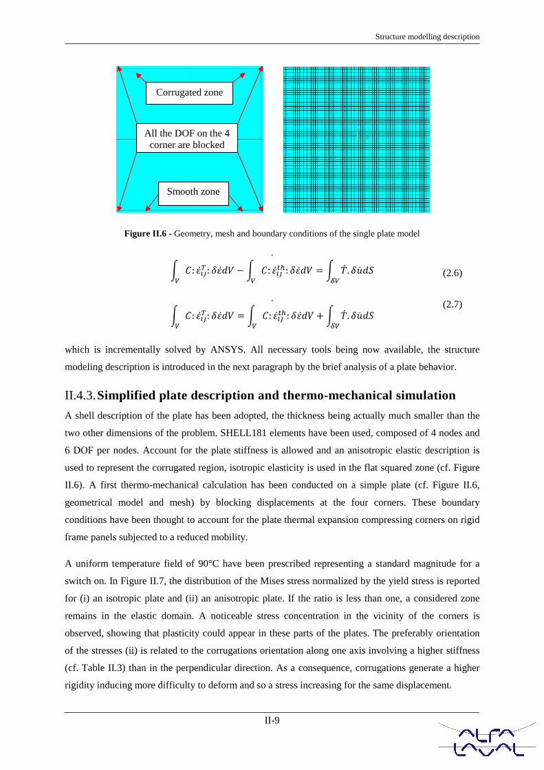
Structure modelling description
II-9
Figure II.6 - Geometry, mesh and boundary conditions of the single plate model
% �: ����# : ���&'($% �: ������: ���&'(
= % �� . �+� &,-(
� (2.6)
% �: ����# : ���&'(
= % �: ������: ���&'(�% �� . �+� &,
-(
�
(2.7)
which is incrementally solved by ANSYS. All necessary tools being now available, the structure
modeling description is introduced in the next paragraph by the brief analysis of a plate behavior.
II.4.3. Simplified plate description and thermo-mechanical simulation
A shell description of the plate has been adopted, the thickness being actually much smaller than the
two other dimensions of the problem. SHELL181 elements have been used, composed of 4 nodes and
6 DOF per nodes. Account for the plate stiffness is allowed and an anisotropic elastic description is
used to represent the corrugated region, isotropic elasticity is used in the flat squared zone (cf. Figure
II.6). A first thermo-mechanical calculation has been conducted on a simple plate (cf. Figure II.6,
geometrical model and mesh) by blocking displacements at the four corners. These boundary
conditions have been thought to account for the plate thermal expansion compressing corners on rigid
frame panels subjected to a reduced mobility.
A uniform temperature field of 90°C have been prescribed representing a standard magnitude for a
switch on. In Figure II.7, the distribution of the Mises stress normalized by the yield stress is reported
for (i) an isotropic plate and (ii) an anisotropic plate. If the ratio is less than one, a considered zone
remains in the elastic domain. A noticeable stress concentration in the vicinity of the corners is
observed, showing that plasticity could appear in these parts of the plates. The preferably orientation
of the stresses (ii) is related to the corrugations orientation along one axis involving a higher stiffness
(cf. Table II.3) than in the perpendicular direction. As a consequence, corrugations generate a higher
rigidity inducing more difficulty to deform and so a stress increasing for the same displacement.
All the DOF on the 4 corner are blocked
Smooth zone
Corrugated zone

Thermo-mechanical modelling and durab
Figure II.7 - Influence of the mode
Figure II.8 - Geometry
A) Link between 2
joint ledges in shell
1mm thickness
B)
pla
(i) Isotropic plate
(i)
rability analysis of welded heat exchangers
II-10
odel dimension on the distribution of the Von Mises Stre
yield stress reported in Table II.1
try of a two plates model and corresponding boundary c
2 plates: 2 butt
ell elements of
Upper ledge of the upper
late in shell elements of 1mm
2 weld
Elastic domain
late (ii) Considerationthe corrugation
Corrugationsdirection
Ux = 0 Uy = 0
(ii)
(iii)
tress, normalized by the
y conditions
lded “papillotes”
ion of ions
ns

Structure modelling description
II-11
However boundary conditions are for the moment very conservative to make any additional
conclusion concerning zones of interest. Consequently, these results indicate that a refinement of the
structure response is necessary in these locations, by approaching progressively the real design of the
exchanger. Always keeping in mind the step by step aspect of the methodology, a two plates assembly
is now going to be introduced in the next paragraph.
Thermo-mechanical modelling and durab
II.4.4. A two plates assem
In order to refine the structure res
crossed plates assembly has bee
directions are perpendicular from
assembled for each pair of plates
also modelled with a 2D surface a
In the same way, the respective u
half of this surface in order to a
will give the possibility to buil
including a parameterized numbe
blocked in displacement in orde
Then plate corners show now a “
that is ultimate welded along the
part, they are modelled with she
each plate. Basically the “papillot
Concerning the mesh, it is progre
regions of stress concentration (c
work is nevertheless constrained
mm wide). It imposes a maximal
too fine comparing to the global
smooth and the corrugated zone
corrugations contact between two
model a stress equation between
other. This numerical tool allows
making an effect closed to a rea
conservative, it has been shown
stress concentration location an
displacement at the end of the “
connection with a frame part tota
more accurate description of this
carried out still assuming a homo
vicinity of the “papillote” locati
seems to react identically as a
involving a larger stress conce
conservativeness of the boundary
the moment.
rability analysis of welded heat exchangers
II-12
embly
response in the vicinity of the corners where the pap
been described (cf. Figure II.8); “crossed” meanin
rom one plate to the other. Along the edges of t
es to create the channels of the heat exchanger. The
e and to mesh them with 3D shell elements of 1mm
e upper and lower edges of the top and bottom plate
allow a simple translation of this basis model. L
uild the crossed channel of the exchanger to rea
ber n of plate. For this configuration, the end of th
der to estimate stress distribution in this region (
a “papillote”, i.e. a vertical extension created durin
he z direction (cf. paragraph II.4.5). Introducing a f
hell elements also in the continuity of these top a
llote” form a 45° angle in relation to x and y axis.
gressively developed and optimized to be as coarse
centre of the plate) and refined in the vicinity of
ed by the width of the smooth zone (10mm for a C
al mesh size of 10mm in this zone. Smaller elemen
al structure, it is necessary to adapt the mesh in the
one with this constrain. Another important point
two plates. The most realistic and simple solution
een each superposed nodes (same x,y location) fr
ws to link the displacement along the z axis of bo
real contact between both. Appearing to be a poin
n that this numerical criterion does not have a m
and intensity particularly in the zone of interes
e “papillotes”, the 2 plates dilatation is always co
otally rigid. As these boundary conditions are still
is transition zone remains necessary. A calculation
ogeneous thermal field of 90 °C. Until now, stress
tion. Figure II.9 shows similar effects. Each pl
a one plate model, the higher stiffness in the co
centration at the corner of which diagonal is p
ary conditions, this effect is less visible on the “pa
papillotes are located, a
ning that corrugations
f the plates, a wall is
he flat parts have been
m thickness (CPK75).
lates are modelled with
Later this anticipation
reach finally a model
f the “papillote” is now
(cf. Figure II.8 - iii).
uring the plate forming
a first link to the frame
and bottom ledges of
rse as possible far from
of the ”papillote”. This
CPK75 plate of 730.2
ent size being probably
the border between the
int to introduce is the
on would have been to
from one plate to the
both corrugated zones,
oint of view a little bit
major influence in the
rest. Imposing a zero
considered in a direct
till very conservative, a
ion has been regardless
esses concentrate in the
plate taken separately
corrugations direction
s parallel. Due to the
“papillote” reaction for

Structure modelling description
II-13
Figure II.9 - Distribution of the Von Mises stress on a crossed plates assembly
II.4.5. Introduction of a more realistic boundary conditions case
II.4.5.1. Account for the column liner in the FE model
During the last paragraph, all steps necessary to build a one and two plates model have been
successively presented. The influence of different parameters as the corrugations (with their contact),
the thermal load and the meshing and the considering of a crossed plate geometry has been more
particularly pointed out. At this time, the two first points seems to constitute key parameters in the
stress concentration location and intensity. Nevertheless more accurate boundary conditions of the
exchanger core structure in duty still need to be described. The modelling of the “papillotes”
associated with a crossed plates geometry has been a first development, boundary conditions until now
supposing plate corners totally fixed. To be more representative of the service conditions, the link
between “papillote” and frame part is now taken more carefully into account. As shown in Figure II.1
and Figure II.10 (in purple), heart and frame parts are maintained together thanks to a piece called the
column liner. This “intermediate” part of the heat exchanger is expected to play a major role in the
strength transmission and so in the stress concentration location.
Figure II.10 shows a cross-section of the region of interest including the plates stack (in black), the
“papillote” (in blue, both already considered in our previous models), the frame part (frame panels +
girder in red) and the column liner (in purple). Showing that the girder is able to slide inside the
column liner design, the real configuration also reveals a gap j between both expected as being a way
to unload considerably the “papillote”. The column liner used to join the plate of the exchanger with
the assumed rigid frame is so going to be introduced in the model. Part of the displacement generated
by the thermo-elastic response is now accommodated by the structure as depicted in Figure II.11.

Thermo-mechanical modelling and durab
Figure I
Figure II. 11
During the start of the unit (onset
in Figure II.10) is expected to re
increases rapidly. Therefore plat
allow it to occupy more space. In
frame to remain flat or to be bloc
along the girder. Displacement fr
and connected to the end edge of
Assumption: Frame part is fixed as
beginning of the exchan
Blocked surfaces in the
Ux = 0
Uy =
rability analysis of welded heat exchangers
II-14
II .10 - Cross section of the heat exchanger model
11 - Boundary conditions imposed on the column liner
set of the transient heating time), the frame part (zo
remain totally cold when the temperature of the
late pack expansion would happen in an environm
. In this way, this hypothesis implies surfaces and li
locked in the normal direction but can potentially
ree surfaces modelling a gap between the plate dia
of the “papillote” are finally represented.
j
j
H: jx and jy -> 0
as at the hanger duty
the xy plane
Free surfaces ia more flexib
C
Uy = 0
Ux = 0
= 0
(zone striped in orange
he heat exchanger core
nment which does not
d lines in contact to the
ly slip (in their planes)
diagonal and the girder
es inducing xible zone
Corrugated zone
x
y

Structure modelling description
II-15
Figure II.12 - Stresses concentration comparison with (iii, iv, v) and without (i, ii) column liner
Nevertheless two conditions should be preliminary imposed. The first one supposes a unit onset as
transient regime, as in this case it seems to be rational to foresee a plates expansion in their plane. This
physical reaction should normally make the column liner completely pinned against the girder. The
second condition is a consequence of the first one as it is suggested to neglect jx and jy in Figure II.10.
Considering the fact only the bottom part of the model will be firstly blocked in z to run a linear
calculation, different responses under a uniform thermal loading of 90°C are presented in Figure II.12.
Here stress distribution is shown in two corners (pictures (i) and (iii) in the corrugations direction,
inversely (ii) and (iv) in the opposite one). As expected, it is clearly observable that stresses in the
“papillote” sharply decrease (until a value below the yield stress) thanks to the column liner elasticity.
In addition, no more plastic deformation seems to appear in the smooth zones of the plates whatever
the corrugations direction. The influence of the “papillotes” thickness has also been investigated.
Effectively, papillote are not directly linked on its external side to the column liner but by the two
folded plate edges with the same thickness welded on its both sides. Therefore in a first approach, a
calculation has been carried out considering a thickness corresponding to the sum of the three plates
(picture (v) in Figure II.12). Under the same boundary conditions, it is shown that the whole crossed
plate geometry, including the “papillotes” stays in the elastic domain. Nevertheless, for any thickness,
the relaxation of these “papillotes” seems to correlate with a high stress level in the column liner (cf.
Figure II.12 - iii, iv and v). After several tests, this observation is apparently not a consequence
imposed by the girder reaction on the column liner, but rather the supposed compression applied by
static frame panels situated in its extremities. In any cases, the account of the column liner allows
some mechanical accommodation of the “papillote” implying a stress concentration drop.
(ii)
(iii)
(i)
(iv)
(v)
Two thicknesses involved
for the “papillote” mesh
- 1mm (i, ii, iii, iv)
- 3mm (v)

Thermo-mechanical modelling and durab
Reminding the hypothesis of fram
is a good alternative to avoid t
recommendation is very import
calculation time. In addition to th
would have finally supposed cont
II.4.5.2. Influen
It is necessary to deal will the str
order to reach the more realistic c
fact the superposition of three su
together on each side by laser we
located in the middle between the
one (not considered in Figure II.1
between plate pack and “papillot
in order to anticipate the future
have been introduced in the FE
corresponding to tied displaceme
equivalent numerical tool needs
joint straight. Having a careful de
can be carried out. Boundary con
and bottom lines are blocked in z,
The first thing to note is the vari
part of the structure. If the colum
Figure II.12) and (ii) (cf. Figure
“papillote” now exhibits a large
blocked expansion along the z ax
between the core and frame part,
observed. Thus stresses increase
Another interesting point conce
welding zone generates stresses c
This one appears to be particularl
coincides with the zone where da
the column liner is finally less e
instant of the transient regime in
structure would constitute the
macroscopic model.
rability analysis of welded heat exchangers
II-16
rame constituents supposed thermally stable, applica
the consideration of volume panels and girders
ortant for the rest of the study the possible dra
the consideration of further volume element, takin
ontact elements introduction, a solution naturally co
ence of the welded zone on the strength tra
strength transmission between the column liner an
configuration of boundary conditions. Reminding
superposed 1mm plates, a more careful look shows
welding technics. Two main vertical welded joints
the column liner and the plates pack going along th
13 and introduced in Figure II.17) being at the lev
lotes”. Two other horizontal joints are added at the
re insertion of end plate. Figure II.13 shows how
FE model. Their locations represented by green l
ments imposed to nodes respectively in front of o
s nevertheless a perfect mapped meshing in order
l description of the model geometry and meshing, a
onditions remain those depicted in Figure II.11 exc
z, simulating the presence of future top and bottom
ariation difference in the stress distribution due to
lumn liner does not show so much difference betw
re II.13 where a uniform temperature loading of 90
rger stress concentration, showing the non-negligi
axis. Then concerning more precisely the strength t
rt, the loose of the stresses homogeneity at least in
se closer to the column liner, where a flexible disp
cerns the zone circled in red in Figure II.13. Th
s concentration at the link between the “papillote”
arly located at the top of the structure. It is worth n
damage occurs in the real duty. The important str
s expected, certainly due to a lower temperature
in reality thanks to the contact with the colder gird
elementary model for the following building
lication of their rigidity
ers in the model. This
drastic increase of the
ing frame into account
costly.
transmission
and the plates pack, in
ng that “papillote” is in
ws that they are linked
ts are thus respectively
g the z axis, the second
level of the folded zone
the top and bottom part
w these welded zones
n links are observable,
f one to the other. The
er to make the welded
g, an elastic calculation
xcept from now on top
tom rigid frame panels.
to blocking of the top
etween pictures (v) (cf.
90°C is still used), the
igible influence of the
h transmission analysis
t in the plates is clearly
isplacement is allowed.
The modelling of the
te” and the plates pack.
noting that this region
stress concentration in
re increase in the first
irder. In any cases this
ing of the whole 3D

Structure modelling description
II-17
Figure II.13 - (i) Description of the welded joints along the plane of the “papillote”, influence of (iii) welded
joints description on the stress distribution compared to (ii) a modelling describing the superposition of the three
surfaces as one area of 3mm thickness
Figure II.14 - Repetition of the elementary model
It is finally important to note that the welding of the plates are considered here only through the
boundary conditions and not by a possible change in mechanical properties certainly caused by the
thermal welding cycle. It has been in fact considered that the main structural evolution of the 316 L
steel could be an increase of a grain size. Nevertheless, due to the fact that laser welding involves
highly isothermal cycle, the phenomenon is considered to be negligible.
Welded joints
(ii) (iii)
(i)
Thermo-mechanical modelling and durab
II.5. Construction of
II.5.1. Repetition of the e
The global structure of the exch
times the elementary model (n us
Specific commands are precisely
structure as much as it is necessa
has been built (cf. Figure II.14)
been carried out, boundary cond
development in Figure II.13. The
II.14). Stress distribution here rem
final step of the structure constru
in the introduction of the end p
elementary model can be easily re
II.5.2. Account for the en
Simple fixed displacements hav
exchanger. End plate expansion
region between the core and the t
presented in Figure II.15. Colum
horizontal plates called end plat
showing the same size of corru
mainly flat, they are surrounded b
an orange arrows in Figure II.16)
considering a great thermal in
corresponding boundary conditio
displacement (Ux and UY equals
panels (red contour) are prescribe
the end plate, almost the entire
Figure II.15 (ii). Interior blue a
freedom to move along z axis as c
contrary, nodes located on both o
channel borders) lines have bee
papillotes together with the colum
the coarser one suitable in or
demonstrated after several tests (
joint is now in addition observabl
rability analysis of welded heat exchangers
II-18
of a full 3D FE model of the ex
e elementary model
changer core shows effectively that it is built by
used as a parameter) according to the plate numbe
ely available under ANSYS software to duplicate a
ssary. In example, a stack of twelve times the cros
) corresponding to a model with 24 plates. An el
nditions and thermal loading still remaining the s
The updated meshing and corresponding results ar
remain globally identical whatever the number of
truction is necessary to point out the full structure
plate in the next. It is nevertheless interesting t
repeated to obtain the main part of the 3D exchang
end plates to reach a full structure d
ave been previously considered at the bottom a
on is now accounted for to reach a realistic descr
e top rigid panels. Thus the full FE description of t
lumn liners (described by yellow contour) are now
lates. The main part of these ones is similar to th
rrugated zone. If the extended parts between eac
d by some additional corrugations of the same rigi
) located in regions welded with the inner core and
inertia between frame and the inner part of t
itions are globally described in addition in Figure
als to zero) along the external part of the end pla
ibed, as well as on the column liner pinned against t
re surface is submitted to Uz=0, except final corr
areas (iii) (corresponding to orange arrow posit
as corrugation pattern here prevent the contact with
orange (top of the column liner) and grey (top of
een blocked. In Figure II.17, a structured mesh
lumn liner and the end plate are represented. This
order to have no influence on the stress dist
ts (cf. paragraph II.6.3 on model validation). A sec
able according to the real building process of the ex
exchanger
y a superposition of n
ber of the studied case.
and translate easily a
rossed plates geometry
elastic calculation has
e same as the previous
are plotted (cf. Figure
of plates considered. A
re response, consisting
g to highlight that the
anger model.
description
and top part of the
scription of the critical
f the exchanger core is
now connected to long
the other in the core,
ach column liners are
igidity (cf. Figure II.15
and column liners. Still
f the heat exchanger,
ure II.15 (i, iii). Fixed
plates in contacts with
st the girder. Regarding
orrugations depicted in
sition) have kept their
th the end plate. On the
of the “papillotes” and
sh and the way to tie
mesh corresponds to
istribution magnitude,
second vertical welded
exchanger.

Structure modelling description
II-19
Figure II.15 - End plates in the macroscopic FE model and (i) corresponding global boundary conditions, (ii)
local representation of particular corrugations and their rigid direction, (iii) influence on the boundary conditions
Figure II.16 - Additional corrugations on the end plate - Zoom of Figure II.1 (a)
Contact with the frame panel
Contact with the girder
Full end plate in contact with top panel except
corrugations in (ii): uz = 0
Blue area interiors free to move
(i)
(ii)
(iii) y
x
Additional corrugations
Classical corrugations pattern “K”

Thermo-mechanical modelling and durab
II.5.3. Influence of the en
A linear thermo-mechanical inve
edge length) model by prescribin
This particular configuration ha
prediction application to be prese
distribution is presented. By loo
increase of intensity is observa
Corrugations direction of the end
corners, while the plate pack rem
stress concentration diagonal sho
than corners located in the
concentration is observable near
level of the first plate just below
plate in this direction allow the fi
meet of its corrugations. In this w
as the critical zone of the exchan
of the exchanger core showing th
corner, even though it is not kno
the thermal field applied here wh
with a supposed cold girder. In a
shown necessary. Observations
plate shows a peak stress due to th
A 3D FE description of the exc
allowing to be able to easily vary
meshing, or the material models
chapter 3). The first mechanica
procedure developed involving
made some hypothesis and used
thus to be in agreement with som
mainly in the corners. If stress le
be necessary concerns. Neverthe
coming from the assumption of a
last part of this chapter has fir
response during transient regime
about the model efficiency, the o
helped to judiciously choose the r
rability analysis of welded heat exchangers
II-20
end plate on the stress distribution
nvestigation has been so carried out on a 40 plate
bing a uniform temperature interval of + 167K on
has been chosen in order to prepare its future u
sented later in this chapter. In Figure II.18, equival
looking deeply in the regions where stress conce
rvable near the edge between the end plate and
end plate is pointed out by heterogeneous stress d
remains in the elastic domain. End plate corners lo
show a transfer of the peak stress in the neighbou
perpendicular corrugations direction. Actually
ar the edge between the end plate and the column l
ow (pictures (i) and (ii) in Figure II.18). The loss o
e first plate just below to overstress the “papillotes
s way, this region having shown fracture in practic
anger durability. Picture (iii) makes finally a zoom
that column liner still shows a relatively high stres
nown as potential damage zone in practice. This co
which involves higher temperature than the real o
any case, accounted for a detailed description of t
of the stress distribution in the critical region co
o the end plate expansion in faced to a frame part.
exchanger core is now available. This model has
ary different features such as the plate number, the
els (i.e. for corrugations pattern, plasticity aspects
ical response observations result until now from
g an accurate representation of the “papillote” e
ed particular numerical tools (as tied displacement
some reported damage cases by showing critical z
levels still remain high, the use of a non-linear m
theless, it could be also due to the strong boundary
f a rigid frame par during the first instant of the tra
firstly allowed to validate the assumption concer
me through an experimental fatigue tests on proto
e observation of stress concentration location (cf. F
e region where strain gauges have been implemente
lates CPKP75 (750mm
on the whole structure.
e use in a fatigue life
valent Von Mises stress
centrates, a noticeable
and the column liner.
s distribution along the
located in the highest
ouring “papillote” less
ally, noticeable stress
n liner as well as at the
s of rigidity of the end
” due this time to the
tice will be considered
om of the external part
tress level whatever the
could be explained by
l one due to its contact
f the end plates is thus
connecting to the end
as been parameterized
the geometrical length,
cts being introduced in
rom a model building
environment. Having
ents), the model seems
l zone location located
material model should
ary conditions implied
transient regimes. The
cerning the exchanger
rototypes. To conclude
Figure II.18) has then
nted on the exchanger.
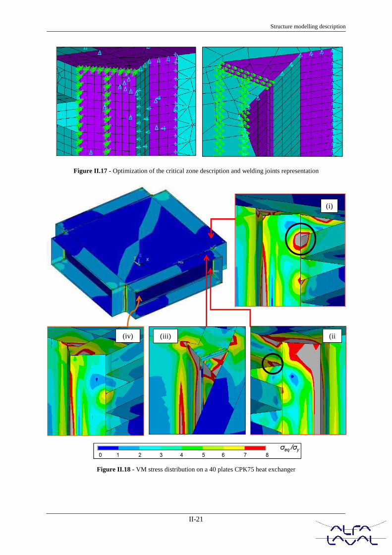
Structure modelling description
II-21
Figure II.17 - Optimization of the critical zone description and welding joints representation
Figure II.18 - VM stress distribution on a 40 plates CPK75 heat exchanger
(i)
(ii(iii) (iv)

Thermo-mechanical modelling and durab
II.6. First validation
II.6.1. Exchanger design
A first thermal fatigue test on a m
at the Thermal Product Test Cen
CPX120 made of 120mm edge w
moment, it was the only availab
design was different from the one
taken into account by geometr
exchanger denomination) implie
this way, the current anisotropic
stress distribution. The predicti
measurement on a real exchanger
model being represented in Figu
circulating in the exchanger, the
can be thus expected, allowing
comparison. Two alternated hot
cold water (12°C) during two cyc
temperature and the time set to
prescribed (cf. Figure II.20).
II.6.2. Boundary conditio
The goal of this thermal analysi
compared to the core, relating bo
here in recording the temperature
panels. As described in Figure
channels. In the case of the we
directly in front of the flow (T
thermocouples (Th. 5 and 6) resp
has allowed to make the compari
in contact with the fluid whereas
The system obviously losing he
temperature lower than one of the
thick frame panel sides will be ve
rability analysis of welded heat exchangers
II-22
on of the 3D FE model
gn and thermal fatigue test introducti
a macroscopic prototype has been prepared by the
enter of Alfa Laval Lund AB. The heat exchang
e with only 1 pass, i.e. a single hot/cold circuit, an
ilable exchanger suggested by Alfa Laval, but un
one studied until now. If the sizes and thickness var
etrical parameters involved in the modelling, th
lies another corrugations pattern with a slight diff
ic material definition will assume to not have so m
ictions of the 3D FE model have been then
ger subjected to a simplified thermal fatigue load, th
igure II.19. Only one of the 2 channels has been
e second remaining dry. A more uniform temperat
ing a simpler application of a thermal loading
t flow (80°C, maximum temperature allowed by th
cycles of time will be considered. The test has been
to change from cold to warm temperature and
itions justification by local temperatu
ysis is to justify the assumption of a thermal inert
boundary conditions with a rigid frame. In this wa
ure variations in specific locations between thin pl
re II.21, 10 thermocouples have been welded in
wet channel, there are 2 main measurement point
Th. 1 and 2) in order to observe core temperat
espectively located in the internal and external sid
arison with the frame temperature variation. The in
as the external is totally submerged in the air at room
heat in duty, the external side of the frame will
the hot after a certain. As a consequence, the veloc
very low. To conclude concerning the thermal ine
ction
e Lars Fogelberg team
nger tested has been a
and 20 plates. At this
unfortunately the core
variations can be easily
the “X” (in the heat
different anisotropy. In
much influence on the
compared to strains
, the corresponding FE
en used to make fluids
rature field distribution
g for the mechanical
the strain gauges) and
een performed at room
nd inversely has been
ture analysis
ertia of the frame part
way, the study consists
plates and thick frame
in both wet and dry
ints on the plate pack
rature rise. Two other
side of the frame panel
internal one is directly
oom temperature.
reach an asymptotic
locity variation of these
nertia of the frame part

Structure modelling description
II-23
and the possibility to consider it rigid at the onset of the transient regime, it is necessary to point out
the time needed for this last one to start the temperature increase and to reach its maximum.
Figure II.19 - Finite element model of the prototype structure tested in Alfa Laval Lund AB
Figure II.20 - Mean thermal load in the plate pack
Or
B side - Dry channel A side
Temp. (°C)
Time (min)
0 30 60 …. 12
80 Hot water
Water
105

Thermo-mechanical modelling and durab
Fig
Figure II.22 - Temperature varia
Temperature variation of thermo
side of the frame panel) and 6 (in
green straight lines are related to
thermocouple 1 shows a very q
temperature in less than 30 seco
10
15
20
25
30
35
40
45
50
55
60
65
70
75
80
85
3 780 3 810 3 840 3 870
Te
mp
era
ture
in
°C
Platepack
Panel
∆tinertia
e
Core at thot fluid T
rability analysis of welded heat exchangers
II-24
igure II.21 - Locations of the thermocouples
riation on the plate pack and on the internal/external side
ocouple 1 (directly in front of the flow on the pla
(internal side of the frame panel) are considered in F
to both cold and hot fluid temperature, respectively
quick temperature increase of the plate pack, re
conds. Although, thermocouple 5 seems to begin
3 900 3 930 3 960 3 990 4 020 4 050 4 080 4 110 4 14
Time in s
Dry channel
B side
Flow direction
ate ck
Head
Internal side of the frame
tia
Plate pack
Beginning of the frame e
t the d T°C
External side of the frame
ide of the frame panel
plate pack), 5 (internal
Figure II.22. The two
ely 12 and 80°C. Thus
reaching the maximal
in to react in the same
4 140 4 170 4 200
T1 (°C)
T5 (°C)
T6 (°C)
e expansion

Structure modelling description
II-25
time, even a little bit sooner (probably due to the quick contact of the fluid with the thermocouple), the
growth is then clearly slighter. Progressively, this internal frame temperature will reach the maximal
one in an asymptotical way. This conduction velocity is even slower considering thermocouple 6 in
the external side of the frame part, panels thickness here assuming to play a non-negligible role in the
thermal transfer process. Starting from the room temperature as the exchanger being not insulated,
thermocouple 6 exhibits an onset of increase about two minutes after the thermocouple 1 reached its
maximum temperature. In addition, the analysis of the full temperature cycle in appendix show that
this temperature need more than 45 minutes to stabilize at a value of 70°C, when the internal side
takes almost 20 minutes to reach the thee hot fluid temperature. Thus, if the strongest frame effect on
the core occurs in fact in the earliest stages of the transient regime, this kind of loading on this
exchanger design shows that “papillotes” will be loaded in a decreasing magnitude during almost 45
minutes. In any cases, this time interval corresponding to the thermal inertia of the frame is
sufficiently important to suppose a totally rigid frame part in the earlier moments of duty. In this way,
it seems to be realistic to avoid the frame part consideration the FE exchanger modelling by directly
taking into account its reaction with rigid boundary conditions as reported in Figure II.15.
Figure II.23 - Zoom on the (ii) strain gauges dposition according to (i) the stress distribution
II.6.3. Validation of the FE model
II.6.3.1. Location of the strain gauges
From the observation of the existing thermal inertia of the frame and supposing boundary conditions
reported in Figure II.15, strains recorded in duty by specific strain gauges placed at appropriated
locations (cf. Figure II.23) with numerical strains predicted by the finite element simulation can now
be compared. Figure II.23 shows (ii) the position of 5 Gauges (Rosette of 3 elements, type FRA-1-17-
x
y x1
45°
G1 G2
G4 G3
G5
H/4
H/21

Thermo-mechanical modelling and durab
5L) recording strains along 3 di
previous local stress distribution o
far from the corners to prevent zo
where stresses concentrate, gauge
heterogeneity reported in the prev
The three others have been posi
gauges 2 and 4 are thus located a
plate. However, only three gauge
along the “papillotes” (number 1
middle of the pass. Local strains
Figure II.24 for two cycles of he
by a sharp variation of the stra
discrepancy along x axis in gaug
cycle in gauge 3.
-0,08
-0,06
-0,04
-0,02
0
0,02
0,04
0,06
0,08
0,1
0,12
0,14
0 1 200
Loca
l st
rain
ε
(%)
Instabilialong x a
Heat cyc
rability analysis of welded heat exchangers
II-26
directions in a plane described on the same pictu
n observation, two of them are located in the vicini
zones of possible high plasticity gradient. Howeve
uges 1 and 3 are expected to give insight of the ma
revious thermo-elastic calculations.
ositioned on other locations where less deformati
d along the column liner, when the gauge 5 has be
ges have been able to give exploitable results. Two
r 1 and 3) and one another (number 2) located
ins variation as a function of the time at the three
heating/cooling. The change of fluid temperature i
train intensity. A first observation of the results
uge 1 and a sudden sharp growth of the y strain in
2 400 3 600 4 800 6 000 7 200
Time (s)
Gauge
bility x axis
ycle Cooling cycle
cture. According to (i)
inity of the “papillotes”
ver located in the zone
magnitude of the stress
ation is expected. The
been glued on the end
wo of them are situated
on the profile in the
ee locations is depicted
e is clearly remarkable
lts pertinence shows a
n in the second heating
8 400
1X [%]
1Y [%]
1Z [%]
ge 1 (i)

Structure modelling description
II-27
Figure II.24 - Local strain gauges for 1, 2 and 3
-0,03
-0,02
-0,01
0
0,01
0,02
0,03
0,04
0,05
0,06
0,07
0,08
0,09
0 1200 2400 3600 4800 6000 7200 8400
Loca
l st
rain
ε
(%)
Time (s)
2X [%]
2Y [%]
2Z [%]
-0,04-0,02
00,020,040,060,08
0,10,120,140,160,18
0,20,220,240,260,28
0 1 200 2 400 3 600 4 800 6 000 7 200 8 400
Loca
l st
rain
ε
(%)
Time (s)
3X [%]
3Y [%]
3Z [%]
Gauge 2 (ii)
Gauge 3 (iii)
Instability along y axis
Full cycle

Thermo-mechanical modelling and durab
Figur
-0,18-0,16-0,14-0,12
-0,1-0,08-0,06-0,04-0,02
00,020,040,060,08
0,10,120,140,160,18
0,20,220,240,26
0 1200
Pri
nci
pa
l st
rain
(%
)
-0,06-0,05-0,04-0,03-0,02-0,01
00,010,020,030,040,050,060,070,080,09
0,10,110,120,130,14
0 1200
Pri
nci
pa
l st
rain
(%
)
-0,08-0,06-0,04-0,02
00,020,040,060,08
0,10,120,140,160,18
0,20,220,240,260,28
0 1200
Pri
nci
pa
l st
rain
(%
)
Three εL for the co
Three εfor the
rability analysis of welded heat exchangers
II-28
ure II.25 - Principal strain for gauges 1, 2 and 3
2400 3600 4800 6000 7200 840Time (s)
2400 3600 4800 6000 7200 840
Time (s)
2400 3600 4800 6000 7200 840
Time (s)
Gauge 1
Gauge 2
Gauge 3
values used e comparison
Three εL values used for the comparison
e εL values used he comparison
8400
εL1
εT1
8400
εL2
εT2
8400
εL3
εT3
e 1 (i)
2 (ii)
3 (ii i)

Structure modelling description
II-29
II.6.3.2. Strain variation analysis and processing
A cycle of heating up to 80°C and cooling down to 13°C is represented and repeated one time in
Figure II.24. The three gauges points out a first steep variation of the strain response followed by a
plateau. This sequence is clearly reproducible for the gauge 2. Regarding the gauge 3, each branch of
the variation is quantitatively comparable although no plateau is observed in the second cycle. For the
gauge 1, the two branches along the vertical and horizontal direction are reproducible, not hat at 45° in
blue. The records of the first cycle are expected to be reliable, the cyclic repetition of the fluid flow
being able to have damaged the gauges 1 and 3. Form these experimental records in Figure II.24, the
components of the plane principal strain have been derived in Figure II.25 by the methodology
described in appendix. The longitudinal component is given in blue when the transverse in red.
The first graphic (i) shows the strain variation for the gauge 1 located on the “papillotes” in the middle
of the pass. The different response between the two temperature rises is here confirmed, the two
components showing diverging variation in each cycle. During both heating and cooling, the two
principal strains seem to reach quasi instantaneously a plateau. Regarding the gauge 3 (iii) located on
the “papillotes” closed to the end plate (cf. Figure II.23), the second heating cycle still shows some
non-stable response. It is nevertheless interesting to point out the similar response (in intensity and
curvature) between gauges 1 and 3 despite the instability picks noticed for gauge 1 during cycle 1. The
gauge 2 located on the column liner in the middle of the pass near the junction with the “papillotes”
still exhibits a comparable variation during the two cycles. This can be explained by the particularity
to point out no more longitudinal strain during cooling, as an elastic comeback to the initial stage.
Whatever the gauges considered, the transient regimes clearly underline a steep strain variation related
to the cyclic thermal load. Three points circle for each gauges in Figure II.25 are used for the
comparison. The minimal and maximal values delimit the error bar around a medium value supposed
to be the most representative. Having now introduced a way to carry out a comparison from the
experimental results analysis with the predictions, Figure II.26 gives a procedure to read representative
equivalent numerical strain concerning gauges 1 and 3. Thus, mesh size analysis is introduced to study
more carefully its influence on the local response in the critical zones.
II.6.3.3. Comparison with the FE predictions and discussion
Two types of “papillote” mesh are presented here among the 3 tested to analyse their influence on the
mechanical response (cf. Figure II.26). The first one used until now is noted A, the structure definition
being then refined two times to make the mesh case B, and again 2 times to obtain finally mesh case
C. Considering each mesh size, a green region represents the zone covered in the experiment by the
gauge 1 or 3. It takes respectively into account 9, 25 and 81 nodes for mesh cases (A), (B) and (C)
mesh.

Thermo-mechanical modelling and durab
Figure II.26 - Di
The longitudinal strain calculate
presented in red in Figure II.27
average value of the respective p
been extracted across an area corr
maximal strain compared to the a
abscissa, is represented the gaug
were available concerning the c
experimental value, points 3 and
corrugations direction and in th
second case therefore its possibl
mean value and interval of the rec
II.25) are reported in blue in Fig
the comparison.
The experimental values are glob
while the predicted range varys
column liner (not depending of
experimental one (almost 0.15
observation can be explained by
“papillote”, thus involving no cy
close to the corners where a stre
having a look at the values distrib
situated far from the (numerical)
to it. In this way, if the minimal
experiment (always for gauge 1
gives additional difficulty to
perpendicular direction of the end
Meshing A Element size = 1.25mm
rability analysis of welded heat exchangers
II-30
Different mesh refinements used to describe the “papillo
lated from each mesh refinement of the green z
27 for the comparison. For each gauges dependi
e principal strains and its standard deviation for th
orresponding of the gauge surface. The difference b
e average value corresponds to one time the standa
uge number from 1 to 3. Concerning gauge numb
corrugations orientation of the closer end plate.
nd 4 respectively make the comparison with the pr
the opposite one. The stress concentration actual
ible influence is examined here. Regarding the ex
recorded principal strains (corresponding to circles
igure II.27. In all cases, the major principal strain
lobally smaller than the predicted one. Their avera
ys from 0.15 to 0.50%. The prediction for the gau
of the mesh refinement or corrugations direction)
15 versus 0.10%). As previously shown in Fig
y the fact that this region points out no strain grad
cyclic hardening effect. On the contrary, those for
tress concentration is observed exhibit a larger di
tribution at each nodes, the ones presenting relative
al) welded joint, the strains appearing to increase s
al numerical value is of the same order of magnit
1 and 3), strain heterogeneity implying a certain
o make a representative comparison. Gauge 3
nd plate shows a slight higher strain level.
Meshing B
Element size = 0.65mm
illote”
n zone is respectively
nding of the mesh, an
the interval error have
e between minimal and
dard deviation. On the
mber 3, no information
te. Therefore the same
prediction taken in the
ually maximum in the
experimental part, the
les introduced in Figure
ain εL is considered for
erage is around 0.10%
gauge 2 located on the
) is very close to the
Figure II.25 (ii), this
adient compared to the
for the gauges 1 and 3
discrepancy. Actually,
ve good agreements are
e sharply getting closer
nitude compared to the
ain incertitude interval
3 positioned in the

Structure modelling description
II-31
Figure II.27 - Comparison of experimental and predicted first principal strain
for the 3 meshing refinements (i) A, (ii) B and (iii) C of the green zone
0,00
0,05
0,10
0,15
0,20
0,25
0,30
0,35
0,40
0,45
0,50
0,55
0,60
0,65
0,70
1 2 3 4
ε1
(%
) A
Gauge number
Mean FEA
Mean meas.
0,000,050,100,150,200,250,300,350,400,450,500,550,600,650,700,750,800,85
1 2 3 4
ε1
(%
) B
Gauge number
Mean FEA
Mean meas.
0,000,050,100,150,200,250,300,350,400,450,500,550,600,650,700,750,800,850,90
1 2 3 4
ε1
(%
) C
Gauge number
Mean FEA
Mean meas.
Meshing C (ii i)
Meshing A (i)
Meshing B (ii)

Thermo-mechanical modelling and durab
Figure II.28 - Com
for 2 meshi
Comparing different meshing cas
heterogeneity is also observed. A
value as well as its heterogeneity.
the welded joint, certainly due to
Figure II.26 also introduces a way
the welding zone in order to get b
refinement is also carried out on m
heterogeneity as possible uncerta
more than 30% per cent for gauge
0,00
0,05
0,10
0,15
0,20
0,25
0,30
0,35
0,40
0,45
0,50
0,55
0,60
1
ε1
(%
) B
0,00
0,05
0,10
0,15
0,20
0,25
0,30
0,35
0,40
0,45
0,50
0,55
0,60
1
ε1
(%
) C
Meshing C (v)
Meshing B (iv)
rability analysis of welded heat exchangers
II-32
omparison of experimental and predicted first principal s
shing refinements (iv) B and (v) C of the yellow zone
cases (A), (B) and (C), a clear influence of the refin
Actually, decreasing mesh division size tends to
ity. This one can be so explained by a sharp increas
to the use of tie displacement to take it into consid
ay to reduce the interested region size by removing
et back the yellow zone for meshing B (9 nodes). T
n meshing C (25 nodes) allowing to take into accou
rtainty about gauges position (cf. Figure II.28). The
uges 1 and 3 in Figure II.28 (iv) compared to Figure
2 3 4Gauge number
2 3 4Gauge number
)
al strain
finement on the strains
to increase strain mean
ase of the strains along
sideration. In this way,
ing the nodes closed to
The same region size
count strain distribution
he strains decreased of
ure II.27 (ii).
Mean FEA
Mean meas.
Mean FEA
Mean meas.
Structure modelling description
II-33
If tied displacements can model in a strong way the welded joint, in practice forces transfer between
frame and plate pack through these ones can explain additional local dropped strains. It is important to
remind that residual stresses due to the welding process could also been involved although it is here
difficult to give a rough idea of their value. In any cases, if the gauge located in the perpendicular
corrugations direction still shows higher strain intensity, considering values a little bit far from the
welded joints implies lower heterogeneities more in adequacy with experimental results. A lower
influence of the mesh refinement is finally observable as a slight diminution of the mean value
intensity is detectable in Figure II.28.
II.6.3.4. Possible origins of the discrepancy
In this part, the features potentially responsible for the discrepancy between experimental and
predicted results are discussed. Even firstly considering the lower experimental values in the Figure
II.27 and Figure II.28, the first thing to note is that plasticity appears to be already involved in the
“papillotes” for this kind of thought “light” loading. As expected, material model used were not
adequate for this study in a first approach justifying its first coarse introduction in the last graph (vi).
This observation naturally implies the necessity to describe the real behaviour of rolled 316L steel
under cyclic plastic loading.
The thermal loading used in the FE simulation can also have a particular influence in regions closed to
the frame as the column liner. If experiment conditions have been thought to make the thermal loading
as uniform as possible, recorded temperature variations close to the end plate show that the thermal
field does not reach the maximal value (80°C). Actually thermocouple 9 precisely situated in the dry
channel (between the end plate and the top panel Figure II.21) shows a very slow temperature growth
during hot fluid circulation (cf. appendix). Whereas plate pack has already reached 80°C in the earlier
critical stage, temperature there has only increased of 5°C reaching a maximum of 30°C at the end of
the transient regime. Thus, it would have been interesting to make the fluid flowing directly in contact
with the end plate. Actually, it implies that the uniform thermal loading considered in the corner of the
numerical study should overestimate the real fluid temperature there and globally in the whole dry
channel. This phenomenon is even more expected on the column liner situated in this channel,
exhibiting no temperature variation due to its contact with the cold girder. It could be so explained the
high numerical mean value of the local strain in the “papillote”. In this way column liner in contact
with the girder could also show a slighter increase of the temperature and probably a lower
temperature would have to be applied there.
Numerical strain heterogeneity in the corners has been also identified as a possible explanation of
intensities overestimation. In fact, the gauges in this location are covering a region with possible high
strain gradient between two nodes side by side, implying local magnitude beyond the range of the
gauge.

Thermo-mechanical modelling and durab
II.6.3.5. Conclus
Faced to the low strains involved
of the structure reaction in servi
material description influence in
to be performed to confirm thes
corresponding exchanger type or
solicited. As doubt remains co
numerical strain heterogeneity, th
The comparison between the exp
acceptable for gauge 1 and 3. In
concentration other different par
plates manufactured with a slight
here, inducing a change in the pl
exchanger involved thicker plate
material parameters evolution. I
previous thermal fatigue test for
hardened. Finally coming back
hypothesis used to determine them
be complete, these ones have be
(along z axis) blue zone (excepted
rability analysis of welded heat exchangers
II-34
lusion is this first thermal test
ed in this study, FEM seems to have reached a relat
rvice, at least in a monotonic loading case here. B
in the structure response, more experimental fatigue
hese relative good results, as simply firstly carryi
or utilizing the good channel to make the end plate
concerning the accurate gauges dispositions in
his first comparison, can be taken as very encoura
xperiments and the predictions is good for gauge 2
In this case some discrepancy is observed that can
arameters. Actually, the heat exchanger CPX120
htly different corrugation pattern compared to the “
plate rigidity reaction on the “papillotes”. In additi
ates (1,2mm) meaning a different rolling strain and
It is also necessary to note that this prototype
for another project application, probably inducing
ck to the boundary conditions and their strong
hem has been so validated during the first paragraph
been then updated thanks to this analysis by int
ted orange and black lines) of the end plate (cf. Fig
lative good description
Before characterising
gue tests need naturally
rying out a test on the
ates (and corners) more
in addition to a high
raging.
e 2, as some points are
an originate from stress
0 is also composed of
e “K” form considered
dition, this type of heat
and an eventual elastic
pe had been used in a
ing a material already
g influence, the main
aph of this part II.6. To
introducing move free
igure II.15).

Structure modelling description
II-35
Figure II.29 - 40 plates CP75 prototype
II.7. Second thermal test for evaluating the FE model
II.7.1. Design of the prototype and test specifications
The design of the tested unit is this time a 40-plates CPK75 prototype (cf. Figure II.29). As the
previous test, the heat exchanger is subjected to a Steam /Water thermal load imposed at the A-Side
(cf. Figure II.19). The test has been also performed at room temperature at the Thermal Products Test
Centre of Alfa Laval Lund AB. If localization of the fatigue failure and the corresponding number
cycle at which it occurs is the main goal of this test (cf. Chapter 3), the objective is also to verify the
model developed in a configuration closer to one taken into account.
The cyclic thermal loading has been conducted as shown in Figure II.30. One test cycle includes the
heat up with a 180°C steam during 20 minutes and the cooling down to 15 °C (with the same ramp)
during one half hour, separating by 20 seconds of draining or emptying. Being able to carry out a cycle
of maximum 50 minutes, both heat and cooling length have been chosen in order to allow to reach
temperature stabilization of the frame part (referring to the last thermal analysis in Figure II.22). This
aspect is actually mandatory to make sure that the heat exchanger solicitations in service are respected.
A-side have been this time chosen to involve end plates in contact with the fluid in order to be as
closed as possible of a homogeneous thermal field for the future comparison with the prediction.
Five strain gauges have been glued along the “papillotes” in the dry circuit (cf.
Figure II.31) allowing measurements in the same 3 directions than the previous thermal fatigue test.
Their positions have been chosen to allow a more accurate appreciation of strain variation in the

Thermo-mechanical modelling and durab
“papillote” plane. In Table II.4,
numbering.
Figur
Figure II.31
Plates number
Table II.4 - Accu
Actually among a total of 38 in t
corrugations of the closest end pl
more interesting to put gauges on
with critical zone pointed out in
there in practice therefore they ha
Temp. (°C)
13
180
Y
rability analysis of welded heat exchangers
II-36
, gauges location is reported along z axis as a f
ure II.30 - Mean thermal load in the plate pack
- Location of the 4 strain gauges along the “papillote”
Gauge 1 Gauge 2 Gauge 3 Gau
2/38 6/38 18/38 37
ccurate gauges position as a function of the plate number
n the core, numbering starts inside the top end plat
plate is in the perpendicular direction. It could hav
one and five respectively at the level 1/38 and 38/3
in Figure II.18. Due to manufacturing reasons, no
have been moved at the level of the plate just nea
Tim
0 20 50
Steam
Water
X
Z
Gauge 1
Gauge 2
Gauge 3
Gauge 4
a function of the plate
te”
auge 4
37/38
bering
late corner from which
have been nevertheless
8/38 to be in adequacy
no place was available
earby. In addition, five
ime (min)

Structure modelling description
II-37
thermocouples have been respectively welded closed to each strain gauge and 10 other in the rest of
the exchanger to confirm the graph obtained in Figure II.22.
-0,10
-0,08
-0,06
-0,04
-0,02
0,00
0,02
0,04
0,06
0,08
0,10
0,12
0,14
0,16
0,18
0,20
0,22
0 300 600 900 1 200 1 500 1 800 2 100 2 400 2 700 3 000 3 300 3 600
Loca
l st
rain
(%
)
Time (s)
X [%]
Y [%]
X1 [%]
Gauge 1 (i)

Thermo-mechanical modelling and durab
Figure II.32 - Expe
-0,080
-0,065
-0,050
-0,035
-0,020
-0,005
0,010
0,025
0,040
0,055
0,070
0,085
0,100
0,115
0,130
0,145
0 300 600 900
Loca
l st
rain
(%
)
-0,06
-0,05
-0,04
-0,03
-0,02
-0,01
0
0,01
0,02
0,03
0,04
0,05
0,06
0 300 600 900
Loca
l st
rain
(%
)
rability analysis of welded heat exchangers
II-38
perimental local strains for gauges 1 & 4 closed to the co
900 1 200 1 500 1 800 2 100 2 400 2 700
Time (s)
X [%]
Y [%]
X1 [%]
900 1200 1500 1800 2100 2400 2700
Time (s)
X [%]
Y [%]
X1 [%]
Gauge 4 (
Gauge 2 (
e corners
3 000 3 300 3 600
X1 [%]
3000 3300 3600
X [%]
Y [%]
X1 [%]
4 (ii)
2 (i)

Structure modelling description
II-39
Figure II.33 - Experimental local strains for gauges 2 & 3 far from the corners
II.7.2. Results analysis
In Figure II.32 and Figure II.33, strain variation recordings during the heating and cooling of the first
cycle are reported respectively for gauges 1 and 4, then 2 and 3. For each gauge, the three curves
correspond to the three axis x, y and x1 with (x,y) = 90°, (x,x1) = 45° = (x1,y), x and y approximately
belonging along the horizontal and vertical direction. It is worth noting that during the heating cycle,
no plateau is reached for any gauge neither one of their component. This is likely due to a sequence of
heating the core with the frame remaining cold, showing a temperature progressively increasing. Thus
the magnitude of the strain record during the first transient regime has been used. The values reported
here do not account for a temperature dependence and only the strain gauge factor is considered.
Figure II.32 also point out the expected difference of behaviour thanks to the corner position faced to
the corrugations orientation of the end plate. If in the perpendicular orientation, papillote is more able
to deform along its x length, y strain show a lower intensity. It is nevertheless difficult here to make
any parallel of strains variation with the previous thermal fatigue test in Figure II.24 due different
gauges position except possibly gauge 3. In this case, the behaviour seems to differ completely
supposing that too much discrepancies are involved between both experiments to point out an eventual
correlation. Actually, exchanger size, plate thickness, corrugations pattern, thermal loading and
particularly plates number have evaluated since the last time. The involved plate number could be the
-0,17
-0,155
-0,14
-0,125
-0,11
-0,095
-0,08
-0,065
-0,05
-0,035
-0,02
-0,005
0,01
0,025
0,04
0,055
0,07
0 300 600 900 1 200 1 500 1 800 2 100 2 400 2 700 3 000 3 300 3 600
Loca
l st
rain
(%
)
Time (s)
X [%]
Y [%]
X1 [%]
Gauge 3 (ii)
Thermo-mechanical modelling and durab
parameter the most influencing he
in the last experiment, considerin
the “papillote” is able to show a l
In Figure II.34, principal plane st
magnitude ranges from 0.00 to 0.
to -0.12% (i), 0.00 to 0.17% (ii) f
mean and interval error values u
evolution, almost no recording in
gauge 4 (representative of the c
quickly after the first steep decre
start-up of the unit carried out in
exchanger working. On the contr
way after a first pick at the begi
maximal absolute value soon af
corners situated in the perpendic
another transient effect in a seco
life durability process as 316L ste
locally a strain amplitud
Unlike gauge 4, only a small co
reversed strain path necessary to
reached from a certain time of co
detrimental influence in the corn
localization. Figure II.34 also ex
globally the same evolution at a lo
rability analysis of welded heat exchangers
II-40
here. Keeping in mind similarities between the thre
ring an exchanger with a higher plate number here
a less constraint response far from the corners.
strains variations are reported for the gauges 1, 4 (
0.20% (i), 0.00 to 0.09% (ii) for the maximal comp
for the minimal component. The circles reported h
s used for the comparison with the prediction. Ana
instability is observed for the four gauges. Principa
corner situated in the corrugation diagonal) show
crease. Thus after the first stages of the transient
in the reality), this corner seems to show no much
ntrary, the gauge 1 points out strain state still vary
eginning of the heating. Both curves seem also to
after the end of the hot fluid circulation. In this
dicular direction to the corrugations of the end p
cond stage. This second step of strain increase is
steel described by a hardening composed of part (cf
tude still increasing during the full
compressive state remains after a small strain rela
to imply cyclic effect in the low cycle fatigue p
cold fluid circulation. Thus, inertia frame effect se
orner closed to the gauge 1, according to the su
exhibits results for gauges 2 and 3 in graph (ii)
a lower intensity level.
three gauges recordings
ere seems to show that
4 (i) and 2, 3 (ii). Their
mponent and from 0.00
d here also indicate the
nalysing globally data
ipal strains variation of
hows stabilization very
nt regime (or once the
uch reaction due to the
rying in an asymptotic
to potentially reach an
this way, relaxation of
plate seems to imply
is not negligible in the
(cf. Chapter 3) implied
ull heating cycle.
elaxation meaning that
e process seems to be
t seems to have a more
supposed critical zone
(ii). Here strains show

Structure modelling description
II-41
-0,13
-0,11
-0,09
-0,07
-0,05
-0,03
-0,01
0,01
0,03
0,05
0,07
0,09
0,11
0,13
0,15
0,17
0,19
0,21
0 300 600 900 1 200 1 500 1 800 2 100 2 400 2 700 3 000 3 300 3 600
Pri
nci
pa
l st
rain
(%
)
Time (s)
EL1
ET1
EL4
ET4
-0,17
-0,15
-0,13
-0,11
-0,09
-0,07
-0,05
-0,03
-0,01
0,01
0,03
0,05
0,07
0,09
0,11
0 300 600 900 1 200 1 500 1 800 2 100 2 400 2 700 3 000 3 300 3 600
Pri
nci
pa
l st
rain
(%
)
Time (s)
EL2
ET2
EL3
ET3
Three εL values used for the comparison for each gauges
Three εL values used for the comparison for each gauges
(ii)
(i)
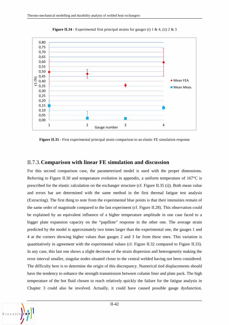
Thermo-mechanical modelling and durab
Figure II.34 - Exper
Figure II.35 - First experime
II.7.3. Comparison with
For this second comparison cas
Referring to Figure II.30 and tem
prescribed for the elastic calculat
and errors bar are determined
(Extracting). The first thing to no
the same order of magnitude com
be explained by an equivalent i
bigger plate expansion capacity
predicted by the model is approx
4 at the corners showing higher
quantitatively in agreement with
In any case, this last one shows a
error interval smaller, singular no
The difficulty here is to determin
have the tendency to enhance the
temperature of the hot fluid chos
Chapter 3 could also be invol
0,00
0,05
0,10
0,15
0,20
0,25
0,30
0,35
0,40
0,45
0,50
0,55
0,60
0,65
0,70
0,75
0,80
1
ε1
(%
)
rability analysis of welded heat exchangers
II-42
perimental first principal strains for gauges (i) 1 & 4, (ii)
mental principal strain comparison to an elastic FE simu
h linear FE simulation and discussion
case, the parameterized model is used with the
temperature evolution in appendix, a uniform temp
lation on the exchanger structure (cf. Figure II.35 (
d with the same method in the first thermal f
note from the experimental blue points is that their
ompared to the last experiment (cf. Figure II.28). Th
t influence of a higher temperature amplitude in
ity on the “papillote” response in the other one
oximately two times larger than the experimental o
er values than gauges 2 and 3 far from these on
ith the experimental values (cf. Figure II.32 compa
s a slight decrease of the strain dispersion and heter
nodes situated closer to the central welded having
ine the origin of this discrepancy. Numerical tied d
he strength transmission between column liner and
hosen to reach relatively quickly the failure for th
olved. Actually, it could have caused possible
2 3 4Gauge number
(ii) 2 & 3
ulation response
ion
he proper dimensions.
mperature of 167°C is
(i)). Both mean value
l fatigue test analysis
eir intensities remain of
This observation could
in one case faced to a
ne. The average strain
one, the gauges 1 and
ones. This variation is
pared to Figure II.33).
terogeneity making the
g not been considered.
d displacements should
nd plate pack. The high
the fatigue analysis in
le gauge dysfunction.
Mean FEA
Mean Meas.

Structure modelling description
II-43
However, a high temperature can potentially increase the thermal field heterogeneity, making the
uniform temperature loading used in the calculation sufficiently coarse to cause these discrepancies.
The assumption of a linear elastic response is finally also questionable.
II.7.4. Thermal tests summary
Two thermal fatigue tests have been performed to evaluate the heat exchanger structure model for
simplified configurations. The record of the temperatures variation between the plate pack and the
frame during thermal cyclic loads has evidenced a thermal inertia between these two parts, the panels
reaction being always deleted in time. This observation has especially motivated the use of fixed
displacements at the core - frame boundary, preventing the consideration of this last one in the
modelling. Strain gauges measurements mainly located at different places along the “papillotes” have
been compared to numerical prediction obtained by the FE model. For the two validation tests
performed during this work, the comparison between the measures and the numerical results
quantitatively in agreement. The magnitude of the strains on the “papillotes” is maximum near the
corners and minimum in the center of the plate pack. To some extent, these are quantitatively in
agreement with the experiments. Thus, thanks to the thermal analysis, the boundary conditions seem to
be able to reproduce the “papillote” response at least far from the corners. If corners often show high
values dispersion, high strain concentration is globally also observed, potentially consistent with the
analysis of the Trouble Shooting Department from Alfa Laval Vicarb.
The discrepancy between measures and predictions can originate in an over simplified temperature
loading, mainly in the second case which is likely to be non-uniform. Details related to the description
of the welded joints have also shown to induce large heterogeneities in the estimation of the
deformation, tied displacements representing a relative conservative and rigid way to consider them. It
is finally important to keep in mind that the goal of the parts II.6 and 0 was to validate structural
behaviour of the heat exchanger structure without particularly utilizing a thermal load. If experiment
have been designed to make the temperature distribution as uniform as possible, it has been pointed
out that it is not really the case, mainly in the dry channel. This point has previously been expected to
be at the origin of the potential divergence in the corners. A potential way to get round of this problem
should have to make circulating alternatively hot and fluid in the two channels. However, the
modelling of the structure presented here is shown useful as a marker of regions where stress
concentrates and where damage and failure are expected. This requires a realistic description of the
elastic-plastic response of the material and the use of a specific criterion for failure to be presented in
the sequel.

Local material behaviour in a low cycle fatigue regime
III-1
III. LOCAL MATERIAL BEHAVIOUR IN A LOW CYCLE
FATIGUE (LCF) REGIME
The region of the exchangers where the stress concentrates are now identified in the analysis of the
structure reported in Chapter 1. In the present part, the elastic-plastic mechanical response of the 316L
steel under consideration I identified with the use of combined isotropic and kinematic hardening. An
energy equivalent method is proposed to estimate the magnitude of the equivalent plastic deformation
from the analysis at the level of the structure. This estimation is used to predict the exchanger life from
a Manson-Coffin criterion identified in the low cycle fatigue regime. The prediction is finally
compared to available experimental data.

Thermo-mechanical modelling and durab
III.1. Table of co
III. Local material behaviour
III.1. Table of contents .....
III.2. Identification of the p
III.2.1. Combined hardeni
III.2.2. Hardening parame
III.2.3. Results and discus
III.3. Numerical response u
III.3.1. Hardening model i
III.3.2. Investigation of th
III.4. Identification of a low
III.4.1. LCF model introdu
III.4.2. Experimental proc
III.4.3. Alternated four po
III.4.4. Account for the ro
III.4.5. Experimental iden
III.5. Fatigue lifetime pred
III.5.1. Introduction of a d
III.5.2. Comparison of the
III.6. References ...............
rability analysis of welded heat exchangers
III-2
f contents
ur in a low cycle fatigue (LCF) regime.....................
...................................................................................
e plastic material response .......................................
ening characterization ...............................................
meters identification .................................................
ussion .......................................................................
se under elementary loads .........................................
el implementation in ANSYS software ....................
the material response for a simple case study .........
low cycle fatigue life model .....................................
oduction ....................................................................
rocedures ...................................................................
points bending for numerical LCF characterization
rolls in the FE analysis of the cyclic bending test ...
entification of the LCF criterion ..............................
ediction of the exchanger .........................................
a durability prediction methodology.........................
the final prediction with the 2nd thermal fatigue test
...................................................................................
.............................. III-1
.............................. III-2
.............................. III-3
.............................. III-4
.............................. III-4
.............................. III-6
.............................. III-8
.............................. III-8
.............................. III-8
............................ III-13
........................... III-13
.......................... III-13
on ........................ III-14
.......................... III-16
............................ III-21
............................ III-23
............................ III-23
st ........................ III-25
............................ III-27

Local material behaviour in a low cycle fatigue regime
III-3
III.2. Identification of the plastic material response
Compact welded heat exchangers are designed to be used in severe operating conditions (temperature,
pressure and aggressive fluid for instance). Fatigue failure has been observed after relatively low cycle
number (less than 1000 in laboratory tests). Thus the assumption that large cyclic strains due to
thermo-mechanical cyclic loads seems to be valid and the description with an elastic-plastic
constitutive law appears to be necessary to consider stainless steel sheet of one 1mm thickness. In this
way, a combined non-linear hardening model for rate independent plasticity has been identified. This
material model accounts for an isotropic hardening characterized by a Voce formulation and a
kinematic part based on a Armstrong-Fredericks description (1966) [1]. It presents the advantage to
have a popularity making this model already implemented in several commercial finite element codes.
Within the framework of generalised standart material presented by Lemaitre and Chaboche [1] and
related normality rules, the rate independent description of plasticity is based on the yield surface
���, �, �� = �� − ���������� − ���� − � (3.1)
where σY is the initial yield stress, R�p� the isotropic hardening, p the cumulated plastic strain, XXXX the
kinematic hardening and σσσσ denoting the equivalent Von Mises stress √3��. The response would be
elastic for � < 0, � = 0 and �� = 0 defining the conditions for plasticity. The Voce formulation for the
isotropic hardening is
���� = ���1 − �� !" (3.2)
�� and b being material parameters, p defined as
� = $ %23 '�()! �*�: '�()! �*�,*-.
(3.3)
The kinematic stress tensor is initially null and varies according to the Armstrong-Fredericks
formulation
/�() = 230���: '�()! − 1���/()�� (3.4)
with �� = %23 '�()! : '�()!
(3.5)
C and γ being kinematic hardening parameters. The role of γ is precisely here to determine the rate at
which the saturation value of kinematic hardening decreases with the increase of plastic strain. If C
and γ are supposed to be constants, the saturation of back stress in the reversed load part is the same in
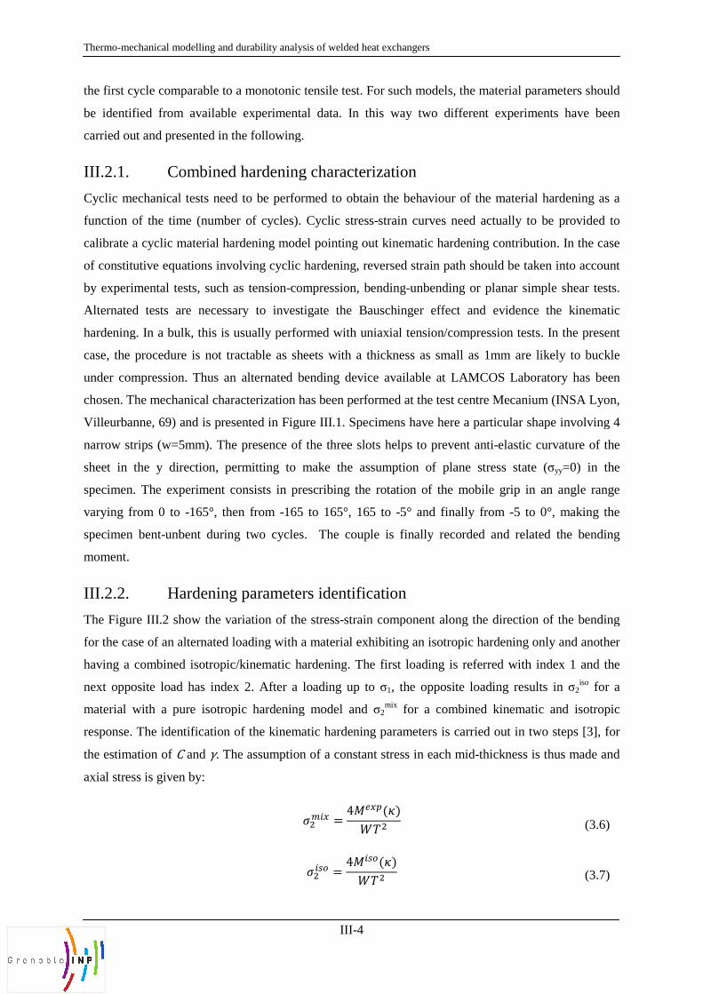
Thermo-mechanical modelling and durab
the first cycle comparable to a mo
be identified from available exp
carried out and presented in the fo
III.2.1. Combined har
Cyclic mechanical tests need to
function of the time (number of
calibrate a cyclic material harden
of constitutive equations involvin
by experimental tests, such as te
Alternated tests are necessary t
hardening. In a bulk, this is usua
case, the procedure is not tractab
under compression. Thus an alte
chosen. The mechanical character
Villeurbanne, 69) and is presente
narrow strips (w=5mm). The pre
sheet in the y direction, permit
specimen. The experiment consi
varying from 0 to -165°, then fr
specimen bent-unbent during tw
moment.
III.2.2. Hardening pa
The Figure III.2 show the variati
for the case of an alternated loadi
having a combined isotropic/kine
next opposite load has index 2.
material with a pure isotropic h
response. The identification of th
the estimation of C and γ. The as
axial stress is given by:
rability analysis of welded heat exchangers
III-4
monotonic tensile test. For such models, the materi
experimental data. In this way two different exp
e following.hardening characterization
to be performed to obtain the behaviour of the ma
of cycles). Cyclic stress-strain curves need actual
ening model pointing out kinematic hardening con
ving cyclic hardening, reversed strain path should b
tension-compression, bending-unbending or plana
y to investigate the Bauschinger effect and evid
ually performed with uniaxial tension/compression
table as sheets with a thickness as small as 1mm
alternated bending device available at LAMCOS L
terization has been performed at the test centre Mec
nted in Figure III.1. Specimens have here a particul
presence of the three slots helps to prevent anti-ela
mitting to make the assumption of plane stress
nsists in prescribing the rotation of the mobile gri
from -165 to 165°, 165 to -5° and finally from
two cycles. The couple is finally recorded and
parameters identification
iation of the stress-strain component along the dire
ading with a material exhibiting an isotropic harden
inematic hardening. The first loading is referred w
2. After a loading up to σ1, the opposite loading
c hardening model and σ2mix for a combined kine
the kinematic hardening parameters is carried out
assumption of a constant stress in each mid-thickn
�4(5 = 4785!�9�:;�
�(<= = 47(<=�9�:;�
erial parameters should
xperiments have been
aterial hardening as a
ually to be provided to
ontribution. In the case
d be taken into account
nar simple shear tests.
vidence the kinematic
ion tests. In the present
m are likely to buckle
S Laboratory has been
ecanium (INSA Lyon,
cular shape involving 4
elastic curvature of the
ss state (σyy=0) in the
grip in an angle range
-5 to 0°, making the
nd related the bending
irection of the bending
ening only and another
d with index 1 and the
ng results in σ2iso for a
inematic and isotropic
ut in two steps [3], for
kness is thus made and
(3.6)
(3.7)

Local material behaviour in a low cycle fatigue regime
III-5
Figure III.1 - Device for the alternated bending test and its corresponding sample geometry
(The width of the strip is w = 4.25mm, the length being L = 59mm)
Figure III.2 - Identification methodology based on tension-compression diagram
(from Carbonnière et al. [3], 2009)

Thermo-mechanical modelling and durab
With Mexp the experimental bend
direction being defined in Figure
tests presented in Chapter 2 (Tab
have given Miso. One can show
difference ∆σ (between numeric
opposite bending time (cf. Figure
with �� = −
assuming
/�where p
2ε and p2ε are respective
material characterized in the reali
�from which a linearization is appl
>?�Equation (1.13) with several loca
has given γ and X1 (giving itself
each integration point through th
best accuracy with the experimen
III.2.3. Results and di
This test has been performed thre
a function of the curvature consid
If no kinematic hardening effect
this last one is reversed. Thus, it
the experimental curve in this
described by a combined harde
observable considering a modifi
parameter (as suggested by Meca
rability analysis of welded heat exchangers
III-6
ending moment applied, t the thickness and W = 4
ure III.1. The isotropic hardening parameters obtai
able II.1) from which their first use in a simulation
[3] that the initial identification of C and γ is th
rical isotropic and experiment combined hardeni
re III.2). From a uniaxial stress configuration, it can
�4(5 = /� − ��
− �(<= − /� = − �(<= − 01 �1 − exp�−1'�!"" /B = 01 �1 − exp�−1'B!""
= −01 C D/B C 01E exp F−1�'�! − 'B!"G ively the equivalent plastic strain at locations “1” an
ality by a mixed hardening (meaning σexp = σmix), on
�4(5 − �(<= = 2/BexpF−1�'�! − 'B!"G pplied by a logarithmic function
� �4(5 − �(<=� = >?�2/B� − 1�'�! − 'B!" cations “2” (but only the location “1” once the ben
elf C). Knowing the first set of (C, γ), more equiva
the thickness give more other values couples. The
ental data has been kept.
discussion
ree times to check its reproducibility. Figure III.3 s
sidering one bending-unbending loading test for co
ct is normally visible in the loading case, it is clear
it shows that isotropic hardening model used alone
is second case. Cyclic material behaviour appea
rdening model (orange dotted line). Excellent c
dified Voce law including also some additional k
canium but not used in the present study).
= 4w the total width, x
tained from the tensile
tion of the bending test
the result of the stress
ening case) during the
can be written:
(3.8)
"" (3.9)
(3.10)
(3.11)
and “2”. Considering a
one can obtained:
(3.12)
(3.13)
bending stage finished)
ivalent computations at
he couple showing the
shows the moment as
cold rolled 316L steel.
early pointed out when
one does not fit so well
pears to be accurately
t correlation is finally
l kinematic hardening

Figure III.3 – Ex
Quanti
Q
b
C
γγγγ
Table III.1 - Sum
In Table III.1 are recapitulated bo
values of the parameters do no
following, average values have
Poisson’s ration as well as Yield
configuration seems to best descr
-0,1 -0,075 -0,05
Mo
men
t (N
.mm
)
Experiment with m
Combined hardeni
Opposite
bending
Local material behaviour in a
III-7
Experimental and predicted moment vs curvature variat
Quantity Test A Test B Test C
Q 620 686 621
b 2,659 2,258 2,131
C 1313 1433 1658
γγγγ 3,585 4,220 4,046
ummary of the identified kinematic and isotropic parame
both kinematic and isotropic hardening parameter
not show large variations whatever the sample
ve been considered. It can be finally noticed th
eld stress at 0.2% will be kept from uniaxial tensile
scribe the loading mode applied on the papillote in p
-3000
-2500
-2000
-1500
-1000
-500
0
500
1000
1500
2000
2500
3000
-0,025 0 0,025 0,05
Curvature (mm-1) with machine stiffness Isotropic hardening
ardening
Bending
Unbending
Inversion
n a low cycle fatigue regime
iation
meters
ters for the 3 tests. The
ple considered. In the
that Young modulus,
sile test as this loading
n practice.
0,075 0,1
dening
nding

Thermo-mechanical modelling and durab
III.3. Numerical
III.3.1. Hardening mo
Once the material model identifi
finite element code proposes a la
combined as it is needed (elast
hardening, hardening itself bein
behaviour involved in a given s
Modulus and Poisson’s ratio) is u
accounted for with two independ
classical Voce law parameters,
implementation of a new materia
ANSYS code. It is nevertheless
kinematic hardening by the way
line in Figure III.3 is so going to b
III.3.2. Investigation
Once the rolled 316L material m
insight on the material behaviou
influence of loading conditions
the final fracture strain) on the res
parameters to take into account in
hexahedral elements is subjected
identified elastic-plastic material
into account in the material behav
III.3.2.1. Force d
In order to test the material m
configuration by the application o
tensile stress in tension is analy
experimental response introduced
the experimental material behavio
The material response under cyc
axial load cyclically varying fro
(according to Lemaitre & Chabo
Fredricks [1]).
rability analysis of welded heat exchangers
III-8
cal response under elementary l
model implementation in ANSYS softwa
tified, it has to be implemented in ANSYS softwa
large panel of material models. Moreover these m
astic or not, independent of the time or not, iso
eing able to be linear or not) depending on the
n study. In the present case, the linear isotropic
s used together with rate independent plasticity. Co
ndent data table. The first one entitled “NLISO” al
rs, except additional kinematic parameters. To p
rial in ANSYS code, it is suggested to use (only)
ss possible to use the precise Armstrong-Frederic
ay of the data table simply called “CHABOCHE”
to be considered in the project.
n of the material response for a simple ca
l model is implemented, a simple finite element m
our (cf. Figure III.4). These simple case studies e
s (intensity of the cycle, imposed stress or displac
response of the material. In a second step, it has all
t in a fatigue model. In Figure III.4, a representativ
ted to pure cyclic tension-compression test conditi
ial model. Both force and displacement loading ca
haviour analysis.
driven cyclic tests
model reliability in ANSYS, a simple uniaxia
n of a loading force of 1050 MPa, almost correspon
alysed. Numerical response is reported in the F
ced from Chapter 2. It is shown that the curve obta
viour in the longitudinal rolling direction.
cyclic load can be now explored. Repeated tensile
from 0 and to a force F has shown no kinematic
boche definition of the non-linear kinematic harde
y loads
ware
tware. In this way, this
e models are able to be
isotropic or kinematic
e mechanical material
ic description (Young
Combined hardening is
allows to consider the
o prevent a fastidious
y) the part available in
rick description of the
E”. The orange dotted
e case study
t model is used to gain
s enable to explore the
lacement, influence on
allowed to identify key
tive volume meshed in
ditions by applying the
cases have been taken
xial monotonic tensile
ponding to the ultimate
Figure III.5 with the
btained by FEM agrees
sile test considering an
atic hardening ifluence
rdening of Armstrong-

Local material behaviour in a low cycle fatigue regime
III-9
Figure III.4 - Cyclic solicitation on a simple FEM
In order to reveal the Bauschinger effect, it is suggested to continue the test until a certain level of
plasticity in compression, as shown below (cf. Figure III.6) with a R=-1 stress ratio (R=σmin/σmax). The
kinematic part of the hardening shows up, meaning that a reversed strain path is mandatory to look at
this phenomenon.
As described in the theorical part in Chapter 1, two main types of hysteresis stabilization can be
moreover distinguished here. In the case where R=-1 and until a maximal load σmax almost equal to the
ultimate tensile stress (almost 1050 MPa), material elastic adaption occurs after a number of cycle
increasing with σmax intensity (cf. Figure III.6, graph on left studying the case of σmax=600Mpa).
Considering higher level of load, the elastic-plastic loop describes a plastic accommodation after a
certain number of cycle (graph on the right), the stored energy remaining the same each cycle once the
stabilization reached. Nevertheless this second case is physically not reproducible as the material is
supposed to fail before the end of the first tensile cycle.
σyy or εyy
0 N cycles
Uxyz=0 Uy=0
Ux=0
σyy or εyy

Thermo-mechanical modelling and durab
Figure III.5 - Uniaxial tensile test s
Figure III.6 - Ten cycles tensio
Figure III.7 -
0
200
400
600
800
1 000
1 200
0,00 0,05 0,10
Tru
e s
tress
σv
(MP
a)
625
500
375
250
125
0
-125
-250
-375
-500
-625
1,3 2,6 3,9 5,2 6,5 7,8
-16 -8 0 8 16 24 32
σyy
(MPa)
σyy
(MPa)
625
500
375
250
125
0
-125
-250
-375
-500
-625
0
rability analysis of welded heat exchangers
III-10
t stress-strain response of the laminated 316L steel comp
sion compression (R = -1) FE model for σmax = (i) 600 a
Influence of the cyclic load on the kinematic hardenin
0,15 0,20 0,25 0,30 0,35 0,40
True strain εv = ln(L/L0)
316L_MATEIS_Tractio
316L_MATEIS_Tractio
316L_MATEIS_Tractio
316L_ANSYS_Predicti
625
500
375
250
125
0
-125
-250
-375
-500
-625
εyy
εyy
,8 9,1 10,4 11,7 0 8 16 24 32 40
40 48 56 0 40 80 120 160 200
σyy
(MPa)
σyy
(MPa)
1250
1000
750
500
250
0
-250
-500
-750
-1000
-1250
mpared to the prediction
0 and (ii) 1100 MPa
ing
0,40 0,45 0,50
S_Traction_long
S_Traction_45
S_Traction_Travers
_Prediction
εyy
εyy
48 56 64 72 80
240 280 320

Local material behaviour in a low cycle fatigue regime
III-11
Then Figure III.7 shows two responses issued from a cyclic calculation using just the kinematic part of
the hardening. Considering R=-1 symmetric cyclic load (cf. Figure III.7 picture on the left), plastic
accommodation is reached right from the first cycle. In the same way, it is shown that Ratchetting can
only occur under non-symmetric cyclic loading (picture on the right where R=-2/3) because the initial
slope of the tangent modulus of the stress–strain curve in compression differs from that in tension. In
conclusion, both Figure III.6 and Figure III.7 point out that if a combined hardening behaviour is used,
an elastic adaption of the material is in principle expected when the stress strain curve stabilizes.
III.3.2.2. Displacement driven cyclic tests
Material mechanical response subjected to cyclic displacement (or deformation) is considered in this
paragraph. This kind of loading appears to fairly reproduce the mechanical load classically involved in
thermal fatigue analysis. Actually, it amounts to see the “papillotes” subjected to displacement
induced by expansion and contraction of the plates during transient regimes. Thus the responses to
different cyclic loads are presented in Figure III.8. The left and right graphs respectively suppose
displacement Umin = 0 and Umin = 0,4 mm (> 0) applied in compression, both cases involving the same
Umax = 0,7mm in tension on a initial length of L0 = 1mm. Whatever the cyclic load considered, the
material shows an identical behaviour. It is observed that strain amplitude remains almost constant
with N (property very interesting for the future steps of the study), when axial stress amplitude
increases every cycle. A cyclic material hardening is so occurring until the stress state saturate after a
certain number of cycles.
Figure III.9 plots the variation of the axial stress with the number of cycles, confirming that stress
amplitude stabilizes after a certain number of cycles. This value appears to be very closed to the
ultimate tensile stress observed in monotonic tension whatever the displacement amplitude intensity
applied here. In order to get a simple model for failure in fatigue, it is interesting to find a way to link
the number of cycles before stabilization and the number of cycles to failure. For this purpose, the next
experiment has aimed at a physical meaning to this saturation.
As a conclusion of this part, the majority of the low cycle fatigue model is dealing with constant strain
amplitude along the time resulting from a displacement driven problem. In the case of metals, this
material response is in addition the most representative of their fatigue behaviour as described by a
combination of isotropic and kinematic hardening. This is finally particularly true in the thermal
fatigue configuration, in which the heat exchanger is currently solicited. Under these conditions, the
next part introduces the fatigue model used to study the heat exchanger behaviour in duty.

Thermo-mechanical modelling and durab
Figure III.8 - Fift
Figur
Figure III. 10
Δεyy (%)
0 4
0 0,8 1,6 2,4 3,2 4 4,8
σyy
(MPa)
σyy
(MPa
1250
1000
750
500
250
0
-250
-500
-750
-1000
-1250
1250
1000
750
500
250
0
-250
-500
-750
-1000
-1250
rability analysis of welded heat exchangers
III-12
ifteen cycles tension compression FEM lead in displacem
ure III.9 - Predicted cyclic plasticity hardening
10 - Cyclic parameters describing fatigue phenomenon
8
1000
800
600
400
200
0
-200
-400
-600
-800
-1000
N/2
8 12 16 20 24 28 32 36 40
4,8 5,6 6,4 7,2 0 0,8 1,6 2,4 3,2 4
σyy
(MPa)
MPa)
εyy
(%)
cement
Δεyy (%)
40
4,8 5,6 6,4 7,2 8
εyy
(%)

Local material behaviour in a low cycle fatigue regime
III-13
III.4. Identification of a low cycle fatigue life model
III.4.1. LCF model introduction
Fatigue laws define damage increment per cycle. In the oligocyclic fatigue domain (cf. Chapter 1),
plastic strain is sufficiently large to permit a consideration of certain time or frequency effect by
supposing a cyclic damage function of the plastic strain amplitude [1] under a power law form:
HIHJ = IK . DM'!20 E
B 4N (3.14)
Supposing a hysteresis stabilized during a cyclic loading, this last equation has been integrated from
the first cycle J�I = 0� = 0 to the last one JO = J�I = IK� = JP. The most common law linking
plastic deformation with the number of cycle to failure is due to Manson-Coffin [5,6] as
JP4 M'!2 = 0 (3.15)
The two parameters C and m (respectively fatigue ductility coefficient and ductility exponent)
describes a power law curve. Moreover negligible influence of the temperature has been observed
below 400°C, corresponding almost to the maximum temperature involved in the heat exchanger duty
and respecting the ratio T/TF < 0.5. The Manson-Coffin criterion is usually considered in the
oligocyclic regime (Nf smaller than 103 to 104 [1]). It has been also observed that it tends to over-
predict the cycle life under extremely low cycle fatigue (ELCF) condition particularly considering
high temperatures (below 100 cycles). It is mainly due to a change of damage mechanisms from
fatigue fracture to accumulation of ductile damage, ductility being itself reduced by the initiation of
small cracks. Fatigue life could be so dominated by surface crack growth and cyclic damage would
have no more influence on the crack growth rate.Different models have been suggested to overcome
this small divergence in a range of number cycle to failure being sometimes able to concern the heat
exchanger in duty. Faced with the other assumptions already involved, Manson-Coffin law is
supposed to be valid in the present study. It is viewed as an alternative expression for a crack growth
law, determined by crack length and applied stress strain.
III.4.2. Experimental procedures
The identification of the Manson-Coffin criterion has to be performed in experimental fatigue tests. As
for the study of the hardening, cyclic repeated test at different constant strain amplitude are needed to
trigger the Bauschinger effect. The only difference is now the necessity to reach the failure in order to
make a link between a critical cycle number and a plastic strain amplitude constant with the time (so
far as it is possible).

Thermo-mechanical modelling and durab
Figure III. 11
Two possibilities are suggested
axial fatigue test, such as tractio
under a certain level of strain am
bending test has been chosen to id
has been considered allowing to
specimen. The loading parameter
i). Moreover it should enable
Alternated strain-controlled bend
used for this fatigue test is rolle
1mm thickness and 10 mm wid
experimental set-up. Due to prac
been fixed respectively at 20 and
) have been applied to external c
number of cycle to failure for all
the moment when the onset of a p
III.4.3. Alternated fou
FE simulation has been conside
couple. A first FE representation
Thanks to the application of the
out a material behaviour follow
Coffin law identification. As sho
considered due to symmetries.
Thus sue to the symmetry, the ho
enables to adopt a plane strain co
zone subjected to the maximal co
advantage of this modelling is to
specimen. It allows to avoid her
costs.
rability analysis of welded heat exchangers
III-14
11 - Experimental set-up of the alternated bending test
d here: classical traction-compression and alternat
tion-compression, specimens with low thickness ar
amplitude. To prevent this non desirable effect, oth
o identify Δεp–Nf curve. An alternated four points b
to represent a local tension-compression zone i
ter are now the bending as a function of the curvatu
le fully reversed constant strain amplitude unde
nding tests have been carried out under room cond
lled (plates) 316L austenitic stainless steel. Recta
idth have been machined. Figure III.11 gives a
ractical reasons and to maximize the prescribed st
nd 45mm. Starting from this state, different displace
al cylinders. It is finally necessary to establish a p
all the fatigue test of the identification. Nf has bee
a primary crack occurred.
four points bending for numerical LCF ch
idered to give back plastic strain amplitude for a
tion of the sample in test conditions is so presen
he combined hardening model, this analysis should
wing a constant strain amplitude evolution adapt
shown in Figure III.12, just the half of the central
horizontal displacement of the left edge is Ux = 0
configuration. The interest is here to concentrate o
constant moment and for sure the maximal equival
to avoid a consideration of the rigid cylinder imp
here the introduction of contact elements leading t
nated bending tests. In
are prone to buckling
other kind of alternated
s bending configuration
e in the middle of the
ature (cf. Figure III.12-
der uniform bending.
onditions. The material
ctangular specimens of
a brief scheme of the
strain, S1 and S2 have
acement loads (Uy+, Uy
-
procedure to read the
been thus defined to be
characterization
r a given displacement
ented in Figure III.12.
uld also allow to point
apted for the Manson-
ral zone has been here
= 0. The ratio b/h = 10
e only on the specimen
valent strain. The other
mplying a force on the
g to higher calculation
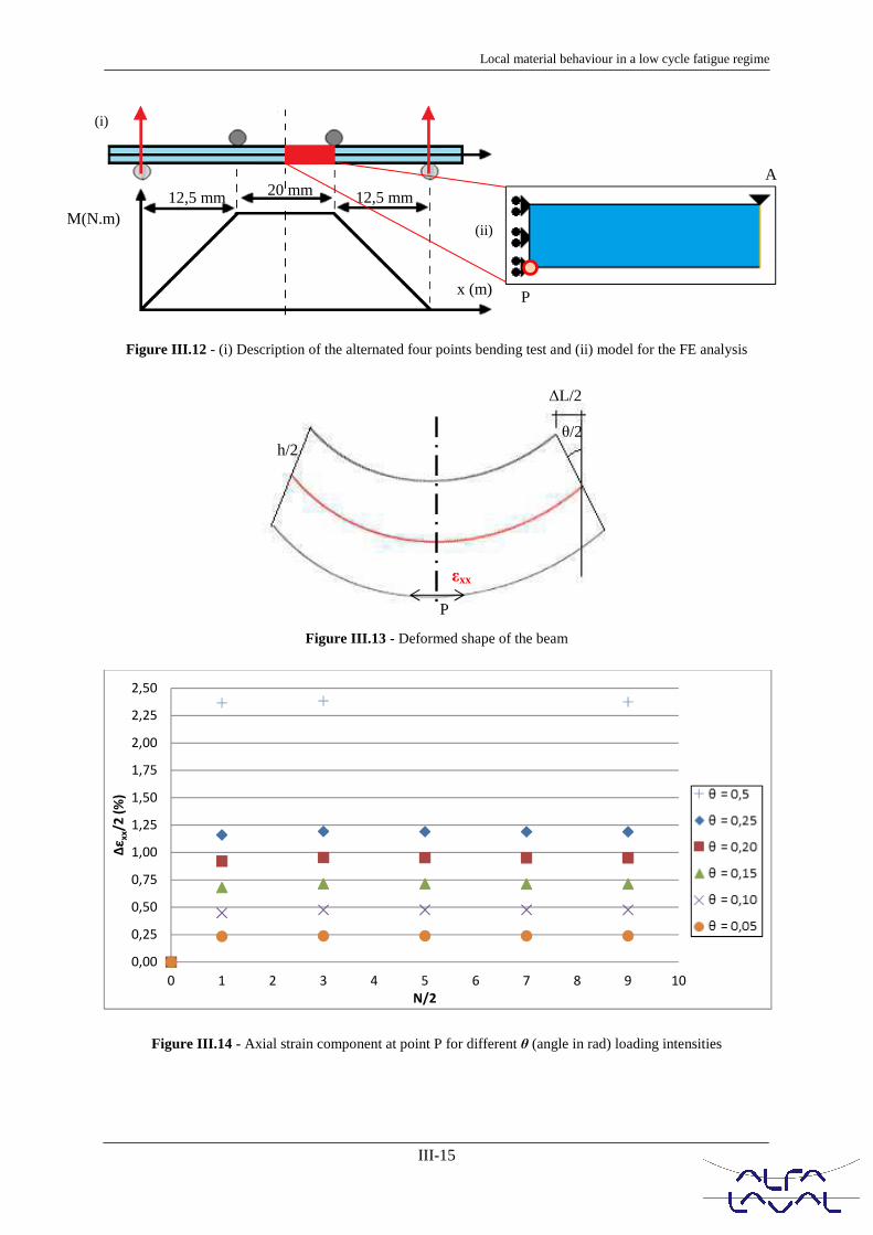
Local material behaviour in a low cycle fatigue regime
III-15
Figure III.12 - (i) Description of the alternated four points bending test and (ii) model for the FE analysis
Figure III.13 - Deformed shape of the beam
Figure III.14 - Axial strain component at point P for different θ (angle in rad) loading intensities
0,00
0,25
0,50
0,75
1,00
1,25
1,50
1,75
2,00
2,25
2,50
0 1 2 3 4 5 6 7 8 9 10
Δε
xx/2
(%
)
N/2
θ/2
∆L/2
h/2
20 mm
x (m)
M(N.m) 12,5 mm 12,5 mm
(i)
(ii)
P
A
εxx
P

Thermo-mechanical modelling and durab
Concerning loading conditions, i
the right edge in Figure III.12. O
blocked in the y direction to prev
equations in such a way that oran
axis surfaces being supposed to
compression configuration (cf. Fi
Figure III.14 shows the axial st
curvature. It is pointed out that
,assimilated to an equivalent app
changes can even be observed fro
by a slow softening to stabilize a
as cyclic loading leads to an axia
with the time after the first cycle
law, as number of cycles to failur
nevertheless difficult to make a
cycle number to accommodation
Figure III.14 does not directly po
strain stabilization is relatively
Nevertheless if applying a consta
of the loading rolls, determinin
experiment remains difficult. Ind
theory is here not successful. M
mandatory as introduced in Figur
III.4.4. Account for th
The combined hardening model
test. Nodes on the left edge are
along x axis as represented in
diagonal) are used in one bending
being fixed) and then Uy- on R3,
material and subjected to constra
master node unique for each ro
between the specimen and cylind
for a full alternated cycle. Plastic
(later called configuration (C1), a
both pictures (i) and (ii) show the
rability analysis of welded heat exchangers
III-16
, identical θ curvature has been imposed on every
. Other degrees of freedom remain free except for
revent any rigid body motion. This curvature has be
range line remains straight even after deformation.
to be submitted locally to the maximal strain amp
Figure III.13), stress-strain evolution is extracted at
strain variation as a function of the number of c
the strain reaches rapidly an asymptotic value.
pplied ΔU on the rolls, has an influence on the stra
from θ = 0.50 rad, deformation state reaching a fir
e at a lower asymptotic value. As a first result, imp
xial plastic strain amplitude and a vertical displacem
le. This observation is important for a simple use o
lure would only be a function of a variable θ consta
link between experimental cycle number to failu
n NA as it has been first proposed.
point out this kind of behaviour since the time nece
ely constant after the first cycle, whatever the
stant rotation angle appears to numerically correspo
ing analytically the resulting displacement for th
Indeed, due to the induced plasticity, the use of cla
. Modelling the whole symmetric part of the test
ure III.15.
r the rolls in the FE analysis of the cyclic
el applied to 2D plane strain elements is used to d
subjected to symmetric conditions, implying a b
in Figure III.15. Four rolls are here described b
ing force application direction by imposing alternat
3, R1 remaining this time rigid. They are considere
traint equations rigidifying all their degrees of free
roll. Contact elements without friction have bee
inders. Thus Figure III.16 shows the corresponding
tic strain distribution is reported for the configurati
), alternation of a positive and a negative displacem
the two steps of going up/down for one calculation c
ery node located along
or the node A which is
been applied by stress
n. Specimen symmetry
mplitude in a traction-
at point P.
f cycle for different θ
. θ curvature intensity
strain amplitude. Some
firstly a peak followed
mposing rotation angle
cement almost constant
e of the Coffin-Manson
stant with the time. It is
ilure NR and numerical
ecessary to observe the
the loading intensity.
spond to a constant ΔU
the analogy with the
classical elastic beams
est appears thus to be
lic bending test
o describe the bending
a blocked displacement
but only two (in the
natively Uy+ on R4 (R2
ered as linear isotropic
reedom together with a
een finally introduced
ing numerical response
ation Uy- = -Uy
- = 5mm
ement, cf. Table III.2),
n cycle.

Local material behaviour in a low cycle fatigue regime
III-17
Figure III.15 - Alternated bending test modelling including rolls and contact elements
Figure III.16 - Total strain state evolution in the specimen
Both top and bottom central zone areas of the specimen are alternatively subjected to the maximal
strain amplitude in a tension-compression loading mode (cf. Figure III.16). It is in agreement with the
expected failure location during equivalent experimental tests. Plastic strain has been extracted a P’
point for different loading cases. In this way, Figure III.17 to Figure III.19 show the strain-stress
hysteresis obtained in the simulation after a limited number of cycles for configurations from (C1) to
(C8) as detailed in Figure III.19.
2 3
1 4 P’ First step Uy
+
Second step Uy-
(i) Cycle1 – first step: roll 4 up
P'
P’
(ii) Cycle1 – second step: roll 3 down
10-2 %
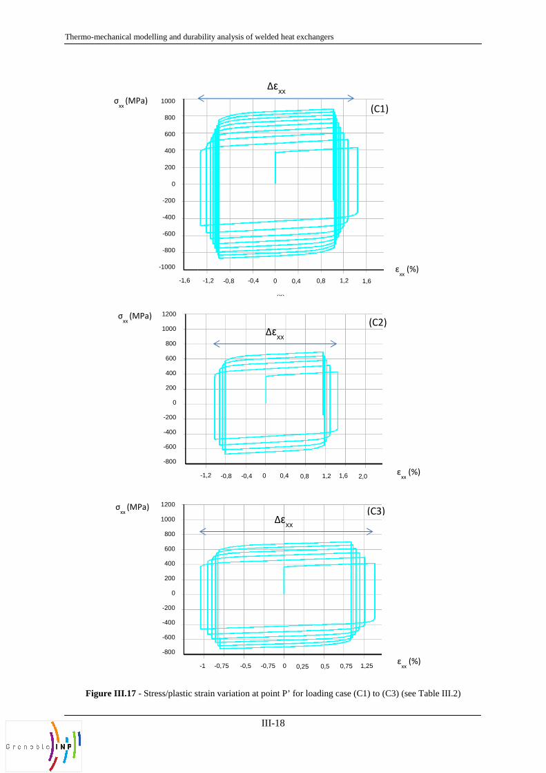
Thermo-mechanical modelling and durab
Figure III.17 - Stress/plastic st
-1,25
-1,6
1000
800
600
400
200
0
-200
-400
-600
-800
-1000
1200
1000
800
600
400
200
0
-200
-400
-600
-800
σxx
(MPa)
σxx
(MPa)
1200
1000
800
600
400
200
0
-200
-400
-600
-800
σxx
(MPa)
-1,6
rability analysis of welded heat exchangers
III-18
strain variation at point P’ for loading case (C1) to (C3)
Δεxx
(C1)
-1,2 -0,8 -0,4 0 0,4 0,8 1,2 1,6
Δεxx
-1 -0,75 -0,5 -0,75 0 0,25 0,5 0,75 1,25
-1,2 -0,8 -0,4 0 0,4 0,8 1,2 1,6 2,0
(C2) Δεxx
(C3)
Δεxx
3) (see Table III.2)
εxx
(%)
εxx
(%)
εxx
(%)
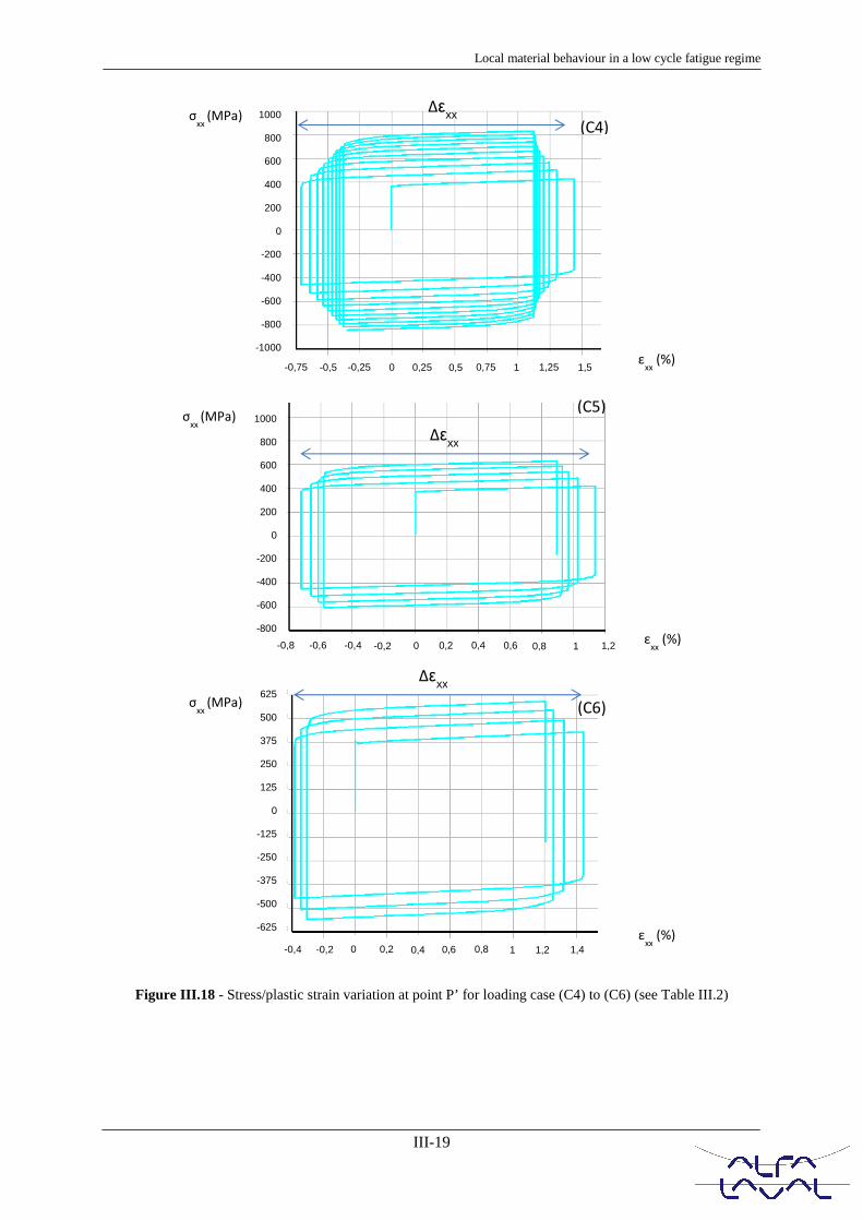
Local material behaviour in a low cycle fatigue regime
III-19
Figure III.18 - Stress/plastic strain variation at point P’ for loading case (C4) to (C6) (see Table III.2)
Δεxx
-0,6 -0,4 -0,2 0 0,2 0,4 0,6 0,8 1 1,2 ε
xx (%)
(C4)
-0,4 -0,2 0 0,2 0,4 0,6 0,8 1 1,2 1,4
Δεxx
εxx
(%)
(C6)
(C5)
εxx
(%)
Δεxx
0,25 0,5 0,75 1 1,25 1,5
1000
800
600
400
200
0
-200
-400
-600
-800
-1000
σxx
(MPa)
1000
800
600
400
200
0
-200
-400
-600
-800
σxx
(MPa)
-0,8
-0,75 -0,5 -0,25 0
625
500
375
250
125
0
-125
-250
-375
-500
-625
σxx
(MPa)
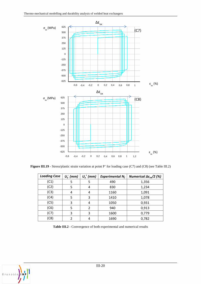
Thermo-mechanical modelling and durab
Figure III.19 - Stress/plastic str
Loading Case Uy- (mm)
(C1) 5
(C2) 5
(C3) 4
(C4) 5
(C5) 3
(C6) 5
(C7) 3
(C8) 2
Table III.2 - C
-0,8
-0,6
625
500
375
250
125
0
-125
-250
-375
-500
-625
625
500
375
250
125
0
-125
-250
-375
-500
-625
σxx
(MPa)
σxx
(MPa)
rability analysis of welded heat exchangers
III-20
strain variation at point P’ for loading case (C7) and (C8
(mm) Uy+ (mm) Experimental Nf Numerical
5 490 1,356
4 830 1,2
4 1160 1,091
3 1410 1,078
4 1050 0,931
2 940 0,913
3 1600 0,779
4 1690 0,7
Convergence of both experimental and numerical result
-0,6 -0,4 -0,2 0 0,2 0,4 0,6 0,8
Δεxx
1
Δεxx
-0,4 -0,2 0 0,2 0,4 0,6 0,8 1 1,2
(C8)
(C7)
C8) (see Table III.2)
erical Δεxx/2 (%)
356
1,234
091
1,078
931
0,913
0,779
0,782
ults
εxx
(%)
εxx
(%)

Local material behaviour in a low cycle fatigue regime
III-21
III.4.5. Experimental identification of the LCF criterion
The account for contact elements in this second FE modelling makes the observation a hysteresis
stabilisation for more than one cycle. If stress amplitude appears to need more time to reach its
maximum unlike the previous experiment, plastic strain amplitude seems to stabilize more rapidly
after a few number of cycles. The half value of the difference between the maximal and the minimal
plastic strain during the first cycle is finally used and considered as a representative plastic strain
amplitude for in the identification. Although overestimating the value at stabilisation better
reproducing the material response during a certain number of cycles, this higher value has been chosen
probably corresponding more carefully to the experimental conditions.
Indeed, whatever the configuration, failure experimentally occured close to a central roll (cf. Figure
III.20), in spite of numerical simulation predicting the maximum strain amplitude in the symmetry axis
of the sample (cf. Figure III.16). Thus, the physical contact between the sample and the roll in addition
to “effets de bord” tend to increase locally the strain. The plastic accommodation appears to occur long
before experimental failure, pointing out the necessity to carry out experimental fatigue tests.
Plastic strain amplitude is a function of the loading intensity, in terms of displacement prescribed on
the rolls (cf. Table III.2). For any numerical loading case analysed, it has been carried out the
corresponding alternated bending test thanks to a four points bending device available at SIMAP
laboratory (University of Grenoble, cf. Figure III.20). The previous calculations have also allowed to
adjust displacement loading to make number of cycle to failure with an order of magnitude coinciding
with the utilization of a Manson-Coffin low (almost 103). Effectively, data concerning 316L steel
behaviour in the low cycle regime are available in the literature [7] for the raw material. As expected,
loading intensity is here not directly inversely linked to number of cycle to failure simply due to
random experimental fatigue effects.
In Figure III.21 are represented the seven points identified in a logarithmic scale. The set up has been
unfortunately developed for sheets normally thinner than the studied plates, allowing not to apply
larger displacement amplitude (cf. Table III.2). Therefore no failure for very low number of cycle
could have been determined, although it could better describe the exchanger loaded in the LCF regime.
Thus identifying a possible non-linearity of the curve for the lowest values is not tractable.
Nevertheless considering other assumptions already induced in the study, the current material
behaviour description in the low cycle fatigue should remain sufficiently accurate. In any cases, the
eight available points plotted in Figure III.21 are used to identify the parameters m and C involved in
the Manson-Coffin criterion.

Thermo-mechanical modelling and durab
Figure III. 20
Figure III.
Ta
In Figure III.21, the linearized pl
the rolled 316L steel can be easil
data reported in the literature, for
to apply the full methodology t
prediction to available data.
0,5
5
300
Δε
xx/2
(%)
rability analysis of welded heat exchangers
III-22
20 - Four points bending device (University of Grenoble)
21 - Identification of Coffin Manson law parameters
C m
16,880 -0,405
Table III.3 - Manson-Coffin law parameters
plot is reported and Manson-Coffin power law C a
sily extracted and given in Table III.3. These value
for instance in [7] for the same material. The next p
to realistic exchanger failure case by finally co
y = 16,88x-0,405
Nf
Identification
Failure occurreone of the cen
Equation f∆εp/2=C.N
le)
and m parameters for
lues are comparable to
t paragraph allows now
comparing fatigue life
3000
rrence under entral rolls
n form C.Nf
m

Local material behaviour in a low cycle fatigue regime
III-23
III.5. Fatigue lifetime prediction of the exchanger
In Chapter 2, results from a second thermal fatigue test on a prototype have been introduced.
Temperature of the hot fluid (180°C) had been precisely chosen to encourage a quick occurrence of
the exchanger failure. Circulating alternatively with a colder water at 13°C, the resulting temperature
amplitude can be here simplified to a uniform temperature field of 167°C. This thermal load has been
considered for the elastic structure response, first step of the methodology introduced in the following.
III.5.1. Introduction of a durability prediction methodology
From both thermo-elastic FE description of the structure (cf. Figure III.22 (i), result already presented
in Chapter 2) and an accurate definition of the material hardening, it is now necessary to find a way to
introduce these features in the LCF model. In this way, the first step of the process is to extract a
representative strain amplitude of this elastic response of the structure, preventing an elastic-plastic
calculation on the full model. The significant exchanger model size could actually involve
convergence difficulties and a resulting long calculation time. Instead of performing a full non-linear
analysis at the scale of the structure, a methodology in two steps has been adopted to make easier its
future use in an industrial context (cf. Figure III.22 and Figure III.23). Thus, firstly an elastic
calculation is carried out on the full core structure supposing a real thermal loading previously defined.
In picture (i) of the Figure III.22, linear exchanger response under a uniform thermal loading of 167°C
is given, approximating the thermal loading of the second thermal fatigue test. The regions where the
stress concentrates are expected to trigger damage. An almost square zoom (h being the space between
two plates and p/2 the half length of a “papillote”) in the region highly stress concentrated is thus
considered (ii) on both sides of the first plate below the end plate. A meshing description named B in
Chapter 2 has been adopted. Equivalent elastic strain energy density WOABCD stored during one half
cycle (iii) is then extracted in six elements of the square. The mean value of the ones showing the
smaller gradient has been actually considered (circle in black in picture (iii) of Figure III.22). In Figure
III.23, an equivalent uniaxial tensile test has been numerically modelled by only one element (ii) (from
the one already introduced in Figure III.4-b) such a way the estimation of the equivalent total strain
amplitude is made by energy equivalence. In picture (i), two areas representative of strain energy are
depicted. The elastic density WOABCD determined in Figure III.22 is found again by the orange
triangle from which the area should equal the equivalent plastic density stored during the simplified
uniaxial test (yellow area).
Numerical procedure Nf comparison
∆T°C We εeq/2 Prediction Experiment
167 27,123 6,365 11 23
Table III.4 - Application of the methodology

Thermo-mechanical modelling and durab
O
A
B
D
C
εe
σyy
σel,vm
Figure III.22 - Elastic
Figure III.23 - Methodology to
extraction of the elastic strain energy
the plastic strain amplitude groping
volume, v
Step by step, a uniaxial force σyy
yellow surface area as closed as p
taken as the equivalent plastic st
cycle, supposing an identical opp
now directly considered in the LC
Stress distribution in
the critical zone
(i)
(ii
p/2
h
rability analysis of welded heat exchangers
III-24
C E
F
∆εpeq/2
ic energy dissipation lecture for a CPK75 submitted to Δ
to estimate number of the number of cycle to failure Nf
rgy density WOABCD from a thermo-elastic analysis, then
ng for σyy to make WOACEFD = WOABCD during a tension l
e, value finally used in the Manson-Coffin criterion
yy is applied on the extremity of the reference volu
s possible to the orange. The involved equivalent pl
strain amplitude characterizing the critical region
pposite deformation during the exchanger shut dow
LCF model.
(ii ) (iii)
First plate
WOACritical zone consideration
Uy=
Ux=0
Uxyz=0
σ
(i) (ii)
ΔT=167°C
f with firstly (i) the
en (i and ii) estimation of
n load on an elementary
olume element to make
plastic strain is finally
on response during one
own. This value can be
ABCD in MPa
=0
σyy

Local material behaviour in a low cycle fatigue regime
III-25
III.5.2. Comparison of the final prediction with the 2nd thermal fatigue test
Table III.4 gives a summary of the two main terms involved in the numerical fatigue life prediction
procedure, that is to say the mean value of the corresponding equivalent strain amplitude obtained by
the procedure illustrated in Figure III.23. This table finally allows to compare the predicted number
cycle to failure to experimental value from which the first internal leakage zoomed in Figure III.24
occurred and the correlation is pretty good.
Having reached the same order of magnitude of the experimental is obviously encouraging. Actually,
knowing that this procedure concerns fatigue phenomenon, the dispersion risk of experimental data
used to characterize the LCF model was large. In addition, although simplifications are done in the
structure modelling assumptions considered in the mechanical analysis, involving boundary
conditions, simple thermal loading, specific numerical tools or energy equivalence, have thus shown
relevance for this methodology. Ideally some more comparisons would have to be carried out to adjust
for example some particularly steps of the methodology as the critical zone size considered in Figure
III.22. Another test considering real service conditions could also permits to make definitive
conclusion concerning the methodology validity.
In any case, fatigue failure identified during the second test Figure III.24 and Figure III.25 are also in
agreement with the regions highly stress concentrated identified in Chapter 2, the first showing failure
having occurred after 23 cycles between the first and the second plate just below the end plate. It is
moreover interesting to notice that the corner involved in this leakage corresponds to the one situated
in the perpendicular direction of the end plate papillote. Two other fatigue failure cases have been
reported almost 10 cycles later on the external side of the end plate. Both are corresponding to stress
concentration regions already pointed out in Chapter 2.

Thermo-mechanical modelling and durab
Figure III.24 - Intern
Figure III.25 - Exter
rability analysis of welded heat exchangers
III-26
ternal fatigue failure after the second experiment on a pro
ternal fatigue failure after the second experiment on a pr
(i)
prototype
prototype
(ii)

Local material behaviour in a low cycle fatigue regime
III-27
III.6. References
[1] Lemaitre J, Chaboche J-L, Benallal A, Desmorat R. Mécanique de matériaux solides, 3e édition,
Editions Dunod.
[2] Simon P, Sabourin F, Morestin F, Phan L. Direct identification of a combined hardening with a
cyclic bending test. IDDRG 2005. Besançon (France), 2005-06-20-2005-06-22
[3] Carbonnière J, Thuillier S, Sabourin F, Brunet M, Manach P.Y. Comparison of the work hardening
of metallic sheets in bending-unbending and simple shear, International Journal of Mechanical
Sciences, Accepted, ref n°IJMS-08-182R1.
[4] Coffin Jr LF. Low cycle fatigue – a review. Appl Mater Res 1962;1(3):129–41.
[5] Manson SS. Behavior of materials under conditions of thermal stress. Technical Report NACA-
TR-1170, National Advisory Committee for Aeronautics ; 1954.
[6] Coffin Jr LF. A study of the effects of cyclic thermal stresses on a ductile metal. Trans Am Soc
Mech Eng 1954 ; 76:931–50.
[7] Hong S, Thuillier S, Yoon S, Lee S. The effect of temperature on low-cycle fatigue behavior of
prior cold worked 316L stainless steel, International Journal of Fatigue, Volume 25, Issues 9–11,
September–November 2003, Pages 1293-1300
[8] Coffin Jr LF. A note on low cycle fatigue laws. J Mater JMLSA 1971 ; 6(2): 388–402.

General Conclusion
Conclusion-1
GENERAL CONCLUSION

Thermo-mechanical modelling and durab
Reminder of the project goal
The motivation of this PhD projec
conditions more severe than thos
new markets. There have been
already considered as the weake
located at the border of the core
called “weak region do coincide
mismatch between the core and t
thermal inertia between both part
at guarantying the durability of
more severe. Numerical tools hav
to improve their construction.
recommendations for an appropri
Main outcomes reached durin
The work has combined a thermo
material response under cyclic
corrugated plate with an anisotro
was firstly to estimate the stress d
frame. The description of this reg
core and the frame, including the
been shown necessary. Upon con
regions where the stress concentr
have been then compared to exp
out on prototypes. It has been sh
consider a rigid frame when the
and cooling stage of the loading.
the predictions at locations far fr
reasons presented in the presen
information for the magnitude of
In a second step, the aspect of the
the level of the structure showed
stress. This suggested that non-li
and kinematic hardening involvi
hardening of the rolled 316L stee
rability analysis of welded heat exchangers
Conclusion-2
ject was to evaluate the lifetime of welded plates he
ose prescribed at the moment, allowing Alfa Laval
n some reported cases where damage could be e
akest part of the core at the beginning of this wo
ore (constituted of thin plates) with the thicker fra
ide with parts of the material subjected to a stron
d the frame. It is due to a temperature difference th
arts during transient cyclic regime heating/cooling.
of the exchangers whereas the operating condition
have been developed so that Alfa Laval Vicarb has
n. In a second stage, these tools should all
priate use of the unit.
ring the project.
mo-elastic FE modeling of the exchanger and a det
ic loadings. At the scale of the exchanger, the
tropic elastic modulus tensor allows a drastic sim
s distribution along the “papillotes”, connecting the
region is shown critical and an accurate account of
the column liner, the “papillotes” and the involve
onstructed, thermo-elastic thermal loadings have be
ntrates detected. The strain prediction of the FE m
xperimental measurements obtained from thermal
shown experimentally that there is a thermal ine
he thermal plate expands and contracts respectivel
g. Measurements of the thermo-elastic strains agree
from the regions where stress concentrates quanti
sent report. The description is though realistic
of load in the heat exchanger.
thermal fatigue of the structure has been considere
ed stress concentration with a magnitude larger tha
linear behaviour were so expected. As the materia
ing cyclic effects, low cycle fatigue has finally
teel has been identified by the use a combined non
heat exchangers under
val Vicarb to expand in
expected in a region
work. This region was
frame panels. The so-
ong thermal behaviour
that originates from a
g. Thus this work aims
ions became more and
has now acquired skills
allow to give useful
detailed analysis of the
the description of the
implification. The goal
the core plates with the
t of the part linking the
lved welded region has
been simulated and the
model of the structure
al fatigue tests carried
inertia large enough to
vely during the heating
reed quantitatively with
ntitatively due to some
tic enough to provide
ered. The calculation at
than the material yield
rial exhibited isotropic
ly been suggested. The
on-linear isotropic and

General Conclusion
Conclusion-3
kinematic hardening through alternated bending tests. Once implemented in ANSYS, its mechanical
response under different cyclic loadings has been investigated. Classical thermal fatigue problem
being strain controlled, the plastic strain amplitude has been identified as representative fatigue
parameter of the material. A Manson-Coffin fatigue model relying this latter to the number of cycle to
failure has been finally identified through cyclic alternated bending tests. Through a simple
methodology combining the calculation at the scale of the structure and the identification of the
mechanical characteristics of the material, lifetime predictions are presented. Thus from the full
thermo-elastic response of a given structure subjected to a thermal loading, the region stress
concentrated has been carefully considered by locally reading the strain energy density. An uniaxial
plastic strain amplitude has been obtained by energy equivalence with an elastic-plastic calculation
performed on a elementary volume. Its magnitude is used in the LCF criterion for the lifetime
prediction. This methodology particularly allowed to prevent an elastic-plastic calculation of the full
structure, probably too costly in term of time. The corresponding lifetime estimation was finally
consistent with experiment value reported by the second thermal fatigue test, in spite of the coarse
thermal field used for the elastic response of the exchanger.
Perspectives
This methodology has been developed for one particular type of heat exchanger. Nevertheless the FE
model of the full exchanger core has been described by parameterizing for example all geometrical
length, the number of plates, the mesh refinement or material models. The methodology can be easily
adapted to different model of heat exchanger, by providing mechanical properties of other corrugation
patterns or materials used to build the unit (as for example the titanium). Although if the mechanical
behaviour of the exchanger has been carefully studied this project, it could be necessary to incorporate
a realistic description of the thermal field prescribed the unit in operating conditions. In addition, Alfa
Laval Vicarb engineers are currently working on a way to introduce the frame part in the modelling,
feature obviously necessary to better describe the thermal loading. Actually, the full FE analysis could
be divided in two steps, both carried out the same meshing in ANSYS software. The first one would
consist in the thermal loading characterization with the necessity to identify some parameters from the
operating conditions as the fluid temperature, the room temperature and the different exchange
coefficients. The second would allow to simply perform the mechanical calculation using the thermal
response previously obtained.

Appendix
IV-1
IV. APPENDIX
IV. Appendix ................................................................................................................................ IV-1
IV.1. Heterogeneous thermal field in the FEM ....................................................................... IV-2
IV.2. Temperature recordings during a thermal loading ......................................................... IV-3
IV.3. Calculation of the principal strains components from strain gauges measurements ...... IV-4
IV.4. Strain heterogeneity in gauges location .......................................................................... IV-6
IV.5. Temperature recordings for thermal test 2 ..................................................................... IV-7
IV.6. Elastic response of the bigger 500 plates model ............................................................. IV-9
IV.7. Elastic response under a real thermal field ................................................................... IV-10
IV.8. Elastic-plastic response of the 40 plates model used in the thermal test 2 ................... IV-12

Thermo-mechanical modelling and durab
IV.1. Heterogen
A heat exchanger unit in service i
carried out to investigate the stre
simulation of the detailed tempe
center. The temperature field d
simplified distribution (or a un
temperature conditions, a heterog
(i). Figure IV.1 (ii) Figure IV.2 (
a plate, with the end of the papill
that stress concentrates in the vici
Figure IV.1 – Heterog
Figure IV.2 - Influence of the te
Uniform temperature field
of ∆T = 90°C
rability analysis of welded heat exchangers
IV-2
eneous thermal field in the FEM
e is subjected to a heterogeneous thermal field. A p
tress distribution in corrugated plates subjected to
perature field is tractable and handled at Lund’
due to the crossed heat and cool circuits is h
uniform one) will be considered here. From
rogeneous thermal field is considered and present
(ii) shows the thremoelastic response and related
illotes being fixed. These locations support more o
icinity of the “papillotes”.
ogeneous temperature field considered along the corruga
e temperature field on the distribution of the Von Mises S
normalised with the yield stress
eld
Lund heterogene
temperature
(i)
(i)
EM
preliminary studywas
to thermal loadings. A
d’s Alfalaval research
s heterogeneous but a
realistic entry fluid
nted in in Figure IV.1
ed stress distribution in
e of the deformation so
ugated plate
s Stress distribution,
d neous re field
(ii)
(ii)

Appendix
IV-3
IV.2. Temperature recordings during a thermal loading
The Figure IV.3 shows the temperature variation for the 10 different thermocouples of which location
is presented in Figure II.21. We observe that the thermocouple number 6 (external side of the frame
panel) partially worked (only for the cycle 2) and the number 2 (just beside the number 1 in front of
the plate pack) not at all. The cycle 2 has been more carefully studied in Figure II.22.
Figure IV.3 - Temperature variation in ten different thermocouple locations (cf. Figure II.21 in Chapter 2)
The low temperature variation at positions 7, 8, 9 and 10 indicates that a modest temperature variation
in the external parts of the frame but a problem during the record could be the reason for such a low
signal. No reliable information can be extracted from these probes. Thermocouples 7 and 8 are located
in the vicinity of thermocouples 5 and 6 in the dry channel. They exhibit an onset of temperature
increase only in the second cycle, showing that the variation is very slow there. In the same way, no
variation is observed in thermocouples 9 and 10 located on both sides of the top panel in contact with
end plate. Thus, the fact that the fluid do not circulate in the dry channel involves a very
heterogeneous thermal field in these parts being able to influence the strain field. Unfortunately, using
only one channel of the exchanger remains the only way to have thermal field as homogeneous as
possible.
10
15
20
25
30
35
40
45
50
55
60
65
70
75
80
85
0 600 1 200 1 800 2 400 3 000 3 600 4 200 4 800 5 400 6 000 6 600 7 200 7 800 8 400
Te
mp
era
ture
in
°C
Time in s
T1 (°C)
T3 (°C)
T4 (°C)
T5 (°C)
T6 (°C)
T7 (°C)
T8(°C)
T9 (°C)
T10 (°C)
Cycle 1 Cycle 2

Thermo-mechanical modelling and durab
IV.3. Calculation
from strain gauge
Three axes strain gauges have be
along the three directions x, x1 an
Figure IV.4 –
For a 2D problem and referring to
written in the papillote plane as b
The knowledge of the directional
components. For an isotropic ma
strain. In the case of the current
remains the only unknown value
�. In order to identify the nece
projection on x and y axis:
Thus
The resulting transition matrix is final
Now based on this relation, the w
rability analysis of welded heat exchangers
IV-4
tion of the principal strains com
ges measurements
been used as depicted in Figure IV.4. We denote t
and y.
description of the strain gauges used in the experiment
g to the (xy) coordinate system in Figure IV.4, loca
below:
ε� � �ε�� ε��ε�� ε���
nal strains along 3 different axis is sufficient to calc
material, these components coincide with the princ
ent strain tensor , � and � being recorded by th
lue. Moreover based on the knowledge of �, it icessary base change matrix (or the transition matri
e��� � �e���. e���e�� � �e���. e���e��
e��� � �e���. e���e�� � �e���. e���e��
e��� � cos� e�� � sin� e�� e��� � � sin� e�� � cos� e��
sition matrix is finally
��� � � cos� sin�� sin� cos��
writing of � in the xy coordinate system gives
x
y x1 x2
omponents
te the strain component
ents
cal strain tensor can be
(1.1)
alculate principal strain
incipal direction of the
the strain gauges, �
it is possible to extract
atrix), one can write by
(1.2)
(1.3)
(1.4)
(1.5)
(1.6)

Appendix
IV-5
ε�������� � a��a� ε� ���� (1.7)
ε���� � aε�� � a��a� ε� (1.8)
��� � cos� � � � 2 cos� sin� � � sin� � � (1.9)
Rearranging the forgoing equations, wehave
� � 12 tan� � �
tan�2 � � 1
2 cos� sin� ��� (1.10)
ε�� � ())*(++� � ε���� for α � 45° (1.11)
The shear strain value being now calculated, the eigenvalues of the strain tensor are extracted to
estimate the principal strain components. This has been prost-process as
012 3ε� � 4 ε��ε�� ε� � 45 � 0 (1.12)
7 � ε�� � ε�� � 4ε��� � 2ε�ε� (1.13)
The two solutions correspond finally to the first and second principal strains in the gauge plan.
ε8 �ε� � ε� �9ε�� � ε�� � 4�ε� � ε�2 � ε������ � 2ε�ε�
2 (1.14)
ε: �ε� � ε� �9ε�� � ε�� � 4�ε� � ε�2 � ε������ � 2ε�ε�
2
(1.15)
Figure IV.5 - Strain gauges 1 & 2 on the prototype
Gauge 2
Gauge 1
Gauge 5

Thermo-mechanical modelling and durab
IV.4. Strain hete
Figure IV.6, Figure IV.7 and F
Elements simulations and point
location of the gauges. The comp
and 3 as a noticeable strain hetero
tensile zone to a compression on
load distribution in the vicinity o
position of the gauges and the ar
Tables.
Experimental results
Gauge 1 Cycle 1 Cycle
Exx 0,02 0,1
Eyy 0,07 0,0
Ex1 0,05 0,0
Figure IV.6 - Numeric
Experimental results
Gauge 2 Cycle 1 Cycle
Exx 0,07 0,0
Eyy -0,01 -
Ex1 0,03 0,0
Figure IV.7 - Numeric
Experimental results
Cycle 1 Cycle
εxx -0,03 -
εyy 0,1 0,1
Ex1 0,1 0,1
Figure IV.8 - Numerical prediction
rability analysis of welded heat exchangers
IV-6
eterogeneity in gauges location
Figure IV.8 show the numerical strain distribut
int out the heterogeneity observed in the area c
parison with experimental measurements appears
erogeneity is observed. The strain on the “papillotes
one along the x axis. This high strain gradient also
of the “papillotes”. In the figures below, the red
area they cover The values recorded by the gauge
Cycle 2
0,13
0,06
0,05
rical prediction compared to experimental recordings for
Cycle 2
0,07
-0,01
0,03
rical prediction compared to experimental recordings for
Cycle 2
-0,03
0,15
0,15
n compared to experimental recordings for Gauge 3
εxx
x
y
x
y
x
εxx
on
bution from the Finite
corresponding to the
rs difficult for gauges 1
tes” can change from a
lso shows the potential
ed circles indicates the
ges are reported in the
for Gauge 1
for Gauge 2
x y
εyy
εxx
εyy
εyy

Appendix
IV-7
IV.5. Temperature recordings for thermal test 2
Figure IV.10 show the temperature variation in 15 different locations represented in Figure IV.9 for
the second thermal test. The thermocouples 14 and 15 inside the pipe, as 4 and 5 direct in front of the
fluid flow obviously show the quicker temperature increase. Recordings are globally consistent with
the first thermal test, except the thermocouples 7 and 8.
Figure IV.9 - Thermocouples location
Figure IV.10 - Temperature variation in the 15 locations
0
10
20
30
40
50
60
70
80
90
100
110
120
130
140
150
160
170
180
190
0 600 1 200 1 800 2 400 3 000 3 600
Te
mp
era
ture
in
°C
Time in °C
T1 (°C)
T2 (°C)
T3 (°C)
T4 (°C)
T5 (°C)
T6 (°C)
T7 (°C)
T8 (°C)
T9 (°C)
T10 (°C)
T11 (°C)
T12 (°C)
T13 (°C)
T14 (°C)
T15 (°C)
The thermocouples 9 to 13 are located on the
“papillotes” respectively close to strain
gauges 1 to 4 (Thermocouple 12 being in
front of the fifth gauge which didn’t work ).
The thermocouples 14 and 15 give
temperature variation inside the pipes
respectively at the inlet and outlet fluid.
Flow direction
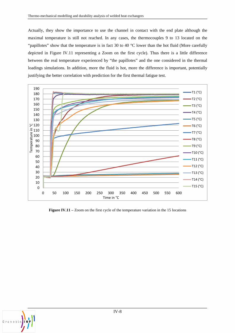
Thermo-mechanical modelling and durab
Actually, they show the importa
maximal temperature is still not
“papillotes” show that the tempe
depicted in Figure IV.11 represe
between the real temperature exp
loadings simulations. In addition
justifying the better correlation w
Figure IV.11 – Zoom o
0
10
20
30
40
50
60
70
80
90
100
110
120
130
140
150
160
170
180
190
0 50 100 150
Te
mp
era
ture
in
°C
rability analysis of welded heat exchangers
IV-8
rtance to use the channel in contact with the end
not reached. In any cases, the thermocouples 9 t
perature is in fact 30 to 40 °C lower than the hot f
esenting a Zoom on the first cycle). Thus there
experienced by “the papillotes” and the one consi
ion, more the fluid is hot, more the difference is im
with prediction for the first thermal fatigue test.
on the first cycle of the temperature variation in the 15
200 250 300 350 400 450 500 550
Time in °C
end plate although the
to 13 located on the
t fluid (More carefully
re is a little difference
nsidered in the thermal
s important, potentially
15 locations
550 600
T1 (°C)
T2 (°C)
T3 (°C)
T4 (°C)
T5 (°C)
T6 (°C)
T7 (°C)
T8 (°C)
T9 (°C)
T10 (°C)
T11 (°C)
T12 (°C)
T13 (°C)
T14 (°C)
T15 (°C)

Appendix
IV-9
IV.6. Elastic response of the bigger 500 plates model
In order to illustrate the flexibility of the model developed during this work, we present in Figure
IV.12 a case with 500 plates. We reort the stress distribution for a thermoelastic loading for a uniform
temperature variation of 167°C. The large size of the structure (almost 7,000,000 degrees of freedom)
involves a CPU time for the calculation close to two hours using four processor of a computer. If it
remains reasonable to carry out this type of calculation from elastic material properties, a non linear
calculations with account for plasticity would noticeably increase the calculation time. This has
motivated the adopted methodology with a two scales and two steps approach based on the energy
equivalences has been provides (see chapter 3). The figure (ii) shows a similar stres distribution near
the corner as the case with the 40 plates model presented in Figure II.18 (i). Thus more beyond some
amount of plates, corner reaction is independent of this number for a given uniform thermal field.
(i) (ii)

Thermo-mechanical modelling and durab
Figure IV.12 -
IV.7. Elastic res
Our colleagues at alfalaval Vic
surrounding frame to perform t
exchanger. A elastic calculation p
suggested that the rigid assumptio
rability analysis of welded heat exchangers
IV-10
- Linear calculation of 500 plates subjected to a uniform
response under a real thermal fie
Vicarb have developed in parallel a model ma
thermal simulations of the transient and station
n performed on the system made of a plates with th
tion for the frame is realistic.
(i)
orm
field
made of a plate plus
ionary response in the
the surrounding frame

Appendix
IV-11
Figure IV.13 - (ii) Elastic response of 200 plates model subjected to (i) real thermal field obtained in ANSYS
(ii)

Thermo-mechanical modelling and durab
IV.8. Elastic-pla
used in the therm
Figure IV.14 and Figure IV.15
uniform ∆T=167°C. The stress c
that the location of the maxim
experimentally, thus indicating an
Figure IV.14 - Von Mises stress
Figure IV.15 - Equivalent plas
Figure IV.13 shows an elastic res
calculated at Alfalaval Vicarb is p
to the calculation but their magnit
rability analysis of welded heat exchangers
IV-12
plastic response of the 40 plates
rmal test 2
shows the elastic plastic response of 40 plates m
s concentrates in the vicinity of the corners and pa
imum plastic strain coincides with those where
an oligocyclic fatigue.
ess response after an elastic-plastic calculation under a u
lastic strain in experimental failure region (circled in red
response of a 200 plates model. A realistic heterog
is prescribed. The stress distribution is slightly diffe
nitude is similar and the location of concentration a
tes model
s model subjected to a
papillotes. We observe
re failure is observed
a uniform ΔT=167°C
red in Figure IV.14)
ogeneous thermal field
ifferent when compared
n also.

RESUME
L’objectif de ce travail est de proposer une méthodologie simple pour évaluer l’intégrité et la durée de
vie d’échangeurs thermiques soudés. Une approche à deux échelles est proposée. Une description
macroscopique avec la prise en compte de la structure de l’échangeur est menée pour permettre des
calculs thermoélastiques par éléments finis. La réponse mécanique de l’échangeur pour des
chargements thermiques, cycliques, simples est évaluée. Notamment, les zones de concentration de
contraintes sont repérées. A partir cette étude, une étude micromécanique du comportement du
matériau composant l’échangeur est menée. Le matériau considéré est un acier 316L. Son
comportement élastoplastique est identifié avec un écrouissage isotrope et cinématique. La tenue
mécanique pour des chargements en fatigue oligocyclique est évaluée à l’aide d’un dispositif de
flexion 4 points alternée et un critère de Manson-Coffin est identifié. Ce critère est utilisé pour évaluer
le nombre de cycle admissible par l’échangeur pour une amplitude de chargement donnée. Pour cela,
la déformation plastique attendue dans l’échangeur est évaluée à partir d’une équivalence en énergie
aux endroits où la contrainte se concentre. Les prédictions du modèle ont été comparées de manière
satisfaisante avec les résultats expérimentaux menés sur un échangeur test, pour la réponse
thermoélastique que pour l’évaluation du nombre de cycles à rupture.
Mots clés : échangeurs thermiques, fatigue oligocyclique, comportement thermomécanique
ABSTRACT
This study proposes a simple methodology to estimate the mechanical response and lifetime of welded
heat exchangers subjected to thermal loadings. The structure of the heat exchanger is modeled to
estimate its mechanical response for thermal loads. Thermoelastic calculations are carried out with the
finite elements method. From these simulations, the regions where the stress concentrates are
identified. Then, a micromechanics approach is adopted to identify the material’s elastic plastic
response with isotropic and kinematic hardening. Its durability under oligocyclic fatigue is
investigated with an original 4 points alternate bending.d vice. From these experiments, a Manson-
Coffin criterion is identified. This criterion is used to estimate the heat exchangers lifetime in terms of
maximum cycles for thermal loadings with different magnitude. To this end, the plastic deformation is
estimated from the macroscopic calculation with an energy equivalence between the thermoelastic
calculation and the non linear one. The predictions are found in agreement with experimental data
carried out on test-heat exchangers, for both the thermoelastic response and the number at cycles at
rupture.
Keywords: welded heat exchangers, fatigue, thermomechanical description
Copyright © 2022 FDOKUMEN