Modeling transport and deposition of level 1 substances to the Great Lakes
241
LBNL-56801 Modeling Transport and Deposition of Level 1 Substances to the Great Lakes Matthew MacLeod, William J. Riley, and Thomas E. McKone Environmental Energy Technologies Division April 2005 This work was supported by the U.S. Environmental Protection Agency Great Lakes National Program Office and the National Exposure Research Laboratory through the U.S. Department of Energy under Contract No. DE-AC03-76SF00098. ERNEST ORLANDO LAWRENCE BERKELEY NATIONAL LABORATORY
-
Upload
independent -
Category
Documents
-
view
0 -
download
0
Transcript of Modeling transport and deposition of level 1 substances to the Great Lakes
LBNL-56801
Modeling Transport and Deposition of Level 1 Substances to the Great Lakes Matthew MacLeod, William J. Riley, and
Thomas E. McKone
Environmental Energy Technologies Division April 2005 This work was supported by the U.S. Environmental Protection Agency Great Lakes National Program Office and the National Exposure Research Laboratory through the U.S. Department of Energy under Contract No. DE-AC03-76SF00098.
ERNEST ORLANDO LAWRENCE BERKELEY NATIONAL LABORATORY

Disclaimer
This document was prepared as an account of work sponsored by the United States Government. While this document is believed to contain correct information, neither the United States Government nor any agency thereof, nor The Regents of the University of California, nor any of their employees, makes any warranty, express or implied, or assumes any legal responsibility for the accuracy, completeness, or usefulness of any information, apparatus, product, or process disclosed, or represents that its use would not infringe privately owned rights. Reference herein to any specific commercial product, process, or service by its trade name, trademark, manufacturer, or otherwise, does not necessarily constitute or imply its endorsement, recommendation, or favoring by the United States Government or any agency thereof, or The Regents of the University of California. The views and opinions of authors expressed herein do not necessarily state or reflect those of the United States Government or any agency thereof, or The Regents of the University of California. Ernest Orlando Lawrence Berkeley National Laboratory is an equal opportunity employer.
ii
Modeling Transport and Deposition of Level 1 Substances to the Great Lakes
Matthew MacLeod1,2, William J. Riley3,and Thomas E. McKone1,4
1Environmental Energy Technologies Division Lawrence Berkeley National Laboratory
Berkeley, CA 94720
2Institute for Chemical and Bioengineering
Swiss Federal Institute of Technology CH-8093 Zürich, Switzerland
3Earth Sciences Division
Lawrence Berkeley National Laboratory Berkeley, CA 94720
4School of Public Health University of California
Berkeley, CA 94720
Submitted to: Edwin R. (Ted) Smith and Todd Nettesheim
United States Environmental Protection Agency Great Lakes National Program Office
77 West Jackson Blvd. (G-17J) Chicago, IL 60604-3590
April 2005
This work was supported by the U.S. Environmental Protection Agency (EPA) Great Lakes National Program Office and the National Exposure Research Laboratory through Interagency Agreements No. DW-899-4807501 and No. DW-988-38190-01-0 and carried out at the Lawrence Berkeley National Laboratory (LBNL) through U.S. Department of Energy under Contract Grant No. DE-AC03-76SF00098.

iii
1.0 SUMMARY
Mass balance modeling of 18 chemicals that are representative of Level I substances
identified under the Great Lakes Binational Toxics Strategy and targeted for virtual
elimination from the Great Lakes has been carried out using a suite of models. The goals
of this work are to assess the potential of each substance for transport from local and
distant sources and subsequent deposition to the surface of the Great Lakes, and to make
estimates of the contribution to total atmospheric loading attributable to emissions at
different locations in North America and globally. Models are applied to analyze the
efficiency of long-range transport and deposition of Level I substances to the Great Lakes
(the Great Lakes transfer efficiency, GLTE). The GLTE is the percentage of chemical
released to air in a source region that is expected to be deposited from the atmosphere to
the surface waters of the Great Lakes.
Modeling at the North American and global scale is carried out using two models based
on the Berkeley-Trent (BETR) contaminant fate modeling framework: BETR North
America and BETR Global. Model-based assessments of Great Lakes transfer efficiency
are used to group the substances according to the spatial scale of emission likely to
impact the Lakes: (1) Local or regional scale substances: Dieldrin, Aldrin and
benzo[a]pyrene, (2) Continental scale: chlordane, 2,3,7,8-tetrachlordibenzodioxin, p,p-
DDT, toxaphene, octachlorostyrene and mirex, (3) Hemispheric scale: PCBs, (4) Global
scale: hexachlorobenzene and α-HCH.
Using available emissions estimates and the models, the contribution of emissions of
Level I substances in different regions of North America and globally to the total
atmospheric loading to the Lakes has been estimated. These estimates are subject to
large uncertainties, most notably because of uncertainties in emission scenarios,
degradation rates of the substances in environmental media. However, model
uncertainties due to simplified descriptions of exchange processes between
environmental media and environmental conditions also contribute to overall uncertainty
in the assessment. Mass balance calculations are presented for seven PCB congeners and

iv
toxaphene at the North American spatial scale and for the PCBs and α-HCH at the global
scale. Comparison of cumulative historical emissions scenarios with estimated emissions
in the year 2000 indicates that relative contributions from sources outside North America
are increasing as sources are curtailed in the United States and Canada. In particular,
Eastern Europe appears to be becoming a relatively more important source to the Lakes.
However, under all emission scenarios considered, the majority of PCB deposition to the
Lakes from the atmosphere is attributable to sources in North America.
The mass balance models presented in this report provide a quantitative framework for
assembling the best available information about properties, sources, partitioning,
degradation, transport, and the ultimate fate of persistent organic substances. The
uncertainties associated with these assessments are believed to be dominated by
uncertainties in emission estimates and environmental degradation rates for the Level I
substances and further research should be focused on better characterization of emissions
and studies of degradation reactions in various environmental media. Given these
uncertainties in the overall mass balance calculations, further model-based studies should
concentrate on assessing the influence of more refined descriptions of fate and transport
processes within the existing model frameworks, and not on increasing the spatial and
temporal resolution of the existing models. Once our understanding of the basic
mechanisms resulting in deposition to the Lakes has improved sufficiently, research
should focus on spatial and temporal scaling issues.

v
TABLE OF CONTENTS 1.0 SUMMARY............................................................................................................ iii TABLE OF CONTENTS ................................................................................................ v 2.0 INTRODUCTION..................................................................................................... 1 3.0 MODELING TOOLS............................................................................................... 5
3.1 The BETR North America Model ....................................................................... 5 3.2 The BETR Global Model.................................................................................... 8 3.3 Metrics of Long-range Transport Potential.......................................................... 9 3.3.1 Characteristic Travel Distance (CTD) .......................................................... 10 3.3.2 Great Lakes Transfer Efficiency (GLTE) ..................................................... 11
4.0 MODELING RESULTS......................................................................................... 13 4.1 Physicochemical Properties of Level I Substances ............................................ 13 4.2 Generic Modeling of Persistence and Long-range Transport Potential
of Level I Substances...................................................................................... 18 4.3 Great Lakes Transfer Efficiency of Level I Substances from within
North America................................................................................................ 23 4.4 Global Great Lakes Transfer Efficiency of Level I Substances.......................... 42
5.0 EMISSION ESTIMATES ...................................................................................... 61 5.1 North American Emissions of PCBs and Toxaphene......................................... 61 5.3 Global-scale Modeling of PCB Concentrations in Air....................................... 87
6.0 REGIONAL CONTRIBUTIONS TO ATMOSPERIC LOADINGS OF LEVEL I SUBSTANCES..................................................................................... 93
6.1 North American Contributions to Loadings of PCBs and Toxaphene ................ 93 6.2 Global Contributions to Loadings of PCBs and α-HCH.................................. 103
7.0 CONCLUSIONS AND RECOMENDATIONS.................................................... 120 7.1 Conclusions .................................................................................................... 120 7.2 Recommendations .......................................................................................... 122
8.0 REFERENCES..................................................................................................... 124 APPENDIX A: ChemSCORER Hazard Profiles for the Level 1 Substances............... 127

1
2.0 INTRODUCTION
Under the Great Lakes Binational Toxics Strategy (1) the United States and Canada have
agreed to take steps to virtually eliminate persistent toxic substances from the Great
Lakes environment. A set of 12 chemicals or chemical groups (the “Level 1 substances”)
were selected for immediate action, and significant emission reductions within the Great
Lakes Basin have been achieved for many of these substances. As local sources are
identified and eliminated the contribution of contaminant loadings to the Great Lakes
system from distant sources by atmospheric transport and deposition may become the
controlling factor determining of reduction rates of contaminants in the Lakes.
This report describes the application of mass balance contaminant fate models to improve
our current understanding of the relative contributions of local and distant sources of
Level 1 substances to the Great Lakes. The Level I substances include polychlorinated
biphenyls (PCBs), dioxins and furans, hexachlorobenzene (HCB), benzo(a)pyrene
(B[a]P), octachlorostyrene (OCS), chlordane, aldrin/dieldrin, DDT, mirex, toxaphene,
mercury, and alkyl lead. The models used in this study are based on the Berkeley-Trent
(BETR) contaminant fate modeling framework (2), and have been developed by
researchers at the Lawrence Berkeley National Laboratory, Berkeley, California and
Trent University, Peterborough, Ontario, Canada.
The models are most appropriate for describing long-term partitioning, fate, and transport
of organic chemicals; therefore alkyl lead and mercury were not modeled in this study.
The ten organic substances listed as Level I substances were modeled as well as α-
hexachlorocyclohexane, a “Level II substance” for which there is an available global-
scale emissions inventory. The models are applied to characterize the combined
atmospheric transport and deposition efficiency of these substances and, where possible,
to estimate the contribution of sources in different regions of North America and the
world to atmospheric loadings to the Great Lakes.

2
The general goal of this research is to systematically assess the long-range transport
potential of the Level I substances with a particular focus on transport and deposition to
the Great Lakes. The assessment strategy is made up of four stages, as shown in Table
2.1.
Table 2.1. Four-stage assessment strategy for assessing long-range transport potential
and depositional efficiency to the Great Lakes for Level I substances.
Stage 1 Compilation of physico-chemical properties and degradation rates
in environmental media
Stage 2
Modeling of long-range transport potential and transport
efficiency to the Great Lakes over continental and global scales
for generic emissions scenarios
Stage 3 Compilation of emissions estimates and observed environmental
concentrations
Stage 4 Assessment of regional contributions to atmospheric loading to
the Great Lakes over continental and global scales
The assessment strategy was designed to sequentially build up information about the
long-range transport potential for the Level I substances, from general information about
physico-chemical properties (Stage 1) to generic indicators of long-range transport
potential and transport and depositional efficiency to the Great Lakes (Stage 2) and
finally provide comprehensive estimates of the contribution of emissions in different
locations to atmospheric deposition rates to the Lakes (Stage 4).
At the outset of this project we anticipated that completing all four stages of the
assessment strategy would be possible for only a subset of the Level I substances. We
expected the availability of emission estimates required for Stage 3 and Stage 4 to be a
limiting factor. From a survey of available literature we have assembled emissions
information for seven PCB congeners, and α-HCH on a global scale, and for the PCB
congeners and toxaphene on a continental scale. For the other Level I substances we
have completed Stages 1 and 2, and these model results can be combined with emission

3
information as it comes available to estimate regional contributions to atmospheric
loadings to the Lakes. This can be achieved without re-running the models since the
equations describing transport and deposition are linear. Therefore the model results for
the generic emission scenario can be scaled by the proportion of total emissions in each
region to deduce the fraction of loading attributable to emissions in each region when
data become available.
This report is organized into seven sections and two appendices.
Section 1 is a condensed summary of the study results and recommendations for future
research.
This is Section 2, an introduction to the project and a guide to the information presented
in the project report.
Section 3 provides background information about the Berkeley-Trent North American
Contaminant Fate Model (BETR North America) and the Berkeley-Trent Global
Contaminant Fate Model (BETR Global).
Section 4 presents results from Stage 1 and 2 of the assessment process for all of the
Level I substances, including physico-chemical properties and degradation half-lives,
generic modeling of transport potential and transport and deposition efficiency, and
results of Great Lakes Transfer Efficiency calculations on North American and global
scales.
Section 5 summarizes emissions inventories at the North American scale for seven PCB
congeners and toxaphene, and at the global scale for the PCBs and α-HCH. Modeled
concentrations of PCBs in air obtained from the BETR Global model are compared with
data from eleven long-term monitoring stations in the Northern Hemisphere, including
the International Atmospheric Deposition Network (IADN), which is located in the Great
Lakes Basin.
4
Section 6 combines information from the generic modeling and emissions estimates to
calculate the fraction of total loading from the atmosphere that is attributable to sources
in different regions of North America and the world.
Section 7 presents overall conclusions from the study, and suggests avenues for future
research to further improve our ability to identify sources of atmospherically derived
persistent pollutants in the Lakes, and to more accurately quantify the relative
contributions of these sources to total loadings.

5
3.0 MODELING TOOLS This section provides background information about the Berkeley-Trent North American
Contaminant Fate Model (BETR North America) and the Berkeley-Trent Global
Contaminant Fate Model (BETR Global).
3.1 The BETR North America Model
A detailed description of the BETR model framework and environmental
parameterization for North America is provided by MacLeod et al. (2) and Woodfine et al. (3). The BETR model describes contaminant partitioning and fate in the environment
using mass balance equations based on the fugacity concept. General background on the
application of fugacity-based models to environmental problems can be found in the text
by Mackay (4), and a review of the application of models of this type in fate and exposure
assessments is provided by McKone and MacLeod (5).
The BETR North America model describes the North American environment as 24
ecological regions, as illustrated in Figure 3.1.1. Within each region, contaminant fate is
described using a 7-compartment fugacity model including a vertically segmented
atmosphere, vegetation, soil, freshwater, freshwater sediments, and coastal ocean/sea
water. Contaminants can be transported between adjacent regions of the model in the
atmosphere and in flowing rivers and by near-shore ocean currents.

6
Figure 3.1.1. Regional segmentation of the BETR North America model.
Each of the BETR North America regions is parameterized to represent local
environmental conditions, including hydrology, meteorology, and physical attributes.
This requires the specification of more than 70 individual input parameters for each
region. Geographic Information System (GIS) software has been used in combination
with geo-referenced data sets from a variety sources to efficiently and accurately
parameterize the North American environment in the model.
In the BETR North America model, the environment within each region is described as a
connected system of seven discrete, homogeneous compartments. Figure 3.1.2 illustrates
the seven compartment regional environment of the BETR model framework.

7
Figure 3.1.2. Contaminant fate and transport processes considered in each region of the
BETR North America model. E values represent primary emissions to each compartment
and D values indicate fate and transport processes available to the substance in each
compartment.
Individual regional environments are connected in the BETR framework by inter-regional
flows of air in the upper and lower atmosphere, and of fresh and coastal water. These
inter-regional linkages are illustrated in Figure 3.1.2 and are specified in the model as
five matrices of volumetric flow rates that describe movement of air or water in both
directions across all regional boundaries. In total, the North American model requires
compilation of five volumetric flow rate matrices: two for the atmosphere (upper and
lower), one for freshwater exchange, one for freshwater flowing into coastal waters of an
adjacent region and one for the exchange of coastal water. To satisfy the conditions of
long-term steady state in each region the volumetric inflow rate of air, freshwater, and
coastal water are balanced by an equal outflow rate.

8
Seven equations describe contaminant fate in each region, and therefore a total of 168
mass balance equations make up the 24-region linked model for North America. This
system of seven equations and the seven unknown fugacities have been solved
analytically using linear algebra, and by matrix algebra using a Gauss elimination
algorithm. The BETR North America model can also be applied to describe the time
course of contaminant concentrations in the linked set of regions by expressing the mass
balance equations as a set of seven differential equations.
3.2 The BETR Global Model
The BETR-Global model is based on the same Berkeley-Trent contaminant fate modeling
framework as the BETR North America Model, and many of the equations used to
describe contaminant fate in BETR-Global are identical to those in BETR North
America. However, the BETR Global model incorporates several refinements to the
general structure to allow more flexibility and to describe the global environment in more
detail and with higher temporal resolution. Previous applications of the BETR model
framework use a single set of parameters to describe the long-term average transfer rates
of air and water between the regions within the model domain. As a result, temporal
resolution has been limited to describing trends in contaminant concentrations that take
place over several years. The BETR Global model uses a monthly time scale to specify
atmospheric conditions and other selected parameters, and a 15° by 15° grid coverage of
the globe, resulting in 288 multimedia regions (Figure 3.2.1). Compared to previous
multimedia models based on the BETR framework this approach significantly increases
both spatial and temporal resolution.

9
Figure 3.2.1. Regional segmentation of the BETR Global model showing numerical
naming scheme for individual regions.
A complete description of the BETR Global model and its development can be found in
MacLeod et al. (6).
3.3 Metrics of Long-range Transport Potential
Potential for long-range transport in the environment is recognized as an important
indicator of environmental hazard for chemical substances. The Long Range Transport
Potential (LRTP) can be characterized using model calculations; however several
alternative models and modeling approaches are being used for this purpose. As a result,
several different metrics for LRTP have been suggested in the literature. A key
distinction is between (1) “transport-oriented” metrics that describe the potential for
transport in air and/or water with simultaneous exchange with the surface media, and (2)
“target-oriented” metrics, describing the percentage of emitted substance that migrates to
surface media in selected target regions as a consequence of transport in air and/or water
and subsequent deposition (7). Great Lakes Transfer Efficiency is a “target-oriented”

10
LRTP metric. We have also examined LRTP of the Level I substances using the
“transport-oriented” metric CTD.
3.3.1 Characteristic Travel Distance (CTD)
The Characteristic Travel Distance (CTD, (km)) is a transport-oriented long-range
transport potential metric defined as the distance from a point source at which the
concentration has decreased to 1/e (≈ 37%) of the initial value (8):
ecc /)CTD( 0=
Beyer et al. (9) showed that in a single region steady-state model the CTD in the mobile
media air or water could be approximated as the product of the overall persistence (POV,
hours), the fraction of chemical partitioning to the mobile medium (φ, dimensionless) and
an assumed velocity of the mobile media (ν, km h-1).
CTD = POV φ ν.
CTD can therefore be calculated from the results provided by any multimedia model
which estimates POV and φ.
For the present purposes, we conduct CTD calculations using ChemSCORER (10), which
is based on the generic Level III model developed by Mackay (4). While it is possible to
calculate CTD from the output of the BETR model, we have instead applied
ChemSCORER since it provides an independent second model for comparison. CTDs
calculated by a generic Level III model and by BETR were observed to be highly
correlated in initial investigations using a set of hypothetical chemical property
combinations. The ChemSCORER software also provides an informative generic hazard
profile for each substance, including comparative scores for Persistence (POV),

11
Bioaccumulation potential (B), and LRTP. Results from ChemSCORER for the Level I
substances are included in Appendix A.
3.3.2 Great Lakes Transfer Efficiency (GLTE)
Great Lakes Transfer Efficiency is a target oriented long-range transport potential metric
using the fresh water in the Great Lakes Basin as the target ecosystem (11). It is defined
as the ratio of the deposition mass flux from air to water in the Great Lakes Basin to the
emission mass flux in a source region (Figure 3.3.2.1). GLTE can be calculated for
simple emission scenarios (i.e., emissions individually to air, water, or soil in a single
source region) or for combined emission to several media in several regions.
Figure 3.3.2.1. Conceptual illustration of the Great Lakes Transfer Efficiency calculated
for transport from the Mississippi River Delta Region using BETR North America.
Conceptually, the Great Lakes transfer efficiency represents the percentage of chemical
released to air in a source region that is expected to be deposited from the atmosphere to

12
the surface waters of the Great Lakes. The GLTE is a convenient LRTP metric for the
BETR North America model since the regional segmentation is partially based on
watershed boundaries. Thus there is a model region that explicitly represents the Great
Lakes Basin watershed, and it is a simple matter to calculate the depositional flux to
water in this region.
In the BETR Global model the Great Lakes straddle the boundary between two model
regions. Therefore GLTE calculations are made by combining the mass flux to
freshwater in these two regions in the numerator. Because it is not based on watershed
boundaries, GLTE calculated by the BETR Global model includes deposition to surface
water outside of the Great Lakes Basin. Based only on freshwater areas in the two
model’s target regions, GLTE calculated using the BETR Global model is expected to be
a factor of 2.4 higher than that calculated using BETR North America.

13
4.0 MODELING RESULTS
In this section, we provide results from Stage 1 and 2 of the assessment process for all of
the Level I substances, including physico-chemical properties and degradation half-lives,
generic modeling of transport potential and transport and deposition efficiency, and
results of Great Lakes Transfer Efficiency calculations on North American and global
scales.
4.1 Physicochemical Properties of Level I Substances
Chemical properties required as inputs for the multimedia models include molecular
mass, equilibrium partition coefficients between air, water and octanol, and estimates of
degradation half lives in air, water, soil, and sediments. The BETR North America and
BETR Global models describe contaminant fate in realistic environmental systems with
different conditions, for example, temperature, soil, water, etcetera. Enthalpies of phase
change that describe the temperature dependence of the partition coefficients between air,
water, and octanol are therefore also required as inputs to the models. In addition, the
BETR Global model applies generic corrections to estimated media-specific degradation
half-lives to account for reduced degradability in colder environments. These correction
factors are the same for all chemicals considered in this study, and they result in roughly
doubling the degradation rate constants in all media for a temperature increase of 10o
above the reference temperature of 25oC. In Stage 1 of the assessment procedure for the
Level I substances we conducted a literature search to select appropriate values for these
properties for use in the modeling exercises.
Accurate measurement of partitioning properties is challenging, particularly for semi-
volatile organic chemicals that may have properties at or near the limits of analytical
techniques. Pontolillo and Eganhouse (12), who recently reviewed data for DDT and
DDE on aqueous solubility and octanol-water partition coefficients, report high
variability in reported values, and reporting errors. These findings raised questions about
14
available data quality for these chemical properties. They recommended improvement of
measurement and reporting techniques in order to increase data reliability of reported
physicochemical properties of hydrophobic organic compounds. An important
contribution in this regard was made by Cole and Mackay (13) who suggested partitioning
data be evaluated for consistency using thermodynamic relationships linking the
solubilities in air, water, and octanol and the three corresponding partition coefficients—
air/water, octanol/water, and octanol/air. This “three solubility” approach can be extended
to interpret data on the temperature dependence of partitioning properties since the
relationships between the three solubilities and the three partition coefficients are valid at
any temperature. The temperature dependence of solubilities and partition coefficients
can be expressed in terms of energies of phase transition (ΔU), and the ΔU values must
conform to similar constraints as the partition coefficients (14).
Table 4.1.1 presents values for partitioning properties of the Level I substances gathered
from our literature search and used in the modeling described in this report. Whenever
possible we have used data that have been harmonized to conform to thermodynamic
constraints using the three solubility adjustment procedure recommended by Beyer et al. (14). This ensures that no incompatible data for individual property measurements of a
given substance are used in the assessment.
Also listed in Table 4.1.1 are estimated degradation half-lives for the Level I substances
in environmental media. These half-life estimates encompass all possible transformation
reactions that might alter the chemical structure of the substance, including reaction with
hydroxyl radicals in the gas phase, hydrolysis, photolysis and biodegradation, for
example by microbes. Unfortunately, these data are highly uncertain and quality
assurance procedures akin to the three solubility approach that was applied to the
partitioning properties are not available. Uncertainties associated with these estimated
degradation half lives are estimated to be approximately an order of magnitude, and
contribute significantly to the overall uncertainty in the model assessments. Uncertainties
in the overall assessment process are discussed in detail in Section 7.0.

15
Tabl
e 4.
1.1.
Phy
sico
-che
mic
al p
rope
rties
and
est
imat
ed d
egra
datio
n ha
lf-liv
es o
f the
Lev
el I
subs
tanc
es.
[1
] Par
titio
ning
pro
perti
es a
nd e
ntha
lpie
s of
pha
se tr
ansi
tion
from
Li,
N, F
. Wan
ia, Y
.D. L
ei a
nd G
.L. D
aly.
200
3. A
com
preh
ensi
ve a
nd c
ritic
al
com
pila
tion,
eva
luat
ion
and
sele
ctio
n of
phy
sica
l-che
mic
al p
rope
rty d
ata
for s
elec
ted
poly
chlo
rinat
ed b
iphe
nyls
. Jo
urna
l of P
hysi
cal C
hem
ical
R
efer
ence
Dat
a, 3
2 (4
), 15
45 -
1590
.
[2] D
egra
datio
n ha
lf-liv
es fr
om M
acka
y, D
., W
.Y. s
hiu
and
K.C
. Ma.
200
0. I
llust
rate
d ha
ndbo
ok o
f phy
sica
l-che
mic
al p
rope
rties
and
env
ironm
enta
l fa
te.
Cha
pman
& H
all/C
RC
netB
ase,
Boc
a R
aton
, FL.
[3] P
artit
ioni
ng p
rope
rties
from
She
n, L
. and
F. W
ania
. 20
04.
Com
pila
tion,
eva
luat
ion
and
sele
ctio
n of
phy
sica
l-che
mic
al p
rope
rty d
ata
for
orga
noch
lorin
ated
pes
ticid
es.
Jour
nal o
f Phy
sica
l Che
mis
try R
efer
ence
Dat
a (In
Pre
ss).
[4] D
egra
datio
n ha
lf-liv
es fr
om M
cKon
e, T
. E. 1
993.
Cal
TOX,
a m
ultim
edia
tota
l exp
osur
e m
odel
for h
azar
dous
was
te s
ites.
Par
t 1: E
xecu
tive
sum
mar
y. U
CR
L-C
R-1
1145
6PTI
, pre
pare
d fo
r the
Dep
artm
ent o
f Tox
ic S
ubst
ance
s C
ontro
l, C
alifo
rnia
Env
ironm
enta
l Pro
tect
ion
Agen
cy. L
iver
mor
e,
CA:
Law
renc
e Li
verm
ore
Nat
iona
l Lab
orat
ory.

16
[5] E
ntha
lpie
s of
pha
se tr
ansi
tion
estim
ated
as
the
gene
ric v
alue
s su
gges
ted
by W
ebst
er, E
., D
. Mac
kay,
A. D
i Gua
rdo,
D. K
ane,
and
D. W
oodf
ine.
20
04. R
egio
nal D
iffer
ence
s in
Che
mic
al F
ate
Mod
el O
utco
me.
Che
mos
pher
e. 5
5: 1
361-
1376
.
[6] P
artit
ioni
ng p
rope
rties
and
ent
halp
ies
of p
hase
cha
nge
from
She
n, L
. and
F. W
ania
. 20
04.
Com
pila
tion,
eva
luat
ion
and
sele
ctio
n of
phy
sica
l-ch
emic
al p
rope
rty d
ata
for o
rgan
ochl
orin
ated
pes
ticid
es.
Jour
nal o
f Phy
sica
l Che
mis
try R
efer
ence
Dat
a (In
Pre
ss).
[7] P
artit
ioni
ng p
rope
rties
and
ent
halp
ies
of p
hase
tran
sitio
n fro
m B
eyer
, A.,
F. W
ania
, T. G
ouin
, D. M
acka
y an
d M
. Mat
thie
s. 2
002.
Sel
ectin
g in
tern
ally
con
sist
ent p
hysi
coch
emic
al p
rope
rties
of o
rgan
ic c
ompo
unds
. En
viro
nmen
tal T
oxic
olog
y an
d C
hem
istry
. 21
(5),
941-
953.
[8] D
egra
datio
n ha
lf-liv
es a
re th
e re
com
men
ded
valu
es o
f M. S
cher
inge
r, E
TH Z
uric
h (P
erso
nal C
omm
unic
atio
n, 2
004)
use
d in
the
OEC
D m
ulti-
med
ia m
odel
com
paris
on e
xerc
ise.
[9
] Deg
rada
tion
half-
lives
from
Too
se, L
., D
.G. W
oodf
ine,
M. M
acLe
od, D
. Mac
kay
and
J. G
ouin
. 20
04. E
nviro
nmen
tal P
ollu
tion
128,
223
-240
. [1
0] P
rope
rties
sel
ecte
d by
Mac
Leod
, M.,
D.G
. Woo
dfin
e, J
.R. B
rimac
ombe
, L. T
oose
and
D. M
acka
y. 2
002.
A d
ynam
ic m
ass
budg
et fo
r tox
aphe
ne
in N
orth
Am
eric
a. E
nviro
nmen
tal T
oxic
lolo
gy a
nd C
hem
istry
21(
8), 1
628-
1637
. [1
1] P
artit
ioni
ng p
rope
rties
and
deg
rada
tion
half-
lives
est
imat
ed u
sing
the
EP
IWIN
qua
ntita
tive
stru
ctur
e-ac
tivity
rela
tions
hip
prog
ram
: ht
tp://
ww
w.e
pa.g
ov/o
ppt/e
xpos
ure/
docs
/epi
suite
dl.h
tm
[12]
Log
Kow
reco
mm
ende
d va
lue
from
Mac
kay,
D.,
W.Y
. Shi
u an
d K.
C. M
a. 2
000.
Illu
stra
ted
hand
book
of p
hysi
cal-c
hem
ical
pro
perti
es a
nd
envi
ronm
enta
l fat
e. C
hapm
an &
Hal
l/CR
Cne
tBas
e, B
oca
Rat
on, F
L. L
og K
aw fr
om Y
in, C
.Q. a
nd J
.P. H
asse
tt. 1
986.
Gas
-Par
titio
ning
App
roac
h Fo
r Lab
orat
ory
and
Fiel
d St
udie
s of
Mire
x Fu
gaci
ty in
Wat
er.
Envi
ronm
enta
l Sci
ence
and
Tec
hnol
ogy,
20(
12),
1213
-121
7.

17
Fi
gure
4.1
.1.
Scre
enin
g as
sess
men
t of p
oten
tial f
or tr
ansp
ort a
nd d
epos
ition
to th
e G
reat
Lak
es b
ased
on
parti
tioni
ng p
rope
rties
.
Parti
tioni
ng o
f the
Lev
el I
subs
tanc
es a
re in
dica
ted
by th
e fo
llow
ing
sym
bols
: 28
– P
CB
28,
52
– PC
B 5
2, 1
01 –
PC
B 1
01, 1
38 –
PC
B
138,
153
– P
CB
153
, 180
– P
CB
180
, Dn
– D
ield
rin, A
– A
ldrin
, H –
HC
B, C
– to
tal C
hlor
dane
s, di
– 2
,3,7
,8-T
CD
D, α
– α
-HC
H, D
–
p,p-
DD
T, T
– to
xaph
ene,
O –
oct
achl
oros
tyre
ne, B
– b
enzo
[a]p
yren
e, M
– M
irex.

18
An initial screening of the Level I substances for potential for long-range transport and
deposition to the Great Lakes is possible at this stage using the graphical method derived
from results from the BETR North America model (11). Figure 4.1.1 shows the position
of each of the Level I substances in the KOW/KAW partitioning space with the five regions
of dominant fate and transport processes identified by MacLeod and Mackay. This
preliminary analysis illustrates that the majority of the Level I substances have
partitioning properties that make transport and deposition to the Lakes possible, provided
the substances are sufficiently persistent in the atmosphere.
4.2 Generic Modeling of Persistence and Long-range Transport Potential of Level I Substances
Generic modeling of POV and LRTP is possible using the data gathered on
physicochemical properties and degradation half lives. Generic assessments are useful
for building an understanding of how the environmental hazards posed by substances
varies with their inherent physicochemical properties. Assessments of this type are
useful and informative and they do not require estimates of actual emission rates or
emission patterns. They can be used to rank or score chemicals based on intrinsic
environmental hazard. Generic assessments also provide a valuable reference point and
information about the likely behavior of substances. These generic assessments can be
compared against results of more detailed site-specific and emission scenario-specific
modeling.
Table 4.2.1 provides model results from ChemSCORER for overall persistence and
characteristic travel distance of each of the Level I substances, and Great Lakes Transfer
Efficiencies calculated from BETR North America and BETR Global. The GLTE values
presented here are for emissions to air in Region 16 (Sierra Nevada Pacific Coast) in the
BETR North America model, and for emissions to air in Eastern China (Region 92) in the
BETR Global model. These emission scenarios were selected as representative of
continental and global-scale transport, respectively, to the Great Lakes target region.

19
Tabl
e 4.
2.1.
Gen
eric
mod
elin
g re
sults
for o
vera
ll pe
rsis
tenc
e (P
OV) a
nd lo
ng-r
ange
tran
spor
t pot
entia
l of t
he L
evel
I su
bsta
nces
.
(CTD
– c
hara
cter
istic
trav
el d
ista
nce,
BET
R N
A –
BET
R N
orth
Am
eric
a m
odel
, GLT
E –
Gre
at L
akes
tran
sfer
eff
icie
ncy)
.
Po
v an
d C
TD c
alcu
late
d fro
m L
evel
III C
hem
SCO
RER
Bet
a1.0
1 (h
ttp://
ww
w.tr
entu
.ca/
cem
c/m
odel
s/C
hem
Scor
.htm
l).
BET
R N
orth
Am
eric
a G
LTE
for e
mis
sion
s to
low
er a
ir in
Reg
ion
16 (S
ierr
a N
evad
a-Pa
cific
Coa
st)
BET
R G
loba
l GLT
E fo
r em
issi
ons
to lo
wer
air
in R
egio
n 92
(eas
tern
Chi
na)
20
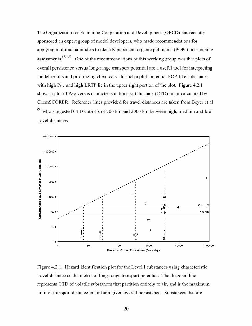
The Organization for Economic Cooperation and Development (OECD) has recently
sponsored an expert group of model developers, who made recommendations for
applying multimedia models to identify persistent organic pollutants (POPs) in screening
assessments (7,15). One of the recommendations of this working group was that plots of
overall persistence versus long-range transport potential are a useful tool for interpreting
model results and prioritizing chemicals. In such a plot, potential POP-like substances
with high POV and high LRTP lie in the upper right portion of the plot. Figure 4.2.1
shows a plot of POV versus characteristic transport distance (CTD) in air calculated by
ChemSCORER. Reference lines provided for travel distances are taken from Beyer et al (9) who suggested CTD cut-offs of 700 km and 2000 km between high, medium and low
travel distances.
Figure 4.2.1. Hazard identification plot for the Level I substances using characteristic
travel distance as the metric of long-range transport potential. The diagonal line
represents CTD of volatile substances that partition entirely to air, and is the maximum
limit of transport distance in air for a given overall persistence. Substances that are

21
conventional persistent organic pollutants (POPs) combine high long-range travel
potential with high overall persistence. 28 – PCB 28, 52 – PCB 52, 101 – PCB 101, 118
– PCB 118, 138 – PCB 138, 153 – PCB 153, 180 – PCB 180, Dn – Dieldrin, A – Aldrin,
H – HCB, C – total Chlordanes, di – 2,3,7,8-TCDD, α – α-HCH, D – p,p-DDT, T –
toxaphene, O – octachlorostyrene, B – benzo[a]pyrene, M – Mirex.
Figure 4.2.1 confirms that the majority of the Level I substances are expected to behave
like conventional POPs in the environment, i.e., they have high persistence and potential
for long-range transport. Exceptions are Dieldrin, Aldrin and Benzo(a)pyrene, which are
persistent, but exhibit relatively low LRTP compared to other Level I substances. It is
notable that α-HCH has remarkably high LRTP, especially considering its relatively low
POV. This is attributable to its resistance to degradation in air and partitioning properties
that favor distribution to all available environmental media.
Great Lakes-specific POV vs. LRTP plots of this type from BETR North America and
BETR Global are shown in Figures 4.2.2 and 4.2.3. These results are broadly consistent
with those from ChemSCORER using CTD as the metric of LRTP. On the continental
scale, low, and middle-range chlorination level PCBs (28, 52 and 101) are more
efficiently transported and deposited to the Great Lakes than higher chlorination level
congeners (138, 153 and 180). However, on the Global scale the GLTE of the lighter
congeners is comparable to that of the higher chlorinated congeners. This shift in the
relative LRTP of the PCB congeners may be due to the higher proportion of water in the
global model, which enhances the diffusive deposition rates for lighter congeners more
than heavier congeners. Hexachlorobenzene and α-HCH exhibit the highest GLTE over
both continental and global scales.

22
Figure 4.2.2. Hazard identification plot for the Level I substances using Great Lakes
transfer efficiency calculated by BETR North America as the metric of long-range
transport potential, assuming emissions to air in Region 16 (Sierra Nevada Pacific Coast).
28 – PCB 28, 52 – PCB 52, 101 – PCB 101, 118 – PCB 118, 138 – PCB 138, 153 – PCB
153, 180 – PCB 180, Dn – Dieldrin, A – Aldrin, H – HCB, C – total Chlordanes, di –
2,3,7,8-TCDD, α – α-HCH, D – p,p-DDT, T – toxaphene, O – octachlorostyrene, B –
benzo[a]pyrene, M – Mirex.

23
Figure 4.2.3. Hazard identification plot for the Level I substances using Great Lakes
transfer efficiency calculated by BETR Global as the metric of long-range transport
potential, assuming emissions to air in Region 92 (East China Coast). 28 – PCB 28, 52 –
PCB 52, 101 – PCB 101, 118 – PCB 118, 138 – PCB 138, 153 – PCB 153, 180 – PCB
180, Dn – Dieldrin, A – Aldrin, H – HCB, C – total Chlordanes, di – 2,3,7,8-TCDD, α –
α-HCH, D – p,p-DDT, T – toxaphene, O – octachlorostyrene, B – benzo[a]pyrene, M –
Mirex.
4.3 Great Lakes Transfer Efficiency of Level I Substances from within North America
For each of the individual chemicals selected to represent the Level I substances, Figures
4.3.1 – 4.3.18 present Great Lakes transfer efficiency for emissions to air in each region
of the BETR North America Model. Color shading using a semi-logarithmic scale
relative to the maximum calculated GLTE is provided to aid visual interpretation of the
figures.

24
Figure 4.3.1. Great Lakes Transfer Efficiency of PCB 28 for emissions to air in each of
the 24 regions of the BETR North America model.

25
Figure 4.3.2. Great Lakes Transfer Efficiency of PCB 52 for emissions to air in each of
the 24 regions of the BETR North America model.

26
Figure 4.3.3. Great Lakes Transfer Efficiency of PCB 101 for emissions to air in each of
the 24 regions of the BETR North America model.
27
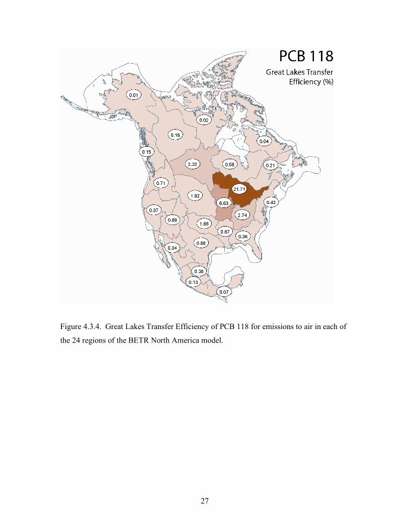
Figure 4.3.4. Great Lakes Transfer Efficiency of PCB 118 for emissions to air in each of
the 24 regions of the BETR North America model.

28
Figure 4.3.5. Great Lakes Transfer Efficiency of PCB 138 for emissions to air in each of
the 24 regions of the BETR North America model.
29
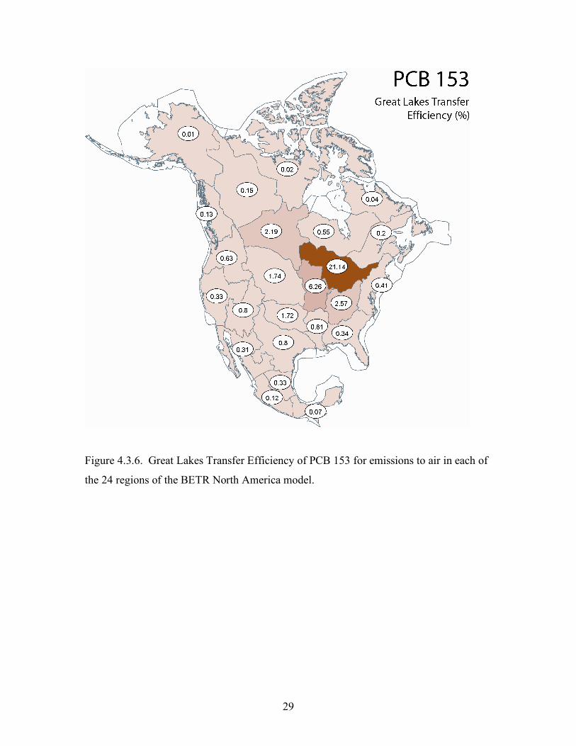
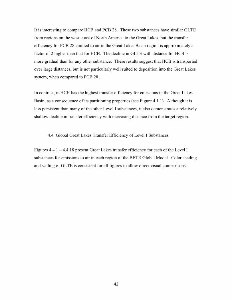
Figure 4.3.6. Great Lakes Transfer Efficiency of PCB 153 for emissions to air in each of
the 24 regions of the BETR North America model.

30
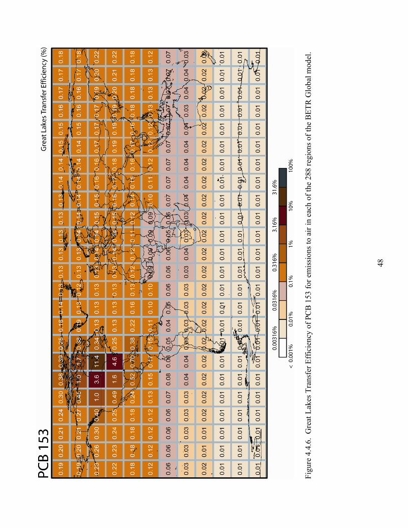
Figure 4.3.7. Great Lakes Transfer Efficiency of PCB 180 for emissions to air in each of
the 24 regions of the BETR North America model.

31
Figure 4.3.8. Great Lakes Transfer Efficiency of Dieldrin for emissions to air in each of
the 24 regions of the BETR North America model.

32
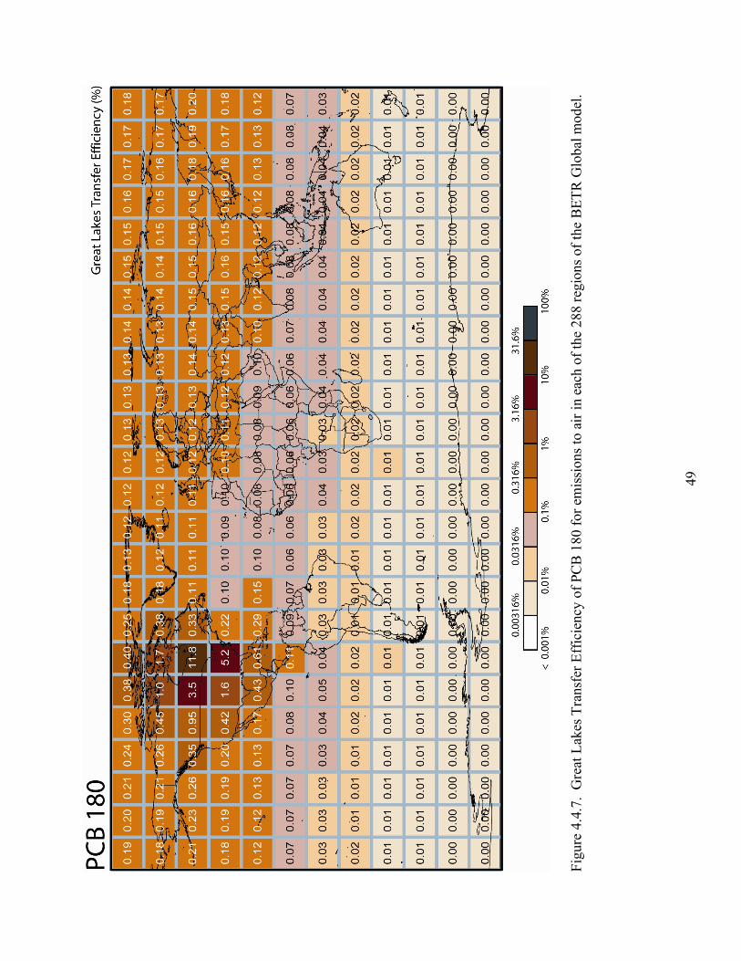
Figure 4.3.9. Great Lakes Transfer Efficiency of Aldrin for emissions to air in each of
the 24 regions of the BETR North America model.

33
Figure 4.3.10. Great Lakes Transfer Efficiency of hexachlorobenzene (HCB) for
emissions to air in each of the 24 regions of the BETR North America model.

34
Figure 4.3.11. Great Lakes Transfer Efficiency of total chlordanes for emissions to air in
each of the 24 regions of the BETR North America model.

35
Figure 4.3.12. Great Lakes Transfer Efficiency of 2,3,7,8-tetrachlorodibenzodioxin for
emissions to air in each of the 24 regions of the BETR North America model.
36
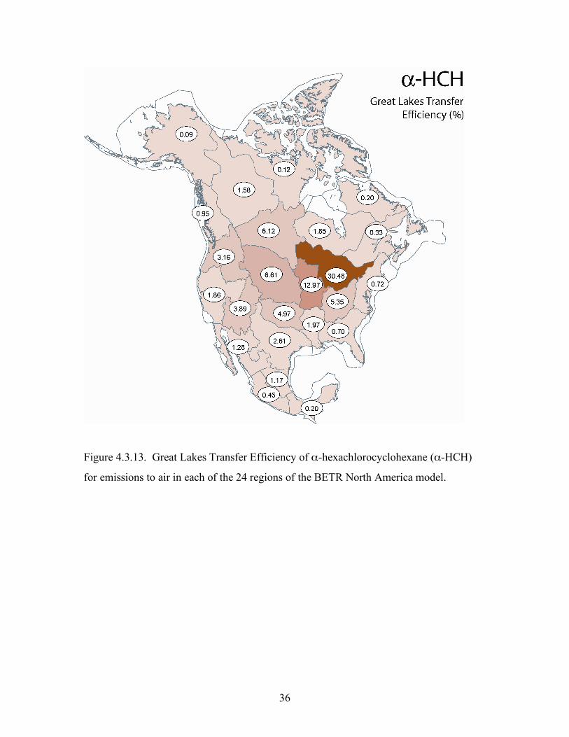
Figure 4.3.13. Great Lakes Transfer Efficiency of α-hexachlorocyclohexane (α-HCH)
for emissions to air in each of the 24 regions of the BETR North America model.

37
Figure 4.3.14. Great Lakes Transfer Efficiency of p,p’-DDT for emissions to air in each
of the 24 regions of the BETR North America model.

38
Figure 4.3.15. Great Lakes Transfer Efficiency of toxaphene for emissions to air in each
of the 24 regions of the BETR North America model.

39
Figure 4.3.16. Great Lakes Transfer Efficiency of octachlorostyrene (OCS) for emissions
to air in each of the 24 regions of the BETR North America model.

40
Figure 4.3.17. Great Lakes Transfer Efficiency of benzo[a]pyrene (B[a]P) for emissions
to air in each of the 24 regions of the BETR North America model.

41
Figure 4.3.18. Great Lakes Transfer Efficiency of Mirex for emissions to air in each of
the 24 regions of the BETR North America model.
The model results shown in Figures 4.3.1 – 4.3.18 build upon the generic model results
illustrated by the hazard identification plots, in particular Figure 4.2.2. Great Lakes
transfer efficiencies for Aldrin, Dieldrin and B[a]P decline relatively sharply with
increasing distance of the source region from the Great Lakes basin. The less chlorinated
PCBs are more efficiently transported and deposited over continental scales than the
higher chlorinated congeners.
42
It is interesting to compare HCB and PCB 28. These two substances have similar GLTE
from regions on the west coast of North America to the Great Lakes, but the transfer
efficiency for PCB 28 emitted to air in the Great Lakes Basin region is approximately a
factor of 2 higher than that for HCB. The decline in GLTE with distance for HCB is
more gradual than for any other substance. These results suggest that HCB is transported
over large distances, but is not particularly well suited to deposition into the Great Lakes
system, when compared to PCB 28.
In contrast, α-HCH has the highest transfer efficiency for emissions in the Great Lakes
Basin, as a consequence of its partitioning properties (see Figure 4.1.1). Although it is
less persistent than many of the other Level I substances, it also demonstrates a relatively
shallow decline in transfer efficiency with increasing distance from the target region.
4.4 Global Great Lakes Transfer Efficiency of Level I Substances
Figures 4.4.1 – 4.4.18 present Great Lakes transfer efficiency for each of the Level I
substances for emissions to air in each region of the BETR Global Model. Color shading
and scaling of GLTE is consistent for all figures to allow direct visual comparisons.

43
Figu
re 4
.4.1
. G
reat
Lak
es T
rans
fer E
ffic
ienc
y of
PC
B 2
8 fo
r em
issi
ons t
o ai
r in
each
of t
he 2
88 re
gion
s of t
he B
ETR
Glo
bal m
odel
.

44
Figu
re 4
.4.2
. G
reat
Lak
es T
rans
fer E
ffic
ienc
y of
PC
B 5
2 fo
r em
issi
ons t
o ai
r in
each
of t
he 2
88 re
gion
s of t
he B
ETR
Glo
bal m
odel
.

45
Figu
re 4
.4.3
. G
reat
Lak
es T
rans
fer E
ffic
ienc
y of
PC
B 1
01 fo
r em
issi
ons t
o ai
r in
each
of t
he 2
88 re
gion
s of t
he B
ETR
Glo
bal m
odel
.

46
Figu
re 4
.4.4
. G
reat
Lak
es T
rans
fer E
ffic
ienc
y of
PC
B 1
18 fo
r em
issi
ons t
o ai
r in
each
of t
he 2
88 re
gion
s of t
he B
ETR
Glo
bal m
odel
.

47
Figu
re 4
.4.5
. G
reat
Lak
es T
rans
fer E
ffic
ienc
y of
PC
B 1
38 fo
r em
issi
ons t
o ai
r in
each
of t
he 2
88 re
gion
s of t
he B
ETR
Glo
bal m
odel
.
48
Fi
gure
4.4
.6.
Gre
at L
akes
Tra
nsfe
r Eff
icie
ncy
of P
CB
153
for e
mis
sion
s to
air i
n ea
ch o
f the
288
regi
ons o
f the
BET
R G
loba
l mod
el.
49
Figu
re 4
.4.7
. G
reat
Lak
es T
rans
fer E
ffic
ienc
y of
PC
B 1
80 fo
r em
issi
ons t
o ai
r in
each
of t
he 2
88 re
gion
s of t
he B
ETR
Glo
bal m
odel
.

50
Figu
re 4
.4.8
. G
reat
Lak
es T
rans
fer E
ffic
ienc
y of
Die
ldrin
for e
mis
sion
s to
air i
n ea
ch o
f the
288
regi
ons o
f the
BET
R G
loba
l mod
el.
51
Figu
re 4
.4.9
. G
reat
Lak
es T
rans
fer E
ffic
ienc
y of
Ald
rin fo
r em
issi
ons t
o ai
r in
each
of t
he 2
88 re
gion
s of t
he B
ETR
Glo
bal m
odel
.

52
Figu
re 4
.4.1
0. G
reat
Lak
es T
rans
fer E
ffic
ienc
y of
hex
achl
orob
enze
ne fo
r em
issi
ons t
o ai
r in
each
of t
he 2
88 re
gion
s of t
he B
ETR
G
loba
l mod
el.

53
Fi
gure
4.4
.11.
Gre
at L
akes
Tra
nsfe
r Eff
icie
ncy
of c
hlor
dane
for e
mis
sion
s to
air i
n ea
ch o
f the
288
regi
ons o
f the
BET
R G
loba
l m
odel
.

54
Figu
re 4
.4.1
2. G
reat
Lak
es T
rans
fer E
ffic
ienc
y of
2.3
,7,8
-tetra
chlo
rodi
benz
odio
xin
for e
mis
sion
s to
air i
n ea
ch o
f the
288
regi
ons o
f th
e B
ETR
Glo
bal m
odel
.

55
Figu
re 4
.4.1
3. G
reat
Lak
es T
rans
fer E
ffic
ienc
y of
α-h
exac
hlor
ocyc
lohe
xane
for e
mis
sion
s to
air i
n ea
ch o
f the
288
regi
ons o
f the
B
ETR
Glo
bal m
odel
.

56
Fi
gure
4.4
.14.
Gre
at L
akes
Tra
nsfe
r Eff
icie
ncy
of p
-p’-
DD
T fo
r em
issi
ons t
o ai
r in
each
of t
he 2
88 re
gion
s of t
he B
ETR
Glo
bal
mod
el.

57
Figu
re 4
.4.1
5. G
reat
Lak
es T
rans
fer E
ffic
ienc
y of
toxa
phen
e fo
r em
issi
ons t
o ai
r in
each
of t
he 2
88 re
gion
s of t
he B
ETR
Glo
bal
mod
el.

58
Figu
re 4
.4.1
6. G
reat
Lak
es T
rans
fer E
ffic
ienc
y of
oct
achl
oros
tyre
ne fo
r em
issi
ons t
o ai
r in
each
of t
he 2
88 re
gion
s of t
he B
ETR
G
loba
l mod
el.
59
Fi
gure
4.4
.17.
Gre
at L
akes
Tra
nsfe
r Eff
icie
ncy
of b
enzo
[a]p
yren
e fo
r em
issi
ons t
o ai
r in
each
of t
he 2
88 re
gion
s of t
he B
ETR
Glo
bal
mod
el.

60
Fi
gure
4.4
.18.
Gre
at L
akes
Tra
nsfe
r Eff
icie
ncy
of M
irex
for e
mis
sion
s to
air i
n ea
ch o
f the
288
regi
ons o
f the
BET
R G
loba
l mod
el.
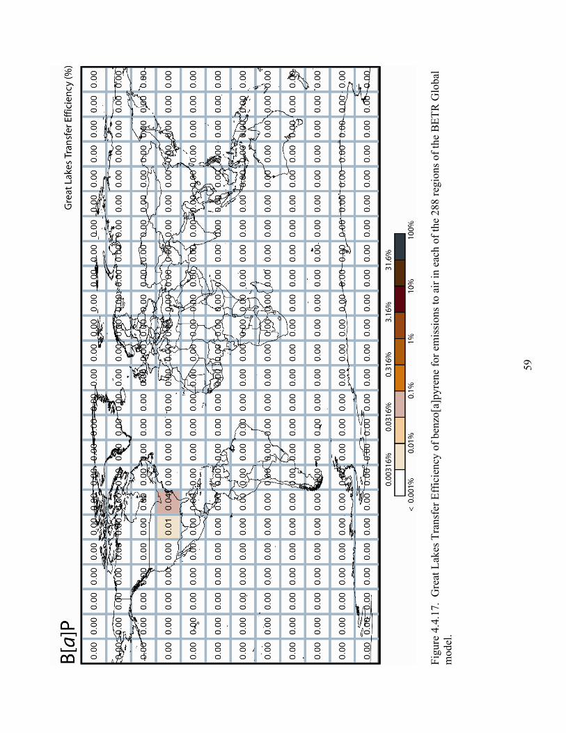
61
As was the case for the results from the North American Model, the maps of GLTE from
each region of the BETR Global model are best interpreted with reference to the generic
results, which are provided in see Figure 4.2.3. Dieldrin, Aldrin, and B[a]P show very
rapid declines in GLTE with distance from the target region. Atmospheric deposition of
these three Level I substances is likely dominated by local and regional sources.
Chlordane, 2,3,7,8-TCDD, DDT, toxaphene, OCS, and Mirex all have GLTE from within
North America that are within a factor of about 30 of transfer efficiencies for releases in
the target region itself, but lower efficiencies for emissions from outside North America.
These substances can therefore be classified as having potential for continental scale
transport and deposition to the Great Lakes. The seven PCB congeners show GLTE from
locations in the Northern Hemisphere that are within approximately a factor of 30 of
transfer efficiencies for local emissions, but transfer from the Southern Hemisphere is
less efficient. HCB and α-HCH are transported and deposited to the Lakes from any
emission location in the world with efficiencies that are within a factor of 30 to 60 of
efficiencies for local releases. Thus, our model results indicate that these pollutants are
subject to global-scale transport and redistribution.
5.0 EMISSION ESTIMATES In this section, we summarize emissions inventories at the North American scale for
seven PCB congeners and toxaphene, and at the global scale for our full set of PCBs and
α-HCH. Modeled concentrations of PCBs in air obtained from the BETR Global model
are compared with data from nine long-term monitoring stations in the Northern
Hemisphere, including the International Atmospheric Deposition Network (IADN),
which is located in the Great Lakes Basin.
5.1 North American Emissions of PCBs and Toxaphene
PCB emission estimates to air for Canada, the United States, and Mexico have been made
by Breivik et al. (16,17) for individual congeners as part of their global emissions
inventory. Breivik et al. (16,17) report large uncertainties in these estimates. In order to
62
convey these uncertainties they provide three emissions scenarios (maximum, default, and
minimum) to reflect the range of possible emissions that are consistent with their analysis.
The range of emissions estimates between the minimum and maximum scenarios spans
more than two orders of magnitude.
In order to estimate emissions in each BETR region, we apportioned the country-specific
emissions estimates made by Breivik et al. (16,17) into the regions of the BETR North
America model based on geographically referenced global population distribution using
data provided by Environment Canada (18). Figures 5.1.1 – 5.1.7 show the proportion of
total emissions in the default emission scenario allotted to each BETR North America
region using this methodology.
Emissions estimates for toxaphene in North America appropriate for use in BETR North
America have been made previously by MacLeod et al. (19) and are shown in Figure
5.1.8.

63
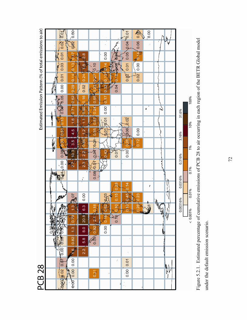
Figure 5.1.1. Estimated percentage of cumulative emissions of PCB 28 to air in North
America occurring in each region of the BETR North America model.

64
Figure 5.1.2. Estimated percentage of cumulative emissions of PCB 52 to air in North
America occurring in each region of the BETR North America model.

65
Figure 5.1.3. Estimated percentage of cumulative emissions of PCB 101 to air in North
America occurring in each region of the BETR North America model.

66
Figure 5.1.4. Estimated percentage of cumulative emissions of PCB 118 to air in North
America occurring in each region of the BETR North America model.

67
Figure 5.1.5. Estimated percentage of cumulative emissions of PCB 138 to air in North
America occurring in each region of the BETR North America model.

68
Figure 5.1.6. Estimated percentage of cumulative emissions of PCB 153 to air in North
America occurring in each region of the BETR North America model.

69
Figure 5.1.7. Estimated percentage of cumulative emissions of PCB 180 to air in North
America occurring in each region of the BETR North America model.

70
Figure 5.1.8. Estimated percentage of cumulative emissions of toxaphene to air in North
America occurring in each region of the BETR North America model.

71
5.2 Global Emissions of PCBs and α-Hexachlorocyclohexane (α-HCH)
Breivik and al. (16,17) have compiled global estimates of emissions to air for individual
PCB congeners on a country by country basis between 1930 and 2000. As emissions
input for the BETR Global model, we have apportioned these emissions into individual
model regions based on population distribution exploiting the geographically referenced
population data available from Environment Canada (18). As discussed above, there are
three emission scenarios (maximum, default, and minimum) that reflect the uncertainty
range of the emissions estimates. In Figures 5.1.1 – 5.1.14, we present emissions data
from the default scenario in two ways: (1) as the fraction of cumulative emissions
between 1930 and 2000 that occurred in each model region, and (2) as the fraction of
emissions in the year 2000 in each region.
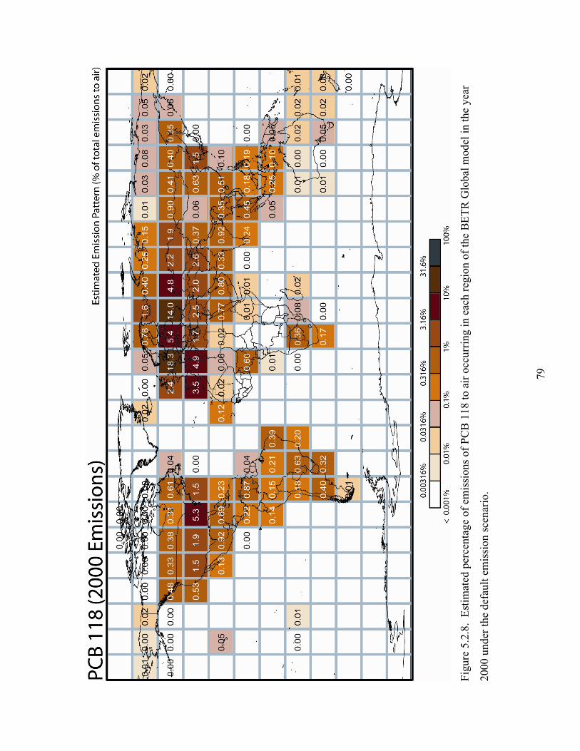
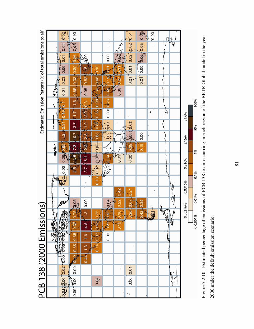
In reviewing these figures, we note that the proportion of global PCB emissions taking
place in close proximity to the Great Lakes was much lower in 2000 than over the entire
use-history of PCBs. The geographic profile of PCB emissions in 2000 has shifted much
more toward Eastern Europe and Asia, and away from North America and Western
Europe. This pattern reflects the aggressive emission reduction programs that have been
pursued in Canada, the United States and Western European countries.
72
Fi
gure
5.2
.1.
Estim
ated
per
cent
age
of c
umul
ativ
e em
issi
ons o
f PC
B 2
8 to
air
occu
rrin
g in
eac
h re
gion
of t
he B
ETR
Glo
bal m
odel
unde
r the
def
ault
emis
sion
scen
ario
.

73
Fi
gure
5.2
.2.
Estim
ated
per
cent
age
of e
mis
sion
s of P
CB
28
to a
ir oc
curr
ing
in e
ach
regi
on o
f the
BET
R G
loba
l mod
el in
the
year
2000
und
er th
e de
faul
t em
issi
on sc
enar
io.

74
Fi
gure
5.2
.3.
Estim
ated
per
cent
age
of c
umul
ativ
e em
issi
ons o
f PC
B 5
2 to
air
occu
rrin
g in
eac
h re
gion
of t
he B
ETR
Glo
bal m
odel
unde
r the
def
ault
emis
sion
scen
ario
.

75
Fi
gure
5.2
.4.
Estim
ated
per
cent
age
of e
mis
sion
s of P
CB
52
to a
ir oc
curr
ing
in e
ach
regi
on o
f the
BET
R G
loba
l mod
el in
the
year
2000
und
er th
e de
faul
t em
issi
on sc
enar
io.
76
Fi
gure
5.2
.5.
Estim
ated
per
cent
age
of c
umul
ativ
e em
issi
ons o
f PC
B 1
01 to
air
occu
rrin
g in
eac
h re
gion
of t
he B
ETR
Glo
bal m
odel
unde
r the
def
ault
emis
sion
scen
ario

77
Fi
gure
5.2
.6.
Estim
ated
per
cent
age
of e
mis
sion
s of P
CB
101
to a
ir oc
curr
ing
in e
ach
regi
on o
f the
BET
R G
loba
l mod
el in
the
year
2000
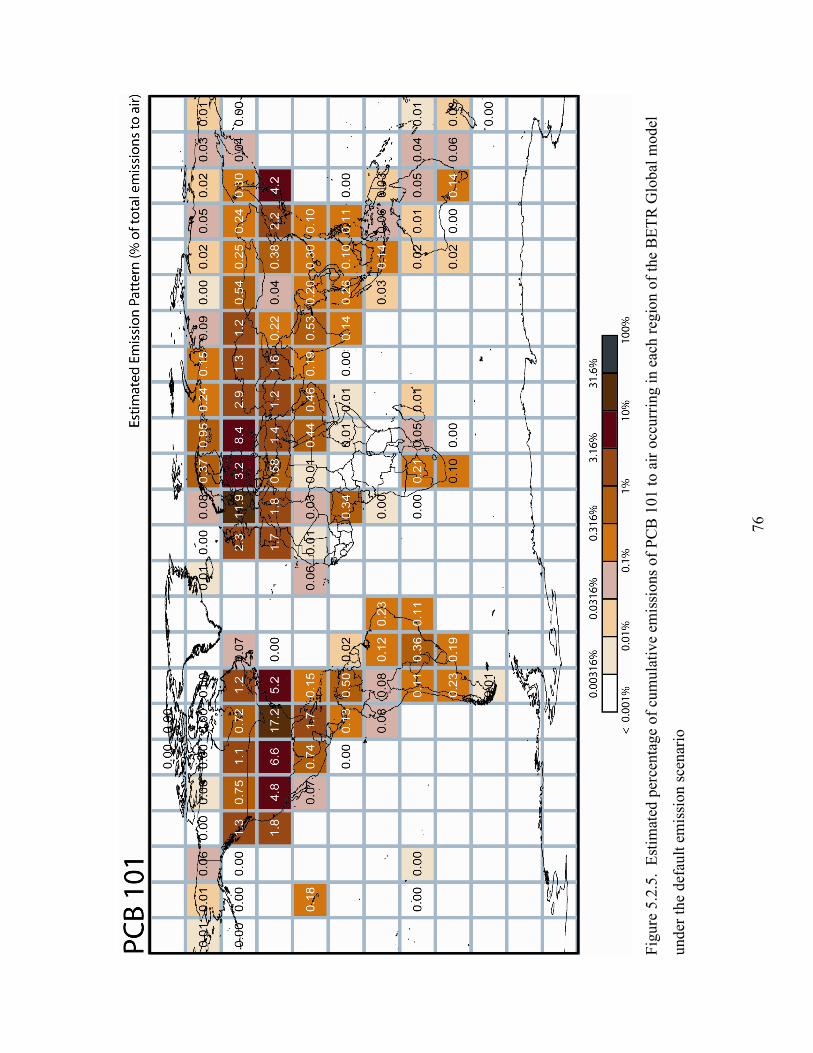
und
er th
e de
faul
t em
issi
on sc
enar
io.
78
Fi
gure
5.2
.7.
Estim
ated
per
cent
age
of c
umul
ativ
e em
issi
ons o
f PC
B 1
18 to
air
occu
rrin
g in
eac
h re
gion
of t
he B
ETR
Glo
bal m
odel
unde
r the
def
ault
emis
sion
scen
ario
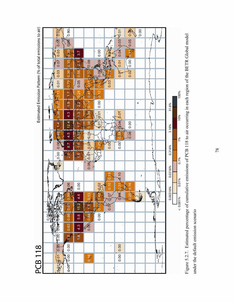
79
Fi
gure
5.2
.8.
Estim
ated
per
cent
age
of e
mis
sion
s of P
CB
118
to a
ir oc
curr
ing
in e
ach
regi
on o
f the
BET
R G
loba
l mod
el in
the
year
2000
und
er th
e de
faul
t em
issi
on sc
enar
io.

80
Fi
gure
5.2
.9.
Estim
ated
per
cent
age
of c
umul
ativ
e em
issi
ons o
f PC
B 1
38 to
air
occu
rrin
g in
eac
h re
gion
of t
he B
ETR
Glo
bal m
odel
unde
r the
def
ault
emis
sion
scen
ario
81
Fi
gure
5.2
.10.
Est
imat
ed p
erce
ntag
e of
em
issi
ons o
f PC
B 1
38 to
air
occu
rrin
g in
eac
h re
gion
of t
he B
ETR
Glo
bal m
odel
in th
e ye
ar
2000
und
er th
e de
faul
t em
issi
on sc
enar
io.

82
Fi
gure
5.2
.11.
Est
imat
ed p
erce
ntag
e of
cum
ulat
ive
emis
sion
s of P
CB
153
to a
ir oc
curr
ing
in e
ach
regi
on o
f the
BET
R G
loba
l mod
el
unde
r the
def
ault
emis
sion
scen
ario

83
Fi
gure
5.2
.12.
Est
imat
ed p
erce
ntag
e of
em
issi
ons o
f PC
B 1
53 to
air
occu
rrin
g in
eac
h re
gion
of t
he B
ETR
Glo
bal m
odel
in th
e ye
ar
2000
und
er th
e de
faul
t em
issi
on sc
enar
io.
84
Fi
gure
5.2
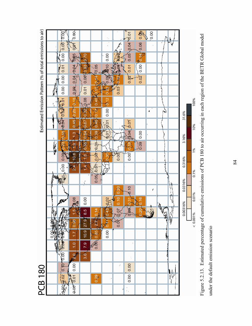
.13.
Est
imat
ed p
erce
ntag
e of
cum
ulat
ive
emis
sion
s of P
CB
180
to a
ir oc
curr
ing
in e
ach
regi
on o
f the
BET
R G
loba
l mod
el
unde
r the
def
ault
emis
sion
scen
ario

85
Fi
gure
5.2
.14.
Est
imat
ed p
erce
ntag
e of
em
issi
ons o
f PC
B 1
80 to
air
occu
rrin
g in
eac
h re
gion
of t
he B
ETR
Glo
bal m
odel
in th
e ye
ar
2000
und
er th
e de
faul
t em
issi
on sc
enar
io.

86
Fi
gure
5.2
.15.
Est
imat
ed p
erce
ntag
e of
cum
ulat
ive
emis
sion
s of a
-HC
H to
air
occu
rrin
g in
eac
h re
gion
of t
he B
ETR
Glo
bal m
odel
.
87
5.3 Global-scale Modeling of PCB Concentrations in Air
We evaluate the performance of the BETR Global model as a descriptor of
chemical fate by comparing model results with measured concentrations of persistent
contaminants at eleven locations in the global environment. A complete description of
our work on development and evaluation of the BETR Global model can be found in the
paper by MacLeod et al. (6). We focus here on the model results for the PCB congeners.
We gathered reported measurements of atmospheric PCB concentrations from eleven
long-term monitoring sites located in seven different model regions, including data from
the International Atmospheric Deposition Network in the Great Lakes region (See Table
5.3.1 for details). We calculated the corresponding atmospheric concentrations of the
PCB congeners with the model by simulating a 70-year period using each of the three
emissions scenarios proposed by Breivik et al. (16,17) for the period 1930 - 2000.
Figures 5.3.1 – 5.3.3 compare modeled and measured concentrations of the seven
selected PCB congeners in air at the eleven monitoring sites for the two emission
scenarios. The diagonal lines are provided for comparison, representing perfect
agreement between the model and measurements, agreement within a factor of 3.16
(=100.5), and agreement within a factor of 10. Correlation coefficients between observed
and modeled concentrations are statistically significant under all three emission
scenarios. Inspection of these figures indicates that concentrations are dramatically
under-predicted using the “minimum” emission scenario, slightly under-predicted using
the “default” emission scenario, and slightly over-predicted by the “maximum” scenario.
When we use the “maximum” scenario, 60% of the 479 modeled concentrations are
within a factor of 3.16 of the measured concentration and 96% are within a factor of 10.
Therefore the residual error that represents the difference between modeled and measured
concentrations has a 96% confidence interval of ± 1 order of magnitude. This means that
96% of the measured concentration data is within and order of magnitude or less of the
corresponding modeled concentration. From this we conclude that agreement between
88
modeled and measured PCB concentrations in air is satisfactory. This exercise
demonstrates that the model is providing a verifiable description of PCB concentrations
in the atmosphere of the Northern Hemisphere.
In the global scale modeling of PCBs, the most important aspect of the emissions profile
is the geographical distribution of emissions to air, and the relationship between
emissions of the different congeners, and not the absolute amount emitted. Recognizing
our goals, we have selected the “default” emission scenario as most appropriate for use in
our model assessments since it produces modeled concentrations with slopes between
modeled and measured data closest to unity. The “default” emissions scenario therefore
produces model results that are most representative of the temporal, spatial, and
congener-to-congener variability in air concentrations that are observed at long-term
monitoring stations.

89
Tabl
e 5.
3.1.
Sou
rces
of i
nfor
mat
ion
for l
ong-
term
mon
itorin
g da
ta o
f atm
osph
eric
PC
B c
once
ntra
tions
.
Abb
revi
atio
n Si
te N
ame
BET
R-G
loba
l M
odel
Reg
ion
Loca
tion
Dat
a pe
riod
Use
d in
A
naly
sis
Dat
a av
aila
bilit
y
Zepp
elin
Ze
ppel
in S
tatio
n 14
Sv
alba
rd, N
orw
ay
1998
– 2
000
[a]
IAD
N E
GH
IA
DN
- Ea
gle
Har
bour
55
M
ichi
ngan
, USA
19
91 –
200
0 [b
] IA
DN
BN
T IA
DN
- B
urnt
Isla
nd
55
Ont
ario
, Can
ada
1993
– 2
000
[b]
Haz
elrig
g H
azel
rigg
Wea
ther
Sta
tion
60
Lanc
aste
r, En
glan
d 19
94 –
200
0 [c
] C
ZK
Kos
etic
e O
bser
vato
ry
61
Cze
ch R
epub
lic
1999
– 2
000
[a]
IVL
Ror
vik
Ror
vik
61
Ror
vik,
Sw
eden
19
95 –
200
0 [d
] IV
L A
spvr
eten
A
spvr
eten
62
A
spvr
eten
, Sw
eden
19
96 –
200
0 [d
] IV
L Pa
llas
Palla
s 62
Pa
llas,
Swed
en
1996
– 2
000
[d]
IAD
N S
BD
IA
DN
- Sl
eepi
ng B
ear D
unes
79
M
ichi
gan,
USA
19
92 –
200
0 [b
] IA
DN
STP
IA
DN
- St
urge
on P
oint
79
N
ew Y
ork,
USA
19
92 –
200
0 [b
] IA
DN
PPT
IA
DN
- Po
int P
etre
79
O
ntar
io, C
anad
a 19
92 –
200
0 [b
] [a
] – b
y re
ques
t fro
m D
r. W
eche
Aas
, Nor
weg
ian
Inst
itute
for A
ir R
esea
rch
(NIL
U),
waa
@ni
lu.n
o [b
] – b
y re
ques
t fro
m E
nviro
nmen
t Can
ada,
http
://w
ww
.msc
-sm
c.ec
.ca/
iadn
/Dat
a/fo
rm/fo
rm_e
.htm
l
[c] –
by
requ
est f
rom
Dr.
Rob
ert G
. M. L
ee, I
nstit
ute
of E
nviro
nmen
tal a
nd N
atur
al S
cien
ces,
Lanc
aste
r Uni
vers
ity,
r.g.le
e@la
ncas
ter.a
c.uk
[d] –
ava
ilabl
e fo
r dow
nloa
d fr
om IV
L Sw
edis
h En
viro
nmen
tal R
esea
rch
Inst
itute
, http
://w
ww
.ivl.s
e/m
iljo/
db/s
tartk
art.a
sp

90
Figure 5.3.1. Comparison of yearly averaged measured and modeled atmospheric PCB
congener concentrations for the “minimum” emission scenario reported by Breivik et al. (16,17) Measurement data are from eleven long-term monitoring stations located in seven
different model regions.

91
Figure 5.3.2. Comparison of yearly averaged measured and modeled atmospheric PCB
congener concentrations for the “default” emission scenario reported by Breivik et al. (16,17) Measurement data are from eleven long-term monitoring stations located in seven
different model regions.

92
Figure 5.3.3. Comparison of yearly averaged measured and modeled atmospheric PCB
congener concentrations for the “maximum” emission scenario reported by Breivik et al. (16,17) Measurement data are from eleven long-term monitoring stations located in seven
different model regions.

93
6.0 REGIONAL CONTRIBUTIONS TO ATMOSPERIC LOADINGS OF LEVEL I SUBSTANCES
In this section we combine information from the generic modeling and emissions
estimates to calculate the fraction of total loading from the atmosphere that is attributable
to sources in different regions of North America and the world.
6.1 North American Contributions to Loadings of PCBs and Toxaphene
Using the Great Lakes Transfer Efficiencies presented in Section 4.0 and the North
American-scale emissions estimates in Section 5.0, we derive here the relative
contribution from different regions of North America to atmospheric deposition of PCBs
and toxaphene to the Great Lakes water shed. We provide results of this analysis in
Figures 6.1.1 – 6.1.8.

94
Figure 6.1.1. Fraction of atmospheric loading of PCB 28 to the Great Lakes attributable
to emissions in each region of the BETR North America model.

95
Figure 6.1.2. Fraction of atmospheric loading of PCB 52 to the Great Lakes attributable
to emissions in each region of the BETR North America model.

96
Figure 6.1.3. Fraction of atmospheric loading of PCB 101 to the Great Lakes attributable
to emissions in each region of the BETR North America model.
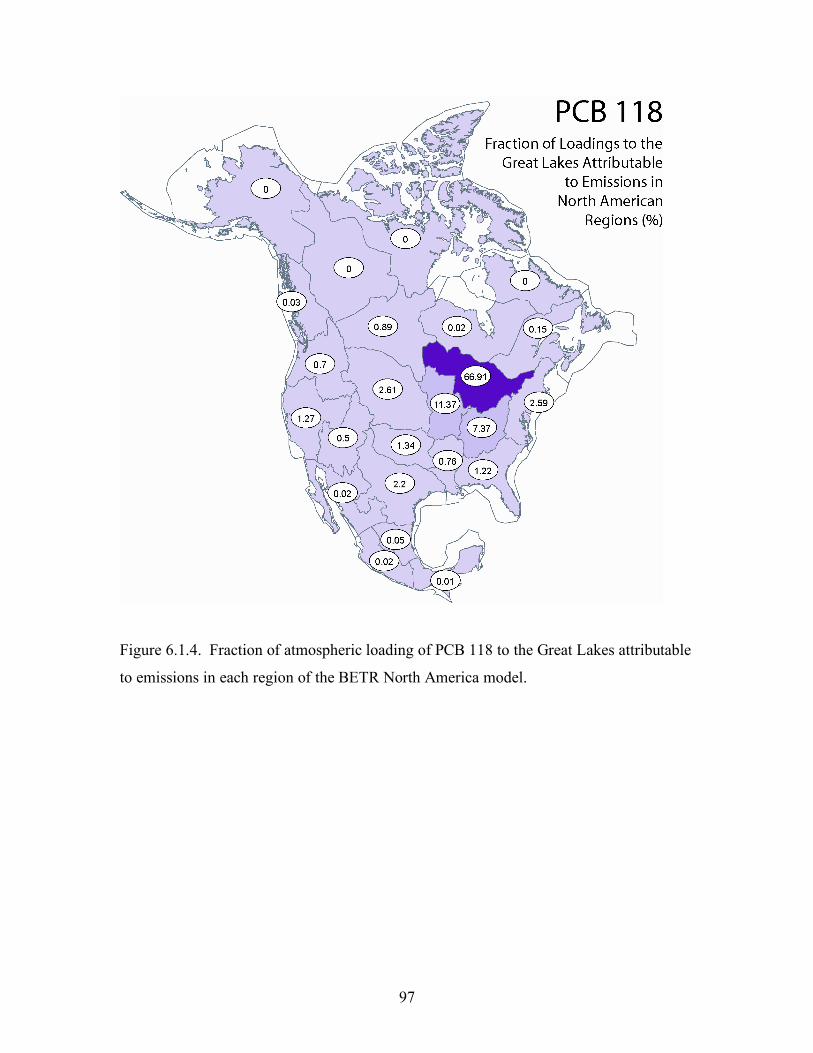
97
Figure 6.1.4. Fraction of atmospheric loading of PCB 118 to the Great Lakes attributable
to emissions in each region of the BETR North America model.

98
Figure 6.1.5. Fraction of atmospheric loading of PCB 138 to the Great Lakes attributable
to emissions in each region of the BETR North America model.

99
Figure 6.1.6. Fraction of atmospheric loading of PCB 153 to the Great Lakes attributable
to emissions in each region of the BETR North America model.

100
Figure 6.1.7. Fraction of atmospheric loading of PCB 180 to the Great Lakes attributable
to emissions in each region of the BETR North America model.
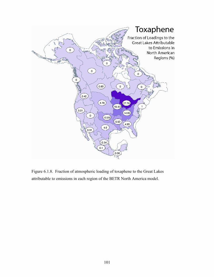
101
Figure 6.1.8. Fraction of atmospheric loading of toxaphene to the Great Lakes
attributable to emissions in each region of the BETR North America model.

102
As can be seen from Figures Figures 6.1.1 – 6.1.7, the majority of PCB deposition from
the atmosphere to the Lakes for all of the congeners examined is due to emissions within
the Great Lakes Basin. Moreover, the relative contribution of local sources increases
with increasing chlorination level, and ranges from 53% for PCB 28 and PCB 52 to 72%
for PCB 180.
In interpreting these results it is important to consider issues that impact their reliability.
First of all, we note that our estimates of contributions to Great Lakes loadings reflect the
cumulative emissions of PCBs to the atmosphere over the entire use history of these
compounds. Because of data limitations associated with applying the country-specific
global-scale emissions estimates of Breivik et al. (16,17) at the North American scale, we
have not examined the relative contributions to loadings at the end of the emission
scenario in the North American model. The emissions inventory only provides an
estimate of total emissions in the United States, Canada and Mexico, and these emissions
are then apportioned based on population density. Therefore we lack spatially resolved
information on the relative rate of PCB emission reductions in different parts of North
America. A spatially resolved emissions inventory for North America that included
information about the relative rates of emission reductions in different parts of the
continent would be required to perform such an analysis.
As discussed in detail by MacLeod et al.(19) the contribution of local sources of
toxaphene to atmospheric deposition to the Lakes due to emissions in North America is
approximately 30%. Differences between the results for toxaphene in Figure 6.1.8 and
those presented by MacLeod et al. are due to different assumptions about emission
patterns. MacLeod and Mackay assumed 70% emissions to soil, 25% to air, and 5% to
surface water to represent typical usage of toxaphene, while this study assumes 100%
emissions to air to focus on atmospheric transport and deposition explicitly, and to allow
direct comparison between toxaphene and the PCB congeners.

103
6.2 Global Contributions to Loadings of PCBs and α-HCH
We use the BETR Global model and the data and methods described in Sections 3
through 5 to derive the relative contribution from different global regions to atmospheric
loading of the PCB congeners and α-HCH. We present the results of these analyses in
Figures 6.2.1 – 6.2.15. The results for the PCB congeners reflect an emission scenario
representing the cumulative emissions from 1930 – 2000 under the Breivik et al. (16,17)
“default” emission scenario, and for emissions representative of the pattern in 2000 under
the “default” scenario.

10
4
Fi
gure
6.2
.1.
Estim
ated
frac
tion
of a
tmos
pher
ic lo
adin
g of
PC
B 2
8 to
the
Gre
at L
akes
attr
ibut
able
to e
mis
sion
s in
each
regi
on o
f the
BET
R G
loba
l mod
el u
nder
the
cum
ulat
ive
defa
ult e
mis
sion
scen
ario
.

10
5
Fi
gure
6.2
.2.
Estim
ated
frac
tion
of a
tmos
pher
ic lo
adin
g of
PC
B 2
8 to
the
Gre
at L
akes
attr
ibut
able
to e
mis
sion
s in
each
regi
on o
f the
BET
R G
loba
l mod
el d
ue to
yea
r 200
0 em
issi
ons u
nder
the
defa
ult e
mis
sion
scen
ario
.
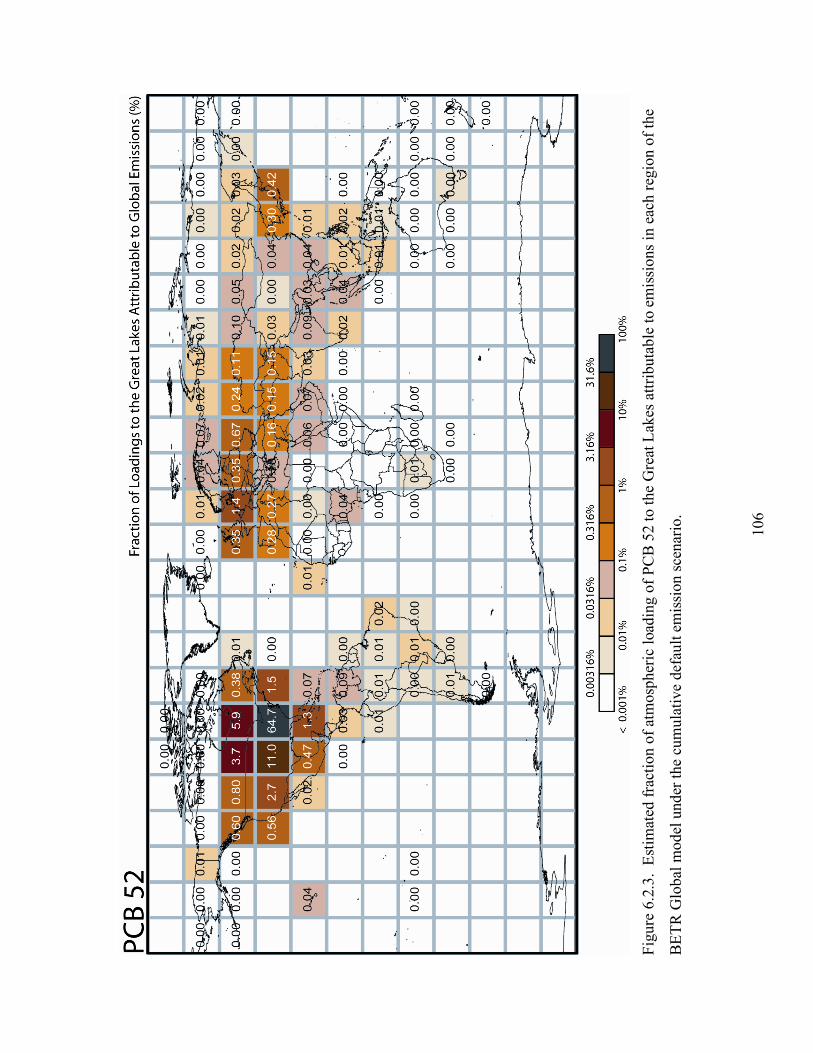
10
6
Fi
gure
6.2
.3.
Estim
ated
frac
tion
of a
tmos
pher
ic lo
adin
g of
PC
B 5
2 to
the
Gre
at L
akes
attr
ibut
able
to e
mis
sion
s in
each
regi
on o
f the
BET
R G
loba
l mod
el u
nder
the
cum
ulat
ive
defa
ult e
mis
sion
scen
ario
.

10
7
Fi
gure
6.2
.4.
Estim
ated
frac
tion
of a
tmos
pher
ic lo
adin
g of
PC
B 5
2 to
the
Gre
at L
akes
attr
ibut
able
to e
mis
sion
s in
each
regi
on o
f the
BET
R G
loba
l mod
el d
ue to
yea
r 200
0 em
issi
ons u
nder
the
defa
ult e
mis
sion
scen
ario
.
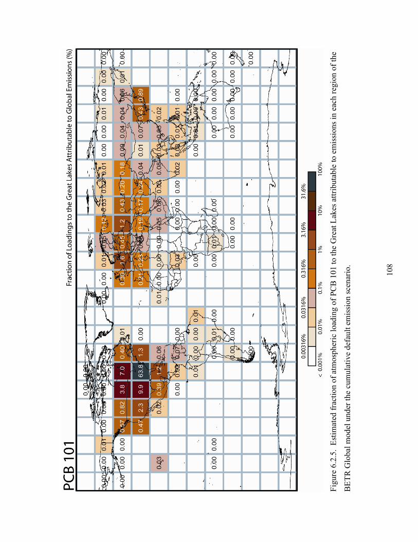
10
8
Fi
gure
6.2
.5.
Estim
ated
frac
tion
of a
tmos
pher
ic lo
adin
g of
PC
B 1
01 to
the
Gre
at L
akes
attr
ibut
able
to e
mis
sion
s in
each
regi
on o
f the
BET
R G
loba
l mod
el u
nder
the
cum
ulat
ive
defa
ult e
mis
sion
scen
ario
.

10
9
Fi
gure
6.2
.6.
Estim
ated
frac
tion
of a
tmos
pher
ic lo
adin
g of
PC
B 1
01 to
the
Gre
at L
akes
attr
ibut
able
to e
mis
sion
s in
each
regi
on o
f the
BET
R G
loba
l mod
el d
ue to
yea
r 200
0 em
issi
ons u
nder
the
defa
ult e
mis
sion
scen
ario
.

11
0
Fi
gure
6.2
.7.
Estim
ated
frac
tion
of a
tmos
pher
ic lo
adin
g of
PC
B 1
18 to
the
Gre
at L
akes
attr
ibut
able
to e
mis
sion
s in
each
regi
on o
f the
BET
R G
loba
l mod
el u
nder
the
cum
ulat
ive
defa
ult e
mis
sion
scen
ario
.

11
1
Fi
gure
6.2
.8.
Estim
ated
frac
tion
of a
tmos
pher
ic lo
adin
g of
PC
B 1
18 to
the
Gre
at L
akes
attr
ibut
able
to e
mis
sion
s in
each
regi
on o
f the
BET
R G
loba
l mod
el d
ue to
yea
r 200
0 em
issi
ons u
nder
the
defa
ult e
mis
sion
scen
ario
.

11
2
Fi
gure
6.2
.9.
Estim
ated
frac
tion
of a
tmos
pher
ic lo
adin
g of
PC
B 1
38 to
the
Gre
at L
akes
attr
ibut
able
to e
mis
sion
s in
each
regi
on o
f the
BET
R G
loba
l mod
el u
nder
the
cum
ulat
ive
defa
ult e
mis
sion
scen
ario
.

11
3
Fi
gure
6.2
.10.
Est
imat
ed fr
actio
n of
atm
osph
eric
load
ing
of P
CB
138
to th
e G
reat
Lak
es a
ttrib
utab
le to
em
issi
ons i
n ea
ch re
gion
of
the
BET
R G
loba
l mod
el d
ue to
yea
r 200
0 em
issi
ons u
nder
the
defa
ult e
mis
sion
scen
ario
.

11
4
Fi
gure
6.2
.11.
Est
imat
ed fr
actio
n of
atm
osph
eric
load
ing
of P
CB
153
to th
e G
reat
Lak
es a
ttrib
utab
le to
em
issi
ons i
n ea
ch re
gion
of
the
BET
R G
loba
l mod
el u
nder
the
cum
ulat
ive
defa
ult e
mis
sion
scen
ario
.

11
5
Fi
gure
6.2
.12.
Est
imat
ed fr
actio
n of
atm
osph
eric
load
ing
of P
CB
153
to th
e G
reat
Lak
es a
ttrib
utab
le to
em
issi
ons i
n ea
ch re
gion
of
the
BET
R G
loba
l mod
el d
ue to
yea
r 200
0 em
issi
ons u
nder
the
defa
ult e
mis
sion
scen
ario
.

11
6
Fi
gure
6.2
.13.
Est
imat
ed fr
actio
n of
atm
osph
eric
load
ing
of P
CB
180
to th
e G
reat
Lak
es a
ttrib
utab
le to
em
issi
ons i
n ea
ch re
gion
of
the
BET
R G
loba
l mod
el u
nder
the
cum
ulat
ive
defa
ult e
mis
sion
scen
ario
.
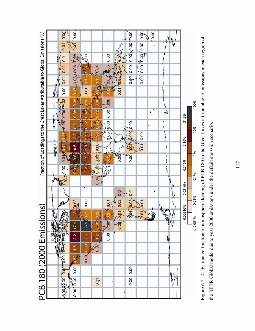
11
7
Fi
gure
6.2
.14.
Est
imat
ed fr
actio
n of
atm
osph
eric
load
ing
of P
CB
180
to th
e G
reat
Lak
es a
ttrib
utab
le to
em
issi
ons i
n ea
ch re
gion
of
the
BET
R G
loba
l mod
el d
ue to
yea
r 200
0 em
issi
ons u
nder
the
defa
ult e
mis
sion
scen
ario
.

11
8
Fi
gure
6.2
.15.
Est
imat
ed fr
actio
n of
atm
osph
eric
load
ing
of α
-HC
H to
the
Gre
at L
akes
attr
ibut
able
to e
mis
sion
s in
each
regi
on o
f the
BET
R G
loba
l mod
el.

119
In the case of the global-scale assessment for year 2000 releases, we find that the
modeled contributions to atmospheric deposition to the Great Lakes for the PCB
congeners shift from local sources toward more distant contributions. When cumulative
(1930-2000) emissions are considered, local sources tend to dominate overall loading to
the Great Lakes. But under the year 2000 scenario, there is a shift toward a larger
influence of sources in Asia and particularly Eastern Europe to Great Lakes loading.
Because the GLTE from all locations is identical under both emission scenarios, this shift
is directly attributable to the more rapid rate of emission reductions in the United States
and Canada relative to Asia and Eastern Europe.
As an example of the shift to distant sources of PCB deposition to the Great Lakes, we
consider PCB 52. When we consider cumulative emissions between 1930 and 2000,
greater than 70% of atmospheric loadings of PCB 52 to surface water in model regions
including the Great Lakes are attributable to sources in close proximity to the Lakes, and
sources in North America account for 90% of loadings. Under the year 2000 emission
scenario the contribution of local sources of PCB 52 is less than 50%, the North
American contribution is less than 70 %, and the bulk of the balance is made up of
contributions from sources in Eastern Europe.
Atmospheric loadings of α-HCH to the Great Lakes are mostly attributable to emissions
in Asia, consistent with very low usage in North America and efficient transport over the
global scale.

120
7.0 CONCLUSIONS AND RECOMENDATIONS
In this section, we present overall conclusions from the study and suggest avenues for
future research. We recommend actions to further improve our ability to identify sources
of atmospherically derived persistent pollutants in the Great Lakes and to more accurately
quantify the relative contributions of these sources to total loadings.
7.1 Conclusions
The first component of our assessment as reported here was to demonstrate a screening-
level analysis to evaluate Level I substances for persistence and long-range transport
potential. We selected all the organic chemicals among the Level I substances as
identified in the Great Lakes Binational Toxics Strategy. Using a suite of mass balance
contaminant fate models, we evaluated these chemicals for both persistence and potential
for long-range transport and deposition to the Great Lakes. We compiled
physicochemical properties and carried out generic modeling for 18 individual chemicals
representing the Level I substances. Based on a screening analysis of partitioning
properties alone, all of the substances examined demonstrated the potential for
continental-scale transport and deposition to the Lakes provided they are sufficiently
persistent. Modeling of Characteristic Travel Distance and Great Lakes Transfer
Efficiency using generic emission scenarios indicated that the majority of the substances
were sufficiently persistent to undergo significant continental, hemispheric or global-
scale transport to the Great Lakes.
Generic transport and deposition efficiency modeling of the Level I substances over
continental and global scales allowed us to categorize them according to the likely spatial
scale of emissions that could significantly impact the Great Lakes. Our results are as
follows:
(1) Local or regional scale: Dieldrin, Aldrin, benzo[a]pyrene

121
(2) Continental scale: Chlordane, 2,3,7,8-TCDD, p,p’-DDT, toxaphene,
octachlorostyrene, mirex
(3) Hemispheric scale: PCBs
(4) Global scale: hexachlorobenzene, α-HCH.
In order to calculate total atmospheric loading to the Lakes, we used available emissions
estimates and the contribution of Level I substance emissions in different regions of
North America and the world. The estimates of regional contributions to atmospheric
loading are subject to large uncertainties most notably because of uncertainties in
emission scenarios. There are also uncertainties attributable to chemical property inputs
and to conceptual assumptions of multimedia fate models. Examples are the assumption
that partitioning among environmental media is fast relative to inter-regional transfer and
uncertainty in the empirical relationships between partition coefficients and
environmental partitioning used in the model. However, these conceptual restrictions
have been evaluated in a number of model evaluation studies and shown not be
significant limitations on model performance. A more important source of uncertainty in
these assessments is the limited quality, quantity, and relevance of data available on rates
of chemical transformation in environmental media among the large and diverse
landscapes considered in the BETR model applications. But in spite of the key
uncertainties contributed by emissions and reaction rate uncertainties, based on available
emissions estimates for seven PCB congeners we have assembled mass budgets for the
period 1930 to 2000 that exhibit satisfactory agreement with observed atmospheric
concentrations in the late 1990s at long term monitoring stations in the Northern
Hemisphere. The uncertainty in the comparison between modeled and observed
concentrations demonstrates the extent of our overall understanding of the sources and
long-term fate and transport of PCBs in the global environment.
Calculated loadings attributable to different regions under emissions scenarios
representing total historical PCB emissions and emissions in the year 2000 suggest that
more rapid reductions of emissions in the United States and Canada relative to other parts
of the world are shifting atmospheric deposition of PCBs to more distant sources.

122
However, as of the year 2000 the majority of PCBs deposited to the Lakes can still be
attributed to sources to the atmosphere within the Great Lakes Basin and neighboring
regions in North America. Therefore, our analysis suggests efforts aimed at further
reductions in atmospheric loading to the Lakes should still be focused primarily on
identifying and eliminating sources of PCBs within the Great Lakes Basin and
neighboring regions.
We offer a hypothetical example to illustrate how model results can be used to support
management decisions and to allocate resources. Consider an EPA official with a fixed
allocation of funds to spend on eliminating emissions of PCBs to the atmosphere with the
goal of maximizing cost-effectiveness in reducing atmospheric loading to the Great
Lakes. Inspection of Figures 4.4.1 – 4.4.7 indicates that on average one kilogram of PCB
emitted to air in the immediate vicinity of the Great Lakes will result in approximately 60
times as much atmospheric loading to the Lakes as one kilogram emitted in China, and
approximately 100 times as much loading as one kilogram emitted in Eastern Europe.
Therefore, to be cost effective, 60 – 100 times greater emission reduction per dollar spent
would be required in China or Eastern Europe, relative to possible emission reductions in
the Great Lakes region.
7.2 Recommendations
The model results presented here for PCBs and toxaphene at the North American spatial
scale and for PCBs and α-HCH at the global scale provide a quantitative synthesis of
current knowledge about the sources, transport, and ultimate fate of these persistent
pollutants. Compiling these mass balances is a challenging task because information
from a variety of sources must be gathered and harmonized into a coherent picture. We
found that mass balances for many of the Level I substances could not be assembled
because of a lack of quantitative information on emissions. This limitation confirms the
need for further work on developing emission inventories. This effort should be made a
priority to improve understanding of source-receptor relationships for all the Level 1
substances. We did, however, discover that even without information from emission

123
estimates it is possible to learn a great deal from the generic modeling evaluations of
persistence and long-range transport, and to gain insight into the important processes
controlling transport and deposition of persistent substances.
With regard to uncertainties, we have not conducted a systematic uncertainty analysis of
the assessments, however considering both model uncertainty and input uncertainty it is
apparent that the key contributors to uncertainties in model calculations for the Level I
substances derive from incomplete emissions data and from unreliable chemical
properties data —primarily transformation rates. Further refinements to the models to
introduce more detailed descriptions of environmental conditions or higher spatial
resolution will not reduce these uncertainties (6). Only more accurate emissions
inventories and additional studies to characterize the partitioning properties and
degradability of the Level I substances in various environmental media will reduce this
fundamental uncertainty. Uncertainties in physico-chemical properties are likely highest
for octachlorostyrene, for which estimated values where used because no measured
property values could be found. Once emissions and degradability uncertainties are
reduced, the next phase in reducing overall model uncertainties will be addressing spatial
and temporal heterogeneity in land-surface properties, degradation mechanisms and
atmospheric transport.
In considering future model development work to build on the assessments presented
here, we recommend additional modeling exercises to examine the importance of fate and
transport processes that are not described in the current model, and continued work to
improve the reliability of the empirical equations used in the model. For example, the
models do not treat chemical fate processes associated with snow and ice, which
dominate the landscape for a significant portion of the year, and the current version of
BETR Global includes a highly simplified description of the circulation of ocean water.
Additional model-based studies of fate and transport processes will help to refine the
existing models and eventually contribute to reducing uncertainties in the overall
assessments.

124
8.0 REFERENCES
(1) United States Environmental Protection Agency and Environment Canada
"The Great Lakes Binational Toxics Strategy," 1997.
(2) MacLeod, M.; Woodfine, D. G.; Mackay, D.; McKone, T.; Bennett, D.;
Maddalena, R. "BETR North America: A regionally segmented multimedia contaminant
fate model for North America" Environmental Science and Pollution Research 2001, 8,
156-163.
(3) Woodfine, D. G.; MacLeod, M.; Mackay, D.; Brimacombe, J. R.
"Development of continental scale multimedia contaminant fate models: Integrating GIS"
Environmental Science and Pollution Research 2001, 8, 164-172.
(4) Mackay, D. Multimedia environmental models: The fugacity approach.;
Lewis Publishers: Boca Raton, Florida, 2001.
(5) McKone, T. E.; MacLeod, M. In Annual Review of Environment and
Resources; Matson, P. A., Gadgil, A., Kammen, D. M., Eds.: Palo Alto, California, 2003;
Vol. 28, pp 463-492.
(6) MacLeod, M.; Riley, W. J.; McKone, T. "Assessing the Influence of
Climate Variability on Atmospheric Concentrations of Persistent Organic Pollutants
Using a Global-Scale Mass Balance Model (BETR-Global)" Environmental Science and
Technology 2005, (In Review).
(7) Fenner, K.; Scheringer, M.; MacLeod, M.; Matthies, M.; McKone, T.;
Stroebe, M.; Beyer, A.; Bonnell, M.; Le Gall, A.-C.; Klasmeier, J.; Mackay, D.; van de
Meent, D.; Pennington, D.; Scharenberg, B.; Suzuki, N.; Wania, F. "Comparing
Estimates of Persistence and Long-Range Transport Potential among Multimedia
Models" Environmental Science and Technology 2005, (In Press).
(8) Bennett, D. H.; McKone, T.; Matthies, M.; Kastenberg, W. E. "General
formulation of characteristic travel distance for semivolatile organic chemicals in a
multimedia environment" Environmental Science & Technology 1998, 32, 4023-4030.
(9) Beyer, A.; Mackay, D.; Matthies, M.; Wania, F.; Webster, E. "Assessing
Long-Range Transport Potential of Persistent Organic Pollutants" Environmental Science
& Technology 2000, 34, 699-703.

125
(10) Canadian Environmental Modelling Centre. "ChemSCORER Beta V1.00"
http://www.trentu.ca/cemc/models/ChemScor.html 2004.
(11) MacLeod, M.; Mackay, D. "Modeling transport and deposition of
contaminants to ecosystems of concern: A case study for the Laurentian Great Lakes"
Environmental Pollution 2004, 128, 241 - 250 (Errata:
http://www.mattmacleod.com/research_files/ENPOFig242ERRATA.pdf).
(12) Pontolillo, J.; Eganhouse, R. P. "The Search for Reliable Aqueous
Solubility (Sw) and Octanol-Water Partition Coefficient (Kow) Data for Hydrophobic
Organic Compounds: DDT and DDE as a Case Study," Water-Resources Investigations
Report 01-4201 (http://water.usgs.gov/pubs/wri/wri014201/), 2001.
(13) Cole, J. G.; Mackay, D. "Correlating environmental partitioning properties
of organic compounds: The three solubility approach" Environmental Toxicology and
Chemistry 2000, 19, 265-270.
(14) Beyer, A.; Wania, F.; Gouin, T.; Mackay, D.; Matthies, M. "Selecting
internally consistent physicochemical properties of organic compounds" Environmental
Toxicology and Chemistry 2002, 21, 941-953.
(15) Organization for Economic Cooperation and Development (OECD)
"Guidance Document on the Use of Multimedia Models for Estimating Overall
Environmental Persistence and Long-range Transport," OECD Environment, Health and
Safety Publications. Series on Testing and Assessment, No. 45, 2004.
(16) Breivik, K.; Sweetman, A.; Pacyna, J. M.; Jones, K. C. "Towards a global
historical emission inventory for selected PCB congeners - a mass balance approach 1.
Global production and consumption" Science of the Total Environment 2002, 290, 181-
198.
(17) Breivik, K.; Sweetman, A.; Pacyna, J. M.; Jones, K. C. "Towards a global
historical emission inventory for selected PCB congeners - a mass balance approach 2.
Emissions" Science of the Total Environment 2002, 290, 199-224.
(18) Environment Canada "Global Pesticides Release Database,"
http://www.msc.ec.gc.ca/data/gloperd/index_e.cfm, 2004.
126
(19) MacLeod, M.; Woodfine, D.; Brimacombe, J.; Toose, L.; Mackay, D. "A
dynamic mass budget for toxaphene in North America" Environmental Toxicology &
Chemistry 2002, 21, 1628-1637.

127
APPENDIX A: ChemSCORER Hazard Profiles for the Level 1 Substances

Page 1 of 6
Summary Rankings for: EPA PCB28
This chemical ... is more PERSISTENT (P) than 94 % of chemicals in the reference set. is more BIOACCUMMULATIVE (B) than 91 % of chemicals in the reference set. No data on mammalian toxicity was supplied. has greater LONG RANGE TRANSPORT (LRT) than 80 % of chemicals in the reference set.
Possible HazardUnlikely Hazard
ChemSCORER Beta101 Assessment - Summary RankingEPA PCB28
Environmental Hazard IndexLikely Hazard
0%
20%
40%
60%
80%
100%P
B
T
LRT

Page 2 of 6
ChemSCORER Beta101 - Level I Model ResultsEPA PCB28
Details of Level I calculation for: EPA PCB28
Compartment Z(mol/m^3Pa) (mol/m^3) (mg/L) (ug/g) kg %
Air 4.03E-04 3.00E-11 7.72E-09 6.51E-06 772 0.772Water 6.19E-02 4.60E-09 1.18E-06 1.18E-06 237 0.237Soil 5.62E+02 4.17E-05 1.08E-02 4.48E-03 96768 96.768Sediment 1.12E+03 8.35E-05 2.15E-02 8.96E-03 2150 2.150Suspended Sediment 3.51E+03 2.61E-04 6.72E-02 4.48E-02 67 0.067Biota (Fish) 1.43E+03 1.06E-04 2.73E-02 2.73E-02 5 0.005Total 100000 100.000
Molar Mass 257.54 g/mol
Vapor Pressure 1 Pa Log Kow 5.66 Air 1.04E-01Aqueous Solubility 15.94 g/m^3 Log Kaw -2.19 Water 1.59E+01Log Kow 5.664 Log Koa 7.85 Octanol 7.35E+06Melting Point -999 deg C
The Level I chemical distibution represents long term equilibrium
partitioning of the chemical. Many persistent chemicals partition
predominantly to soils. Long range transport usually requires
partitioning (at least 1%) to one of the mobile media (air or water).
Bioconcentration Factor (BCF)
23066
The calculated BCF is greater than the generally accepted cut-off between
bioaccumulative and non-bioaccumulative substances of 5000. In the absence of rapid metabolism by organisms, this
substance is expected to bioaccumulate.
Input Parameters Partition Coefficients Three Solubilities(g/m^3)
Concentration AmountEquilibrium Chemical Distribution
Physical Chemical Data and Partition Coefficients
Level I Chemical DistributionAir1%Water
0%
Soil97%
Sediment2%

Page 3 of 6
ChemSCORER Beta101 - Level II Model ResultsEPA PCB28
407 days 1.12 years
1870 days 5.12 years
521 days 1.43 years
Details of Level II calculation for: EPA PCB28
Half-life RemovalReaction Advection Reaction Advection(mol/Pa h) (mol/Pa h) (kg/h) (kg/h)
Air 550 5.08E+07 4.03E+08 9.51E+01 7.55E+02 84.983Water 17000 5.05E+05 1.24E+07 9.44E-01 2.32E+01 2.410Soil 55000 6.37E+07 0 1.19E+02 0 11.921Sediment 55000 1.42E+06 2.25E+06 2.65E+00 4.21E+00 0.685Total 1.16E+08 4.18E+08 2.18E+02 7.82E+02Reaction + Advection
Equilibrium Partitioning Persistence Information
The figure at right identifies environmental media that have a
controlling influence on the overall rate of reactive degradation of this
substance. Substances that fall near the center of the diagram are expected to accumulate in all media, and overall
persistence will be influenced by all degradation rates. The relative
importance of advection and reaction to the regional-scale removal of this
substance, and the media from which these processes take place are depicted
in the pie charts below.
The equilibrium distribution reaction residence time calculated for this
substance can be measured in years, and is comparable to that of
pentachlorobenzene (2 years). Reactive and advective residence times are
comparable, indicating the substance may be mobile to other regions.
Removal Processes - Equilibrium Distribution
5.35E+08 1000
Overall Residence Time:Reaction Residence Time:Advection Residence Time:
Compartment(hours) %
100.000
D Values Loss Rates
-15-14-13-12-11-10-9-8-7-6-5-4-3-2-10123456789
10
-4 -3 -2 -1 0 1 2 3 4 5 6 7 8 9 10
Log Kow
Log
Kaw
Air
Water Octanol
Air& Octanol
Water & Octanol
Air & Water
Removal PathwaysReaction
22%
Advection78%
Media of Reaction
Air44%
Water0%
Soil55%
Sediment1%
Media of Advection
Air96%
Water3%
Sediment1%

Page 4 of 6
ChemSCORER Beta101 - Level III Model ResultsEPA PCB28
Emission to Air
(hours) 14788.8(days) 616.2
(years) 1.7
Emission to Water
(hours) 37221.4(days) 1550.9
(years) 4.2
Emission to Soil
(hours) 78088.8(days) 3253.7
(years) 8.9
Emission to All 3
(hours) 27848.6(days) 1160.4
(years) 3.2
Details of Level III calculation for: EPA PCB28
Air Water Soil Air Water Soil Sediment TotalAir 1000 0 0 6.48E+05 1.71E+05 8.34E+06 5.63E+06 1.48E+07
Water 0 1000 0 4.05E+05 9.33E+05 5.20E+06 3.07E+07 3.72E+07Soil 0 0 1000 1.26E+04 1.33E+04 7.76E+07 4.36E+05 7.81E+07All 3 600 300 100 5.12E+05 3.84E+05 1.43E+07 1.26E+07 2.78E+07
Air 1000 0 0 817 7 105 71 1000Water 0 1000 0 510 38 66 387 1000Soil 0 0 1000 16 1 978 5 1000All 3 600 300 100 645 16 181 159 1000
Persistence under the standard emission scenario is comparable to that of hexachlorobenzene (2300 days).
Emissions to air partition
significantly to soil and
sediment.
Emissions to water partition significantly to sediment and
may migrate to soil.
Emissions to soil remain
predominantly in the soil
compartment.
Persistence of air emissions is comparable to that of hexachlorobenzene (2200 days).
Persistence of water emissions is comparable to that of hexachlorobenzene (2300 days).
Persistence of soil emissions is comparable to that of hexachlorobenzene (3200 days).
Emission Rate (kg/h) Inventory at Steady State (kg)
Emission Rate (kg/h) Reaction Loss Rate (kg/h)
Persistence
Persistence
Persistence
Persistence
Steady State DistributionAir4%
Water1%
Soil57%
Sediment38%
Steady State Distribution
Air1%
Water3%
Soil14%
Sediment82%
Steady State Distribution
Air0%
Water0%
Soil99%
Sediment1%
Steady State DistributionAir2%
Water1%
Soil52%
Sediment45%
Reactive Removal
Air81%
Water1%
Soil11%
Sediment7%
Reactive Removal
Air50%
Water4%
Soil7%
Sediment39%
Reactive Removal
Air2%Water0%
Soil97%
Sediment1%
Reactive Removal
Air64%Water
2%
Soil18%
Sediment16%

Page 5 of 6
ChemSCORER Beta101 - Transport Model ResultsEPA PCB28
TaPL II - Equilibrium distribution Characteristic Travel Distance
Air (km) Water (km)
4988 383
TaPL III - Mode of entry assessmentsEmission to air - Characteristic Travel Distance in Air
Air (km)
9337
Emission to water - Characteristic Travel Distance in Water
Water (km)
3360
Emission to soil - Effective Travel Distance
Air (km) Water (km)
0 0
Under equilibrium partitioning conditions, this chemical is likely to be transported most effectively in
air.
Characteristic Travel Distance in air is high, and is comparable to that of
hexachlorinated PCBs (4200 km). This chemical may be subject to
long range transport and deposition in the arctic.
Characteristic Travel Distance in water is high, and is comparable to that of toxaphene (9700 km). This
chemical may be subject to long range transport in surface and
ocean waters.
Emissions directly to soil are not expected to partition significantly to air or water, and are not likely to be
subject to transport.
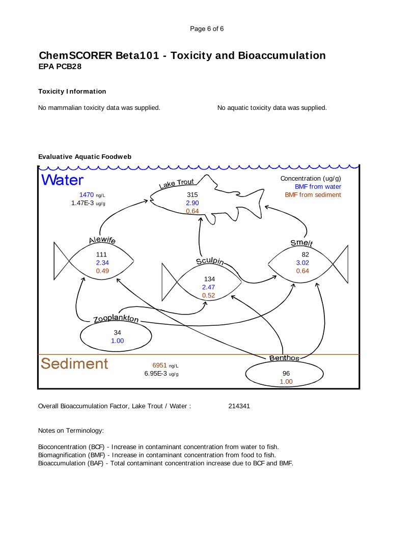
Page 6 of 6
ChemSCORER Beta101 - Toxicity and BioaccumulationEPA PCB28
Toxicity Information
No mammalian toxicity data was supplied. No aquatic toxicity data was supplied.
Evaluative Aquatic Foodweb
Concentration (ug/g)BMF from water
1470 ng/L 315 BMF from sediment1.47E-3 ug/g 2.90
0.64
111 822.34 3.020.49 0.64
1342.470.52
341.00
6951 ng/L
6.95E-3 ug/g 961.00
Overall Bioaccumulation Factor, Lake Trout / Water : 214341
Notes on Terminology:
Bioconcentration (BCF) - Increase in contaminant concentration from water to fish.Biomagnification (BMF) - Increase in contaminant concentration from food to fish.Bioaccumulation (BAF) - Total contaminant concentration increase due to BCF and BMF.
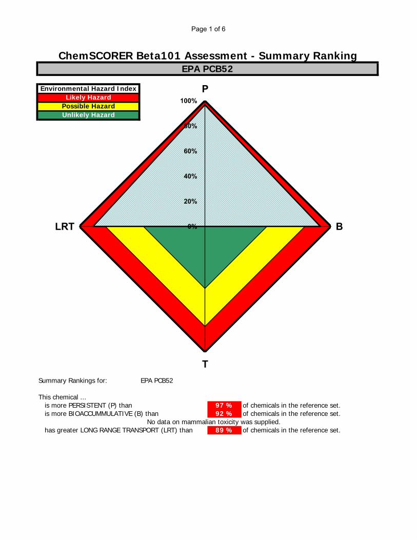
Page 1 of 6
Summary Rankings for: EPA PCB52
This chemical ... is more PERSISTENT (P) than 97 % of chemicals in the reference set. is more BIOACCUMMULATIVE (B) than 92 % of chemicals in the reference set. No data on mammalian toxicity was supplied. has greater LONG RANGE TRANSPORT (LRT) than 89 % of chemicals in the reference set.
Possible HazardUnlikely Hazard
ChemSCORER Beta101 Assessment - Summary RankingEPA PCB52
Environmental Hazard IndexLikely Hazard
0%
20%
40%
60%
80%
100%P
B
T
LRT

Page 2 of 6
ChemSCORER Beta101 - Level I Model ResultsEPA PCB52
Details of Level I calculation for: EPA PCB52
Compartment Z(mol/m^3Pa) (mol/m^3) (mg/L) (ug/g) kg %
Air 4.03E-04 1.13E-11 3.31E-09 2.79E-06 331 0.331Water 8.27E-02 2.32E-09 6.78E-07 6.78E-07 136 0.136Soil 1.32E+03 3.70E-05 1.08E-02 4.50E-03 97298 97.298Sediment 2.64E+03 7.40E-05 2.16E-02 9.01E-03 2162 2.162Suspended Sediment 8.23E+03 2.31E-04 6.76E-02 4.50E-02 68 0.068Biota (Fish) 3.35E+03 9.41E-05 2.75E-02 2.75E-02 5 0.005Total 100000 100.000
Molar Mass 291.99 g/mol
Vapor Pressure 1 Pa Log Kow 5.91 Air 1.18E-01Aqueous Solubility 24.13365746 g/m^3 Log Kaw -2.31 Water 2.41E+01Log Kow 5.9085 Log Koa 8.22 Octanol 1.95E+07Melting Point -999 deg C
The Level I chemical distibution represents long term equilibrium
partitioning of the chemical. Many persistent chemicals partition
predominantly to soils. Long range transport usually requires
partitioning (at least 1%) to one of the mobile media (air or water).
Bioconcentration Factor (BCF)
40501
The calculated BCF is substantially greater than the generally accepted cut-off between bioaccumulative and non-
bioaccumulative substances of 5000. In the absence of metabolism by organisms, this substance may bioaccumulate similar to DDT (BCF 63000) or PCBs (BCFs up to
300000).
Input Parameters Partition Coefficients Three Solubilities(g/m^3)
Concentration AmountEquilibrium Chemical Distribution
Physical Chemical Data and Partition Coefficients
Level I Chemical DistributionAir0%
Water0%
Soil98%
Sediment2%

Page 3 of 6
ChemSCORER Beta101 - Level II Model ResultsEPA PCB52
854 days 2.34 years
2998 days 8.21 years
1194 days 3.27 years
Details of Level II calculation for: EPA PCB52
Half-life RemovalReaction Advection Reaction Advection(mol/Pa h) (mol/Pa h) (kg/h) (kg/h)
Air 1700 1.64E+07 4.03E+08 2.77E+01 6.78E+02 70.612Water 55000 2.08E+05 1.65E+07 3.50E-01 2.78E+01 2.815Soil 55000 1.49E+08 0 2.51E+02 0 25.128Sediment 55000 3.32E+06 5.27E+06 5.58E+00 8.86E+00 1.445Total 1.69E+08 4.25E+08 2.85E+02 7.15E+02Reaction + Advection
Equilibrium Partitioning Persistence Information
The figure at right identifies environmental media that have a
controlling influence on the overall rate of reactive degradation of this
substance. Substances that fall near the center of the diagram are expected to accumulate in all media, and overall
persistence will be influenced by all degradation rates. The relative
importance of advection and reaction to the regional-scale removal of this
substance, and the media from which these processes take place are depicted
in the pie charts below.The equilibrium distribution reaction
residence time calculated for this substance is greater than five years,
and is comparable to that of hexachlorobenzene (7.6 years).
Reactive and advective residence times are comparable, indicating the
substance may be subject to long range transport.
Removal Processes - Equilibrium Distribution
5.95E+08 1000
Overall Residence Time:Reaction Residence Time:Advection Residence Time:
Compartment(hours) %
100.000
D Values Loss Rates
-15-14-13-12-11-10-9-8-7-6-5-4-3-2-10123456789
10
-4 -3 -2 -1 0 1 2 3 4 5 6 7 8 9 10
Log Kow
Log
Kaw
Air
Water Octanol
Air& Octanol
Water & Octanol
Air & Water
Removal Pathways
Reaction28%
Advection72%
Media of ReactionAir
10%Water0%
Soil88%
Sediment2%
Media of Advection
Air95%
Water4%
Sediment1%

Page 4 of 6
ChemSCORER Beta101 - Level III Model ResultsEPA PCB52
Emission to Air
(hours) 46439.1(days) 1935.0
(years) 5.3
Emission to Water
(hours) 64323.0(days) 2680.1
(years) 7.3
Emission to Soil
(hours) 79037.8(days) 3293.2
(years) 9.0
Emission to All 3
(hours) 55064.1(days) 2294.3
(years) 6.3
Details of Level III calculation for: EPA PCB52
Air Water Soil Air Water Soil Sediment TotalAir 1000 0 0 1.05E+06 3.35E+05 2.85E+07 1.65E+07 4.64E+07
Water 0 1000 0 4.80E+05 1.01E+06 1.30E+07 4.98E+07 6.43E+07Soil 0 0 1000 1.04E+04 1.21E+04 7.84E+07 5.98E+05 7.90E+07All 3 600 300 100 7.75E+05 5.05E+05 2.89E+07 2.49E+07 5.51E+07
Air 1000 0 0 428 4 360 208 1000Water 0 1000 0 196 13 164 627 1000Soil 0 0 1000 4 0 988 8 1000All 3 600 300 100 316 6 364 314 1000
Persistence under the standard emission scenario is comparable to that of hexachlorobenzene (2300 days).
Emissions to air partition
predominantly to soil and
sediment.
Emissions to water partition significantly to sediment and
may migrate to soil.
Emissions to soil remain
predominantly in the soil
compartment.
Persistence of air emissions is comparable to that of hexachlorobenzene (2200 days).
Persistence of water emissions is comparable to that of hexachlorobenzene (2300 days).
Persistence of soil emissions is comparable to that of hexachlorobenzene (3200 days).
Emission Rate (kg/h) Inventory at Steady State (kg)
Emission Rate (kg/h) Reaction Loss Rate (kg/h)
Persistence
Persistence
Persistence
Persistence
Steady State DistributionAir2%
Water1%
Soil61%
Sediment36%
Steady State Distribution
Air1%Water2%
Soil20%
Sediment77%
Steady State Distribution
Air0%
Water0%
Soil99%
Sediment1%
Steady State DistributionAir1%
Water1%
Soil53%
Sediment45%
Reactive Removal
Air43%
Water0%
Soil36%
Sediment21%
Reactive Removal
Air20% Water
1%
Soil16%
Sediment63%
Reactive Removal
Air0%
Water0%
Soil99%
Sediment1%
Reactive Removal
Air32%
Water1%Soil
36%
Sediment31%

Page 5 of 6
ChemSCORER Beta101 - Transport Model ResultsEPA PCB52
TaPL II - Equilibrium distribution Characteristic Travel Distance
Air (km) Water (km)
3430 351
TaPL III - Mode of entry assessmentsEmission to air - Characteristic Travel Distance in Air
Air (km)
15122
Emission to water - Characteristic Travel Distance in Water
Water (km)
3637
Emission to soil - Effective Travel Distance
Air (km) Water (km)
0 0
Under equilibrium partitioning conditions, this chemical is likely to
be transported by both air and water.
Characteristic Travel Distance in air is high, and is comparable to that of
hexachlorinated PCBs (4200 km). This chemical may be subject to
long range transport and deposition in the arctic.
Characteristic Travel Distance in water is high, and is comparable to that of toxaphene (9700 km). This
chemical may be subject to long range transport in surface and
ocean waters.
Emissions directly to soil are not expected to partition significantly to air or water, and are not likely to be
subject to transport.

Page 6 of 6
ChemSCORER Beta101 - Toxicity and BioaccumulationEPA PCB52
Toxicity Information
No mammalian toxicity data was supplied. No aquatic toxicity data was supplied.
Evaluative Aquatic Foodweb
Concentration (ug/g)BMF from water
1642 ng/L 828 BMF from sediment1.64E-3 ug/g 3.89
0.91
260 2312.80 4.350.59 0.91
3253.060.64
671.00
7811 ng/L
7.81E-3 ug/g 1901.00
Overall Bioaccumulation Factor, Lake Trout / Water : 504001
Notes on Terminology:
Bioconcentration (BCF) - Increase in contaminant concentration from water to fish.Biomagnification (BMF) - Increase in contaminant concentration from food to fish.Bioaccumulation (BAF) - Total contaminant concentration increase due to BCF and BMF.

Page 1 of 6
Summary Rankings for: EPA PCB101
This chemical ... is more PERSISTENT (P) than 97 % of chemicals in the reference set. is more BIOACCUMMULATIVE (B) than 94 % of chemicals in the reference set. No data on mammalian toxicity was supplied. has greater LONG RANGE TRANSPORT (LRT) than 78 % of chemicals in the reference set.
Possible HazardUnlikely Hazard
ChemSCORER Beta101 Assessment - Summary RankingEPA PCB101
Environmental Hazard IndexLikely Hazard
0%
20%
40%
60%
80%
100%P
B
T
LRT

Page 2 of 6
ChemSCORER Beta101 - Level I Model ResultsEPA PCB101
Details of Level I calculation for: EPA PCB101
Compartment Z(mol/m^3Pa) (mol/m^3) (mg/L) (ug/g) kg %
Air 4.03E-04 3.14E-12 1.03E-09 8.66E-07 103 0.103Water 1.00E-01 7.82E-10 2.55E-07 2.55E-07 51 0.051Soil 4.26E+03 3.32E-05 1.08E-02 4.52E-03 97604 97.604Sediment 8.53E+03 6.64E-05 2.17E-02 9.04E-03 2169 2.169Suspended Sediment 2.66E+04 2.08E-04 6.78E-02 4.52E-02 68 0.068Biota (Fish) 1.08E+04 8.44E-05 2.76E-02 2.76E-02 6 0.006Total 100000 100.000
Molar Mass 326.43 g/mol
Vapor Pressure 1 Pa Log Kow 6.33 Air 1.32E-01Aqueous Solubility 32.74501782 g/m^3 Log Kaw -2.40 Water 3.27E+01Log Kow 6.3344 Log Koa 8.73 Octanol 7.07E+07Melting Point -999 deg C
The Level I chemical distibution represents long term equilibrium
partitioning of the chemical. Many persistent chemicals partition
predominantly to soils. Long range transport usually requires
partitioning (at least 1%) to one of the mobile media (air or water).
Bioconcentration Factor (BCF)
107987
The calculated BCF is substantially greater than the generally accepted cut-off between bioaccumulative and non-
bioaccumulative substances of 5000. In the absence of metabolism by organisms, this substance may bioaccumulate similar to DDT (BCF 63000) or PCBs (BCFs up to
300000).
Input Parameters Partition Coefficients Three Solubilities(g/m^3)
Concentration AmountEquilibrium Chemical Distribution
Physical Chemical Data and Partition Coefficients
Level I Chemical DistributionAir0%
Water0%
Soil98%
Sediment2%

Page 3 of 6
ChemSCORER Beta101 - Level II Model ResultsEPA PCB101
1722 days 4.72 years
3206 days 8.78 years
3718 days 10.19 years
Details of Level II calculation for: EPA PCB101
Half-life RemovalReaction Advection Reaction Advection(mol/Pa h) (mol/Pa h) (kg/h) (kg/h)
Air 1700 1.64E+07 4.03E+08 1.73E+01 4.24E+02 44.128Water 55000 2.53E+05 2.01E+07 2.66E-01 2.11E+01 2.135Soil 55000 4.83E+08 0 5.08E+02 0 50.816Sediment 55000 1.07E+07 1.71E+07 1.13E+01 1.79E+01 2.922Total 5.11E+08 4.41E+08 5.37E+02 4.63E+02Reaction + Advection
Equilibrium Partitioning Persistence Information
The figure at right identifies environmental media that have a
controlling influence on the overall rate of reactive degradation of this
substance. Substances that fall near the center of the diagram are expected to accumulate in all media, and overall
persistence will be influenced by all degradation rates. The relative
importance of advection and reaction to the regional-scale removal of this
substance, and the media from which these processes take place are depicted
in the pie charts below.The equilibrium distribution reaction
residence time calculated for this substance is greater than five years,
and is comparable to that of hexachlorobenzene (7.6 years).
Reactive and advective residence times are comparable, indicating the
substance may be subject to long range transport.
Removal Processes - Equilibrium Distribution
9.51E+08 1000
Overall Residence Time:Reaction Residence Time:Advection Residence Time:
Compartment(hours) %
100.000
D Values Loss Rates
-15-14-13-12-11-10-9-8-7-6-5-4-3-2-10123456789
10
-4 -3 -2 -1 0 1 2 3 4 5 6 7 8 9 10
Log Kow
Log
Kaw
Air
Water Octanol
Air& Octanol
Water & Octanol
Air & Water
Removal Pathways
Reaction54%
Advection46%
Media of ReactionAir3%
Water0%
Soil95%
Sediment2%
Media of Advection
Air91%
Water5%
Sediment4%

Page 4 of 6
ChemSCORER Beta101 - Level III Model ResultsEPA PCB101
Emission to Air
(hours) 61744.9(days) 2572.7
(years) 7.0
Emission to Water
(hours) 75545.0(days) 3147.7
(years) 8.6
Emission to Soil
(hours) 79302.2(days) 3304.3
(years) 9.1
Emission to All 3
(hours) 67640.7(days) 2818.4
(years) 7.7
Details of Level III calculation for: EPA PCB101
Air Water Soil Air Water Soil Sediment TotalAir 1000 0 0 5.62E+05 1.92E+05 4.50E+07 1.60E+07 6.17E+07
Water 0 1000 0 1.22E+05 7.78E+05 9.75E+06 6.49E+07 7.55E+07Soil 0 0 1000 2.00E+03 7.15E+03 7.87E+07 5.96E+05 7.93E+07All 3 600 300 100 3.74E+05 3.49E+05 3.78E+07 2.91E+07 6.76E+07
Air 1000 0 0 229 2 567 202 1000Water 0 1000 0 50 10 123 818 1000Soil 0 0 1000 1 0 992 8 1000All 3 600 300 100 152 4 476 367 1000
Persistence under the standard emission scenario is comparable to that of hexachlorobenzene (2300 days).
Emissions to air partition
predominantly to soil and
sediment.
Emissions to water partition significantly to sediment and
may migrate to soil.
Emissions to soil remain
predominantly in the soil
compartment.
Persistence of air emissions is comparable to that of hexachlorobenzene (2200 days).
Persistence of water emissions is comparable to that of hexachlorobenzene (2300 days).
Persistence of soil emissions is comparable to that of hexachlorobenzene (3200 days).
Emission Rate (kg/h) Inventory at Steady State (kg)
Emission Rate (kg/h) Reaction Loss Rate (kg/h)
Persistence
Persistence
Persistence
Persistence
Steady State DistributionAir1%
Water0%
Soil73%
Sediment26%
Steady State Distribution
Air0%Water1%
Soil13%
Sediment86%
Steady State Distribution
Air0%
Water0%
Soil99%
Sediment1%
Steady State DistributionAir1%
Water1%
Soil55%
Sediment43%
Reactive Removal
Air23%
Water0%
Soil57%
Sediment20%
Reactive Removal
Air5%
Water1%
Soil12%
Sediment82%
Reactive Removal
Air0%
Water0%
Soil99%
Sediment1%
Reactive Removal
Air15% Water
0%
Soil48%
Sediment37%
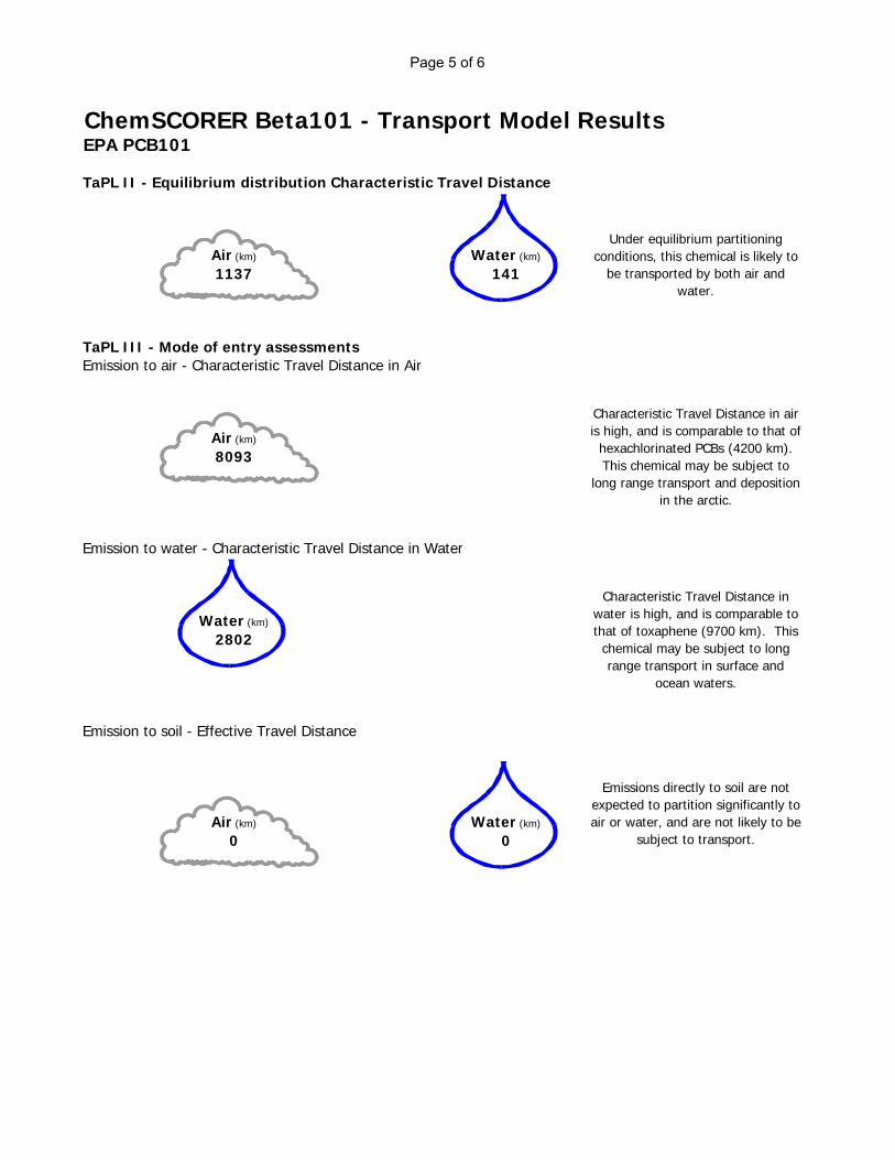
Page 5 of 6
ChemSCORER Beta101 - Transport Model ResultsEPA PCB101
TaPL II - Equilibrium distribution Characteristic Travel Distance
Air (km) Water (km)
1137 141
TaPL III - Mode of entry assessmentsEmission to air - Characteristic Travel Distance in Air
Air (km)
8093
Emission to water - Characteristic Travel Distance in Water
Water (km)
2802
Emission to soil - Effective Travel Distance
Air (km) Water (km)
0 0
Under equilibrium partitioning conditions, this chemical is likely to
be transported by both air and water.
Characteristic Travel Distance in air is high, and is comparable to that of
hexachlorinated PCBs (4200 km). This chemical may be subject to
long range transport and deposition in the arctic.
Characteristic Travel Distance in water is high, and is comparable to that of toxaphene (9700 km). This
chemical may be subject to long range transport in surface and
ocean waters.
Emissions directly to soil are not expected to partition significantly to air or water, and are not likely to be
subject to transport.

Page 6 of 6
ChemSCORER Beta101 - Toxicity and BioaccumulationEPA PCB101
Toxicity Information
No mammalian toxicity data was supplied. No aquatic toxicity data was supplied.
Evaluative Aquatic Foodweb
Concentration (ug/g)BMF from water
717 ng/L 1446 BMF from sediment7.17E-4 ug/g 5.84
1.57
379 4643.49 7.490.73 1.57
5024.050.85
771.00
3427 ng/L
3.43E-3 ug/g 2221.00
Overall Bioaccumulation Factor, Lake Trout / Water : 2016652
Notes on Terminology:
Bioconcentration (BCF) - Increase in contaminant concentration from water to fish.Biomagnification (BMF) - Increase in contaminant concentration from food to fish.Bioaccumulation (BAF) - Total contaminant concentration increase due to BCF and BMF.

Page 1 of 6
Summary Rankings for: EPA PCB118
This chemical ... is more PERSISTENT (P) than 98 % of chemicals in the reference set. is more BIOACCUMMULATIVE (B) than 96 % of chemicals in the reference set. No data on mammalian toxicity was supplied. has greater LONG RANGE TRANSPORT (LRT) than 65 % of chemicals in the reference set.
Possible HazardUnlikely Hazard
ChemSCORER Beta101 Assessment - Summary RankingEPA PCB118
Environmental Hazard IndexLikely Hazard
0%
20%
40%
60%
80%
100%P
B
T
LRT

Page 2 of 6
ChemSCORER Beta101 - Level I Model ResultsEPA PCB118
Details of Level I calculation for: EPA PCB118
Compartment Z(mol/m^3Pa) (mol/m^3) (mg/L) (ug/g) kg %
Air 4.03E-04 7.38E-13 2.41E-10 2.03E-07 24 0.024Water 1.90E-01 3.47E-10 1.13E-07 1.13E-07 23 0.023Soil 1.82E+04 3.33E-05 1.09E-02 4.52E-03 97709 97.709Sediment 3.64E+04 6.65E-05 2.17E-02 9.05E-03 2171 2.171Suspended Sediment 1.14E+05 2.08E-04 6.79E-02 4.52E-02 68 0.068Biota (Fish) 4.62E+04 8.45E-05 2.76E-02 2.76E-02 6 0.006Total 100000 100.000
Molar Mass 326.43 g/mol
Vapor Pressure 1 Pa Log Kow 6.69 Air 1.32E-01Aqueous Solubility 61.95055924 g/m^3 Log Kaw -2.67 Water 6.20E+01Log Kow 6.6875 Log Koa 9.36 Octanol 3.02E+08Melting Point -999 deg C
The Level I chemical distibution represents long term equilibrium
partitioning of the chemical. Many persistent chemicals partition
predominantly to soils. Long range transport usually requires
partitioning (at least 1%) to one of the mobile media (air or water).
Bioconcentration Factor (BCF)
243484
The calculated BCF is substantially greater than the generally accepted cut-off between bioaccumulative and non-
bioaccumulative substances of 5000. In the absence of metabolism by organisms, this substance may bioaccumulate similar to DDT (BCF 63000) or PCBs (BCFs up to
300000).
Input Parameters Partition Coefficients Three Solubilities(g/m^3)
Concentration AmountEquilibrium Chemical Distribution
Physical Chemical Data and Partition Coefficients
Level I Chemical DistributionAir0%
Water0%
Soil98%
Sediment2%

Page 3 of 6
ChemSCORER Beta101 - Level II Model ResultsEPA PCB118
2645 days 7.25 years
3284 days 9.00 years
13577 days 37.20 years
Details of Level II calculation for: EPA PCB118
Half-life RemovalReaction Advection Reaction Advection(mol/Pa h) (mol/Pa h) (kg/h) (kg/h)
Air 1700 1.64E+07 4.03E+08 6.23E+00 1.53E+02 15.908Water 55000 4.78E+05 3.80E+07 1.81E-01 1.44E+01 1.456Soil 55000 2.06E+09 0 7.81E+02 0 78.143Sediment 55000 4.58E+07 7.28E+07 1.74E+01 2.76E+01 4.493Total 2.13E+09 5.14E+08 8.05E+02 1.95E+02Reaction + Advection
Equilibrium Partitioning Persistence Information
The figure at right identifies environmental media that have a
controlling influence on the overall rate of reactive degradation of this
substance. Substances that fall near the center of the diagram are expected to accumulate in all media, and overall
persistence will be influenced by all degradation rates. The relative
importance of advection and reaction to the regional-scale removal of this
substance, and the media from which these processes take place are depicted
in the pie charts below.The equilibrium distribution reaction
residence time calculated for this substance is greater than five years,
and is comparable to that of hexachlorobenzene (7.6 years).
Reactive and advective residence times are comparable, indicating the
substance may be subject to long range transport.
Removal Processes - Equilibrium Distribution
2.64E+09 1000
Overall Residence Time:Reaction Residence Time:Advection Residence Time:
Compartment(hours) %
100.000
D Values Loss Rates
-15-14-13-12-11-10-9-8-7-6-5-4-3-2-10123456789
10
-4 -3 -2 -1 0 1 2 3 4 5 6 7 8 9 10
Log Kow
Log
Kaw
Air
Water Octanol
Air& Octanol
Water & Octanol
Air & Water
Removal Pathways
Reaction81%
Advection19%
Media of ReactionAir1%Water0%
Soil97%
Sediment2%
Media of Advection
Air79%
Water7%
Sediment14%
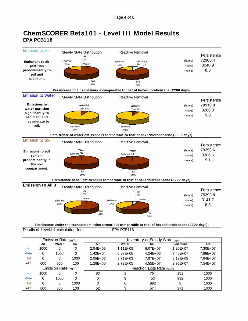
Page 4 of 6
ChemSCORER Beta101 - Level III Model ResultsEPA PCB118
Emission to Air
(hours) 72980.4(days) 3040.9
(years) 8.3
Emission to Water
(hours) 78918.9(days) 3288.3
(years) 9.0
Emission to Soil
(hours) 79358.6(days) 3306.6
(years) 9.1
Emission to All 3
(hours) 75399.8(days) 3141.7
(years) 8.6
Details of Level III calculation for: EPA PCB118
Air Water Soil Air Water Soil Sediment TotalAir 1000 0 0 2.04E+05 1.11E+05 6.07E+07 1.20E+07 7.30E+07
Water 0 1000 0 1.42E+04 6.83E+05 4.24E+06 7.40E+07 7.89E+07Soil 0 0 1000 2.05E+02 5.71E+03 7.87E+07 6.18E+05 7.94E+07All 3 600 300 100 1.26E+05 2.72E+05 4.55E+07 2.95E+07 7.54E+07
Air 1000 0 0 83 1 764 151 1000Water 0 1000 0 6 9 53 932 1000Soil 0 0 1000 0 0 992 8 1000All 3 600 300 100 52 3 574 371 1000
Persistence under the standard emission scenario is comparable to that of hexachlorobenzene (2300 days).
Emissions to air partition
predominantly to soil and
sediment.
Emissions to water partition significantly to sediment and
may migrate to soil.
Emissions to soil remain
predominantly in the soil
compartment.
Persistence of air emissions is comparable to that of hexachlorobenzene (2200 days).
Persistence of water emissions is comparable to that of hexachlorobenzene (2300 days).
Persistence of soil emissions is comparable to that of hexachlorobenzene (3200 days).
Emission Rate (kg/h) Inventory at Steady State (kg)
Emission Rate (kg/h) Reaction Loss Rate (kg/h)
Persistence
Persistence
Persistence
Persistence
Steady State DistributionAir0%
Water0%
Soil84%
Sediment16%
Steady State Distribution
Air0%
Water1%
Soil5%
Sediment94%
Steady State Distribution
Air0%
Water0%
Soil99%
Sediment1%
Steady State DistributionAir0%
Water0%
Soil61%
Sediment39%
Reactive Removal
Air8%
Water0%
Soil77%
Sediment15%
Reactive Removal
Air1%Water1%
Soil5%
Sediment93%
Reactive Removal
Air0%
Water0%
Soil99%
Sediment1%
Reactive RemovalAir5%
Water0%
Soil58%
Sediment37%

Page 5 of 6
ChemSCORER Beta101 - Transport Model ResultsEPA PCB118
TaPL II - Equilibrium distribution Characteristic Travel Distance
Air (km) Water (km)
273 64
TaPL III - Mode of entry assessmentsEmission to air - Characteristic Travel Distance in Air
Air (km)
2932
Emission to water - Characteristic Travel Distance in Water
Water (km)
2461
Emission to soil - Effective Travel Distance
Air (km) Water (km)
0 0
Under equilibrium partitioning conditions, this chemical is likely to
be transported by both air and water.
Characteristic Travel Distance in air is high, and is comparable to that of
hexachlorinated PCBs (4200 km). This chemical may be subject to
long range transport and deposition in the arctic.
Characteristic Travel Distance in water is high, and is comparable to that of toxaphene (9700 km). This
chemical may be subject to long range transport in surface and
ocean waters.
Emissions directly to soil are not expected to partition significantly to air or water, and are not likely to be
subject to transport.

Page 6 of 6
ChemSCORER Beta101 - Toxicity and BioaccumulationEPA PCB118
Toxicity Information
No mammalian toxicity data was supplied. No aquatic toxicity data was supplied.
Evaluative Aquatic Foodweb
Concentration (ug/g)BMF from water
321 ng/L 1778 BMF from sediment3.21E-4 ug/g 7.11
2.07
420 6203.84 9.910.80 2.07
5764.610.96
781.00
1537 ng/L
1.54E-3 ug/g 2241.00
Overall Bioaccumulation Factor, Lake Trout / Water : 5537523
Notes on Terminology:
Bioconcentration (BCF) - Increase in contaminant concentration from water to fish.Biomagnification (BMF) - Increase in contaminant concentration from food to fish.Bioaccumulation (BAF) - Total contaminant concentration increase due to BCF and BMF.

Page 1 of 6
Summary Rankings for: EPA PCB138
This chemical ... is more PERSISTENT (P) than 99 % of chemicals in the reference set. is more BIOACCUMMULATIVE (B) than 98 % of chemicals in the reference set. No data on mammalian toxicity was supplied. has greater LONG RANGE TRANSPORT (LRT) than 53 % of chemicals in the reference set.
Possible HazardUnlikely Hazard
ChemSCORER Beta101 Assessment - Summary RankingEPA PCB138
Environmental Hazard IndexLikely Hazard
0%
20%
40%
60%
80%
100%P
B
T
LRT

Page 2 of 6
ChemSCORER Beta101 - Level I Model ResultsEPA PCB138
Details of Level I calculation for: EPA PCB138
Compartment Z(mol/m^3Pa) (mol/m^3) (mg/L) (ug/g) kg %
Air 4.03E-04 3.35E-13 1.21E-10 1.02E-07 12 0.012Water 1.12E-01 9.32E-11 3.37E-08 3.37E-08 7 0.007Soil 3.63E+04 3.01E-05 1.09E-02 4.52E-03 97736 97.736Sediment 7.26E+04 6.02E-05 2.17E-02 9.05E-03 2172 2.172Suspended Sediment 2.27E+05 1.88E-04 6.79E-02 4.52E-02 68 0.068Biota (Fish) 9.22E+04 7.65E-05 2.76E-02 2.76E-02 6 0.006Total 100000 100.000
Molar Mass 360.88 g/mol
Vapor Pressure 1 Pa Log Kow 7.21 Air 1.46E-01Aqueous Solubility 40.5805548 g/m^3 Log Kaw -2.44 Water 4.06E+01Log Kow 7.2148 Log Koa 9.66 Octanol 6.65E+08Melting Point -999 deg C
The Level I chemical distibution represents long term equilibrium
partitioning of the chemical. Many persistent chemicals partition
predominantly to soils. Long range transport usually requires
partitioning (at least 1%) to one of the mobile media (air or water).
Bioconcentration Factor (BCF)
819917
The calculated BCF is substantially greater than the generally accepted cut-off between bioaccumulative and non-
bioaccumulative substances of 5000. In the absence of metabolism by organisms, this substance may bioaccumulate similar to DDT (BCF 63000) or PCBs (BCFs up to
300000).
Input Parameters Partition Coefficients Three Solubilities(g/m^3)
Concentration AmountEquilibrium Chemical Distribution
Physical Chemical Data and Partition Coefficients
Level I Chemical DistributionAir0%
Water0%
Soil98%
Sediment2%

Page 3 of 6
ChemSCORER Beta101 - Level II Model ResultsEPA PCB138
2911 days 7.98 years
3306 days 9.06 years
24382 days 66.80 years
Details of Level II calculation for: EPA PCB138
Half-life RemovalReaction Advection Reaction Advection(mol/Pa h) (mol/Pa h) (kg/h) (kg/h)
Air 5500 5.08E+06 4.03E+08 1.06E+00 8.43E+01 8.541Water 55000 2.83E+05 2.25E+07 5.92E-02 4.70E+00 0.476Soil 55000 4.12E+09 0 8.60E+02 0 86.037Sediment 55000 9.14E+07 1.45E+08 1.91E+01 3.03E+01 4.947Total 4.21E+09 5.71E+08 8.81E+02 1.19E+02Reaction + Advection
Equilibrium Partitioning Persistence Information
The figure at right identifies environmental media that have a
controlling influence on the overall rate of reactive degradation of this
substance. Substances that fall near the center of the diagram are expected to accumulate in all media, and overall
persistence will be influenced by all degradation rates. The relative
importance of advection and reaction to the regional-scale removal of this
substance, and the media from which these processes take place are depicted
in the pie charts below.The equilibrium distribution reaction
residence time calculated for this substance is greater than five years,
and is comparable to that of hexachlorobenzene (7.6 years).
Reactive and advective residence times are comparable, indicating the
substance may be subject to long range transport.
Removal Processes - Equilibrium Distribution
4.78E+09 1000
Overall Residence Time:Reaction Residence Time:Advection Residence Time:
Compartment(hours) %
100.000
D Values Loss Rates
-15-14-13-12-11-10-9-8-7-6-5-4-3-2-10123456789
10
-4 -3 -2 -1 0 1 2 3 4 5 6 7 8 9 10
Log Kow
Log
Kaw
Air
Water Octanol
Air& Octanol
Water & Octanol
Air & Water
Removal Pathways
Reaction88%
Advection12%
Media of ReactionAir0%
Water0%
Soil98%
Sediment2%
Media of Advection
Air71%
Water4%
Sediment25%
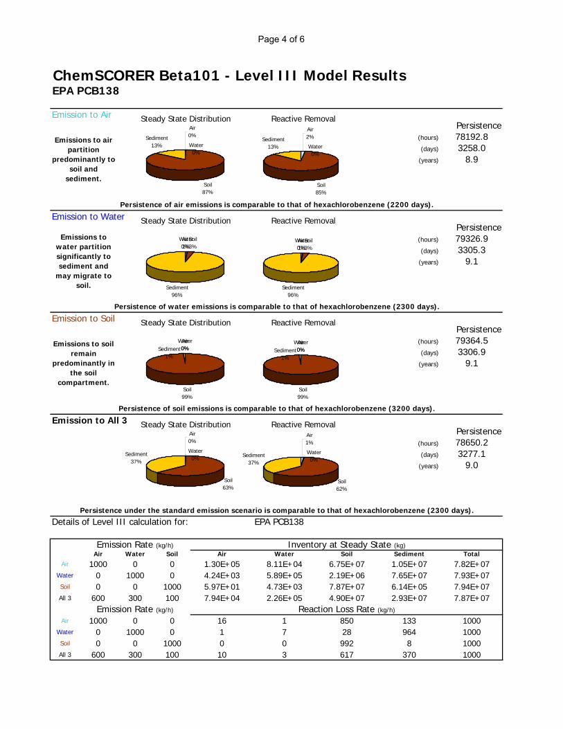
Page 4 of 6
ChemSCORER Beta101 - Level III Model ResultsEPA PCB138
Emission to Air
(hours) 78192.8(days) 3258.0
(years) 8.9
Emission to Water
(hours) 79326.9(days) 3305.3
(years) 9.1
Emission to Soil
(hours) 79364.5(days) 3306.9
(years) 9.1
Emission to All 3
(hours) 78650.2(days) 3277.1
(years) 9.0
Details of Level III calculation for: EPA PCB138
Air Water Soil Air Water Soil Sediment TotalAir 1000 0 0 1.30E+05 8.11E+04 6.75E+07 1.05E+07 7.82E+07
Water 0 1000 0 4.24E+03 5.89E+05 2.19E+06 7.65E+07 7.93E+07Soil 0 0 1000 5.97E+01 4.73E+03 7.87E+07 6.14E+05 7.94E+07All 3 600 300 100 7.94E+04 2.26E+05 4.90E+07 2.93E+07 7.87E+07
Air 1000 0 0 16 1 850 133 1000Water 0 1000 0 1 7 28 964 1000Soil 0 0 1000 0 0 992 8 1000All 3 600 300 100 10 3 617 370 1000
Persistence under the standard emission scenario is comparable to that of hexachlorobenzene (2300 days).
Emissions to air partition
predominantly to soil and
sediment.
Emissions to water partition significantly to sediment and
may migrate to soil.
Emissions to soil remain
predominantly in the soil
compartment.
Persistence of air emissions is comparable to that of hexachlorobenzene (2200 days).
Persistence of water emissions is comparable to that of hexachlorobenzene (2300 days).
Persistence of soil emissions is comparable to that of hexachlorobenzene (3200 days).
Emission Rate (kg/h) Inventory at Steady State (kg)
Emission Rate (kg/h) Reaction Loss Rate (kg/h)
Persistence
Persistence
Persistence
Persistence
Steady State DistributionAir0%
Water0%
Soil87%
Sediment13%
Steady State Distribution
Air0%
Water1%
Soil3%
Sediment96%
Steady State Distribution
Air0%
Water0%
Soil99%
Sediment1%
Steady State DistributionAir0%
Water0%
Soil63%
Sediment37%
Reactive RemovalAir2%
Water0%
Soil85%
Sediment13%
Reactive Removal
Air0%
Water1%
Soil3%
Sediment96%
Reactive Removal
Air0%
Water0%
Soil99%
Sediment1%
Reactive RemovalAir1%
Water0%
Soil62%
Sediment37%

Page 5 of 6
ChemSCORER Beta101 - Transport Model ResultsEPA PCB138
TaPL II - Equilibrium distribution Characteristic Travel Distance
Air (km) Water (km)
138 19
TaPL III - Mode of entry assessmentsEmission to air - Characteristic Travel Distance in Air
Air (km)
1876
Emission to water - Characteristic Travel Distance in Water
Water (km)
2122
Emission to soil - Effective Travel Distance
Air (km) Water (km)
0 0
Under equilibrium partitioning conditions, this chemical is likely to
be transported by both air and water.
Characteristic Travel Distance in air is moderate, and is comparable to
that of DDT (830 km). This chemical may be found in remote
areas, but is not necessarily transported over very long
distances.
Characteristic Travel Distance in water is high, and is comparable to that of toxaphene (9700 km). This
chemical may be subject to long range transport in surface and
ocean waters.
Emissions directly to soil are not expected to partition significantly to air or water, and are not likely to be
subject to transport.

Page 6 of 6
ChemSCORER Beta101 - Toxicity and BioaccumulationEPA PCB138
Toxicity Information
No mammalian toxicity data was supplied. No aquatic toxicity data was supplied.
Evaluative Aquatic Foodweb
Concentration (ug/g)BMF from water
95 ng/L 1911 BMF from sediment9.49E-5 ug/g 7.68
2.40
432 7173.97 11.520.83 2.40
6064.871.02
781.00
455 ng/L
4.55E-4 ug/g 2241.00
Overall Bioaccumulation Factor, Lake Trout / Water : 20147458
Notes on Terminology:
Bioconcentration (BCF) - Increase in contaminant concentration from water to fish.Biomagnification (BMF) - Increase in contaminant concentration from food to fish.Bioaccumulation (BAF) - Total contaminant concentration increase due to BCF and BMF.

Page 1 of 6
Summary Rankings for: EPA PCB153
This chemical ... is more PERSISTENT (P) than 99 % of chemicals in the reference set. is more BIOACCUMMULATIVE (B) than 97 % of chemicals in the reference set. No data on mammalian toxicity was supplied. has greater LONG RANGE TRANSPORT (LRT) than 55 % of chemicals in the reference set.
Possible HazardUnlikely Hazard
ChemSCORER Beta101 Assessment - Summary RankingEPA PCB153
Environmental Hazard IndexLikely Hazard
0%
20%
40%
60%
80%
100%P
B
T
LRT

Page 2 of 6
ChemSCORER Beta101 - Level I Model ResultsEPA PCB153
Details of Level I calculation for: EPA PCB153
Compartment Z(mol/m^3Pa) (mol/m^3) (mg/L) (ug/g) kg %
Air 4.03E-04 5.55E-13 2.00E-10 1.69E-07 20 0.020Water 1.49E-01 2.05E-10 7.42E-08 7.42E-08 15 0.015Soil 2.19E+04 3.01E-05 1.09E-02 4.52E-03 97720 97.720Sediment 4.37E+04 6.02E-05 2.17E-02 9.05E-03 2172 2.172Suspended Sediment 1.37E+05 1.88E-04 6.79E-02 4.52E-02 68 0.068Biota (Fish) 5.56E+04 7.64E-05 2.76E-02 2.76E-02 6 0.006Total 100000 100.000
Molar Mass 360.88 g/mol
Vapor Pressure 1 Pa Log Kow 6.87 Air 1.46E-01Aqueous Solubility 53.89121564 g/m^3 Log Kaw -2.57 Water 5.39E+01Log Kow 6.8716 Log Koa 9.44 Octanol 4.01E+08Melting Point -999 deg C
The Level I chemical distibution represents long term equilibrium
partitioning of the chemical. Many persistent chemicals partition
predominantly to soils. Long range transport usually requires
partitioning (at least 1%) to one of the mobile media (air or water).
Bioconcentration Factor (BCF)
372023
The calculated BCF is substantially greater than the generally accepted cut-off between bioaccumulative and non-
bioaccumulative substances of 5000. In the absence of metabolism by organisms, this substance may bioaccumulate similar to DDT (BCF 63000) or PCBs (BCFs up to
300000).
Input Parameters Partition Coefficients Three Solubilities(g/m^3)
Concentration AmountEquilibrium Chemical Distribution
Physical Chemical Data and Partition Coefficients
Level I Chemical DistributionAir0%
Water0%
Soil98%
Sediment2%

Page 3 of 6
ChemSCORER Beta101 - Level II Model ResultsEPA PCB153
2741 days 7.51 years
3303 days 9.05 years
16114 days 44.15 years
Details of Level II calculation for: EPA PCB153
Half-life RemovalReaction Advection Reaction Advection(mol/Pa h) (mol/Pa h) (kg/h) (kg/h)
Air 5500 5.08E+06 4.03E+08 1.66E+00 1.32E+02 13.345Water 55000 3.76E+05 2.99E+07 1.23E-01 9.76E+00 0.988Soil 55000 2.48E+09 0 8.10E+02 0 81.009Sediment 55000 5.51E+07 8.75E+07 1.80E+01 2.86E+01 4.658Total 2.54E+09 5.21E+08 8.30E+02 1.70E+02Reaction + Advection
Equilibrium Partitioning Persistence Information
The figure at right identifies environmental media that have a
controlling influence on the overall rate of reactive degradation of this
substance. Substances that fall near the center of the diagram are expected to accumulate in all media, and overall
persistence will be influenced by all degradation rates. The relative
importance of advection and reaction to the regional-scale removal of this
substance, and the media from which these processes take place are depicted
in the pie charts below.The equilibrium distribution reaction
residence time calculated for this substance is greater than five years,
and is comparable to that of hexachlorobenzene (7.6 years).
Reactive and advective residence times are comparable, indicating the
substance may be subject to long range transport.
Removal Processes - Equilibrium Distribution
3.06E+09 1000
Overall Residence Time:Reaction Residence Time:Advection Residence Time:
Compartment(hours) %
100.000
D Values Loss Rates
-15-14-13-12-11-10-9-8-7-6-5-4-3-2-10123456789
10
-4 -3 -2 -1 0 1 2 3 4 5 6 7 8 9 10
Log Kow
Log
Kaw
Air
Water Octanol
Air& Octanol
Water & Octanol
Air & Water
Removal Pathways
Reaction83%
Advection17%
Media of ReactionAir0%
Water0%
Soil98%
Sediment2%
Media of Advection
Air77%
Water6%
Sediment17%

Page 4 of 6
ChemSCORER Beta101 - Level III Model ResultsEPA PCB153
Emission to Air
(hours) 77668.3(days) 3236.2
(years) 8.9
Emission to Water
(hours) 79269.5(days) 3302.9
(years) 9.0
Emission to Soil
(hours) 79363.7(days) 3306.8
(years) 9.1
Emission to All 3
(hours) 78318.2(days) 3263.3
(years) 8.9
Details of Level III calculation for: EPA PCB153
Air Water Soil Air Water Soil Sediment TotalAir 1000 0 0 1.89E+05 1.01E+05 6.54E+07 1.20E+07 7.77E+07
Water 0 1000 0 1.06E+04 6.36E+05 3.68E+06 7.49E+07 7.93E+07Soil 0 0 1000 1.51E+02 5.21E+03 7.87E+07 6.14E+05 7.94E+07All 3 600 300 100 1.16E+05 2.52E+05 4.82E+07 2.97E+07 7.83E+07
Air 1000 0 0 24 1 824 151 1000Water 0 1000 0 1 8 46 944 1000Soil 0 0 1000 0 0 992 8 1000All 3 600 300 100 15 3 608 374 1000
Persistence under the standard emission scenario is comparable to that of hexachlorobenzene (2300 days).
Emissions to air partition
predominantly to soil and
sediment.
Emissions to water partition significantly to sediment and
may migrate to soil.
Emissions to soil remain
predominantly in the soil
compartment.
Persistence of air emissions is comparable to that of hexachlorobenzene (2200 days).
Persistence of water emissions is comparable to that of hexachlorobenzene (2300 days).
Persistence of soil emissions is comparable to that of hexachlorobenzene (3200 days).
Emission Rate (kg/h) Inventory at Steady State (kg)
Emission Rate (kg/h) Reaction Loss Rate (kg/h)
Persistence
Persistence
Persistence
Persistence
Steady State DistributionAir0%
Water0%
Soil85%
Sediment15%
Steady State Distribution
Air0%
Water1%
Soil5%
Sediment94%
Steady State Distribution
Air0%
Water0%
Soil99%
Sediment1%
Steady State DistributionAir0%
Water0%
Soil62%
Sediment38%
Reactive RemovalAir2%
Water0%
Soil83%
Sediment15%
Reactive Removal
Air0%
Water1%
Soil5%
Sediment94%
Reactive Removal
Air0%
Water0%
Soil99%
Sediment1%
Reactive RemovalAir1%
Water0%
Soil62%
Sediment37%

Page 5 of 6
ChemSCORER Beta101 - Transport Model ResultsEPA PCB153
TaPL II - Equilibrium distribution Characteristic Travel Distance
Air (km) Water (km)
229 42
TaPL III - Mode of entry assessmentsEmission to air - Characteristic Travel Distance in Air
Air (km)
2715
Emission to water - Characteristic Travel Distance in Water
Water (km)
2288
Emission to soil - Effective Travel Distance
Air (km) Water (km)
0 0
Under equilibrium partitioning conditions, this chemical is likely to
be transported by both air and water.
Characteristic Travel Distance in air is high, and is comparable to that of
hexachlorinated PCBs (4200 km). This chemical may be subject to
long range transport and deposition in the arctic.
Characteristic Travel Distance in water is high, and is comparable to that of toxaphene (9700 km). This
chemical may be subject to long range transport in surface and
ocean waters.
Emissions directly to soil are not expected to partition significantly to air or water, and are not likely to be
subject to transport.

Page 6 of 6
ChemSCORER Beta101 - Toxicity and BioaccumulationEPA PCB153
Toxicity Information
No mammalian toxicity data was supplied. No aquatic toxicity data was supplied.
Evaluative Aquatic Foodweb
Concentration (ug/g)BMF from water
212 ng/L 1893 BMF from sediment2.12E-4 ug/g 7.50
2.25
434 6803.93 10.780.82 2.25
6024.771.00
791.00
1015 ng/L
1.01E-3 ug/g 2261.00
Overall Bioaccumulation Factor, Lake Trout / Water : 8933519
Notes on Terminology:
Bioconcentration (BCF) - Increase in contaminant concentration from water to fish.Biomagnification (BMF) - Increase in contaminant concentration from food to fish.Bioaccumulation (BAF) - Total contaminant concentration increase due to BCF and BMF.

Page 1 of 6
Summary Rankings for: EPA PCB180
This chemical ... is more PERSISTENT (P) than 99 % of chemicals in the reference set. is more BIOACCUMMULATIVE (B) than 98 % of chemicals in the reference set. No data on mammalian toxicity was supplied. has greater LONG RANGE TRANSPORT (LRT) than 54 % of chemicals in the reference set.
Possible HazardUnlikely Hazard
ChemSCORER Beta101 Assessment - Summary RankingEPA PCB180
Environmental Hazard IndexLikely Hazard
0%
20%
40%
60%
80%
100%P
B
T
LRT

Page 2 of 6
ChemSCORER Beta101 - Level I Model ResultsEPA PCB180
Details of Level I calculation for: EPA PCB180
Compartment Z(mol/m^3Pa) (mol/m^3) (mg/L) (ug/g) kg %
Air 4.03E-04 8.81E-14 3.48E-11 2.94E-08 3 0.003Water 4.41E-01 9.63E-11 3.81E-08 3.81E-08 8 0.008Soil 1.26E+05 2.75E-05 1.09E-02 4.53E-03 97743 97.743Sediment 2.52E+05 5.49E-05 2.17E-02 9.05E-03 2172 2.172Suspended Sediment 7.86E+05 1.72E-04 6.79E-02 4.53E-02 68 0.068Biota (Fish) 3.20E+05 6.98E-05 2.76E-02 2.76E-02 6 0.006Total 100000 100.000
Molar Mass 395.32 g/mol
Vapor Pressure 1 Pa Log Kow 7.16 Air 1.60E-01Aqueous Solubility 174.3146759 g/m^3 Log Kaw -3.04 Water 1.74E+02Log Kow 7.16137 Log Koa 10.20 Octanol 2.53E+09Melting Point -999 deg C
The Level I chemical distibution represents long term equilibrium
partitioning of the chemical. Many persistent chemicals partition
predominantly to soils. Long range transport usually requires
partitioning (at least 1%) to one of the mobile media (air or water).
Bioconcentration Factor (BCF)
725003
The calculated BCF is substantially greater than the generally accepted cut-off between bioaccumulative and non-
bioaccumulative substances of 5000. In the absence of metabolism by organisms, this substance may bioaccumulate similar to DDT (BCF 63000) or PCBs (BCFs up to
300000).
Input Parameters Partition Coefficients Three Solubilities(g/m^3)
Concentration AmountEquilibrium Chemical Distribution
Physical Chemical Data and Partition Coefficients
Level I Chemical DistributionAir0%
Water0%
Soil98%
Sediment2%
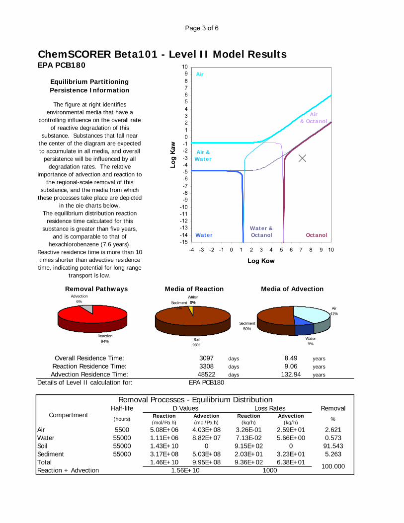
Page 3 of 6
ChemSCORER Beta101 - Level II Model ResultsEPA PCB180
3097 days 8.49 years
3308 days 9.06 years
48522 days 132.94 years
Details of Level II calculation for: EPA PCB180
Half-life RemovalReaction Advection Reaction Advection(mol/Pa h) (mol/Pa h) (kg/h) (kg/h)
Air 5500 5.08E+06 4.03E+08 3.26E-01 2.59E+01 2.621Water 55000 1.11E+06 8.82E+07 7.13E-02 5.66E+00 0.573Soil 55000 1.43E+10 0 9.15E+02 0 91.543Sediment 55000 3.17E+08 5.03E+08 2.03E+01 3.23E+01 5.263Total 1.46E+10 9.95E+08 9.36E+02 6.38E+01Reaction + Advection
Equilibrium Partitioning Persistence Information
The figure at right identifies environmental media that have a
controlling influence on the overall rate of reactive degradation of this
substance. Substances that fall near the center of the diagram are expected to accumulate in all media, and overall
persistence will be influenced by all degradation rates. The relative
importance of advection and reaction to the regional-scale removal of this
substance, and the media from which these processes take place are depicted
in the pie charts below.The equilibrium distribution reaction
residence time calculated for this substance is greater than five years,
and is comparable to that of hexachlorobenzene (7.6 years).
Reactive residence time is more than 10 times shorter than advective residence time, indicating potential for long range
transport is low.
Removal Processes - Equilibrium Distribution
1.56E+10 1000
Overall Residence Time:Reaction Residence Time:Advection Residence Time:
Compartment(hours) %
100.000
D Values Loss Rates
-15-14-13-12-11-10-9-8-7-6-5-4-3-2-10123456789
10
-4 -3 -2 -1 0 1 2 3 4 5 6 7 8 9 10
Log Kow
Log
Kaw
Air
Water Octanol
Air& Octanol
Water & Octanol
Air & Water
Removal Pathways
Reaction94%
Advection6%
Media of ReactionAir0%
Water0%
Soil98%
Sediment2%
Media of Advection
Air41%
Water9%
Sediment50%

Page 4 of 6
ChemSCORER Beta101 - Level III Model ResultsEPA PCB180
Emission to Air
(hours) 78808.2(days) 3283.7
(years) 9.0
Emission to Water
(hours) 79358.4(days) 3306.6
(years) 9.1
Emission to Soil
(hours) 79365.0(days) 3306.9
(years) 9.1
Emission to All 3
(hours) 79029.0(days) 3292.9
(years) 9.0
Details of Level III calculation for: EPA PCB180
Air Water Soil Air Water Soil Sediment TotalAir 1000 0 0 6.19E+04 7.17E+04 6.95E+07 9.22E+06 7.88E+07
Water 0 1000 0 7.38E+02 6.07E+05 8.28E+05 7.79E+07 7.94E+07Soil 0 0 1000 1.07E+01 4.86E+03 7.87E+07 6.25E+05 7.94E+07All 3 600 300 100 3.73E+04 2.26E+05 4.98E+07 2.90E+07 7.90E+07
Air 1000 0 0 8 1 875 116 1000Water 0 1000 0 0 8 10 982 1000Soil 0 0 1000 0 0 992 8 1000All 3 600 300 100 5 3 627 365 1000
Persistence under the standard emission scenario is comparable to that of hexachlorobenzene (2300 days).
Emissions to air partition
predominantly to soil and
sediment.
Emissions to water partition significantly to sediment and
may migrate to soil.
Emissions to soil remain
predominantly in the soil
compartment.
Persistence of air emissions is comparable to that of hexachlorobenzene (2200 days).
Persistence of water emissions is comparable to that of hexachlorobenzene (2300 days).
Persistence of soil emissions is comparable to that of hexachlorobenzene (3200 days).
Emission Rate (kg/h) Inventory at Steady State (kg)
Emission Rate (kg/h) Reaction Loss Rate (kg/h)
Persistence
Persistence
Persistence
Persistence
Steady State DistributionAir0%
Water0%
Soil88%
Sediment12%
Steady State Distribution
Air0%
Water1%
Soil1%
Sediment98%
Steady State Distribution
Air0%
Water0%
Soil99%
Sediment1%
Steady State DistributionAir0%
Water0%
Soil63%
Sediment37%
Reactive RemovalAir1%
Water0%
Soil87%
Sediment12%
Reactive Removal
Air0%
Water1%
Soil1%
Sediment98%
Reactive Removal
Air0%
Water0%
Soil99%
Sediment1%
Reactive RemovalAir0%
Water0%
Soil63%
Sediment37%

Page 5 of 6
ChemSCORER Beta101 - Transport Model ResultsEPA PCB180
TaPL II - Equilibrium distribution Characteristic Travel Distance
Air (km) Water (km)
40 22
TaPL III - Mode of entry assessmentsEmission to air - Characteristic Travel Distance in Air
Air (km)
891
Emission to water - Characteristic Travel Distance in Water
Water (km)
2184
Emission to soil - Effective Travel Distance
Air (km) Water (km)
0 0
Under equilibrium partitioning conditions, this chemical is likely to
be transported by both air and water.
Characteristic Travel Distance in air is moderate, and is comparable to
that of DDT (830 km). This chemical may be found in remote
areas, but is not necessarily transported over very long
distances.
Characteristic Travel Distance in water is high, and is comparable to that of toxaphene (9700 km). This
chemical may be subject to long range transport in surface and
ocean waters.
Emissions directly to soil are not expected to partition significantly to air or water, and are not likely to be
subject to transport.

Page 6 of 6
ChemSCORER Beta101 - Toxicity and BioaccumulationEPA PCB180
Toxicity Information
No mammalian toxicity data was supplied. No aquatic toxicity data was supplied.
Evaluative Aquatic Foodweb
Concentration (ug/g)BMF from water
106 ng/L 1893 BMF from sediment1.06E-4 ug/g 7.70
2.40
427 7063.97 11.480.83 2.40
5994.871.02
771.00
508 ng/L
5.08E-4 ug/g 2211.00
Overall Bioaccumulation Factor, Lake Trout / Water : 17867941
Notes on Terminology:
Bioconcentration (BCF) - Increase in contaminant concentration from water to fish.Biomagnification (BMF) - Increase in contaminant concentration from food to fish.Bioaccumulation (BAF) - Total contaminant concentration increase due to BCF and BMF.

Page 1 of 6
Summary Rankings for: EPA Dieldrin
This chemical ... is more PERSISTENT (P) than 86 % of chemicals in the reference set. is more BIOACCUMMULATIVE (B) than 95 % of chemicals in the reference set. No data on mammalian toxicity was supplied. has greater LONG RANGE TRANSPORT (LRT) than 48 % of chemicals in the reference set.
Possible HazardUnlikely Hazard
ChemSCORER Beta101 Assessment - Summary RankingEPA Dieldrin
Environmental Hazard IndexLikely Hazard
0%
20%
40%
60%
80%
100%P
B
T
LRT

Page 2 of 6
ChemSCORER Beta101 - Level I Model ResultsEPA Dieldrin
Details of Level I calculation for: EPA Dieldrin
Compartment Z(mol/m^3Pa) (mol/m^3) (mg/L) (ug/g) kg %
Air 4.03E-04 8.76E-14 3.34E-11 2.81E-08 3 0.003Water 1.60E+00 3.47E-10 1.32E-07 1.32E-07 26 0.026Soil 1.31E+05 2.85E-05 1.09E-02 4.52E-03 97725 97.725Sediment 2.63E+05 5.70E-05 2.17E-02 9.05E-03 2172 2.172Suspended Sediment 8.21E+05 1.78E-04 6.79E-02 4.52E-02 68 0.068Biota (Fish) 3.34E+05 7.24E-05 2.76E-02 2.76E-02 6 0.006Total 100000 100.000
Molar Mass 380.93 g/mol
Vapor Pressure 1 Pa Log Kow 6.62 Air 1.54E-01Aqueous Solubility 609.570253 g/m^3 Log Kaw -3.60 Water 6.10E+02Log Kow 6.62 Log Koa 10.22 Octanol 2.54E+09Melting Point -999 deg C
The Level I chemical distibution represents long term equilibrium
partitioning of the chemical. Many persistent chemicals partition
predominantly to soils. Long range transport usually requires
partitioning (at least 1%) to one of the mobile media (air or water).
Bioconcentration Factor (BCF)
208435
The calculated BCF is substantially greater than the generally accepted cut-off between bioaccumulative and non-
bioaccumulative substances of 5000. In the absence of metabolism by organisms, this substance may bioaccumulate similar to DDT (BCF 63000) or PCBs (BCFs up to
300000).
Input Parameters Partition Coefficients Three Solubilities(g/m^3)
Concentration AmountEquilibrium Chemical Distribution
Physical Chemical Data and Partition Coefficients
Level I Chemical DistributionAir0%
Water0%
Soil98%
Sediment2%
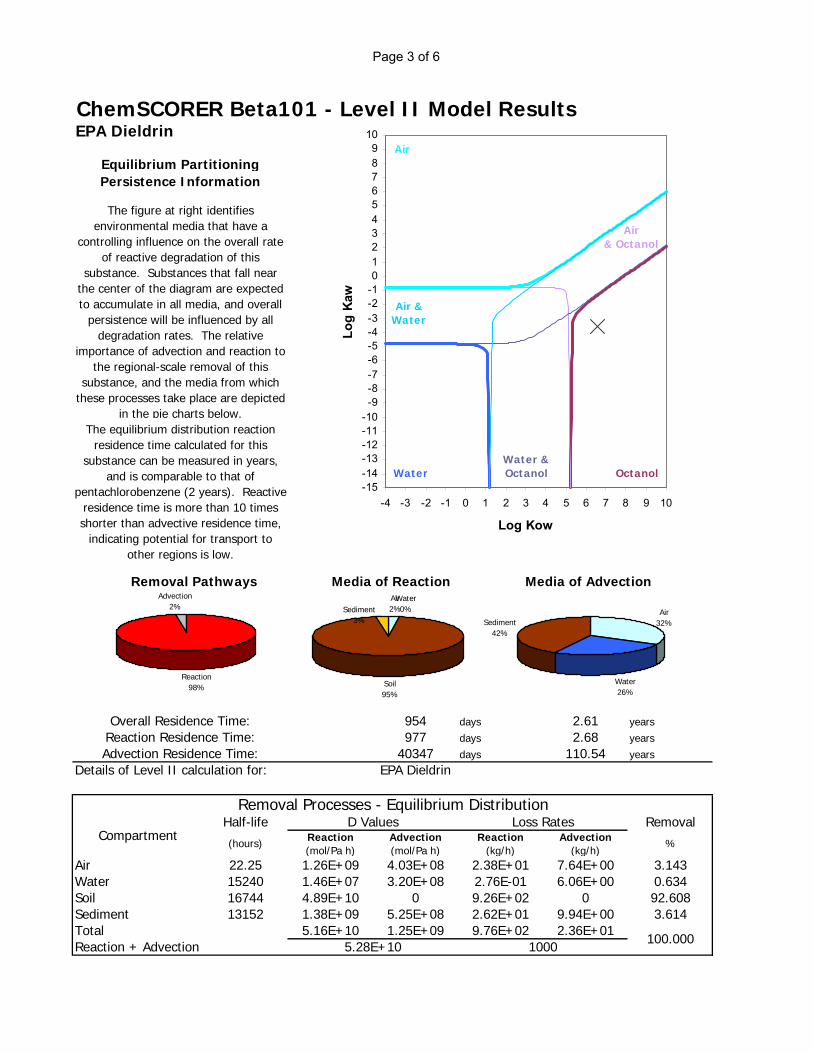
Page 3 of 6
ChemSCORER Beta101 - Level II Model ResultsEPA Dieldrin
954 days 2.61 years
977 days 2.68 years
40347 days 110.54 years
Details of Level II calculation for: EPA Dieldrin
Half-life RemovalReaction Advection Reaction Advection(mol/Pa h) (mol/Pa h) (kg/h) (kg/h)
Air 22.25 1.26E+09 4.03E+08 2.38E+01 7.64E+00 3.143Water 15240 1.46E+07 3.20E+08 2.76E-01 6.06E+00 0.634Soil 16744 4.89E+10 0 9.26E+02 0 92.608Sediment 13152 1.38E+09 5.25E+08 2.62E+01 9.94E+00 3.614Total 5.16E+10 1.25E+09 9.76E+02 2.36E+01Reaction + Advection
Equilibrium Partitioning Persistence Information
The figure at right identifies environmental media that have a
controlling influence on the overall rate of reactive degradation of this
substance. Substances that fall near the center of the diagram are expected to accumulate in all media, and overall
persistence will be influenced by all degradation rates. The relative
importance of advection and reaction to the regional-scale removal of this
substance, and the media from which these processes take place are depicted
in the pie charts below.The equilibrium distribution reaction
residence time calculated for this substance can be measured in years,
and is comparable to that of pentachlorobenzene (2 years). Reactive
residence time is more than 10 times shorter than advective residence time,
indicating potential for transport to other regions is low.
Removal Processes - Equilibrium Distribution
5.28E+10 1000
Overall Residence Time:Reaction Residence Time:Advection Residence Time:
Compartment(hours) %
100.000
D Values Loss Rates
-15-14-13-12-11-10-9-8-7-6-5-4-3-2-10123456789
10
-4 -3 -2 -1 0 1 2 3 4 5 6 7 8 9 10
Log Kow
Log
Kaw
Air
Water Octanol
Air& Octanol
Water & Octanol
Air & Water
Removal Pathways
Reaction98%
Advection2%
Media of ReactionAir2%
Water0%
Soil95%
Sediment3%
Media of Advection
Air32%
Water26%
Sediment42%

Page 4 of 6
ChemSCORER Beta101 - Level III Model ResultsEPA Dieldrin
Emission to Air
(hours) 8191.5(days) 341.3
(years) 0.9
Emission to Water
(hours) 18963.0(days) 790.1
(years) 2.2
Emission to Soil
(hours) 24147.6(days) 1006.2
(years) 2.8
Emission to All 3
(hours) 13018.6(days) 542.4
(years) 1.5
Details of Level III calculation for: EPA Dieldrin
Air Water Soil Air Water Soil Sediment TotalAir 1000 0 0 2.10E+04 1.57E+04 7.42E+06 7.35E+05 8.19E+06
Water 0 1000 0 1.35E+02 3.96E+05 4.79E+04 1.85E+07 1.90E+07Soil 0 0 1000 1.26E+00 1.01E+03 2.41E+07 4.74E+04 2.41E+07All 3 600 300 100 1.26E+04 1.28E+05 6.88E+06 6.00E+06 1.30E+07
Air 1000 0 0 653 1 307 39 1000Water 0 1000 0 4 18 2 976 1000Soil 0 0 1000 0 0 997 2 1000All 3 600 300 100 393 6 285 316 1000
Persistence under the standard emission scenario is comparable to that of hexachlorobenzene (2300 days).
Emissions to air partition
predominantly to soil and
sediment.
Emissions to water partition significantly to sediment and
may migrate to soil.
Emissions to soil remain
predominantly in the soil
compartment.
Persistence of air emissions is comparable to that of the tetrachlorobenzenes (110 days).
Persistence of water emissions is comparable to that of hexachlorobenzene (2300 days).
Persistence of soil emissions is comparable to that of hexachlorobenzene (3200 days).
Emission Rate (kg/h) Inventory at Steady State (kg)
Emission Rate (kg/h) Reaction Loss Rate (kg/h)
Persistence
Persistence
Persistence
Persistence
Steady State DistributionAir0%
Water0%
Soil91%
Sediment9%
Steady State Distribution
Air0%Water2%Soil0%
Sediment98%
Steady State Distribution
Air0%
Water0%
Soil100%
Sediment0%
Steady State DistributionAir0%
Water1%
Soil53%
Sediment46%
Reactive Removal
Air65%
Water0%
Soil31%
Sediment4%
Reactive Removal
Air0%Water2%Soil0%
Sediment98%
Reactive Removal
Air0%
Water0%
Soil100%
Sediment0%
Reactive Removal
Air39%
Water1%
Soil28%
Sediment32%

Page 5 of 6
ChemSCORER Beta101 - Transport Model ResultsEPA Dieldrin
TaPL II - Equilibrium distribution Characteristic Travel Distance
Air (km) Water (km)
11 22
TaPL III - Mode of entry assessmentsEmission to air - Characteristic Travel Distance in Air
Air (km)
302
Emission to water - Characteristic Travel Distance in Water
Water (km)
1427
Emission to soil - Effective Travel Distance
Air (km) Water (km)
0 0
Under equilibrium partitioning conditions, this chemical is likely to
be transported by both air and water.
Characteristic Travel Distance in air is low. This chemical is not likely to be transported a significant distance
in the atmosphere.
Characteristic Travel Distance in water is moderate, and is
comparable to that of chlorobenzene (1300 km). This
chemical may be subject to transport in surface and near-shore
marine waters.
Emissions directly to soil are not expected to partition significantly to air or water, and are not likely to be
subject to transport.

Page 6 of 6
ChemSCORER Beta101 - Toxicity and BioaccumulationEPA Dieldrin
Toxicity Information
No mammalian toxicity data was supplied. No aquatic toxicity data was supplied.
Evaluative Aquatic Foodweb
Concentration (ug/g)BMF from water
170 ng/L 480 BMF from sediment1.70E-4 ug/g 4.23
2.65
123 1622.47 5.691.15 2.65
1312.311.07
351.00
366 ng/L
3.66E-4 ug/g 461.00
Overall Bioaccumulation Factor, Lake Trout / Water : 2821351
Notes on Terminology:
Bioconcentration (BCF) - Increase in contaminant concentration from water to fish.Biomagnification (BMF) - Increase in contaminant concentration from food to fish.Bioaccumulation (BAF) - Total contaminant concentration increase due to BCF and BMF.

Page 1 of 6
Summary Rankings for: EPA Aldrin
This chemical ... is more PERSISTENT (P) than 84 % of chemicals in the reference set. is more BIOACCUMMULATIVE (B) than 95 % of chemicals in the reference set. No data on mammalian toxicity was supplied. has greater LONG RANGE TRANSPORT (LRT) than 46 % of chemicals in the reference set.
Possible HazardUnlikely Hazard
ChemSCORER Beta101 Assessment - Summary RankingEPA Aldrin
Environmental Hazard IndexLikely Hazard
0%
20%
40%
60%
80%
100%P
B
T
LRT

Page 2 of 6
ChemSCORER Beta101 - Level I Model ResultsEPA Aldrin
Details of Level I calculation for: EPA Aldrin
Compartment Z(mol/m^3Pa) (mol/m^3) (mg/L) (ug/g) kg %
Air 4.03E-04 1.65E-11 6.01E-09 5.07E-06 601 0.601Water 8.83E-03 3.61E-10 1.32E-07 1.32E-07 26 0.026Soil 7.24E+02 2.96E-05 1.08E-02 4.50E-03 97141 97.141Sediment 1.45E+03 5.92E-05 2.16E-02 8.99E-03 2159 2.159Suspended Sediment 4.53E+03 1.85E-04 6.75E-02 4.50E-02 67 0.067Biota (Fish) 1.84E+03 7.51E-05 2.74E-02 2.74E-02 5 0.005Total 100000 100.000
Molar Mass 364.93 g/mol
Vapor Pressure 1 Pa Log Kow 6.62 Air 1.47E-01Aqueous Solubility 3.220807236 g/m^3 Log Kaw -1.34 Water 3.22E+00Log Kow 6.62 Log Koa 7.96 Octanol 1.34E+07Melting Point -999 deg C
The Level I chemical distibution represents long term equilibrium
partitioning of the chemical. Many persistent chemicals partition
predominantly to soils. Long range transport usually requires
partitioning (at least 1%) to one of the mobile media (air or water).
Bioconcentration Factor (BCF)
208435
The calculated BCF is substantially greater than the generally accepted cut-off between bioaccumulative and non-
bioaccumulative substances of 5000. In the absence of metabolism by organisms, this substance may bioaccumulate similar to DDT (BCF 63000) or PCBs (BCFs up to
300000).
Input Parameters Partition Coefficients Three Solubilities(g/m^3)
Concentration AmountEquilibrium Chemical Distribution
Physical Chemical Data and Partition Coefficients
Level I Chemical DistributionAir1%
Water0%
Soil97%
Sediment2%

Page 3 of 6
ChemSCORER Beta101 - Level II Model ResultsEPA Aldrin
590 hours 24.59 days
612 hours 25.51 days
16439 hours 684.96 days
Details of Level II calculation for: EPA Aldrin
Half-life RemovalReaction Advection Reaction Advection(mol/Pa h) (mol/Pa h) (kg/h) (kg/h)
Air 2.86 9.78E+09 4.03E+08 8.60E+02 3.55E+01 89.548Water 2670 4.58E+05 1.77E+06 4.03E-02 1.55E-01 0.020Soil 3830 1.18E+09 0 1.04E+02 0 10.374Sediment 26700 3.76E+06 2.90E+06 3.31E-01 2.55E-01 0.059Total 1.10E+10 4.08E+08 9.64E+02 3.59E+01Reaction + Advection
Equilibrium Partitioning Persistence Information
The figure at right identifies environmental media that have a
controlling influence on the overall rate of reactive degradation of this
substance. Substances that fall near the center of the diagram are expected to accumulate in all media, and overall
persistence will be influenced by all degradation rates. The relative
importance of advection and reaction to the regional-scale removal of this
substance, and the media from which these processes take place are depicted
in the pie charts below.The equilibrium distribution reaction
residence time calculated for this substance can be measured in months,
and is comparable to that of the tetrachlorobenzenes (120 days).
Reactive residence time is more than 10 times shorter than advective residence time, indicating potential for transport
to other regions is low.
Removal Processes - Equilibrium Distribution
1.14E+10 1000
Overall Residence Time:Reaction Residence Time:Advection Residence Time:
Compartment(hours) %
100.000
D Values Loss Rates
-15-14-13-12-11-10-9-8-7-6-5-4-3-2-10123456789
10
-4 -3 -2 -1 0 1 2 3 4 5 6 7 8 9 10
Log Kow
Log
Kaw
Air
Water Octanol
Air& Octanol
Water & Octanol
Air & Water
Removal Pathways
Reaction96%
Advection4%
Media of Reaction
Air89%
Water0%
Soil11%
Sediment0%
Media of Advection
Air99%
Water0%
Sediment1%

Page 4 of 6
ChemSCORER Beta101 - Level III Model ResultsEPA Aldrin
Emission to Air
(hours) 20.79(days) 0.87
(years) 0.00
Emission to Water
(hours) 27524.39(days) 1146.85
(years) 3.14
Emission to Soil
(hours) 5536.17(days) 230.67
(years) 0.63
Emission to All 3
(hours) 8823.41(days) 367.64
(years) 1.01
Details of Level III calculation for: EPA Aldrin
Air Water Soil Air Water Soil Sediment TotalAir 1000 0 0 4.12E+03 1.64E+02 4.35E+03 1.21E+04 2.08E+04
Water 0 1000 0 8.24E+02 3.68E+05 8.70E+02 2.72E+07 2.75E+07Soil 0 0 1000 3.04E+00 2.15E+02 5.52E+06 1.59E+04 5.54E+06All 3 600 300 100 2.72E+03 1.10E+05 5.55E+05 8.16E+06 8.82E+06
Air 1000 0 0 999 0 1 0 1000Water 0 1000 0 200 95 0 705 1000Soil 0 0 1000 1 0 999 0 1000All 3 600 300 100 659 29 100 212 1000
Persistence under the standard emission scenario is comparable to that of the tetrachlorobenzenes (130 days).
Emissions to air partition
significantly to soil and
sediment.
Emissions to water partition significantly to sediment and
may migrate to soil.
Emissions to soil remain
predominantly in the soil
compartment.
Persistence of air emissions is comparable to that of benzene (25 hours).
Persistence of water emissions is comparable to that of hexachlorobenzene (2300 days).
Persistence of soil emissions is comparable to that of the tetrachlorobenzenes (250 days).
Emission Rate (kg/h) Inventory at Steady State (kg)
Emission Rate (kg/h) Reaction Loss Rate (kg/h)
Persistence
Persistence
Persistence
Persistence
Steady State Distribution
Air20%
Water1%
Soil21%
Sediment58%
Steady State Distribution
Air0%Water1%Soil0%
Sediment99%
Steady State Distribution
Air0%
Water0%
Soil100%
Sediment0%
Steady State Distribution
Air0%Water1%
Soil6%
Sediment93%
Reactive Removal
Air100%
Water0%Soil0%
Sediment0%
Reactive Removal
Air20%
Water10%
Soil0%Sediment
70%
Reactive Removal
Air0%
Water0%
Soil100%
Sediment0%
Reactive Removal
Air66%Water
3%
Soil10%
Sediment21%
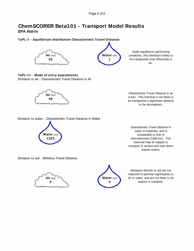
Page 5 of 6
ChemSCORER Beta101 - Transport Model ResultsEPA Aldrin
TaPL II - Equilibrium distribution Characteristic Travel Distance
Air (km) Water (km)
53 1
TaPL III - Mode of entry assessmentsEmission to air - Characteristic Travel Distance in Air
Air (km)
59
Emission to water - Characteristic Travel Distance in Water
Water (km)
1323
Emission to soil - Effective Travel Distance
Air (km) Water (km)
0 0
Under equilibrium partitioning conditions, this chemical is likely to be transported most effectively in
air.
Characteristic Travel Distance in air is low. This chemical is not likely to be transported a significant distance
in the atmosphere.
Characteristic Travel Distance in water is moderate, and is
comparable to that of chlorobenzene (1300 km). This
chemical may be subject to transport in surface and near-shore
marine waters.
Emissions directly to soil are not expected to partition significantly to air or water, and are not likely to be
subject to transport.

Page 6 of 6
ChemSCORER Beta101 - Toxicity and BioaccumulationEPA Aldrin
Toxicity Information
No mammalian toxicity data was supplied. No aquatic toxicity data was supplied.
Evaluative Aquatic Foodweb
Concentration (ug/g)BMF from water
146 ng/L 537 BMF from sediment1.46E-4 ug/g 5.50
2.21
132 1833.10 7.500.91 2.21
1643.360.99
301.00
497 ng/L
4.97E-4 ug/g 621.00
Overall Bioaccumulation Factor, Lake Trout / Water : 3668028
Notes on Terminology:
Bioconcentration (BCF) - Increase in contaminant concentration from water to fish.Biomagnification (BMF) - Increase in contaminant concentration from food to fish.Bioaccumulation (BAF) - Total contaminant concentration increase due to BCF and BMF.

Page 1 of 6
Summary Rankings for: EPA Hexachlorobenzene
This chemical ... is more PERSISTENT (P) than 99 % of chemicals in the reference set. is more BIOACCUMMULATIVE (B) than 92 % of chemicals in the reference set. No data on mammalian toxicity was supplied. has greater LONG RANGE TRANSPORT (LRT) than 97 % of chemicals in the reference set.
Possible HazardUnlikely Hazard
ChemSCORER Beta101 Assessment - Summary RankingEPA Hexachlorobenzene
Environmental Hazard IndexLikely Hazard
0%
20%
40%
60%
80%
100%P
B
T
LRT

Page 2 of 6
ChemSCORER Beta101 - Level I Model ResultsEPA Hexachlorobenzene
Details of Level I calculation for: EPA Hexachlorobenzene
Compartment Z(mol/m^3Pa) (mol/m^3) (mg/L) (ug/g) kg %
Air 4.03E-04 1.44E-10 4.10E-08 3.46E-05 4100 4.100Water 9.68E-03 3.45E-09 9.84E-07 9.84E-07 197 0.197Soil 1.02E+02 3.65E-05 1.04E-02 4.33E-03 93554 93.554Sediment 2.05E+02 7.30E-05 2.08E-02 8.66E-03 2079 2.079Suspended Sediment 6.39E+02 2.28E-04 6.50E-02 4.33E-02 65 0.065Biota (Fish) 2.60E+02 9.27E-05 2.64E-02 2.64E-02 5 0.005Total 100000 100.000
Molar Mass 284.79 g/mol
Vapor Pressure 1 Pa Log Kow 5.73 Air 1.15E-01Aqueous Solubility 2.756004369 g/m^3 Log Kaw -1.38 Water 2.76E+00Log Kow 5.73 Log Koa 7.11 Octanol 1.48E+06Melting Point 230 deg C
The Level I chemical distibution represents long term equilibrium
partitioning of the chemical. Many persistent chemicals partition
predominantly to soils. Long range transport usually requires
partitioning (at least 1%) to one of the mobile media (air or water).
Bioconcentration Factor (BCF)
26852
The calculated BCF is greater than the generally accepted cut-off between
bioaccumulative and non-bioaccumulative substances of 5000. In the absence of rapid metabolism by organisms, this
substance is expected to bioaccumulate.
Input Parameters Partition Coefficients Three Solubilities(g/m^3)
Concentration AmountEquilibrium Chemical Distribution
Physical Chemical Data and Partition Coefficients
Level I Chemical Distribution
Air4%
Water0%
Soil94%
Sediment2%

Page 3 of 6
ChemSCORER Beta101 - Level II Model ResultsEPA Hexachlorobenzene
96 days 0.26 years
2047 days 5.61 years
101 days 0.28 years
Details of Level II calculation for: EPA Hexachlorobenzene
Half-life RemovalReaction Advection Reaction Advection(mol/Pa h) (mol/Pa h) (kg/h) (kg/h)
Air 22600 1.24E+06 4.03E+08 2.91E+00 9.47E+02 95.037Water 34100 3.93E+04 1.94E+06 9.24E-02 4.55E+00 0.464Soil 34100 1.87E+07 0 4.39E+01 0 4.393Sediment 341000 4.16E+04 4.09E+05 9.76E-02 9.61E-01 0.106Total 2.00E+07 4.06E+08 4.70E+01 9.53E+02Reaction + Advection
Equilibrium Partitioning Persistence Information
The figure at right identifies environmental media that have a
controlling influence on the overall rate of reactive degradation of this
substance. Substances that fall near the center of the diagram are expected to accumulate in all media, and overall
persistence will be influenced by all degradation rates. The relative
importance of advection and reaction to the regional-scale removal of this
substance, and the media from which these processes take place are depicted
in the pie charts below.The equilibrium distribution reaction
residence time calculated for this substance can be measured in years,
and is comparable to that of pentachlorobenzene (2 years).
Advective residence time is more than 10 times shorter than reactive residence time, indicating the substance may be
transported to other regions.
Removal Processes - Equilibrium Distribution
4.26E+08 1000
Overall Residence Time:Reaction Residence Time:Advection Residence Time:
Compartment(hours) %
100.000
D Values Loss Rates
-15-14-13-12-11-10-9-8-7-6-5-4-3-2-10123456789
10
-4 -3 -2 -1 0 1 2 3 4 5 6 7 8 9 10
Log Kow
Log
Kaw
Air
Water Octanol
Air& Octanol
Water & Octanol
Air & Water
Removal PathwaysReaction
5%
Advection95%
Media of ReactionAir6%
Water0%
Soil94%
Sediment0%
Media of Advection
Air100%
Water0%
Sediment0%

Page 4 of 6
ChemSCORER Beta101 - Level III Model ResultsEPA Hexachlorobenzene
Emission to Air
(hours) 80036.0(days) 3334.8
(years) 9.1
Emission to Water
(hours) 107748.9(days) 4489.5
(years) 12.3
Emission to Soil
(hours) 50764.5(days) 2115.2
(years) 5.8
Emission to All 3
(hours) 85422.7(days) 3559.3
(years) 9.8
Details of Level III calculation for: EPA Hexachlorobenzene
Air Water Soil Air Water Soil Sediment TotalAir 1000 0 0 1.23E+07 7.60E+05 2.58E+07 4.12E+07 8.00E+07
Water 0 1000 0 1.13E+07 1.32E+06 2.37E+07 7.14E+07 1.08E+08Soil 0 0 1000 5.38E+05 3.75E+04 4.82E+07 2.04E+06 5.08E+07All 3 600 300 100 1.08E+07 8.55E+05 2.74E+07 4.64E+07 8.54E+07
Air 1000 0 0 377 15 524 84 1000Water 0 1000 0 346 27 482 145 1000Soil 0 0 1000 16 1 979 4 1000All 3 600 300 100 332 17 557 94 1000
Persistence under the standard emission scenario is comparable to that of hexachlorobenzene (2300 days).
Emissions to air partition
significantly to soil and
sediment.
Emissions to water partition significantly to sediment and
may migrate to soil.
Emissions to soil partition
significantly to other media.
Persistence of air emissions is comparable to that of hexachlorobenzene (2200 days).
Persistence of water emissions is comparable to that of the PCBs (up to 80 years).
Persistence of soil emissions is comparable to that of hexachlorobenzene (3200 days).
Emission Rate (kg/h) Inventory at Steady State (kg)
Emission Rate (kg/h) Reaction Loss Rate (kg/h)
Persistence
Persistence
Persistence
Persistence
Steady State Distribution
Air15% Water
1%
Soil32%
Sediment52%
Steady State DistributionAir10%
Water1%
Soil22%
Sediment67%
Steady State Distribution
Air1%Water0%
Soil95%
Sediment4%
Steady State Distribution
Air13%
Water1%
Soil32%
Sediment54%
Reactive Removal
Air38%
Water2%
Soil52%
Sediment8%
Reactive Removal
Air35%
Water3%
Soil47%
Sediment15%
Reactive Removal
Air2%Water0%
Soil98%
Sediment0%
Reactive Removal
Air33%
Water2%Soil
56%
Sediment9%

Page 5 of 6
ChemSCORER Beta101 - Transport Model ResultsEPA Hexachlorobenzene
TaPL II - Equilibrium distribution Characteristic Travel Distance
Air (km) Water (km)
29010 348
TaPL III - Mode of entry assessmentsEmission to air - Characteristic Travel Distance in Air
Air (km)
176980
Emission to water - Characteristic Travel Distance in Water
Water (km)
4741
Emission to soil - Effective Travel Distance
Air (km) Water (km)
10203 0
Under equilibrium partitioning conditions, this chemical is likely to be transported most effectively in
air.
Characteristic Travel Distance in air is extremely high, and is comparable to that of
hexachlorobenzene (110 000 km). This chemical is likely subject to
long range transport and deposition in the arctic.
Characteristic Travel Distance in water is high, and is comparable to that of toxaphene (9700 km). This
chemical may be subject to long range transport in surface and
ocean waters.
Emissions directly to soil may partition to air and be subject to
transport in the atmosphere.
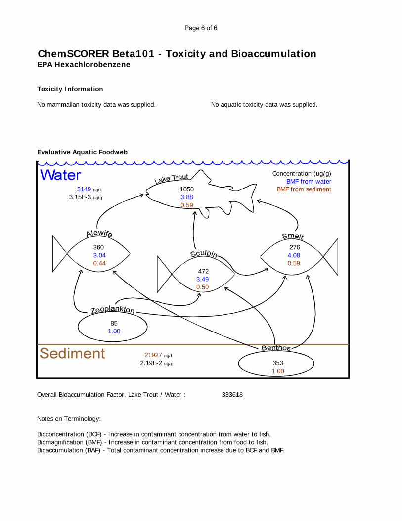
Page 6 of 6
ChemSCORER Beta101 - Toxicity and BioaccumulationEPA Hexachlorobenzene
Toxicity Information
No mammalian toxicity data was supplied. No aquatic toxicity data was supplied.
Evaluative Aquatic Foodweb
Concentration (ug/g)BMF from water
3149 ng/L 1050 BMF from sediment3.15E-3 ug/g 3.88
0.59
360 2763.04 4.080.44 0.59
4723.490.50
851.00
21927 ng/L
2.19E-2 ug/g 3531.00
Overall Bioaccumulation Factor, Lake Trout / Water : 333618
Notes on Terminology:
Bioconcentration (BCF) - Increase in contaminant concentration from water to fish.Biomagnification (BMF) - Increase in contaminant concentration from food to fish.Bioaccumulation (BAF) - Total contaminant concentration increase due to BCF and BMF.

Page 1 of 6
Summary Rankings for: EPA Total Chlordanes
This chemical ... is more PERSISTENT (P) than 92 % of chemicals in the reference set. is more BIOACCUMMULATIVE (B) than 92 % of chemicals in the reference set. No data on mammalian toxicity was supplied. has greater LONG RANGE TRANSPORT (LRT) than 73 % of chemicals in the reference set.
Possible HazardUnlikely Hazard
ChemSCORER Beta101 Assessment - Summary RankingEPA Total Chlordanes
Environmental Hazard IndexLikely Hazard
0%
20%
40%
60%
80%
100%P
B
T
LRT

Page 2 of 6
ChemSCORER Beta101 - Level I Model ResultsEPA Total Chlordanes
Details of Level I calculation for: EPA Total Chlordanes
Compartment Z(mol/m^3Pa) (mol/m^3) (mg/L) (ug/g) kg %
Air 4.03E-04 1.79E-12 7.32E-10 6.17E-07 73 0.073Water 3.04E-01 1.34E-09 5.51E-07 5.51E-07 110 0.110Soil 5.98E+03 2.65E-05 1.08E-02 4.52E-03 97575 97.575Sediment 1.20E+04 5.29E-05 2.17E-02 9.03E-03 2168 2.168Suspended Sediment 3.74E+04 1.65E-04 6.78E-02 4.52E-02 68 0.068Biota (Fish) 1.52E+04 6.72E-05 2.75E-02 2.75E-02 6 0.006Total 100000 100.000
Molar Mass 409.8 g/mol
Vapor Pressure 0.00045 Pa Log Kow 6.00 Air 7.44E-05Aqueous Solubility 0.056 g/m^3 Log Kaw -2.88 Water 5.60E-02Log Kow 6 Log Koa 8.88 Octanol 5.60E+04Melting Point 103 deg C
The Level I chemical distibution represents long term equilibrium
partitioning of the chemical. Many persistent chemicals partition
predominantly to soils. Long range transport usually requires
partitioning (at least 1%) to one of the mobile media (air or water).
Bioconcentration Factor (BCF)
50000
The calculated BCF is substantially greater than the generally accepted cut-off between bioaccumulative and non-
bioaccumulative substances of 5000. In the absence of metabolism by organisms, this substance may bioaccumulate similar to DDT (BCF 63000) or PCBs (BCFs up to
300000).
Input Parameters Partition Coefficients Three Solubilities(g/m^3)
Concentration AmountEquilibrium Chemical Distribution
Physical Chemical Data and Partition Coefficients
Level I Chemical DistributionAir0%
Water0%
Soil98%
Sediment2%

Page 3 of 6
ChemSCORER Beta101 - Level II Model ResultsEPA Total Chlordanes
716 days 1.96 years
845 days 2.31 years
4706 days 12.89 years
Details of Level II calculation for: EPA Total Chlordanes
Half-life RemovalReaction Advection Reaction Advection(mol/Pa h) (mol/Pa h) (kg/h) (kg/h)
Air 55 5.08E+08 4.03E+08 1.59E+02 1.26E+02 28.434Water 17000 2.48E+06 6.07E+07 7.72E-01 1.89E+01 1.971Soil 17000 2.19E+09 0 6.84E+02 0 68.380Sediment 55000 1.51E+07 2.39E+07 4.70E+00 7.46E+00 1.215Total 2.72E+09 4.88E+08 8.48E+02 1.52E+02Reaction + Advection
Equilibrium Partitioning Persistence Information
The figure at right identifies environmental media that have a
controlling influence on the overall rate of reactive degradation of this
substance. Substances that fall near the center of the diagram are expected to accumulate in all media, and overall
persistence will be influenced by all degradation rates. The relative
importance of advection and reaction to the regional-scale removal of this
substance, and the media from which these processes take place are depicted
in the pie charts below.
The equilibrium distribution reaction residence time calculated for this
substance can be measured in years, and is comparable to that of
pentachlorobenzene (2 years). Reactive and advective residence times are
comparable, indicating the substance may be mobile to other regions.
Removal Processes - Equilibrium Distribution
3.21E+09 1000
Overall Residence Time:Reaction Residence Time:Advection Residence Time:
Compartment(hours) %
100.000
D Values Loss Rates
-15-14-13-12-11-10-9-8-7-6-5-4-3-2-10123456789
10
-4 -3 -2 -1 0 1 2 3 4 5 6 7 8 9 10
Log Kow
Log
Kaw
Air
Water Octanol
Air& Octanol
Water & Octanol
Air & Water
Removal Pathways
Reaction85%
Advection15%
Media of ReactionAir
19%Water0%
Soil80%
Sediment1%
Media of Advection
Air83%
Water12%
Sediment5%

Page 4 of 6
ChemSCORER Beta101 - Level III Model ResultsEPA Total Chlordanes
Emission to Air
(hours) 4972.6(days) 207.2
(years) 0.6
Emission to Water
(hours) 62811.4(days) 2617.1
(years) 7.2
Emission to Soil
(hours) 24639.5(days) 1026.6
(years) 2.8
Emission to All 3
(hours) 24290.9(days) 1012.1
(years) 2.8
Details of Level III calculation for: EPA Total Chlordanes
Air Water Soil Air Water Soil Sediment TotalAir 1000 0 0 6.89E+04 4.32E+04 2.43E+06 2.43E+06 4.97E+06
Water 0 1000 0 1.31E+04 1.09E+06 4.61E+05 6.12E+07 6.28E+07Soil 0 0 1000 7.13E+01 3.35E+03 2.44E+07 1.89E+05 2.46E+07All 3 600 300 100 4.53E+04 3.53E+05 4.04E+06 1.99E+07 2.43E+07
Air 1000 0 0 869 2 99 31 1000Water 0 1000 0 165 44 19 772 1000Soil 0 0 1000 1 0 997 2 1000All 3 600 300 100 571 14 165 250 1000
Persistence under the standard emission scenario is comparable to that of hexachlorobenzene (2300 days).
Emissions to air partition
predominantly to soil and
sediment.
Emissions to water partition significantly to sediment and
may migrate to soil.
Emissions to soil remain
predominantly in the soil
compartment.
Persistence of air emissions is comparable to that of the tetrachlorobenzenes (110 days).
Persistence of water emissions is comparable to that of hexachlorobenzene (2300 days).
Persistence of soil emissions is comparable to that of hexachlorobenzene (3200 days).
Emission Rate (kg/h) Inventory at Steady State (kg)
Emission Rate (kg/h) Reaction Loss Rate (kg/h)
Persistence
Persistence
Persistence
Persistence
Steady State DistributionAir1%
Water1%
Soil49%
Sediment49%
Steady State Distribution
Air0%Water2%Soil1%
Sediment97%
Steady State Distribution
Air0%
Water0%
Soil99%
Sediment1%
Steady State Distribution
Air0%Water1%
Soil17%
Sediment82%
Reactive Removal
Air87%
Water0%
Soil10%
Sediment3%
Reactive Removal
Air17%
Water4%
Soil2%
Sediment77%
Reactive Removal
Air0%
Water0%
Soil100%
Sediment0%
Reactive Removal
Air58%
Water1%
Soil16%
Sediment25%

Page 5 of 6
ChemSCORER Beta101 - Transport Model ResultsEPA Total Chlordanes
TaPL II - Equilibrium distribution Characteristic Travel Distance
Air (km) Water (km)
214 80
TaPL III - Mode of entry assessmentsEmission to air - Characteristic Travel Distance in Air
Air (km)
993
Emission to water - Characteristic Travel Distance in Water
Water (km)
3916
Emission to soil - Effective Travel Distance
Air (km) Water (km)
0 0
Under equilibrium partitioning conditions, this chemical is likely to
be transported by both air and water.
Characteristic Travel Distance in air is moderate, and is comparable to
that of DDT (830 km). This chemical may be found in remote
areas, but is not necessarily transported over very long
distances.
Characteristic Travel Distance in water is high, and is comparable to that of toxaphene (9700 km). This
chemical may be subject to long range transport in surface and
ocean waters.
Emissions directly to soil are not expected to partition significantly to air or water, and are not likely to be
subject to transport.

Page 6 of 6
ChemSCORER Beta101 - Toxicity and BioaccumulationEPA Total Chlordanes
Toxicity Information
No mammalian toxicity data was supplied. No aquatic toxicity data was supplied.
Evaluative Aquatic Foodweb
Concentration (ug/g)BMF from water
1059 ng/L 729 BMF from sediment1.06E-3 ug/g 4.30
1.04
220 2102.96 4.960.62 1.04
2783.280.69
531.00
5044 ng/L
5.04E-3 ug/g 1511.00
Overall Bioaccumulation Factor, Lake Trout / Water : 688249
Notes on Terminology:
Bioconcentration (BCF) - Increase in contaminant concentration from water to fish.Biomagnification (BMF) - Increase in contaminant concentration from food to fish.Bioaccumulation (BAF) - Total contaminant concentration increase due to BCF and BMF.

Page 1 of 6
Summary Rankings for: EPA 2,3,7,8-TCDD
This chemical ... is more PERSISTENT (P) than 99 % of chemicals in the reference set. is more BIOACCUMMULATIVE (B) than 96 % of chemicals in the reference set. No data on mammalian toxicity was supplied. has greater LONG RANGE TRANSPORT (LRT) than 54 % of chemicals in the reference set.
Possible HazardUnlikely Hazard
ChemSCORER Beta101 Assessment - Summary RankingEPA 2,3,7,8-TCDD
Environmental Hazard IndexLikely Hazard
0%
20%
40%
60%
80%
100%P
B
T
LRT

Page 2 of 6
ChemSCORER Beta101 - Level I Model ResultsEPA 2,3,7,8-TCDD
Details of Level I calculation for: EPA 2,3,7,8-TCDD
Compartment Z(mol/m^3Pa) (mol/m^3) (mg/L) (ug/g) kg %
Air 4.03E-04 4.67E-13 1.51E-10 1.27E-07 15 0.015Water 3.23E-01 3.75E-10 1.21E-07 1.21E-07 24 0.024Soil 2.91E+04 3.37E-05 1.09E-02 4.52E-03 97716 97.716Sediment 5.82E+04 6.74E-05 2.17E-02 9.05E-03 2171 2.171Suspended Sediment 1.82E+05 2.11E-04 6.79E-02 4.52E-02 68 0.068Biota (Fish) 7.39E+04 8.57E-05 2.76E-02 2.76E-02 6 0.006Total 100000 100.000
Molar Mass 321.98 g/mol
Vapor Pressure 1 Pa Log Kow 6.66 Air 1.30E-01Aqueous Solubility 104.1531518 g/m^3 Log Kaw -2.90 Water 1.04E+02Log Kow 6.66 Log Koa 9.56 Octanol 4.76E+08Melting Point -999 deg C
The Level I chemical distibution represents long term equilibrium
partitioning of the chemical. Many persistent chemicals partition
predominantly to soils. Long range transport usually requires
partitioning (at least 1%) to one of the mobile media (air or water).
Bioconcentration Factor (BCF)
228544
The calculated BCF is substantially greater than the generally accepted cut-off between bioaccumulative and non-
bioaccumulative substances of 5000. In the absence of metabolism by organisms, this substance may bioaccumulate similar to DDT (BCF 63000) or PCBs (BCFs up to
300000).
Input Parameters Partition Coefficients Three Solubilities(g/m^3)
Concentration AmountEquilibrium Chemical Distribution
Physical Chemical Data and Partition Coefficients
Level I Chemical DistributionAir0%
Water0%
Soil98%
Sediment2%

Page 3 of 6
ChemSCORER Beta101 - Level II Model ResultsEPA 2,3,7,8-TCDD
6057 days 16.59 years
8869 days 24.30 years
19105 days 52.34 years
Details of Level II calculation for: EPA 2,3,7,8-TCDD
Half-life RemovalReaction Advection Reaction Advection(mol/Pa h) (mol/Pa h) (kg/h) (kg/h)
Air 720 3.88E+07 4.03E+08 2.11E+01 2.19E+02 23.988Water 10300 4.35E+06 6.47E+07 2.36E+00 3.51E+01 3.745Soil 160000 1.13E+09 0 6.15E+02 0 61.525Sediment 49400 8.16E+07 1.16E+08 4.43E+01 6.31E+01 10.742Total 1.26E+09 5.85E+08 6.83E+02 3.17E+02Reaction + Advection
Equilibrium Partitioning Persistence Information
The figure at right identifies environmental media that have a
controlling influence on the overall rate of reactive degradation of this
substance. Substances that fall near the center of the diagram are expected to accumulate in all media, and overall
persistence will be influenced by all degradation rates. The relative
importance of advection and reaction to the regional-scale removal of this
substance, and the media from which these processes take place are depicted
in the pie charts below.
The equilibrium distribution reaction residence time calculated for this
substance is greater than ten years, and is comparable to that of Total PCBs
(77 years). Reactive and advective residence times are comparable,
indicating the substance is likely to be subject to long range transport.
Removal Processes - Equilibrium Distribution
1.84E+09 1000
Overall Residence Time:Reaction Residence Time:Advection Residence Time:
Compartment(hours) %
100.000
D Values Loss Rates
-15-14-13-12-11-10-9-8-7-6-5-4-3-2-10123456789
10
-4 -3 -2 -1 0 1 2 3 4 5 6 7 8 9 10
Log Kow
Log
Kaw
Air
Water Octanol
Air& Octanol
Water & Octanol
Air & Water
Removal Pathways
Reaction68%
Advection32%
Media of ReactionAir3%
Water0%
Soil91%
Sediment6%
Media of Advection
Air69%
Water11%
Sediment20%

Page 4 of 6
ChemSCORER Beta101 - Level III Model ResultsEPA 2,3,7,8-TCDD
Emission to Air
(hours) 178335(days) 7431
(years) 20
Emission to Water
(hours) 73548(days) 3064
(years) 8
Emission to Soil
(hours) 227095(days) 9462
(years) 26
Emission to All 3
(hours) 151775(days) 6324
(years) 17
Details of Level III calculation for: EPA 2,3,7,8-TCDD
Air Water Soil Air Water Soil Sediment TotalAir 1000 0 0 1.34E+05 9.43E+04 1.68E+08 9.63E+06 1.78E+08
Water 0 1000 0 5.86E+03 6.42E+05 7.37E+06 6.55E+07 7.35E+07Soil 0 0 1000 2.56E+02 1.53E+04 2.26E+08 1.57E+06 2.27E+08All 3 600 300 100 8.21E+04 2.51E+05 1.26E+08 2.56E+07 1.52E+08
Air 1000 0 0 129 6 730 135 1000Water 0 1000 0 6 43 32 919 1000Soil 0 0 1000 0 1 977 22 1000All 3 600 300 100 79 17 545 359 1000
Persistence under the standard emission scenario is comparable to that of the PCBs (up to 80 years).
Emissions to air partition
predominantly to soil and
sediment.
Emissions to water partition significantly to sediment and
may migrate to soil.
Emissions to soil remain
predominantly in the soil
compartment.
Persistence of air emissions is comparable to that of the PCBs (up to 80 years).
Persistence of water emissions is comparable to that of hexachlorobenzene (2300 days).
Persistence of soil emissions is comparable to that of the PCBs (up to 80 years).
Emission Rate (kg/h) Inventory at Steady State (kg)
Emission Rate (kg/h) Reaction Loss Rate (kg/h)
Persistence
Persistence
Persistence
Persistence
Steady State Distribution
Air0%
Water0%
Soil95%
Sediment5%
Steady State Distribution
Air0%
Water1%
Soil10%
Sediment89%
Steady State Distribution
Air0%
Water0%
Soil99%
Sediment1%
Steady State DistributionAir0%
Water0%
Soil83%
Sediment17%
Reactive Removal
Air13%
Water1%
Soil72%
Sediment14%
Reactive Removal
Air1%
Water4%
Soil3%
Sediment92%
Reactive Removal
Air0%
Water0%
Soil98%
Sediment2%
Reactive Removal
Air8%
Water2%
Soil54%
Sediment36%
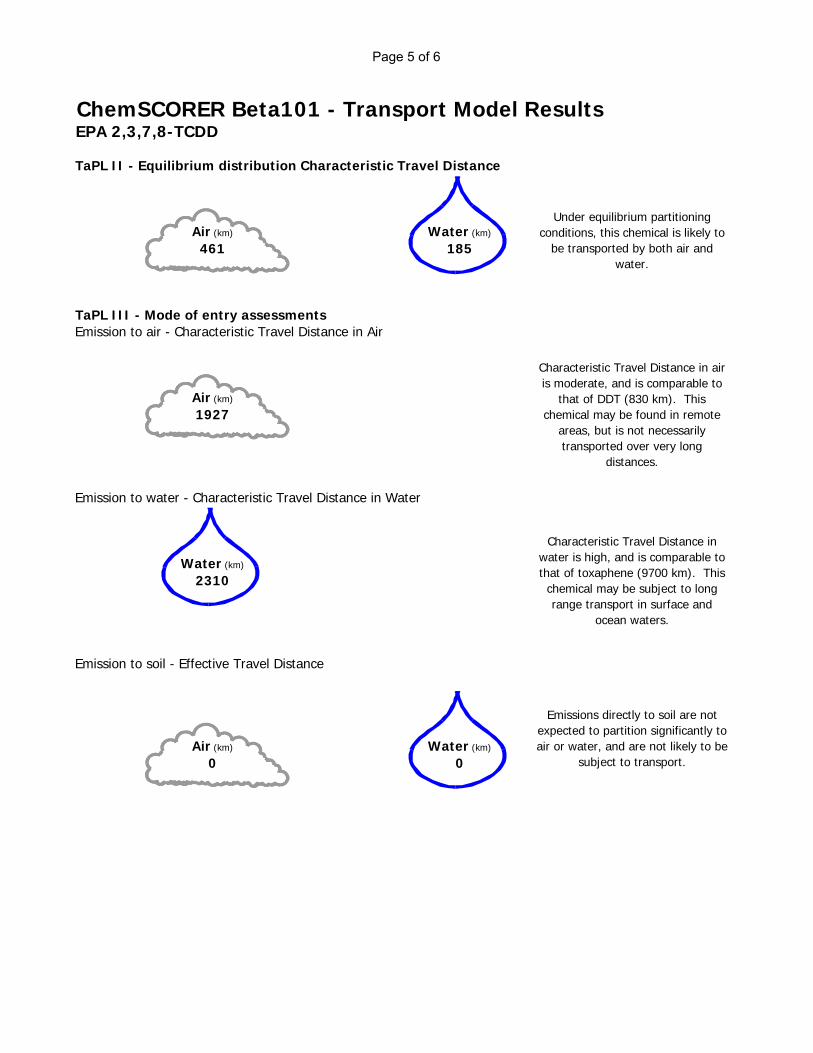
Page 5 of 6
ChemSCORER Beta101 - Transport Model ResultsEPA 2,3,7,8-TCDD
TaPL II - Equilibrium distribution Characteristic Travel Distance
Air (km) Water (km)
461 185
TaPL III - Mode of entry assessmentsEmission to air - Characteristic Travel Distance in Air
Air (km)
1927
Emission to water - Characteristic Travel Distance in Water
Water (km)
2310
Emission to soil - Effective Travel Distance
Air (km) Water (km)
0 0
Under equilibrium partitioning conditions, this chemical is likely to
be transported by both air and water.
Characteristic Travel Distance in air is moderate, and is comparable to
that of DDT (830 km). This chemical may be found in remote
areas, but is not necessarily transported over very long
distances.
Characteristic Travel Distance in water is high, and is comparable to that of toxaphene (9700 km). This
chemical may be subject to long range transport in surface and
ocean waters.
Emissions directly to soil are not expected to partition significantly to air or water, and are not likely to be
subject to transport.

Page 6 of 6
ChemSCORER Beta101 - Toxicity and BioaccumulationEPA 2,3,7,8-TCDD
Toxicity Information
No mammalian toxicity data was supplied. No aquatic toxicity data was supplied.
Evaluative Aquatic Foodweb
Concentration (ug/g)BMF from water
310 ng/L 1548 BMF from sediment3.10E-4 ug/g 6.82
2.06
369 5363.72 9.450.81 2.06
5004.410.96
711.00
1423 ng/L
1.42E-3 ug/g 1951.00
Overall Bioaccumulation Factor, Lake Trout / Water : 4989267
Notes on Terminology:
Bioconcentration (BCF) - Increase in contaminant concentration from water to fish.Biomagnification (BMF) - Increase in contaminant concentration from food to fish.Bioaccumulation (BAF) - Total contaminant concentration increase due to BCF and BMF.
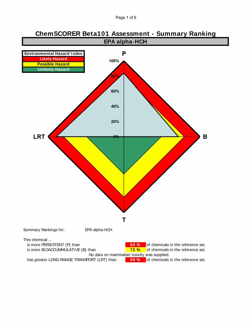
Page 1 of 6
Summary Rankings for: EPA alpha-HCH
This chemical ... is more PERSISTENT (P) than 84 % of chemicals in the reference set. is more BIOACCUMMULATIVE (B) than 72 % of chemicals in the reference set. No data on mammalian toxicity was supplied. has greater LONG RANGE TRANSPORT (LRT) than 89 % of chemicals in the reference set.
Possible HazardUnlikely Hazard
ChemSCORER Beta101 Assessment - Summary RankingEPA alpha-HCH
Environmental Hazard IndexLikely Hazard
0%
20%
40%
60%
80%
100%P
B
T
LRT

Page 2 of 6
ChemSCORER Beta101 - Level I Model ResultsEPA alpha-HCH
Details of Level I calculation for: EPA alpha-HCH
Compartment Z(mol/m^3Pa) (mol/m^3) (mg/L) (ug/g) kg %
Air 4.03E-04 5.61E-11 1.63E-08 1.38E-05 1633 1.633Water 1.37E+00 1.90E-07 5.53E-05 5.53E-05 11064 11.064Soil 2.34E+02 3.26E-05 9.48E-03 3.95E-03 85342 85.342Sediment 4.69E+02 6.52E-05 1.90E-02 7.90E-03 1896 1.896Suspended Sediment 1.46E+03 2.04E-04 5.93E-02 3.95E-02 59 0.059Biota (Fish) 5.95E+02 8.28E-05 2.41E-02 2.41E-02 5 0.005Total 100000 100.000
Molar Mass 290.85 g/mol
Vapor Pressure 1 Pa Log Kow 3.94 Air 1.17E-01Aqueous Solubility 397.5797299 g/m^3 Log Kaw -3.53 Water 3.98E+02Log Kow 3.94 Log Koa 7.47 Octanol 3.46E+06Melting Point -999 deg C
The Level I chemical distibution represents long term equilibrium
partitioning of the chemical. Many persistent chemicals partition
predominantly to soils. Long range transport usually requires
partitioning (at least 1%) to one of the mobile media (air or water).
Bioconcentration Factor (BCF)
435
The calculated BCF is below the generally accepted cut-off between bioaccumulative and non-bioaccumulative substances of 5000. This substance is not expected to bioaccumulate to a significant degree.
Input Parameters Partition Coefficients Three Solubilities(g/m^3)
Concentration AmountEquilibrium Chemical Distribution
Physical Chemical Data and Partition Coefficients
Level I Chemical DistributionAir2%
Water11%
Soil85%
Sediment2%

Page 3 of 6
ChemSCORER Beta101 - Level II Model ResultsEPA alpha-HCH
2063 hours 85.97 days
4754 hours 198.06 days
3646 hours 151.91 days
Details of Level II calculation for: EPA alpha-HCH
Half-life RemovalReaction Advection Reaction Advection(mol/Pa h) (mol/Pa h) (kg/h) (kg/h)
Air 2880 9.71E+06 4.03E+08 8.11E+00 3.37E+02 34.497Water 3240 5.85E+07 2.73E+08 4.88E+01 2.28E+02 27.712Soil 3240 4.51E+08 0 3.77E+02 0 37.663Sediment 55000 5.90E+05 9.37E+05 4.93E-01 7.83E-01 0.128Total 5.20E+08 6.78E+08 4.34E+02 5.66E+02Reaction + Advection
Equilibrium Partitioning Persistence Information
The figure at right identifies environmental media that have a
controlling influence on the overall rate of reactive degradation of this
substance. Substances that fall near the center of the diagram are expected to accumulate in all media, and overall
persistence will be influenced by all degradation rates. The relative
importance of advection and reaction to the regional-scale removal of this
substance, and the media from which these processes take place are depicted
in the pie charts below.The equilibrium distribution reaction
residence time calculated for this substance can be measured in months,
and is comparable to that of the tetrachlorobenzenes (120 days).
Reactive and advective residence times are comparable, indicating the
substance may be mobile to other regions.
Removal Processes - Equilibrium Distribution
1.20E+09 1000
Overall Residence Time:Reaction Residence Time:Advection Residence Time:
Compartment(hours) %
100.000
D Values Loss Rates
-15-14-13-12-11-10-9-8-7-6-5-4-3-2-10123456789
10
-4 -3 -2 -1 0 1 2 3 4 5 6 7 8 9 10
Log Kow
Log
Kaw
Air
Water Octanol
Air& Octanol
Water & Octanol
Air & Water
Removal Pathways
Reaction43%
Advection57%
Media of ReactionAir2%
Water11%
Soil87%
Sediment0%
Media of Advection
Air60%
Water40%
Sediment0%

Page 4 of 6
ChemSCORER Beta101 - Level III Model ResultsEPA alpha-HCH
Emission to Air
(hours) 5403.30(days) 225.14
(years) 0.62
Emission to Water
(hours) 6519.17(days) 271.63
(years) 0.74
Emission to Soil
(hours) 4703.83(days) 195.99
(years) 0.54
Emission to All 3
(hours) 5668.11(days) 236.17
(years) 0.65
Details of Level III calculation for: EPA alpha-HCH
Air Water Soil Air Water Soil Sediment TotalAir 1000 0 0 9.60E+05 1.75E+06 1.80E+06 9.01E+05 5.40E+06
Water 0 1000 0 2.34E+05 3.86E+06 4.39E+05 1.99E+06 6.52E+06Soil 0 0 1000 7.27E+03 6.05E+04 4.60E+06 3.13E+04 4.70E+06All 3 600 300 100 6.47E+05 2.21E+06 1.67E+06 1.14E+06 5.67E+06
Air 1000 0 0 231 373 384 11 1000Water 0 1000 0 56 825 94 25 1000Soil 0 0 1000 2 13 985 0 1000All 3 600 300 100 156 473 357 14 1000
Persistence under the standard emission scenario is comparable to that of the tetrachlorobenzenes (130 days).
Emissions to air partition
significantly to other media.
Emissions to water partition significantly to other media.
Emissions to soil remain
predominantly in the soil
compartment.
Persistence of air emissions is comparable to that of the tetrachlorobenzenes (110 days).
Persistence of water emissions is comparable to that of the tetrachlorobenzenes (140 days).
Persistence of soil emissions is comparable to that of the tetrachlorobenzenes (250 days).
Emission Rate (kg/h) Inventory at Steady State (kg)
Emission Rate (kg/h) Reaction Loss Rate (kg/h)
Persistence
Persistence
Persistence
Persistence
Steady State Distribution
Air18%
Water32%
Soil33%
Sediment17%
Steady State Distribution
Air4%
Water58%
Soil7%
Sediment31%
Steady State Distribution
Air0%Water1%
Soil98%
Sediment1%
Steady State Distribution
Air11%
Water40%Soil
29%
Sediment20%
Reactive Removal
Air23%
Water37%
Soil39%
Sediment1%
Reactive Removal
Air6%
Water82%
Soil9%
Sediment3%
Reactive Removal
Air0%Water1%
Soil99%
Sediment0%
Reactive Removal
Air16%
Water47%
Soil36%
Sediment1%

Page 5 of 6
ChemSCORER Beta101 - Transport Model ResultsEPA alpha-HCH
TaPL II - Equilibrium distribution Characteristic Travel Distance
Air (km) Water (km)
1118 1893
TaPL III - Mode of entry assessmentsEmission to air - Characteristic Travel Distance in Air
Air (km)
13821
Emission to water - Characteristic Travel Distance in Water
Water (km)
13879
Emission to soil - Effective Travel Distance
Air (km) Water (km)
0 3503
Under equilibrium partitioning conditions, this chemical is likely to
be transported by both air and water.
Characteristic Travel Distance in air is high, and is comparable to that of
hexachlorinated PCBs (4200 km). This chemical may be subject to
long range transport and deposition in the arctic.
Characteristic Travel Distance in water is high, and is comparable to that of toxaphene (9700 km). This
chemical may be subject to long range transport in surface and
ocean waters.
Emissions directly to soil may run-off to water and be subject to transport in surface water and
oceans.
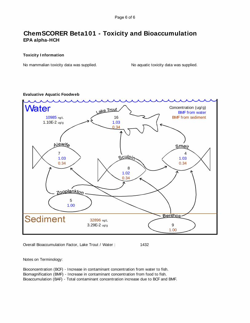
Page 6 of 6
ChemSCORER Beta101 - Toxicity and BioaccumulationEPA alpha-HCH
Toxicity Information
No mammalian toxicity data was supplied. No aquatic toxicity data was supplied.
Evaluative Aquatic Foodweb
Concentration (ug/g)BMF from water
10985 ng/L 16 BMF from sediment1.10E-2 ug/g 1.03
0.34
7 41.03 1.030.34 0.34
81.020.34
51.00
32896 ng/L
3.29E-2 ug/g 91.00
Overall Bioaccumulation Factor, Lake Trout / Water : 1432
Notes on Terminology:
Bioconcentration (BCF) - Increase in contaminant concentration from water to fish.Biomagnification (BMF) - Increase in contaminant concentration from food to fish.Bioaccumulation (BAF) - Total contaminant concentration increase due to BCF and BMF.

Page 1 of 6
Summary Rankings for: EPA p,p'-DDT
This chemical ... is more PERSISTENT (P) than 94 % of chemicals in the reference set. is more BIOACCUMMULATIVE (B) than 94 % of chemicals in the reference set. No data on mammalian toxicity was supplied. has greater LONG RANGE TRANSPORT (LRT) than 66 % of chemicals in the reference set.
Possible HazardUnlikely Hazard
ChemSCORER Beta101 Assessment - Summary RankingEPA p,p'-DDT
Environmental Hazard IndexLikely Hazard
0%
20%
40%
60%
80%
100%P
B
T
LRT

Page 2 of 6
ChemSCORER Beta101 - Level I Model ResultsEPA p,p'-DDT
Details of Level I calculation for: EPA p,p'-DDT
Compartment Z(mol/m^3Pa) (mol/m^3) (mg/L) (ug/g) kg %
Air 4.03E-04 5.22E-13 1.85E-10 1.56E-07 19 0.019Water 7.76E-01 1.00E-09 3.56E-07 3.56E-07 71 0.071Soil 2.36E+04 3.06E-05 1.09E-02 4.52E-03 97667 97.667Sediment 4.73E+04 6.12E-05 2.17E-02 9.04E-03 2170 2.170Suspended Sediment 1.48E+05 1.91E-04 6.78E-02 4.52E-02 68 0.068Biota (Fish) 6.01E+04 7.78E-05 2.76E-02 2.76E-02 6 0.006Total 100000 100.000
Molar Mass 354.5 g/mol
Vapor Pressure 0.00002 Pa Log Kow 6.19 Air 2.86E-06Aqueous Solubility 0.0055 g/m^3 Log Kaw -3.28 Water 5.50E-03Log Kow 6.19 Log Koa 9.47 Octanol 8.52E+03Melting Point 108.5 deg C
The Level I chemical distibution represents long term equilibrium
partitioning of the chemical. Many persistent chemicals partition
predominantly to soils. Long range transport usually requires
partitioning (at least 1%) to one of the mobile media (air or water).
Bioconcentration Factor (BCF)
77441
The calculated BCF is substantially greater than the generally accepted cut-off between bioaccumulative and non-
bioaccumulative substances of 5000. In the absence of metabolism by organisms, this substance may bioaccumulate similar to DDT (BCF 63000) or PCBs (BCFs up to
300000).
Input Parameters Partition Coefficients Three Solubilities(g/m^3)
Concentration AmountEquilibrium Chemical Distribution
Physical Chemical Data and Partition Coefficients
Level I Chemical DistributionAir0%
Water0%
Soil98%
Sediment2%
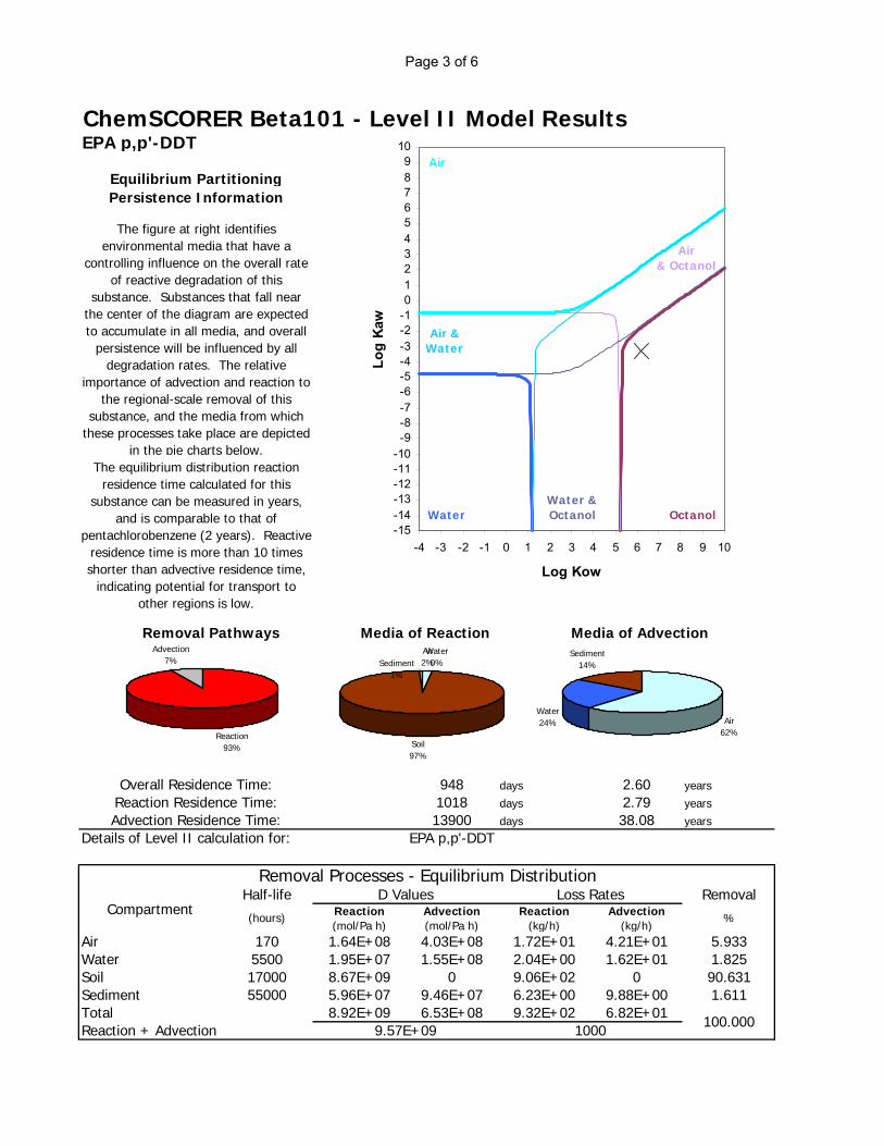
Page 3 of 6
ChemSCORER Beta101 - Level II Model ResultsEPA p,p'-DDT
948 days 2.60 years
1018 days 2.79 years
13900 days 38.08 years
Details of Level II calculation for: EPA p,p'-DDT
Half-life RemovalReaction Advection Reaction Advection(mol/Pa h) (mol/Pa h) (kg/h) (kg/h)
Air 170 1.64E+08 4.03E+08 1.72E+01 4.21E+01 5.933Water 5500 1.95E+07 1.55E+08 2.04E+00 1.62E+01 1.825Soil 17000 8.67E+09 0 9.06E+02 0 90.631Sediment 55000 5.96E+07 9.46E+07 6.23E+00 9.88E+00 1.611Total 8.92E+09 6.53E+08 9.32E+02 6.82E+01Reaction + Advection
Equilibrium Partitioning Persistence Information
The figure at right identifies environmental media that have a
controlling influence on the overall rate of reactive degradation of this
substance. Substances that fall near the center of the diagram are expected to accumulate in all media, and overall
persistence will be influenced by all degradation rates. The relative
importance of advection and reaction to the regional-scale removal of this
substance, and the media from which these processes take place are depicted
in the pie charts below.The equilibrium distribution reaction
residence time calculated for this substance can be measured in years,
and is comparable to that of pentachlorobenzene (2 years). Reactive
residence time is more than 10 times shorter than advective residence time,
indicating potential for transport to other regions is low.
Removal Processes - Equilibrium Distribution
9.57E+09 1000
Overall Residence Time:Reaction Residence Time:Advection Residence Time:
Compartment(hours) %
100.000
D Values Loss Rates
-15-14-13-12-11-10-9-8-7-6-5-4-3-2-10123456789
10
-4 -3 -2 -1 0 1 2 3 4 5 6 7 8 9 10
Log Kow
Log
Kaw
Air
Water Octanol
Air& Octanol
Water & Octanol
Air & Water
Removal Pathways
Reaction93%
Advection7%
Media of ReactionAir2%Water0%
Soil97%
Sediment1%
Media of Advection
Air62%
Water24%
Sediment14%
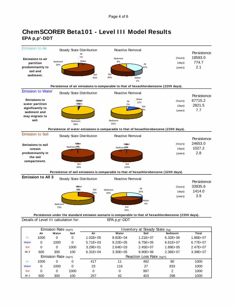
Page 4 of 6
ChemSCORER Beta101 - Level III Model ResultsEPA p,p'-DDT
Emission to Air
(hours) 18593.0(days) 774.7
(years) 2.1
Emission to Water
(hours) 67715.2(days) 2821.5
(years) 7.7
Emission to Soil
(hours) 24653.0(days) 1027.2
(years) 2.8
Emission to All 3
(hours) 33935.6(days) 1414.0
(years) 3.9
Details of Level III calculation for: EPA p,p'-DDT
Air Water Soil Air Water Soil Sediment TotalAir 1000 0 0 1.02E+05 8.82E+04 1.21E+07 6.32E+06 1.86E+07
Water 0 1000 0 5.71E+03 9.22E+05 6.75E+05 6.61E+07 6.77E+07Soil 0 0 1000 3.29E+01 2.64E+03 2.45E+07 1.89E+05 2.47E+07All 3 600 300 100 6.31E+04 3.30E+05 9.90E+06 2.36E+07 3.39E+07
Air 1000 0 0 417 11 492 80 1000Water 0 1000 0 23 116 27 833 1000Soil 0 0 1000 0 0 997 2 1000All 3 600 300 100 257 42 403 298 1000
Persistence under the standard emission scenario is comparable to that of hexachlorobenzene (2300 days).
Emissions to air partition
predominantly to soil and
sediment.
Emissions to water partition significantly to sediment and
may migrate to soil.
Emissions to soil remain
predominantly in the soil
compartment.
Persistence of air emissions is comparable to that of hexachlorobenzene (2200 days).
Persistence of water emissions is comparable to that of hexachlorobenzene (2300 days).
Persistence of soil emissions is comparable to that of hexachlorobenzene (3200 days).
Emission Rate (kg/h) Inventory at Steady State (kg)
Emission Rate (kg/h) Reaction Loss Rate (kg/h)
Persistence
Persistence
Persistence
Persistence
Steady State DistributionAir1%
Water0%
Soil65%
Sediment34%
Steady State Distribution
Air0%Water1%
Soil1%
Sediment98%
Steady State Distribution
Air0%
Water0%
Soil99%
Sediment1%
Steady State Distribution
Air0%Water1% Soil
29%
Sediment70%
Reactive Removal
Air42%
Water1%
Soil49%
Sediment8%
Reactive Removal
Air2%
Water12%
Soil3%
Sediment83%
Reactive Removal
Air0%
Water0%
Soil100%
Sediment0%
Reactive Removal
Air26%
Water4%
Soil40%
Sediment30%

Page 5 of 6
ChemSCORER Beta101 - Transport Model ResultsEPA p,p'-DDT
TaPL II - Equilibrium distribution Characteristic Travel Distance
Air (km) Water (km)
65 63
TaPL III - Mode of entry assessmentsEmission to air - Characteristic Travel Distance in Air
Air (km)
1472
Emission to water - Characteristic Travel Distance in Water
Water (km)
3320
Emission to soil - Effective Travel Distance
Air (km) Water (km)
0 0
Under equilibrium partitioning conditions, this chemical is likely to
be transported by both air and water.
Characteristic Travel Distance in air is moderate, and is comparable to
that of DDT (830 km). This chemical may be found in remote
areas, but is not necessarily transported over very long
distances.
Characteristic Travel Distance in water is high, and is comparable to that of toxaphene (9700 km). This
chemical may be subject to long range transport in surface and
ocean waters.
Emissions directly to soil are not expected to partition significantly to air or water, and are not likely to be
subject to transport.

Page 6 of 6
ChemSCORER Beta101 - Toxicity and BioaccumulationEPA p,p'-DDT
Toxicity Information
No mammalian toxicity data was supplied. No aquatic toxicity data was supplied.
Evaluative Aquatic Foodweb
Concentration (ug/g)BMF from water
813 ng/L 1044 BMF from sediment8.13E-4 ug/g 5.19
1.33
289 3213.29 6.370.69 1.33
3773.740.78
631.00
3879 ng/L
3.88E-3 ug/g 1801.00
Overall Bioaccumulation Factor, Lake Trout / Water : 1285014
Notes on Terminology:
Bioconcentration (BCF) - Increase in contaminant concentration from water to fish.Biomagnification (BMF) - Increase in contaminant concentration from food to fish.Bioaccumulation (BAF) - Total contaminant concentration increase due to BCF and BMF.

Page 1 of 6
Summary Rankings for: EPA Toxaphene
This chemical ... is more PERSISTENT (P) than 97 % of chemicals in the reference set. is more BIOACCUMMULATIVE (B) than 91 % of chemicals in the reference set. No data on mammalian toxicity was supplied. has greater LONG RANGE TRANSPORT (LRT) than 80 % of chemicals in the reference set.
Possible HazardUnlikely Hazard
ChemSCORER Beta101 Assessment - Summary RankingEPA Toxaphene
Environmental Hazard IndexLikely Hazard
0%
20%
40%
60%
80%
100%P
B
T
LRT
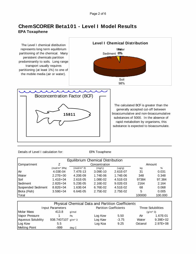
Page 2 of 6
ChemSCORER Beta101 - Level I Model ResultsEPA Toxaphene
Details of Level I calculation for: EPA Toxaphene
Compartment Z(mol/m^3Pa) (mol/m^3) (mg/L) (ug/g) kg %
Air 4.03E-04 7.47E-13 3.09E-10 2.61E-07 31 0.031Water 2.27E+00 4.20E-09 1.74E-06 1.74E-06 348 0.348Soil 1.41E+04 2.61E-05 1.08E-02 4.51E-03 97384 97.384Sediment 2.82E+04 5.23E-05 2.16E-02 9.02E-03 2164 2.164Suspended Sediment 8.82E+04 1.63E-04 6.76E-02 4.51E-02 68 0.068Biota (Fish) 3.59E+04 6.64E-05 2.75E-02 2.75E-02 5 0.005Total 100000 100.000
Molar Mass 413.8 g/mol
Vapor Pressure 1 Pa Log Kow 5.50 Air 1.67E-01Aqueous Solubility 938.7407107 g/m^3 Log Kaw -3.75 Water 9.39E+02Log Kow 5.5 Log Koa 9.25 Octanol 2.97E+08Melting Point -999 deg C
The Level I chemical distibution represents long term equilibrium
partitioning of the chemical. Many persistent chemicals partition
predominantly to soils. Long range transport usually requires
partitioning (at least 1%) to one of the mobile media (air or water).
Bioconcentration Factor (BCF)
15811
The calculated BCF is greater than the generally accepted cut-off between
bioaccumulative and non-bioaccumulative substances of 5000. In the absence of rapid metabolism by organisms, this
substance is expected to bioaccumulate.
Input Parameters Partition Coefficients Three Solubilities(g/m^3)
Concentration AmountEquilibrium Chemical Distribution
Physical Chemical Data and Partition Coefficients
Level I Chemical DistributionAir0%
Water0%
Soil98%
Sediment2%

Page 3 of 6
ChemSCORER Beta101 - Level II Model ResultsEPA Toxaphene
1998 days 5.48 years
3009 days 8.24 years
5951 days 16.30 years
Details of Level II calculation for: EPA Toxaphene
Half-life RemovalReaction Advection Reaction Advection(mol/Pa h) (mol/Pa h) (kg/h) (kg/h)
Air 170 1.64E+08 4.03E+08 6.05E+01 1.48E+02 20.875Water 55000 5.72E+06 4.54E+08 2.10E+00 1.67E+02 16.889Soil 55000 1.60E+09 0 5.89E+02 0 58.853Sediment 55000 3.56E+07 5.65E+07 1.31E+01 2.08E+01 3.384Total 1.81E+09 9.14E+08 6.64E+02 3.36E+02Reaction + Advection
Equilibrium Partitioning Persistence Information
The figure at right identifies environmental media that have a
controlling influence on the overall rate of reactive degradation of this
substance. Substances that fall near the center of the diagram are expected to accumulate in all media, and overall
persistence will be influenced by all degradation rates. The relative
importance of advection and reaction to the regional-scale removal of this
substance, and the media from which these processes take place are depicted
in the pie charts below.The equilibrium distribution reaction
residence time calculated for this substance is greater than five years,
and is comparable to that of hexachlorobenzene (7.6 years).
Reactive and advective residence times are comparable, indicating the
substance may be subject to long range transport.
Removal Processes - Equilibrium Distribution
2.72E+09 1000
Overall Residence Time:Reaction Residence Time:Advection Residence Time:
Compartment(hours) %
100.000
D Values Loss Rates
-15-14-13-12-11-10-9-8-7-6-5-4-3-2-10123456789
10
-4 -3 -2 -1 0 1 2 3 4 5 6 7 8 9 10
Log Kow
Log
Kaw
Air
Water Octanol
Air& Octanol
Water & Octanol
Air & Water
Removal Pathways
Reaction66%
Advection34%
Media of ReactionAir9%
Water0%
Soil89%
Sediment2%
Media of Advection
Air44%
Water50%
Sediment6%
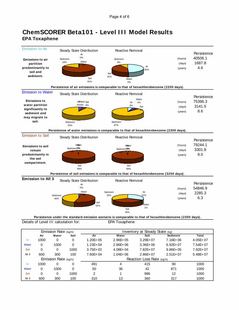
Page 4 of 6
ChemSCORER Beta101 - Level III Model ResultsEPA Toxaphene
Emission to Air
(hours) 40506.1(days) 1687.8
(years) 4.6
Emission to Water
(hours) 75396.3(days) 3141.5
(years) 8.6
Emission to Soil
(hours) 79244.1(days) 3301.8
(years) 9.0
Emission to All 3
(hours) 54846.9(days) 2285.3
(years) 6.3
Details of Level III calculation for: EPA Toxaphene
Air Water Soil Air Water Soil Sediment TotalAir 1000 0 0 1.20E+05 2.96E+05 3.29E+07 7.16E+06 4.05E+07
Water 0 1000 0 1.23E+04 2.86E+06 3.36E+06 6.92E+07 7.54E+07Soil 0 0 1000 3.75E+02 4.08E+04 7.82E+07 9.86E+05 7.92E+07All 3 600 300 100 7.60E+04 1.04E+06 2.86E+07 2.51E+07 5.48E+07
Air 1000 0 0 491 4 415 90 1000Water 0 1000 0 50 36 42 871 1000Soil 0 0 1000 2 1 986 12 1000All 3 600 300 100 310 13 360 317 1000
Persistence under the standard emission scenario is comparable to that of hexachlorobenzene (2300 days).
Emissions to air partition
predominantly to soil and
sediment.
Emissions to water partition significantly to sediment and
may migrate to soil.
Emissions to soil remain
predominantly in the soil
compartment.
Persistence of air emissions is comparable to that of hexachlorobenzene (2200 days).
Persistence of water emissions is comparable to that of hexachlorobenzene (2300 days).
Persistence of soil emissions is comparable to that of hexachlorobenzene (3200 days).
Emission Rate (kg/h) Inventory at Steady State (kg)
Emission Rate (kg/h) Reaction Loss Rate (kg/h)
Persistence
Persistence
Persistence
Persistence
Steady State DistributionAir0%
Water1%
Soil81%
Sediment18%
Steady State Distribution
Air0%
Water4%
Soil4%
Sediment92%
Steady State Distribution
Air0%
Water0%
Soil99%
Sediment1%
Steady State DistributionAir0%
Water2%
Soil52%
Sediment46%
Reactive Removal
Air50%
Water0%
Soil41%
Sediment9%
Reactive Removal
Air5%
Water4%
Soil4%
Sediment87%
Reactive Removal
Air0%
Water0%
Soil99%
Sediment1%
Reactive Removal
Air31%
Water1%Soil
36%
Sediment32%

Page 5 of 6
ChemSCORER Beta101 - Transport Model ResultsEPA Toxaphene
TaPL II - Equilibrium distribution Characteristic Travel Distance
Air (km) Water (km)
322 904
TaPL III - Mode of entry assessmentsEmission to air - Characteristic Travel Distance in Air
Air (km)
1735
Emission to water - Characteristic Travel Distance in Water
Water (km)
10296
Emission to soil - Effective Travel Distance
Air (km) Water (km)
0 0
Under equilibrium partitioning conditions, this chemical is likely to
be transported by both air and water.
Characteristic Travel Distance in air is moderate, and is comparable to
that of DDT (830 km). This chemical may be found in remote
areas, but is not necessarily transported over very long
distances.
Characteristic Travel Distance in water is high, and is comparable to that of toxaphene (9700 km). This
chemical may be subject to long range transport in surface and
ocean waters.
Emissions directly to soil are not expected to partition significantly to air or water, and are not likely to be
subject to transport.

Page 6 of 6
ChemSCORER Beta101 - Toxicity and BioaccumulationEPA Toxaphene
Toxicity Information
No mammalian toxicity data was supplied. No aquatic toxicity data was supplied.
Evaluative Aquatic Foodweb
Concentration (ug/g)BMF from water
4295 ng/L 516 BMF from sediment4.30E-3 ug/g 2.37
0.51
195 1302.05 2.390.44 0.51
2302.120.45
681.00
20193 ng/L
2.02E-2 ug/g 1921.00
Overall Bioaccumulation Factor, Lake Trout / Water : 120143
Notes on Terminology:
Bioconcentration (BCF) - Increase in contaminant concentration from water to fish.Biomagnification (BMF) - Increase in contaminant concentration from food to fish.Bioaccumulation (BAF) - Total contaminant concentration increase due to BCF and BMF.
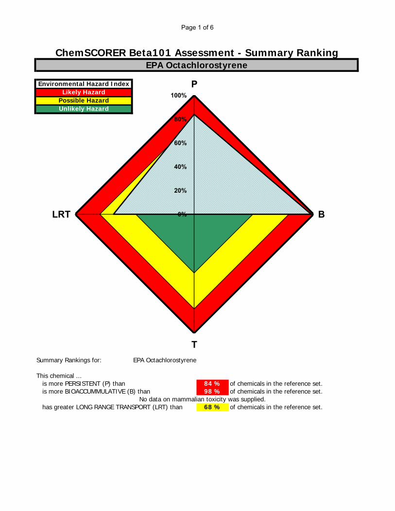
Page 1 of 6
Summary Rankings for: EPA Octachlorostyrene
This chemical ... is more PERSISTENT (P) than 84 % of chemicals in the reference set. is more BIOACCUMMULATIVE (B) than 98 % of chemicals in the reference set. No data on mammalian toxicity was supplied. has greater LONG RANGE TRANSPORT (LRT) than 68 % of chemicals in the reference set.
Possible HazardUnlikely Hazard
ChemSCORER Beta101 Assessment - Summary RankingEPA Octachlorostyrene
Environmental Hazard IndexLikely Hazard
0%
20%
40%
60%
80%
100%P
B
T
LRT

Page 2 of 6
ChemSCORER Beta101 - Level I Model ResultsEPA Octachlorostyrene
Details of Level I calculation for: EPA Octachlorostyrene
Compartment Z(mol/m^3Pa) (mol/m^3) (mg/L) (ug/g) kg %
Air 4.03E-04 2.96E-12 1.13E-09 9.50E-07 113 0.113Water 6.85E-03 5.03E-11 1.91E-08 1.91E-08 4 0.004Soil 3.89E+03 2.86E-05 1.08E-02 4.52E-03 97640 97.640Sediment 7.78E+03 5.71E-05 2.17E-02 9.04E-03 2170 2.170Suspended Sediment 2.43E+04 1.79E-04 6.78E-02 4.52E-02 68 0.068Biota (Fish) 9.88E+03 7.26E-05 2.76E-02 2.76E-02 6 0.006Total 100000 100.000
Molar Mass 379.71 g/mol
Vapor Pressure 0.00176 Pa Log Kow 7.46 Air 2.70E-04Aqueous Solubility 0.0045776 g/m^3 Log Kaw -1.23 Water 4.58E-03Log Kow 7.46 Log Koa 8.69 Octanol 1.32E+05Melting Point -999 deg C
The Level I chemical distibution represents long term equilibrium
partitioning of the chemical. Many persistent chemicals partition
predominantly to soils. Long range transport usually requires
partitioning (at least 1%) to one of the mobile media (air or water).
Bioconcentration Factor (BCF)
1442016
The calculated BCF is substantially greater than the generally accepted cut-off between bioaccumulative and non-
bioaccumulative substances of 5000. In the absence of metabolism by organisms, this substance may bioaccumulate similar to DDT (BCF 63000) or PCBs (BCFs up to
300000).
Input Parameters Partition Coefficients Three Solubilities(g/m^3)
Concentration AmountEquilibrium Chemical Distribution
Physical Chemical Data and Partition Coefficients
Level I Chemical DistributionAir0%
Water0%
Soil98%
Sediment2%

Page 3 of 6
ChemSCORER Beta101 - Level II Model ResultsEPA Octachlorostyrene
204 days 0.56 years
217 days 0.59 years
3552 days 9.73 years
Details of Level II calculation for: EPA Octachlorostyrene
Half-life RemovalReaction Advection Reaction Advection(mol/Pa h) (mol/Pa h) (kg/h) (kg/h)
Air 227 1.23E+08 4.03E+08 1.68E+01 5.51E+01 7.197Water 3600 2.64E+05 1.37E+06 3.60E-02 1.87E-01 0.022Soil 3600 6.74E+09 0 9.21E+02 0 92.057Sediment 14400 3.74E+07 1.56E+07 5.11E+00 2.13E+00 0.724Total 6.90E+09 4.20E+08 9.43E+02 5.74E+01Reaction + Advection
Equilibrium Partitioning Persistence Information
The figure at right identifies environmental media that have a
controlling influence on the overall rate of reactive degradation of this
substance. Substances that fall near the center of the diagram are expected to accumulate in all media, and overall
persistence will be influenced by all degradation rates. The relative
importance of advection and reaction to the regional-scale removal of this
substance, and the media from which these processes take place are depicted
in the pie charts below.The equilibrium distribution reaction
residence time calculated for this substance can be measured in years,
and is comparable to that of pentachlorobenzene (2 years). Reactive
residence time is more than 10 times shorter than advective residence time,
indicating potential for transport to other regions is low.
Removal Processes - Equilibrium Distribution
7.32E+09 1000
Overall Residence Time:Reaction Residence Time:Advection Residence Time:
Compartment(hours) %
100.000
D Values Loss Rates
-15-14-13-12-11-10-9-8-7-6-5-4-3-2-10123456789
10
-4 -3 -2 -1 0 1 2 3 4 5 6 7 8 9 10
Log Kow
Log
Kaw
Air
Water Octanol
Air& Octanol
Water & Octanol
Air & Water
Removal Pathways
Reaction94%
Advection6%
Media of ReactionAir2%Water0%
Soil97%
Sediment1%
Media of Advection
Air96%
Water0%
Sediment4%

Page 4 of 6
ChemSCORER Beta101 - Level III Model ResultsEPA Octachlorostyrene
Emission to Air
(hours) 2183.77(days) 90.99
(years) 0.25
Emission to Water
(hours) 19318.84(days) 804.95
(years) 2.21
Emission to Soil
(hours) 5201.88(days) 216.74
(years) 0.59
Emission to All 3
(hours) 7626.10(days) 317.75
(years) 0.87
Details of Level III calculation for: EPA Octachlorostyrene
Air Water Soil Air Water Soil Sediment TotalAir 1000 0 0 2.42E+05 1.21E+04 1.15E+06 7.81E+05 2.18E+06
Water 0 1000 0 7.53E+03 2.94E+05 3.57E+04 1.90E+07 1.93E+07Soil 0 0 1000 3.01E+01 1.55E+02 5.19E+06 1.00E+04 5.20E+06All 3 600 300 100 1.48E+05 9.56E+04 1.22E+06 6.16E+06 7.63E+06
Air 1000 0 0 739 2 221 38 1000Water 0 1000 0 23 57 7 913 1000Soil 0 0 1000 0 0 999 0 1000All 3 600 300 100 450 18 235 297 1000
Persistence under the standard emission scenario is comparable to that of the tetrachlorobenzenes (130 days).
Emissions to air partition
significantly to soil and
sediment.
Emissions to water partition significantly to sediment and
may migrate to soil.
Emissions to soil remain
predominantly in the soil
compartment.
Persistence of air emissions is comparable to that of the tetrachlorobenzenes (110 days).
Persistence of water emissions is comparable to that of hexachlorobenzene (2300 days).
Persistence of soil emissions is comparable to that of the tetrachlorobenzenes (250 days).
Emission Rate (kg/h) Inventory at Steady State (kg)
Emission Rate (kg/h) Reaction Loss Rate (kg/h)
Persistence
Persistence
Persistence
Persistence
Steady State DistributionAir
11%
Water1%
Soil52%
Sediment36%
Steady State Distribution
Air0%Water2%Soil0%
Sediment98%
Steady State Distribution
Air0%
Water0%
Soil100%
Sediment0%
Steady State Distribution
Air2%
Water1%
Soil16%
Sediment81%
Reactive Removal
Air74%
Water0%
Soil22%
Sediment4%
Reactive Removal
Air2%
Water6%
Soil1%
Sediment91%
Reactive Removal
Air0%
Water0%
Soil100%
Sediment0%
Reactive Removal
Air45%
Water2%
Soil23%
Sediment30%

Page 5 of 6
ChemSCORER Beta101 - Transport Model ResultsEPA Octachlorostyrene
TaPL II - Equilibrium distribution Characteristic Travel Distance
Air (km) Water (km)
84 1
TaPL III - Mode of entry assessmentsEmission to air - Characteristic Travel Distance in Air
Air (km)
3486
Emission to water - Characteristic Travel Distance in Water
Water (km)
1059
Emission to soil - Effective Travel Distance
Air (km) Water (km)
0 0
Under equilibrium partitioning conditions, this chemical is likely to be transported most effectively in
air.
Characteristic Travel Distance in air is high, and is comparable to that of
hexachlorinated PCBs (4200 km). This chemical may be subject to
long range transport and deposition in the arctic.
Characteristic Travel Distance in water is moderate, and is
comparable to that of chlorobenzene (1300 km). This
chemical may be subject to transport in surface and near-shore
marine waters.
Emissions directly to soil are not expected to partition significantly to air or water, and are not likely to be
subject to transport.

Page 6 of 6
ChemSCORER Beta101 - Toxicity and BioaccumulationEPA Octachlorostyrene
Toxicity Information
No mammalian toxicity data was supplied. No aquatic toxicity data was supplied.
Evaluative Aquatic Foodweb
Concentration (ug/g)BMF from water
24 ng/L 492 BMF from sediment2.37E-5 ug/g 4.50
2.96
122 1852.56 6.781.12 2.96
1362.491.08
341.00
54 ng/L
5.43E-5 ug/g 471.00
Overall Bioaccumulation Factor, Lake Trout / Water : 20770986
Notes on Terminology:
Bioconcentration (BCF) - Increase in contaminant concentration from water to fish.Biomagnification (BMF) - Increase in contaminant concentration from food to fish.Bioaccumulation (BAF) - Total contaminant concentration increase due to BCF and BMF.

Page 1 of 6
Summary Rankings for: EPA B[a]p
This chemical ... is more PERSISTENT (P) than 78 % of chemicals in the reference set. is more BIOACCUMMULATIVE (B) than 94 % of chemicals in the reference set. No data on mammalian toxicity was supplied. has greater LONG RANGE TRANSPORT (LRT) than 4 % of chemicals in the reference set.
Possible HazardUnlikely Hazard
ChemSCORER Beta101 Assessment - Summary RankingEPA B[a]p
Environmental Hazard IndexLikely Hazard
0%
20%
40%
60%
80%
100%P
B
T
LRT

Page 2 of 6
ChemSCORER Beta101 - Level I Model ResultsEPA B[a]p
Details of Level I calculation for: EPA B[a]p
Compartment Z(mol/m^3Pa) (mol/m^3) (mg/L) (ug/g) kg %
Air 4.03E-04 3.46E-14 8.74E-12 7.37E-09 1 0.001Water 1.16E+01 9.99E-10 2.52E-07 2.52E-07 50 0.050Soil 5.01E+05 4.30E-05 1.09E-02 4.52E-03 97704 97.704Sediment 1.00E+06 8.61E-05 2.17E-02 9.05E-03 2171 2.171Suspended Sediment 3.13E+06 2.69E-04 6.79E-02 4.52E-02 68 0.068Biota (Fish) 1.27E+06 1.09E-04 2.76E-02 2.76E-02 6 0.006Total 100000 100.000
Molar Mass 252.3 g/mol
Vapor Pressure 1 Pa Log Kow 6.34 Air 1.02E-01Aqueous Solubility 2937 g/m^3 Log Kaw -4.46 Water 2.94E+03Log Kow 6.34 Log Koa 10.80 Octanol 6.43E+09Melting Point 177.5 deg C
The Level I chemical distibution represents long term equilibrium
partitioning of the chemical. Many persistent chemicals partition
predominantly to soils. Long range transport usually requires
partitioning (at least 1%) to one of the mobile media (air or water).
Bioconcentration Factor (BCF)
109388
The calculated BCF is substantially greater than the generally accepted cut-off between bioaccumulative and non-
bioaccumulative substances of 5000. In the absence of metabolism by organisms, this substance may bioaccumulate similar to DDT (BCF 63000) or PCBs (BCFs up to
300000).
Input Parameters Partition Coefficients Three Solubilities(g/m^3)
Concentration AmountEquilibrium Chemical Distribution
Physical Chemical Data and Partition Coefficients
Level I Chemical DistributionAir0%
Water0%
Soil98%
Sediment2%

Page 3 of 6
ChemSCORER Beta101 - Level II Model ResultsEPA B[a]p
308 days 0.84 years
311 days 0.85 years
40615 days 111.27 years
Details of Level II calculation for: EPA B[a]p
Half-life RemovalReaction Advection Reaction Advection(mol/Pa h) (mol/Pa h) (kg/h) (kg/h)
Air 1.52 1.84E+10 4.03E+08 2.95E+01 6.46E-01 3.012Water 56.08151099 2.88E+10 2.33E+09 4.61E+01 3.73E+00 4.983Soil 5487.166023 5.70E+11 0 9.13E+02 0 91.288Sediment 28140 2.47E+09 2.00E+09 3.96E+00 3.21E+00 0.717Total 6.19E+11 4.74E+09 9.92E+02 7.59E+00Reaction + Advection
Equilibrium Partitioning Persistence Information
The figure at right identifies environmental media that have a
controlling influence on the overall rate of reactive degradation of this
substance. Substances that fall near the center of the diagram are expected to accumulate in all media, and overall
persistence will be influenced by all degradation rates. The relative
importance of advection and reaction to the regional-scale removal of this
substance, and the media from which these processes take place are depicted
in the pie charts below.The equilibrium distribution reaction
residence time calculated for this substance can be measured in years,
and is comparable to that of pentachlorobenzene (2 years). Reactive
residence time is more than 10 times shorter than advective residence time,
indicating potential for transport to other regions is low.
Removal Processes - Equilibrium Distribution
6.24E+11 1000
Overall Residence Time:Reaction Residence Time:Advection Residence Time:
Compartment(hours) %
100.000
D Values Loss Rates
-15-14-13-12-11-10-9-8-7-6-5-4-3-2-10123456789
10
-4 -3 -2 -1 0 1 2 3 4 5 6 7 8 9 10
Log Kow
Log
Kaw
Air
Water Octanol
Air& Octanol
Water & Octanol
Air & Water
Removal Pathways
Reaction99%
Advection1%
Media of ReactionAir3%
Water5%
Soil92%
Sediment0%
Media of AdvectionAir9%
Water49%
Sediment42%

Page 4 of 6
ChemSCORER Beta101 - Level III Model ResultsEPA B[a]p
Emission to Air
(hours) 397.21(days) 16.55
(years) 0.05
Emission to Water
(hours) 4491.44(days) 187.14
(years) 0.51
Emission to Soil
(hours) 7914.82(days) 329.78
(years) 0.90
Emission to All 3
(hours) 2377.24(days) 99.05
(years) 0.27
Details of Level III calculation for: EPA B[a]p
Air Water Soil Air Water Soil Sediment TotalAir 1000 0 0 2.08E+03 3.91E+02 3.71E+05 2.40E+04 3.97E+05
Water 0 1000 0 5.27E-01 7.21E+04 9.40E+01 4.42E+06 4.49E+06Soil 0 0 1000 3.89E-02 6.37E+01 7.91E+06 3.90E+03 7.91E+06All 3 600 300 100 1.25E+03 2.19E+04 1.01E+06 1.34E+06 2.38E+06
Air 1000 0 0 948 5 47 1 1000Water 0 1000 0 0 891 0 109 1000Soil 0 0 1000 0 1 999 0 1000All 3 600 300 100 569 270 128 33 1000
Persistence under the standard emission scenario is comparable to that of the tetrachlorobenzenes (130 days).
Emissions to air partition
predominantly to soil and
sediment.
Emissions to water partition significantly to sediment and
may migrate to soil.
Emissions to soil remain
predominantly in the soil
compartment.
Persistence of air emissions is comparable to that of chlorobenzene (250 hours).
Persistence of water emissions is comparable to that of the tetrachlorobenzenes (140 days).
Persistence of soil emissions is comparable to that of the tetrachlorobenzenes (250 days).
Emission Rate (kg/h) Inventory at Steady State (kg)
Emission Rate (kg/h) Reaction Loss Rate (kg/h)
Persistence
Persistence
Persistence
Persistence
Steady State Distribution
Air1%Water0%
Soil93%
Sediment6%
Steady State Distribution
Air0%Water2%Soil0%
Sediment98%
Steady State Distribution
Air0%
Water0%
Soil100%
Sediment0%
Steady State DistributionAir0%
Water1%
Soil43%
Sediment56%
Reactive Removal
Air95%
Water0%
Soil5%
Sediment0%
Reactive Removal
Air0%
Water89%
Soil0%
Sediment11%
Reactive Removal
Air0%
Water0%
Soil100%
Sediment0%
Reactive Removal
Air57%
Water27%
Soil13%
Sediment3%

Page 5 of 6
ChemSCORER Beta101 - Transport Model ResultsEPA B[a]p
TaPL II - Equilibrium distribution Characteristic Travel Distance
Air (km) Water (km)
1 14
TaPL III - Mode of entry assessmentsEmission to air - Characteristic Travel Distance in Air
Air (km)
30
Emission to water - Characteristic Travel Distance in Water
Water (km)
260
Emission to soil - Effective Travel Distance
Air (km) Water (km)
0 0
Under equilibrium partitioning conditions, this chemical is likely to be transported most effectively in
water.
Characteristic Travel Distance in air is low. This chemical is not likely to be transported a significant distance
in the atmosphere.
Characteristic Travel Distance in water is low. This chemical is not
likely to be transported a significant distance in water.
Emissions directly to soil are not expected to partition significantly to air or water, and are not likely to be
subject to transport.

Page 6 of 6
ChemSCORER Beta101 - Toxicity and BioaccumulationEPA B[a]p
Toxicity Information
No mammalian toxicity data was supplied. No aquatic toxicity data was supplied.
Evaluative Aquatic Foodweb
Concentration (ug/g)BMF from water
45 ng/L 75 BMF from sediment4.45E-5 ug/g 4.81
1.76
20 242.93 6.150.84 1.76
243.120.89
51.00
156 ng/L
1.56E-4 ug/g 101.00
Overall Bioaccumulation Factor, Lake Trout / Water : 1683335
Notes on Terminology:
Bioconcentration (BCF) - Increase in contaminant concentration from water to fish.Biomagnification (BMF) - Increase in contaminant concentration from food to fish.Bioaccumulation (BAF) - Total contaminant concentration increase due to BCF and BMF.
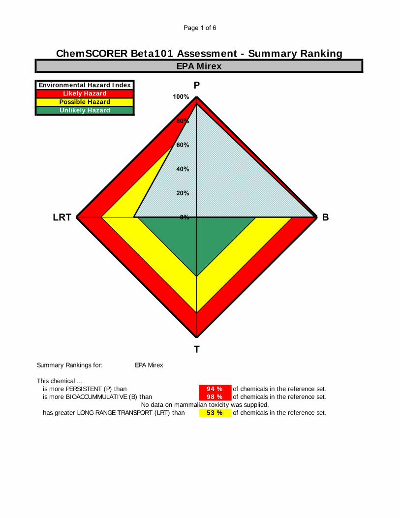
Page 1 of 6
Summary Rankings for: EPA Mirex
This chemical ... is more PERSISTENT (P) than 94 % of chemicals in the reference set. is more BIOACCUMMULATIVE (B) than 98 % of chemicals in the reference set. No data on mammalian toxicity was supplied. has greater LONG RANGE TRANSPORT (LRT) than 53 % of chemicals in the reference set.
Possible HazardUnlikely Hazard
ChemSCORER Beta101 Assessment - Summary RankingEPA Mirex
Environmental Hazard IndexLikely Hazard
0%
20%
40%
60%
80%
100%P
B
T
LRT

Page 2 of 6
ChemSCORER Beta101 - Level I Model ResultsEPA Mirex
Details of Level I calculation for: EPA Mirex
Compartment Z(mol/m^3Pa) (mol/m^3) (mg/L) (ug/g) kg %
Air 4.03E-04 5.69E-13 3.10E-10 2.62E-07 31 0.031Water 2.49E-02 3.51E-11 1.91E-08 1.91E-08 4 0.004Soil 1.41E+04 1.99E-05 1.09E-02 4.52E-03 97720 97.720Sediment 2.82E+04 3.98E-05 2.17E-02 9.05E-03 2172 2.172Suspended Sediment 8.82E+04 1.24E-04 6.79E-02 4.52E-02 68 0.068Biota (Fish) 3.59E+04 5.06E-05 2.76E-02 2.76E-02 6 0.006Total 100000 100.000
Molar Mass 545.59 g/mol
Vapor Pressure 1 Pa Log Kow 7.46 Air 2.20E-01Aqueous Solubility 13.57130365 g/m^3 Log Kaw -1.79 Water 1.36E+01Log Kow 7.46 Log Koa 9.25 Octanol 3.91E+08Melting Point -999 deg C
The Level I chemical distibution represents long term equilibrium
partitioning of the chemical. Many persistent chemicals partition
predominantly to soils. Long range transport usually requires
partitioning (at least 1%) to one of the mobile media (air or water).
Bioconcentration Factor (BCF)
1442016
The calculated BCF is substantially greater than the generally accepted cut-off between bioaccumulative and non-
bioaccumulative substances of 5000. In the absence of metabolism by organisms, this substance may bioaccumulate similar to DDT (BCF 63000) or PCBs (BCFs up to
300000).
Input Parameters Partition Coefficients Three Solubilities(g/m^3)
Concentration AmountEquilibrium Chemical Distribution
Physical Chemical Data and Partition Coefficients
Level I Chemical DistributionAir0%
Water0%
Soil98%
Sediment2%

Page 3 of 6
ChemSCORER Beta101 - Level II Model ResultsEPA Mirex
2370 days 6.49 years
2975 days 8.15 years
11655 days 31.93 years
Details of Level II calculation for: EPA Mirex
Half-life RemovalReaction Advection Reaction Advection(mol/Pa h) (mol/Pa h) (kg/h) (kg/h)
Air 170 1.64E+08 4.03E+08 7.19E+01 1.76E+02 24.839Water 170 2.03E+07 4.97E+06 8.87E+00 2.18E+00 1.105Soil 55000 1.60E+09 0 7.00E+02 0 70.030Sediment 55000 3.56E+07 5.65E+07 1.56E+01 2.47E+01 4.026Total 1.82E+09 4.65E+08 7.97E+02 2.03E+02Reaction + Advection
Equilibrium Partitioning Persistence Information
The figure at right identifies environmental media that have a
controlling influence on the overall rate of reactive degradation of this
substance. Substances that fall near the center of the diagram are expected to accumulate in all media, and overall
persistence will be influenced by all degradation rates. The relative
importance of advection and reaction to the regional-scale removal of this
substance, and the media from which these processes take place are depicted
in the pie charts below.The equilibrium distribution reaction
residence time calculated for this substance is greater than five years,
and is comparable to that of hexachlorobenzene (7.6 years).
Reactive and advective residence times are comparable, indicating the
substance may be subject to long range transport.
Removal Processes - Equilibrium Distribution
2.29E+09 1000
Overall Residence Time:Reaction Residence Time:Advection Residence Time:
Compartment(hours) %
100.000
D Values Loss Rates
-15-14-13-12-11-10-9-8-7-6-5-4-3-2-10123456789
10
-4 -3 -2 -1 0 1 2 3 4 5 6 7 8 9 10
Log Kow
Log
Kaw
Air
Water Octanol
Air& Octanol
Water & Octanol
Air & Water
Removal Pathways
Reaction80%
Advection20%
Media of ReactionAir9%
Water1%
Soil88%
Sediment2%
Media of Advection
Air87%
Water1%
Sediment12%

Page 4 of 6
ChemSCORER Beta101 - Level III Model ResultsEPA Mirex
Emission to Air
(hours) 32993.3(days) 1374.7
(years) 3.8
Emission to Water
(hours) 23637.6(days) 984.9
(years) 2.7
Emission to Soil
(hours) 78901.2(days) 3287.6
(years) 9.0
Emission to All 3
(hours) 34777.4(days) 1449.1
(years) 4.0
Details of Level III calculation for: EPA Mirex
Air Water Soil Air Water Soil Sediment TotalAir 1000 0 0 1.32E+05 1.19E+04 3.13E+07 1.60E+06 3.30E+07
Water 0 1000 0 1.73E+03 1.71E+05 4.09E+05 2.31E+07 2.36E+07Soil 0 0 1000 7.46E+01 1.36E+03 7.87E+07 1.84E+05 7.89E+07All 3 600 300 100 7.97E+04 5.86E+04 2.67E+07 7.89E+06 3.48E+07
Air 1000 0 0 538 48 394 20 1000Water 0 1000 0 7 697 5 290 1000Soil 0 0 1000 0 6 992 2 1000All 3 600 300 100 325 239 337 99 1000
Persistence under the standard emission scenario is comparable to that of hexachlorobenzene (2300 days).
Emissions to air partition
predominantly to soil and
sediment.
Emissions to water partition significantly to sediment and
may migrate to soil.
Emissions to soil remain
predominantly in the soil
compartment.
Persistence of air emissions is comparable to that of hexachlorobenzene (2200 days).
Persistence of water emissions is comparable to that of hexachlorobenzene (2300 days).
Persistence of soil emissions is comparable to that of hexachlorobenzene (3200 days).
Emission Rate (kg/h) Inventory at Steady State (kg)
Emission Rate (kg/h) Reaction Loss Rate (kg/h)
Persistence
Persistence
Persistence
Persistence
Steady State Distribution
Air0%
Water0%
Soil95%
Sediment5%
Steady State Distribution
Air0%
Water1%
Soil2%
Sediment97%
Steady State Distribution
Air0%
Water0%
Soil100%
Sediment0%
Steady State DistributionAir0%
Water0%
Soil77%
Sediment23%
Reactive Removal
Air54%
Water5%
Soil39%
Sediment2%
Reactive Removal
Air1%
Water69%
Soil1%
Sediment29%
Reactive Removal
Air0%
Water1%
Soil99%
Sediment0%
Reactive Removal
Air32%
Water24%
Soil34%
Sediment10%

Page 5 of 6
ChemSCORER Beta101 - Transport Model ResultsEPA Mirex
TaPL II - Equilibrium distribution Characteristic Travel Distance
Air (km) Water (km)
319 10
TaPL III - Mode of entry assessmentsEmission to air - Characteristic Travel Distance in Air
Air (km)
1900
Emission to water - Characteristic Travel Distance in Water
Water (km)
616
Emission to soil - Effective Travel Distance
Air (km) Water (km)
0 0
Under equilibrium partitioning conditions, this chemical is likely to be transported most effectively in
air.
Characteristic Travel Distance in air is moderate, and is comparable to
that of DDT (830 km). This chemical may be found in remote
areas, but is not necessarily transported over very long
distances.
Characteristic Travel Distance in water is low. This chemical is not
likely to be transported a significant distance in water.
Emissions directly to soil are not expected to partition significantly to air or water, and are not likely to be
subject to transport.

Page 6 of 6
ChemSCORER Beta101 - Toxicity and BioaccumulationEPA Mirex
Toxicity Information
No mammalian toxicity data was supplied. No aquatic toxicity data was supplied.
Evaluative Aquatic Foodweb
Concentration (ug/g)BMF from water
15 ng/L 491 BMF from sediment1.45E-5 ug/g 7.33
2.36
114 1903.88 11.320.81 2.36
1604.781.00
211.00
70 ng/L
6.95E-5 ug/g 601.00
Overall Bioaccumulation Factor, Lake Trout / Water : 33808120
Notes on Terminology:
Bioconcentration (BCF) - Increase in contaminant concentration from water to fish.Biomagnification (BMF) - Increase in contaminant concentration from food to fish.Bioaccumulation (BAF) - Total contaminant concentration increase due to BCF and BMF.