Modeling the temporal dynamics of

monoterpene emission by isotopic labeling in

Quercus ilex leaves

S.M. Noe a,∗, U. Niinemets a, J-P. Schnitzler b

aDepartment of Plant Physiology, Institute of Agricultural and Environmental

Sciences, Estonian University of Life Sciences, Kreutzwaldi 1, EE-51014 Tartu,

Estonia

bResearch Centre Karlsruhe Institute for Meteorology and Climate Research

(IMK-IFU) Kreuzeckbahnstrasse 19, D-82467 Garmisch-Partenkirchen, Germany

Abstract

A mathematical model to study the temporal dynamics of stable isotope 13C in-

corporation into monoterpene molecules, emitted from Mediterranean evergreen

sclerophyll oak Quercus ilex L. leaves, was developed. The box model uses leaf level

gas exchange and monoterpene emission data to assess biochemical and diffusional

processes of the light-dependent monoterpene biosynthesis and emission within the

leaf tissues. We estimated total leaf monoterpene pool exchange half-lifes against

these processes. The slowest response took up to 38 hours, while the fastest response

occurred within one hour, taking the sum of the lumped processes time constants

into account. Separately, the turnover half-lives of the biochemical processes ranged

between 26 minutes up to more than 4 hours. The diffusional processes turnover

times, driven by the physico-chemical properties of the monoterpene molecule, have

been found to range between 32 minutes and 3 hours, depending on the number of

Preprint submitted to Atmospheric Environment 18 March 2010

13C-labeled carbon atoms. As a consequence, the steady state assumption that is

used in many larger scale emission models, may not hold in all cases and the ap-

plication of process-based algorithms is beneficial to overcome such long transient

pool dynamics of light-dependent monoterpene emission.

Key words: stable isotope, 13C, mathematical model, monoterpene emission,

temporal emission dynamics

1 Introduction1

Terpene emissions from leaves of many plant species (Kesselmeier and Staudt,2

1999) play a major role in atmospheric chemistry. These volatile compounds3

react rapidly with hydroxyl radicals in the atmosphere and, in the presence4

of reactive nitrogen (NOx), lead to the formation of ozone and secondary5

organic aerosols (SOA) (Kulmala et al., 2004; Tsirgaridis et al., 2005). As SOA6

particles play a role in cloud formation the release of monoterpenes may change7

the radiative energy transfer or water availability, at least regionally which,8

in turn set constraints on carbon dioxide (CO2) uptake and monoterpene9

emission of the ecosystem. So far, the temporal patterns and dynamics of the10

biosynthesis and emission of biogenic volatile compounds (BVOC) is not taken11

into account in most of the larger scale model approaches (Arneth et al., 2007,12

2008). They employ, like many leaf level studies, empirical parameterizations13

(Guenther et al., 1993; Niinemets et al., 2002) that are only valid under steady14

state assumptions.15

∗ Corresponding author.

Email addresses: steffen.noe@emu.ee (S.M. Noe), ylo.niinemets@emu.ee (U.

Niinemets), Joerg-Peter.Schnitzler@imk.fzk.de (J-P. Schnitzler).

2

On the cellular level, the incorporation of stable isotopes such as 13C into16

molecules have been widely used to investigate the metabolic pathways of17

plants by means of metabolic flux analysis (MFA) and metabolic control anal-18

ysis (MCA) (Morgan and Rhodes, 2002; Rios-Estepa and Lange, 2007). These19

labeling techniques are ”state of the art” methods in research on terpene20

(hemi-, mono-, and sesquiterpenes) emissions and the regulation of the terpene21

biosynthetic pathways (Tholl et al., 2006). Impact of environmental effects on22

the hemi- (isoprene) and monoterpene emission patterns have been intensively23

studied by means of labeling experiments (Loreto et al., 2000, 2006) on leaf24

level. The availability of fast online measurement systems such as proton trans-25

fer reaction mass spectrometry (PTR-MS) has further increased the number26

of 13C-labeling studies to investigate the origin and processing of carbon in27

the emitted isoprene molecules (Karl et al., 2002; Kreuzwieser et al., 2002;28

Hayward and Hewitt, 2003; Schnitzler et al., 2004; Brilli et al., 2007).29

Yet, all these studies had focused on isoprene (Schnitzler et al., 2004; Wolfertz30

et al., 2004) and none studied the incorporation dynamics of 13C during the31

light-dependent biosynthesis of monoterpenes. On leaf level, the temporal32

emission patterns are the result of an interplay of several transport, diffu-33

sion and biochemical reaction processes within the ”system” leaf, that are34

additionally altered by the molecules physico-chemical properties (Niinemets35

and Reichstein, 2002; Noe et al., 2006, 2008).36

In this work, we employed a mathematical model to describe the temporal37

dynamics of monoterpene emissions from leaves of Quercus ilex, a evergreen38

Mediterranean tree species that emit monoterpenes in a light-dependent pro-39

cess (Kesselmeier et al., 1997) closely linked to the availability of recently fixed40

carbon. We took the advantage of the availability of fast online analysis us-41

3

ing PTR-MS in connection with a leaf cuvette system. Using our model, we42

became able to apply ”easy” accessible 13C incorporation profiles to predict43

the temporal dynamics of underlying processes in monoterpene biosynthesis,44

diffusion and emission.45

2 Materials and Methods46

2.1 Model description47

To describe temporal patterns of Q. ilex monoterpene emissions on leaf level,48

in minimum, three processes have to be taken into account; (a) CO2 diffusion49

into the leaf, (b) biochemical incorporation of recently fixed carbon into pho-50

tosynthetic intermediates. The formation of monoterpene molecules via the51

plastidic methyl erythritol (MEP)-pathway from those intermediates, includ-52

ing ”old” carbon sources, and (c) diffusion of the monoterpene molecules to the53

atmosphere. These processes can be described by means of a box model where54

the fluxes into and out of the boxes are defined by the time constants of the55

underlying processes. Estimates of these time constants give a first criterion56

to define the structure of the model.57

Assumed leaves with open stomata, the timescale of CO2 diffusion into the leaf58

is in seconds given the published diffusion constants and path lengths (Aalto59

and Juurola, 2002; Aalto et al., 1999; Vesala et al., 1996; Parkhurst, 1994).60

Niinemets et al. (2005) reported leaf age depended mesophyll conductances61

for Q. ilex leaves, which are in the same range as found for other species.62

Time constants of photosynthetic carbon fixation dynamics are as well in the63

range of several minutes to reach steady state after changes in environmental64

4

parameters (Fridlyand and Scheibe, 1999) and due to changes in enzyme ac-65

tivities. The turnover time within the Calvin cycle can be estimated by means66

of metabolic control analysis tools (Fridlyand et al., 1999; Giersch et al., 1990)67

or alternatively by fitting analytical models to measured data (Noe and Gier-68

sch, 2004). Both, CO2 diffusion and carbon fixation, have short time ranges69

within some minutes, if compared to the time range needed for the diffusion70

of the monoterpene molecules through the leaf tissues back to the atmosphere71

(Niinemets and Reichstein, 2002; Noe et al., 2006), which can take several72

minutes up to hours. Beside these diffusion depending processes, the turnover73

time of the plastidic MEP-pathway (Lichtenthaler, 1999; Rohmer, 2003) for74

terpene synthesis also influences the temporal emission pattern. Analyzing the75

time constants of the enzymatic steps and steady state modeling studies with76

the biochemical part of the SIM-BIM (version 2) model as initially described77

by Zimmer et al. (2000), further developed and enhanced with the monoter-78

pene synthesis pathway by Grote et al. (2006), gives estimates for the time79

constants of that process, which was found to be around 15-20 minutes (see80

appendix A). Because of those findings, we haven’t implemented in the current81

model a specific diffusion term for the CO2 diffusion into the leaf, as the time82

scale of that process is a factor of one or more magnitudes smaller than of all83

other processes.84

It is known from several studies, that the incorporation of 13C into isoprene85

and monoterpenes never reaches 100%, due to the fact that alternative ”old”86

carbon sources within the leaf and the whole plant always provide unlabeled87

molecules (Delwiche and Sharkey, 1993; Loreto et al., 2000; Schnitzler et al.,88

2004; Wolfertz et al., 2004). Therefore, the model should include the possibility89

that a mixture of 12C and 13C containing molecules are present in the same90

5

time. Monoterpene isotopes are generally identified by their mass-to-charge91

ratio m/z which ranges for differently labeled monoterpenes, as seen from92

PTR-MS data, between 137 and 147.93

A box model approach, would need n+2 boxes to describe the temporal incor-94

poration pattern of 13CO2 into the leaf monoterpene pool, where n denotes the95

number of carbon atoms within the terpene molecule. In the case of monoter-96

penes, n = 10 and thus, the model will finally have 12 boxes, representing97

the state of the system which could be described textually as a ”volume that98

contains a leaf”. The state of these boxes and the fluxes between them are99

defined by several biochemical and diffusion processes, which may not neces-100

sarily map to one explicit process such as photosynthetic carbon fixation or101

the diffusion and non-specific storage of monoterpenes for instance.102

Figure 1 gives an overview of the model scheme for arbitrary numbers of C-103

atoms as it is developed in this work. We could combine the two boxes, denoted104

by their time integrated functions, y1(t) and y2(t) as one lumped box in which105

the process of photosynthetic carbon fixation, incorporation into the plastidic106

MEP pathway and monoterpene diffusion through the leaf tissues could take107

place. The split into two explicit boxes allow us to express a clear distinction108

between the labeled and unlabeled monoterpene fractions, even if y2(t) is a109

”virtual” construct due to mathematical abstraction. We further define the110

rate constant k1 that describes the temporal behaviour of the biochemical111

processes and d1 that describes the monoterpene diffusion in the unlabeled112

case. The additional rate constant α can be interpreted as the fraction of113

labeled carbon that is distributed into metabolic pathways other than the114

plastidic MEP-pathway and by that building up a pool of labeled carbon115

skeletons of all possible combinations which are used as labeled alternative116

6

carbon sources. We have not implemented an explicit dependency on that part117

of the labeled carbon sources as the measurement methodology does not allow118

to discriminate them. They should be an inherent part of the time constants119

described explicitly in the model. The inflow arrow enables the incorporation120

of carbon either from air or alternative sources into the system. Starting with121

y3(t) until yn+2(t), the boxes have the same set of processes denoted by their122

rate constants. For the biochemical part they are denoted by ki, and for the123

diffusion part by di. The remaining influence of the unlabeled isotope on each124

step is denoted by rate constants k1,i where i = 2...n + 1. All rate constants125

have the unit of a reciprocal time, in our case h−1. This model was formulated126

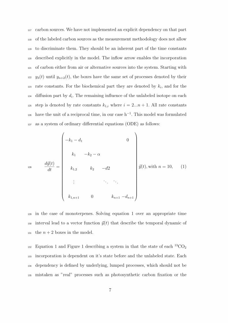
as a system of ordinary differential equations (ODE) as follows:127

d~y(t)

dt=

−k1 − d1 0

k1 −k2 − α

k1,2 k2 −d2

.... . . . . .

k1,n+1 0 kn+1 −dn+1

~y(t),with n = 10, (1)128

in the case of monoterpenes. Solving equation 1 over an appropriate time129

interval lead to a vector function ~y(t) that describe the temporal dynamic of130

the n+ 2 boxes in the model.131

Equation 1 and Figure 1 describing a system in that the state of each 13CO2132

incorporation is dependent on it’s state before and the unlabeled state. Each133

dependency is defined by underlying, lumped processes, which should not be134

mistaken as ”real” processes such as photosynthetic carbon fixation or the135

7

plastidic MEP-pathway, which indeed are not pure sequential steps. Each136

state in the system is expressed as labeled or unlabeled emitted monoterpene137

molecule.138

All rate constants ρi are convertible into time constants τi and vice versa139

by the relation τi = ln(2)/ρi where ρ is a placeholder for k, d or α. A total140

pool turnover, in terms of the model as described above, is completed if the141

maximum of emitted monoterpene molecules is fully labeled, i.e. all carbon in142

the leaf is labeled except for the ”old” carbon coming from alternative sources143

within the plant. With that, we can calculate the total monoterpene pool144

turnover in the leaf according to the reciprocal sum of the time constants:145

1

τtotal=

m∑i=1

1

τi, (2)146

where m denote the number of boxes to be combined in the model.147

2.2 Plant Material and experimental design148

Two-year-old Mediterranean evergreen oak Q. ilex plants, grown from acorns149

in pots under natural light conditions within a greenhouse were used for the150

labeling experiment. The plants were grown on a sand/peat (1:1) soil mix-151

ture. They were irrigated daily and fertilized monthly according to standard152

procedures (Grote et al., 2006). The measurements were conducted in early153

spring, after transferring plants from outside into controlled climate chamber154

conditions (30◦C) and higher light intensity (1000 µmol quanta m−2 s−1). The155

analyses were performed on fully expanded mature leaves that had developed156

under the climate chamber conditions. A total of five plants out of twelve have157

been chosen for the labeling experiment.158

8

Unlabeled 12CO2 was added for the gas exchange analysis to purified artifi-159

cial air to reach an ambient CO2 concentration of 370 ppmv. The 13C isotope160

containing air has been readily mixed with a level of 370 ppm 13CO2 (Air161

Liquide, Griesheim, Germany). Change between labeled and unlabeled arti-162

ficial air was conducted by manually switching between both sources. The163

flow in the whole system was controlled by flow controllers and set to 800 ml164

min−1. As a cuvette system, the GFS-3000 portable IRGA system (Heinz Walz165

GmbH, Effeltrich, Germany) was used to control and monitor the plant gas166

exchange. The cuvette flow was set accordingly to the total flow. An aliquot167

(70 ml min−1) of cuvette outlet air was transferred to the PTR-MS (Ionicon168

Analytik, Innsbruck, Austria) for monoterpene emission analysis. The param-169

eters for the PTR-MS measurements have been throughout the experiments170

chosen as E/N = 110 Td, pdrift = 1.7375 mbar, V = 550, T = 43◦C and O2+171

and NO+ < 2% of H3O+.172

2.3 Determination of leaf gas exchange and monoterpene emissions173

Isotopic labeling is changing the infrared absorption bands of CO2 and due to174

that, a proper detection of CO2 is not possible during the labeling phase. We175

recorded the net CO2 assimilation rates before and after switching the inlet176

air to the labeled source. As the detection of water vapor is not affected by177

the change in the carbon source, we tracked the evaporation throughout the178

experiment. Together with the relative photosynthesis rate, these data help to179

assess the plants physiological state while labeling (Figure 4).180

Pilot experiments showed, that maximum monoterpene emissions from Q. ilex181

leaves were reached at 35◦C, so this temperature was chosen for the labeling182

9

experiments. Photosynthetic photon flux density (PPFD) was set to 1000 µmol183

quanta m−2 s−1 throughout the whole experiment and the time of labeling was184

chosen to be 12 hours, starting 1 hour after onset of light and stabilization185

of net CO2 assimilation and monoterpene emission. At the end of the 13C-186

labeling period gas exchange and monoterpene emission were recorded for an187

additional hour under 12CO2 atmosphere. The mean monoterpene flux and188

standard error prior to the labeling was 4.3 ± 0.7 nmol m−2 s−1 under the189

chosen settings.190

Online monoterpene measuring was conducted by the PTR-MS (Behnke et al.,191

2007), tracking the whole range of 13C labeled mass isomers, that are possible192

to appear in a C10 skeleton of a monoterpene with a molecular mass at 136193

u. The proton transfer reaction, that takes place in the PTR-MS, leads to a194

molecule mass of m + 1, the tracked range was chosen to span over m/z 137195

to 147. As bigger molecules tend to fragment in the PTR-MS, we also tracked196

the masses starting at m/z 81 through to m/z 87 representing the fragments197

of labeled monoterpenes to control the labeling process. Even though the198

fragments provide a better signal, they are useless to assess the total labeling of199

the monoterpene molecule as they consist of only 6 C-atoms. As a robust, mass200

independent calibration of the system we diluted a 11 (including α-pinene)201

VOC mixture-standard in N2 (1 ppmv, Apel-Riemer Environmental, Denver,202

USA) into humidified cuvette air. Prior to each analysis the empty cuvette203

emissions were background corrected. The monoterpene emission rates were204

expressed as nmol m−2 s−1 based on the α-pinene signal from the standard205

gas.206

10

2.4 Model validation procedure207

To solve the model numerically we implemented the ODE system into the208

Mathematica software environment (Mathematica Version 5.1, Wolfram Re-209

search, Inc.,IL, USA) where also the fitting procedure to the measured PTR-210

MS data was conducted. As we were interested to describe the temporal dy-211

namics of the isotope emission pattern, we normalized and pooled the data212

from 3 out of 5 independent experiments into one data set. Normalization was213

conducted according to the 12C-emissions such that the average of the steady214

state monoterpene emission before the labeling was set to one for each mea-215

sured set of data. In addition, all data sets give the standard error of the 3216

minutes running average over the measurement time period. We selected one217

point each 6 minutes throughout the data set as validation points to simply218

reduce the amount of data for the fitting procedure.219

Fitting the model to data was done by means of minimizing the root mean220

squared distance (RMSD) between the modeled and measured data points:221

RMSD =ν∑j=1

√(fj,µ − fj,δ)2

ν, (3)222

where ν denote the size of the data set, fj,µ is the model result at point j223

and fj,δ is the value of the data set at that point. We calculated this fitting224

procedure for each mass isomer of the system as follows:225

min[RMSDi],with i = 1..12 (4)226

to obtain optimal values for the time constants, ki, k1,i and di.227

11

3 Results and Discussions228

3.1 Model validation229

To validate the model, we used the emission data obtained by PTR-MS mea-230

surements that track the release of 12C- and 13C-labeled monoterpene mass231

isomers online. As can be seen from Figure 2, monoterpene emissions decreased232

slightly over the course of the day, probably due to the long time where the233

leaves were kept under constant light and temperature within the cuvette.234

Analysis of net CO2 assimilation prior and after 13CO2 labeling showed a de-235

cline of photosynthesis by approximately 29% (Figure 4). It is known from236

the Mediterranean sclerophyllous oak Quercus suber L. e.g. that it declines237

photosynthesis in the afternoon even if there is no water stress due to in-238

creased light, temperature or leaf-to-air vapor pressure deficit (Faria et al.,239

1996; Chaves et al., 2002). To overcome this situation, we could handle the240

data as been overlaid by a systematic error and de-trend the data set or we241

could add an empirical term that mimics the decay. As it remains unsure, if242

the decay is only due to a systematic error which has been introduced by our243

experimental setup or a physiological response, we decided to use the data as244

they were measured and introduced an empirical function245

F (t) = σt, (5)246

where, σ equals to 0.02 h−1 and denotes an empirical factor that lowers the247

photosynthetic capacity by time. We linked that empirical function to the248

first equation in the differential equation system (Equation 1) as an additional249

12

outflow of the 12C carbon box and the first equation alters to250

y1(t)

dt= (−k1 − d1)y1(t) − F (t). (6)251

With that empirical extension, the model follows the decay within the mea-252

sured data as shown in Figure 2.253

3.2 Estimation of the time constants254

As the PTR-MS data have a high resolution in time but a low selectivity255

between molecules of the same molecular mass, it is not possible to distinct256

between several monoterpene species. Therefore, we considered an ”average257

monoterpene” in our calculation to obtain first guess values for the timescales258

of the leaf pool turnover. By applying the same light and temperature input we259

used during the measurements to the biochemical part of the SIM-BIM (ver-260

sion 2) model, we obtained estimates for the turnover of the MEP-pathway261

(Appendix A). In the case of monoterpenes, the half-life for the formation262

obtained was τMT = 16 minutes. Combining this result with the time scales263

for the turnover of the photosynthesis process, the half-life of carbon in the264

described Q. ilex system against biochemical processing to form a monoter-265

pene should be around 20 minutes. Indeed, the time constant found by fitting266

to data for the biochemical processing of the non-labeled isotope τbio,1 = 26267

minutes (0.43 hours). Table 1 summarizes the optimized time constants for268

the biochemical and diffusion processes. For the diffusion process, we found as269

maximum time scale τdif,11 = 3 hours and 9 minutes (3.15 hours). Compared270

with the values given in Niinemets and Reichstein (2002) for Q. ilex, the time271

constants in the present work matched the range of time constants reported272

13

there.273

The optimization procedure for the reaction rate α gave a value of 3.3 h−1.274

This parameter reflects the fact that the distribution of the recently fixed275

carbon to several metabolic pathways has to be considered in the model to276

maintain the homeostatic balance of the organism. In the present case with277

Q. ilex leaves we estimated a 1.5% carbon use by the MEP-pathway related278

to total carbon flow within the leaf system. This value is in the same range of279

an earlier observation of Kesselmeier et al. (2002) who determined that under280

non-stressed situations about 1.2% of the carbon gained by Q. ilex leaves can281

be emitted back as monoterpenes.282

3.3 Model performance283

Overall, the model fits very well to the measured data (Figure 2). We obtained284

r2 = 0.953 for the sum of labeled monoterpenes and r2 = 0.978 for the unla-285

beled monoterpene. The model slightly overestimated the measured values of286

the sum of 13C labeled monoterpene emissions, but well within the boundaries287

of the standard errors. The unlabeled monoterpene emission was in the first288

half of the time course slightly underestimated by the model and after 7 hours289

the model overestimated again slightly the measured values.290

Figure 3 shows the comparison of the model data and the measurements for291

each mass-to-charge ratio. As the monoterpene molecules consist of 10 carbon292

atoms, we should have the range from unlabeled to fully labeled, m/z 137293

until 147, to exchange all carbon atoms available in the molecule with a 13C294

isotopic carbon atom, because the measured data for m/z 147 (fully 13C-295

14

labeled) were often below the detection limit of the measurement system, we296

did not use them for model fitting. The model itself calculates m/z 147 and297

therefore, the molecule was included in the calculations of the pool turnover298

times. For m/z 138, the isotope molecule with one 13C atom, the model does299

not followed the steep initial slope in the measurement but after the first 2300

hours it agrees to the measurement with a slight overestimation. It is likely,301

that due to the simplification introduced by the model the temporal dynamics302

over the first hours show some uncertainty. On the other hand, we might have303

missed other processes in the model, that are important on that stage of the304

incorporation of 13C into the monoterpene molecule. Possible candidates for305

such processes have been recently proposed (Monson et al., 2007; Wilkinson306

et al., 2009), such as cellular regulation mechanisms of the MEP-pathway307

by phosphoenolpyruvate carboxylase (PEPC) as dependent on atmospheric308

carbon dioxide levels. All other isotope masses fitted well to the initial slopes309

of the inclusion dynamics and the higher the masses become, the better was310

the fit of the model to the measured data. The r2 values ranged between 0.969311

and 0.997 and by that, each fit to a single m/z ratio showed a higher accuracy312

as the value obtained for the sum of labeled monoterpene emission.313

3.4 Temporal dynamics of 13C isotope incorporation into the monoterpene314

molecules315

We investigated the temporal behavior of the labeling process as affected by316

the processes described before and the possibility to develop a model tool to317

estimate and study time scales and dynamics of these underlying processes on318

the leaf level. Table 1 compiles together the time constants for the biochemical319

15

τbio and the diffusion τdif processes. In both cases, we found an increase in the320

half-life times against these processes with rising masses. While the biochemi-321

cal time constants start at 26 and 30 minutes for τ1 and τ2, they reach up to 4322

hours and 38 minutes for τ11. Using Equation 2, they sum up to 21 hours and323

42 minutes for the total biochemical processes turnover half-life. The diffusion324

process was the time-limiting process only in the case of the unlabeled and325

the molecule with one 13C carbon atom included. For the higher masses, the326

diffusion process was found to be faster than the biochemical process. The327

diffusional time constants ranged from 32 minutes for d1 to 3 hours and 9328

minutes for d11. We summed up these time constants and reached 16 hours329

and 30 minutes for the half-life of the total diffusional process turnover.330

It is not surprising, that the time constants changed as the mass of the331

monoterpene molecule rises, because it is well known that due to the change in332

molecular mass, both, the chemical and the physical properties are changing.333

Especially for research on enzymatic pathways the ”kinetic isotope effect” was334

used to get insight into the enzymatic networks (Cleland, 2003). Furthermore,335

the stable isotope analysis is based on the fact that biochemical and physical336

processes are discriminating between stable isotopes. Due to that fact, one can337

use accumulation or depletion information on stable isotopes within probes to338

discriminate the processes which lead to the formation of that probe (Farquhar339

et al., 1989; Ehleringer et al., 2000; Ekblad and Hogberg, 2001; Eglin et al.,340

2009). It has been already described by Ekblad and Hogberg (2001), that341

the photosynthetic intermediates of leaves are depleted in 13C due to assim-342

ilation and respiration processes that prefer the more abundant 12C isotope.343

The MEP-pathway itself is also discriminating against 13C and the emitted344

isoprene was found to be further depleted in 13C than the assimilated car-345

16

bon (Sharkey et al., 1991; Affek and Yakir, 2003). Within the MEP pathway,346

deoxyxylulose-5-phosphate synthase (DXP) is likely to discriminate against347

13C and it has been also reported by Melzer and Schmidt (1987) that the348

pyruvate dehydrogenase (PYRDH) reaction is depleting 13C on the stage of349

the major precursors (pyruvate and acetyl-CoA) of the MEP-pathway. This350

was assumed to cause at least a portion of the observed depletion in the351

emitted BVOC compounds. However, the present model was not designed to352

address these changes in the isotopic composition but the rise in the time con-353

stants may reflect these changes in the compounds physico-chemical properties354

and possible regulatory steps preferring 12C which are not explicitly addressed355

here.356

In Table 1, we also show the values for the influence of the 12C carbon on the357

emitted labeled compound, k1,n. This numbers are descending from 0.95 h−1358

to 0.001 h−1, demonstrating that the influence of the unlabeled carbon, origi-359

nated from alternative sources (Kreuzwieser et al., 2002; Schnitzler et al., 2004)360

within the plant, only marginally effected the almost fully labeled monoter-361

penes but played a role in the determination of the timely behavior of the362

monoterpene emissions. Thus, the temporal dynamics were mostly determined363

by the biochemical and diffusional processes but the alternative carbon sources364

and the distribution of the labeled and unlabeled molecules within the leaf lead365

to a kind of additional memory effect of the system.366

3.5 The model as a predictive tool367

The present model can be used to predict the labeling and emission patterns368

and changes in those patterns for molecules of arbitrary length. Due to the369

17

abstraction, the time constants can be issued to more or less lumped processes370

of same kind, such as biochemical processing or diffusion through tissues. This371

allows insight into the temporal pattern of the underlying processes or let one372

gain information about the lumped processes dynamics as well. In that sense,373

the model can be seen as a tool to predict such temporal dynamic behavior of374

biochemical or diffusional processes. The inclusion of process-based method-375

ology into larger scale models has recently been proposed (e.g. Arneth et al.,376

2007). However, moving from smaller to larger scales is usually connected to a377

loss of information due to fact that the measured signal therein is further pro-378

cessed as the measured signal on the smaller scale. To circumvent that scaling379

problem, one can either try to put in more details but, this is usually limited380

by the available information, or, build an abstraction layer where the smaller381

scale dynamics are mapped into the larger scale. Our present model is build382

in the latter sense. We used data from the whole leaf level and described the383

dynamics of processes that take place on a smaller organizational scale within384

the leaf itself.385

In the case of the inclusion of 13C into the monoterpene pools of Q. ilex, the386

model predicted time scales for all isotopic combinations that can be found387

within the monoterpene molecule that is emitted and, as well gives estimates388

of the half-live for the total pool turnover times. In case of Q. ilex leaves these389

times were rather long summing up in the ”worst case” to almost 38 hours390

and in the ”best case” to just one hour. Such long term dynamic changes can391

indeed influence the set up of recent larger scale models as many of them run392

based on daily time steps (Cramer et al., 2001; Guenther et al., 2006; Sitch393

et al., 2003). So far, the emission processes have been considered to be fast394

enough to be already in steady state and the daily step is large compared to395

18

their dynamic, but for Q. ilex, with no specific terpene storage structure, this396

seems not always to be the case. As a consequence, the use of an empirical,397

steady state algorithm (e.g. Guenther et al., 1993) seems not always to fit best398

to describe emissions with daily time steps.399

Another implication of the present study relates to the question posed by Ar-400

neth et al. (2008). They showed that the variation in the results of several401

monoterpene emission models are almost freely diverging while that is not the402

case for isoprene emission models. Maybe the fact, that monoterpene emis-403

sions are possibly still in a transient state, even on daily time scale, while404

the isoprene emissions are not is partly explaining the difference. Isoprene405

formation should have a shorter time scale in the biochemical processing as406

it has a ”shorter” formation pathway, and it has lower diffusional constraints407

compared to the longer and structural more complex monoterpene molecule.408

Because of that, it is likely that the isoprene emissions temporal dynamics409

have already reached a steady state within the often used daily time step of410

larger scale models. Thus, the selection of an empirical steady state parame-411

terization algorithm for isoprene is less critical but this is not always the case412

for monoterpenes.413

4 Conclusions414

We observed the possibility that the turnover of the monoterpene pool in Q.415

ilex leaves can exceed one day. Due to that finding, the use of empirical steady416

state algorithms in connection with daily monoterpene emission estimates417

which employ still a transient emission pattern in that time scale might be418

the wrong choice. Indeed, the present model exercise supports the need of an419

19

inclusion of process-based methods into larger scale models as a beneficial step420

in increasing their prediction accuracy.421

The present work demonstrates, that the use of a model that is located on a422

higher integrated level of organization (”volume with a leaf”) can very well423

predict the temporal behavior of processes that are located on a lower inte-424

grated level (”biochemical processes or diffusion within the leaf tissues”). The425

prerequisite for such an application is the ability to describe the time constants426

of those processes in a single or lumped manner. Our modeling exercise can,427

as well, be seen as a step towards a possible solution to tackle with the prob-428

lem of the upscaling procedure by solving an inverse problem on the higher429

integrated level with information input from the lower integrated level.430

Acknowledgements431

Financial support from the Human Frontier Science Program (http://www.hfsp.org),432

the Estonian Academy of Sciences, the Estonian Science Foundation (Grants433

7645, 8110), the Estonian Ministry of Education and Science (Grant SF1090065s07)434

is gratefully acknowledged. We would like to thank Dr. Almut Arneth and An-435

drea Ghirardo for their cooperation and fruitful discussions.436

References437

Aalto, T., Juurola, E., 2002. A three-dimensional model of CO2 transport in438

airspaces and mesophyll cells of a silver birch leaf. Plant, Cell and Environ-439

ment 25, 1399–1409.440

Aalto, T., Vesala, T., Mattila, T., Simbierowicz, P., Hari, P., 1999. A Three-441

20

dimensional Stomatal CO2 Exchange Model Including Gaseous Phase and442

Leaf Mesophyll Separated by Irregular Interface. J. theor. Biol. 196, 115–443

128.444

Affek, H. P., Yakir, D., 2003. Natural Abundance Carbon Isotope Composition445

of Isoprene Reflects Incomplete Coupling between Isoprene Synthesis and446

Photosynthetic Carbon Flow. Plant Physiol. 131 (4), 1727–1736.447

Arneth, A., Monson, R. K., Schurges, G., Niinemets, U., Palmer, P. I., 2008.448

Why are estimates of global terrestrial isoprene emissions so similar (and449

why is this not so for monoterpenes)? Atmospheric Chemistry and Physics450

8, 4605–4620.451

Arneth, A., Niinemets, U., Pressley, S., Back, J., Hari, P., Karl, T., Noe, S.,452

Prentice, I. C., Serca, D., Hickler, T., Wolf, A., Smith, B., 2007. Process-453

based estimates of terrestrial ecosystem isoprene emissions: incorporating454

the effects of a direct CO2-isoprene interaction. Atmospheric Chemistry and455

Physics 7, 31–53.456

Brilli, F., Barta, C., Fortunati, A., Lerdau, M., Centritto, M., 2007. The re-457

sponse of isoprene emission and carbon metabolism to drought in white458

poplar (Populus alba) saplings. New Phytologist 175 (2), 244–254.459

Chaves, M. M., Pereira, J. S., Maroco, J., Rodrigues, M. L., Ricardo, C. P. P.,460

Ososrio, M. L., Carvalho, I., Faria, T., Pinheiro, C., 2002. How Plants Cope461

with Water Stress in the Field? Photosynthesis and Growth. Ann Bot 89 (7),462

907–916.463

Cleland, W. W., 2003. The Use of Isotope Effects to Determine Enzyme Mech-464

anisms. J. Biol. Chem. 278 (52), 51975–51984.465

Cramer, W., Bondeau, A., Woodward, F. I., Prentice, I. C., Betts, R. A.,466

Brovkin, V., Cox, P. M., Fisher, V., Foley, J. A., Friend, A. D., Kucharik,467

C., Lomas, M. R., Ramankutty, N., Sitch, S., Smith, B., White, A., Young-468

21

Molling, C., Apr 2001. Global response of terrestrial ecosystem structure469

and function to CO2 and climate change: results from six dynamic global470

vegetation models. Global Change Biology 7 (4), 357–373.471

Delwiche, C., Sharkey, T., 1993. Rapid appereance of 13C in biogenic isoprene472

when 13CO2 is fed to intact leaves. Plant, Cell and Environment 16, 587–591.473

Eglin, T., Fresneau, C., Lelarge-Trouverie, C., Francois, C., Damesin, C., 2009.474

Leaf and twig δ13C during growth in relation to biochemical composition475

and respired CO2. Tree Physiol 29 (6), 777–788.476

Ehleringer, J. R., Buchmann, N., Flanagan, L. B., 2000. Carbon isotope ratios477

in belowground carbon cycle processes. Ecological Applications 10 (2), 412–478

422.479

Ekblad, A., Hogberg, P., 2001. Natural abundance of 13C in CO2 respired480

from forest soils reveals speed of link between tree photosynthesis and root481

respiration. Oecologia 127 (3), 305–308.482

Faria, T., Garcia-Plazaola, J. I., Abadia, A., Cerasoli, S., Pereira, J. S., Chaves,483

M. M., 1996. Diurnal changes in photoprotective mechanisms in leaves of484

cork oak (Quercus suber) during summer. Tree Physiology 16, 115–123.485

Farquhar, G. D., Ehleringer, J. R., Hubick, K. T., 1989. Carbon isotope dis-486

crimination and photosynthesis. Annual Review of Plant Physiology and487

Plant Molecular Biology 40 (1), 503–537.488

Fridlyand, L. E., Backhausen, J. E., Scheibe, R., 1999. Homeostatic regulation489

upon changes of enzyme activities in the calvin cycle as an example for490

general mechanisms of flux control. what can we expect from transgenic491

plants? Photosynthesis Research 61, 227–239.492

Fridlyand, L. E., Scheibe, R., 1999. Regulation of the Calvin cycle for CO2493

fixation as an example for general control mechanisms in metabolic cycles.494

BioSystems 51, 79–93.495

22

Giersch, C., Lammel, D., Farquhar, G. D., 1990. Control analysis of photo-496

synthetic CO2 fixation. Photosynthesis Research 42, 75–86.497

Grote, R., Mayrhofer, S., Fischbach, R., Steinbrecher, R., Staudt, M., Schnit-498

zler, J.-P., 2006. Process-based modelling of isoprenoid emissions from ever-499

green leaves of Quercus ilex (L.). Atmospheric Environment 40, S152–S165.500

Guenther, A., Karl, T., Harley, P., Wiedinmyer, C., Palmer, P. I., Geron, C.,501

2006. Estimates of global terrestrial isoprene emissions using megan (model502

of emissions of gases and aerosols from nature). Atmospheric Chemistry and503

Physics 6, 3181–3210.504

Guenther, A., Zimmermann, P., Harley, P., Monson, R. K., Fall, R., 1993.505

Isoprene and monoterpene emission rate variability: model evaluation and506

sensitivity analysis. J. Geophys. Res. 98, 12609–12617.507

Hayward, S., Hewitt, N., 2003. On-line analysis of VOC emissions from Sitka508

spruce (Picea sitchensis). In: Hansel, A., Mark, T. (Eds.), Proceedings of509

the 1st International Conference on Proton Transfer Reaction Mass Spec-510

trometry and Its Applications. Vol. 1. Institut fur Ionephysik, Universitat511

Innsbruck, Technikerstrasse 25,6020 Innsbruck, Austria, pp. 33–36.512

Karl, T., Curtis, T. N., Rosenstiel, R. K., Monson, R. K., Fall, R., 2002.513

Transient releases of acetaldehyde from tree leaves - products of a pyruvate514

overflow mechanism? Plant, Cell and Environment 25, 1121–1131.515

Kesselmeier, J., Ciccioli, P., Kuhn, U., Stefani, P., Biesenthal, T., Rotten-516

berger, S., Wolf, A., Vitullo, M., Valentini, R., Nobre, A., Kabat, P., An-517

dreae, M. O., 2002. Volatile organic compound emissions in relation to plant518

carbon fixation and the terrestrial carbon budget. Global Biochemical Cy-519

cles 16 (4), pp 73–1.520

Kesselmeier, J., Staudt, M., 1999. Biogenic volatile organic compounds (voc):521

an overview on emission, physiology and ecology. Journal of Atmospheric522

23

Chemistry 33 (1), 23–88.523

Kreuzwieser, J., Graus, M., Wisthaler, A., Hansel, A., Rennenberg, H., Schnit-524

zler, J.-P., 2002. Xylem-transported glucose as an additional carbon source525

for leaf isoprene formation in Quercus robur. New Phytologist 156 (2), 171–526

178.527

Kulmala, M., Suni, T., Lehtinen, K. E. J., Dal-Maso, M., Boy, M., Reissell,528

A., Rannik, U., Aalto, P., Keronen, P., Hakola, H., Back, J., Hoffmann,529

T., Vesala, T., Hari, P., 2004. A new feedback mechanism linking forests,530

aerosols, and climate. Atmospheric Chemistry and Physics 4, 557–562.531

Lichtenthaler, H. K., 1999. The 1-deoxy-d-xylulose-5-phosphate pathway of532

isoprenoid biosynthesis in plants. Annual Review of Plant Physiology 50,533

47–65.534

Loreto, F., Barta, C., Brilli, F., Nogues, I., 2006. On the induction of volatile535

organic compound emissions by plants as consequence of wounding or fluc-536

tuations of light and temperature. Plant, Cell and Environment 29, 1820–537

1828.538

Loreto, F., Ciccioli, P., Brancaleoni, E., Frattoni, M., Delfine, S., 2000. Incom-539

plete 13C labelling of α-pinene content of Quercu ilex leaves and appearance540

of unlabelled C in α-pinene emissions in the dark. Plant, Cell and Environ-541

ment 23, 229–234.542

Melzer, E., Schmidt, H., 1987. Carbon isotope effects on the pyruvate dehy-543

drogenase reaction and their importance for relative carbon-13 depletion in544

lipids. J. Biol. Chem. 262 (17), 8159–8164.545

Monson, R. K., Trahan, N., Rosenstiel, T. N., Veres, P., Moore, D., Wilkin-546

son, M., Norby, R. J., Volder, A., Tjoelker, M. G., Briske, D. D., Karnosky,547

D. F., Fall, R., 2007. Isoprene emission from terrestrial ecosystems in re-548

sponse to global change: minding the gap between models and observations.549

24

Philosophical Transactions of the Royal Society A: Mathematical, Physical550

and Engineering Sciences 365 (1856), 1677–1695.551

Morgan, J. A., Rhodes, D., 2002. Mathematical modeling of plant metabolic552

networks. Metabolic Engineering 4, 80–89.553

Niinemets, U., Cescatti, A., Rodeghiero, M., Toosens, T., 2005. Leaf internal554

diffusion conductance limits photosynthesis more strongly in older leaves of555

mediterranean evergreen broad-leaved species. Plant, Cell and Environment556

28, 1552–1566.557

Niinemets, U., Reichstein, M., 2002. A model analysis of the effects of nonspe-558

cific monoterpenoid storage in leaf tissues on emission kinetics and compo-559

sition in Mediterranean sclerophyllous Quercus species. Global Biochemical560

Cycles 16 (4), 57/1–57/26.561

Niinemets, U., Seufert, G., Steinbrecher, R., Tenhunen, J. D., 2002. A model562

coupling foliar monoterpene emissions to leaf photosynthetic characteristics563

in Mediterranean evergreen Quercus species. New Phytologist 153 (2), 257–564

275.565

Noe, S. M., Ciccioli, P., Brancaleoni, E., Loreto, F., Niinemets, U., 2006.566

Emissions of monoterpenes linalool and ocimene respond differently to en-567

vironmental changes due to differences in physico-chemical characteristics.568

Atmospheric Environment 40 (25), 4649–4662.569

Noe, S. M., Copolovici, L., Niinemets, U., Vaino, E., 2008. Foliar limonene up-570

take scales positively with leaf lipid content: ”non-emitting” species absorb571

and release monoterpenes. Plant Biol (Stuttg) 10 (1), 129–137.572

Noe, S. M., Giersch, C., 2004. A simple dynamic model of photosynthesis in573

oak leaves: coupling leaf conductance and photosynthetic carbon fixation574

by a variable CO2 pool. Functional Plant Biology 31, 1195–1204.575

Parkhurst, D. F., 1994. Tansley Review No. 65 - Diffusion of CO2 and other576

25

gases inside leaves. New Phytologist 126, 449–479.577

Rios-Estepa, R., Lange, B. M., 2007. Experimental and mathematical ap-578

proaches to modeling plant metabolic networks. Phytochemistry 68, 2351–579

2374.580

Rohmer, M., 2003. Mevalonate-independend methylerythritol phosphate path-581

way for isoprenoid biosynthesis. Pure and Applied Chemistry 75 (2-3), 375–582

387.583

Schnitzler, J.-P., Graus, M., Kreuzwieser, J., Heizmann, U., Rennenberg, H.,584

Wisthaler, A., Hansel, A., 2004. Contribution of different carbon sources to585

isoprene biosynthesis in poplar leaves. Plant Physiology 135, 152–160.586

Sharkey, T. D., Loreto, F., Delwiche, C. F., Treichel, I. W., 1991. Fractiona-587

tion of Carbon Isotopes during Biogenesis of Atmospheric Isoprene . Plant588

Physiol. 97 (1), 463–466.589

Sitch, S., Smith, B., Prentice, I. C., Arneth, A., Bondeau, A., Cramer, W.,590

Kaplan, J. O., Levis, S., Lucht, W., Sykes, M. T., Thonicke, K., Venevsky,591

S., 2003. Evaluation of ecosystem dynamics, plant geography and terrestrial592

carbon cycling in the LPJ dynamic global vegetation model. Global Change593

Biology 9 (2), 161–185.594

Tholl, D., Boland, W., Hansel, A., Loreto, F., Rose, U. S. R., Schnitzler, J.-P.,595

2006. Practical approaches to plant volatile analysis. The Plant Journal 45,596

540–560.597

Tsirgaridis, K., Lathiere, J., Kanakidou, M., Hauglustaine, D. A., 2005. Natu-598

rally driven variability in the global secondary organic aerosol over a decade.599

Atmospheric Chemistry and Physics 5, 1891–1904.600

Vesala, T., Ahonen, T., Hari, P., Krissinel, E., Shokhirev, N., 1996. Analysis of601

stomatal CO2 uptake by a three-dimensional cylindrically symmetric model.602

New Phytologist 132, 235–245.603

26

Wilkinson, M., Monson, R. K., Trahan, N., Lee, S., Brown, E., Jackson, R.,604

Polley, H., Fay, P., Fall, R., 2009. Leaf isoprene emission rate as a function of605

atmospheric CO2 concentration. Global Change Biology 15 (5), 1189–1200.606

Wolfertz, M., Sharkey, T. D., Boland, W., Kuhnemann, F., 2004. Rapid regula-607

tion of the methylerythritol 4-phosphate pathway during isoprene synthesis.608

Plant Physiology 135, 1939–1945.609

Zimmer, W., Bruggemann, N., Emeis, S., Giersch, C., Lehning, A., Stein-610

brecher, R., Schnitzler, J.-P., 2000. Process-based modelling of isoprene611

emission by oak leaves. Plant, Cell and Environment 23, 585–595.612

27

Tables613

Table 1

m/z

constant 137 138 139 140 141 142 143 144 145 146 147 sum

τbioa 0.43 0.50 0.89 0.98 1.26 1.98 2.10 2.31 2.77 3.85 4.63 21.7

τdifa 0.53 0.55 0.63 0.79 1.02 1.73 1.87 1.93 1.98 2.31 3.15 16.5

k1,nb - 0.95 0.8 0.45 0.25 0.08 0.02 0.008 0.005 0.003 0.001 2.567

n 1 2 3 4 5 6 7 8 9 10 11

a unit in hours

b unit in h−1

28

Figures614

12C

13C1

13Cn

k1

k1,2

d1

d2

y1(t)12

y3(t)

yn+2(t)dn+1k1,n+1

k3

kn+1

k2

y2(t)13

13C

!

Fig. 1.

29

0 2 4 6 8 10 120

0.2

0.4

0.6

0.8

1

1.2

1.4

Time in hours

norm

aliz

ed m

onot

erpe

ne e

mis

sion

Fig. 2.

30

0

0.5

1

0

0.5

0

0.25

norm

aliz

ed m

onot

erpe

ne e

mis

sion

s

0

0.25

0 2 4 6 8 10 120

0.15

Time in hours2 4 6 8 10 12

m/z 137r2 = 0.978

m/z 139r2 = 0.979

m/z 140r2 = 0.987

m/z 142r2 = 0.989

m/z 141r2 = 0.983

m/z 143r2 = 0.993

m/z 144r2 = 0.995

m/z 145r2 = 0.995

m/z 146r2 = 0.997

m/z 138r2 = 0.969

Fig. 3.

31

0 2 4 6 8 10 120.8

1

1.2

1.4Ev

apor

atio

n m

mol

m−2

s−1

0 2 4 6 8 10 120.6

0.8

1

1.2

Time in hours

rel.

phot

osyn

thes

isA

B

Fig. 4.

32

Captions615

Table 1. Time constants used in the model for stable isotope 13C incorpora-616

tion into the emitted monoterpene molecules. τbio is calculated from the rate617

constant as τn = ln(2)/kn for different mass isomers (n). τdif denote the similar618

time constants for the diffusion in the system. k1,n is the rate constant of the619

influence from the unlabeled fractions on the monoterpene emission denoting620

”old” carbon inflow, for instance from sources in the leaf. n is the number of621

carbon atoms in the monoterpene molecule.622

Fig. 1. Scheme of the defined boxes and the flows between them. The rate con-623

stants ki, i = 1...n + 1 describe the dynamics of the incorporation of the 13C624

atoms by the biochemical pathways, k1,i, i = 2...n+ 1 the influence of the re-625

maining 12C isotopes and the di, i = 1...n+1 the diffusion of the monoterpenes626

through the leaf tissues. α denotes the fraction of labeled carbon skeletons that627

is distributed within the leaf biochemical pathways. n equals the number of628

carbon atoms in the monoterpene molecule.629

Fig. 2. Modeled (lines) and measured (dots) normalized values of the emission630

of the 12C monoterpene (dashed) and the sum of 13C labeled mass isomer631

monoterpene (solid) over the course of the experiment. The grey areas denote632

the upper and lower bounds of the standard errors of the measurements. The633

data of three independent experiments were normalized with respect to the634

12C isomer in the non-labeled leaves under steady-state photosynthesis and635

monoterpene emission.636

Fig. 3. Modeled (solid line) and measured (dots) normalized values for the637

12C (m/z 137) and the 13C (m/z 138 - 146) mass isomers of the monoterpene638

33

emission. Standard errors of the measurements are given as grey areas. r2639

values have been calculated according to equations 3 and 4.640

Fig. 4. Mean and standard error of the measured evaporation (A) and relative641

photosynthesis (B) during the labeling experiment. Within the 12 hours of642

labeling, where the leaf was kept in constant light and temperature, a decline643

in the photosynthetic capacity occurred.644

34

Appendix645

A Estimation of the MEP pathway time constants from steady-646

state simulations647

To estimate the time constants of the MEP pathway we used a typical ”dose-648

effect” simulation experiment. We implemented the biochemical part (BIM)649

of the SIM-BIM (version 2) model including the synthetic steps until geranyl-650

diphosphate (GDP) into a compartment model. This model consist of a total651

of 10 compartments representing the intermediates within the MEP pathway,652

including pools for isoprene and monoterpenes. Time constants have been653

taken either from Zimmer et al. (2000) and Grote et al. (2006) or by personal654

communication. Additionally, the system includes a photosynthesis module,655

providing triose phosphates as input to the MEP pathway. Assumed a steady656

state and non stressed situation, changes in the biochemical intermediate pools657

can be initiated by changes in the precursors (3-phosphoglyceric acid, PGA658

and glyceraldehyde-3-phosphate, GAP) while energy supply and temperature659

are held constant.660

Analyzing the recovery time of the steady-state in the products (isoprene and661

monoterpene pools) leaded to an average half-life for the isoprene pool of 5662

minutes which is in accordance to Delwiche and Sharkey (1993) showing that663

the half-life to label isoprene molecules was 4.78 minutes. Furthermore, they664

showed, that the time to label 80% of the isoprene pool took 18 minutes. In665

the case of the monoterpene pool, additional steps to reach to GDP and to666

form the monoterpene molecule, leaded to 15-20 minutes for the lifetime of667

carbon in the intermediate pools leading to monoterpenes.668

35