Individual-tree diameter growth model for rebollo oak (Quercus pyrenaica Willd.) coppices

This article was published in an Elsevier journal. The attached copyis furnished to the author for non-commercial research and

education use, including for instruction at the author’s institution,sharing with colleagues and providing to institution administration.

Other uses, including reproduction and distribution, or selling orlicensing copies, or posting to personal, institutional or third party

websites are prohibited.

In most cases authors are permitted to post their version of thearticle (e.g. in Word or Tex form) to their personal website orinstitutional repository. Authors requiring further information

regarding Elsevier’s archiving and manuscript policies areencouraged to visit:

http://www.elsevier.com/copyright

http://www.elsevier.com/copyright

Author's personal copy

Individual-tree diameter growth model for rebollo oak

(Quercus pyrenaica Willd.) coppices

Patricia Adame a,*, Jari Hynynen b, Isabel Canellas c, Miren del Rıo c

a Departamento de Investigacion y Experiencias Forestales de Valonsadero, Junta de Castilla y Leon, Aptdo 175, Soria 42080, Spainb Finnish Forest Research Institute, P.O. Box 18, FIN-010301 Vantaa, Finland

c Forest Research Centre (CIFOR-INIA), Ctra A Coruna km 7,5, Madrid 28040, Spain

Received 3 October 2006; received in revised form 11 September 2007; accepted 4 October 2007

Abstract

In this study, a distance-independent mixed model was developed for predicting the diameter growth of individual trees in Mediterranean oak

(Quercus pyrenaica Willd.) coppices located in northwest Spain. The data used to build the model came from 41 permanent plots belonging to the

Spanish National Forest Inventory with the dependent variable being 10-year diameter increment over bark for trees larger than 7.5 cm at breast

height. The basic field data required for predictions had been divided into four main groups: size of the tree, stand variables, competition indices

and biogeoclimatic variables. The most significant independent variables were the individual-tree diameter, the basal area of trees larger than the

subject tree, dominant height, site index and biogeoclimatic stratum. The model was defined as a mixed linear model with random plot effect,

achieving an efficiency of 44.38%. The accuracy of the model was tested against the modelling data and against independent data from the same

stands. Mixed model calibration of diameter increment was carried out with the independent data using a different sample of complementary

observations of the dependent variable. The calibrated model was an improvement on the trivial model, which assumes constancy in diameter

increment for a short projection period, especially the pattern of residuals with respect to predicted diameter and the independent variables.

# 2007 Elsevier B.V. All rights reserved.

Keywords: Individual-tree model; Mixed model; Diameter growth; Quercus pyrenaica

1. Introduction

The species Quercus pyrenaica Willd., commonly known as

rebollo oak or pyrenean oak, is widely distributed across the

Iberian Peninsula, but is mainly found in the mountain ranges of

the north-west (Fig. 1) (Costa et al., 1996). According to the

Second Spanish National Forest Inventory (DGCN, 1996), the

total surface area covered by this Mediterranean oak in Spain is

659,000 ha. Owing to its widespread distribution, great

variability exists among stands in terms of silvicultural and

ecological conditions. The traditional treatments applied in

these stands (usually coppice management) have been

progressively abandoned due to the decrease in use of firewood

and charcoal as an energy source and to rural emigration to the

cities. Furthermore, Q. pyrenaica stands have been frequently

affected by forest fires. As a result of these determining factors,

stands today are generally coppice and somewhat diverse,

ranging from diminished stands with low densities to open-

woodlands with large diameters, although well-stocked

coppices represent around 43% of stands (DGCN, 1996). To

avoid putting the existence of these coppices at risk in the long

term, it is necessary to establish a sustainable forest manage-

ment plan for each kind of stand. Moreover, the increasing

interest in using these stands for either direct production (such

as wine barrels) or indirect production (such as silvopastoral

uses, recreation, environmental preservation) justifies the

urgent need to guarantee a sustainable management of rebollo

oak stands (Canellas et al., 2004).

The availability of information on diameter increment and

growth patterns for individual trees is an important asset in

forest management which allows the selection of tree species

for logging or protection as well as the estimation of cutting

cycles and the prescription of silvicultural treatments. Diameter

increment measurements are also required to feed statistical

models of forest dynamics both for modelling and simulation

(Pereira da Silva et al., 2002). In this way, growth models can

www.elsevier.com/locate/foreco

Available online at www.sciencedirect.com

Forest Ecology and Management 255 (2008) 1011–1022

* Corresponding author.

E-mail address: [email protected] (P. Adame).

0378-1127/$ – see front matter # 2007 Elsevier B.V. All rights reserved.

doi:10.1016/j.foreco.2007.10.019


facilitate the search for solutions in the management of rebollo

oak stands, especially in the case of coppices where the growth

pattern often justifies investment in silvicultural treatments.

Individual-tree growth models enable a more detailed

description of the stand structure and its dynamics than stand-

level models (Vanclay, 1994a; Chojnacky, 1997; Mabvurira and

Miina, 2002). They also allow silvicultural treatments to be

simulated and permit comparison with alternative thinning

regimes (Mabvurira and Miina, 2002). These kinds of models

would seem suitable for rebollo oak coppices given their high

structural variability. Furthermore, this approach usually

performs better than stand models for short-term predictions

(Burkhart, 2003), being especially useful when the models are

going to be used with national forest inventories.

Many tree diameter growth models have been fitted on the

basis of national forest inventory data (Wykoff, 1990;

Monserud and Sterba, 1996; Lessard et al., 2001; Andreassen

and Tomter, 2003). This kind of data set permits the use of a

large amount of data although the sampling methodology was

not specifically designed to develop growth and yield models

and may lead to large errors when measuring radial increment

(Trasobares et al., 2004). Nevertheless, assuming that

measurement errors are random, the large sample should

compensate for this deficiency (Monserud and Sterba, 1996).

Modelling data sets for individual-tree growth have a

hierarchical stochastic structure. This type of structure occurs

when multiple measurements are taken from individual sampling

units, and measurements are combined across sampling units

(West et al., 1984; Fox et al., 2001), so there is a violation of the

OLS regression assumption of independent residuals and results

in biased estimates of the standard error of parameter estimation

(West et al., 1984; Schabenberger and Gregoire, 1995). The

modelling data are mutually correlated (trees within plots) and,

thus, cannot be regarded as an independent sample of the basic

tree population (West, 1981; West et al., 1984; Fox et al., 2001).

The evolution of the mixed modelling methodology provided

a statistical method capable of explicitly modelling hierarchical

stochastic structure (Biging, 1985; Lappi, 1986; Hokka et al.,

1997; Fox et al., 2001; Calama and Montero, 2005). Linear mixed

models are composed of a fixed functional part, common to the

complete population, and random components acting at each

sampling level. The explanatory variables in the fixed part were

either measured or estimated tree variables, stand variables and

site attributes, and they are selected based on statistical properties

and biological principles (Zhao et al., 2004). These explanatory

variables do not explain the total variation in tree growth, so the

mixed models allow the different sources of stochastic variability

to be identified (Calama and Montero, 2005).

Ojansuu (1993) states that the application of a stochastic

model such as this would be limited to new data, although this

limitation can be removed by regressing nested stochastic

parameters for external stand-level variables. Lappi (1991) and

Calama and Montero (2005) proposed a calibration based on

predicting the random components using best linear unbiased

predictors (BLUP). This last predictor is calculated using a

sample of complementary observations of the dependent

variable.

The objective of this study was to develop a diameter growth

model for Q. pyrenaica Willd. coppices growing in northwest

Spain, that allows the development and evaluation of growth

functions for later improvement of existing stand-based long-

term forest management planning packages. A mixed model-

ling approach was emphasised due to the hierarchical structure

of the data set, including both fixed and random components.

Different calibrations using 1, 2 or 3 trees per plot were

calculated to find out how many tree measurements were

necessary to achieve good diameter growth estimation.

2. Materials and methods

2.1. Data set

The data were obtained from 200 plots belonging to the

Spanish National Forest Inventory (SNFI) in the northwest area

Fig. 1. Distribution of Quercus pyrenaica Willd., biogeoclimatic strata and sample plots in studied area.

P. Adame et al. / Forest Ecology and Management 255 (2008) 1011–10221012


of Spain (Castilla y Leon region), which had been used and

complementary measured to study the autoecology and the

growth of rebollo oak in Castilla y Leon region. According to

Elena Rosello (1997), the region is covered by two ecoregions,

being the Q. pyrenaica stands mainly in Ecoregion 2,

characterized by a Mediterranean climate with low precipita-

tion and extreme temperatures. The author classified the

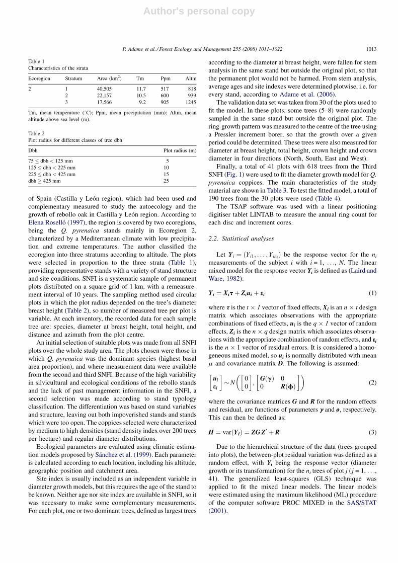
ecoregion into three stratums according to altitude. The plots

were selected in proportion to the three strata (Table 1),

providing representative stands with a variety of stand structure

and site conditions. SNFI is a systematic sample of permanent

plots distributed on a square grid of 1 km, with a remeasure-

ment interval of 10 years. The sampling method used circular

plots in which the plot radius depended on the tree’s diameter

breast height (Table 2), so number of measured tree per plot is

variable. At each inventory, the recorded data for each sample

tree are: species, diameter at breast height, total height, and

distance and azimuth from the plot centre.

An initial selection of suitable plots was made from all SNFI

plots over the whole study area. The plots chosen were those in

which Q. pyrenaica was the dominant species (highest basal

area proportion), and where measurement data were available

from the second and third SNFI. Because of the high variability

in silvicultural and ecological conditions of the rebollo stands

and the lack of past management information in the SNFI, a

second selection was made according to stand typology

classification. The differentiation was based on stand variables

and structure, leaving out both impoverished stands and stands

which were too open. The coppices selected were characterized

by medium to high densities (stand density index over 200 trees

per hectare) and regular diameter distributions.

Ecological parameters are evaluated using climatic estima-

tion models proposed by Sanchez et al. (1999). Each parameter

is calculated according to each location, including his altitude,

geographic position and catchment area.

Site index is usually included as an independent variable in

diameter growth models, but this requires the age of the stand to

be known. Neither age nor site index are available in SNFI, so it

was necessary to make some complementary measurements.

For each plot, one or two dominant trees, defined as largest trees

according to the diameter at breast height, were fallen for stem

analysis in the same stand but outside the original plot, so that

the permanent plot would not be harmed. From stem analysis,

average ages and site indexes were determined plotwise, i.e. for

every stand, according to Adame et al. (2006).

The validation data set was taken from 30 of the plots used to

fit the model. In these plots, some trees (5–8) were randomly

sampled in the same stand but outside the original plot. The

ring-growth pattern was measured to the centre of the tree using

a Pressler increment borer, so that the growth over a given

period could be determined. These trees were also measured for

diameter at breast height, total height, crown height and crown

diameter in four directions (North, South, East and West).

Finally, a total of 41 plots with 618 trees from the Third

SNFI (Fig. 1) were used to fit the diameter growth model for Q.

pyrenaica coppices. The main characteristics of the study

material are shown in Table 3. To test the fitted model, a total of

190 trees from the 30 plots were used (Table 4).

The TSAP software was used with a linear positioning

digitiser tablet LINTAB to measure the annual ring count for

each disc and increment cores.

2.2. Statistical analyses

Let Yi ¼ ðYi1; . . . ; YiniÞ be the response vector for the ni

measurements of the subject i with i = 1, . . ., N. The linear

mixed model for the response vector Yi is defined as (Laird and

Ware, 1982):

Yi ¼ Xitþ Ziui þ ei (1)

where t is the t � 1 vector of fixed effects, Xi is an n � t design

matrix which associates observations with the appropriate

combinations of fixed effects, ui is the q � 1 vector of random

effects, Zi is the n � q design matrix which associates observa-

tions with the appropriate combination of random effects, and ei

is the n � 1 vector of residual errors. It is considered a homo-

geneous mixed model, so ui is normally distributed with mean

m and covariance matrix D. The following is assumed:

ui

ei

� ��N

0

0

� �;

GðgÞ 0

0 RðfÞ

� �� (2)

where the covariance matrices G and R for the random effects

and residual, are functions of parameters g and ø, respectively.

This can then be defined as:

H ¼ varðYiÞ ¼ ZG Z0 þ R (3)

Due to the hierarchical structure of the data (trees grouped

into plots), the between-plot residual variation was defined as a

random effect, with Yi being the response vector (diameter

growth or its transformation) for the ni trees of plot j (j = 1, . . .,41). The generalized least-squares (GLS) technique was

applied to fit the mixed linear models. The linear models

were estimated using the maximum likelihood (ML) procedure

of the computer software PROC MIXED in the SAS/STAT

(2001).

Table 1

Characteristics of the strata

Ecoregion Stratum Area (km2) Tm Ppm Altm

2 1 40,505 11.7 517 818

2 22,157 10.5 600 939

3 17,566 9.2 905 1245

Tm, mean temperature (8C); Ppm, mean precipitation (mm); Altm, mean

altitude above sea level (m).

Table 2

Plot radius for different classes of tree dbh

Dbh Plot radius (m)

75 � dbh < 125 mm 5

125 � dbh < 225 mm 10

225 � dbh < 425 mm 15

dbh � 425 mm 25

P. Adame et al. / Forest Ecology and Management 255 (2008) 1011–1022 1013


Different combinations of independent variables were tested

to ascertain their importance with respect to diameter growth.

The following aspects were considered for this purpose

(Andreassen and Tomter, 2003): (i) desired variables (tree

size, competition, site index and stand descriptions); (ii)

logically interpretable sign for the estimates of these variables;

and (iii) available variables in a common inventory. On the

purely statistical side, the level of significance for the

parameters, reduction in the values of the components of the

variance–covariance matrices and the Likehood Ratio Test

(LRT) were used (Calama and Montero, 2005).

Different forms of diameter growth were considered for the

dependent variable: diameter increment (D2 � D1), 10-year

diameter growth rate (D_rate = (DD/D1)), square diameter

increment ðD22 � D2

1Þ, and the natural logarithm of each. The

tested explanatory variables can be divided into three main

groups:

1. Single-tree size variables: diameter at breast height, D1 (cm);

and total height, HT (m). Natural logarithmic and inverse

transformations of these variables were also tested.

2. Stand variables: number of stems, N (stems/ha); dominant

height, H0 (m); quadratic mean diameter, DG (cm); mean

diameter, DM (cm); basal area, BA (m2/ha); and site index, SI

(m) according to Adame et al. (2006). Natural logarithmic and

inverse transformations of these variables were also tested.

Table 3

Mean and standard deviation (S.D.) of the main characteristics in the study material

Stratum 1 2 3

Plots 9 10 22

Trees 164 122 332

Diameter at breast height (D1) (cm)

Mean (min–max) 18.4 (7.5–98.6) 27.6 (7.5–80.5) 24.7 (7.5–99.3)

Median 15.3 23.7 19.0

S.D. 11.2 15.0 16.2

Total height (HT) (m)

Mean (min–max) 10.6 (4.5–17.0) 9.2 (3.5–15.5) 11.2 (3.0–21.5)

Median 10.8 9.0 11.0

S.D. 2.7 2.4 3.3

Diameter increment for 10 years (D2 – D1) (cm)

Mean (min–max) 1.53 (0.05–7.8) 2.3 (0.2–7.1) 2.59 (0.1–10.5)

Median 1.37 2.12 2.4

S.D. 0.99 1.21 1.52

Stand age (years)

Mean (min–max) 71.9 (30.8–91.0) 70.1 (29.2–139.0) 68.3 (30.9–106.0)

Median 67.3 72.0 69.6

S.D. 12.9 26.6 15.6

Number of stems (N) (stems/ha)

Mean (min–max) 1087.4 (359.1–1655.2) 424.6 (100.2–795.8) 896.3 (24.3–2164.5)

Median 1114.1 473.9 604.8

S.D. 476.4 212.0 667.3

Dominant height (H0) (m)

Mean (min–max) 11.6 (5.5–15.8) 9.5 (6.2–12.3) 12.5 (7.1–16.9)

Median 11.8 9.4 12.9

S.D. 2.4 1.7 2.7

Quadratic mean diameter (DG) (cm)

Mean (min–max) 16.2(8.6–31.4) 23.8 (9.4–38.3) 19.3 (10.3–41.6)

Median 13.9 23.4 18.3

S.D. 5.8 9.2 7.4

Mean diameter (DM) (cm)

Mean (min–max) 15.0 (8.5–24.4) 22.4 (9.3–35.4) 17.4 (10.2–41.6)

Median 13.5 23.0 15.3

S.D. 4.1 8.7 6.6

Basal area (BA) (m2/ha)

Mean (min–max) 19.2 (3.7–27.8) 15.4 (5.5–27.6) 19.2 (3.3–38.4)

Median 16.7 14.1 17.9

S.D. 6.1 7.5 9.4

Site index (SI) (m)

Mean (min–max) 10.9 (7.1–15.9) 10.0 (4.3–16.7) 13.0 (8.3–17.8)

Median 12.0 9.1 13.4

S.D. 2.6 3.2 2.4



3. Variables referring to competition/competition variables:

ratio between subject tree breast height diameter and mean

squared diameter, (D1/DG); and basal area of the trees larger

than the subject tree, BAL (m2/ha).

4. Biogeoclimatic variables: altitude (m), slope (%), insolation,

texture, annual and seasonal (spring, summer, autumn and

winter) rainfall (mm), average annual and seasonal (summer

and winter) temperature (8C), fluctuation in temperature

(difference between hottest month average temperature and

coldest month average temperature in 8C), potential

evapotranspiration (mm), surplus (mm), deficit (mm), water

index, drought period, cold period (months where average

temperature <6 8C), vegetative period (months where

average temperature >7 8C) and biogeoclimatic stratum

(STR) defined by Elena Rosello (1997) (Table 1).

A logarithmic transformation of the dependent variable was

made in order to linearize the relationship between the response

variable and explanatory variables and to homogenize the

variance (Baule, 1917; Jonsson, 1969; Hokka et al., 1997). A

transformation can bias the results because logarithmic

regression theoretically estimates ‘‘medians’’ instead of the

desired ‘‘means’’. Therefore, a bias correction was needed to

transform the model predictions back to the original units

(Flewelling and Pienaar, 1981). An empirical ratio estimator

suggested by Snowdon (1991) was applied:

id10

exp½ln id_10�;

where id10 is the mean of measured diameter increments for a

future 10-year period and id10 is the mean of estimated diameter

increments. Estimation of proportional bias from the ratio of the

sample mean of the predicted values from the sample generally

gave better corrections than the corrections using Finney’s

approximation (Finney, 1941) or Barkerville’s method (Basker-

ville, 1972). Snowdon (1991) confirms that this ratio is more

robust than corrections estimated from variance.

2.3. Model evaluation

Residual plots (in logarithmic and in arithmetic scales) were

calculated to check any trends in residuals against different

independent variables of the fixed part of the model (Hynynen,

1995; Hokka et al., 1997; Mabvurira and Miina, 2002; Calama

and Montero, 2005).

To determinate the accuracy of the model predictions, the

bias and precision of the models were calculated (Vanclay,

1994b). In the reliability tests for the fitting data, the means

(Bias, cm; rBias, %), standard deviations of residuals (RMSE,

cm; rRMSE, %) and the estimates of modelling efficiency

(Mef) were achieved using the statistics shown in Table 5.

When applying the mixed model in the validation data set,

only the fixed part can be used unless the random parameters

can be predicted. A main advantage of mixed models is that the

value for the random parameters vector u, specific for a given

unit, can be predicted if a complementary sample of

observations taken from that sampling unit is available. These

random components can be obtained by calibrating the model

with the diameter increment for the trees from the validation

data set. The best linear unbiased predictor (where ‘‘best’’

means minimum mean squared error), or BLUPs for the

random components using complementary increments was

calculated using the following expression (Searle et al., 1992)

u ¼ DZTðRþ ZDZTÞ�1e (4)

where u is a vector of BLUPs for the random components,

acting at plot level. D is a block diagonal matrix whose

dimension is given by the number of random effects to be

predicted. Z is the design matrix for the random components

specific to the additional observations. R is the estimated matrix

for the residual variance. e is a vector whose dimension is the

number of observations, and whose components are the values

for the marginal unconditional residuals of the model (differ-

ence between the observed increment and the predicted incre-

ment using the fixed effects marginal model).

To solve u, a SAS program was developed using IML

language. To evaluate the accuracy of the calibration, the

standwise calibration (Lappi, 1986; Calama and Montero,

2005) was used. This type of calibration involves using the

random plot components predicted from the increments of a

small sample of trees per plot to predict the increment of the

trees within the plot not used in the calibration. In this case, the

calibration was made with 1, 2 and 3 trees per plot. For each

option and plot, 500 random realizations were performed,

including a different sub-sample of trees for each one.

Table 4

Mean and standard deviation (S.D.) of the main characteristics in the test data

Stratum 1 2 3

N8 Plots 5 4 21

N8 Trees 33 23 134

Diameter at breast height (cm)

Mean 21.7 20.8 23.3

S.D. 8.9 9.9 14.3

Diameter increment for 10 years (cm)

Mean 0.85 0.66 1.24

S.D. 0.3 0.37 0.63

Table 5

Model performance evaluation criteria

Performance criterion Symbol Formula Ideal

Absolute bias BiasPn

i¼1obsi�esti

n0

Relative bias rBiasPn

i¼1ðobsi�esti=estiÞ

n

0

Root mean square error RMSE Pn

i¼1ðobsi�estiÞ2

n

� �1=2 0

Relative root mean square error rRMSE Pn

i¼1½obsi�esti=esti �2

n

� �1=2 0

Coefficient of

determination/model

efficiency

R2/Mef1�

Pn

i¼1ðesti�obsiÞ2Pn

i¼1ðobsi�obsÞ2

1

esti, ith estimated value; obsi, ith observed value; n, number of observations.



Errors were calculated within each realization and divided

into a mean value, a between-plot component (with variance

SD2out) and a within plot component (with variance SD2

in).

Average values for each component were computed over the

500 realizations. Root mean square error was computed as the

root of the sum of the squared mean error and the variance

components of the error averaged for each option (Lappi,

1986). Besides the calibrated model, the model including

only fixed effects and the trivial model, which assumes tree

diameter increment remains constant for a 10-year period

(id�10 = id+10), was applied in the validation data set. Previous

comparison statistics were also calculated.

3. Results

After considering different forms of diameter growth, the

logarithm of tree diameter growth (ln(D2 � D1+1) was chosen

as the dependent variable for the response model. The constant

value 1 was added to each growth observation before making

the logarithm transformation to obtain normally distributed

residuals with constant variance (Hokka et al., 1997; Hokka and

Groot, 1999; Calama and Montero, 2005). Several models were

set up and compared with the basic data thorough an iterative

process by analysing the residuals in relation to the input

variables. Variables for which the associated parameter

estimates were not significantly different statistically from

zero were excluded from the model. After some testing, the best

biological as well as statistical properties were shown with the

following independent variables:

a. Single-tree size variables: natural logarithm of diameter of

breast height (ln D1) square value of diameter at breast

height ðD21Þ.

b. Stand variables: number of stems (N); dominant height (H0);

and site index (SI).

c. Variables referring competition/competition variables: basal

area of the trees larger than the subject tree (BAL) (m2/ha).

d. Biogeoclimatic variables: biogeoclimatic stratum (STR).

The fixed parameter estimates were logical and significant at

the 0.05 level. The random parameter estimate of the plot factor

was significant at the 0.01 level. The empirical ratio estimator

suggested by Snowdon (1991) was 1.047088161. The expres-

sion of the individual-tree diameter growth model for Q.

pyrenaica coppices was:

lnððDi j2 � Di j1Þ þ 1Þ¼ 0:8351ð0:2085Þ þ 0:1273ð0:05586ÞlnðDi j1Þ� 0:00006ð0:00002ÞD2

i j1 � 0:01216ð0:00302ÞBALi j

� 0:00016ð0:00006ÞN j � 0:03386ð0:01222ÞH0 j

þ 0:04917ð0:01165ÞSI j � 0:1991ð0:07089ÞSTRk þ u j þ ei j

(5)

u j�Nð0; 0:02467Þei j�Nð0; 0:08966Þ

where Dij2 = breast height diameter over the following 10 years

(cm) belong to the observation i taken in the j plot; Dij1 = pre-

sent breast height diameter belong to the observation i taken in

the j plot (cm); BALij = present basal area of trees larger than

the subject tree i in the j plot (m2/ha); H0j = present dominant

height in j plot (m); SIj = site index at an index age of 60 years

in j plot (m); STRk = stratum k whose value is 1 if the observa-

tion comes from stratum 1 and 0 if not; uj is a random plot

parameter specific to the observations taken in the j plot: and eij

are residual error terms. In brackets the standard error of the

parameter is shown.

The fit statistics for the model obtained are included in

Table 6. The random model (prediction obtained by Eq. (5))

shows a bias quite similar to that of the fixed model (prediction

obtained by the fixed part of Eq. (5)), but better efficiency and

RMSE. In the final model, there were no discernible trends in

the residuals at logarithmic scale (Fig. 2) or arithmetic scale

(Fig. 3) with respect to the predicted diameter growth or with

respect to the regressor variables of the model. However, high

predicted values show some variability trends because of the

less number of data for high diameter increments greater than

4 cm (49 trees of 606 total trees) (Fig. 3a).

The results for the model including only fixed effects, trivial

approach (it assumes constancy in diameter increment) and

calibrated random model approach in the validation data set are

shown in Table 7. The trivial model performs correctly

compared with the model including only fixed effects,

presenting better results for RMSE, rRMSE, Mef, SDout and

SDin, but worse results for Bias and rBias. The residuals of the

trivial approach display a biased prediction for some of the

explanatory variables of the proposed model (Fig. 4b for D1

Fig. 4c for BAL; Fig. 4d for N; Fig. 4e for H0; Fig. 4f for SI). The

performance criterion for calibrated predictions is significantly

better than with the model including only fixed effects. The

results are similar to those obtained with the trivial model but

there is a substantial improvement for Bias, rBias and SDin. The

efficiency increases from 0.02 to 0.49 if just one diameter

increment per plot is measured to calibrate the model. The

calibration of 2 or 3 trees significantly improves Bias and rBias

compared to the calibration of one tree and slightly improves

the rest of the statistics.

4. Discussion

This study presents an individual-tree diameter growth

model for Q. pyrenaica coppices in northwest Spain (Castilla-

Table 6

Fit statistics for the distance-independent individual-tree diameter growth

model

Performance criterion Fitting data

Fixed model Random model

Bias �2.1164E-15 6.7419E-16

rBias 0.0025 �0.0049

RMSE 1.1396 0.9355

rRMSE 0.3572 0.2808

Mef 0.1748 0.4438



Leon region), based on permanent sample plots measured twice

by the Spanish National Forest Inventory. The proposed model

is stochastic, where a fixed part explains the mean value for the

diameter increment and unexplained residual variability is

described by including random parameters. Potential predictor

variables were selected based on their biological importance for

tree growth rather than simply fitting statistics because if a

model does not make biological sense, it will not perform well

for any data set other than that used for model development

(Hamilton, 1986). The predictor variables are related to tree

size, stand variables, competition index and biogeoclimatic

variables.

After testing different independent variables, the following

were included in the model as explanatory variables constitut-

ing the fixed part: the diameter at breast height (D1), basal area

of larger trees (BAL), number of stems (N), dominant height

(H0), site index (SI) and biogeoclimatic stratum (STR) as well as

a random parameter acting at plot level. Taking into account the

explained variability, in descending order this would be BAL, N,

SI, STR, H0 and D1.

The shape of the relationship between diameter at breast

height (D1) and diameter growth have the skewed unimodal

form that is typical of tree growth processes (Fig. 5). The square

diameter D21 hastens the approach to zero for large diameters,

Fig. 2. Residuals (means � S.D.) in log scale of diameter growth model (Eq. (5)) with respect to predicted diameter growth (a), diameter at breast height (D1) (b),

basal area of larger trees (BAL) (c), number of stems (N) (d), dominant height (H0) (e), site index (SI) (f) and biogeoclimatic stratum (STR) (g).



meanwhile the variance of observed ln(D1) is more or less

constant over the observed range of logarithmic variable

(Wykoff, 1990).

The basal area of larger trees (BAL) confirms that an increase

in competition leads to a reduction in the diameter growth. The

basal area of larger trees has been considered as a variable to

capture competition for light (Schwinning and Weiner, 1998).

The light is seen as a surrogate of one-sided competition (Yao

et al., 2001), which occurs when the larger trees have a

competitive advantage over smaller ones, but these smaller

neighbours do not affect the growth and survival of larger trees

(Cannel et al., 1984). The trees analysed are not growing in

sparse stands, so this kind of competition has a significant

influence on the diameter growth. Number of stems also has

negative parameter, which shows a decrease in the growth rate

as the stand becomes more crowded. Unless grown openly, a

tree always experiences some competition from its neighbors,

competing for limited physical space and resources such as

light, water and soil nutrients (Yang et al., 2003). In this case,

number of stems represents a two-sided competition, as all trees

impose some competition on their neighbors, regardless of their

size (Cannel et al., 1984). Rebollo oak stands are generally

coppices, so competition is high for both water and soil

nutrients. If both variables are compared, BAL explains more

Fig. 3. Residuals (means � S.D.) in real scale of diameter growth model (Eq. (5)) with respect to predicted diameter growth (a), diameter at breast height (D1) (b),

basal area of larger trees (BAL) (c), number of stems (N) (d), dominant height (H0) (e), site index (SI) (f) and biogeoclimatic stratum (STR) (g).



variability than density because of the coppice stand structure

in which high densities occur in groups. For other Mediterra-

nean species, two-sided competition is more significant than

one-sided (Calama and Montero, 2005; Sanchez-Gonzalez

et al., 2006).

A negative parameter for the dominant height (H0) effect

implies that the diameter growth rate of trees generally

decreases as dominant height increases. This means that in two

stands with the same site index, greater dominant height

indicates older trees or mature stands, and consequently,

smaller diameter increments than younger stands (Calama and

Montero, 2005).

Site index (SI) is positively related to increment; therefore

trees will attain greater diameter increments in better sites. This

variable usually exerts a significant effect in diameter growth

models (Hynynen, 1995; Gobakken and Naesset, 2002;

Andreassen and Tomter, 2003).

The relationships between diameter growth and the various

biogeoclimatic characteristics tested are not statistically

significant in this study and are only considered indirectly in

terms of biogeoclimatic stratum. This result conflicts with those

of other publications on the holm oak (Mayor and Roda, 1994)

and conifers (Yeh and Wensel, 2000), in which precipitation

and temperature could explain the high variation in diameter

growth. This apparent contradiction might be explained if one

takes into account that the climatic characteristics reflected are

average values measured at the nearest weather station to the

plot, meaning that microsite and annual values are not

considered. According to Kangas (1998), if growth and yield

predictions are made assuming average weather conditions, the

real diameter growth could deviate about 25% from the

expected growth in a given year. The negative parameter

estimate of the dummy variable STR from stratum 1 as against

strata 3 and 2 implies that these sites are more beneficial for

growth. These strata are situated at a higher altitude with higher

precipitation, lower temperatures (Table 1), and medium stand

characteristics, underlining the highest dominant height and

best site index (Table 3).

The previously mentioned relationships between indepen-

dent variables and diameter growth can be seen in Fig. 5. All the

graphs indicate that the higher the BAL, the smaller the

diameter increment, apart from the differences in number of

stems (Fig. 5a versus Fig. 5b and Fig. 5c versus Fig. 5d) and in

site index (Fig. 5a versus Fig. 5c and Fig. 5b versus Fig. 5d).

The random effects at plot level were highly significant and

the inclusion of the random parameter in the complete model

greatly improves the fixed model. The efficiency rose from 17.5

to 44.4%, and the results were also slightly better for the rest of

the performance criteria. The low efficiency of the model

including only fixed effects may result from one or all of the

following aspects: (i) the particular characteristics of the

species, (ii) omission of silvicultural treatments and past

incidents such as fires, (iii) unknown variables not included in

the model (soil attributes or climatic annual characteristics).

Nevertheless, the value is similar to that of other diameter

growth models, reaching efficiencies of 48.72% for Pinus pinea

L. (Calama and Montero, 2005), 36% for other broadleaves in

Norway (Andreassen and Tomter, 2003) and between 43.2%

and 72.3% for hardwood stands in the lower Mississippi (Zhao

et al., 2004).

The differences in the performance of the mixed and fixed

models is supported by the findings of Guilley et al. (2004), who

observed for Quercus petraea that most of the between-tree

variability in terms of wood density was shown to occur at the

within-stand level. However, the between-plot variability could

be the result of not taking into account past silvicultural

treatments (Hynynen, 1995; Hokka et al., 1997). The

silvicultural practices applied in the study area vary greatly

and this factor is not considered in the model. Since forest

management has a considerable influence on diameter growth,

the silvicultural treatments could explain a large portion of the

residual variance in the diameter growth model. Canellas et al.

(2004) concluded that thinning plots of rebollo oak (testing

three different treatments of 25%, 35% and 50% basal area

removal) increased mean stem diameter increment in compar-

ison to unthinned plots (from 0.99 mm yr�1 for unthinned plots

to 2.11 mm yr�1 for thinned plots). Moreover, the growth of

larger stems was stimulated by thinning more than that of

smaller trees.

It should also be taken into account that diameter growth in

fitting data is determined as the difference between diameter

measurements taken at 10-year intervals by SNFI. This

Table 7

Comparison between fixed effect model, classic approach and calibrated model in validation data set

Fixed model Trivial model Calibrated model

1 tree 2 trees 3 trees

Plots 30 30 30 30 30

Trees 190 190 190 190 190

Bias (S.D.) 1.4047E-15 �0.1150 �0.00036 (0.0168) 6.0481E-18 (2.8103E-17) 3.8391E-18 (2.9449E-17)

rBias (S.D.) 0.0374 �0.1240 0.0022 (0.0149) 0.0026 (0.0012) 0.0025 (0.0014)

RMSE (S.D.) 0.5899 0.4006 0.4194 (0.017) 0.4089 (0.0213) 0.4001 (0.0292)

rRMSE (S.D.) 0.3060 0.3259 0.348 (0.012) 0.3363 (0.0132) 0.3147 (0.017)

Mef (S.D.) 0.0241 0.5277 0.4959 (0.0316) 0.5172 (0.0293) 0.5569 (0.0410)

SDout (S.D.) 0.4030 0.2865 0.4207 (0.0172) 0.4105 (0.0214) 0.4022 (0.0294)

SDin (S.D.) 0.3962 0.2071 0.0521 (0.0039) 0.0524 (0.0042) 0.0496 (0.0067)

The calibrated model results are obtained as the average from 500 random realizations, including different trees in the calibration data set. S.D.: standard deviation.

SDout, between-plot variance; SDin, within-plot variance.



methodology has some disadvantages (Trasobares et al., 2004):

the breast height diameter may not have been measured at

exactly the same height or in the same direction on each

occasion. The annual variation in diameter growth is an

important source of uncertainty in future growth predictions,

especially in short-term predictions (from 5 to 10 years) (Eid,

2000; Gobakken and Naesset, 2002). Furthermore, because it is

not possible to know the age of every tree, some complemen-

tary age measurements are necessary to calculate the site index.

Calibration using complementary measurements leads to a

great improvement in the application of the model. The

accuracy of the prediction improves greatly with just one

increment measurement per plot (efficiency from 0.024 to

0.4959). However, it is better to measure at least two samples

Fig. 4. Residuals (means � S.D.) of trivial model with respect to predicted diameter growth (a), diameter at breast height (D1) (b), basal area of larger trees (BAL) (c),

number of stems (N) (d), dominant height (H0) (e), site index (SI) (f) and biogeoclimatic stratum (STR) (g).



because the standard deviation of the statistics will be lower

than for a single-tree calibration (Table 7).

For the validation data set, the trivial model performs

correctly compared with the random model and its performance

is much better than that of the fixed model. This might be due to

the fact that the Quercus genus is generally made up of slow-

growing species (compared to the Pinus genus) and its growth

is also quite constant. These slower rates of stem diameter

growth are due on the one hand to the particular characteristics

of the species and on the other to environmental conditions (e.g.

water deficits, . . .). Even so, the residuals of the trivial model

give a biased forecast (Fig. 4), leading to an overestimation if

the trivial model is applied in the growth prediction of large

growths.

With regard to the validation data set, the measurement

process differs from that used for the fitting data set. Taking

cores with a Pressler increment borer presents difficulties in this

species because the growth centre is not usually in the centre of

the tree, and two or more different growth centres may be found

at breast height. This characteristic is somewhat inconvenient if

tree age is required to estimate the site index. In future research,

radial increments should be recorded by averaging two

perpendicular measurements at breast height using a Pressler

increment borer, or even through stem analysis.

The low-density stands are not included in the analysis, so

large diameters are not proportionally represented in the study.

The results of this report might be analysed in future research,

applying them to open stands, which are very important in

Spain from an ecological point of view as well as in terms of

landscape. In this respect, Cabanettes et al. (1999) tested the

possibility of adapting conventional forest growth models to

widely spaced oak trees. Preliminary indications on growth

trends suggested that the diameter growth curves of widely

spaced trees reach a point of inflexion at a later age than those in

closed forest stands, as well as having a higher asymptote.

Q. pyrenaica coppice stands present one of the biggest

challenges that forestry research currently faces in Spain.

Traditional uses are being progressively abandoned and they

are at risk of fire and degradation. Therefore, further study into

evolution and management alternatives is necessary. Forecast-

ing diameter growth is one of the primary components of

individual-tree growth models, which are essential for

managing and predicting long-term growth performance.

These models allow detailed analyses to be carried out on

stand structure, production and economics in relation to

species, layers and silvicultural methods.

Acknowledgements

This study was carried out during P. Adame’s research

period at the Vantaa Research Center (Finnish Forest Research

Institute, METLA) in Helsinki, Finland. Funding for this

collaboration was provided by the Consejo Social of the

Universidad Politecnica de Madrid (UPM). Thanks to Rafael

Calama at CIFOR-INIA for his comments. Data set were

provided by the project ‘‘Estudio autoecologico y modelos de

gestion de los rebollares (Quercus pyrenaica Willd.) y normas

selvıcolas para Pinus pinea L. y Pinus sylvestris L. en Castilla y

Leon’’, collaboration agreement between CIFOR-INIA and

Junta de Castilla y Leon.

References

Adame, P., Canellas, I., Roig, S., del Rio, M., 2006. Modelling dominant height

growth and site index curves for rebollo oak (Quercus pyrenaica Willd).

Ann. For. Sci. 63, 929–940.

Fig. 5. Relationship between proposed model and independent variables.



Andreassen, K., Tomter, S.M., 2003. Basal area growth models for individual

trees of Norway spruce, Scots pine, birch and other broadleaves in Norway.

For. Ecol. Manage. 180, 11–24.

Baskerville, G.L., 1972. Use of logarithmic regressions in the estimation of

plant biomass. Can. J. For. Res. 2, 49–53.

Baule, B., 1917. Zu Mitscherliches Gesetz del physiologischen Beziehung.

Landw. Jahrbuch 51, 363–385.

Biging, G.S., 1985. Improved estimates of site index curves using varying-

parameter model. For. Sci. 31, 248–257.

Burkhart, H.E., 2003. Suggestion for choosing an appropriate level for model-

ling forest stands. In: Amaro, A., Reed, D., Soares, P. (Eds.), Modelling

Forest Systems. CAB International, Wallingford, pp. 3–10.

Cabanettes, A., Auclair, D., Imam, W., 1999. Diameter and height growth

curves for widely spaced trees in European agroforestry. Agroforestry Syst.

43, 169–181.

Calama, R., Montero, G., 2005. Multilevel linear mixed model for tree diameter

increment in Stone pine (Pinus pinea): a calibrating approach. Silva Fenn.

39, 37–54.

Canellas, I., Del Rıo, M., Roig, S., Montero, G., 2004. Growth response to

thinning in Quercus pyrenaica Willd. coppice stands in Spanish central

mountain. Ann. For. Sci. 61, 243–250.

Cannel, M.G.R., Rothery, P., Ford, E.D., 1984. Competition within stands of

Picea sitchensis and Pinus contorta. Ann. Bot. 53, 349–362.

Chojnacky, D.C., 1997. Modeling diameter growth for pinyon and juniper trees

in dryland forests. For. Ecol. Manage. 93, 21–31.

Costa, M., Morla, C., Sainz, H., 1996. Los Bosques Ibericos. Una interpretacion

geobotanica. Ed. Planeta.

DGCN, 1996. II Inventario Forestal Nacional 1986–1996. Direccion General de

Conservacion de la Naturaleza, Ministerio de Medio Ambiente, Madrid.

Eid, T., 2000. Use of uncertain inventory data in forestry scenario models and

consequential incorrect harvest decisions. Silva Fenn. 34, 89–100.

Elena Rosello, R., 1997. Clasificacion biogeoclimatica de Espana Peninsular y

Balear. MAPA, Madrid.

Finney, D.J., 1941. On the distribution of a variate whose logarithm is normally

distributed. J. R. Stat. Soc. 7 (Suppl.), 55–61.

Flewelling, J.W., Pienaar, L.V., 1981. Multiplicative regression with lognormal

errors. For. Sci. 27, 281–289.

Fox, J.C., Ades, P.K., Bi, H., 2001. Stochastic structure and individual-tree

growth models. For. Ecol. Manage. 154, 261–276.

Gobakken, T., Naesset, E., 2002. Spruce diameter growth in young mixed stands

of Norway spruce (Picea abies (L) Karst.) and birch (Betula pendula Roth

B. pubescens Ehrh.). For. Ecol. Manage. 171, 297–308.

Guilley, E., Herve, J.C., Nepveu, G., 2004. The influence of site quality,

silviculture and region on wood density mixed model in Quercus petraea

Liebl. For. Ecol. Manage. 189, 111–121.

Hamilton Jr., D.A., 1986. A logistic model of mortality in thinned and unthinned

mixed conifer stands of northern Idaho. For. Sci. 32, 989–1000.

Hokka, H., Alenius, V., Penttila, T., 1997. Individual-tree basal area growth

models for scots pine, pubescens birch and norway spruce on drained

peatlands in Finland. Silva Fenn. 31, 161–178.

Hokka, H., Groot, A., 1999. An individual-tree basal area growth model

for black spruce in second-growth peatland stands. Can. J. For. Res. 29,

621–629.

Hynynen, J., 1995. Predicting the growth response to thinning for Scots Pine

stands using individual-tree growth models. Silva Fenn. 29, 225–246.

Jonsson, B., 1969. Studier over den av vaderleken orsakade variationene i

arrsringsbredderna hos tall och gran i Sverige. Summary: Studies of

variations in the widths of annual rings in Scots pine and Norway spruce

due to weather conditions in Sweden. Department of Forest Yield Research,

Royal College of Forestry, Stockholm.

Kangas, A.S., 1998. Uncertainty in growth and yield projections due to annual

variation of diameter growth. For. Ecol. Manage. 108, 223–230.

Laird, N.M., Ware, J.H., 1982. Random-effects models for longitudinal data.

Biometrics 38, 963–974.

Lappi, J., 1986. Mixed linear models for analyzing and predicting stem

form variation of Scots pine. Communicationes Instituto Forestalis Fenniae

134, 1–69.

Lappi, J., 1991. Calibration of height and volume equations with random

parameters. For. Sci. 37, 781–801.

Lessard, V.C., McRoberts, R.E., Holdaway, M.R., 2001. Diameter growth

models using Minnesota Forest Inventory and analysis data. For. Sci. 47,

301–310.

Mabvurira, D., Miina, J., 2002. Individual-tree growth and mortality models for

Eucalyptus grandis (Hill.) maiden plantations in Zimbabwe. For. Ecol.

Manage. 161, 231–245.

Mayor, X., Roda, F., 1994. Effects of irrigation and fertilization on stem

diameter growth in a Mediterranean holm oak forest. For. Ecol. Manage.

68, 119–126.

Monserud, R.A., Sterba, H., 1996. A basal area increment model for individual

trees growing in even- and uneven-aged forests stands in Austria. For. Ecol.

Manage. 80, 57–80.

Ojansuu, R., 1993. Prediction of Scots pine increment using a multivariate

variance component model. Acta For. Fenn. 239, 1–71.

Pereira da Silva, R., dos Santos, J., Siza Tribuzy, E., Chambers, J.Q., Nakamura,

S., Higuchi, N., 2002. Diameter increment and growth patterns for indivi-

dual tree growing in Central Amazon. Brazil. For. Ecol. Manage. 166,

295–301.

Sanchez, O., Sanchez, F., Carretero, M.P., 1999. Modelos y cartografıa de

estimaciones climaticas termopluviometricas para la Espana peninsular.

INIA, Madrid.

Sanchez-Gonzalez, M., del Rio, M., Canellas, I., Montero, G., 2006. Distance

independent tree diameter growth model for cork oak stands. For. Ecol.

Manage. 225, 262–270.

SAS, I.I., 2001. The SAS System for Windows Release 6.12. In.

Schabenberger, O., Gregoire, T.G., 1995. A conspectus on estimating function

theory and its application to recurrent modelling issues in forest biometry.

Silva Fenn. 29, 49–70.

Schwinning, S., Weiner, J., 1998. Mechanisms determining the degree of size

asymmetry in competition among plants. Oecologia 113, 447–455.

Searle, S.R., Casella, G., McCulloch, C.E., 1992. Variance Components. John

Wiley, New York.

Snowdon, P., 1991. A ratio estimator for bias correction in logarithmic regres-

sions. Can. J. For. Res. 21, 720–724.

Trasobares, A., Pukkala, T., Miina, J., 2004. Growth and yield model for

uneven-aged mixtures of Pinus sylvestris L. and Pinus nigra Arn. in

Catalonia, north-east Spain. Ann. For. Sci. 61, 9–24.

Vanclay, J.K., 1994a. Modelling Forest Growth and Yield – Application to

Mixed Tropical Forests. CAB International, UK.

Vanclay, J.K., 1994b. Sustainable timber harvesting: simulations studies in the

tropical rainforests of north Queensland. For. Ecol. Manage. 69, 299–320.

West, O.W., 1981. Simulation of diameter growth and mortality in regrowth

eucalypt forest Southern Tasmania. For. Sci. 27, 603–616.

West, P.W., Ratkowsky, D.A., Davis, A.W., 1984. Problems of hypothesis

testing of regressions with multiple measurements from individual sampling

units. For. Ecol. Manage. 7, 207–224.

Wykoff, W.R., 1990. A basal area increment model for individual conifers in the

Northern Rocky Mountains. For. Sci. 36, 1077–1104.

Yang, Y., Titus, S.J., Huang, S., 2003. Modeling individual tree mortality for

white spruce in Alberta. Ecol. Model. 163, 209–222.

Yao, X., Titus, S.J., MacDonald, S.E., 2001. A generalized logistic model of

individual tree mortality for aspen, white spruce, and lodgeple pine in

Alberta mixedwood forests. Can. J. For. Res. 31, 283–291.

Yeh, H.Y., Wensel, L.C., 2000. The relationship between tree diameter growth

and climate for coniferous species in northern California. Can. J. For. Res.

30, 1463–1471.

Zhao, D., Borders, B., Wilson, M., 2004. Individual-tree diameter growth and

mortality models for bottomland mixed-species hardwood stands in the

lower Mississippi alluvial valley. For. Ecol. Manage 199, 307–322.


Individual-tree diameter growth model for rebollo oak (Quercus pyrenaica Willd.) coppices

Documents

Transcript of Individual-tree diameter growth model for rebollo oak (Quercus pyrenaica Willd.) coppices