SD144..07A45no-69cop.2

;ulletin 69 January 1991

Diameter Growth Equations forFourteen Tree Species in SouthwestOregonDavid W. HannDavid R. Larsen

College of Forestry Oregon State University

The Forest Research Laboratory of Oregon State University was estab-lished by the Oregon Legislature to conduct research leading to expandedforest yields, increased use of forest products, and accelerated economicdevelopment of the State. Its scientists conduct this research in laboratoriesand forests administered by the University and cooperating agencies andindustries throughout Oregon. Research results are made available to potentialusers through the University's educational programs and through Laboratorypublications such as this, which are directed as appropriate toforest landownersand managers, manufacturers and users of forest products, leaders of gov-ernment and industry, the scientific community, and the general public.

As a research bulletin, this publication is one of a series that comprehen-sively and in detail discusses a long, complex study or summarizes availableinformation on a topic.

The AuthorsDavid W. Hann is an Associate Professor, Department of Forest Resources,

Oregon State University, Corvallis, and David R. Larsen is a Graduate ResearchAssistant, College of Forest Resources, University of Washington, Seattle.

AcknowledgmentsThis study was conducted as part of the Forestry Intensified Research

(FIR) Program, a cooperative effort of Oregon State University, the USDA ForestService, and the USDI Bureau of Land Management. We thank Boise CascadeCorporation and Medford Corporation for their special assistance.

Legal NoticeThe Forest Research Laboratory at Oregon State University (OSU)

prepared this publication. Neither OSU nor any person acting on behalf ofsuch: (a) makes any warranty or representation, express or implied, withrespect to the accuracy, completeness, or usefulness of the informationcontained in this report; (b) claims that the use of any information or methoddisclosed in this report does not infringe privately owned rights; or (c) assumesany liabilities with respect to the use of, or for damages resulting from the useof, any information, chemical, apparatus, or method disclosed in this report.

DisclaimerThe mention of trade names or commercial products in this publication

does not constitute endorsement or recommendation for use.

To Order CopiesCopies of this and other Forest Research Laboratory publications are

available from:

Forestry Publications OfficeOregon State UniversityForest Research Laboratory 225Corvallis, OR 97331-5708

Please include author(s), title, and publication number if known.

5D

-,c7Diameter Growth Equations for AHD

Fourteen Tree Species in SouthwestOregon

Contents1 Abstract1 Introduction1 Previous Work

2 Forming the Dependent Variable2 Forming the Independent Variable2 Equation Form

4 Parameter Estimation5 Data Description8 Data Analysis

11 Results and Discussion

16 Summary

17 Literature Cited

AbstractEquations are presented that predict indi-

vidual-tree 5-year diameter growth, outside bark,for 14 tree species in southwest Oregon. The dataused to develop the equations came from 19,245trees sampled from 391 stands in the study area.These equations express diameter growth as a

IntroductionTree diameter growth or basal area growth

equations have traditionally been used as one ofthe primary types of growth equations for indi-vidual tree growth models (Holdaway 1984, Ritchieand Hann 1985, Wykoff 1986, Wensel et al. 1987,Dolph 1988). Along with height growth, diametergrowth is needed to calculate volume growth andproduct potential of individual trees, and it is usedwith height growth and mortality equations tocompute basal area growth and volume growth ofstands.

This Bulletin presents equations to predict 5-year diameter increment, outside bark, for thefollowing species in the mixed-conifer zone (Franklinand Dyrness 1973) of southwest Oregon:

Abies concolor (cord. & Glend.) Lindl. exHildebr., white fir

A. grandis (Dougl. ex D. Don) Lindl., grand fir

Acer macrophyllum Pursh, bigleaf maple

Arbutus menziesii Pursh, Pacific madrone

Castanopsis chrysophylla (Dougl.) A. DC.,giant chinkapin

Previous WorkBecause diameter is one of the easiest and

most commonly measured of a tree's attributes,there has been much previous work in developingequations for predicting change in diameter atbreast height. This review will therefore concen-trate only on those published equations that havebeen developed as components for the followingsingle-tree/distance-independent growth andyieldmodels: the northern Rocky Mountain version ofPROGNOSIS (Wykoff 1986), the Sierra Nevada

function of diameter at breast height, crown ratio,site index, total stand basal area, and stand basalarea in trees with diameters larger than the subjecttree's diameter. The parameters of the equationswere estimated by using weighted, nonlinear re-gression.

Libocedrus decurrens Torr., incense-cedar

Lithocarpus densiflorus (Hook & Arn.) Rehd.,tanoak

Pinus lambertiana Dougl., sugar pine

P. ponderosa Dougl. ex Laws., ponderosapine

Pseudotsuga menziesii (M irb.) Franco, Doug-las-fir

Quercus chrysolepsis Liebm., canyon live oak

Q. garryana Dougl. ex Hook, Oregon whiteoak

Q. kelloggii Newb., California black oak

Tsuga heterophylla (Raf.) Sarg., westernhemlock

These equations form an important component ofthe southwest Oregon version of the single-tree/distance-independent growth and yield model,ORGANON, that has been developed for the area(Hester et al. 1989).

version of PROGNOSIS (Dolph 1988), the LakeStates version of STEMS (Holdaway 1984), CACTOS(Wensel et al. 1987), and the western WillametteValley version of ORGANON (Ritchie and Hann1985).

There are four major choices that must bemade in the process of developing an equation: (1)what basic attribute should be used to form thedependent variable, (2) what basic attributes shouldbe used to form the independent variables, (3)

1

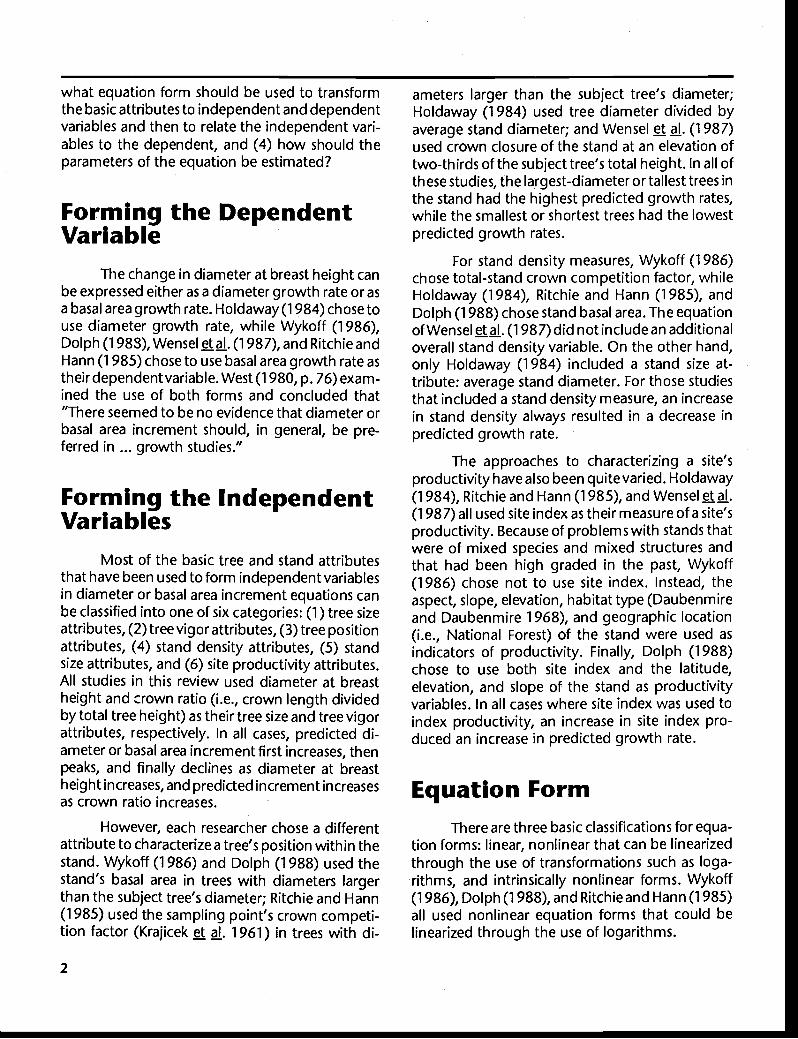
what equation form should be used to transformthe basic attributes to independent and dependentvariables and then to relate the independent vari-ables to the dependent, and (4) how should theparameters of the equation be estimated?

Forming the DependentVariable

The change in diameter at breast height canbe expressed either as a diameter growth rate or asa basal area growth rate. Holdaway (1984) chose touse diameter growth rate, while Wykoff (1986),Dolph (1983), Wensel et al. (1987), and Ritchie andHann (1985) chose to use basal area growth rate astheir dependent variable. West (1980, p. 76) exam-ined the use of both forms and concluded that"There seemed to be no evidence that diameter orbasal area increment should, in general, be pre-ferred in ... growth studies."

Forming the IndependentVariables

Most of the basic tree and stand attributesthat have been used to form independent variablesin diameter or basal area increment equations canbe classified into one of six categories: (1) tree sizeattributes, (2) tree vigor attributes, (3) tree positionattributes, (4) stand density attributes, (5) standsize attributes, and (6) site productivity attributes.All studies in this review used diameter at breastheight and Crown ratio (i.e., crown length dividedby total tree height) as their tree size and tree vigorattributes, respectively. In all cases, predicted di-ameter or basal area increment first increases, thenpeaks, and finally declines as diameter at breastheight increases, and predicted increment increasesas crown ratio increases.

However, each researcher chose a differentattribute to characterize a tree's position within thestand. Wykoff (1986) and Dolph (1988) used thestand's basal area in trees with diameters largerthan the subject tree's diameter; Ritchie and Hann(1985) used the sampling point's crown competi-tion factor (Krajicek et al. 1961) in trees with di-

ameters larger than the subject tree's diameter;Holdaway (1984) used tree diameter divided byaverage stand diameter; and Wensel et al. (1987)used crown closure of the stand at an elevation oftwo-thirds of the subject tree's total height. In all ofthese studies, the largest-diameter or tallest trees inthe stand had the highest predicted growth rates,while the smallest or shortest trees had the lowestpredicted growth rates.

For stand density measures, Wykoff (1986)chose total-stand crown competition factor, whileHoldaway (1984), Ritchie and Hann (1985), andDolph (1988) chose stand basal area. The equationofWensel et al. (1987) did not include an additionaloverall stand density variable. On the other hand,only Holdaway (1984) included a stand size at-tribute: average stand diameter. For those studiesthat included a stand density measure, an increasein stand density always resulted in a decrease inpredicted growth rate.

The approaches to characterizing a site'sproductivity have also been quite varied. Holdaway(1984), Ritchie and Hann (1985), and Wensel et al.(1987) all used site index as their measure of a site'sproductivity. Because of problems with stands thatwere of mixed species and mixed structures andthat had been high graded in the past, Wykoff(1986) chose not to use site index. Instead, theaspect, slope, elevation, habitat type (Daubenmireand Daubenmire 1968), and geographic location(i.e., National Forest) of the stand were used asindicators of productivity. Finally, Dolph (1988)chose to use both site index and the latitude,elevation, and slope of the stand as productivityvariables. In all cases where site index was used toindex productivity, an increase in site index pro-duced an increase in predicted growth rate.

Equation FormThere are three basic classifications for equa-

tion forms: linear, nonlinear that can be linearizedthrough the use of transformations such as loga-rithms, and intrinsically nonlinear forms. Wykoff(1986), Dolph (1988), and Ritchieand Hann (1985)all used nonlinear equation forms that could belinearized through the use of logarithms.

2

1. Wykoff (1986):

BAG = EXP(HAB + LOC + a1 SL[cos(ASP)] + a2SL[sin(ASP)] + a3SL + a4SL2

+ aSEL + a6EL2 + a7ln(DBH) + a8DBH2 + a9CR + a10CR2

+ all BAL + a12BAL/In(DBH + 1.0) + al 3CCF}

where

BAG

HAB

LOC =

SL =

ASP =

EL =

DBH =

CR =

BAL =

CCF =

basal area growth of the tree,

a constant term based on habitattype of the stand,

a constant term based on the Na-tional Forest of the stand,

stand slope ratio,

stand aspect,

stand elevation,

diameter at breast height of thetree,

crown ratio of the tree,

basal area in trees with a DBHlarger than the subject tree's DBH,and

crown competition factor for thestand.

where

(1)

PCCFL = crown competition factor (CCF)in trees on the sampling pointwith a DBH larger than the sub-ject tree's DBH,

and other terms are as defined previously.

The remaining two studies used intrinsicallynonlinear equation forms in which the potential, ormaximum, growth rate is estimated and thenmultiplied by a modifier function that reduces thegrowth rate for increased competition within thestand and thus accounts for reduced tree vigor.

1. Holdaway (1984):

DG = (POT)(MOD) (4)

where

2. Dolph (1988):

BAG = EXP{;AT+a1ln(DBH) +a2DBH2+a3CR2/ln(DBH + 1.0)

+ a4BAL/In(DBH + 1.0)+ a,Sln(BA) + a6EL + a7SL +a8SL2

+ a9Sl}

where

LAT = a constant term based upon thelatitude of the stand,

BA = basal area of the stand,

SI = site index of the stand

DG =

POT =

(2)

MOD =

in which

and other terms are as defined previously. X, _

X2 =

3. Ritchie and Hann (1985): X3 =

diameter growth rate of thetree,

potential diameter growth rateof the tree

ao + a, DBHa2 +a 3[(SI)(CR)(DBH)]a4

modifier function for the tree

1.0 - EXP[-(X,)(X2)(X3)]

a5{1.0 - EXP[a6(DBH/AD)]}a' + a8

a9(AD +1.0)a, o

[(MBA - BA)/ BA]' i2

BAG = EXP(a0 + a1 ln(DBH) + a2DBH2 + a3+CR + a4ln(SI) + asPCCFL+ a6BA) (3)

3

=

AD = mean stand diameter,

MBA = maximum basal area for the stand,

and all other terms are as defined previously.

2. Wensel et al. (1987):

BAG = (POT)(MOD)

where

(5)

POT = potential basal area growth ratefor the tree

= [a,Sla2 + a3DBH2a4],/a4 - DBH2

MOD = modifier function for growthrate of tree basal area

= {EXP[a5(CC66)a6}/{1.0 - EXP[4.0 -a,CR]}

cc66 = crown closure of the stand at two-thirds of the height of the subjecttree,

and other terms are as defined previously.

The definition of the members of the "po-tential" growth rate population differed betweenthe two studies. The "potential" equation used byHoldaway (1984) divided the dominant andcodominant trees for each species into mutuallyexclusive 1-inch DBH, 1 0-foot site index and 10-percent crown ratio cells. The "potential" popula-tion was then defined as the 5 percent of the treeswithin each cell with the fastest diameter growthrates. Wensel et al. (1987, p. 13), on the otherhand, selected their trees for measuring potentialdiameter growth rate for each species "from thelargest 33 percent of the trees in each stand (bybasal area) provided that the trees had live crownratios greater than 0.5."

Parameter EstimationThe choice of the method for estimating the

parameters of an equation depends upon the formof the equation and whetherthe error is additive ormultiplicative, and upon whether the data violateany of the assumptions of regression. As an ex-

ample of the latter consideration, the variance ofresiduals about diameter or basal area growth rateequations can exhibit heterogeneity (West 1980,Martin and Ek 1984).

Wykoff (1986) and Dolph (1988) linearizedequations (1) and (2), respectively, through the useof logarithms and then estimated the parametersby using linear regression. The use of the logtransformation assumes that the error about theuntransformed dependent variable is multiplica-tive. As a result, the log transformation can homog-enize variances that increase with the size of thedependent variable so that weighting is unneces-sary. The estimated parameters are unbiased forpredicting the log of basal area growth, but theyare biased for predicting basal area growth itself(Flewelling and Pienaar 1981).

While a number of log-bias correction proce-dures have been developed, most of them assumethat the residuals are normally distributed (Flewellingand Pienaar 1981). Ritchie and Hann (1985) com-pared both the use of the log transformation andunweighted, linear regression and the use ofweighted, nonlinear regression for estimating theparameters of equation (3). They found that theresiduals of the log of basal area growth were notnormally distributed and, as a result, that correc-tion for log bias was difficult. They therefore usedweighted, nonlinear regression with a weight of1.0/DBH2. It should be noted that the parametersestimated from nonlinear regression are only unbi-ased asymptotically as sample size increases.

The parameters of the POT portion ofHoldaway's (1984) equation (4) were estimated bynonlinear regression. The dependent variable forthe modifier function was then formed by dividingactual diameter growth rate by predicted potentialdiameter growth rate. The parameters of the modi-fier were then estimated in two steps by nonlinearregression that had been constrained to avoidimplausible parameter estimates. In the first step,the parameters for X2 were estimated with X, set to1. With the parameters of X2 determined, the pa-rameters of X, were then estimated. This two-stepprocess was used to guarantee that X, would equal1 when DBH was equal to AD. What effect thistwo-step estimation process has upon the statisti-cal properties of the modifier function's parameters

4

is difficult to assess. However, when validatingequation (4) on an independent data set, Holdaway(1984) found that it over-predicted diametergrowth.

Wensel et al. (1987, p. 13) tried to estimateall of the parameters in their equation (5) simulta-neously by nonlinear regression, but they foundthat the approach "confounded the potential andcompetition effects." They therefore used an itera-.tive approach in which they first fit the potentialequation to the potential data set on the assump-

Data DescriptionThe data for this study were collected during

the summers of 1981, 1982, and 1983 as part ofthe southwest Oregon Forestry Intensified Research(FIR) Growth and Yield Project. The study area(Figure 1) extended from near the California bor-der (42° 10' N) on the south to the Cow Creekdrainage (43° 00' N) on the north and from theCascade crest (122° 15' W) on the east to approxi-mately 15 miles west of Glendale (123'50'W).Elevation ranges from 900 to 5,100 feet, Januarymean minimum temperature from 23°to 32°F, andJuly mean maximum temperature from 79°to 90°F.Annual precipitation varies from 29 to 83 inches,with less than 10 percent of the total falling duringJune, July, and August.

CANYONVILLEDUTCHMAN

BUTTE

GLENDALE

6 MILES

PROSPECT

MTN r--j;tSEXTONRUSTLER0

PEAKBUTTEFALLS

GRANTSPASS

Figure 1. The study area (shaded).

s 1 OUGHLIN

tion that the modifier value was 1. Second, themodifier function was fit to all trees in the data setby the previously determined "potential" equa-tion. Finally, the parameters of the "potential"equation were re-estimated by using all trees in thedata set and the modifier function parametersdetermined in the second step. Again, it is difficultto assess the effect upon the statistical properties ofthe parameters of using this iterative estimationprocess rather than the more usual simultaneousmethod.

Temporary plots were established with in 391stands selected from the study area. The followingcriteria were used to select these stands:

1. The majority of the trees in the standmust have an age under 120 years oldwhen measured at breast height;

2. The majority of the trees in the standmust be either Doug las-fir, white fir, grandfir, ponderosa pine, sugar pine, incense-cedar, or a mixture of them (hereafter,these will be called the "six targetedconifer species");

3. The stand must have a uniform standstructure so that the species mix, com-petitive structure, and resulting potentialmanagement practices are essentiallyunchanged throughout the stand;

4. The stand must have a common bed-rock, landform, and soil series, and besimilar in aspect, slope, and elevationthroughout the stand;

5. The stand must not have been treatedwithin the past 5 years.

Within each stand, a cluster of from 4 to 10variable-radius plots and 2 nested, fixed-area sub-plots was installed in a random fashion to measurethe attributes on all trees taller than 6 inches high.A variable-radius plot with a basal area factor of 20

5

was used for trees with an 8.1 -inch or greaterdiameter outside bark at breast height (DBH); acircular fixed-area subplot with a radius of 15.56feet was used for trees with a 4.1- to 8-inch DBH;and a circular fixed-area subplot with a radius of7.78 feet was used for trees with a DBH of 4 inchesor less.

Tree measurements taken at the end of themost recent 5-year growth period (i.e., measure-ments subscripted with a 2) included a mortalityindicator of whether the tree died in the past5 years, DBH (DBH2), total tree height (H2), heightto live-crown base (HCB2), and horizontal distancefrom plot center to tree center (DIST). In addition,past 5-year radial growth and height growth weremeasured on subsamples of the trees.

The dating of when trees died was basedupon physical features of the dead tree as describedin USDA Forest Service (1978) and Cline et al. (1980).Breast-height diameter was measured to the near-est 0.1 inch with a diameter tape. Both heightmeasurements were taken by the tangent method(Curtis and Bruce 1968, Larsen et al. 1987). Theposition of the base of the crown was determinedby visual reconstruction of the crown such that anygaps in the crown were filled-in with branches frombelow the crown base. The distance from plotcenter to tree center was determined by measuringthe horizontal distance from plot center to tree faceand then adding one-half DBH2, expressed in feet,to it.

Past radial growth at breast height was mea-sured with an increment borer on all trees with aDBH large enough to accept the borer (approxi-mately 2 inches DBH). The boring occurred on theside of the tree facing plot center, and the resultingcore was measured to the nearest 40th of an inch,ignoring the currentyear's growth. The inside-barkradial growth measurements were converted tooutside-bark diameter and basal area growth mea-surements by using the prediction equations forthe ratio of diameter inside bark to diameter out-side bark as developed for the six targeted coniferspecies of southwest Oregon by Larsen and Hann(1985) and for California hardwoods by Pillsburyand Kirkley (1984). Finally, the diameter growthmeasurements for the six targeted conifer specieswere adjusted, by using the equation presented in

Zumrawi (1990), to eliminate the measurementbias that occurs when increment borings are usedinstead of repeated measurements of DBH to deter-mine outside-bark diameter growth.

All undamaged trees under 25 feet tall weremeasured for 5-year height growth rates with a 25-foot telescoping pole. For trees taller than 25 feet,a subsample of up to six trees on each plot wasfelled and sectioned at the first and sixth whorls;the ages at these whorls were determined to ensurea true 5-year growth period, and finally the dis-tance between the two whorls was measured for 5-year height growth.

Because the objective of the project is topredict future rather than past diameter growthrates, it was necessary to backdate all of the treemeasurements in order to estimate their values atthe start of the previous 5-year growth period (i.e.,measurements subscripted with a 1). The proce-dures used to backdate the tree measurements aredescribed in detail in Hann and Wang (1990). Fortrees that died during the growth period, it wasassumed that the values at the start of the growthperiod were the same as those at the end of it.

It should be pointed out that backdating theattributes used to construct the independent vari-ables can introduce measurement errors into theindependent variables. If the measurement error inthe independent variable is independent of theerror of the residuals about the regression surface,then the parameters are unbiased (Kmenta 1971).However, if the measurement error is correlatedwith the error of the residuals, then biased param-eters can occur. Unfortunately, the measurementerror associated with backdating can only be elimi-nated through repeated measurements from per-manent plots, and methods for ascertaining whetherthe errors are correlated are not readily available. Asa result, the potential problems introduced bybackdating temporary data sets are usually ignored.

Once the basic tree variables had beenbackdated to the start of the growth period, anumber of tree, tree-position, and stand variableswere then calculated. Crown ratio at the start of thegrowth period (CR) was determined as follows:

CR1 = 1.0 - (HCB,)/(HT,)

6

where

HCB1= height to crown base at the startof the growth period and

HT, = total height at the start of thegrowth period.

Three variables-basal area in larger trees(BAL), crown competition factor in larger trees(CCFL,), and crown closure at the top of the tree(CCH)-were used to quantify a tree's positionwithin the stand at the start of the growth period.BAL, has been previously used as a tree-positionvariable in equations for predicting tree basal areagrowth (Ritchie and Hann 1985, Wykoff 1986,Dolph 1988); CCFL1 has been used in equations forpredicting tree height to crown base (Ritchie andHann 1987, Zumrawi and Hann 1990); and CCH1has been used in equations for predicting treeheight growth (Hann and Ritchie 1988).

BAL1 is the sum of the basal area in trees withDBH,'s larger than the subject tree's DBH,. There-fore, the largest-diameter tree in the stand wouldhave a BAL, value of zero, while the smallest-diam-eter tree in the stand would have a BAL, value nearbut somewhat less than the stand's total basal area.

Similarly, CCFL, is the crown competitionfactor in trees with DBH,'s larger than the subjecttree's DBH,. As described by Krajicek et al. (1961),crown competition factor (CCF) is the ratio result-ing when the sum of the square-foot maximumcrown areas for all trees of interest in the stand orplot is divided by the square-foot area of the standor plot. This ratio is then multiplied by 100 toexpress it as a percentage. Maximum crown areaswere computed from the maximum crown widthequations developed for southwest Oregon byPaine and Hann (1982).

A series of calculations was made to deter-mine the CCH1 of a particular tree. First, HT, wasused to define a reference height. Next, crownwidths at the reference height for all trees in thestand were estimated with the relative crown-width equations found in Ritchie and Hann (1985)and the maximum crown-width equations foundin Paine and Hann (1982). If the reference heightfell above the top of a tree, crown width was zero;if it fell below the crown base of a tree, crown widthat crown base was used. Finally, each crown width

was converted to crown area by the formula for thearea of a circle, and thesevalues were then summedand expressed as a percentage of the area of anacre.

The above three tree-position variables weredefined in relation to all trees measured in thestand. Three additional tree-position variables werealso computed to determine whether tree positiondefined in relation to only those trees existing oneach sample point would improve the ability topredict diameter growth rate. These variables arebasal area in larger trees for the sample point(PBAL), crown competition factor in larger treesfor the sample point (PCCFL,), and crown closureat the top of the tree for the sample point (PCCH1).PCCFL1 has been previously used in equations forpredicting tree basal area growth (Ritchie andHann 1985).

Variables calculated for the stand includedtotal basal area at the start of the growth period(BA) and total crown competition factor at thestart of the growth period (CCF1. In addition,sample-point total basal area at the start of thegrowth period (PBA) and sample-point total crowncompetition factor at the start of the growth period(PCCF1) were also computed.

Also, the site index of each stand was com-puted with equations developed from a local dataset (Hann and Scrivani 1987). However, becausethe stands in southwest Oregon are often of mixedspecies with uneven-aged stand structures and canbe severely affected by early competing vegeta-tion, local foresters expressed reservations aboutusing site index in the area. Therefore, we alsodecided to try a number of alternative, productiv-ity-related variables.

Variables measured from maps included el-evation, latitude, annual rainfall, rainfall during thegrowing season, and bedrock type. Informationcollected from soil pits in each stand includedamount and size of coarse fragments, abundanceof roots, and the water-holding capacities of eachhorizon. Finally, variables measured directly oneach plot included slope, aspect, and vertical anglesto the tops of ridges that might block the sun.

The directly measured variables were thenused to compute other productivity variables such

7

as average monthly minimum and maximum tem-peratures, solar irradiation (Kaufmann andWeatherred 1982), and net photosynthesis(Emmingham and Waring 1977) at the site. Addi-tional variables such as indicators of the occurrenceof a given species on a site were also computed.

Data AnalysisWe decided to use the general approach of

Wykoff (1986), Dolph (1988), and Ritchie andHann (1985) instead of the approach of Holdaway(1984) and Wensel et al. (1987) for three reasons:

1. We were uncomfortable with the defini-tions of the "potential" populations usedby Holdaway (1984) and Wensel et al.(1987) because they seemed to be some-what arbitrary.

2. We were concerned about the statisticalproperties of the iterative parameter es-timators used by Holdaway (1984) andWensel et al. (1987).

3. With the approaches of Wykoff (1986),Dolph (1988), and Ritchie and Hann(1985), the ability to linearize equations(1) and (2) through the application oflogarithms would allow the use of pow-erful independent-variable screeningtools that are available in many linearregression packages. If desired, the re-sulting parameter estimates could thenbe re-estimated by using nonlinear re-gression.

Both basal area growth and diameter growthwere tried as the dependent variable, and it wasdecided to use diameter growth for two reasons.First, many of the other component equations forthe southwest Oregon version of ORGANON usedtree diameter rather than basal area (e.g., Paineand Hann 1982, Walters et al. 1985, Walters andHann 1986a,b, Larsen and Hann 1987, Ritchie andHann 1987, Hann and Wang 1990) and, as a result,it was necessary for the model to be able to projecttree diameters into the future. Second, transforma-tion of the basal area growth equation to predict

A summary of the variables used in the equa-tions for predicting final individual-tree diametergrowth rate is presented in Table 1.

diameter growth provided unreasonable predic-tions for trees with small diameters.

The alternative productivity variables wereexamined by using a number of all-combinationscreening runs on the log linearization of equation(3); the logarithm of diameter growth was used asthe dependent variable and the parameters wereestimated with the linear regression package REX(Grosenbaugh 1967). Various transformations ofthe alternative productivity variables were tried,with one set of runs including log of site index as asindependent variable and a separate set of runswithout a site index variable. From these runs, wefound that site index was the strongest productivityvariable and that, while some alternatives weresignificant, no combination of them explainedmore than 3 or 4 percent of the variation whenused alone or more than 2 percent when used withsite index. Because of the considerable cost associ-ated with collecting and computing many of thestatistically significant alternative productivity vari-ables, we decided not to include any of them in thefinal diameter growth equation.

We also used all-combination screening toexamine alternatives to the following independentvariables in equation (3): ln(DBH,), CR1, PCCFL1and BA,. As alternatives for ln(DBH,), we triedln(DBH1+K1) with K1 being assigned values of 0.0,0.5, 1.0, 1.5, 2.0, 2.5, or 3.0. Adding a positiveconstant to the log transformation of diameter in-creases predicted diameter growth for trees withsmall diameters. We found that the value of 1.0provided the lowest mean square error for all butone minor species. To standardize the equationform, we chose to use ln(DBH1+1.0) for all species.

For the crown ratio (CR) term, we tried bothCR1 and ln[(CR,+K2)/1.0+K2)], with K2 being ei-ther 0.0, 0.1, 0.2 or 0.3. From the screenings, the

8

Table 1. Selected descriptive statistics for the data set on diameter growth rate.

Tree-diameterStand basal area in

trees larger thangrowth rate

(in./5 yr.)Tree

diameter (in.)Tree

crown ratioStand

site index (ft)subject tree

(ft2/acre)Stand basal

area (ft2/acre)

SpeciesNumberof trees Mean Range Mean Range Mean Range Mean Range Mean Range Mean Range

SOFTWOODS

Douglas-fir 11,974 0.97 0.00-4.68 13.8 0.3-83.8 0.50 0.02-1.0 93.4 54.1-141.1 94.6 0.0-380.0 191.9 0.1-393.2Grand fir 942 1.07 0.00-5.48 12.5 0.8-48.9 0.55 0.01-1.0 94.8 59.4-124.3 100.3 0.0-387.2 177.8 10.5-393.2Incense-cedar 1,008 0.71 0.00-4.88 10.1 0.2-66.3 0.54 0.05-1.0 88.8 54.8-124.3 110.8 0.0-322.4 166.0 2.6-331.9Ponderosa pine 1,594 0.88 0.00-5.18 14.9 0.1-59.6 0.47 0.05-1.0 88.8 54.8-141.1 74.5 0.0-272.1 172.9 6.5- 331.9Sugar pine 350 1.34 0.00-4.98 18.1 1.1-59.9 0.52 0./0-/.0 86.3 54.1-126.6 49.4 0.0-261.8 171.8 3.5-326.2Western hemlock 105 0.82 0.00-3.08 8.4 1.4-21.4 0.70 0.02-1.0 88.9 63.2-124.3 64.3 0.0-295.0 111.7 14.8-321.8White fir 1,373 0.97 0.00-3.68 13.4 0.6-51.1 0.53 0.03-1.0 92.4 62.3-141.1 108.0 0.0-385.0 189.2 10.0-393.2

HARDWOODS

Bigleaf maple 41 0.58 0.20- 2.20 7.7 1.9- 19.8 0.38 0.13-0.96 99.8 75.7-141.1 153.8 2.0- 267.1 186.2 38.1-270.8California black oak 300 0.36 0.10-1.50 13.1 2.0-48.4 0.40 0.05-1.00 85.9 54.8-121.1 97.6 0.0-294.4 172.8 46.2-302.9Canyon live oak 89 0.45 0.10-1.60 4.6 2.4- 9.2 0.57 0.08-1.00 84.0 54.1-107.9 168.0 0.0-291.3 186.7 14.8-293.5Giant chinkapin 399 0.49 0.10-1.60 6.3 1.1-26.5 0.47 0.07-1.00 92.2 54.1-125.6 126.6 0.0-302.0 168.9 14.8-326.2Madrone 793 0.51 0.10-3.00 9.0 1.5-44.5 0.41 0.01-1.00 91.3 54.1-141.1 104.7 0.0-303.2 171.6 3.0-317.9Oregon white oak L9 0.21 0.10-0.30 8.8 2.9-24.4 0.42 0.23-0.64 60.0 55.3- 80.2 78.1 3.3-194.8 149.3 119.6-197.0Tanoak 63 0.44 0.10-1.20 4.9 1.3- 11.8 0.51 0.18-0.97 93.1 73.0-117.0 104.3 0.0-229.7 147.1 2.6-239.0

'0

second expression with a K2 value of 0.2 resulted inthe lowest mean square error for all of the species.

In addition to the PCCFL1 variable, the alter-native tree-position variables we examined includedstand crown competition factor in larger trees(CCFL1), stand and point crown closure at treetop(CCH1 and PCCH), stand and point basal area inlarger trees (BALI and PBAL), stand and point basalarea in large, trees squared (BAL12 and PBAL12), BALI/ln(DBH+K3), PBAL1/In(DBH+K3), BAL12/ln(DBH+K3), and PBAL12/ln(DBH+K3), with K be-ing set to 1,2,3,4,5, and 6. From these screenings,we found that BAL12/In(DBH+5) had the lowestmean square error for six of the species. Theequations for the remaining eight species did notinclude a stand position variable.

The final set of variables we screened acrosswere used to characterize total stand density. Wefirst tried point basal area (PBA) and crown com-petition factor (PCCF1) and stand basal area (BA)and crown competition factor(CCF). Of these, BA1minimized the mean square error. We next triedpowers of 0.5,1.0,1.5, and 2.0 on BA1.Of the sevenspecies that included a BA1 term in their equations,six minimized their mean square errorwith a powerof 0.5 and the remaining one (western hemlock)had a minimum with a power of 1.0. We thereforechose to standardize on a value of 0.5, whichincreased the mean square error for western hem-lock only slightly. The best equation form to emergefrom this variable selection process was

BAL1 =

BA1

basal area at the start of the growthperiod in trees with diameters largerthan the subject tree, square feet,and

total stand basal area at the start ofthe growth period, square feet.

We examined both the use of the log trans-formation and linear regression combination andthe use of weighted, nonlinear regression to esti-mate the parameters of equation (6). Like Ritchieand Hann (1985), we also found that, because oftheir skewness and kurtosis statistics, the residualsof the log-tranformation were not normally distrib-uted. As a result, standard log-bias correction pro-cedures (Flewelling and Pienaar 1981) producedmean residuals that were not zero for diametergrowth itself. In addition, Furnival's (1961) index offit for the weighted, nonlinear equation was lowerthan the log-transformation equation. Therefore,we chose to use weighted, nonlinear regression toestimate the parameters.

Alternative weights based on the reciprocalof DBH1, DBH1 squared, predicted diameter growth(Y), and predicted diameter growth squared werealso evaluated with Furnival's (1961) index of fit todetermine which weight minimized the index. Thebest turned out to be the reciprocal of predicteddiameter growth. Therefore, it was necessaryto usean iterative fitting procedure, analogous to theiterative procedure described in Kmenta (1971) for

DGRO = EXP(b0 + b1+In(DBH1 + 1) + b2DBH12 + b3ln[(CR1 + 0.2)11.2]

+ b4.ln(SI - 4.5) + b5(BAL12)/[ln(DBH1 + 5)] + b6.BA1112} (6)

where

DGRO = future 5-year diameter growth rate,inches,

DBH1 = diameter at breast height at thestart of the growth period, inches,

CR1 = crown ratio atthe start ofthegrowthperiod,

SI = Hann and Scrivani's (1987) defini-tion of Douglas-fir site index for thestand, feet,

linear regression, to estimate the regression param-eters. The first step in this process was to estimatethe parameters by using unweighted, non-linearregression procedures. These parameters were thenentered into the weight function and the param-eters re-estimated by weighted, non-linear regres-sion. In the next cycle, the parameter estimatesfrom the previous weighted, non-linear regressionfit were entered into the weight function and theparameters re-estimated with these new weights.This process continued until the new parameterestimates were identical to the previous ones.

10

Distinguishing between white fir and grandfir can be difficult in southwest Oregon because thetwo species can interbreed. Therefore, analysis ofcovariance was used to determine if they hadstatistically similar diameter growth equations.Analysis of covariance was also used to evaluatewhether four data sets with small sample sizescould be combined with two stronger data sets toproduce the following two groups of species: giantchinkapin and tanoak; Oregon white oak, Califor-nia black oak, and canyon live oak.

As a final check of the equations, both theweighted and the unweighted residuals were ex-amined for systematic trends across predicted di-ameter growth and the independent variables. Thisanalysis was done by (1) dividing the range of

predicted diameter growth and the independentvariables into classes, (2) computing the meanweighted or unweighted residual and the standarddeviation of the residuals in each class, (3) plottingthe mean residual, the mean residual plus twostandard deviations, and the mean residual minustwo standard deviations across the mean classvalues for predicted diameter growth or the inde-pendent variable, and (4) visually examining theplots for systematic trends that might indicate lackof fit. The mean residual plus two standard devia-tions and the mean residual minus two standarddeviations were added to the plots to indicate themagnitude of the variation existing in the residuals.If the residuals in each cell were normally distrib-uted, then these two values would approximatelybracket 95 percent of the residuals in the cell.

Results and DiscussionAs a result of the analyses of covariance,

white fir was combined with grand fir, giantchinkapin was combined with tanoak, and all of thecoefficients except bo in the California black oak,Oregon white oak, and canyon live oak group werecombined. Table 2 gives the regression coefficientsand the adjusted coefficient of determination foreach of the resulting 12 species groups. A zerovalue for a coefficient indicates that the coefficientwas not significantly different from zero (p = 0.05).Regression coefficients with truncated values werenot significant (p = 0.05) but were required to givedesired behavior; therefore, the truncated valuereported in Table 2 was forced into the equation.

The standard errors in Table 2 were com-puted under the assumption that each tree wasrandomly selected from the population. Because alltrees on a plot were measured, their selection wasnot truly random; therefore, their measurementsare probably correlated with each other. As a result,the standard errors presented in Table 2 are prob-ably underestimated (Dolph 1988).

The residual analysis indicated that therewere no systematic trends across predicted 5-yeardiameter growth or any of the independent vari-ables for both the weighted and the unweighted

residuals. For example, Figure 2 shows the graphsof the summary cell statistics for the unweightedresiduals plotted across the mean cell value forpredicted 5-year diameter growth of Douglas-fir,grand/white fir, ponderosa pine, sugar pine, andincense-cedar. Also plotted on these graphs are thenumbers of observations used to compute eachcell's values. Visual inspection of these graphsindicates that the mean residual values are cen-tered around zero and that there are no systematictrends away from zero.

Equation (6) can be better understood if it ispartitioned into a component for maximum pre-dicted growth rate and three multiplicative modi-fiers to that maximum rate. The rate component isdetermined by setting CR1 to 1 and both BAL1 andBA, to zero. The maximum predicted growth rateis then reduced by a decrease from 1 in the tree'sCR,, by an increase from zero in the tree's BAL,, orby an increase from zero in BA,. Partitioning theequation in this fashion allows us to examine morethoroughly how altering the stand's characteristicsaffects diameter growth.

Figure 3 shows the graphs of the six targetedconifer species' maximum predicted diametergrowth rates plotted across DBH1 for three site in-

11

Table 2. Regression coefficients and associated statistics for equation (6).1

Number Coefficients UnweightedSpecies of trees b0 b1 b2 b3 b4 b5 b6 adjusted R2

SOFTWOODS

Douglas-fir 11,974 -3.33258 0.401284 -0.000444053 1.34652 0.778012 -0.000049654 0 -0.0151775 0.5781(.11524) (.014442) (.000018121) (.02204) (.024847) (.0000014408) (.0022995)

Incense-cedar 1,008 0.680328 0.294091 -0.000153983 1.51324 0.0 -0.000031986 5 -0.0762573 0.6510

(.067199) (.042901) (.000056416) (.09973) (.0000058609) (.0088595)

Ponderosapine 1,594 -1.30372 0.494510 -0.000348437 1.57636 0.419129 0.0 -0.0810353 0.6213

(.40327) (.038320) (.000059459) (.07202) (.087825) (.0064139)

Sugar pine 350 -1.99775 0.475468 -0.000354162 1.26503 0.519814 0.0 -0.0430817 0.3796(.57019) (.075619) (.000091941) (.12129) (.122921) (.0105704)

Westernhemlock 105 -6.01009 0.404185 -0.0004 0.950304 1.29805 0.0 -0.0557239 0.4546

(1.38668) (.120356) (.305529) (.28973) (.0175274)

White &grand fir 2,315 -3.57581 0.707145 -0.001070590 1.33263 0.646635 -0.000046261 7 0.0 0.5285

(.30899) (.033018) (.000070135) (.04738) (.069172) (.0000025448)

HARDWOODS

Bigleafmaple 41 0.0 0.485882 -0.0014 0.0 0.0 0.0 -0.117409 0.2266

(.101242) (.021105)

Californiablack oak 300 -2.76395 0.0925835 -0.0001 0.337396 0.405687 0.0 0.0 0.0934

(.66505) (.0474371) (.096073) (.145705)

Canyonlive oak 89 -2.56270 ------ -All other values are the same as for California black

Giant chinkapin& tanoak 462 -3.88293 0.222768 -0.0007 0.670268 0.746788 -0.0000231015 0.0 0.3306

(.52589) (.057638) (.096330) (.114032) (.0000036696)

Madrone 793 0.210329 0.134582 -0.0003 0.490452 0.0 0.0 -0.0675144 0.3003(.089769) (.041420) (.081358) (.0068228)

Oregonwhite oak 29 -3.13126 --------All other values are the same as for California black oak- -- - - - -

I Standard errors appear in parentheses beneath each coefficient.

12

0.4

C °°13

IN,-

0.6

`, N.

1313

-1

-2

-3

-40.24,-

3

-40

e

0.8 1.2

13

1.0

1.6 2.0 2.4 2.8

111313

13

13013 °13DO13O13

1.4 1.8 2.62.2

1313 - .i'._.._\1313 V

p131313 O13

0.4 0.8 1.2 1.6 2.0 2.4

PREDICTED DIAMETER GROWTH (in.)

1000

875

750

625

500

375

250

125

0

200

175

150

125

100

75

50

25

0

200

175

150

125

100

75

50

25

0

b

0.4

------------

0.7

130

d0.8

13

-1

-2

-3

-4

p0.5 0.9

1.2

13

1.1 1.3

Er _,, ,.

1.6 2.0 2.4

1.5 1.7 1.9

PREDICTED DIAMETER GROWTH (in.)

OBSERVATIONS

MEAN RESIDUALS PLUS 2 STD. DEV.

------- MEAN RESIDUAL--- MEAN RESIDUALS MINUS 2 STD. DEV.

2.1

Figure 2. Mean unweighted residuals, mean unweighted residuals plus two standard deviations, meanunweighted residuals minus two standard deviations, and the number of observations in each predicted 5-yeardiameter growth rate cell plotted across the mean predicted 5-year diameter growth rate for each cell: (a)Douglas-fir, (b) white/grand fir, (c) ponderosa pine, (d) sugar pine, and (e) incense-cedar.

dexes. The maximum diameter growth rate forDouglas-fir is also plotted on each graph to aid inmaking comparisons. These plots reflect the rela-tive maximum diameter growth rate of the sixtargeted conifer species. For site index 100, pon-derosa pine has the highest maximum diametergrowth rate, then sugar pine, incense-cedar, Doug-

las-fir, and finally grand/white fir. All of these curvesexhibit a pronounced mounded shape, with thepeak of the mound occurring at DBH,'s that rangefrom 18.1 inches for grand/white fir to 31.7 inchesfor incense-cedar. incense-cedar is the only tar-geted conifer species without site index as anindependent variable. The remaining targeted co-

13

Figure 3. Maximum predicted 5-year diameter growth rate plotted across DBH for site indices of 60, 100, and120 feet: (a) ponderosa pine and Douglas-fir, (b) sugar pine and Douglas-fir, (c) incense-cedar and Douglas-fir,and (d) white/grand fir and Douglas-fir.

nifer species show an in-crease in maximum di-ameter growth rate as siteindex increases.

Figure 4 is a graphof the crown ratio modifi-ers of maximum diametergrowth rate for the sixtargeted conifer species.In general, the graphsshow that long-crownedtrees have proportionallyhigher diameter growthrates than do short-crowned trees. Ponderosapine had the lowest curve,indicating that its pre-dicted diameter growthrates are the most sensi- predicted S-year diameter growth rate realized by the tree.

Figure 4. The effect of the tree's crown ratio on the proportion of the maximum

14

tive to changes in crown ratio. The nextmost sensitive is incense-cedar, thenDouglas-fir, grand/white fir, and sugarpine.

The BAL, modifier of the maxi-mum diameter growth rate was signifi-cant for only four of the six targestedconifer species: Douglas-fir, grand/white fir, and incense-cedar (Figure 5).The graphs in Figure 5 show the reduc-tion in the proportion of the maximumdiameter growth rate that occurs asbasal area in larger trees increases. Thiseffect is more severe in small-diameterthen in large-diameter trees. BecauseBAL, is used to index a tree's competi-tive position within the stand, a BAL,value near zero indicates that the treeis probably in a dominant position,while a large BAL, value indicates thatthe tree is probably in the understory.Therefore, for a given DBH,, the tree'sdiameter growth rate should probablydecrease as BAL, increases, as it does inFigures 5a-c. The figure also shows thata tree with a small diameter is morenegatively influenced by a given levelof BALI than is one with a large diam-eter, indicating that older, larger treesare less affected by position in thestand than are younger, smaller trees.A comparison of these plots for thefourtargeted conifer species shows thatincense-cedar is the least sensitive toincreases in BAL, and that Douglas-fir isthe most sensitive.

Finally, Figure 6 shows the BA,modifier of the maximum diametergrowth rate for those targeted coniferspecies in which it was significant. Theoverall effect of the BA, modifier is toreduce maximum diameter growth rate

100 200 300

STAND BASAL AREA IN LARGER TREES (ft2/acre)

400

as BA, increases. The reduction is the Figure S. The effect of the stand's basal area in trees with DBH'sgreatest for ponderosa pine, with in- larger than the subject tree's DBH on the proportion of the maximumcense-cedar showing almost as large predicted 5-year diameter growth rate realized by the tree, for treean effect. Douglas-fir has the smallest DBH's of 1.0, S. 0, 10.0, 15.0, 20.0, and 30.0 inches: (a) Douglas-reduction. fir, (b) white/grand fir, and (c) incense-cedar.

15

1.0

0.9

0.8-

0.7-

0.6-

0.5-

0.4-

0.3

0.2

0.1

0

DOUGLAS-FIR-'- PONDEROSA PINE--- SUGAR PINE-"- INCENSE-CEDAR

I

50 100 150 200 250 300 350

STAND BASAL AREA (ft2 /acre)

400

Figure 6. The effect of the stand's basal area on the proportion of the maximumpredicted 5-year diameter growth rate realized by the tree.

Interpreting the joint effect of both the BALIand BA, modifiers is also instructive. If a species hasonly a BA, modifier, its diameter growth rate will beaffected just as severely by understory basal area asby overstory basal area. Therefore, the diametergrowth rates of ponderosa pine and sugar pine are

SummaryThe individual-tree, 5-year diameter growth

rate equations produced in this study are the firstreported for the mixed-conifer zone of southwestOregon. For the six targeted conifer species (i.e.,Douglas-fir, white fir, grand fir, ponderosa pine,incense-cedar, and sugar pine), the variation indiameter growth rates explained by these equa-tions ranged from 40 percent for sugar pine to 65percent for incense-cedar. For the minor coniferand hardwood species, the equations explainedbetween 10 and 45 percent of the variation. De-

reduced by increas-ing basal area, re-gardless of their posi-tions within the stand.Species such as grandand white firs, whichhave only a BALImodifier, will benegatively affectedonly by the basal areain overstory trees. In-terpretation whenboth of the modifiersare in the equationdepends upon therelative effect of thetwo modifiers. Doug-las-fir shows a rela-tively small reductionacross BA, and a largereduction acrossBALI. Therefore,Douglas-fir will bemore strongly influ-

enced by the overstory than by the understory. Onthe other hand, incense-cedar shows strong reduc-tionsacross both BA, and BALI, indicating that, whilethe overstory is the most influential, the understorybasal area also has a strong influence upon diam-eter growth rate.

tailed examination of the equations has shown thatpredictions from them are consistent with ourcurrent biological and silvicultural knowledge.However, it should be emphasized that the dataused to develop these equations came from tem-porary plots measured over a 3-year period. There-fore, long-term predictions from these equationsshould be viewed as being reasonable hypothesesbased on current, limited knowledge, rather thanas absolute truth.

16

Literature CitedCLINE, S.P., A.B. BERG, and H.M. WIGHT. 1980.

Snag characteristics and dynamics in Douglas-fir forests, western Oregon. Journal of WildlifeManagement 44:773-786.

CURTIS, R.O., and D. BRUCE. 1968. Tree heightswithout a tape. Journal of Forestry 66:60-61.

DAUBENMIRE, R., and J.B. DAUBENMIRE. 1968.Forest vegetation of eastern Washington andnorthern Idaho. Washington Agricultural Ex-periment Station, Pullman, Washington. Tech-nical Bulletin 60. 104 p.

DOLPH, K.L. 1988. Prediction of periodic basal areaincrement for young-growth mixed conifers inthe Sierra Nevada. USDA Forest Service, PacificSouthwest Forest and Range Experiment Sta-tion, Berkeley, California. Research Paper PSW-190. 20 p.

EMMINGHAM, W.H., and R.H. WARING. 1977. Anindex of photosynthesis for comparing forestsites in western Oregon. Canadian Journal ofForest Research 7:165-174.

FLEWELLING, J.W., and L.V. PIENAAR. 1981. Mul-tiplicative regression with lognormal errors.Forest Science 7:337-341.

FRANKLIN, J.F., and C.T. DYRNESS. 1973. Naturalvegetation of Oregon and Washington. USDAForest Service, Pacific Northwest Forest andRange Experiment Station, Portland, Oregon.General Technical Report PNW-8.417 p.

FURNIVAL, G.M. 1961. An index for comparingequations used in constructing volume tables.Forest Science 7:281-289.

GROSENBAUGH, L.R. 1967. REX - FORTRAN - 4SYSTEM for combinatorial screening or con-ventional analysis of multivariate regressions.USDA Forest Service, Pacific Southwest Forestand Range Experiment Station, Berkeley, Cali-fornia. Research Paper PSW-44. 16 p.

HANN, D.W., and M.W. RITCHIE. 1988. Heightgrowth rate of Douglas-fir: a comparison ofmodel forms. Forest Science 34:165-175.

HANN, D.W., and J.A. SCRIVANI. 1987. Dominantheight growth and site index equations forDouglas-fir and ponderosa pine in southwestOregon. Forest Research Laboratory, OregonState University, Corvallis, Oregon. ResearchBulletin 59.13 p.

HANN, D.W., and C.H. WANG. 1990. Mortalityequations for individual trees in the mixed-conifer zone of southwest Oregon. Forest Re-search Laboratory, Oregon State University,Corvallis, Oregon. Research Bulletin 67. 17 p.

HESTER,A.S., D.W. HANN, and D.R. LARSEN. 1989.ORGANON: Southwest Oregon growth andyield model user manual - Version 2.0. ForestResearch Laboratory, Oregon State University,Corvallis, Oregon. 59 p.

HOLDAWAY, M.R. 1984. Modeling the effect ofcompetition on tree diameter growth as ap-plied in stems. USDA Forest Service, NorthCentral Forest Experiment Station, St. Paul,Minnesota. General Technical Report NC-94.8 p.

KAUFMANN, M.R., and J.D. WEATHERRED. 1982.Determination of potential direct beam solarirradiance. USDA Forest Service, Rocky Moun-tain Forest and Range Experiment Station, FortCollins, Colorado. Research Paper RM-242.23 p.

KMENTA, J. 1971. Elements of Econometrics.Macmillan Publishing Co., New York. 655 p.

KRAJICEK,J.E., K.A. BRINKMAN, and S.F. GINGRICH.1961. Crown competition - a measure of den-sity. Forest Science 7:35-42.

LARSEN, D.R., and D.W. HANN. 1985. Equationsfor predicting diameter and squared diameterinside bark at breast height for six major coni-fers of southwest Oregon. Forest ResearchLaboratory, Oregon State University, Corvallis,Oregon. Research Note 77. 4 p.

LARSEN, D.R., and D.W. HANN. 1987. Height-diameter equations for seventeen tree speciesin southwest Oregon. Forest Research Labora-tory, Oregon State University, Corvallis, Or-egon. Research Paper 49. 16 p.

LARSEN, D.R., D.W. HANN, and S.S. STEARNS-SMITH. 1987. Accuracy and precision of thetangent method of measuring tree height.Western Journal of Applied Forestry 2:26-28.

MARTIN, G.L., and A.R. EK. 1984. A comparison ofcompetition measures and growth models forpredicting plantation red pine diameter andheight growth. Forest Science 30:731-743.

17

PAINE, D.P., and D.W. HANN. 1982. Maximumcrown width equations for southwestern Or-egon tree species. Forest Research Laboratory,Oregon State University, Corvallis, Oregon.Research Paper 46. 20 p.

PILLSBURY, N.H., and M.L. KIRKLEY. 1984. Equa-tions for total, wood, and saw-log volume forthirteen California hardwoods. USDA ForestService, Pacific Northwest Forest and RangeExperiment Station, Portland, Oregon. ResearchNote PNW-414. 52 p.

RITCHIE, M.W., and D.W. HANN. 1985. Equationsfor predicting basal area increment in Douglas-fir and grand fir. Forest Research Laboratory,Oregon State University, Corvallis, Oregon.Research Bulletin 51. 9 p.

RITCHIE, M.W., and D.W. HANN. 1987. Equationsfor predicting height to crown base for four-teen tree species in southwest Oregon. ForestResearch Laboratory, Oregon State University,Corvallis, Oregon. Research Paper 50. 14 p.

USDA FOREST SERVICE. 1978. Region 1 field in-structions for stand examination and forestinventory. Region 1, Missoula, Montana. For-est Service Handbook 2409.21, Chapter 300.113 p.

WALTERS, D.K., and D.W. HANN. 1986a. Predict-ing merchantable volume in cubic feet to avariable top and in Scribner board feet to a 6-inch top for six major conifers of southwestOregon. Forest Research Laboratory, OregonState University, Corvallis, Oregon. ResearchBulletin 52. 107 p.

WALTERS, D.K., and D.W. HANN. 1986b. Taperequations for six conifer species in southwest

Oregon. Forest Research Laboratory, OregonState University, Corvallis, Oregon. ResearchBulletin 56. 41 p.

WALTERS, D.K., D.W. HANN, and M.A. CLYDE.1985. Equations and tables predicting grosstotal stem volumes in cubic feet for six majorconifers of southwest Oregon. Forest ResearchLaboratory, Oregon State University, Corvallis,Oregon. Research Bulletin 50. 36 p.

WENSEL, L.C., W.J. MEERSCHAERT, and G.S.BIGING. 1987. Tree height and diametergrowth models for northern California coni-fers. Hilgardia 55:1-20.

WEST, P.W. 1980. Use of diameter increment andbasal area increment in tree growth studies.Canadian Journal of Forest Research 10:71-77.

WYKOFF, W.R. 1986. Supplement to user's guidefor the stand prognosis model-version 5.0.USDA Forest Service, Intermountain Forest andRange Experiment Station, Ogden, Utah. Gen-eral Technical Report INT-208. 36 p.

ZUMRAWI, A.A. 1990. Examining bias in estimat-ing the response variable and assessing theeffect of using alternative plot designs to mea-sure predictor variables in diameter growthmodeling. Ph.D. dissertation, Oregon StateUniversity, Corvallis, Oregon. 78 p.

ZUMRAWI, A.A., and D.W. HANN.1990. Equationsfor predicting the height to crown base of sixtree species in the central western WillametteValley of Oregon. Forest Research Laboratory,Oregon State University, Corvallis, Oregon.Research Paper 52. 9 p.

18

HANN, D.W., and D.R. LARSEN. 1990. DIAMETER GROWTH EQUATIONS FORFOURTEEN TREE SPECIES IN SOUTHWEST OREGON. Forest Research Laboratory,Oregon State University, Corvallis. Research Bulletin 69. 18 p.

Equations are presented that predict individual-tree 5-year diameter growth,outside bark, for 14 tree species in southwest Oregon. The data used to develop theequations came from 19,245 trees sampled from 391 stands in the study area. Theseequations express diameter growth as a function of diameter at breast height, crownratio, site index, total stand basal area, and stand basal area in trees with diameterslarger than the subject tree's diameter. The parameters of the equations wereestimated by using weighted, nonlinear regression.

HANN, D.W., and D.R. LARSEN. 1990. DIAMETER GROWTH EQUATIONS FORFOURTEEN TREE SPECIES IN SOUTHWEST OREGON. Forest Research Laboratory,Oregon State University, Corvallis. Research Bulletin 69. 18 p.

Equations are presented that predict individual-tree 5-year diameter growth,outside bark, for 14 tree species in southwest Oregon. The data used to develop theequations came from 19,245 trees sampled from 391 stands in the study area. Theseequations express diameter growth as a function of diameter at breast height, crownratio, site index, total stand basal area, and stand basal area in trees with diameterslarger than the subject tree's diameter. The parameters of the equations wereestimated by using weighted, nonlinear regression.