Modeling the spatio-temporal dynamics and interactions of households, landscapes, and giant panda...

hl©

K

pB

0

Ecological Modelling 183 (2005) 47–65

Modeling the spatio-temporal dynamics and interactions ofhouseholds, landscapes, and giant panda habitat

Marc A. Lindermana,∗, Li Ana, Scott Bearera, Guangming Hea,b a
Zhiyun Ouyang, Jianguo Liu
a Department of Fisheries& Wildlife, Michigan State University, East Lansing, MI 48824, USAb Department of Systems Ecology, Research Center for Eco-Environmental Sciences, Chinese Academy of Sciences, Beijing, China

Received 17 November 2003; received in revised form 15 June 2004; accepted 12 July 2004

nd globalarticularly

and-covers such as

ivities andlandscapeplication,useholds,

ng habitatution of

Abstract

Human modification of land-cover has been a leading cause of floral and faunal species extirpation and loss of local abiodiversity. As natural areas are impacted, habitat and populations can become fragmented and isolated. This is pevident in the mountainous areas of southwestern China that support the remaining populations of giant pandas (Ailuropodamelanoleuca). Giant panda populations have been restricted to remnants of habitat from extensive past land use and lchange. Households are a basic socio-economic unit that continues to impact the remaining habitat through activitiefuelwood consumption and new household creation. Therefore, we developed a spatio-temporal model of human acttheir impacts by directly integrating households into the landscape. The integrated model allows us to examine thefactors influencing the spatial distribution of household activities and household impacts on habitat. As an example apwe modeled household activities in a giant panda reserve in China and examined the spatio-temporal dynamics of hothe landscape, and their mutual interactions. Human impacts are projected to result in the loss of up to 16% of all existiwithin the reserve over the next 30 years. In addition, we found that accessibility largely controls the spatial distrib

ousehold activities and considerable changes in management and household activities will be required to maintain the currentevel of habitat within the reserve.

2004 Elsevier B.V. All rights reserved.

eywords:Landscape; Households; Giant panda; Habitat; Model; Hu

∗ Corresponding author. Present address: Department of Geogra-hy, University of Louvain, Place Pasteur 3, 1348 Louvain-la-Neuve,elgium. Tel.: +32 10472871; fax: +32 10472877.E-mail address:[email protected] (M.A. Linderman).

1

andatat

304-3800/$ – see front matter © 2004 Elsevier B.V. All rights reservedoi:10.1016/j.ecolmodel.2004.07.026

man impacts

. Introduction

Appropriation of natural areas through urban
gricultural expansion has drastically altered much of
he land surface (Vitousek et al., 1997; Rutledge etl., 2001). Modification of habitat through less in-

ense land use such as fuelwood collection has also

d.

4 logica

r2 s fore ersis-tru h-i tely1 eb (e.g.S ri-c er ofm pop-u -t ue r-ea edt icso itat,at habi-t onsb andah s pro-v an-a

t att isionai s thedh foree turals inter-a ionsf tom eiri ped,i ,1 npS tiono notcMitd

t ents eti ngr nt inw bes

ndL lopa tio-t ratedi d ag thei ought inga de-t capea anst holdp s ap inga turals

tet use-h est-e andw itht ivid-u rac-t , andw ret holdc tiono fac-t eser vari-o gated tifiedi rac-t

2

8 M.A. Linderman et al. / Eco

esulted in drastic changes in natural systems (Liu et al.,001). These changes have enormous implicationcosystem processes, biodiversity, and species p

ence (Ceballos and Ehrlich, 2002). This is particularlyelevant for the conservation of the giant panda (Ail-ropodamelanoleuca). Habitat destruction and poac

ng have reduced the wild population to approxima000 pandas (Schaller et al., 1985). Many studies haveen conducted on panda biology and behaviorchaller et al., 1985). Most of the studies are empial or field based. There have been also a numbodeling studies, which have simulated pandalation dynamics (Zhou and Pan, 1997), panda rela

ionships to bamboo dynamics (Reid et al., 1989; Wt al., 1996; Carter et al., 1999), and household prefences and characteristics related to panda habitat (An etl., 2001, 2002). However, few studies have examin

he factors influencing the spatio-temporal dynamf households, their impacts on giant panda habnd their mutual interactions (Liu et al., 1999). To bet-

er understand household impacts on giant pandaat, we developed a model in which the interactietween households, the landscape, and giant pabitat could be studied and based on the analyseided practical information for conservation and mgement planning.

Much of human land-cover change is carried ouhe household level as households are basic decnd consumption units (Liu et al., 2003). The rapid

ncrease in the number of households increaseemand for more resources (Liu et al., 2003). Couplingousehold activities with natural processes is theressential to accurately model human impacts on naystems, to increase our understanding of humanctions with landscapes, and to provide viable opt

or mitigating future impacts. Various approachesodeling spatially explicit human activities and th

mpacts on natural systems have been develoncluding statistical techniques (Mertens and Lambin997), agent-based models (Berger, 2001; An et al., iress), and cellular approaches (Balzter et al., 1998).tatistical models have provided detailed informaf the spatial dynamics of systems, but are oftenonducive to generic frameworks (Lambin, 1994).
ore complex agent-based approaches allow increas-
ngly detailed human interactions with each other andhe environment in which they live. However, buildingescriptive agent-based models is often difficult given

2

t

l Modelling 183 (2005) 47–65

he complexity of the models and human–environmystems (Couclelis, 2001). Cellular models, discren time and space, allow for simplified modelielationships and provide a structured environmehich various interactions and levels of detail cantudied (Benenson, 1999).

The overall goal of the model, Household Aandscape Integration Model (HALIM) was to devegeneralized modeling approach in which spa

emporal household processes could be integnto realistic landscapes. For this study, we useeneric spatially explicit cellular model to examine

nteractions of households and panda habitat thrheir mutual relationships with the landscape. Usgeneric cellular framework facilitated the use of

ailed digital data to accurately describe the landsnd household characteristics while providing a me

o integrate inherently different natural and houserocesses. Furthermore, this flexibility provideractical and accessible framework in which varyspects and complexity of socio-economic and naystems and their interactions can be integrated.

As a preliminary study, we used HALIM to evaluahe spatio-temporal effects of landscape-level hoold activities on giant panda habitat in southwrn China by integrating households, forest cover,ildlife habitat through their mutual relationships w

he landscape. This allowed us to examine the indal spatio-temporal dynamics and the various inte

ions between the landscape, household activitiesildlife habitat. Our specific aims of this study we

o examine the influence of landscape-level househaracteristics on the quantity and spatial distribuf panda habitat and to determine the landscape

ors influencing these household activities. Using thesults, we examined possible consequences ofus policy scenarios, provided suggestions to mitiamage to the remaining panda habitat, and iden

mportant landscape, household, and habitat inteions for future modeling efforts.

. Methods

.1. Study area

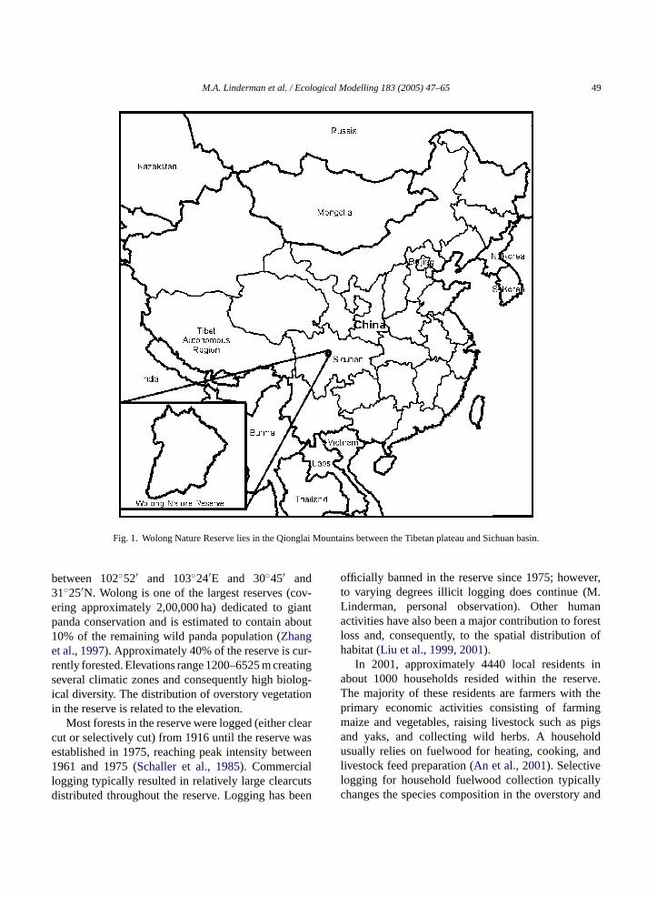
Our field study was conducted in the Wolong Na-ure Reserve in southwestern China (Fig. 1), located

M.A. Linderman et al. / Ecological Modelling 183 (2005) 47–65 49

lai Mo

b3 ov-e iantp bout1e ur-r tings log-i ioni

learc ase1ld

o ver,t M.L ana restl n ofh

ina rve.T thep ingm pigsa old

Fig. 1. Wolong Nature Reserve lies in the Qiong

etween 102◦52′ and 103◦24′E and 30◦45′ and1◦25′N. Wolong is one of the largest reserves (cring approximately 2,00,000 ha) dedicated to ganda conservation and is estimated to contain a0% of the remaining wild panda population (Zhangt al., 1997). Approximately 40% of the reserve is cently forested. Elevations range 1200–6525 m creaeveral climatic zones and consequently high biocal diversity. The distribution of overstory vegetatn the reserve is related to the elevation.

Most forests in the reserve were logged (either cut or selectively cut) from 1916 until the reserve w
stablished in 1975, reaching peak intensity between961 and 1975 (Schaller et al., 1985). Commercial
ogging typically resulted in relatively large clearcutsistributed throughout the reserve. Logging has been

ullc

untains between the Tibetan plateau and Sichuan basin.

fficially banned in the reserve since 1975; howeo varying degrees illicit logging does continue (inderman, personal observation). Other humctivities have also been a major contribution to fo

oss and, consequently, to the spatial distributioabitat (Liu et al., 1999, 2001).

In 2001, approximately 4440 local residentsbout 1000 households resided within the resehe majority of these residents are farmers withrimary economic activities consisting of farmaize and vegetables, raising livestock such asnd yaks, and collecting wild herbs. A househ
sually relies on fuelwood for heating, cooking, and
ivestock feed preparation (An et al., 2001). Selectiveogging for household fuelwood collection typicallyhanges the species composition in the overstory and

5 logica

r n isr holdc ithi holdc ughv fo-c ccesst ities.

2

ut oru ellited pixels ed tod ofh ther werec ourha oldl e onp t wasue

icm M)w opea ma-t omt and1 The1 uireda ellitep uthD , andt o ac-c eent for-e seeL

ousf tionp ail-avic

g gedf late1 s tob esf tely8 t tob aver

estsi for1 ef tely3 ughs ntlyi in-c re-g andr wthm d ons one.M dis-ta elsw ento

8 to2 ther edo ac-t cio-e nals waso in-f ther tiono veysa holdm In-c , ando tely0 en tob eena h yearb ately


educes canopy cover until all overstory vegetatioemoved. Since 1974, immigration and new housereation have largely been dictated by local policy wmmigration restricted by marriage and new housereation limited or inadvertently encouraged throarious policies. Households have traditionallyused on subsistence agriculture, but increasing ao markets has provided some cash crop opportun

.2. Data and model parameterization

Several sources of data were used as model inpsed to parameterize and validate the model. Satata and topographic maps were resampled to aize corresponding to the landscape grid and usescribe the abiotic features and the distributionousehold activities and vegetation throughouteserve. Socio-economic and demographic dataollected from local government agencies andousehold surveys conducted from 1998 to 2001 (An etl., 2001) to determine fuelwood collection, househ

ocations, and household creation rates. Literaturanda behavior and landscape analyses of habitased to parameterize the habitat sub-model (Schallert al., 1985; Ouyang et al., 1996; Liu et al., 2001).

Abiotic information was derived from topographaps of the reserve. A Digital Elevation Model (DEas interpolated from digitized 100-m contours. Slnd aspect data were derived from the DEM. Infor

ion on the distribution of forests was obtained frhe classification of four dates (1965, 1974, 1987,997) when remote sensing data were obtained.965 data are Corona stereo-pair photographs acqs part of the Corona photo-reconnaissance satroject (USGS Eros Data Center, Sioux Falls, Soakota). The 1974 data are Landsat MSS images

he 1987 and 1997 data are Landsat TM images. Tount for the spectral and spatial differences betwhe data, each image was visually interpreted intost and non-forest areas (for classification detailsiu et al., 2001).

Uncertainty in the 1965 stand volume of the variorest types posed the most difficult parameterizaroblem. While basic coverage information was av
ble from satellite photographs, data on the averageolume throughout the reserve were scant. Quantitativenformation dating back nearly 40 years is either diffi-ult to obtain or non-existent.Schaller et al. (1985)sug-
2

t1

l Modelling 183 (2005) 47–65

est that much of the reserve was commercially logrom 1916 until 1975. Measurements taken in the990s indicated much of the lower altitude foreste well below old-growth volumes. Average volum

or broadleaf forests below 2600 m were approxima0 m3/ha. It is likely that these forests were the firse harvested in the first half of the century and hegrown to current volume levels.

Based on regrowth data for the broadleaf forn Wolong, we estimated the average volume965 to be approximately 45 m3/ha. Stand volum

or subalpine conifers was on average approxima00 m3/ha. Subalpine stand volume was high enouch that variations in estimates would not significanfluence the model results. Forest regrowth wasluded in the model to allow for previously loggedions to regenerate and the addition of biomassegrowth in selectively logged cells. Separate regroodels were developed for each forest type base

pecies composition, stand age, and altitudinal zodel parameters were derived from over 30 plots

ributed throughout the reserve (Liu et al., 1999), andpproximation of species regrowth and yield modas derived from the data of the Sichuan Departmf Forestry (Yang and Li, 1992).

A household survey was conducted from 199001 and included 220 of the households withineserve (An et al., 2001). Households were querin fuelwood use, fuelwood collection, agricultural

ivity, household creation, and other associated soconomic and demographic information. Additioocio-economic and demographic informationbtained from local government records. Census

ormation was obtained from each township withineserve. Local governments also maintain informan land allocated to each household. From the surnd census data, it was found that each houseaintains on average 0.7 ha of agricultural land.

luding the area of the physical house, garden areather buildings, the typical total area is approxima.8 ha. Therefore, the scale of the model was chose 90 m× 90 m (0.81 ha). New households have bdded to the reserve at a rather steady number eacetween 1965 and 1997. On average, approxim
4 new households were created each year.
We measured the location of each householdhrough the use of field measurements or Ikonos-m resolution satellite imagery. Ikonos imagery

logical Modelling 183 (2005) 47–65 51

a ncedw balP bleP aseS gesa cre-a tiono restc

ey ofo f an-n db -n them l-w om-p tionsa d lo-c mt oldss pre-fa ion.

at asae 1T g am estc eart eda giantp ulti-p nda theo

2

S(a -l lingo nd-s geo-risfl

s kovc oth-e

c-t ndah ofh iantp s tob diceso tionsa y-n s oft nflu-e restr enta thes omf

M.A. Linderman et al. / Eco

cquired in 2000 by SpaceImaging was georefereith ground control points measured using a Gloositioning System with sub-meter accuracy (Trimathfinder Pro XRS receiver and Community Btation). We then identified households in the imand recorded the location. We used all householdsted on or before 1965 to create the initial distribuf households to correspond to the initial 1965 foover information.

Fuelwood use was calculated based on a survver 50 households and physical measurements oual use (An et al., 2001). The volume of wood varieetween 8 and 30 m3 and averaged 15 m3. A base anual volume of wood used by each household inodel was then 15 m3. We derived preference for fueood collection and household creation sites by caring DEM and slope coverages, and house locand fuelwood sites. Distances between householations to fuelwood collection sites varied from 50o over 5 km. The average distance for 100 househurveyed was approximately 500 m. Householdserred to collect fuelwood in flat areas (<20◦ slope)nd had a decreasing probability relative to elevat

Behavioral studies have described panda habitfunction of forest cover, slope, and altitude (Schallert al., 1985; Ouyang et al., 1996; Liu et al., 200).herefore, we determined habitat suitability usinultiplicative combination of the three factors (for

over, altitude, and slope) available for the 30-yime span (Liu et al., 2001). Because non-forestreas are considered unsuitable habitat for theanda, forest/non-forest classifications were mlicative factors of 1 or 0, respectively. Slope altitude multiplicative factors were proportional tobserved use by pandas.

.3. Model description

Our model (HALIM) was developed using SELESpatially Explicit Landscape Event Simulator) (Fallnd Fall, 2001; Fall et al., 2001). SELES is a high

evel programming language that facilitates modef the temporal and spatial dynamics of gridded lacapes. SELES also allows the incorporation of
eferenced raster data, the definition of systems thatnteract on gridded landscapes, and the temporal andpatial dynamics of these systems. SELES provides theexibility to incorporate these various systems through
cp(

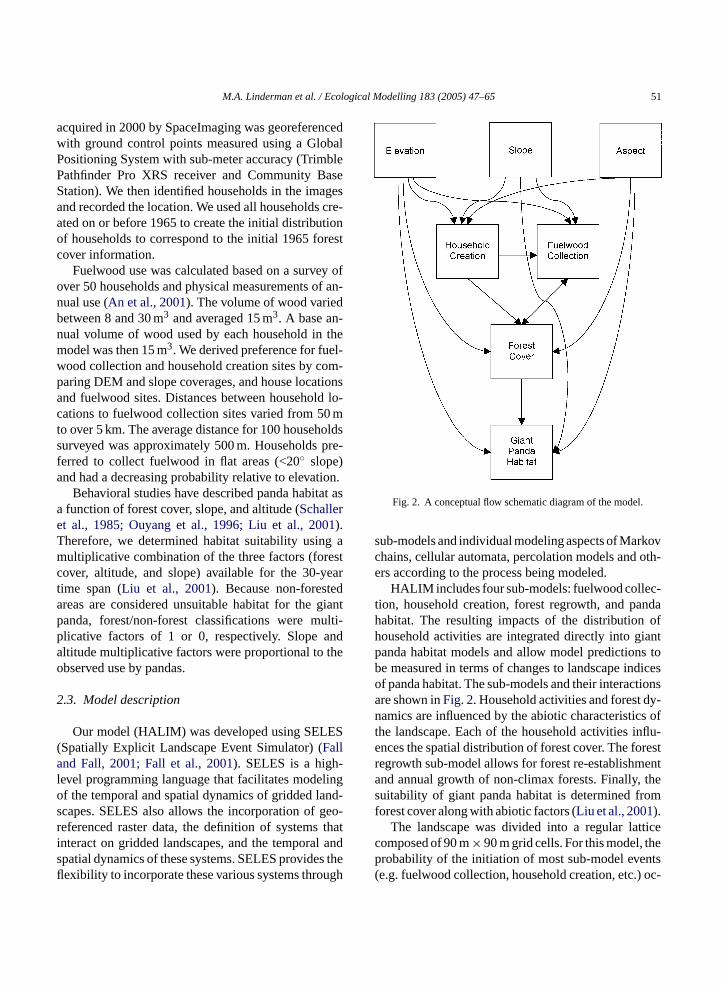
Fig. 2. A conceptual flow schematic diagram of the model.

ub-models and individual modeling aspects of Marhains, cellular automata, percolation models andrs according to the process being modeled.

HALIM includes four sub-models: fuelwood colleion, household creation, forest regrowth, and paabitat. The resulting impacts of the distributionousehold activities are integrated directly into ganda habitat models and allow model predictione measured in terms of changes to landscape inf panda habitat. The sub-models and their interacre shown inFig. 2. Household activities and forest damics are influenced by the abiotic characteristic

he landscape. Each of the household activities inces the spatial distribution of forest cover. The foegrowth sub-model allows for forest re-establishmnd annual growth of non-climax forests. Finally,uitability of giant panda habitat is determined frorest cover along with abiotic factors (Liu et al., 2001).

The landscape was divided into a regular latticeomposed of 90 m× 90 m grid cells. For this model, therobability of the initiation of most sub-model eventse.g. fuelwood collection, household creation, etc.) oc-

5 logica

c ixelv dingo r ofs l pa-r allyd itha oc-c witha bil-i cesso entst notc iono oodc

ex-a s:

• e-bil-

ionhegingd byscol-

theandnceilityath

s a

eter-elyestel-of

stedofn a

•

ble.fectholdined.h itsoc-n ofagri-tesodelters:otichecelds,nd,ere

tablelope,ity

rewasdatalely

sht.

andithinjor

• st,andtheand

zoneer-ed


urring at each grid cell was determined by the palues (data layer values) of the cell and, depenn the sub-model, surrounding cells. The numbeub-model events is determined by the sub-modeameters with the location of the event stochasticetermined by a relative cell probability (e.g. a cell wprobability of 0.5 has twice the probability of the

urrence of a landscape event compared to a cell0.25 probability, but does not have a 50% proba

ty of an event occurrence). Depending on the prof interest the model also allows for landscape ev

o spread to neighboring cells (e.g. if a cell doesontain sufficient fuelwood for the annual collectf a household’s fuelwood needs, necessary fuelwollection can take place in a neighboring cell).

The sub-models are described below along withmples of the parameters and probability function

Fuelwood collection– It was assumed that houshold residents collect fuelwood based on availaity, accessibility, and previous fuelwood collectactivity. Typically, fuelwood is collected around thousehold. As these areas are diminished, foraextends to the neighboring areas characterizeeasy accessibility (Liu et al., 2001). Many residenthave been forced to travel several kilometers tolect annual stocks of fuelwood (An et al., 2001).Accessibility is characterized in this model bydistance to collection site, slope, and elevationis defined as a cost function relative to the distato roads and main paths and topographic variab(i.e. slope and elevation difference along the pto the cell location). The probability function walinearly decreasing function of increasing cost:

P(fuelwood|cost)=(

1 −(

Cost

Maximum cost

))

Forest cover and average yield per hectare dmined availability. Households are also more likto return to the same cell location, if sufficient forvolume exists, or neighboring cells of previous fuwood extraction. Therefore, a higher probabilitycollection was assigned to cells previously harveand to neighboring cells. The overall probabilityfuelwood extraction for each forested cell is the
multiplicative combination of these factors.Household creation– The number of new house-holds each year was predetermined based onpotential policy and socio-economic impacts. For
l Modelling 183 (2005) 47–65

example, past trends have been relatively staPolicies, however, have been shown to afhousehold creation. Therefore, a range of housecreation rates about the past trend was examEach new household was presumed to establisown agriculture land, clearing the forest area orcupying previously deforested area. The locatioeach new household was dependant on suitableculture land and proximity to transportation rouand other households. The household sub-mwas, therefore, determined by three paramedistance–cost factor to transportation, abifactors, and proximity to other households. TpreciseX andY coordinates of the actual residenwere not included in this model. Rather, househoincluding the physical residence, agriculture lagarden area, and various other buildings, wpresumed to occupy cells of the landscape. Suiagriculture areas are based on abiotic factors: saspect, and elevation. While agriculture activoccurs on slopes up to 40◦, low-slope areas apreferred. Preference for low-elevation areasalso considered. For example, based on surveyprobabilities for household placement based soon elevation were measured as:

P(household|e) =

{0.00 (e > 2500)}{0.08 (2250< e ≤ 2500)}{0.82 (1750< e ≤ 2250)}{1.00 (e ≤ 1750)}

In areas of higher elevation (e), preference wagiven to slopes facing south to maximize sunligHouseholds were also more likely to develop ladjacent to previously established houses and wshort distances (typically less than 2 km) of matransportation routes.Forest cover– Four forest categories (non-foreevergreen broadleaf, deciduous broadleaf,subalpine conifer) were identified throughoutreserve based on remote sensing, elevation,species distribution (Schaller et al., 1985). Initialstand volume was estimated for each elevationbased on approximate time and intensity of commcial logging activity. Each forested cell was assum
to increase in biomass and each non-forested pixelhad a probability to re-establish based on proximityto other forest pixels and time since deforestation.Regrowth models were derived for each of the pre-

logica

rom

prox-e.

tile-gmether.

• nourally

tedmnt.ilityicson,

restr firstl stab-l lturald nualf re-g ilityo

2

ereb itiald off pho-t wasb 965.T for3dvh

t ualp onet e tom

holda thes f itsc byc yingp eholdd ntedt thes func-t otici . Wem etricsb con-d ualp thep ions incep estsb nty,s restsw

se-h ictedl ions.P thei has-t tiala ar-e olde nt ofh larlyc rcento (1,2

redb ts tof ex-a s andt to ad (i.e.


dominant species within each elevation zone fpublished and empirical data (Yang and Li, 1992).Regrowth is calculated based on species and apimations of logistic regrowth curves of total volumAn example of the calculation is given below:

V (t, Van, Vmax) = {0.0 (t < tlag)}{V + Van(t>tlag andV<Vmax)}

where t is the time since harvest,tlag is a nor-mally distributed lag time since harvest unre-establishment,Van is the annual volume incrment, andVmax is the maximum volume accordinto species type. Upper asymptotic limits on voluwere controlled by stand maximum values rathan time due to concurrent fuelwood collectionHabitat suitability– The final habitat classificatiowas a categorized suitability measure of fclasses termed highly suitable, suitable, marginsuitable, and unsuitable (Liu et al., 2001). Theimpacts from household activities are reflecin the habitat suitability model as impacts frofuelwood activity and agriculture developmeMeasures of panda habitat quantity and suitaballow analysis of the temporal and spatial dynamof, the influence of household characteristicsand future giant panda habitat.

Landscape events (e.g. fuelwood collection, foegrowth) occurred on an annual time frame. Theandscape event in the model each year is the eishment of new households and associated agricuevelopment. Each household then collects its an

uelwood volume. At the end of the year, forestrowth occurs for each forested cell and the suitabf panda habitat is updated.

.4. Model validation and sensitivity analyses

Model validation and sensitivity analyses wased on simulations started in 1965 with the inistribution of forest based on the classification

orest/non-forest categories from the 1965 Coronaographs. The original distribution of householdsased on all households established prior to or in 1he sensitivity and validation simulations were run
2 years to correspond to the latest remote sensingata available (1997). We measured sensitivity througharying individual parameters such as the rate of newousehold creation, fuelwood use, and forest charac-
acht

l Modelling 183 (2005) 47–65 53

eristics and the relative influence of each individarameter on the model output. Validation was d

hrough comparison of model output over this timeasured habitat and household distributions.We conducted sensitivity analyses for the house

nd fuelwood collection sub-models. We examinedensitivity of the household sub-model to each oomponents (abiotic, proximity, and cost function)omparing scenarios excluding components or vararameter estimations and the measured housistribution in 1997. This was done because we wa

o show the overall influence each function had onelection of new households and because someions could not be varied systematically (e.g. abinfluences were based on conditional probabilities)

easured accuracy and calculated landscape mased on the average of 20 simulations. We alsoucted systematic analyses of sensitivity of individarameters for the fuelwood sub-model, such asropensity to return to previous fuelwood collectites and distance to fuelwood collection sites. Sarameterization of stand volumes for broadleaf forelow 2600 m contained relatively large uncertaieveral average stand volumes for the broadleaf foere tested, including 30, 45, 60, 75, and 90 m3/ha.The accuracy of the predicted distribution of hou

olds was measured through comparison of predocations of households in 1997 to measured locatrecise cell-by-cell prediction, however, was not

ntention of this model. Foremost, the model is stocic. In addition, households do not occupy all potengricultural areas within the reserve. This leads toas with similar probabilities available for househstablishment. However, as the spatial arrangemeouseholds may have an impact on habitat, particurucial secondary habitat, we also examined the pef predicted households falling in close proximity, and 3 cells) of measured households.

Impacts from fuelwood collection were measuy comparison of predicted and measured impac

orest cover and habitat. Again, we did not expectct correspondence between the model prediction

he measured distributions. Collections sites are,egree, stochastically chosen both by the model
s with households, not all potential fuelwood sites arehosen) and households (i.e. some degree of house-old decisions is unpredictable regardless of informa-
ion available). In addition, the natural variability of the

5 logica

f ca-t iond y ata n-c mentd

u-e alysest tri-b atem od.W ionm ata;d nd ac aredp ualc 97s dm andd d in1 s-s ithe ored ver.A ictedc ictedn Thisi causeo tya verf heh ionsa forc rors.

eent andl , andc gb ndn cyc them de-t ure.T alsorocm

( ss,aG .

2

enth ty ofs sce-n use-h odelp odelp ts ofp ationsw ram-e perh mi-g onsw overt e toc acts.W to gi-a andh

oodc my , 24,1 re-m ns oft possi-b newp s, re-s city.F ndr ub-s ningf re-s on.E form ok-i en-e ture( ono duce


orests was not fully captured in the visual classifiions (i.e. the visual interpretation of forest distributid not include all forest gaps and edge complexit90-m resolution) and illicit logging activities not i

luded in the model make a direct accuracy assessifficult.

To minimize the effect of natural and other inflnces on the accuracy assessments, we limited an

o regions within 5 km of the current household disution. This distance corresponds to the approximaximum distance residents travel to collect fuelwoithin the 5 km buffers, we used three validatethods: visual appraisals of multitemporal direct comparison to a supervised classification; aomparison between landscape indices. We compredicted fuelwood impacts on forest cover to vislassifications of forest cover from 1974 to 19atellite imagery (Liu et al., 2001). We compareeasurements of the distribution of householdsigital classifications of forest cover as measure997 to final outputs from the model. Digital claification of the 1997 forest cover was possible wxtensive ground sample data and provided a metailed snapshot of the distribution of forest coccuracy is reported as the percentage of predells that correspond to measured cells (e.g. predon-forest versus measured non-forest cells).

gnores possible omission errors and was used bef the difficulty in distinguishing natural variabilind human impacts (e.g. illicit logging) on forest co

rom household activities even within 5 km of touseholds. Visual comparisons of model predictnd measured forest cover change are shownomparison between commission and omission er

In addition, comparisons were made betwhe quantity of forest area and disturbed areasandscape metrics such as patch size, shapeomplexity. Given the difficulty in distinguishinetween timber logging, fuelwood collection, aatural variability in forest cover, simple accuraomparisons of the model predictions relative toeasured landscape (particularly those from the

ailed classification) do not provide a complete picthe impacts measured from simulations were
eported as the landscape indices relative to the impactf interest (e.g. household distribution and forestover). Indices used include total number of patches,ean patch size, corrected perimeter to area (p/a) ratio
fgtt

l Modelling 183 (2005) 47–65

Baker and Cai, 1992) describing patch compactnend connectivity between patch centroids (Forman andodron, 1986) that describes clustering of patches

.5. Household impacts

To examine the relative influences of differousehold conditions on the landscape, a variecenarios were run from 1965 until 2030. Eachario was started using 1965 land-cover and hoold data. From 1965 to 1997, we based the marameters on measured values. We then varied marameters for 1997–2030 to examine the impacossible changes. These scenarios represent situhere new policies were introduced after 1997. Paters we examined included fuelwood consumptionousehold and the household growth rate (or imration/emigration rate). The length of the simulatias chosen based on the reliability of the model

he previous 32 years and to permit sufficient timompare various scenarios and predict future impe compared model scenarios based on impacts

nt panda habitat as deforestation from fuelwoodousehold construction removed habitat.

These scenarios included changes in fuelwonsumption levels of 30, 15, 10, 5, and 03/ear/household and household growth rates of 362, 0,−12, and−24 new households created oroved each year after 1997, as well as combinatio

hese parameters. We chose these levels to reflectle future household characteristics resulting fromolicies and management efforts such as subsidietrictions, and/or increased accessibility to electrior example, efforts to limit fuelwood collection aeclaim agriculture land were initiated in 2000. Sidies have been offered in exchange for maintaiorests. The administration has also attempted totrict the location and quantity of fuelwood collectilectricity prices are also currently unaffordableost local farmers, particularly for heating and co

ng purposes. Affordable and consistent alternativergy sources may influence fuelwood use in the fuAn et al., 2002). Each of these or the combinatif these changes may provide an incentive to re

uelwood use. In addition, efforts to encourage emi-ration out of the reserve are being instituted poten-

ially decreasing the number of households. However,here is an increasing preference by younger adults to

logica

e bsidyo ntlyi here-f osef entm thec am-i in-c ationo holdc

3

3

olds e tot ds),s erec testf eree thei erec delp odeli abi-oa sim-i sub-m ize,a ea-s -e holds( acedi s ofe ndt tesyT s themwo ingoar(

onsa dis-tr nceh , 68,a n 0,1T holdse suredt ncef re-d use-h e toc wasn ioticf racyo

fu-e tionsii oodf nta-t tiono re-t hesa mityf and3 ra g ast ncec ingt dis-p is iss allerp n-n ara patchn ches.P r var-i reasei

ndv ucedf in


stablish new households, and in response to supportunities, new households have actually rece

ncreased at much higher rates than in the past. Tore, to reflect the possible range of values, we chuelwood consumption levels ranging from the curraximum known household consumption (double

urrent average) to no fuelwood use. We also exned household creation rates varying from a 50%rease in household establishment to a net emigrf households to reflect policy influences on housereation over the next 30 years.

. Results

.1. Model validation and sensitivity

To examine the overall influence of the househub-model parameters (e.g. topography, distancransportation, and proximity to other householeveral variations of the household sub-model wompared. We could not do a typical sensitivityor this sub-model as some of the parameters wmpirical look-up tables. Therefore, to examine

nfluence of each parameter, model outputs wompared for several combinations of sub-moarameters. For example, the household sub-m

ncluding all three hypothesized parameters (tic, distance, and proximity) (Fig. 3a) resulted inpproximately the same number of patches and

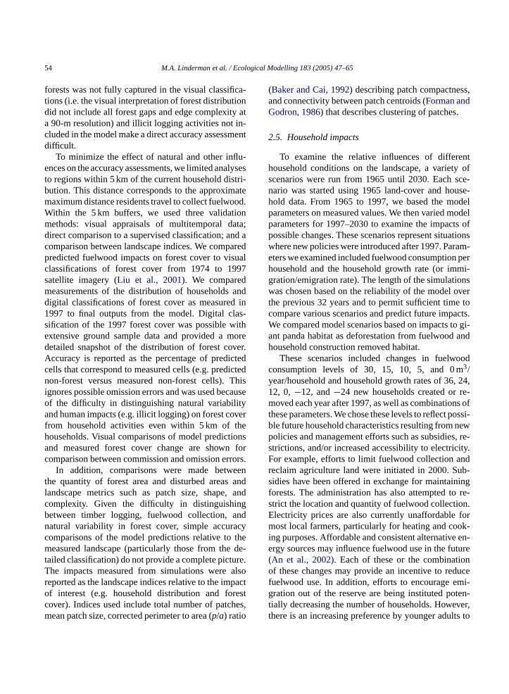
lar p/a ratio as the measured households. Thisodel also led to a 44% larger mean patch snd slightly higher connectivity compared to the mured distribution (Table 1). Excluding abiotic prefrences resulted in 71% more patches of houseTable 1) and caused some households to be pln regions of atypical topographic relief (e.g. areaxtreme slope) (Fig. 3b). Excluding the distance aopographic variation from main transportation rouielded a wide distribution of households (Fig. 3c).he number of patches was more than three timeeasured distribution. Mean patch size andp/a ratioere both considerably lower (Table 1). And, the lackf a proximity factor resulted in decreased clump
f households (low connectivity), smaller patch sizend an increase in the number of patches (Table 1)elative to the measured distribution of householdsFig. 3d).
pusp

l Modelling 183 (2005) 47–65 55

Accuracy in terms of predicted household locatigreeing with measured cell locations of household

ribution varied from 20 to 27% (Table 2). Incorpo-ating all of the parameters hypothesized to influeousehold placement resulted in an accuracy of 27nd 82, and 88% for predicted households withi, 2, and 3 cells from measured households (Table 2).his suggests that the model was predicting housessentially within the same areas as those mea

o also contain households. Not including the distaunction yielded the lowest accuracy of 63% for picted households within 3 cells of measured hoolds. The accuracy was 80% when a preferencreate new households next to existing householdsot included. Excluding the selection based on ab

actors (i.e. slope and elevation) achieved an accuf 81% within 3 cells.

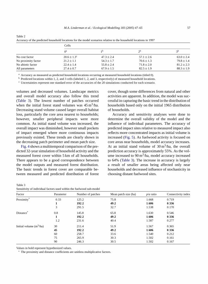
Sensitivity analyses conducted for each of thelwood parameters showed influences from varia

n the distance and proximity factors (Table 3). Relax-ng the tendency for households to collect fuelwrom previously cleared areas led to more fragmeion and is reflected in the landscape metrics. Variaf the proximity factor three times more likely to

urn to previous sites resulted in 35% fewer patcnd 54% larger patch sizes. Reducing the proxi

actor three times resulted and 52% more patches4% smaller patch size (Table 3). In addition, perimetend connectivity indices show increasing clusterin

he proximity factor is increased. Varying the distaost factor by 20% resulted in similar results. Eashe influence of the distance factor generated moreersed impacts occurring in smaller patches. Theen in the patch characteristics with more and smatches and decreasedp/a ratios and diminished coectivity (Table 3). Increased probability of using nereas conversely increased patch size, decreasedumber, and increased connectivity between patatch size varied by 17.9–33.7% and patch numbe

ed by 24.1 and 20.5% for a 20% decrease and incn the cost factor, respectively (Table 3).

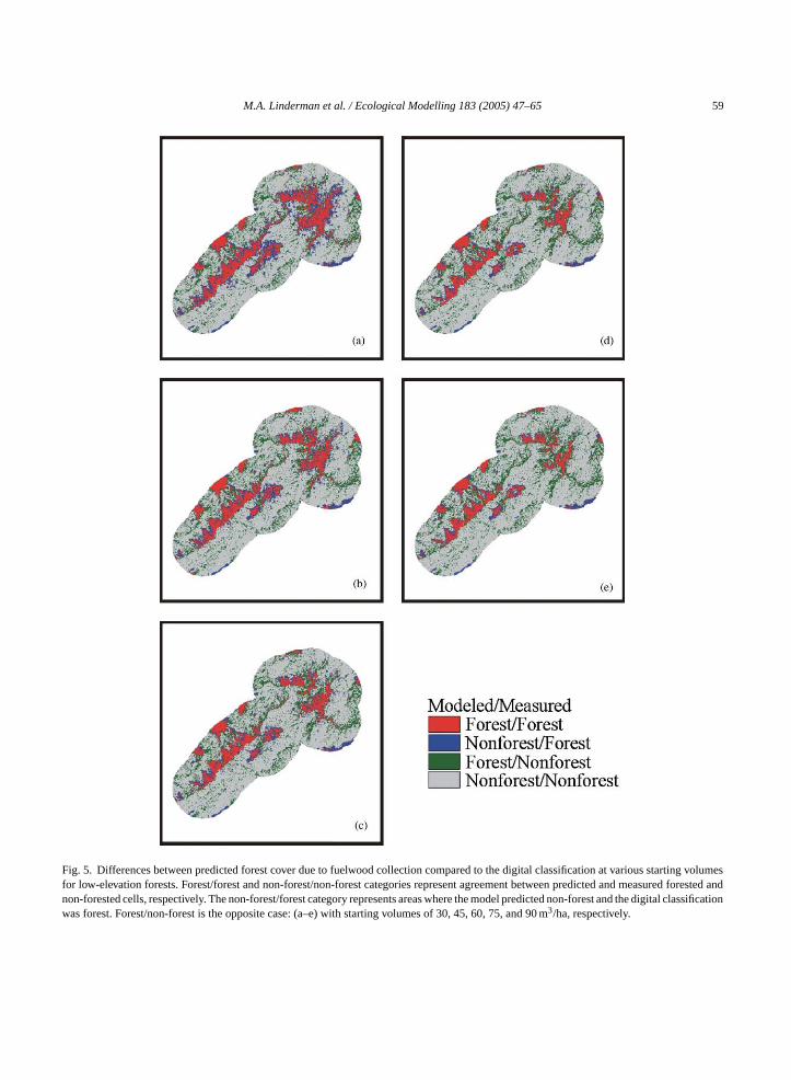
Trends in deforestation relative to initial staolume were decreasing area of impact and redragmentation since more volume was available
referred collection areas (Table 3). While the outputssing each of the five initial volumes shown inFig. 5doeemingly conform largely to expectations, increasederipheral impacts occur at both increased initial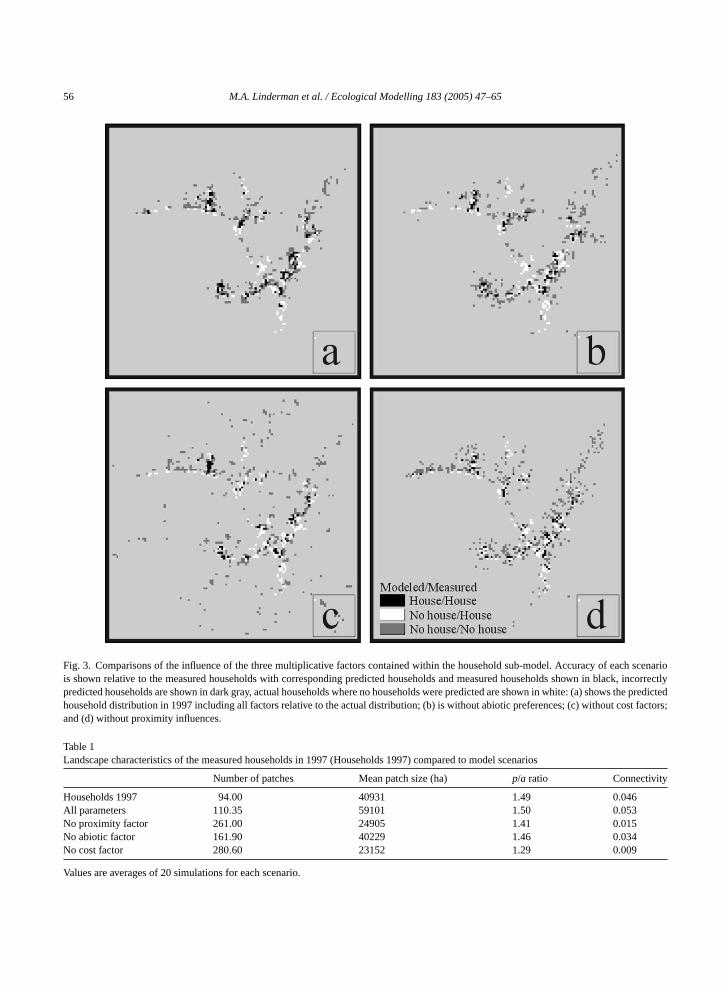

56 M.A. Linderman et al. / Ecological Modelling 183 (2005) 47–65

Fig. 3. Comparisons of the influence of the three multiplicative factors contained within the household sub-model. Accuracy of each scenariois shown relative to the measured households with corresponding predicted households and measured households shown in black, incorrectlypredicted households are shown in dark gray, actual households where no households were predicted are shown in white: (a) shows the predictedhousehold distribution in 1997 including all factors relative to the actual distribution; (b) is without abiotic preferences; (c) without cost factors;and (d) without proximity influences.

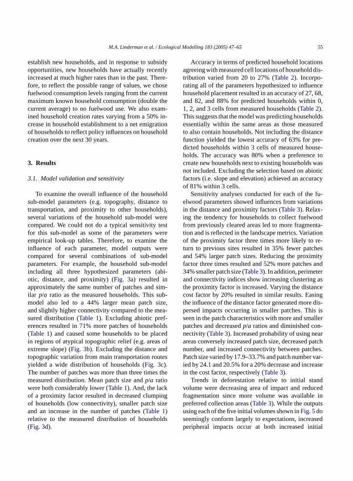
Table 1Landscape characteristics of the measured households in 1997 (Households 1997) compared to model scenarios

Number of patches Mean patch size (ha) p/a ratio Connectivity

Households 1997 94.00 40931 1.49 0.046All parameters 110.35 59101 1.50 0.053No proximity factor 261.00 24905 1.41 0.015No abiotic factor 161.90 40229 1.46 0.034No cost factor 280.60 23152 1.29 0.009

Values are averages of 20 simulations for each scenario.


Table 2Accuracy of the predicted household locations for the model scenarios relative to the household locations in 1997

Cells

0a 1b 2b 3b

No cost factor 20.6± 1.3c 47.3± 2.4 57.1± 2.6 63.0± 2.4No proximity factor 21.2± 1.1 54.3± 1.7 70.6± 1.3 79.8± 1.4No abiotic factor 22.4± 1.4 55.8± 2.4 71.8± 2.0 81.2± 2.3All parameters 27.4± 0.7 67.9± 1.5 82.5± 1.9 88.3± 1.9

ccurrind 3, ress of th

v etricsa nd( redwD bitatl olds;h orec theo ketso actsp n int ize.

re-d them lds.TtTt

TS

F

P

D

I

V

c thera suc-c n ofh tiono

tod thei y ofp alsor e isi nc ases.A llp vol-u ed

a Accuracy as measured as predicted household locations ob Predicted locations within 1, 2, and 3 cells (labeled 1, 2, anc Uncertainties represent one standard error of the accuracie

olumes and decreased volumes. Landscape mnd overall model accuracy also follow this treTable 3). The lowest number of patches occurhen the initial forest stand volumes was 45 m3/ha.ecreasing stand volume caused larger overall ha

oss, particularly the core area nearest to househowever, smaller peripheral impacts were mommon. As initial stand volume was increased,verall impact was diminished, however small pocf impact emerged where more continuous impreviously existed. These trends are clearly show

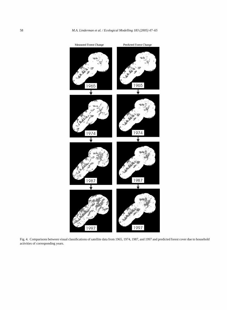
he decreasing patch perimeter and mean patch sFig. 4shows a multitemporal comparison of the p

icted 32-year simulation of household activity andeasured forest cover within 5 km of all househo
here appears to be a good correspondence between
he model outputs and measured forest distribution.he basic trends in forest cover are comparable be-

ween measured and predicted distribution of forest

able 3ensitivity of individual factors used within the fuelwood sub-model

actor Parameter Number of patches

roximity* 0.33 125.21 192.23 291.5

istance* 0.8 145.81 192.21.2 231.6

nitial volume (m3/ha) 30 211.445 192.260 258.775 265.990 246.3

alues in bold represent hypothesized values.∗ The proximity and distance coefficients are unitless multiplicative

tahc

g at measured household locations (titled 0).pectively) of measured household locations.

e 20 simulations conducted for each scenario.

over, though some differences from natural and octivities are apparent. In addition, the model wasessful in capturing the basic trend in the distributioouseholds based only on the initial 1965 distribuf households.

Accuracy and sensitivity analyses were doneetermine the overall validity of the model and

nfluence of individual parameters. The accuracredicted impact sites relative to measured impacteflects more concentrated impacts as initial volumncreased (Fig. 5). As fuelwood activity is focused oore areas near households, model accuracy incret an initial stand volume of 30 m3/ha, the overarediction accuracy is approximately 55%. As theme increased to 90 m3/ha, model accuracy increas

Mean patch size (ha) p/a ratio Connectivity index

75.8 1.668 0.71949.2 1.606 0.33632.7 1.538 0.170

65.8 1.630 0.54649.2 1.606 0.33640.4 1.587 0.277

51.9 1.567 0.36549.2 1.606 0.33633.6 1.540 0.21230.3 1.502 0.16130.5 1.502 0.167

factors.

o 64% (Table 3). The increase in accuracy is largelyresult of smaller areas being affected only near

ouseholds and decreased influence of stochasticity inhoosing distant fuelwood sites.


Fig. 4. Comparisons between visual classifications of satellite data from 1965, 1974, 1987, and 1997 and predicted forest cover due to householdactivities of corresponding years.


Fig. 5. Differences between predicted forest cover due to fuelwood collection compared to the digital classification at various starting volumesfor low-elevation forests. Forest/forest and non-forest/non-forest categories represent agreement between predicted and measured forested andnon-forested cells, respectively. The non-forest/forest category represents areas where the model predicted non-forest and the digital classificationwas forest. Forest/non-forest is the opposite case: (a–e) with starting volumes of 30, 45, 60, 75, and 90 m3/ha, respectively.

60 M.A. Linderman et al. / Ecologica

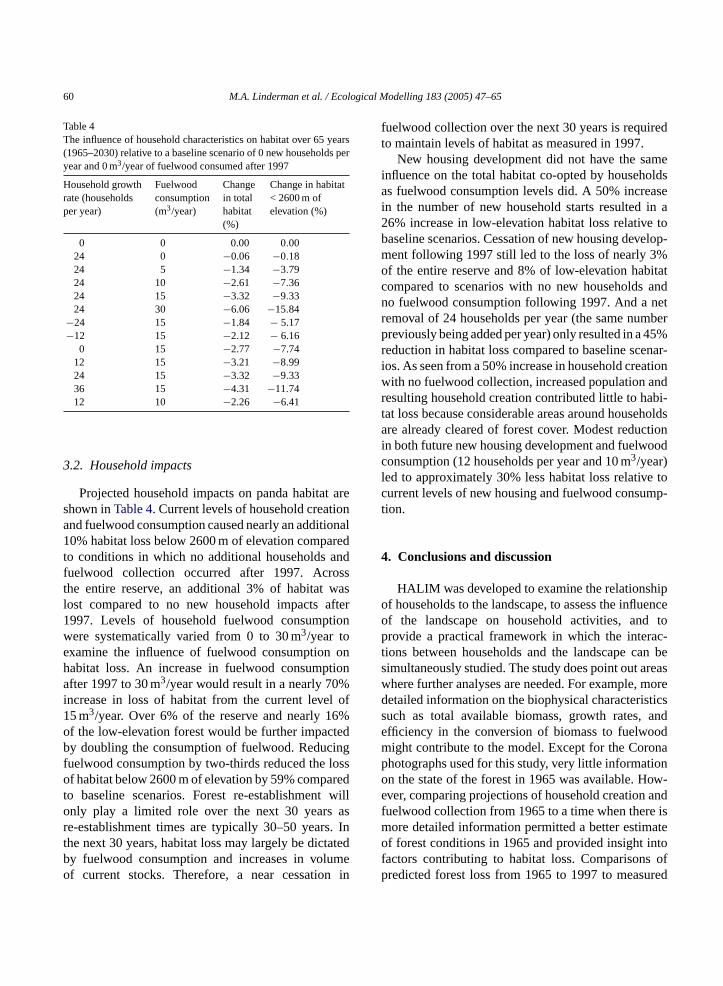
Table 4The influence of household characteristics on habitat over 65 years(1965–2030) relative to a baseline scenario of 0 new households peryear and 0 m3/year of fuelwood consumed after 1997

Household growthrate (householdsper year)

Fuelwoodconsumption(m3/year)

Changein totalhabitat(%)

Change in habitat< 2600 m ofelevation (%)

0 0 0.00 0.0024 0 −0.06 −0.1824 5 −1.34 −3.7924 10 −2.61 −7.3624 15 −3.32 −9.3324 30 −6.06 −15.84

−24 15 −1.84 − 5.17−12 15 −2.12 − 6.16

0 15 −2.77 −7.7412 15 −3.21 −8.9924 15 −3.32 −9.3336 15 −4.31 −11.74

3

t ares iona onal1 redt andf sst wasl fter1 tionwe onh tiona %i l of1 6%o tedb ingf losso redt willo asrtbo

f iredt

amei oldsa asei in a2 e tob elop-m %o itatc andn netr mberp 45%r nar-i ationw andr bi-t eholdsa tioni oodcl e toc mp-t

4

hipo enceo top ac-t n bes reasw mored ticss ande odm onap iono ow-e andf e is

12 10 −2.26 −6.41

.2. Household impacts

Projected household impacts on panda habitahown inTable 4. Current levels of household creatnd fuelwood consumption caused nearly an additi0% habitat loss below 2600 m of elevation compa

o conditions in which no additional householdsuelwood collection occurred after 1997. Acrohe entire reserve, an additional 3% of habitatost compared to no new household impacts a997. Levels of household fuelwood consumpere systematically varied from 0 to 30 m3/year toxamine the influence of fuelwood consumptionabitat loss. An increase in fuelwood consumpfter 1997 to 30 m3/year would result in a nearly 70

ncrease in loss of habitat from the current leve5 m3/year. Over 6% of the reserve and nearly 1f the low-elevation forest would be further impacy doubling the consumption of fuelwood. Reduc

uelwood consumption by two-thirds reduced thef habitat below 2600 m of elevation by 59% compa

o baseline scenarios. Forest re-establishmentnly play a limited role over the next 30 years
e-establishment times are typically 30–50 years. Inhe next 30 years, habitat loss may largely be dictatedy fuelwood consumption and increases in volumef current stocks. Therefore, a near cessation in
mofp

l Modelling 183 (2005) 47–65

uelwood collection over the next 30 years is requo maintain levels of habitat as measured in 1997.

New housing development did not have the snfluence on the total habitat co-opted by househs fuelwood consumption levels did. A 50% incre

n the number of new household starts resulted6% increase in low-elevation habitat loss relativaseline scenarios. Cessation of new housing devent following 1997 still led to the loss of nearly 3f the entire reserve and 8% of low-elevation habompared to scenarios with no new householdso fuelwood consumption following 1997. And aemoval of 24 households per year (the same nureviously being added per year) only resulted in aeduction in habitat loss compared to baseline sceos. As seen from a 50% increase in household creith no fuelwood collection, increased population

esulting household creation contributed little to haat loss because considerable areas around housre already cleared of forest cover. Modest reduc

n both future new housing development and fuelwonsumption (12 households per year and 10 m3/year)ed to approximately 30% less habitat loss relativurrent levels of new housing and fuelwood consuion.

. Conclusions and discussion

HALIM was developed to examine the relationsf households to the landscape, to assess the influf the landscape on household activities, androvide a practical framework in which the inter

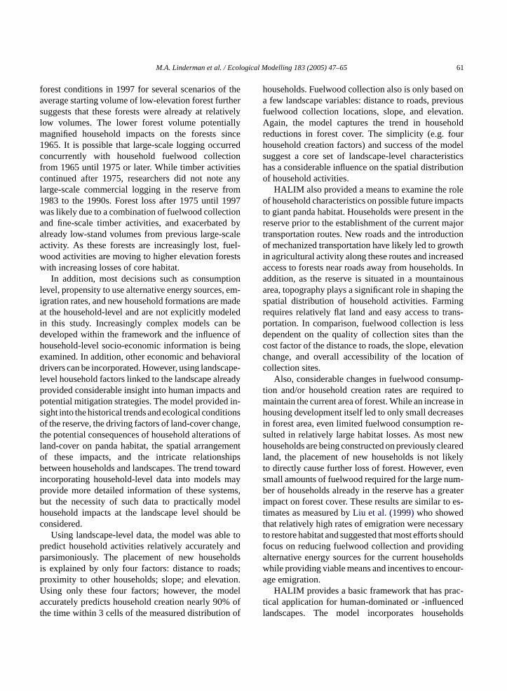
ions between households and the landscape caimultaneously studied. The study does point out ahere further analyses are needed. For example,etailed information on the biophysical characterisuch as total available biomass, growth rates,fficiency in the conversion of biomass to fuelwoight contribute to the model. Except for the Corhotographs used for this study, very little informatn the state of the forest in 1965 was available. Hver, comparing projections of household creationuelwood collection from 1965 to a time when ther
ore detailed information permitted a better estimatef forest conditions in 1965 and provided insight into
actors contributing to habitat loss. Comparisons ofredicted forest loss from 1965 to 1997 to measured

logica

f thea hers tivelyl llym ince1 rredc onf esc anyl rom1 997w iona d bya calea el-w stsw

tionl , em-i adea ledi bed ofh inge iorald ape-l eadyp andp in-s onso nge,t ns ofl mento hipsb wardi ayp ms,b delh d bec

le top andp oldsi ds;pUat

h d ona viousf ion.A holdr urh odels isticsh tiono

oleo actst n ther ajort tiono wthi seda ds. Ina nousa thes ingr ans-p essd thec ationc ofc

mp-t d tom se inh asesi re-s newh aredl elyt vens um-b eateri es-tt saryt houldf inga oldsw our-


orest conditions in 1997 for several scenarios ofverage starting volume of low-elevation forest furtuggests that these forests were already at relaow volumes. The lower forest volume potentia

agnified household impacts on the forests s965. It is possible that large-scale logging occuoncurrently with household fuelwood collectirom 1965 until 1975 or later. While timber activitiontinued after 1975, researchers did not notearge-scale commercial logging in the reserve f983 to the 1990s. Forest loss after 1975 until 1as likely due to a combination of fuelwood collectnd fine-scale timber activities, and exacerbatelready low-stand volumes from previous large-sctivity. As these forests are increasingly lost, fuood activities are moving to higher elevation foreith increasing losses of core habitat.In addition, most decisions such as consump

evel, propensity to use alternative energy sourcesgration rates, and new household formations are mt the household-level and are not explicitly mode

n this study. Increasingly complex models caneveloped within the framework and the influenceousehold-level socio-economic information is bexamined. In addition, other economic and behavrivers can be incorporated. However, using landsc

evel household factors linked to the landscape alrrovided considerable insight into human impactsotential mitigation strategies. The model providedight into the historical trends and ecological conditif the reserve, the driving factors of land-cover cha

he potential consequences of household alteratioand-cover on panda habitat, the spatial arrangef these impacts, and the intricate relationsetween households and landscapes. The trend to

ncorporating household-level data into models mrovide more detailed information of these systeut the necessity of such data to practically moousehold impacts at the landscape level shoulonsidered.

Using landscape-level data, the model was abredict household activities relatively accuratelyarsimoniously. The placement of new househ

s explained by only four factors: distance to roa
roximity to other households; slope; and elevation.sing only these four factors; however, the modelccurately predicts household creation nearly 90% of
he time within 3 cells of the measured distribution of

a

tl

l Modelling 183 (2005) 47–65 61

ouseholds. Fuelwood collection also is only basefew landscape variables: distance to roads, pre

uelwood collection locations, slope, and elevatgain, the model captures the trend in house

eductions in forest cover. The simplicity (e.g. foousehold creation factors) and success of the muggest a core set of landscape-level characteras a considerable influence on the spatial distribuf household activities.

HALIM also provided a means to examine the rf household characteristics on possible future imp

o giant panda habitat. Households were present ieserve prior to the establishment of the current mransportation routes. New roads and the introducf mechanized transportation have likely led to gro

n agricultural activity along these routes and increaccess to forests near roads away from householddition, as the reserve is situated in a mountairea, topography plays a significant role in shapingpatial distribution of household activities. Farmequires relatively flat land and easy access to trortation. In comparison, fuelwood collection is lependent on the quality of collection sites thanost factor of the distance to roads, the slope, elevhange, and overall accessibility of the locationollection sites.

Also, considerable changes in fuelwood consuion and/or household creation rates are requireaintain the current area of forest. While an increaousing development itself led to only small decre

n forest area, even limited fuelwood consumptionulted in relatively large habitat losses. As mostouseholds are being constructed on previously cle

and, the placement of new households is not liko directly cause further loss of forest. However, emall amounts of fuelwood required for the large ner of households already in the reserve has a gr

mpact on forest cover. These results are similar toimates as measured byLiu et al. (1999)who showedhat relatively high rates of emigration were neceso restore habitat and suggested that most efforts socus on reducing fuelwood collection and providlternative energy sources for the current househhile providing viable means and incentives to enc
ge emigration.
HALIM provides a basic framework that has prac-ical application for human-dominated or -influencedandscapes. The model incorporates households

6 logica

d cur-r thel them tiono entss ma-t ssess bood anst use-h hel

A

tra-t c-o ang,

A

S

S

H

F

H romD wersw Ina ortf nis-t theN ndB alI ltha canA ohnD anS onG ter-n ceFoundation of China, the Chinese Academy of Sci-ences, Ministry of Science and Technology of China(G2000046807), and China Bridges International(North America).


irectly into landscapes alongside naturally ocing dynamics and examines the influences ofandscapes on household activities. In addition,

ethod used is flexible enough to allow the integraf additional human and landscape componuch as the more detailed socio-economic inforion discussed above and other natural proceuch as household impacts on understory bamynamics. This approach provides a useful me

o better understand and predict impacts of hoolds on wildlife habitat and interactions with t

andscape.

cknowledgements

We thank the Wolong Nature Reserve Adminision for their logistic support of our fieldwork and regnize the assistance from Jinyan Huang, Jian Y

ppendix A

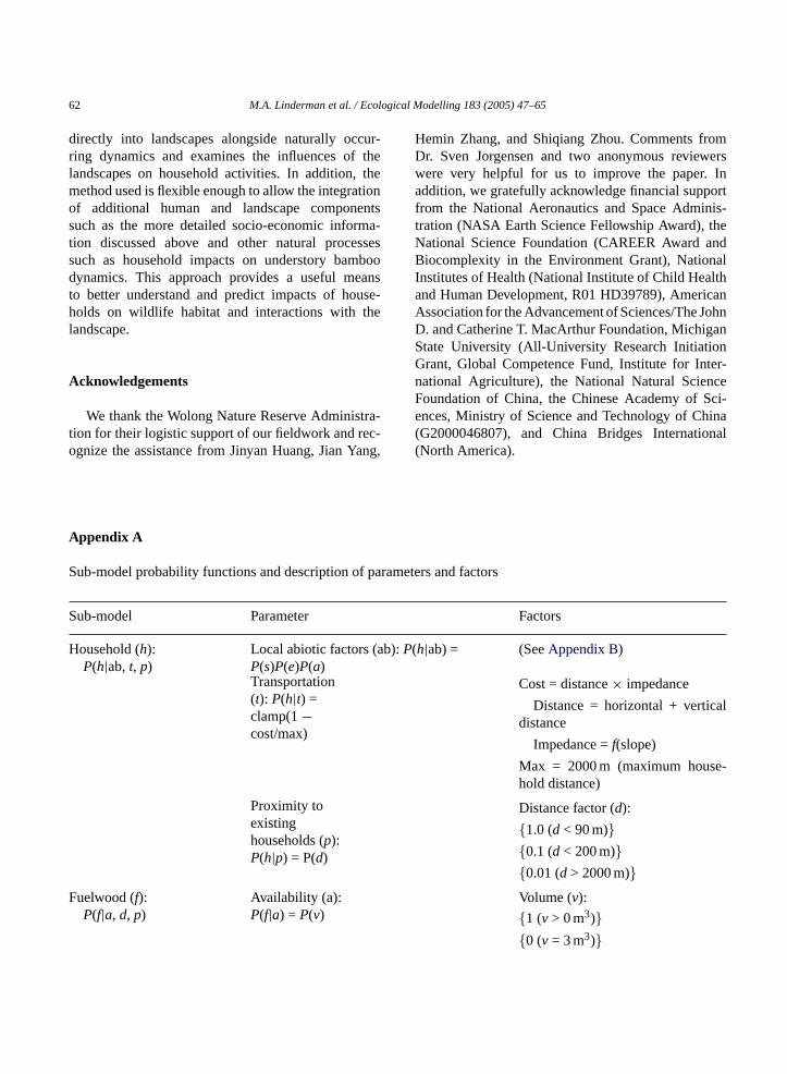
ub-model probability functions and description of para

ub-model Parameter

ousehold (h):P(h|ab,t, p)

Local abiotic factors (ab):P(P(s)P(e)P(a)Transportation(t): P(h|t) =clamp(1−cost/max)

Proximity toexistinghouseholds (p):P(h|p) = P(d)

uelwood (f):P(f|a, d, p)

Availability (a):P(f|a) = P(v)

l Modelling 183 (2005) 47–65

emin Zhang, and Shiqiang Zhou. Comments fr. Sven Jorgensen and two anonymous revieere very helpful for us to improve the paper.ddition, we gratefully acknowledge financial supp

rom the National Aeronautics and Space Admiration (NASA Earth Science Fellowship Award),ational Science Foundation (CAREER Award aiocomplexity in the Environment Grant), Nation

nstitutes of Health (National Institute of Child Heand Human Development, R01 HD39789), Amerissociation for the Advancement of Sciences/The J. and Catherine T. MacArthur Foundation, Michigtate University (All-University Research Initiatirant, Global Competence Fund, Institute for Inational Agriculture), the National Natural Scien

meters and factors

Factors

h|ab) = (SeeAppendix B)

Cost = distance× impedance

Distance = horizontal + verticaldistance

Impedance =f(slope)

Max = 2000 m (maximum house-hold distance)

Distance factor (d):

{1.0 (d < 90 m)}

{0.1 (d < 200 m)}

{0.01 (d > 2000 m)}

Volume (v):

{1 (v > 0 m3)}

{0 (v = 3 m3)}


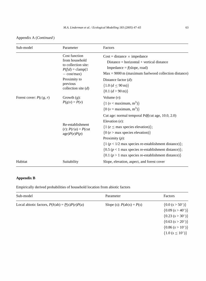
Appendix A (Continued)

Sub-model Parameter Factors

Cost functionfrom householdto collection site:P(f|d) = clamp(1− cost/max)

Cost = distance× impedance

Distance = horizontal + vertical distance

Impedance =f(slope, road)

Max = 9000 m (maximum fuelwood collection distance)

Proximity topreviouscollection site (d)

Distance factor (d):

{1.0 (d≤ 90 m)}

{0.1 (d > 90 m)}

Forest cover:P(c|g, r) Growth (g):P(g|v) = P(v)

Volume (v):

{1 (v < maximum, m3)}

{0 (v = maximum, m3)}

Re-establishment(r): P(r|a) = P(cutage)P(e)P(p)

Cut age: normal temporal Pdf(cut age, 10.0, 2.0)

Elevation (e):

{1 (e≤ max species elevation)};

{0 (e> max species elevation)}

Proximity (p):

{1 (p < 1/2 max species re-establishment distance)};

{0.5 (p < 1 max species re-establishment distance)};

{0.1 (p > 1 max species re-establishment distance)}

Habitat Suitability Slope, elevation, aspect, and forest cover

Appendix B

Empirically derived probabilities of household location from abiotic factors


Local abiotic factors,P(h|ab) =P(s)P(e)P(a) Slope (s): P(ab|s) = P(s) {0.0 (s> 50◦)}

{0.09 (s> 40◦)}

{0.23 (s> 30◦)}

{0.63 (s> 20◦)}

{0.86 (s> 10◦)}

{1.0 (s≤ 10◦)}


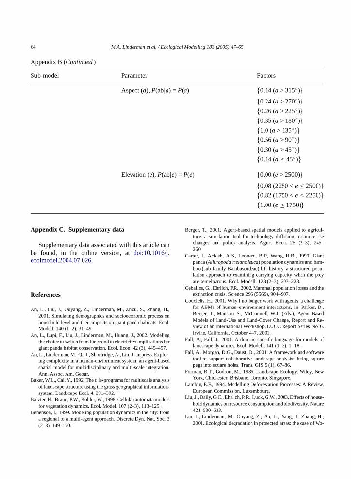
Appendix B (Continued)


Aspect (a), P(ab|a) = P(a) {0.14 (a > 315◦)}

{0.24 (a > 270◦)}

{0.26 (a > 225◦)}

{0.35 (a > 180◦)}

{1.0 (a > 135◦)}

{0.56 (a > 90◦)}

{0.30 (a > 45◦)}

{0.14 (a≤ 45◦)}

Elevation (e), P(ab|e) = P(e) {0.00 (e> 2500)}

{0.08 (2250 <e≤ 2500)}

A

canb .e

R

A H.,ss onEcol.

A ingfor57.

A lor-ased

ion.

B lysisation-

B

B

B ricul-use45–

C iant-

opu-prey

C d the

C ngeD.,sedRe-. 6.

F ls of

F areuare

F New

L view.

ppendix C. Supplementary data

Supplementary data associated with this articlee found, in the online version, atdoi:10.1016/jcolmodel.2004.07.026.

eferences

n, L., Liu, J., Ouyang, Z., Linderman, M., Zhou, S., Zhang,2001. Simulating demographics and socioeconomic procehousehold level and their impacts on giant panda habitats.Modell. 140 (1–2), 31–49.

n, L., Lupi, F., Liu, J., Linderman, M., Huang, J., 2002. Modelthe choice to switch from fuelwood to electricity: implicationsgiant panda habitat conservation. Ecol. Econ. 42 (3), 445–4

n, L., Linderman, M., Qi, J., Shortridge, A., Liu, J., in press. Exping complexity in a human-enviornment system: an agent-bspatial model for multidisciplinary and multi-scale integratAnn. Assoc. Am. Geogr.

aker, W.L., Cai, Y., 1992. The r. le-programs for multiscale anaof landscape structure using the grass geographical informsystem. Landscape Ecol. 4, 291–302.

alzter, H., Braun, P.W., Kohler, W., 1998. Cellular automata modelsfor vegetation dynamics. Ecol. Model. 107 (2–3), 113–125.

enenson, I., 1999. Modeling population dynamics in the city: froma regional to a multi-agent approach. Discrete Dyn. Nat. Soc. 3(2–3), 149–170.

L

L

{0.82 (1750 <e≤ 2250)}

{1.00 (e≤ 1750)}

erger, T., 2001. Agent-based spatial models applied to agture: a simulation tool for technology diffusion, resourcechanges and policy analysis. Agric. Econ. 25 (2–3), 2260.

arter, J., Ackleh, A.S., Leonard, B.P., Wang, H.B., 1999. Gpanda (Ailuropodamelanoleuca) population dynamics and bamboo (sub-family Bambusoideae) life history: a structured plation approach to examining carrying capacity when theare semelparous. Ecol. Modell. 123 (2–3), 207–223.

eballos, G., Ehrlich, P.R., 2002. Mammal population losses anextinction crisis. Science 296 (5569), 904–907.

ouclelis, H., 2001. Why I no longer work with agents: a challefor ABMs of human–environment interactions, in: Parker,Berger, T., Manson, S., McConnell, W.J. (Eds.), Agent-BaModels of Land-Use and Land-Cover Change, Report andview of an International Workshop, LUCC Report Series NoIrvine, California, October 4–7, 2001.

all, A., Fall, J., 2001. A domain-specific language for modelandscape dynamics. Ecol. Modell. 141 (1–3), 1–18.

all, A., Morgan, D.G., Daust, D., 2001. A framework and softwtool to support collaborative landscape analysis: fitting sqpegs into square holes. Trans. GIS 5 (1), 67–86.

orman, R.T., Godron, M., 1986. Landscape Ecology. Wiley,York, Chichester, Brisbane, Toronto, Singapore.

ambin, E.F., 1994. Modelling Deforestation Processes: A ReEuropean Commission, Luxembourg.

iu, J., Daily, G.C., Ehrlich, P.R., Luck, G.W., 2003. Effects of house-hold dynamics on resource consumption and biodiversity. Nature421, 530–533.

iu, J., Linderman, M., Ouyang, Z., An, L., Yang, J., Zhang, H.,2001. Ecological degradation in protected areas: the case of Wo-


long Nature Reserve for giant pandas. Science 292 (5514), 98–101.

Liu, J., Ouyang, Z., Yang, Z., Taylor, W., Groop, R., Tan, Y., Zhang,H., 1999. A framework for evaluating the effects of human factorson wildlife habitat: The case of giant pandas. Conservation Biol.13 (6), 1360–1370.

Mertens, B., Lambin, E.F., 1997. Spatial modeling of deforestationin southern Cameroon. Appl. Geography 17 (2), 143–162.

Ouyang, Z., Tang, Y., Zhang, H., 1996. Biodiversity spatial patternanalysis in Wolong. China Man Biosphere, 3.

Reid, D.G., Hu, J., Dong, S., Wang, W., Huang, Y., 1989. GiantpandaAiluropoda melanoleucabehaviour and carrying capacityfollowing a bamboo die-off. Biol. Conservation 49, 85–104.

Rutledge, D.T., Lepczyk, C.A., Xie, J., Liu, J., 2001. Spatio-temporaldynamics of endangered species hotspots in the United States.Conservation Biol. 15 (2), 475–487.

Schaller, G.B., Hu, J., Pan, W., Zhu, J., 1985. The Giant Pandas ofWolong. The University of Chicago Press, Chicago and London.

Vitousek, P.M., Mooney, H.A., Lubchenco, J., Melillo, J.M., 1997.Human domination of Earth’s ecosystems. Science 277 (5325),494–499.

Wu, H., Stoker, R.L., Gao, L.C., 1996. A modified Lotka-Volterrasimulation model to study the interaction between arrow bam-boo (Sinarundinaria fangiana) and giant panda (Ailuropodamelanoleuca). Ecol. Model. 84 (1–3), 11–17.

Yang, Y., Li, C. (Eds.), 1992. Sichuan Forests. China Forestry Press,Yunnan.

Zhang, H., Li, D., Wei, R., Tang, C., Tu, J., 1997. Advances in conser-vation and studies on reproductivity of giant pandas in Wolong.Sichuan J. Zool. 16, 31–33.

Zhou, Z.H., Pan, W.S., 1997. Analysis of the viability of a giantpanda population. J. Appl. Ecol. 34 (2), 363–374.

Modeling the spatio-temporal dynamics and interactions of households, landscapes, and giant panda...

Documents

Transcript of Modeling the spatio-temporal dynamics and interactions of households, landscapes, and giant panda...