Particle Identification with theEndcap Disc DIRC for PANDA

Dissertation zur Erlangung des

Doktorgrades der Naturwissenschaften

im Fachbereich 07

(Mathematik und Informatik, Physik, Geographie)

der Justus-Liebig-Universitat Gießen

vorgelegt von

Mustafa Andre Schmidt,

II. Physikalisches Institut

Justus-Liebig-Universitat Gießen

Gießen,

Dezember 2017

For Khadija,my beloved daughter

and source of inspiration.

Abstract

The PANDA experiment at the FAIR (Facility for Antiproton and Ion Research) accel-erator complex in Darmstadt is designed to study hadronic interactions of antiprotonswith momenta up to 15 GeV/c, scattered off an internal proton target. For the purposeof excellent particle identification, two Cherenkov detectors for the target spectrometerare currently under development: The Barrel DIRC with a cylindrical shape around thetarget and the Endcap Disc DIRC (EDD) that will be placed in the forward endcap regionof the PANDA target spectrometer.

The EDD covers the polar angle range 5 ≤ θ ≤ 22. It is designed to separate pionsand kaons up to momenta of p = 4 GeV/c with a minimum π/K separation power of 3standard deviations. The desired detector performance regarding the Cherenkov angleresolution and photon yield for different setups and parameters has been validated withthe help of Monte-Carlo simulations. One of the main goals was the implementation ofthe dedicated simulation and reconstruction algorithms in the analysis framework Pan-daRoot.

In addition to that, an analysis of a specific physics channel including the decay of theglueball candidate f0(1500) has been performed. New testbeam results obtained in theDESY facility with an upgraded detector prototype have been analyzed and comparedwith Monte-Carlo simulations in order to validate the desired detector resolution andphoton yield.

The free running data acquisition in PANDA requires an online reconstruction for alldetectors in combination with event filtering algorithms. As a feasibility study, as simpleonline reconstruction algorithm has been designed and tested on an FPGA board. It canbe extended to provide event filtering in the final detector.

Furthermore, the upgrade of an existing device for cosmic muons in combination witha EDD prototype has been investigated. This test stand is planed to be used for detailedtests of the detector prototype and final detector.

i

Zusammenfassung

Das PANDA-Experiment am FAIR (Facility for Antiproton and Ion Research) Beschleu-nigerkomplex in Darmstadt wurde entwickelt, um hadronische Wechselwirkungen vonAntiprotonen mit Impulsen bis 15 GeV/c zu studieren, die an einem internen Protonen-target gestreut werden. Um eine exzellente Teilchenidentifikation zu gewahrleisten, wer-den zur Zeit zwei Cherenkov-Detektoren fur das Target-Spektrometer entwickelt: DerBarrel DIRC, der in zylindrischer Form das Targetspektrometer umhullt und der EndcapDisc DIRC (EDD), der an der vorderen Endkappe des Target-Spektrometers angebrachtwerden soll.

Der EDD deckt den Polarwinkelbereich 5 ≤ θ ≤ 22 ab. Er wird zur Separationvon Pionen und Kaonen mit Impulsen bis zu p = 4 GeV/c mit einer π/K Separati-onsfahigkeit von mindestens 3 Standardabweichungen genutzt. Das gewunschte Detek-torverhalten in Bezug auf die Auflosung des Cherenkov-Winkels und die Photonenzahlfur verschiedene Design-Konfigurationen ist mit der Hilfe von Monte-Carlo-Simulatio-nen untersucht worden. Eines der wichtigsten Ziele ist die Implementierung zugehorigerSimulations- und Rekonstruktionsalgorithmen in das Analyse-System PandaRoot.

Zusatzlich dazu ist ein bestimmter Physikkanal analysiert worden, der den Zerfall ei-nes Glueball-Kandidaten f0(1500) beinhaltet. Die aktuellen Ergebnisse des letzten Test-beams am DESY mit einem erweiterten Prototypen sind analysiert und mit Monte-Carlo-Simulationen verglichen worden, um zu zeigen, dass die gewunschte Detektorauflosungerreicht werden kann.

Die kontinuierliche Datennahme in PANDA macht eine Online-Rekonstruktion fur alleDetektoren in Kombination mit dem Filtern von Events notig. In einer Machbarkeitsstu-die wurde ein einfacher Algorithmus fur eine Online-Rekonstruction geschrieben undauf einer FPGA-Karte gestet. Dieser kann erweitert werden, um im finalen Detektor in-teressante Events herauszufiltern.

Außerdem ist die Aufrustung eines bestehenden Teststandes fur kosmische Myonenzusammen mit einem Prototypen fur den EDD untersucht worden. Dieser Teststand sollfur weitere detaillierte Studien des Prototypen und finalen Detektors verwendet werden.

ii

Contents

List of Acronyms vii

1. Introduction 1

1.1. Overview . . . . . . . . . . . . . . . . . . . . . . . . . . . . . . . . . . . . . . 11.2. Particle Physics . . . . . . . . . . . . . . . . . . . . . . . . . . . . . . . . . . 2

1.2.1. Standard Model of Particle Physics . . . . . . . . . . . . . . . . . . . 21.2.2. Quantum Chromodynamics . . . . . . . . . . . . . . . . . . . . . . . 41.2.3. Meson Spectroscopy . . . . . . . . . . . . . . . . . . . . . . . . . . . 51.2.4. Glueballs . . . . . . . . . . . . . . . . . . . . . . . . . . . . . . . . . . 6

1.3. Cherenkov Effect . . . . . . . . . . . . . . . . . . . . . . . . . . . . . . . . . 81.3.1. Cherenkov Cone . . . . . . . . . . . . . . . . . . . . . . . . . . . . . 81.3.2. Photon Yield . . . . . . . . . . . . . . . . . . . . . . . . . . . . . . . . 10

1.4. Scintillation Process . . . . . . . . . . . . . . . . . . . . . . . . . . . . . . . . 111.4.1. Organic Scintillators . . . . . . . . . . . . . . . . . . . . . . . . . . . 111.4.2. Inorganic Scintillators . . . . . . . . . . . . . . . . . . . . . . . . . . 13

1.5. Optics . . . . . . . . . . . . . . . . . . . . . . . . . . . . . . . . . . . . . . . . 131.5.1. Geometrical Aberration . . . . . . . . . . . . . . . . . . . . . . . . . 131.5.2. Light Refraction . . . . . . . . . . . . . . . . . . . . . . . . . . . . . . 141.5.3. Photon Losses . . . . . . . . . . . . . . . . . . . . . . . . . . . . . . . 17

1.6. Particle Interaction with Matter . . . . . . . . . . . . . . . . . . . . . . . . . 191.6.1. Multiple Scattering . . . . . . . . . . . . . . . . . . . . . . . . . . . . 191.6.2. Energy Loss . . . . . . . . . . . . . . . . . . . . . . . . . . . . . . . . 19

1.7. Photon Sensors . . . . . . . . . . . . . . . . . . . . . . . . . . . . . . . . . . 201.7.1. Silicon Photomultipliers . . . . . . . . . . . . . . . . . . . . . . . . . 201.7.2. Microchannel Plates . . . . . . . . . . . . . . . . . . . . . . . . . . . 21

1.8. CMOS Chips . . . . . . . . . . . . . . . . . . . . . . . . . . . . . . . . . . . . 251.8.1. CMOS Technology . . . . . . . . . . . . . . . . . . . . . . . . . . . . 251.8.2. Active Pixel Sensors . . . . . . . . . . . . . . . . . . . . . . . . . . . 26

2. PANDA 27

2.1. FAIR . . . . . . . . . . . . . . . . . . . . . . . . . . . . . . . . . . . . . . . . 272.2. PANDA Spectrometer . . . . . . . . . . . . . . . . . . . . . . . . . . . . . . 28

2.2.1. Target System . . . . . . . . . . . . . . . . . . . . . . . . . . . . . . . 282.2.2. Magnetic Field . . . . . . . . . . . . . . . . . . . . . . . . . . . . . . 302.2.3. Tracking System . . . . . . . . . . . . . . . . . . . . . . . . . . . . . 302.2.4. Calorimeter . . . . . . . . . . . . . . . . . . . . . . . . . . . . . . . . 322.2.5. PID Detectors . . . . . . . . . . . . . . . . . . . . . . . . . . . . . . . 33

iii

Contents

2.2.6. Forward Spectrometer . . . . . . . . . . . . . . . . . . . . . . . . . . 362.3. Physics Program . . . . . . . . . . . . . . . . . . . . . . . . . . . . . . . . . . 37

2.3.1. Open Charm Studies . . . . . . . . . . . . . . . . . . . . . . . . . . . 372.3.2. Exotic Matter & Nuclear Form Factors . . . . . . . . . . . . . . . . . 372.3.3. Hypernuclear Physics . . . . . . . . . . . . . . . . . . . . . . . . . . 38

2.4. Data Acquisition . . . . . . . . . . . . . . . . . . . . . . . . . . . . . . . . . 392.4.1. Requirements . . . . . . . . . . . . . . . . . . . . . . . . . . . . . . . 392.4.2. Compute Nodes . . . . . . . . . . . . . . . . . . . . . . . . . . . . . 41

3. Disc DIRC Detector 43

3.1. Detector Setup . . . . . . . . . . . . . . . . . . . . . . . . . . . . . . . . . . . 433.1.1. Geometry . . . . . . . . . . . . . . . . . . . . . . . . . . . . . . . . . 433.1.2. Assembly . . . . . . . . . . . . . . . . . . . . . . . . . . . . . . . . . 443.1.3. Magnetic Field . . . . . . . . . . . . . . . . . . . . . . . . . . . . . . 45

3.2. Readout System . . . . . . . . . . . . . . . . . . . . . . . . . . . . . . . . . . 463.2.1. MCP Based Readout . . . . . . . . . . . . . . . . . . . . . . . . . . . 463.2.2. Front End Electronics . . . . . . . . . . . . . . . . . . . . . . . . . . 46

3.3. Reconstruction & Particle Identification . . . . . . . . . . . . . . . . . . . . 473.3.1. Geometrical Model . . . . . . . . . . . . . . . . . . . . . . . . . . . . 473.3.2. Calibration . . . . . . . . . . . . . . . . . . . . . . . . . . . . . . . . . 493.3.3. Reconstruction Algorithm . . . . . . . . . . . . . . . . . . . . . . . . 503.3.4. Hit Pattern Matching . . . . . . . . . . . . . . . . . . . . . . . . . . . 533.3.5. Separation Power & Misidentification . . . . . . . . . . . . . . . . . 53

3.4. Resolution Studies . . . . . . . . . . . . . . . . . . . . . . . . . . . . . . . . 543.4.1. Theoretical Description . . . . . . . . . . . . . . . . . . . . . . . . . 543.4.2. Simplified Monte-Carlo Simulations . . . . . . . . . . . . . . . . . . 55

3.5. Photon Trapping . . . . . . . . . . . . . . . . . . . . . . . . . . . . . . . . . 57

4. Simulation Studies 59

4.1. PandaRoot Framework . . . . . . . . . . . . . . . . . . . . . . . . . . . . . . 594.1.1. Data Flow . . . . . . . . . . . . . . . . . . . . . . . . . . . . . . . . . 594.1.2. Detector Geometry . . . . . . . . . . . . . . . . . . . . . . . . . . . . 604.1.3. Simulation Parameters . . . . . . . . . . . . . . . . . . . . . . . . . . 62

4.2. Track Reconstruction . . . . . . . . . . . . . . . . . . . . . . . . . . . . . . . 644.2.1. Track Fitting . . . . . . . . . . . . . . . . . . . . . . . . . . . . . . . . 644.2.2. Helix Propagator . . . . . . . . . . . . . . . . . . . . . . . . . . . . . 654.2.3. Track Resolution . . . . . . . . . . . . . . . . . . . . . . . . . . . . . 67

4.3. Time Based Simulations . . . . . . . . . . . . . . . . . . . . . . . . . . . . . 684.4. Geometrical Reconstruction . . . . . . . . . . . . . . . . . . . . . . . . . . . 694.5. Detector Performance . . . . . . . . . . . . . . . . . . . . . . . . . . . . . . . 70

4.5.1. Probe Tracks . . . . . . . . . . . . . . . . . . . . . . . . . . . . . . . . 704.5.2. High Resolution Studies . . . . . . . . . . . . . . . . . . . . . . . . . 72

4.6. Benchmark Channel . . . . . . . . . . . . . . . . . . . . . . . . . . . . . . . 754.6.1. Event Generation . . . . . . . . . . . . . . . . . . . . . . . . . . . . . 76

iv

Contents

4.6.2. Combined Likelihood . . . . . . . . . . . . . . . . . . . . . . . . . . 77

4.6.3. Mass Reconstruction . . . . . . . . . . . . . . . . . . . . . . . . . . . 78

4.7. Further Analysis . . . . . . . . . . . . . . . . . . . . . . . . . . . . . . . . . . 78

5. Cosmics Test Stand 81

5.1. Cosmic Muons . . . . . . . . . . . . . . . . . . . . . . . . . . . . . . . . . . . 81

5.1.1. Muon Creation . . . . . . . . . . . . . . . . . . . . . . . . . . . . . . 81

5.1.2. Muon Flux . . . . . . . . . . . . . . . . . . . . . . . . . . . . . . . . . 82

5.1.3. Simulation Parameters . . . . . . . . . . . . . . . . . . . . . . . . . . 83

5.2. Test Stand Upgrade . . . . . . . . . . . . . . . . . . . . . . . . . . . . . . . . 83

5.2.1. Proposed Setup . . . . . . . . . . . . . . . . . . . . . . . . . . . . . . 83

5.2.2. Track Reconstruction . . . . . . . . . . . . . . . . . . . . . . . . . . . 86

5.2.3. Resolution Studies . . . . . . . . . . . . . . . . . . . . . . . . . . . . 88

5.2.4. Detector Calibration . . . . . . . . . . . . . . . . . . . . . . . . . . . 89

5.3. Alternative Approaches . . . . . . . . . . . . . . . . . . . . . . . . . . . . . 90

5.3.1. CMOS Camera Modules . . . . . . . . . . . . . . . . . . . . . . . . . 90

5.3.2. Single Photon Camera . . . . . . . . . . . . . . . . . . . . . . . . . . 93

6. Online Reconstruction 95

6.1. Online Reconstruction Algorithm . . . . . . . . . . . . . . . . . . . . . . . . 95

6.2. SiTCP Package . . . . . . . . . . . . . . . . . . . . . . . . . . . . . . . . . . . 96

6.3. Testing FPGA Board . . . . . . . . . . . . . . . . . . . . . . . . . . . . . . . 97

6.4. Computation Algorithms . . . . . . . . . . . . . . . . . . . . . . . . . . . . 97

6.4.1. Lookup Tables . . . . . . . . . . . . . . . . . . . . . . . . . . . . . . . 98

6.4.2. CORDIC Algortihm . . . . . . . . . . . . . . . . . . . . . . . . . . . 99

6.4.3. Further Numerical Algorithms . . . . . . . . . . . . . . . . . . . . . 101

6.5. Resolution Studies . . . . . . . . . . . . . . . . . . . . . . . . . . . . . . . . 102

7. Testbeam Results 105

7.1. Experimental Setup . . . . . . . . . . . . . . . . . . . . . . . . . . . . . . . . 105

7.1.1. Testbeam Facility . . . . . . . . . . . . . . . . . . . . . . . . . . . . . 105

7.1.2. Testbeam Setup . . . . . . . . . . . . . . . . . . . . . . . . . . . . . . 105

7.1.3. Prototype Configuration . . . . . . . . . . . . . . . . . . . . . . . . . 107

7.2. Data Acquisition . . . . . . . . . . . . . . . . . . . . . . . . . . . . . . . . . 109

7.3. Monte-Carlo Simulations . . . . . . . . . . . . . . . . . . . . . . . . . . . . . 111

7.4. Event Reconstruction . . . . . . . . . . . . . . . . . . . . . . . . . . . . . . . 112

7.4.1. Resolution & Photon Yield . . . . . . . . . . . . . . . . . . . . . . . 112

7.4.2. Event Combination . . . . . . . . . . . . . . . . . . . . . . . . . . . . 114

7.4.3. Result Extrapolation . . . . . . . . . . . . . . . . . . . . . . . . . . . 115

8. Conclusion & Outlook 117

A. Simulation Results 119

v

Contents

B. Testbeam Results 121

List of Figures 127

List of Tables 129

Bibliography 134

vi

List of Acronyms

ADC Analog-to-Digital Converter

ALD Atomic Layer Deposition

APD Avalanche Photo Diode

APS Active Pixel Sensor

ATLAS A Toroidal Large Apparatus

ASIC Application-Specific Integrated Circuit

BSDF Bidirectional Reflectance Distribution Function

CAD Computer Aided Design

CERN European Organization for Nuclear Research

CFD Constant Fraction Discriminator

CMOS Complementary metal-oxide-semiconductor

CMS Compact Muon Solenoid

CORDIC Coordinate Rotation Digital Algorithm

CR Collector Ring

DAQ Data Acquisition

DC Data Concentrator

DCR Darkcount Rate

DESY Deutsches Elektron-Synchrotron

DIRC Detection of Internal Reflected Cherenkov Light

dSiPM Digital Silicon Photomultipliers

EDD Endcap Disc DIRC

EMC Electromagnetic Calorimeter

vii

Contents

FAIR Facility for Antiproton and Ion Research

FIFO First In - First Out

FEE Front-End Electronics

FEL Focusing Element

FET Field Effect Transistor

FT Forward Tracker

FSM Finite State Machine

FPGA Field Programmable Grid Array

FS Forward Spectrometer

GEM Gas Electron Multiplier

GPIO general-purpose input/output

GSI Gesellschaft fur Schwerionenforschung

HEP High Energy Physics

HESR High Energy Storage Ring

LAPD Large Area Photo Diode

LQCD Lattice QCD

LINAC Linear Accelerator

LHC Large Hadron Collider

LUT Lookup Table

LSB Least Significant Bit

MCP Microchannel Plate

MDT Micro-Drift Tube

MOSFET metal-oxide-semiconductor field-effect-transistor

MVD Micro Vertex Detector

NIM Nuclear Instrument Standard

NMOS N-type metal-oxide-semiconductor

OS Operating System

viii

Contents

PANDA Antiproton Annihilation at Darmstadt

PASTA PANDA Strip ASIC

PCB Printed Circuit Board

PDE Photon Detection Efficiency

PDF Probability Density Function

PET Positron Electron Tomography

PID Particle Identification

pin positive intrinsic negative

PMT Photo Multiplier Tube

PWO Lead Tungsten Oxide

RAM Random Access Memory

RESR Recycled Experimental Storage Ring

RICH Ring Imaging Detector

RMS Root Mean Square

ROM Readout Module

SciTil Scintillator Tile

SiPM Silicon Photomultiplier

SIS Schwerionen-Synchrotron

SLAC Stanford Linear Accelerator

SM Standard Model of Particle Physics

SODA Synchronization of Data Acqusition

STT Straw Tube Tracker

TCP Transmission Control Protocol

TDC Time to Digital Converter

TDR Technical Design Report

TIS Total Integrated Scattering

TOF Time of Flight

ix

Contents

TOFPET Time of Flight Positron Electron Tomography

ToT Time over Threshold

TOP Time of Propagation

TRB TDC Readout Board

TS Target Spectrometer

TTL Transistor-Transistor Logic

QED Quantum Electrodynamics

QCD Quantum Chromodynamics

VHDL Very High Speed Integrated Circuit Hardware Description Language

VMC Virtual Monte-Carlo

x

1. Introduction

1.1. Overview

For precision measurements of physics inside the SM or discoveries outside the SM, alarge variety of particle accelerators for leptons, hadrons, or ions have been produced.One famous example is the LHC in Geneva (Switzerland) which is designed as a storagering for protons with a center-of-mass energy up to 14 TeV [BCL+04]. Particle collisions,that take place in these accelerators, are measured in sophisticated detector systems andconsist of subsystems that serve dedicated services. With the first 4π detector in historyof high energy physics, the so-called Mark I at SLAC, the discovery of the J/ψ and τlepton was possible [DC66].

A new 4π detector called PANDA, which will be used in the future FAIR facility, is afixed-target spectrometer for proton-antiproton collisions with a typical onion-shell con-figuration for studying a large spectrum of physics programs. A detailed overview overthe PANDA spectrometer including all subdetectors will be given in chapter 2. A hugeamount of interesting particle decays, which are planed to be observed in PANDA, re-sult in a production of charged pions and kaons in the final state. Therefore, an excellentPID of these two particle types, which will be performed by three Cherenkov detectors,is very important. One of these Cherenkov detectors is a RICH detector in the forwarddirection and the two others are DIRC detectors near the interaction point surroundingthe target in order to cover the full solid angle.

The Barrel DIRC will cover the polar angle range 22 ≤ θ < 140 while the Disc DIRCdetector is designed for the polar angle interval 5 ≤ θ < 22. In this polar angle region,the Disc DIRC is designed to provide a separation power of 3 standard deviations forthe separation of π± and K±. Chapter 3 introduces the Disc DIRC detector and describesthe most important physics parameters for understanding the details of the detector andfurther simulation analysis.

The content of this thesis and my work related to the Disc DIRC development can be di-vided into the following 4 major categories: The main subject has been the optimizationof the Disc DIRC detector by using Monte-Carlo simulations. Several design conceptswith different parameters have been investigated before the decision for the actual de-sign has been made. All obtained results regarding detector performance and PID for aspecific benchmark channel are presented in chapter 4.

Furthermore, a cosmics test stand has been developed at the University of Giessenwhich will be used to study the detector performance with cosmic muons instead ofhadrons. For the design optimization regarding the spatial and angular resolution of thetest stand, Monte-Carlo studies have been performed and will be discussed in chapter 5.

1

1. Introduction

Additionally, this chapter includes two other design options of the test stand that hadbeen investigated previously.

Since a hardware trigger will be absent in PANDA, an online reconstruction of theCherenkov angle in combination with event-filtering algorithms has to be applied as anonline trigger before the data from the FEEs can be stored. A prototype for such anonline reconstruction algorithm has been designed and tested with an ML403 Virtex-4FPGA board. The results will be summarized and discussed in chapter 6.

Finally, a prototype of the EDD has been developed, and the performance had beenstudied in the year 2016 during a testbeam campaign at DESY. Special analysis tech-niques have been used to analyze the testbeam data and to compare the results to ded-icated Monte-Carlo simulations. The setup and analysis together with the promisingresults will be described in Chapter 7.

1.2. Particle Physics

1.2.1. Standard Model of Particle Physics

The SM contains a canonical summary of all discoveries on the scale of elementary par-ticles. It consists of 12 elementary particles that are grouped into 3 generations, and 4vector bosons. Each generation includes one pair that consists of one lepton and the neu-trino. The first generation contains the electron e and the electron neutrino νe. The secondgeneration includes the muon µ and the muon neutrino νµ while the tau τ and tau neu-trino ντ are located in the third generation. Additionally, the SM contains the followingsix quarks: up u and down d in the first generation, strange s and charm c in the secondone, and top t and bottom b in the third generation.

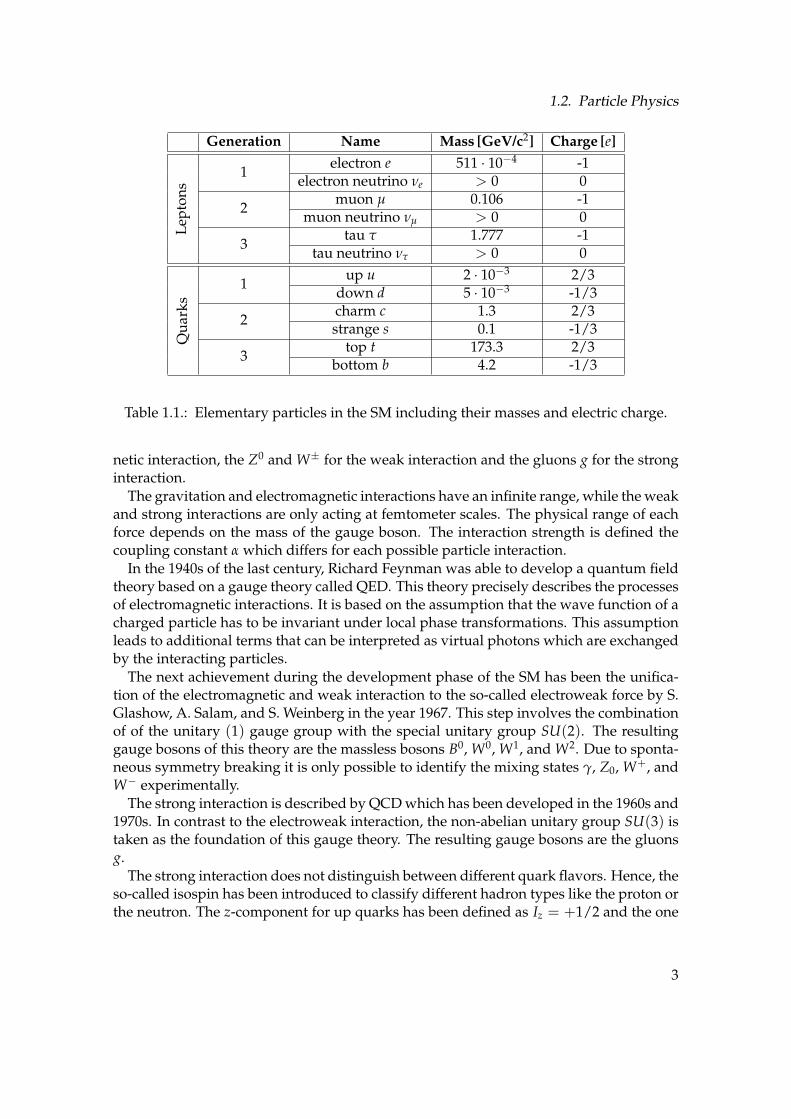
Leptons and quarks are fermions with a half-integer spin. Table 1.1 gives an overviewover these fermions with their masses and electrical charge in units of the elementarycharge e = 1.6 · 10−19 C. All particles with a quark content are called hadrons. Pairsof a quark and an antiquark can combine to particles called mesons while systems, thatcontain 3 quarks, are called baryons. One well-known example is the proton that containstwo up and one down quark. Other multi-quark states with more than 3 quarks arepossible and currently under investigation.

Three interactions between leptons and quarks are described in the SM with the help ofgauge theories: the electromagnetic, the weak and the strong interaction. These 3 forcesdiffer in range, strength and coupling partners. While the weak interaction couples tothe weak charge of all particles, the strong interaction couples only to the color charge ofquarks and the electromagnetic interaction only to electrically charged particles. Addi-tionally, there is the gravitational force that couples to the mass of particles. However, thisfourth interaction could not be implemented into the SM until now. Theories of quantumgravitation in the string theory or loop quantum gravity are subject of actual research.

As a result of the gauge theories, every interaction comes along with at least one so-called gauge boson that has an integer spin and is exchanged between the interactingparticles: the hypothetical graviton for the gravitation, the photon γ for the electromag-

2

1.2. Particle Physics

Generation Name Mass [GeV/c2] Charge [e]

Lep

ton

s1

electron e 511 · 10−4 -1electron neutrino νe > 0 0

2muon µ 0.106 -1

muon neutrino νµ > 0 0

3tau τ 1.777 -1

tau neutrino ντ > 0 0

Qu

ark

s

1up u 2 · 10−3 2/3

down d 5 · 10−3 -1/3

2charm c 1.3 2/3strange s 0.1 -1/3

3top t 173.3 2/3

bottom b 4.2 -1/3

Table 1.1.: Elementary particles in the SM including their masses and electric charge.

netic interaction, the Z0 and W± for the weak interaction and the gluons g for the stronginteraction.

The gravitation and electromagnetic interactions have an infinite range, while the weakand strong interactions are only acting at femtometer scales. The physical range of eachforce depends on the mass of the gauge boson. The interaction strength is defined thecoupling constant α which differs for each possible particle interaction.

In the 1940s of the last century, Richard Feynman was able to develop a quantum fieldtheory based on a gauge theory called QED. This theory precisely describes the processesof electromagnetic interactions. It is based on the assumption that the wave function of acharged particle has to be invariant under local phase transformations. This assumptionleads to additional terms that can be interpreted as virtual photons which are exchangedby the interacting particles.

The next achievement during the development phase of the SM has been the unifica-tion of the electromagnetic and weak interaction to the so-called electroweak force by S.Glashow, A. Salam, and S. Weinberg in the year 1967. This step involves the combinationof of the unitary (1) gauge group with the special unitary group SU(2). The resultinggauge bosons of this theory are the massless bosons B0, W0, W1, and W2. Due to sponta-neous symmetry breaking it is only possible to identify the mixing states γ, Z0, W+, andW− experimentally.

The strong interaction is described by QCD which has been developed in the 1960s and1970s. In contrast to the electroweak interaction, the non-abelian unitary group SU(3) istaken as the foundation of this gauge theory. The resulting gauge bosons are the gluonsg.

The strong interaction does not distinguish between different quark flavors. Hence, theso-called isospin has been introduced to classify different hadron types like the proton orthe neutron. The z-component for up quarks has been defined as Iz = +1/2 and the one

3

1. Introduction

for down quarks as Iz = −1/2. The remaining quarks take their own quantum numbers:the strangeness S for the s, the charmness C for the c, the bottomness B for the b and thetopness T for the t.

In addition to energy, charge and angular momentum conservation for all interactions,a conservation law for S, B, C and T exists for the strong and electromagnetic interaction.Additionally, there is a particle flavor conservation law of all particle reactions. However,the weak and electromagnetic interactions contain some exceptions from these rules. Inboth interactions, the isospin of the particle can change. Additionally, the S, B, C, Tvalues, and the z-component of the isospin Iz are not conserved by the weak interaction.

The phycisist Chien-Shiung Wu could further proof in the well-known Wu experimentthe theoretical assumption that the weak interaction violates parity. This assumptionhas been derived from the fact that almost all electrons of the β− decay of Cobalt atomsare emitted into the opposite direction of the nuclear spin. The important result of thisexperiment leads to the interpretation that the gauge bosons of the weak interaction onlycouple to left-handed particles with a negative helicity and right-handed antiparticleswith a positive helicity. The particle helicity is defined as

h =~S · ~p

|~S| · |~p|(1.1)

with ~S being the spin vector and ~p being the momentum of the particle. Further explana-tions of the SM and related gauge theories can be found for instance in [Gri87].

1.2.2. Quantum Chromodynamics

According to the rules of quantum theory, the ∆++ with the quark content uuu cannotexist as the resulting symmetric wave function would violate the Pauli principle. To solvethis problem, the QCD introduces 3 additional quantum numbers red, blue, and green asso-called color charges for quarks in addition to their electrical and weak charge. Withthis additional degree of freedom, the quarks in the ∆++ differ again in one quantumnumber and the resulting wave function becomes anti-symmetric. According to the rulesof QCD, a quark always carries a color while an antiquark carries an anticolor.

Gluons carry a combination of a color charge and an anticolor charge, which resultsin a self-interaction between these gauge bosons. This can be seen as the main reasonfor the short range of the strong interaction and the dependency of the so-called runningcoupling constant αs on the momentum transfer q:

αs(q2) =

12π

(33 − 2n f ) log(

q2

Λ2

) (1.2)

The value of Λ is called scale parameter and n f is the number of interacting quark flavors.With this coupling constant, the potential of a particle with a color charge can be writ-

ten as

V(r) = −4

3

αS(r)

r+ κr (1.3)

4

1.2. Particle Physics

For small distances below 1 fm, the potential between quarks decreases as a function ofthe inverse distance 1/r. Thus, the interacting quarks can be seen as quasi-free parti-cles and described sufficiently by using a perturbation ansatz. Hence, this state is calledasymptotic freedom.

For larger distances, the linear term κr dominates and the potential increases. In thiscase, perturbation calculations, as they are normally used inside the QED, are not pos-sible and have to be replaced with mathematical approximations like e.g. LQCD. Dueto this reason, it is impossible to derive the exact mass of quark systems analytically. Asan example, the rest mass of a proton has been measured as being mp ≈ 938 MeV/c2

whereas the sum of the rest masses of the containing quarks can be approximated tomq ≈ 10 MeV/c2.

Furthermore, it has turned out in experiments that quark colors cannot be observedindividually. This effect is called Confinement and can be explained with color mixing,i.e. quarks always combine to a white color particle qq including 2 quarks with color andanticolor or to systems containing 3 quarks with the 3 existing colors or anticolors.

1.2.3. Meson Spectroscopy

The classification of mesons into groups according to their quark content is called mesonspectroscopy [SG98]. Theoretically 6 × 6 = 36 different quark-antiquark combinationsare possible by taking the 6 known quark flavors into account. Practically, there are ex-perimental limitations and mixing of quarks with similar masses, that modify the statesof observed mesons. Two quarks with the spin S = 1/2 can couple to a meson as a spinsinglet with S = 0 or triplet with S = 1. An additional angular momentum number L > 0results in excitation states of the quark system. The total momentum is then given by:

~J = ~S +~L (1.4)

The possible eigenvalues of the total angular momentum have to fulfill the followingcondition:

|L − S| ≤ J ≤ L + S (1.5)

The intrinsic parity and charge parity operator of mesons have the following expecta-tion values:

P = (−1)L+1 (1.6)

C = (−1)L+S (1.7)

A possible radial excitation, defined by the quantum number n, is used in combinationwith JPC to classify existing and hypothetical mesons. If only the light quarks u, d ands are taken into account, then for every value of JPC there are 3 × 3 = 9 different quarkcombinations possible. This is a direct result of the SU(3) flavor symmetry.

Two important particles are the π± and K± mesons which are part of the meson nonetwith the quantum numbers JPC = 0−+:

π+ = |ud〉 (1.8)

5

1. Introduction

π− = |ud〉 (1.9)

π0 =1√2|dd − uu〉 (1.10)

K+ = |us〉 (1.11)

K− = |us〉 (1.12)

K0 = |ds〉 (1.13)

K0 = |ds〉 (1.14)

η(548) =1√6|uu + dd − 2ss〉 (1.15)

η′(958) =1√3|uu + dd + ss〉 (1.16)

Because of identical quark flavors, it could be assumed that the masses of the pseudo-scalar mesons with J = 0 and pseudo-vector mesons with J = 1 would be identical.However, there is an observable mass difference between hadrons in different spin stateslike in the case of the π and $ meson for instance. This effect can be explained by a spin-spin coupling between the valence quarks and becomes more prominent for mesons withlighter quarks.

The two nonets for JPC = 0−+ and JPC = 0++ for the ground state with n = 0 re-garding their strangeness S and z-component of the isospin are presented in Figure 1.1.The graphical representation shows that four f0 particles with these quantum numbershave been observed already but only two would fit into the related nonet. Hence, twoof them must be supernumerary and cannot be classical two-quark states in the form qq.The f0(1500) is therefore a promising glueball candidate as it will be described in thefollowing.

1.2.4. Glueballs

One example for new physics is the investigation of so-called glueballs which have somesimilarities with normal mesons [PM99]. In LQCD the existence of mesons is possiblethat contain only gluons and no valence quarks. They are part of the group of isoscalarmesons because of the vanishing isospin I = 0.

Due to the absence of quarks, a glueball can only be created or decay via the stronginteraction. An electroweak interaction is only possible in higher orders and thereforesuppressed. According to calculations from LQCD, the quantum numbers of the groundstate of the lightest glueballs should be JPC = 0++ and of the first excited state JPC = 2++.Because of similar masses with classical mesons, a mixing between two-quark states andglueballs with the same quantum numbers can be expected. This makes it difficult todistinguish glueballs from a standard two-quark system.

One additional property is that, according to LQCD calculations, glueballs can takequantum numbers which would be in principle forbidden for normal meson systems. Forexperimental studies it is important that the decay of a glueball has different branchingratios compared to ordinary hadrons from qq pairs.

6

1.2. Particle Physics

Iz

S

−1 0 1

−1

0

1

K−

π−

K0

K0

π+

K+

η

π0η′

Iz

S

−1 0 1

−1

0

1

K∗−0

a−0

K∗00

K∗0

a+0

K∗+0

f0

f0a00

Figure 1.1.: The two different meson nonets for 0−+ (left) and 0++ (right) in the groundstate with the radial excitation number n = 0. The value S denotes thestrangeness of the meson.

As mentioned above, in total 5 isoscalar mesons have been observed already for thequantum state JPC = 0++ [KZ07]. Two of them are the f0(1500) and the f0(1710) particle.Since one of the two states f0(1500) and f0(1710) is a supernumerary particle outside ofthe 0++ nonet, there is a strong indication for one of these two particles to be a glueball.The f0(1500) decays mainly into two charged pions while for the f0(1710) a decay intoK+ and K− is the dominant channel. Therefore, it could be assumed, that the f0(1500)particle contains a combination of u and d while the f0(1710) should consist of a combi-nation of s quarks due to the conservation of strangeness in strong interactions.

At Belle, glueballs are searched in the collisions of two photons. Because photons donot carry charge, they cannot directly interact with each other. However, an interaction athigher orders is possible if each photon converts into a pair of fermion and antifermion.The analysis of these 2γ reactions did not indicate the above-mentioned π± signal of thef0(1500). Hence, the weak and electromagnetic interaction of this state seem to be highlysuppressed.

The results indicate that it is unlikely that the f0(1500) consists of a combination oflight quarks. Additionally, the narrow width and enhanced production at low transversemomentum pt in central collisions support the absence of quarks in the f0(1500) stateand point to the interpretation that f0(1500) consists of gluons only.

For the performance study of the EDD in combination with the investigation of newphysics at PANDA it has been decided to analyze the decay of the glueball candidatef0(1500) into K± and use π± as a possible dominant background channel. The results ofthis benchmark channel analysis are presented in section 4.6.

7

1. Introduction

0 1 2 3 4

~c′

θc ~v

Transparent Medium

Particle

Cherenkov Cones

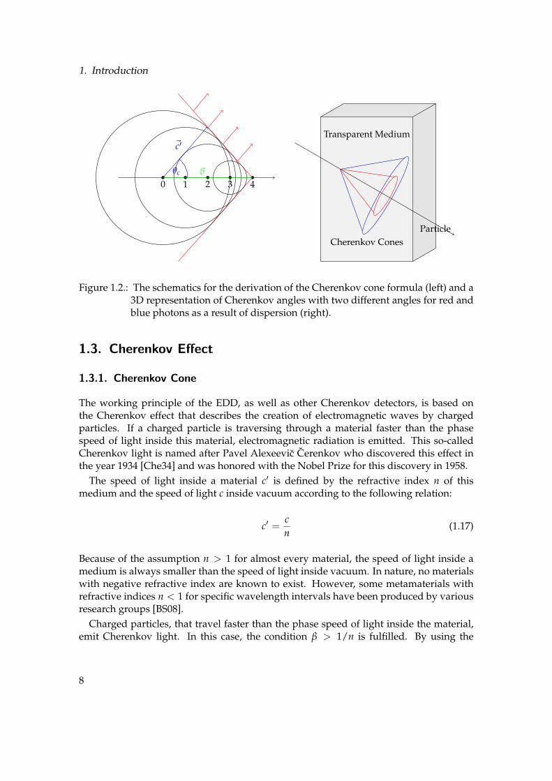
Figure 1.2.: The schematics for the derivation of the Cherenkov cone formula (left) and a3D representation of Cherenkov angles with two different angles for red andblue photons as a result of dispersion (right).

1.3. Cherenkov Effect

1.3.1. Cherenkov Cone

The working principle of the EDD, as well as other Cherenkov detectors, is based onthe Cherenkov effect that describes the creation of electromagnetic waves by chargedparticles. If a charged particle is traversing through a material faster than the phasespeed of light inside this material, electromagnetic radiation is emitted. This so-calledCherenkov light is named after Pavel Alexeevic Cerenkov who discovered this effect inthe year 1934 [Che34] and was honored with the Nobel Prize for this discovery in 1958.

The speed of light inside a material c′ is defined by the refractive index n of thismedium and the speed of light c inside vacuum according to the following relation:

c′ =c

n(1.17)

Because of the assumption n > 1 for almost every material, the speed of light inside amedium is always smaller than the speed of light inside vacuum. In nature, no materialswith negative refractive index are known to exist. However, some metamaterials withrefractive indices n < 1 for specific wavelength intervals have been produced by variousresearch groups [BS08].

Charged particles, that travel faster than the phase speed of light inside the material,emit Cherenkov light. In this case, the condition β > 1/n is fulfilled. By using the

8

1.3. Cherenkov Effect

Wavelength [nm]300 400 500 600 700 800

Chere

nkov A

ngle

[ra

d]

0.81

0.82

0.83

0.84

Simulations

Theoretical Model

Wavelength [nm]300 350 400 450 500 550 600 650 700 750 800

Entr

ies

0

100

200

300

400

500

600Simulations

Theoretical Model

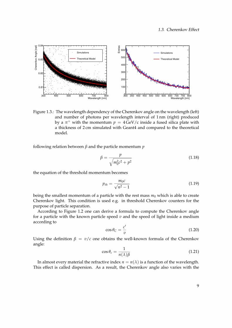
Figure 1.3.: The wavelength dependency of the Cherenkov angle on the wavelength (left)and number of photons per wavelength interval of 1 nm (right) producedby a π+ with the momentum p = 4 GeV/c inside a fused silica plate witha thickness of 2 cm simulated with Geant4 and compared to the theoreticalmodel.

following relation between β and the particle momentum p

β =p

√

m20c2 + p2

(1.18)

the equation of the threshold momentum becomes

pth =m0c√n2 − 1

(1.19)

being the smallest momentum of a particle with the rest mass m0 which is able to createCherenkov light. This condition is used e.g. in threshold Cherenkov counters for thepurpose of particle separation.

According to Figure 1.2 one can derive a formula to compute the Cherenkov anglefor a particle with the known particle speed v and the speed of light inside a mediumaccording to

cos θC =c′

v(1.20)

Using the definition β = v/c one obtains the well-known formula of the Cherenkovangle:

cos θc =1

n(λ)β(1.21)

In almost every material the refractive index n = n(λ) is a function of the wavelength.This effect is called dispersion. As a result, the Cherenkov angle also varies with the

9

1. Introduction

Particle Momentum [GeV/c]1 1.5 2 2.5 3 3.5 4 4.5 5 5.5 6

Chere

nkov A

ngle

[ra

d]

0.7

0.72

0.74

0.76

0.78

0.8

0.82

0.84

0.86

0.88

0.9

Particle Momentum [GeV/c]1 1.5 2 2.5 3 3.5 4 4.5 5 5.5 6

Chere

nkov A

ngle

[ra

d]

0.7

0.72

0.74

0.76

0.78

0.8

0.82

0.84

0.86

0.88

0.9

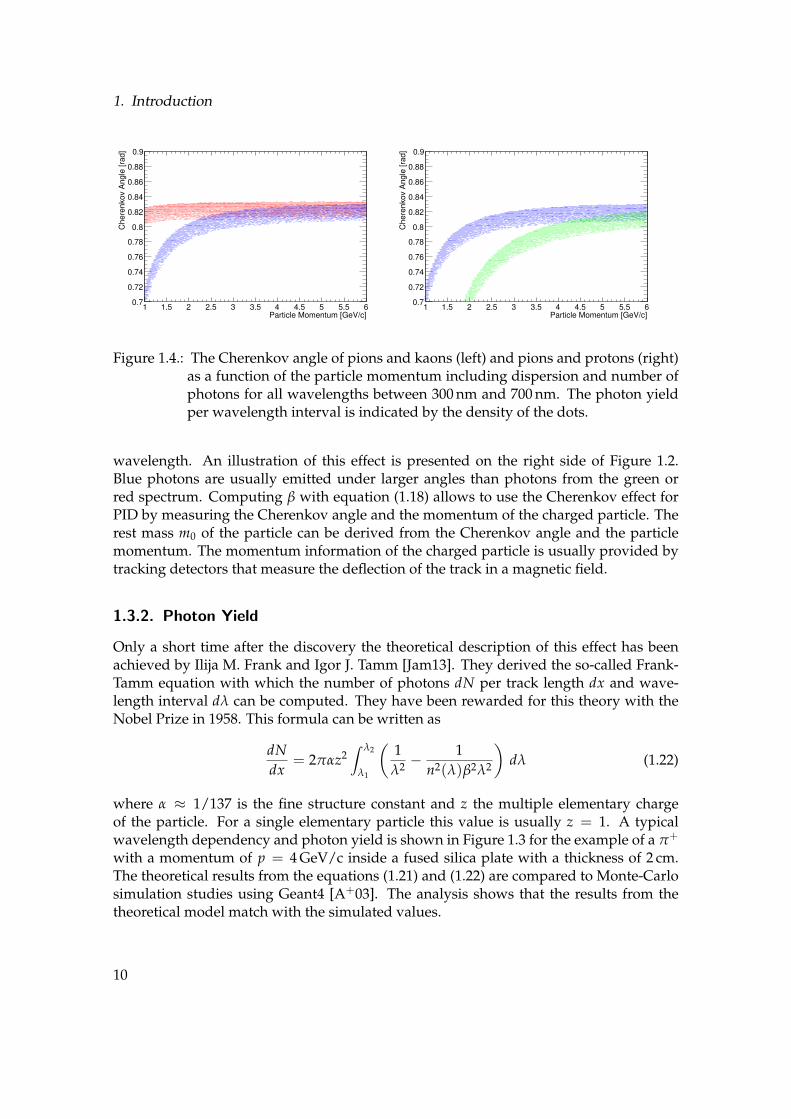
Figure 1.4.: The Cherenkov angle of pions and kaons (left) and pions and protons (right)as a function of the particle momentum including dispersion and number ofphotons for all wavelengths between 300 nm and 700 nm. The photon yieldper wavelength interval is indicated by the density of the dots.

wavelength. An illustration of this effect is presented on the right side of Figure 1.2.Blue photons are usually emitted under larger angles than photons from the green orred spectrum. Computing β with equation (1.18) allows to use the Cherenkov effect forPID by measuring the Cherenkov angle and the momentum of the charged particle. Therest mass m0 of the particle can be derived from the Cherenkov angle and the particlemomentum. The momentum information of the charged particle is usually provided bytracking detectors that measure the deflection of the track in a magnetic field.

1.3.2. Photon Yield

Only a short time after the discovery the theoretical description of this effect has beenachieved by Ilija M. Frank and Igor J. Tamm [Jam13]. They derived the so-called Frank-Tamm equation with which the number of photons dN per track length dx and wave-length interval dλ can be computed. They have been rewarded for this theory with theNobel Prize in 1958. This formula can be written as

dN

dx= 2παz2

∫ λ2

λ1

(1

λ2− 1

n2(λ)β2λ2

)

dλ (1.22)

where α ≈ 1/137 is the fine structure constant and z the multiple elementary chargeof the particle. For a single elementary particle this value is usually z = 1. A typicalwavelength dependency and photon yield is shown in Figure 1.3 for the example of a π+

with a momentum of p = 4 GeV/c inside a fused silica plate with a thickness of 2 cm.The theoretical results from the equations (1.21) and (1.22) are compared to Monte-Carlosimulation studies using Geant4 [A+03]. The analysis shows that the results from thetheoretical model match with the simulated values.

10

1.4. Scintillation Process

The left side of Figure 1.4 shows the Cherenkov angles of pions and kaons as a functionof the particle momentum including the chromatic dispersion in the wavelength windowbetween 300 nm and 700 nm. The density of the points indicate the amount of emittedphotons per wavelength interval. Above the momentum of around p = 2.3 GeV/c, anoverlap of the two bands is clearly visible. This effect of chromatic error in combinationwith additional geometrical errors are the main limitations of the Cherenkov detectorperformance.

The width of each band can be reduced by applying a wavelength filter or achieving ahigh photon statistics. It is possible, to obtain the best result by a trade-off between pho-ton statistics and chromatic dispersion as shown in chapter 3. The right side of Figure 1.4shows the same overlap between kaons and protons. Here, the overlap starts at a largermomentum of approx. p = 4 GeV/c which indicates that the separation of protons frompions or kaons is easier compared to a separation between pions and kaons.

1.4. Scintillation Process

In order to test different Disc DIRC prototypes, a cosmic test stand has been developed asdescribed in chapter 5. This test stand uses scintillators [Kno10] to detect cosmic muons.Such scintillators work as follows: Due to the energy loss of a particle traversing througha transparent medium the molecules of this medium can be excited. A material is calledscintillator if the molecules fall back into their ground state by emitting photons. Thetwo possibilities of light emission are phosphorescence and fluorescence. The major dif-ference between these two mechanisms is the time interval in which the molecule remainsin the excited state. In the latter case, the time scale is in the order of nanoseconds whilein the first case the molecules can remain for hours in the excited state.

In general, a suitable scintillator material is chosen according to specific parameterslike a high photon yield in a desired wavelength interval or a high resistance againstchemical or radiation damages. There are two types of scintillator materials available:organic and inorganic ones. The main differences between them are described in thefollowing.

1.4.1. Organic Scintillators

Organic scintillators can consist of liquids or plastic materials with hydrocarbon and ben-zene ring connections. They are commonly used in HEP applications. The advantageof organic scintillators are the short time scale of light emission down to values below1 ns and the simple production processes. Organic materials are usually less radiationhard and strongly affected by chemical reactions with other materials. Figure 1.5 showsthe term scheme and working principle of a typical plastic scintillator material. If themolecules of the scintillator material in the ground state S0 are getting ionized, a recom-bination with other molecules takes place which brings them into one arbitrary excitationstate Si. The transition from the state S0 to the states Si can also take place directly.

11

1. Introduction

S0

S1

S2

S3

I

Ion

izat

ion

Rec

om

bin

atio

n

Flu

ore

scen

ce

Inter-systemcrossing T1

T2

T3

Rec

om

bin

atio

n

Ph

osp

ho

resc

ence

Figure 1.5.: The term scheme of an arbitrary scintillator material including 3 singlet statesSi and 3 triplet states Ti including some of their vibrational sub states.

From the states Si the molecule decays with a high probability successively to the stateS1 and from there to one of the vibration states with energy levels above the ground stateS0. Hence, the emitted photon has a longer wavelength than needed to bring anothermolecule into an excitation state or ionize it. As a result, the medium becomes transparentfor scintillation light. This energy gap is also known as the so-called Stokes shift and acharacteristic property of the fluorescence mechanism.

Since the wavelength of the emitted light is usually short and placed in the ultravioletregion, special color centers have to be induced into the scintillator material. These colorcenters are also called wavelength shifters and change the photon color into visible lightspectrum. Otherwise, the scintillation light cannot be detected by photon sensors.

Another possibility for the molecules for loosing their excitation energy is to jumpinto a triplet state. The direct decay of this state into the ground state is forbidden. Byinteracting with another molecule in the same state, it can jump into the excited state S1

from where it decays back into the ground state. This reaction is much slower than theprompt direct decay which leads to a longer lifetime of the triplet state. Hence, the timebehavior of scintillators can be described in general by a sum of two exponential decayswith the fast decay time τf and the slow one τs

N(t) = A exp

(

− t

τf

)

+ B exp

(

− t

τs

)

(1.23)

where the proportional factor A is usually the dominating one. New materials, that areused as so-called triplet harvesters, change the energy of these states and make a fastdecay possible. With this method it is even possible to emit different colors to identifythe type of the primary particle that traverses through the scintillator [ADF12].

12

1.5. Optics

1.4.2. Inorganic Scintillators

Typical inorganic scintillators are glass scintillators or noble gases. In contrast to organicscintillators they can have a higher density which leads to shorter radiation lengths and ahigher photon yield. Additionally, inorganic scintillators can be produced with a higherradiation hardness and therefore have a longer lifetime. The main disadvantages of inor-ganic scintillators are the longer decay times and the possibility of binding water.

Because inorganic scintillators usually consist of insulating materials there is an energygap between the valence band and conducting band. By doping the scintillator materialwith atoms from other materials, new energy levels between these bands are created.From there, the electrons can fall back into the valence band and emit scintillation light.The created electron-hole pair can also remain electrostatically bounded and become ex-cited. It can move as a quasi-particle inside the material until it reaches an activationcenter and then decays into its ground state by emitting a photon.

1.5. Optics

Cherenkov and other imaging based detectors underlie optical effects that will be ex-plained in the following. These effects have to to be taken into account for theoreticalcalculations and Monte-Carlo simulations that aim to optimize the detector performance.In case of the EDD, light reflection and photon absorption processes are important for arealistic detector model. In chapter 4, the implementation for simulation studies will bedescribed.

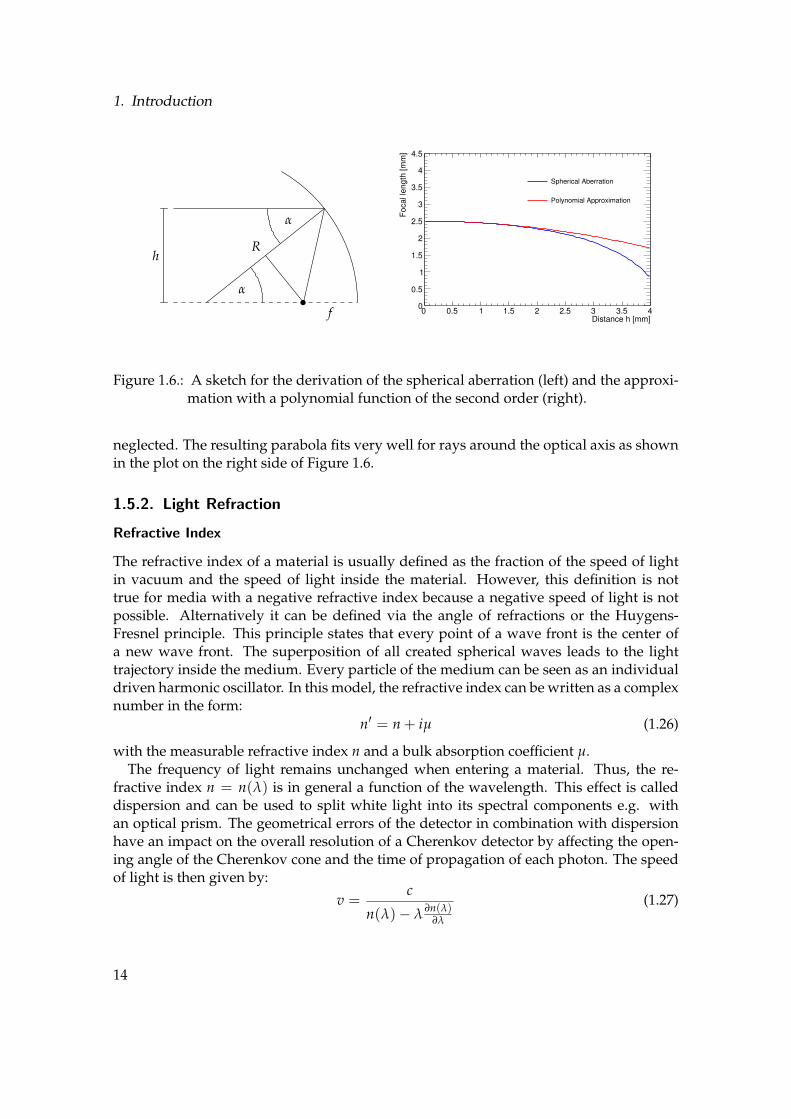
1.5.1. Geometrical Aberration

Imaging optics are commonly applied in detector systems that are used for photon acqui-sition. Spherical and cylindrical shaped mirrors and lenses are easy to produce. However,the resulting performance issues have to be weighted up against achievable advantagesfor aspherical optics.

In general, a cylindrical or spherical mirror with the radius R focuses only paraxiallight rays in one single spot. For light rays, that have the distance h from the optical axis,the focal length f shifts according to the following equation:

f (h) = R

(

1 − R

2√

R2 − h2

)

(1.24)

The derivation for this equation can be taken from the sketch on the left side of Fig-ure 1.6. This effect is called spherical aberration. The correlation between f and h can beexpanded into a Taylor series:

f (h) ≈ R

2− x2

4R− 3x4

16R3− . . . (1.25)

Due to the symmetry of the system, uneven terms cancel and the resulting approximationmust be even. For smaller distances h, sum terms with coefficients larger than 2 can be

13

1. Introduction

α

f

hR

α

Distance h [mm]0 0.5 1 1.5 2 2.5 3 3.5 4

Focal le

ngth

[m

m]

0

0.5

1

1.5

2

2.5

3

3.5

4

4.5

Spherical Aberration

Polynomial Approximation

Figure 1.6.: A sketch for the derivation of the spherical aberration (left) and the approxi-mation with a polynomial function of the second order (right).

neglected. The resulting parabola fits very well for rays around the optical axis as shownin the plot on the right side of Figure 1.6.

1.5.2. Light Refraction

Refractive Index

The refractive index of a material is usually defined as the fraction of the speed of lightin vacuum and the speed of light inside the material. However, this definition is nottrue for media with a negative refractive index because a negative speed of light is notpossible. Alternatively it can be defined via the angle of refractions or the Huygens-Fresnel principle. This principle states that every point of a wave front is the center ofa new wave front. The superposition of all created spherical waves leads to the lighttrajectory inside the medium. Every particle of the medium can be seen as an individualdriven harmonic oscillator. In this model, the refractive index can be written as a complexnumber in the form:

n′ = n + iµ (1.26)

with the measurable refractive index n and a bulk absorption coefficient µ.The frequency of light remains unchanged when entering a material. Thus, the re-

fractive index n = n(λ) is in general a function of the wavelength. This effect is calleddispersion and can be used to split white light into its spectral components e.g. withan optical prism. The geometrical errors of the detector in combination with dispersionhave an impact on the overall resolution of a Cherenkov detector by affecting the open-ing angle of the Cherenkov cone and the time of propagation of each photon. The speedof light is then given by:

v =c

n(λ)− λ ∂n(λ)∂λ

(1.27)

14

1.5. Optics

The refractive index can be approximated with the Sellmeier equation that has thefollowing form [PS03]:

n2(λ) = 1 +3

∑i=1

Biλ2

λ2 − Ci(1.28)

This equation can be used to parameterize the refractive index of a material with usu-ally six constants Bi and Ci for Monte-Carlo studies. It turns out that the error of thisapproximation is less than 10−6 for most materials in the visible spectrum.

Fresnel Equations

If light passes from one medium with the refractive n1 into another medium with therefractive index n2, each light ray is divided into two separate rays. One of these raysis transmitted into the second medium while the other ray is reflected into the samemedium. The amount of transmitted and reflected light depends on the polarization ofthe photon.

The amplitude reflectivity for perpendicular s and parallel p linear polarized light canbe calculated with the so-called Fresnel equations [Hec01]

rs =n1 cos α − µr1

µr2

√

n22 − n2

1 sin2 α

n1 cos α + µr1

µr2

√

n22 − n2

1 sin2 α(1.29)

rp =n2

2µr1

µr2cos α − n1

√

n22 − n2

1 sin2 α

n22

µr1

µr2cos α + n1

√

n22 − n2

1 sin2 α(1.30)

where α is the angle of incidence. The fraction of the permeability constants is usuallyclose to µ1/µ2 = 1. The Fresnel equations can be derived from the Maxwell equationsby using the boundary conditions for the electric field at a current-free and charge-freeinterface between two materials. The reflection probability for light rays is then given by

Rs,p = rs,p · r∗s,p = r2s,p (1.31)

The overall reflection probability for unpolarized light is the average of the probabili-ties for both polarization states:

Rs,p =1

2(Rs + Rp) (1.32)

By redefining the refractive indices n1 and n2 according to:

n′1,s = n1 cos α and n′

1,s = n2 cos β (1.33)

n′1,p = n1/ cos α and n′

2,p = n2/ cos β (1.34)

15

1. Introduction

Angle of Incidence [deg]0 10 20 30 40 50 60 70 80 90

Reflectivity [%

]

0

10

20

30

40

50

60

70

80

90

100

Polarization

Perpendicular

PolarizationParallel

Angle of Incidence [deg]0 10 20 30 40 50 60 70 80 90

Reflectivity [%

]

0

10

20

30

40

50

60

70

80

90

100

Polarization

Perpendicular

PolarizationParallel

Figure 1.7.: The reflectivity of photons resulting from the Fresnel equations for the re-fractive indices n1 = 1.0 resp. n2 = 1.47 (left) and n1 = 1.47 resp. n2 = 1.0(right) of the two materials.

the Fresnel equations (1.29) and (1.30) can be simplified to:

rs =n′

1,s − n′2,s

n′1,s + n′

2,s

(1.35)

rp =n′

1,p − n′2,p

n′1,p + n′

2,p

(1.36)

The fraction of photons, which are not reflected, must be transmitted from one materialto the other. The transmission probability can therefore be written as:

Ts,p = 1 − Rs,p (1.37)

Figure 1.7 shows the reflection probability for two different cases, in which the photonsare polarized either parallel or perpendicularly to the surface borders. The photons onthe left side of Figure 1.7 enter a material with a larger refractive index while the photonson the right side enter a material with a smaller refractive index.

If photons propagate into a material with a higher optical density, all photons withan angle of incidence of α = 0 enter the material with a very low probability of beingreflected. The reflection probability increases for larger angles and reaches a maximumof nearly 100% around α = 90. If the photons enter a material with a smaller opti-cal density, the reflection reflectivity increases steeply around the angle of total internalreflection.

Total Internal Reflection

In the case of entering a material with a lower optical density the reflectivity increasessteeply around the angle of total internal reflection that can be calculated from Snell’s

16

1.5. Optics

law of refraction:n1 sin α = n2 sin β (1.38)

Applying the condition β > 90 leads to the following result of the minimum angle ofinternal reflection:

α = arcsin

(n2

n1

)

(1.39)

All photons with an angle larger than α have a reflection probability of nearly 100%, asit can be also shown with the Fresnel equations, and are therefore captured inside thematerial. Since the refractive index n is in general a function of the photon wavelength λ,the angle of the internal reflection is not a constant value for all photon wavelengths.

However, it follows from Maxwell’s equations that the wave can enter the other mate-rial with the smaller refractive index where the amplitude of the electric field decreasesaccording to the following exponential function:

E(z) = E0e− z

d0 (1.40)

The penetration depth d0 can be calculated with

d0 =λ

2πn1

√

sin2 α − (n2/n1)2(1.41)

This effect has to be taken into account if a material with a larger refractive index thanthe surrounding material is brought near to the material, in which photons propagate viatotal internal reflections. In this case, these photons have a probability, that is larger than0%, to tunnel through this barrier into the other medium.

1.5.3. Photon Losses

Bulk Absorption

The differential decrease dI/dx for photons with the intensity I0 traversing through atransparent medium is proportional to the actual light intensity I with the wavelengthdependent proportionality factor µ:

dI = −Iµ(λ) dx (1.42)

The factor µ is equal to the one introduced in equation (1.26) and also a function of thephoton wavelength. The solution of this differential equation, that is analog to the ra-dioactive decay of particles, leads to the Beer-Lambert law [Mat95]

I(x) = I0e−µ(λ)x (1.43)

which is valid if the material is homogeneous and multiple scattering of the photons canbe neglected. For simulation studies, measured values for the absorption coefficient areusually provided as a lookup table for different wavelengths.

17

1. Introduction

Rayleigh Scattering

The scattering of photons can be derived from Maxwell’s equations of electromagneticphenomena. It is highly dominated by elastic scattering of photons and described forsmall photon wavelengths λ d compared to diameter of the scattering center by theRayleigh scattering cross section [You81]

σR =2π5

3

d6

λ4

(n2 − 1

n2 + 1

)2

(1.44)

that is inversely proportional to the fourth power of the photon wavelength. The photonlosses for this cross section has been derived as:

αR =8π

3

n8

λ4p2βT(TF)kBTF (1.45)

where kB denotes the Boltzmann constant, TF the fictive temperature, p the photo elasticconstant and βF(TF) the isothermal compressibility of the material.

Surface Losses

In addition to absorption processes and scattering inside a material, photons can also getlost on the surface between two materials if the surface is not perfectly smooth, which isin general the case for all real surfaces. Measurements of the RMS value of the surfaceroughness are limited by the sampling length of the measurement device. The resultingRMS value is given by:

Rq =

√√√√ 1

N

N

∑i=1

z2i (1.46)

where N is the number of sampling points and zi the height profile of the sample at thispoint with the number i.

The BSDF [FOB81] is defined as the fraction of the scattered flux Li and the incidentflux Lo as a function of the solid angles ωo and ωi:

f (ωi, ωo) =dLo(ωo)

Li(ωi) cos θi dωi(1.47)

For different combinations of polar angles θ and azimuth angles φ, wavelengths λ, andx-y positions on an arbitrary surface, this equation becomes very complex. Hence, simpli-fications are needed when using these functions in Monte-Carlo simulations as describedin the following.

An integration of this equation as an approximation for near to perfectly smooth sur-faces leads to the value of TIS

TTIS =(

4π cos θiRqn

λ

)2(1.48)

18

1.6. Particle Interaction with Matter

which is equal to the probability of transmission and scattering of a single photon. Thevalue θi is defined as the angle of incidence. The reflection probability for a photon incase of total internal reflection can therefore be written as follows:

RTIS = 1 −(

4π cos θiRqn

λ

)2(1.49)

From this equation, the overall probability for a photon to be reflected N times can bederived to:

P = RNTIS (1.50)

By defining a surface roughness Rq, the reflection probability P for each photon becomessimply a function of the angle of incidence θi.

1.6. Particle Interaction with Matter

A charged particle, that traverses a medium, looses energy due to ionization processesand bremsstrahlung. Scattering on atoms inside the medium leads to an angular strag-gling [GS08]. The simulation results for both effects will be discussed in section 4.1.3.

1.6.1. Multiple Scattering

The scattering of charged particles in matter is mainly a result of the Coulomb interactionwith the electrons in the medium. The effect of the strong interaction in case of hadronscan usually be neglected. Due to multiple scattering inside the medium, the resultingdisplacement can be described by a Gaussian distribution. The RMS of the scatteringangle after traversing through a volume with the thickness x can be approximated usingthe following relation:

σθ =13.6 MeV

βcpz

√x

X0

(

1 + 0.038 ln

(x

X0

))

(1.51)

Here, p is referring to the particle momentum, βc to the velocity, z to the particle chargenumber, and X0 to the radiation length of the used material. From this equation, onecan see that the angular straggling increases for smaller particle momenta and shorterradiation lengths.

1.6.2. Energy Loss

The mean energy loss of a charged particle in matter can be estimated with the Betheequation

⟨

−dE

dx

⟩

= Kz2 Z

A

1

β2

[1

2ln

2mec2β2γ2Wmax

I2− β2 − δ(βγ)

2

]

(1.52)

including the factorK = 4πNAr2

e mec2 = 0.307 mol−1 · cm2 (1.53)

19

1. Introduction

The maximum energy transfer from a particle with the mass M to an electron in onecollision can be exactly calculated with the following equation:

Wmax =2mec

2β2γ2

1 + γ meM +

(meM

)2(1.54)

For thin detector volumes the energy loss follows a Landau distribution. The mean en-ergy loss can then be written as

〈∆E〉 = ξ

[

ln2mc2β2γ2

I+ ln

ξ

I+ j − β2 − δ(βγ)

]

(1.55)

where ξ is defined as follows:

ξ =K

2

⟨Z

A

⟩x

β2(1.56)

In this equation m stands for the particle mass and I for mean excitation potential of thematerial. The detector thickness x is given in units of g cm−2 by multiplying the absorberthickness in cm with its density. The value 〈Z/A〉 is the mean ratio of the atomic numberZ and atomic mass A of the absorber material, and the material and particle independentconstants are given as j = 0.2 and K = 0.307075 MeV mol−1 cm−2. The additional densitycorrection factor δ(βγ) was not part of the original equation and can be theoreticallycalculated with Sternheimer’s equations, whereas in most of the cases the very smallcorrections can be neglected. Further details about angle straggling and energy loss ofparticles can be found in [Group16].

1.7. Photon Sensors

1.7.1. Silicon Photomultipliers

An APD consists, similar to a standard diode, of a p-n junction with a positively p+

and negatively n+ doped semiconducting materials (see Figure 1.8). The large amountof doping material is indicated by the plus sign in the upper index. Additionally, anintrinsic undoped or weakly p doped layer is placed between the p+ and n+ layer leadingto larger depletion region. This layer defines the place where the photons are absorbedand create the electron hole pairs. Due to a higher amount of charge carriers providedby this i layer, the maximum current of these so-called pin diodes can be increased tohigher values compared to normal diodes. The application of another weakly doped player between the intrinsic and n+ doped layers leads to a higher electric field in this areaand as a result to an amplification process. In general, a negative bias voltage near thebreakdown voltage is applied to the APD. This leads to an amplification factor between100 and 500. Special diodes called G-APDs have been developed to be operated in theGeiger mode for detecting single photons by applying bias voltages slightly above thebreakdown voltage and increasing the amplification factor up to 108.

20

1.7. Photon Sensors

p+ i p n+

− +

Figure 1.8.: The scheme of an APD including the highly doped layers p+ and n+, theintrinsic layer i and the lightly doped layer p.

SiPMs consist of an array of these G-APD that are connected parallel. The advantageof this setup is the large active area and a higher signal in case of multiple photon hits.By using this method, it is not possible to to obtain any information about the positionof the photon hit which leads to a worse time resolution. It is therefore suitable for thecollection of photons that are created in one single scintillator bar where no further spatialinformation of the incoming photon is required.

One possibility to solve these problems has addressed by dSiPMs which directly pro-vide a digital signal of every single APD and makes an additional readout device obso-lete. The spatial information can be taken directly from the identification number of thereadout channel that belongs to one individual pixel. The disadvantages of dSiPM arerelated to their limited radiation hardness which makes it impossible to use them for theEDD in PANDA.

The DCR increases after an exposure radiation, e.g. to hadron or high energetic leptonfluxes. This can be explained by the creation of impurities in the atom structures of theAPD. Noisy pixels can worsen the resolution of a photon detector since they cannot bedistinguished from normal photon hits. Radiation damages can also create metastablestates in the band structure which lead to the induction of further avalanches and createafter-pulsing effects. Another important issue of dSiPMs is the optical cross-talk that iscreated by fluorescence light, when electron-hole pairs in the APD recombine.

1.7.2. Microchannel Plates

Working Principle

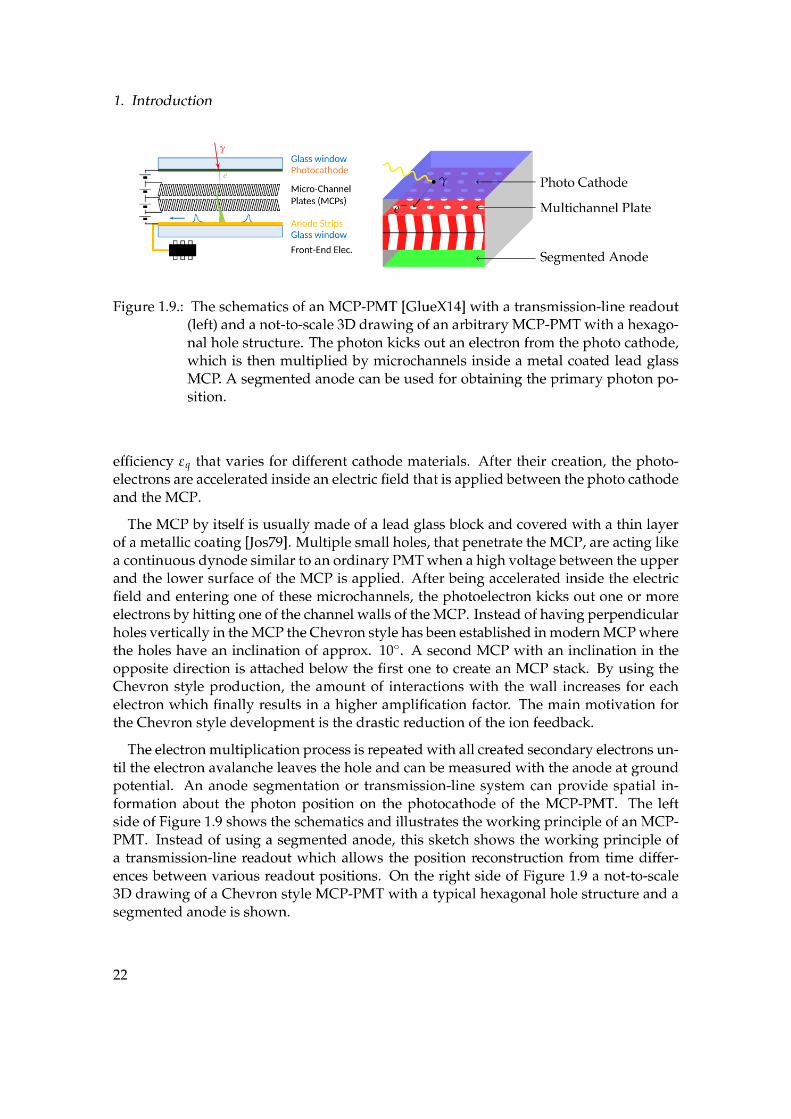
The chosen photo detectors for the EDD are MCP-PMTs. The first MCP-PMT has beenpresented in 1930 by Philo T. Farnsworth. It is used for detecting single photons and con-sists mainly of a vacuum tube with a photon sensitive photocathode, an MCP stack anda grounded readout anode. A photon reaching the photo cathode can create a photoelec-tron. The probability for this process is defined by the wavelength dependent quantum

21

1.7. Photon Sensors

Detection Efficiency

The probability for each electron to enter one channel is defined as the collection effi-ciency of the MCP. The collection efficiency can be approximated analytically with thefraction of the area πr2 of all Nh holes inside a unit cell and its full active area A:

εc =Nhπr2

A(1.57)

Typical values for standard MCP-PMTs, which are currently on the market, vary around65 %. New types of MCPs promise a higher collection efficiency up to 90 % or even higherby using different conic shapes for the mircochannels. However, the time resolution ofthe new devices deteriorates slightly because the additional collected electrons need totravel a longer. This leads to a second time peak which is shifted by time values between100 ps and 200 ps and has to be taken into account in the reconstruction algorithm of thedetector.

The overall PDE of an MCP-PMT results from the product of the quantum and collec-tion efficiency:

εp = εq · εc (1.58)

This can be interpreted as the probability to detect a single photon that reaches the photocathode of the MCP-PMT. Another possibility to define the detection efficiency is theratio

εp =Ndet

Nin(1.59)

of detected photons Ndet to the number Nin of incoming photons that reach the photo-cathode.

Time Resolution

Because of the short electron trajectories between the photocathode and the anode, verysmall time resolutions down to 27 ps are reachable. The time resolution depends on themethod by which the time information is measured. It can be obtained directly from asignal of the MCP, if it provides secondary electrons during the avalanche process, orfrom the anode signal.

The first method is mainly used for TOF measurements, i.e. for PID purposes with-out using the spatial information of the photoelectrons. In the latter case the resolutiondepends on the readout system that is used to determine the position from the anodepad. The time resolution of the whole system have to be taken as input parameters forMonte-Carlo simulations regarding the performance of a detector that uses MCP-PMTsfor the photon detection.

Rate Stability & Radiation Hardness

Another important factor is the rate stability and radiation hardness of an MCP-PMTswhich effect the lifetime of such tube. The rate stability is basically limited by the geo-metrical acceptance of the particle detector and amount of created photons per event. A

23

1. Introduction

high rate has a negative impact on the gain of the MCP-PMT because the large amountof charge in the MCP influences the electric field.

Depending on the target wavelength interval and desired quantum efficiency, photo-cathodes can be made of several bialkali or multialkali materials. A reaction of antimonywith potassium and cesium leads to the bialkali material Sb-K-Cs. Additionally, sodiumcan be added resulting in the multialkali photocathode Na-K-Sb-Cs.

A high irradiation dose of photons can damage the photo cathode and induce a dete-rioration of the quantum efficiency. However, this effect is not completely understooduntil now. One theory states that it can be caused by ions which are created during theelectron avalanche production and travel back along the electric field lines. The collisionof these ions with the photocathode create irreversible damages as these photo cathodesare reacting very sensitive to chemical impurities.

Several approaches have been developed and are still under investigation in order toreduce the degeneration of the photo cathode, e.g. using other materials or placing anelectrostatic grid between the photo cathode and the MCP to collect the drifting ions.An important and promising method is called ALD: A very thin coating on the MCPprevents the surface from out-gassing and can increase the lifetime up to a factor of 50.Using this method, MCPs have been devloped that have lifetimes beyond 6C/cm2 show-ing almost no degeneration symptoms and are sufficient for the application in the EDD[L+17].

Magnetic Field

If an MCP-PMT is placed in a magnetic field, the photoelectrons can take a path to aneighboring channel which creates an offset in the position measurement. However, thiseffect could be simply compensated by a calibration that compensates the shift. Anothereffect is the bending of the photoelectron trajectory which leads to a helix track with adiameter that can be derived from the Larmor radius. It usually results in a drop ofgain because the electron can pass through a channel without colliding with the wall.However, it is also possible to increase the gain depending on the strength and directionof the magnetic field.

Charge sharing effects, that are a result of the finite size of the electron hitting morethan one anode pad simultaneously, can be also reduced by applying a magnetic field.This effect can be also explained with the bending of the trajectory of the electron cloudleading to a smaller diameter. In case of a segmented anode the number of pixels withphoton hits usually decreases by applying a higher magnetic field. However, this effectcan also lead to under-sampling if the smaller electron avalanche hits the place betweenthe anode pixels and is therefore not registered. This problem has to be taken into accountwhen choosing the readout system for the MCP-PMT.

24

1.8. CMOS Chips

p

n+ n+

GateMetal Oxide

Bulk (Casing)

Source Drain

VCC

Input Output

Figure 1.10.: The sketch of a typical p typed MOSFET structure with the four connectionsSource, Drain, Gate and Bulk (left) and a standard CMOS inverter circuitincluding two MOSFET (right).

1.8. CMOS Chips

1.8.1. CMOS Technology

Some proposed upgrade possibilities of the cosmics test stand, as described in chap-ter 5, involve the application and readout of CMOS chips. The CMOS technology usesMOSFET on the same substrate for creating complex circuits in one chip, such as ampli-fiers or logic gates. A sketch of a standard p typed MOSFET is shown on the left side ofFigure 1.10. Two n+ doped layers are placed in a p doped semiconductor volume whichcreates a p-n junction between them acting like a capacitor. The Bulk (B) connection tothe p substrate is internally connected to the Source (S) or Drain (D) connection in manyof the available MOSFET types.

A positive voltage between the Gate (G) and the Bulk connection enlarges the depletionzone, which increases the resistance between the Source and Drain resulting in a lowercurrent. An additional current between the Gate and the Source or Drain of a MOSFET isnot necessary, which is a huge advantage of a MOSFET compared to a standard transistor.For an n typed MOSFET it has to be taken into account that the signal polarity must beinverted.

The main feature of the CMOS technology is the complementary connection of two pand n type MOSFET as presented in Figure 1.10 on the right-hand side. If a logical 0is applied and the input is on ground potential, the upper n type transistor gets a lowresistance and the applied voltage VCC is given to the output. In the other case of alogical 1 the resistance of the p type transistor decreases, and the output is set to ground.

In contrast to other technologies like NMOS, where only one transistor is used, anadditional load resistor can be omitted. Hence, a current in a CMOS gate does onlyflow for a short period after switching the input signals. This principle implies a smallercurrent consumption and heat development in the chip. The application of a second FET

25

1. Introduction

Trst

Tamp

VCC

TselOut

Read

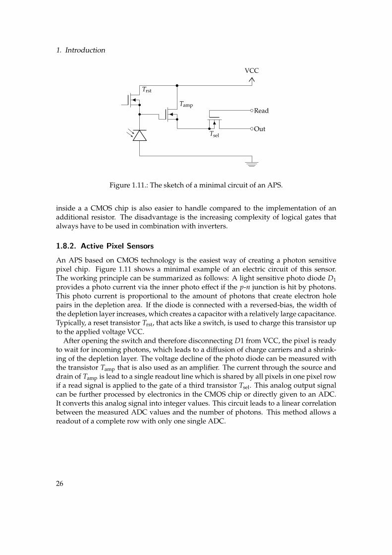
Figure 1.11.: The sketch of a minimal circuit of an APS.

inside a a CMOS chip is also easier to handle compared to the implementation of anadditional resistor. The disadvantage is the increasing complexity of logical gates thatalways have to be used in combination with inverters.

1.8.2. Active Pixel Sensors

An APS based on CMOS technology is the easiest way of creating a photon sensitivepixel chip. Figure 1.11 shows a minimal example of an electric circuit of this sensor.The working principle can be summarized as follows: A light sensitive photo diode D1

provides a photo current via the inner photo effect if the p-n junction is hit by photons.This photo current is proportional to the amount of photons that create electron holepairs in the depletion area. If the diode is connected with a reversed-bias, the width ofthe depletion layer increases, which creates a capacitor with a relatively large capacitance.Typically, a reset transistor Trst, that acts like a switch, is used to charge this transistor upto the applied voltage VCC.

After opening the switch and therefore disconnecting D1 from VCC, the pixel is readyto wait for incoming photons, which leads to a diffusion of charge carriers and a shrink-ing of the depletion layer. The voltage decline of the photo diode can be measured withthe transistor Tamp that is also used as an amplifier. The current through the source anddrain of Tamp is lead to a single readout line which is shared by all pixels in one pixel rowif a read signal is applied to the gate of a third transistor Tsel. This analog output signalcan be further processed by electronics in the CMOS chip or directly given to an ADC.It converts this analog signal into integer values. This circuit leads to a linear correlationbetween the measured ADC values and the number of photons. This method allows areadout of a complete row with only one single ADC.

26

2. PANDA

2.1. FAIR

The accelerator complex of FAIR is planned as an extension of the present acceleratorsetup of the GSI near Darmstadt in Germany. A 3D sketch can be seen in Figure 2.1. FAIRis used to create antiprotons for proton-antiproton collisions in the PANDA spectrome-ter which is important for many physics studies. In general, the pp collisions have theadvantage of achieving other physics than pp reactions because of the vanishing baryonnumber and total charge.

The first step in the production of antiprotons that are stored in the HESR storage ringis the p-LINAC. It accelerators protons up to a kinetic energy of Ekin = 70 MeV. After thisacceleration has taken place, the protons are boosted to a kinetic energy of 29 GeV by thetwo synchrotron accelerators SIS18 and SIS100.

A collision of these highly energetic protons with a copper target will create antiprotonsthat can be separated from the various other created particles with a magnetic horn. Inthe next step a fast cooling of the antiprotons is taking place in the CR. The RESR hasthe task to accumulate the antiprotons and inject them into the HESR. The accumulationstep in the RESR can also be skipped and the antiprotons directly injected from the CR.However, this has the drawback of a smaller luminosity. In the racetrack-shaped ring ofthe HESR antiprotons can be stored in the momentum range between 1.5 and 15 GeV/c.

Two beam cooling methods are provided: The first one is an electron cooling up to anantiproton momentum of 9 GeV/c. For this technique a beam of electrons is acceleratedto the same average velocity as the antiproton beam. After the electrons are brought toan overlap with the particle beam on a straight track, the antiprotons looses energy viaCoulomb scattering with the electrons until a thermal equilibrium is reached.

The second cooling method is stochastic cooling that can be applied over the full mo-mentum range of the antiprotons. A sensor measures the deviation of the particles fromthe nominal closed orbit and a kicker is used to push the particle trajectory to the re-quired beam position. An overlap of pulses for many particles leads in average to asmaller phase space and therefore a smaller energy variance.

The total circumference of the HESR has a circumference of 575 m and can be operatedin two modes: a high luminosity and a high resolution mode. The high resolution modecan be used for scanning resonances with a defined momentum distribution of the an-tiprotons which has a momentum uncertainty of ∆p/p ≈ 4 · 10−5. In this mode around1010 antiprotons can be stored and a luminosity of approx. 2 · 1031 cm−2 s−1 is reachable.The high luminosity mode can only be operated if the RESR is available, and providesa luminosity by a factor of 10 higher. The disadvantage of this mode is the worse mo-

27

2. PANDA

Figure 2.1.: A sketch of the Facility for Antiproton and Ion Research. The PANDA spec-trometer is placed in the HESR storage ring for antiprotons which are pro-duced with the antiproton target and cooled in the CR. The existing facility ofthe GSI is colored in blue while the red lines indicate the planned facility.

mentum resolution around ∆p/p ≈ 10−4. However, for rare events, which require a highamount of statistics, this mode has to be chosen.

2.2. PANDA Spectrometer

The PANDA [SC12] spectrometer is planned as a typical onion shell detector with almost4π solid angle coverage. An actual drawing of the final detector according to the pro-posed design is shown in Figure 2.2. The forward boost of the reaction products due tothe fixed target and kinematics favors to an asymmetric shape of for detector relative tothe polar angle. Therefore, the PANDA spectrometer is divided into a TS and an FS. Thelatter one measures the higher energetic particles with a smaller polar angle distributionand will be described at the end. Both parts contain a large variety of subdetectors fortracking purposes, energy measurements and PID.

2.2.1. Target System

The target system of PANDA is designed for the provision of a constant luminosity andcontrollable collision rate. Hence, the density variations inside the target have to be re-duced to a minimum. The target consists mainly of hydrogen atoms which will providecollisions between protons and antiprotons. Target prototypes with an amount of hy-

28

2.2. PANDA Spectrometer

Figure 2.2.: A sketch of the PANDA spectrometer according to the actual proposal. TheEDD is marked with the orange text.

drogen atoms in the order between 1014 and 1016 atoms cm−2 were produced and testedalready. Two design options have been investigated: a frozen hydrogen pellet target anda cluster jet target option.

Pellet Target

The pallet target provides small droplets of frozen hydrogen created in a triple pointchamber with diameters between 10 and 30 µm. These droplets can be vertically injectedinto the target tube and then distributed into the vacuum of the beam pipe. The fallingspeed is around 60 m/s at a flow rate of 100,000 pellets per second. This target is prefer-able option for reaching high luminosities and has the advantage that one knows theexact point of interaction. Hence, the primary vertex position is fully determined. How-ever, the division into small droplets leads to inhomogeneities in the target density whichcan be seen as a disadvantage.

Cluster Jet Target

The cluster jet target is complementary to the advantages and disadvantages regardingthe pellet target. The main working principle is the expansion of pre-cooled and com-pressed hydrogen gas into the beam pipe of the HESR. This results in the creation ofcluster jets that move with supersonic speed during a condensation phase.

Unlike the pellet target, the cluster jets can be tuned in their size, speed, and densitywhich results in a controllable luminosity. The typical cluster size is given by 103 to 105

29

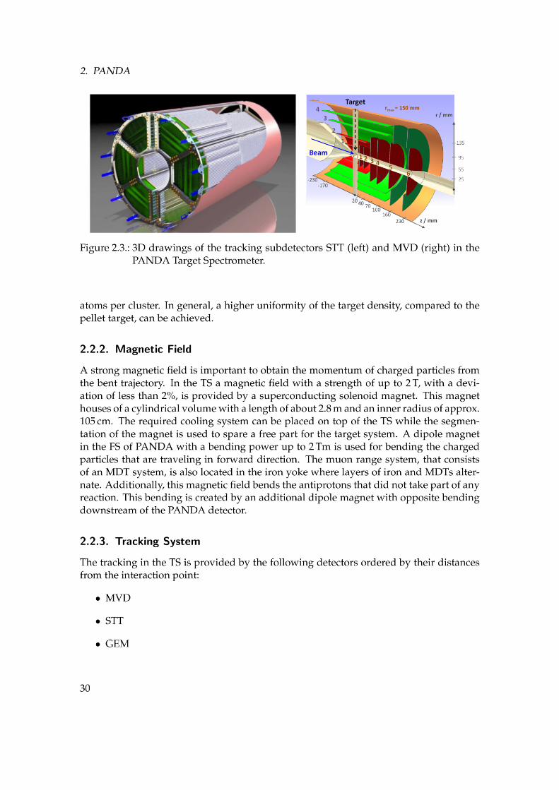
2.2. PANDA Spectrometer

All three tracking detectors are going to provide tracking information of the createdcharged particles. The trajectory bending as a result of the applied magnetic field canbe used for the computation of the particle momentum by using the equation of motionobtained from the Lorentz force

d~p⊥dt

=q

m(~v⊥ × ~B) (2.1)

where ~B is the magnetic field and ~p⊥ the particle momentum perpendicular to the fieldlines. From that equation the relation between the helix radius $ and absolute value ofthe relativistic particle momentum p⊥ can be derived to

$ =p⊥qB

(2.2)

It has to be taken into account that the magnetic field is inhomogeneous and therefore afunction of the particle position. For every position the ~B field vector has to be taken froman exactly measured field map. The tracking information is additionally needed for someother detectors like the EDD that provide PID information about the traversing particle.

Micro Vertex Detector

Because of long decay times of some particles like charged D mesons in the order of10−12 s the decay does not happen instantaneously at the target which leads to a displaceddecay vertex of particles. The information about this vertex is going to be collected bythe MVD [PEK+12] which is a silicon pixel detector with an accuracy of about 100 µm.This detector consists of four barrel parts and 6 disks placed around the interaction point.Since this detector is the inner most one in a series of other subsystems in PANDA, thematerial budget has to be kept as small as possible. Additionally, a high radiation hard-ness of the detector and the readout system has to be achieved. For this purpose an ASICnamed PASTA has been designed that provides 64 channels and is based on the TOFPETASIC [RBG+13].

Straw Tube Detector

The STT [PANDA13] consists of 4636 cylindrical gaseous proportional counters made of a27 µm thin aluminized foil. Each counter has a diameter of 10 mm, a length of 1.5 m and isfilled with the counting gas mixture Ar-CO2 up to a pressure of 2 bars. This overpressurekeeps the foil of the straws in the desired cylindrical shape. The high electric field for theproportional counting mode in the center of the straw is created by gold-plated tungstenwire with a very small diameter of around 20 µm.

If a particle traverses the STT, it ionizes the gas atoms and creates electron-ion pairs.The electrons are accelerated by the high electric field from the thin wire, which leadsto an electron avalanche and therefore to an amplification process. From the time infor-mation a position of the particle with respect to the distance of the central wire can becomputed. By applying a Riemann fit on the acquired hits, the helix trajectory compo-nent of the charged particle can be reconstructed.

31

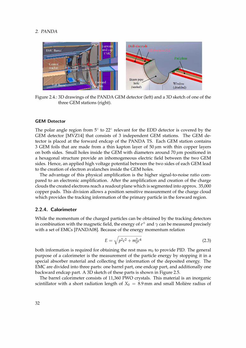
2. PANDA

Figure 2.4.: 3D drawings of the PANDA GEM detector (left) and a 3D sketch of one of thethree GEM stations (right).

GEM Detector

The polar angle region from 5 to 22 relevant for the EDD detector is covered by theGEM detector [MVZ14] that consists of 3 independent GEM stations. The GEM de-tector is placed at the forward endcap of the PANDA TS. Each GEM station contains3 GEM foils that are made from a thin kapton layer of 50 µm with thin copper layerson both sides. Small holes inside the GEM with diameters around 70 µm positioned ina hexagonal structure provide an inhomogeneous electric field between the two GEMsides. Hence, an applied high voltage potential between the two sides of each GEM leadto the creation of electron avalanches inside the GEM holes.

The advantage of this physical amplification is the higher signal-to-noise ratio com-pared to an electronic amplification. After the amplification and creation of the chargeclouds the created electrons reach a readout plane which is segmented into approx. 35,000copper pads. This division allows a position sensitive measurement of the charge cloudwhich provides the tracking information of the primary particle in the forward region.

2.2.4. Calorimeter

While the momentum of the charged particles can be obtained by the tracking detectorsin combination with the magnetic field, the energy of e± and γ can be measured preciselywith a set of EMCs [PANDA08]. Because of the energy momentum relation

E =√

p2c2 + m20c4 (2.3)

both information is required for obtaining the rest mass m0 to provide PID. The generalpurpose of a calorimeter is the measurement of the particle energy by stopping it in aspecial absorber material and collecting the information of the deposited energy. TheEMC are divided into three parts: one barrel part, one endcap part, and additionally onebackward endcap part. A 3D sketch of these parts is shown in Figure 2.5.

The barrel calorimeter consists of 11,360 PWO crystals. This material is an inorganicscintillator with a short radiation length of X0 = 8.9 mm and small Moliere radius of

32

2.2. PANDA Spectrometer

Figure 2.5.: The EMC for PANDA in the TS excluding the backward part. The partsrelated to the endcap part are colored green and the material of the barrelpart is indicated with blue color. The PWO crystals and the supporting frameare also shown.

20 mm, which leads to a very small transversal expansion of the electromagnetic shower.Charged particles create bremsstrahlung inside each of crystals that is then converted intoe± pairs. These created particles emit photons via bremsstrahlung that creates a cascadeof secondary particles. This process keeps itself alive until the primary particle has lostall its energy inside the crystals. Hence, a short radiation length X0 is very important tomake sure that the particle does not leave calorimeter and deposits all its energy.

In case of the EMC, the total length of 20 cm leads to an accumulated distance of 22X0.Additionally, the used material has a small decay time of less than 10 ns which is im-portant for a good time resolution. The barrel part is going to be covered in reflectivefoils. They will keep the created photons inside the calorimeter volume which then willbe detected using LAPDs.

The forward part of the EMC will hold 3,600 PWO crystals and the backward part 592ones. All parts together guarantee an almost 4π coverage to detect all created electro-magnetic particles. The energy resolution, that can be reached with the EMC, is expectedto be smaller than

σE

E= 1% ⊕ 2%

√

E[GeV](2.4)

2.2.5. PID Detectors

Since it has been decided not to use a hadronic calorimeter in PANDA the PID of someimportant mesons like π± or K± have to be performed with other techniques. PID can

33

2.2. PANDA Spectrometer

Figure 2.7.: A 3D drawing of the PANDA Barrel DIRC with the view from the forwardendcap, showing the bars, expansion volumes, and MCP-PMTs (left), and theseparation power for π/K separation with different combinations of particlemomentum p and polar angles θ (right).

where m1 and m2 are the rest masses of the particles and p their absolute momentum.The separation power nσ of different particle species is then given by:

nσ =∆t

σt(2.7)

The left side of Figure 2.6 shows the achievable separation power as a function of theparticle momentum obtained from equation (2.6) for three different arbitrary time reso-lutions.

This method will be used by the Barrel TOF detector [BGM+14] in PANDA. This so-called SciTil hodoscope is planned to contain 5,760 small plastic scintillator tiles with sizesof about 30 × 30 × 5 mm3 that are read out by SiPMs. The geometry of a conceptionaldesign, which is used for simulation purposes, can be seen on the right side of Figure 2.6.The detector will be placed as a barrel around the target between the Barrel DIRC andEMC with a radius of approx. 50 cm to cover large polar angles in forward and backwarddirection. The large amount of detected photons result in a sufficient time resolution ofaround 100 ps. The overall time resolution scales statistically with the factor

√N if N hits

have been acquired and an average is computed. The TOFPET system is foreseen for theFEE to process the signals provided by the SiPMs.

Barrel DIRC

The polar angles in the range 5 ≤ θ ≤ 140 are covered by the two Cherenkov detectorsEDD and Barrel DIRC [PANDA17a]. Since the EDD is the main part of this thesis, it willbe explained in the following chapters in detail.

The Barrel DIRC detector is based on the BaBar DIRC detector design that has firstbeen used at SLAC. The 3D drawing on the left side of Figure 2.7, obtained from the

35

2. PANDA

implemented Geant4 geometry, shows the actual design of the detector. It is placed in acylindrical shape around the interaction point and covers the polar angles 22 ≤ θ ≤ 140

with a separation of more than 3 standard deviations for π± and K± separation in themomentum range from 1.5 to 3.5 GeV/c. The separation power as a function of particlemomentum p and polar angle θ is presented on the right side of Figure 2.7. These resultshave been obtained from Monte-Carlo simulations and validated in various testbeamsexperiments e.g. at the CERN.

The Barrel DIRC consists of 16 synthetic fused silica bars with a width of 53 mm and160 mm wide plates. In total 240 MCP-PMTs are used to detect the photons that areinternally reflected to the readout plane. The backside of each bar, which is opposite tothe MCP-PMTs, is coated with a reflective surface in order to reflect additional light to thephotosensors. An expansion volume, also made of fused silica, between the bars and theMCP-PMTs is used to spread the Cherenkov photons onto a larger plane and thereforecreate a better spatial and angular resolution. A lens system, which consists of sphericalor cylindrical lens multiplets, focuses the light on the readout plane and improves thesingle photon resolution.

For the reconstruction LUTs are implemented with special interpolation methods usedthat are obtained from Monte-Carlo simulations of photon paths in the expansion volumein order to remove all possible ambiguities. At the end, the measured hit information iscombined with the tracking detectors of PANDA which results in a direct computation ofthe Cherenkov angle. A likelihood method is used that relates the measured Cherenkovangle and the nominal single photon resolution. A similar method is used for the calcula-tion of a likelihood value for the photon propagation time. To obtain the best probabilityfor a specific particle hypothesis, the geometry and time based method are used.

2.2.6. Forward Spectrometer

The TS of PANDA has similar components to the TS with respect to particle spectroscopy.A large dipole magnet is used to deflect the charged particles that will be tracked withthe FT which covers the polar angles −10 ≤ θ < 10 in horizontal direction and −5 ≤θ < 5 in vertical direction. It mainly consists of 3 pairs of planar tracking layers. Theexpected spatial resolution is σ = 0.1 mm per detection layer which leads to a momentumresolution of better than 1%.

The PANDA Forward RICH is used for PID with a similar polar angle interval. It isdesigned to provide a separation power for π± and K± of 3 standard deviations up toparticle momenta of 10 GeV/c. The main component is a thin Aeorogel radiator for thecreation of the Cherenkov cone. The emitted photons are then reflected at a planar mirrorto a PMT array on the top of the detector volume.

The Forward EMC will be placed behind the dipole magnet and will consist of 378modules. Each module is planned as a sandwich of 380 layers of lead absorber platesand plastic scintillators. The created photons are acquired with PMTs. The providedenergy resolution is given by

σE

E=

b√

E[GeV]⊕ c (2.8)

36

2.3. Physics Program

with the parameters b = (3.04 ± 0.06)% and c = (0.62 ± 0.05)% according to measure-ments with one specific configuration [PANDA17b].

2.3. Physics Program

The physics program of PANDA covers a large spectrum of particles for understandingthe effects of QCD in a better way. Studying bound states of quarks inside the QCD isimportant to evaluate theoretical predictions of the particle spectra with effective fieldtheories or LQCD. The major goals of the PANDA physics program are described forinstance in [PANDA09]. The most important studies regarding the open charm sectorand exotic matter will be briefly summarized in the following.

2.3.1. Open Charm Studies

One part of the physics program in PANDA is the study of the open charm sector. Anopen charm state results from a decay of a charmonium meson with cc into two mesonswith one charm and one light quark each. One example is the D+ meson that consists ofone c and one d quark. These states are interesting regarding strong decay modes and theinvestigation of the CP violation in the weak interaction. They might be also a possiblehint for physics beyond the SM. The results of previous and ongoing measurements inexperiments like BaBar or Belle agree in general with the theoretical predictions. How-ever, some discrepancies have been observed in the past due to experimental limitationsor large background levels.

While e± colliders produce less hadronic background they have the disadvantage ofnot being able to create non vector states. This follows from the fact that the exchangedphoton is a vector boson with spin S = 1 and the angular momentum has to be conserved.Hence, the production of excited charmonium states with all possible quantum numberscan only be possible with pp reactions. In contrast to e± colliders the mass and widthresolution does not depend on the detector resolution of PANDA but on the phase-spacecooled antiproton momenta which is excellent in the HESR. Additionally, the PANDAdetector has the ability to scan the resonance mass and can achieve an excellent PID incombination with a good vertex resolution. These conditions are important to study someof the already known open charm states in a more detailed way.

2.3.2. Exotic Matter & Nuclear Form Factors

Another physics goal is to find exotic matter with quantum numbers that cannot be takenby ordinary mesons. Two examples of exotic states are states with the forbidden quan-tum numbers JPC = 0−− or JPC = 2+−. They could be taken by hypothetical glueballs,hybrids, or multiquark systems.

The high momentum resolution of the HESR allows a mass resolution of better than∆m/m = 10−4. This makes a search for exotic states with a center-of-mass energy in therange from 2.2 to 5.5 GeV/c2 with the PANDA spectrometer is possible. Until now, the

37

2. PANDA

mass region of observable states has been restricted to values below 2.2GeV/c2 becauseof experimental limitations. These small mass regions contain the disadvantage of a highdensity of ordinary two-quark states.

Additionally, the high luminosity of the HESR is needed for a high production yieldas most of these states are formed with cross sections in the order of nanobarn. With theforeseen luminosity of the HESR several thousand exotic particles can be created per daywhich is an outstanding quality of PANDA compared to other experiments. Togetherwith a very good antiproton beam energy definition the decay widths of exotic particlesare going to be measured precisely down to values in the order of 10 keV.

A analysis of simulation data including the sample exotic meson candidate X(3872)with a rest mass of 3871.68 ± 0.17 MeV/c2 for performance studies of the PANDA detec-tor has been done already. This particle has been discovered by Belle in 2003 and does notfit into the standard quark model because of its quantum numbers JPC = 1++ which arenot allowed in the SM. The obtained results look promising to achieve the desired physicsgoals with the given detector configuration according to the hadronic background.

In addition to exotic particle states, nuclear form factors are planned be measured withPANDA. In general, two possible reactions can be used: The space-like

e− + p → e− + p (2.9)

and the time-likep + p → e+ + e− (2.10)

region. The names are related to the orientation of the related Feynman diagrams.The electromagnetic form factors in the time-like region by using pp collisions have

not been studied until now due to several reasons such as the low intensity of existingantiproton beams or missing precision in the measurement of the momentum transferq2. The HESR is designed to provide all necessary specifications for the determination ofnuclei form factors in the time-like region and makes determination of the form factorspossible. Previous measurement of the reaction e+e− → pp up to an energy of 4.5 GeVhave been performed with BABAR [AtBC07].

2.3.3. Hypernuclear Physics

Hyperons are baryons like protons or neutrons which can be created by exchanging one uor d with one of the heavier quarks. One well-known hyperon is the so-called Λ baryonwith the quark content uds which has been discovered already several decades ago. Ithas a rest mass of 1115.683 ± 0.006 MeV/c2 and a positive intrinsic parity. QCD rulesforbid a decay of a ground state Λ hyperon via the strong interaction. The preferreddecay channels are the following decays that involve the weak interaction:

Λ → p + π− (2.11)

Λ → n + π0 (2.12)

It has to be taken into account that the probability for a decay into π− is by a factor of2 higher than the decay into a π0. At whole, 17 resonances of the Λ hyperon have been

38

2.4. Data Acquisition

observed already but experimental limitations did not allow precise measurements ofmost of the hyperson states. Studying hyperon resonances in PANDA allows probingQCD in energy scales of 100 MeV related to the heavy rest mass of the s quark. Furtherstudies of hyperons with a c instead of an s quark can increase this scale by more thanone order of magnitute to approx. 1300 MeV.

Hypernuclei, that are formed by an atomic nucleus and at least one hyperon, can bealso studied in PANDA. This state can be interpreted as the replacement of u and dquarks in a nucleus with s quarks. By using proton-antiproton collisions, also hypernu-clei with more than one s quark can be created efficiently which makes PANDA com-petitive with other planned facilities. Especially hyperatoms containing an Ω hyperon,which has the quark content sss and could be observed in 1964, are interesting becauseof their long lifetime and non-vanishing quadrupole moment.

2.4. Data Acquisition

2.4.1. Requirements

The highest planned event rate in PANDA is 20 MHz. Because of the decision, to not usea hardware trigger in PANDA, all subdetectors must contain self-triggering electronicsand are therefore free running which leads to event sizes up to 20 kB. Hence, the DAQmust be able to deal with data processing up to 200 GB/s. Calculations have shown thatdue to this high data rate the disk space of the PANDA computing system would be filledin a few days.

The maximum achievable rate for data storage is estimated to 25 · 103 events per sec-ond. This rate makes an online reduction by a factor of around 1000 necessary. Forinvestigating n physics channels in parallel in one run a further reduction by a factor ofn has to be performed because of an OR connection between these trigger channels. Acomplete description about the DAQ system and online reconstruction in PANDA can befound in [Wag16]. The working principle is summarized in the form of a flow diagramin Figure 2.8.

The first step in the DAQ scheme is the detection of hits with each detector FEE. Thisdigital information is then sent to data multiplexers which select important hits for thefurther processing. The time synchronization and distribution to all subdetectors is donewith the help of the so-called SODANET. It consists of one timing source that sends theSODANET protocol, which is based on the TRBnet protocol, to related SODANET hubs.These hubs then distribute the received protocol to the DC. The next step in the on-line reconstruction scheme is the time ordering and building of physics events inside theevent/burst builder that will run on special Compute Codes.

The data is then sent to a computing farm where the online processing of completeevents is taking place. This is also the place where the decisions are made whether anevent can be accepted or has to be rejected. The event filtering is done by using combina-torics or mass window selections based on specific interesting physics channels.

Currently, 17 trigger channels for the investigation of different resonances including

39

2.4. Data Acquisition

J/ψ or D+ are planned to be used. At the end these accepted events have to be storedand can later be used for a more sophisticated offline reconstruction.

2.4.2. Compute Nodes

Examples for computations on the Compute Nodes, that have been tested already, arecluster finding of the EMCs, track finding with the STT. A possible online reconstructionof the EDD could also run on these Compute Nodes. The processing part of such aCompute Node consists mainly of 4 user-programmable FPGA cards. A 5th card is usedto manage the communication between them and other Compute Nodes through thebackplane.

The first prototypes of the Compute Node were made of 5 Virtex-4 FPGA cards whichhave been later upgraded to Virtex-5 boards. Every card has access to 5 × 2 GB of DDR2RAM. During the next upgrade, this value will be increased to 5 × 4 GB. The 4 FPGAcards in the processing part are interconnected with the RocketIO package which is atransceiver package especially provided by Xilinx, the communication FPGA card is con-nected to all of them using GPIOs. In total 8 optical links each with transfer rates ofapprox. 6.5 Gigabit per second are used. Hence, an overall bandwidth of around 32 Gbitper second can be achieved. Additionally, every FPGA will contain an RJ45 GBit Ethernetconnector which can be connected to the FEE for data transportation.

41

3. Disc DIRC Detector

3.1. Detector Setup

3.1.1. Geometry

The EDD and the Barrel DIRC are two Cherenkov detectors that are used for PID in theTS of PANDA. Various setups, including a TOP design, have been proposed during thelast years before the final decision was made for the current Disc DIRC concept. The maincomponent of the EDD is the radiator plate that consists of four identical and indepen-dent quadrants. They are made of highly polished synthetic fused silica with a thicknessof 2 cm and a surface roughness of 1.5 nm or better.

If a charged particle enters one of the quadrants, the emitted Cherenkov light prop-agates via total internal reflection to the outer rim. Because of a small gap betweenneighboring quadrants most of the photons are internally reflected and cannot leave thequadrant to enter a neighbored one. The other photons are absorbed by the mechanicalstructure between the quadrants. This leads to an overlap of hit patterns from differentreflections which have to be distinguished from the direct pattern by applying time cuts.The side faces can be covered additionally with an aluminum mirror coating. However,it has been shown that using the process of internal reflection results in a higher photonstatistics because of avoiding absorption processes in the mirror.

When passing the outer rim of the quadrants, the photons enter one of the 72 sensorelements that are glued to the edges. In total 288 sensor elements for the whole radiatorplate are used to focus the captured Cherenkov light and then use the information aboutthe Cherenkov angle for PID. Each sensor element consists of a bar with a width of 1.6 cmthat is used to connect one FEL to the sides of the radiator plate.

The backside surface of each FEL has a cylindrical shape and is coated with aluminum.This coating makes the backside acting like a cylindrical mirror to focus incoming Cherenkovphotons on a focal plane which matches with the photocathode of an attached MCP-PMTs. The imaging optics guarantees a nearly linear correlation between the position onthe photocathode of the MCP-PMT and the Cherenkov angle of the acquired photon.

Optical errors due to the cylindrical shape have to be taken into account. Previous de-signs with a proposed aspheric mirror shape, that can be described by a polynomial func-tion, have been rejected. They were designed to have a better imaging of the Cherenkovphotons. Some of these designs have the advantage of avoiding an additional mirrorcoating by using internal reflection. However, the production of an FEL with an asphericsurface is too complex and costly.

The anode of the MCP-PMT must be segmented with a high granularity in order toobtain the photon position with a sufficient resolution. The radius of the mirror has

43

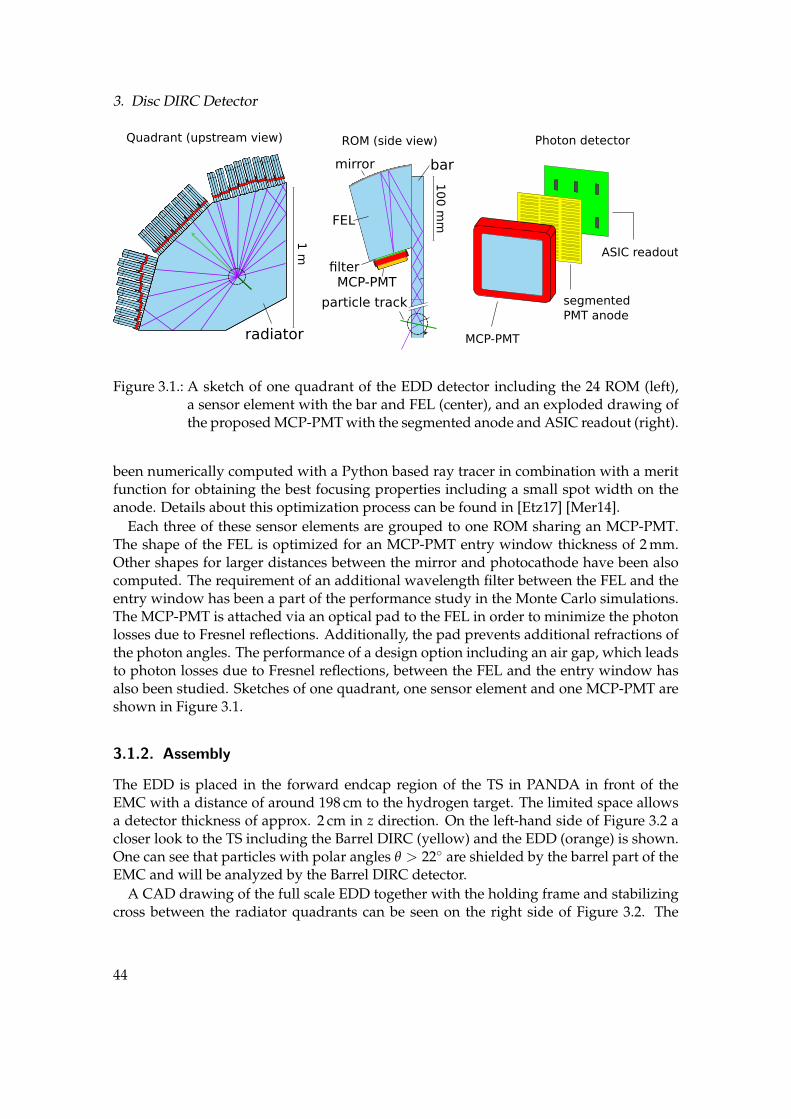
3. Disc DIRC Detector

bar

FEL

MCP-PMT

radiator

ROM (side view)

particle track

mirror

filter

Quadrant (upstream view)

ASIC readout

segmented

PMT anode

MCP-PMT

Photon detector

10

0 m

m

1 m

Figure 3.1.: A sketch of one quadrant of the EDD detector including the 24 ROM (left),a sensor element with the bar and FEL (center), and an exploded drawing ofthe proposed MCP-PMT with the segmented anode and ASIC readout (right).

been numerically computed with a Python based ray tracer in combination with a meritfunction for obtaining the best focusing properties including a small spot width on theanode. Details about this optimization process can be found in [Etz17] [Mer14].

Each three of these sensor elements are grouped to one ROM sharing an MCP-PMT.The shape of the FEL is optimized for an MCP-PMT entry window thickness of 2 mm.Other shapes for larger distances between the mirror and photocathode have been alsocomputed. The requirement of an additional wavelength filter between the FEL and theentry window has been a part of the performance study in the Monte Carlo simulations.The MCP-PMT is attached via an optical pad to the FEL in order to minimize the photonlosses due to Fresnel reflections. Additionally, the pad prevents additional refractions ofthe photon angles. The performance of a design option including an air gap, which leadsto photon losses due to Fresnel reflections, between the FEL and the entry window hasalso been studied. Sketches of one quadrant, one sensor element and one MCP-PMT areshown in Figure 3.1.

3.1.2. Assembly

The EDD is placed in the forward endcap region of the TS in PANDA in front of theEMC with a distance of around 198 cm to the hydrogen target. The limited space allowsa detector thickness of approx. 2 cm in z direction. On the left-hand side of Figure 3.2 acloser look to the TS including the Barrel DIRC (yellow) and the EDD (orange) is shown.One can see that particles with polar angles θ > 22 are shielded by the barrel part of theEMC and will be analyzed by the Barrel DIRC detector.

A CAD drawing of the full scale EDD together with the holding frame and stabilizingcross between the radiator quadrants can be seen on the right side of Figure 3.2. The

44

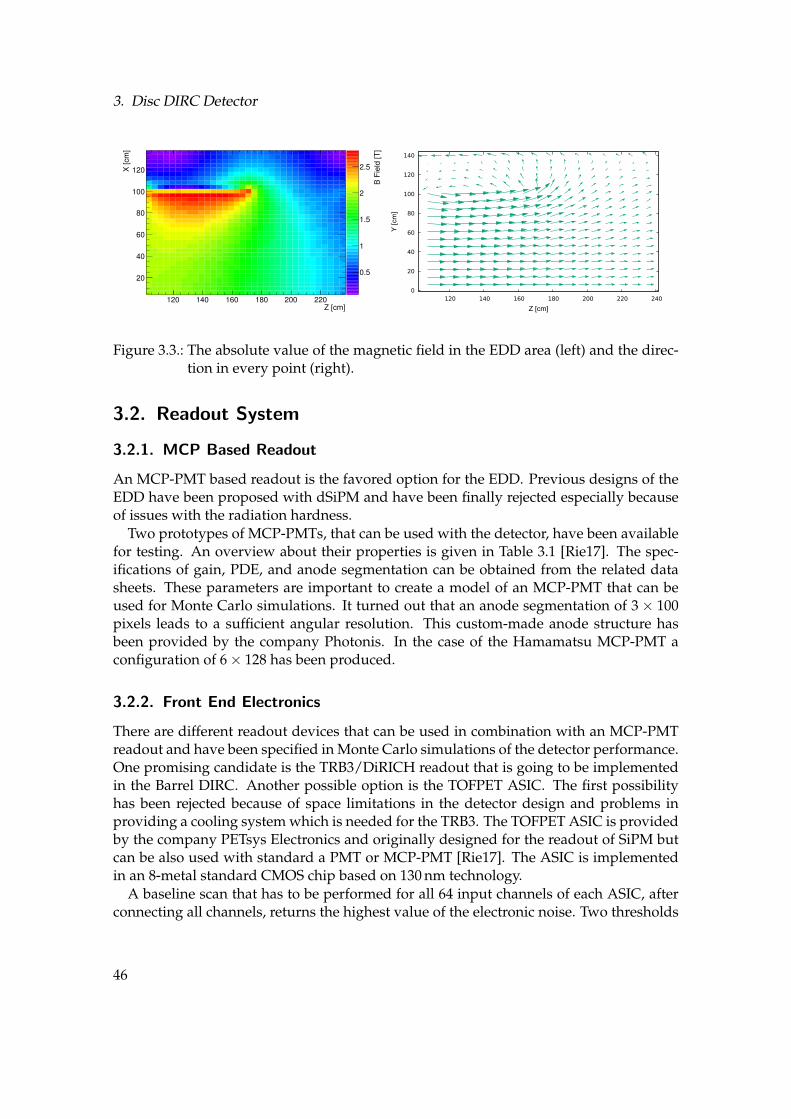
3. Disc DIRC Detector

B F

ield

[T

]

0.5

1

1.5

2

2.5

Z [cm]120 140 160 180 200 220

X [cm

]

20

40

60

80

100

120

0

20

40

60

80

100

120

140

120 140 160 180 200 220 240

Y [cm

]

Z [cm]

Figure 3.3.: The absolute value of the magnetic field in the EDD area (left) and the direc-tion in every point (right).

3.2. Readout System

3.2.1. MCP Based Readout

An MCP-PMT based readout is the favored option for the EDD. Previous designs of theEDD have been proposed with dSiPM and have been finally rejected especially becauseof issues with the radiation hardness.

Two prototypes of MCP-PMTs, that can be used with the detector, have been availablefor testing. An overview about their properties is given in Table 3.1 [Rie17]. The spec-ifications of gain, PDE, and anode segmentation can be obtained from the related datasheets. These parameters are important to create a model of an MCP-PMT that can beused for Monte Carlo simulations. It turned out that an anode segmentation of 3 × 100pixels leads to a sufficient angular resolution. This custom-made anode structure hasbeen provided by the company Photonis. In the case of the Hamamatsu MCP-PMT aconfiguration of 6 × 128 has been produced.

3.2.2. Front End Electronics

There are different readout devices that can be used in combination with an MCP-PMTreadout and have been specified in Monte Carlo simulations of the detector performance.One promising candidate is the TRB3/DiRICH readout that is going to be implementedin the Barrel DIRC. Another possible option is the TOFPET ASIC. The first possibilityhas been rejected because of space limitations in the detector design and problems inproviding a cooling system which is needed for the TRB3. The TOFPET ASIC is providedby the company PETsys Electronics and originally designed for the readout of SiPM butcan be also used with standard a PMT or MCP-PMT [Rie17]. The ASIC is implementedin an 8-metal standard CMOS chip based on 130 nm technology.

A baseline scan that has to be performed for all 64 input channels of each ASIC, afterconnecting all channels, returns the highest value of the electronic noise. Two thresholds

46

3.3. Reconstruction & Particle Identification

Photonis Hamamatsu

Specification XP85132-S-MD3 R13266-07-M768

Photocathode Bialkali Multialkali

Active area 53 × 53 mm2 53 × 53 mm2

Anode configuration 3 × 100 6 × 128

Anode dimensions 16.8 × 0.35 mm2 8.48 × 0.3 mm2

Column pitch 0.51 mm 0.4 mm

Overall high voltage 2400. . . 2800 V 3200. . . 3600 V

MCP type Chevron Chevron

MCP channel diameter 10 µm 10 µm

Comments Custom anode layout Protective film on first MCP

Table 3.1.: An overview over the properties of two MCP-PMT, that are suitable for thephoton detection of the EDD.

can be set relatively to this baseline: one is used to trigger on the falling edge of thenegative MCP-PMT signal, while the other one is used for triggering on the rising edge.Each time the first threshold is exceeded, a unique time stamp in picoseconds is sent tothe DAQ. The time between both thresholds is used to calculate the ToT value for eachsignal.

Two timers in the ASIC, a coarse and a fine one, are used for the acquisition of thecorrect time stamp. The coarse timer has a resolution of several nanoseconds and is notsufficient for application in the final EDD version. Therefore, both times are needed.

The intrinsic time resolution of the TOFPET ASIC including the fine timer is given by25 ps and the smallest measurable time difference is limited by an LSB of 50 ps. Addi-tionally, the ToT value is stored, that can be used to reconstruct the signal height andcentroiding of the charge cloud. It is also used for time walk corrections which are neces-sary because of the constant threshold that leads to a correlation between the time stampand the signal height. The dynamic range of each channel is 300 pC which is a typical sig-nal charge range of many photon detectors. The clock frequency of the ASIC can be set tovalues between 80 MHz and 160 MHz. Furthermore, a sophisticated dark count rejectionalgorithm is used together with a very low intrinsic noise which allows the applicationof very low thresholds.

3.3. Reconstruction & Particle Identification

3.3.1. Geometrical Model

For the Cherenkov angle reconstruction a geometrical model of the final Detector isneeded. This model has been introduced first by O. Merle and the complete derivation isgiven in [Mer09]. The geometrical model allows a fully analytic reconstruction approachwithout the need of lookup tables based on Monte-Carlo simulations (see chapter 4). Fig-

47

3. Disc DIRC Detector

Particle

φrel

αFEL

Radiator (Top View)

FEL

Radiator (Side View)

Particle

θc ϕ

FEL and Bar

ϕ′

Figure 3.4.: Definitions of all parameters, that are relevant for the reconstruction.

ure 3.4 shows the important parameters that are needed to compute the Cherenkov angleof each measured photon. The angle φrel is defined as the angle between the measuredphoton and the trajectory of the primary particle while ϕ′ is the angle measured by thesensor. The correlation between the z-coordinate on the focal plane of the sensor and ϕ′

is almost linear and given by

ϕ′(z) = mz + b (3.1)

where the parameters m and b can be calculated theoretically from the geometry of thefocusing element or with the help of Monte-Carlo simulations. However, there is a de-pendency of the angle ϕ on the azimuthal position of the active FEL which can be writtenas

tan ϕ′ =tan ϕ

cos αFEL(3.2)

where αFEL is the angle between the active FEL and the photon trajectory. This de-pendency refers to the measurement of a 2D projection of the Cherenkov cone. Theabove mentioned parameters of the primary particle provided by the tracking system ofPANDA together with the sensor hit pattern are sufficient to reconstruct the Cherenkovangle.

If the particle angles θp resp. φp and coordinates xp resp. yp are obtained by the prop-agation from the last tracked position to the radiator plate surface, the Cherenkov anglecan be computed fully geometrical with the following equation:

θc = arccos(sin θp cos φrel cos ϕ + cos θp sin ϕ) (3.3)

48

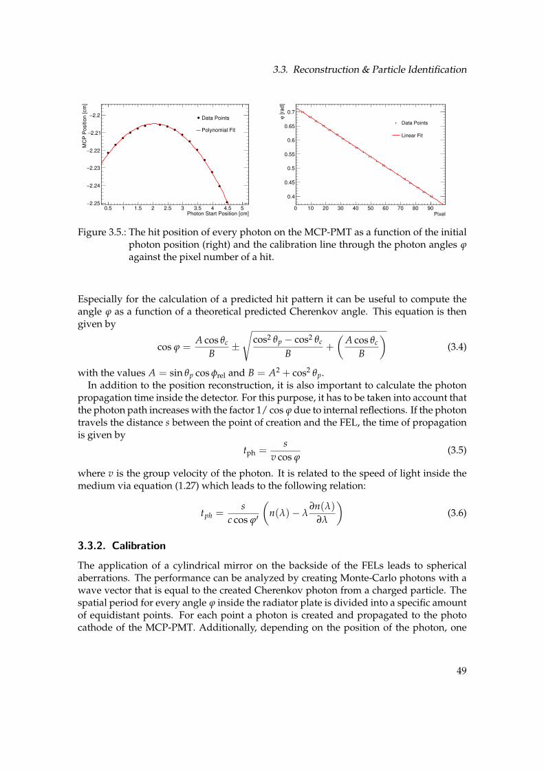
3.3. Reconstruction & Particle Identification

Photon Start Position [cm]0.5 1 1.5 2 2.5 3 3.5 4 4.5 5

MC

P P

ositio

n [cm

]

2.25−

2.24−

2.23−

2.22−

2.21−

2.2−Data Points

Polynomial Fit

Pixel0 10 20 30 40 50 60 70 80 90

[ra

d]

ϕ

0.4

0.45

0.5

0.55

0.6

0.65

0.7

Data Points

Linear Fit

Figure 3.5.: The hit position of every photon on the MCP-PMT as a function of the initialphoton position (right) and the calibration line through the photon angles ϕagainst the pixel number of a hit.

Especially for the calculation of a predicted hit pattern it can be useful to compute theangle ϕ as a function of a theoretical predicted Cherenkov angle. This equation is thengiven by

cos ϕ =A cos θc

B±

√

cos2 θp − cos2 θc

B+

(A cos θc

B

)

(3.4)

with the values A = sin θp cos φrel and B = A2 + cos2 θp.In addition to the position reconstruction, it is also important to calculate the photon

propagation time inside the detector. For this purpose, it has to be taken into account thatthe photon path increases with the factor 1/ cos ϕ due to internal reflections. If the photontravels the distance s between the point of creation and the FEL, the time of propagationis given by

tph =s

v cos ϕ(3.5)

where v is the group velocity of the photon. It is related to the speed of light inside themedium via equation (1.27) which leads to the following relation:

tph =s

c cos ϕ′

(

n(λ)− λ∂n(λ)

∂λ

)

(3.6)

3.3.2. Calibration

The application of a cylindrical mirror on the backside of the FELs leads to sphericalaberrations. The performance can be analyzed by creating Monte-Carlo photons with awave vector that is equal to the created Cherenkov photon from a charged particle. Thespatial period for every angle ϕ inside the radiator plate is divided into a specific amountof equidistant points. For each point a photon is created and propagated to the photocathode of the MCP-PMT. Additionally, depending on the position of the photon, one

49

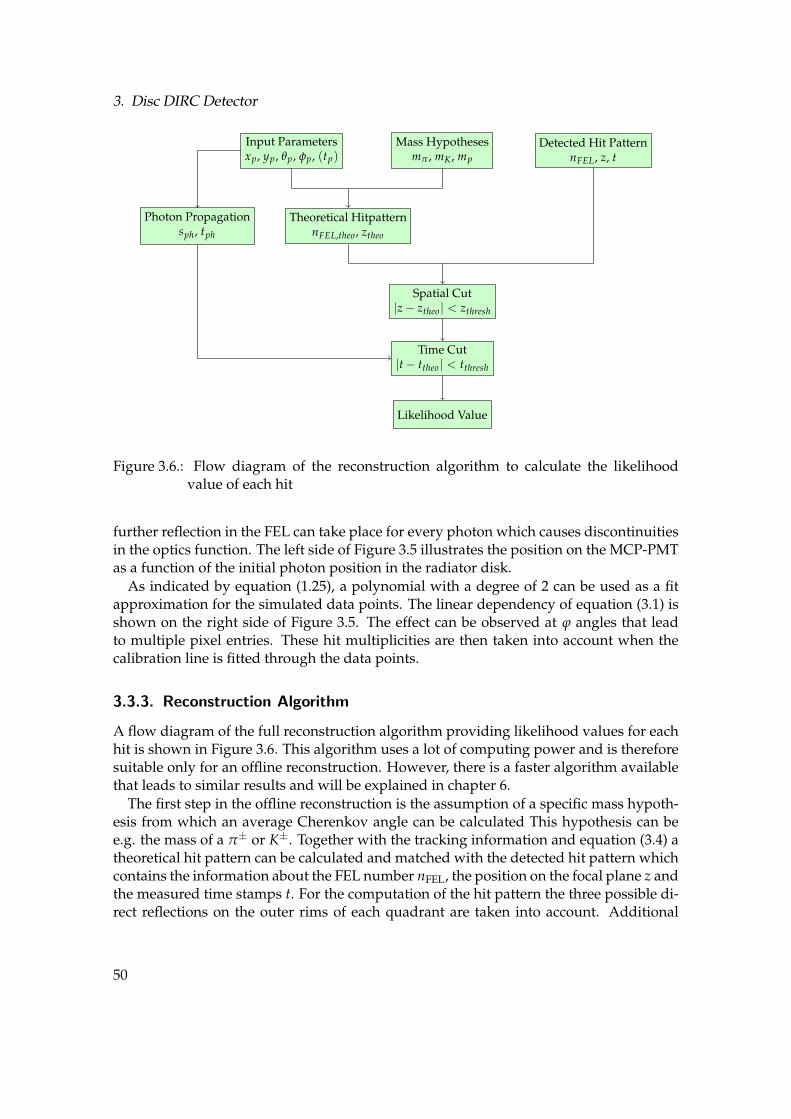
3. Disc DIRC Detector

Input Parametersxp, yp, θp, φp, (tp)

Mass Hypothesesmπ , mK , mp

Detected Hit PatternnFEL, z, t

Theoretical HitpatternnFEL,theo, ztheo

Photon Propagationsph, tph

Spatial Cut|z − ztheo| < zthresh

Time Cut|t − ttheo| < tthresh

Likelihood Value

Figure 3.6.: Flow diagram of the reconstruction algorithm to calculate the likelihoodvalue of each hit

further reflection in the FEL can take place for every photon which causes discontinuitiesin the optics function. The left side of Figure 3.5 illustrates the position on the MCP-PMTas a function of the initial photon position in the radiator disk.

As indicated by equation (1.25), a polynomial with a degree of 2 can be used as a fitapproximation for the simulated data points. The linear dependency of equation (3.1) isshown on the right side of Figure 3.5. The effect can be observed at ϕ angles that leadto multiple pixel entries. These hit multiplicities are then taken into account when thecalibration line is fitted through the data points.

3.3.3. Reconstruction Algorithm

A flow diagram of the full reconstruction algorithm providing likelihood values for eachhit is shown in Figure 3.6. This algorithm uses a lot of computing power and is thereforesuitable only for an offline reconstruction. However, there is a faster algorithm availablethat leads to similar results and will be explained in chapter 6.

The first step in the offline reconstruction is the assumption of a specific mass hypoth-esis from which an average Cherenkov angle can be calculated This hypothesis can bee.g. the mass of a π± or K±. Together with the tracking information and equation (3.4) atheoretical hit pattern can be calculated and matched with the detected hit pattern whichcontains the information about the FEL number nFEL, the position on the focal plane z andthe measured time stamps t. For the computation of the hit pattern the three possible di-rect reflections on the outer rims of each quadrant are taken into account. Additional

50

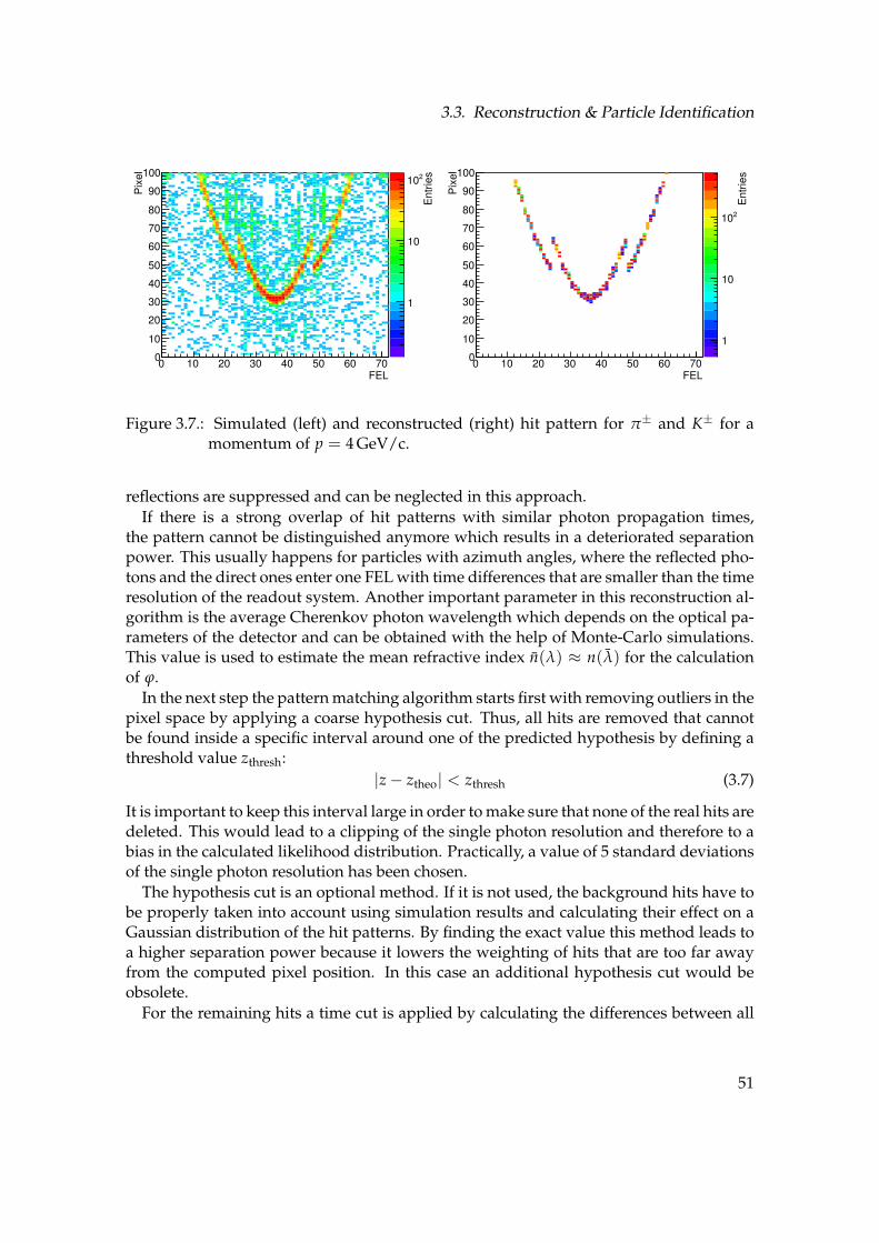
3.3. Reconstruction & Particle Identification

FEL0 10 20 30 40 50 60 70

Pix

el

0

10

20

30

40

50

60

70

80

90

100

En

trie

s

1

10

210

FEL0 10 20 30 40 50 60 70

Pix

el

0

10

20

30

40

50

60

70

80

90

100

En

trie

s

1

10

210

Figure 3.7.: Simulated (left) and reconstructed (right) hit pattern for π± and K± for amomentum of p = 4 GeV/c.

reflections are suppressed and can be neglected in this approach.

If there is a strong overlap of hit patterns with similar photon propagation times,the pattern cannot be distinguished anymore which results in a deteriorated separationpower. This usually happens for particles with azimuth angles, where the reflected pho-tons and the direct ones enter one FEL with time differences that are smaller than the timeresolution of the readout system. Another important parameter in this reconstruction al-gorithm is the average Cherenkov photon wavelength which depends on the optical pa-rameters of the detector and can be obtained with the help of Monte-Carlo simulations.This value is used to estimate the mean refractive index n(λ) ≈ n(λ) for the calculationof ϕ.

In the next step the pattern matching algorithm starts first with removing outliers in thepixel space by applying a coarse hypothesis cut. Thus, all hits are removed that cannotbe found inside a specific interval around one of the predicted hypothesis by defining athreshold value zthresh:

|z − ztheo| < zthresh (3.7)

It is important to keep this interval large in order to make sure that none of the real hits aredeleted. This would lead to a clipping of the single photon resolution and therefore to abias in the calculated likelihood distribution. Practically, a value of 5 standard deviationsof the single photon resolution has been chosen.

The hypothesis cut is an optional method. If it is not used, the background hits have tobe properly taken into account using simulation results and calculating their effect on aGaussian distribution of the hit patterns. By finding the exact value this method leads toa higher separation power because it lowers the weighting of hits that are too far awayfrom the computed pixel position. In this case an additional hypothesis cut would beobsolete.

For the remaining hits a time cut is applied by calculating the differences between all

51

3. Disc DIRC Detector

nσ2 σ1

nσ2 σ2

2 2.5 3 3.5 4 4.5 5Separation Power

0

2

4

6

8

10

12

14

16

Mis

identification [%

]

Figure 3.8.: Definition of the separation power between two probability density func-tions (left) and the calculated misidentification as a function of the separationpower (right)

hit times t and calculated arrival times that are obtained from equation (3.5). This methodis based on the truncated mean calculation: First t0 is computed for every hit from thedifference between the time stamp t and calculated propagation time tph according to

t0 = t − tph (3.8)

After calculating the average arrival time t0 the hit with the largest time difference tot0 is rejected if this value is above a specific threshold tthresh. With ttheo = t0 + tph thecondition for the remaining hits can be written as follows:

|t − ttheo| < tthresh (3.9)

If the threshold value is too small, real hits from the Cherenkov photons might be rejected,and if it is too large, dark counts or hits from scattered light can deteriorate the detectorresolution. The optimum value has been figured with the help of simulation studies byassuming a specific dark count rate for each pixel. The computation of the mean value oft0 is repeated until all time differences are placed below this threshold and no further hitis being rejected.

At the end a Gaussian distribution of the z coordinates and time values t is assumedand the likelihood values can be simply calculated with the following equation:

lnL =N

∑i=0

(lnG(zi|ztheo,i; σz) + lnG(ti|ttheo,i; σt)) (3.10)

For calculating the errors of z the method of error propagation has been used by takingthe given analytical equations into account. In the case of σt the intrinsic resolution of thereadout system is used in the reconstruction part and has been also implemented as aninput parameter in the digitization step.

52

3.3. Reconstruction & Particle Identification

3.3.4. Hit Pattern Matching

As mentioned above, one of the key features of the offline reconstruction is the patternmatching algorithm. The left side of Figure 3.7 illustrates a typical accumulated hit pat-tern for π± and K± with a particle momentum of p = 4 GeV/c obtained from Monte-Carlo simulations with a simple particle gun including 1000 events. The polar and az-imuth angles have been set to θp = 16 and φ = 45. The segmentation of the patternstructure into three subdivisions is a result of the quadrant geometry.

Because of the logarithmic scale of the z-axis of Figure 3.7, additional hits from Fres-nel reflections can be observed which results in a background signal in every event. Thechromatic and geometrical error of the EDD lead to a smearing of the pattern structurethat makes a separation with the naked eye almost impossible. However, the presentedreconstruction algorithm is able to distinguish between these hit patterns up to the mo-mentum value of p = 4 GeV/c.

The reconstructed hit pattern can be seen on the right side of Figure 3.7. The overlap ofthe reconstructed hit patterns can be explained with angular straggling and energy lossof the particles that result in an additional smearing effect.

3.3.5. Separation Power & Misidentification

By plotting the reconstructed Cherenkov angles or the differences of the logarithmic like-lihood values into two histograms for the π and K hypothesis, the result consists of twoGaussian distributions. The separation power can be naturally defined as the differencebetween the two expectation values µπ and µK divided by the average value of both stan-dard deviations σπ and σK. Therefore, it can be obtained with the following equation:

nσ =µπ − µK

12 (σπ + σK)

(3.11)

The separation power can be used to define a classifier C dividing the two distribu-tion into equal areas. The position of the classifier is given by the following equationdepending on the mean values of both particle hypotheses:

xC = µπ +nσ

2σπ = µK +

nσ

2σK (3.12)

The left side of Figure 3.8 illustrates the usage of the definition of the classifier for twoprobability distributions with different standard deviations. The probability for misiden-tified particle is then equal to the area of each distribution starting from the classifier andreaching up to infinity:

Pmisid =1√2π

∫ ∞

nσ/2e−

t2

2 dt (3.13)

For this purpose the Gaussian distribution has been shifted to µ = 0 without the lossof generality. The misidentification probability as a function of the separation power isshown on the right side of Figure 3.8.

53

3. Disc DIRC Detector

1 2 3 4 5 6 7 8 9 10Detector Resolution [mrad]

0

1

2

3

4

5

6

7

Se

pa

ratio

n P

ow

er

Particle Momentum:

2 GeV/c

3 GeV/c

4 GeV/c

0 0.2 0.4 0.6 0.8 1 1.2 1.4Tracking Resolution [mrad]

0

0.5

1

1.5

2

2.5

3

3.5

4

4.5

5

De

tecto

r R

eso

lutio

n [m

rad

]

Separation Power:

2 s.d.

3 s.d.

4 s.d.

Figure 3.9.: The separation power as a function of the overall detector resolution (left)and the dependency of the required detector resolution as a function of thetracking resolution (right).

3.4. Resolution Studies

3.4.1. Theoretical Description

The angular resolution of the EDD, that depends on the resolution of the photon mea-surements and the tracking of the charged particle, can be calculated according to thefollowing relation:

σ2θC

=σ2

ph

N+ σtrack (3.14)

where σph contains the geometrical error σgeom and chromatic error σchrom of the detector.It can therefore be split into

σ2ph = σ2

geom + σ2chrom (3.15)

The error of σph scales with the value√

N for detecting N photon hits per event. Thevalue of σtrack results from the error σerr of the tracking detectors of the PANDA spec-trometer, the error σMS of multiple scattering, and σloss the error due to energy loss of theparticle inside the radiator plate. Hence, it is eligible to write

σ2track = σ2

err + σ2MS + σ2

loss (3.16)

This resolution is fixed for each particle and cannot be increased by the acquisition of ahigher photon yield.

The left side of Figure 3.9 illustrates the achievable separation power for a given detec-tor resolution and different particle momenta. In order to achieve a separation power of3 standard deviations for 4 GeV/c π± and K± a detector resolution of approx 2.2 mrad isrequired.

The plot on the right side of Figure 3.9 shows the required detector resolution depend-ing on the tracking resolution of PANDA which is needed in order to guarantee the re-

54

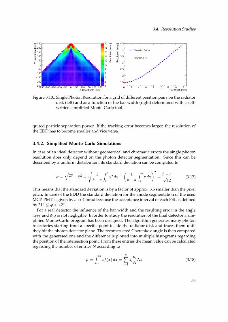
3.4. Resolution Studies

Re

so

lutio

n [

mra

d]

0

2

4

6

8

10

12

14

16

18

20

X Coordinate [mm]250− 200− 150− 100− 50− 0 50 100 150 200 250

Y C

oo

rdin

ate

[m

m]

250−

200−

150−

100−

50−

0

50

100

150

200

250

Bar Width [mm]0 2 4 6 8 10 12 14 16

Re

so

lutio

n [

mra

d]

1.5

2

2.5

3

3.5

4

4.5

Simulated Points

Polynomial Fit

Figure 3.10.: Single Photon Resolution for a grid of different position pairs on the radiatordisk (left) and as a function of the bar width (right) determined with a self-written simplified Monte-Carlo tool.

quired particle separation power. If the tracking error becomes larger, the resolution ofthe EDD has to become smaller and vice versa.

3.4.2. Simplified Monte-Carlo Simulations

In case of an ideal detector without geometrical and chromatic errors the single photonresolution does only depend on the photon detector segmentation. Since this can bedescribed by a uniform distribution, its standard deviation can be computed to

σ =

√

x2 − x2 =

√

1

b − a

∫ b

ax2 dx −

(1

b − a

∫ b

ax dx

)2

=b − a√

12(3.17)

This means that the standard deviation is by a factor of approx. 3.5 smaller than the pixelpitch. In case of the EDD the standard deviation for the anode segmentation of the usedMCP-PMT is given by σ ≈ 1 mrad because the acceptance interval of each FEL is definedby 21 ≤ ϕ < 42.

For a real detector the influence of the bar width and the resulting error in the angleαFEL and φrel is not negligible. In order to study the resolution of the final detector a sim-plified Monte-Carlo program has been designed. The algorithm generates many photontrajectories starting from a specific point inside the radiator disk and traces them untilthey hit the photon detector plane. The reconstructed Cherenkov angle is then comparedwith the generated one and the difference is plotted into multiple histograms regardingthe position of the intersection point. From these entries the mean value can be calculatedregarding the number of entries N according to

µ =∫ ∞

∞x f (x) dx =

N

∑i=1

xini

N∆x (3.18)

55

3. Disc DIRC Detector

Polar Angle [deg]6 8 10 12 14 16 18 20 22

Num

ber

of P

hoto

ns

300

400

500

600

700

800

900

1000

Pions 2 GeV/c Pions 3 GeV/c

Pions 4 GeV/c Kaons 2 GeV/c

Kaons 3 GeV/c Kaons 4 GeV/c

Protons 2 GeV/c Protons 3 GeV/c

Protons 4 GeV/c

Figure 3.11.: Trapped photons in the radiator disk with a thickness of 2 cm.

where xi is the center of the bin and ni the number of its entries. The bin width ∆x is fixedfor all bins. The standard deviation can then be computed regarding its definition

σ =

√∫ ∞

∞(x − µ)2 f (x) dx =

√√√√

N

∑i=1

(xi − µ)2ni

N∆x (3.19)

In this case the standard deviation is equal to the single photon resolution. Additionally,it is possible to add packages that take other effects like dispersion or multiple scatteringof the primary particle into account.

Figure 3.10 shows the simulated single photon resolution for a bar width of 16 mm andan arbitrary FEL in the center of the x-axis and the upper position of the y-axis. For largerdistances the influence of the finite bar width is very small but it increases with enlargingthe distance in x direction and shrinking the distance in y direction. The white spacesin the histogram occur for photons which are outside of the accepted angle range of thefocusing plane.

Another important parameter is the influence of the bar width on the resolution for aspecific position on the radiator plate. For this purpose the center position of the radiatordisk has been chosen. As expected, an increase of the bar width leads to a worse singlephoton resolution. A polynomial fit with the order of 4 can be used to find an acceptableapproximation for the resulting behavior. The final results can be used for optimizing thedetector performance by changing different parameters.

56

3.5. Photon Trapping

3.5. Photon Trapping

The amount of Cherenkov photons, that are trapped via total internal reflection, can becalculated fully analytically. The wavelength dependency of the refractive index has animpact on the opening angle of the Cherenkov cone, the photon yield and the conditionof internal reflection. Therefore, the equations (1.21), (1.22) and (1.39) can be used tocalculate the fraction of trapped photons for every wavelength interval by calculatingthe dot product of the photon tracks in a specific azimuth angle interval and the normalvector of the radiator surface by using spherical coordinates.

Figure 3.11 shows the amount of trapped photons inside the EDD radiator for the par-ticle species π±, K± and p± as the function of their polar angles θp. The amount of createdphotons increases for larger polar angles because of the longer distance d/cosθp that thecharged particle travels inside the fused silica. The average amount of trapped photonsis a value around 75 % for high momentum particles with β → 1. Additional filters, ge-ometrical acceptances, and detection efficiencies of the MCP-PMTs can reduce this valueby factor of 30 as it will be shown in chapter 4.

57

4. Simulation Studies

4.1. PandaRoot Framework

4.1.1. Data Flow

The offline reconstruction of data from the PANDA detector is planned to be done ina framework called PandaRoot [StPC11]. It depends on the software packages FairSoftand FairRoot provided by the FAIR collaboration. In addition to that, a possibility fordetector simulation is implemented in PandaRoot. One of the advantages of PandaRootis the high modularity that makes it easy to implement new detectors without interferingwith the existing ones.

For the simulation part of the PandaRoot reconstruction chain the VMC method hasbeen chosen. It uses the Geant4 transport algorithm and can easily be implemented inan existing ROOT [A+09] installation. VMC provides the possibility of running differentMonte-Carlo simulations without the necessity of changing the user code.

The Monte-Carlo simulation data is stored in a ROOT tree which can be further pro-cessed by the digitization part. The output of the digitization part is supposed to be iden-tical to the real data of the FEE in the PANDA detector. No additional information fromthe Monte-Carlo simulations are allowed and all relevant detector information shouldbe included. The flow diagram of the implementation of the EDD regarding simulation,digitization, reconstruction, and PID in PandaRoot including the relevant class names ispresented in Figure 4.1.

The first step is the generation of the Monte-Carlo simulation data with the Geant4transport algorithm. The simulation includes the generation of particle tracks, the track-ing and the generation of Cherenkov photons. It stores the important data of the pri-mary particle like the position and momentum when entering the radiator plate and thephoton information on the photocathode of the MCP-PMT. The next step uses the dig-itization part which converts the Monte-Carlo data into pixel information such as pixelnumber and binned TDC time information including a possible smearing according tothe TOFPET data. An additional class for the description of the sensor geometry andproperties is implemented for this purpose and can be easily extended to other sensortypes such as SiPMs.

The stored data can be analyzed inside the reconstruction part where the theoreti-cal hit pattern is calculated. The reconstruction algorithm should not use any Monte-Carlo information of the originally generated tracks and only rely on the digitizationoutput. However, for performance studies of the EDD the Monte-Carlo truth data hasbeen copied from the simulation part into the digitization file in order to use them inthe reconstruction step for comparison. The calculated hit pattern information from the

59

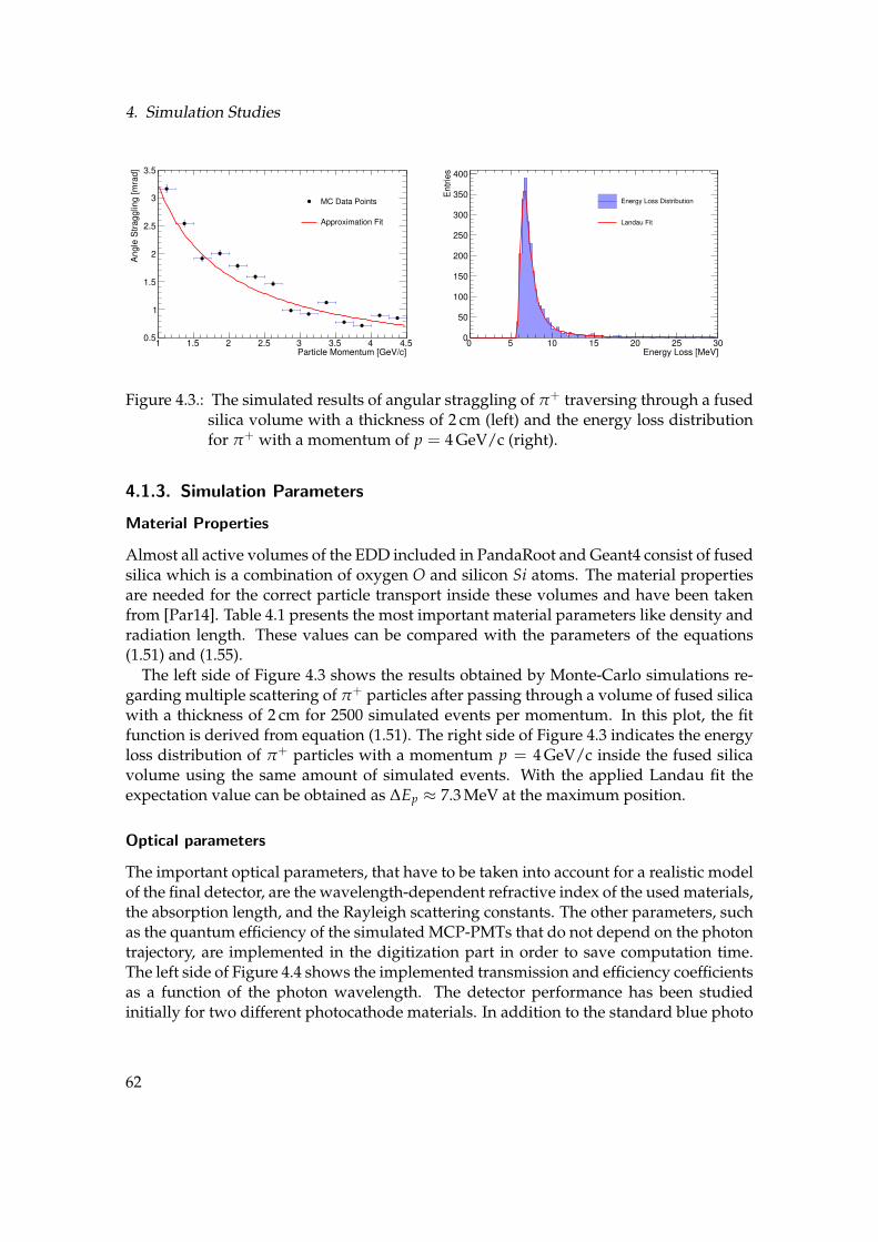
4. Simulation Studies

Particle Momentum [GeV/c]1 1.5 2 2.5 3 3.5 4 4.5

Angle

Str

agglin

g [m

rad]

0.5

1

1.5

2

2.5

3

3.5

MC Data Points

Approximation Fit

Energy Loss [MeV]0 5 10 15 20 25 30

Entr

ies

0

50

100

150

200

250

300

350

400

Energy Loss Distribution

Landau Fit

Figure 4.3.: The simulated results of angular straggling of π+ traversing through a fusedsilica volume with a thickness of 2 cm (left) and the energy loss distributionfor π+ with a momentum of p = 4 GeV/c (right).

4.1.3. Simulation Parameters

Material Properties

Almost all active volumes of the EDD included in PandaRoot and Geant4 consist of fusedsilica which is a combination of oxygen O and silicon Si atoms. The material propertiesare needed for the correct particle transport inside these volumes and have been takenfrom [Par14]. Table 4.1 presents the most important material parameters like density andradiation length. These values can be compared with the parameters of the equations(1.51) and (1.55).

The left side of Figure 4.3 shows the results obtained by Monte-Carlo simulations re-garding multiple scattering of π+ particles after passing through a volume of fused silicawith a thickness of 2 cm for 2500 simulated events per momentum. In this plot, the fitfunction is derived from equation (1.51). The right side of Figure 4.3 indicates the energyloss distribution of π+ particles with a momentum p = 4 GeV/c inside the fused silicavolume using the same amount of simulated events. With the applied Landau fit theexpectation value can be obtained as ∆Ep ≈ 7.3 MeV at the maximum position.

Optical parameters

The important optical parameters, that have to be taken into account for a realistic modelof the final detector, are the wavelength-dependent refractive index of the used materials,the absorption length, and the Rayleigh scattering constants. The other parameters, suchas the quantum efficiency of the simulated MCP-PMTs that do not depend on the photontrajectory, are implemented in the digitization part in order to save computation time.The left side of Figure 4.4 shows the implemented transmission and efficiency coefficientsas a function of the photon wavelength. The detector performance has been studiedinitially for two different photocathode materials. In addition to the standard blue photo

62

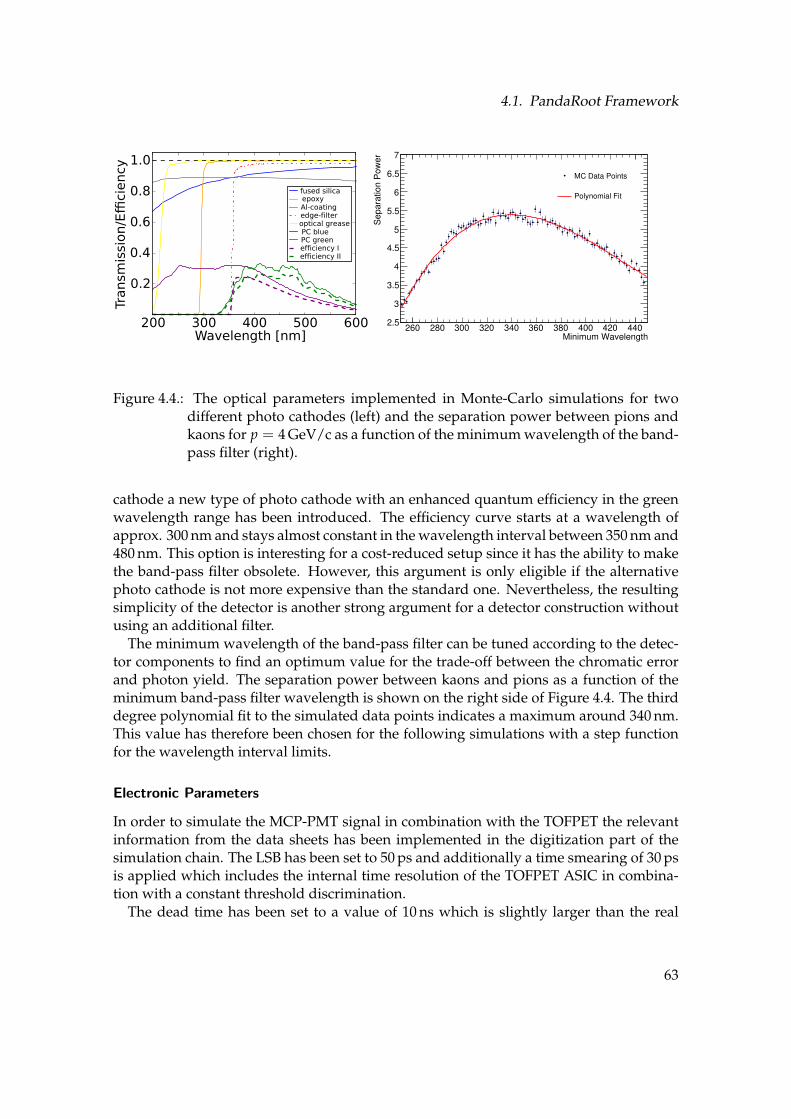
4.1. PandaRoot Framework

200 300 400 500 600

0.2

0.4

0.6

0.8

1.0

Transm

issio

n/Effi

cie

ncy

fused silicaepoxyAl-coatingedge-filteroptical greasePC bluePC greenefficiency Iefficiency II

Wavelength [nm] Minimum Wavelength260 280 300 320 340 360 380 400 420 440

Separa

tion P

ow

er

2.5

3

3.5

4

4.5

5

5.5

6

6.5

7

MC Data Points

Polynomial Fit

Figure 4.4.: The optical parameters implemented in Monte-Carlo simulations for twodifferent photo cathodes (left) and the separation power between pions andkaons for p = 4 GeV/c as a function of the minimum wavelength of the band-pass filter (right).

cathode a new type of photo cathode with an enhanced quantum efficiency in the greenwavelength range has been introduced. The efficiency curve starts at a wavelength ofapprox. 300 nm and stays almost constant in the wavelength interval between 350 nm and480 nm. This option is interesting for a cost-reduced setup since it has the ability to makethe band-pass filter obsolete. However, this argument is only eligible if the alternativephoto cathode is not more expensive than the standard one. Nevertheless, the resultingsimplicity of the detector is another strong argument for a detector construction withoutusing an additional filter.

The minimum wavelength of the band-pass filter can be tuned according to the detec-tor components to find an optimum value for the trade-off between the chromatic errorand photon yield. The separation power between kaons and pions as a function of theminimum band-pass filter wavelength is shown on the right side of Figure 4.4. The thirddegree polynomial fit to the simulated data points indicates a maximum around 340 nm.This value has therefore been chosen for the following simulations with a step functionfor the wavelength interval limits.

Electronic Parameters

In order to simulate the MCP-PMT signal in combination with the TOFPET the relevantinformation from the data sheets has been implemented in the digitization part of thesimulation chain. The LSB has been set to 50 ps and additionally a time smearing of 30 psis applied which includes the internal time resolution of the TOFPET ASIC in combina-tion with a constant threshold discrimination.

The dead time has been set to a value of 10 ns which is slightly larger than the real

63

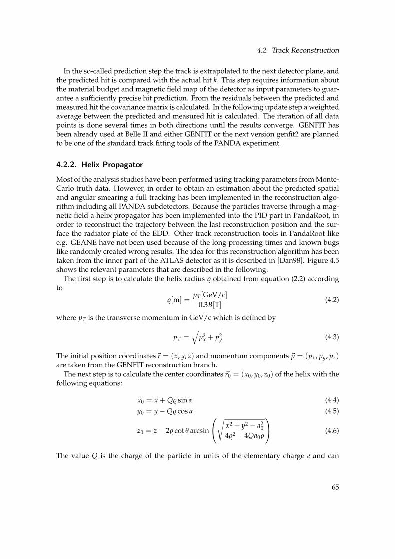
4.2. Track Reconstruction

In the so-called prediction step the track is extrapolated to the next detector plane, andthe predicted hit is compared with the actual hit k. This step requires information aboutthe material budget and magnetic field map of the detector as input parameters to guar-antee a sufficiently precise hit prediction. From the residuals between the predicted andmeasured hit the covariance matrix is calculated. In the following update step a weightedaverage between the predicted and measured hit is calculated. The iteration of all datapoints is done several times in both directions until the results converge. GENFIT hasbeen already used at Belle II and either GENFIT or the next version genfit2 are plannedto be one of the standard track fitting tools of the PANDA experiment.

4.2.2. Helix Propagator

Most of the analysis studies have been performed using tracking parameters from Monte-Carlo truth data. However, in order to obtain an estimation about the predicted spatialand angular smearing a full tracking has been implemented in the reconstruction algo-rithm including all PANDA subdetectors. Because the particles traverse through a mag-netic field a helix propagator has been implemented into the PID part in PandaRoot, inorder to reconstruct the trajectory between the last reconstruction position and the sur-face the radiator plate of the EDD. Other track reconstruction tools in PandaRoot likee.g. GEANE have not been used because of the long processing times and known bugslike randomly created wrong results. The idea for this reconstruction algorithm has beentaken from the inner part of the ATLAS detector as it is described in [Dan98]. Figure 4.5shows the relevant parameters that are described in the following.

The first step is to calculate the helix radius $ obtained from equation (2.2) accordingto

$[m] =pT[GeV/c]

0.3B[T](4.2)

where pT is the transverse momentum in GeV/c which is defined by

pT =√

p2x + p2

y (4.3)

The initial position coordinates~r = (x, y, z) and momentum components ~p = (px, py, pz)are taken from the GENFIT reconstruction branch.

The next step is to calculate the center coordinates ~r0 = (x0, y0, z0) of the helix with thefollowing equations:

x0 = x + Q$ sin α (4.4)

y0 = y − Q$ cos α (4.5)

z0 = z − 2$ cot θ arcsin

√

x2 + y2 − a20

4$2 + 4Qa0$

(4.6)

The value Q is the charge of the particle in units of the elementary charge e and can

65

4. Simulation Studies

Momentum [GeV/c]1.5 2 2.5 3 3.5 4

x [

mm

]∆

0.15−

0.1−

0.05−

0

0.05

0.1

0.15

Momentum [GeV/c]1.5 2 2.5 3 3.5 4

[m

rad

]θ

∆

3−

2.5−

2−

1.5−

1−

0.5−

Figure 4.6.: The x-position (left) and polar angle (right) resolution of the reconstructedparticle track for π+ particles as a function of the particle momentum. Theerror bars indicate the error of the mean value, and the yellow band repre-sents the resolution.

therefore take the values +1 or −1. The trigonometrical functions of α are given by

cos α =px

pT(4.7)

sin α =py

pT(4.8)

while the transverse impact parameter a0 is being calculated with

a0 = Q

(√

x20 + y2

0 − $

)

(4.9)

Finally the initial phase φ0 of the helix track is necessary for the calculation of the trackpropagation. It is given by the relation

φ0 =

arctan(

y0

x0

)

+ 12 Qπ for x0 < 0

arctan(

y0

x0

)

+ 12 Qπ + π for x0 > 0 and y0 < 0

arctan(

y0

x0

)

+ 12 Qπ − π for x0 > 0 and y0 > 0

(4.10)

With these values the coordinates at the radiator surface can be calculated accordingto:

x′(λ) = x0 + Q$ sin(Qλ − φ0) (4.11)

y′(λ) = y0 + Q$ cos(Qλ − φ0) (4.12)

66

4.2. Track Reconstruction

Event 1 Event 2 Event 3Event 1 Event 2 Event 3Event 1 Event 2 Event 3Event 1 Event 2 Event 3Event 1 Event 2 Event 3Event 1 Event 2 Event 3Event 1 Event 2 Event 3Event 1 Event 2 Event 3Event 1 Event 2 Event 3Event 1 Event 2 Event 3Event 1 Event 2 Event 3Event 1 Event 2 Event 3Event 1 Event 2 Event 3Event 1 Event 2 Event 3Event 1 Event 2 Event 3Event 1 Event 2 Event 3Event 1 Event 2 Event 3Event 1 Event 2 Event 3Event 1 Event 2 Event 3Event 1 Event 2 Event 3Event 1 Event 2 Event 3Event 1 Event 2 Event 3Event 1 Event 2 Event 3Event 1 Event 2 Event 3Event 1 Event 2 Event 3

Figure 4.7.: The working principle of time-based simulations. The start time of eachevent is obtained from the Monte-Carlo simulations. Every row contains thehits related to one specific event which is indicated by a unique color. In thelast row the sum of all hits shows the overlap of all detector hits.

If z′ is the z-coordinate of the radiator disc and the relation cot θ given by:

cot θ =pz

pT(4.13)

the propagation parameter λ can be computed with

λ =z′ − z0

$ cot θ(4.14)

where z0 is the z coordinate of the last reconstructed particle position and z′ the z coordi-nate of the radiator disk.

4.2.3. Track Resolution

The angular and spatial tracking resolution of the implemented helix propagator is cal-culated by comparing the reconstructed results with the Monte-Carlo data of the particlewhen it enters the radiator plate. The results of this investigation can be seen in Figure 4.6.

Pions with varying momenta between 1.5 GeV/c and 4 GeV/c have been created undera polar of angle of θ = 15 and an arbitrary azimuth angle in the interval 0 ≤ φ ≤ 360.The data points with the calculated error bars displaying the errors of the mean valueshow the offset between the simulated and the reconstructed data while the yellow bandrepresents the resolution taken from the Gaussian fits.

As a result, the average spatial resolution could be obtained as a value of 150 µm, andthe average angular resolution of the polar angle θ has been computed to 0.5 mrad over

67

4. Simulation Studies

Radiator Quadrant (Upstream)

~rFEL

~p~d

~x0

~xFEL

Bar (Top View)

αFEL

Figure 4.8.: The spatial and angular parameters (left) used for the geometrical reconstruc-tion and the reconstruction of αFEL for the entering photon (right).

the whole momentum range. The implementation of better extrapolation methods couldincrease the resolution even more. The overall track resolution also depends on the num-ber of GEM tracking stations which have been assumed to be fully equipped. If less than3 stations are available, the resolution will most probably deteriorate.

An interesting behavior can be observed in the reconstruction of the momentum reso-lution as the offset is a function of the particle momentum. This effect can be explainedby inhomogeneities in the magnetic field as one can see from the plotted field maps. Thisdependency has to be compensated by fitting a polynomial function second degree to thedata points and insert the resulting parameters into the reconstruction code.

4.3. Time Based Simulations

Geant4 and VMC do only support event based simulations, i.e. a new event is definedtogether with the creation of a primary particle. The processing usually ends after allparticles fulfill specific conditions such as leaving the mother volume. These events arecreated independently from each other, and one event has no information about anotherevent.

This method is in general a suitable approach for detector assemblies with low inter-action rates. However, for higher rates in experiments like PANDA, which do not usea hardware trigger, it can only be a coarse approximation. A better approach is the im-plementation of so-called time-based simulations that can be used in combination withPandaRoot.

Figure 4.7 outlines the working principle of time-based simulations. The black lines in-dicate the real start time of each event and the colored lines represent the hits in the EDD

68

4.4. Geometrical Reconstruction

Cherenkov Angle [rad]0.8 0.81 0.82 0.83

En

trie

s

50

100

150

200

250

0.84

5

10

15

20

25

30

35

40

En

trie

s

Cherenkov Angle [rad]0.8 0.81 0.82 0.83 0.84

Figure 4.9.: Single photon distribution of the EDD for π+ particles with the momentump = 4 GeV/c.

in combination with their time information. Every event contains its own related hitsand can additionally contain hits from previous and subsequent events. In the PANDAdetector the real start time of one event is not known and has to be reconstructed fromthe time stamps of all hits.

The code of the EDD has been adapted to be compatible with this simulation methodin order to obtain realistic simulation results. The average time difference between theevents can be defined in the digitization step. A special class called RingSorter, which isalready implemented in PandaRoot, has been used in order to rearrange the simulatedhits according to the presented scheme.

4.4. Geometrical Reconstruction

The left side of Figure 4.8 shows the important parameters that are needed for the ge-ometrical reconstruction in the 2D projection. The charged particle enters the radia-tor quadrant at the reconstructed position ~x0 = (x0, y0) with the projected momentum~p = (px, py). From the components of ~p the polar angle

cos θp =pz

|~p| =pz

√

p2x + p2

y + p2z

(4.15)

of the charged particle can be calculated. Instead of the azimuth angle φ the angle φrel ,which has been introduced in chapter 3, between the particle and measured photon is

used. The vector ~d = (x0 − xFEL, y0 − yFEL) is then defined as the difference between theposition of the FEL and the point of particle intersection. It is further equal to the 2Dprojection of the photon trajectory.

69

4. Simulation Studies

Polar Angle [deg]10 12 14 16 18 20 22

Azim

uth

An

gle

[d

eg

]

0

10

20

30

40

50

60

70

80

90 ]σ

Se

pa

ratio

n P

ow

er

[n

0

1

2

3

4

5

6

Mean: 4.43732

Polar Angle [deg]10 12 14 16 18 20 22

Azim

uth

An

gle

[d

eg

]

0

10

20

30

40

50

60

70

80

90 ]σ

Se

pa

ratio

n P

ow

er

[n

0

1

2

3

4

5

6Mean: 4.8322

Figure 4.10.: The reconstructed separation power as a function of the polar and azimuthangles for the blue (left) and green (right) photocathode

With these values the angle φrel can simply be calculated with the dot-product

cos(φrel) =~d · ~p

√

~d2 · ~p2

(4.16)

For the computation of the angle αFEL the orientation vector~rFEL = (cos α, sin α) of thereferring FEL has to be taken into account:

cos(αFEL) =dx cos α + dy sin α

√

d2x + d2

y

(4.17)

where α is the azimuth angle of the FEL.On the right side of Figure 4.8 the expected error in the angle uncertainty of αFEL is

illustrated. If the charged particle enters the radiator plate close to the FEL, the photonhas several possible paths to enter the FEL. For the computation of the theoretical hitpattern only the average position of the FEL, represented by the red line, can be takeninto account. This usually results in a large error for small distances as indicated by thetwo black lines. The dashed line represents the real photon path while the normal linerepresents the reconstructed path. The error in αFEL influences of the overall geometricalresolution of the detector.

4.5. Detector Performance

4.5.1. Probe Tracks

The single photon Cherenkov angle distribution from the reconstructed Cherenkov an-gles for 1000 events of π+ with a momentum of 4 GeV/c is presented on the left side of

70

4.5. Detector Performance

Num

ber

of H

its

0

5

10

15

20

25

30

Photon Hits

Polar Angle [deg]10 12 14 16 18 20 22

Azim

uth

Angle

[deg]

0

10

20

30

40

50

60

70

80

90

Mean: 21.1583

Photon Hits

Num

ber

of H

its

0

5

10

15

20

25

30

Photon Hits

Polar Angle [deg]10 12 14 16 18 20 22

Azim

uth

Angle

[deg]

0

10

20

30

40

50

60

70

80

90

Mean: 25.7761

Photon Hits

Figure 4.11.: The detected photon hits as a function of the polar and azimuth angles forthe blue (left) and green (right) photocathode

Figure 4.9. The thin peaks are a result of the fine granularity of the MCP-PMTs whilethe deviation of these peaks is related to the geometrical smearing and resolution. Anglestraggling and energy loss of the charged particles, before entering and inside the radia-tor plate, lead to a smearing of the reconstructed Cherenkov angles and therefore resultin an overlap of the peak structure. The distribution of the averaged Cherenkov anglesis presented in the right histogram of Figure 4.9. The RMS values of both distributionsdiffer as expected by factor of approx.

√N according to the number N of acquired hits.

The separation power for the coarse 2D angle scan with π+ and K+ for a momentumof p = 4 GeV/c without applying a magnetic field is shown in Figure 4.10. The asym-metric shape, that can be observed in the case of both photocathodes, is a result of theadditional reflection on the tilted quadrant side for specific azimuth angles. This effectcould be removed if this surface is changed from polished fused silica to one that absorbsphotons. This analysis validates the detector performance, as previously defined insidethe PANDA collaboration, up to polar angles of θ = 22 by obtaining a separation powerlarger than 3 standard deviations at p = 4 GeV/c.

The number of acquired photon hits for each angle combination by implementing theblue and green photocathode is shown in Figure 4.11. Using the green photocathodeleads to a higher photon yield and has to be taken into account for the estimation of theMCP-PMT lifetime. Further results regarding the detector resolution and reconstructionefficiency are given in Appendix A.

As shown in Figure 4.12 the separation power for the green photocathode is slightlyhigher than the one for the blue photocathode. The separation power is higher for smallerpolar angles due to smaller effects of the geometrical errors in the reconstruction algo-rithm, although the number of detected photon hits decreases for larger distances to theFEL. Therefore, the local minimum around 15 for 4 GeV/c momenta can be explainedby the trade-off between the geometrical errors and photon hit numbers.

71

4. Simulation Studies

Polar Angle [deg]12 14 16 18 20 22

Se

pa

ratio

n P

ow

er

0

5

10

15

20

25

30

Blue Cathode

2 GeV/c

3 GeV/c

4 GeV/c

Green Cathode

2 GeV/c

3 GeV/c

4 GeV/c

Figure 4.12.: The separation power as a function of the polar angle for two different photocathode options.

4.5.2. High Resolution Studies

For the following analysis π+ and K+ are created with uniformly distributed polar anglesθ and azimuth angles in the interval −30 < φ ≤ 120 with high statistics in the orderof 108 events. An additional modification of the number of created events with the factor1/ cos θ in the simulation part is necessary because of the decreasing statistics for largerpolar angles. The fine binning on the radiator plate has been done after the reconstructionstep. Each bin has a size of approx. 1 cm in both directions and is small enough tostudy local variances in the detector performance. This method makes sure that particlesarriving far away from their expected point due to multiple scattering are still taken intoaccount.

Additionally, the influence of the solenoid magnetic field has been implemented in thesimulation part. The Geant4 transport algorithm propagates the charged particles fromthe target point to the radiator plate on a helix trajectory. Hence, a more realistic modelof the particle transport comparable with the conditions in PANDA can be simulated.

The results for the momentum p = 4 GeV/c are presented on the left of Figure 4.13.Hits with polar angles with θ > 22 have been excluded because they will be shieldedby the barrel EMC and not be available for reconstruction. The deterioration of the sep-aration power on the horizontal side of the quadrant is an effect of the overlapping hitpatterns of the direct and reflected photons.

If the time difference between both photon trajectories is in the same order as theTOFPET resolution, the hits cannot be separated anymore without getting ambiguities.Strong overlaps in the hit pattern can worsen the separation power up to a factor of 3.However, for very small distances between the charged particle and the rim an increase

72

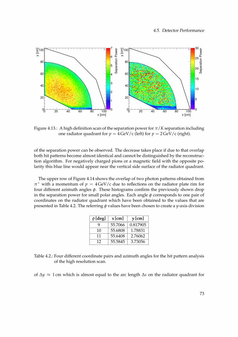
4.5. Detector Performance

Separa

tion P

ow

er

0

1

2

3

4

5

6

7

x [cm]0 20 40 60 80 100

y [cm

]

0

20

40

60

80

100

Separa

tion P

ow

er

0

5

10

15

20

25

30

x [cm]0 20 40 60 80 100

y [cm

]

0

20

40

60

80

100

Figure 4.13.: A high definition scan of the separation power for π/K separation includingone radiator quadrant for p = 4 GeV/c (left) for p = 2 GeV/c (right).

of the separation power can be observed. The decrease takes place if due to that overlapboth hit patterns become almost identical and cannot be distinguished by the reconstruc-tion algorithm. For negatively charged pions or a magnetic field with the opposite po-larity this blue line would appear near the vertical side surface of the radiator quadrant.

The upper row of Figure 4.14 shows the overlap of two photon patterns obtained fromπ+ with a momentum of p = 4 GeV/c due to reflections on the radiator plate rim forfour different azimuth angles φ. These histograms confirm the previously shown dropin the separation power for small polar angles. Each angle φ corresponds to one pair ofcoordinates on the radiator quadrant which have been obtained to the values that arepresented in Table 4.2. The referring φ values have been chosen to create a y-axis division

φ [deg] x [cm] y [cm]

9 55.7066 0.817905

10 55.6808 1.78831

11 55.6408 2.76062

12 55.5845 3.73056

Table 4.2.: Four different coordinate pairs and azimuth angles for the hit pattern analysisof the high resolution scan.

of ∆y ≈ 1 cm which is almost equal to the arc length ∆s on the radiator quadrant for

73

4. Simulation Studies

Sensor ID40 45 50 55 60 65 70

Pix

el N

um

be

r

0

10

20

30

40

50

60

70

80

90

100

En

trie

s0

2

4

6

8

10

12

14

16

18

20

22

24

Sensor ID40 45 50 55 60 65 70

Pix

el N

um

be

r

0

10

20

30

40

50

60

70

80

90

100

En

trie

s

0

5

10

15

20

25

Sensor ID40 45 50 55 60 65 70

Pix

el N

um

be

r

0

10

20

30

40

50

60

70

80

90

100

En

trie

s

0

5

10

15

20

25

30

Sensor ID40 45 50 55 60 65 70

Pix

el N

um

be

r

0

10

20

30

40

50

60

70

80

90

100

En

trie

s

0

5

10

15

20

25

Sensor ID40 45 50 55 60 65 70

Pix

el N

um

be

r

0

10

20

30

40

50

60

70

80

90

100

Sensor ID40 45 50 55 60 65 70

Pix

el N

um

be

r

0

10

20

30

40

50

60

70

80

90

100

Sensor ID40 45 50 55 60 65 70

Pix

el N

um

be

r

0

10

20

30

40

50

60

70

80

90

100

Sensor ID40 45 50 55 60 65 70

Pix

el N

um

be

r

0

10

20

30

40

50

60

70

80

90

100

Figure 4.14.: The simulated (up) and reconstructed (down) hit pattern for different az-imuth angles regarding the high resolution scan. The four columns showthe hit pattern for different positions of the π+ on the radiator plate.

small azimuth angles:

∆y ≈ ∆s = π d tan θ︸ ︷︷ ︸

R

∆φ

180(4.18)

Here θ stands for the polar angle of the particle and d for the distance between the targetand the EDD. As one can see, the particle is bent by an angle of approx. 8 due to theinfluence of the magnetic field.

The lower row of Figure 4.14 represents the reconstructed hit patterns for the samecoordinates. The hits from the direct photons are indicated by the blue colored entrieswhile the red dots mark the entries of the reflection on the rim. For increasing y valuesthe pattern start to overlap which leads to the drop in the separation power. If both pat-terns overlap completely, an increase of the separation power is expected. However, thissituation does not occur because of the tilting of the particle trajectory as a result of thesolenoid field. Hence, the assumed peak inside the plotted valley cannot be observed,and an increasing distance between the pattern structures results in a better detector per-formance.

In case of p = 2 GeV/c particle momentum, as shown on the right side of Figure 4.13,the line with the deteriorated performance shifts to larger polar angles. This shift canbe explained by the smaller bending radius of the particle curvature due to the smallermomentum.

74

4.6. Benchmark Channel

[deg]θPolar Angle 0 20 40 60 80 100 120 140 160 180

Mom

entu

m [G

eV

/c]

0

1

2

3

4

5

6

7

8

9

10

Entr

ies

0

2

4

6

8

10

12

[deg]θKaon 1 Polar Angle 0 10 20 30 40 50 60 70 80 90

[deg]

θK

aon 2

Pola

r A

ngle

0

10

20

30

40

50

60

70

80

90

Entr

ies

0

1

2

3

4

5

6

Figure 4.15.: The kaon phase space (left) and the polar angle distribution of the K+/K−

decay branch (right).

4.6. Benchmark Channel

For the analysis of the EDD under PANDA conditions a specific benchmark channel hasbeen chosen. This analysis shows the possible results that can be obtained from the realPANDA experiment at small beam momenta. In order to add new physics to the perfor-mance analysis the following decay

pp → f0π0 → K+K−π0 (4.19)

has been investigated. The collision of protons and antiprotons creates a pair of the glue-ball candidate f0(1500) with the rest mass 1500 MeV/c2 and a neutral π0. The f0 particledecays into two kaons K+ and K− that can be identified with the EDD alone or in combi-nation with other PID detectors. The beam momentum has been set to p = 6.5 GeV/c.

Including the neutral particle π0 is necessary to fulfill the momentum conservation asit takes momentum fraction of the system of protons and antiprotons. Other particlessuch as η0 or φ0 can also be used instead of the π0 but these cases have not been studied.However, the results of these different possibilities look very similar.

The kaon phase space is shown on the left side of Figure 4.15. Because of the fixedbeam momentum a cut-off value around 6.5 GeV/c is observed. Figure 4.15 right panelshows a plot with the polar angles of the two kaons plotted against each other. In thishistogram, a momentum cut of 1.5 < p ≤ 4 GeV/c has been applied in order to filter outuninteresting events.

If a data point is situated inside the blue rectangle, both kaons enter the EDD. In case ofthe events with points inside the red rectangles one kaon traverses the EDD and the otherone the Barrel DIRC. For some events, which are placed outside of these three rectangles,both kaons enter the Barrel DIRC.

The azimuth angle correlation between both kaons is shown in Figure 4.16. In thisplot, no momentum cut has been applied in order to investigate the amount of pileup

75

4. Simulation Studies

[deg]φKaon 1 Azimuth Angle 150− 100− 50− 0 50 100 150

[d

eg

]φ

Ka

on

2 A

zim

uth

An

gle

150−

100−

50−

0

50

100

150

En

trie

s

0

0.5

1

1.5

2

2.5

3

I

II

III

IV

III

III IV

x

y

Figure 4.16.: The azimuth angle distribution between two kaons created by a f0 decay(left) and the corresponding labeled quadrant (right).

events in one radiator quadrant. Each hit in one of the four numbered rectangles rep-resents an event, in which both created kaons enter the same quadrant of the radiatorplate and cause pileups that might influence the reconstruction efficiency. However, thisdepends on the difference in the arrival time, absolute momentum, and azimuth angle ofthe charged particles. Additionally, these pileup events are rather rare at the given beammomentum.

4.6.1. Event Generation

The event generation is implemented in PandaRoot with the EvtGen package. The decaybranches of each particle can be defined in separate decay files. The standard decaychannels of the f0(1500) are already included in PandaRoot and can be seen in Listing 4.1.

Decay f 0 ( 1 5 0 0 )0 .019 e ta eta ’ PHSP ;0 .051 e ta ata PHSP ;0 .1410 pi0 pi0 pi0 pi0 PHSP ;0 .3540 pi+ pi− pi+ pi− PHSP ;0 .2330 pi+ pi− PHSP ;0 .1160 pi0 pi0 PHSP ;0 .0430 K+ K− PHSP ;0 .0215 K S0 K S0 PHSP ;0 .0215 K L0 K L0 PHSP ;Enddecay

Listing 4.1: Decay file of f0(1500) with the related branching ratios. The entry PHSP statesthe kinematics is calculated according to phase space calculations.

76

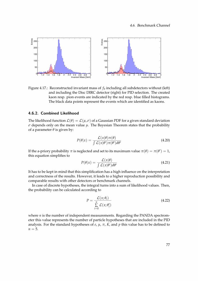
4.6. Benchmark Channel

Invariant Mass [GeV]1 1.2 1.4 1.6 1.8 2 2.2 2.4 2.6 2.8 3

En

trie

s

0

50

100

150

200

250

Invariant Mass [GeV]1 1.2 1.4 1.6 1.8 2 2.2 2.4 2.6 2.8 3

En

trie

s

0

50

100

150

200

250

Figure 4.17.: Reconstructed invariant mass of f0 including all subdetectors without (left)and including the Disc DIRC detector (right) for PID selection. The createdkaon resp. pion events are indicated by the red resp. blue filled histograms.The black data points represent the events which are identified as kaons.

4.6.2. Combined Likelihood

The likelihood function L(θ) = L(µ, σ) of a Gaussian PDF for a given standard deviationσ depends only on the mean value µ. The Bayesian Theorem states that the probabilityof a parameter θ is given by:

P(θ|x) = L(x|θ)π(θ)∫L(x|θ′)π(θ′)dθ′

(4.20)

If the a-priory probability π is neglected and set to its maximum value π(θ) = π(θ′) = 1,this equation simplifies to

P(θ|x) = L(x|θ)∫L(x|θ′)dθ′

(4.21)

It has to be kept in mind that this simplification has a high influence on the interpretationand correctness of the results. However, it leads to a higher reproduction possibility andcomparable results with other detectors or benchmark channels.

In case of discrete hypotheses, the integral turns into a sum of likelihood values. Then,the probability can be calculated according to

P =L(x; θi)

n

∑i=0

L(x; θ′i)(4.22)

where n is the number of independent measurements. Regarding the PANDA spectrom-eter this value represents the number of particle hypotheses that are included in the PIDanalysis. For the standard hypotheses of e, µ, π, K, and p this value has to be defined ton = 5.

77

4. Simulation Studies

The combined likelihood value can be computed from the product of the likelihoodvalue Lj of each subdetector j. Therefore, the probability for n particle hypotheses and Nsubdetectors can be written as:

P =

N

∏j=0

Lj(xj; µi, σi)

n

∑i=0

N

∏j=0

Lj(xj; µi, σi)

(4.23)

4.6.3. Mass Reconstruction

The center-of-mass energy for two particles i = 1, 2 with the four momentum vectors

pi =

(Ei/c~pi

)

(4.24)

and its squared values = E2

CMS = (p1 + p2)2 (4.25)

is invariant under Lorentz transformations. If these two particles are products of a parti-cle decay, the energy ECMS is equal to the rest energy of the mother particle. Accordingto the algebraic rules of four vector calculations the rest mass can therefore be computedwith the following equation:

E0 =√

m21c4 + m2

2c4 + 2E1E2/c2 − ~p1 · ~p2 (4.26)

The assumption for the rest mass of both particles have to be taken from the probabilityvalues of the PID detectors. The information about their total energies E and momenta ~pis taken from the reconstructed particle track.

The left panel in Figure 4.17 shows the correctly reconstructed invariant mass of thef0 particle with a combined likelihood value of all subdetectors without the EDD. Byinserting the EDD into the PANDA spectrometer the number of reconstructed eventsincreases by a factor of approx. 1.24 as predicted as it can be seen on the right side ofFigure 4.17. Computing the amount of reconstructed events from both kaons shows thatincluding the EDD in PANDA leads to an increase of 56% in the signal-to-backgroundratio. This result can be obtained by comparing the correctly identified kaon events withthe misidentified background events as indicated by the black data points. The increasein the area of the red highlighted histogram is clearly visible.

4.7. Further Analysis

Several other performance studies of the EDD have been done with Monte-Carlo simu-lations. In addition to the blue and green photo cathode a third cathode material withdifferent quantum efficiency values has been studied. Because of its spectral sensitivity,

78

4.7. Further Analysis

10 12 14 16 18 20 22Polar Angle [deg]

2.5

3

3.5

4

4.5

5

5.5

6

6.5

7

Separa

tion P

ow

er

Without Gap, CE65, Blue, Filter 355

With Gap, CE65, Blue, Filter 355

Without Gap, CE65, Aqua, Filter 355

Without Gap, CE90, Blue, Filter 355

Without Gap, CE65, Aqua, No Filter

Without Gap, CE90, Aqua, No Filter

Figure 4.18.: The simulated detector performance of the EDD for different setup com-binations of photocathodes, MCP collection efficiencies (CE), filters and ge-ometries.

it is called aqua photo cathode. Additionally, an air gap of 1 mm has been inserted intothe detector geometry between the ROM and MCP-PMT and the optical grease has beenremoved.

Another variable parameter is the implementation of the band-pass filter with a mini-mum wavelength of around 340 nm which is located in the blue color part of the visiblespectrum. As the fourth option, the detector performance has been studied in combina-tion with a higher collection efficiency of the MCP-PMTs. Although these types have notbeen tested until now, the higher collection efficiency of more than 90 % promises a betterdetector resolution.

The drawback of the higher efficiency MCP-PMTs is a second signal peak at largertimings because these additionally captured electrons need to travel a longer path beforethey reach one of the MCP pores. This effect has been compensated in the reconstructionalgorithm by calculating ttheo two times and shifting all time stamps by the value of thepeak differences.

The effect on the separation power has been studied by adding a time offset to thesehits with an additional Gaussian smearing. In the reconstruction procedure this peakhas to be taken into account by shifting all hits to larger time values and compute thetruncated time mean two times. The promising results are shown in Figure 4.18.

The presented plot shows that the best results can be obtained by a blue photocathode,represented by the blue line, in combination with a band-pass filter and a high collectionefficiency. The worst results are achieved by adding an air gap and using the already

79

4. Simulation Studies

described standard MCP-PMT configuration with the blue photocathode as indicated bythe red line. It drops slightly below 3 standard deviations around the maximum polarangle θ = 22. The reason for the deteriorated separation power is the decrease of thephoton statistics because of Fresnel losses at the transition layer between the FEL and theMCP-PMT.

If it becomes possible to use an aqua photo cathode with high a collection efficiency, theoptical filter can be omitted without significantly loosing a lot of detector performance.The advantage of this method is the cost saving factor and the simplicity of the detectorassembly. However, an additional air gap leads to a performance drop over the wholepolar angle range. In this case, a trade-off between the simplicity of the setup and detectorperformance has to be taken into account. Summing up, one can conclude that almost allsimulation results are giving sufficient results for the final detector.

80

5. Cosmics Test Stand

5.1. Cosmic Muons

5.1.1. Muon Creation

Cosmic rays reach the outer atmosphere of the earth with a rate of approx. 1000 m−2s−1

from various galactic and extragalactic sources like supernova explosions or jets fromblack holes. Around 98% of cosmic rays consist of atomic nuclei with a dominating pro-ton fraction of around 87%. The energy range of these particles starts in the order of GeVand reaches up to several PeV. Particles with energies above 6 · 1019 eV have not beenobserved until now. If they exist they interact with cosmic background radiation creating∆+ resonances. This so-called GZK cutoff [Gre66] value has been theoretically calculatedin 1966 by the physicists K. Greisen, G. Sazepin, and W. Kusmin.

Cosmic muons are created in the atmosphere in a height of around 20 km mainlyby collisions between high energetic protons and nitrogen nuclei from the atmosphere[Group16]. If the energy of such a proton exceeds a value of approx. 10 GeV, secondarycosmic rays can be created. In addition to electromagnetic showers, that mainly consist ofelectrons, positrons, and photons, these showers usually include a hadronic component.

The particles created in these hadronic showers are protons, neutrons, pions, and kaons.The charged pions decay with an average decay time of τ = 26 ns into muons while theneutral pions decay into 2 photons. The most important decay reactions are the follow-ing:

π0 → 2γ (5.1)

π+ → µ+ + νµ (5.2)

π− → µ− + νµ (5.3)

In addition to that, muons can also be created by the following kaon decays with a kaonlifetime of τ = 12.4 ns:

K+ → µ+ + νµ (5.4)

K− → µ− + νµ (5.5)

Due to charge conservation the amount of positively charged muons is by a factor ofaround 1.25 higher than the one of negatively charged muons.

The average lifetime of a muon has been determined to τ = 2.2 µs. With an assumedLorentz factor of γ ≈ 10 at an average energy of E = 2 GeV, the mean traveling distancebecomes γcτ ≈ 6 km. Hence, around 4% of the created muons reach the earth surface atsea level and can be used for a cosmic test stand for the EDD.

81

5. Cosmics Test Stand

100101 1000

100

1000

pµ

[GeV/c]

pµ

2.7dN

/dp

µ[m

−2

s−1

sr−1(G

eV

/c)1

.7]

Figure 5.1.: The momentum spectrum for cosmic muons [Group16] from different exper-iments. The results with a maximum around 200 are obtained under a polarangle of θ = 75.

5.1.2. Muon Flux

The integrated vertical muon flux for muons above 1 GeV/c momentum on sea level isabout [SC00]

I0 = 83 m−2 sr−1 s−1 (5.6)

The dependency of the muon flux I(θ) on the polar angle θ is given as:

I(θ) = I0 cos2 θ (5.7)

The total amount of muons per time and area for all azimuth and polar angles canthen be derived from equation (5.6) by integrating the muon flux over all polar angles0 < θ < π/2 and azimuth angles 0 ≤ φ < 2π. This leads to the following result of theamount of muons per time and area:

n[min] =∫

I0 cos2 θ dΩ = 2π · I0 ·∫ π/2

0cos2 θ sin θ dθ ≈ 1

min cm2(5.8)

In case of a quadratic detector with the side length a and an angle acceptance ∆θ, thenumber of detected muons per hour can be approximated to:

N[h] = 3600s

h· A · Ω · I0 = 187.7 · 104 · a2 · ∆θ

1

m2 h rad(5.9)

The momentum spectrum of cosmic muons is shown in Figure 5.1. By neglecting the θdependency the energy distribution can be simply written as

dN

dE dΩ≈ 0.14E−2.7

cm2 s sr GeV(5.10)

82

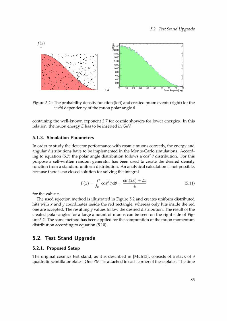
5.2. Test Stand Upgrade

x

f (x)

[deg]θPolar Angle 0 10 20 30 40 50 60 70 80 90

Entr

ies

0

200

400

600

800

1000

1200

1400

1600

1800

2000

2200

Figure 5.2.: The probability density function (left) and created muon events (right) for thecos2θ dependency of the muon polar angle θ

containing the well-known exponent 2.7 for cosmic showers for lower energies. In thisrelation, the muon energy E has to be inserted in GeV.

5.1.3. Simulation Parameters

In order to study the detector performance with cosmic muons correctly, the energy andangular distributions have to be implemented in the Monte-Carlo simulations. Accord-ing to equation (5.7) the polar angle distribution follows a cos2 θ distribution. For thispurpose a self-written random generator has been used to create the desired densityfunction from a standard uniform distribution. An analytical calculation is not possible,because there is no closed solution for solving the integral

F(x) =∫ x

0cos2 θ dθ =

sin(2x) + 2x

4(5.11)

for the value x.The used rejection method is illustrated in Figure 5.2 and creates uniform distributed

hits with x and y coordinates inside the red rectangle, whereas only hits inside the redone are accepted. The resulting y values follow the desired distribution. The result of thecreated polar angles for a large amount of muons can be seen on the right side of Fig-ure 5.2. The same method has been applied for the computation of the muon momentumdistribution according to equation (5.10).

5.2. Test Stand Upgrade

5.2.1. Proposed Setup

The original cosmics test stand, as it is described in [Muh13], consists of a stack of 3quadratic scintillator plates. One PMT is attached to each corner of these plates. The time

83

5. Cosmics Test Stand

x Layer

y Layer

µ+ µ−

Figure 5.3.: A sketch of the cosmics test stand upgrade using 4 layers of scintillation barswith a pitch of 1/3 of the bar width.

and amplitude information of the PMT signals was used to reconstruct the intersectionposition on each scintillator plate. By fitting a straight line through these points the 3Dmuon trajectory can be computed. Additionally, a lead absorber has been placed betweenthe middle and the lower plate. Therefore, low energetic muons are filtered and onlymuons with an almost constant Cherenkov angle can be used for the analysis.

Since the achievable resolution with the previous setup has not been sufficient to de-termine the performance of the EDD, an upgrade of the test stand has become necessary.IInstead of a single scintillator plate, four layers of scintillator bars for each detector layerare used for the track reconstruction. A combination of two layers is used for the recon-struction of the x coordinate, while the other two layers are rotated by an angle of 90

around the z axis to determine the y coordinate.

Quantity Value

Density 1032 g · cm−3

Refractive index 1.58

Radiation length 43 cm

Photon yield 10000 MeV−1

Peak wavelength 425 nm

Rise time τ1 = 0.9 ns

Falling time τ2 = 2.1 ns

Signal pulse width (FWHM) 2.5 ns

Absorption length 400 cm

Table 5.1.: Important parameters of the used scintillator material BC408 for the cosmicstest stand.

The scintillator bars in each of these two-layer combinations are shifted by 1/3 of their

84

5.2. Test Stand Upgrade

Optical Table

Disc DIRC Prototype

Scintillator Bar Matrix 1

Scintillator Bar Matrix 2

Trigger Scintillator 1

Lead Block

Trigger Scintillator 2µ+

x

y

z

Figure 5.4.: A sketch of the proposed cosmics test stand upgrade including the two scintil-lator bar matrices, the optical table, the lead block, and the two trigger coun-ters.

width. This method is used to establish an overlap of the bars and avoiding a visiblegap. This way, the resolution additionally increases around a factor of 3 compared to asingle bar but the number of readout channels rises only by a factor of 2. The width ofeach scintillator bar has been fixed to be 20 mm and the height is 15 mm. The parametersof the used scintillator material BC408, which are also implemented in the Monte-Carlosimulation, are presented in Table 5.1.

One SiPM is coupled to each scintillator bar and connected to one channel of theTOFPET readout system. Each SiPM of the type PM3350 from the company KETEK hasa size of 3 × 3 mm2 and is especially designed for applications in high energy physics. Ifno over-voltage is applied, the DCR can be estimated to 100 kHz/mm2 according to thedata sheet. In case of the maximum voltage this value increases by a factor of 10. For agiven time window of a few nanoseconds by using coincidence measurements includingdifferent scintillator bar layers this rate can still be neglected.

Figure 5.3 shows a sketch of a two-layer combinations for the x and y position recon-struction for two arbitrary muon tracks. Because the projection of every cell increases forlarge polar angles (blue track) the resolution deteriorates slightly which has additionallybeen shown with Monte-Carlo simulations.

85

5. Cosmics Test Stand

Figure 5.5.: The CAD drawing of the cosmics test stand upgrade with the view into they-z (left) and x-z (right) plane.

The complete setup will be positioned on an optical table. A 30 cm thick layer of leadwill be additionally placed below the table and above a scintillator plate that is going tobe read out with 4 PMT. These 4 PMTs could be connected to discriminators before usinga coincidence unit to create an AND connection between them. In this case, the outputsignal of this coincidence unit can be directly processed by the TOFPET ASIC. For thefinal setup, it has been decided to store the hit information of all PMTs with their channelnumbers and time stamps in order to be more flexible in the offline analysis and to getindependent from the discriminator thresholds.

The lead absorber is designed to filter out muons with momenta below p = 0.75 GeV/c.Future solutions with other filtering mechanisms could be used to increase the detectorperformance. A sketch of the complete setup is illustrated in Figure 5.4 including thecoordinate system defined for the data analysis. The polar angle acceptance range can beadjusted by the positioning of the scintillator bar matrices.

5.2.2. Track Reconstruction

In the reconstruction algorithm, an average value of the bar hits per layer is used tocalculate the nearest point to the real muon coordinate. After calculating the x and y

86

5.2. Test Stand Upgrade

Polar/Azimuth Angle [mrad]80− 60− 40− 20− 0 20 40 60 80

En

trie

s

0

1000

2000

3000

4000

5000

Polar Angle Distribution

Azimuth Angle Distribution

X Position [mm]250− 200− 150− 100− 50− 0 50 100 150 200 250

Y P

ositio

n [m

m]

250−

200−

150−

100−

50−

0

50

100

150

200

250

Entr

ies

0

10

20

30

40

50

60

Figure 5.6.: The angular (left) and spatial acceptance (right) range of the cosmics teststand.

coordinate, spherical coordinates are used for the reconstruction of the polar angle θ

θ = arctan∆z

r= arctan

∆z√

(∆x)2 + (∆y)2(5.12)

and azimuth angle

φ =

arctan(

∆y∆x

)

for ∆x > 0

sgn(y)π2 for ∆x = 0

arctan(

∆y∆x

)

+ π for ∆x < 0 and y0 ≥ 0

arctan(

∆y∆x

)

− π for ∆x < 0 and ∆y < 0

(5.13)

where ∆x and ∆y are the differences of the reconstructed coordinates in each layer and∆z the distance between the layers in z direction. The vector ∆r, that coincides with themomentum vector, is then given by

∆r =

∆x∆y∆z

(5.14)

The reconstructed coordinates (x0, y0) of the muon on the surface of the radiator platecan be simply calculated with

(x0

y0

)

=z0 − z1

∆z

(∆x∆y

)

(5.15)

with z0 as the z coordinate of the radiator disk and z1 of the upper scintillation bar matrix.In Figure 5.5 a CAD drawing of the cosmics test stand is shown from two different per-

spectives. The two scintillator bar matrices can be shifted in one direction. This method

87

5. Cosmics Test Stand

Spatial Coordinate [mm]50− 40− 30− 20− 10− 0 10 20 30 40 50

En

trie

s

0

500

1000

1500

2000

2500

3000

3500

4000

X Distribution

Y Distribution

Polar/Azimuth Angle [mrad]50− 40− 30− 20− 10− 0 10 20 30 40 50

En

trie

s

0

1000

2000

3000

4000

5000Polar Distribution

Azimuth Distribution

Figure 5.7.: The spatial (left) and polar/azimuth angle (right) resolution of the cosmicstest stand.

makes it possible to adjust one angle under which a maximum amount of muons can bemeasured and should be placed in the center of the polar acceptance range of the EDD.The lead block is tilted by the angle of maximum statistics in order to equalize the ab-sorption length for almost all muon angles.

The polar and azimuth angle acceptance range can be seen on the right of Figure 5.6.For these simulation studies, the mean polar angle θ = 13 has been chosen. The de-scribed shift of the polar angle distribution to larger values between 5 and 20 is clearlyvisible. This polar angle window has been chosen in order to study those angles with ahigher statistics which will be also covered by the EDD in the PANDA spectrometer. Thereconstructed spatial coordinates on the surface of the radiator plate are shown on theright side of Figure 5.6. The coordinate reconstruction has been performed according toequation (5.15). The high statistics in the center of the radiator plate and a decrease nearthe rim is a result of the detector geometry.

5.2.3. Resolution Studies

The spatial and angular resolutions of the cosmics test stand are obtained with Monte-Carlo simulations in Geant4. A simulation model has been implemented to compare theresults with the Monte-Carlo simulations. In the simulation process, the created cosmicmuons are uniformly generated in x and y direction as well as the azimuth angle withthe limits 0 < φ < 2π above the upper scintillator matrix. The track reconstruction takesplace after the completion of the simulation and can be performed without the knowl-edge of Monte-Carlo truth information as it will be done later in the real experiment.

The spatial resolution of the cosmics test stand is plotted on the left side of Figure 5.7.For obtaining these values, the position of the muon on the radiator plate according toequation (5.15) has been computed. After that, the difference between the reconstructedhit and Monte-Carlo truth has been calculated and binned in one histogram. The sim-ulation results show that a spatial resolution of approx. 4.5 mm in both directions is

88

5.2. Test Stand Upgrade

Polar Angle [deg]8 9 10 11 12 13 14 15 16 17

Pola

r A

ngle

Resolu

tion [m

rad]

2.8

3

3.2

3.4

3.6

3.8

Reconstructed Cherenkov Angle [rad]0.76 0.78 0.8 0.82 0.84 0.86 0.88 0.9

Entr

ies

0

100

200

300

400

500

600

700

Figure 5.8.: The polar angle resolution as a function of the polar angle (left) and the ob-tained single photon resolution with the cosmics test stand (right).

achievable. The offset between the two distributions is a result of the bar positions.

In case of the angular distribution, as shown on the left side of Figure 5.7, a polarangle resolution of 3 mrad is achievable. The azimuth angle resolution is estimated toa value of around 20 mrad. The limiting factor of the spatial and angular resolution isthe angle straggling in the scintillation bars. However, an increase of the resolution by afactor of almost 20 compared to the previous setup has been achieved. Nevertheless, theresolution is slightly worse than the one that we have avhieved in test beam facilities byusing electrons or hadrons.

The left side of Figure 5.8 illustrates the polar angle resolution as a function of thepolar angle taken from the Monte-Carlo data. The above mentioned resolution decreasefor larger polar angles is clearly visible. The fluctuation of data points comes from thelimited statistics of the simulated data. The average value is equal to the one obtainedfrom the presented distribution of all polar angles.

The achievable single photon resolution for the chosen center FEL can be extractedfrom the right side of Figure 5.8. Events in the upper half of the radiator plate with y > 0have been filtered out for the analysis in order to minimize the geometrical error on thesingle photon resolution. Additionally, a momentum cut has been performed to filter outlow energetic muons. A Gaussian fit returns a value of σ = 9.1 mrad.

5.2.4. Detector Calibration

In addition to the single photon resolution, the measurements with cosmic muons canbe used for the FEL calibration. For this method, only muons inside the azimuth angleinterval −10 < φ < 10 have been taken into account. Additionally, a spatial cut in xdirection has been used to filter out muons that reach the radiator plate at large distancesdx to the used FEL. For all events, each pixel hit of one FEL inside a polar angle interval of∆θ = 1 is filled into a histogram. After the reconstruction process has been completed,the mean pixel positions are taken from these histograms.

89

5. Cosmics Test Stand

Polar Angle [rad]0.12 0.14 0.16 0.18 0.2 0.22 0.24 0.26 0.28 0.3

Pix

el P

ositio

n

30

40

50

60

70

80

Figure 5.9.: The obtained calibration line between pixel position and polar angle.

The result of a sample calibration obtained with Monte-Carlo simulation is presentedin Figure 5.9 by plotting the mean pixel position against the reconstructed muon polarangle. The error bars represent the error of the mean value. Together with the theoret-ically calculated Cherenkov angle of cosmic muons a calibration line similar to the onethat is shown in chapter 4 can be created and used for the final detector. However, inorder to use small polar angle intervals and filter out unwanted muons a high amountof statistics is necessary. Using the cosmics test stand for calibration purposes makes asmall variance in the Cherenkov angle necessary. Thus, filtering out low energetic muonsand a small wavelength interval of the optical filter becomes very essential.

5.3. Alternative Approaches

For the construction of a cost optimized cosmics test stand in combination with a highresolution various alternative designs have been proposed before the above mentionedupgrade has been realized. However, all approaches contain certain problems that willbe discussed in the following. The focus lies on the two most promising possibilities.

5.3.1. CMOS Camera Modules

Setup with Raspberry PIs

In order to achieve a spatial resolution with a granularity in the order of micrometers thepossibility of using standard CMOS camera chips has been studied. If a muon passesthrough the depletion zone of the photo cathode, it creates electron hole pairs along its

90

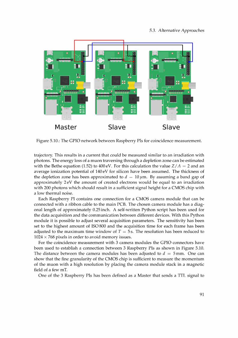
5. Cosmics Test Stand

Frame0 20 40 60 80 100

AD

C V

alu

e

2

4

6

8

10

12

14

16

Noise Time Dependency

Pixels X Direction0 100 200 300 400 500 600 700

Pix

els

Y D

ire

ctio

n

0

200

400

600

800

1000

Ba

se

line

Va

lue

s

1

10

210

Figure 5.11.: The time behaviour of the measured noise with a CMOS camera modules(left) and the obtained baseline for one pixel of the camera module(right).

the other Slave devices when starting the capture of a new frame. For the connection ashielded cable has been used in order to avoid false signals induced by electronic noise.After the Slave devices have saved the captured image, the GPIOs are switched frominput to output, and a TTL signal via the same cable is sent to the Master device. Whenboth signals are received and the frame capturing has been completed, the Master devicestarts a new data acquisition. This process continues until a specified amount of frameshas been recorded.

Data Acquisition

Before the data acquisition starts, the noise level of each pixel has been recorded for alarge amount of frames in order to investigate the time behavior. The results for onesample pixel and one color can be seen on the left side of Figure 5.11. The presented plotshows fluctuations around a mean ADC value.

These long-time measurements have been used to obtain the maximum noise level foreach pixel. This value is defined as the baseline of the referring pixel. In the analysisscript, a threshold can be set according to this baseline in order to filter out noisy pixelsand mask hot pixels that always return high ADC values in every frame. The right sideof 5.11 shows the logarithmic baseline values for one color and all pixels in one samplemodule. The high ADC values on the left side of the histogram are a result of the thermalnoise induced by the readout system of the CMOS chip.

After the data acquisition, all events with less than one hit in each camera moduleare rejected. In the remaining events all hits of the upper and lower layer are used tocompute straight line fits through these data points in order to get a 3 dimensional muontrack. The obtained residuals for the middle layer should be distributed around a specificvalue if the coincidence measurement is successful. The analysis of all captured eventshas shown that the residuals are nearly uniformly distributed which can only be true ifthe acquired hits are noisy pixels. However, a deeper analysis has to be made in order to

92

5.3. Alternative Approaches

judge the feasibility of this promising method. An additional cooling of the chips for thepurpose of noise reduction might be also a useful approach.

It seems that cheap standard CMOS chips are, most likely due to the high noise level,not sufficient to build a reliable cosmics detector. Due to the required amount of sensitivearea, dedicated expansive chips will be more expansive than a cosmics detector withscintillator strips.

5.3.2. Single Photon Camera

Another possible approach, that has been studied during the assembly of the test standupgrade, is the position measurement with a single photon camera. The idea is that thecosmic muons traverse through a scintillator plate and generate tracks of scintillationlight which are recorded as an image in a sensitive camera. A sketch of the setup, thathas been used for feasibility studies, is shown on the left side of Figure 5.12. The cam-era consists mainly of an MCP-PMT with a phosphor screen which replaces the anode.The amplified electrons illuminate the screen and the created photons are coupled withfiber optics to a CMOS chip on the lower side of the camera. A customized software isused to obtain the time and position information from the CMOS chip and to save it in azero suppressed data format. Due to the high granularity of the MCP channels of about10 µm and of the CMOS chip a spatial resolution in the order of sub-millimeters can beachievable.

The camera system has been placed inside a metal pipe. The inner part has been addi-tionally covered with black paint in order to reduce the amount of background photons.

An organic scintillator is placed in front of the camera entry hole. If a muon traversesthrough the scintillator, the created photons are focused by an aspheric Fresnel lens ontothe photo cathode of the MCP-PMT. The important criteria for choosing the correct lensis the photon yield that can be obtained. The light yield depends mainly on the f-numberN of the lens which is defined as fraction of the focal length f and the diameter D of thelens:

N =f

D(5.16)

For a projection-scale of 1 the lens formula can be written as

1

f=

2

g(5.17)

where g is defined as the distance between the scintillator and the Fresnel lens. Thefraction of captured photons to created photons is given by

k =π (D/2)2

4πg2(5.18)

Inserting equations (5.16) and (5.17) leads to the relation

k =1

16N2(5.19)

93

6. Online Reconstruction

6.1. Online Reconstruction Algorithm

This chapter describes the first attempt of a possible design for a future online recon-struction system for the EDD. The online reconstruction algorithm has to fulfill someconstraints regarding speed and calculation steps. The reconstruction algorithm, whichis presented in Figure 6.1, is faster than the method described in chapter 3 and suitablefor online reconstruction.

It has some similarities with the offline reconstruction algorithm. As a first step, theinformation of the charged particle from the tracking PANDA tracking system is used asinput parameters. After that, all additional reflections on the outer rims of the radiatorhave to be taken into account.

Together with this information it is possible to calculate the Cherenkov angle θc ofevery acquired hit by using equation (3.3). From equation (1.39) and the refractive indexof the shortest possible wavelength the largest possible angle ϕ for the possibility of totalinternal reflection for the given parameters can be computed. In addition, all hits whichdo not fulfill that condition are filtered out.

The maximum possible Cherenkov angle for the shortest wavelength can be calculatedaccording to equation (1.21). Photons with Cherenkov angles larger than the theoreti-cal maximum are additionally removed by taking an additional safety margin into ac-count. After removing all the described unphysical hits, a time cut is performed. Forthis purpose, the photon propagation time is calculated with equation (3.5) by calculat-ing the speed with an average refractive index. As described in the offline reconstructionalgorithm, an average value with the truncated mean method is used to compute theestimated arrival time t0 of the charged particle on the radiator plate.

The last step is the summing over all hits in order to obtain the average Cherenkov an-gle for the given track. By defining the correct classifier it would be possible to use theseCherenkov angles to perform PID. However, it is more convenient to obtain the particleprobability with likelihood values in combination with the Bayesian approach. Theo-retical Cherenkov angles for all relevant particle hypotheses are calculated with equa-tion (1.21) by assuming an average refractive index. An average detector resolution canbe obtained with the help of Monte-Carlo simulations. Assuming a Gaussian distributionaround the theoretical Cherenkov angle, the likelihood values can simply be obtained byevaluating the Gaussian function at the measured value.

This reconstruction algorithm has the advantage of being able to achieve a reasonabletrade-off between computation speed and performance but is affected by problems withpileup resulting from high particle rates. However, a comparison between the online

95

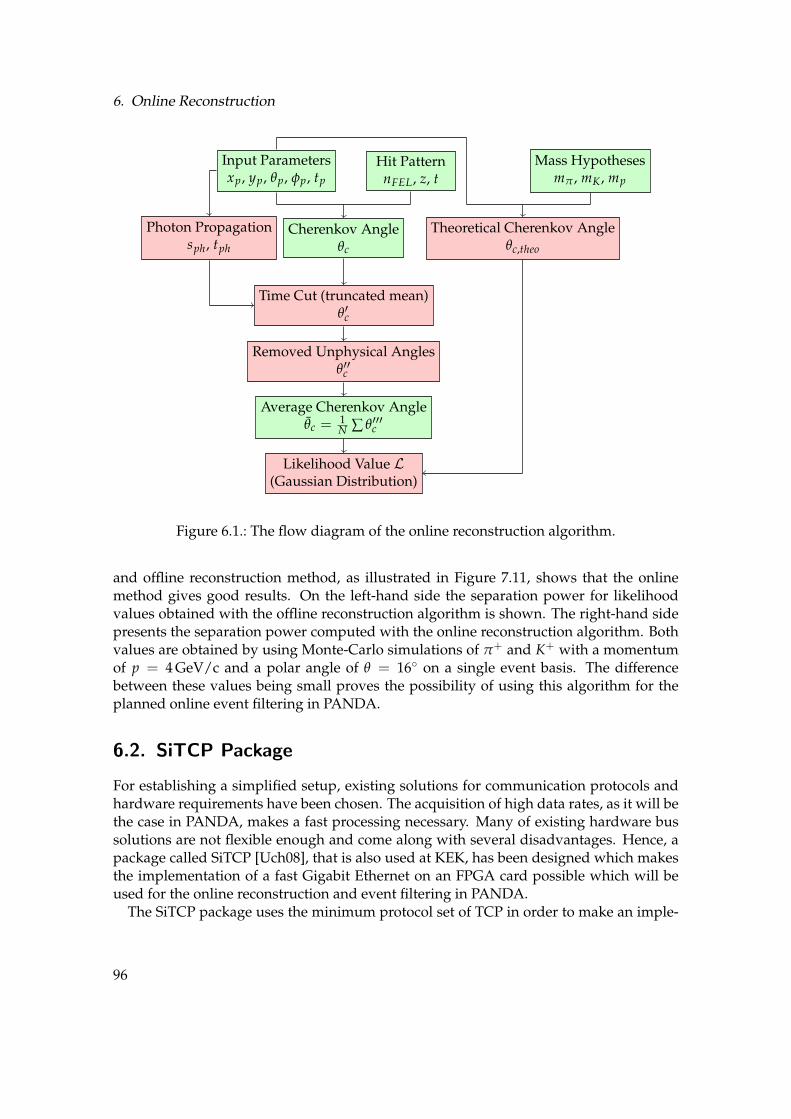
6. Online Reconstruction

Input Parametersxp, yp, θp, φp, tp

Hit PatternnFEL, z, t

Mass Hypothesesmπ , mK , mp

Cherenkov Angleθc

Time Cut (truncated mean)θ′c

Photon Propagationsph, tph

Removed Unphysical Anglesθ′′c

Average Cherenkov Angleθc =

1N ∑ θ′′′c

Likelihood Value L(Gaussian Distribution)

Theoretical Cherenkov Angleθc,theo

Figure 6.1.: The flow diagram of the online reconstruction algorithm.

and offline reconstruction method, as illustrated in Figure 7.11, shows that the onlinemethod gives good results. On the left-hand side the separation power for likelihoodvalues obtained with the offline reconstruction algorithm is shown. The right-hand sidepresents the separation power computed with the online reconstruction algorithm. Bothvalues are obtained by using Monte-Carlo simulations of π+ and K+ with a momentumof p = 4 GeV/c and a polar angle of θ = 16 on a single event basis. The differencebetween these values being small proves the possibility of using this algorithm for theplanned online event filtering in PANDA.

6.2. SiTCP Package

For establishing a simplified setup, existing solutions for communication protocols andhardware requirements have been chosen. The acquisition of high data rates, as it will bethe case in PANDA, makes a fast processing necessary. Many of existing hardware bussolutions are not flexible enough and come along with several disadvantages. Hence, apackage called SiTCP [Uch08], that is also used at KEK, has been designed which makesthe implementation of a fast Gigabit Ethernet on an FPGA card possible which will beused for the online reconstruction and event filtering in PANDA.

The SiTCP package uses the minimum protocol set of TCP in order to make an imple-

96

6.3. Testing FPGA Board

)) - Log(L(K))πLog(L(20− 15− 10− 5− 0 5 10 15 20

En

trie

s

0

10

20

30

40

50

60

70

80

Separation Power: 5.04672Pion Likelihood

Kaon Likelihood

)) - Log(L(K))πLog(L(50− 40− 30− 20− 10− 0 10 20 30 40 50

En

trie

s

0

10

20

30

40

50

60

Separation Power: 4.88687 Pion Likelihood

Kaon Likelihood

Figure 6.2.: A comparison between the online and offline reconstruction algorithms.

mentation on a single chip and the access with standard OS socket functions possible.This makes the communication between the FPGA card and intelligent devices like PCsvery simple. Additionally, the package is designed with optimized pipeline-based cir-cuits to guarantee data receiving and transmission at the same time. The small circuitsize of about 300 slices makes it possible to implement it together with additional usercircuits on an FPGA card. The system clock is set to a value of 130 MHz which results ina time step of approximately 7.7 ns per clock cycle. After the data is transferred via anEthernet cable, every data frame is stored inside an FIFO buffer. The size of each dataframe is limited to a width of 8-bit in order to reduce the circuit size further.

6.3. Testing FPGA Board

The SiTCP package has been evaluated with the ML403 FPGA board. This board includesa Virtex-4 FPGA with the type number XC4VFX12-FF668-10. The board is shown in Fig-ure 6.3. The board contains 64 MB DDR SDRAM and a 100 MHz clock oscillator. It ispossible to extend the RAM up to 256 MB which are supported by the board. However,the configurable Block RAM is limited to blocks of 18 kbits. The implemented Virtex-4FPGA chip contains 36 of these blocks resulting in a total memory of 648 kbits which isequal to 81 kB. That memory can be used e.g. for storing lookup tables.

6.4. Computation Algorithms

The computation of complex functions with short latencies is very important to guaran-tee the desired performance. There are several known algorithms available that can beused. However, all of them contain certain disadvantages that have to be taken into ac-count. Some algorithms can only be used for specific functions or need a large amount ofcomputation steps. The applied algorithms for calculating the average Cherenkov anglewith an FPGA card will be presented in the following.

97

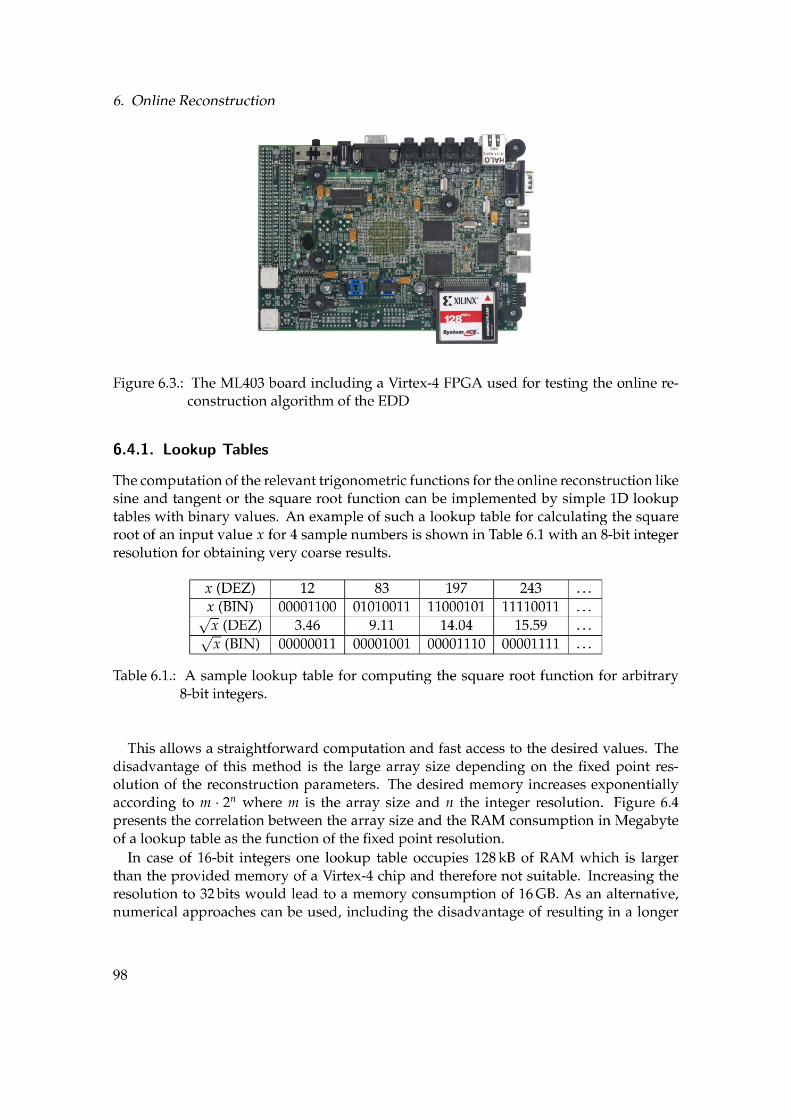
6.4. Computation Algorithms

Fixed Point Resolution [bits]0 5 10 15 20 25 30

Lookup T

able

Siz

e [M

B]

6−10

5−10

4−10

3−10

2−10

1−10

1

10

210

310

Figure 6.4.: The calculated memory consumption of a 1 dimensional lookup table as afunction of the fixed point integer resolution

latency for every calculation step as will be explained in the following.

6.4.2. CORDIC Algortihm

The CORDIC algorithm [Vol59] can be used for a precise computation of trigonometricalfunctions like sine, cosine or arcus tangent. Implementing additional changes allows theCORDIC algorithm to be able to compute hyperbolic functions and square roots. It isbased mainly on the rotation of a vector ~x0 = (x0, x1) to a new vector ~x1 = (x1, y1), whichcan be described mathematically by using the rotation matrix:

(x1

y1

)

=

(cosθ − sin θsin θ cos θ

)

·(

x1

y1

)

(6.1)

Inserting the trigonometric relation

cos θ =1√

1 + tan2 θ(6.2)

and using tan θ = sin θ/ cos θ this function can be rewritten as:(

x1

y1

)

=1√

1 + tan2 θ

(1 − tan θ

tan θ 1

)

·(

x0

y0

)

(6.3)

The transformation angle θ can be written as a linear combination of small angles αi:

θ =n−1

∑i=0

σi · αi (6.4)

99

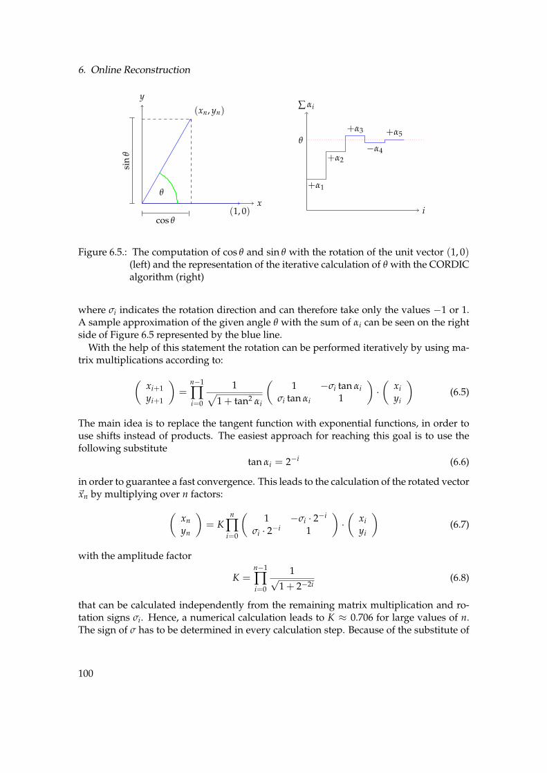
6. Online Reconstruction

x

y

(1, 0)

(xn, yn)

cos θ

sin

θ

θ

i

∑ αi

+α1

+α2

+α3

−α4

+α5θ

Figure 6.5.: The computation of cos θ and sin θ with the rotation of the unit vector (1, 0)(left) and the representation of the iterative calculation of θ with the CORDICalgorithm (right)

where σi indicates the rotation direction and can therefore take only the values −1 or 1.A sample approximation of the given angle θ with the sum of αi can be seen on the rightside of Figure 6.5 represented by the blue line.

With the help of this statement the rotation can be performed iteratively by using ma-trix multiplications according to:

(xi+1

yi+1

)

=n−1

∏i=0

1√

1 + tan2 αi

(1 −σi tan αi

σi tan αi 1

)

·(

xi

yi

)

(6.5)

The main idea is to replace the tangent function with exponential functions, in order touse shifts instead of products. The easiest approach for reaching this goal is to use thefollowing substitute

tan αi = 2−i (6.6)

in order to guarantee a fast convergence. This leads to the calculation of the rotated vector~xn by multiplying over n factors:

(xn

yn

)

= Kn

∏i=0

(1 −σi · 2−i

σi · 2−i 1

)

·(

xi

yi

)

(6.7)

with the amplitude factor

K =n−1

∏i=0

1√1 + 2−2i

(6.8)

that can be calculated independently from the remaining matrix multiplication and ro-tation signs σi. Hence, a numerical calculation leads to K ≈ 0.706 for large values of n.The sign of σ has to be determined in every calculation step. Because of the substitute of

100

6.4. Computation Algorithms

Iteration Steps0 2 4 6 8 10 12 14 16 18 20

co

s(θ

)

0.3

0.35

0.4

0.45

0.5

0.55

0.6

CORDIC

Figure 6.6.: The computed cosine angle with the CORDIC algortihm as a function of theiteration steps. The red line indicates the real value.

tan αi the sum of the partition angles, that are used to calculate the value of σ, is given by:

θi+1 = θi − σi · arctan(

2−i)

(6.9)

This method makes only one lookup table for the arcus tangent function necessary whichcan be implemented with a high resolution depending on the existing memory.

If θi+1 becomes larger than the input parameter θ, the value of σ has to be changed to−1, otherwise it remains +1. Computing the matrix multiplication leads to the followingcoupled equations which have to computed stepwise:

xi+1 = xi − σi · 2−i (6.10)

yi+1 = yi − σi · 2−i (6.11)

The results of the stepwise calculation of the cosine angle can be seen in Figure 6.6. Af-ter the calculation of around 8 steps, the computed value converges sufficiently to thetheoretical one.

6.4.3. Further Numerical Algorithms

Although libraries for numerical calculations are available in VHDL to perform stan-dard operations like integer divisions, it has been decided to use self-written functionsto make the code synthezisable. Hence, self-written algorithms have been used in theFPGA firmware for the Cherenkov angle reconstruction. The square root of a number

101

6. Online Reconstruction

Cherenkov Angle [rad]0.8 0.81 0.82 0.83 0.84 0.85 0.86

Entr

ies

0

5

10

15

20

25

30

35

40

45

Pions

Kaons

Cherenkov Angle [rad]0.8 0.81 0.82 0.83 0.84 0.85 0.86

Entr

ies

0

10

20

30

40

50

60

70

Pions

Kaons

Figure 6.7.: The distribution of the reconstructed Cherenkov angle for 8 bit (left) and16 bit (right) integer resolution.

can be also calculated with the CORDIC algorithm. However, an easier and faster ap-proach has been made by simply using binary operations in combination with a loopedprocess.

The algorithm starts with the two values a = 1 and δ = 3. In every step the value of δ isadded to a. At the same time the integer 2 is added to δ. This process continues until thevalue of a is larger than the given radicand. The returned integer value of δ/2 − 1 is thenequal to the square root of the radicand. The number of steps needed for the calculationof one square root is identical to the integer length of the radix. The computation of thesquare root of an 8-bit integer can be done in 4 clock cycles.

The implemented integer division algorithm is based on the principle of the standardlong division for decimal numbers and requires one clock cycle per integer bit, i.e. 8clock cycles are needed to divide 8-bit integers. In every calculation step the divisor issubtracted from the numerator. After that, it is checked whether the divisor is larger thanthe difference. In this case a 0 is added to the result and the next bit is added to thedifference. If the divisor is smaller, the result is extended by the value 1.

Both algorithms as well as the CORDIC algorithm can be implemented sequentially,e.g. in the form of an FSM, or parallel. In case of a sequential implementation everycalculation step requires one clock cycle. If a parallel implementation is used, many cal-culation steps can be performed in one clock cycle which shortens the processing time.However, the amount of required FPGA resources increases drastically.

6.5. Resolution Studies

The above-mentioned algorithms are ideal for calculating dot products and can be usedto reconstruct the Cherenkov angle according to equation (3.3). The cosine of the po-lar angle θp of the charged particle can be calculated with the CORDIC algorithm usingequation (4.15) where the three components of the momentum vector are used as input

102

6.5. Resolution Studies

Integer Size [bits]8 9 10 11 12 13 14 15

Chere

nkov A

ngle

[ra

d]

0.81

0.815

0.82

0.825

0.83

0.835

0.84

Figure 6.8.: The shift of the mean value of the reconstructed Cherenkov angle distribu-tion as a function of the integer resolution. The detector resolution is indi-cated by the error bars.

parameters. From this relation the sine of value of θp is being computed with the trigono-

metric relation sin θp =√

1 − cos2 θp.

The acquired angle ϕ′, which is derived from the pixel information, is used in combi-nation with αFEL to calculate ϕ according to equation (3.2). The angle αFEL is calculatedaccording to the dot product in equation (4.17). For this purpose, the positions and anglesof all FELs have to be stored in a lookup table. Due to symmetry only the informationof one quadrant has to be saved. In the next step, equation (4.16) is used to computecos(φrel) which is needed to get the value of θc.

For the performance studies event-based Monte-Carlo simulations have been used topretend the existence of real data from PANDA. The reconstruction algorithm has beenimplemented on the ML403 FPGA card. The tracking data and hit patterns are sent with aself-written C++ client via fast Ethernet with different resolutions for testing purposes tothe FPGA card where the Cherenkov angles are computed. All numbers are divided into8-bit blocks according to the FIFO buffer of the SiTCP package. The average Cherenkovvalue for each event is sent back via fast Ethernet to the PC and stored there as a fixedpoint value. A small fraction of the code of the PC client can be found in listing 6.1. Itshows the division of an arbitrary number into 8 bit integers with the shift operator andsending the integer packages to the connected socket. After that, the client listens to thesocket to receive an 8 bit integer back from the card.

103

6. Online Reconstruction

# include <sys/types . h># include <sys/socket . h># include <n e t i n e t /in . h># include <arpa/ i n e t . h>

i n t main ( )

short number = 1423 ;

u i n t 8 t num1 = number1 &0xFF ;u i n t 8 t num2 = number1 >> 8 ;

i n t conn sock ;s t r u c t sockaddr in server addr ;conn sock=socket ( AF INET , SOCK STREAM, 0 ) ;

server addr . s i n f a m i l y =AF INET ;server addr . s i n p o r t =htons ( 2 4 ) ;server addr . s in addr . s addr=ine t addr ( ” 1 9 2 . 1 6 8 . 1 0 . 1 6 ” ) ;

connect ( conn sock , ( s t r u c t sockaddr ∗)& server addr ,s i ze o f ( server addr ) ) ;

send ( conn sock , &num1, s i ze o f (num1) , 0 ) ;send ( conn sock , &num2, s i ze o f (num2) , 0 ) ;

u i n t 8 t num3 [ 8 ] ;i n t r e s u l t = recv ( conn sock , &rece ive ,

s i ze o f ( r e c e i v e ) , 0 ) ;

Listing 6.1: Sample code for sending and receiving 8-bit data blocks with the SiTCP pack-age

The left side of Figure 6.7 presents the reconstructed Cherenkov angle distribution forπ+ and K+ with a momentum of p = 4 GeV/c and a fixed point resolution of 8 bit. Theshift of the mean values due to rounding issues comes along with a decreased resolutionand therefore a deteriorated separation power.

The right side of Figure 6.7 shows the detector resolution using a 16 bit integer reso-lution. This value has been found to be sufficient for online event filtering. A detailedanalysis for different resolutions is presented in Figure 6.8. The data points illustrate theshift of the mean value of the Cherenkov angle while the error bars represent the recon-structed detector resolution.

With a first approach for a possible online reconstruction framework, which can beused as an initial step for a dedicated event filtering system, it was already possible toobtain promising results without exceeding the given constraints. However, further stud-ies, which might include a tuning of the algorithms and using different binary resolutionfor the various variables, are necessary.

104

7. Testbeam Results

Figure 7.2.: The Disc DIRC prototype setup used for the DESY 2016 testbeam

The hole of the second collimator should to be larger than the one of the first collimatorso that the second collimator is not hit by the electron beam but scrapes away the edge-scattered particles of the first collimator.

The entry window size of the first collimator has been chosen as 5× 5 mm2. The lengthand width of the second one is chosen as 15 × 15 mm2. These values have been adjustedafter taking a measurement series at the beginning of the testbeam campaign to find thebest setting.

After leaving the second collimator, the electron beam is traversing through scintillat-ing counters from the University of Gottingen which, in the end, have not been usedfor the data acquisition because of their limited efficiency. Behind these scintillators, theEDD prototype is placed on a turning table with an angular scale. The turning table itselfhas been fixed on a horizontal and vertical movable plate that can be shifted smoothly inthe x-y plane perpendicular to the beam trajectory.

Scintillating finger counters behind the prototype are connected to a CFD that discrim-inates their signals at a constant fraction of their amplitudes. In contrast to a discrimi-nation with a fixed threshold, this method guarantees an amplitude independent triggersignal and a suppresses possible time-walk effects.

After passing an additional lead shielding with a hole, which filters out electrons hav-ing a large angular divergence due to multiple scattering, the electron beam enters acalorimeter that has been also connected to a CFD. The task of the calorimeter is to se-lect electrons that are not scattered and did not loose energy on their way through theexperimental setup. Additionally, all events including particle showers, that are inducedby the electron beam, can be rejected by measuring the electron energy. The three dis-criminated signals from the scintillating counters and the calorimeter are processed in anAND gatter which creates an NIM pulse as an output signal only under the condition ofa coincidence between all signals.

106

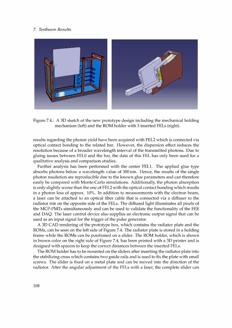
7.2. Data Acquisition

Angle of Incidence [deg]2 4 6 8 10 12 14 16 18 20 22

Pix

el

0

10

20

30

40

50

60

70

80

90

Hits/T

rigger

3−

10

2−10

1−10

Y-Position [mm]0 50 100 150 200 250 300 350 400 450 500

Pix

el

0

10

20

30

40

50

60

70

80

90

Hits/T

rigger

3−

10

2−10

1−10

Figure 7.5.: The results from the angle scan (left) including a reflection pattern from thelower plate side and the y position scan (right) with a polar angle of θ = 10.The exact beam position information can be taken from Figure 7.3

be taken out which simplifies the attachment of the MCP-PMTs to the FELs.

7.2. Data Acquisition

Before data acquisition started, different tests have been performed to find the optimalparameters for the setup. After the baseline scan of the TOFPET ASICs a laser run withthe diffuser has been used to verify that all channels are working and all baselines andthresholds are set properly. In the next step, different beam collimator settings have beenadjusted to find the best entry window sizes regarding statistics, background signals,and single photon resolution. For this purpose, a self-written online reconstruction scripthas been used to verify the results directly after each run. Additionally, high voltage andthreshold scans have been used to find the best set of parameters for the photon detectionsystem.

The DESY testbeam setup provides the possibility to verify the detector performancewith different measurement series. The most important ones, that are also used for thelater analysis, are the angle scan at a specific beam position and a position scan for aconstant polar angle. The average beam positions of each scan are shown in Figure 7.3.Because the rotation axis of the prototype could not be placed in the center of the radia-tor plate, the x position has slightly changed during the angle scan as a function of theapplied angle of incidence.

The minimum distance between the intersection point and the FELs is given by ∆x =449.8 mm for the polar angle θ = 2, and maximum distance has been measured to ∆x =462.1 mm for an angle of θ = 22. For the y-axis scan a distance of ∆x = 347.1 mm hasbeen chosen. The distance in y-direction between the neighboring data points has beenset to ∆y = 17 mm. This value is derived from the 16 mm bar width and 1 mm distancebetween the FELs. All parameters have been calculated theoretically and verified after a

109

7. Testbeam Results

Pixel

0 10 20 30 40 50 60 70 80 90

En

trie

s

0

10000

20000

30000

40000

50000Hit Projection

Double Gauss Fit

n = 546024

= 1.44σ

Pixel

0 10 20 30 40 50 60 70 80 90

En

trie

s

0

10000

20000

30000

40000

50000

60000

70000

Hit Projection

Double Gauss Fit

n = 801728

= 1.63σ

Pixel

0 10 20 30 40 50 60 70 80 90

En

trie

s

0

10000

20000

30000

40000

50000

60000

70000

Hit Projection

Double Gauss Fit

n = 986341

= 2.26σ

Figure 7.6.: The accumulated pixel distributions for one beam angle and position includ-ing the upper FEL0 (left), the center FEL1 (center) and the lower FEL2 (right)showing the number n of entries and the standard deviation σ of the mainCherenkov peak.

specific amount of runs.

The left side of Figure 7.5 shows the results from the angle scan. The histogram illus-trates the projection of the Cherenkov cone to the pixel space of the referring MCP-PMTcolumn. Each column in the histogram represents a different angle of incidence. The ad-ditional reflection on the lower side of the radiator plate is clearly visible in the parallelshifted hit pattern in y-direction.

On the right side of Figure 7.5, the results from the y position scan are shown. Thisscan looks like the well-known two-dimensional projection of the Cherenkov cone that isexpected for a larger amount of photo sensors. On the upper left corner, some of the ad-ditional reflections on the rim of the radiator plate can be also observed. Both histogramsare normalized by the amount of triggers per run in order to create comparable results.The results for the angle and y-axis scan including all three FELs of the prototype can beseen found in Appendix B. These pattern structures are similar to the expected ones inthe final detector.

A logarithmic scale for the color axis has been chosen to study the background signalsand additional hit patterns due to reflections inside the detector. One can see in the yaxis scan that the background increases if the beam does not enter the radiator plate.This behavior could be explained by electron scattering in different parts of the detectormaterial surrounding the radiator plate.

Figure 7.6 shows the projection in the pixel space for each FEL starting from the lefthistogram for the upper FEL0 up to the last one for the lower FEL2. The histograms havebeen created for one beam position and angle of incidence containing an equal amount ofaccumulated events. The standard deviation has been computed for the main Cherenkovpeak by using a double Gaussian fit for a sufficient background approximation. The

110

7.3. Monte-Carlo Simulations

Cluster Size [Pixel]

0 1 2 3 4 5 6 7

Entr

ies

20

40

60

80

100

120

310×

Multiplicity

0 1 2 3 4 5 6 7 8 9

En

trie

s

0.1

0.2

0.3

0.4

0.5Testbeam Data

MC Simulations

Figure 7.7.: The cluster size of the measured angle scan at θ = 14 (left) and the compar-ison of the photon hit distributions between simulation and testbeam dataafter applying a charge sharing model (right)

smaller peak on the right edge of each histogram indicates the additional reflection onthe bottom small face.

The standard deviation σ is given in pixels and can be multiplied by the factor 3.5 inorder to compute the Cherenkov angle resolution in mrad. The first histogram containsapproximately 30% less entries than the second one. This effect is a result of the gluingproblems at the upper FEL. Even though more photons are lost because of the glue layerincluding air bubbles, the single photon resolution increases slightly.

The second histogram contains the center FEL that has also been chosen for the furtheranalysis. The epoxy glue between the FEL and bar results in a cut-off wavelength around300 nm and can be interpreted as a band-pass filter. Hence, the standard deviation andthe number of entries is smaller than the one in the previous histogram because photonswith smaller wavelengths are additionally accepted. In addition to a larger amount ofentries it leads to an increase of the projection resolution and therefore the single photonresolution. Because of the large distance between the beam point of intersection andthe ROM the measured projection resolution is almost identical to the Cherenkov angleresolution.

7.3. Monte-Carlo Simulations

The given constraints of the testbeam facility and prototype setup have been used as in-put parameters for a full Geant4 Monte-Carlo simulation study. In the simulation, theelectrons are created at the position of the collimator that is equal to the measured dis-tance between the collimator and radiator plate in the testbeam setup. The polar angle ofthe simulated particle is set to the real angle of incidence in the testbeam data.

For the x and y positions of the start vertex a uniform distribution with a width of 5 mmin both directions has been chosen to simulate the behavior of the adjustable collimator

111

7. Testbeam Results

4 6 8 10 12 14 16 18 202

3

4

5

6

7

8

9

10

11

12

Angle of Incidence [deg]

MC Simulation

Testbeam Data

Sin

gle

Ph

oto

n R

eso

lutio

n [

mra

d]

4 6 8 10 12 14 16 18 20

0.6

0.7

0.8

0.9

1

1.1

Num

ber

of H

its

Angle of Incidence [deg]

MC Simulation

Testbeam Data

Figure 7.8.: Comparison of the single photon resolution (left) and photon yield (right)between testbeam data and Monte-Carlo simulations

in order to approximate the smearing of the electron beam. The angular divergence hasbeen smeared with a Gaussian distribution around the mean value and a suitable stan-dard deviation of 1 mrad. In addition to the digitized hits, the position and momentum ofthe particle, that leaves the radiation plate, is saved. With this information the function-ality of the calorimeter can be included into the simulations by rejecting events with lowenergy electrons and the ones having a large beam divergence. For the reconstruction ofthe Cherenkov angle the calculated position of the beam on the radiator plate has beentaken into account.

The effect of the plastic cover on the particle background, that shields the radiatorplate from mechanical destruction, has been shown in comparison with the simulatedresults. After implementing the 2 mm cover into the Monte-Carlo geometry, the heightof the background signal comes closer to that of the measured data. The main reason forthis effect could be found in the creation of highly energetic delta-electrons in the plasticlayer reaching the radiator plate and creating additional Cherenkov light under differentangles. Other effects have to be studied in order to analyze the particle backgroundfurther. The scattering of electrons in the air volume between the point of creation andthe radiator plate leads to an additional deterioration of the single photon resolution.

7.4. Event Reconstruction

7.4.1. Resolution & Photon Yield

The testbeam data, containing different angle and position scans, can be used for com-puting the single photon resolution and photon yield of each triggered event. The resultscan be compared with Monte-Carlo simulations containing a realistic model of the test-beam parameters. However, there is a limitation of statistics due to the availability ofonly one usable ROM.

In order to validate the detector performance, the implementation of a charge sharing

112

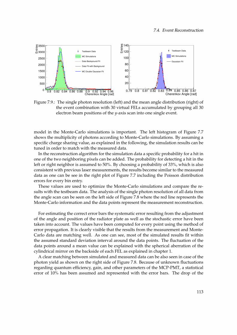
7.4. Event Reconstruction

Cherenkov Angle [rad]0.8 0.82 0.84 0.86 0.88 0.9 0.92 0.94 0.96

En

trie

s

0

500

1000

1500

2000

2500

3000

3500

Testbeam Data

MC Simulations

Data Background Fit

Data Fit with Background

MC Double Gaussian Fit

Cherenkov Angle [rad]0.79 0.8 0.81 0.82 0.83 0.84 0.85 0.86 0.87

Entr

ies

20

40

60

80

100

120

140

Testbeam Data

MC Simulations

Gaussian Fit

Figure 7.9.: The single photon resolution (left) and the mean angle distribution (right) ofthe event combination with 30 virtual FELs accumulated by grouping all 30electron beam positions of the y-axis scan into one single event.

model in the Monte-Carlo simulations is important. The left histogram of Figure 7.7shows the multiplicity of photons according to Monte-Carlo simulations. By assuming aspecific charge sharing value, as explained in the following, the simulation results can betuned in order to match with the measured data.

In the reconstruction algorithm for the simulation data a specific probability for a hit inone of the two neighboring pixels can be added. The probability for detecting a hit in theleft or right neighbor is assumed to 50%. By choosing a probability of 33%, which is alsoconsistent with previous laser measurements, the results become similar to the measureddata as one can be see in the right plot of Figure 7.7 including the Poisson distributionerrors for every bin entry.

These values are used to optimize the Monte-Carlo simulations and compare the re-sults with the testbeam data. The analysis of the single photon resolution of all data fromthe angle scan can be seen on the left side of Figure 7.8 where the red line represents theMonte-Carlo information and the data points represent the measurement reconstruction.

For estimating the correct error bars the systematic error resulting from the adjustmentof the angle and position of the radiator plate as well as the stochastic error have beentaken into account. The values have been computed for every point using the method oferror propagation. It is clearly visible that the results from the measurement and Monte-Carlo data are matching well. As one can see, most of the simulated results fit withinthe assumed standard deviation interval around the data points. The fluctuation of thedata points around a mean value can be explained with the spherical aberration of thecylindrical mirror on the backside of each FEL as explained in chapter 1.

A clear matching between simulated and measured data can be also seen in case of thephoton yield as shown on the right side of Figure 7.8. Because of unknown fluctuationsregarding quantum efficiency, gain, and other parameters of the MCP-PMT, a statisticalerror of 10% has been assumed and represented with the error bars. The drop of the

113

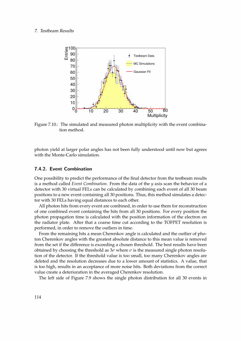
7. Testbeam Results

Multiplicity0 10 20 30 40 50 60

En

trie

s

0

10

20

30

40

50

60

70

80

90

100

Testbeam Data

MC Simulations

Gaussian Fit

Figure 7.10.: The simulated and measured photon multiplicity with the event combina-tion method.

photon yield at larger polar angles has not been fully understood until now but agreeswith the Monte-Carlo simulation.

7.4.2. Event Combination

One possibility to predict the performance of the final detector from the testbeam resultsis a method called Event Combination. From the data of the y axis scan the behavior of adetector with 30 virtual FELs can be calculated by combining each event of all 30 beampositions to a new event containing all 30 positions. Thus, this method simulates a detec-tor with 30 FELs having equal distances to each other.

All photon hits from every event are combined, in order to use them for reconstructionof one combined event containing the hits from all 30 positions. For every position thephoton propagation time is calculated with the position information of the electron onthe radiator plate. After that a coarse time cut according to the TOFPET resolution isperformed, in order to remove the outliers in time.

From the remaining hits a mean Cherenkov angle is calculated and the outlier of pho-ton Cherenkov angles with the greatest absolute distance to this mean value is removedfrom the set if the difference is exceeding a chosen threshold. The best results have beenobtained by choosing the threshold as 3σ where σ is the measured single photon resolu-tion of the detector. If the threshold value is too small, too many Cherenkov angles aredeleted and the resolution decreases due to a lower amount of statistics. A value, thatis too high, results in an acceptance of more noise hits. Both deviations from the correctvalue create a deterioration in the averaged Cherenkov resolution.

The left side of Figure 7.9 shows the single photon distribution for all 30 events in

114

7.4. Event Reconstruction

Cherenkov Angle [rad]0.8 0.825 0.85

Entr

ies

0

20

40

60

80

100

120

140

160

Cherenkov Angle [rad]0.8 0.825 0.85

Entr

ies

0

20

40

60

80

100

120

140

160

Cherenkov Angle [rad]0.8 0.825 0.85

Entr

ies

0

50

100

150

200

250

Cherenkov Angle [rad]0.8 0.825 0.85

Entr

ies

0

20

40

60

80

100

120

140

160

180

200

220

Cherenkov Angle [rad]0.8 0.825 0.85

Entr

ies

0

50

100

150

200

250

Figure 7.11.: The evolution of the testbeam result for validating the simulation resultsof one detector quadrant in PANDA starting from the testbeam setup withelectrons (left) and reaching to the detector resolution of the final EDD inPANDA (right).

comparison with Monte-Carlo simulations. The peak of the Monte-Carlo simulation ishigher than the one obtained with simulations. However, the background level of themeasured data is higher than the simulated one. As a result, the integrals over bothhistograms are equal which leads to a similar photon yield. The standard deviation ofthe simulated data is obtained to σ = 7.42 mrad, and for the measured data it is slightlyworse and given by σ = 07.46 mrad according to the Gaussian fit.

The resulting histogram of the mean Cherenkov angle distribution is shown on theright side of Figure 7.9 with an average amount of n = 14 hits after removing the outlierswith the truncated mean method. The obtained resolution has a value of σ = 2.5 mradcompared to σ = 2.0 from the Monte-Carlo simulations. Simulation studies of the finaldetector show that in case of hadrons together with a long-pass filter and a better trackresolution a mean resolution of σ = 1.5 mrad can be achieved.

The comparison of the photon multiplicity between measurement and simulation re-sults are shown in Figure 7.10. The average value is placed around 26 hits per eventwhich is comparable to previous simulation results for the final detector including anoptical filter.

7.4.3. Result Extrapolation

One possibility to validate the performance of a complete quadrant in the PANDA experi-ment with the testbeam data is an evolution of the obtained results by changing differentparameters. The first histogram in Figure 7.11 shows the single photon resolution that

115

7. Testbeam Results

has been measured in the testbeam during the angle scan with a polar angle θ = 12 andwhich agrees with Monte-Carlo simulations. As described above, the obtained result isσ = 6.3 mrad. Changing the primary particle from e to π+ and keeping all other param-eters constant, the resolution increases by approximately 0.3 mrad to σ = 5.9 mrad as itcan be seen in the neighbor histogram. This effect can be explained with differences inenergy loss and angle scattering for pions compared to electrons.

The next distribution illustrates the result after switching the simulation environmentfrom the testbeam to the PANDA setup without the implementation of an optical fil-ter. The spatial and angular smearing is changed from the testbeam environment to thePANDA tracking resolution. The better tracking resolution result in an increase of thesingle photon resolution. The new value is then given by σ = 4.8 mrad.

Using a filter improves the single photon resolution again to the value σ = 3.5 mradas shown in the neighboring histogram. In the last step, the detector resolution has beencomputed by averaging all hits in one event which leads to the final result of σ = 1.8 mradfor π+ particles with a momentum of p = 3 GeV/c as it can be seen in the last histogram.This value will be used for the computation of the likelihood values in the online recon-struction system of the final experiment.

116

8. Conclusion & Outlook

It has been shown with the help of Monte-Carlo simulation that the desired detector per-formance of the EDD for PANDA can be achieved over the requested phase space in thepolar angle region 5 ≤ θ ≤ 22 and particle momenta up to p = 4 GeV/c. Two typesof reconstruction algorithms for an online event filter and an offline reconstruction havebeen designed. Both have been tested with the help of Monte-Carlo simulations, in thePandaRoot framework and in a Geant4 standalone version to evaluate the resulting sep-aration power. An additional self-written Monte-Carlo tool for fast simulation purposeshas been designed and was used to optimize several detector parameters.

The existing simulation frameworks for PANDA have been used to validate the de-sired resolution of the tracking detectors by implementing a self-written helix propaga-tor. A small spatial and angular standard deviation is important to guarantee a sufficientCherenkov angle reconstruction. Theoretical calculations of particle scattering and en-ergy loss inside the radiator plate have been used to estimate the detector resolution.Additionally, it has been shown that using another type of photocathode in combinationwith a higher collection efficiency can lead to a cost saving setup by renouncing the filteror applying an additional air gap between the ROM and MCP-PMT.

An implementation of time-based simulation and reconstruction algorithms is impor-tant to evaluate the detector performance in combination with high rates and pileups.Computing combined likelihood values for all PID detectors in PANDA gives the pos-sibility to study certain benchmark channels as it has been done for a glueball decaychannel. Even though the presented results are very promising further simulations incombination with different background channels and event studies are necessary.

Simulation results have shown that the cosmics test stand at the University of Giessen(JLU) can be used to measure the single photon resolution of one EDD quadrant suf-ficiently. For this reason a Geant4 based model and reconstruction algorithm has beendesigned that can easily be used for additional analysis. Additional studies for a possibleupgrade of the cosmics stand have been made with various design possibilities but havenot been realized for various reasons.

In addition to the reconstruction algorithms a self-written VHDL based online recon-struction software has been designed and tested on an FPGA board. The resolutionhas been investigated as a function of the fixed point integer resolution and an aver-age amount of calculation step per hit has been computed. However, further studies incombination with a full DAQ system are necessary.

The testbeam at DESY in 2016 show excellent results regarding the detector perfor-mance of the EDD prototype using the proposed MCP-PMT and FEE. Using an eventmixing method results, that mock-up the final detector performance, could be obtainedand verified by comparison with simulations.

117

8. Conclusion & Outlook

The next step will be the construction of a fully equipped radiator quadrant prototypethat can be evaluated with the cosmics test stand or another testbeam campaign. Thisprototype is also planned to be used and tested in the PANDA detector.By placing the ra-diator plate in the PANDA solenoid field, an increase of the detector performance shouldbe observed. To sum up, the promising results obtained by Monte-Carlo simulations andtestbeam measurements are sufficient to continue with the construction of the PANDADisc DIRC and to the confidence that it will fulfill the anticipated performance.

118

A. Simulation Results

Resolu

tion [m

rad]

0.8

1

1.2

1.4

1.6

1.8

2

Mean Cherenkov Resolution

Polar Angle [deg]10 12 14 16 18 20 22

Azim

uth

Angle

[deg]

0

10

20

30

40

50

60

70

80

90

Mean: 1.46916

Mean Cherenkov Resolution

Effic

iency [%

]

80

82

84

86

88

90

92

94

96

98

100

Reconstruction Efficiency

Polar Angle [deg]10 12 14 16 18 20 22

Azim

uth

Angle

[deg]

0

10

20

30

40

50

60

70

80

90

Mean: 96.0722

Reconstruction Efficiency

Resolu

tion [m

rad]

0.8

1

1.2

1.4

1.6

1.8

2

Mean Cherenkov Resolution

Polar Angle [deg]10 12 14 16 18 20 22

Azim

uth

Angle

[deg]

0

10

20

30

40

50

60

70

80

90

Mean: 1.36076

Mean Cherenkov Resolution

Effic

iency [%

]

80

82

84

86

88

90

92

94

96

98

100

Reconstruction Efficiency

Polar Angle [deg]10 12 14 16 18 20 22

Azim

uth

Angle

[deg]

0

10

20

30

40

50

60

70

80

90

Mean: 96.0378

Reconstruction Efficiency

Figure A.1.: The simulation results for the 2D angle scan without applying an magneticfield for the blue (left) and green (right) photocathode.

119

B. Testbeam Results

Y-Position [mm]0 50 100 150 200 250 300 350 400 450 500

Pix

el

10

20

30

40

50

60

70

80

90

Hits/T

rigger

3−10

2−10

1−10

Y-Position [mm]0 50 100 150 200 250 300 350 400 450 500

Pix

el

0

10

20

30

40

50

60

70

80

90

Hits/T

rigger

3−10

2−10

1−10

Y-Position [mm]0 50 100 150 200 250 300 350 400 450 500

Pix

el

0

10

20

30

40

50

60

70

80

90

Hits/T

rigger

3−10

2−10

1−10

Angle of Incidence [deg]0 2 4 6 8 10 12 14 16 18 20 22

Pix

el

10

20

30

40

50

60

70

80

90

Hits/T

rigger

3−10

2−10

1−10

Angle of Incidence [deg]0 2 4 6 8 10 12 14 16 18 20 22

Pix

el

0

10

20

30

40

50

60

70

80

90

Hits/T

rigger

3−10

2−10

1−10

Angle of Incidence [deg]0 2 4 6 8 10 12 14 16 18 20 22

Pix

el

0

10

20

30

40

50

60

70

80

90

Hits/T

rigger

3−10

2−10

1−10

Figure B.1.: The qualitative testbeam results for the y-axis scan (left) and angle scan (right)including FEL0 (up), FEL1 (center), and FEL2 (down).

121

Acknowledgements

First of all, my most important thanks go to Michael Duren and the HGS-HIRe graduateschool for giving me the great chance and financial support to start my doctoral studies inthis very interesting field of detector development for a new kind of Cherenkov detectorthat has not been used by any other high energy physics experiment before. SecondlyI want to thank our 3 postdocs Erik Etzelmuller, Klaus Fohl, and Avetik Hayrapetyanfor all discussions about particle and detector physics. In the 3 years of being a part ofthis research group they have become very good friends. And I want to thank especiallySoren Lange for his continuous support during my PhD time and his participation in thePhD committees.

Additionally, I want to thank my former colleagues Julian Rieke and Kristof Kreutzfeldt.Without them, an analysis of testbeam results would not have been possible. The sameapplies for our former master student Klim Bigunenko with who I shared the office for along time.

And it is very important to thank my predecessor Oliver Merle who already establishedthe fundamental basics for the used reconstruction and PID algorithms. Furthermore, Iwant to thank Marc Strickert resp. Katja Wolf, who is resp. was responsible for the com-puter administration in our research group, for always giving me a great support in thecases of emerging hard- or software problems. In addition to the PANDA collaboration, Iwant to thank Christian Heinz and Hasko Stenzel for being a part of our research groupand their supportive help.

I am also happy to thank our new master student Simon Bodenschatz for discussionsabout the upgrade of our cosmics test stand. Special thanks also go to the secretary ofour research group Daniela Museaus for always helping me in the case of organizationalwork. Of course my thanks also go to everyone else in our institute and in the PANDAcollaboration for helping me regarding different physics problems.

In adition to my time in Gießen, I want to thank Ivor Fleck for giving me chance tofinish my master’s degree at the University of Siegen successfully by supervising mymaster thesis related to the future ILC.

Besides research, I want to thank especially my wife Saiqa Shahid for her moral sup-port and loving care. And I want to thank my parents Monika and Frank Schmidt, mygrandparents, and all my relatives for growing me up and giving me the right education.All my friends from my previous university education in Siegen, from my work place inthe company Steinel and all friends from the last decades to who I lost contact are alsoincluded in my acknowledgments.

123

List of Figures

1.1. Two different meson nonets . . . . . . . . . . . . . . . . . . . . . . . . . . . 71.2. Sketch of the Cherenkov angle . . . . . . . . . . . . . . . . . . . . . . . . . 81.3. Wavelength dependency of the Cherenkov angle and photon yield . . . . 91.4. Cherenkov angle overlap . . . . . . . . . . . . . . . . . . . . . . . . . . . . . 101.5. Scintillator term schemes . . . . . . . . . . . . . . . . . . . . . . . . . . . . . 121.6. Spherical Aberration . . . . . . . . . . . . . . . . . . . . . . . . . . . . . . . 141.7. Graphical representation of Fresnel equations for reflection probability . . 161.8. Scheme of an APD . . . . . . . . . . . . . . . . . . . . . . . . . . . . . . . . 211.9. Working Principle of an MCP-PMT . . . . . . . . . . . . . . . . . . . . . . . 221.10. Sketch of MOSFET and CMOS inverter . . . . . . . . . . . . . . . . . . . . 251.11. Sketch of an APS . . . . . . . . . . . . . . . . . . . . . . . . . . . . . . . . . 26

2.1. Facility for Antiproton and Ion Research . . . . . . . . . . . . . . . . . . . . 282.2. PANDA Spectrometer . . . . . . . . . . . . . . . . . . . . . . . . . . . . . . 292.3. 3D drawings of the PANDA STT and MVD . . . . . . . . . . . . . . . . . . 302.4. 3D drawings of the GEM stations of PANDA . . . . . . . . . . . . . . . . . 322.5. PANDA electromagnetic calorimeter . . . . . . . . . . . . . . . . . . . . . . 332.6. Separation power for TOF measurements and SciTil design . . . . . . . . . 342.7. 3D drawing of the PANDA Barrel DIRC and separation power . . . . . . . 352.8. Schematics of the data acquisition concept in PANDA . . . . . . . . . . . . 40

3.1. Proposed EDD detector geometry . . . . . . . . . . . . . . . . . . . . . . . . 443.2. Assembly of the EDD . . . . . . . . . . . . . . . . . . . . . . . . . . . . . . . 453.3. Magnetic field strength and direction in PANDA . . . . . . . . . . . . . . . 463.4. Reconstruction Parameters . . . . . . . . . . . . . . . . . . . . . . . . . . . . 483.5. Calibration of MCP-PMT . . . . . . . . . . . . . . . . . . . . . . . . . . . . . 493.6. Flow diagram of reconstruction algorithm . . . . . . . . . . . . . . . . . . . 503.7. Simulated and reconstructed hit pattern . . . . . . . . . . . . . . . . . . . . 513.8. Definition of separation power and misidentification . . . . . . . . . . . . 523.9. Separation power and resolution . . . . . . . . . . . . . . . . . . . . . . . . 543.10. Simplified Monte-Carlo simulation studies . . . . . . . . . . . . . . . . . . 553.11. Trapped photons in the radiator disk with a thickness of 2 cm. . . . . . . . 56

4.1. PandaRoot Disc DIRC data flow . . . . . . . . . . . . . . . . . . . . . . . . 604.2. PandaRoot event display . . . . . . . . . . . . . . . . . . . . . . . . . . . . . 614.3. Simulated angle straggling and energy loss of π+ . . . . . . . . . . . . . . 624.4. Optical parameters for simulations . . . . . . . . . . . . . . . . . . . . . . . 63

125

List of Figures

4.5. Definitions of helix propgator . . . . . . . . . . . . . . . . . . . . . . . . . . 644.6. Track resolution with helix propagator . . . . . . . . . . . . . . . . . . . . . 664.7. Working principle of time-based simulations . . . . . . . . . . . . . . . . . 674.8. Geometrical reconstruction of the EDD . . . . . . . . . . . . . . . . . . . . . 684.9. Single photon and detector resolution of the EDD . . . . . . . . . . . . . . 694.10. Separation power of the EDD as function of polar angle . . . . . . . . . . . 704.11. Polar and azimuth angle scan of the EDD . . . . . . . . . . . . . . . . . . . 714.12. Separation power as function of polar angle . . . . . . . . . . . . . . . . . . 724.13. High definition 2D scan of the EDD . . . . . . . . . . . . . . . . . . . . . . 734.14. Hit pattern for high resolution scan . . . . . . . . . . . . . . . . . . . . . . . 744.15. Kaon phase space and polar angle distribution for benchmark channel . . 754.16. Azimuth kaon distribution for benchmark channel . . . . . . . . . . . . . . 764.17. Reconstructed invariant f0 mass . . . . . . . . . . . . . . . . . . . . . . . . 774.18. Detector performance for different setups . . . . . . . . . . . . . . . . . . . 79

5.1. Momentum spectrum of cosmic muons . . . . . . . . . . . . . . . . . . . . 825.2. Polar angle density function . . . . . . . . . . . . . . . . . . . . . . . . . . . 835.3. Cosmics test stand upgrade with scintillation bars . . . . . . . . . . . . . . 845.4. Sketch of the proposed cosmics test stand upgrade . . . . . . . . . . . . . . 855.5. CAD drawing of the cosmics test stand upgrade . . . . . . . . . . . . . . . 865.6. The angular (left) and spatial acceptance (right) range of the cosmics test

stand. . . . . . . . . . . . . . . . . . . . . . . . . . . . . . . . . . . . . . . . . 875.7. Spatial and angular resolution . . . . . . . . . . . . . . . . . . . . . . . . . . 885.8. Angular resolution as function of polar angle and single photon resolution 895.9. Calibration line with cosmics . . . . . . . . . . . . . . . . . . . . . . . . . . 905.10. Network of Raspberry PIs . . . . . . . . . . . . . . . . . . . . . . . . . . . . 915.11. Time behavior of CMOS modules and baseline calibration . . . . . . . . . 925.12. Setup with single photon camera and measured photons . . . . . . . . . . 94

6.1. Flow diagram of reconstruction algorithm . . . . . . . . . . . . . . . . . . . 966.2. Comparison between online and offline algorithm . . . . . . . . . . . . . . 976.3. Photo of ML403 Virtex-4 FPGA board . . . . . . . . . . . . . . . . . . . . . 986.4. The calculated memory consumption of a 1 dimensional lookup table as a

function of the fixed point integer resolution . . . . . . . . . . . . . . . . . 996.5. Working principle of the CORDIC algorithm . . . . . . . . . . . . . . . . . 1006.6. Convergence of CORDIC algorithm . . . . . . . . . . . . . . . . . . . . . . 1016.7. Cherenkov angle distribution for different integer resolutions . . . . . . . 1026.8. Detector resolution as function of integer resolution . . . . . . . . . . . . . 103

7.1. DESY testbeam area . . . . . . . . . . . . . . . . . . . . . . . . . . . . . . . . 1057.2. Testbeam Setup . . . . . . . . . . . . . . . . . . . . . . . . . . . . . . . . . . 1067.3. Testbeam prototype setup with beam positions . . . . . . . . . . . . . . . . 1077.4. New mechanical design of the prototype box . . . . . . . . . . . . . . . . . 1087.5. Results of y position and angle scan from testbeam data . . . . . . . . . . . 109

126

List of Figures

7.6. Accumulated pixel projection of testbeam data . . . . . . . . . . . . . . . . 1107.7. Cluster size and Poisson distribution of testbeam data . . . . . . . . . . . . 1117.8. Cluster size and Poisson distribution . . . . . . . . . . . . . . . . . . . . . . 1127.9. Single photon and detector resolution with event combinations . . . . . . 1137.10. Photon multiplicity of event combination method . . . . . . . . . . . . . . 1147.11. Result evolution . . . . . . . . . . . . . . . . . . . . . . . . . . . . . . . . . . 115

A.1. Simulations for 2D angle scan . . . . . . . . . . . . . . . . . . . . . . . . . . 119

B.1. Qualitative testbeam results . . . . . . . . . . . . . . . . . . . . . . . . . . . 121

127

List of Tables

1.1. Elementary particles in the SM . . . . . . . . . . . . . . . . . . . . . . . . . 3

3.1. Properties of MCP-PMT . . . . . . . . . . . . . . . . . . . . . . . . . . . . . 47

4.1. Material properties of fused silica . . . . . . . . . . . . . . . . . . . . . . . . 614.2. Coordinate pairs for fine scan . . . . . . . . . . . . . . . . . . . . . . . . . . 73

5.1. Scintillator BC408 properties . . . . . . . . . . . . . . . . . . . . . . . . . . . 84

6.1. Sample lookup table for square root . . . . . . . . . . . . . . . . . . . . . . 98

129

Bibliography

[A+03] S. Agostinelli et al., Geant4 – a simulation toolkit, Nuclear Instrumentsand Methods in Physics Research Section A: Accelerators, Spectrometers,Detectors and Associated Equipment 506(3), 250 – 303 (2003).

[A+09] I. Antcheva et al., ROOT: A C++ framework for petabyte data storage,statistical analysis and visualization, Comput. Phys. Commun. 180, 2499–2512 (2009), 1508.07749.

[ADF12] M. Allendorf, F. Doty and P. Feng, Designer colors for radiation detection,09 2012.

[AtBC07] F. Anulli and the Babar Collaboration, Proton Form Factors measurementsin the time-like region, Journal of Physics: Conference Series 69(1), 012014(2007).

[BCL+04] O. S. Bruning, P. Collier, P. Lebrun, S. Myers, R. Ostojic, J. Poole andP. Proudlock, LHC Design Report Vol.1: The LHC Main Ring, CERNDocument (2004).

[BGM+14] S. E. Brunner, L. Gruber, J. Marton, H. Orth and K. Suzuki, Time resolutionbelow 100 ps for the SciTil detector of PANDA employing SiPM, JINST 9,C03010 (2014), 1312.4153.

[BS08] A. Boltasseva and V. M. Shalaev, Fabrication of optical negative-indexmetamaterials: Recent advances and outlook, Metamaterials 2(1), 1 – 17(2008).

[Che34] P. A. Cherenkov, Visible emission of clean liquids by action of γ radiation,Doklady Akademii Nauk 2(451) (1934).

[Dan98] R. J. Dankers, The Physics Performance of and Level 2 Trigger for the InnerDetector of ATLAS, PhD thesis, University Of Twente, Twente, October1998.

[DC66] D. Dupen and S. L. A. Center, The Story of Stanford’s Two-mile-longAccelerator, SLAC-62, Clearinghouse, 1966.

[Etz17] E. Etzelmuller, Developments towards the technical design and prototypeevaluation of the PANDA Endcap Disc DIRC, PhD thesis, University ofGiessen, Gießen, 2017.

131

Bibliography

[FOB81] W. L. W. F. O. Bartell, E. L. Dereniak, The Theory And Measurement OfBidirectional Reflectance Distribution Function (BRDF) And BidirectionalTransmittance Distribution Function (BTDF), 1981.

[GlueX14] M. Dugger et al. (GlueX Collaboration), A study of decays to strange finalstates with GlueX in Hall D using components of the BaBar DIRC, arXiv(2014), 1408.0215.

[Gre66] K. Greisen, End to the Cosmic-Ray Spectrum?, Phys. Rev. Lett. 16, 748–750 (Apr 1966).

[Gri87] D. Griffiths, Introduction to elementary particles, Wiley, New York, 1987.

[Group16] C. Patrignani et al. (Particle Data Group Collaboration), Review of ParticlePhysics, Chin. Phys. C40(10), 100001 (2016).

[GS08] C. Grupen and B. Schwartz, Particle Detectors, Cambridge UniversityPress, 2008.

[Hec01] E. Hecht, Optics, Addison-Wesley, 2001, 2nd Edition.

[HNKP10] C. Hoppner, S. Neubert, B. Ketzer and S. Paul, A novel generic frame-work for track fitting in complex detector systems, Nuclear Instrumentsand Methods in Physics Research Section A: Accelerators, Spectrometers,Detectors and Associated Equipment 620(2–3), 518–525 (2010).

[Jam13] C. W. James, Electromagnetic radiation in the Tamm prob-lem, AIP Conference Proceedings 1535(1), 152–156 (2013),http://aip.scitation.org/doi/pdf/10.1063/1.4807539.

[Jos79] Joseph Ladislas Wiza, Microchannel plate detectors, Nuclear Instrumentsand Methods 162(1), 587 – 601 (1979).

[Kno10] G. Knoll, Radiation detection and measurement, John Wiley, Hoboken,N.J, 2010.

[KZ07] E. Klempt and A. Zaitsev, Glueballs, Hybrids, Multiquarks. Experimentalfacts versus QCD inspired concepts, arXiv (2007), arXiv:0708.4016.

[L+17] A. Lehmann et al., Tremendously increased lifetime of MCP-PMTs, Nucl.Instrum. Meth. A845, 570–574 (2017).

[Mat95] L. Matter, Lebensmittel- und Umweltanalytik mit der Spektrometrie: Tips,Tricks und Beispiele fur die Praxis, VCH, Weinheim New York, 1995.

[Mer09] O. Merle, Development of Reconstruction Methods and Algorithms forthe PANDA Disc DIRC, Master’s thesis, University of Giessen, Giessen,October 2009.

132

Bibliography

[Mer14] O. Merle, Development, design and optimization of a novel Endcap DIRCfor PANDA, PhD thesis, University of Giessen, Gießen, December 2014.

[Muh13] D. Muhlheim, Design und Aufbau eines Teststandes fur den PANDA 3DDisc DIRC-Detektor, Master’s thesis, University of Giessen, Giessen, June2013.

[MVZ14] D. Melnychuk, B. Voss and B. Zwieglinski, Study of resolution of thePANDA GEM detector with Garfield, Hyperfine Interactions 229(1), 165–168 (Oct 2014).

[PANDA08] W. Erni et al. (PANDA Collaboration), Technical Design Report forPANDA Electromagnetic Calorimeter (EMC), arXiv (2008), 0810.1216.

[PANDA09] M. F. M. Lutz et al. (PANDA Collaboration), Physics Performance Reportfor PANDA: Strong Interaction Studies with Antiprotons, arXiv (2009),0903.3905.

[PANDA13] W. Erni et al. (PANDA Collaboration), Technical design report for thePANDA (AntiProton Annihilations at Darmstadt) Straw Tube Tracker, Eur.Phys. J. A49, 25 (2013), 1205.5441.

[PANDA17a] B. Singh et al. (PANDA Collaboration), Technical Design Report for thePANDA Barrel DIRC Detector, arXiv (2017), 1710.00684.

[PANDA17b] B. Singh et al. (PANDA Collaboration), Technical Design Report for thePanda Forward Spectrometer Calorimeter, arXiv (2017), 1704.02713.

[Par14] Particle Data Group, Atomic and Nuclear Properties of Materials for morethan 300 materials, 2014.

[PEK+12] PANDA Collaboration, W. Erni, I. Keshelashvili, B. Krusche,M. Steinacher, Y. Heng, Z. Liu, H. Liu, X. Shen, Q. Wang and et al.,Technical Design Report for the: PANDA Micro Vertex Detector, ArXive-prints (July 2012), 1207.6581.

[PM99] W. O. Peter Minkowski, The JPC = 0++ scalar meson nonet and glueballof lowest mass, arXiv (1999), arXiv:hep-ph/9905250.

[PS03] D. Poelman and P. F. Smet, Methods for the determination of the opticalconstants of thin films from single transmission measurements: a criticalreview, Journal of Physics D: Applied Physics 36(15), 1850 (2003).

[RBG+13] M. D. Rolo, R. Bugalho, F. Goncalves, G. Mazza, A. Rivetti, J. C. Silva,R. Silva and J. Varela, TOFPET ASIC for PET applications, Journal ofInstrumentation 8(02), C02050 (2013).

[Rie17] J. Rieke, Design of a compact photon detection system for the PANDADisc DIRC prototype, PhD thesis, University of Giessen, Gießen, 2017.

133

Bibliography

[SC00] M. S. S. Cecchini, Cosmic Ray Muon Physics, CERN Document Server(hep-ex/0002052) (2000).

[SC12] C. Schwarz and P. Collaboration, The PANDA Experiment at FAIR, Jour-nal of Physics: Conference Series 374(1), 012003 (2012).

[SG98] J. N. Stephen Godfrey, Light Meson Spectroscopy, arXiv (1998), arXiv:hep-ph/9811410.

[StPC11] S. Spataro and the PANDA Collaboration, The PandaRoot framework forsimulation, reconstruction and analysis, Journal of Physics: ConferenceSeries 331(3), 032031 (2011).

[Uch08] T. Uchida, Hardware-Based TCP Processor for Gigabit Ethernet, IEEETransactions on Nuclear Science 55(3), 1631–1637 (June 2008).

[Vol59] J. E. Volder, The CORDIC Trigonometric Computing Technique, IRETransactions on Electronic Computers EC-8(3), 330–334 (Sept 1959).

[Wag16] M. N. Wagner, Studies towards the data acquisition of the PANDA exper-iment & measurement of a new upper limit of the production cross sectionof pp → hc, PhD thesis, University of Giessen, Gießen, 2016.

[Wol16] R. Wolker, Measurement of the Momentum Spread of a DESY Test-BeamLine Using CMS Pixel Modules, Report paper, DESY, 2016.

[You81] A. T. Young, Rayleigh scattering, Appl. Opt. 20(4), 533–535 (Feb 1981).

134

Selbststandigkeitserklarung

Ich erklare: Ich habe die vorgelegte Dissertation selbststandig und ohne unerlaubte fremde Hilfe

und nur mit den Hilfen angefertigt, die ich in der Dissertation angegeben habe. Alle Textstel-

len, die wortlich oder sinngemaß aus veroffentlichten Schriften entnommen sind, und alle An-

gaben, die auf mundlichen Auskunften beruhen, sind als solche kenntlich gemacht. Ich stimme

einer evtl. Uberprufung meiner Dissertation durch eine Antiplagiat-Software zu. Bei den von mir

durchgefuhrten und in der Dissertation erwahnten Untersuchungen habe ich die Grundsatze gu-

ter wissenschaftlicher Praxis, wie sie in der”Satzung der Justus-Liebig -Universitat Gießen zur

Sicherung guter wissenschaftlicher Praxis“ niedergelegt sind, eingehalten.

135