1%

0 50 100 150 200 250 300 350 400x (pixels)

0

50

100

150

200

250

300

350

400

y (

pix

els

)

instrument: "i030a000", λ= 1. 0 µm

10-3

10-2

10-1

100

101

Fν(J

y)

5_arms

MODELING THE POLARIZATIONOF RADIATION BY COSMIC DUST

Peter Christian Peest

Supervisor:Prof. Maarten Baes

Doctoral thesisJuly 2015–September 2018

Contents

1 Introduction 91.1 Cosmic dust . . . . . . . . . . . . . . . . . . . . . . . . . . . . . . . . 101.2 Monte Carlo radiative transfer . . . . . . . . . . . . . . . . . . . . . . . 151.3 Polarization in astrophysics . . . . . . . . . . . . . . . . . . . . . . . . 191.4 Goals and outline of this thesis . . . . . . . . . . . . . . . . . . . . . . 27

2 Polarization in Monte Carlo radiative transfer and dust scattering polarizationsignatures of spiral galaxies 292.1 Abstract . . . . . . . . . . . . . . . . . . . . . . . . . . . . . . . . . . 302.2 Introduction . . . . . . . . . . . . . . . . . . . . . . . . . . . . . . . . 302.3 Polarization . . . . . . . . . . . . . . . . . . . . . . . . . . . . . . . . 32

2.3.1 Stokes vector . . . . . . . . . . . . . . . . . . . . . . . . . . . 322.3.2 Conventions . . . . . . . . . . . . . . . . . . . . . . . . . . . 34

2.4 Method . . . . . . . . . . . . . . . . . . . . . . . . . . . . . . . . . . . 362.4.1 SKIRT code . . . . . . . . . . . . . . . . . . . . . . . . . . . . 362.4.2 North direction . . . . . . . . . . . . . . . . . . . . . . . . . . 372.4.3 Scattering phase function . . . . . . . . . . . . . . . . . . . . 382.4.4 Sampling the phase function . . . . . . . . . . . . . . . . . . . 392.4.5 Updating the photon package . . . . . . . . . . . . . . . . . . 402.4.6 Peel-off photon package . . . . . . . . . . . . . . . . . . . . . 402.4.7 North direction for new photon packages . . . . . . . . . . . . 41

2.5 Validation . . . . . . . . . . . . . . . . . . . . . . . . . . . . . . . . . 422.5.1 Test setup . . . . . . . . . . . . . . . . . . . . . . . . . . . . 422.5.2 Linear polarization . . . . . . . . . . . . . . . . . . . . . . . . 462.5.3 Circular polarization . . . . . . . . . . . . . . . . . . . . . . . 49

2.6 Benchmark tests . . . . . . . . . . . . . . . . . . . . . . . . . . . . . . 502.6.1 Disk galaxy . . . . . . . . . . . . . . . . . . . . . . . . . . . . 502.6.2 Dusty disk around star . . . . . . . . . . . . . . . . . . . . . . 52

2.7 Application: spiral galaxy models . . . . . . . . . . . . . . . . . . . . . 532.8 Conclusion . . . . . . . . . . . . . . . . . . . . . . . . . . . . . . . . . 582.9 Acknowledgements . . . . . . . . . . . . . . . . . . . . . . . . . . . . 59

3

3 Optical depth in polarized Monte Carlo radiative transfer 613.1 Abstract . . . . . . . . . . . . . . . . . . . . . . . . . . . . . . . . . . 623.2 Introduction . . . . . . . . . . . . . . . . . . . . . . . . . . . . . . . . 623.3 Unpolarized radiative transfer . . . . . . . . . . . . . . . . . . . . . . . 643.4 Polarized radiative transfer . . . . . . . . . . . . . . . . . . . . . . . . 66

3.4.1 The Stokes formalism . . . . . . . . . . . . . . . . . . . . . . 663.4.2 Spherical grains . . . . . . . . . . . . . . . . . . . . . . . . . 663.4.3 Spheroidal grains . . . . . . . . . . . . . . . . . . . . . . . . . 673.4.4 Spheroidal grains with uniform alignment . . . . . . . . . . . . 713.4.5 Calculation of the optical depth . . . . . . . . . . . . . . . . . 72

3.5 Summary and outlook . . . . . . . . . . . . . . . . . . . . . . . . . . . 74

4 Implementation of optical light polarization due to spheroidal dust grains inMCRT codes 774.1 Abstract . . . . . . . . . . . . . . . . . . . . . . . . . . . . . . . . . . 784.2 Introduction . . . . . . . . . . . . . . . . . . . . . . . . . . . . . . . . 784.3 Radiative transfer with polarization . . . . . . . . . . . . . . . . . . . . 804.4 Monte Carlo solution of polarized radiative transfer . . . . . . . . . . . . 83

4.4.1 Orienting the Stokes vector . . . . . . . . . . . . . . . . . . . 854.4.2 Propagating the photon package . . . . . . . . . . . . . . . . . 854.4.3 Optical depth along a path . . . . . . . . . . . . . . . . . . . . 864.4.4 Path length from optical depth . . . . . . . . . . . . . . . . . 864.4.5 Calculating the albedo . . . . . . . . . . . . . . . . . . . . . . 874.4.6 Sampling the scattering Müller matrix . . . . . . . . . . . . . . 884.4.7 Detection of exiting photon Stokes vector . . . . . . . . . . . . 894.4.8 Directed scattering (peel-off) . . . . . . . . . . . . . . . . . . 904.4.9 Inverse ray-tracing . . . . . . . . . . . . . . . . . . . . . . . . 91

4.5 Validation . . . . . . . . . . . . . . . . . . . . . . . . . . . . . . . . . 924.5.1 Scattering . . . . . . . . . . . . . . . . . . . . . . . . . . . . 934.5.2 Dichroism and birefringence . . . . . . . . . . . . . . . . . . . 954.5.3 Albedo test case . . . . . . . . . . . . . . . . . . . . . . . . . 96

4.6 Summary and outlook . . . . . . . . . . . . . . . . . . . . . . . . . . . 984.7 Acknowledgements . . . . . . . . . . . . . . . . . . . . . . . . . . . . 984.8 Appendix: Calculation of the exit angle . . . . . . . . . . . . . . . . . . 98

5 Additional mathematical background 1015.1 Enabling polarization for the perspective instrument . . . . . . . . . . . 1025.2 Wave equations and Stokes parameters . . . . . . . . . . . . . . . . . . 1035.3 Sampling the scattering matrix using the inversion method . . . . . . . . 107

6 Summary, conclusions and outlook 1116.1 Summary and conclusions . . . . . . . . . . . . . . . . . . . . . . . . . 1116.2 Outlook . . . . . . . . . . . . . . . . . . . . . . . . . . . . . . . . . . . 117

4

7 Nederlandse samenvatting 1217.1 Samenvatting en conclusies . . . . . . . . . . . . . . . . . . . . . . . . 1217.2 Een blik vooruit . . . . . . . . . . . . . . . . . . . . . . . . . . . . . . 127

5

6

Acknowledgements

No man is an island. Even though my name is on this thesis, it would not exist without thework of so many others.

First and foremost Maarten Baes and Ralf Siebenmorgen. Ralf, you encouragedme to followmy instincts and trust my judgment. Maarten, you taught me how to put my instincts inwords and equations. Both of you were always there to help me when I was stuck andmotivated me to carry on, because you could already discern the solution in the distance (orat least it seemed you did). When I encountered gaps in my knowledge, you guided me andthen pointed me towards the relevant literature.

This thesis was only possible because of financial support, in particular by the ESO stu-dentship programme and CHARM (Contemporary physical challenges in Heliospheric andAstRophysical Models), a Phase-VII Interuniversity Attraction Pole program organized byBELSPO, the BELgian federal Science Policy Office.

Peter Camps, you gave me a crash course in software design and had an incredible amountpatience with me and the code snippets that I tried to submit. Marko Stalevski, you startedthe polarization project that should become my PhD and helped me get up to speed. Fed-erico Lelli, my fellow mentor at ESO, you guided me and prepared me for the time afterthe PhD. Thank you all for working with me, for patiently going over drafts and providingthoughtful input, but also thank you for laughing with me throughout the years.

Theresa Falkendal, you are my Swedish princess. I am looking forward to the future we arebuilding together. You are amazing and motivate me to be my very best self.

Sam Verstocken and Chiara Circosta, my former officemates, thank you for indulgingme andmy office hours and entertaining me when my codes crashed, which happened all too often.Of course all the other wonderful people I spent timewith in Belgium helped, whether I tech-nically worked with you or officially relaxed with you, Aleksandr, Ana, Angelos, Bieke, Dries,Dukhang, Febe, Fernanda, Flor, Gert, Gianfranco, Kyla, Marjorie, Pieter, Sébastien, Shivangee,Steffi, Waad and Wouter. And the colleagues in Munich, Bruno, Darshan, Dietrich, Dinko, Do-minika, Eric, Franci, Jason, Johanna, Miranda, Mischa, Rob, Tereza, Thabs, the APEX team andeveryone I forgot to list. You all made my PhD so much more enjoyable than I had hoped.

I only got this far because my parents, Almut and Dietrich, raised me to be fascinated by

7

science. You are great. Joachim, Ulrike and Henning, thank you for being my guides when Iwas growing up.

8

Chapter 1

Introduction

9

Figure 1.1: Detailed view of the Coalsack Nebula. The dense dust dims the radiation from thestars behind it. The image is around 90 arc minutes wide, equivalent to three full moons.Credit: ESO/Digitized Sky Survey 2. Acknowledgment: Davide De Martin

1.1 Cosmic dust

We’re made of star stuff. This slogan was used more than 25 years ago by Carl Sagan —it is kitschy, but nevertheless true. The only stable elements created during the phase ofprimordial nucleosynthesis, roughly 10 seconds to 20 minutes after the Big Bang, are hydro-gen (75% by mass), helium (25%) and traces of lithium (0.00000001%). Essentially all otherelements have since been produced by stellar nucleosynthesis in stars. In the later stagesof their lifetime, evolving and exploding stars expel some of the material they created intothe void between the stars, enriching the so-called interstellar medium. These elementscan form molecules, and when these cool down, they can form microscopic particles in thesolid phase, which are generally called dust particles. Cosmic dust grains in the interstellaror circumstellar medium may clump into pebbles, rocks, planetesimals, and finally planets.On these planets creatures might evolve that wonder where they came from.

Observational evidence of cosmic dust has been around since people have looked at thesky. It appears as dark patches against the brighter background of stellar fields. The moststriking example might be the Coalsack Nebula in the southern skies, as shown in Fig. 1.1.Every untrained observer will discover it within minutes of looking at the sky from a darklocation in the southern hemisphere. It sits in the middle of a bright part of the Milky Wayand because of its prominence it is sometimes called the “Dark Magellanic cloud”. The rea-son for this darkening of the sky was initially poorly understood. Over the last century theknowledge about what constitutes the Coalsack Nebula has grown significantly, from thedistance to it (150 – 200 pc), the average dimming (2.5 magV), the total mass (14 M⊙), andto the magnetic field within (93 ± 23 μG) (see, e.g. Unsöld 1929; Rodgers 1960; Tapia 1973;

10

Bok 1977; Jones et al. 1980; Nyman et al. 1989; Andersson and Potter 2005).

Our knowledge about cosmic dust in general has grown. But since we cannot travel to in-terstellar dust clouds and take samples, the chemical composition of cosmic dust has to beestimated indirectly. An indirect method relies on the spectra of nearby stars. The spec-tra contain information about the abundance of different chemical elements in the stellaratmospheres. It is possible to infer from this the chemical composition of the cloud thatthe stars were born in (Nieva and Przybilla 2012). Spectroscopic measurements can alsodetermine the abundance of different gases in cosmic clouds. There is usually a differencebetween the inferred and themeasured cloud compositions. Some elements are rarer in thegas of the clouds and are called “depleted from the gas phase” (Jenkins 2014), as the cloudmeasurements do not detect atoms locked in solid particles. As an estimation for the ISM inthe solar neighborhood, for every 1 million hydrogen atoms, the number of atoms that aremissing from the gas phase are around 190 ± 70 for oxygen, 100 ± 20 for carbon, 35 ± 4for magnesium, 33 ± 2 for iron, and 29 ± 4 for silicon (Nieva and Przybilla 2012). Thesevalues can serve as first estimations, but dense clouds usually have higher depletions thanthin clouds.

Instead of measuring the atmospheres of stars, it is also possible to simulate stars andcalculate the elements they produce during their lifetime. Subsequent predictions of howmuch of which elements the stars will expel at the end of their lifetime can lead to a pictureof the ratios of the chemical elements which are returned to the ISM (see e.g. McWilliam1997, and references therein).

The dust grains are also being processed in the interstellar medium (Mathis 1990). Theygrow through coagulation with other dust grains and condensation of material onto them.At the same time they can break apart or evaporate due to cosmic rays, shocks, collisionswith other grains or being heated to over 2000 K by nearby stars. All these processes canhappen at the same time and, depending on the local environment, different processes dom-inate. The dust grains can also process the interstellar medium, as their surface acts as acatalyst for chemical reactions of the gas around it, e.g. by binding OH− radicals to theirsurface until they react with H+ ions to water (Hollenbach and Salpeter 1971).

The most prominent feature of cosmic dust clouds is obviously that they act as screens andshield the radiation of the stars behind it from our telescopes. The dust scatters or absorbsparts of the stellar radiation that crosses the cloud. Together these effects are called extinc-tion and they are the reason why the Coalsack Nebula is dark. It was found that the CoalsackNebula is only about 10% as bright as the Milky Way around it. The extinction is generallystronger in the optical and UV part of the spectrum andweaker in the near-infrared (NIR), asseen in dashed black in Fig. 1.2. Extinction due to dust is therefore often called the reddeningof stars, because their spectra are less blue than the spectra of comparable, but unobscuredstars.

However, the extinction is not exclusively a hindrance for astronomers. It is actively beingused to measure properties of the dust remotely. By comparing with unobscured stars we

11

2 4 6 8 101/λ (µm-1)

0

1

2

3

4

τ / τ

V

Si

sSi

aC

PAHgr

HD93250model

Figure 1.2: Extinction due to dust. Figure reprinted from Siebenmorgen et al. (2014). Thedashed black line shows the amount dimming of radiation from the star HD 93250 due todust, with 1 σ error bars as the hatched area. It is normalized to the dimming of opticallight. The x-axis shows the reciprocal wavelength from near-infrared (left) to UV (right). Inpink is the best fitting dust model. The dimming due to the constituents of the dust modelare plotted underneath. Measurement data from Fitzpatrick and Massa (2007) and Gordonet al. (2009).

can determine the extinction due to the dust at different wavelengths.

The dust extinction curve is not completely smooth, there is a distinct “bump” at around2175 Ångström (in Fig. 1.2 this is 4.6 μm−1). It was discovered by Stecher (1965) that thedust (or some of its constituents) is especially efficient at extinguishing radiation of thiswavelength. The explanation of the 2175 Ångström bump is not completely settled. Initiallythe most likely candidates to explain the bump were graphite grains (Draine 1989, bluedashed line in Fig. 1.2). Since then, polycyclic aromatic hydrocarbons (PAHs) gained popular-ity in explaining the bump (Desert et al. 1990; Siebenmorgen et al. 2014, red dashed line inFig. 1.2). Additionally there are weaker features in the extinction curve, e.g. at 9.7 μm and18 μm, which are attributed to silicate minerals or amorphous silicates (Min et al. 2007; Hen-ning 2010). Diffuse interstellar absorption bands (DIBs) at visible and NIR wavelengths aregenerally attributed to populations of PAHs (Krełowski 2002). Two DIBs were unanomouslyidentified to stem from large spherical carbon molecules, so called “Bucky balls” (Campbellet al. 2015). The word “band” can be misleading, the features are at most a nanometer wide,but this is much broader than absorption lines, which are normally less than a tenth of ananometer across. The resolution in Fig. 1.2 is too low to see DIBs.

Due to the absorption of radiation and energy from chemical processes on its surface, e.g.forming molecular hydrogen from the gas phase (Andersson et al. 2015), the dust is heated.Heated objects emit radiation. Molecules and atoms emit radiation when electrons changefrom a higher energy level to a lower energy level. The transition energies are fixed and theemitted radiation has specific frequencies. While there are a number of physical effects thatcan change and/or broaden the lines, each atom and molecule has a specific line spectrum.

12

1 10 100 1000wavelength (µm)

10-28

10-27

10-26

10-25

ν I ν

/ N

H (

erg

/s s

r H

)PAH sSigr

aC+Si

ISM

Figure 1.3: Emission of radiation by dust of the ISM. Reprinted from Siebenmorgen et al.(2014). The y-axis is emission per hydrogen atom. Observations (Arendt et al. 1998;Finkbeiner et al. 1999) with 1σ error bars in grey, best fitting model in solid black. Modelresults at observation bands as purple dots. Dashed and dotted lines: contributions by PAHs,small silicates (sSi), graphite (gr), amorphous carbon (aC) and large silicates (Si).

Dust grains however, are easily so large that they have continuous emission spectra. Thepeak of the emission depends on the temperature of the grains. The warmer the dust, theshorter the wavelength. The emission of radiation cools the dust.

Dust in diffuse interstellar clouds emits most of its radiation at around 140 μm, in the farinfrared (FIR), as seen in Fig. 1.3. This corresponds to a temperature of around 20 K (Draineand Lee 1984; Planck Collaboration et al. 2014). Earth’s atmosphere is opaque at 140 μm,so observations of FIR emission have to be undertaken using balloon missions or satellites.The most notable satellite missions were IRAS (Neugebauer et al. 1984, active 1983), ISO(Kessler 1989, active 1996–1998), Spitzer (Werner et al. 2004, active 2003–2009, still par-tially functioning) andHerschel (Doyle et al. 2009, active 2009–2013). Observations showedthat there is also an excess of radiation at 1–60 μm, which should stem from grains at tem-peratures of around 100 K. This can be explained by very small grains, of sizes between 0.5and 5 nm, noted as sSi and gr in Fig. 1.3. These particles are so small that a single UV pho-ton heats them up to hundreds of Kelvin. They radiate the energy away by emitting manyinfrared photons and cool down to below their average temperature, until they absorb thenext high energy photon. Even smaller particles, the PAHs, emit predominantly in broadbands, and only weakly continuously. Indeed, observations show various emission bandsbetween 3 μm and 11 μm, seen as spikes in Fig. 1.3. Cosmic dust reprocesses higher energyphotons into multiple photons of lower energy. This can affect large fractions of the pho-tons emitted by the stars. In spiral galaxies that are viewed edge-on, most of the radiationhas been reprocessed by dust.

Based on the accumulated knowledge on the effects of dust, there have beenmany attemptsto determine the typical mixture of particles that constitutes cosmic dust. Exemplary wehighlight four types of dust grain models:

13

• Solid spheres. In this class of dust grain models, the dust is usually considered to beamixture of silicate and graphite spheres with radii between roughly 0.0025 μm and0.25 μm. A widely used dust model of this type was proposed by Mathis, Rumpl andNordseick (MRN, Mathis et al. 1977), and is based on the extinction curve between0.11 μm and 1 μm. It introduced a power law size distribution with an exponent ofaround −3.5, which is commonly called the MRN size distribution and still in usetoday. The dust model was extended later, e.g. when the effects of PAHs becameclear (Siebenmorgen and Krügel 1992). Draine and Lee (1984) calculated the opticalproperties and wavelengths of graphite and an artificial material coined “astronomi-cal silicates” for a wide range of grain sizes. The properties of astronomical silicateswere based on olivine, but altered in the infrared, to match observational features.

• Coated spheres and aggregates. Zubko, Dwek and Arendt (Zubko et al. 2004) com-pared different possible dust mixes. The constraints were the extinction curve fromUV to NIR, the diffuse IR emission and elemental abundances. They concluded thatthe solid spheres model can satisfy the abundance constraints, but their best fit-ting model additionally contains aggregates of the particles, coated in ice or organicmaterials. These aggregates could also contain empty spaces, half or more of theirvolumes can be vacuum (Mathis and Whiffen 1989).

• Evolutionary models. The THEMIS dust mix (Jones et al. 2013, 2017) focuses on theevolution of the dust grains over time. It allows for different species of dust grainsin different environments. This permits a very flexible dust model but requires amuch more in depth consideration of the environmental conditions. They base theirmodel on abundance constraints, fit the extinction and emission and also considerpolarization measurements.

• Spheroidal grains. As wewill show in Sect. 1.3, since the 1950s it is clear that interstel-lar dust grains cannot (exclusively) be spherical. The data can be fit with spheroidaldust grains that are partially aligned (Rogers and Martin 1979; Voshchinnikov 1990;Gupta et al. 2005). Draine and Fraisse (2009) propose different dust mixes con-taining varying amounts of carbonaceous particles (including PAHs) and amorphoussilicate grains. All models fit abundance constraints, as well as extinction and dichro-ism measurements1 . Draine and Fraisse (2009) find that it is possible to distinguishbetween the models based on the polarized emission of the dust at wavelengthsabove 40 μm.

In general, it is expected that polarization can help in constraining multiple parametersof the dust grain models. For example the shape of the grains is only accessible throughpolarization measurements. The shape has a direct connection to the dust mass necessaryto achieve a certain level of extinction: Spheres have the largest volume per surface area,making the dust heavier than if other dust grain shapes are assumed.

1Dichroism describes how much radiation becomes linearly polarized by being extinguished

14

1.2 Monte Carlo radiative transfer

Based on these or other dust grain models, the interaction of radiation with the cosmic dustcan be simulated. Themathematical description of systems of dust and radiation is radiativetransfer (RT).

The intent of RT calculations is to determine the radiation field of the system, namely thespecific intensity,

I(λ, r, k) [Wm−2 sr−1 μm−1] . (1.1)

The specific intensity is a function of the wavelength λ, the position r, and the direction ofthe radiation k. It describes the rate of radiative transfer of energy from r towards k. We usethe differential approach of RT, describing the change of the specific intensity when we stepby ds along k through the field. There are three factors that change the specific intensity,

• Emission. Radiation is emitted into the beam by primary sources j⋆(λ, r), e.g. stars,and secondary sources jD(λ, r, k, I), e.g. dust, gas. Primary sources normally emitisotropically and independent of the radiation field. Secondary sources can emitanisotropically and depend nonlinearly on the radiation field. The unit of the sourcesis 1 Wm−2sr−1μm−1 . If only emissionwould change the specific intensity, the RT equa-tion would read,

dds

I(λ, r, k) = j⋆(λ, r) + jD(λ, r, k, I) . (1.2)

• Extinction. Dust grains absorb radiation or scatter it in a different direction. Botheffects are combined in the extinction cross section per dust grain, Cext(λ). All crosssections have the unit of an area, m2 . The extinction also depends on the local num-ber density of the dust, n(r) with the unit density, m−3 . The part of the RT equationthat describes extinction is

dds

I(λ, r, k) = −n(r)Cext(λ)I(λ, r, k) . (1.3)

• Scattering. Radiation can also be scattered into the beam. The scattering cross sec-tion Csca(λ) describes how efficient a grain scatters. The scattering behavior of thegrain is encoded in the phase function Φ(λ, k, k′). It specifies how likely radiationtraveling towards k′ is scattered towards k. By integrating the product of the phasefunction, the specific intensity and the scattering cross section at r over the unitsphere, we calculate the total amount of radiation per grain scattered into the beam.Multiplied with the local dust density n(r), we calculate the scattering part of the RTequation,

dds

I(λ, r, k) = n(r)∫4π

Φ(λ, k, k′)Csca(λ)I(λ, r, k′)dΩ′ . (1.4)

15

In a realistic system all effects occur at once. The fundamental RT equation is therefore

dds

I = j⋆ + jD + n∫4π

Φ Csca I′ dΩ′ − nCextI (1.5)

One way to solve the RT equation even in complex geometries is the Monte Carlo (MC)method (Whitney 2011; Steinacker et al. 2013). The basic principle of this method is to re-place an analytic formula with repeated random instantiations of the problem. These arethen used to calculate an approximation of the result of the formula. As an example weconsider the question “How likely will a fair coin show heads every time in a series of 5coin throws?”. Probability theory – in particular the chain rule of probability – tells us thatthe likelihood is 1/25 = 3.125%. A Monte Carlo approach could be to let the computergenerate a random number ξ between 0 and 1. If it is higher than 0.5, it counts as “heads”,otherwise not. After drawing five numbers, we knowwhether in this instantiation there wasonly heads or not. We can approximate the probability for the initial question by creatingmany of these instantiations. Assume that during 200 instantiations, 5 instances of “fivetimes heads” happen. Then the answer would be “The chance is 5 out of 200, or 2.5%”. If8 instances had happened, the answer would be 4%. This random noise is the biggest chal-lenge for the MC method. We expect the noise to drop with the square root of the numberof instantiations, but the existence of random noise is an unavoidable trade-off when usingthe MC technique.

The computer based Monte Carlo method was originally developed during the ManhattanProject in the 1940s at Los Alamos by Stanislaw Ulam and John von Neumann. In line withthe randomness inherent to the method, its name was based on a casino in Monaco, the“Casino de Monte-Carlo” (Metropolis and Ulam 1949; Eckhardt 1987; Metropolis 1987). WhileMC was initially used to calculate the behavior of neutrons, it was quickly used in virtuallyall fields of natural and social sciences. Uses have been found, e.g. in physical chemistry(behavior of polymers in solution), meteorology (forecasts), economics (testing of employ-ment equations), biology (phylogenetic trees), political science (behavior of US SupremeCourt judges) and of course in astrophysics (Verdier and Stockmayer 1962; Leith 1974; Arel-lano and Bond 1991; Huelsenbeck et al. 2001; Martin and Quinn 2002). The flexibility of theMC method is one reason for its success. Uncertainties and correlations of the input param-eters can easily be accounted for. Another advantage is that MC removes the need for someof themathematics of the problem. In the example above, we do not need to know the chainrule of probability. We can even empirically discover the chain rule of probability by varyingthe number of throws and observing how the chance changes.

The standardMC procedure for solving the RT equation in astronomy, is to instantiate (nearly)monochromatic packages of radiation (hereafter photons) and their paths through the dustymedium. The creation position of a photon is drawn randomly based on the sources j⋆/D .The photons then propagate through the field with some random initial direction k. Thechances for an interaction of the photonswith the dust are calculated from the optical depthalong the path, which is the product of n(r) and Cext . In case of an interaction the photoneither scatters, or is absorbed. The decision is based on the albedo, the ratio of Csca to Cext .

16

When scattering, the phase function Φ(λ, k, k′) is used to randomly draw a new propagationdirection. When the photon is absorbed, its path ends and the temperature of the dust atthis position is raised. The radiation field I(λ, r, k) is determined by recording all photonsat the position r with the direction k.

The dust distribution in MCRT codes is usually discretized into small cells. The temperatureand density inside any one cell are assumed to be uniform. The actual shape of each cell iscompletely free; the only requirement is that the cells tessellate the simulation volume (i.e.,the cells do not overlap, and each point in the simulation volume is contained in exactly onecell). From a practical point of view, it is important that the calculation of arbitrary pathsthrough the grid is straight forward: for any straight line, we have to be able to efficientlycalculate an ordered list with all the cells crossed by the line, together with the entry andexit points. Beyond any doubt, 3D Cartesian grids, in which all cells are cuboids, are thesimplest grid structures for MCRT. For an axis-symmetric system, a grid based on sphericalor cylindrical coordinates is probably better. For many systems, a certain area is of specialinterest and a higher resolution there desirable. There is a lot of work being done to findefficient grids that adapt to given dust distributions (see, e.g. Niccolini and Alcolea 2006;Bianchi 2008; Lunttila and Juvela 2012; Camps et al. 2013; Saftly et al. 2014; Hubber et al.2016).

The emission from the secondary sources poses significant difficulty for RT calculations be-cause of positive feedback. The source, e.g. a cloud of large dust grains, is heated by theradiation field. Its temperature depends linearly on the absorbed energy from the radia-tion field. If the grains emit like black bodies according to Planck’s law, then the emissionscales exponentially with the temperature. This changes the radiation field and leads tomore absorption and a higher temperature. In analytical RT, this feedback effect can oftenbe solved using equilibrium considerations. In the MC method, there are multiple differentapproaches commonly employed:

• The trivial solution is to ignore secondary emission. This can be a valid strategy, e.g.if observations in the UV, optical, or NIR are modeled. In this wavelength regime, thedust emission is negligible. Many MCRT codes do not contain secondary emission,at least when they are are first published, e.g. Pinball (Watson and Henney 2001),STOKES (Goosmann and Gaskell 2007), or tlac (Gronke and Dijkstra 2014).

• The “standard” MC method was described by Lefevre et al. (1982, 1983). First, onlythe primary sources emit photons, yielding a partial radiation field Ii . The secondarysources use Ii to determine their temperature. Next, only the secondary sources emitradiation, yielding I1 . Now an iterative process is started: The temperature of thesecondary sources is updated using the partial field and the latest iteration, Ii + In .With this updated temperature map, the next radiation field In+1 is calculated. Thisis repeated until the new field converges, In+1 = In . RT codes using this method arefor example DIRTY (Misselt et al. 2001; Gordon et al. 2001), SKIRT (Baes et al. 2003,2011; Camps and Baes 2015), and TRADING (Bianchi 2008).

17

• Another approach to solve the problem is the Lucy (1999)method. In this method, allsources are considered simultaneously. The temperature of the dust is continuouslyupdatedwhenever a radiation package is absorbed inside the cell. Immediately aftera photon is absorbed, a new one is emitted from the same cell. The wavelengthis based on the current local dust temperature. The temperature in each cell willincrease each time a photon is absorbed. The spectrum from which the emittedphoton is sampled changes therefore during the simulation. Early photons use a too“cold” temperature and sample thewrong emission spectrum. This can be omitted byperforming iteration steps, i.e. resetting the radiation field while keeping the latestdust cell temperatures, until the radiation field converges. MCRT codes using theLucy method are e.g. TORUS (Harries et al. 2004) and HYPERION (Robitaille 2011).

• Bjorkman and Wood (2001) suggested an adjustment of the Lucy method to performthe radiative transfer in one iteration. Simplified, they proposed that in order toaccount for the too “cold” emission spectrum from which the first photons are sam-pled, the later photons can be sampled from a too “hot” spectrum. Baes et al. (2005)showed additional advantages of this method, but concluded that it will sometimesfail, e.g. when small grains are part of the dust model. Nevertheless, the method isregularly employed. Some codes that use the Bjorkman & Wood method or similarschemes are MCFOST (Pinte et al. 2006), MC3D (Krügel 2008; Heymann and Sieben-morgen 2012), MCMax (Min et al. 2009), Sunrise (Jonsson et al. 2010), and RADMC-3D(Dullemond et al. 2012).

As stated above, MC codes necessarily contain random noise. At its heart, the Monte Carlomethod is a stochastic process, and increasing the number of repetitions by some factorreduces the noise by the square root of the factor. Beyond this “brute force” attempt at re-ducing the noise, there are many optimizations for different parts of the MCRT codes. Theseaim at calculating some effects analytically and removing these “solved” parts from the pos-sible choices of the photon. In turn, the photon has to be “biased”, reflecting that the chanceof the photon following the path has been altered. A common example is the “absorption-scattering split” technique (Steinacker et al. 2013). When a photon interacts with dust, thealbedo (a) gives the fractional probability that the photon will scatter vs. it being absorbed.The photon is split into two parts, one part is absorbed and the other scattered. The ab-sorbed part raises the internal energy of the dust by an amount of (1− a) times the amountenergy of the photon. The scattered part continues on, but its energy is reduced by the factora. Other common optimizations are, e.g., forcing the photon to interact within the simula-tion volume, instead of allowing it to leave (Cashwell and Everett 1959), calculating for eachcrossed cell the part of the photon that is absorbed and raising the local temperature (Lucy1999; Niccolini et al. 2003; Baes et al. 2011), or calculating the part of the photon that wouldbe scattered/emitted towards one or more distant observers and creating a “peel-off” pho-ton for creating images of the simulated area (Yusef-Zadeh et al. 1984). An overview ofthese and more techniques is given in Steinacker et al. (2013).

18

Linearly polarized Light

Right-handedCircularly polarized light

Unpolarized light

Quarter-wave plate

Linear polarizer

Figure 1.4: Different forms of polarized radiation. A wave train of unpolarized light arrivesfrom right at a linear polarizer. Depicted are the electrical field vectors of the radiationoscillating in random planes. The polarizer filters out all waves that are not oscillatingalong its polarization axis. The remaining waves are in the same plane and called linearpolarized. A quarter wave plate delays the part of the waves that is polarized along themain axis of the plate. The waves oscillate first up and slightly later to the right, leadingto a corkscrew curve called circular polarization. Original credit: Dave3457 [Public Domain],Wikimedia Commons

1.3 Polarization in astrophysics

Polarization is a fundamental property of electromagnetic radiation, together with wave-length and intensity. In the wave representation of radiation, the electric and magneticfield change over time, and the wave propagates forward (see Fig. 1.4). The electric field os-cillates in a certain plane. If this plane changes randomly, the radiation is unpolarized. If theplane stays constant, the radiation is linearly polarized. In the special case that the planerotates with the frequency of the wave, the wave is called circularly polarized.2 Throughoutthis thesis the Stokes formalism is used to describe polarized radiation. It was developedby Sir George Gabriel Stokes to describe polarized light (Chandrasekhar 1960). The param-eters are chosen to be convenient for the experimenter. This differs from mathematicallymotivated descriptions, e.g. using the polarization ellipse. The four-dimensional Stokes vec-tor S describes the intensity and polarization state of a beam of radiation. The four values(I, Q, U, V) are determined through six measurements. In each measurement the radiationis directed through a polarizer and the intensity behind the polarizer is measured. The Qcomponent is the difference between the intensity behind a vertical and a horizontal linearpolarizer. The U component is the difference between the intensity behind linear polarizersat 45◦and 135◦to vertical. The V component is the difference in intensity behind a right andleft handed circular polarizer. The intensity I is the first component and is calculated asthe sum of intensities of either measurement pair. This repeated determination of the first

2In the particle interpretation of radiation the spin of the photon determines whether the photon is righthanded polarized (spin up) or left handed polarized (spin down). Superposition states create the other polar-izations.

19

component can be used to find errors in the measurement set-up.

S =⎛⎜⎜⎜⎜⎜⎜⎝IQUV

⎞⎟⎟⎟⎟⎟⎟⎠ =⎛⎜⎜⎜⎜⎜⎜⎝

I0◦ + I90◦I0◦ − I90◦I45◦ − I135◦Irh − Ilh

⎞⎟⎟⎟⎟⎟⎟⎠ =⎛⎜⎜⎜⎜⎜⎜⎝I45◦ + I135◦I0◦ − I90◦I45◦ − I135◦Irh − Ilh

⎞⎟⎟⎟⎟⎟⎟⎠ =⎛⎜⎜⎜⎜⎜⎜⎝

Irh + IlhI0◦ − I90◦I45◦ − I135◦Irh − Ilh

⎞⎟⎟⎟⎟⎟⎟⎠ (1.6)

The definition of the Stokes vector is ambiguous (see, e.g., Hamaker and Bregman 1996).The convention in which direction the 45◦are measured and what constitutes right and lefthandedness, changes depending on the author. For some applications the primary directionsare better not chosen vertical and horizontal, but for example “in the plane of scattering”and perpendicular to it. Changes in the primary directions change the Q and U component.We therefore use the “North” direction instead of the vertical direction. The peculiaritiesof the Stokes vector are discussed in this thesis where they apply. A more mathematicaldescription, linking the Stokes parameters to the wave equations of radiation can be foundin Sec. 5.2. Interested readers are also referred to the excellent chapters on the Stokes vectorin Mishchenko et al. (2002) and Demtröder (2006).

Natural processes normally emit unpolarized radiation. As such, the radiation from starsis generally unpolarized. After radiation has interacted with matter, it is often polarized.This can be explained by considering microscopic effects. The electric field of the incom-ing radiation drives an oscillation of the electrons of the material in the same plane.3 Thestrength of this oscillation and its phase depend on the material. The oscillating electronemits electromagnetic radiation of the same frequency as the incoming radiation, but witha different phase. If the phase is 180◦ to the original wave, it interferes destructively andthe intensity of the original wave is reduced. The energy has been absorbed by the material.If the phase is not 180◦ , then macroscopically, the light is scattered. The emitted radiationnormally propagates in a different direction than the original radiation did. Interferenceeffects of multiple electrons being driven at the same time can force a scattering in certaindirections. The interference can e.g. force the radiation to continue forward. Because ofthe interaction, the wave is slowed. This is the microscopic explanation of why the speed oflight in a medium is less than the speed of light in vacuum (Born and Wolf 2013).

If unpolarized radiation hits the surface of a material under an oblique angle, some of itswaves will oscillate parallel to the surface, and some perpendicular to it. The mobility of theelectrons for these two directions is different, as they either oscillate along the surface, orperpendicular to the surface of the material. If the surface is flat, interference will normallyallow exactly two directions for the wave to continue. Into the material, or reflection at thesurface. The probability for either depends on the mobility of the electrons, which dependson the polarization of the incoming radiation. The reflected and the transmitted radiation istherefore (at least partially) polarized. An optical grating allows several different reflectionangles, which differ for different light frequencies. The light is dispersed (Demtröder 2006).

3The atomic nuclei are too heavy and slow to react and can be ignored for most effects.

20

If the radiation falls onto a particle comparable to or smaller than its wavelength, the for-ward and backward scattering directions are much more likely than sideways scattering.This phenomenon is called the “gegenschein” and is visible during dark nights in the sky asa “bright” spot directly opposite the sun. The dust that scatters the light is interplanetarydust, which is everywhere in plane of the ecliptic of our solar system. The sideways scat-tering is also faintly visible, it is called the “zodiacal light” and connects the sun and thegegenschein along the plane of the ecliptic. Since the zodiacal light, as well as the lightfrom the planets, their moons, comets, etc. is scattered sunlight, it is polarized. Polarizedradiation from the Moon has been observed at least since 1811 (Arago 1888), from Venussince 1878 (Rosse 1878), and from Mars since 1894 (Pickering 1894). Finally in the 1920s,Bernard Lyot constructed an improved polarimeter and detected and measured polarizedlight from all planets out to Saturn, as described in his doctoral thesis (Lyot 1929, 1964).The polarization degree is a few percent for all these objects.

The light scattered by interstellar dust is also polarized. This radiative transfer process can-not be described using the fundamental radiative transfer equation (1.5). It needs to beextended to include polarization and polarized scattering,

dds

S(λ, r, k) = j⋆(λ, r)+jD(λ, r, k, I)+n(r)∫4π

Z(λ, k, k′)S(λ, r, k′)dΩ′−n(r)Cext(λ)S(λ, r, k)(1.7)

with the Stokes vector S instead of the intensity. The emission terms are often unpolarized,j⋆/D = (j⋆/D, 0, 0, 0)T , as neither stars nor spheres emit polarized radiation. The phasefunction and the scattering cross section are combined and replaced with a 4 × 4 scatter-ing (Müller) matrix Z(λ, k, k′), which creates and mixes polarization states when radiationscatters. For spheres, the integral over unit sphere of the first element of the scatteringmatrix, Z11 , equals the scattering cross section Csca . The probability of radiation scatteringat spherical dust is independent of its polarization state. This extended version of the ra-diative transfer equation is able to describe polarization due to scattering of radiation. Thescatterer can be planetary surfaces as well as cosmic dust. Eq. (1.5) can be considered aspecial case of the equation above, in which the off-axis elements of the scattering matrixare zero.

Radiative transfer with electrons or a dust model of spherical grains follows Eq. (1.7) andcan explain certain polarization phenomena in astrophysics. As an example, consider Seyfertgalaxies. Until 1985, there were two main types of Seyfert galaxies known to astronomers.Type I Seyfert galaxies exhibit very broad emission lines and narrower emission lines. TypeII Seyfert galaxies only exhibit the narrower emission lines. The difference between theseclasses of objects was unclear. Antonucci and Miller (1985) presented spectropolarimetricmeasurements that allowed them to find a unification scheme for Seyfert galaxies. They ob-served a type II Seyfert galaxy and multiplied the spectrum with the wavelength dependentpolarization degree. In this “polarization spectrum” they could identify the broad lines thatare characteristic for Type I Seyfert galaxies. They concluded that types I and II are differentsight lines onto the same type of object, an accreting black hole surrounded by a dusty torus.In type I galaxies we are looking directly onto the black hole region. In type II galaxies the

21

innermost region is obscured by the torus. Radiation from the inner region can be scatteredtowards us by free electrons that are “above” the inner region with free sight lines towardsboth the center and us. The broad lines are therefore only visible in the scattered light andhence polarized.

A number of MCRT codes treat the polarization due to spherical dust grains and have beenpresented in the literature, e.g. TORUS (Harries 2000), Pinball (Watson and Henney 2001),MCFOST (Pinte et al. 2006), stsh (Murakawa et al. 2008), MCMAX (Min et al. 2009), HYPERION(Robitaille 2011), tlac (Gronke and Dijkstra 2014; Eide et al. 2018), STOKES (Goosmann et al.2014), and RADMC-3D (Kataoka et al. 2015), as well as unnamed codes by Voshchinnikov andKarjukin (1994), and Bianchi et al. (1996). These codes have been applied to a wide rangeof objects, including massive stars, protoplanetary disks, AGN, Ly-α and disk galaxies.

However, the treatment of polarization due to scattering is not sufficient to explain all ob-servations of polarization. In the 1940s the radiation from some stars was expected tobe polarized by itself. Chandrasekhar (1946) predicted that for certain eclipsing binariesthe polarization degree could reach up to 11%. In this scenario, a binary companion wouldeclipse most of an early type star, so that only a part of the limb would be visible. The limbwas expected to be a source of polarized radiation, which should then become evident. Innon-eclipsed stars the whole disk is visible and the polarization at the limbs cancels out.William Hiltner and John Hall were the first to publish measurements of the polarization ofextrasolar radiation (Hiltner 1949; Hall 1949).4 Both had observed distant stars and foundpolarization degrees of up to 12%. The predictions of Chandrasekhar (1946) were, that thepolarization due to scattering around the stars themselves would depend on the stellartype. Instead, Hall showed that the polarization degree did correlate with the amount ofreddening that the stellar radiation had experienced on its path. Additionally, the polariza-tion angles of stars close to each other on the sky were found to be similar, which was notexpected for polarization due to effects local to the stars. This suggested that the originof the polarization had to be interstellar matter between the stars and us. The measuredpolarization degrees were too large to stem only from radiation scattered into the sight lineby the dust. It had to also be produced by extinction of unpolarized stellar radiation. Hiltnerand Hall had indeed discovered polarization due to extinction of radiation by interstellardust along the line of sight. Radiation from stars that are next to each other on the skycrosses the same interstellar dust clouds and is polarized similarly.

The polarization due to interstellar extinction has been found to be maximal usually around0.6 μm and to decrease towards both shorter and longer wavelengths, as seen in Fig. 1.5.The curve shows an empirical wavelength dependence, first described by Serkowski (1973)and therefore called “Serkowski curve”,

p(λ) = pmaxe−K ln2(λmax/λ) (1.8)

4They initially worked together but parted ways before publishing. Their articles appeared side by side inthe same issue of Science.

22

Figure 1.5: The very first Serkowski curve, c.f. Serkowski (1973). Each marker shape is for adifferent cosmic dust cloud with varying λmax and pmax . The solid line is following Eq. (1.8).

with pmax the maximum degree of polarization, found at λmax . The constant K sets the widthof the curve and was initially thought to be 1.1. It was later found to scale with λmax (c.f.Wilking et al. 1982),

K = (−0.10 ± 0.05) + (1.86 ± 0.09)λmax/μm . (1.9)

Mathis (1986) noted that the relation between K and λmax can be explained by varying thesize of smallest aligned grains. The Serkowski curve has been observed for many moresight lines (e.g. Zickgraf and Schulte-Ladbeck 1989; Orsatti et al. 1998; Schultz et al. 2004;Bagnulo et al. 2017).

A symmetry argument shows that spherical dust grains cannot cause polarization due toextinction: Consider a sphere. It is rotationally symmetric and linearly polarized radiationencounters the same sphere no matter what the plane of polarization is. If the particles areidentical, then the extinction must be identical for the different types of linear polarization.One type of linear polarization cannot be diminished stronger than another type. Therefore,extinction due to spheres cannot create linear polarization. The polarization must be dueto nonspherical particles. The particles must also have a mechanism for at least a partialalignment on large scales.

To explain the Serkowski curve, we need a more complicated grain shape. If we stretch orcompress a sphere along one axis, we get a spheroidal shape, as seen in Fig. 1.6. The precisedefinition of a spheroid is “The 3D shape that is created when a 2D ellipse is rotated aroundone of its two semiaxes”. The axis ratio is the length of the symmetry axis divided by thelength of the second axis and often abbreviated “a/b”. If the symmetry axis is the majorsemiaxis, the spheroid is prolate and roughly egg shaped. Oblate spheroids are character-ized by a/b < 1 and look more like hockey pucks.

One advantage of assuming that interstellar dust grains are spheroids, is that the opticalproperties of spheroids can be computed for a wide range of grain parameters and wave-lengths in a reasonable time5 . Because of their shape, the separation of variables method

5A reasonable dust grain model should contain grain sizes from 0.05 μm to 0.3 μm and wavelengths from

23

can be used to solve Maxwell’s equations and determine the interaction of radiation withthem (Asano and Yamamoto 1975; Voshchinnikov and Farafonov 1993). For slightly moregeneral particles, namely all rotationally symmetric objects, there is the so-called T-matrixmethod (Mishchenko 1991; Mishchenko et al. 1996) to simplify the calculation of the opti-cal properties. For general nonspherical particles, neither method is applicable. The mostgeneral method is to discretize the shape into a regular grid of dipoles and to calculatethe optical properties of this system. This is how e.g. the code DDSCAT works (Purcell andPennypacker 1973). It has been refined (Draine 1988; Draine and Flatau 1994) and is beingapplied to a growing number of problems (Yurkin and Hoekstra 2007). For the MCRT codes,it is ultimately irrelevant which method is used to calculate the optical properties. All of themethods are orders of magnitudes too slow to be run for every scattering event. Instead,their results are tabulated beforehand and used as input files for the codes. For spheroids,these input files can easily be dozens of GB in size, as we show in the later chapters. Anotherissue is an ambiguity in the definition of the Stokes vector, as we show in Chapter 2. Thetables of optical properties from the grain codes therefore sometimes need to be convertedbetween conventions.

The cosmic dust grains are somehow aligned. Themechanisms doing this have to act againstthe randomization of motion that happens when grains collide with the gas (mostly hy-drogen) around them. Because the interstellar medium is so thin, a collision happens onaverage a few times per hour6 (Davis and Greenstein 1951). The mass of a grain is muchhigher, therefore randomizing the motion of a grain takes tens to hundreds of thousandsof years. There are two major theories of how the grains overcome the randomization. TheDavis-Greenstein mechanism and the radiative torque alignment mechanism (Anderssonet al. 2015). Both assume that the grains contain metal inclusions. In the Davis-Greensteinrelaxation model, the dust grains spin initially randomly. Because of the metal inclusions,they interact with themagnetic field, and spin around themagnetic field lines. Their motioninitially contains precession and nutation moments. Over thousands of years the metal in-clusions dissipate the energy in thesemoments and the grains are left with a stable rotationaxis (Davis and Greenstein 1951; Purcell 1979). A more recent theory is the radiative torque(RAT) alignment (Dolginov and Mitrofanov 1976). In the RAT model the grains start spinningwhen they are hit by a photon. Slight irregularities in their shape make them helical, lead-ing to different scattering efficiencies for left and right handed circular polarized radiation.Every scattering of a photon will transmit a small amount of torque. Through nonlinearfeedback the grains spin up and align with the magnetic field (Lazarian and Hoang 2007).

The alignment in both cases is such that the short axis aligns with the magnetic field. Asoblate grains have only one short axis, they spin like a regular spinning top. Prolate grainswill spin like an egg on a countertop, the magnetic field being vertical, as seen in Fig. 1.6.The extinction for radiation polarized parallel to the long axis is higher than for radiation

0.1 μm to 1000 μm. The calculation of the optical properties takes half a second for a small grain at long wave-lengths and up to 20 seconds for a large grain at short wavelengths.

6The exemplary calculation yielded approximately 2000 s between collisions for a grain both in HI regionsof T ≈ 100 K and nH ≈ 10 cm−3 and in HII regions of T ≈ 10 K and nH ≈ 1 cm−3 .

24

BB

Figure 1.6: A prolate (green) and oblate (blue) spheroid rotate in a vertical magnetic field B.They align along their short axis, the volumes of the spheroids are equal.

polarized perpendicular to it. This effect is called dichroism. A ray of photons crossing acloud of magnetically aligned grains will therefore exit the cloud polarized parallel to themagnetic field. Radiation emitted by spheroids is polarized preferably parallel to the longaxis. Therefore thermal emission from the same cloud will be linearly polarized perpendic-ular to the magnetic field. The difference in polarization angles between absorption (shortwavelengths) and emission (long wavelengths) has been observed e.g. in the Orion molecu-lar cloud and towards the Galactic Center (Clayton and Mathis 1988; Hildebrand et al. 1984;Werner et al. 1988).

In reality, the alignment of the grains is not quite as tidy as presented in the previous para-graphs (Lazarian 2007). Firstly, it is thought that the alignment needs magnetic inclusions,that are only present in silicates. Therefore only silicate particles are expected to be aligned,but not carbonaceous particles (Mathis 1986). Secondly, the alignment of the silicate parti-cles seems to be limited to silicate particles with a radius larger than 0.1 μm (Kim andMartin1995; Siebenmorgen et al. 2018). Thirdly, in certain cases the alignment can be with the longaxis parallel to the magnetic field, as observed by Rao et al. (1998). These limitations onthe alignment process complicate the implementation further. MCRT codes with spheroidaldust grains have to decide whether and how to take these effects into account.

The radiative transfer equation is substantially more complicated for nonspherical particles,

dds

S(λ, r, k) = j⋆(λ, r) + jD(λ, r, k, I) + n(r)∫4π

Z(λ, r, k, k′)S(λ, r, k′)dΩ′− n(r)K(λ, r, k)S(λ, r, k) (1.10)

In this equation the primary emission j⋆ is still isotropic and unpolarized, j⋆ = (j⋆, 0, 0, 0)T .The secondary emission jD is now (linearly) polarized, as well as anisotropic. The scatteringmatrix Z is generally more complex for spheroids than for spheres. Also, the probabilityof scattering now depends on the polarization of the incoming radiation, as we show inChapter 4. The extinction matrix K replaces the extinction cross section. Extinction due tospheroids normally results in dichroism and birefringence7 , and depends on the polarizationof the radiation, as we show in Chapters 3 and 4.

7Birefringence describes how much the speed of light in the medium depends on the linear polarization.

25

There have been few implementations of the polarization due to nonspherical grains. Thesecodes vary significantly in their scope:

• The first MCRT code to treat spheroidal dust grains was presented by Wolf et al.(2002). They implemented scattering at nonspherical grains and presented theoret-ical considerations of how dichroism could be treated. The concept was apparentlyabandoned however, as the subsequent version of the code only considers sphericaldust grains (Wolf 2003). Recently, there has been some development towards treat-ing spheroids again. (Bertrang andWolf 2017) presented a version of MC3D that usesspherical grains for the dust heating and scattering processes. It then uses aspher-ical grains aligned by radiative torques and magnetic fields for the dust emissionphase. They applied their code to study the polarized sub-millimeter emission ofprotoplanetary disks.

• The code developed by Whitney and Wolff (2002) treats scattering, dichroic extinc-tion and birefringence due to perfectly aligned spheroids. They apply their code toembedded protostellar envelopes, and later to massive young stellar objects (Simp-son et al. 2013).

• Lucas (2003) also presented a code which treats scattering, dichroic extinction andbirefringence due to perfectly aligned oblate spheroids. The code is applied to amodels of a young stellar object, and subsequently to circumstellar envelopes (Lucaset al. 2004).

• The POLARIS code (Reissl et al. 2016) calculates the polarized emission, scattering,dichroic extinction and birefringence of spheroids. Extensive consideration is givento the different alignmentmechanisms of the grains. The code is optimized to handleinput from magneto-hydrodynamic simulations. They applied their code to investi-gate the role of magnetic field in star forming processes.

In conclusion, polarized dustMCRT promises to be useful inmost fields inwhich themagneticfield, the dust and/or scattered radiation is relevant. Concrete examples include

• The Planck CMB mission. It measures, among other things, the polarization of thesky at 353 GHz (849 μm). At this wavelength, the Milky Way creates a linearly polar-ized foreground. The emission comes from nonspherical dust grains that spin in thegalactic magnetic field (Planck Collaboration et al. 2015).

• Stars form in parsec scale clouds of molecular hydrogen. When a cloud collapsesunder its own gravity, it normally fragments. The fragmentation is influenced bymagnetic fields. The initial mass function (IMF) of stars therefore depends on themagnetic field, which can be probed using polarized dust emission (Zhang et al.2014).

• Type Ia Supernovae (SNe Ia) are probably the most important standard candles forcosmology. Some of them show non standard behavior, with very low visual-to-selective extinction ratio (RV < 0.2), meaning the SNe are reddened more than

26

expected from their extinction. They also have the maximum polarization degreeat short wavelengths (λmax < 0.4μm). This behavior means that the extinguishingcosmic dust has to be peculiar, either in their host galaxies, or around the Super-novae themselves. This could potentially have ramifications for Supernova distanceestimates (see, e.g., Hoang 2017).

• Protoplanetary disks are a mixture of dust and gas around forming stars. Dust co-agulates inside them to form planetesimals and grow to planets. This coagulationchanges the dust shape, size distribution and is influenced by magnetic fields (Aven-haus et al. 2014).

• Planetary nebulae (PNe) are shells of (mostly) ionized gas around evolved stars.They form when a red giant star sheds its surface and becomes a white dwarf. PNeshow a variety of shapes and symmetries, as the ionized gas transverses the mag-netic field of the star (García-Segura et al. 1999). Through PNe large amounts ofheavy elements are blown out into the interstellar medium (ISM). Dust grains arealso expected to form when the gas cools down, making PNe a perfect target forpolarized dust MCRT.

1.4 Goals and outline of this thesis

Polarization has proven in the past to be an important source of information and has led,e.g., to the AGN unification scheme. It stands to reason that this will continue in the future.It is unlikely that analytic radiative transfer calculations will be possible in complex realis-tic geometries. The purpose of this thesis is therefore to facilitate polarization calculationsin the MCRT codes SKIRT and MC3D, especially using spheroidal dust grain models. This willcreate tools capable of interpreting polarizationmeasurements of a variety of astrophysicalstructures, ranging from proto-planetary discs and molecular clouds, to AGN tori and galax-ies. The concrete advantages of considering polarization are difficult to assess in advance.Polarization opens a new window of observational parameters, like the polarization degreeand angle, the circular polarization degree and these vary over the frame. Given what thephysical basics for polarization are, it stands to reason that inferences about the dust grainshape, material and size distribution, the alignmentmechanism and degree, and/or themag-netic field can be made using the code. Some groups have developed first MCRT codes withspheroidal dust grain models and polarization, but the implementation is not yet common.Many questions regarding the applicability and validity remain open.

In Chapter 2 we present the implementation of polarization due to spherical dust grainsinto the dust MCRT code SKIRT. Special care is taken to ensure the reusability of the methodsand compatibility with other codes in the future. The implementation uses co-moving refer-ence frames that are independent of the dust grid orientation. The code fully supports thepeel-off mechanism that is crucial for the efficient calculation of images in 3D MC codes. Re-producible test cases are developed that push the limits of our code. Validation is achieved

27

by comparison with analytically calculated solutions. Additionally, results of a previouslypublished benchmark test are reproduced. Models of dusty spiral galaxies at near-infraredand optical wavelengths are calculated. Polarization degree maps are derived and shownto contain signatures tracing characteristics of the dust arms independent of the inclinationor rotation of the galaxy.

Next we consider spheroidal dust grains. In Chapter 3 we highlight the calculation of theoptical depth of clouds of spheroidal dust grains from a mathematical perspective. Thetreatment of dichroism changes howessential functions of theMCRT codes are implemented.In order to keep the chapters self contained, there is some repetition in the mathematicaldescriptions of this and the next chapter.

In Chapter 4 we describe the implementation of spheroidal dust grains in MCRT codes. Themathematical description of dichroic extinction, birefringence and scattering is presented.Special solutions for code optimizations (peel-off, forced scattering) are outlined. A mech-anism is developed to treat scattering at spheres as if it was scattering at spheroids. Themechanism is used to apply the test cases from Chapter 2 to the implementation of scat-tering at spheroids and validate the code. Additional tests validate the implementation ofdichroism and birefringence.

In Chapter 5 we present additional equations and derivations for different features of po-larized MCRT. Some of these bits of information have been published by other groups andonly provide a new perspective. Other parts have simply not yet found their way into publi-cations. As polarization is not always intuitively understood, a second view can sometimesbe helpful. In this chapter we also explore the wave representation of dichroic extinction.

In Chapter 6 we summarize the progress made towards developing general purpose polar-ization capable 3D MCRT codes and conclude our findings. We give an outlook on wherepolarization research in astrophysics is headed in general and what can be achieved withpolarization capable MCRT codes in particular. A Dutch summary is given in Chapter 7.

28

Chapter 2

Polarization in Monte Carlo radiativetransfer and dust scatteringpolarization signatures of spiralgalaxies

C. Peest1,2, P. Camps1, M. Stalevski1,3,4, M. Baes1, and R. Siebenmorgen2

1 Sterrenkundig Observatorium, Universiteit Gent, Krijgslaan 281, S9, 9000 Gent, Belgium2 European Southern Observatory, Karl-Schwarzschild-Str. 2, 85748 Garching b. München,Germany3 Universidad de Chile, Observatorio Astronomico Nacional Cerro Calan, Camino El Observa-torio 1515, Santiago, Chile4 Astronomical Observatory, Volgina 7, 11060 Belgrade, Serbia

Received 29 November 2016/ Accepted 17 February 2017

A&A 601, A92 (2017)DOI: 10.1051/0004-6361/201630157© ESO 2017

29

2.1 Abstract

Polarization is an important tool to further the understanding of interstellar dust and thesources behind it. In this paper we describe our implementation of polarization that isdue to scattering of light by spherical grains and electrons in the dust Monte Carlo radia-tive transfer code SKIRT. In contrast to the implementations of other Monte Carlo radiativetransfer codes, ours uses co-moving reference frames that rely solely on the scattering pro-cesses. It fully supports the peel-off mechanism that is crucial for the efficient calculationof images in 3D Monte Carlo codes. We develop reproducible test cases that push the lim-its of our code. The results of our program are validated by comparison with analyticallycalculated solutions. Additionally, we compare results of our code to previously publishedresults. We apply our method to models of dusty spiral galaxies at near-infrared and opticalwavelengths. We calculate polarization degree maps and show them to contain signaturesthat trace characteristics of the dust arms independent of the inclination or rotation of thegalaxy.

2.2 Introduction

Many astronomical objects contain or are shrouded by dust. Often, a non-negligible frac-tion of ultraviolet (UV) to near-infrared (NIR) radiation emitted by embedded sources isscattered or absorbed by dust grains before leaving the system. Scattered radiation is gen-erally polarized. The polarization state of the light can be used to deduce information aboutthe grains that would not be available using intensity measurements alone (Scicluna et al.2015). There are indications that dust properties differ widely and systematically betweengalaxies (Fitzpatrick and Massa 1990; Gordon et al. 2003; Rémy-Ruyer et al. 2015; Dale et al.2012; De Vis et al. 2016) and that they can vary significantly within a galaxy (Draine et al.2014; Mattsson et al. 2014). Polarimetric studies can help in constraining these properties.Theoretical frameworks for modeling radiative transfer therefore usually include a sectionon polarization (see, e.g., Chandrasekhar 1960; Van De Hulst 1957).

Numerical simulations of dust radiative transfer most commonly use the Monte Carlo tech-nique (see, e.g., Whitney 2011; Steinacker et al. 2013). Codes using this method track manyindividual photon packages as they propagate through the dusty medium, simulating emis-sion, scattering, and absorption events based on random variables drawn from the appropri-ate probability distributions. While it is conceptually straightforward to track the polariza-tion state of a photon package as part of this process, there are many details to be consid-ered, and the implementation complexity depends on the assumptions and approximationsone is willing to make. Moreover, the dust model used by the code must provide the extraproperties necessary to calculate the changes to the polarization state for each interactionwith a dust grain.

As a result, various authors have made different choices for implementing polarization in

30

k

dN−U+U

γel. fieldvector

−Q

+Q

Figure 2.1: Illustration of the Stokes vector conventions recommended by Contopoulos andJappel (1974) and used in this paper. The radiation beam travels along its propagation di-rection, k, out of the page. The electric field vector describes an ellipse over time. The linearpolarization angle, γ, is given by the angle between the primary axis of the ellipse (greenline) and the North direction, dN . The position angle of the electric field vector increaseswith time, the beam has right-handed circular polarization.

Monte Carlo radiative transfer (MCRT) codes. Most commonly, the MCRT codes consider onlyscattering by spherical dust grains (e.g., Bianchi et al. 1996; Pinte et al. 2006; Min et al.2009; Robitaille 2011; Goosmann et al. 2014). Some codes include more advanced supportfor polarization by absorption and scattering off aligned spheroids (Whitney andWolff 2002;Lucas 2003; Reissl et al. 2016) and/or for polarized dust emission (Reissl et al. 2016).

To verify the correctness of the various polarization implementations, authors sometimescompare the results between codes (e.g. Pinte et al. 2009). Because of the variations inassumptions and capabilities, however, such a comparison is tricky and the ‘correct’ resultis usually simply assumed to be the result obtained by a majority of the codes. Even whenthe basic assumptions about grain shape and alignment as well as the dust mixture are thesame and the codes support the same polarization processes, comparing results is usuallycomplicated.

In this paper we present a robust framework that is independent of a coordinate systemfor implementing polarization in a three-dimensional (3D) MCRT code. The mathematicalformulation and the numerical calculations in our method rely solely on reference framesdetermined by the physical processes under study (i.e., the propagation direction or the scat-tering plane) and not on those determined by the coordinate system (i.e., the z-axis). Thisapproach avoids numerical instabilities for special cases (i.e., a photon package propagatingin the direction of the z-axis or close to it) and enables a more streamlined implementation.

31

We have implemented this framework in SKIRT1 (Baes et al. 2003, 2011; Camps and Baes2015), a versatile multipurpose Monte Carlo dust radiative transfer code. It has been de-signed and optimized for systems with a complex 3D structure, as multiple components areconfigured separately and construct a more complex model for the dust and/or radiationsources (Baes and Camps 2015). The code is equipped with a range of efficient grid struc-tures on which the dust can be spatially discretized, including octree, k-d tree, and Voronoigrids (Saftly et al. 2013, 2014; Camps et al. 2013). A powerful hybrid parallelization schemehas been developed that guarantees an optimal speed-up and load balancing (Verstockenet al. 2017), and it opens up a wide range of possible polarization applications. In orderto test the correct behavior and the accuracy of our implementation, we have developeda number of analytical test cases designed to validate polarization implementations in astructured manner. Furthermore, we carefully match our polarimetric conventions to therecommendations issued by the International Astronomical Union (Contopoulos and Jappel1974).

In large-scale dust systems complex geometries arise and need to be handled by the codes.We first apply our method to some elementary models of dusty disk galaxies, enabling aqualitative comparison with the two-dimensional (2D) models of Bianchi et al. (1996). Wealso perform the polarization part of the Pinte et al. (2009) benchmark and compare withthe published results.

We then implement spiral arms into dusty disk galaxy models and show that this producesa marked polarimetric signature tracing the positions of the arms. Our current implemen-tation supports only scattering by spherical grains. Dichroic extinction and more complexgrain shapes may also have a strong influence (Voshchinnikov 2012; Siebenmorgen et al.2014; Draine and Fraisse 2009) and will be supported in future work.

In Sect. 2.3 we summarize the notation and conventions used in this paper to describe thepolarization state of electromagnetic radiation, and we provide recipes for translation intoother conventions. We then present our method and its implementation in Sect. 2.4, andthe accompanying analytical test cases and their results in Sect. 2.5. The application of ourmethod to benchmark tests is described in Sect. 2.6. The dusty spiral galaxy model is de-scribed and implemented in Sect. 2.7. We summarize and conclude in Sect. 2.8.

2.3 Polarization

2.3.1 Stokes vector

The polarization state of electromagnetic radiation is commonly described by the Stokes vec-tor, S (see, e.g., VanDeHulst 1957; Chandrasekhar 1960; Bohren andHuffman 1998;Mishchenko

1http://www.skirt.ugent.be

32

et al. 2000),

S =⎛⎜⎜⎜⎜⎜⎜⎝IQUV

⎞⎟⎟⎟⎟⎟⎟⎠ , (2.1)

where I represents the intensity of the radiation, Q and U describe linear polarization, andV describes circular polarization. The degrees of total and linear polarization, P and PL , canbe written as a function of the Stokes parameters,

P =√Q2 + U2 + V2/I, (2.2)

PL =√Q2 + U2/I. (2.3)

The (linear) polarization angle, γ, can be written as

γ = 12

arctan2 (UQ ) , (2.4)

where arctan2 denotes the inverse tangent function that preserves the quadrant. CombiningEqs. (2.3) and (2.4), we can also write

Q = IPL cos 2γ, (2.5a)

U = IPL sin 2γ. (2.5b)

The values of Q andU depend on the polarization angle γ, which describes the angle betweenthe direction of linear polarization and a given directionNorth, dN , in the plane orthogonal tothe propagation direction, k. The angle is measured counter-clockwise when looking at thesource, as illustrated in Fig. 2.1. A linear polarization angle in the range 0 < γ < π/2 impliesa positive U value. A radiation beam is said to have right-handed circular polarization (withV > 0) when the electric field vector position angle increases with time, and left-handedwhen it decreases.

The North direction, dN , can be chosen arbitrarily as long as it is well defined and perpendic-ular to the propagation direction. However, when the polarization state changes as a resultof an interaction (e.g., a scattering event), most recipes for properly adjusting the Stokesvector require the North direction to have a specific orientation (e.g., lying in the scatteringplane). Before applying the recipe, the existing North direction must be rotated about thepropagation direction to match this requirement. This is accomplished by multiplying theStokes vector by a rotation matrix, R(φ),

Snew = R(φ) S. (2.6)

A rotation about the direction of propagation by an angleφ, counter-clockwisewhen lookingtoward the source of the beam, is described by the matrix

R(φ) = ⎛⎜⎜⎜⎜⎜⎜⎝1 0 0 00 cos 2φ sin 2φ 00 − sin 2φ cos 2φ 00 0 0 1

⎞⎟⎟⎟⎟⎟⎟⎠ . (2.7)

33

To record the polarization state change for a scattering event, the Stokes vector is multipliedby the Müller matrix, M, corresponding to the event, assuming that the North direction liesin the scattering plane (as well as in the plane orthogonal to the propagation direction). TheMüller matrix components depend on the geometry of the scattering event and the physicalproperties of the scatterer, and they often depend on the wavelength. In general, the Müllermatrix is

M(θ, λ) = ⎛⎜⎜⎜⎜⎜⎜⎝S11 S12 S13 S14S21 S22 S23 S24S31 S32 S33 S34S41 S42 S43 S44

⎞⎟⎟⎟⎟⎟⎟⎠ , (2.8)

where θ is the angle between the propagation directions before and after the scatteringevent, and λ is the wavelength of the radiation. For clarity of presentation, we drop thedependencies from the notation for the individual Müller matrix components. Including theNorth direction adjustments before and after the actual scattering event, φ and φnew , thetransformation of a Stokes vector for a scattering event can thus be written as

Snew = R(φnew)M(θ, λ) R(φ) S. (2.9)

For scattering by spherical particles, the Müller matrix simplifies to (Krügel 2002)

MSph(θ, λ) = ⎛⎜⎜⎜⎜⎜⎜⎝S11 S12 0 0S12 S11 0 00 0 S33 S340 0 −S34 S33

⎞⎟⎟⎟⎟⎟⎟⎠ , (2.10)

again assuming that the North direction lies in the scattering plane. The Müller matrices fora particular grain size and material can be calculated using Mie theory (see e.g., Voshchin-nikov and Farafonov 1993; Bohren and Huffman 1998; Peña and Pal 2009).

For scattering by electrons, also called Thomson scattering, the Müller matrix is wavelength-independent and can be expressed analytically as a function of the scattering angle (Bohrenand Huffman 1998),

MTh(θ) = 12

⎛⎜⎜⎜⎜⎜⎜⎜⎝cos2 θ + 1 cos2 θ − 1 0 0cos2 θ − 1 cos2 θ + 1 0 0

0 0 2 cos θ 00 0 0 2 cos θ

⎞⎟⎟⎟⎟⎟⎟⎟⎠ . (2.11)

2.3.2 Conventions

In this paper we define the Stokes vector following the recommendations of the Interna-tional Astronomical Union (Contopoulos and Jappel 1974), as presented in Sect. 2.3.1 andillustrated in Fig. 2.1. Historically, however, authors have used various conventions for the

34

Table 2.1: Conventions adopted by various authors regarding the sign of the Stokes parame-ters U and V relative to Contopoulos and Jappel (1974) (+U,+V).

+U −U

+V

Contopoulos and Jappel (1974) Chandrasekhar (1960)Martin (1974) Van De Hulst (1957)Tsang et al. (1985) Hovenier and Van der Mee (1983)*Trippe (2014) Fischer et al. (1994)*

Code and Whitney (1995)*Mishchenko et al. (2000)*Gordon et al. (2001)*Lucas (2003)Górski et al. (2005)

−VShurcliff (1962) Bohren and Huffman (1998)Bianchi et al. (1996)* Mishchenko et al. (2002)

* Convention indicated by citing papers with this convention

signs of the Stokes parameters U and V (Hamaker and Bregman 1996, see also a recentIAU announcement2). For example, the polarization angle γ is sometimes measured whilelooking toward the observer rather than toward the source, flipping the sign of both U and V.Reversing the definition of circular polarization handedness also flips the sign of V. Table 2.1lists a number of references with the conventions adopted by the authors.

Assuming that the adopted conventions are properly documented, translating the values ofthe Stokes parameters from one convention into another is straightforward – by flippingthe signs appropriately. When comparing or mixing formulas and recipes constructed fordifferent conventions, changes in the signs of U and V affect the sign of the Müller matrixcomponents (Eq. 2.8) in the third row and column and fourth row and column, respectively.Mathematically this can be described bymultiplying theMüllermatrix by signaturematrices,

M+U,+V =⎛⎜⎜⎜⎜⎜⎜⎝1 0 0 00 1 0 00 0 σ 00 0 0 ς

⎞⎟⎟⎟⎟⎟⎟⎠MσU,ςV

⎛⎜⎜⎜⎜⎜⎜⎝1 0 0 00 1 0 00 0 σ 00 0 0 ς

⎞⎟⎟⎟⎟⎟⎟⎠ =⎛⎜⎜⎜⎜⎜⎜⎝

S11 S12 σS13 ςS14S21 S22 σS23 ςS24σS31 σS32 S33 σςS34ςS41 ςS42 σςS43 S44

⎞⎟⎟⎟⎟⎟⎟⎠ ,(2.12)

with σ and ς being +1 or −1. In case of the rotation matrix, Eq. (2.7), this implies that thesigns in front of the sine functions change based on the chosen convention.

2http://iau.org/static/archives/announcements/pdf/ann16004a.pdf

35

2.4 Method

2.4.1 SKIRT code

SKIRT (Baes et al. 2003, 2011; Camps and Baes 2015) is a public multipurpose MCRT code forsimulating the effect of dust on radiation in astrophysical systems. It offers full treatmentof absorption and multiple anisotropic scattering by the dust, self-consistently computesthe temperature distribution of the dust and the thermal dust reemission, and supportsstochastic heating of dust grains (Camps et al. 2015). The code handles multiple dust mix-tures and arbitrary 3D geometries for radiation sources and dust populations, including grid-or particle-based representations generated by hydrodynamical simulations (Camps et al.2016).

SKIRT is predominantly used to study dusty galaxies (Baes et al. 2010; De Looze et al. 2012,2014; De Geyter et al. 2014, 2015; Saftly et al. 2015; Mosenkov et al. 2016; Viaene et al. 2017),but it has also been applied to active galactic nuclei (Stalevski et al. 2012, 2016), molecularclouds (Hendrix et al. 2015), and binary systems (Deschamps et al. 2015; Hendrix et al. 2016).

Employing the MCRT technique, SKIRT represents electromagnetic radiation as a sequenceof discrete photon packages. Each photon package carries a specific amount of energy (lu-minosity) at a given wavelength. A SKIRT simulation follows the individual paths of manyphoton packages as they propagate through the dusty medium. The photon package lifecycle is governed by various events determined stochastically by drawing random numbersfrom the appropriate probability distributions. A photon package is created at a random po-sition based on the luminosities of the sources and is emitted in a random direction depend-ing on the (an)isotropy of the selected source. Depending on the dust material propertiesand spatial distribution, the photon package then undergoes a number of scattering eventsat random locations (using forced scattering; see Cashwell and Everett 1959), and is atten-uated by absorption along its path (using continuous absorption; see Lucy 1999; Niccoliniet al. 2003).

To boost the efficiency of the simulation and reduce the noise levels at the simulated ob-servers, SKIRT employs the common peel-off optimization technique (Yusef-Zadeh et al.1984). Rather than waiting until a photon package happens to leave the system understudy in the direction of one of the observers, a special photon package is peeled off inthe direction of each observer at each emission and scattering event, including an appropri-ate luminosity bias for the probability that a photon package would indeed be emitted orscattered in that direction. Meanwhile, the original or main photon package continues itstrajectory through the dust until its luminosity has become negligible and the package isdiscarded.

For the purposes of this paper, we assume that a newly emitted photon package representsunpolarized radiation, and its polarization state is not affected by the attenuation alongits path through the dusty medium. We assume that the photon package is scattered by

36

n

k

nnew

ϕ

knewθ

Figure 2.2: Geometry of a scattering event. The angle θ is between the incoming and outgo-ing propagation directions k and knew . The angle φ is given by the normals of the previousand the present scattering planes n and nnew .

spherical dust grains (which does affect the polarization state). This leaves us with threetypes of events: scattering the main photon package into a new direction, peeling off aspecial photon package toward a given observer, and detecting a peel-off photon packageat an observer. As a first step toward describing the procedures for each of these events, wediscuss our approach for handling the Stokes vector North direction.

2.4.2 North direction

As noted in Sect. 2.3, the Stokes vector describing the polarization state of a photon packageis defined relative to a given North direction, dN , in the plane perpendicular to the propaga-tion direction. We define a new direction, n, perpendicular to both the propagation direction,k, and the North direction, dN , which are perpendicular to each other as well, so that

n = k × dN and dN = n × k, (2.13)

assuming all three vectors are unit vectors. By definition, the scattering plane contains boththe incoming and outgoing propagation directions k and knew . Consider the situation beforethe event (also, see Fig. 2.2). If the North direction dN , which is always perpendicular to k,lies in the scattering plane as well, then n corresponds to the normal of the scattering plane.A similar situation applies after the scattering event. We store n rather than dN with eachphoton package, and our procedures below are described in terms of n.

Some authors (e.g., Chandrasekhar 1960; Code and Whitney 1995; Gordon et al. 2001) chooseto rotate the North direction in between scattering events into the meridional plane of thecoordinate system. Their procedure uses two rotation operations for each scattering event,

37

one before and one after the event, and requires special care to avoid numerical instabil-ities when the propagation direction is close to the z-axis. The latter occurs because themeridional plane is then ill defined.

We leave the North direction unchanged after a scattering event and instead perform a sin-gle rotation as part of the next scattering event. This method is also applied by Fischer et al.(1994) and Goosmann and Gaskell (2007) and illustrated in Fig. 2.2. The current scatteringplane (red) includes the incoming and outgoing propagation directions k and knew , definingthe scattering angle θ. After the previous scattering event, the North direction has been leftin the previous scattering plane (blue), so the angle between the normals n and nnew to theprevious and the current scattering planes determines the angle φ over which the Stokesvector must be rotated to end up in the current scattering plane. The transformation of theStokes vector given in Eq. (2.9) can therefore be simplified to

Snew = M(θ, λ) R(φ) S. (2.14)

Care must be taken to properly set a reference normal n for newly emitted photon packagesthat have not yet experienced a scattering event. Because we assume our sources to emitunpolarized radiation, we can pick any direction perpendicular to the propagation direction.We postpone the details and justification for this procedure to Sect. 2.4.7.

2.4.3 Scattering phase function

The probability that a photon package leaves a scattering event along a particular directionknew for an incoming direction k is given by the phase function, Φ(k, knew) ≡ Φ(θ, φ), whereθ andφ represent the inclination and azimuthal angles of knew relative to k, and where weomit the wavelength dependency from the notation. In the formulation of Sect. 2.3, we cansay that the phase function is proportional to the ratio of the beam intensities, I and Inew ,before and after the scattering event,

Φ(θ, φ) ∝ Inew(θ, φ)I

. (2.15)

For spherical grains, combining Eqs. (2.7), (2.10), and (2.14) leads to

Inew(θ, φ) = IS11 + S12 (Q cos 2φ + U sin 2φ) (2.16)

and therefore,

Φ(θ, φ) ∝ S11 + S12 (QI cos 2φ +UIsin 2φ) . (2.17)

Using Equation (2.5) and introducing a proportionality factor, N, we can write

Φ(θ, φ) = N S11 (1 + PLS12S11

cos 2(φ − γ)) . (2.18)

38

The proportionality factor is determined by normalizing the phase function (a probabilitydistribution) to unity. Integration over the unit sphere yields

N = 1

∫ 2π0 ∫ π

0 (S11 + PLS12 cos 2(φ − γ)) sin θ dθ dφ(2.19)

= 1

2π ∫ π0 S11 sin θ dθ

. (2.20)

2.4.4 Sampling the phase function

After scattering, a new direction of the photon package is determined by sampling randomvalues for θ and φ from the phase function Φ(θ, φ). To accomplish this, we use the con-ditional probability technique. We reduce the phase function to the marginal distributionΦ(θ),

Φ(θ) = ∫ 2π

0Φ(θ, φ) dφ = 2π N S11 =

S11∫ π0 S11 sin θ′ dθ′

. (2.21)

We sample a random θ value from this distribution through numerical inversion, that is tosay, by solving the equation

ξ =∫ θ0 S11 sin θ′ dθ′

∫ π0 S11 sin θ′ dθ′

(2.22)

for θ, where ξ is a uniform deviate, that is, a random number between 0 and 1 with uniformdistribution. Once we have selected a random scattering angle θ, we sample a randomazimuthal angleφ from the normalized conditional distribution,

Φθ(φ) = Φ(θ, φ)∫ 2π0 Φ(θ, φ′) dφ′

(2.23)

= 12π

(1 + PLS12S11

cos 2(φ − γ)) , (2.24)

where the ratio S12/S11 depends on θ. This can again be done through numerical inversion,by solving the equation

ξ′ = ∫ φ

0Φθ(φ′) dφ′ (2.25)

= 12π

(φ + PLS12S11

sinφ cos(φ − 2γ)) (2.26)

forφ, with ξ′ being a new uniform deviate.

39

2.4.5 Updating the photon package

After randomly selecting both angles θ andφ, we can use Eq. (2.14) to adjust themain photonpackage’s Stokes vector. We can also calculate the outgoing propagation direction knew andthe new reference normal nnew from the incoming propagation direction k and the previousreference normal n (see Fig. 2.2). We use Euler’s finite rotation formula (Cheng and Gupta1989) to rotate a vector v about an arbitrary axis a over a given angle β (clockwise whilelooking along a),

vnew = v cos β + (a × v) sin β + a(a ⋅ v)(1 − cos β). (2.27)

The last term of the right-hand side vanishes when the vector v is perpendicular to therotation axis a.

In our configuration, the reference normal n rotates about the incoming propagation direc-tion k over the azimuthal angleφ. Because n is perpendicular to k, we have

nnew = n cosφ + (k × n) sinφ. (2.28)

Furthermore, the propagation direction rotates in the current scattering plane, that is, aboutnnew , over the scattering angle θ. Again, k is perpendicular to nnew , so that

knew = k cos θ + (nnew × k) sin θ. (2.29)

2.4.6 Peel-off photon package

As described in Sect. 2.4.1, a commonMCRT optimization is to send a peel-off photon packagetoward every observer fromeach scattering site. The peel-off photon packagemust carry thepolarization state after the peel-off scattering event, and its luminosity must be weightedby the probability that a scattering event would indeed send the outgoing photon packagetoward the observer. To obtain this information, we need to calculate the scattering anglesθobs andφobs , given the outgoing direction of the peel-off scattering event, or in otherwords,the direction toward the observer, kobs . This is effectively the scattering problem in reverse,in which random angles were chosen based on their probability, and the new propagationdirection was calculated from these angles.

Finally, when the peel-off photon package reaches the observer, its North direction must berotated so that it lines up with the direction of north in the observer frame, kN , accordingto the Contopoulos and Jappel (1974) conventions. The scattering angle θobs is easily foundthrough the scalar product of the incoming and outgoing directions,

cos θobs = k ⋅ kobs. (2.30)

Because 0 ≤ θobs ≤ π, the cosine unambiguously determines the angle.

40

To derive the azimuthal angle φobs , we recall (Fig. 2.2) that it is the angle between thenormal to the previous scattering plane, n, and the normal to the peel-off scattering plane,nobs . The latter can be obtained through the cross product of the incoming and outgoingdirections,

nobs =k × kobs∣∣k × kobs∣∣ . (2.31)

We need both cosine and sine to unambiguously determine φobs in its 2π range. We easilyhave

cosφobs = n ⋅ nobs. (2.32)

Because k is perpendicular to both n and nobs , the following relation holds,

sinφobs k = n × nobs, (2.33)

or, after projecting both sides of the equation on k,

sinφobs = (n × nobs) ⋅ k. (2.34)

This derivation ofφobs breaks down for a photon package that happens to be lined up withthe direction toward the observer before the peel-off event. Indeed, in this special case ofperfect forward or backward peel-off scattering, Eq. (2.31) is undefined. However, becausethe scattering plane does not change, it is justified to simply setφobs = 0 instead.

We insert the calculated θobs and φobs values into Eq. (2.14) to adjust the peel-off photonpackage’s Stokes vector, and we also update the reference normal to nobs . When the photonpackage’s polarization state is recorded at the observer, its North direction must be paral-lel to the North direction of the observer, kN . This is equivalent to orienting the referencenormal along the east direction, kE = kobs × kN . The angle, αobs , between nobs and kE canbe determined using a similar reasoning as forφobs , so that

cos αobs = nobs ⋅ kE (2.35)

andsin αobs = (nobs × kE) ⋅ kobs. (2.36)

The final adjustment to the Stokes vector is thus a rotation (see Eqs. 2.6 and 2.7) with thematrix R(αobs). The Stokes vector is indifferent to rotations by π. Using kW = −kE yields thesame result.

2.4.7 North direction for new photon packages

We now return to the issue of selecting a North direction, or more precisely, a reference nor-mal, for newly emitted photon packages. We stated at the end of Sect. 2.4.2 that we can pickany direction perpendicular to the propagation direction, because we assume our sourcesto emit unpolarized radiation. Indeed, it is easily seen from Eq. (2.24) that the probability

41

distribution for the azimuthal angleφ becomes uniform for unpolarized incoming radiation,that is, with PL,in = 0. Consequently, our choice of reference normal in the plane perpen-dicular to the propagation direction will be completely randomized after the application ofthe scattering transformation (Eq. (2.14)).

We determine the reference normal, n = (nx, ny, nz), perpendicular to the propagationdirection, k = (kx, ky, kz), using

nx = −kxkz /√1 − k2z (2.37)

ny = −kykz /√1 − k2z (2.38)

nz =√1 − k2z . (2.39)

When k is very closely aligned with the Z-axis, the root in these equations vanishes, and weinstead select n = (1, 0, 0) as the reference direction.

2.5 Validation

2.5.1 Test setup

In order to confirm the validity of our method and its implementation in SKIRT, we developfour test cases for which the results can be calculated analytically. The analytical resultsare obtained solely using the formalisms of Sect. 2.3, so that taken together, the test casesverify most aspects of the procedures presented in Sect. 2.4.

The overall setup for the test cases is illustrated in Fig. 2.3. A central source illuminates twophysically and optically thin slabs ofmaterial, which scatter part of the radiation to a distantobserver. The slabs are arranged on the sides of a square rotated by 45◦ relative to the lineof sight and are spatially resolved by the observer’s instrument. To simplify the calculationswe only consider radiation detected close to the xy plane, essentially reducing the geometryto two dimensions. Because of the low scattering probability in the slabs, the path with theleast number of scattering events will greatly dominate the polarization state at each instru-ment position. This allows us to deduce the dominating scattering angle, θ, correspondingto each instrument position along the x-axis. Referring to Fig. 2.3, geometrical reasoningleads to

θ = π2± arctan ( 1∣x∣ − 1) , (2.40)

with the plus sign for x > 0 and the minus sign for x < 0. In combination with analyticalscattering properties for the slabmaterial, it then becomes possible to derive a closed-formexpression for the components of the Stokes vector at each position.

42

θ

y

xz

θ

θ

TC1sourceslab

slab

ℓ

ℓ

ℓ

TC2source

TC3/4source

(-1,0,0)

(0,-1,0)

(0,1,0)

(1,0,0)

0

2

1

Flu

x [a

rb. u

nit

]

Figure 2.3: Top: Geometry used in the analytical test cases. The z-axis is toward the reader.For test case 1, a central point source illuminates thin slabs of electrons that are slanted by45◦ toward the observer. The central source is replaced by a small blob of electrons for theother test cases. The blob is illuminated by a collimated beam from within the xy plane fortest case 2 and from below the xy plane for test cases 3 and 4. Bottom: Intensity map oftest case 1 as seen from the observer.

43

0

1

2

Inte

nsit

y(a

rb.u

nits

)

0.0

0.5

1.0

1.5

0.0

0.5

1.0

020406080

100

Lin

ear

pola

riza

tion

degr

ee(%

)

020406080

100

020406080

100

−1.0 −0.5 0.0 0.5 1.0

Test case 1: x extent

−0.03

−0.02

−0.01

0.00

0.01

0.02

0.03

Pola

riza

tion

angl

efr

omno

rth

(◦)

−1.0 −0.5 0.0 0.5 1.0

Test case 2: x extent

−0.03

−0.02

−0.01

0.00

0.01

0.02

0.03

6080

100120140160180

−0.05

0.05

±5%rel.−0.05

0.05

±5%rel.−0.05

0.05

±5%rel.

−0.05

0.05

±0.1%rel.−0.2

0.00.2

±0.2%rel. −1.5−0.5

0.5

±1%rel.

−1.0 −0.5 0.0 0.5 1.0

Test case 3: x extent

−1

1

±0.5%rel.

Figure 2.4: Intensity (top row), linear polarization degree (middle row), and polarizationangle (bottom row) of the observed radiation in test cases 1 through 3 (left to right columns).The top section in each panel shows the analytical solution (black) and the model results(dashed orange). The bottom section in each panel shows the absolute differences (blue)and relative differences (shaded area) of the analytic solution and the model. The greenlines are calculated using twice the resolution of the θ scattering angle.

44

−1

0

1

zex

tent

(arb

.uni

ts)

+30.0%

−10

0

10

20

30

Cir

cula

rpo

lari

zati

onV

/I(%

)

−1.0 −0.5 0.0 0.5 1.0

x extent (arb. units)

−0.6

−0.2

0.2

0.6

±2%rel.

10−3 10−2 Flux (Jy)

Figure 2.5: Fraction of circular polarization, V/I, of the observed radiation in test case 4.The top panel shows the observed surface brightness overlaid with arrows indicating thehandedness. The arrow length scales linearly with the magnitude. The middle and bottompanels compare the analytical solution with the model results, as in Fig. 2.4.

Because the observer is considered to be at ‘infinite’ distance, we can use parallel projec-tion, and the distance from the slabs to the observer does not vary with x. However, wedo need to take into account the variations in the path length ℓ from the central source tothe slabs because it affects the amount of radiation arriving at the slabs as a function of x.Geometrical reasoning in Fig. 2.3 again leads to

ℓ =√x2 + (1 − ∣x∣)2. (2.41)

The scattering properties of the slabs and the makeup of the central source vary betweenthe test cases. For test cases 1 through 3, the slabs contain electrons, with scattering matrixMTh given by Eq. (2.11). We study the observed intensity, I, the degree of linear polarization, PL ,and the linear polarization angle, γ, of these test cases in Sect. 2.5.2. Scattering by electronsnever causes circular polarization. Therefore in Sect. 2.5.3 we introduce slabs that containsynthetic particles with custom-designed scattering properties (test case 4). This allows usto study the observed circular polarization.

Test case 1 has a central point source. For the remaining test cases, the central source isreplaced by a small blob of electrons illuminated by a collimated beampositioned at varyingangles, so that the center becomes the site of first scattering.

A numerical implementation of the test cases will always discretize certain aspects of thetheoretical test setup. For our implementation in SKIRT, we made the following choices. Thespatial domain of the setup is divided into 601×601×61 cuboidal grid cells lined upwith thecoordinate axes (we use odd numbers to ensure that the origin lies in the center of a cell).

45

The cells overlapping the slabs (and where applicable, the central blob) contain electrons,the other cells represent empty space. The edges of the cells and slabs are not aligned.Each detector pixel provides averages over multiple cells, and the slabs are optically thin(τ = 10−3 along their depth). The length of the slabs is 1.141, their depth is 0.006, and theirheight is 2 × 10−5 . The detector in the observer plane has a resolution of 201 pixels alongthe x-axis. We use 1010 photon packages for each test case to minimize the stochastic noisecharacteristic of Monte Carlo codes. SKIRT uses precomputed tables of various quantitieswith a resolution of 1◦ in θ and φ, to help perform the numerical inversions in Eqs. (2.22)and (2.26).

2.5.2 Linear polarization

Test case 1 is designed to test the peel-off procedure described in Sect. 2.4.6. The slabscontain electrons, and the central point source emits unpolarized photon packages. Whena photon package’s direction is toward one of the slabs, the forced interaction algorithm ofSKIRT initiates a scattering event at the slab and a peel-off photon package is sent towardthe observer. Because the slabs are optically thin, the luminosity of the scattered originalphoton package is small. It is subsequently deleted and a new photon package is launched.

As a result, the Stokes vector of the observed photon packages can be written as

STC1 = ℓ−2R (π

2) MTh(θ) (1, 0, 0, 0)T, (2.42)

reflecting from right to left a scattering transformation starting from an unpolarized state(and thus φ = 0), a rotation to align the North direction with the observer frame, and thedependency on the path length from the source to the slab. We can now substitute Eqs. (2.7),(2.11), (2.40), and (2.41) into this equation. Because the arctangent of Eq. (2.40) is used asan argument for the cosine in Eq. (2.11), the final equations for the intensity and the linearpolarization degree reduce to polynomials,

ITC1 =3x2 − 4∣x∣ + 2

2(2x2 − 2∣x∣ + 1)2 , (2.43)

PTC1L = x2

3x2 − 4∣x∣ + 2. (2.44)

The orientation of the polarization is perpendicular to the scattering plane, that is, north/southor along the y-axis in the observer frame.

In test case 2 we add a scattering event to verify part of the procedures for scattering themain photon package. To this end, we replace the central point source with a small blobof electrons at the same location, and illuminate this electron blob with a collimated beampositioned at (−1, 1, 0) and oriented parallel to the slabs toward the bottom right (seeFig. 2.3). In this setup, a photon package emitted by the collimated source can reach the

46

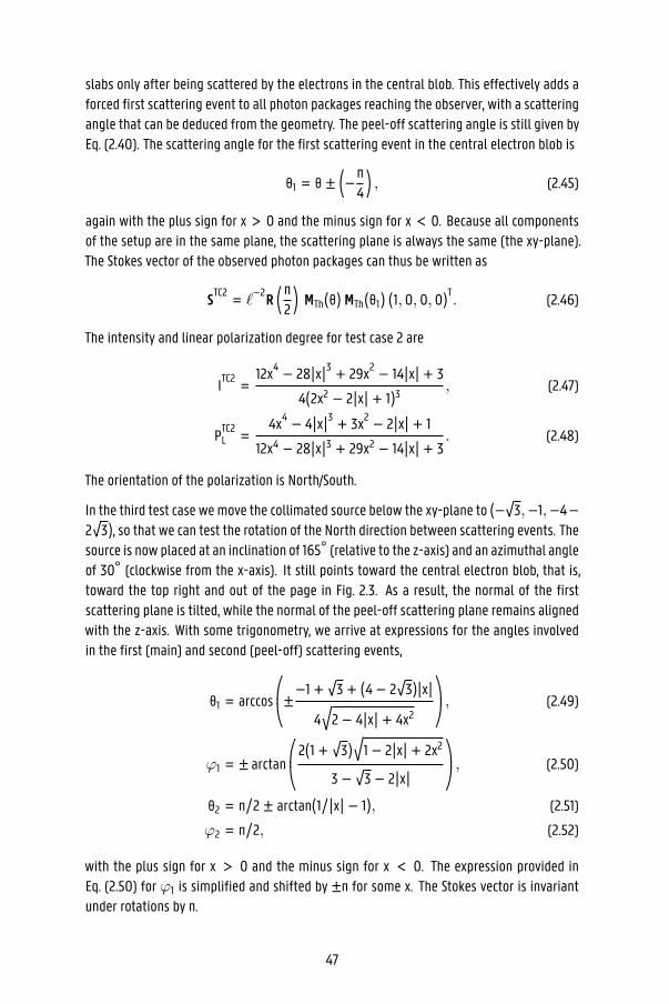
slabs only after being scattered by the electrons in the central blob. This effectively adds aforced first scattering event to all photon packages reaching the observer, with a scatteringangle that can be deduced from the geometry. The peel-off scattering angle is still given byEq. (2.40). The scattering angle for the first scattering event in the central electron blob is

θ1 = θ ± (−π4) , (2.45)

again with the plus sign for x > 0 and the minus sign for x < 0. Because all componentsof the setup are in the same plane, the scattering plane is always the same (the xy-plane).The Stokes vector of the observed photon packages can thus be written as

STC2 = ℓ−2R (π

2) MTh(θ) MTh(θ1) (1, 0, 0, 0)T. (2.46)

The intensity and linear polarization degree for test case 2 are

ITC2 =12x4 − 28∣x∣3 + 29x2 − 14∣x∣ + 3

4(2x2 − 2∣x∣ + 1)3 , (2.47)

PTC2L =

4x4 − 4∣x∣3 + 3x2 − 2∣x∣ + 1

12x4 − 28∣x∣3 + 29x2 − 14∣x∣ + 3. (2.48)

The orientation of the polarization is North/South.

In the third test case wemove the collimated source below the xy-plane to (−√3,−1,−4−2√3), so that we can test the rotation of the North direction between scattering events. The

source is now placed at an inclination of 165◦ (relative to the z-axis) and an azimuthal angleof 30◦ (clockwise from the x-axis). It still points toward the central electron blob, that is,toward the top right and out of the page in Fig. 2.3. As a result, the normal of the firstscattering plane is tilted, while the normal of the peel-off scattering plane remains alignedwith the z-axis. With some trigonometry, we arrive at expressions for the angles involvedin the first (main) and second (peel-off) scattering events,

θ1 = arccos⎛⎜⎝±−1 +

√3 + (4 − 2

√3)∣x∣

4√2 − 4∣x∣ + 4x2

⎞⎟⎠ , (2.49)

φ1 = ± arctan⎛⎜⎝2(1 + √

3)√1 − 2∣x∣ + 2x2

3 −√3 − 2∣x∣ ⎞⎟⎠ , (2.50)

θ2 = π/2 ± arctan(1/∣x∣ − 1), (2.51)

φ2 = π/2, (2.52)

with the plus sign for x > 0 and the minus sign for x < 0. The expression provided inEq. (2.50) for φ1 is simplified and shifted by ±π for some x. The Stokes vector is invariantunder rotations by π.

47

The Stokes vector of the observed photon packages can now be written as

STC3 = ℓ−2R(φ2) MTh(θ2) R(φ1) MTh(θ1) (1, 0, 0, 0)T. (2.53)

To limit the complexity of presentation, we provide expressions for the Stokes parametersfromwhich the linear polarization degree and angle can be calculated using Eqs. (2.3) and (2.4),

ITC3 = 1

32ℓ6[(62 − 16

√3)x4 − (150 − 30

√3)∣x∣3 + (156 − 25

√3)x2−(78 − 8

√3)∣x∣ + 18 −

√3] , (2.54)

QTC3 = 1

32ℓ6[(2 − 16

√3)x4 + (22 + 34

√3)∣x∣3 − (28 + 39

√3)x2+(14 + 24

√3)∣x∣ − (2 + 7

√3)] , (2.55)

UTC3 = 18ℓ4

[(1 + √3)x2 − (1 + 2

√3)∣x∣ + √

3] , (2.56)

VTC3 = 0. (2.57)

Figure 2.4 compares the analytical solutions and SKIRT results for the observed intensity,linear polarization degree, and polarization angle for these three test cases. The intensitycurves show a relative noise level of on average about 3%. The linear polarization degreesare identical to below 0.1% absolute for test cases 1 and 2 and below 1% absolute for testcase 3. The polarization angles from north are correct to below 0.05◦ for test cases 1 and2 and below 1◦ for test case 3. While the linear polarization degree and position angle canbe determined from a simulation with relatively few photon packages, reducing the noisein the intensity requires significantly more photon packages. This is because the number ofphoton packages arriving at each pixel is subject to Poisson noise, whereas the path thateach photon package takes to the same pixel is defined within tight boundaries. The inten-sity curve depends on the number of photons. The linear polarization degree and angle areindependent of the number of photon packages. Their noise is due to the size of the pixels.Slightly different paths and scattering angles might contribute to the same pixel.

The polarization angle for test case 1 shows an intriguing spike near x = 0. As we can seein the linear polarization degree curve and from Eq. (2.44), the radiation arriving at x = 0is unpolarized. This implies that both the Q and U components of the Stokes vector arezero and the polarization angle becomes undefined (see Eq. 2.4). This in turn causes smallnumerical inaccuracies in the calculations for photon packages arriving very close to x = 0.

The relative differences for the other quantities are generally smaller than a fraction of apercent. In the results of test case 3 the residuals of the linear polarization degree andpolarization angle contain spikes that are resolved by multiple pixels each and symmetricwith respect to x = 0. The residual of the intensity curve shows a similar effect. It tends tobe lower than expected in the outer regions and higher than expected in the inner region.These orderly deviations indicate a systematic difference rather than noise. In fact, these

48

discrepancies are caused by resolution effects in the SKIRT implementation of our method(see Sect. 2.5.1 for a description of our discretization choices). For example, consider theinterval 0.6 < x < 0.7 for test case 3, which is resolved by 10 pixels along the x-axis ofthe detector in the observer frame. The corresponding interval for scattering angle θ1 (seeEq. 2.49) is 75.0◦ < θ1 < 75.1◦ , that is, only a fraction of the 1◦ resolution in the SKIRTcalculations related to θ. It is obvious that this lack of angular resolution relative to theoutput resolution will cause inaccuracies. We calculated the residuals in the polarizationdegree and angle from north using twice the θ resolution and show them in pale green inFig. 2.4. They confirm that increasing the θ resolution in the calculations indeed reduces thediscrepancies accordingly.

2.5.3 Circular polarization

To include circular polarization in test case 4, we use synthetic particles similar to electrons,but with a scattering matrix that mixes the U and V components of the Stokes vector:

Msyn(θ) = 12

⎛⎜⎜⎜⎜⎜⎜⎜⎜⎝cos2 θ + 1 cos2 θ − 1 0 0cos2 θ − 1 cos2 θ + 1 0 0

0 0 2 cos2 θ −2 cos θ sin θ0 0 2 cos θ sin θ 2 cos2 θ

⎞⎟⎟⎟⎟⎟⎟⎟⎟⎠ . (2.58)

We use the same geometry as for test case 3, replacing the electrons in the two slabs andin the central blob by particles described by Eq. (2.58). The angles are still described byEqs. (2.49) through (2.52), Eq. (2.53) still holds, and the Stokes parameters of the observedphoton packages become

ITC4 =ITC3, (2.59)

QTC4 =QTC3, (2.60)

UTC4 = ±18ℓ5

[(1 + √3)∣x∣3 − (2 + 3

√3)x2 + (1 + 3

√3)∣x∣ − √

3] , (2.61)

VTC4 = 18ℓ5

[−(1 + √3)∣x∣3 + (1 + 2

√3)x2 − √

3∣x∣] . (2.62)

In Eq. (2.61) the plus sign is again for x > 0 and the minus sign for x < 0.

Figure 2.5 shows the (relative) circular polarization, V/I, for this test case, again comparingthe analytical solutions with the SKIRT results. The relative differences between the analyt-ical and simulated results for ∣x∣ < 0.7 are below one percent. The larger discrepancies for∣x∣ > 0.7 are again due to the limited resolution in the SKIRT calculations related to θ. Thepale green line again shows the residuals when calculating with 0.5◦ resolution and has asignificantly smaller residual curve. Disregarding the outer part, the circular polarization iscorrect to 0.1% absolute.

49

30%−24

−12

0

12

24

Exte

nt

(kpc)

20 ◦

30%

75 ◦

30%

90 ◦

1%−24

−12

0

12

24

Exte

nt

(kpc)

20 ◦

1%

75 ◦

1%

90 ◦

1%−24 −12 0 12 24

Extent (kpc)

−24

−12

0

12

24

Exte

nt

(kpc)

20 ◦

1%−24 −12 0 12 24

Extent (kpc)

75 ◦

1%−24 −12 0 12 24

Extent (kpc)

90 ◦

10-6

10-5

10-4

10-3

10-2

10-1

100

Surf

ace

bri

ghtn

ess

(arb

. unit

s)

Figure 2.6: B-band surface brightness maps (color scale) overlaid with linear polarizationmaps (line segments) for inclinations of 20◦(left), 75◦(middle), and 90◦(right column). Thetop row shows a model with only a stellar bulge, the middle row a model with only a stellardisk, and the bottom row a model with both stellar bulge and disk with a ratio of bulge tototal luminosity of B/T=0.5. The dust disk is the same in the three cases and has a centralface-on V-band optical depth of 10.

2.6 Benchmark tests

2.6.1 Disk galaxy

We compare results of our code to Bianchi et al. (1996) as a first test of our implication of dustscattering polarization (rather than just Thompson scattering). Bianchi and collaboratorsdescribe the polarization effects of scattering by spherical dust grains in monochromaticMCRT simulations of 2D galaxy models at the B band (0.44 μm) and I band (0.9 μm). Themodels include a stellar bulge, a stellar disk, and a dust disk. The stellar bulge is describedby Jaffe (1983) (scale radius 1.86 kpc, truncated at 14.8 kpc), and the stellar disk is a double-exponential disk (scale length 4 kpc, truncated at 24 kpc; scale height 0.35 kpc, truncated at2.1 kpc). The relative strength of the stellar components and the stellar sources is varied. In

50

i =69.5°

1

2

3

TORUS

MCFOST

MCMax

Pinball

SKIRT

i =87.1°

4

5

6

0% 25% 50% 75% 100%Polarization degree

0%

20%

40%

60%

80%

100%Pola

riza

tion d

egre

e1

0.10

0.05

0.00

0.05

0.10

Diffe

rence

2 3

0%

20%

40%

60%

80%

100%

Pola

riza

tion d

egre

e

4

400 200 0 200 400Extent [AU]

0.10

0.05

0.00

0.05

0.10

Diffe

rence

5

400 200 0 200 400Extent [AU]

6

400 200 0 200 400Extent [AU]

Figure 2.7: Polarization degree maps for two inclinations of a disk with high optical density(τ = 106). On the left are the linear polarization degree maps we calculated using SKIRT.The dust grain size is the same as the wavelength (1 μm), creating the intricate pattern ofthe polarization degree. On the right are cuts 1–6 through the maps along with results ofvarious codes. Pinball (Watson and Henney 2001) in green, MCMax (Min et al. 2009) in black,MCFOST (Pinte et al. 2006) in blue, TORUS (Harries 2000) in dashed orange, and SKIRT in red.The data of the other codes were taken from the official website.

51

all models, the dust is assumed to be homogeneously distributed in a double-exponentialdisk embedded in the stellar disk, with the same horizontal parameters as the stellar disk,but much thinner vertically (scale height 0.14 kpc, truncated at 0.84 kpc). The central face-on optical depth of the dust disk τV is a free parameter. The properties of the dust aretaken from the MRN dust model (Mathis et al. 1977), which includes graphite grains andastronomical silicates with a size distribution n(a) ∝ a−3.5 , 0.005 μm < a < 0.25 μm.Polycyclic aromatic hydrocarbons (PAHs) and very small grains are not included.

Figure 2.6 displays our results, which correspond to the Bianchi et al. (1996) model shownin their Figure 8. We use the same geometry, described above, and the same bulge-to-totalratio (B/T=0.5), wavelength (λ = 0.44 μm), and optical depth (τV = 10). We use a differentdustmodel. It includes awider range of graphite and silicate grain sizes following the Zubkoet al. (2004) size distribution, in addition to a small fraction of PAHs as described in Campset al. (2015). The differences between the dust models do not affect the qualitative resultsat optical wavelengths, but do prevent a quantitative comparison.

Surface brightness maps (color scale) overlaid with a linear polarization maps (line seg-ments) are shown in Fig. 2.6. The inclinations range from nearly face-on (20◦ , left) to edge-on (90◦ , right). The top and middle rows show models from which the stellar disk and thestellar bulge, respectively, was removed. The bottom row shows the B/T=0.5 model, that isto say, the model including both stellar bulge and stellar disk. The dust disk is identical forthe three models.

Overall, our results are compatible with those reported by Bianchi et al. (1996). The largestpolarization degrees are observed near the major axis. For pure disks, the face-on viewshows very little polarization. The polarization degree increases with inclination to a maxi-mum near an inclination of about 80◦ and slightly decreases again when approaching 90◦ .The polarization degree averaged over all pixels is below 1% for all inclinations. For purebulges, the maximum polarization degree is largely independent of the inclination. In theouter regions of the dust disk, the linear polarization degree is 22%. In the mixed B/T=0.5model, the polarization degrees are drastically reduced. We find values up to 1.6%, compara-ble to the results of Bianchi et al. (1996), who find 1 to 1.5%.

We also test the corresponding model for the I band (λ = 0.9 μm) with a color-adjustedbulge luminosity (B − I = 1 mag), again confirming overall agreement Bianchi et al. (1996).

2.6.2 Dusty disk around star

To test the performance of our code on a problem of a different scale, we compute polariza-tion results of Pinte et al. (2009). In it, a thick dusty disk surrounds a central star. The starextends out to 2 AU and has a temperature of 4000 K. The dust consists of spherical grainswith a radius of 1 μm, and the light has a wavelength of 1 μm as well. The dust density

52

distribution ρ is cylindrical,

ρ(R, z) = 3Σ02R0

( RR0)−5/2

exp [− 12( zh0)2 ( R

R0)−9/4] , (2.63)

with a surface density Σ0 , scale radius R0 = 100 AU, radial distance from the center R,vertical distance from the midplane z, and scale height h0 = 10 AU. The disk is truncatedat Rmin = 0.1 AU and Rmax = 400 AU. The surface density depends on the total dust massm = 3 × 10−5 M⊙ by

Σ0 = m/ [ 125(2π)3/2h0R0 ((Rmin/R0)5/8 − (Rmax/R0)5/8)] (2.64)

and the albedo of the dust is 0.6475 and the opacity 4752 cm2/g at 1 μm. We adopt thescattering matrix as provided by Pinte et al. (2009).3 The system is resolved at a distanceof 140 pc by a detector with 251 × 251 pixels covering 900 × 900 AU2 .

Figure 2.7 shows the linear polarizationmaps calculated by our code for inclinations of 69.5◦

and 87.1◦ . The flux difference from the borders to the center area is about 17 orders ofmagnitude. The maps are displayed in gray outside the truncation radius, where no flux wasrecorded. The intricate pattern of the polarization degree is a result of the uniform grainradius being equal to thewavelength. The phase function therefore contains resonances andsteep gradients for small changes of the scattering angle. We compare our results to theresults of the four polarization capable codes in Pinte et al. (2009) along six cuts through themaps. The first and third row show the polarization degree along the cuts, and the secondand fourth row show the difference of the codes to the average of all results. The TORUScode (Harries 2000) is not included in calculating the averages because its signal-to-noiseratio is too low. In the central area the codes agree within 10% of absolute polarization, butas the true result is unknown, a quantitative analysis of the results of this benchmark isdifficult. In general, the results of the SKIRT code are close to the average result, and SKIRTseems to agree particularly well with the Pinball code (Watson and Henney 2001). Pinballemploys some of the same optimization techniques that SKIRT uses (e.g., forced interactionand peel-off, named “forced escape” in their paper).

2.7 Application: spiral galaxy models

We study the polarization properties of a 3D galaxy model including spiral arms to investi-gate how the spiral arm structure is imprinted in the polarization structure. We also studythis in the edge-on view when the structure is not easily characterized from the intensityalone.

3http://ipag.osug.fr/ pintec/benchmark/

53

2%−10

−5

0

5

10

Face

-on v

iew

(kp

c)

2% 2%

2%−8

−4

0

4

8

Incl

ined v

iew

(kp

c)

2% 2%

2%−6

−3

0

3

6

Edge-o

n v

iew

(kp

c)

2% 2%

−10 −5 0 5 10

Dusty spiral: x extent (kpc)

0.0

0.1

0.2

0.3

0.4

0.5

0.6

0.7

Edge-o

n p

ola

riza

tion d

egre

e (

%)

−10 −5 0 5 10

Rotated dusty spiral: x extent (kpc)−10 −5 0 5 10

Stellar Disk: x extent (kpc)

10-1

100

101

102

Surf

ace

bri

ghtn

ess

(M

Jy/s

r)

Figure 2.8: Spiral galaxy model described in Sect. 2.7 and Table 2.2 observed at a wavelengthof 1 μm. Rows from top to bottom: face-on, inclined (53◦), and edge-on surface brightness(color scale) overlaid with linear polarization degree and orientation (line segments); linearpolarization degree of the edge-on view, averaged over the vertical axis. Columns from leftto right: the reference model; the same model observed from a different azimuth angle(rotated clockwise by 120◦); a model without the spiral arm perturbations in the stellardisks, with the rotated orientation.

54

Figure 2.9: Linear polarization degree, averaged over the vertical axis, of the rotated model(column B of Fig. 2.8) observed at 1 μm, for inclinations ranging from edge-on (i=90◦) toface-on (i=0◦).

Figure 2.10: Averaged linear polarization degree for one side of the edge-on view of therotated model, observed at optical and near-infrared wavelengths from 0.28 μm to 2.84 μm.The red vertical bands correspond to the bands in Fig. 2.9 and trace the tangent points ofthe dust spiral arms.

55

Table 2.2: Parameters for our spiral galaxy model, including the blackbody temperature andthe bolometric luminosity of the stellar components, and the total dust mass in the dustcomponent.

Sérsic profile Bulge

Sérsic index 3Effective radius 1.6 kpcFlattening parameter 0.6Temperature 3500 KLuminosity 3 × 1010 L⊙

Exponential disks Old stars Young stars Dust

Scale length 4 kpc 4 kpc 4 kpcHorizontal cutoff 20 kpc 20 kpc 20 kpcScale height 0.35 kpc 0.2 kpc 0.2 kpcVertical cutoff 1.75 kpc 1 kpc 1 kpcNumber of arms 2 2 2Pitch angle 20◦ 20◦ 20◦

Radius zero-point 4 kpc 4 kpc 4 kpcPhase zero-point 0◦ 20◦ 20◦

Perturbation weight 0.25 0.75 0.75Arm-interarm size ratio 5 5 5Temperature 3500 K 10000 KLuminosity / mass 4 × 1010 L⊙ 1 × 1010 L⊙ 2 × 107 M⊙

56

We still assume a homogeneous distribution for the stellar sources and the dust. The modelincludes a stellar bulge and disk with an older star population, a second stellar disk witha younger star population, and a dust disk. The relevant parameters are listed in Table 2.2.The bulge is modeled by a spheroidal density distribution obtained by flattening a sphericalSérsic profile (Sérsic 1963), as implemented by Baes and Camps (2015). The distributions ofthe two stellar and the dust disks are truncated double-exponential disks. The spiral armstructure is introduced by adding a perturbation to the overall density profile, as presentedby Baes and Camps (2015). We have made the spiral arms in the older stellar population‘lead’ those in the younger stellar population and in the dust disk by varying the spiral armphase zero-points. The emission of the stellar populations is modeled as blackbody spectraat the indicated temperatures. We use the dust model of Sect. 2.6.1 (Camps et al. 2015). Thetotal dust mass is given in Table 2.2, the central face-on B-band optical depth of the dustdisk is τV ≈ 1.3.

Figure 2.8 shows surface brightness maps (color scale) overlaid with linear polarizationmaps (line segments). The leftmost column is for this model at 1 μm. The top row shows themodel face-on, the second row inclined (53◦), and the third row edge-on. The polarizationdegree is up to 1% around the central part of themodels and over thewholemap the averagepolarization degree is similar to the average polarization degree from the B/T=0.5 modelfrom before. As in the B/T=0.5 model, the orientation of the polarization is circular aroundthe central bulge, and for the inclined view the polarization degree left and right of thecenter increases, while it decreases behind and in front of it. In contrast to the azimuthallyuniform model, there is a spiral structure in the polarization map. The linear polarizationdegree is higher in the arm regions and disappears in the interarm region. The maximumpolarization degree is slightly inward from the regions of the armswith the highest flux. Thepanel in the bottom row plots the linear polarization degree for the edge-on view, averagedover the vertical axis. This average is obtained by summing each individual component ofthe Stokes vector and calculating the polarization degree from these totals. Regions withhigher linear polarization (up to 2%) clearly trace the spiral arms and are prominent at allinclinations, including the edge-on view. The maxima in the polarization signature of theedge-on view match the positions of the spiral arms along the line of sight.

To verify this, the middle column of Fig. 2.8 shows the same model from a different azimuthangle. The peaks in the polarization signature align with the tangent points of the spiralarms, which are now farther out from the center of the galaxy.

In the rightmost column of Fig. 2.8 we remove the spiral arms perturbations from the stellardisks in the model. The polarization signature remains essentially unchanged; the maximaare slightly higher (by a factor of up to 1.2), but the structure is the same. The signaturecould also be produced by the different phase zero-points of the old stars and the dust (seeTable 2.2). We calculated results using the same phase zero-point for all components (notshown here). The outer maxima are lower (by a factor of 0.8), while the inner maxima areunchanged. This confirms that the polarization signature is created by the distribution ofthe dust and not by the distribution of the sources.

57

In Fig. 2.9 we further study the effect of inclination on the observed polarization signaturefor the reference model. In the central region (r ≲ 2 kpc), the bulge emission masks mostpolarization at inclinations above 40◦ . Outside this region, however, the form of the curvesis very similar for all inclinations. Although the polarization degree generally decreasestoward lower inclinations, the peaks remain at the spiral arm tangent points, and the ratiobetween themaximum andminimum polarization degree remains roughly stable at a factorof about 2.

In Fig. 2.10 we compare the edge-on polarization signature of our reference model for vari-ous optical and near-infrared wavelengths. The polarization peaks remain prominent overthe wavelength range 0.5 μm ≲ λ ≲ 2 μm. At shorter wavelengths the general polariza-tion degree is higher and the signature is reversed, light from within the arms is slightlyless polarized than light from the inter-arm regions. The increased interaction cross sectioncauses the inter-arm dust to become efficient at scattering the stellar radiation, boostingthe polarization degree. We find that in the spiral arms the ratio of once scattered to mul-tiple times scattered light is 2.5:1, while in the inter-arm region it is 3.3:1. The polarizationorientation after multiple scatterings is less uniform, which lowers the polarization degreein the arm regions.

At longer wavelengths, the signature retains the same form, but the reduced scattering effi-ciency of the dust causes the polarization degree to be very low, so that the peaks becomehard to discern.

Our results imply that polarization measurements could be used, at least in principle, tostudy the spiral structure of edge-on spiral galaxies, where intensity measurements alonehave limited diagnostic power. The contrast would be highest at around 1 μm and with anexpected polarization degree of up to 0.6%, this is well within the capabilities of currentpolarization capable telescopes.

We note that the polarization degree of the edge-on galaxy NGC 891 was mapped by Mont-gomery and Clemens (2014) at 1.6 μm. They found polarization degrees of below 1% thatvaried along the disk profile. We expect the orientation of polarization due to scattering tobe perpendicular to the disk. Montgomery and Clemens (2014) found the orientation to berather parallel to the disk and attributed most of it to dichroic extinction. Our code does notyet support dichroic extinction, so we cannot compare the strength of these two effects.

2.8 Conclusion

We presented a robust framework that is independent of a coordinate system for imple-menting polarization in a 3D MCRT code, focusing on scattering by spherical dust grains.The mathematical formulation and the numerical calculations in our method rely solely onthe scattering planes determined by the physical processes rather than by the coordinatesystem. This approach avoids numerical instabilities for special cases and enables a more

58

streamlined implementation. We described four test cases with well-defined geometriesand material properties, yielding analytical solutions. These setups are designed to vali-date the calculated results in a structured manner, and they can serve as benchmarks forother implementations as well.

We reconstructed a selection of the 2D models of Bianchi et al. (1996), confirming that ourimplementation reproduces their results at least qualitatively. A quantitative comparisonis not possible because of differences in the dust model. We then calculated results for thepolarization part of the Pinte et al. (2009) benchmark and obtained similar results as theother codes that took part in it. As an application of our code we constructed a 3D spiralgalaxy model including a stellar bulge and disk with an older star population, a secondstellar diskwith a younger star population, and a dust disk. The stellar and dust distributionsfeature an analytical spiral arm perturbation. We showed that scattering of light at the dustin the spiral arms produces a marked polarimetric signature. It traces the tangent positionsof the arms for wavelengths in the range 0.5 μm ≲ λ ≲ 2 μm, regardless of inclination.

It is fair to note, however, that our current implementation is limited to scattering by spher-ical dust grains. We plan to add support for polarized emission and for scattering and ab-sorption by (partially) aligned spheroidal grains in future work. With the relevant physicsincluded, we can also study the influence of changes to dust properties on the polarizationsignature, which we have not addressed in this paper.

2.9 Acknowledgements

C.P., P.C., and M.B. acknowledge the financial support from CHARM (Contemporary physicalchallenges in Heliospheric and AstRophysical Models), a Phase-VII Interuniversity AttractionPole program organized by BELSPO, the BELgian federal Science Policy Office. M.S. acknowl-edges support by FONDECYT through grant no. 3140518 and by the Ministry of Education,Science and Technological Development of the Republic of Serbia through the projects As-trophysical Spectroscopy of Extragalactic Objects (176001) and Gravitation and the LargeScale Structure of the Universe (176003). We thank Rene Goosmann, Francesco Tamborra,and Frederic Marin for many useful discussions and providing insights on the operation ofthe STOKES code. We wish to thank the anonymous referee for their constructive input tothis paper.

59

60

Chapter 3

Optical depth in polarized MonteCarlo radiative transfer

M. Baes1, C. Peest1,2, P. Camps1, and R. Siebenmorgen2

1 Sterrenkundig Observatorium, Universiteit Gent, Krijgslaan 281, S9, 9000 Gent, Belgium2 European Southern Observatory, Karl-Schwarzschild-Str. 2, 85748 Garching b. München,Germany

Received 9 July 2018 / Accepted ?

© ESO 2018

61

3.1 Abstract

The Monte Carlo method is the most widely used method to solve radiative transfer prob-lems in astronomy, especially in a fully general 3D geometry. A crucial concept in any MonteCarlo radiative transfer code is the random generation of the next interaction location. Inpolarized Monte Carlo radiative transfer with aligned nonspherical grains, the nature ofdichroism complicates the concept of optical depth.

We investigate in detail the relation between optical depth and the optical properties anddensity of the attenuating medium in polarized Monte Carlo radiative transfer codes thattake into account dichroic extinction.

Based on solutions for the radiative transfer equation, we discuss the optical depth scale inpolarized radiative transfer with spheroidal grains. We compare the true optical depth tothe extinction and total optical depth scale.

In a dichroic medium, the optical depth is not equal to the usual extinction optical depth,nor to the so-called total optical depth. For representative values of the optical proper-ties of dust grains, the relative difference between both optical depth scales can be severalten percent. A closed expression for the optical depth cannot be given, but it can be de-rived efficiently through an algorithm that is based on the analytical result correspondingto elongated grains with a uniform grain alignment.

Optical depth is more complex in dichroic media than in systems without dichroic attenua-tion, and this complexity needs to be considered when generating random free path lengthsin Monte Carlo radiative transfer simulations. There is no benefit in using approximationsinstead of the true optical depth.

3.2 Introduction

Radiative transfer is a broad field in astronomy and beyond that aims to describe the inter-action between radiation and matter. In an astronomical context, the Monte Carlo methodis by far the most widely used method to solve radiative transfer problems. In the pastdecades, many different Monte Carlo codes have been developed to address different astro-physical radiative transfer problems, including photoionisation, absorption and scatteringby cosmic dust, the origin of infrared emission, and resonant line scattering heating (e.g.,Gordon et al. 2001; Ercolano et al. 2003; Robitaille 2011; Yajima et al. 2012; Whitney et al.2013; Camps and Baes 2015; Reissl et al. 2016). General reviews on Monte Carlo transportcan be found in e.g. Dupree and Fraley (2002) or Kalos and Whitlock (2008), and dedicatedreviews on radiative transfer in astrophysics include Whitney (2011) and Steinacker et al.(2013).

The essence of the Monte Carlo method is to represent the radiation field as the flow of a

62

large but finite number of photon packages. The life cycle of each photon package is fol-lowed individually, and at every stage in this life cycle, the characteristics that determinethe path of each photon package are determined in a probabilistic way by generating ran-dom numbers from the appropriate probability density function (PDF). At the end of thesimulation, the radiation field, or more specifically the intensity of the radiation field, isrecovered from a statistical analysis of the photon package paths.

An important ingredient of Monte Carlo radiative transfer is the knowledge of the appropri-ate PDF for a given characteristic, and the accurate and efficient sampling of random num-bers from these PDFs. For some characteristics, the PDFs are simple and sampling randomnumbers from them is trivial. For example, most sources send out radiation isotropically,which implies that the generation of propagation directions after an emission event simplycomes down to generating a random point on the unit sphere. The PDF that controls the ran-dom starting positions for the photon package is dictated by the 3D luminosity density ofthe sources, and specific methods have been developed to generate such random positionsfrom a range of 3D density distributions (Baes and Camps 2015).

An aspect that is central to any Monte Carlo radiative transfer code is the random gener-ation of the next interaction location. More specifically, if a photon package is emitted orscattered into a given direction, one needs to randomly generate a free path length s to thenext interaction. To do so, we need to know the appropriate PDF p(s). In this context, theconcept of optical depth τ plays a crucial role. In optical depth space, the PDF p(τ) is a sim-ple exponential distribution (Cashwell and Everett 1959; Steinacker et al. 2013). This impliesthat the next interaction location can be found by randomly generating a random opticaldepth from an exponential distribution, and converting this optical depth to a physical pathlength. This last aspect is a critical point: we need to know the relation τ(s), or inverselys(τ) to properly calculate the next interaction location.

In radiative transfer problems where polarization is not taken into account, τ(s) can immedi-ately be calculated from the density and the optical properties along the path, and does notdepend on the intensity of the radiation field. The situation becomes more complex whenpolarization comes into play. In the case of spherical or randomly oriented particles, po-larized Monte Carlo radiative transfer is only slightly more difficult than unpolarized MonteCarlo radiative transfer. The main added complexity is that a Stokes vector needs to be intro-duced to characterize the polarization status of each photon package, and that this Stokesvector can alter during a scattering event (e.g., Fischer et al. 1994; Code and Whitney 1995;Bianchi et al. 1996; Peest et al. 2017). The relation between optical depth and path length isthe same as for unpolarized Monte Carlo radiative transfer.

The real complexity arises when the attenuating particles are nonspherical and aligned, asin the case of elongated dust grains in the interstellar medium. Such dust grains will bealignedwith respect to themagnetic fields through a variety of processes (Jones and Spitzer1967; Aannestad and Greenberg 1983; Lazarian 1994, 2007). An interesting feature in thiscontext is dichroism, which means that radiation of different polarization experiences dif-ferent amounts of extinction. The nature of dichroism complicates the relation between

63

optical depth and the physical path length.

In this paper, we investigate in detail whether an optical depth scale can still be used ina meaningful way in polarized Monte Carlo radiative transfer codes that take into accountdichroic extinction. In Section 3.3 we discuss optical depth and the generation of randompath lengths in standard unpolarized Monte Carlo radiative transfer codes. In Section 3.4 weextend this discussion to polarized Monte Carlo radiative transfer, in particular for the caseof elongated aligned grains. In Section 3.5 we discuss these results and we sum up.

3.3 Unpolarized radiative transfer

As discussed in the Introduction, one of the essential steps in the life cycle of a photon pack-age in a Monte Carlo radiative transfer simulation is the calculation of the next interactionlocation, or equivalently, the physical path length s covered before the next interaction. Todo that, we need to generate a random s from the appropriate probability distribution func-tion p(s). The appropriate PDF p(s) can be found by considering the variation of the specificintensity I(s) along the path. The probability that the photon package has not interactedalong the path between 0 and s is equal to I(s)/I0 , with I0 the specific intensity of the pho-ton package at the start of the path.1 Therefore, the cumulative density function P(s) canbe written as

P(s) = ∫ s

0p(s′) ds′ = 1 −

I(s)I0

(3.1)

In general, we define the optical depth τ(s) asτ(s) = − ln [ I(s)

I0] (3.2)

Combining these two equations, we find

P(s) = 1 − e−τ(s) (3.3)

and when we take the derivative of this cumulative density function,

p(τ) = e−τ (3.4)

This yields the well-know result that the PDF describing the next interaction location isan exponential distribution in optical depth space. Generating a random optical depth caneasily be done by picking a uniform deviate ξ, setting τ = − ln(1 − ξ), and subsequentlyconverting this random τ to a physical path length s.

1Many of the quantities in this paper are dependent on wavelength, including the extinction cross sectionand the optical depth. In order not to overload the notations, we do not explicitly mention the wavelengthdependence.

64

The difficulty is that we need to know the solution I(s) to calculate the optical depth scale.This solution is found by solving the appropriate radiative transfer equation. For a photonpackage moving through an attenuating medium with density n(s) and extinction cross sec-tion Cext(s), the radiative transfer equation reads

dIds(s) = −n(s) Cext(s) I(s) (3.5)

Note that no additional emission along the path or scattering into the line-of-sight areincluded, as this is not relevant for this particular photon package. This equation is a simplefirst-order ordinary differential equation that is easy to solve,

I(s) = I0 e−τext(s) (3.6)

with the extinction optical depth τext(s) defined as

τext(s) = ∫ s

0n(s′) Cext(s′) ds′ (3.7)

Comparing equations (3.2) and (3.6), we see that τ(s) = τext(s). In particular, the opticaldepth scale from which random path lengths can be sampled only depends on the densityand optical properties of the material, and not on the properties of the photon package (inthis simple case, the only property of the photon package that could matter is I0).

While the strategy described above is conceptually very simple, some challenges need to beaddressed. In particular, the conversion of extinction optical depth to physical path length isusually not a straightforward inversion, and except for some simple idealized cases, needs tobe done numerically. In most Monte Carlo radiative transfer codes, the attenuating mediumis subdivided into a large number of individual cells, each with a constant density and uni-form properties. The codes are typically equipped with a routine to calculate paths throughthis tessellated medium; this routine returns an ordered list of all the cells m that the pathcrosses, aswell as the length Δsm of the path segments corresponding to them’th cell. Giventhis ordered list, we can calculate the running values for the path length sm and the opticaldepth τext,m at the exit point of each cell crossed by the path. The problem hence reducesto finding the first cell in the array for which τext,m exceeds the randomly generated valueof τext , and subsequently applying a linear interpolation to convert τext to s.2

These integrations through the dust grid often form the most time-consuming part of aradiative transfer simulation. In order to make these calculations as efficient as possible,

2The MC3D radiative transfer code (Krügel 2008; Heymann and Siebenmorgen 2012) adopts an alternativemethod to find the next interaction point. For every dust cell along a path, they generate a new optical depth τfrom an exponential distribution, and they compare this to the extinction optical depth Δτext,m within that cell.If τ < Δτext,m , the interaction position is determined by linear interpolation; otherwise, the dust cell is crossedand the procedure is repeated for the next cell along the path. This methodology is equivalent to the methodused by most other Monte Carlo codes, but seems computationally more expensive, and not straightforward tocombine with optimization techniques as path length stretching (Levitt 1968; Spanier et al. 1970; Baes et al.2016) or forced scattering (Cashwell and Everett 1959; Steinacker et al. 2013).

65

especially in 3D geometries, advanced grid construction and grid traversal techniques arerequired (Niccolini and Alcolea 2006; Bianchi 2008; Lunttila and Juvela 2012; Camps et al.2013; Saftly et al. 2013, 2014; Hubber et al. 2016).

3.4 Polarized radiative transfer

3.4.1 The Stokes formalism

The characterization of the radiation field by the specific intensity, and the correspondingradiative transfer equation (3.5), are no longer suitable when polarization is considered.In order to take into account the polarization state of radiation, one can use the Stokesformalism, which characterizes the radiation field by means of the 4D Stokes vector

S =⎛⎜⎜⎜⎜⎜⎜⎝IQUV

⎞⎟⎟⎟⎟⎟⎟⎠ (3.8)

The first Stokes parameter, I, is still the specific intensity. The Stokes parameters Q and Udescribe the state of linear polarization and V describes the state of circular polarizationof the radiation. The Stokes parameters are always defined with respect to a referencedirection to be chosen freely from the plane perpendicular to the propagation direction.For a detailed description of the Stokes vector and its connection to the monochromatictransverse electromagnetic waves, we refer to Mishchenko et al. (2000).

When we consider the full Stokes vector, the simple radiative transfer equation (3.5) be-comes

dSds(s) = −n(s) K(s) S(s) (3.9)

where K is now the extinction matrix, a 4×4 matrix that describes how the different Stokescomponents are affected when radiation passes through the medium.

3.4.2 Spherical grains

When the dust grains are spherical, or nonspherical but arbitrarily oriented, the extinctionmatrix is a simple diagonal matrix and all components of the Stokes vector are affected inthe same way, and

K =⎛⎜⎜⎜⎜⎜⎜⎝Cext 0 0 00 Cext 0 00 0 Cext 00 0 0 Cext

⎞⎟⎟⎟⎟⎟⎟⎠ (3.10)

66

This implies that there is no mixture of the different Stokes components due to extinction,and the solution of the radiative transfer equation can directly be written as

S(s) = S0 e−τext(s) (3.11)

In particular, the specific intensity I(s) still behaves according to equation (3.6), exactly asin the case of nonpolarized radiative transfer. We can immediately conclude that, also inthis case, the PDF describing the net interaction location is an exponential distribution inextinction optical depth space.

3.4.3 Spheroidal grains

Complexity arises when the dust grains are nonspherical and (partially) aligned. In this case,the extinctionmatrix K is not a diagonal matrix, but a full 4×4matrix with 16 nonzero crosssections, but only seven independent ones (Van De Hulst 1957; Hovenier and van der Mee1996). Fortunately, in the case of spheroidal grains, K is significantly less complex. If wedenote the orientation of the grain alignment at a distance s along the path as β(s), K canbe expressed as (Martin 1974; Wolf et al. 2002)

K(s) = R(−β(s)) Kref(s) R(β(s)) (3.12)

with R(β) a Mueller rotation matrix

R(β) = ⎛⎜⎜⎜⎜⎜⎜⎝1 0 0 00 cos 2β sin 2β 00 − sin 2β cos 2β 00 0 0 1

⎞⎟⎟⎟⎟⎟⎟⎠ (3.13)

and Kref the extinction matrix in the reference frame of the grain,

Kref =⎛⎜⎜⎜⎜⎜⎜⎝Cext Cpol 0 0Cpol Cext 0 00 0 Cext Ccpol0 0 −Ccpol Cext

⎞⎟⎟⎟⎟⎟⎟⎠ (3.14)

Note that Kref has only three independent elements: the extinction cross section Cext , po-larization cross section Cpol , and circular polarization cross section Ccpol (Mishchenko et al.2000; Whitney and Wolff 2002).

The non-diagonal character of the extinctionmatrix has an important effect on the radiationfield: the different components of the Stokes vector are coupled and will get mixed alongthe path. In particular, radiation that is initially unpolarized can develop linear and evencircular polarization just by propagating through the medium (Serkowski 1962; Martin 1972,1974).

67

In the case of a nontrivial extinction matrix K, it is clear that the attenuation of the specificintensity is not completely determined by the classical extinction cross section Cext = K11 .Mishchenko et al. (2000) and Whitney and Wolff (2002) introduce the so-called total ex-tinction cross section, which allegedly describes the attenuation of an incident beam witharbitrary initial polarization state S0 ,

Cext = K11 +Q0

I0K12 +

U0

I0K13 +

V0

I0K14 (3.15)

For the case of aligned spheroidal grains, characterized by the extinction matrix (3.12), thisbecomes

Cext = Cext + (Q0

I0cos 2β +

U0

I0sin 2β) Cpol (3.16)

Based on this total extinction cross section, we can define the total optical depth in a similarway as we had for the extinction optical depth (3.7),

τext(s) = ∫ s

0n(s′) Cext(s′) ds′ (3.17)

or explicitly,

τext(s) = τext(s) + Q0

I0∫ s

0n(s′) Cpol(s′) cos 2β(s′) ds′ + U0

I0∫ s

0n(s′) Cpol(s′) sin 2β(s′) ds′

(3.18)This expression does not only depend on the density and optical properties of the medium,but also on the polarization state of the incoming radiation.

A number of previous studies (e.g., Wolf et al. 2002) use this total optical depth (3.17) ratherthan the simple extinction optical depth (3.7) to determine the next interaction point. Algo-rithmically, this is not much more difficult than using the extinction optical depth. Indeed,instead of calculating the running values for τext,m at the entry point of every cell along thepath, one now has to simply track τext,m .

However, one can easily see that neither τext nor τext can be the true optical depth. Indeed,the true optical depth, defined through the definition (3.2), is based on the behavior of thespecific intensity I(s) along the path, i.e. on the solution of the radiative transfer equation.With an extinction matrix given by expression (3.12), the radiative transfer equation is a setof four coupled first-order ordinary differential equations with varying coefficients. Thefull solution for I(s), and hence the optical depth τ(s), will depend on all elements of theextinction matrix, and on all initial Stokes components. As a result, it is impossible that thetotal extinction (3.17), which does not depend on the circular polarization cross section Ccpolnor on the initial circular polarization V0 , is equivalent to the true optical depth.

If neither the extinction optical depth, nor the total optical depth are equivalent to the trueoptical depth, what is the correct expression for the true optical depth? For a medium withnon-uniform grain alignment, the answer to this question is somewhat disappointing: giventhe non-trivial coupling of all four components of the radiative transfer equation, it is not

68

possible to write down a closed formula for I(s), or for the optical depth τ(s). Obtaining thesolution I(s) can be achieved numerically using standard vector ODE solution techniques.Onemightwonderwhether τext or τext , forwhichwe have a closed expression, are reasonableapproximations for the true optical depth. To answer this question, we have performed somenumerical tests.

We have adopted a hypothetical example where n(s) = β(s) = s, i.e. the density of materialincreases linearly with increasing distance, and the grain alignment rotates around the path.Furthermore, we have assumed that the optical properties do not vary along the path, andwe set Cext = 1 and Cpol = Ccpol = 0.2 (representative values of Cpol/Cext go up to 0.3and more). On the one hand, we have calculated the true optical depth τ(s) by numericallysolving the vector radiative transfer equation using an explicit Runge-Kutta method withvariable step size control. On the other hand, we have used equations (3.7) and (3.17) tocalculate τext(s) and τext(s), and we have calculated the relative differences

δ =τext − τ

τ δ =τext − τ

τ (3.19)

We calculated these quantities for initial Stokes vectors that are 100% linearly polarised,with the linear polarisation angle

θ = 12

arctanU0

Q0= 1

2arccos

Q0

I0(3.20)

gradually changing between 0◦ and 90◦ in steps of 5◦ .

In the upper left panel of Figure 3.1 we show δ as a function of the optical depth τ alongthe path. The extinction optical depth scale has the advantage that it is simple and doesnot explicitly depend on the polarization state of the photon package, such that the relationbetween s and τext can in principle be precomputed. It is clear, however, that τext is a poorapproximation for the true optical depth: depending on the value of Q0/I0 it can both un-derestimate and overestimate the true optical depth by up to 20 percent. Most importantly,the differences between τ and τext can be large even at small optical depths.

The relative difference δ in the bottom left panel shows a very different behaviour. The totaloptical depth always overestimates the true optical depth. A second important differenceis that δ is usually smaller than (the absolute value of) δ. This is particularly true in theoptically thin limit, where τ approximates τ very well. At large optical depths, τ > 10, itturns out that the total optical depth is not always a reliable approximation to the trueoptical depth: τext can even become a poorer approximation to the true optical depth thanthe more simple approximation τext .

69

0.1 1 10τ

0.2

0.1

0.0

0.1

0.2

0.3

δ=

(τext−τ)/τ

ψ(s) = s

0.1 1 10τ

0.2

0.1

0.0

0.1

0.2

0.3

δ=

(τext−τ)/τ

ψ(s) = 0

0.1 1 10τ

0.2

0.1

0.0

0.1

0.2

0.3

δ=

(τext−τ)/τ

0.1 1 10τ

0.2

0.1

0.0

0.1

0.2

0.3

δ=

(τext−τ)/τ

Figure 3.1: Top left: the relative differences δ between the extinction optical depth τext andthe true optical depth τ for the hypothetical example with density and grain alignment in-creasing linearly with increasing path length. The different curves correspond to differentinput Stokes vectors: in each case the photon package is initially fully linearly polarized, butthe Stokes vector orientation θ increases in steps of 5◦ . The red lines corresponds to θ = 0◦

(Q0/I0 = 1), the purple line to θ = 90◦ (Q0/I0 = −1). Bottom left: similar as top left panel,but now showing the relative difference δ between the total optical depth τext and the trueoptical depth. Right: same as the panels on the left, but now for a model with uniform grainalignment.

70

3.4.4 Spheroidal grains with uniform alignment

We can gain more insight into these results by considering the special case β(s) = 0, i.e., thegrains are all uniformly aligned along the path.3 In this special case, the rotation matricesin (3.12) are the identity matrices, and K = Kref . With this relatively simple block-diagonalextinction matrix, the four different components of the Stokes vector are paired instead offully coupled: I and Q are linked, and U and V. It is possible write to down the full solutionof the radiative transfer equation,

I(s) = e−τext(s) [I0 cosh τpol(s) − Q0 sinh τpol(s)] (3.21a)

Q(s) = e−τext(s) [Q0 cosh τpol(s) − I0 sinh τpol(s)] (3.21b)

U(s) = e−τext(s) [U0 cos τcpol(s) − V0 sin τcpol(s)] (3.21c)

V(s) = e−τext(s) [V0 cos τcpol(s) + U0 sin τcpol(s)] (3.21d)

with

τpol(s) = ∫ s

0n(s′) Cpol(s′) ds′ (3.22)

τcpol(s) = ∫ s

0n(s′) Ccpol(s′) ds′ (3.23)

Combining equation (3.2) with the solution (3.21a) for the specific intensity, we find an ex-plicit expression for the true optical depth

τ(s) = τext(s) − ln [cosh τpol(s) − Q0

I0sinh τpol(s)] (3.24)

In the right-hand side panels of Figure 3.1 we show δ and δ as a function of the optical depthτ along the path for the case with β = 0. Again, τext is a poor approximation for the trueoptical depth, even at small optical depths. Based on the explicit expression (3.24), we cancalculate the extreme values for δ, which correspond to Q0/I0 = ±1,

δ± = ∓Cpol

Cext ± Cpol(3.25)

For our example, these differences run up to −17 and 25%. On the other hand, the totaloptical depth is in general a better approximation to the true optical depth, especially inthe optically thin limit τ ≪ 1. This can be understood by considering the Taylor expansionfor expression (3.24) for τpol ≪ 1,

τ = τext +Q0

I0τpol + ▵(τ2pol) (3.26)

3We can always perform a rotation to the initial Stokes vector to ensure that it is aligned with the grainorientation.

71

0.1 1 10τ

10-25

10-22

10-19

10-16

10-13

10-10

10-7

10-4

10-1

102

Sto

kes

com

ponents

I

|Q|

|U|

|V|

0.1 1 10τ

0.5

0.0

0.5

1.0Sto

kes

rati

os

Q/I

U/I

V/I

linear polarisation

total polarisation

Figure 3.2: Evolution of an initially unpolarized Stokes vector propagating through amediumof aligned grains where the grain alignment rotates around the path. The dots are the resultfromaRunge-Kutta numerical integration of the vector radiative transfer equation, the solidlines correspond to the method outlined in Section 3.4.

This result indicates that the total optical depth scale agrees to the true optical depth scaleto first order in τpol . Note, however, that the total optical depth is not guaranteed to be areliable estimator for the true optical depth: at large optical depths, τext overestimates τsignificantly.

3.4.5 Calculation of the optical depth

The bottomline is that, for an accurate calculation of the next interaction position in a MonteCarlo loop, one should use neither τext(s) nor τext(s). Instead, we need an efficient calcula-tion of the true optical depth τ(s) along the path. Fortunately, there is an efficient routine tosolve the radiative transfer equation (see alsoWhitney andWolff 2002; Lucas 2003). Indeed,we can progressively solve the radiative transfer equation in each individual cell along thepath. Assume again that the path is split into individual cells, small enough that the density,optical properties and grain orientation can be considered uniform within each cell, and de-note the Stokes vector at the entry point of cell m as Sm−1 . We first rotate the Stokes vectorover an angle βm to align it with the grain orientation within cell m,

S′m−1 = R(βm) Sm−1 (3.27)

72

As the grain orientation with the cell is constant, we can directly apply the solution (3.21)for the radiative transfer to calculate the Stokes vector at the exit point s = sm of the cell,

Δτxxx,m = nm Cxxx,m Δsm (3.28)

I′m = e−Δτext,m [I′m−1 cosh Δτpol,m − Q′m−1 sinh Δτpol,m] (3.29)

Q′m = e−Δτext,m [Q′m−1 cosh Δτpol,m − I′m−1 sinh Δτpol,m] (3.30)

U′m = e−Δτext,m [U′m−1 cos Δτcpol,m − V′m−1 sin Δτcpol,m] (3.31)

V′m = e−Δτext,m [V′m−1 cos Δτcpol,m + U′m−1 sin Δτcpol,m] (3.32)

Whenwe rotate the resulting Stokes vector back to the laboratory frame, we find the desiredresult Sm ,

Sm = R(−βm) S′m (3.33)

This recipe can be repeated for all cells along the path.

We have tested this strategy using the same example as discussed before. The comparisonbetween the brute-force Runge-Kutta approach and the algorithmdescribed above is shownin Figure 3.2 for an initially unpolarized Stokes vector. The top panel shows the evolutionof the individual Stokes components, the bottom panels shows the Stokes ratios, as well asthe degree of linear and total polarization,

pL =√Q2 + U2

I, p =

√Q2 + U2 + V2

I(3.34)

The two methods clearly agree. As the photon, initially unpolarized, propagates along thepath, it gradually develops linear polarization as a result of dichroic extinction, and later onalso circular polarization. From τ ≳ 8, the circular polarization starts to dominate the linearpolarization, and at τ = 50, the photon is almost 100% polarized.

The determination of a random path length now follows the same strategy as discussed forthe unpolarizedMonte Carlo radiative transfer in Section 3.3. From the solution of the Stokesvector Sm , we calculate the optical depth τm at the exit point of each cell, and we search forthe first cell for which τm exceeds the randomly determined τ. One additional differenceneeds to be taken into account. In the case of unpolarized radiation transfer, the increasein optical depth within each cell is directly proportional to the increase in path length,

τ(s) = τm−1 + nm Cext,m (s − sm−1) sm−1 ⩽ s ⩽ sm (3.35)

To find the exact path length s corresponding to a given τ, we can therefore use simple linearinterpolation,

s − sm−1 =τ − τm−1

nm Cext,m= ( sm − sm−1

τm − τm−1) (τ − τm−1) (3.36)

In the case of dichroic attenuation, this is no longer the case, as

τ(s) = τm−1 + nm Cext,m (s − sm−1)− ln [cosh(nm Cpol,m (s − sm−1)) − Q′m−1

I′m−1sinh(nm Cpol,m (s − sm−1))] (3.37)

73

again with sm−1 ⩽ s ⩽ sm . For a randomly determined τ, we should in principle use thisequation to determine the correct value of s, which can be done using standard root-findingalgorithms. In practice, however, we suggest to use linear interpolation: given the approxi-mations due to the discretization itself, the gain in accuracy by applying an exact root findingalgorithm is probably not worth the additional computational cost. Only in cases where theindividual cells have a high optical depth, it might be useful to consider a more advanced(and numerically more costly) higher-order interpolation scheme.

One could argue that, in spite of the errors made, it would still be advantageous to use theextinction or total optical depth instead of the true optical depth, because the calculation ofthe true optical depth is numerically more demanding. Indeed, calculating τext(s) or τext(s)involves just a single summation along the path, whereas the calculation of τ(s) requires thepropagation of the entire Stokes vector, including rotations and hyperbolic function evalua-tions at every grid cell. However, it should be realized that this operation has to be executedanyway in the Monte Carlo loop: the calculation of the Stokes vector up to the next inter-action point is required, because the albedo and scattering matrix explicitly depend on thepolarization state of the radiation (Mishchenko et al. 2000; Wolf et al. 2002). Rather thanbeing a numerically expensive extra, the calculation of the true optical depth comes for free.We can conclude that there is no benefit at all in using τext , τext , or any other approximation,instead of the true optical depth to calculate the next interaction location.

3.5 Summary and outlook

We have performed an analysis of the attenuation of radiation when it passes through amedium of aligned spheroidal grains, fully taking into account the effects of dichroism. Themost important conclusions from this analysis are the following:

• In a dichroic medium, the true optical depth is no longer equivalent to the usualextinction optical depth τext , i.e. the integral of the product of number density andextinction cross section along the path. For representative values of the optical prop-erties of dust grains, the relative difference between both optical depth scales canbe several ten percent, even at low optical depths.

• It has been suggested that the extinction cross section can be “corrected” to takeinto account dichroic attenuation, which leads to the so-called total extinction crosssection. The corresponding total optical depth τext approximates the true opticaldepth to first order, but always overestimates it. Relative differences between totaland true optical depth are small at low optical depths, but can also run up to severalten percent at high optical depths.

• An accurate calculation of the true optical depth requires the full solution of the in-tensity profile along the path. In the general case of a dichroic medium, the radiativetransfer equation becomes a set of four coupled first-order differential equations

74

with varying coefficients, and a closed expression for the true optical depth cannotbe derived. However, the exact solution corresponding to a medium with uniformgrain alignment can be used to find the full solution in an elegant way without anyfurther numerical integration. There is no benefit in using τext , τext , or any otherapproximation instead of the true optical depth to calculate the next interaction lo-cation.

Our results have implications for Monte Carlo radiative transfer codes that wish to incorpo-rate the attenuation by elongated dust grains. If scattering polarization by spherical grainsalready adds some complexity to Monte Carlo radiative transfer codes, dealing with non-spherical grains increases this complexity to a new level. Compared to spherical grains,the scattering process is significantly more complex. The scattering properties of sphericalgrains are fully described by just the albedo and the scattering phase function; for elon-gated grains, a full 4 × 4 scattering matrix comes into play (Mishchenko et al. 2000), andthe random determination of a new propagation direction after a scattering event is nottrivial (Wolf et al. 2002; Whitney and Wolff 2002; Lucas 2003). A related complexity con-cerns the amount of data that needs to be stored and accessed: each of the elements ofthe extinction matrix and the scattering matrix is not only dependent on grain material,size and wavelength, but also on shape and incidence angle. Moreover, each element of thescattering matrix needs to be discretized on the unit sphere. Finally, the process of dichroicextinction adds yet another level of complexity, and the results in this paper show that thisalso affects the random generation of the next interaction location.

So far, only a limited number of Monte Carlo radiative transfer codes have attempted toactually calculate dichroic attenuation by nonspherical aligned grains.4 Wolf et al. (2002)were the first to include nonspherical aligned grains in their Monte Carlo radiative transfercalculations. They presented multiple light scattering calculations, and demonstrated thatthe incorporation of elongated grains is important to explain the circular polarization oflight. They discussed the concepts of dichroism and birefringence, but did not include theseeffects in the simulations they presented. Whitney and Wolff (2002) presented a MonteCarlo code that models the effects of scattering and dichroic absorption by aligned grains incircumstellar environments. While their code is presented for general geometries, they onlydiscussed models with a uniform grain alignment. Simpson et al. (2013) applied this codeto massive young stellar objects with more complex magnetic field configurations. Lucas(2003) presented a third Monte Carlo code with more or less the same characteristics asthe code by Whitney and Wolff (2002), and also with the modeling of young stellar objectsas the prime science objective. Applications of this code were presented by Lucas et al.(2004) and Chrysostomou et al. (2007). Peest et al. (in prep.) discuss the implementationof polarisation by elongated grains in the vectorised Monte Carlo code MC3D developedby (Krügel 2008; Heymann and Siebenmorgen 2012). Finally, a new Monte Carlo radiativetransfer code, POLARIS, was presented by Reissl et al. (2016). It handles dichroic extinction

4Several codes (Wood 1997; Wood and Jones 1997; Seon 2018) use an approximate treatment of dichroicattenuation, based on a nonlinear relationship between themagnitude of dichroic polarisation and optical depthin our Milky Way (Jones 1989; Whittet et al. 2008).

75

and polarized emission, and is optimized to handle data that results from sophisticatedmagneto-hydrodynamic simulations (Brauer et al. 2017; Reissl et al. 2017, 2018). None ofthese codes are publicly available, and it is not entirely clear which of them are still activelymaintained.

The work we have presented here fits into a broader effort to fully integrate the attenuation,polarization and thermal emission by elongated interstellar dust grains into the publiclyavailable radiative transfer code SKIRT (Camps and Baes 2015). The advantage of imple-menting elongated grains in SKIRT is that the code can then use many of the useful ingredi-ents that are already available, such as a suite of optimization techniques (Baes et al. 2011,2016), a library of input geometries for sources and sinks (Baes and Camps 2015), advancedspatial grids and grid traversal techniques (Camps et al. 2013; Saftly et al. 2013, 2014), thecoupling to the output of grid-based and particle-based hydrodynamic codes (Saftly et al.2015; Camps et al. 2016), and hybrid parallelisation techniques for shared and distributedmemory machines (Verstocken et al. 2017).

Contrary to the currently available radiative transfer codes that incorporate elongated grains,SKIRT mainly focuses on galaxy-wide scales (e.g., De Looze et al. 2012, 2014; Viaene et al.2017; Trayford et al. 2017). The magnetic and turbulent energy densities in nearby galax-ies are found to be roughly in equipartition, and therefore magnetic fields are expectedto be important for the evolution of galaxies (Boulares and Cox 1990; Beck et al. 1996).High-resolution cosmological zoom simulations have recently started to take into accountmagnetic fields (Pakmor et al. 2014, 2017; Grand et al. 2017). Radiative transfer codes thatcan fully incorporate dichroic extinction and emission by elongated aligned grains could beimportant tools to compare such simulations to observations.

76

Chapter 4

Implementation of optical lightpolarization due to spheroidal dustgrains in MCRT codes

C. Peest1,2, R. Siebenmorgen1, and M. Baes2

1 European Southern Observatory, Karl-Schwarzschild-Str. 2, 85748 Garching b. München,Germany2 Sterrenkundig Observatorium, Universiteit Gent, Krijgslaan 281, S9, 9000 Gent, Belgium

In preparation

77

4.1 Abstract

Aims. We present a general framework of how the polarization of radiation due to dichroicextinction due to and scattering at perfectly aligned spheroidal dust grains can be imple-mented in 3D Monte Carlo Radiative Transfer (MCRT) codes. This includes the validation ofsaid implementation using reproducible analytical test cases.

Methods. We derive the equations governing the change of the Stokes parameters and theoptical cross sections of spheroidal grains. An established MCRT code is used and its ca-pabilities extended to include of the Stokes vector, dichroic and birefringent changes ofthe polarization of radiation, and the resulting changes in the calculations of optical depthand albedo. Implementations of the scattering at spheroidal grains both for random walksteps as well as for directed scattering (peel-off) are described. The polarization of radia-tion from the modeled system is determined through a angle binning method for photonpackages leaving the model space, as well as through an inverse ray-tracing routine for thegeneration of images. Analytically solvable model problems are derived for verifying theimplementation of both the scattering and dichroic and birefringent extinction.

Results. The code is in excellent agreement with the analytic solutions of the test cases,proving its validity.

4.2 Introduction

Dust processes the radiation that astronomical objects emit. Especially ultraviolet to op-tical light is scattered or absorbed. The dust also emits radiation, mostly at infrared tosub-millimeter wavelengths. Nearly all astronomical objects are seen through dust shroudsand their spectral energy distributions (SED) are changed by this. Dust also polarizes theradiation that is scattered by it or extincted while passing through it. Observations haveshown the polarization of radiation due to dust e.g. around active galactic nuclei (Millerand Goodrich 1990), around supernovae (Tran et al. 1997), around single stars (Forrest et al.1975), in the galactic interstellar medium (Serkowski et al. 1975), or in other galaxies (Mont-gomery and Clemens 2014).

An analytic description of the effects of dust on the radiation field is only possible whenmany simplifications are allowed. Realistic dust clouds have complex morphologies, a vary-ing density profile, and contain aspherical dust grains of various sizes and materials whichmay be partially aligned.

The most common technique to account for all these different parameters is to use MonteCarlo radiative transfer (MCRT). In this procedure photon packages propagate probabilisti-cally through a simulation of the area under study. Effects like emission, scattering, andabsorption are explicitly carried out and effects on the dust temperature recorded. A vastbody of theoretical work has been developed for MCRT, a starting point is the recent review

78

by Steinacker et al. (2013). There is a large number of computer codes that employ theMCRT method. They vary in their optimization techniques and in which parameters can bemodified by the users.

The polarization of radiation influences how it interacts with the dust and the interactionwith the dust influences the polarization. A number of MCRT codes therefore started treatingpolarization. The first step is usually the calculation of polarization due to scattering atspherical dust grains and electrons. Codes capable of this polarization mechanism havebeen presented by Voshchinnikov and Karjukin (1994), Bianchi et al. (1996), Harries (2000,TORUS), Watson and Henney (2001, Pinball), Pinte et al. (2006, MCFOST), Min et al. (2009,MCMAX), Robitaille (2011, HYPERION), Goosmann et al. (2014, STOKES), and Kataoka et al.(2015, RADMC-3D), to name a few. We also started with treating this source of polarizationand presented this in Peest et al. (2017), hereafter called P17.

Very few codes calculate more paths of how dust can polarize the radiation. Among theseare the codes developed by Whitney and Wolff (2002) and Lucas (2003), which treat scatter-ing, dichroic extinction and birefringence due to perfectly aligned spheroids. The POLARIScode (Reissl et al. 2016) calculates the polarized emission, scattering, dichroic extinctionand birefringence due to (imperfectly) aligned oblate grains. The MC3D code (Bertrang andWolf 2017) uses spherical grains for the dust heating and scattering processes. It then usesaspherical grains aligned by radiative torques and magnetic fields for the dust emissionphase. Finally MoCafe (Lee et al. 2008; Seon 2018) uses spherical grains including polariza-tion by scattering and an empirical formula to emulate dichroism based on optical depthand magnetic field alignment.

A code that implements or improves an established functionality can be verified by compar-ing its results with previous codes. Such benchmark tests are available in the literature andtest the scattering, extinction and emission of radiation due to dust in various environments,e.g. Ivezic et al. (1997); Pascucci et al. (2004); Pinte et al. (2009). For polarization implemen-tations such tests are not yet available. To the knowledge of the authors the only test thathas been repeatedly used is the polarization part in the Pinte et al. (2009) benchmark. Itcompares scattering polarization images of a flared dust disk around a central star. The dustis spherical and extends optically thin above and below the optically thick disk. Due to thegeometry of the test, it mostly probes the accuracy of the polarization of singly scatteredradiation. The results of the codes show clear differences and the correct result is unknown,as we discussed in P17. Flexible and easily reproducible tests are necessary in order to verifythe current and future implementations of polarization due to aspherical dust.

In this paper we present simple but efficient implementations of the polarization of radia-tion due to dichroic and birefringent extinction, as well as scattering at spheroidal particles.We provide test cases for the implementations and verify that our code functions as intended.The goal of this paper is to enable more codes to correctly implement these mechanismsand so that the many different areas in which polarization is significant can be explored bydifferent groups searching for insights.

79

In Section 4.3 we describe the basic equations governing dichroic extinction and scatteringof radiation at spheroidal dust grains. We illustrate the functionality of our code and detailhow we implement these polarization mechanisms in Sec. 4.4. Our validation methods aredemonstrated in Sec. 4.5 and confirm that our implementations work as desired. We discussand conclude our results in Sec. 4.6.

4.3 Radiative transfer with polarization

The radiative transfer (RT) equation describes the interaction of radiation with matter. Fora medium that emits, absorbs, and scatters radiation, the basic RT equation reads

dds

I(r, k) = jD(r, k) − n(r)CextI(r, k) + n(r)Csca ∫4π

Φ(k, k′)I(r, k′)dΩ′ (4.1)

with the specific intensity of the radiation field I1 , the matter density n, anisotropic emissionof radiation jD , scattering cross section Csca , phase function Φ and extinction cross sectionCext . The values change based on position in the medium r, and direction of the radiation k.

This description is incomplete, as it does not consider the polarization of the radiation. Weuse the Stokes formalism instead, in which the radiation field is the 4D Stokes vector S,

I ⇒ S =⎛⎜⎜⎜⎜⎜⎜⎝IQUV

⎞⎟⎟⎟⎟⎟⎟⎠ . (4.2)

The first element describes the intensity of the radiation, the second and third the linearpolarization and the fourth the circular polarization (Stokes 1852). There are differing con-ventions in the literature concerning the handedness (Hamaker and Bregman 1996; Peestet al. 2017), we use the convention favored by the IAU (Contopoulos and Jappel 1974).

Changes to the Stokes vector are described by 4 × 4 Müller matrices M,

Snew = M S =⎛⎜⎜⎜⎜⎜⎜⎝M11 M12 M13 M14

M21 M22 M23 M24

M31 M32 M33 M34

M41 M42 M43 M44

⎞⎟⎟⎟⎟⎟⎟⎠⎛⎜⎜⎜⎜⎜⎜⎝IQUV

⎞⎟⎟⎟⎟⎟⎟⎠ (4.3)

The linear polarization refers to a reference direction, which can be any direction perpen-dicular to the propagation direction. In analogy to observations, we will call this directionNorth, dN , not to be confused with the magnetic North. North would be “up” when looking

1Many of the quantities in this paper are dependent on the wavelength, including the intensities and theoptical cross sections. In order not to overload the notations, we do not explicitly mention the wavelengthdependencies.

80

towards the source. The East direction is then “left”. The Stokes vector changes dependingon the choice of North. It is multiplied with a rotation matrix R(φ)when rotating the Northdirection byφ about the propagation direction of the radiation,

Srot = R(φ) S =⎛⎜⎜⎜⎜⎜⎜⎝1 0 0 00 cos 2φ sin 2φ 00 − sin 2φ cos 2φ 00 0 0 1

⎞⎟⎟⎟⎟⎟⎟⎠ S . (4.4)

The ideal choice of reference direction depends on the phenomenon. For radiation scatteringat spherical grains, North is usually chosen in the plane of scattering, defined by the propa-gation direction before scattering k and the propagation direction after scattering k′ (see e.g.Chandrasekhar 1960). This allows for more efficient approaches when calculating the scat-tering, by simplifying the scattering matrix (see below) to only four independent elements.The method is widely applied (e.g. Goosmann and Gaskell 2007). For spheroidal grains, thesimplest form is usually attained when North is in the plane of incidence (Mishchenko et al.2002), defined by the propagation direction before scattering k and the grain orientation o(see Fig. 4.1).

The 4 × 4 scattering matrix Z is the Müller matrix describing scattering events. For allincoming radiation it describes the probability of scattering towards any direction. In thegeneral case Z is a full matrix, but the components are not independent. Up to seven canbe independent, the other elements can in principle be calculated from these (Bohren andHuffman 1998; Abhyankar and Fymat 1969). The elements depend on the dust grain shape,size and optical constants, aswell as thewavelength and direction of incoming and outgoingradiation. There are several publicly available codes that can calculate Z for spheroids (e.g.Savenkov 2009; Voshchinnikov and Farafonov 1993; Purcell and Pennypacker 1973).

Because of the rotational symmetry of spheroids, the direction of the incoming radiationcan be described by one angle, the angle of incidence α. It is defined by the direction ofpropagation and the grain symmetry axis (see Fig. 4.1).

The scattering part of the RT equation changes when polarization is considered as follows

nCsca ∫4π

Φ(k, k′)I(k′)dΩ′ ⇒ n∫4π

Z(k, k′)S(k′)dΩ′ (4.5)

FollowingWhitney and Wolff (2002) and Mishchenko et al. (2002) we can calculate the totalscattering cross section Csca . It is defined as the integral over all the scattered intensity Isca

81

relative to the intensity I incident onto a spheroidal grain,

Csca =1I∫

4πIscadΩ

′ (4.6)

= 1I∫

4π(Z11I + Z12Q + Z13U + Z14V) dΩ′ (4.7)

= ∫4π

Z11dΩ′ +

QI∫

4πZ12dΩ

′ (4.8)

= Csca + Csca,polQI

(4.9)

the integrals over Z13 and Z14 are zero, because the grains are rotationally symmetric andwe integrate over the solid angle (see Van De Hulst 1957, p. 47–51). Csca is the “classical”scattering cross section and Csca,pol is the polarization scattering cross section.

The probability that a photon is scattered by a spheroid depends on the polarization of theradiation. This also applies to the absorption by spheroids. These effects are called dichro-ism and birefringence. Dichroism means that the extinction differs for differently polarizedradiation. Birefringence means that the travel speed through the medium differs for differ-ent polarizations. The RT equation can be expanded to contain these effects, in particularthe extinction part of the equation,

− nCextI(k) ⇒ −nKS(k) (4.10)

with the extinction matrix K. For spheroids with North in the plane of incidence (see Fig. 4.1)the extinction matrix has a block diagonal shape (Martin 1974; Mishchenko 1991; Whitneyand Wolff 2002; Lucas 2003; Voshchinnikov 2012),

K =⎛⎜⎜⎜⎜⎜⎜⎝Cext Cpol 0 0Cpol Cext 0 00 0 Cext Ccpol0 0 −Ccpol Cext

⎞⎟⎟⎟⎟⎟⎟⎠ (4.11)

The “classical” extinction cross section is Cext . The dichroism cross section Cpol describes howmuch more a radiation wave polarized parallel to the North direction is extincted than a ra-diation wave polarized parallel to the East direction. The birefringence cross section Ccpolrepresents how much more an East polarized wave is slowed down than a North polarizedwave. All cross sections depend on the grain shape, size and optical constants, the wave-length and the angle of incidence. The same publicly available codes mentioned above thatcan calculate the scattering matrix can also calculate the elements of the extinction matrix.

In summary, when we consider polarization due to spheroids, the basic RT equation (4.1)becomes the following partial integrodifferential vector equation

dds

S(r, k) = jD(r, k) − n(r)K(k)S(r, k) + n(r)∫4π

Z(k, k′)S(k′)dΩ′ (4.12)

82

α

k

o

North (TM)

East (TE)

Figure 4.1: Visualization of the plane of incidence. Radiation with the propagation directionk arrives at a spheroidal grain (green) with the symmetry axis o. The angle of incidence α isbetween k and o. Radiation is North (TM, Q > 0) polarized when the electrical field vectoroscillates in the plane of incidence (blue). East (TE, Q < 0) polarized radiation oscillatesperpendicular to the plane (yellow).

4.4 Monte Carlo solution of polarized radiative transfer

We implement polarization mechanisms in the Monte Carlo radiative transfer (MCRT) codeMC3D developed by Krügel (2008).2 The run time of the code was significantly acceleratedby Heymann and Siebenmorgen (2012) who vectorized it using graphical processing units(GPUs) and applied for optically thin cells the treatment by Lucy (1999) and for optically thickcells the method by Fleck and Canfield (1984). A ray-tracing routine allows the computationof images of areas of interest at any wavelength. It uses the scattering and absorptionevents treated in the simulation and also enables the calculation of SEDs of subdomainsof the model. The code has been applied to describe the effective extinction curve whenphotons are scattering in and out of the observing beam (Krügel 2009). It has been usedto investigate the structure of disks around T Tauri and Herbig Ae stars (Siebenmorgen andHeymann 2012), to create a two phase AGN SED library (Siebenmorgen and Heymann 2012),to study the effects of a clumpy ISM on the extinction curve (Scicluna and Siebenmorgen2015), and to examine the appearance of dusty filaments at different viewing angles (Chiraet al. 2016). A time dependentMCRT versionwas used to discuss the impact of a circumstellardust halo on the photometry of supernovae Ia (Krügel 2015).

The basic functionality of MC3D is as follows: The simulation is set up by discretizing themodel space into cubes. Each cube may be divided into subcubes. The dust density n(r) isassumed to be uniform within each dust cell. The cells have a temperature which is initiallyzero Kelvin. Many photon packages (109 or more) propagate through the simulation. Each

2It shares the name with MC3D (Wolf et al. 1999; Wolf 2003; Bertrang and Wolf 2017), but is not connectedto it.

83

package is generated in a cell which represents the source, e.g. a star. The photon packageshave a unique luminosity, frequency, and an initial arbitrary propagation direction. The dis-tance Δs along the propagation direction to the edge of the current cell is calculated. Theoptical depth to the edge of the cell is calculated from the dust density, the extinction crosssection and the physical distance Δτ = nCextΔs. A random roll ξ determines at which opticaldepth the photon will interact in the cell. If the optical depth to the edge of the cell is lower,Δτ < − ln ξ, the photon propagates to the edge of the cell and enters the next cell. If thephoton reaches the edge of the model space, it is detected, its direction and frequency isrecorded and the photon is deleted. If the optical depth is higher than the roll, Δτ ⩾ − ln ξ,the photon interacts. The length s to the interaction point is calculated, s = − ln ξ/nCext .The photon is propagated to the interaction point. The albedo Λ of the dust is calculated. Anew random roll ξ′ decides whether the photon scatters, Λ > ξ′ , or is absorbed, Λ ⩽ ξ′ , bythe dust. Scattering changes the propagation direction of the photon based on the Henyey-Greenstein phase function (Henyey and Greenstein 1941). In case of absorption the temper-ature in the cell rises and the photon package is re-emitted from the interaction point witha wavelength based on the current cell temperature. This is the Bjorkman & Wood methodto calculate the radiation field in one iteration (Bjorkman and Wood 2001). Re-emission isconsidered isotropic. The photon starts from the interaction point or from the edge of thenext cell. It repeats the steps as above starting with calculating Δs until it leaves the modelspace. The simulation finishes when all photons have left the model.

So far polarization had not been considered in the code. We present aMCRT dust polarizationimplementation for spheroidal grains that keeps the code backward compatible. Thismeansthat the logical order of the processing steps remains as before and that all calculationsrequired for the polarization treatment are located in a module separate from the mainprogram. The most important change compared to the previous MCRT code is that we addthe Stokes vector to each photon package beside its frequency, origin, and direction. Namelywe store the East direction dE and the Stokes Q, U and V parameters, as motivated in Peestet al. (2017).

In the following sections we describe the changes when we include polarization. The Stokesvector has to be oriented so that North is in the plane of incidence (Sect. 4.4.1). A photonpackage propagating through a cloud of spheroids continuously changes its Stokes vector(Sect. 4.4.2). The optical depth of a cloud of spheroids for radiation of arbitrary polarizationis derived (Sect. 4.4.3). The path length in a cloud of spheroids is estimated from the opticaldepth of the path (Sect. 4.4.4). The dust albedo for spheroids is derived, which depends onthe polarization of the radiation (Sect. 4.4.5). If the photon is scattered by a dust particlewe sample the scattering Müller matrix via rejection sampling (Sect. 4.4.6). The polarizationof photons exiting the model space is recorded (Sect. 4.4.7). We implement a routine tocalculate the probability of directed scattering (peel-off, Sect. 4.4.8). A dichroism capableinverse ray-tracing routine for the generation of polarizationmaps is presented (Sect. 4.4.9).

84

4.4.1 Orienting the Stokes vector

The polarization of the radiation changes as it propagates through the simulation. As de-scribed in Sec. 4.3, these changes are encoded in Müller matrices, which are valid only ifthe reference direction of the Stokes vector has a certain orientation. For spheroids, theMüller matrices are only applicable if the North direction of the radiation is in the planeof incidence, given by the propagation direction k and the grain orientation o (see Fig. 4.1).The propagation direction, the North direction and the East direction are unit vectors anddescribe a right handed coordinate system,

dE = k × dN and dN = dE × k . (4.13)

In case the propagation direction k and the grain symmetry axis o are (anti-) parallel, thephoton arrives at the spheroid along its symmetry axis. The North and East polarized partsencounter the same shape of the particle and any North direction is acceptable. This isnormally not the case and we confirm this by calculating the angle of incidence α,

α = arccos (k ⋅ o) (4.14)

If the angle of incidence is not 0◦or 180◦ , we can compute the normal to the plane of inci-dence ninc from the propagation direction and the grain symmetry axis,

ninc =k × o∣k × o∣ (4.15)

Let β be the angle that describes the rotation so that the North direction is in the plane ofincidence. Then β is also the angle so that the East direction is perpendicular to the planeof incidence. Therefore β is the angle between dE and ninc . We calculate β from the twodirections and the vector algebra relations,

cos β = dE ⋅ ninc (4.16)

sin β = k ⋅ (dE × ninc) (4.17)

We then rotate the Stokes vector S by β,

S′ = R(β) S (4.18)

The plane of incidence and the angle of incidence depend on both k and o. The steps abovehave to be repeated when either changes, e.g. when the photon scatters or enters a cellwith a different grain orientation.

4.4.2 Propagating the photon package

The photon packages transversing the simulation area will change their polarization viadichroism and birefringence, evenwhen not being absorbed or scattered. Tomathematically

85

describe this, we consider a beam of light propagating through a dusty medium. Withoutemission or radiation scattering into the beam the polarized RT equation (4.12) simplifies,

dds

S(λ, r, k) = −n(r)K(λ, k)S(λ, r, k) (4.19)

This linear differential matrix equation can be solved analytically. Using Eq. (4.11) and thefact that n is constant in each cell we obtain two coupled systems and their solution is (Lucas2003; Whitney and Wolff 2002)

S(s) = e−Cextns

⎛⎜⎜⎜⎜⎜⎜⎝I0 cosh(Cpolns) − Q0 sinh(Cpolns)Q0 cosh(Cpolns) − I0 sinh(Cpolns)U0 cos(Ccpolns) − V0 sin(Ccpolns)V0 cos(Ccpolns) + U0 sin(Ccpolns)

⎞⎟⎟⎟⎟⎟⎟⎠ (4.20)

This equation describes the change of the Stokes vector due to dichroic extinction and bire-fringence in each cell. Mathematically, we consider the specific intensity and physically wefollow the explicit path of one photon package. Therefore the inverse-square law does notapply here. The change of the Stokes vector is therefore Eq. (4.20) normalized by I(s),

SMC(s) = ⎛⎜⎜⎜⎜⎜⎜⎝1

Q(s)/I(s)U(s)/I(s)V(s)/I(s)

⎞⎟⎟⎟⎟⎟⎟⎠ . (4.21)

4.4.3 Optical depth along a path

To determine whether the photon package will interact in a given cell, we need to know theoptical depth through the cell. The cell has the dust density n and the length of the paththrough it is sc . As we describe in Chapter 3, the optical depth for dichroically extinctedradiation is calculated as

τ = − ln ( I(sc)I(0) ) (4.22)

= Cextnsc − ln (cosh(Cpolnsc) − sinh(Cpolnsc)Q0

I0) (4.23)

The right hand side of the equation can, except for special cases, not be simplified.

4.4.4 Path length from optical depth

When the photon package interacts in a cell, we determine where this interaction happens.The random number ξ gives the optical depth at which the interaction happens. The pathlength in the cell s is calculated from this optical depth along the ray. Because we only cross

86

0 1s1 s2

Path length s through cell

0

1

ξ

Change o

f th

e S

toke

s para

mete

rse−τ · s

I(s)

Q(s)

Q/I= 0. 3

Q/I= 0. 6 Q/I= 0. 9

Figure 4.2: Change of the Stokes parameters I and Q of an initially unpolarized photon in anextremely dichroic cell. Thick black line: Stokes I following Eq. (4.20), Green line and dots:Stokes Q. Blue line: exponential decay using τ. Red lines: Positions s1 and s2 at which I(s)and the exponential decay are extinguished to the same ξ. The difference between s1 ands2 highlights the inherent problem of the approximate solution Eq. (4.24).

a single cell, we can use the linear approximation, Eq. 3.36. When applied to a single cell, itreads

s ≈− ln(ξ)

τ sc (4.24)

this is not exact, as the cross section changes along the path. One type of linear polarization,usually the one parallel to the long axis of the grain, is extincted stronger than the other.In the beginning of the path, the change in intensity of this part of the radiation dominatesthe total change of the intensity. Towards the end of the path, the other linear polarizationdominates the change of the intensity. The effective optical depth averages over the wholepath and leads to an overestimation of s (see Fig. 4.2). For usual dust grains and incidenceangles we find the magnitude of Cpol to be up to a third of Cext , and usually less than a tenthof Cext . With this we calculate that Eq. (4.24) will overestimate s by up to 1% of the length ofthe cell and usually by less than 0.1% for a cell with around unity optical density.

4.4.5 Calculating the albedo

When radiation interacts with matter, the ratio of scattered intensity versus extincted in-tensity defines the albedo Λ. Using Eqs. (4.9) and (4.11) we can calculate the albedo of aspheroid including polarization effects,

Λ =CscaCext

=Csca + Csca,pol ⋅ Q/ICext + Cpol ⋅ Q/I =

CscaI + Csca,polQCextI + CpolQ

(4.25)

87

θ [ ◦]

030

6090

120150

180

ϕ [◦ ]

060

120180

240300

360

ζ

0

5

10

15

20

Figure 4.3: Visualization of the rejection method. Blue: An arbitrary probability densityfunction P(φ, θ), Yellow: the ceiling value vceil . An angle pair (φ, θ) is accepted if a thirdrandom number ζ ∈ (0, vceil) is smaller than P(φ, θ). For two angle pairs the segments ingreen and red visualize the ζ leading to acceptance and rejection respectively.

This equation can be seen as a more general equation of the albedo. For unpolarized radia-tion, or if the polarization scattering cross section and the dichroism cross section are zero,Eq. (4.25) reduces to its common form.

4.4.6 Sampling the scattering Müller matrix

We decided to sample the scattering matrix using the rejection sampling method. Thismethod is a comparatively simple method to sample any probability distribution (Von Neu-mann 1951; Baes and Camps 2015). We randomly generate a scattering angle pair (φ, θ) andaccept it if another random number is lower than the probability of scattering in this partic-ular direction, see Fig. 4.3. A ceiling value vceil gives the maximum probability for any of theangles and is used to scale the third random number. The actual implementation beginswith calculating two scattering angles based on uniform deviates ξi ,

φ = ξ1 ⋅ 2π (4.26)

θ = ξ2 ⋅ π (4.27)

It is important to note here, that we sample uniform in θ, which means that we samplemore angles per surface area in the forward and backward directions. This is motivated bythe fact that dust grains scatter preferably forward or backward. The sampling density hasto be taken into account when we calculate the probability of scattering in the directionφ, θ. We calculate a ceiling value vceil , which is representative for the highest probability

88

of scattering towards a direction φ, θ. Following Eq. (4.3) with the scattering matrix Z theoutgoing intensity Inew for an incoming photon with the Stokes vector S is

vceil = max [Inew(φ, θ) sin θ] (4.28)

= max [(Z11I + Z12Q + Z13U + Z14V) sin θ] (4.29)

with Zij(λ, α, φ, θ) the elements of the scattering matrix. The factor sin θ compensates foroversampling the forward and backward regions and reduces the ceiling value vceil . Theceiling value is different for each scattering event, as the Stokes parameters Q, U and V, theangle of incidence α and the wavelength λ differ. The decision whether the angle pair isaccepted is based on a third random number, ξ3 ,

ζ = ξ3 ⋅ vceil (4.30)

The anglesφ and θ are accepted, if

ζ ⩽ Inew(φ, θ) sin θ (4.31)

A low ceiling value vceil , will increase the probability of accepting an angle pair. Our methodof changing the sampling density is a simple approach to reduce the average number ofdraws until a pair is accepted. There can be more sophisticated methods, using the scatter-ing behavior of the dust mixture used in the simulations.

After accepting an angle pair (φ, θ) we apply the scattering Matrix and because we followthe path of the radiation probabilistically, the resulting Stokes vector is normalized. Thepropagation direction after scattering is calculated following P17 Eq. (30),

knew = k cos θ + (dE × k)(cosφ + sinφ) sin θ (4.32)

The scattering matrix also defines where the North direction is after the scattering event.This is a convention that is established by the code that calculates the scattering matrix Z.One convention is that the North direction is in the plane of scattering, similar to scatteringat spheres. The convention we use is that the North direction is in the plane of departureafter scattering. This plane is given by the direction after scattering knew and the symmetryaxis of the grain o, similar to the plane of incidence. Therefore the East direction afterscattering is

dE,new =knew × o∣knew × o∣ (4.33)

and the photon package continues its path through the simulation.

4.4.7 Detection of exiting photon Stokes vector

Some photon packages will leave the model space. We record their exiting directions k andwavelengths. Photons that exit with the same wavelength and with similar angles to the

89

simulation z-axis are binned together. For z-axis symmetric geometries this method allowsfor the quick calculation of the spectral energy distribution of the simulated volume underdifferent viewing angles. The Stokes vector of the photon packages is rotated upon leaving,such that North is in the plane given by the exiting direction and the z-axis of the simula-tion. This permits the addition of the Stokes vectors of photon packages that were binnedtogether.

4.4.8 Directed scattering (peel-off)

MCRT codes commonly allow viewing the model space from (arbitrary) directions kobs . Thissimulates an observation by a distant observer. The chance of a photon scattering directlytowards the observer is low. We therefore employ the peel-off method (Yusef-Zadeh et al.1984) in which the probability of scattering towards the observer is calculated explicitly.During the simulation we store for all scattering events the position, direction k and polar-ization S of the photon packages before scattering. After the simulation finishes we usethe scattering matrix Z to calculate the Stokes vector Sobs of the radiation that would havescattered towards kobs ,

Sobs = C−1scaZ(λ, α, φobs, θobs)S (4.34)

where C−1sca is used as a normalization factor (see below), λ the wavelength, α the angle of

incidence from eq. (4.14), and φobs and θobs the angles by which the photon is scatteredtowards the observer. The scattering angle θobs is calculated from the direction before andafter scattering,

cos θobs = k ⋅ kobs (4.35)

and the rotation angle φobs from the East direction dE and the normal to the scatteringplane calculated from k and kobs ,

cosφobs = dE ⋅ ( k × kobs∣k × kobs∣ ) (4.36)

sinφobs = k ⋅ (dE × ( k × kobs∣k × kobs∣ )) (4.37)

The normalization C−1sca of the scattering matrix is essential for calculating the peel-off prob-

ability using Eq. (4.34). The scattering matrix is stored internally as a multi-dimensionalarray, with Nφ and Nθ elements along the respective angle axes. Following Eq. (4.9), thesum of the Z11 elements over the unity sphere is NφNθCsca . The probability of scattering hasbeen considered during the simulation, therefore we divide by Csca .

The intensity of the radiation that is scattered towards the observer is then the first compo-nent of the Stokes vector resulting from Eq. (4.34). The intensity of the radiation that wouldreach the observer has to be reduced to account for (dichroic) extinction between the pointof scattering and the observer. This is examined in the next section.

90

4.4.9 Inverse ray-tracing

The code is capable of calculating spatially resolved maps of the simulated volume. Forthese it is necessary to know the optical depth from a scattering event towards the syntheticobserver. We compute the map by sending rays in the direction −kobs from the observer toan area of themodel. A pixel of the observation from kobs of the simulated area is realized bysending rays along−kobs . A ray encounters cells that we number i = 1, ...,m. We calculatefor each cell i the amount of radiation that would be scattered and emitted towards kobs

and attenuate this according to the optical depth τout to the entry point of the ray. Themap is created by varying the position at which the ray enters the model, see Heymann andSiebenmorgen (2012) for details.

Without considering polarization the intensity of the radiation leaving the simulation is de-termined by the optical depth to the edge of the simulation area, τout . By stepping throughthe system along −kobs the optical depth increases. The ray crosses the cells 1, ...,m andin each cell i, the optical depth to the edge increases by the product of the extinction crosssection of the dust Cext,i , its density ni and the path length sc,i ,

τouti = τouti−1 + Cext,inisc,i (4.38)

The radiation that is scattered or emitted in cell i towards the observer with an intensity I,

will exit the simulation area and reach the observer with the reduced intensity Ie−τouti .

When we take dichroism into account, the optical depth through cell i depends on the polar-ization of the radiation. Also, the polarization of the radiation will change along kobs . Botheffects are described by Eq. (4.20). One also has to consider the orientation of the grains,as it can be different for each cell. Consider the change of the stokes vector S of the photonpackage on its way from cell m along kobs out of the simulation area. It is given by an initialrotation into the frame of the cell, R, and then an alternating application of a dichroic extinc-tion step towards the edge of the cell followed by a rotation into the plane of incidence ofthe next cell. This can be written as a single equation by combining Eq. (4.20) and Eq. (4.4),

Souti = R1e−τext,1E1 ⋅ ... ⋅ Rie

−τext,iEi ⋅ RS . (4.39)

For each cell j (0 ⩽ j ⩽ i), the rotation into the cell j− 1 is Rj , and R1 is the rotation of Northinto the reference frame of the observer. The optical depth inside j is τext,j = Cext,jnjsc,j andthe dichroism and birefringence matrix is Ej ,

Ej =⎛⎜⎜⎜⎜⎜⎜⎝

cosh τpol,j − sinh τpol,j 0 0− sinh τpol,j cosh τpol,j 0 0

0 0 cos τcpol,j − sin τcpol,j0 0 sin τcpol,j cos τcpol,j

⎞⎟⎟⎟⎟⎟⎟⎠ (4.40)

where the dichroism depth is given by τpol,j = Cpol,jnjsc,j , and the birefringence depth isgiven by τcpol,j = Ccpol,jnjsc,j .

91

o

k

α

n

nsca

ϕnscaθ

kout

γ

nout

Figure 4.4: Geometry of a scattering event. Black: Grain symmetry axis and angle of inci-dence. Orange: Photon package initial direction, plane of incidence and normal to the plane.Blue: Scattering angles φ and θ and the normal to the scattering plane. Green: Scatteredphoton package direction, plane of departure, normal to it and exit angle γ.

The ray-tracing equation, Eq. (4.39), assumes that the photon package is emitted or scat-tered at the edge between the cell i and cell i + 1. A more realistic approximation is toassume it happens in the middle of cell i, and halving the path length sc of cell i.

The advantage of Eq. (4.39) is that it can be evaluated while stepping along the pencil beam.The product of the matrices of the previous cells is sufficient to calculate the next cell. Onlythe term RS changes for each photon. One can store one matrix that is updated in each cell.The compounded exponential factor is stored separately to keep the entries of the matrixcloser to unity and prevent numerical instabilities.

4.5 Validation

It is advantageous to confront numerical results with analytical solutions. Such comparisonsare easy to reproduce, and are of interest for other teams aiming to verify their MCRT codes.In this Section we develop analytical test cases to verify the correct numerical implemen-tation of scattering, dichroism, and birefringence due to spheroidal dust. The treatment ofscattering of radiation by spheroidal dust is confirmed using slightly updated versions of theanalytical test cases for spherical grains presented in P17. We then develop new analyticaltest cases for proving the numerical accuracy of our MCRT implementation of the dichroism

92

0

1

2

Inte

nsi

ty (

arb

. unit

s)

0.0

0.5

1.0

1.5

0.0

0.5

1.0

020406080

100

Linear

pola

riza

tion

degre

e (

%)

020406080

100

020406080

100

1.0 0.5 0.0 0.5 1.0

Test case 1: x extent

1

0

1

Pola

riza

tion a

ngle

f

rom

nort

h (◦)

1.0 0.5 0.0 0.5 1.0

Test case 2: x extent

0.1

0.0

0.1

6080

100120140160180

0.050.05

±5%rel. 0.1

0.1

±10%rel.0.03

0.03

±5%rel.

0.05

0.05

±0.1%rel.

0.050.05

±0.1%rel.

0.3

0.3

±0.5%rel.

1.0 0.5 0.0 0.5 1.0

Test case 3: x extent

0.2

0.2

±0.2%rel.

Figure 4.5: Test cases 1 through 3 (left to right columns) from Peest et al. (2017) using thespheroid-like Müller matrix, Eq. (4.42). The given orientation is along the z-axis. Intensity(top row), linear polarization degree (middle row), and polarization angle (bottom row) ofthe observed radiation. The panels show the analytical solution (black) and the model re-sults (orange). The bottom panels show the absolute differences (blue) and relative differ-ences (shaded area) of the analytic solution and the model.

and birefringence mechanisms.

4.5.1 Scattering

In P17 we considered radiation scattering at spherical grains. We introduced several analyti-cal test cases to validate the numerical procedure for solving this radiative transfer problem.In these tests we use a simple geometry that allows calculating the correct results. The sce-narios are incrementally more complex and validate more of the complete implementation.

Here we expand the test scenarios, to cover the case of scattering at spheroidal dust parti-cles. For spheres and sphere-like particles the scattering matrix is simplest when the Northdirection is in the plane of scattering. After the scattering event the North direction contin-ues to be in the plane of scattering. The scattering matrix Z◯ reduces to a block diagonal

93

2010

010203040

Cir

cula

r pola

riza

tion V

/I (

%)

1.0 0.5 0.0 0.5 1.0x extent (arb. units)

0.100.050.000.05

±0. 5%rel.

Figure 4.6: Circular polarization test case from P17 using the spheroid-like Müller matrix,Eq. (4.42). The given orientation is along the z-axis. Top panel: Analytic solution (black)and model (orange). Bottom panel: Difference of model and solution, absolute (blue) andrelative (shaded area).

shape, which depends only on the scattering angle θ,

Z◯(θ) = ⎛⎜⎜⎜⎜⎜⎜⎝a(θ) b(θ) 0 0b(θ) a(θ) 0 00 0 c(θ) d(θ)0 0 −d(θ) c(θ)

⎞⎟⎟⎟⎟⎟⎟⎠ (4.41)

For spheroids and spheroidal particles the scattering matrix is usually given for North inthe plane of incidence. We use the convention that North is in the plane of departure (seeFig. 4.4) after the scattering event. We use the spherical grains in the spheroidal grain testcases. So we assign the spherical grains an orientation o and treat them like spheroids.The orientation can be fixed or randomly changing, the results still have to be the same.The scattering matrix Z◯ changes. To account for the different orientations of the Northdirection for spheres and spheroids, we multiply the scattering matrix of the spheres withtwo rotation matrices R. They describe the rotation of the North direction from the planeof incidence in the plane of scattering by φ and the rotation from the plane of scatteringin the plane of departure by γ. The scattering matrix Zsph of spheres with an orientation istherefore,

Zsph = R(γ)Z◯(θ)R(φ) = ⎛⎜⎜⎜⎜⎜⎜⎝a bx by 0bp apx − cqy apy + cqx dq−bq −aqx − cpy −aqy + cpx dp0 dy −dx c

⎞⎟⎟⎟⎟⎟⎟⎠ (4.42)

where x = cos 2γ, y = sin 2γ, p = cos 2φ, and q = sin 2φ. The angle γ can be calculatedusing the angle of incidence α and the scattering angles θ and φ, see appendix 4.8. In the

94

1.0

0.8

0.6

0.4

0.2

0.0

0.2

0.4

0.6

Sto

kes

para

mete

r [a

.u.]

I

Q/I

U/I

V/I

0 10 20 30 40 50 60 70 80 90Viewing angle [deg]

5

0

5

rel. e

rror

[%]

Figure 4.7: Dichroism and birefringence test case. Top panel: Intensity (black), linear po-larization (cyan, magenta) and circular polarization (orange) for different viewing angles.Lines are analytic solutions (Eq. 4.45) and markers are model results. Bottom panel: rela-tive error of the code.

convention that after a scattering event the North direction is in the plane of scattering, onecan set γ ≡ 0

We can now run the test cases 1–3 of P17 using the scatteringMatrix Zsph and pretending thatsphere-like grains have an orientation and therefore need to be treated as spheroids. Wechoose a grain orientation along +ez . In Fig. 4.5 and 4.6 we compare the numerical resultsof these test cases against the the analytical solutions that are given in P17.

In general we find that the numerical results are consistent with the analytical solution. Par-ticular shortcomings in the numerical treatment are visible when x is around zero, becausein this case the linear polarization degree tends against zero and the polarization anglebecomes undefined. There are also some spikes present in the numerical treatment thatcan be overcome by increasing the photon satistics. We also repeated the test cases withdifferent and randomly changing orientations, yielding a similar numerical uncertainty tothe analytical solution.

4.5.2 Dichroism and birefringence

In order to check the numerical implementation of the dichroism and birefringence mech-anisms we consider a spherical distribution of dust with density n and radius r around acentral source. The “dust” dichroically absorbs and slows radiation, but does not scatter it.This is to remove any side effects from the scattering implementation on our results. Such

95

hypothetical dust particles can be chosen to be analytically simple,

Cext ⋅ n ⋅ r = 2.2 (4.43a)

Cpol ⋅ n ⋅ r = 2 sin α (4.43b)

Ccpol ⋅ n ⋅ r = cos α (4.43c)

Csca ⋅ n ⋅ r = 0 (4.43d)

Csca,pol ⋅ n ⋅ r = 0 (4.43e)

The angle α is the angle of incidence and the sine and cosinemake it such that the transitionis smooth for sight lines around α = 0.

Consider initially right handed circular polarized radiation, S = (1, 0, 0, 1), that is travelingthrough the dust cloud. Its direction and the grain orientation have a constant angle ofincidence α. Following Eq. (4.20), upon leaving the simulation area the Stokes vector of thephoton package will be

S = e−2.2

⎛⎜⎜⎜⎜⎜⎜⎝cosh(2 sin α)− sinh(2 sin α)− sin(cos α)cos(cos α)

⎞⎟⎟⎟⎟⎟⎟⎠ (4.44)

We choose the orientation of the dust grains to be the z-axis, so α is equal to the viewingangle onto the simulation. The analytic solutions for the reduced Stokes parameters are,

I = e−2.2 cosh(2 sin α) (4.45a)

Q/I = − tanh(2 sin α) (4.45b)

U/I = − sin(cos α)cosh(2 sin α) (4.45c)

V/I = cos(cos α)cosh(2 sin α) (4.45d)

under the different viewing angles α towards the z-axis. We use this scenario to validateour implementation of dichroism and birefringence. In Fig. 4.7 we compare the results ofour code with the analytic solutions.

4.5.3 Albedo test case

The albedo of spheroids and spheroid-like particles usually depends on the polarization ofthe radiation interacting with the grains. The code handles this using Eq. (4.25). The albedoconnects the effects of scattering and extinction, and a test of the implementation needs toconsider both effects simultaneously.

We set up a test in which a collimated beam of right handed circular polarized radiationpropagates along an elongated dust cloud of length r. The dust cloud dichroically extincts

96

1.0

0.5

0.0

0.5

1.0

Sto

kes

para

mete

r

I (rescaled)

Csca, pol = 0

Csca, pol = − 0. 1

Q/I

U/I

V/I

0.0 0.2 0.4 0.6 0.8 1.0Depth through cloud (s/r)

202

rel. e

rr.

[%]

Figure 4.8: Albedo test case. Top panel: Intensity (black, multiplied by 11 for readability),linear polarization (cyan, magenta) and circular polarization (orange) for radiation scatteredout of an elongated dust cloud. Lines are analytic solutions (Eq. 4.50) and markers aremodel results. Dashed: How the intensity would have changed if Csca,pol = 0. Bottom panel:relative error of the code.

and scatters the radiation. The orientation of the dust grains is perpendicular to the beam(α = 90◦) and no radiation scatters into the beam. We use an artifical dust grain thatscatters isotropically while preserving the Stokes parameters. This is obtained by using the4D unity matrix as the scattering matrix,

Ziso(λ, α, φ, θ) = 14 . (4.46)

The cross sections are similar to the previous test (Eq. 4.43), but with the scattering crosssections differing from zero. At an incidence perpendicular to the orientation, α = 90◦ , weset them

Csca ⋅ n ⋅ r = 0.1 (4.47a)

Csca,pol ⋅ n ⋅ r = −0.1 (4.47b)

The Stokes vector along the length of the dust cloud before scattering becomes

S(s) = e−2.2s/r ⎛⎜⎜⎜⎜⎜⎜⎝cosh(2s/r)− sinh(2s/r)

01

⎞⎟⎟⎟⎟⎟⎟⎠ . (4.48)

As the beam is collimated, the inverse square law does not apply here. The scattering prob-ability is given by Eq. (4.9),

Csca = 0.1(1 + tanh(2s/r)) . (4.49)

97

Multiplying the previous two equations yields the Stokes vector of the radiation exiting thedust. Normalizing it to the reduced Stokes vector results in

I = 0.1e−0.2 s/r (4.50a)

Q/I = − tanh(2 s/r) (4.50b)

U/I = 0 (4.50c)

V/I = 1/ cosh(2 s/r) (4.50d)

In Fig. 4.8 we show the results of our code along with the analytic solutions. We also plotthe analytic solution for Csca,pol = 0, which clearly shows an exponential decay that is notvisible in the correct solution.

4.6 Summary and outlook

We have implemented polarization of radiation by spheroids due to scattering, dichroic ex-tinction and birefringence in a state-of-the-art Monte Carlo radiative transfer (MCRT) code.In the spirit of open source we described our routines and equations in depth. We developedanalytic solutions for test cases that verify the correct functionality of our code.

So far, only a very limited number of MCRT codes support polarization due grains more com-plicated than spheres. This is despite the fact that extinction due to spheres cannot explainthe Serkowski curve(Serkowski et al. 1975). We hope that this paper will help expand thenumber of codes that can calculate the polarization due to more complex grains.

4.7 Acknowledgements

C.P. and M.B. acknowledge the financial support from CHARM (Contemporary physical chal-lenges in Heliospheric and AstRophysical Models), a Phase-VII Interuniversity AttractionPole program organized by BELSPO, the BELgian federal Science Policy Office.

4.8 Appendix: Calculation of the exit angle

We begin with the vectors of the symmetry axis of the grain o, the propagation directionbefore scattering k and the normal to the plane of incidence n. By rotating n around k byφ we obtain the normal to the scattering plane nscat . Rotating k around nscat by θ resultsin the propagation direction after scattering kout . The (as of yet unknown) exit angle γis used to rotate nscat around kout into the normal of the plane of departure nout . Theserotations can be calculated with Euler’s finite rotation formula (Cheng and Gupta 1989) and

98

simplified by taking into account that many pairs of these vectors are perpendicular. Withthe substitutions cx = cos x and sx = sin x we can write

nout = n(cφcγ − sφcθsγ) + k × n(sφcγ + cθcφsγ) + k sθsγ (4.51)

This normal must be perpendicular to the symmetry axis of the grain, o ⋅ nout = 0. Thisleads to

0 = −sα(sφcγ + cφcθsγ) + cαsθsγ (4.52)

which can be solved for γ,

γ = tan−1 ( sαsφcαsθ − sαcφcθ

) (4.53)

The solution has numerical problems if either sφ = 0 and α = θ, or if sα = 0 and sθ = 0.The first case means that the scattering plane is the plane of incidence (because φ = 0),therefore the plane of scattering is the plane of departure as well, γ = 0 (or γ = π). Inthe second case the propagation direction before scattering is (anti-)parallel to the grainorientation and the scattering plane will be the plane of departure, again γ = 0.

99

100

Chapter 5

Additional mathematical background

101

Perspective projection

Eye position

View port

Parallel projection

Distant observer

Figure 5.1: Visualization of the different projection methods used in SKIRT. In case of parallelprojection the distance and direction to the observer is equal for all points of the simulation.For perspective projection this is not the case.

The chapters 2, 3, and 4 are self contained. The mathematical formulations in them havebeen partially expanded in this thesis from their originally published form, to help the under-standing of the derivations. Some subtleties however, do not fit in the frame of the papersand are presented here instead. They are alternative mathematical descriptions arriving atthe same result from different viewpoints or substitute methods for the polarization imple-mentation.

In Sect. 5.1 we consider a different form of projection, namely the perspective projection.Normally observations are done using parallel projection, which is why the polarization im-plementation was done for this type of projection. We show that a small change in thepolarization implementation allows the calculation of polarization maps for perspectiveprojection as well.

In Sect. 5.2 we show a connection between the extinction of plane waves and the changeof their Stokes parameters. This connection is very useful for developing an intuitive under-standing of the Stokes parameters and can for example be used to translate and verify thechosen conventions of other groups.

In Sect. 5.3 we show how the rejection sampling for scattering of radiation at spheroids canbe replaced with an inversion method. The advantage of the inversion method is that tworandom numbers will always suffice to calculate the scattering angles. The risk of repeatedsampling of random numbers can be mitigated for a moderate cost in memory.

5.1 Enabling polarization for the perspective instrument

The SKIRT code has two fundamentally different methods for creating images of the simu-lation. The usual one is called parallel projection. In this method the observer is positionedat a very large distance in a certain direction, much further away than the size of the sim-ulation area. This is how real observers on earth see most galaxies in the universe. Ourneighboring galaxy, the Andromeda galaxy, might be a fringe case with a diameter of about140’000 light years at a distance of 2’500’000 light years. Most galaxies are much further

102

away and/or smaller. For them, the direction and distance towards the observer on earthis the same for all their stars. When using parallel projection in a simulation, the size andshape of an area of the model in the frame of the observer does not depend on the positionof the area inside the model.

In certain cases the parallel projection is not desirable. For example if one wants to cre-ate “fly over” snapshots or videos of the simulation area, to highlight three-dimensionalfeatures of the model. For this to look natural to our eyes, there need to be perspectivechanges and distortions. In SKIRT the perspective instrument records these types of images.It is set up using a “view port” and an “eye position” to determine the field of view of theobserver (see Fig. 5.1). Lines of sight from different positions of the simulation to the eyeposition are recorded, if they pass through the view port. The direction to the observer there-fore changes based on the position in the simulation. When using perspective projection ina simulation, the size and shape of an area of the model in the frame of the observer doesdepend on the position of the area inside the model. Areas close to the viewport or in thecenter of the image cover more pixels in the image than areas further away or towards theedges of the image.

Fig. 5.1 shows a visualization of the perspective projection. The direction towards the ob-server is generally not perpendicular to the frame of the observer, which is called the viewport. This is a problem for the detection of the polarization of radiation arriving at the per-spective instrument. In Sect. 2.4.6 we describe how the polarization of radiation is detectedwhen using parallel projection. In short, the North axis of the photon package is alignedwith the North axis of the observer frame, which is the y-axis, or “up”. When we use theperspective projection this is not always possible, because the North axis of the observerframe is not always perpendicular to the line of sight.

The photon package cannot be rotated to have North parallel to North of the observer frame.However, we can use the same concept as with detecting the Stokes vector of photons leav-ing the model space containing spheroids, see Sect. 4.4.7. We rotate the North direction ofthe radiation into the plane given by the direction towards the observer (= line of sight)and the North direction in the frame of the observer (= y-axis). With this minor modifica-tion SKIRT canmeasure the polarization of radiation while using the perspective instrument.The perspective instrument implemented in SKIRT already handles all necessary transforma-tions and the flux calibration.

5.2 Wave equations and Stokes parameters

Consider a monochromatic plane wave of electromagnetic radiation traveling through vac-uum towards+ez . An observer positioned at r looking towards−z can measure its polariza-tion state. For this, the observer considers the wave a superposition of two perpendicularbase polarization states, which is possible for any polarization state (Bohren and Huffman1998). In order to use a rigorous definition for these “base polarization states”, we choose

103

“North” and “East” (N and E), as an observing astronomer would name their “up” and “left”directions when looking towards the stars. The often used “r” and “l” (perpendiculaR andparalleL to the plane of scattering) or “⊥” and “∥” are ambiguous, as they allow two direc-tions each. This can lead to problems when we define left and right handedness. Besides,there is no plane of scattering for an observer, as there is no scattering event. In our polar-ization base the wave will be represented as

E(r, t) = EN(r, t) + EE(r, t) = ⎛⎜⎜⎜⎝ENe

i(ωt−ωN−k⋅r)EEe

i(ωt−ωE−k⋅r)0

⎞⎟⎟⎟⎠ (5.1)

with the amplitudes E, frequency ω, phase offsets1 ωN/E and the wavevector k = (0, 0, 1)T .We define the difference between the phase offsets as δω = ωE −ωN , this difference might,depending on the author, be defined in reverse. The Stokes vector S then follows as (see e.g.Bohren and Huffman 1998; Van De Hulst 1957),

S =⎛⎜⎜⎜⎜⎜⎜⎝IQUV

⎞⎟⎟⎟⎟⎟⎟⎠ =

⎛⎜⎜⎜⎜⎜⎜⎜⎝E2N + E2

E

E2N − E2

E2ENEE cos δω2ENEE sin δω

⎞⎟⎟⎟⎟⎟⎟⎟⎠ (5.2)

It must be noted, that while this equation is nearly always found in the literature, the mean-ing can differ. This is because the definition of the phase difference can be the opposite(as such in Bohren and Huffman 1998), as well as the “⊥” direction might be the “West”direction of an observer (as such in Van De Hulst 1957; Bohren and Huffman 1998). In thefirst case the V component changes its sign, and in the latter the U as well as the V compo-nent switch their respective signs. Using the convention changing signature matrices, seeEq. (2.12), we can transform between the different representations.

Extinction of a plane wave

We now consider what happenswhen the polarized electromagnetic wave gets extinguishedwhile traveling through a slim homogeneous slab of material with depth s and density n.As we can consider the beam a superposition of two perpendicular polarization states, theeffects of the extinction apply to each beam individually (andmight be identical or different).For each partial wave the following holds:

1. The amplitude is reduced depending on the path length in the medium, EN/E =EN/E(s). The dependence is given through the Lambert-Beer law, EN/E(s) = EN/E,0e−σN/Ens .

2. The phase changes continuously, depending on the path length in themedium, ωN/E =ωN/E(s). We assume it to be a linear relation, ωN/E(s) = ωN/E,0 + ρN/Ens.

1The word phase delay might be useful to make clear that the offset delays the wave. In other conventionsthe “−ωN/E” in Eq. (5.1) is “+ωN/E”. Then it is not a delay, but rather a “head start” of the wave.

104

3. We do not consider a change in polarization direction, as the interstellar medium isgenerally thought not to be optically active, d

dsN ≡ ddsE ≡ 0.

4. We do not consider a change in propagation direction, ddsk ≡ 0.

The extinguished wave equation is therefore

E(r, t, s) = ⎛⎜⎜⎜⎝EN(s)ei(ωt−ωN(s)−k⋅r)EE(s)ei(ωt−ωE(s)−k⋅r)

0

⎞⎟⎟⎟⎠ (5.3)

To calculate the extinguished Stokes parameters, we replace the amplitude EN/E and phaseoffset ρN/E in Eq. (5.2) with these values,

S(s) = ⎛⎜⎜⎜⎜⎜⎜⎝I(s)Q(s)U(s)V(s)

⎞⎟⎟⎟⎟⎟⎟⎠ =

⎛⎜⎜⎜⎜⎜⎜⎜⎝E2Ne

−2σNns + E2Ee

−2σEns

E2Ne

−2σNns − E2Ee

−2σEns

2ENe−σNnsEEe

−σEns cos(δω + δρns)2ENe

−σNnsEEe−σEns sin(δω + δρns)

⎞⎟⎟⎟⎟⎟⎟⎟⎠ (5.4)

with δρ = ρE − ρN . This vector can be written as a linear combination of the Stokes param-eters before extinction by using the identities

E2N =

(E2N + E2

E) + (E2N − E2

E)2

=I(0) + Q(0)

2(5.5)

E2E =

(E2N + E2

E) − (E2N − E2

E)2

=I(0) − Q(0)

2(5.6)

cos(δω + δρns) = cos(δω) cos(δρns) − sin(δω) sin(δρns)=

U(0)2ENEE

cos(δρs) − V(0)2ENEE

sin(δρns) (5.7)

sin(δω + δρns) = sin(δω) cos(δρns) + cos(δω) sin(δρns)=

V(0)2ENEE

cos(δρns) + U(0)2ENEE

sin(δρns) (5.8)

105

We can now write the Stokes vector as a matrix equation,

S(s) = ⎛⎜⎜⎜⎜⎜⎜⎜⎜⎝I(0)+Q(0)

2 e−2σNns + I(0)−Q(0)2 e−2σEns

I(0)+Q(0)2 e−2σNns − I(0)−Q(0)

2 e−2σEns

U(0)e−σNnse−σEns cos(δρs) − V(0)e−σNnse−σEns sin(δρs)V(0)e−σNnse−σEns cos(δρs) + U(0)e−σNnse−σEns sin(δρs)

⎞⎟⎟⎟⎟⎟⎟⎟⎟⎠ (5.9)

=

⎛⎜⎜⎜⎜⎜⎜⎜⎜⎜⎝e−2σNns+e−2σEns

2 I(0) + e−2σNns−e−2σEns

2 Q(0)e−2σNns−e−2σEns

2 I(0) + e−2σNns+e−2σEns

2 Q(0)e−σNnse−σEns cos(δρs)U(0) − e−σNnse−σEns sin(δρs)V(0)e−σNnse−σEns sin(δρs)U(0) + e−σNnse−σEns cos(δρs)V(0)

⎞⎟⎟⎟⎟⎟⎟⎟⎟⎟⎠ (5.10)

⎛⎜⎜⎜⎜⎜⎜⎝I(s)Q(s)U(s)V(s)

⎞⎟⎟⎟⎟⎟⎟⎠ =

⎛⎜⎜⎜⎜⎜⎜⎜⎝(a2 + b2)/2 (a2 − b2)/2 0 0(a2 − b2)/2 (a2 + b2)/2 0 0

0 0 ab cos(c) −ab sin(c)0 0 ab sin(c) ab cos(c)

⎞⎟⎟⎟⎟⎟⎟⎟⎠⎛⎜⎜⎜⎜⎜⎜⎝I(0)Q(0)U(0)V(0)

⎞⎟⎟⎟⎟⎟⎟⎠ (5.11)

where a, b and c are dependent on the optical depth of the medium, a = e−σNns , b = e−σEns ,c = δρns. These three parameters are connected to the more common cross sections Cext ,Cpol and Ccpol . I derive the connection by comparing these results to the equation of theextinguished Stokes vector, Eq. (4.20). We can easily see that(a2 + b2)/2 = e−Cextns cosh(Cpolns) (5.12)(a2 − b2)/2 = e−Cextns sinh(Cpolns) (5.13)

ab cos(c) = e−Cextns cos(Ccpolns) (5.14)

ab sin(c) = e−Cextns sin(Ccpolns) (5.15)

And from here we identify the parameters

Cext = σN + σE (5.16)

Cpol = σN − σE (5.17)

Ccpol = δρ (5.18)

We can now explain the meaning of the extinction, dichroism and birefringence cross sec-tions Cext , Cpol and Ccpol using wave representations. The meaning of Cext is “How much theaverage extinction of North and East polarized waves?”. The meaning of Cpol is “How muchmore does a North polarized wave get extinguished compared to an East polarized wave?”.And finally, themeaning of Ccpol is “Howmuchmore does a North polarized wave get sloweddown compared to an East polarized wave?”.

106

5.3 Sampling the scattering matrix using the inversion method

In Sect. 4.4.6 we describe one way of how to sample the two scattering angles φ and θfrom the scattering matrix Z. The method is called rejection sampling, because we sample arandom angle pairφ, θ and based on a third random number, we either reject the pair, or weaccept it. We repeat the sampling using these three random number, until an angle pair isaccepted. This method works best, if all angles are similar in their probability of happening.If the spheroid has strongly anisotropic scattering, we are likely to reject many angle pairs.The generation of random numbers is an essential part of any MCRT code and depending onthe desired “randomness” of the numbers, the calculation can be computationally expensive.We therefore propose a different scheme for sampling the scattering matrix. The scatteringmatrix Z of a spheroid reads

Z(grain, λ, α, φ, θ) = ⎛⎜⎜⎜⎜⎜⎜⎝Z11 Z12 Z13 Z14Z21 Z22 Z23 Z24Z31 Z32 Z33 Z34Z41 Z42 Z43 Z44

⎞⎟⎟⎟⎟⎟⎟⎠ (5.19)

and each element Zij depends on the grain properties (material, size, shape, ...), the wave-length λ, the angle of incidence α and the two scattering angles φ and θ. The parametersother thanφ and θ are known for before the scattering event. The phase function describesthe probability of scattering towards an angle pair,

Φ(φ, θ) ∝ Inew(φ, θ)I

(5.20)

= Z11(φ, θ) + Z12(φ, θ)Q + Z13(φ, θ)U + Z14(φ, θ)V (5.21)

with the intensity of the scattered radiation Inew , and the Stokes parameters of the incomingradiation I, Q, U, V. We assume here, that the Stokes vector is normalized such that I is 1. Thisis justified, as MCRT codes usually keep track of the weight (intensity) of a photon packageseparately from its polarization. We normalize the phase function by calculating the integralover the surface of the unit sphere,

N = ∫4π

dΩ (Z11(φ, θ) + Z12(φ, θ)Q + Z13(φ, θ)U + Z14(φ, θ)V) (5.22)

= ∫ 2π

0∫ π

0(Z11(φ, θ) + Z12(φ, θ)Q + Z13(φ, θ)U + Z14(φ, θ)V) sin θ dθ dφ (5.23)

= Zφθ11 + Zφθ

12 Q + Zφθ13 U + Zφθ

14 V (5.24)

with the Zφθxx being the integrals over the unit sphere of the corresponding components,

Zφθxx = ∫ 2π

0∫ π

0Zxx(φ, θ) sin θ dθ dφ (5.25)

107

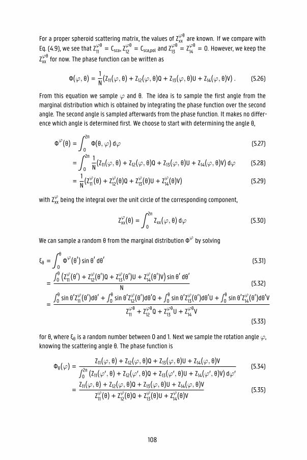
For a proper spheroid scattering matrix, the values of Zφθxx are known. If we compare with

Eq. (4.9), we see that Zφθ11 = Csca , Z

φθ12 = Csca,pol and Zφθ

13 = Zφθ14 = 0. However, we keep the

Zφθxx for now. The phase function can be written as

Φ(φ, θ) = 1N(Z11(φ, θ) + Z12(φ, θ)Q + Z13(φ, θ)U + Z14(φ, θ)V) . (5.26)

From this equation we sample φ and θ. The idea is to sample the first angle from themarginal distribution which is obtained by integrating the phase function over the secondangle. The second angle is sampled afterwards from the phase function. It makes no differ-ence which angle is determined first. We choose to start with determining the angle θ,

Φφ(θ) = ∫ 2π

0Φ(θ, φ) dφ (5.27)

= ∫ 2π

0

1N(Z11(φ, θ) + Z12(φ, θ)Q + Z13(φ, θ)U + Z14(φ, θ)V) dφ (5.28)

= 1N(Zφ11 (θ) + Zφ12(θ)Q + Zφ13(θ)U + Zφ14(θ)V) (5.29)

with Zφxx being the integral over the unit circle of the corresponding component,

Zφxx(θ) = ∫ 2π

0Zxx(φ, θ) dφ (5.30)

We can sample a random θ from the marginal distribution Φφ by solving

ξθ = ∫ θ

0Φφ(θ′) sin θ′ dθ′ (5.31)

=∫ θ0 (Zφ11 (θ′) + Zφ12(θ′)Q + Zφ13(θ′)U + Zφ14(θ′)V) sin θ′ dθ′

N(5.32)

=∫ θ0 sin θ′Zφ11 (θ′)dθ′ + ∫ θ

0 sin θ′Zφ12(θ′)dθ′Q + ∫ θ0 sin θ′Zφ13(θ′)dθ′U + ∫ θ

0 sin θ′Zφ14(θ′)dθ′VZφθ11 + Zφθ

12 Q + Zφθ13 U + Zφθ

14 V(5.33)

for θ, where ξθ is a random number between 0 and 1. Next we sample the rotation angleφ,knowing the scattering angle θ. The phase function is

Φθ(φ) = Z11(φ, θ) + Z12(φ, θ)Q + Z13(φ, θ)U + Z14(φ, θ)V∫ 2π0 (Z11(φ′, θ) + Z12(φ′, θ)Q + Z13(φ′, θ)U + Z14(φ′, θ)V) dφ′

(5.34)

=Z11(φ, θ) + Z12(φ, θ)Q + Z13(φ, θ)U + Z14(φ, θ)V

Zφ11 (θ) + Zφ12(θ)Q + Zφ13(θ)U + Zφ14(θ)V (5.35)

108

with the same definition of Zφxx(θ) as above. We again sample by inversion, solving

ξφ =∫φ0 (Z11(φ′

, θ) + Z12(φ′, θ)Q + Z13(φ′

, θ)U + Z14(φ′, θ)V)dφ′

Zφ11 (θ) + Zφ12(θ)Q + Zφ13(θ)U + Zφ14(θ)V (5.36)

=∫φ0 Z11(φ′

, θ) dφ′ + ∫φ0 Z12(φ′, θ) dφ′ Q + ∫φ0 Z13(φ′

, θ) dφ′ U + ∫φ0 Z14(φ′, θ)dφ′ V

Zφ11 (θ) + Zφ12(θ)Q + Zφ13(θ)U + Zφ14(θ)V(5.37)

forφ, with ξφ being a new uniform deviate.

How to use in the actual code

In the codewewant to calculate Eqs. (5.33) and (5.37). We tabulate the integrals beforehand.In the following equations we use xx ∈ [11, 12, 13, 14] and we omit the dependencies onthe grain parameters, wavelength and angle of incidence,

∫ φ

0Zxx(φ′

, θ)dφ′ ≈μφ

∑i=0

(Zxx(i, μ′θ)ωi) = SZxx(μφ, μ′θ) (5.38)

∫ 2π

0∫ θ

0Zxx(φ, θ′) sin θ′ dθ′ dφ ≈

μ′θ

∑i=0

(SZxx(μ2π, i) sin(θi) ω′i) = SSZxx(μ′θ) (5.39)

the index functions μφ and μ′θ translate the angles into their corresponding indexes, and de-pend on the angle resolution. The width functions ωφ and ω′

θ list the widths of the spacing,which might not be equal for all angles. And finally θi is the ith theta angle. The normaliza-tion values are the last elements of the tables, Zφxx(θ) ≈ SZxx(μ2π, μ

′θ), and Zφθ

xx ≈ SSZxx(μ′π).The SZxx tables are of the same dimension as the Zxx of the scatteringmatrix. They thereforeincrease the neededmemory by a quarter, as we have 4 values instead of 16. The SSZxx tableshave one dimension (φ) collapsed and do not needed much to the memory in comparison.Omitting the dependencies on the grain parameters, wavelength and angle of incidence, thesampling Eqs. (5.33) and (5.37) become

ξθ =SSZ11(μ′θ) + SSZ12(μ′θ)Q + SSZ13(μ′θ)U + SSZ14(μ′θ)VSSZ11(μ′π) + SSZ12(μ′π)Q + SSZ13(μ′π)U + SSZ14(μ′π)V (5.40)

ξφ =SZ11(μφ, μ′θ) + SZ12(μφ, μ′θ)Q + SZ13(μφ, μ′θ)U + SZ14(μφ, μ′θ)VSZ11(μ2π, μ′θ) + SZ12(μ2π, μ′θ)Q + SZ13(μ2π, μ′θ)U + SZ14(μ2π, μ′θ)V (5.41)

With these equations we generate a lookup table on the fly, find the right indices and fromthese calculate the θ andφ angles to scatter with.

109

110

Chapter 6

Summary, conclusions and outlook

6.1 Summary and conclusions

The purpose of this dissertation was to enable polarization capabilities in state of the artMonte Carlo radiative transfer (MCRT) codes. MCRT calculations are commonly applied inastrophysics. Applications include the calculation of results from models in order to com-pare these with observations or the post-processing of results of magneto-hydrodynamicssimulations. Polarization in MCRT codes is as of today a rare quality that deserves moreattention as it can help disentangle degeneracies in the parameter space.

To enable polarization calculations, we started by implementing the polarization of radia-tion due to scattering at spherical dust grains. This makes up Chapter 2 in this thesis, andwas published in Peest et al. (2017, A&A, 601, A92). The next (and very big) stepwas the imple-mentation of dichroic extinction, birefringence and scattering of radiation due to spheroidaldust grains. We first critically investigate the concept of optical depth, which becomes sig-nificantly more complex when the dusty medium contains aligned, elongated grains. Thisis discussed in Chapter 3, and is submitted for publication (Baes et al. 2018, A&A, submit-ted). The complete implementation of extinction and scattering due to spheroidal grains ina Monte Carlo code is described in Chapter 4, and a paper is currently in preparation (Peestet al. 2018, A&A, in preparation).

There aremany equations and conclusions that could not be included in these three chapters.We listed some of these in Chapter 5. It provides additional mathematical context of the in-teraction of radiation and cosmic dust. It can serve as starting points for later improvementsand expansions of the codes.

In the following sections I summarize my main findings and conclusions.

111

Mathematical background

Central to the treatment of polarization in MCRT codes is the Stokes formalism. It describesthe polarization state of radiation with four parameters I, Q, U, V. These describe the inten-sity (I), the linear polarization (Q, U), and the circular polarization (V). I showed that theliterature is split on whether the same wave is considered right or left handed circular po-larized and in which direction polarization angles are measured. My work strictly adheres tothe definitions of the International Astronomical Union (IAU). I derived the transformationsthat translate equations and results from one convention to another and conclude that ev-eryone is free to choose their own convention, but unclear definitions lead to errors whenequations or results are used by other groups.

In order to prevent future ambiguities, the cardinal directions to polarization descriptionshave been introduced. The North direction in its customary use is chosen in such a way thatit simplifies calculations as much as possible, especially for navigation. For polarization, thesame principle applies: North is a direction that should be adjusted to make calculations aseasy as possible. For a wave scattering at a plane surface, at a sphere or at an electron, thisis the plane of scattering, given by the propagation directions of the incoming wave andof the scattered wave. For a scattering event off a spheroid, this is the plane of incidence,given by the propagation direction of the incoming wave and the symmetry axis of the grain.A change of the North direction is realized by applying a rotation matrix R to the Stokesparameters. In conclusion, using the North direction to describe what the polarization refersto is a flexible and vivid method.

I highlighted the connection between plane waves and the Stokes parameters. The planewave formalism is an alternative representation to describe the polarization of radiation. Iused it to derive the equations governing dichroic extinction and to further clarify the phys-ical meaning of the dichroism and birefringence cross sections. They respectively answerthe questions “How much more does a North polarized wave get extinguished compared toan East polarized wave?” and “How much more does a North polarized wave get sloweddown compared to an East polarized wave?”. Having multiple different representations ofthe same phenomenon can help confirming results and offer alternativeways to understandthem.

Scattering of radiation at spheres

I implemented polarization due to scattering at spheres into theMCRT codes SKIRT andMC3D.These codes differ significantly, as listed in Table 6.1. Despite their differences, I was able toimplement polarization due to scattering with few differences between the codes. This wasachieved by keeping the polarization routines separate from the main code and allowingcommunication only through restricted interfaces. I took into account that modern MCRTcodes have many optimization algorithms to speed up calculations, in particular vectoriza-tion and parallelization on CPU or GPU. I developed routines that are geometry indepen-

112

Table 6.1: Some aspects of how the codes SKIRT and MC3D differ. This list is not meant to becomprehensive, it focuses on the main characteristics that relate to the implementation ofpolarization.

Aspect SKIRT MC3D

Programming language C++ Fortran with OMP and CUDAPrimary source Distributed sources Point sourceDust self heating Iterative scheme InstantlyDust cell shape Unknown before runtime CuboidalDust cell τ (550 nm) Aim: as low as possible Aim: unityContinuous absorption Always Optically thin cells

Additional features Forced interaction Inverse ray tracingContinuous scattering Dust destruction

dent and compatible with the well-known peel-off mechanism. This mechanism considersthe fraction of a photon package that will be scattered towards an observer, taking intoaccount the scattering phase function.

There are currently no satisfying benchmark tests for polarization available in the litera-ture. The correct solution of the most common polarization benchmark (Pinte et al. 2009)is unknown and the codes that participated in it disagree quantitatively by large factors.The typical absolute difference of the codes is 10%, for a linear polarization degree of lessthan 40%. Even worse, it seems that random pairs of codes agree for small stretches onlyto divert a few pixels further. I reproduced some of the 2D galaxy models of Bianchi et al.(1996). Again, a qualitative agreement was found, but the differences in the dust modelprevented a quantitative comparison. My conclusion was that comparing with other codesis not sufficient to check the accuracy of the implementations I have added to the SKIRT andMC3D codes.

I developed four test cases for which the exact analytical solution can be derived, and thentested the numerical codes against the analytical formulas. The tests are simple geometriesviewed from fixed directions and are designed to incrementally use more routines. The firstthree test cases use electrons as the “dust” at which radiation is scattered.

• In the first test case the accuracy of the implementation of the peel-off mechanismis tested. Light from a central source is scattered once and directed towards the ob-server. The results of the codes show that the linear polarization degree is accurateto below 0.05% in absolute terms and does not depend on the number of photonpackages. The noise level in the intensity is around 3% for this and all following testcases and can be reduced by increasing the number of photon packages.

• The second test case adds a first scattering event to the previous test. It tests the

113

regular scattering routine as well as the peel-off routine. The linear polarizationdegree is accurate to below 0.2% in absolute error.

• The third test case adds a rotation of the scattering plane, which leads to a changingpolarization angle in the solution. The linear polarization degree calculated by thecodes is correct to below 0.5% in absolute terms and the polarization angles arecorrect to less than a degree, or 0.5% in relative terms.

• The fourth test case checks the implementation of circular polarization. It is identicalto the third test case except that it uses an artificial particle that gives rise to circularpolarization. The accuracy of the circular polarization degree of the codes is betterthan 0.1% in absolute terms and scales with the scattering angle resolution.

The test cases are extremely sensitive to numerical inaccuracies of the codes. This is high-lighted by the fact that the scattering angle discretization of the codes is easily seen in theresults (either 0.5◦ or 1◦ was used in the simulations). I conclude that these solutions canbe used as benchmark tests for future codes. Indeed, they have already been used as suchin Seon (2018).

Finally, I have applied the scattering polarization mechanism to a modern 3D spiral galaxymodel with multiple stellar populations. The spiral structure of the dust leads to a sig-nature in the optical polarization. This signature persists for wavelengths in the range of0.5 μm ≲ λ ≲ 2 μm, nearly independent of the inclination of the host galaxy. I comparedthis to observations, which showmarkedly different results, and concluded that MCRT codesalso need to treat dichroism to make realistic predictions. Seon (2018) very recently calcu-lated polarizationmaps of edge-on galaxies including scattering polarization and an ad-hocapproximation to dichroism, using the MCRT code MoCafe. Unfortunately, the models arewithout a spiral dust structure and therefore cannot make predictions about the signature.

Extinction and scattering of radiation at spheroids

The shape of the polarization curve of the ISM in the optical and the near-infrared can berepresented by an empirical formula called the “Serkowski law”. This law can be reproducedassuming the dust consists of nonspherical grains such as spheroids. Spheroids are axisym-metric bodies and can either be prolate (like an egg) or oblate (like a thick onion). Realgrains are probably highly irregular, but because dust grains are expected to spin, the aver-age shape might be close to spheroidal. In contrast to spheres, (partially) aligned spheroidsresult in dichroism and birefringence.

The equations to treat dichroism, birefringence, and scattering at spheroids in MCRT codeshave been derived. While the basic equations regarding these effects are available in theliterature, my main contribution was to tie them into the framework of MCRT codes. Indeed,the consideration of spheroids adds multiple layers of complexity. In this context it is most

114

useful to detach the polarization routines from the rest of the code as much as possible, andto use the programming techniques of functional and object oriented programming.

A first increase in complexity relates to the random generation of the next interaction lo-cation. In polarised Monte Carlo radiative transfer with aligned nonspherical grains, thenature of dichroism complicates the concept of optical depth. Based on solutions for theradiative transfer equation, I discuss the several possible interpretations of optical depth. Idemonstrate that the actual optical depth is not equal to the usual extinction optical depth,nor to the so-called total optical depth. For representative values of the optical proper-ties of dust grains, the relative difference between the optical depth scales can be severalten percent. A closed expression for the optical depth cannot be given, but it can be derivedefficiently through an algorithm that is based on the analytical result corresponding to elon-gated grains with a uniform grain alignment. This complexity needs to be considered whengenerating random free path lengths in Monte Carlo radiative transfer simulations. Thereis no benefit in using approximations instead of the actual optical depth.

Other modifications are also necessary if one wants to implement dichroic extinction andscattering off spheroidal grains in an MCRT code. Such an implementation would benefitfrom a standardization of the routines and clear guidelines on how to adopt them. Thisis why I took care to specify where which modifications are to be adopted. Some of thesemodifications do not have a counterpart in MCRT without polarization.

• I explain how the Stokes vector is to be oriented for calculating the interaction withspheroids. It is then possible to calculate the dichroism and birefringence effects,which change the Stokes vector even when the photon package does not scatter orget absorbed inside a cell.

• An interaction can either be an absorption or a scattering event, depending on thealbedo of the dust grain. The albedo is also polarization dependent, as I illustrate.

• I discuss a possible way of calculating the scattering angles.

• I demonstrate multiple ways of recording the polarization of photon packages. Idiscuss photon packages that leaving the simulation area and the tracking of theirpolarization. An implementation of the directed scattering (peel-off) mechanism ispresented, and an inverse ray-tracing routine is proposed.

The validity of the procedures is checked by again employing test cases. The scattering im-plementation was verified using an updated version of the sphere scattering test cases. Itreat the spherical particles as if they were spheroids, and assign them an alignment direc-tion. A spheroid-like scattering matrix is calculated by applying two rotation matrices tothe original scattering matrix. The correct solution does not change, but the code treats theparticles as if they were spheroids. The results of the test cases show significant noise, alsoin parts where there was initially no noise at all. The deviations of the linear polarizationdegree are for most parts well below 5% in relative terms. The polarization angle is correctto below 1◦ if the polarization degree is above 5%. The higher noise level can be attributed

115

to a combination of the discretization of the scatteringmatrix over multiple dimensions andof dust grid resolution effects. I conclude that a high resolution of at least 2 to 5 degrees inthe incidence angle α, the rotation angle φ, and scattering angle θ is necessary to ensureaccurate results.

New test cases were developed to confirm the implementations of dichroism and birefrin-gence, as well as of the albedo. Right-handed circular polarized light passes through adichroic and birefringent dust cloud. The Stokes parameter changes, and so do the extinctionand scattering cross sections. In the first test, the scattering cross sections are zero and theradiation only gets dichroically extinguished while crossing the dust at different angles ofincidence. In the second test case, the scattering cross sections are different from zero. Theradiation scatters out of an elongated cloud towards the observer after being dichroicallyextinguished. The results of both tests show that the calculated Stokes parameters devi-ate from the correct solutions by less than 5% in relative terms. The relative uncertaintyincreases only if the Stokes parameters become smaller than 10%.

The polarization signature of spiral arms that we found in an earlier chapter can not be val-idated just yet. The reasons for this are twofold. Firstly, the code that the spheroidal dustgrains were implemented in does not yet support spiral galaxymodels. Secondly, there is norealistic spheroid dust mix available yet. It should include multiple grain materials, a rangeof dust grain sizes, and many wavelengths. Typical codes calculating optical properties pro-vide the results for exactly one material, grain size and one wavelength. The results need tobe checked for numerical problems, averaged over abundances and size distributions andpartial alignment needs to be considered. This is a complex task that went beyond the scopeof this thesis. The routines presented here can therefore not yet fully address the physicalconditions that give rise to polarization.

I also note that the step from scattering at spheres to scattering at spheroids comes with aheavy computational cost. While the calculation of the scattering angles does not becomemuch more complex, the memory required to store the scattering matrix becomes expen-sive. For spheres, the scattering matrix can be compacted to 4 entries, which depend on thescatterer, the wavelength and the scattering angle θ. For spheroids, the 16 entries of thescattering matrix additionally depend on the rotation angle φ and the angle of incidenceα. For modest resolutions of α (40 values), φ (70) and θ (90), and 100 wavelengths, thematrix contains 4× 108 entries. Storing this scattering matrix with double precision valuesrequires 3 GB of memory. Calculating the scattering matrix whenever needed is not a viableoption for efficiency reasons, and alternative options need to be explored.

Side projects

As a side project, I also contributed to Siebenmorgen et al. (2018). In this paper we investi-gated the variability of dust characteristics between different dust clouds in the Milky Way.We used low-resolution spectropolarimetric data obtained in the context of the Large Inter-

116

stellar Polarization Survey (LIPS) towards 59 sight lines in the Southern Hemisphere. Usinghigh resolution spectroscopicmeasurements, we identify sight lines that only intersect a sin-gle dust cloud, while the other sight lines intersect multiple dust clouds. The single cloudshave a generally higher polarization degree. They show correlations between extinction pa-rameters that are not valid for sight lines through multiple dust clouds. My contributions tothis paper were centered around the determination of the correlations and their uncertain-ties.

6.2 Outlook

Research is never finished.

Astronomers have a name for observations that can lead to new insights, but where thescientific merit is not guaranteed. They call them fishing expeditions. Including polariza-tion mechanisms in MCRT codes is more than a fishing expedition though, because polariza-tion has a bright future: there are already some powerful instruments that can routinelymeasure polarization across the electromagnetic spectrum, and additional telescopes andinstruments will become available in the near future. Some examples:

• At the shortest wavelengths, the future for polarimetry looks particularly bright inthe X-ray regime. The Imaging X-ray Polarimetry Explorer (IXPE) is scheduled tolaunch in 2021, aswell as numerous smaller balloon and rocket based X-ray polarime-ters (Weisskopf et al. 2016; Marin 2018).

• In the optical regime, several powerful polarimetric instruments are currently oper-ational, including SPHERE with ZIMPOL (Thalmann et al. 2008) at ESO’s Very LargeTelescope in Chile.

• In the far-infrared regime, thermal emission by interstellar dust is the dominantemission mechanism. The Planck mission, primarily designed to map the cosmicmicrowave background, has delivered beautiful maps of the polarised dust emissionin our own Milky Way. The Space Infrared Telescope for Cosmology and Astrophysics(SPICA) has just been selected as one of three remaining candidates as ESA’s M5mission, with onboard the polarimetric SAFARI-POL instrument (Reveret 2018).

• The Atacama Large Millimeter/submillimeter Array (ALMA) begins its first cycle withcalibrated full polarization measurements in October 2018. 100 proposals were sub-mitted for in total over 1000 hours of measurements in one year.1

These instruments will generate a wealth of observational data that can shed new light ondust in a variety of astrophysical objects. The interpretation of these polarization measure-ments will have to be backed by theoretical models of dust grains, and how these interactwith the radiation.

1https://almascience.eso.org/news/cycle-6-proposal-submission-statistics

117

It should be clear that simple models, for which analytical solutions are available, are usu-ally not sufficient. In recent years, numerical (magneto)hydrodynamic simulations havebecome a major tool to interpret observational data. In order to translate such simulationsto the observational domain, detailed 3D radiative transfer simulations are required. In sim-ulations where magnetic fields are important, and hence where dust grains are expected tobecome aligned, it is important to have tools at our disposal that can fully take into accountthe effects of dichroism, birefringence, scattering and thermal emission by nonsphericalgrains.

I am convinced that the Monte Carlo approach is the ideal technique to take these effectsinto account. The technique is flexible and naturally suited for 3D geometries. When realitybecomes too complex to express in a single formula, MCRT is the right tool to push on. Forthis task, MCRT needs solid interfaces and robust implementations. This dissertation helpswith this by defining clear conventions and practical implementations, and by providinganalytical test cases that identify the limits of the codes. Exploratory MCRT studies of polar-ization due to dichroism, birefringence and scattering can predict signatures that will ariseif the respective theories are correct, andmight open up new diagnostics that have not beenthought of yet. Possible targets are the dust tori of active galactic nuclei, protoplanetarydisks, red supergiants, and the global interstellar medium of external galaxies. There areindications that the polarized light curves of type Ia supernovas might create challenges tothe dark energy paradigm.

During this thesis, progress has been made towards interpreting observations. More effortshave to be made though, to draw concrete conclusions from them. The MCRT frameworkthat we have presented in this thesis is not yet complete, and there are several aspects thatshould be improved in the future.

An important aspect that I did not particularly focus on, but that is essential for realisticMCRT calculations, is the availability of realistic dust grain models, and the relevant opticalproperties of the grains (extinction matrices, scattering matrices, etc.). Up to now, nearlyall dust grain models are based on spherical dust grains, and the models are constrainedmainly by extinction and thermal emission in the Milky Way, and sometimes by additionaldepletion constraints (e.g. Jones et al. 2017; Draine and Li 2007; Zubko et al. 2004). Severalteams are currently generating novel dust grain models that are composed of elongatedgrains, and that will effectively take into account polarization as an additional constraint(e.g. Draine and Hensley 2017; Hensley and Draine 2015). The critical comparison of thesedust grain models to observational data will again call for radiative transfer codes that canhandle the different physical mechanisms at play.

Other aspects not explicitly addressed in this work include the alignment mechanisms ofdust grains, and the polarised emission by spheroidal dust grains. Some interesting ap-proaches to include these aspects into MCRT codes, mainly in order to simulate the polarisedemission fromMHD simulations, are presented by Reissl et al. (2016) and Bertrang and Wolf(2017). Furthermore, while spheroidal grains are a major step forwards compared to spheri-cal grains, there are probably also porous or irregularly shaped grains in cosmic dust clouds.

118

For such grains, the equations used in this dissertation do not apply, and an even moregeneral and complex treatment is required.

I believe that this dissertation is a small step forward in our quest to understand the na-ture of cosmic dust. Ultimately, we want to know the answer to the question of what theinterplanetary, circumstellar, or interstellar dust is made of, and what shape and opticalproperties it has.

After all, we are made of this star dust.

119

120

Chapter 7

Nederlandse samenvatting

7.1 Samenvatting en conclusies

Het doel van deze scriptie was om polarisatieberekeningen mogelijk te maken in state-of-the-art Monte Carlo stralingsoverdrachtscodes (MCRT codes). MCRT berekeningen zijn pop-ulair in de hedendaagse computationele sterrenkunde. Voorbeelden van toepassingen zijnde berekening van modelresultaten met het doel om deze met waarnemingen te vergeli-jken, of het post-processen van de resultaten vanmagneto-hydrodynamische simulaties. Devolwaardige behandeling van polarisatie in MCRT codes is vandaag een redelijk zeldzaamgegeven dat meer aandacht verdient, aangezien het ontaardingen in de parameterruimtekan helpen oplossen.

We zijn in deze thesis gestart met het implementeren van de polarisatie van straling doorverstrooiing aan sferische stofdeeltjes. Dit staat beschreven in Hoofdstuk 2 van deze thesis,en is gepubliceerd in Peest et al. (2017, A&A, 601, A92). De volgende, en grootste, stap wasde implementatie van dichroïsche extinctie, dubbelbreking en verstrooiing van straling doorsferoïdale stofdeeltjes. We hebben eerst kritisch het concept optische diepte onderzocht,aangezien dit aanzienlijk complexer wordt wanneer het medium uitgelijnde stofdeeltjesbevat. Dit staat beschreven in Hoofdstuk 3, en is aangeboden ter publicatie (Baes et al. 2018,A&A, aangeboden). De volledige implementatie van extinctie en verstrooiing door sferoïdaledeeltjes in een Monte Carlo code staat beschreven in Hoofdstuk 4, en een artikel met dezebevindingen wordt momenteel voorbereid (Peest et al. 2018, A&A, in voorbereiding).

Dit werk bevat vele vergelijkingen en bevindingen die niet onmiddellijk in drie hoofdstukkenthuishoren. We hebben een aantal van deze aspecten behandeld in Hoofdstuk 5. Dit hoofd-stuk biedt een bijkomende wiskundige context over de interactie tussen straling en kos-misch stof. Het kan dienen als een vertrekpunt voor verdere implementatie en uitbreidingenvan de codes.

In de volgende secties vat ik mijn bevindingen en conclusies samen.

121

Wiskundige achtergrond

Een centraal gegeven in de behandeling van polarisatie in MCRT codes is het Stokes formal-isme. Het beschrijft de polarisatiestaat van straling aan de hand van vier parameters I, Q,U, V. Deze beschrijven de intensiteit (I), de lineaire polarisatie (Q, U), en de circulaire polar-isatie (V). Ik heb aangetoond dat in de literatuur verschillende opvattingen bestaan overwatbeschouwd wordt als linkshandige of rechtshandige circulaire polarisatie, en over de richt-ing waarin polarisatiehoeken worden gemeten. Mijn werk houdt zich strikt aan de definitiesvan de Internationale Astronomische Unie (IAU). Ik heb transformaties afgeleid die vergeli-jkingen en resultaten transformeren tussen verschillende conventies, en concludeer dat hetiedereen vrij staat om zijn eigen conventie te kiezen, hoewel onduidelijke definities onvermi-jdelijk tot fouten leiden wanneer vergelijkingen of resultaten door andere auteurs wordengebruikt.

Om verdere dubbelzinnigheden te vermijden werden de kardinale richtingen ingevoerd ompolarisatie te beschrijven. De noordrichtingwordt traditioneel zo gekozen dat het berekenin-gen zo veel mogelijk vereenvoudigt, in het bijzonder voor navigatie. Hetzelfde principekan gehanteerd worden voor polarisatie: het noorden kan best zo gekozen worden dat deberekeningen zo eenvoudig mogelijk worden. Voor een vlakke golf die verstrooit aan eenvlak oppervlak, een sferisch deeltje of een electron, wordt de noordrichting best gekozenin het verstrooiingsvlak, gegeven door de voortplantingsrichting van de inkomende en uit-gaande golf. Voor een verstrooiing door een sferoïdaal deeltje wordt het noorden bestgekozen in het invalsvlak, bepaald door de voortplantingsrichting van de inkomende golfen de symmetrieas van het deeltje. Een verandering van de noordrichting kan worden ge-realiseerd door de Stokes vector te vermenigvuldigen met een rotatiematrix R. Het besluitis dat een flexibele aanpassing van de noordrichting het proces van polarisatie sterk kanvereenvoudigen.

Ik heb verder ook nog het verband tussen vlakke golven en de Stokes parameters belicht. Hetvlakke golf formalisme is een alternatieve representatie om de polarisatie van straling tebeschrijven. Ik heb dit gebruikt om de vergelijkingen die dichroïsche extinctie beschrijvenaf te leiden, en om de fysische betekenis van de werkzame doorsneden voor dichroïsmeen dubbelbreking verder te duiden. Deze processen geven respectievelijk antwoord op devragen “In welke mate wordt een noordelijk gepolariseerde golf sterker verduisterd daneen oostelijk gepolariseerde golf?” en “In welke mate wordt een noordelijk gepolariseerdegolf sterker afgeremd dan een oostelijk gepolariseerde golf?”. Het ter beschikking hebbenvan verschillende representaties van hetzelfde fenomeen kan helpen om resultaten op eenonafhankelijke manier te bevestigen, en kan andere manieren aanreiken om fenomenen tebegrijpen.

122

Verstrooiing aan sferische deeltjes

Ik heb de polarisatie door verstrooiing aan sferische deeltjes geïmplementeerd in de MCRTcodes SKIRT enMC3D. Ondanks de substantiële verschillende tussen beide codes, was ik staatom deze implementatie tot een goed einde te brengen met slechts enkele verschilpuntentussen beide codes. Dit was mogelijk door de polarisatieroutines gescheiden te houdenvan de hoofdcode, en door enkel communicatie toe te laten via beperkte interfaces. Ik hebrekening gehouden met de verschillende optimalisatie-algoritmen die in moderne MCRTcodes zijn ingebouwd om de berekeningen te versnellen, in het bijzonder vectorisatie enparallellisatie op CPUs en GPUs. Ik heb routines ontwikkeld die onafhankelijk zijn van degeometrie van het model, en die compatibel zijn met het gekende peel-off mechanisme.Dit mechanisme beschouwt het gedeelte van een fotonpakket dat wordt verstrooid in derichting van de waarnemer, waarbij de fasefunctie in rekening wordt gebracht.

Er zijn momenteel geen bevredigende benchmark testen voor polarisatie beschikbaar in deliteratuur. De juiste oplossing voor de meest voorkomende polarisatiebenchmark (Pinteet al. 2009) is onbekend, en de codes die eraan hebben deelgenomen vertonen soms sub-stantile onderlinge verschillen. Het typische absolute verschil tussen de codes is 10% vooreen lineaire polarisatiegraad van minder dan 40%. Erger nog, willekeurige paren codeslijken vaak in overeenstemming te zijn over een klein gebied, om slechts enkele pixelsverder sterk van elkaar af te wijken. Ik heb een aantal van de 2D-modellen voor stofrijkemelkwegstelsel van Bianchi et al. (1996) gereproduceerd. Opnieuw werd een kwalitatieveovereenkomst gevonden, maar de verschillen in het stofmodel verhinderden een kwanti-tatieve vergelijking. Mijn conclusie was dat het vergelijkenmet andere codes niet voldoendeis om de nauwkeurigheid te controleren van de implementaties die ik heb toegevoegd aande SKIRT en MC3D codes.

Ik heb vier test cases ontwikkeld waarvoor de exacte analytische oplossing kan hebbenafgeleid, en vervolgens de numerieke codes met de analytische formules vergeleken. Detest cases zijn gebaseerd op eenvoudige geometrieën vanuit vaste richtingen en zijn ont-worpen om stapsgewijs meer routines te gebruiken. De eerste drie test cases gebruikenelektronen als het “stof” waaraan straling wordt verstrooid

• De eerste test onderzoekt de implementatie van het peel-off mechanisme. Licht vaneen centrale bron wordt één keer verstrooid in de richting van de waarnemer. De re-sultaten van de codes laten zien dat de lineaire polarisatiegraad in absoluut opzichttot minder dan 0.05% nauwkeurig is en onafhankelijk is van het aantal fotonpakket-ten dat gebruikt is in de simulatie. Het ruisniveau in de intensiteit is ongeveer 3%voor deze en alle volgende testgevallen en kan worden verminderd door het aantalfotonpakketten te vergroten.

• De tweede test case voegt een eerste verstrooiing toe aan de vorige test. Het testde normale verstrooiingsroutine en het peel-off mechanisme. De lineaire polar-isatiegraad is nauwkeurig tot 0.2% in absolute fout.

123

• De derde test case voegt een rotatie toe van het verstrooiingsvlak, wat leidt tot eenveranderende polarisatiehoek in de oplossing. De lineaire polarisatiegraad berek-end door de codes is in absolute termen correct tot minder dan 0.5% en de polar-isatiehoeken zijn correct tot minder dan een graad, of 0.5% in relatieve termen.

• De vierde test case controleert de implementatie van circulaire polarisatie. Het isidentiek aan de derde test case, behalve dat het een kunstmatig deeltje gebruiktdat aanleiding geeft tot circulaire polarisatie. De absolute fout op de circulaire po-larisatiegraad van de codes is kleiner dan 0.1% en schaalt met de resolutie van deverstrooiingshoek.

De test cases zijn uiterst gevoelig voor numerieke onnauwkeurigheden van de codes. Ditwordt geïllustreerd door het feit dat de resolutie van de discretisatie van de verstrooiing-shoek in de codes gemakkelijk zichtbaar is in de resultaten (resoluties van 0.5◦ of 1◦ zijngebruikt). Het besluit is dat de test cases die ik heb gepresenteerd kunnen worden gebruiktals benchmark testen voor toekomstige codes. Ze zijn zelfs al als zodanig gebruikt in Seon(2018).

Ten slotte heb ik het mechanisme van polarisatie door verstrooiing aan sferische deeltjestoegepast op een modern 3D spiraalvormig melkwegmodel met meerdere sterpopulaties.De spiraalstructuur van het stof leidt tot een signatuur in de optische polarisatie. Deze“handtekening” blijft bestaan voor golflengten in het bereik van 0.5 μm ≲ λ ≲ 2 μm, vrijwelonafhankelijk van de inclinatie van het stelsel. Ik heb deze resultaten vergeleken met po-larimetrische waarnemingen, die duidelijk verschillende resultaten laten zien. Hieruit moetgeconcludeerdworden datMCRT codes ook andere polarisatiemechanismen, in het bijzonderdichroïsme, moeten behandelen om realistische voorspellingen te doen. Heel onlangs heeftSeon (2018) de polarisatie van edge-on sterrenstelsels gesimuleerdmet behulp van deMCRTcode MoCafe, waarbij verstrooiingspolarisatie en een ad-hoc-benadering tot dichroïsme inrekening werden gebracht. Helaas hebben zijn modellen geen spiraalvormige stofstructuuren kunnen er dus geen voorspellingen worden gedaan over de polarisatiesignatuur.

Extinctie en verstrooiing aan sferoïdale deeltjes

De vorm van de polarisatiecurve van het interstellaire medium in het optische en het nabijeinfrarood kan worden voorgesteld door een empirische formule die de “Serkowski-wet”wordt genoemd. Dezewet kanworden gereproduceerd in de veronderstelling dat het stof uitniet-sferische deeltjes bestaat, zoals sferoïden. Sferoïden zijn axiaal-symmetrische lichamenen kunnen ofwel prolaat zijn (zoals een ei) of oblaat (zoals een dikke ui). Echte stofdeeltjeszijn waarschijnlijk zeer onregelmatig van vorm, maar omdat stofkorrels naar verwachtingroteren, kan de gemiddelde vorm bij benadering sferoïdaal worden verondersteld. In tegen-stelling tot sferische deeltjes geven (gedeeltelijk) uitgelijnde sferoïdale deeltjes aanleidingtot dichroïsme en dubbele breking.

De vergelijkingen voor het behandelen van dichroïsme, dubbele breking en verstrooiing bij

124

sferoïden in MCRT codes zijn afgeleid. Hoewel de basisvergelijkingen met betrekking totdeze effecten beschikbaar zijn in de literatuur, was mijn belangrijkste bijdrage om ze tekaderen in het framework van MCRT codes. Dit is verre van triviaal, aangezien de overgangvan sferische naar sferoïdale deeltjes meerdere lagen van complexiteit toevoegt. Hierbij ishet van belang om de polarisatieroutines zoveel mogelijk van de rest van de code los temaken, door middel van functionele en objectgeoriënteerde programmering.

Een eerste toename in complexiteit heeft betrekking op het willekeurig genereren van devolgende interactielocatie. In MCRT codes met uitgelijnde sferoïdale deeltjes, bemoeilijkthet fenomeen van dichroïsme het concept van optische diepte. Op basis van oplossingenvoor de stralingsoverdrachtsvergelijking bespreek ik verschillende mogelijke interpretatiesvan optische diepte. Ik laat zien dat de werkelijke optische diepte niet gelijk is aan de ge-bruikelijke extinctie optische diepte, noch aan de zogenaamde totale optische diepte. Voorrepresentatieve waarden van de optische eigenschappen van stofkorrels kan het relatieveverschil tussen de verschillende optische diepteschalen enkele tientallen procenten zijn.Een gesloten uitdrukking voor de optische diepte kan niet worden gegeven, maar deze kanefficiënt worden afgeleid via een algoritme dat is gebaseerd op het analytische resultaatdat correspondeert met sferoïdale deeltjes met een uniforme uitlijning. Deze complexiteitmoet worden overwogen bij het genereren van willekeurige vrije padlengten in MCRT simu-laties. Het heeft geen zin ombenaderingen te gebruiken in plaats van dewerkelijke optischediepte.

Andere aanpassingen zijn ook nodig als men dichroïsche extinctie en verstrooiing aan sferoï-dale deeltjes in een MCRT code wil implementeren. Een dergelijke implementatie heeft baatbij een standaardisatie van de routines en duidelijke richtlijnen voor de manier waarop zemoeten worden toegepast. Dit is de reden waarom ik ervoor heb gezorgd om eenduidig engedetailleerd aan te geven waar welke wijzigingen moeten worden aangebracht. Sommigevan deze wijzigingen hebben geen tegenpool in MCRT zonder polarisatie.

• Ik leg uit hoe de Stokes vector georiënteerd moet worden voor het berekenen vande interactie met sferoïden. Het is dan mogelijk om de effecten van dichroïsme endubbele breking te berekenen. Deze effecten veranderen de Stokes vector en dusde polarisatiegraad van een fotonpakket, zelfs wanneer het niet in een cel wordtverstrooid of geabsorbeerd.

• Een interactie kan een absorptie of een verstrooiing zijn, afhankelijk van het albedovan de stofdeeltjes. In tegenstelling tot de normale MCRT stralingsoverdracht, is hetalbedo ook afhankelijk van de polarisatiestaat van het fotonpakket, zoals ik illus-treer.

• Ik bespreek een mogelijke manier om de verstrooiingshoeken te berekenen.

• Ik demonstreer meerdere manieren om de gepolariseerde fotonpakketten te reg-istreren. Ik bespreek fotopakketten die het simulatiegebied verlaten en volg hunpolarisatie. Een implementatie van het peel-off mechanisme wordt gepresenteerd,en een inverse ray-tracing routine wordt voorgesteld.

125

De validiteit van de procedures wordt gecontroleerd door opnieuw test cases te gebruiken.De verstrooiingsimplementatie werd geverifieerd met behulp van een bijgewerkte versievan de test cases die werden gebruikt bij verstrooiing aan sferische deeltjes. Hierbij wor-den sferische deeltjes behandeld alsof ze sferoïdaal zijn (dat zijn ze ook), en krijgen ze eenbepaalde alignering mee. Een sferoïde-achtige verstrooiingsmatrix wordt berekend doortwee rotatiematrices toe te passen op de oorspronkelijke verstrooiingsmatrix. De juisteoplossing verandert niet, maar de code behandelt de deeltjes alsof ze sferoïden zijn. Deresultaten van de testcases laten veel ruis zien, ook in delen waar aanvankelijk helemaalgeen ruis was. De afwijkingen van de lineaire polarisatiegraad liggen voor de meeste ge-bieden ver onder 5% in relatieve termen. De polarisatiehoek is correct tot op 1◦ als de po-larisatiegraad hoger is dan 5%. Het hogere ruisniveau kan worden toegeschreven aan eencombinatie van de discretisatie van de verstrooiingsmatrix over meerdere dimensies en vanresolutie-effecten in het stofrooster. Ik concludeer dat een hoge resolutie van ten minste 2tot 5 graden in de invalshoek α, de rotatiehoekφ en de verstrooiingshoek θ noodzakelijk isom nauwkeurige resultaten te garanderen.

Nieuwe testgevallen werden ontwikkeld om de implementaties van dichroïsme, dubbelebreking, en albedo te bevestigen. Rechtshandig circulair gepolariseerd licht passeert eendichroïsche en dubbelbrekende stofwolk. De Stokes parameter verandert, en dat geldt ookvoor de werkzame doorsneden voor extinctie en verstrooiings. In de eerste test is de werk-zame doorsnede voor verstrooiing nul en wordt de straling alleen dichroïsch gedoofd tij-dens het doorkruisen van het stof onder verschillende invalshoeken. In het tweede test-geval verschilt de werkzame doorsnede voor verstrooiing, en verstrooit de straling uit eenlanggerekte wolk naar de waarnemer na dichroïsche extinctie te hebben ondervonden. Deresultaten van beide tests laten zien dat de berekende Stokes parameters in relatieve ter-men minder dan 5% afwijken van de juiste oplossingen. De relatieve onzekerheid neemtalleen toe als de Stokes parameters kleiner worden dan 10%.

Ik merk ook op dat de stap van verstrooiing aan sferische deeltjes naar verstrooiing aan sfer-oïdale deeltjes gepaard gaat met hoge computationele kosten. Hoewel de berekening vande verstrooiingshoeken niet veel complexer wordt, wordt het geheugen dat vereist is om deverstrooiingsmatrix op te slaan duur. Voor sferische deeltjes kan de verstrooiingsmatrixwor-den gecomprimeerd tot 4 elementen, die afhankelijk zijn van de verstrooier, de golflengteen de verstrooiingshoek θ. Voor sferoïdale deeltjes zijn de 16 elementen van de verstrooi-ingsmatrix bovendien afhankelijk van de rotatiehoekφ en de invalshoek α. Voor bescheidenresoluties van α (40 waarden), φ (70 waarden) en θ (90 waarden) en 100 golflengten be-vat de matrix 4 × 108 elementen. Het opslaan van deze verstrooiingsmatrix met dubbeleprecisie vereist 3 Gb geheugen. Het berekenen van de verstrooiingsmatrix wanneer nodigis, om redenen van efficiëntie, geen haalbare optie, en alternatieve opties moeten wordenonderzocht.

126

Nevenprojecten

Als nevenproject heb ik ook bijgedragen aan Siebenmorgen et al. (2018). In dit artikelhebben we de variabiliteit van stofeigenschappen tussen verschillende stofwolken in deMelkweg onderzocht. We gebruikten spectropolarimetrische gegevens met lage resolutieverkregen in de context van de Large Interstellar Polarization Survey (LIPS) naar 59 gezicht-slijnen op het zuidelijk halfrond. Met behulp van spectroscopische metingen met hoge res-olutie, identificeren we gezichtslijnen die slechts een enkele stofwolk doorkruisen, terwijlde andere gezichtslijnen meerdere stofwolken doorkruisen. De enkele wolken hebben eenin het algemeen hogere polarisatiegraad. Ze tonen correlaties tussen extinctieparametersdie niet geldig zijn voor gezichtslijnen doorheen meerdere stofwolken. Mijn bijdragen aandit artikel waren gecentreerd rond de bepaling van de correlaties en hun onzekerheden.

7.2 Een blik vooruit

Onderzoek is nooit af.

Polarisatie heeft een mooie toekomst. Er zijn op dit moment al enkele krachtige instru-menten beschikbaar die routinematig polarisatie over het elektromagnetische spectrumkunnen meten, en in de nabije toekomst zullen er nieuwe telescopen en instrumenten bi-jkomen. Een paar voorbeelden:

• Op de kortste golflengten ziet de toekomst voor polarimetrie er bijzonder helderuit in het Röntgenregime. De Imaging X-ray Polarimetry Explorer (IXPE) is geplandvoor lancering in 2021, net zoals talrijke kleinere Röntgenpolarimeters op ballon- enraketmissies (Weisskopf et al. 2016; Marin 2018).

• In het optische regime zijn momenteel verschillende krachtige polarimetrische in-strumenten operationeel, waaronder SPHERE met ZIMPOL (Thalmann et al. 2008)aan ESO’s Very Large Telescope in Chili.

• In het verre-infrarood is thermische emissie door interstellair stof het dominanteemissiemechanisme. De Planck-missie, voornamelijk ontworpen om de kosmischeachtergrondstraling in kaart te brengen, heeft prachtige kaarten van de gepolari-seerde stofemissie in onze eigen Melkweg opgeleverd. De Space Infrared Telescopefor Cosmology and Astrophysics (SPICA) is onlangs geselecteerd als één van de drieoverblijvende kandidaten voor ESA’s M5 missie, met aan boord het polarimetrischeSAFARI-POL instrument (Reveret 2018).

• De Atacama Large Millimeter/submillimeter Array (ALMA) begint zijn eerste cyclusmet gekalibreerde volledige polarisatiemetingen in oktober 2018. 100 voorstellenzijn ingediend voor in totaal meer dan 1000 uur aan metingen in één jaar tijd.

127

Deze instrumenten zullen een schat aan observationele data genereren die een nieuw lichtkunnen werpen op stof in een verscheidenheid aan astrofysische objecten. De interpretatievan deze polarisatiemetingen zal moeten worden ondersteund door theoretische modellenvoor interstellair stof en hoe deze in wisselwerking staan met de straling.

Hetmoge duidelijk zijn dat eenvoudigemodellen, waarvoor analytische oplossingen beschik-baar zijn, meestal niet voldoende zijn. De afgelopen jaren zijn numerieke (magneto-) hy-drodynamische simulaties een belangrijk hulpmiddel geworden om waarnemingsgegevenste interpreteren. Om dergelijke simulaties naar het waarnemingsdomein te vertalen, zijngedetailleerde 3D stralingsoverdrachtsimulaties vereist. In simulaties waarbij magnetischevelden belangrijk zijn, en dus waar stofkorrels naar verwachting in lijn komen te liggen, ishet belangrijk om tools tot onze beschikking te hebben die volledig rekening kunnen houdenmet de effecten van dichroïsme, dubbele breking, verstrooiing en thermische emissie doorniet-sferische stofdeeltjes.

Ik ben ervan overtuigd dat Monte Carlo de ideale techniek is ommet deze effecten rekeningte houden. De techniek is flexibel en van nature geschikt voor 3D geometrieën. Wanneerde realiteit te complex wordt om te worden gevat in een enkele formule, is MCRT de juistetool om in deze complexiteit door te dringen. Voor deze taak heeft MCRT solide interfacesen robuuste implementaties nodig. Dit proefschrift helpt hierbij door duidelijke conventiesen praktische implementaties te definiëren en door analytische testgevallen te bieden diede grenzen van de codes identificeren. MCRT onderzoeken naar polarisatie als gevolg vandichroïsme, dubbele breking en verstrooiing kunnen voorspellingen doen om bestaande the-orieën kritisch te testen, en mogelijk nieuwe diagnostieken aanbrengen die nog niet zijnbedacht. Mogelijke doelen zijn de stoftori van actieve galactische kernen, protoplanetaireschijven, rode superreuzen en het globale interstellaire medium van externe sterrenstelsels.Er zijn aanwijzingen dat de gepolariseerde lichtcurven van type Ia supernovae een uitdagingkunnen vormen voor het donkere-energie paradigma.

Anderzijds is het MCRT raamwerk dat we in dit proefschrift hebben gepresenteerd nog nietvolledig en kunnen er in de toekomst verschillende aspecten worden verbeterd.

Een belangrijk aspect waar ikme niet speciaal op heb geconcentreerd, maar dat essentieel isvoor realistischeMCRT berekeningen, is de beschikbaarheid van realistische stofmodellen ende relevante optische eigenschappen van de stofdeeltjes (extinctiematrices, verstrooiings-matrices, enz.). Tot nu toe zijn bijna alle stofmodellen gebaseerd op sferische stofdeeltjes,en geijkt op basis van extinctie en thermische emissie in de Melkweg, met soms bijkomendeconstraints uit depletie (bv. Jones et al. 2017; Draine and Li 2007; Zubko et al. 2004). Verschil-lende teams genererenmomenteel nieuwe stofmodellen die zijn samengesteld uit langwer-pige korrels en die effectief rekening zullen houden met polarisatie als een extra constraint(bv. Draine and Hensley 2017; Hensley and Draine 2015). De kritische vergelijking van dezestofmodellen met waarnemingsgegevens zal opnieuw stralingsoverdrachtscodes vereisenwaarin de verschillende fysische mechanismen die spelen behandeld moeten kunnen wor-den.

128

Andere aspecten die niet expliciet aan de orde komen in dit werk zijn de uitlijningsmecha-nismen van stofdeeltjes en de gepolariseerde emissie door sferoïdale deeltjes. Enkele inter-essante manieren om deze aspecten in MCRT codes op te nemen, voornamelijk om de gepo-lariseerde emissie van MHD simulaties te simuleren, zijn onlangs voorgesteld door Reisslet al. (2016) en Bertrang and Wolf (2017). Een derde aspect betreft de vorm van de stofdeelt-jes. Sferoïdale deeltjes zijn een grote stap vooruit zijn in vergelijking met sferische deeltjes,maar kosmische stofwolken bevatten waarschijnlijk ook poreuze of onregelmatig gevormdekorrels. Voor dergelijke deeltjes zijn de in dit proefschrift gebruikte vergelijkingen niet vantoepassing en is een nog algemenere en complexere behandeling vereist.

Ik geloof dat dit proefschrift een kleine stap voorwaarts is in onze zoektocht om de aard vankosmisch stof te begrijpen. Uiteindelijk willen we het antwoord weten op de vraag waaruithet interplanetaire, circumstellaire of interstellaire stof gemaakt is, en welke vorm en optis-che eigenschappen het heeft. We zijn tenslotte allemaal gemaakt uit dit sterrenstof…

129

130

Bibliography

Aannestad, P. A. and Greenberg, J. M. (1983). Interstellar polarization, grain growth, andalignment. ApJ, 272:551–562.

Abhyankar, K. D. and Fymat, A. L. (1969). Relations between the Elements of the Phase Matrixfor Scattering. Journal of Mathematical Physics, 10:1935–1938.

Andersson, B.-G., Lazarian, A., and Vaillancourt, J. E. (2015). Interstellar Dust Grain Alignment.ARA&A, 53:501–539.

Andersson, B.-G. and Potter, S. B. (2005). A high sampling-density polarization study of theSouthern Coalsack. MNRAS, 356:1088–1098.

Antonucci, R. R. J. and Miller, J. S. (1985). Spectropolarimetry and the nature of NGC 1068.ApJ, 297:621–632.

Arago, F. (1888). Astronomie populaire, volume 3. M. J. A. Barral.

Arellano, M. and Bond, S. (1991). Some Tests of Specification for Panel Data: Monte CarloEvidence and an Application to Employment Equations. The Review of Economic Studies,58(2):277–297.

Arendt, R. G., Odegard, N., Weiland, J. L., Sodroski, T. J., Hauser, M. G., Dwek, E., Kelsall, T.,Moseley, S. H., Silverberg, R. F., Leisawitz, D., Mitchell, K., Reach, W. T., and Wright, E. L.(1998). The COBE Diffuse Infrared Background Experiment Search for the Cosmic InfraredBackground. III. Separation of Galactic Emission from the Infrared Sky Brightness. ApJ,508:74–105.

Asano, S. and Yamamoto, G. (1975). Light scattering by a spheroidal particle. Appl. Opt.,14:29–49.

Avenhaus, H., Quanz, S. P., Schmid, H. M., Meyer, M. R., Garufi, A., Wolf, S., and Dominik, C. (2014).Structures in the Protoplanetary Disk of HD142527 Seen in Polarized Scattered Light. ApJ,781:87.

Baes, M. and Camps, P. (2015). SKIRT: The design of a suite of input models for Monte Carloradiative transfer simulations. Astronomy and Computing, 12:33–44.

131

Baes, M., Davies, J. I., Dejonghe, H., Sabatini, S., Roberts, S., Evans, R., Linder, S. M., Smith,R. M., and de Blok, W. J. G. (2003). Radiative transfer in disc galaxies - III. The observedkinematics of dusty disc galaxies. MNRAS, 343:1081–1094.

Baes, M., Fritz, J., Gadotti, D. A., Smith, D. J. B., Dunne, L., da Cunha, E., Amblard, A., Auld, R.,Bendo, G. J., Bonfield, D., Burgarella, D., Buttiglione, S., Cava, A., Clements, D., Cooray, A.,Dariush, A., de Zotti, G., Dye, S., Eales, S., Frayer, D., Gonzalez-Nuevo, J., Herranz, D., Ibar,E., Ivison, R., Lagache, G., Leeuw, L., Lopez-Caniego, M., Jarvis, M., Maddox, S., Negrello, M.,Michałowski, M., Pascale, E., Pohlen, M., Rigby, E., Rodighiero, G., Samui, S., Serjeant, S., Temi,P., Thompson, M., van der Werf, P., Verma, A., and Vlahakis, C. (2010). Herschel-ATLAS: Thedust energy balance in the edge-on spiral galaxy UGC 4754. A&A, 518:L39.

Baes, M., Gordon, K. D., Lunttila, T., Bianchi, S., Camps, P., Juvela, M., and Kuiper, R. (2016).Composite biasing in Monte Carlo radiative transfer. A&A, 590:A55.

Baes, M., Stamatellos, D., Davies, J. I., Whitworth, A. P., Sabatini, S., Roberts, S., Linder, S. M., andEvans, R. (2005). Radiative equilibrium in Monte Carlo radiative transfer using frequencydistribution adjustment. New A, 10:523–533.

Baes, M., Verstappen, J., De Looze, I., Fritz, J., Saftly, W., Vidal Pérez, E., Stalevski, M., and Valcke,S. (2011). Efficient Three-dimensional NLTE Dust Radiative Transfer with SKIRT. ApJS,196:22.

Bagnulo, S., Cox, N. L. J., Cikota, A., Siebenmorgen, R., Voshchinnikov, N. V., Patat, F., Smith, K. T.,Smoker, J. V., Taubenberger, S., Kaper, L., Cami, J., and LIPS Collaboration (2017). LargeInterstellar Polarisation Survey (LIPS). I. FORS2 spectropolarimetry in the Southern Hemi-sphere. A&A, 608:A146.

Beck, R., Brandenburg, A., Moss, D., Shukurov, A., and Sokoloff, D. (1996). Galactic Magnetism:Recent Developments and Perspectives. ARA&A, 34:155–206.

Bertrang, G. H.-M. and Wolf, S. (2017). 3D radiative transfer of intrinsically polarized dustemission based on aligned aspherical grains. MNRAS, 469:2869–2878.

Bianchi, S. (2008). Dust extinction and emission in a clumpy galactic disk. An application ofthe radiative transfer code TRADING. A&A, 490:461–475.

Bianchi, S., Ferrara, A., and Giovanardi, C. (1996). Monte Carlo Simulations of Dusty SpiralGalaxies: Extinction and Polarization Properties. ApJ, 465:127.

Bjorkman, J. E. and Wood, K. (2001). Radiative Equilibrium and Temperature Correction inMonte Carlo Radiation Transfer. ApJ, 554:615–623.

Bohren, C. F. and Huffman, D. R. (1998). Absorption and scattering of light by small particles.New York (N.Y.): Wiley-Interscience.

Bok, B. J. (1977). Dark Nebulae, Globules, and Protostars. PASP, 89:597.

132

Born, M. and Wolf, E. (2013). Principles of Optics: Electromagnetic Theory of Propagation,Interference and Diffraction of Light. Elsevier.

Boulares, A. and Cox, D. P. (1990). Galactic hydrostatic equilibrium with magnetic tensionand cosmic-ray diffusion. ApJ, 365:544–558.

Brauer, R., Wolf, S., Reissl, S., and Ober, F. (2017). Magnetic fields in molecular clouds: Limita-tions of the analysis of Zeeman observations. A&A, 601:A90.

Campbell, E. K., Holz, M., Gerlich, D., and Maier, J. P. (2015). Laboratory confirmation of C60+

as the carrier of two diffuse interstellar bands. Nature, 523:322–323.

Camps, P. and Baes, M. (2015). SKIRT: An advanced dust radiative transfer code with a user-friendly architecture. Astronomy and Computing, 9:20–33.

Camps, P., Baes, M., and Saftly, W. (2013). Using 3D Voronoi grids in radiative transfer simu-lations. A&A, 560:A35.

Camps, P., Misselt, K., Bianchi, S., Lunttila, T., Pinte, C., Natale, G., Juvela, M., Fischera, J., Fitzger-ald, M. P., Gordon, K., et al. (2015). Benchmarking the calculation of stochastic heating andemissivity of dust grains in the context of radiative transfer simulations. Astronomy &Astrophysics, 580:A87.

Camps, P., Trayford, J. W., Baes, M., Theuns, T., Schaller, M., and Schaye, J. (2016). Far-infraredand dust properties of present-day galaxies in the EAGLE simulations. MNRAS, 462:1057–1075.

Cashwell, E. and Everett, C. (1959). A practical manual on the Monte Carlo method for ran-dom walk problems. International tracts in computer science and technology and theirapplication. Pergamon Press.

Chandrasekhar, S. (1946). On the Radiative Equilibrium of a Stellar Atmosphere. X. ApJ,103:351.

Chandrasekhar, S. (1960). Radiative transfer. New York: Dover.

Cheng, H. and Gupta, K. (1989). An historical note on finite rotations. Journal of AppliedMechanics, 56(1):139–145.

Chira, R. A., Siebenmorgen, R., Henning, T., and Kainulainen, J. (2016). Appearance of dustyfilaments at different viewing angles. A&A, 592.

Chrysostomou, A., Lucas, P. W., and Hough, J. H. (2007). Circular polarimetry reveals helicalmagnetic fields in the young stellar object HH135-136. Nature, 450:71–73.

Clayton, G. C. and Mathis, J. S. (1988). On the relationship between optical polarization andextinction. ApJ, 327:911–919.

Code, A. D. and Whitney, B. A. (1995). Polarization from scattering in blobs. ApJ, 441:400–407.

133

Contopoulos, G. and Jappel, A., editors (1974). Transactions of the IAU, volume 15B. SpringerNetherlands.

Dale, D. A., Aniano, G., Engelbracht, C. W., Hinz, J. L., Krause, O., Montiel, E. J., Roussel, H., Ap-pleton, P. N., Armus, L., Beirão, P., Bolatto, A. D., Brandl, B. R., Calzetti, D., Crocker, A. F.,Croxall, K. V., Draine, B. T., Galametz, M., Gordon, K. D., Groves, B. A., Hao, C.-N., Helou, G.,Hunt, L. K., Johnson, B. D., Kennicutt, R. C., Koda, J., Leroy, A. K., Li, Y., Meidt, S. E., Miller, A. E.,Murphy, E. J., Rahman, N., Rix, H.-W., Sandstrom, K. M., Sauvage, M., Schinnerer, E., Skibba,R. A., Smith, J.-D. T., Tabatabaei, F. S., Walter, F., Wilson, C. D., Wolfire, M. G., and Zibetti, S.(2012). Herschel Far-infrared and Submillimeter Photometry for the KINGFISH Sample ofnearby Galaxies. The Astrophysical Journal, 745(1):95.

Davis, Jr., L. and Greenstein, J. L. (1951). The Polarization of Starlight by Aligned Dust Grains.ApJ, 114:206.

De Geyter, G., Baes, M., Camps, P., Fritz, J., De Looze, I., Hughes, T. M., Viaene, S., and Gentile, G.(2014). The distribution of interstellar dust in CALIFA edge-on galaxies via oligochromaticradiative transfer fitting. MNRAS, 441:869–885.

De Geyter, G., Baes, M., De Looze, I., Bendo, G. J., Bourne, N., Camps, P., Cooray, A., De Zotti,G., Dunne, L., Dye, S., Eales, S. A., Fritz, J., Furlanetto, C., Gentile, G., Hughes, T. M., Ivison,R. J., Maddox, S. J., Michałowski, M. J., Smith, M. W. L., Valiante, E., and Viaene, S. (2015).Dust energy balance study of two edge-on spiral galaxies in the Herschel-ATLAS survey.MNRAS, 451:1728–1739.

De Looze, I., Baes, M., Bendo, G. J., Ciesla, L., Cortese, L., de Geyter, G., Groves, B., Boquien,M., Boselli, A., Brondeel, L., Cooray, A., Eales, S., Fritz, J., Galliano, F., Gentile, G., Gordon,K. D., Hony, S., Law, K.-H., Madden, S. C., Sauvage, M., Smith, M. W. L., Spinoglio, L., andVerstappen, J. (2012). The dust energy balance in the edge-on spiral galaxy NGC 4565.MNRAS, 427:2797–2811.

De Looze, I., Fritz, J., Baes, M., Bendo, G. J., Cortese, L., Boquien, M., Boselli, A., Camps, P.,Cooray, A., Cormier, D., Davies, J. I., De Geyter, G., Hughes, T. M., Jones, A. P., Karczewski,O. Ł., Lebouteiller, V., Lu, N., Madden, S. C., Rémy-Ruyer, A., Spinoglio, L., Smith, M. W. L., Vi-aene, S., and Wilson, C. D. (2014). High-resolution, 3D radiative transfer modeling. I. Thegrand-design spiral galaxy M 51. A&A, 571:A69.

De Vis, P., Dunne, L., Maddox, S., Gomez, H., Clark, C., Bauer, A., Viaene, S., Schofield, S., Baes, M.,Baker, A. J., Bourne, N., Driver, S. P., Dye, S., Eales, S. A., Furlanetto, C., Ivison, R. J., Robotham,A. S. G., Rowlands, K., Smith, D. J. B., Smith, M. W. L. Valiante, E., and Wright, A. H. (2016).Herschel-ATLAS: Revealing dust build-up and decline across gas, dust and stellar massselected samples: I. Scaling relations. Monthly Notices of the Royal Astronomical Society,page stw2501.

Demtröder, W. (2006). Experimentalphysik 2. Springer-Verlag Berlin Heidelberg.

134

Deschamps, R., Braun, K., Jorissen, A., Siess, L., Baes, M., and Camps, P. (2015). Non-conservative evolution in Algols: where is the matter? A&A, 577:A55.

Desert, F.-X., Boulanger, F., and Puget, J. L. (1990). Interstellar dust models for extinctionand emission. A&A, 237:215–236.

Dolginov, A. Z. and Mitrofanov, I. G. (1976). Orientation of cosmic dust grains. Ap&SS, 43:291–317.

Doyle, D., Pilbratt, G., and Tauber, J. (2009). The Herschel and Planck Space Telescopes. IEEEProceedings, 97:1403–1411.

Draine, B. (1989). On the Interpretation of the λ 2175 Å Feature. In Interstellar Dust, volume135, page 313.

Draine, B. T. (1988). The discrete-dipole approximation and its application to interstellargraphite grains. ApJ, 333:848–872.

Draine, B. T., Aniano, G., Krause, O., Groves, B., Sandstrom, K., Braun, R., Leroy, A., Klaas, U., Linz,H., Rix, H.-W., Schinnerer, E., Schmiedeke, A., and Walter, F. (2014). Andromeda’s Dust. ApJ,780:172.

Draine, B. T. and Flatau, P. J. (1994). Discrete-dipole approximation for scattering calculations.Journal of the Optical Society of America A, 11:1491–1499.

Draine, B. T. and Fraisse, A. A. (2009). Polarized Far-Infrared and Submillimeter Emissionfrom Interstellar Dust. ApJ, 696:1–11.

Draine, B. T. and Hensley, B. S. (2017). On the Shapes of Interstellar Grains: Modeling Ex-tinction and Polarization by Speroids and Continuous Distributions of Ellipsoids. ArXive-prints, page arXiv:1710.08968.

Draine, B. T. and Lee, H. M. (1984). Optical Properties of Interstellar Graphite and SilicateGrains. ApJ, 285:89.

Draine, B. T. and Li, A. (2007). Infrared Emission from Interstellar Dust. IV. The Silicate-Graphite-PAH Model in the Post-Spitzer Era. ApJ, 657:810–837.

Dullemond, C. P., Juhasz, A., Pohl, A., Sereshti, F., Shetty, R., Peters, T., Commercon, B., and Flock,M. (2012). RADMC-3D: A multi-purpose radiative transfer tool. Astrophysics Source CodeLibrary.

Dupree, S. A. and Fraley, S. K. (2002). A Monte Carlo Primer: A Practical Approach to RadiationTransport. Springer Science & Business Media.

Eckhardt, R. (1987). Stan Ulam, John von Neumann, and the Monte Carlo method. Los AlamosScience, 15:131–136.

Eide, M. B., Gronke, M., Dijkstra, M., and Hayes, M. (2018). Unlocking the Full Potential ofExtragalactic Lyα through Its Polarization Properties. ArXiv e-prints.

135

Ercolano, B., Barlow, M. J., Storey, P. J., and Liu, X.-W. (2003). MOCASSIN: a fully three-dimensional Monte Carlo photoionization code. MNRAS, 340:1136–1152.

Finkbeiner, D. P., Davis, M., and Schlegel, D. J. (1999). Extrapolation of Galactic Dust Emissionat 100 Microns to Cosmic Microwave Background Radiation Frequencies Using FIRAS. ApJ,524:867–886.

Fischer, O., Henning, T., and Yorke, H. W. (1994). Simulation of polarization maps. 1: Protostel-lar envelopes. A&A, 284:187–209.

Fitzpatrick, E. L. and Massa, D. (1990). An analysis of the shapes of ultraviolet extinctioncurves. III-an atlas of ultraviolet extinction curves. The Astrophysical Journal SupplementSeries, 72:163–189.

Fitzpatrick, E. L. and Massa, D. (2007). An Analysis of the Shapes of Interstellar ExtinctionCurves. V. The IR-through-UV Curve Morphology. ApJ, 663:320–341.

Fleck, Jr., J. A. and Canfield, E. H. (1984). A random walk procedure for improving the compu-tational efficiency of the implicit Monte Carlo method for nonlinear radiation transport.Journal of Computational Physics, 54:508–523.

Forrest, W. J., Gillett, F. C., and Stein, W. A. (1975). Circumstellar grains and the intrinsic polar-ization of starlight. ApJ, 195:423–440.

García-Segura, G., Langer, N., Różyczka, M., and Franco, J. (1999). Shaping Bipolar and Ellipti-cal Planetary Nebulae: Effects of Stellar Rotation, Photoionization Heating, and MagneticFields. ApJ, 517:767–781.

Goosmann, R. W. and Gaskell, C. M. (2007). Modeling optical and UV polarization of AGNs. I.Imprints of individual scattering regions. A&A, 465:129–145.

Goosmann, R. W., Gaskell, C. M., and Marin, F. (2014). Off-axis irradiation and the polarizationof broad emission lines in active galactic nuclei. Advances in Space Research, 54:1341–1346.

Gordon, K. D., Cartledge, S., and Clayton, G. C. (2009). FUSE Measurements of Far-UltravioletExtinction. III. The Dependence on R(V) and Discrete Feature Limits from 75 Galactic Sight-lines. ApJ, 705:1320–1335.

Gordon, K. D., Clayton, G. C., Misselt, K. A., Landolt, A. U., and Wolff, M. J. (2003). A Quantita-tive Comparison of the Small Magellanic Cloud, Large Magellanic Cloud, and Milky WayUltraviolet to Near-Infrared Extinction Curves. ApJ, 594:279–293.

Gordon, K. D., Misselt, K., Witt, A. N., and Clayton, G. C. (2001). The dirty model. I. Monte Carloradiative transfer through dust. The Astrophysical Journal, 551(1):269.

Górski, K. M., Hivon, E., Banday, A. J., Wandelt, B. D., Hansen, F. K., Reinecke, M., and Bartelmann,M. (2005). HEALPix: A Framework for High-Resolution Discretization and Fast Analysis ofData Distributed on the Sphere. The Astrophysical Journal, 622(2):759.

136

Grand, R. J. J., Gómez, F. A., Marinacci, F., Pakmor, R., Springel, V., Campbell, D. J. R., Frenk, C. S.,Jenkins, A., and White, S. D. M. (2017). The Auriga Project: the properties and formationmechanisms of disc galaxies across cosmic time. MNRAS, 467:179–207.

Gronke, M. and Dijkstra, M. (2014). Directional Lyα equivalent boosting - I. Spherically sym-metric distributions of clumps. MNRAS, 444:1095–1103.

Gupta, R., Mukai, T., Vaidya, D. B., Sen, A. K., and Okada, Y. (2005). Interstellar extinction byspheroidal dust grains. A&A, 441:555–561.

Hall, J. S. (1949). Observations of the Polarized Light from Stars. Science, 109:166–167.

Hamaker, J. and Bregman, J. (1996). Understanding radio polarimetry. III. Interpreting theIAU/IEEE definitions of the Stokes parameters. Astronomy and Astrophysics SupplementSeries, 117(1):161–165.

Harries, T. J. (2000). Synthetic line profiles of rotationally distorted hot-star winds. MonthlyNotices of the Royal Astronomical Society, 315(4):722–734.

Harries, T. J., Monnier, J. D., Symington, N. H., and Kurosawa, R. (2004). Three-dimensionaldust radiative-transfer models: the Pinwheel Nebula of WR 104. MNRAS, 350:565–574.

Hendrix, T., Keppens, R., and Camps, P. (2015). Modelling ripples in Orion with coupled dustdynamics and radiative transfer. A&A, 575:A110.

Hendrix, T., Keppens, R., van Marle, A. J., Camps, P., Baes, M., and Meliani, Z. (2016). Pinwheelsin the sky, with dust: 3D modeling of the Wolf-Rayet 98a environment. MNRAS.

Henning, T. (2010). Cosmic Silicates. Annual Review of Astronomy and Astrophysics, 48:21–46.

Hensley, B. and Draine, B. T. (2015). A Unified Model of Polarized Extinction and Emissionfrom Interstellar Dust. In American Astronomical Society Meeting Abstracts, page 216.02.

Henyey, L. G. and Greenstein, J. L. (1941). Diffuse radiation in the Galaxy. ApJ, 93:70–83.

Heymann, F. and Siebenmorgen, R. (2012). GPU-based Monte Carlo Dust Radiative TransferScheme Applied to Active Galactic Nuclei. ApJ, 751:27.

Hildebrand, R. H., Dragovan, M., and Novak, G. (1984). Detection of submillimeter polarizationin the Orion nebula. ApJ, 284:L51–L54.

Hiltner, W. A. (1949). Polarization of Light from Distant Stars by Interstellar Medium. Science,109:165.

Hoang, T. (2017). Properties and Alignment of Interstellar Dust Grains toward Type Ia Super-novae with Anomalous Polarization Curves. ApJ, 836:13.

Hollenbach, D. and Salpeter, E. E. (1971). Surface Recombination of Hydrogen Molecules. ApJ,163:155.

137

Hovenier, J. and Van der Mee, C. (1983). Fundamental relationships relevant to the transferof polarized light in a scattering atmosphere. Astronomy and Astrophysics, 128:1–16.

Hovenier, J. W. and van der Mee, C. V. M. (1996). Testing scattering matrices: a compendiumof recipes. Journal of Quantitative Spectroscopy and Radiative Transfer, 55:649–661.

Hubber, D. A., Ercolano, B., and Dale, J. (2016). Observing gas and dust in simulations of starformation with Monte Carlo radiation transport on Voronoi meshes. MNRAS, 456:756–766.

Huelsenbeck, J. P., Ronquist, F., Nielsen, R., and Bollback, J. P. (2001). Bayesian Inference ofPhylogeny and Its Impact on Evolutionary Biology. Science, 294:2310–2314.

Ivezic, Z., Groenewegen, M. A. T., Men’shchikov, A., and Szczerba, R. (1997). Benchmark prob-lems for dust radiative transfer. MNRAS, 291:121–124.

Jaffe, W. (1983). A simple model for the distribution of light in spherical galaxies. MonthlyNotices of the Royal Astronomical Society, 202(4):995–999.

Jenkins, E. B. (2014). Depletions of Elements from the Gas Phase: A Guide on Dust Composi-tions. arXiv preprint arXiv:1402.4765.

Jones, A. P., Fanciullo, L., Köhler, M., Verstraete, L., Guillet, V., Bocchio, M., and Ysard, N. (2013).The evolution of amorphous hydrocarbons in the ISM: dust modelling from a new vantagepoint. A&A, 558:A62.

Jones, A. P., Köhler, M., Ysard, N., Bocchio, M., and Verstraete, L. (2017). The global dust mod-elling framework THEMIS. A&A, 602:A46.

Jones, R. V. and Spitzer, Jr., L. (1967). Magnetic Alignment of Interstellar Grains. ApJ, 147:943.

Jones, T., Hyland, A., Robinson, G., Smith, R., and Thomas, J. (1980). Infrared observations ofa BOK globule in the Southern Coalsack. The Astrophysical Journal, 242:132–140.

Jones, T. J. (1989). Infrared Polarimetry and the Interstellar Magnetic Field. ApJ, 346:728.

Jonsson, P., Groves, B. A., and Cox, T. J. (2010). High-resolution panchromatic spectral modelsof galaxies including photoionization and dust. MNRAS, 403:17–44.

Kalos, M. H. and Whitlock, P. A. (2008). Monte Carlo Methods: Second Revised and EnlargedEdition. Wiley-VCH Verlag.

Kataoka, A., Muto, T., Momose, M., Tsukagoshi, T., Fukagawa, M., Shibai, H., Hanawa, T., Mu-rakawa, K., and Dullemond, C. P. (2015). Millimeter-wave Polarization of ProtoplanetaryDisks due to Dust Scattering. The Astrophysical Journal, 809(1):78.

Kessler, M. F. (1989). The Infrared Space Observatory (ISO). In Infrared Spectroscopy inAstronomy, page 553.

Kim, S.-H. and Martin, P. G. (1995). The Size Distribution of Interstellar Dust Particles asDetermined from Polarization: Spheroids. ApJ, 444:293.

138

Krełowski, J. (2002). Organic molecules and the diffuse interstellar bands. Advances inSpace Research, 30(6):1395 – 1407.

Krügel, E. (2002). The Physics of Interstellar Dust. Series in Astronomy and Astrophysics.CRC Press.

Krügel, E. (2008). An introduction to the physics of interstellar dust. CRC Press.

Krügel, E. (2009). The influence of scattering on the extinction of stars. A&A, 493:385–397.

Krügel, E. (2015). Photometry of variable dust-enshrouded stars. Supernovae Ia. A&A, 574.

Lazarian, A. (1994). Gold-Type Mechanisms of Grain Alignment. MNRAS, 268:713.

Lazarian, A. (2007). Tracingmagnetic fieldswith aligned grains. J. Quant. Spec. Radiat. Transf.,106:225–256.

Lazarian, A. and Hoang, T. (2007). Radiative torques: analytical model and basic properties.MNRAS, 378:910–946.

Lee, D. H., Seon, K. I., Min, K. W., Park, Y. S., Yuk, I. S., Edelstein, J., Korpela, E. J., Sankrit, R., Park,S. J., and Ryu, K. S. (2008). Far-Ultraviolet Observations of the Ophiuchus Region withSPEAR. ApJ, 686:1155–1161.

Lefevre, J., Bergeat, J., and Daniel, J.-Y. (1982). Numerical simulation of radiative transfer incircumstellar dust shells. I - Spherical shells. A&A, 114:341–346.

Lefevre, J., Daniel, J.-Y., and Bergeat, J. (1983). Numerical simulation of radiative transfer incircumstellar dust shells. II - Ellipsoidal shells. A&A, 121:51–58.

Leith, C. E. (1974). Theoretical Skill of Monte Carlo Forecasts. Monthly Weather Review,102:409.

Levitt, H. (1968). Testing for Sequential Dependencies. Acoustical Society of America Journal,43:65.

Lucas, P. (2003). Computation of light scattering in young stellar objects. Journal of Quanti-tative Spectroscopy and Radiative Transfer, 79:921–937. Electromagnetic and Light Scat-tering by Non-Spherical Particles.

Lucas, P. W., Fukagawa, M., Tamura, M., Beckford, A. F., Itoh, Y., Murakawa, K., Suto, H., Hayashi,S. S., Oasa, Y., Naoi, T., Doi, Y., Ebizuka, N., and Kaifu, N. (2004). High-resolution imagingpolarimetry of HL Tau and magnetic field structure. MNRAS, 352:1347–1364.

Lucy, L. B. (1999). Computing radiative equilibria withMonte Carlo techniques. A&A, 344:282–288.

Lunttila, T. and Juvela, M. (2012). Radiative transfer on hierarchial grids. A&A, 544:A52.

139

Lyot, B. (1929). 1re thèse: recherches sur la polarisation de la lumière des planètes et dequelques substances terrestres; 2me thèse: propositions données par la Faculté. PhDthesis, H. Tessier.

Lyot, B. (1964). Research on the polarization of light from planets and from some terrestrialsubstances. National Aeronautics and Space Administration.

Marin, F. (2018). The Growth of Interest in Astronomical X-Ray Polarimetry. Galaxies, 6:38.

Martin, A. D. and Quinn, K. M. (2002). Dynamic Ideal Point Estimation via Markov Chain MonteCarlo for the U.S. Supreme Court, 1953–1999. Political Analysis, 10(2):134–153.

Martin, P. (1974). Interstellar polarization from a medium with changing grain alignment.The Astrophysical Journal, 187:461–472.

Martin, P. G. (1972). Interstellar circular polarization. MNRAS, 159:179.

Mathis, J. S. (1986). The alignment of interstellar grains. ApJ, 308:281–287.

Mathis, J. S. (1990). Interstellar dust and extinction. ARA&A, 28:37–70.

Mathis, J. S., Rumpl, W., and Nordsieck, K. H. (1977). The size distribution of interstellar grains.The Astrophysical Journal, 217:425–433.

Mathis, J. S. and Whiffen, G. (1989). Composite Interstellar Grains. ApJ, 341:808.

Mattsson, L., Gomez, H. L., Andersen, A., Smith, M. W. L., De Looze, I., Baes, M., Viaene, S., Gentile,G., Fritz, J., and Spinoglio, L. (2014). The Herschel exploitation of local galaxy Andromeda(HELGA)–V. Strengthening the case for substantial interstellar grain growth. MonthlyNotices of the Royal Astronomical Society, 444(1):797–807.

McWilliam, A. (1997). Abundance ratios and galactic chemical evolution. Annual Review ofAstronomy and Astrophysics, 35(1):503–556.

Metropolis, N. (1987). The beginning of the Monte Carlo method. Los Alamos Science, 15:125–130.

Metropolis, N. and Ulam, S. (1949). The Monte Carlo Method. Journal of the American Statis-tical Association, 44(247):335–341.

Miller, J. S. and Goodrich, R. W. (1990). Spectropolarimetry of High-Polarization Seyfert 2Galaxies and Unified Seyfert Theories. ApJ, 355:456.

Min, M., Dullemond, C. P., Dominik, C., de Koter, A., and Hovenier, J. W. (2009). Radiativetransfer in very optically thick circumstellar disks. A&A, 497:155–166.

Min, M., Waters, L. B. F. M., de Koter, A., Hovenier, J. W., Keller, L. P., and Markwick-Kemper, F.(2007). The shape and composition of interstellar silicate grains. A&A, 462:667–676.

Mishchenko, M. I. (1991). Extinction and polarization of transmitted light by partially alignednonspherical grains. The Astrophysical Journal, 367:561–574.

140

Mishchenko, M. I. (1991). Light scattering by randomly oriented axially symmetric particles.Journal of the Optical Society of America A, 8:871–882.

Mishchenko, M. I., Hovenier, J. W., and Travis, L. D. (2000). Light scattering by nonsphericalparticles: theory, measurements, and applications. Elsevier.

Mishchenko, M. I., Travis, L. D., and Lacis, A. A. (2002). Scattering, absorption, and emission oflight by small particles. Cambridge university press.

Mishchenko, M. I., Travis, L. D., and Mackowski, D. W. (1996). T-matrix computations of lightscattering by nonspherical particles: a review. Journal of Quantitative Spectroscopy andRadiative Transfer, 55:535–575.

Misselt, K. A., Gordon, K. D., Clayton, G. C., and Wolff, M. J. (2001). The DIRTY Model. II. Self-consistent Treatment of Dust Heating and Emission in a Three-dimensional RadiativeTransfer Code. ApJ, 551:277–293.

Montgomery, J. D. and Clemens, D. P. (2014). Near-infrared polarimetry of the edge-on galaxyNGC 891. The Astrophysical Journal, 786(1):41.

Mosenkov, A. V., Allaert, F., Baes, M., Bianchi, S., Camps, P., De Geyter, G., De Looze, I., Fritz,J., Gentile, G., Hughes, T. M., Lewis, F., Verstappen, J., Verstocken, S., and Viaene, S. (2016).HERschel Observations of Edge-on Spirals (HEROES). III. Dust energy balance study of IC2531. A&A, 592:A71.

Murakawa, K., Preibisch, T., Kraus, S., and Weigelt, G. (2008). HK-band imaging polarime-try and radiative transfer modeling of the massive young stellar object CRL 2136. A&A,490:673–684.

Neugebauer, G., Habing, H. J., van Duinen, R., Aumann, H. H., Baud, B., Beichman, C. A., Bein-tema, D. A., Boggess, N., Clegg, P. E., de Jong, T., Emerson, J. P., Gautier, T. N., Gillett, F. C.,Harris, S., Hauser, M. G., Houck, J. R., Jennings, R. E., Low, F. J., Marsden, P. L., Miley, G.,Olnon, F. M., Pottasch, S. R., Raimond, E., Rowan-Robinson, M., Soifer, B. T., Walker, R. G.,Wesselius, P. R., and Young, E. (1984). The Infrared Astronomical Satellite (IRAS) mission.ApJ, 278:L1–L6.

Niccolini, G. and Alcolea, J. (2006). 3D continuum radiative transfer. A new adaptive gridconstruction algorithm based on the Monte Carlo method. A&A, 456:1–12.

Niccolini, G., Woitke, P., and Lopez, B. (2003). High precision Monte Carlo radiative transferin dusty media. A&A, 399:703–716.

Nieva, M.-F. and Przybilla, N. (2012). Present-day cosmic abundances. A comprehensive studyof nearby early B-type stars and implications for stellar and Galactic evolution and inter-stellar dust models. A&A, 539:A143.

Nyman, L.-A., Bronfman, L., and Thaddeus, P. (1989). A CO survey of the Southern Coalsack.A&A, 216:185–192.

141

Orsatti, A. M., Vega, E., and Marraco, H. G. (1998). Polarimetry of the Highly Reddened OpenClusters HOGG 15 and Lyngå 14. AJ, 116:266–273.

Pakmor, R., Gómez, F. A., Grand, R. J. J., Marinacci, F., Simpson, C. M., Springel, V., Campbell,D. J. R., Frenk, C. S., Guillet, T., Pfrommer, C., and White, S. D. M. (2017). Magnetic fieldformation in the Milky Way like disc galaxies of the Auriga project. MNRAS, 469:3185–3199.

Pakmor, R., Marinacci, F., and Springel, V. (2014). Magnetic Fields in Cosmological Simulationsof Disk Galaxies. ApJ, 783:L20.

Pascucci, I., Wolf, S., Steinacker, J., Dullemond, C. P., Henning, T., Niccolini, G., Woitke, P., andLopez, B. (2004). The 2D continuum radiative transfer problem. Benchmark results fordisk configurations. A&A, 417:793–805.

Peest, C., Camps, P., Stalevski, M., Baes, M., and Siebenmorgen, R. (2017). Polarization in MonteCarlo radiative transfer and dust scattering polarization signatures of spiral galaxies. As-tronomy & Astrophysics, 601:A92.

Peña, O. and Pal, U. (2009). Scattering of electromagnetic radiation by amultilayered sphere.Computer Physics Communications, 180(11):2348–2354.

Pickering, W. H. (1894). The seas of Mars. A&A, 13:553–556.

Pinte, C., Harries, T., Min, M., Watson, A., Dullemond, C., Woitke, P., Ménard, F., and Durán-Rojas,M. (2009). Benchmark problems for continuum radiative transfer-High optical depths,anisotropic scattering, and polarisation. Astronomy & Astrophysics, 498(3):967–980.

Pinte, C., Ménard, F., Duchêne, G., and Bastien, P. (2006). Monte Carlo radiative transfer inprotoplanetary disks. A&A, 459:797–804.

Planck Collaboration, Abergel, A., Ade, P. A. R., Aghanim, N., Alves, M. I. R., Aniano, G., Armitage-Caplan, C., Arnaud, M., Ashdown, M., Atrio-Barandela, F., Aumont, J., Baccigalupi, C., Ban-day, A. J., Barreiro, R. B., Bartlett, J. G., Battaner, E., Benabed, K., Benoît, A., Benoit-Lévy, A.,Bernard, J. P., Bersanelli, M., Bielewicz, P., Bobin, J., Bock, J. J., Bonaldi, A., Bond, J. R., Borrill,J., Bouchet, F. R., Boulanger, F., Bridges, M., Bucher, M., Burigana, C., Butler, R. C., Cardoso,J. F., Catalano, A., Chamballu, A., Chary, R. R., Chiang, H. C., Chiang, L. Y., Christensen, P. R.,Church, S., Clemens, M., Clements, D. L., Colombi, S., Colombo, L. P. L., Combet, C., Couchot, F.,Coulais, A., Crill, B. P., Curto, A., Cuttaia, F., Danese, L., Davies, R. D., Davis, R. J., de Bernardis,P., de Rosa, A., de Zotti, G., Delabrouille, J., Delouis, J. M., Désert, F. X., Dickinson, C., Diego,J. M., Dole, H., Donzelli, S., Doré, O., Douspis, M., Draine, B. T., Dupac, X., Efstathiou, G., Enßlin,T. A., Eriksen, H. K., Falgarone, E., Finelli, F., Forni, O., Frailis, M., Fraisse, A. A., Franceschi, E.,Galeotta, S., Ganga, K., Ghosh, T., Giard, M., Giardino, G., Giraud-Héraud, Y., González-Nuevo,J., Górski, K. M., Gratton, S., Gregorio, A., Grenier, I. A., Gruppuso, A., Guillet, V., Hansen, F. K.,Hanson, D., Harrison, D. L., Helou, G., Henrot-Versillé, S., Hernández- Monteagudo, C., Her-ranz, D., Hildebrandt, S. R., Hivon, E., Hobson, M., Holmes, W. A., Hornstrup, A., Hovest, W.,Huffenberger, K. M., Jaffe, A. H., Jaffe, T. R., Jewell, J., Joncas, G., Jones, W. C., Juvela, M., Kei-

142

hänen, E., Keskitalo, R., Kisner, T. S., Knoche, J., Knox, L., Kunz, M., Kurki-Suonio, H., Lagache,G., Lähteenmäki, A., Lamarre, J. M., Lasenby, A., Laureijs, R. J., Lawrence, C. R., Leonardi, R.,León-Tavares, J., Lesgourgues, J., Levrier, F., Liguori, M., Lilje, P. B., Linden-Vørnle, M., López-Caniego, M., Lubin, P. M., Macías-Pérez, J. F., Maffei, B., Maino, D., Mandolesi, N., Maris, M.,Marshall, D. J., Martin, P. G., Martínez-González, E., Masi, S., Massardi, M., Matarrese, S.,Matthai, F., Mazzotta, P., McGehee, P., Melchiorri, A., Mendes, L., Mennella, A., Migliaccio, M.,Mitra, S., Miville-Deschênes, M. A., Moneti, A., Montier, L., Morgante, G., Mortlock, D., Munshi,D., Murphy, J. A., Naselsky, P., Nati, F., Natoli, P., Netterfield, C. B., Nørgaard-Nielsen, H. U.,Noviello, F., Novikov, D., Novikov, I., Osborne, S., Oxborrow, C. A., Paci, F., Pagano, L., Pajot,F., Paladini, R., Paoletti, D., Pasian, F., Patanchon, G., Perdereau, O., Perotto, L., Perrotta, F.,Piacentini, F., Piat, M., Pierpaoli, E., Pietrobon, D., Plaszczynski, S., Pointecouteau, E., Po-lenta, G., Ponthieu, N., Popa, L., Poutanen, T., Pratt, G. W., Prézeau, G., Prunet, S., Puget, J. L.,Rachen, J. P., Reach, W. T., Rebolo, R., Reinecke, M., Remazeilles, M., Renault, C., Ricciardi,S., Riller, T., Ristorcelli, I., Rocha, G., Rosset, C., Roudier, G., Rowan- Robinson, M., Rubiño-Martín, J. A., Rusholme, B., Sandri, M., Santos, D., Savini, G., Scott, D., Seiffert, M. D., Shellard,E. P. S., Spencer, L. D., Starck, J. L., Stolyarov, V., Stompor, R., Sudiwala, R., Sunyaev, R., Sureau,F., Sutton, D., Suur-Uski, A. S., Sygnet, J. F., Tauber, J. A., Tavagnacco, D., Terenzi, L., Toffolatti,L., Tomasi, M., Tristram, M., Tucci, M., Tuovinen, J., Türler, M., Umana, G., Valenziano, L., Valivi-ita, J., Van Tent, B., Verstraete, L., Vielva, P., Villa, F., Vittorio, N., Wade, L. A., Wandelt, B. D.,Welikala, N., Ysard, N., Yvon, D., Zacchei, A., and Zonca, A. (2014). Planck 2013 results. XI.All-sky model of thermal dust emission. A&A, 571:A11.

Planck Collaboration, Ade, P. A. R., Aghanim, N., Alina, D., Alves, M. I. R., Armitage-Caplan,C., Arnaud, M., Arzoumanian, D., Ashdown, M., Atrio-Barandela, F., Aumont, J., Baccigalupi,C., Banday, A. J., Barreiro, R. B., Battaner, E., Benabed, K., Benoit-Lévy, A., Bernard, J. P.,Bersanelli, M., Bielewicz, P., Bock, J. J., Bond, J. R., Borrill, J., Bouchet, F. R., Boulanger, F.,Bracco, A., Burigana, C., Butler, R. C., Cardoso, J. F., Catalano, A., Chamballu, A., Chary, R. R.,Chiang, H. C., Christensen, P. R., Colombi, S., Colombo, L. P. L., Combet, C., Couchot, F., Coulais,A., Crill, B. P., Curto, A., Cuttaia, F., Danese, L., Davies, R. D., Davis, R. J., de Bernardis, P., deGouveia Dal Pino, E. M., de Rosa, A., de Zotti, G., Delabrouille, J., Désert, F. X., Dickinson, C.,Diego, J. M., Donzelli, S., Doré, O., Douspis, M., Dunkley, J., Dupac, X., Efstathiou, G., Enßlin,T. A., Eriksen, H. K., Falgarone, E., Ferrière, K., Finelli, F., Forni, O., Frailis, M., Fraisse, A. A.,Franceschi, E., Galeotta, S., Ganga, K., Ghosh, T., Giard, M., Giraud-Héraud, Y., Gonzá lez-Nuevo, J., Górski, K. M., Gregorio, A., Gruppuso, A., Guillet, V., Hansen, F. K., Harrison, D. L.,Helou, G., Hernández- Monteagudo, C., Hildebrandt, S. R., Hivon, E., Hobson, M., Holmes,W. A., Hornstrup, A., Huffenberger, K. M., Jaffe, A. H., Jaffe, T. R., Jones, W. C., Juvela, M.,Keihänen, E., Keskitalo, R., Kisner, T. S., Kneissl, R., Knoche, J., Kunz, M., Kurki-Suonio, H., La-gache, G., Lähteenmäki, A., Lamarre, J. M., Lasenby, A., Lawrence, C. R., Leahy, J. P., Leonardi,R., Levrier, F., Liguori, M., Lilje, P. B., Linden-Vørnle, M., López- Caniego, M., Lubin, P. M.,Macías-Pérez, J. F., Maffei, B., Magalhães, A. M., Maino, D., Mandolesi, N., Maris, M., Marshall,D. J., Martin, P. G., Martínez-González, E., Masi, S., Matarrese, S., Mazzotta, P., Melchiorri, A.,Mendes, L., Mennella, A., Migliaccio, M., Miville-Deschênes, M. A., Moneti, A., Montier, L., Mor-gante, G., Mortlock, D., Munshi, D., Murphy, J. A., Naselsky, P., Nati, F., Natoli, P., Netterfield,

143

C. B., Noviello, F., Novikov, D., Novikov, I., Oxborrow, C. A., Pagano, L., Pajot, F., Paladini, R.,Paoletti, D., Pasian, F., Pearson, T. J., Perdereau, O., Perotto, L., Perrotta, F., Piacentini, F.,Piat, M., Pietrobon, D., Plaszczynski, S., Poidevin, F., Pointecouteau, E., Polenta, G., Popa, L.,Pratt, G. W., Prunet, S., Puget, J. L., Rachen, J. P., Reach, W. T., Rebolo, R., Reinecke, M., Re-mazeilles, M., Renault, C., Ricciardi, S., Riller, T., Ristorcelli, I., Rocha, G., Rosset, C., Roudier,G., Rubiño-Martín, J. A., Rusholme, B., Sandri, M., Savini, G., Scott, D., Spencer, L. D., Stolyarov,V., Stompor, R., Sudiwala, R., Sutton, D., Suur-Uski, A. S., Sygnet, J. F., Tauber, J. A., Terenzi, L.,Toffolatti, L., Tomasi, M., Tristram, M., Tucci, M., Umana, G., Valenziano, L., Valiviita, J., VanTent, B., Vielva, P., Villa, F., Wade, L. A., Wandelt, B. D., Zacchei, A., and Zonca, A. (2015). Planckintermediate results. XIX. An overview of the polarized thermal emission from Galacticdust. A&A, 576:A104.

Purcell, E. M. (1979). Suprathermal rotation of interstellar grains. ApJ, 231:404–416.

Purcell, E. M. and Pennypacker, C. R. (1973). Scattering and Absorption of Light by Nonspher-ical Dielectric Grains. ApJ, 186:705–714.

Rao, R., Crutcher, R. M., Plambeck, R. L., andWright, M. C. H. (1998). High-ResolutionMillimeter-Wave Mapping of Linearly Polarized Dust Emission: Magnetic Field Structure in Orion. ApJ,502:L75–L78.

Reissl, S., Klessen, R. S., Mac Low, M.-M., and Pellegrini, E. W. (2018). Spectral shifting stronglyconstrains molecular cloud disruption by radiation pressure on dust. A&A, 611:A70.

Reissl, S., Seifried, D., Wolf, S., Banerjee, R., and Klessen, R. S. (2017). The origin of dust polar-ization in molecular outflows. A&A, 603:A71.

Reissl, S., Wolf, S., and Brauer, R. (2016). Radiative transfer with POLARIS. I. Analysis of mag-netic fields through synthetic dust continuum polarization measurements. A&A, 593:A87.

Rémy-Ruyer, A., Madden, S., Galliano, F., Lebouteiller, V., Baes, M., Bendo, G., Boselli, A., Ciesla,L., Cormier, D., Cooray, A., et al. (2015). Linking dust emission to fundamental propertiesin galaxies: the low-metallicity picture. Astronomy & Astrophysics, 582:A121.

Reveret, V. (2018). The Polarization-Sensitive Bolometers for SPICA and their Potential Usefor Ground-Based Application. In Atacama Large-Aperture Submm/mm Telescope (At-LAST), page 31.

Robitaille, T. P. (2011). HYPERION: an open-source parallelized three-dimensional dust con-tinuum radiative transfer code. A&A, 536:A79.

Rodgers, A. W. (1960). Three-colour photometry in the Southern Coalsack. MNRAS, 120:163.

Rogers, C. and Martin, P. G. (1979). On the shape of interstellar grains. ApJ, 228:450–464.

Rosse, F. R. S. (1878). Preliminary note on some measurements of the polarization of thelight coming from the moon and from the planet venus. The scientific proceedings of theRoyal Dublin Society, 1:19–20.

144

Saftly, W., Baes, M., and Camps, P. (2014). Hierarchical octree and k-d tree grids for 3D radia-tive transfer simulations. A&A, 561:A77.

Saftly, W., Baes, M., De Geyter, G., Camps, P., Renaud, F., Guedes, J., and De Looze, I. (2015).Large and small-scale structures and the dust energy balance problem in spiral galaxies.A&A, 576:A31.

Saftly, W., Camps, P., Baes, M., Gordon, K. D., Vandewoude, S., Rahimi, A., and Stalevski, M. (2013).Using hierarchical octrees in Monte Carlo radiative transfer simulations. A&A, 554:A10.

Savenkov, S. N. (2009). Jones and Mueller matrices: structure, symmetry relations and infor-mation content. In Light Scattering Reviews 4, pages 71–119. Springer.

Schultz, J., Hakala, P., and Huovelin, J. (2004). Polarimetric Survey of Low-Mass X-ray Binaries.Baltic Astronomy, 13:581–595.

Scicluna, P. and Siebenmorgen, R. (2015). Extinction and dust properties in a clumpymedium.A&A, 584.

Scicluna, P., Siebenmorgen, R., Wesson, R., Blommaert, J., Kasper, M., Voshchinnikov, N., andWolf, S. (2015). Large dust grains in thewind of VY CanisMajoris. Astronomy&Astrophysics,584:L10.

Seon, K.-I. (2018). Polarization as a probe of thick dust disk in edge-on galaxies: applicationto NGC 891. ArXiv e-prints.

Serkowski, K. (1962). Polarization of starlight. Advances in Astronomy and Astrophysics,1:289–352.

Serkowski, K. (1973). Interstellar Polarization (review). In Greenberg, J. M. and van de Hulst,H. C., editors, Interstellar Dust and Related Topics, volume 52 of IAU Symposium, page 145.

Serkowski, K., Mathewson, D. S., and Ford, V. L. (1975). Wavelength dependence of interstellarpolarization and ratio of total to selective extinction. ApJ, 196:261–290.

Sérsic, J. L. (1963). Influence of the atmospheric and instrumental dispersion on the bright-ness distribution in a galaxy. Boletin de la Asociacion Argentina de Astronomia La PlataArgentina, 6:41.

Shurcliff, W. A. (1962). Polarized Light. Harvard University Press, Cambridge, Mass, pages165–170.

Siebenmorgen, R. and Heymann, F. (2012). Shadows, gaps, and ring-like structures in proto-planetary disks. A&A, 539.

Siebenmorgen, R. and Krügel, E. (1992). Dust model containing polycyclic aromatic hydrocar-bons in various environments. A&A, 259:614–626.

Siebenmorgen, R., Voshchinnikov, N., and Bagnulo, S. (2014). Dust in the diffuse interstellar

145

medium - Extinction, emission, linear and circular polarisation. Astronomy & Astrophysics,561:A82.

Siebenmorgen, R., Voshchinnikov, N. V., Bagnulo, S., Cox, N. L. J., Cami, J., and Peest, C. (2018).Large Interstellar Polarisation Survey. II. UV/optical study of cloud-to-cloud variations ofdust in the diffuse ISM. A&A, 611:A5.

Simpson, J. P., Whitney, B. A., Hines, D. C., Schneider, G., Burton, M. G., Colgan, S. W. J., Cotera,A. S., Erickson, E. F., and Wolff, M. J. (2013). Aligned grains and inferred toroidal magneticfields in the envelopes of massive young stellar objects. MNRAS, 435:3419–3436.

Spanier, J., Gelbard, E. M., and Bell, G. (1970). Monte Carlo Principles and Neutron TransportProblems. Physics Today, 23:56.

Stalevski, M., Fritz, J., Baes, M., Nakos, T., and Popović, L. Č. (2012). 3D radiative transfermodelling of the dusty tori around active galactic nuclei as a clumpy two-phase medium.MNRAS, 420:2756–2772.

Stalevski, M., Ricci, C., Ueda, Y., Lira, P., Fritz, J., and Baes, M. (2016). The dust covering factorin active galactic nuclei. MNRAS, 458:2288–2302.

Stecher, T. P. (1965). Interstellar Ectinction in the Ultraviolet. ApJ, 142:1683.

Steinacker, J., Baes, M., and Gordon, K. D. (2013). Three-Dimensional Dust Radiative Transfer*.Annual Review of Astronomy and Astrophysics, 51:63–104.

Stokes, G. G. (1852). On the Composition and Resolution of Streams of Polarized Light fromdifferent Sources. Transactions of the Cambridge Philosophical Society, 9:399–416.

Tapia, S. (1973). The u, b, v, r, and i Extinctions in Four Areas of the Southern Coalsack. InGreenberg, J. M. and van de Hulst, H. C., editors, Interstellar Dust and Related Topics, vol-ume 52 of IAU Symposium, page 43.

Thalmann, C., Schmid, H. M., Boccaletti, A., Mouillet, D., Dohlen, K., Roelfsema, R., Carbillet, M.,Gisler, D., Beuzit, J.-L., Feldt, M., Gratton, R., Joos, F., Keller, C. U., Kragt, II, J., Pragt, J. H.,Puget, P., Rigal, F., Snik, F., Waters, R., and Wildi, F. (2008). SPHERE ZIMPOL: overview andperformance simulation. In Ground-based and Airborne Instrumentation for AstronomyII, volume 7014 of Proc. SPIE, page 70143F.

Tran, H. D., Filippenko, A. V., Schmidt, G. D., Bjorkman, K. S., Jannuzi, B. T., and Smith, P. S. (1997).Probing the Geometry and Circumstellar Environment of SN 1993J in M81. Publicationsof the Astronomical Society of the Pacific, 109:489–503.

Trayford, J. W., Camps, P., Theuns, T., Baes, M., Bower, R. G., Crain, R. A., Gunawardhana, M. L. P.,Schaller, M., Schaye, J., and Frenk, C. S. (2017). Optical colours and spectral indices of z =0.1 eagle galaxies with the 3D dust radiative transfer code skirt. MNRAS, 470:771–799.

Trippe, S. (2014). Polarization and Polarimetry: A Review. arXiv preprint arXiv:1401.1911.

146

Tsang, L., Kong, J. A., and Shin, R. T. (1985). Theory of microwave remote sensing. Wiley-Interscience.

Unsöld, A. (1929). Star Counts in the Region of the Coal Sack. Harvard College ObservatoryBulletin, 870:13–15.

Van De Hulst, H. C. (1957). Light scattering by small particles. Courier Corporation.

Verdier, P. H. and Stockmayer, W. H. (1962). Monte Carlo Calculations on the Dynamics ofPolymers in Dilute Solution. J. Chem. Phys., 36:227–235.

Verstocken, S., Van De Putte, D., Camps, P., and Baes, M. (2017). SKIRT: Hybrid parallelizationof radiative transfer simulations. Astronomy and Computing, 20:16–33.

Viaene, S., Baes, M., Tamm, A., Tempel, E., Bendo, G., Blommaert, J. A. D. L., Boquien, M., Boselli,A., Camps, P., Cooray, A., De Looze, I., De Vis, P., Fernández-Ontiveros, J. A., Fritz, J., Galametz,M., Gentile, G., Madden, S., Smith, M. W. L., Spinoglio, L., and Verstocken, S. (2017). TheHerschel Exploitation of Local Galaxy Andromeda (HELGA). VII. A SKIRT radiative transfermodel and insights on dust heating. A&A, 599:A64.

Von Neumann, J. (1951). 13. various techniques used in connection with random digits. Appl.Math Ser, 12(36-38):3.

Voshchinnikov, N. (2012). Interstellar extinction and interstellar polarization: Old and newmodels. Journal of Quantitative Spectroscopy and Radiative Transfer, 113(18):2334–2350.

Voshchinnikov, N. and Farafonov, V. (1993). Optical properties of spheroidal particles. Astro-physics and Space Science, 204(1):19–86.

Voshchinnikov, N. and Karjukin, V. (1994). Multiple scattering of polarized radiation in cir-cumstellar dust shells. Astronomy and Astrophysics, 288:883–896.

Voshchinnikov, N. V. (1990). Optical Properties of Spheroidal Dust Grains - Forward ScatteredRadiation. Soviet Ast., 34:535.

Watson, A. M. and Henney, W. J. (2001). An Efficient Monte Carlo Algorithm for a RestrictedClass of Scattering Problems in Radiation Transfer. Rev. Mexicana Astron. Astrofis., 37:221–236.

Weisskopf, M. C., Ramsey, B., O’Dell, S., Tennant, A., Elsner, R., Soffitta, P., Bellazzini, R., Costa,E., Kolodziejczak, J., Kaspi, V., Muleri, F., Marshall, H., Matt, G., and Romani, R. (2016). TheImaging X-ray Polarimetry Explorer (IXPE). Results in Physics, 6:1179–1180.

Werner, M. W., Davidson, J. A., Morris, M., Novak, G., Platt, S. R., and Hildebrand, R. H. (1988).The polarization of the far-infrared radiation from the Galactic center. ApJ, 333:729–734.

Werner, M. W., Roellig, T. L., Low, F. J., Rieke, G. H., Rieke, M., Hoffmann, W. F., Young, E., Houck,J. R., Brandl, B., Fazio, G. G., Hora, J. L., Gehrz, R. D., Helou, G., Soifer, B. T., Stauffer, J., Keene,J., Eisenhardt, P., Gallagher, D., Gautier, T. N., Irace, W., Lawrence, C. R., Simmons, L., Van

147

Cleve, J. E., Jura, M., Wright, E. L., and Cruikshank, D. P. (2004). The Spitzer Space TelescopeMission. The Astrophysical Journal Supplement Series, 154:1–9.

Whitney, B. A. (2011). Monte Carlo radiative transfer. Bulletin of the Astronomical Society ofIndia, 39:101–127.

Whitney, B. A., Robitaille, T. P., Bjorkman, J. E., Dong, R., Wolff, M. J., Wood, K., and Honor, J.(2013). Three-dimensional Radiation Transfer in Young Stellar Objects. ApJS, 207:30.

Whitney, B. A. and Wolff, M. J. (2002). Scattering and Absorption by Aligned Grains in Circum-stellar Environments. The Astrophysical Journal, 574(1):205.

Whittet, D. C. B., Hough, J. H., Lazarian, A., and Hoang, T. (2008). The Efficiency of Grain Align-ment in Dense Interstellar Clouds: a Reassessment of Constraints from Near-InfraredPolarization. ApJ, 674:304–315.

Wilking, B. A., Lebofsky, M. J., and Rieke, G. H. (1982). The wavelength dependence of inter-stellar linear polarization - Stars with extreme values of lambda/max/. AJ, 87:695–697.

Wolf, S. (2003). MC3D-3D continuum radiative transfer, Version 2. Computer Physics Com-munications, 150:99–115.

Wolf, S., Henning, T., and Stecklum, B. (1999). Multidimensional self-consistent radiativetransfer simulations based on the Monte-Carlo method. Astronomy and Astrophysics,349:839–850.

Wolf, S., Voshchinnikov, N. V., and Henning, T. (2002). Multiple scattering of polarized radia-tion by non-spherical grains: First results. A&A, 385:365–376.

Wood, K. (1997). Scattering and Dichroic Extinction: Polarimetric Signatures of Galaxies. ApJ,477:L25–L28.

Wood, K. and Jones, T. J. (1997). Modeling Polarization Maps of External Galaxies. AJ, 114:1405.

Yajima, H., Li, Y., Zhu, Q., and Abel, T. (2012). ART2: coupling Lyα line and multi-wavelengthcontinuum radiative transfer. MNRAS, 424:884–901.

Yurkin, M. A. and Hoekstra, A. G. (2007). The discrete dipole approximation: An overview andrecent developments. J. Quant. Spec. Radiat. Transf., 106:558–589.

Yusef-Zadeh, F., Morris, M., and White, R. L. (1984). Bipolar reflection nebulae - Monte Carlosimulations. ApJ, 278:186–194.

Zhang, Q., Qiu, K., Girart, J. M., Liu, H. B., Tang, Y.-W., Koch, P. M., Li, Z.-Y., Keto, E., Ho, P. T. P., Rao,R., Lai, S.-P., Ching, T.-C., Frau, P., Chen, H.-H., Li, H.-B., Padovani, M., Bontemps, S., Csengeri,T., and Juárez, C. (2014). Magnetic Fields and Massive Star Formation. ApJ, 792:116.

Zickgraf, F. J. and Schulte-Ladbeck, R. E. (1989). Polarization characteristics of galactic Bestars. A&A, 214:274–284.

148

Zubko, V., Dwek, E., and Arendt, R. G. (2004). Interstellar Dust Models Consistent with Extinc-tion, Emission, and Abundance Constraints. ApJS, 152:211–249.

149