MANAGEMENT SCIENCEVol. 50, No. 8, August 2004, pp. 1082–1094issn 0025-1909 �eissn 1526-5501 �04 �5008 �1082

informs ®

doi 10.1287/mnsc.1040.0245©2004 INFORMS

Modeling the Impact of Merging Capacity inProduction-Inventory Systems

Ananth V. IyerKrannert Graduate School of Management, Purdue University, West Lafayette, Indiana 47907,

aiyer@mgmt.purdue.edu

Apurva JainUniversity of Washington Business School, Seattle, Washington 98195, apurva@u.washington.edu

We model two separate, decentralized systems, each consisting of a warehouse and a production capac-ity. The demand processes experienced by the systems have different variabilities. The two decentralized

systems consider an agreement to pool their production capacities. We examine the impact of the pooling ofcapacity on inventory costs under two operating rules: (i) the orders from the two warehouses are treated in afirst-come–first-served manner, and (ii) the orders from the lower-variability warehouse are given nonpreemp-tive priority.We examine this issue using an analytical model that integrates base-stock inventory models with queuing

models for the production capacity. The higher-variability demand is modeled as a hyperexponential renewalprocess, and the lower-variability demand is modeled as a Poisson process. In case of pooled capacity, the arrivalprocess at the production queue is the superposition of the two processes. We prove conditions under whichthe first-come–first-served operating rule will fail to achieve a Pareto improvement over the separate systemsbecause it would increase inventory cost at the lower-variability warehouse. We then show cases under whichthe high-variability warehouse will see a reduction in inventory cost over the split system even if it acceptslower priority.

Key words : priority queues; queues with multiple arrival processes; stochastic inventory/production systemsHistory : Accepted by William S. Lovejoy, operations and supply chain management; received July 14, 2000.This paper was with authors 12 months for 4 revisions.

1. IntroductionWe model two separate, decentralized production-inventory chains. Each chain consists of an inventorylocation, called a warehouse, that supplies a marketand places replenishment orders with its productioncapacity. The demand processes in the two marketshave different variabilities. The two chains have dif-ferent ownerships that are concerned with the inven-tory costs at their own warehouses. We consider anagreement that proposes pooling the two productioncapacities and prescribes operating rules that will beused to schedule the production of orders from thetwo warehouses at the pooled capacity. Our objectiveis to examine the questions faced by the operatingmanagers of the two chains: When is it beneficial foreach of them to join the agreement, and what impactwill the choice of an operating rule have on theirdecisions?In particular, we examine whether pooling pro-

duction capacity and using an operating rule thatprocesses replenishment orders in order of arrival(first-come–first-served (FCFS)) will decrease the in-ventory cost at each warehouse—that is, if it is Pareto

improving (the Pareto-improving criterion requiresthat neither warehouse should see a cost increase andat least one should see a cost decrease). We then con-sider an operating rule that provides nonpreemptivepriority to orders from the warehouse that serves thelower-variability demand and examines whether itis Pareto improving. Our goal is to (a) evaluate theimpact of each of the two rules described earlier oneach inventory location and (b) show that the operat-ing rule used with pooled capacity does affect whetherpooling of capacity generates Pareto-improving bene-fits over the original system with separate productioncapacities. Our analysis suggests that managers shouldcarefully consider the operating rules when trying todevelop a rationale for pooling capacity across decen-tralized owners.The distinctive feature of this paper is that it exam-

ines the case of pooling capacity in the presence oftwo demand streams of differing variability. From adecentralized perspective, the commonly understoodview is based on an M/M/1 queuing system whereboth arrival streams are Poisson and will be better offby pooling capacity with an FCFS rule. As we show

1082

Iyer and Jain: Modeling the Impact of Merging Capacity in Production-Inventory SystemsManagement Science 50(8), pp. 1082–1094, © 2004 INFORMS 1083

in this paper, pooling production capacities with anFCFS rule does not always achieve Pareto improve-ment over separate capacities when the demand pro-cesses have different variability. This is because, withpooling, the warehouse that experiences the demandwith low variability may see an increase in its inven-tory cost. We further show that in such cases, thewarehouse with the high-variability demand pro-cess would be willing to take the nonintuitive stepof accepting lower priority at the pooled capacitybecause that restores the Pareto-improving property.

1.1. Model MotivationThere are a number of problem contexts where thebasic idea of managing split or pooled capacity inthe presence of demand streams with different vari-ability plays a crucial role. An example is the 1984merger of the aluminum-rolling capacities of AlcanAluminum Ltd. and Arco’s Atlantic Ritchfield Co. Thejoint-production capacity, at a plant in Logan County,Kentucky, produces aluminum can body stock. Thejoint-venture firm, called Logan Aluminium, Inc., isresponsible for managing the production capacity. Atthe time of the merger, Alcan was already in that busi-ness and had an established market and demand. Arcohad just entered the market and faced more variabledemand (Potts 1984). The antitrust authorities allowedthe merger only under certain conditions: The partieswere prohibited from communicating with each otherand with the joint-venture firm about future produc-tion schedules, volume of shipments, etc. (Macleodet al. 2001). Thus, the information available to eithercompany about the other company’s orders and thecurrent state of production was limited. Given limitedinformation and control on the production capacity,the two parties needed to decide on an operatingagreement and analyze its effect on each of their costsrelative to their ownership of separate productioncapabilities. Our model captures the tradeoffs in suchsystems.Eisenstein and Iyer (1996) provide an example of

split warehouse and distribution capacity servingdemands with different levels of predictability. Inthe school system they studied, all orders were pro-cessed FCFS. The proposed system matched capac-ity and lead time to product demand characteris-tics. Such an interpretation is consistent with theresults we derive in this paper. Fisher (1997) dis-cusses the problem of matching a product’s supplychain to demand characteristics, suggests splitting thecapacity in some contexts, and discusses the conse-quences of supply chain and product mismatches.Our paper captures that idea by focusing on the con-sequences of sharing a supply chain across productswith different variability characteristics. Narus andAnderson (1996) discuss the case of Volvo’s heavytruck division. Volvo had separated the distribution of

emergency orders from scheduled orders to improvethe performance of each segment. Again, our resultsare consistent with the results discussed in that case.Recently, Gupta and Gerchak (2002) provided severalexamples about the issue of operational synergies ina merger/acquisition between parties with differentcharacteristics. Our model also addresses the questionof the operational value of a merger from an individ-ual party’s perspective.We develop a model that abstracts the essential

features of these situations: difference in demandvariability, decentralized inventory ownership, andimpact of combining capacities.

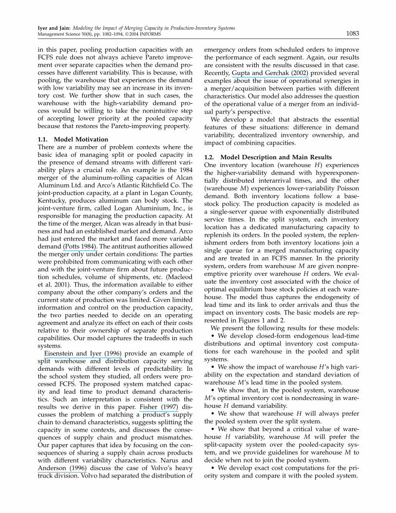
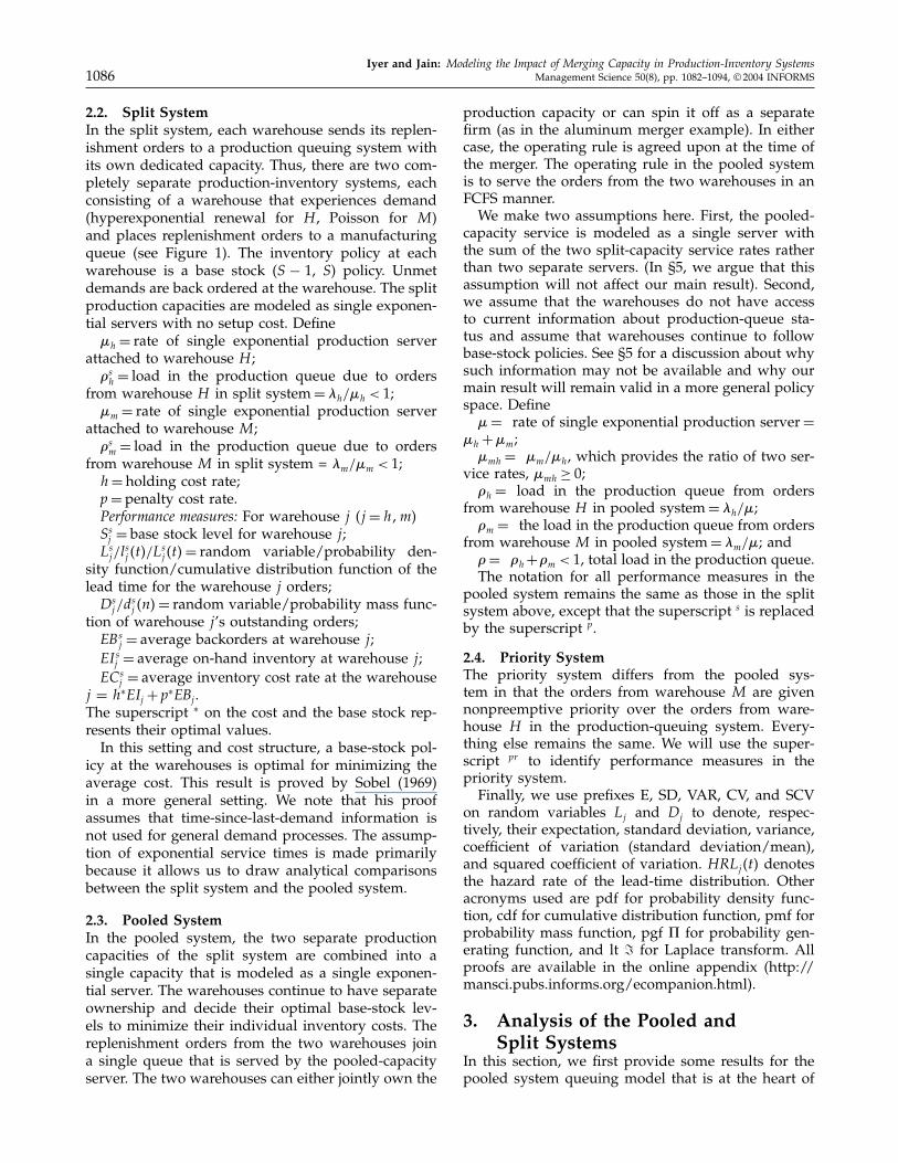
1.2. Model Description and Main ResultsOne inventory location (warehouse H ) experiencesthe higher-variability demand with hyperexponen-tially distributed interarrival times, and the other(warehouse M) experiences lower-variability Poissondemand. Both inventory locations follow a base-stock policy. The production capacity is modeled asa single-server queue with exponentially distributedservice times. In the split system, each inventorylocation has a dedicated manufacturing capacity toreplenish its orders. In the pooled system, the replen-ishment orders from both inventory locations join asingle queue for a merged manufacturing capacityand are treated in an FCFS manner. In the prioritysystem, orders from warehouse M are given nonpre-emptive priority over warehouse H orders. We eval-uate the inventory cost associated with the choice ofoptimal equilibrium base stock policies at each ware-house. The model thus captures the endogeneity oflead time and its link to order arrivals and thus theimpact on inventory costs. The basic models are rep-resented in Figures 1 and 2.We present the following results for these models:• We develop closed-form endogenous lead-time

distributions and optimal inventory cost computa-tions for each warehouse in the pooled and splitsystems.• We show the impact of warehouse H ’s high vari-

ability on the expectation and standard deviation ofwarehouse M ’s lead time in the pooled system.• We show that, in the pooled system, warehouse

M ’s optimal inventory cost is nondecreasing in ware-house H demand variability.• We show that warehouse H will always prefer

the pooled system over the split system.• We show that beyond a critical value of ware-

house H variability, warehouse M will prefer thesplit-capacity system over the pooled-capacity sys-tem, and we provide guidelines for warehouse M todecide when not to join the pooled system.• We develop exact cost computations for the pri-

ority system and compare it with the pooled system.

Iyer and Jain: Modeling the Impact of Merging Capacity in Production-Inventory Systems1084 Management Science 50(8), pp. 1082–1094, © 2004 INFORMS

Figure 1 Split System

Warehouse M

Warehouse H

Optimalbase-stock

policy

PoissonDemand

Process rate λm

HyperexponentialRenewal DemandProcess rate λ

Coefficientof Variation = hcv

Exp. Ser. rate µm

Exp. Ser. rate µh

Outstanding Orders Dm

s

Outstanding Orders Dh

s

ProductionSystem Load ρm

s

ProductionSystem Load ρh

s

Lead TimeLm

s

Lead TimeLh

s

h

Note. Warehouse Inventory Costs: h—holding cost rate, p—backorder cost rate.

The model suggests how various parameters affectthe Pareto-improving capacity configurations as wellas the associated optimal base-stock inventory costs.

1.3. Related WorkOur use of the concept of Pareto improvement asa criterion to suggest agreements follows Donohue(2000) and Iyer and Bergen (1997), among others. Iyerand Bergen (1997) analyzed quick response in theapparel industry. They showed that in the absence ofan agreement, quick response was not Pareto improv-ing and suggested a number of possible agreementsto generate the Pareto-improving property. We take asimilar approach.In decentralized control models of supply chains,

most work focuses on inventory systems at both lev-els and is limited to single-period perspective. Cachonand Zipkin (1999) present a two-echelon inventorymodel in a periodic setting. They assume that bothparties follow base-stock policy and then focus onfinding equilibrium base-stock levels. Our assump-tion of base-stock policies at the warehouses takes asimilar approach.In the research stream that takes a centralized

perspective, the dynamic-scheduling literature has

Figure 2 Pooled and Priority Systems

Exp. Ser. Rateµ = µm + µh

Lead Time

Warehouse M

Warehouse H

Optimalbase-stock

policy

PoissonDemand

Process rate λ

HyperexponentialRenewal DemandProcess rate λh

Coefficientof Variation = hcv

ProductionSystem Loadρ = ρm + ρh

Outstanding Orders

Outstanding Orders

prpriority system Dh

prpriority system Dm

ppooled system Dm

prpriority system Lh

ppooled system Lh

Lead Time

prpriority system Lm

ppooled system Lm

ppooled system Dh

system definitionspooled: FCFSpriority: to M, nonpreemptive

m

Note. h—holding cost rate, p—backorder cost rate.

focused on evaluating total costs under heuristicrules. Rubio and Wein (1996) assume a base-stock con-trol policy and develop formulas for optimal base-stock levels when the production system is an openqueuing network. They also show that, when separateproducts (or locations) operate individual base-stockpolicies, then the optimal base-stock-level decisionsseparate into each location, determining that facility’soptimal policy using its marginal distribution of out-standing orders. Zheng and Zipkin (1990) assume thatthe same base-stock optimal policy is used at eachlocation and study the effect of the LQ (longest queuefirst) scheduling rule when the two products are com-peting for the same production capacity. The aboveresearch assumes that the same variability (Poissonprocesses) exists for all demand streams. There is alsoresearch with very general models, such as Nguyen(1998), that focuses on developing approximationsfor evaluating inventory performance measures. Ourmodel complements that research by focusing on themanagement of order streams whose variabilities dif-fer. We develop a model in line with the assumptionsmade in the existing literature. Our specific modelallows us to present exact results and to developdeeper insights that can be generally useful for the

Iyer and Jain: Modeling the Impact of Merging Capacity in Production-Inventory SystemsManagement Science 50(8), pp. 1082–1094, © 2004 INFORMS 1085

managers of decentralized production-inventory sys-tems.In other related work, a recent paper byWhitt (1999)

considers the effect of increased service time variabil-ity that may occur by merging arrivals with very dif-ferent service requirements. That research focuses onqueuing performance measures and presents exam-ples and approximations to compare split and pooledsystems without any associated scheduling systemand with similar customer policies. Our researchaddresses a question that is similar in spirit on thearrival side.In the next section, we provide a detailed descrip-

tion of the model. Section 3 analyzes and comparesthe split and pooled systems. In §4 we analyze thesystem that gives priority to the lower-variabilityorder stream. In §5 we discuss the impact ofassumptions.

2. The Production-Inventory ModelsWe describe three production-inventory systems: split,pooled, and priority. The three systems are similar inthat each has two inventory locations (warehouses)and the two demand streams experienced by the twowarehouses are the same across all three systems. Thedemand experienced by the two warehouses differs inits variability. In all three systems, the warehouse expe-riencing higher demand variability is termed H (forhyperexponential, or high variability), and the other istermed M (for Markovian, or medium/low variabil-ity). The three systems differ in the way productioncapacity is modeled. In the split system, the replenish-ment orders from the two warehouses go to two differ-ent queues served by different dedicated productioncapacities. In the pooled system, the orders go to thesame queue and are served by a combined productioncapacity in an FCFS manner. In the priority system, thecombined production capacity gives priority to ordersfrom the low-variability order stream from warehouseM . Figures 1 and 2 provide a schematic representationof the split system and the pooled-priority systems.Since the difference in demand variability is a key fea-ture, we begin by describing the demand models.

2.1. Demand ModelsWe model the demand process at warehouse H as arenewal process where the interarrival times followhyperexponential distribution of two degrees (H2).A hyperexponential distribution is a probabilistic mix-ture of exponential distributions. If two exponentialdistributions are mixed, then the degree of the hyper-exponential distribution is 2. Given four parameters,k1� k2� r1, and r2, its probability density function isgiven as

a�t= k1r1e−r1t + k2r2e

−r2t ∀ t ≥ 0�0≤ k1� k2 ≤ 1� k1+ k2 = 1

The cumulative distribution function of H2 is given byA�t= 1−k1e

−r1t −k2e−r2t , and its Laplace transform is

given by ��z= k1r1/�r1+ z+ k2r2/�r2+ z. We use H2

with balanced means, which uses the normalizationk1/r1 = k2/r2.The balanced mean assumption is a common one

(see Whitt 1993) and is primarily used to reducethe number of parameters to describe hyperexpo-nential from three to two—mean and coefficient ofvariation. Define �h as intensity and hcv as coef-ficient of variation of the interarrival time of thedemand process at warehouse H . Let X representthe H random variable for the demand interarrivaltime and E�x�� SD�x� represent its expectation andstandard deviation, respectively; then E�x�= 1/�h andSD�x� = E�x� ∗ hcv. Given the above two inputs andthe balanced-means assumption, the parameters forH2 are as follows:

k1 = 0 5

(1+

√�hcv2− 1�hcv2+ 1

)� r1 = 2k1�h�

k2 = 1− k1 and r2 = 2k2�h

(see Tijms 1986). c = 2�k21+k22 is a measure of variabil-ity of warehouse H demand process where 1≤ c < 2.By definition, a hyperexponential distribution hashcv ≥ 1, and this mapping from hcv to c allows usto compress the entire variability range to 1 ≤ c < 2and thus simplifies further analysis. Also note that cis increasing in hcv. When hcv = 1, the hyperexpo-nential distribution degenerates into an exponentialdistribution.The hyperexponential distribution is commonly

used in the literature to model high-variability arrivalprocesses (Whitt 1993). It is used to model the super-position of high-variability arrival processes (Albin1984). It is also a good model for time-varying arrivalrates because its corresponding arrival process (calledinterrupted Poisson process; see Fischer and Meier-Hellstern 1992) can define a Poisson arrival processthat is alternatively on and off for exponential peri-ods. Superimposed with a Poisson process, it can cap-ture the time-varying demand patterns generated byprice promotions (see Iyer and Jain 2003) or seasonal-ity. It has also been used to model the overflow in datatraffic systems. The choice of hyperexponential distri-bution is useful because (a) the model can be used todifferentiate between the variability of two demandprocesses based on a single parameter hcv and (b) itallows us to take an analytical approach to all threesystems.We model the demand process experienced by

warehouse M as a Poisson process. Define �m =intensity of Poisson demand process at warehouse M .

Iyer and Jain: Modeling the Impact of Merging Capacity in Production-Inventory Systems1086 Management Science 50(8), pp. 1082–1094, © 2004 INFORMS

2.2. Split SystemIn the split system, each warehouse sends its replen-ishment orders to a production queuing system withits own dedicated capacity. Thus, there are two com-pletely separate production-inventory systems, eachconsisting of a warehouse that experiences demand(hyperexponential renewal for H , Poisson for M)and places replenishment orders to a manufacturingqueue (see Figure 1). The inventory policy at eachwarehouse is a base stock (S − 1, S) policy. Unmetdemands are back ordered at the warehouse. The splitproduction capacities are modeled as single exponen-tial servers with no setup cost. Define

�h = rate of single exponential production serverattached to warehouse H ;

�sh = load in the production queue due to orders

from warehouse H in split system= �h/�h < 1;�m = rate of single exponential production server

attached to warehouse M ;�s

m = load in the production queue due to ordersfrom warehouse M in split system = �m/�m < 1;

h= holding cost rate;p= penalty cost rate.Performance measures: For warehouse j �j = h�mSs

j = base stock level for warehouse j ;Ls

j /lsj �t/L

sj �t= random variable/probability den-

sity function/cumulative distribution function of thelead time for the warehouse j orders;

Dsj /d

sj �n= random variable/probability mass func-

tion of warehouse j’s outstanding orders;EBs

j = average backorders at warehouse j ;EIs

j = average on-hand inventory at warehouse j ;ECs

j = average inventory cost rate at the warehousej = h∗EIj + p∗EBj .The superscript ∗ on the cost and the base stock rep-resents their optimal values.In this setting and cost structure, a base-stock pol-

icy at the warehouses is optimal for minimizing theaverage cost. This result is proved by Sobel (1969)in a more general setting. We note that his proofassumes that time-since-last-demand information isnot used for general demand processes. The assump-tion of exponential service times is made primarilybecause it allows us to draw analytical comparisonsbetween the split system and the pooled system.

2.3. Pooled SystemIn the pooled system, the two separate productioncapacities of the split system are combined into asingle capacity that is modeled as a single exponen-tial server. The warehouses continue to have separateownership and decide their optimal base-stock lev-els to minimize their individual inventory costs. Thereplenishment orders from the two warehouses joina single queue that is served by the pooled-capacityserver. The two warehouses can either jointly own the

production capacity or can spin it off as a separatefirm (as in the aluminum merger example). In eithercase, the operating rule is agreed upon at the time ofthe merger. The operating rule in the pooled systemis to serve the orders from the two warehouses in anFCFS manner.We make two assumptions here. First, the pooled-

capacity service is modeled as a single server withthe sum of the two split-capacity service rates ratherthan two separate servers. (In §5, we argue that thisassumption will not affect our main result). Second,we assume that the warehouses do not have accessto current information about production-queue sta-tus and assume that warehouses continue to followbase-stock policies. See §5 for a discussion about whysuch information may not be available and why ourmain result will remain valid in a more general policyspace. Define

�= rate of single exponential production server=�h +�m;

�mh = �m/�h, which provides the ratio of two ser-vice rates, �mh ≥ 0;

�h = load in the production queue from ordersfrom warehouse H in pooled system= �h/�;

�m = the load in the production queue from ordersfrom warehouse M in pooled system= �m/�; and

�= �h+�m < 1, total load in the production queue.The notation for all performance measures in the

pooled system remains the same as those in the splitsystem above, except that the superscript s is replacedby the superscript p.

2.4. Priority SystemThe priority system differs from the pooled sys-tem in that the orders from warehouse M are givennonpreemptive priority over the orders from ware-house H in the production-queuing system. Every-thing else remains the same. We will use the super-script pr to identify performance measures in thepriority system.Finally, we use prefixes E, SD, VAR, CV, and SCV

on random variables Lj and Dj to denote, respec-tively, their expectation, standard deviation, variance,coefficient of variation (standard deviation/mean),and squared coefficient of variation. HRLj�t denotesthe hazard rate of the lead-time distribution. Otheracronyms used are pdf for probability density func-tion, cdf for cumulative distribution function, pmf forprobability mass function, pgf + for probability gen-erating function, and lt for Laplace transform. Allproofs are available in the online appendix (http://mansci.pubs.informs.org/ecompanion.html).

3. Analysis of the Pooled andSplit Systems

In this section, we first provide some results for thepooled system queuing model that is at the heart of

Iyer and Jain: Modeling the Impact of Merging Capacity in Production-Inventory SystemsManagement Science 50(8), pp. 1082–1094, © 2004 INFORMS 1087

our model. The results for the split system are thenderived from the pooled system. The rest of the sub-sections are devoted to comparing the two systems.

3.1. Analysis of the Pooled SystemIn the setting of our pooled system model, theorder-arrival process at the production queue is thesuperposition of the demand processes at the twowarehouses. The lead-time distribution for a ware-house is the same as the sojourn-time distributionfor that warehouse’s orders in the production queue.Similarly, the distribution of a warehouse’s outstand-ing orders is the same as that warehouse’s number-in-system distribution in the production queue. Theanalysis of the pooled system requires analysis ofthe queue H2 +M/M/1 with an FCFS discipline. Anapproach to solving this queuing system that lendsitself to closed-form expressions and analytical proofsis provided by Kuczura (1972). The basic idea is thatif we embed a Markov chain at the H arrival instants,its transition probabilities can be derived from thetransient solution of an M/M/1 queue. That analy-sis, extended by Iyer and Jain (2003), leads to the fol-lowing results. Let u1�u2�u3 be the three roots of thefollowing cubic function and let -2 = 1/u2�-3 = 1/u3:

D�u = �m��m + c�hu3

− ��2m + 2�m + 2�m�h + 2�2h + c�h�1−�hu2

+ �1+ 2�m + 2�hu− 1 Define:

p0 =�1−-2�1−-3

�1−�mu1� A1 =

p0�-2−�mu1

�-2−-3�1−-2�

A2 =p0�-3−�mu1

�-2−-3�1−-3� B1 =

�hA1

�-2−�m�

B2 =�hA2

��m −-3

The lead time and outstanding orders distributionsfor the two warehouses are put forth in Theorem (3.1).

Theorem 3.1. The cdf of the warehouse H lead time isL

p

h�t = 1−A1e−t��1−-2 +A2e

−t��1−-3 and the pmf of itsoutstanding orders is

dp

h�n = A1

[1−�h

1−����1−-2

�1−-2

]

−A2

[1−�h

1−����1−-3

�1−-3

]for n= 0

= A1�h

�1−����1−-2�

�1−-2

2

�����1−-2�n−1

−A2�h

�1−����1−-3�

�1−-3

2

�����1−-3�n−1

for n= 1�2�3

The cdf of the warehouse M lead time is Lpm�t =

1−B1e−t��1−-2 −B2e

−t��1−-3 and the pmf of its outstand-

ing orders is

dpm�n= B1

�1−-2�nm

�1+�m −-2n+1 +B2

�1−-3�nm

�1+�m −-3n+1

Given the explicit expressions for the pmf of out-standing orders for both warehouses, we can obtainthe closed-form expressions for the expected backorders EB

pj for a given base-stock level S

pj �j = h�m

as follows:

EBpj =

∑i=S

pj +1

(i− S

pj

)d

pj �i

Then EIpj = S

pj − ED

pj + EB

pj and EC

pj = hEI

pj + pEB

pj

gives the inventory cost. For a newsboy fractile ofp/�h+ p, we can obtain the optimal base-stock levelS

p∗j and optimal inventory cost EC

p∗j . The choice of

a warehouse’s base-stock level does not affect theproduction queue; therefore, each decentralized ware-house deciding the optimal base stock to minimizeits own cost provides an equilibrium. This anal-ysis for computing costs based on marginal out-standing orders distribution follows Rubio and Wein(1996) and Zheng and Zipkin (1990). Specifically,Proposition 1 in Rubio and Wein (1996) states thatfor a very general production-queuing system, witheach product following a base-stock policy and undera similar cost structure, the optimal base-stock leveldepends only on that product’s outstanding order(referred to as WIP).The next set of results is a technical, intermediate

step; the relationships of the roots with the param-eters drive many results in the later sections. We stateand prove the properties of these roots in the onlineappendix. Note that even the simplest performancemeasures of warehouse M are expressions involvingthese three roots of a cubic equation. In the follow-ing result, we reduce these expressions to functionsof only one root and obtain simplified expressionsrequired for further analysis.

Lemma 3.2.

�a ELpm=

�1−u1�1−�u1

��h�1−��2−cu21

�b SCVLpm=1+

2�1−�u1

2��h�1−�h�2−cu21+�2hu

21

−�1−u1�1−�u1�

�c ELp

h=��1−�mEL

pm−1

��h

3.2. Influence of Warehouse H ’s Variability onWarehouse M in the Pooled System

The pooled system model allows us to analyzethe effect of the demand variability faced by onewarehouse on the performance measures of the

Iyer and Jain: Modeling the Impact of Merging Capacity in Production-Inventory Systems1088 Management Science 50(8), pp. 1082–1094, © 2004 INFORMS

other warehouse. We begin by proving the follow-ing theorem, which establishes that the expectedvalue and standard deviation of warehouse M ’s leadtime, as well as outstanding orders, are both non-decreasing in warehouse H variability.

Theorem 3.3.

(a)0EL

pm

0hcv≥ 0� 0ED

pm

0hcv≥ 0�

(b)0SCVL

pm

0hcv≥ 0� 0SDD

pm

0hcv≥ 0

The above result confirms the intuition that thevariability of one order stream has a detrimental effecton mean and standard deviation of the lead timefaced by the other order stream. However, in ourmodel, we focus on the optimal base-stock inventorycost at the warehouses. While the standard deviationof outstanding orders is often used as a proxy for theinventory cost, for exact analysis of optimal cost, weneed to show the effect of hcv on the hazard rate ofwarehouse M ’s lead time, defined as l

p

h�t/�1−Lp

h�t.That, in turn, allows us to show the impact of hcv onthe optimal cost.

Theorem 3.4.

(a)0HRL

pm�t

0hcv≤ 0�

(b)0S

p∗m

0hcv≥ 0� 0EC

p∗m

0hcv≥ 0

The hazard rate of warehouse M ’s lead time isnonincreasing in warehouse H ’s variability. From thestructure of warehouse M ’s lead time, we alreadyknow that it has a decreasing hazard rate property.These two facts allow us to show that any increasein the hcv will change the distribution of ware-house M ’s lead time to increase its optimal inventorycost.

3.3. Analysis of the Split SystemIn the split-capacity system, the two order streamsfrom the warehouses do not merge and are pro-duced by their own separate production capacity.Thus the two queuing systems of interest are H2/M/1for warehouse H and M/M/1 for warehouse M .The warehouse H production system is described byparameters of load �s

h = �h/�h and arrival variabilitymeasure c. The warehouse M production system isdescribed by the load parameter �s

m = �m/�m. Usingthe transformation �mh = �m/�h, we see that for agiven �h, when �mh = 0, we get the warehouse H splitsystem, and for a given �m, when �mh = , we getthe warehouse M split system. The results are sum-marized below.

Proposition 3.5. The cdf of the warehouse H lead timeis Ls

h�t = 1− e−t�h�1−-s2, and the pmf of its outstanding

orders is

dsh�n = 1−�s

h

1−���h�1−-s2�

�1−-s2

for n= 0�

= �sh

�1−���h�1−-s2�

2

�1−-s2

����h�1−-s2�

n−1

for n > 0

The cdf of the warehouse M lead time is Lsm�t = 1 −

e−t�m�1−�sm, and the pmf of its outstanding orders is

dsm�n= �1−�s

m��smn.

As a validity check, we can check the above resultswith the standard analysis of M/M/1 and H2/M/1systems. Note that the pmf of outstanding orders forwarehouse M is the same as for an M/M/1 systemwhere the load is �s

m, and for warehouse H it is thesame as the standard result for an H2/M/1 system,where -s

2 is the unique root in (0, 1) of the equation-= ���h�1−-�. Finally, the cost computations can becarried out as described above for the pooled system.

3.4. Comparison of Split and Pooled Systems forWarehouse H

We examine the impact on warehouse H ’s perfor-mance measures as it moves from a split system toa pooled system. By moving to a pooled system,warehouse H sees additional production capacity buthas to share that capacity with some load from thewarehouse M split system. Given �h, this additionalproduction capacity is reflected by �mh, and it is heav-ily loaded or lightly loaded depending on the valueof the load parameter �s

m. The following result sug-gests that, irrespective of relative loads, warehouseH always sees an improvement in its performancemeasures.

Theorem 3.6. (a) 0ELp

h/0�mh ≤ 0, (b) CVLp

h ≤ CVLsh,

(c) SDLp

h ≤ SDLsh.

The first part of the result is as expected; that is,merging of two capacities reduces idleness, and bothorder streams benefit from it, irrespective of theirindividual loads. This is well understood in the casewhen both order streams are Poisson. Part (a) showsthat this result continues to hold for the warehouseH order stream, irrespective of its variability. Further-more, parts (b) and (c) suggest that the benefit towarehouse H also includes reduction in the variabil-ity of its performance measures. At hcv= 1, the ware-house H lead time is exponential in the split as well asin the pooled system, and the coefficient of variationis 1 in both systems. At higher hcv, it is less than 1 inthe pooled system. Higher hcv increases the “bunchi-ness” of warehouse H ’s order process, allowing more

Iyer and Jain: Modeling the Impact of Merging Capacity in Production-Inventory SystemsManagement Science 50(8), pp. 1082–1094, © 2004 INFORMS 1089

of its orders to get ahead of warehouse M orders. Thisresult suggests that warehouse H may always benefitfrom pooling production capacity with warehouse Munder an FCFS operating rule.

3.5. Comparison of Split and Pooled Systems forWarehouse M

In this section, we compare the warehouse inven-tory costs associated with the optimal base-stock pol-icy for the pooled and split systems. Note that, aswe argued above, warehouse H always benefits bypooling. Our focus is the impact on warehouse M ,which faces the following tradeoff: It gains accessto additional capacity by pooling with warehouse Hbut also faces potential delays due to the bunchedarrivals from the warehouse H demand stream. Thefollowing result suggests a threshold beyond whichwarehouse M prefers the split system over the pooledsystem.

Theorem 3.7. For any warehouse M in a split systemcharacterized by 2�m��m3, there exists a set of critical val-ues 2�∗

h�hcv∗��m��m��h��h3 such that for all warehouseH split systems characterized by 2�h > �∗

h��h�hcv >hcv∗3, the warehouse M will prefer the split system overthe pooled system; that is, EC

p∗m > ECs∗

m .

We know from Theorem (3.4) that warehouse M ’soptimal expected inventory cost is nondecreasing inhcv. After a critical point hcv∗, the cost in the pooledsystem will be larger than the cost in the split system(which is independent of hcv). The existence of hcv∗

is a result of two competing forces on warehouse Min the pooled-capacity system—the benefit of accessto larger service capacity versus the disruptive effectof H arrivals on M . At low values of hcv, the benefitof additional capacity serves as a powerful force thatis not offset by the variability of warehouse H orders.At the lowest value, hcv= 1, warehouse M will neverprefer the split-capacity system. However, for highenough values of hcv (greater than hcv∗), the disrup-tive impact of warehouse H ’s variability on the per-formance measures of warehouse M outweighs thebeneficial effects of access to additional capacity.

3.6. Pareto-Improving Region—ManagerialImplications Based on Computations

We examine the question: When does pooling gener-ate Pareto-improving benefits over the split system?A managerially useful representation of the answeris obtained by dividing the parametric space in twozones, one where both warehouses H and M do bet-ter in the pooled system than in the split system, andthe other where warehouse M sees an increase in costfrom pooling. To gain insight, we first characterizethe Pareto-improving region in the limiting case ofhcv→ (see the note in the proof of Proposition (3.8)

Figure 3 Identification of Worst-Case �hcv → � Pareto-ImprovingRegion in Pooled System

0.010.0

0.2

0.4

0.6

0.8

1.0

0.10 0.20 0.30 0.40 0.50 0.60 0.70 0.80 0.90 0.99

Warehouse M Arrival Rate

War

eho

use

H A

rriv

al R

ate

Non-feasible parametric spaceabove this line

Pareto-improvingregion below this line

Non-Pareto-improvingregion

Note. Parameter values: �sm = �sh �= 1 h= 1 p= 9. Broken lines: boundsfrom §3.6.

for an understanding of the arrival process in thelimit). Figure 3 shows the region for a specific set ofparameter values. That is, for a given set of capacities,�h and �m, warehouse M will never find it beneficialto pool capacities with warehouse H if ��m��h fall inthe non-Pareto-improving region in Figure 3.

Proposition 3.8. In the high-variability limit hcv →, warehouse M will prefer a split system to a pooled sys-tem �ECs∗

m < ECp∗m if �h > ��m+�h−�m/2. WarehouseM

will prefer a pooled system to a split system �ECp∗m < ECs∗

m if �h < 0 5 ∗�h.

This limiting characterization is a useful decision-making tool because it allows warehouse M to makea worst-case decision at a glance. If warehouse Hfalls in the Pareto-improving region when hcv →,then warehouse M will prefer to pool capacity andhave an FCFS operating rule over the split system forall values of hcv. This result provides only the suf-ficient conditions for a Pareto-improving region—asFigure 3 shows, the actual boundary separating thetwo regions falls in between these two conditions.Intuitively, smaller values of hcv will increase the

Pareto-improving region and push the boundary up.Figure 4 confirms this notion. Figures 3 and 4 aredrawn when �s

m = �sh; that is, both warehouses bring

capacities in proportion to their demand rates. For�s

m < �sh, the additional capacity warehouse M gains

access to by pooling decreases and so does the benefitof pooling to that warehouse. Thus a smaller disrup-tive effect from warehouse H will be able to counterthe benefit, and therefore hcv∗ goes down, shrink-ing the Pareto-improving region. The opposite resultholds when �s

m > �sh.

We have shown that the pooled system may notalways be Pareto improving over the split system. Inthe next section, we consider whether the priority sys-tem is Pareto improving over the split system.

Iyer and Jain: Modeling the Impact of Merging Capacity in Production-Inventory Systems1090 Management Science 50(8), pp. 1082–1094, © 2004 INFORMS

Figure 4 Pareto-Improving Region in Pooled System for Different hcvValues

0.010.0

0.2

0.4

0.6

0.8

1.0

0.10 0.20 0.30 0.40 0.50 0.60 0.70 0.80 0.90 0.99

Warehouse M Arrival Rate

War

eho

use

H A

rriv

al R

ate

Non-feasible parametric spaceabove this line

hcv = 10hcv = 5 hcv = 3

Pareto-improvingregion

Non-Pareto-improving region

Note. Parameter values: �sm = �sh �= 1 h= 1 p= 9.

4. The Priority System AnalysisIn this section, we focus on the operating rule inwhich the combined production capacity providesnonpreemptive priority to warehouse M orders overwarehouse H orders. As earlier, given that each inven-tory location chooses its optimal base-stock policy,we obtain the optimal base-stock equilibrium policiesfor the two locations. The queuing system of inter-est is H2 +M/M/1 with nonpreemptive priority pro-vided to M . We employ two different approaches toobtain the Laplace transforms of the lead times forthe two warehouses. For warehouse H , the analy-sis is based on integrating a sample-path analyticalapproach due to Hooke (1972), with results from thepooled-capacity model. For warehouse M , the analy-sis is based on integrating an existing Schmidt (1984)result and the results of a multiclass priority M/G/1queue.

4.1. Warehouse H Performance Measures inPriority System

We use the approach from Hooke (1972) andStanford (1997) to analyze this production queue.This approach reduces the analysis of such a prior-ity system to the solution of a GI/G/1 queue, whichoften may not have an explicit solution. However,for our model, we are able to draw upon the pooledsystem analysis to obtain the Laplace transform ofthe lead-time distribution. The analysis relies on theobservation that the waiting time for an order fromwarehouse H is the special busy period of an M/M/1queue initiated by the unfinished work seen by thatorder on arrival.

Proposition 4.1.

ELpr

h = 1��1−�m

·(

A1�1−�m�1−-2

�1−-2− A2�1−�m�1−-3

�1−-3

)

The online appendix shows how to develop thepgf of warehouse H ’s outstanding orders. While ana-lytically inverting this pgf does not seem possible,numerical inversion gives very good results. We usedAbate and Whitt’s algorithm (1992) to obtain the pmfby numerically inverting the pgf. We checked theaccuracy of these numerical values with the exact val-ues obtained by repeated differentiation and found nosignificant difference between the two sets of num-bers. Finally, the cost computations can be carried outas described above for the pooled system.

4.2. Warehouse M Performance Measures inPriority System

To analyze the system from the perspective of ware-house M , we use a result from Schmidt (1984), whichstates that the waiting time distribution in a nonpre-emptive priority

∑ki=1Mi +

∑Ni=k+1GIi/Gi/1 queue, for

any Poisson arrival stream k for which higher-priorityclasses all have Poisson arrival processes as well, isthe same as if all classes (above and below) featuredPoisson arrivals with the total load <1. As high-priority Poisson arrivals only see the time averages,their waiting times are influenced by only the averagearrival rates of the lower-priority general arrivals andnot by these general arrivals’ specific distributions. Inour case, this result means that the lead time for thewarehouse M will be the same as the lead time ofhigh-priority customers in a two-class M/M/1 non-preemptive priority queuing system. Conway et al.(1967) characterized this queuing system, and after alittle simplification—

Lprm �s = �h�+ ��−�m −�h�s+�

�s+��s+�−�mand

ELprm = �

��1−�m+ 1

�

The pgf of outstanding orders can be obtained as+D

prm �z = L

prm ��m − �mz. This pgf can be inverted,

or repeated differentiation can be used to obtain exactvalues for number-in-system probabilities. From thispoint, the optimal base-stock value and related opti-mal cost can be computed as for the pooled system.

4.3. Comparison of Split and Priority SystemsFor warehouse M , the priority system decreases costsover the split system—it provides access to additionalcapacity and at the same time avoids any loss dueto interference by warehouse H orders. Intuitively,Schmidt’s (1984) result in the previous section sug-gests that, for warehouse M , the priority system isthe same as if warehouse H were also Poisson. Ware-house M will always prefer merging capacity with aPoisson stream and taking priority over it. Thus, ware-house M will always prefer the priority system to thesplit system.

Iyer and Jain: Modeling the Impact of Merging Capacity in Production-Inventory SystemsManagement Science 50(8), pp. 1082–1094, © 2004 INFORMS 1091

The situation is not as clear for warehouse H ; thatis, is the advantage it gains in the pooled system overthe split system counterbalanced by the loss it suffersfrom giving priority to warehouse M orders? We firstfocus on the expected lead-time performance mea-sure and suggest that, in most cases, warehouse Hmay prefer the priority system over the split system.We then computationally show that, in those casesin which the pooled system fails to achieve Paretoimprovement over the split system, the priority sys-tem does achieve Pareto improvement over the splitsystem.Let us analyze the two limit cases: low variability

hcv = 1 and high variability hcv →. For the ware-houses’ expected lead-time performance measure, itis possible to identify a region in which warehouse Hwill prefer the priority system to the split system atboth limits of hcv.

Proposition 4.2. For hcv = 1 or hcv →, if Lsh and

Lpr

h have finite means and if �sh ≥ �s

m, then ELsh ≥ EL

pr

h .

Thus, when �sh ≥ �s

m, under the priority schemewarehouse H will have a smaller expected leadtime at both extremes of the hcv range. To developsome intuition about what happens between the twoextremes, we can divide ELs

h − ELpr

h into a benefitcomponent, ELs

h − ELp

h, and a loss component, ELpr

h −EL

p

h. Recall that the warehouse H order stream mayget better (as compared to warehouse M) access toa shared capacity because of its “bunched” nature.Thus, intuition suggests that the benefit componentwill be increasing in hcv. As far as the loss componentis concerned, the impact of increasing hcv is sharedwith warehouse M in the pooled system but not inthe priority system. This suggests that an increase inhcv will increase the loss component. Computationalresults also confirm that both benefit and loss areincreasing in hcv; the rates of increase are differentand can cross each other between the two variabilitylimits. However, the benefit and loss curves are wellenough behaved to only cross once. That lends addi-tional significance to the above proposition by sug-gesting that, if benefit is greater than loss at the twoends of the variability scale, it would be true for allvalues of hcv. We have made the above argumentsfor expected lead-time measure, but we computation-ally confirm that they are true for optimal expectedcost measure as well. The tables in the next sectionspresent our results for the whole parametric space.

4.4. Pareto-Improving Region—ManagerialImplications Based on Computations

This section discusses how different parameter valuesaffect the Pareto-improving property of the two oper-ating rules. Table 1 presents a set of representativecombinations that cover the entire range of param-eter values. For ease of presentation, the parameters

we have chosen for this table are in the context ofthe pooled system. All the split system parameterscan be directly calculated from these (see §3.3). Allvalues are normalized assuming the pooled servicerate is �= 1. The parameters and their values aretotal load in the pooled system � ∈ 20 3�0 6�0 93; frac-tion of warehouse M arrival rate contributing to thetotal arrival rate �m/��m + �h ∈ 20 25�0 5�0 753 andthe fraction of warehouse M service rate contribut-ing to the total service rate �m/��m +�h. Note that,given the first two parameters, �m/��m +�h can onlytake values in a specific range to ensure the two splitsystems are stable. The values are chosen so that theycover the whole range of split system loads, namely,�s

m = 0 99; �sm = �s

h; �sh = 0 99. Put together, the three

levels of these three parameters can cover the entireparametric space. The cost figures are h= 1 and p= 9.The first three columns of Table 1 list the parameter

values. The next column gives hcv∗ as defined in §3.5.In the three columns listed under the heading “pri-ority system,” the first and the third columns reportif ECs∗

h > ECpr∗h is true or not at the two variability

extremes hcv = 1 and hcv = (1,000 for computa-tional purposes). In case the condition changes fromhcv = 1 to hcv =, the middle column provides thevalue of hcv at which it changed. Note that in all thecomputations, there is only one value of hcv at whichthe condition changes (if it changes at all). We dis-cussed this point in the previous section in contextof expected lead-time measure. The last two columnslay down the conditions under which the pooled sys-tem and priority system achieve a Pareto improve-ment over the split system: “Always” means that aPareto improvement is always achieved, and “never”means it is never achieved.The most interesting observation we make from

this table is that whenever the pooled system failsto achieve Pareto improvement, the priority systemcan achieve it. In extensive computations, we did notfind a case in which both systems fail to achieve aPareto improvement over the split system. This sug-gests a simple strategy for the warehouse H man-agers: First, offer a pooled system to warehouse M ,and second, if warehouse M rejects it, offer a prioritysystem.The table also confirms our earlier results. In almost

all of the cases in which pooling is always Paretoimproving, the �s

h ≤ 0 5, which was the lower boundon Pareto-improving region in §3.6. In all cases inwhich �s

h ≥ �sm, warehouse H always prefers com-

bining capacity and accepting lower priority, as sug-gested in the previous section. Also, notice that underlow or medium � and high �s

m, warehouse H alwaysprefers the split system over the priority system.These are the cases in which warehouse H ’s split sys-tem is very lightly loaded, and merging with a heav-ily loaded warehouse M and accepting lower priority

Iyer and Jain: Modeling the Impact of Merging Capacity in Production-Inventory Systems1092 Management Science 50(8), pp. 1082–1094, © 2004 INFORMS

Table 1 Pareto Improvement for Different Parameter Values

Parameter values �= 1 h= 1 p= 9

�m + �h�m

��m + �h�

�m

��m +�h�

Pooled system hcv ∗

�ECs∗m ≥ ECp∗

m

for hcv ≤ hcv ∗)

Priority system is ECs∗h > ECpr∗

h Pareto-improving condition

hcv = 1 Changes at hcv hcv = Pooled system Priority system

0.3 0.25 �sm = 0�09 no no always never�sm = �sh yes yes always always�sh = 0�99 1�06 yes yes hcv ≤ 1�06 always

0.5 �sm = 0�99 no no always never�sm = �sh yes yes always always�sh = 0�99 1�1 yes yes hcv ≤ 1�1 always

0.75 �sm = 0�99 no no always never�sm = �sh yes yes always always�sh = 0�99 1�2 yes yes hcv ≤ 1�2 always

0.6 0.25 �sm = 0�99 no no always never�sm = �sh 5�76 yes yes hcv ≤ 5�76 always�sm = 0�99 1�04 yes yes hcv ≤ 1�04 never

0.5 �sm = 0�99 no no always never�sm = �sh 5 yes yes hcv ≤ 5 always�sm = 0�99 1�04 yes yes hcv ≤ 1�04 always

0.75 �sm = 0�99 no no always never�sm = �sh yes yes always always�sh = 0�99 1�05 yes yes hcv ≤ 1�05 always

0.9 0.25 �sm = 0�99 11�48 no 4�9 yes hcv ≤ 11�48 hcv ≥ 4�9�sm = �sh 3�18 yes yes hcv ≤ 3�18 always�sm = 0�99 1�11 yes yes hcv ≤ 1�11 always

0.5 �sm = 0�99 9�99 no 6 yes hcv ≤ 9�99 hcv ≥ 6�sm = �sh 2�37 yes yes hcv ≤ 2�37 always�sm = 0�99 1�11 yes yes hcv ≤ 1�11 always

0.75 �sm = 0�99 12�35 no 8�8 yes hcv ≤ 12�35 hcv ≥ 8�8�sm = �sh 2�04 yes yes hcv ≤ 2�04 always�sh = 0�99 1�11 yes yes hcv ≤ 1�11 always

does not make sense. It is interesting that the sameconditions ensure that warehouse M will always pre-fer to pool capacity and that therefore a pooled systemremains a Pareto-improving solution over a split sys-tem. We see that high �s

m and low �sh make the pooled

system more attractive for warehouse M and the pri-ority system less attractive for warehouse H . At high�s

h, the value of hcv∗ is very close to 1 and not affectedmuch by other parameters. It makes sense, as a heavyload at warehouse H means that the benefit to ware-house M of accessing additional capacity is less andthe possibility of disruption is greater. As warehouseM ’s contribution to the total arrival rate increases, allother things being the same, the hcv∗ decreases andthen increases.

5. Impact of AssumptionsIn this section, we examine whether the assumptionsinherent in our model affect the main results, espe-cially the existence of hcv∗. The first assumption weconsider is that warehouses follow base-stock pol-icy in the pooled system. The optimal policy is not

known: (i) Most of the related literature deals withcentralized control, and the optimal policy is notknown there. (ii) From an individual perspective indecentralized control setting, even without any gam-ing between two warehouses, the optimal policy isnot known for cases such as ours in which the sup-ply system is evolving and influenced by warehouseorders. In a periodic setting, Song and Zipkin (1996)come the closest: In this model the supply systemis evolving but warehouse orders do not influenceit. (iii) In the most difficult case in which gaming isallowed between the two warehouses, there has notyet been an attempt, to the best of our knowledge,to characterize the form of optimal policy. Given thisstate, the assumption of a base-stock policy is quitecommon in models that take any of these perspectives(as in Rubio and Wein 1996, Zheng and Zipkin 1990).In the decentralized setting with gaming, the modelthat comes closest is Cachon and Zipkin (1999), whichis a two-echelon inventory model that assumes a base-stock policy at each echelon. Our assumption followsthis tradition.

Iyer and Jain: Modeling the Impact of Merging Capacity in Production-Inventory SystemsManagement Science 50(8), pp. 1082–1094, © 2004 INFORMS 1093

Any argument that claims a base-stock policy is notoptimal for a warehouse in pooled system will requirecurrent information about the state of the queue andthe other warehouse’s last order arrival. The proof ofoptimality for a base-stock policy in a split system(see Sobel 1969) also assumes that current informationabout time-since-last demand is not used. We furtherpoint out that even in the simplest continuous-timeinventory systems, a base-stock policy is optimal onlywhen ordering is limited to demand epochs and thusdoes not use current information about time-since-last-demand (see Moinzadeh 2001). Thus, comparingsplit and pooled systems under a similar informationstructure would suggest that one follow a base-stockpolicy in both systems. Moreover, the current infor-mation may not be available. In the Alcan/Atlanticmerger example, antitrust authorities did not allowsuch current information to be exchanged. In this set-ting, we think that the use of base-stock policy bypractitioners is justified.We suggest that the threshold hcv∗ may exist even

when the two warehouses follow more general inven-tory policies (i.e., policies other than base stock).Recall that the proof of the existence of hcv∗ usesthe condition that hcv → ⇒ EC

p∗m → , which

occurs under the condition �h > ��m +�h −�m/2(Proposition (3.8)). It can be shown that as hcv →, the hyperexponential renewal arrival process candegenerate to a Poisson process with double thearrival rate (see the note in the proof of Proposition(3.8) for formal details). Under inventory policies forwhich the warehouse’s long-run order rate matchesits long-run demand rate, the conditions hcv→ and�h > ��m +�h −�m/2 (which simplifies to 2�h +�m >�m + �h lead to an unstable queue at the manufac-turer and thus result in EC

p∗m →. This suggests the

existence of hcv∗ under more general inventory poli-cies at the warehouses. We leave such extensions forfuture research.The next assumption we consider is the modeling

of pooled-capacity service rate. Our model assumesequivalence between the split system’s two exponen-tial servers of rate �m, �h and the pooled system’s oneexponential server of rate �. A more accurate descrip-tion of a pooled-capacity system will be a two-serverqueuing system. Our model for the pooled systemprovides a lower bound on the performance mea-sures of a pooled system modeled with two servers;thus, our hcv∗ is an upper bound on the actual criticalvalue and, if anything, we underestimate the size ofnon-Pareto-improving region. Moreover, in one par-ticular case, �m =�h, we can exactly compute the per-formance measures in the two-server model of thepooled system (based on the analysis of the H2 +M/M/2 queue). Extensive computations confirm thatall our results continue to hold in this case.

Next, the assumption of a hyperexponential distri-bution for warehouse H and the assumption of anexponential distribution for service times allow us toobtain closed-form expressions and prove analyticalresults. In the absence of these assumptions, it is notpossible to completely repeat our analysis, but wecan still show the interaction effect of the non-Poissonarrival’s variability on the Poisson arrival’s expectedlead time performance measure. Let us consider twosystems GIi +M/G/1, i = 1�2 with the same Poissonarrival rate and general service random variable. Letthe GIi interarrival time random variable Ai be morevariable in system 2 in the convex ordering sense(see the online appendix for a definition). Then theexpected lead time performance measures for M willbe larger in the more variable system.

Proposition 5.1. If A2 ≥cx A1 then EL2m ≥ EL1m.

Finally, Iyer and Jain (2003) develop approxima-tions and simulations to generalize the pooled systemto (i) more than two warehouses, (ii) bulk arrivals,and (iii) batch ordering. We can report that insightswe draw from our pooled system model continue toremain valid.

6. ConclusionWe focused here on two decentralized production/inventory systems that experience demand processesof different variability and ask whether pooling ofcapacity will always reduce both systems’ inventorycosts. Our model captures the essential features ofseveral business situations and allows us to analyt-ically identify conditions in which the pooling ofcapacity may not be Pareto improving under two dif-ferent operating rules for pooled capacity. Analysis ofour model allows us to present a possible explanationfor managerial decisions to split capacity reported inthe business press and literature.An electronic companion to this article is available

at http://mansci.pubs.informs.org/ecompanion.html.

AcknowledgmentsThe authors are grateful to the anonymous referees, theassociate editor, and the department editors for many valu-able suggestions.

ReferencesAbate, J., W. Whitt. 1992. The Fourier-series method for inverting

transforms of probability distributions. Queueing Systems 105–88.

Albin, S. L. 1984. Approximating a point process by a renewal pro-cess II: Superposition arrival processes to queues. Oper. Res. 321133–1162.

Bartoszewicz, J. 1985. Dispersive ordering and monotone failurerate distributions. Adv. Appl. Probab. 17(2) 472—474.

Bertsimas, D., D. Nakazato. 1995. The distributional Little’s law andits applications. Oper. Res. 43 298–310.

Iyer and Jain: Modeling the Impact of Merging Capacity in Production-Inventory Systems1094 Management Science 50(8), pp. 1082–1094, © 2004 INFORMS

Cachon, G., P. Zipkin. 1999. Competitive and cooperative inven-tory policies in a two-stage supply chain. Management Sci. 45936–953.

Conway, R., W. Maxwell, I. Miller. 1967. Theory of Scheduling.Addison Wesley, Reading, MA.

Cox, D. R. 1962. Renewal Theory. Chapman and Hall, London, U.K.Donohue, K. L. 2000. Efficient supply contracts for fashion goods

with forecast updating and two production modes. Manage-ment Sci. 46 1397–1411.

Eisenstein, D. D., A. V. Iyer. 1996. Separating logistics flows in theChicago public school system. Oper. Res. 44 265–273.

Fischer, W., K. Meier-Hellstern. 1992. The Markov-modulatedPoisson process (MMPP) cookbook. Performance Eval. 18149–171.

Fisher, M. 1997. What is the right supply chain for your product?Harvard Bus. Rev. 75 105–116.

Gupta, D., Y. Gerchak. 2002. Quantifying operational synergies ina merger/acquisition. Management Sci. 48 517–533.

Hammond, J. 1995. Barilla SpA (A), (B), (C), (D), HBS Case. HarvardBusiness School Press, Boston, MA.

Hooke, J. A. 1972. A priority queue with low-priority arrivals gen-eral. Oper. Res. 20 373–380.

Iyer, A., M. Bergen. 1997. Quick response in manufacturer-retailerchannels. Management Sci. 43 559–570.

Iyer, A. V., A. Jain. 2003. The logistics impact of a mixture of order-streams in a manufacturer-retailer system. Management Sci 49890–906.

Jewell, W. S. 1960. The properties of recurrent-event processes. Oper.Res. 8 446–472.

Kleinrock, L. 1975. Queuing Systems, Vols. 1 & 2. John Wiley,New York.

Kuczura, A. 1972. Queues with mixed renewal and Poisson inputs.Bell System Tech. J. 51 1305–1326.

Macleod, W. C., M. H. Knight, M. J. Fell-Casler. 2001. Antitrustand collaborative arrangements: A primer. Nistevo Corpora-tion, http://resourcecenter.nistevo.com/pdfs (July).

Moinzadeh, K. 2001. An improved ordering policy for continuousreview inventory systems with arbitrary inter-demand timedistributions. IIE Trans. 33 111–118.

Narus, J., J. C. Anderson. 1996. Rethinking distributions: Adaptivechannels. Harvard Bus. Rev. 74(4) 112–120.

Nguyen, V. 1998. A multiclass hybrid production center in heavytraffic. Oper. Res. 46 S13–S25.

Ott, T. J. 1984. On the M/G/1 queue with additional inputs. J. Appl.Probab. 21 129–142.

Potts, M. 1984. Arco Aluminum sale to Alcan gets approval. TheWashington Post. (October 6) G1.

Rolski, T. 1986. Upper bounds for single server queues withdoubly stochastic Poisson arrivals. Math. Oper. Res. 11442–450.

Rubio, R., L. M. Wein. 1996. Setting base stock levels using product-form queueing networks. Management Sci. 42 259–268.

Schmidt, V. 1984. The stationary waiting time process in single-server priority queues with general low priority arrival pro-cess. Math. Oper. Statist. Ser. Optim. 15(2) 301–312.

Shaked, M., J. G. Shanthikumar. 1994. Stochastic Orders and TheirApplications. Academic Press, San Diego, CA.

Sobel, M. J. 1969. Optimal average cost policy for a queue withstart-up and shut-down costs. Oper. Res. 17 145–162.

Song, J. S. 1994. The effect of leadtime uncertainty in a simplestochastic inventory model. Management Sci. 40 603–613.

Song, J. S., P. H. Zipkin. 1996. Inventory control with informationabout supply conditions. Management Sci. 42 1409–1419.

Stanford, D. A. 1997. Waiting and interdeparture times in pri-ority queues with general-arrival streams. Oper. Res. 45(5)725–735.

Tijms, H. C. 1986. Stochastic Modeling and Analysis: A ComputationalApproach. John Wiley & Sons, New York.

Whitt, W. 1993. Approximations for the GI/G/m queue. ProductionOper. Management 2 114–161.

Whitt, W. 1999. Partitioning customers into service groups. Manage-ment Sci. 45 1579–1592.

Wolff, R. W. 1989. Stochastic Modeling and the Theory of Queues. Pren-tice Hall, Upper Saddle River, NJ.

Zheng, Y. S., P. Zipkin. 1990. A queuing model to analyze thevalue of centralized inventory information. Oper. Res. 38296–307.