ELSEVIER . Ecological Modelling 115 (1999) 77-93

Modeling potential future individual tree-species distributions in the eastern United States under a climate change scenario: a

case study with Pinus virginiana

Louis R. Iverson ".*, Anantha Prasad ", Mark W. Schwartz

" United States Department of Agricultzrre, Forest Service, Nortlreastern Researcl~ Srarion, 359 Main Rood, Delmvore. OH 43015, USA

Center for Popularion Studies, University of Calqornia-Davis, Davis. CA, USA

Received 23 June 1998; accepted 28 October 1998

Abstract

We are using a deterministic regression tree analysis model (DISTRIB) and a stochastic migration model (SHIFT) to examine potential distributions of - 66 individual species of eastern US trees under a 2 x C02 climate change scenario. This process is demonstrated for Virginia pine (Pinus virginiana). USDA Forest Service Forest Inventory and Analysis data for more than 100000 plots and nearly 3 million trees east of the 100th meridian were analyzed and aggregated to the county level to provide species importance values for each of more than 2100 counties. County-level data also were compiled on climate, soils, land use, elevation, and spatial pattern. Regression tree analysis (RTA) was used to devise prediction rules from current species-environment relationships, which were then used to replicate the current distribution and predict the potential future distributions under two scenarios of climate change (2 x CO,). RTA allows different variables to control importance value predictions at different regions, e.g. at the northern versus southern range limits of a species. RTA outputs represent the potential 'environmental envelope' shifts required by species, while the migration model predicts the more realistic shifts based on colonization probabilities from varying species abundances within a fragmented landscape. The model shows severely limited migration in regions of high forest fragmentation, particularly when the species is low in abundance near the range boundary. These tools are providing mechanisms for evaluating the relationships among various environmental and landscape factors associated with tree-species importance and potential migration in a changing global climate. 0 1999 Elsevier Science B.V. All rights reserved.

. Keywords: Climate change; GIs; Landscape ecology; Species distribution: Migration; Regression tree analysis; FIA; Model

* Corresponding author. Tel.: + 1-740-3680097; fax: + 1-740-3680152; e-mail: Jiversonlne-de@fs.fed.us.

0304-3800/99/S - see front matter 0 1999 Elsevier Science B.V. All rights reserved. PII: SO304-3800(98)00200-2

78 L. R . Ioerson er nl. / Ecologic

1. Introduction

With mounting evidence of a general trend toward global warming, (MacCracken, 1995), var- ious climate models are predicting increases in global temperatures of 1-4.5"C during the next century due to a doubling of atmospheric CO, (Kattenberg et al., 1996). It is projected that these increases will have profound biological effects, including changes in species distributions (Over- peck et al., 1991; Peters et al., 1992; Shriner and Street, 1998). Some ecological studies have at- tributed observed northward shifts in species dis- tribution to ongoing global warming (Barry et al., 1995; Parmesan, 1996). Paleontological studies of North American plants during the Holocene warming have shown that: (a) species generally shifted northward (Delcourt and Delcourt, 1988); (b) species did not shift in unison (Davis, 1981; Webb, 1992); (c) variations in competition and dispersal mechanisms seemed to have little influ- ence on vegetation migration patterns or rates (i.e. historical data show little distinction in past mi- gration patterns between trees with wind-dis- persed or animal-dispersed propagules (Malanson, 1993); (d) while species generally re- sponded in a uniform manner (Webb et al., 1987; COHMAP, 1988). evidence o f occasional migra- tion lags strongly suggests that, among all organ- isms, species tended to migrate at a rate near their physical maximum (Huntley, 1991). For example, beetle carapaces, which are indicators of relatively warm water temperatures, appeared in northern lakes long before the vegetation that would be expected under such a climate (Coope, 1977, 1979; Huntley, 1991).

Scenarios of global warming project climate changes that may be both faster and greater in magnitude than those of the Holocene period (Overpeck et al., 1991; Davis and Zabinski, 1992), though recent evidence suggests that past climate changes could be rapid, potentially about - 5°C in as few as several decades (Nicholls, 1996). Past tree migrations, however, were largely a result of plants moving through unfragmented landscapes. With today's fragmented landscapes, there are fewer individuals producing propagules and fewer sites for these propagules to colonize. Dramatic

ecological changes in the modern landscape sug- gest that life-history attributes (e.g. dispersal mode, age to mortality), ecological attributes (e.g. competitive ability, shade tolerance, habitat breadth), and context (e.g. landscape pattern, habitat availability) may be critical in predicting future plant assemblages.

Many models are being used to assess possible outcomes of climate change on the Earth's forest biota (Pitelka et al., 1997). Because these models cannot be truly validated (Rastetter, 1996; Rykiel, 1996), multiple approaches are being used to look for convergence (e.g. Hobbs, 1994; VEMAP mem- bers, 1995; Lauenroth, 1996). Several models as- sess changes in global biomes (e.g. Prentice et al., 1992; Woodward, 1992; Neilson, 1999, including recent models that couple vegetation effects di- rectly into the global circulation models (GCM) so that feedbacks are continuously incorporated into the outcome (e.g. Foley et al., 1996). Others assess several species over a regional scale (e.g. Overpeck et al., 1991; Botkin and Nisbet, 1992; Burton and Cumming, 1995; Dyer, 1995; Schulze and Kunz, 1995; Hughes et al., 1996; Starfield and Chapin, 1996; Sykes et al., 1996). According to Pitelka et al., (1997), the best research approach in reducing uncertainty associated with possible future outcomes is to analyze specific regions and vegetation types.

In this paper we focus on the development and trial application of three procedures required to predict future transient distributions of trees. First, we estimate the current distribution of tree abundance. Second, we use a deterministic model, called DISTRIB, to predict potential suitable habitat and future species abundance for individ- ual tree species by relating current climate and other environmental variables to their present dis- tribution and abundance and then project these values onto future climate scenarios. These two steps have been completed for SO tree species from the eastern United States, and are being published in an atlas which details the distributions of im- portance, the environmental variables related to each species' importance, and the potential future suitable habitat modeled from DISTRIB for each species (Iverson et al., in press). Third, we use a stochastic model, called SHIFT, to model likely

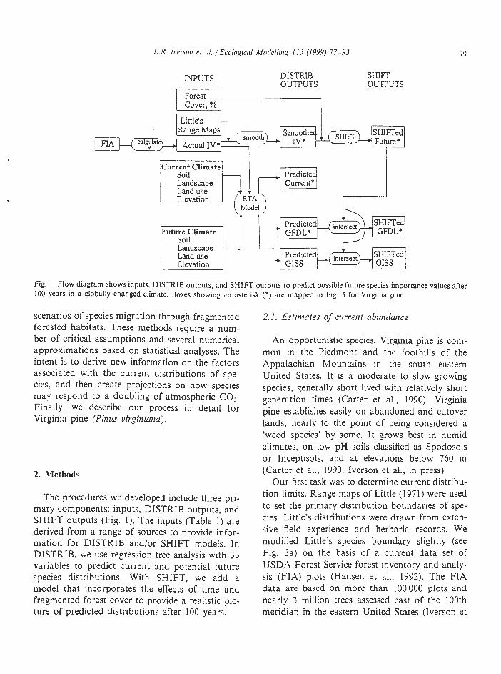
INPUTS DISTRIB SHIFT OUTPUTS OUTPUTS

Forest Cover, %

Range Maps

I FIA K-11 IV Acmal Iv*

Current Climate Soil Predicted Landscape Current* Land use Elevmon

1 Future Climate .n' d-p$ijywl Landscape Land use SHIFTed Elevation GISS

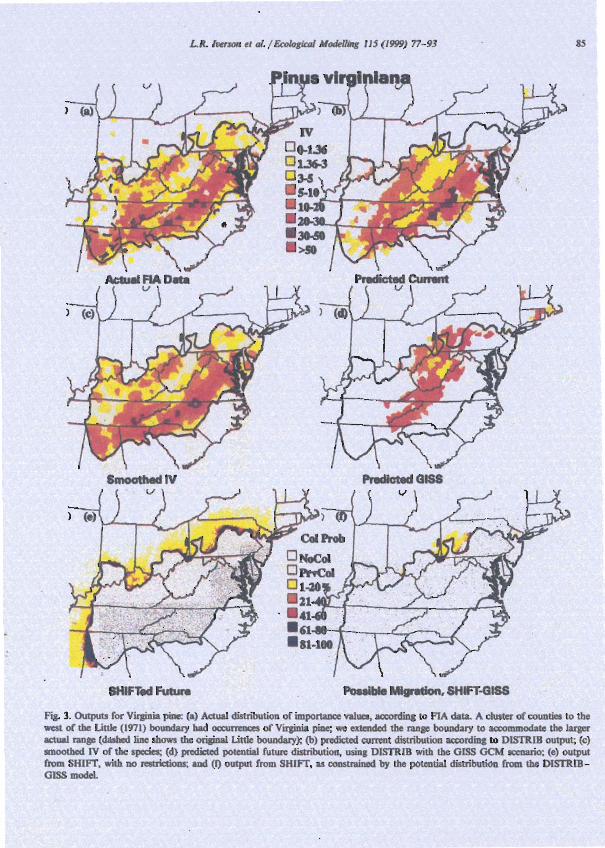
Fig. I . Flow diagram shows inputs. DISTRIB outputs, and SHIFT outputs to predict possible future species importance values after 100 years in a globally changed climate. Boxes showing an asterisk (*) are mapped in Fig. 3 for Virginia pine.

scenarios of species migration through fragmented forested habitats. These methods require a num- ber of critical assumptions and several numerical approximations based on statistical analyses. The intent is to derive new information on the factors associated with the current distributions of spe- cies, and then create projections on how species may respond to a doubling of atmospheric CO,. Finally, we describe our process in detail for Virginia pine (Pinus virginiana).

The procedures we developed include three pri- mary components: inputs, DISTRIB outputs, and SHIFT outputs (Fig. 1). The inputs (Table I) are derived from a range of sources to provide infor- mation for DISTRIB and/or SHIFT models. In DISTRIB, we use regression tree analysis with 33 variables to predict current and potential future species distributions. With SHIFT, we add a model that incorporates the effects of time and fragmented forest cover to provide a realistic pic- ture of predicted distributions after 100 years.

2.1. Estimates of current abundance

An opportunistic species, Virginia pine is com- mon in the Piedmont and the foothills of the Appalachian Mountains in the south eastern United States. It is a moderate to slow-growing species, generally short lived with relatively short generation times (Carter et al., 1990). Virginia pine establishes easily on abandoned and cutover lands, nearly to the point of being considered a 'weed species' by some. It grows best in humid climates, on low pH soils classified as Spodosols or Inceptisols, and at elevations below 760 m (Carter et al., 1990; Iverson et al., in press).

Our first task was to determine current distribu- tion limits. Range maps of Little (1971) were used to set the primary distribution boundaries of spe- cies. Little's distributions were drawn from exten- sive field experience and herbaria records. We modified Little's species boundary slightly (see Fig. 3a) on the basis of a current data set of USDA Forest Service forest inventory and analy- sis (FIA) plots (Hansen et al., 1992). The FIA data are based on more than 100000 plots and nearly 3 million trees assessed east of the 100th meridian in the eastern United States (Iverson et

80 L. R. Icerson ct ul. / Ecolo~qic

al., 1996). Because FIA data (and other data sets) are reported by county rather than a on standard

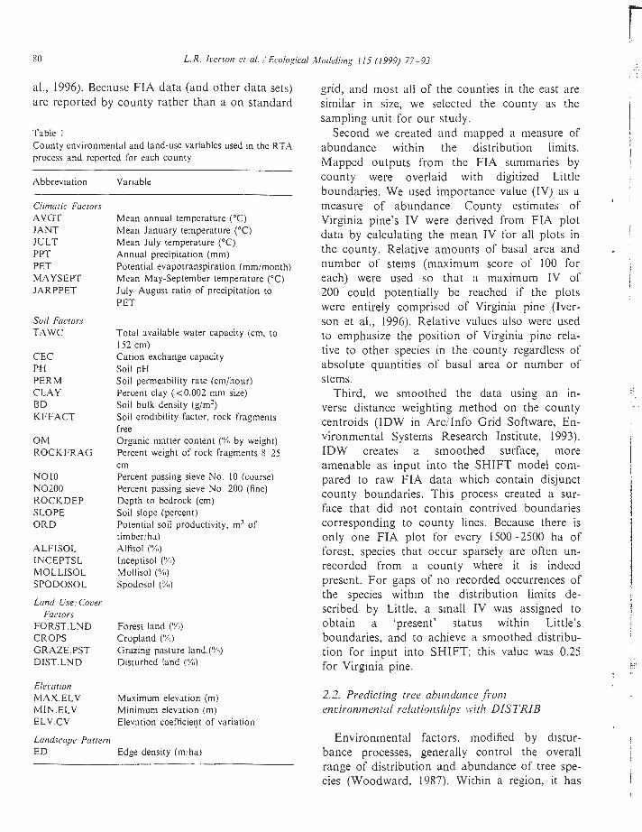
Table 1 County environmental and land-use variables used in the RTA process and reported for each county

Abbreviation Var~able

Climcrtic Factors AVGT JANT JULT PPT PET MAYSEPT JARPPET

Sail Fr,ctors TAWC

CEC PH PERM CLAY B D KFFACT

OM ROCKFRAG

NO10 NO200 ROCKDEP SLOPE O R D

ALFTSOL INCEPTSL MOLLISOL SPODOSOL

Land UselCo~,er F(~ctors

FORST.LND CROPS GRAZE.PST DIST.LND

Mean annual temperature (OC) Mean January temperature ("C) Mean July temperature ("C) Annual precipitation (mm) Potential evapotranspiration (rnm/month) Mean May-September temperature ("C) July-August ratio of precipitation to PET

Total available water capacity (cm, to 152 cm) Cation exchange capacity Soil pH Soil permeability rate (crnlhour) Percent clay (<0.002 mm size) Soil bulk density (g/m2) Soil erodibility factor, rock fragments free Organic matter content ('XI by weight) Percent weight of rock fragments 8-25 cm Percent passing sieve No. 10 (coarse) Percent passing sieve No. 200 (fine) Depth to bedrock (cm) Soil slope (percent) Potential soil productivity, ms of timberjha) Alfisol ('XI) lnceptisol ( 'Kt)

Mollisol (%I) Spodosol ('%I)

Forest land ('%,) Cropland ('%I) Grazing pasture land.(%) Disturbed land (I%,)

Eleccrf ion MAX.ELV Maximum elevation (m) MIN.ELV Minimum elevation (rn) ELV.CV Elevation coefficient of variation

La~~dscupe Pcirtenl E D Edge density (rn:ha)

grid, and most all of the counties in the east are similar in size, we selected the county as the sampling unit for our study.

Second we created and mapped a measure of abundance within the distribution limits. Mapped outputs from the FIA summaries by county were overlaid with digitized Little boundaries. We used importance value (IV) as a measure of abundance. County estimates of Virginia pine's IV were derived from FIA plot data by calculating the mean IV for all plots in the county. Relative amounts of basal area and number of stems (maximum score of 100 for each) were used so that a maximum IV of 200 could potentially be reached if the plots were entirely comprised of Virginia pine (Iver- son et al., 1996). Relative values also were used to emphasize the position of Virginia pine rela- tive to other species in the county regardless of absolute quantities of basal area or number of stems.

Third, we smoothed the data using an in- verse distance weighting method on the county centroids (IDW in ArciInfo Grid Software, En- vironmental Systems Research Institute, 1993). IDW creates a smoothed surface, more amenable as input into the SHIFT model com- pared to raw FIA data which contain disjunct county boundaries. This process created a sur- face that did not contain contrived boundaries corresponding to county lines. Because there is only one FIA plot for every 1500-2500 ha of forest, species that occur sparsely are often un- recorded from a county where it is indeed present. For gaps of no recorded occurrences of the species within the distribution limits de- scribed by Little, a small IV was assigned to obtain a 'present' status within Little's boundaries, and to achieve a smoothed distribu- tion for input into SHIFT; this value was 0.25 for Virginia pine.

2.2. Preclicting rrer nbru1(lr17ce f,wn maironrnent~rl rrlc~tiortships 1r.itlt DISTRIB

Environmental factors. modified by distur- bance processes, generally control the overall range of distribution and abundance of tree spe- cies (Woodward, 1987). Within a region, i t has

L.R. Icerson et 01. / Eco1ogicul modelling 115 (1999) 77-93 81

been assumed that species respond primarily to regional climate factors, whereas variations in ter- rain, soil, and land-use history tend to control local distributions. However, we have found that soil and elevation factors also can be important with respect to the regional IV distributions of some species (Iverson and Prasad, 1998). We are interested in predicting potential species range shifts following climate warming. Working at a continental scale, different variables may drive species abundances within different portions of their ranges. Thus, the preferred statistical tech- nique is one that is flexible enough to capture these spatial variations in driving variables. Re- gression tree analysis (RTA, also known as clas- sification and regression trees, or CART) is well suited for this purpose because it is based on recursive sampling of the data to form prediction rules and it automatically incorporates the possi- bility of interactions among the predictors (Brei- man et al., 1984).

Although a relatively new technique in the eco- logical sciences, RTA is rapidly gaining in popu- larity for devising prediction rules for rapid and repeated evaluation, as a screening method for variables, as a diagnostic technique to assess the adequacy of linear models, and for summarizing large multivariate data sets (Clark and Pergibon, 1992). RTA uses a binary recursive partitioning approach to split a data set, based on a single predictor variable at each split, into increasingly homogeneous subsets until another split is infeasi- ble. The variables that operate at large scales usually split the data early in the model, while variables that influence the response variable at more local scales operate later. The process is explained in Michaelsen et al. (1994) and Iverson and Prasad (1998).

For the development of our model, DISTRIB, more than 100 predictor variables were gathered or calculated for each of more than 2100 counties in the FIA data set. These variables were reduced to 33, which included: (a) seven climatic variables (US Environmental Protection Agency, 1993); (b) 18 soil variables (Olson et al., 1980; US Depart- ment of Agriculture and Soil Conservation Ser- vice, 1991); (c) three elevation variables (US Geological Survey, 1987); (d) four land uselland

cover variables (Olson et al., 1980; Zhu and Evans, 1994); (e) one landscape pattern variable (based on satellite land cover data (Zhu and Evans, 1994) analyzed by FRAGSTATS (Mc- Garigal and Marks, 1995)). Selection of final vari- ables was accomplished by: (a) correlation analysis to remove some highly redundant or irrelevant variables (from 138 to 65 variables); (b) summary and weighting of variable importance with RTA analysis of 103 species (65 to 44 vari- ables); (c) expert opinion on relevancy and inter- pretability (44 to 37 variables); and (d) removal of climate variables that have no analog in future GCM scenarios (37 to 33 variables) (Table 1). Trial RTA runs with various subsets of variables showed that the models were not appreciably affected by the reductions in variables. Processing of soil variables via STATSGO data is explained in Iverson et al. (1996); for information on data sources, see Iverson and Prasad (1998).

RTA was conducted so that the IV's of Virginia pine, as derived from actual FIA plot data could be compared with those of a predicted current distribution according to RTA modeled output. We then estimated potential future IV's for Vir- ginia pine by changing the climate inputs as pre- dicted by two GCM outputs: GFDL (Wetherald and Manabe, 1988) and GISS (Hansen et al., 1988). Predicted future climate data as processed from those models were obtained from the US Environmental Protection Agency (1993). The output of potential distribution then becomes the 'envelope' into which the species is allowed to migrate with the SHIFT model. Assumptions for the model are as follows: (a) the GCM scenarios are realistic with respect to future temperature and precipitation; (b) only the climate variables listed in Table 1 will change with the climate- change scenario, though in reality one would also expect various soil and landscape variables to change to some degree; (c) the suite of county- level data, used as predictor variables, is reliable and representative of the habitat requirements for Virginia pine; (d) changes in competition among species and/or water-use efficiency due to in- creased C 0 2 would not affect outcomes; (e) the distribution and IV's of Virginia pine are in equi-

82 L.R . Iuerson er 01. / Ecologicul .Llotlel/ing 115 (1999) 77-93

librium with the present climate; (f) violations of statistical assumptions, including spatial autocor- relation, would not change the predictions markedly.

In addition, while RTA may be the most appro- priate tool for analyzing data sets with many possibly interacting predictor variables and for separating macro and micro-level effects on the response, there are limitations. The ideal response should be approximately normal since least squares and the group mean are used in deriving the best split (Clark and Pergibon, 1992); this condition is not always met because of the high frequency of zeros. However, since the regression is local, the effect of long tails is much more confined than in a linear regression model (B.D. Ripley, personal communication).

In a criticism of model-based assessments of climate change effects on forests, Loehle and LeBlanc (1996) noted that many forest simulation models assume that tree species occur in all envi- ronments where it is possible for them to survive, and that they cannot survive outside the climatic conditions of their current range (fundamental vs. realized niche). The DISTRIB model addresses this criticism by considering a wide range of variables and evaluating only potential range changes due to climate change. DISTRIB also assumes equi- librium, but acknowledges that soil, land use, and elevation can be barriers to migration. In the next section we describe how the SHIFT model incor- porates time and spatial context into migration.

2.3. Simulation of species migration

A spatially explicit, cellular automata simulation model, SHIFT, was developed to describe a prob- ability distribution for the colonization of cur- rently unoccupied habitats (Schwartz, 1992). SHIFT uses three variables (habitat availability, within-stand abundance in occupied cells, and distance between occupied and unoccupied cells) to calculate a colonization probability for each unoc- cupied cell in each generation of a simulation run. SHIFT minimizes assumptions about and approx- imations of biologically important variables (e.g. seedling establishment, juvenile mortality, inter- specific competition) in favor of the simple as-

sumption that species can maintain an average migration rate of 50 kmlcentury in fully forested regions. This rate is the upper end of the range of observed migration rates during the Holocene (Davis, 1981, 1989). SHIFT predicts migration rates to slow as habitat availability decreases, leaving fewer colonization opportunities and a greater mean distance between cells. In a hypothet- ical landscape, migration rates are observed to be as low as 10 kmlcentury when 20% of the land- scape remains as suitable habitat (Schwartz, 1992). These results do not differ greatly from similar models that have specified more biological vari- ables to predict migration response to habitat fragmentation (e.g. Dyer, 1994, 1995; Collingham et al., 1996).

The equation SHIFT uses to determine the probability of an unoccupied cell becoming colo- nized (Ci) is:

Ci= Hi x S (H, x F, x l/D;) (1)

where H represents habitat availability in occupied ( j ) and unoccupied (i) cells, F, represents the within-stand abundance (IV) of the target popula- tion in occupied cells, and Dii represents the dis- tance between occupied and unoccupied cells. SHIFT uses an inverse power parameter (a) of the distance between sites (Du) to determine coloniza- tion probability (Schwartz, 1992). This dispersal function was chosen based on fitting of the tails of empirical seed-dispersal data sets (Portnoy and Willson, 1993). The inverse power function allows more long-distance dispersal than a negative expo- nential function, the other commonly used disper- sal function. The coefficient (a) was determined by calibrating the species to mi~ra te through the habitat matrix at 50 kmlcentury when habitat availability was high (80% of all cells) and forest abundance was moderate.

Habitat availability of occupied (H j ) and unoc- cupied (Hi) cells was determined by AVHRR- derived forest density (percent forest by AVHRR

., pixel) (Zhu and Evans, 1994), as modified by forest type.(i.e. extremely high agricultural regions in the Midwest were coded as non-forest). Species abun- ,

dance of occupied cells (5) was estimated from a smoothed IV map of FIA data as described previ- ously.

L. R. Icerson el crl. /Ecological

SHIFT was run with a grain size of 3 km and with an extent of the eastern United States as described earlier. SHIFT was run to simulate 100 years, or five generations, based on an estimated (and optimistic) average maturation period of 20 years (Altman and Dittmer, 1962) for growth of Virginia pine within forested stands. One hundred years also approximates the time projected by the Intergovernmental Panel on Climate Change (IPCC) for the Earth to reach 2 x CO, (500 ppmv, which approaches twice the preindustrial levels of 280 ppmv (Houghton et al., 1996)). This simulation process was repeated for 50 replica- tions to describe each initially unoccupied cell by a colonization probability over the next century.

Along with its relatively simple math, SHIFT carries several simplifying assumptions. First, we make several assumptions for computational con- venience: (a) local extinctions are not possible (these would tend to lower migration rates); (b) habitat is coded simply as a percentage of forested habitat per cell so that variations in forest type or matrix quality are not considered; and (c) colo- nization is equally likely in all directions from an occupied site. Second, we assume that biological processes, such as species autecologies and inter- specific interactions, that gave rise to observed Holocene migration rates continue to dominate migration responses of trees.

We know that anthropogenically introduced species and species moving through agriculture or along roadsides move very fast; they probably are not migration limited. Among trees this is a lim- ited subset and probably includes only several trees along with many shrubs. We do not have sufficient ecological data to identify all these spe- cies precisely. In addition, many trees (such as Virginia pine) may move quite well into disturbed second growth forest. Since we do not distinguish between low- and high-quality forest (only quan- tity of forest within a 3 x 3 km cell), we assume that all forest is of high habitat quality. Thus we do not underestimate habitat availability for weedy trees but will overestimate availability for trees more specific to high-quality forests. The model, as it stands, seems appropriate for Virginia pine. We also assume that there will be relatively few patches that move from a non-forested to a

forested state, and that they are balanced by patches moving in the opposite direction. For the past 30 years we have seen forest percentages grow in many parts of the eastern United States, but this trend is now slowing or reversing due largely to urbanization (Powell et al., 1993).

Finally, trees with animal-dispersed seeds have the potential to be net benefactors of habitat loss and fragmentation because their seed dispersers may sometimes be moving longer distances, on average, as they move from patch to patch. This would increase the mean distance of long-distance dispersal events or the frequency of long-distance dispersal events. We do not have sufficient disper- sal information on most of these species to distin- guish this effect. Historical data show little distinction in the past migration patterns between trees with wind-dispersed or animal-dispersed propagules. For our purposes, we use this histori- cal fact as justification for not distinguishing among life histories of trees for attributes other than mean generation time.

2.4. illerging DISTRlB and SHIFT

By combining results from the estimation of current distribution, the RTA analysis of future potential distribution (DISTRIB) and migration (SHIFT), we predict the potential response of Virginia pine to global warming over the next century. Simple intersection of the results from both models yields maps where constraints on future distributions are provided by each model: DISTRIB gives those areas where suitable habitat can occur, while SHIFT provides realistic scenar- ios of migration rates over the next century. We create a plausible prediction of the extent to which the region of climatically suitable habitat will shift and the extent to which this new distri- bution envelope will be saturated due to species migration through the landscape as it currently exists. Of course, the model is fraught with as- sumptions and is best viewed as a hypothesis for potential response. This is an important step, however, in that it will guide the scale of empirical studies to examine for global warming responses of trees. and provide early information on forest management.

L.R . luerson er al. /Ecological rbiodelling 1 15 (1999) 77-93

f801~~~467.42 [581 [I701 MAXI V<889.31[5] r - l

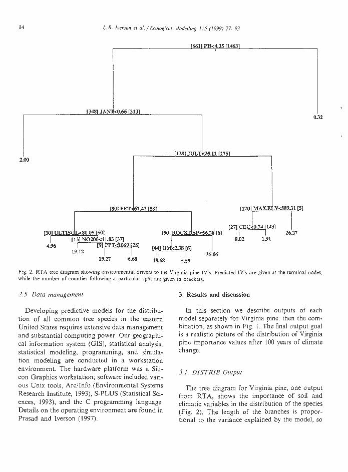
Fig. 2. RTA tree diagram showing environmental drivers to the Virginia pine IV's. Predicted IV's are given at the terminal nodes, while the number of counties following a particular split are given in brackets.

2.5. Data management 3. Results and discussion

Developing predictive models for the distribu- tion of all common tree species in the eastern United States requires extensive data management and substantial computing power. Our geographi- cal information system (GIs), statistical analysis, statistical modeling, programming, and simula- tion modeling are conducted in a workstation environment. The hardware platform was a Sili- con Graphics workstation; software included vari- ous Unix tools, Arc/Info (Environmental Systems Research Institute, 1993), S-PLUS (Statistical Sci- ences, 1993), and the C programming language. Details on the operating environment are found in Prasad and Iverson (1997).

In this section we describe outputs of each model separately for Virginia pine, then the com- bination, as shown in Fig. 1. The final output goal is a realistic picture of the distribution of Virginia pine importance values after 100 years of climate change.

3.1. DISTRIB Output

The tree diagram for Virginia pine, one output from RTA, shows the importance of soil and climatic variables in the distribution of the species (Fig. 2). The length of the branches is propor- tional to the variance explained by the model, so

86 L.R. loerson el al. /Ecological .C!oclelling I I5 (1999) 77-93

that pH, January temperature, and July tempera- ture each explain similar amounts of variance in the model. pH causes the initial split of the data records, with most of the Virginia pine occurring in locations with pH <4.35. If the pH is low (below 4.35), the greatest IV's are found when the mean January temperature exceeds 0.66OC. Within those 313 counties, maximum IV's (IV = 35.1) are reached for eight counties in the south- ern Appalachians that have warmer July temperatures ( > 25. I0C), but also potential evap- otranspiration in excess of 67.4 mmlmonth and a depth to bedrock of at least 56.3 cm (Figs. 2 and 3b). The next best conditions for Virginia pine are when the pH is ~ 4 . 3 5 , the January temperature is > 0.66"C, the mean July temperature is < 25.1°C, and elevations exceed 889 m; under these conditions, IV's can reach up to 26.3 (Fig. 2). Temperatures and PET would be expected to change under 2 x CO,, but soil pH (assumed here not to change under future climate scenarios) remains as the most important variable dictating the current (and future) distribution of Virginia pine.

The DISTRIB-predicted current estimate shows a reasonable relationship (correlation coefficient of 0.71) to the actual FIA data as aggregated to the county level (Fig. 3a,b). The zones of rela- tively high importance (IV > 25), primarily in the southern Appalachians, are replicated on the ac- tual and predicted current maps, with more error associated with the locations of low IV. As de- scribed in Iverson and Prasad (1998), a 20% vali- dation data set was withheld for comparison to DISTRIB estimates, with good agreement. Be- cause we have established a model that predicts current IV reasonably well for Virginia pine, we proceeded to 'change' the climate and evaluate potential future distributions based on this changed climate.

The smoothed IV map (Fig. 3c) shows the modified IV's for the current distribution of Vir- ginia pine that are used as input into the SHIFT model. This smoothed map allowed a more gener- alized output from SHIFT than when migration is depicted out from disjunct, rectangular counties near the edge of its range.

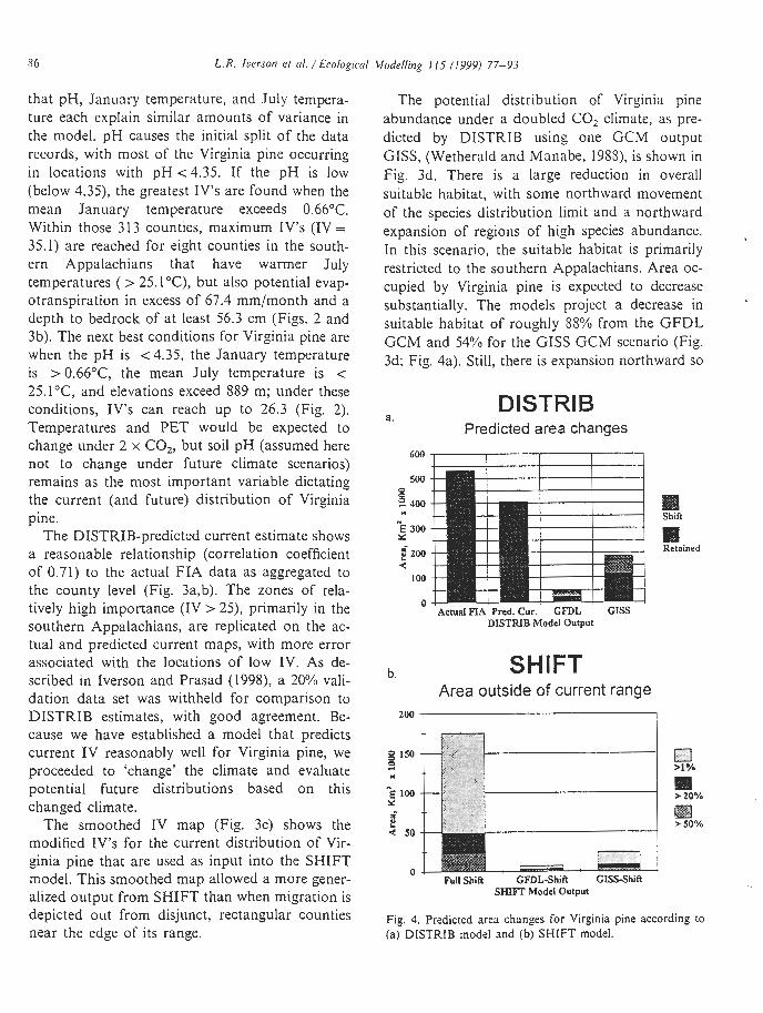
The potential distribution of Virginia pine abundance under a doubled CO, climate, as pre- dicted by DISTRIB using one GCM output GISS, (Wetherald and Manabe, 1988), is shown in Fig. 3d. There is a large reduction in overall suitable habitat, with some northward movement of the species distribution limit and a northward expansion of regions of high species abundance. In this scenario, the suitable habitat is primarily restricted to the southern Appalachians. Area oc- cupied by Virginia pine is expected to decrease substantially. The models project a decrease in suitable habitat of roughly 88% from the GFDL GCM and 54% for the GISS GCM scenario (Fig. 3d; Fig. 4a). Still, there is expansion northward so

a. DISTRIB

Predicted area changes

600

500

3- 400 Shift "

E 300 Y

f 200

ma Retained

d LOO

0 Actual FIA Pred. Cur. GFDL GISS

DISTRIB Model OuQut

Area outside of current range

Full Shift GFDLShiR GISS-Shift SHIFT Model Output

Fig. 4. Predicted area changes for Virginia pine according to (a) DISTRIB model and (b) SHIFT model.

L.R. Icerson el 01. / Ecologicul

Maximum N Movement of Front 500

400 II > I %

300 Cl E >200/* Y

200 M >50%

100 DlSTRlB

0 DISTRIB-GFDL G I S S - S H I ~

DISTRIB-GISS GFDL-SHIFT SHIFT alone

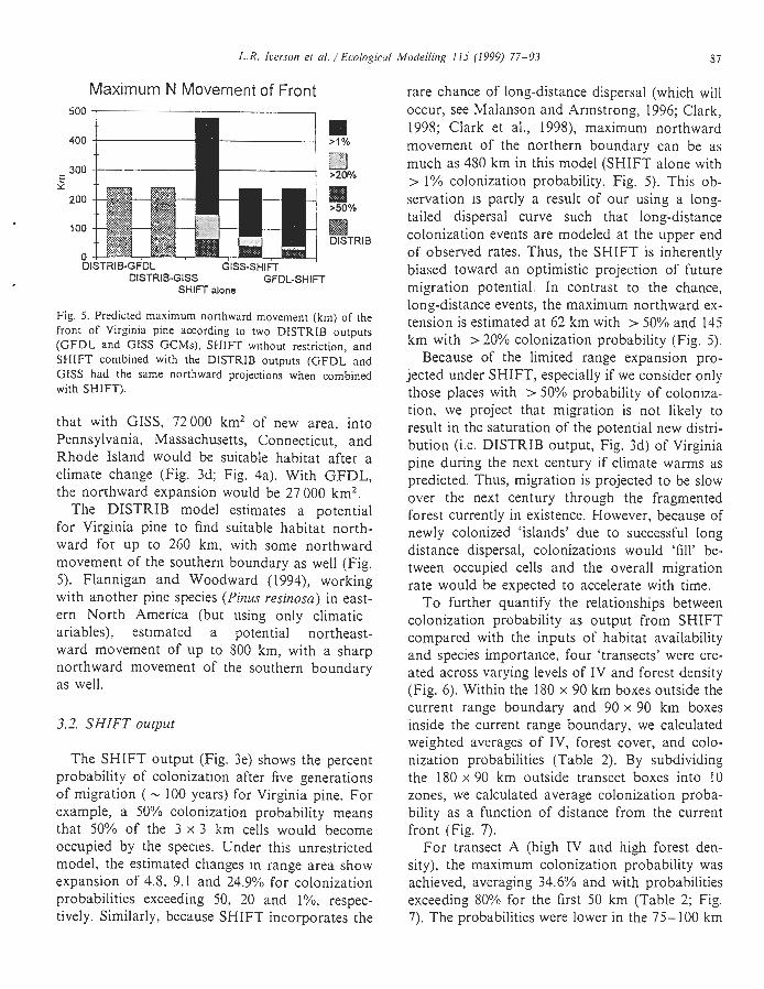
Fig. 5. Predicted maximum northward movement (km) of the front of Virginia pine according ro two DlSTRlB outputs ( G F D L and GISS GCMs), S H I n without restriction, and SHIFT combined with the DISTRIB outputs (GFDL and GISS had the same northward projections when combined with SHIFT).

that with GISS, 72000 km2 of new area, into Pennsylvania, Massachusetts, Connecticut, and Rhode Island would be suitable habitat after a climate change (Fig. 3d; Fig. 4a). With GFDL, the northward expansion would be 27 000 km2.

The DISTRIB model estimates a potential for Virginia pine to find suitable habitat north- ward for up to 260 km, with some northward movement of the southern boundary as well (Fig. 5). Flannigan and Woodward (1994), working with another pine species (Pinzu resinosa) in east- ern North America (but using only climatic ariables), estimated a potential northeast- ward movement of up to 800 km, with a sharp northward movement of the southern boundary as well.

3.2. SHIFT otitput

The SHIFT output (Fig. 3e) shows the percent probability of colonization after five generations of migration ( - 100 years) for Virginia pine. For example, a 50% colonization probability means that 50% of the 3 x 3 km cells would become occupied by the species. Under this unrestricted model, the estimated changes in range area show expansion of 4.8, 9.1 and 24.9% for colonization probabilities exceeding 50, 20 and 1%, respec- tively. Similarly, because SHIFT incorporates the

rare chance of long-distance dispersal (which will occur, see blalanson and Armstrong, 1996; Clark, 1998; Clark et al., 1998), maximum northward movement of the northern boundary can be as much as 480 km in this model (SHIFT alone with > 1% colonization probability, Fig. 5). This ob- servation is partly a result of our using a long- tailed dispersal curve such that long-distance colonization events are modeled at the upper end of observed rates. Thus, the SHIFT is inherently biased toward an optimistic projection of future migration potential. In contrast to the chance, long-distance events, the maximum northward ex- tension is estimated at 62 km with > 50% and 145 km with > 20% colonization probability (Fig. 5).

Because of the limited range expansion pro- jected under SHIFT, especially if we consider only those places with > 50% probability of coloniza- tion, we project that migration is not likely to result in the saturation of the potential new distri- bution (i.e. DISTRIB output, Fig. 3d) of Virginia pine during the next century if climate warms as predicted. Thus, migration is projected to be slow over the next century through the fragmented forest currently in existence. However, because of newly colonized 'islands' due to successful long distance dispersal, colonizations would 'fill' be- tween occupied cells and the overall migration rate would be expected to accelerate with time.

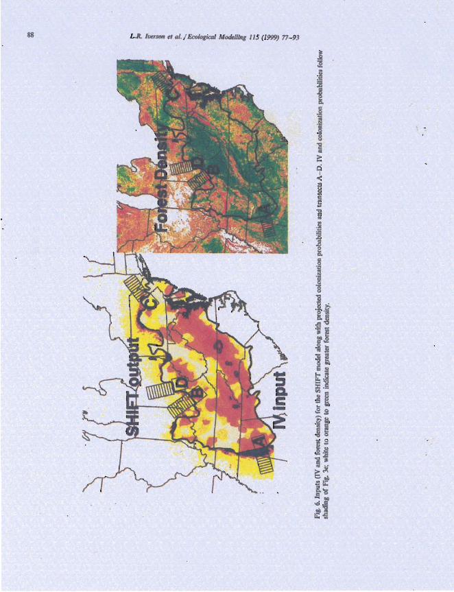
To further quantify the relationships between colonization probability as output from SHIFT compared with the inputs of habitat availability and species importance, four 'transects' were cre- ated across varying levels of IV and forest density (Fig. 6). Within the 180 x 90 km boxes outside the current range boundary and 90 x 90 km boxes inside the current range boundary, we calculated weighted averages of IV, forest cover, and colo- nization probabilities (Table 2). By subdividing the 180 x 90 km outside transect boxes into 10 zones, we calculated average colonization proba- bility as a function of distance from the current front (Fig. 7).

For transect A (high IV and high forest den- sity), the maximum colonization probability was achieved, averaging 34.6% and with probabilities exceeding 80% for the first 50 km (Table 2; Fig. 7). The probabilities were lower in the 75- 100 km

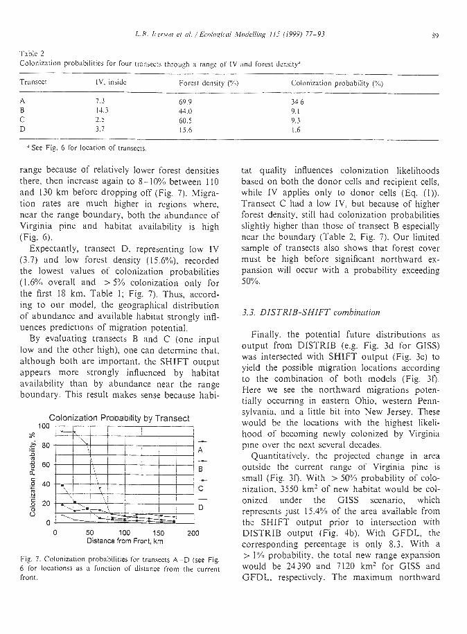
L.R. Ircrson el ti/. / Ecologictrl ~Worlcllit~g 115 11999) 77-93 89

Tablc 2 Colonization probabilities for four tranjects through a range of IV and forest density.'

-

Transect IV, inside Forest density ('%I) Colonization probability ('A,)

" S e e Fiz. 6 for locatiorl of tranxcts.

range because of relatively lower forest densities there, then increase again to 8- 10% between 1 10 and 130 km before dropping off (Fig. 7). Migra- tion rates are much higher in regions where, near the range boundary, both the abundance of Virginia pine and habitat availability is high (Fig. 6).

Expectantly, transect D, representing low IV (3.7) and low forest density (15.6%). recorded the lowest values of colonization probabilities (1.6% overall and > 5% colonization only for the first 18 km, Table I ; Fig. 7). Thus, accord- ing to our model, the geographical distribution of abundance and available habitat strongly infl- - - uences predictions of migration potential.

By evaluating transects B and C (one input low and the other high), one can determine that, although both are important, the SHIFT output appears more strongly influenced by habitat availability than by abundance near the range boundary. This result makes sense because habi-

Colonization Probability by Transect 100 41 I 1 1 ) ap ! I

0 50 100 150 200 Distance from Front, km

Fig. 7. Colonization probabilities for transects A - D (see Fig, 6 for locations) as a function of distance from the current front.

tat quality influences colonization likelihoods based on both the donor cells and recipient cells, while IV applies only to donor cells (Eq. (I)). Transect C had a low IV, but because of higher forest density. still had colonization probabilities slightly higher than those of transect B especially near the boundary (Table 2; Fig. 7). Our limited sample of transects also shows that forest cover must be high before significant northward ex- pansion will occur with a probability exceeding 50%.

3.3. DISTRIB-SHIFT combination

Finally. the potential future distributions as output from DISTRIB (e.g. Fig. 3d for GISS) was intersected with SHIFT output (Fig. 3e) to yield the possible migration locations according to the combination of both models (Fig. 30. Here we see the northward migrations poten- tially occurring in eastern Ohio, western Penn- sylvania, and a little bit into New Jersey. These would be the locations with the highest likeli- hood of becoming newly colonized by Virginia pine over the next several decades.

Quantitatively, the projected change in area outside the current range of Virginia pine is small (Fig. 30. With > 50% probability of colo- nization, 3550 km' of new habitat would be col- onized under the GISS scenario, which represents just 15.4% of the area available from the SHIFT output prior to intersection with DISTRIB output (Fig. 4b). With GFDL, the corresponding percentage is only 8.3. With a > !'XI probability, the total new range expansion would be 24390 and 7120 km' for GISS and GFDL. respectively. The maximum northward

90 L.R. lcerson et ul. / Ecologrcul .I

shift would be about 30-40 km with a > 50% colonization probability, and about 240 km with a colonization probability of > l"/o (the rare, long-distance events, Fig. 5).

4. Conclusions

Using three computational steps to predict smoothed current abundance and distribution, potential future distribution and abundance, and migration potential into the new window of dis- tribution, we have tried to produce realistic sce- narios for the future distribution of Virginia pine under a 2 x C 0 2 climate. This effort con- tributes to two areas previously lacking in mi- gration research on real landscapes: (1) the effects of fragmented habitat and varying species abundance on rates of migration; and (2) the effects of unsuitable future habitats (e.g. barriers in soil quality, elevation, climate regimes) on possible migration outcomes (Davis and Sugita, 1997).

Because of the uncertainty connected with many assumptions imbedded in the models, pro- jections of future distribution and migration po- tential must be viewed as hypotheses for future responses. Still, this approach uses a two-prong method to increase the acceptability of model outputs. First, we capture current bounds on species importance that then can be adjusted ac- cording to potential future climate scenarios (en- velope analysis). Second, we simulate the actual movement of the species through actual land- scapes and time to represent the possible future distributions within the suitable envelope. These results provide a quantified model against which observational data may be collected to measure both validity of current abundance predictions and future distribution and abundance changes, These predictions are important because they suggest a scale of research with which we can verify vegetation change in response to climatic change. Indeed, we need to build similar projec- tions as more is learned about climate change (Schneider and Root, 1996).

From the combination of the two model out- puts for Virginia pine (DISTRIB and SHIFT),

one can determine that both of the following scenarios apply: ( 1 ) although land may be 'suit- able' for colonization (as determined by DIS- TRIB), limitations of species abundance and forest habitat preclude the migration of the spe- cies into the new potential habitat; (2) although the species may have the physical abundance near the range boundary and the forest cover to migrate into (as determined especially by long- distance rare events in SHIFT), the remaining environmental factors may not be suitable for the species to survive a r d reproduce.

There will be migration lag time, especially since we are working with generally long-lived trees. SHIFT was calibrated for an average of 50 kmlcentury of migration; here we project a maxirn~im migration of 30-40 km in 100 years with a > 50% colonization probability. Many re- gions of low IV and habitat will have migrations near zero over the next 100 years. Both habitat availability and species abundance are important for migration to proceed. Of the two, habitat availability seems the more critical component if the species is present at some level.

For Virginia pine, our models show a large decrease in suitable habitat and a fairly small northward migration of range for the 2 x CO, scenarios of the GISS and especially GFDL models. Thus, the current distribution of Vir- ginia pine, though not seriously threatened, would see a restriction in habitat from a 2 x CO1-driven climate change. Current studies, us- ing DISTRIB on SO species, indicate that roughly equal numbers of tree species in the eastern United States will have a reduced versus expanded range of suitable habitat after climate change (Iverson and Prasad, 1998; Iverson et al., in press). Efforts continue, usmg SHIFT, to de- termine colonization probabilities of the new suitable habitat for additional species.

Acknowledgements

We thank all those who provided data for this effort, and acknowledge the support of the USDA Forest Service's Northern Global Change Program. We also thank David Mladenoff,

L.R. luerson cf ol. / Ecologiccil

Monica Turner, Charles Scott, David Randall and two anonymous reviewers for technical re- views, and Mary Boda for final edits to the manuscript.

References

Altman. P.L., Dittmer, D.S., 1962. Growth including repro- duction and morphological development. Federation of American Societies for Experimental Biology, Washington, DC.

Barry. J.P., Baxter, C.H., Sagarin, R.D., Gilman, S.E., 1995. Climate-related, long-term faunal changes in a California rocky intertidal community. Science 267, 672-675.

Botkin, D.B., Nisbet, R.A., 1992. Projecting the effects of climate change on biological diversity in forests. In: Peters, R.L., Lovejoy, T.E. (Eds.), Global warming and biological diversity. Yale University Press. New Haven, CT, pp. 277-293.

Breiman, L., Freidman. J., Olshen, R., Stone, C., 1984. Clas- sification and regression trees. Wadsworth, Belmont, CA.

Burton, P.J., Cumming, S.G., 1995. Potential effects of cli- matic change on some western Canadian forests, based on phenological enhancements to a patch model of forest succession, Water. Air and Soil Pollution 82. 401 -414.

Carter, K.K., Snow, A.G., Jr 1990. Pinris virginiana Pvlill. Virginia pine. In: Burns, R.M. and Honkala, B.H. (Eds.), Silvics of North America. Volume I . Conifers. US Depart- ment of A_ericulture, Agriculture Handbook 654. Washing- ton, DC, pp. 513-519.

Clark, J.S., 1998. Why trees migrate so fast: confronting theory with dispersal biology and the paleorecord. Am. Nat. 152, 204-224.

Clark, J.S.. Fastie, C., Hurtt, G., Jackson. S.T., Johnson, C., King, G., Lewis, M.. Lynch, J., Pacala. S.. Prentice, 1.C.. 1998. Reid's Paradox of rapid plant migration. BioScience 48, 13-24.

Clark, L.A., Pergibon. D., 1992. Tree-based models. In: Hastie, T.J. (Ed.), Statistical models in S. Wadsworth, CA, Pacific Grove, CA. pp. 377-419.

Collingham, Y.C., Hill, M.O., Huntley, B., 1996. The migra- tion of sessile organisms: a simulation model with measur- able parameters. J. Vegetation Sci. 7, 83 1-846.

COHMAP. 1988. Climatic changes of the last 18000 years: observations and model simulations. Science 241:1043- 1052.

Coope, G.R.. 1977. Fossil coleopteran assemblages as sensitive indicators of climatic changes during the Devensian (last) cold stage. Phil. Trans. Royal Soc. Lond. B Biol. Sci. 280, 31 3-340.

Coope. G.R., 1979. Late Cenezoic fossil Coleoptera: evolu- tion. biogeography, and ecology. Ann. Rev. Ecol. Syst. 10, 247-267.

Davis. M.B.. 1981. Quaternary history and the stability of forest communities. In: West, D.C., Shugart, H.H. (Eds.). Forest succession. Springer-Verlag, NY, pp. 132-153.

Davis. M.B., 1989. Lags in vegetation response to greenhouse warming. Clim. Change 15, 75-82.

Davis, bl., Sugita, S., 1997. Patterns and mechanisms of plant migration and plant distribution in the Quaternary. Bull. Ecol. Soc. Amer. 78, 1 1 .

Davis, b1.B.. Zabinski, C., 1992. Changes in geographical range resulting from greenhouse warming: effects on biodi- versity in forests. In: Peters, R.L.. Lovejoy. T.E. (Eds.). Global warming and biological diversity. Yale University Press, New Haven, CT, pp. 297-308.

Delcourt, H.R., Delcourt, P.A., 1988. Quaternary landscape ecology: relevant scales in space and time. Landsc. Ecol. 2. 23-44.

Dyer, J.M., 1994. Implications of habitat fragmentation on climate chanse-induced forest migration. Prof. Geogr. 46, 449-459.

Dyer, J . PI., 1995. Assessment of climatic warming using a model of forest species migration. Ecol. Modell. 79. 199- 219.

Environmental Systems Research Institute, 1993. Arc/Info GRID command reference. Environmental Systems Re- search Institute, Redlands, CA.

Flannigan, M.D., Woodward, F.I., 1994. Red pine abundance: current climatic control and responses to future warming. Can. J. Forest Res. 24, 1166-1 175.

Foley, J.A., Prentice. I.C., Ramankutty. N., Levis, S., Pollard, B., Sitch. S., Haxeltine, A., 1996. An integrated biosphere model of land surface processes, terrestrial carbon balance and vegetation dynamics. Global Biogeo. Cycles 10, 603- 628.

Hansen. J., Fung, I.. Lacis, A., Rind, D., Lebedeff, S., Ruedy. R., 1988. Global climate changes as forecast by Goddard Institute for Space Studies three-dimensional model. J. Geophysical Res. 93, 934 1 -9364.

Hansen, M.H.. Frieswyk. T., Glover, J.F.. Kelly. J.F. 1992. The eastwide forest inventory data base: users manual. US Department of Agriculture. Forest Service, North Central

, Forest Experiment Station. Gen. Tech. Rep. NC- 151.

Hobbs, R.J., 1994. Dynamics of vegetation mosaics: Can we predict responses to global change? EcoScience 1, 346-356.

Houghton, J.T.. Meira Filho, L.G., Callander, B.A., Harris. N., Kattenberg, A., Maskell. K., 1996. Climate chanp 1995: the science of climate change. Cambridge University Press, Cambridge, UK.

Hughes. L., Cawsey. E.M., Westoby, M., 1996. Climatic range sizes of Eucalyptus species in relation to future climate change. Global Ecol. Biogeog. Lett. 5. 23-29.

Huntley. B. 1991. How plants respond to climate change: migration rates. individualism and the consequences for plant communities. Ann. Bot. 67 (Suppl.). 15-22.

Iverson, L.R.. Prasad, A., Scott, C.T. 1996. Preparation of forest inventory and analysis (FIA) and state soil e o - graphic data base (STATSGO) data for global change

research in the eastern United States. In: Hom, J., Birdsey. R., O'Brixn, K. (Eds.) Proceedings, 1995 meeting of the northern global change program. US Department of Agri- culture, Forest Serv~ce, Northeastern Forest Experimen~ Station, Gen. Tech. Rep. NE-214, pp. 209-214.

Iverson. L.R., Prasad, A., 1998. Predicting potential future abundance of 80 tree species following climate change in the eastern United States. Ecol. blonogr. 68, 465-485.

Iverson, L.R., Prasad, A.M.. Hale, B.J.. Sutherland. E.K. 1998. An atlas of current and potential future distributions of common trees of the eastern United States. Northeast- ern Research Station, USDA Forest Service, General Technical Report (in press).

Kattenberg, A., Giorgi. F., Grassl, H., Meehl, G.A., Mitchell, J.F.B., Stouffer, R.J., Tokioka. T., Weaver, A.J., Wigley, T.M.L., 1996. Climate models - projections of future climate. In: Houghton. J.T., Me~ra-Filho, L.G., Callander, B.A., Harris, N., Kattenberg, A., Maskell, K. (Eds.), Cli- mate change 1995: the science o f climate change. Univer- sity Press. Cambridge, UK. pp. 285-357.

Lauenroth, W.K., 1996. Application of patch models to exam- Ine regional sensitivity to climate change. Climatic Change 34, 155- 160.

Little, E.L. 1971. Atlas of United States rrees. Volume I. Conifers and important hardwoods. US Department of Agriculture Forest Service. Miscellaneous Publication 1146.

Loehle, C., LeBlanc, D., 1996. Model-based assessments of climate change effects on forests: a critical review. Ecol. Modell. 90. 1-31.

MacCracken, M.C., 1995. The evidence mounts up. Nature 376. 645-646.

Malanson. G.P., 1993. Comment on modeling ecological re- sponse to climatic change. Climatic Change 23, 95- 105.

Malanson. G.P., Armstrong, M.P.. 1996. Dispersal probability and forest diversity in a fragmented landscape. Ecol. Mod- ell. 87. 91 - 102.

~WcGarigal, K. and Marks, B.J. 1995. FRAGSTATS: spatial pattern analysis program for quantifying landscape struc- ture. US Department of Agriculture. Forest Service, Pacific Northwest Research Station. USDA Forest Service. Port- land, OR. General Technical Report PNW-GTR-351.

Michaelsen. J., Schimel, D.S., Friedl. M.A., Davis. F.W.. Dubayah, R.C., 1994. Regress~on tree analysis of satellite and terrain data to guide vegetation sampling and surveys. J. Vegetation Sci. 5, 673-686.

Neilson, R.P., 1995. A model for predicting continental-scale vegetation distribut~on and water balance. Ecol. Appl. 5 (2). 362-385.

Nicholls. N., 1996. An incriminating fingerprint. Nature 382, 27-28.

Olson. R.J., Emerson. C.J., Nungesser. M.K. 1980. Geoecol- ogy: a county level environmental data base for the conter- minous United States. Oak Ridge National Laboratory, Environmental Sciences Division, Oak Ridge. TN. Publica- tion No. 1537.

Overpeck, J.T., Bartlein, P.J., Webb, T . Ill., 1991. Potential mugnitude ol' future vegetation change in Eastern North America: compnrisons with the pus[. Science 254, 692-695.

Parmesun, C.. 1996. Climate and species range. Nature 382. 763-766.

Peters. R.L.. Lovejoy. T.E. (Eds.). 1991. Global warming and biological diversity. Yale University Press. New Haven. C T .

Pitelka, L.F. and Plant Migration Workshop Group, 1997. Plant migration and climate change. Am. Sci. 85:464-473.

Portnoy. S., Willson, M.F., 1993. Seed dispersal curves: behav- ior of the tail of the distribution. Evol. Ecol. 7. 25-44.

Powell, D.S., Faulkner, J.L.. Darr, D.R. Zliu, Z., MacCleery, D.W. 1993. Forest resources of the Un~ted States. 1992. Rocky Mountain Forest and Range Experiment Station. Ft. Collins. CO, Gen. Tech. Rep. RM-234.

Prasad, A., Iverson, L.R. 1997. Modelling tree distributions in eastern United States using Arc/lnfo G I s and S-PLUS statistical package. Proceedings. 1997 Arcilnfo conference. Environmental Systems Research Institute. Redlands, CA. http://www.esri.comlbase/common/userconflproc97/ PROC97/to200/PAP2OO/pZOO.htm

Prentice, 1.C.. Cramer. W., Harrison. S.P., Leemans, R., Mon- serud, R.A., Solomon. A.M., 1992. A global biome model based on plant physiology and dominance. soil properties and climate. 1. Biogeogr. 19. 117-134.

Rastetter, E.B., 1996. Validating models of ecosystem response to global change. BioScience 46. 190- 197.

Rykiel, E.J.. 1996. Testing ecological models: The meaning of validation. Ecol. Modell. 90, 229-244.

Schneider. S.H., Root. T.L.. 1996. Ecolog~cal implications of climate c h a n ~ e will Include surprises. Biodivers. Conserv. 5. 1109- 1 120.

Schulze. R.E.. Kunz, R.P., 1995. Potential shifts in optimum growth areas of selected commercial tree species and sub- tropical crops in southern Africa due to global warming. J Biogogr. 22. 679-688.

Schwartz, M.W.. 1992. Modeling the effect of habitat loss on potential rates of range change for trees In response to global warming. Biodivers. Conserv. 2. j 1-6 1 .

Shriner, D.S., Street, R.B.. 1998. North America. In: Watson. R.T., Zinyowera, M.C.. Moss. R.H. (Eds.), The reg~onal impacts of climate change. Cambridge Un~vers~ty Press, New York. NY. pp. 253-330.

Statistical Sciences. 1993. S-PLUS guide to statistical and mathematical analys~s. vers. 3.2. Statistical Sciences. Seat- tle, WA.

Starfield. A.M.. Chapin. F.S., 1996. Model of transient changes in arctic and boreal vegetation in response to climate and land use change. Ecol. Appl. 6. 842-864.

Sykes. M.T.. Prentice. I.C.. Cramer. W.. 1996. A bioclimatic model for the potential distributions o r north European tree species under present and future climates. J . Biogeogr. 23, 203-234.

US Department of Agriculture. Soil Conservation Service. 1991. State soil geographic data base [STATSGO) data users guide. US Department of Agriculture. Soil Conserva- tion Service. Miscellaneous Publication 1492.

L. R. Irerson c~ rrl. / Ecologicul ib/.lotlelling 1 I? 11999) 77-93 93

US Environmental Protection Agenc). 1993. EPA-Corvallis model-derived climate database and 2 x CO, predictions I'or long-term mean monthly temperature, vapor pressure. wind velocity and potential evapotranspiration from the Regional Water Balance Model and precipitation from the PRISM model. for the conterminous United States. Digital raster data on a I0 x 10 km, 470 x 295 Albers Equal Area grid, in Image Processing Workbench format. US Environ- mental Protection Agency. Environmental Research Labo- ratory. Corvallis. OR.

US Geological Survey. 1987. Digital elevation models: US Geological Survey data user's guide 5. US Geological Survey. Reston. VA.

VESlAP members, 1995. Vegetation ecosystem modeling and analysis project: comparing biogeography ~ i n d biogeo- chemistry models in a continental-scale study of terrestrial ecosystem reposnses to climate change and C 0 2 doubling. Global Biogeochem. Cycles 9, 407-437.

Webb, T. Ill, Bertlein, P.J.. K~ltzblch. J.E. 1987. Climatic change in eastern North America during the past 18000

years: comparisons of pollen data with model results. In: Wright. W.F., Wright. H.E.. J r (Eds.), North America and adjacent oce;lns d u r i n ~ the last deglaciation. Geologicnl Soc~ety of America, Boulder. CO. pp. 447-462.

Webb Ill. T.. 1992. Past changes in vegetation and climate: lessons for the future. In: Peters. R.L.. Lovejoy, T.E. (Eds.). Global warming and biological diversity. Yale Uni- versity Press. New Haven, CT, pp. 59-75.

Wetherald. R.T.. klanabe. S.. 1988. Cloud feedback processes in n general circulat~on model. J . Atmosph. Sci. 45, 1397- 1415.

Woodward. F.I.. 1987. Climate and plant distribution. Cnm- bridge University Press, NY.

Woodwnrd. F.I., 1997. Tansley Review no. 41. Predicting pli~nt responses to global environmental change. New Phy- tol. 122. 239-251.

Zhu. 2.. Evans, D.L.. 1994. US forest types and predicted percent forest cover from AVHRR data. Photogram. Eng. Remote Sens. 60. 525-53 1.