Modeling of Bone Conduction of Sound in the HumanHead Using hp Finite Elements I. Code Design and

Verification

L. Demkowicz, P. Gatto, J. Kurtz, M. Paszynski, W. Rachowicz,E. Bleszynski, M. Bleszynski, M. Hamilton, and C. Champlin

The Institute for Computational Engineering and SciencesThe University of Texas at AustinAustin, Texas 78712

by

ICES REPORT 10-02

February 2010

MODELING OF BONE CONDUCTION OFSOUND IN THE HUMAN HEADUSING hp FINITE ELEMENTS

I. CODE DESIGN AND VERIFICATION

L. Demkowicza, P. Gattoa, J. Kurtza, M. Paszynskib, W. Rachowiczc, E. Bleszynskid, M.Bleszynskid, M. Hamiltone, C. Champlinf

a Institute for Computational Engineering and Sciences, University of Texas at Austinb AGH University of Science and Technology, Cracow, Poland

c Cracow University of Technology, Cracow, Polandd Monopole Research

e Dept. of Mechanical Engineering, University of Texas at Austinf College of Communications, University of Texas at Austin

1. Introduction

Motivation

Hearing impairment remains the primary disability among military personnel. Sound pressurelevels caused by proximity to aircraft engines or impulse noise from large caliber weapons mayeasily exceed the pain threshold value of 100 dB.

The focus of this project is to to develop a reliable numerical model for investigating the bone-conducted sound in the human head. The problem is difficult because of a lack of fundamentalknowledge regarding the transmission of acoustic energy through non-airborne pathways to thecochlea. A fully coupled model based on the acoustic/elastic interaction problem with a detailedresolution of the cochlea region and its interface with the skull and the air pathways, should providean insight into this fundamental, long standing research problem.

The project builds on an interaction of experts in numerical wave propagation – Drs. Elisabethand Marek Bleszynski from Monopole Research with a team at the University of Texas headed byDr. Leszek Demkowicz and including two experts on wave propagation and hearing science: Dr.Mark Hamilton and Dr. Greg Champlin.

Literature review

Bone-conducted sound.. The fact that vibration of the skull causes a hearing sensation has beenknown since the 19th century. This mode of hearing was termed hearing by bone conduction. Al-

1

though there has been more than a century of research on hearing by bone conduction, its physiologyis not completely understood. For and early account of the phenomenon as cause of partial deafnesssee [8]. Further summaries of those early works can be found in Hood (J. Acoust. SOC. Am., 34:1325-1332, 1962) and Naunton (Chapter I in Modern Development in Audiology, J. Jerger, ed.,Academic Press, New York, 1963). Lately, new insights into the physiology of hearing by boneconduction have been reported. Knowledge of the physiology, clinical aspects, and limitations ofbone conduction sound is important for clinicians dealing with hearing loss. Factors contributingto bone conduction of sound, such as inertia of the middle ear ossicles and of the cochlear fluids,and sound radiated into the external ear canal have been investigated by S. Stenfelt and R. Goode in[19]. The effects of bone conduction of sound were studied via a finite element model by F. BohnkeF, and W. Arnold in [7]. This study showed the influence of bone conduction on pressure signals atthe cochlea wall. The first simultaneous sound pressure measurements in scala vestibuli and scalatympani of the cochlea in human cadaveric temporal bones were presented by E. Olson et al. in[14]. Finally, among other fundamental works done by E. Olson on bone conduction of sound andits interplay with the cochlea we want to recall [15] and [6].

Coupled (visco)-elasticity with acoustics.. The variational formulation for the coupled elasticity/acousticsproblem utilized in this project is classical and has been extensively studied over the last twodecades, see e.g. [9]. The term weak coupling has different meanings. The involved variables:elastic displacement u and acoustic pressure p are not forced to match each other on the elas-tic/acoustic interface. Instead, the variational formulation incorporates additional off-diagonal fluxterms representing the interaction in between the two fields and resulting from the interface condi-tions. It is essential that either field represents a dual quantity for the other. Hence the term “weak”contrary to “strong” couplings where two variables match each other at both continuous and discretelevels along the interface. A second meaning of the term “weak coupling” refers to the fact that thecoupling terms represent compact perturbations of the terms on the main diagonal correspondingto elasticity and acoustics. This guarantees automatically that the Galerkin discretization of theproblem will be asymptotically stable.

hp-elements.. The presented work builds on FE technology of hp-adaptive finite elements, see[2, 4] and the literature therein. Motivated with our 2D experience [5] and the needs of this project,we have started to build a new version of our hp3D code for multiphysics applications and coupledproblems.

Overview of the paper.

We begin with Section 2 describing the specifics of the governing coupled problem and nu-merical challenges. Section 3 provides an short overview on geometrical modeling and our FEtechnology. For project of this complexity, code verification is a critical issue, and we report on ourverification tests in Section 4. Section 5 describes in detail a geometry model used for this project

2

and offers sample numerical results illustrating the possibilities of the presented technology. Finalcomments and plan of future work presented in Section 6 conclude the presentation.

2. The Head Problem

In this section we review shortly specifics of the head problem. The problem falls into thecategory of general coupled elasticity/acoustics problems discussed in Appendix AppendixA witha few minor modifications. The domain Ω in which the problem is defined is the interior of a ballincluding a model of the human head, and it is split into an acoustic part Ωa, and an elastic part Ωe.Depending upon a particular example we shall study, the acoustic part Ωa includes:

• air surrounding the human head, bounded by the head surface and a truncating sphere; thispart of the domain may include portions of air ducts leading to the middle ear through mouthand nose openings;

• cochlea,

• an additional layer of air bounded by the truncating sphere and the outer sphere terminatingthe computational domain, where the equations of acoustics are replaced with the correspond-ing Perfectly Matched Layer (PML) modification.

The elastic part of the domain includes:

• skull,

• tissue.

By the term tissue we understand here all parts of the head that are not occupied by the skull (bone)and the cochlea. This includes the thin layer of the skin and the entire interior of the head withthe brain. We will assume that the elastic constants for the whole tissue domain are the same. Asthe viscosity constant for the tissue is four orders of magnitude smaller than that for the skull, analternative approach would be to model the tissue as an acoustical fluid, neglecting the shear wavesin the brain.

The acoustic wave is represented as the sum of an incident wave pinc and a scattered wave p.Only the scattered wave is assumed to satisfy the radiation (Sommerfeld) condition,

∂p

∂r+ ikp ∈ L2(IR3) (2.1)

The different types of boundaries discussed in Appendix AppendixA reduce only to the interfacebetween the elastic and acoustic subdomains, and the outer Dirichlet boundary for the acousticdomain. Material interfaces between the skull and tissue, as well between the air and the PML airdo not require any special treatment.

3

The final formulation of the problem has the form A.11, with the bilinear and linear formsdefined as follows.

bee(u,v) =

∫Ωe

(Eijkluk,lvi,j − ρsω2uivi

)dx

bae(p,v) =

∫ΓI

pvn dS

bea(u, q) = −ω2ρf

∫ΓI

unq dS

baa(p, q) =

∫Ωa

(∇p∇q − k2pq

)dx

le(v) = −∫

ΓI

pincvn dS

la(q) = −∫

ΓI

∂pinc

∂nq dS

(2.2)

A symmetric formulation is enabled by dividing the equations of acoustics with factor ρfω2,

bee(u,v) =

∫Ωe

(Eijkluk,lvi,j − ρsω2uivi

)dx

bae(p,v) =

∫ΓI

pvn dS

bea(u, q) = −∫

ΓI

unq dS

baa(p, q) = 1ω2ρf

∫Ωa

(∇p∇q − k2pq

)dx

le(v) = −∫

ΓI

pincvn dS

la(q) = − 1ω2ρf

∫ΓI

∂pinc

∂nq dS

(2.3)

Notice that we refer to the outer normal unit vector n always locally, i.e. in the formula for thecoupling bilinear form bae involving elasticity test functions v, versor n points outside of the elasticdomain, whereas in the formula for the coupling bilinear form bea involving acoustic test functionsq, versor n points outside of the acoustic domain. The normal components vn and un present in thecoupling terms are thus opposite to each other, and the formulation is indeed symmetric.

2.1. Non-dimensionalization. Material and temporar scales

The material data are summarized in Table 1. For elastic materials, the speed of compressionalwaves and shear waves is given by the formulas.

c2p =

E(1− ν)

(1 + ν)(1− 2ν)ρ, c2

s =E

2(1 + ν)ρ(2.4)

This is a purely mechanical problem and we can choose three independent units for for setting up anon-dimensional version of the equations:

4

material E[MPa] ν ρ[kg/m3 cp[m/s] cs[m/s]tissue (brain) 0.67 0.48 1040 75 15skull (bone) 6500 0.22 1412 2293 1374cochlea (water) 1000 1500air 1.2 344

Table 1: Material constants and speed of sound for compressional and shear waves.

Reference length h0 represents length of a tetrahedron in the geometry model necessary to resolvegeometrical details. We choose h0 = 1[cm] = 10−2[m]. Parameter h0 should not be confusedwith the finite element length which varies accordingly to wave number regime and orderof approximation. The choice of reference length implies that geometry data for the headproblem (non-dimensional nodal coordinates) will be of order 1-10.

Reference angular velocity: ωref = 2π · 200Hz[rad/s]. The reference angular velocity corre-sponds to the dominating frequency in the spectrum of the actual sound source.

Reference pressure: p0. We choose p0 = 100 [Pa], a value corresponding to the threshold of painfor the human ear in air.

We introduce now the following non-dimensional quantities:

Coordinates: xi = xih0

,

Elastic displacements: ui = uih0

Angular frequency: ω = ωωref

,

Incident pressure: pinc = pinc

p0,

Scattered pressure: p = pp0

,

Elastic module: (for both skull and tissue) E = Ep0

,

Densities: (for skull, tissue, cochlea and air) ρ =ρω2

refh20

p0,

Wave speeds: (for skull, tissue, cochlea and air:) c = cωrefh0

.

The form of the equations remains identical with the original formulation, with the non-dimensionalquantities replacing the original ones. As usual, we drop the “hats” in the notation.

5

2.2. Optimal scaling

The weak coupling offers the possibility of an additional scaling of elastic displacements. Weset

ui = tuiThis is possible because there are no strong continuity conditions relating pressure and elastic dis-placements across the fluid/solid interfaces. Replacing ui with tui in the variational formulation,we get

tbee(u,v) + bae(p,v) = le(v) ∀v

tbea(u, q) + baa(p, q) = la(q) ∀q

o To preserve the symmetry of the formulation, we divide the second equation by the scaling factorto obtain the final form of the equations.

tbee(u,v) + bae(p,v) = le(v) ∀v

bea(u, q) + 1t baa(p, q) = 1

t la(q) ∀q

In order to improve the conditioning and minimize the round-off effects, we choose the scalingparameter in such a way that, after the scaling, the stiffness terms in elasticity (for the skull) andacoustics (air) are of the same order, i.e.

tE =1

tρfω2⇒ t =

1√Eρfω

Notice that as a byproduct of the optimal scaling, the rescaled elastic displacement is expected tobe of order one. Indeed, with the new stiffness terms being of the same order, the rescaled elasticdisplacements and pressure should be of the same order. As the intensity of the scattered pressureis expected to be of order of incident pressure, the non-dimensional scattered pressure should be oforder one and, therefore, the same should hold for the rescaled elastic displacements.

2.3. PML modification

In the PML part of the acoustical domain, the bilinear form baa is modified as follows:

baa(p, q) =

∫Ωa,PML

(z2

z′r2

∂p

∂r

∂q

∂r+z′

r2

∂p

∂ψ

∂q

∂ψ+

z′

r2 sin2 ψ

∂p

∂θ

∂q

∂θ

)r2 sinψdrdψdθ (2.5)

Here r, ψ, θ denote the standard spherical coordinates and z = z(r) is the PML stretching factordefined as follows,

z(r) = (1− i

k

[r − ab− a

]α)r (2.6)

Here a is the radius of the truncating sphere, b is the external radius of the computational domain(b− a is thus the thickness of the PML layer), i denotes the imaginary unit, k is the acoustical wave

6

number, and r is the radial coordinate. In computations, all derivatives with respect to sphericalcoordinates are expressed in terms of the standard derivatives with respect to Cartesian coordinates.In all reported computations, parameter α = 6. For a detailed discussion on derivation of PMLmodifications and effects of higher order discretizations see [13, 4].

3. Overview of the FE Technology

3.1. Geometry Modeling

Mesh Based Geometry Description.. Geometry modeling is the foundation of any FE code. Thepresented technology builds on the concept of the Mesh Based Geometry (MBG) description, dis-cussed extensively in e.g. [2, 4]. The object of interest is partitioned into a mesh-like structureconsisting of blocks of the same shapes as those used for finite elements: prisms, hexas, tets andpyramids for 3D problems, and quads and triangles for 2D applications. Each of the blocks comeswith a parametrization, i.e. a map xb(η) mapping a corresponding reference block onto the par-ticular block within the physical domain. These parametrizations must be at least C0- compatible.Intuitively speaking, if the reference prisms, hexas, tets and pyramids are covered with uniformmeshes and identical number of partitions (elements) along the edges, the geometry maps will mapthose uniform meshes onto a regular FE mesh in the physical domain. This is precisely the conceptbehind the classical algebraic mesh generators.

There are two fundamental technical difficulties in constructing a MBG description for an ob-ject. The first one deals with partitioning of the object into blocks and setting appropriate con-nectivities - the task encountered in any unstructured mesh generation. For academic geometriesconsisting just of few blocks, this can be done “by hand”, by preparing an appropriate input file.For more complicated geometries, we write separate short programs that prepare the input files, see[21] for non-trivial examples. But for most practical problems, we have to resort to third party meshgenerators like NETGEN [16] that we have used in this project.

The second technical task deals with the construction of compatible parametrizations. The mainidea here is to employ a bottom-up approach used e.g. in unstructured mesh generation. Besides thegeometrical blocks, we introduce geometrical entities of lower dimension: points (vertices), (seg-ments of) curves, and quads and triangles. Having defined the points, we define first (parametriza-tions for) the curves connectining the points. Next, we construct parametrizations for quadrilateraland triangular faces in such a way that they match the already defined parametrizations for edges.Mathematically speaking, given a quad or triangle, the task is to extend parametrization of its edgesto the interior of the figure. This is done using techniques of transfinite interpolation and implicitparametrizations. For C0-conforming parametrizations, the task is relatively easy; if we demandmore global regularity, these constructions become quite technical (see e.g. [3]). Finally, havingconstructed the parametrizations for faces, we use again the transfinite parametrization techniquesto extend them to the whole blocks.

7

Interfacing with NETGEN.. To describe geometries involved in this project, we have interfacedwith Joachim Schoeberl’s NETGEN [16]. NETGEN takes on input a Constructive Solid Geometry(CSG) description of the geometrical object. Given a number of primitives like half-space, interioror exterior of a sphere, cylinder or cone, etc., we use Boolean operations to define the object.NETGEN identifies then the resulting 2D polygonal interfaces, 1D edges and vertices, and usesDelaunay and Advancing Front mesh generation techniques to generate a mesh consisting of lineartetrahedra. The mesh generation is done using the bottom-up approach. First, nodes are placedat CSG vertices, then 1D meshes are generated along the CSG edges, followed by generation oftriangular meshes on interfaces and, finally, generation of tetrahedral meshes inside of the resulting3D polyhedral domains. NETGEN generates meshes with a minimum number of tetrahedra impliedby geometrical scales. This fits perfectly the philosophy of MBG description.

Extruding membranes and adding prismatic layers.. An attempt to mesh thin-walled structures likemembranes present in this project, with tetrahedral meshes leads to a prohibitive number of ele-ments and distorted tets. To avoid the problem, the membranes are first identified as 2D interfaces,forcing NETGEN to generate meshes conforming to the membranes and only then extruded intothin 3D objects. More precisely, defining a membrane involves setting up the surface occupied bythe membrane, a set of surfaces bounding the actual membrane, and an additional set of surfacesbounding the extrusion domain. The simplest example is provided by extruding a membrane insideof a cylindrical shell, see Fig. ??. The membrane is first identified with a plane cutting throughthe cylinder. The inner cylinder bounds the actual extruded 3D membrane, while the outer cylinderterminates the set of extruded triangles. All vertex points in the interior of the 2D membrane areextruded into line segments, whereas the points on the outer cylinder stay unduplicated. All trian-gles within the inner cylinder are extruded into prisms. Triangles within the cylinder wall may beextruded into prisms, tets or pyramids, depending upon the number of triangle vertices located onthe outer cylindrical surface.

In this way, the extrusion process has forced us to introduce into the code both prisms and pyra-mids. The prisms are also the element of choice for discretizing problems with spherical geometry(used for code verification in this project) and implementation of Perfectly Matched Layer. In bothcases, we start with a triangular mesh on a sphere and extrude it in the radial direction into a numberof layers of prismatic elements.

Upgrading to curvilinear geometry.. Generation of geometrical models used in this project is donewithin a separate Geometrical Modeling Package (GMP) and consists of the following steps.

Step 1: Prepare an input file defining involved surfaces (planes, spheres, cylinders and cones).

Step 2: Use the surfaces and CSG description to prepare input for NETGEN. Generate the mesh.

8

Step 3: Read into GMP information on the mesh generated by NETGEN: a list of vertex coor-dinates, tets to vertex connectivities and, triangles to vertex connectivities, for all triangleslocated on surfaces input into NETGEN. Along with the connectivities, NETGEN returnsalso the corresponding subdomain number (for tets) or surface number (for triangles). Theroutine interfacing with NETGEN generates then automatically the remaining GMP objectsfor the linear geometry: e dges (curves, straight line segments at this point) and remainingtriangles (within the interior of subdomains) along with curve to point, and triangle to pointconnectivities.

Step 4: Extrude membranes and additional prism layers.

Step 5: Complete the connectivities: blocks to triangles and quads, blocks to curves, triangles andquads to curves. The connectivities include also information on orientations.

Step 6: Use the information on surfaces defined in Step 1 and transfinite interpolation techniques toupgrade the model to fully curvilinear tets, prisms and pyramids conforming to the predefinedsurfaces.

Step 7: Verify shape regularity checking for negative jacobians.

The information about surfaces and the complete info on connectivities are necessary for the trans-finite interpolation, see [10] for details.

Despite every attempt to automate the process of model generation, we have not managed toeliminate the human interface. Input of data into NETGEN is done manually. Two general purposeroutines extrude membranes and add additional layers of prismatic elements. Upgrading, however,the extruded blocks to curvilinear geometries involves providing an additional information which wehave not managed to automate and which requires a user provided geometry customization routine.

The final step in defining the geometry includes checking for negative jacobians done at a setof discrete points corresponding to a uniform mesh in the reference domain with 10 segments perGMP curve.

3.2. Finite Element Discretization

Design assumptions. Multiphysics and weak couplings.. The project has been done using a new 3Dhp code being developed at ICES. More precisely, this very project has forced us to go back to thedrawing board and build a new 3D hp code. Building on technology described in [4], we have madea number of assumptions extending significantly from our previous work.

Elements of all shapes. Supporting prisms, hexas, tets and pyramids in a single code forces anobject oriented programming style. For instance, a single element routine serves elements ofall shapes.

9

Multiphysics. The code supports all discretizations forming the exact sequence: H1-, H(curl)-,H(div)-, and L2-conforming elements. In this project, though, we use the continuous ele-ments only. Different variables may be supported throughout the whole domains, or in spe-cific subdomains only, like in the discussed project. An extra attribute - subdomain number,included in GMP data structure, is used to specify variables (elastic displacement, pressure)to be supported within the subdomain along with corresponding material data.

Weak couplings. Nodes on subdomain interfaces support variables for all adjacent subdomains.For this project, nodes on elastic/acoustic interface support both elastic displacement u andpressure p. This enables weak couplings through additional terms in the global stiffnes matrixlike in this project.

Costrained approximation. The code supports 1-irregular meshes. Accounting for constrainednodes is done automatically and remains hidden from the user.

On top of the geometry definition, introducing a specific problem requires a number of userprovided routines including a routine setting physical attributes (unknown fields to be supported)for each subdomains, order of approximation for the initial mesh elements and boundary conditions.The user has to provide also element routines computing element matrices for the specific problem.The logic of the code enables flexible definition of the multiphysics setting. For instance, the “brain”in this project may be modeled using elasticity or just acoustics. Changing the model requiresmodifying literally a single line in the routine setting up the definition of physics for the subdomains.

Initial mesh generation. Exact geometry and isoparametric elements.. Each GMP block corre-sponds to a single element in the initial FE mesh. Generation of finer meshes, including thosecorresponding to uniform h-refinements, is done through mesh refinements. The initial mesh gen-eration has thus been reduced to a simple interface between the GMP and the hp3D code. Allconnectivities and orientations are copied from GMP into hp3D data structure. The only non-trivialoperation is the generation of geometry d.o.f. which is done by performing Projection Based (PB)interpolation of the GMP maps for edges, faces and elements. The C0-compatibility of the GMPparametrizations guarantees consistency of the resulting geometry d.o.f. The code supports the useof both isoparametric and exact geometry elements. The latter utilize directly the GMP maps andrequire the two codes be linked together. Both types of elements have their advantages and dis-advantages. With the exact geometry elements, the geometry errors are eliminated, whereas theisoparametric elements reproduce global (linearized) rigid body modes (at the discrete level). For adetailed discussion on PB interpolation, exact geometry and isoparametric elements, see [2, 4].

Hierarchical shape functions.. One of the many challenges we had to face in this project was theconstruction of hierarchical spaces of shape functions for elements of all types, including the muchneglected pyramid. In order to obtain anH1 conforming FE space, such spaces must be constructed

10

in a way such the global basis functions are continuous across interlement faces and edges. In 2Dand for hexas only meshes, compatibility of element shape functions on common faces and edgesis enforced by the use of sign factors originally proposed by Szabo, see [20, 2, 4]. The use of signfactors is accounted for in the assembling procedure and complicates significantly implementationof constrained approximation (hanging nodes).

The situation is much more difficult for elements with triangular faces. The inherent conflictbetween hierarchical construction of shape functions and irrotational invariance may result in a sit-uation when a single face shape function for an element must be connected with all shape functionsfor the neighboring element, even for regular meshes. One way to avoid the problem is to set upelement coordinates in a proper way. For tets only meshes, Ainsworth and Coyle [1] have shownthat one can solve the problem by considering tetrahedra of two types. Implementing the procedurerequires resetting tets to vertex connectivities.

In the presented implementation we have followed a more radical way proposed originally byPh. Devloo1. The edge and face basis functions are defined first on edges and faces using the edgeand face parametrizations, and then extended into the neighboring elements. In other words, wefirst define the global basis functions and only then identify element shape functions as restrictionsof the basis functions to the elements. This implies that the orientations (maps from local to globalcoordinates for edges and faces) are accounted for in the shape functions routines. One may thinkthus about not a single element but a family of elements for all possible variations of orientations.The input to element shape functions includes thus element type (prism, brick, tet, pyramid), orderand orientation for element nodes and master element coordinates xii of a point within the element.The routine returns then the number of the element shape functions, their values and derivatives.For a detailed description of the element shape functions, see [10]. For alternative constructions seethe work of Solin [], Zaglmair and Schoeberl [17] and, for pyramids, Nigam and Phillips [].

3.3. Parallel Multifrontal Direct Solver

Multi-physics problems usually generate huge linear systems of equations, which are not wellconditioned, and thus, the applicability of iterative solvers is frequently limited. In addition, iterativesolvers typically exhibit lack of robustness (indefinite problems, high-contrast materials, elongatedelements, etc.). Moreover, iterative solvers may be slower than direct solvers when a system ofequations with several right hand sides needs to be solved, as it occurs in this problem (multipleillumination directions). For these reasons we have decided to use a direct solver.

The large size of coupled multiphysics problems typically requires the use of parallel directsolvers. The current state-of-the-art are the parallel multi-frontal solvers, e.g. MUMPS solver (http://graal.ens-lyon.fr/MUMPS/ ). However, due to wide fronts (high p) of variable size (adaptiv-

1Private communication.

11

ity), a direct use of such solvers is rather limited.

The parallel multi-frontal solver, whose development has been partially motivated by this project,interfaces with the hp3D code utilizing the domain decomposition paradigm. The FE mesh is par-titioned into multiple subdomains. Each sub-domain is associated with a single processor, possiblywith multiple cores, allowing for the multi-thread execution. The solver utilizes a three level elim-ination tree. The bottom and the middle levels are generated for each subdomain separately, whilethe top level is created globally for all subdomains (processors). The bottom level builds upon thenodal trees created during the h refinements executed by the FE code. The middle level of the elim-ination tree is created by a graph partitioning algorithm, based on a graph representation of a singlesubdomain, consisting of multiple initial mesh elements. Finally, the top level of the eliminationtree builds upon the partition of the computational mesh into multiple subdomains. At this point ofcode development, standard libraries like METIS are used to construct both the middle-level andthe top level elimination trees.

The algorithm can be summarized in the following steps.

Step 1: A sequential frontal solver is executed in parallel for each sub-domain. The solver usesthe bottom and the middle level elimination trees and computes partial LU factorizations toobtain the Schur complement of the subdomain internal degrees of freedom with respect tothe interface degrees of freedom. The LU factorizations are stored at nodes of the eliminationtree for a possible future reutilization.

Step 2: The global interface problem is solved. This is done by utilizing a mutli-level eliminationpattern based on nested dissections algorithm and the global elimination tree. The subdo-mains Schur complements are joined into pairs, and fully assembled degrees of freedom areeliminated. New Schur complements corresponding to those degrees of freedom that haven’tbeen eliminated yet, are computed. The step is repeated until a single interface problem isobtained. Every step of the elimination is executed using a parallel solver run on multipleprocessors, with the number of processors doubled in each step. The final interface problemis solved using all processors.

Step 3: Backsubstitution is executed in a reverse order utilizing LU decompositions obtained dur-ing the first two steps of the algorithm.

The key for an efficiency of the multi-frontal solver lies in a flexible numbering algorithm forlocal degrees of freedom at each node of the elimination tree. This is done by building on thenodal-based data structure of hp3D. Recall that by nodes we mean element vertices, edges, facesand interiors. Each node owns a variable number of d.o.f. corresponding to the node type, itsorder p, and the number of supported variables. Partially assembled stiffness matrices and their LUdecompositions are stored using the concept of a hyper matrix. The hyper matrix consists of several

12

sub-matrices corresponding to FE nodes. The nodes keep links (in a hash table manner) to thecorresponding matrices called the p-blocks. The degrees of freedom to be eliminated are identifiedby browsing nodes, following the links to the p-blocks and recognizing the p-blocks which havebeen fully assembled.

At this point of the code development, the sequential and parallel versions of the MUMPS solverare used in all discussed steps of the algorithm.

3.4. Graphical post-processing

The graphical output from the code is produced by an interface with the Visualization Toolkit(VTK) [18]. VTK is a freely available collection of C++ classes that enable the visualization ofa wide variety of datasets. The present interface is based most directly on the class vtkUnstruc-turedGrid. In VTK, an unstructured grid is represented by an array of points with associated scalaror vector-valued data, and a collection of linear cells that connect the points to form, for example,tetrahedra, prisms, pyramids and hexahedra. Curvilinear geometry and higher order solutions arerepresented by introducing a user specified number of subdivisions on top of the existing finite el-ement mesh. This abstract representation is then passed through a visualization pipeline that eitherrenders an image on the screen or writes the output to an image file. The user is then able to interactwith the dataset by for example, rotating the object, zooming in or out, clicking on individual ele-ments to make them invisible, or ”clipping” the entire dataset with a plane to see the solution in theinterior. The interface also allows the user to generate an animation for the complex valued solutionto a time-harmonic problem by generating a sequence of frames that display the quantity <eiωtp atdiscrete times t (here p is the complex pressure).

4. Code Verification

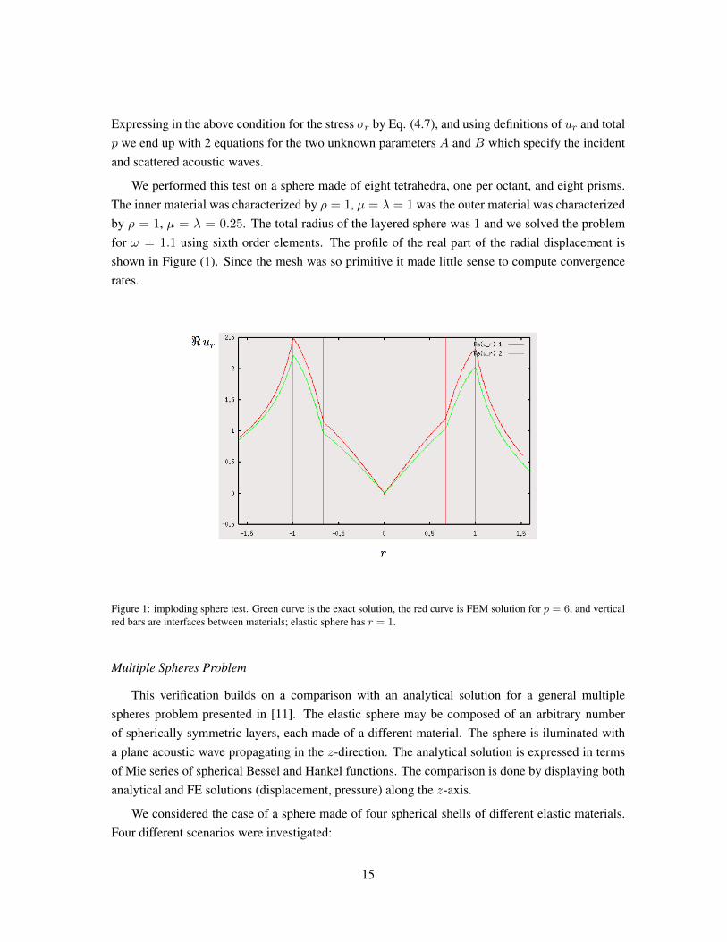
Code verification was one of the most tedious aspect we had to face in this project. We startedwith a simple case of an imploding spherical acoustic wave hitting a sphere composed of two elasticmaterials and comparing the numerical solution to the analytical solution. This was a rather prim-itive test since only eight tetrahedra – one per octant – and eight prisms approximate the elasticsphere, and there is no high contrast between the material constants. The second test dealing witha multilayered elastic sphere illuminated with a aplane way, was considerably more challenging.The FE solution was compared with the analytical Mie series solution in terms of Bessel and Han-kel functions. The test was run for four possible scenarios with different material constants anddifferent number of elements.

An Imploding Sphere Problem

The first verification test was performed by hitting the elastic sphere with an imploding sphericalacoustic wave. An analytical solution of the elastic displacement u can be easily derived. We

13

postulate a spherically-symmetric solution of the form ui = xif(r) cosωt which implies that

ur = rf(r) cosωt

After we introduce the displacement into the Navier-Stokes equations of elastodynamics

µuj,kk + (λ+ µ)uk,kj = %uj

we find a differential equation for f which has the non singular solution

f(r) = Ckr cos kr − sin kr

r3

where k2 = %ω2/(2µ + λ) and C is a constant. By means of Hook’s law, the stress correspondingto u is:

σrr = 2µ∂ur∂r

+ λ

(2urr

+∂ur∂r

). (4.7)

Let’s now consider the acoustic pressure p. If we assume a time-harmonic solution of the homoge-neous wave equation, then p = p(xi) satisfies the Helmholtz equation of acoustics:

−∆p− k′2p = 0

where k′ is the wavenumber. Again, if we assume a spherically-symmetric solutions we have(∂2

∂r2+

2

r

∂

∂r+ k′2

)p = 0

and after applying the substitution p = f/r we obtain that f satisfies the simple equation

f ′′ + k′2f = 0

which implies that f = Aeik′r + Be−ik

′r and p = (Aeik′r + Be−ik

′r)/r. We may call the abovetwo componets of p as the incident, pin, and the scattered wave, psc, respectively.

One way to obtain the spherically-symmetric solution of coupled elastodynamics and acousticsis to assume the incident acoustic wave (parameter A), and evaluate the scattered acoustic wave(parameter B) and amplitude of vibrations in the solid (parameter C), so that adequate continuityconditions between solid and fluid are satisfied. Alternatively, we can prescribe the vibrations ofthe solid (by setting, for instance, C = 1), and find the incident and scattered acoustic waves(parameters A and B). We follow the second approach. Thus we assume the solution in the solidas:

ur =k

rcos kr − 1

r2sin kr

The coupling conditions on the surface of the solid sphere, at r = a, satisfy:

Continuity:∂p

∂r= ω2%fur(a)

Equilibrium: σr(a) = −p(a)

14

Expressing in the above condition for the stress σr by Eq. (4.7), and using definitions of ur and totalp we end up with 2 equations for the two unknown parameters A and B which specify the incidentand scattered acoustic waves.

We performed this test on a sphere made of eight tetrahedra, one per octant, and eight prisms.The inner material was characterized by ρ = 1, µ = λ = 1 was the outer material was characterizedby ρ = 1, µ = λ = 0.25. The total radius of the layered sphere was 1 and we solved the problemfor ω = 1.1 using sixth order elements. The profile of the real part of the radial displacement isshown in Figure (1). Since the mesh was so primitive it made little sense to compute convergencerates.

Figure 1: imploding sphere test. Green curve is the exact solution, the red curve is FEM solution for p = 6, and verticalred bars are interfaces between materials; elastic sphere has r = 1.

Multiple Spheres Problem

This verification builds on a comparison with an analytical solution for a general multiplespheres problem presented in [11]. The elastic sphere may be composed of an arbitrary numberof spherically symmetric layers, each made of a different material. The sphere is iluminated witha plane acoustic wave propagating in the z-direction. The analytical solution is expressed in termsof Mie series of spherical Bessel and Hankel functions. The comparison is done by displaying bothanalytical and FE solutions (displacement, pressure) along the z-axis.

We considered the case of a sphere made of four spherical shells of different elastic materials.Four different scenarios were investigated:

15

(P1) low contrast material constants and many prismatic layers within each elastic spherical shell,see Table (2);

(P2) low contrast material constants and fewer prismatic layers within each elastic spherical shell,see Table (3);

(P3) high contrast material constants and many prismatic layers within each elastic spherical shell,see Table (4);

(P4) high contrast material constants and fewer prismatic layers within each elastic spherical shell,see Table (5).

Problems (P1) and (P3) are quite large - the number of d.o.f. ramps up to 5 million d.o.f for p = 6,while problems (P2) and (P4) are a bit smaller with 2.5 million d.o.f for p = 6. We were able tosolve problem (P1) and (P3) with p = 2, 3, 4 and problem (P2) and (P4) with p = 2, 3, 4, 5 in thelow frequency regime ω = 1.1. For all four cases we have obtained a perfect matching with theanalytical solution for all p’s as it can be seen from Figures ??, and 5.

(a) real part of the radial displacement (b) imaginary part of the radial displacement

Figure 2: problem (P1). Radial component of the elastic displacement; the vertical red lines represents the interfacesbetween the 4 materials.

5. Numerical Experiments

5.1. Geometry

Our simplified model of the head is constituted by 19288 elements: 16004 tetrahedra, 3228prisms and 56 pyramids. As previously discussed, the pyramid is needed as a connecting elementbetween a tetrahedron and a prism. The total number of nodes is 89961. The fully curvilineargeometry reconstructed by our code is shown in Figure 6. We solved the problem for 13 different

16

(a) real part of the radial displacement (b) imaginary part of the radial displacement

Figure 3: problem (P2). Radial component of the elastic displacement; the vertical red lines represents the interfacesbetween the 4 materials.

Shell Material # of layers Density Young modulus, Poisson ration Radius% <E =E < ν = ν r

I a - 1.0 0.625 0.0 0.2 0.0 0.3II a 1 1.0 0.625 0.0 0.2 0.0 0.37III b 3 1.0 2.5 0.0 0.25 0.0 0.58IV c 3 0.3 0.5 0.0 0.2 0.0 0.79V d 3 2.0 5.0 0.0 0.3 0.0 1.0VI air 4VII PML 2

Table 2: problem (P1). Four ideal materials with material constants of same order of magnitude are considered.

incident directions of an acoustic plane wave; they correspond to increments of π/12 in the (x, y)-plane starting from (0,−1, 0). We were able to solve the problem for p = 2, 3, 4, 5; in the case ofp = 5 the system has 1070190 degrees of freedom.

5.2. Results

We computed the pressure of the lower and upper interface of the basilar membrane with thecochlea as a function of the incidence. The results as shown in Figure 7 and 8; notice that we areobtaining very good agreement for p = 3, 4, 5 for all incident directions. As seen from Figure 7(a)and 7(c) the results we obtained for p = 2 is totally off. We observed a similar behavior for theimaginary part of the pressure, hence the results for case p = 2 are not shown in Figure 8. A possibleexplanation of the poor results for p = 2 is that membranes lock for this order of approximation.This is one the many reason why the use of high order elements is essential for a successful studyof the phenomenon.

17

Shell Material # of layers Density Young modulus, Poisson ration Radius% <E =E < ν = ν r

I a - 1.0 0.625 0.0 0.2 0.0 0.45II b 1 1.0 2.5 0.0 0.25 0.0 0.56III c 2 0.3 0.5 0.0 0.2 0.0 0.78IV d 2 2.0 5.0 0.0 0.3 0.0 1.0V air 3VI PML 2

Table 3: problem (P2). Four ideal materials with material constants of same order of magnitude are considered.

(a) real part of the radial displacement (b) real part of the radial displacement in the sphere

(c) imaginary part of the radial displacement (d) imaginary part of the radial displacement in the sphere

Figure 4: Radial component of the elastic displacement; the vertical red lines represents the interfaces between the 4materials.

6. Conclusions and Future Work

Geometry.. As mentioned in Section 3, we have not managed to fully automate the process ofdefining the geometry. To make it worse, our code still contains a “prayer component”. NETGENchecks the shape regularity of generated tetrahedra but does it only for affine simplices. After the

18

(a) real part of the radial displacement (b) real part of the radial displacement in the sphere

(c) imaginary part of the radial displacement (d) imaginary part of the radial displacement in the sphere

Figure 5: Radial component of the elastic displacement; the vertical red lines represents the interfaces between the 4materials.

Shell Material # of layers Density Young modulus, Poisson ration Radius% <E =E < ν = ν r

I tissue - 835.4 29616.41 1.952 1.388 E-5 2.876 E-5 0.56II tissue 1 835.4 29616.41 1.952 1.388 E-5 2.876 E-5 0.7III skull 3 1.0 2.6 0.0 0.3 0.0 0.784IV cork 3 150.0 539.715 0.0 0.173 0.0 0.964V steel 3 6666.7 5964829.39 0.0 0.355 0.0 1.0VI air 4VII PML 2

Table 4: problem (P3). Four materials with material constants of different order of magnitude are considered.

upgrade to curvilinear geometry, we pray that the generated maps have no negative jacobians as wehave no guarantee that this will not happen. Indeed, generating the model discussed in this papertook a couple of iterations with NETGEN. Quality assurance for the geometrical model generationshould be done within the mesh generator and it requires a more tied interface between NETGEN

19

Shell Material # of layers Density Young modulus, Poisson ration Radius% <E =E < ν = ν r

I tissue - 835.4 29616.41 1.952 1.388 E-5 2.876 E-5 0.7II skull 1 1.0 2.6 0.0 0.3 0.0 0.784III cork 2 150.0 539.715 0.0 0.173 0.0 0.964IV steel 2 6666.7 5964829.39 0.0 0.355 0.0 1.0V air 3VI PML 2

Table 5: problem (P4). Four materials with material constants of different order of magnitude are considered.

and GMP.

On the positive side, once the geometry has been defined, we can use it for multiple FE sim-ulations involving different loads and material data, as the control of discretization error is donethrough local p- or h-refinements rather than multiple mesh regenerations.

hp refinements.. Examples presented in this paper have been obtained using p-refined meshes only.The use of higher order elements is absolutely critical for succesful simulations of the discussedproblem as the difference between the results obtained using quadratic and higher order elementsindicates locking. This suggests starting with p = 3, at least for the thin-walled subdomains in theproblem (membranes, skull). We have not experimented yet with (local) p-adaptivity.

We are in process of adding h-refinements to the code. This challenging extension of the code in-cludes development of data structure algorithms for supporting the refinements and the constrainedapproximation package. The main challenge here are the complexity of the algorithms (code) andtheir efficiency. We pursue the idea of data structures and algorithms based on FE nodes [2, 4] butwith some non-trivial modifications, and we hope to report soon on this part of the work.

Parallel solver.. Even the simplest verification examples reported in this paper, involve solutionof systems of equations with many milion d.o.f. and large fronts resulting from the use of higherorder elements. This necessitated the development of the parallel direct solver without which noneof the more complicated examples could be solved. The solver, builds on the idea of the nodaltrees borrowed from our hp3D data structures but it is being developed as an independent piece ofsoftware that could be interfaced with other FE codes.

Bone conduction study.. The actual parameter and sensitivity study on the presented problem us-ing the described geometrical model, will be reported in a forthcoming second part of this paper.Our ultimate goal includes building a more complicated geometry model from MRI scans usinggeometry reconstruction techniques [3].

20

(a) skull (b) cross section of skull

(c) middle ear

Figure 6: head model. Mesh has 19288 elements.

AppendixA. Formulation of the Coupled Elasticity/Acoustics Problem

In this opening section, we review the derivation of the variational formulations for acoustics,elasticity and then for the ultimate coupled elasticity/acoustics problem.

AppendixA.1. Linear Acoustics Equations

The classical linear acoustics equations are obtained by linearizing the isentropic form of thecompressible Euler equations expressed in terms of density ρ and velocity vector vi, around the

21

Figure 7: pressure on lower interface of basilar membrane.

Figure 8: pressure on upper interface of basilar membrane.

hydrostatic equilibrium position ρ = ρ0, vi = 0. Perturbing the solution around the equilibriumposition,

ρ = ρ0 + δρ, vi = 0 + δvi,

22

and linearizing the Euler equations, see e.g. [12], we obtain a system of four first order equations interms of unknown perturbations of density δρ and velocity δvi,

(δρ),t + ρ0(δvj),j = 0

ρ0(δvi),t + (δp),i = 0 ,

with δp denoting the perturbation in pressure. For the isentropic2 flow, the pressure is simply analgebraic function of density,

p = p(ρ)

Linearization around the equilibrium position leads to the relation between the perturbation in den-sity and the corresponding perturbation in pressure

p = p(ρ0)︸ ︷︷ ︸p0

+dp

dρ(ρ0)δρ

Here p0 is the hydrostatic pressure, and the derivative dpdρ(ρ0) is interpreted a posteriori as the sound

speed squared, and denoted by c2. Consequently, the perturbation in pressure and density are relatedby the simple linear equation,

δp = c2δρ

It is customary to express the equations of linear acoustics in pressure rather than density. Droppingdeltas in the notation, we obtain,

c−2p,t +ρ0vj,j = 0

ρ0vi,t +p,i = 0

In this report, we shall consider only time-harmonic problems. Assuming ansatz,

p(t,x) = eiωtp(x), ui(t,x) = eiωtui(x) ,

we reduce the acoustics equations to,c−2iωp +ρ0vj,j = 0

ρ0iωvi +p,i = 0

or in the operator form, c−2iωp +ρ0∇ · v = 0

ρ0iωvi +∇p = 0(A.1)

2The entropy is assumed to be constant throughout the whole domain

23

Eliminating the velocity, we obtain the Helmholtz equation for the pressure,

−∆p− k2p = 0 ,

with the wave number k = ω/c.

Having obtained the second order problem, we can proceed now with the derivation of the weakformulation, as it is usually done in most of text books on the subject. It is a little more iluminatingto obtain the same variational formulation starting with the first order system. First of all, we make aclear choice in a way we treat the two equations. The equation of continuity (conservation of mass)is going to be satisfied only in the weak sense, i.e. we multiply it with a test function q, integrateover domain Ω and integrate the second term by parts to obtain,∫

Ω

(iω

c2pq − ρ0v∇q

)dx+ ρ0

∫Γvnq dS = 0, ∀q (A.2)

Here vn = vjnj denotes the normal component of the velocity on the boundary.

The second equation (conservation of momentum) is satisfied in the strong sense, i.e. pointwise.Solving for the velocity, we get,

v = − 1

ρ0iω∇p (A.3)

In particular, the normal component of the velocity is related to the normal derivative of the pressure,

vn = − 1

ρ0iω

∂p

∂n

At this point we introduce different boundary conditions:

• a soft boundary ΓD,p = p0

• a hard boundary ΓN ,vn = v0

• and an impedance condition with a constant d > 0,

vn = dp+ v0

Multiplying Equation A.2 with iω, substituting the boundary data into the boundary term, and elim-inating the velocity in the domain integral term, using formula A.3, we get the final variationalformulation.

p = p0 on ΓD∫Ω

(∇p∇q −

(ωc

)2pq

)dx+ iωρ0d

∫ΓC

pq dS = −∫

ΓN∪ΓC

v0q dS

∀q : q = 0 on ΓD

(A.4)

24

We have obtained the weak formulation without introducing the second order problem at all! Wehave a clear understanding which of the starting equations is understood in the weak, and whichin a strong sense. The momentum equations, consistently with their pointwise interpretation, havebeen extended to the boundary to yield the appropriate boundary conditions. We mention only thatall these considerations can be made more precise by introducing the language of distributions andSobolev spaces.

AppendixA.2. Linear Elasticity

The time-harmonic linear elasticity equations include:

• balance of momentum,−ρω2ui − σij,j = fi

• Cauchy displacement-strain relation,

εij =1

2(ui,j + uj,i)

• consititutive law,σij = Eijklεkl

The tensor of elasticities satisfies the usual symmetry assumptions,

Eijkl = Ejikl, Eijkl = Eijlk, Eijkl = Eklij .

In the case of an isotropic material,

Eijkl = µ(δikδjl + δilδjk) + λδijδkl

and the constitutive law reduces to the Hooke’s law,

σij = 2µεij + λεkkδij

Utilizing the Cauchy geometric relations, we eliminate the strain tensor and represent the stressesdirectly in terms of the displacement gradient,

σij = Eijkluk,l (A.5)

or, for the Hooke’s law,σij = µui,j + λuk,kδij (A.6)

The momentum equations will be satisfied in the weak sense. We multiply them with a test functionvi, integrate over Ω and integrate by parts to obtain,∫

Ω

(σijvi,j − ρω2uivi

)dx−

∫Γσijnjvi dS =

∫Ωfivi dx, ∀vi (A.7)

We introduce now the boundary conditions,

25

• prescribed displacements on ΓD,ui = ui,D

• prescribed tractions on ΓN ,ti := σijnj = gi

• prescribed impedance on ΓC ,ti + βijuj = gi

We restrict ourselves now to vi = 0 on ΓD, substitute the boundary data into the boundary term inEquation A.7, to obtain,∫

Ω

(σijvi,j − ρω2uivi

)dx+

∫ΓC

βijujvi dS =

∫Ωfivi dx+

∫ΓN∪ΓC

givi dS

∀vi : vi = 0 on ΓD

The final variational formulation is obtained by substituting formula A.5 for stresses,ui = ui,D on ΓD∫

Ω

(Eijkluk,lvi,j − ρω2uivi

)dx+

∫ΓC

βijujvi dS =

∫Ωfivi dx+

∫ΓN∪ΓC

givi dS

∀vi : vi = 0 on ΓD

(A.8)

We record the final fomulas for the bilinear and linear forms.

X = H1(Ω) := (H1(Ω))3

b(u,v) =

∫Ω

(Eijkluk,lvi,j − ρω2uivi

)dx+

∫ΓC

βijujvi dS

l(v) =

∫Ωfivi dx+

∫ΓN∪ΓC

givi dS

(A.9)

AppendixA.3. Elasticity Coupled with Acoustics

Let Ω be a domain in IR3. In the following discussion we shall assume that the domain Ω isbounded. The case of an unbounded domain will be discussed in Chapter ??. We assume thatΩ is split into two disjoint parts: a subdomain Ωe occupied by a linear elastic medium, and asubdomain Ωa occupied by an acoustical fluid. The two subdomains are separated by an interfaceΓI . Neither the subdomains nor the interface need to be connected (they may consist of severalseparate pieces). The external boundary ∂Ω will be partitioned into Dirichlet, Neumann and Cauchyparts: ΓD,ΓN ,ΓC , respectively. Each of these boundary parts may consist of a part belonging to theboundary ∂Ωe of the elastic subdomain, or the boundary ∂Ωa of the acoustical subdomain. Using amore precise mathematical language, Ωe,Ωa are assumed to be opened and disjoint and,

Ω = Ωe ∪ Ωa .

26

Similarly, elastic and acoustics parts of the Dirichlet boundary: ΓDe,ΓDa, of the Neumann bound-ary: ΓNe,ΓNa, and the Cauchy boundary: ΓCe,ΓCa, are open submanifolds of ∂Ω and,

∂Ω = ΓDe ∪ ΓDa ∪ ΓNe ∪ ΓNa ∪ ΓCe ∪ ΓCa ,

as well as,∂Ωe = ΓI ∪ ΓDe ∪ ΓNe ∪ ΓCe ∂Ωa = ΓI ∪ ΓDa ∪ ΓNa ∪ ΓCa .

A two-dimensional illustration of the scenario is shown in Figure A.9.

Figure A.9: Topology of a coupled problem

The coupled problem involves solving linear elasticity equations discussed in Section AppendixA.2satisfied in subdomain Ωe coupled with the equations of linear acoustics discussed in Section AppendixA.1and satisfied in subdomain Ωa. The unknowns include the components of the displacement vectorui(x),x ∈ Ωe and the acoustical pressure p(x),x ∈ Ωa. The two sets of equations are accompa-nied by appropriate boundary conditions and coupled by the following interface conditions:

iωuini = vini = − 1

ρf iω

∂p

∂xini, ti = σijnj = −pni

The first equation above expresses the continuity of normal component of the velocity: the normalelastic velocity has to match the normal component of the acoustical velocity. The second equation

27

expresses the continuity of stresses: the normal elastic stress must be equal to the (negative) pres-sure, whereas the tangential component of the elastic stress vector is set to zero, since the fluid doesnot support a shear stress. As usual, ω is the angular frequency, i is the imaginary unit, ρf standsfor the density of the fluid, and ni denote components of a unit vector normal to interface ΓI whichwe will assume to be directed from the elastic into the acoustical subdomain. Multiplying the firstinterface condition by ρf iω, we get,

ρfω2un =

∂p

∂n, ti = σijnj = −pni (A.10)

where un = uini denotes the normal displacement. From the mathematical point of view, theconditions of this type are classified as weak coupling conditions. The word “weak” refers hereto the fact that the primary variable for elasticity - the displacement vector, matches the secondaryvariable (the flux) for the acoustic problem - the normal velocity which is related to the normalderivative of pressure. Conversely, the primary variable for the acoustic problem - the pressure,defines the flux for the elasticity problem. This “cross-coupling” is very essential in proving thewell-posedness of the problem, and stability of Galerkin approximations.

On top of the interface conditions we have the usual boundary conditions for acoustics,

• prescribed pressure on ΓDa,p = pD

• prescribed normal velocity on ΓNa,vn = v0

• an impedance condition with an impedance constant d > 0 on ΓCa,

vn = dp+ v0

and for the elasticity,

• prescribed displacements on ΓDe,ui = ui,D

• prescribed tractions on ΓNe,ti := σijnj = gi

• prescribed impedance on ΓCe,ti + iωβijuj = gi

28

We proceed now with the derivation of the variational formulation. We start with the weak formof the continuity equation for acoustics,∫

Ωa

(iω

c2pq − ρfv∇q

)dx+ ρf

∫∂Ωa

vnq dS = 0, ∀q

and the weak form of the conservation of momentum for elasticity,∫Ωe

(σijvi,j − ρsω2uivi

)dx−

∫∂Ωe

σijnjvi dS =

∫Ωe

fivi dx, ∀vi

with ρs and fi denoting the density of solid and body forces, respectively. Boundary ∂Ωa of theacoustic subdomain is now split into the interface ΓN and parts ΓDa,ΓNa,ΓCa. For the interfaceΓI , we use the first interface condition to replace the flux term ρfvn with iωρfun, and proceed inthe standard way with the acoustic boundary conditions, to obtain the variational statement,

p = pD on ΓDa∫Ωa

(iω

c2pq +

1

iω∇p∇q

)dx+

∫ΓCa

ρfd pq dS +

∫ΓI

iωρfun q dS =

∫ΓNa∪ΓCa

ρfv0q dS,

∀q : q = 0 on ΓDa

Similarly, boundary ∂Ωe of the elastic subdomain is split into the interface ΓN and parts ΓDe,ΓNe,ΓCe.For the interface ΓI , we use the second interface condition to replace the flux term σijnj with−pni,and use the boundary conditions to obtain the variational statement,u = uD on ΓDe∫

Ωe

(Eijkluk,lvi,j − ρsω2uivi

)dx+ iω

∫ΓCe

βijujvi dS +

∫ΓI

pvn dS =

∫Ωe

fivi dx+

∫ΓNe∪ΓCe

givi dS,

∀v : v = 0 on ΓDe

Multiplying the variational statement for acoustics by factor iω, we get the final variational formu-lation for the coupled problem in the form,

u ∈ uD + V , p ∈ pD + V,

bee(u,v) + bae(p,v) = le(v), ∀v ∈ V

bea(u, q) + baa(p, q) = la(q), ∀q ∈ V

(A.11)

where:

29

• the bilinear and linear forms are given by the formulas:

bee(u,v) =

∫Ωe

(Eijkluk,lvi,j − ρsω2uivi

)dx+ iω

∫ΓCe

βijujvi dS

bae(p,v) =

∫ΓI

pvn dS

bea(u, q) = −ω2ρf

∫ΓI

unq dS

baa(p, q) =

∫Ωa

(∇p∇q − k2pq

)dx+ iω

∫ΓCa

ρfd pq dS

le(v) =

∫Ωe

fivi dx+

∫ΓNe∪ΓCe

givi dS

la(q) = iωρf

∫ΓNa∪ΓCa

v0q dS ,

(A.12)

• uD ∈ H1(Ωe) := (H1(Ωe))3 is a finite energy lift of displacements uD prescribed on ΓDe,

pD ∈ H1(Ωa) is a finite enery lift of pressure pD prescribed on ΓDa,

• V and V are the spaces of the test functions,

V = v ∈H1(Ωe) : v = 0 on ΓDe

V = q ∈ H1(Ωa) : q = 0 on ΓDa(A.13)

• k = ω/c is the acoustic wave number.

Coupled problem A.11 is symmetric if and only if diagonal forms bee and baa are symmetric and,

bae(p,u) = bea(u, p) .

Thus, in order to enable the symmetry of the formulation3, we need to rescale problem by, forinstance, dividing the second equation by factor −ω2ρf .

[1] M. Ainsworth and J. Coyle. Hierarchic finite element bases on unstructured tetrahedralmeshes. Int. J. Num. Meth. Eng., 58(14):2103–2130, December 2003.

[2] L. Demkowicz. Computing with hp Finite Elements. I.One- and Two-Dimensional Elliptic andMaxwell Problems. Chapman & Hall/CRC Press, Taylor and Francis, October 2006.

[3] L. Demkowicz, P. Gatto, W. Qiu, and A. Joplin. G1-interpolation and geometry reconstructionfor higher order finite elements. Comput. Methods Appl. Mech. Engrg., 2008. published online:http://dx.doi.org/10.1016/j.cma.2008.05.026.

3This is essential, among other reasons, from the point of view of using a direct solver.

30

[4] L. Demkowicz, J. Kurtz, D. Pardo, M. Paszynski, W. Rachowicz, and A. Zdunek. Computingwith hp Finite Elements. II. Frontiers: Three-Dimensional Elliptic and Maxwell Problems withApplications. Chapman & Hall/CRC, October 2007.

[5] L. Demkowicz, J. Kurtz, and F. Qiu. hp-adaptive finite elements for coupled multiphysicswave propagation problems. In M. Kuczma and K. Wilmanski, editors, Computer Methods inMechanics - Lectures of the CMM 2009. Springer Verlag, 2009. in print.

[6] W. Dong and E.S. Olson. Supporting evidence for reverse cochlear traveling waves. J. Acoust.Soc. Am., pages 222–240, 2008.

[7] Bohnke F. and W. Arnold. Bone conduction in a three-dimensional model of the cochlea.Journal of Oto-Rhino-Laryngology, 68(6):393–396, 2006.

[8] Bekesy G. Vibration of the head in a sound field and its role in hearing by bone conduction.The Journal of the Acoustical Society of America, 20(6):749–760, 1948.

[9] G.N. Gatica, A. Marquez, and S. Meddahi. Analysis of the coupling of primal and dual-mixedfinite element methods for a two-dimensional fluid-solid interaction problem. SIAM J. Numer.Anal., 45(5):2072–2097, 2007.

[10] P. Gatto and L. Demkowicz. Construction of h1-conforming hierarchical shape functions forelements of all shapes and transfinite interpolation. Technical Report 14, ICES, 2009. FiniteElements in Analysis and Design, in review.

[11] Bleszynski M. and Bleszynski E. Mie series solution for a coupled acoustics/elasticity multa-layer speher problem, 2009.

[12] A. Majda. Compressible Fluid Flow and Systems of Conservation Laws in Several SpaceVariables, volume 53 of Applied Mathematical Sciences. Springer-Verlag, New York, 1984.

[13] Ch. Michler, L. Demkowicz, J. Kurtz, and D. Pardo. Improving the performance of perfectlymatched layers by means of hp-adaptivity. Numer. Meth. Part. D. E., 2007. published online26 April 2007 in Wiley InterScience.

[14] H.H. Nakajima, W. Dong, E.S. Olson, S.N. Merchant, M.E. Ravicz, and J.J. Rosowski. Differ-ential intracochlear sound pressure measurements in normal human temporal bones. Journalof the Association for Research in Otolaryngology, 10(1):23–36, 2009.

[15] M.E. Ravicz, E.S. Olson, and J.J. Rosowski. Sound pressure distribution and energy flowwithin the gerbil ear canal from 100 hz to 80 khz. J. Acoust. Soc. Am., 122:2154–2173, 2007.

[16] J. Schoberl. NETGEN - An advancing front 2D/3D-mesh generator based on abstract rules.Comput.Visual.Sci, 1:41–52, 1997. available from ( http://www.hpfem.jku.at/netgen/).

31

[17] J. Schoberl and S. Zaglmayr. High order nedelec elements with local complete sequenceproperty. COMPEL: International Journal for Computation and Mathematics in Electricaland Electronic Engineering, 24(2), 2005.

[18] W. Schroeder, K. Martin, and B. Lorensen. The Visualization Toolkit: An Object-OrientedApproach To 3D Graphics. Kitware, Inc., 4th edition edition.

[19] S. Stenfelt and Goode R.L. Bone-conducted sound: Physiological and clinical aspects. Otol-ogy and Neurotology, 2005.

[20] B.A. Szabo and I. Babuska. Finite Element Analysis. Wiley, New York, 1991.

[21] R. Tews and W. Rachowicz. Application of an automatic hp adaptive finite element method forthin-walled structures. Comput. Methods Appl. Mech. Engrg., 198(21-26):1967–1984, 2009.

32