Ann Reg Sci (2014) 53:423–452DOI 10.1007/s00168-014-0616-2

SPECIAL ISSUE PAPER

Modeling knowledge networks in economic geography:a discussion of four methods

Tom Broekel · Pierre-Alexandre Balland ·Martijn Burger · Frank van Oort

Received: 4 December 2013 / Accepted: 22 May 2014 / Published online: 10 June 2014© Springer-Verlag Berlin Heidelberg 2014

Abstract The importance of network structures for the transmission of knowledgeand the diffusion of technological change has been recently emphasized in economicgeography. Since network structures drive the innovative and economic performanceof actors in regional contexts, it is crucial to explain how networks form and evolve overtime and how they facilitate inter-organizational learning and knowledge transfer. Theanalysis of relational dependent variables, however, requires specific statistical proce-dures. In this paper, we discuss four different models that have been used in economicgeography to explain the spatial context of network structures and their dynamics.First, we review gravity models and their recent extensions and modifications to dealwith the specific characteristics of networked (individual level) relations. Second, wediscuss the quadratic assignment procedure that has been developed in mathemati-cal sociology for diminishing the bias induced by network dependencies. Third, wepresent exponential random graph models that not only allow dependence betweenobservations, but also model such network dependencies explicitly. Finally, we dealwith dynamic networks, by introducing stochastic actor-oriented models. Strengths

T. Broekel (B)Institute of Economic and Cultural Geography, Leibniz University of Hannover,Schneiderberg 50, 30167 Hannover, Germanye-mail: broekel@wigeo.uni-hannover.de

P.-A. Balland · F. van OortDepartment of Economic Geography, Utrecht University, Utrecht, The Netherlandse-mail: p.balland@uu.nl

F. van Oorte-mail: f.g.vanoort@uu.nl

M. BurgerDepartment of Applied Economics, Erasmus University Rotterdam, Rotterdam, The Netherlandse-mail: mburger@ese.eur.nl

123

424 T. Broekel et al.

and weaknesses of the different approach are discussed together with domains ofapplicability the geography of innovation studies.

JEL Classification R11 · O32 · D85

1 Introduction

Knowledge networks play a crucial role in the economic development of regions(Van Oort and Lambooy 2013). R&D collaborations among organizations (Hagedoorn2002), labor mobility (Almeida and Kogut 1999), and personal acquaintances of inven-tors (Breschi and Lissoni 2009) drive innovation activities, technological change, andeconomic performance of organizations and regions. Beyond these iconic channelsof knowledge transfer, the structure of knowledge networks can more generally bedefined as the set of direct and indirect connections that individuals and organizationsuse to access knowledge (within and outside the region). Given the economic valueassociated with the structure of knowledge networks and their striking spatial dimen-sion1, empirical studies of networks have attracted a growing interest in the geographyof innovation over the last twenty years2 (Grabher 2006; Burger et al. 2009a; Maggioniand Uberti 2011; Ter Wal and Boschma 2009).

The increased interest in the empirics of knowledge networks can be seen as aresponse to the traditional metaphorical treatment of networks in economic geographyand regional science in general and the study of agglomeration economics in particular(Sunley 2008). Despite over twenty years of research on the benefits of agglomera-tion, the empirical literature remains inconclusive about the mechanisms and processesthat lead to more than proportional regional economic growth. Despite the fact thatthe micro-foundations (such as knowledge spillovers, labor market pooling, and inputsharing) that underlie agglomeration economies have theoretically been specified,agglomeration is often treated as a black box in empirical studies (Burger et al. 2009a;Van Oort and Lambooy 2013). This is exemplified by the fact that most empiricalstudies on agglomeration economics merely research the relationship between urbanor cluster size and regional economic development (see Melo et al. 2009 and De Grootet al. 2009 for meta-analyses of this literature) and do not examine the different chan-nels through which the concentration of economic activities affect regional economicdevelopment.

The analysis of networks, either formal or informal, can help us to identify thesechannels and get a glimpse of what is in the black box of agglomeration economies(Burger et al. 2009a), hereby extending the current discourse on agglomeration exter-nalities in which new conceptual and methodological approaches are needed (Van Oortand Lambooy 2013). Over the past years, a large literature has developed in economicgeography, regional science, management, and sociology that predominantly address

1 A burgeoning literature starts to integrate the geographical dimension in sociology and network science:see for instance the special issue 34.1 in Social Networks of January 2012 on Capturing Context: IntegratingSpatial and Social Network Analysis, edited by Jimi Adams, Katherine Faust and Gina Lovasi.2 See the special issue 43.3 in The Annals of Regional Science of September 2009 on Embedding NetworkAnalysis in Spatial Studies of Innovation, edited by Edward Bergman.

123

Modeling knowledge networks in economic geography 425

the determinants of knowledge and information transfer, focusing on spinoff firms,labor mobility and R&D collaboration (Boschma and Frenken 2006). One of the mainfindings of this literature is that firms in agglomerations do not profit automaticallyfrom colocation. Instead, knowledge spillovers mainly take place between firms thatare networked and strongly locally embedded. A second finding that has come out ofthis strand of research is that a substantial part of information and knowledge transfertakes place over longer distances as firms have many network relations outside the cityor cluster they are located in. From this, it evidently follows that cities and clustersare not spatially isolated entities, but embedded in a system of cities. In the end, anexplicit focus on the transfer and network mechanisms of knowledge diffusion cannot only help us to identify the channels through which firms benefit from agglom-eration, but also help us to identify (1) which firms profit from knowledge spilloversand (2) the spatial extent of information and knowledge transfer. These are importantingredients of current innovation and network-based (“smart”) growth strategies in theEuropean Union (Thissen et al. 2013). In the European Union, knowledge networks,free movement of knowledge workers, information flows, and knowledge-based coop-eration opportunities in research and development are hypothesized to contribute tolocal innovation opportunities by academics and policymakers alike (Hoekman et al.2009; Balland et al. 2013). Without a network perspective on knowledge, trade, andinvestments, a proper assessment of place-based growth strategies as advocated by theEuropean Union (Barca et al. 2012) is impossible (Thissen et al. 2013).

In this light, the increased attention for modeling the determinants of networkformation is very much needed, especially in order to get a fully fledged understand-ing of information and knowledge transfer in and across regions. It enables us toexplain why individuals, organizations, and regions differ in their embeddedness ininformation and knowledge networks, why they vary in their learning and innovationcapabilities, and whether this results in variation in their performance. Analyzing theformation and evolution of network structures, however, is more complex than com-puting structural descriptive statistics like degree, betweenness, clustering coefficient,or average geodesic distance. Explaining the structure of knowledge networks requiresan inferential statistics framework, where the dependent variable is related to the over-all structure of the network. Even when networks are decomposed to their smallestunit, the dyad, relational data does not fit well into traditional regression frameworks.A fundamental property of network structures lies in the existence of conditionaldependencies between observations, especially between dyads that have actors incommon (Linders et al. 2010). By nature, such network dependencies violate standardstatistical inference procedures that assume independence among observations. Butmore than only correcting for such dependencies, the main challenge is to use theinformation included in these dependencies to model structural predictors of networkformation.

In this paper, we provide a discussion of the main empirical strategies that have beenproposed recently in economic geography to explain the formation and structure of net-works. Although these strategies are briefly mentioned in a few methodological papers(Ter Wal and Boschma 2009; Broekel and Hartog 2013a; Maggioni and Uberti 2011),a global discussion of their respective range of applicability, strengths, and weaknessesin the context of economic geography is still missing. We believe such a discussion to

123

426 T. Broekel et al.

be useful for economic geographers and regional scientists aiming at modeling net-work formation, especially because the different models have emerged out of differentscientific traditions. Moreover, they are often based on different assumptions, vary interms of conceptual and empirical issues (like micro–macro relations, network dynam-ics, and network-geography interdependencies), and frequently require different typesof relational data. This paper provides a discussion and an introduction to four maintypes of empirical strategies: gravity models (GM), quadratic assignment procedures(QAP), exponential random graph models (ERGMs), and stochastic actor-orientedmodels (SAOMs).

Section 2 discusses GM, a class of econometric models generally used in economicsto explain the flow between geographical units as a function of supply and demandfactors and the distance between the units. These have recently been extended to dealwith the specific characteristics of network data. To account for more complex networkdependencies, QAP has been developed in mathematical sociology on the principleof bootstrapping procedures. The class of ERGM has been developed on the basis ofa Markov chain to include not only dyadic effects but also structural effects at thenetwork level. Lastly, SAOMs have been introduced again in mathematical sociologyto provide a class of statistical models for network dynamics. This allows for treatingof longitudinal rather than cross-sectional data, and therefore the analysis of changingnetwork relationships.

2 Gravity models

2.1 The history of gravity models

In economic geography and regional economics, network structures are frequentlypredicted and elucidated with an analogy to Newton’s law of universal gravitation.In its most elementary form, the gravity model predicts that the flow or interactionintensity between two objects (e.g., origin and destination) is assumed to be directlycorrelated with the masses of the objects and inversely correlated with the physicaldistance between the objects. More formally,

Ii j = KMβ1

i Mβ2j

dβ3i j

(1)

where Ii j is the interaction intensity between object i and j, K a proportionalityconstant, Mi the mass of the object i (e.g., origin), M j the mass of object j (e.g.,destination), and di j the physical distance between the two objects. β1, β2, and β3 areparameters to be estimated. β1 refers to the potential to generate flows, β2 is relatedto the potential to attract flows, and β3 is an impedance factor reflecting the rate ofincrease of the friction of physical distance.

The first appearance of the gravity model in the social sciences dates back to themid-ninth century when it was applied to the study of human interaction patterns(Carey 1858), who used the analogy to Newton’s law to answer the question why acity was more likely to attract people than a small town.

123

Modeling knowledge networks in economic geography 427

The first empirical studies using the gravity model framework appeared at theend of the nineteenth and early twentieth century, when it was applied to the studyof migration (Ravenstein 1885), railway travel (Lill 1991) , and retail trade (Reilly1931). The modern use of the gravity model was popularized in the school of socialphysics after the Second World War and formalized by Stewart (1948), Isard (1956),and Tinbergen (1962).3 Over the course of the years, the model has been applied to awide variety of spatial interaction patterns, such as international trade, foreign directinvestment, tourism, migration, commuting, and shopping. Within the context of thegeography of innovation and knowledge transfer, the gravity model framework hasbeen used in studies on inter-alia co-inventorship and co-publishing (Maggioni et al.2007; Ponds et al. 2007; Hoekman et al. 2009), citation networks (Peri 2005; Fischeret al. 2006), R&D collaboration through European programs (Scherngell and Barber2009), inventor mobility (Miguélez and Moreno 2013), foreign direct investment inR&D facilities (Castellani et al. 2013), and trade in high-technology products (Liuand Lin 2005). In most empirical research using gravity models, the objects are spatialunits, such as cities, regions, or nations. However, disaggregated data at the firm orindividual level are increasingly employed to assess the spatial dimension of innovationnetworks within a gravity model context (see, e.g., Autant-Bernard et al. 2007; Breschiand Lissoni 2009).4

2.2 The working principles of the gravity model

Unlike the later introduced QAP, ERGM, and SAOM, the gravity model is a conceptualmodel and not just a statistical method.5 Traditionally, the gravity model as presentedin Eq. (1) has been estimated using Ordinary Least Squares (OLS). Taking logarithmsof both sides of Eq. (1) and including a disturbance term, this multiplicative form canbe transformed into a linear stochastic form. It results in a testable Eq. (2), in whichεi j is assumed to be identical and independently distributed (i.i.d):

ln Ii j = ln K + β1 Mi + β2 M j − β3di j + εi j (2)

The model can be extended to a panel data framework, so that it becomes possibleto study the development of relational structures over time. In addition, the empiricalgravity model can be easily augmented to include other factors that influence networkstructures. Accordingly, in most of the above-mentioned studies rather than the New-tonian version but a more general form of the gravity model is used, in which the flowbetween two objects is hypothesized to be dependent on supply factors at the originthat generate flows, demand factors at the destination that attract flows, and by stimu-lating or restraining factors (e.g., proximity or distance) pertaining to the specific flow

3 For an early overview of studies that applied the gravity model in economic geography, see Lukermannand Porter (1960).4 However, the term “gravity model” is not often used when studies are conducted at the micro-level. Ratherscholars research the effect of geographical proximity on network formation.5 In practice, it would be possible to estimate the gravity model with these techniques.

123

428 T. Broekel et al.

between the two objects. For example, it can be argued that the flow of knowledge innetworks of R&D collaboration is not only dependent on the physical distance, but alsoon the cultural, social, and institutional distance between the two regions (Boschma2005). Likewise, it is not only public investments in R&D that generates knowledgeflows, but also the presence of human capital in a region.

However, there are also some serious problems with the traditional OLS specifica-tion of the gravity model. Most importantly, the OLS specification does not controlfor dependencies present in network data nor is it very well able to model networkdependencies. In particular, the traditional equation assumes that flows between twoactors are independent from other relationships between actors within the network.Since this strong assumption of structural independency is very unlikely to hold, thiscan lead to biased estimates of the gravity equation. Two main issues arise: One isthe omitted variables bias (i.e., bias of coefficients) and the other is the clustering oferror components (i.e., bias of standard deviation of coefficients). Although the factthat the flow between two locations is dependent on the characteristics and the numberof alternative locations is well known in the gravity literature (see already the workof Stouffer 1940), this has until recently not been explicitly addressed in empiricalgravity models.

In the recent literature on gravity models, several extensions and modificationsof the gravity model have been proposed to deal with this issue (Gómez-Herrera2013). Although most of these originate from the spatial and international economicsliterature on the gravity model of trade, they can easily be applied to the study ofinnovation networks.6 First, researchers have tried to control for network structureby correcting standard errors. More specifically, use has been made of the sandwichstyle standard errors using multiway clustering on the origin and destination (Lindgren2010) or a spatial error model (Fischer and Griffith 2008; Scherngell and Lata 2013).7

These procedures allow for a more careful modeling of the error structure, controllingfor correlations that may arise in the error terms. However, as pointed out by Snijders(2011), such empirical strategies mainly treat the network as nuisance and do notmodeling network dependencies explicitly. Accordingly, these approaches mainly takecare of error clustering in order to get correct standard deviations of coefficients, butdo not tackle the problem of omitted variable bias.

Second, an empirical strategy to handle omitted variable bias is to include an indi-cator for remoteness Ri to account for third party effects, which proxies the averagetransaction costs faced by a location:

6 Please note that we only discuss problems specifically pertaining to network data. Other problems relatedto, for example, the fact that the outcome is not always a continuous numeric variable and the many zeros inthe network (e.g., Helpman et al. 2008; Burger et al. 2009b) and causality (e.g., Egger 2004) are discussedelsewhere in the literature. Although these are problems that all empirical researchers are facing, a discussionof these issues is beyond the scope of this paper.7 Another (non-spatial) method that controls for the network structure but is not often used in the gravitymodel literature is the multiple regression quadratic assignment procedure (MRQAP). A more elaboratediscussion of this method can be found in the next section.

123

Modeling knowledge networks in economic geography 429

Ri =∑

j

di j(y j/yworld

) (3)

Where the numerator represents the bilateral distance between countries i and j , andthe denominator is for instance the share of country j’s GDP in the world’s GDP (see,e.g., Frankel and Wei 1998; Wagner et al. 2002; Coe et al. 2007).8 The remotenessvariable proxies the full range of potential destinations to a given origin, taking intoaccount the importance of the respective destinations and average distance of a countryto all other countries. The advantage of this empirical strategy is that such a remotenessvariable is easy to construct. However, as indicated by several authors, this empiricalstrategy fails to capture other barriers than distance that may hamper interaction (e.g.,national borders) (Head and Mayer 2014).9

Third and as an alternative strategy to handle omitted variable bias, a fixed-effectsspecification can be employed to deal with the problem of intervening opportunities. Ina cross-sectional setting, this implies including country-specific exporter and importerdummy variables in Eq. (2). Such specification controls for country-specific fixedeffects related to origins and destinations, such as the supply, demand, and origin-and destination-specific transaction costs, which are often difficult to measure, butinfluence the structure of the network. Following Anderson and Wincoop (2003) andFeenstra (2004), such a specification of the gravity equation would be in line withthe theoretical concerns regarding the correct specification of the model and yieldsconsistent parameter estimates for the variables of interest. However, when such astrategy is employed, it is impossible to incorporate any origin- or destination-specific(or individual-specific) factors within a cross-sectional setting. In addition, Behrenset al. (2012) point out that such fixed-effects estimations do not fully capture thespatial interdependence among flows, and hence, the assumption of independence ofobservations might still be violated.

Fourth, there are a couple of other, more complex strategies to deal with structuraldependencies in the gravity model, including estimation of multilateral resistanceterms (Anderson and Wincoop 2003) and a spatial autoregressive moving averagespecification for the gravity model (Behrens et al. 2012).10 These strategies have incommon that they try to model dependencies present in network data directly andare becoming increasingly popular within the gravity modeling literature, especiallywithin the fields of spatial and international economics. Focusing on trade, Andersonand Wincoop (2003) show that bilateral barriers between two countries do not deter-mine the flow of bilateral trade only, but also how easy it is for these countries totrade with the rest of the world. Anderson and Wincoop (2003) try to capture theserelative barriers by including country-specific price indices, called multilateral resis-tance terms, which are estimated using a multi-step nonlinear least squares procedure.However, since the method is computationally intensive, it has not been implemented

8 Comparable alternative specifications of remoteness terms in gravity equations are provided by Helliwell(1997) and Head and Mayer (2000).9 For a more elaborate critique on the use of remoteness indices, see Anderson and Wincoop (2003).10 Less well known but comparable empirical strategies in this respect are provided by Bikker (2010) andLinders et al. (2010).

123

430 T. Broekel et al.

by many researchers, which tend to prefer a fixed-effects estimation using OLS orcount data models.

Although specifications including multilateral resistance terms provide consistentestimates of the gravity model, the specification of Anderson and Wincoop (2003) isunable to deal with spatial interdependence (Behrens et al. 2012). As an alternative,Behrens et al. propose a spatial econometric estimation of the gravity model (e.g.,LeSage and Pace 2008, 2009), accounting for cross-sectional correlations betweenflows and controlling for possible cross-sectional correlations in the error terms, here-with simultaneously addressing both the problem of omitted variables bias and theclustering of error components. Focusing on trade between US and Canadian regions,Behrens et al. (2012) find that the exports of any region to a market negatively dependon the exports from the other regions to that market, which themselves depend on thewhole distribution of bilateral trade barriers. In addition, the model can incorporateheterogeneous coefficients, allowing relationships to vary across units, for example,the distance decay of trade might differ across regions. Along these lines, the modelproposed by Behrens et al. (2012) provides also a subtle link between theory andempirical methods when it comes to trade network research. At the same time, suchempirical strategy can be easily extended to other types of flows to capture struc-tural dependencies in general and spatial competition effects in particular (see, e.g.,LeSage and Pace 2008; LeSage and Polasek 2008; Graaff et al. 2009). Although spatialeconometric approaches incorporating spatial lags of the dependent variable to modelstructural dependencies are becoming increasingly popular in empirical applications,there is, however, still no standard implementation in software packages and moststudies have been conducting using Matlab and the appropriateness and applicabilityof these methods has to be further evaluated.11 For a more elaborate overview of thesemethods the reader is referred to the work by LeSage and Pace (2009) and LeSageand Fischer (2010); an historical overview of these methods is provided by Griffith(2007).

3 Multiple regression quadratic assignment procedure

The empirical strategy involving the multiple regression quadratic assignment proce-dure (MRQAP in the following) starts from a similar viewpoint as the gravity model. Inthe context of economic geography and knowledge networks, the dependent variableof interest is the relational intensity of knowledge exchange between individuals, orga-nizations, or spatial units, such as cities or regions. However, in contrast to the gravitymodel’s conceptual basis, it can be seen as a purely statistical approach to account forstructural dependencies among relational data. In principle, the correction procedurethat is proposed can also be put into a gravity model framework, which, to the bestof our knowledge, has, however, not been done so far. More precisely, the multipleregression quadratic assignment procedure model is a logit or OLS regression model,

11 The mathematical appendix and Matlab codes of the approach by Behrens et al. (2012) can be foundin the Web Appendix of their article, available at the Journal of Applied Econometrics website. Likewise,James LeSage offers a spatial econometrics toolbox at http://www.spatial-econometrics.com/.

123

Modeling knowledge networks in economic geography 431

which incorporates relational variables and considers their inherent interdependencieswhen assessing their statistical relevance.12

MRQAP approaches are applied in a number of studies on inter-organizationalnetworks. However, only recently it found its way into the literature on knowledgenetworks in economic geography. Among the first is the study by Bell (2005) whouses a bivariate quadratic assignment correlation procedures to statistically infer aboutcorrelations between friendship, information, and advice networks among executivesfrom within and outside the Toronto industry cluster. Subsequently, the MRQAP pro-cedure has been used to study the intensity of co-inventing among patent inventorslocated in the region of Jena (Cantner and Graf 2006). It was also used to explorethe relevance of cognitive, social, institutional, and geographical proximity for theknowledge network connecting Dutch organizations active in the field of aerospace(Broekel and Boschma 2012), and to study the relationship between regional flowsof internet hyperlinks, co-patenting relations, EU-funded research collaboration, andthe flow of Erasmus exchange students (Maggioni and Uberti 2007). Nevertheless,MRQAP is much less prominent in this context than gravity models.

3.1 The history of MRQAP

Mantel introduced the quadratic assignment procedure in 1967, when he was workingat the National Cancer Institute in Maryland and reviewed a number of common empir-ical approaches used to identify (non-random) time-space clustering of disease (Mantel1967). The basic statistical problem was the clustering of disease cases in space and intime. While statistical tools were available dealing with spatial or temporal clustering,the simultaneous (two-dimensional) occurrence of the two clustering types remainedan empirical challenge. Mantel proposed an uncorrected correlation coefficient esti-mated as the cross-product of the distances in the two dimensions’ empirical matrices(spatial distances and temporal distances). To overcome the problem of highly inter-related n2 values, Mantel constructed repetitively data sets corresponding to the nullhypothesis of no correlation between the two matrices by permuting the rows andcolumns of the two matrices in the same way and such that the values of any rowand of a column combination remain together (but change their positions within thematrix). If the null hypothesis is correct than these permutations “should be equallylikely to produce a larger or a smaller coefficient” (Schneider and Borlund 2007,p. 7). On this basis, the Mantel test was developed for estimating the correlationbetween any two distances matrices (Mantel and Valand 1970). Although Mantel’sapproach was initially developed for the identification of disease clusters, the proce-dure can without any difficulties be applied to other contexts (Mantel 1967).

Hubert and Schulz (1976) introduced the notion of the “quadratic assignment pro-cedure” as an equivalent to the Mantel test. From there, the test statistics were refinedand generalized in multiple ways (see for a review Hubert (1987)). In social net-work analysis, this approach became popular through the works of Krackhardt (1987,

12 Accordingly, MRQAP is rather a particular permutation method for hypothesis testing and not a modelon its own. However, we will refer to it as model in the following to keep a consistent terminology.

123

432 T. Broekel et al.

1988). He extended the QAP methodology to test the relationship between multiplerelational matrices in a regression framework. Since then, the methodology has beensubject to multiple refinements including among others more advanced approachesto deal with multicollinearity and certain types of autocorrelation (see, e.g., Dekkeret al. 2007).

3.2 The working principles of MRQAP

At its core, a QAP regression is a combination of the Mantel test, i.e., quadraticassignment procedure and a standard OLS or Logit regression. The dependent variableis hereby the matrix of inter-actor relations. Whether to use an OLS or a Logit modeldepends on the available network data. For a valued network, OLS is appropriate whilebinary (0/1) network data require the logit regression. As before, the independentvariables are factors whose influence is to be tested on the structure of the network.

As pointed out in the previous section, network data are characterized by frequentrow/column/block autocorrelation because on dependent observations implying thatstandard tools of inference are therefore invalid. In the style of the Mantel test, Krack-hardt (1987, 1988) therefore suggests comparing the regression statistics to the dis-tribution of such statistics resulting from large numbers of simultaneous row/columnpermutation of the considered variables. The QAP is a permutation- or randomization-based semi-parametric test of dependence between two (matrix) variables of the samedimension. The p value is thereby estimated on the basis of the relative frequency ofthe statistic’s values in the reference distribution (obtained by permutation) that arelarger than or equal to the empirically observed value (Dekker et al. 2007).

In order to apply the quadratic assignment procedure for inference on multipleregression coefficients (MRQAP), a number of approaches have been employed. Cur-rently, the double-semi-partialing approach by Dekker et al. (2007) seems to be thepreferred way. In this approach, the effects of other explanatory variables are par-tialed out from the effect of a focal explanatory variable. The resulting residuals aresubsequently QAP-permutated and included in a regression of the dependent vari-able on all explanatory variables but the focal one giving the reference values for thetest statistics. This approach can be applied to standard ordinary least squares (whenthe network variable is continuous) and logistic regression analysis (when networkvariable is binary). The interpretation of the obtained parameter values then dependson the type of regression function used. The approach is relatively well explored forordinary least square (OLS) regression. Nevertheless, there are still issues that deservefuture research. Among these are spuriousness, multicollinearity, and skewness (seeDekker et al. 2007). In contrast to OLS, rarely any study evaluates the application ofMRQAP for logistic regression.

4 Exponential random graph models

ERG-models are well known and established in many disciplines. For example in bio-sciences, Saul and Filkov (2007) use ERGM to explain the structure of cell networks.

123

Modeling knowledge networks in economic geography 433

Fowler et al. (2009) employ ERGM to model genetic variation in human social net-works in life science. They are also frequently used in sociology and political science,for instance to analyze the structure of networks of friendship networks (Lubbersand Snijders 2007) or political international conflicts (Cranmer and Desmarais 2011).While there are a number of studies that focus on the role geography plays for the for-mation of social networks (see, e.g., Daraganova et al. 2012), ERGM have rarely foundtheir way into the analysis of knowledge networks in economic geography. Recent con-tributions using an ERGM approach include studies on inter-organizational knowledgenetworks in the Dutch aviation industry (Broekel and Hartog 2013a), networks amongbiotechnology organizations as created by participating in the EU Framework Pro-grammes (Hazir and Autant-Bernard 2013), and determinants of cross-regional R&Dcollaboration networks (Broekel and Hartog 2013b).

4.1 The history of ERG-Models

In contrast to the previous approaches, the roots of the ERGMs are more difficultto identify. Surely the work of Solomonoff and Rapoport (1951) on random graphswas fundamental. Solomonoff a physicist and Rapoport a mathematician conductedthe “the first systematic study on what we would now call a random graph”(Newman et al. 2006, p.12). These authors already discussed a number of importantproperties of such graphs (e.g., average component size). However, it took anotherten years before Erdös and Rènyi (1960) finally popularized the concept of randomgraphs. They put forward the Bernoulli random graph distribution, which could beused to estimate configurations of individual links between actors. However, Erdösand Rényi assumed independent links among nodes, which is clearly problematic formany networks. The next major step in the development of ERG-models was the intro-duction of p1 models by Holland and Leinhardt (1981). Holland and Leinhardt (1981)proposed a family of exponential distribution (p1 distribution) that could be used asnull-hypothesis for assessing real-world networks (conditional on the density of thenetwork and the number of links to and from a node). In a direct comment to Hollandand Leinhardt’s article, Fienberg and Wasserman (1981) showed that these models canalso be estimated using log-linear modeling techniques, which significantly increasedthe use of p1 models. However, the p1 approach is troubled by the assumption ofdyad-independence that is frequently found to be incorrect (Newman 2003).

Another major breakthrough was the work by Besag (1974, 1975) who showed thata class of probability distributions existed, which are consistent with the (Markovian)condition that the value of one node is dependent only on the values of its adjacentneighbors.13 On this basis, the seminal work by Ove and Strauss (1986) proposed theuse of Markov random graphs to overcome the problems related to dyad-independencemade in p1 models. In the context of networks, Markov dependence is used to modela link between node A and B being contingently dependent on other possible linksof A and B. This marked a significant shift from dyad-independence as two links are

13 Besag (1974, 1975) applied this idea the context of spatial data the idea is, however, also applicable inthe context of network data.

123

434 T. Broekel et al.

assumed to be conditionally (Markov) dependent (Robins et al. 2007). However, thisassumption of Markov dependence might be theoretically correct but frequently doesnot hold empirically (Snijders et al. 2006). Hence, this issue is still subject of futureresearch.

Park and Newman (2004) link ERGM to kinetic mechanics and prove that they “arenot merely an ad hoc formulation studied primarily for their mathematical convenience,but a true and correct extension of the statistical mechanics of Boltzmann and Gibbsto the network world” (Park and Newman 2004, p. 2). Ten years after Ove and Strauss(1986), Wasserman and Pattison popularized these Markov random graphs in a moregeneralized form, which are also known as p* models (see, e.g., Wasserman andPattison 1996; Pattison and Wasserman 1999). These models are still the basic buildingblocks for ERGM (Snijders et al. 2010a).

4.2 The working principles of ERGM

ERGM are stochastic models that perceive link creation being a continuous process,which takes place over time.14 It implies that an empirically observed network atone particular moment in time can be seen as “one realization from a set of possiblenetworks with similar important characteristics (at the very least, the same number ofactors), that is, as the outcome of some (unknown) stochastic process” (2007, p. 175).The basic idea of ERGM is to find a model of a network formation process thatmaximizes the likelihood of an observed network (x) being created at some pointin time in this process. As pointed out above, the ERGM builds upon the ideas ofexponential graphs, which show in their general specification as (see Robins et al.2007):

Pr(X = x) =(

1

κ

)exp

{∑

A

ηAgA(x)

}(4)

Pr(X = x) represents the probability that the network (X) created in the exponentialrandom graph process is identical (in terms of a number of specific characteristics) withthe empirically observed network (x). ηA is the parameter corresponding to networkconfiguration A, and gA(x) represents the network statistic. Network configurationscan be factors at the node level, dyad level, and structural dependencies. Their cor-responding network statistics obtain values of 1 if the corresponding configuration isobserved in the network y and 0 if not. κ is a normalizing constant ensuring that theequation is a proper probability distribution (summing up to 1). It is defined as

κ =∑

x

exp

{∑

A

ηAgA(x)

}(5)

14 See Lusher et al. (2013) for a more detailed introduction to ERGM.

123

Modeling knowledge networks in economic geography 435

with χ (n) being the space of all possible networks with n nodes. Accordingly, theprobability Pr(X = x) depends on the network statistics gA(x) in the network x andon the parameters represented by ηA for all considered configurations A. The valueof ηA indicates the impact of the configuration on the log-odds of the appearance of atie between two nodes.15

In an ERGM estimation Eq. (4) is solved such that parameter values are identi-fied for each configuration that maximize the probability of the resulting (simulated)network being identical to the one empirically observed. Preferably this is achievedwith Maximum Pseudo Likelihood or Markov Chain Monte Carlo Maximum Likeli-hood Estimation. The latter is nowadays most preferred as it yields the most accurateresults (Snijders 2002; Duijn et al. 2009). The procedure involves the generation ofa distribution of random graphs by stochastic simulation from a starting set of para-meter values, and subsequent refinement of those parameter values by comparing theobtained random graphs against the observed graph. The process is repeated until theparameter estimates stabilize. In case they do not, the model might fail to convergeand hence becomes unstable (see for technical details, e.g., Hunter et al. 2008).

An essential part of an analysis using ERGM is the testing of the model’s “goodnessof fit.” This involves checking whether the parameters predict the observed network ina sufficient manner. The structures of the simulated networks are thereby compared tothe structure of the observed network. According to Hunter et al. (2008) such involves acomparison of the networks’ degree distributions, their distribution of edgewise-sharedpartners, and their geodesic distributions. The edgewise-shared partner statistic refersto the number of those links in which two organizations have exactly k partners incommon, for each value of k. The geodesic distribution represents the number of nodepairs for which the shortest path in between is of length k, for each value of k. Themore these statistics are similar for the estimated and empirically observed networkthe better the former’s fit, which implies it being more accurate and hence deliveringmore reliable parameters for the network statistics of interest.

In addition to these goodness-of-fit tests, the traces of the simulated parametervalues over the course of iteration should be relatively stable and vary more or lessaround the mean value (see for a discussion, Goodreau et al. 2008).

The parameters of the ERGM can be interpreted as non-standardized coefficientsobtained from logistic regression analysis, which can be transformed into odd ratios.

Very recently, Hanneke and Xing (2007) and Cranmer and Desmarais (2011) put for-ward the so-called temporal ERGM (TERGM), which has been extended by Krivitskyand Handcock (2013) to the “separable temporal ERGM” (STERGM) model, whichallows for considering longitudinal network data in the context of ERGM. STERGMis a fascinating new approach that brings the strength of ERGM to longitudinal net-work analysis. Krivitsky and Handcock (2013) formulate an ERGM for discrete-timenetwork evolution by distinguishing between two processes: the first concerns factorsthat matter for rate of new link formation. The second process describes the durationof link existence. In essence, a STERGM involves formulating two ERGM formulas.Both processes are assumed to be independent of each other within the same time

15 More details can be found in Robins et al. (2007).

123

436 T. Broekel et al.

step but might be dependent across time steps. While also two sets of parameters areobtained (one for the formation and one for the dissolution), the two processes arejointly estimated.

5 Stochastic actor-oriented models

With the growing interest on network dynamics, the availability of longitudinalrelational data, and more powerful computers, applications of stochastic actor-oriented models (SAOMs) have started to recently emerge in economic geog-raphy. Given the actor-based nature of the model, this strategy is particularlywell suited to modeling the evolution of knowledge networks. In fact, mostof the recent literature in economic geography has used SAOM to analyze onthe spatial dynamics of R&D collaboration networks, co-inventor ties or advicesnetworks. Balland (2012) analyses the influence of different proximity dimen-sions on the evolution of collaboration networks in the navigation by satelliteindustry in Europe. Balland et al. (2013) and Ter Wal (2013) test the chang-ing influence of network drivers (geographical distance for instance) at differ-ent stages of the industry life cycle for the video games and biotech industry,respectively. Besides the literature focusing on the role of geography in shapingglobal knowledge networks, SAOMs have also been used to analyze the evolu-tion of knowledge networks within clusters. For instance, Giuliani (2013) exam-ines the micro-level mechanisms underpinning the formation of new knowledgeties among wineries in a cluster in Chile. In another context, Balland et al. (2014)model the evolution of technical and business knowledge ties in a Spanish toycluster.

5.1 The history of SAOM

In contrast to the previously presented approaches, SAOMs are a class of statisticalmodels that have been specifically developed for the analysis of network dynamics.The most well-known SAO models have been proposed by Snijders (2001) in orderto provide a statistical model able to analyze empirically the evolution of complexnetwork structures. By combining random utility models, Markov processes and sim-ulation (Bunt and Groenewegen 2007), the SAOM has permitted to study the dynamicof networks and thus to provide recently new results in many fields of social sci-ence. A general introduction to SAOM can be found in Snijders et al. (2010b), whilemathematical foundations of these models are detailed in Snijders (2001). In thisdiscussion, we refer to SAOM implemented in the RSiena statistical package (Ripleyet al. 2011).16

16 This class of models is often referred to directly as SIENA models. SIENA stands for “SimulationInvestigation for Empirical Network Analysis.” The RSiena package is implemented in the R language andcan be downloaded from the CRAN website: http://cran.r-project.org/web/packages/RSiena/.

123

Modeling knowledge networks in economic geography 437

5.2 Working principles of SAOM

5.2.1 General approach

The main objective of this class of models is to explain observed changes in the globalnetwork structure by modeling choices of actors at a micro-level. In that respect, thecomplex web of knowledge ties is understood as emerging out of micro-level decisionsof actors to try to access external knowledge. More precisely, this statistical modelsimulates network evolution between observations and estimates parameters for under-lying mechanisms of network dynamics by combining discrete choice models, Markovprocesses, and simulation (Snijders et al. 2010b). Similarly to ERGM, SAOMs notonly account for statistical dependence of observations, but also explicitly model struc-tural dependencies, like triadic closure. Endogeneity of network structures, i.e., thefact that networks reproduce themselves over time is not perceived as an econometricissue that needs to be corrected, but as a rich source of information used to modelthe complex evolution of network structures. SAOM are probably the most promisingclass of models allowing for statistical inference of network dynamics.

The dependent variable in SAOM is not a list of dyads, but the structure result-ing from relationships between a set of actors (R&D collaboration, co-inventorship,co-authorship, advice exchanges, knowledge spillovers…), i.e., the particular wayrelationships between actors are organized. The dynamic nature of SAOM lies in thefact that the model explains how the observed structure of relations evolves from timet to time t + 1. Therefore, the dependent variable is a set of consecutive observationsof links between actors, which are organized as time series x(t), t ∈ {t1, . . . tm} for aconstant set of organizations N = {1, . . . , n}. These network structures are modeled asa continuous-time Markov chain X (t). Thus, t1 to tm are embedded in a continuous setof time points T = [t1, tm] = {t ∈ �|t1 ≤ t ≤ tm}. As specified in Steglich et al (2006,p. 3) the basic idea “is to take the totality of all possible network configurations on agiven set of actors as the state space of a stochastic process, and to model observednetwork dynamics by specifying parametric models for the transition probabilitiesbetween these states.” Each observation is represented by a n × n matrix x = (xi j ),where xi j represents the link from the actor i to the actor j (i, j = 1, . . . , n). In thesimplest specification of the model, the links between the n actors are represented bydirected dichotomous (0/1) linkages implying the analysis of asymmetric adjacencymatrices. However, the analysis of undirected networks and valued networks is alsopossible (Snijders et al. 2010b).

5.2.2 Assumptions of SAOM

The modeling of the evolution of network structures in SAOM is based on a certainnumber of underlying assumptions.17 Most of these assumptions are related to thefact that the evolution of network structures is modeled as a time-continuous Markovchain, driven by probability choices at the actor level. Therefore, this Markov chain

17 For a discussion of these assumptions, see Federico (2004), while for a summary, the reader is referredto Snijders et al. (2010a).

123

438 T. Broekel et al.

is a dynamic process where the network in t + 1 is generated stochastically from itsarchitecture in t , which allows for the existence of statistical dependence betweenobservations. The implication of this modeling strategy is that change probabilitiesexclusively depend on the current state of the network and not on past configurations.Since history, and memory of past configurations is important, though, it is essential toexogenously include the variables that capture relevant information about joint historyor intensity of collaborations to make this assumption more realistic (Steglich et al.2010). It is also assumed that time runs continuously between observations, whichimplies that observed change is in fact assumed to be the result of an unobservedsequence of micro steps. Although this assumption is very realistic, it implies thatcoordination between a set of actors is not modeled. More precisely, at each micro-step, actors can change only one link variable at a time, inducing that a group of actorscannot decide to start relationships simultaneously. If we observed the formation ofa closed triangle between i , j , and h from one period to another, we assume forinstance that i has interacted with j , then j with h, and then h with i . Third, andmore importantly, it is assumed that network dynamics are based on actors’ choicesdepending on their preferences and constraints, i.e., the model is “actor-oriented.” Thisassumption is realistic for most economic networks, and it allows including variablesat a structural level, as well as also at a dyadic or individual level. In that respect,explaining the spatial dynamics of knowledge networks first requires to model theaccess of actors to external knowledge. What is truly modeled is the decision of anactor to build a knowledge tie. In the case of a directed network such as an advicenetwork, it means modeling the decision of an actor i to ask an advice to another actorj than the other way around. In a similar vein, if ones wants to model the dynamicsof patent citations in space (Boschma et al. 2011), what should be modeled as an out-going knowledge tie is the action to cite, rather than the situation to be cited. Actorsdo not decide to be cited, but they decide to cite. Network structures change becauseactors develop strategies to create links with others (Jackson and Rogers 2007), whichis based on their knowledge of the network configuration. This assumption is notplausible when actors are not able to elaborate their strategic decisions, or in the casewhere information about relationships of others is impossible to access.

5.2.3 Modeling change opportunities

SAOMs are built upon the idea that actors can change their relations with other actors bydeciding to create, maintain, or dissolve links at stochastically determined moments.These opportunities are determined by the so-called rate function (Snijders et al.2010b), and opportunities to change a link occur according to a Poisson process withrate λi for each actor i . In its simplest specification, all the actors have the sameopportunity of change, i.e., equal to a constant parameter λi = pm . In more complexmodels, heterogeneity in change opportunities can be introduced, in order to considerthat actor characteristics (attributes or network positions) may considerably influenceopportunities to change relationships. Thus, when individual attribute (vi ) and degree(∑

j xi j)

are considered for instance, the rate function is given by the following log-arithmic link function:

123

Modeling knowledge networks in economic geography 439

λi (x0, v) = pm exp

⎛

⎝α1vi + α2

∑

j

xi j

⎞

⎠ (6)

The set of permitted new states of the Markov chain, following on a current statex0, is C(x0) and the product of the two model components λi and pi (pi defines theprobability distribution of choices, see Eq. 6) determines the transition rate matrix(Q-matrix) of which the elements are given by (Snijders 2008):

qx0,x = limdt↓0

P{

X (t + dt) = x |X (t) = x0}

dt(7)

where qx0,x = 0 whenever xi j �= x0i j for more than one element (i, j) and qx0,x =

λi (x0, v, w)pi (x0, x, v, w) for digraphs x and x0, which differ from each other onlyin the element with index (i, j).

Since the rate function sets the frequency of opportunities to change relationships,it models the speed of change of the dependent variable, i.e., network structures withhigh values implying strong dynamics.

5.2.4 Modeling choice opportunities

Given that an actor i has the opportunity to make a relational change, the choice forthis actor is to change one of the link variables xi j , because actors can only changeone link variable at a time. Changing the link variables xi j will lead to a new statex, x ∈ C(x0). In order to model choice probabilities, a traditional multinomial logisticregression specified by an objective function fi is used (Snijders et al. 2010b):

p{

X (t) changes to x |i has a change opportunity at time t, X (t) = x0}

= pi (x0, x, v, w) = exp( fi (x0, x, v, w))∑

x ′∈X (x0) exp(

fi (x0, x ′, v, w)) (8)

When actors have the opportunity to change their relations, they choose their partnersby trying to maximize their objective function fi . This objective function describespreferences and constraints of actors. More formally, collaboration choices are thendetermined by a linear combination of effects, depending on the current state (x0),the potential new state (x), individual attributes (v), and attributes at a dyadic level(w). Effects related to the current state of the network are endogenous implying aself-reproduction of network structures, like transitive closure. Individual attributesare effects modeling the propensity of certain types of actors to form or to receive morelinkages. Dyadic effects express the tendency of actors with similar attributes to formrelationships, like actors that are located in the same region. Including these differenttypes of effects, one can then disentangle the effect of geographical proximity from

123

440 T. Broekel et al.

structural, individual other forms of proximity.

fi (x0, x, v, w) =∑

k

βkski (x0, x, v, w) (9)

5.2.5 Parameter estimates

The estimation of the different parameters βk of the objective function is based onsimulation procedures. More precisely, as proposed by Snijders (2001), the estimationof the effects βk is achieved by the mean of an iterative Markov chain Monte Carloalgorithm based on the method of moments. The stochastic approximation algorithmsimulates the evolution of the network and estimates the parameters βk that minimizethe deviation between observed and simulated networks. Over the iteration procedure,the provisional parameters of the probability model are progressively adjusted in away that the simulated networks fit the observed networks. The parameter is then heldconstant to its final value, in order to evaluate the goodness of fit of the model and thestandards errors. Lospinoso and Snijders (2011) provide detailed procedures to assessthe goodness of fit. The different parameter estimates of SAOM can be interpretedas non-standardized coefficients obtained from logistic regression analysis (Steglichet al. 2010). Therefore, the parameter estimates are log-odds ratio, and they can bedirectly interpreted as how the log-odds of link formation change with one unit changein the corresponding independent variable.

6 Discussion

Above, we have briefly presented the four different statistical models and we now turntoward comparing their strengths and weaknesses. Moreover, we propose a guidelinefor the decision to use one model or another in empirical research on knowledgenetworks. The guideline involves seven dimensions: (I) the type of relational data dealtwith, (II) the type of network to be analyzed, (III) the size, (IV) the dynamic of thenetwork, (V) the complex interplay between geography and networks, (VI) the main(independent) variables of interest and last but not least (VII) practical considerations.

(I) The type of relational data to be analyzed.

The first point concerns the difference between purely relational and network data.For the first, the independence assumption among links can safely be assumed to hold.For instance, one might assume that when analyzing short-term cross-regional knowl-edge flows, the flow between region A and B is independent of the flow between regionsB and C or C and D. When such type of relational data is present, one obviously doesnot need to account for network dependencies and network autocorrelation implyingthat gravity models are the preferred empirical strategy. However, this assumptionclearly becomes invalid for longer time periods with knowledge diffusing and trans-forming within the network of cross-regional relations, which is formed by socialprocesses.

(II) The type of network to be analyzed.

123

Modeling knowledge networks in economic geography 441

Two types of knowledge networks are often analyzed in economic geography:networks constructed from links between actors (firms, individuals) and networksconstructed from links between geographical units (regions, countries). A fundamentalassumption of SAOM (Markov models) is that nodes are actors, and that they controlthe formation of links, while GM-MRQAP are not built on this assumption. In the caseof ERGM, this issue is somewhat more complicated, as in general the modeling processseeks to mimic actors’ link formation behavior. However, no actor-based behavioralassumptions are necessarily required in the estimation (Park and Newman 2004). Incase of using SAOM to model knowledge networks between regions with Markovmodels would hence first require a discussion on the agency of the geographical unitor the reason for aggregating individual and organizational networks to a spatial level.GM and MRQAP do not impose these assumptions and hence are better choices.18

As pointed out above, ERGM are somewhat in between.Related to this issue is whether the observed networks are one-mode or two-mode

(bipartite) in nature. The observation of direct interactions between actors (coopera-tion, trading of goods, etc.) allows for constructing “standard” one-mode networks.In practice, however, so-called two-mode network data are more common. In theircase, no direct interactions between actors are observed. Rather it is known that actorsparticipate in the same event. Co-publication is a classic example in this respect. Whileit is frequently assumed that authors directly interact when writing a paper, all that isactually known is that they participate in the event of “writing a paper.” The actual con-tributions and interaction intensities remain unobserved and are frequently subject toheavy assumptions. This issue is far from trivial, as it means that on the basis of suchassumptions, two-mode network data are commonly projected into one-mode data.However, this can strongly alter the structure of networks, as it tends to increase thecliqueness of the network19 (see for further discussions Opsahl 2013). If one wishes toavoid problems related to the projection of two-mode networks, ERGM and SAOM20

are preferred because they offer possibilities to directly handle two-mode network data(cf. Wang et al. 2009).

(III) Size of networks.

Another, rather practical, issue is the size of the network of interest. While GM canbe used to analyze large networks, in authors’ experiences, MRQAP–ERGM–SAOMare computationally intensive and generally limited to a few thousands nodes whenonly common software and hardware are available.

18 See Liu et al. (2013) for an example of how GM can be used to model regional networks.19 As pointed out by one of the referee, it is possible to avoid complete cliquishness or to go beyond assumingsymmetric ties in two-mode networks if researchers have detailed data on the level of involvement/learningof actors in a given event.20 In SAOM, it is assumed that all agency ruling the dynamics of the network comes from the actors ofthe first mode of the two-mode network (Snijders et al. 2013). As a result, the second mode is passive andcannot decide to establish a link with the first mode. Besides, no coordination is possible between the firstand second mode.

123

442 T. Broekel et al.

(IV) Static or dynamic?

From the above presentation, SAOMs seem to be the natural choice for studyingnetwork dynamics, as they were the only approach introduced for dynamic networkdata. However, GM is frequently extended to deal with longitudinal relational datawithin a panel data setting. We refrain from discussing this approach in more detail asall arguments in favor or against its application in the cross-sectional case also applyto the longitudinal case.

This is somewhat different in the case of ERGM and in this respect STERGM. Sofar tests on the separability assumption (of formation and dissolution), which is at theheart of STERGM, are missing. This assumption might, however, become problematicwhen time steps of network evolution involve longer time periods or specific types oftwo-mode network data (see for a discussion: Krivitsky and Goodrea 2012). Moreover,STERGM currently also do require fixed node counts and node attributes. In light ofthese (in comparison with SOAM) shortcomings and the larger number of existingstudies using SOAM, SOAM might still be the better choice when studying networkdynamics in the field of Economic Geography. However, sound information on howit compares (in particular in practice) to SAOMs are still missing. In comparisonwith SAOM, STERGM particularly circumvents the assumption of actors controllingthe formation (and dissolution) of links, which makes it particularly attractive whennetwork nodes are territorial units and alike.

However, given the tremendous speed of development in the according researchareas, this recommendation of SAOM in favor of STERGM needs to be regularlyevaluated.

(V) The main variables of interest.

When analyzing the geography of knowledge networks, one of the main hypothesesto be tested is the impact of geographical distance on the formation of knowledge linksbetween nodes. All four models can be used for this purpose, and it is also possibleto test the influence of other forms of distance, since distance is a dyadic variable (anattribute of a pair of nodes). However, the models primarily differ in their possibilitiesto consider factors at the node and structural network level. The MRQAP is the mostrestricted model in this respect as it only allows considering dyad level variables. Thismeans that factors at the node and structural network level can be incorporated onlyif translated into dyad level factors. For instance, it might be interesting to test theimpact of the regions’ sizes on the structure of a network. In a MRQAP model, itwill be tested whether the probability of two large regions being linked is higher thanthat of two small regions. Such is similar but still distinct from an argument at thenode level, which might rather be that large regions are generally better embedded.In contrast to the MRQAP, such node-level factors can directly be included in GM,ERGM, and SAOM.

However, only ERGM and SAOM are able to simultaneously incorporate node,dyad, and structural network level factors. In order to include factors at the structuralnetwork level in MRQAP and Gravity models, these need to be translated to the nodeor dyad level. An example could be triadic closure. Triadic closure implies that a linkbetween region A and B is more likely if both are also linked to region C. Translating

123

Modeling knowledge networks in economic geography 443

such to the dyadic level is often impossible, even in an approximate fashion. Triadicclosure is a good example in this respect because its dyadic representation would haveto be based on the dependent variable (the existence of a link between A and C aswell as B and C), which raises serious concerns regarding the independence of theindependent variables.

Tendencies toward triadic closure and multi-connectivity are frequently argued tobe relevant to explain the structure of inter-organizational networks in economic geog-raphy (see, e.g., Glückler 2007; Ter Wal 2013). This clearly favors the application ofERGM and SAOM with their abilities to explicitly consider these structural depen-dencies.

In addition, if the dependent variables concern simultaneously the structure of anetwork and a node attribute (innovation performance for instance) and longitudinalnetwork data are available, SAOMs are to be used because they offer a co-evolutionmodel (to deal with the causality issues between network structure and node attribute).

(VI) More complex interplay between geography and networks

Some recent features of these network models can be exploited to better understandthe complex interplay between geography and networks. In particular in the case ofSAOM, it is possible to separate partner selection from social influence, which is akey question in social science more broadly (Leij 2011). In a geographical context,it means that SAOM offers the opportunity to understand whether actors colocate(dynamics of geographical proximity) because they already have knowledge ties (orif they start to build relationships because they are already spatially close (networkdynamics). SAOM therefore allows analyzing the co-evolutionary dynamics betweengeography and networks.

The empirical strategy requires an important level of dynamics both in terms of spa-tial choices and network ties. We would have to favor a disaggregated level of analysiswhere actors are spatially mobile (engineers, scientists movements rather than locationchoices for firms’ headquarter). Instead of looking at the (dyadic) physical distanceamong actors, it is possible to represent choices of actors as a bimodal network (whenactor i move to city C we draw a spatial ties between i and C), and relation choices asa traditional one-mode network (between i and j). This idea fits with the recent statis-tical framework proposed by Snijders et al. (2013) and SAOM can be used to analyzethe co-evolution of the (spatial) two-mode network and the (knowledge) one-modenetworks to disentangle the effects of selection and influence. Similar seems to be pos-sible in light of the new developments in ERGM techniques (TERGM, STERGM).However, these methods still require fixed node counts and node attributes, which donot allow for analyzing the co-evolution of nodes and networks. Moreover, Lerner etal. (2013) conclude “conditional independence models are inappropriate as a generalmodel for network evolution and can lead to distorted substantive findings on structuralnetwork effects, such as transitivity. On the other hand, the conditional independenceassumption becomes less severe when inter-observation times are relatively short“(p. 275).

The Markov random graphs used in ERGM moreover imply that links betweentwo nodes are assumed to be contingent on their links to other nodes (conditionaldependence). Accordingly, ERGM are very appropriate for modeling, for instance,

123

444 T. Broekel et al.

processes involving gatekeeper organizations whose attractiveness as collaborationpartner is primarily caused by their (specific) links to other (region external) orga-nizations (cf. Graf (2010). However, in these models, it is also possible to drop alllink dependencies and rather assume links being independent of each other. In thiscase, the model is based on Bernoulli graphs. The empirical strategies presented byAnderson and Wincoop (2003) and Behrens et al. (2012) for GM also allow researchersto deal with structural dependencies. Here, especially the approach of Behrens et al.(2012), which uses spatial econometric techniques to account for cross-sectional cor-relations between flows and cross-sectional correlations in the error terms, seems tobe highly promising. However, future research is needed to evaluate the appropri-ateness of this empirical strategy. These aspects represent just some aspects that arepossible with advanced models like SAOM, ERGM, and GM using spatial economet-ric techniques, which will surely be exploited in more detail in future studies in thefield.

(VII) Practical considerations.

The greater applicability and power of ERGM and SAOM, and to a lesser extentGM, comes at a price of complexity. In this respect, the MRQAP has the advantage ofits “simplicity and accessibility” (Dekker et al. 2007, p. 564). Moreover, while beingadvanced in many ways, ERGM and SAOM are still limited in seemingly simple issues.For instance, SAOMs only account for valued links using multiple dependent networksof a binary nature. For ERGM only, recently extensions have been put forward thatalso allow considering valued network data (see, e.g., Krivitsky 2012), which are bynow also available in specific software packages.

Another example in this respect is the way researchers can identify the most accu-rate model. GM and MRQAP offer a wide range of goodness-of-fit statistics. Inaddition, they can easily be compared across varying parameter specifications andsets of considered independent variables. Despite recent efforts in this direction,similar cannot be said about ERGM and SAOM without restrictions. For instance,ERGMs offer goodness-of-fit, AIC, and BIC statistics, which provide a good assess-ment of the final model’s quality, i.e., the model that converges and represents theobserved network well. However, they are of limited value in the process of find-ing the best parameter combinations and set of explanatory factors to be consid-ered. This is particularly the case when node and dyadic factors as well as structuraldependencies correlate, and when (for some reason), the model fail to converge. Inthis case, researchers have to rely on a manual iterative trail-and-error process ofestimating varying model specifications. Given the procedure’s substantial compu-tational requirements (in particular in cases of large networks), this frequently turnsout to be very cumbersome. The problem is moreover intensified by the necessityof specifying decay parameters for certain structural dependencies such as the geo-metrically weighted shared partner statistic (see, e.g., Snijders et al. 2006), whichcan be used to evaluate the importance of triadic closure. The recent developmentof curved exponential family models may provide some relieve to the latter issue(Hunter 2007).

Tables 1 and 2 summarizes the main characteristics of the four network model-ing strategies, indicating the respective strengths and weaknesses and suggesting the

123

Modeling knowledge networks in economic geography 445

Tabl

e1

Stat

istic

alm

odel

sfo

rth

efo

rmat

ion

ofkn

owle

dge

netw

orks

inec

onom

icge

ogra

phy

Cha

ract

eris

tics

Gra

vity

mod

els

(GM

)Q

uadr

atic

assi

gnm

ent

proc

edur

e(Q

AP)

Exp

onen

tialr

ando

mgr

aph

mod

els

(ER

GM

)St

ocha

stic

acto

r-or

ient

edm

odel

s(S

AO

Ms)

Err

orty

pe1

(und

eres

timat

ion

ofst

anda

rder

rors

)

Can

beco

rrec

ted

Cor

rect

edC

orre

cted

Cor

rect

ed

Stru

ctur

alde

pend

enci

es(i

.e.,

tria

dic

clos

ure)

Can

beco

ntro

lled

for

toso

me

exte

nt,b

utad

ditio

nale

cono

met

ric

mod

elin

gne

eded

Not

mod

eled

Mod

eled

Mod

eled

Prox

imity

(geo

grap

hica

lor

othe

rdy

adic

vari

able

s)

Ava

ilabl

eA

vaila

ble

Ava

ilabl

eA

vaila

ble

Nod

ele

velv

aria

bles

(i.e

.,R

&D

expe

nditu

res)

Ava

ilabl

eN

otav

aila

ble

Ava

ilabl

eA

vaila

ble

Con

cept

ualiz

ing

know

ledg

etr

ansf

erIm

plic

itIm

plic

it,du

eto

lack

ofin

divi

dual

effe

cts

mod

elin

g

Exp

licit,

mod

elin

gof

acce

ssto

exte

rnal

know

ledg

e

Exp

licit,

mod

elin

gof

acce

ssto

exte

rnal

know

ledg

e

Type

ofno

des

All

All

All

Act

ors

(firm

s,in

divi

dual

s…)

Dis

trib

utio

nas

sum

ptio

nPa

ram

etri

cSe

mi-

para

met

ric

Para

met

ric

Para

met

ric

Type

ofβ

(int

erpr

etat

ion

ofes

timat

edco

effic

ient

s)

Flex

ible

(dep

ends

onex

plan

ator

yva

riab

le)

Flex

ible

(dep

endi

ngon

expl

anat

ory

vari

able

)N

onst

anda

rdiz

edL

og-o

dds

ratio

Non

stan

dard

ized

Log

-odd

sra

tio

Thi

sta

ble

show

sth

em

ain

com

mon

aliti

esan

ddi

ffer

ence

sbe

twee

nth

efo

urm

odel

ing

stra

tegi

esba

sed

onth

eore

tical

grou

nds

and

unde

rlyi

ngm

athe

mat

ical

prin

cipl

es

123

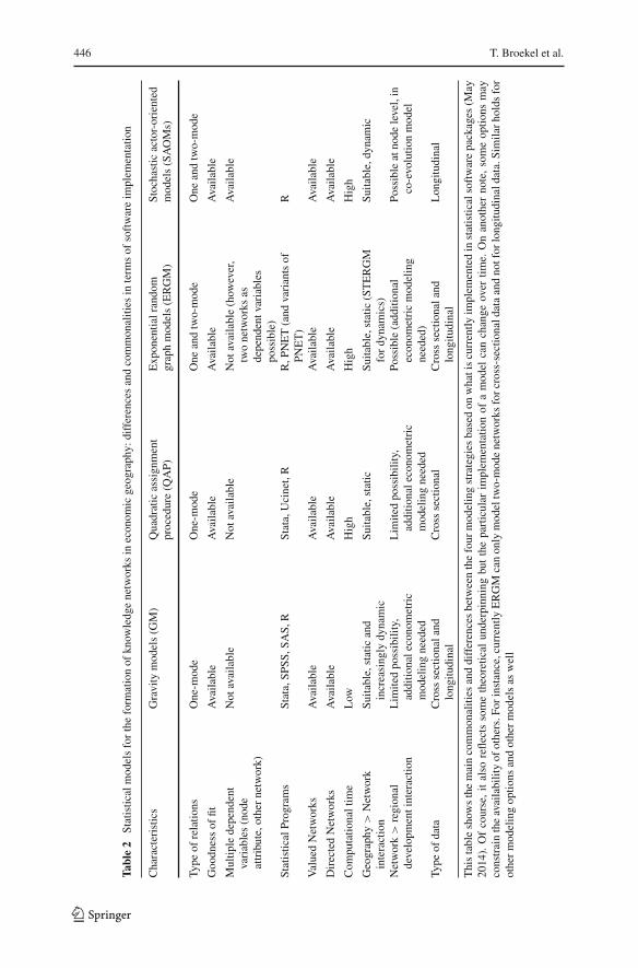
446 T. Broekel et al.

Tabl

e2

Stat

istic

alm

odel

sfo

rth

efo

rmat

ion

ofkn

owle

dge

netw

orks

inec

onom

icge

ogra

phy:

diff

eren

ces

and

com

mon

aliti

esin

term

sof

soft

war

eim

plem

enta

tion

Cha

ract

eris

tics

Gra

vity

mod

els

(GM

)Q

uadr

atic

assi

gnm

ent

proc

edur

e(Q

AP)

Exp

onen

tialr

ando

mgr

aph

mod

els

(ER

GM

)St

ocha

stic

acto

r-or

ient

edm

odel

s(S

AO

Ms)

Type

ofre

latio

nsO

ne-m

ode

One

-mod

eO

nean

dtw

o-m

ode

One

and

two-

mod

e

Goo

dnes

sof

fitA

vaila

ble

Ava

ilabl

eA

vaila

ble

Ava

ilabl

e

Mul

tiple

depe

nden

tva

riab

les

(nod

eat

trib

ute,

othe

rne

twor

k)

Not

avai

labl

eN

otav

aila

ble

Not

avai

labl

e(h

owev

er,

two

netw

orks

asde

pend

entv

aria

bles

poss

ible

)

Ava

ilabl

e

Stat

istic

alPr

ogra

ms

Stat

a,SP

SS,S

AS,

RSt

ata,

Uci

net,

RR

,PN

ET

(and

vari

ants

ofPN

ET

)R

Val

ued

Net

wor

ksA

vaila

ble

Ava

ilabl

eA

vaila

ble

Ava

ilabl

e

Dir

ecte

dN

etw

orks

Ava

ilabl

eA

vaila

ble

Ava

ilabl

eA

vaila

ble

Com

puta

tiona

ltim

eL

owH

igh

Hig

hH

igh

Geo

grap

hy>

Net

wor

kin

tera

ctio

nSu

itabl

e,st

atic

and

incr

easi

ngly

dyna

mic

Suita

ble,

stat

icSu

itabl

e,st

atic

(ST

ER

GM

for

dyna

mic

s)Su

itabl

e,dy

nam

ic

Net

wor

k>

regi

onal

deve

lopm

enti

nter

actio

nL

imite

dpo

ssib

ility

,ad

ditio

nale

cono

met

ric

mod

elin

gne

eded

Lim

ited

poss

ibili

ty,

addi

tiona

leco

nom

etri

cm

odel

ing

need

ed

Poss

ible

(add

ition

alec

onom

etri

cm

odel

ing

need

ed)

Poss

ible

atno

dele

vel,

inco

-evo

lutio

nm

odel

Type

ofda

taC

ross

sect

iona

land

long

itudi

nal

Cro

ssse

ctio

nal

Cro

ssse

ctio

nala

ndlo

ngitu

dina

lL

ongi

tudi

nal

Thi

sta

ble

show

sth

em

ain

com

mon

aliti

esan

ddi

ffer

ence

sbe

twee

nth

efo

urm

odel

ing

stra

tegi

esba

sed

onw

hati

scu

rren

tlyim

plem

ente

din

stat

istic

also

ftw

are

pack

ages

(May

2014

).O

fco

urse

,it

also

refle

cts

som

eth

eore

tical

unde

rpin

ning

but

the

part

icul

arim

plem

enta

tion

ofa

mod

elca

nch

ange

over

time.

On

anot

her

note

,so

me

optio

nsm

ayco

nstr

ain

the

avai

labi

lity

ofot

hers

.For

inst

ance

,cur

rent

lyE

RG

Mca

non

lym

odel

two-

mod

ene

twor

ksfo

rcr

oss-

sect

iona

ldat

aan

dno

tfor

long

itudi

nald

ata.

Sim

ilar

hold

sfo

rot

her

mod

elin

gop

tions

and

othe

rm

odel

sas

wel

l

123

Modeling knowledge networks in economic geography 447

degree of applicability in geography of innovation studies. We also name some soft-ware packages that include the according procedures. This list does not, however,make a claim to be complete.

7 Conclusion

We have discussed the scientific roots and the working principles of four main statisti-cal models that are increasingly used to analyze and explicitly model the geography ofknowledge networks: GM, MRQAP, ERGMs, and SAOMs. All four research strate-gies and models turn out to have advantages and disadvantages. They are embeddedin their respective epistemic communities of practice—explaining why four varyingmodeling techniques exist next to each other. GM and MRQAP are more conventionalmodeling types that require less information and computational efforts—but conse-quently exploit also less information on the structure of networks than ERGM andSAOM. Also, GM and MRQAP are only implicitly linked to knowledge transmissionmechanisms, although gravity modeling (GM) develops into more advanced networkanalysis applying individual level effects and using spatial econometric techniques.These differences influence their range of applicability in economic geography. Wealso derive a guideline helping researchers in this field to decide which model to usein what situations.

All four modeling types bring geography and network structures together in explain-ing the web of knowledge links between nodes (actors or regions). The reverserelationship—network positions partly determining local and regional developmentopportunities—constitutes an interesting research direction in economic geography.In such a conceptualization, local development is determined by hub positions in keyknowledge networks next to hotspot characteristics in regions. Although the mod-els discussed mainly focus in bringing (exogenous) geography into (endogenous)knowledge networks, analyzing endogenous regional development from (also endoge-nous) knowledge networks seems to be a major challenge for future research. For thisrelationship to be studied, additional (spatial) econometric modeling techniques arerequired, in which networked interactions between regions and actors function ascarriers of knowledge and innovation diffusion.

Acknowledgments The authors would like to thank two anonymous referees and Tom Snijders for veryhelpful comments and suggestions. Of course, all remaining errors are ours.

References

Almeida P, Kogut B (1999) Localization of knowledge and the mobility of engineers in regional networks.Manag Sci 45:905–917

Anderson JE, van Wincoop E (2003) Gravity with gravitas: a solution to the border puzzle. Am Econ Rev93(1):170–192

Autant-Bernard C, Billand P, Frachisse D, Massard N (2007) Social distance versus spatial distance in R&Dcooperation: empirical evidence from European collaboration choices in micro and nanotechnologies.Pap Reg Sci 86:495–519

123

448 T. Broekel et al.

Balland PA (2012) Proximity and the evolution of collaboration networks: evidence from research anddevelopment projects within the global navigation satellite system (GNSS) industry. Reg Stud 46:741–756

Balland PA, Belso-Martínez JA, Morrison A (2014) The dynamics of technological and business networksin industrial clusters: embeddedness, status or proximity? Pap Evolut Econ Geogr 14:12

Balland PA, de Vaan M, Boschma R (2013) The dynamics of interfirm networks along the industry lifecycle: the case of the global video games industry 1987–2007. J Econ Geogr (forthcoming)

Barca F, McCann P, Rodriguez-Pose A (2012) The case for regional development intervention: place-basedversus place-neutral approaches. J Reg Sci 52:134–152

Behrens K, Ertur C, Koch W (2012) Dual’ gravity: using spatial econometrics to control for multilateralresistance. J Appl Econom 27(5):773–794

Bell GG (2005) Clusters, networks, and firm innovativeness. Strateg Manag J 24:287–295Besag J (1974) Spatial interaction and the statistical analysis of lattice systems. J R Stat Soc Ser B (Method-

ological) 36(2):192–236Besag J (1975) Statistical analysis of non-lattice data. J R Stat Soc Ser D (The Statistician) 24:179–195Bikker JA (2010) An extended gravity model with substitution applied to international trade flows. In: van

Bergeijk PAG, Brakman S (eds) The gravity model in international trade: advances and applications.Cambridge University Press, Cambridge, pp 135–162

Boschma R (2005) Proximity and innovation: a critical assessment. Reg Stud 39:61–74Boschma R, Balland PA, Kogler D (2011) A relational approach to knowledge spillovers in biotech. Network

structures as drivers of inter-organizational citation patterns. Papers in evolutionary economic geography11.20, Utrecht University, Utrecht

Boschma R, Frenken K (2006) Why is economic geography not an evolutionary science? Towards anevolutionary economic geography. J Econ Geogr 6:273–302

Breschi S, Lissoni F (2009) Mobility of skilled workers and co-invention networks: an anatomy of localizedknowledge flows. J Econ Geogr 9:439–468

Broekel T, Hartog M (2013a) Explaining the structure of inter-organizational networks using exponentialrandom graph models: does proximity matter? Ind Innov 20(3):277–295

Broekel T, Hartog M (2013b) Determinants of cross-regional R and D collaboration networks: an applicationof exponential random graph models. Working Papers on Innovation and Space, #13.4

Broekel T, Boschma RA (2012) Knowledge networks in the Dutch aviation industry: the proximity paradox.J Econ Geogr 12:409–433

Burger MJ, Van Oort FG, Frenken K, Van der Knaap B (2009a) Networks and economic agglomerations:introduction to the special issue. Tijdschr voor Econ Soc Geogr 100:139–144

Burger MJ, Van Oort FG, Linders GJM (2009b) On the specification of the gravity model of trade: zeros,excess zeros and zero-inflated estimation. Spat Econ Anal 4:167–190

Cantner U, Graf H (2006) The network of innovators in Jena: an application of social network analysis. ResPolicy 35(4):463–480

Carey HC (1858) Princ Soc Sci. Lippincott, PhiladelphiaCastellani D, Palmero AJ, Zanfei A (2013) How remote are R&D labs? Distance factors and international

innovative activities. J Int Bus Stud 44:649–675Coe DT, Subramanian A, Tamirisa NT (2007) The missing globalization puzzle: evidence of the declining

importance of distance. IMF Staff Pap 54:34–58Cranmer SJ, Desmarais BA (2011) Inferential network analysis with exponential random graph models.

Polit Anal 19(1):66–86Daraganova G, Pattison P, Koskinen J, Mitchell B, Bill A, Watts M, Baum S (2012) Networks and geography:

modelling community network structures as the outcome of both spatial and network processes. Soc Netw34:6–17

De Federico A (2004) L’analyse longitudinal de réseaux sociaux totaux avec SIENA: méthode, discussionet application. Bull Méthodol Sociol 84:5–39

De Graaff T, Boter J, Rouwendal J (2009) On spatial differences in the attractiveness of Dutch museums.Environ Plan A 41:2778–2797

De Groot HLF, Poot J, Smit MJ (2009) Agglomeration externalities, innovation and regional growth:theoretical perspectives and meta-analysis. In: Capello R, Nijkamp P (eds) Handb Reg Growth DevTheor. Edward Elgar, Cheltenham

Dekker D, Krackhardt D, Snijders TAB (2007) Sensitivity of MRQAP tests to collinearity and autocorre-lation conditions. Psychometrika 72:564–581

123

Modeling knowledge networks in economic geography 449

Egger P (2004) On the Problem of Endogenous Unobserved Effects in the Estimation of Gravity Models.Journal of Economic Integration 19:182–191

Erdös P, Rènyi A (1960) On the evolution of random graphs. Publ Math Inst Hung Acad Sci 5:17–61Feenstra RC (2004) Advanced international trade: theory and evidence. Princeton University Press,

PrincetonFienberg S, Wasserman S (1981) An exponential family of probability distributions for directed graphs:

comment. J Am Stat Assoc 76:54–57Fischer MM, Griffith DA (2008) Modeling spatial autocorrelation in spatial interaction data: an application

to patent citation data in the European Union. J Reg Sci 48:969–989Fischer MM, Scherngell T, Jansberger E (2006) The geography of knowledge spillovers between high-

technology firms in Europe: evidence from a spatial interaction modeling perspective. Geogr Anal38:288–309

Frankel JA, Wei SJ (1998) Regionalization of world trade and currencies: economic and politics. In: FrankelJA (ed) The regionalization of the world economy. University of Chicago Press. National Bureau ofEconomic Research Project Report, pp 189–226

Fowler JH, Dawes CT, Chistakis NA (2009) Model of genetic variation in human social networks. Proc NatAcad Sci 206:1720–1724

Giuliani E (2013) Network dynamics in regional clusters: evidence from Chile. Res Policy 42:1406–1419Glückler J (2007) Economic geography and the evolution of networks. J Econ Geogr 7:619–634Gómez-Herrera E (2013) Comparing alternative methods to estimate gravity models of bilateral trade.

Empir Econ 44(3):1087–1111Goodreau SM, Handcock MS, Hunter DR, Butts CT, Morris M (2008) A statnet Tutorial. J Stat Softw

24(9):1–27Grabher G (2006) Trading routes, bypasses, and risky intersections: mapping the travels of “networks”

between economic sociology and economic geography. Prog Hum Geogr 30:163–189Graf H (2010) Gatekeepers in Regional Networks of Innovation. Camb J Econ (online account, doi:10.

1093/cje/beq001), pp 173–198Griffith DA (2007) Spatial structure and spatial interaction: 25 years later. Rev Reg Stud 37:28–38Hagedoorn J (2002) Inter-firm R&D partnerships: an overview of major trends and patterns since 1960.

Res Policy 31:477–492Hanneke S, Xing EP (2007) Discrete temporal models of social networks. In: Statistical network analysis:

models, issues, and new directions. Lecture Notes in Computer Science, vol 4503. Springer, Berlin,Germany, pp 115–125

Hazir CS, Autant-Bernard C (2012) Using affiliation networks to study the determinants of multilateralresearch cooperation: some empirical evidence from EU framework programs in biotechnology. GATEWorking Paper No. 1212

Head K, Mayer T (2000) Non-Europe: the magnitude and causes of market fragmentation in the EU. RevWorld Econ 136:285–314

Head K, Mayer T (2014) Gravity equations: workhorse, toolkit, and cookbook. In: Gopinath G, HelpmanE, Rogoff K, Handbook of international economics, vol 4. North Holland, pp 131–195

Helliwell J (1997) National borders, trade and migration. Pac Econ Rev 2:165–185Helpman E, Melitz M, Rubinstein Y (2008) Estimating trade flows: trading partners and trading volumes.

Q J Econ 123:441–487Hoekman J, Frenken K, Van Oort FG (2009) The geography of collaborative knowledge production in

Europe. Ann Reg Sci 43:721–738Holland PW, Leinhardt S (1981) An exponential family of probability distributions for directed graphs

(with discussion). J Am Stat Assoc 76:33–65Hubert LJ (1987) Assignment methods in combinatorial data analysis. Marcel Dekker, New YorkHubert L, Schulz J (1976) Quadratic assignment as a general data analysis strategy. Br J Math Stat Psychol

29(2):1900241Hunter DR (2007) Curved exponential family models for social networks. Soc Netw 29:216–230Hunter DR, Goodreau SM, Handcock MS (2008) Goodness of fit for social network models. J Am Stat

Assoc 103:248–258Isard W (1956) Location and space-economy. MIT Press, CambridgeJackson MO, Rogers BW (2007) Meeting strangers and friends of friends: how random are social networks?

Am Econ Rev 97:890–915Krackhardt D (1987) QAP partialling as a test of spuriousness. Soc Netw 9:171–186

123

450 T. Broekel et al.

Krackhardt D (1988) Predicting with networks: nonparametric multiple regression analysis of dyadic data.Soc Netw 10:359–381

Krivitsky PN (2012) Exponential-family random graph models for valued networks. Electr J Stat 6:1100–1128

Krivitsky PN, Goodrea SM (2012) STERGM—separable temporal ERGMs for modeling discrete relationaldynamics with statnet, STERGM Tutorial: https://statnet.csde.washington.edu/trac/raw-attachment/wiki/Resources/STERGMtutorial.pdf (21.11.2013)

Krivitsky PN, Handcock MS (2013) A separable model for dynamic networks. JRSS Ser B (StatisticalMethodology) 76(1):29–46

LeSage JP, Fischer MM (2010) Spatial econometric modeling of origin-destination flows. In: Fischer MM,Getis A (eds) Handbook of applied spatial analysis. Springer, Berlin, pp 409–433

LeSage JP, Pace RK (2008) Spatial econometric modeling of origin-destination flows. J Reg Sci 48:941–967LeSage JP, Pace RK (2009) Introduction to Spatial Econometrics. CRC Press, ClevelandLeSage JP, Polasek W (2008) Incorporating transportation network structure in spatial econometric models

of commodity flows. Spat Econ Anal 3:225–245Lill E (1891) Das Reisegesetz und seine Anwendung auf den Eisenbahnverkehr, ViennaLinders G-J, Patuelli R, Griffith DA (2010) The space of gravity: spatial filtering estimation of a gravity

model for bilateral trade. MimeoLindgren KO (2010) Dyadic regression in the presence of heteroscedasticity—an assessment of alternative

approaches. Soc Netw 32:279–289Liu WH, Lin YC (2005) Foreign patent rights and high-tech exports: evidence from Taiwan. Appl Econ

37:1534–1555Liu X, Derudder B, Liu Y (2013) Regional geographies of intercity corporate networks: The use of expo-

nential random graph models to assess regional network-formation, Papers in Regional Science (forth-coming)

Lerner J, Indlekofer N, Nick B, Brandes U (2013) Conditional independence in dynamic networks. J MathPsychol 57(6):275–283

Lospinoso JA, Snijders TAB (2011) Goodness of fit for stochastic actor oriented models. Working paperLubbers MJ, Snijders TAB (2007) A comparison of various approaches to the exponential random graph

model: a reanalysis of 102 student networks in school classes. Soc Netw 29:489–507Lukermann F, Porter PW (1960) Gravity and potential models in economic geography. Ann Assoc Am

Geogr 50:493–504Lusher D, Koskinen J, Robins G, Lusher D, Koskinen J, Robins G (2013) Exponential random graph models

for social networks. Structural analysis in the social sciences. Cambridge University Press, New YorkMaggioni MA, Uberti TE (2007) Inter-regional knowledge flows in Europe: an econometric analysis. In:

Frenken K (ed) Applied evolutionary economics and economic geography. Edward Elgar, CheltenhamMaggioni M, Uberti E (2011) Networks and geography in the economics of knowledge flows. Qual Quant

45 (forthcoming)Maggioni MA, Nosvelli M, Uberti TE (2007) Space versus networks in the geography of innovation: a

European analysis. Pap Reg Sci 86(3):471–493Mantel N (1967) The detection of disease clustering and a generalized regression approach. Cancer Res

27(2 Part 1):209–220Mantel N, Valand RS (1970) A technique of nonparametric multivariate analysis. Biometrics 26:547–558Melo PC, Graham DJ, Noland RB (2009) A meta-analysis of estimates of urban agglomeration economies.

Reg Sci Urban Econ 39:332–342Miguélez E, Moreno R (2013) Research networks and inventors’ mobility as drivers of innovation: evidence

from Europe. Reg Stud 47(10):1668–1685Newman MEJ (2003) The structure and function of complex networks. SIAM Rev 45(2):167–256Newman M, Barabási AL, Watts DJ (2006) The structure and dynamics of networks. Princeton University

Press, PrincetonOpsahl T (2013) Triadic closure in two-mode networks: redefining the global and local clustering coeffi-

cients. Soc Netw 35 doi:10.1016/j.socnet.2011.07.001Ove F, Strauss D (1986) Markov Graphs. J Am Stat Assoc 81(395):832–842Park J, Newman MEJ (2004) The Statistical Mechanics of Networks. Physical Review E 70(6)Pattison P, Wasserman S (1999) Logit models and logistic regressions for social networks. II. Multivariate

relations. Br J Math Stat Psychol 52:169–194Peri G (2005) Determinants of knowledge flows and their effect on innovation. Rev Econ Stat 87:308–322

123

Modeling knowledge networks in economic geography 451

Ponds R, Van Oort F, Frenken K (2007) The geographical and institutional proximity of research collabo-ration. Pap Reg Sci 86:423–444

Ravenstein EG (1885) The laws of migration. J Stat Soc 48:167–235Reilly W E (1931) The law of retail gravitation, Knickerbocker Press, New YorkRipley RM, Snijders TAB, Preciado Lopez P (2011) Manual for RSiena, University of Oxford, Department

of Statistics, Nuffield College, October 7Robins G, Morris M, Pattison P, Kalish Y, Lusher D (2007) An introduction to exponential random graph

(p*) models for social networks. Soc Netw 29(2):173–191Saul ZM, Filkov V (2007) Exploring biological network structure using exponential random graph models.

Bioinformatics 23(19):2604–2611Scherngell T, Barber MJ (2009) Spatial interaction modelling of cross-region R&D collaborations: empirical

evidence from the 5th EU Framework Programme. Pap Reg Sci 88:531–546Scherngell T, Lata R (2013) Towards an integrated European Research Area? Findings from Eigenvector

spatially filtered spatial interaction models using European Framework Programme data. Pap Reg Sci92:555–577

Schneider JW, Borlund P (2007) Matrix comparison, part 2: measuring the resemblance between proximitymeasures or ordination results by use of the mantel and procrustes statistics. J Am Soc Inf Sci Technol58(11):1596–1609

Snijders TAB (2001) The statistical evaluation of social network dynamics. In: Sobel M, Becker M (eds)Sociological Methodology. Basil Blackwell, Boston and London, pp 361–395

Snijders TAB (2002) Markov Chain Monte Carlo Estimation of Exponential Random Graph Models. J SocStruct 3(2)

Snijders TAB (2008) Longitudinal methods of network analysis. In: Meyers B (ed) Encyclopedia of com-plexity and system science. Springer, Berlin

Snijders TAB (2011) Statistical models for social networks. Ann Rev Sociol 37:131–153Snijders TAB, van de Bunt G, Steglich C (2010a) Introduction to stochastic actor-based models for network

dynamics. Soc Netw 32(1):44–60Snijders TAB, Steglich C, Schweinberger M, Huisman M (2010b) Manual for SIENA version 3.2. Provi-

sional version. Oxford: University of Oxford, Department of StatisticsSnijders TAB, Pattison PE, Robins G, Handcock MS (2006) New specifications for exponential random

graph models. Sociol Methodol 36:99–153Snijders TAB, Lomi A, Torló VJ (2013) A model for the multiplex dynamics of two-mode and one-mode

networks, with an application to employment preference, friendship, and advice. Soc Netw 35(2):265–276

Solomonoff R, Rapoport A (1951) Connectivity of random nets. Bull Math Biophys 13:107–117Steglich CEG, Snijders TAB, West P (2006) Applying SIENA: An illustrative analysis of the co-evolution

of adolescents’ friendship networks, taste in music, and alcohol consumption. Methodology 2:48–56Steglich C, Snijders TAB, Pearson M (2010) Dynamic networks and behavior: separating selection from

influence. Sociol Methodol 40:329–393Stewart JQ (1948) Demographic gravitation: evidence and application. Sociometry 1:31–58Stouffer SA (1940) Intervening opportunities: a theory relating mobility and distance. Am Sociol Rev

5:845–867Sunley P (2008) Relational economic geography: a partial understanding or a new paradigm? Econ Geogr

84:1–26Ter Wal ALJ (2013) The spatial dynamics of the inventor network in German biotechnology: geographical

proximity versus triadic closure. J Econ Geogr (forthcoming)Ter Wal A, Boschma R (2009) Applying social network analysis in economic geography: theoretical and

methodological issues. Ann Reg Sci 43:739–756Thissen M, Van Oort F, Diodato D, Ruijs A (2013) Regional competitiveness and smart specialization in

Europe. Place-based development in international economic networks. Edward Elgar, CheltenhamTinbergen J (1962) Shaping the world economy. Twentieth Century Fund, New YorkVan de Bunt G, Groenewegen P (2007) An actor-oriented dynamic network approach: the case of interor-

ganizational network evolution. Organ Res Methods 10(3):463Van der Leij MJ (2011) Experimenting with buddies. Science 334:1220–1221Van Duijn MAJ, Gile KJ, Handcock MS (2009) A framework for the comparison of maximum pseudo-

likelihood and maximum likelihood estimation of exponential family random graph models. Soc Netw31(1):52–62

123

452 T. Broekel et al.

Van Oort F, Lambooy J (2013) Cities, knowledge and innovation. Chapter. In: Fischer M, Nijkamp P (eds)Handbook of regional science. Springer, Berlin, pp 475–488

Wagner D, Head K, Ries J (2002) Immigration and the trade of provinces. Scott J Polit Econ 49:507–525Wang P, Sharpe K, Robins G, Pattison P (2009) Exponential random graph (p*) models for affiliation

networks. Soc Netw 31(1):12–25Wasserman S, Pattison P (1996) Logit models and logistic regressions for social networks. I. An introduction

to Markov graphs and p*. Psychometrika 61:401–425

123