In: Bevers, Michael; Barrett, Tara M., comps. 2005. Systems Analysis in Forest Resources: Proceedings of the 2003 Symposium. General Technical ReportPNW-GTR-656. Portland, OR: U.S. Department of Agriculture, Forest Service, Pacific Northwest Research Station.1 M. Thor is a program leader at Skogforsk, Uppsala Science Park, S-751 83 Uppsala, Sweden; T. Möykkynen is a researcher at the Faculty of Forestry,University of Joensuu, Finland; J.E. Pratt is a forestry officer (emeritus) at the Northern Research Station, Scotland; T. Pukkala is a professor at the Facultyof Forestry, University of Joensuu, Finland, J. Rönnberg is a researcher at the Southern Swedish Forest Research Centre, Alnarp, Sweden; C.G. Shaw III isa national program leader for pathology research, USDA Forest Service, Washington D.C. USA; J. Stenlid is a professor at the Swedish University ofAgricultural Sciences, Dept. Forest Mycology and Pathology, Uppsala, Sweden; G. Ståhl is a professor at Swedish University of Agricultural Sciences,Dept. Forest Resource Management and Geomatics, Umeå, Sweden; S. Woodward is Head of Discipline Agriculture & Forestry, School of BiologicalSciences, Univerity of Aberdeen, Scotland.

Systems Analysis in Forest Resources: Proceedings of the 2003 Symposium

MODELING INFECTION AND SPREAD OFHETEROBASIDION ANNOSUM IN CONIFEROUS

FORESTS IN EUROPE

M. Thor, T. Möykkynen, J.E. Pratt, T. Pukkala, J. Rönnberg, C.G. Shaw III, J. Stenlid, G. Ståhl and S. Woodward 1

INTRODUCTION

The pathogenic fungus Heterobasidion annosum (Fr.)Bref. causes severe problems for forestry throughout thenorthern temperate zone, infecting mainly coniferous trees.Annual losses in the European Union are estimated at €790million. In Sweden annual revenue losses attributed todecay and impacts on growth reach approximately €60 mil-lion. Apart from affecting income for the forest owner, H.annosum impacts the industry: pulp and paper manufactur-ers and sawmills experience log quality problems becauseof the fungus.

The extent of decay is difficult to estimate in standingtrees; even so, some deduction for the risk of decay gener-

ABSTRACT

The pathogenic fungus Heterobasidion annosum causes severe problems for forestry throughout the northern temperatezone, infecting mainly coniferous trees. Annual losses in the European Union are estimated at €790 million. The infectionbiology of the fungus is well described, although variation is considerable. This paper describes two modeling projects inEurope. The first, MOHIEF (Modeling of Heterobasidion infection in European forests), is a project within the EuropeanUnion aiming to produce a decision-support tool for forest managers, as well as a tool for scientists throughout Europe.MOHIEF models infection and spread of the pathogen for various tree species over a range of forest conditions. The otherproject, Heureka, aims to produce a system for forest planning on strategic, tactical and operative levels in Sweden. Althoughnational in scope, the model can be applied at regional and local levels. In Heureka the impact of H. annosum is one factoramongst other components that include growth and yield, wood properties, biodiversity, biomass-carbon relationships andforest-owner behavior. In this paper simulations of infection by Heterobasidion are demonstrated together with examples ofhow the models can be exploited, from a forest manager’s and a scientist’s perspective.

105

ally is built into stumpage prices. The likelihood of infec-tion can be minimized by active means such as selection of the right season for cutting, stump treatment, or stumpremoval. These measures have a cost, however, and thusmust be integrated into forest planning to fit the “right”operations to the “right” stands.

THE PATHOGEN

H. annosum forms perennial fruiting bodies that pro-duce vast numbers of spores under suitable environmentalconditions. In Sweden, spore dispersal takes place duringthe whole growing season (April to September) with a peak

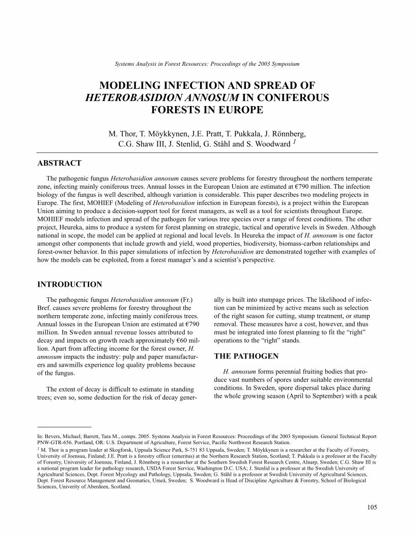
in the summer months, whereas in warmer climates, the falland winter periods appear more favorable for spore produc-tion. Spores germinate on fresh woody tissue, favoringnewly cut stumps (Rishbeth, 1951a). The mycelium growsinto the stump and its roots, and infects neighboring treesvia root contacts and grafts. Damage occurs as decayedwood on standing spruce and fir, and death of young pines.Fungal mycelium may remain viable in old stumps fordecades, providing inoculum for the next generation oftrees. In summary, H. annosum enters a stand primarily viastump surfaces and injuries, spreads from fresh stumps totrees, from tree to tree and/or from old stumps to standingtrees (fig. 1).

The incidence of H. annosum disease can be higherunder certain conditions; for example, high soil pH (Rishbeth1951b), in first rotation stands (Rennerfelt, 1946), a highnumber of stems per hectare (Venn & Solheim, 1994) andon mineral soils with fluctuating water table (von Euler &Johansson, 1983). On the other hand, the risks of infectionand spread appear to be lower on peat soil (Redfern, 1998),during rainfall (for example, Sinclair, 1964) and in standswith mixed tree species (Huse, 1983; Piri and others, 1990).

An active way to control H. annosum is to preventstump infection by logging during a safe period when fewspores are present, or by treating stumps with an agent thatinhibits spore germination. In Europe protective stumptreatment, with biological or chemical agents, is carried outon more than 200.000 hectares annually at an average costof €1.2 per m3 (Thor, 2002). A remedial method of controlis to remove old stumps prior to the establishment of a newstand. This expensive action is carried out on especiallysensitive sites in the United Kingdom (UK) (Pratt, 1998).Silvicultural measures such as planting of less susceptibletree species, admixture of species, shortening the rotationperiod, or minimizing stand entries are other options thatactively reduce spread of H. annosum. All in all, there isample scope and complexity to apply a modeling approachto resolve this forest management problem. Models areuseful for forest managers as well as scientists in order tounderstand the mechanisms of infection development andimpact of H. annosum.

MODELING

An empirical model of H. annosum infection in Norwayspruce exists for southern Sweden and Denmark (Vollbrecht& Agestam 1995, Vollbrecht & Jorgensen, 1995). Mechanisticmodels have been developed for H. annosum on Sitka spruce(Picea sitchensis Bong Carr.) in the UK (Pratt and others,1989) and for H. annosum on Norway spruce in Finland

(for example Möykkynen, Miina & Pukkala, 2000). Otherroot diseases that have been modeled include Phellinusweirii on Douglas fir (Pseudotsuga menziesii (Mirb.) Franco)(Bloomberg, 1988). See also Pratt and others (1998) forfurther details about modeling disease development inforest stands.

The most comprehensive modeling effort to date, how-ever, is the western root disease (WRD) model describingthe dynamics of H. annosum, Armillaria spp. and Phellinusweirii in, for example, stands of fir (Abies spp.) andPonderosa pine (Pinus ponderosa Dougl. ex Laws.) inwestern North America (Frankel, 1998). The WRD modelwas developed by American and Canadian forest patholo-gists over a period of more than ten years. In addition tothe pathogens, the effect of windthrow and bark beetles canbe simulated in the model which is linked to growth andyield models that respond to management actions.

The WRD model has inspired a European ConcertedAction, MOHIEF (Woodward and others, 2003), in which a set of mechanistic models of H. annosum is to be devel-oped for European conditions covering the range of, forexample, soil, climate, geography and hosts.

In MOHIEF (Modeling of Heterobasidion infection inEuropean forests) forest pathologists, forest managers andmodelers are preparing a prototype decision-support tool toestimate potential losses from Heterobasidion attack. Thework is divided into three subtasks; 1) establish the output

106

Figure 1—Spores of H. annosum germinate on fresh woody tissue, forexample, stumps. Subsequently, fungal mycelium can spread to adjacentroot systems and stems, which are decayed. Illustration from Swedjemark(1995).

requirements needed by the end-users of such a tool, 2)clarify and collate the biological and management inputsrequired, and 3) construct a simulation prototype model.The project has been ongoing for 24 out of 36 months.Draft models and an interface have been produced, and arebeing tested. The range of conditions in the participatingcountries – as regards climate, forestry conditions, soilsetc. – is challenging to the model. Also the basic growthand yield models differ significantly across the participat-ing countries. Nevertheless, significant progress has beenmade: it is likely that the goals set for the project will beachieved within the 3-year time frame.

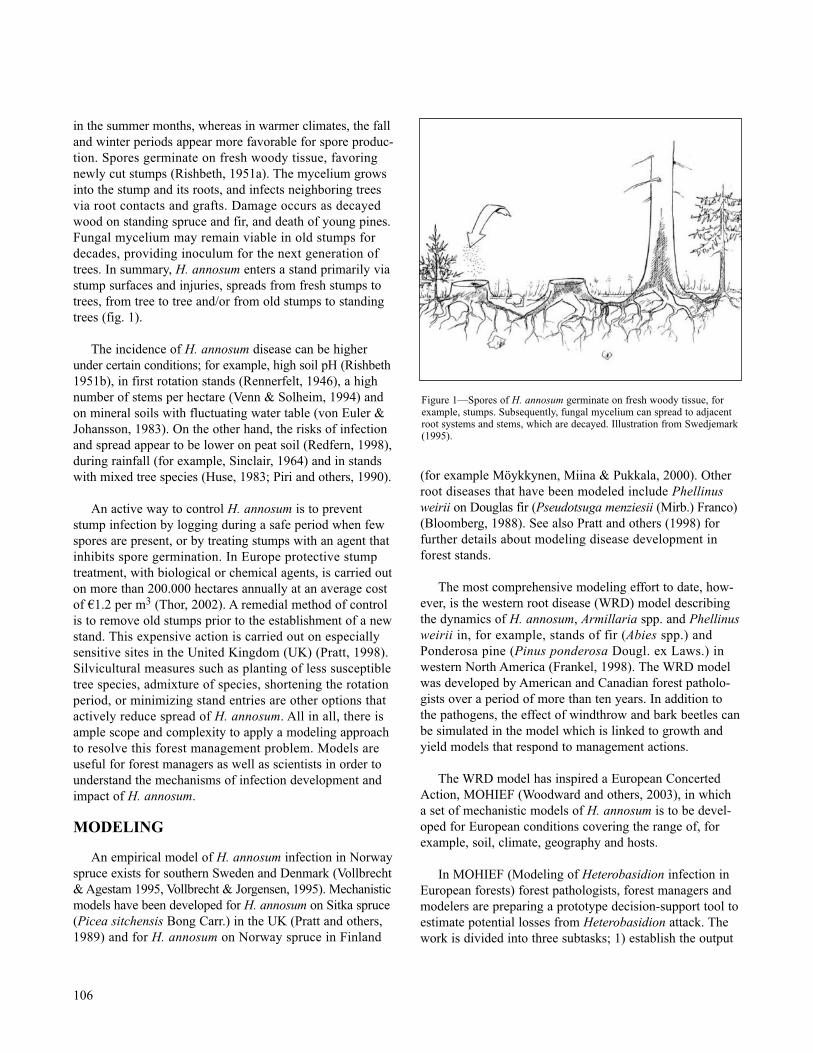
Heureka (Lämås & Eriksson, 2002) is a research programme developing computer based tools for forestanalysis and planning in Sweden. Heureka uses a multi-disciplinary approach that includes 13 subprojects (fig. 2).Modeling of Heterobasidion is one of the 13 Heureka projects, with disease dynamics handled as in MOHIEF.Integrated applications will be designed from the projects,and associated systems will be developed. The project aimsat four applications to serve different user groups.

1. National and Regional Analysis This analyses modeling outcomes in terms of the state

of the forest ecosystem, and supply and demand for variousutilities. Basic data for this application could be the National

forest inventory, remote sensing data or information fromestate data bases. Possible users include the Board ofForestry, the Environmental Protection Agency, forest own-ers’ associations and organizations for forest fuels.

2. Strategic Planning in Large Forest EnterprisesThe main focus is on wood production, but other values

are also considered. Large forest areas can be handled.Optimizing methods are used to generate a strategic planfor the business. The application can generate future levelsof cutting, net revenues etc., and also a list of stands pro-posed for harvest over the next 6 months to 3 years.

3. Operational PlanningThe basis for operational planning in the short term (1 to

6 months) is the list of stands available for harvest createdin the strategic planning application. The application willoptimize the net revenues from timber and forest fuels, andallocate operations and transport.

4. Planning for Small-Scale ForestryThis application is aimed at smaller estates, and can

also handle multi-purpose forestry and environmental issues.A problem area linked to this application is methods fordata capture that keep costs low. The users are private for-est owners, forest owners’ associations, consultants andproducers of forest management plans.

107

Figure 2—The principle of inter-disciplinary subprojects and syntheses in the multi-disciplinary Heureka project.

MODELING INITIAL CONDITIONS

Before modeling of disease dynamics, initiating data onthe incidence of root rot are needed. At present, such infor-mation in stand records is limited. Consequently, the nor-mal situation would be to model the root rot incidence in astand. Current work (Thor and others 2005) uses a numberof stand and site variables to model the probability of decayaffecting a single tree. Data from the national forest inven-tory in Sweden were used to build the model. Records fromover 45,000 Norway spruce trees were evaluated. Thesewere analyzed for correlation between root rot incidenceand environmental conditions. In a stepwise logistic re-gression, sets of functions were developed to show sig-nificance for the variables: stand age, site class index,temperature sum, elevation above sea level, tree diameterat breast height, soil moisture and texture, proportion ofspruce in the stand, the occurrence of peat, and longitude.These parameters are commonly noted in most standrecords in larger forest enterprises.

So far, the model only estimates the incidence of decayat breast height. A calibrating function is being developedto transform this to provide an estimate of rot frequency atstump level.

MODELING DISEASE DYNAMICS

For Fennoscandian conditions a model will be publishedwithin the MOHIEF structure (Pukkala and others, 2005).Dynamics of the disease are modeled on the basis of thedevelopment of the stand and by the changes in fungaldynamics over time. These sub-models are, however, notindependent of each other.

To simulate tree growth, distance-dependent or dis-tance–independent growth models for individual trees canbe used. For cases in which there are no individual treemeasurements available, a rectangular plot is generated fromstand-level variables. Tree growth is calculated in 5 yeartime steps. The timing for thinning and clear-fell operationsis triggered by basal area.

Modeling of the disease is based on the biology of H.annosum (Woodward and others 2003, Pratt and others1998). The probability of spore infection is estimated forScots pine and Norway spruce, depending on time of theyear and the use of any stump treatment. Not all stumpsthat are spore infected transmit disease to adjacent trees.Growth and infectivity of the root system depends on itssize, age and vitality. The growth rate of H. annosum is

much higher in dying roots of a stump than in a living tree. Once colonized, the root system is assigned a probabilityfor transferring the pathogen to adjacent root systems. Thisprocess depends on soil conditions. When the fungus hasreached a neighboring tree, the growth rate in the root sys-tem is simulated, as well as the spread of decay into thestem.

In cases of advanced decay in Norway spruce, treegrowth is reduced. Young Scots-pine trees die more fre-quently after attack by H. annosum than do spruce trees.

MODELING ECONOMIC OUTCOMES

The effect of disease on the economic performance of astand depends on growth reduction of infected trees, reallo-cation of produce assortments and their change in price, thecosts of prophylactic treatment, interest rate, etc.

Once the models of the initial conditions and the dynam-ics of the disease are in place, the economic outcome for anumber of feasible management schemes can be estimated.One tool for modeling the outcome of assortments isTimAn, developed at Skogforsk. TimAn is a softwarepackage for advanced analysis of bucking-to-order, and itcovers stand inventory, construction of price lists, analysisand follow-up of the actual outcome. TimAn uses stemprofiles for individual trees, which will be useful in theseanalyses.

APPLICATIONS OF THE MODELS

One of the main objectives of the disease model is toincorporate knowledge of root rot problems into forestplanning by means of functions built into the planning sys-tems of various forest enterprises. Stand-alone applicationscould be useful teaching tools, but will not help foresters orforest production researchers appreciate the significance ofroot rot problems.

Forester’s point-of-viewWhen making strategic decisions it is crucial to include

the impact of root rot in the analysis. For example, actionsby large forest enterprises will definitely affect and mayexacerbate future disease development. Issues to considerinclude altering the length of the rotation, modifying thin-ning schedules, exercising choice of tree species and use of protective treatments on stumps.

In turn, these factors will affect the potential harvestvolumes and the assortment mix. One approach could be

108

scenario-handling, where different conceivable scenariosare hypothesized and the consequences are subsequentlyanalyzed with the models. The models should predict aver-age outcomes for large areas of forest: the high endemicvariation requires caution when interpreting estimates onrelatively small units, such as single stands or forests.Strategic decisions and policies based on this type of analysis are a practical way to use the models.

In the short term, down to a planning horizon of oneyear, the root rot situation should be considered as part ofthe ordering priority in which stands will be harvested. Whatare the consequences – for customers, for the supply organ-ization, for the forest – of harvesting a Norway-sprucestand during the low-risk period instead of the high-riskperiod? What is the cost/benefit of applying stump treat-ment in thinning and clear-fell operations?

Supply organizations are likely to apply the models differently than companies with large forest holdings. Never-theless, the basic need to incorporate root rot modeling intothe planning process remains important for both groups.

Researcher’s Point of ViewA good model will describe the disease impact and

improve understanding of the mechanisms involved in dis-ease development. A sensitivity analysis can identify param-eters critical to the outcome, and thus help to identify needsfor research. Current work suggests that some issues arecrucial, and need to be further investigated. They includethe rate of expansion of disease centers and the probabilityof disease transfer in various soil types.

The type of modeling described above enables us tohave a more complete understanding of the dynamics of H. annosum. In the typical sequence a primary descriptivemodel is developed (which has already been completed inseveral countries for root disease). After a period of research,data become available that allow for development of amore complex mechanistic model. Ideally this modelimproves our understanding so that critical processes canbe described in further detail, enabling an iterative mecha-nistic approach to the process of modeling to be adopted.Used in this manner, modeling is a powerful means toachieve a more complete understanding of the processesinvolved in complex systems, such as the interactionsbetween pathogen, host, soil, climate and human activity.

PRESENT CONDITIONS AND TIME-TABLE

With regard to modeling of H. annosum, there is a well-developed mechanistic model for Western North America(WRD model). In Europe a number of mechanistic modelsfor H. annosum dynamics in a stand are under development.These models could be available, at least as prototypes,before the end of 2004.

Models to describe initial conditions in Sweden will beready for practical use in 2004.

Models and simulation tools for detailed analyses ofassortments and cost/revenue calculations exist, but theyneed to be modified to accommodate root disease dynamics.

COSTS AND REVENUES

In Sweden the primary problem with H. annosumoccurs in Norway-spruce trees. However, the variation inconditions (rotation periods, management schemes, time ofthinning and clear-felling) suggests a clear need for reliablequantification of the benefits of varying managementschemes and measures taken in order to minimize theimpact of root rot. Intuitively, stump treatment appearsprofitable in stands growing on productive soils with shortrotations. The economic benefit is not equally obvious instands growing on poorer sites with longer rotation periods.To handle this problem, tools are required; tools that thecurrent projects could help to develop.

In Sweden, the difference between conifer pulpwood (inwhich decay is allowed to occupy 50 percent of the cross-section of a single log) and saw timber (in which no decayallowed) is about US$ 19 (150 SEK) per cubic meter(Brunberg, 2003). With severe decay, a fuel assortment mustbe prepared, which doubles the value difference. Degradationdue to decay has a significantly higher economic impactthan a change from a higher timber class to a lower. Becauselarge timber volumes are involved, even a small improve-ment in decay reduction results in large savings. A simpleexample from Sweden suffices: The annual saw-timbervolume derived from Norway spruce is about 16 millioncubic meters. Every one-percent of timber which could bereallocated from decayed to sound wood is worth US$ 3 to6 million (25-50 million SEK) to forest owners.

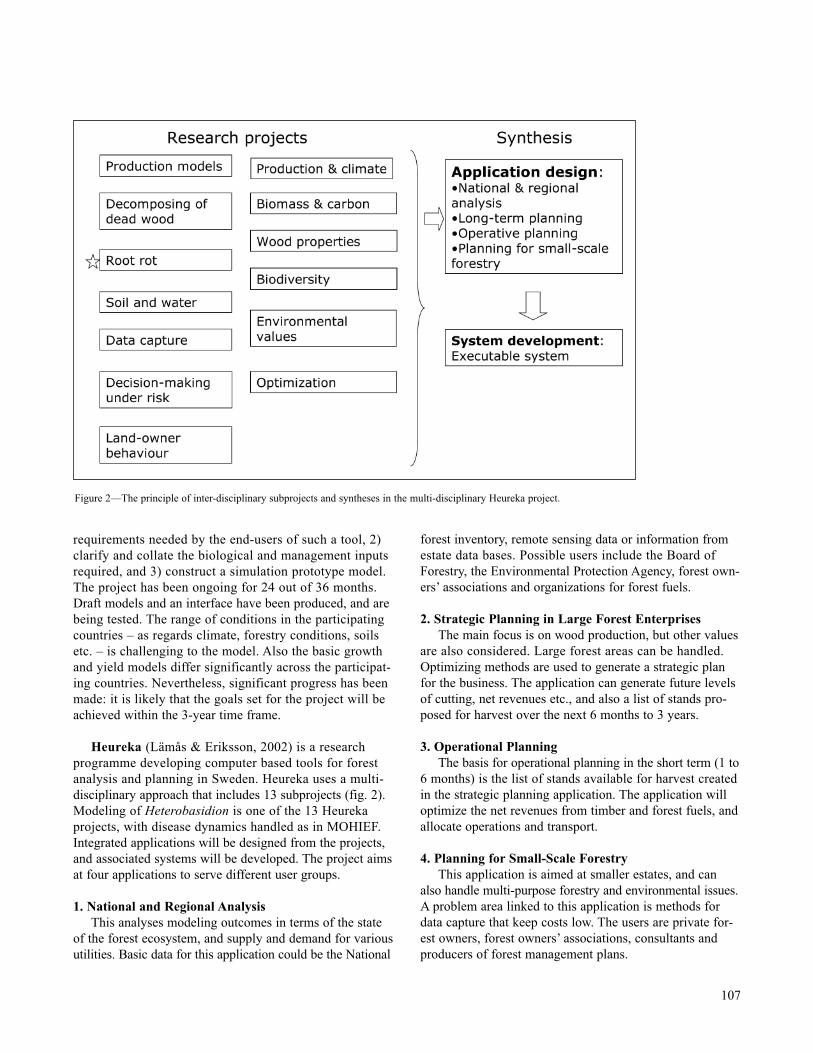
A typical stand with average Fennoscandian conditionswould produce model outputs similar to those presented in

109

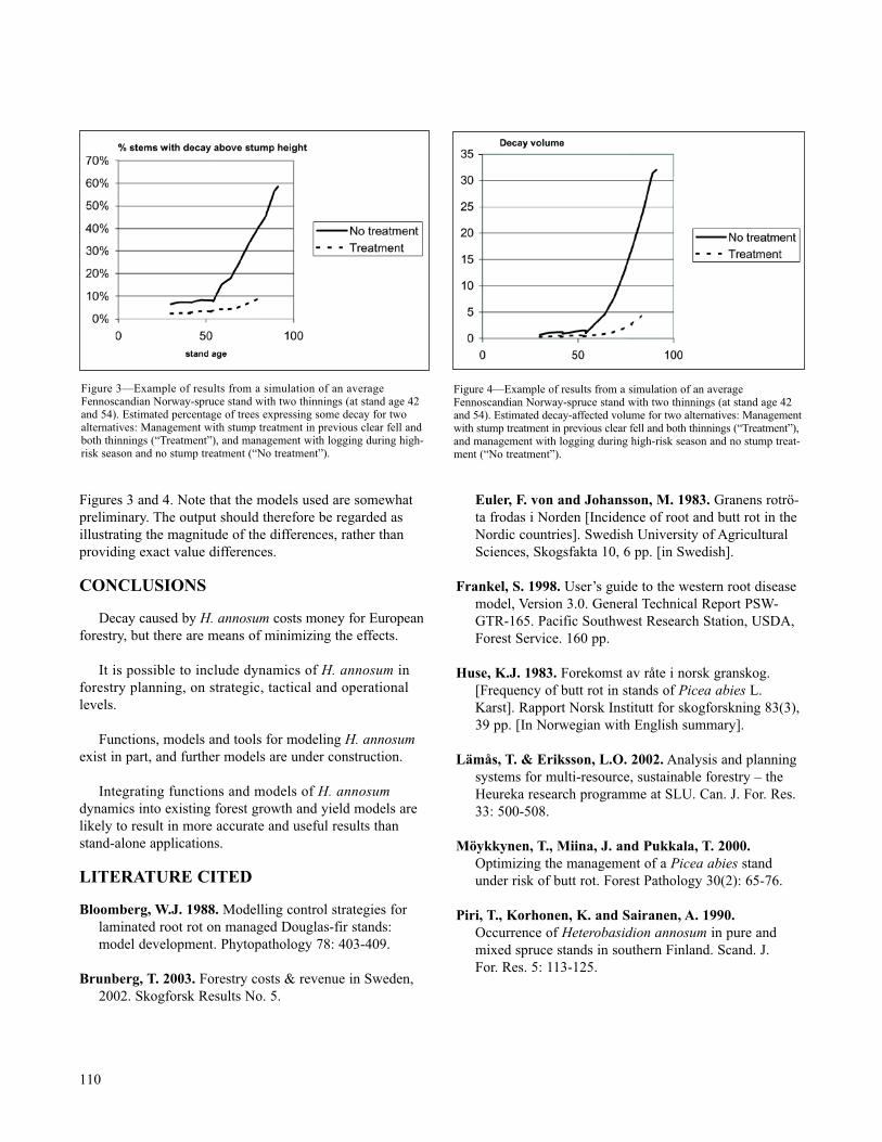
Figures 3 and 4. Note that the models used are somewhatpreliminary. The output should therefore be regarded asillustrating the magnitude of the differences, rather thanproviding exact value differences.

CONCLUSIONS

Decay caused by H. annosum costs money for Europeanforestry, but there are means of minimizing the effects.

It is possible to include dynamics of H. annosum inforestry planning, on strategic, tactical and operational levels.

Functions, models and tools for modeling H. annosumexist in part, and further models are under construction.

Integrating functions and models of H. annosumdynamics into existing forest growth and yield models arelikely to result in more accurate and useful results thanstand-alone applications.

LITERATURE CITED

Bloomberg, W.J. 1988. Modelling control strategies for laminated root rot on managed Douglas-fir stands:model development. Phytopathology 78: 403-409.

Brunberg, T. 2003. Forestry costs & revenue in Sweden, 2002. Skogforsk Results No. 5.

Euler, F. von and Johansson, M. 1983. Granens rotrö-ta frodas i Norden [Incidence of root and butt rot in theNordic countries]. Swedish University of AgriculturalSciences, Skogsfakta 10, 6 pp. [in Swedish].

Frankel, S. 1998. User’s guide to the western root disease model, Version 3.0. General Technical Report PSW-GTR-165. Pacific Southwest Research Station, USDA,Forest Service. 160 pp.

Huse, K.J. 1983. Forekomst av råte i norsk granskog. [Frequency of butt rot in stands of Picea abies L.Karst]. Rapport Norsk Institutt for skogforskning 83(3),39 pp. [In Norwegian with English summary].

Lämås, T. & Eriksson, L.O. 2002. Analysis and planning systems for multi-resource, sustainable forestry – theHeureka research programme at SLU. Can. J. For. Res.33: 500-508.

Möykkynen, T., Miina, J. and Pukkala, T. 2000.Optimizing the management of a Picea abies standunder risk of butt rot. Forest Pathology 30(2): 65-76.

Piri, T., Korhonen, K. and Sairanen, A. 1990.Occurrence of Heterobasidion annosum in pure andmixed spruce stands in southern Finland. Scand. J. For. Res. 5: 113-125.

110

Figure 4—Example of results from a simulation of an averageFennoscandian Norway-spruce stand with two thinnings (at stand age 42and 54). Estimated decay-affected volume for two alternatives: Managementwith stump treatment in previous clear fell and both thinnings (“Treatment”),and management with logging during high-risk season and no stump treat-ment (“No treatment”).

Figure 3—Example of results from a simulation of an averageFennoscandian Norway-spruce stand with two thinnings (at stand age 42and 54). Estimated percentage of trees expressing some decay for twoalternatives: Management with stump treatment in previous clear fell andboth thinnings (“Treatment”), and management with logging during high-risk season and no stump treatment (“No treatment”).

Pratt, J.E. 1998. Economic appraisal of the benefits of control treatments. In: Woodward, S., Stenlid, J.,Karjalainen, R and Hütterman, A. (eds.). Heterobasidionannosum: Biology, Ecology, Impact and Control. CABInternational, ISBN 0-85199-275-7, pp. 315-332.

Pratt, J.E., Redfern, D.B. and Burnand, A.C. 1989. Modelling the spread of Heterobasidion annosum inSitka spruce plantations in Britain. In: Morrison, D.J.(ed.). Proceedings of the Seventh InternationalConference on Root and Butt rots, Canada, August1988. Forestry Canada, Victoria, British Columbia, pp. 308-319.

Pratt, J.E., Shaw, C.G. III and Vollbrecht, G. 1998.Modelling Disease Development in Forest Stands. In: Woodward, S., Stenlid, J., Karjalainen, R andHütterman, A. (eds.). Heterobasidion annosum: Biology,Ecology, Impact and Control. CAB International, ISBN0-85199-275-7, pp. 213-234.

Pukkala, T., Möykkynen, T., Thor, M., Rönnberg, J. and Stenlid, J. 2005. Modelling infection and spread of Heterobasidion annosum in Fennoscandian coniferstands. Can. J. For. Res. 35(1): 74-84.

Redfern, D.B. 1998. The effect of soil on root infection and spread by Heterobasidion annosum. In: Delatour,C., Guillaumin, J.J., Lung-Escarmant, B. and Marçais,B. (eds.). Proceedings of the Ninth InternationalConference on Root and Butt Rots, Carcans, France,September 1997. INRA Colloques No. 89. ISBN 2-7380-0821-6, pp. 267-273.

Rennerfelt, E. 1946. Om rotrötan (Polyporus annosus Fr.) i Sverige. Dess utbredning och sätt att uppträda.Meddelande från Statens Skogsforskningsinstitut 35: 1-88. [In Swedish with English summary].

Rishbeth, J. 1951. a. Observations on the biology of Fomes annosus with particular reference to EastAnglian pine plantations. II. Spore production, stumpinfection, and saprophytic activity in stumps. Ann. Bot.15: 1-21.

Rishbeth, J. 1951b. Observations on the biology of Fomesannosus with particular reference to East Anglian pineplantations. III. Natural and experimental infection ofPines and some factors affecting severity of the disease.Ann. Bot. 15: 221-246.

Swedjemark, G. 1995. Heterobasidion annosum root rot in Picea abies: Variability in aggressiveness and resist-ance. Swedish University of Agricultural Sciences,Dept. For. Mycol. Path. Dissertation. ISBN 91-576-5053-5.

Sinclair, W.A. 1964. Root and butt-rot of conifers caused by Fomes annosus, with special reference to inoculumand control of the disease in New York. Memoir No.391, Cornell University Agriculture Experiment Station,New York State College of Agriculture, Ithaca, NewYork, USA, 54 pp.

Thor, M. 2002. Operational stump treatment against root rot – European survey. Skogforsk Results No. 1.

Thor, M., Ståhl, G. and Stenlid, J. 2005. Modelling root rot incidence in Sweden using tree, site and stand vari-ables. Scand. J. For. Res. 20(2): 165-176.

Venn, K. and Solheim, H. 1994. Root and butt rot in first generation of Norway spruce affected by spacing andthinning. In: Johansson, M. and Stenlid, J. (eds.).Proceedings of the Eighth International Conference onRoot and Butt Rots. Swedish University of AgriculturalSciences, Uppsala. pp. 642-645.

Vollbrecht, G. & Agestam, E. 1995. Modelling incidence of root rot in Picea abies plantations in southernSweden. Scand. J. For. Res. 10(1): 74-81.

Vollbrecht, G. and Jorgensen, B.B. 1995. Modelling the incidence of butt rot in plantations of Picea abies inDenmark. Can. J. For. Res. 25: 1887-1896.

Woodward, S., Stenlid, J., Karjalainen, R. and Hüttermann, A. (eds.). 1998. Heterobasidion annosum:Biology, ecology, impact and control. CAB International,ISBN 0 85199 275 7.

Woodward, S., Pratt, J.E., Pukkala, T., Spanos, K.A., Nicolotti, G., Tomiczek, C., Stenlid, J. Marçais, B.and Lakomy, P. 2003. MOHIEF: Modelling ofHeterobasidion annosum in European forests, a EU-funded research program. In: LaFlamme, G., Bérubé, J.and Bussières, G. (eds.). Root and Butt Rot of ForestTrees - Proceedings of the IUFRO Working Party7.02.01 Quebec City, Canada, September 16-22, 2001.Canadian Forest Service, Information Report LAU-X-126. pp. 423-427.

111

This page is intentionally left blank.

FORESTASSESSMENT AND

PLANNING CASESTUDIES

This page is intentionally left blank.

In: Bevers, Michael; Barrett, Tara M., comps. 2005. Systems Analysis in Forest Resources: Proceedings of the 2003 Symposium. General Technical ReportPNW-GTR-656. Portland, OR: U.S. Department of Agriculture, Forest Service, Pacific Northwest Research Station.1 H.M. Hoganson is an Associate Professor, Dept of Forest Resources, Univ. of MN, North Central Research and Outreach Center, 1861 Highway 169 East, Grand Rapids, Minnesota, 55744; 2 Y. Wei is a Research Associate, Dept. of Forest Resources, Univ. of MN, 115 Green Hall, 1530 NorthCleveland Avenue, St Paul, MN 55108, and 3 R.H. Hokans is Regional Analyst, USDA Forest Service Eastern Region, 626 East Wisconsin Avenue,Milwaukee, WI 53202.

Systems Analysis in Forest Resources: Proceedings of the 2003 Symposium

INTEGRATING SPATIAL OBJECTIVES INTO FORESTPLANS FOR MINNESOTA’S NATIONAL FORESTS

Howard M. Hoganson1, Yu Wei2, and Rickard H. Hokans3

INTRODUCTION

The Chippewa and Superior National Forests in Minnesotareleased their draft forest plans in April 2003. Analyses forthe draft plans used the University of Minnesota’s Dualplanforest management-scheduling model. Additional modelingwork is refining schedules using DPspace, a spatial modelbased on dynamic programming. DPspace addressesexplicitly the core area of mature forest produced over timein each major landscape ecosystem. Integrating the spatialmodel with the Dualplan model has been a critical step inthe analysis process.

First, this paper describes the two models and an approachto link them. Then, the Minnesota situation is describedand test results are presented for the Chippewa NationalForest. Results presented are draft and deliberative testruns for the National Forests. They are not linked directly

ABSTRACT

National Forests in Minnesota are currently developing new management plans. Analyses for the plans are integratingthe Dualplan forest management-scheduling model with DPspace, a dynamic programming model to schedule core area ofmature forest over time. Applications have been successful in addressing a wide-range of forest-wide constraints involving60,000 to 100,000 analysis areas, each with potentially thousands of treatment options. A key aspect for practical applica-tion has been trimming the list of possible treatment options for each analysis area without impacting optimality characteris-tics of the model formulations. Draft and deliberative results for the Chippewa National Forest suggest that the core area ofmature forest can be increased substantially with little reduction in sustainable timber production levels. This is somewhatcontrary to results from an aspatial model. Results also indicate that core area concerns are more of an immediate naturebecause past plans have not addressed spatial objectives. Careful planning is needed because existing core area of matureforest cannot be replaced rapidly once it is harvested. Given more lead-time, planning can increase core area over time.

115

with a specific forest-wide alternative presented in the draftenvironmental impact statement (USDA Forest Service2003).

DUALPLAN

Dualplan is a forest management-scheduling modelsimilar to linear programming (LP) models like the USDAForest Service Spectrum model. Key differences withDualplan are that it focuses on the dual formulation of theLP problem rather than the primal formulation (Hogansonand Rose 1984), and it subdivides the dual problem intomany small subproblems that are each easy to analyze.Each subproblem of the dual is a simple stand-level opti-mization problem for one analysis area (stand). Estimatesof the marginal costs of achieving the forest-wide con-straints of the LP primal formulation are key to tying thesubproblem analyses together. These estimates are used

like market prices in the dual to value the effects of eachstand-level treatment option on each forest-wide constraint.Initially the user estimates these marginal costs for Dualplan.Dualplan iteratively re-estimates them after using them todevelop a forest-wide schedule. This initial schedule isoptimal mathematically, but likely infeasible because oferrors in the estimates of the marginal costs. Dualplan thenuses information about the infeasibilities of the forest-wideconstraints to re-estimate the marginal costs of the forest-wide constraints. For example, if the harvest volume for a specific time period is constrained to meet a minimumlevel and the resulting management schedule falls short of that level, then the estimate of the marginal cost for thatconstraint is likely too low, so the estimate is increased forthe next iteration in Dualplan. In early applications ofDualplan, like those for the Minnesota Generic ImpactStatement on Timber Harvesting in Minnesota (JaakkoPöyry Consulting 1994), emphasis was on satisfying forest-wide constraints associated with timber production. Recently,many options have been added to track and constrain forestecological conditions over time. Currently the USDAForest Service is using Dualplan to analyze a range of forest-wide alternatives for the two National Forests inMinnesota. Besides constraints on timber production levels,these applications have recognized constraints that helpdescribe desired future ecological conditions for the forest.Constraints have addressed: (1) the age distribution of theforest in each landscape ecosystem, (2) area targets forselected forest cover types over time in each landscapeecosystem, and (3) biodiversity values associated with having a mix of forest cover types and ages. This last set of constraints is similar to the concept of downward slopingdemand curves for timber where less of a forest conditionin a given time period implies a higher value for that con-dition in that period.

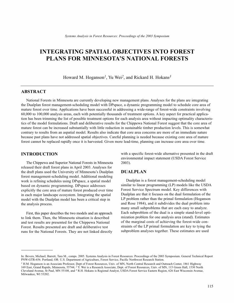
Dualplan can use either a model I or model II type of formulation for addressing the stand level problems(Johnson and Scheurman 1977). A model II formulation is usually more efficient because it eliminates the need toenumerate many combinations of first-rotation treatmenttypes and rotation lengths with similar options for futurerotations. Dynamic programming can be used to solve thestand level decision trees. An example decision tree (fig. 1)helps show how the size of such trees depends more on thenumber of options considered for future rotations than onthe number of options considered for the current rotation.Options to convert to other forest cover types at the end ofthe first rotation can increase substantially the size of thedecision trees for individual stands.

DPSPACE

DPspace is a forest management-scheduling modeldesigned to address the spatial arrangement of the forest.Specifically, it can track and value the amount of corearea produced. It uses a dynamic programming (DP) for-mulation of the problem similar to the formulation used byHoganson and Borges (1998) to address adjacency con-straints. Also similar to Hoganson and Borges (1998), aseries of overlapping subproblems are used to address largeproblems. These overlapping subproblems are similar tomoving windows used in geographic information systemswhere a separate DP formulation of the problem is solvedfor each window. For each window in the moving windowsprocess only a portion of the solution will be accepted. Theportion accepted is the portion of the window not to beincluded in the next window. It is the portion farthest fromthe remainder of the forest yet to be analyzed in the mov-ing windows.

Core area is assumed to be area of the forest that meetsspecific age requirements and is surrounded by a protective

116

Figure 1—A stand-level decision tree linking first rotation options withregeneration options.

buffer. Öhman and Eriksson (1998) recognized core area asan important spatial factor to address in forest managementscheduling models. Core area of mature forest was identifiedas an important spatial measure to address in planning in Minnesota by the interdisciplinary planning team forMinnesota’s National Forest (USDA Forest Service 2003).For DPspace applications for both the Chippewa andSuperior National Forests in Minnesota focus has been onthe production of core area of mature forest. A 328-foot(100-meter) protective buffer distance has been assumedwith minimum ages for core area varying by forest covertype and approximately equal to the age of financial matu-rity for each forest cover type. Minimum age for protectivebuffer also vary by forest cover type and are approximately20 years younger than the age requirement for the core area.

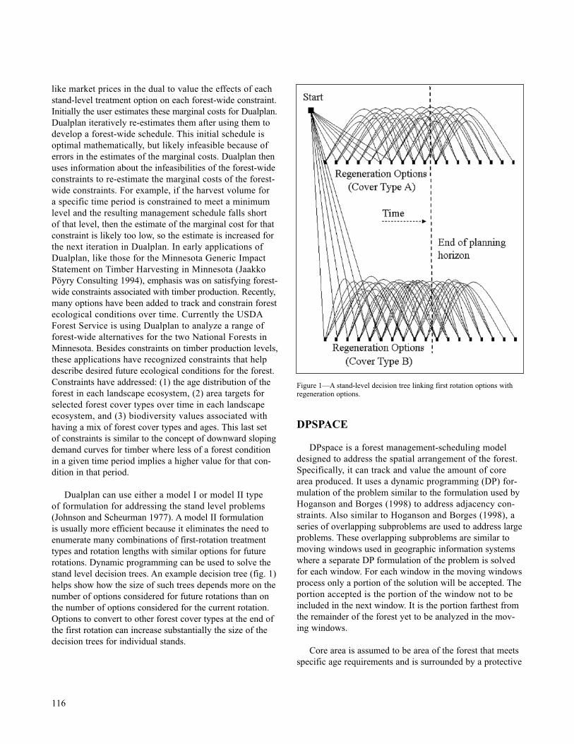
DPspace uses “influence zones” to define the spatialinterrelationships that impact the production of core area.The set of influence zones for a forest can be thought of assimply a map of the forest that indicates, for each point inthe forest, those stands that influence that point in terms ofits potential to produce core area. Each influence zone is aregion of the forest that is influenced by the same set of

stands. Each influence zone may not be contiguous. In mostexisting large stands there will be a center core area that isinfluenced only by that stand itself. Other areas in the samestand are influenced by additional stands if they are withinthe core area buffer distance of the stand boundary. Generallyfor a forest as a whole there are many more influence zonesthan stands. Each influence zone can be labeled by thestands that influence it, and the number of stands influenc-ing it can be considered the influence zone’s dimension.For example an influence zone ABC is influenced by standA, stand B, and stand C because all of that influence zoneis within the core area buffer distance from each of thosestands. It has a dimension of three because it is influencedby three stands. A frequency distribution of influence zonenumbers by influence zone dimension for the Minnesota’sNational Forests (fig. 2) shows that the dimensions can be large and that the distribution is quite sensitive to theassumed core area buffer distance. Many influence zonesinvolve three or more stands. Comparing the frequencydistributions (fig. 2) with corresponding distributions ofinfluence zone area (fig. 3) shows that the lower dimen-sioned influence zones are substantially larger in area onaverage. They contain a much larger portion of the forest

117

Figure 2—Breakdown of the Minnesota National Forests in terms of thenumber of influence zones by influence zone dimension.

Figure 3—Breakdown of the Minnesota National Forests in terms of thearea of influence zones by influence zone dimension.

than the frequency distributions might suggest. With a 328-foot core area buffer distance, relatively little area is ininfluence zones involving more than six stands. As onewould expect, with larger buffer widths, more of the forestinvolves more area in higher-dimensioned influence zones(fig. 3).

Each stage in the DP formulation used for solving eachsubproblem (moving window) corresponds with a stand-level decision. The decision addressed at each stage in thenetwork is the choice of the management treatment optionto assign to the corresponding stand. Treatment options aredefined using a model I format (Johnson and Scheurman1977) with a separate arc for each option. State variablesfor each stage describe the treatment options selected forsome stands addressed in earlier stages of the network(much like a simple decision tree). Each stand remains as a state dimension of the DP tree in later stages of the net-work until all other stands it “influences” have also beenrepresented by a stage decision. A stand influences anotherstand if there exists an influence zone that both standsinfluence. Each influence zone is incorporated into thedecision tree at the last stage in tree that corresponds withone of the stands that makes up its influence zone dimen-sion. For example, assuming influence zone ABC is influ-enced by stand A, stand B and stand C, and stand C is thelast of the three stands addressed in the DP network, thenthe condition of the influence zone can be evaluated for allarcs associated with stage C nodes. This condition is basedon: (1) the treatment option for the corresponding stand Carc and (2) the corresponding conditions for stand A andstand B as defined by the stand A and stand B state vari-ables for the corresponding node at the start of stage C.

Addressing the production of core area in the DP net-work is complicated somewhat by the assumption that thebuffer area surrounding core area need not meet the requiredage of core area itself. In effect, each subcomponent ofeach influence zone (subcomponents defined in terms ofthe stand in which the it resides) must be examined sepa-rately. For all stands making up the influence zone, its por-tion of the influence zone will produce core area if thestand meets the age requirements of core area and all otherstands in the influence zone meet the minimum buffer agerequirements for core area. When addressing each influencezone in the DP network, these checks must be made for allsubcomponents of the influence zone. It is not simply an allor none answer as to whether an influence zone producescore area during each period.

INTEGRATING COMPONENTS

A shortcoming of the DPspace model is its inability toaddress forest-wide constraints directly. Its focus is on inte-grating spatial and aspatial considerations assuming thatthe aspatial value of each stand-level treatment option isknown. Net present value (NPV) estimates for the aspatialaspects of each treatment option for each stand is a key inputto the model. These input values need not be based strictlyon timber returns. They provide an opportunity for a directlinkage with the Dualplan model to consider forest-wideconstraints. In the Dualplan solution process, stand-leveltreatment options are valued taking into account forest-wideconstraints. Rather than view the Dualplan process as select-ing one option for each stand, one can use the same approachto estimate the aspatial value of various treatment optionsto be recognized in DPspace.

The linkage described above is straightforward. Butseveral factors make the problem challenging. First, theDPspace model will be impractical to use for large prob-lems if most stands require a large number of treatmentoptions to be considered in the spatial model. DPspace usesa model I format. Converting stand-level decision trees,like those shown in figure 1, to a model I format results inmany treatment options per stand. Second, if spatial valuesaddressed in DPspace are large, then the aspatial solutionmay be impacted substantially causing some violations ofthe forest-wide constraints in the aspatial model. In otherwords, the shadow price estimates from Dualplan alone arenot likely accurate estimates of the marginal costs of themodeled, aspatial forest-wide constraints if they don’t takealso into account the spatial aspects of the problem.

To help keep the number of treatment options small forthe spatial model without eliminating potentially optimaltreatment options, a treatment trimming model was devel-oped that uses both the results from Dualplan and a detailedanalysis of the influence zones that define the potential foreach stand to contribute to the production of core area. Twobasic factors are considered for dropping a treatment optionin the trimming process. First, treatments are dropped ifcrediting the treatment option for spatial benefits from allstands it influences spatially cannot raise its total value abovethe maximum aspatial value of the stand based on its bestaspatial treatment option. Second, a treatment option can bedropped if there exists another treatment option that has agreater aspatial net present value and that other option spa-tially dominates the treatment option to be dropped. A treat-ment option spatially dominates another if it meets core areacondition requirements in all time periods that the othertreatment option meets core area condition requirements.

118

To recognize the impact of spatial considerations onachieving aspatial forest-wide constraints, Dualplan andDPspace were linked such that the DPspace solution becomesan intermediate solution in the Dualplan iterative process.Essentially the subproblems of the Dualplan model are nolonger independent, single stand-level problems. Instead,the overlapping subproblems from DPspace are the Dualplansubproblems. Dualplan uses a summary of the DPspacesolutions in terms of the measures of the forest-wide con-straints to re-estimate the shadow prices for the forest-wideconstraints. The process is repeated until schedules arefound that are “near-feasible” in terms of the forest wideconstraints. For each repetition (iteration), stand-level treat-ment options are re-evaluated and trimmed for use inDPspace based on the updated forest-wide shadow priceestimates from Dualplan.

Multiple runs of the entire system can be done to exam-ine a range of assumptions about the value for core area.Management schedules are easy to link with GIS systemsfor further analysis because schedules produced are spatiallyexplicit.

MINNESOTA APPLICATIONS

Dualplan has been used to analyze seven forest-widealternatives for each National Forest in Minnesota. Thesealternatives have focused on sustaining timber harvest levelsover time while moving the forest closer to desired futureconditions. Desired future conditions are defined specificallyfor each of seven landscape ecosystems in the ChippewaNational Forest and each of eight landscape ecosystems inthe Superior National Forest. Forest-wide alternatives differin terms of assumptions defining desired future conditionsand the rate at which the forest is moved towards theassumed desired future conditions.

For both forests the planning horizon consists of tenten-year periods. Analysis areas (AA’s) are spatially explicitwith over 67,000 AA’s for the 549,000 acres modeled forthe Chippewa National Forest. Over 101,000 AA’s are usedfor the 1,212,000 acres modeled for the Superior NationalForest. Many of the AA’s are substands representing riparianareas along lakes and streams. Seventeen silvicultural treat-ment types were recognized, representing various types ofeven-aged and uneven-aged management. For each treat-ment type, a range of harvest timings was considered. Twentyforest cover types were recognized for each forest with fivetimber-productivity site-quality classes for most all types.Desired future conditions for each landscape ecosystem weredefined in terms of a desired mix of forest cover types anda desired stand age distribution. Natural succession wasmodeled recognizing that some stands change forest cover

type over time without treatment. Estimates of pre-settle-ment age distributions and stand replacement fire intervalsserved as a benchmark for defining desired future condi-tions and the rate at which harvesting is applied to mimicstand replacement fires.

Forest cover type conversion (restoration) options werean important consideration for stand-level decisions becausedesired future forest-wide conditions were defined in termsof a desired forest cover type mix. This added substantiallyto the number of treatment options modeled for most stands.Five key map layers influenced the set of treatment optionsconsidered for each stand. Besides the landscape ecosystemand riparian map layers described earlier, other layersincluded a map of management areas, a map of scenic classesand a map identifying sensitive areas for a number of plantand animal species. The map of management areas included18 classifications used by the Forest Service to help definethe theme of each alternative. For some forest-wide alter-natives that emphasize older forest conditions, managementarea classifications limited treatment options substantially.

Tests of the spatial model for the National Forest appli-cations focused on a forest–wide alternative somewhat sim-ilar to the alternative with the highest timber harvest levelin the draft forest plan. That alternative was identified inthe draft environmental impact statement (USDA ForestService 2003) as the forest-wide alternative with the mostfragmentation of mature forest over time. That alternativewould also likely be the most complicated alternative tomodel simply because, on average, it is the least restrictiveand thus involves more possible treatment options for eachanalysis area. Multiple model runs of the integrated model-ing system were applied, varying the value of mature forestcore area between applications. For each application, multi-ple iterations of the integrated model were needed to accountfor the impact of valuing core area on the marginal costestimates for the many aspatial constraints. These aspatialconstraints defined desired future conditions for each land-scape ecosystem and sustained timber harvest levels overtime. For all the values of mature forest core area examined,the aspatial constraints were satisfied after multiple itera-tions of the integrated modeling system. The resulting man-agement schedules are potentially improved schedules in thatthey are near-feasible in terms of the aspatial constraintsand produce more core area of mature forest.

Core area is valued in terms of dollars per acre perdecade with values assumed to occur at the end of eachdecade. Assuming a four percent annual discount rate, aprice of $100 per acre per decade for core area, and that themidpoint of the first decade is used as the base year for

119

NPV calculations, then an acre that produces core area inevery decade over an infinite horizon has a NPV ofapproximately $253 per acre.

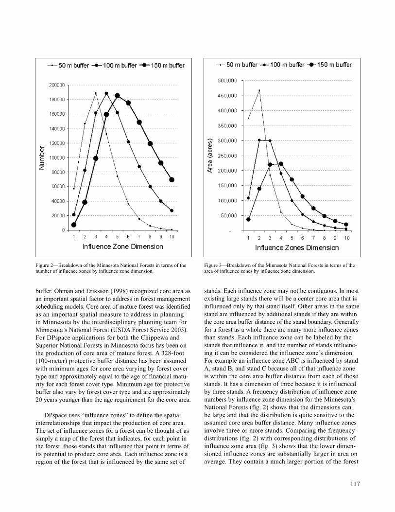
Results of the test applications were similar for bothNational Forests. Here, results are presented only forChippewa National Forest. Two types of core area werevalued and tracked for both forests: upland forest core areaand lowland forest core area. Both types had core areaminimum stand age requirements that varied by forestcover types with a minimum age of at least 40 years for allforest cover types. Core area value assumptions impactedcore area production levels quite similarly for both uplands(fig. 4) and lowlands (fig. 5). Results for the $0 per acreper decade value are equivalent to the Dualplan resultswhere core area was not valued. Without valuing core area,core area levels decline substantially over the first twodecades (fig. 4 and fig. 5). It should not be surprising thatthe draft environmental impact statement for the MinnesotaForest Plan (USDA Forest Service 2003) raises concern

about potential declines in core area of mature forest. Raisingthe core area values to $100 per acre per decade raises theamount of mature area for both uplands (fig. 4) and low-lands (fig. 5) in the later decades, but there is still a declinein the early decades from the starting condition. A core areaprice of approximately $300 per acre per decade is neededbefore such a drop is not present in the early decades. Forthe core area values modeled, higher values for core arealed to higher core area output levels for both uplands andlowlands, with levels substantially higher in the long-termthan in the short-term. Increases are less in the short-termbecause of the time required to produce larger blocks ofmature forest that are relatively well suited for producingcore area. In past planning efforts producing core area ofmature forest was not a primary objective, so it is not sur-prising that the intermediate-aged stands are not arrangedspatially such that they can produce large quantities of corearea when they soon reach the minimum age requirementsfor core area of mature forest. With more lead-time andplanning, substantially more core area can be produced inthe longer-term (fig. 4 and fig. 5).

120

Figure 4—Impact of core area values on upland core area production forfive model runs for the Chippewa National Forest.

Figure 5—Impact of core area values on lowland core area production forfive model runs for the Chippewa National Forest.

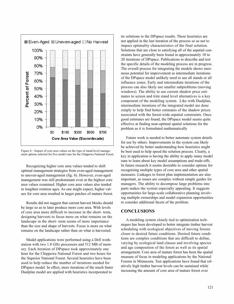
Recognizing higher core area values tended to shiftoptimal management strategies from even-aged managementto uneven-aged management (fig. 6). However, even-agedmanagement was still predominant even at the highest corearea values examined. Higher core area values also tendedto lengthen rotation ages. As one might expect, higher val-ues for core area resulted in larger patches of mature forest.

Results did not suggest that current harvest blocks shouldbe large so as to later produce more core area. With levelsof core area more difficult to increase in the short- term,designing harvests to focus more on what remains on thelandscape in the short- term seems of more importancethan the size and shape of harvests. Focus is more on whatremains on the landscape rather than on what is harvested.

Model applications were performed using a Dell work-station with two 1.8 GHz processors and 512 MB of mem-ory. Each iteration of DPspace took approximately onehour for the Chippewa National Forest and two hours forthe Superior National Forest. Several heuristics have beenused to help reduce the number of iterations needed forDPspace model. In effect, more iterations of the much fasterDualplan model are applied with heuristics incorporated to

tie solutions to the DPspace results. These heuristics arenot applied in the last iteration of the process so as not toimpact optimality characteristics of the final solution.Solutions that are close to satisfying all of the aspatial con-straints have generally been found in approximately 10 to20 iterations of DPspace. Publications to describe and testthe specific details of the modeling process are in progress.The overall process for integrating the models shows enor-mous potential for improvement as intermediate iterationsof the DPspace model unlikely need to use all stands or allinfluence zones. Early and intermediate iterations of theprocess can also likely use smaller subproblems (movingwindows). The ability to use current shadow price esti-mates to screen and trim stand level alternatives is a keycomponent of the modeling system. Like with Dualplan,intermediate iterations of the integrated model are donesimply to help find better estimates of the shadow pricesassociated with the forest-wide aspatial constraints. Oncegood estimates are found, the DPspace model seems quiteeffective at finding near-optimal spatial solutions for theproblem as it is formulated mathematically

Future work is needed to better automate system detailsfor use by others. Improvements in the system can likelybe achieved by better understanding how heuristics mightbe best used to help speed the solution process. Clearly, akey in application is having the ability to apply many modelruns to learn about key model assumptions and trade-offs.In future research it seems desirable to consider options forrecognizing multiple types of core area and other spatialmeasures. Linkages to forest plan implementation are alsoimportant, as issues are complex without simple guides formanagers. The ability to decompose large problems intoparts makes the system especially appealing. It suggestsopportunities for large-scale collaborative planning involv-ing multiple ownerships and model expansion opportunitiesto consider additional facets of the problem.

CONCLUSIONS

A modeling system closely tied to optimization tech-niques has been developed to better integrate timber harvestscheduling with ecological objectives of moving forestscloser to desired future conditions. Desired future condi-tions are complex conditions that are difficult to define,varying by ecological land classes and involving speciesand age composition of the forest as well as its spatialarrangement. Core area of mature forest has been the spatialmeasure of focus in modeling applications by the NationalForests in Minnesota. Test applications have found that rel-atively high timber harvest levels can be sustained whileincreasing the amount of core area of mature forest over

121

Figure 6—Impact of core area values on the type of stand-level manage-ment options selected for five model runs for the Chippewa National Forest.

time. Spatial arrangement of the forest has not receivedattention in past planning efforts so it is not surprising thatconsiderable time is needed to improve spatial conditionsover time. Without recognizing spatial detail in planning,timber harvesting can reduce the existing core area ofmature forest quite rapidly.

LITERATURE CITED

Hoganson, H.M.; Borges, J.G. 1998. Using dynamic programming and overlapping subproblems to addressadjacency in large harvest scheduling problems. ForestScience. 44(4): 526-538.

Hoganson, H.M.; Rose, D.W. 1984. A simulation approach for optimal timber management scheduling.Forest Science. 30(1): 220-238.

Jaakko Pöyry Consulting, Inc. 1994. Generic Environmental Impact Statement on Timber Harvestingand Forest Management in Minnesota. Tarrytown, NY:Jaakko Pöyry Consulting, Inc. 813 p.

Johnson, K.N.; Scheurman, H.L. 1977. Techniques for prescribing optimal timber harvest and investmentunder different objectives—discussion and synthesis.Forest Science Monograph No. 18. 31 p.

Öhman, K.; Eriksson, L.O. 1998. The core area concept in forming contiguous areas for long-term forest plan-ning. Canadian Journal of Forest Research. 28: 1032-1039.

USDA Forest Service. 2003. Draft environmental impact statement: forest plan revision: Chippewa NationalForest and Superior National Forest. MilwaukeeWisconsin. 695 p.

122

In: Bevers, Michael; Barrett, Tara M., comps. 2005. Systems Analysis in Forest Resources: Proceedings of the 2003 Symposium. General Technical ReportPNW-GTR-656. Portland, OR: U.S. Department of Agriculture, Forest Service, Pacific Northwest Research Station.1 Brian McGinley and Gary Marsh are Resource Planners, 2 Allison Reger is a Forest Resource Analyst, and 3 Kirk Lunstrum is a Wildlife Biologist. Coauthors work on the Willamette National Forest, Oregon.

Systems Analysis in Forest Resources: Proceedings of the 2003 Symposium

LANDSCAPE CHANGES FROM MANAGING YOUNG STANDS

A Fall Creek LSR Modeling Study

Brian McGinley1, Allison Reger2, Gary Marsh1, and Kirk Lunstrum3

INTRODUCTION

Public land agencies continually seek a better under-standing of spatial and temporal changes to forested landscapes and to use this understanding in successivemanagement decisions. Recent focus has moved towardcomplex assessments of forest habitat changes acrosslarge landscapes. This shift has been partially prompted in the Pacific Northwest by desires to protect old growthforests and its dependent species.

The 1994 Northwest Forest Plan, with a network ofLate-Successional Reserves (LSRs), is an example of thisfocus on managing forest habitat changes across large-scalelandscapes. One option in the LSR network strategy is

123

using silviculture treatments to improve late-successionalhabitat conditions within young stands less than 80 yearsold.

Thinning is accepted as a useful tool for acceleratingvegetative development toward late seral conditions(USDA,USDI 1994; USDA,USDI 1998). Although muchdebate still remains on the best treatments or stand-leveldesigns to apply, thinnings can effectively influence speciescomposition, stem growth, canopy complexity, and under-story communities in residual stands.

With most thinning in LSRs occurring in establishedplantations, managers should anticipate the temporal andspatial influence these plantations can have in shaping the

ABSTRACT

Public land agencies continually seek a better understanding of spatial and temporal changes in forested landscapes to guidesuccessive management decisions. The 1994 Northwest Forest Plan developed a network of Late-Successional Reserves (LSR)with the primary goal of protecting and improving late-succesional habitat. Improving LSR habitat can involve silviculturetreatments in stands less than 80 years old, which would improve stem growth, canopy height complexity and understory com-munity development. The Fall Creek Modeling Study, using TELSA (Tool for Exploratory Landscape Scenario Analysis),explores connections among young stand management strategies and resulting landscape habitat patterns. TELSA is a spatiallyexplicit planning tool that simulates succession, natural disturbances, and management actions on a landscape over time. TheFall Creek LSR is a typical mosaic of young stands, fragmented late successional habitat, and high road densities created byintense forest management. The impetus for this project was insufficient funding to promote late-successional habitat by thethinning of all available hectares over the next 50 years. This modeling study evaluated a number of resource-driven scenariosfor selecting prescriptions and prioritizing stands for treatment. The team used spatial mapping and stand simulation tools toassess the effects of these thinning scenarios on LSR habitat patterns over a 200 year period. For specific landscape objectives,such as interior habitat or mimicking natural fire patterns, location of habitat improvements from thinning are shown to bemore valuable than total hectares of improved habitat.

landscape patterns of late-successional habitat. Plantationscomprise around 25 to 35 percent of most large LSRs inthe Mid-Willamette network, making their landscape rolesignificant.

The Fall Creek Modeling Study explores the connec-tions among young stand management strategies andresulting landscape habitat patterns.

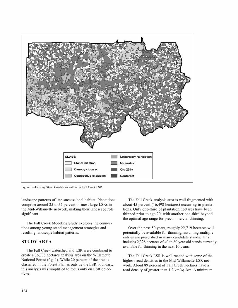
STUDY AREA

The Fall Creek watershed and LSR were combined tocreate a 36,338 hectares analysis area on the WillametteNational Forest (fig. 1). While 20 percent of the area isclassified in the Forest Plan as outside the LSR boundary,this analysis was simplified to focus only on LSR objec-tives.

The Fall Creek analysis area is well fragmented withabout 45 percent (16,498 hectares) occurring in planta-tions. Only one-third of plantation hectares have beenthinned prior to age 20, with another one-third beyond the optimal age range for precommercial thinning.

Over the next 50 years, roughly 22,719 hectares willpotentially be available for thinning, assuming multipleentries are prescribed in many candidate stands. Thisincludes 2,328 hectares of 40 to 80 year old stands currentlyavailable for thinning in the next 10 years.

The Fall Creek LSR is well roaded with some of thehighest road densities in the Mid-Willamette LSR net-work. About 89 percent of Fall Creek hectares have aroad density of greater than 1.2 km/sq. km. A minimum

124

Figure 1—Existing Stand Conditions within the Fall Creek LSR.

road network for this LSR includes only 23 percent (226kilometers) of its total road system.

MANAGEMENT SITUATION

The Forest Plan identifies two principal goals for thin-ning stands less than 80 years old in LSR’s: 1) to developold growth forest characteristics, and 2) to reduce the riskof large-scale disturbance events like wildfire (USDA,USDI 1994, pp. B-5-6).

The Mid-Willamette LSR Assessment identifies moreinterior habitat and lower road densities as key manage-ment objectives for the Fall Creek LSR (USDA, USDI1998). Enhancing late seral connective corridors along itseastern boundary is another focus for the Fall Creek LSR.While plenty of thinning opportunities exist in the analysisarea, the Willamette National Forest does not expect tohave sufficient funding or staffing to thin all availablehectares over the next 50 years.

Current thinning efforts are using the same oldest/largest/closest-first priority strategy used in placing clearcuts onthe landscape. A thinning strategy built from resourceobjectives for prioritizing stands is likely to create greaterlandscape habitat benefits.

MANAGEMENT SCENARIOS

This analysis evaluated a number of resource-drivenmanagement scenarios for selecting thinning prescriptionsand prioritizing young stands for treatment. The followingbriefly describes the scenarios examined.

Management ScenariosScenarios are comprised of management constraints, a

stand priority strategy, and thinning prescriptions. Commercialthinning prescriptions could potentially occur at one ormore of three stand ages (40, 60 and 80 years) and at oneof three treatment intensities (light, medium, heavy). Therewere six scenarios studied, each meeting a single resourceobjective or providing a benchmark for comparison.

1) The No Action scenario was modeled to provide apoint of comparison. In this scenario no action was takenon any stands permitting the managed stands to now follownatural succession.

2) The Owl Sites scenario focuses on young standswithin 2.0 kilometers of nesting activity centers and usesnesting success to prioritize activity centers. The objectiveof this scenario was to improve habitat near northern spot-ted owl nest sites.

3) The Roads scenario focuses thinning on habitatimprovement and reducing road densities in land blocks(roadsheds) possessing high aquatic risk ratings (USDA,1999). Thinning entries into roadsheds were spaced atleast 20 years apart to allow for road closures and decom-missioning. The objective of this scenario was to reduceaquatic risks through habitat improvement and lower roaddensities.

4) The Natural Fire scenario uses thinning to createhabitat conditions predicted from defined natural fireregimes. Fire frequency, fire intensity and slope positionwere used to define resulting habitat conditions andassign treatments. This scenario was developed to mimicvegetative patterns created by natural fire regimes.

5) The Interior Habitat scenario focuses on youngstands surrounded by or next to large interior habitat blocks.Thinning intensity was reduced to minimize edge effectson existing late-successional habitat and to expand largeinterior habitat blocks.

6) Finally, a Two-Thin Benchmark was applied to all young stands to provide an upper limit of thinning forcomparing with other scenarios. This scenario was themost aggressive thinning strategy.

Several iterations of each scenario were tested to look at a range of possibilities.

Analysis ToolsThe analysis team used spatial mapping and stand simu-

lation modeling tools to assess the effects of thinning treat-ments on LSR habitat patterns. TELSA (Tool for ExploratoryLandscape Scenario Analysis) is a strategic, landscape-level planning tool that can project planning strategies ontoa landscape and assess long-term spatial and temporaleffects using a range of performance indicators (ESSA,1999).

PNW_GAP (originally ZELIG-PNW) is a stand growthsimulator used to track stand attributes along developmentcurves in response to thinning treatments (Garman, 1999).Garman (1999) tested a variety of thinning prescriptionsfor accelerating the development of late-successional standattributes. These tools were used to apply thinning sched-ules for each scenario to the landscape and project late-suc-cessional attribute development over a 200-year time period.

Late-Successional Stand Attributes with Minimum Thresholds

Garman (1999) simulated a wide range of thinning

125

treatments on a 40-year old Douglas-fir stand that had beenprecommercially thinned at age 12 years. He tracked thin-ning effects on five late-successional attributes and thetime needed to reach threshold values. (See attributes withminimum thresholds below).

Garman also used a composite Late-SuccessionalIndex (LSI) for tracking when stands meet all three livestand attribute thresholds. The Fall Creek analysis teamfocused only on the three live stand attributes and LSI toevaluate scenario influences on late-successional habitatand other management goals. The snag and downed woodattributes were not used in this study, because they couldbe readily created (topping or felling) once minimumlarge bole densities were achieved.

Thinning prescriptions selected from Garman’s simu-lations for this analysis quickly met thresholds for the livestand attributes and matched other scenario objectives.

Late-successional Criterion

The TELSA spatial model was used to map stand attrib-utes across the landscape at different time points for eachscenario. Other key landscape attributes were used to eval-uate scenarios (see below).

BUILDING RESOURCE SCENARIOS

TELSA, a spatially explicit model, requires data in avector-based format. Several GIS layers used in this analy-sis included vegetation and planning area boundaries.

Using GIS technology the landscape was stratified intoplanning zones. Planning zones signify areas with discretemanagement goals or areas requiring separate reporting ofresults. Planning zones common to all scenarios were theproject area boundary and transportation routes.

Transportation routes entered into TELSA tracked whichroads were used during thinning operations and how longeach road was left inactive (unused by thinning activities).

A combination of unique planning zones and thinningprescriptions customized each scenario to achieve keyresource objectives highlighted by the scenario. In responseto limited budget assumptions, the Fall Creek analysis teamalso created priority management goals for thinning withinplanning zones. These unique planning zones defined thekey difference between resource scenarios. Each scenariohad 1 to 2 additional planning zones added for stratifyingthe landscape based on differing management goals.Planning zones specific to each scenario are discussedbelow.

1) No Action Scenario: This scenario used no uniqueplanning zones and no management was applied to thelandscape. The scenario provided a point from which tomeasure the effects of thinning stands.

2) Owl Scenario: This scenario focuses habitat improve-ment in young stands near known spotted owl (Strix occi-dentalis caurina) activity centers. Based on monitoring dataon the nest site occupancy and reproductive success, owlhabitat centers were ranked into three site categories. A1.1-km buffer around nest sites and the sites correspondingranking became planning zones in the TELSA model. Atwo-thin prescription (a moderate thin at age 60 years, lightthin at 80 years) was selected for all stands.

This prescription was selected by the analysis team to maintain forest cover and canopy closure for potentialowl dispersal and foraging opportunities, while attainingthreshold values of late-successional attributes quickly.

Owl scenario iterations differed in which owl circleswere treated and which were left to natural succession.

3) Roads Scenario: This scenario divides the landscapeinto management blocks called “roadsheds”—lands thatwould feasibly log to a local road system. Roadsheds var-ied in size from 1,500 to 4,000 hectares. Two criteria wereused to prioritize roadsheds for thinning and resulting roadclosures:

a. Aquatic risk ratingb. Plantation hectares available for thinning

The roadsheds and priority ranking were integrated intothe TELSA model as a planning zone.

126

1. Density of large boles >100 cm• 10 boles per hectare

2. Canopy Height Diversity Index• Index = 8.0

3. Density of shade tolerant boles >40 cm• 10 boles per hectare

4. Density of snags >50 cm• 10 boles per hectare

5. Mass of logs >10 cm at large end• 30 Mg/ha

4) Natural Fire Scenario: Fire regimes defined in theIntegrated Natural Fuels Management Strategy (USDA,USDI 2000) served as a template for the Natural Fire sce-nario. These fire regimes as identified for the study areabecame a key planning zone map in the model. These threeregimes can be briefly described as:

1. moderate frequency/mixed severity; 2. low frequency/mixed severity; and 3. low frequency/high severity.

Slope position (lower 50 percent of the slope and theupper 50 percent of the slope) was a second planning zoneadded to include the variation of fire effects due to slopeposition. Thinning prescriptions were selected to match thestand conditions likely to result from representative fireevents under these regimes. Moderate frequency areasreceived a two thin prescription (upper slopes – heavy atage 40 years, moderate at 80 years; and lower slopes –moderate at 40 years, light at 80 years). Low frequencyareas received one heavy thin at age 60 years in the upperslopes only.

5) Interior Habitat Scenario: Old growth dependentspecies thrive best in late succesional interior habitat,which provides higher relative humidity, moderated tem-peratures, and desirable physical structure. Interior habitat(IH) is also generally free of invasive and competing non-native species. As a rule, interior habitat conditions in late-successional stands improve as you move further fromedges with early seral conditions.

This scenario was designed to focus thinning in youngstands that help expand existing interior habitat (IH) blocks.Four landscape blocks were identified for prioritizing treat-ments and are listed by priority:

1. Stands within largest IH blocks2. Stands creating sinuosity on the edge of the largest IH

block3. Stands connecting large IH blocks4. All other stands

Because thinning may increase the risk of edge effects(edaphic changes and blowdown) on adjacent late-succes-sional habitat, prescriptions were varied based on distancefrom late-successional edge:

• Within 120 meters of habitat edges—Moderate thin at 60 years, and light thin at 80 years.

• Beyond 120 meters from habitat edges—Heavy thin at 60 years, and moderate thin at 80 years.

Landscape blocks and distance from edge both became key planning zones in the TELSA model.

6) The Two Thin scenario prescribed a two-thin pre-scription (heavy thin at age 40 years, medium thin at 60years) to all candidate stands with a constraint that reentryinto any roadshed should not occur for at least 20 years.This constraint reduced open road densities by increasingopportunities for road decommissioning work.

Comparing Resource Scenarios The following management goals were selected to

compare resource scenarios:

• Total hectares of late-successional habitat (an LSI rating above 75 percent)

• Total hectares of interior late-successional habitat

• Total hectares of late-successional habitat within owl nesting circles.

• Total hectares of late-successional habitat within

moderate fire intensity areas.

• Total kilometers of roads remaining inactive for 10 and 20 years.

Management goals were also expressed as relative meas-ures of total hectares thinned. Resource scenarios were alsoevaluated and compared visually, as seen in figures 2 and 3,to generally understand how landscape habitat patternschange under each scenario. Finally the flow of thinninghectares across the analysis timeline was considered foroperational reasonability.

ANALYSIS RESULTS

After 70 years, resource scenarios had thinned between8,600 and 13,000 hectares. By contrast, the Two-ThinBenchmark thinned 31,000 hectares in just 50 years and theNo Action scenario 0 hectares. Harvest levels by decadevaried noticeably between scenarios. The Roads scenariocreated a tri-modal harvest pattern due to the 20-year har-vest constraint for roadsheds, while other scenarios moreequitably spaced harvest over time.

By analysis year 80, scenarios had increased late-suc-cessional habitat (hectares with an LSI rating above 75 percent) by 2 to 17 percent above the No Action scenario.Scenarios had increased LS habitat within owl circles by 3 to 13 percent above the No Action scenario.

127

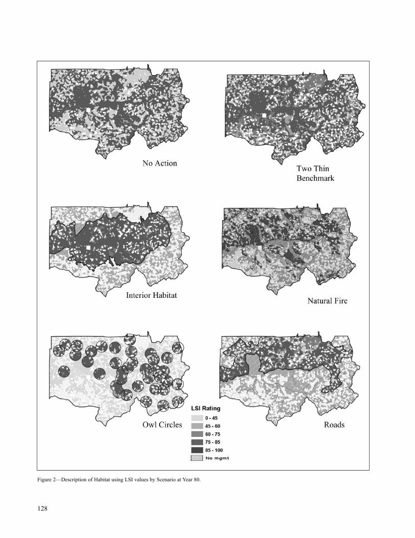
128

Figure 2—Description of Habitat using LSI values by Scenario at Year 80.

129

Figure 3—Description of Habitat using LSI values by Scenario at Year 120.

By analysis year 80, scenarios had increased interiorhabitat by 2 to 40 percent above the No Action scenario.The Roads and Interior Habitat scenarios achieved highestgains in interior habitat.

By analysis year 40, scenarios were able to keep 327 to 395 km of roads inactive (or unused) for more than 20years. These roads are considered good candidates for clo-sure. The Roads scenario created the most kilometers ofinactive roads, largely due to the 20-year re-entry schedul-ing constraint and its narrow focus on only high-risk road-sheds.

Habitat patterns varied notably between scenarios,though total late-successional habitat differences were notgreat (figures 2 and 3). The Owl Site scenario concentrateshabitat improvement efforts around only 37 nest sites spreadacross the landscape. The Natural Fire scenario also tendedto spread thinning treatments across the landscape, in highfire frequency areas.

By contrast, the Roads scenario focused thinnings onthe north side of the landscape, where aquatic risk ratingswere highest. Similarly, the Interior Habitat scenario con-centrated treatments within the core of the landscape alongFall Creek.

Efforts to include precommercial thinning options in the analysis were stymied by incompatible data sets ofstand development curves, and were eventually abandoned.

CONCLUSIONS

Modeling helps to visualize the cumulative benefits/impacts of thinning strategies on LSR landscapes and compare management strategies. The Fall Creek analysisshould provide useful reference points for future projectanalysis or creation of a 5-year action plan of thinningprojects.

Results should prove useful for building public andagency confidence in using thinning to improve habitatconditions within LSR landscapes. For interior habitat val-ues, location of habitat improvements on the landscape canbe more important than total hectares of habitat improved.Landscape objectives help drive this placement of thinningefforts. Landscape attributes or habitat indices used to com-pare management scenarios are more useful when maderelative to total treatment hectares.

NEXT STEPS IN THIS INVESTIGATION

• Model other resource scenarios of interest to managers.¡ Connectivity (travel corridors) between LSRs.¡ Combine several resource objectives into one scenario.¡ Allocate resource scenarios to different sections of the

LSR and pursue simultaneously.

• Strengthen the simulations by testing complicated prescriptions involving precommercial thinning.

• Introduce implementation constraints (planning, budget, resource issues) into the scenarios.

• Use modeling results to create a five-year action plan of thinnings.

LITERATURE CITED

Garman, S.L. 1999. Accelerating development of late-successional conditions in young managed Douglas-firstands: a simulation study. USDA, Forest Service,Willamette National Forest. On file with: WillametteNational Forest, 211 E. 7th Avenue, Eugene, OR 97401.

ESSA Technologies LTD. 1999. TELSA: Tool for Exploratory Landscape Scenario Analyses, User’s GuideVersion 1.0. Vancouver, BC: ESSA Technologies Ltd. 164 p.

USDA Forest Service and USDI Bureau of Land Management. 1994. Record of Decision for Amendmentsto Forest Service and Bureau of Land ManagementPlanning Documents within the Range of the NorthernSpotted Owl. http:/www.oregon.gov/library/

USDA Forest Service and USDI Bureau of Land Management. 1998. Mid-Willamette Late-SuccessionalReserve Assessment. On file with: Willamette NationalForest, 211 E. 7th Avenue, Eugene, OR 97401.

USDA Forest Service.1999. Fall Creek/Little Fall Creek Access and Travel Management Environmental Assess-ment. Willamette National Forest. On file with:Willamette National Forest, 211 E. 7th Avenue, Eugene,OR 97401.

130

In: Bevers, Michael; Barrett, Tara M., comps. 2005. Systems Analysis in Forest Resources: Proceedings of the 2003 Symposium. General Technical ReportPNW-GTR-656. Portland, OR: U.S. Department of Agriculture, Forest Service, Pacific Northwest Research Station.1 P. Bettinger is an Associate Professor, Warnell School of Forest Resources, University of Georgia, Athens, GA 30602. 2 J. Drake is an Assistant Professor,Warnell School of Forest Resources, University of Georgia, Athens, GA 30602.

Systems Analysis in Forest Resources: Proceedings of the 2003 Symposium

EXAMINATION OF TRADEOFFS BETWEEN TIMBER PRODUCTION AND SPOTTED OWL

HABITAT IN COASTAL OREGON

Pete Bettinger1, and Jason Drake2

INTRODUCTION

As forest and wildlife sciences evolve, researchers andpractitioners become increasingly exposed to new hypothe-ses concerning the link between management (and hencelandscape condition) and ecological and social values. Thedevelopment of new hypotheses also provides opportunitiesfor their integration with management models and subse-quent evaluations of impact, effect, and association. Advancesin wildlife habitat relationships research have provided for-est planning the opportunity to more closely incorporatehabitat goals into forest planning processes. The type ofmathematical programming approach used to accomplishthis integration will depend on the wildlife species underconsideration and type of relationships used to evaluate thecapability of a landscape to provide habitat. One exampleof new research on wildlife-habitat relationships is thatprovided by McComb and others (2002), who developed a wildlife capability model for the northern spotted owl(Strix occidentalis caurina).

ABSTRACT

A forest planning model was developed to assess the trade-offs among timber production and spotted owl (Strix occiden-talis caurina) habitat in coastal Oregon. The model utilized a threshold accepting heuristic technique to schedule, via 1-optmoves, timber harvests subject to spotted owl, adjacency, and green-up goals. The forest planning model was designed as aModel I problem, and only clearcut harvest decisions were made. The trade-offs among timber production and habitat goalsare presented as a set of production possibility frontiers. With this preliminary analysis, it seems that there is a linear rela-tionship between even-flow timber harvest levels and an allowable decrease in habitat levels (from projections of habitatunder a “grow-only” scenario), up to a point. When habitat levels were allowed to decrease beyond 20% of the “grow-only”levels, no effect on timber harvest levels was noted. While this model helps managers and policy makers understand thetrade-offs among timber production and spotted owl habitat levels, results may be limited to the landscape examined andthe range of constraints tested.

131

The McComb and others (2002) owl habitat capabilityindex (HCI) model includes both a within-stand nestingcomponent and a home-range analysis, and thus requiresmeasuring the characteristics of forest vegetation up to2,400 m from each area of interest. Since a managementactivity scheduled to a management unit can affect thehabitat quality of other management units up to 2,400 maway, this suggests the need for integer decision variables.A number of mixed integer and integer formulations of for-est planning problems have been addressed in the forestryliterature, from the pioneering work of Hof and Joyce (1992),Hof and Raphael (1993), and Hof and others (1994) usingthe exact techniques, to approaches provided by Bettingerand others (1997, 2002) and Calkin and others (2002)using heuristic techniques. This paper presents a processthat integrates McComb and others (2002) HCI model withcommodity production goals in a heuristic forest planningmodel.

METHODS

We selected a large landscape in western Oregon to usein modeling the integration of spotted owl HCI and com-modity production goals in a forest planning context. Thelandscape (fig. 1) represents approximately 235,000 ha ofland, mostly forested, and mainly managed by state andindustrial land managers. Pixels in figure 1 are coloredbased on their vegetation class, and while not completelyinformative of the vegetative structure across the landscape,the figure allows one to locate the agricultural, urban, andcleared areas (the light colors), and to discern changes intopography based on the variations in the gray scale. Thevegetation database was acquired from the CLAMS project(CLAMS 2002), and consists of a raster GIS database con-taining 3,752,714 pixels with a spatial resolution of 25 m.Each pixel in the vegetation GIS database has associatedwith it a tree list, as the database was created using a gradi-ent nearest neighbor approach to classification that facili-tates this association (see Ohmann and Gregory 2002). Atree list is simply a list of trees used to represent the forestedconditions within each pixel. The lists used were derivedfrom the U.S. Forest Service’s Forest Inventory andAnalysis program, the U.S. Forest Service’s ContinuousVegetation Survey program, and research plots. Ohmannand Gregory (2002) provide more detailed informationregarding the classification approach and assignment oftree lists to pixels in the GIS database.

The vegetation data associated with each pixel includesstanding timber volume, average tree age, quadratic meandiameter, and several measures of coarse woody debris.This data facilitates measuring the impact of activities onboth commodity production and habitat goals. The ageclass distribution of this area (fig. 2) shows that most of theforest vegetation is between 20 and 50 years old. A GISdatabase describing management units was acquired fromthe CLAMS project. Management units average 6-8 ha insize. The spatial relationship of each management unit inrelation to others of which it shares a side was also devel-oped, to facilitate the modeling of adjacency and green-uprestrictions. Pixel data within management units are aggre-gated to arrive at average stand ages, volumes, and so on,for each management unit.

Objective functionThe forest planning problem we solved attempts to

maximize even-flow of timber harvest volume subject toadjacency, green-up, minimum harvest age, and spottedowl habitat constraints. The objective function was designedto measure and minimize the deviations of actual scheduledharvest volume from some target harvest volume.

minimize ∑ ∑(xit vit) –TV2

132

Figure 1—A 235,000 ha landscape in the CoastRange of Oregon.

T

t=1

N

i=1

Where:t = a time periodT = total number of time periodsi = a management unitN = total number of management unitsTV = target timber harvest volume per time period

(a constant)xit = a binary (0,1) variable indicating whether or not man-

agement unit i is clearcut during time period tvit = the volume available in management unit i during

time period t

In this research, the time horizon was assumed to be 40 years, and consisted of eight 5-year time periods. Therewere 39,500 management units in the study area, each con-taining approximately 100 pixels. It is possible that not allof the pixels in a management unit could be harvested ineach time period. A number of factors may prevent harvestof a pixel, including the following: it is represented as hav-ing a non-forest vegetation condition, its age is below theminimum harvest age, it is located within a riparian area, it is reserved as a leave-tree clump. Therefore, vit for eachmanagement unit only represents the available volume during that time period.

ConstraintsThere are five main constraints contained within this

planning process. First, we assume that each managementunit could only be scheduled for harvest once during thetime horizon.

∑xit ≤ 1 i

Second, each management unit, based on the averageage of its forested pixels, had to be above a minimum har-vest age before a clearcutting activity could be scheduled.Thus the average harvest age of each management unit dur-ing each time period was computed, then the set of potentialchoices for each management unit was determined.

∑ (aj Agejt)

∑ (aj)

If AHAit ≥ MHA Then xit ∈ {0,1}Else xit = 0

Where:j = a pixel within a management unitJi = the set of forested pixels contained within management

unit iaj = area of a pixelAgejt = age of trees contained within pixel j during time

period tAHAit = average potential harvest age of management unit

i during time period tMHA = the minimum harvest age for a set of trees within a

management unit

The third constraint indicates that clearcut sizes are lim-ited to a maximum of 48.6 ha (120 acres). The schedulingprocess used a recursive function to determine the actualsize of all proposed clearcuts by sensing the size of poten-tial clearcuts from neighbors of proposed sales, and theirneighbors, and so on.

xit CAit + ∑ xzt CAzt ≤ MCA i,t

Where:CAit = potential clearcut area of management unit i during

time period tz = an adjacent management unitNi = the set of all management units adjacent to manage-

ment unit iSi = the set of all management units adjacent to those man-

agement units adjacent to management unit iMCA = the maximum clearcut area assumed (48.6 ha)

This definition is very similar to that proposed byMurray (1999) for area restriction problems. Si is essentiallythe set of clearcut units that contain all units adjacent to theneighbors of unit i, and all units adjacent to the neighborsof neighbors, etc. It is referred to as a recursive function

133

Figure 2—Age class distribution of forest land in a 235,000 ha landscapein the Coast Range of Oregon.

Ji

Ji

T

j=1

j=1

t=1

A

A

z∈Ni∪Si

= AHAit i,t

A

because of the potentially sprawling cluster group that mustbe assessed depending on the direct or indirect contiguity(of other clearcut units) with management unit i (Murray1999).

The fourth constraint is related to the heterogeneity ofvegetation contained in the initial raster vegetation GISdatabase. Given the salt and pepper nature of resultingclassifications of satellite images, we wanted to ensure thata significant proportion of the forested area of each man-agement unit was actually available for clearcut harvestprior to allowing a clearcut to be scheduled. While thisconstraint may seem redundant, given the minimum harvestage constraint noted above, it does prevent the schedulingof small (and very old) portions of management units. Here,the percentage of forest pixels that are available for clearcutharvest are summed each time period, and if this percent-age is higher than a minimum percentage, the managementunit may be available for clearcut harvest. A minimum har-vest area of 65% was chosen based on numerous evaluationsconducted within the CLAMS project. Higher minimum per-centages significantly constrain harvest levels, while lowerpercentages allow small parts of management units to beharvested.

If γit ≥ MHP Then xit ∈ {0,1}Else xit = 0

Where:γit = the percentage of management unit i available for

clearcut harvest during time period tMHP = the minimum harvest percent (minimum percent-

age area available for clearcut harvest within eachmanagement unit)

Finally, the fifth constraint allows the scheduling modelto constrain activities to those that are possible withoutreducing the “grow only” spotted owl HCI levels “toomuch.” Here, the spotted owl HCI levels were first com-puted for the landscape under the assumption that no har-vests will occur over the 40 year time frame. Then, amaximum allowable decrease was determined for eachtime period.

LHCIt ≥ w (“grow only” LHCIt ) t

Where:LHCIt = the potential spotted owl HCI level for the entire

landscape during time period tw = the maximum percentage decrease (0 ≤ w ≤ 1)

The landscape HCI levels are computed from individualmanagement unit HCI estimates

∑ (Ait HCIit)

∑ Ait

Where:Ait = forested area of management unit i during time period

tHCIit = the HCI estimate for management unit i during

time period t

We utilized the “model 2” spotted owl HCI modeldeveloped by McComb and others (2002) to make the HCIevaluations across the landscape. The spotted owl HCImodel was developed to measure the capability of a patchand its surrounding neighbors to provide conditions impor-tant to survival and reproduction of spotted owls. HCI levelswere estimated by computing a nest stand capability indexand a landscape capability index:

HCIit = (NCIit2 LCIit )(1 / 3)

Where:NCIit = the nest stand capability index component of the

HCI for management unit i during time period tLCIit = the landscape capability index component of the

HCI for management unit i during time period t

NCIit is a function of the density of trees 10-25 cm dbh,trees 25-50 cm dbh, and trees 75+ cm dbh, as well as adiameter diversity index. LCIit is a function of the percent-age of large and medium sized trees within three zonesaround each management unit: 28 ha, 202 ha, and 1,810 ha.These spatial zones were translated to radii around eachmanagement unit: 300 m, 800 m, and 2,400 m. The cen-troid of each management unit was used as the base pointof each evaluation, and if any other management unit’scentroid was within these search distances, they con-tributed to LCIit. This represents a simplification of theprocess described in McComb and others (2002), whereLCI was computed as a moving window around each pixel,more precisely measuring the zonal areas. Here, we com-puted management unit HCI levels, and by basing the LCIcomputations on this, gain significant processing speedduring the scheduling process. The disadvantage of thisapproach is that the difference in the evaluation of owl

134

A

A

N

Ni=1

j=1

= LHCIit t

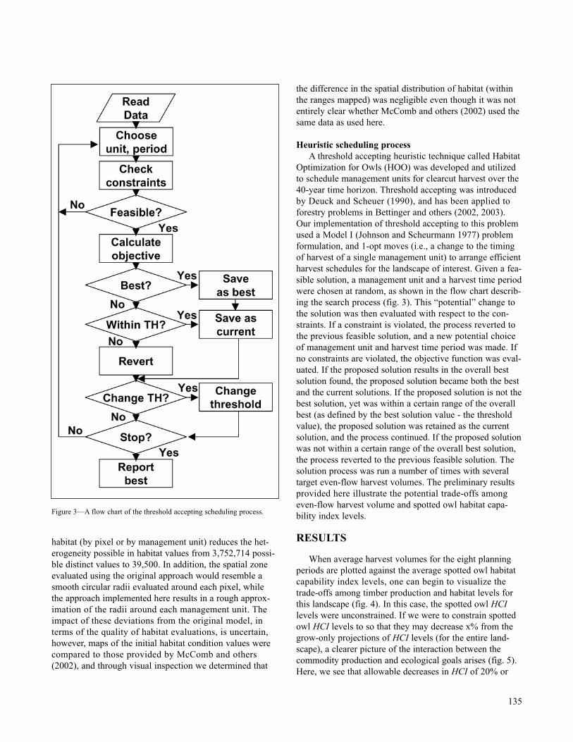
habitat (by pixel or by management unit) reduces the het-erogeneity possible in habitat values from 3,752,714 possi-ble distinct values to 39,500. In addition, the spatial zoneevaluated using the original approach would resemble asmooth circular radii evaluated around each pixel, whilethe approach implemented here results in a rough approx-imation of the radii around each management unit. Theimpact of these deviations from the original model, interms of the quality of habitat evaluations, is uncertain,however, maps of the initial habitat condition values werecompared to those provided by McComb and others(2002), and through visual inspection we determined that

the difference in the spatial distribution of habitat (withinthe ranges mapped) was negligible even though it was notentirely clear whether McComb and others (2002) used thesame data as used here.

Heuristic scheduling processA threshold accepting heuristic technique called Habitat

Optimization for Owls (HOO) was developed and utilizedto schedule management units for clearcut harvest over the40-year time horizon. Threshold accepting was introducedby Deuck and Scheuer (1990), and has been applied toforestry problems in Bettinger and others (2002, 2003).Our implementation of threshold accepting to this problemused a Model I (Johnson and Scheurmann 1977) problemformulation, and 1-opt moves (i.e., a change to the timingof harvest of a single management unit) to arrange efficientharvest schedules for the landscape of interest. Given a fea-sible solution, a management unit and a harvest time periodwere chosen at random, as shown in the flow chart describ-ing the search process (fig. 3). This “potential” change tothe solution was then evaluated with respect to the con-straints. If a constraint is violated, the process reverted tothe previous feasible solution, and a new potential choiceof management unit and harvest time period was made. Ifno constraints are violated, the objective function was eval-uated. If the proposed solution results in the overall bestsolution found, the proposed solution became both the bestand the current solutions. If the proposed solution is not thebest solution, yet was within a certain range of the overallbest (as defined by the best solution value - the thresholdvalue), the proposed solution was retained as the currentsolution, and the process continued. If the proposed solutionwas not within a certain range of the overall best solution,the process reverted to the previous feasible solution. Thesolution process was run a number of times with severaltarget even-flow harvest volumes. The preliminary resultsprovided here illustrate the potential trade-offs amongeven-flow harvest volume and spotted owl habitat capa-bility index levels.

RESULTS

When average harvest volumes for the eight planningperiods are plotted against the average spotted owl habitatcapability index levels, one can begin to visualize thetrade-offs among timber production and habitat levels forthis landscape (fig. 4). In this case, the spotted owl HCIlevels were unconstrained. If we were to constrain spottedowl HCI levels to so that they may decrease x% from thegrow-only projections of HCI levels (for the entire land-scape), a clearer picture of the interaction between thecommodity production and ecological goals arises (fig. 5).Here, we see that allowable decreases in HCI of 20% or

135

Figure 3—A flow chart of the threshold accepting scheduling process.

more had no effect on timber harvest levels. When HCIwas constrained to an allowable decrease of less than 20%,there was almost a linear relationship between the allow-able decrease and the resulting even-flow timber harvestlevels. Similarly, average HCI levels decreased in a nearlylinear fashion as the allowable decrease in HCI from thegrow-only condition increased, up to 20% (fig. 6). Allowabledecreases in HCI beyond 20% seemed to have no effect onaverage HCI levels on this landscape. The HCI level at thispoint (0.168) represents the level most likely under full utilization of the landscape under economic objectives.Allowing small deviations in owl habitat levels from the“grow only” case constrains the achievement of economicobjectives to a point (up to a 20% allowable decrease), butbeyond this point this constraint has no impact on solution

values - HCI levels are at their lowest given the age classdistribution of the landscape, the management direction,and the other constraints recognized (e.g., adjacency).Figures 5 and 6 contribute to this insight.

While we have been relating timber harvest levels toaverage HCI levels over the 40-year planning horizon, HCIlevels were not static, and generally increased over time(fig. 7). The trend in the increase of HCI levels over timeseemed to be consistent no matter what target even-flowharvest level was specified in the HOO model. The ‘no-cut’ HCI levels in figure 7 were the levels obtained whenthe landscape was projected under a grow-only policy. It isfrom these levels that the allowable decrease in HCI wasmeasured when HCI is constrained.

136

Figure 4—Production possibility frontier relating average HCI level to average even-flow timber harvest level, when HCI levels are unconstrained.

Figure 5—Even-flow harvest levels when HCI is allowed to decrease from1 to 40 percent from grow-only projections of the landscape.

Figure 7—Actual HCI levels over the planning horizon under three differ-ent policies regarding the desired even-flow timber harvest levels (i.e., thetarget harvest levels).

Figure 6—Average HCI levels when HCI is allowed to decrease from 1 to40 percent from grow-only projections of the landscape.

Spotted owl HCI levels can also be mapped, as the HCIfor each management unit is reported by HOO. It is ourintent to perform some spatial analyses of these maps toinvestigate the spatial effects of various timber harvestlevel goals, although those analyses are not provided here.Figure 8 illustrates the change in HCI levels from the ini-tial condition of the landscape to the end of the time hori-zon, when the target even-flow harvest level was 20million board feet per year.

DISCUSSION

The HOO model can be viewed as an optimizationmodel that allows the evaluation of different policies con-taining both economic and ecological goals, and one thatcan be applied across a broad area and over a long timeframe. This ability, however, is not unique, as other heuris-tic models have also been described in the literature wherecomplex habitat relationships are incorporated into a math-ematical programming context. HOO merges strategic andtactical planning considerations, so that processes at a vari-ety of temporal and spatial scales can be represented. Wehave shown here the use of the area restriction model for

handling adjacency relationships of almost 40,000 manage-ment units (resulting potentially 320,000 integer variables),which may be intractable in other mathematical optimiza-tion processes.

The quality of solutions generated by a model such as HOO can be assessed in three general ways. First, onecould compare the results provided here to solutions gener-ated by formulating and solving the problems with linearprogramming (LP) techniques. These LP results would nec-essarily should be viewed as “relaxed” results, as one ormore constraints (i.e., adjacency and owl habitat) wouldneed to be ignored to allow the LP model to solve the prob-lem. However, if produced, the LP results could be viewedas an upper bound on potential solutions to the problem.Second, the problems could be formulated and solved withinteger programming (IP) techniques, resulting in directcomparisons with the heuristic solutions, since the con-straints may be formulated in such as way that they can allbe recognized. Given the number of potential integer vari-ables, however, this seems an unreasonable goal. Finally,one could generate an estimated global optimum solutionfrom a set of heuristic solutions, as proposed by Bettinger

137

Figure 8—Spatial representation of the HCI levels for the initial condition of the landscape, and the ending condition(after the 40-year planning horizon) when the target

et al. (1998) and Boston and Bettinger (1999). This latterapproach has its drawbacks, including the time required to generate a sufficient set of solutions, the assumptionsrequired to confidently use extreme value theory, and thefact that a bad heuristic can produce a misleading estimateof the global optimum solution to a problem. For these reasons, we leave this work for the future.

Other capabilities are being integrated into the HOOmodel beyond those described here. For example, sincevegetation is represented at the pixel level, the ability torestrict management within certain distances of the streamsystem is possible. In addition, the ability to model leaving“leave tree clumps” in clearcut areas is possible. We planto, given a desired level of retention specified by a user ofHOO, randomly leave x% of potential clearcut pixels uncutin harvest units. This would facilitate analyses of potentiallegacy policies as well as voluntary ecological-orientedcontributions of landowners. HOO also facilitates an exam-ination of a variety of green-up and adjacency policies, asthe length of the green-up period and the size of the maxi-mum clearcut is not fixed, but variable, and adjustable byusers of the model.

Other management activities have been suggested asways to accelerate the development of spotted owl habitatin the Pacific Northwest. Thinnings, in particular, mayresult in faster growth rates of residual trees, thus acceler-ated development of spotted owl habitat. However, giventhe short tenure of the planning horizon (40 years), it remainsto be seen whether the potential gains through thinning canbe realized via this modeling process. Thinnings could,however, have an effect on total timber harvest volumeproduced, thus could potentially increase the maximumeven-flow harvest levels. Thinnings are, however, lesswidely used in steep terrain, as the cost of logging mayexceed the revenues generated, so it remains to be seenwhether the impact of thinnings is significant on timberharvest levels (i.e., more than 10 percent, which is acommon assumption about how much thinning volumecontributes to overall harvest levels in the Pacific Northwest).

LITERATURE CITED

Bettinger, P.; Graetz, D.; Boston, K.; Sessions, J.; Chung, W. 2002. Eight heuristic planning techniquesapplied to three increasingly difficult wildlife planningproblems. Silva Fennica. 36: 561-584.

Bettinger, P.; Johnson, D.; Johnson, K.N. 2003. Spatial forest plan development with ecological and economicgoals. Ecological Modelling. 169: 215-236.

Bettinger, P.; Sessions, J.; Johnson, K.N. 1998. Ensuring the compatibility of aquatic habitat and commodity pro-duction goals in eastern Oregon with a Tabu search pro-cedure. Forest Science. 44: 96-112.

Bettinger, P.; Sessions, J.; Boston, K. 1997. Using Tabu search to schedule timber harvests subject to spatialwildlife goals for big game. Ecological Modelling. 94:111-123.

Boston, K.; Bettinger, P. 1999. An analysis of Monte Carlo integer programming, simulated annealing, andtabu search heuristics for solving spatial harvest sched-uling problems. Forest Science. 45: 292-301.

Calkin, D.; Montgomery, C.A.; Schumaker, N.H.; Polasky, S.; Arthur, J.L.; Nalle, D.J. 2002.Developing a production possibility set of wildlifespecies persistence and timber harvest value using sim-ulated annealing. Canadian Journal of Forest Research.32: 1329-1342.

CLAMS (Coastal Landscape Analysis and Modeling Study). 2003. Home page. http://www.fsl.orst.edu/clams/ (accessed 11/5/03).

Deuck, G.; Scheuer, T. 1990. Threshold accepting: Ageneral purpose optimization algorithm appearing supe-rior to simulated annealing. Journal of ComputationalPhysics. 90: 161-175.

Hof, J.; Bevers, M.; Joyce, L.; Kent, B. 1994. An integer programming approach for spatially and temporallyoptimizing wildlife populations. Forest Science. 40:177-191.

Hof, J.G.; Joyce, L.A. 1992. Spatial optimization for wildlife and timber in managed forest ecosystems.Forest Science. 38: 489-508.

Hof, J.G.; Raphael, M.G. 1993. Some mathematical programming approaches for optimizing timber age-class distributions to meet multispecies wildlife popula-tion objectives. Canadian Journal of Forest Research.23: 828-834.

Johnson, K.N.; Scheurman, H.L. 1977. Techniques for prescribing optimal timber harvest and investmentunder different objectives - discussion and synthesis.Forest Science. Monograph 18. 31 pp.

138

McComb, W.C.; McGrath, M.T.; Spies, T.A.; Vesely, D. 2002. Models for mapping potential habitat at landscapescales: An example using northern spotted owls. ForestScience. 48: 203-216.

Murray, A.T. 1999. Spatial restrictions in harvest schedul-ing. Forest Science. 45: 45-52.

Ohmann, J.L.; Gregory, M.J. 2002. Predictive mapping of forest composition and structure with direct gradientanalysis and nearest neighbor imputation in coastalOregon, USA. Canadian Journal of Forest Research. 32: 725-741.

139

This page is intentionally left blank.

In: Bevers, Michael; Barrett, Tara M., comps. 2005. Systems Analysis in Forest Resources: Proceedings of the 2003 Symposium. General Technical ReportPNW-GTR-656. Portland, OR: U.S. Department of Agriculture, Forest Service, Pacific Northwest Research Station.1 Bruce Meneghin is GIS Analyst with USDA Forest Service, Inventory and Monitoring Institute, Fort Collins, CO, USA. 2 Allison Reger and Neal Forrester are operations research analyst and planner, on the Willamette National Forest, Eugene, OR, USA.

Systems Analysis in Forest Resources: Proceedings of the 2003 Symposium

ASSESSING SHORT- AND LONG-TERM THINNING OPPORTUNITIES ON THE WILLAMETTE NATIONAL FOREST

Bruce Meneghin1, Allison Reger2, and Neal Forrester2

INTRODUCTION

The Willamette National Forest is comprised of 1.6 million acres of land on the western side of the Cascademountains in western Oregon, USA. From the 1960’sthrough the early 1990’s the Willamette was a significanttimber producing forest, harvesting between 500 and 800million board feet of timber annually. Since that time, man-agement objectives of the forest have shifted dramatically.The current management direction, established by theWillamette Forest Plan (USDA Forest Service 1990) andthe Northwest Forest Plan (USDA Forest Service 1994),emphasizes the establishment and maintenance of a systemof Late Seral Reserves (LSRs), and implementing an aquaticconservation strategy for protecting riparian habitat andnative fish stocks. This management direction has dividedthe Forest into three broad land allocation classes, shownin figure 1. One third of the forest is allocated to LSRswhile another 14 percent is designated as riparian areascritical to the implementation of the aquatic conservationstrategy. The remainder of the lands are referred to as

ABSTRACT

The Willamette National Forest conducted an analytical exercise to examine thinning treatments in the short and longterm. Objectives of the analysis were to verify short-term thinning estimates; to gain an understanding of long-term impli-cations and capabilities of commercial thinning on the forest; to develop a model to be used for analyzing vegetation man-agement proposals and policies in the future; and to provide useful information about thinning that could be linked withshort, mid and long-term management strategies. A linear programming model was constructed, and scenarios with varyingmixes of operational and allocation constraints were examined. Where practical, multiple entry prescriptions offered thebest prospect of achieving a sustained flow of forest products. Limiting thinning to Late Seral Reserve (LSR) lands orstands previously managed greatly reduces available harvest volumes in the short term. Issues that need further investigationare fuels treatments and management objectives on lands outside of LSRs.

141

matrix lands – a mix of vegetation types and land alloca-tions that surround the LSRs and riparian areas.

Under the current management direction the harvestlevels are projected to be 116 million board feet annually.However, timber harvests in mature and old-growth forestsusing clearcutting are very controversial on the Willamette.Therefore, the most promising opportunity for achievingthe planned harvest levels is to conduct thinnings in the350,000 acres of young forest that were created during thelast forty years.

STUDY OBJECTIVES

This analysis was driven by four key questions frommanagers:

• What would the maximum harvest level be if thinningwas the only harvest activity?

• What would the maximum harvest level be if thin-nings were limited to lands that had been previouslymanaged?

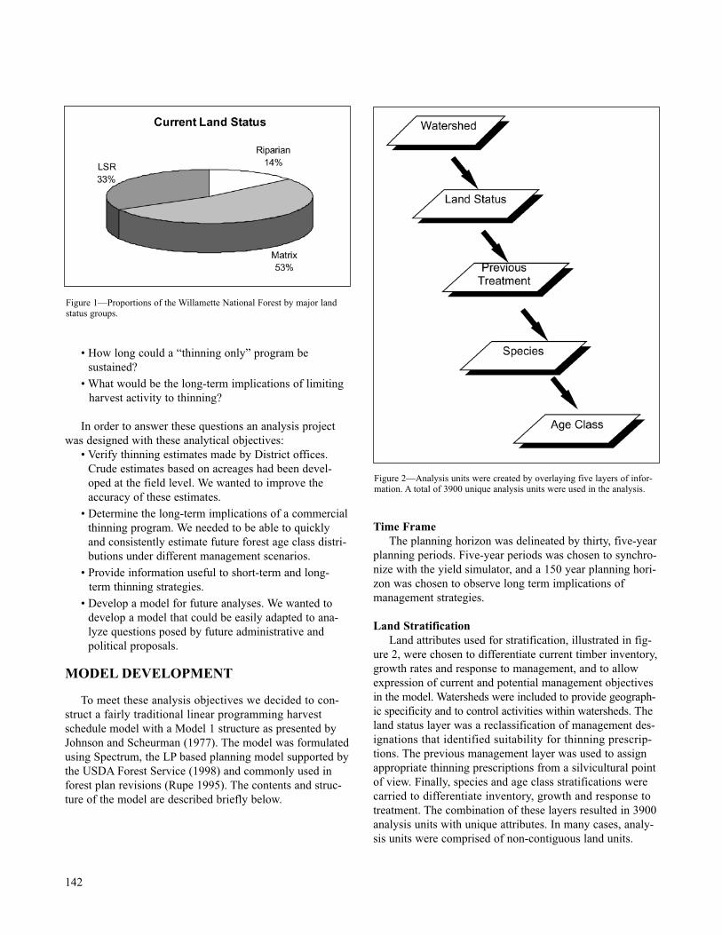
• How long could a “thinning only” program be sustained?

• What would be the long-term implications of limiting harvest activity to thinning?

In order to answer these questions an analysis projectwas designed with these analytical objectives:

• Verify thinning estimates made by District offices.Crude estimates based on acreages had been devel-oped at the field level. We wanted to improve theaccuracy of these estimates.

• Determine the long-term implications of a commercial thinning program. We needed to be able to quicklyand consistently estimate future forest age class distri-butions under different management scenarios.

• Provide information useful to short-term and long-term thinning strategies.

• Develop a model for future analyses. We wanted to develop a model that could be easily adapted to ana-lyze questions posed by future administrative andpolitical proposals.

MODEL DEVELOPMENT

To meet these analysis objectives we decided to con-struct a fairly traditional linear programming harvest schedule model with a Model 1 structure as presented byJohnson and Scheurman (1977). The model was formulatedusing Spectrum, the LP based planning model supported bythe USDA Forest Service (1998) and commonly used inforest plan revisions (Rupe 1995). The contents and struc-ture of the model are described briefly below.

Time FrameThe planning horizon was delineated by thirty, five-year

planning periods. Five-year periods was chosen to synchro-nize with the yield simulator, and a 150 year planning hori-zon was chosen to observe long term implications ofmanagement strategies.

Land StratificationLand attributes used for stratification, illustrated in fig-

ure 2, were chosen to differentiate current timber inventory,growth rates and response to management, and to allowexpression of current and potential management objectivesin the model. Watersheds were included to provide geograph-ic specificity and to control activities within watersheds. Theland status layer was a reclassification of management des-ignations that identified suitability for thinning prescrip-tions. The previous management layer was used to assignappropriate thinning prescriptions from a silvicultural pointof view. Finally, species and age class stratifications werecarried to differentiate inventory, growth and response totreatment. The combination of these layers resulted in 3900analysis units with unique attributes. In many cases, analy-sis units were comprised of non-contiguous land units.

142

Figure 1—Proportions of the Willamette National Forest by major landstatus groups.

Figure 2—Analysis units were created by overlaying five layers of infor-mation. A total of 3900 unique analysis units were used in the analysis.

Management optionsA variety of thinning treatment options were developed

for each analysis unit. Within LSR areas, these treat-ments are intended to encourage the development of keyold-growth characteristics desired in LSRs (Spies 1991;Willamette National Forest 1998). These included regimeswith and without pre-commercial thinning, and regimesthat had one, two or three commercial thinnings during the planning horizon.

Outputs and EffectsTo keep the model simple, a small number of outputs

and effects were modeled. Timber growth and yield projec-tions were developed using the Forest Vegetation Simulator(FVS). These simulations provided estimates of inventoryand harvest amounts as well as estimates of fuels producedfrom thinning operations. The per-acre cost of thinningoperations was also estimated. These costs varied by com-binations of land status, species group and thinning intensity.

Management ObjectivesManagement objectives that were likely to intersect

with harvesting objectives were represented in the model.These objectives and their representation in the model arelisted by resource area.

Fish and Watershed—• Limit potential ground disturbance and possible sedimen-

tation or impacts to streamside vegetation, amphibians,and arthropod populations.

• Ensure not all closed canopy dispersal corridors in a given watershed are impacted at the same time and limitpotential adverse cumulative effects within desired levels.

• Maintain or minimize disruption of microclimates in riparian reserves and minimize edge impact on streamsidestands.

• Minimize stream course impacts during peak flow events.

These objectives were represented in two sets of con-straints in the model. The first controlled the number ofacres within riparian areas that could be harvested in aperiod. Willamette biologists felt that limiting the harvest-ing to less than seven percent of the riparian acres per peri-od would keep cumulative impacts to an acceptable level(equation 6, below). The second set of constraints aimed at protecting the fish resource was the enforcement of stan-dards established in the Northwest Forest Plan (USDA ForestService 1994). This standard limits the acres harvested inselected watersheds to less than fifteen percent of the acresin that watershed per period (equation 8).

Wildlife—• Conduct silvicultural treatments in young stands within

LSRs to promote recruitment into suitable old-growthhabitat.

• Provide dispersal habitat for spotted owls as well as maintaining some level of landscape continuity and dis-persal habitat for other species.

These objectives were modeled with decision variablesrepresenting management choices designed to producedesired habitat and with constraints that limited the numberof acres treated within LSRs. Specialists felt that limitingthe treatments to less than twenty five percent of an LSR ina ten-year period would ensure that habitat requirementscould be met (equation 7).

SCENARIO DESIGN

In order to meet the analysis objectives, three broadlevel scenarios were studied. Scenario 1, designed as abenchmark, sought to maximize harvest levels with fewconstraints. Scenario 2 was designed to represent the man-agement objectives for fish, wildlife and watershed thatmight interact with timber production objectives. Finally,Scenario 3 was similar to Scenario 2 but harvest activitieswere limited to stands that had been previously managed.The mathematical formulation for Scenario 2, stated as inClutter et al. (1983), is shown below.

Maximize:

30 R(1) Z = ∑ ∑ ∑ Vijk Xjk

i=1 j=1 k∈LSR

2 R N(2) Z′ = ∑ ∑ ∑ Vijk Xjk

i=1 j=1 k=1

30 R N(3) Z″ = ∑ ∑ ∑ Vijk Xjk

i=1 j=1 k=1

Subject to:

R N R N(4) ∑ ∑ Vi+1jk Xjk ≤ ∑ ∑ 1.25Vijk Xjk (i = 1,2...29)

j=1 k=1 i=1 k=1

R N R N(5) ∑ ∑ Vi+1jk Xjk ≥ ∑ ∑ 0.75Vijk Xjk (i = 1,2...29)

j=1 k=1 j=1 k=1

R R(6) ∑ ∑ Hijk Xjk ≤ ∑ ∑ 0.05Xjk (i = 1,2...30)

j=1 k∈1 j=1 k∈RZ

143

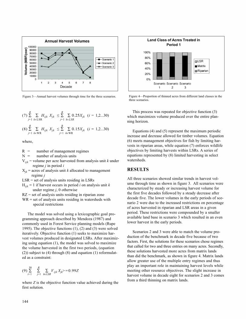
R R(7) ∑ ∑ Hijk Xjk ≤ ∑ ∑ 0.25Xjk (i = 1,2...30)

j=1 k∈LSR j=1 k∈LSR

R R(8) ∑ ∑ Hijk Xjk ≤ ∑ ∑ 0.15Xjk (i = 1,2...30)

j=1 k∈WR j=1 k∈WR

where,

R = number of management regimesN = number of analysis unitsVijk = volume per acre harvested from analysis unit k under

regime j in period iXjk = acres of analysis unit k allocated to management

regime jLSR = set of analysis units residing in LSRsHijk = 1 if harvest occurs in period i on analysis unit k

under regime j, 0 otherwiseRZ = set of analysis units residing in riparian zoneWR = set of analysis units residing in watersheds with

special restrictions

The model was solved using a lexicographic goal pro-gramming approach described by Mendoza (1987) andcommonly used in Forest Service planning models (Rupe1995). The objective functions (1), (2) and (3) were solvediteratively. Objective function (1) seeks to maximize har-vest volumes produced in designated LSRs. After maximiz-ing using equation (1), the model was solved to maximizethe volume harvested in the first two periods, (equation(2)) subject to (4) through (8) and equation (1) reformulat-ed as a constraint:

30 R(9) ∑ ∑ ∑ V ijk Xjk>=0.99Z

i=1 j=1 k∈LSR

where Z is the objective function value achieved during thefirst solution.

This process was repeated for objective function (3)which maximizes volume produced over the entire plan-ning horizon.

Equations (4) and (5) represent the maximum periodicincrease and decrease allowed for timber volumes. Equation(6) meets management objectives for fish by limiting har-vests in riparian areas, while equation (7) enforces wildlifeobjectives by limiting harvests within LSRs. A series ofequations represented by (8) limited harvesting in selectwatersheds.

RESULTS

All three scenarios showed similar trends in harvest vol-ume through time as shown in figure 3. All scenarios werecharacterized by steady or increasing harvest volume forthe first five decades followed by a steady decrease afterdecade five. The lower volumes in the early periods of sce-nario 2 were due to the increased restrictions on percentageof acres harvested in riparian and LSR areas in a givenperiod. These restrictions were compounded by a smalleravailable land base in scenario 3 which resulted in an evenlower harvest in the early periods.

Scenarios 2 and 3 were able to match the volume pro-duction of the benchmark in decade five because of twofactors. First, the solutions for these scenarios chose regimesthat called for two and three entries on many acres. Secondly,these solutions harvested more acres from matrix landsthan did the benchmark, as shown in figure 4. Matrix landsallow greater use of the multiple entry regimes and thusplay an important role in maintaining harvest levels whilemeeting other resource objectives. The slight increase inharvest volume in decade eight for scenarios 2 and 3 comesfrom a third thinning on matrix lands.

144

Figure 4—Proportion of thinned acres from different land classes in thethree scenarios.

Figure 3—Annual harvest volumes through time for the three scenarios.

All three scenarios show a transition in the long term to a forest that is greater than 95% late successional stands.For all scenarios, the decline in acres available for thinningbegins in decade five and continues. Natural disturbance,not accounted for in the model, will be the only means forregenerating the forest.

CONCLUSIONS

This analysis shows a potential for the WillametteNational Forest to sustain a “thinning only” harvest pro-gram for seventy to eighty years. During that time harvestlevels climb from 65 mmbf on 4500 acres to 91 mmbf on6200 acres annually for scenario 2. If harvests are limitedto managed stands, then early harvest levels fall to 40 mmbfon 3200 acres annually. If LSR lands are maintained andthe aquatic conservation strategy objectives are met, thegreatest opportunities for harvest come from multiple-entrythinning regimes on matrix lands.

In addition to answering the questions outlined at thebeginning of the study, this analysis also raised new ques-tions. The large proportion of thinning from matrix landscalled for by scenarios 2 and 3 will require that clear silvi-cultural objectives be established for these treatments. Somemid-level analysis may also be needed to determine thin-ning priorities and entry schedules in sensitive watersheds.Finally, additional analysis will surely be needed to exam-ine the potential fire risks associated with fuels generatedfrom thinning operations.

LITERATURE CITED

Clutter, J. L.; et al. 1983. Timber management: a quantita-tive approach. New York: John Wiley & Sons. 333 p.

Johnson, K.N.; Scheurman, H.L. 1977. Techniques for prescribing optimal timber harvest and investmentunder different objectives – discussion and synthesis.Forest Science Monograph 18. 31 p.

Mendoza, G.A. 1987. Goal programming formulations and extensions: An overview and analysis. Can. J. For.Res., 17: 575 – 581.

Rupe, J.B. 1995. The analysis of competing policy choices for the revised Black Hills forest plan: Ecosystemrestoration or sustained timber harvest levels? In:Thompson, J.E. (compiler). Analysis in Support ofEcosystem Management; Analysis Workshop III.; 1995April 10 – 13; Fort Collins, CO: USDA Forest Service:241 - 250.

Spies, T.A.; Franklin, J.F. 1991. The structure of natural young, mature, and old-growth Douglas-fir forests inOregon and Washington. In: Wildlife and vegetation ofunmanaged Douglas-fir forests. Ruggiero, L.F., KB.Aubry, A.B. Carey, M.H. Huff, Tech Coordinators.USDA For. Serv. Gen. Tech. Rep. PNW-GTR-285. pp. 91-109.

USDA Forest Service, Inventory and Monitoring Institute. 1998. Spectrum Users Guide.http://www.fs.fed.us/institute/PAG/SPECTRUM.shtml

USDA Forest Service and USDI Bureau of Land Management. 1994.Record of Decision for Amendmentsto Forest Service and Bureau of Land ManagementPlanning Documents within the Range of the NorthernSpotted Owl. USDA Forest Service PNW Region, P.O.Box 3623, Portland, OR 97208.

USDA Forest Service, Willamette National Forest. 1990. Land and Resource Management Plan. http:/www.fs.fed.us/rc/willamette/manage/forestplan/ index.html

145

This page is intentionally left blank.

In: Bevers, Michael; Barrett, Tara M., comps. 2005. Systems Analysis in Forest Resources: Proceedings of the 2003 Symposium. General Technical ReportPNW-GTR-656. Portland, OR: U.S. Department of Agriculture, Forest Service, Pacific Northwest Research Station.1 Susan King is an Operations Research Analyst and 2 Brett Butler is a Research Forester at the USDA Forest Service; Northeastern Research Station; 11 Campus Blvd., Suite 200; Newtown Square, PA 19073.

Systems Analysis in Forest Resources: Proceedings of the 2003 Symposium

GENERATING A FOREST PARCELIZATIONMAP FOR MADISON COUNTY, NY

Susan L. King1 and Brett J. Butler2

INTRODUCTION

A parcel is a contiguous polygon of land owned by asingle ownership. An ownership is an individual, group ofindividuals, business, or public agency that has legal title tothe polygon of land. Between 1994 and 2002, the numberof private landowners in the United States increased by 7percent (Butler 2004). At the same time, the area of forestland collectively owned by these families, individuals, com-panies, and other groups increased by less than 3 percent(www.fs.fed.us/woodlandowners). This continuing trend offorest land ownership increasing faster than forest land isresulting in the fragmentation of forest ownerships or forestparcelization. An alternative way to define parcelization isa decrease in the average landowner’s landholdings.

ABSTRACT

It is well documented that the size of forested landholdings directly affects the management of forest resources. Tradi-tionally, this information has been presented in tabular format. A spatial format will provide a more useful mechanism forsummarizing and utilizing this important information and can provide new insight into the causes, or at least correlates,with differences in sizes of forest landholdings. The objective of this study was to investigate techniques for modeling for-est parcel size in order to facilitate future efforts to generate a national map depicting the distribution of forest parcel sizes.County tax records and land-cover data for Madison County, New York, were used to generate a dataset containing forestparcel size by owner. This area was selected because, unlike most of the country, the land ownership parcel data are readilyavailable in a format conducive to spatial analysis. Ancillary data included both social and biophysical predictor variables.Multiple linear regression, neural network, and decision trees were used to model these data. The models were tested usingvalidation datasets and accuracy was assessed with enhanced kappa statistics. A decision tree was selected as the finalmethod because it provided superior validation results, fewer parameters to adjust, and ease of explanation and visualizationto non-experts.

KEYWORDS: Parcelization, decision trees, simple kriging with a varying local mean, neural networks.

147

The consequences of parcelization are not fully under-stood, but they have important implications for the preser-vation of working forest land (Sampson 2000). A basiclimitation imposed by parcelization is related to economiesof scale (Row 1978). For working forest land to be sus-tained, it is necessary for the land to be profitable, and tim-ber is the most profitable market commodity from suchtracts. The profitability of a timber harvest is a function ofthe realized stumpage value and fixed and variable costs.While the variable costs can be adjusted, at least partially, to reflect the size of the parcel being treated, the fixed costs(e.g., transportation of equipment) by definition are invari-ant to treatment area.

Forest parcelization, itself is not detrimental to eco-system functions, though it often is a catalyst for change.

Specifically, parcelization often precedes the conversion offorest land to other land uses, e.g., residential development,which, in turn, leads to fragmentation of the physical forestresource. Forest fragmentation has been shown to be detri-mental to ecosystem functions ranging from water qualityto the availability of nesting habitat (Rochelle et al. 1999;Saunders et al. 1991).

Likewise, parcelization may not directly affect theresources available to people desiring access (e.g., hunters),but access will be hampered by the need to contact anincreasing number of land owners. This access also affectsprograms designed to educate or influence landowners. Asthe number of owners increases, the cost of implementingcost sharing or extension programs will be affected.

The characteristics of the owners also are correlatedwith the size of landholdings (Butler 2004; Birch 1996).Landowners of smaller forested tracts are more likely tohave objectives related to home ownership and aesthetics,whereas owners of larger forested tracts are likely toactively manage their forests for timber production.

To accurately predict forest parcelization patterns, theprocesses or patterns of the underlying forces must beunderstood. To date, most of the information on forestparcelization has been obtained from coarse-scale owner-ship surveys that allow only tabular summaries, limitedspatial resolution, and limited ability to combine with otherdata sources. Mehmood and Zhang (2001) built a multiplelinear regression model to describe parcelization for theUnited States. Their dependent variable, a measure of

parcelization, is the change in average nonindustrial privateforest size between 1978 and 1994 on a per-state basis.Their independent variables are suited for a state-levelmodel and reflect changes over time. Our model is a geo-graphical approach; that is, we investigated methods thatmodel forest parcelization both on a continuous and cate-gorical scale. The purpose of this case study was to gainexperience using different modeling techniques and inde-pendent variables which will enable us to build a nationalmap that depicts the size of forest parcels. This map will

148

Figure 2—Agricultural and forest land are the predominate land uses. Anurban corridor exists along Interstate 90 at the edge of the Lake plainsphysiographic region. Syracuse is a major population center to the west.

Figure 1—Madison County, located incentral New York, is bordered to thenorth by Oneida Lake. The Lake Plainsphysiographic region surrounds OneidaLake; the southern portion of the countyis part of the Appalachian Uplands phys-iographic region. Numerous lakes areinterspersed among the rolling hills.

allow us to increase our understanding of the processesunderlying forest parcelization and its consequences.

METHODS

Study AreaThe study area was Madison County in the center of New

York State (fig. 1). The county contains numerous lakesinterspersed among the flat plains and rolling hills of theLake Plains and Appalachian Uplands physiographic regions.Agricultural and forest lands are the major land uses (fig.2), but, as in many parts of the county, these industrieshave been superseded by service and retail sectors in thelocal economies. Currently, 69,000 people live in MadisonCounty (U.S. Census Bureau 2001). The county covers 661mi2 giving it an average population density of 104 peopleper mi2.

This area was selected because it is one of relativelyfew counties in the United States where tax records have been digitized in a format that is amenable to further analyses and are publicly available for a nominal fee(www.madisoncounty.org). All legal property boundariesfor this county have been digitized with polygon topologyand information about the ownership of each parcel isavailable.

VariablesThe dependent variable, size of forest parcel, was

derived by combining county’s tax records and remotelysensed imagery. The (total landholdings) parcel map wascreated by assigning every ownership in the county a

unique numerical identifier and then combining adjacentparcels to remove “artificial” boundaries. A forest/nonfor-est map was created by reclassifying the 30m pixels in a1992 National Land Cover Data (Vogelmann 2001) imagefor Madison County as 1 for forest or 0 for all other land-cover categories. The total number of forest pixels within aparcel (based on pixel centroid) were calculated and multi-plied by 0.2 ac to obtain the total forest area per parcel.

The independent variables for this analysis (table 1)were limited to data that were publicly available and havenational coverage. Thus, the results can be used to create aproduct that covers a larger geographic area. The physicalvariables originated from remotely sensed imagery, digitalelevation models (DEM), and census data. Percent forest,agriculture, and urban were derived from the 1992 NationalLand Cover Data. Slope and elevation were estimated fromthe DEM (Defense Mapping Agency 1997).

The Census Bureau (U.S. Census Bureau 2001) was thesource of the socioeconomic variables available at the cen-sus block or block group level. Data for the finest spatialresolution available were incorporated. Variables related tothe number of people across the landscape included popu-lation, dwelling, and family density. These variables are allhighly correlated, but not completely redundant. The aver-age income and education of the people within a censusblock group were tested. A dummy variable indicating pub-lic ownership was derived from county tax records, thoughthis variable can also be derived from regional or nationaldata sources (McGhie 1996).

149

Table 1—Dependent and independent variables used in the study.

Variable Abbreviation Description

Forest parcel ForParc Area (acres) of forest in a parcelPercent forest PerFor Percent forest within (1, 5, 25, or 100) acres of the parcel centroidPercent agriculture PerAg Percent agriculture within (1, 5, 25, or 100) acres of the parcel centroidPercent urban PerUrb Percent urban within (1, 5, 25, or 100) acres of the parcel centroidPopulation density PopDen People per square mile within a census blockDwelling density DwDen Dwellings or houses per square mile within a census blockFamily density FamDen Families or households per square mile within a census blockPublic ownership PubOwn Dummy variable indicating parcel centroid is within a public ownershipDistance to roads DistRoad Distance (mi) of parcel centroid to nearest improved roadDistance to water DistWater Distance (mi) of parcel centroid to nearest census waterSlope Slope Average slope within (5 or 100) acres of parcel centroidElevation Elev Average elevation within (5 or 100) acres of parcel centroidIncome Inc Average annual income (US$) within a block groupEducation Ed Percent of population with a college degree within a census block groupGravity Index Grav Weighted distance of the census block centroid to population centers

A gravity index (Kline 2001; Haynes 1984) was includedto represent the relative influence of population centers.Parcels closer to an urban area are more likely to be subjectto urban land-use influences. It is hypothesized that this willresult in smaller parcels. The index was calculated as:

3 (Populationk)0.5

Gravity indexi = ∑k=i

Distanceik

wherei = U.S. Census block group centroidk = a city having a large urban influence

The selection of three nearest cities was based on thework of Kline and Alig (2001). Cities within an 50 mibuffer of the county were included. The city with thelargest population (163,860 people) was Syracuse, locatedwest of the county. The remaining urban centers ranged inpopulation from 166 to 68,637.

MODELS

Several procedures for mapping parcelization wereinvestigated. Both simple kriging with a varying local meanand decision trees were investigated. In simple kriging witha varying local mean, the large-scale variability is modeledusing a nonspatial approach such as multiple linear regres-sion, neural networks, or generalized additive models. Alinear model, multiple linear regression, and a nonlinearapproach (neural networks) were investigated. Forest parcel-ization is predicted on a continuous scale with simple krig-ing and on a categorical scale with decision trees.

Multiple Linear Regression vs. Neural NetworksIn multiple linear regression, the relationship between

independent and dependent variables is assumed to be lin-ear in the unknown parameters and interactions betweenthe independent variables must be specified a priori by theuser. The parameters are estimated by least squares. In neu-ral networks, there is no assumed relationship between theindependent and dependent variables. The relationshipbetween independent and dependent variables is learnedthrough an iterative process.

A neural network requires no assumptions about the distributions, mean, or correlation of the errors. Neural networks may provide a superior solution over a traditionalstatistical procedure when the distributions are unknownand possibly nonlinear, outliers may exist, and noise ispresent in the data (Burke 1991). In this research, a feed-forward neural network with backpropagation, the mostwidely used learning algorithm, is implemented. Briefly, abackpropagation network consists of processing elements

analogous to the brain’s neuron. The backpropagation net-work is hierarchical, consisting of at least three layers. The first layer is an input layer with the same number ofprocessing elements as independent variables, which arethought to relate to the output classification signal. Thislayer typically operates as a simple input buffer and uses alinear transfer function to distribute each of the input attrib-utes to the second layer processing units. The second layeris the hidden layer. There can be multiple hidden layers,but usually only one is used. The number of processingunits in the hidden layer is undeterminable a priori. Each ofthe hidden layers uses some form of a nonlinear sigmoidaltransfer function, which usually has the same number ofweights as the number of input attributes. The third andusually final layer, the output layer, typically has the samenumber of processing units as classification categories. The output signals from each of the hidden layer’s transferfunctions feed into another sigmoidal function at the outputlayer. The difference between the observed and estimatedvalues of the dependent variable is formulated as a functionof weights. This is an unconstrained minimized problemand there are numerous solution techniques available (King1999). Selection of initial weights can influence the con-vergence to an optimum solution and ultimately the finalset of weights which are used on new data.

Simple Kriging with a Varying Local MeanBecause each datum has a geographical reference,

geostatistical procedures are feasible. One geostatisticalapproach for incorporating secondary information is simplekriging with a varying local mean. Large-scale variabilityis modeled using multiple linear regression or neural net-works; small-scale variability is modeled using simplekriging (Majure et al. 1996; Metzger 1997; Hunner et al.1998; Goovaerts 2000; Lister et al. 2000). The two surfacesare then added to produce the final map. If there is no small-scale variability, the large-scale map may stand alone.

Decision TreeDecision trees partition the decision space into smaller

segments defined in terms of the input variables. Thesepartitions define the predictive relationship between theinputs and the dependent variable. This partitioning contin-ues until the subsets cannot be partitioned further usinguser-defined stopping criteria. The homogenous groupsallow for greater accuracy in predicting the dependent vari-able from the independent variables. Chi-Square AutomaticInteraction Detector (CHAID), the decision-tree algorithmused in this study, selects the most significant predictorwith the lowest adjusted probability at each level based onthe Bonferroni adjusted Chi-Square statistics (KASS 1980).A small p-value indicates that the observed association

150

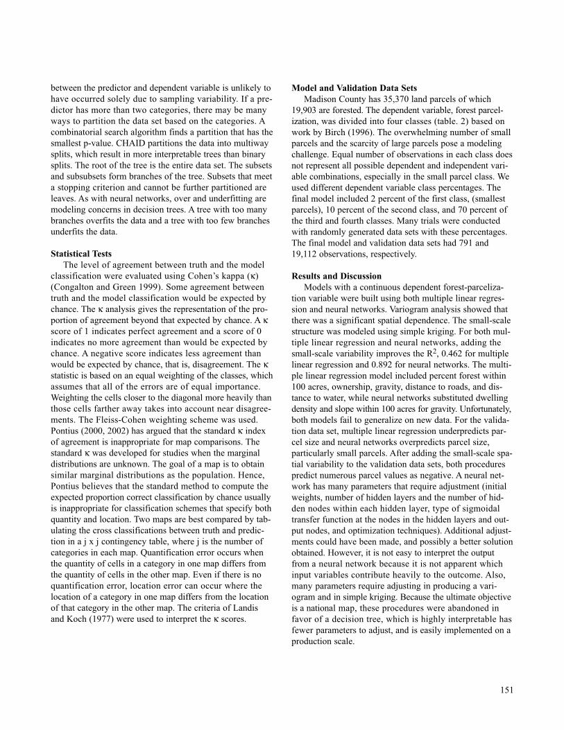
between the predictor and dependent variable is unlikely tohave occurred solely due to sampling variability. If a pre-dictor has more than two categories, there may be manyways to partition the data set based on the categories. Acombinatorial search algorithm finds a partition that has thesmallest p-value. CHAID partitions the data into multiwaysplits, which result in more interpretable trees than binarysplits. The root of the tree is the entire data set. The subsetsand subsubsets form branches of the tree. Subsets that meeta stopping criterion and cannot be further partitioned areleaves. As with neural networks, over and underfitting aremodeling concerns in decision trees. A tree with too manybranches overfits the data and a tree with too few branchesunderfits the data.

Statistical TestsThe level of agreement between truth and the model

classification were evaluated using Cohen’s kappa (κ)(Congalton and Green 1999). Some agreement betweentruth and the model classification would be expected bychance. The κ analysis gives the representation of the pro-portion of agreement beyond that expected by chance. A κscore of 1 indicates perfect agreement and a score of 0indicates no more agreement than would be expected bychance. A negative score indicates less agreement thanwould be expected by chance, that is, disagreement. The κstatistic is based on an equal weighting of the classes, whichassumes that all of the errors are of equal importance.Weighting the cells closer to the diagonal more heavily thanthose cells farther away takes into account near disagree-ments. The Fleiss-Cohen weighting scheme was used.Pontius (2000, 2002) has argued that the standard κ indexof agreement is inappropriate for map comparisons. Thestandard κ was developed for studies when the marginaldistributions are unknown. The goal of a map is to obtainsimilar marginal distributions as the population. Hence,Pontius believes that the standard method to compute theexpected proportion correct classification by chance usuallyis inappropriate for classification schemes that specify bothquantity and location. Two maps are best compared by tab-ulating the cross classifications between truth and predic-tion in a j x j contingency table, where j is the number ofcategories in each map. Quantification error occurs whenthe quantity of cells in a category in one map differs fromthe quantity of cells in the other map. Even if there is noquantification error, location error can occur where thelocation of a category in one map differs from the locationof that category in the other map. The criteria of Landisand Koch (1977) were used to interpret the κ scores.

Model and Validation Data SetsMadison County has 35,370 land parcels of which

19,903 are forested. The dependent variable, forest parcel-ization, was divided into four classes (table. 2) based onwork by Birch (1996). The overwhelming number of smallparcels and the scarcity of large parcels pose a modelingchallenge. Equal number of observations in each class doesnot represent all possible dependent and independent vari-able combinations, especially in the small parcel class. Weused different dependent variable class percentages. Thefinal model included 2 percent of the first class, (smallestparcels), 10 percent of the second class, and 70 percent ofthe third and fourth classes. Many trials were conductedwith randomly generated data sets with these percentages.The final model and validation data sets had 791 and19,112 observations, respectively.

Results and DiscussionModels with a continuous dependent forest-parceliza-

tion variable were built using both multiple linear regres-sion and neural networks. Variogram analysis showed thatthere was a significant spatial dependence. The small-scalestructure was modeled using simple kriging. For both mul-tiple linear regression and neural networks, adding thesmall-scale variability improves the R2, 0.462 for multiplelinear regression and 0.892 for neural networks. The multi-ple linear regression model included percent forest within100 acres, ownership, gravity, distance to roads, and dis-tance to water, while neural networks substituted dwellingdensity and slope within 100 acres for gravity. Unfortunately,both models fail to generalize on new data. For the valida-tion data set, multiple linear regression underpredicts par-cel size and neural networks overpredicts parcel size,particularly small parcels. After adding the small-scale spa-tial variability to the validation data sets, both procedurespredict numerous parcel values as negative. A neural net-work has many parameters that require adjustment (initialweights, number of hidden layers and the number of hid-den nodes within each hidden layer, type of sigmoidaltransfer function at the nodes in the hidden layers and out-put nodes, and optimization techniques). Additional adjust-ments could have been made, and possibly a better solutionobtained. However, it is not easy to interpret the outputfrom a neural network because it is not apparent whichinput variables contribute heavily to the outcome. Also,many parameters require adjusting in producing a vari-ogram and in simple kriging. Because the ultimate objectiveis a national map, these procedures were abandoned infavor of a decision tree, which is highly interpretable hasfewer parameters to adjust, and is easily implemented on aproduction scale.

151

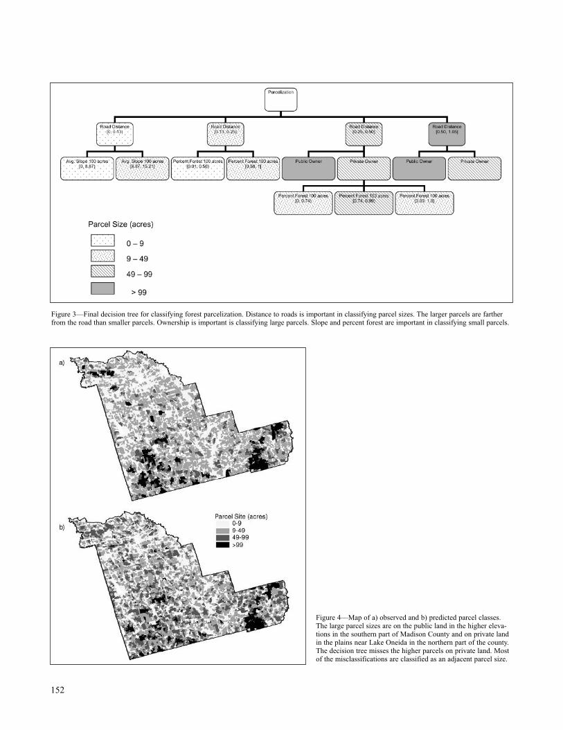
152

Figure 3—Final decision tree for classifying forest parcelization. Distance to roads is important in classifying parcel sizes. The larger parcels are fartherfrom the road than smaller parcels. Ownership is important is classifying large parcels. Slope and percent forest are important in classifying small parcels.

Figure 4—Map of a) observed and b) predicted parcel classes.The large parcel sizes are on the public land in the higher eleva-tions in the southern part of Madison County and on private landin the plains near Lake Oneida in the northern part of the county.The decision tree misses the higher parcels on private land. Mostof the misclassifications are classified as an adjacent parcel size.

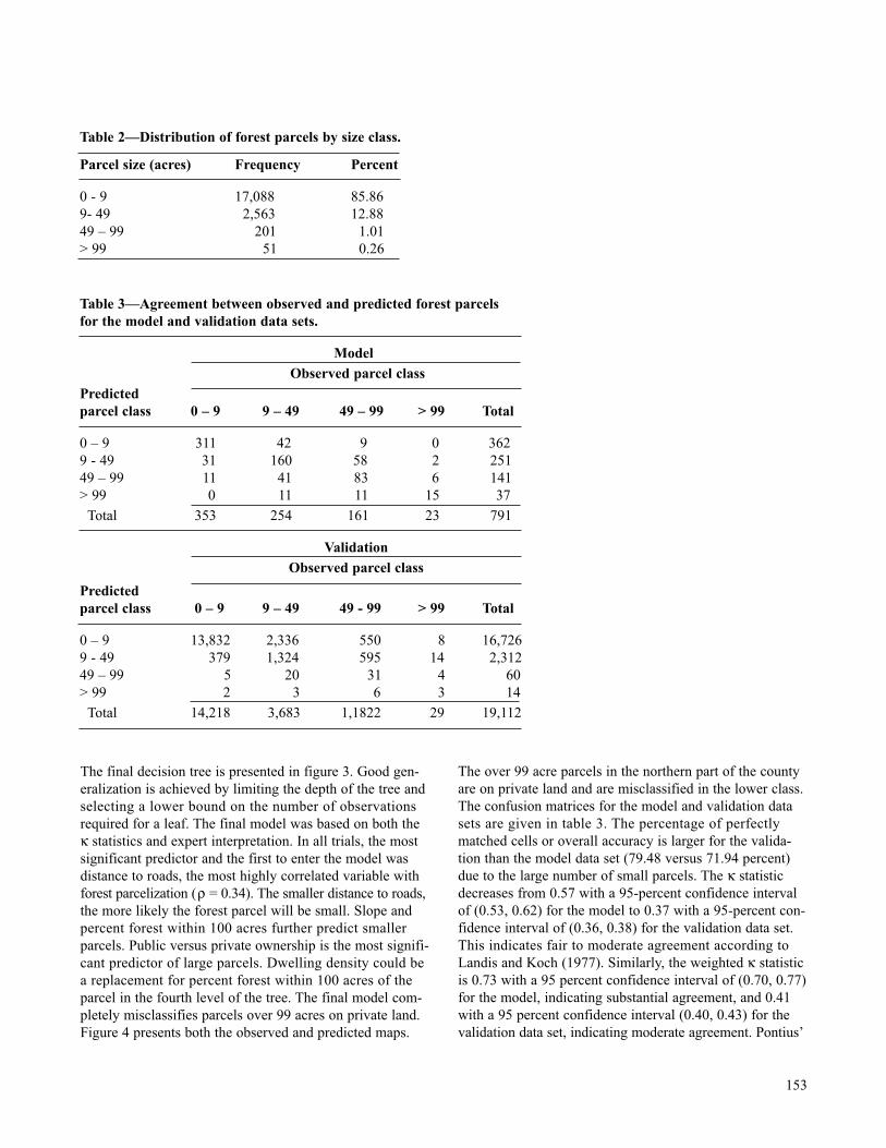
The final decision tree is presented in figure 3. Good gen-eralization is achieved by limiting the depth of the tree andselecting a lower bound on the number of observationsrequired for a leaf. The final model was based on both the κ statistics and expert interpretation. In all trials, the mostsignificant predictor and the first to enter the model wasdistance to roads, the most highly correlated variable withforest parcelization (ρ = 0.34). The smaller distance to roads,the more likely the forest parcel will be small. Slope andpercent forest within 100 acres further predict smallerparcels. Public versus private ownership is the most signifi-cant predictor of large parcels. Dwelling density could be a replacement for percent forest within 100 acres of theparcel in the fourth level of the tree. The final model com-pletely misclassifies parcels over 99 acres on private land.Figure 4 presents both the observed and predicted maps.

The over 99 acre parcels in the northern part of the countyare on private land and are misclassified in the lower class.The confusion matrices for the model and validation datasets are given in table 3. The percentage of perfectlymatched cells or overall accuracy is larger for the valida-tion than the model data set (79.48 versus 71.94 percent)due to the large number of small parcels. The κ statisticdecreases from 0.57 with a 95-percent confidence intervalof (0.53, 0.62) for the model to 0.37 with a 95-percent con-fidence interval of (0.36, 0.38) for the validation data set.This indicates fair to moderate agreement according toLandis and Koch (1977). Similarly, the weighted κ statisticis 0.73 with a 95 percent confidence interval of (0.70, 0.77)for the model, indicating substantial agreement, and 0.41with a 95 percent confidence interval (0.40, 0.43) for thevalidation data set, indicating moderate agreement. Pontius’

153

Table 2—Distribution of forest parcels by size class.

Parcel size (acres) Frequency Percent

0 - 9 17,088 85.869- 49 2,563 12.8849 – 99 201 1.01> 99 51 0.26

Table 3—Agreement between observed and predicted forest parcels for the model and validation data sets.

ModelObserved parcel class

Predicted parcel class 0 – 9 9 – 49 49 – 99 > 99 Total

0 – 9 311 42 9 0 3629 - 49 31 160 58 2 25149 – 99 11 41 83 6 141> 99 0 11 11 15 37

Total 353 254 161 23 791

ValidationObserved parcel class

Predicted parcel class 0 – 9 9 – 49 49 - 99 > 99 Total

0 – 9 13,832 2,336 550 8 16,7269 - 49 379 1,324 595 14 2,31249 – 99 5 20 31 4 60> 99 2 3 6 3 14

Total 14,218 3,683 1,1822 29 19,112

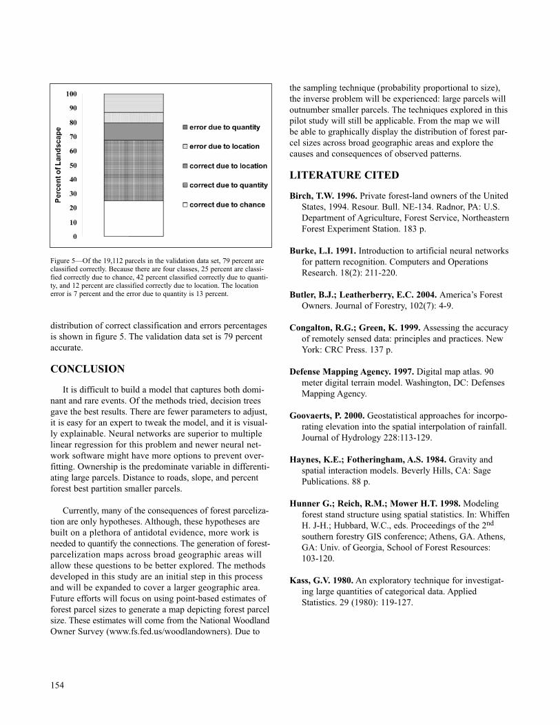
distribution of correct classification and errors percentagesis shown in figure 5. The validation data set is 79 percentaccurate.

CONCLUSION

It is difficult to build a model that captures both domi-nant and rare events. Of the methods tried, decision treesgave the best results. There are fewer parameters to adjust,it is easy for an expert to tweak the model, and it is visual-ly explainable. Neural networks are superior to multiplelinear regression for this problem and newer neural net-work software might have more options to prevent over-fitting. Ownership is the predominate variable in differenti-ating large parcels. Distance to roads, slope, and percentforest best partition smaller parcels.

Currently, many of the consequences of forest parceliza-tion are only hypotheses. Although, these hypotheses arebuilt on a plethora of antidotal evidence, more work isneeded to quantify the connections. The generation of forest-parcelization maps across broad geographic areas willallow these questions to be better explored. The methodsdeveloped in this study are an initial step in this processand will be expanded to cover a larger geographic area.Future efforts will focus on using point-based estimates offorest parcel sizes to generate a map depicting forest parcelsize. These estimates will come from the National WoodlandOwner Survey (www.fs.fed.us/woodlandowners). Due to

the sampling technique (probability proportional to size),the inverse problem will be experienced: large parcels willoutnumber smaller parcels. The techniques explored in thispilot study will still be applicable. From the map we willbe able to graphically display the distribution of forest par-cel sizes across broad geographic areas and explore thecauses and consequences of observed patterns.

LITERATURE CITED

Birch, T.W. 1996. Private forest-land owners of the United States, 1994. Resour. Bull. NE-134. Radnor, PA: U.S.Department of Agriculture, Forest Service, NortheasternForest Experiment Station. 183 p.

Burke, L.I. 1991. Introduction to artificial neural networks for pattern recognition. Computers and OperationsResearch. 18(2): 211-220.

Butler, B.J.; Leatherberry, E.C. 2004. America’s Forest Owners. Journal of Forestry, 102(7): 4-9.

Congalton, R.G.; Green, K. 1999. Assessing the accuracy of remotely sensed data: principles and practices. NewYork: CRC Press. 137 p.

Defense Mapping Agency. 1997. Digital map atlas. 90 meter digital terrain model. Washington, DC: DefensesMapping Agency.

Goovaerts, P. 2000. Geostatistical approaches for incorpo-rating elevation into the spatial interpolation of rainfall.Journal of Hydrology 228:113-129.

Haynes, K.E.; Fotheringham, A.S. 1984. Gravity and spatial interaction models. Beverly Hills, CA: SagePublications. 88 p.

Hunner G.; Reich, R.M.; Mower H.T. 1998. Modeling forest stand structure using spatial statistics. In: WhiffenH. J-H.; Hubbard, W.C., eds. Proceedings of the 2nd

southern forestry GIS conference; Athens, GA. Athens,GA: Univ. of Georgia, School of Forest Resources: 103-120.

Kass, G.V. 1980. An exploratory technique for investigat-ing large quantities of categorical data. AppliedStatistics. 29 (1980): 119-127.

154

Figure 5—Of the 19,112 parcels in the validation data set, 79 percent areclassified correctly. Because there are four classes, 25 percent are classi-fied correctly due to chance, 42 percent classified correctly due to quanti-ty, and 12 percent are classified correctly due to location. The locationerror is 7 percent and the error due to quantity is 13 percent.

King, Susan L. 1999. Neural networks vs. multiple linear regression for estimating previous diameter. In Stringer,Jeffrey W.; Loftis, David L., eds. Proceedings 12th

central hardwood forest conference; Lexington, KY.Asheville, NC: Gen. Tech. Rep. SRS-24. US Departmentof Agriculture, Forest Service, Southern ResearchStation: 159-166.

Kline, J.D.; Alig, R.J. 2001. A spatial model of land use change in western Oregon and western Washington.Res. Pap. PNW-RP-528. Portland, OR: U.S. Departmentof Agriculture, Forest Service, Pacific NorthwestResearch Station, 24 p.

Landis, J.; Koch, G. 1977. The measurement of observer agreement for categorical data. Biometrics. 33: 159-174.

Majure J,N.; Cressie, N.; Cook D.; Symanzik J. 1996.GIS, spatial statistical graphics, and forest health. In:Third international conference on integrating GIS and environmental modeling. National Center forGeographic Information and Analysis. Sante Fe, NM,Santa Barbara, CA: National Center for GeographicInformation and Analysis. CD.

McGhie, R.G. 1996. Creation of a comprehensive man-aged areas spatial database for the conterminous UnitedStates: summary project technical report (NASA-NAGW-1743). Tech. Rep. 96-4. Santa Barbara, CA:National Center for Geographic Information andAnalysis. 53 p.

Mehmood, S.R.; Zhang, D. 2001. Forest parcelization in the United States: a study of contributing factors.Journal of Forestry. 99(4):30-34.

Metzger, K.L. 1997. Modeling forest stand structure to a ten meter resolution using Landsat TM data. FortCollins, CO: Colorado State University, Department of Forest Sciences. 123 p. M.S. thesis.

Pontius, R.G., Jr. 2000. Quantification error versus location error in comparison of categorical maps.Photogrammetric Engineering & Remote Sensing.66(8): 1011-1016.

Pontius, R.G., Jr. 2002. Statistical methods to partition effects of quantity and location during comparison ofcategorical maps at multiple resolutions. PhotogrammetricEngineering & Remote Sensing, 68(10): 1041-1049.

Sampson, R.N.; DeCoster, L. 2000. Forest fragmentation: implications for sustainable private forests. Journal ofForestry. 98(3): 4-8.

Smith, W.B.; Miles, P.D.; Vissage, J.S. 2004. Forest resources of the United States, 2002. Gen. Tech. Rep.NC-241 St. Paul, MN: U.S. Department of Agriculture,Forest Service, North Central Research Station.

Rochelle, J.A.; Lehmann, L.A.; Wisniewsk. J. 1999.Forest fragmentation: wildlife and management implica-tions. Leiden, The Netherlands: Koninklijke Brill NV325 p.

Row, C. 1978. Economies of tract size in timber growing. Journal of Forestry. 76(9): 576-582.

Saunders, D.A.; Hobbs, R.J.; Margules, C.R. 1991. Biological consequences of ecosystem fragmentation: a review. Conservation Biology. 5:18-32.

U.S. Census Bureau. 2001. Census 2000 summary file 1 (SFI). Washington, DC. U.S. Department of Commerce;Census Bureau.

Vogelmann, J.E.; Howard, S.M.; Yang, L.; Larson, C.R.; Wylie, B.K.; Van Driel, N. 2001. Completion ofthe 1990s national land cover data set for the contermi-nous United States from Landsat Thematic Mapper dataand ancillary data sources. Photogrammetric Engineer-ing and Remote Sensing. 67: 650-652.

155

This page is intentionally left blank.

In: Bevers, Michael; Barrett, Tara M., comps. 2005. Systems Analysis in Forest Resources: Proceedings of the 2003 Symposium. General Technical ReportPNW-GTR-656. Portland, OR: U.S. Department of Agriculture, Forest Service, Pacific Northwest Research Station.1 James Merzenich is an analyst, U.S. Forest Service, Pacific Northwest Region, P.O. Box 3623, Portland, OR 97208. 2 Leonardo Frid is a systems ecologist, ESSA Technologies Ltd., #300-1765 West 8th Ave., Vancouver, B.C. V6J 5C6.

Systems Analysis in Forest Resources: Proceedings of the 2003 Symposium

PROJECTING LANDSCAPE CONDITIONS IN SOUTHERN UTAH BY USING VDDT

James Merzenich1 and Leonardo Frid2

INTRODUCTION

The Vegetation Dynamic Development Tool (VDDT) isa simulation model used to project landscape-scale vegeta-tive conditions over long time frames (Beukema and others2003; Merzenich and others 1999). VDDT models the effectsof alternative levels of management treatments on vegeta-tion as influenced by stochastic disturbances such as wild-fire.

Discrete states are defined in VDDT on the basis of avegetative cover type and structure class. In each modelrun VDDT uses up to fifty thousand simulation units toproject change. Simulation units are initially assigned tostates based on the proportion of area contained in thosestates. These simulation units then progress along time-dependent successional pathways or change states inresponse to probabilistically applied disturbances or man-agement treatments. VDDT projects the proportion of units

ABSTRACT

The Vegetation Dynamics Development Tool (VDDT) is a state-transition modeling system that integrates the effects ofsuccession and natural disturbances such as wildfire with management treatments. VDDT is used to evaluate the responseof non-spatial indicators to management actions. This study used VDDT to project changes in vegetation in response to dif-ferent management scenarios for a mixed forest and range watershed in southwest Utah. The vegetative composition of thislandscape has been significantly altered because of the effects of fire suppression and grazing. Pinyon-juniper acreage hasincreased from historic levels while aspen, sage, and oak habitats have declined. Key environmental factors projected byVDDT include the percent of area dominated by open shrubs, pinyon-juniper, and aspen, and the percent of dry-site coniferacres at high risk of uncharacteristically severe wildfire. The analysis shows that an aggressive vegetation treatment sched-ule is needed to reverse current trends and restore ecological conditions and processes in this area.

KEYWORDS: Landscape modeling, natural disturbance, simulation, forest dynamics, vegetative succession.

157

(or area) contained in each state and the levels of distur-bances that may be expected.

The U.S. Forest Service, Pacific Southwest Station, isconducting a study comparing landscape-scale fuel treat-ment models at seven major locations in the United States(Weise and others 2001). Two reports describing the use ofVDDT in conjunction with this study are available. In aretrospective analysis, VDDT models were used to predictstand replacement fires between 1937 and 1996 in Yosemitenational park (Arbaugh and others, 2001). In the Bitterrootfront of western Montana VDDT was used to estimate thelevel of fuel treatments needed to restore ecological condi-tions and reduce the risk of uncharacteristic stand-replace-ment wildfires (Merzenich and others, 2001). This paperpresents the results of applying VDDT to the Beaver Riverdrainage, an area of mixed range and forest, in southwestUtah.

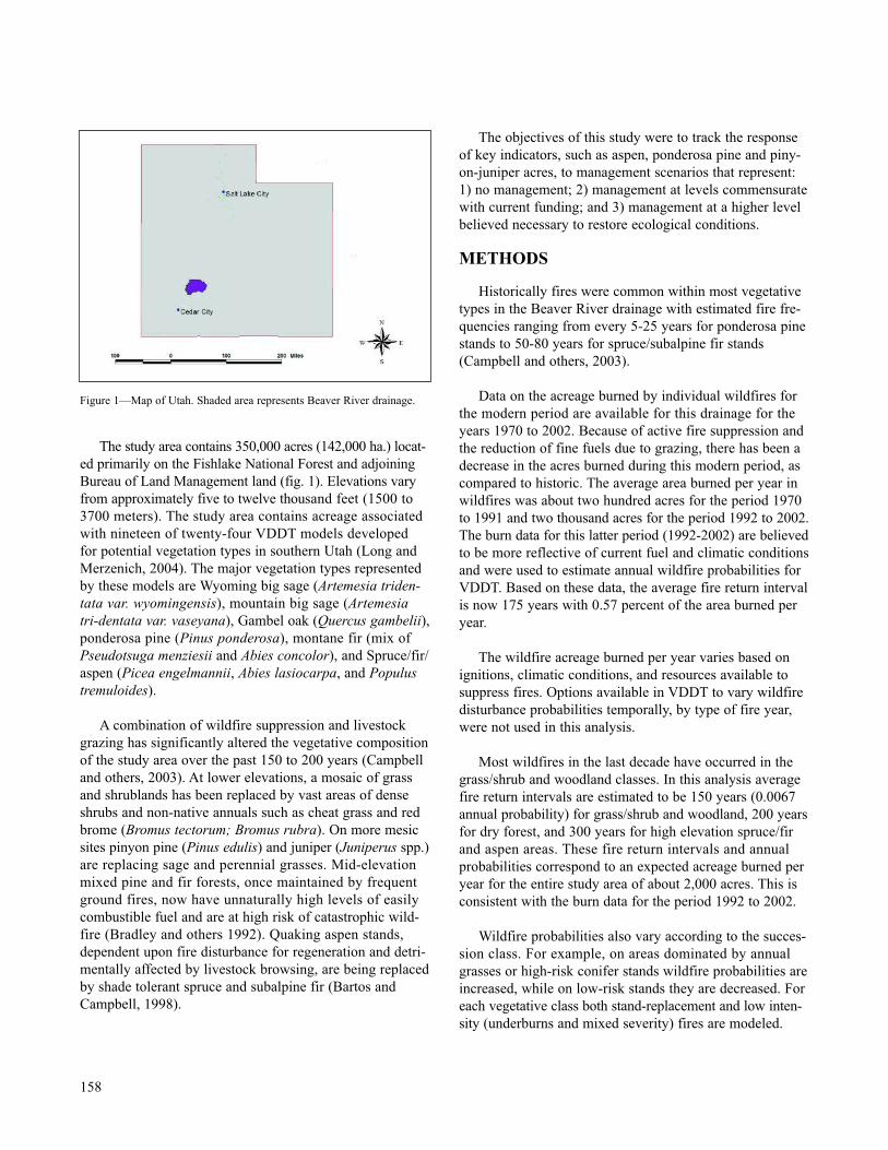
The study area contains 350,000 acres (142,000 ha.) locat-ed primarily on the Fishlake National Forest and adjoiningBureau of Land Management land (fig. 1). Elevations varyfrom approximately five to twelve thousand feet (1500 to3700 meters). The study area contains acreage associatedwith nineteen of twenty-four VDDT models developed for potential vegetation types in southern Utah (Long andMerzenich, 2004). The major vegetation types representedby these models are Wyoming big sage (Artemesia triden-tata var. wyomingensis), mountain big sage (Artemesia tri-dentata var. vaseyana), Gambel oak (Quercus gambelii),ponderosa pine (Pinus ponderosa), montane fir (mix ofPseudotsuga menziesii and Abies concolor), and Spruce/fir/aspen (Picea engelmannii, Abies lasiocarpa, and Populustremuloides).

A combination of wildfire suppression and livestockgrazing has significantly altered the vegetative compositionof the study area over the past 150 to 200 years (Campbelland others, 2003). At lower elevations, a mosaic of grassand shrublands has been replaced by vast areas of denseshrubs and non-native annuals such as cheat grass and redbrome (Bromus tectorum; Bromus rubra). On more mesicsites pinyon pine (Pinus edulis) and juniper (Juniperus spp.)are replacing sage and perennial grasses. Mid-elevationmixed pine and fir forests, once maintained by frequentground fires, now have unnaturally high levels of easilycombustible fuel and are at high risk of catastrophic wild-fire (Bradley and others 1992). Quaking aspen stands,dependent upon fire disturbance for regeneration and detri-mentally affected by livestock browsing, are being replacedby shade tolerant spruce and subalpine fir (Bartos andCampbell, 1998).

The objectives of this study were to track the responseof key indicators, such as aspen, ponderosa pine and piny-on-juniper acres, to management scenarios that represent:1) no management; 2) management at levels commensuratewith current funding; and 3) management at a higher levelbelieved necessary to restore ecological conditions.

METHODS

Historically fires were common within most vegetativetypes in the Beaver River drainage with estimated fire fre-quencies ranging from every 5-25 years for ponderosa pinestands to 50-80 years for spruce/subalpine fir stands(Campbell and others, 2003).

Data on the acreage burned by individual wildfires forthe modern period are available for this drainage for theyears 1970 to 2002. Because of active fire suppression andthe reduction of fine fuels due to grazing, there has been adecrease in the acres burned during this modern period, ascompared to historic. The average area burned per year inwildfires was about two hundred acres for the period 1970to 1991 and two thousand acres for the period 1992 to 2002.The burn data for this latter period (1992-2002) are believedto be more reflective of current fuel and climatic conditionsand were used to estimate annual wildfire probabilities forVDDT. Based on these data, the average fire return intervalis now 175 years with 0.57 percent of the area burned peryear.

The wildfire acreage burned per year varies based onignitions, climatic conditions, and resources available tosuppress fires. Options available in VDDT to vary wildfiredisturbance probabilities temporally, by type of fire year,were not used in this analysis.

Most wildfires in the last decade have occurred in thegrass/shrub and woodland classes. In this analysis averagefire return intervals are estimated to be 150 years (0.0067annual probability) for grass/shrub and woodland, 200 yearsfor dry forest, and 300 years for high elevation spruce/firand aspen areas. These fire return intervals and annualprobabilities correspond to an expected acreage burned peryear for the entire study area of about 2,000 acres. This isconsistent with the burn data for the period 1992 to 2002.

Wildfire probabilities also vary according to the succes-sion class. For example, on areas dominated by annualgrasses or high-risk conifer stands wildfire probabilities areincreased, while on low-risk stands they are decreased. Foreach vegetative class both stand-replacement and low inten-sity (underburns and mixed severity) fires are modeled.

158

Figure 1—Map of Utah. Shaded area represents Beaver River drainage.

Three scenarios were developed to estimate the effect of alternative levels of management treatments over a 50-year time frame. This time frame was chosen to make thisanalysis consistent with other analyses comparing land-scape-scale fuel treatment models (Weise and others 2001).The VDDT models for this area are actually designed toallow projections for 300 or more years.

The following assumptions apply to all scenarios: activewildfire suppression will continue; regeneration harvest isused to promote aspen; partial harvests are used to reducefuels and promote early seral species; and livestock grazingwill continue at current levels. The three scenarios aredescribed as follows.

1) No_mgt: No management except fire suppressionand grazing

2) Full_mgt: Management at a level designed to restore and maintain ecological function as quickly as practi-cable.

3) Current_mgt: Management at a level commensurate with current funding. The treatment level is assumedto be one-third that of the full-management scenario.

An explanation of the full-management scenario (sce-nario 2) as it applies to the major vegetation types follows.Table 1 shows projected treatment levels associated withthis scenario along with the estimated historic and currentfire return intervals.

Grass and Shrublands: Approximately 42 percent of the study area was historically dominated by perennialgrass and sagebrush. Two major management issues inthese vegetation types are the proportion of acres in whichpinyon-juniper is dominant and the amount of open versusclosed shrub. Pinyon pine and juniper develop slowly andare susceptible to mortality by wildfire. Historically piny-on-juniper stands were mostly confined to rocky outcrops

or other areas that frequently escaped wildfire (Bradley and others 1992). The area dominated by pinyon-juniper ispresently at least three times higher than the historic level(O’Brien 1999). Pinyon-juniper stands reduce water yieldand streamflow through evapo-transpiration, and retard thegrowth of grasses, forbs and shrubs. Pinyon-juniper standsare often fire resistant due to the lack of fine fuels in theunderstory.

Most sage stands are presently closed canopied. Naturalsagebrush areas maintained by fire would have nearly equalacreage in perennial grass, open shrub, and closed shrub.

Few large wildfires presently occur in this landscape.An average fire return interval of 150 years was applied toareas dominated by perennial grass, shrubs and pinyon-juniper. On areas dominated by annual grasses (e.g. redbrome or cheatgrass) the assumed fire return interval is 50to 75 years. If large areas of contiguous annual grasseswere to develop wildfire probabilities could dramaticallyincrease. In cheatgrass dominated landscapes in southernIdaho average fire-return intervals are now less than 10years (Paysen and others, 2000).

The primary prescription is to apply mechanical treat-ment (Dixie harrow, brush choppers, cut and burn) and pre-scribed fire to closed shrub classes and classes containingpinyon-juniper at a ratio of 75 percent mechanical treatmentto 25 percent prescribed fire. This is done at a 50-year returninterval for Wyoming sage and a 30-year interval for moun-tain sage areas. These treatments include seeding annualgrass areas to perennial grass where appropriate with anassumed success rate of 50 percent. The purpose of thesetreatments is to remove pinyon-juniper and to lower thedensity of sage. The closed shrub and pinyon-juniper class-es younger than 200 or 250 years are the target areas to betreated. Some non-target areas are burned with prescribedfire, however. When applying prescribed fire we assumedthat perennial grass, annual grass, and open shrub areas

159

Table 1—Wildfire frequencies and treatment levels for Full_mgt scenario (Campbell and others, 2003)

Vegetation Fire freq. Fire freq. Trt freqtype (historic) (current) Treatment Ann rate Targeted classes

Wyo. Sage 40-60 150 Mech/Pres burn 50 (2%) All stands with pj or closed shrubMtn. Sage 20-40 150 Mech/Pres burn 30 (3.3%) All stands with pj or closed shrubOak woodland 20-50 150 Pres burn 50 (2%) All but seedlingsDry forest 5-25 200 Pres burn 30 (3.3%) Pole and larger open

Thin/burn 50 (2%) Mature denseSprucefir/aspen 50-80 300 Pres burn 50 (2%) All mature/old

Regen harv 100 (1%) Mature sprucefir/aspen

will be burned at a ratio that is approximately one-thirdthat of the other classes. Thus, if targeted states wereburned at a rate of 3 percent per year, these non-targetstates would be burned at a rate of 1 percent per year.

Woodlands: Oak and associated woodlands compriseabout 29 percent of the Beaver River landscape. Historicallyfires occurred in these areas every 20 to 50 years (Campbelland others, 2003). Pinyon-juniper now dominates a majorityof this acreage. The major issue is controlling the amountof pinyon-juniper and maintaining young oak stands com-mensurate with the historic fire return interval. The assumedcurrent fire return interval for these areas is 150 years. Theprimary treatment is to prescribe burn these areas at a rateof 2 percent per year.

Dry Forest: Approximately 10 percent of the study areais comprised of dry forest comprised mostly of ponderosapine, Douglas fir, and white fir. These stands often have anaspen associate. The historic fire return interval is 5 to 25years (Campbell and others, 2003). Wildfires in dry forestsare now uncharacteristically severe and most areas thatwere dominated by ponderosa pine and aspen are nowoverstocked with white fir and Douglas fir. Major issuesare the decline of aspen and ponderosa pine. Fuel treat-ments are needed to restore the natural role of fire. Theassumed current fire return interval for these areas is 200years. The primary treatment is to apply a salvage treat-ment (partial harvest and burn) to the mature and old high-risk classes at a rate of 2 percent of these areas per year.This treatment should transform these stands to the low-risk class. Immature, mature, and old low-risk stands arethen prescribed burned every 30 years to maintain them inan open-canopied low-risk state.

High Elevation SpruceFir/Aspen forests: Approx-imately 12 percent of the study area is comprised of higherelevation forests. Dominant cover types are subalpine fir,Engelmann spruce and aspen. Historically fires occurred in these areas every 50 to 80 years, maintaining about 80 percent of the area in aspen (Campbell and others, 2003).Presently most acres are dominated by spruce and fir. Themajor management issue is the decline in the acreage andvigor of aspen. The primary treatments are to prescribeburn the mature aspen and spruce/fir stands capable of sup-porting aspen at a rate of 2 percent per year and to applyregeneration harvest to mature spruce/fir stands still con-taining an aspen component at a rate of 1 percent per year.These treatments restore aspen and reduce the amount ofoverage spruce/fir. In southwest Utah all aspen reproductionis by vegetative sprouting usually triggered by disturbance(Bartos and Campbell 1998).

RESULTS

Four key environmental variables are used to comparethe results of each scenario over the next 50 years.

1) Acres dominated by pinyon–juniper within both the grass/shrub and woodland models. Pinyon-juniperacreage has increased at least three fold from historiclevels. The treatment objective is to reduce this acreage.

2) The acres of open versus closed shrub in grass/shrubareas. A relatively even proportion of open and closedshrub provides near optimal sage grouse habitat and ismore reflective of historic conditions. Presently nearly90 percent of sage stands are closed.

3) Acres dominated by aspen in forested areas. The intentof the treatments is to increase the aspen acreage at theexpense of montane fir and spruce/fir.

4) Acres of low-risk stands in dry forest areas. These arethe poletimber and larger stands historically maintainedby frequent surface fires. Most dry forest stands arepresently at high-risk for a stand replacement wildfiredue to missed fire cycles and the associated fuel buildup.

Figure 2 shows the projected acreages dominated bypinyon-juniper for the three scenarios. In the full-manage-ment scenario pinyon-juniper dominated acres decrease 41percent from 115 to 68 thousand acres over the next 50years. With no treatment this acreage would increase 35percent to 155 thousand acres over this same period. Atcurrent treatment levels pinyon-juniper acres are relativelyconstant.

The ratio of open to closed shrub area is graphed in figure 3. This ratio increases substantially with the full-management scenario and slightly when no treatments areapplied. Changes in the no-treatment option are in responseto projected wildfire acreage. If wildfires continue at the

160

Figure 2—Scenario comparison: Pinyon-Juniper dominant acres

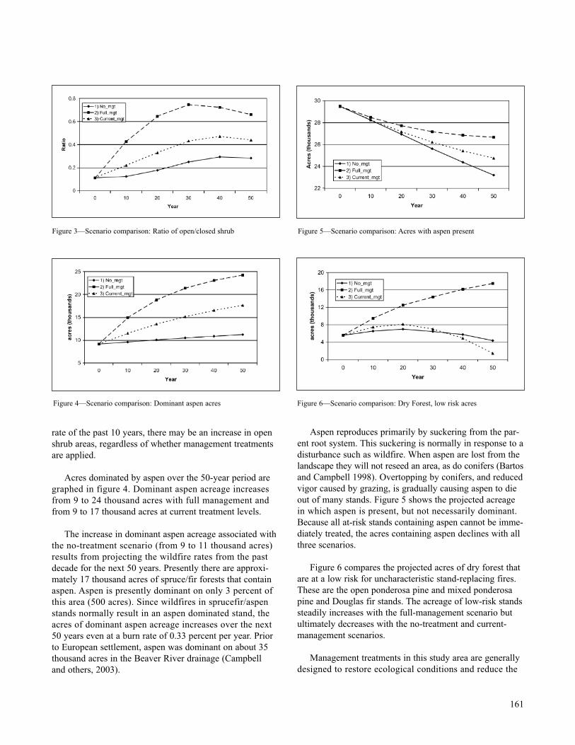
rate of the past 10 years, there may be an increase in openshrub areas, regardless of whether management treatmentsare applied.

Acres dominated by aspen over the 50-year period aregraphed in figure 4. Dominant aspen acreage increasesfrom 9 to 24 thousand acres with full management andfrom 9 to 17 thousand acres at current treatment levels.

The increase in dominant aspen acreage associated withthe no-treatment scenario (from 9 to 11 thousand acres)results from projecting the wildfire rates from the pastdecade for the next 50 years. Presently there are approxi-mately 17 thousand acres of spruce/fir forests that containaspen. Aspen is presently dominant on only 3 percent ofthis area (500 acres). Since wildfires in sprucefir/aspenstands normally result in an aspen dominated stand, theacres of dominant aspen acreage increases over the next 50 years even at a burn rate of 0.33 percent per year. Priorto European settlement, aspen was dominant on about 35thousand acres in the Beaver River drainage (Campbell and others, 2003).

Aspen reproduces primarily by suckering from the par-ent root system. This suckering is normally in response to adisturbance such as wildfire. When aspen are lost from thelandscape they will not reseed an area, as do conifers (Bartosand Campbell 1998). Overtopping by conifers, and reducedvigor caused by grazing, is gradually causing aspen to dieout of many stands. Figure 5 shows the projected acreagein which aspen is present, but not necessarily dominant.Because all at-risk stands containing aspen cannot be imme-diately treated, the acres containing aspen declines with allthree scenarios.

Figure 6 compares the projected acres of dry forest thatare at a low risk for uncharacteristic stand-replacing fires.These are the open ponderosa pine and mixed ponderosapine and Douglas fir stands. The acreage of low-risk standssteadily increases with the full-management scenario butultimately decreases with the no-treatment and current-management scenarios.

Management treatments in this study area are generallydesigned to restore ecological conditions and reduce the

161

Figure 3—Scenario comparison: Ratio of open/closed shrub

Figure 4—Scenario comparison: Dominant aspen acres

Figure 5—Scenario comparison: Acres with aspen present

Figure 6—Scenario comparison: Dry Forest, low risk acres

intensity of wildfire. In range areas within the Beaver Riverdrainage these treatments result in a slight increase inpotential wildfires. This is due to the increased acreage ofannual and perennial grasslands, which are more prone tofire. In forested areas management results in a small declinein potential wildfire acres. The net result of these two factorsis that the total wildfire acreage is projected to be nearly thesame for the three scenarios.

DISCUSSION

VDDT is a non-spatial model intended mainly for broadscale analysis. VDDT projects changes in vegetative condi-tions in response to succession, disturbances, and manage-ment treatments. In the Beaver River drainage key indicatorsare used to estimate environmental conditions under differ-ent management scenarios, as projected by VDDT.

Major shifts in vegetative composition have occurred as a result of fire suppression and grazing. Historicallyfires burned vegetative types within the Beaver River areaat frequencies ranging from every 5 to 80 years. In the pastdecade only 0.57 percent of this area burned per year for anaverage fire frequency of 175 years. In the previous twodecades (1973 – 1992) virtually no acres burned. Currentconditions in this drainage are reflective of conditions onthe Fishlake National Forest as a whole. On the FishlakeNational Forest spruce and fir acreage are estimated to haveincreased 238 percent from historic levels, while aspen hasdeclined 259 percent. Pinyon-juniper acreage is believed tohave increased 357 percent, while sage/grass/forb acreagehas declined 295 percent (Campbell and others, 2003).These changes result in reduced streamflows caused byincreased coverage of conifers including pinyon-juniper,reduced habitat for sage and aspen dependent wildlife species,and increased risk of uncharacteristically severe wildfiresin dry forest areas.

This analysis suggests that if management treatmentsare maintained at current levels, vegetative conditions willmost likely stabilize or decline further over the next fiftyyears. Active management, with treatment levels designedto mimic natural processes, would be necessary to restorethis area and reverse current environmental trends.

The VDDT software, manual, and tutorial exercises canbe downloaded from the website http://www.essa.com.

LITERATURE CITED

Arbaugh, M.J.; Schilling, S.J.; Merzenich, J.; Van Wagtendonk, J.W. 1999. A Test of the Strategic FuelsManagement Model VDDT using Historical Data fromYosemite National Park. In Proceedings of The JointFire Sciences Conference and Workshop. Boise, IDJune 15-17, 1999. Vol II 85-89. Univ of Idaho press.

Bartos, D.L.; Campbell, R.B. 1998. Decline of Quaking Aspen in the interior West – Examples from Utah.Rangelands. Vol 20, No. 1, February 1998. SanAntonio, Texas: Society for Range Management.

Beukema, S.J.; Kurz, W.A.; Pinkham, C.B.; Milosheva, K.; Frid, L. 2003. Vegetation Dynamics DevelopmentTool users’ guide, Version 4.4, ESSA Technologies Ltd.,Vancouver, BC. 234 pp.

Bradley, A.F., Noste, N.; Fischer, W.C. 1992. Fire Ecology of Forests and Woodlands in Utah. Gen. Tech.Rep. INT-287. Ogden, UT: U. S. Department ofAgriculture, Forest Service, Intermountain ResearchStation. 128 pp.

Campbell, R.B., Chappell, L., Greenhalgh, K. 2003. Personal communication, data from unpublishedFishlake National Forest Wildland Fire Use Plan. Table 16: Analysis by Vegetation Cover Type for the Combination of all Subsections for the FishlakeNational Forest. Richfield, UT 84701.

Long, D. and Merzenich, J. (in prep). Chapter 19: Development and application of the LANDSUM andVDDT models for the Southern Utah Fuel Manage-ment Demonstration Project. In: Long, Donald; Ryan, Kevin, editors. The Southern Utah Fuel ManagementDemonstration Project: Development andApplication ofModels. General Technical Report RMRS-GTR vol 4.FortCollins, CO: U.S. Department of Agriculture, ForestService, Rocky Mountain Research Station.

Merzenich, J.; Kurz, W.A.; Beukema, S.J.; Arbaugh, M.; Schilling, S. 1999. Long Range Modeling ofStochastic Disturbances and management treatmentsusing VDDT and TELSA. In Proceedings of the SAF1999 National Convention, 349-355, Bethesda, MD:Society of American Foresters.

162

O’Brien, R.A. 1999. Comprehensive inventory of Utah’s forest resources, 1993. Resource Bulletin RMRS-RB-1.Ogden, UT: U.S. Department of Agriculture, ForestService, Rocky Mountain Research Station.105 p.

Payson, T.E., Ansley R.J., Brown, J.K., and others. 2000. Fire in western shrubland, woodland, and grass-land ecosystems. In: Brown, J.K., Smith, J.K., editors.Wildland fire in ecosystems: Effects of fire on flora.Gen. Tech. Rep. RMRS-GTR-42-volume 2. Ogden, UT:U.S. Department of Agriculture, Forest Service, RockyMountain Research Station, pp 121-159.

Weise, D.R., R. Kimberlin, M. Arbaugh, J. Chew, J. Merzenich, J.W. Van Wagtendonk, and M. Wiitala1999. A Risk-Based Comparison of Potential FuelTreatment Trade-Off Models. Proceedings: The JointFire Sciences Conference and Workshop. Boise, IDJune 15-17, 1999. Vol II pp 96-102. Univ of Idaho press.

163

This page is intentionally left blank.

FIRE SUPPRESSION, FIRE PLANNING, ANDFUEL MANAGEMENT

This page is intentionally left blank.

In: Bevers, Michael; Barrett, Tara M., comps. 2005. Systems Analysis in Forest Resources: Proceedings of the 2003 Symposium. General Technical ReportPNW-GTR-656. Portland, OR: U.S. Department of Agriculture, Forest Service, Pacific Northwest Research Station.1 M. Acuña is Graduate Research Assistant, Department of Forest Engineering, Oregon State University, Corvallis, OR 97331. 2 C. Palma is Professor of Forest Management, Departmento de Ciencias Forestales, Pontificia Universidad Catolica de Chile, Santiago, Chile. 3 A. Weintraub is Professor ofLogistics and Operations Management, Department of Industrial Engineering, University of Chile, Santiago, Chile. 4 D. Martell is Professor of FireManagement, Faculty of Forestry, University of Toronto, Toronto, Canada. 5 W. Cui is a Postdoctoral Assistant, Faculty of Forestry, University of Toronto,Toronto, Canada.

Systems Analysis in Forest Resources: Proceedings of the 2003 Symposium

INTEGRATED TIMBER HARVESTAND FIRE MANAGEMENT PLANNING

Mauricio A. Acuña1, Cristian D. Palma2, Andrés Weintraub3, David L. Martell4, and Wenbin Cui5

INTRODUCTION

Fire, a natural component of most forest ecosystems,has a significant impact on peoples’ safety, public and private property, and economic activities based on forestryresources, such as wood production and recreation (Martelland Boychuk, 1997). Likewise, fire plays a significant rolein innumerable functions of the ecosystem, such as biodi-versity, the creation of habitat for animal life, etc.

Different studies have examined the effect of fire on woodsupply (Reed and Errico, 1986; Van Wagner, 1979, 1983;Martell, 1994), applying linear programming approachesand stochastic losses. These studies all indicate that verysmall burn fractions translate into substantial reductions tolong-term wood supply. Moreover, all these approximationshave considered fire losses as variables exogenous to theproblem of forest planning, without considering that forest

ABSTRACT

Harvest planners often consider potential fire losses and timber production plans can influence fire management, butmost timber harvest planning and fire management planning activities are carried out largely independently of each other.But road construction, timber harvesting and silvicultural activities can influence the flammability of a forest, so the proce-dure applied in this work considers an integrated fire and forest management planning methodology that accounts for andexploits such interactions using a fire spread model, a network model that identifies crucial stands that can influence thespread of fires across a landscape, and a spatially explicit timber harvest scheduling model. The model and how it is beingapplied to a forest management unit in the boreal forest region of Canada are described.

KEYWORDS: Mixed integer programming, heuristics, forest planning.

167

management decisions can have positive effects in terms ofreducing fire spread. Thus, for example, Hirsch and Pengelly(1997) state that including certain forest management crite-ria, such as harvest planning and the design of cutting units,could reduce the probability of fires by considerable mag-nitudes. In other words, the strategic fragmentation of theforest that results from harvesting could have a firebreakeffect, which would translate into a reduction of the burnarea.

The forest management planning systems use the outputsfrom the fire management system (annual burn fraction) asan exogenous parameter. Forest management decisions,however, particularly the areas and timing of harvestingdirectly affect fuel continuity and therefore fire spread.This integration requires the design of decision-makingsupport systems that can be used jointly by persons asso-ciated with both forest and fire management to develop,

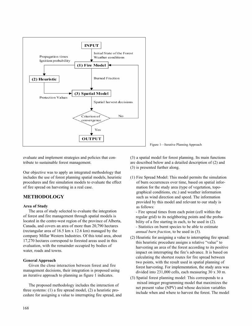
evaluate and implement strategies and policies that con-tribute to sustainable forest management.

Our objective was to apply an integrated methodology thatincludes the use of forest planning spatial models, heuristicprocedures and fire simulation models to evaluate the effectof fire spread on harvesting in a real case.

METHODOLOGY

Area of StudyThe area of study selected to evaluate the integration

of forest and fire management through spatial models islocated in the centre-west region of the province of Alberta,Canada, and covers an area of more than 20,790 hectares(rectangular area of 16.5 km x 12.6 km) managed by thecompany Millar Western Industries. Of this total area, about17,270 hectares correspond to forested areas used in thisevaluation, with the remainder occupied by bodies ofwater, roads and towns.

General ApproachGiven the close interaction between forest and fire

management decisions, their integration is proposed usingan iterative approach to planning as figure 1 indicates.

The proposed methodology includes the interaction ofthree systems: (1) a fire spread model, (2) a heuristic pro-cedure for assigning a value to interrupting fire spread, and

(3) a spatial model for forest planning. Its main functionsare described below and a detailed description of (2) and(3) is presented further along.

(1) Fire Spread Model: This model permits the simulationof burn occurrences over time, based on spatial infor-mation for the study area (type of vegetation, topo-graphical conditions, etc.) and weather informationsuch as wind direction and speed. The information provided by this model and relevant to our study is as follows:- Fire spread times from each point (cell within the regular grid) to its neighboring points and the proba-bility of a fire starting in each, to be used in (2).- Statistics on burnt species to be able to estimate annual burn fraction, to be used in (3).

(2) Heuristic for assigning a value to interrupting fire spread:this heuristic procedure assigns a relative “value” toharvesting an area of the forest according to its positiveimpact on interrupting the fire’s advance. It is based oncalculating the shortest routes for fire spread betweentwo points, with the result used in spatial planning offorest harvesting. For implementation, the study area wasdivided into 231,000 cells, each measuring 30 x 30 m.

(3) Spatial forest planning model: This corresponds to amixed integer programming model that maximizes the

net present value (NPV) and whose decision variablesinclude when and where to harvest the forest. The model

168

Figure 1—Iterative Planning Approach

includes losses of wood that result from fires, expressedas the annual burn fraction, and considers the positiveimpact that harvesting can have on interrupting firespread when it is associated with management decisionsto achieve minimum “protection” levels.

This system proceeds as follows. Initial informationabout the state of the forest feeds the fire module. Thisgenerates (a) the information necessary (fire spread times,probable fire starts, etc.) for calculating a “protection value”using a heuristic procedure and (b) information on the frac-tion of the forest that burns given current conditions fordetermining management decisions within the spatial model.Meanwhile, protection values generated by heuristic proce-dures are included in the spatial model. Because the spatialharvesting decisions obtained modify the original conditionsfor fire spread and, as a result, its behavior and the fractionof forest burned, spatial model decisions are again fed intothe fire module, generating new information for calculatingprotection values and for the spatial model. The process isstopped upon reaching a specific convergence criterion.

Procedure for Assigning a Value to Interrupting Fire Spread

This heuristic procedure assigns a value to each cell for interrupting the fire spread. As a fire starting in a cellshould reach a destination cell along the route of leastresistance to the fire it can be represented by the differentshortest routes found for each pair of cells (Finney, 2002).

The importance of each route, R(i,j), will vary accord-ing to the ignition probability in the cell of origin I(i), thevalue to be protected in the destination cell V(j), and thefire spread time between both cells i and j T(i,j), and it iscalculated as R(i,j) = I(i) * V(j) / T(i,j). The higher theprobability of a fire occurring at a point or the higher thevalue to be protected in the destination cell (which willburn if the fire reaches it), the more important it is to blockthis route. Similarly, if the fire takes too much time to reachthe destination cell, blocking its spread by harvesting a cellwill be less important, since it is more likely the fire willbe suppressed through active measures. In our case, thevalue to protect in the destination cell corresponds to thevolume of wood available, but it could also consider thepresence of towns or critical infrastructure. The value ofthe different routes, R(i,j), is added to cells that belong tothe corresponding route, so the protection value assigned toeach cell of forest will vary according to the quantity andimportance of the fires that it can interrupt.

Finally, the procedure permits the creation of an indexor ranking that represents the cells’ belonging to different

routes for possible fires. Thus, regions prone to fire spreadwill form part of many fire routes and their protection val-ues will be higher.

Spatial Forest Planning Model The model is for a mixed integer programming problem,

implemented by using the modeling language GAMS/IDEv.19.6® and the solver CPLEX v.7.1®. The model estab-lishes a spatial harvesting schedule that integrates fire pro-tection. To do so, the model uses as its basis Model III byReed and Errico (1986) and the variation proposed byMartell (1994), in order to maximize the NPV over an 80-year planning horizon, divided into eight 10-year periods.Model assumptions included:- Completely accessed forest, so no road-building

decisions were included. - Harvest flows (volumes of wood) were accepted

varying ± 30% between periods.- Harvested and burned areas regenerate naturally at no

cost. The model does not include reforesting decisions,which means that once harvested the forest will alwaysreforest with the same species.

- Transportation and harvesting (logging) costs per cut-ting unit were included, along with income per m3 ofwood harvested.

- There is an inventory of every age class when the planning horizon ends.

- Harvesting occurs at the mid-point of the period.- If the decision is made to cut a stand during the period,

it is completely harvested.- No adjacency restrictions are included.- It is assumed that the fire consumes some fixed propor-

tion of the area not harvested in each age class and thatthis proportion does not vary over time. As indicatedpreviously, this is referred to as the burn fraction.

- Fire protection values are included for each cutting unit.To do so, protection values for all the cells belonging toa cutting unit are added together to reach its final pro-tection value.

As output, the spatial model determines a harvestingschedule for all cutting units over time and the supply ofwood arising from the allowable annual cut.

Information the Model Requires—As input, thismodel receives the initial state of the forest, which consistsmainly of cutting units, species, the commercial volumeper species and age classes, all of which form part of MillarWestern Industry’s inventory information for the study area.

Cutting unit: To define the cutting units we used the geo-graphic information system ArcInfo®, as our objective was

169

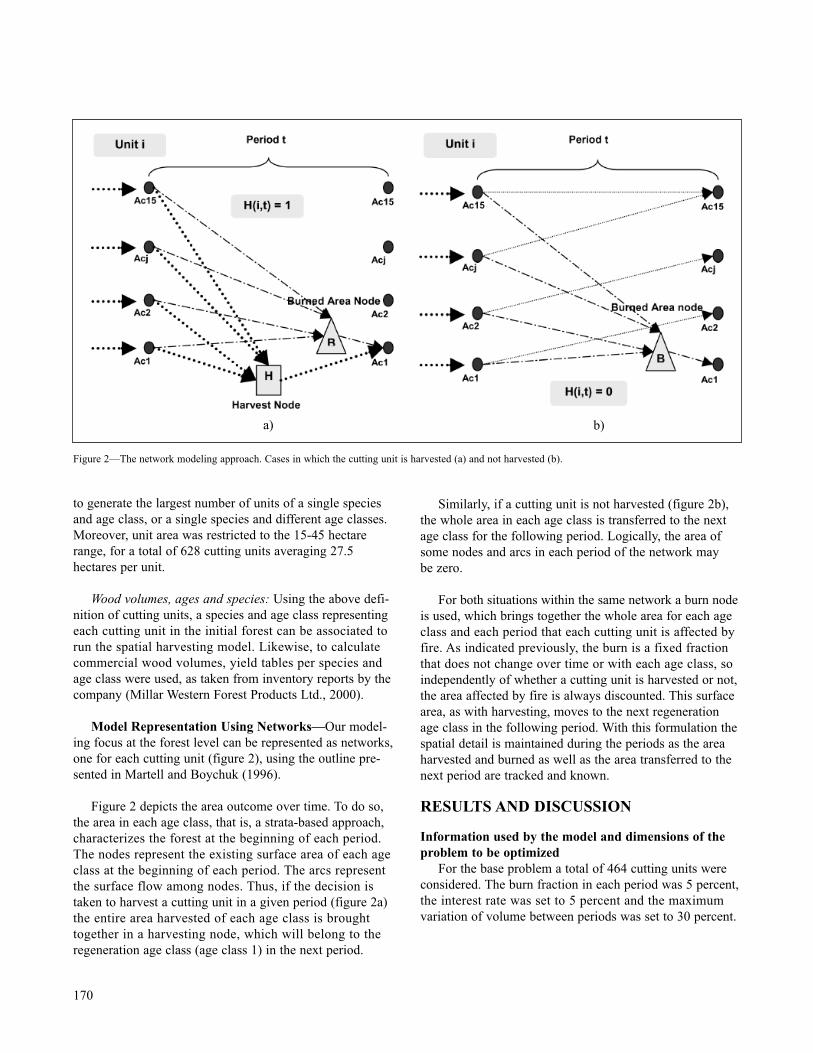
to generate the largest number of units of a single speciesand age class, or a single species and different age classes.Moreover, unit area was restricted to the 15-45 hectarerange, for a total of 628 cutting units averaging 27.5hectares per unit.

Wood volumes, ages and species: Using the above defi-nition of cutting units, a species and age class representingeach cutting unit in the initial forest can be associated torun the spatial harvesting model. Likewise, to calculatecommercial wood volumes, yield tables per species andage class were used, as taken from inventory reports by thecompany (Millar Western Forest Products Ltd., 2000).

Model Representation Using Networks—Our model-ing focus at the forest level can be represented as networks,one for each cutting unit (figure 2), using the outline pre-sented in Martell and Boychuk (1996).

Figure 2 depicts the area outcome over time. To do so,the area in each age class, that is, a strata-based approach,characterizes the forest at the beginning of each period.The nodes represent the existing surface area of each ageclass at the beginning of each period. The arcs representthe surface flow among nodes. Thus, if the decision istaken to harvest a cutting unit in a given period (figure 2a)the entire area harvested of each age class is broughttogether in a harvesting node, which will belong to theregeneration age class (age class 1) in the next period.

Similarly, if a cutting unit is not harvested (figure 2b),the whole area in each age class is transferred to the nextage class for the following period. Logically, the area ofsome nodes and arcs in each period of the network may be zero.

For both situations within the same network a burn nodeis used, which brings together the whole area for each ageclass and each period that each cutting unit is affected byfire. As indicated previously, the burn is a fixed fractionthat does not change over time or with each age class, soindependently of whether a cutting unit is harvested or not,the area affected by fire is always discounted. This surfacearea, as with harvesting, moves to the next regenerationage class in the following period. With this formulation thespatial detail is maintained during the periods as the areaharvested and burned as well as the area transferred to thenext period are tracked and known.

RESULTS AND DISCUSSION

Information used by the model and dimensions of theproblem to be optimized

For the base problem a total of 464 cutting units wereconsidered. The burn fraction in each period was 5 percent,the interest rate was set to 5 percent and the maximumvariation of volume between periods was set to 30 percent.

170

Figure 2—The network modeling approach. Cases in which the cutting unit is harvested (a) and not harvested (b).

a) b)

As for the problem to be optimized, this one had thefollowing features:- Total number of variables: 345,260- Number of binary variables: 3,712- Number of equations: 349,443- Number of iterations: 53,557- Resolution time: 801 seconds

AnalysisA number of scenarios were evaluated in order to inves-

tigate the variation of timber volume in each period and theeconomic effects of different strategies of fire protection.

Effect of different burn fractions on the harvestschedule—The model was run varying the annual burnfraction starting from a 0 percent level to a burn fraction

of 10 percent. Five different scenarios were evaluatedwhose burn fractions per period were 0, 1, 3, 5, and 10percent, respectively.

The results obtained from these scenarios, their effectson the objective function as well as the area and the totalvolume harvested are shown in Table 1.

With an annual burn fraction of 10 percent the volumeand the objective function decrease about 24 percent in aperiod of 80 years compared to the situation with no fire.This situation can be more negative if the results are pro-jected over a longer-term horizon, in other words, 200years or more, where the losses can be dramatically higherthan the ones presented here (Martell, 1994).

171

Table 1—Impact of different levels of burn fraction on volume harvested and NPV

Total area Total volume ObjectiveScenario Burn fraction burned (ha) harvested (MM m3) function (MM $)

0 0% 0.0 1.758 21.4381 1% 129.6 1.714 20.9072 3% 388.9 1.635 19.8993 5% 648.2 1.554 19.0684 10% 1296.4 1.341 16.312

Table 2—Effect of fire protection on the total timber volume harvested

Burn fraction Burn fraction Volume before Volume afterbefore protection after protection protection protection Difference

Protection (%) (%) (%) (MM m3) (MM m3) (%)

10 5 4.85 1.554 1.554 010 5 4 1.554 1.590 2.210 5 3 1.554 1.625 4.610 5 2 1.554 1.668 7.3

Table 3—Effect of fire protection on the Net Present Value (NPV)

Burn fraction Burn fraction NPV before NPV afterbefore protection after protection protection protection Difference

Protection (%) (%) (%) (MM $) (MM $) (%)

10 5 4.85 19.068 19.068 010 5 4 19.068 19.376 1.610 5 3 19.068 19.697 3.310 5 2 19.068 19.978 4.8

In this work a burn fraction of 5 percent was used to runthe models. With this relatively small amount of fire on thelandscape, it is possible to observe losses of about 11 per-cent in volume and in NPV, corresponding to 204 millioncubic meters and 2.37 million dollars respectively. Logically,these losses are considerably higher if the burn fraction isincreased (e.g. 30 or 40 percent). As the losses associatedto the presence of fire appear to increase exponentially,they can become an important risk for the company’s woodsupply.

Effect of different fire protection levels on the harvest schedule and their impact on the annual burnfractions—As described in the methodology, a number ofdifferent fire protection levels were used for running themodel and evaluating its effects.

Being an ongoing research the results are preliminaryand some of them are generated under assumptions (tables2 and 3). Firstly the model was run with a 5 percent burnfraction which represented the base level and whose valuewas of 3.302E+7 units. Then we used two different protec-tion levels, 10 and 20 percent, which were included intothe model along with the benefit of a reduced area burnachieved with this higher protection. In this paper we onlypresent the results for a 10 percent of protection.

We analyzed the case of timber volume and NPV. Forthe case with 10 percent of protection it is necessary toreduce the actual burn fraction 0.15 percent, to a level of4.85 percent in order to have no additional benefits in vol-ume or in NPV. With a higher fire protection the modelbecomes more constrained which means a decrease both inthe objective function and the volume harvested. However,at the same time this negative effect in the objective func-tion is neutralized with a reduced burn fraction as theprotection increases.

If it is possible to reduce the burn fraction only from 5percent to 4 percent, the total volume harvested increases a little more than 35,000 cubic meters, or a 2.2 percent.Likewise, reducing the burn fraction 1 percent with a pro-tection of 10 percent increases the NPV 1.6 percent, or$307,991.

Conversely, in an optimistic scenario with a protectionlevel of 10 percent over the base level and a reduction ofthe burn fraction to 2 percent the volume increases in 7.3percent or more than 114,166 cubic meters compared to thescenario with no protection. The positive effect in NPV isslightly lower than the benefit in volume. NPV increases

$910,000 for the entire horizon or 4.8%. As we used log-ging costs generated by a uniform distribution and a fixedincome for each cubic meter harvested, different resultswould be obtained by using real information.

CONCLUSIONS

From these results further research might be focused onstudying the effect of having higher initial burn fractions inthe landscape with no protection and the effects of greaterreductions in burn fraction as more protection is applied. Itis clear that the benefits are higher in landscapes stronglyaffected by fire and when the spatial harvest planning gen-erated by this methodology is able to considerably reducethe annual burn fraction.

It is also necessary to study the effects of different foreststructures and age class distributions and their impact onthe timber volume to be harvested in each period. The for-est information and data used for carrying out this studypresent much heterogeneity characterized by a considerablenumber of different species and ages. In a commerciallymanaged forest the positive effect of applying this method-ology both in volume and NPV can be higher than theresults presented here. Therefore, this methodology shouldbe tested in different kinds of forests with different struc-tures and management in order to have more realisticresults and conclusions.

Finally it is important to continue studying and evaluat-ing the methodology presented in this paper, in particularthe procedure for calculating the protection values as ameasure to stop fire propagation. We have just consideredthe shortest paths between pairs of cells in order to knowthe different routes for the fires. It might be useful to eval-uate the effect of other paths, perhaps the K-shortest pathsthat fires can take as alternatives routes. As this can becomputationally challenging and may not provide betteranswers, other solution schemes such as using simulationin a pro-babilistic way, for example Monte Carlo simula-tion, might be studied in a further research.

LITERATURE CITED

Finney, M.A. 2002. “Fire Growth Using Minimum Travel Time Methods.” Can. J. For. Res. 32(8): 1420-1424.

Hirsch, K. and I. Pengelly. 1997. “Forest Fuels Management in Theory and Practice.” Pp. 112-116 inProc. Symp. on Stand Density Management: Planningand Implementation, C.R. Bamsey (ed.). Edmonton,Alberta, Canada.

172

Martell, D.L. 1994. “The Impact of Fire on Timber Supply in Ontario.” For. Chron. 70(2): 164-173.

Martell, D.L. and D. Boychuk. 1996. “A Multistage Stochastic Programming Model For Level TimberSupply Under Risk of Fire.” For. Sci. 42(1): 10-26.

Martell, D.L. and D. Boychuk. 1997. “Level of Fire Protection For Sustainable Forestry In Ontario: FinalReport.” Report prepared for the Canada-Ontario NorthernOntario Development Agreement, Sustainable ForestryDevelopment/Decision Support Project: DevelopingAnalytical Procedures for Establishing the Level ofProtection for Forest Fire Management to SupportSustainable Forestry in Ontario.

Millar Western Forest Products Ltd. 2000. Detailed Forest Management Plan 1997-2000. Vol. 1, Ch. 1.Edmonton, Alberta, Canada.

Reed, W.J. and D. Errico. 1986. “Optimal Harvest Scheduling at the Forest Level in the Presence of theRisk of Fire.” Can. J. For. Res. 16: 266-278.

Van Wagner, C.E. 1979). “The Economic Impact of Individual Fires on the Whole Forest.” For. Chron.55(2): 47-50.

Van Wagner, C.E. 1983. “Simulating the Effect of Forest Fires on Long Term Timber Supply.” Can. J. For. Res.13: 451-457.

173

This page is intentionally left blank.

In: Bevers, Michael; Barrett, Tara M., comps. 2005. Systems Analysis in Forest Resources: Proceedings of the 2003 Symposium. General Technical ReportPNW-GTR-656. Portland, OR: U.S. Department of Agriculture, Forest Service, Pacific Northwest Research Station.1 M.R. Wiitala is an Operations Research Analyst and 2 A.E. Wilson is a Resource Information Specialist at the Pacific Southwest Research Station, USDAForest Service, 620 SW Main Street, Suite 400, Portland Oregon, 97205; e-mail: mrwiitala@fs.fed.us.

Systems Analysis in Forest Resources: Proceedings of the 2003 Symposium

A SYSTEMS ANALYSIS MODEL FOR WILDLAND FIRE PREPAREDNESS PLANNING

Marc R. Wiitala1 and Andrew E. Wilson 2

INTRODUCTION

The initial attack system remains a critical componentin the protection of the nation’s resources at risk to wild-land fire. Planning the appropriate amount and use of fire-fighting personnel and equipment to effectively deal withthe fire fighting workload presented by impending fire seasons remains problematic for federal land managementagencies (GAO 2002).

Operations research technologies are available to improvethe quality of analytical tools for wildland fire planning.The method of system simulation is particularly suitablefor application to the fire planning problem. Industry hasoften used simulation to model complex systems such asroad transportation systems, emergency services delivery,mining operations, and supply systems. In Canada, theprovince of Ontario is successfully using system simulationfor fire preparedness planning (Martell and others 1994;McAlpine and Hirsch 1999). System simulation offers a

175

great opportunity to capture the salient operating character-istics of the initial attack resource delivery system. Anappropriately designed computer simulation model wouldprovide fire managers a powerful analytical tool to evaluatethe relative performance of initial attack program alterna-tives and resource deployment policies. Investments in otherwildfire protection programs, like prevention, detection,and fuels treatment, would also lend themselves to exami-nation by the model.

The need for a modern wildland fire planning and policyanalysis tool is the target of a research and developmentproject funded by the National Fire Plan (USDA and USDI2001). The project has designed and built a new initialattack simulation model based on currently available simu-lation technologies. The model is currently undergoing test-ing and validation on the Umatilla National Forest in easternOregon and Washington. This paper describes the anatomyof this simulation model—the Wildfire Initial ResponseAssessment System (WIRAS). Before beginning, we briefly

ABSTRACT

Planning an effective and efficient initial attack wildfire suppression organization in preparation for an uncertain fire seasonis a challenging task for fire planners. This paper describes features of WIRAS, a discrete-event stochastic simulation modelthat can assist fire planners in wildfire preparedness planning and policy analysis. WIRAS simulates, according to user-definedrules, all phases of initial attack resource management and movement to meet the service needs in response to the ebb and flowof fire workload over the landscape and through time. In an operational setting WIRAS is used to test alternative preparednessprograms against annual historical fire occurrence datasets to gauge performance with respect to spatially and temporally vari-able fire seasons. Planning capability at the national and regional scales is complemented by a unique ability of WIRAS toevaluate local preparedness programs within a larger geographic context to account for the impact of external competition forshared suppression resources, like airtankers, helitack, and smokejumpers.

look at the nature of fire planning problem and the initialattack environment.

PLANNING PROBLEM

In preparation for fire seasons, wildland fire managerschoose the size, composition, and location of the fire sup-pression organization that best meets land management andprotection objectives, usually with respect to alternativelevels of fiscal constraint. Managers make this decision inthe face of uncertainty, where fire seasons in many loca-tions of North America vary greatly in intensity over timeand across the landscape.

Choosing an appropriate presuppression organizationmore specifically involves selecting, for example, the num-ber, size, location, and term of hand and engine crews tohire and long-term investments in capital equipment andfacilities like fire engines and helicopter bases. Fire pre-paredness planning also develops dispatch policies for usingnot only locally controlled resources but also for those sharedamong jurisdictions, for example, airtankers and smoke-jumpers.

Initial Attack EnvironmentThe initial attack setting has been aptly described by

Martell and others (1984) and Wiitala (1998). We summa-rize the account given by the latter, but with reference toinitial attack activity on federal lands in a region containingnorthern California, the Pacific Northwest, Idaho, andwestern Montana.

The initial attack process in this broad area consists ofthe collective action of many administrative units deploy-ing wildland fire suppression forces in response to a sea-sonal flow of fires distributed temporally and geographically.The number of fires in this region can exceed 10,000 persummer season. Several hundred fires can occur on a givenday and approach 1,000 on several consecutive days (figure 1).

Because thunderstorms are responsible for these peakperiods of fire activity, fires tend to cluster spatially andtemporally. This phenomenon creates localized heavy fireworkloads that can tax the capabilities of local initial attackorganizations and result in larger project fires. In a largegeographic area, multiple thunderstorm cells often give riseto spatially dispersed fire clusters, creating competition foraerial initial attack resources shared over larger geographicscales.

176

Figure 1—Comparing the temporal distribution of single and consecutive three-day fire starts in the northwestern United States in 1994.

As a general characterization of the local initial attackprocess, when fire activity commences, the resource dis-patching process begins. Rules for resource dispatchingvary between administrative units. The type and effort ofresponse vary with uncertain conditions of the fire environ-ment, land management objectives, and available resources.In general, dispatchers favor use of local ground resourceswith the shortest response times, provided the responsetimes are reasonable for the conditions of the fire and pro-tection objectives. Otherwise, dispatchers will deploy aeri-ally delivered fire fighters, if available. Dispatchers mayalso request the support of airtankers to deliver retardant or water to the fire. Or, after delivery by helicopter, a crewmay request a helicopter to support fireline constructionwith water drops.

Initial attack resources work a fire until it is containedor becomes unmanageable. In the latter instance, a largefire suppression organization assumes management of thefire. In either case, how quickly initial attack resourcesdemobilize and return to a ready status depends on a vari-ety of conditions including the time required for fire mop-up, the level of fire activity, time of day, and accessibilityto transportation.

MODEL

WIRAS uses a process-oriented approach (Law andKelton 1991) in its design of a discrete-event, stochasticcomputer simulation model representing the initial attacksystem. An enhanced variant of the discrete-event simulationlanguage General Purpose Simulation System (Hendriksenand Crain 1989) originally developed by Gordon (1962), isthe language used to build the simulation model. WIRASshares many attributes and capabilities with the clock-driven,next-event simulation models of Fried and Gilless (1988),Martell et al. (1994), and Wiitala (1998), which address howthe frequency and magnitude of multiple fire events andspatial interactions of initial attack affect program per-formance.

WIRAS distinguishes itself from its predecessors byfeaturing the ability to plan both local and national fire pre-paredness programs. It also pioneers the ability to conductlocal planning within the context of the national fire envi-ronment and fire fighting activity. This embedded planningapproach allows fire planners to design a local programwhile taking into account their success in competing fornationally shared aerial resources. To describe the structureof WIRAS, we present its major components.

Suppression ResourcesWIRAS contains distinct subsystems to simulate the

activities of various types of aerial and ground resources inthe initial attack system. Each resource subsystem featuresa unique design to capture disparate operational features.

Airtanker, Smokejumper, and Helitack resources—The aerial subsystems deliver both water and retardant andcrews to fires. The airtanker subsystem consists of singleand multiple engine airtankers delivering retardant from asystem of geographically fixed airtanker bases. Additionally,the single engine aircraft can operate from a mobile base.Not all bases can accommodate all airtanker types. For thisreason, each airtanker and retardant base carries attributeswithin the model to permit imposing base use or capacityrestrictions on some airtankers. Attributes affecting air-tanker operations within the model include airspeed, retardantcarrying capacity, loaded weight, refueling and reloadingtimes, and a single engine airtanker identifier.

Major time-consuming operations modeled at an air-tanker base include landing, taxiing, taking-off, refueling,and loading. The simulation model monitors daily airtankerflight hours to determine when to refuel an airtanker aswell as when to limit use due to daily flight-hour restric-tions. The number of loading bays, refueling trucks, andparking spaces specified for bases affects their ability toservice airtankers and ultimately affects retardant deliverysystem performance.

The model’s helitack subsystem is responsible for thedelivery of crews, water, and retardant. After delivering acrew to a fire, the model may augment crew fireline build-ing activity with helicopter water bucket support. In themodel, bucket support continues until there is a need for thehelicopter to refuel, deliver a crew, or return to base beforenightfall. Helitack is modeled as a locally controlled resourceoperating from a system of bases with varying numbers ofdeliverable crew members. This subsystem permits sharinghelicopters between bases but not crews.

The fixed-wing aircraft deliver smokejumpers primarilyto fires that are remote or when the supply of local resourcesis exhausted. Smokejumpers are highly mobile at the nationalscale. Wiitala and Dammann (2003) provide a detailed des-cription of the smokejumper subsystem as used in WIRAS.In summary, smokejumpers and their delivery aircraftattack fires from a system of bases dispersed across thewestern United States. The simulation model moves smoke-jumper assets between bases in response to demands createdby the ebb and flow of fire activity across the nationallandscape.

177

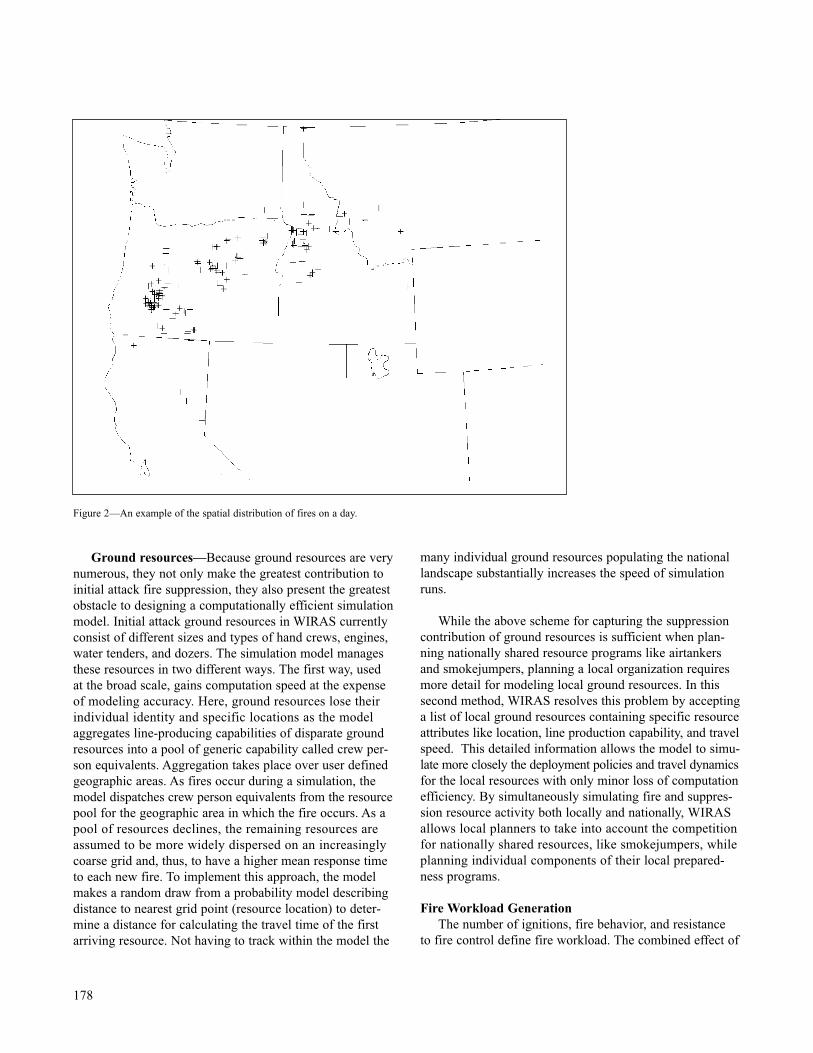
Ground resources—Because ground resources are verynumerous, they not only make the greatest contribution toinitial attack fire suppression, they also present the greatestobstacle to designing a computationally efficient simulationmodel. Initial attack ground resources in WIRAS currentlyconsist of different sizes and types of hand crews, engines,water tenders, and dozers. The simulation model managesthese resources in two different ways. The first way, usedat the broad scale, gains computation speed at the expenseof modeling accuracy. Here, ground resources lose theirindividual identity and specific locations as the modelaggregates line-producing capabilities of disparate groundresources into a pool of generic capability called crew per-son equivalents. Aggregation takes place over user definedgeographic areas. As fires occur during a simulation, themodel dispatches crew person equivalents from the resourcepool for the geographic area in which the fire occurs. As apool of resources declines, the remaining resources areassumed to be more widely dispersed on an increasinglycoarse grid and, thus, to have a higher mean response timeto each new fire. To implement this approach, the modelmakes a random draw from a probability model describingdistance to nearest grid point (resource location) to deter-mine a distance for calculating the travel time of the firstarriving resource. Not having to track within the model the

many individual ground resources populating the nationallandscape substantially increases the speed of simulationruns.

While the above scheme for capturing the suppressioncontribution of ground resources is sufficient when plan-ning nationally shared resource programs like airtankersand smokejumpers, planning a local organization requiresmore detail for modeling local ground resources. In thissecond method, WIRAS resolves this problem by acceptinga list of local ground resources containing specific resourceattributes like location, line production capability, and travelspeed. This detailed information allows the model to simu-late more closely the deployment policies and travel dynamicsfor the local resources with only minor loss of computationefficiency. By simultaneously simulating fire and suppres-sion resource activity both locally and nationally, WIRASallows local planners to take into account the competitionfor nationally shared resources, like smokejumpers, whileplanning individual components of their local prepared-ness programs.

Fire Workload GenerationThe number of ignitions, fire behavior, and resistance

to fire control define fire workload. The combined effect of

178

Figure 2—An example of the spatial distribution of fires on a day.

temporal variation in fire occurrence (figure 1) and spatialvariation in ignition pattern (figure 2) is an important deter-minant of initial attack program performance both locallyand nationally. To preserve the impact of spatial and tem-poral autocorrelation on program performance, WIRASsimulates program performance for an entire set of firesfrom a season. Because fire workload varies significantlybetween years, WIRAS addresses the implications of fireworkload variation on initial attack performance by testinga preparedness program against a range of fire seasons.Historical fire records currently provide WIRAS with thenecessary time stream of geographically located fire igni-tions.

Strength of ResponseWIRAS mimics an administrative unit’s dispatch rules

for determining the strength and priority of initial response

to a fire. Initial response policies revolve around dispatchblocks. Each dispatch block is a geographic area that reflectsa difference in one or more of the following: managementand protection objectives, fire behavior potential, and levelof fire activity (figure 3).

As is true operationally, when the first resource arriveson a fire, the simulation model reassesses the neededstaffing level based on actual fire conditions (figure 4).Depending on assessed needs and the strength of the initialresponse, the model may look for additional resources orhalt the response of some resources in transit to the fire. Inaccordance with local practice, the model may also initiateairtanker support.

Resource Dispatching and AllocationWIRAS controls resource dispatching through a system

of Boolean variables that mimics the rules and prioritiesgoverning an administrative unit’s dispatch policies (figure5). The model maintains and updates several state variablesused by the Boolean variables to reflect the types of infor-mation typically available to dispatchers. This system ofBoolean variables is sufficiently flexible to permit plannersto set the conditions for the dispatching ground resourcesbased on attack times, fire behavior potential, and protec-tion objectives.

179

Figure 3—Factors determining the preplanned initial response to a fire.

Figure 4—Factors affecting reassessment of fire staffing needs upon firstresource arrival.

Figure 5—Resource dispatch decision process for staffing fires.

During a simulation, if the conditions for a groundresource response are not met, the model attempts to dis-patch helitack crews. Failing this, WIRAS searches thesmokejumper system for available suppression resources.The search for resources to dispatch to a fire continuesuntil meeting fire staffing needs as determined by the ini-tial response or by reassessment upon first resource arrival.If no initial attack resources are available, the model queuesthe staffing request. When a resource becomes available fordispatching, WIRAS selects from the service queue thehighest priority fire serviceable by the resource. The modeluser can set the priority scheme based on protection objec-tives and fire behavior potential. However, WIRAS alwaysattempts to complete unfulfilled fire staffing needs beforestaffing new fires.

Response Time CalculationsAccurate modeling of resource response times is critical

to the successful modeling of the initial attack system. InWIRAS, components of response time include getaway,reloading, refueling, and travel time. Travel time is usuallythe largest component. For aircraft, distance between travelpoints and airspeed combine to calculate travel time. Duringperiods of high fire activity, the response time of airtankerscan lengthen if they have to wait for a retardant loadingbay at congested airtanker bases.

For ground resources, WIRAS combines vehicle travelalong a road network and off-road travel for groundresource travel time (Wilson and Wiitala, this proceedings).The simulation model integrates a computationally efficientleast-cost-path algorithm to estimate ground resource traveltimes. To improve simulation time, many of the groundresource response times are computed prior to simulationbased on known origins and destinations. During a simu-lation, a ground resource in transit to a fire may be divertedto another fire. At this point in the simulation, its locationis calculated and the least-cost-path algorithm invoked tocalculate response times to all fires to which the resourcemight respond.

Fire Growth and ContainmentWIRAS implements a time-dependent accounting

process operating on a five-minute time step to calculatefire perimeter growth, track resource arrivals, and computefireline to determine when a fire is contained or escapesinitial attack. The forward rate of fire growth is estimatedat 2:00 PM from historical data for the fuel and environ-mental conditions at the location and on the day of fireoccurrence. Fire growth is diurnally adjusted to account forwide differences in growth rates over a 24-hour period. A

double elliptical growth algorithm calculates perimeterexpansion over time (Anderson 1983). Fire line constructionoccurs on the flanks of the fire from the point of ignition.WIRAS contains fires according to a model developed byQuintilio and Anderson (1976) that accounts for the effectof fireline production in moderating the growth of a fire’sperimeter.

Fires are considered contained when fireline reaches auser specified percentage of fire perimeter. WIRAS escapesa fire (removes it from initial attack status) when fireperimeter exceeds constructed fireline by a user specifiedamount or fire area reaches a defined threshold.

Demobilization and Return to ServiceAssumptions regarding how quickly initial attack resources

become available for dispatching after fire containment orescape can greatly influence program performance. WIRASencodes these assumptions into user changeable rules thatprovide the opportunity to evaluate how alternative demo-bilization and return to service policies affect system per-formance.

Under the existing default rules, when finished fightinga fire, WIRAS returns initial attack resources to service onthe next day following fire containment and on the secondfollowing day if the fire escapes initial attack. The modelmakes two exceptions to this rule. First, if ground resourcesin roaded areas contain a fire sufficiently early in the day,the model may dispatch them to other fires awaiting service,response time permitting. Second, those crews simulated aswalking deep in wilderness or unroaded areas will remainwith the fire a full burning period after containment. Thispolicy assures full fire control and minimizes the risk of asubsequent response to a reigniting fire in a remote area ofhigh cost for aerial delivery or long response times forground-based crews.

MODEL OUTPUTS

During a simulation, WIRAS collects a variety of oper-ational statistics. These statistics help planners judge thephysical and economic performance of alternative approachesto organizing a fire preparedness program for their admin-istrative units. For example, information collected onresource utilization allows planners to identify underutilizedresources and bases.

Planners can also combine a program’s cost with sup-pression costs and projected natural resource losses esti-mated from model outputs to evaluate relative economic

180

efficiency of alternative preparedness programs. Programbudgeting issues are also addressable. Other statistics includeacres burned, escaped fire numbers, fire dispatches, aircraftflight hours, gallons of delivered retardant, and frequencydistributions for contained fire sizes and resource attacktimes.

CONCLUSION

The purpose of this paper was to briefly describe theanatomy of WIRAS—a stochastic simulation model for firepreparedness planning. Stochastic simulation is proving tobe a powerful operations research method for planninghighly complex initial attack service delivery systems.Taking a system analysis perspective in the design of theWIRAS, the resulting initial attack simulation model canaddress a wide range of program and policy issues not pre-viously addressable by other fire planning technologies.Not only can fire planners use WIRAS to determine thebest program composition, they can also use it to improvetheir resource deployment and dispatch policies—locally,regionally, and nationally.

Opportunities for the application of WIRAS are nowbecoming apparent. In one recent application at the nation-al level, WIRAS identified effective alternatives to the useof heavy airtankers in support of initial attack activities.Geographic area command centers are interested in thepotential of WIRAS to examine and implement aerialresource prepositioning strategies during a fire season inresponse to fire severity forecasts. Also under considerationis the use of WIRAS to quantify improved initial attackprogram performance and consequent benefits of reducedsuppression costs resulting from hazardous fuels treatment.Each new application of WIRAS generally necessitates cre-ating a new variant of the core simulation model to addressthe unique characteristics of the new problem.

LITERATURE CITED

Anderson, H.A. 1983. Predicting wind-driven wild land fire size and shape. Res. Paper INT-305. Ogden, UT:U.S. Department of Agriculture, Forest Service,Intermountain Forest and Range Experiment Station. 26 p.

Fried, J.S., and J.K. Gilless. 1988. Modification of an initial attack simulation model to include stochasticcomponents. In: Proceedings of the 1988 system symposium on forest resources. USDA For. Serv. Gen. Tech. Rep RM-161. pp. 235-240.

U.S. Government Accounting Office. 2002. Improved planning will help agencies better identify fire-fightingpreparedness needs: Report to Congress. GAO-02-158Wildland fire management. Washington, D.C. 32 p.

Gordon, G. 1962. A General Purpose System Simulator. IBM Systems Journal 1(1). pp. 18-32.

Henriksen, J.O., and R.C. Crain. 1989. GPSS/H Reference Manual. Third edition. Wolverine SoftwareCorporation. Annandale, Virginia.

Law, A.M., and W.D. Kelton. 1991. Simulation modeling and analysis. McGraw-Hill,Inc., New York. 759 p.

Martell, D.L., R.J. Drysdale, G.E.Doan, and D. Boychuk. 1984. An evaluation of forest fire initial attackresources. Interfaces 14(5), pp. 20-32.

Martell, D.L., D. Boychuk, J.I. , MacLellan, B.M. Sakowicz, and R. Saporta. 1994. Decision analysis of the level of forest fire protection in Ontario. In:Proceedings of the sixth symposium on systems analy-sis in forest resources, 1994 September 6-9, PacificGrove. Society of American Foresters, Bethesda, MD.pp. 138-149.

McAlpine, R.S. and K.G. Hirsch. 1999. An overview of LEOPARDS: The level of protection analysis system.The Forestry Chronicle 75(4): 615-621.

U.S. Department of Agriculture, Forest Service. 1985. National fire management analysis system user’s guideof the initial action assessment (FPL-IAA2.2).Washington, D.C.

U.S. Departments of Agriculture and Interior. 2001. Acollaborative approach for reducing wildland fire risksto communities and the environment: 10-year compre-hensive strategy. Washington, D.C.

Quintilio, D., and A.W. Anderson. 1976. Simulation study of initial attack fire operations in the Whitecourt Forest,Alberta. Canadian Forestry Service Information ReportNOR-X-166. 43 p.

Wiitala, M.R. 1998. Modeling the spatial and temporal dynamics of initial attack fire suppression using GPSS.In: Proceedings of the III international conference onforest fire research and 14th conference on fire and forest meteorology, 1998 November 16-20, Lusco-Coimbra, Portugal. pp. 2389-2403.

181

Wiitala, M.R., and C.L. Dammann. 2003. Simulating a smokejumper service delivery system. Systems analysisin forest resources: proceedings of the eighth sympo-sium held September 27-30, 2000, Snowmass Village,Colorado, U.S.A., G.J. Arthaud and T.M. Barrett (eds.),Kluwer Academic Publishers, Dordrecht. pp. 71-79.

182

In: Bevers, Michael; Barrett, Tara M., comps. 2005. Systems Analysis in Forest Resources: Proceedings of the 2003 Symposium. General Technical ReportPNW-GTR-656. Portland, OR: U.S. Department of Agriculture, Forest Service, Pacific Northwest Research Station.1 Andrew G. Kirsch is a Program Analyst with the National Park Service, NIFC Boise, ID 83705. 2 Douglas B. Rideout is a Professor of Fire Economics at Colorado State University, Fort Collins, CO 80523.

Systems Analysis in Forest Resources: Proceedings of the 2003 Symposium

OPTIMIZING INITIAL ATTACK EFFECTIVENESS BY USING PERFORMANCE MEASURES

Andrew G. Kirsch1 and Douglas B. Rideout2

INTRODUCTION

Estimating the preparedness organization for an upcom-ing wildfire season on public lands is a complex process.Federal land management agencies expend considerableeffort to estimate the budget and to decide upon the resourcesthat will be needed to protect public lands from wildfireeach year. In preparedness planning, a fire manager’s deci-sions often include the type and number of firefightingresources to have available. The difficulty of determiningthe number of resources is often compounded by the occur-rence of simultaneous ignitions and having to plan for thepossibility of receiving alternative appropriation levels. A suitable analysis of the tradeoffs of all of the possiblecombinations of appropriation levels, resources, and uses,requires a sound analytic system and a definitive measureof performance.

Many approaches have been suggested to assist decisionmakers in analyzing parts of the preparedness problem.

ABSTRACT

Increased scrutiny of federally funded programs combined with changes in fire management has created a demand for a new fire program analysis model. There is now a need for a model that displays tradeoffs between initial attack effective-ness and alternative funding levels. The model is formulated as an integer linear program that operates in a performancebased, cost-effectiveness analysis (CEA) environment. Using the performance measure of weighted area protected (WAP),the model employs a non-monetized approach to interagency fire planning. The model optimizes the initial attack deploy-ment for a user-defined set of fires that a manager would like to be prepared for across alternative budget levels. The papershows how an integer programming formulation can use optimal deployment to address the annual fire program. It is alsoshown, for the first time how simultaneous ignitions can be incorporated into an optimization approach. This compact androbust model can provide the basis for a wider scale formulation with the potential to measure an organization’s perform-ance and promote a higher level of accountability and efficiency in fire programs.

183

Approaches employing optimization have their roots inWorld War II and the birth of operations research. Much of the optimization literature extends Parks (1964) whodesigned a deterministic model to minimize the cost ofsuppression plus damages to find an optimal constantworkforce. See Parlar and Vickson (1982), Parlar (1983),Aneja and Parlar (1984) for models that extend the Parksformulation. Boychuk and Martell (1988) also evaluatedseasonal forest fire fighter requirements utilizing the leastcost plus loss framework by using Markov chains. Recently,Donovan and Rideout (2003) used an integer linear pro-gramming model to optimize a firefighting resource alloca-tion to a single fire using a cost plus net value changeframework.

Despite the difference in optimization approaches, mostprevious models have relied heavily on derivatives of thecost plus loss theory first applied to wildfire in the early20th century (Sparhawk 1925). The cost plus loss frame-work requires monetization of the damages caused by wild-fires. As a fire advances across a landscape it can affect a

myriad of natural resources, each posing its own challengefor accurate valuation. The valuation of fire damage contin-ues to be an extremely difficult and costly task (Cleaves1985; Pyne and others 1996).

Non-monetized approaches have also been used in afew fire management applications. For example, Kourtzand O’Regan (1968) used a cost effectiveness analysis(CEA) to assess fire detection systems, Nautiyal and Doan(1974) used iso-dissatisfaction curves to assess tradingplanned cut for wildfire protection expenditures, Omi andothers (1981) used a damage reduction index to optimizefuel treatments, and Mees and Strauss (1992) used a utilitymeasure of the relative importance of holding differentconstructed fireline segments to evaluate strategies for thetactical deployment of resources to a single large fire. Ourresearch has been enriched by these previous studies as wehave developed an optimization model in a non-monetizedsystem.

Here we provide the first non-monetized application of an optimization model applied to preparedness planning.This approach shows how a strategic fire managementplanning effort can utilize integer linear programming toorganize and optimize the initial attack response, in a CEAframework. The output of the model gives the planner anoptimal list of resources to have available for an entire season across a range of possible budget appropriations.The model accounts for simultaneous ignitions, which areimportant planning elements that have not previously beenconsidered in an optimization model.

DEVELOPING THE MODEL

Our approach demonstrates how a performance basedoptimization model can inform strategic planning decisions.For example, the model can provide information to aidwith the development of a menu of initial attack firefight-ing resources that would be available for the fire seasonwhile considering both single and simultaneous fires. Thisstrategic scope is in contrast to tactical or real-time deci-sion-making such as the deployment of specific resourcesto a specific fire event. Because we optimize initial attackperformance, as opposed to extended attack or large fires,only local resources affecting the planning unit’s budgetallocation are included in the model.

We use a deterministic integer linear programming (ILP)optimization approach to model the initial attack planningproblem for several reasons. First, strategic planning involvesdecisions that are often integer or binary. These decisionsinclude the number, location, and type of resources to have

available for deployment to a set of fires. Second, an ILPallows for the evaluation of thousands of decisions in acompact and flexible formulation. Our optimization modelemploys a performance-based CEA to display the tradeoffsbetween funding levels and initial attack performance. Costeffectiveness analysis helps decision makers allocate limit-ed resources efficiently when performance measures areused in lieu of monetized benefit estimates (Robinson andothers 1995; Osborne and Plastrik 2000). The results of aCEA are often displayed by forming a frontier as in figure1, where costs are compared with effectiveness. While allpoints on the interior of the frontier are possible, they aretechnically inferior to points that comprise the frontier. Forany interior point, there is at least one point on the frontierthat can be shown to be preferable. Optimization enablesthe analyst to focus on solutions or points that define thefrontier.

To compare the effectiveness of different initial attackorganizations, we provide a performance measure definedas the weighted area protected (WAP). A WAP is a geo-graphical area (for example, acre or hectare) assigned aproportional numerical weight representing the importanceof protecting that area relative to another area from damag-ing wildfires. The WAP combines both qualitative andquantitative assessments of damage caused unwanted wild-fires. Not all fires are created equal and the WAP capturesthe importance of protecting our natural treasures in a waythat dollars values could not. Tradeoffs are clear to see andare directly related to performance on the ground. DefiningWAP as a performance measure will allow the model toweigh the possibility of using scarce resources to containmore important fires while letting less important fires escape.Using a frontier estimated from the collection of a program’sanalyses, the overall effectiveness of the initial attackorganizations can be displayed and analyzed as in figure 1.

The model requires an input set of fires that reflect theexpected workload of a future fire season. Initially, themodel needs predetermined initial response analysis period.This time can take on any value and each time step doesnot have to be constant allowing for a flexible analysis.Each fire is defined by an initial reporting size at time zeroand its total cumulative perimeter and area burned for eachtime step in the analysis period. The fire’s perimeter isdirectly related to cost through resource production ratesand the fire’s burned area is directly related to performancethrough WAP. Other fire behavior characteristics such asflame length and fire intensity can be reflected in the fire-fighting resources’ ability to construct fireline. This allowsmanagers to incorporate tactical firefighting standards,such as a fire with flame lengths of four to eight feet can

184

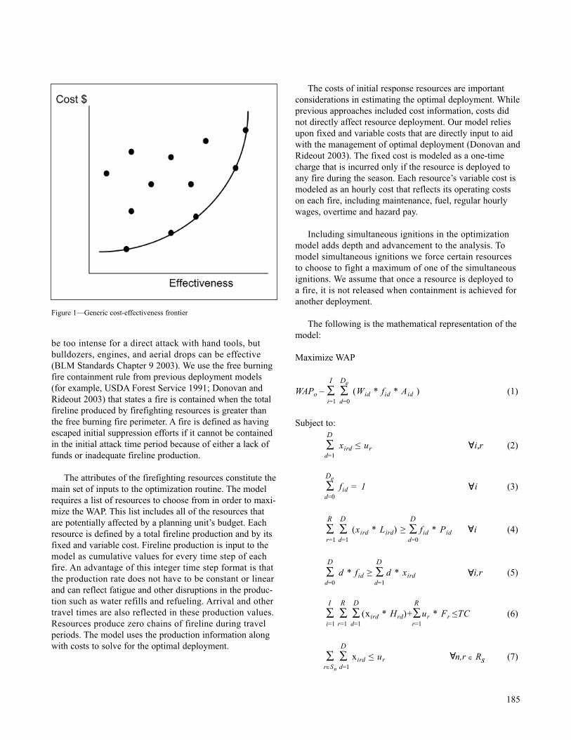
be too intense for a direct attack with hand tools, but bulldozers, engines, and aerial drops can be effective(BLM Standards Chapter 9 2003). We use the free burningfire containment rule from previous deployment models(for example, USDA Forest Service 1991; Donovan andRideout 2003) that states a fire is contained when the totalfireline produced by firefighting resources is greater thanthe free burning fire perimeter. A fire is defined as havingescaped initial suppression efforts if it cannot be containedin the initial attack time period because of either a lack offunds or inadequate fireline production.

The attributes of the firefighting resources constitute themain set of inputs to the optimization routine. The modelrequires a list of resources to choose from in order to maxi-mize the WAP. This list includes all of the resources thatare potentially affected by a planning unit’s budget. Eachresource is defined by a total fireline production and by itsfixed and variable cost. Fireline production is input to themodel as cumulative values for every time step of eachfire. An advantage of this integer time step format is thatthe production rate does not have to be constant or linearand can reflect fatigue and other disruptions in the produc-tion such as water refills and refueling. Arrival and othertravel times are also reflected in these production values.Resources produce zero chains of fireline during travelperiods. The model uses the production information alongwith costs to solve for the optimal deployment.

The costs of initial response resources are importantconsiderations in estimating the optimal deployment. Whileprevious approaches included cost information, costs didnot directly affect resource deployment. Our model reliesupon fixed and variable costs that are directly input to aidwith the management of optimal deployment (Donovan andRideout 2003). The fixed cost is modeled as a one-timecharge that is incurred only if the resource is deployed toany fire during the season. Each resource’s variable cost ismodeled as an hourly cost that reflects its operating costson each fire, including maintenance, fuel, regular hourlywages, overtime and hazard pay.

Including simultaneous ignitions in the optimizationmodel adds depth and advancement to the analysis. Tomodel simultaneous ignitions we force certain resources to choose to fight a maximum of one of the simultaneousignitions. We assume that once a resource is deployed to a fire, it is not released when containment is achieved foranother deployment.

The following is the mathematical representation of themodel:

Maximize WAP

I DeWAPo – ∑ ∑ (Wid * fid * Aid ) (1)

i=1 d=0

Subject to:D

∑ xird ≤ ur i,r (2)d=1

De∑ fid = 1 i (3)d=0

R D D

∑ ∑ (xird * Lird) ≥ ∑ fid * Pid i (4)r=1 d=1 d=0

D D

∑ d * fid ≥ ∑ d * xird i,r (5)d=0 d=1

I R D R

∑ ∑ ∑ (xird * Hrd)+∑ur * Fr ≤TC (6)i=1 r=1 d=1 r=1

D

∑ ∑ xird ≤ ur n,r ∈ Rs (7)r∈Sn d=1

185

Figure 1—Generic cost-effectiveness frontier

A

A

A

A

A

Decision Variables

xird = Binary(0,1) = 1 if resource (r) is used for (d) timeperiods on fire (i). = 0 if resource (r) is not used on fire(i) for (d) time periods.

fid = Binary (0,1) = 1 if fire (i) burns for (d) time periods.= 0 if fire (i) does not burn for (d)time periods.

ur = Binary(0,1) = 1 if resource (r) is deployed to anyfire for any duration.= 0 if resource (r) is never used.

ParametersI = set of all fires indexed by i.R = set of all firefighting resources indexed by r.D = resource deployment and contained fire duration

indexed by d.De = escaped fire duration. De is defined as D+1.Sn= (n)th set of simultaneous ignitions.

Sn I.Rs = set of firefighting resources that are restricted to fight

at most one of the fires that ignite simultaneously. Rs R.

Fr = fixed cost for resource (r).Hrd = total hourly cost accrued for resource (r) for (d) time

periods.Lird = total (cumulative) fireline produced by resource (r)

for (d) time periods during fire (i).Wid = relative weight for the area burned by fire (i) after

(d) time periods.Pid = total fire perimeter of the burned area for fire (i) after

(d) time periods. Aid = total area burned by fire (i) after (d) time periods.

Calculated from Pid.TC = total cost of initial attack input to the model.WAPo = total weighted area of the fire planning unit.

The objective function (1) maximizes effectivenessdefined as the weighted area protected for a given budget.Equation (2) limits a resource to at most one deploymentper fire. For example, a firefighting resource cannot bedeployed for two time periods and four time periods to the same fire. The equalities in (3) force each fire to haveexactly one burn duration. Equations (4) are the contain-ment constraints. For each contained fire, the total amountof fireline produced by all resources must be greater thanor equal to the fire’s burn perimeter. Equations (5) forceeach fire to burn at least as long as the longest duration of any resource deployed to that fire. For example, if on agiven fire there were two resources used, one for three timeperiods and the other for six time periods, the fire would

burn for six time periods. Inequality (6) is the budget con-straint. The total cost of all resources deployed to all fires,both hourly and fixed, must be less than or equal to thetotal cost denoted as TC. Equations (7) are used for firesthat are modeled as simultaneous ignitions. Fires in thesegroups compete for firefighting resources. We assume thata resource can only be deployed to one fire in each groupof simultaneous ignitions.

CONCLUSION

Our formulation provides an approach to performancebased initial attack planning that incorporates the tenets ofCEA in an optimization model. The performance measureof WAP shows how a non-monetized performance basedsystem could be applied while addressing key elements ofpreparedness planning. While this model expanded previ-ous work to optimize simultaneous ignitions, future effortscould continue to expand the scope of analysis. For exam-ple, one could change the deterministic model to incorpo-rate stochastic elements, such as a range of likely fireoccurrences. Other possible scope extensions could includelinear or piecewise linear approaches to reduce the solutiontimes.

LITERATURE CITED

Aneja, Y.P., and M. Parlar. 1984. Optimal staffing of a forest fire fighting organization. Can. J. For. Res. 14:589-594.

Boychuk, D., and D.L. Martell. 1988. A Markov chain model for evaluating seasonal forest fire fighter require-ments. For. Sci. 34(3): 647-661.

Bureau of Land Management. 2003. Interagency Standards for Fire and Aviation Operations. BLMHandbook 9213-1.

Cleaves, D.A. 1985. Net Value Changes in Fire Management:Issues and Application Problems. Fire management: thechallenge of protection and use: proceedings of a sym-posium. Logan, Utah.

Donovan, G.H., and D.B. Rideout. 2003. An integer programming model to optimize resource allocation forwildfire containment. For. Sci. 49(2): 331-335.

Kourtz, P.H., and W.G. O’Regan. 1968. A cost-effective-ness analysis of simulated forest fire detection systems.Hilgardia 39(12): 341-366.

186

⊃

⊃

Mees, R., and D. Strauss. 1992. Allocating resources to large wildland fires: a model with stochastic productionrates. For. Sci. 38(4): 842-853.

Nautiyal, J.C., and G.E. Doan. 1974. Economics of forest fire control: trading planned cut for protectionexpenditure. Can. J. For. Res. 4: 82-90.

Omi, P.N.; J.L. Murphy; L.C. Wensel. 1981. A linear programming model for wildland fuel managementplanning. For. Sci. 27(1): 81-94.

Osborne, D.E., and P. Plastrik. 2000. The reinventor’s fieldbook: Tools for transforming your government.Jossey-Bass, San Francisco.

Parks, G.M. 1964. Development and application of a model for suppression of forest fires. Man. Sci. 10(4):760-766.

Parlar, M. 1983. Optimal forest fire control with limited reinforcements. Opt. Cont. Appl. Meth. 4(2): 185-191.

Parlar, M., and R.G. Vickson. 1982. Optimal forest fire control: an extension of parks’ model. For. Sci. 28(2):345-355.

Pyne, S.J.; P.L. Andrews; R.D. Laven, 1996. Introduction to wildland fire. Wiley, New York. 769 p.

Robinson, R.; W. Hansen; K. Orth. 1995. Evaluation of Environmental Investments Procedures Manual. IWRReport 95-R-1. U.S. Army Corps of Engineers, Institutefor Water Resources. Alexandria, VA. 81 p.

Sparhawk, W.N. 1925. The use of liability ratings in planning forest fire protection. J. Ag. Res. 8: 693-762.

USDA Forest Service. 1991. National fire management analysis systems users’ guide of the initial action assess-ment. (FPL-IAA 2.3). USDA For. Serv., Washington,D.C.

187

This page is intentionally left blank.

In: Bevers, Michael; Barrett, Tara M., comps. 2005. Systems Analysis in Forest Resources: Proceedings of the 2003 Symposium. General Technical ReportPNW-GTR-656. Portland, OR: U.S. Department of Agriculture, Forest Service, Pacific Northwest Research Station.1 A.E. Wilson is a Resource Information Specialist and 2 M.R. Wiitala is an Operations Research Specialist at the Pacific Southwest Research Station, USDA Forest Service, 620 SW Main Street, Suite 400, Portland Oregon, 97205; e-mail: aewilson@fs.fed.us.

Systems Analysis in Forest Resources: Proceedings of the 2003 Symposium

AN EMPIRICALLY BASED MODELFOR ESTIMATING WILDFIRE

SUPPRESSION RESOURCE RESPONSE TIMES

Andrew E. Wilson1 and Marc R. Wiitala2

INTRODUCTION

Planning for wildfire suppression is one of many waysto help increase the efficiency of a forest fire-fightingorganization. Pre-suppression planning and analysis involvesassessing how many resources to use, where to locate them,and how they will be dispatched. While there are severalapproaches to planning a pre-suppression organization, mostaccount for and place great importance on the time it takesthe suppression forces to move from their location to a fireincident. Mees (1986) found response time to be one of themost influential factors in his study of suppression resourcebase locations.

In that same study, Mees also describes suppressionresource response time as having two major components:getaway time and travel time. For the initial response to afire, the getaway time is the time between a dispatcher’srequest for a resource to respond and the beginning oftransport to the fire. Travel time begins with the start oftransport and ends with arrival at the fire.

ABSTRACT

Suppression resource response times are an important component in planning models used to evaluate the effectivenessof wildfire preparedness organizations. Most fire planning models rely on subjective estimates of travel times between pre-determined points on the landscape. This paper describes a raster-based travel time model that provides greater accuracy,objectivity, and flexibility in estimating travel times between points on the landscape. The methodology used to create thetravel time prediction model integrates existing GIS data with empirical travel data collected using GPS. Although the needto develop this rose from development of WIRAS (Wildland Initial Response Assessment System), it will be useful to manywildland fire pre-suppression planning efforts where there is a relationship between the time it takes fire suppression resourcesto respond and the final size and resultant costs of suppression.

189

Different types of fire fighting resources travel differ-ently over the landscape. Travel time for aerial resources iseasily determined by assuming flights are made in straightlines between locations. Accounting for terrain, transporta-tion infrastructure, equipment capabilities, and other uncer-tainties complicates the computation of ground resourcetravel times.

The need for improved techniques for predicting traveltimes arose during the development of the Wildland InitialResponse Assessment System; also know as WIRAS (Wiitalaand others, this proceedings). WIRAS is a simulation sys-tem designed for use in planning and analyzing strategicpre-suppression decisions, such as quantities and locationsof fire fighting resources and deployment rules. To proper-ly assess the effectiveness of the system, the response timesfor aerial and ground resources are evaluated on an event-by-event basis as the scenario unfolds. WIRAS uses theseresponse times in two primary ways: first, to select thequickest arriving fire fighting resources from a pool of

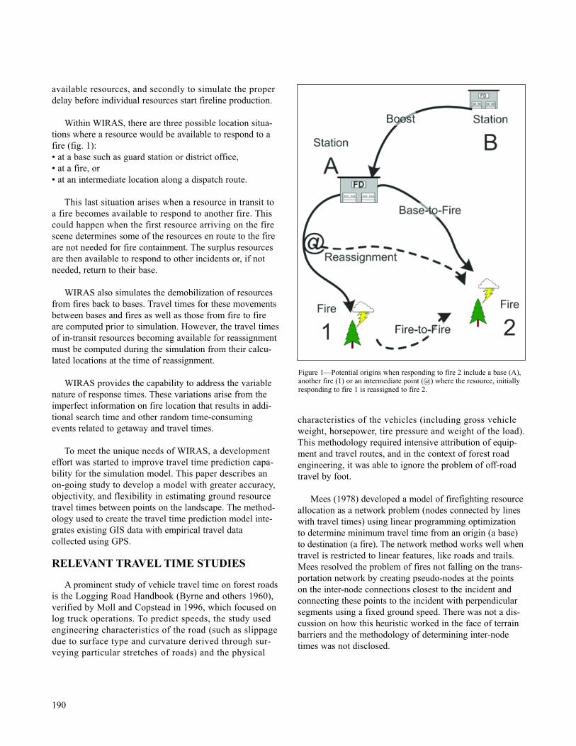
available resources, and secondly to simulate the properdelay before individual resources start fireline production.

Within WIRAS, there are three possible location situa-tions where a resource would be available to respond to afire (fig. 1): • at a base such as guard station or district office, • at a fire, or • at an intermediate location along a dispatch route.

This last situation arises when a resource in transit to a fire becomes available to respond to another fire. Thiscould happen when the first resource arriving on the firescene determines some of the resources en route to the fireare not needed for fire containment. The surplus resourcesare then available to respond to other incidents or, if notneeded, return to their base.

WIRAS also simulates the demobilization of resourcesfrom fires back to bases. Travel times for these movementsbetween bases and fires as well as those from fire to fireare computed prior to simulation. However, the travel timesof in-transit resources becoming available for reassignmentmust be computed during the simulation from their calcu-lated locations at the time of reassignment.

WIRAS provides the capability to address the variablenature of response times. These variations arise from theimperfect information on fire location that results in addi-tional search time and other random time-consumingevents related to getaway and travel times.

To meet the unique needs of WIRAS, a developmenteffort was started to improve travel time prediction capa-bility for the simulation model. This paper describes an on-going study to develop a model with greater accuracy,objectivity, and flexibility in estimating ground resourcetravel times between points on the landscape. The method-ology used to create the travel time prediction model inte-grates existing GIS data with empirical travel datacollected using GPS.

RELEVANT TRAVEL TIME STUDIES

A prominent study of vehicle travel time on forest roadsis the Logging Road Handbook (Byrne and others 1960),verified by Moll and Copstead in 1996, which focused onlog truck operations. To predict speeds, the study usedengineering characteristics of the road (such as slippagedue to surface type and curvature derived through sur-veying particular stretches of roads) and the physical

characteristics of the vehicles (including gross vehicleweight, horsepower, tire pressure and weight of the load).This methodology required intensive attribution of equip-ment and travel routes, and in the context of forest roadengineering, it was able to ignore the problem of off-roadtravel by foot.

Mees (1978) developed a model of firefighting resourceallocation as a network problem (nodes connected by lineswith travel times) using linear programming optimizationto determine minimum travel time from an origin (a base)to destination (a fire). The network method works well whentravel is restricted to linear features, like roads and trails.Mees resolved the problem of fires not falling on the trans-portation network by creating pseudo-nodes at the pointson the inter-node connections closest to the incident andconnecting these points to the incident with perpendicularsegments using a fixed ground speed. There was not a dis-cussion on how this heuristic worked in the face of terrainbarriers and the methodology of determining inter-nodetimes was not disclosed.

190

Figure 1—Potential origins when responding to fire 2 include a base (A),another fire (1) or an intermediate point (@) where the resource, initiallyresponding to fire 1 is reassigned to fire 2.

Travel speed by fire fighters on foot has been reportedin relation to escaping from fires (Dakin 2002; and Butlerand others 2000). While the former study focused on short(250 m) courses, the latter used historical records of firefighter travel rates at two well-documented incidents tomake estimates of sustainable travel rates over broad slopecategories. Howley and Franks (1992), in the context ofsports medicine, used human physiology to determinewalking speeds over varying slopes based on a fixed rate of energy output. A comparison in figure 2 of the physio-logical walking model derived from this work and the sus-tained travel rates that Butler and others found shows theresults are similar.

The intensive development of physical characteristicsrequired for the engineering approach to this problem sug-gested by the Logging Road Handbook did provide insightinto important factors in travel time, the time and costs ofimplementation were not compatible with the broad natureof fire pre-suppression planning across forest or landscapelevels. The simple approach suggested by the linear pro-gramming approach forwarded by Mees did not adequatelyaddress the problems of access across varied terrain wherethe shortest distance is not necessarily the quickest dis-tance.

STUDY AREA

The Umatilla National Forest was selected for the siteof the study. The forest occupies about 1.4 million acres inan area 110 miles by 130 miles in the Blue Mountains ofNortheast Oregon and Southwest Washington. It has fourdistricts, two in the steeper, wetter north half of the forestand two in the drier, more rolling south half. Outside wilder-ness and inventoried roadless areas, fires are moderatelyaccessible with 64 percent of the forest within 4 mile of anopen road, a distance within which fires can generally beattacked by an engine hose lay.

The Umatilla fire season has about 136 fires in a yearwith the majority of them spread across July, August andSeptember. The forest directly employs about 20 engineand hand crews. Cooperators and contractors provide addi-tional sources of dozers, tenders, engines and hand crews.A typical initial attack resource deployment at a districtincludes three engines and two or three hand crews. ThePendleton Interagency Communications Center, which dis-patches fire suppression resources for the Umatilla NationalForest and cooperatively protected lands, provided much ofinformation on initial attack resource assignment requiredby this study.

METHODOLOGY

The study’s methods consist of two parts: the develop-ment of a raster-based model to calculate travel times andan empirical analysis of travel times. To predict travel times,a raster-based rather than network approach was selected tomaximize computational speed and facilitate travel timecalculations anywhere across the landscape. This modeluses a travel resistance surface that incorporates both vehi-cle and foot travel. The travel time model incorporates aminimum cost path algorithm (Hatfield and others, thisproceedings), which can calculate in a few seconds theresponses of twenty or more resources spread across theforest to a single fire. Using the raster approach allows abetter representation of the walk-in portion of the responsetime that can be affected significantly by terrain.

A major component of the travel time study is theempirical collection and analysis of travel time data.Empirical travel times provide a basis for testing accuracyof the minimum cost-path algorithm time calculations andadjusting the model for identified systematic bias. Thedeterministic predictions of the raster-based travel timemodel are expected to be different from actual travel times.As noted earlier, these statistical differences arise fromvariable search times due to imperfect initial fire reportsand other delays experienced during an initial attackresponse. The empirical travel time data will be used to

191

Figure 2—A comparison of walking model estimates of a firefighter’s sus-tainable walking speed with sustainable walking speeds found in Butlerand others (2000).

quantify these underlying statistical processes for incorpo-ration into the travel time prediction mode for use inWIRAS.

To acquire the necessary data to develop the travel timesurface and support our verification and statistical analysis,we chose to collect empirical data on response speeds overthe fire season. Three different data sets were collected:position-velocity logging, dispatch records, and radio trans-mission position logs.

Position-velocity logging units were installed in engineand crew vehicles and kept a record of the vehicles veloci-ty based on time and position. The data (the time, the loca-tion of the vehicle and its speed) were determined withinthe unit with GPS and recorded at 15-second intervals aslong as the vehicle was moving, regardless of whether thevehicle was responding to an initial attack incident or not.The data was stored on removable storage media and man-ually downloaded periodically.

To determine the data points where the vehicle wasresponding to a dispatch, we gathered the dispatch recordinformation on resources ordered for each incident, includ-ing the unit identifier, when the dispatch order was sent andwhere the unit was, and when the unit arrived at the inci-dent or was reassigned/released. The unit identifier and thedispatch start and stop times were used as key fields to fil-ter the excess data from the logged velocity points. Byexamining the time series of logged position-velocity datapoints associated with each run, we could detect and quan-tify travel delays for resources responding to incidents. Themagnitude of a delay is measured by the difference inexpected response time and actual response time. Thisinformation is used to determine the nature of the vari-ability of these delays.

There is always the possibility of confusion over whichresources were involved in a dispatch and where they werelocated at the time of dispatch (especially in the reassign-ment case). We attempted to reduce the possibility of thisconfusion by augmenting the resource position informationin the dispatch record with a resource position data setbased on a radio-based real-time position tracking system.This position tracking system provided a GPS-derivedcoordinate/time pair for each radio transmission from thefire fighting resource that helped precisely determine unitinitial attack response start and stop times and positions.Since the position information was displayed in real-timein the coordination center, it improved dispatch knowledgeof resources and subsequent record keeping.

Once the velocity data was associated with initial attackincidents, the position information was used to determinethe attributes of the predictors. Based on forest engineeringstudies like Byrne and others (1960) and discussions withengineering staff, we selected a set of available and fairlycomplete data elements from the Forest Service database(INFRA) that stores travel route information linked to a GISroute system. While the INFRA database had relatively fineattribute detail, it was sparse beyond the boundaries of for-est Service administrative boundaries. We augmented theINFRA data these areas with information from the GTRNtransportation database (BLM 2002) developed by theBureau of Land Management. The other needed piece ofspatial information was the terrain database. We resampledthe 10-meter database from the national elevation dataset(USGS 2003) to 30-meter resolution, as we believed thatthis was the size of ground relevant to the movements atthe forest scale. The specific road attributes examinedincluded surface type (paved, gravel, improved native andnative), operational maintenance level (closed, high clear-ance, suitable for passenger cars, moderate degree of usercomfort and high degree of user comfort) and two derivedattributes, Grade and Alignment. Deriving these two attrib-utes required segmenting the linear road dataset to a finerresolution detail – rather than segments that connect inter-sections, the segments were split so that the maximumlength was 4-mile. This length was chosen to approximatethe average area of influence the attributes would have on a vehicle’s speed and, given the rate of sampling, to ensurethat pieces would not be missed in normal transit. To deriveGrade, the elevation difference between each segment’sendpoints was divided by the connecting road length seg-ment. The Alignment measure was determined by dividingthe straight-line distance between two points by the actualroad distance depicted in the data. This resulted in a contin-uous measure of alignment, where the straighter the roadwas, the closer to unity the alignment value would be.

The other portion of the trip to the fire involves walkingto the fire from where the vehicles are parked. Ideally,empirical data of the entire trip could be collected muchlike the velocity-position logging that was gathered onvehicles. Unfortunately, a cost-effective method to collectthis type of data has not been discovered. Instead, the phys-iological-based model introduced above was applied andwill be tested against the empirical data from the dispatchrecord and radio transmission logs. This model uses theassumption of constant energy expenditure based on energyrequirements for walking (Howley and Franks 1992). Thesum of vertical and horizontal net oxygen costs determinesthe change in speed as slope varies. This simplifies to aquadratic slope–speed relationship.

192

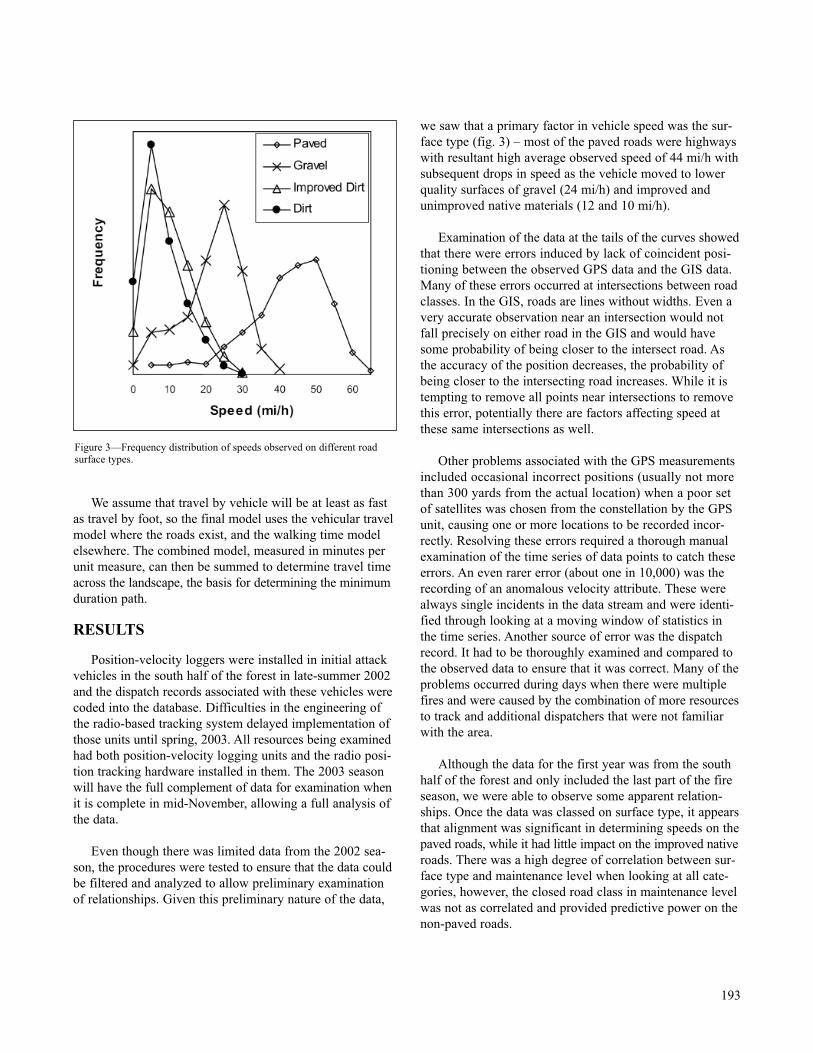
We assume that travel by vehicle will be at least as fastas travel by foot, so the final model uses the vehicular travelmodel where the roads exist, and the walking time modelelsewhere. The combined model, measured in minutes perunit measure, can then be summed to determine travel timeacross the landscape, the basis for determining the minimumduration path.

RESULTS

Position-velocity loggers were installed in initial attackvehicles in the south half of the forest in late-summer 2002and the dispatch records associated with these vehicles werecoded into the database. Difficulties in the engineering ofthe radio-based tracking system delayed implementation ofthose units until spring, 2003. All resources being examinedhad both position-velocity logging units and the radio posi-tion tracking hardware installed in them. The 2003 seasonwill have the full complement of data for examination whenit is complete in mid-November, allowing a full analysis ofthe data.

Even though there was limited data from the 2002 sea-son, the procedures were tested to ensure that the data couldbe filtered and analyzed to allow preliminary examinationof relationships. Given this preliminary nature of the data,

we saw that a primary factor in vehicle speed was the sur-face type (fig. 3) – most of the paved roads were highwayswith resultant high average observed speed of 44 mi/h withsubsequent drops in speed as the vehicle moved to lowerquality surfaces of gravel (24 mi/h) and improved andunimproved native materials (12 and 10 mi/h).

Examination of the data at the tails of the curves showedthat there were errors induced by lack of coincident posi-tioning between the observed GPS data and the GIS data.Many of these errors occurred at intersections between roadclasses. In the GIS, roads are lines without widths. Even avery accurate observation near an intersection would notfall precisely on either road in the GIS and would havesome probability of being closer to the intersect road. Asthe accuracy of the position decreases, the probability ofbeing closer to the intersecting road increases. While it istempting to remove all points near intersections to removethis error, potentially there are factors affecting speed atthese same intersections as well.

Other problems associated with the GPS measurementsincluded occasional incorrect positions (usually not morethan 300 yards from the actual location) when a poor set of satellites was chosen from the constellation by the GPSunit, causing one or more locations to be recorded incor-rectly. Resolving these errors required a thorough manualexamination of the time series of data points to catch theseerrors. An even rarer error (about one in 10,000) was therecording of an anomalous velocity attribute. These werealways single incidents in the data stream and were identi-fied through looking at a moving window of statistics inthe time series. Another source of error was the dispatchrecord. It had to be thoroughly examined and compared tothe observed data to ensure that it was correct. Many of theproblems occurred during days when there were multiplefires and were caused by the combination of more resourcesto track and additional dispatchers that were not familiarwith the area.

Although the data for the first year was from the southhalf of the forest and only included the last part of the fireseason, we were able to observe some apparent relation-ships. Once the data was classed on surface type, it appearsthat alignment was significant in determining speeds on thepaved roads, while it had little impact on the improved nativeroads. There was a high degree of correlation between sur-face type and maintenance level when looking at all cate-gories, however, the closed road class in maintenance levelwas not as correlated and provided predictive power on thenon-paved roads.

193

Figure 3—Frequency distribution of speeds observed on different roadsurface types.

It should be noted that using the raster approach asdescribed above might not be an appropriate tool for real-time routing of emergency response services. Individualroutes determined optimal with the model may, in reality,be infeasible or may have longer durations than the modelspecifies. As well, complex traffic controls, such as one-way roads and restricted intersections are more difficult toaddress. However, the model works well within this strate-gic planning realm of wildfire suppression.

CONCLUSION

This paper describes development of a model to esti-mate the response time of initial attack resources for use instrategic planning. It discusses data collected and used indeveloping the model. Problems with the GPS-derived dataare pointed out and methods to remove errors are posited.Finally, preliminary results are presented and indicate thatthis will be an effective improvement in the determinationof response times in analysis of wildland fire pre-suppres-sion planning.

LITERATURE CITED

Bureau of Land Management, Oregon State Office. 2002. BLM ground transportation (roads & trails).Retrieved April 2, 2002 from http://www.or.blm.gov/gis/data/catalog/dataset.asp?cid=39

Butler, B.W.; Cohen, J.D.; Putnam, T.; Bartlette, R.A.; Bradshaw, L.S. 2000. A method for evaluating theeffectiveness of firefighter escape routes. Pages 42-45in Butler, B.W. and K. Shannon (eds.) Proceedings fromthe International Wildfire Safety Summit (Oct 10-12,2000, Edmonton, Alberta). Int. Assoc. Wildland Fire,Montana City, Mont.

Byrne, J.; Nelson, R.; Googins, P. 1960. Logging road handbook: the effect of road design on hauling costs.Agriculture Handbook No. 183. U.S. Department ofAgriculture, Forest Service.

Dakin, G. 2002. Ground rates of travel by fire crews using escape routes: an interim report. Advantage 3(15).Forest Engineering Research Institute of Canada.

Howley, E.T.; Franks, B.D. 1992. Energy costs of activity. In Health fitness: instructor’s handbook. 2nd edition.Human Kinetics, Champaign, Illinois, pp. 131-139.

Mees, R.M. 1978. Computing arrival times of firefighting resources for initial attack. Gen. Tech. Rep. PSW-27.U.S. Department of Agriculture, Forest Service, PacificSouthwest Forest and Range Experiment Station.

Mees, R.M. 1986. Locating suppression resources by travel time to wildfires. Res. Note PSW-387. U.S.Department of Agriculture, Forest Service, PacificSouthwest Forest and Range Experiment Station.

Moll, J.; Copstead, R. 1996. Travel time models for forest roads: a verification of the Forest Service logging road handbook. Pub. 677 1202 – STDC. U.S. Department of Agriculture, Forest Service, San Dimas Technology Development Center. SanDimas, California.

U.S. Geological Survey, EROS Data Center. 2003.National elevation dataset. Retrieved February 2003from http://gisdata.usgs.net/ned/default.asp.

194

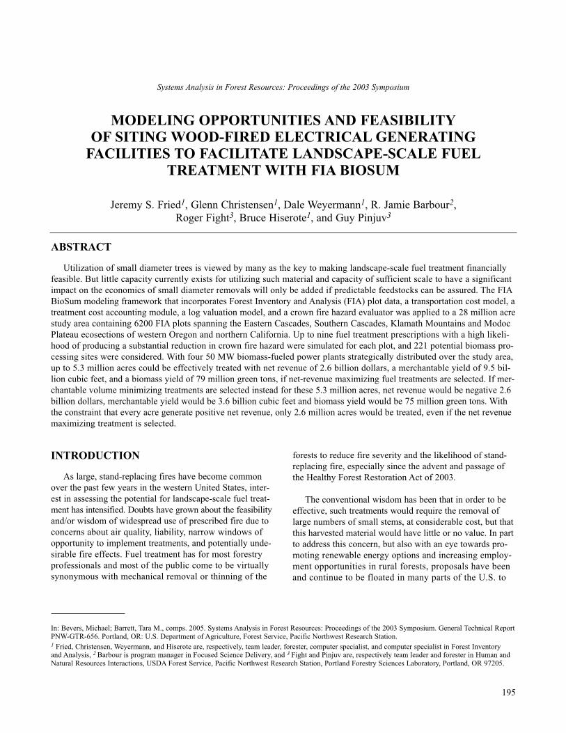
In: Bevers, Michael; Barrett, Tara M., comps. 2005. Systems Analysis in Forest Resources: Proceedings of the 2003 Symposium. General Technical ReportPNW-GTR-656. Portland, OR: U.S. Department of Agriculture, Forest Service, Pacific Northwest Research Station.1 Fried, Christensen, Weyermann, and Hiserote are, respectively, team leader, forester, computer specialist, and computer specialist in Forest Inventoryand Analysis, 2 Barbour is program manager in Focused Science Delivery, and 3 Fight and Pinjuv are, respectively team leader and forester in Human andNatural Resources Interactions, USDA Forest Service, Pacific Northwest Research Station, Portland Forestry Sciences Laboratory, Portland, OR 97205.

Systems Analysis in Forest Resources: Proceedings of the 2003 Symposium

MODELING OPPORTUNITIES AND FEASIBILITYOF SITING WOOD-FIRED ELECTRICAL GENERATING

FACILITIES TO FACILITATE LANDSCAPE-SCALE FUELTREATMENT WITH FIA BIOSUM

Jeremy S. Fried1, Glenn Christensen1, Dale Weyermann1, R. Jamie Barbour2,Roger Fight3, Bruce Hiserote1, and Guy Pinjuv3

INTRODUCTION

As large, stand-replacing fires have become commonover the past few years in the western United States, inter-est in assessing the potential for landscape-scale fuel treat-ment has intensified. Doubts have grown about the feasibilityand/or wisdom of widespread use of prescribed fire due toconcerns about air quality, liability, narrow windows ofopportunity to implement treatments, and potentially unde-sirable fire effects. Fuel treatment has for most forestryprofessionals and most of the public come to be virtuallysynonymous with mechanical removal or thinning of the

ABSTRACT

Utilization of small diameter trees is viewed by many as the key to making landscape-scale fuel treatment financiallyfeasible. But little capacity currently exists for utilizing such material and capacity of sufficient scale to have a significantimpact on the economics of small diameter removals will only be added if predictable feedstocks can be assured. The FIABioSum modeling framework that incorporates Forest Inventory and Analysis (FIA) plot data, a transportation cost model, atreatment cost accounting module, a log valuation model, and a crown fire hazard evaluator was applied to a 28 million acrestudy area containing 6200 FIA plots spanning the Eastern Cascades, Southern Cascades, Klamath Mountains and ModocPlateau ecosections of western Oregon and northern California. Up to nine fuel treatment prescriptions with a high likeli-hood of producing a substantial reduction in crown fire hazard were simulated for each plot, and 221 potential biomass pro-cessing sites were considered. With four 50 MW biomass-fueled power plants strategically distributed over the study area,up to 5.3 million acres could be effectively treated with net revenue of 2.6 billion dollars, a merchantable yield of 9.5 bil-lion cubic feet, and a biomass yield of 79 million green tons, if net-revenue maximizing fuel treatments are selected. If mer-chantable volume minimizing treatments are selected instead for these 5.3 million acres, net revenue would be negative 2.6billion dollars, merchantable yield would be 3.6 billion cubic feet and biomass yield would be 75 million green tons. Withthe constraint that every acre generate positive net revenue, only 2.6 million acres would be treated, even if the net revenuemaximizing treatment is selected.

195

forests to reduce fire severity and the likelihood of stand-replacing fire, especially since the advent and passage ofthe Healthy Forest Restoration Act of 2003.

The conventional wisdom has been that in order to beeffective, such treatments would require the removal oflarge numbers of small stems, at considerable cost, but thatthis harvested material would have little or no value. In partto address this concern, but also with an eye towards pro-moting renewable energy options and increasing employ-ment opportunities in rural forests, proposals have beenand continue to be floated in many parts of the U.S. to

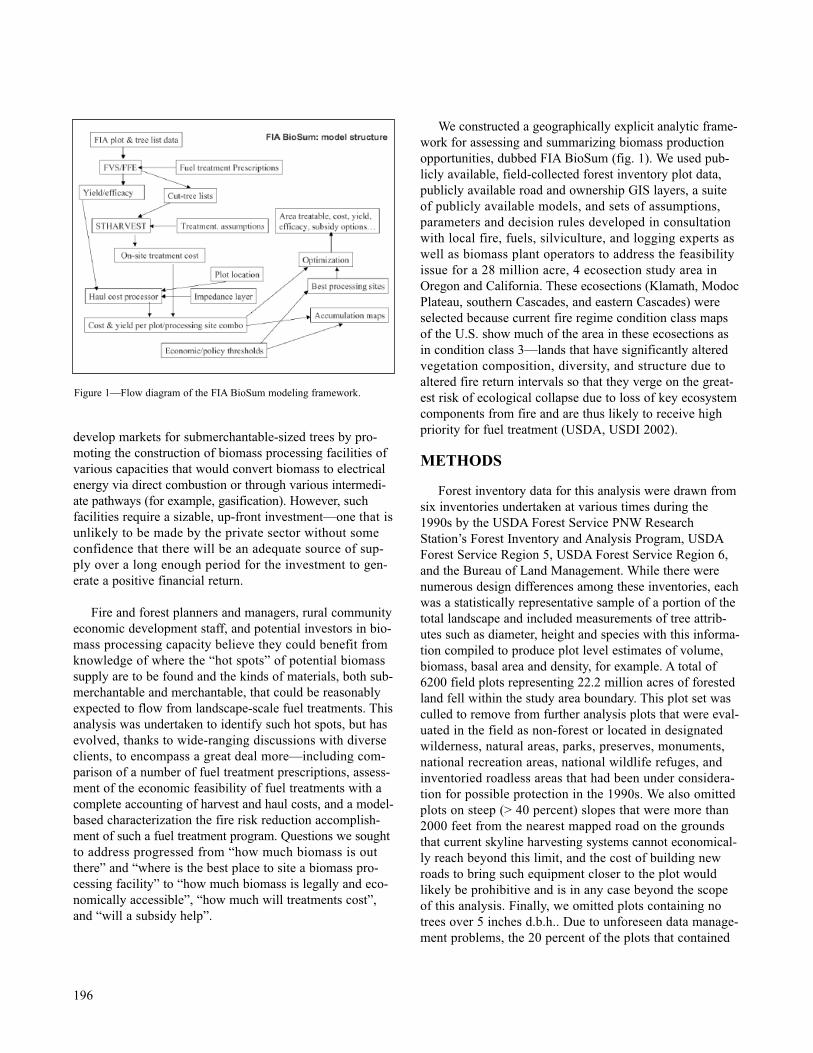
develop markets for submerchantable-sized trees by pro-moting the construction of biomass processing facilities ofvarious capacities that would convert biomass to electricalenergy via direct combustion or through various intermedi-ate pathways (for example, gasification). However, suchfacilities require a sizable, up-front investment—one that isunlikely to be made by the private sector without someconfidence that there will be an adequate source of sup-ply over a long enough period for the investment to gen-erate a positive financial return.

Fire and forest planners and managers, rural communityeconomic development staff, and potential investors in bio-mass processing capacity believe they could benefit fromknowledge of where the “hot spots” of potential biomasssupply are to be found and the kinds of materials, both sub-merchantable and merchantable, that could be reasonablyexpected to flow from landscape-scale fuel treatments. Thisanalysis was undertaken to identify such hot spots, but hasevolved, thanks to wide-ranging discussions with diverseclients, to encompass a great deal more—including com-parison of a number of fuel treatment prescriptions, assess-ment of the economic feasibility of fuel treatments with acomplete accounting of harvest and haul costs, and a model-based characterization the fire risk reduction accomplish-ment of such a fuel treatment program. Questions we soughtto address progressed from “how much biomass is outthere” and “where is the best place to site a biomass pro-cessing facility” to “how much biomass is legally and eco-nomically accessible”, “how much will treatments cost”,and “will a subsidy help”.

We constructed a geographically explicit analytic frame-work for assessing and summarizing biomass productionopportunities, dubbed FIA BioSum (fig. 1). We used pub-licly available, field-collected forest inventory plot data,publicly available road and ownership GIS layers, a suiteof publicly available models, and sets of assumptions,parameters and decision rules developed in consultationwith local fire, fuels, silviculture, and logging experts aswell as biomass plant operators to address the feasibilityissue for a 28 million acre, 4 ecosection study area inOregon and California. These ecosections (Klamath, ModocPlateau, southern Cascades, and eastern Cascades) wereselected because current fire regime condition class mapsof the U.S. show much of the area in these ecosections asin condition class 3—lands that have significantly alteredvegetation composition, diversity, and structure due toaltered fire return intervals so that they verge on the great-est risk of ecological collapse due to loss of key ecosystemcomponents from fire and are thus likely to receive highpriority for fuel treatment (USDA, USDI 2002).

METHODS

Forest inventory data for this analysis were drawn fromsix inventories undertaken at various times during the1990s by the USDA Forest Service PNW ResearchStation’s Forest Inventory and Analysis Program, USDAForest Service Region 5, USDA Forest Service Region 6,and the Bureau of Land Management. While there werenumerous design differences among these inventories, eachwas a statistically representative sample of a portion of thetotal landscape and included measurements of tree attrib-utes such as diameter, height and species with this informa-tion compiled to produce plot level estimates of volume,biomass, basal area and density, for example. A total of6200 field plots representing 22.2 million acres of forestedland fell within the study area boundary. This plot set wasculled to remove from further analysis plots that were eval-uated in the field as non-forest or located in designatedwilderness, natural areas, parks, preserves, monuments,national recreation areas, national wildlife refuges, andinventoried roadless areas that had been under considera-tion for possible protection in the 1990s. We also omittedplots on steep (> 40 percent) slopes that were more than2000 feet from the nearest mapped road on the groundsthat current skyline harvesting systems cannot economical-ly reach beyond this limit, and the cost of building newroads to bring such equipment closer to the plot wouldlikely be prohibitive and is in any case beyond the scope of this analysis. Finally, we omitted plots containing notrees over 5 inches d.b.h.. Due to unforeseen data manage-ment problems, the 20 percent of the plots that contained

196

Figure 1—Flow diagram of the FIA BioSum modeling framework.

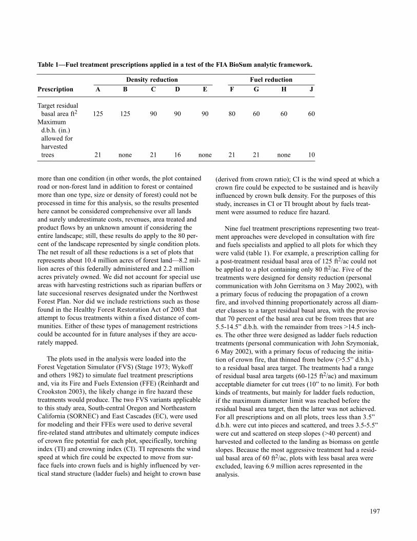
more than one condition (in other words, the plot containedroad or non-forest land in addition to forest or containedmore than one type, size or density of forest) could not beprocessed in time for this analysis, so the results presentedhere cannot be considered comprehensive over all landsand surely underestimate costs, revenues, area treated andproduct flows by an unknown amount if considering theentire landscape; still, these results do apply to the 80 per-cent of the landscape represented by single condition plots.The net result of all these reductions is a set of plots thatrepresents about 10.4 million acres of forest land—8.2 mil-lion acres of this federally administered and 2.2 millionacres privately owned. We did not account for special useareas with harvesting restrictions such as riparian buffers orlate succesional reserves designated under the NorthwestForest Plan. Nor did we include restrictions such as thosefound in the Healthy Forest Restoration Act of 2003 thatattempt to focus treatments within a fixed distance of com-munities. Either of these types of management restrictionscould be accounted for in future analyses if they are accu-rately mapped.

The plots used in the analysis were loaded into theForest Vegetation Simulator (FVS) (Stage 1973; Wykoffand others 1982) to simulate fuel treatment prescriptionsand, via its Fire and Fuels Extension (FFE) (Reinhardt andCrookston 2003), the likely change in fire hazard thesetreatments would produce. The two FVS variants applicableto this study area, South-central Oregon and NortheasternCalifornia (SORNEC) and East Cascades (EC), were usedfor modeling and their FFEs were used to derive severalfire-related stand attributes and ultimately compute indicesof crown fire potential for each plot, specifically, torchingindex (TI) and crowning index (CI). TI represents the windspeed at which fire could be expected to move from sur-face fuels into crown fuels and is highly influenced by ver-tical stand structure (ladder fuels) and height to crown base

(derived from crown ratio); CI is the wind speed at which acrown fire could be expected to be sustained and is heavilyinfluenced by crown bulk density. For the purposes of thisstudy, increases in CI or TI brought about by fuels treat-ment were assumed to reduce fire hazard.

Nine fuel treatment prescriptions representing two treat-ment approaches were developed in consultation with fireand fuels specialists and applied to all plots for which theywere valid (table 1). For example, a prescription calling fora post-treatment residual basal area of 125 ft2/ac could notbe applied to a plot containing only 80 ft2/ac. Five of thetreatments were designed for density reduction (personalcommunication with John Gerritsma on 3 May 2002), witha primary focus of reducing the propagation of a crownfire, and involved thinning proportionately across all diam-eter classes to a target residual basal area, with the provisothat 70 percent of the basal area cut be from trees that are5.5-14.5” d.b.h. with the remainder from trees >14.5 inch-es. The other three were designed as ladder fuels reductiontreatments (personal communication with John Szymoniak,6 May 2002), with a primary focus of reducing the initia-tion of crown fire, that thinned from below (>5.5” d.b.h.)to a residual basal area target. The treatments had a rangeof residual basal area targets (60-125 ft2/ac) and maximumacceptable diameter for cut trees (10” to no limit). For bothkinds of treatments, but mainly for ladder fuels reduction,if the maximum diameter limit was reached before theresidual basal area target, then the latter was not achieved.For all prescriptions and on all plots, trees less than 3.5”d.b.h. were cut into pieces and scattered, and trees 3.5-5.5”were cut and scattered on steep slopes (>40 percent) andharvested and collected to the landing as biomass on gentleslopes. Because the most aggressive treatment had a resid-ual basal area of 60 ft2/ac, plots with less basal area wereexcluded, leaving 6.9 million acres represented in theanalysis.

197

Table 1—Fuel treatment prescriptions applied in a test of the FIA BioSum analytic framework.

Density reduction Fuel reductionPrescription A B C D E F G H J

Target residual basal area ft2 125 125 90 90 90 80 60 60 60

Maximum d.b.h. (in.)allowed for harvestedtrees 21 none 21 16 none 21 21 none 10

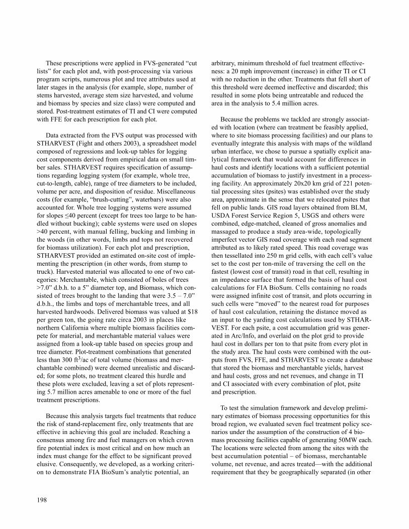
These prescriptions were applied in FVS-generated “cutlists” for each plot and, with post-processing via variousprogram scripts, numerous plot and tree attributes used atlater stages in the analysis (for example, slope, number ofstems harvested, average stem size harvested, and volumeand biomass by species and size class) were computed andstored. Post-treatment estimates of TI and CI were computedwith FFE for each prescription for each plot.

Data extracted from the FVS output was processed withSTHARVEST (Fight and others 2003), a spreadsheet modelcomposed of regressions and look-up tables for loggingcost components derived from empirical data on small tim-ber sales. STHARVEST requires specification of assump-tions regarding logging system (for example, whole tree,cut-to-length, cable), range of tree diameters to be included,volume per acre, and disposition of residue. Miscellaneouscosts (for example, “brush-cutting”, waterbars) were alsoaccounted for. Whole tree logging systems were assumedfor slopes ≤40 percent (except for trees too large to be han-dled without bucking); cable systems were used on slopes>40 percent, with manual felling, bucking and limbing inthe woods (in other words, limbs and tops not recoveredfor biomass utilization). For each plot and prescription,STHARVEST provided an estimated on-site cost of imple-menting the prescription (in other words, from stump totruck). Harvested material was allocated to one of two cat-egories: Merchantable, which consisted of boles of trees>7.0” d.b.h. to a 5” diameter top, and Biomass, which con-sisted of trees brought to the landing that were 3.5 – 7.0”d.b.h., the limbs and tops of merchantable trees, and allharvested hardwoods. Delivered biomass was valued at $18per green ton, the going rate circa 2003 in places likenorthern California where multiple biomass facilities com-pete for material, and merchantable material values wereassigned from a look-up table based on species group andtree diameter. Plot-treatment combinations that generatedless than 300 ft3/ac of total volume (biomass and mer-chantable combined) were deemed unrealistic and discard-ed; for some plots, no treatment cleared this hurdle andthese plots were excluded, leaving a set of plots represent-ing 5.7 million acres amenable to one or more of the fueltreatment prescriptions.

Because this analysis targets fuel treatments that reducethe risk of stand-replacement fire, only treatments that areeffective in achieving this goal are included. Reaching aconsensus among fire and fuel managers on which crownfire potential index is most critical and on how much anindex must change for the effect to be significant provedelusive. Consequently, we developed, as a working criteri-on to demonstrate FIA BioSum’s analytic potential, an

arbitrary, minimum threshold of fuel treatment effective-ness: a 20 mph improvement (increase) in either TI or CIwith no reduction in the other. Treatments that fell short ofthis threshold were deemed ineffective and discarded; thisresulted in some plots being untreatable and reduced thearea in the analysis to 5.4 million acres.

Because the problems we tackled are strongly associat-ed with location (where can treatment be feasibly applied,where to site biomass processing facilities) and our plans toeventually integrate this analysis with maps of the wildlandurban interface, we chose to pursue a spatially explicit ana-lytical framework that would account for differences inhaul costs and identify locations with a sufficient potentialaccumulation of biomass to justify investment in a process-ing facility. An approximately 20x20 km grid of 221 poten-tial processing sites (psites) was established over the studyarea, approximate in the sense that we relocated psites thatfell on public lands. GIS road layers obtained from BLM,USDA Forest Service Region 5, USGS and others werecombined, edge-matched, cleaned of gross anomalies andmassaged to produce a study area-wide, topologicallyimperfect vector GIS road coverage with each road segmentattributed as to likely rated speed. This road coverage wasthen tessellated into 250 m grid cells, with each cell’s valueset to the cost per ton-mile of traversing the cell on thefastest (lowest cost of transit) road in that cell, resulting inan impedance surface that formed the basis of haul costcalculations for FIA BioSum. Cells containing no roadswere assigned infinite cost of transit, and plots occurring insuch cells were “moved” to the nearest road for purposesof haul cost calculation, retaining the distance moved as an input to the yarding cost calculations used by STHAR-VEST. For each psite, a cost accumulation grid was gener-ated in Arc/Info, and overlaid on the plot grid to providehaul cost in dollars per ton to that psite from every plot inthe study area. The haul costs were combined with the out-puts from FVS, FFE, and STHARVEST to create a databasethat stored the biomass and merchantable yields, harvestand haul costs, gross and net revenues, and change in TIand CI associated with every combination of plot, psite and prescription.

To test the simulation framework and develop prelimi-nary estimates of biomass processing opportunities for thisbroad region, we evaluated seven fuel treatment policy sce-narios under the assumption of the construction of 4 bio-mass processing facilities capable of generating 50MW each.The locations were selected from among the sites with thebest accumulation potential – of biomass, merchantablevolume, net revenue, and acres treated—with the additionalrequirement that they be geographically separated (in other

198

words, one per ecosection) so as to have little influence onone anothers’ markets. Each of the 1556 plots (representingthe 5.4 million acres that could be treated effectively) wasallocated to the psite with the lowest haul cost: Grants PassOR, Burney CA, Klamath Falls OR, or Bend OR, and therest of the analysis proceeds with those allocations (fig. 2).Four of the treatment scenarios were: treat all treatable plotsand select the prescription for each plot that 1) maximizesnet revenue, or 2) maximizes improvement in TI, or 3)minimizes the merchantable material removed, or 4) maxi-mizes improvement in CI. The other three scenarios 1A,2A and 3A, corresponded to scenarios 1, 2 and 3, exceptthat only plots with non-negative net revenue would betreated. Scenario 1 was designed to make as much profit aspossible subject to the non-trivial constraint that all treat-ments were designed with an eye towards reducing crownfire potential, not maximizing economic return or even

facilitating a positive cash flow. Scenarios 2 and 4 representa no-holds-barred policy of reducing fire hazard as theparamount objective, while scenario 3 might be moreappealing to groups or individuals who favor the achieve-ment of some measure of fuel reduction but do not supportthe removal of sawtimber-sized trees and or the generationof profits from fuel treatment activity.

RESULTS

The fuel treatment policy scenarios 1-3 lead to quitedifferent distributions of treatments. The most frequentlyselected treatments for scenario 1 were H, G, and J, forscenario 2 were G, H, and F, and for scenario 3 were J, Gand F (fig. 3). Given the substantial differences in the treat-ments selected, we expected to see substantial differencesin the aggregate results; however, the most substantial dif-ferences among scenarios were in net revenue, while thebiomass yield was rather robust under this range of scenar-ios (table 2). Under scenario 1, net revenue was positivefor every psite when all effectively treatable plots weretreated. Even when selecting prescriptions that minimizemerchantable yield (scenario 3), there would still be 3.6billion ft3 of merchantable volume produced, though theaggregate net revenue under this scenario is extremely neg-ative. Under every scenario, the acres feeding material tothe psite at Grants Pass generated the greatest merchantablevolume and the greatest biomass.

With the added constraint that, as proposed in theHealthy Forests Initiative, “every acre pays its own way”,the area that could be treated would be reduced to no morethan 12 percent of the forested landscape (table 3) in sce-narios 1A, 2A and 3A. Of the four sites, Grants Pass againresults in the greatest amount of net revenue, acres treated,

199

Figure 2—The Oregon-California study area with ecosections, accessibleplots and the four potential processing sites considered in this analysis.

Figure 3—Number of acres for which each fuel treatment prescriptionwas selected; numbers below prescription letters are target residual basalarea in ft2/upper diameter limit in inches.

biomass yield, and merchantable yield under scenario 1A.Scenario 3A treats about the same area as scenarios 1A and2A, but produces less than half the net revenue, largelybecause there is much less revenue from merchantable volume in the prescriptions selected for this scenario thatcould be used to offset treatment costs.

All scenarios produced quite different opportunities interms of the potential longevity of a biomass plant (table4). Under scenario 2, sufficient biomass could be collectedto operate 50 MW generating stations at Grants Pass andBurney for about 50 years, and in all likelihood, much

longer given that this was a static analysis (that did notaccount for regeneration and continued growth of the resid-ual trees and involved no harvest scheduling component),and preliminary analysis of post-treatment plots modeledforward with FVS indicates a need to re-treat as soon as 20years after the initial treatment for fire hazard reduction tobe maintained. Requiring every acre to pay its own waydramatically cuts the projected longevity of biomass sup-ply, and scenario 3A (minimum merchantable yield andnonnegative net revenue) would appear to all but eliminatethe opportunity to attract capital investment for the con-struction of new biomass generating capacity except atGrants Pass.

200

Table 2—Aggregate net revenue, area treated, and yields of merchantable volume and sub-merchantable biomass by potential processing site for three, fuel treatment policy scenarios in which all effectively treatable plots are treated.

Scenario 1: Net Acres MerchantableMaximize net revenue revenue treated volume Biomass

(Millions of (Millions (MillionsProcessing site dollars) (Thousands) of cubic feet) of tons)

Burney 542 1,546 2,635 24Klamath Falls 593 1,101 1,741 14Bend 343 741 998 12Grants Pass 1,162 1,962 4,153 30

Total 2,640 5,351 9,527 79

Scenario 2:Maximize torching index Net Acres Merchantableimprovement revenue treated volume Biomass

(Millions of (Millions (MillionsProcessing site dollars) (Thousands) of cubic feet) of tons)

Burney -12 1,546 2,256 30Klamath Falls 415 1,101 1,602 15Bend 144 741 822 11Grants Pass 376 1,962 3,940 37

Total 923 5,351 8,620 94

Scenario 3:Minimize merchantable Net Acres Merchantableyield revenue treated volume Biomass

(Millions of (Millions (MillionsProcessing site dollars) (Thousands) of cubic feet) of tons)

Burney -795 1,546 974 21Klamath Falls -157 1,101 773 12Bend -148 741 384 9Grants Pass -1,465 1,962 1,444 34

Total -2,565 5,351 3,574 75

Not surprisingly, average effectiveness of fuel treatmentsin terms of both TI and CI was usually greatest under sce-nario 2, as shown in figure 4 for CI. What was surprisingwas that the average improvement in both indices wascomparable between with scenario 1, in which the fueltreatment with the greatest net revenue was selected.Scenario 3 was substantially less effective on the plotsfeeding every psite, with an average CI improvement of 20to 40 mph, most likely because prescriptions that removeless merchantable material also leave stands with highercanopy bulk-density.

Table 5 summarizes the aggregate results for scenarios1, 2 and 3 plus scenario 4 (maximize improvement incrowning index). Scenario 4 has greater yields of both biomass and merchantable material, most likely because it favors treatments that reduce canopy bulk density (byremoving more of the medium-sized trees greater than 7”d.b.h. and generally less than 21” d.b.h.). It is the addition-al merchantable component that accounts for the boost innet revenue as compared with scenario 2. The pre-treat-ment TI and CI averaged 7 and 23, respectively, so onaverage, all of the scenarios lead to substantial improve-ments in these indices.

201

Table 3—Aggregate net revenue, area treated, and yields of merchantable volume and sub-merchantable biomass by potential processing site for three, alternate fuel treatment policyscenarios in which only the effectively treatable plots that generate positive net revenue aretreated.

Scenario 1A: NR+ Net Acres MerchantableMaximize net revenue revenue treated volume Biomass

(Millions of (Millions (MillionsProcessing site dollars) (Thousands) of cubic feet) of tons)

Burney 1,112 735 2,017 11Klamath Falls 891 524 1,482 7Bend 536 335 833 8Grants Pass 2,382 1,023 3,478 16

Total 4,921 2,616 7,809 42

Scenario 2A:Maximize torching index Net Acres Merchantablechange, NR+ revenue treated volume Biomass

(Millions of (Millions (MillionsProcessing site dollars) (Thousands) of cubic feet) of tons)

Burney 944 711 1,873 12Klamath Falls 798 516 1,407 7Bend 486 329 780 8Grants Pass 2,184 1,014 3,295 17

Total 4,413 2,569 7,355 44

Scenario 3A:Minimize merchantable Net Acres Merchantableyield revenue treated volume Biomass

(Millions of (Millions (MillionsProcessing site dollars) (Thousands) of cubic feet) of tons)

Burney 442 735 1,320 12Klamath Falls 357 524 898 7Bend 238 335 539 8Grants Pass 942 1,023 2,182 21

Total 1,978 2,616 4,939 47

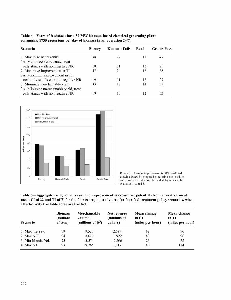
202

Table 4—Years of feedstock for a 50 MW biomass-based electrical generating plant consuming 1750 green tons per day of biomass in an operation 24/7.

Scenario Burney Klamath Falls Bend Grants Pass

1. Maximize net revenue 38 22 18 471A. Maximize net revenue, treat

only stands with nonnegative NR 18 11 12 252. Maximize improvement in TI 47 24 18 582A. Maximize improvement in TI,

treat only stands with nonnegative NR 19 11 12 273. Minimize merchantable yield 33 18 14 533A. Minimize merchantable yield, treat

only stands with nonnegative NR 19 10 12 33

Table 5—Aggregate yield, net revenue, and improvement in crown fire potential (from a pre-treatment mean CI of 22 and TI of 7) for the four ecoregion study area for four fuel treatment policy scenarios, when all effectively treatable acres are treated.

Biomass Merchantable Net revenue Mean change Mean change (millions volume (millions of in CI in TI

Scenario of tons) (millions of ft3) dollars) (miles per hour) (miles per hour)

1. Max. net rev. 79 9,527 2,639 63 962. Max ∆ TI 94 8,620 922 83 983. Min Merch. Vol. 75 3,574 -2,566 23 354. Max ∆ CI 93 9,765 1,817 80 114

Figure 4—Average improvement in FFE-predictedcrowing index, by proposed processing site to whichrecovered material would be hauled, by scenario forscenarios 1, 2 and 3.

DISCUSSION

There is plenty of biomass to supply four 50 MW powerplants for decades under the most aggressive scenarios (forexample, scenario 2), but supply under the most conserva-tive scenarios (for example, 3A) would be far more limited.Another alternative that we have not yet analyzed would beto operate several smaller or less heavily capitalized powerplants for a shorter period of time in order to reduce haulcosts and make treatment feasible over a greater area.

By any basis of calculation, most of the material removedin these treatments is merchantable and would fetch higherprices than the $18 per green ton currently paid for bio-mass-sized material by power plant operators in northernCalifornia. For scenario 1, 75 percent of the total tonnageof wood removed is merchantable, with the remaining 25percent in biomass-sized material composed of trees lessthan 7 inches and the tops and limbs of larger trees. And ofthe biomass-sized material, only 20 percent is in trees lessthan 7 inches (i.e., only 5 percent of the total wood tonnageremoved). On a value basis, merchantable wood recoveredaccounts for 90 percent of the total value recovered. Thishelps explain why prescriptions that do not maximize netrevenue or that reduce the quantity of merchantable-sizedmaterial recovered fare so poorly on a net revenue basis.

Both harvest costs and haul costs are considerable,averaging $1634 and $560 per acre, respectively, underscenario 1, with the haul costs for biomass alone averaging$127 per acre. And with the configuration of four process-ing sites we specified, haul costs alone averaged $8.53 pergreen ton, nearly half the $18 per green ton that biomasswas assumed to fetch upon delivery, suggesting stronglythat biomass rarely pays its own way out of the woods,given that harvest costs averaged $22 per ton over all sizeclasses of material, and are surely greater for biomass-sizedmaterial.

The average net revenue per acre under scenario 1 was $493, though on some acres, the net revenue is muchgreater, and on others, it is negative, sometimes consider-ably so. For some plots, if none of the biomass-sized mate-rial was hauled to processing sites but was instead left atthe landing, the net revenue per acre would be greater, butin all likelihood, in situ disposal costs for this material, forexample by burning, would likely drive net revenue to zeroor below. Leaving the biomass-sized material in the woodswould reduce harvest costs and increase net revenue, butmake the estimated fire risk reduction benefits moredubious.

While it is possible to focus on acres where net revenueis positive, for example, under scenario 1A, this results ina 51 percent reduction in the area treated relative to the areathat could be treated effectively, and calls into questionwhether the fuels reduction achieved would be effective ata landscape scale. Furthermore, some caveats must be takeninto account in interpreting this analysis that could evenreduce the estimate of 2.2 million acres that could be treat-ed effectively and generate positive net revenue. At almostevery decision point requiring an assumption, we assumedmaximum land availability, minimum cost and maximumrevenue. For example, we assumed that all non-reservedacres would be allocated to a fuels-reduction treatment. Infact, some private landowners might well choose other pre-scriptions that generate more net revenue and achieve lessor no fuel reduction benefit, while others would be unwill-ing to consider any treatment. And, much of the NationalForest land in the study area may be in late successionalreserves, riparian reserves, or other designated uses thatcould be considered incompatible with the fuel reductiontreatments we’ve considered. Nor did we include the costsof planning, administration, site clean-up, environmentalassessments, or litigation. In estimating accessibility, weassumed that any road on the map actually exists on theground and would be passable by the equipment needed totransport equipment to the site and material from the site toa processing facility. In haul cost calculations, the nature of the grid-based cost accumulation carries the implicitassumption that any 250 m cell containing a road containsa road heading in the direction of the processing site. Further-more, the price used for biomass-sized material derives froma competitive market price paid by a large-capacity bio-mass-fired power plant; yet in this analysis, we dispersedbiomass conversion facilities to assure a source of supplysufficient to provide feedstocks for a number of years, butthis geographic separation also makes them unlikely tocompete with one another. So the cost and value calcula-tions and the area availability calculations embedded in thisanalysis represent best-case conditions and are optimistic.We also assumed that all treatable lands were treated imme-diately; however, this would be unrealistic and even ifspread out over a few years, would still generate wood at a rate so much greater than current harvest patterns, thatwood product prices would likely be substantially depressed,reducing net revenue even below the estimates reportedhere.

Other caveats are that we did not consider existing pro-cessing capacity, either for biomass or merchantable mate-rial, so our results are not a justification for adding newcapacity, particularly in places like Shasta County that

203

already have substantial capacity. Nor did we factor in thecapital costs of building any processing capacity. Addingbiomass processing facilities at additional sites (beyond thefour modeled in this analysis) would reduce the haul costsfor many acres, thereby increasing net revenue. However,the plants would need to have smaller capacity, and eco-nomies of scale, and the assumed biomass price, could becompromised.

Key strengths of the BioSum analytic framework are: 1) it is based on a statistically representative sample of theentire landscape, 2) it is connected to detailed ground obser-vations that permit an extremely high level of resolution incharacterizing outcomes (for example, knowing the speciesand size distribution of the material recovered, and beingable to model the improvement in crown fire potential), 3)the raster-based haul cost module enables a level of spatialdetail not previously attempted without imposing enormouscosts for first building an error-free vector based road net-work, and 4) the approach is adaptable to any place in theUnited States, by virtue of its reliance on FIA data (avail-able nationwide as part of a National Program), publiclyavailable models (for example, FVS and STHARVEST),and even topologically inferior GIS road coverages.

ACKNOWLEDGEMENTS

We gratefully acknowledge helpful reviews of this paperprovided by Kent Connaughton, Ted Bilek, and DaveAzuma; the data collection efforts of the PNW-FIA datacollection team, John Szymoniak and John Gerritsma forguidance on prescriptions, Bruce Hartsough and GlennMurphy for assistance with STHARVEST and the harvestcost assumptions, Nick Crookston and Don Vandendrieschefor assistance with FVS, and those who provided criticalfunding support: Roger Condit of the Western Forest Leader-ship Coalition, David Cleaves of the National Fire Plan,and the USDA Forest Service PNW Research Station’sFIA, Human and Natural Resource Interactions, andFocused Science Delivery Programs.

LITERATURE CITED

Fight, Roger D.; Zhang, Xiaoshan; Hartsough, Bruce R. 2003. Users guide for STHARVEST: software to esti-mate the cost of harvesting small timber. Gen. Tech.Rep. PNW-GTR-582. Portland, OR: U.S. Department of Agriculture, Forest Service, Pacific NorthwestResearch Station. 12 p.

Reinhardt, Elizabeth; Crookston, Nicholas L. (TechnicalEditors). 2003. The Fire and Fuels Extension to theForest Vegetation Simulator. Gen. Tech. Rep. RMRS-GTR-116. Ogden, UT: U.S. Department of Agriculture,Forest Service, Rocky Mountain Research Station. 209 p.

Stage, A.R. 1973. Prognosis Model for stand development. Res. Pap. INT-137. Ogden, UT: U.S. Department ofAgriculture, Forest Service, Intermountain Forest andRange Experiment Station. 14 p.

USDA, USDI (U.S. Department of Agriculture Forest Service, U.S. Department of the Interior). 2002. Acollaborative approach for reducing wildland fire risksto communities and the environment, 10-year compre-hensive strategy. US Department of Agriculture ForestService, US Department of Interior, Washington DC. 21 p. Online: http://www.fireplan.gov/reports/11-23-en.pdf.

Wykoff, W.R.; Crookston, N.L.; Stage, A.R. 1982. User’s guide to the stand Prognosis Model. Gen. Tech. Rep.INT-133. Ogden, UT: U.S. Department of Agriculture,Forest Service, Intermountain Forest and RangeExperiment Station. 112 p.

204 Continue