Modeling Call Arrivals on VoIP Networks as Linear

Gaussian Process under Heavy Traffic Condition

Imad AL Ajarmeh

James Yu

School of Computing and Digital Media

DePaul University

Chicago, USA

{iajarmeh, jyu}@cdm.depaul.edu

Mohamed Amezziane

Dept. of Mathematical Sciences

DePaul University

Chicago, USA

mamezzia@depaul.edu

Abstract—we propose a new model for call arrival process on

VoIP tandem networks under heavy traffic condition. Based on

empirical evidence, such call arrivals can be modeled as linear

Gaussian processes. We show that this approach can provide a

very intuitive and accurate representation for different traffic

patterns. In addition, the Gaussian approximation allows finding

explicit mathematical equations for the model parameters, and

provides easy model validation and significance testing. The

model is illustrated by using hundreds of millions of call records

collected from real tandem network in the U.S.. We use least-

square estimation method to build the model and conduct

goodness-of-fit tests to validate it. We achieve a coefficient of

determination, R2, of 0.9973 which means that 99.73% of the

variability in the data is explained by the proposed model. The

significance of the proposed model is confirmed empirically by its accurate prediction of future traffic.

Keywords-VoIP traffic engineering; linear gaussian process;

traffic modeling, call arrival rate

I. INTRODUCTION

A common assumption in telecommunication traffic engineering is that calls arrivals follow a Poisson process. In fact, this assumption has been used by engineers for decades to design phone systems and networks. Inspired by this assumption, Erlang model [1] [2] in addition to several other models [3][4][5] have been proposed to fit traffic on different networks. Because of the flexible and dynamic nature of modern networks, call arrivals are rarely stationary and are often subject to both external events (holidays, weather, etc.) and to intrinsic factors (time of the day, day of the week, etc.). Therefore, the traditional traffic engineering models fall short in capturing the characteristics of modern traffic patterns. Non-homogeneous Poisson (NHP) processes provide more flexible and quite adequate models that can take into account the effects of different factors and variables that shape the daily pattern of call arrivals. In [6] the authors proposed using a NHP process with piecewise constant rate to model call arrivals on call center, they provided mathematical as well as empirical evidences for the advantages of NHP approach over the traditional Poisson approach. Also in our previous work [7] we presented a detailed framework on how to model call arrival rate as a NHP process and find mathematical functions that capture traffic pattern.

Fitting NHP models to the data is usually done through the method of maximum likelihood estimation. However, since the log-likelihood function is a nonlinear function of the model parameters, it is impossible to obtain explicit formula of the optimal parameters which can only be obtained through numerical optimization methods such as Fisher scoring or Gauss-Newton algorithms. In addition, NHP models describe the effects that factors and variables have on the process intensity function (represented in this case by the call arrival rate) not on the call arrival itself, so the model might fall short from providing a cause-effect interpretation that is usually expected from models describing physical phenomena. Furthermore, the NHP model parameters cannot be explicitly expressed as functions of the call arrival data and hence lack physical meaning.

Ideally engineers would like to use a model that can be easily fit to the data, that is directly related to the systems factors and variables and whose parameters have a physical meaning. Generalized linear models, such as the Poisson, which are used to fit discrete stochastic processes such as the number of calls, lack these simplistic characteristics. Gaussian linear models on the other hand benefit greatly from such properties. In fact, if we let N(t) denote the number of calls that arrive between time t and (t-1) then we can write the model as:

Where and are the expected number of calls between t and (t-1) and their variance at time t. is the sampling error at time t which represents the random component of the number of calls and is assumed to follow a standard Gaussian distribution.

Advantages of using a Gaussian model are many. For instance tests of significance for both the parameters and the model can be easily constructed and assumptions related to model building can be easily checked and validated. We can also build confidence intervals for future observations that allow us to predict the system behavior.

However, the simplicity and benefits of using the Gaussian model does not justify its accuracy and adequacy to describe a phenomenon that is perfectly fit by a Poisson process. The validity of such model resides in the fact that Poisson Process behave like a Gaussian process when its expected value is large [8]. Such is the case of our system which operates under heavy

traffic conditions, thus making the number of calls sufficiently large for the Gaussian approximation to be appropriate. The accuracy of such approximation is is a direct consequence of the Berry-Esseen Theorem which puts a bound on the discrepancy between certain distributions and the Gaussian distribution. In the case of the call arrival process, the difference between the Poisson distribution and its Gaussian approximation at time t, is inversely proportional to the square root of the expected number of calls at that time, as shown in the Berry-Esseen equation below [12]:

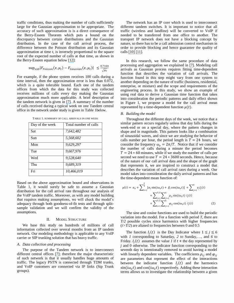
For example, if the phone system receives 100 calls during a time interval, then the approximation error is less than 0.072, which is a quite tolerable bound. Each one of the tandem offices from which the data for this study was collected receives millions of calls every day making the Gaussian approximation much more applicable. A brief description of the tandem network is given in [7]. A summary of the number of calls received during a typical week on one Tandem central office in the network under study is given in Table 1below.

TABLE 1. SUMMARY OF CALL ARRIVALS IN ONE WEEK

Day of the week Total number of calls

Sat 7,642,482

Sun 5,568,602

Mon 9,629,297

Tue 9,667,976

Wed 9,528,640

Thu 9,689,319

Fri 10,466,019

Based on the above approximation bound and observations in Table 1, it would surely be safe to assume a Gaussian distribution for the call arrival rate throughout our analysis of the VoIP tandem traffic. Moreover, as with any model building that requires making assumptions, we will check the model’s adequacy through both goodness-of-fit tests and through split-sample validation and we will confirm the validity of the assumptions.

II. MODEL STRUCTURE

We base this study on hundreds of millions of call information collected over several months from an IP tandem network. Our modeling methodology is applicable to any VoIP carrier or SIP trunking solution that has heavy traffic.

A. Data collection and processing

The purpose of the Tandem network is to interconnect different central offices [7]; therefore the major characteristic of such network is that it usually handles huge amounts of traffic. The legacy PSTN is connected through TDM trunks, and VoIP customers are connected via IP links (Sip Trunk groups).

The network has an IP core which is used to interconnect different tandem switches. It is important to notice that all traffic (wireless and landline) will be converted to VoIP if needed to be transferred from one office to another. The transport IP network does not have a blocking concept by nature, so there has to be a call admission control mechanism in order to provide blocking and hence guarantee the quality of calls [10] [11].

In this research, we follow the same procedure of data processing and aggregation we explained in [7]. Modeling call arrivals as Gaussian process requires fitting time-dependent function that describes the variation of call arrivals. The function found in this step might vary from one system to another depending on the nature of traffic (business, residential, enterprise, or mixture) and the scope and requirements of the engineering process. In this study, we show an example of using real data to derive a Gaussian time function that takes into consideration the periodic patterns and daily effect shown in Figure 1, we propose a model for the call arrival mean represented by a time-dependent function .

B. Building the model

Throughout the different days of the week, we notice that a similar pattern occurs regularly unless that day falls during the week-end or on a special day, where the pattern changes in shape and in magnitude. This pattern looks like a combination of sinusoidal waves, and since we are studying the behavior of calls number per hour, the period length is hours, we consider the frequency Notice that if we consider the number of calls during a minute the period becomes minutes, while if we study the number of calls per second we need to use seconds. Hence, because of the nature of our call arrival data and the shape of the graph that represents it, we are inspired to construct a model that describes the variation of call arrival rates during a week. Our model takes into consideration the daily arrival patterns and has the time-dependent mean function of:

The sine and cosine functions are used to build the periodic variation into the model. For a function with period T, there are T/2 possible cycles since harmonics with higher frequencies (i>T/2) are aliased to frequencies between 0 and 0.5

The function is the Day Indicator where

with 1 corresponding to Saturday, 2 to Sunday,…, and 6 to Friday. assumes the value 1 if the day represented by

j and 0 otherwise. The indicator function corresponding to the seventh day is intentionally removed to avoid having a model

with linearly dependent variables. The coefficients and

are parameters that represent the effect of the interactions

between the indicator function and the harmonics

and respectively. Adding these interaction terms allows us to investigate the relationship between a given

harmonic term and the number of calls in a given day. The

effects of the interactions coefficients and are different

from those of and which represent the effects of harmonic terms on the call numbers throughout the week.

Since the empirical data does not exhibit non-constant variability due to sampling error, we can safely assume that the model is homoscedastic and that the variance function is constant over time. When that is not the case, we apply certain transformations to stabilize the data or use weighted least squares to estimate the parameters [13]. Efficient transformations for count-type data include the logarithm, square root and quadratic root.

III. MODEL PARAMETERS ESTIMATION

We use the least-squares (LS) method [13] to estimate the parameters in the proposed model of . The advantages of least-squares estimation are that it does not require knowledge of the underlying distribution of the error component and when the model is linear it delivers explicit expressions for the parameters’ estimates. In addition when is assumed to have a Gaussian distribution, it is possible to make inferences about the parameters’ significance and about the model’s validity and usefulness, and hence use the model to make predictions about future observations.

As explained in [7], we process call arrival data by aggregating arrivals into non-overlapping time intervals of length 1 second, or 1 minute or 1 hour. Thus we will use the total number of calls within time intervals rather than the exact call time of arrival.

Let denote the number of calls arrived at the system in non-overlapping time intervals , such that tk=tk-1+ . Least-squares estimators are thus obtained by minimizing the loss function in (3), which is expressed as sum of squared deviations between the observed and expected numbers of calls:

Replacing by its expression in (2), we obtain:

The LS estimators are obtained when minimizing SS, with

respect to each of the model parameters .

This is done through taking partial derivatives of SS with respect to the parameters which leads to the following system of linear equations:

Define the m-dimensional vectors n=[n1,…,nm], and the coefficient vectors

, and

where the prime sign is used to denote the transpose of a matrix or vector. Therefore, is the vector that contain all the coefficients in the linear model. Also, define the

(mxT/2) matrices, M1 and M2 whose (k,i)th entries are

respectively, and ; (mx6) matrix, M3 whose (k,j)th entry is ; and (mx(6T/2)) matrices, M4 and

M5 whose (k,(j-1)T/2+i)th entries are respectively and . If we define the

(mx(7T+6)) matrix X=[ M1, M2, M3, M4, M5], then the above system of 7(1+T) equations can be written as:

– = 0

– = 0

– = 0

– = 0

– = 0

– = 0

This set of equations can be further summarized as:

– = which is equivalent to the equation:

= If the size of the data, m, was larger than the number of

parameters 7(1+T), the design matrix X would have a full rank, i.e., its columns would be linearly independent, so would be nonsingular and the solution to the linear system of equations (4) would be:

However, this might not always be the case, and the solution

to (6) might involve a generalized inverse of the matrix ,

which we denote by and hence the solution is:

The vector contains the LS estimates of the parameters in model (2). By combining equations (1) and (4), we can show

that the covariance of is or depending on

the rank of X, where

. The standard errors of the parameters are the diagonal of

the covariance matrix and they will come in handy when we

conduct inferences about the parameters.

Notice that in order to obtain these estimators; we didn’t

need to make any assumptions about the distribution of the number of calls. The Gaussian assumption becomes of outmost importance when we test the significance of the parameters and their real contribution to model. The assumption is also crucial to test the usefulness of the model as a whole in explaining the behavior of the call arrival data.

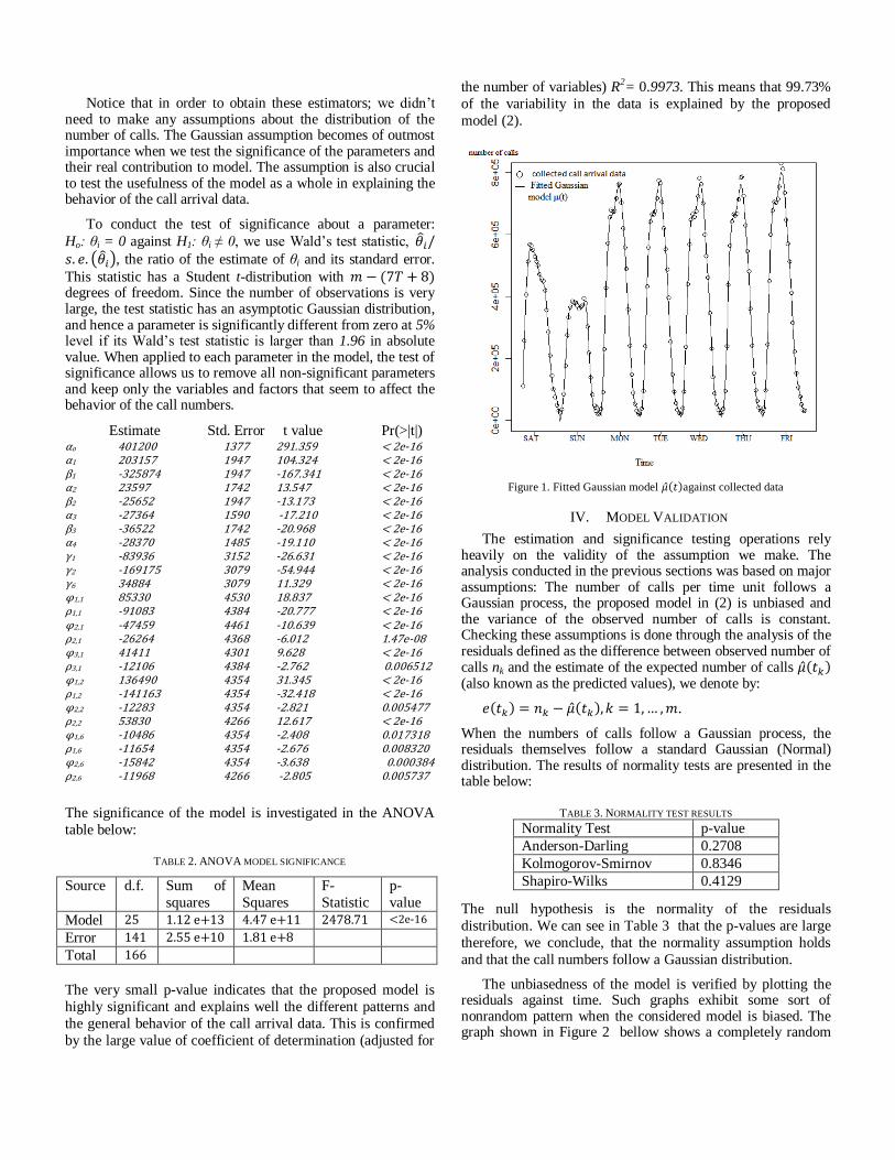
To conduct the test of significance about a parameter:

Ho: θi = 0 against H1: θi ≠ 0, we use Wald’s test statistic, , the ratio of the estimate of θi and its standard error.

This statistic has a Student t-distribution with degrees of freedom. Since the number of observations is very large, the test statistic has an asymptotic Gaussian distribution, and hence a parameter is significantly different from zero at 5% level if its Wald’s test statistic is larger than 1.96 in absolute value. When applied to each parameter in the model, the test of significance allows us to remove all non-significant parameters and keep only the variables and factors that seem to affect the behavior of the call numbers.

Estimate Std. Error t value Pr(>|t|) αo 401200 1377 291.359 < 2e-16 α1 203157 1947 104.324 < 2e-16 β1 -325874 1947 -167.341 < 2e-16 α2 23597 1742 13.547 < 2e-16 β2 -25652 1947 -13.173 < 2e-16 α3 -27364 1590 -17.210 < 2e-16 β3 -36522 1742 -20.968 < 2e-16 α4 -28370 1485 -19.110 < 2e-16 γ1 -83936 3152 -26.631 < 2e-16 γ2 -169175 3079 -54.944 < 2e-16 γ6 34884 3079 11.329 < 2e-16 φ1,1 85330 4530 18.837 < 2e-16 ρ1,1 -91083 4384 -20.777 < 2e-16 φ2,1 -47459 4461 -10.639 < 2e-16 ρ2,1 -26264 4368 -6.012 1.47e-08 φ3,1 41411 4301 9.628 < 2e-16 ρ3,1 -12106 4384 -2.762 0.006512 φ1,2 136490 4354 31.345 < 2e-16 ρ1,2 -141163 4354 -32.418 < 2e-16 φ2,2 -12283 4354 -2.821 0.005477 ρ2,2 53830 4266 12.617 < 2e-16 φ1,6 -10486 4354 -2.408 0.017318 ρ1,6 -11654 4354 -2.676 0.008320 φ2,6 -15842 4354 -3.638 0.000384 ρ2,6 -11968 4266 -2.805 0.005737

The significance of the model is investigated in the ANOVA

table below:

TABLE 2. ANOVA MODEL SIGNIFICANCE

Source d.f. Sum of

squares

Mean

Squares

F-

Statistic

p-

value

Model 25 1.12 e+13 4.47 e+11 2478.71 <2e-16

Error 141 2.55 e+10 1.81 e+8

Total 166

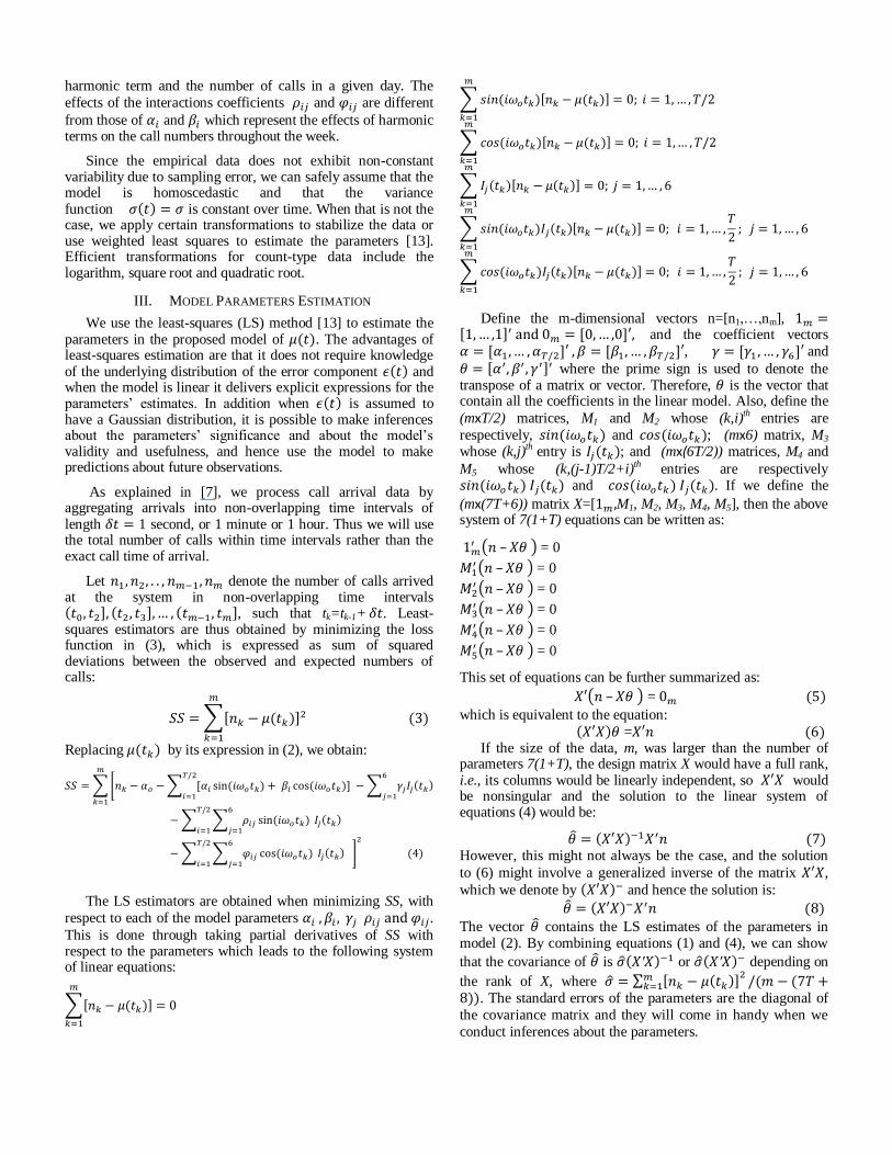
The very small p-value indicates that the proposed model is

highly significant and explains well the different patterns and

the general behavior of the call arrival data. This is confirmed

by the large value of coefficient of determination (adjusted for

the number of variables) R2= 0.9973. This means that 99.73%

of the variability in the data is explained by the proposed

model (2).

Figure 1. Fitted Gaussian model against collected data

IV. MODEL VALIDATION

The estimation and significance testing operations rely heavily on the validity of the assumption we make. The analysis conducted in the previous sections was based on major assumptions: The number of calls per time unit follows a Gaussian process, the proposed model in (2) is unbiased and the variance of the observed number of calls is constant. Checking these assumptions is done through the analysis of the residuals defined as the difference between observed number of calls nk and the estimate of the expected number of calls (also known as the predicted values), we denote by:

.

When the numbers of calls follow a Gaussian process, the residuals themselves follow a standard Gaussian (Normal) distribution. The results of normality tests are presented in the table below:

TABLE 3. NORMALITY TEST RESULTS

Normality Test p-value

Anderson-Darling 0.2708

Kolmogorov-Smirnov 0.8346

Shapiro-Wilks 0.4129

The null hypothesis is the normality of the residuals

distribution. We can see in Table 3 that the p-values are large

therefore, we conclude, that the normality assumption holds

and that the call numbers follow a Gaussian distribution.

The unbiasedness of the model is verified by plotting the residuals against time. Such graphs exhibit some sort of nonrandom pattern when the considered model is biased. The graph shown in Figure 2 bellow shows a completely random

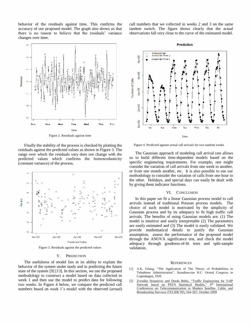
behavior of the residuals against time. This confirms the accuracy of our proposed model. The graph also shows us that there is no reason to believe that the residuals’ variance changes over time.

Figure 2. Residuals against time

Finally the stability of the process is checked by plotting the

residuals against the predicted values as shown in Figure 3. The range over which the residuals vary does not change with the predicted values which confirms the homoscedasticity (constant variance) of the process.

Figure 3. Residuals against the predicted values

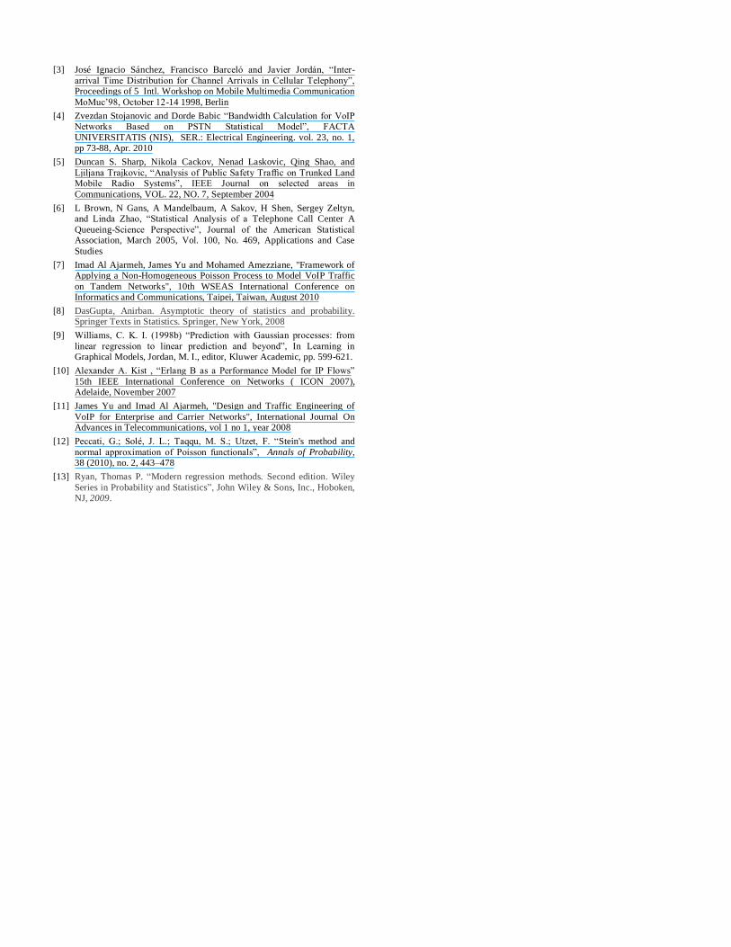
V. PREDICTION

The usefulness of model lies in its ability to explain the behavior of the system under study and in predicting the future state of the system [9] [13]. In this section, we use the proposed methodology to construct a model based on data collected in week 1 and then use the model to predict data for following two weeks. In Figure 4 below, we compare the predicted call numbers based on week 1’s model with the observed (actual)

call numbers that we collected in weeks 2 and 3 on the same tandem switch. The figure shows clearly that the actual observations fall very close to the curve of the estimated model.

Figure 4. Predicted against actual call arrivals for two random weeks

The Gaussian approach of modeling call arrival rate allows us to build different time-dependent models based on the specific engineering requirements. For example, one might consider the variation of call arrivals from one week to another, or from one month another, etc. It is also possible to use our methodology to consider the variation of calls from one hour to the other. Holidays, and special days can easily be dealt with by giving them indicator functions.

VI. CONCLUSION

In this paper we fit a linear Gaussian process model to call arrivals instead of traditional Poisson process models. The choice of such model is motivated by the simplicity of Gaussian process and by its adequacy to fit high traffic call arrivals. The benefits of using Gaussian models are: (1) The model is intuitive and easily interpretable (2) The parameters are easily estimated and (3) The model is easily validated. We provide mathematical details to justify the Gaussian assumption, assess the performance of the proposed model through the ANOVA significance test, and check the model adequacy through goodness-of-fit tests and split-sample validation.

REFERENCES [1] A.K. Erlang, “The Application of The Theory of Probabilities in

Telephone Administration”, Scandinavian H.C. Orsted Congress in Copenhagen, 1920

[2] Zvezdan Stojanovic and Dorde Babic, “Traffic Engineering for VoIP

Network based on PSTN Statistical Models,” 9th International

Conferences on Telecommunication in Modern Satellite, Cable, and

Broadcasting Services (TELSIK’09), 564-567, October 2009

[3] José Ignacio Sánchez, Francisco Barceló and Javier Jordán, “Inter-

arrival Time Distribution for Channel Arrivals in Cellular Telephony”, Proceedings of 5 Intl. Workshop on Mobile Multimedia Communication

MoMuc’98, October 12-14 1998, Berlin

[4] Zvezdan Stojanovic and Dorde Babic “Bandwidth Calculation for VoIP Networks Based on PSTN Statistical Model”, FACTA

UNIVERSITATIS (NIS), SER.: Electrical Engineering. vol. 23, no. 1, pp 73-88, Apr. 2010

[5] Duncan S. Sharp, Nikola Cackov, Nenad Laskovic, Qing Shao, and

Ljiljana Trajkovic, “Analysis of Public Safety Traffic on Trunked Land Mobile Radio Systems”, IEEE Journal on selected areas in

Communications, VOL. 22, NO. 7, September 2004

[6] L Brown, N Gans, A Mandelbaum, A Sakov, H Shen, Sergey Zeltyn, and Linda Zhao, “Statistical Analysis of a Telephone Call Center A

Queueing-Science Perspective”, Journal of the American Statistical Association, March 2005, Vol. 100, No. 469, Applications and Case

Studies

[7] Imad Al Ajarmeh, James Yu and Mohamed Amezziane, "Framework of Applying a Non-Homogeneous Poisson Process to Model VoIP Traffic

on Tandem Networks", 10th WSEAS International Conference on Informatics and Communications, Taipei, Taiwan, August 2010

[8] DasGupta, Anirban. Asymptotic theory of statistics and probability. Springer Texts in Statistics. Springer, New York, 2008

[9] Williams, C. K. I. (1998b) “Prediction with Gaussian processes: from

linear regression to linear prediction and beyond”, In Learning in Graphical Models, Jordan, M. I., editor, Kluwer Academic, pp. 599-621.

[10] Alexander A. Kist , “Erlang B as a Performance Model for IP Flows”

15th IEEE International Conference on Networks ( ICON 2007), Adelaide, November 2007

[11] James Yu and Imad Al Ajarmeh, "Design and Traffic Engineering of

VoIP for Enterprise and Carrier Networks", International Journal On Advances in Telecommunications, vol 1 no 1, year 2008

[12] Peccati, G.; Solé, J. L.; Taqqu, M. S.; Utzet, F. “Stein's method and

normal approximation of Poisson functionals”, Annals of Probability, 38 (2010), no. 2, 443–478

[13] Ryan, Thomas P. “Modern regression methods. Second edition. Wiley

Series in Probability and Statistics”, John Wiley & Sons, Inc., Hoboken, NJ, 2009.