Tomographic imaging by reflected and refracted arrivals at the North Sea

$: Tomographic imaging by reflected and refracted arrivals at the North Sea$
GEOPHYSICS, VOL. 64, NO. 6 (NOVEMBER-DECEMBER 1999): P. 1852-1862,19 FIGS.

Tomographic imaging by reflected and refractedarrivals at the North Sea

Aldo L. Vesnaver*, G. Bohm*, G. Madrussani *,

S. A. Petersen, and G. Rossi*

ABSTRACT

We discuss some processing steps of a marine 3-D dataset from the Oseberg field, North Sea. We compare theprestack depth-migrated images obtained by the veloc-ity fields provided by different tools: velocity spectra,reflection tomography, and joint tomographic inversionof reflected and refracted arrivals. The last ones are def-initely better. We also produced a synthetic example bymodeling the estimated earth structure and the actualrecording geometry, and we reached similar conclusions.

The correlation between reflected and refracted sig-nals may be unclear for later arrivals because of their re-ciprocal interference and multiple reflections. We adopta technique based on a surgical mute in the r-p domain,which allows coupling the signals coming from the sameelastic interface.

INTRODUCTION

Prestack depth migration is becoming a standard processingtool for imaging complex 3-D structures where less expensiveprocedures (such as poststack migration) do not adequatelyreconstruct the earth structure. Unfortunately, this procedurecontains a circular problem: we get good results (i.e., well re-solved depth sections) if we know in advance most of the soughtsolution (i.e., the earth structure).

Circular problems sometimes occur in seismic processing.For example, residual static corrections enhance stacked sec-tions but are better estimated if fair reference traces are avail-able, e.g., from the stacked sections themselves. One can solvesuch problems by an iterative procedure. Starting with a prelim-inary guess, we approximate the solution by using the previousoutput in sequence as improved input information.

In principle, an iterative procedure can also be used forprestack depth migration (Stork, 1992a). In practice, it is nota viable solution because (especially in 3-D models) its com-putational cost is too high at present. A possible compromisecould be to carry out the iterative procedure at a few selectedpoints and to interpolate the local estimates to the whole 3-Dmodel. Whitcombe (1994) and Kim et al. (1996) suggest moreglobal approaches. They pick a number of reflected arrivals inthe seismic records and improve the velocity macromodel bya point migration, based on cheap ray tracing. Then they usesuch a model for the prestack depth migration of traces, whichis carried out once (if the focusing check is good) or by a fewiterations at most.

The philosophy of our approach (Figure 1) is similar to thatof Kim et al. (1996). We select some major horizons accordingto their geological meaning and reflectivity, usually in a stackedor common offset section; then we pick the traveltimes of therelated events in the prestack domain. For each profile, weestimate the velocity field and the reflectors' depth in two di-mensions by reflection tomography; by interpolating the 2-Ddepth models so obtained, we build a new 3-D macromodel.Then we update in sequence (and separately) the velocity fieldand the reflectors' structure until their variations become suf-ficiently small (see also Carrion et al., 1993a,b; Bohm et al.,1996a,b).

The nonuniqueness of solutions is a basic problem fortraveltime inversion. Several different approaches have beenproposed to reduce this uncertainty, such as introducinghard constraints (Carrion, 1991; Vasco, 1991), using statisticalanalysis (Vasco et al., 1996), and controlling singular values(see Stork and Clayton, 1991; Stork, 1992b; Michelena, 1993);the most popular is imposing smooth solutions (see Phillipsand Fehler, 1991; Zhou, 1993). Krey (1989) and Sorin (1994)prove that in some pathological cases these ambiguities cannotbe solved at all.

Manuscript received by the Editor May 22, 1997; revised manuscript received December 17, 1998. Online publication:*Osservatorio Geofisico Sperimentale, P.O. Box 2011, 34016 Trieste, Italy. E-mail: [email protected]; [email protected]; [email protected]; [email protected] Hydro, Sandsliveien 90, N-5020 Bergen, Norway.© 1999 Society of Exploration Geophysicists. All rights reserved.

1852

Downloaded 25 Jan 2012 to 95.244.2.85. Redistribution subject to SEG license or copyright; see Terms of Use at http://segdl.org/

Tomographic Imaging at the North Sea

1853

Our approach belongs to Occam's school (Constable et al.,1987; deGroot-Hedlin and Constable, 1990; LaBrecque et al.,1996): we prefer a coarse inversion for the ill-posed modelparameter by iteratively adapting the local pixel density andshape (Vesnaver, 1994, 1996a,b). In other words, we avoid mod-els with too much detail with respect to the available data.The instabilities that arise otherwise are often controlled inthe standard approach by external constraints from indepen-dent origin, i.e., so-called a priori information. Unfortunately,this information may be missing (e.g., the well logs) or simplywrong (e.g., the geological interpretation of seismic data).

In the following sections, we describe the real data set weused to compare different methods for building velocity macro-models in depth; then we sketch the procedures applied (veloc-ity spectra, reflection tomography, joint inversion) by lookingat their intermediate processing steps. Finally, we compare theprestack depth-migrated images obtained from the differentvelocity fields.

DATA DESCRIPTION

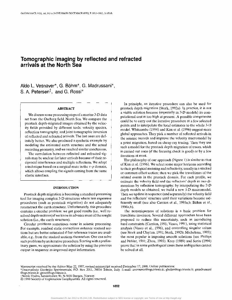
The data set we considered is a 3-D marine prospect acquiredin 1989 at the Oseberg Field, North Sea (Figure 2). The reser-voir is part of the Brent Group at a depth between 2400 and2700 m. The actual thickness of the Oseberg Formation rangesfrom 40 to 200 m.

We processed nine nearly parallel lines, acquired for a 3-Dsurvey in 1989. The ship was towing two streamers from east towest; thus, we actually had 18 profiles available. The distancebetween the lines was not regular, but the distance betweenthe two streamers in the same line was about 100 m. The off-sets between source and receiver ranged from 80 to 3050 m.Since there were 120 channels per streamer, the interval be-tween adjacent hydrophones was 25 m. The shot interval was25 m, and the total number was about 500 for most lines. Thesampling rate was 4 ms, and the record duration was 4 s. Forfurther details, see Johnstad et al. (1993, 1995).

A simple processing sequence was adopted:

1) spike and noise burst editing;2) source and streamer statics (5 and 6 m, respectively);3) compensation of geometrical spreading;4) prestack predictive deconvolution, with an operator

length of 250 ms and a prediction lag of 65 ms; and5) stacking velocity analysis.

We avoided procedures such as f-k or r-p domain multi-ple removal (which could be useful in our case) because they

affect the waveforms in the prestack traces too much, makingthe traveltime picking difficult. Fortunately, the chosen decon-volution operator attenuated the first sea-floor multiple andalmost cancelled the higher order ones.

Figure 3 shows the stacked section of part of line 7. The seafloor is at nearly 160 ms (i.e., about 110 m). It is our first pickedhorizon, marked A. Because of its high reflectivity, it producesa strong multiple at 320 ms, which partly interferes with a clearprimary reflection. Nevertheless, we chose this latter primaryevent as the second reference horizon (indicated as B) for

FIG. 2. (a) Detailed map of the shotpoints of the processedlines and (b) location of Oseberg field. Line 8 was not usedhere, so it is not displayed.

FIG. 1. Block diagram for the adopted inversion procedure. FIG. 3. Stacked section of part of line 7.


1854

Vesnaver et al.

velocity analysis and traveltime inversion. It seemed inter-esting from both the geological and the seismic stratigraphicpoints of view: an erosion surface separating domains with dif-ferent signal properties.

The third, fourth, and fifth horizons were chosen for the samereasons and are depicted as C, D, and E (at about 870, 1960,and 2200 ms, respectively). They are sufficiently continuousand distinct from background noise or sparse signals. The fifthhorizon is the top of an oil- and gas-bearing formation, so itssurroundings are of particular interest. To better reconstructthe area, we also picked a couple of spot horizons below itwhere amplitude and lateral continuity were adequate.

In the interval between horizons C and D, we notice manydiffractions and some weak primaries. We avoided picking suchevents because we felt this procedure was quite unreliable inthat part. On the other hand, we recognize at least two differentdomains in that area: a zone between 870 and 1200 ms charac-terized by dipping, strong and discontinuous events, overlyinganother one between 1200 and 1960 ms where the reflectivityis uniformly weak and chaotic.

IMAGING BY STACKING VELOCITIES

Stacking velocity analysis is a standard procedure for ob-taining a stacked section in time (Taner and Kohler, 1969) anda first guess for the velocity field. In our data set, the upper-most interfaces are quite flat and the observed diffractions aremainly from local roughness effects. Therefore, we expectedthat a plain stacking velocity analysis could be a sound tool for

building a depth macromodel via the Dix formula (1955) andthat dip moveout (DMO) correction could be superfluous.

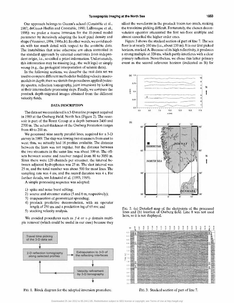
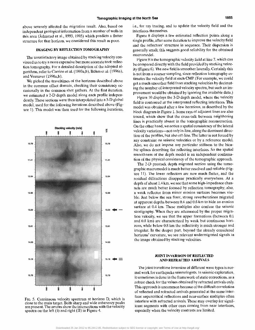
We computed what we call a net of velocity spectra, i.e.,22 conventional spectra [one for every 50 common midpoints(CMPs), i.e., 625 m apart] intersecting five continuous-velocityspectra along the picked horizons. We imposed the consis-tency of the chosen velocity functions at the crossing pointsamong conventional and continuous velocity spectra. Theseconstraints helped stabilize the velocity field. In various areasthe coherency peaks are very broad, so their picking is prone toa relevant personal bias (Figures 4 and 5). We obtained thesespectra by a coherency function as the normalized complexcrosscorrelation (Sguazzero and Vesnaver, 1987), which effec-tively reduces this kind of ambiguity.

By means of the Dix formula, we computed the interval ve-locity field in depth (Figure 6). It is quite smooth in the upperpart, close to the sea floor, but we notice some velocity anoma-lies in the central part. We checked carefully, by revising thecoherency spectra, and discovered that these instabilities resultfrom the data only and not to imprecise picking.

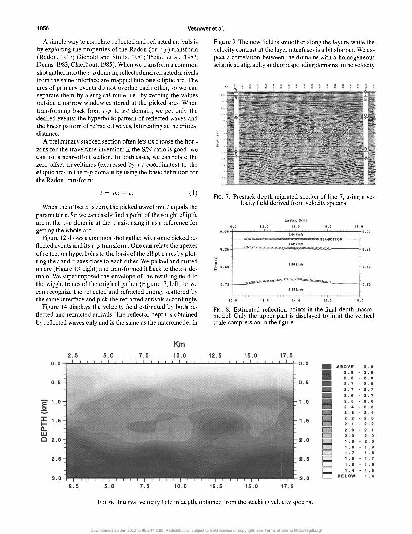
Figure 7 displays the 2-D prestack depth migrated sectionof line 7, obtained by using the velocity field in Figure 6. Inthe upper part just below the sea floor, we distinguish morereflectors than in the stacked section (Figure 3). In the cen-tral area, most of the diffracted energy was migrated, butsome residual diffractions are still visible. In the lower part wehave serious problems: the fifth horizon appears undulated,unlike in the stacked section. Therefore, in the conversionfrom time to depth domain, the velocity anomalies mentioned

FIG. 4. Two conventional velocity spectra where relevant ambiguities occur.



1855

above severely affected the migration result. Also, based onindependent geological information from a number of wells inthis area (Johnstad et al., 1993, 1995) which predicts a flatterstructure for that horizon, we considered this result as poor.

IMAGING BY REFLECTION TOMOGRAPHY

The unsatisfactory image obtained by stacking velocity con-vinced us to try a more expensive but more accurate tool: reflec-tion tomography. For a detailed description of the adopted al-gorithms, refer to Carrion et al. (1993a,b), Bohm et al. (1996a),and Vesnaver (1996a,b).

We picked the traveltimes of the horizons described abovein the common offset domain, checking their consistency oc-casionally in the common shot gathers. At the first iteration,we estimated a 2-D depth model along each profile indepen-dently. These sections were then interpolated into a 3-D globalmodel, used for the following iterations described above (Fig-ure 1). This model was then used for the following iterations,

i.e., for ray tracing, and to update the velocity field and theinterfaces themselves.

Figure 8 displays a few estimated reflection points along asingle profile, after some iteration to improve the velocity fieldand the reflectors' structure in sequence. Their dispersion isgenerally small; this suggests good reliability for the obtainedmacromodel.

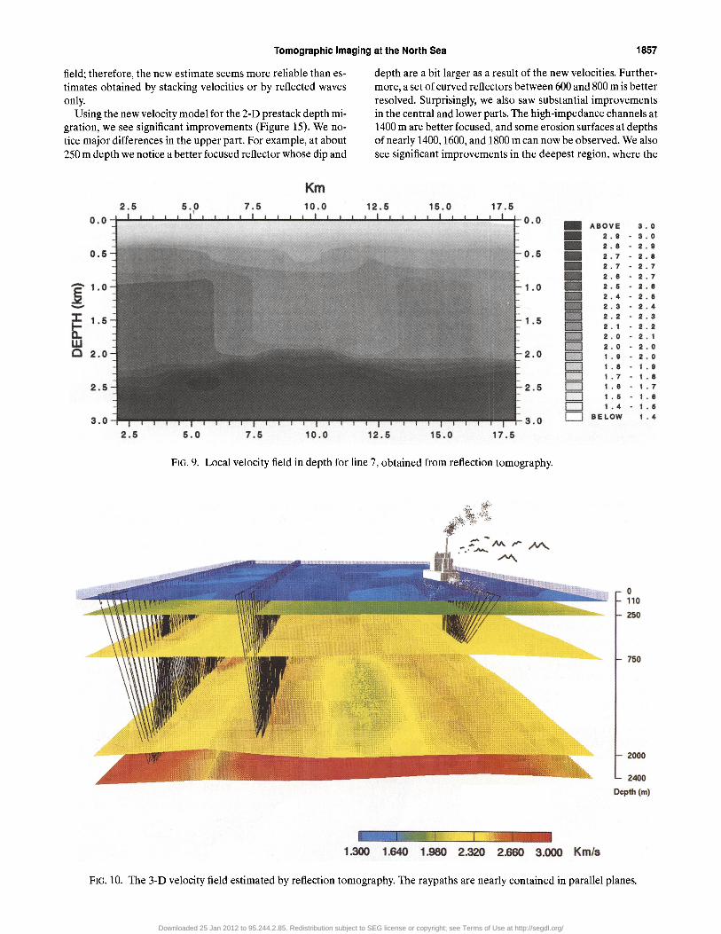
Figure 9 is the tomographic velocity field at line 7, which canbe compared directly with the field provided by stacking veloc-ity (Figure 6). The new field is smoother laterally. Certainly thisis not from a coarser sampling, since reflection tomography es-timates the velocity field at each CME (For example, we couldget a much smoother field from stacking velocities by decimat-ing the number of interpreted velocity spectra, but such an im-provement would be obtained by ignoring the available data.)

Figure 10 displays the 3-D depth model, where the velocityfield is contoured at the interpreted reflecting interfaces. Thismodel was obtained after a few iterations, as described by theblock diagram in Figure 1. Some rays of adjacent lines are alsotraced, which show that the cross-talk between neighboringlines is practically absent in the tomographic reconstruction.On the other hand, we notice a spatial consistency of the lateralvelocity variations—not only in-line, along the dominant direc-tion of the profiles, but also off-line. The latter is not forced byany constraint on seismic velocities or by a reference model.Also, we do not impose any particular stiffness to the bicu-bic splines describing the reflecting interfaces. So the spatialsmoothness of the depth model is an independent confirma-tion of the physical consistency of the tomographic approach.

The 2-D prestack depth migrated section using the tomo-graphic macromodel is much better resolved and reliable (Fig-ure 11). The lower reflectors are now much flatter, and theresidual diffractions disappear practically everywhere. At adepth of about 1.4 km, we see that some high-impedance chan-nels are much better focused by reflection tomography; also,a weak reflector from minor erosion surfaces becomes visi-ble. Just below the sea floor, strong reverberations migratedat apparent depths between 0.4 and 0.6 km to hide an erosionsurface at 0.4 km. These multiples also confuse the seismicstratigraphy. When they are attenuated by the proper migra-tion velocity, we see that the upper formations (between 0.1and 0.8 km) are characterized by weak but continuous hori-zons, while below 0.8 km the reflectivity is much stronger andirregular. In the deeper part, beyond the already consideredhorizons' curvature, we see relevant undermigrated signals inthe image obtained by stacking velocities.

JOINT INVERSION OF REFLECTEDAND REFRACTED ARRIVALS

FIG. 5. Continuous velocity spectrum at horizon D, which isclose to the main target. Both sharp and wide coherency peaksare present. The arrows show the intersections with the velocityspectra on the left (I) and right (II) in Figure 4.

The joint traveltime inversion of different wave types is nor-mal work for earthquake seismologists. In seismic exploration,it sometimes is done in the framework of static corrections, as arobust check for the values obtained by refracted arrivals only.This approach is uncommon because of the difficult correlationof reflected and refracted arrivals generated at the same inter-face: supercritical reflections and near-surface multiples ofteninterfere with refracted arrivals. These may overlap for signif-icant segments with other ones coming from near interfaces,especially when the velocity contrasts are limited.


1856

Vesnaver et al.

A simple way to correlate reflected and refracted arrivals isby exploiting the properties of the Radon (or r-p) transform(Radon, 1917; Diebold and Stoffa, 1981; Treitel et al., 1982;Deans, 1983; Claerbout, 1985). When we transform a commonshot gather into the r -p domain, reflected and refracted arrivalsfrom the same interface are mapped into one elliptic arc. Thearcs of primary events do not overlap each other, so we canseparate them by a surgical mute, i.e., by zeroing the valuesoutside a narrow window centered at the picked arcs. Whentransforming back from r -p to x-t domain, we get only thedesired events: the hyperbolic pattern of reflected waves andthe linear pattern of refracted waves, bifurcating at the criticaldistance.

A preliminary stacked section often lets us choose the hori-zons for the traveltime inversion; if the SIN ratio is good, wecan use a near-offset section. In both cases, we can relate thezero-offset traveltimes (expressed by x-t coordinates) to theelliptic arcs in the r -p domain by using the basic definition forthe Radon transform:

t = px + v. (1)

When the offset x is zero, the picked traveltime t equals theparameter r. So we can easily find a point of the sought ellipticarc in the r -p domain at the t axis, using it as a reference forgetting the whole arc.

Figure 12 shows a common shot gather with some picked re-flected events and its r -p transform. One can relate the apexesof reflection hyperbolas to the basis of the elliptic arcs by plot-ting the t and r axes close to each other. We picked and mutedan arc (Figure 13, right) and transformed it back to the x-t do-main. We superimposed the envelope of the resulting field tothe wiggle traces of the original gather (Figure 13, left) so wecan recognize the reflected and refracted energy scattered bythe same interface and pick the refracted arrivals accordingly.

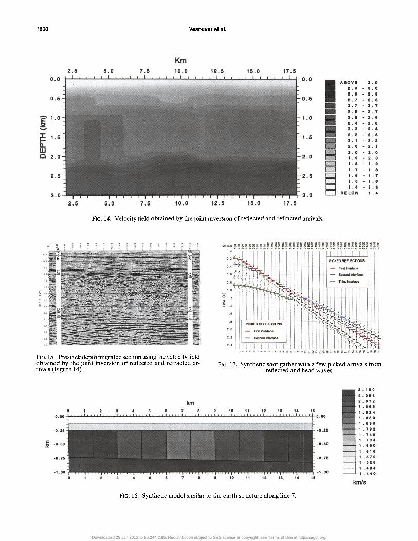
Figure 14 displays the velocity field estimated by both re-flected and refracted arrivals. The reflector depth is obtainedby reflected waves only and is the same as the macromodel in

Figure 9. The new field is smoother along the layers, while thevelocity contrast at the layer interfaces is a bit sharper. We ex-pect a correlation between the domains with a homogeneousseismic stratigraphy and corresponding domains in the velocity

FIG. 7. Prestack depth migrated section of line 7, using a ve-locity field derived from velocity spectra.

FIG. 8. Estimated reflection points in the final depth macro-model. Only the upper part is displayed to limit the verticalscale compression in the figure.

FIG. 6. Interval velocity field in depth, obtained from the stacking velocity spectra.



1857

field; therefore, the new estimate seems more reliable than es-timates obtained by stacking velocities or by reflected wavesonly.

Using the new velocity model for the 2-D prestack depth mi-gration, we see significant improvements (Figure 15). We no-tice major differences in the upper part. For example, at about250 m depth we notice a better focused reflector whose dip and

depth are a bit larger as a result of the new velocities. Further-more, a set of curved reflectors between 600 and 800 m is betterresolved. Surprisingly, we also saw substantial improvementsin the central and lower parts. The high-impedance channels at1400 m are better focused, and some erosion surfaces at depthsof nearly 1400,1600, and 1800 m can now be observed. We alsosee significant improvements in the deepest region, where the

FIG. 9. Local velocity field in depth for line 7, obtained from reflection tomography.

FIG. 10. The 3-D velocity field estimated by reflection tomography. The raypaths are nearly contained in parallel planes.


1858

Vesnaver et al.

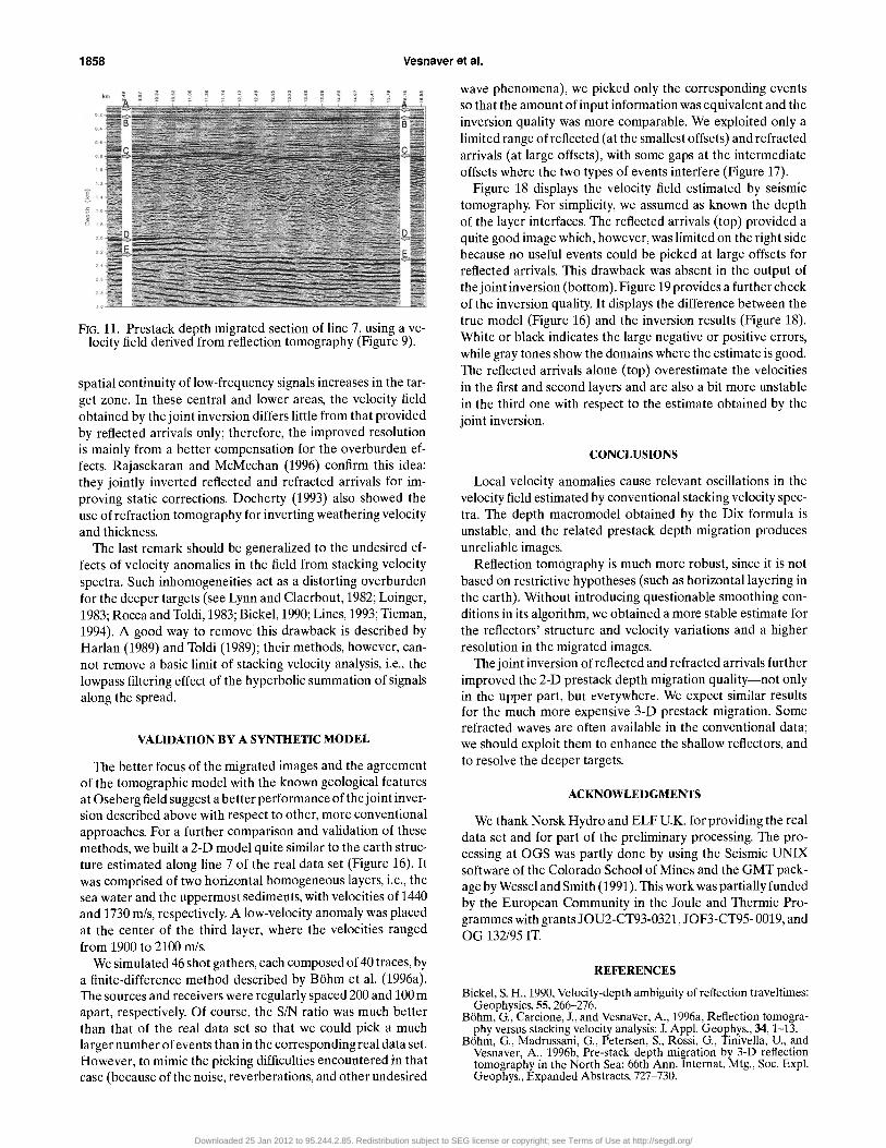
FIG. 11. Prestack depth migrated section of line 7, using a ve-locity field derived from reflection tomography (Figure 9).

spatial continuity of low-frequency signals increases in the tar-get zone. In these central and lower areas, the velocity fieldobtained by the joint inversion differs little from that providedby reflected arrivals only; therefore, the improved resolutionis mainly from a better compensation for the overburden ef-fects. Rajasekaran and McMechan (1996) confirm this idea:they jointly inverted reflected and refracted arrivals for im-proving static corrections. Docherty (1993) also showed theuse of refraction tomography for inverting weathering velocityand thickness.

The last remark should be generalized to the undesired ef-fects of velocity anomalies in the field from stacking velocityspectra. Such inhomogeneities act as a distorting overburdenfor the deeper targets (see Lynn and Claerbout, 1982; Loinger,1983; Rocca and Toldi, 1983; Bickel,1990; Lines,1993; Tiernan,1994). A good way to remove this drawback is described byHarlan (1989) and Toldi (1989); their methods, however, can-not remove a basic limit of stacking velocity analysis, i.e., thelowpass filtering effect of the hyperbolic summation of signalsalong the spread.

VALIDATION BY A SYNTHETIC MODEL

The better focus of the migrated images and the agreementof the tomographic model with the known geological featuresat Oseberg field suggest a better performance of the joint inver-sion described above with respect to other, more conventionalapproaches. For a further comparison and validation of thesemethods, we built a 2-D model quite similar to the earth struc-ture estimated along line 7 of the real data set (Figure 16). Itwas comprised of two horizontal homogeneous layers, i.e., thesea water and the uppermost sediments, with velocities of 1440and 1730 m/s, respectively. A low-velocity anomaly was placedat the center of the third layer, where the velocities rangedfrom 1900 to 2100 m/s.

We simulated 46 shot gathers, each composed of 40 traces, bya finite-difference method described by Bohm et al. (1996a).The sources and receivers were regularly spaced 200 and 100 mapart, respectively. Of course, the S/N ratio was much betterthan that of the real data set so that we could pick a muchlarger number of events than in the corresponding real data set.However, to mimic the picking difficulties encountered in thatcase (because of the noise, reverberations, and other undesired

wave phenomena), we picked only the corresponding eventsso that the amount of input information was equivalent and theinversion quality was more comparable. We exploited only alimited range of reflected (at the smallest offsets) and refractedarrivals (at large offsets), with some gaps at the intermediateoffsets where the two types of events interfere (Figure 17).

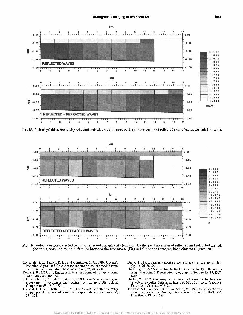
Figure 18 displays the velocity field estimated by seismictomography. For simplicity, we assumed as known the depthof the layer interfaces. The reflected arrivals (top) provided aquite good image which, however, was limited on the right sidebecause no useful events could be picked at large offsets forreflected arrivals. This drawback was absent in the output ofthe joint inversion (bottom). Figure 19 provides a further checkof the inversion quality. It displays the difference between thetrue model (Figure 16) and the inversion results (Figure 18).White or black indicates the large negative or positive errors,while gray tones show the domains where the estimate is good.The reflected arrivals alone (top) overestimate the velocitiesin the first and second layers and are also a bit more unstablein the third one with respect to the estimate obtained by thejoint inversion.

CONCLUSIONS

Local velocity anomalies cause relevant oscillations in thevelocity field estimated by conventional stacking velocity spec-tra. The depth macromodel obtained by the Dix formula isunstable, and the related prestack depth migration producesunreliable images.

Reflection tomography is much more robust, since it is notbased on restrictive hypotheses (such as horizontal layering inthe earth). Without introducing questionable smoothing con-ditions in its algorithm, we obtained a more stable estimate forthe reflectors' structure and velocity variations and a higherresolution in the migrated images.

The joint inversion of reflected and refracted arrivals furtherimproved the 2-D prestack depth migration quality—not onlyin the upper part, but everywhere. We expect similar resultsfor the much more expensive 3-D prestack migration. Somerefracted waves are often available in the conventional data;we should exploit them to enhance the shallow reflectors, andto resolve the deeper targets.

ACKNOWLEDGMENTS

We thank Norsk Hydro and ELF U.K. for providing the realdata set and for part of the preliminary processing. The pro-cessing at OGS was partly done by using the Seismic UNIXsoftware of the Colorado School of Mines and the GMT pack-age by Wessel and Smith (1991). This work was partially fundedby the European Community in the Joule and Thermie Pro-grammes with grants JOU2-CT93-0321, JOF3-CT95- 0019, andOG 132/95 IT.

REFERENCES

Bickel, S. H., 1990, Velocity-depth ambiguity of reflection traveltimes:Geophysics, 55, 266-276.

Bohm, G., Carcione, J., and Vesnaver, A., 1996a, Reflection tomogra-phy versus stacking velocity analysis: J. Appl. Geophys., 34, 1-13.

Bohm, G., Madrussani, G., Petersen, S., Rossi, G., Tinivella, U., andVesnaver, A., 1996b, Pre-stack depth migration by 3-D reflectiontomography in the North Sea: 66th Ann. Internat. Mtg., Soc. Expl.Geophys., Expanded Abstracts, 727-730.



1859

FIG. 12. (a) Common shot gather and (b) its r-p transform. The small bars show some picked reflected arrivals.

FIG. 13. Wiggle traces of the same common shot gather superimposed to the envelope of the (a) selected event and (b) the mutedr-p transform. The small bars show the refracted (green and reflected (yellow) arrivals from the chosen horizon.

Carrion, P., 1991, Dual tomography for imaging complex structures: Carrion, P., Marchetti, A., Bohm, G., Pettenati, E, and Vesnaver, A.,Geophysics, 56, 1395-1404. 1993b, Tomographic processing of Antarctica's data: First Break, 11,

Carrion, P., Bohm, G., Marchetti, A., Pettenati, F., and Vesnaver, A., 295-301.1993a, Reconstruction of lateral gradients from reflection tomogra- Claerbout, J. F., 1985, Imaging the earth's interior: Blackwell, Scientificphy: J. Seis. Explr., 2, 55-67. Publishers, Inc.


1860 Vesnaver et al.

FIG. 14. Velocity field obtained by the joint inversion of reflected and refracted arrivals.

FIG, 15. Prestack depth migrated section using the velocity fieldobtained by the joint inversion of reflected and refracted ar- FIG. 17. Synthetic shot gather with a few picked arrivals fromrivals (Figure 14). reflected and head waves.

FIG. 16. Synthetic model similar to the earth structure along line 7.



1861

FIG.18. Velocity field estimated by reflected arrivals only (top) and by the joint inversion of reflected and refracted arrivals (bottom).

FIG. 19. Velocity errors detected by using reflected arrivals only (top) and by the joint inversion of reflected and refracted arrivals(bottom), obtained as the difference between the true model (Figure 16) and the tomographic estimates (Figure 18).

Constable, S. C., Parker, R. L., and Constable, C. G., 1987, Occam'sinversion: A practical algorithm for generating smooth models fromelectromagnetic sounding data: Geophysics, 52, 289-300.

Deans, S. R., 1983, The Radon transform and some of its applications:John Wiley & Sons, Inc.

deGroot-Hedlin, C., and Constable, S., 1990, Occam's inversion to gen-erate smooth two-dimensional models from magnetotelluric data:Geophysics, 55,1613-1624.

Diebold, J. B., and Stoffa, P. L., 1981, The traveltime equation, tau-pmapping and inversion of common mid-point data: Geophysics, 46,238-254.

Dix, C. H., 1955, Seismic velocities from surface measurements: Geo-physics, 20, 68-86.

Docherty, P., 1992, Solving for the thickness and velocity of the weath-ering layer using 2-D refraction tomography: Geophysics, 57,1307-1318.

Harlan, W., 1989, Tomographic estimation of seismic velocities fromreflected ray paths: 59th Ann. Internat. Mtg., Soc. Expl. Geophys.,Expanded Abstracts, 922-924.

Johnstad, S. E., Seymour, R. H., and Smith, P. J., 1995, Seismic reservoirmonitoring over the Oseberg Field during the period 1989-1992:First Break, 13,169-183.


1862

Vesnaver et al.

Johnstad, S. E., Uden, R. C., and Dunlop, K. N. B., 1993, Seismicreservoir monitoring over the Oseberg Field: First Break, 11, 177-185.

Kim, Y. C., Samuelsen, C. M., and Hauge, T. A., 1996, Efficient velocitymodel building for pre-stack depth migration: The Leading Edge, 15,751-753.

Krey, T., 1989, The nonuniqueness of the determination of intervalvelocities from moveout velocities: Geophysics, 54, 1209-1211.

LaBrecque, D. J., Miletto, M., Daily, W., Ramirez, A., and Owen, E.,1996, The effects of noise on Occam's inversion of resistivity tomog-raphy data: Geophysics, 61, 538-548.

Lines, L., 1993, Ambiguity in analysis of velocity and depth: Geo-physics, 58, 596-597.

Loinger, E., 1983, A linear model for velocity anomalies: Geophys.Prosp., 31, 98-118.

Lynn, W. S., and Claerbout, J. F., 1982, Velocity estimation in laterallyvarying media: Geophysics, 47, 884-897.

Michelena, R., 1993, Singular value decomposition for cross-well to-mography: Geophysics, 58,1655-1661.

Phillips, W. S., and Fehler, 1991, Traveltime tomography: A comparisonof popular methods: Geophysics, 56, 1639-1649.

Radon, J., 1917, Uber die Bestimmung von Functionen durch ihre In-tegralwerte langs gewisser Mannigfaltigkeiten: Berichte der Sach.Akad. der Wissensch., 69, 262-267.

Rajasekaran, S., and McMechan, G. A., 1996, Tomographic estimationof the spatial distribution of statics: Geophysics, 61, 1198-1208.

Rocca, F., and Toldi, J., 1983, Lateral velocity anomalies: 53rd Ann.Internat. Mtg., Soc. Expl. Geophys., Expanded Abstracts, 572-574.

Sguazzero, P, and Vesnaver, A., 1987, A comparative analysis of algo-rithms for seismic velocity estimation, in Bernabini, M., Rocca, E,Treitel, S., and Worthington, M., Eds., Deconvolution and inversion,Blackwell Scientific Publications, Inc. 267-286.

Sorin, V., 1994, Nonuniqueness of velocity determination for one typeof layered model: Geophysics, 59,161-164.

Stork, C., 1992a, Reflection tomography in the postmigrated domain:Geophysics, 57, 680-692.

1992b, Singular-value decomposition of the velocity-reflectordepth tradeoff, part 2: High-resolution analysis of a generic model:Geophysics, 57, 933-943.

Stork, C., and Clayton, R. W., 1991, Linear aspects of tomographicvelocity analysis: Geophysics, 56, 483-495.

Taner, M. T., and Kohler, E, 1969, Velocity spectra—digital computerderivation and application of velocity functions: Geophysics, 34,859-881.

Tiernan, H. J., 1994, Investigating the velocity-depth ambiguity of re-flection traveltimes: Geophysics, 59, 1763-1773.

Toldi, J., 1989, Velocity analysis without picking: Geophysics, 54, 191-199.

Treitel, S., Gutowski, P. R., and Wagner, D. E., 1982, Plane-wave de-composition of seismograms: Geophysics, 47, 1375-1401.

Vasco, D. W., 1991, Bounding seismic velocities using a tomographicmethod: Geophysics, 56, 472-482.

Vasco, D. W., Peterson, J. E., and Majer, E. L., 1996, Nonuniquenessin traveltime tomography: Ensemble inference and cluster analysis:Geophysics, 61,1209-1227.

Vesnaver, A., 1994, Towards the uniqueness of tomographic inversionsolutions: J. Seis. Expl., 3, 323-334.

1996a, Irregular grids in seismic tomography and minimum timeray tracing: Geophys. J. Internat., 125, 147-165.

1996b, The contribution of reflected, refracted and transmit-ted waves to seismic tomography: A tutorial: First Break, 14, 159-168.

Wessel, P, and Smith, W. H. E, 1991, Free software helps map anddisplay data. EOS Trans. Amer. Geophys. U., 72, 445-446.

Whitcombe, D. N., 1994, Fast model building using denigration andsingle-step ray migration: Geophysics, 59, 439-449.

Zhou, H., 1993, Traveltime tomography with a spatial coherency filter:Geophysics, 58, 720-726.


Tomographic imaging by reflected and refracted arrivals at the North Sea

Documents

Transcript of Tomographic imaging by reflected and refracted arrivals at the North Sea