Modeling and Simulation of WSNs for Agriculture Applications using Dynamic Transmit Power Control Algorithm

L.M. Kamarudin1,2 , R.B. Ahmad1, D. Ndzi2,3, A. Zakaria2, B.L. Ong1, K. Kamarudin2, A. Harun2,S.M.Mamduh2

1 School of Computer and Communication Engineering,Universiti Malaysia Perlis, Perlis, Malaysia 2Centre of Excellance for Advanced Sensor Technology (CEASTech), Universiti Malaysia Perlis, Perlis, Malaysia

3School of Engineering, University of Portsmouth, Portsmouth, PO1 3DJ, U.K, {latifahmunirah,badli}@unimap.edu.my, david.ndzi@port.ac.uk, {ammarzakaria,drlynn}@unimap.edu.my,

arul.unimap@gmail.com ,zz_harun@yahoo.com, mamduh_shred87@yahoo.com

Abstract— Simulation platforms have become important tools in the design and evaluating of protocols for Wireless Sensor Networks. Thus the use of realistic models in simulation is important for the development of protocols. However, most of the reported studies based on simulations tend to use simple or non-realistic parameters and assumptions. This paper proposes a transmit power control algorithm with a realistic radio energy model based on different propagation models to mimic different deployment scenarios. Results show that the implementation of transmit power control extends the network lifetime by 5.3% when free space path loss model is used. However, a greater efficiency of 8.7% is achieved when the network is assumed to be deployed in the presence of vegetation using Weissberger’s vegetation attenuation model.

Keywords- wireless sensor networks, OMNeT++, power control, CC2420

I. INTRODUCTION Wireless sensor network (WSN) technology has a wide

range of potential applications that include precision agriculture, target tracking and emergency relief. Such networks consist of a large number of distributed nodes [1]. In some applications the nodes are expected to work independently in very harsh environments for long periods of time. It is therefore difficult and time consuming to experimentally assess all sensor nodes in the different types of environments in which they may be deployed. Hence, simulation platforms offer an easier and repeatable environment to investigate and evaluate the performances of WSNs, especially for energy efficiency. Energy consumption in WSNs can be addressed from a routing perspective as well as from the applications or services point of view [2]-[4]. Whatever the application or protocol in use, energy consumption at the physical layer (communication unit) is common to all services. Thus improving its energy efficiency will improve the overall network.

Modeling of wireless sensor network architecture on simulation platforms is often over simplified with many using simple radio energy models that do not consider the complexities of the radio propagation environment or assuming infinite transmit power levels. For example, the radio energy model originally proposed for LEACH [5] assumes free space and two ray radio link to estimate the

transmission power. The energy consumed by a transmitter over a short distance is proportional to the square distance between the transceivers, d2, whereas the energy consumed in a data transmission over longer distances (such as from a cluster head to the base station) is proportional to d4 [5]. Hence, the corresponding energy consumption calculated using this method will always be different for two different distances. The assumption of infinite transmit power levels often lead to a biased performance results in an optimistic manner, and results in incorrect estimates of performance metrics such as network lifetime, energy consumed per bit, and network connectivity[6][7].

In reality, the transmit power levels of most sensor nodes can only be adjusted to discrete values that may result in one transmit power level for multiple distances. Therefore, the resulting energy consumption for two links of different distances can be equivalent. The radio energy model used in this paper is similar to the model proposed in [8] that focused on the Chipcon CC2420 device for radio communication [9]. However, this paper assesses the energy consumption performances of the network using two propagation channel models and transmit power control algorithm. In order to conduct the studies, extensions have been made to the OMNeT++ simulation package to include a transmit power control algorithm with a realistic radio energy model. Two propagation channel models have also been implemented to mimic the environments under investigation. In this study, the focus is on environments with vegetation in the communication path.

The rest of this paper is organized as follow: Section II presents related work. It is followed by Section III which presents the radio propagation channel models used in this study, discusses the radio energy consumption models in different radio state based on CC2420 transceiver and the transmit power control algorithm proposed. Section V describes the simulation environments and the results are presented in section VI. Finally, section VII concludes the paper.

2012 Third International Conference on Intelligent Systems Modelling and Simulation

978-0-7695-4668-1/12 $26.00 © 2012 IEEE

DOI 10.1109/ISMS.2012.109

614

2012 Third International Conference on Intelligent Systems Modelling and Simulation

978-0-7695-4668-1/12 $26.00 © 2012 IEEE

DOI 10.1109/ISMS.2012.109

616

II. RELATED WORK Significant research activities have been undertaken to

develop more realistic energy consumption accounting models for WSN. Kellner et al. [10] used finite state machines to model energy consumption in WSN nodes, including onboard electronic devices, to produce an on-line energy accounting system. They also propose a sensor node management device that can be used to measure the energy consumption of a node at various stages of operation. Other tools that aim to make simulation platforms more energy aware include TOSSIM [11] and AEON [12]. These models and tools are developed to capture the low level details and energy consumption by the device in every state. They, however, ignore energy fluctuations within each state that may not be negligible [13]. Despite these, little attention has been paid to the complexities of the radio propagation channels that could be used to determine the power level setting of each node or the network routing technique that would be more suitable. In general, WSN devices have the main function of sensing and transmitting information, with more energy spent in communicating than processing information.

Accurate channel models and the implementation of appropriate energy management systems can significantly improve network lifetime estimates. Optimal connectivity is an important requirement in order to maintain a good quality of service. Significant indoor and outdoor WSN propagation channel studies have been reported in open literature [14]-[17]. Very limited studies have been carried out to assess WSN performance in the presence of vegetation. In [18], a log-distance model is proposed for WSN coverage in a forest. The proposed model has no frequency scaling term and does not account for vegetation density. A similar model is proposed by Lu et al. [19] but it is not supported by any results. Unlike in most environments, vegetative channels exhibit spatial and temporal variations characterized by complex vegetation densities that are hitherto be quantified [20]. In this paper, the focus is on WSN in the presence of vegetation.

III. MODELING AND POWER CONTROL ALGORITHM

A. Radio Propagation Model

The radio propagation models used in this paper are based on previous work in [21] and [22]. For radio wave propagation in free space, the path loss, , can be predicted using the free space loss (FSL) equation, LFSL 27.56 20log d 20log f (1)

where f is the frequency in MHz, d is the distance between the isotropic transmitting and receiving antennas in meters. In the presence of a ground reflected component, the

received signal can be modeled using the Plane Earth (PE) model as given by (2). LPE 40log d 20 log hT 20 log10 hR (2)

where d is the distance in meters and, and are the transmitter and receiver antenna heights, respectively, in meters.

The FSL and PE models are simplistic models that significantly underestimate the complexity of the signal propagation condition. This complexity and the lack of a unifying model have made these models to be used as benchmark models for comparing the performances of different communication technologies.

When there is vegetation in the radio waves propagation path, the signal undergoes scattering, absorption and blockage. The congruent effect is additional attenuation of the signal when compared to losses predicted using FSL or PE models. One of the well-known empirical models that is often used to estimate signal attenuation due to vegetation is Weissberger’s modified exponential decay model[23] represented by (3).

dB 1.33 . . 14 4000.45 . , 0 14 3

where f is the frequency in GHz, and is the foliage depth in meters. A number of models have subsequently been proposed using the same formulation as in (3) but with different parameter values [24]. However, none of the models provide consistent results for measurements on different tree species and climates. Therefore in this study, the original model is used to assess network performance in the presence of vegetation.

B. Radio Energy Modeling The aim of the transceiver modeling and simulation is to

allow accurate evaluation of different parameters that influence energy consumption in wireless sensor devices. Power consumption in WSN nodes can be divided into two parts: energy consumed by the onboard electronics (sensors, display, CPU, etc) and energy consumed by the communication unit. Research has identified the radio communication unit (in all its modes: transmitting, receiving, idle, listening, and sleeping) as the main energy consumer [6][7]. Energy consumption in most devices is non-linear as part is dissipated as heat, thermal noise and a fraction is channeled to accomplish the task [7]. The former two energy consumptions cannot be standardized and, for the purpose of this study, are assumed to be constant. Thus the focus of this study is on energy consumed by the radio communication module.

The total energy, consumed by sensor node in Joules is calculated using (4).

615617

∑ ∑ (4)

where the index state refers to the operational state of the mote: Sleep, Transmit (Tx), Receive (Rx) or Idle. Pstate is the power consumed (in Watt) in each state based on Table I which can be computed using (5). (5)

The term Istate denotes the current drawn by the node in A and V represents the supply voltage. tstate is the time spent in the corresponding state which depends on the amount of information being transmitted or received. This can be calculated using (6):

(6)

where LPacket is the packet length in bits and RBit is the data rate in kbps.

Since the radio communication unit is the main consumer of the battery power, the energy consumptions of the device’s circuitry (sensors, CPU and display) can reasonably be assumed to be a non-variant constant.

Using the Chipcon CC2420 radio transceiver specifications [9], the energy consumption whilst in the transmission state, ET , at a given transmission power level can be determined. The cost of the radio to transmit a packet of length, L, at a power level setting of pLevel can be define by (7)

The term PT L denotes the power consumption at pLevel, as shown in Table I. The value of can be set to 1.8 based on Chipcon CC2420 specifications and the packet length, , is set to 100 .

TABLE I. POW E R CO N S U M P T I O N VA L U E S F O R T H E CH I P C O N CC2420 R A D I O T R A N S C E I V E R D U R I N G T R A N S M I SS I O N

pLevel Pout (dBm) IpLevel (mA) PTx (mW ) ETx (mJ)0 -25 8.53 15.3 0.049 1 -15 9.64 17.35 0.056 2 -10 10.68 19.22 0.062 3 -7 11.86 21.35 0.068 4 -5 13.11 23.60 0.075 5 -3 14.09 25.36 0.081 6 -1 15.07 27.13 0.087 7 0 16.22 29.20 0.093

In the reception state, the current drawn, IRx, is constant. Therefore the energy consumed to receive one packet, ERx, is also constant. The CC2420 datasheet specifies that the current drawn during the receiving state, , is 19.7 . This indicates that more power is consumed when receiving than when transmitting at the highest power level setting. Energy spent to receive a packet, ER , is defined by

(8)

where can be calculated using (5). Based on CC2420 specification, the current drawn in the

sleep state, Isleep, is 80 . Power consumption is constant and thus energy depleted during the sleep state, Esleep, depends only on the time spent in this state and is given by (9). (9)

where the term Psleep denotes the power consumption in the sleep state per unit time.

Based on (7) to (9), energy consumption of the network, is define by: ∑ (10)

The term represents the number of nodes in the network.

C. Transmit Power Control Algorithm In this paper, the Received Signal Strength Indicator

(RSSI) is used to determine the power level required to transmit between two nodes. To estimate the RSSI, radio propagation models, as described in Section A and in previous work in [21] and [22], are used. When a packet is received, based on the signal to noise ratio (SNR) of the channel, the packet can be decoded with a certain probability of error. As the transmit power level increases, the probability of error decreases, which reduces the packet error ratio, assuming a constant noise power and wide sense stationary fixed channel. However, as the transmit power level increases, the battery power is also depleted at a faster rate. Therefore, there are tradeoffs between the transmit power level, packet failure ratio and network lifetime.

The flow diagram of the algorithm implemented for the transmission power level is shown in Fig. 1. In this study direct communication between the sensor node (SN) and the Base Station (BS) is used to show the effect of transmit power control algorithm in different types of environments using different propagation channel models. The BS transmit power level, pLevel, is set to maximum, assuming that it is connected to an energy source that will support the network as long as there are nodes that are able to receive or transmit. This is to ensure that all SNs will receive the packets. The algorithm allows SNs to select the appropriate power levels to communicate with the BS. Table I provides the values o f the transmit power levels, where pLevel0 corresponds to the lowest transmit power level and pLevel7 is the highest level. When a SN receives a packet, it estimates the received signal power, computes the path loss and sets the transmit power level accordingly. Based on the received signal power, path loss calculated

616618

and the transmit power level, it estimates the received signal power at the BS. If the estimated received signal power is higher than the receiver sensitivity, the current transmit power level is maintained, otherwise, the transmit power level is increased. The procedure is repeated until the power level that ensures data packets are received or the maximum transmit power is reached.

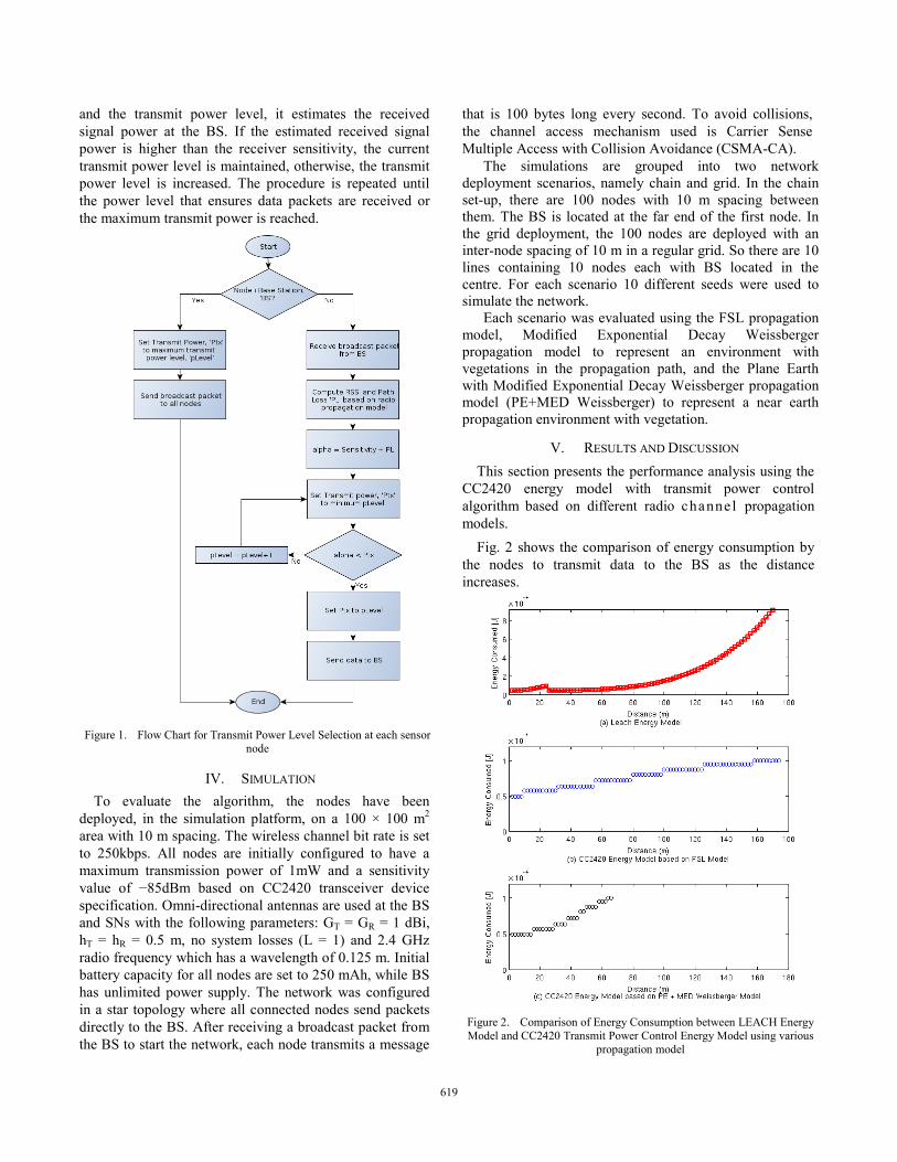
Figure 1. Flow Chart for Transmit Power Level Selection at each sensor

node

IV. SIMULATION To evaluate the algorithm, the nodes have been

deployed, in the simulation platform, on a 100 × 100 m2 area with 10 m spacing. The wireless channel bit rate is set to 250kbps. All nodes are initially configured to have a maximum transmission power of 1mW and a sensitivity value of −85dBm based on CC2420 transceiver device specification. Omni-directional antennas are used at the BS and SNs with the following parameters: GT = GR = 1 dBi, hT = hR = 0.5 m, no system losses (L = 1) and 2.4 GHz radio frequency which has a wavelength of 0.125 m. Initial battery capacity for all nodes are set to 250 mAh, while BS has unlimited power supply. The network was configured in a star topology where all connected nodes send packets directly to the BS. After receiving a broadcast packet from the BS to start the network, each node transmits a message

that is 100 bytes long every second. To avoid collisions, the channel access mechanism used is Carrier Sense Multiple Access with Collision Avoidance (CSMA-CA).

The simulations are grouped into two network deployment scenarios, namely chain and grid. In the chain set-up, there are 100 nodes with 10 m spacing between them. The BS is located at the far end of the first node. In the grid deployment, the 100 nodes are deployed with an inter-node spacing of 10 m in a regular grid. So there are 10 lines containing 10 nodes each with BS located in the centre. For each scenario 10 different seeds were used to simulate the network.

Each scenario was evaluated using the FSL propagation model, Modified Exponential Decay Weissberger propagation model to represent an environment with vegetations in the propagation path, and the Plane Earth with Modified Exponential Decay Weissberger propagation model (PE+MED Weissberger) to represent a near earth propagation environment with vegetation.

V. RESULTS AND DISCUSSION This section presents the performance analysis using the

CC2420 energy model with transmit power control algorithm based on different radio channel propagation models.

Fig. 2 shows the comparison of energy consumption by the nodes to transmit data to the BS as the distance increases.

Figure 2. Comparison of Energy Consumption between LEACH Energy Model and CC2420 Transmit Power Control Energy Model using various

propagation model

617619

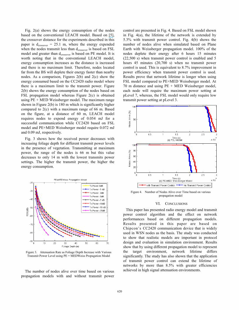
Fig. 2(a) shows the energy consumption of the nodes based on the conventional LEACH model. Based on [5], the crossover distance for the experiments described in this paper is dcrossover = 25.1 m, where the energy expended when the nodes transmit less than dcrossover is based on FSL model and greater than dcrossover is based on PE model. It is worth noting that in the conventional LEACH model, energy consumption increases as the distance is increased and there is no maximum limit. Therefore, nodes located far from the BS will deplete their energy faster than nearby nodes. As a comparison, Figures 2(b) and 2(c) show the energy consumed based on the CC2420 radio model where there is a maximum limit to the transmit power. Figure 2(b) shows the energy consumption of the nodes based on FSL propagation model whereas Figure 2(c) is obtained using PE + MED Weissberger model. The maximum range shown in Figure 2(b) is 180 m which is significantly higher compared to 2(c) with a maximum range of 66 m. Based on the figure, at a distance of 60 m, LEACH model requires nodes to expend energy of 0.054 mJ for a successful communication while CC2420 based on FSL model and PE+MED Weissberger model require 0.072 mJ and 0.09 mJ, respectively.

Fig. 3 shows how the received power decreases with increasing foliage depth for different transmit power levels in the presence of vegetation. Transmitting at maximum power, the range of the nodes is 66 m but this value decreases to only 14 m with the lowest transmits power settings. The higher the transmit power, the higher the energy consumption.

Figure 3. Attenuation Rate as Foliage Depth Increase with Various Transmit Power Level using PE + MEDWeiss Propagation Model

The number of nodes alive over time based on various propagation models with and without transmit power

control are presented in Fig. 4. Based on FSL model shown in Fig. 4(a), the lifetime of the network is extended by 5.3% with transmit power control. Fig. 4(b) shows the number of nodes alive when simulated based on Plane Earth with Weissberger propagation model. 100% of the nodes deplete their energy after 6 hours 15 minutes (22,500 s) when transmit power control is enabled and 5 hours 45 minutes (20,700 s) when no transmit power control is used. This is equivalent to 8.7% improvement in power efficiency when transmit power control is used. Results prove that network lifetime is longer when using FSL model compared to PE+MED Weissberger model. At 70 m distance and using PE + MED Weissberger model, each node will require the maximum power setting at pLevel 7, whereas, the FSL model would only require low transmit power setting at pLevel 3.

Figure 4. Number of Nodes Alive over Time based on various propagation model

VI. CONCLUSIONS This paper has presented radio energy model and transmit

power control algorithm and the effect on network performances based on different propagation models. Results presented in this paper are based on Chipcon’s CC2420 communication device that is widely used in WSN nodes as the basis. The study was conducted to show that realistic models are important in protocol design and evaluation in simulation environment. Results show that by using different propagation model to represent the target environment, network lifetime differs significantly. The study has also shown that the application of transmit power control can extend the lifetime of networks by more than 8.5% with greater efficiencies achieved in high signal attenuation environments.

618620

ACKNOWLEDGEMENTS

The authors acknowledge the sponsorships provided by UniMAP and Ministry of Higher Education Malaysia (MOHE), under the Academic Staff Training Scheme.

REFERENCES

[1] G. J. Pottie and W. J. Kaiser, “Wireless integrated network sensors,” Commun. ACM, vol. 43, pp. 51–58, May 2000.

[2] J. Wu and F. Dai, “Efficient broadcasting with guaranteed coverage in mobile ad hoc networks,” IEEE Transactions Mobile Computing, vol. 4 (3), June. 2005, pp. 259 - 270, doi: 10.1109/TMC.2005.40.

[3] V. Kanakaris, D. Ndzi and K. Ovaliadis, “Improving the Performance of AODV using Dynamic Density Driven Route Request Forwarding,” International Journal of Wireless & Mobile Networks (IJWMN) Vol. 3, No. 3, June 2011

[4] J. Domingues, A. Damaso, R. Nascimento, and N. Rosa, “An Energy-Aware Middleware for Integrating Wireless Sensor Networks and the Internet,” International Journal of Distributed Sensor Networks, vol. 2011, 2011. doi:10.1155/2011/672313

[5] W. R. Heinzelman, A. Chandrakasan, and H. Balakrishnan, “Energy- Efficient Communication Protocol for Wireless Microsensor Networks,” in Proceedings of the 33rd Hawaii International Conference on System Sciences-Volume 8, ser. HICSS ’00. Washington, USA: IEEE Computer Society, 2000

[6] M. S. Alejandro, M. G. P. Jose-Maria, E. L. Esteban, V. A. Javier, J. L. Leandro, and G.-H. Joan, “An accurate radio channel model for wireless sensor networks simulation,” Journal of Communications and Networks, vol. 7, no. 4, pp. 401–407, December 2004.

[7] A. Förster, Teaching Networks How to Learn: Data Dissemination in Wireless Sensor Networks with Reinforcement Learning. Südwestdeutscher Verlag, 2009.

[8] N. Aslam, W. Phillips, and W. Robertson, “Performance analysis of wsn clustering algorithms using discrete power control,” IPSI Transactions on Internet Research, vol. 5, no. 1, pp. 10–15, January 2009.

[9] “Chipcon CC2420 Datasheet: http://focus.ti.com/lit/ds/symlink/cc2420.pdf, Texas Instruments,” 2007

[10] S. Kellner, M. Pink, D. Meier, E.-O. Blass, “Towards a Realistic Energy Model for Wireless Sensor Networks,” Fifth Annual Conference on Wireless on Demand Network Systems and Services (WONS 2008), Garmisch-Partenkirchen, Germany, June 2008, doi: 10.1109/WONS.2008.4459362.

[11] E. Perla, A. O. Catháin, R. S. Carbajo, M. Huggard, C. M. Goldrick, “PowerTOSSIM z: realistic energy modelling for wireless sensor network environments,” Proceedings of the 3nd ACM workshop on Performance monitoring and measurement of heterogeneous wireless and wired networks (2008), pp. 35-42. doi:10.1145/1454630.1454636

[12] O. Landsiedel, K. Wehrle, and S. G¨otz, “Accurate prediction of

power consumption in sensor networks,” in Proceedings of the second IEEE Workshop on Embedded Networked Sensors (EmNetS-II), May 2005.

[13] A. Karagiannis, S. Kokkorikos, and P. Constantinou, “Energy Consumption Analysis and Optimization techniques for Wireless Sensor Networks,” in IEEE Symposium on Computers and Communications (ISCC 2009), Sousse, July 2009, doi: 10.1109/ISCC.2009.5202380 .

[14] W. Su, and M. Alzaghal, “Channel propagation characteristics of wireless MICAz sensor nodes,” Ad Hoc Networks, 1-11, 2008.

[15] X. Jin and M. Ali, “Embedded antennas in dry and saturated concrete for application in wireless sensors,” Progress in Electromagnetics Research, Vol. 102, 197-211, 2010.

[16] Chen, Y., Z. Zhang and T. Qin, “Geomatrically based channel model for indoor radio propagation with directional antennas,” Progress in Electromagnetics Research B, Vol. 20, 109-124, 2010.

[17] Howitt, L. and M. S. Khan, “A mode based approach for characterizing RF propagation in conduits” Progress in Electromagnetics Research B, Vol. 20, 49-64, 2010.

[18] J. A. Gay-Fernandez, M. Garcia Sanchez, I. Cuinas, A. V. Alejos, J. G. Sanchez, and J. L. Miranda-Sierra, "Propagation analysis and deployment of a wireless sensor network in a forest," Progress In Electromagnetics Research, Vol. 106, 121-145, 2010.

[19] J. Lu, D. Lu, X. Huang, “Channel Model for Wireless Sensor Networks in Forest Scenario,” 2nd International Asia Conference on Informatics in Control, Automation and Robotics (CAR), Wuhan, China, March 2010, doi: 10.1109/CAR.2010.5456600

[20] N. Savage, D. L. Ndzi, A. Seville, E. Vilar, J. Austin, "Radiowave Propagation Through Vegetation: Factors Influencing Signal Attenuation," Radio Science, Vol 38, No 5, October 2003.

[21] L. Kamarudin, R. Ahmad, B. Ong, F. Malek, A. Zakaria, and M. Arif, “Review and modeling of vegetation propagation model for wireless sensor networks using OMNET++,” in Network Applications Protocols and Services (NETAPPS), 2010 Second International Conference on, Sept. 2010, pp. 78–83.

[22] L. Kamarudin, R. Ahmad, B. Ong, A. Zakaria, and D. Ndzi, “Modeling and simulation of near-earth wireless sensor networks for agriculture based application using OMNET++,” in Computer Applications and Industrial Electronics (ICCAIE), Intern. Conf. on, dec. 2010, pp. 131–136.

[23] M. A. Weissberger, “An initial critical summary of models for predicting the attenuation of radio waves by foliage,” ECAC-TR-81-101, Electromagnetic Compatibility Analysis Center, USA, 1981.

[24] D. L. Ndzi, L. M. Kamarudin, A. A. Muhammad Ezanuddin, A. Zakaria, R. B. Ahmad, M. F. b. A. Malek, A. Y. M. Shakaff, and M. N. Jafaar, "Vegetation attenuation measurements and modeling in plantations for wireless sensor network planning," Progress In Electromagnetics Research B, Vol. 36, 283-301, 2012

619621