Computational Statistics & Data Analysis 48 (2005) 525–547www.elsevier.com/locate/csda

Modeling and prediction of multivariatespace–time random %elds

S. De Iacoa ;∗ , M. Palmaa , D. Posaa;b

aDipartimento di Scienze Economiche e Matematico-Statistiche, Facolt�a di Economia,Via per Monteroni, Ecotekne, Lecce 73100, Italy

bIRMA-CNR, Via Amendola 122/I Bari 70126, Italy

Received 18 March 2003; received in revised form 24 February 2004; accepted 24 February 2004

Abstract

In various environmental studies multivariate spatial–temporal correlated data are involved,hence appropriate techniques to enhance space–time prediction are in great demand. An extensionof multivariate spatial geostatistics to a spatio-temporal domain might be a straightforward task;nevertheless, up to now, little has been done in a multivariate spatial–temporal context. Modelingand prediction techniques are described for a multivariate space–time random %eld, moreoversome theoretical and practical aspects are investigated for a bivariate space–time random %eldthrough a case study.c© 2004 Elsevier B.V. All rights reserved.

Keywords: Multivariate space–time random %eld; Space–time linear coregionalization model; Space–timeprediction

1. Introduction

In various environmental studies, data usually consist of measurements for severalcorrelated variables observed at some locations in a geographic area of interest andfor a certain period of time. Hence, multivariate geostatistical techniques applied to aspace–time domain are appropriate for modeling and prediction purposes. Although theextension of multivariate geostatistics from the spatial case to the spatio-temporal one

∗ Corresponding author. Tel.: +39-0832-298786; fax: +39-0832-298737.E-mail addresses: sdeiaco@tiscalinet.it (S. De Iaco), palma m@libero.it (M. Palma),

posa@economia.unile.it (D. Posa).URL: http://www.donatoposa.it

0167-9473/$ - see front matter c© 2004 Elsevier B.V. All rights reserved.doi:10.1016/j.csda.2004.02.011

526 S. De Iaco et al. / Computational Statistics & Data Analysis 48 (2005) 525–547

might be straightforward from a mathematical point of view, up to now these techniqueshave been mainly developed and applied in a spatial context (Journel and Huijbregts,1981; Wackernagel, 1998; Goovaerts, 1997; Myers, 1982; Isaaks and Srivastava, 1989).In literature, one of the %rst attempts can be found in Rouhani and Wackernagel (1990),where space–time multivariate data were considered as long time series collected at fewspatial locations, or even in Goovaerts and Sonnet (1993), where data were consideredas realizations of regionalized variables at each observed time; moreover, in the reviewpaper by Kyriakidis and Journel (1999) multivariate space–time prediction problemswere not addressed at all. In De Iaco et al. (2002), total air pollution measurements,obtained through principal component analysis, were used and a space–time functionalform for total air pollution index was determined through the dual form of kriging,i.e., radial basis functions. An introduction of vectorial space–time random %eld wasalso given in Christakos and Hristopulos (1998).

In this paper, an extension of multivariate geostatistical techniques to space–time ispointed out in order to incorporate both spatial and temporal information. Firstly, abrief review of multivariate space–time random %eld (STRF) theory is presented, thenthe space–time linear coregionalization model (LCM), recently proposed by De Iacoet al. (2003), is considered for multivariate space–time analysis. Although the space–time basic variograms of an LCM might be modelled by choosing one of the modelsknown in literature, it will be pointed out throughout the paper that the generalizedproduct–sum model (De Iaco et al., 2001) allows the %tting procedure to be moreFexible. Bivariate STRF, as a particular and interesting case of a multivariate STRF,is introduced and some theoretical aspects are discussed for spatial–temporal vectorialdata, which can be seen as a special case of bivariate spatio-temporal data.

At last, a case study is presented by using hourly measurements of two space–time variables, such as relative humidity and temperature, taken at several monitoringstations in Lombardy region (Italy) during August 2000. Spatio-temporal observationsfor the two variables are considered as a realization of a bivariate non-stationary STRFwhere the trend component is described by a temporal component (accounting for thediurnal cycle), modelled for each monitoring station separately, together with a spatialcomponent, which is constant over moving space–time neighborhoods. The variogrammatrix of the residuals, used for prediction purposes, is modelled through a space–timeLCM based on the generalized product–sum model.

2. Multivariate STRF

Starting from multivariate spatial random %eld theory, little has to be changedfrom the mathematical point of view in order to formalize multivariate STRF anal-ysis. The space–time extension of several variants of cokriging or optimal multivari-ate spatial interpolation has been reported in various references, e.g., Daley (1991),Christakos (1992). Apart from substituting the spatial coordinate with the spatial–temporal one, some diGculties are encountered in modeling a multivariate STRF, asspeci%ed hereafter.

S. De Iaco et al. / Computational Statistics & Data Analysis 48 (2005) 525–547 527

Let

{Z(s; t); (s; t) ∈D × T ⊆ Rd+1}; (1)

be a multivariate STRF, with

Z(s; t) = [Z1(s; t); : : : ; Zp(s; t)]T; p¿ 2; (2)

where s=(s1; s2; : : : ; sd) ∈D (generally, d6 3) denotes the spatial coordinates and t ∈Tis the temporal coordinate.

Under second-order stationarity, the mean vector exists and does not depend on (s; t):

E[Z(s; t)] = [M1; : : : ; Mp]T =M; (s; t) ∈D × T; (3)

and the covariance and variogram (p × p) matrices de%ned for two multivariatespace–time random variables, Z(s; t) and Z(s′; t′), exist and depend on the space–timeseparation vector h

C(Z(s; t);Z(s′; t′)) = E[(Z(s; t) −M)(Z(s′; t′) −M)T]

=C(h) = [C �(h)];

�(Z(s; t);Z(s′; t′)) = E[(Z(s; t) − Z(s′; t′))(Z(s; t) − Z(s′; t′))T]

=�(h) = [� �(h)];

where

• h = (hs; ht), with hs = (s − s′) and ht = (t − t′);• C �(h) and � �(h); ; � = 1; : : : ; p, are, respectively, the cross-covariance and cross-

variogram between the space–time random variables Z (s; t) and Z�(s + hs; t + ht),when �= �, and the direct covariance and variogram of the th STRF, when =�.

2.1. Modeling a multivariate STRF

A crucial step in multivariate prediction procedures is the modeling of variogrammatrix. In literature, it is well known how to estimate and model the spatial variogrammatrix (Cressie, 1991; ChilLes and Del%ner, 1999) and the most commonly used modelis the LCM (Journel and Huijbregts, 1981). A straightforward extension of the LCMformalism to the spatial–temporal case is presented herein.

Given a second-order stationary multivariate STRF de%ned in (1), let

Yl(s; t) = [Y l1(s; t); : : : ; Y l

p(s; t)]T; l = 1; : : : ; L;

be vectors of uncorrelated second-order stationary STRF, such that Z(s; t) is modelledas follows:

Z(s; t) =L∑

l=1

AlYl(s; t) +M; (4)

where

E[Yl(s; t)] = 0; l = 1; : : : ; L;

528 S. De Iaco et al. / Computational Statistics & Data Analysis 48 (2005) 525–547

Al is a (p × p) coeGcient matrix for each l = 1; : : : ; L, and M is the mean vectorde%ned in (3).

The variogram matrix �(h) of (4), known as LCM, can be written as

�(h) = �(hs; ht) =L∑

l=1

Blgl(hs; ht); (5)

where

Bl = AlATl ; l = 1; : : : ; L;

are positive de%nite (p × p) matrices and gl(hs; ht); l = 1; : : : ; L, are basic space–timevariograms which correspond to diMerent scales of variability.

Some diGculties could be encountered in order to de%ne positive de%nite (p×p)matrices Bl; l = 1; : : : ; L, as well as to model basic space–time variograms gl(hs; ht);l = 1; : : : ; L, required in (5).

In literature, an iterative algorithm which generates large matrices Bl, in a spatialcontext, has been proposed by Goulard and Voltz (1992). Hence, the same techniquemight be used in a space–time domain. However, an extension of the LCM to the space–time domain can be found in De Iaco et al. (2003), where each space–time basicvariogram is modelled as a generalized product–sum model (De Iaco et al., 2001). Theauthors successfully applied the space–time LCM based on the generalized product–sum model to an environmental data set involving carbon monoxide and nitrogen diox-ide hourly concentrations measured in Milan district (Italy) during February 1999. Thus,by using the procedure suggested in De Iaco et al. (2003), the basic variograms canbe modelled and the matrices Bl can be easily generated. The technique is brieFyreviewed herein.

Each basic variogram gl(hs; ht) is modelled as a generalized product–sum model:

gl(hs; ht) = �l(hs; 0) + �l(0; ht) − kl�l(hs; 0)�l(0; ht); l = 1; : : : ; L; (6)

where �l(hs; 0) and �l(0; ht); l = 1; : : : ; L, are spatial and temporal marginal variogrammodels, while kl; l = 1; : : : ; L, are parameters given by

kl =sill[�l(hs; 0)] + sill[�l(0; ht)] − sill[gl(hs; ht)]

sill[�l(hs; 0)] · sill[�l(0; ht)] ; l = 1; : : : ; L; (7)

which must satisfy the following necessary and suGcient condition for the admissibilityof gl(hs; ht):

0¡kl61

max{sill[�l(hs; 0)]; sill[�l(0; ht)]} ; l = 1; : : : ; L;

where the sill is the limiting value reached by a variogram (ChilLes and Del%ner, 1999).By using (6) in (5), the space–time LCM with basic generalized product–sum var-

iogram models is determined by two marginal LCM, one in space

�(hs; 0) =L∑

l=1

Bl�l(hs; 0); (8)

S. De Iaco et al. / Computational Statistics & Data Analysis 48 (2005) 525–547 529

and the other one in time

�(0; ht) =L∑

l=1

Bl�l(0; ht): (9)

After modeling marginal direct variograms, the diagonal elements of Bl are determined,while the oM-diagonal elements are obtained by marginal cross-variogram models insuch a way to ensure positive de%niteness of the matrices Bl.

Remarks.

• In the space–time LCM (5), the basic variograms might be modelled by using one ofthe space–time models known in literature, such as the metric model(Dimitrakopoulos and Luo, 1994), the linear model (Rouhani and Hall, 1989), theproduct model (De Cesare et al., 1997) and other models (Cressie and Huang, 1999;Gneiting, 2002). However, by using the metric model and other non-separable mod-els, some problems arise in identifying the L basic structures gl, since each of themshould correspond to a diMerent scale of space–time variability, which requires thede%nition of a range in space–time.

• The main advantage which derives from using the generalized product–sum model isrepresented by the Fexibility in estimating and modeling the spatial–temporal vari-ability. That is, by obtaining the space–time correlation structures from the marginalsin space and time, admissibility problems and %tting aspects are easily overtaken.

• By using the generalized product–sum model (6), the matrices Bl are generatedthrough the marginal direct and cross-variograms.

• Finally, the generalized product–sum model has a nice feature as it clearly admitsa diMerent variance along space and along time (the sill of �l(hs; 0) model can bediMerent from the sill of the �l(0; ht) model).

2.2. Prediction of multivariate STRF

After modeling multivariate STRF, a spatial–temporal prediction procedure has tobe developed.

By recalling the spatial case (Myers, 1982), a linear space–time predictor of thespace–time random vector de%ned in (2) is

Z(u) =n∑

i=1

"i(u)Z(ui); (10)

where u=(s; t) ∈D×T is an unsampled point in the space–time domain, ui=(s; t)i ∈D×T; i = 1; : : : ; n, are the sampled points in the same domain and "i(u); i = 1; : : : ; n, are(p×p) matrices of weights whose elements � �i (u) are the weights assigned to thevalue of the �th variable, � = 1; : : : ; p, at the ith sampled point to predict the thvariable, = 1; : : : ; p, at the unsampled point u∈D × T .

The predicted space–time random vector at u∈D × T ,

Z(u) = [Z1(u); : : : ; Zp(u)]T;

530 S. De Iaco et al. / Computational Statistics & Data Analysis 48 (2005) 525–547

is such that each component is obtained by using all information at the sampled pointsui = (s; t)i ∈D × T , that is

Z (u) =n∑

i=1

p∑�=1

� �i (u)Z�(ui); = 1; : : : ; p: (11)

For geostatisticians, this might be thought as an extension of ordinary cokriging(Journel and Huijbregts, 1981) to a space–time domain.

The matrices of weights "i ; i = 1; : : : ; n, are determined by ensuring:

(1) the unbiased condition:

E[Z(u) − Z(u)] = 0; (12)

(2) the eGciency condition, which can be obtained by minimizing the error variance,de%ned in Myers (1982) as follows:

Tr{Var[Z(u) − Z(u)]} = Tr{E{[Z(u) − Z(u)][Z(u) − Z(u)]T}}= E{[Z(u) − Z(u)]T[Z(u) − Z(u)]}; (13)

where Tr denotes the trace of a matrix.By considering the following suGcient condition for (12):

n∑i=1

"i(u) = I; (14)

where I is the (p×p) identity matrix, minimization of the error variance under theconstraint (14) yields the following system:

�(u1 − u1) : : : �(u1 − un) I

......

...

�(un − u1) : : : �(un − un) I

I : : : I 0

"1

...

"n

#

=

�(u1 − u)...

�(un − u)I

; (15)

where # is a (p×p) matrix of Lagrange multipliers, while �(ui − uj), i; j = 1; : : : ; n,and �(ui−u); i=1; : : : ; n, are (p×p) matrices of direct and cross-variograms computedfor all vector distances (ui − uj) and (ui − u), respectively.

It is clear that the cokriging system (15) must be solved for the unknown matrix["1; : : : ;"n;#]T, which depends on �(ui − uj); i; j = 1; : : : ; n, and �(ui − u); i = 1; : : : ; n.

Note that, since (14) is only suGcient, other conditions on the matrix of weightsmight guarantee the unbiasedness of the predictor (10), hence diMerent systems ofcokriging might be de%ned. From this point of view, there does not exist a uniquesolution for the unknown matrix of weights.

S. De Iaco et al. / Computational Statistics & Data Analysis 48 (2005) 525–547 531

3. Bivariate STRF

A particular and interesting case of multivariate STRF is the bivariate STRF. Severalexamples of bivariate spatio-temporal data, which can be considered as a realizationof a bivariate STRF, can be highlighted, such as concentrations of two air pollutants,measurements of two atmospheric variables, two soil components which are observedat several spatial locations and for diMerent times. A signi%cant case is also representedby two-dimensional vectorial data, as it will be shown in the next section. In all thesecases, data provide bivariate spatio-temporal information which need to be studied bymeans of multivariate techniques de%ned in a space–time context.

3.1. Spatio-temporal vectorial data

Two-dimensional vectorial data observed at several spatial locations and for diMerenttimes arise from measurements in various diMerent areas, such as wind speed anddirection, in meteorology; readings of earthquakes in a given region, in geography;geological processes which involve transporting matter from one place to another intime.

Spatio-temporal vectorial data, in a two-dimensional spatial domain D, can be con-sidered as a realization of a bivariate STRF

{Z(s; t); (s; t) ∈D × T ⊆ R3};where

Z(s; t) = [Z1(s; t); Z2(s; t)]T: (16)

The components Z1(s; t) and Z2(s; t), in a two-dimensional cartesian system, are de%nedin the following way:

Z1(s; t) = �(s; t) cos[�(s; t)]

and

Z2(s; t) = �(s; t) sin[�(s; t)];

where the direction �(s; t) and the magnitude �(s; t) are the corresponding vector com-ponents in a polar system.

Generally, the sampling scheme for such kind of data is isotopic in space–time,since realizations for the two components, Z1(s; t) and Z2(s; t), are available at thesame sample points.

In literature, several techniques for analyzing vectorial data have been developed(Mardia and Jupp, 1999). However, they mainly concern observations which are unitvectors either in the plane or in three-dimensional space, thus the sample space istypically either a circle or a sphere. In Young (1987), some geostatistical techniques formodeling vectorial spatial data were introduced in order to study the spatial variabilityof fractures characterizing earth structures, but the author merely considered fractureorientations as unit vectors projected on the reference hemisphere and expression wasconsidered to predict the unit vectors at an unsampled location. A completely diMerentapproach can be found in Lajaunie and BLejaoui (1991) and Grzebyk (1993), where

532 S. De Iaco et al. / Computational Statistics & Data Analysis 48 (2005) 525–547

vectorial data were considered as a realization of a complex-valued spatial random %eldand procedures for modeling and estimation were based on covariance functions givenby a real and an imaginary part.

However, since spatio-temporal vectorial data can be considered as a realization of abivariate STRF, modeling and prediction techniques developed for any bivariate STRFcan be generally used for vector components. Anyway, interpolation of a vector %eldis ambiguous, owing to the somewhat arbitrary nature of the vector norm (Schaeferand Doswell, 1979). Since in a two-dimensional spatial domain a vector %eld can bespeci%ed by two scalar quantities, which can be separately interpolated, the ambiguitycan be resolved by forcing the interpolated %eld to preserve some properties (in thecase of a wind %eld, vorticity and divergence) associated with the raw data.

Moreover, a fundamental problem is that of non-uniqueness of vector %eld interpola-tion (Levinson and RedheMer, 1970), since interpolation of cartesian components doesnot necessarily yield the same results as interpolation of polar components (magnitudeand direction).

4. Some practical aspects

Although modeling and interpolation techniques for multivariate STRF can be easilyobtained by extending the well-known spatial approaches (i.e., LCM, cokriging), somepractical aspects must be pointed out:

• modeling the variogram matrix in space–time by LCM is not an easy task, since itrequires to identify diMerent scales of space–time variability;

• some computational aspects must be solved: although software for spatial data anal-ysis is available (Deutsch and Journel, 1998), there is no commercial software formodeling multivariate space–time data, but only personalized routines for speci%cpurposes;

• for two or more correlated variables, one might be interested in predicting onlyone variable using the information from the other ones, hence the prediction at anunsampled point is not computed simultaneously for all the variables, but only forthe one of interest;

• in the particular case of vectorial data considered as a realization of a bivariate STRF,the predicted components at an unsampled point are simultaneously required in orderto reconstruct the original vector: by means of the Pythagoras relation, prediction ofthe original vector at an unsampled point can be computed.

5. A case study

A multivariate approach is applied to analyze the direct and the cross correlation fortwo space–time atmospheric variables, such as relative humidity and temperature. Theadvantages of using a multivariate space–time technique to predict one of the variables,taking into account available measurements for the two correlated variables are pointed

S. De Iaco et al. / Computational Statistics & Data Analysis 48 (2005) 525–547 533

out. Moreover, a comparison between ordinary cokriging and kriging is provided in aspace–time context, which con%rms the improvements obtained by cokriging when theprimary variable is scarcely sampled with respect to the secondary variables.

In the present case study, the following aspects are considered:

(1) structural analysis for two atmospheric variables measured at some space–timepoints;

(2) ordinary space–time cokriging in order to obtain prediction maps for the primaryvariable and to make comparisons with ordinary space–time kriging.

5.1. The data set

The data set, provided by the Environmental Protection Agency of Lombardy re-gion, Italy, consists of relative humidity (per cent values) and temperature (◦C) hourlyaverages measured from the 1st to the 28th of August 2000 at 30 and 37 monitoringstations, respectively (Fig. 1). This data set has been used in order to model the spatial–temporal correlation of the two variables.

The negative association between the two atmospheric variables, which is a well-known consequence of fundamental thermodynamic laws, has been con%rmed by look-ing at the spatial and temporal pro%les of the two variables (Figs. 2 and 3).

In Fig. 2, the box-plots, where temperature and relative humidity measurements havebeen grouped by daily hour, show their temporal pro%les.

In Fig. 3, the location maps, where temperature and relative humidity measurementshave been averaged in time, for each station, display the spatial distributions.

However, starting from the 29th of August, just 8 stations (Fig. 1), among the 30monitoring stations, have been considered for relative humidity, in order to emphasize

Fig. 1. Location map of the survey stations used for structural analysis and predictions.

534 S. De Iaco et al. / Computational Statistics & Data Analysis 48 (2005) 525–547

(a) (b)

Fig. 2. Box-plots of temperature (a) and relative humidity (b) hourly averages.

(a) (b)

Fig. 3. Location maps of temperature (a) and relative humidity (b) averaged over the period 1–28 August2000.

the cokriging eGciency. Therefore, prediction maps of relative humidity, obtained byordinary cokriging, have been computed and comparisons between kriging and cokrig-ing have been outlined for the 30th and the 31st of August 2000.

5.2. Structural analysis

As previously pointed out, spatio-temporal observations for the two variables havebeen considered as a realization of a bivariate non-stationary STRF Z, which is de-composed as follows:

Z(s; t) = Y(s; t) +M(s; t); (s; t) ∈D × T;

S. De Iaco et al. / Computational Statistics & Data Analysis 48 (2005) 525–547 535

where

• Y(s; t) is a second-order stationary STRF, with

E[Y(s; t)] = 0;

CY(hs; ht) = Cov[Y(s + hs; t + ht);Y(s; t)]

�Y(hs; ht) = 12 E{[Y(s + hs; t + ht) − Y(s; t)][Y(s + hs; t + ht) − Y(s; t)]T};

• M(s; t) is a trend component

M(s; t) = [M1(s; t); M2(s; t)]T

with

Mi(s; t) = !i(s; t) + �i(s); (s; t) ∈D × T; i = 1; 2; (17)

where �i(s) is constant over moving space–time neighborhoods and !i(s; t) repre-sents the periodicity at 24 h of the variable i, which satis%es the following properties:

(a) !i(s; t) = !i(s; t + 24); s∈D; t; t + 24 ∈T ,(b)

∑24r=1 !i(s; r) = 0; s∈D.In the following, i= 1 stands for relative humidity, while i= 2 for temperature.

5.2.1. Missing values and removal of the diurnal componentBecause the diurnal component is only relevant in time, it has been estimated and

removed for each station separately. At this step, the space–time data set has beenviewed as a collection of time series, one for each spatial location. In order to applytime series analysis in the presence of missing values, time interpolation has been pre-viously performed; moreover, the diurnal component has been estimated and removedby a FORTRAN routine (De Cesare et al., 2002). Particularly,

(a) sequences with a maximum of 5 consecutive missing values have been linearlyinterpolated (there is no interpolation if there are more than 5 consecutive missingvalues);

(b) the moving average estimation (MAE) method (Brockwell and Davis, 1987) hasbeen applied to sequences with at least 60 consecutive values: for each of thesesequences the diurnal component has been separately computed. Sequences withfewer than 60 consecutive values have not been used for estimating the diurnalcomponent.

After removing the diurnal component at each station, structural analysis has beenperformed on the residuals.

5.2.2. Estimating and modelingIn order to generate an LCM, based on the generalized product–sum model, the

sample marginal variograms in space and time for the residuals of the two variables

536 S. De Iaco et al. / Computational Statistics & Data Analysis 48 (2005) 525–547

(a)

(b)

Fig. 4. Sample marginal variograms in space (a) and time (b) and their models.

have been %rstly computed (Fig. 4) and the %tted models have been the following:

�11(hs; 0) = 17�1(hs; 0) + 11�2(hs; 0) + 35�3(hs; 0); (18)

�11(0; ht) = 17�1(0; ht) + 11�2(0; ht) + 35�3(0; ht); (19)

S. De Iaco et al. / Computational Statistics & Data Analysis 48 (2005) 525–547 537

for relative humidity residuals, and

�22(hs; 0) = 0:55�1(hs; 0) + 0:7�2(hs; 0) + 1:5�3(hs; 0); (20)

�22(0; ht) = 0:55�1(0; ht) + 0:7�2(0; ht) + 1:5�3(0; ht); (21)

for temperature residuals, where the marginal basic structures in space and time aregiven below:

�1(hs; 0) =

{0 if ‖hs‖ = 0;

1 if ‖hs‖¿ 0;(22)

�2(hs; 0) = 1 − exp(

− 3‖hs‖25000

); (23)

�3(hs; 0) = 1 − exp(

− 3‖hs‖42000

); (24)

�1(0; ht) =

{0 if |ht | = 0;

0:05 if |ht |¿ 0;(25)

�2(0; ht) = 3:9[1 − exp

(−3|ht |

24

)]; (26)

�3(0; ht) = 2:45[1 − exp

(−3|ht |

48

)]: (27)

Fig. 5 displays the sample space–time variogram surfaces and the %tted product–sumnested models of the residuals of the two variables; these last models have been ob-tained by properly choosing the coeGcients k1 = 0:1, k2 = 0:08 and k3 = 0:14, whichhave been computed as in expression (7).

Then, the sample marginal cross-variograms for the residuals of the two variables(Fig. 6) have been %tted by the following models:

�12(hs; 0) = �21(hs; 0) = −1�1(hs; 0) − 2:7�2(hs; 0) − 1:3�3(hs; 0); (28)

�12(0; ht) = �21(0; ht) = −1�1(0; ht) − 2:7�2(0; ht) − 1:3�3(0; ht); (29)

where �1(hs; 0); �2(hs; 0); �3(hs; 0), �1(0; ht); �2(0; ht) and �3(0; ht) have been previouslyde%ned.

As above pointed out, �11, �22 and �12 pertain to the residuals after removing thetrend (diurnal component).

The marginal cross-variograms (28) and (29) have been determined in such a waythat the matrices Bl; l = 1; : : : L, are positive de%nite and the space–time LCM is apermissible model. Hence, the variogram matrix (5) for relative humidity and temper-ature residuals has been modelled by %tting product–sum nested models to the samplespace–time variograms and cross-variogram. Hence, the space–time LCM for the

538 S. De Iaco et al. / Computational Statistics & Data Analysis 48 (2005) 525–547

Fig. 5. Sample space–time variogram surfaces and their product–sum models for relative humidity andtemperature residuals (k1 = 0:1; k2 = 0:08; k3 = 0:14).

analyzed variables is of the following form:

�(hs; ht) = B1g1(hs; ht) + B2g2(hs; ht) + B3g3(hs; ht); (30)

where the matrices Bl; l = 1; 2; 3, are, respectively

B1 =

(17 −1

−1 0:55

); B2 =

(11 −2:7

−2:7 0:7

); B3 =

(35 −1:3

−1:3 1:5

);

(31)

S. De Iaco et al. / Computational Statistics & Data Analysis 48 (2005) 525–547 539

(a) (b)

Fig. 6. Spatial (a) and temporal (b) sample marginal cross-variograms and their models.

and the basic structure gl(hs; ht); l = 1; 2; 3, are de%ned as follows:

g1(hs; ht) = �1(hs; 0) + �1(0; ht) − 0:1�1(hs; 0)�1(0; ht);

g2(hs; ht) = �2(hs; 0) + �2(0; ht) − 0:08�2(hs; 0)�2(0; ht);

g3(hs; ht) = �3(hs; 0) + �3(0; ht) − 0:14�3(hs; 0)�3(0; ht);

with �1(hs; 0); �2(hs; 0), �3(hs; 0), �1(0; ht); �2(0; ht) and �3(0; ht), previously obtained by%tting the marginals in space and time.

5.3. Space–time cokriging

The LCM (30) has been used by space–time cokriging technique to obtain predictionmaps of relative humidity for the 30th and the 31st of August 2000 and to makecomparisons with ordinary kriging for the same days.

Starting from the 29th of August, just 8 stations (Fig. 1), among the 30 monitoringstations, have been considered for relative humidity. Hence, predictions for the last 2days of August have been based on a space–time neighborhood which considers theavailable hourly relative humidity and temperature values at, respectively, 8 and 37monitoring stations for cokriging, while only the available data of relative humidity forkriging.

Moreover, it is important to highlight that hourly predictions for each day, the 30thand the 31st of August, have been computed by using space–time observations updatedwith the true values till the day before predictions. In other words, predictions for the30th have been obtained by considering data from the 1st to the 29th of August and%nally hourly residuals for the 31st have been predicted by considering data from the1st to the 30th of August.

540 S. De Iaco et al. / Computational Statistics & Data Analysis 48 (2005) 525–547

5.3.1. Prediction maps of relative humiditySpace–time ordinary cokriging technique has been applied in order to provide pre-

diction maps of relative humidity for the last 2 days of August 2000. In this case, thediurnal component !1(s; t) in (17) has been modelled as follows:

!1(s; t) = V1(s)�1(t); (s; t) ∈D × T; (32)

where, V1(s) is a second-order stationary spatial random %eld which describes themagnitude of the diurnal cycle of relative humidity at location s, �1(t) is a periodicfunction, which satis%es the following properties:

(a) �1(t) = �1(t + 24) t; t + 24 ∈T ,(b)

∑24r=1 �1(r) = 0.

Model (32) allows estimating the diurnal component at all spatial locations in thedomain, even at the unsampled ones.

The components �1(t) and V1(s) of !1(s; t) have been computed as follows:

(1) the diurnal component has been estimated for each monitoring station by the MAEmethod (Brockwell and Davis, 1987), as described in Section (5.2.1);

(2) the diurnal component at 24 h has been standardized;(3) the following periodic function:

�1(t) = cos[

2$24

(t − 3:8)]; t = 1; : : : ; 24;

has been %tted to the diurnal standardized components for all the survey stations(Fig. 7);

Fig. 7. Standardized diurnal component for relative humidity and its model.

S. De Iaco et al. / Computational Statistics & Data Analysis 48 (2005) 525–547 541

Fig. 8. Sample spatial variogram of V1(s) and its model.

(4) the standard deviations of the diurnal components, estimated for each survey sta-tion, have been considered as a realization of the random %eld V1(s); hence, thesample variogram for V1(s) has been computed and the following model has been%tted (Fig. 8):

�V1 (hs) =

0 ‖hs‖ = 0

2:5 + 6

[1:5

‖hs‖15000

− 0:5( ‖hs‖

15000

)3]

0¡ ‖hs‖6 15000

8:5 ‖hs‖¿ 15000:

This last model has been used to estimate V1 over the area of interest.

Space–time cokriging has been used to predict relative humidity hourly residuals for thelast 2 days of the month over 43×27 grid nodes which cover the spatial domain; then,the predicted hourly residuals have been added to the estimated diurnal component.

Note that moving data neighborhoods have been de%ned for prediction, hence, thelocation-dependent mean �i(s) is considered constant over each neighborhood andspace–time ordinary cokriging is equivalent to using a non-stationary STRF model withvarying mean but stationary variogram (Journel and Rossi, 1989; Matheron, 1971). Apredicted value has been computed for each grid node by using a maximum of 10observations (4 for relative humidity and 6 for temperature) falling in a nearby space–time neighborhood characterized by a search radius in space equal to 30 km and asearch radius in time up to 6 h back.

Fig. 9 shows the spatial–temporal behavior of relative humidity over the area un-der study for the last two days of August 2000. In order to provide a summarizedand signi%cant visualization of the spatial–temporal evolution for relative humidity, the

542 S. De Iaco et al. / Computational Statistics & Data Analysis 48 (2005) 525–547

Fig. 9. Contour maps for predicted relative humidity values averaged for each quarter of the 2 days.

S. De Iaco et al. / Computational Statistics & Data Analysis 48 (2005) 525–547 543

predicted hourly values have been averaged for each quarter of the day. As previouslydiscussed, because of the negative association between temperature and relative humid-ity, note that the lowest values for relative humidity correspond to the 3rd quarter ofthe day, which is characterized by the highest temperature values.

5.3.2. Space–time cokriging vs. space–time krigingIt is well known that cokriging can improve ordinary kriging predictions by using

information on other cross-correlated variables, especially when secondary variables aredensely sampled with respect to the primary variable. The comparison between cokrig-ing and kriging is proposed in the space–time domain not only to con%rm the abovefeature, but also to verify the eGciency of the space–time LCM using the product–sum generalized model.

The comparison between cokriging and kriging has been done for the 30th and the31st of August 2000 through the following steps:

(1) predicting relative humidity hourly residuals at the remaining 22 survey stationsfor the last 2 days, by using space–time ordinary cokriging and kriging techniquesand the %tted variogram models;

(2) adding, to the predicted residuals, the diurnal component previously estimated bythe MAE method for each station, in order to obtain the predicted relative humidityvalues;

(3) plotting, for each day, the daily averages of the available true relative humid-ity values towards the predicted ones obtained by using space–time kriging and,alternatively, by using space–time cokriging;

(4) computing, for each day, the linear correlation coeGcients between relative humid-ity observations and predicted values, obtained through kringing and cokriging;

(5) illustrating the error variances for predictions of daily hours as a function of theforecast lead time.

For prediction purposes described in step (1), the LCM (30) has been used for space–time ordinary cokriging and the product–sum nested model �11(hs; ht) of relativehumidity residuals, namely:

�11(hs; ht) = 17g1(hs; ht) + 11g2(hs; ht) + 35g3(hs; ht)

has been used for space–time ordinary kriging.As a second step, predicted residuals have been added to the diurnal component in

order to obtain the predicted values. Then, a comparison between the daily averagesof the true relative humidity observations, available for the last two days of Augustat the remaining stations, and the predicted ones, at the same spatial–temporal points,has been performed in order to check the goodness of space–time cokriging comparedwith space–time kriging. Note that only 20 of the remaining stations are used for com-parison, since there were missing values at two monitoring stations for the 30th andthe 31st of August 2000. Fig. 10 shows the scatterplots of the true values towards thepredicted ones by using space–time kriging and cokriging. It is evident that the corre-lation coeGcients between true values and predicted ones are higher when predictions

544 S. De Iaco et al. / Computational Statistics & Data Analysis 48 (2005) 525–547

Fig. 10. Scatter plots of the daily averages of the true values towards the predicted ones by space–timekriging and cokriging.

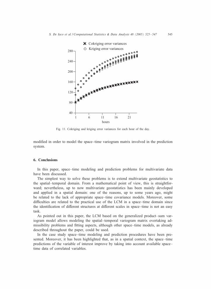
are obtained by space–time cokriging. In Fig. 11 cokriging and kriging error variancesfor each hour of the day and at each monitoring station have been compared. Notethat the well-known relation between cokriging and kriging error variance (ChilLes andDel%ner, 1999) is graphically clear, that is, the cokriging error variance is lower thankriging. Moreover, for both techniques the error variances, as a function of the forecastlead time, show an increasing behaviour.

As regards computational aspects, space–time prediction has been implemented byusing the GSLib routine Cokb3d (Deutsch and Journel, 1998), which has been properly

S. De Iaco et al. / Computational Statistics & Data Analysis 48 (2005) 525–547 545

Fig. 11. Cokriging and kriging error variances for each hour of the day.

modi%ed in order to model the space–time variogram matrix involved in the predictionsystem.

6. Conclusions

In this paper, space–time modeling and prediction problems for multivariate datahave been discussed.

The simplest way to solve these problems is to extend multivariate geostatistics tothe spatial–temporal domain. From a mathematical point of view, this is straightfor-ward; nevertheless, up to now multivariate geostatistics has been mainly developedand applied in a spatial domain: one of the reasons, up to some years ago, mightbe related to the lack of appropriate space–time covariance models. Moreover, somediGculties are related to the practical use of the LCM in a space–time domain sincethe identi%cation of diMerent structures at diMerent scales in space–time is not an easytask.

As pointed out in this paper, the LCM based on the generalized product–sum var-iogram model allows modeling the spatial–temporal variogram matrix overtaking ad-missibility problems and %tting aspects, although other space–time models, as alreadydescribed throughout the paper, could be used.

In the case study space–time modeling and prediction procedures have been pre-sented. Moreover, it has been highlighted that, as in a spatial context, the space–timepredictions of the variable of interest improve by taking into account available space–time data of correlated variables.

546 S. De Iaco et al. / Computational Statistics & Data Analysis 48 (2005) 525–547

As regards computational aspects, it has been necessary to implement personalizedFortran routines. However, advanced and interactive software, which could oMer thepossibility to easily analyze two or more spatial–temporal correlated variables, formodeling and prediction purposes, should be implemented.

References

Brockwell, P.J., Davis, R.A., 1987. Time Series: Theory and Methods. Springer, New York, 577pp.ChilLes, J., Del%ner, P., 1999. Geostatistics. Wiley, New York, 687pp.Christakos, G., 1992. Random Field Models in Earth Sciences. Academic Press, San Diego, CA, 474pp.Christakos, G., Hristopulos, D.T., 1998. Spatiotemporal Environmental Health Modelling—A Tractatus

Stochasticus. Kluwer Academic Press, Boston, MA, 400pp.Cressie, N., 1991. Statistics for Spatial Data. Wiley, New York, 900pp.Cressie, N., Huang, H., 1999. Classes of nonseparable, spatial–temporal stationary covariance functions.

J. Amer. Statist. Assoc. 94 (448), 1330–1340.Daley, R., 1991. Atmospheric Data Analysis. Cambridge University Press, San Diego, CA.De Cesare, L., Myers, E.D., Posa, D., 1997. Spatial–temporal modeling of SO2 in Milan district. In:

Baa%, E.Y., Scho%eld, N.A. (Eds.), Geostatistics Wollongong ’96. Vol. 2. Kluwer Academic Publishers,Dordrecht, pp. 1031–1042.

De Cesare, L., Myers, E.D., Posa, D., 2002. FORTRAN programs for space–time modeling. Comput. Geosci.28 (2), 205–212.

De Iaco, S., Myers, E.D., Posa, D., 2001. Space–time analysis using a general product–sum model. Statist.Probab. Lett. 52 (1), 21–28.

De Iaco, S., Myers, E.D., Posa, D., 2002. Space–time variograms and a functional form for total air pollutionmeasurements. Comput. Statist. Data Anal. 41 (2), 311–328.

De Iaco, S., Myers, E.D., Posa, D., 2003. The linear coregionalization model and the product–sum space–time variogram. Math. Geol. 35 (1), 25–38.

Deutsch, C.V., Journel, A.G., 1998. GSLIB: Geostatistical Software Library and User’s Guide. OxfordUniversity Press, New York, 368pp.

Dimitrakopoulos, R., Luo, X., 1994. Spatiotemporal modeling: covariance and ordinary kriging systems. In:Dimitrakopoulos, R. (Ed.), Geostatistics for the next century. Kluwer Academic Publishers, Dordrecht,pp. 88–93.

Gneiting, T., 2002. Nonseparable, stationary covariance functions for space–time data. J. Amer. Statist. Assoc.97 (458), 590–600.

Goovaerts, P., 1997. Geostatistics for Natural Resources Evaluation. Oxford University Press, Oxford, 487pp.Goovaerts, P., Sonnet, P., 1993. Study of spatial and temporal variations of hydrogeochemical variables

using factorial kriging analysis. In: Soares, A. (Ed.), Geostatistics Troia ’92, Vol. 2. Kluwer AcademicPublishers, Dordrectht, pp. 745–756.

Goulard, M., Voltz, M., 1992. Linear coregionalization model: tool for estimating and choice ofcross-variogram matrix. Math. Geol. 24 (3), 269–286.

Grzebyk, M., 1993. Ajustement d’une corLegionalisation stationnaire. Doctoral Thesis, Ecole de Mines, Paris.Isaaks, E.H., Srivastava, R.M., 1989. Applied Geostatistics. Oxford University Press, Oxford, 561pp.Journel, A.G., Huijbregts, C.J., 1981. Mining Geostatistics. Academic Press, London, 600pp.Journel, A.G., Rossi, M., 1989. When do we need a trend model in kriging? Math. Geol. 21 (7), 715–739.Kyriakidis, P.C., Journel, A.G., 1999. Geostatistical space–time models: a review. Math. Geol. 31 (6),

651–684.Lajaunie, C., BLejaoui, R., 1991. Sur le krigeage des fonctions complexes. Publication N-23/91/g, Centre de

GLeostatistique, Fontainebleau, Paris.Levinson, N., RedheMer, R.M., 1970. Complex Variables. Holden-Day, San Fransisco, CA, 429pp.Matheron, G., 1971. La thLeorie des variables rLegionalisLees et ses applications. Ecole des Mines, Paris,

Fasc. 5.Mardia, K.V., Jupp, P.E., 1999. Directional Statistics. Wiley, London, 429pp.

S. De Iaco et al. / Computational Statistics & Data Analysis 48 (2005) 525–547 547

Myers, E.D., 1982. Matrix formulation of co-kriging. Math. Geol. 14 (3), 249–257.Rouhani, S., Hall, T.J., 1989. Space–time kriging of groundwater data. In: Armstrong, M. (Ed.), Geostatistics,

Vol. 2. Kluwer Academic Publishers, Dordrecht, pp. 639–651.Rouhani, S., Wackernagel, H., 1990. Multivariate geostatistical approach to space–time data analysis. Water

Resour. Res. 36 (4), 585–591.Schaefer, J.T., Doswell, C., 1979. On the interpolation of a vector %eld. Monthly Weather Rev. 107,

458–476.Wackernagel, H., 1998. Multivariate Geostatistics. 2nd Edition. Springer, Berlin, 291pp.Young, D.E., 1987. Random vectors and spatial analysis by geostatistics for geotechnical applications. Math.

Geol. 19 (6), 467–479.