Washington University in St. LouisWashington University Open Scholarship

All Theses and Dissertations (ETDs)

5-24-2010

Modeling And Detection Of Uterine ContractionsUsing MagnetomyographyPatricio La RosaWashington University in St. Louis

Follow this and additional works at: http://openscholarship.wustl.edu/etd

This Dissertation is brought to you for free and open access by Washington University Open Scholarship. It has been accepted for inclusion in AllTheses and Dissertations (ETDs) by an authorized administrator of Washington University Open Scholarship. For more information, please contactdigital@wumail.wustl.edu.

Recommended CitationLa Rosa, Patricio, "Modeling And Detection Of Uterine Contractions Using Magnetomyography" (2010). All Theses and Dissertations(ETDs). Paper 867.

WASHINGTON UNIVERSITY IN ST. LOUIS

School of Engineering and Applied Science

Department of Electrical & Systems Engineering

Dissertation Examination Committee:Dr. Arye Nehorai, Chair

Dr. Hiro MukaiDr. Hubert Preissl

Dr. Jung-Tsung ShenDr. Nan Lin

Dr. R. Martin Arthur

MODELING AND DETECTION OF UTERINE CONTRACTIONS USING

MAGNETOMYOGRAPHY

by

Patricio Salvatore La Rosa Araya

A dissertation presented to the Graduate School of Arts and Sciencesof Washington University in partial fulfillment of the

requirements for the degree of

DOCTOR OF PHILOSOPHY

August 2010Saint Louis, Missouri

ABSTRACT OF THE DISSERTATION

Modeling and Detection of Uterine Contractions using Magnetomyography

by

Patricio Salvatore La Rosa Araya

Doctor of Philosophy in Electrical Engineering

Washington University in St. Louis, August 2010

Research Advisor: Dr. Arye Nehorai

In this dissertation, we develop a novel mathematical framework for modeling and

analyzing uterine contractions using biomagnetic measurements. The study of my-

ometrium contractility during pregnancy is relevant to the field of reproductive as-

sessment. Its clinical importance is grounded in the need for a better understanding

of the bioreproduction mechanisms. For example, in the last decade the number of

preterm labors has increased significantly. Preterm birth can cause health problems

or even be fatal for the fetus if it happens too early, and, at the same time, it im-

poses significant financial burdens on health care systems. Therefore, it is critical to

develop models and statistical tools that help to monitor non-invasively the uterine

activities during pregnancy.

We derive a forward electromagnetic model of uterine contractions during pregnancy.

Existing models of myometrial contractions approach the problem either at an organ

level or lately at a cellular level. At the organ level, the models focus on generating

contractile forces that closely resemble clinical measurements of normal intrauterine

ii

pressure during contractions in labor. At the cellular level, the models focus on pre-

dicting the changes of ionic concentrations in a uterine myocyte during a contraction,

and, as a consequence, on modeling the transmembrane potential evolution as a func-

tion of time. In this work, we propose an electromagnetic modeling approach taking

into account electrophysiological and anatomical knowledge jointly at the cellular,

tissue, and organ levels. Our model aims to characterize myometrial contractions us-

ing magnetomyography (MMG) and electromyography (EMG) at different stages of

pregnancy. In particular, we introduce a four-compartment volume conductor geom-

etry, and we use a bidomain approach to model the propagation of the myometrium

transmembrane potential on the human uterus. The bidomain approach is given by

a set of reaction-diffusion equations. The diffusion part of the equations governs

the spatial evolution of the transmembrane potential, and the reaction part is given

by the local ionic current cell dynamics. Here we introduce a modified version of

the Fitzhugh-Nagumo (FHN) equation for modeling ionic currents in each myocyte,

assuming a plateau-type transmembrane potential. We incorporate the anisotropic

nature of the uterus by considering conductivity tensors in our model. In particular,

we propose a general approach to design the conductivity-tensor orientation and to

estimate the conductivity-tensor values in the extracellular and intracellular domains

for any uterine shape. We use finite element methods (FEM) to solve our model,

and we illustrate our approach by presenting a numerical example to model a uterine

contraction at term. Our results are in good agreement with the values reported in

the experimental technical literature, and these are potentially important as a tool

for helping in the characterization of contractions and for predicting labor.

iii

We propose an automatic, robust, single-channel statistical detector of uterine MMG

contractions. One common restriction of previous techniques is that algorithm pa-

rameters, such as the detection threshold and the window length of analysis need to

be calibrated experimentally, based on a particular data set. Therefore, the detection

performance might change from patient to patient, for example, because of differences

in the pregnancy stage and tissue conductivities. In contrast, the proposed algorithm

does not require the use of a sliding window of analysis, and the detection threshold

is determined analytically; thus, it does not need to be calibrated. Our detection

algorithm consists of two stages: In the first stage, we segment the measurements

using a multiple change-point estimation algorithm and assuming a piecewise con-

stant time-varying autoregressive model of the measurements; In the second stage,

we apply the non-supervised K-means cluster algorithm to classify each time seg-

ment, using the RMS and FOZC as candidate features. As a result a discrete-time

binary decision signal is generated indicating the presence of a contraction. Moreover,

since each single channel detector provides local information regarding the presence

of a contraction, we propose a spatio-temporal estimator of the magnetic activity

generated by uterine contractions. The algorithm, when evaluated with real MMG

measurements, detects uterine activity much earlier than the patient begins to sense

it. It also enables visualizing the relative location of the origin of uterine contraction

and quantifying the amount of energy delivered during a contraction. These results

are important in obstetrics, e.g., as a tool for helping to characterize contractions and

to predict labor.

For the aforementioned problem of multiple change-point estimation, a class of one-

dimensional segmentation, we also compute fundamental mathematical results for

iv

minimal bounds on mean-square error estimation. Indeed, if an estimator is avail-

able, the evaluation of its performance depends on knowing whether it is optimal or

if further improvement is still possible. In our segmentation problem the parameters

are discrete therefore the conventional Cramer-Rao bound does not apply. Hence,

we derive Barankin-type lower bounds, the greatest lower bound on the covariance

of any unbiased estimator, which are applicable to discrete parameters. The compu-

tation of the bound is challenging, as it requires finding the supremum on a finite

set of symmetric matrices with respect to the Loewner ordering, which is not a lat-

tice order. Therefore, we discuss the existence of the supremum, propose a minimal

upper-bound by using tools from convex geometry, and compute closed-form solutions

for the Barankin information matrix for several distributions. The results have broad

biomedical applications, such as DNA sequence segmentation, MEG and EEG seg-

mentation, and uterine contraction MMG detection, and they also have applications

for signal segmentation in general, such as speech segmentation and astronomical

data analysis.

v

Acknowledgments

I am very grateful for being blessed with very joyful years of PhD studies in the

United States of America. I am happy to look back on the path that I have walked,

and remember all the people who, in many different ways, helped me in this journey.

My deepest thanks go to my research advisor and mentor, Professor Arye Nehorai,

for providing me with an exceptional PhD training experience. I am very thankful

to him for his excellent and dedicated guidance in the pursuit of high quality and

state-of-the-art research experiences. During these past years, I have been very much

inspired by his pioneering research work in statistical array signal processing and I

am very grateful for his leading me in performing multidisciplinary research, having

both breadth and depth. I am also thankful for providing me with fruitful teaching

opportunities with graduate and undergraduate students, and especially for all his

constructive feedback and caring which helped me greatly to develop my teaching

skills. His words of wisdom and advice have been an strong help in my process of

personal maturity. I feel fortunate to have been part of his excellent research groups

at the University of Illinois at Chicago (UIC) and later at Washington University in

Saint Louis (WUSTL).

I would like to thank my dissertation committee members, including Dr. Martin

Arthur, Dr. Nan Lin, Dr. Hiro Mukai, Dr. Hubert Preissl, and Dr. Jung-Tsung

Shen, for carefully revising and providing constructive suggestions to this dissertation.

Also, I would like to thank our scientific collaborators, particularly, I thank Dr.

Hary Eswaran and Dr. Hubert Preissl for their feedback and discussions on several

technical aspects of uterine magnetomyography, for kindly hosting my visits to their

research facilities, and for providing us with the experimental measurements used

in this work. I am very grateful to Dr. Carlos Muravchik for our discussions on

several technical aspects of our work about lower bounds on mean-squared error

estimates, and for carefully reviewing several parts of this dissertation. I am grateful

for his encouragement and advice at different stages of my PhD studies. I thank Dr.

Alexandre Renaux for presenting the subject of performance bounds and discussing

its application to the problem of multiple change-point estimation. I enjoyed working

and learning from his expertise during his postdoctoral work at Professor Nehorai’s

vi

lab at WUSTL. I especially thank Prof. Jim Ballard for all his editorial suggestions

on this dissertation.

I convey my sincere gratitude to my UIC instructors, specially to Dr. Dibyen Ma-

jumdar for providing me with a deep foundation in linear and multivariate statistics.

His excellent lectures were very inspiring and beneficial for performing my research

work. I also thank for their dedicated instruction to Dr. Daniel Graupe, Dr. Derong

Liu, Dr. Klaus Miescke, Dr. T. E. S. Raghavan, and Dr. Milos Zefran.

My warm thanks go to my past and present labmates at UIC and WUSTL. Their

friendships and positive spirit towards life in general made our lab a welcoming and

pleasant place to work. In particular, I thank Dr. Tong Zhao, Dr. Gang Shi, Dr.

Jian Wang, and Dr. Nannan Cao for their detailed comments on several parts of my

work and for sharing with me about China and their rich culture. I appreciate very

much their continuous encouragement. I thank Dr. Pinaki Sarder for his long lasting

and warm friendship during all this journey. I am very grateful for his interesting

discussions on several topics and for sharing with me his delicious culinary creations

from India. I cannot forget to thank Mr. Heeralal Choudhary for always looking to

cheer me up with creative jokes and for teaching me several Indian recipes, including

the outstanding masala tea. His friendship and support are very valuable to me. I

also thank Dr. Martin Hurtado, Dr. Marija Nikolic, Mr. Simone Ferrera, Mr. Murat

Akcakaya, Mr. Satyabrata Sen, Ms. Vanessa Tidwell, Mr. Gongguo Tang, Mr. Tao Li,

Mr. Kofi Adu-Labi, Mr. Sandeep Gogineni, and Mr. Phani Chavali, for their scientific

discussions with me and for being very good labmates during all these years.

I would like to thank all the staff members of the Electrical & Systems Engineering

Department: Ms. Rita Drochelman, Ms. Sandra Devereaux, Ms. Elaine Murray, Ms.

Shauna Dollison, Mr. Ed Richter, and Mr. David Goodbary for their time and help.

Last but not least, I offer my sincere appreciation to my parents and my wife for

all their support and love. Their care and encouragement through this journey have

been a vital source of inspiration.

Patricio Salvatore La Rosa Araya

Washington University in Saint Louis

August 2010

vii

AMGD - Dedicated to Salvador and Rosa, my parents, and to Alicia, my wife.

viii

Contents

Abstract . . . . . . . . . . . . . . . . . . . . . . . . . . . . . . . . . . . . . . ii

Acknowledgments . . . . . . . . . . . . . . . . . . . . . . . . . . . . . . . . vi

List of Tables . . . . . . . . . . . . . . . . . . . . . . . . . . . . . . . . . . . xii

List of Figures . . . . . . . . . . . . . . . . . . . . . . . . . . . . . . . . . . xiii

1 Introduction . . . . . . . . . . . . . . . . . . . . . . . . . . . . . . . . . . 11.1 Noninvasive contraction sensing . . . . . . . . . . . . . . . . . . . . . 21.2 Our contributions . . . . . . . . . . . . . . . . . . . . . . . . . . . . . 4

2 Forward Electromagnetic Modeling of Uterine Contractions DuringPregnancy . . . . . . . . . . . . . . . . . . . . . . . . . . . . . . . . . . . 82.1 Introduction . . . . . . . . . . . . . . . . . . . . . . . . . . . . . . . . 8

2.1.1 Uterine microanatomy: . . . . . . . . . . . . . . . . . . . . . . 82.1.2 Uterine contraction models . . . . . . . . . . . . . . . . . . . . 9

2.2 Forward electromagnetic model . . . . . . . . . . . . . . . . . . . . . 132.2.1 Volume conductor model . . . . . . . . . . . . . . . . . . . . . 132.2.2 Extrauterine magnetic field and electrical potential . . . . . . 132.2.3 Current source model . . . . . . . . . . . . . . . . . . . . . . . 162.2.4 Ionic current model . . . . . . . . . . . . . . . . . . . . . . . . 192.2.5 Stimulus current model . . . . . . . . . . . . . . . . . . . . . . 20

2.3 Myometrial conductivity tensors . . . . . . . . . . . . . . . . . . . . . 212.4 Monodomain approximation and boundary conditions . . . . . . . . . 252.5 Numerical computation . . . . . . . . . . . . . . . . . . . . . . . . . . 262.6 Results and discussion . . . . . . . . . . . . . . . . . . . . . . . . . . 282.7 Summary . . . . . . . . . . . . . . . . . . . . . . . . . . . . . . . . . 35

3 Detection of Uterine Contractions Using MMG . . . . . . . . . . . 363.1 Introduction . . . . . . . . . . . . . . . . . . . . . . . . . . . . . . . . 363.2 Model-based time-domain segmentation . . . . . . . . . . . . . . . . . 39

3.2.1 Detection principle . . . . . . . . . . . . . . . . . . . . . . . . 403.2.2 AR-modeling based segmentation . . . . . . . . . . . . . . . . 423.2.3 Performance analysis . . . . . . . . . . . . . . . . . . . . . . . 50

3.3 Classification . . . . . . . . . . . . . . . . . . . . . . . . . . . . . . . 543.3.1 Candidate features . . . . . . . . . . . . . . . . . . . . . . . . 54

ix

3.3.2 Classification algorithm . . . . . . . . . . . . . . . . . . . . . . 563.3.3 Cluster labelling and binary decision signal . . . . . . . . . . . 573.3.4 Performance evaluation . . . . . . . . . . . . . . . . . . . . . . 58

3.4 Experimental results . . . . . . . . . . . . . . . . . . . . . . . . . . . 593.4.1 Data acquisition and preprocessing . . . . . . . . . . . . . . . 593.4.2 Model order estimation, feature evaluation, and cluster labelling 623.4.3 Performance analysis and discussion . . . . . . . . . . . . . . . 65

3.5 Summary . . . . . . . . . . . . . . . . . . . . . . . . . . . . . . . . . 70

4 Performance Bounds on Multiple Change-point Estimation . . . . 734.1 Introduction . . . . . . . . . . . . . . . . . . . . . . . . . . . . . . . . 734.2 Problem formulation . . . . . . . . . . . . . . . . . . . . . . . . . . . 78

4.2.1 Observation model . . . . . . . . . . . . . . . . . . . . . . . . 784.2.2 Barankin bound . . . . . . . . . . . . . . . . . . . . . . . . . . 79

4.3 Barankin bound type for multiple change-point estimation . . . . . . 844.3.1 Diagonal elements of Φ . . . . . . . . . . . . . . . . . . . . . . 854.3.2 Non-diagonal elements of Φ . . . . . . . . . . . . . . . . . . . 854.3.3 Barankin information matrix Φ − 1q×q . . . . . . . . . . . . . 884.3.4 Computation of the supremum . . . . . . . . . . . . . . . . . 93

4.4 Change in parameters of Gaussian and Poisson distributions . . . . . 1014.4.1 Gaussian case . . . . . . . . . . . . . . . . . . . . . . . . . . . 1024.4.2 Poisson case . . . . . . . . . . . . . . . . . . . . . . . . . . . . 107

4.5 Numerical examples . . . . . . . . . . . . . . . . . . . . . . . . . . . . 1084.5.1 Maximum likelihood estimation . . . . . . . . . . . . . . . . . 1084.5.2 Changes in the mean of a Gaussian distribution . . . . . . . . 1094.5.3 Changes in the variance of a Gaussian distribution . . . . . . 1134.5.4 Changes in the mean rate of a Poisson distribution . . . . . . 115

4.6 Summary . . . . . . . . . . . . . . . . . . . . . . . . . . . . . . . . . 119

5 Conclusions and Future Work . . . . . . . . . . . . . . . . . . . . . . . 1205.1 Conclusions . . . . . . . . . . . . . . . . . . . . . . . . . . . . . . . . 1205.2 Future work . . . . . . . . . . . . . . . . . . . . . . . . . . . . . . . . 124

Appendix A Designing Uterine Anisotropy . . . . . . . . . . . . . . . 126

Appendix B Determination of Cα for the SIC Change-point DetectorBased on an AR-model . . . . . . . . . . . . . . . . . . . . . . . . . . . 130

Appendix C Proof of Lemma 1 . . . . . . . . . . . . . . . . . . . . . . 132

Appendix D Computing Elements of the Barankin Information Ma-trix . . . . . . . . . . . . . . . . . . . . . . . . . . . . . . . . . . . . . . . 133

D.0.1 Computing diagonal elements of Φ . . . . . . . . . . . . . . . 133D.0.2 Computing non-diagonal elements of Φ . . . . . . . . . . . . . 134

x

D.0.3 Computing the elements of Φ for changes in mean and covari-ance matrix of Gaussian distribution . . . . . . . . . . . . . . 135

References . . . . . . . . . . . . . . . . . . . . . . . . . . . . . . . . . . . . . 139

Vita . . . . . . . . . . . . . . . . . . . . . . . . . . . . . . . . . . . . . . . . . 148

xi

List of Tables

2.1 Conductivity values of the volume conductor geometry. . . . . . . . . 292.2 Myocyte dimensions and Archie’s law parameters. . . . . . . . . . . . 292.3 Ionic current model parameters. . . . . . . . . . . . . . . . . . . . . . 31

3.1 Dataset Summary c©[2008] IEEE. . . . . . . . . . . . . . . . . . . . 663.2 Average DR, FAR, and CORR computed in channel groups 1, 2, and

3, bandpass filtered in the frequencies ranges 0.1 to 0.4 Hz, and 0.2 to0.4 Hz for d = 0, 1, 2, . . . , 5 with α = 0.01 c©[2008] IEEE. . . . . . . . 67

xii

List of Figures

1.1 (a) A simplified illustration of the sensing array and the uterine MMGfield. (b) The SARA system installed at the University of Arkansasfor Medical Sciences (UAMS) Hospital. (c) 151-channel sensor arrayembedded under the concave surface upon which the patient leans herabdomen. The sensor coils are placed 3 cm apart, covering a total areaof approximately 1350 cm2. . . . . . . . . . . . . . . . . . . . . . . . 4

2.1 Diagram of microanatomy of pregnant human myometrium [1]. Redlines represent current flows. . . . . . . . . . . . . . . . . . . . . . . . 9

2.2 Illustration of the proposed modeling approach. . . . . . . . . . . . . 112.3 Representation of the four-compartment volume conductor geometry

and the forward electromagnetic problem of uterine contractions. . . . 142.4 Illustration of the bidomain modeling approach. . . . . . . . . . . . . 172.5 Four-compartment volume conductor geometry used in the numerical

examples. (a) View of z-x plane, and (b) z-y plane. Each compartmentis assigned a different color. The myometrium has a non-uniform colorto denote that its conductivity is anisotropic. . . . . . . . . . . . . . . 28

2.6 Geometry and fiber orientation in spherical myometrium given by α =45o. . . . . . . . . . . . . . . . . . . . . . . . . . . . . . . . . . . . . . 30

2.7 FEM solution at time instants t = 10 [s], 36 [s], 55 [s] for one pacemakeron the fundus of a spherical myometrium, assuming anisotropy. (a)-(c) transmembrane potential and source current density distribution atthe myometrium, (d)-(f) electrical potential at the abdominal surface,and (g)-(i) magnetic field density at the abdominal surface. . . . . . . 33

2.8 (a) Temporal response of FEM solutions for transmembrane poten-tial at different elevations; (b) Percentage of contracting myometrialvolume as a function of time. . . . . . . . . . . . . . . . . . . . . . . 34

3.1 A diagram of the proposed single channel detector to detect uterinecontractions, using MMG. . . . . . . . . . . . . . . . . . . . . . . . . 39

3.2 (a) Computed probability of false alarm (PFA) and asymptotic PFA asa function of γ for n = 100 and n = 1000 samples. (b) The receiveroperating characteristic (ROC) for different change points. (c) ROCfor different ǫ values. (d) ROC for different sample sizes. c©[2008]IEEE. . . . . . . . . . . . . . . . . . . . . . . . . . . . . . . . . . . . 52

xiii

3.3 (a) Average value of the detection delay as a function of the changepoint for n = 100, α = 0.01, and ǫ = 1, 2, and 4. (b) Average valueof the detection delay as a function of the change point for n = 100,ǫ = 2, and α = 0.005, 0.01, 0.02, and 0.03. (c) Probability of detection(PD) as a function of the change point for n = 100, α = 0.01, and ǫ= 1, 2, and 4. (d) PD as a function of the change point for n = 100,ǫ = 2, and α = 0.005, 0.01, 0.02, and 0.03. c©[2008] IEEE. . . . . . . 53

3.4 (a) SARA system installed at the University of Arkansas for MedicalSciences (UAMS) Hospital. (b) 151-channel sensor array embeddedunder the concave surface upon which the patient leans her abdomen.The sensor coils are placed 3 cm apart, covering a total area of approx-imately 1350 cm2. (c) Diagram of sensor array with channels identi-fication numbers. The circles indicate the groups of channel G1, G2,and G3. c©[2008] IEEE. . . . . . . . . . . . . . . . . . . . . . . . . . 60

3.5 Power spectral density (PSD) computed using Welch’s method on sam-ples from channels 2, 50, and 120 obtained from six different patientswith gestational ages between 38 and 40 weeks. c©[2008] IEEE. . . . 62

3.6 Bandpass filtered records from channel 2 of patient 6 with a gestationalage of 40 weeks: (a) Preprocessed channel with grid lines indicatingthe estimated change points for d = 1 and α = 0.01; (b) RMS in eachtime segment; (c) FOZC in each time segment; (d) cluster groups usingRMS features; (e) estimated contraction segments; (f) time segmentswith contractions according to the patient feedback. c©[2008] IEEE. . 65

3.7 Illustration of our distributed processing approach for analyzing thearray of temporal-spatial detection signals obtained after applying thealgorithm for detecting uterine contractions in each MMG channel. . 68

3.8 From left to right: total RMS and percentage of active sensors asa function of time for patients 1, 5, and 6. The time interval of acontraction according to the patients’ feedback is indicated by the highlevel of the pulse train in each figure, respectively. Note that the pulseamplitude is just for illustration purposes. c©[2008] IEEE. . . . . . . 70

3.9 Snapshots of the reconstructed measurement surface from patient 6masked with the binary decision signals in the frequency band 0.2 to0.4 Hz. The time selected coincides with the presence of a contraction,according to the patient’s feedback. c©[2008] IEEE. . . . . . . . . . . 71

4.1 (a) Case of overlapping; (b) Case of no overlapping. . . . . . . . . . . 874.2 Illustration of Lowner-John ellipsoid of a set formed by three ellipsoids

in which two are maximal elements of the set. . . . . . . . . . . . . . 99

xiv

4.3 Performance analysis for estimating change-points of the mean in aGaussian distribution: (a) Mean values as a function of sample timefor different SNR values; (b) Test points associated with the BB givenby the minimal-upper bound of C, BBsup, as a function of SNR; (c)MSE of the change-point vector using the MLE of t and its Barankinbound given by BBsup, and by the matrix with maximum trace inC, BBtr; (d) MSE of each change-point as a function of SNR usingthe MLE of t1, t2, and t3 and their corresponding Barankin boundBBsup(ti), i = 1, . . . , 3; (e) MSE of change-point vector using the MLEof t and its Barankin bound, BBsup(t), as a function of the distancebetween t2 and t1 for SNR = −6 [dB]; (f) MSE of each change-pointand their respective BBsup as a function of the distance between t2and t1 for SNR = −6 [dB]. c©[2010] IEEE. . . . . . . . . . . . . . . . 110

4.4 Performance analysis for estimating change-points of the variance ina Gaussian distribution: (a) Sigma-parameter values as a function ofsample time for different SNR values; (b) Test points associated withthe BB given by the minimal-upper bound of C, BBsup, as a functionof SNR; (c) MSE of the change-point vector using the MLE of t and itsBarankin bound given by BBsup; (d) MSE of each change-point as afunction of SNR using the MLE of t1, t2, and t3 and their correspond-ing Barankin bound BBsup(ti), i = 1, . . . , 3; (e) MSE of change-pointvector using the MLE of t and its Barankin bound, BBsup(t), as afunction of the distance between t2 and t1 for SNR = 4 [dB]; (f) MSEof each change-point and their respective BBsup as a function of thedistance between t2 and t1 for SNR = 4 [dB]. c©[2010] IEEE. . . . . 116

4.5 Performance analysis for estimating change-points in the mean rate ofa Poisson distribution distribution: (a) Mean-rate-values as a functionof sample time for different SNR values; (b) Test points associated withthe BB given by the minimal-upper bound of C, BBsup, as a functionof SNR; (c) MSE of the change-point vector using the MLE of t and itsBarankin bound given by BBsup; (d) MSE of each change-point as afunction of SNR using the MLE of t1, t2, and t3 and their correspond-ing Barankin bound BBsup(ti), i = 1, . . . , 3; (e) MSE of change-pointvector using the MLE of t and its Barankin bound, BBsup(t), as afunction of the distance between t2 and t1 for SNR = −6 [dB]; (f)MSE of each change-point and their respective BBsup as a function ofthe distance between t2 and t1 for SNR = −6 [dB]. c©[2010] IEEE. . . 118

xv

A.1 Simplified illustrations of a3(r) with respect to the local coordinatesaxis given by n(r), t1(r), t2(r). The blue plane contains the vectors

n(r), k(r), and t1(r), and it is perpendicular to the gray plane formedby vectors t1(r), t1(r) and a3(r). The orange plane is the cross section

of the uterus perpendicular to the vector drC(t)dt

∣∣∣t0

. The gray curve is

the curve of symmetry rC (t) with rC (t1) and rC (t2) extreme pointsof the curve. . . . . . . . . . . . . . . . . . . . . . . . . . . . . . . . . 128

xvi

Chapter 1

Introduction

Assessment of fetal health is important to reduce perinatal mortality and morbidity.

It is based on the prediction, detection and management of fetal malformations,

disorders of growth in utero, and premature labor. Labor is the physiologic process

that results in the expulsion of the fetus and placenta from the uterus via the cervix

and vagina [2]. The occurrence of labor begins with the appearance of periodic

contractions which, in general, change the intrauterine-pressure to the point that

cervix dilatation is manifested. However, from clinical experience, not all uterine

contractions lead to a completion of labor, in which case the process is referred to as

false labor. Labor is expected to occur after the 37th week of pregnancy, but in the

last decade, the number of preterm labors has increased significantly. Preterm birth

can cause health problems or even be fatal for the fetus if it happens too early, and,

at the same time, it imposes significant financial burdens on health care systems [3].

In general, it is well accepted that monitoring the frequency and intensity of the

uterine activity provides sensitive information for distinguishing between false and

true labor [4]. However, there are no objective methods for consistently assessing the

efficiency of contractions and thus reliably predicting pre-term labor. Therefore, a

1

better understanding of the mechanisms behind uterine contractions would allow for

developing more effective ways to predict and control the occurrence of labor. We

claim that this understanding can be achieved by developing the following:

• Non-invasive sensing devices with high spatio-temporal resolution for imaging

functionalities of the uterus

• Physical models that interrelate system properties at the organ, tissue, and

cellular imaging levels

• Efficient statistical algorithms for solving the imaging problems at each level.

In the following we will describe non-invasive techniques for sensing uterine activity.

Our contributions will be specific to physical modeling and statistical algorithms for

analyzing uterine contractions.

1.1 Noninvasive contraction sensing

Uterine contractions can be described by their mechanical and electrophysiological

aspects. A mechanical contraction is manifested as a result of stimulation, which

results in propagation of electrical activities in the uterine muscle, and appears as

an intrauterine pressure change. Different techniques have been developed to quan-

tify uterine contractions, such as tocography (TOCO), electrohysterography (EHG)

or electromyography (EMG), and magnetomyography (MMG). TOCO measures the

strength of the force the uterine muscle exerts on the abdominal wall, using an exter-

nal mechanical method, and the contractions are recorded using tensometric trans-

ducers attached to the patient’s abdomen. This technique is attractive because it

2

is noninvasive and simple, but it is of limited value due to its low sensitivity and

accuracy [5].

EMG and MMG are functional imaging techniques of the bioelectromagnetic type.

They reconstruct and image current density distributions associated with the elec-

trophysiological activity of muscles, using either electrical potential or magnetic field

measurements or both. The uterine EMG measures the action potentials of the my-

ometrium cells, using either internal electrodes or abdominal surface electrodes [6,7].

This technique has a high temporal resolution and has captured attention in the past

decade, in particular filtering techniques have been developed for noise and artifacts

suppression and for time-frequency characterization of the EMG waveforms [6–11].

However, because of differences in the conductivities of tissue layers, the uterine EMG

signals get filtered during their propagation to the surface of the maternal abdomen.

The uterine MMG is a non-invasive technique that measures the magnetic fields as-

sociated with muscle action potentials. The first MMG recordings were reported

by Eswaran et al. in 2002 [5], using a 151-channel non-invasive device, known as

the superconducting quantum interference device array for reproductive assessment

(SARA). They established the feasibility of recording uterine contractile activities

with a spatial-temporal resolution high enough to determine localized regions of ac-

tivation and propagation through the uterus. Unlike electrical recordings, magnetic

recordings are independent of any references, thus ensuring that each sensor mainly

records localized activities. However, MMG is of limited applicability because it is

expensive (in the range of $ 2 - 3 million dollars) and non-portable.

3

(a) (b) (c)

Figure 1.1: (a) A simplified illustration of the sensing array and the uterine MMGfield. (b) The SARA system installed at the University of Arkansas for MedicalSciences (UAMS) Hospital. (c) 151-channel sensor array embedded under the concavesurface upon which the patient leans her abdomen. The sensor coils are placed 3 cmapart, covering a total area of approximately 1350 cm2.

1.2 Our contributions

In this dissertation, we propose a forward electromagnetic model of uterine contrac-

tions during pregnancy [12, 13], derive statistical algorithms for automatic detection

of uterine contractions based on time-series segmentation and an unsupervised clus-

tering approach [14, 15], and derive performance bounds for the class of unbiased

model-based segmentation algorithms [16, 17].

Physical model: Having an electromagnetic model of uterine contractions is rele-

vant to predicting and interpreting uterine activity using MMG and EMG measure-

ments. In particular, our model aims to describe the electrophysiological aspects

of uterine contractions during pregnancy at both the cellular and the organ levels.

We introduce a four-compartment volume conductor geometry and use a bidomain

4

approach [18, 19] to model the propagation of the myometrium transmembrane po-

tential. The bidomain approach is given by a set of reaction-diffusion equations.

The diffusion part of the equations governs the spatial evolution of the transmem-

brane potential, and the reaction part is given by the ionic current cell dynamics

locally. Assuming a plateau-type transmembrane potential, we introduce a modified

version of the Fitzhugh-Nagumo (FHN) equation [20–22] for modeling ionic currents

in each myocyte, and we incorporate the anisotropic nature of the uterus by designing

conductivity-tensor fields. In particular, we propose a general approach to design the

conductivity-tensor orientation and to estimate the conductivity-tensor values in the

extracellular and intracellular domains for any uterine shape. We use finite element

methods (FEM) to solve our model, and we illustrate our approach by presenting a

numerical example to model a uterine contraction at term. Our results are in good

agreement with the values reported in the experimental technical literature, and these

are potentially important as a tool for helping in the characterization of contractions

and for predicting labor.

Statistical detection of uterine contractions: Biomagnetic measurements obtained us-

ing the aforementioned SARA system contain the electrophysiological activities of

several organs in the vicinity of the abdomen, as well as the fetus. Therefore, to ana-

lyze uterine contractions, it is necessary to first filter out non-desired signals from the

measurements, and also to detect the time span in which the contraction takes place.

In our work, we propose a distributed processing framework to process the measure-

ments from an array of magnetometers. Our method is based on a single-channel,

two-stage statistical detector of uterine contractions that is robust and automatic.

Unlike in previous approaches, the proposed detection algorithm does not require

the use of a sliding window of analysis, and the detection threshold is determined

5

analytically. In the first stage, we propose a model-based segmentation procedure,

which detects multiple change-points in the parameters of a piecewise constant time-

varying autoregressive model using a robust formulation of the Schwarz information

criterion (SIC) and a binary search approach. We compute and evaluate the relative

energy variation [root mean square (RMS)] in discriminating between time segments

with and without contractions. Thus, in the second stage, we apply a nonsupervised

K-means cluster algorithm to classify the detected time segments using the RMS

values. We validate our method using real MMG measurements and compare the

detected time intervals with the patients’ feedback. This method proves to be helpful

in understanding the uterine MMG contraction activity spatially and temporally.

Performance bounds on model-based segmentation algorithms: The literature is abun-

dant concerning estimation algorithms for change-point estimation (see, e.g., [23–25]).

However, less work has been done concerning the ultimate performance of such algo-

rithms in terms of mean-square error (MSE). Indeed, if an estimator is available, the

evaluation of its performance depends on knowing whether it is optimal or if further

improvement is still possible. Unfortunately, for discrete time-measurement models,

as in our aforementioned time-series segmentation problem, the change-point location

parameter is discrete, therefore the Cramer-Rao bound [26] is not applicable. Con-

sequently, we focus on computing the Barankin bound (BB) [27], the greatest lower

bound on the covariance of any unbiased estimator, which is still valid for discrete pa-

rameters. To the best of our knowledge, performance bounds have never been derived

in the multiple change-point context. In our work, we compute the multi-parameter

version of the Hammersley-Chapman-Robbins, which is a Barankin-type lower bound

in the context of an independent vector sequence. The computation of the BB re-

quires finding the supremum of a finite set of positive definite matrices with respect

6

to the Loewner partial ordering. Although each matrix in this set of candidates is

a lower bound on the covariance matrix of the estimator, the existence of a unique

supremum for this set, i.e., the tightest bound, might not be guaranteed. To overcome

this problem, we compute a suitable minimal-upper bound on this set given by the

matrix associated with the Lowner-John Ellipsoid of the set of hyper-ellipsoids asso-

ciated to the set of candidate lower-bound matrices. We present numerical examples

to compare the proposed approximated BB with the performance achieved by the

maximum likelihood estimator.

The organization of this dissertation is as follows: In Chapter 2, basic uterine anatomy

is discussed, and the electromagnetic modeling of uterine contractions is presented.

In Chapter 3, our automatic algorithm for detecting uterine contraction using MMG

measurements is derived. In Chapter 4, the performance bounds for time-series seg-

mentation algorithms are computed. Finally, in Chapter 5, we summarize the contri-

butions of this dissertation and discuss future work.

7

Chapter 2

Forward Electromagnetic Modeling

of Uterine Contractions During

Pregnancy

2.1 Introduction

In the following chapter we will describe the details of our physical model of the

electromagnetic activity associated to uterine contractions. We begin by discussing

briefly the uterine microanatomy and previous uterine contraction models.

2.1.1 Uterine microanatomy:

The adult uterus is a thick walled, hollow, muscular organ formed by three lay-

ers: the external serous perimetrium, the myometrium, and the inner mucous en-

dometrium [28]. The myometrium is responsible for contractions and it is formed by

fasciculi which comprise sheet-like and cylindrical bundles of myocytes embedded in

8

a connective tissue matrix [1]. The myocytes in a cylindrical bundle contract, thus

shortening the smooth tissue and increasing uterus wall tension, hence increasing the

intrauterine pressure. Fig. 2.1 illustrates the microanatomy of the pregnant human

myometrium.

Figure 2.1: Diagram of microanatomy of pregnant human myometrium [1]. Red linesrepresent current flows.

The uterine microanatomy is consistent with action potential propagation [1]: (i)

myocytes are densely packed within a bundle, (ii) bundles are contiguous within a

fasciculus, and (iii) fasciculi are contiguous via communicating bridges formed with

myocytes. In addition, the uterine changes during gestation is accompanied by the

formation of gap junctions which are one of the mechanisms for coordinated trans-

mission of contractile activity from cell to cell [1, 28]. The structure of the fasiculata

within the uterus has not yet been well defined, but generally it makes the propagation

of the action potential anisotropic [29, 30].

2.1.2 Uterine contraction models

Uterine contractions can be described by their mechanical and electrophysiological

aspects. A mechanical contraction is manifested as a result of the excitation as well

9

as the propagation of electrical activities in the uterine muscle, and appears in the

form of an intrauterine pressure increase.

Existing models approach the problem separately at organ level [31, 32], or lately

at a cellular level [33–35]. At the organ level, the models focus on predicting the

contractile forces that closely resemble clinical measurements of normal intrauterine

pressure during contractions in labor. In [31], the authors assume that the uterus

is a hollow ovoid formed by discrete contractile elements that propagate electrical

impulses, generate tension, and have defined contracting and refractory periods. The

envisioned mechanism for intercellular communication is based on action potential

propagation, which is simulated by using a discrete state model for each cell. In [32],

the author uses a discrete state model for combining two mechanisms of intercellular

communication, namely, action potential propagation and intercellular calcium wave

propagation. However, in both [31] and [32], mathematical and physical descriptions

of their models are not provided. On the other hand, at a cellular level, the mod-

els focus on predicting the changes of ionic concentrations in the intracellular and

extracellular mediums during a contraction, and, as a consequence, on modeling the

transmembrane potential evolution of a myocyte as a function of time. In [33, 34] a

model is developed to simulate the complete process of a single myometrial smooth

muscle contraction, which is initiated by depolarization. The model is based on the

electrophysiological properties of a myocyte, and on the cellular mechanisms that

relate the rise in concentration levels of intracellular ion calcium C2+a to stress pro-

duction.

In this work, we propose a forward electromagnetic model of human myometrial con-

tractions during pregnancy taking into account electrophysiological and anatomical

knowledge jointly at the cellular, tissue, and organ levels. Our model aims to helping

10

Figure 2.2: Illustration of the proposed modeling approach.

in the characterization of contractions and for predicting labor using MMG [5] and

EMG [36]. Here we extend our partial results presented in [12]. Fig. 2.2 illustrates the

different levels considered in our modeling approach. In particular, our approach is

two fold: first, we model the current source density at the myometrium, using models

of myocyte electrophysiological activity and anisotropic conductivity; And second,

we solve the forward electromagnetic problem, namely, we compute the magnetic

field and the action potential at the abdominal surface generated by the myometrial

current-source density, using Maxwell’s equations subject to a volume conductor ge-

ometry. To model the current source density at the myometrium we propose to apply

a bidomain approach. The bidomain equations is a set of reaction-diffusion equa-

tions derived first for modeling the current sources of the myocardium as a function

of the cardiac-myocyte transmembrane potential, and these equations proved to be a

successful approach to study heart functioning [18,19]. The diffusion part of the equa-

tions governs the spatial evolution of the transmembrane potential, and the reaction

part is given by the ionic current cell dynamics locally. Here we introduce a modified

version of the FitzHugh-Nagumo (FHN) equation for modeling ionic currents in each

11

myocyte. Though FHN does not consider explicitly the Ca2+ dynamics, the simplicity

of the FHN model makes it an attractive candidate for modeling the propagation of

depolarization waves in large 2D and 3D simulations as in the numerical examples

presented in this work. We propose a general approach to design conductivity-tensor

orientation for any uterine shape. We estimate the conductivity-tensor values in the

extracellular and intracellular domains, using Archie’s law [37] and an analytical ex-

pression of the transmembrane potential propagation speed, derived in this work, as

a function of the model parameters.

The notational convention adopted in this paper is as follows: italic font indicates

a scalar quantity, as in a; lowercase boldface indicates a vector quantity, as in a,

except for vector fields used in Maxwell’s equations such as electric field E, magnetic

field B, and current density J ; upper case italic indicates a matrix quantity, as in

A. The matrix transpose is indicated by a superscript “T ” as in AT , and the identity

matrix of size n× n is denoted In. The set Sn denotes the vector space of symmetric

n × n matrices and the subsets of nonnegative definite matrices and positive definite

matrices are denoted by Sn+ and Sn

++, respectively. The inner product and norm

defined in the Euclidean space is denoted by 〈·, ·〉 and ‖·‖, respectively.

This chapter is organized as follows: Section 2.2, describes the volume conductor

geometry of the problem and the forward electromagnetic model; Section 2.3, presents

the current source model based on the bidomain equations; Section 2.4 describes our

approach for modeling the myometrial conductivity tensors. Section 2.5 , introduces

the monodomain approximation, boundary conditions, and numerical computations

of our model; Section 2.6 presents the numerical examples and discussion; And in

Section 2.7 a summary of the chapter is provided.

12

2.2 Forward electromagnetic model

In this section we discuss the forward electromagnetic model of myometrial contrac-

tions. We will introduce a four-compartment volume conductor model formed by

an anisotropic bidomain myometrium, and we will present the expressions for the

extrauterine electrical potential and magnetic field, respectively.

2.2.1 Volume conductor model

Fig. 2.3 illustrates the four-compartment volume conductor geometry for our problem,

where A represents the abdominal cavity and ∂A the boundary surface defined by

the abdomen, M represents the myometrium, and ∂M and ∂U are its external and

internal boundary surfaces, respectively. The volume denoted by U represents the

space filled with amniotic fluid which exists between the internal uterine wall ∂U and

the boundary ∂F defined by the fetus volume F . The vectors r and r′

indicate the

positions of the observation point and source, respectively, with respect to the main

axis of reference.

2.2.2 Extrauterine magnetic field and electrical potential

The electromagnetic analysis of uterine contractions can be derived by solving a set

of Maxwell’s equations [38] subject to given boundary conditions given by the vol-

ume conductor geometry. Moreover, since common bioelectrical phenomena contain

mostly frequencies below 1 KHz and the characteristic length scale is much larger

than the diameter of the uterus, it is suitable to use the quasi-static approximation of

13

Figure 2.3: Representation of the four-compartment volume conductor geometry andthe forward electromagnetic problem of uterine contractions.

Maxwell’s equations. Therefore, the extrauterine magnetic field B(r, t) at a position

r and instant t is given as follows:

∇× 1

µo

B(r, t) = J(r, t), (2.1)

where µo is the permeability of the free space and J (r, t) is the total current density

(in A/m2). J (r, t) is given by

J (r, t) = J s (r, t) + G (r)E (r, t) , (2.2)

where J s (r, t) is the uterine current density source, and G (r)E (r, t) is the conduc-

tion current density (or return currents), as described by Ohm’s law, with E (r, t)

14

the electric field established by J s (r, t) and G (r) ∈ S3++ is the conductivity tensor

defined by each compartment. Then from the quasi-static conditions, ∇·J (r, t) = 0,

so ∇ ·G (r)E (r, t) = −∇ ·J s (r, t). Moreover, since ∇×E (r, t) = 0, it follows that

E (r, t) = −∇φ (r, t), where φ (r, t) denotes the potential. Thus, the equation that

governs the relationship between the electromyogram potentials and uterus current

sources is

∇ · G (r)∇φ (r, t) = ∇ · J s (r, t) . (2.3)

Therefore, solving the forward electromagnetic problem of uterine contractions implies

computing B(r, t) and φ (r, t) at ∂A using Eqs. (2.1) and (2.3) assuming known

J s (r, t) in M and G (r) in all the domain defined by the volume conductor geometry

(see Fig. 2.3).

The biological current sources J s (r, t) in the myometrium are the transmembrane

ionic fluxes, due to concentration gradients, which flow across the surface membrane

of the myocyte (smooth cells) from the extracellular medium into the intracellular

medium and vice versa. The density of these ionic currents is also referred to as

impressed current density since its origin is non electrical in nature, and it is the pri-

mary cause for the establishment of an electric field which induces secondary density

currents in a conductive domain. We will model J s (r, t) using a bidomain approach,

which has proved to be a successful method to study electrophysiological activity in

the myocardium [18,19].

15

2.2.3 Current source model

In the myometrium both the intracellular and extracellular domains are physically

connected through membrane gates, and the intracellular domain is connected though

gap junctions [28, 36]. Therefore, we model the myometrium using the bidomain

modeling approach. This approach represents the tissue (myometrium) as two inter-

penetrating extra-intracellular continuous domains, with different conductivity values

along and across the direction of the fiber [18,19], and it models the tissue using the

generalized-passive cable equation. The bidomain modeling approach was originally

derived for modeling the propagation of the transmembrane potential of the my-

ocardium and proved to be a successful approach to study heart functioning [18,19].

Fig. 2.4 shows a simplified illustration of the tissue and the bidomain approach, where

φi (r, t) and φe (r, t) are the intracellular and interstitial potentials, respectively, and

vm (r, t) = φi (r, t)−φe (r, t) is transmembrane potential. The conductivity tensors in

the intracellular and extracellular domains are denoted by G′

i and G′

e (in S/m), and,

using Ohm’s law, the current densities in each domain are given by J i,e (r, t) = −G′

i,e

∇φi,e (r, t) . The transmembrane volume current density in (A/m3) is denoted by

jm (r, t) and is given by

jm (r, t) = am cm∂vm

∂t+ jion − jstim, (2.4)

= am

(cm

∂vm

∂t+ J ion − J stim

), (2.5)

where jion (r, t) is the ionic volume current density (in A/m3) of a myocyte, jstim (r, t)

is the stimulus volume current density (in A/m3), cm is the membrane capacitance

per unit area (in F/m2), and am is the surface-to-volume ratio of the membrane (in

1/m).

16

Figure 2.4: Illustration of the bidomain modeling approach.

Applying conservation of charges to both domains, we obtain the following relation-

ships:

∇ · J e (r, t) = jm (r, t) , and (2.6)

∇ · J i (r, t) = −jm (r, t) . (2.7)

Adding (2.6) and (2.7), we have that ∇ · (J i (r, t) + J e (r, t)) = 0. Hence, the total

current density in the myometrium is given by

J (r, t) = −G′

i∇φi (r, t) − G′

e∇φe (r, t) , r ∈ M, (2.8)

which can be expressed in terms of vm (r, t) and φe (r, t) as follows:

J (r, t) = −G′

i∇vm (r, t) − G′

M∇φe (r, t) , r ∈ M, (2.9)

where G′

M =(G

′

e + G′

i

)∈ S

3++ is the bulk myometrium conductivity tensor. Since

spatial variations of vm (r, t) depend on the local establishment of a transmembrane

current density, jm (r, t) 6= 0, then we define the impressed current-density source

17

as J s(r, t) = −G′i∇vm(r, t). Note that J s(r, t) exists only when the spatial gradi-

ent exists, i.e., only in a region where the myometrium is undergoing depolarization

(excitation) or repolarization.

The total current at the myometrium J (r, t) depends on the spatio-temporal varia-

tions of vm (r, t) and φe (r, t) , which are governed by the system of equations formed

by Eqs. (2.4), (2.6) and (2.7). Using simple algebraic manipulations, the aforemen-

tioned system of equations can be written in terms of vm (r, t) and φe (r, t) only,

obtaining the following equivalent expressions:

∇ · G′i∇(vm (r, t) + φe (r, t)) = am

(cm

∂vm (r, t)

∂t+ J ion (r, t) − J stim (r, t)

),(2.10)

∇ · (G′i + G′

e)∇φe (r, t) = −∇ · G′i∇vm (r, t) . (2.11)

This set of reaction-diffusion equations is also known as bidomain equations [18,

19]. The diffusion part of the equations governs the spatial evolution of both the

transmembrane and extracellular potentials, and the reaction part is given by the

local ionic current cell dynamics. The solutions for vm (r, t) and φe (r, t) depend

on J ion (r, t), J stim (r, t), and the conductivity tensors, in addition to boundary and

initial conditions. Since our goal is to model the propagation of the electrical activity

in the myometrium, we are interested in the class of traveling wave solutions of

these equations which waveform depends on J ion (r, t) and its initiation depends

on J stim (r, t). In what follows, we describe the models for both current densities

J ion (r, t) and J stim (r, t), respectively.

18

2.2.4 Ionic current model

The predominant type of transmembrane-potential waveforms measured in the human

myometrium are spike and plateau [28, 39, 40]. In this work, we focus on modeling

the plateau-type transmembrane potential, as it has been more frequently observed

[28,39–41]. Therefore, we model J ion (r, t) , using a variation of the FitzHugh-Nagumo

(FHN) equations [20–22], as follows:

J ion(r, t) = − 1

ǫ1

(k (vm − v1) (v2 − vm) (vm − v3) − w) , and (2.12)

∂w

∂t= ǫ2 (βvm − γw + δ) , (2.13)

where ǫ1, ǫ2, k, v1, v2, v3, δ, γ, and β are model constants, and w (in V) is a state

variable of the model. The parameter ǫ1 (in Ωm2) controls the sharpness of the

leading and trailing edges of the action potential waveform: the smaller ǫ1 is, the

more vertical the edge is. Note that ǫ1 has unit of resistivity, therefore the smaller

its value the larger the membrane permeability to ionic flux. The parameter ǫ2 (in

s−1) controls the action potential duration: the smaller ǫ2, the longer it takes a cell

to recover. The parameters v1, v2, v3 (in V), and k (in 1/V2) control the range

of vm(r, t). Note that for a given set of parameters values k, v1, v2, v3 and γ, the

parameters β and δ (in V) control the excitability threshold of the cell. The larger β,

the lower the excitability threshold setting the cell dynamic to an oscillatory stable

behavior between resting and exciting states. Over a certain value, the cell dynamic

becomes bistable; namely, if the cell starts from a resting potential, it changes to an

excited state and remains there. On the other hand, a very negative β value results

in a permanent resting state. In Section Results and Discussion we select the model

parameters using phase-space analysis, and using as a reference the transmembrane

19

potentials recorded from isolated human myometrial strips at term [33, 40]. This

model does not consider explicitly the C2+a dynamics, and, moreover, it assumes that

changes in the intra- and extra-cellular ion concentrations are insignificant even after

several depolarizations. However, its simplicity facilitates modeling the propagation

of depolarization waves in large 2D and 3D domains.

2.2.5 Stimulus current model

We also introduce a temporal-spatial model for J stim, representing the stimulus due

to pacemaker areas [28, 36], as follows:

J stim(r, t) =1

ǫ1

Np∑

i=1

νihi(r, t), (2.14)

where hi(r, t) is a spatio-temporal function with range in [0, 1], νi is the amplitude

(in V), and Np is the number of pacemaker areas. Intuitively, the former should

modify the excitability of the cell at a certain instant of time based on the threshold

value. In particular, our model assumes that the uterine myocyte can act as either

a pacemaker or pace-follower, namely, the spontaneous electrical behavior exhibited

by the myometrium is an inherent property of the uterine myocyte (see [36] for more

details.) Note that the size, duration, and intensity of the pacemaker area need to be

chosen such that a stable traveling waveform solution to the bidomain equations on

the myometrium is granted.

20

2.3 Myometrial conductivity tensors

The structure of the fasiculata within the uterus has not been well-defined, but it

generally runs in a structured organization [29, 30]. In [29] the authors investigated

the global fiber architecture of the non-pregnant uterus by magnetic resonance (MR)

diffusion tensor imaging (DTI). From the ex-vivo analysis of five non-pregnant uteri,

the authors identified an inner circular layer around the uterine cavity on slices or-

thogonal to the long axis of the organ. In the regions outside the inner circular layer,

they could not identify a global structure, but did find several locally aligned groups

of fibers. At the level of the cervix, they found an outer circular layer and an inner

region with mostly longitudinal components. In the following we will introduce an

approach for designing the conductivity tensors in the myometrium.

Assume that the conductivity tensors are diagonal in a local coordinate system

which is defined with respect to each myocyte and characterized by the unit vec-

tors e1, e2, e3. In particular, Gi and Ge are diagonal matrices ∈ S3++ given by

Gi =

σix 0 0

0 σiy 0

0 0 σiz

, Ge =

σex 0 0

0 σey 0

0 0 σez

. (2.15)

In order to take into account variable fiber orientation in the myometrium, we need to

describe it in a global Cartesian coordinate system in which the local basis is defined

at any point r as A= [a1(r), a2(r), a3(r)] where a3(r) is parallel to the main fiber

axis. The representation of the tensors Gi and Ge in terms of a global coordinate

21

system is given by

G′i = AGiA

T , G′e = AGeA

T . (2.16)

Assuming that the myocyte fiber conductivities in both domains have a cylindrical

symmetry, then σex = σey = σet, σix = σiy = σit, σiz = σil, and σez = σel. Therefore,

the conductivity tensors can be expressed as follows [42]:

G′i = (σil − σit) a3(r)aT

3 (r) + σit I3, and (2.17)

G′e = (σel − σet)a3(r)aT

3 (r) + σet I3. (2.18)

Hence, to construct the conductivity tensors as a function of r, because of the cylin-

drical symmetry assumption, it is enough to define the vector field a3(r) in each

location of the anisotropic domain, as well as the conductivity values σil and σel. To

design a3(r) at each point r, we represent the uterus as a hollow volume with uniform

thickness, and we describe it by the union of mutually disjoint closed surfaces or lay-

ers. We use the implicit definition of a surface, namely, the set of points r satisfying

f(r) = 0. Then, at each point r, we define a set of local orthonormal coordinates

axes given by n(r), t1(r), t2(r), where n(r) = ∇f(r)‖∇f(r)‖ is the normal vector to the

layer containing r, and t1(r) and t2(r) are mutually orthogonal vectors which belong

to the tangent plane of the respective layer at point r. We define t1(r) and t2(r),

using as a reference the curve of symmetry of the uterine inner-circular layer [29].

This curve goes from the fundus to the cervix, and it coincides with the long axis

of the non-pregnant uterus (see Appendix A for more details on the computation of

t1(r) and t2(r)). Hence, given t1(r) and t2(r), we define a3(r) as follows:

a3(r) = t1(r) cos (α) + t2(r) sin (α) , (2.19)

22

where α is the fiber orientation angle with respect to t1(r).

To the best of our knowledge, values of the intracellular and extracellular conductivity

tensors have not been reported for the human myocyte, and therefore, these have

to be estimated. To estimate the extracellular conductivity values σel and σet, we

assume a grid-type distribution of myocytes in the myometrium and use an estimate of

the extracellular conductivity the human myometrium obtained by applying Archie’s

law [37]. Human myocytes can be best be described as long cylinders with diameter

dcell and axis length lcell, such that dcell ≪ lcell. Assuming that myocytes are uniformly

arranged in a cubical grid whose length lT = lcell + 2∆e and whose cross section has

sides dT = dcell + 2∆e, then we have that σel and σet are given as follows:

σel = σe

(1 − π

(dcell

2

)2

d2T

), and (2.20)

σet = σe

(1 − dcelllcell

dTlT

), (2.21)

where σe is the conductivity of the extracellular medium in the myometrium. σe

can be computed using the effective myometrium conductivity σM, available in the

literature, and Archie’s law [37] as follows:

σe =σM

(1 − p)m , (2.22)

with p the volume fraction occupied by the myocytes and collagenous fibers in the

tissue, and m the so-called cementation factor, which depends on the shape and

orientation of the myocyte in the tissue.

23

To compute the intracellular conductivities σil and σit, we assume that the intracel-

lular and extracellular domains have equal anisotropy ratios, i.e.,

Gi = ςGe, (2.23)

and thus we need to compute ς . We obtain an analytical expression for ς, using

reported values of the propagation speed of a transmembrane potential waveform

traveling on isolated tissue strips from pregnant human myometrium at term [41].

In particular, replacing (2.23), (2.12), and (2.13) in the bidomain equations (2.10)

and (2.11), and solving vm (r, t) for a traveling wave solution vm (ξ · r−c t) , with

ξ a unitary vector pointing along the main axis of the myocyte and c the speed of

propagation, we obtain the following expression for ς:

ς = g

(2 c2ǫ1am c2

m

σel k (v∗1 − 2 v∗

2 + v∗3)

2

), (2.24)

where g (x) = x1−x

. Further, v∗1, v∗

2 , and v∗3 are the roots of the following polynomial

in vm:

f (vm) = (vm − v1) (v2 − vm) (vm − v3) −1

kγ(βvmr + δ) , (2.25)

with vmr the resting transmembrane potential of the human myocyte. Note that in

order to ς ≥ 0, then ǫ1 has to satisfy the following inequality:

0 < ǫ1 <σel k (v∗

1 − 2 v∗2 + v∗

3)2

2 c2am c2m

. (2.26)

24

2.4 Monodomain approximation and boundary con-

ditions

The equal anisotropy ratio assumption, Eq. (2.23), simplifies the solution of the

bidomain equations (2.10) and (2.11) by decoupling them as follows:

∇ · ς

(ς + 1)G′

e∇vm(r, t) = am

(cm

∂vm(r, t)

∂t+ J ion(r, t) − J stim(r, t)

), in M,(2.27)

∇ · (ς + 1)

ςG′

e∇φe(r, t) = −∇ · G′e∇vm(r, t), in M. (2.28)

The above simplification is also known as the monodomain approximation of the

bidomain equations, which, under suitable boundary conditions, allows to computing

vm and, thus, J s, independent from φe.

To set boundary conditions for computing electrical potentials, we need to take into

account the volume conductor geometry (see Fig. 2.3 ). In particular, we have two

bidomain-monodomain interfaces: One between the myometrium M and abdomi-

nal volume A, and one between the myometrium and the intrauterine cavity U .

Therefore, we have the following boundary conditions, namely, (i) continuity of the

interstitial potential φe at the perimetrium surface ∂M to the abdomen potential

φA, (ii) flow of the normal component of J that crosses over from the uterus to the

abdominal medium, (iii) no flow of the normal component of J s to the abdominal

medium, (iv) continuity of the interstitial potential φe at the endometrium surface

∂U to the intrauterine cavity potential φU (v) flow of the normal component of J that

crosses over from the uterus to the intrauterine cavity filled with amniotic fluid, (vi)

no flow of the normal component of J s to the intrauterine cavity, (vii) no flow of the

normal component of J that crosses over from the abdominal cavity to air, and (viii)

25

no flow or flow of the normal component of J that crosses over from the intrauterine

cavity, filled with amniotic fluid, to the fetus depending if it is covered with vernix

caseosa (λ = 0) or not (λ = 1) [43]. These boundaries conditions are summarized as

follows:

φe(r, t) = φA(r, t), in ∂M, (2.29)

nM · (G′i∇φi(r, t) + G′

e∇φe(r, t)) = nM · GA∇φA(r, t), in ∂M, (2.30)

nM · G′i∇vm(r, t) = 0, in ∂M, (2.31)

φe(r, t) = φU(r, t), in ∂U (2.32)

nU · (G′i∇φi(r, t) + G′

e∇φe(r, t)) = nU · GU∇φU(r, t), in ∂U , (2.33)

nU · G′i∇vm(r, t) = 0, in ∂U , (2.34)

nA · GA∇φA(r, t) = 0, in ∂A (2.35)

nF · GU∇φU(r, t) = λ (nF · GF∇φF (r, t)) , in ∂F , (2.36)

where nj is the normal vector to the surface j in each case.

2.5 Numerical computation

The computation of vm (r, t), φ (r, t), and B(r, t) are given by the following proce-

dure:

26

• Step 1: Solve for vm(r, t) using Eqs. (2.27), (2.12), (2.13), and (2.14) subject

to boundary conditions (2.31) and (2.34), and to initial conditions given by

vm(r, 0) = vmr, (2.37)

wm(r, 0) =

(β

γvmr +

δ

γ

), (2.38)

∂vm(r, 0)

∂t= 0, and (2.39)

∂wm(r, 0)

∂t= 0. (2.40)

• Step 2: Solve for φe(r, t) in M and φ(r, t) in A and U , using the solution of

vm(r, t), computed in Step1, and the following expressions:

∇ · (ς + 1)

ςG′

e∇φe(r, t) = −∇ · G′e∇vm(r, t), in M, (2.41)

∇ · GA∇φ(r, t) = 0, in A, (2.42)

∇ · G′U∇φ(r, t) = 0, in U , (2.43)

subject to boundary conditions (2.29), (2.30), (2.32), (2.33), (2.35), and (2.36).

• Step 3: Solve for B(r, t) using Eq. (2.1), and computing the total current

density J(r, t) in all the domain using the solutions of vm(r, t), φe(r, t), and

φ(r, t), obtained in Steps 1 and 2.

To compute the solution in each of the above steps, we use the FEM solver COMSOL

Multiphysics running on a server with 8 64-bit processors at 2.3GHz, with 32 Gb

RAM.

27

2.6 Results and discussion

In the following we illustrate our modeling approach by considering the electrophysio-

logical and anatomical characteristics of the uterus at term. In Figure 2.5 we illustrate

the four-compartment volume conductor geometry used in the numerical examples.

We defined a spherical myometrium of 16 cm radius measured from the center to ∂M

and the uterine wall has a uniform thinness of 1 cm. We also consider an spherical

fetus of 12 cm radius concentric to the myometrium fully covered with vernix caseosa,

i.e., λ = 0 in (2.36). The adnominal compartment is also spherical with 21 cm radius

shifted −3 cm from the center of the myometrium in the x axis. We set the coordinate

axis of reference at the center of the myometrium.

(a) (b)

Figure 2.5: Four-compartment volume conductor geometry used in the numerical ex-amples. (a) View of z-x plane, and (b) z-y plane. Each compartment is assigned adifferent color. The myometrium has a non-uniform color to denote that its conduc-tivity is anisotropic.

The conductivity values for each compartment are given in Table 2.1. In particular,

to compute the extracellular myometrial conductivity tensors, we use average values

28

for the uterine myocyte dimensions at term based on data reported in [1, 28, 32] (see

Table 2.2). The average human myocyte can be best described as a long cylinder

with a small cross section, therefore, we use a cementation factor m = 4/3 (see [37]

for more details on the computation of this factor). The volume fraction p occupied

by myocytes and collagenous fibers in the myometrium is set equal to 0.6. In order to

consider an average myometrial fiber architecture, which ranges between circular and

oblique fibers, we choose the fiber orientation angle α to be 45o. Figure 2.6 illustrates

the global structural of the myometrial fiber orientation for this angle.

Table 2.1: Conductivity values of the volume conductor geometry.

Symbol Value ReferenceGA 0.2 S/m [43]GU 1.74 S/m [43]GF 0.2 S/m [43]σel 0.68 S/m Eq. (2.20)σet 0.22 S/m Eq. (2.21)ς 0.8 Eq. (2.24)

Table 2.2: Myocyte dimensions and Archie’s law parameters.

Symbol Value Referencedcell 7 µm [28]lcell 450 µm [28]dT 8 µmlT 451 µmσM 0.5 S/m [43]m 4/3 [1, 37]p 0.6 [29, 37]

We select the model parameters of the ionic current model using phase-space analysis,

and using as a reference the average plateau-type transmembrane potentials recorded

from isolated tissue strips of human myometrium at term [33, 40]. In particular, the

29

Figure 2.6: Geometry and fiber orientation in spherical myometrium given by α = 45o.

average resting potentials, considering the results reported from the 37th weeks of

pregnancy onwards, is approximately −56 mV. The plateau has an average depolar-

ization of −27±1 mV that terminates in 0.9±0.2 minutes by an abrupt repolarization

to the resting level [33, 40]. Table 2.3 has the parameter values used in the numer-

ical example. Note that we compute the surface-area to volume-ratio am using the

myocyte dimensions in Table 2.2.

In [36] has been indicated that in the human uterus there may be a preferential

direction of propagation of contractions, and thus of transmembrane potential prop-

agation, from the fundus toward the isthmus, which could aid in the expulsion of the

fetus. Therefore, in order to study this assumption with our model, we consider jstim

30

Table 2.3: Ionic current model parameters.

Symbol Value Referencecm 0.01 F/m2 [43]vmr −0.056 V [40]am 5.7587105 m−1 Table 2.2ǫ1 200 ω m2

ǫ2 0.09 1/sv1 −0.02 Vv2 −0.04 Vv3 −0.065 Vk 104 1/V2

δ 0.0520 Vγ 0.1β 1c 1.15 cm/sec [41]

with Np = 1, ν1 = 2 V, and h1(r , t) as follows:

h1(r , t) = 1, if 0 ≤ t ≤ 0.1 , 0.15 ≤ ‖r‖ ≤ 0.16 and z ≥ 0.15 ; 0, otherwise.

The size and intensity of the pacemaker area are chosen in order to obtain a stable

traveling waveform solution to the bidomain equations on the spherical myometrium.

Figs. 2.7 show several snapshots of the FEM solution for one pacemaker on the fundus

of a spherical myometrium, assuming anisotropy given by Fig. 2.6. Figs. 2.7 (a)-(c)

illustrate the transmembrane potential and source current density distribution at the

myometrium, Figs. 2.7 (d)-(f) the electrical potential at the abdominal surface, and

Figs. 2.7 (g)-(i) the magnetic field density at the abdominal surface. The magnetic

field measured at the abdominal surface, BMMG, is proportional to BnA, the projec-

tion of B onto the normal vector of the abdominal surface, nA. Note that, because of

the anisotropy in the conductivity, the direction of the current density J s is rotated

31

on a certain angle from the main direction of the propagating transmembrane poten-

tial vm, and it is the transversal component of this current, parallel to the x-y plane,

which generates the magnetic field BnA. This observation is in agreement with the

analysis presented in [44] and it is important to take it into account when interpreting

the magnetic field measurements generated by uterine contractions in the presence of

volume conductor geometry. Therefore, the spatial signature of BnAis highly depen-

dent on the fiber orientation of the myometrium. Because of the proximity between

the sensors and the myometrium, it is not strictly applicable to assume a moving

dipole parallel to the direction of propagation of the transmembrane potential, as the

main model for the current source generated the measured magnetic field. This last

interpretation might be suitable in case the transversal length of the transmembrane

potential front is short in com-parison to the area covered by the array of sensors. In

contrast, if the transversal length is larger and thus no covered by the measured area,

for example when several cells are recruited, then it suitable to consider a moving

line source (stretched ring) model instead.

In Fig. 2.8 (a) we illustrate the temporal response of FEM solutions for the transmem-

brane potential at different elevations at times. It can be seen that a stable traveling

waveform has been established as the shape remains same. Also, the maximum depo-

larization is −16 mV, the average potential in the plateau area is of −25 mV, and the

transmembrane potential duration, before hyperpolarization, is around 35 s, which is

a fair approximation with respect to the average recorded transmembrane potentials

discussed in [33,40]. Note that our ionic current model introduces hyperpolarization,

which constrains the excitability of the cell and, thus, consecutive contractions can

only take place until vm reaches resting potential. In our case, the minimum time be-

tween two consecutive contractions is 240 s. In Fig. 2.8(b) we illustrate the percentage

32

Time = 10 [sec] Time = 10 [sec] Time = 10 [sec]

(a) (d) (g)Time = 36 [sec] Time = 36 [sec] Time = 36 [sec]

(b) (e) (h)Time = 55 [sec] Time = 55 [sec] Time = 55 [sec]

(c) (f) (i)

Figure 2.7: FEM solution at time instants t = 10 [s], 36 [s], 55 [s] for one pacemaker onthe fundus of a spherical myometrium, assuming anisotropy. (a)-(c) transmembranepotential and source current density distribution at the myometrium, (d)-(f) electricalpotential at the abdominal surface, and (g)-(i) magnetic field density at the abdominalsurface.

33

0 20 40 60 80 100−0.07

−0.06

−0.05

−0.04

−0.03

−0.02

−0.01

Time [sec]

Transmembrane potential [V]

z=0.1240

z=0.1075

z=0.738

0 20 40 60 80 1000

0.1

0.2

0.3

0.4

0.5

0.6

0.7

0.8

0.9

1

Time sec

Percentage

myometrial volume contracting

(a) (b)

Figure 2.8: (a) Temporal response of FEM solutions for transmembrane potential atdifferent elevations; (b) Percentage of contracting myometrial volume as a functionof time.

of contracting myometrial volume as function of time, which in [31, 32] was used as

a reference to compute the changes in the intrauterine pressure due to a contraction.

Interestingly, we observe that the percentage of myometrial cell contracting has the

symmetric properties and length of the intrauterine pressure waveforms of human

pregnant myometrium at term, as discussed in [32]. Note that a larger ǫ2 value can

extend the transmembrane potential duration to values closer to the average duration

reported on [33, 40], however, it also extends the duration of hyperpolarization and

the plateau of the curve describing the percentage of contracting myometrial volume.

34

2.7 Summary

We proposed a forward electromagnetic model of uterine contractions during preg-

nancy. Our model incorporates knowledge of the electrophysiological aspects of the

uterine contractions during pregnancy at both the cellular and organ levels. We

applied a bidomain approach for modeling the propagation of the myometrium trans-

membrane potential vm on the uterus and used this to compute the action potential

φ and the magnetic field B at the abdominal surface. We introduced a modified

version of the FitzHugh-Nagumo equation for modeling the ionic currents in each

cell. Though our ionic current model does not consider explicitly C2+a dynamics, the

simplicity of the FitzHugh-Nagumo allows for capturing the nuances of the uterine

myocyte response, but it can be used to model the propagating action potential under

well defined conditions as shown in this paper. We also proposed a general approach

to design conductivity tensors in the myometrium and to estimate the conductivity

tensor values in the extracellular and intracellular domains. We introduced a sim-

plified geometry for the problem and proposed a discretized model solution based

on a finite element method approach. Finally, we illustrated our modeling approach

through a numerical example modeling a uterine contractions at term. Our model is

potentially important as a tool for helping in the characterization of contractions and

for predicting labor using MMG and EMG.

35

Chapter 3

Detection of Uterine Contractions

Using MMG1

3.1 Introduction

As we elaborated in Chapter 1, the analysis of uterine contractions during pregnancy

is clinically important for predicting labor [6,45]. Therefore, an automated method to

detect uterine contractions can be very helpful in the clinical evaluation of a patient.

Detection of uterine contractions has been performed in the past using either a single

EHG channel [9–11,46] or an array of MMG channels [47]. Among these references, we

find time domain and multiresolution domain analyses. In the time-domain analysis,

the uterine contractions are detected by applying a discrimination rule (threshold)

on the values of a function (feature) evaluated in a sliding time window. For exam-

ple, using EHG measurements, the authors in [48] discriminate the root mean square

(RMS) values using an experimental threshold. In [9] the authors discuss the feasibil-

ity of using the first-order zero-crossing (FOZC) as a feature. However, no threshold

1Based on P. S. La Rosa, A. Nehorai, H. Eswaran, C. Lowery, and H. Preissl, “Detection of uterineMMG contractions using a multiple change point estimator and the K-means cluster algorithm,”IEEE Trans. on Biomedical Engineering, Vol. 55, pp. 453-467, Feb. 2008. c©[2008] IEEE.

36

for detection is provided. In [11], the authors discriminate the RMS values using an

adaptive threshold level, determined by applying a moving-media average filter on an

overlapping sliding window of EHG measurements. In [47] the authors propose to use

the generalized synchronization index as an indicator of uterine contractions, using

an array of MMG channels.

In a multiresolution analysis, a single EHG measurement is represented in a higher

dimensional linear space, which is formed by decomposing the signal into several

subspaces spanned by a set of basis functions [49]. For example, in [46] a single channel

EHG measurement is decomposed using a set of biorthogonal wavelet functions, and

the contraction is detected using a two-stage algorithm. In the first stage, the authors

design a multivariable sequential cumulative likelihood ratio test to sequentially detect

changes in the covariance matrix of the decomposed signal. Then, in the second

stage, the diagonal parameters of the covariance matrices are classified using a neural

network trained by an expert. As with the time-domain techniques, to detect changes

in the parameters, the segmentation stage of this multiresolution approach requires

setting up a time window as well as a threshold level. Also, the basis functions

(wavelets) are selected based on the average performance obtained in the classification

stage.

One common restriction of the above techniques is that the time-window length, as

well as the threshold level, is determined experimentally based on a particular data

set. In general the selection of the time-window length depends on the length of the

shortest event to be detected, on the global detection delay, and on the number of

samples required to properly estimate the hypothesis parameters [46]. Therefore, the

detection performance might change from patient to patient because of, for example,

differences in the pregnancy stage, tissue conductivities, etc.

37

In this chapter we propose a single channel two-stage time-segment discriminator

of uterine-contraction magnetomyograms (MMGs). In the first stage, we propose

a model-based segmentation procedure, which detects multiple change-points in the

parameters of a piecewise constant time-varying autoregressive model using a robust

formulation of the Schwarz information criterion (SIC) and a binary search approach.

This novel segmentation technique does not require the use of a sliding window as

in previous work. In particular, we propose a test statistic that depends on the

SIC, derive its asymptotic distribution, and obtain closed-form optimal detection

thresholds in the sense of the Neyman-Pearson criterion; therefore, we control the

probability of false alarm and maximize the probability of change-point detection

in each stage of the binary search algorithm. Then, in the second stage, we apply

the non-supervised K-means cluster algorithm to classify each time segment, using

the RMS and FOZC as candidate features. Finally, we provide a discrete-time binary

decision signal indicating the presence of a contraction. We validate our method using

real MMG measurements and compare the detected time intervals with the patient’s

feedback. Since each single channel detector provides local information regarding the

presence of a contraction, we also analyze the fusion of the decision signals from all

the sensors, as in the parallel distributed detection approach. As we illustrate with

real data, this approach proves to be helpful in understanding uterine-contraction

MMGs spatially and temporally. Figure 3.1 illustrates the proposed single channel

scheme to estimate the contraction intervals.

This chapter is organized as follows: in Section II we present the model-based time-

domain segmentation method and analyze its performance; in Section III we define

the feature space and describe the classification method. We discuss the performance

38

Figure 3.1: A diagram of the proposed single channel detector to detect uterinecontractions, using MMG.

of our algorithm using real MMG data in Section IV, and summarize our results in

Section V.

3.2 Model-based time-domain segmentation

Let y(t), t = 1, . . . , n be the samples of an MMG measurement acquired from a

position close to the abdominal surface of the patient, where n is the number of

total samples. Let x(t) = f(y(1), y(2), . . . , y(l)) for l ≤ n, t = 1, . . . , n, be the

preprocessed measurement, where f : Rl 7→ R is a function defined over the MMG

samples. In our case, f represents the downsampling followed by a bandpass filtering.

Using the central limit theorem, we assume that the distribution of the preprocessed

samples’ amplitudes is Gaussian with unknown mean and variance. Also, as shown in

[50,51], EMG measurements can be considered as a series of stationary segments with

Gaussian distributed amplitudes. Therefore, we design a time-series segmentation

algorithm that detects multiple change points in the distributions parameters.

39

3.2.1 Detection principle

The statistical problem of segmentation can be formulated as follows: assuming that

(i) x(t) is a piecewise stationary real process so that there exist instants t′i, i > 0

such that (x(t′i + 1), . . . , x(t′i+1)) is stationary ∀ i ∈ N. Assume that the probability

distribution of the samples between t′i + 1 and t′i+1 belongs to the same family of

distributions P(θ), where θ ∈ Rm are the unknown parameters. Then our problem

consists of detecting changes in the distribution of x(t), 1 ≤ t ≤ n associated with

changes in θ. Therefore, we apply a statistical test looking for changes in θ. Usually

the statistical inference about change points has two aspects: the first is to detect

if there is any change in the sequence of random variables observed, and the second

is to estimate the number of change points and their corresponding locations. In

particular, the statistical inference of the change-point problem consists of testing

the following hypotheses:

H0 : θ(1) = θ(2) = · · · = θ(n) = θ0, (3.1)

H1 : θ(1) = · · · = θ(t′1) 6= θ(t′1 + 1) = · · · = θ(t′2) 6= · · · 6= θ(t′q + 1) = · · · = θ(n),

(3.2)

where θ is the unknown parameter vector, q is the unknown number of the change

points, and 1 < t′1 < t′2 < · · · < t′q < n are the unknown positions of the change points.

Therefore, our problem is to estimate the set of change points t′1, . . . , t′q. Note that in

our case, we assume that all the data are available, and thus our detection approach

is offline or, at best, has a delay of n.

The problem of detecting multiple change points has been addressed by means of a

binary segmentation procedure in [52, 53]. Essentially, this approach simplifies the

40

general problem by evaluating iteratively the alternative hypothesis of detecting a

single change point in the parameter. It can be described as follows. First, detect a

single change. If there is no change, then the null hypothesis is accepted. If there

is a change, then the estimated change point divides the original sequence into two

subsequences. For each subsequence, detect a change as in the first step, and continue

the process until no more changes can be found in any of the subsequences. Using

the above approach, the alternative hypothesis becomes

H1 : θ(1) = · · · = θ(t′0) = θ1 6= θ(t′0 + 1) = · · · = θ(n) = θ2. (3.3)

Here we estimate the change point t′0 using the Schwarz information criterion (SIC)2

[55], which is defined as

SIC(τ) = −2 ln(L(θτ )) + mτ ln(n), τ = 1, . . . , n (3.4)

where L(·) is the likelihood function of the samples, θτ is the maximum likelihood

estimation of θτ = [θ1, θ2] (assuming a change point at sample t = τ ), and mτ = 2m

is the number of unconstrained parameters in the model under H1 of (3.3), with

t′0 = τ . The case τ = n corresponds to the situation without a change point, thus,

θτ = [θ0] and mτ = m. The SIC has been applied in [53] to estimate the change

points of the variance of a normal distribution. They preferred using the SIC over

the AIC, because the minimum of the SIC among the possible models has been

proved to be an asymptotically unbiased estimator of the model order of the true

model [53, 55], which makes this criterion appropriate for designing a change point

test [53]. Hence, the decision to accept H0 or H1 is based on the principle of the

minimum information criterion. Thus H0 is accepted if SIC(n) ≤ minτ SIC(τ), and

2SIC is a modification of the Akaike information criterion (AIC) proposed by Akaike in 1973 [54].

41

H0 is rejected if SIC(n) > SIC(τ) for some τ . In the latter case the change point t′0

is estimated by t′0 such that

SIC(t′0) = minm<τ<n−m−1

SIC(τ), (3.5)

where SIC(n) is the SIC under H0, SIC(τ ) is the SIC under H1 for τ = m+1, . . . , n−

m − 1, and m is the total number of unconstrained parameters under H0. Note that

τ is constrained to the set m < τ < n−m− 1 so that we can compute the maximum

likelihood estimates of the parameters, and n > 2m + 1.

The SIC approach for testing change points does not require resorting to the dis-

tribution of the test statistic [53] as in the classical testing procedures, such as the

generalized likelihood ratio test. If the SIC values are very close, then it is of in-

terest to test if this difference is caused by data fluctuation when there is actually

not change. To avoid misleading change-point detections, in [53] a robust SIC-based

change-point detector is proposed. We will derive a test for the same purpose but

based on a time-varying AR-model of the preprocessed measurements x(t).

3.2.2 AR-modeling based segmentation

Assume that we model the time series x(t) using a stable autoregressive (AR) model

of fixed known order d, with time-varying coefficients; driven by a zero-mean white

Gaussian process with time-varying variance. Let x(t), 1 ≤ t ≤ n be the sequence

of preprocessed measurements. Then

x(t) = ϕ1(t)x(t − 1) + . . . + ϕd(t)x(t − d) + ϕ0(t) + w(t), (3.6)

42

or equivalently

w(t) = x(t) − ΦT (t) xt−d,t, (3.7)

where xβ,υ = [x(β), x(β + 1), . . . , x(υ), 1]T , β < υ, Φ(t) = [ϕd(t), . . . , ϕ1(t), ϕ0(t)]T ,

and w(t) is a zero-mean Gaussian process with variance σ2(t). Then, we test the

following hypothesis,

H0 : φ(1) = φ(2) = · · · = φ(n) = φ0, (3.8)

H1 : φ(1) = · · · = φ(t′1) 6= φ(t′1 + 1) = · · · = φ(t′2) 6= · · · 6= φ(t′q + 1) = · · · = φ(n),

(3.9)

where φ(t) = [ϕd(t), · · · , ϕ1(t), ϕ0(t), σ2(t)]T is unknown, q is the unknown number

of change points, and 1 < t′1 < t′2 · · · < t′q < n are the unknown instants of the

change points. Hence, our problem is to estimate the set of change points t′1, · · · , t′q.

Accordingly, using the binary search procedure, the alternative hypothesis becomes

H1 : φ(1) = · · · = φ(t′0) = φ1 6= φ(t′0 + 1) = · · · = φ(n) = φ2. (3.10)

Let xβ,υ = [x(β), x(β + 1), . . . , x(υ)]T , where β < υ. We approximate the likelihood

function of the n samples under both hypotheses by considering the n − d samples

conditioned on the d initial values. This approximation allows us to obtain closed form

solutions for the maximum likelihood estimates of the parameters and to reduce the

computational complexity of the algorithm. Therefore, under H0, the approximate

43

likelihood function is given by

L(φ0|H0) = Pr[xd+1,n|x1,d]

=1

(2 π σ20)

n−d2

exp

−1

2 σ20

n∑

t=d+1

(x(t) − ΦT0 xt−d,t)

2

. (3.11)

Then the approximate log likelihood is

ln L(φ0|H0) = −n − d

2ln(2πσ2

0)

− 1

2 σ20

Φ0

TRx,x(d + 1, n)Φ0 − 2Φ0T rx,x(d + 1, n) +

n∑

t=d+1

x2(t)

,

(3.12)

where rx,x(d + 1, n) ∈ Rd+1×1 with rx,x(d + 1, n) =∑n

t=d+1 xt−d,tx(t), and Rx,x(d +

1, n) ∈ Rd+1×d+1 with Rx,x(d + 1, n) =∑n

t=d+1 xt−d,txTt−d,t. Then, the maximum

likelihood estimates σ20 and Φ0 are obtained by equating to zero the derivatives of

(3.12) with respect to σ20 and Φ0, respectively, and are given by

σ20 =

∑nt=d+1(x(t) − ΦT

0 xt−d,t)2

n − dand Φ0 = Rx,x(d + 1, n)−1 rx,x(d + 1, n).

(3.13)

Now, replacing the concentrated likelihood (i.e., the likelihood function written, when

possible, as a function of a particular parameter) as a function of σ20 in (3.4) with

mn = d + 2, we have the SIC(n) given by

SIC(n) = (n − d) ln(2π) + (n − d) ln(σ20) + (n − d) + (d + 2) ln (n). (3.14)

44

Under H1, considering a change point at time τ , we obtain the likelihood function as

L(φ1, φ2|H1) = Pr[xd+1,n|x1,d]

= Pr[xd+1,τ |x1,d] Pr[xτ+1,n|xτ−d+1,τ ], (3.15)

where

Pr[xd+1,τ |x1,d] =1

(2 π σ21)

τ−d2

exp

−1

2 σ21

τ∑

t=d+1

(x(t) − ΦT1 xt−d,t)

2

, (3.16)

and

Pr[xτ+1,n|xτ−d,τ ] =1

(2 π σ22)

n−τ2

exp

−1

2 σ22

n∑

t=τ+1

(x(t) − ΦT2 xt−d,t)

2

. (3.17)

Then, applying the natural logarithm to (3.15), we have

ln L(φ1, φ2|H1) = −n − d

2ln(2π) − τ − d

2ln(σ2

1) −n − τ

2ln(σ2

2) −

1

2 σ21

Φ1

TRx,x(d + 1, τ)Φ1 − 2Φ1T rx,x(d + 1, τ) +

τ∑

t=d+1

x2(t)

−

1

2 σ22

Φ2

TRx,x(τ + 1, n)Φ1 − 2Φ1T rx,x(τ + 1, n) +

n∑

t=τ+1

x2(t)

,

(3.18)

where the maximum likelihood estimates σ21 and Φ1 are given by (3.13) by substituting

n = τ , and σ22 and Φ2 are given by

σ22 =

∑nt=τ+1(x(t) − ΦT

2 xt−d,t)2

n − τand Φ2 = Rx,x(τ + 1, n)−1 rx,x(τ + 1, n).

(3.19)

45

Then replacing the concentrated likelihood as a function of σ21 and σ2

2 in (3.4) with

mn = 2(d + 2), the SIC(τ ) is given as follows,

SIC(τ) = (n− d) ln(2π) + (τ − d) ln(σ21) + (n− τ) ln(σ2

2) + (n− d) + 2 (d + 2) ln (n),

(3.20)

and the change point t′0 is estimated by t′0 such that

SIC(t′0) = mind+2<τ≤n−d−3

SIC(τ ). (3.21)

Then, for improving the robustness in detecting a change-point, the hypothesis H0 is

accepted when SIC(n) < mind+2<τ≤n−d−3 SIC(τ) + γ, where γ is a threshold value to

be determined. Let λSIC be the test statistic defined as

λSIC = SIC(n) − mind+2<τ≤n−d−3

SIC(τ )

= maxd+2<τ≤n−d−3

SIC(n) − SIC(τ). (3.22)

Then H0 or H1 is accepted if

λSIC

H1

TH0

γ. (3.23)

Hence, if we know the probability function of λSIC, we can determine an optimal

γ = Cα using, for example, the Neyman-Pearson criterion as follows,

Pr [λSIC < Cα|H0] = 1 − α, (3.24)

where α is the significance level of the test. One possibility to determine the proba-

bility distribution of λSIC under H0 would be to estimate it empirically (histogram)

46

using Monte Carlo simulations. However, the test statistic depends on the sample

size, which is not fixed, and it also depends on the binary search procedure; there-

fore, we would have to compute a histogram for all possible sample sizes, which is

impractical. Here, for 2d+1 < τ ≤ n− d− 3, we obtain and apply an approximation

of the distribution of λSIC under H0 as follows (see Appendix B for details on the

derivation),

Pr [λSIC < Cα|H0] ∼= exp

(−2 exp−

(Cα + (d + 2) ln(n) − bn(d + 2)

2 an(d + 2)

)),(3.25)

where

bn(x) =2 ln ln(n) + x/2 ln ln ln(n) − ln(Γ(x/2))2

2 ln ln(n)(3.26)

an(x) =

√( bn(x)

2 ln ln(n)

), (3.27)

and

λSIC = max2d+1 <τ≤n−d−3

(n − d) ln(σ20) − (τ − d) ln(σ2

1) − (n − τ ) ln(σ22) − (d + 2) ln(n).

(3.28)

Therefore, applying the above approximation in (3.24) we find that α and Cα are

related as follows,

Cα(m, n) ≈ bn(m) − 2an(m)ln(2) − ln ln((1 − α)−1)

− (m) ln(n), (3.29)

where m = d+2. The constant Cα(m, n) depends on the sample size n, the significance

level α, and the number of parameters m. Note that, if n < 3d + 4, then the given

47

segment is not tested for changes and H0 is accepted. The binary search procedure

is finalized when the hypothesis H0 is accepted for all time segments.

Remark - Here, we derived a robust SIC change-point test to detect changes in the

distribution of the preprocessed measurements x(t). In particular, we assumed that

the preprocessed samples are modelled by a piecewise time-varying autoregressive

(AR) model of order d with input given by a white Gaussian noise with time-varying

variance. We also consider the special case assuming that the AR model order is zero,

and thus x(t), 1 ≤ t ≤ n is a sequence of independent zero-mean normal random

variables.

Special case

Assume that d = φ0 = 0 in (3.6). Then x(t), 1 < t < n is a sequence of

independent zero-mean normal random variables with parameters σ2(1), σ2(2), . . .,

σ2(n). Hence, our problem is reduced to looking for changes in the variance of a

sequence of independent normal random variables. Similarly, the multiple change-

point problem is given by (3.8) with φ(t) = [σ2(t)], and the alternative hypothesis

becomes as in (3.10). The SIC for H0 is

SIC(n) = n ln(2π) + n ln(σ20) + n + ln n, (3.30)

and for H1 is

SIC(τ ) = n ln(2π) + τ ln(σ21) + (n − τ) ln(σ2

2) + n + 2 ln n, (3.31)

48

where σ2 =∑n

i=1 x2i /n, σ2

1 =∑τ

i=1 x2i /τ , and σ2

2 =∑n

i=τ+1 x2i /(n − τ ) are the maxi-

mum likelihood estimators under H0 and H1, respectively. The test statistic for this

problem is

λSIC = max1<τ≤n−2

SIC(n) − SIC(τ) . (3.32)

The approximate distribution of λ under H0 is given by (3.25) with m = 1, and the

approximate threshold value is Cα(1, n).

Model order estimation

The model order d in (3.6) is typically unknown and needs to be estimated. A

possible information criterion approach to estimate the model order is by minimizing

the overall SIC, which is the SIC computed on x(t), 1 ≤ t ≤ n using the estimated

change points for a given set of d values. It is given by

SICT = −2 ln(L(θd(t′1), . . . , θd(t

′u + 1))) + (u + 1) (d + 2) ln(n), (3.33)

where θd(t′i), i = 1, . . . , u + 1 is the maximum likelihood estimate of θd(t

′i) using the

estimated change points t′1, . . . , t′u and assuming a model order d. Therefore, d

can be estimated by,

d = arg

mind

SICT

. (3.34)

49

3.2.3 Performance analysis

Using terminology from signal detection theory3, we analyze the performance of the

change-point detector by computing the probability of detection (PD) and the prob-

ability of false alarm (PFA). PD of our problem is given by

PD = Pr(λSIC > γ|H1), (3.35)

and PFA is

PFA = Pr(λSIC > γ|H0), (3.36)

where γ ∈ R is the threshold that defines the decision regions. Using (3.25), we

approximate PFA as follows:

PFA∼= 1 − exp

−2 exp

−γ + (m) ln(n) − bn(m)

2 an(m)

. (3.37)

To analyze PD as a function of PFA, we plot the receiver operating characteristic

(ROC), which is a parametric plot of PD versus PFA. We compute the PD and PFA

as a function of γ for a sample size n equal to 100 and 1,000, and d = φ0 = 0 using

1,000 Monte Carlo simulations. Figure 3.2(a) illustrates the PFA computed through

Monte Carlo simulations and the PFA using (3.37). As expected, when the sample

size n increases, the PFA given by (3.37) approaches the PFA computed numerically,

and both decrease their values as γ increases.

3In signal detection theory the probability of a type I error is called the probability of false alarm(PFA), whereas the probability of a type II error is called the probability of a miss (PM). Thequantity 1 - PM is the probability of detection (PD).

50

The test statistic λ under H1 depends on σ21, σ2

2, t, and n. For the purpose of

analysis, we set σ22 = σ1

2 + ǫ, −σ12 < ǫ. Then, we study the sensitivity of ROC

for different combinations of n, τ , and ǫ. Figure 3.2(b) shows the ROC curves for

τ = 10, 30, 60, 85, n = 100, and ǫ = 1. As intuitively expected, it can be seen

that for a given PFA, the PD increases as the change point approaches the middle of

the time segment and the PD decreases when the change points are towards the end

points of the time segment. The latter occurs because of the poor performance (higher

variance) of the maximum likelihood estimate obtained from the shorter segment due

to the reduced number of samples. As a consequence, the presence of a change point

might pass unnoticed when ǫ is small. For example, in Figure 3.2(c) we observe that

for τ = 15, n = 100, ǫ = 0.2, 1, 2, 4, and a given PFA value, the PD increases with ǫ.

Finally, in Figure 3.2(d) for τ = 15, n = 50, 100, 200, 500, ǫ = 2, and a given PFA,

we cannot observe significant differences between the PDs as n increases.

Next, under H1 and for λ > Cα, we study the estimation bias (detection delay)

δt = t − t, where t = argmin2≤τ≤n−2 SIC(τ ). In our setup δt ∈ N, i.e., we can

expect negative delays. Note that in a sequential detection setup a negative delay

will be considered as a false alarm. Here, we are interested in studying the mean

value of the detection delay:

E[δt|λ > Cα, H1]. (3.38)

We compute (3.38) using 1000 Monte Carlo simulations. Figures 3.3(a) and 3.3(b)

illustrate the average value of δt in (3.38) as a function of the change point t, in (a)

for n = 100, α = 0.01, ǫ = [1, 2, 4]; and in (b) for n = 100, α = [0.005, 0.01, 0.02, 0.03],

ǫ = 2. As expected, the average delay decreases for larger ǫ values. Also, for change

points near the origin of the time segment, the expected delay is large compared

with the one obtained for change points located near the center of the time window.

51

0 0.2 0.4 0.6 0.8 10

0.2

0.4

0.6

0.8

1

PF

PD

(b)

ε = 1, k = 10, N =100

ε = 1, k = 30, N =100

ε = 1, k = 60, N =100

ε = 1, k = 85, N =100

0 0.2 0.4 0.6 0.8 10

0.2

0.4

0.6

0.8

1

PF

PD

(c)

ε = 0.2, k = 15, N =100

ε = 1, k = 15, N =100

ε = 2, k = 15, N =100

ε = 4, k = 15, N =100

0 0.2 0.4 0.6 0.8 10

0.2

0.4

0.6

0.8

1

PF

PD

(d)

ε = 1, k = 15, N =50

ε = 1, k = 15, N =100

ε = 1, k = 15, N =200

ε = 1, k = 15, N =500

0 5 10 150

0.1

0.2

0.3

0.4

0.5

Cα

PF

(a)

N = 100

N = 100 asympt

N = 1000

N = 1000 asympt

Figure 3.2: (a) Computed probability of false alarm (PFA) and asymptotic PFA asa function of γ for n = 100 and n = 1000 samples. (b) The receiver operatingcharacteristic (ROC) for different change points. (c) ROC for different ǫ values. (d)ROC for different sample sizes. c©[2008] IEEE.

As a reference in Figures 3.3(c) and (d) we illustrate the PD for the respective α

values. Note that for a given PFA = α, the PD for change points at the end of the

window is smaller than the PD for change points in the center. Therefore, if ǫ is large

enough, then PD = 1 over a large number of change points, and the expected delay

is approximately uniform over the same range of change points.

The mean-square error (MSE) performance of change-point estimation algorithms is

also an interesting and useful criterion to study. However, because finding analytical

expressions of the MSE is usually intractable, an alternative procedure is to derive

52

10 20 30 40 50 60 70 80 900

2

4

6

E[δ

t|λ >

Cα,

H1]

changepoint t

(a)

10 20 30 40 50 60 70 80 900

0.5

1

1.5

2

2.5

E[δ

t|λ >

Cα,

H1]

changepoint t

(b)

10 20 30 40 50 60 70 80 900

0.2

0.4

0.6

0.8

1

PD =

Pr[

λ >

Cα| H

1]

changepoint t

(c)

10 20 30 40 50 60 70 80 900

0.2

0.4

0.6

0.8

1

PD =

Pr[

λ >

Cα| H

1]

changepoint t

(d)

α = 0.01, ε = 1

α = 0.01, ε = 2

α = 0.01, ε = 4

α = 0.005, ε = 2

α = 0.01, ε = 2

α = 0.02, ε = 2

α = 0.03, ε = 2

α = 0.01, ε = 1

α = 0.01, ε = 2

α = 0.01, ε = 4

α = 0.005, ε = 2

α = 0.01, ε = 2

α = 0.02, ε = 2

α = 0.03, ε = 2

Figure 3.3: (a) Average value of the detection delay as a function of the change pointfor n = 100, α = 0.01, and ǫ = 1, 2, and 4. (b) Average value of the detection delayas a function of the change point for n = 100, ǫ = 2, and α = 0.005, 0.01, 0.02, and0.03. (c) Probability of detection (PD) as a function of the change point for n = 100,α = 0.01, and ǫ = 1, 2, and 4. (d) PD as a function of the change point for n = 100,ǫ = 2, and α = 0.005, 0.01, 0.02, and 0.03. c©[2008] IEEE.

lower bounds on the MSE. In Chapter 4, we will study in detail the derivation of

lower bounds on the MSE for the general case of multiple change-point estimates.

So far we have provided a statistical segmentation technique based on some prior

knowledge of the data distribution. In particular, we have assumed that x(t), t =

1, . . . , n is piecewise stationary and that the probability distribution of x(t) belongs

to same family P(θ), θ ∈ Rm with piecewise constant time-varying parameters. A

uterine contraction time segment can be modelled by several piecewise stationary

53

processes. Thus, in our approach, it can be modeled by a subset of P(θ), so we need

to define features that characterize each P(θ) in order to be able to classify the time

segments that belong to a uterine contraction. In the next section we describe the

candidate features and the K-means cluster algorithm.

3.3 Classification

The classification of each detected time segment is based on the values of certain

features. In general, a classification problem requires the definition of an appropriate

feature space and a classification algorithm. In this section we introduce the RMS

and FOZC as candidate features for discriminating whether a time segment belongs

to a uterine contraction or background activities. We describe the K-means cluster

algorithm to discriminate the feature values. Then, we define the binary decision

signal and introduce the criterion to evaluate the performance of detection.

3.3.1 Candidate features

Let tcp = t′1, . . . , t′j, t′j+1, . . . , t′u be the time index sequence of the estimated

change points, and define t′cp = 1, tcp, n. The samples of a time segment are de-

fined by x(t) : t′j ≤ t ≤ t′j+1. Let x(t′j+1) = [x(t′j), x(t′j + 1), . . . , x(t′j+1 − 1)]T ,

be a vector that contains the samples between the change points t′j and t′j+1. Let

ζ i(·) : Rq 7→ R, i = 1, . . . , m, be a mapping function, where q = t′j+1 − t′j and m is

the total number of feature mappings. The selection of ζ i(·) is associated with the

particular application. In our case, in order to detect uterine contractions, we need

54

to find ζ i(·) whose values differentiate a uterine contraction from background activity

coexisting in the same frequency bandwidth and time segment of analysis.

In [9,48] the application of RMS and FOZC have been effectively used to discriminate

uterine contractions in EHG measurements. Uterine contractions have been shown to

appear as high amplitude variations in the recorded MMG [5]. Thus it is intuitively

reasonable to evaluate RMS and FOZC as features in MMG recordings, defined as

follows:

• RMS of a sample vector x(t′j+1) is defined as

RMS(x(t′j+1)) =

√√√√√ 1

t′j+1 − t′j

t′j+1−1∑

t=t′j

x(t)2, ∀ t′j , t′j+1 ∈ t′cp. (3.39)

• FOZC is the first-order count of the number of zero crossings on the time series

in a given time segment [56]. It is given by

FOZC(x(t′j+1)) =

t′j+1−2∑

t=t′j

1

4sgn(∇(x(t+1)))−sgn(∇(x(t)))2, ∀ t′j , t′j+1 ∈ t′cp,

(3.40)

where ∇(x(t)) = x(t + 1) − x(t) and sgn(·) denotes the sign function defined

as sgn(w) = 1 if w ≥ 0, and 0 otherwise. In general, zero crossing analysis

is an effective tool for modeling the spectral characteristics of stochastic pro-

cesses [56] and it has been applied for signal detection and estimation [56].

For example, in [9] the authors show that the FOZC is applicable in detect-

ing uterine contractions in EHG measurements. In particular, the dominant

frequency principle [56] says that the normalized expected zero-crossing rate

πE[FOZC/(t′j+1−t′j)], which is a weighted average of the spectral mass, tends to

55

admit values in the neighborhood of a significantly dominant frequency. There-

fore, it is a practical way to discriminate changes in the spectrum between time

segments.

3.3.2 Classification algorithm

To discriminate the features, we use the K-means clustering algorithm [57], which

classifies the time segments into K groups based on a set of features (RMS or FOZC,

or both). K-means is one of the simplest unsupervised learning algorithms (although

it requires a priori K) that solve the well-known clustering problem. This algorithm

finds a partition in which objects within a cluster are as close to each other as possible,

and as far from objects in other clusters as possible. The centroid of each cluster is the

point at which the sum of the distances from all objects in that cluster is minimized.

The grouping is done by minimizing the criterion J , which is the sum of the squared

distances between the feature vectors and the corresponding cluster centroid:

J =K∑

j=1

∑

i∈t′cp

||ζj(x(i)) − ζj||2, (3.41)

where ζj(x(i)) = [ζ1(x(i)), . . . , ζj(x(i)), . . . , ζq(x(i))]T for i ∈ t′cp is the time-segment

feature vector, ζj is the centroid for the jth cluster, K is the total number of clusters

fixed a priori, and || · || is the Euclidean distance. The minimization of J is performed

using an iterative algorithm, which essentially moves objects between clusters until

the sum cannot be decreased further. The algorithm is briefly described as follows [58]:

the first step consists of randomly selecting K time-segment feature vectors from the

population. These features represent initial centroids. In the second step, it assigns

each feature to the cluster that has the closest centroid. After all the features have

56

been assigned, as a third step, the positions of the K centroids are recalculated. The

second and third steps are repeated until the K centroids no longer move. Note that

if the number of segments is less than the number of clusters K, then no classification

can be performed and we assume that no contraction has taken place. For example, if

the total number of clusters is K = 3 and the total number of time segments detected

is equal to 2, we have only two feature values to be classified, so no classification is

performed and it is assumed that there is no contraction in the measurements.

3.3.3 Cluster labelling and binary decision signal

An advantage of the K-means cluster algorithm is that it is a non-supervised data

classification technique. However, in order to interpret the results, namely cluster

labelling, it is required to have some knowledge of the feature space. In this sense, for

example, if the RMS is used as a feature, then we might expect the centroid with the

largest RMS value to be labelled as a contraction. Similarly, if the FOZC is used, we

might assign as a contraction the centroid with the lowest FOZC value. In practice,

as we discuss in the experimental results section, the feasibility of discriminating

a uterine contraction using the RMS and FOZC depends also on the segmentation

stage.

Let NK := 1, . . . , k, . . . , K be the set of clusters labels, where 1 ≤ k ≤ K is the

label assigned arbitrarily by the classification algorithm to a resulting cluster. Also,

let NC ⊂ NK be the set of clusters assigned as a contraction based on a certain

criterion. Therefore, a time segment i ∈ t′cp is classified as a contraction if its feature

57

ζj(x(i)) ∈ NC . Then, the binary decision signal s(t) is defined as follows,

s(t) :=

1 if ζ(x(t′j+1)) ∈ NC , t′j < t < t′j+1,

0 otherwise,(3.42)

where t′j , t′j+1 ∈ t′cp.

3.3.4 Performance evaluation

Let r(t), 1 ≤ t ≤ n be the binary reference signal according, for example, to the

patient’s feedback, i.e., r(t) = 1 indicates the presence of a contraction at sample

t. Then, we evaluate the performance of the detection algorithm by computing the

detection ratio (DR), false alarm ratio (FAR), and correlation coefficient (CORR)

which are defined as follows,

DR =

∑nt=1 s(t)r(t)∑n

t=1 r(t), (3.43)

FAR =

∑nt=1 s(t)(1 − r(t))∑n

t=1(1 − r(t)), (3.44)

CORR =

∑nt=1 s(t)r(t)√∑n

t=1(r(t))2∑n

l=1(s(l))2

0 if∑n

t=1 r(t) = 0 or∑n

t=1 s(t) = 0.

(3.45)

The DR computes the percentage of agreements in detection between s(t) and r(t)

for 1 ≤ t ≤ n, given the total number of time-samples with contractions according to

r(t). The FAR computes the percentage of disagreements in detection (false alarms)

between s(t) and r(t) for 1 ≤ t ≤ n, given the total number of time-samples without

58

contractions according to r(t). The CORR indicates how similar the sequences s(t)

and r(t) are in the time interval 1 ≤ t ≤ n.

3.4 Experimental results

In this section we show the performance of the proposed detection scheme using real

MMG data. In particular we evaluate the performance of the pre-segmentation tech-

niques as well as the discrimination capabilities of RMS and FOZC. Also, we analyze

the fusion of the decision signals from all the sensors as in the parallel distributed

detection approach, allowing us to study the temporal and spatial distribution of the

uterine contraction activities.

3.4.1 Data acquisition and preprocessing

The uterine MMG recordings were obtained using a 151-channel magnetic field sensor

array system named SARA4(SQUID Array for Reproductive Assessment). SARA is a

passive, stationary, floor-mounted instrument on which the patient sits and leans her

abdomen against a concave surface which contains an array of sensors (Figure 3.4a).

The sensor array covers a region of approximately 45 cm high and 33 cm wide, with

a surface of 1300 cm2 inclined at 45o. Figure 3.4(c) shows the 151-channel array

embedded under the concave surface upon which the patients leans her abdomen.

The whole system is in a 3-layer magnetically shielded room (MSR) and is equipped

with high-order synthetic gradiometer noise cancellation, which effectively eliminates

the vibrational noise transmitted by the mother. Recordings were performed on

4SARA was built in collaboration with VSMMedTech Ltd., Canada and is installed at the Uni-versity of Arkansas for Medical Sciences (UAMS) Hospital.

59

10 patients who presented themselves in the labor and delivery unit complaining of

contractions, at gestational ages ranging from 31 to 40 weeks. Table 3.1 illustrates

the individual gestation ages of the patients used in this study. The recording session

was 10 minutes long, with a sampling rate of 250 Hz. The records also contain an

additional channel that registers the beginning and end of the contraction according

to the patient’s feedback, which we used here to evaluate the performance of our

method. Note that the perception of contraction by the mother is limited, because it

is well known that this subjective report is not exact. However, if a mother reports

contraction, we can be assured that a contraction occurred. In this respect, we may

miss some contractions, but it can be assured that the reported contractions are real

ones.

(a) (b) (c)

Figure 3.4: (a) SARA system installed at the University of Arkansas for MedicalSciences (UAMS) Hospital. (b) 151-channel sensor array embedded under the concavesurface upon which the patient leans her abdomen. The sensor coils are placed 3 cmapart, covering a total area of approximately 1350 cm2. (c) Diagram of sensor arraywith channels identification numbers. The circles indicate the groups of channel G1,G2, and G3. c©[2008] IEEE.

60

We remove the presence of artifacts, such as fetal and maternal magnetocardiogram

MCG and maternal breathing, by first downsampling the data to 5 Hz and then

applying a bandpass filter focusing on the primary uterine magnetic activity. This

activity is represented by a low frequency, typically between 0.1 and 0.4 Hz [47, 59].

The MMG activity in this range likely represents the plateau and repolarization

phase of the action potentials [47,59]. Note that the biomagnetic signal also includes

possible contributions from motions of the fetus or intestines. However based on the

investigated frequency band, these contributions are limited, and, in addition, there

is no hypotheses of their occurrence during contractions.

In Figure 3.5 we illustrate the normalized power spectral density (PSD), computed

using Welch’s method on samples from channels 2, 50, and 120 and obtained from six

different patients. The PSDs were computed using all samples from the 10 minutes

of measurements from each patient, thus, they do contain contractions. We chose

the above channels (sensor positions) to illustrate three different abdominal areas.

Figure 3.4(c) illustrates the spatial location of the selected channels. We chose three

pairs of patients at 38, 39, and 40 weeks of pregnancy, respectively. It can be seen

that we could not distinguish a common PSD pattern among the different patients.

Therefore, we studied the performance of the detection algorithm in the frequency

ranges from 0.1 to 0.4 Hz, and 0.2 to 0.4 Hz, looking for an adequate band range

that maximized the average of the detection of contractions. In each case, we applied

equiripple FIR bandpass filters to the downsampled measurement, with lower and

upper pass frequency limits flp and fup, respectively, given by the limits of the fre-

quency ranges defined above. The upper and lower stop frequencies were fls = flp−δf

and fus = fup + δf , respectively, with δf = 0.03. The gains in the pass and stop band

61

are constrained to 0 dB and -60 dB, respectively, and the maximum allowed ripple in

both bands was 0.05 dB.

0.1 0.2 0.3 0.4 0.50

0.2

0.4

0.6

0.8

1

No

rmali

zed

Po

wer/

Fre

qu

en

cy [

1/H

z]

Patient 1: 38 weeks

Channel 2

Channel 50

Channel 120

0.1 0.2 0.3 0.4 0.50

0.2

0.4

0.6

0.8

1

Patient 2: 38 weeks

Channel 2

Channel 50

Channel 120

0.1 0.2 0.3 0.4 0.50

0.5

1

Patient 3: 39 weeks

Channel 2

Channel 50

Channel 120

0.1 0.2 0.3 0.4 0.50

0.5

1

Patient 4: 39 weeks

Channel 2

Channel 50

Channel 120

0.1 0.2 0.3 0.4 0.50

0.5

1

Patient 5: 40 weeks

Channel 2

Channel 50

Channel 120

0.1 0.2 0.3 0.4 0.50

0.5

1

Frequency [Hz]

Patient 6: 40 weeks

Channel 2

Channel 50

Channel 120

Figure 3.5: Power spectral density (PSD) computed using Welch’s method on samplesfrom channels 2, 50, and 120 obtained from six different patients with gestational agesbetween 38 and 40 weeks. c©[2008] IEEE.

3.4.2 Model order estimation, feature evaluation, and cluster

labelling

The segmentation stage requires the estimation of the model order d, which can be

estimated, for example, using the approach proposed in section 3.2.2. In practice, we

found that this approach performed well in only a portion of channels, while in the

62

remaining part, it did not lead to good performance. Namely, in channels signaling

the clear presence of contractions, we found that the model order that minimized

the SICT had a large value and did not lead to detection of changes. However, we

also found that for all the channels the number of change points detected tended to

decrease as the model order increased. Therefore, in practice, the model order can be

thought as a resolution parameter in terms of the number of change points detected.

We evaluated the discriminating capabilities of the RMS and FOZC by computing

them on the time segments detected in both frequency ranges for d = 0, . . . , 5 and with

a significance value α = 0.01. We found that the RMS is a good candidate feature

to discriminate between time segments with and without contractions according to

the patient’s feedback. In particular, we found that in both frequency ranges the

time segments with contractions usually have larger RMS values than time segments

without contractions. In the case of the FOZC, we were not able to find a consistent

pattern for discrimination. One possible reason might be the reduced length of some

estimated time segments, especially when a contraction is taking place. Therefore,

in our examples below we use the RMS as a feature to identify the presence of a

contraction in a particular time segment.

Assuming that the preprocessed records in the analyzed frequency ranges contain

only the presence of uterine contractions, then RMS values are related to the energy

evolution of the burst of uterine activities. Therefore, if we divide the RMS value into

three groups, the largest values of RMS correspond to the peak phase of the burst of

activities, the second largest ones correspond to the rising and falling phase, and the

smallest values represent the resting state. Using the assumption above, we classify

the RMS values in all the examples below using the K-means cluster algorithm by

fixing the number of clusters (K) at three. Thus, we label as a contraction the time

63

segments during which the RMS values belong to the two clusters with the largest

centroids. In practice, we observed that the RMS values are more likely to be classified

in three groups rather than two, specially due to the presence of large RMS values or

peaks. In this sense the classification using only two groups assigns centroids around

the peaks, and as a consequence, very often assigns the middle level RMS values as

background noise.

As an example, we illustrate in Figure 3.6 the records from channel 2 of patient 6 at

40 weeks of pregnancy, bandpass filtered between 0.2 and 0.4 Hz. Figure 3.6(a) shows

the downsampled and filtered signals. The vertical grid lines indicate the estimated

change points according to an AR model with order d = 1 and α = 0.01. We choose

d = 1 since, as we discuss in the next subsection, the detection methods achieves

on average the maximum DR and CORR in the given frequency range. It can be

seen that the number of change points estimated increases at the time intervals when

the patient indicates the presence of a contraction. This observation suggests that

the samples that belong to the contraction interval might be modelled by an AR

model with a larger model order. Figures 3.6(b) and 3.6(c) illustrate the RMS and

FOZC computed on the estimated time segments. In general we observe that in this

frequency range the FOZC does not identify the presence of a contraction very well

according to the patient’s feedback. Figure 3.6(d) shows the cluster groups obtained

after applying the K-means algorithm on the RMS values. The cluster labels are

given in ascending order according to the centroid RMS values, i.e., label 3 is the

centroid with largest RMS value. Figure 3.6(e) shows the binary decision signal s(t)

amplified by 1.2 times the maximum value of the preprocessed measurements. In this

case, the RMS values that belong to the two clusters with the largest centroid values

64

were classified as a contraction. Figure 3.6(f) illustrates the time-intervals in which

the patient acknowledged the presence of a contraction.

62.256 538.456 5000

0

5000

fT

(a)

62.256 538.4560

5

10x 10

6 (b)

σ2

62.256 538.4560

0.2

0.4

(c)

FO

ZC

62.2560

1

2

3

(d)

Clu

ste

r la

bel

100 150 200 250 300 350 400 450 500 5000

0

5000

Estim

ation (e)

100 150 200 250 300 350 400 450 5000

1

2

Time [seg]

Feedback

(f)

Figure 3.6: Bandpass filtered records from channel 2 of patient 6 with a gestationalage of 40 weeks: (a) Preprocessed channel with grid lines indicating the estimatedchange points for d = 1 and α = 0.01; (b) RMS in each time segment; (c) FOZC ineach time segment; (d) cluster groups using RMS features; (e) estimated contractionsegments; (f) time segments with contractions according to the patient feedback.c©[2008] IEEE.

3.4.3 Performance analysis and discussion

We evaluated the DR, FAR, and CORR of the detector algorithm in 10 patients in

4 groups of channels defined in Table 3.1. We selected the groups according to their

relative position in the array. Figure 3.4(c) illustrates the array with the selected

group of channels.

65

Table 3.1: Dataset Summary c©[2008] IEEE.Patient 1 2 3 4 5 6 7 8 9 10

Gestation age 38 38 39 39 40 40 31 37 38 38

Channels G1 2, 3, 15, 18, 21, 85, 88, 91Channels G2 44, 45, 49, 50, 51, 56, 57Channels G3 114, 115, 119, 120, 121, 126, 127Channels G4 G1, G2, G3, 4, 5, 6, 7

Table 3.2 illustrates the average and standard deviation of DR, FAR, and CORR

computed in each group of channels G1, G2, G3, and G4 for the 10 patients used

in this study, for d = 0, 1, . . . , 5 with α = 0.01. The case d = 0, assumes that the

mean of the process is zero, therefore, we looked for changes in variance. Here, to

simplify our analysis below, we applied the same d value to all channels from the

same patient. From the results obtained, the detector performance with respect to

the frequency band and with respect to the sensor positions. We observe that the

maximum average DR and average CORR are achieved consistently in all groups of

channels for d equal to 0 and 1, in the frequency range 0.2-0.4 Hz. Also, in the same

frequency range for d = 0, 1, the lowest average FAR are obtained in the group of

channels G1. We further see that in the frequency range 0.1-0.4 Hz, the maximum

average DR and average CORR are obtained for d = 0, 3.

66

Table 3.2: Average DR, FAR, and CORR computed in channel groups 1, 2, and 3, bandpass filtered in the frequenciesranges 0.1 to 0.4 Hz, and 0.2 to 0.4 Hz for d = 0, 1, 2, . . . , 5 with α = 0.01 c©[2008] IEEE.

f: 0.1 - 0.4 [Hz] f: 0.2 - 0.4 [Hz]Channels d : 0 1 2 3 4 5 0 1 2 3 4 5

Group 1

DRavg 0.46 0.28 0.27 0.37 0.28 0.19 0.55 0.58 0.38 0.46 0.25 0.31std 0.21 0.15 0.12 0.22 0.19 0.16 0.11 0.14 0.12 0.14 0.12 0.21

FARavg 0.33 0.14 0.20 0.24 0.23 0.15 0.36 0.39 0.22 0.27 0.19 0.20std 0.11 0.05 0.06 0.08 0.15 0.14 0.12 0.14 0.09 0.12 0.10 0.14

Corravg 0.16 0.13 0.12 0.16 0.10 0.07 0.21 0.22 0.18 0.19 0.09 0.08std 0.09 0.08 0.08 0.10 0.10 0.06 0.09 0.10 0.06 0.08 0.05 0.04

Group 2

DRavg 0.40 0.33 0.26 0.31 0.24 0.28 0.57 0.56 0.41 0.31 0.38 0.23std 0.22 0.26 0.19 0.24 0.29 0.23 0.19 0.20 0.13 0.11 0.32 0.30

FARavg 0.35 0.27 0.22 0.27 0.27 0.28 0.52 0.51 0.35 0.33 0.38 0.20std 0.18 0.20 0.11 0.20 0.28 0.24 0.24 0.24 0.16 0.19 0.29 0.26

Corravg 0.15 0.11 0.11 0.14 0.11 0.08 0.19 0.19 0.17 0.13 0.13 0.07std 0.10 0.06 0.08 0.11 0.12 0.08 0.10 0.10 0.09 0.09 0.11 0.08

Group 3

DRavg 0.31 0.21 0.25 0.40 0.34 0.08 0.59 0.65 0.38 0.41 0.33 0.10std 0.20 0.22 0.18 0.27 0.27 0.13 0.27 0.25 0.15 0.26 0.34 0.22

FARavg 0.27 0.19 0.20 0.33 0.35 0.08 0.45 0.56 0.26 0.31 0.26 0.11std 0.13 0.18 0.11 0.17 0.28 0.11 0.25 0.28 0.16 0.18 0.24 0.17

Corravg 0.14 0.10 0.13 0.16 0.11 0.05 0.21 0.23 0.18 0.17 0.10 0.02std 0.10 0.09 0.09 0.10 0.11 0.11 0.11 0.15 0.10 0.10 0.13 0.04

Group 4

DRavg 0.39 0.27 0.26 0.38 0.29 0.19 0.57 0.59 0.38 0.41 0.31 0.24std 0.15 0.13 0.11 0.18 0.19 0.13 0.13 0.11 0.11 0.14 0.22 0.21

FARavg 0.32 0.20 0.22 0.31 0.28 0.17 0.45 0.48 0.28 0.31 0.28 0.19std 0.10 0.11 0.07 0.09 0.15 0.12 0.13 0.16 0.09 0.09 0.16 0.15

Corravg 0.15 0.11 0.12 0.15 0.11 0.07 0.21 0.21 0.17 0.17 0.10 0.06std 0.09 0.06 0.07 0.09 0.10 0.06 0.10 0.11 0.08 0.08 0.07 0.04

67

Consider that each single channel detector decides the presence of a contraction based

on local spatial information. Thus, a detection classified as FA might be indicating

the occurrence of a burst of activity in the myometrium; however its power and

surface distribution might not be sufficient to be detected by the patient. Therefore,

we also analyzed the temporal-spatial detection of the sensor array by fusing the

decision signals as in the parallel distributed detection approach. In particular, we

proposed and analyzed the following criteria: the percentage of active sensors as a

function of time, which is the result of adding all binary decision signals, obtained

from processing every channel, normalized by the total number of channels; the total

RMS as function of time, which is the result of adding the RMS value computed on

the time segment estimated as contraction in each sensor; and the spatio-temporal

propagation of uterine contractions and their RMS values by keeping only the sensor

measurements detected as contractions (masking). In Figure 3.7 we illustrate our

distributed processing approach for analyzing uterine contractions using an array of

magnetometers.

Figure 3.7: Illustration of our distributed processing approach for analyzing the ar-ray of temporal-spatial detection signals obtained after applying the algorithm fordetecting uterine contractions in each MMG channel.

The distributed processing approach proved to be helpful in understanding the uterine

MMG contraction activity spatially and temporally. As an example, in Figure 3.8

68

we illustrate the total RMS and the percentage of active sensors as a function of

time for patients 1, 5, and 6 using d = 1 and α = 0.01 in the frequency band 0.2

to 0.4 Hz. The time interval of a contraction according to the patient’s feedback is

indicated by the high level of the pulse train in each figure. The pulse amplitude

is just for purposes of illustration. In the case of patient 5, we detected only the

first two contractions. Interestingly, we found that the power variation associated

with the other three contractions were detectable in the frequency band 0.4 to 0.45

Hz (see the PSD of patient 5 in Figure 3.5). We also observed that in patient 6,

the maximum agreement in detection, as well as in RMS values, coincided with the

starting point of 3 contractions, rather than the 5 evidenced in this graph according

the patient’s feedback. However, comparison with intrauterine pressure is required in

order to quantify the above observations.

We also illustrate the spatial and temporal distribution of the activity detected based

on each sensor decision in the frequency band 0.2 to 0.4 Hz. In Figure 3.9, we il-

lustrate snapshots of the reconstructed measurement surface for patient 6 using the

array of measurements zi(t) = si(t)xi(t), i = 1, . . . , 151, which are the preprocessed

measurements masked with their corresponding binary decision signals. The time

interval illustrated contains a contraction, based on patients’ feedback between 246

and 286 seconds (see also Figure 3.8, patient 6). It can be seen that the maximum

number of activated sensors occurs between snapshots at 252 to 260 seconds. It is

interesting to note that the percentage of activated sensors increases from 15% to

80% in 3 seconds, just a couple of seconds before the patient starts acknowledging

the presence of a contraction. On the other hand, the percentage of activated sensors

decreases from 85% to 50% in 25 seconds. This difference might lead us to the con-

clusion that the contractions rise faster than they fall in terms of spatial distribution;

69

however, we could not generalize such observation in other contraction segments in

the same patient.

100 200 300 400 5000

0.5

1

1.5

2

x 107

Tota

l R

MS

Time [sec]

Patient 6

100 200 300 400 5000

0.5

1

% o

f A

ctive s

ensors

Time [sec]

Patient 6

100 200 300 400 5000

0.5

1

1.5

2x 10

6

Tota

l R

MS

Time [sec]

Patient 1

100 200 300 400 5000

0.2

0.4

0.6

0.8

1

Patient 1

% o

f A

ctive s

ensors

Time [sec]

100 200 300 400 5000

2

4

x 106

Tota

l R

MS

Time [sec]

Patient 5

100 200 300 400 5000

0.5

1

Patient 5

Time [sec]%

of A

ctive s

ensors

Figure 3.8: From left to right: total RMS and percentage of active sensors as afunction of time for patients 1, 5, and 6. The time interval of a contraction accordingto the patients’ feedback is indicated by the high level of the pulse train in each figure,respectively. Note that the pulse amplitude is just for illustration purposes. c©[2008]IEEE.

3.5 Summary

In this chapter we have developed a general analysis for the detection of uterine MMG

contractions. In particular, we have proposed a two-stage statistical time-segment

discriminator using a single channel of MMG measurements. We assumed that the

70

261.256 [s]

10 0 10

20

0

20

263.256 [s]

10 0 10

20

0

20

[cm]

[cm

]

265.256 [s]

10 0 10

20

0

20

267.256 [s]

10 0 10

20

0

20

269.256 [s]

10 0 10

20

0

20

271.256 [s]

10 0 10

20

0

20

273.256 [s]

10 0 10

20

0

20

235.256 [s]

10 0 10

20

0

20

237.256 [s]

10 0 10

20

0

20

239.256 [s]

10 0 10

20

0

20

241.256 [s]

10 0 10

20

0

20

243.256 [s]

10 0 10

20

0

20

245.256 [s]

10 0 10

20

0

20

247.256 [s]

10 0 10

20

0

20

249.256 [s]

10 0 10

20

0

20

251.256 [s]

10 0 10

20

0

20

253.256 [s]

10 0 10

20

0

20

255.256 [s]

10 0 10

20

0

20

257.256 [s]

10 0 10

20

0

20

259.256 [s]

10 0 10

20

0

20

2000

0

2000

Figure 3.9: Snapshots of the reconstructed measurement surface from patient 6masked with the binary decision signals in the frequency band 0.2 to 0.4 Hz. Thetime selected coincides with the presence of a contraction, according to the patient’sfeedback. c©[2008] IEEE.

preprocessed channels are modeled by a piecewise time-varying AR model of a certain

order with an input given by a white Gaussian noise with time-varying variance.

Therefore, we first designed a statistical model-based segmentation algorithm based

on the SIC to estimate the time-instants of changes in the parameters. To discriminate

time segments that contain a contraction, we evaluated features such as the time

segment power (RMS) and the dominant frequency component (FOZC). Then, we

applied the non-supervised cluster algorithm K-means to classify the RMS values,

obtaining then a discrete-time binary decision signal indicating the presence of a

contraction. Since each single channel detector provided local information regarding

71

the presence of a burst of activities, we also analyzed the fusion of the decision signals

from all the sensors as in the parallel distributed detection approach. This approach

proved helpful in understanding the uterine MMG contraction activity both spatially

and temporally.

72

Chapter 4

Performance Bounds on Multiple

Change-point Estimation5

4.1 Introduction

In Chapter 3 we developed a robust detector of uterine contractions based on a

multiple-change point estimation algorithm. We also analyzed the performance of

detection for a single change point in a data segment. In this chapter, we study

the global mean-square error (MSE) performance for the class of unbiased estima-

tor of change points in an independent sequence, including the case for a Gaussian

distribution with changes of variance (d = 0 in our previous chapter).

Estimation of changes in time series is an important and active research area with

several applications, for example, in fault detection, medical imaging, genetics, and

econometrics. Many estimation algorithms for change-point estimation (see, e.g.,

[23–25]) have been proposed in past. However, less work has been done concerning

5Based on P. S. La Rosa, A. Renaux, C. Muravchik, and A. Nehorai,, “Barankin-type LowerBound on Multiple Change-point Estimation,” to appear in IEEE Trans. on Signal Processing,

2010. c©[2010] IEEE.

73

the ultimate performance of such algorithms in terms of MSE. Indeed, if an estimator

is available, the evaluation of its performance depends on knowing whether it is

optimal or if further improvement is still possible. Note that some other criteria of

performance in the context of sequential detection of a change-point are available in

the literature, see, e.g., [60, 61] and references therein.

The classic way to analyze the performance of an estimator in terms of MSE is to

compute the well-known Cramer-Rao bound (CRB) [26]. Unfortunately, for discrete

time-measurement models the change-point location parameter is discrete; therefore

the CRB, which is a function of the derivative of the likelihood of the observations

w.r.t. the parameters, is not defined.

Several authors have proposed solutions to this problem. Indeed, in the change-point

estimation framework, the CRB has already been studied using approximations (see,

e.g., [62–67]). Depending on the particular parametrization of the data likelihood,

two main challenges have been addressed concerning the CRB computation on the

change-point time index: (i) the discrete nature of the aforementioned parameter

and (ii) the regularity conditions of the likelihood of the observation. The former

implies that the parameter does not have a defined derivative because of its discrete

nature [65], and the latter implies that the likelihood of the observations has to be

smooth (details are given in [26] and [68]), which is not the case for signal parameters

with sudden changes. To overcome the discrete nature of the change-point time index,

a continuous parametrization has been proposed (see, e.g., [67, 69]). To satisfy the

regularity conditions of the data likelihood, the step-like function, which represents

a change in parameter, is generally approximated by another function with smooth

properties (e.g., the so-called sigmoidal function introduced in [64] and [67], or a

Heaviside function filtered by a Gaussian filter, as in [62]). This new function depends

74

on parameters that have to be adjusted, and it tends to the step-like function when

the appropriate values of these parameters are used. The main problem that appears

when using this technique is that the CRB tends to zero when the approximate

function tends to the step-like function [63, 67].

Moreover, it is noteworthy that these previous works concerning change-point estima-

tion were always done in the framework of a single change point. To the best of our

knowledge, performance bounds have never been derived in a multiple change-point

context. The latter is important in off-line estimation of change points where batch-

data are available, for example, in biomedical applications, such as DNA sequence

segmentation [70], rat EEG segmentation (see [25], Chapter 2), detection of uterine

contraction using MMG [14,15], and in signal segmentation in general, such as speech

segmentation [71] and astronomical data analysis [72].

In this paper, we analyze the Barankin bound (BB) [27] for multiple change-point

estimation in the context of an independent vector sequence. The Barankin bound

is the greatest lower bound for any unbiased estimator. Moreover, in contrast to the

CRB, its computation is not limited by the discrete nature of the parameter and the

regularity assumptions on the likelihood of the observations [68,73]. However, the BB

requires the use of parameters called test points. The choice of these test points is

left to the user, and, in order to obtain the best (i.e., the tightest) bound, a nonlinear

maximization over these test points has to be performed. This requirement explains

why this bound is so much less used and less known than the CRB; nevertheless, the

BB is often a practical bound for realistic scenarios, see e.g., [74].

75

To the best of our knowledge, minimal bounds other than the CRB have been pro-

posed in the context of change-point estimation only in the foundational communica-

tion of Ferrari and Tourneret [75]. A simplified and practical version of the BB (i.e.,

one test point per parameter), the so-called Hammersley-Chapman-Robbins (HCR)

bound, [73, 76], is studied in that paper. As in the previous works on the CRB, only

one change point is considered.

In this chapter we extend the results presented in [75] to the case of multiple change

points. We consider the multi-parameter HCR bound, and we show that the so-called

Barankin information matrix (BIM), which has to be inverted, has an interesting

structure (viz., a block diagonal matrix structure). We show that the estimation of

one change point is corrupted by its neighboring change points, and we give the details

of the computation for the two change-point case. This case facilitates the derivation

of a closed-form expression for the inverse of the BIM. Note that it is possible to find

tighter bounds by using more test-points per parameter; however, such an approach

does not allow for obtaining closed-form expressions of the BIM and its inverse as

derived here. We also discuss on the existence of the supremum of the finite set

formed by all possible BB solutions and, following ideas from [77] and from convex

optimization, we compute a suitable minimal-upper bound to this candidate set with

respect to the Loewner cone, the set of semipositive definite matrices. In particular,

we show that its computation is given by the matrix associated with the Lowner-John

ellipsoid of the candidate set, which is the minimum-volume hyper-ellipsoid covering

the set of hyper-ellipsoids associated to each matrix in the candidate set. We apply the

bounds to the case of changes in the parameters of Gaussian and Poisson observations.

We finally present numerical examples for comparing our bound to the performance

achieved by the maximum likelihood estimator (MLE).

76

The notational convention adopted in this chapter is as follows: italic indicates a scalar

quantity, as in A; lowercase boldface indicates a vector quantity, as in a; uppercase

boldface indicates a matrix quantity, as in A. The matrix transpose is indicated by

a superscript T , as in AT . The mth-row and nth-column element of the matrix A is

denoted by [A]mn. The identity matrix of size N × N is denoted IN . By 1M×N , we

define the matrix such that [1]mn = 1, ∀m = 1 . . .M and ∀n = 1 . . . N , and D (a) is

a diagonal matrix formed by the elements of the row vector a. The trace operator is

defined as Tr .. The determinant of a matrix is denoted by |.| and cardinality when

applying to a set. Sn denotes the vector space of symmetric n × n matrices, and the

subsets of nonnegative definite matrices and positive definite matrices are denoted by

Sn+ and Sn

++, respectively. The notation A B means that for A, B ∈ Sn, A − B

∈ Sn+, also known as Loewner partial ordering of symmetric matrices [78, 79]. The

absolute value is denoted by abs(.). The indicator function of a set S is denoted by

IS(.) and the expectation operator is denoted by E [.]. The observation space and the

parameter space are denoted, respectively, by Ω and Θ.

The remainder of this chapter is organized as follows: In Section 4.2, we present

the signal model and the assumptions, and we introduce the general structure of

the Barankin bound for the signal model parameters. The computation and analysis

of the Barankin bound for the change-point localization parameters are provided in

Section 4.3. In Section 4.4, we analyze the cases of changes in the parameters of Gaus-

sian and Poisson distributions. To illustrate our results, simulations are presented in

Section 4.5. Finally, in Section 4.6 we summarize this chapter.

77

4.2 Problem formulation

4.2.1 Observation model

We consider the general case of N independent vector observations X = [x1, x2, . . . , xN ] ∈

RM×N , which can be obtained, for example, by a multiple sensor system and are mod-

eled as follows:

xi ∼ p1 (xi; η1) for i = 1, . . . , t1,

xi ∼ p2 (xi; η2) for i = t1 + 1, . . . , t2,

...

xi ∼ pq+1

(xi; ηq+1

)for i = tq + 1, . . . , N,

(4.1)

where M is the size of the sample vector (e.g., the number of sensors), q is the number

of change-points, and pj is a probability density function (or mass function for discrete

random variables) with parameters ηj ∈ RL. In other words,

xi ∼ pj

(xi; ηj

)for i = tj−1 + 1, . . . , tj , (4.2)

with j = 1, . . . , q + 1,

where we define t0 = 0 and tq+1 = N . Note that if M = 1, the problem is reduced

to the estimation of changes in a time series. We assume that all probability density

functions pj belong to a common distribution. The unknown parameters of interest

are the change-point locations t1, t2, . . . , tq with tk ∈ N − 0 , k = 1, . . . , q,

1 < t1 < t2 < · · · < tq < N , and q < N − 2. The observations between two

consecutive change points are assumed to be stationary. Consequently, the q × 1

78

vector of unknown true parameters for this model is

t = [t1, t2, . . . , tq]T . (4.3)

The observation model (4.2) is useful in signal processing; several examples were men-

tioned in the Introduction. Note that, since we focus on the change-point estimation,

we assume that the parameters ηj are known. The resulting bound will still be useful

if these parameters are unknown, but overly optimistic. Moreover, the complexity of

the bound derivation increases for unknown ηj and therefore we do not consider this

case in this work.

4.2.2 Barankin bound

The P -order BB of a vector θ0 ∈ Rq, denoted by BBP (θ0,Hq×P ), is given as follows

(see [80–83] for more details):

Cov(θ) BBP (θ0,Hq×P ) = Hq×P (Φ − 1P×P )−1HTq×P , (4.4)

where Cov(θ) is the covariance matrix of an unbiased estimator θ of the parameter

vector θ0. The matrix H = [θ1 − θ0, . . . , θP − θ0] is a function of the set θ1, . . . ,

θP, the so-called “test points”, which are left to the user. We define hi = θi − θ0

such that the matrix H ∈ Rq×P becomes H = [h1, . . . , hP ]. Moreover, note that

θ0 + hj ∈ Θ. In the following, for simplicity, we use the term “test point” for the

vectors hi. Finally, Φ is a RP×P matrix whose elements [Φ]kl are given by

[Φ]kl = E[L(X, θ0,hk)L(X, θ0,hl)], (4.5)

79

where L(X, θ0,hj) is defined by,

L(X, θ0,hj) =p(X; θ0 + hj)

p(X; θ0), (4.6)

where p(X; ϕ) is the likelihood of the observations with parameter vector ϕ. Note

that the matrix Φ−1P×P is sometimes referred to as the Barankin information matrix

(BIM) [84].

As already stated, the choice of test points is left to the user, since any set of test

points in BBP (θ0) satisfies the inequality (4.4). Thus, the tightest BB, denoted by

BB(θ0), is given as follows:

BB(θ0) = limP−→|Θ|

suph1,...,hP

BBP (θ0,Hq×P ) CRB(θ0), (4.7)

where |Θ| is the cardinality of the set Θ formed by all possible parameter values,

and CRB(θ0) is the CRB of θ0, which, assuming that it exists, is smaller than the

BB(θ0) in the Loewner ordering sense. The computation of BB(θ0) is costly, since

the limit on P usually implies that a large, possibly infinite, number of test points

needs to be considered, e.g. for Θ ⊆ Rq, a nonlinear maximization over the test

points has to be performed, and the inverse of the BIM has to be computed.

Concerning the BB for the parameter vector given in (4.3), i.e., θ0 = t, and |Θ|

depends on the number of samples N and change points q as follows:

|Θ| =

N−q∑

t1=1

N−q+1∑

t2=t1+1

· · ·N−1∑

tq−1=tq−2+1

(N − tq−1 − 1) ,

=

(N − 1

q

). (4.8)

80

Note that |Θ| → ∞ as (N − q) → ∞, and for N finite then |Θ| is finite. In practice,

the number of test points and the particular structure of the matrix H is usually

chosen based on the analytical and computational complexity associated with it,

which lead to approximated versions of the BB. In the latter case it would be useful

to have some knowledge of how different Barankin bound approximations compare

among each other w.r.t. Loewner partial ordering. In the following proposition we

provide with a general guideline for this purpose:

Lemma 1 Let A ∈ Sq++, B ∈ S

q+ with rank (B) = m < q, and let λ1 ≥ λ2 ≥ · · · ≥

λm > 0 and λm+1 = · · · = λq = 0 be the roots of the characteristic equation

|B− λA| = 0. If λ1 ≤ 1, then A ≻ B, otherwise A and B are not mutually compa-

rable. Proof. See Appendix C

If rank (Hq×P ) = q, then BBP (θ0,Hq×P ) ∈ Sq++, since (Φ− 1)−1 ∈ S

q++ by construc-

tion, and if rank (Hq×P ′) < q then BBP (θ0,Hq×P ′) ∈ Sq+. The lemma can now be

used with A = BBP (θ0,Hq×P ) and B = BBP ′(θ0, Hq×P ′), provided rank (Hq×P ) =

q > rank(Hq×P ′

). Note that rank

(Hq×P ′

)< q implies that the number of test-

points P ′ < q, therefore, a matrix bound BBP ′(θ0, Hq×P ′) cannot be larger, w.r.t.

Loewner partial ordering, than any matrix bound given by a test-point matrix Hq×P

consisting of P = q independent test-point vectors. Consequently, in the following

we will use an approximate version of the BB that allows us to derive efficiently

computed closed-form expressions for the BIM and its inverse in the context of our

multiple change-point estimation problem. In particular, we will compute the multi-

parameter HCR bound with the classical assumption of one test point per parameter

81

(P = q) , i.e., hj = [0, . . . , αj, . . . , 0]T . Then, H is a diagonal matrix given by

H = [h1, . . . , hq] (4.9)

= D (α) ,

where the vector α = [α1, . . . , αq]T corresponds to the set of test points associated

to the parameters t = [t1, t2, . . . , tq]T . Note that αj 6= 0 is defined such that tj +αj

ranges over all possible values of tj , for j = 1, . . . , q. Thus, αj ∈ Z ∩ [tj−1 − tj + 1,

tj+1 − tj − 1]−0. Let S ⊂ Zq be a set formed by all possible values of α. The set

S is finite given that tq+1 is finite.

The matrix Φ − 1q×q corresponds to the BIM for change-point locations t, denoted

here by BIMt. The approximated BB, BBt, q, is then obtained from

BBt, q = sup[h1,...,hq]

BBq(t,Hq×q),

= supα ∈ S

D (α) BIM−1t

D (α)T . (4.10)

By construction, the finite set C := BBq(t,D (α)), α ∈ S is a subset of the par-

tially ordered set (Sq,) with partial order ”” given by the Loewner ordering [78,79].

This partial order is not a lattice ordering, i.e., each finite subset of Sq may not be

closed under the least-upper (infimum) and greatest-lower bounds (supremum) [79].

In other words, the notion of a unique supremum or an infimum of C might not exist

with respect to the Loewner ordering. The supremum does not exist if there is no

upper bound to the set, or if the set of upper bounds does not have a least element.

If the supremum exists, it does not need to be defined in the set, but if it belongs

82

to it, then it is the greatest element6 in the set. Note that a set with respect to the

partially order set (Sq,) may have several maximal7 and minimal elements without

having a greatest and least element in the set, respectively. If the set has a greatest

or least element, then it is the unique maximal or minimal element, and therefore it

is the supremum or infimum of the set. Here, we will approach the computation of

the supremum by computing a suitable minimal element of the set of upper bounds

of C, namely, a minimal-upper bound Bq ∈ Sq++ such that Bq C and which is

minimal in the sense that there is not smaller matrix B′q Bq such that B′

q C.

From Eq. (4.4), Cov(θ) belongs to set of upper bounds of C, therefore if the set of

upper bounds has a unique minimal element, i.e., a least element, then Cov(θ) Bq.

However, if the set of upper bounds has several minimal elements, then in general we

can expect that Cov(θ) Bq, or that Cov(θ) and Bq are not mutually comparable.

Having a closed form for BIM−1t

makes the task of computing Bq much less compu-

tationally demanding than having to invert BIMt for every α ∈ S. In the following

section, we will first derive the elements of BIMt and obtain closed-form expressions

for BIM−1t

. Then, we will introduce the approach for computing the minimal-upper

bound Bq.

6Bi ∈ C is the greatest element of C w.r.t. (Sq,) if Bi Y for all Y ∈ C. If the greatestelement exists it is an upper-bound of C contained in it. The least element of C is defined similarly,considering Bi Y.

7Bi ∈ C is a maximal element of C w.r.t. (Sq,) if there is not Y ∈ C such that Y Bi andis a minimal element if there is not Y ∈ C such that Bi Y.

83

4.3 Barankin bound type for multiple change-point

estimation

To compute the BB for the change point localization parameters, we first need to

compute BIMt, which depends on the matrix Φ. From Equations (4.5) and (4.6),

the elements of [Φ]kl, for k, l = 1, . . . , q are given by

[Φ]kl =

∫

Ω

p (X; t + hk) p (X; t + hl)

p (X; t)dX, (4.11)

where p (X; t) is given by

p (X; t) =t1Πi=1

p1(xi; η1) · · ·tkΠ

i=tk−1+1pk(xi; ηk) · · ·

N

Πi=tq+1

pq+1(xi; ηq+1), (4.12)

and p (X; t + hk) is given by

p (X; t + hk) =t1Πi=1

p1(xi; η1) · · ·tk+αk

Πi=tk−1+1

pk(xi; ηk) · · ·N

Πi=tq+1

pq+1(xi; ηq+1),(4.13)

and where p (X; t + hl) is same as Equation (4.13) (k = l).

In order to study and to simplify Φ, we will analyze its diagonal and non-diagonal

elements separately.

84

4.3.1 Diagonal elements of Φ

Replacing k = l in (4.11) and using (4.13), we obtain the following expression:

[Φ]kk =

∫

Ω

p2 (X; t + hk)

p (X; t)dX

=

∫

Ω

t1Πi=1

p21(xi; η1) · · ·

tk+αk

Πi=tk−1+1

p2k(xi; ηk) · · ·

N

Πi=tq+1

p2q+1(xi; ηq+1)

t1Πi=1

p1(xi; η1) · · ·N

Πi=tq+1

pq+1(xi; ηq+1)

dX.(4.14)

This equation can be further simplified by considering the the cases αk > 0 and

αk < 0, obtaining the following expression (see Appendix D.0.1 for details on its

derivation):

[Φ]kk =

(∫Ω

p2k(x;ηk)

pk+1(x;ηk+1)dx)αk

, if αk > 0,(∫

Ω

p2k+1(x;ηk+1)

pk(x;ηk)dx)−αk

, if αk < 0.(4.15)

4.3.2 Non-diagonal elements of Φ

The computation of the off-diagonal elements of Φ can be simplified by using the fact

that the matrix Φ is symmetric; therefore, we can focus on either the upper or lower

triangular part of Φ. In our derivations below we consider the upper triangular part,

i.e., k < l, then by using (4.11) and (4.13), we obtain the following expression for the

85

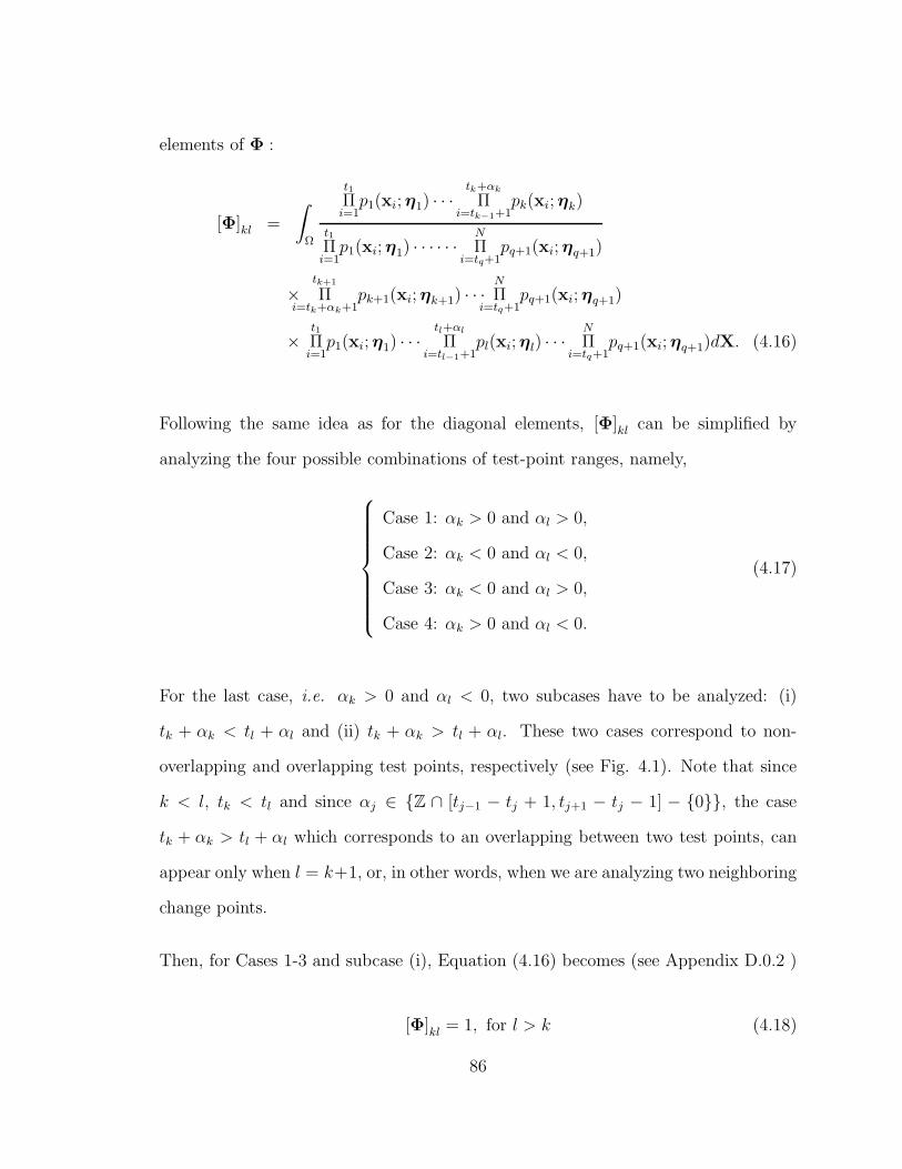
elements of Φ :

[Φ]kl =

∫

Ω

t1Πi=1

p1(xi; η1) · · ·tk+αk

Πi=tk−1+1

pk(xi; ηk)

t1Πi=1

p1(xi; η1) · · · · · ·N

Πi=tq+1

pq+1(xi; ηq+1)

×tk+1

Πi=tk+αk+1

pk+1(xi; ηk+1) · · ·N

Πi=tq+1

pq+1(xi; ηq+1)

×t1Πi=1

p1(xi; η1) · · ·tl+αl

Πi=tl−1+1

pl(xi; ηl) · · ·N

Πi=tq+1

pq+1(xi; ηq+1)dX. (4.16)

Following the same idea as for the diagonal elements, [Φ]kl can be simplified by

analyzing the four possible combinations of test-point ranges, namely,

Case 1: αk > 0 and αl > 0,

Case 2: αk < 0 and αl < 0,

Case 3: αk < 0 and αl > 0,

Case 4: αk > 0 and αl < 0.

(4.17)

For the last case, i.e. αk > 0 and αl < 0, two subcases have to be analyzed: (i)

tk + αk < tl + αl and (ii) tk + αk > tl + αl. These two cases correspond to non-

overlapping and overlapping test points, respectively (see Fig. 4.1). Note that since

k < l, tk < tl and since αj ∈ Z ∩ [tj−1 − tj + 1, tj+1 − tj − 1] − 0, the case

tk + αk > tl + αl which corresponds to an overlapping between two test points, can

appear only when l = k+1, or, in other words, when we are analyzing two neighboring

change points.

Then, for Cases 1-3 and subcase (i), Equation (4.16) becomes (see Appendix D.0.2 )

[Φ]kl = 1, for l > k (4.18)

86

tk

tk-1

tk+1

k

k+1

tk+

ktk+1

+k+1

tk+2

(a)

tk

tk-1

tk+1

k

k+1

tk+

ktk+1

+k+1

tk+2

(b)

Figure 4.1: (a) Case of overlapping; (b) Case of no overlapping.

and for subcase (ii), keeping in mind that αk > 0 and αk+1 < 0, Equation (4.16)

becomes

[Φ]kl =

(∫Ω

pk(x;ηk)pk+2(x;ηk+2)

pk+1(x;ηk+1)dx)βk

, for l = k + 1,

1, for l > k + 1,(4.19)

where βk = (tk + αk) − (tk+1 + αk+1) .

Remark: This last result is fundamental because it proves the natural intuition that

the estimation of q change points is not equivalent to q times the estimation of one

change point. In other words, it means that the estimation of one change point is

perturbed by its two neighbors. We now summarize the previous results.

87

4.3.3 Barankin information matrix Φ− 1q×q

Using Equations (4.15), (4.18), and (4.19), it is clear that BIMt has at least a tri-

diagonal structure:

BIMt =

A1 B1 0 · · · 0

B1 A2

. . .. . .

...

0. . .

. . .. . . 0

.... . .

. . . Aq−1 Bq−1

0 · · · 0 Bq−1 Aq

, (4.20)

where

Ak = [Φ]kk − 1, for k = 1, . . . , q (4.21)

=

(∫Ω

p2k(x;ηk)

pk+1(x;ηk+1)dx)αk − 1 if αk > 0,

(∫Ω

p2k+1(x;ηk+1)

pk(x;ηk)dx)−αk

− 1 if αk < 0,

and

Bk = [Φ]kk+1 − 1, for k = 1, . . . , q − 1 (4.22)

=

0, if βk < 0,(∫

Ω

pk(x;ηk)pk+2(x;ηk+2)

pk+1(x;ηk+1)dx)βk − 1,

if βk > 0.

In the case of one change-point estimation, BIMt is reduced to a scalar A1, and

by replacing α1 = α we re-obtain the result proposed by Ferrari and Tourneret (see

88

Equations (5) and (6) in [75]):

A1 =

(∫Ω

p21(x;η1)

p2(x;η2)dx)α

− 1 if α > 0,(∫

Ω

p22(x;η2)

p1(x;η1)dx)−α

− 1 if α < 0.(4.23)

Note also that the diagonal elements of BIMt can be computed numerically in one

step (i.e., ∀αk ≷ 0) as follows:

Ak =

(∫

Ω

(pk(x; ηk)

pk+1(x; ηk+1)

)ǫk

pk+1(x; ηk+1)dx

)abs(αk)

− 1, (4.24)

where ǫk = 12

(3 αk

abs(αk)+ 1)

.

The next step of our analysis is to compute (BIMt)−1. For a given set of test

points, it is clear that tk + αk > tk+1 + αk+1 =⇒ tk+1 + αk+1 < tk+2 + αk+2, since

αj ∈ Z ∩ [tj−1 − tj + 1, tj+1 − tj − 1] − 0. In other words, ∀k, if Bk 6= 0, then

Bk+1 = Bk−1 = 0; therefore, BIMt is block diagonal and the maximum size of one

block is 2×2. Since the problem is reduced to finding, at worst, the inverse of several

2 × 2 matrices with the same structure, we will have a straightforward inversion. In

this section, we detail the case of two change points, we give the generalization to two

neighboring points, and we use this to derive a closed-form expression for the inverse

of BIMt and thus BBq(t,D (α)).

89

The case of two change points

In this case we have q = 2, t = [t1, t2]T , and BBq(t,D (α)) becomes

BB2(t,D (α)) =

α1 0

0 α2

A1 B1

B1 A2

−1

α1 0

0 α2

=1

A1A2 − B21

α21A2 −α1α2B1

−α1α2B1 α22A1

,

(4.25)

with

A1 =

(∫Ω

p21(x;η1)

p2(x;η2)dx)α1

− 1 if α1 > 0,(∫

Ω

p22(x;η2)

p1(x;η1)dx)−α1

− 1 if α1 < 0,(4.26)

A2 =

(∫Ω

p22(x;η2)

p3(x;η3)dx)α2

− 1 if α2 > 0,(∫

Ω

p23(x;η3)

p2(x;η2)dx)−α2

− 1 if α2 < 0,(4.27)

B1 =

0 if β1 < 0,(∫

Ωp1(x;η1)p3(x;η3)

p2(x;η2)dx)β1 − 1

if β1 > 0,

(4.28)

where β1 = (t1 + α1) − (t2 + α2) .

Consequently, depending on the given set of test points, the following five combina-

tions, corresponding respectively to cases (1), (2), (3) , and (4) in (4.17), are possible

90

for BB2(t,D (α)):

α21

∆α1112−1

0

0α2

2

∆α2223−1

,

α21

∆abs(α1)221 −1

0

0α2

2

∆abs(α2)332 −1

,

α21

∆abs(α1)221 −1

0

0α2

2

∆α2223−1

,

α21

∆α1112−1

0

0α2

2

∆abs(α2)332 −1

,

κ−1

α21

(∆

abs(α2)332 − 1

)α1α2

(1 − ∆

β1132

)

α1α2

(1 − ∆

β1132

)α2

2 (∆α1112 − 1)

(4.29)

where we define

∆ijk =

∫

Ω

pi(x; ηi)pj(x; ηj)

pk(x; ηk)dx,

and κ = (∆α1112 − 1)

(∆

abs(α2)332 − 1

)−(∆

β1132 − 1

)2

.

Generalization to q change points

Note that for more change points the process is the same, except that the inversion

has to be computed because of the increase of possibilities. However, the matrix to be

inverted is block diagonal, with block of size 1× 1 or 2× 2, as stated in the previous

section. In particular, depending on the values of α, the elements of[BIM−1

t

]kl

for

1 < k < q and l = k, k + 1, with BIMt, Ak, and Bk given by Equations (4.20),

(4.21), and (4.22), respectively, and α0 = αq = 0 and Bq = 0, have the following

possible values:

91

If tk+1 + αk+1 < tk + αk, then αk > 0, Bk 6= 0 and Bk−1 = Bk+1 = 0, thus

[BIM−1

t

]kl

=

Ak+1

AkAk+1−B2k, for l = k,

− Bk

AkAk+1−B2k, for l = k + 1.

(4.30)

If tk + αk < tk−1 + αk−1, then αk < 0, Bk−1 6= 0 and Bk−2 = Bk = 0, thus

[BIM−1

t

]kl

=

Ak−1

AkAk−1−B2k−1

, for l = k,

0, for l = k + 1.(4.31)

If tk−1 + αk−1 < tk + αk < tk+1 + αk+1, then Bk−1 = Bk = 0, thus

[BIM−1

t

]kl

=

1Ak

, for l = k,

0, for l = k + 1.(4.32)

Therefore, the elements of[BIM−1

t

]kl

for k, l = 1, . . . , q, which is a symmetric matrix,

are given by

[BIM−1

t

]kl

=

Ak−1I[−∞,−1](αk)+Ak+1I[1,∞](αk)

Ak(Ak−1I[−∞,−1](αk)+Ak+1I[1,∞](αk))−(B2k−1+B2

k),

for l = k,

−Bk

AkAk+1−B2k, for l = k + 1,

0, for l > k + 1.

(4.33)

Since the matrix BBq(t,D (α)) is given by

BBq(t,D (α))= D (α) BIM−1t

D (α)T , (4.34)

92

then, [BBq(t,D (α))]kl for k, l = 1, . . . , q is given as follows:

[BBq(t,D (α))]kl =

α2k(Ak−1I[−∞,−1](αk)+Ak+1I[1,∞](αk))

Ak(Ak−1I[−∞,−1](αk)+Ak+1I[1,∞](αk))−(B2k−1+B2

k),

for l = k,

− αkαk+1Bk

AkAk+1−B2k, for l = k + 1,

0, for l > k + 1,

(4.35)

where [BBq(t,D (α))]kl = [BBq(t,D (α))]lk . If for a given set of test points there is

no overlap with the neighboring change-points tk−1 and tk+1, then Bk−1 = Bk =

0 in (4.35) and we obtain the particular result [BBq(t,D (α))]kk = α2k/Ak and

[BBq(t,D (α))]kk+1 = [BBq(t,D (α))]k+1k = 0. This is equivalent to the bound

obtained using the same set of test points and assuming one change-point located

in the time interval between tk−1 and tk+1 with total numbers of time-samples

N = tk+1 − tk−1.

4.3.4 Computation of the supremum

To obtain the tightest bound from the finite set C := BBq(t,D (α)), α ∈ S ⊂

Sq++, we need to compute the supremum of C with respect to the partially order

set (Sq,) . The partial order is given by the Loewner ordering, which is defined

via the cone of positive semidefinite matrices [78, 79]. In general, this problem is

indeed very complex since it requires to look for α∗∈ S such that BBq (t,D (α∗))

BBq (t,D (α)) for all α ∈ S . To the best of our knowledge, no formal approach for

solving this problem has been proposed in the technical literature of minimal bounds.

For example, in [81, 85] the choice of the test point α is guided by some physical

considerations of the model being studied. Also, from an optimal design context [78],

93

an approximation for solving this problem is to compute the matrix in C with the

largest trace, BBtr. However, the fact that Tr BBtr > Tr Bi for Bi ∈ C, does

not imply that BBtr ≻ Bi, only the converse statement is valid. In fact, only if C

has a greatest element, i.e., the supremum of the set, then it is given by the matrix in

C with the largest trace. Let Bj = sup C, with Bj ∈ C, then by definition Bj Bi,

for all Bi ∈ C with i 6= j. Let G = Bj − Bi, thus G ∈ Sq+ and Tr G > 0. Hence,

Tr Bj > Tr Bi , for all Bi ∈ C with i 6= j, but as we discussed at the end of

Section II, a unique supremum or an infimum with respect to the Loewner partial

ordering in the finite set C might not exist.

Here we address the computation of the supremum by finding a minimal-upper bound

Bq ∈ Sq++ to the set C such that Bq C and which is minimal in the sense that

there is no smaller matrix B′q Bq such that B′

q C. In [77], the authors implicitly

introduced an algorithm for computing a minimal-upper bound to a finite set of

positive definite matrices and redefined this element as the supremum of the set.

Before discussing more details about it, we need to introduce the so-called penumbra

P (M) of a matrix M ∈ Sq as the set P (M) := N ∈ Sq : N M [77, 78] and the

following proposition:

Proposition 2 Define M and N ∈ Sq, then M N iff P (N) ⊆ P (M) .

Proof. If P (N) ⊆ P (M), then N ∈ P (M) and then, by the definition of penumbra,

M N. To prove the other implication, we define a matrix G ∈ Sq such that N

G. Then if M N we have, by the transitivity property of the Loewner order, M

G, namely, M N G. Therefore, all the matrix elements in P (N) are also in

P (M), thus, P (N) ⊆ P (M).

94

The penumbra P (M) is seen as an inverted cone of vertex M characterizing all matri-

ces that are smaller than M [77,78]. The authors in [77,78] redefined the supremum

of a set of matrices as the matrix associated to the vertex of the minimal penumbra

covering the penumbras of all the matrices in the set. The minimal-penumbra vertex

is a minimal-upper bound to the set with respect to the partially order set (Sq,).

In [77], the minimal-penumbra vertex is computed by associating with each matrix

M ∈ Sq a ball in the subspace SA = A : Tr A = 0, and the authors show that

it is determined by the smallest ball enclosing the set of balls associated to each ma-

trix in the set. The latter algorithm is implemented in an approximate manner, by

solving instead the problem of finding the smallest enclosing ball of a set of points

which correspond to samples from the boundaries of each ball. The success of this

method to obtain a minimal-upper bound matrix depends on the samples chosen.

For example, in the case of having two balls, it is easy to show that the smallest

enclosing ball is tangent to each ball border at the two farthest points from the set

of points defined by the intersection of a line passing through each ball center and

each ball boundary. Therefore if the sampling procedure does not include this pair

of points, then the resulting ball does not completely enclose both balls and, thus,

the resulting matrix is not a minimal-upper bound. Moreover, when the dimension

is larger than two, a simple analytical computation shows that this algorithm fails to

obtain a minimal-upper bound matrix for the set formed by two diagonal matrices

not comparable to each other according to Loewner order.

Here, instead, we propose a method for computing a suitable Bq for any dimension.

First, we show that computing Bq is equivalent to finding the minimum-volume hyper-

ellipsoid covering the set of hyper-ellipsoids associated to each matrix in the set

C. And second, we show that this problem can be written as a convex objective

95

function with convex constraints which can be solved efficiently using semidefinite

programming. An hyper-ellipsoid ε ⊂ Rq with non-empty interior and centered at

the origin can be represented by the set ε (F) =xTF−1x ≤ 1

, where F ∈ S

q++.

Suppose ε(F)

is another hyper-ellipsoid similarly represented, where F ∈ Sq++. Then,

the following statement holds:

Lemma 3 F F iff ε (F) ⊇ ε(F). Proof. By the S-procedure [86], we have that

ε(F)⊆ ε (F) if and only if there is a λ > 0 such that

F−1 0

0 −1

λ

F−1 0

0 −1

,

with equality when λ = 1, implying the necessary condition F F.

Given a finite set of hyper-ellipsoids Cε := ε (Fi) | Fi ∈ Sq++, i = 1, . . . , R, we can

always find a unique minimum volume hyper-ellipsoid, ε (Fjl), containing the set Cε,

i.e, containing all ε (Fi) [86]. Since Cε is convex, ε (Fjl) is known as the Lowner-John

ellipsoid of Cε [86] and, as we show in the following statement, Fjl is a minimal-upper

bound of the set CF := Fi, i = 1, . . . , R formed by all the matrices associated to

the hyper-ellipsoids in Cε.

Theorem 4 The matrix Fjl, associated to the Lowner-John ellipsoid of the set Cε,

is a minimal-upper bound of the set CF w.r.t to the Loewner partial ordering.

Proof. We will demonstrate this by contradiction. From the previous Lemma

we have that Fjl Fi, i = 1,. . ., R. Assume that there exists a matrix Fo /∈ CF

such that Fjl Fo Fi , therefore ε (Fo) ⊇ ε (Fi), for i = 1,. . ., R, and thus

ε (Fo) ⊇P∪

i=1ε (Fi). Given that the volume of ε (Fjl) is less than the volume of ε (Fo),

96

since it is the minimum volume hyper-ellipsoid enclosing all Fi, then |Fjl| ≤ |Fo|, but

by construction Fjl Fo, thus |Fjl| ≥ |Fo|, which is a contradiction. Thus Fo = Fjl,

and Fjl is a minimal-upper bound of the set CF .

Therefore, computing a minimal-upper bound matrix Bq of the set C, defined by

C := BBq(t,D (α)), α ∈ S ⊂ Sq++, (4.36)

is equivalent to finding the Lowner-John ellipsoid of the set of hyper-ellipsoids as-

sociated to C. This is a particular case of a more general problem of computing

the minimum volume hyper-ellipsoid ε (B) =xTB−1x+2

(B−1/2 b

)Tx + bTb ≤ 1

which covers the union of a set of non centered hyper-ellipsoids parameterized by the

quadratic inequalities εi (Bi) =xTB−1

i x+ 2bTi x+ ci ≤ 0

for i = 1, . . . , m. This

problem can be posed as follows [86]:

maxB, b

log(det(B1/2

))(4.37)

subject to :

τ 1 ≥ 0, τ 2 ≥ 0, . . . , τm ≥ 0,

B−1 − τ iB−1i B−1/2 b− τ ibi

(B−1/2 b− τ ibi

)TbT b− 1 − τ ici

0,

i = 1, . . . , m.

The objective function and the set of constraints are convex, so it can be solved

efficiently using semidefinite programming. In particular, we solve this problem us-

ing CVX, a package for specifying and solving convex programs [87, 88], for Bi =

BBq(t,D (αi)) for αi ∈ S , bi = b = 0, and ci = 1. Therefore, the minimal-upper

97

bound Bq of the set C is given by

Bq= B∗, (4.38)

where B∗ is the optimal solution of (4.37.)

Using the following statement, we can even reduce the number of constraints in the

above problem by considering only the set Cm ⊆ C formed by all the maximal elements

of C.

Theorem 5 Define CFm as the subset of CF formed by all the maximal elements of

CF . Then, the Lowner-John ellipsoid ε (Fjl) of Cε is also the Lowner-John ellipsoid of

the set Cεm formed by the hyper-ellipsoids associated to the matrices in CFm. Proof.

Since CFm is formed by all the maximal elements of CF , then for Fi ∈ CFm and

any Fj ∈ CFc = CF − CFm, we have that Fi Fj . From Lemma 2, ε (Fi) ⊇

ε (Fj) , for all Fj ∈ CFc , which is true for all Fi ∈ CFm, i.e., for all ε (Fi) ∈ Cεm,

thus Cεm ⊇ ε (Fj) , for all Fj ∈ CFc and Cε = Cεm ∪ ε (Fj) , for all Fj ∈ CFc =

Cεm. Therefore, ε (Fjl) is the Lowner-John ellipsoid for the set Cε and Cεm.

In Figure 4.2 we illustrate the Lowner-John ellipsoid of a set formed by three ellipsoids

in which two are maximal elements of the set.

Hence, using the above result we decrease the number of constraints in (4.37) by

performing a pre-step which identifies the set Cm. Note that if C has a greatest

element, it is the unique maximal element of C and therefore it is the supremum of

the set and its associated hyper-ellipsoid is the Lowner-John ellipsoid of the set of

hyper-ellipsoids associated to C. Therefore, there is no need to solve problem (4.37).

Our algorithm searches and removes from the set of constraints the matrices whose

98

Figure 4.2: Illustration of Lowner-John ellipsoid of a set formed by three ellipsoids inwhich two are maximal elements of the set.

hyper-ellipsoid is fully enclosed by other hyper-ellipsoids. In particular, we evaluate

in an iterative manner the membership in Cm of all elements in C. We define a

membership indicator vector iCm where [iCm ]i = ICm (Fi) and the algorithm begins

by assuming that all elements belong to Cm, namely, iCm = 1R×1, where R = |C| .

Then, all the values of the elements of iCm are evaluated using the following iterative

procedure:

• Step 0 : Initialize iCm = 1R×1 and set indexes k = 1, l = 1.

• Step 1 : Evaluate membership of Fk to Cm (if k > R, terminate the algorithm):

If ICm (Fk) =

0, set k = k + 1 and restart Step 1,

1, set l = l + 1 and go to Step 2.

• Step 2 : Evaluate membership of Fl to Cm (if l > R, set k = k + 1, l = 1, and

go to Step 1 ):

99

If ICm (Fl) =

0, set l = l + 1 and restart Step 2,

1, go to Step 3.

• Step 3 : Compare Fk versus Fl w.r.t. the Loewner ordering:

if Fk Fl, set ICm (Fl) = 0, l = l + 1, and go to Step 2,

if Fl Fk, set ICm (Fk) = 0, k = k + 1, l = 1, and go to Step 1,

if not comparable, set ICm (Fl) = 1, l = l + 1, and go to Step 2.

Finally, once the algorithm terminates, the set Cm will be given by all elements such

that ICm (Fi) = 1. To compare Fk versus Fl, w.r.t. to the Loewner ordering, we

apply the determinant test [89] to the matrix, G = Fk − Fl. This test evaluates the

principal minors of G and concludes on the matrix definiteness as follows: (i) G is

positive definite, i.e., Fk ≻ Fl, if and only if all its leading principal minors are strictly

positive, and it is negative definite, i.e., Fl ≻ Fk, if its k -th order leading principal

minor is < 0 for k odd and > 0 for k even; (ii) G is positive semidefinite, i.e., Fk Fl,

if and only if all the principal minors are non-negative, and it is negative semidefinite,

i.e., Fl Fk, if all the k -th order principal minors are ≤ 0 for k odd and ≥ 0 for k

even; (iii) G is indefinite, i.e., Fk and Fl are not comparable, if none of the previous

conditions are satisfied. Since all the matrices in the set C are block diagonal and the

maximum size of one block is 2 × 2, then every matrix G is a symmetric tridiagonal

matrix, of which the leading principal minors fG (r) , r = 1, . . . , q can be computed

iteratively as follows [90]:

fG (r) =

1, for r = 0,

[G]11 , for r = 1,

[G]r r fG (r − 1) −([G]r r−1

)2fG (r − 2) , for 2 < r < q.

100

Note that the determinant of the tridiagonal matrix G is given by |G| = fG (q), and

since all the principal minors of G are also tridiagonal matrices, then their values are

computed efficiently using the above expression.

Following the ideas of [77], the issue of having a unique supremum of a set of pos-

itive definite matrices can be overcome by redefining the supremum as the matrix

associated to the Lowner-John Ellipsoid of the set of hyperellipsoids associated to the

maximal elements of the set C formed by the P-order BB matrices. This matrix Bq

is unique in the sense that there is no other ellipsoid with minimal volume covering

the hyper-ellipsoids associated to the set of maximal elements of C. It also has the

properties of continuity, namely, it is positive definite.

In the following section we will derive the elements of the Barankin information matrix

for the problem of changes in the parameters of Gaussian and Poisson distributions.

4.4 Change in parameters of Gaussian and Poisson

distributions

In this section, we apply the proposed bound for two distributions generally encoun-

tered in signal processing. We analyze these two cases in a very general way, which

means that the results presented here can be applied to a wide variety of estimation

problems. Indeed, the parameters involved in the Gaussian distribution (mean and

covariance) and in the Poisson distribution are assumed to be a function of the param-

eters ηj, which generally represent physical parameters of interest in signal processing.

An example of change of parameters in a Gaussian distribution in the radar context

is direction-of-arrival (DOA) estimation. The varying cross-section fluctuations are

101

modeled with a Swerling 0 model [91], where the DOAs are hidden in the mean of

the observations, leading, for example, to the so-called conditional MLE [92]. On the

other hand, when the emitted signals are modeled with a Swerling 1-2, the DOAs are

hidden in the covariance of the observations, leading, for example, to the so-called

unconditional MLE [93]. In the context of particle detection, the Poisson distribution

is generally used to model the particle counting process; i.e., the observations and the

parameter involved in the Poisson distribution become a function of the DOA [94].

4.4.1 Gaussian case

Let us assume that the vector of observations xi ∈ RM , for i = 1, . . . , N, is modeled

as follows:

xi = f(νj) + ni, (4.39)

where f (·) is a vector of known functions; νj ∈ RF is a known parameter vector;

ni is a zero-mean Gaussian random vector with covariance matrix M(ϕj

), with

M (·) a symmetric positive definite matrix of known functions; and ϕj ∈ RG is a

known parameter vector. Then ηj =[νT

j , ϕTj

]T ∈ RL, with L = F + G, and xi are

distributed as N(f(νj),M

(ϕj

)). Here we are interested in deriving the elements

of the Barankin information matrix for changes in the pdf parameters of xi, i.e., the

mean and covariance matrix. First, we analyze the general case of piecewise changes of

mean and covariance. Second, we deduce two particular cases: i) piecewise changes

of the mean and constant covariance matrix, i.e., M(ϕj

)= M (ϕ) = Σ; and ii)

piecewise changes of covariance and constant mean vector, i.e., f(νj) = f(ν) = µ.

Note that we restrict our analysis to the set of parameter vectors νj andϕj

such that the functions in f(νj) and M(ϕj

)are injective. In other words, a change

102

in the values of νj changes the values of f(νj), the mean of the distribution of xi.

Similarly, a change in the values of ϕj implies a change in values of the covariance

matrix M(ϕj

). Below, we compute the elements of the Barankin information matrix

BIMt. Then, for each case, respectively, we derive closed-form expressions for the

elements Φ − 1q×q (see Appendix D.0.3 for details on their derivation) which are

different from zero; namely, we evaluate

[Φ]kk for

αk > 0,

αk < 0,

[Φ]kk+1 for tk + αk > tk+1 + αk+1.

(4.40)

Piecewise changes of mean and covariance matrix

For αk > 0, using Equation (4.15), we have that [Φ]kk is given by

[Φ]kk =

(|M(ϕk+1)|1/2|M−1

k |1/2

|M(ϕk)|

)αk

× expαk

2gT

k M−1k gk

× exp−αk fT (νk) (M (ϕk))

−1 f(νk)

× exp

αk

2fT (νk+1)

(M(ϕk+1

))−1f(νk+1)

,

for Mk ∈ SM++,

∞, otherwise,

(4.41)

where Mk =(2 (M (ϕk))

−1 −(M(ϕk+1

))−1)

and gk = 2 (M (ϕk))−1 f(νk) −

(M(ϕk+1

))−1f(νk+1).

103

For αk < 0, using Equation (4.15), we have that [Φ]kk is given by

[Φ]kk =

(|M(ϕk)|1/2|M−1

k+1|1/2

|M(ϕk+1)|

)−αk

× exp

−αk

2gT

k+1M−1k+1gk+1

× exp

αk fT (νk+1)(M(ϕk+1

))−1f(νk+1)

× exp−αk

2fT (νk) (M (ϕk))

−1 f(νk)

,

for Mk+1 ∈ SM++,

∞, otherwise,

(4.42)

where Mk+1 = 2(M(ϕk+1

))−1 − (M (ϕk))−1

and gk+1 = 2(M(ϕk+1

))−1f(νk+1) − (M (ϕk))

−1 f(νk).

For tk + αk > tk+1 + αk+1, using Equation (4.19), we have that [Φ]kk+1is given as

follows:

[Φ]kk+1 =

(|M(ϕk+1)|1/2|M−1

k |1/2

|M(ϕk)|1/2|M(ϕk+2)|1/2

)βk

× exp

βk

2gT

k M−1

k gTk

× exp−βk

2fT (νk) (M (ϕk))

−1 f(νk)

× exp−βk

2fT (νk+2)

(M(ϕk+2

))−1f(νk+2)

× exp

βk

2fT (νk+1)

(M(ϕk+1

))−1f(νk+1)

,

for M−1

k ∈ SM++,

∞, otherwise,

(4.43)

where Mk = (M (ϕk))−1 +

(M(ϕk+2

))−1 −(M(ϕk+1

))−1,

and gk = (M (ϕk))−1 f(νk)+

(M(ϕk+2

))−1f(νk+2) −

(M(ϕk+1

))−1f(νk+1).

104

Piecewise changes of mean and constant covariance matrix

In this case M(ϕj

)= M (ϕ) = Σ, ηj =

[νT

j , ϕT]T

, and [Φ]kl is given as follows:

For αk > 0, using Equation (4.41) and replacing M (ϕk) and M(ϕk+1

)by Σ, we

have straightforwardly for [Φ]kk:

[Φ]kk = expαk

(f(νk) − f(νk+1)

)TΣ−1

(f(νk) − f(νk+1)

). (4.44)

For αk < 0, using Equation (4.42), [Φ]kk is given as follows:

[Φ]kk = exp−αk

(f(νk+1) − f(νk)

)TΣ−1

(f(νk+1) − f(νk)

). (4.45)

For tk + αk > tk+1 + αk+1, using Equation (4.43), then[Φ]kk+1is given as follows:

[Φ]kk+1 =

(exp

βk

2

((f(νk+1) − f(νk)

)Σ−1

(f(νk+1) − f(νk)

)T

+(f(νk+2) − f(νk+1)

)Σ−1

(f(νk+2) − f(νk+1)

)T

−(f(νk) − f(νk+2)

)Σ−1

(f(νk) − f(νk+2)

)T)). (4.46)

Piecewise changes of covariance matrix and constant mean vector

In this case f(νj) = f(ν) = µ, ηj =[νT , ϕT

j

]T, and [Φ]kl is given as follows:

105

For αk > 0 using Equation (4.41) and replacing f(νk) and f(νk+1) by µ, we have

straightforwardly for [Φ]kk:

[Φ]kk =

(|M(ϕk+1)|1/2

|M(ϕk)||Mk|1/2

)αk

, for Mk ∈ SM++,

∞, otherwise,

(4.47)

where Mk = 2 (M (ϕk))−1 −

(M(ϕk+1

))−1.

For αk < 0, using Equation (4.42), [Φ]kk is given as follows:

[Φ]kk =

(|M(ϕk)|1/2

|M(ϕk+1)||Mk+1|1/2

)−αk

, for Mk+1 ∈ SM++,

∞, otherwise,

(4.48)

where Mk+1 = 2(M(ϕk+1

))−1 − (M (ϕk))−1.

For tk + αk > tk+1 + αk+1, using Equation (4.43), then[Φ]kk+1is given as follows:

[Φ]kk+1 =

(|M(ϕk+1)|1/2

|M(ϕk)|1/2|M(ϕk+2)|1/2|Mk|1/2

)βk

,

for Mk ∈ SM++,

∞, otherwise,

(4.49)

where Mk = (M (ϕk))−1 +

(M(ϕk+2

))−1 −(M(ϕk+1

))−1.

The elements of the Barankin bound for each case are obtained by using Equation

(4.35), recalling that Ak = [Φ]kk − 1 and Bk = [Φ]kk+1 − 1, from Equations (4.21)

and (4.22), respectively.

106

4.4.2 Poisson case

Assume that the measurements xi ∈ N+ 0 , for i = 1, . . . , N, are distributed as

a Poisson distribution with parameter f(ηj), where f(·) is a known function and

ηj ∈ RL is a known parameter vector. Similarly to the Gaussian case, we restrict our

analysis to the set of parameter vectorsηj

such that the function f(ηj) is injective.

Therefore, we derive closed-form expressions for the elements of the matrix Φ− 1q×q

for piecewise changes of the parameter ηj. Below, we evaluate [Φ]kk for αk > 0 and

αk < 0, and [Φ]kk+1 for tk + αk > tk+1 + αk+1. Note that since xi ∈ N we replace the

integral operator by the summation operator.

For αk > 0, [Φ]kk becomes

[Φ]kk = exp

αk

(f(ηk+1)−f(ηk)

)2

f(ηk+1)

, (4.50)

For αk < 0, [Φ]kk becomes

[Φ]kk = exp

−αk

(f(ηk)−f(ηk+1)

)2

f(ηk)

. (4.51)

For tk + αk > tk+1 + αk+1, [Φ]kk+1is given as follows:

[Φ]kk+1 = exp

βk

(f(ηk+1)−f(ηk)

)2

2f(ηk+1)

× exp

βk

(f(ηk+2)−f(ηk+1)

)2

2f(ηk+1)

× exp

−βk

(f(ηk)−f(ηk+2)

)2

2f(ηk+1)

. (4.52)

107

Similarly, as in the Gaussian case, the elements of the Barankin bound for each case

are obtained by using Equation (4.35) with Ak = [Φ]kk − 1 and Bk = [Φ]kk+1 − 1.

4.5 Numerical examples

In this section, as an illustration, we compare the MSE between the true values of the

change-point locations and their maximum likelihood estimations with our bounds.

In particular, we first introduce the MLE of change-point locations assuming the total

number of changes is known. Then we analyze the cases of multiple changes in (i) the

mean of a Gaussian distribution with fixed variance, (ii) the variance of a Gaussian

assuming a fixed mean, and (iii) the mean rate of a Poisson distribution.

4.5.1 Maximum likelihood estimation

The MLE of t is the solution to the following problem:

tML = arg maxt

q+1∑

i=1

ln pi(xti−1+1, . . . ,xti ; ηi), (4.53)

where t0 = 0 and tq+1 = N by definition. There is no known closed-form expres-

sion for tML so it has to be estimated via numerical computations. To solve this

multidimensional optimization problem efficiently, we apply dynamic programming

(DP), explained in detail in [95], in our context of change-point estimation. The main

advantage of the DP approach is that it does not need to evaluate all the possible

combinations of values for t in (4.53). The details on how to implement DP to solve

(4.53) can be found in [95], Chapter 12. In all our examples below, we illustrate the

108

average MSE performance of the MLE for 1000 Monte Carlo experiments. We stud-

ied the performance as a function of the signal-to-noise ratio (SNR), which is defined

accordingly in each example, and as a function of the distance between change points.

Here we chose q = 3 and the number of samples N = 80. In each example below, we

set t2 = 40, and t3 = 60, and we analyze two scenarios for change point t1: In the

first one, we set t1 = 20 such that each segment has the same number of samples,

and in the second scenario, t1 ∈ [2, 38]. Note that the unbiasedness properties of

the MLE have been studied in [96] for a single change-point and for multiple change-

points in [97]. The asymptotic results derived in [96] and [97] are applicable only

for the case of a Gaussian distribution with changes in the mean. However, in the

case of having a finite interval the MLE is expected to be biased independently of the

distribution. On the other hand, it seems reasonable to assume that for large SNR

values the MLE is unbiased for a subset of the parameter space, i.e, subintervals, and

specially for change-points located equidistant from their neighboring change-points

or the interval limits. For example, in all the examples below, the bias of the MLE

for t = [20 40 60] is approximately zero for all the SNR ranges considered in each

scenario.

4.5.2 Changes in the mean of a Gaussian distribution

We consider the scenario of a time series with three change points in the mean values of

a Gaussian distribution with common variance. We recall the closed-form expressions

obtained for computing [Φ]kk, namely, Equations (4.44) and (4.45), and define the

SNR for the kth change point as follows:

SNRk =(f(νk+1) − f(νk)

)TΣ−1

(f(νk+1) − f(νk)

), (4.54)

109

(a) (b)

10 20 30 40 50 60 70 80

1

1.5

2

2.5

3

Samples

Mean−

para

mete

r va

lue

ν(t) for SNR 4 dB

ν(t) for SNR 0 dB

ν(t) for SNR −4 dB

ν(t) for SNR −8 dB

−8 −6 −4 −2 0 2 4 6 8 1015

20

25

30

35

40

45

50

55

60

65

70

SNR [dB]

Test

poin

t

t3+h*

3

t2+h*

2

t1+h*

1

(c) (d)

−8 −6 −4 −2 0 2 4 6 8 10−40

−30

−20

−10

0

10

20

30

SNR [dB]

MS

E [

dB

]

MSE(t) unknown parameters

MSE(t) known parameters

Trace(BBsup

(t))

Trace(BBtr(t))

−8 −6 −4 −2 0 2−10

−5

0

5

10

15

20

SNR [dB]

MS

E [

dB

]MSE(t

1) known parameters

MSE(t2) known parameters

MSE(t3) known parameters

BBsup

(t1)

BBsup

(t2)

BBsup

(t3)

(e) (f)

0 5 10 15 20 25 30 35 4015

20

25

30

Distance between t2 and t

1

MS

E [

dB

]

MSE(t)

Trace(BBsup

(t))

0 5 10 15 20 25 30 35 408

10

12

14

16

18

20

22

24

26

28

30

Distance between t2 and t

1

MS

E [

dB

]

MSE(t1) MSE(t

2) MSE(t

3) BB

sup(t

1) BB

sup(t

2) BB

sup(t

3)

Figure 4.3: Performance analysis for estimating change-points of the mean in a Gaus-sian distribution: (a) Mean values as a function of sample time for different SNRvalues; (b) Test points associated with the BB given by the minimal-upper bound ofC, BBsup, as a function of SNR; (c) MSE of the change-point vector using the MLEof t and its Barankin bound given by BBsup, and by the matrix with maximum tracein C, BBtr; (d) MSE of each change-point as a function of SNR using the MLE oft1, t2, and t3 and their corresponding Barankin bound BBsup(ti), i = 1, . . . , 3; (e)MSE of change-point vector using the MLE of t and its Barankin bound, BBsup(t),as a function of the distance between t2 and t1 for SNR = −6 [dB]; (f) MSE of eachchange-point and their respective BBsup as a function of the distance between t2 andt1 for SNR = −6 [dB]. c©[2010] IEEE.

110

where f(νk) ∈ RM is the mean vector of the kth segment and Σ ∈ RM×M is the

common covariance matrix. In our example, M = 1 and, without loss of generality,

we choose f(νk) = νk and Σ = σ2 = 1, thus ηk =[νT

k , 1]T

. Here, we set ν1 = 1,

and ν2, ν3, and ν4 are set such that SNR1 = SNR2 = SNR3 = SNR. In particular,

νk = νk−1+(−1)k√

σ2SNR for k = 2, 3, 4. Figure 4.3(a) illustrates the mean values as

a function of sample time for different SNR values. In Figure 4.3(c), we illustrate the

MSE performance of the MLE for the change-point vector, and the BB as a function

of the SNR. In particular, MSEknown is the MSE performance of the MLE for the

change-point vector, assuming knowledge of the means and variance. MSEunknown is

the MSE performance of the MLE for a more realistic case when no knowledge of the

distribution parameters is available. The BBsup is given by the minimal-upper bound

matrix Bq of the set C computed using the algorithm presented in Section III.D, and

BBtr is the matrix in C that has the maximum trace. We illustrate the trace of

BBsup and BBtr since we are comparing the MSE performance for the change-point

vector estimates. Note that, in view of the discussion presented in Section III.D, we

compute BBtr only in this example to show that BBtr does not necessarily coincide

with supremum of the set unless BBsup ∈ C. In this particular scenario, we found that

BBsup belongs to the set C for SNR values equal to and larger than 2 dB. Therefore,

we have the optimal test points α∗1, α∗

2, α∗3 associated to the matrix BBsup defining

the Lowner-John Ellipsoid , which are presented in Figure 4.3(b). For SNR values

above 2 dB no change point is overlapped, therefore, each bound depends only on

its corresponding diagonal element [Φ]ii, which is equivalent to the resulting analysis

of considering one change point located at t = 20, assuming N = 40. Moreover,

it is important to mention that in this example, [Φ]ii is symmetric with respect to

αi, and since all segments have the same length, then both αi and −αi are optimal

solutions for the bound on ti. In Figure 4.3(b) we illustrate only one optimal solution.

111

When the SNR > 2 dB, we found the set C had several maximal elements that are

not mutually comparable, thus, BBsup /∈ C and did not show up in Figure 4.3(b).

Finally, it can be seen that the test point approached the true change point values as

the SNR increases; i.e., α2 tends to -1 as SNR increases.

In Figure 4.3(d), we illustrate the MSEknown and BBsup for change-point ti, i = 1, 2, 3

as a function of SNR. It is noteworthy to mention that we did not illustrate the

performance for higher SNR range in this example, since we found that for SNR values

larger than 10 dB the bound tends quickly to zero. On the other hand, computing

MSE values in these examples for larger SNR requires a large number of Monte Carlo

simulations, since the higher the SNR, the smaller the probability of an error. For

example, a single realization with an error of only 1 unit in one of the change-points,

among 1000 realizations in the Monte Carlo simulation, amounts to an MSE of -30dB.

Similar observations hold for the example of changes in the mean rate of a Poisson

distribution.

We also analyze the MSE performance as a function of the distance between change

points for a fixed SNR value. In Figure 4.3(e), for SNR = −6 dB, we illustrate the

diagonal elements of BBsup and the MSE of the MLE for the change-point vector

t, assuming knowledge of the distribution parameters, as a function of the distance

between change points t1 and t2. In Figure 4.3(f) we illustrate the BB and the MSE

of the MLE for each change-point. We observe that the MSE of the MLE for t1 and t2

increases as the distance between change points t1 and t2 decreases. Similarly, their

respective BB predict the same behavior for distances between t1 and t2 equal to

and larger than 10 time-units; however, for distances smaller than 10 time-units their

respective bounds decrease to the same value, as the did for distances larger than 22

time-units. This bound behavior is expected to take place as our Barankin-type lower

112

bound approximation considers only one change-point per parameter. Therefore,

in our problem the test-point values are lower and upper bounded by the adjacent

change-point parameters, which does not allow for evaluating errors, in estimating

each change-point, beyond these limits. Thus, as the change-points get closer, the

test-point domains become limited, and the bound cannot take into account either

estimated errors given by estimates of t1 which are larger than the true value of t2,

or estimated errors given by estimates of t2 which are lower than the true value of t1.

4.5.3 Changes in the variance of a Gaussian distribution

We consider the same scenarios as above, but with a time series with three change

points in the variance of a Gaussian distribution and a common mean. We recall the

closed-form expressions obtained for computing [Φ]kk, namely, Equations (4.47) and

(4.48), and define the SNR for the kth change point as follows:

SNRk =

∣∣M(ϕk+1

)∣∣|M (ϕk)|

, (4.55)

where M (ϕk) ∈ RM×M is the covariance matrix of the kth segment. In our example,

M = 1, and, without loss of generality, we choose M (ϕk) = ϕk, and the mean to be

equal to zero since the BIM does not depend on the mean, thus ηk = [0, ϕk]T . Here,

we set ϕ1 = 1, and variances ϕ2, ϕ3, and ϕ4 are set such that SNR1 = SNR2 =

SNR3 = SNR. In practice, ϕk = ϕk−1SNR. In Figure 4.4(a), we illustrate sigma-

parameter values as a function of sample time for different SNR values. In Figure

4.4(c), we illustrate the MSE performance of the MLE for the change-point vector

as a function of the SNR and its respective Barankin bound, BBsup. In particular,

we illustrate the MSEunknown and MSEknown of t for SNR ranging from 1 to 30 dB.

113

In Figure 4.4(d) we focus on SNR ranging between 1 to 10 dB, and we illustrate the

MSE for change-point estimates of t1, t2, and t3, using the MLE and their respective

bounds given by the diagonal elements of BBsup. In this scenario BBsup belongs to

set C for SNR values larger than 4 dB. It can be seen that the MSE of the MLE slowly

approaches the BB as the SNR increases. In this example, the BB is the same for all

change-points for SNR values above 2 dB. It can be seen that for all the SNR ranges

illustrated, the maximum differences between the BB and both the MSEknown and

MSEunknown are approximately 7 dB and 17 dB, respectively. For SNR values lower

than 2 dB the BBsup is greater than the MSE of the MLE because the Barankin

bound derivation does not consider the set of admissible values of the estimator. In

our example, the MLE computation restricts the search to the range between 1 and N ,

and thus the MLE variance has an upper limit, which the BB computation does not

consider. Moreover, the BB assumes that the estimator is unbiased at the test-points,

thus for low SNR the comparison against the MLE’s MSE is inappropriate because

the optimal test-points tend to go to the extreme of the intervals associated to each

change-point causing some bias. Also, we illustrate in Figure 4.4(b), the optimal test

points [α∗1, α∗

2, α∗3]

T associated to the matrix BBsup. It can be seen that for all the

SNR range there are no overlaps between test points and, as in the previous example,

all test points approach to 1 or -1, namely, they are close to the true change-point

values as SNR increases. Therefore, for large SNR values [BBsup]kk =√

2 SNRk−1SNRk

,

which tends to 0 as SNRk → ∞.

In Figures 4.4(e) and (f), for SNR = 4 dB, we illustrate the BB and the MSE of

the MLE for t1, t2, and t3, assuming knowledge of the distribution parameters, as a

function of the distance between change points t1 and t2. Above 10 units, the BB for

all the change-points remains the same for distances between change-points t1 and

114

t2. The BB for t1 increases as the distance between change-points t1 and t2 increases

from zero to 10 units. As in the previous example, the bound in this range is overly

optimistic since the test-point domains become limited.

4.5.4 Changes in the mean rate of a Poisson distribution

Now we consider a time series with three change points in the mean rate of a Poisson

distribution. As in the previous examples, we recall the closed-form expressions for

[Φ]kk, i.e., Equations (4.50) and (4.51). Then we define the SNR for the kth change

point detector as follows,

SNRk =

(f(ηk)−f(ηk+1)

)2

f(ηk)2 , (4.56)

where f (ηk) is the mean rate of the kth segment. Here, without loss of generality, we

set f (ηk) = ηk. The mean rate is set to η1 = 1 and the mean rates η2, η3, and, η4 are

set such that SNR1 = SNR2 = SNR3 = SNR. In practice, ηk = ηk−1

(1 +

√SNR

).

In Figure 4.5(a), we illustrate the mean-rate-values as a function of sample time for

different SNR values

Figures 4.5(c) and (d), illustrate the MSEunknown and MSEknown performance for the

change-point vector and each change points t1, t2, and t3, respectively. In this case,

the MSE values, as well as the bounds for t1, t2, and t3, are not the same for the

same SNR values. In fact, it can be seen that the MSE values for t3 are lower

than the MSE values for t2, and these last are lower than the MSE values for t1. This

difference in performance is due to the fact that in our example the difference between

the means of contiguous segments are not the same, which is a direct consequence

115

(a) (b)

10 20 30 40 50 60 70 800

2

4

6

8

10

12

14

16

18

20

22

24

26

28

30

32

Samples

Sig

ma−

para

mete

r va

lues

σ2(t) for SNR 5 dB

σ2(t) for SNR 4 dB

σ2(t) for SNR 3 dB

σ2(t) for SNR 2 dB

1 4 7 10 13 16 19 22 25 28 3015

20

25

30

35

40

45

50

55

60

65

70

SNR [dB]

Test

poin

t

t3+h*

3

t2+h*

2

t1+h*

1

(c) (d)

1 4 7 10 13 16 19 22 25 28 30−10

−5

0

5

10

15

20

25

30

35

SNR [dB]

MS

E [

dB

]

MSE(t) unknown parameters

MSE(t) known parameters

Trace(BBsup

(t))

1 2 3 4 5 6 7 8 9 10

0

5

10

15

20

25

30

SNR [dB]

MS

E [

dB

]

MSE(t1) known parameters

MSE(t2) known parameters

MSE(t3) known parameters

BBsup

(t1)

BBsup

(t2)

BBsup

(t3)

(e) (f)

0 5 10 15 20 25 30 35 4018

19

20

21

22

23

24

25

26

Distance between t2 and t

1

MS

E [

dB

]

MSE(t)

Trace(BBsup

(t))

0 5 10 15 20 25 30 35 408

10

12

14

16

18

20

22

24

Distance between t2 and t

1

MS

E [

dB

]

MSE(t1) MSE(t

2) MSE(t

3) BB

sup(t

1) BB

sup(t

2) BB

sup(t

3)

Figure 4.4: Performance analysis for estimating change-points of the variance in aGaussian distribution: (a) Sigma-parameter values as a function of sample time fordifferent SNR values; (b) Test points associated with the BB given by the minimal-upper bound of C, BBsup, as a function of SNR; (c) MSE of the change-point vectorusing the MLE of t and its Barankin bound given by BBsup; (d) MSE of each change-point as a function of SNR using the MLE of t1, t2, and t3 and their correspondingBarankin bound BBsup(ti), i = 1, . . . , 3; (e) MSE of change-point vector using theMLE of t and its Barankin bound, BBsup(t), as a function of the distance between t2and t1 for SNR = 4 [dB]; (f) MSE of each change-point and their respective BBsup

as a function of the distance between t2 and t1 for SNR = 4 [dB]. c©[2010] IEEE.116

of the definition used for SNR. In practice, for any SNR, the differences between the

means for segments [t3 + 1, N ] and [t2 + 1, t3] is larger than the difference between

the means for segments [t2 + 1, t3] and [t1 + 1, t2]. In Figure 4.5(b) we illustrate the

test points associated to the matrix BBsup. As in the previous examples, the test

points tend to the true change-point values as the SNR increases. Finally, in Figures

4.5(e) and (f), we illustrate the MSE performance, assuming known mean rates, as

a function of the distance between change points for SNR = −6 dB. The bounds for

change-point t2 and t3 are constant in all the illustrated range, though, the MSE of

the MLE for t2 slightly varies as t1 approaches t2. As we discussed in the previous

examples, the bound for t1 is overly optimistic for small distances between t2 and t1,

due to the constrained test-point domain.

117

(a) (b)

10 20 30 40 50 60 70 800

1

2

3

4

5

6

7

8

9

Samples

Mean−

rate

−para

mete

r valu

es

λ(t) for SNR 0 dB

λ(t) for SNR −2 dB

λ(t) for SNR −4 dB

λ(t) for SNR −6 dB

−8 −6 −4 −2 0 2 4 6 8

20

30

40

50

60

70

SNR [dB]

Test

poin

t

t3+h*

3

t2+h*

2

t1+h*

1

(c) (d)

−8 −6 −4 −2 0 2 4 6 8 10−10

−5

0

5

10

15

20

25

30

SNR [dB]

MS

E [

dB

]

MSE(t) unknown parameters

MSE(t) known parameters

Trace(BBsup

(t))

−8 −7 −6 −5 −4 −3 −2 −1 0−15

−10

−5

0

5

10

15

20

SNR [dB]

MS

E [

dB

]MSE(t

1) known parameters

MSE(t2) known parameters

MSE(t3) known parameters

BBsup

(t1)

BBsup

(t2)

BBsup

(t3)

(e) (f)

0 5 10 15 20 25 30 35 4012

14

16

18

20

22

24

26

Distance between t2 and t

1

MS

E [

dB

]

MSE(t)

Trace(BBsup

(t))

0 5 10 15 20 25 30 35 405

10

15

20

25

Distance between t2 and t

1

MS

E [

dB

]

MSE(t1) MSE(t

2) MSE(t

3) BB

sup(t

1) BB

sup(t

2) BB

sup(t

3)

Figure 4.5: Performance analysis for estimating change-points in the mean rate of aPoisson distribution distribution: (a) Mean-rate-values as a function of sample timefor different SNR values; (b) Test points associated with the BB given by the minimal-upper bound of C, BBsup, as a function of SNR; (c) MSE of the change-point vectorusing the MLE of t and its Barankin bound given by BBsup; (d) MSE of each change-point as a function of SNR using the MLE of t1, t2, and t3 and their correspondingBarankin bound BBsup(ti), i = 1, . . . , 3; (e) MSE of change-point vector using theMLE of t and its Barankin bound, BBsup(t), as a function of the distance between t2and t1 for SNR = −6 [dB]; (f) MSE of each change-point and their respective BBsup

as a function of the distance between t2 and t1 for SNR = −6 [dB]. c©[2010] IEEE.118

4.6 Summary

We investigated a simplified version of the Barankin bound on multiple change-point

estimation. The approximate Barankin information matrix was spelled, revealing an

interesting tri-diagonal structure, meaning that the estimation of one change point

is naturally perturbed by its two neighbors. Moreover, the Barankin information

matrix can be reduced to a block diagonal structure leading to closed-form for the

elements of its inverse. The main limitation posed by this HCR approximation is

a reduced search space for the BIM that leads to a loose Barankin bound. We

also discussed the existence and computation of the supremum with respect to the

Loewner partial ordering, on the finite set of candidate BB solutions. To overcome this

problem, we computed a suitable minimal-upper bound to this set given by the matrix

associated with the Lowner-John Ellipsoid of the set of hyper-ellipsoids associated

to each maximal element of the set of candidate bound matrices. Two important

distributions in signal and image processing were investigated, the Gaussian case and

the Poisson case, for which we obtained closed-form expressions for all the elements

of the Barankin information matrix. Finally, we illustrated our analysis by presenting

various simulation results, including our problem of estimating changes in the variance

of a Gaussian distribution (d = 0).

119

Chapter 5

Conclusions and Future Work

In this chapter, we summarize the key contributions of our work in Section 5.1 and

then provide future work in Section 5.2.

5.1 Conclusions

In this dissertation, we contributed with a physical model and with statistical al-

gorithms for analyzing uterine contractions using MMG. In particular, we proposed

a forward electromagnetic model of human myometrial contractions. Our modeling

approach takes into account electrophysiological and anatomical knowledge jointly at

the cellular, tissue, and organ level. We applied a bidomain approach for modeling the

propagation of the myometrium transmembrane potential vm on the uterus and used

this approach to compute the action potential φ and the magnetic field B at the ab-

dominal surface. We introduced a modified version of the FitzHugh-Nagumo equation

for modeling the ionic currents in each cell. Though our ionic current model does not

explicitly consider C2+a dynamics, the simplicity of the FitzHugh-Nagumo allowed for

capturing the nuances of the uterine myocyte response, but it can be used to model

120

the propagating action potential under well defined conditions, as shown in this work.

We also incorporated the anisotropic nature of the uterus by considering conductivity

tensors, and we proposed a general approach to design conductivity-tensor orienta-

tion for any uterine shape. Using Archie’s law and an analytical expression for the

transmembrane potential propagation speed as function of the model parameters, we

estimated conductivity-tensor values in the extracellular and intracellular domains.

We introduced a four-compartment volume conductor geometry for the problem and

proposed a discretized model solution using finite element methods. We illustrated

our approach through a numerical example of a uterine contraction at term. Con-

sidering a spherical uterus and one pacemaker located in the fundus, we obtained

a travelling transmembrane potential depolarizing from -56mV to -16 mV and an

average potential in the plateau area of −25 mV with a duration, before hyperpolar-

ization, of 35 [s], which is a good approximation with respect to the average recorded

transmembrane potentials reported in the technical literature. Similarly, the percent-

age of myometrial cells contracting as a function of time had the same symmetric

properties and length as the intrauterine pressure waveforms of a pregnant human

myometrium at term.

We also developed a general analysis for the detection of uterine MMG contractions.

In particular, we have proposed a two-stage statistical time-segment discriminator

using a single channel of MMG measurements. We assumed that the preprocessed

channels are modeled by a piecewise time-varying AR model of a certain order, with

an input given by a white Gaussian noise with time-varying variance. Therefore,

we first designed a statistical model-based segmentation algorithm based on the SIC

to estimate the time-instants of changes in the parameters. To discriminate time

segments that contain a contraction, we evaluated features such as the time segment

121

power (RMS) and the dominant frequency component (FOZC). Then, we applied the

non-supervised cluster algorithm K-means to classify the RMS values, obtaining then

a discrete-time binary decision signal indicating the presence of a contraction. Since

each single channel detector provided local information regarding the presence of a

burst of activities, we also analyzed the fusion of the decision signals from all the

sensors, as in the parallel distributed detection approach. We proposed a distributed

processing approach providing estimates of spatial-temporal propagation of uterine

activities and RMS values, the time evolution of a percentage of active sensors and

the time evolution of total RMS values.

We applied our detection algorithm to real MMG records obtained from 10 patients

with gestational ages between 31 and 40 weeks, who were admitted to the hospi-

tal for contractions. We found that the RMS values discriminated the presence of

time segments with contractions. However, that result was not obtained in the case

of the FOZC values. We evaluated the performance of our detection algorithm by

computing the DR, FAR, and CORR, respectively, using as a reference the patient’s

feedback. We observed that the maximum average DR and average CORR were

achieved consistently in all groups of channels when d equaled to 0 and 1, in the

frequency range 0.2-0.4 Hz. Also, in the same frequency range for d = 0, 1, the lowest

average FAR were obtained in the group of channels G1. We found that in the fre-

quency range 0.1-0.4 Hz, the maximum averages for DR and CORR were obtained for

d = 0, 3. Thus, on average, a variance based algorithm (d = 0) is suitable to detect

contractions using the RMS values. Our distributed processing approach, applied to

real data, proved helpful in understanding uterine MMG contraction activity both

spatially and temporally. For example, our approach detected uterine activity much

earlier than the patient began to sense it. It also enabled visualizing the relative

122

location of the origin of uterine contractions and quantifying the amount of energy

delivered during a contraction.

Our statistical model-based segmentation algorithm is based on the detection of mul-

tiple change points, using a binary search algorithm; therefore, the problem is sim-

plified by testing the hypothesis for a single change point. Using the asymptotic

distribution of the test statistics based on SIC, we obtained optimal thresholds in

the sense of the Neyman-Pearson criterion; therefore, we controlled the probability

of false alarm and maximized the probability of change-point detection in each stage

of the binary search algorithm. We also proposed an estimate of the model order

d. However, in practice, this approach performed well only in a group of channels

from the same patient, suggesting that a different model for segmentation should be

attempted. For example, to avoid over segmentation, time segments with piecewise

constant time-varying model orders should be considered.

We also investigated in detail the performance of multiple change-point estimates as a

function of the MSE for an independent vector sequence, including our aforementioned

problem of estimating changes in the variance of a Gaussian distribution (d = 0). We

studied the global performance for the class of unbiased estimator of change points

in a sequence assuming known the number of changes. In particular, we studied the

Hammersley-Chapman-Robbins (HCR) bound, a simplified version of the Barankin

bound, on multiple change-point estimation. The approximate Barankin information

matrix was derived, revealing an interesting tri-diagonal structure, meaning that the

estimation of one change point is naturally perturbed by its two neighbors. Moreover,

the Barankin information matrix can be reduced to a block diagonal structure leading

to closed-form for the elements of its inverse. The main limitation posed by this HCR

approximation is a reduced search space for the BIM that leads to a looser Barankin

123

bound. With respect to the Loewner partial ordering, we also discussed the existence

and computation of the supremum on the finite set of candidate BB solutions. To

overcome this problem, we computed a suitable minimal-upper bound to this set,

given by the matrix associated with the Lowner-John Ellipsoid of the set of hyper-

ellipsoids associated to each maximal element of the set of candidate bound matrices.

Two important distributions in signal and image processing were investigated, the

Gaussian case and the Poisson case, for which we obtained closed-form expressions

for all the elements of the Barankin information matrix. Finally, we analyzed the

case of piecewise changes of variance(d = 0) and evaluated the MSE performance as

a function of the variances and distances between the change point.

5.2 Future work

In future work, we will consider a more realistic model for the geometry of the uterus,

fetus, and abdominal shape. We will also include more realistic ionic current models

as in [33–35], and will consider spatial variations of the fiber orientation.

In further studies using MMG measurements, we will address the optimization of the

detection by evaluating additional features of the preprocessed measurements. We

will also develop a biomagnetically compatible pressure measurement device for a

better recording of the intrauterine pressure and provide a more precise approach to

validate the performance of our method with real measurements, as well as to allow

for comparison with other methods.

124

We will further study Barankin-type lower bounds, considering distribution param-

eters in addition to the multiple change-point localizations for the time-dependent

case.

125

Appendix A

Designing Uterine Anisotropy

Denote C as the curve of symmetry and define it using the following parametric

representation as a function of a single parameter t:

C : t 7−→ rC (t) , t1 ≤ t ≤ t2, (A.1)

where rC (t) is a point defined with respect to the global coordinate system, and

rC (t1) and rC (t2) represent the extreme points of the curve. For example, rC (t) =

(x (t) , y (t) , z (t)) with respect to the Cartesian system. Define k(r) = drC(t)dt

∣∣∣t0

/∥∥∥∥drC(t)

dt

∣∣∣t0

∥∥∥∥as the unitary vector field with direction given by the tangent vector of rC (t) at t0,

where rC (t0) is the closest point to r such that

⟨drC(t)

dt

∣∣∣t0

,−−−−−−→rC (t0) r

⟩= 0. Then, we

define t1(r) to be contained in the plane formed by k(r) and n(r) as follows:

t1(r) = βk(r) + γn(r), (A.2)

subject to the following conditions:

⟨t1(r), n(r)

⟩= 0, and (A.3)

⟨t1(r), t1(r)

⟩2

= 1. (A.4)

126

Therefore, replacing (A.2) in (A.3) and (A.4) we obtain the following system of equa-

tions:

β⟨k(r), n(r)

⟩+ γ = 0, and (A.5)

β2 + γ2 + 2 β γ⟨k(r), n(r)

⟩= 1. (A.6)

Solving for all r, such that⟨k(r), n(r)

⟩6= 1, we obtain that β = ± 1√

1−〈k(r),n(r)〉and

γ = ∓ 〈k(r),n(r)〉√1−〈k(r),n(r)〉 . Then t2(r) = t1(r) × n(r) = βk(r) × n(r), since by definition

it is mutually orthogonal to t1(r). Hence, given t1(r) and t2(r), we define a3(r) as

follows:

a3(r) = t1(r) cos (α) + t2(r) sin (α) , (A.7)

where α is the fiber orientation angle with respect to t1(r). In order to take into

account complex fiber orientations α can be modeled as a spatial function defined

over the domain of interest. Given our uterine volume assumptions, the points rC (t1)

and rC (t2) are the only points that satisfy the condition⟨k(r), n(r)

⟩= 1. Since at

rC (t1) and rC (t2) we cannot define t1(r) and t2(r) using the curve C as a global

reference, we set a3(r) = 0, defining a point of isotropic conductivity. In Fig. A.1 we

represent the fiber orientation a3(r) with respect to the local coordinate axes given

by n(r), t1(r), t2(r).

For the case of a uterine volume such that C is parallel to the z axis, then a3(r) can

be written as a function of n(r) as follows:

a3(r) = (P cos (α) + F sin (α)) n(r), (A.8)

127

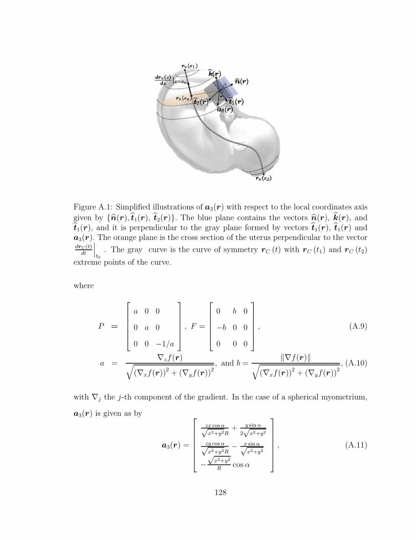
Figure A.1: Simplified illustrations of a3(r) with respect to the local coordinates axis

given by n(r), t1(r), t2(r). The blue plane contains the vectors n(r), k(r), andt1(r), and it is perpendicular to the gray plane formed by vectors t1(r), t1(r) anda3(r). The orange plane is the cross section of the uterus perpendicular to the vectordrC(t)

dt

∣∣∣t0

. The gray curve is the curve of symmetry rC (t) with rC (t1) and rC (t2)

extreme points of the curve.

where

P =

a 0 0

0 a 0

0 0 −1/a

, F =

0 b 0

−b 0 0

0 0 0

, (A.9)

a =∇zf(r)√

(∇xf(r))2 + (∇yf(r))2, and b =

‖∇f(r)‖√(∇xf(r))2 + (∇yf(r))2

, (A.10)

with ∇j the j-th component of the gradient. In the case of a spherical myometrium,

a3(r) is given as by

a3(r) =

zx cos α√x2+y2R

+ y sin α

2√

x2+y2

zy cos α√x2+y2R

− x sinα√x2+y2

−√

x2+y2

Rcos α

, (A.11)

128

where R =√

x2 + y2 + z2. Note that for α = 0 the main axis of the fibers runs

vertically from the fundus to the cervix.

129

Appendix B

Determination of Cα for the SIC

Change-point Detector Based on

an AR-model

Let ζn = maxτζn(τ ) : 2d + 1 < τ ≤ n − d − 3, where ζn(τ ) = (n − d) ln σ20 − (τ −

d) ln ˆσ21(τ ) − (n − τ) ln ˆσ2

2(τ). [98] showed that the asymptotic distribution of ζn is

given by

Pr[ζn − bn(d + 2)

an(d + 2)≤ x]

D−−−→n→∞

exp−2 exp−x/2, (B.1)

where

bn(x) =2 ln ln(n) + x/2 ln ln ln(n) − ln(Γ(x/2))2

2 ln ln(n)

an(x) =

√bn(x)

2 ln ln(n).

130

Let λ = max2d+1 <τ≤n−d−3SIC(n) − SIC(τ). Then, ζn = λ + (d + 2) ln(n). Thus

1 − α = Pr(SIC(n) < min2 d+1≤τ≤n−d−3

SIC(τ) + Cα|H0)

= Pr( max2 d+1≤τ≤n−d−2

SIC(n) − SIC(τ ) < Cα|H0)

= Pr(λ + (d + 2) ln(n) < Cα + (d + 2) ln(n)|H0)

= Pr(ζn − bn(d + 2) < Cα + (d + 2) ln(n) − bn(d + 2)|H0)

= Pr(ζn − bn(d + 2)

an(d + 2)<

Cα + (d + 2) ln(n) − bn(d + 2)

an(d + 2)|H0). (B.2)

(B.3)

Hence, using (B.1)

1 − α ∼= exp

(−2 exp−

(Cα + (d + 2) ln(n) − bn(d + 2)

2 an(d + 2)

))

(B.4)

Then, solving for Cα

Cα = bn(d + 2) − 2 an(d + 2)ln ln((1 − α)−1) − ln(2)

− (d + 2) ln(n). (B.5)

131

Appendix C

Proof of Lemma 1

Proof. We need to proof that for all y ∈ Rq with y 6= 0, yT (A −B)y > 0 if

λ1 ≤ 1. Since A is pd and B is psd, there exist a non-singular matrix F such that

FTBF = diag (λ1, . . . , λm, λm+1, . . . , λq) = Λ and (C.1)

FTAF = I (C.2)

Thus, B =(FT)−1

Λ (F)−1 and A =(FT)−1

I (F)−1 and

yT (A − B)y = yT(FT)−1

(I − Λ) (F)−1 y. Let z = (F)−1 y, because F is not sin-

gular (F)−1 y = 0 for y = 0, therefore our problem is equivalent to analyze the

positiveness of r = zT (I − Λ) z, for z 6= 0. Since λm+1 = · · · = λq = 0, r =m∑

i=1

(1 − λi) z2i +

m∑i=1

z2i . Hence, if λ1 ≤ 1, then (1 − λi) ≥ 0, for i = 1, . . . , m thus

r > 0 and A ≻ B. On the other hand, if λ1 > 1, we can always find a z vector such

that r ≤ 0 or r > 0, thus A and B are not mutually comparable.

132

Appendix D

Computing Elements of the

Barankin Information Matrix

D.0.1 Computing diagonal elements of Φ

For αk > 0, Equation (4.14) becomes

[Φ]kk =

∫

Ω

t1Πi=1

p21(xi; η1) · · ·

tk+αk

Πi=tk−1+1

p2k(xi; ηk)

t1Πi=1

p1(xi; η1) · · ·N

Πi=tq+1

pq+1(xi; ηq+1)

×tk+1

Πi=tk+αk+1

p2k+1(xi; ηk+1) · · ·

N

Πi=tq+1

p2q+1(xi; ηq+1)dX

[Φ]kk =

∫

Ω

t1Πi=1

p1(xi; η1) · · ·tkΠ

i=tk−1+1pk(xi; ηk)

×

tk+αk

Πi=tk+1

p2k(xi; ηk)

tk+αk

Πi=tk+1

pk+1(xi; ηk+1)

×tk+1

Πi=tk+αk+1

pk+1(xi; ηk+1) · · ·N

Πi=tq+1

pq+1(xi; ηq+1)dX.

133

After some straightforward simplifications, we have that

[Φ]kk =

∫

Ω

tk+αk

Πi=tk+1

p2k(xi; ηk)

pk+1(xi; ηk+1)dxtk+1 · · · dxtk+αk

=

∫

Ω

p2k(x; ηk)

pk+1(x; ηk+1)dx

αk

.

Similar analysis can be applied to solve for αk < 0.

D.0.2 Computing non-diagonal elements of Φ

For αk > 0 and αl > 0, Equation (4.16) becomes

[Φ]kl =

∫

Ω

tk+αk

Πi=tk−1+1

pk(xi; ηk)tk+1

Πi=tk+αk+1

pk+1(xi; ηk+1)

tk

Πi=tk−1+1

pk(xi; ηk)tk+1

Πi=tk+1

pk+1(xi; ηk+1)

×p (X; θ0 + hl) dX

[Φ]kl =

∫

Ω

tk+αk

Πi=tk+1

pk(xi; ηk)

tk+αk

Πi=tk+1

pk+1(xi; ηk+1)

t1Π

i=1p1(xi; η1)

· · ·tk+αk

Πi=tk+1

pk+1(xi; ηk+1)tk+1

Πi=tk+αk+1

pk+1(xi; ηk+1)

· · ·tl+αl

Πi=tl−1+1

pl(xi; ηl) · · ·N

Πi=tq+1

pq+1(xi; ηq+1)dX

= 1.

The cases (αk < 0, αl < 0), (αk < 0, αl > 0), and tk + αk < tl + αl are solved using

same approach as above. For the overlapping case, i.e., tk + αk > tl + αl, is more

difficult. Replacing l = k+1 and keeping in mind that αk > 0 and αk+1 < 0, Equation

(4.16) becomes

134

[Φ]kk+1 =

∫

Ω

t1Π

i=1p1(xi; η1) · · · ×

tk+αk

Πi=tk−1+1

pk(xi; ηk)tk+1

Πi=tk+αk+1

pk+1(xi; ηk+1)

tk

Πi=tk−1+1

pk(xi; ηk)tk+1

Πi=tk+1

pk+1(xi; ηk+1)

×

tk+1+αk+1

Πi=tk+1

pk+1(xi; ηk+1)tk+2

Πi=tk+1+αk+1+1

pk+2(xi; ηk+2)

tk+2

Πi=tk+1+1

pk+2(xi; ηk+2)

· · · ×N

Πi=tq+1

pq+1(xi; ηq+1)dX

[Φ]kk+1 =

∫

Ω

t1Π

i=1p1(xi; η1)

tk+αk

Πi=tk+1+αk+1+1

pk(xi; ηk)pk+2(xi; ηk+2)

pk+1(xi; ηk+1)

· · ·N

Πi=tq+1

pq+1(xi; ηq+1)dX

=

∫

Ω

pk(x; ηk)pk+2(x; ηk+2)

pk+1(x; ηk+1)dx

βk

,

where βk = (tk + αk) − (tk+1 + αk+1) .

D.0.3 Computing the elements of Φ for changes in mean and

covariance matrix of Gaussian distribution

In this case ηj =[νT

j , ϕTj

]T, and the data likelihood is given as follows,

p (X; t) =1

(2π)N M/2

q+1

Πj=1

∣∣M(ϕj

)∣∣(tj−tj−1)/2× exp

−1

2Tr

q+1∑

j=1

M(ϕj

)−1

×

tj∑

i=tj−1+1

(xi − f(νj)

)(xi − f(νj)

)T

.

For αk > 0, using Equation (4.15), we have that [Φ]kk is given as follows:

135

[Φ]kk =

∫

RM

(2π)M/2 ∣∣M(ϕk+1

)∣∣1/2

((2π)

M/2 |M (ϕk)|1/2)2

× exp(− (xi − f(νk))

T(M (ϕk))

−1(xi − f(νk))

)

× exp

+

1

2

(xi − f(νk+1)

)T (M(ϕk+1

))−1 (

xi − f(νk+1))

dxi

)αk

[Φkk =

( ∣∣M(ϕk+1

)∣∣1/2

(2π)M/2 |M (ϕk)|

)αk

∫

RM

exp

−1

2

(xT

i Mkxi − 2gTk xi

)dxi

αk

× exp−αk

2fT (νk)2 (M (ϕk))

−1f(νk)

× expαk

2fT (νk+1)

(M(ϕk+1

))−1

f(νk+1)

,

where Mk =(2 (M (ϕk))

−1 −(M(ϕk+1

))−1)

and

gk = 2 (M (ϕk))−1 f(νk)−

(M(ϕk+1

))−1f(νk+1). The integral above has a finite value

for Mk positive definite (pd). Hence, and after some straightforward algebraic deriva-

tions, we obtain the expression in (4.41). The case αk < 0 is obtained proceeding

similarly as above.

136

For tk + αk > tk+1 + αk+1, using Equation (4.19), we have that [Φ]kk+1is given as

follows:

[Φkk+1 =∫

RM

∣∣M(ϕk+1

)∣∣1/2

(2π)M/2 |M (ϕk)|1/2 ∣∣M

(ϕk+2

)∣∣1/2

× exp

−1

2(xi − f(νk))

T(M (ϕk))

−1(xi − f(νk))

× exp

−1

2

(xi − f(νk+2)

)T (M(ϕk+2

))−1 (

xi − f(νk+2))

× exp

1

2

(xi − f(νk+1)

)T (M(ϕk+1

))−1 (

xi − f(νk+1))

dxi)βk

[Φkk+1 =

( ∣∣M(ϕk+1

)∣∣1/2

(2π)M/2 |M (ϕk)|1/2 ∣∣M

(ϕk+2

)∣∣1/2

)βk

∫

RM

exp

−1

2

(xT

i Mkxi − 2gTk xi

)dx

βk

× exp

−βk

2fT (νk) (M (ϕk))

−1f(νk)

× exp

−βk

2fT (νk+2)

(M(ϕk+2

))−1

f(νk+2)

× exp

βk

2fT (νk+1)

(M(ϕk+1

))−1

f(νk+1)

where

Mk = (M (ϕk))−1 +(M(ϕk+2

))−1 −

(M(ϕk+1

))−1

,

and

gk = (M (ϕk))−1

f(νk)+(M(ϕk+2

))−1

f(νk+2)

−(M(ϕk+1

))−1

f(νk+1).

137

Hence, and after some straightforward algebraic derivations, we obtain the expression

in (4.43)

138

References

[1] R. Young and R. O. Hession, “Three-dimensional structure of the smooth musclein the term-pregnant human uterus,” Obstetrics and Gynecology, vol. 93, pp. 94–99, January 1999.

[2] McGraw-Hill Concise Dictionary of Modern Medicine. The McGraw-Hill Com-panies, Inc., 2002.

[3] R. Lamont, “Looking to the future,” BJOG: An International Journal of Ob-stetrics and Gynaecology, vol. 110, pp. 131–135, April 2003.

[4] J. D. Iams, F. F. Johnson, and C. Hamer, “Uterine activity and symptoms aspredictors of preterm labor,” Obstetrics and Gynecology, vol. 76, no. 1, pp. 42S–46S, 1990.

[5] H. Eswaran, H. Preissl, J. D. Wilson, P. Murphy, S. Robinson, and C. Lowery,“First magnetomyographic recordings of uterine activity with spatial-temporalinformation with 151-channel sensor array,” American Journal of Obstetrics andGynecology, vol. 187, pp. 145–151, 2002.

[6] J. Gondry, J. Duchene, and C. Marque, “First results on uterine EMG monitoringduring pregnancy,” IEEE, pp. 2609–2610, 1992.

[7] D. Devedeux, C. Marque, D. Mansour, S. Germain, and J. Duchene, “Uterineelectromyography: a critical review,” American Journal of Obstetrics and Gyne-cology, vol. 169, pp. 1636–1653, 1993.

[8] J. Duchene, D. Devedeux, D. Mansour, and C. Marque, “Analyzing uterineEMG: tracking instantaneous burst frequency,” IEEE Engineering in Medicineand Biology, vol. 14, pp. 125–132, 1993.

[9] N. Radhakrishnan, J. D. Wilson, C. Lowery, H. Eswaran, and P. Murphy, “Afast algorithm for detecting contractions in uterine electromyography,” IEEEEngineering in Medicine and Biology, vol. 19, pp. 89–94, March - April 2000.

[10] K. Horoba, J. Jezewski, J. Wrobel, and S. Graczyk, “Algorithm for detection ofuterine contractions from electrohysterogram,” in Proc.23rd Int. Conference ofIEEE EMBS, pp. 461–464, 2001.

139

[11] J. Jezewski, K. Horoba, A. Matonia, and J. Wrobel, “Quantitative analysis ofcontraction patterns in electrical activity signal of pregnant uterus as an alterna-tive to mechanical approach,” Physiological Measurement, vol. 26, pp. 753–767,July 2005.

[12] P. S. La Rosa, H. Eswaran, C. Lowery, H. Preissl, and A. Nehorai, “Forwardmodeling of uterine EMG and MMG contractions,” in IFMBE Proceedings 11thWorld Congress on Medical Physics and Biomedical Engineering (O. Dssel andW. C. Schlegel, eds.), vol. 25/4, (Munich, Germany), pp. 1600–1603, SpringerBerlin Heidelberg, Sept. 2009.

[13] P. S. La Rosa, H. Eswaran, C. Lowery, H. Preissl, and A. Nehorai, “Forwardelectromagnetic model of uterine contractions during pregnancy,” submitted toPhysics in Medicine and Biology, 2010.

[14] P. S. La Rosa, A. Nehorai, H. Eswaran, C. Lowery, and H. Preissl, “Detectinguterine MMG contractions using a multiple change point detector and the K-means cluster algorithm,” in International Congress Series (Cheyne, B. Ross,G. Stroink, and H. Weinberg, eds.), vol. 1300, pp. 745–748, June 2007.

[15] P. S. La Rosa, A. Nehorai, H. Eswaran, C. Lowery, and H. Preissl, “Detectionof uterine MMG contractions using a multiple change point estimator and theK-means cluster algorithm,” Transactions of Biomedical Engineering, vol. 55,pp. 453–467, Feb. 2008.

[16] P. S. La Rosa, A. Renaux, and A. Nehorai, “Barankin bounds for multiple changepoints estimation,” in Second IEEE International Workshop on ComputationalAdvances in Multi-Sensor Adaptive Processing (CAMSAP), (St. Thomas, U.S.Virgin Islands.), pp. 37–40, IEEE, Dec. 2007.

[17] P. S. La Rosa, A. Renaux, C. Muravchik, and A. Nehorai, “Barankin-type lowerbound on multiple change-point estimation,” To appear in Transactions on Sig-nal Processing, 2010.

[18] L. Tung, A bidomain model for describing ischemic myocardial D-C potentials(Ph. D. thesis). M.I.T. Cambridge, Massachusets., 1978.

[19] W. Miller and D. Geselowitz, “Simulation studies of the electrocardiogram, i.the normal heart,” Circulation Research, vol. 43, no. 2, pp. 301–315, 1978.

[20] R. FitzHugh, “Impulses and physiological states in theoretical models of nervemembrane,” Biophysical J., vol. 1, pp. 445–466, 1961.

[21] J. Nagumo, S. Arimoto, and S. Yoshizawa, “An active pulse transmission linesimulating nerve axon,” in Proc. IRE, vol. 50, 1962.

140

[22] R. FitzHugh, “Mathematical models of excitation and propagation in nerve,”H.P. Schwan, ed. Biological Engineering, vol. Chapter 1, pp. 1–85, 1969.

[23] A. Benveniste and M. Basseville, Detection of Abrupt Changes in Signals andDynamical Systems. Springer-Verlag, Berlin, 1986.

[24] M. Basseville and I. V. Nikiforov, Detection of Abrupt Changes, Theory andApplication. Englewood Cliffs, NJ: Prentice-Hall, Apr. 1993.

[25] F. Gustafsson, Adaptive Filtering and Change Detection. Wiley, 1 ed., Oct. 2000.

[26] H. Cramer, Mathematical Methods of Statistics, vol. 9 of Princeton Mathematics.New-York: Princeton University Press, Sept. 1946.

[27] E. W. Barankin, “Locally best unbiased estimates,” The Annals of MathematicalStatistics, vol. 20, pp. 477–501, Dec. 1949.

[28] T. Chard and J. G. Grudzinskas, The Uterus. Cambridge, University Press,first ed., 1995.

[29] S. Weiss, T. Jaermann, P. Schmid, P. Staempli, P. Niederer, R. Caduff, andM. Bajka, “Three-dimensional fiber architecture of the nonpregnant humanuterus determined ex vivo using magnetic resonance diffusion tensor imaging,”Anatomical Record. Part A, Discoveries in Molecular, Cellular, and EvolutionaryBiology, vol. 288, no. 1, pp. 84–90, 2006.

[30] R. C. Young, “Myocytes, myometrium, and uterine contractions.,” Annals of theNew York Academy of Sciences, vol. 1101, no. 1, pp. 72–84, 2007.

[31] H. F. Andersen and M. L. Barclay, “A computer model of uterine contrac-tions based on dicrete contractile elements,” Obstetrics and Gynecology, vol. 86,pp. 108–111, 1995.

[32] R. Young, “A computer model of uterine contractions based on action potentialpropagation and intercellular calcium waves,” Obstetrics and Gynecology, vol. 89,pp. 604–608, 1997.

[33] L. Bursztyn, O. Eytan, A. J. Jaffa, and D. Elad, “Modeling myometrial smoothmuscle contraction,” Annals of the New York Academy of Sciences, vol. 1101,no. 1, pp. 110–138, 2007.

[34] L. Bursztyn, O. Eytan, A. J. Jaffa, and D. Elad, “Mathematical model ofexcitation-contraction in a uterine smooth muscle cell,” American Journal ofPhysiology - Cell Physiology, vol. 292, no. 5, pp. C1816–C1829, 2007.

[35] S. Rihana and C. Marque, “Modelling the electrical activity of a uterine cell, amathematical model apporach,” in Proc. The 3rd Eurpean Medical and BiologicalEngineering Conference, Prague, 2005.

141

[36] R. E. Garfield and W. L. Maner, “Physiology and electrical activity of uterinecontractions,” Seminars in Cell and Developmental Biology, vol. 18, pp. 289–295,Jun. 2007.

[37] M. J. Peters, J. G. Stinstra, and M. Hendriks, “Estimation of the electricalconductivity of human tissue,” Electromagnetics, vol. 21, pp. 545–557, 2001.

[38] R. Plonsey and D. B. Heppner, “Considerations of quasistationarity in electro-physiological systems,” Bull. Math. Biophys., vol. 29, no. 4, pp. 657–664, 1967.

[39] T. Kawarabayashi, T. Kishikawa, and H. Sugimori, “Effect of oxytocin on spon-taneous electrical and mechanical activities in pregnant human myometrium,”American Journal of Obstetric and Gynecology, vol. 155, pp. 671–676, Sept. 1986.

[40] H. C. Parkington, M. A. Tonta, S. P. Brennecke, and H. A. Coleman, “Contractileactivity, membrane potential, and cytoplasmic calcium in human uterine smoothmuscle in the third trimester of pregnancy and during labor,” American Journalof Obstetrics and Gynecology, vol. 181, pp. 1445–1451, December 1999.

[41] M. Wikland and B. Lindblom, “Relationship between electrical and mechanicalactivity of the isolated term-pregnant human myometrium,” European Journalof Obstetrics and Gynecology and Reproductive Biology, vol. 20, pp. 337–346,December 1985.

[42] P. C. Franzone, L. Guerri, and S. Tentoni, “Mathematical modeling of the ex-citation process in myocardial tissue: Influence of fiber rotation on wavefrontpropagation and otential field,” Mathematical Bioscienses, vol. 101, pp. 155–235, 1990.

[43] M. J. Peters, J. G. Stinstra, S. Uzunbajakau, and N. Srinivasan, “Fetal magneto-cardiography,” In Advances in Electromagnetic Fields in Living Systems, vol. 4,pp. 1–40, 2005.

[44] R. Weber and F. Dickstein, “On the influence of a volume conductor on the ori-entation of currents in a thin cardiac issue,” Lecture Notes in Computer Science,vol. 2674, pp. 111–121, December 2003.

[45] H. Eswaran, H. Preissl, J. D. Wilson, P. Murphy, and C. Lowery, “Prediction oflabor in term and preterm pregnancies using non-invasive magnetomyographicrecordings of uterine contractions,” The Journal of Maternal-Fetal and NeonatalMedicine, vol. 190, pp. 1598–1603, 2004.

[46] M. Khalil and J. Duchene, “Uterine EMG analysis: a dynamic approach forchange detection and classification,” IEEE Transactions on Biomedical Engi-neering, vol. 47, pp. 748–756, June 2000.

142

[47] C. Ramon, H. Preissl, P. Murphy, J. D. Wilson, C. Lowery, and H. Eswaran,“Synchronization analysis of the uterine magnetic activity during contractions,”BioMedical Engineering Online, vol. 4:55, 2005.

[48] J. Ramondt, C. van Kooten, A. Verhoeff, and H. Wallenburg, “Computer anal-ysis of mechanical and electrical uterine activity,” Medicine Biology EngineeringComputation, vol. 24, pp. 351–355, 1986.

[49] S. Mallat, “A theory for multiresolution signal decomposition: the wavelet rep-resentation.,” IEEE Transactions on Pattern Analysis and Machine Intelligence,pp. 674–693, June 1989.

[50] J. Duchene and F. Goubel, “Surface electromyogram during voluntary con-traction: processing tools and relation to physiological events,” Critical reviewbiomedical engineering, vol. 21, pp. 313–397, June 1993.

[51] G. Inbar, J. Allin, O. Paiss, and H. Kranz, “Monitoring surface EMG spectralchanges by the zero crossing rate,” Medicine Biology Engineering Computation,vol. 31, p. 597, 1984.

[52] L. J. Vostrikova, “Detecting ‘disorder’ in multidimensional random processes,”Soviet Mathematics Doklady, vol. 24, pp. 55–59, 1981.

[53] J. Chen and A. K. Gupta, “Testing and locating variance changepoints withapplications to stock,” Journal of the American Statistical Association, vol. 92,pp. 739–747, June 1997.

[54] H. Akaike, “Information theory and an extension of the maximum likelihoodprinciple,” in Proceedings of the 2nd international symposium of informationtheory (B. N. Petrov and B. A. K. E. Csaki, eds.), pp. 267–281, 1973.

[55] G. Schwarz, “Estimating the dimension of a model,” The Annals of Statistics,vol. 6, pp. 461–464, March 1978.

[56] B. Kedem, “Spectral analysis and discrimination by zero-crossings,” Proceedingsof the IEEE, vol. 74, pp. 282–304, November 1986.

[57] K. Horoba, J. Jezewski, J. Wrobel, and S. Graczyk, “Some methods for classifi-cation and analysis of multivariate observations,” in Proceedings of 5-th Berke-ley Symposium on Mathematical Statistics and Probability, no. 1, pp. 281–297,Berkeley, University of California Press, 1967.

[58] C. M. Bishop, Neural Networks for Pattern Recognition. Oxford, England: Ox-ford University Press, 1995.

143

[59] R. Nagarajan, H. Eswaran, J. D. Wilson, P. Murphy, C. Lowery, and H. Preissl,“Analysis of uterine contractions: a dynamical approach,” The Journal ofMaternal-Fetal and Neonatal Medicine, vol. 14, pp. 8–21, March 2003.

[60] B. Brodskya and B. Darkhovskyb, Non-Parametric Statistical Diagnosis. Prob-lems and Methods. Kluwer Academic Publishers Dordrecht/Boston/London,2000.

[61] B. Brodskya and B. Darkhovskyb, “Asymptotically optimal methods of change-point detection for composite hypotheses,” Journal of Statistical Planning andInference, vol. 133, pp. 123–138, 2005.

[62] R. Kakarala and A. O. Hero, “On achievable accuracy in edge localization,” IEEETransactions on Pattern Analysis and Machine Intelligence, vol. 14, pp. 777–781,July 1992.

[63] A. Bartov and H. Messer, “Analysis of inherent limitations in localizing step-like singularities in a continuous signal,” in Proc. of the IEEE-SP InternationalSymposium on Time-Frequency and Time-Scale Analysis, (Paris, FR), pp. 21–24,June 1996.

[64] A. M. Reza and M. Doroodchi, “Cramer-Rao lower bound on locations of suddenchanges in a steplike signal,” IEEE Transactions on Signal Processing, vol. 44,pp. 2551–2556, Oct. 1996.

[65] J.-Y. Tourneret, M. Chabert, and M. Ghogho, “Detection and estimation ofmultiplicative jumps,” in Proc. of the 8th IEEE Signal Processing Workshop onStatistical Signal and Array Processing, pp. 20–23, June 1996.

[66] A. Bartov and H. Messer, “Lower bound on the achievable DSP performancefor localizing step-like continuous signals in noise,” IEEE Transactions on SignalProcessing, vol. 46, pp. 2195–2201, Aug. 1998.

[67] A. Swami and B. Sadler, “Analysis of multiscale products for step detection andestimation,” IEEE Transactions on Information Theory, vol. 44, pp. 1043–1051,Apr. 1999.

[68] S. Zacks, The Theory of Statistical Inference. J. Wiley & Sons, N. York, 1971.

[69] A. Swami and B. Sadler, “Cramer-Rao bounds for step-change localization in ad-ditive and multiplicative noise,” in Proceedings IEEE-SP Workshop on StatisticalSignal and Array Proc., Portland, OR, pp. 403–406, Sept. 1998.

[70] J. V. Braun and H. G. Muller, “Statistical methods for DNA sequence segmen-tation,” Statistical Science, vol. 13, no. 2, pp. 142–162, 1998.

144

[71] C. H. Wu and C. H. Hsieh, “Multiple change-point audio segmentation and clas-sification using an MDL-based Gaussian model,” IEEE Transactions on Audio,Speech, and Language Processing, vol. 14, pp. 647–657, Mar. 2006.

[72] N. Dobigeon, J.-Y. Tourneret, and J. D. Scargle, “Change-point detection inastronomical data by using a hierarchical model and a Bayesian sampling ap-proach,” in IEEE/SP 13th Workshop on Statistical Signal Processing, pp. 369–374, July 2005.

[73] D. G. Chapman and H. Robbins, “Minimum variance estimation without regu-larity assumptions,” The Annals of Mathematical Statistics, vol. 22, pp. 581–586,Dec. 1951.

[74] L. Knockaert, “The Barankin bound and threshold behaviour in frequency esti-mation,” IEEE Transactions on Signal Processing, vol. 45, pp. 2398–2401, Sept.1997.

[75] A. Ferrari and J.-Y. Tourneret, “Barankin lower bound for change-points in inde-pendent sequences,” in Proc. of IEEE Workshop on Statistical Signal Processing(SSP), (St. Louis, MO, USA), pp. 557–560, Sept. 2003.

[76] J. M. Hammersley, “On estimating restricted parameters,” Journal of the RoyalStatistical Society. Series B (Methodological), vol. 12, no. 2, pp. 192–240, 1950.

[77] B. Burgeth, A. Bruhna, N. Papenberga, M. Welka, and J. Weickert, “Mathe-matical morphology for matrix fields induced by the Loewner ordering in higherdimensions,” Signal Processing, vol. 87, pp. 277–290, Feb. 2007.

[78] F. Pukelsheim, Optimal Design of Experiments. John Wiley & Sons, INC.,1st ed., 1993.

[79] J. Borwein and A. Lewis, Convex Analysis and Nonlinear Optmization: Theoryand Examples. Springer-Verlag, 1st ed., 2000.

[80] J. D. Gorman and A. O. Hero, “Lower bounds for parametric estimation withconstraints,” IEEE Transactions on Information Theory, vol. 26, Nov. 1990.

[81] I. Reuven and H. Messer, “A Barankin-type lower bound on the estimationerror of a hybrid parameter vector,” IEEE Transactions on Information Theory,vol. 43, pp. 1084–1093, May 1997.

[82] R. J. McAulay and L. P. Seidman, “A useful form of the Barankin lower boundand its application to PPM threshold analysis,” IEEE Transactions on Informa-tion Theory, vol. 15, pp. 273–279, Mar. 1969.

145

[83] R. J. McAulay and E. M. Hofstetter, “Barankin bounds on parameter estima-tion,” IEEE Transactions on Information Theory, vol. 17, pp. 669–676, Nov.1971.

[84] J. S. Abel, “A bound on mean square estimate error,” IEEE Transactions onInformation Theory, vol. 39, pp. 1675–1680, Sept. 1993.

[85] J. Tabrikian and J. Krolik, “Barankin bounds for source localization in an un-certain ocean environment,” IEEE Transactions on Signal Processing, vol. 47,pp. 2917–2927, Nov. 1999.

[86] S. Boyd and L. Vandenberghe, Convex Optimization. Cambridge UniversityPress, 2004.

[87] M. Grant and S. Boyd, “CVX: Matlab software for disciplined convex program-ming (web page and software),” http://stanford.edu/ boyd/cvx, December 2008.

[88] M. Grant and S. Boyd, “Graph implementations for nonsmooth convex pro-grams,” Recent Advances in Learning and Control (a tribute to M. Vidyasagar),December 2008.

[89] G. Strang, Introduction to Linear Algebra. Wellesley, MA : Wellesley-CambridgePress, 2005.

[90] T. Muir, A treatise on the theory of determinants. Dover Publications, 1960.

[91] P. Swerling, “Probability of detection for fluctuating targets,” IEEE Transactionson Information Theory, vol. 6, pp. 269–308, Apr. 1960.

[92] J. F. Bohme, “Estimation of source parameters by maximum likelihood andnon linear regression,” in Proc. of IEEE International Conference on Acoustics,Speech, and Signal Processing (ICASSP), pp. 731–734, 1984.

[93] J. F. Bohme, “Estimation of spectral parameters of correlated signals in wave-fields,” Signal Processing, vol. 10, pp. 329–337, 1986.

[94] Z. Liu, A. Nehorai, and E. Paldi, “Statistical analysis of a generalized compoundeye detector array,” in Proc. 4th IEEE Sensor Conference, Oct.-Nov. 2005.

[95] S. M. Kay, Fundamentals of Statistical Signal Processing, Volume 2: DetectionTheory. Prentice Hall PTR, 1st ed., Jan. 1998.

[96] D. V. Hinkley, “Inference about the change-point in a sequence of random vari-ables,” Biometrika, vol. 57, no. 1, pp. 1–17, 1970.

[97] Y.-C. Yao and S. T. Au, “Least-squares estimation of a step function,” Sankhya:The Indian Journal of Statistics, Series A, vol. 51, pp. 370–381, October 1989.

146

[98] R. A. Davis, D. Huang, and Y. Yao, “Testing for a change in the parametervalues and order of an autoregressive model,” The Annals of Statistics, vol. 23,pp. 282–304, February 1995.

147

Vita

Patricio Salvatore La Rosa Arayapatricio.larosa@go.wustl.edu

Campus Box 8005, 660 South Euclid Avenue

Division of General Medical Sciences

Department of Internal Medicine

Washington University School of Medicine

St. Louis, MO 63112

Summary: Ph.D. in Electrical Engineering from the Electrical and Systems Engi-

neering Department at Washington University in St. Louis (WUSTL) USA, August

2010. Ph.D. work involves modeling and detection of uterine contractions using mag-

netomyography and derivations of lower bounds on the mean-squared error for 1-D

segmentation algorithms, under the guidance of Professor Arye Nehorai. Recipient

of student travel-support award, following presentation of article at IEEE CAMSAP,

2007. Co-advisor of the undergraduate research project awarded first-place at the St.

Louis Area Undergraduate Research Symposium (STLAURS), 2009. Departmental

representative responsible for accompanying six ESE undergraduate students during

their study abroad program on Medical Imaging at the University of Tbingen MEG-

Center, and the Max Planck Institute for Biological Cybernetics, Germany, 2009. M.

Sc. degree in Electrical Engineering from University of Chile with maximum distinc-

tion, 2003.

Research Interests: Statistical Array Signal Processing and Applications to Med-

ical Imaging and Biosignal Processing; Physical Modeling, including Bioelectromag-

netism, Optical Mapping, and Non-linear Dynamics.

148

Education:

• 2003 to 2010: Ph.D. in Electrical Engineering, Washington University in St.

Louis; Adviser: Prof. Arye Nehorai; Dissertation: Modeling and Detection of

Uterine Contractions using Magnetomyography;

• 2010: M.Sc. in Electrical Engineering, Washington University in St. Louis;

Adviser: Prof. Arye Nehorai

• 2001 to 2003: M.Sc. in Electrical Engineering, University of Chile, Santiago,

Chile ; Adviser: Prof. Guillermo Gonzalez R.; Specialization: System Identifica-

tion and Control; Thesis: Recognition of handwritten numbers in the principal

component space and its orthogonal extensions

• 1995 to 2000: B.Sc. in Engineering at the Pontifical Catholic University of

Chile, Santiago, Chile; Major: Civil Industrial and Electrical Engineering

Research Experience:

• August 2010-: Postdoctoral Research Associate in the General Medical Sciences

Division of the Department of Internal Medicine at the Washington University

School of Medicine; Advisor: Dr. William Shannon

• Jan. 2006 to July 2010: Research Assistant at the Center for Sensor Signal and

Information Processing of the Electrical and Systems Engineering Department

at Washington University in St. Louis; Adviser: Prof. Arye Nehorai; Research

on detection and modeling of uterine contractions using magnetomyography

• Aug. 2003 to Dec. 2005: Research Assistant at the Signal and Image Research

Laboratory of the Electrical and Computer Engineering Department at the

University of Illinois at Chicago; Adviser: Prof. Arye Nehorai; Research on

robust mean-squared error beamforming for narrowband and wideband signals

• M arch 2002 to June 2003: Research Assistant at the Electrical Engineering

Department, University of Chile; Adviser: Prof. Guillermo Gonzalez; Research

on fault detection and diagnosis in time-variable nonlinear dynamic systems

using wavelet transform; Project funded by the National Agency of Science and

Technology of Chile: FONDECYT 1020741

• Aug. 2000 to March 2002: Research Assistant at the Electrical Engineering De-

partment, University of Chile; Adviser: Prof. Guillermo Gonzalez; Research on

149

system identification theory to pattern recognition of handwritten numbers us-

ing statistical quadratics discriminators and neural networks; Project funded by

the National Agency of Science and Technology of Chile: FONDECYT 1000977

Awards:

• Jan. 2008: Recipient of student travel-support, following evaluation and pre-

sentation of conference paper, at the Second IEEE International Workshop on

Computational advances in Multi-Sensor Adaptive Processing (CAMSAP)

• M ay 2003: Graduated with maximum distinction from the Master in Sciences

Program in Electrical Engineering at University of Chile

• 1995-2000: Recipient of the John Paul II Foundation scholarship for pursu-

ing undergraduate studies in Engineering Sciences at the Pontifical Catholic

University of Chile

Activities and Professional Affiliation:

• Reviewer for: IEEE Transactions on Signal Processing and IEEE Transactions

on Biomedical Engineering

• Student Member of IEEE Signal Processing Society since 2003

Dissertation and Thesis:

• P. S. La Rosa, “Modeling and Detection of Uterine Contractions using Mag-

netomyography,” Dissertation to obtain the degree of Ph.D. in Electrical Engi-

neering, Washington University in St. Louis, MO, USA. August, 2010

• P. S. La Rosa, “Filtering and Recognition of Manuscript and Printed Digits in

the Principal Component Space and its Orthogonal Extensions”, (in Spanish)

Thesis to obtain the degree of M. Sc. In Electrical Engineering, University of

Chile, Santiago, Chile, May, 2003

150

Journal Papers:

1. P. S. La Rosa, A. Renaux, C. H. Muravchik, and A. Nehorai, “Barankin-type

lower bound for multiple change-point estimation,” to appear in IEEE Trans.

on Signal Processing, 2010

2. P. S. La Rosa, A. Nehorai, H. Eswaran, C. Lowery, and H. Preissl, “Detection

of uterine MMG contractions using a multiple change-point estimator and the

K-means cluster algorithm,” IEEE Trans. on Biomedical Engineering, Vol. 55

(1), No. 2, pp. 453-467, Feb. 2008

3. Y. Eldar, A. Nehorai, and P. S. La Rosa, “A competitive mean-squared error

approach to beamforming,” IEEE Trans. on Signal Processing, Vol. 55, pp.

5143 - 5154, Nov. 2007

4. Y. Eldar, A. Nehorai, and P. S. La Rosa, “An expected least-squares beamform-

ing approach to signal estimation with steering vector uncertainties,” IEEE

Signal Processing Letters, Vol. 13, No. 5, pp. 288-291, May 2006

5. M. Duarte and P. La Rosa, “Designing SISO observers with unknown input,”

Journal of Mathematical Control and Information (IMA), Vol. 20, No. 4, pp.

387-391, December 2003

6. G. D. Gonzalez, C. Perez, and P. La Rosa, “Enfoque global de la identificacin

de sistemas mediante modelos de caja negra,(Global approach for system iden-

tification by black box models),” Anales del Instituto de Ingenieros de Chile

(Review of Chilean Institute of Engineers), Vol. 114, No. 2, pp. 47-61, August

2002

Journal Papers in Preparation:

1. P. S. La Rosa, H. Eswaran, H. Preissl, and A. Nehorai, “Forward electromag-

netic model of uterine contractions during pregnancy” submitted to Physics in

Medicine and Biology, Jun. 2010

Conference Papers:

1. P. S. La Rosa, H. Eswaran, C. Lowery, H. Preissl, and A. Nehorai, “Forward

modeling of uterine EMG and MMG contractions,” in IFMBE Proceedings 11th

151

World Congress on Medical Physics and Biomedical Engineering, O. Dssel and

W. C. Schlegel, Eds., Vol. 25/4, Munich, Germany, pp. 1600-1603, Springer

Berlin Heidelberg, Sept. 2009

2. P. S. La Rosa, A. Renaux, A. Nehorai, “Barankin bounds for multiple change

points estimation,” in Proceedings of the Second IEEE International Workshop

on Computational Advances in Multi-Sensor Adaptive Processing (CAMSAP),

St. Thomas, U.S. Virgin Islands, pp. 35-40, Dec. 2007 (Invited paper for special

session on minimal bounds in estimation; Recipient of student travel-support

award following presentation at CAMSAP)

3. P. S. La Rosa, A. Nehorai, H. Eswaran, C. Lowery, and H. Preissl, “Detection

of uterine MMG contractions using a multiple change-point estimator and K-

means cluster algorithm,” I nternational Congress Series, Vol. 1300, pp. 745-748,

Jun. 2007

4. G. D. Gonzalez, G. Ceballos, R. Paut, D. Miranda, P. La Rosa, “Fault detection

and identification through variance of wavelet transform of system outputs,” in

Recent Advances in Intelligent Systems and Signal Processing, N. E. Mastorakis,

C. Manikoupoulos, G. E. Antoniou, V. M. Mladenov, and I. F. Gonos, Eds.

Athens, Greece: WSEAS Press, pp. 47-53, 2003

5. R. Salazar, P. Rodrguez, M. A. Duarte-Mermoud, P. S. La Rosa, M. A. Bustos

and R. I. Gonzlez, ”Control of a levitation system by adaptive feedback pas-

sivity,” Proceedings of the 10 Latin-American Congress on Automatic Control,

Guadalajara, Mexico, December 3-6, 2002. Proceedings in CD, Track No. 156,

6 pages

6. M. Duarte and P. La Rosa, “MRAC using observers with unknown inputs,” I n

Recent Advances in Circuits, Systems and Signal Processing, E. Mastorakis and

G. Antoniou Eds. Electrical and Computer Engineering Series, WSEAS Press,

pp. 238-243, July 2002 (ISBN: 960-8052-64-5)

7. G. D. Gonzalez, C. Perez, P. Rodriguez and P. La Rosa, “Linear regression

applied to digit recognition,” Proceedings of the Third International Confer-

ence on Intelligent Processing and Manufacturing of Materials (IPMM2001),

Vancouver, Canada, July 2001 (CD ROM Proceedings)

Talks & Poster Presentations:

1. “Detection and modeling of uterine contractions using magnetomyography,”

invited talk at the Department of Radiology, WUSTL, May 6 th, 2010

152

2. “Detection and modeling of uterine MMG,” invited talk at the MEG-Center,

U. Tubingen, Germany, May 14 th, 2009

3. “Detection of uterine contractions using MMG,” invited talk at the Statistics

Seminar of the Mathematics Department, WUSTL, Jan. 20 th, 2009

4. “Detection of uterine contractions using MMG,” invited talk at the Electri-

cal Engineering Department, Pontifical Catholic University of Chile, Santiago,

Chile, Jan. 16 th, 2009

5. “Forward modeling of uterine contractions using EMG and MMG,” poster pre-

sentation at the Imaging Science Pathway Retreat: 21st-century Imaging Sci-

ences: Pathways to Discovery, St. Louis, MO, April 18 th, 2008

6. “Barankin bounds for multiple change-point estimation,” presentation at the

Special Session on Minimal Bounds in Estimation, Second International Work-

shop on Computational Advances in Multi-Sensor Adaptive Processing (CAM-

SAP), St. Thomas, U.S. Virgin Islands, Dec. 12 th, 2007

Teaching Experience:

• Aug. 2007 to May 2010: Instructor of ESE 497 Undergraduate Research at the

Department of Electrical and Systems Engineering, Washington University in

St. Louis; Responsible for teaching and guiding undergraduate students in the

execution of research projects in the areas of microphone array signal processing

and robotic sensing

• M ay 2007 to Dec. 2009: Instructor of study groups on Detection and Estima-

tion Theory, Introduction to Mathematical Statistics, Linear Statistical Models,

Multivariate Analysis, and Linear Algebra at the Center for Signal and Sens-

ing Information Processing, Department of Electrical and Systems Engineering,

Washington University in St. Louis; Responsible for teaching as well as assign-

ing, grading, and correcting homework for junior graduate students; Responsible

for preparing lecture notes on Introduction to Mathematical Statistics, Linear

Statistical Models, and Multivariate Analysis.

• Aug. 2001 to July 2003: Lecturer of MMS620 Microprocessors and Micron-

trollers, Programs of Applied Electrical Engineering and Industrial Process

and Automatization Engineering, Professional Institute DUOC U.C. Santiago,

Chile; Responsible for teaching as well as assigning, grading, and correcting

homework for undergraduate students

153

• Aug. 2001 to July 2003: Lecturer of EIS411 Power Electronics, Programs of

Applied Electrical Engineering and Industrial Process and Automatization En-

gineering, Professional Institute DUOC U.C. Santiago, Chile; Responsible for

teaching as well as assigning, grading, and correcting homework for undergrad-

uate students

• M ar. 2002 to July 2002: Teaching Assistant of IEE3633 System Design in Auto-

matic Control at the Department of Electrical Engineering, Pontifical Catholic

University of Chile, Santiago, Chile; Responsible for teaching helping sessions

as well as grading homework

• M ar. 2002 to July 2002: Teaching Assistant of EM717 System Identification

for Control Systems at the Department of Electrical Engineering, University

of Chile, Santiago, Chile; Responsible for teaching helping sessions as well as

grading homework

• Aug. 2001 to Dec. 2001: Teaching Assistant of EL63E Optimization for Auto-

matic Control at the Department of Electrical Engineering, University of Chile,

Santiago, Chile; Responsible for teaching helping sessions as well as grading

homework

• M ar. 2001 to July 2001: Teaching Assistant of EL42D Control Systems at

the Department of Electrical Engineering, University of Chile, Santiago, Chile;

Responsible for teaching helping sessions as well as grading homework

• M ar. 2001 to July 2001: Teaching Assistant of IEE2512 Telecommunications

at the Department of Electrical Engineering, Pontifical Catholic University of

Chile, Santiago, Chile; Responsible for grading homework

Advising Experience:

• June 2009 to Dec. 2009: Undergraduate research co-advisor of the former ME

student Chase La-Font; Project title: “Robotic Microphone Sensing: Optimiz-

ing Source Estimation and Algorithms for Adaptive Control,” Electrical and

Systems Engineering Department, WUSTL

• June 2009 to Dec. 2009: Undergraduate research co-advisor of the ESE stu-

dents Evan Nixon and Ian Beil; Project title: “Source Localization: Acoustic

Vector-sensor Array Processing,” Electrical and Systems Engineering Depart-

ment, WUSTL

154

• June 2009 to Dec. 2009: Undergraduate research co-advisor of the ESE students

Raphael Schwartz and Zachary Knudsen; Project title: “Robotic Microphone

Sensing: Data Processing Architectures for Real-Time, Acoustic Source Position

Estimation,” Electrical and Systems Engineering Department, WUSTL

• June 2009 to Dec. 2009: Undergraduate research co-advisor of the ESE stu-

dent Joy Chiang; Project title: “Characterizing Odors Using Electronic Nose

Sensors,” Electrical and Systems Engineering Department, WUSTL

• M ay 2009: Departmental representative responsible for accompanying six ESE

undergraduate students during their study abroad program on Medical Imaging

at the University of Tbingen MEG-Center, and the Max Planck Institute for

Biological Cybernetics, Germany

• Jan. 2009 to May 2009: Undergraduate research co-advisor of the former EE

student Joshua York; Project title: “3D Acoustic Source Location Using Acous-

tic Vector Sensors,” Electrical and Systems Engineering Department, WUSTL

• June 2008 to Dec. 2009: Undergraduate research co-advisor of the former EE

student Joshua York; Project title: “Acoustic Source Localization Using Mi-

crophone Array and Cross-Correlation Methods,” Electrical and Systems Engi-

neering Department, WUSTL. Winner of first place award for best overall pre-

sentation at St. Louis Area Undergraduate Research Symposium (STLAURS),

April 2009

• 2002 to 2003: Undergraduate thesis advisor of the former EE students Clau-

dio Montagno and Miguel Dussaillant; Project title: “Methods for command

recognition based on acoustic and articulation techniques.” Thesis to obtain

the degree in Applied Engineering, Program of Industrial Process and Autom-

atization Engineering, DUOC U.C. Chile

August 2010

155

Biomagnetic Analysis of Uterine Activity, La Rosa Araya, Ph.D. 2010