Modeling and Analysis for Workflow Constrained by Resources and Nondetermined Time: An Approach...

802 IEEE TRANSACTIONS ON SYSTEMS, MAN, AND CYBERNETICS—PART A: SYSTEMS AND HUMANS, VOL. 38, NO. 4, JULY 2008

Modeling and Analysis for Workflow Constrainedby Resources and Nondetermined Time: An

Approach Based on Petri NetsHuaiqing Wang and Qingtian Zeng

Abstract—Time and resource management and verification aretwo important aspects of workflow management systems. In thispaper, we present a modeling and analysis approach for a kind ofworkflow constrained by resources and nondetermined time basedon Petri nets. Different from previous modeling approaches, thereare two kinds of places in our model to represent the activities andresources of a workflow, respectively. For each activity place, itsinput and output transitions represent the start and terminationof the activity, respectively, and there are two timing functionsin it to define the minimum and maximum duration times of thecorresponding activity. Using the constructed Petri net model, theearliest and latest times to start each activity can be calculated.With the reachability graph of the Petri net model, the timingfactors influencing the implementation of the workflow can becalculated and verified. In this paper, the sufficient conditions forthe existence of the best implementation case of a workflow areproved, and the method for obtaining such an implementation caseis presented. The obtained results will benefit the evaluation andverification of the implementation of a workflow constrained byresources and nondetermined time.

Index Terms—Nondetermined time, Petri net, resource manage-ment, workflow.

I. INTRODUCTION

WORKFLOW modeling and analysis have been studiedfor decades, and by now, there has been much research

in the field [1]–[4]. However, because of the complexity of aworkflow system, it is usually difficult to present a uniformmodeling and analysis method for all kinds of workflows. Asmethods of modeling and analyzing physical systems, Petrinets [5]–[7] have shown their abilities to deal with concurrenceand conflict and have been widely used to model, analyze, andverify workflow [8]–[12]. There are at least three good reasonsfor using Petri nets for workflow modeling and analysis [13]:1) Petri net is a graphical language, and its semantics have been

Manuscript received June 16, 2006; revised April 10, 2007. This work wassupported in part by the Natural Science Foundation of China under Grant60603090 and 90718011, by the UGC CERG Research Grant under GrantCityU 120805 from the Hong Kong SAR Government, by the InternationalCooperative Research Project of China under Grant 2006DFA73180, by theStrategic Research Grant under Grant 7001896 from the City University ofHong Kong, and by the Taishan Scholar Program and Excellent ScientistFoundation of Shandong Province under Grant 2006BS01019. This paper wasrecommended by Associate Editor M. Jeng.

H. Wang is with the Department of Information Systems, City University ofHong Kong, Kowloon, Hong Kong (e-mail: [email protected]).

Q. Zeng is with the College of Information Science and Technology,Shandong University of Sciences and Technology, Qingdao 266510, China(e-mail: [email protected]).

Color versions of one or more of the figures in this paper are available onlineat http://ieeexplore.ieee.org.

Digital Object Identifier 10.1109/TSMCA.2008.923056

defined formally; 2) Petri net is state based instead of eventbased, so the state of the case can be modeled explicitly in aPetri net; and 3) Petri nets are characterized by the availabilityof many analysis techniques.

In the previous models of workflow based on Petri nets, mostresearch has focused on structural constraints of workflows,such as [4], [8], and [10], and some of the models and modelingapproaches have considered the time factors, such as [2] and[9]–[12]. In addition to structural and temporal constraints, re-source constraints are also implied in workflow, because activ-ities in a workflow usually access some resources during theirimplementation [2], [14]. However, resource factors are usuallyignored in the workflow model based on Petri nets, particularlyin the model constrained by time [8]–[12]. In this paper, weaddress one kind of workflow constrained by resources andnondetermined time in which the duration of each activitycannot be determined before its implementation. The processmodelers can only estimate the minimum and maximumduration times of each activity in the workflow at build time.At the same time, the implementation of some of the activitiesrequires resources to support it. One activity must wait for therequired resources to be released if they have been occupiedexclusively and locked by other activities being implemented.

In this paper, we discuss the modeling and analysis approachfor this kind of workflow based on Petri net. In previous model-ing approaches for workflow based on Petri nets, the activitiesof workflow are represented by the transitions of the Petri net[4], [8], [10]. If the workflow is constrained by time, a timingfunction usually is added onto the set of transitions of the Petrinet [2], [9], [10], [12]. Different from previous approaches, weuse places instead of transitions to represent the activities soas to keep the atomic properties of transitions in the Petri net.There are two kinds of places in the proposed Petri net modelfor workflow constrained by resources and nondetermined time.One kind is used to represent activity, and the other is usedto represent resources. For each activity place in the model,there are two kinds of timing functions to define the minimumand maximum duration times of each activity. If an activityplace contains a token in the Petri net model, it means that thecorresponding activity is being implemented. If a resource placecontains a token in the model, it means that the correspondingresource is available. This kind of Petri net introduced to modelthe workflow constrained by resources and nondetermined timeis named as the R/NT_WF_Net.

With the obtained R/NT_WF_Net, the earliest and latesttimes to start each activity can be calculated. Using the earliesttime of each activity, the process implementer can determinethe latest time to prepare all required resources for the activity.

1083-4427/$25.00 © 2008 IEEE

WANG AND ZENG: MODELING AND ANALYSIS FOR WORKFLOW CONSTRAINED BY RESOURCES AND TIME 803

If an activity cannot be started before the latest time, it willaffect the start of other activities, and the whole workflowcannot be ensured to be finished in a predefined time. Giventhe R/NT_WF_Net for the workflow, the reachability graph canbe constructed in which each directed path from the initial tothe termination state represents one implementation case of theworkflow. Four relevant timing factors about each implementa-tion state can be calculated, with which the best implementationcase that will ensure the entire workflow is finished withoutany problems can be obtained. In this paper, the sufficientconditions for the best implementation case of a workfloware proved, and an algorithm is presented to obtain the bestimplementation case of a workflow based on the reachabilitygraph. The obtained results will benefit the evaluation andverification of the implementation of a workflow constrainedby resources and nondetermined time.

This paper is organized as follows. Section II presents thereview of related work in this field. Section III offers a formaldefinition for workflow constrained by resources and nondeter-mined time. Section IV introduces the R/NT_WF_Net modeland the modeling approach for workflow constrained by re-sources and nondetermined time and proposes a set of reductionrules for R/NT_WF_Net. Section V discusses how to calculatethe earliest and latest times to start each activity. Section VIpresents the timing factors influencing the implementation ofthe workflow and the method to obtain the best implementationcase. Section VII gives a case study to show the modeling andanalysis approach. Section VIII concludes this paper.

II. RELATED WORK

The applications of Petri net for the modeling and analysisof workflow are not new ideas, and in recent years, there hasbeen much research on modeling and verification for workflowbased on Petri net [2], [4], [8]–[12]. In order to deal with thedifferent changes in the data and the various rules of workflowsystems [4], a number of Petri net classes have been proposedby different researchers, for example, workflow nets [8], infor-mation control nets [15], [16], temporal constraint Petri nets[10], modular process nets [17], colored generalized stochasticPetri nets [18], and so on.

Dealing with time and time constraints is crucial in de-signing and managing business processes. Consequently, timemanagement should be a crucial part of workflow managementsoftware systems and should be considered as a serious limita-tion in applying workflow technologies to complex enterprises[19]–[21]. At build time, when workflow schemes are defined,workflow modelers need to represent time-related aspects ofbusiness processes (activity durations, time constraints betweenactivities, etc.) and check their feasibility. At run time, whenworkflow instances are instantiated and executed, process man-agers need proactive mechanisms for receiving notifications ofpossible time-constraint violations [22]. Eder et al. [22], [23]define a timed workflow graph by augmenting each activitynode with the earliest and latest end times. Temporal constraintscan be calculated by using the modified critical path methodat build and process instantiation times and then enforced atrun time. Marjanovic and Orlowska [24], [25] assign a timeinterval to individual workflow activities as duration constraintsand check various temporal requirements and inconsistencies

of workflow systems by using the proposed verification algo-rithms. Sadiq et al. [26] think that the dynamism of businessenvironments is manifested in the form of changing processrequirements and time constraints, and they primarily addressthe modeling and management of changes occurring in businessprocesses. Ling and Schmidt [12] provide a time interval exten-sion of wokflow nets for the purpose of modeling and analyzingtime-constraint workflow systems. They put more emphasis onchecking the soundness of workflow process definitions butconsider very few time constraints. Adam et al. [10] apply thetemporal constraint Petri nets to specify workflows and thentest the temporal feasibility for a workflow at build time. Inaddition, Li et al. [9] discuss schedulability and boundednessof a workflow model by considering timing constraints basedon a workflow net extended with time information.

In addition to temporal constraints, resource constraints arealso implied in workflow specifications because activities ina workflow usually access some resources during their im-plementations. At the start of an activity implementation, therequired resources must be satisfied. During its implementation,the required resources are assumed to be occupied exclusivelyby the activity. The resources are released after the completion,and then, they can be accessed by other activities. In the eventthat a resource constraint between two activities within a work-flow specification is not represented correctly, the activitiesprobably compete for the same resources in a workflow, andthis results in a conflict. Therefore, it should be analyzed toensure that the workflow specification is resource consistent atbuild time [14]. Li et al. [14] discuss the analysis of resourceconstraints of a workflow specification and present an approachfor the resource consistency of the workflow specification. Eder[23] determines the timing inconsistencies at model time andfinds the optimal workflow execution resources at run time,using the time information generated. Recently, Li et al. [2]have proposed a multidimension workflow (MWF) net thatincludes multiple workflow nets and the organization and re-source information, and they present a method for computingthe lower bound of average turnaround time of transactioninstances processed in an MWF net.

Most of these existing approaches are mainly about themodeling and verification of structural correctness and temporalconsistency. However, resource constraints are implied in thesemantics of a workflow specification and may influence thestate or the result of some or all workflows. A correct work-flow specification should also include resource consistency.In this paper, we focus on resource consistency verificationand timing analysis for workflow constrained by resources andnondetermined time. In our approach, the Petri net model forworkflow constrained by resources and nondetermined timediffers from previous research works [2], [8]–[10], [14], [23]in the following ways.

1) The model is used for workflow that is constrained bothby resources and nondetermined time.

2) The place/transition system is extended with timing fac-tors as models for workflow in which two kinds ofplaces are used to represent activities and resources,respectively.

3) Places instead of transitions are used to represent activi-ties so as to keep the atomic properties of transitions inthe Petri net.


Based on the Petri net model for workflow constrained byresources and nondetermined time, we present the following:

1) the calculation method to determine the earliest and latesttimes to start each activity;

2) timing analysis for each implementation state to find thekey factors influencing the implementation of a workflow;

3) an algorithm to obtain the best implementation case ofworkflow without any risks.

III. WORKFLOW CONSTRAINED BY RESOURCES

AND NONDETERMINED TIME

In this section, we first present the formal definition of a kindof workflow constrained by resources and nondetermined timeand then give a simple example.

A. Definition of a Workflow Constrained by Resourcesand Nondetermined Time

Definition 1: A workflow constrained by resourcesand nondetermined time is a six-tuple Workflow =〈Activity,Resource, T ime,Relation, fTR, FTT 〉, where thefollowing are given.

1) Activity={activity1, activity2, . . . activityn} (n ≥ 1)is the activity set of a workflow.

2) Resource = { resource1, resource2, . . . , resourcem}(m ≥ 0) is the resource set of a workflow.

3) Time = {time1, time2, . . . , timel} (l ≥ 0) is the timeset of a workflow. ∀ timei ∈ Time (0 ≤ i ≤ l),timei ≥ 0.

4) Relation ⊆ Activity ×Activity denotes the relationset of a workflow.

5) fTR : Activity → P(Resource) is the resource functionof a workflow, where P(Resource) is the power set ofResource.

6) FTT = {f1, f2} is the time function of a workflow,wherea) f1 : Activity → Time, for activity ∈ Activity and

time ∈ Time. If f1(activity) = time, it means thatto finish the activity requires at least time units (forexample, day or hour). f1(activity) is named as theminimum duration time of the activity.

b) f2 : Activity → Time, for activity ∈ Activity andtime ∈ Time. If f2(activity) = time, it means thatto finish the activity requires at most time units.f2(activity) is named as the maximum duration timeof the activity.

c) ∀ activity ∈ Activity, f1(activity) ≤ f2(activity).Definition 1 presents the formal definition of a workflow

constrained by resources and nondetermined time, where thefollowing are given.

1) The set Activity defines all the activities involved in theworkflow.

2) The set Resource defines the required resources of allactivities in the workflow. In this paper, we assumed thatall the resources can be prepared before the implementa-tion of each activity, which means that it takes no time toprepare the resources.

3) For activity ∈ Activity and R1 ⊆ Resource, iffTR(activity) = R1, it means that the implementation

of activity requires R1. ∀ activity ∈ Activity, the im-plementation of activity does not require any resourceif fTR(activity) = φ. In the workflow, the resource isoccupied by the activity exclusively. If the implemen-tation of activity ∈ Activity requires resources R1 ⊆Resource, R1 will be locked while activity is beingimplemented.

4) For activity1, activity2∈Activity, if fTR(activity1) ∩fTR(activity2) = φ, we say activity1 and activity2

share common resources. If R1 ⊆ Resource is sharedby activity1 and activity2, R1 will be locked whileactivity1 is being implemented. The activity2 must waituntil activity1 is finished and R1 is released.

5) Relation defines the connection relations betweenactivities. ∀ activity1, activity2 ∈ Activity, if(activity1, activity2) ∈ Relation, it means activity2

cannot start until activity1 has been finished. We sayactivity1 is one of the preactivities of activity2, andactivity2 is one of the postactivities of activity1.

6) The set Time presents the time constraints on eachactivity of the workflow. For each activity, there are twotiming factors, which are the minimum and maximumtimes to finish the activity. These two timing constraintsdefine the time interval of the actual implementationfor each activity. If the actual implementation timeof activity is Atime, then f1(activity) ≤ Atime ≤f2(activity). The duration of one activity is determinedif f1(activity) = f2(activity).

B. Simple Example

A simple example of a workflow constrained by resourcesand nondetermined time is presented in this section.

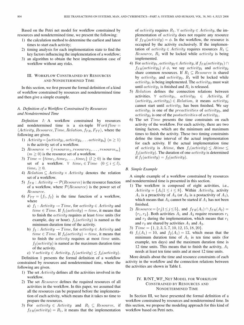
1) The workflow is composed of eight activities, i.e.,Activity = {Ai|1 ≤ i ≤ 8}. Within Activity, activityA1 is a preactivity of A3 (or A3 is a postactivity of A1),which means that A3 cannot be started if A1 has not beenfinished.

2) Resource={rj|1≤j≤5}, and fTR(A1) ∩ fTR(A2) ={r1, r2}. Both activities A1 and A2 require resources r1

and r2 during the implementation, which means that r1

and r2 are shared by activities A1 and A2.3) Time = {1, 2, 3, 5, 7, 10, 12, 15, 18, 20}.4) f1(A1) = 10, and f2(A1) = 12, which mean that the

minimum duration time of A1 is ten time units (forexample, ten days) and the maximum duration time is12 time units. This means that to finish the activity, A1

needs at least ten time units and at most 12 time units.More details about the time and resource constraints of each

activity in the workflow and the connection relations betweenthe activities are shown in Table I.

IV. R/NT_WF_NET MODEL FOR WORKFLOW

CONSTRAINED BY RESOURCES AND

NONDETERMINED TIME

In Section III, we have presented the formal definition of aworkflow constrained by resources and nondetermined time. Inthis section, we propose the modeling approach for this kind ofworkflow based on Petri nets.


TABLE ISIMPLE WORKFLOW CONSTRAINED BY RESOURCES

AND NONDETERMINED TIME

A. Basic Concepts of Petri Nets

It is assumed that readers are familiar with the basic conceptsof Petri nets [5]–[7]. Some of the essential terminologies andnotations regarding the Petri net used in this paper are presentedas follows:

A tuple N = (P, T ;F ) is named as a net iff the following aresatisfied.

1) P ∩ T = φ; P ∪ T = φ.2) F ⊆ (P × T ) ∪ (T × P ).3) Dom(F ) ∪ Cod(F ) = P ∪ T .

For all x ∈ P ∪ T , the set •x={y|y ∈ P ∪ T ∧ (y, x) ∈ F}is the preset of x, and x• = {y|y ∈ P ∪ T ∧ (x, y) ∈ F} is thepostset of x.

A Petri net is a four-tuple Σ = (P, T ;F,M0), where N =(P, T ;F ) is a net and M0 : P → Z+ (Z+ is the nonnegativeinteger set) is the initial marking of Σ. A marking M isreachable from M0 if there is a transition firing sequence σsuch that M0[σ > M . We use R(M0) to represent the set of allreachable markings from M0. If there is an integer k holdingthat ∀ M ∈ R(M0), ∀ p ∈ P such that M(p) ≤ k, we sayΣ = (P, T ;F,M0) is bounded. Otherwise, Σ = (P, T ;F,M0)is unbounded.

The reachability graph is a useful tool for the property analy-sis of Petri net. If a Petri net Σ = (P, T ;F,M0) is bounded, theset of all the reachable markings R(M0) is a finite set. In thiscase, we can use the reachability graph RMG(Σ) to describethe changes of the states of Σ. RMG(Σ) is a directed graphwith R(M0) as the vertex set. ∀ M1,M2 ∈ R(M0), if ∃t ∈ Tsuch that M1[t > M2, then there is a directed edge from M1 toM2 in RMG(Σ), and the edge is labeled with t.

B. R/NT_WF_Net: Petri Net Model for WorkflowConstrained by Resources and Nondetermined Time

Before proposing the modeling approach, a formal definitionof a Petri net model for the workflow constrained by resourcesand nondetermined time (R/NT_WF_Net) is introduced.Definition 2: Σαβ = (P, T ;F,M0, α, β) is an R/NT_

WF_Net iff the following are satisfied.

1) (P, T ;F,M0) is a Petri net.2) P = PA ∪ PR, PA ∩ PR = φ, where PA represents the

activities of workflow and PR represents the resources ofworkflow.

3) ∀ p ∈ PA, PR1 ⊆ PR, the implementation of p requiresPR1 iff PR1 ⊆ (p•)• and PR1 ⊆ •(•p).

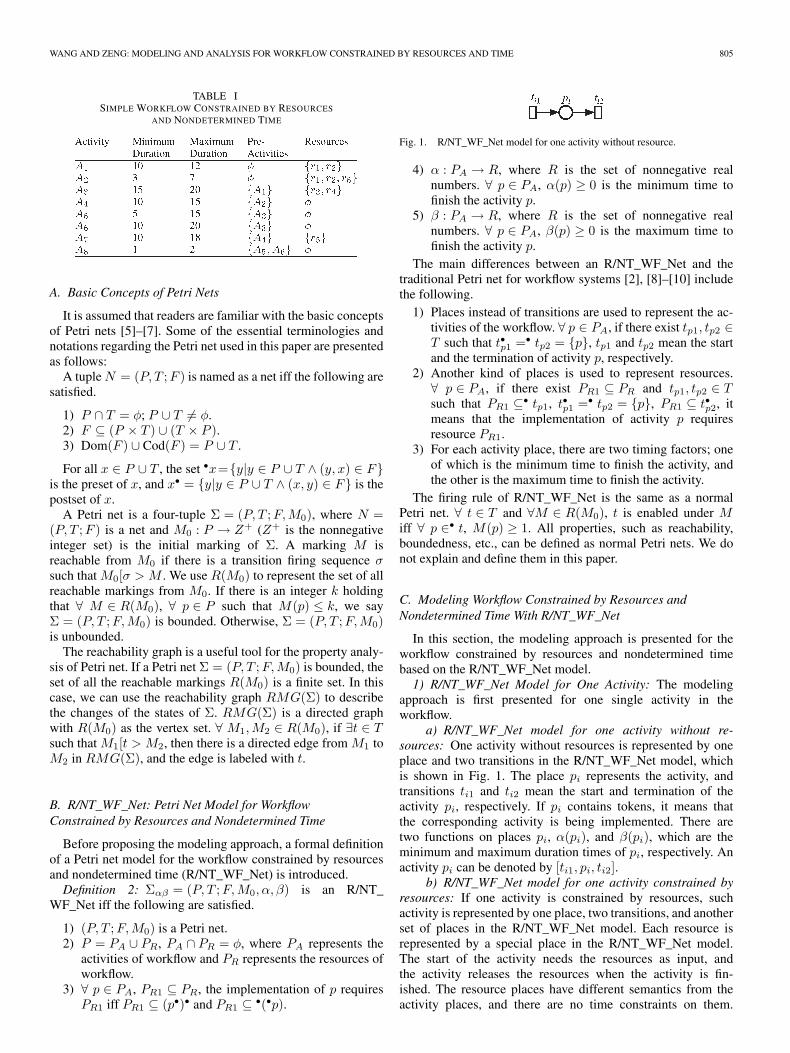
Fig. 1. R/NT_WF_Net model for one activity without resource.

4) α : PA → R, where R is the set of nonnegative realnumbers. ∀ p ∈ PA, α(p) ≥ 0 is the minimum time tofinish the activity p.

5) β : PA → R, where R is the set of nonnegative realnumbers. ∀ p ∈ PA, β(p) ≥ 0 is the maximum time tofinish the activity p.

The main differences between an R/NT_WF_Net and thetraditional Petri net for workflow systems [2], [8]–[10] includethe following.

1) Places instead of transitions are used to represent the ac-tivities of the workflow. ∀ p ∈ PA, if there exist tp1, tp2 ∈T such that t•p1 =• tp2 = {p}, tp1 and tp2 mean the startand the termination of activity p, respectively.

2) Another kind of places is used to represent resources.∀ p ∈ PA, if there exist PR1 ⊆ PR and tp1, tp2 ∈ Tsuch that PR1 ⊆• tp1, t•p1 =• tp2 = {p}, PR1 ⊆ t•p2, itmeans that the implementation of activity p requiresresource PR1.

3) For each activity place, there are two timing factors; oneof which is the minimum time to finish the activity, andthe other is the maximum time to finish the activity.

The firing rule of R/NT_WF_Net is the same as a normalPetri net. ∀ t ∈ T and ∀M ∈ R(M0), t is enabled under Miff ∀ p ∈• t, M(p) ≥ 1. All properties, such as reachability,boundedness, etc., can be defined as normal Petri nets. We donot explain and define them in this paper.

C. Modeling Workflow Constrained by Resources andNondetermined Time With R/NT_WF_Net

In this section, the modeling approach is presented for theworkflow constrained by resources and nondetermined timebased on the R/NT_WF_Net model.1) R/NT_WF_Net Model for One Activity: The modeling

approach is first presented for one single activity in theworkflow.

a) R/NT_WF_Net model for one activity without re-sources: One activity without resources is represented by oneplace and two transitions in the R/NT_WF_Net model, whichis shown in Fig. 1. The place pi represents the activity, andtransitions ti1 and ti2 mean the start and termination of theactivity pi, respectively. If pi contains tokens, it means thatthe corresponding activity is being implemented. There aretwo functions on places pi, α(pi), and β(pi), which are theminimum and maximum duration times of pi, respectively. Anactivity pi can be denoted by [ti1, pi, ti2].

b) R/NT_WF_Net model for one activity constrained byresources: If one activity is constrained by resources, suchactivity is represented by one place, two transitions, and anotherset of places in the R/NT_WF_Net model. Each resource isrepresented by a special place in the R/NT_WF_Net model.The start of the activity needs the resources as input, andthe activity releases the resources when the activity is fin-ished. The resource places have different semantics from theactivity places, and there are no time constraints on them.


Fig. 2. R/NT_WF_Net model for one activity constrained by two kinds ofresources.

Fig. 3. R/NT_WF_Net model for two sequence activities.

Formally, if the activity is [ti1, pi, ti2], and the required resourceplaces are {pr1, pr2, . . . , prk}, then {pr1, pr2, . . . , prk} ⊆• ti1,{pr1, pr2, . . . , prk} ⊆ t•i2, α(prj) = 0, and β(prj) = 0 (1 ≤j ≤ k).

The Petri net for one activity constrained by two kinds ofresources is shown in Fig. 2, where the places drawn withbroken lines represent resources.2) R/NT_WF_Net Model for Workflow: The R/NT_WF_Net

model of the whole workflow constrained by resources andnondetermined time can be obtained by the following approach.

a) Sequence activities: If activity [ti1, pi, ti2] is one ofthe preactivities of [tj1, pj , tj2] (i.e., (pi, pj) ∈ Relation in theworkflow), then a new place pij is added between transitions ti2and tj1 to connect the activities [ti1, pi, ti2] and [tj1, pj , tj2],which is shown in Fig. 3. The new place pij satisfies •pij ={ti2}, pij

• = {tj1}, α(pij) = 0, and β(pij) = 0. The placesto keep the connections between activities, such as pij , arenamed as virtual places, which have no real semantics withinthe workflow.

b) Activities sharing resources: If the resources{pr1, pr2, . . . , prk} are shared by the activities [ti1, pi, ti2] and[tj1, pj , tj2] (i.e., fTR(pi) ∩ fTR(pj) = {pr1, pr2, . . . , prk} inthe workflow), then {ti2, tj2} ⊆• prj and {ti1, tj1} ⊆ p•rj (1 ≤j ≤ k) are added into the R/NT_WF_Net model. The modelfor two activities sharing two kinds of resources is shown inFig. 4.

c) Activities without preactivities: For the activities[ti1, pi, ti2] without preactivities (i.e., •ti1 = φ), a set of virtualactivities is added to connect them, and the start transitions ofthese added virtual activities are overlapped and represented bythe same transition, which are denoted by ts. Another new placeps is added as the start of the workflow, such that •ts = {ps},p•s = {ts}, and •ps = φ.

Formally, if {pi|1 ≤ i ≤ k} ⊆ PA (pi = ps) are activi-ties without preactivities (i.e., •ti1 = φ, where (ti1, pi) ∈F ), {ps} ∪ {psi|1 ≤ i ≤ k} and ts are added into theR/NT_WF_Net model such that •ps = φ, p•s = {ts}, •ts ={ps}, t•s = {psi|1 ≤ i ≤ k}, •psi ={ts}, p•si ={ti1}, α(p)=0,and β(p) = 0, where p ∈ {ps} ∪ {psi|1 ≤ i ≤ k}.

The R/NT_WF_Net model for three activities without preac-tivities is shown in Fig. 5.

d) Activities without postactivities: For the activities[ti1, pi, ti2] without postactivities (i.e., t•i2 = φ), a set of virtualactivities is added to connect them, and the termination tran-sitions of these newly added virtual activities are overlappedand represented by the same transition, which are denotedby te. Another new place pe is added as the termination of theworkflow, such that •pe = {te}, t•e = {pe} and pe

• = φ.

Fig. 4. R/NT_WF_Net model for two activities sharing a resource.

Fig. 5. R/NT_WF_Net model for three activities without preactivities.

Fig. 6. R/NT_WF_Net model for three activities without postactivities.

Formally, if {pi|1 ≤ i ≤ k} ⊆ PA (pi = pe) are activi-ties without postactivities (i.e., t•i2 = φ, where (pi, ti2) ∈F ), {pe} ∪ {pei|1 ≤ i ≤ k} and te are added into theR/NT_WF_Net model such that p•e = φ, •pe = {te}, t•e ={pe}, •te = {pei|1 ≤ i ≤ k}, p•ei = {te}, •pei = {ti2}, α(p) =0, and β(p) = 0, where p ∈ {pe} ∪ {pei|1 ≤ i ≤ k}.

The R/NT_WF_Net model for three activities withoutpostactivities is shown in Fig. 6.

e) Initial marking: The initial marking M0 ofR/NT_WF_Net Σαβ = (P, T ;F,M0, α, β) satisfies thefollowing:

M0(p) ={

1, If p = ps or p ∈ PR

0, Otherwise.

Based on the aforementioned modeling details, an algorithmto transform a workflow constrained by resources and non-determined time into the R/NT_WF_Net model is given inAlgorithm 1.Algorithm 1: Transform a workflow constrained by re-

sources and nondetermined time to an R/NT_WF_Net.

INPUT: Workflow=〈Activity,Resource, T ime,Relation, fTR, FTT 〉, where FTT = {f1, f2}.

OUTPUT: Σαβ = (P, T ;F,M0, α, β)Step 1: P←φ, PA←φ, PR←φ, T←φ, F←φ, M0←0,

α←φ, β ← β;Step 2: PA ← Activity, PR ← Resource, P ← PA ∪ PR;Step 3: For i = 1 to |PA|, do(3.1) α(pi)← f1(pi);(3.2) β(pi)← f2(pi);(3.3) T ← T ∪ {ti1, ti2};(3.4) F ← F ∪ {(ti1, pi), (pi, ti2)};(3.5) If fTR(pi) = φ; then, for each pr ∈ fTR(pi), F ← F ∪{(pr, ti1), (ti2, pr)}.


Step 4: ∀pi, pj ∈ PA(1 ≤ i, j ≤ |Pa|, i = j), if (pi, pj) ∈Relation, then

(4.1) PA ← PA ∪ {pij};(4.2) α(pij)← 0;(4.3) β(pij)← 0;(4.4) F ← F ∪ {(ti2, pij), (pij , tj1)};Step 5: PS ← {pi|pi ∈ PA, (ti1, pi) ∈ F ∧• ti1 = φ}.(5.1) PA←PA∪{ps}; T ← T ∪ {ts}; F ← F ∪ {(ps, ts)};

α(ps)← 0; β(ps)← 0;(5.2) For each pi ∈ PS (1 ≤ i ≤ |PS |), where (ti1, pi) ∈ F ,(5.2.1) PA ← PA ∪ {psi};(5.2.2) α(psi)← 0;(5.2.3) β(psi)← 0;(5.2.4) F ← F ∪ {(ts, psi), (psi, ti1)};Step 6: PE ← {pi|pi ∈ PA, (pi, ti2) ∈ F ∧ t•i2 = φ}.(6.1) PA←PA∪{pe}; T ← T ∪ {te}; F ← F ∪ {(te, pe)};

α(pe)← 0; β(pe)← 0;(6.2) For each pi ∈ PE (1 ≤ i ≤ |PE |), where (pi, ti2) ∈ F ,(6.2.1) PA ← PA ∪ {pei};(6.2.2) α(pei)← 0;(6.2.3) β(pei)← 0;(6.2.4) F ← F ∪ {(ti2, pei), (pei, te)};Step 7: M0(ps)← 1; and For i = 1 to |PR|, M0(pi)← 1,

where pi ∈ PR;Step 8: Output Σαβ ← (P, T ;F,M0, α, β).

3) Model Refinement: With the modeling approach givenin Algorithm 1, the constructed R/NT_WF_Net model maycontain many places and transitions; therefore, it is not easyto analyze the properties of the model. A refinement methodis required to reduce the scale of the R/NT_WF_Net model bydeleting some of the virtual places.Definition 3: Let Σαβ = (P, T ;F,M0, α, β) be an

R/NT_WF_Net, where P = PA ∪ PR. ∀ pi ∈ PA, pi is avirtual place (activity) if α(pi) = 0 and β(pi) = 0.Refinement Rule: A virtual place pi ∈ PA (pi = ps and

pi = pe) can be deleted from the model if the deleting ofthe place keeps the connection relation between activitiesinvariant. If a virtual place pi is deleted from the model suchthat (ti1, pi) ∈ F and (pi, ti2) ∈ F , its input transition ti1and output transition ti2 will be combined into one ti12. Afterrefinement, all the places corresponding to the activities andtheir connection relations stay invariant. All the virtual placesthat cannot be deleted from the model will be regarded asvirtual activities of workflow. They have no real meaning, andthey are only used for connections between activities to keepthe sequences invariant.

Taking the workflow in Table I as an example, we presentits R/NT_WF_Net model after the refinement, as shown inFig. 7. In Fig. 7, place Ai (1 ≤ i ≤ 8) represents activities;places ps, p1, p2, p3, p4, and pe are virtual activities, amongwhich ps and pe represent the start and termination of the work-flow, respectively. Place pj (1 ≤ j ≤ 4) has no real semantics.To distinguish from the activity places, the resource placesprk (1 ≤ k ≤ 5) are represented by circles in broken lines.

D. Reduction of R/NT_WF_Net

Although the refinement method can reduce a number ofvirtual activities (places) from the model, if the workflow is

Fig. 7. R/NT_WF_Net model for the workflow shown in Table I.

complex, the scale of the R/NT_WF_Net model will also bevery large. For example, in Fig. 7, there are 19 places and11 transitions in the R/NT_WF_Net model after refinement,although there are only eight activities and four kinds of re-sources in the workflow. There are many reduction methods forthe standard Petri net [27], [28]; a set of reduction rules is intro-duced in the following to reduce the scale of the R/T_WF_Netmodel and keep time and resource constraints invariant in theworkflow. To save space, we only present the definition for eachreduction rule. The proofs for their correctness are not given inthis paper.Rule 1: Let Σαβ = (P, T ;F,M0, α, β) be an R/NT_

WF_Net. If pi, pj ∈ PA such that •pi = {ti1}, p•i = {tij} =•pj , and p•j = {tj2} and their timing constraints are α(pi),β(pi), α(pj), and β(pj), respectively, then places pi and pj

and transition tij can be deleted from Σαβ , and a new placepij is added into Σαβ such that •pij = {ti1}, p•ij = {tj2},α(pij) = α(pi) + α(pj), and β(pij) = β(pi) + β(pj).

With Rule 1, some of the sequence places can be reducedfrom an R/NT_WF_Net model.Rule 2: Let Σαβ = (P, T ;F,M0, α, β) be an

R/NT_WF_Net. If pi, pj ∈ PA such that •pi =• pj = {tij} andp•i = p•j = {tji} and their timing constraints are α(pi), β(pi),α(pj), and β(pj), respectively, then places pi and pj can bedeleted from Σαβ , and a new place pij is added into Σαβ suchthat •pij = {tij}, p•ij = {tji}, α(pij) = max{α(pi), α(pj)},and β(pij) = max{β(pi), β(pj)}.

With Rule 2, some of the concurrent places can be reducedfrom an R/NT_WF_Net model.Rule 3: Let Σαβ = (P, T ;F,M0, α, β) be an

R/NT_WF_Net. If the implementation of activity pi ∈ PA

requires resource pr ∈ PR, i.e., {pr} ⊆• ti1, such that•pi = {ti1} and p•i = {ti2} {pr} ⊆ t•i2, and pi does not sharepr with other activities, then place pr can be deleted from Σαβ .

With Rule 3, some of the resource places can be reducedfrom an R/NT_WF_Net model, which will not affect the imple-mentation of the activity because they are not shared by otheractivities.Rule 4: Let Σαβ = (P, T ;F,M0, α, β) be an

R/NT_WF_Net. If two sequence activities [ti1, pi, ti2] and[tj1, pj , tj2] (i.e., (pi, pj) ∈ Relation in the workflow) shareresources pr ∈ PR, (i.e., {pr} ⊆• ti1, {pr} ⊆ t•i2, {pr} ⊆• tj1,{pr} ⊆ t•j2) and pr is not shared by other activities, then placepr can be deleted from Σαβ .

In reduction Rule 4, the condition of sequence activities(i.e., (pi, pj) ∈ Relation in the workflow) means that thereis a directed path from pi to pj in the graph of Σαβ . Thetwo sequence activities pi and pj in the model indicate thatpj always starts after the termination of pi in the workflow;


Fig. 8. Reduction result of the R/NT_WF_Net model in Fig. 7.

TABLE IIDIFFERENCE BETWEEN THE SCALES OF THE R/T_WF_NET

MODEL BEFORE AND AFTER REDUCTION

thus, there is no resource conflict between pi and pj . WithRule 4, we can reduce some of the shared resource places froman R/NT_WF_Net model.Rule 5: Let Σαβ = (P, T ;F,M0, α, β) be an

R/NT_WF_Net. If two activities [ti1, pi, ti2] and [tj1, pj , tj2]share resources pr1, pr2 ∈ PR, i.e., {pr1, pr2} ⊆• ti1,{pr1, pr2} ⊆ t•i2, {pr1, pr2} ⊆• tj1, and {pr1, pr2} ⊆ t•j2,and pr1 or pr2 is not shared by other activities, then placespr1 and pr2 can be deleted from Σαβ , and a new place pr12 isadded into Σαβ such that pr12 ∈• ti1, pr12 ∈ t•i2, pr12 ∈• tj1,pr12 ∈ t•j2, and M0(pr12) = 1.

With Rule 5, we can reduce some of the shared resourceplaces from an R/NT_WF_Net model, which will not affect theimplementation of the activity.

Although the reduction rules, from Rules 1 to 5, cannot en-sure that the R/T_WF_Net is the simplest model after reduction,they can reduce a lot of places from the model to keep theresources and nondetermined time invariant.

If we take the R/T_WF_Net model in Fig. 7 as an example,the reduction result of the model is shown in Fig. 8. In Fig. 8,place pr12 is obtained from pr1 and pr2 by the reductionRule 5; place A3568 is obtained from A3, A5, A6, and A8 bythe reduction Rules 2 and 1; and place A47 is obtained fromA4 and A7 by the reduction Rule 1. Moreover, α(A3568) =α(A3) + max{α(A5), α(A6)}+ α(A8) = 15 + 10 + 1 = 26,β(A3568) = β(A3) + max{β(A5), β(A6)} + β(A8) = 20 +20 + 2 = 42, α(A47) = α(A4) + α(A7) = 10 + 10 = 20, andβ(A47) = β(A4) + β(A7) = 15 + 18 = 33.

To compare the difference between the scales of theR/T_WF_Net model before and after reduction, Table II pro-vides information about the number of their activity andresource places and transitions, respectively. In Table II,we can clearly see that the scale of the R/T_WF_Netmodel after reduction is smaller than the original one. TheR/T_WF_Net model after reduction will be regarded as themodel of a workflow constrained by resources and nondeter-mined time.

V. EARLIEST AND LATEST TIMES TO START

EACH ACTIVITY IN THE WORKFLOW

We have presented the modeling and reduction approach fora workflow constrained by resources and nondetermined time,

using R/T_WF_Net. In this section, the earliest and latest timesto start each activity in the workflow are discussed.

A. Key Activities Influencing the Time to Finish the Workflow

Without considering the influence of resources, if each ac-tivity is finished in its minimum duration during the imple-mentation of the workflow, the earliest time to start activityp(p ∈ PA), which is denoted by Te1(p), is as follows:

Te1(p) ={

0, p = ps

max {Te1(p′) + α(p′)|p′ ∈• (•p)} , Otherwise.(1)

Without considering the influence of resources, if each activ-ity is finished in its maximum duration time, the earliest timeto start activity p (p ∈ PA), which is denoted by Te2(p), is asfollows:

Te2(p) ={

0, p = ps

max {Te2(p′) + β(p′)|p′ ∈• (•p)} , Otherwise.(2)

Let TE1 = Te1(pe) and TE2 = Te2(pe), where pe is thetermination activity of the workflow. Without considering theinfluence of resources, it is clear that TE1 and TE2 are the min-imum and maximum times to finish the workflow, respectively.

In order to ensure that the whole workflow can be finishedin TE1, the latest time to start activity p (p ∈ PA), which isdenoted by Tl1(p), is as follows:

Tl1(p) ={

TE1(p), p = pe

min {Tl1(p′)− α(p)|p′ ∈ (p•)•} , Otherwise.(3)

In order to ensure that the whole workflow can be finishedin TE2, the latest time to start activity p (p ∈ PA), which isdenoted by Tl2(p), is as follows:

Tl2(p) ={

TE2(p), p = pe

min {Tl2(p′)− β(p)|p′ ∈ (p•)•} , Otherwise.(4)

Theorem 1: Let Σαβ = (P, T ;F,M0, α, β) be an R/NT_WF_Net, where P = PA ∪ PR. In the graph of Σαβ , the fol-lowing are given.

1) There exists one directed path from ps to pe, on whicheach place p ∈ PA such that Te1(p) = Tl1(p).

2) There exists one directed path from ps to pe, on whicheach place p ∈ PA such that Te2(p) = Tl2(p).Proof: We first prove 1). With the aforementioned analy-

sis, Te1(pe) = Tl1(pe) = TE1, where pe is the terminationactivity of the workflow. With (1) and (3), there must existp′ ∈• (•pe) such that Te1(p′) = Tl1(p′). For p′, there also mustexist p′′ ∈• (•p′) such that Te1(p′′) = Tl1(p′′). We can obtainthat Te1(ps) = Tl1(ps) finally by repeating the aforementionedstep. Thus, a directed path from ps to pe is obtained, on whicheach place p ∈ PA such that Te1(p) = Tl1(p).

The proof for 2) can also be presented similarly. �In the R/NT_WF_Net, Σαβ = (P, T ;F,M0, α, β) for a

workflow, which is the directed path from ps to pe on whicheach place p ∈ PA such that Te1(p) = Tl1(p) (or Te2(p) =Tl2(p)), is the key activity path influencing the time to finish the


TABLE IIITe1(p), Te2(p), Tl1(p), AND Tl2(p) OF THE WORKFLOW IN TABLE I

whole workflow in TE1 (or TE2). All the activities on the keypath are key activities influencing the time to finish the wholeworkflow in TE1 (or TE2).

Take the workflow in Fig. 8 as an example. Te1(p), Te2(p),Tl1(p), and Tl2(p) for each activity are calculated and shown inTable III. With the information in Table III, ps → p1 → A1 →A3568 → pe is a key activity line for the workflow in Table I.

B. Earliest Time to Start Activity

In a workflow constrained by resources and nondeterminedtime, one activity can be started only after the termination ofthe implementations of all of its preactivities and under thecondition that its required resources are not locked by any otheractivities.

In this paper, we assumed that all the resources can be pre-pared well before the start of each activity; thus, the preparationfor resources will not delay the start of each activity. However,if a set of resources is shared by two activities p1 and p2, andp1 is being implemented and the resources are occupied byp1, p2 must wait until p1 is finished and the resources havebeen released. If the resources Pr1 are shared by activitiesp1 and p2, it is denoted by p1 � p2 = Pr1, and p1 � p2 isused to represent p1 and p2 to satisfy the relation of sharingresources.

During the implementation of the workflow, if each activitycan be finished in its minimum duration, Te1(p) is clearly notthe earliest time to start the activity p (p ∈ PA) because someof the activities prior to p may be delayed due to the waiting

for the required resources. The earliest time to start activity p,which is denoted by E1(p), is given in

E1(p) =

{ 0, p = ps

max {E1(p′) + α(p′) + W1(p, p′′)|p′ ∈• (•p), p� p′′} , Otherwise

(5)

where W1(p, p′′) is the waiting time of p for the resourcesoccupied by other activities like p′′. W1(p, p′′) = 0 if there isno p′′ ∈ PA such that p� p′′.

For any activity p ∈ PA, we denote Tps1(p) =max{E1(p′) + α(p′)|p′ ∈• (•p)}.

If p� p′′, W1(p, p′′) is determined and calculated by basingon their positions in the workflow.

1) If p that is but p′′ is not a key activity influencing theworkflow finished in TE1, the priority to start p shouldbe higher than that of p′′ in order to ensure that the timeto finish the whole workflow is as short as possible (ap-proach to TE1). Thus, the resources should be occupiedby p first, and p′′ has to wait. In this case, W1(p, p′′) = 0,and the expression for W1(p′′, p) is shown at the bottomof the page.

2) If p′′ that is but p is not a key activity influencing theworkflow finished in TE1, the priority to start p′′ shouldbe higher than that of p in order to ensure that the time tofinish the whole workflow is as short as possible. Thus,the resources should be occupied by p′′ first, and p has towait. In this case W1(p′′, p) = 0, and the expression forW1(p, p′′) is shown at the bottom of the page.

3) If p and p′′ are both key activities, their start prioritiesare equal because they both influence the finish time ofthe workflow. However, it should ensure that the waitingtimes of all activities be as short as possible so that thewhole workflow can be finished at the earliest time. Inthis case,a) If W1(p, p′′) = 0, then W ′

1(p′′, p) is as shown at the

bottom of the pageb) If W1(p′′, p) = 0, then W ′

1(p, p′′) is as shown at thebottom of the page.

W1(p′′, p) ={

0, Tps1(p) + α(p) ≤ Tps1(p′′)Tps1(p) + α(p)− Tps1(p′′), Otherwise

W1(p, p′′) ={

0, Tps1(p′′) + α(p′′) ≤ Tps1(p)Tps1(p′′) + α(p′′)− Tps1(p), Otherwise

W ′1(p′′, p) =

{0, Tps1(p) + α(p) ≤ Tps1(p′′)Tps1(p) + α(p)− Tps1(p′′), Otherwise

W ′1(p, p′′) =

{0, Tps1(p′′) + α(p′′) ≤ Tps1(p)Tps1(p′′) + α(p′′)− Tps1(p), Otherwise


In this case, we compare the difference in the waitingtimes. If W ′

1(p′′, p) < W ′

1(p, p′′), let W1(p, p′′)← 0 andW1(p′′, p)←W ′

1(p′′, p); otherwise, W1(p′′, p)← 0 and

W1(p, p′′)←W ′1(p, p′′).

4) If both p and p′′ are not key activities, their start prioritiesare equal. It should also ensure that the waiting timesof all activities be as short as possible. In this case, thecalculations of W1(p, p′′) and W1(p′′, p) are the same asin case 3).

Similarly, if each activity is finished in its maximum durationduring the implementation of the workflow, the earliest timeto start activity p (p ∈ PA), which is denoted by E2(p), isgiven in (6), shown at the bottom of the page, where W2(p, p′′)is the waiting time of p for the resources occupied by otheractivities like p′′. W2(p, p′′) = 0 if there is p′′ ∈ PA such thatp� p′′.

Whereas p� p′′, the method to calculate W2(p, p′′) is alsobased on the positions of p and p′′, which is similar toW1(p, p′′). We therefore do not repeat the details of it here.

For each p ∈ PA, E1(p) and E2(p) are the earliest times tostart activity p in the case that all the activities p′ before p canbe finished in α(p′) and β(p′), respectively. To calculate E1

and E2 for each activity within the workflow, we can determinethe earliest time to start each activity. Before the start of oneactivity, all of the required resources must be well prepared soas not to delay the start of the workflow.

With the R/NT_WF_Net graph constructed for the workflow,we can calculate E1 and E2 with (5) and (6) for each activityon each directed path from the start place ps to the terminationplace pe.

The following conclusion can be proved easily by the afore-mentioned definitions of E1(p) and E2(p).

Proposition 1: Let Σαβ = (P, T ;F,M0, α, β) be anR/NT_WF_Net, where P = PA ∪ PR. For each p ∈ PA,E1(p) ≤ E2(p).

Proof: It is obvious based on the definitions of E1(p) andE2(p). �

C. Latest Time to Start Activity

If we denote TE1 = E1(pe) and TE2 = E2(pe), where pe

is the termination activity of the workflow, then TE1 and TE2

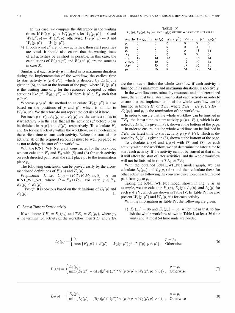
TABLE IVE1(p), E2(p), L1(p), AND L2(p) OF THE WORKFLOW IN TABLE I

are the times to finish the whole workflow if each activity isfinished in its minimum and maximum durations, respectively.

In the workflow constrained by resources and nondeterminedtime, there must be a latest time to start each activity in order toensure that the implementation of the whole workflow can befinished in time TE1 or TE2, where TE1 = E1(pe), TE2 =E2(pe), and pe is the termination of the workflow.

In order to ensure that the whole workflow can be finished inTE1, the latest time to start activity p (p ∈ PA), which is de-noted by L1(p), is given in (7), shown at the bottom of the page.

In order to ensure that the whole workflow can be finished inTE2, the latest time to start activity p (p ∈ PA), which is de-noted by L2(p), is given in (8), shown at the bottom of the page.

To calculate L1(p) and L2(p) with (7) and (8) for eachactivity within the workflow, we can determine the latest time tostart each activity. If the activity cannot be started at that time,it will affect the start of later activities, and the whole workflowwill not be finished in time TE1 or TE2.

With the obtained R/NT_WF_Net model graph, we cancalculate L1(pe) and L2(pe) first and then calculate these forother activities following the converse direction of each directedpath from ps to pe.

Taking the R/NT_WF_Net model shown in Fig. 8 as anexample, we can calculate E1(p), E2(p), L1(p), and L2(p) foreach p ∈ PA, which are shown in Table IV. In Table IV, we alsopresent W1(p, p′′) and W2(p, p′′) for each activity.

With the information in Table IV, the following are given.

1) E1(pe) = 36 and E2(pe) = 54, which mean that, to fin-ish the whole workflow shown in Table I, at least 36 timeunits and at most 54 time units are needed.

E2(p) ={

0, p = ps

max {E2(p′) + β(p′) + W2(p, p′′)|p′ ∈• (•p), p� p′′} , Otherwise (6)

L1(p) ={

E1(p), p = pe

min {L1(p′)− α(p)|p′ ∈ (p•)• ∨ (p� p′ ∧W1(p′, p) > 0)} , Otherwise(7)

L2(p) ={

E2(p), p = pe

min {L2(p′)− β(p)|p′ ∈ (p•)• ∨ (p� p′ ∧W2(p′, p) > 0)} , Otherwise(8)


Fig. 9. Reachability graph of the R/NT_WF_Net in Fig. 8.

2) E1(A3568) = 10 and E2(A3568) = 12. Activity A3568

can be started at the tenth time unit after the start of theworkflow if activity A1 is started before A2, and A1 canbe finished in ten time units. Otherwise, A3 can only bestarted at the 12th time unit.

3) L1(A3568) = 10 and L2(A3568) = 12. Activity A3568

must be started at the tenth (or 12th) time unit to ensurethat the whole workflow can be finished in 36 (or 54)timing units.

4) Activities A1 and A2 share resource pr12. Because A1

is a key activity, A2 has to wait for the resource.The waiting time of A2 is ten (or 12) time units ifA1 can be finished in its minimum (or maximum)duration.

VI. TIMING ANALYSIS FOR THE IMPLEMENTATION STATE

TO OBTAIN THE BEST IMPLEMENTATION CASE

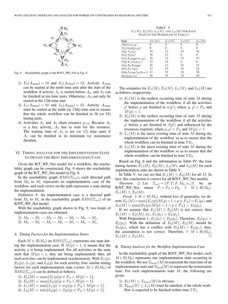
Given the R/T_WF_Net model for a workflow, the reacha-bility graph can be constructed. Fig. 9 shows the reachabilitygraph of the R/T_WF_Net model in Fig. 8.

In the reachability graph RMG(Σαβ), each directed pathfrom M0 to Me represents an implementation case of theworkflow, and each vertex on the path represents a state duringthe implementation.Definition 4: An implementation case is a directed path

from M0 to Me in the reachability graph RMG(Σαβ) of anR/NT_WF_Net model.

With the reachability graph shown in Fig. 9, two kinds ofimplementation cases are obtained.

1) M0 →M1 →M2 →M4 →M6 →M8 →Me.2) M0 →M1 →M3 →M5 →M7 →M8 →Me.

A. Timing Factors for the Implementation States

Each M ∈ R(M0) on RMG(Σαβ) represents one state dur-ing the implementation case. If M(p) = 1, it means that theactivity p is being implemented. For all activities in the statesuch that M(p) = 1, they are being implemented; thus, allsuch activities can be implemented synchronously. With E1(p),E2(p), L1(p), and L2(p) for each activity, four similar timingfactors for each implementation state (vertex M ∈ R(M0) ofRMG(Σαβ)) can be defined as follows.

1) E1(M) = max{E1(p)|p ∈ PA ∧M(p) = 1}.2) E2(M) = max{E2(p)|p ∈ PA ∧M(p) = 1}.3) L1(M) = min{L1(p) + α(p)|p ∈ PA ∧M(p) = 1}.4) L2(M) = min{L2(p) + β(p)|p ∈ PA ∧M(p) = 1}.

TABLE VE1(M), E2(M), L1(M), AND L2(M) FOR EACH

STATE OF THE WORKFLOW IN TABLE I

The semantics for E1(M), E2(M), L1(M), and L2(M) areas follows, respectively.

1) E1(M) is the earliest occurring time of state M duringthe implementation of the workflow, if all the activitiesp′ before p are finished in α(p′), where p, p′ ∈ PA andM(p) = 1.

2) E2(M) is the earliest occurring time of state M duringthe implementation of the workflow, if all the activitiesp′ before p are finished in β(p′) and influenced by theresources required, where p, p′ ∈ PA and M(p) = 1.

3) L1(M) is the latest existing time of state M during theimplementation of the workflow so as to ensure that thewhole workflow can be finished in time TE1.

4) L2(M) is the latest existing time of state M during theimplementation of the workflow so as to ensure that thewhole workflow can be finished in time TE2.

Based on Fig. 8 and the information in Table IV, the fourtiming factors E1(M), E2(M), L1(M), and L2(M) for eachimplementation state are shown in Table V.

In Table V, we can see that E1(M) ≤ E2(M) for all M . Infact, this conclusion is correct for all R/NT_WF_Net models.Theorem 2: Let Σαβ = (P, T ;F,M0, α, β) be an

R/NT_WF_Net, where P = PA ∪ PR. ∀ M ∈ R(M0),E1(M) ≤ E2(M).

Proof: ∀M ∈ R(M0), without loss of generality, we de-note E1(M)=max{E1(p)|M(p)=1 ∧ p ∈ PA}=E1(pi) andE2(M) = max{E2(p)|M(p) = 1 ∧ p ∈ PA} = E2(pj).

If we assume that E1(M) ≤ E2(M) is not correct, thenE1(M) > E2(M), i.e., E1(pi) > E2(pj).

With Proposition 1, E1(pi) ≤ E2(pi). Therefore, E2(pi) >E2(pj). With the definition of E2(M), E2(M) should beE2(pi), which has a conflict with E2(M) = E2(pj); thus,the assumption is not correct. Therefore, ∀ M ∈ R(M0),E1(M) ≤ E2(M). �

B. Timing Analysis for the Workflow Implementation Case

In the reachability graph of the R/NT_WF_Net model, eachM ∈R(M0) represents one implementation state occurring inthe workflow. We use TStart(M) to represent the start time of animplementation state and TEnd(M) to represent the terminationtime. For each implementation state M , the following aregiven.

1) E1(M) ≤ TStart(M) is obvious.2) TEnd(M) ≤ L1(M) must be satisfied, if the whole work-

flow is expected to be finished within time TE1.


TABLE VIEFFECT OF THE FOUR TIMING FACTORS ON

THE WORKFLOW IMPLEMENTATION

3) TEnd(M) ≤ L2(M) must be satisfied, if the whole work-flow is expected to be finished within time TE2.

In this section, we discuss the effect of the four timingfactors of each state, which are E1(M), E2(M), L1(M),and L2(M), on the implementation of the workflow. Amongthe four timing factors, for all M ∈ R(M0), it has beenproved that E1(M) ≤ E2(M) in Theorem 2; therefore, therelations between E1(M), E2(M), L1(M), and L2(M) canbe concluded as the six cases shown in Table VI, and theireffects on the workflow implementation are also shown inTable VI.

C. Best Implementation Case of Workflow

In the previous section, we have discussed the influences ofthe timing factors on the implementation of the workflow basedon the states in the reachability graph of the R/NT_WF_Netmodel. With the conclusions presented in Table VI, it isexpected that all the implementation states of the workflowcould satisfy the first case (the best case) but not the fifth andparticularly the sixth case.Definition 5: Let Σαβ = (P, T ;F,M0, α, β) be an

R/NT_WF_Net and RMG(M0) be the reachability graphof Σαβ . A directed path from M0 to Me in RMG(M0) isnamed as an ideal implementation case of the workflow, if allthe implementation states M ∈ R(M0) within this case satisfyE1(M) ≤ L1(M).

With Table V, we can show that M0 →M1 →M2 →M4 →M6 →M8 →Me is an ideal implementation case ofthe workflow shown in Table I.

It can be proved that there must exist one ideal implemen-tation case for each workflow constrained by resources andnondetermined time. Before the proof, a lemma is first given.Lemma 1: Let Σαβ = (P, T ;F,M0, α, β) be an

R/NT_WF_Net. ∀ M ∈ R(M0), there exists one place

p ∈ PA such that M(p) = 1, and p is a key activity of theworkflow.

Proof: It would not be difficult to prove. �Lemma 2: Let Σαβ = (P, T ;F,M0, α, β) be an

R/NT_WF_Net and RMG(M0) be the reachability graph ofΣαβ . If M ∈ R(M0) (M = Me) satisfies E1(M) ≤ L1(M),there must exist t ∈ T and M ′ ∈ R(M0) such that M [t > M ′and E1(M ′) ≤ L1(M ′).

Proof: Because M = Me, there exists t ∈ T such thatM [t >. If there is one and only one t satisfying the condi-tions, and let M [t > M ′, it is obvious that E1(M ′) ≤ L1(M ′).Otherwise, we select one t to fire such that pa ∈• t, where pa

satisfies M(pa) = 1 and is a key activity of the workflow. LetM [t > M ′, then

E1(M ′)=max{max{E1(p)|p∈M−•t},max{E1(p′)|p′ ∈ t•}}.

In this case, the following are given.

1) max{E1(p)|p ∈M −• t} ≤ E1(M) ≤ L1(M) ≤L1(M ′).

2) max{E1(p′)|p′ ∈ t•} = max{E1(pa) + α(pa) +W1(pa, p′a)|pa ∈• t} ≤ E1(pa) + α(pa) +W1(pa, p′a) ≤ E1(M) + α(pa) + W1(pa, p′a) ≤L1(M) + α(pa) + W1(pa, p′a) ≤ L1(M ′).

Based on 1) and 2), E1(M ′) ≤ L1(M ′). �Now, we prove that there must exist one ideal implemen-

tation case for each workflow constrained by resources andnondetermined time.Theorem 3: Let Σαβ = (P, T ;F,M0, α, β) be an

R/NT_WF_Net and RMG(M0) be the reachability graphof Σαβ . There must exist one directed line from M0 to Me inRMG(M0), which is an ideal implementation case of Σαβ ,i.e., E1(M) ≤ L1(M) for each M on the line from M0 to Me.

Proof: It is obvious that E1(M0) ≤ L1(M0). Based onLemma 2, there must exist t1 ∈ T and M1 ∈ R(M0) suchthat M0[t > M1 and E1(M1) ≤ L1(M1). If M1 = Me, theconclusion is proved. Otherwise, there must exist t2 ∈ T andM2 ∈ R(M0) such that M1[t > M2 and E1(M2) ≤ L1(M2).To repeat this process until Mi = Me (i = 1, 2, . . .), a directedline from M0 to Me in RMG(M0) is thus obtained on whichE1(M) ≤ L1(M) for each M . �Definition 6: Let Σαβ = (P, T ;F,M0, α, β) be an

R/NT_WF_Net and RMG(M0) be the reachability graphof Σαβ . A directed path from M0 to Me in RMG(M0) isnamed as a reliable implementation case of the workflow, if allthe implementation states M ∈ R(M0) within the case satisfyE2(M) ≤ L2(M).

With Table V, we can show that M0 →M1 →M2 →M4 →M6 →M8 →Me is also a reliable implementation caseof the workflow shown in Table I.

It also can be proved that there must exist one reliable im-plementation case for each workflow constrained by resourcesand nondetermined time. First, a lemma like Lemma 2 isgiven.Lemma 3: Let Σαβ = (P, T ;F,M0, α, β) be an

R/NT_WF_Net and RMG(M0) be the reachability graph ofΣαβ . If M ∈ R(M0) (M = Me) satisfies E2(M) ≤ L2(M),there must exist t ∈ T and M ′ ∈ R(M0) such that M [t > M ′and E2(M ′) ≤ L2(M ′).


Proof: It can be proved as the proof of Lemma 2. �Theorem 4 proves that there must exist one reliable imple-

mentation case for each workflow constrained by resources andnondetermined time.Theorem 4: Let Σαβ = (P, T ;F,M0, α, β) be an

R/NT_WF_Net and RMG(M0) be the reachability graphof Σαβ . There must exist one directed line from M0 to Me inRMG(M0), which is a reliable implementation case of Σαβ ,i.e., E2(M) ≤ L2(M) for each M on the line from M0 to Me.

Proof: It can be proved as the proof of Theorem 3. �Definition 7: An implementation case is one of the best

implementation cases if it is ideal and reliable.Based on Table VI, M0 →M1 →M2 →M4 →M6 →

M8 →Me is one of the best implementation case of the work-flow shown in Table I. M0 →M1 →M3 →M5 →M7 →M8 →Me is not an ideal case, nor a reliable one, nor one ofthe best implementation cases.

Theorems 3 and 4 indicate that there must exist one idealand one reliable implementation cases for each workflow con-strained by resources and nondetermined time. However, it ispossible that the ideal and the reliable implementation casesare different. This would mean that the best implementationcase of a workflow does not exist even though both theideal and reliable cases exist in the workflow. This conclusioncan be proved by changing the duration time of activities inTable I. In analyzing and verifying a workflow constrainedby resources and nondetermined time, the focus is to obtainthe best implementation case. The sufficient conditions for theexistence of the best implementation case of a workflow con-strained by resources and nondetermined time are presented inTheorem 5.Theorem 5: Let Σαβ = (P, T ;F,M0, α, β) be an

R/NT_WF_Net, where P = PR ∪ PA, and RMG(M0) be thereachability graph of Σαβ . There is one best implementationcase of the workflow, if ∀ M ∈ RMG(M0), ∃p ∈ PA suchthat

1) L1(M) = L1(p) + α(p).2) L2(M) = L2(p) + β(p).

Proof: For the initial state M0 of Σαβ , M0(ps) = 1,L1(M) = L1(ps) + α(ps), and L2(M) = L2(ps) + β(ps).

Suppose that M ∈ R(M0) and M = Me are in the bestcase, then L1(p) + α(p) = min{L1(p′) + α(p′)|M(p′) = 1},and L2(p) + β(p) = min{L2(p′) + β(p′)|M(p′) = 1}.

Let p• = {t}; then, M [t > M ′ based on Lemmas 2 and 3,E1(M ′) ≤ L1(M ′), and E2(M ′) ≤ L2(M ′).

Thus, there is one directed path from M0 to Me on which∀ M ∈ R(M0) such that E1(M) ≤ L1(M) and E2(M) ≤L2(M). �

In the best implementation case M0 →M1 →M2 →M4 →M6 →M8 →Me, it can be proved that, for eachMi (i = 0, 1, 2, 4, 6, 8), ∃p ∈ PA, satisfying the conditions inTheorem 5, which are ps, p1, A1, p2, A2, A3568 (or A47), andpe, respectively.

D. Algorithm to Obtain the Best Implementation Case

Based on the earlier discussion and analysis, an algorithmto obtain the best implementation case of a workflow con-strained by resources and nondetermined time is presented inAlgorithm 2.

Algorithm 2: Obtain the best implementation case.

INPUT: Σαβ = (P, T ;F,M0, α, β)OUTPUT: Ideal(Σαβ), Reliable(Σαβ), and Best(Σαβ),

which represent the ideal, reliable and best implementationcases of Σαβ , respectively.

Step 1: Ideal(Σαβ)← φ, Reliable(Σαβ)← φ, andBest(Σαβ)← φ;

Step 2: Calculate E1(p), E2(p), L1(p) and L2(p) with (5),(6), (7), and (8) for each p ∈ PA based on R/NT_WF_Netmodel.

Step 3: Construct the reachability graph RMG(Σαβ) for theR/NT_WF_Net Σαβ .

Step 4: Obtain all implementation cases (the directed linesfrom M0 to Me) based on RMG(Σαβ) and denoted byICase(Σαβ).

Step 5: Calculate E1(M), E2(M), L1(M), and L2(M) foreach state M ∈ R(M0) based on RMG(Σαβ).

Step 6: For each implementation case iCase inICase(Σαβ),

(6.1) Ideal(Σαβ)← Ideal(Σαβ) ∪ {iCase}, if all theimplementation states M ∈ R(M0) within iCase satisfyE1(M) ≤ L1(M).

(6.2) Reliable(Σαβ)← Reliable(Σαβ) ∪ {iCase}, if allthe implementation states M ∈ R(M0) within iCase satisfyE2(M) ≤ L2(M).

(6.3) Best(Σαβ)← Best(Σαβ) ∪ {iCase}, if all the imple-mentation states M ∈ R(M0) within iCase satisfy E1(M) ≤L1(M) and E2(M) ≤ L2(M).

Step 7: Outputs Ideal(Σαβ), Reliable(Σαβ), andBest(Σαβ).

Algorithm 2 only presents the framework to obtain the bestimplementation case for a workflow constrained by resourcesand nondetermined time. Its correctness can be validated by theearlier discussion and analysis.

VII. CASE STUDY

To show the modeling and analysis approach for the work-flow constrained by resources and nondetermined time based onR/NT_WF_Net proposed in this paper, we present a simplifiedworkflow for production manufacture and sale, which is shownin Fig. 10. The workflow contains 14 activities, i.e., Activity ={Ai|1≤ i≤14}, and three kinds of resources, i.e., Resource ={Product Dictionary, Computer, Product Buyer}. Theinformation about each activity in the workflow, includ-ing meaning, connection relation, the minimum and max-imum duration times, and resources required, is shown inTable VII.

With the modeling approach presented in Section IV, theR/NT_WF_Net model Σαβ2 = (P2, T2;F2,M02, α2, β2) forthe workflow after refinement and reduction is shown in Fig. 11,where the following are given.

1) P2 = P2R ∪ P2A denotes the places of Σαβ2.a) P2R = {pr12, pr3} is the set of resources, where

pr12 = {Product Dictionary, Computer} andPr3 = {Product Buyer}.


Fig. 10. Simplified workflow for production manufacture and sale.

TABLE VIIINFORMATION ABOUT THE ACTIVITIES OF THE WORKFLOW IN FIG. 10

b) P2A={Ai|i=1∼2, 3, 4, 5∼6, 7, 8, 9, 10, 11, 12, 13∼4}∪{pj |j = s, e, 1, 2, 3, 4, 5, 6, 7, 8} is the set ofactivities, where {pj |j = 1, 2, 3, 4, 5, 6, 7, 8} isthe set of virtual activities. ps and pe are the start andtermination of the workflow, respectively. ActivitiesA1∼2, A5∼6, and A13∼4 are obtained by the reductionof activities A1, A2, A5, A6, A13, and A14.

2) T2 = {ti|1 ≤ i ≤ 14} denotes the transitions of Σαβ2.3) The initial marking of Σαβ2 is as follows:

M02(p) ={

1, If p = ps or p ∈ P2R

0, Otherwise.

With the graph of the R/NT_WF_Net model shown inFig. 11, Te1(p), Te2(p), Tl1(p), and Tl2(p) for each p ∈ P2A

can be calculated, which are not presented in this paper. Basedon Te1(p), Te2(p), Tl1(p), and Tl2(p) for each p, it can beobtained that ps → A1∼2 → p2 → A4 → p4 → A5∼6 →A9 → A12 → A13∼4 → pe is the key activity line for theworkflow.

With the graph of the R/NT_WF_Net model shown inFig. 11, E1(p), E2(p), L1(p), and L2(p) for each p ∈ P2A

can be calculated, which are shown in Table VIII. BecauseE1(pe) = 64 and E2(pe) = 100, to finish the whole workflowrequires at least 64 and at most 100 time units.

The reachability graph RMG(Σαβ2) is constructed andshown in Fig. 12.

Based on the reachability graph RMG(Σαβ2), we can obtainall the implementation cases. There are 22 kinds of implemen-tation cases of the workflow, which are represented hereafter,

Fig. 11. R/NT_WF_Net model for the workflow shown in Fig. 10.

where {Path1 + Path2} represents the Path1 or Path2 thatoccurs in the implementation cases.

M0 →M1 →M2 → {M3 →M5 →M7 + M4 →M6

→M8} →M9 →M10 →M11 → {M12 →M15 →M17

→M20 →M23 + M12 →M15 →M18 →M21 →M23

+ M12 →M15 →M18 →M21 →M24 + M12 →M15

→M18 →M20 →M23 + M12 →M14 →M18 →M20

→M23 + M12 →M14 →M18 →M21 →M23 + M12

→M14 →M18 →M21 →M24 + M13 →M14 →M18

→M20 →M23 + M13 →M14 →M18 →M21 →M23

+ M13 →M14 →M18 →M21 →M24 + M13 →M16

→M19 →M22 →M24} →M25 →M26 →Me.

Based on the reachability graph RMG(Σαβ2), the tim-ing factors E1(M), E2(M), L1(M), and L2(M) for each


TABLE VIIIE1(p), E2(p), L1(p), AND L2(p) OF THE WORKFLOW IN FIG. 10

Fig. 12. Reachability graph RMG(Σαβ2).

implementation state can be calculated, which are shownin Table IX.

With the timing information for each state of the workflowshown in Table VII, all implementation cases can be analyzedand classified. In Table VII, M3, M5, M7, M15, M17, and M19

do not satisfy E1(M) ≤ L1(M), and M3, M5, M7, M15, M16,M17, and M19 do not satisfy E2(M) ≤ L2(M). Therefore, thefollowing are given.

1) The ideal implementation cases are as follows:

M0 →M1 →M2 →M4 →M6 →M8 →M9 →M10

→M11 → {M12 + M13} →M14 →M18 → {M20

→M23 + M21 →M23 + M21 →M24} →M25

→M26 →Me.

TABLE IXE1(M), E2(M), L1(M), AND L2(M) FOR

THE REACHABILITY STATES OF Σαβ2

2) The reliable implementation cases are as follows:

M0 →M1 →M2 →M4 →M6 →M8 →M9 →M10

→M11 → {M12 + M13} →M14 →M18 → {M20

→M23 + M21 →M23 + M21 →M24} →M25

→M26 →Me.

3) The best implementation cases are as follows:

M0 →M1 →M2 →M4 →M6 →M8 →M9 →M10

→M11 → {M12 + M13} →M14 →M18 → {M20

→M23 + M21 →M23 + M21 →M24} →M25

→M26 →Me.

VIII. CONCLUSION AND DISCUSSION

Time and resource management are two important challengesfor workflow management systems. We present a modelingand analysis approach for a kind of workflow constrained byresources and nondetermined time based on a Petri net. Withthe obtained R/NT_WF_Net model and its reachability graph,we analyze the timing factors influencing the implementationof the whole workflow, present the methods to verify the risksof all implementation cases, and find the best implementationcase for the workflow.

The main contributions of this paper include the following:1) R/NT_WF_Net model and modeling approach for work-

flow constrained by resources and nondetermined time.To keep the atomic properties of transitions in the Petri


net, the activities of the workflow are represented byplaces, which are different from the traditional modelingapproach for workflow based on Petri net;

2) a refinement method and a set of reduction rules for theR/NT_WF_Net model, which can reduce the scale of theR/NT_WF_Net model effectively;

3) the methods to calculate the earliest and latest times tostart each activity in the workflow;

4) the methods to verify each implementation case of theworkflow to find the hidden risks;

5) an algorithm to obtain the best implementation caseof a workflow based on the reachability graph of itsR/NT_WF_Net model. In addition, the sufficient condi-tions of the existence of the best implementation case areproved and presented.

In this paper, we assume that all required resources havebeen prepared well before the start of the activity. Preparingresources usually requires time to complete. Therefore, theseresources, like activities, should also have time constraintsin the workflow specification. This problem is not difficultto solve with the approach proposed in this paper, becauseall the resource places in the R/NT_WF_Net model can beregarded as a set of special activities (e.g., activities to prepareresources). Thus, for each resource place pr, we can also useα(pr) and β(pr) to represent the minimum and maximumof its preparation time. The analysis and calculation methodsproposed in this paper can also be adapted to this extendedworkflow constrained by resource preparation time.

The methods and conclusions are both presented before thestart of the workflow, which are based on the specification atbuild time. During the implementation of the workflow, theminimum and maximum duration times in the specificationof the finished activities will be replaced by the actual im-plementation time. In this case, we can calculate and analyzethe timing and resource factors influencing the implementationof the remainder activities, using the methods presented inthis paper, which will benefit the implementation of the entireworkflow.

We have presented a modeling and analysis approach for aworkflow constrained by resources and nondetermined time.The work of this paper opens the door to future research onthe following subjects.

1) We only consider the simple situation of a workflowconstrained by resources. The types and amount of theresources have not been considered with more emphasis.To examine a workflow using more detailed informationregarding the characteristics of resources (e.g., type oramount), it is possible to adopt an advanced Petri net (e.g.,predicate-transition net [29] or colored Petri net [30]) asa model.

2) Workflow (process) mining is currently a hot researchtopic [3]. If the workflow running logs can record theinformation regarding implementation time and requiredresources, the methods of rediscovering the model fromthe timed logs can be researched.

The resource usage in the workflow constrained by resourceand nondetermined time presented in this paper is similar to thatfor a shared-resource manufacturing system. Moreover, thereare many ways of using Petri nets to represent a shared-resourcemanufacturing system [31]–[35], in which the shared-resource

manufacturing system is usually denoted by the processes thatcontrol the manufacturing resources and the interactions amongthe processes. However, most of the Petri net models formanufacturing systems with shared-resources are used to provethe existence or absence of deadlocks [31]–[35]. In contrast tothe research work in this paper, they did not handle the timingoptimization and control issue. Based on the R/NT_WF_Netproposed in this paper, the earliest time to start each activ-ity can be calculated, and the key activities influencing theimplementation time of a workflow can be determined, withwhich the resource conflicts between activities can also bechecked. Therefore, the existence and control of deadlocksbased on R/NT_WF_Net model will be addressed in thefuture.

REFERENCES

[1] J. Nichols, H. Demirkan, and M. Goul, “Autonomic workflow executionin the grid,” IEEE Trans. Syst., Man, Cybern. C, Appl. Rev., vol. 36, no. 3,pp. 353–364, May 2006.

[2] J. Li, Y. Fan, and M. C. Zhou, “Performance modeling and analysis ofworkflow,” IEEE Trans. Syst., Man, Cybern. A, Syst., Humans, vol. 34,no. 2, pp. 229–242, Mar. 2004.

[3] W. M. P. van der Aalst, T. Weijters, and L. Maruster, “Workflow mining:Discovering process models from event logs,” IEEE Trans. Knowl. DataEng., vol. 16, no. 9, pp. 1128–1142, Sep. 2004.

[4] G. K. Janssens, B. W. Jan Verelst, and B. Weyn, “Techniques for modelingworkflows and their support for reuse,” in Business Process Manage-ment: Models, Techniques, and Empirical Studies, W. van der Aalst, Ed.Berlin, Germany: Springer-Verlag, 2000, pp. 1–15.

[5] C. A. Petri, “Kommunikation mit automaten,” Ph.D. dissertation, Inst.Instrumentelle Math., Bonn, Germany, 1962.

[6] W. Reisig, “Petri nets: An introduction,” in Monographs in TheoreticalComputer Science: An EATCS Series, vol. 4. Berlin, Germany: Springer-Verlag, 1985.

[7] T. Murata, “Petri nets: Properties, analysis and applications,” Proc. IEEE,vol. 77, no. 4, pp. 541–580, Apr. 1989.

[8] W. M. P. van der Aalst, “The application of Petri nets to workflow man-agement,” J. Circuits Syst. Comput., vol. 8, no. 1, pp. 21–66, 1998.

[9] J. Li, Y. Fan, and M. C. Zhou, “Timing constraint workflow nets forworkflow analysis,” IEEE Trans. Syst., Man, Cybern. A, Syst., Humans,vol. 33, no. 2, pp. 179–193, Mar. 2003.

[10] N. R. Adam, V. Atluri, and W. K. Huang, “Modeling and analysis ofworkflows using Petri nets,” J. Intell. Inf. Syst., vol. 10, no. 2, pp. 131–158, Mar. 1998.

[11] J. Li, Y. Fan, and M. C. Zhou, “Approximate performance analysis ofworkflow model,” in Proc. IEEE Int. Conf. Syst., Man, Cybern., Oct. 5–8,2003, vol. 2, pp. 1175–1180.

[12] S. Ling and H. Schmidt, “Time Petri nets for workflow modellingand analysis,” in Proc. IEEE Int. Conf. SMC, Nashville, TN, 2000,pp. 3039–3044.

[13] W. M. P. van der Aalst, “Three good reasons for using a Petri-net-based workflow management system,” in Proc. Int. Working Conf.IPIC, S. Navathe and T. Wakayama, Eds., Cambridge, MA, Nov. 1996,pp. 179–201.

[14] H. Li, Y. Yang, and T. Y. Chen, “Resource constraints analysis of work-flow specifications,” J. Syst. Softw., vol. 73, no. 2, pp. 271–285, Oct. 2004.

[15] C. A. Ellis and G. J. Nutt, “Workflow: The process spectrum,” in Proc.NSF Workshop Workflow Process Autom. Inf. Syst.: State-of-the-Art Fu-ture Directions, Athens, GA, 1996, pp. 140–145.

[16] C. A. Ellis and G. J. Nutt, “Modeling and enactment of workflowsystems,” in Proc. 14th Int. Conf., M. A. Marsan, Ed. London, U.K.:Springer-Verlag, 1993, vol. 691, pp. 1–16.

[17] D. Wikarski, “An introduction to modular process nets,” ICSI, Berkeley,CA, Tech. Rep. TR-96-019, 1996.

[18] A. K. Schömig and H. Rau, “A Petri net approach for the performanceanalysis of business processes,” Univ. Würzburg, Würzburg, Germany,Rep. 116 Seminar at IBFI, Schloss Dagstuhl, May 22–26, 1995.

[19] H. Li and Y. Fan, “Time management in workflow system,” J. Softw.,vol. 13, no. 8, pp. 1552–1558, 2002. (in Chinese).

[20] V. Gruhn and R. Laue, “Using timed model checking for verifying work-flows,” in Proc. 7th ICEIS, Miami, FL, May 24–28, 2005.


[21] E. De Maria, A. Montanari, and M. Zantoni, “An automaton-based ap-proach to the verification of timed workflow schemas,” in Proc. 13th Int.Symp. TIME, Budapest, Hungary, Jun. 2006.

[22] J. Eder, E. Panagos, and M. Rabinovich, “Time constraints inworkflow systems,” in Proc. 11th Int. CAiSE, Heidelberg, Germany, 1999,pp. 286–300.

[23] J. Eder, E. Panagos, H. Pozewaunig, and M. Rabinovich, “Time man-agement in workflow systems,” in Proc. 3rd Int. Conf. Bus. Inf. Syst.,W. Abramowicz and M. E. Orlowska, Eds., Poznan, Poland, 1999,pp. 265–280.

[24] O. Marjanovic and M. E. Orlowska, “On modeling and verification oftemporal constraints in production workflows,” Knowl. Inf. Syst., vol. 1,no. 2, pp. 157–192, May 1999.

[25] O. Marjanovic, “Dynamic verification of temporal constraints inproduction workflows,” in Proc. 11th ADC, Canberra, Australia, 2000,pp. 74–81.

[26] S. W. Sadiq, O. Marjanovic, and M. Orlowska, “Managing change andtime in dynamic workflow processes,” Int. J. Coop. Inf. Syst., vol. 9,no. 1/2, pp. 93–116, Mar.–Jun. 2000.

[27] K. Hyunglee, “Generalized Petri net reduction method,” IEEE Trans.Syst., Man, Cybern., vol. SMC-17, no. 2, pp. 297–303, Mar./Apr. 1987.

[28] I. Suzuki, “A method for stepwise refinement and abstraction of Petrinets,” J. Comput. Syst. Sci., vol. 27, no. 1, pp. 51–76, Aug. 1983.

[29] T. Murata and D. Zhang, “A predicate-transition net model for parallelinterpretation of logic programs,” IEEE Trans. Softw. Eng., vol. 14, no. 4,pp. 481–497, Apr. 1988.

[30] K. Jensen, Coloured Petri Nets—Basic Concepts. New York: Springer-Verlag, 1996.

[31] M. C. Zhou and F. DiCesare, “Petri net design method for automated man-ufacturing systems with shared resources,” in Proc. IEEE Conf. Robot.Autom., 1990, pp. 526–531.

[32] M. C. Zhou and F. DiCesare, “Parallel and sequential mutual exclusionsfor Petri net modeling of manufacturing systems with shared resources,”IEEE Trans. Robot. Autom., vol. 7, no. 4, pp. 515–527, Aug. 1991.

[33] J. Ezpeleta, J. M. Colom, and J. Martinez, “A Petri net based deadlock pre-vention policy for flexible manufacturing systems,” IEEE Trans. Robot.Autom., vol. 11, no. 2, pp. 173–184, Apr. 1995.

[34] N. Viswanadham, Y. Narahari, and T. L. Johnson, “Deadlock preventionand deadlock avoidance in flexible manufacturing systems using Petrinet models,” IEEE Trans. Robot. Autom., vol. 6, no. 6, pp. 713–723,Dec. 1990.

[35] M. D. Jeng and F. DiCesare, “Synthesis using resource control nets formodeling shared-resource systems,” IEEE Trans. Robot. Autom., vol. 11,no. 3, pp. 317–327, Jun. 1995.

Huaiqing Wang received the Ph.D. degree in com-puter science from the University of Manchester,Manchester, U.K., in 1987.

He is currently a Professor with the Department ofInformation Systems, City University of Hong Kong,Kowloon, Hong Kong. He specializes in the researchand development of business intelligence systemsand intelligent agents and their applications (such asmultiagent-supported financial information systems,virtual learning systems, knowledge managementsystems, and conceptual modeling).

Qingtian Zeng received the Ph.D. degree incomputer software and theory from the Institute ofComputing Technology, Chinese Academy ofSciences, Beijing, in 2005.

He was a Senior Research Associate with theDepartment of Information Systems, City Universityof Hong Kong, Kowloon, Hong Kong, in 2006. Heis currently an Associate Professor with the Collegeof Information Science and Technology, ShandongUniversity of Science and Technology, Qingdao,China. His research interests are in the areas of Petri

net, process mining, ontology, knowledge acquisition, and management.Dr. Zeng received the support from the Natural Science Foundation of China

and the Excellent Young Scientist Foundation of Shandong Province, China.He is serving on the editorial board of the Journal of Software Engineering andthe Asian Journal of Information Management. He was the Program Cochairof the 2007 International Conference on Knowledge Science, Engineeringand Management; the 2007 International Conference on Grid and CooperativeComputing, and the 2007 International Workshop on Workflow Managementand Application in Grid Environments.

Modeling and Analysis for Workflow Constrained by Resources and Nondetermined Time: An Approach...

Documents

Transcript of Modeling and Analysis for Workflow Constrained by Resources and Nondetermined Time: An Approach...